Testing Lin's Social Capital Theory in an Informal African Urban Economy
Upload
khangminh22Category
view
2download
0
1
A model of the informal economy with an application to Ukraine Simon Commander1
EBRD One Exchange Square
London EC2A 2JN, United Kingdom E-mail: [email protected]
Natalia Isachenkova2
Faculty of Business and Law, Kingston University London
Kingston Hill, Kingston upon Thames, Surrey, KT2 7LB, United Kingdom Phone: +44(0) 20 8547 8206 Fax: +44(0) 20 8547 7026
E-mail: [email protected]
Yulia Rodionova3 University College London,
School of Slavonic and East European Studies, 16 Taviton Street, LONDON WC1H 0BW, United Kingdom
E-mail: [email protected]
This version 21 September 20094
Abstract
The size of the informal economy has grown sharply in many transition countries, particularly in the Former Soviet Union. To provide a better understanding of this phenomenon, our paper develops a model of how the structure of labour compensation inherited from central planning affects labour allocation. Using a panel dataset on individuals and households from the Ukraine Longitudinal Monitoring Surveys (ULMS) for 2003 and 2004, we first quantify the size of the Ukraine informal economy. We then write down a model of an economy with state and private sectors and formal and informal work, where all sectors can employ both full- and part-time workers. Private firms choose whether to be formal - and pay payroll taxes - or stay informal, subject to some probability of detection for evading payroll tax. This setting allows us to derive the impact of social benefits, as well as demand shocks and detection rates, on the allocation of employment across different labour market states. Predictions from our model are then tested econometrically using the ULMS data. Keywords: informal sector, labour mobility, structure of labour non-monetary compensation,
Ukraine
JEL Classification: J2, P2.
1 First author; E-mail: [email protected]. 2 Corresponding author; E-mail: [email protected]. 3E- mail: [email protected]. The authors are listed in the alphabetical order. 4 We are grateful for helpful comments to Suren Basov, Randolph Bruno, Xiao Chen, Hsueh-Ling Huynh, Stanislav Kolenikov, Anna Lukyanova, Alexander Muravyev, Sophia Rabe-Hesketh, Sergei Roschin, Andrei Tolstopiatenko, Tolga Yuret, and to the participants in the research seminars and conferences held at EBRD, London Business School, Oxford University, and LIRT-HSE. Earlier drafts of the paper were presented at an IZA-EBRD Conference on Labour Market Dynamics, Role of Institutions and Internal Labour Markets, held at the University of Bologna, May 5-8 2005, and at a LIRT-HSE’s seminar in the spring of 2009. We thank EBRD and UK DFID for support.

2
1. Introduction
A substantial informal economy - defined as employment in firms that do not pay payroll tax - is a
characteristic of many developing countries. The last decade has seen a strong growth of the
informal economy for most transition countries, accounting for between 35-44% of GDP in the
countries of the Former Soviet Union (FSU) and between 21-33% in Central and Eastern Europe
(Bernabe, 1999; Schneider and Enste, 2000; Yoon et al, 2003; Krstic, 2003; Commander and
Rodionova, 2005).
Attempts to understand why there has been such growth have mostly emphasized the role of
public policy. In particular, high payroll tax rates may have raised the incentive for creating
informal jobs. In addition, where the business environment has been problematic informal sectors
have tended to be relatively large. Yet in the transition economies, it is interesting to note that cross-
country estimations of the size of the informal economy find no robust association between size and
the extent of reform, whereas the latter is clearly highly correlated with the quality of the business
environment. This suggests that the size of the informal economy is not simply an issue for the
early or slow reformers.
While existing models of the informal economy tend to be organised around two distinct
sectors – formal and informal - a defining feature of the transition country context has been the
prevalence of multiple job-holding, whereby individuals combine formal sector employment with
informal sector employment. Recent research has highlighted the important consequences for
creating incentives for multiple job-holding of the dynamic interplay between such factors as control
regimes in state sector firms, the structure of compensation and the level of outside opportunities –
particularly unemployment benefits – made available to separated workers5.
Accordingly, to reflect this complexity and incorporate the phenomenon of multiple job-
holding, this paper uses a multi sector model of labour allocation, including a mixed
formal/informal sector. Based on this formalisation, we show the relevance to the informal
economy growth of the inheritance of central planning, particularly the structure of labour
compensation where the provision of housing subsidies, health and child care and other social
benefits was common.
The paper proceeds by first quantifying the size of the informal economy based on unique
individual and household data from the Ukraine Longitudinal Monitoring Surveys (ULMS) for
2003 and 2004. We then describe transitions of workers between the three sectors: formal,
informal and formal/informal. We find that, over the course of 1991-2004, the share of
employment in Ukraine’s informal sector has jumped from around 10-16% to between 17-23%.
This increase is far higher if people involved in agricultural production for their own use are also

3
considered.
Second, based on an analytical model of an economy with state and private sectors and involving
formal, informal and full and part-time work, we are able to derive testable propositions as to how the
reallocation of labour is affected by such factors as the amount of non-monetary compensation, the
extent to which such benefits are subsidized by the state, and the probability of the firm being detected
evading payroll tax. The panel element of the ULMS dataset is then used to assess the empirical
validity of the main prediction from our theoretical model. Employing state-of-the-art econometrics,
such as mixed logit, our paper provides important first evidence on the significant effects of non-
monetary benefits on the static allocation of labour across the three sectors. In addition, we analyse the
dynamics using multinomial logit for transitions of workers between the sectors, which also conditions
on the detection probability, involuntary temporary unemployment (when the worker remains on the
firm’s payroll but receives no wage), and occupation. Our overall conclusion points to the important
attaching role social benefits play in determining the mix of formal/informal sector employment.
The paper is organised as follows. In Section 2, we quantify the informal sector in Ukraine using
various employment measures and micro-data from the ULMS. Section 3 presents a model of the
informal sector and formulates hypotheses for empirical testing. Section 4 gives a brief description of
the econometric approach and reports estimation results. Section 5 concludes.
2. The informal sector: evidence from Ukraine
Existing estimates for Ukraine of the size of the informal economy, derived from physical inputs,
such as electricity consumption, or based on money demand functions, not only indicate that a large
informal sector came into existence near the start of transition in 1992 but show that in the 1990s the
country appears to have had one of the sharpest rates of increase in the informal economy. Johnson et
al (1998) estimated that informal activity accounted for around 16% of GDP in 1989/90, rising to
over 47% by 1994/95, while Lacko (1999) had a yet higher estimate of around 54% at the latter
date. Schneider (2005) placed the informal sector share of GDP at around 53/54% in 2001-2003. The
extent of informal employment is comparable with the estimates for the FSU countries during the same
time period. For instance, Schneider and Enste (2000) using physical inputs suggest that by 1995, the
informal economy accounted for between 35-44% of GDP in the FSU (see also Bernabe, 1999; Yoon
et al, 2003; Commander and Rodionova, 2005). The extent of informal employment has also been
higher than a reported in Krstic (2003) for Central and Eastern Europe level of 21-33% of GDP. If
most transition economies are indeed developing economies, then the rapid growth in the size of the
informal sector may simply reflect convergence. However, it may also reflect some of the particular
institutional and other features of the transition economies. Explanations for why this has been the
5For example, Rein, Friedman and Worgotter (1997).

4
case in Ukraine have mostly emphasised the slow and partial nature of reforms and the continuing
high level of payroll taxation. Indeed, throughout the transition, the payroll tax rate has remained
above 40%.Yet, aggregate measures give little or no sense of what constitutes the informal economy
and how that may have changed over time. Indeed, measurement error is a challenge for research and
can only be adequately addressed by adopting a cross-level focus and using household-level data
containing observations over time.
Given the shortcomings of the approaches relying on aggregate measures, this paper makes
use of the comprehensive and representative sample of Ukrainian households, created in two rounds
of the ULMS. The first round was implemented for 4056 households and 8641 individuals in 2003 with
a retrospective part covering some – but not all – items of the questionnaire for the years, 1986, 1991,
1997-2001. A second round was completed in late 2004 and covered 3500 households and 7201
individuals. The reference period for the second round was 2003 and 2004. The ULMS data provide
extensive information on household income and expenditure, as well as individual-level information
about employment status, working hours, earnings, non-monetary (social) benefits and other
components of income. Based on this data we are able to put together a number of estimates of the
size of the informal economy – as measured by the percentage of total employment - for 1991, 1997,
2003 and 2004. Measure 1 in the first column of Table 1 reports the share of employment in informal
activity outside of agriculture. This comprises individuals with an unregistered job as well as those
who are self-employed or have a second job or are involved in occasional supplementary work.
Broadening the conceptualisation of the informal economy, Measure 2 adds those involved in non-
agricultural household production and sale of agricultural goods on a secondary basis. Measure 3
further augments the estimates by including all individuals involved in agricultural production for
their own use.
Not surprisingly the size of the informal economy is significantly affected by whether agriculture
is included. On Measure 3, informal employment accounted for over 66% of employment at its peak
in 2004. By contrast, when excluding individuals involved in agricultural activity, the informal
economy share dropped to 17%. Because agriculture is largely an untaxed part of the economy in
most developing countries, to ensure comparability, we focus our attention on the second - and
significantly narrower - measure of the extent of informal activity - which includes only those with
secondary agricultural output for sale. This measure gives an informal employment share of 16%
in 1991 rising to 26% in 1997. The share falls substantially in 2003 before rising again to 23% in
2004.
Turning to employment distributions across formal and informal sectors, in 1997 nearly three
quarters of workers had jobs solely in the formal sector. A further 20% were employed in informal
work only, whereas about 6% held multiple jobs, participating in both formal and informal work.

5
By 2003-04, formal employment remained roughly constant at between 75-80% while the share of
informal employment ranged between 7-15%. The share of multiple job holders was comparable
ranging between 9-12%.
Table 2 shows transitions across the three employment states for 2003-04, calculated for
2824 individuals with complete records in both years. Amongst individuals with formal
employment in 2003, 90% did not change their status and further 4-6% moved to either informal or
multiple job holding. A substantial proportion of multiple job holders switched entirely into the informal
economy.
As regards the associated structure of labour compensation, and in particular the intensity of
use by state-owned and privatised firms of non-monetary or social benefits, such as housing subsidy,
provision of health and child care and other services, the ULMS data indicate that in both 2003 and
2004 around 36% of individuals in the sample were in receipt of non-monetary compensation. It
is notable that more than 50% of multiple jobholders in the sample received social benefits.
3. A model of the informal economy
We take the economy to be populated by three types of firms: state-owned, private formal and
private informal firms. All types can employ both full-time and part-time labour. We now
outline the optimization problem for each type of the firm.
3.1. State sector firms
Full-time employees in the state sector receive monetary wages and also non-monetary or social
benefits. Part-time employees receive only non-monetary benefits. State firms pay payroll taxes
for their full-time employees but not for their part-timers. Part-time employees working in the
state sector can also work in the private sector and receive a wage. That wage will, however, be
discounted by the probability of detection for not paying taxes if they work informally.
We model state- or insider-run firms by analogy with trade unions6. In the context of
developed market economies, these firms have often been modelled as either maximizing
wages, or maximizing utility with respect to both wage and employment, subject to a zero
constraint on profits. In the Ukraine context, we assume that, instead of maximizing wages,
state-owned firms maximize employment (i.e., they prefer not to fire existing workers), setting
wages consistent with their employment objective. This can be modelled as the state firm
picking the largest full-time employment possible subject to a zero-profit constraint. Clearly,
the resulting wage-employment combination is inefficient.
6 See, for instance, Farber (1987).

6
Alternatively, state-owned firms can be assumed to pick a combination of employment and
wages to maximize rents subject to a zero-profit constraint. In this case, the wage-employment
solution will be efficient. In terms of the validity of both assumptions, the existing research (see,
for instance, Commander et al (1993, 1996a, 1996b) and Commander and Tolstopiatenko (1997)
find support for both types of firm behaviour, with more profitable enterprises adopting joint
maximization with respect to wages and employment, and less well performing firms choosing
to optimize with respect to employment only with resultant labour hoarding. Anticipating the
results from empirical tests described in the next section, the joint wage-employment
maximization hypothesis modelled below is strongly supported by our findings on the
comparative statics of labour allocation among states. Additional ( not reported here) results that
support our general conclusion about the relevance of social benefits and wage differences to
understanding the informal economy, come from the predictions of a distinctly different
theoretical framework developed in this study to analyse the case of state firms maximising
employment only, that have been tested by using multinomial logit and the ULMS information
on workers’ transitions between the three employment sectors.7
We assume that the state (formal) sector is populated by identically skilled risk-neutral
workers, who can combine formal sector employment with informal sector employment. We
label the workers who do this ‘formal/informal’8.
The utility of the state firm is given by
( ) ( ) ( ) ( ) ( )( ) ,1111,, 00 MbwwNwNwNNU Fp
Ip
Sp
SSf
SSp
Sf +−−+−+−= τθϕθτ (1)
where:
θ = share of part-time employees who work in the informal private sector;
7 The employment maximisation only model and a set of corresponding empirical results from multinomial logit are available from the authors upon request. The estimation results suggest that among those who hold jobs in the formal sector, enjoying greater benefits increases the chances of their taking an additional job in the formal-informal sector but decreases the likelihood of moving out of the formal sector completely and taking up a full-time job in the informal sector. It has also to be noted that the model presents the case of inter-sector, but not inter-firm, transitions. In other words, workers keep their jobs in the formal sector firm and take up an additional job in the informal sector outside the firm, which shifts them into the mixed formal/informal sector without changing their main employment firm. We checked whether this assumption is satisfied in our sample. Indeed, it turns out to be the case: out of 154 movers from formal to formal/informal only 3 changed main jobs (firms) in 2004. However, even if it was not the case, we could easily get around this by assuming not a single formal firm, but a measure one of identical insider-dominated firms. 8 Friebel and Guriev (2005) study the effect of employer concentration on the attaching role of social benefits and regional worker mobility.

7
b = social or non-monetary benefits provided by the state sector;
N fS
= full-time employment in the state sector;
NpS
= part-time employment in the state sector;
M = state sector’s total employment;
wS = gross state sector wage;
0τ = income tax (part of payroll tax) levied on the formal sector employees’ pay;
τ = payroll tax paid by the employer on the formal sector employees’ pay;
ϕ = probability of detecting the non-paying payroll tax employer;
)( IF
Ip ww = part (full)-time wages in the informal private sector and,
)( FF
Fp ww = part (full)-time wages in the formal private sector.
Due to the potential presence of labour market rigidities, we assume that both formal private and
informal private part-time expected wages, Fpw and
Ipw , are increasing functions of the net (after-
tax) state sector wage, but that the total net state sector wage is not necessarily equal to its total
expected multiple job sector counterpart:
( )01 τ−Fpw = ( )),1( 0τ−Swg 0(.)' >g (2)
and
( ) ( ) .0(.)' ),1(1 0 >−=− zwzw SIp τϕ (3)
We also suppose that the state sector's total employment is fixed at M - in other words, the state
sector does not hire or fire, it only moves workers between full-time and part-time employment9:
.MNN Sp
Sf =+ (4)
With a quadratic production function10 and assuming substitutability of part-time for full-time
labour - albeit with some efficiency loss ]1,0[∈δ - the firm's zero-profit constraint can be
written as
9 This assumption holds for the ULMS data in 2003 and 2004. 10 We use a quadratic production function as it satisfies the assumptions we make about the two types of labour (full- and part-time) being substitutes as well as decreasing returns to scale.

8
),1()1()1( τδ ++−=+− SSf
Sf wNbsMMNp (5)
where s = the subsidy rate provided by the government to cover the cost of providing social or
non-monetary benefits, τ = the rate of payroll tax that the firm pays on its full-time employees,
and p is the output price.
We assume that in the state firm workers maximize rents (which in our case of linear utility
means maximizing the total wage bill) with respect to wages and full-time (formal sector only)
employment, subject to a zero-profit constraint. In this case, the optimization problem of the
state sector firm looks as follows:
( ) ( ) ( ) ( ) ( )( ) (6) 1111,, 00 MbwwNwNwNNMaxU Fp
Ip
Sp
SSf
SSp
Sf +−−+−+−= τθϕθτ
( ) ,, respect towith SSf wN
subject to
(7) .)1()1()1( τδ ++−=+− SSf
Sf wNbsMMNp
Graphically, condition )7( could be represented in ( )SSf wN , space as a set of
inverted U-shaped lines.
The efficient combination of ( )SSf wN , will be found at the point where :MRTMRS =
( ) ( )
)8( ,)1(
)1(2
1 )1(
)1(
)1()1(2
1
τ
δδτ
τ
τδδ
π
π
+
+−−−+
=+
+−+−
−
−=−== SfN
MSf
N
pSw
SfN
SwMS
fN
p
Sw
Sf
N
SfdN
SdwMRT
( ) ( ) ( ) ( )( ) (9) ,
01
011101
τ
τθϕθτ
−
−−+−−−−=−=
= SfN
FpwI
pwSw
SwU
Sf
NU
SfdN
SdwMRS
( ) −=MRSSign
( ) ( ) ( ) ( )( ){ } (10) . 1111 00 τθϕθτ −−+−−− Fp
Ip
S wwwsign
Then solving for SfN ; we can find part-time state sector employment S
pN from
.Sf
Sp NMN −= (11)

9
We also have conditions (2) and (3) on wages, and assume that part-time private sector wage
(either formal or informal) is a proportion δ of its full-time counterpart, e.g.
.IF
IP ww δ= (12)
This gives us the supply of part-time labour to the private sector.
3.2. Private sector firms
Private firms can choose whether to be in the formal sector and pay payroll taxes or be in the
informal sector, by comparing the relative pay-offs to both states, VF and V I . While private
informal firms do not pay payroll tax but face the probability of being detected - ϕ , with the
corresponding fine F , private formal sector firms pay the payroll tax on both full- and part-time
labour.11 Both private informal and private formal firms maximize profit subject to the supply of
part-time labour from the state sector, as well as conditions (2) and (3) for wages, and the
condition for equilibrium in the market for part-time labour
.Sp
Fp
Ip NNN =+ (14)
We assume that the constraint on the supply of full-time labour for private firms is not binding.
3.2.1. Informal private sector firms
If the firm chooses to be informal, it receives an expected payoff of
(15) . ))1(1(})(){)(1max[( FNwNwNbNpNNVIf
Ip NNI
pIp
If
If
Ip
If
If
Ip
I +−−−−−++−= ϕϕ
The firm faces the following optimization problem
.))1(1(}])(){1[( FNwNwNbNpMax Ip
Ip
If
If
Ip
If ϕϕ −−−−−+− (16)
with respect to ),( Ip
If NN and subject to (2), (3) and (14).
3.2.2. Formal private sector firms
If the firm chooses to be formal, its payoff is given by
11 Note that this feature of the model does not play a role in econometric tests with the data available to us, due to the very small number of observations on workers with part time employment in the private formal sector.
10
)].1()1()(max[ ττ +−+−+= Fp
Fp
Ff
Ff
Fp
Ff
F NwNwNbNpV (17)
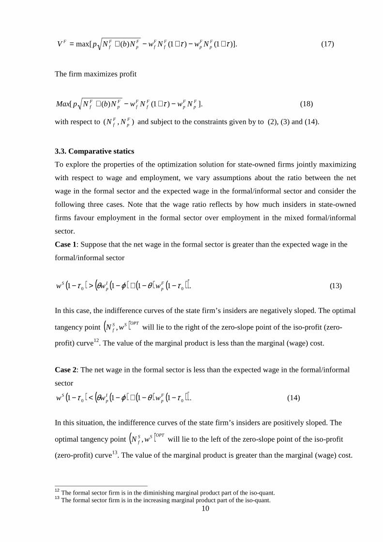
The firm maximizes profit
].)1()([ Fp
Fp
Ff
Ff
Fp
Ff NwNwNbNpMax −+−+ τ (18)
with respect to ),( Fp
Ff NN and subject to the constraints given by to (2), (3) and (14).
3.3. Comparative statics
To explore the properties of the optimization solution for state-owned firms jointly maximizing
with respect to wage and employment, we vary assumptions about the ratio between the net
wage in the formal sector and the expected wage in the formal/informal sector and consider the
following three cases. Note that the wage ratio reflects by how much insiders in state-owned
firms favour employment in the formal sector over employment in the mixed formal/informal
sector.
Case 1: Suppose that the net wage in the formal sector is greater than the expected wage in the
formal/informal sector
( ) ( ) ( ) ( )( ) )13( .1111 00 τθϕθτ −−+−>− Fp
Ip
S www
In this case, the indifference curves of the state firm’s insiders are negatively sloped. The optimal
tangency point ( )OPTSSf wN , will lie to the right of the zero-slope point of the iso-profit (zero-
profit) curve12. The value of the marginal product is less than the marginal (wage) cost.
Case 2: The net wage in the formal sector is less than the expected wage in the formal/informal
sector
( ) ( ) ( ) ( )( ) (14) . 1111 00 τθϕθτ −−+−<− Fp
Ip
S www
In this situation, the indifference curves of the state firm’s insiders are positively sloped. The
optimal tangency point ( )OPTSSf wN , will lie to the left of the zero-slope point of the iso-profit
(zero-profit) curve13. The value of the marginal product is greater than the marginal (wage) cost.
12 The formal sector firm is in the diminishing marginal product part of the iso-quant. 13 The formal sector firm is in the increasing marginal product part of the iso-quant.

11
Case 3: The net wage in the formal sector equals the expected wage in the formal/informal sector
( ) ( ) ( ) (15) . )1(111 00 τθϕθτ −−+−=− Fp
Ip
S www
The indifference curves of the state firm’s insiders are horizontal. The optimal tangency point
N fS ,wS OPT
will be at the zero-slope point of the iso-profit (zero-profit) curve. The value of
the marginal product is equal to the marginal (wage) cost.
These three possible outcomes have different implications for our main question of interest: the
differences in the impact that social benefits have on the employment in the formal,
formal/informal and informal sectors.
We can now sign the effects on employment in the various sectors and states of a change
in subsidies )(s , benefits )(b , the payroll tax rate )(τ , the detection probability )(ϕ and prices
)( p . Column b of the below table summarizes the signs for the expected directions of the
relationships in the model.
For Case 1, as social benefits increase from b0 to ,01 bb > the zero-profit curve shifts
downwards, and the optimum ( )OPTSSf wN , shifts in, resulting in lower wages and lower formal
sector employment, NfS , and higher formal/informal employment.
N s b M τ φ p Nf
S + - + - + + Nf
I + - - + - + Np
I - + + + - - Nf
F + - - - + + Np
F - + + - + -
We call this property the "attaching" property of social benefits, in the sense that despite lower
expected wages in the formal/informal sector, a higher level of social benefits leads to an inflow
of workers into that sector. A higher subsidy (Column s in the above table) would have an
opposite effect to that of an increase in benefits, leading to a higher formal sector employment,
NfS. A positive shock to aggregate demand (a higherp ) would also lead to higher formal sector
employment, but higher wages as well.
Note that we have assumed that workers who seek multiple jobs in both formal and
informal sectors can find employment there. Since these formal/informal workers are substitutes,
with some efficiency loss, for those who are employed solely in the informal sector, the inflow
of workers from the formal to the formal/informal sector will reduce informal sector

12
employment, as well as expected wages in the formal/informal and informal sectors.14
A higher probability of detection (columnϕ ) will increase full-time state sector employment and
private formal employment, but will reduce informal and formal/informal employment.
Cases 2 and 3 produce drastically different results. In Case 2, as social benefits increase and the
zero-profit curve shifts down, the optimal point ( )OPTSSf wN , shifts down to the right of the old
optimum, so that formal sector employment is higher, while formal sector wages are lower than
before and formal/informal employment decreases. Higher prices bring about lower formal
sector employment but also higher wages. Case 3 offers much the same results15.
There are important testable propositions to be gleaned from the first-order conditions.
First, when the ratio between formal wage to expected formal/informal wage is less than unity,
the slope of the insiders’ indifference curve is positive, indicating that full-time formal
employment within the firm is an economic “bad” for the insiders, and that their utility is
decreasing in it, or, conversely, that insiders’ utility is increasing in part-time employment
(naturally, as both groups receive equal benefits). So when the iso-profit curve shifts up due to
an exogenous decrease in benefits or an increase in the subsidy to benefits, implying that higher
employment can be sustained for the same zero profit, the insiders will shed their “bad”
consumption good (full-time labour) and acquire more of the “good” one (part-time labour). In
contrast, when the formal sector wage is high relative to the mixed formal/informal sector, a
decrease in benefits (and/or an increase in the subsidy to benefits) shifts the iso-profit curve up
leading to a higher “consumption” of the preferred type of employment, so that full-time
employment of insiders will go up and mixed sector employment will fall. The opposite happens
when benefits increase.
4. Testing the model with Ukrainian data
We now test the model’s propositions regarding the impact of changes in the structure and
financing of compensation on labour allocation across the three sectors. We use micro data from
the ULMS, exploiting information on employment by sector. We use a mixed multinomial logit
model of sector choice that integrates correlated errors arising from repeated measurements on
workers.
4.1. A mixed multinomial logit estimation of sector choice
14 As for the shift from the formal/informal and the formal into the informal sector, we do not model it explicitly but we expect social benefits to play an attaching role. We also expect a higher subsidy to social benefits and a positive shock to aggregate demand to have a similar effect. 15 Detailed results are available on request.

13
The revealed choice between J alternative sectors for work ity is observed for individual
worker i on occasion t. The choice set contains just three alternatives. These are: (i) being
employed in the informal sector; (ii) being employed in the formal sector; and (iii) holding
multiple jobs in the formal/informal (mixed) sector. Associated with each alternative sector j is a
probability of being employed in this sector, jitπ . In our paper, predictors of labour allocation
(sector choice) include the focal independent variables - the count of social (non-monetary)
benefits, the presence of subsidy to benefits, and wages - and the control variables that capture
economic and socio-demographic characteristics of individual i and contextual factors operating
on the firm and sector levels. Table 3A describes the main independent variables and the control
variables and Table 3B gives their descriptive statistics. The predictors reside in a matrix of
explanatory variables X it =(x it1 ,…, x it
J ), with x itj being a column vector associated with the
probability jitπ .
We use an extension of the multinomial logit model, where the response probabilities jitπ
depend on the nonlinear transformations of the linear function, ijit uX +β , and where because of
heterogeneity between individuals, individual-specific random intercepts iu account for intra-
individual correlation caused by multiple observations for individual i. (see, for instance, Rabe-
Hesketh and Skrondal, 2006). With a predictor vector x itj that includes a constant term, and
with the last among Jj ,...,1= alternatives as the reference category, the conditional
probability of a particular choice j can be written as follows:
( ) ( )( ).exp
exp,|Pr
11 ikitj
Jk
ijitjjitiitit
uX
uXuXjy
++∑
++=== −
= βαβα
π (16)
The effect of x im (the mth characteristic for individual i) on the logit of choice j relative to
choice k ( i.e. on the log-odds) is obtained as the contrast kmjm ββ − . The random effects ui
are assumed to be independent and identically distributed according to a normal distribution.
Note that in our specification, the vector u i allows for random variation in intrinsic preferences
across individuals with respect to their choice of employment sector but remains constant over
time and between alternatives for work.
In the model above (see Section 3), the effect of social benefits depends on the ratio of
expected formal to formal/informal wages in both sign and magnitude. The sign is dependent
upon the wage ratio being more or less than unity. To test this proposition, we add to the model

14
an interaction term between the wage ratio dummy and the social benefits variable, where the
wage ratio dummy takes the value of one if the relative wage is greater than one.16 We expect to
see a negatively-signed coefficient on this interaction variable. We also include a second
interaction term that is constructed as the product of the predicted wage ratio and the benefits
variable. This second interaction term is expected to show the impact of changes in the wage
ratio on the relative magnitude of the effect of social benefits on sector choice. Our conjecture is
that taking up work in the formal/informal sector will overall be positively (negatively)
influenced by the provision of social benefits (subsidies to benefits), and by whether workers
have experienced compulsory leave (temporary lay-offs), which is an indicator of the level of
activity in the firm17.
Using the ULMS data, we now create a sub-sample comprised of 6160 individual-years with
complete records for 2003 and 2004 for the variables listed in Table 3. Table 4 shows the
estimation results when the regression coefficients represent log-odds ratios. A positive
coefficient for an independent variable implies higher odds of observing an individual being in
the destination sector j rather than in the formal/informal (mixed) sector that is taken as the
reference category.
To allow for the possibility of a non-linear relation between the amount of social benefits and
employment sector choice, we categorize the count variable for social benefits by using four
categories (Table 3). For all the categories of the categorised variable for benefits, the main
effects are positive and significant (Table 4). This result is robust and holds for various
specifications, suggesting that non-monetary benefits are an important factor affecting sector
choice. The preference for being in the formal sector over the formal/informal sector is positively
related to the amount of benefits per se. However, the total effect of social benefits also depends
on the wage ratio between the formal sector and formal/informal sector. As predicted by the
model, wage ratios greater than unity are associated with a higher level of benefits leading to the
formal/informal sector being chosen with a higher probability. To explore this prediction further,
we compute the economic effects for the benefits and the benefits-wage ratio dummy
interactions. Because available statistical software that handles quantification of such effects for
categorical variables is restricted to binary logit models,18 we estimate a binary logit for choice
as an approximation of the first equation of Table 4 so that we can compute the total effect of
benefits on the probability of being in the mixed, formal/informal sector. We can quantify the
effects in a dummy-by-dummy interaction and hence use the four-category representation for the
16 Note that a continuous scale is assumed for the benefits variable in the interaction term. 17 It is a proxy for an aggregate demand shock. 18 Note that in the mixed logit framework, such effects are nonlinear and depend on the realised values of the other covariates (Mitchell and Chen, 2005).

15
benefits variable. We estimate a specification where the categorical variable for benefits is
interacted with the wage ratio dummy. The full set of estimation results from binary logit is
available upon request, while Table 5 displays the corresponding results from a mixed logit
model that has the same set of independent variables.
The results of the binary logit estimation are consistent with, and complement, the mixed
logit results of Table 419 and Table 520. Of particular interest are the total effects of each of the
benefits groups and subsidy. We find that while all benefit dummies are positive and significant,
for benefits16_group2 (one or two benefits) and benefits16_group4 (four to six benefits) the
interaction dummies are insignificant. However, in the case of having three benefits, both the
main effect for benefits16_group3 and the interaction term are significant. For the wage ratio
dummy equal to zero, the benefits16_group3 (three benefits) dummy decreases the probability of
choosing the formal/informal sector by 6 per cent, while for the wage ratio dummy equal to one,
the benefits16_group3 dummy actually increases this probability by 1 per cent. This result
supports the prediction of our model.
We conclude that for high enough formal sector wages, social benefits play an “attaching”
role in the mixed (formal/informal) sector, thus also influencing the composition of the purely
informal sector and formal employment. Subsidy to benefits is insignificant21 for the formal
sector work alternative, but tends to reduce informal employment. A higher predicted relative
formal wage increases the probability of working in the formal sector. It also increases the
probability to be employed in the informal sector since higher formal employment leads to lower
mixed employment.22
5. Conclusion The growth of an informal economy has been a feature of many transition countries. This paper looks
particularly at the case of Ukraine. Relying on the data from the ULMS, we started by estimating the
size and composition of the informal sector over the period from 1991-2004, and tried to shed some
light on individual and firm-level factors behind employment choices through a novel analytical
model of the firm-level utility maximization by insiders. Our approach, while building up on the
standard models of trade unions’ behaviour, brings in a number of original features that describe an
19 The wage ratio and the wage ratio interacted with continuous benefits are both excluded from the binary logit specification due to multicollinearity. 20 In this estimation, we also control for respondent’s age, age squared, gender, educational attainment and settlement type. 21 In the binary logit specification corresponding to that in Table 5, subsidy to benefits actually turns positive and significant. In particular, at the median level of the other covariates, subsidy raises the probability of being in the formal sector by 4 per cent. 22 Compulsory leave was always insignificant and was dropped. Employer size was not included due to endogeneity concerns, as data limitations precluded the inclusion of lagged variables. Note also that these results are robust to

16
economy with a strong inheritance from the planned economy, such as the importance of non-
monetary benefits in workers’ compensation, labour hoarding in the form of unpaid temporary
compulsory leave and state subsidies to benefits. When the model’s predictions are tested on the
ULMS panel data using mixed multinomial logit, we find that, in terms of labour allocation among
formal, mixed (formal/informal) and informal sectors at a given point of time, non-monetary
compensation plays an attaching role in the mixed formal/informal sector for a high enough predicted
formal/mixed wage ratio. Our findings confirm, if only at the sectoral level, previous results by
Commander and Schankerman (1997) and Friebel and Guriev (2005) on the important worker-
attaching role of social benefits at the firm level. We also find for the static case of the model that the
empirical results point to the joint maximization of the firm’s utility with respect to both employment
and wages. In the dynamic setting, the results from a multinomial logit analysis of transitions between
sectors again suggest the same important attaching role of non-monetary benefits. However, the
optimization problem here tends to be with respect to employment only. This is one puzzle that
merits further analysis. One possible explanation for this could be the underlying optimization policy
of firms from which transitions take place. For the mover starting in the formal sector, her decision to
make a transition may reflect the response to her current firm’s policy to optimize with respect to
only employment. Finally, our results have implications for policies aiming at improving
efficiency of labour allocation in transition countries. Although our findings relate to Ukraine,
we suspect that they may generalize beyond its borders, in particular to the other countries of the
Former Soviet Union.
adding the wage ratio term to the set of regressors. The results are available on request.

17
References
Bernabe, Sabine, 1999. A profile of informal employment: the case of Georgia. International Labour Office, Geneva.
Commander, Simon, Rodionova, Yulia, 2005. The informal sector in Ukraine: its size, structure and dynamics. EBRD and London Business School, mimeo.
Commander, Simon, Tolstopiatenko, Andrei, 1997. A model of the informal economy in transition. World Bank, mimeo.
Commander, Simon, Schankerman, Mark, 1997. Enterprise restructuring and social benefits. Economics of Transition, 5, pp. 1-24.
Commander, Simon, Sumana Dhar, Yemtsov, Ruslan, 1996a. How Russian firms make their wage and employment decisions. In: Commander, Simon, Fan, Qimiao, Schaffer, Mark, E. (Eds.), Enterprise Restructuring and Economic Policy in Russia. Washington, D.C.: The World Bank, pp. 15–51.
Commander, Simon, Lee, Une, J., Tolstopiatenko, Andrei, 1996b. Social benefits and the Russian industrial firm. In: Commander, Simon, Fan, Qimiao, Schaffer, Mark, E. (Eds.), Enterprise Restructuring and Economic Policy in Russia. Washington, D.C.: The World Bank, pp. 52–83.
Commander, Simon, Liberman, Leonid, Yemtsov, Ruslan, 1993. Wage and employment decisions in the Russian economy: an analysis of developments in 1992. Working Paper No. 1205. EDI. Washington, D.C.
Farber, Henry S., 1987. The analysis of union behaviour. In: Ashenfelter, O., Layard, R., and Card, D. (Eds.), Handbook of Labor Economics, Ch.18, Elsevier. pp. 1039-1089.
Friebel, Guido, Guriev, Sergei, 2005. Attaching workers through in-kind payments: theory and evidence from Russia. World Bank Economic Review, 19, pp. 175-202.
Johnson, Simon, Kaufman, Daniel, Schleifer, Andrei, 1997. The unofficial economy in transition. Brookings Papers on Economic Activity, 2, December.
Krstic, Gorana, 2003. Empirical aspects of the formal and informal labour market in the Federal Republic of Yugoslavia. PhD, University of Sussex.
Lacko, Maria, 2000. Hidden economy – an unknown quantity? Economics of Transition, 8, pp 117-149. Mitchell, Michael N. and Chen, Xiao, 2005. Visualizing main effects and interactions for binary logit models. Stata Journal, 5, pp. 64–82.
Rabe-Hesketh, Sophia, Skrondal, Andrei, 2006. Multilevel modelling of complex survey data. Journal of Royal Statistical Society Association, 169, Part 4, pp. 805–82.
Rein, Martin, Friedman, Barry, L., Worgotter, Andreas, 1997. Enterprise and social benefits after communism. Cambridge University Press, Cambridge.
Schneider, Friedrich, Enste, Dominik H., 2000. Shadow economies: size, causes and consequences. Journal of Economic Literature, 38, pp. 77-114.
Yoon, Yang-Ro, Reilly, Barry, Krstic, Gorana, Bernabe, Sabine, 2003. A study of informal labour market activity in the CIS-7. World Bank, mimeo.

18
Tables:
Table 1: Ukraine: informal sector employment in 1991, 1997, 2003 & 2004 (% of all working)
1991 1997 2003 2004 Measure 1: share of employment in informal activity outside of agriculture 10 17 13 17
Measure 2: Measure 1 plus individuals involved in non-agricultural household production and sale of agricultural goods on a secondary basis
16 26 16 23
Measure 3: Measure 2 plus individuals involved in agricultural production for their own use
50 65 58 66
Table 2: Transition matrix for 2003 -2004 (%)
N obs = 2824 Formal only Formal / Informal Informal only Formal only 90 6 4 Formal/Informal 45 35 20 Informal only 28 4 68

19
Table 3A: Definition of variables
Variable name Variable description Employer characteristics and wage differences across sectors
Social benefits (count of benefits1-6; reference category Benefits_group1 = No social benefits)
Benefits16_group2 (1 or 2 benefits) Dummy = 1 if respondent receives one or two types of benefits
Benefits16_group3 ( 3 benefits) Dummy = 1 if respondent receives three types of benefits
Benefits16_group4 (4-6 benefits) Dummy = 1 if respondent receives four to six types of benefits
Subsidy to benefits Dummy = 1 if the enterprise is a budgetary enterprise, or a state enterprise,
or a local municipal enterprise, or a state or collective farm
Employer size (reference category Employer size 1 = 1-9 employees (micro firms)
Employer_size 2 10-49 people Dummy = 1 if the enterprise has 10 to 49 employees
Employer_size 3 50-249 people Dummy = 1 if the enterprise has 50 to2 49 employees
Employer_size 4 250 people and more Dummy = 1 if the enterprise has >250 employees
Ratio of predicted formal sector wage to predicted formal/informal sector wage
Ratio of predicted wages constructed using Heckman estimation.
Wage Ratio Dummy Dummy =1 if (Predicted formal sector wage/ Predicted formal/informal
sector wage) >1
Benefits x (Predicted formal sector wage/ Predicted formal/informal sector wage)
Benefits variable treated as continuous times the Ratio of predicted wages constructed using Heckman estimation.
Benefits ××××Wage Ratio Dummy Benefits variable treated as continuous times Wage Ratio Dummy
Employment sector Categorical variable = 1 if respondent has formal employment, = 2 if respondent has both formal and informal employment, = 3 if respondent has informal employment only.
(continued on next page)

20
Table 3A: cont. Variable name
Variable description
Worker characteristics socio-demographics and measures of access to, and level of education; previous unemployment, occupation
Age Age of respondent, in years
Female Dummy = 1 for female respondent
Settlement Type (reference category Village)
PGT (small settlement of town type) Dummy = 1 if respondent lives in PGT
Small or medium-sized town Dummy = 1 if respondent lives in small or medium-sized town
Large city Dummy = 1 if respondent lives in a large city
Capital city Dummy = 1 if respondent lives in the capital city
Education (reference category Education1 = diploma of high school /general secondary education)
Education2 Dummy = 1 if respondent has incomplete professional higher education, or bachelors, masters, or candidate of sciences degree
Education3 Dummy = 1 if respondent has completed grades 1-6, 7-9, 10-11 or
received a PTU diploma
Previous unemployment (i.e. whether was temporarily laid off)
Compulsory leave Dummy = 1 if respondent experienced compulsory leave in the current employment
Occupation / Job Type (reference category “being manager or professional”)
Technician Dummy = 1 if respondent works as technician
Clerks Dummy = 1 if respondent works as clerk
Service worker Dummy = 1 if respondent works as service worker
Skilled agricultural worker Dummy = 1 if respondent works as skilled agricultural worker
Artisan Dummy = 1 if respondent works as artisan
Plant operator Dummy = 1 if respondent works as plant operator
Elementary occupation Dummy = 1 if respondent has an elementary occupation
Armed Forces Dummy = 1 if respondent serves in armed forces

21
Table 3B: Descriptive statistics for the main independent variables Variable Mean StD Median Subsidy_(to)_benefits 0.6 0.5 1 Overall
0.6 0.5 1 2003
0.5 0.5 1 2004
Benefits_cat == 1 0.2 0.4 0 Overall
0.2 0.4 0 2003
0.3 0.4 0 2004
Benefits_cat == 2 0.2 0.4 0 Overall
0.2 0.4 0 2003
0.2 0.4 0 2004
Benefits_cat == 3 0.3 0.5 0 Overall
0.4 0.5 0 2003
0.3 0.5 0 2004
Benefits_cat == 4 0.2 0.4 0 Overall
0.2 0.4 0 2003
0.2 0.4 0 2004
Employer size 2.69 1.11 na Overall
2.57 1.14 na 2003
2.63 1.12 na 2004
Wage ratio : Ratio of predicted formal sector wage to predicted formal/informal sector wage
0.8
0.5
0.6
Overall
0.7 0.4 0.7 2003
0.8 0.6 0.6 2004
Wage ratio × benefits 2.0 1.7 1.6 Overall
1.9 1.3 1.7 2003
2.0 2.0 1.5 2004
Wage ratio dummy 0.2 0.4 0.0 Overall
0.1 0.3 0 2003
0.2 0.4 0 2004
Benefits × Wage ratio dummy 0.4 1.0 0 Overall
0.3 0.9 0 2003
0.5 1.1 0 2004
Gender 0.5 0.5 0 Overall
0.5 0.5 0 2003
0.5 0.5 0 2004
Age 40.0 12.2 41 Overall
40.2 12.4 41 2003
39.9 11.9 41 2004
Sample frequencies for the settlement type variable
Village PGT Small town Medium-sized
town Large town Capital city
0.26 0.13 0.01 0.12 0.24 0.24 Overall
0.28 0.13 0.02 0.10 0.23 0.24 2003
0.24 0.14 0.01 0.13 0.25 0.24 2004

22
Table 4: Estimation results for sector choice from mixed logit, with benefits entering the Benefits ×××× Wage Ratio interactions as a continuous variable23
Dependent variable: Sector for Work Choice Reference category: Work in Formal/Informal Sector
Equation I: Work in Formal Sector
Equation II: Work in Informal Sector
Independent variables: Employer characteristics and wage differences across sectors:
Social benefits (relative to Benefits_group1 = No social benefits) Benefits16_group2 (1 or 2 benefits) 1.280*** -1.665*** (0.272) (0.382)
Benefits16_group3 ( 3 benefits) 1.268*** -3.011*** (0.385) (0.560) Benefits16_group4 (4-6 benefits) 1.150** -3.190*** (0.501) (0.899) Subsidy to benefits dummy -0.004 -2.047*** (0.173) (0.342) Predicted formal sector wage/ Predicted formal/informal sector wage 1.241*** 0.841* (0.430) (0.480) Benefits × (Predicted formal sector wage/ Predicted formal/informal sector wage) -0.322 -0.247
(0.197) (0.295) Wage Ratio Dummy: 1 if (Predicted formal sector wage/ Predicted formal/informal sector wage)>1
dropped dropped
Benefits × Wage Ratio Dummy -0.614*** -0.794*** (0.160) (0.262) Compulsory leave Not included Not included Employer size (relative to Employer size 1 = 1-9 employees, i.e. micro firms) Not included Not included Employer_size 2 (10-49 people) Employer_size 3 (50-249 people) Employer_size 4 (250 people and more) Year dummy for 2004 0.771*** 1.701*** (0.064) (0.048)
Constant -1544.943*** -3406.27*** (127.488) (95.465)
Variance of random intercepts 3.573 (0.387)
No. of observations 6160 6160 Reported: coefficients (log odds ratios), robust standard errors in parentheses.
Significance levels: * - 10%, ** - 5%, *** - 1%. Weighted by sample (population) weights.
23 In this estimation, we also control for respondent’s age, age squared, gender, educational attainment and settlement type.

23
Table 5: Estimation results for sector choice using mixed logit, with benefits entering the Benefits ×××× Wage Ratio interaction as a categorical variable24
Dependent variable: Sector for Work Choice Reference category: Work in Formal/Informal Sector
Equation I: Work in Formal Sector
Equation II: Work in Informal Sector
Independent variables: Employer characteristics and wage differences across sectors:
Social benefits (relative to Benefits_group1 = No social benefits) Benefits16_group2 (1 or 2 benefits) 2.024*** -0.962***
(0.292) (0.372) Benefits16_group3 ( 3 benefits) 1.026*** -3.225***
(0.257) (0.467) Benefits16_group4 (4-6 benefits) 0.117 -4.118***
(0.301) (0.634) Subsidy to benefits dummy -0.026 -2.101***
(0.173) (0.342) Predicted formal sector wage/ Predicted formal/informal sector wage dropped dropped Benefits × (Predicted formal sector wage/ Predicted formal/informal sector wage) dropped dropped Wage Ratio Dummy: 1 if (Predicted formal sector wage/ Predicted formal/informal sector wage)>1
-0.164 (0.323)
-0.788***
(0.336) Benefits16_group2 × Wage Ratio Dummy -2.584*** -2.141***
Benefits16_group3 × Wage Ratio Dummy Benefits16_group4 × Wage Ratio Dummy
(0.629) -1.828***
(0.560) dropped
(0.842) -1.450 (0.984) dropped
Compulsory leave Not included Not included Employer size (relative to Employer size 1 = 1-9 employees, i.e. micro firms) Not included Not included Employer_size 2 (10-49 people) Employer_size 3 (50-249 people) Employer_size 4 (250 people and more) Year dummy for 2004 0.969*** 1.922*** (0.0004) (0.068) Constant -1943.548*** -3850.498*** (0.907) (136.963) Variance of random intercepts 2.708 (0.230) No. of observations 6160 6160 Reported: coefficients (log odds ratios), robust standard errors in parentheses. Significance levels: * - 10%, ** - 5%, *** - 1%. Weighted by sample (population) weights.
24 In this estimation, we also control for respondent’s age, age squared, gender, educational attainment and settlement type.
Copyright © 2022 FDOKUMEN