A Method for Handling Data that Exhibit Mixed Spatial Variation
12
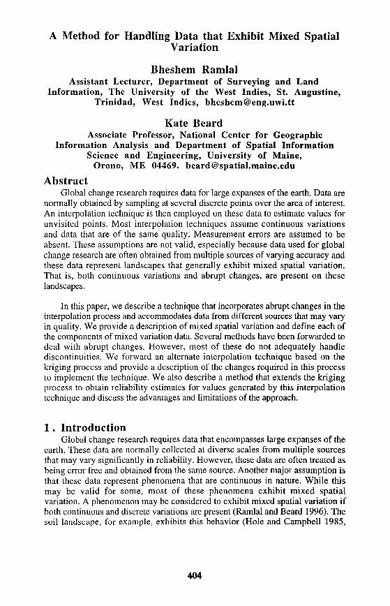
A Method for Handling Data that Exhibit Mixed Spatial Variation Bheshem Ramlal Assistant Lecturer, Department of Surveying and Land Information, The University of the West Indies, St. Augustine, Trinidad, West Indies, [email protected] Kate Beard Associate Professor, National Center for Geographic Information Analysis and Department of Spatial Information Science and Engineering, University of Maine, Orono, ME 04469. [email protected] Abstract Global change research requires data for large expanses of the earth. Data are normally obtained by sampling at several discrete points over the area of interest. An interpolation technique is then employed on these data to estimate values for unvisited points. Most interpolation techniques assume continuous variations and data that are of the same quality. Measurement errors are assumed to be absent. These assumptions are not valid, especially because data used for global change research are often obtained from multiple sources of varying accuracy and these data represent landscapes that generally exhibit mixed spatial variation. That is, both continuous variations and abrupt changes, are present on these landscapes. In this paper, we describe a technique that incorporates abrupt changes in the interpolation process and accommodates data from different sources that may vary in quality. We provide a description of mixed spatial variation and define each of the components of mixed variation data. Several methods have been forwarded to deal with abrupt changes. However, most of these do not adequately handle discontinuities. We forward an alternate interpolation technique based on the kriging process and provide a description of the changes required in this process to implement the technique. We also describe a method that extends the kriging process to obtain reliability estimates for values generated by this interpolation technique and discuss the advantages and limitations of the approach. 1. Introduction Global change research requires data that encompasses large expanses of the earth. These data are normally collected at diverse scales from multiple sources that may vary significantly in reliability. However, these data are often treated as being error free and obtained from the same source. Another major assumption is that these data represent phenomena that are continuous in nature. While this may be valid for some, most of these phenomena exhibit mixed spatial variation. A phenomenon may be considered to exhibit mixed spatial variation if both continuous and discrete variations are present (Ramlal and Beard 1996). The soil landscape, for example, exhibits this behavior (Hole and Campbell 1985, 404
-
Upload
westindiesstaugustine -
Category
Documents
-
view
1 -
download
0
Transcript of A Method for Handling Data that Exhibit Mixed Spatial Variation
A Method for Handling Data that Exhibit Mixed SpatialVariation
Bheshem RamlalAssistant Lecturer, Department of Surveying and Land
Information, The University of the West Indies, St. Augustine,Trinidad, West Indies, [email protected]
Kate BeardAssociate Professor, National Center for Geographic
Information Analysis and Department of Spatial Information Science and Engineering, University of Maine,
Orono, ME 04469. [email protected]
AbstractGlobal change research requires data for large expanses of the earth. Data are
normally obtained by sampling at several discrete points over the area of interest. An interpolation technique is then employed on these data to estimate values for unvisited points. Most interpolation techniques assume continuous variations and data that are of the same quality. Measurement errors are assumed to be absent. These assumptions are not valid, especially because data used for global change research are often obtained from multiple sources of varying accuracy and these data represent landscapes that generally exhibit mixed spatial variation. That is, both continuous variations and abrupt changes, are present on these landscapes.
In this paper, we describe a technique that incorporates abrupt changes in the interpolation process and accommodates data from different sources that may vary in quality. We provide a description of mixed spatial variation and define each of the components of mixed variation data. Several methods have been forwarded to deal with abrupt changes. However, most of these do not adequately handle discontinuities. We forward an alternate interpolation technique based on the kriging process and provide a description of the changes required in this process to implement the technique. We also describe a method that extends the kriging process to obtain reliability estimates for values generated by this interpolation technique and discuss the advantages and limitations of the approach.
1. IntroductionGlobal change research requires data that encompasses large expanses of the
earth. These data are normally collected at diverse scales from multiple sources that may vary significantly in reliability. However, these data are often treated as being error free and obtained from the same source. Another major assumption is that these data represent phenomena that are continuous in nature. While this may be valid for some, most of these phenomena exhibit mixed spatial variation. A phenomenon may be considered to exhibit mixed spatial variation if both continuous and discrete variations are present (Ramlal and Beard 1996). The soil landscape, for example, exhibits this behavior (Hole and Campbell 1985,
404
Voltz and Webster 1990). Usually these landscapes are treated as being either completely continuous with transitional variations or comprised of discrete, well defined, homogeneous units (Burrough 1993). Neither of these approaches fully capture all the variations that are present in the landscape (Burrough 1989, Heuvelink 1993). The representations provided by these models are therefore limited (Burrough 1993, Ernstrom and Lytle 1993, Ramlal and Beard 1996). Although some researchers have acknowledge the presence of discontinuities, most interpolation methods avoid the incorporation of the line of discrete change in the process (Marechal 1983, Stein et al. 1988, Voltz and Webster 1990, McBratney et al 1991, Brus 1994).
This paper describes an interpolation technique that processes data that: (i) exhibit mixed spatial variations, (ii) may have been obtained from different sources, and (iii) may vary in quality. The soil landscape is used as an example here. Note that while the discussion focuses on soil data at scales larger than global, the solution that are being forwarded may be adapted to other phenomena that exhibit global variations. The second section of this paper provides a description of mixed spatial variation and defines each of the components of mixed variation data. Several methods have been forwarded to deal with abrupt changes. The third section discusses these methods, and their advantages and limitations for handling discontinuities. The fourth section of the paper presents an alternate interpolation technique based on the kriging process and provides a description of the changes required in this process to implement the technique. This section also describes methods for incorporating discontinuities in the computation of the semi-variogram and generating estimates for unvisited points. The fifth section forwards a method to extend the kriging process to obtain reliability estimates for values generated by this interpolation technique and discusses the advantages and limitations of this approach. The last section presents a discussion of the benefits and limitations of the proposed technique.
2. The Components of Mixed Spatial Variation DataCapturing mixed spatial variation requires the use of sampling strategies
that capture both continuous variations and abrupt changes. The soil landscape cannot be completely sampled because this will destroy it (Burrough 1993). Other phenomena, such as rainfall, are not completely captured because it is financially unfeasible to obtain a comprehensive coverage of samples for large expanses of the earth. Point samples taken at intervals over the landscape suffice to provide a representation of the continuous variation that are present in phenomena that exhibit mixed spatial variations. Several sampling strategies are discussed in the literature for locating sample points for the soil landscape. See for example Burgess and Webster (1980), Van Kuilenberg et al. (1982), McBratney and Webster (1983), and Webster and Oliver (1992).
Phenomena that exhibit mixed spatial variations also contain discontinuities. These abrupt changes occur along lines for surfaces, and surfaces for volumes. These changes may be visible on the surface, may occur beneath the surface or may not be visible at all for some phenomena. They may be
405
vertical or inclined. Throughout this paper the term line of abrupt change is used to denote both lines and surfaces of abrupt change.
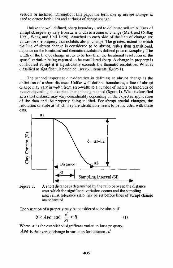
Unlike the well defined, sharp boundary used to delineate soil units, lines of abrupt change may vary from zero-width to a zone of change (Mark and Csillag 1991, Wang and Hall 1996). Attached to each side of the line of change are values for the property that exhibits abrupt change. The greatest extent to which the line of abrupt change is considered to be abrupt, rather than transitional, depends on the locational and thematic resolutions defined prior to sampling. The width of the line of change needs to be less than the locational resolution of the spatial variation being captured to be considered sharp. A change in property is considered abrupt if it significantly exceeds the thematic resolution. What is classified as significant is based on user requirements (figure 1).
The second important consideration in defining an abrupt change is the definition of a short distance. Unlike well-defined boundaries, a line of abrupt change may vary in width from zero-width to a number of meters or hundreds of meters depending on the phenomenon being mapped (figure 1). What is classified as a short distance may vary considerably depending on the expected application of the data and the property being studied. For abrupt spatial changes, the resolution or scale at which they are identifiable needs to be included with these data.
g -t-j§ U
.siSampling interval (SI)
Figure 1. A short distance is determined by the ratio between the distance over which the significant variation occurs and the sampling interval. A tolerance ratio may be set before lines of abrupt change are delineated
The variation of a property may be considered to be abrupt if
8<Ave and — <R (1)SI
Where 8 is the established significant variation for a property,Ave is the average change in variation for distance , d
406
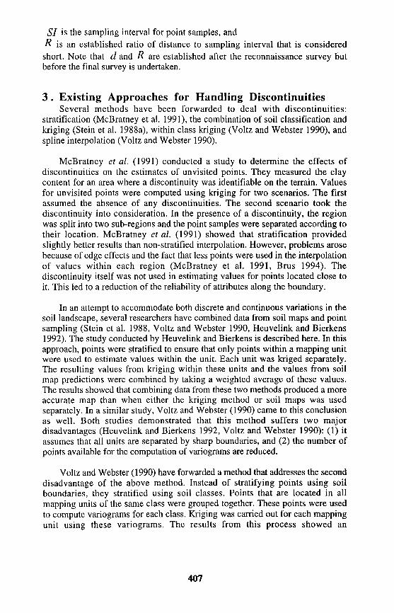
57 is the sampling interval for point samples, andR is an established ratio of distance to sampling interval that is considered short. Note that d and R are established after the reconnaissance survey But before the final survey is undertaken.
3. Existing Approaches for Handling DiscontinuitiesSeveral methods have been forwarded to deal with discontinuities:
stratification (McBratney et al. 1991), the combination of soil classification and kriging (Stein et al. 1988a), within class kriging (Voltz and Webster 1990), and spline interpolation (Voltz and Webster 1990).
McBratney et al. (1991) conducted a study to determine the effects of discontinuities on the estimates of unvisited points. They measured the clay content for an area where a discontinuity was identifiable on the terrain. Values for unvisited points were computed using kriging for two scenarios. The first assumed the absence of any discontinuities. The second scenario took the discontinuity into consideration. In the presence of a discontinuity, the region was split into two sub-regions and the point samples were separated according to their location. McBratney et al. (1991) showed that stratification provided slightly better results than non-stratified interpolation. However, problems arose because of edge effects and the fact that less points were used in the interpolation of values within each region (McBratney et al. 1991, Brus 1994). The discontinuity itself was not used in estimating values for points located close to it. This led to a reduction of the reliability of attributes along the boundary.
In an attempt to accommodate both discrete and continuous variations in the soil landscape, several researchers have combined data from soil maps and point sampling (Stein et al. 1988, Voltz and Webster 1990, Heuvelink and Bierkens 1992). The study conducted by Heuvelink and Bierkens is described here. In this approach, points were stratified to ensure that only points within a mapping unit were used to estimate values within the unit. Each unit was kriged separately. The resulting values from kriging within these units and the values from soil map predictions were combined by taking a weighted average of these values. The results showed that combining data from these two methods produced a more accurate map than when either the kriging method or soil maps was used separately. In a similar study, Voltz and Webster (1990) came to this conclusion as well. Both studies demonstrated that this method suffers two major disadvantages (Heuvelink and Bierkens 1992, Voltz and Webster 1990): (1) it assumes that all units are separated by sharp boundaries, and (2) the number of points available for the computation of variograms are reduced.
Voltz and Webster (1990) have forwarded a method that addresses the second disadvantage of the above method. Instead of stratifying points using soil boundaries, they stratified using soil classes. Points that are located in all mapping units of the same class were grouped together. These points were used to compute variograms for each class. Kriging was carried out for each mapping unit using these variograms. The results from this process showed an
407
improvement over the use of simple kriging or the use of soil maps separately (Voltz and Webster 1990). However, this approach suffers many disadvantages. Homogeneity within soil classes was assumed. This is not necessarily valid (Voltz and Webster 1990). Additionally, sharp boundaries and homogeneous mapping units were assumed. These assumptions do not always hold. Another problem with this method is that the spatial context is lost when points are grouped together based on soil classes. Both this and the previous method do not address the problem of edge effects that occur at the boundaries of mapping units.
Voltz and Webster (1990) also examined the use of spline interpolation for handling discontinuities. They chose joining points for spline curves, called knots, such that local variations, especially soil boundaries, will not be smoothed out. The results of this method were compared with the results from within class kriging, soil classification, and stratification using soil mapping units. Spline interpolation performed better than traditional soil classification. However, both stratification and within class kriging performed better than spline interpolation. Voltz and Webster (1990) concluded that the major limitation of this approach is that it over-accentuates boundaries and fluctuates more than kriging curves, which implied too much influence from local variations.
4. An Alternate ApproachUnlike the methods forwarded by Stein et al. (1988) and Voltz and Webster
(1990) to handle discontinuities, there are no soil mapping units and soil classes in the mixed variation model. These two approaches are not appropriate here. The method presented by McBratney et al. (1991) assumes a single discontinuity that spanned the entire length of the area. Two separate areas were therefore easily identifiable. In the mixed variation model, more than one line of abrupt change is present. As a consequence, an alternate solution is required. An alternate method that accommodates discontinuities and generates reliability estimates for interpolated points is presented. This method is based on the kriging process. Discussions of kriging may be found in Cressie (1991), Burrough (1993), Burgess and Webster (1980), and Davis (1991).
4.1 Generating Semi-VariogramsThe inclusion of values from lines of abrupt change in the computation of
semi- variograms requires the use of points on these lines rather than the lines themselves. Points are used instead of lines so that over-influence on the resulting semi-variograms, by these lines, is avoided. The following procedure is forwarded to achieve this. The assumption here is that lines of abrupt change are used to stratify points into regions and that these lines will influence the range of the semi-variogram. Since discontinuities may not be present in all directions, separate semi-variograms should be computed for different directions. This may be done for eight directions (Webster and Oliver 1990).
408
>" Intersection points
^S- Point samples
Line of abrupt change
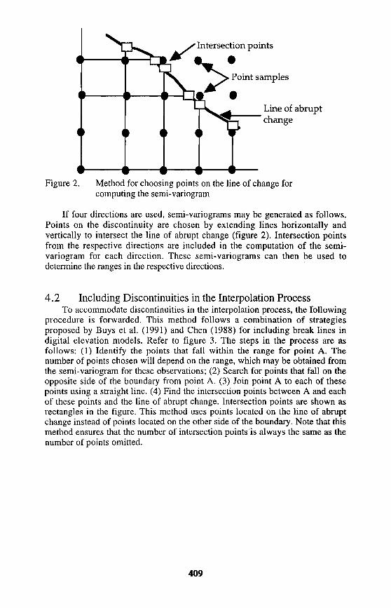
Figure 2. Method for choosing points on the line of change for computing the semi-variogram
If four directions are used, semi-variograms may be generated as follows. Points on the discontinuity are chosen by extending lines horizontally and vertically to intersect the line of abrupt change (figure 2). Intersection points from the respective directions are included in the computation of the semi- variogram for each direction. These semi-variograms can then be used to determine the ranges in the respective directions.
4.2 Including Discontinuities in the Interpolation ProcessTo accommodate discontinuities in the interpolation process, the following
procedure is forwarded. This method follows a combination of strategies proposed by Buys et al. (1991) and Chen (1988) for including break lines in digital elevation models. Refer to figure 3. The steps in the process are as follows: (1) Identify the points that fall within the range for point A. The number of points chosen will depend on the range, which may be obtained from the semi-variogram for these observations; (2) Search for points that fall on the opposite side of the boundary from point A. (3) Join point A to each of these points using a straight line. (4) Find the intersection points between A and each of these points and the line of abrupt change. Intersection points are shown as rectangles in the figure. This method uses points located on the line of abrupt change instead of points located on the other side of the boundary. Note that this method ensures that the number of intersection points 'is always the same as the number of points omitted.
409
Kernel
Intersection point
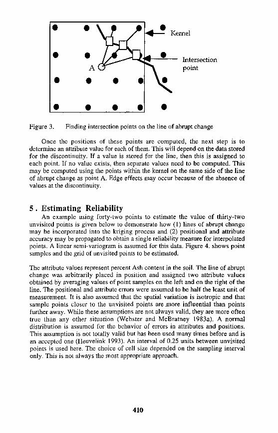
Figure 3. Finding intersection points on the line of abrupt change
Once the positions of these points are computed, the next step is to determine an attribute value for each of them. This will depend on the data stored for the discontinuity. If a value is stored for the line, then this is assigned to each point. If no value exists, then separate values need to be computed. This may be computed using the points within the kernel on the same side of the line of abrupt change as point A. Edge effects may occur because of the absence of values at the discontinuity.
5. Estimating ReliabilityAn example using forty-two points to estimate the value of thirty-two
unvisited points is given below to demonstrate how (1) lines of abrupt change may be incorporated into the kriging process and (2) positional and attribute accuracy may be propagated to obtain a single reliability measure for interpolated points. A linear semi-variogram is assumed for this data. Figure 4. shows point samples and the grid of unvisited points to be estimated.
The attribute values represent percent Ash content in the soil. The line of abrupt change was arbitrarily placed in position and assigned two attribute values obtained by averaging values of point samples on the left and on the right of the line. The positional and attribute errors were assumed to be half the least unit of measurement. It is also assumed that the spatial variation is isotropic and that sample points closer to the unvisited points arejnore influential than points further away. While these assumptions are not always valid, they are more often true than any other situation (Webster and McBratney 1983a). A normal distribution is assumed for the behavior of errors in attributes and positions. This assumption is not totally valid but has been used many times before and is an accepted one (Heuvelink 1993). An interval of 0.25 units between unvisited points is used here. The choice of cell size depended on the sampling interval only. This is not always the most appropriate approach.
410
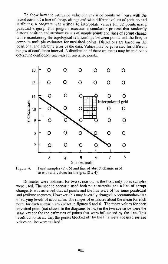
To show how the estimated value for unvisited points will vary with the introduction of a line of abrupt change and with different values of position and attributes, a program was written to interpolate values for 32 points using punctual kriging. This program executes a simulation process that randomly distorts position and attribute values of sample points and lines of abrupt change while maintaining the topological relationships between points and the line, to compute multiple estimates for unvisited points. Distortions are based on the positional and attribute error of the data. Values may be generated for different ranges of confidence interval. A distribution of these estimates may be studied to determine confidence intervals for unvisited points.
13-Q 0 O 0 O 0
12 - 0 000 O
110)•*-> OS
1 10JHOO
> 9
8
- o- 0
- 0
- o7 - O
0
o oInterpolated grid
0 0
0
o
Figure 4.
34567 X coordinate
Point samples (7 x 6) and line of abrupt change used to estimate values for the grid (8 x 4)
Estimates were obtained for two scenarios. In the first, only point samples were used. The second scenario used both point samples and a line of abrupt change. It was assumed that all points and the line were of the same positional and attribute accuracy. However, this may be easily changed to accommodate data of varying levels of accuracies. The ranges of estimates about the mean for each point for each scenario are shown in figures 5 and 6. The mean values for each unvisited point (not shown in the diagrams below) in the two scenarios were the same except for the estimates of points that were influenced by the line. This result demonstrate that the points blocked off by the line were not used instead values on line were utilized.
411
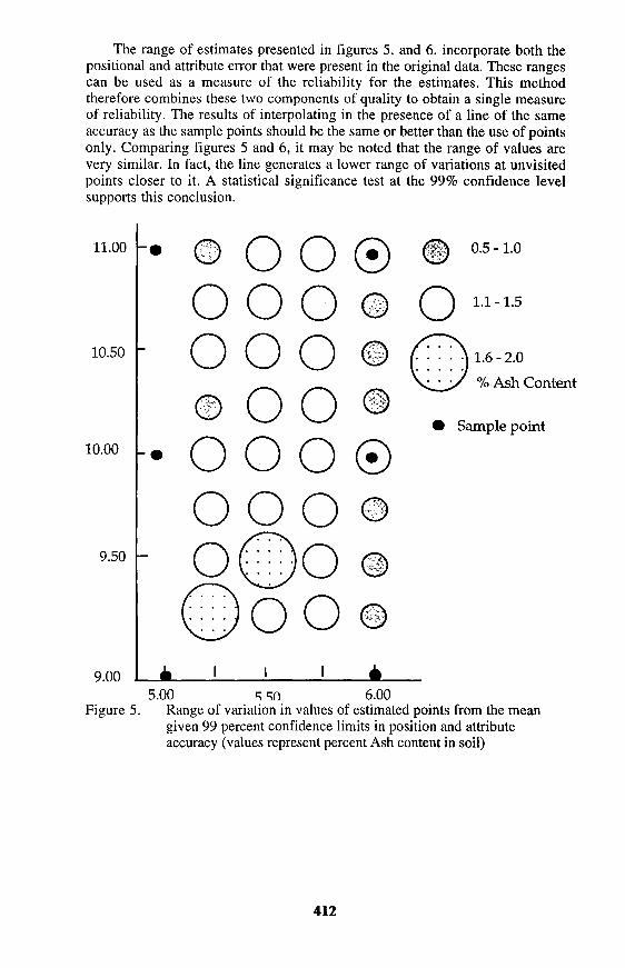
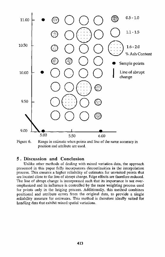
The range of estimates presented in figures 5. and 6. incorporate both the positional and attribute error that were present in the original data. These ranges can be used as a measure of the reliability for the estimates. This method therefore combines these two components of quality to obtain a single measure of reliability. The results of interpolating in the presence of a line of the same accuracy as the sample points should be the same or better than the use of points only. Comparing figures 5 and 6, it may be noted that the range of values are very similar. In fact, the line generates a lower range of variations at unvisited points closer to it. A statistical significance test at the 99% confidence level supports this conclusion.
11.00
10.50
10.00
9.50
© oo© ooo @ ooo
0.5 -1.0
O "-
ooo©ooo
1.6 - 2.0% Ash Content
Sample point
I9.005.00 s RO 6.00
Figure 5. Range of variation in values of estimated points from the mean given 99 percent confidence limits in position and attribute accuracy (values represent percent Ash content in soil)
412
11.00
10.50
10.00
9.50
ooooooo
000
0.5 -1.0
1.1 -1.5
1.6 - 2.0
% Ash Content
Sample points
Line of abrupt change
5.00 5.50 6.00Range in estimate when points and line of the same accuracy in position and attribute are used.
5. Discussion and ConclusionUnlike other methods of dealing with mixed variation data, the approach
presented in this paper fully incorporates discontinuities in the interpolation process. This .ensures a higher reliability of estimates for unvisited points that are located close to the line of abrupt change. Edge effects are therefore reduced. The line of abrupt change is incorporated such that its importance is not over emphasized and its influence is controlled by the same weighting process used for points only in the kriging process. Additionally, this method combines positional and attribute errors from the original data, to provide a single reliability measure for estimates. This method is therefore ideally suited for handling data that exhibit mixed spatial variations.
413
ReferencesBrus, D.J. (1994). "Improving design-based estimation of spatial means by soil map stratification. A case study of phosphate saturation." Geoderma 62: 233- 246.
Burgess, T.M. and Webster, R. (1980a). "Optimal interpolation and isarithmic mapping of soil properties I. The semi-variogram and punctual Kriging." Journal of Soil Science 31: 315-331.
Burgess, T.M. Webster, R. McBratney, A.B. (1981) "Optimal interpolation and isarithmic mapping of soil properties IV. Sampling Strategy." Journal of Soil Science 32:643-659.
Burrough, P.A. (1993). "Soil variability: a late 20th century view." Soil and Fertilizers 56.5: 529-562.
Buys, J. Messerschmidt, H.J. Botha, J.F. (1991). "Including known discontinuities directly into a triangular irregular mesh for automatic contouring purposes." Computers and Geosciences 17.7: 875-881.
Chen, Z. (1988). Break lines on terrain surface. GIS/LIS'88.
Cressie, N. (1993) Statistics for Spatial Data (Revised Edition^ Toronto: Wiley and Sons.
Davis, J.C. (1991). Statistics and Data Analysis in Geology (2nd Edition). New York: Wiley and Sons.
Ernstrom, D. J. and Lytle, D. (1993). "Enhanced soil information systems from advances in computer technology." Geoderma 60: 327-341.
Heuvelink, G.B.M. and Bierkens, M.F.P. (1992). "Combining soil maps with interpolations from point observations to predict quantitative soil properties." Geoderma 55: 1-15.
Heuvelink, G.B.M. (1993). Error propagation in quantitative spatial modelling: application in geographical information systems Published PhD. Thesis, University of Utrecht, The Netherlands.
Heuvelink, G.B.M. and Burrough, P.A. (1993). "Error propagation in cartographic modelling using Boolean logic and continuous classification." Int. J. Geographical Information Systems 7.3: 231-246.
Hole, F.D. and Campbell, J.B. (1985). Soil Landscape Analysis. New Jersey: Rowman and Allanheld.
414
Mark, D.M. and Csillag, F. (1991). "The Nature of Boundaries on "Area-Class" Maps." Cartographica 26: 65-78.
McBratney, A.B. Hart. G.A. McGarry, D. (1991). "The use of partitioning to improve the representation of geostatistically mapped soil attributes." Journal of Soil Science 42: 513-532.
McBratney, A.B. and Webster, R. (1983a). "How many observations are needed for regional estimation of soil properties." Journal of Soil Science 38.3: 177- 183.
McBratney, A.B. and Webster, R. (1983b). "Optimal interpolation and isarithmic mapping of soil properties V. Co-regionalization and multiple sampling strategy." Journal of Soil Science 34: 137-162.
Ramlal, B. and Beard, K. (1996). " An alternate paradigm for the representing mixed spatial variations." Third NCGIA conference on Environmental Modeling and GIS, Santa Fe, New Mexico.
Stein, A. Hoogerwerf, M. Bouma, J. (1988). "Use of soil-map delineations to improve (co-)kriging of point data on moisture deficits." Geoderma 43: 163-177.
Van Kuilenburg, J. De Gruijter, J.J. Marsman, B.A. Bouma, J. (1982). "Accuracy of spatial interpolation between point data on soil moisture supply capacity, compared witlvestimates from mapping units." Geoderma 27: 311-325.
Voltz, M. and Webster, R. (1990). "A comparison of kriging, cubic splines and classification for predicting soil properties from sample information." Journal of Soil Science 41: 473-490.
Wang, F. and Brent Hall, G. (1996). " Fuzzy representation of geographical boundaries in GIS." IJGIS Vol. 10 No. 5: 573-590
Webster, R. and Oliver, M.A. (1990). Statistical Methods in Soil and Land Resources Survey. Oxford: Oxford University Press.
Webster, R. and Oliver, M.A. (1992). "Sample adequately to estimate variograms of soil properties." Journal of Soil Science 43: 177-192.
415