A LARGE-SCALE, MULTISPECIES STATUS ASSESSMENT: ANADROMOUS SALMONIDS IN THE COLUMBIA RIVER BASIN

964

Ecological Applications, 13(4), 2003, pp. 964–989q 2003 by the Ecological Society of America

A LARGE-SCALE, MULTISPECIES STATUS ASSESSMENT: ANADROMOUSSALMONIDS IN THE COLUMBIA RIVER BASIN

MICHELLE M. MCCLURE,1 ELIZABETH E. HOLMES, BETH L. SANDERSON, AND CHRIS E. JORDAN

Northwest Fisheries Science Center, National Marine Fisheries Service, National Oceanographic and AtmosphericAdministration, 2725 Montlake Blvd. E., Seattle, Washington 98112 USA

Abstract. Twelve salmonid evolutionarily significant units (ESUs) throughout the Co-lumbia River Basin are currently listed as threatened or endangered under the EndangeredSpecies Act; these ESUs are affected differentially by a variety of human activities. Wepresent a standardized quantitative status and risk assessment for 152 listed salmonid stocksin these ESUs and 24 nonlisted stocks. Using data from 1980–2000, which represents atime of stable conditions in the Columbia River hydropower system and a period of oceanconditions generally regarded as poor for Columbia Basin salmonids, we estimated thestatus of these stocks under two different assumptions: that hatchery-reared spawners werenot reproducing during the period of the censuses, or that hatchery-reared spawners werereproducing and thus that reproduction from hatchery inputs was masking population trends.We repeated the analyses using a longer time period containing both ‘‘good’’ and ‘‘bad’’ocean conditions (1965–2000) as a first step toward determining whether recent apparentdeclines are a result of sampling a period of poor ocean conditions.

All the listed ESUs except Columbia River chum showed declining trends with estimatedlong-term population growth rates (l’s) ranging from 0.85 to 1.0, under the assumptionthat hatchery fish were not reproducing and not masking the true l. If hatchery fish werereproducing, the estimated l’s ranged from 0.62 to 0.89, indicating extremely low naturalreproduction and survival. For most ESUs, there was no significant decline in populationgrowth rates calculated for the 1980–2000 vs. 1965–2000 time periods, suggesting that thecurrent population status for most ESUs is not solely a result of changes in ocean conditions,and that without other changes, risks will persist even during upturns in ocean conditions.However, estimated population growth rates for the Snake River spring–summer chinooksalmon and steelhead ESUs were significantly lower during the longer time period. Thisdifference may be due to a period of dam building on the Snake River during the 1960sand 1970s. For 33 stocks and seven ESUs, the probability of extinction could be estimated.The estimates were generally low for all ESUs with the exception of Upper Columbia Riverspring chinook and Upper Willamette River steelhead. The probability of 90% decline couldbe estimated for all stocks. The mean probability of 90% decline in 50 years was highestfor Upper Columbia River spring chinook (95% mean probability across all stocks withinthe ESU) and Lower Columbia River steelhead (80% mean probability).

We estimated the effects of two different management actions on long-term growthrates for the ESUs. Harvest reductions offer a means to mitigate risks for ESUs that bearsubstantial harvest pressure, but they are unlikely to increase population growth rates enoughto produce stable or increasing trends for all ESUs. Similarly, anticipated improvementsto passage survival through the Snake and mainstem Columbia hydropower systems maybe important, but additional actions are likely to be necessary to recover affected ESUs.

Key words: conservation; extinction risk; population growth rates; quantitative risk assessment;salmon; steelhead.

INTRODUCTION

Evaluating the status of multiple species or popu-lations in large biological systems poses a tremendouschallenge to conservation biologists and managers.Large-scale systems not only typically face a varietyof threats, but also data quality and extent may be in-consistent across the species or populations of interest.

Manuscript received 30 October 2000; revised 4 January 2002;accepted 27 August 2002; final version received 24 December2002. Corresponding Editor: L. B. Crowder.

1 E-mail: [email protected]

Broad-scale quantitative assessments have the potentialto play several extremely important roles in conser-vation planning in these large systems, especially whenstandardized assessments can be conducted, with dataof variable quality. First, they can provide the oppor-tunity to prioritize conservation needs from a biologicalstandpoint, by expressing status in a common currencyacross all populations. They can also help prioritizeefforts that include economic or social considerations.Second, standardized, quantitative, status assessmentscan provide the basis for subsequent analyses that eval-uate the effect of human actions on status. In particular,

August 2003 965STATUS OF COLUMBIA RIVER SALMONIDS

they can be used in retrospective analyses that explorethe relationship between population status and envi-ronmental conditions or anthropogenic impacts, or theycan provide the starting point from which to gauge theanticipated effects of actions across species and/or pop-ulations.

In this paper, we conduct a standardized status as-sessment for threatened and endangered salmonids inthe Columbia River Basin, as an important first step inrecovery planning efforts for these species. FollowingCaswell (2000), we adopted the long-term populationgrowth rate (l) as the main measure for comparativerisk analysis. This is a critical parameter in viabilityassessment, not least because most population extinc-tions are the result of steady declines, l , 1, (Caughley1994). We use l combined with the year-to-year var-iability to estimate probabilities of extinction and de-cline using methods that require only simple time seriesof abundance or density and that have been developedfor data sets with high sampling error and age-structurecycles (Holmes 2001). These methods have been ex-tensively tested using simulations (E. Holmes, unpub-lished manuscript), and cross-validated with time seriesdata (Holmes and Fagan 2002). In our analysis, weincluded currently threatened and endangered popu-lations as well as several stocks widely believed to beat low risk. The inclusion of these nonlisted stocksgives us a basis of comparison for interpreting the es-timated status of the more imperiled stocks.

Columbia River salmon and steelhead

The Columbia River Basin spans over 640 000 km2

and encompasses a diverse variety of ecotypes, fromwetlands to coniferous forest to shrub steppes. Twelvesalmonid evolutionarily significant units (ESUs) in theColumbia Basin that represent genetically and demo-graphically independent groups of fish (Waples 1991)have been listed as threatened or endangered under theUnited States Endangered Species Act (ESA). TheseESUs, which generally comprise several populationsor stocks, belong to four species of anadromous sal-monids: chinook salmon (Oncorhynchus tshawytscha),sockeye salmon (O. nerka), chum salmon (O. keta),and steelhead (O. mykiss), and are distributed acrossthe wide variety of habitats found in the basin.

The Columbia River once supported one of the mostproductive salmon fisheries in the world, with an es-timated 7–8 3 106 (Chapman 1986) to 15 3 106 (North-west Power Planning Council [NPPC] 1986) anadro-mous fish returning to spawn each year. However, thefar-ranging distribution of salmon during differentparts of the life cycle has made them vulnerable to awide variety of anthropogenic influences in freshwater,estuarine, and ocean habitats. Heavy fishing pressuresinitiated a decline in these populations beginning in the1870s that has been exacerbated by a variety of factors,including continuing fishing pressure on some ESUs.Freshwater habitat throughout the basin has been de-

graded and lost through agriculture, ranching, mining,timber harvest, and urbanization. Estuarine marshesand swamps have been diked and drained. The con-struction and operation of hydropower and other damsthroughout the basin have made dramatic changes toriver systems. In addition, hatchery programs, intendedto improve population status, may have worsened thesituation, not only by increasing harvest rates on wildpopulations that are part of mixed-stock fisheries, butalso through potential inadvertent negative genetic andecological interactions (Thomas 1983, NRC [NationalResearch Council] 1996, Williams et al. 1999). As aresult of these many factors, wild coho (Oncorhynchuskisutch), which were once abundant, are now extinctin the interior basin; Columbia River sockeye, alsoonce abundant, are maintained in a captive broodstockprogram; and every subbasin of the Columbia currentlyaccessible to anadromous fishes contains at least onethreatened or endangered salmonid ESU (Fig. 1).

However, these human factors are not the only in-fluences on salmon population status. Recently, decad-al-scale changes in ocean conditions due to climaticcycles (the Pacific Decadal Oscillation or PDO) havebeen implicated as a factor affecting Pacific salmonpopulations (e.g., Hare and Francis 1995), with Co-lumbia River stocks experiencing 20–30-year periodsof ‘‘good’’ ocean conditions associated with coolertemperatures in the northeast Pacific. These alternatewith periods of warmer temperatures in the northeastPacific, which are generally ‘‘bad’’ for Columbia Riversalmonids (Mantua et al. 1997, Hare et al. 1999). Otherglobal climatic events may also affect Pacific salmonpopulations. In particular, there are El Nino/SouthernOscillation (ENSO) events, which are qualitativelysimilar to the warmer phase of the PDO, and are cor-respondingly ‘‘bad’’ for Columbia River salmonids. Itis anticipated that these will increase in frequency andintensity in the future (Johnson 1988, Hare et al. 1999,Meehl et al. 2001). Global warming is also anticipatedto generally worsen conditions for Columbia River sal-monids (Chatter et al. 1995). Clearly, projections ofpopulation status or risks are likely to be affected byany assumptions about future ocean or climatic con-ditions.

Although the 12 listed ESUs in the Columbia RiverBasin have been the focus of many policy decisionsaffecting harvest management, hydropower dam op-erations, and a variety of other human activities (e.g.,National Marine Fisheries Service [NMFS] 1995,1999a b, 2000), few formal population viability anal-yses for any Pacific salmon species have been devel-oped (the exceptions being Ratner et al. 1997 and Bots-ford and Brittnacher 1998). The salmonid speciesthroughout the Columbia River Basin share many hab-itats and are impacted by many of the same manage-ment decisions—sometimes in differing manners. Con-sequently, there is a tremendous need to determine thestatus of stocks and ESUs throughout the basin, in a

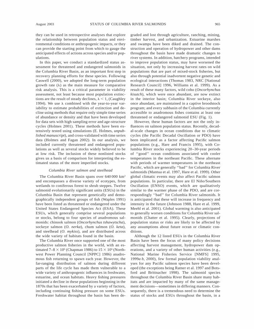
966 MICHELLE M. MCCLURE ET AL. Ecological ApplicationsVol. 13, No. 4

FIG. 1. The Columbia River Basin (Washington, USA). Heavy solid lines denote rivers accessible to anadromous fishes;thin solid lines denote portions of the Columbia and Snake Rivers blocked by dams. Numbers define regions, with analyzedsalmonid stocks as follows: (1) Washington coast, nonlisted chinook stocks; (2) lower Columbia River, steelhead, chum, andchinook salmon listed as threatened; (3) upper Willamette River, steelhead and chinook listed as threatened; (4) middleColumbia River, steelhead listed as threatened and spring chinook nonlisted; (5) upper Columbia River, steelhead and springchinook listed as endangered; (6) upper Columbia River, nonlisted summer/fall chinook stocks; (7) Snake River, steelhead,spring/summer chinook, and fall chinook listed as threatened; sockeye salmon listed as endangered.

manner that allows comparison between stocks, ESUs,and species. Such comparable quantitative reviews ofpopulation status are an important component of effortsto prioritize populations for recovery and conservationactions (Allendorf et al. 1997). They can also serve asa foundation for analytical efforts to determine themagnitude of natural anthropogenic impacts on pop-ulation status or the potential of different restorationactions.

Efforts to determine salmonid population status,however, must deal with the complicating presence oflarge numbers of hatchery-reared fish, which may bereproducing along with wild-born fish. Regardless ofwhether the presence of hatchery-reared fish has a neg-ative impact on wild-born fish, reproduction by hatch-

ery fish presents an accounting problem that compli-cates the estimation of population status. This occursbecause the wild population is being supplemented byan external population (the hatchery). Simply removingthe hatchery spawners from the time series is not suf-ficient, since one must account for the hatchery fishoffspring, their offspring’s offspring, etc. Properly ac-counting for hatchery fish reproduction requires infor-mation on the relative reproductive success of hatcheryfish. While it appears that hatchery-reared fish thatspawn in the wild generally have lower breeding suc-cess than wild-born fish (Fleming 1982, Fleming andGross 1993, 1994, Berejikian 1995), the estimates oftheir relative reproductive success are quite variableand range from 10% to 13% of that of wild-born spawn-


ers, for nonnative domesticated stock across the entirelife cycle (Chilcote et al. 1986) to 80% of the wild fishrate, for local stock in the egg to the yearling stageonly (Reisenbichler and McIntyre 1977). In our anal-yses, we correct for hatchery reproduction by contrast-ing two different assumptions. In the first case, weassume that hatchery fish have not been reproducing.This gives the most optimistic estimates of populationstatus. In the second case, we assume that hatchery fishhave been reproducing at the same rate as wild-bornspawners. This gives the most pessimistic estimates.The true rate of hatchery fish reproduction is some-where between these extremes.

Using these different assumptions, we then conducta status assessment and analysis that focuses on thefollowing: (1) What is the rate of population decline(or growth) and the associated risk of decline for listedColumbia River stocks and ESUs under the most recent(poor) ocean conditions (1980–2000)? (2) How dothose estimates change, given the potential for hatcheryfish to reproduce in the wild? (3) Do parameter andrisk estimates change significantly if data includingboth ‘‘good’’ and ‘‘bad’’ ocean conditions (1965–2000)are used in the assessment?

Complete viability analyses will consider other fac-tors in addition to these strictly demographic ones(Soule and Gilpin 1986). Genetic diversity, the prob-ability of catastrophes, Allee effects or depensation,and a variety of other potential factors can all affectpopulation status. However, many of these concerns,such as the probability of catastrophe, are difficult orimpossible to estimate (Coulson et al. 2001). In addi-tion, for the majority of stocks in the region, only themost basic time-series data are available. Thus, we pro-vide these demographic analyses as a first step towardsa complete viability analysis.

METHODS

We estimated population trends and risk estimatesfor 152 stocks in 11 ESUs listed as threatened or en-dangered throughout the Columbia River Basin and for24 stocks in three nonlisted ESUs regarded as‘‘healthy.’’ We did not assess the status of Snake Riversockeye, the 12th listed ESU, because this entire ESUis currently maintained in a captive broodstock pro-gram. Estimation of the long-term population growthrate (l) was one of the main foci of our analysis. ‘‘Man-aging for l’’ has been suggested as a strategy of achiev-ing species viability and productivity (Caswell 2001),since any population with a declining growth rate (l, 1) will eventually go extinct, regardless of initialsize. Populations with a positive trend (l . 1) increasein number and ultimately have a lower extinction risk.In addition, ESUs in the Columbia River Basin areseverely depleted and one current management objec-tive is to recover these populations to higher levels,which necessarily entails a l . 1.

Time periods analyzed

We assessed the status of stocks and ESUs over twotime periods: 1980–2000 and 1965–2000. Regimeshifts in the Pacific Decadal Oscillation occurred in1947 and 1977 (Francis and Hare 1994). Thus, the1980–2000 time period gave an estimate of populationgrowth rates during ocean conditions that are consid-ered to have been poor for Columbia River salmonids(Mantua et al. 1997). Risk estimates projected frompopulation growth rates using 1980–2000 time seriesthus carry the assumption that the warm ocean con-ditions characteristic of this time period persist indef-initely into the future. Note that most models of globalclimate change suggest that ENSO events (which aresuperficially similar to the warm phase of the PDO)will increase in frequency and intensity (Meehl et al.2001). Thus, projections using the 1980–2000 periodmay be a surrogate for continued warm conditions dueto global climate change. The configuration of the Co-lumbia and Snake River hydropower system (includingwater storage capacity, which affects the Columbiaplume and estuarine conditions) was also relatively uni-form during this time period. Survival of juvenile chi-nook from the Snake River through the hydropowersystem did improve over these 20 years, but in com-parison with the larger change in passage survival be-tween the mid–late 1970s and early 1980s, it was rel-atively constant (Williams et al. 2001).

The longer time period (1965–2000) encompassesboth ‘‘good’’ and ‘‘bad’’ ocean conditions. Risk esti-mates or projections of population growth rates fromthis time period implicitly incorporate the assumptionthat ocean conditions will cycle between these two re-gimes into the future, meaning that the poor ocean con-ditions of the late 20th century will not persist indef-initely. The 1965–2000 period also includes an episodeof dam construction, particularly focused on the LowerSnake River; risk estimates for this area therefore alsoinclude a substantial perturbation. The 1965–1980 datawere available for approximately half of the stocks weexamined, in all ESUs except Upper Willamette Riverchinook and steelhead, Upper Columbia River steel-head, Washington Coastal chinook, and Columbia Riv-er chum. However, data prior to 1965 were not widelyavailable, making pre-1965 analyses for the majorityof stocks impossible.

Data used in analyses

Our analyses required, at the minimum, a time seriesof spawner abundance. Spawner abundance data con-sisted of either direct counts of returning adults at damsor weirs, index counts of spawner numbers, or esti-mates of total returning spawners. Index counts, suchas ‘‘redds per mile’’ (a redd is the gravel nest made byspawning female) give a relative index rather than anabsolute count of the total number of spawners. At thestock level, spawner estimates were typically derived


from redd surveys of a portion of a particular river orcreek, although dam or weir counts were available forsome stocks. For seven ESUs (Snake River steelhead,fall chinook and spring/summer chinook, Upper Co-lumbia River spring chinook and steelhead, and UpperWillamette River chinook and steelhead), total spawnerestimates for the entire ESU were available via damcounts at the downstream end of the ESU. In order tobest represent the number of fish on the spawninggrounds, we subtracted fish from the time series thatwere harvested in-river or taken into hatcheries up-stream, after dam counts. For three other ESUs (LowerColumbia River chinook and steelhead and Middle Co-lumbia River steelhead), we created an ESU-level in-dex count by aggregating all stocks within that ESUfor which a total live spawner time series was available.No ESU-level counts were possible for Columbia Riverchum or the three nonlisted ESUs since the majorityof time series within these ESUs were index counts.

Estimates of the proportion of hatchery-rearedspawners in the time series were available for approx-imately half of the stocks analyzed. Estimates of theproportion of hatchery fish on the spawning groundswere based either on direct observations of fin-clippedfish or were derived from estimated hatchery strayrates. When the proportion of hatchery and wild spawn-ers was unknown, we conducted our analyses on thetotal spawner counts, which include both wild- andhatchery-reared spawners.

The age at which individuals return to spawn variesby species and stock, and not all individuals within agiven species and stock return at the same age. Thedistribution of the spawning age was available for mostESUs but variably available for individual stocks. Ageneric ESU-level spawner age distribution was usedfor those stocks without data. The raw spawner count,age, and hatchery-fraction data are supplied in the Sup-plement.

Estimating population-level parameters

We used time series of spawner counts to estimatepopulation growth rates and risks by fitting a stochasticexponential decline model:

N 5 N exp(m 1 «)t11 t (1)

[where « is distributed Normal(0, s2)] to the data andthen using diffusion approximation methods (Denniset al. 1991) to estimate risks. However, the parameterestimation methods described by Dennis et al. (1991)were not appropriate for raw spawner counts for severalreasons. First, spawner counts represent only a singlelife stage and are therefore not a representative sampleof the entire population. In addition, salmon life his-tory, particularly iteroparity and delays between birthand reproduction, make salmon prone to boom and bustcycles in annual spawner numbers. These cycles con-found parameter estimation. Second, sampling error islikely to be very high in spawner count data (Hilborn

et al. 1999). Large sampling error results in overesti-mates of the environmental variance, which lead tocorrespondingly poor estimates of any risk metrics thatincorporate this measure of variance (Holmes 2001,Holmes and Fagan 2002). We used the following ap-proach to deal with these issues.

First, we used a uniform running sum of four con-secutive counts to filter out sampling error and age-structure cycles:

4

R 5 S . (2)Ot t1j21j51

We tested the running sum transformed counts for theirfit to the assumptions of the underlying stochastic pro-cess: (1) that the relationship between the variance andthe lag, t, in ln(Rt1t /Rt) was linear, using the R2 of aleast-squares fit through the variance data; (2) thatln(Rt11/Rt) was distributed normally and there were nosignificant outliers (using the dffits statistic .2 [Chat-terjee and Hadi 1988]); (3) that density-dependent pro-cesses were not apparent (following Dennis and Taper1994); (4) that statistically significant temporal trendsin m were not present (using a method analogous toDennis and Taper’s test for density dependence); and(5) that there was no significant serial autocorrelationin the Rt11/Rt ratios (by detrending the ratios and usingSpearman’s rank correlation test). All tests were doneat the P , 0.05 significance level with no adjustmentfor the fact that multiple tests were conducted. Wefound a good fit to all assumptions with the followingexceptions: the Upper Columbia spring chinook ESU-level data showed a downward trend in Rt11/Rt ratios,as do most of the stocks within that ESU. This down-ward trend was also seen in a few stocks in most otherESUs. It should be kept in mind that simulations (oursand Shenk et al. 1998) indicate that significant trendsappear by chance 25–30% of the time in 20-year sam-ples of stochastic age-structured processes. Severalstocks also showed evidence of density-depensatory orcompensatory processes (Table 1). Risk estimates willtend to be overly optimistic when there is depensatorydensity dependence or declining trends in Rt11/Rt ratios.A handful of stocks and the Upper Columbia Riversummer/fall chinook ESU showed evidence of first or-der autocorrelation in Rt11/Rt ratios. When autocorre-lation is present, s2 is underestimated using our meth-ods, but m should be unaffected (Tuljapurkar 1989).

While we have not conducted sensitivity analysesfor each of these factors, a recent cross-validation studyof diffusion approximation (DA) methods (Holmes andFagan 2002) used long-term salmon time series to lookimplicitly at the effects of violations of simple DAmodel assumptions, such as no density-dependent pro-cesses, low autocorrelation, and no trends. This studyfound that DA methods gave unbiased estimates of land of the probability of decline. Only for rapidly in-creasing populations were biases in the estimation of


l seen that were sufficient to cause overestimation ofthe risk of decline.

We estimated m for each stock and ESU from theratios of consecutive running sums:

m 5 mean[ln(R /R )].run t11 t (3)

This method gives an estimate of m that is resistantto severe age-structure perturbations and samplingerror (Holmes 2001). We used a slope method toestimate s2

Rt1t2s 5 slope of var ln vs. t (4)slp 1 2[ ]Rt

for t 5 1, 2, 3, and 4. This estimate of s2 is significantlyless biased in the face of severe sampling error (Holmesand Fagan 2002). These parameter estimation methodshave been cross validated using a large collection ofwest-coast salmon time series by Holmes and Fagan(2002).

Using estimates of m and s2, we calculated the fol-lowing metrics of risk to assess the status of thesepopulations.

Long-term rate of population change.—The estimateof the long-term rate of population change (denoted

) isl

l 5 exp(m). (5)

Note that we use l to denote the long-term populationgrowth rate, defined as l 5 Nt1t /Nt

1/t as t → `. If l isless than 1, the population will go extinct with certaintyover the long term, and over the short-term l denotesthe median observed growth rate. Our use of l followsthe concept of the time-averaged long-term rate of sto-chastic growth suggested by Caswell (2001). In Denniset al. (1991), l is used to indicate the mean (ratherthan median) annual growth rate (5 exp[m 1 s2/2]);however, we do not use the mean as our metric sincethe mean is not the long-term growth rate nor doesexp(m 1 s2/2) , 1 indicate extinction with certainty.

A range of underlying stochastic processes (with dif-ferent m and s2) could have produced the observed timeseries. The 95% confidence intervals on l give an es-timate of the range of true ls that could have producedthe observed data. From Holmes and Fagan (2002), Eq.4, the 95% confidence intervals on l are

2exp 3m 2 t Ïs /g (n 2 4) 40.025,df

2exp 3m 1 t Ïs /g (n 2 4) 4 (6)0.025,df

where g is a constant (ø1) and ta,df is the quantile ofa student’s t distribution at probability a and degreesof freedom df. The degrees of freedom for the t dis-tribution are given by the degrees of freedom of the

: df ø 0.333 1 0.212 n 2 0.387 L, where L is the2sslp

number of counts summed together to form Rt (in ourcase L 5 4) and n is the time series length (followingHolmes and Fagan 2002).

Probability of extinction.—To estimate extinctionprobabilities, we required an estimate of populationsize. For this, we estimated the total number of wild-born fish alive at year t that do eventually return tospawn. We denote this TSt. We can calculate TSt usingthe mean age distribution of returning spawners:

TS 5 w S 1 (1 2 F )w St t t 1 t11 t11

1 (1 2 F 2 F )w S 1 · · · (7)1 2 t12 t12

where St is the spawner count at year t, Fi is the fractionof spawners that return at age i, and wt is the fractionof year t spawners that were wild-born (vs. hatchery-reared). Note F0 5 0, that is, no individuals return tospawn the same year that they are born.

The probability of reaching a given threshold pop-ulation size, TSe, before the end of te years (Eq. 16 3Eq. 84 in Dennis et al. [1991]) is

2ln(TS /TS ) 1 zmzt0 e eGp9 5 p9F [ ]sÏte

2 ln(TS /TS )zmz0 e1 exp2[ ]s

2ln(TS /TS ) 2 zmzt0 e e3 F , t . 0 (8)e[ ]sÏte

where

1 m # 0p9 5

25exp[22m ln(TS /TS )/s ] m . 0.0 e

The function F is the standard normal cumulative dis-tribution function. The most recent TSt estimate foreach stock is denoted TS0 and is given in Table 1. Forextinction, we used TSe 5 1 and te 5 50 years.

Probability of 90% decline.—In many cases, theprobability of extinction could not be calculated, sinceTSt requires total spawner counts rather than indexcounts, an estimate of the age distribution of returningspawners, and an estimate of the fraction of spawnersin the time series that are wild born. Therefore, we alsocalculated the probability that the population is 90%lower at the end of te years 5 50 years (cf. Eq. 6 inDennis et al. 1991):

TS 10 ln(10/1) 1 mtt eePr , 5 1 2 F . (9)1 2 [ ]TS 1 sÏt0 e

This risk metric could be calculated when only indexcounts were available or if spawner age data or hatch-ery fraction data were missing. The risk of 90% declinealso gives another risk perspective for large popula-tions that have a low extinction probability due to theirsize while still having a substantial probability of se-vere declines due to underlying dynamics.

We used parametric bootstrapping to estimate theconfidence intervals on the probability of extinctionand 90% decline by sampling from the estimated dis-tributions of and 2 (Holmes and Fagan 2002). Them sestimated distribution of is specified by 1m m


TABLE 1. Parameter estimates, risk of extinction and 90% decline in abundance in 50 years, and needed percentage increasesin l to achieve l 5 1 and to reduce 50-year risk of decline or extinction to below 5%.

ESU and stock(population size estimate)

Population parameter estimates†

m s2 l (95% CI)

Pr (l)

,1.0 ,0.9

Increaseneeded

(%)

Lower Columbia River chinookAbernathy Creek f-t (1587)Bear Creek fallBig Creek fallClackamas River fallClatskanie River fallCoweman River f-t (2923)Cowlitz River f-t (7903)Cowlitz River springElochoman River f-tGermany Creek f-tGnat Creek fallGrays River f-tKalama River springKalama River f-tKlickitat River f-tLewis River f-b (34652)Lewis River springLewis East Fork f-t (853)Mill Creek f-tPlympton Creek fallSandy River fallSandy River f-l (3790)Sandy River f-t (398)Skamokawa Creek f-tWashougal River f-tWhite Salmon River f-tWind River f-tWind River springYoungs River fall

0.0020.0320.1420.0620.0420.02

0.2320.0320.03

0.050.01

20.0320.1020.11

0.020.08

20.0220.0420.0120.1020.02

0.170.00

20.2120.10

0.0420.1320.10

0.0120.03

0.030.020.280.070.040.680.190.100.030.400.140.400.420.220.470.130.050.460.020.260.110.330.020.100.140.020.120.810.051.21

0.99 (0.68, 1.44)0.98 (0.82, 1.15)0.87 (0.45, 1.66)0.94 (0.76, 1.16)0.96 (0.71, 1.30)0.98 (0.50, 1.93)1.26 (0.82, 1.94)0.97 (0.71, 1.33)0.97 (0.83, 1.14)1.05 (0.57, 1.96)1.01 (0.67, 1.52)0.97 (0.56, 1.71)0.90 (0.48, 1.70)0.90 (0.57, 1.42)1.02 (0.52, 2.00)1.08 (0.73, 1.59)0.98 (0.79, 1.22)0.96 (0.50, 1.85)0.99 (0.85, 1.15)0.91 (0.37, 2.24)0.98 (0.73, 1.32)1.19 (0.74, 1.90)1.00 (0.82, 1.23)0.81 (0.14, 1.78)0.90 (0.63, 1.30)1.04 (0.90, 1.21)0.88 (0.62, 1.23)0.90 (0.37, 2.18)1.01 (0.81, 1.27)0.97 (0.39, 2.40)

0.500.580.710.680.590.520.140.560.610.400.470.540.650.690.460.320.550.560.530.640.540.200.470.740.710.310.770.630.430.53

0.270.230.540.330.310.340.070.290.230.240.260.340.470.480.290.160.240.380.180.460.280.100.210.610.470.110.550.460.180.37

03

15642033003

1111

00241

10200

2311

01411

03

Upper Columbia River chinook (3381)Entiat River spring (168)Methow River spring (486)Wenatchee River spring (1466)

20.1620.1420.1420.17

0.130.040.350.08

0.85 (0.62, 1.17)0.87 (0.73, 1.03)0.87 (0.51, 1.47)0.84 (0.65, 1.09)

0.820.860.730.86

0.630.640.540.68

17151518

Snake River spring/summer chinook(21683)Alturas Lake Creek springBear Valley/Elk Creek (713)Beaver Creek springBig Creek springBig Sheep Creek springCamas Creek springCape Horn Creek springCatherine Creek springCatherine Creek North Fork springCatherine Creek South Fork springChamberlain Creek springGrande Ronde River springImnaha River spring (610)Johnson Crek summer (432)Knapp Creek springLake Creek summerLemhi River springLookingglass Creek springLoon Creek summerLostine River springMarsh Creek spring (286)Minam River spring (322)Minam River Upper springMinam River Lower springPoverty Creek (951)Salmon River EF summerSalmon River SF summerSalmon River Upper springSalmon River Upper summerSecesh River summerSulphur Creek spring (200)

20.0320.26

0.0320.14

0.0020.0820.14

0.0220.1020.0620.1120.1020.0920.06

0.0120.20

0.0320.0220.20

0.0020.01

0.010.010.010.100.01

20.060.06

20.0920.1120.02

0.03

0.010.070.160.250.181.770.120.220.150.250.860.090.180.060.050.280.090.320.150.030.070.150.230.120.310.080.280.120.050.100.000.47

0.97 (0.89, 1.06)0.77 (0.62, 0.96)1.03 (0.74, 1.44)0.87 (0.53, 1.41)1.00 (0.69, 1.45)0.93 (0.34, 2.55)0.87 (0.62, 1.22)1.02 (0.64, 1.61)0.91 (0.68, 1.22)0.94 (0.58, 1.53)0.90 (0.36, 2.22)0.91 (0.46, 1.81)0.92 (0.66, 1.27)0.94 (0.77, 1.15)1.01 (0.83, 1.22)0.82 (0.49, 1.36)1.04 (0.78, 1.38)0.98 (0.62, 1.56)0.82 (0.61, 1.10)1.00 (0.88, 1.14)0.99 (0.82, 1.21)1.01 (0.73, 1.39)1.01 (0.68, 1.49)1.01 (0.76, 1.34)1.11 (0.70, 1.75)1.01 (0.80, 1.28)0.95 (0.61, 1.45)1.07 (0.80, 1.41)0.91 (0.76, 1.08)0.90 (0.66, 1.23)0.98 (0.94, 1.03)1.03 (0.59, 1.81)

0.680.940.420.740.490.590.710.340.730.600.630.660.700.670.450.810.390.530.880.460.510.470.470.450.300.450.610.320.790.740.680.43

0.140.860.220.560.270.430.580.250.460.390.470.460.440.350.170.660.180.320.730.130.190.250.260.210.160.200.380.140.450.490.070.26

329

015

08

150

106

1110

960

2302

22010000060

1011

20


TABLE 1. Extended.

Risk of extinction‡

50 years(95% CI) Pr(VHER)

Increaseneeded (%)

Risk of 90% decline§

50 years(95% CI) Pr(VHRD)

Increaseneeded (%)

Additionalnotes\

NA0.00 (0, 0.43)NANANANA

NA0.28NANANANA

NA0

NANANANA

0.05 (0, 1)0.17 (0, 1)0.90 (0, 1)0.63 (0, 1)0.40 (0, 1)0.41 (0, 1)

0.510.550.770.690.600.60

02

2585

22

ill,h,ih,it,l,h,ih,i

0.00 (0, 0.13)NANANANANANANANANA0.00 (0, 0.08)NA0.00 (0, 0.27)NANA

0.13NANANANANANANANANA0.19NA0.26NANA

0NANANANANANANANANA

0NA

0NANA

0.00 (0, 0.67)0.33 (0, 1)0.25 (0, 1)0.14 (0, 1)0.15 (0, 1)0.41 (0, 1)0.72 (0, 1)0.82 (0, 1)0.25 (0, 1)0.01 (0, 0.99)0.19 (0, 1)0.49 (0, 1)0.06 (0, 1)0.77 (0, 1)0.3 (0, 1)

0.180.590.570.470.510.610.720.740.530.360.540.630.480.690.58

06374

16251913

03

191

206

hl,hhhhhl,d,h,fhl,h

t,a,h

l,h

NA0.00 (0, 0.01)0.98 (0, 1)NANANANANANA0.54 (0, 1)0.93 (0, 1)0.69 (0, 1)0.76 (0, 1)

0.00 (0, 0)NA

NA0.240.76NANANANANANA0.650.830.760.76

0.09NA

NA0

19NANANANANANA10102111

0NA

0.01 (0, 0.98)0.01 (0, 1)1.00 (0, 1)0.85 (0, 1)0.00 (0, 0.94)0.96 (0, 1)0.67 (0, 1)0.03 (0, 1)0.45 (0, 1)0.99 (0.01, 1)1.00 (0.22, 1)0.87 (0, 1)1.00 (0.01, 1)

0.15 (0, 1)1.00 (0.92, 1)

0.260.440.780.750.300.800.710.440.620.890.880.780.88

0.530.96

00

2716

01936

03522162821

132

t,h,illhhhhhh,it,da,dt,dt,d

ll,h,i

0.01 (0, 0.95)NANANANANANANANANANA0.03 (0, 1)0.00 (0, 0.59)NANA

0.37NANANANANANANANANANA0.490.30NANA

0NANANANANANANANANANA

00

NANA

0.09 (0, 1)0.92 (0, 1)0.22 (0, 1)0.57 (0, 1)0.97 (0, 1)0.16 (0, 1)0.82 (0, 1)0.56 (0, 1)0.68 (0, 1)0.89 (0, 1)0.75 (0, 1)0.66 (0, 1)0.05 (0, 1)0.98 (0.01, 1)0.03 (0, 1)

0.460.790.540.690.810.810.770.660.710.700.740.690.440.850.42

225

65320

51514381316

80

330

h,it,h,iiid,iih,iit,h,ii

d,h,id,h,i

NANANANA0.03 (0, 0.99)0.07 (0, 0.99)NANA0.00 (0, 0.84)NANANANANA0.17 (0, 1)

NANANANA0.460.48NANA0.30NANANANANA0.55

NANANANA

01

NANA

0NANANANANA

8

0.37 (0, 1)1.00 (0.10, 1)0.02 (0, 1)0.14 (0, 1)0.17 (0, 1)0.21 (0, 1)0.11 (0, 1)0.04 (0, 1)0.08 (0, 1)0.56 (0, 1)0.01 (0, 0.98)0.94 (0.01, 1)0.91 (0, 1)0.00 (0, 0.86)0.21 (0, 1)

0.590.910.400.500.510.520.480.360.470.670.350.800.770.340.51

1329

0346302

150

1115

011

h,iil,h,ii

ih,i

h,id,h,ih,it,h,il,h,i


TABLE 1. Continued.

ESU and stock(population size estimate)


m s2 l (95% CI)

Pr (l)

,1.0 ,0.9

Increaseneeded

(%)

Valley Creek Upper springValley Creek Upper summerWallowa Creek springWenaha River South Fork springYankee Fork summerYankee West Fork summerYankee West Fork spring

0.0420.0820.07

0.0320.19

0.0020.17

0.630.200.620.100.310.240.14

1.04 (0.54, 1.99)0.92 (0.59, 1.43)0.93 (0.51, 1.69)1.03 (0.81, 1.31)0.83 (0.48, 1.43)1.00 (0.62, 1.61)0.84 (0.58, 1.22)

0.430.660.610.390.790.490.81

0.260.430.430.170.630.280.63

0980

210

19Snake River fall chinook (1946)Up. Willamette River chinook (8770)

McKenzie River (5112)

20.0520.01

0.01

0.040.230.20

0.95 (0.76, 1.18)0.99 (0.65, 1.53)1.01 (0.68, 1.51)

0.650.500.46

0.320.290.25

510

Columbia River chumGrays River WFGrays River fallHardy Creek fallCrazy J CreekHamilton Creek fallHamilton Springs

NA0.21

20.030.040.14

20.080.09

NA0.230.100.060.030.050.51

NA1.23 (0.81, 1.88)0.97 (0.73, 1.29)1.04 (0.86, 1.26)1.15 (0.98, 1.34)0.92 (0.75, 1.13)1.10 (0.61, 1.97)

NA0.150.580.340.110.740.33

NA0.070.300.130.050.400.19

NA030080

Lower Columbia River steelheadClackamas River summer (2155)Clackamas River winter (1041)Green River winter (450)Kalama River summer (6445)Kalama River winter (4975)Lewis River East Fork winterSandy River winter (4535)Sandy River summerToutle River SF winterTrout Creek summerWashougal River summerWind River summer (1218)

20.0420.0920.1020.1520.0420.0220.1720.0620.0420.1020.2520.1220.06

0.000.090.060.250.140.010.020.030.090.000.030.010.00

0.96 (0.94, 0.98)0.91 (0.71, 1.17)0.91 (0.73, 1.13)0.86 (0.17, 4.46)0.96 (0.67, 1.38)0.98 (0.87, 1.09)0.84 (0.15, 4.84)0.94 (0.79, 1.11)0.96 (0.75, 1.22)0.91 (0.88, 0.93)0.78 (0.08, 0.95)0.89 (0.64, 1.24)0.95 (0.51, 1.76)

0.840.730.770.670.570.610.760.710.620.790.800.730.64

0.100.460.460.520.340.190.610.320.310.430.690.510.34

4101016

42

1965

102812

6Middle Columbia River steelhead

Bear Creek summerBeaver Creek North Fork summerBeech Creek summerBeech Creek East Fork summerCamp Creek summerCanyon Creek summerCanyon Creek Mid. Fork summerDeep Creek summerDeer Creek summerDeschutes River summer (3052)Eightmile Creek winterFields Creek summerFifteen Mile Creek winterKahler Creek summerMcclellan Creek summerMill Creek summerMurderers Creek summerOlive Creek summerParrish Creek summerRamsey Creek winterRiley Creek summerShitike Creek summerTex Creek summerUmatilla River summer (5384)Wall Creek summerWarm Springs summer (729)Wind Creek summerYakima River summer

20.0620.0820.0620.0220.0220.0120.0320.0620.0320.0420.0620.0820.1120.0120.0220.0520.0320.1820.0220.03

0.0620.0620.0620.1520.0120.0220.0620.06

0.14

0.140.070.170.170.170.160.170.160.180.400.161.620.110.030.510.150.000.250.190.511.650.240.030.330.050.220.080.030.21

0.94 (0.69, 1.27)0.92 (0.69, 1.22)0.95 (0.69, 1.29)0.98 (0.70, 1.38)0.98 (0.71, 1.34)0.99 (0.73, 1.35)0.97 (0.71, 1.33)0.94 (0.69, 1.29)0.97 (0.70, 1.34)0.96 (0.60, 1.56)0.94 (0.70, 1.27)0.92 (0.15, 5.89)0.90 (0.70, 1.15)0.99 (0.81, 1.20)0.98 (0.57, 1.68)0.95 (0.70, 1.28)0.97 (0.91, 1.03)0.83 (0.57, 1.22)0.98 (0.70, 1.37)0.97 (0.57, 1.68)1.06 (0.16, 6.83)0.94 (0.61, 1.46)0.94 (0.80, 1.10)0.86 (0.56, 1.34)0.99 (0.84, 1.17)0.98 (0.69, 1.40)0.94 (0.74, 1.19)0.94 (0.83, 1.06)1.15 (0.59, 2.24)

0.650.710.630.540.540.510.560.640.560.560.640.570.780.540.530.630.690.820.550.540.440.610.730.760.510.530.660.780.27

0.380.430.360.290.290.260.300.370.300.360.380.430.510.220.340.360.170.650.300.340.300.390.330.570.190.290.360.280.15

696221363468

121263

2023067

1612670

Upper Columbia River steelhead (2822) 0.00 0.15 1.00 (0.66, 1.52) 0.50 0.27 0Snake River steelhead (41035)

Butte Creek summer ACamp Creek summer ACrow Creek summer ADevils Run Creek summer AFive Points Creek summer AFly Creek summer AMcCoy Creek summer A

20.040.060.020.030.050.000.000.08

0.030.650.180.250.250.110.280.10

0.96 (0.84, 1.10)1.07 (0.57, 1.97)1.02 (0.73, 1.40)1.03 (0.70, 1.50)1.05 (0.72, 1.55)1.00 (0.78, 1.30)1.00 (0.67, 1.50)1.09 (0.85, 1.39)

0.650.390.450.420.370.470.480.25

0.230.230.220.220.190.210.270.10

40000000


TABLE 1. Continued, Extended.

Risk of extinction‡


Increaseneeded (%)

Risk of 90% decline§

50 years(95% CI) Pr (VHRD)

Increaseneeded (%)

Additionalnotes\

NANANANANANANA0.00 (0, 0.99)0.01 (0, 0.99)0.00 (0, 0.97)NANANANANA

NANANANANANANA0.370.350.33NANANANANA

NANANANANANANA

000

NANANANANA

0.22 (0, 1)0.72 (0, 1)0.60 (0, 1)0.05 (0, 1)0.96 (0, 1)0.24 (0, 1)0.99 (0, 1)0.58 (0, 1)0.29 (0, 1)0.18 (0, 1)

NA0.00 (0, 0.86)0.38 (0, 1)0.01 (0, 0.99)0 (0, 0.001)

0.510.710.690.420.830.540.850.650.560.51NA0.260.610.350.13

141628

033

724

685

NA0700

h,ih,f,ih,iit,l,h,ih,ih,i

il,il,il,il,i

NANANA0.11 (0, 1)0.13 (0, 1)0.73 (0, 1)0.01 (0, 1)0.00 (0, 0)NA0.00 (0, 0.71)NANANANA0.00 (0, 1)

NANANA0.530.550.700.390.19NA0.30NANANANA0.38

NANANA

22

1800

NA0

NANANANA

0

0.86 (0, 1)0.10 (0, 1)0.05 (0, 1)0.87 (0, 1)0.93 (0, 1)0.93 (0, 1)0.42 (0, 1)0.07 (0, 1)1.00 (0, 1)0.73 (0, 1)0.49 (0, 1)1.00 (1, 1)1.00 (0, 1)1.00 (0, 1)0.91 (0, 1)

0.750.410.490.760.780.720.610.510.780.700.640.800.830.750.61

1060

131225

81

18676

2810

3

it,a,l,iltttdli

t,hl,it,hl,h,il

NANANANANANANANANANA0.06 (0, 0.99)NANANANA

NANANANANANANANANANA0.47NANANANA

NANANANANANANANANANA

1NANANANA

0.62 (0, 1)0.85 (0, 1)0.57 (0, 1)0.34 (0, 1)0.34 (0, 1)0.25 (0, 1)0.37 (0, 1)0.58 (0, 1)0.38 (0, 1)0.47 (0, 1)0.61 (0, 1)0.57 (0, 1)0.91 (0, 1)0.11 (0, 1)0.41 (0, 1)

0.690.730.670.590.590.550.600.680.600.640.680.660.800.520.52

111112

8868

129

17125016

219

ih,f,iif,if,if,if,if,il,f,if,i

it,f,ih,f,ia,f,i

NANANANANANANANANA0.00 (0, 0.05)NA0.06 (0, 1)NANA0.00 (0, 1)

NANANANANANANANANA0.21NA0.50NANA0.36

NANANANANANANANANA

0NA

1NANA

0

0.56 (0, 1)0.02 (0, 1)0.97 (0, 1)0.36 (0, 1)0.42 (0, 1)0.29 (0, 1)0.58 (0, 1)0.79 (0, 1)0.89 (0, 1)0.10 (0, 1)0.33 (0, 1)0.63 (0, 1)0.79 (0, 1)0.01 (0, 1)0.19 (0, 1)

0.670.500.860.600.620.520.670.710.810.500.580.680.740.320.53

110

299

193214

628

299605

f,il,f,if,if,if,iif,ih,if,idf,i

f,itt

0.00 (0, 0.003)NANANANANANANA

0.16NANANANANANANA

0NANANANANANANA

0.38 (0, 1)0.17 (0, 1)0.15 (0, 1)0.15 (0, 1)0.08 (0, 1)0.15 (0, 1)0.26 (0, 1)0.00 (0, 0.94)

0.610.470.500.490.430.550.550.28

412

452390

a,iia,it,ih,iii


TABLE 1. Continued.

ESU or stock(population size estimate)


m s2 l (95% CI)

Pr(l)

,1.0 ,0.9

Increaseneeded

(%)

Meadow Creek summer APeavine Creek summer APhillips Creek summer APrairie Creek summer ASnake River A (39585)Snake River B (9115)Summit Creek summer ASwamp Creek summer AWallowa River summer A

0.000.07

20.030.16

20.0320.08

0.030.01

20.11

0.140.290.090.380.030.070.360.110.10

1.00 (0.75, 1.33)1.07 (0.69, 1.67)0.97 (0.77, 1.23)1.18 (0.74, 1.88)0.97 (0.85, 1.11)0.93 (0.76, 1.14)1.03 (0.65, 1.63)1.01 (0.78, 1.31)0.89 (0.64, 1.26)

0.480.350.570.210.600.680.430.450.74

0.230.190.260.110.200.410.240.200.50

00303800

12Upper Willamette River steelhead (9898)

Agency Creek winterCalapooia River late (196)Mill Creek winterMollala River late (573)N. Santiam River late (2286)S. Santiam River winter (1061)S. Santiam River late (1202)Willamette River winter

20.070.00

20.070.04

20.1420.12

0.0120.1320.08

0.050.460.210.100.100.050.020.070.08

0.93 (0.75, 1.16)1.00 (0.52, 1.94)0.93 (0.60, 1.46)1.04 (0.76, 1.41)0.87 (0.68, 1.11)0.89 (0.75, 1.06)1.01 (0.90, 1.14)0.88 (0.72, 1.08)0.92 (0.73, 1.16)

0.700.490.630.390.840.840.390.840.72

0.370.310.410.190.610.540.100.580.41

7070

1512

014

8Washington Coast chinook

Hoh River fallHoh River springQueets River fall (16333)Willapa River fall

0.0020.02

0.000.050.01

0.100.030.090.040.05

1.00 (0.76, 1.32)0.98 (0.85, 1.14)1.00 (0.79, 1.26)1.05 (0.77, 1.42)1.01 (0.68, 1.50)

0.470.570.500.280.47

0.220.190.210.210.25

02000

Upper Columbia River summer/fallchinookHanford Reach fallMethow River summerOkanogan River summerSimilkameen River summerWenatchee River summer

NA0.040.010.100.080.00

NA0.160.010.150.150.02

NA1.04 (0.70, 1.55)1.01 (0.92, 1.11)1.11 (0.72, 1.70)1.09 (0.72, 1.65)1.00 (0.86, 1.16)

NA0.390.410.290.320.47

NA0.210.120.150.160.17

NA00000

Middle Columbia River spring chinookAmerican RiverBeaver CreekBull Run CreekClear CreekGranite CreekJohn Day RiverJohn Day River Middle ForkJohn Day River North ForkKlickitat RiverMill CreekNaches RiverShitike CreekWarm Springs RiverWind RiverYakima River

NA20.0520.05

0.030.010.020.060.060.050.050.000.05

20.0220.03

0.010.00

NA0.080.060.030.070.020.040.130.070.230.070.180.010.060.050.00

NA0.95 (0.72, 1.26)0.95 (0.77, 1.16)1.03 (0.89, 1.18)1.01 (0.82, 1.23)1.02 (0.92, 1.14)1.06 (0.92, 1.22)1.07 (0.81, 1.40)1.05 (0.86, 1.29)1.06 (0.66, 1.69)1.00 (0.80, 1.23)1.05 (0.39, 2.78)0.98 (0.90, 1.07)0.97 (0.79, 1.19)1.01 (0.81, 1.27)1.00 (0.99, 1.01)

NA0.630.670.350.460.330.240.310.310.380.500.420.620.590.430.48

NA0.340.310.100.170.080.080.130.120.210.200.260.120.250.180.18

NA550000000002300

Notes: The most recent TSt estimates for stocks with total spawner counts are noted in parentheses after the stock or ESUname. Abbreviations: f-t, fall thules; f-b, fall brights. ESU-level estimates are in bold. Estimates were made assuming nohatchery fish reproduction. When hatchery fraction data were available, the hatchery input correction was used. Otherwiseestimates used the total (wild 1 hatchery) spawner count data. Population size estimate is an estimate of the total spawnerpopulation. The first 11 ESUs are listed under the U.S. Endangered Species Act; the three nonlisted ESUs follow.

† ‘‘Increase needed’’ refers to the percentage increase in l needed to achieve l 5 1.‡ Pr(VHER) is the probability of very high extinction risk (the probability that extinction risk in 50 years is over 25%).

‘‘Increase needed’’ refers to the percentage increase in l needed to reduce the 50-year risk of extinction to below 5%.\ Tests for underlying assumptions were made on the running sums of wild-spawner-only counts where possible; otherwise

total mixed counts were used. The codes designate tests that failed at (P , 0.05). Note that a number of the ‘‘fails’’ are falsefails since the P value was not adjusted for 152 tests being conducted. If the P value is adjusted (P , 0.001) to reduce theprobability of a false positive to less than 5%, none of the time series fail the diagnostic tests. Definitions of codes are asfollows: a, significant first-order autocorrelation in ln(Rt11/Rt) was found; d, a model with depensatory density dependencefit the data significantly better than a model with no density dependence (this indicates that the risk estimates are pessimistic);t, a model with a trend in m fit the data significantly better than the model with no trend (this indicates that the risk estimatesare optimistic); l, the variance vs. t plot was nonlinear (R2 , 0.7), indicating an underestimate of s2. Reasons for NA in theextinction estimates column: i, index data, no extinction estimates possible; h, no hatchery data, no extinction estimatespossible, risk estimates calculated on (wild 1 hatchery) spawner count; f, no age of spawners data, no extinction estimatespossible.

§ Pr(VHRD) is the probability of very high risk of decline (the probablility that the risk of 90% decline in 50 years isover 25%). ‘‘Increase needed’’ refers to the percentage increase in l needed to reduce the 50-year risk of decline to below5%.


TABLE 1. Continued, Extended.

Risk of extinction


Increaseneeded (%)

Risk of 90% decline

50 years(95% CI) Pr(VHRD)

Increaseneeded (%)

AdditionalNotes\

NANANANA0.00 (0, 0)0.00 (0, 0.94)NA

NANANANA0.140.41NA

NANANANA

00

NA

0.18 (0, 1)0.07 (0, 1)0.32 (0, 1)0.02 (0, 0.96)0.21 (0, 1)0.79 (0, 1)0.19 (0, 1)

0.520.410.590.280.560.710.50

42603

108

iiia,h,i

iNANA0.00 (0, 0.97)NA0.40 (0, 1)NA0.69 (0, 1)0.14 (0, 0.99)0.00 (0, 0)0.40 (0, 1)NANANANA0.00 (0, 0.07)

NANA0.33NA0.67NA0.760.540.150.66NANANANA0.23

NANA

0NA10NA11

206

NANANANA

0

0.11 (0, 1)0.93 (0, 1)0.78 (0, 1)0.31 (0, 1)0.64 (0, 1)0.03 (0, 1)0.98 (0.01, 1)0.99 (0.05, 1)0.00 (0, 0.77)0.98 (0.01, 1)0.8 (0, 1)0.12 (0, 1)0.13 (0, 1)0.16 (0, 1)0.00 (0, 1)

0.470.770.710.560.680.420.860.860.330.860.740.500.520.510.41

315

81414

01914

01611

2230

ih,i

h,f,i

h,f,itt

h,fiha,h

NA

NANANANANANANANANANANANANANA

NA


NA


0.04 (0, 1)

NA0.06 (0, 1)0.00 (0, 0.69)0.01 (0, 0.96)0.01 (0, 0.99)0.01 (0, 1)NA0.55 (0, 1)0.57 (0, 1)0.00 (0, 0.95)0.08 (0, 1)0.00 (0, 0.69)0.00 (0, 0.75)0.01 (0, 0.99)

0.49

NA0.440.320.330.360.43NA0.650.670.320.460.280.240.35

0

NA10000

NA8701000

h

NAt,a,hl,h,ih,ih,f,ih,iNAh,il,h,f,il,h,f,ih,f,il,h,f,ih,ih,i

NANANANANANANANA

NANANANANANANANA

NANANANANANANANA

0.01 (0, 0.94)0.07 (0, 1)0.13 (0, 1)0.06 (0, 1)0.05 (0, 1)0.32 (0, 1)0.03 (0, 1)0.55 (0, 1)

0.330.440.500.470.470.590.440.65

02211500

h,ihh,f,ih,ih,f,ih,ihl,h,f,i

3 tdf, where tdf is a t-distributed random2Ïs /g(n 2 4)variable with df degrees of freedom. The estimateddistribution of is a chi-squared (df) random variable2smultiplied by 2/df, where df is specified as discussedsfor Eq. 6. Confidence intervals on these risk metricsare generally very large. For example, the 95% con-fidence intervals on probabilities of 90% decline orextinction are often 0 to 1 (Table 1). However, cross-validation work suggests that within a collection ofpopulations, the mean probability of decline gives anunbiased estimate of the fraction of populations thatwill decline (Holmes and Fagan 2002)—although onedoes not know which populations will decline. Thevariability of the mean is much less than the variability

of individual estimates, and thus we use the mean prob-ability of decline or extinction of all stocks within anESU to give us a relatively tight estimate of the meanrisk to those stocks.

Presenting levels of support for different risk met-rics.—The bootstrapped confidence intervals indicatehow variable the risk estimates are, but they do notnecessarily give a good sense of the degree to whichthe data support different conjectures about the risklevels, for example, whether the true rate of populationdecline is l , 0.95, say. To examine the data supportfor different risk levels, we used Bayesian techniqueswith uniform priors to calculate the probability that thetrue risks were above or below certain thresholds.


FIG. 2. Illustration of the Bayesian risk metrics, the prob-ability that the true l is less than 0.9 and the probability thatthe true risk of decline or extinction is very high. This requiresfirst calculating the posterior probability density functions (p)of the parameters. The surfaces in panels (A) and (B) areillustrations of p’s. (A) The probability that l is less than 0.9is calculated by integrating the p for m over those m for whichl , 0.9. (B) The probability that the true risk of decline orextinction is very high is calculated by integrating the jointp’s for m and s2 over those values of m and s2 for which theprobability of 90% decline (VHDR) or probability of extinc-tion (VHER) is greater than 25%.

Bayesian approaches are commonly used in conser-vation biology to express risks in this manner (Wade2000), and E. Holmes (unpublished manuscript) givesalgorithms for calculating the probability that l is lessthan some threshold given the observed data and theprobability that the risk of the population declining orgoing extinct is greater than some threshold. Usingthese methods, we estimated the probability that thestock has a very high extinction risk (VHER) or a veryhigh decline risk (VHRD). VHER is defined as a .25%probability of extinction in 50 years. VHRD is definedas a .25% probability of 90% decline in 50 years. Tocalculate the probability that a stock falls in the VHERor VHRD category, we first calculated the posteriorprobability distributions of the parameters m and s2 andthen integrated over the distributions, assuming uni-form priors, over those values of m and s2 that gave aVHER or VHRD. This is shown diagrammatically inFig. 2.

Adjusting parameter estimates for inputs fromhatchery-origin spawners

The introduction of reproducing hatchery-bornspawners (in effect, fish from another population) con-

founds the parameter estimates of the long-term pop-ulation growth rate due to natural reproduction andsurvival. If hatchery fish reproduce successfully in-stream, we must account for these inputs, otherwise m(and any risk estimates incorporating m) will be over-estimated. Our adjustment responds to an accountingproblem rather than a negative ecological or geneticeffect of the hatchery fish. Because information onhatchery fish reproductive success is sparse and vari-able, we estimated parameters under two assumptionsthat, taken together, bracket the range of possible sit-uations:

(1) Hatchery fish were assumed not to reproduce.That is, all wild-born spawners observed had wild-bornparents. Parameters were estimated using Eqs. 3 and 4with hatchery spawners removed from the time seriesbefore analysis. When no estimates of the fraction ofhatchery fish were available, the parameters were es-timated using the total spawner or index count, whichmay include hatchery-reared spawners. If the propor-tion of hatchery fish in the time series does not changesubstantially through time, and those hatchery fish donot reproduce, the resulting estimates of m and s2 willbe the same as if the hatchery fish had been removedfrom the time series prior to parameter estimation.

(2) Hatchery fish were assumed to reproduce at arate equal to that of wild fish, and thus, wild spawnersin the time series may have had wild- or hatchery-bornparents. Our estimates of m in this case were

1 St11m 5 mean ln(w ) 1 ln (10)t 1 2[ ]T St

where wt is the proportion of the spawning populationthat was born in the wild (of wild- or hatchery-rearedparents), St is the total number of spawners (wild plushatchery-born) at year t. Our estimates of s2 were notadjusted since simulations indicated that corrected2sslp

for the extra variability due to variable hatchery inputs.E. Holmes (unpublished manuscript) gives a derivationof Eq. 10.

Comparing time periods

To assess the effect of a parameterization time periodthat included cooler, ‘‘good’’ ocean conditions, we re-peated the analyses for the 83 stocks with data begin-ning in 1965 (Appendix B), and we then comparedthese estimates to the estimates using 1980–2000 data.We compared the mean l between the two time periodsfor stocks within each ESU using a two-tailed pairedt test. Only the 83 stocks with both 1965–2000 and1980–2000 data were used in this comparison.

RESULTS

In many of the listed ESUs, the estimated totalspawner population (TS) showed marked decline since1980 (Fig. 3). While it is apparent from these trendsalone that these populations are at considerable de-mographic risk if such declines continue into the future,


FIG. 3. Time series of TSt, the estimated total living current or future spawner population size, for each ESU in theColumbia River basin, plus Hanford Reach and coastal chinook. In these plots, Rt was estimated from total (wild 1 hatcheryorigin) spawner-count time series spanning 1980–1999. All y-axis numbers are in thousands.

a quantitative assessment of this status allows us tocompare formally the status of listed and unlistedstocks; to estimate the wild population growth rate withmasking from hatchery inputs; and finally, to studywhether these downward trends have been persistentthrough periods of both good and bad ocean conditions.When presenting the results, we contrast three differentlevels of estimates: (1) the ESU-level estimate. This isthe estimate of the risk to the ESU as a unit, i.e., therisk estimated from the total number of spawners withinthe ESU; (2) the stock-level estimate. This is the riskestimate for a single stock, generally the fish spawningin a single creek or section of a larger river; (3) themean risk to stocks within the ESU. This mean stockstatus is different than the ESU-level risk. For example,the ESU as whole may appear to be at low risk due toa few large, relatively healthy, stocks even though theESU as a whole contains mostly smaller, rapidly de-clining, stocks.

Population trends from 1980 to the present

Given the trajectories seen at the ESU level (Fig. 3),it is not surprising that, for most ESUs, the estimatedlong-term population growth rate indicated a decliningpopulation. We had an ESU-level time series and thuswere able to estimate an ESU-level l, for 10 of the 11ESUs; the exception was Columbia River chum. Fornine of these, the point estimate of l was less than 1.0

(Table 1, Fig. 4a), and for four ESUs, the estimated lwas ,0.95. The ESU in the worst apparent conditionwas Upper Columbia River spring chinook, for whichthe ESU-level l was ,0.9. At the stock level, the lestimates were more variable, and most ESUs con-tained some stocks with estimated l’s greater than 1.0.However, in all listed ESUs, except Columbia Riverchum, the majority of stock-level l’s were ,1.0. Inaddition, two ESUs, Lower Columbia River steelhead(with 12 stocks), and Upper Columbia River springchinook (with three stocks), did not have a single stockwith an estimated l . 1.0, and the Middle ColumbiaRiver steelhead ESU had only two stocks (out of 28)with an estimated l . 1.0.

In contrast, the majority of l estimates for stocks inthe unlisted ESUs were $1.0 (Table 1), with a meanvalue of 1.02. In fact, the population growth rates ofthe unlisted ESUs and stocks were significantly higherthan those of the listed stocks (one-tailed t test, P ,0.001). The estimated risks faced by these populationswere correspondingly lower (Figs. 4–6).

The confidence intervals on l estimates were gen-erally wide, primarily due to our uncertainty in esti-mation of s2. Thus, we cannot rule out the possibilitythat the underlying dynamics in the listed ESUs arepositive (l . 1.0) and that the declining trends wereobserved by chance as can occur when s2 is large. Theconsistent declining trend estimates across the listed


FIG. 4. Estimated long-term rate of population decline, l, at the individual stock level (circles) and at the ESU level(bar). (A) Estimates assuming that no masking of the parameter m occurred due to hatchery fish reproduction (i.e., hatcheryreproduction 5 0). The dotted line shows l 5 1.0. Below 1.0, the population is estimated to be declining. Above 1.0, thepopulation is estimated to be increasing. (B) Estimated probability that the stocks have a true l of less than 0.9. A l of lessthan 0.9 translates to a mean yearly decline of at least 10%. The dotted line indicates the level of 50% data support; above50%, the data give more support to the conjecture that l , 0.9.

ESUs but not in the unlisted ESUs, however, makessuch a conjecture seem unlikely, at least for most ofthe listed ESUs. In addition, when we made a quan-titative assessment of our uncertainty, by calculatingthe probability that l , 1.0, we found that for almosthalf the listed stocks and seven of the listed ESUs,there was considerable data support (.60% probabil-ity) for a long-term declining trend (Table 1). For theconjecture that the stocks and ESUs are undergoingrapid decline, l , 0.90, there was generally low butnot negligible data support, roughly a 20% probabilityfor most ESUs. Upper Columbia River chinook wasthe exception with high data support (72% probability)

for a l , 0.90. For perspective, populations with along-term population growth rate of 0.9 are decliningrapidly enough that the population can be anticipatedto halve in less than seven years.

These low estimates of population growth rate trans-late into substantial risks of decline and extinction. Atthe broad scale, all ESUs except Lower Columbia Riversteelhead had a probability greater than 50% of VHRD(Fig. 5, Table 1), indicating that the data gave moresupport than not to the possibility that there is a 25%chance of serious decline in the next 50 years. At thestock level, the picture was similar. For every ESUexcept Columbia River chum, the mean probability of


FIG. 5. Histograms of the stock-level estimates of the probability of 90% decline in 50 years for each ESU includingthree nonlisted ESUs: Washington coast chinook, upper Columbia summer/fall chinook, and middle Columbia River springchinook. The mean probability of 90% decline is shown above the histogram bars (diamonds). The 95% confidence intervalson the mean probabilities, , of the n stock estimates for an ESU are shown ( ) where s is the unbiasedx x 6 t s/Ïn 2 10.025,n21

sample variance of the n estimates. If n 5 1 (only one stock estimate in the ESU), the mean probability of 90% decline wasplotted with no error bars. The point estimate for the ESU as a whole is shown by the cross above the histogram bars.

VHRD at the stock level was also .50% (Fig. 5, Table1). In addition to the risk of decline, we were also ableto estimate extinction risk for seven ESUs with totalspawner estimates from dam counts. There was high(69%) support for a .25% chance of extinction(VHER) for the Upper Columbia River chinook ESU.However, the probability of VHER for the remainingESUs was generally low, ranging from 9% to 37% (Fig.6, Table 1). Estimates of extinction probability and de-cline have wide confidence intervals (Table 1). Ratherthan focusing on the precise point estimates for an in-dividual ESU or stock, one should focus on the overallpatterns within the basin across multiple ESUs or ofstocks within an ESU. The mean risk estimated acrossmultiple ESUs or stocks gives a broad picture of therisk and has much smaller confidence intervals thanthe individual point estimates (Figs. 5 and 6).

We also used our estimates of long-term populationgrowth and risk to determine how much change in pop-ulation growth rate would be necessary to mitigate thecurrent risks. At both stock and ESU levels, we cal-culated the percent change required to achieve a pointestimate of l 5 1.0, as well as the change necessary

to reduce the probability of 90% decline in 50 yearsto ,5%. When estimates of total population size wereavailable, we also calculated the percentage increasein l necessary to reduce the risk of extinction to ,5%in 50 years. Although these calculations do not suggestspecific management actions, they can contribute toestablishing management goals by giving rough esti-mates of the magnitude of changes required. We didnot evaluate the potential for changes in variance toreduce risks of decline or extinction for these stocks,although this may present another way in which man-agement actions might alter the status of the stocks.

To reduce the risk of a 90% decline in 50 years to,5%, the necessary improvements in l at the stocklevel ranged from 0% to 53%, with a mean of 10%(Fig. 7, Table 1). Reducing the long-term risk of ex-tinction required improvements ranging from 0% to41%, with a mean of 4% (Table 1). The slightly greaterimprovements required to avoid long-term declines aredue in part to the fact that larger, less steeply decliningpopulations can have a low probability of reaching theextinction threshold over the analyzed time frame, but


FIG. 6. Histogram of the stock-level estimates of the probability of extinction in 50 years. See Fig. 5 for a descriptionof the error bars.

still have a reasonably high probability of a substantialdecrease in abundance.

There are several considerations for specific stocksor ESUs that are worth noting when interpreting theseresults. First, Upper Columbia River chinook had thelowest estimated l (l 5 0.85) by far and the highestconsequent risks. Also the stocks within this ESU ap-pear to have an increasing rate of decline through time,which will cause both l and risk estimates to be overlyoptimistic. In addition, none of the three stocks withinthis ESU had a point estimate of l corresponding toan increasing or stable trend. This combination of fac-tors suggests that the Upper Columbia River springchinook ESU may be an ESU that is disproportionatelyat risk within the Columbia River Basin. Second, whenconsidering the stock-level estimates in the Snake Riv-er steelhead ESU, note that stock-level data were avail-able only for ‘‘A-run’’ stocks in the state of Oregon.The majority of these stocks are experiencing stablegrowth trajectories. However, counts at the LowerGranite Dam, which encompass the entire ESU, andinclude Idaho and ‘‘B-run’’ stocks, show a decidedlynegative trend. Because the stock-level data from thisESU are not a representative sample of the ESU, es-timates from the stock data should be viewed with cau-tion. Given the trends in counts at Lower Granite Dam,

actual risks faced by this ESU are likely to be largerthan is apparent from the stock-level data.

Accounting for possible hatchery fish reproduction

We next examined the potential for the true statusof the population to be obscured or masked by hatcheryfish reproducing naturally. The effect we evaluated isnot due to an impact of the hatchery fish on wild pop-ulations, although such negative interactions may cer-tainly exist. Rather, it is a matter of determining thepopulation growth rate due to wild reproduction alonewhen the wild population receives an infusion of fishfrom another population (namely, the hatchery) eachyear. If hatchery fish reproduce, their reproduction ef-fectively masks the component of population growthdue to reproduction and survival in the wild.

Given the large numbers of hatchery fish in the Co-lumbia River Basin, population trends and associatedrisks certainly have the potential to be substantiallymasked by hatchery fish reproduction. We had hatcheryfraction data for nine of the 11 listed ESUs. When wecorrected for hatchery fish in the ESU-level time seriesand assumed that hatchery- and wild-born fish repro-duce at the same rate, the estimated l’s were ,0.9 forevery ESU and were ,0.8 for four of the nine (Ap-pendix A). For two ESUs with especially high numbers


FIG. 7. Mean percentage increases in l required to reduce the risk of (A) 90% decline or (B) extinction in 50 years tobelow 5%. The error bars show the standard errors. No error bars were plotted when only one estimate was available forthe ESU. In (B), the results only include those stocks and ESUs for which a population size estimate was possible (whentotal live spawner counts, hatchery fractions, and spawner ages were available). The parameters were estimated assumingthat no masking of the parameter m occurred due to hatchery fish reproduction (i.e., hatchery reproduction 5 0).

of hatchery spawners (Upper Willamette River chinookand Upper Columbia River steelhead), the estimatedl’s dropped from near 1.0 to 0.62 and 0.69 respectively.At the stock level (Table 2), the changes were similar.Such severely low estimated l’s indicate that if thehatchery-reared spawners have been reproducing, thenthe underlying reproduction and survival in the wildfor the listed salmonids in the Columbia River Basinhas been extremely low. The ESUs with the lowestestimate of long-term growth also shifted with the as-sumption of 100% effective hatchery-fish reproduction.Upper Willamette River chinook stood out with an es-pecially low estimate (l 5 0.62) while most of the restof the ESUs had l estimates in the range of 0.77–0.89.

Derived risk estimates were similarly changed forthe worse when hatchery reproduction was assumed.Probability of extinction could be estimated for sevenof the ESUs. For six of these, the point estimates ofextinction risk in 50 years increased from near zero,assuming no hatchery fish reproduction, to a mean 62%probability of extinction, assuming equal hatchery fishreproduction (Appendix A). The probability of 90%decline in 50 years could be estimated for eight ESUs.The point estimates indicated a greater than 90% prob-ability of severe decline for all eight ESUs when hatch-ery fish were assumed to be reproducing. Because ex-tinction and decline risk estimates are highly variable,we present these values to suggest the magnitude of


TABLE 2. Comparison of the estimated in-stream l under different assumptions about hatcheryfish reproduction.

ESU

Mean l estimates

Hatcheryfish do

not reproduce

Hatchery fishreproduce at the samerate as wild-born fish

Lower Columbia River chinookUpper Columbia River spring chinookSnake River spring/summer chinookSnake River fall chinookUpper Willamette River chinookColumbia River chumLower Columbia River steelheadMiddle Columbia River steelheadUpper Columbia River steelheadSnake River steelheadUpper Willamette River steelheadWashington Coast chinook†

0.990.860.970.951.011.070.920.971.001.020.911.05

0.950.830.930.880.861.070.810.950.630.960.851.03

Upper Columbia River summer/fall chinook† no hatchery dataMiddle Columbia River spring chinook† no hatchery data

Notes: Mean l estimates are shown for those stocks where hatchery fraction information isavailable. Mean l is defined as exp(mean of the stock m’s).

† Not listed under the U.S. Endangered Species Act.

change in risk that is possible, rather than to providea precise estimate of that change. The true rate at whichhatchery-born fish spawn in the wild lies between thetwo extremes of no reproduction and reproductionequal to wild fish. Thus the risk estimates shown inFigs. 4–7 and Table 1, which assume no hatchery fishreproduction, should be viewed as somewhat optimisticand those in Appendix A, which assume hatchery fishreproduction is equivalent to wild fish reproduction,should be viewed as somewhat pessimistic.

When interpreting these low estimates of the ‘‘nat-ural’’ l and high risk estimates, it is important to notethat our analysis cannot distinguish between whetherthe hatchery fish are supporting collapsing wild pop-ulations (playing a positive role) or are instead causinglow natural reproduction and survival (playing a neg-ative role). A relationship between the natural l andhatchery fraction cannot be examined since we wereonly able to estimate the minimum natural l by as-suming 100% hatchery fish reproduction. In reality,reproduction by hatchery-reared fish is not 100% aseffective as reproduction by wild-born fish and the re-productive effectiveness of hatchery-reared fish almostcertainly varies across ESUs and species.

Ocean cycles and population status

Finally, we calculated population growth rates andassociated risk over two time periods, 1980–2000 and1965–2000, that reflect different ocean conditions formost Columbia River salmonids (Mantua et al. 1997;Appendix B). This comparison is a simple test of thesensitivity of our status and risk estimates to the timeperiod we evaluated. We had sufficient data from 86stocks in nine ESUs for this comparison. We did nothave ESU-level data before 1979 in most cases andthus we compared mean stock-level l estimates. For

four ESUs, the mean population growth rate was slight-ly higher over the longer time period as might be ex-pected if pre-1977 years were under ‘‘good’’ oceanconditions. However, the difference was only signifi-cant for Upper Columbia River spring chinook (Table3); this ESU shows a steady declining trend in pro-ductivity since the 1970s. Higher growth rates in the1980–2000 period (the opposite expectation based onocean conditions) were seen in five of the nine ESUswith significant differences seen in the Snake Riverspring/summer chinook, Snake River steelhead, andMiddle Columbia River chinook ESUs (Table 3). Inaddition, Upper Columbia River summer/fall chinook‘‘healthy’’ stocks had a lower mean l over the 1965–2000 time period than during the 1980–2000 time pe-riod; this difference was nearly significant (Table 3).

Potential for management actions to mitigate risk

Determining whether specific management actionscan achieve the changes necessary to mitigate the riskscurrently faced by threatened and endangered popu-lations in the Columbia River Basin is an enormouschallenge, in no small part because the effects of mostrecovery or restoration activities on salmon survivalare not well quantified. However, there are two casesin which human-caused salmonid mortality has beenrelatively well documented. The first is harvest of adultfish, in both commercial and sport fisheries. The secondis the survival rate of juveniles and adult spawnersmigrating through the Columbia River and Snake Riverhydropower dams. As a first step toward addressing thepotential for specific management actions to achievethe needed improvements in population growth rate, l,we assessed the maximum possible change to l thatcould be achieved by reducing harvest and by imple-menting the proposed improvements to fish passage


TABLE 3. Paired t test for differences between the mean l for stocks within ESUs from 1965to the present and from 1980 to the present.

ESUNo.

stocks

l,1965–2000

l,1980–2000 P

Lower Columbia River chinookUpper Columbia River spring chinookSnake River spring/summer chinookSnake River fall chinook

123

361

0.990.890.910.90

1.000.860.950.95

0.450.030.01n/a

Upper Willamette River chinook no early data availableColumbia River chum no early data availableLower Columbia River steelhead 1 0.96 0.91 n/aUpper Columbia River steelhead no early data availableMiddle Columbia River steelheadSnake River steelhead

79

0.930.97

0.911.03

0.230.02

Upper Willamette River steelhead no early data availableWashington Coast chinook† no early data availableUpper Columbia River summer/fall chinook†Middle Columbia River spring chinook†

56

1.001.00

1.051.04

0.060.02

Notes: All stocks with complete time series for both time periods were included. Mean l isdefined as exp(mean of the stock m’s). Bold P values indicate that the two time ranges aresignificantly different.

† Not listed under the U.S. Endangered Species Act.

through the dams outlined in the NMFS BiologicalOpinion on the Federal Columbia River Power System(NMFS 2000).

We can use the approximation, where T is1/Tl 5 R0

the mean generation time (Caswell 2001), to explorethe potential impacts on l of changes in harvest ratesor survival through the hydropower system. Exploi-tation rates for salmon are expressed in terms of thefraction of spawners that did not return but would havewithout harvest, e.g., an exploitation rate of 0.80 in-dicates that number of returning spawners is 20% ofwhat it would be if there had been no harvest. Ex-ploitation rates are expressed in this way so that harvestthat occurs in-stream vs. in-ocean can be compared viaa common currency. Given that the exploitation rate isexpressed this way, the reproductive rate is

R 5 s F (1 2 h)R 1 s (1 2 F )s F (1 2 h)R0 1 1 1 1 2 2

1 s (1 2 F )s (1 2 F )s F (1 2 h)R · · · (11)1 1 2 2 3 3

where h is the exploitation rate, si is the survival fromage i 2 1 to i, and Fi is the fraction of spawners thatreturn at age i, R is the mean offspring per spawner.Using the relationship between l and R0, we can cal-culate the proportional change in l from a change inh alone

1/T 1/TRl 2 l 1 2 h0,newnew old new5 2 1 5 2 1. (12)1 2 1 2l R 1 2 hold 0,old old

To estimate the impact of harvest over the 1980–1999time period, we calculated the mean total (ocean andin-river) exploitation rates for each ESU (or componentof an ESU that is subject to different harvest regula-tions) for those years (Table 4). For most ESUs, therehas been a substantial reduction in harvest in the mid-to-late 1990s in response to conservation concerns andESA-listings; the average harvest rates include this re-

duction. We then determined the effect on l of com-pletely eliminating harvest, hnew 5 0, using Eq. 12. Wedid not assess the impact of harvest on the ColumbiaRiver chum ESU, since we did not have total populationsize estimates, and therefore could not estimate totalharvest rate.

The potential response of ESUs or components ofESUs to this hypothetical change in harvest manage-ment varied with exploitation rate and current popu-lation status. At a broad scale, harvest moratoria hadthe largest effect on the Lower Columbia River chi-nook, Upper Willamette River chinook, and Snake Riv-er fall chinook ESUs, resulting in .15% increases inl (Table 4). For context, the optimistic point estimatesof l for these ESUs, which assume no hatchery fishreproduction, require a 1–5% increase to be equal to1.0 (Table 1) and the pessimistic point estimates of l,which assume high hatchery fish reproduction, requirea 1–23% increase with most required increases muchless than 15% (Appendix A).

Improving the survival of both juvenile and adultfish migrating through the Columbia and Snake Riverdams has been the focus of much effort, and is an-other human impact that has been relatively well-quantified. NMFS (2000) has recently required thatagencies operating the Federal Columbia River Pow-er System implement a variety of activities, includ-ing increased spill, improved passage facilities, andincreased transportation as a means of improving thatsurvival. The dams affect survival during both down-stream migration as juveniles pass through the hy-dropower system on their way to the ocean and againduring upstream migration as adults return to theirnatal streams to spawn. Denoting adult spawner andjuvenile survival through the hydropower system asds and dj, respectively, the reproductive rate is givenby the following:


TABLE 4. Harvest rates for ESUs in the Columbia River Basin, from 1980 to 1999, and expected changes if no fish wereharvested.

ESU

l,1980–2000

Meanreturntime

Meanexploi-

tation rate,1980–1999

Percentageincreasein l with

no harvest

Current allowabletotal exploitation

rate†

Addi-tionalnotes‡

Lower Columbia River chinookFall TuleFall BrightSpring

Upper Columbia River spr chinook

0.970.980.960.86

3.73.83.84.3

0.560.410.840.09

251562

2

0.65no specific limit,0.15,0.06–0.19

abcd

Snake River spring/summer chinookSpring 0.94 4.5 0.08 2 ,0.06–0.19 dSummer

Snake River fall chinookUpper Willamette River Spring

chinook

0.960.950.99

4.33.74.4

0.030.620.48

13016

,0.06;0.50in development; max. likely to

be 0.15, expected 0.09–0.11

efc

Lower Columbia River steelheadSummerWinter

Middle Columbia River steelheadUpper Columbia River steelhead

0.940.900.961.00

5.24.54.83.8

0.260.290.190.25

6848

expected ,0.10expected ,0.10max. 0.20, expected ,0.15no specific limits

Snake River steelheadA-runB-run

Upper Willamette River steelhead

0.970.920.94

5.06.54.0

0.160.360.12

473

expected ,0.17expected 0.17,0.02

g

Notes: Harvest impact on chum was not assessed, because the total population size (and thus harvest rate) was unknown.Exploitation rate data were obtained from the NMFS Sustainable Fisheries Division, CTC (2001), ODFW (2001a–e), WDFW(2001), Beamesderfer et al. (1998), Chilcote (2001), and Cooney (2000). Estimates of l for subgroups within an ESU arethe mean of all stocks in that subgroup, or a dam count of that subgroup when available. The l calculation assumed zerohatchery fish reproduction. Estimates of l for ESUs without subgroups are the ESU-level l estimates. Note that most wildsteelhead fishing has been catch-and-release since 1992. Currently allowable mortality rates on steelhead result from hookingmortality and incidental take in other fisheries and are generally not met.

† As set by the National Marine Fisheries Service or state agencies.‡ Explanation of codes: a, harvest rates on fall-tule stocks have been much lower (0.45) than allowable limits in recent

years, maximum allowable exploitation rate likely to be lowered to 0.50; b, fishery managed for 5700 fish escapement to N.F. Lewis River; c, fishery selective for marked hatchery fish only; d, allowable harvest depends on returns of aggregateupriver Columbia and wild Snake River stocks; e, harvest rate has been below allowable limits in recent years; f, oceanexploitation has been substantially below allowable levels in recent years, current allowable exploitation rate represents a30% reduction from 1988–1993 period); g, fishery on A-run managed through limits on B-run fishery.

R 5 d s F d R 1 d s (1 2 F )s F d R0 j 1 1 s j 1 1 2 2 s

1 d s (1 2 F )s (1 2 F )s F d R · · · . (13)j 1 1 2 2 3 3 s

If we denote the product of the dam survivals, ds 3 dj,as d, then the proportional change in l due to changein d can be calculated as

1/T 1/TRl 2 l d0,newnew old new5 2 1 5 2 1. (14)1 2 1 2l R dold 0,old old

Using Eq. 14, anticipated improvements in l due tothe proposed changes in the hydropower system op-eration ranged from 1% to 9% across all ESUs (Table5). For most ESUs, the estimated increase in l rep-resented one-quarter to one-half of the estimated re-quired increase in l to achieve l 5 1, under theoptimistic assumption of zero hatchery fish repro-duction. The exception was Snake River fall chinookfor which the estimated increase in l was 3–9%,comparing favorably to the estimated required in-crease of 5%.

DISCUSSION

Columbia River Basin anadromous salmonid status

Regardless of the risk metric chosen, our estimatesof the risks faced by the threatened and endangeredsalmon populations in the Columbia River Basin sug-gest that the majority of these populations are unlikelyto be viable. Even under the optimistic assumption ofzero hatchery fish reproduction, nine of the 11 listedESUs had point estimates of long-term populationgrowth rate, indicating declining trends. We had suf-ficient data to estimate the extinction risk for seven ofthese ESUs. The estimated probability of extinction in50 years was zero or nearly so for six of the seven,with the striking exception being Upper Columbia Riv-er chinook with a 54% estimated probability of ex-tinction in 50 years. Despite the predominance of zeropoint estimates for the risk of extinction, there wasmuch higher estimated risk that the ESUs are severely(90%) below current levels in 50 years. This risk could


TABLE 5. Potential impact of anticipated improvements to the hydropower system, aimed at increasing adult and juvenilemigration survival (NMFS 2000).

ESUl

1980–2000

Meanreturntime

Anticipated increase injuvenile and adult (combined)

migration survival (%)Increasein l (%)

Lower Columbia River chinookSpringFall

Upper Columbia River chinook

0.960.980.85

3.83.74.3

5–66–14

16–21

12–44–5

Snake River chinookSpring/summerFall

Upper Willamette River chinookColumbia River chumLower Columbia River steelheadUpper Columbia River steelheadSnake River steelheadMiddle Columbia River steelheadUpper Willamette River steelhead

0.970.950.991.060.9610.960.940.93

4.33.74.43.64.73.85.24.84.1

5–611–39

06–141–48–176–108–17

0

13–9

02–40–12–41–22–3

0

Notes: Estimates of l were made assuming hatchery fish do not reproduce. The range of anticipated improvements forSnake River ESUs includes estimated indirect mortality attributable to barging. The Columbia River chum value is the meanof the stock estimates.

be estimated for 10 of the 11 listed ESUs. For six ofthese, the probability was a .25% that the ESUs willbe one-tenth of current levels in 50 years. The pointestimates give an estimate of the most likely probabilityof extinction or severe decline given the available data.However, both the extinction and decline probabilitymetrics tend to be highly sensitive to parameter un-certainty. Thus, given the uncertainty in our analyses,the true risks may be high, even when the point esti-mates were low.

Most scientific and political attention to date hasbeen focused on the threatened Snake River spring/summer chinook stocks. However, our results suggestthat this ESU is not necessarily the management unitmost at risk. Rather, Upper Columbia River stocks andsteelhead throughout the basin had the lowest meanlong-term population growth rates at the ESU level. Infact, the Upper Columbia River chinook and the LowerColumbia River steelhead ESUs did not include a sin-gle stock with a point estimate of l greater than 1.0.The Snake River spring/summer chinook ESU, on theother hand, included 16 (out of 38) stocks with pointestimates of population growth rates equal to or greaterthan one. Obviously, this is not to say that the SnakeR. spring/summer chinook ESU is viable under currentconditions (in fact, the l estimated at ESU-level andfor many of the component stocks is less than 1), butrather that attention should be directed toward the sta-tus of stocks throughout the Columbia River drainage.

In contrast to the threatened and endangered ESUsin the Columbia River Basin are the Washington Coast-al, Middle Columbia River spring chinook and UpperColumbia River summer/fall chinook stocks widely(and apparently appropriately) regarded as ‘‘healthy.’’The mean l value of these stocks was not only .1,with correspondingly low probabilities of VHER andVHRD, but also significantly greater than the mean l

for listed stocks. Demographically, at least, these un-listed ESUs appear to be more viable than their listedcounterparts.

One important consideration for this, or any otherstatus assessment, is appropriate population definition.Salmon data have been traditionally collected on astream-by-stream basis and treated as de facto popu-lations. However, little work has been done to verifythis assumption, and fish in multiple streams or riversmay belong to a single population, or may behave assources and sinks. Alternatively, a single stream maycontain more than one population. Either case maycomplicate the interpretation of adult census data(Brawn and Robinson 1996). Because recovery-plan-ning efforts depend on estimates of the status of pop-ulations, it is critical that demographically independentpopulations be defined (McElhany et al. 2000).

Naturally spawning hatchery fish—an additionallayer of uncertainty

Our results also suggest that our lack of informationabout the reproductive success of hatchery-reared fishspawning in the wild is a critical information gap forColumbia River salmonids. Our population growth rateestimates varied widely depending on our assumptionabout hatchery fish spawning success. This variationhas a cascading effect on other risk estimates. Withoutknowing the proportion of hatchery spawners in a pop-ulation count and the actual relative reproductive suc-cess of those fish, it is only possible to determine thebest and worst case scenarios for population status, andnot the true population status. Without knowing wheth-er wild populations are stable or declining, or by howmuch they are declining, it will be challenging (at best)to determine appropriate management actions to rem-edy the situation. Recently, National Marine FisheriesService (NMFS; 2000) has required that many hatchery


fish in the Columbia River Basin be marked. Althoughthe nature of this marking program has not yet beenestablished, when implemented, it will enable man-agers to determine the proportion of hatchery spawnersspawning in the wild more reliably for many stocks. Acomplete marking program would improve our abilityto determine population growth rates even further.However, the reproductive success of hatchery fish isstill largely unknown. It will be important to conductpaternity studies of wild and hatchery-reared fishspawning in the wild to reduce this uncertainty.

Ocean conditions and the status ofColumbia River salmonids

Changes in oceanographic conditions are often im-plicated in salmon population regulation (Francis andHare 1994, Mantua et al. 1997). We evaluated popu-lation status across two time periods: one that includedonly years from the warm (‘‘bad’’) phase of the PDO,and a second that included years from both the warmand cold (‘‘bad’’ and ‘‘good’’) phases of this climaticcycle as one means to assess the possibility that recentdeclines are primarily a result of the most recent (post-1977) downturn in ocean conditions. For most ESUswith sufficient data for analysis, we found that therewas either no significant difference in the mean pop-ulation growth rate of stocks between the two timeperiods or a significant increase in the growth in themore recent period. There was hydropower dam build-ing during the 1970s which could have offset the effectsof good ocean conditions during that period; however,the dam building mainly affected stocks in the SnakeRiver Basin. If we look only at the ESUs least affectedby the dam construction during this period, namelyLower and Middle Columbia River ESUs, there is noindication that the l estimates using the 1980–2000period have been skewed lower due this time periodbeing in a PDO cycle with poor ocean conditions. Over-all our results suggest that the declines seen over thelast 20 years are not solely due to a temporary periodof poor ocean conditions, but are more likely to be amore long-term phenomenon. Indeed, salmon in theColumbia River Basin have maintained a steady declinesince the late 1800s (National Research Council [NRC]1996). Regime shifts to more positive ocean conditionsfor Columbia River salmon, such as those believed tohave occurred in 1998, will certainly help listed ESUsin this region. In fact, record runs (including the hatch-ery component) have been recorded at Bonneville Damin 2000 and 2001. However, given our results, we sug-gest that recovery is unlikely to be achieved by relyingon improvements in ocean conditions alone.

Snake River spring/summer chinook and Snake Riv-er steelhead stocks both had significantly lower pop-ulation growth rates over the 1965–present time periodthan over the more recent 1980–present time period.The single Snake River fall chinook stock also expe-rienced a large drop in population growth rate (0.97 in

the recent time period; 0.89 in the longer time period).The period from 1965 to 1977 was a period of dramaticchange in the hydropower system for these ESUs, asthree major dams on the Snake and one on the mainstemColumbia were constructed. The lower populationgrowth rates seen during this period are likely to be atleast in part, a reflection of this large perturbation.Snake River spring/summer chinook also experiencedan increase in productivity in the early 1980s. This mayhave caused the mean population growth rate to beoverestimated in the 1980–present time period. This isnot true for Snake River steelhead, however, or forSnake River fall chinook. If a precautionary approachto status assessment is desired, it may be appropriateto use population growth rates derived from the longertime periods for the ocean-type ESUs, and for SnakeRiver spring/summer chinook (due to the increase inproductivity in the early 1980s that this ESU experi-enced).

Mitigating risks

Using estimates of the potential magnitude of harvestreductions and increases in survival through the Co-lumbia Basin hydropower system, we did a coarse eval-uation of the potential improvements in l from theseactions. These analyses suggest that both harvest re-duction and hydropower passage improvements pro-vide biologically viable means of improving populationgrowth rates. Changes in the harvest levels could haverelatively large effects on the population growth ratesof the Upper Willamette River, Snake River fall, andLower Columbia River chinook ESUs. These threeESUs are subject to harvest both in the ocean and in-river, resulting in higher overall harvest rates than thoseseen in other ESUs. Changes from past harvest levelscould also have a moderate (4–7%) impact on severalsteelhead ESUs (Table 4). However, it should be keptin mind that harvest rates have already been reducedrecently (1992–1996) for many ESUs due to conser-vation concerns, and the mean exploitation rate for the1980–1999 time period which we used in our analysisis, in many cases, higher than current exploitation rates.Thus some portion of the potential improvements in lfrom harvest reduction may have already been achievedvia recent reductions.

Improving survival for adults and juveniles as theymigrate through the hydropower corridor is anotheravenue by which population growth rates might be in-creased. In fact, past improvements to the passage sys-tem appear to have been important in increasing overallsurvival for Snake River spring/summer chinook (Kar-eiva et al. 2000). Anticipated additional improvementsto the hydropower system are less likely to producelarge changes in population growth rates for most ESUs(Table 5). One exception to this generalization is theSnake River fall chinook ESU, which currently hasvery poor survival through the hydropower system(NMFS 2000). Given the challenge of finding other


actions that produce ESU-wide improvements in sur-vival, these improvements, even if they result in rel-atively moderate l increases, can be an important com-ponent of a suite of actions aimed at recovery.

Unfortunately, evaluating the potential for othermanagement actions to improve population growthrates is extremely challenging. In particular, breachingthe four lower Snake River dams has been proposed asa high-profile means of recovering Snake River ESUs.Determining the magnitude of response to dam breach-ing is complicated by the potential for indirect mor-tality that could be attributable to the hydropower sys-tem (Marmorek et al. 1999). Schaller et al. (1999) com-pared the productivity of stocks upstream and down-stream of the Snake River dams and concluded thatthere was substantial indirect mortality caused by thedams. However, a more recent analysis comparingthose stocks in a formal BACI design suggests thatpatterns of productivity in the Snake River were similarto those seen in the control (downstream) region, sug-gesting that dams are not currently causing a substantialreduction in population growth rates of Snake Riversalmon stocks (Levin and Tolimieri 2001). Clearly,evaluating definitively the potential for removal of thefour lower Snake River dams to improve populationstatus is problematic.

In the hatchery and habitat arenas, there is a dearthof studies that quantitatively link specific actions orimpacts with fish population responses. In many cases,we lack information even about the distribution of im-pacts and efforts to reduce them. Because of this lackof information, it will be critical for future recoveryactions (including dam breaching, if this option is cho-sen) to be conducted as formal experiments. The quan-titative and mechanistic links that such experiments canprovide will be a crucial component of conservationplanning for these fishes.

Lack of knowledge about the impact of various man-agement actions is not the only uncertainty importantwhen mitigating risks to listed ESUs. Continuing deg-radation in environmental conditions due to human ac-tivities will affect the magnitude of improvement thatis needed to recover listed ESUs. As human impactson the landscape increase, they have the potential tooffset benefits achieved through other means, thus re-quiring additional improvements. For example, harvestrates on several ESUs, including the Snake Riverspring/summer chinook and Upper Columbia Riverspring chinook were reduced well before 1980. In-creased mortality through the hydropower system,however, may have worked together with a variety ofother factors (such as ocean conditions) to continue thedecline of these ESUs even after harvest was reduced.

Beyond status assessment: using standardizedcomparative risk analyses

This status assessment is clearly not a final recoveryplan for Columbia Basin salmon and steelhead. Rather

it is a first step that quantifies the status of listed ESUswith respect to a repeatable and standard metric (l)that is critical for population viability. It also beginsto assess the impact of two important anthropogenicsources of mortality across ESUs. However, this typeof assessment is also likely to play an role as a startingpoint for additional analyses that contribute to a morecomplete recovery planning analysis.

For instance, many recovery planning prioritizationschemes will include economic and political consid-erations as well as biological ones. Identifying situa-tions where only minor improvements are necessary,and those where drastic action will be required is im-portant to economic and political planning. Similarly,many conservation efforts seek to preserve areas thatare currently in the best biological condition, as theseefforts are both biologically and economically expe-dient (Allendorf et al. 1997). Having biological criteriain a common currency allows more ready integrationof different considerations, especially when that com-mon currency incorporates uncertainty, for example theprobability that l is less than a certain value. In ad-dition, these standard metrics have the potential to con-tribute to analyses linking environmental or other con-ditions to population status. There are a variety of ef-forts in the U.S. Pacific Northwest to quantify the dis-tribution of geologic and climatic factors as well as thedistribution and magnitude of anthropogenic impactson anadromous fishes. Combining these locally explicitassessments of habitat and other factors with a standarddescription of population status can provide the op-portunity to begin to link fish population responses tospecific environmental conditions.

ACKNOWLEDGMENTS

We thank Tom Cooney, Rich Hinrichsen, Peter Kareiva,Phil Levin, Paul McElhany, Rich Zabel, Michael Schiewe,and two anonymous reviewers for discussion and commentsthat greatly improved this manuscript. We also thank LisaHolsinger, who created the map of the Columbia River Basin,and Henry Carson and Jessica Piasecke, who assisted withgeneral manuscript preparation. The views expressed in thispaper are not the official views of the National Marine Fish-eries Service.

LITERATURE CITED

Allendorf, F. W., D. Bayles, D. L. Bottom, K. P. Currens, C.A. Frissell, D. Hankin, J. A. Lichatowich, W. Nehlsen, P.C. Trotter, AND T. H. Williams. 1997. Prioritizing Pacificsalmon stocks for conservation. Conservation Biology 11:140–152.

Beamesderfer, R. C. P., H. A. Schaller, M. P. Zimmerman, C.P. Petrosky, O. P. Langness, and L. LaVoy. 1998. Spawner–recruit data for spring and summer chinook salmon pop-ulations in Idaho, Oregon, and Washington. Pages 1–78 inD. R. Marmorek and C. N. Peters, editors. Plan for ana-lyzing and testing hypotheses (PATH): retrospective andprospective analyses of spring/summer chinook reviewedin FY 1997. ESSA Technologies, Vancouver, British Co-lumbia, Canada.

Berejikian, B. A. 1995. The effects of hatchery and wildancestry and experience on the relative ability of steelheadtrout fry (Oncorhynchus mykiss) to avoid a benthic predator.


Canadian Journal of Fisheries and Aquatic Sciences 52:2476–2482.

Botsford, L. W., and J. G. Brittnacher. 1998. Viability ofSacramento River winter-run chinook salmon. Conserva-tion Biology 12:65–79.

Brawn, J. D., and S. K. Robinson. 1996. Source–sink pop-ulation dynamics may complicate the interpretation of long-term census data. Ecology 77:3–12.

Caswell, H. 2001. Matrix population models. Sinauer, Sun-derland, Massachusetts, USA.

Caughley, G. 1994. Directions in conservation biology. Jour-nal of Animal Ecology 63:215–244.

Chapman, D. W. 1986. Salmon and steelhead abundance inthe Columbia River in the nineteenth century. Transactionsof the American Fisheries Society 115:662–670.

Chatterjee, S., and A. S. Hadi. 1988. Sensitivity analysis inlinear regression. John Wiley and Sons, New York, NewYork, USA.

Chatters, J. C., V. L. Butler, M. J. Scott, D. J. Anderson, andD. A. Neitzel. 1995. A paleoscience approach to estimatingthe effects of climatic warming on salmonid fisheries ofthe Columbia River Basin. Pages 489–496 in R. J. Beam-ish, editor. Climate change and northern fish populations.Canadian Special Publications Fisheries and Aquatic Sci-ence 121.

Chilcote, M. W. 2001. Conservation assessment of steelheadpopulations in Oregon—Draft, 6 February 2001. OregonDepartment of Fish and Wildlife, Portland, Oregon, USA.

Chilcote, M. W., S. A. Leider, and J. J. Loch. 1986. Differ-ential reproductive success of hatchery and wild summer-run steelhead under natural conditions. Transactions of theAmerican Fisheries Society 115:726–735.

Cooney, T. 2000. Upper Columbia River steelhead and springchinook salmon quantitative analysis report. Final Tech-nical Review Draft. National Marine Fisheries Service,Northwest Region, Portland, Oregon, USA.

Coulson, T., G. M. Mace, E. Hudson, and H. Possingham.2001. The use and abuse of population viability analysis.Trends in Ecology and Evolution 16:219–221.

CTC (Chinook Technical Committee). 2001. Annual ex-ploitation rate analysis and model calibration. Pacific Salm-on Commission Report TCCHINOOK (01)-2. Vancouver,British Columbia, Canada.

Dennis, B., P. L. Munholland, and J. M. Scott. 1991. Esti-mation of growth and extinction parameters for endangeredspecies. Ecological Monographs 61:115–143.

Dennis, B., and M. L. Taper. 1994. Density dependence intime series observations of natural populations: estimationand testing. Ecological Monographs 64:205–224.

Fleming, I. A. 1982. Reproductive behavior of hatchery andwild coho salmon (Oncorhynchus kisutch): does it differ?Aquaculture 103(2):101–121.

Fleming, I. A., and M. R. Gross. 1993. Breeding success ofhatchery and wild coho salmon (Oncorhynchus kisutch) incompetition. Ecological Applications 3:230–245.

Fleming, I. A., and M. R. Gross. 1994. Breeding competitionin a Pacific salmon (coho: Oncorhynchus kisutch): measuresof natural and sexual selection. Ecological Applications 48:637–657.

Francis, R. C., and S. R. Hare. 1994. Decadal-scale regimeshifts in the large marine ecosystems of the Northeast Pa-cific: a case for historical science. Fisheries and Ocean-ography 3:279–291.

Hare, S. R., and R. C. Francis. 1995. Climate change andsalmon production in the northeast Pacific Ocean. Pages357–372 in R. J. Beamish, editor. Climate change andnorthern fish populations. Canadian Special PublicationsFisheries and Aquatic Sciences 121.

Hare, S. R., N. J. Mantua, and R. C. Francis. 1999. Inverseproduction regimes: Alaska and West Coast Pacific salmon.Fisheries 24:6–14.

Hilborn, R., B. G. Bue, and S. Sharr. 1999. Estimating spawn-ing escapements from periodic counts: a comparison ofmethods. Canadian Journal of Fisheries and Aquatic Sci-ences 56:888–896.

Holmes, E. E. 2001. Estimating risks in declining populationswith poor data. Proceedings of the National Academy ofSciences (USA) 98:5072–5077.

Holmes, E. E., and W. F. Fagan. 2002. Validating populationviability analyses for corrupted data sets. Ecology 83:2379–2386.

Johnson, S. L. 1988. The effects of the 1983 El Nino onOregon’s coho (Oncorhynchus kisutch) and chinook (O.tshawytscha) salmon. Fisheries Research 6:105–123.

Kareiva, P., M. Marvier, and M. McClure. 2000. Recoveryand management options for spring/summer chinook salm-on in the Columbia River Basin. Science 290:977–979.

Levin, P. S., and N. Tolimieri. 2001. Differences in the im-pacts of dams on the dynamics of salmon populations. An-imal Conservation 4:291–299.

Mantua, N. J., S. R. Hare, Y. Zhang, J. M. Wallace, and R.C. Francis. 1997. A Pacific interdecadal climate oscillationwith impacts on salmon production. Bulletin of the Amer-ican Meteorological Society 78:1069–1079.

Marmorek, D. R., C. N. Peters, and I. Parnell. 1999. Planfor analyzing and testing hypothesis (PATH): final reportfor fiscal year 1998. ESSA Technologies, Vancouver, Brit-ish Columbia, Canada.

McElhany, P., M. H. Ruckelshaus, M. J. Ford, T. C. Wain-wright, and E. P. Bjorkstedt. 2000. Viable salmonid pop-ulations and the recovery of evolutionarily significant units.U.S. Department of Commerce, NOAA Technical Memo-randum, NMFS-NWFSC-42.

Meehl, G. A., F. Zwiers, J. Evans, T. Knutson, L. Mearns,and P. Whetton. 2001. Trends in extreme weather and cli-mate events: issues related to modeling extremes in pro-jections of future climate change. Bulletin of the AmericanMeteorological Society 81:427–436.

NMFS (National Marine Fisheries Service). 1995. Reinitia-tion of consultation on 1994–1998 operation of the federalColumbia River power system and juvenile transportationprogram in 1995 and future years. Endangered Species Act,Section 7 consultation, Biological Opinion. U.S. Depart-ment of Commerce, NOAA, National Marine Fisheries Ser-vice, Northwest Region, Seattle, Washington, USA.

NMFS (National Marine Fisheries Service). 1999a. Colum-bia River federal navigation channel deepening. Endan-gered Species Act, Section 7 consultation, Biological Opin-ion. U.S. Department of Commerce, NOAA, National Ma-rine Fisheries Service, Northwest Region Northwest Re-gion, Seattle, Washington, USA.

NMFS (National Marine Fisheries Service). 1999b. Endan-gered Species Act, reinitiated section 7 consultation—ap-proval of the Pacific Salmon Treaty by the U.S. Departmentof State and management of the Southeast Alaska salmonfisheries subject to the Pacific Salmon Treaty. U.S. De-partment of Commerce, NOAA, National Marine FisheriesService, Northwest Region, Northwest Region, Seattle,Washington, USA.

NMFS (National Marine Fisheries Service). 2000. Operationof the federal Columbia River power system including thejuvenile fish transportation program and the Bureau of Rec-lamation’s 31 projects, including the entire Columbia BasinProject. U.S. Department of Commerce, NOAA, NationalMarine Fisheries Service, Northwest Region, NW Region,Seattle, Washington, USA.

NPPC (Northwest Power Planning Council). 1986. Compi-lation of information on salmon and steelhead losses in theColumbia River Basin. Northwest Power Planning Council,Portland, Oregon, USA.


NRC (National Research Council). 1996. Upstream; salmonand society in the Pacific Northwest. National AcademyPress, Washington, D.C., USA.

ODFW (Oregon Department of Fish and Wildlife). 2001a.Fisheries management and evaluation plan: mid-Columbiasteelhead ESU. Deschutes River, small direct Columbiatributaries, Fifteenmile, Mill, and Chenowith Creeks, sum-mer steelhead, trout and salmon fisheries. Oregon Depart-ment of Fish and Wildlife, Portland, Oregon, USA.

ODFW (Oregon Department of Fish and Wildlife). 2001b.Fisheries management and evaluation plan: mid-Columbiasteelhead ESU. John Day River, steelhead, trout and warm-water fisheries. Oregon Department of Fish and Wildlife,Portland, Oregon, USA.

ODFW (Oregon Department of Fish and Wildlife). 2001c.Fisheries management and evaluation plan: mid-Columbiasteelhead ESU. Umatilla River, summer steelhead, trout andwarmwater fisheries. Oregon Department of Fish and Wild-life, Portland, Oregon, USA.

ODFW (Oregon Department of Fish and Wildlife). 2001d.Fisheries management and evaluation plan: mid-Columbiasteelhead ESU. Walla Walla River, summer steelhead andtrout fisheries. Oregon Department of Fish and Wildlife,Portland, Oregon, USA.

ODFW (Oregon Department of Fish and Wildlife). 2001e.Fisheries management and evaluation plan: upper Willam-ette River winter steelhead in sport fisheries of the upperWillamette basin. Oregon Department of Fish and Wildlife,Portland, Oregon, USA.

Ratner, S., R. Lande, and B. B. Roper. 1997. Populationviability analysis of spring chinook salmon in the SouthUmpqua River, Oregon. Conservation Biology 11:879–889.

Reisenbichler, R. R., and J. D. McIntyre. 1977. Genetic dif-ferences in growth and survival of juvenile hatchery andwild steelhead trout, Salmo gairdneri. Journal of the Fish-eries Research Board of Canada 34:123–128.

Schaller, H. A., C. E. Petrosky, and O. P. Langness. 1999.Contrasting patterns of productivity and survival rates forstream-type chinook salmon (Oncorhynchus tshawytscha)populations of the Snake and Columbia Rivers. CanadianJournal of Fisheries and Aquatic Sciences 56:1031–1045.

Shenk, T. M., G. C. White, and K. P. Burnham. 1998. Sam-pling-variance effects on detecting density dependencefrom temporal trends in natural populations. EcologicalMonographs 68:445–463.

Soule, M. E., and M. E. Gilpin. 1986. Minimum viable pop-ulations: processes of species extinction. Pages 19–34 inM. E. Soule, editor. Conservation biology: the science ofscarcity and diversity. Sinauer, Sunderland, Massachusetts,USA.

Thomas, D. W. 1983. Secondary changes in the ColumbiaRiver estuary habitat types of the past century. ColumbiaRiver Estuary Study Taskforce (CREST), Astoria, Oregon,USA.

Tuljapurkar, S. D. 1989. An uncertain life: demography inrandom environments. Theoretical Population Biology 35:227–294.

Wade, P. R. 2000. Bayesian methods in conservation biology.Conservation Biology 14:1308–1316.

Waples, R. S. 1991. Definition of ‘‘species’’ under the En-dangered Species Act: application to Pacific salmon. U.S.Department of Commerce, NOAA Technical MemorandumNMFS-NWFSC-194.

WDFW (Washington Department of Fish and Wildlife). 2001.Draft: fisheries management and evaluation plan; LowerColumbia River. Washington Department of Fish and Wild-life, Olympia, Washington, USA.

Williams, J. G., S. G. Smith, and W. D. Muir. 2001. Survivalestimates for downstream migrant yearling juvenile sal-monids through the Snake and Columbia River hydropowersystem, 1966–1980 and 1993–1999. North American Jour-nal of Fisheries Management 21:310–317.

Williams, R. N., et al. 1999. Scientific issues in the resto-ration of salmonid fishes in the Columbia River. Fisheries24(3):10–19.

APPENDIX A

Parameter and risk estimates assuming that hatchery-born spawners reproduce as well as wild-born spawners are availablein ESA’s Electronic Data Archive: Ecological Archives A013-015-A1.

APPENDIX B

Parameter and risk estimates using all 1960–present data (rather than only 1980–present) is available in ESA’s ElectronicData Archive: Ecological Archives A013-015-A2.

SUPPLEMENT

A table showing spawner counts, age structures, and the fraction of wild fish in each population used in the analysis isavailable in ESA’s Electronic Data Archive: Ecological Archives A013-015-S1.

A LARGE-SCALE, MULTISPECIES STATUS ASSESSMENT: ANADROMOUS SALMONIDS IN THE COLUMBIA RIVER BASIN

Documents

Transcript of A LARGE-SCALE, MULTISPECIES STATUS ASSESSMENT: ANADROMOUS SALMONIDS IN THE COLUMBIA RIVER BASIN