A Hacker-Centric Perspective to Empower Cyber Defense

A Hacker-Centric Perspective to Empower Cyber Defense

by

Ericsson Santana Marin

A Dissertation Presented in Partial Fulfillmentof the Requirements for the Degree

Doctor of Philosophy

Approved April 2020 by theGraduate Supervisory Committee:

Paulo Shakarian, ChairAdam Doupe

Huan LiuEmilio Ferrara

ARIZONA STATE UNIVERSITY

May 2020

ABSTRACT

Malicious hackers utilize the World Wide Web to share knowledge. Previous work

has demonstrated that information mined from online hacking communities can be used

as precursors to cyber-attacks. In a threatening scenario, where security alert systems are

facing high false positive rates, understanding the people behind cyber incidents can help

reduce the risk of attacks. However, the rapidly evolving nature of those communities leads

to limitations still largely unexplored, such as: who are the skilled and influential individuals

forming those groups, how they self-organize along the lines of technical expertise, how ideas

propagate within them, and which internal patterns can signal imminent cyber offensives?

In this dissertation, I have studied four key parts of this complex problem set. Initially, I

leverage content, social network, and seniority analysis to mine key-hackers on darkweb

forums, identifying skilled and influential individuals who are likely to succeed in their

cybercriminal goals. Next, as hackers often use Web platforms to advertise and recruit

collaborators, I analyze how social influence contributes to user engagement online. On

social media, two time constraints are proposed to extend standard influence measures, which

increases their correlation with adoption probability and consequently improves hashtag

adoption prediction. On darkweb forums, the prediction of where and when hackers will

post a message in the near future is accomplished by analyzing their recurrent interactions

with other hackers. After that, I demonstrate how vendors of malware and malicious exploits

organically form hidden organizations on darkweb marketplaces, obtaining significant

consistency across the vendors’ communities extracted using the similarity of their products

in different networks. Finally, I predict imminent cyber-attacks correlating malicious

hacking activity on darkweb forums with real-world cyber incidents, evidencing how social

indicators are crucial for the performance of the proposed model. This research is a hybrid

of social network analysis (SNA), machine learning (ML), evolutionary computation (EC),

and temporal logic (TL), presenting expressive contributions to empower cyber defense.

i

To my beloved and inspiring family.

ii

ACKNOWLEDGMENTS

I would like to thank my Ph.D. advisor, Dr. Paulo Shakarian, for his supervision

throughout the dissertation. I am grateful for his methodical advice during the development

of my research. I will never forget our weekly meetings, and how day after day, his

suggestions significantly contributed to my success as a doctoral researcher. Besides, I

would like to thank my defense committee members Dr. Adam Doupe, Dr. Huan Liu, and

Dr. Emilio Ferrara, who carefully invested their attention and time to review my work.

I have enjoyed the company of my friends and collaborators from CySIS lab, a team that

I am proud to have been part of it: Ahmad Diab, Ashkan Aleali, Dr. Elham Shaabani, Dr.

Eric Nunes, Jana Shakarian, Dr. Hamidreza Alvari (Dr. Ghazaleh Beigi), John Robertson,

Dr. Mohammed Almukaynizi, Ruocheng Guo, Dr. Soumajyoti Sarkar, and Vivin Paliath.

I also want to thank Professor Farideh Navabi and Dr. Hessam Sarjoughian for the TA

assistantships and moments of learning that will help me during my journey as a professor.

I could not forget to thank Dr. Cedric L. de Carvalho (my master’s advisor at UFG -

Brazil), who encouraged me to continue my research journey through the Ph.D., and also Dr.

Thierson C. Rosa and Dr. Telma Soares who helped me to reach ASU.

Finally, I especially thank my beloved family. My beautiful wife Lilian Frota and cute

stepdaughter Chloe. My parents Edson Marin and Cassia M. M. S. Marin. My brother,

sister, in-laws, nephews, and nieces, Dr. Evelyn C. Marin, Everton Marin, Amanda Zardini,

Humberto Barbieri, Enzo M. Barbieri, Lisa M. Barbieri, and Melina Z. Marin. In simple

words, I would not have even started this work without their support and encouragement. I

know that I always have them to count on, and that is why I love them more than anything.

This dissertation would not have been possible without the funding from the National

Council for Scientific and Technological Development (CNPq-Brazil), through the “Science

without Borders” program, the Office of Naval Research, the ASU Global Security Initiative

(GSI), the Intelligence Advanced Research Projects Activity (IARPA), and CYR3CON, Inc.

iii

TABLE OF CONTENTS

Page

LIST OF TABLES . . . . . . . . . . . . . . . . . . . . . . . . . . . . . . . . . . . . . . . . . . . . . . . . . . . . . . . . . . . . . . . . ix

LIST OF FIGURES . . . . . . . . . . . . . . . . . . . . . . . . . . . . . . . . . . . . . . . . . . . . . . . . . . . . . . . . . . . . . . . xi

CHAPTER

1 INTRODUCTION . . . . . . . . . . . . . . . . . . . . . . . . . . . . . . . . . . . . . . . . . . . . . . . . . . . . . . . . . 1

1.1 Motivation . . . . . . . . . . . . . . . . . . . . . . . . . . . . . . . . . . . . . . . . . . . . . . . . . . . . . . . . . . . 2

1.2 Contributions . . . . . . . . . . . . . . . . . . . . . . . . . . . . . . . . . . . . . . . . . . . . . . . . . . . . . . . . . 3

1.3 Applications and Impact . . . . . . . . . . . . . . . . . . . . . . . . . . . . . . . . . . . . . . . . . . . . . . 6

1.4 Literature Overview . . . . . . . . . . . . . . . . . . . . . . . . . . . . . . . . . . . . . . . . . . . . . . . . . . 6

1.5 Organization . . . . . . . . . . . . . . . . . . . . . . . . . . . . . . . . . . . . . . . . . . . . . . . . . . . . . . . . . 9

2 MINING KEY-HACKERS ON DARKWEB FORUMS . . . . . . . . . . . . . . . . . . . . . . 10

2.1 Introduction . . . . . . . . . . . . . . . . . . . . . . . . . . . . . . . . . . . . . . . . . . . . . . . . . . . . . . . . . . 10

2.2 Darkweb Hacking Forums . . . . . . . . . . . . . . . . . . . . . . . . . . . . . . . . . . . . . . . . . . . . 12

2.2.1 Dataset . . . . . . . . . . . . . . . . . . . . . . . . . . . . . . . . . . . . . . . . . . . . . . . . . . . . . . . 13

2.3 Leveraging Users’ Reputation to Obtain Ground Truth Data . . . . . . . . . . . . 15

2.4 Problem Statement . . . . . . . . . . . . . . . . . . . . . . . . . . . . . . . . . . . . . . . . . . . . . . . . . . . . 17

2.5 Feature Engineering . . . . . . . . . . . . . . . . . . . . . . . . . . . . . . . . . . . . . . . . . . . . . . . . . . 18

2.5.1 Activity . . . . . . . . . . . . . . . . . . . . . . . . . . . . . . . . . . . . . . . . . . . . . . . . . . . . . . . 19

2.5.2 Expertise . . . . . . . . . . . . . . . . . . . . . . . . . . . . . . . . . . . . . . . . . . . . . . . . . . . . . 20

2.5.3 Knowledge Transfer Behavior . . . . . . . . . . . . . . . . . . . . . . . . . . . . . . . . . 26

2.5.4 Structural Position . . . . . . . . . . . . . . . . . . . . . . . . . . . . . . . . . . . . . . . . . . . . 28

2.5.5 Influence . . . . . . . . . . . . . . . . . . . . . . . . . . . . . . . . . . . . . . . . . . . . . . . . . . . . . 29

2.5.6 Coverage . . . . . . . . . . . . . . . . . . . . . . . . . . . . . . . . . . . . . . . . . . . . . . . . . . . . . 30

2.6 Supervised Learning Experiments . . . . . . . . . . . . . . . . . . . . . . . . . . . . . . . . . . . . . 31

2.6.1 Genetic Algorithms . . . . . . . . . . . . . . . . . . . . . . . . . . . . . . . . . . . . . . . . . . . 32

iv

CHAPTER Page

2.6.2 Multiple Linear Regression . . . . . . . . . . . . . . . . . . . . . . . . . . . . . . . . . . . . 33

2.6.3 Random Forests and Support Vector Machines . . . . . . . . . . . . . . . . . 33

2.6.4 Results . . . . . . . . . . . . . . . . . . . . . . . . . . . . . . . . . . . . . . . . . . . . . . . . . . . . . . . 34

2.7 Related Work . . . . . . . . . . . . . . . . . . . . . . . . . . . . . . . . . . . . . . . . . . . . . . . . . . . . . . . . . 38

2.8 Summary . . . . . . . . . . . . . . . . . . . . . . . . . . . . . . . . . . . . . . . . . . . . . . . . . . . . . . . . . . . . . 40

3 TEMPORAL ANALYSIS OF INFLUENCE TO PREDICT USER ADOP-

TION ON SOCIAL MEDIA . . . . . . . . . . . . . . . . . . . . . . . . . . . . . . . . . . . . . . . . . . . . . . . . 41

3.1 Introduction . . . . . . . . . . . . . . . . . . . . . . . . . . . . . . . . . . . . . . . . . . . . . . . . . . . . . . . . . . 41

3.2 Framework for Consideration of Time Constraints . . . . . . . . . . . . . . . . . . . . . . 44

3.3 Problem Formalization . . . . . . . . . . . . . . . . . . . . . . . . . . . . . . . . . . . . . . . . . . . . . . . . 49

3.4 Experimental Setup . . . . . . . . . . . . . . . . . . . . . . . . . . . . . . . . . . . . . . . . . . . . . . . . . . . 49

3.4.1 Microblogs Dataset . . . . . . . . . . . . . . . . . . . . . . . . . . . . . . . . . . . . . . . . . . . 49

3.4.2 Sampling . . . . . . . . . . . . . . . . . . . . . . . . . . . . . . . . . . . . . . . . . . . . . . . . . . . . . 51

3.4.3 Filters of User Activity . . . . . . . . . . . . . . . . . . . . . . . . . . . . . . . . . . . . . . . . 52

3.4.4 Correlation Between Influence Measures and Adoption Probability 53

3.5 Influence Measures . . . . . . . . . . . . . . . . . . . . . . . . . . . . . . . . . . . . . . . . . . . . . . . . . . . 54

3.5.1 Connectivity . . . . . . . . . . . . . . . . . . . . . . . . . . . . . . . . . . . . . . . . . . . . . . . . . . 55

3.5.2 Temporal . . . . . . . . . . . . . . . . . . . . . . . . . . . . . . . . . . . . . . . . . . . . . . . . . . . . . 58

3.5.3 Recurrence . . . . . . . . . . . . . . . . . . . . . . . . . . . . . . . . . . . . . . . . . . . . . . . . . . . 60

3.5.4 Transitivity . . . . . . . . . . . . . . . . . . . . . . . . . . . . . . . . . . . . . . . . . . . . . . . . . . . 60

3.5.5 Centrality . . . . . . . . . . . . . . . . . . . . . . . . . . . . . . . . . . . . . . . . . . . . . . . . . . . . . 64

3.5.6 Reciprocity . . . . . . . . . . . . . . . . . . . . . . . . . . . . . . . . . . . . . . . . . . . . . . . . . . . 65

3.5.7 Structural Diversity . . . . . . . . . . . . . . . . . . . . . . . . . . . . . . . . . . . . . . . . . . . 66

3.6 Classification Experiments . . . . . . . . . . . . . . . . . . . . . . . . . . . . . . . . . . . . . . . . . . . . 68

v

CHAPTER Page

3.6.1 Training and Testing . . . . . . . . . . . . . . . . . . . . . . . . . . . . . . . . . . . . . . . . . . 69

3.6.2 Individual Feature Analysis . . . . . . . . . . . . . . . . . . . . . . . . . . . . . . . . . . . . 70

3.6.3 Combined Feature Analysis . . . . . . . . . . . . . . . . . . . . . . . . . . . . . . . . . . . 72

3.6.4 Performance of Baseline Methods. . . . . . . . . . . . . . . . . . . . . . . . . . . . . . 73

3.7 Related Work . . . . . . . . . . . . . . . . . . . . . . . . . . . . . . . . . . . . . . . . . . . . . . . . . . . . . . . . . 75

3.8 Summary . . . . . . . . . . . . . . . . . . . . . . . . . . . . . . . . . . . . . . . . . . . . . . . . . . . . . . . . . . . . . 77

4 PREDICTING HACKER ADOPTION ON DARKWEB FORUMS . . . . . . . . . . 78

4.1 Introduction . . . . . . . . . . . . . . . . . . . . . . . . . . . . . . . . . . . . . . . . . . . . . . . . . . . . . . . . . . 78

4.2 Darkweb Dataset . . . . . . . . . . . . . . . . . . . . . . . . . . . . . . . . . . . . . . . . . . . . . . . . . . . . . 80

4.3 Sequential Rule Mining Task . . . . . . . . . . . . . . . . . . . . . . . . . . . . . . . . . . . . . . . . . . 80

4.3.1 Problem Formalization . . . . . . . . . . . . . . . . . . . . . . . . . . . . . . . . . . . . . . . . 81

4.4 Experimental Setting. . . . . . . . . . . . . . . . . . . . . . . . . . . . . . . . . . . . . . . . . . . . . . . . . . 86

4.4.1 Training . . . . . . . . . . . . . . . . . . . . . . . . . . . . . . . . . . . . . . . . . . . . . . . . . . . . . . 87

4.4.2 Rule Significance Analysis . . . . . . . . . . . . . . . . . . . . . . . . . . . . . . . . . . . . 91

4.4.3 Testing and Performance Analysis . . . . . . . . . . . . . . . . . . . . . . . . . . . . . 92

4.4.4 Baseline . . . . . . . . . . . . . . . . . . . . . . . . . . . . . . . . . . . . . . . . . . . . . . . . . . . . . . 94

4.5 Related Work . . . . . . . . . . . . . . . . . . . . . . . . . . . . . . . . . . . . . . . . . . . . . . . . . . . . . . . . . 97

4.6 Summary . . . . . . . . . . . . . . . . . . . . . . . . . . . . . . . . . . . . . . . . . . . . . . . . . . . . . . . . . . . . . 98

5 DETECTING COMMUNITIES OF MALWARE AND EXPLOIT VENDORS

ON DARKWEB MARKETPLACES. . . . . . . . . . . . . . . . . . . . . . . . . . . . . . . . . . . . . . . . 99

5.1 Introduction . . . . . . . . . . . . . . . . . . . . . . . . . . . . . . . . . . . . . . . . . . . . . . . . . . . . . . . . . . 99

5.2 Darkweb Hacking Marketplaces . . . . . . . . . . . . . . . . . . . . . . . . . . . . . . . . . . . . . . . 101

5.2.1 Dataset . . . . . . . . . . . . . . . . . . . . . . . . . . . . . . . . . . . . . . . . . . . . . . . . . . . . . . . 101

5.3 Methodology . . . . . . . . . . . . . . . . . . . . . . . . . . . . . . . . . . . . . . . . . . . . . . . . . . . . . . . . . 102

vi

CHAPTER Page

5.3.1 Creating a Bipartite Network of Vendors and Products . . . . . . . . . . 102

5.3.2 Clustering the Products in Product Categories . . . . . . . . . . . . . . . . . . 104

5.3.3 Splitting the Marketplaces into Two Disjoint Sets . . . . . . . . . . . . . . . 105

5.3.4 Creating Bipartite Networks of Vendors and Product Categories . 106

5.3.5 Projecting Bipartite Networks of Vendors and Product Categories

into a Monopartite Network of Vendors . . . . . . . . . . . . . . . . . . . . . . . . 108

5.3.6 Finding the Communities of Vendors in Each Set of Markets . . . . 109

5.3.7 Calculating the Community Overlapping between the Two Sets

of Markets . . . . . . . . . . . . . . . . . . . . . . . . . . . . . . . . . . . . . . . . . . . . . . . . . . . . 112

5.3.8 Significance analysis . . . . . . . . . . . . . . . . . . . . . . . . . . . . . . . . . . . . . . . . . . 113

5.4 Related Work . . . . . . . . . . . . . . . . . . . . . . . . . . . . . . . . . . . . . . . . . . . . . . . . . . . . . . . . . 114

5.5 Summary . . . . . . . . . . . . . . . . . . . . . . . . . . . . . . . . . . . . . . . . . . . . . . . . . . . . . . . . . . . . . 115

6 REASONING ABOUT FUTURE CYBER-ATTACKS THROUGH SOCIO-

TECHNICAL HACKING INFORMATION . . . . . . . . . . . . . . . . . . . . . . . . . . . . . . . . . 116

6.1 Introduction . . . . . . . . . . . . . . . . . . . . . . . . . . . . . . . . . . . . . . . . . . . . . . . . . . . . . . . . . . 116

6.2 Dataset . . . . . . . . . . . . . . . . . . . . . . . . . . . . . . . . . . . . . . . . . . . . . . . . . . . . . . . . . . . . . . . 118

6.2.1 Darkweb Hacking Forums . . . . . . . . . . . . . . . . . . . . . . . . . . . . . . . . . . . . . 118

6.2.2 NVD . . . . . . . . . . . . . . . . . . . . . . . . . . . . . . . . . . . . . . . . . . . . . . . . . . . . . . . . . 119

6.2.3 EDB. . . . . . . . . . . . . . . . . . . . . . . . . . . . . . . . . . . . . . . . . . . . . . . . . . . . . . . . . . 120

6.2.4 Enterprise External Threats . . . . . . . . . . . . . . . . . . . . . . . . . . . . . . . . . . . . 120

6.3 Annotated Probabilistic Temporal Logic (APT-logic) . . . . . . . . . . . . . . . . . . . 121

6.3.1 Syntax . . . . . . . . . . . . . . . . . . . . . . . . . . . . . . . . . . . . . . . . . . . . . . . . . . . . . . . . 121

6.3.2 Semantics . . . . . . . . . . . . . . . . . . . . . . . . . . . . . . . . . . . . . . . . . . . . . . . . . . . . 125

6.4 Inductive and Deductive Learning . . . . . . . . . . . . . . . . . . . . . . . . . . . . . . . . . . . . . 127

vii

CHAPTER Page

6.4.1 Induction . . . . . . . . . . . . . . . . . . . . . . . . . . . . . . . . . . . . . . . . . . . . . . . . . . . . . 127

6.4.2 Deduction . . . . . . . . . . . . . . . . . . . . . . . . . . . . . . . . . . . . . . . . . . . . . . . . . . . . 135

6.5 Extending the Framework to Predict Within a Period of Time ∆t . . . . . . . 139

6.6 Related Work . . . . . . . . . . . . . . . . . . . . . . . . . . . . . . . . . . . . . . . . . . . . . . . . . . . . . . . . . 144

6.7 Summary . . . . . . . . . . . . . . . . . . . . . . . . . . . . . . . . . . . . . . . . . . . . . . . . . . . . . . . . . . . . . 145

7 CONCLUSION . . . . . . . . . . . . . . . . . . . . . . . . . . . . . . . . . . . . . . . . . . . . . . . . . . . . . . . . . . . . 146

7.1 Summary of the Contributions . . . . . . . . . . . . . . . . . . . . . . . . . . . . . . . . . . . . . . . . . 146

7.2 Future Directions . . . . . . . . . . . . . . . . . . . . . . . . . . . . . . . . . . . . . . . . . . . . . . . . . . . . . 148

REFERENCES . . . . . . . . . . . . . . . . . . . . . . . . . . . . . . . . . . . . . . . . . . . . . . . . . . . . . . . . . . . . . . . . . . . 151

viii

LIST OF TABLES

Table Page

1.1 Contributions of this Dissertation. . . . . . . . . . . . . . . . . . . . . . . . . . . . . . . . . . . . . . . . . . 9

2.1 Statistics of the Three Analyzed Darkweb Hacker Forums. . . . . . . . . . . . . . . . . . 13

2.2 Network Component Analysis. . . . . . . . . . . . . . . . . . . . . . . . . . . . . . . . . . . . . . . . . . . . . 15

2.3 Feature Engineering. . . . . . . . . . . . . . . . . . . . . . . . . . . . . . . . . . . . . . . . . . . . . . . . . . . . . . 18

2.4 Sample of Keywords Used for String-Match. . . . . . . . . . . . . . . . . . . . . . . . . . . . . . . 22

3.1 Statistics of the Datasets. . . . . . . . . . . . . . . . . . . . . . . . . . . . . . . . . . . . . . . . . . . . . . . . . . 50

3.2 Filters of Users’ Activity. . . . . . . . . . . . . . . . . . . . . . . . . . . . . . . . . . . . . . . . . . . . . . . . . . 53

3.3 Social Influence Measures. . . . . . . . . . . . . . . . . . . . . . . . . . . . . . . . . . . . . . . . . . . . . . . . 55

3.4 Individual Feature Performances. . . . . . . . . . . . . . . . . . . . . . . . . . . . . . . . . . . . . . . . . . 70

3.5 Individual Feature Performances Considering the Time Constraints. . . . . . . . . 72

3.6 Performances of All Features Combined. . . . . . . . . . . . . . . . . . . . . . . . . . . . . . . . . . . 73

3.7 Baselines comparisons. . . . . . . . . . . . . . . . . . . . . . . . . . . . . . . . . . . . . . . . . . . . . . . . . . . . 74

4.1 ForumX Information. . . . . . . . . . . . . . . . . . . . . . . . . . . . . . . . . . . . . . . . . . . . . . . . . . . . 80

4.2 Modeling a Forum as a Sequence Database. . . . . . . . . . . . . . . . . . . . . . . . . . . . . . . . 82

4.3 Sample of Mined Sequential Rules from Table 4.2. . . . . . . . . . . . . . . . . . . . . . . . . 84

4.4 Sequential Rule Measures Considering Different Time-Windows. . . . . . . . . . . 86

4.5 Representation of Different Posting Time Granularities. . . . . . . . . . . . . . . . . . . . . 88

4.6 Number of Distinct Users in the Generated Rules. . . . . . . . . . . . . . . . . . . . . . . . . . 91

4.7 Significance Analysis of the Generated Rules. . . . . . . . . . . . . . . . . . . . . . . . . . . . . . 92

5.1 Darkweb Marketplace Statistics. . . . . . . . . . . . . . . . . . . . . . . . . . . . . . . . . . . . . . . . . . . 101

5.2 Scraped Data from Darkweb Marketplaces. . . . . . . . . . . . . . . . . . . . . . . . . . . . . . . . . 103

5.3 Product Categories. . . . . . . . . . . . . . . . . . . . . . . . . . . . . . . . . . . . . . . . . . . . . . . . . . . . . . . . 105

5.4 Results of the Marketplaces Split. . . . . . . . . . . . . . . . . . . . . . . . . . . . . . . . . . . . . . . . . . 106

5.5 Similarity Metrics. . . . . . . . . . . . . . . . . . . . . . . . . . . . . . . . . . . . . . . . . . . . . . . . . . . . . . . . 108

ix

Table Page

6.1 Darkweb Hacking Forum Data. . . . . . . . . . . . . . . . . . . . . . . . . . . . . . . . . . . . . . . . . . . . 118

6.2 Predicate Symbols Used to Learn APT Rules. . . . . . . . . . . . . . . . . . . . . . . . . . . . . . 129

6.3 Prediction Results Compared to the Baseline. . . . . . . . . . . . . . . . . . . . . . . . . . . . . . . 134

6.4 APT-Logic Program Kcyber1. . . . . . . . . . . . . . . . . . . . . . . . . . . . . . . . . . . . . . . . . . . . . . . 136

6.5 APT-Logic Program Kcyber2. . . . . . . . . . . . . . . . . . . . . . . . . . . . . . . . . . . . . . . . . . . . . . . 137

6.6 Prediction Results. . . . . . . . . . . . . . . . . . . . . . . . . . . . . . . . . . . . . . . . . . . . . . . . . . . . . . . . 143

x

LIST OF FIGURES

Figure Page

1.1 Research Studies Carried Out in this Dissertation. . . . . . . . . . . . . . . . . . . . . . . . . . 3

2.1 Directed Graph Generated Using the Users’ Posts. . . . . . . . . . . . . . . . . . . . . . . . . . 14

2.2 Posting Pattern of the Highest and the Lowest Reputable Hackers on the

Three Darkweb Forums Analyzed. . . . . . . . . . . . . . . . . . . . . . . . . . . . . . . . . . . . . . . . . 16

2.3 Distribution of Reputation Score in (a) Forum 1, (b) Forum 2, and (c) Forum

3 (log-log scale). . . . . . . . . . . . . . . . . . . . . . . . . . . . . . . . . . . . . . . . . . . . . . . . . . . . . . . . . . 17

2.4 Overlap10% Performance when Algorithms are Trained on Forum 1 and

Tested on Forum 2/Forum 3. . . . . . . . . . . . . . . . . . . . . . . . . . . . . . . . . . . . . . . . . . . . . . . 34





2.7 Analysis of Algorithms’ Performance Using Different Values for OverlapX%. 37

2.8 Comparison Between the OverlapX% Curves. . . . . . . . . . . . . . . . . . . . . . . . . . . . . . 38

3.1 Effects of Susceptible Span and Forgettable Span for Estimating Social

Influence. . . . . . . . . . . . . . . . . . . . . . . . . . . . . . . . . . . . . . . . . . . . . . . . . . . . . . . . . . . . . . . . . 42

3.2 Neighborhood Creation Process. . . . . . . . . . . . . . . . . . . . . . . . . . . . . . . . . . . . . . . . . . . 45

3.3 Effect of Susceptible Span. . . . . . . . . . . . . . . . . . . . . . . . . . . . . . . . . . . . . . . . . . . . . . . . 46

3.4 Effect of Forgettable Span.. . . . . . . . . . . . . . . . . . . . . . . . . . . . . . . . . . . . . . . . . . . . . . . . 47

3.5 Histogram of the Number of Retweets Over Users in Log-Log Scale for (a)

Twitter, (b) Sina Weibo. . . . . . . . . . . . . . . . . . . . . . . . . . . . . . . . . . . . . . . . . . . . . . . . . . . 50

3.6 Sampling Process. . . . . . . . . . . . . . . . . . . . . . . . . . . . . . . . . . . . . . . . . . . . . . . . . . . . . . . . . 52

3.7 Gain (or Loss) of the Correlation Coefficient BetweenNAN and Probability

of Adoption When the Time Constraints are Applied. . . . . . . . . . . . . . . . . . . . . . . 56

xi

Figure Page

3.8 Gain (or Loss) of the Correlation Between PNE and Probability of Adop-

tion When the Time Constraints are Applied. . . . . . . . . . . . . . . . . . . . . . . . . . . . . . . 58

3.9 Gain (or Loss) of the Correlation Between CDI and Probability of Adoption

When the Time Constraints are Applied. . . . . . . . . . . . . . . . . . . . . . . . . . . . . . . . . . . . 59

3.10 Gain (or Loss) of the Correlation Between PRR and Probability of Adoption


3.11 Gain (or Loss) of the Correlation Between CLT and Probability of Adoption


3.12 Gain (or Loss) of the Correlation Between CLC and Probability of Adoption


3.13 Gain (or Loss) of the Correlation Between HUB and Probability of Adoption


3.14 Gain (or Loss) of the Correlation Between MUR and Probability of Adoption


3.15 Gain (or Loss) of the Correlation Between ACC and Probability of Adoption


3.16 Gain (or Loss) of the Correlation Between ACR and Probability of Adoption


4.1 Sample Timeline of Forum Topics. . . . . . . . . . . . . . . . . . . . . . . . . . . . . . . . . . . . . . . . . 81

4.2 Considered Time-Windows When ∆t � 3 for Topic θ1 of Table 4.2. . . . . . . . . . 85

4.3 Sequential Representation of Posts Using Different Time Granularities. . . . . . 88

4.4 Number of Rules Generated for 10 Values of ∆t Considering Each Time

Granularity (y-axis is in log-scale to better visualization). . . . . . . . . . . . . . . . . . . 90

xii

Figure Page

4.5 Performance of Our Model When Predicting Hacker Adoption, Considering

(a) Precision and (b) Number of Predictions (y-axis is in log-scale). . . . . . . . . . 93

4.6 Baseline Evaluation When Predicting Hacker Adoption, Considering (a)

Precision and (b) Number of Predictions (y-axis is in log-scale). . . . . . . . . . . . . 95

4.7 Precision Gain of Our Model Compared to the Baseline. . . . . . . . . . . . . . . . . . . . 96

5.1 Methodology. (a) Creating a Bipartite Network of Vendors and Products, (b)

Clustering the Products in Product Vategories, (c) Splitting the Marketplaces

into Two Disjoint Sets (green and blue), (d) Creating Bipartite Networks

of Vendors and Product Categories, (e) Projecting Bipartite Networks of

Vendors and Products Categories into Monopartite Networks of Vendors, (f)

Finding the Communities of Vendors in Each set of Markets, (g) Calculating

the Community Overlapping Between the Two Sets of Markets. . . . . . . . . . . . . 102

5.2 Distribution of (a) Shared Vendors Over Markets, (b) Products Over Shared

Vendors (in log-log scale). . . . . . . . . . . . . . . . . . . . . . . . . . . . . . . . . . . . . . . . . . . . . . . . . 103

5.3 Sample of the Network of Vendors, Products, and Product Categories (a).

The Same Network is Shown in Panel (b) but Hiding the Products. . . . . . . . . . 107

5.4 Distribution of Vendors Over Product Categories in Sets (a) M1 and (b) M2. 107

5.5 Sample of the Network of Vendors and Product Categories (a) Projected

into a Network of Vendors (b). . . . . . . . . . . . . . . . . . . . . . . . . . . . . . . . . . . . . . . . . . . . . 109

5.6 Communities Found for δ � 0.51 in M1 (a) and M2 (b) Using Jaccard

Similarity Metric. . . . . . . . . . . . . . . . . . . . . . . . . . . . . . . . . . . . . . . . . . . . . . . . . . . . . . . . . 111

5.7 Distribution of Vendors per Community in M1 (a) and M2 (b). . . . . . . . . . . . . . 112

5.8 Curve of Adjusted Rand Index (ARI) Produced for Our Four Networks

When We Vary the Threshold δ. . . . . . . . . . . . . . . . . . . . . . . . . . . . . . . . . . . . . . . . . . . . 113

xiii

Figure Page

6.1 Distribution of CVE’s per CPE. . . . . . . . . . . . . . . . . . . . . . . . . . . . . . . . . . . . . . . . . . . . 119

6.2 Month-Wise Distribution of Cyber-Attacks Reported by Enterprise 1. . . . . . . 121

6.3 Sample Timeline of Conditions and Actions. . . . . . . . . . . . . . . . . . . . . . . . . . . . . . . 123

6.4 Significance Analysis of the Generated APT Rules. . . . . . . . . . . . . . . . . . . . . . . . . 132

6.5 Performance (F1 Score) Comparison Between the Baseline and Our Model

After the Induction and Deduction Phases. . . . . . . . . . . . . . . . . . . . . . . . . . . . . . . . . . 139

6.6 Threshold Analysis for Final Predictions After Deduction. . . . . . . . . . . . . . . . . . 139

6.7 Significance Analysis of the Generated APT Rules Considering efr. . . . . . . . 142

xiv

Chapter 1

INTRODUCTION

With the widespread of cyber-attack incidents, such as those recently experimented by

Facebook, Instagram, Dow Jones, AMC Networks, T-Mobile, Disney+, Adobe, Choice

Hotels, State Farm, and U.S. Customs and Border Protection [60], cybersecurity has become

a serious concern for organizations. A security bulletin published by Kaspersky Lab [66]

informed that about 2,672,579 cyber-attacks were repelled daily by the company in 2019

(30 per second), reflecting the average activity of criminals involved in the creation and

distribution of cyber threats. No major operating system, application or even hardware

seem to be immune to cyber offensive operations [93]. Worldwide, cyber-attacks cost

organizations an estimate U$600 billion in 2017 [68] (0.8% of global income) and U$5.2

trillion in additional costs and lost revenue are expected until 2024 [3]. Those attacks have

potential to cause serious damage for the target organizations, strengthening the security

specialists’ claim towards prevention compared to remediation [37].

Information regarding the preparation of cyber-attacks has been increasingly shared by

malicious hackers on online communities [104]. In those environments, cybercriminals

discuss how to: 1) identify vulnerabilities, 2) create or purchase exploits, 3) choose a

target and recruit collaborators, 4) obtain access to the infrastructure needed, and 5) plan

and execute the attack [113], making what was once a hard-to-penetrate market becomes

accessible to a much wider population. Many works detail how hackers rely on online

communities to accomplish their goals [92, 104, 93]. Although this behavior helps to

produce a huge amount of malware, it also provides intelligence for defenders, as the

information shared online can be leveraged as precursors to various types of cyber-attacks

(see examples of attack prediction by using Twitter [109, 35, 63] or darkweb data [7, 9, 8]).

1

In this context, an intimate understanding of the adversaries present in online hacking

communities will greatly aid proactive cybersecurity, allowing security teams to reduce the

risk of attacks. However, the rapidly evolving nature of those communities leads to important

limitations still largely unexplored, such as: who are the skilled and influential individuals

forming those groups, how they self-organize along the lines of technical expertise, how ideas

propagate within those communities, and which internal patterns can signal imminent cyber

offensives? In this dissertation, I have studied four key parts of this complex problem set:

(1.) identification of skilled and influential hackers, (2.) analysis of user/hacker engagement

driven by social influence, (3.) disclosure of the community structure of highly specialized

technical experts, and (4.) prediction of cyber-attacks by mining malicious hacking activity.

The proposed research is a hybrid of social network analysis (SNA), machine learning (ML),

evolutionary computation (EC), and temporal logic (TL), being conducted using data from

social platforms specialized in malicious hacking on the darkweb and social media.

1.1 Motivation

Recent approaches derived from proactive cyber threat intelligence are still facing high

false positive rates when predicting cyber-attacks [17, 6, 8], keeping organizations exposed

while they counter irrelevant cyber threats. These methods suffer from not knowing which

vulnerabilities might be of interest to malicious hackers, as they often concentrate only on

the technical aspects involved [93]. However, the correlation between high user engagement

on online hacking communities and vulnerability exploitation [5, 7] provides us an important

insight: understanding the people behind cyber incidents can help reduce the risk of attacks.

Thus, we focus on scrutinizing the actors creating, manipulating, and distributing malicious

code online, as well as the groups they form, as an alternative technique to help security

teams anticipate the actions of their adversaries. By considering our proposed models,

organizations’ assets likely to be targeted can be protected before the attackers operate.

2

1.2 Contributions

Figure 1.1 illustrates the four research studies conducted in this dissertation, each with

their respective contribution to empower cyber defense.

Identification of Skilled and Influential Hackers

Analysis of User/Hacker Engagement Driven by Social Influence

Disclosure of the Community Structure of Highly Specialized Technical Experts

(Study 1: Chapter 2)

(Study 2: Chapters 3, 4)


Prediction of Cyber-Attacks byMining Malicious Hacking Activity


Fig. 1.1: Research Studies Carried Out in this Dissertation.

In our first study, we identify skilled and influential users on popular darkweb 1 hacking

forums: the so-called “key-hackers”. As these individuals are likely to succeed in their

cybercriminal goals [89], they foment a promising vulnerability exploitation threat market

from where defenders can locate emerging cyber threats. However, as most users on those

forums seem to be unskilled or have fleeting interests [13], the identification of key-hackers

becomes a complex problem. Moreover, as ground truth data is rare for this task, there is a

lack of a method to validate the results. To counter those problems, we develop a profile

for each forum member using features derived from content, social network, and seniority

analysis, aiming to differentiate standard from key cyber-actors. Then, after defining a

metric for collecting ground truth data (key-hackers are formed by the top 10% of users

according to their reputation), we train our model on a given forum using optimization (EC)

and (ML) algorithms fed with those features to later test its performance on a different1Collection of websites that exist on encrypted networks of the World Wide Web. It is a

region intentionally hidden from users, search engines, and regular browsers, being one of themost widespread environment for the investigation of malicious hacking [80, 92, 104, 113].

3

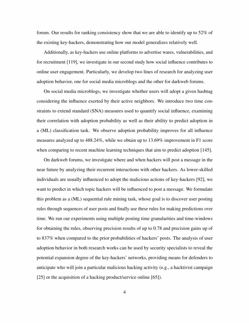
forum. Our results for ranking consistency show that we are able to identify up to 52% of

the existing key-hackers, demonstrating how our model generalizes relatively well.

Additionally, as key-hackers use online platforms to advertise wares, vulnerabilities, and

for recruitment [119], we investigate in our second study how social influence contributes to

online user engagement. Particularly, we develop two lines of research for analyzing user

adoption behavior, one for social media microblogs and the other for darkweb forums.

On social media microblogs, we investigate whether users will adopt a given hashtag

considering the influence exerted by their active neighbors. We introduce two time con-

straints to extend standard (SNA) measures used to quantify social influence, examining

their correlation with adoption probability as well as their ability to predict adoption in

a (ML) classification task. We observe adoption probability improves for all influence

measures analyzed up to 488.24%, while we obtain up to 13.69% improvement in F1 score

when comparing to recent machine learning techniques that aim to predict adoption [145].

On darkweb forums, we investigate where and when hackers will post a message in the

near future by analyzing their recurrent interactions with other hackers. As lower-skilled

individuals are usually influenced to adopt the malicious actions of key-hackers [92], we

want to predict in which topic hackers will be influenced to post a message. We formulate

this problem as a (ML) sequential rule mining task, whose goal is to discover user posting

rules through sequences of user posts and finally use these rules for making predictions over

time. We run our experiments using multiple posting time granularities and time-windows

for obtaining the rules, observing precision results of up to 0.78 and precision gains up of

to 837% when compared to the prior probabilities of hackers’ posts. The analysis of user

adoption behavior in both research works can be used by security specialists to reveal the

potential expansion degree of the key-hackers’ networks, providing means for defenders to

anticipate who will join a particular malicious hacking activity (e.g., a hacktivist campaign

[25] or the acquisition of a hacking product/service online [65]).

4

Moving to our third study, we analyze whether vendors of malware and malicious exploit

organically form hidden organizations on darkweb hacking marketplaces. We search for

communities of individuals with similar expertise in specific subfields of hacking, a feature

typically owned by key-hackers that can be used for surveillance purposes [94]. For instance,

vendors linked to emerging cyber threats can be automatically identified if at least one of the

community members is confirmed as offering a similar exploit online, allowing defenders to

predict their subsequent product offerings. As there is no direct communication between

vendors on those markets, detecting their communities becomes challenging, especially with

the absence of ground truth data. Thus, we develop a method based on (SNA) techniques

that identifies implicit communities of hacking-related vendors using the similarity of their

products. We validate our method cross-checking the community assignments of these

individuals on two mutually exclusive sets of marketplaces, achieving 0.445 of consistency

between more than 30 communities of vendors revealed in each subset of markets.

Finally, we design an AI tool that uses a (TL) framework to accomplish two tasks: 1)

induct rules that correlate malicious hacking activity with real-world cyber incidents in

order to predict future cyber-attacks; 2) leverage a deductive approach that combines attack

predictions for more accurate security warnings. The framework considers technical and

socio-personal indicators of attacks, deriving the latter from the social models proposed

in our previous studies. Results demonstrate considerable prediction gains in F1 score (up

to 150.24%) compared to the baseline when the pre-conditions of the rules include those

socio-personal indicators of attacks, highlighting their relevance for the identification of

imminent threats. Besides, we also observe a higher performance of our framework when

the predictions made for a given day are combined using deduction, obtaining gains in

F1 score of up to 182.38%. Those achievements evidence how the interdisciplinary work

conducted in this dissertation allows security specialists to mine the interest of credible

malicious hackers, given defenders a better chance in the security battle against attackers.

5

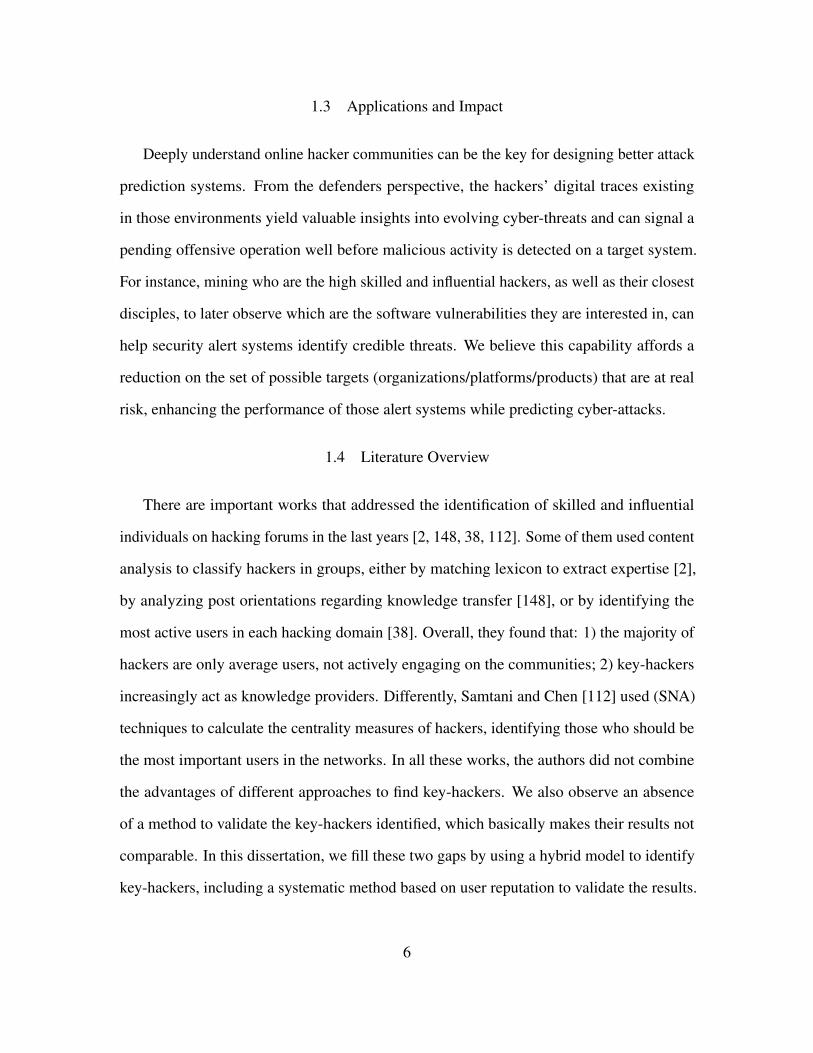
1.3 Applications and Impact

Deeply understand online hacker communities can be the key for designing better attack

prediction systems. From the defenders perspective, the hackers’ digital traces existing

in those environments yield valuable insights into evolving cyber-threats and can signal a

pending offensive operation well before malicious activity is detected on a target system.

For instance, mining who are the high skilled and influential hackers, as well as their closest

disciples, to later observe which are the software vulnerabilities they are interested in, can

help security alert systems identify credible threats. We believe this capability affords a

reduction on the set of possible targets (organizations/platforms/products) that are at real

risk, enhancing the performance of those alert systems while predicting cyber-attacks.

1.4 Literature Overview

There are important works that addressed the identification of skilled and influential

individuals on hacking forums in the last years [2, 148, 38, 112]. Some of them used content

analysis to classify hackers in groups, either by matching lexicon to extract expertise [2],

by analyzing post orientations regarding knowledge transfer [148], or by identifying the

most active users in each hacking domain [38]. Overall, they found that: 1) the majority of

hackers are only average users, not actively engaging on the communities; 2) key-hackers

increasingly act as knowledge providers. Differently, Samtani and Chen [112] used (SNA)

techniques to calculate the centrality measures of hackers, identifying those who should be

the most important users in the networks. In all these works, the authors did not combine

the advantages of different approaches to find key-hackers. We also observe an absence

of a method to validate the key-hackers identified, which basically makes their results not

comparable. In this dissertation, we fill these two gaps by using a hybrid model to identify

key-hackers, including a systematic method based on user reputation to validate the results.

6

We also report three relevant works that analyzed user susceptibility to influence on

social media, as they can be used to map the expanding networks of hackers [145, 51, 40].

The first one considered two functions based on pair-wise influence and structural diversity to

predict adoptions [145]. The second and third works used joint probabilities to calculate the

total influence that active neighbors exert on users to make them adopt a particular behavior

[51, 40]. All these works found a positive correlation between the number of active neighbors

and probability of influence, specially for hashtags that carry social risks. However, we note

those authors have not fully explored the dynamics of social influence, building their models

upon static relationships and invariable social stimulus. In our proposed work, we address

these issues by dynamically building our social networks to more accurately measure social

influence, showing significant improvements for adoption prediction.

To the best of our knowledge, we propose the first applied study where hacker engage-

ment on darkweb forums is investigated through adoption prediction. Even so, we present

here some works carried out on the surfaceweb 2 that can be used to predict opinions,

activities, and link formation. For instance, the framework proposed in [101] inferred users’

stance according to their arguments, interactions, and attributes, but it was unable to estimate

where and when a user would engage. The same issue is observed in the model proposed in

[49], where the authors tracked online activity of users to predict their future interactions.

Although the model estimated browse-content, browse-comments, upvote, downvote, or

do-nothing behavior for each post visualized, the technique was not able to anticipate a new

message. Also, the authors in [110] developed a time-series methodology for predicting link

formation in discussion forums, which was unable to forecast when specific interactions

between users would occur. Note how the prediction of hackers’ posts, considering patterns

of interactions driven mainly by social influence, is an important contribution of our work.

2Section of the Web accessed from any browser and regularly indexed by search engines.

7

Another contribution of this dissertation is an applied study where social network

information of malware and exploit vendors is derived from malicious hacking marketplaces

on the darkweb, since previous studies only examined characteristics of hacking and non-

hacking darkweb forums for this task. For instance, two topic-based social networks were

created in [69], one from the topic creator perspective and the other from the repliers

perspective. There are also works where the authors tried to form clusters of users based on

their messages’ timestamps [142] or based on the similarities of the posts’ meta-information

(author, timestamp, thread, etc.) [10]. It is widely known that social relationships of forum

users can be directly inferred from their posts/replies, while on marketplaces there is no

explicit communications among vendors, highlighting the novel aspect of our research.

Finally, only few research works focus on predicting cyber-attacks against specific

corporations by analyzing online hacking discussions. Most works that proactively investi-

gated cybersecurity either searched for cyber-threats to mitigate risks [103, 7, 93, 113, 5] or

predicted the exploitation of software vulnerabilities [109, 9, 17, 132]. However, similar

to our goal, Khandpur et al. [63] proposed an unsupervised approach to detect ongoing

cyber-attacks discussed on Twitter, by using a limited set of seed event triggers and a query

expansion strategy based on convolutional kernels and dependency parses. Goyal et al.

[52] described deep neural networks and autoregressive time series models that leveraged

signals from security blogs and vulnerability databases to predict attacks. Deb et al. [30]

applied sentiment analysis to darkweb forum posts to correlate sentiment trends over time

with potential attacks. Almukaynizi et al. [8] proposed a logical framework to predict

the magnitude of attacks by analyzing vulnerability mention on the darkweb. Although

those approaches contributed with proactive cyber threat intelligence, they neglected the

individuals behind the threats. Besides the technical information involved, we also rely on

social-personal indicators of attacks in this dissertation. Then, we are able to differentiate the

hackers in terms of capability, significantly increasing the accuracy of our attack predictions.

8

1.5 Organization

The remaining of this dissertation is organized as follows:

Chapter 2: Mining Key-Hackers on Darkweb Forums. In this Chapter, we describe the

proposed model used to identify the existing key-hackers on darkweb forums [83].

Chapter 3: Temporal Analysis of Influence to Predict User Adoption on Social Media.

In this Chapter, we detail the two proposed time constraints to extend standard (SNA)

influence measures while predicting hashtag adoption on social media [81, 82].

Chapter 4: Predicting Hacker Adoption on Darkweb Forums. In this Chapter, we

describe the proposed model to predict hacker engagement on darkweb forums, anticipating

in which topic hackers will be influenced to post a message in the near future [76].

Chapter 5: Detecting Communities of Malware and Exploit Vendors on Darkweb

Marketplaces. In this Chapter, we describe the proposed model to reveal hidden communi-

ties of hacking-related vendors on darkweb marketplaces [77, 80].

Chapter 6: Reasoning About Future Cyber-Attacks Through Socio-Technical Hack-

ing Information. In this Chapter, we describe the proposed framework to predict future

cyber offensives, considering technical and socio-personal indicators of attacks [78, 79].

Chapter 7: Final Considerations. In this chapter, we recapitulate the main ideas and

results presented in the dissertation, also considering some directions for future work.

Table 1.1 summarize the contributions presented in each chapter of this dissertation.

Table 1.1: Contributions of this Dissertation.

Chapters Contribution

02 Identification of key-hackers on darkweb forums.

03, 04 Analysis of user/hacker engagement on social media and darkweb forums.

05 Disclosure of hidden hacker communities existing on darkweb marketplaces.

06 Prediction of imminent cyber-attacks using socio-technical hacking information.

9

Chapter 2

MINING KEY-HACKERS ON DARKWEB FORUMS

2.1 Introduction

Malicious hacker communities have participants with different levels of knowledge, and

those who want to identify emerging cyber threats need to scrutinize these individuals to

find key cybercriminals [148]. We denote those malicious cyber-actors as key-hackers, since

they have higher hacking skills and influence when compared to the great majority of users

present in online hacking communities. As this select group of hackers foment a promising

vulnerability exploitation threat market [5], it forms “natural lens” through which security

alert systems can look at while predicting cyber-attacks.

To support our assumption, consider when beginners or standard-level hackers are

planning to launch an attack. As those actors are utility-maximizing, they opt for rewarding

vulnerabilities for which there exist threats with proved attack and concealment capabilities

to increase their chance of success [5]. Overall, the skills to implement and spread those

threats belong to key-hackers [7], as they are able to craft advanced hacking tools 1 , find

zero-days vulnerabilities 2 , recruit and orchestrate teams in attack campaigns 3 , and maintain

low profiles of activity [126, 97]. As key-hackers often succeed in their cybercrimes [89],

they provide profitable resources that are more appealing for the others [73].1Ex. of advanced hacking tools crafted by key-hackers: Retefe and TrickbotGo

banking Trojans, Nitol and DoublePulsar backdoors, Gh0st RAT, EternalRocks andMicroBotMassiveNet computer worms and WannaCry and NotPetya ransomwares.

2Ex. of zero-day exploits crafted by key-hackers: Stuxnet computer worm, 666 RAT,Tobfy ransomware, and LadyBoyle action script.

3Ex. of APT watering hole attack campaigns conducted by key-hackers: Web2Crew,Taidoor, th3bug, and Operation Ephemeral Hydra.

10

The challenge here is that key-hackers form only a small percentage of the community

members, making their identification a complex problem. In the literature, two approaches

have been empirically considered for this task: content analysis [2, 148, 38] and social

network analysis [147, 112]. In both approaches, the idea is to generate features and rank

the community users based on their feature values, being the top ranked users considered as

key-hackers [2]. However, there is a serious complication for this identification task: the

lack of ground truth (the key-hackers of the communities) to validate the results. As it is

difficult to obtain this information, previous works neglected this validation task or have it

done manually - e.g., by leveraging security consulting companies [91]. Finally, it is unclear

if these methods can generalize, as training and testing are done using the same forum data.

In this Chapter, we address the key-hacker identification problem including a systematic

method to validate the results. Particularly, we study how content, social network, and

also seniority analysis perform individually and combined in this task. We conduct our

experiments using informative features extracted from three highly ranked darkweb hacker

forums. Information related to activity, expertise, knowledge transfer behavior, structural

position, influence, and coverage are mined to develop a profile for each community member,

aiming to understand which features characterize key cybercriminals. To train and test our

model, we use an optimization metaheuristic and compare its performance with machine

learning algorithms. We leverage the users’ reputation provided by the forums analyzed to

cross-validate the results among those sites - models trained in one forum are generalized to

make predictions on different ones. Our work is novel since it offers researchers a strategy

to find key-hackers in forums with no users’ reputation or with a deficient user reputation

system. We observe this is the case of the vast majority of hacking forums, representing over

80% of the 36 scraped for this study. We summarize the main contributions of this work as:

1. We show that a hybridization of features derived from content, social network, and

seniority analysis is able to identify key-hackers up to 17% more precisely than those

11

derived from any of these strategies by itself;

2. We explain and evidence why reputable hackers form a strong indicator of key-

cybercriminals;

3. We demonstrate how a model learned in a given forum to identify its key-hackers can

be generalized to a different forum which was not used to train the model, obtaining

up to 52% of ranking consistency;

4. We compare the performance of different models when trying to identify key-hackers,

showing how an optimization metaheuristic obtains up to 35% of predictive improve-

ment over machine learning algorithms.

The remainder of this Chapter is organized as follows. Section 2.2 details darkweb

forums and our dataset. Next, we show in Section 2.3 how we leverage users’ reputation to

obtain ground truth data. Section 2.4 defines our problem. Section 2.5 describes the features

we derive to profile hackers. Section 2.6 presents our experiments and corresponding results.

Section 2.7 shows some related work. Finally, Section 2.8 summarizes the Chapter.

2.2 Darkweb Hacking Forums

Many people involved in malicious cyber activity rely on trustful online communities,

among which, forums are one of the most prevalent [2]. For example, the recent “WannaCry”

ransomware attack directed against hospitals in the UK and numerous other worldwide

targets was discussed several weeks prior on a darkweb forum [127]. Hackers likely

involved in this attack discussed the number of unpatched machines, the exploit to be

used, the industry verticals, and the method of attack (ransomware). These hacking forums

provide user-oriented platforms that enable communication regardless geophysical location,

facilitating the emergence of hackers’ communities.

12

The World Wide Web (Web) is a vast network of linked hypertext files where forums

are accessed via the Internet. The Web can be maily classified into 3 regions: surfaceweb,

deepweb, and darkweb [92]. The Surfaceweb is the open portion of the Internet, where

webpages are publicly accessible and indexed by search engines. On the other hand, the

deepweb refers to the websites hosted on the surfaceweb but not indexed by search engines,

usually because they require authentication. Finally, the darkweb refers to a collection of

websites that exist on encrypted networks of the deepweb. It is a region intentionally and

securely hidden from users and standard search engines and browsers. This is the reason

why darkweb forums constitute one of the most widespread hacking environment, being

commonly used for research studies investigating key cybercriminals [2].

2.2.1 Dataset

We collect data from a commercial version of the system proposed in [92]. This system

currently provided by CYR3CON [28] is responsible for gathering cyber threat intelligence

from various social platforms of the World Wide Web, especially the ones existing on

deepnet and darkweb websites. For this particular work, we select three popular English

hacking forums on the darkweb. We anonymize these forums representing them as Forum

1, Forum 2, and Forum 3, showing their statistics in Table 2.1. All these forums comprise

hacking-related discussions organized in a thread format, where a user initiates a topic that

is followed by many users’ replies.

Table 2.1: Statistics of the Three Analyzed Darkweb Hacker Forums.

Forum 1 Forum 2 Forum 3

Time Period 2013-12-24 : 2016-03-16 2013-12-24 : 2016-08-16 2002-09-14 : 2016-03-15

Number of Users 4,380 2,495 2,802

Number of Topics 5,571 1,077 5,805

Number of Posts 36,453 25,115 49,078

Distinct Values of Users’ Reputation 134 102 37

13

In order to prepare the data for feature extraction, we retrieve the users’ interactions

over time to generate a network of hackers. We denote a set of users V and connections

E as the nodes and edges in a directed graph G � �V,E�, while Θ,M, and T correspond

to a set of topics, messages, and discrete time points. The symbols v, θ,m, t will represent

a specific node, topic, message, and time point. We denote an activity log A containing

all posts (topics and replies) as a set of tuples of the form `v, θ,m, te, where v > V , θ > Θ,

m >M, and t > T . It describes that “v posted in topic θ a message m at time t”. A directed

edge �v, v�� is created when users v and v� post together in a given topic, so that the posting

time of v is greater than of v�. We formalize the set of direct edges E in equation 2.1:

E � ��v, v�� S§`v, θ,m, te > A,§`v�, θ,m�, t�e > A, s.t. v x v�, t A t�� (2.1)

The intuition with this set of direct edges is to make visible to users that are posting in θ

at time t all other users that have already posted in θ prior to t, but not vice-versa. We believe

this strategy can better reproduce the interaction process on online forums (compared to the

general strategy of creating a complete undirected graph including all users that post together

in a topic [112]), since users will only know about previous posts. Figure 2.1 illustrates this

process by showing the original users’ posts in panel (a) and the corresponding generated

social network in panel (b).

1

2

3

4

5

(a) (b)

Topic A

User Post Time

1 01-01-2015 10:23:15

2 01-01-2015 10:25:10

3 01-01-2015 10:30:20

2 01-01-2015 10:31:46

5 01-01-2015 10:40:14

Topic B

User Post Time

2 01-02-2015 15:20:10

1 01-02-2015 16:10:05

3 01-02-2015 16:18:47

2 01-02-2015 17:04:46

4 01-02-2015 20:49:14

Fig. 2.1: Directed Graph Generated Using the Users’ Posts.

14

After generating the social networks, we remove all users who do not belong to the

giant component of their corresponding forum, since they can produce misleading centrality

values. The issue happens because some centralities are computed and normalized for each

component, which tends to produce high values for users in small parts of the networks.

Because of their few connections, these individuals would hardly be considered as key-

hackers. Table 2.2 shows the size of all components of each forum, detailing that 67 users

from Forum 1, 78 users from Forum 2, and 65 users from Forum 3 were removed.

Table 2.2: Network Component Analysis.

Forum 1 Forum 2 Forum 3

Giant Component Size 4,313 2,417 2,737

Component Size = 11 0 1 0




2.3 Leveraging Users’ Reputation to Obtain Ground Truth Data

As hacker communities form meritocracies [104, 118], members own different levels of

capability, expertise, and influence (to mention a few human factors). According to [31],

those factors are organically consolidated in the user reputation score, which is a metric that

codifies users’ standing, driving engagement by measuring participation, activity, content

quality, content rating, etc. Zhang et al. [148] showed that reputable hackers are usually

linked to emerging cyber threats, making them a strong indicator of key cybercriminals.

A case study in our data corroborates with the Zhang’s assumption. In 2016, Anna

Senpai had a high reputation when he released the Mirai Botnet source code on a popular

15

hacker forum [128]. His posts generated a high number of responses, though none more than

the post containing the code. Since user reputation is peer-assigned, the reputation score

is mirroring how other forum members evaluate the usefulness of the users’ contributions.

When we analyze the posting patterns of high and low reputable hackers of Forum 1

presented in Figure 2.2(a), we observe that 36 out of the 44 hackers with the highest

reputation (Top1% of all users) are posting on the 28 spikes of activity (minimal of 4 � σ

above average), while only 8 of them are not engaged in these conversations.

0

10

20

30

40

Nu

mb

er

of

Use

rs

Top 1% of the Highest Reputable Hackers in Forum 1

Posting on the 28 spikes Not posting on the 28 spikes

0

1000

2000

3000

4000

Nu

mb

er

of

Use

rs

≈Top 75% of the Lowest Reputable Hackers in Forum 1

Posting on the 28 spikes Not Posting on the 28 spikes

0

500

1000

1500

2000

Nu

mb

er

of

Use

rs



(b)(a)

0

5

10

15

20

Nu

mb

er

of

Use

rs



(d)(c)

0

5

10

15

20

Nu

mb

er

of

Use

rs



0

1000

2000

3000

Nu

mb

er

of

Use

rs



(f)(e)

Fig. 2.2: Posting Pattern of the Highest and the Lowest Reputable Hackers on the Three

Darkweb Forums Analyzed.

On the other hand, Figure 2.2(b) shows that 870 out of the 4.039 hackers with the lowest

reputation (� Top75% of all users) are posting on those spikes, while 3.169 are not engaged

in these conversations. A similar pattern is observed for the other two forums analyzed.

We investigate those spikes as they offer some intuition about possible interesting topics

16

promoted by skilled and influential hackers on the forums, confirming the user reputation

score as a strong indicator for key-hacker identification.

In this study, we also rely on the assumption that users with high reputation form our

set of key-hackers, using this metric as our ground truth. Thus, we deliberately select

forums that explicitly provide this information, so that the corresponding key-hackers can be

identified. Figure 2.3 shows the distribution of the reputation score in (a) Forum 1, (b) Forum

2, and (c) Forum 3, pointing out the existence of a hacking meritocracy (these curves fit

power-laws with pk � k�0.92, pk � k�0.86 and pk � k�0.78 respectively, where k is the number

of users). As it is observed, only a few number of users (key-hackers) own high reputation in

all the forums, although their corresponding scores vary in magnitude. In addition, although

Table 2.1 shows that Forum 1 and Forum 2 are closer in terms of reputation distinctness

(their scores are formed by 134 and 102 different values respectively while Forum 3 owns

only 37), the similar distribution pattern of all those three forums informs that characteristics

of the highest reputable hackers should be somehow shared by them.

Reputation Score

Nu

mb

er o

f U

sers

(a) (c)(b)

1

10

100

1000

1 100 100001

10

100

1000

1 10 100 1000

1

10

100

1000

1 10 100 1000

Fig. 2.3: Distribution of Reputation Score in (a) Forum 1, (b) Forum 2, and (c) Forum 3

(log-log scale).

2.4 Problem Statement

Based on the finding that the highest reputable hackers form our set of key-hackers, we

want to estimate the user reputation score in order to find key-hackers in forums that do not

provide this score or that have a deficient user reputation system.

17

2.5 Feature Engineering

To estimate users’ reputation, we design the 25 features detailed in Table 2.3 to mine

relevant characteristics and behaviors of key-hackers.

Table 2.3: Feature Engineering.

01. Topics Created

02. Replies Created

Activity 03. Replies by Month

04. Length of Topics

05. Length of Replies

06. Topics Density

Involvement Quality 07. Replies with Knowledge Provision

Content Analysis 08. Replies with Knowledge Acquisition

Expertise 09. Topics with Knowledge Provision

10. Topics with Knowledge Acquisition

Cybercriminal Assets 11. Attachments

12. Technical Jargon

Specialty Lexicons 13. Darkweb Jargon

14. Velocity of Knowledge Provision Pattern in Topics

Knowledge Transfer 15. Velocity of Knowledge Acquisition Pattern in Topics

Behavior 16. Velocity of Knowledge Provision Pattern in Replies

17. Velocity of Knowledge Acquisition Pattern in Replies

18. Degree Centrality

Structural Position 19. Betweenness Centrality

Social Network 20. Closeness Centrality

Analysis 21. Eigenvector Centrality

Influence 22. Page Rank

23. Interval btw User’s & Forum’s First Posts

Seniority Analysis Coverage 24. Distinct Days of Posts

25. Interval btw User’s & Forum’s Last Posts

From these features, 17 are extracted using Content Analysis, subdivided in Activity (3),

Expertise (10), and Knowledge Transfer Behavior (4). We subdivide the 10 features related

to Expertise in Involvement Quality (7), Cybercriminal Assets (1), and Specialty Lexicons (2).

In addition, 5 features are extracted using Social Network Analysis, subdivided in Structural

18

Position (3) and Influence (2). Finally, 3 features are extracted using what we denominate

Seniority Analysis, being all of them related to Coverage. We analyze users’ seniority since

it generates indicators of consistent forum involvement over time, checking how much the

users continuously contribute to the hacker environments [55, 89, 102]. We believe this

set of features comprises a variety of information that could differentiate key-hackers from

the beginners or standard-level hackers, contributing to a better estimation of the users’

reputation. All features have their values normalized to avoid problems with different scales

[131]. We detail the features below.

2.5.1 Activity

The set of features within this category belongs to the content analysis approach and

aims to identify how active the hackers are. It includes the three following features:

Topics Created (TOC). This feature counts how many topics (headers) are initiated by

hackers. According to previous works [147], key-hackers usually create relatively few topics

but with high relevance to the community. We formalize this feature as:

TOC�v� �Qθ

g�`v, θ,m, te� (2.2)

where g�`v, θ,m, te� is defined as:

g�`v, θ,m, te� �¢¦¨¤

1, if `v, θ,m, te > A , ¨`v�, θ,m�, t�e > A, s.t. t� @ t

0, otherwise(2.3)

Replies Created (REC). This feature counts the amount of times users answer the topics.

According to previous works [147, 38, 148, 2], key-hackers usually create a huge quantity

of quality replies, offering relevant help to the lower skilled community members. We

formalize this feature as:

19

REC�v� �Qθ

QmQt

S`v, θ,m, teS � TOC�v�, s.t. `v, θ,m, te > A (2.4)

Replies by Month (REM). This feature averages the replies created by the hackers monthly,

aiming to estimate how often hackers produce answers. Previous works, such as [2], claim

that key-hackers usually have a minimum frequency of answers over time, in order to keep

the status acquired. We formalize this feature as:

REM�v� �REC�v�

SMA�v�S (2.5)

where MA�v� is the set of distinct months in which v created at least one topic answer.

2.5.2 Expertise

This category of features belongs to the content analysis approach and aims to quantify

the users’ skills regarding malicious hacking. It includes the ten following features:

Length of Topics (LET). This feature averages the number of words used by hackers to

create a topic. Previous works, such as [2], state that key-hackers tend to not create extensive

topics since this is a characteristic of low-skilled hackers. We formalize this feature as:

LET�v� �Pθ h�`v, θ,m, te�

TOC�v�

(2.6)

with h�`v, θ,m, te� being defined as:

h�`v, θ,m, te� �¢¨¦¨¤

Length�m�, if `v, θ,m, te > A , ¨`v�, θ,m�, t�e > A,s.t. t� @ t

0, otherwise

(2.7)

20

Length of Replies (LER). This feature averages the number of words used by hackers to

create a reply. According to previous works [147, 2], key-hackers usually produced detailed

answers, as they have interest and knowledge to instruct the other community members. We

formalize this feature as:

LER�v� �PθPmPt i�`v, θ,m, te�

REC�v�

(2.8)

with i�`v, θ,m, te� being defined as:

i�`v, θ,m, te� �¢¨¦¨¤

Length�m�, if `v, θ,m, te > A , §`v�, θ,m�, t�e > A,s.t. t� @ t

0, otherwise

(2.9)

Topics Density (TOD). This feature averages the number of users posting in a given topic.

As discussions started by key-hackers are more relevant to the community, they often

promote a higher user engagement [148]. We formalize this feature as:

TOD�v� �Pθ j�`v, θ,m, te�

TOC�v�

(2.10)

with j�`v, θ,m, te� being defined as:

j�`v, θ,m, te� �¢¨¦¨¤

Pv�Pm�Pt� S`v�, θ,m�, t�eS, if `v, θ,m, te > A ,

¨`v�, θ,m�, t�e > A, s.t. t� @ t

0, otherwise

(2.11)

Replies with Knowledge Provision (RKP). This feature counts the number of replies

containing knowledge provision. Zhang et. al. [148] observed a trend for key-hackers

21

to produce more replies providing than requesting information. To identify knowledge

provision, we apply string-match to a predefined set of keywords. Table 2.4 shows a sample

of the keywords that match knowledge provision.

Table 2.4: Sample of Keywords Used for String-Match.

Knowledge Provision Knowledge Acquisition Technical Jargon Darkweb Jargon

advice request back door tor

suggest ask cookie blockchain

guide doubt crack dispute

tutorial whyd dos bitcoin

recommend how to dump escrow

follow need zero day honeypot

check want xss i2p

yourself troublesom spyware freenet

easy-to-follow fail shell onion

demonstrate struggling phishing pgp

We formalize this feature as:

RKP�v� �Qθ

QmQt

k�`v, θ,m, te� (2.12)

with k�`v, θ,m, te� being defined as:

k�`v, θ,m, te� �¢¨¦¨¤

1, if §w >m ,w >Key�kp� , `v, θ,m, te > A ,

§`v�, θ,m�, t�e > A, s.t. t� @ t

0, otherwise

(2.13)

22

where Key�kp� is the predefined set of knowledge provision keywords.

Replies with Knowledge Acquisition (RKA). This feature counts the number of replies

containing knowledge acquisition. As the opposite of the previous feature, Zhang et. al.

[148] observed a tendency for key-hackers to produce fewer replies acquiring than providing

information. To identify a knowledge acquisition, we also apply string-match to a predefined

set of keywords illustrated in Table 2.4. We formalize this feature as:

RKA�v� �Qθ

QmQt

l�`v, θ,m, te� (2.14)

with l�`v, θ,m, te� being defined as:

l�`v, θ,m, te� �¢¨¦¨¤

1, if §w >m ,w >Key�ka� , `v, θ,m, te > A ,

§`v�, θ,m�, t�e > A, s.t. t� @ t

0, otherwise

(2.15)

where Key�ka� is the predefined set of knowledge acquisition keywords.

Topics with Knowledge Provision (TKP). This feature counts the number of topics con-

taining knowledge provision. It has the same pattern observed for the feature RKP, but with

a different magnitude. We formalize this feature as:

TKP�v� �Qθ

n�`v, θ,m, te� (2.16)

with n�`v, θ,m, te� being defined as:

n�`v, θ,m, te� �¢¨¦¨¤

1, if §w >m ,w >Key�kp� , `v, θ,m, te > A ,

¨`v�, θ,m�, t�e > A, s.t. t� @ t

0, otherwise

(2.17)

23

Topics with Knowledge Acquisition (TKA). This feature counts the number of topics

containing knowledge acquisition. It has the same pattern observed for the feature RKA, but

with a different magnitude. We formalize this feature as:

TKA�v� �Qθ

o�`v, θ,m, te� (2.18)

with o�`v, θ,m, te� being defined as:

o�`v, θ,m, te� �¢¨¦¨¤

1, if §w >m ,w >Key�ka� , `v, θ,m, te > A ,

¨`v�, θ,m�, t�e > A, s.t. t� @ t

0, otherwise

(2.19)

Attachments (ATH). This feature checks for attachments in the posts (topics and replies).

According to [2], key-hackers usually provide relevant cybercriminal assets in form of

attachments. We apply string-match to a predefined set of keywords such as “href” or “http”,

formalizing this feature as:

ATH�v� �Qθ

QmQt

p�`v, θ,m, te� (2.20)

with p�`v, θ,m, te� being defined as:

p�`v, θ,m, te� �¢¦¨¤

1, if §w >m ,w >Key�at� , `v, θ,m, te > A0, otherwise

(2.21)

where Key�at� is the predefined set of keywords related to attachments.

Technical Jargon (TEJ). This feature checks for technical jargon in the posts. According

to [2], key-hackers often use technical jargon to reference some specific hacking technique

24

or tool. To identify technical jargon, we apply string-match to a set of keywords extracted

from a predefined dictionary. Table 2.4 shows a sample of the keywords that match technical

jargon. We formalize this feature as:

TEJ�v� �Qθ

QmQt

q�`v, θ,m, te� (2.22)

with q�`v, θ,m, te� being defined as:

q�`v, θ,m, te� �¢¦¨¤

1, if §w >m ,w >Key�ja� , `v, θ,m, te > A0, otherwise

(2.23)

where Key�ja� is the predefined set of keywords related to technical jargon.

Darkweb Jargon (DWJ). This feature checks for darkweb jargon in the posts. According

to [2], key-hackers often use darkweb jargon to reference some specific hacker environment,

technique or tool. To identify darkweb jargon, we apply string-match to a set of keywords

extracted from a predefined dictionary. Table 2.4 shows a sample of the keywords that match

darkweb jargon. We formalize this feature as:

DWJ�v� �Qθ

QmQt

r�`v, θ,m, te� (2.24)

with r�`v, θ,m, te� being defined as:

r�`v, θ,m, te� �¢¦¨¤

1, if §w >m ,w >Key�dw� , `v, θ,m, te > A0, otherwise

(2.25)

where Key�dw� is the predefined set of keywords related to the darkweb.

25

2.5.3 Knowledge Transfer Behavior

The set of features within this category belongs to the content analysis approach and aims

to identify the behavioral trend of hackers related to knowledge provision and knowledge

acquisition over time. It includes the four following features:

Velocity of Knowledge Provision Pattern in Topics (VPT). This feature checks how fast

the knowledge provision pattern increases or decreases in the topics created by hackers. The

idea is inspired in [148], who examined how this pattern changes by analyzing sequential

posts. According to [148], key-hackers usually present increasing knowledge provision

over time, and this feature measures the velocity of this behavior in the topics. Specifically,

for every sequential 10 topics i where user v engaged, we create a data point xi�v� and

assign the number of topics created by v containing knowledge provision to yi�v�. Then, we

analyze all points created using linear regression, checking the slope a of the line generated

(y � ax). We formalize this feature as:

V PT�v� �y2�v� � y1�v�x2�v� � x1�v� �

y2�v� � y1�v�2 � 1

� y2�v� � y1�v� � a (2.26)

with yi�v� being defined as:

yi�v� ��i�1��10��10

Qθ >TOP�v�, θ��i�1��10��1

n�`v, θ,m, te� (2.27)

where TOP�v� is the set of sorted topics created by v and n is defined in equation 2.17.

Velocity of Knowledge Acquisition in the Topics (VAT). This feature checks how fast

the knowledge acquisition pattern increases or decreases in the topics created by hackers.

We use the same strategy mentioned for the previous feature, but considering knowledge

acquisition now. According to [148], key-hackers usually present decreasing knowledge

26

acquisition over time, and this feature measures the velocity of this behavior in the topics.

We formalize this feature as:

V AT�v� �y2�v� � y1�v�x2�v� � x1�v� �

y2�v� � y1�v�2 � 1

� y2�v� � y1�v� � a (2.28)


yi�v� ��i�1��10��10

Qθ >TOP�v�, θ��i�1��10��1

o�`v, θ,m, te� (2.29)

where TOP�v� is the set of sorted topics created by v and o is defined in equation 2.19.

Velocity of Knowledge Provision in the Replies (VPR). This feature checks how fast the

knowledge provision pattern increases or decreases in the replies created by hackers. The

pattern here should follow the pattern identified by the feature VPT, but with different

magnitude. We formalize this feature as:

V PR�v� �y2�v� � y1�v�x2�v� � x1�v� �

y2�v� � y1�v�2 � 1

� y2�v� � y1�v� � a (2.30)


yi�v� ��i�1��10��10

Qθ >REP�v�, θ��i�1��10��1

k�`v, θ,m, te� (2.31)

where REP�v� is the set of sorted replies created by v and k is defined in equation 2.13.

Velocity of Knowledge Acquisition in the Replies (VAR). This feature checks how fast

the knowledge acquisition pattern increases or decreases in the replies created by hackers.

The pattern here should follow the pattern identified by the feature VAT, but with different

magnitude. We formalize this feature as:

27

V AR�v� �y2�v� � y1�v�x2�v� � x1�v� �

y2�v� � y1�v�2 � 1

� y2�v� � y1�v� � a (2.32)


yi�v� ��i�1��10��10

Qθ >REP�v�, θ��i�1��10��1

l�`v, θ,m, te� (2.33)

where REP�v� is the set of sorted replies created by v and l is defined in equation 2.15.

2.5.4 Structural Position

The set of features within this category belongs to the social network analysis approach

and aims to define the hackers’ relevance based on their structural position in the networks.

This category includes the three following features:

Degree Centrality (DEC). This feature measures the number of direct neighbors connected

to a node [143]. As we deal with directed networks, we defined this measure as the number

of outgoing edges [143]. According to [112], key-hackers usually present high degree

centralities, since each of their many replies produces an outgoing edge. We formalize this

feature as:

DEC�vi� � douti (2.34)

where douti is the out-degree of vi.

Betweenness Centrality (BEC). This feature measures the number of shortest paths that

pass through a node [143], indicating its importance for the information flow. According to

[147], key-hackers usually present high betweenness centralities, since they are very well

connected users who often appear in those shortest paths. We formalize this feature as:

28

BEC�vi� � Qsxtxvi

σst�vi�σst

(2.35)

where σst is the number of shortest paths from node s to t and σst�vi� is the number of

shortest paths from node s to t that pass through vi.

Closeness Centrality (CLC). This feature measures how close an individual is to everyone

else [143]. As key-hackers have a central position in the networks that shrinks distances to

the others, they usually present high closeness centralities. We formalize this feature as:

CLC�vi� �1

lvi(2.36)

where lvi �1n�1 Pvjxvi li,j is node vi’s average shortest path length to other nodes and n

is the number of nodes.

2.5.5 Influence

The set of features within in this category belongs to the social network analysis approach

and aims to identify the level of prestige of hackers. It includes the two following features:

Eigenvector Centrality (EIC). This feature assigns importance to a node if other important

nodes are linked to it [143]. According to [91], key-hackers usually present high eigenvector

centralities, since they form connections among themselves. We formalize this feature as:

EIC�vi� �1

λ

n

Qj�1

Aj,iEIC�vj� (2.37)

where λ is a fixed constant, Aj,i is the adjacent matrix of the directed graph G � �V,E�and n is the number of nodes.

Page Rank (PAR). As a variant of EIC, this feature also checks the quality of the links

pointing to a hacker [143]. According to [91], key-hackers often present high page rank,

29

since they are likely to receive more links from other key-hackers. We formalize this feature

as:

PAR�vi� � αn

Qj�1

Aj,iPAR�vj�doutj

� β (2.38)

where λ, α, and β are fixed constants, Aj,i is the adjacent matrix of the directed graph

G � �V,E� and n is the number of nodes.

2.5.6 Coverage

This category of features belongs to the seniority analysis approach and aims to identify

the active long-term hackers in the forums. It includes the three following features:

Interval between User’s and Forum’s First Posts (IFP). This feature checks the time

interval between the first post in the forum and the first post of a specific hacker. Previous

works [13, 2] argue that founding members are usually key-hackers, being actively involved

in the discussions since the beginning. We formalize this feature as:

IFP �v� �Qθ

QmQt

s�`v, θ,m, te� �Qv�Qθ�Qm�

Qt�u�`v�, θ�,m�, t�e� (2.39)

where s�`v, θ,m, te� and u�`v�, θ�,m�, t�e� are defined as:

s�`v, θ,m, te� �¢¦¨¤t, if `v, θ,m, te > A , ¨`v, θ��,m��, t��e > A, s.t. t�� @ t

0, otherwise(2.40)

u�`v�, θ�,m�, t�e� �¢¦¨¤t, if `v�, θ�,m�, t�e > A , ¨`v��, θ��,m��, t��e > A , s.t. t�� @ t�

0, otherwise(2.41)

Distinct Days of Postings (DDP). This feature checks the hackers’ posting frequency.

Previous works [13, 148] argue that continuous participants are more likely to be key-

30

hackers, since they are often contributing to the communities. We formalize this feature

as:

DDP�v� � SDays�v�S (2.42)

where Days�v� returns the set of distinct days in which v posted.

Interval between User’s and Forum’s Last Posts (ILP). This feature checks the time

interval between the last post in the forum and the last post of a specific hacker. Previous

works [13, 2] argue that key-hackers are usually active in the communities with no fleeting

interests. We formalize this feature as:

ILP �v� �Qθ

QmQt

x�`v, θ,m, te� �Qv�Qθ�Qm�

Qt�y�`v�, θ�,m�, t�e� (2.43)

where x�`v, θ,m, te� and y�`v�, θ�,m�, t�e� are defined as:

x�`v, θ,m, te� �¢¦¨¤t, if `v, θ,m, te > A , ¨`v, θ�,m�, t�e > A, s.t. t� A t

0, otherwise(2.44)

y�`v�, θ�,m�, t�e� �¢¦¨¤t, if `v�, θ�,m�, t�e > A , ¨`v��, θ��,m��, t��e > A , s.t. t�� A t�

0, otherwise(2.45)

2.6 Supervised Learning Experiments

This section presents our supervised learning experiments to mine key-hackers. We first

introduce how we perform training and testing using four different algorithms, including an

optimization metaheuristic and three machine learning methods. Our intention is to verify

which algorithms generalize better when estimating user reputation, using the hackers’ char-

acteristics learned in one forum to test on another one. Then, we compare the performance

31

of our model under two conditions: 1) when it is trained/tested using the features related to

each approach individually and combined; 2) when it is trained/tested using different ranges

for the definition of key-hackers.

We use the 25 features engineered as input to the supervised learning algorithms. We

compare the algorithms’ performance when they use features of content, social network,

and seniority analysis individually and combined. To perform that, we leverage the user

reputation score to maximize the overlap of two distinct sets of hackers: the Top10% found

with their Estimated Reputation Score (ERS) and the Top10% found with their Actual

Reputation Score (ARS). The ARS represents the user’s reputation informed by the forums,

and we want to use this information as our ground truth. This way, we sort the users

according to their reputation in descending order, and the Top10% will represent the key-

hackers - for instance, the Top10% of Forum 1 are the 431 hackers with the highest ARS. The

ERS is the reputation to be estimated by our algorithms based on the features extracted, and

we also want to use the Top10% to infer who should be the key-hackers. With these both

metrics in hands, our goal is to maximize the value of Overlap10% presented in equation

2.46, which is a metric that provides a measure for user ranking consistency [16].

Overlap10% �SERS10% 9ARS10%SSERS10% 8ARS10%S (2.46)

2.6.1 Genetic Algorithms

We train and test four different supervised learning algorithms. The first one comprises

an optimization metaheuristic inspired by the natural selection process: Genetic Algorithms

(GA) [87]. In the training phase, we use this algorithm to perform a linear combination of

our 25 features, calibrating the ERS’s feature weights in equation 2.47 so that Overlap10%

is maximized. As this approach relies on genetic operators such as selection, crossover, and

32

mutation to produce high-quality solutions to optimization problems [87] (we apply the

elitist, two-points, and order-changing methods respectively), we expect it searches through

a huge combination of feature weights to find the ones generating the highest value for

Overlap10%. Then, we use the calibrated linear system trained in a particular forum to test

its performance on a different one, also using the Overlap10%.

ERS�v� � n

Qi�1

wi � vxi (2.47)

where wi is the weight of feature i, vxi is the value of the feature i for user v, and n is

the set of considered features.

2.6.2 Multiple Linear Regression

The second algorithm is a Multiple Linear Regression (MLR) [131]. In the training

phase, we want to model the relationship between our dependent variable (reputation) and

our 25 independent variables (features). This relationship is modeled using linear predictor

functions, whose parameters are estimated from the data to fit a curve that produces the

highest value for Overlap10%. Then, we want to use this curve fitted to a particular forum to

test its performance on a different one, also using theOverlap10%. Note that the correct order

of hackers based on reputation is not required, only the presence of the correct individuals

in the Top10%.

2.6.3 Random Forests and Support Vector Machines

The next two algorithms comprise classifiers: Random Forests (RF) and Support Vector

Machines (SVM) [131]. Here, we define a binary classification problem to identify the

individuals belonging to the positive class (key-hackers). Random Forests are an ensemble

method that use multiple decision trees for training, outputting the class that is the mode

33

of the classes. Support Vector Machines (SVM) are a discriminative classifier formally

defined by a separating hyperplane that gives the largest minimum distance to the training

examples. For both classifiers in the training phase, we want to learn the feature values of

the Top10% reputable hackers of a given forum, in order to apply this knowledge to another

forum (testing phase) maximizing the value of Overlap10%.

2.6.4 Results

Figure 2.4 presents the performance of the algorithms when they are trained using

Forum 1 and tested using Forum 2 and Forum 3. We detail the performances when the

algorithms learn only the features of individual approaches, and when they learn all the

features combined (hybrid approach).

Ove

rlap

10

%

0

0.2

0.4

0.6

Hybrid Approach Content Analysis

SNA Seniority Analysis

0

0.1

0.2

0.3

0.4

0.5



Ove

rlap

10

%

0

0.2

0.4

0.6

Hybrid Approach Content AnalysisSNA Seniority Analysis

0

0.1

0.2

0.3

0.4

0.5



Ove

rlap

10

%

0

0.2

0.4

0.6



0

0.1

0.2

0.3

0.4

0.5



Ove

rlap

10

%

0

0.2

0.4

0.6



0

0.1

0.2

0.3

0.4

0.5



Training on Forum 1Testing on Forum 2


Genetic Algorithm

Multiple Linear Regression

Random Forests

Support Vector Machines



Fig. 2.4: Overlap10% Performance when Algorithms are Trained on Forum 1 and Tested on

Forum 2/Forum 3.

We observe 5 cases when the hybrid approach obtains the best performance, while 1 and

2 cases are verified for content and seniority analysis respectively. The highest value for

34

Overlap10% when testing on Forum 2 (0.52) is achieved by Genetic Algorithms using the

hybrid approach. This result implies that more than half of the Top10% reputable hackers

were identified, which for this forum represents around 121 users. Also, the highest value

for Overlap10% when testing on Forum 3 (0.33) is achieved by using Genetic Algorithms

and SVM using the hybrid approach. This result implies that more than one third of the

Top10% reputable hackers were identified, which for this forum represents around 92 users.

Note these performances correspond to find only 10% of the hackers (those with the highest

reputation), which represents a strict filter of users.

Figure 2.5 presents the performance of the algorithms when they are trained using Forum

2 and tested using Forum 1 and Forum 3. We observe 5 cases when the hybrid approach

obtains the best performance, while 1 case is verified for each of the other approaches.

The highest value for Overlap10% when testing on Forum 1 (0.43) is achieved by Genetic

Algorithms using the hybrid approach. This result implies that almost half of the Top10%

reputable hackers were identified, which for this forum represents around 186 users.

0

0.1

0.2

0.3

0.4

0.5


Ove

rlap

10

%

0

0.1

0.2

0.3

0.4

0.5



0

0.1

0.2

0.3

0.4

0.5



Ove

rlap

10

%

0

0.1

0.2

0.3

0.4

0.5



0

0.1

0.2

0.3

0.4

0.5


Ove

rlap

10

%

0

0.1

0.2

0.3

0.4

0.5



0

0.1

0.2

0.3

0.4

0.5



Ove

rlap

10

%

0

0.1

0.2

0.3

0.4

0.5





Genetic Algorithm


Random Forests





Forum 1/Forum 3.

35

In addition, the highest value forOverlap10% when testing on Forum 3 (0.32) is achieved

by Genetic Algorithms and Random Forests using the hybrid approach. This result implies

that almost one third of the Top10% reputable hackers were identified, which for this forum

represents around 88 users.

Figure 2.6 shows the algorithms’ performance when they are trained using Forum 3

and tested using Forum 1 and Forum 2. We note 5 cases when the hybrid approach has the

best performance, while 1 and 2 cases are verified for content/seniority and social network

analysis respectively. The highest value for Overlap10% when testing on Forum 1 (0.45) is

achieved by Genetic Algorithms using the hybrid approach. This result implies that almost

half of the Top10% reputable hackers were identified, which for this forum represents around

194 users. Also, the highest value for Overlap10% when testing on Forum 2 (0.5) is achieved

by Genetic Algorithms using the hybrid approach. This result implies that half of the Top10%

reputable hackers were identified, which for this forum represents around 121 users.

0

0.1

0.2

0.3

0.4

0.5



Ove

rlap

10

%

0

0.2

0.4

0.6



0

0.1

0.2

0.3

0.4

0.5



Ove

rlap

10

%

0

0.2

0.4

0.6


0

0.1

0.2

0.3

0.4

0.5


Ove

rlap

10

%

0

0.2

0.4

0.6


0

0.1

0.2

0.3

0.4

0.5



Ove

rlap

10

%

0

0.2

0.4

0.6





Genetic Algorithm


Random Forests





Forum 1/Forum 2.

These results show that the hybrid approach is preferable comparing to the individual

36

ones, specially if used by Genetic Algorithms. Overall, the generalization of the model is

satisfying, since we are able to retrieve a considerable part of the existing key-hackers in all

situations analyzed.

Varying the Overlap. In order to observe how the results change according to the fraction

of users that represent the key-hackers, we test different values for OverlapX%. The

idea is to cover different zones for the identification of key-hackers, including Overlap1%,

Overlap5%, Overlap10%, and also what we denominate Overlap10, which means only the

top 10 reputable hackers in the forums. Figure 2.7 presents the performance of the four

algorithms with the exact same previous setting, except that we only consider the hybrid

approach. We include a random key-hacker identification approach for comparison purposes.

Train Test

Genetic Algorithms Multiple Linear Regression Random Forests SVM Random

Top10

Top1%

Top5%

Top10%

Top10

Top1%

Top5%

Top10%

Top10

Top1%

Top5%

Top10%

Top10

Top1%

Top5%

Top10%

Top10

Top1%

Top5%

Top10%

Forum 1 Forum2 0.33 0.39 0.49 0.52 0.33 0.31 0.34 0.36 0.11 0.31 0.37 0.28 0.17 0.22 0.19 0.26 0.00 0.00 0.00 0.02

Forum3 0.11 0.20 0.31 0.33 0.11 0.22 0.25 0.31 0.11 0.22 0.20 0.31 0.11 0.20 0.25 0.33 0.00 0.00 0.00 0.01

Forum 2Forum 1 0.25 0.28 0.37 0.43 0.17 0.24 0.35 0.24 0.11 0.06 0.12 0.19 0.05 0.03 0.05 0.16 0.00 0.00 0.00 0.02

Forum3 0.05 0.20 0.24 0.32 0.05 0.17 0.24 0.29 0.11 0.17 0.25 0.31 0.11 0.14 0.19 0.22 0.00 0.00 0.00 0.01

Forum 3Forum 1 0.17 0.22 0.26 0.45 0.17 0.16 0.17 0.12 0.00 0.06 0.18 0.25 0.00 0.03 0.16 0.29 0.00 0.00 0.00 0.00

Forum2 0.33 0.29 0.44 0.50 0.11 0.05 0.02 0.18 0.00 0.17 0.17 0.29 0.05 0.08 0.34 0.23 0.00 0.00 0.00 0.00

Fig. 2.7: Analysis of Algorithms’ Performance Using Different Values for OverlapX%.

The highlighted cells of Figure 2.7 correspond to the highest values of OverlapX%

computed among all the algorithms analyzed. We observe that Genetic Algorithms have the

best performances in 87.5% of the cases, since they are able to work under very strict search

conditions: the number of individuals to be filtered is considerably low and the search space

is very large. Finally, we show in Figure 2.8 the curves of OverlapX% for all implemented

algorithms, comparing the performances according to the forums used for training and test.

As verified, Genetic Algorithms produce a superior fit. We believe the characteristic of

this strategy - population of candidates searching in multiple directions simultaneously -

produces more adapted solutions, avoiding local optima and overfitting. This condition

makes this optimization metaheuristic suitable to the key-hacker identification problem,

37

leading opportunities for evolutionary algorithms to be considered in cybersecurity research.

0

0.1

0.2

0.3

0.4

0.5

0.6

Top10

Top1%

Top5%

Top10%

GA MLR RF SVM

0

0.05

0.1

0.15

0.2

0.25

0.3

0.35

Top10

Top1%

Top5%

Top10%

GA MLR RF SVM



0

0.1

0.2

0.3

0.4

0.5

Top10

Top1%

Top5%

Top10%

GA MLR RF SVM

0

0.05

0.1

0.15

0.2

0.25

0.3

0.35

Top10

Top1%

Top5%

Top10%

GA MLR RF SVM



0

0.1

0.2

0.3

0.4

0.5

Top10

Top1%

Top5%

Top10%

GA MLR RF SVM

0

0.1

0.2

0.3

0.4

0.5

0.6

Top10

Top1%

Top5%

Top10%

GA MLR RF SVM



Fig. 2.8: Comparison Between the OverlapX% Curves.

2.7 Related Work

Different works have addressed the key-hacker identification problem in the last years.

Abbasi et al. [2] proposed a framework to identify expert hackers in web forums based on

content-mining. First, the authors represented each user with three categories of features:

cybercriminal assets, specialty lexicons, and forum involvement. Then, they profiled the

users into four groups based on their specialties: black market activists, founding members,

technical enthusiasts, and average users. Analyzing the hackers’ interactions, they noted

the average users (86% of the total) were participants that did not actively engage in the

community, being the other groups constituted by key-hackers. Later, Zhang et al. [148] also

used a content-mining approach on a hacking forum to analyze post orientations regarding

38

knowledge transfer. Knowledge acquisition and knowledge provision were noted as the

patterns to construct user profiles, classified by the authors into four ordinal types: guru,

casual, learning, and novice hackers. They found that guru hackers act as key knowledgeable

and respectable members in the communities, increasingly acting as knowledge providers.

In a sequence, Fang et al. [38] developed a framework with a set of topic models for

extracting popular topics, tracking topic evolution, and identifying key-hackers with their

specialties. Using Latent Dirichlet Allocation (LDA), Dynamic Topic Model (DTM), and

Author Topic Model (ATM), they identified five major popular topics, trends related to new

communication channels, and key-hackers in each expertize area.

Using a different approach, Seebruck proposed a weighted arc circumplex model to cap-

ture hacker motivations [115]. The author created a hacker typology based on 5 motivations:

recreation, prestige, revenge, profit, and ideology, and also based on 8 levels of expertise:

novices, crowdsourcers, punks, hacktivists, insiders, criminals, coders, and cyber warriors.

Then, the model should determine (as no experiments were performed) the likelihood of an

organization being targeted by a certain type of hacker. Samtani and Chen [112] performed

social network analysis to identify key-hackers on hacking forums. They analyzed users’

interactions by leveraging metrics such as network diameter and average path length, and

found the importance of users to their communities using centrality measures. Also, Zhang

and Li performed survival analysis using Cox proportional hazard regression model to

examine what generates a high reputable hacker on online forums [147]. They found that

users should reply detailed posts and broaden their interests in multiple topics.

In all these works, we noted the authors did not fully explore a hybrid model to find

key-hackers online, considering the advantages of different approaches. In addition, there

is still a lack of a validation method, which makes the results of these previous works not

comparable. Here, we take the next steps to fill these two gaps, proposing a hybrid model to

identify key-hackers on darkweb forums and a systematic method to validate the results.

39

2.8 Summary

In this Chapter, we address the key-hacker identification problem on darkweb forums

using a hybrid approach that combines content, social network, and seniority analysis. We

start by showing how different algorithms (specially the Genetic Algorithms) perform better

when all the 25 engineered features are used together, highlighting that a hybridization of

approaches improve the results. Then, we demonstrate that our model is able to generalize,

learning features in one particular forum that can be applied to another one. This generaliza-

tion is evaluated by leveraging the user reputation score to systematically cross-validate the

key-hackers identified, providing a strategy to find these users in environments that do not

offer a reputation system or offer a deficient one. Although improvements are necessary in

this area, we explore in this work some ideas to pavement the road - including a comparison

between genetic and machine learning algorithms when they use our predictive model to

identify the high skilled and influential users on malicious hacker forums: the key-hackers.

These insights offer security researchers an alternative strategy for predicting cyber-attacks:

find the key-hackers first, and consequently, their emerging cyber threats.

40

Chapter 3

TEMPORAL ANALYSIS OF INFLUENCE TO PREDICT USER ADOPTION ON

SOCIAL MEDIA

3.1 Introduction

Hacker communities are continually evolving. Due to the social influence effects, values

are transmitted from one person to another (see examples in economy [74], psychology [4],

sociology [18, 26], business [33], public health [22], politics [20]), and this behavior is also

observed among malicious hackers [42, 124, 100, 88]. Holding acknowledged reputation,

key-hackers generally use online platforms to advertize exploits, vulnerabilities, techniques,

code samples, targets, and also to recruit individuals for malicious campaigns [55, 12],

attracting lower-level individuals who aim to quickly improve their skills. Those influential

activities not only expand the key-hackers’ networks, bringing like-minded collaborators and

learners, but also help them to increase their revenue. Therefore, cybersecurity can benefit

with the study of user adoption behavior online, using it as crowdsourced sensor to gain

insight about future users’ activities that may lead to cyber-attacks. Consider for instance,

the prediction of hacktivist campaigns on social media, where notorious hacking collectives

such as Anonymous and LizardSquad often recruit individuals for attacks [25, 104]. This

task would be feasible if we could anticipate the users joining the campaign, leveraging for

that the influence produced by key-hackers who mainly form those malicious groups.

In this Chapter, we use this insight to investigate whether microblog users will adopt

a new behavior given the influential activities produced by their peers, a technique that

might reveal the potential expansion degree of the key-hackers’ networks. We introduce two

simple time constraints to improve standard influence measures and consequently adoption

41

prediction performance: Susceptible Span and Forgettable Span. Susceptible Span (τsus)

refers to the interval when people are able to receive social signals from their neighbors,

“blinding” these individuals to actions coming from connections that are not interesting

anymore. Forgettable Span (τfos) refers to the interval when people are able to remember the

actions performed by their neighbors, making these actions be eventually forgotten due to a

natural human brain limitation. Intuitively, the proposed time constraints specify dynamic

graphs from where influence can be estimated more correctly. Figure 3.1 illustrates this

process for a given behavior (e.g. the adoption of a malicious exploit advertized by a group

of hackers online).

1 1 2 12

3

t t + 1 t + 2 t + 3

12

3

t + 4

4 5

t + 5 t + 6

4

2

0 0 0 0 0 0 0

23 24

t + 7

0

Inactive User (Non Adopter) Active User (Adopter)

-

sus = 3 fos = 2

512

34

12

34

56

12

34

56

7

No Influential User

232 2 23 524

Neighbors

Ego User

Fig. 3.1: Effects of Susceptible Span and Forgettable Span for Estimating Social Influence.

At time t, node 0 has no neighbors. At t � 1, node 0 has one neighbor (node 1, shown

beneath node 0). From this moment, node 0 will be aware of (visualize) node 1’s future

adoptions. At t � 2, node 0 has two neighbors, nodes 1, 2, extending its awareness to the

adoptions of both users. This cumulative process continues until t�4, since τsus was defined

as 3. After this time, node 1 is a node 0’s neighbor who has its new adoptions no more

visualized by node 0, which makes node 0 not be influenced by them. A similar process

happens with another node 0’s neighbor (node 2) from t � 6. The illustration also shows

the node 0’s memory inside the balloons. As we made τfos � 2, node 2’s adoption at t � 3

fades away from node 0’s memory after t � 5, when node 0 is no longer influenced by it.

The same process happens with node 3’s adoption after t � 6. Therefore, at t � 7, node 0

42

is activated only because of the influence of nodes 4 and 5, since: 1) these 2 neighbors

had their adoptions visualized by node 0 in the past; 2) their adoptions are still in node 0’s

memory at t+7.

By conducting an engineering study that investigates retweet networks from Twitter

and Sina Weibo datasets, we tune those two parameters while we examine the correlation

between standard measures of social influence and the probability of adoption as well as the

ability to predict adoption, estimating the real susceptibility and influence that microblog

users are dynamically subjected to. Although there are limitations about using retweets

to analyze influence phenomenon, we observe a better ability to measure influence and

predict adoption when the time constraints are applied. For example, for a simple count

of the “active” neighbors, we obtain up to a 518.75% improvement in correlation with

the probability of adoption, observing comparable results for the other measures analyzed.

Further, when comparing to recent machine learning techniques that aim to predict adoption,

F1 score improves up to 18.89%. Here, we summarize the main contributions of this work:

• We introduce a framework to analyze the effects of τsus and τfos while we measure

social influence, considering multiple network arrangements produced by different

thresholds of user activity;

• We investigate the correlation of 10 standard influence measures with probability of

adoption analyzing 144 combinations of τsus and τfos, showing improvements of up

to 518.75%;

• We examine the performance of contemporary methods [147, 40, 51] for adoption

prediction, demonstrating how our model outperforms them in up to 18.89% and how

they can have their own performance improved up to 10.57% when integrating τsus

and τfos into their models.

43

The remaining of this Chapter is structured as follows. Section 3.2 shows the formaliza-

tion of our framework for considering the proposed time constraints when measuring social

influence. In Section 3.3, we formalize the adoption prediction problem. Section 3.4 presents

the experimental setup to create samples. Section 3.5 introduces the influence measures and

their correlation with adoption probability. Section 3.6 details the classification experiments

and results. Section 3.7 presents the related work. Finally, section 3.8 summarizes the

Chapter.

3.2 Framework for Consideration of Time Constraints

In this section, we describe the notations of this work and how we produce our dynamic

social networks. We denote a set of users V and a set of connections E as the nodes and

edges in a directed social graph G � �V,E�. In addition, we define a set of topics (hashtags)

Θ and a set of discrete time points T . We will use the symbols v, θ, t to represent a specific

node, topic, and time point. To define the active nodes (adopters) w.r.t θ, we use a similar

adoption concept of [147, 144, 149, 141, 146]. According to these works, an adopter of θ

is as a user who retweeted a tweet with θ, and users can only adopt a topic by retweeting

it from previously active neighbors. Note that this adoption concept might produce some

late user activations, which happen when users tweet a hashtag before retweeting the same

hashtag from someone else. However, we show in our experiments how social influence

is still captured in its great magnitude, probably because of the ephemeral aspect of the

hashtags [106, 71, 57]. This ephemerality minimizes the time interval between a possible

real activation (tweet) and the late activation (retweet), reducing the loss of our predictive

model.

This way, we denote an activity log A - containing all retweets performed by users -

as a set of tuples of the form `v1, v2, θ, te, where v1, v2 > V . It describes that “v1 adopted θ

retweeting v2 at time t”, creating a directed edge �v1, v2� > E which makes v2 a neighbor of

44

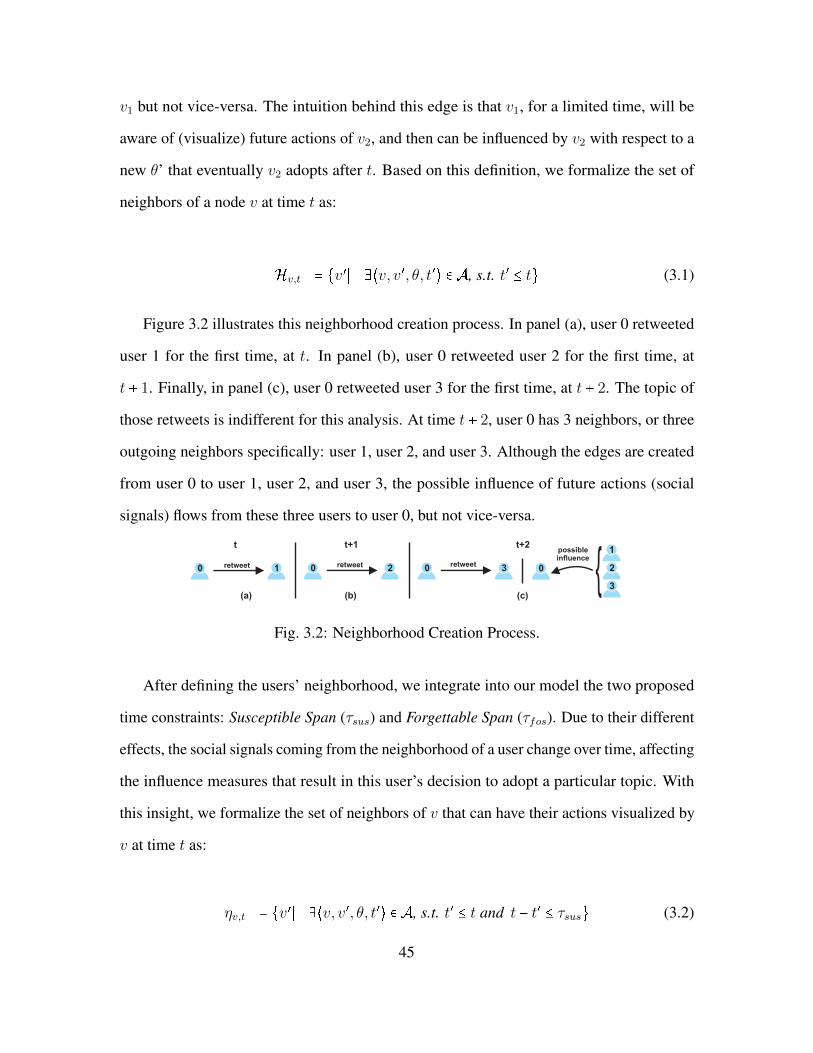
v1 but not vice-versa. The intuition behind this edge is that v1, for a limited time, will be

aware of (visualize) future actions of v2, and then can be influenced by v2 with respect to a

new θ’ that eventually v2 adopts after t. Based on this definition, we formalize the set of

neighbors of a node v at time t as:

Hv,t � �v�S §`v, v�, θ, t�e > A, s.t. t� B t� (3.1)

Figure 3.2 illustrates this neighborhood creation process. In panel (a), user 0 retweeted

user 1 for the first time, at t. In panel (b), user 0 retweeted user 2 for the first time, at

t � 1. Finally, in panel (c), user 0 retweeted user 3 for the first time, at t � 2. The topic of

those retweets is indifferent for this analysis. At time t � 2, user 0 has 3 neighbors, or three

outgoing neighbors specifically: user 1, user 2, and user 3. Although the edges are created

from user 0 to user 1, user 2, and user 3, the possible influence of future actions (social

signals) flows from these three users to user 0, but not vice-versa.

1

t

02

t+1

0

1

20

(a) (b)

retweet retweet 3

t+2

0

(c)

retweet

3}possibleinfluence

Fig. 3.2: Neighborhood Creation Process.

After defining the users’ neighborhood, we integrate into our model the two proposed

time constraints: Susceptible Span (τsus) and Forgettable Span (τfos). Due to their different

effects, the social signals coming from the neighborhood of a user change over time, affecting

the influence measures that result in this user’s decision to adopt a particular topic. With

this insight, we formalize the set of neighbors of v that can have their actions visualized by

v at time t as:

ηv,t � �v�S §`v, v�, θ, t�e > A, s.t. t� B t and t � t� B τsus� (3.2)

45

ηv,t is a subset of Hv,t that contains the neighbors of v whose adoptions since t � τsus

until t will be presented to v. After t� � τsus, the adoptions of v� will not be visualized by

v and therefore will not influence it. Figure 3.3 illustrates this process, considering the

retweets shown in Figure 3.2.

0

1

2

t+2

(a)

3

0

1

2

3

influence

t+3

0

1

2

3

influence

t+4

(b) (c)

influence

0

1

2

3

influence

t+5,t+6,t+7 ...

(d)

influence

sus = 2 Inactive User (Non Adopter) Active User (Adopter)fos = ∞

Fig. 3.3: Effect of Susceptible Span.

As we made in this illustration τsus � 2, user 0 will be aware of (visualize) user 1, user

2, and user 3 activations from t until t � 2, from t � 1 until t � 3, and from t � 2 until t � 4,

respectively. In panel (a), at t � 2, none of the user 0’s neighbors activates. In panel (b), at

t � 3, two of them activate w.r.t θ, user 1 and user 2. However, user 0 cannot visualize the

actions of user 1 from this time, since τsus avoids that. In panel (c), at t � 4, one more of the

user 0’s neighbors activates w.r.t θ (user 3). This way, only the adoptions of users 2 and 3

are visualized by user 0, becoming a possible source of influence w.r.t θ with no time limit,

since τfos was defined in this example as ª. The idea behind this constraint is to “blind”

people from actions coming from out-of-date connections.

In Twitter for instance, after a user v starts following a user u, all activity of u is

automatically presented to v. However, we believe this static relationship does not explain

users’ retweeting behavior as expected. After a period without interacting with u, v can

lose interest in the relationship, no longer checking updates from u (as also suggested by

[21, 141]). We want to approximate this behavior in our model using τsus. In addition, as

influential actions do not last forever [145, 144], we formalize the active neighbors of v that

can influence it to adopt θ at time t as:

46

ηθv,t � �v�S §`v, v�, θ�, t�e > A and §`v�, v��, θ, t��e > A, s.t. t�� t� B τsus and

t � t�� B τfos and t� B t�� B t� (3.3)

ηθv,t is a subset of Hv,t that contains the relevant users to be found in this work: the

influential active neighbors of users. As verified in the equation, v� comprehend the

neighbors of v who had their adoptions at t�� w.r.t θ visualized by v (considering here τsus).

Therefore, the adoptions of v� are influencing v to adopt θ at or after t��. Nevertheless, τfos

guarantees that after t�� τfos, the fact that v� adopted θ is forgotten by v, with v� no more

influencing v in terms of θ. Figure 3.4 illustrates this process considering the retweets of

Figure 3.2.

sus = ∞ Inactive User (Non Adopter) Active User (Adopter)

0

1

2

3

influence

t+3

0

1

2

3

influence

t+4

(a) (b)

influence

fos = 1

0

1

2

3

t+5

(c)

influence

0

1

2

3

t+6,t+7,t+8 ...

(d)

influenceinfluence

influence

Fig. 3.4: Effect of Forgettable Span.

As we made in this illustration τfos � 1, user 0 will be influenced by the visualized

activations of its neighbors for only 1 time unit. In panel (a), at t � 3, two of the user 0’s

neighbors activate, user 1 and user 2. User 0 is able to visualize both activations (as we

defined in this example τsus as ª), being influenced by them from t � 3 on. However, the

influence of those activations disappears after t � 4, due to the effects of τfos. In panel (b),

at t � 4, one more of the user 0’s neighbors activates, user 3. The same influence process

happens for this activation, but now from t � 4 until t � 5. This way, from t � 6 on, none of

the activations of users 1, 2 and 3 are still influencing user 0 to adopts θ.

In Twitter, once a user adopts a hashtag, all its followers can find it in their timelines.

However, as pointed by [40], the hashtag fades away after some time, making it more

47

difficult to be remembered in the future. We want to approximate this behavior in our model

using τfos. Our intention with both time constraints is to mimic the dynamics of online social

networks, aiming to better measure the social influence produced by the set of influential

active neighbors of users.

Conditions for Social Influence. Multiple works argue that there exist three main condi-

tions that prompt users to perform an action - such as a repost - in online social networks

[51, 141]:

• Condition 1: users can be influenced by their friends and family members;

• Condition 2: users can be affected by some external event(s), out of their immediate

neighborhood (1 degree of separation);

• Condition 3: users can be very active, doing things without influence. These users are

often considered in the literature as innovators [138, 39].

In this work, we focus on modeling and learning the influence observed just in condition

1. Given only social network data, influence in condition 2 is hard to be measured, and user

actions conducted because of condition 3 are basically unpredictable.

In the social sciences, there is a standing debate over the primacy of peer influence or

homophily in shaping human behavior [143, 120]. Peer influence is the process in which

one influences the other’s decision, making the influenced node similar to the influential

one. Homophily is realized when similar individuals become friends due to their high

similarity. We believe that homophily is more related to conditions 2 and 3, while peer

influence is more related to condition 1. This assumption makes retweets a natural indicator

to accomplish our goal since they overall bound the neighborhood of users, limiting the

choices and opportunities available in the networks.

48

3.3 Problem Formalization

Given the set of activities (retweets) of a user v that belong to A, and also the set of

activities of its neighbors that belong to A w.r.t θ, the social influence measurements xθv,t

can be calculated based on its corresponding set ηθv,t. The adoption prediction problem is

defined as: given the features xθv,t, the goal is to predict the class label yθv,t. This class label

states if v will adopt or not the hashtag θ until time t.

3.4 Experimental Setup

This section details our datasets, how we collect samples using different values for the

time constraints, which types of filters of users’ activity are applied, and how we measure

the correlation of our features with the probability of adoption. The features included in the

samples will be introduced in the next section.

3.4.1 Microblogs Dataset

Table 3.1 presents the statistics of the two datasets used in this work. The first one

provided by [140] contains a sample of retweets made on Twitter from March 24 to April

25, 2012, offering us the following information regarding each retweet: 1) the pair of users,

2) hashtag(s), and 3) timestamp. In this dataset, there might be multiple sources (tweets)

including the analyzed hashtag considered for adoption, and all of these innovators can be

retweeted by other users.

The second dataset provided by [145] contains a sample of retweets made on Sina

Weibo from October 10 to November 11, 2012, offering the following information to each

retweet: 1) the pair of users and 2) timestamp. Although this dataset does not provide the

hashtag information, it does provide a unique identification number for all posted messages,

49

Table 3.1: Statistics of the Datasets.

Twitter Sina Weibo

Retweets 1,687,700 Retweets 2,553,588

Number of users retweeting 314,756 Number of users retweeting 601,769

Number of users retweeted 251,342 Number of users retweeted 10,539

Number of distinct users 366,291 Number of distinct users 605,622

Number of distinct hashtags 226,490 Number of distinct hashtags 28,645

including tweets and retweets. Then, we use this number to simulate a hashtag, adding it to

the original message (tweet) and all its corresponding retweets. In this scenario, there is only

one source (tweet) including the analyzed hashtag considered for adoption, and therefore,

there is only one innovator.

Figure 3.5 shows the histogram of the number of retweets over users in both datasets.

The first distribution (a) fits a power-law with pk � k�1.8 while the second distribution (b)

fits a power-law with pk � k�1.7, where k represents the number of retweets.

(a) (b)

1

10

100

1000

10000

1 10 100 1000 10000 100000 1000000

Nu

mb

er o

f U

sers

Retweets

1

10

100

1000

10000

1 10 100 1000 10000 100000 1000000

Nu

mb

er o

f U

sers

Retweets

Fig. 3.5: Histogram of the Number of Retweets Over Users in Log-Log Scale for (a) Twitter,

(b) Sina Weibo.

50

3.4.2 Sampling

Following previous works that avoided the problem of imbalanced datasets [145], we

create balanced sets of samples for our experiments. We use a 1:1 ratio strategy to avoid

bias in the samples created. According to this strategy, for a given activity `v, v2, θ, te which

will generate a positive sample using v, we create a negative sample uniformly getting a

user v� from the set:

�v�Sv1 > ηθv,t , v1 > η

θv�,t , `v�, v3, θ, t

�e ~> A,¦v3 > ηθv�,t,¦t

�B t� (3.4)

where v1 is the influential active neighbor of v who first adopted θ.

This set includes all users under influence of v1 w.r.t θ at t (considering the time

constraints) who did not adopt θ before or at time t. Thus, we create `v�, v1, θ, te as the

negative sample for `v, v2, θ, te (our positive sample). We choose v1 so that more information

can be collected during the interval between its activation and t (the time when v activates).

Also, we keep the same timestamp t for the positive sample v and its negative counterpart

v�, allowing them to have approximately the same amount of time to accumulate social

influence. Note that positive and negative samples should have at least one active neighbor

�v1� to be considered in the sampling process.

Figure 3.6 illustrates this process. Although both time constraints are applied during

sampling, we eliminate them here only to facilitate comprehension. User v is a positive

sample, since it activates w.r.t θ at t, influenced by 4 of its 6 neighbors. As our model needs

a corresponding negative sample, we first look for another user who did not adopt θ until

t. However, this user should be, before t, also under the influence of the user v’s neighbor

who first adopted θ, in this case, user v1. This illustration shows that user v� satisfies all

these requirements, since it did not adopt θ until t, and it was under the influence of user v1

51

before this time (at total, user v� was being influenced by 2 of its 6 neighbors w.r.t θ at t).

Thus, user v� can be chosen as a negative sample of user v. We believe this 1:1 ratio strategy

reduces the likelihood of producing bias in the sampling process, providing a reasonable

method to sample users for our model.

v1

vv

influence

influence

Inactive User (Non Adopter) Active User (Adopter)

neighbors

t-7

t-6

t-5

t-4

t-3

t-2

t-1

t

sus = ∞ fos = ∞

t-8

Fig. 3.6: Sampling Process.

3.4.3 Filters of User Activity

We apply the three filters of user’s activity presented in Table 3.2 to exclude users with

less activity than a certain threshold, as their behaviors are hardly explainable by social

influence measures [40, 21] 1 . We follow the researchers’ settings done in [141], who

defined that microblogs users present a minimum activity if they tweet 10-200 per week.

Thus, considering that our both datasets comprise 30 days, we make our users retweet on

average at least 15 times per week, or roughly 60 times per month (filter R60). We also

use the lower bound value of user activity suggested by [141] (40 tweets per month) to

create our second filter of distinct hashtags (H40). Finally, we use a value of 0.5 for the

influenciability score proposed by Goyal et al. at [51]. This score is calculated dividing the

number of reposts for which there is evidence a user v was influenced, by the total number1Without those filters, most of the predictions would be “no adoption”, since a great part

of users do not interact with others.

52

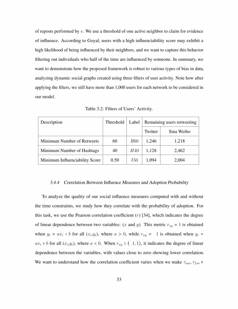
of reposts performed by v. We use a threshold of one active neighbor to claim for evidence

of influence. According to Goyal, users with a high influenciability score may exhibit a

high likelihood of being influenced by their neighbors, and we want to capture this behavior

filtering out individuals who half of the time are influenced by someone. In summary, we

want to demonstrate how the proposed framework is robust to various types of bias in data,

analyzing dynamic social graphs created using three filters of user activity. Note how after

applying the filters, we still have more than 1,000 users for each network to be considered in

our model.

Table 3.2: Filters of Users’ Activity.

Description Threshold Label Remaining users retweeting

Twitter Sina Weibo

Minimum Number of Retweets 60 R60 1,246 1,218

Minimum Number of Hashtags 40 H40 1,128 2,462

Minimum Influenciability Score 0.50 I50 1,094 2,004

3.4.4 Correlation Between Influence Measures and Adoption Probability

To analyze the quality of our social influence measures computed with and without

the time constraints, we study how they correlate with the probability of adoption. For

this task, we use the Pearson correlation coefficient (r) [34], which indicates the degree

of linear dependence between two variables: (x and y). This metric rxy � 1 is obtained

when yi � axi � b for all (xi,yi), where a A 0, while rxy � �1 is obtained when yi �

axi � b for all (xi,yi), where a @ 0. When rxy > ��1,1�, it indicates the degree of linear

dependence between the variables, with values close to zero showing lower correlation.

We want to understand how the correlation coefficient varies when we make τsus, τfos >

53

�8,16,24,48,72,96,120,144,168,336,504,720��hours�, so that we can identify the time

constraints trade-off which produces high-quality social influence measurements (high

positive correlation with probability of adoption). For n samples, the Pearson’s correlation

coefficient is calculated as [105]:

rxy �nPxiyi �PxiP yi»

nPxi2 � �Pxi�2»nP yi2 � �P yi�2

(3.5)

3.5 Influence Measures

In this section, we describe the 10 measures we use to estimate the influence in the active

neighborhood of users in our both datasets. We leverage those measures to recognize the

different structural arrangements in this zone that can affect a user’s decision to adopt or

not a certain topic. For each measure, we first give a formal definition based on the activity

a � `v, v�, θ, te by which we create the sample. Then, we compare the Pearson correlation

coefficient of all possible 144 combinations of τsus and τfos analyzed with the situation

when the time constraints are not applied, plotting the result values using heat maps. The cell

in the right lower corner is always with value zero, as the pair �τsus, τfos� � �720,720� is

equivalent to applying no time constraints (both datasets duration comprehends 1 month or

720 hours). The other cells show the gain (in red color) or loss (in blue color) of correlation

coefficient according to:

rxy�gain loss� � rxy � r�

xy

Sr�xy S � 100% (3.6)

where rxy is computed with �τsus, τfos� ~� �720,720�, while r�xy is computed with

�τsus, τfos� � �720,720�.

We opt to do the correlation gain analysis to show the significance of applying the time

54

constraints. Thus, readers can easily observe which combinations of τsus and τfos improve

the probability of influence for each measure analyzed, something that would be much

harder to be visualized if we had shown only the individual correlation values, for instance.

Table 3.3 presents how we group the 10 social influence measures into 7 distinct cate-

gories created according to their particular characteristics. We discuss each category and

influence measure in the following.

Table 3.3: Social Influence Measures.

Category Description Code

01 - Connectivity 01 - Number of Influential Active Neighbors NAN

02 - Personal Network Exposure PNE

02 - Temporal 03 - Continuous Decay of Influence CDI

03 - Recurrence 04 - Previous Reposts PRR

04 - Transitivity 05 - Closed Triads CLT

06 - Clustering Coefficient CLC

05 - Centrality 07 - Hubs HUB

06 - Reciprocity 08 - Mutual Reposts MUR

07 - Structural Diversity 09 - Active Strongly Connected Components Count ACC

10 - Active Strongly Connected Components Ratio ACR

3.5.1 Connectivity

This group of measures is computed using the influential active neighborhood of users.

Specifically, we study two measures in this category:

Number of Influential Active Neighbors (NAN). Given an activity a � `v, v�, θ, te, this

measure verifies how many neighbors can influence a user v, w.r.t. θ, at time t, under �τsusand τfos�. Most works that analyzed influence considered a plain form of this measure as a

55

baseline [40], claiming that the likelihood of adoption increases with the number of active

neighbors. Because of the time constraints, we adapt here the number of active neighbors to

the number of influential active neighbors, formally representing this measure as:

NAN θv,t � Sηθv,tS (3.7)

Figure 3.7 shows the heat maps (one for each filter) of gain (or loss) of correlation

coefficients between NAN and probability of adoption for our both datasets (panel (a) for

Twitter and panel (b) for Sina Weibo).

[250,∞) [100,250) [50,100) [25,50) [10,25) [0,10) (-10,0) (-25,-10] (-50,25] (-100,-50] (-250,-100] (-∞,-250]

Gain (%) Loss (%)

Filter: H40 Filter: H40

Forgettable Span (𝜏𝑓𝑜𝑠)

Susc

epti

ble

Sp

an (

)

Filter: R60 Filter: R60

Filter: I50 Filter: I50

8 16 24 48 72 96 120 144 168 336 504 720

8

16

24

48

72

96

120

144

168

336

504

720

8 16 24 48 72 96 120 144 168 336 504 720

8

16

24

48

72

96

120

144

168

336

504

720

8 16 24 48 72 96 120 144 168 336 504 720

8

16

24

48

72

96

120

144

168

336

504

720

8 16 24 48 72 96 120 144 168 336 504 720

8

16

24

48

72

96

120

144

168

336

504

720

8 16 24 48 72 96 120 144 168 336 504 720

8

16

24

48

72

96

120

144

168

336

504

720

8 16 24 48 72 96 120 144 168 336 504 720

8

16

24

48

72

96

120

144

168

336

504

720

(a) Twitter (b) Sina Weibo

Fig. 3.7: Gain (or Loss) of the Correlation Coefficient Between NAN and Probability of

Adoption When the Time Constraints are Applied.

Previous works [51, 40] that have not included the time constraints argue that a positive

56

correlation is expected here. Even so, in Figure 3.7, many cells in all heat maps show

correlation gains, which can be understood as combinations of τsus and τfos strengthening

the ability of NAN to explain users’ behaviors under social influence. Nevertheless, other

combinations of the time constraints actually hurt the performance, and they will probably

have a lower chance of being chosen by our model when predicting user adoption. Another

observed trend for NAN is that hot red cells dominate the left lower region of the heat

maps where τsus is relatively high and τfos is relatively low. For the Twitter dataset, we

observe this pattern especially when 72 B τsus B 720 and 8 B τfos B 24, with correlation

coefficient gains varying from 6.25% to 518.75%. For the Sina Weibo dataset, although

with a lower magnitude, we still observe the same pattern especially when 336 B τsus B 720

and 8 B τfos B 48, with correlation coefficient gains varying from 1.16% to 23.46%. Note

how this phenomenon repeats for all three filters of user activity in both datasets.

Personal Network Exposure (PNE). This value is defined as the division between the

number of active neighbors to the total number of neighbors. According to [135], this is a

relevant measure to compute the level of user’s exposure. Considering the time constraints,

we formally represent this measure by:

PNEθv,t �

Sηθv,tSSηv,tS (3.8)

Figure 3.8 presents the heat maps for PNE, with filters R60 and H40 presenting

comparable results in Twitter. For these filters, red cells with correlation gains are mainly

distributed in the area where τsus is relatively high and τfos is relatively low (especially when

168 B τsus B 504 and 8 B τfos B 16). Although filter I50 presents the highest correlation

gains in the same zone of the others, it also tends to keep these gains when τfos is higher. In

general, the gains observed for PNE are between 2.44% and 192.31%. When analyzing

Sina Weibo, filters R60 and I50 present comparable results, with correlation gains mainly

57

distributed in the area where 120 B τsus B 504 and 8 B τfos B 24. In addition, for filter H40,

the gains are roughly spread where the values of τsus and τfos are intermediate. We observe

correlation gains between 1.39% and 414.29%.

Filter: H40

Filter: I50

Filter: H40

Filter: R60

8 16 24 48 72 96 120 144 168 336 504 720

8

16

24

48

72

96

120

144

168

336

504

720

Filter: R60

Filter: I50

8 16 24 48 72 96 120 144 168 336 504 7208

16244872

96120144168336

504720

8 16 24 48 72 96 120 144 168 336 504 720

8

16

24

48

72

96

120

144

168

336

504

720


Susc

epti

ble

Sp

an (

)[250,∞) [100,250) [50,100) [25,50) [10,25) [0,10) (-10,0) (-25,-10] (-50,25] (-100,-50] (-250,-100] (-∞,-250]

Gain (%) Loss (%)

8 16 24 48 72 96 120 144 168 336 504 720

8

16

24

48

72

96

120

144

168

336

504

720

8 16 24 48 72 96 120 144 168 336 504 7208

1624

487296

120144168336504720

8 16 24 48 72 96 120 144 168 336 504 720

8

16

24

48

72

96

120

144

168

336

504

720


Fig. 3.8: Gain (or Loss) of the Correlation Between PNE and Probability of Adoption

When the Time Constraints are Applied.

3.5.2 Temporal

Temporal measures are used to detect how social influence changes over time. We study

the following temporal measure in this work:

Continuous Decay of Influence (CDI). We propose this measure in order to quantify the

continuous decay of influence, since it is known that the neighbors’ influence over users

decays exponentially over time [51]. We formalize this metric as:

58

CDIθv,t � Qu>ηθv,t

e��tu�max��tu�

σ (3.9)

where tu�max� is the time when the latest neighbor in ηθv,t adopted θ and σ is the globally

longest identified time-delay for adoption.

Figure 3.9 presents the heat maps for CDI. In Twitter, all filters present a similar

patter (although filter I50 has lower correlation gains). We observe gains between 15.79%

and 252.63% for this measure, with the highest ones found where 120 B τsus B 336 and

8 B τfos B 24. In Sina Weibo, we observe gains between 2.44% and 129.27% for this

measure, with the highest ones found in the intermediate zone of the heat maps.


Filter: R60

8 16 24 48 72 96 120 144 168 336 504 720

8

16

24

48

72

96

120

144

168

336

504

720

Filter: R608 16 24 48 72 96 120 144 168 336 504 720

816

24

487296

120144168336504720

8 16 24 48 72 96 120 144 168 336 504 7208

1624

4872

96120144

168336504720

[250,∞) [100,250) [50,100) [25,50) [10,25) [0,10) (-10,0) (-25,-10] (-50,25] (-100,-50] (-250,-100] (-∞,-250]

Gain (%) Loss (%)

Filter: I50Filter: I50


Susc

epti

ble

Sp

an (

)

8 16 24 48 72 96 120 144 168 336 504 720

8

16

24

48

72

96

120

144

168

336

504

720

8 16 24 48 72 96 120 144 168 336 504 720

8

16

24

48

72

96

120

144

168

336

504

720

8 16 24 48 72 96 120 144 168 336 504 720

8

1624

48

7296

120144

168

336504

720


Fig. 3.9: Gain (or Loss) of the Correlation Between CDI and Probability of Adoption When

the Time Constraints are Applied.

59

3.5.3 Recurrence

These measures are designed to capture patterns of interaction between users [86]. In

this work, we study one measure regarding recurrence:

Previous Reposts (PRR). This measure verifies how many times an influential active

neighbor in ηθv,t was previously retweeted by v, as a way to detect how strong is the

corresponding relationship. We formalize this measure as:

PRRθv,t �Q

θ�Qu>ηθv,t

Qt�Bt

S`v, u, θ�, t�eS (3.10)

Figure 3.10 presents the heat maps for PRR, with filters H40 and R60 presenting similar

results in the Twitter dataset. Because of the cumulative nature of this measure, there is

a slight tendency that high values to τsus and intermediate values to τfos results in higher

correlation coefficient gains for these 2 filters, especially where 336 B τsus B 720 and

96 B τfos B 144. We observe here gains between 9.52% and 328.57%.

For filter I50, gains are found when the values for τfos are slightly lower. When

analyzing the Sina Weibo dataset, we observe the highest gains (between 1.2% and 85.37%)

for filters R60 and I50, where 336 B τsus B 720 and 8 B τfos B 16. For filter H40, low gains

are basically spread throughout the majority of cells.

3.5.4 Transitivity

Transitivity measures check how influential active neighbors are connected to each other.

Higher values imply a more cohesive neighborhood, which produces more influence for

their followers [108]. Two measures are studied here:

Closed Triads (CLT). This measure enumerates how many triangles are formed by v and

its influential active neighbors in the entire dataset [143]. As our social graphs are directed,

60

[250,∞) [100,250) [50,100) [25,50) [10,25) [0,10) (-10,0) (-25,-10] (-50,25] (-100,-50] (-250,-100] (-∞,-250]

Gain (%) Loss (%)




8 16 24 48 72 96 120 144 168 336 504 720

8

16

24

48

72

96

120

144

168

336

504

720

8 16 24 48 72 96 120 144 168 336 504 720

816

24487296

120144168336

504720

8 16 24 48 72 96 120 144 168 336 504 7208

16

24487296

120144

168

336504720


Susc

epti

ble

Sp

an (

)

8 16 24 48 72 96 120 144 168 336 504 720

8

16

24

48

72

96

120

144

168

336

504

720

8 16 24 48 72 96 120 144 168 336 504 720

8

16

24

48

72

96

120

144

168

336

504

720

8 16 24 48 72 96 120 144 168 336 504 7208

16

24487296

120144

168

336504720


Fig. 3.10: Gain (or Loss) of the Correlation Between PRR and Probability of Adoption


both directions of potential edges are checked in this analysis. We formally define this

measure as:

CLT θv,t � Q�u,z�>ηθv,t,uxz

f��u, z�t� (3.11)

where f��u, z�t� is defined as:

f��u, z�t� �¢¦¨¤

1, if `u, z, θ�, t�e > A , t� B t

0, otherwise(3.12)

Figure 3.11 presents the heat maps for CLT. In Twitter, this measure obtains correlation

61

gains between 10% and 800% through all heat maps in a great part of the cells, especially

over the area where both τsus and τfos have intermediate values. In Sina Weibo, we observe

a similar pattern, although this measure obtains lower gains between 2.08% and 56.36%.

[250,∞) [100,250) [50,100) [25,50) [10,25) [0,10) (-10,0) (-25,-10] (-50,25] (-100,-50] (-250,-100] (-∞,-250]

Gain (%) Loss (%)




8 16 24 48 72 96 120 144 168 336 504 7208

1624487296

120144

168336504720

8 16 24 48 72 96 120 144 168 336 504 7208

1624487296

120144168336504720

8 16 24 48 72 96 120 144 168 336 504 7208

1624

48

72

96120

144168

336504

720


Susc

epti

ble

Sp

an (

)

8 16 24 48 72 96 120 144 168 336 504 7208

1624487296

120144168336504720

8 16 24 48 72 96 120 144 168 336 504 7208

1624487296

120

144

168336504720

8 16 24 48 72 96 120 144 168 336 504 7208

16244872

96120144168336504720


Fig. 3.11: Gain (or Loss) of the Correlation Between CLT and Probability of Adoption


Clustering Coefficient (CLC). The Clustering coefficient is calculated using the number

of closed triads divided by the possible number of triads [143]. It is a normalized value for

transitivity that can be formalized as:

CLCθv,t �

CLT θv,tSηθv,tS � �Sηθv,tS � 1� (3.13)

62

Figure 3.12 presents the heat maps for CLC. For filters H40 and R60 in the Twitter

dataset, relatively high values for τsus and low values for τfos produce higher correlation

gains that vary between 6.67% and 313.33% (pattern observed where 48 B τsus B 504 and

16 B τfos B 48). The highest gains for filter I50 are lower and found in intermediate zones

of both time constraints. In Sina Weibo, high values for τsus and low values for τfos produce

higher correlation gains that vary between 2.78% and 466.67% (pattern observed where

336 B τsus B 504 and 8 B τfos B 16 for all filters of user activity).

[250,∞) [100,250) [50,100) [25,50) [10,25) [0,10) (-10,0) (-25,-10] (-50,25] (-100,-50] (-250,-100] (-∞,-250]

Gain (%) Loss (%)



8 16 24 48 72 96 120 144 168 336 504 7208

16244872

96120

144168336504720

8 16 24 48 72 96 120 144 168 336 504 7208

1624487296

120144

168336504720

Filter: I50 Filter: I508 16 24 48 72 96 120 144 168 336 504 720

81624

487296

120144168336504720


Susc

epti

ble

Sp

an (

)

8 16 24 48 72 96 120 144 168 336 504 720

8

16

24

48

72

96

120

144

168

336

504

720

8 16 24 48 72 96 120 144 168 336 504 7208

1624487296

120

144168

336504

720


8 16 24 48 72 96 120 144 168 336 504 720

8

16

24

48

72

96

120

144

168

336

504

720

Fig. 3.12: Gain (or Loss) of the Correlation Between CLC and Probability of Adoption


63

3.5.5 Centrality

Measures related to centrality try to identify the most important nodes within a graph.

We use the following measure for this category:

Hubs (HUB). This measure enumerates how many hubs are present in the influential active

neighborhood of users. As hubs are highly connected individuals with a number of links that

greatly exceeds the average, they are considered influential [11]. We define this measure as:

HUBθv,t � Q

u>ηθv,t

g�u, t� (3.14)

where g�u, t� is defined as:

g�u, t� �¢¨¦¨¤

1, if Pθ�Px>V Pt�Bt S`x,u, θ�, t�eS A� γ

0, otherwise

(3.15)

with γ being the minimum number of messages reposted by a user to be considered a

hub in our work.

Upon data analysis, we made γ = 104 and γ = 991 for the Twitter and Sina Weibo

datasets respectively, which corresponds to 0.5% of the users (the best-connected) in Twitter

and 5% of the users in Sina Weibo. To reach this value, users should be retweeted daily on

average 3.5 times in Twitter or 33 times in Sina Weibo during the month analyzed in this

work. Figure 3.13 presents the heat maps for HUB. In Twitter, we can again observe the

existence of hot red cells in zones where τsus is relatively high and τfos is relatively low,

especially where 72 B τsus B 336 and 8 B τfos B 24 for all filters. We found correlation gains

64

here between 141.67% and 691.67%. In Sina Weibo, the highest gains (up to 20.78%) are

also present in zones where τsus is relatively high and τfos is relatively low, especially where

168 B τsus B 504 and 8 B τfos B 72 for all filters of user activity.

[250,∞) [100,250) [50,100) [25,50) [10,25) [0,10) (-10,0) (-25,-10] (-50,25] (-100,-50] (-250,-100] (-∞,-250]

Gain (%) Loss (%)




8 16 24 48 72 96 120 144 168 336 504 720

8

16

24

48

72

96

120

144

168

336

504

720

8 16 24 48 72 96 120 144 168 336 504 720

8

16

24

48

72

96

120

144

168

336

504

720

8 16 24 48 72 96 120 144 168 336 504 720

8

16

24

48

72

96

120

144

168

336

504

720


Susc

epti

ble

Sp

an (

)

8 16 24 48 72 96 120 144 168 336 504 720

8

16

24

48

72

96

120

144

168

336

504

720

8 16 24 48 72 96 120 144 168 336 504 7208

16

24487296

120144168336504720


8 16 24 48 72 96 120 144 168 336 504 720

8

16

24

48

72

96

120

144

168

336

504

720

Fig. 3.13: Gain (or Loss) of the Correlation Between HUB and Probability of Adoption


3.5.6 Reciprocity

We compute a category of measures to capture reciprocal behaviors between users, since

this information is relevant for measuring influence [143]. There are many studies analyzing

the importance of reciprocity in interpersonal relationships, and how a lack of this behavior

produces a negative effect [19, 59]. We use the following metric for this measure:

Mutual Reposts (MUR). Mutual reposts represent one of the main forms of reciprocity

65

existing in Twitter and Sina Weibo. We formalized this metric as:

MURθv,t � Q

u>ηθv,t

h�u, t� (3.16)

where h�u, t� is defined as:

h�u, t� �¢¦¨¤

1, if `u, v, θ�, t�e > A , t� B t

0, otherwise(3.17)

Figure 3.14 presents the heat maps for MUR. In Twitter, we observe the highest correla-

tion gains (up to 343.90%) in the area above the diagonal that links the lower-left corner and

the upper-right corner of the heat maps, especially where 96 B τsus B 336 and 8 B τfos B 24

for all filters. In Sina Weibo, we observe the highest correlation gains (up to 38.03%) in the

area where τsus has intermediate values and τfos has relatively low values, especially where

48 B τsus B 144 and 8 B τfos B 16 for all filters of user activity.

3.5.7 Structural Diversity

This group of measures takes into consideration the diversity of communities in the

influential active neighborhood of users. Uganda et al. studied this measure in [134],

highlighting its importance for influence analysis. Two metrics are studied in this category:

Active Strong Connected Components Count (ACC). This measure is defined as the

number of adjacent strongly connected components that include v and at least one of its

influential active neighbors. The function P �V �� V � � C maps the set of nodes V � to the

set of strongly connected components C. Then we formalize this metric as:

ACCθv,t � SP �ηθv,t�S (3.18)

Figure 3.15 presents the heat maps for ACC. In Twitter, the highest correlation gains

are distributed where τsus is intermediate and τfos is relatively low for all filters (although

66

[250,∞) [100,250) [50,100) [25,50) [10,25) [0,10) (-10,0) (-25,-10] (-50,25] (-100,-50] (-250,-100] (-∞,-250]

Gain (%) Loss (%)




8 16 24 48 72 96 120 144 168 336 504 7208

1624487296

120144168336504720

8 16 24 48 72 96 120 144 168 336 504 7208

1624487296

120144168336504

720

8 16 24 48 72 96 120 144 168 336 504 7208

162448

7296

120144

168336504720


Susc

epti

ble

Sp

an (

)

8 16 24 48 72 96 120 144 168 336 504 7208

1624487296

120144168336504720

8 16 24 48 72 96 120 144 168 336 504 7208

1624487296

120144168336504720

8 16 24 48 72 96 120 144 168 336 504 7208

1624487296

120144

168336504720

Fig. 3.14: Gain (or Loss) of the Correlation Between MUR and Probability of Adoption


filter I50 keeps the gains when τfos becomes intermediate). The gains vary between 6.67%

and 66.67% where 72 B τsus B 168 and 8 B τfos B 16. In Sina Weibo, the highest correlation

gains (up to 74.51%) are distributed where τsus is relatively high and τfos is intermediate for

all filters, although filter H40 keeps the gains when τsus becomes intermediate.

Active Strongly Connected Components Ratio (ACR). Since we have defined ACC, we

can normalize this value by the total number of adjacent strongly connected components.

Thus, we define ACR as:

ACRθv,t �

SP �ηθv,t�SSP �ηv,t�S (3.19)

Figure 3.16 presents the heat maps for ACR. The highest correlation gains in the Twitter

dataset are spread through the area where τsus is relatively high and τfos is relatively low,

67

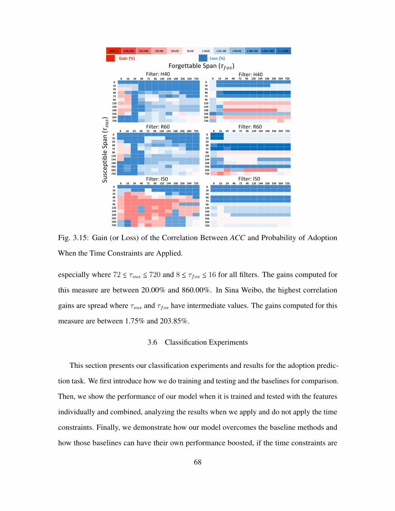
[250,∞) [100,250) [50,100) [25,50) [10,25) [0,10) (-10,0) (-25,-10] (-50,25] (-100,-50] (-250,-100] (-∞,-250]

Gain (%) Loss (%)




8 16 24 48 72 96 120 144 168 336 504 7208

1624487296

120144168336504720

8 16 24 48 72 96 120 144 168 336 504 7208

1624487296

120

144168336504720

8 16 24 48 72 96 120 144 168 336 504 7208

1624487296

120144168336504720


Susc

epti

ble

Sp

an (

)

8 16 24 48 72 96 120 144 168 336 504 7208

1624487296

120144168336504720

8 16 24 48 72 96 120 144 168 336 504 720

8

16

24

4872

96

120144

168

336504

720

8 16 24 48 72 96 120 144 168 336 504 7208

1624487296

120144168336504720

Fig. 3.15: Gain (or Loss) of the Correlation Between ACC and Probability of Adoption


especially where 72 B τsus B 720 and 8 B τfos B 16 for all filters. The gains computed for

this measure are between 20.00% and 860.00%. In Sina Weibo, the highest correlation

gains are spread where τsus and τfos have intermediate values. The gains computed for this

measure are between 1.75% and 203.85%.

3.6 Classification Experiments

This section presents our classification experiments and results for the adoption predic-

tion task. We first introduce how we do training and testing and the baselines for comparison.

Then, we show the performance of our model when it is trained and tested with the features

individually and combined, analyzing the results when we apply and do not apply the time

constraints. Finally, we demonstrate how our model overcomes the baseline methods and

how those baselines can have their own performance boosted, if the time constraints are

68

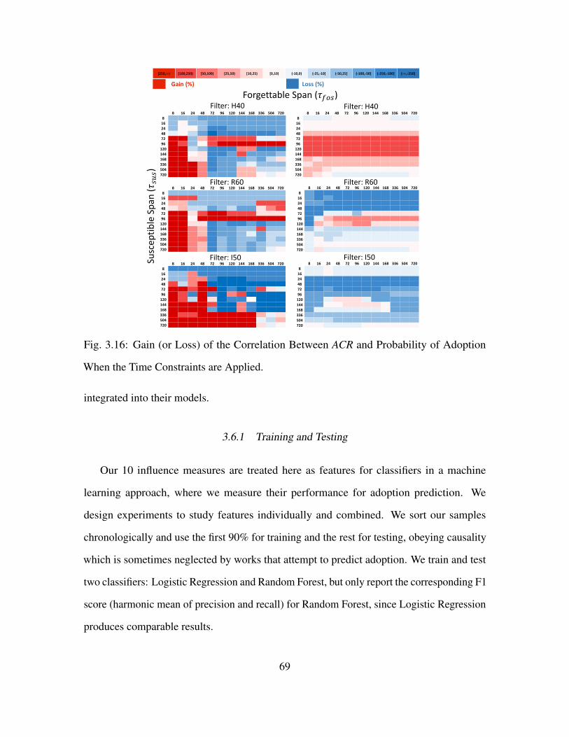
[250,∞) [100,250) [50,100) [25,50) [10,25) [0,10) (-10,0) (-25,-10] (-50,25] (-100,-50] (-250,-100] (-∞,-250]

Gain (%) Loss (%)




8 16 24 48 72 96 120 144 168 336 504 720

8

16

24

48

72

96

120

144

168

336

504

720

8 16 24 48 72 96 120 144 168 336 504 720

81624

487296

120144168336504720

8 16 24 48 72 96 120 144 168 336 504 7208

1624487296

120144168336504720


Susc

epti

ble

Sp

an (

)

8 16 24 48 72 96 120 144 168 336 504 720

8

16

24

48

72

96

120

144

168

336

504

720

8 16 24 48 72 96 120 144 168 336 504 720

8

16

24

48

72

96

120

144

168

336

504

720

8 16 24 48 72 96 120 144 168 336 504 720

8

16

24

48

72

96

120

144

168

336

504

720

Fig. 3.16: Gain (or Loss) of the Correlation Between ACR and Probability of Adoption


integrated into their models.

3.6.1 Training and Testing

Our 10 influence measures are treated here as features for classifiers in a machine

learning approach, where we measure their performance for adoption prediction. We

design experiments to study features individually and combined. We sort our samples

chronologically and use the first 90% for training and the rest for testing, obeying causality

which is sometimes neglected by works that attempt to predict adoption. We train and test

two classifiers: Logistic Regression and Random Forest, but only report the corresponding F1

score (harmonic mean of precision and recall) for Random Forest, since Logistic Regression

produces comparable results.

69

3.6.2 Individual Feature Analysis

Table 3.4 presents the individual classification performance of our 10 features for both

datasets, illustrating the F1 score of the positive class.

Table 3.4: Individual Feature Performances.

Twitter Sina Weibo

Measure w/ time constraints Measure w/o time constraints Measure w/ time constraints Measure w/o time constraints

Filter τsus τfos F1 score Filter F1 score Filter τsus τfos F1 score Filter F1 score

NAN NAN NAN NAN

R60 144 120 0.666 R60 0.605 R60 72 48 0.766 I50 0.629

H40 336 120 0.664 H40 0.567 H40 96 16 0.704 R60 0.550

I50 504 504 0.541 I50 0.502 I50 168 168 0.678 H40 0.492

PNE PNE PNE PNE

I50 336 96 0.671 R60 0.600 R60 504 168 0.738 H40 0.709

H40 144 120 0.669 I50 0.598 H40 720 72 0.715 R60 0.704

R60 72 16 0.634 H40 0.597 I50 144 168 0.713 I50 0.637

CDI CDI CDI CDI

H40 336 72 0.627 H40 0.563 I50 120 16 0.676 I50 0.550

R60 120 96 0.622 R60 0.560 H40 72 48 0.644 H40 0.488

I50 144 96 0.596 I50 0.483 R60 72 72 0.601 R60 0.460

PRR PRR PRR PRR

H40 144 24 0.657 I50 0.561 R60 336 24 0.689 I50 0.614

R60 96 24 0.642 R60 0.524 H40 16 8 0.659 H40 0.557

I50 504 8 0.626 H40 0.485 I50 120 8 0.629 R60 0.406

CLT CLT CLT CLT

R60 168 48 0.680 R60 0.606 R60 96 24 0.735 I50 0.644

H40 120 16 0.671 H40 0.600 H40 96 96 0.678 H40 0.4

I50 144 504 0.610 I50 0.474 I50 168 48 0.657 R60 0.339

CLC CLC CLC CLC

R60 96 72 0.664 I50 0.561 R60 96 16 0.735 I50 0.629

H40 120 96 0.664 R60 0.533 H40 96 16 0.680 R60 0.614

I50 504 504 0.538 H40 0.500 I50 168 120 0.675 H40 0.378

HUB HUB HUB HUB

H40 336 48 0.683 H40 0.634 R60 72 16 0.770 I50 0.629

R60 336 120 0.662 R60 0.609 I50 120 24 0.734 R60 0.561

I50 96 72 0.623 I50 0.472 H40 72 24 0.693 H40 0.479

MUR MUR MUR MUR

R60 24 16 0.637 I50 0.574 I50 96 8 0.384 I50 0.335

H40 96 24 0.628 H40 0.494 R60 16 16 0.308 R60 0.282

I50 72 96 0.620 R60 0.481 H40 16 8 0.302 H40 0.275

ACC ACC ACC ACC

H40 96 72 0.673 R60 0.628 H40 96 16 0.710 I50 0.655

R60 120 72 0.673 H40 0.615 R60 72 48 0.704 H40 0.544

I50 144 336 0.662 I50 0.203 I50 168 144 0.680 R60 0.538

ACR ACR ACR ACR

R60 16 24 0.661 I50 0.623 H40 144 96 0.785 H40 0.695

I50 336 120 0.655 H40 0.557 R60 720 16 0.739 R60 0.649

H40 96 72 0.647 R60 0.526 I50 120 24 0.663 I50 0.588

70

We present all performances among the 3 filters of user activity, showing the results

when they include or not the time constraints. For the great majority of cases (80%), τsus

present values greater than τfos, and in more than half of the cases, τsus present values much

greater than τfos so that adoption is more precisely predicted. This pattern repeats what we

observe for correlation gain between influence measures and the probability of adoption,

pointing a clear requirement of a longer time interval to Susceptible Span when compared

to Forgettable Span. We also confirm this tendency noting that τsus has a value greater or

equal to 96 (hours) in 78.83% of the cases analyzed, while τfos has a value lower or equal to

96 (hours) in 78.66% of these cases.

In the Twitter dataset, the top 5 features which present the highest values for F1 score

when considering the time constraints are: 1) HUB with 0.683, 2) CLT with 0.680, 3) ACC

with 0.673, 4) PNE with 0.671, and 5) NAN with 0.666. In the Sina Weibo dataset, the top

5 features with the highest F1 score are: 1) ACR with 0.785, 2) HUB with 0.770, 3) NAN

with 0.766, 4) PNE with 0.738, and 5) CLT-CLC with 0.735. These results demonstrate the

relevance of features such as HUB, PNE, and NAN for capturing social influence, since they

are all present in the set of features with the highest performances in Twitter and Sina Weibo.

Although the adoption predictions here are considerably high for both datasets, we note

that our model performs slightly better in Sina Weibo, probably because of the limitation

of the Twitter API that produces some indirect links between users retweeting. Another

relevant finding we observe with these results refers to the fact that all three filters of user

activity analyzed in this work obtain roughly comparable performances in each dataset,

although filter I50 has lower performances in some cases. This phenomenon demonstrates

the robustness of the two time constraints regardless of the method used for filtering users.

To complete this individual feature analysis, we sort the features according to their F1

score gain when compared to applying no time constraints in Table 3.5. For this analysis, we

consider only the highest F1 score among the three filters for each feature. Our intention is

71

to check the magnitude with which our features have their prediction performance boosted

when they are subject to τsus and τfos. In Twitter, CLC presents the highest performance

improvement in F1 score (18.36%), followed by PRR, CLT, PNE, and CDI, while ACR

is the feature with the lowest one. In Sina Weibo, CDI presents the highest performance

improvement in F1 score (22.90%), followed by HUB, NAN, CLC, and MUR, while PNE

is the feature with the lowest one. In general, we observe F1 score gains varying between

4.09% and 22.90% for all filters analyzed.

Table 3.5: Individual Feature Performances Considering the Time Constraints.

Twitter Sina Weibo

Feature Filter τsus τfos F1 score Improvements (%) Feature Filter τsus τfos F1 score Improvements (%)

CLC R60 96 72 0.664 18.36 CDI I50 120 16 0.676 22.90

PRR H40 144 24 0.657 17.11 HUB R60 72 16 0.770 22.41

CLT R60 168 48 0.680 12.21 NAN R60 72 48 0.766 21.78

PNE I50 336 96 0.671 11.83 CLC R60 96 16 0.735 16.85

CDI H40 336 72 0.627 11.36 MUR I50 96 8 0.384 14.62

MUR R60 24 16 0.637 10.97 CLT R60 96 24 0.735 14.13

NAN R60 144 120 0.666 10.08 ACR H40 96 16 0.710 12.94

HUB H40 336 48 0.683 7.72 PRR R60 336 24 0.689 12.21

ACC H40 96 72 0.673 7.16 ACC H40 96 16 0.710 8.39

ACR I50 16 24 0.661 6.09 PNE R60 504 168 0.738 4.09

3.6.3 Combined Feature Analysis

Besides evaluating the performance of features individually, we check the performance

of our model when the 10 features are applied combined, comparing the results when we

apply and when we do not apply the time constraints. We show the corresponding results

for both datasets in Table 3.6, sorting them by the F1 score gain. We detect an improvement

of 14.88% and 12.82% in Twitter and Sina Weibo datasets respectively, showing how the

time constraints also work when we use all features together. In addition, the pattern noticed

before for the individual features (adoption is better predicted when τsus Q τfos) is observed

again for the features combined, with the performances achieving significant improvements

when τsus reaches values between 144 and 504 and when τfos reaches values between 16

72

and 96. Averaging all these top performances, we can interpret our results as: 1) users will

stop observing their neighbors roughly after 2 weeks on average, if they do not retweet them

anymore; 2) users will no more remember the activations of their neighbors after a period of

approximately 1.5 days. Therefore, an accordingly parameter tuning is needed to apply the

proposed methods for adoption prediction.

Table 3.6: Performances of All Features Combined.

Twitter Sina Weibo

All features w/ All features w/o All features w/ All features w/o

time constraints time constraints time constraints time constraints

Filter τsus τfos F1 score Improv. (%) Filter F1 score Filter τsus τfos F1 score Improv. (%) Filter F1 score

H40 504 24 0.741 14.88 H40 0.645 R60 336 16 0.862 12.82 R60 0.764

R60 144 16 0.722 13.16 R60 0.638 H40 504 48 0.849 10.11 H40 0.771

I50 504 16 0.713 9.35 I50 0.652 I50 168 96 0.792 8.49 I50 0.730

3.6.4 Performance of Baseline Methods

We compare our model with 3 baselines for measuring social influence and predicting

adoptions. The main idea is to compare the classification results and answer two questions:

1) if our method can outperform all baselines; 2) if the baselines can be improved when the

time constraints are applied to their models. We list the 3 baseline methods below:

• Influence Locality model (LRC-Q). Provided by [145], it was defined by the com-

bination of peer influence and structural diversity (function Q). Peer influence is

computed as a linear combination of the geometric mean of random walk probabilities

of active neighbors while structural diversity combines the social circles formed by

these neighbors.

• Static Bernoulli (SB). In the work proposed in [51], the SB model learns the influence

probability P tu,u� for each edge �u,u�� at time t, predicting the adoption probability of

user v at time t given the set of active neighbors S as: pvt �S� � 1 �Lu>S�1 � ptu,v�.

73

• Complex Probability Model (CPM). The authors in [40] translated the General

Threshold Model [62] to a probabilistic adoption model where the likelihood of adop-

tion increases with more active neighbors. To approximate threshold-like behavior,

they used a logistic sigmoid function to calculate the joint probability of exposures.

Table 3.7 presents the results of those three baselines in our both datasets.

Table 3.7: Baselines comparisons.

Twitter Sina Weibo

LRC-Q w/ LRC-Q w/o LRC-Q w/ LRC-Q w/o



R60 336 16 0.659 9.46 R60 0.602 I50 168 16 0.664 5.73 I50 0.628

H40 48 8 0.646 8.20 H40 0.597 R60 120 48 0.658 5.44 R60 0.624

I50 504 16 0.626 3.98 I50 0.602 H40 96 48 0.639 3.56 H40 0.617

SB w/ SB w/o SB w/ SB w/o



H40 168 24 0.662 8.34 H40 0.611 H40 96 72 0.708 9.42 H40 0.647

R60 504 72 0.654 7.38 R60 0.609 R60 72 24 0.693 8.79 R60 0.637

I50 336 16 0.628 5.36 I50 0.596 I50 336 48 0.659 6.11 I50 0.621

CPM w/ CPM w/o CPM w/ CPM w/o



R60 336 96 0.669 10.57 R60 0.605 H40 96 72 0.721 9.07 H40 0.661

H40 336 72 0.671 9.10 H40 0.615 R60 72 24 0.725 8.20 R60 0.670

I50 504 48 0.633 8.20 I50 0.585 I50 336 8 0.686 6.19 I50 0.646

As verified, our model outperforms the baselines in both situations: when we use an

individual feature such as HUB and when we use all the features combined. For instance,

we observe that by considering all features together, we reach improvements from 7.92% to

12.63% in Twitter, while improvements from 15.45% to 18.89% are computed in Sina Weibo

(both compared to CPM). Note that similar results hold for all filters of user activity. In

addition, we inform in this table how much the time constraints can improve the predictions

of the baseline methods. Basically, τsus and τfos boost all baselines’ performances, with

gains of 9.46% for LRC-Q, 8.34% for SB, and 10.57% for CPM in Twitter. In Sina Weibo,

we have gains of 5.73% for LRC-Q, 9.42% for SB, and 9.07% for CPM. These results

74

highlight the effectiveness of both time constraints for all tested models, recognizing the

pattern detected throughout this work: when τsus Q τfos, social influence is better measured

and adoption is more precisely predicted by the baseline models.

3.7 Related Work

Many works have been proposed to measure social influence and predict users’ adoption.

For instance, the seminal work of Kempe et al. [62] describes two popular models for

information diffusion that were generalized with the General Threshold Model (GTM).

In the GTM, the collective influence produced by the infected neighbors of a person will

trigger its infection once its threshold is exceeded. Later, Saito et al. [111] worked with

predictions of influence probabilities in complex networks, also considering the GTM’s

diffusion concept. They formulated the problem of likelihood maximization and applied

the EM algorithm to solve it, showing reasonable results with the proposed method. In a

sequence, Goyal et al. [51] leveraged a variety of models learned with pairwise influence

probability, finding that the probability of adoption increases with the number of previously

adopters among friends. State and Adamic [125] also found evidence of Goyal’s findings,

looking for evidence of social influence on Facebook. They checked when users overlay their

profile pictures to support same-sex marriage, discovering that the probability of adoption

increases as more neighbors adopt the same behavior.

With an alternative approach, Zhang et al. [145] proposed the influence locality model,

developing two instantiated functions based on pair-wise influence and structural diversity

to predict adoptions. Their analysis reveals that a retweet behavior is positively correlated

with the number of friends who have retweeted the same message before, but it is negatively

correlated with the number of connected circles (a group of socially interconnected people)

formed by these friends. Although the model proposed is quite simple, the authors showed

75

how it performs relatively well. Comparing two different perspectives, Fink et al. [40]

proposed probabilistic contagion models for simple and complex contagion phenomena,

testing their models on 20 Nigerian events in Twitter. By optimizing the threshold for the

complex model and the single adoption probability for the simple model, they showed

that for politically-themed hashtags, the complex contagion model produces a superior fit,

reinforcing the idea that influence grows with more active neighbors.

In addition, there is a wide range of work focusing on cascades prediction in social

networks, whose goal is to detect when information has the potential to go viral through

consecutive user adoptions [138]. For instance, Watts and Dodds demonstrated how cascades

are driven not by “influentials” but by a critical mass of easily influenced individuals [139].

By introducing and using the concept of structural virality, Goel et al. found that popular

events grow through broadcast and also peer-to-peer spreading [50]. Jenders et al. presented

probabilistic models for predicting the spread of tweets, considering a combination of

structural, content, and sentimental-based features [61]. Weng et al. showed how the

popularity of a message on Twitter can be predicted by quantifying its early spreading

pattern in terms of community concentration [140]. Selecting important nodes as sensors,

Cui et al. analyzed historical data to predict cascades based on the behaviors of these sensors

[27]. On a large sample of photo reshare cascades on Facebook, Cheng et al. confirmed that

initially, breadth, rather than depth in a cascade is a better indicator of viral messages [23].

In all these works, we note the authors have not fully explored the dynamics of influence,

building their models basically upon static relationships and invariable social stimulus. Here,

while we also focus on measuring influence to predict adoption, we take the next steps to

apply a pair of time constraints to dynamically build our social graphs, presenting evidence

that influence and adoptions are better measured and predicted when the two proposed time

constraints are considered in both processes.

76

3.8 Summary

In this Chapter, we conduct an engineering study that investigates how a simple pair

of time constraints can considerably contribute to measuring influence and predict user

adoption in social media, as a way to identify potential future collaborators of the ever-

expanding networks of key-hackers. First, we integrate and tune these constraints in a

model composed of 10 standard influence measures, all of them capable of quantifying

different influential factors in the active neighborhood of users. Then, we formulate a binary

classification problem where those influence measures are used as features in a machine

learning approach for predicting whether an individual will adopt a new behavior. Through

the designed and implemented experiments, we show how the dynamic graphs produced

by both time constraints better capture the influence between users over time (especially

when the values of τsus and τfos are relatively high and low respectively), improving the

performance of approaches introduced by us and others. We validate our approach under

a variety of conditions using a sample of Twitter and Sina Weibo datasets, showing how

it outperforms the state of the art methods and enables practical usage of the concepts for

adoption prediction.

77

Chapter 4

PREDICTING HACKER ADOPTION ON DARKWEB FORUMS

4.1 Introduction

Based on the findings presented in Chapter 3 regarding how social influence affects

online user behavior, we postulate whether it would be possible to leverage the spread of

adoption behavior among hackers to predict their activities on online hacking communities.

One direct application of this study would be the prediction of which hackers would buy a

specific hacking product/service that has been offered on a darkweb forum [65]. As standard

hackers, who are often influenced by reputable ones, rely on darkweb hacking forums

to improve their skills and capabilities [83], the anticipation of this interaction could be

accomplished. Finally, adoption behavior could also be used for addressing online cascade

predictions [53] in those environments, whose primary goal is the detection of an early-stage

post with potential to “go viral”, generating multiple subsequent adoptions that strongly

signal imminent cyber-attacks [104].

In this Chapter, we study adoption behavior trying to predict in which topic of a darkweb

hacking forum users will post in the near future, given the influence of their peers. We

formulate our problem as a sequential rule mining task [47], where the goal is to discover

user posting rules through sequences of user posts. Then, we use the mined rules to make

predictions of users posting in a particular forum topic. In general, sequential rule mining

is an important data mining technique that tries to predict event(s) that are likely to follow

other events(s) with a given probability, using patterns mined from sequences [46].

Adapting the problem to our context, we make each rule of the formX � Y only contain

the users responsible for the posts, being interpreted as “if X (a set of users) engages in a

78

given forum topic, Y (a unique user) is likely to engage in the same topic (or adopt it) with

a given confidence afterward, mainly because of the influence of X”. Additionally, as we

demonstrated that influence decreases over time because of effects of time constraints such

as Forgettable Span [81], we only consider rules occurring within defined time-windows.

We also verify how the precision of our model changes according to two posting time

granularities (day and hour). Finally, we compare our results with those produced by the

prior probabilities of hackers’ posts, showing how our predictions and prediction gains are

considerably higher. This Chapter makes the following main contributions:

1. We collect more than 330,000 hacker posts of a popular darkweb forum to create a

sequential rule mining model capable of predicting future posts of hackers;

2. We consider 2 posting time granularities (day and hour) and 10 different time-windows

for each time granularity;

3. During training, we mine more than 362,617 sequential rules with different sizes

(number of users);

4. During testing, we obtain prediction precision results of up to 0.78, while a baseline

model reaches up to 0.18;

5. We observe the highest precision gain [785%, 837%] for time-windows in [3,5] days,

confirming the Forgettable Span [81] effects also on hacking forums of the darkweb.

The remaining of this Chapter is structured as follows. Section 4.2 presents our dataset.

Section 4.3 formalizes our sequential rule mining task applied to hacker adoption prediction.

Section 4.4 presents our experiments and results. Section 4.5 shows some related work.

Finally, Section 4.6 summarizes the Chapter.

79

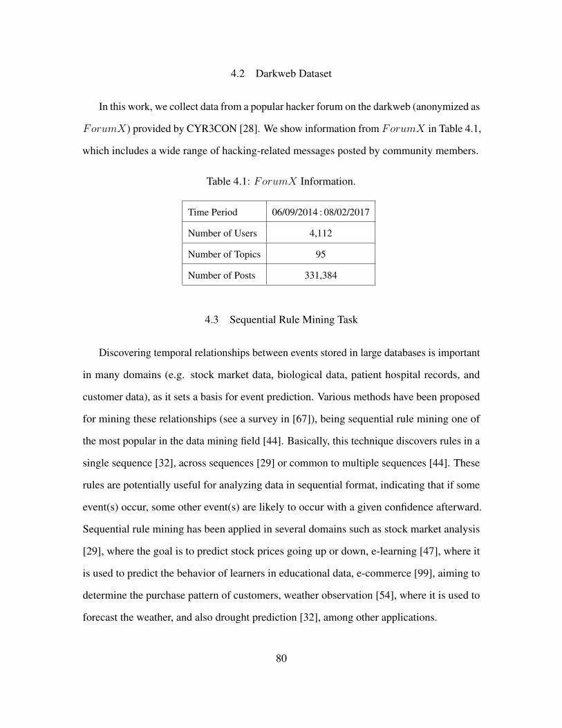
4.2 Darkweb Dataset

In this work, we collect data from a popular hacker forum on the darkweb (anonymized as

ForumX) provided by CYR3CON [28]. We show information from ForumX in Table 4.1,

which includes a wide range of hacking-related messages posted by community members.

Table 4.1: ForumX Information.

Time Period 06/09/2014 : 08/02/2017

Number of Users 4,112

Number of Topics 95

Number of Posts 331,384

4.3 Sequential Rule Mining Task

Discovering temporal relationships between events stored in large databases is important

in many domains (e.g. stock market data, biological data, patient hospital records, and

customer data), as it sets a basis for event prediction. Various methods have been proposed

for mining these relationships (see a survey in [67]), being sequential rule mining one of

the most popular in the data mining field [44]. Basically, this technique discovers rules in a

single sequence [32], across sequences [29] or common to multiple sequences [44]. These

rules are potentially useful for analyzing data in sequential format, indicating that if some

event(s) occur, some other event(s) are likely to occur with a given confidence afterward.

Sequential rule mining has been applied in several domains such as stock market analysis

[29], where the goal is to predict stock prices going up or down, e-learning [47], where it

is used to predict the behavior of learners in educational data, e-commerce [99], aiming to

determine the purchase pattern of customers, weather observation [54], where it is used to

forecast the weather, and also drought prediction [32], among other applications.

80

Bringing to our context, we leverage sequential rule mining applied to multiple sequences

to study the spread of adoption behavior among malicious hackers. The goal is to predict

in which topic of ForumX hackers will post in the near future (topic adoption), given the

influence produced by their peers. This way, we make each of the 95 topics of the forum

analyzed represents a particular sequence, which starts with the oldest post of the topic and

ends with the latest one. In the following, we give a detailed formalization of our problem.

4.3.1 Problem Formalization

We follow the definitions of [47] to specify a sequence database as a set of topics

Θ � �θ1, θ2...θk� and a set of users (malicious hackers) U � �u1, u2, ...um� posting in these

topics. Each topic θx is an ordered list of usersets (set of users) θx � U1, U2, ...Un such that

U1, U2, ...Un b U . Figure 4.1 illustrates a timeline where users are posting on 4 topics.

Topic 1

1Time 2 3 4 5 6 7

Topic 2

Topic 3

Topic 4

7 5632

1

1

43 2

1

2

5

6

621

31

25

5

6

7

Fig. 4.1: Sample Timeline of Forum Topics.

Table 4.2 depicts a sequence database encoding the data presented in Figure 4.1. For

instance, topic θ1 states that users u1 and u2 posted at the same particular time point ti, being

followed successively by: nobody at ti � 1, user u3 at ti � 2, u6 at ti � 3, nobody at ti � 4, u7

at ti � 5, and u5 at ti � 6.

81

Table 4.2: Modeling a Forum as a Sequence Database.

Topics Sequences of Post Users

θ1 {u1,u2},{},{u3},{u6},{},{u7},{u5}

θ2 {u1,u4},{},{u3},{u2},{u1,u2,u5,u6}

θ3 {u1},{u2},{u6},{u5}

θ4 {u3},{u1, u2},{u5},{},{},{u6,u7}

In our context, a sequential rule X � Y is defined as a relationship between two

usersets X (antecedent), Y (consequent) b U such that X 9 Y � g and X,Y x g. A rule

X � Y is said to occur in a topic θx � U1, U2, ...Un if there exists an integer u such that

1 B u @ n,X b 8ui�1Ui and Y b 8ni�u�1Ui. For example, the rule �u1, u2, u3�� u5� occurs

in the topics θ1, θ2 and θ4 of Table 4.2.

According to [47], a rule X � Y is said to be of size v�w if SX S � v and SY S � w. Thus,

the rule �u1, u5� � �u6� is of size 2�1. We only consider in this work sequential rules

containing a single user in the rule consequent (w � 1), since we want to predict one hacker

at a time for the adoption prediction task. Furthermore, a rule of size f�g is larger than

another rule of size h�i if f A h and g C i, or if f C h and g A i [47].

There are two standard measures that we leverage to evaluate the quality of our rules:

the sequential support, which is the fraction of topics where all the users of X appear before

the user of Y and the sequential confidence, which is the number of topics where all the

users of X appear before the user of Y divided by the number of topics where all the users

of X appear. Therefore, the problem of mining sequential rules consists in finding all rules

with support and confidence no less than the user-defined thresholds minsup and minconf

respectively. Those rules are interpreted as “if the users of X post in a given topic, the

user of Y is likely to post in (or adopt) the same topic with a given confidence afterward,

82

mainly because of the influence of X”. Note that in addition to predicting the next user to

post in the near future (Y ), the rules also provide information about the reason for that post

(influence of X), allowing easy interpretation.

There is also one important point about the non-requirement of ordering restriction

between users in X . Fournier pointed out that mining sequential rules has the following

three drawbacks when a strict ordering is applied between items (our users) of the antecedent

or consequent of a rule [45]:

1. Rules may have many variations: There are different variations of the rule �u1�,�u3�� u5� as illustrated with the following rules ri, ri� , ri�� . However, all these variations

describe the same situation: if users u1 and u3 post in a given topic in any order, then

user u5 is likely to post in the same topic after them.

ri � �u1�,�u3�� u5�,

ri� � �u3�,�u1�� u5�,

ri�� u1, u3�� u5�.

2. Similar rules are rated very differently: Considering a strict order, the rules ri and

ri� have support/confidence of 0.5/1.0 and 0.25/0.5 respectively, while the rule ri��

does not appear in our sample database. This condition produces a wrong impression

about the existing sequential relationships. Taken as a whole, the support of the rule

�u1, u3�� u5� grows to 0.75.

3. Rules are less likely to be useful: Rules with a strict order are are less likely to

match with a sequence for future adoption predictions. For example, no rule can be

retrieved from the sample database to match the sequence �u1�,�u2�,�u3� in this

strict order.

83

Thus, in order to avoid these drawbacks of standard sequential rules, we consider

in our model partially-ordered sequential rules [45]. They define a more broad type of

sequential rules common to multiple sequences, such that users in the rule antecedent are

unordered. However, the requirement of a sequential relationship between the antecedent

and consequent of a rule is preserved. According to this partially-ordered definition, the rules

ri, ri� , ri�� presented before can be represented by a single rule �u1, u3�� u5�. We show

in Table 4.3 some rules found in our sample database (Table 4.2), considering minsup � 0.5

and minconf � 0.5.

Table 4.3: Sample of Mined Sequential Rules from Table 4.2.

ID Rule Support Confidence

r1 �u1, u2, u3�� u5� 0.75 1.00

r2 �u1, u2, u6�� u5� 0.50 0.50

r3 �u1, u2�� u5� 1.00 1.00

r4 �u2, u3�� u6� 0.75 1.00

r5 �u3�� u2� 0.50 0.66

r6 �u1�� u2� 0.50 0.50

Finally, we only consider in our model rules occurring within a time-window (∆t), which

is a constraint used by many applications that wish to discover relevant sequential patterns

within a limited time interval [98, 116, 46, 45]. As research has already demonstrated how

social influence decreases over time, mainly because of effects of time constraints such as

Forgettable Span [81], we use time-windows to discard found patterns irrelevant for social

influence. They constitute sequential user posts happening within an interval greater than

the one specified by the time-window, bringing spurious information to our model that is

not related to influence.

84

This way, we make a time-window as a group of consecutive time points in our se-

quences of hacker posts. Then, we check how many time-windows can be generated from

the beginning of a forum topic to its end, one time point at a time (defined by [46] as

a sliding time-window). For example, for ∆t � 3, there are 5 different time-windows

w1,w2,w3,w4,w5 for the topic θ1 of Table 4.2 depicted in Figure 4.2.

ti ti+1 ti+2 ti+3 ti+4 ti+5 ti+6

{u1,u2} {u3} {u6} {u7} {u5}w1

w2

w3

w4

w5

Fig. 4.2: Considered Time-Windows When ∆t � 3 for Topic θ1 of Table 4.2.

Formally, we follow the concepts proposed in [47] and define the problem of mining

sequential rules with a time-window as being the same as the problem of mining sequential

rules, except that a rule X � Y occurs in a topic θx � U1, U2, ...Un if there exist integers j,

k, m such that 1 B j B k @m B n,X b 8ki�jUi, Y b 8mi�k�1Ui and m–j � 1 B ∆t, where ∆t is

defined by the user. We also consider the border cases keeping rules only for j B n �∆t � 1,

so that we always have ∆t time points, and not less, to find the consequent of a rule.

We include the time-window constraint to compute the values of the two measures used

to evaluate the rules. After defining a time-window (∆t), the sequential support becomes

the fraction of topics where all the users of X appear before the user of Y within ∆t, while

the sequential confidence becomes the number of topics where all the users of X appear

before the user of Y within ∆t divided by the number of topics where all the users of X

appear within ∆t. We show in Table 4.4 how the sequential support and confidence of the

rules presented in the Table 4.3 changes for ∆t in [3,4,5].

85

Table 4.4: Sequential Rule Measures Considering Different Time-Windows.

∆t � 3


r1 �u1, u2, u3�� u5� 0.25 0.33

r2 �u1, u2, u6�� u5� 0.00 0.00

r3 �u1, u2�� u5� 0.25 0.25

r4 �u2, u3�� u6� 0.25 0.33

r5 �u3�� u2� 0.50 0.66

r6 �u1�� u2� 0.25 0.25

∆t � 4


r1 �u1, u2, u3�� u5� 0.25 0.33

r2 �u1, u2, u6�� u5� 0.25 0.33

r3 �u1, u2�� u5� 0.50 0.50

r4 �u2, u3�� u6� 0.50 0.66

r5 �u3�� u2� 0.50 0.66

r6 �u1�� u2� 0.50 0.50

∆t � 5


r1 �u1, u2, u3�� u5� 0.50 0.66

r2 �u1, u2, u6�� u5� 0.25 0.25

r3 �u1, u2�� u5� 0.75 0.75

r4 �u2, u3�� u6� 0.50 0.66

r5 �u3�� u2� 0.50 0.66

r6 �u1�� u2� 0.50 0.50

4.4 Experimental Setting

In this section, we present our experiments designed to predict hacker adoption of a

particular forum topic of the darkweb, mining sequential rules of hacker posts. We detail

how we train and test our model under a variety of conditions and also how we compare our

results with a standard baseline.

86

4.4.1 Training

In the training phase, we mine sequential rules from ForumX which contains 95

hacking-related topics. These topics comprise sequences of hacker posts, where each

sequence starts with the oldest post of the topic and ends with the latest one. Our goal here

is to discover the sequential rules that will be used for hacker adoption prediction. As our

dataset has approximately 38 months of sequential data, we use the first 34 months (� 90%

of the period analyzed) to form our training set, which totals 298,245 posts.

Aiming to remove infrequent rules from our training data, since they have a lower chance

of reflecting influence, we define minsup � 0.1 after analyzing some other possible values.

This support value means that any sequential rule of posts must be present in at least 10 out

of 95 topics within the defined time-window. In addition, to increase the correlation between

the antecedent and consequent of the rules during training, we define minconf � 0.8, also

after considering other possible values. This confidence value means that any sequential

rule must have its consequent predicted in 80% of the cases within the defined time-window.

We also use two granularities (day and hour) to represent the hacker posting time

(granularities commonly used for adoption prediction [81]), aiming to observe whether

these granularities affect our prediction results. Table 4.5 illustrates this representation with

random sequential data. As verified, when the time granularity is defined as “day”, the first

three posts are assigned to the same time point “01/01/2017 00:00:00”, since the hours,

minutes, and seconds of these posts are discarded. Following the same idea, the last two

posts are assigned to the same time point “01/02/2017 00:00:00”. On the other hand, when

the time granularity is defined as “hour”, only the first two posts are assigned to the time

point “01/01/2017 10:00:00”, since the hours are not discarded now. Then, the next post is

assigned to the time point “01/01/2017 11:00:00”, while the last two posts are assigned to

the time point “01/02/2017 13:00:00”.

87

Table 4.5: Representation of Different Posting Time Granularities.

Time Granularity (day)

Topic User Original Post Time Representation

θ5 u1 01/01/2017 10:20:18 01/01/2017 00:00:00

θ5 u2 01/01/2017 10:25:32 01/01/2017 00:00:00

θ5 u3 01/01/2017 11:10:55 01/01/2017 00:00:00

θ5 u2 01/02/2017 13:25:12 01/02/2017 00:00:00

θ5 u4 01/02/2017 13:32:19 01/02/2017 00:00:00

Time Granularity (hour)

Topic User Original Post Time Representation

θ5 u1 01/01/2017 10:20:18 01/01/2017 10:00:00

θ5 u2 01/01/2017 10:25:32 01/01/2017 10:00:00

θ5 u3 01/01/2017 11:10:55 01/01/2017 11:00:00

θ5 u2 01/02/2017 13:25:12 01/02/2017 13:00:00

θ5 u4 01/02/2017 13:32:19 01/02/2017 13:00:00

These two representations produce different sequences of user posts as demonstrated

in Figure 4.3, where panel (a) and panel (b) show the sequences created when the time

granularity is defined as “day” and “hour” respectively. In panel (a), there are only two time

points, with the userset �u1, u2, u3� being assigned to the time point “01/01/2017 00:00:00”

and the userset �u2, u4� being assigned to the time point “01/02/2017 00:00:00”.

01/01/2017 00:00:00

{u1,u2,u3} {u2,u4}

01/02/2017 00:00:00

01/01/2017 10:00:00

{u1,u2} {u2,u4}

01/01/2017 11:00:00 01/02/2017 13:00:00

{u3}

(a)

(b)

Fig. 4.3: Sequential Representation of Posts Using Different Time Granularities.

However, in panel (b), there are three time points, being the userset �u1, u2� assigned

to the time point “01/01/2017 10:00:00”, the userset �u3� assigned to the time point

“01/01/2017 11:00:00”, and the userset �u2, u4� assigned to the time point “01/02/2017

88

13:00:00”. Note how panel (b) contains the sequential rules �u1�� u3� and �u2�� u3�,

while panel (a) does not, which makes the user u3 predictable only for panel (b). Setting

the time granularity as “hour” generates more sequences, and we want to investigate if this

implies a higher performance of our model.

In addition, we analyze 10 increasing time-window values for each time granularity,

being ∆t > �2,3,4,5,6,7,8,15,22,31� (sequence d) when considering “days” and ∆t >

�48,72,96,120,144,168,192,360,528,744� (sequence h) when considering “hours”. We

want to vary ∆t while generating rules during training in order to check which configuration

leads to a better prediction accuracy during testing. Although we change the time-windows

magnitude for the corresponding indices of sequences d and h, we maintain the same time

interval for all of them (e.g., 2 days = 48 hours, 3 days = 72 hours, 4 days = 96 hours,

... 31 days = 744 hours). Our intention is to have a fair comparison between both time

granularities when predicting hacker adoption.

TRuleGrowth algorithm. To proceed with the generation of rules, we implement an

extension of the TRuleGrowth algorithm [47, 46]. This algorithm was originally proposed

to discover all partially-ordered sequential rules common to several sequences that have

a support and confidence respectively higher than minsup and minconf . It accepts a

sliding-window constraint to find rules occurring within a maximum amount of time and

the specification of the maximum number of items that can appear in the antecedent and

consequent of a rule. Thus, TRuleGrowth was a natural choice to produce our training data.

It allows us to specify all required constraints to our problem, also providing us an optimized

performance when compared with other algorithms that address the same sequential rule

mining task, such as CMDeo or CMRules [44].

We show in Figure 4.4 the number of rules generated by TRuleGrowth, considering

the 10 defined values of ∆t for each time granularity and the values assigned for minsup,

mincon. The number of rules grows as we increase the value of ∆t, since there is more

89

time to find all users that belong to a specific rule, respecting the sequential constraint

among the antecedent and consequent. Also, there is a considerable difference in the number

of generated rules when “hour” is set as the time granularity. Remember we are dealing

with partially-ordered sequential rules that comprise a set of users in the antecedent, which

makes TRuleGrowth eliminate antecedent variations of the same rule consequent. For

instance, if the algorithm stores the rule �u1, u2, u3� � �u4� it eliminates the rules as

�u2, u1, u3�� u4� or �u3, u1, u2�� u4�. However, TRuleGrowth stores all consequent

variations of the same rule antecedent, since this condition implies in multiple hacker

adoptions derived from the influence of the same individuals. For instance, both rules

�u1, u3�� u5� and �u1, u3�� u6� are stored by the algorithm.

Fig. 4.4: Number of Rules Generated for 10 Values of ∆t Considering Each Time Granularity

(y-axis is in log-scale to better visualization).

As verified, no rule is generated when ∆t � 2 and ∆t � 48 for granularities “day” and

“hour” respectively. This condition informs that there is no sequence of hackers posts

among 2 consecutive days (the consequent is observed one day after the observation of the

antecedent) or 48 consecutive hours in our forum data for this particular set up, pointing out

that a longer time interval is required for social influence to effectively take place. Actually,

many research works claim that social influence gets stronger as the number of “active

90

neighbors” of a given user increases as time goes by (until reaches some kind of limit), since

this user becomes more influenced by all these individuals together [81, 51, 40, 147].

We count in Table 4.6 the number of distinct users in the antecedent a∆t and in the

consequent c∆t of the generated rules for each time granularity and time-window (∆t). Note

how the former is greater than the corresponding number of rules for some cases, which

means that rules with different antecedent sizes (more people influencing together) are

generated. The latter indicates that different consequents (influenced individuals) can be

predicted by the rules.

Table 4.6: Number of Distinct Users in the Generated Rules.

Rule Antecedent. Time Granularity (days).

a2 � 0 a3 � 7 a4 � 8 a5 � 29 a6 � 32

a7 � 68 a8 � 72 a15 � 187 a22 � 227 a31 � 266

Rule Antecedent. Time Granularity (hours).

a48 � 0 a72 � 18 a96 � 52 a120 � 91 a144 � 121

a168 � 147 a192 � 177 a360 � 250 a528 � 283 a744 � 312

Rule Consequent. Time Granularity (days).

c2 � 0 c3 � 2 c4 � 3 c5 � 9 c6 � 10

c7 � 13 c8 � 15 c15 � 57 c22 � 77 c31 � 99

Rule Consequent. Time Granularity (hours).

c48 � 0 c72 � 5 c96 � 9 c120 � 20 c144 � 27

c168 � 37 c192 � 54 c360 � 91 c528 � 117 c744 � 128

4.4.2 Rule Significance Analysis

Finally, we check the significance of the mined rules to determine their utility for

adoption prediction. We accomplish that by comparing the conditional probability of the

consequents given the antecedents with the prior probability of the consequents, considering

each time-window and time granularity. We present the results in Table 4.7, showing that

we obtain probability gains for all possible cases that vary from 145% until 531%.

91

Table 4.7: Significance Analysis of the Generated Rules.

Time Granularity (days).

∆t � 3 ∆t � 4 ∆t � 5 ∆t � 6 ∆t � 7 ∆t � 8 ∆t � 15 ∆t � 22 ∆t � 31

%531 %463 %361 %319 %292 %273 %204 %171 %145

Time Granularity (hours).

∆t � 72 ∆t � 96 ∆t � 120 ∆t � 144 ∆t � 168 ∆t � 192 ∆t � 360 ∆t � 528 ∆t � 744

%488 %410 %358 %321 %293 %273 %204 %172 %146

4.4.3 Testing and Performance Analysis

The testing phase consists in generating adoption predictions for each test case that

represents a hacker or a sequence of hackers posting in the same topic. We accomplish this

task in two steps. First, we identify the rule(s) that match the test case, or the rule(s) whose

users in the antecedent are those who form the test case. Then, after selecting those rule(s),

we choose from their consequent(s) all distinct user(s) to predict that they will adopt the

topic retrieved from the test case.

In order to generate all test cases from our testing set, we use the posts from the last 4

months of our sequential data (� 10% of the period analyzed), which totals 33,139 posts.

For each time granularity and time-window, we retrieve one topic at a time to locate possible

test cases. We start with test cases with size 1 (one user posting) and then move to locate

test cases with size 2 (two users posting), size 3 (three users posting), until we reach the

limit size identified for the antecedent of rules in our training set (5 users).

We evaluate our model computing two distinct measures. The first one is precision,

which is defined as the number of correct predictions divided by the number of predictions

made. The second measure is the number of predictions made, which is higher if the training

set (our mined sequential rules) matches more test cases. Figure 4.5 presents the results.

We observe in panel (a) that, although the two precision curves are similar, our model has

slightly higher precision throughout the time-windows when we set “days” as the time

92

granularity. For this setting, the precision successively increases when the time-window

is 3 (0.416), 4 (0.510), and 5 (0.572), successively decreases through the time-windows

6 (0.440) and 7 (0.411), and successively increases again reaching the highest value in

the last time-window, following 8 (0.442), 15 (0.588), 22 (0.664), 31 (0.786). In addition,

panel (b) shows that more predictions are made when we set “hours” as the time granularity,

since more test cases are generated. However, the difference in rule magnitude (shown in

Table 4.4) between the corresponding time-windows for both time granularities (2-48, 3-72,

..., 31-744) is not reflected in the growing number of predictions, since this number only

doubles in size on average (96 until 34,923 and 96 until 71,000 when considering “days”

and “hours” as time granularity respectively).

Fig. 4.5: Performance of Our Model When Predicting Hacker Adoption, Considering (a)

Precision and (b) Number of Predictions (y-axis is in log-scale).

93

4.4.4 Baseline

In this section, we informally explain a baseline predictor that we use to compare with

our proposed rule-based approach. A very simple baseline approach would be predicting

user engagement in any forum topic with a probability equal to the multiplication of two

terms: (1) the prior probability that a user would post in any time window of length ∆t, and

(2) the average fraction of forum topics on which he/she posts in any time-window with

length of ∆t. Such quantities should be learned from the training dataset.

However, our baseline is less straightforward, since we assume that users vary in their

posting activity. We sought to learn the prior probability of hacker adoption in a time

window of length ∆t, conditioned on the user. Hence, we learn from the training data

those prior probabilities and then predict hacker adoption for each test case. Having a prior

probability for each user, we can predict adoption in different ways: (1) setting a threshold

on prior probability, then predict hacker adoption if their prior probability is greater than the

threshold, and (2) predicting hacker adoption randomly with a chance of being predicted

equivalent to the prior probability 1 . With (1), few users would be predicted to post on every

single topic at each time point we make predictions—such judgment is not desired; hence

we use (2). Clearly, this method is non-deterministic. Therefore, we repeat the experiments

10 times and take the average precision of the runs.

Figure 4.6 presents the results. Evidently, the archived precision is way less than the

rule-learning approach presented in this work. We observe in panel (a) that both curves

are almost identical. They present low precision that successively increases from the first

time-window until the last one, with values varying in [0.047, 0.180]. Note how the precision

value range is much lower than the one outputted by our model, showing we are able to1We do this by generating a random number in [0,1], sampled from a uniform distribution.

If the number falls within the prior probability of a user, we predict his/her adoption,otherwise, we say that user is not going to adopt.

94

identify patters of sequential hacker postings among forum topics. Our assumption is that

these patterns are a natural consequence of the influence process, which encourages hackers

to adopt a topic within a time-window because of the influential activities of their peers.

Fig. 4.6: Baseline Evaluation When Predicting Hacker Adoption, Considering (a) Precision

and (b) Number of Predictions (y-axis is in log-scale).

In panel (b), we observe practically the same number of predictions for both curves

(16,302 until 32,260 when considering “days” as time granularity and 16,171 until 32,015

when considering “hours”). Clearly, the variance is lower than the one produced by our

model, since the method only considers the prior probabilities throughout the time-windows,

neglecting other social aspects as peer-influence. We verify that, although the number of

predictions of our model is relatively small (96 until 702) for short time-windows, when

we increase the time-windows, the number of predictions grows until eventually passing

95

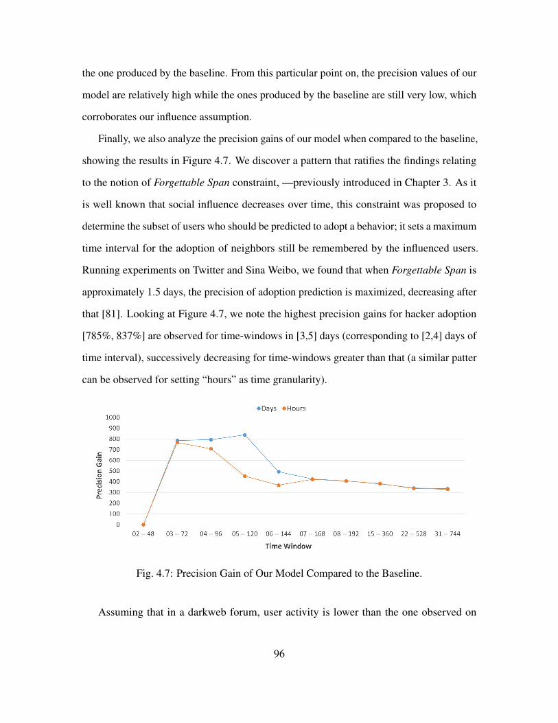
the one produced by the baseline. From this particular point on, the precision values of our

model are relatively high while the ones produced by the baseline are still very low, which

corroborates our influence assumption.

Finally, we also analyze the precision gains of our model when compared to the baseline,

showing the results in Figure 4.7. We discover a pattern that ratifies the findings relating

to the notion of Forgettable Span constraint, —previously introduced in Chapter 3. As it

is well known that social influence decreases over time, this constraint was proposed to

determine the subset of users who should be predicted to adopt a behavior; it sets a maximum

time interval for the adoption of neighbors still be remembered by the influenced users.

Running experiments on Twitter and Sina Weibo, we found that when Forgettable Span is

approximately 1.5 days, the precision of adoption prediction is maximized, decreasing after

that [81]. Looking at Figure 4.7, we note the highest precision gains for hacker adoption

[785%, 837%] are observed for time-windows in [3,5] days (corresponding to [2,4] days of

time interval), successively decreasing for time-windows greater than that (a similar patter

can be observed for setting “hours” as time granularity).

Fig. 4.7: Precision Gain of Our Model Compared to the Baseline.

Assuming that in a darkweb forum, user activity is lower than the one observed on

96

microblogs (where ephemeral hashtags are analyzed to predict user adoption), we understand

these both values are very similar. This finding is relevant since predicting within a short

time is considerably more difficult than when a large time interval is given, once the latter

provides more time to appear hackers posting by chance than the former. Thus, we believe

our model captures the social influence process on hacking forums throughout the time.

4.5 Related Work

To the best of our knowledge, this is the first applied study where adoption prediction is

conducted among malicious hackers on forums of the darkweb. Even so, we introduce here

some works carried out on the surfaceweb that could be used to predict opinions, activities,

link formation, and also participation of hackers on online forums.

Qiu et al. [101] proposed a model which leveraged user arguments, interactions, and

attributes into a collaborative filtering framework for stance prediction on a surfaceweb

forum. Although the model is able to infer public opinion, which could be used for

understanding the hackers reasoning, it can not estimate where (topic) and when (time) a

hacker will post.

Glenski et al. [49] tracked the online activity of 186 users of the popular Reddit forum

over a year, in order to predict their future interactions. They formulated the task as a multi-

class classification, leveraging ranking and semantic features to estimate browse-content,

browse-comments, upvote, downvote, or do-nothing behavior for each post visualized. This

technique can be used to predict behaviors with respect to an existing post, but it is not able

to anticipate a new one.

Yang et al. [129] analyzed user activity in a popular underground forum of the sur-

faceweb, combining social network analysis, logistic regression, and clustering to first

preselect a list of potential key actors (users who have been linked to criminal activities).

Then, they filtered key terms used by those individuals in their posts to predict who is

97

actually a key actor. The idea is relevant to profile skilled hackers, but no predictive method

was included to foresee new content.

Sadeque et al. [110] developed a time-series methodology for predicting link formation

in real-world datasets from Massive Open Online Course (MOOC) discussion forums. They

leveraged neighborhood, path, and post-based quantities between learners as features to

a Long-Short Term Memory (LSTM) Recurrent Neural Network (RNN) units, in order

to forecast interactions between two users (link) in a thread. Although this model can be

used to predict hacker posts, we identify three main drawbacks here: first, training is costly

because of the different nature of the features; second, the prediction is done taking into

consideration only one neighbor; finally, the links are bidirectional, making the prediction

of user u2 given user u1 also valid for cases in the opposite direction.

4.6 Summary

In this Chapter, we study the adoption behavior among hackers on the darkweb, aiming

to predict their future adoptions of a particular forum topic, given the influence produced by

their peers. We accomplish this task by leveraging sequential rule mining to discover user

posting rules through sequences of user posts, to later use these rules to make the predictions.

We analyze the performance of our model when it uses different time granularities to

represent the posts and also multiple time-windows for mining the sequential rules, obtaining

results that by far overcome the prior probabilities of hackers posts. Our model provides an

alternative strategy for security researchers to anticipate the participation of cyber criminals

in hacking-related forum topics. With this insight, organizations can better monitor their

networks for threats and exploitable vulnerabilities, extending their reach to cover forums

where hackers often share valuable information.

98

Chapter 5

DETECTING COMMUNITIES OF MALWARE AND EXPLOIT VENDORS ON

DARKWEB MARKETPLACES

5.1 Introduction

Recently, darkweb hacking marketplaces have become a central venue for online pur-

chasing of malicious products and services by cyber criminals, who take advantage of the

numerous offerings provided especially by trustful and well succeeded key-hackers. An

example that illustrates this fact is given by Nunes et. al in [92]. An exploit targeting a

Microsoft Windows vulnerability CVE-2015-0057 was for sale on a darkweb marketplace

in March 2015. The corresponding vulnerability was disclosed by Microsoft a month earlier,

with no publicly available exploit at that time. Four months after the availability of the

exploit, FireEye reported that the Dyre banking Trojan - designed to target organizations to

steal credit card information - had used the exploit [41]. See [7] for more examples.

In this context, consider the importance of finding communities of vendors with similar

hacking expertise for surveillance purposes. Many vendors possibly linked to the Dyre

Banking Trojan, could be automatically identified if at least one of them had been already

confirmed as offering the exploit online, allowing defenders to anticipate subsequent similar

product offerings. In more complex scenarios, those communities might correspond to

sets of individuals dealing with similar products or services in some specific subfields of

hacking, such as carding, phishing, and keyloggers, which is a feature typically owned by

key-hackers. Therefore, detecting all individuals forming specialized hacker communities

becomes another form of discovering who are in the the expanding network of key-hackers,

helping defenders to anticipate their imminent cybercriminal activities.

99

In this Chapter, we explore a new method based on (SNA) and (ML) techniques to

identify and validate communities of malware and exploit vendors on darkweb hacking

marketplaces. As there is no direct communication between vendors in those environments,

we start by collecting information about their hacking-related product offerings in 20

different markets, from where we produce a similarity matrix of the vendors. To create this

matrix, we leverage unsupervised learning to cluster the vendors’ products into the 34 main

hacking categories proposed by our prior work published at [80]. Then, we quantify the

similarity between vendors by analyzing the number of product categories shared between

them and also the number of products they have in each product category. Finally, as a way

to address the lack of ground truth (the existing vendor communities in the markets), we

split the marketplaces into two disjoint sets to detect the community overlapping between

them. Our results demonstrate how the multiplexity of social ties [137, 75, 85, 84], which

makes individuals interact in multiple domains, help us to validate a considerable part of the

mined communities. This Chapter makes the following main contributions:

• We cluster around 40,000 hacking-related products using 34 product categories;

• We calculate the similarity of hacking vendors applying different metrics over their

products and product categories, inferring the implicit connections among them;

• We perform community finding to detect the communities of hacking-related vendors

in two disjoint sets of marketplaces, validating our results by checking the overlapping

between them. We found the ARI score achieves 0.445 using our method, while

randomly assigning individuals to communities yields an ARI of -0.006.

The remaining of this Chapter is structured as follows. Section 5.2 introduces darkweb

marketplaces and our dataset. Section 5.3 describes our methodology, detailing its modules,

experiments, and corresponding results. We discuss related work in Section 6.6. Finally,

Section 6.7 summarizes the Chapter.

100

5.2 Darkweb Hacking Marketplaces

People who want to shield their product offerings from government surveillance may

require the cover of the darkweb, and that would not be different for malicious hackers

and exploit vendors. These individuals require a marketplace infrastructure to safely com-

mercialize their illegal cyber threats, keeping their activities hidden from law-enforcement

agencies. Basically, all darkweb hacking marketplaces require a registration and a valid

account to get access. Sometimes, this registration process is not trivial, including effort to

answer questions and solve puzzles, mathematical equation or CAPTCHA [80]. Products

are often verified before any funds are released to the vendor. As a way to keep the monetary

transactions untraceable, Bitcoin is the currency often used in those environments [104].

5.2.1 Dataset

In this work, we select 20 popular English hacking-related marketplaces from the

darkweb provided CYR3CON [28]. We anonymously show in Table 5.1 the number of

hacking-related products and the number of vendors found in each market.

Table 5.1: Darkweb Marketplace Statistics.

Marketplace Products Vendors Marketplace Products Vendors

Market 1 22,956 525 Market 11 1,136 87

Market 2 13,423 1,323 Market 12 1,122 63

Market 3 9,936 856 Market 13 995 34

Market 4 7,360 243 Market 14 936 40

Market 5 3,443 1,439 Market 15 739 61

Market 6 3,437 1,625 Market 16 527 6

Market 7 3,328 266 Market 17 328 18

Market 8 1,358 131 Market 18 302 135

Market 9 1,269 589 Market 19 182 26

Market 10 1,264 106 Market 20 159 32

101

5.3 Methodology

This section explains the steps of our methodology designed to reveal the communities

of malicious hacking-related vendors on the darkweb, as illustrated in Figure 5.1.

(a) (b) (c) (d) (f) (g)(e)

Fig. 5.1: Methodology. (a) Creating a Bipartite Network of Vendors and Products, (b)

Clustering the Products in Product Vategories, (c) Splitting the Marketplaces into Two

Disjoint Sets (green and blue), (d) Creating Bipartite Networks of Vendors and Product

Categories, (e) Projecting Bipartite Networks of Vendors and Products Categories into

Monopartite Networks of Vendors, (f) Finding the Communities of Vendors in Each set of

Markets, (g) Calculating the Community Overlapping Between the Two Sets of Markets.

5.3.1 Creating a Bipartite Network of Vendors and Products

The first step of our methodology consists of collecting the malicious hacking products

offered by each vendor on the marketplaces to generate a bipartite network of vendors and

their corresponding products. Therefore, the nodes of this bipartite graph are formed by

vendors and products, while the edges are created only between these two type of nodes. We

use the vendors’ screen-name and products’ names to uniquely identify vendors and products

in this Chapter. By analyzing the vendors’ screen-names, we note that many products are

cross-posted by vendors in multiple sites. This happens since vendors usually adopt the

strategy of using the same screen-name in different marketplaces to transfer their reputation

[92]. As the great majority of screen-names are personal and exotic, we believe that applying

102

string-match over them is a reasonable approach to uniquely identity individuals 1 . Figure

5.2 (a) shows the distribution of vendors who use the same screen-name across multiple

marketplaces. As observed, there is no exclusive vendor for any marketplace, and two of

these environments share almost 200 vendors with other markets.

1

4

16

64

256

1024

4096

16384

65536

1 2 4 8 16

Nu

mb

er o

f P

rod

uct

s

Shared Vendors

1

2

4

8

16

32

64

128

256

1 2 4 8 16 32

Nu

mb

er o

f Sh

ared

Ven

do

rs

Markets

(b)(a)

Fig. 5.2: Distribution of (a) Shared Vendors Over Markets, (b) Products Over Shared

Vendors (in log-log scale).

As our method uses duplicated vendors in different set of marketplaces to validate

the results, we filter our dataset to consider only vendors present in at least two markets,

bringing their corresponding products. Table 5.2 shows the size of the original and the

filtered datasets. By using this filtered data, we generate a bipartite graph considering the

vendors and distinct products as two disjoint sets of nodes, and the total number of products

as the connecting edges.

Table 5.2: Scraped Data from Darkweb Marketplaces.

Original Filtered

Marketplaces 20 Marketplaces 20

Products (Total) 74,200 Products (Total) 40,610

Products (Distinct) 51,902 Products (Distinct) 27,581

Vendors 7,605 Vendors 390

1We leave other methods of similarity-based comparison to future work.

103

5.3.2 Clustering the Products in Product Categories

As we collect data from different sites, there is inconsistency as to how products are

categorized on each site - if such non-trivial categorization even exists for a given site.

Furthermore, there is a clear absence of a standardized method for vendors to register their

products. As a consequence, the majority of the products are unique when compared with

simple matching or regular expression technique. It is valid even in the case where a pair of

vendors with different screen-names post what a human would determine to be the same

product. Figure 5.2 (b) shows the distribution of products and the vendors shared between

them. We observe that around 70% of the distinct products belong to only a single vendor.

In order to mitigate this inconsistency, we cluster the products into the 34 hacking

categories that we defined in [80]. The idea is to make the vendors share more information,

assigning similar products to the same product category. This strategy allows us to generate

a more precise matrix of vendors similarity, using their shared product categories and the

corresponding products. Following the approach in [80], we apply character n-grams (in

the range from 3 to 6) over the product names, aiming to engineer features that represent

products as vectors. Then, we value all features using term frequency - inverse document

frequency (TF-IDF), after eliminating stopping words and executing steaming. Finally, we

run K-Means to produce the 34 product categories ranked and detailed in Table 5.3.

To run k-means, we first manually label 400 samples using those 34 product categories

(the “K” parameter of K-Means), ensuring at least 10 samples for each cluster. We use

those samples to determine the initial centroids for each cluster, instead of doing this

task randomly. Finally, we run K-means using cosine similarity as the distance function

(spherical K-Means [56]) in the entire dataset (27,581 distinct products). As verified in

Table 5.3, “Netflix-related” is the top first product category in terms of number of products

assigned, following a trend observed in [80]. Nevertheless, other product categories emerged

104

Table 5.3: Product Categories.

No of No of No of No of No of No of

Rank Cluster Name Products Markets Vendors Rank Cluster Name Products Markets Vendors

1 Netflix-related 3786 16 186 18 RDP Servers 938 17 130

2 Viruses/Counter AntiVirus 3216 14 61 19 Physical Layer Hacking 935 18 122

3 VPN 3064 14 66 20 Exploit Kits 858 19 123

4 Keyloggers 2662 18 221 21 Smartphone - General 791 17 141

5 Linux-related 1875 14 69 22 Ebay-related 780 16 92

6 Carding 1634 17 171 23 Windows-related 708 17 96

7 Hacking Tools - General 1610 15 111 24 Password Cracking 615 18 113

8 PGP 1609 14 120 25 Network Security Tools 615 15 75

9 Facebook-related 1526 15 97 26 Botnet 611 18 87

10 Point of Sale 1275 18 131 27 Bitcoin 595 16 116

11 Dumps - General 1227 16 99 28 Phishing 587 16 107

12 Network Layer Hacking 1181 17 134 29 Android-related 523 16 69

13 PayPal-related 1148 15 133 30 Hacking Groups Invitation 473 15 92

14 Cashing Credit Cards 1134 18 124 31 Amazon-related 464 16 94

15 Browser-related 1038 15 104 32 Wireless Hacking 442 15 77

16 Banking 959 15 139 33 Links (Lists) 409 12 100

17 RATs 940 16 104 34 Email Hacking Tools 382 16 96

such as “Viruses/Counter AntiVirus”, “VPN”, “Keyloggers”, and “Linux-related”, followed

by the one also pointed by [80] as very active (“Carding”). We also inform the number

of markets and vendors assigned to each product category. “Exploit Kits” appears as the

product category most spread among the 20 markets (19), while “Keyloggers” appears as

the one most spread among vendors (221).

5.3.3 Splitting the Marketplaces into Two Disjoint Sets

In this Chapter, we assume that vendors on darkweb hacking marketplaces strive to

build social status and trust, and one common way to accomplish that is by using the same

screen-name in different environments. This assumption is common across research work

on darkweb data [7, 104]. For this reason, we decide to split our dataset into two partitions,

using an optimization process to produce a division that maximizes the redundancy of

vendors in both partitions. We will leverage this redundancy to check if the communities

found in one part of the data are also present in the other one. Formally, we implement an

105

optimization algorithm to produce the best split of all 20 markets (set M ) into 2 nonempty

and disjoint sets. Thus, M1 x g, M2 x g, M1 9M2 � g, and M1 8M2 � M , and the

complexity of the algorithm for n markets is O�2�n�1� � 1�. Considering VM1 and VM2as the

set of vendors present in M1 and M2 respectively, our objective function seeks to maximize

the number of duplicated vendors in these both sets, as shown in equation 5.1:

max f�VM1 , VM2�, with f�VM1 , VM2� � S�VM1 9 VM2�S (5.1)

Table 5.4 presents the results of the data split algorithm, showing that we found 329

duplicated vendors in our two disjoint sets of markets. We will use these individuals to

verify if they form similar communities in these two different environments.

Table 5.4: Results of the Marketplaces Split.

M1 M2

Number of Markets 10 10

Number of Products 13,486 27,124

Number of Vendors 345 374

Number of Duplicated Vendors in Both Sets 329

5.3.4 Creating Bipartite Networks of Vendors and Product Categories

At this point, we are able to connect the vendors to their product categories in a bipartite

graph, allowing us to check which categories are shared between them. Figure 5.3 illustrates

this process with a subset of the graph within set M1. In panel (a), the vendors are connected

to their products, which in turn are connected to their categories. In panel (b), we plot the

same graph without the products to better visualize the shared product categories between the

vendors. Vendors who were previously disconnected from others (note the 9 disconnected

components highlighted in panel (a), since the vendors mostly own exclusive products) are

now connected using the shared product categories in panel (b).

106

Fig. 5.3: Sample of the Network of Vendors, Products, and Product Categories (a). The

Same Network is Shown in Panel (b) but Hiding the Products.

Figure 5.4 shows the distribution vendors over product categories in sets (a) M1 and (b)

M2. Both distributions are similar and point out the majority of vendors (� 63%) are assigned

to more than one product category in both sets of marketplaces. This condition increases the

probability of creating new connections in the graph, although vendors assigned to a single

product category are in most of the cases sharing it with other individuals.

1

2

4

8

16

32

64

128

1 2 4 8 16 32 64

Nu

mb

er o

f V

end

ors

Number of Product Categories

1

2

4

8

16

32

64

128

1 2 4 8 16 32 64

Nu

mb

er o

f V

end

ors

Number of Product Categories

(b) M2(a) M1

Fig. 5.4: Distribution of Vendors Over Product Categories in Sets (a) M1 and (b) M2.

Overall, the number of connections created between vendors and product categories in

both subsets of markets is around 2,500 (7.5 on average for each one of the 329 duplicated

vendors).

107

5.3.5 Projecting Bipartite Networks of Vendors and Product Categories into a Monopartite

Network of Vendors

After discovering the shared product categories between vendors, our next challenge

is to project the corresponding bipartite graphs of vendors and product categories into

monopartite graphs of vendors. This step is crucial for this work, since the algorithms we

are going to use to find the communities of vendors were designed to work with networks

with single-type nodes (such as vendors), and not to work with multimodal networks [15].

To accomplish this task, we create a similarity matrix between vendors using two pieces

of information: their product categories and their corresponding products. The former

information basically creates a binary matrix connecting vendors and product categories,

where “1” means the vendor has a least one product in the corresponding product category,

and “0” otherwise. The latter information adds magnitude to the product categories owned

by vendors, including the number of products vendors have within each product category.

We use both information to create a similarity matrix between vendors, considering an

edge between two specific individuals if the corresponding similarity (weight) is greater

than a given threshold δ. To calculate this weight, we use four different similarity metrics

according to Table 5.5.

Table 5.5: Similarity Metrics.

Metric Formula

Jaccard [130] J�Vi, Vj� � M11M01�M10�M11

, where Vi and Vj are two binary vectors corresponding to the assignment of existing product categories

for vendors i and j, M11 represents the number of product categories where Vi and Vj both have a value of 1, M01 represents the number

of product categories where the product category of Vi is 0 and the product category of Vj is 1, andM10 represents the number of product cate-

gories where the product category of Vi is 1 and the product category of Vj is 0.

Cosine [130] Cos�Vi, Vj� �ViYVj

ZViZ[Vj[, where Vi and Vj are two non binary vectors corresponding to the assignment of the total number of products

within each existing product categories that belong to vendors i and j.

Correlation [130] Corr�Vi, Vj� �cov�Vi,Vj�σ�Vi��σ�Vj�

, where Vi and Vj are two non binary vectors corresponding to the assignment of the total number of pro-

ducts within each existing product categories that belong to vendors i and j, cov�Vi, Vj� is the covariance of Vi and Vj , and σ�Vi� is the

standard deviation of Vi .

Tanimoto [130] T �Vi, Vj� �ViYVj

ZViZ2�[Vj[2�ViYVj

, where Vi and Vj are two non binary vectors corresponding to the assignment of the total number of

products within each existing product categories that belong to vendors i and j.

108

The idea of calculating those similarity metrics is to use them to weight the edges of our

graphs, since those weights should represent the level of similarity between vendors. We

rely on the assumption that vendors with a high similarity based on their product offerings

will form a community of interests in the real world. Figure 5.5 illustrates this process

of projecting a bipartite network of vendors and product categories - panel (a) - into a

monopartite network of vendors - panel (b). The network shown in Figure 5.5 (a) is the one

shown in 5.3 (b). Note how we can see the vendors directed connected to each others in a

weighed graph in Figure 5.5 (b).

Fig. 5.5: Sample of the Network of Vendors and Product Categories (a) Projected into a

Network of Vendors (b).

5.3.6 Finding the Communities of Vendors in Each Set of Markets

After producing the network of vendors, we search for the existing communities in

both sets of marketplaces. The methods described in this work assume a non-overlapping

community network structure, which means that every vertex (vendor) belongs to only

one of the communities. Algorithms in this context can be broadly grouped into three

types: (1) Hierarchical algorithms construct a tree of communities based on the network

topology, being classified as divisive [48] and agglomerative algorithms [24]; (2) Modularity-

109

based algorithms optimize the modularity objective function to uncover communities in

the networks [90], being our choice for this work; (3) Other algorithms include label

propagation, spectral methods that use eigenvectors of Laplacian or standard matrix, and

methods based on statistical models [43]. In addition, when studying communities, we are

interested in detecting either (1) specific members (member-based community detection)

or (2) specific forms of communities (group-based community detection) [143]. Here, we

work with group-based community detection algorithms, since we are interested in finding

communities that own high modularity.

Modularity is a measure designed to compute the strength of a network division into

modules (groups), checking how likely the community structure found is created at random

[143]. Clearly, community structures should be far from random, therefore, the more distant

they are from randomly generated communities, the more structure they exhibit. Modularity

defines this distance as a scalar value between -1 and 1, and modularity maximization tries

to maximize this distance [90]. Networks with high modularity have dense connections

between the nodes within modules but sparse connections between nodes in different

modules. Consider an undirected graph G�V,E�, SES � m, two nodes vi and vj , with

degrees di and dj , respectively, and a partitioning of the graph into k partitions, P �

�P1, P2, P3, ..., Pk�. For partition Px, the distance from randomly generated communities

can be defined as [143]:

Qvi,vj>Px

Aij �didj2m

(5.2)

Then, this distance can be generalized for partitioning P with k partitions as [143]:

k

Qx�1

Qvi,vj>Px

Aij �didj2m

(5.3)

110

The summation is over all edges m, and because all edges are counted twice �Aij � Aji�,

the normalized version of this distance is defined as modularity Q as [90]:

Q �1

2m� k

Q1

Qvi,vj>Px

Aij �didj2m

� (5.4)

Optimizing the value of Q theoretically results in the best possible grouping of the nodes

of a given network. However, going through all possible iterations of the nodes into groups

is impractical and heuristic algorithms are used. In this work, we use the Louvain heuristic

method of community detection [15] to find our communities of vendors. This method

iteratively finds small communities by optimizing modularity locally on all nodes to later

group each small community into one node. It is similar to the original method proposed by

Newman [90], connecting communities whose combination produces the largest increase

in modularity. Figure 5.6 shows the produced communities and inform the modularity Q

found in M1 (0.579) and M2 (0.514) using Jaccard similarity metric. These values indicate

that both networks present a considerable clustering property. Louvain community detection

algorithm found 46 and 37 communities in M1 and M2 respectively.

M1 M2

Fig. 5.6: Communities Found for δ � 0.51 in M1 (a) and M2 (b) Using Jaccard Similarity

Metric.

The corresponding distribution of vendors per community is presented in Figure 5.7.

111

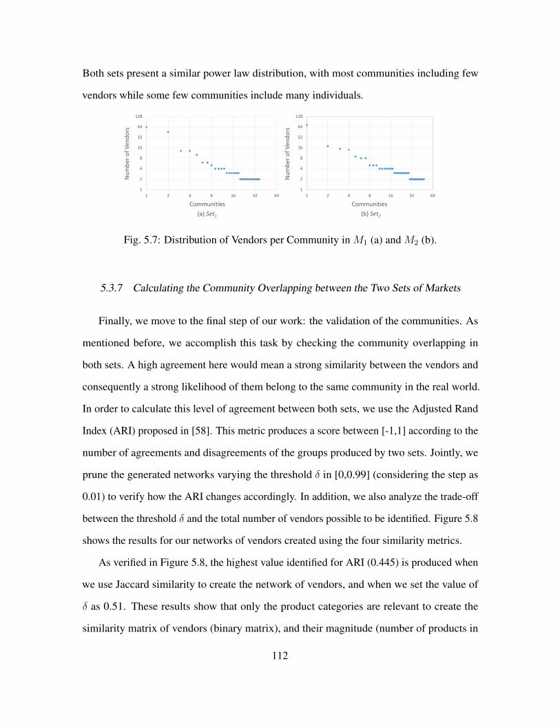
Both sets present a similar power law distribution, with most communities including few

vendors while some few communities include many individuals.

1

2

4

8

16

32

64

128

1 2 4 8 16 32 64

Nu

mb

er o

f V

end

ors

Communities

1

2

4

8

16

32

64

128

1 2 4 8 16 32 64

Nu

mb

er o

f V

end

ors

Communities

(b) Set2(a) Set1

Fig. 5.7: Distribution of Vendors per Community in M1 (a) and M2 (b).

5.3.7 Calculating the Community Overlapping between the Two Sets of Markets

Finally, we move to the final step of our work: the validation of the communities. As

mentioned before, we accomplish this task by checking the community overlapping in

both sets. A high agreement here would mean a strong similarity between the vendors and

consequently a strong likelihood of them belong to the same community in the real world.

In order to calculate this level of agreement between both sets, we use the Adjusted Rand

Index (ARI) proposed in [58]. This metric produces a score between [-1,1] according to the

number of agreements and disagreements of the groups produced by two sets. Jointly, we

prune the generated networks varying the threshold δ in [0,0.99] (considering the step as

0.01) to verify how the ARI changes accordingly. In addition, we also analyze the trade-off

between the threshold δ and the total number of vendors possible to be identified. Figure 5.8

shows the results for our networks of vendors created using the four similarity metrics.

As verified in Figure 5.8, the highest value identified for ARI (0.445) is produced when

we use Jaccard similarity to create the network of vendors, and when we set the value of

δ as 0.51. These results show that only the product categories are relevant to create the

similarity matrix of vendors (binary matrix), and their magnitude (number of products in

112

00.10.20.30.40.50.60.70.80.9

1

0

0.0

6

0.1

2

0.1

8

0.2

4

0.3

0.3

6

0.4

2

0.4

8

0.5

4

0.6

0.6

6

0.7

2

0.7

8

0.8

4

0.9

0.9

6

AR

I

Threshold δ

00.10.20.30.40.50.60.70.80.9

1

0

0.0

6

0.1

2

0.1

8

0.2

4

0.3

0.3

6

0.4

2

0.4

8

0.5

4

0.6

0.6

6

0.7

2

0.7

8

0.8

4

0.9

0.9

6

AR

I

Threshold δ

Jaccard Similarity Cosine Similarity

00.10.20.30.40.50.60.70.80.9

1

0

0.0

6

0.1

2

0.1

8

0.2

4

0.3

0.3

6

0.4

2

0.4

8

0.5

4

0.6

0.6

6

0.7

2

0.7

8

0.8

4

0.9

0.9

6

AR

I

Threshold δ

00.10.20.30.40.50.60.70.80.9

1

0

0.0

6

0.1

2

0.1

8

0.2

4

0.3

0.3

6

0.4

2

0.4

8

0.5

4

0.6

0.6

6

0.7

2

0.7

8

0.8

4

0.9

0.9

6

AR

IThreshold δ

Correlation Similarity Tanimoto Similarity

Fig. 5.8: Curve of Adjusted Rand Index (ARI) Produced for Our Four Networks When We

Vary the Threshold δ.

each category) should be avoided. We observe that the number of vendors correctly assigned

in both sets to the same community is 169, which represents 51.3% of the possible number

of vendors that could be matched.

5.3.8 Significance analysis

After identifying the communities of vendors in both sets, we make a final examination

of the distribution of vendors per communities shown in Figure 5.7. Our intention here is

to check if the creation of those agreements between both sets could not be easily done

at random. In order to accomplish that, we get the number of vendors present in each

community and apply the same distribution to a randomly community assignment method,

carrying out this experiment for both sets. Our results show a value of -0.006 calculated for

ARI, which clearly demonstrates a non-randomness property of our method.

113

5.4 Related Work

To the best of our knowledge, this is the first applied study where social network

information of malware and exploit vendors is derived from darkweb malicious hacking

marketplaces. We note that with the exception of our own work [103, 92, 80, 117] - which

laid the groundwork for the current study - no previous work has examined malicious

hacking marketplaces in this manner. Previous studies examined characteristics of malicious

hacking forums, aspects of non-malicious hacking markets, or the products for sale in a

hacking market. In the following, we will introduce some of them.

In [69], two topic-based social networks were created, one from the topic creator

perspective and the other from the repliers perspective. The authors tried to identify group of

topics as well as group of key-members who created them. These topics could be anything

(e.g. potential home land security thread). Both networks were built over the same database

that consists of a single forum on the darkweb monitored for about 14 months. Yang et.

al [142] used the same dataset with a different approach. They tried to form clusters of

users based on their messages’ timestamps, and then compared user activeness, instead

of depending on messages content or link analysis. The goal was to discover the focused

theme of discussion in each cluster. Anwar et. al [10] treated each post as an entity with

its own related information (author, timestamp, thread, etc.) and tried to cluster them using

agglomerative clustering, based on similarities between each pair of entities. This work used

surfaceweb sites including 58 forums.

Additionally, there is a complementary research on malicious hacking forums (i.e.

[142, 12, 72, 150, 22, 119, 122, 117]). Unlike our study, the relationships in darkweb

forums can be easily observed from the post/reply activities of forum users, while in

marketplaces there is no explicit communications amongst vendors. Then, inferring those

relationships is a significant novel contribution of this work. Our previous studies on

114

marketplaces [103, 92, 80] focused on: 1) a game theoretic analysis of a small subset of

the data in this work; 2) classify products as malicious hacking-related; 3) categorize the

malicious hacking-related products for sale; and did not attempt to find any social structure

of vendors, such as communities.

5.5 Summary

In this Chapter, we mine communities of malware and exploit vendors on 20 darkweb

marketplaces, connecting different vendors based on their product offerings. The multi-

plexity of social ties allows us to find these hidden communities using two different sets

of markets (using social network analysis and machine learning techniques) and then suc-

cessfully validate the results. We start with a bipartite network of vendors and products,

transformed it in a bipartite network of vendors and product categories, to finally project

this network into a monopartite network of vendors. To accomplish that, we use a combina-

tion of product clustering, similarity functions to connect vendors, and community finding

algorithms to identify the community of vendors. Finally, we analyze the overlapping of the

communities identified in our both sets of markets, observing a reasonable value for this

metric. Our method can be considered one further step towards comprehending implicit

hacker networks formed on the darkweb, helping law enforcement agencies track suspicious

hacking-related organizations and their activities in real time.

115

Chapter 6

REASONING ABOUT FUTURE CYBER-ATTACKS THROUGH SOCIO-TECHNICAL

HACKING INFORMATION

6.1 Introduction

To achieve proactive intelligence-driven security, organizations need to identify whether

they will be a target for future cyber-attacks, checking for instance, which software vul-

nerabilities are about to be exploited by malicious hackers [7]. Unfortunately, this is not a

simple predictive task. As cyber-crime absorbs a huge number of vulnerabilities and organi-

zations have limitations on time and resources to keep pace with this underground cyber

world, patching all software flaws is usually not an option. As soon as the security teams

make a progress, a new batch of vulnerabilities arises, keeping the defenders continuously

behind [104]. However, as past research has shown that only a small percentage of those

vulnerabilities are actually exploited in cyber-attacks [9, 6], mining the interest of malicious

hackers allows for a better assessment of the real risk that each vulnerable target is exposed

to. Thus, organizations are constantly trying to identify which are the probable IT targets of

cybercriminals, although the available processes for this task are still not effective [7, 17].

In this Chapter, we combine inductive and deductive reasoning into a temporal logical

framework to predict cyber-attacks. We use causal reasoning [64] and logic programming

(in particular the concepts from Annotated Probabilistic Temporal (APT) logic [121, 123])

to learn predictive rules of the form: “if a relevant malicious hacking activity x is observed,

then there will be a cyber-attack of type y, targeting organization o, after exactly ∆t

time units, with probability in �l, u�” 1 . We consider as malicious hacking activity any

1We also extend our analysis to make predictions within a period of time ∆t.

116

vulnerability mentioned by a hacker in a collection of darkweb forums, and its relevance for

attack prediction is captured by two factors: 1) socio-personal indicators obtained from the

hacker mentioning the vulnerability (e.g., the measured activity, influence or expertise of the

individual); 2) technical indicators obtained from the mentioned vulnerability (e.g., a recent

patch or an exploitation script being released). Cybersecurity research has been showing

that both factors are strongly correlated with cyber-attacks, since skilled and reputable

hackers are usually more successful in their endeavors [5], while newly disclosed exploitable

vulnerabilities attract more hacker attention worldwide [104].

In addition, we collect 239 real-world cyber incidents from the logs of a commercial

enterprise. Thus, malicious hacking activities and cyber incidents are used as pre and

post-conditions during the induction phase, where our goal is to inform when (a precise

day), where (the target company) 2 and how (the method used) a particular attack is likely

to happen. Finally, to improve the accuracy of our model, we perform deduction to combine

multiple attack predictions made for a given day. We accomplish that by finding the tightest

probability bounds of the corresponding cyber-attacks, adjusting the confidence with which

our model makes the predictions. This Chapter makes the following main contributions:

1. We collect more than 7,800 posts with vulnerability mentions from 56 darkweb forums

and correlate them with real-world attack incidents, generating an APT-logic program

able to predict future cyber-attacks;

2. We consider in our model socio-technical indicators of enterprise attacks, demonstrat-

ing how reputable hackers pose credible threats to organizations;

3. During induction, we mine 55,245 APT rules that reach up to 562% in probability

gains when compared to the prior probability of attacks. The framework presents2Although we work with real-world data from a single enterprise, the framework is

prepared to work with data from multiple enterprises simultaneously.

117

average F1 score gains of 125%, 104%, 109%, 73%, 70%, 150%, and 58% for ∆t in

[1, 2, 3, 4, 5, 6, 7] days respectively when compared to a baseline predictor. We also

obtain F1 scores that reach up to 0.75 and 0.87 when the predictions are made within

a period of 2 or 3 days, respectively;

4. During deduction, F1 score increases up to 182% (plus 22.40% compared to the

induction phase) when the predictions made for a given day are combined.

The remaining of this Chapter is structured as follows. Section 6.2 presents our datasets.

Section 6.3 formalizes APT-logic applied to the cybersecurity domain. Section 6.4 details

the inductive and deductive methods that we use to learn rules capable of predicting future

cyber-attacks. This section includes all corresponding results. Section 6.6 shows some

related work. Finally, Section 6.7 summarizes the Chapter.

6.2 Dataset

We combine data from four different datasets to conduct our cyber-attack predictions.

6.2.1 Darkweb Hacking Forums

We collect data from 53 darkweb hacking forums provided by CYR3CON [28], showing

details of this original forum data in Table 6.1.

Table 6.1: Darkweb Hacking Forum Data.

Original data Filtered data

(including 1,213 distinct CVE’s)

Time Period 2016-04-03 : 2017-03-31 2016-04-03 : 2017-03-31

Number of Users 55,224 416

Number of Posts 270,475 7,824

118

6.2.2 NVD

The National Vulnerability Database (NVD) [96], our second dataset, comprises a

collection of publicly disclosed vulnerabilities maintained by the National Institute of

Standards and Technology [1], where each vulnerability is assigned a unique CVE (Common

Vulnerabilities and Exposures) code [95]. To precisely identify vulnerability mentions in

the forums analyzed, we filter all posts containing mentions of any disclosed CVE, since

they can signal the intention of vulnerability exploitation for future cyber-attacks. Table 6.1

also shows this filtered forum data produced with the 1,213 distinct CVE’s identified.

As APT rules are built correlating hacking activity with cyber-attacks, we expect to

have multiple posts mentioning the same CVE. However, we note that most of the CVE’s

identified are not frequently mentioned in the posts, a fact that would necessarily hurt our

model. To solve the issue, we map each CVE to pre-identified CPE’s (Common Platform

Enumeration), which is a list of software programs provided by NVD that are vulnerable

to a given CVE [95]. Then, we cluster those CPE’s into 88 high-level groups according to

their common vendors/products 3 . Figure 6.1 presents the distribution of CVE’s per CPE,

demonstrating how CPE’s group CVE’s to generate frequent technical data in the posts.

0

50

100

150

200

250

300

350

NU

MB

ER O

F C

VE’

S

CPE’S

Fig. 6.1: Distribution of CVE’s per CPE.

3We use soft clustering since each CVE can be mapped to more than one of those 88CPE groups in the NVD software hierarchy, such as: Microsoft-Office and Microsoft-Word.

119

6.2.3 EDB

We also use data from ExploitDB (EDB) [114], which comprises a collection of Proof-

of-Concept (PoC) exploits that have corresponding CVEs, being maintained by Offensive

Security [133]. Those PoC scripts are provided by the white-hat community and demonstrate

approaches to exploit vulnerabilities. We query EDB to check whether a PoC exploit is

available for any CVE mined from the forum posts, since this increases the likelihood of

future cyber-attacks [7]. We found that 149 CVE’s out of 1,213 have verified PoCs in EDB.

6.2.4 Enterprise External Threats

Finally, the fourth dataset used in this work consists of 239 real-world targeted cyber

incidents recorded from the logs of a large enterprise (anonymized here as Enterprise 1).

Those records form our ground truth (GT) data, and correspond to malicious attempts to

gain unauthorized access, alter/destroy data or interrupt services/resources, all detected in

uncontrolled environment by different security defense products. Each (GT) record includes:

ID, Occurrence Time, and Attack Type, with the reported attack types being classified as:

• Malicious Email (m e). A received email containing either a malicious attachment

or a link (embedded URL or IP address) to a known malicious destination;

• Malicious Destination (m d). A visit to URL or IP address that host malicious

content;

• Endpoint Malware (e m). A malware discovered on an endpoint device, such as

ransomware or spyware.

Figure 6.2 shows the distribution of cyber-attacks reported by the targeted enterprise

during the period analyzed.

120

02468

1012141618

Month

Malicious Email Malicious Destination Endpoint Malware

Fig. 6.2: Month-Wise Distribution of Cyber-Attacks Reported by Enterprise 1.

6.3 Annotated Probabilistic Temporal Logic (APT-logic)

In formal logic, the syntax of the representation language specifies the sentences that are

well formed in the knowledge base, while the semantics define the truth of the sentences

with respect to each possible world [107]. In this section, we define the syntax and semantics

of APT-logic programs applied to our cybersecurity domain, which is mainly built upon the

work proposed by Shakarian et al. in [121, 123].

6.3.1 Syntax

We assume the existence of a first-order logical language L, with a finite set Lcons of

constant symbols, a finite set Lpred of predicate symbols, and an infinite set Lvar of variables.

In the following, we formalize the allowable sentences of L.

Conventions: We define that constant and predicate symbols will begin with lowercase let-

ters. For example, we might use the constant symbols adobe reader, enterprise 1, andm e

to represent the CPE “adobe:reader”, the organization “Enterprise 1”, and the attack type

“malicious email” respectively. Differently, variables are all uppercase letters. Both, con-

stants and variables are used as arguments of predicates, such as hackerDiscussion�CV E,ACTOR� or mapping�CV E,adobe reader�.

121

Terms and Atoms: A term is any member of Lcons 8 Lvar, while ground terms must be

present only in Lcons. Atomic sentences (atoms) are formed from a predicate symbol

followed by a parenthesized list of terms. Each predicate symbol p > Lpred has an arity

that informs the number of arguments. If tr1, ... , trn are (ground) terms and p > Lpred, then

p�tr1, ... , trn� is also a (ground) atom.

Herbrand base (Conditions and Actions): We use BL to denote the Herbrand base of L,

or its finite set of ground atoms. Then, we divide BL into two disjoint sets: BL�conditions�

and BL�actions�, so that BL � BL�conditions� 8 BL�actions�. BL�conditions� comprehends the

atoms allowed only in the pre-conditions of our APT rules. They represent conditions or

the malicious activities performed by hackers on darkweb forums, as well as the socio-

personal and technical indicators of attacks, e.g., hackerDiscussion�CV E,ACTOR� or

recentPatch�CV E�. On the other hand, BL�actions� comprehends the atoms allowed only

in the post-conditions of our APT rules, representing actions or the cyber incidents reported

by the target organizations in their facilities, e.g., cyberAttack�enterprise 1,m e�.Regular Formulas: In general, complex sentences (formulas) are constructed recursively

from simpler ones, using parentheses and three logical connectives: ( negation, - disjunc-

tion, , conjunction). A (ground) atom is a (ground) formula, and if F and F � are (ground)

formulas, then F - F �, F , F �, and F are also (ground) formulas. In this work, a formula

could either be a single atom or a conjunction of atoms. As specified for atoms, formulas

representing conditions must be located only in the pre-conditions of APT rules, while

formulas representing actions must be located only in the post-conditions of those rules. As

we want to predict one attack at a time, formulas are always formed by a single atom in the

post-conditions of our APT rules.

Time Formulas: If F is a (ground) formula and t is a time point, then Ft is a (ground) time

formula that states that F is true at time t. If φ, ρ are (ground) time formulas, then φ - ρ,

122

φ , ρ, and φ are also (ground) time formulas. We will represent time and regular formulas

by using Greek (φ, ρ) and capital (F , G) letters respectively.

Probabilistic Time Formulas: If φ and �l, u� represent a (ground) time formula and a

probability interval b [0,1], then φ � �l, u� is a (ground) probabilistic time formula (ptf ).

Intuitively, φ � �l, u� states that φ is true with a probability in �l, u� (or by using the full

notation, Ft � �l, u� states that F is true at time t with a probability in �l, u�). To illustrate

the ptf’s generation process, Figure 6.3 shows a timeline with past data (when t is in �1,6�)and future data (when t is in �7,8�).

Actions

Conditions

G

1Time 2 3 4 5 6 7 8

F F

} }Past Future

? ?GG

F

G G

Fig. 6.3: Sample Timeline of Conditions and Actions.

Past data (conditions and actions) can only be annotated with [1,1], since they refer to

facts that have been already observed. On the other hand, future data can only be annotated

with [0,1] 4 without additional information. Equation 6.1 illustrates the ptf’s derived by

using the data of Figure 6.3.

KB �

��F1 � �1,1� G2 � �1,1� F3 � �1,1� G4 � �1,1�G5 � �1,1� F6 � �1,1� G7 � �0,1� G8 � �0,1�

��(6.1)

4Alternative models can also use the prior probabilities of events as an estimation forannotating future events, and then, make even farther predictions.

123

We want to learn the temporal relationship between past conditions and actions to predict

the probability of actions in the future (induction phase). Then, we want to combine and

tighten the probability boundaries �l, u� of the predictions made for a given day to adjust the

confidence of our model, consequently improving its performance (deduction phase).

APT Rules and Programs: Suppose condition F and action G are (ground) formulas, ∆t

is a time interval, �l, u� is a probability interval, and pfr is a frequency function (these

functions will be defined later with the semantics of APT rules). Then Fpfr G � �∆t, l, u�

is an (ground) APT (Annotated Probabilistic Temporal) rule. We will explain the formal

semantics of APT rules in the next section, but informally saying, this rule computes the

probability of G becomes true exactly ∆t time units after F becomes true. Consider for

instance, the APT rule illustrated in equation 6.2:

hackerDiscussion�CV E,ACTOR� ,

mapping�CV E,adobe reader� ,

hasMinPageRank�ACTOR,0.1� ,

recentPatch�CV E� pfr cyberAttack�enterprise 1,m e� � �2,0.8,0.9� (6.2)

This APT rule is informing that the probability of Enterprise 1 being attacked by a

malicious email, exactly 2 time units after a hacker with minimal PageRank of 0.1 mentions

a CVE that has a recently released patch and that is mapped to the CPE adobe:reader,

is in [0.8,0.9]. APT Rules with high and tight boundaries like this one produce precise

information that can be leveraged by organizations to allocate their limited resources and

patch vulnerabilities before the attacks. Finally, we say an APT-logic program is a finite set

of APT rules and ptf’s (probabilistic time formulas).

124

6.3.2 Semantics

In this section, we provide and detail a formal declarative semantics for APT-logic

programs.

World: A world is any set of ground atoms that belong toBL. The power set of BL (denoted

2BL) is the set of all possible worlds (Herbrand interpretations) that describe possible states

of the domain being modeled by an APT-logic program. A few possible worlds in our

cybersecurity domain are:

• {cyberAttack�enterprise 1,m e�, cyberAttack�enterprise 1, e m�}• {cyberAttack�enterprise 1, e m�}• {cyberAttack�enterprise 1,m e�}• {}

We say a world w satisfies a ground formula F (denoted w à F ), if the following four

conditions hold [70]:

• If F � a for some ground atom a, then a > w;

• If F � F � for some ground formula F �, then w does not satisfy F �;

• If F � F1,F2 for some ground formulas F1 and F2, then w satisfies F1 and w satisfies

F2;

• If F � F1 - F2 for some ground formulas F1 and F2, then w satisfies F1 or w satisfies

F2.

Thread: A sequence of worlds modeling the domain over time form a thread. Th�t�informs that according to the thread Th, the world at time t will be Th�t�. Given a thread

Th and a time formula φ, we say Th satisfies φ (denoted Th à φ) iff:

125

• If φ � Ft for some ground time formula Ft, then Th�t� satisfies F ;

• If φ � ρ for some ground time formula ρ, then Th does not satisfy ρ;

• If φ � ρ1 , ρ2 for some ground time formulas ρ1 and ρ2, then Th satisfies ρ1 and Th

satisfies ρ2;

• If φ � ρ1 - ρ2 for some ground time formulas ρ1 and ρ2, then Th satisfies ρ1 or Th

satisfies ρ2.

We also specify how a ptf can be satisfied. If we consider A as the set of all ptf’s satisfied

by a given thread Th, we say Th satisfies Ft � �l, u� (denoted Th à Ft � �l, u�) iff:

• If F � a for some ground atom a, then §at � �l�, u�� > A s.t. �l, u� b �l�, u��;

• If Ft � �l, u� � F �

t � �l, u� for some ground formula F �, then Th à F �

t � �1 � u,1 � l�;

• If Ft � �l, u� � F �

t � �l, u� , F ��

t � �l, u� for some ground formulas F � and F ��, then

Th à F �

t � �l, u� and Th à F ��

t � �l, u�;

• If Ft � �l, u� � F �

t � �l, u� - F ��

t � �l, u� for some ground formulas F � and F ��, then

Th à F �

t � �l, u� or Th à F ��

t � �l, u�.

If we have a thread Th� satisfying each ptf of a knowledge base, then we can state that

Th� satisfies a given APT-logic program K formed only by those ptf’s (denoted Th� à K),

which makes K consistent. In this work, we assume the existence of a single thread Th that

corresponds to our historical corpus of data. This thread shows how malicious hackers are

posting on darkweb forums and how cyber-attacks are occurring at Enterprise 1.

Frequency Functions: A frequency function fr captures temporal relationships between

worlds within a thread. From the functions proposed by Shakarian et al. in [121], we choose

here the Point Frequency Function (pfr) to construct our APT rules [121], as it captures

126

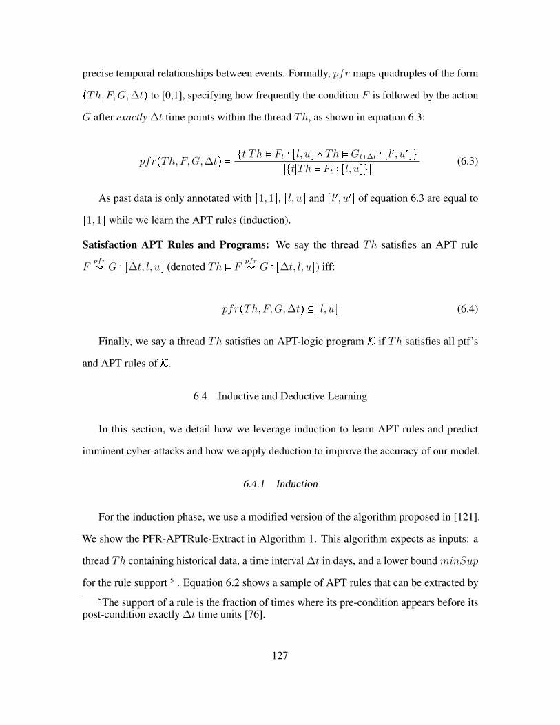
precise temporal relationships between events. Formally, pfr maps quadruples of the form

�Th,F,G,∆t� to [0,1], specifying how frequently the condition F is followed by the action

G after exactly ∆t time points within the thread Th, as shown in equation 6.3:

pfr�Th,F,G,∆t� � S�tSTh à Ft � �l, u� , Th à Gt�∆t � �l�, u��SS�tSTh à Ft � �l, u��S (6.3)

As past data is only annotated with �1,1�, �l, u� and �l�, u�� of equation 6.3 are equal to

�1,1� while we learn the APT rules (induction).

Satisfaction APT Rules and Programs: We say the thread Th satisfies an APT rule

Fpfr G � �∆t, l, u� (denoted Th à F

pfr G � �∆t, l, u�) iff:

pfr�Th,F,G,∆t� b �l, u� (6.4)

Finally, we say a thread Th satisfies an APT-logic program K if Th satisfies all ptf’s

and APT rules of K.

6.4 Inductive and Deductive Learning

In this section, we detail how we leverage induction to learn APT rules and predict

imminent cyber-attacks and how we apply deduction to improve the accuracy of our model.

6.4.1 Induction

For the induction phase, we use a modified version of the algorithm proposed in [121].

We show the PFR-APTRule-Extract in Algorithm 1. This algorithm expects as inputs: a

thread Th containing historical data, a time interval ∆t in days, and a lower bound minSup

for the rule support 5 . Equation 6.2 shows a sample of APT rules that can be extracted by5The support of a rule is the fraction of times where its pre-condition appears before its

post-condition exactly ∆t time units [76].

127

this algorithm.

Algorithm 1 The PFR-APTRule-Extract.1: procedure PFR-APTRULE-EXTRACT(Th, ∆t, minSup)

2: Rules� g, WeakRules� g

3: for each desired combination of conditions and actions do

4: F � current condition, G� current action

5: Fatoms � set of atoms of F , Gatom � atom of G

6: if �Fatoms -Gatom� ~a of any item of WeakRules then

7: supCountF � 0, supCountFG� 0, supFG� 0, trials� 0

8: for t = minTime�Th� to maxTime�Th� �∆t do

9: if Th à Ft � �1,1� then

10: supCountF � supCountF � 1

11: if Th à Gt�∆t � �1,1� then

12: supCountFG� supCountFG � 1

13: trials� trials � 1

14: supFG� supCountFG~trials

15: if supFG CminSup then

16: conFG� supCountFG~supCountF

17: if conFG A PRIOR�G� then

18: σprob �»nTrials�conFG��1�conFG�

nTrials

19: rule� Fpfr G � �∆t, conFG � σprob, conFG � σprob�

20: Rules� Rules - �rule�

21: else

22: WeakRules�WeakRules - �Fatoms -Gatom�

23: Return Rules

Overall, the PFR-APTRule-Extract generates all combinations of conditions and actions

using their predefined atoms, returning rules that satisfy two constraints: 1) the rule support

supFG is not lower than the user-defined threshold minSup (line 15); 2) the rule condition

F is a prima facie cause [64] for the rule action G (line 17). This second constraint is

satisfied when the probability of G occurring after F is greater than the prior probability of

G. To compute the probability intervals of the APT rules, we use one standard deviation of

the corresponding point probability (the rule confidence conFG) in a binomial distribution

[136] (line 18 of the algorithm), where nTrials is the number of events that produced the

128

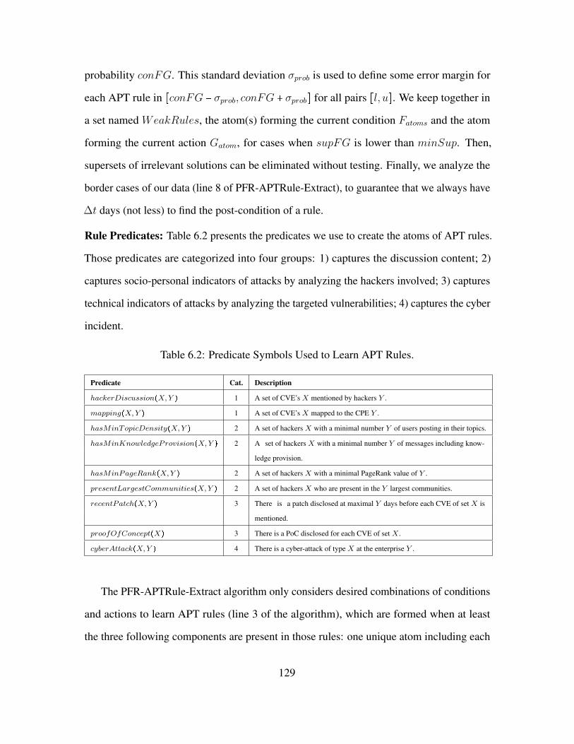
probability conFG. This standard deviation σprob is used to define some error margin for

each APT rule in �conFG � σprob, conFG � σprob� for all pairs �l, u�. We keep together in

a set named WeakRules, the atom(s) forming the current condition Fatoms and the atom

forming the current action Gatom, for cases when supFG is lower than minSup. Then,

supersets of irrelevant solutions can be eliminated without testing. Finally, we analyze the

border cases of our data (line 8 of PFR-APTRule-Extract), to guarantee that we always have

∆t days (not less) to find the post-condition of a rule.

Rule Predicates: Table 6.2 presents the predicates we use to create the atoms of APT rules.

Those predicates are categorized into four groups: 1) captures the discussion content; 2)

captures socio-personal indicators of attacks by analyzing the hackers involved; 3) captures

technical indicators of attacks by analyzing the targeted vulnerabilities; 4) captures the cyber

incident.

Table 6.2: Predicate Symbols Used to Learn APT Rules.

Predicate Cat. Description

hackerDiscussion�X,Y � 1 A set of CVE’s X mentioned by hackers Y .

mapping�X,Y � 1 A set of CVE’s X mapped to the CPE Y .

hasMinTopicDensity�X,Y � 2 A set of hackers X with a minimal number Y of users posting in their topics.

hasMinKnowledgeProvision�X,Y � 2 A set of hackers X with a minimal number Y of messages including know-

ledge provision.

hasMinPageRank�X,Y � 2 A set of hackers X with a minimal PageRank value of Y .

presentLargestCommunities�X,Y � 2 A set of hackers X who are present in the Y largest communities.

recentPatch�X,Y � 3 There is a patch disclosed at maximal Y days before each CVE of set X is

mentioned.

proofOfConcept�X� 3 There is a PoC disclosed for each CVE of set X .

cyberAttack�X,Y � 4 There is a cyber-attack of type X at the enterprise Y .

The PFR-APTRule-Extract algorithm only considers desired combinations of conditions

and actions to learn APT rules (line 3 of the algorithm), which are formed when at least

the three following components are present in those rules: one unique atom including each

129

predicate of category 1 and one unique atom including the predicate of category 4. We

want to investigate the possible combinations of atoms to check which ones produce more

accurate predictions. We detail the predicates now.

• hackerDiscussion�X,Y �: This mandatory predicate generates atoms that inform

mentioned CVE’s and their authors. The example here is hackerDiscussion�CV E,ACTOR�, where the first argument is a variable receiving CVE’s (e.g., cve-2016-0167),

while the second is a variable receiving hackers’ ID, such as darkwolf .

• mapping�X,Y �: This mandatory predicate generates atoms that inform in which CPE

a set of CVE’s are mapped to. One example is mapping�CV E,apache tomcat�,where the first argument is a variable receiving CVE’s, while the second is a constant

receiving a CPE, such as apache tomcat.

• hasMinTopicDensity�X,Y �: This optional predicate generates atoms that inform

hackers with a minimal number of users posting in their topics. One example is

hasMinTopicDensity�ACTOR,0.05�, where the first argument is a variable re-

ceiving hackers, while the second is a constant receiving a topic density 6 .

• hasMinKnowledgeProvision�X,Y �: This optional predicate generates atoms that

inform hackers who have a minimal number of messages including knowledge pro-

vision key-words, such as “yourself”, “recommend” or “suggest”. One example is

hasMinKnowledgeProvision�ACTOR,0.011�, where the first argument is a vari-

able receiving hackers, while the second is a constant receiving a knowledge provision

activity6.

6After normalizing feature values to avoid problems with the different scales of theforums, we check the data distribution to define two thresholds. For topic density, weconsider the values 0.008 and 0.05. For knowledge provision, we consider 0.0003 and 0.011.For PageRank, we consider 0.0002 and 0.0005. For the largest communities, we consider 2and 3. For recent patch, we consider 30 and 60 (days).

130

• hasMinPageRank�X,Y �: This optional predicate generates atoms that inform

the hackers who have a minimal PageRank network value [143]. One example is

hasMinPageRank�ACTOR,0.0005�, where the first argument is a variable receiv-

ing hackers, while the second is a constant receiving the PageRank6. To generate

multiple network of hackers (one for each forum) and compute metrics like PageRank,

we use the same strategy proposed in Chapter 2.

• presentLargestCommunities�X,Y �: This optional predicate generates atoms that

inform which hackers are present in the largest communities. The example is

presentLargestCommunities�ACTOR,3�, where the first argument is a variable

receiving hackers, while the second is a constant informing the number of commu-

nities6. We use the Louvain heuristic method to find the existing communities of

hackers [15]).

• recentPatch�X,Y �: This optional predicate generates atoms that inform CVE’s with

a recent patch disclosed at NVD (compared to the CVE’s mention). One example

is recentPatch�CV E,30�, where the first argument is a variable receiving CVE’s,

while the second is a constant receiving a maximal number of days6.

• proofOfConcept�X�: This optional predicate generates atoms that inform CVE’s

with a disclosed PoC. One example is proofOfConcept�CV E�, where the argument

is a variable receiving CVE’s.

• cyberAttack�X,Y �: This mandatory predicate generates atoms that inform cyber-

attacks happening in organizations. One example is cyberAttack�enterprise 1,m e�,

where the first argument is a constant receiving an organization, such as enterprise 1,

while the second is a constant receiving an attack type, such as m e.

131

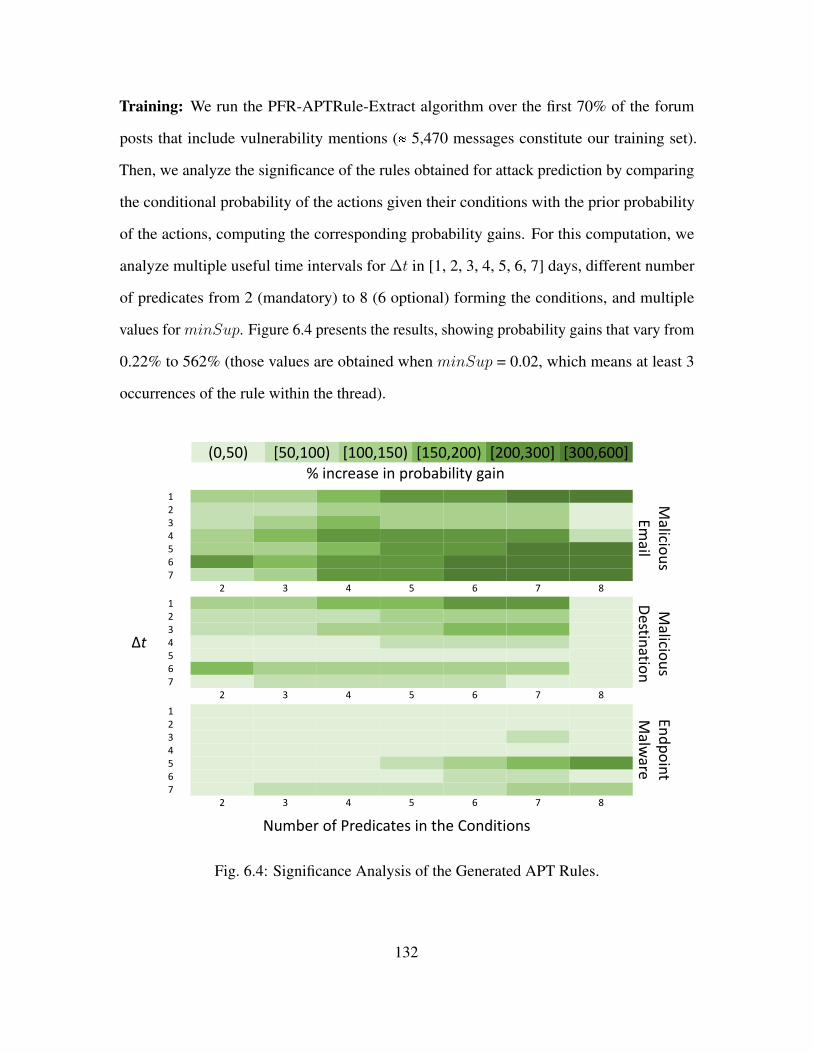
Training: We run the PFR-APTRule-Extract algorithm over the first 70% of the forum

posts that include vulnerability mentions (� 5,470 messages constitute our training set).

Then, we analyze the significance of the rules obtained for attack prediction by comparing

the conditional probability of the actions given their conditions with the prior probability

of the actions, computing the corresponding probability gains. For this computation, we

analyze multiple useful time intervals for ∆t in [1, 2, 3, 4, 5, 6, 7] days, different number

of predicates from 2 (mandatory) to 8 (6 optional) forming the conditions, and multiple

values for minSup. Figure 6.4 presents the results, showing probability gains that vary from

0.22% to 562% (those values are obtained when minSup = 0.02, which means at least 3

occurrences of the rule within the thread).

% increase in probability gain(0,50) [50,100) [100,150) [150,200) [200,300] [300,600]

1234567

2 3 4 5 6 7 8

Malicio

us

Email

Malicio

us

Destin

ation

End

po

int

Malw

are

Δt

1234567

2 3 4 5 6 7 8

1234567

2 3 4 5 6 7 8

Number of Predicates in the Conditions

Fig. 6.4: Significance Analysis of the Generated APT Rules.

132

Overall, we verify that probability gains increase as we include a greater number of

predicates in the conditions, pointing out the relevance of capturing socio-personal and

technical indicators of cyber-attacks by analyzing the hackers and their strategies. The

highest probability gains are located in the zone where the number of predicates is between

6 and 8, indicating which type of APT rules would potentially produce the best cyber-attack

predictions during testing. The total number of rules generated for ∆t in [1, 2, 3, 4, 5, 6, 7]

are 8,581, 6,290, 5,627, 6,713, 7,252, 10,456, and 10,326 respectively, adding up 55,245

APT rules. We also observe higher probability gains for the extreme tested values of ∆t,

such as 1, 6, and 7, signaling which time intervals could potentially generate more accurate

predictions.

Testing: After learning the APT rules, we generate cyber-attack predictions for the last

30% of the forum posts that include vulnerability mentions (� 2,350 messages constitute

our testing set). To accomplish that, we first search for APT rules that match a test case, or

those whose atoms forming their conditions are all applied to the two components of the test

case (vulnerability and hacker). Then, after selecting a rule from this pool, we use its post-

condition to predict the corresponding attack type exactly ∆t days after the vulnerability

mention (this approach will be properly formalized later in Theorem 1). Table 6.3 presents

our prediction results. We sort those results according to the highest % gain in F1 score

obtained by our model when compared to a baseline predictor that solely uses the prior

probability of each attack type (the absolute F1 score values are also sorted in descending

order). The highest performance (in F1 gain) is observed for malicious destination, followed

by malicious email and endpoint malware.

As verified in Table 6.3, the conditions of the best performing APT rules for all at-

tack types include 6 or 7 predicates, following the pattern identified in Figure 6.4. This

confirms the relevance of the indicators integrated into our pfr-based temporal logical frame-

work to predict cyber-attacks. Overall, those conditions are formed by all predicates but

133

Table 6.3: Prediction Results Compared to the Baseline.

Malicious Email

∆t Number of Predicates Precision Recall F1 % gain in F1

1 7 0.601 0.404 0.483 125.86

2 6 0.578 0.285 0.382 78.51

5 6 0.445 0.309 0.365 70.41

3 6 0.431 0.261 0.325 52.07

7 7 0.302 0.261 0.280 30.97

6 7 0.318 0.214 0.256 19.57

4 7 0.317 0.190 0.238 11.15

Malicious Destination


6 6 0.642 0.333 0.439 150.24

3 6 0.447 0.311 0.367 109.19

2 6 0.545 0.266 0.358 104.17

4 6 0.484 0.222 0.304 73.71

1 6 0.382 0.244 0.298 69.68

7 7 0.454 0.2 0.277 58.33

Endpoint Malware


7 6 0.372 0.360 0.366 41.82

1 7 0.376 0.280 0.321 24.49

6 7 0.297 0.310 0.308 19.38

proofOfConcept�X�, which means that only (PoC) exploits were not meaningful for the

predictions. Finally, as expected because of the rule significance analysis conducted before,

the extreme tested values of ∆t indeed improve the performance of our model, which obtains

F1 score gains of 150.24% for malicious destination (when ∆t � 6), 125.86% for malicious

email (when ∆t � 1), and 41.82% for endpoint malware (when ∆t � 7). We interpret this

phenomenon as: once a malicious hacking activity is detected, the start and end of the week

beginning the day after the detection is crucial for organizations to allocate their resources

and patch the corresponding vulnerability.

134

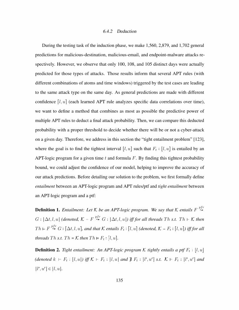
6.4.2 Deduction

During the testing task of the induction phase, we make 1,560, 2,879, and 1,702 general

predictions for malicious-destination, malicious-email, and endpoint-malware attacks re-

spectively. However, we observe that only 100, 108, and 105 distinct days were actually

predicted for those types of attacks. Those results inform that several APT rules (with

different combinations of atoms and time windows) triggered by the test cases are leading

to the same attack type on the same day. As general predictions are made with different

confidence �l, u� (each learned APT rule analyzes specific data correlations over time),

we want to define a method that combines as most as possible the predictive power of

multiple APT rules to deduct a final attack probability. Then, we can compare this deducted

probability with a proper threshold to decide whether there will be or not a cyber-attack

on a given day. Therefore, we address in this section the “tight entailment problem” [123],

where the goal is to find the tightest interval �l, u� such that Ft � �l, u� is entailed by an

APT-logic program for a given time t and formula F . By finding this tightest probability

bound, we could adjust the confidence of our model, helping to improve the accuracy of

our attack predictions. Before detailing our solution to the problem, we first formally define

entailment between an APT-logic program and APT rules/ptf and tight entailment between

an APT-logic program and a ptf:

Definition 1. Entailment: Let K be an APT-logic program. We say that K entails Fpfr

G � �∆t, l, u� (denoted, K à Fpfr G � �∆t, l, u�) iff for all threads Th s.t. Th à K then

Th à Fpfr G � �∆t, l, u�, and that K entails Ft � �l, u� (denoted, K à Ft � �l, u�) iff for all

threads Th s.t. Th à K then Th à Ft � �l, u�.Definition 2. Tight entailment: An APT-logic program K tightly entails a ptf Ft � �l, u�(denoted k ð Ft � �l, u�) iff K à Ft � �l, u� and ~§ Ft � �l�, u�� s.t. K à Ft � �l�, u�� and

�l�, u�� ` �l, u�.135

Now, suppose an APT-logic program Kcyber1 is composed of the APT rule r (inducted

using the PFR-APTRule-Extract algorithm) and the ptf φ shown in Table 6.4:

Table 6.4: APT-Logic Program Kcyber1.

ID Type Definition

r APT rule Fpfr G � �∆t, l, u�

φ ptf Ft � �1,1�

As Kcyber1 entails r and φ, we can place φ into the condition of r to infer that Kcyber1

will also entail Gt�∆t � �l, u�. We formally present this inference in Theorem 1 (this is the

logic used to make the predictions shown in Table 6.3):

Theorem 1. Let K be an APT-logic program, Fpfr G � �∆t, l, u� be an APT rule and

Ft � �1,1� be a ptf. If K à Fpfr G � �∆t, l, u� and K à Ft � �1,1� then K à Gt�∆t � �l, u�.

Proof. The proof here is straightforward by applying Modus Ponens, which states that

�F � G, F �~G [107]. As we have the APT rule Fpfr G � �∆t, l, u� informing that if F

happens at time t, then G will happen with a probability within �l, u� in exactly t �∆t, and

we also have the ptf Ft � �1,1� informing that F happened at time t, then we can infer that

G will happen at t �∆t with probability within �l, u� (keeping all constraints specified in

the APT rule). Formally, the ptf Gt�∆t � �l, u� can be logically inferred.

Now, consider an APT-logic program Kcyber2 composed of the four components (APT

rules and ptf’s) shown in Table 6.5. By using Theorem 1 over the APT rules and ptf’s

(r and φ), (s and ρ), and (u and γ), we can respectively infer the ptf’s: Gt�∆t � �l, u�,Gt��∆t� � �l�, u��, Gt��∆t�� l��, u��. If t �∆t, t� �∆t�, and t�� ∆t�� lead to the same time

point ti, then we can deduct a combined probability for G happening at ti, which is formally

presented in Theorem 2:

136

Table 6.5: APT-Logic Program Kcyber2.

ID Type Definition

r APT rule Fpfr G � �∆t, l, u�

s APT rule F �pfr G � �∆t�, l�, u��

u APT rule F ��pfr G � �∆t��, l��, u��

φ ptf Ft � �1,1�ρ ptf F �

t� � �1,1�γ ptf F ��

t�� 1,1�

Theorem 2. Let K be an APT-logic program, and Gt � �l, u�, Gt � �l�, u�� be two ptf’s. If

K à Gt � �l, u� and K à Gt � �l�, u�� then K à Gt � �max�l, l��,min�u,u�� s.t. �l, u� 9�l�, u�� x g.

Proof. This proof uses the notion of entailment between two ptf’s and the combination

of probabilities. Reasoning from [123, 36], we say a ptf λ � �l, u� entails another ptf

λ� � �l�, u�� (denoted λ � �l, u� à λ� � �l�, u��) iff for all threads Th s.t. Th à λ � �l, u� then

Th à λ� � �l�, u��, which is an implication that becomes true only when �l, u� ` �l�, u��. Also,

if there are two models predicting the same event on a given day with different lower bound

probabilities, the higher one will be valid for both models. On the other hand, if these

models predict with different upper bound probabilities, then the lower one will be valid for

both models. This way, if there exists an intersection between the probability boundaries

of Gt � �l, u� and Gt � �l�, u�� so that both predictions can be considered in our model, this

intersection is formed by the interval �max�l, l��,min�u,u��, which is a subset of �l, u�and also a subset of �l�, u��. Therefore, we can say that Gt � �max�l, l��,min�u,u�� àGt � �l, u� and that Gt � �max�l, l��,min�u,u�� à Gt � �l�, u��, which leads to K à Gt �

�max�l, l��,min�u,u�� s.t. �l, u� 9 �l�, u�� x g.

137

Note that Theorem 2 can be applied recursively if there is an extra ptf possible to be

combined with a previously deducted ptf. For instance, if we consider that:

K à Gt � �max�l, l��,min�u,u�� and K à Gt � �l��, u��, then we can state that:

K à Gt � �max�max�l, l��, l��,min�min�u,u��, u�� s.t. �max�l, l��,min�u,u�� 9�l��, u�� x g.

This way, by using Theorem 1 and Theorem 2, we can guarantee tight entailment

conditions for the APT-logic programs Kcyber1 and Kcyber2 as shown below:

Kcyber1 ð Gt�∆t � �l, u�.Kcyber2 ð Gt � �max�max�l, l��, l��,min�min�u,u��, u�� s.t. �max�l, l��,min�u,u��9�l��, u�� x g.

If there is a case where there is no intersection between the probability boundaries of two

ptf’s leading to the same action at the same time, then our deductive model cannot consider

both ptf’s for predictions. Thus, we eliminate the ptf with the lower probability boundaries

from our APT-logical program. Finally, to decide whether we should make a prediction

or not after combining the probability boundaries of two or more ptf’s, we test different

thresholds δ in [0,1] with step 0.05. Then, if the upper bound of the deducted ptf is greater

or equal to δ, we make the prediction. Figure 6.5 presents the results for this deduction task,

where we compute more than 3,300 combinations of probability intervals.

We compare the highest performances obtained by our model after the deduction phase

with those obtained after the induction (training/testing) phase and also with the ones

provided by the baseline predictor. As observed, the F1 scores increase considerably for all

situations analyzed, with gains varying from 73.83% until 182.38% when compared with

the baseline predictor, and with gains varying from 11.80% until 22.40% when compared

with performance obtained after induction. Those results demonstrate how the combination

138

0.2140.175 0.258

0.4830.439

0.366

0.540.495

0.448

0

0.1

0.2

0.3

0.4

0.5

0.6


F1 S

core

Baseline Our Model After Induction Our Model After Deduction

↑125.86%

↑152.25%

↑150.24%

↑182.38%

↑41.82%

↑73.83%

Fig. 6.5: Performance (F1 Score) Comparison Between the Baseline and Our Model After

the Induction and Deduction Phases.

of ptf’s is a relevant strategy to improve the accuracy of our cyber-attack predictions. We

note that our model achieves the highest prediction performance after deduction when we

set δ in [0.2, 0.4], as shown in Figure 6.6. On average, those threshold values imply the

prior probability plus � 35%.

0

0.1

0.2

0.3

0.4

0.5

0.6

0.0

0

0.1

0

0.2

0

0.3

0

0.4

0

0.5

0

0.6

0

0.7

0

0.8

0

0.9

0

1.0

0

Deduc. Induc. Base.

0

0.1

0.2

0.3

0.4

0.5

0.6

0

0.1

0.2

0.3

0.4

0.5

0.6

0.7

0.8

0.9 1

Deduct. Induct. Base.

00.05

0.10.15

0.20.25

0.30.35

0.40.45

0.5

0

0.1

0.2

0.3

0.4

0.5

0.6

0.7

0.8

0.9 1

Deduc. Induct. Base.


Threshold

F1 S

core

Threshold Threshold

Fig. 6.6: Threshold Analysis for Final Predictions After Deduction.

6.5 Extending the Framework to Predict Within a Period of Time ∆t

As the Point Frequency Function (pfr) captures precise temporal relationships between

events, we can use mined hacking activity to make cyber-attack predictions for a specific

day. However, we also analyze the utility of making predictions withing a period of time ∆t,

139

using the Existential Frequency Function (efr) to construct our APT rules [121]. Formally,

efr maps quadruples of the form �Th,F,G,∆t� to [0,1], specifying how frequently the

condition F is followed by the action G within ∆t time points in the thread Th, as shown in

equation 6.5. Thus, efr allows for the action to fall (becomes true) within some period of

time ∆t rather than exactly ∆t time points after the condition becomes true.

efr�Th,F,G,∆t� � S�tSTh à Ft � p , Th à �∆tt��1Gt�t� � p��S

S�tSTh à Ft � p�S (6.5)

Note how for efr we do not compute probability intervals �l, u� but point probabilities

p. This happens since we will not know the exact day for which a prediction is made when

∆t A 1, considering that a prediction is true if there is an attack in any of the days covered

by ∆t. Thus, we also do not conduct the deduction phase in this analysis, keeping our

experiments focused only on the induction phase. Based on that, we say the thread Th

satisfies an APT rule Fefr G � �∆t, p� (denoted Th à F

efr G � �∆t, p�) iff:

efr�Th,F,G,∆t� C p (6.6)

We extend the PFR-APTRule-Extract to propose the EFR-APTRule-Extract algorithm

shown in Algorithm 2. Note how this new algorithm addresses the requirements of existential

frequency functions, considering a period of time ∆t for the action to be true after the

condition is triggered (line 11 of the algorithm) and outputting point probabilities instead of

probability intervals for the mined APT rules (line 18 of the algorithm). We use the same

predicates shown in Table 6.2 and the same constraints regarding valid combinations of

conditions and actions to learn APT rules. The parameters Th, minSup, and the training

and test set ratio of 70/30 are also kept the same. However, we make the values of ∆t to

140

include now only 2 or 3 days. The reason is because we want to make predictions for short

periods of time, since a value for ∆t greater or equal to 5 (around a week) will basically

create a tautology and will not be useful given the high frequency of attacks in our data.

Algorithm 2 The EFR-APTRule-Extract.1: procedure EFR-APTRULE-EXTRACT(Th, ∆t, minSup)

2: Rules� g, WeakRules� g

3: for each desired combination of conditions and actions do

4: F � current condition, G� current action

5: Fatoms � set of atoms of F , Gatom � atom of G

6: if �Fatoms -Gatom� ~a of any item of WeakRules then

7: supCountF � 0, supCountFG� 0, supFG� 0, trials� 0

8: for t = minTime�Th� to maxTime�Th� �∆t do

9: if Th à Ft � 1 then

10: supCountF � supCountF � 1

11: if Th à �∆tt��1

Gt�t� � 1 then

12: supCountFG� supCountFG � 1

13: trials� trials � 1

14: supFG� supCountFG~trials

15: if supFG CminSup then

16: conFG� supCountFG~supCountF

17: if conFG A PRIOR�G� then

18: rule� Fpfr G � �∆t, conFG�

19: Rules� Rules - �rule�

20: else

21: WeakRules�WeakRules - �Fatoms -Gatom�

22: Return Rules

Figure 6.7 shows the significance of the rules obtained for attack prediction with EFR-

APTRule-Extract algorithm. Repeating the pattern observed for PFR-APTRule-Extract,

we verify that probability gains increase as we include a greater number of predicates in

the conditions. However, we verify that probability gains tend to decrease as we make ∆t

greater, showing how the prior probability of attacks grows fast when we consider higher ∆t

values. We also note the highest probability gains are located in a zone where the number of

predicates is between 4 and 7, repeating what we observed for PFR-APTRule-Extract.

141

% increase in probability gain(0,50) [50,100) [100,150) [150,200)

23

2 3 4 5 6 7 8

23

2 3 4 5 6 7 8

23

2 3 4 5 6 7 8

Malicio

us

Email

Malicio

us

Destin

ation

End

po

int

Malw

are

Δt

Number of Predicates in the Conditions

Fig. 6.7: Significance Analysis of the Generated APT Rules Considering efr.

Table 6.6 presents our prediction results, where we inform which conditions (combina-

tion of atoms generated according to the predicates) obtain the highest percentage in F1 gain

when compared to a baseline predictor that uses the prior probability of each attack type.

The table shows gains from 1% to 123%, with the highest gains observed for the attack type

malicious email, followed by malicious destination and endpoint malware. As the baseline

has its accuracy increased with a greater ∆t, and the performance of our model does not

improve with the same rate, the F1 gains are generally smaller if compared to the ones

obtained when the point frequency function is used. However, the absolute values of the F1

score are higher, since now we have a period of 2 or 3 days to observe the cyber-attack.

Note how in 50% of the cases (3 out of 6 cases analyzed), the conditions are formed by 5

predicates, which follows the pattern shown of Figure 6.7. Since we observe a lower number

of predicates forming the conditions compared to the pfr analysis (5 against 6 or 7), we

investigate which are the recurrent indicators that effectively contribute for more accurate

predictions. For instance, hasMinPageRank is present in 83.3% of the cases (5 out of 6),

indicating how social network metrics that estimate the hackers’ centrality can be important

142

Table 6.6: Prediction Results.

EnterpriseAttack

∆t APT Rule ConditionsBaseline (Prior Prob.) Prop. Framework % gain

in F1Type F1 F1

enterprise 1

m e

2

hackerDiscussion�X,Y � ,

0.336 0.751 123%mapping�X,Y � ,

hasMinTopicDensity�X,Y � ,

presentLargestCommunities�X,Y �

3


0.603 0.872 45%

mapping�X,Y � ,

hasMinKnowledgeProvision�X,Y � ,

hasMinPageRank�X,Y � ,

recentPatch�X,Y �

m d

2


0.371 0.566 52%

mapping�X,Y � ,



presentLargestCommunities�X,Y �


3


0.705 0.748 6%mapping�X,Y � ,


hasMinPageRank�X,Y �

e m

2


0.469 0.508 8%

mapping�X,Y � ,



hasMinPageRank�X,Y �

3


0.643 0.650 1%

mapping�X,Y � ,




to identify credible threats. Following, hasMinTopicDensity is present in 4 out of 6

cases, again strengthening the relevance of finding hackers that produce the most interesting

and useful cyber threats. Also, hasMinKnowledgeProvision occurs in 3 out of 6 cases,

143

indicating how relevant it is to find hackers with expertise to share. Similarly, recentPatch

is present in 3 out of 6 cases, showing the importance of the vulnerability disclosure

information in NVD during the first 30 or 60 days. Finally, presentLargestCommunities

occurs in 2 out of 6 cases, pointing out the relevance of analyzing the biggest communities

of hackers, where reputable individuals are usually coordinating activities.

Overall, those results evidence how the analysis of malicious hackers can be relevant to

identify credible threats in the future, signaling that: once a vulnerability is mentioned, the

next step should be a deep analysis of the hackers involved.

6.6 Related Work

Different research works have been proactively investigating cybersecurity either by

searching cyber-threats to mitigate risks [103, 7, 5] or by predicting the exploitation of soft-

ware vulnerabilities [109, 9, 17]. However, only a few of those studies focus on predicting

cyber-attacks against specific corporations by analyzing online hacking discussions.

For instance, Khandpur et al. [63] proposed an unsupervised approach to detect ongoing

cyber-attacks discussed on Twitter. They achieved a reasonable performance by using a

limited set of seed event triggers and adding a query expansion strategy based on convolu-

tional kernels and dependency parses. Goyal et al. [52] described deep neural networks and

autoregressive time series models that leveraged external signals to predict attacks. They

showed how information from security blogs and vulnerability databases are useful to make

the predictions. Deb et al. [30] applied sentiment analysis to darkweb forum posts to assess

sentiment trends over time, demonstrating a higher prediction performance compared to

a time series model. More similar to our work, Almukaynizi et al. [8] proposed a logical

framework to predict cyber-attacks against specific corporations by mining cyber threat

intelligence from the darkweb. The authors tried to predict the magnitude of a particular

type of attack, achieving reasonable performance when compared to the designed baselines.

144

Although all those works proposed interesting strategies that help organizations to

monitor the cyberspace while searching for credible threats, their implementations partially

or totally fail to be timely, actionable, accurate, and transparent. These four key desired

properties of a cyber-attack prediction tool are successfully addressed by our temporal logic

framework. Besides, those works basically neglected the individuals behind the events. In

addition to the technical information involved, such as the release of a recent patch for a

software vulnerability, we also rely on social-personal indicators of attacks by checking the

hackers and their communities. Then, we are able to differentiate the cybercriminals and

their strategies in terms of capability, significantly increasing the accuracy of our predictions.

6.7 Summary

In this Chapter, we present a temporal logic framework capable of predicting cyber-

attacks in the near future. Particularly, our framework learns Annotated Probabilistic

Temporal (APT) rules that correlate malicious hacking activity with real-world cyber inci-

dents, leveraging these rules for predicting when, where, and how a particular attack is likely

to happen. Then, we leverage a deductive approach to adjust the confidence with which

our model makes attack predictions. Considering socio-personal and technical indicators of

enterprise attacks, our method analyzes the malicious hackers and their strategies, helping

security teams to effectively identify which will be the probable IT targets of cybercriminals.

145

Chapter 7

CONCLUSION

Today’s widespread of cyber-attack incidences makes them one of the primary threat

faced by organizations worldwide. The current methods that attempt to neutralize hacking

attempts have been failing to demonstrate effectiveness, probably for concentrating only

on the technical aspects involved and neglect the actors behind the incidents. We believe

that an intimate understanding of the malicious hacker communities will greatly aid power

to proactive cyber threat intelligence, allowing defenders to be more effective while an-

ticipating cyber threats. However, as the hacking market is in clear expansion in terms of

players and traded exploits, there are important limitations still largely unexplored, such

as: who are the skilled and influential individuals forming those hacker groups, how hacker

communities organize along the lines of technical expertise, how ideas propagate within

those communities, and which internal patterns can signal imminent cyber offensives.

7.1 Summary of the Contributions

This dissertation proposes a hacker centric perspective to empower cyber defense,

demonstrating how the hackers’ digital traces existing in malicious hacking communities

yield valuable insights into evolving cyber threats.

In Chapter 2, we mine “key-hackers” on popular darkweb forums, identifying individuals

who are likely to succeed in their cybercriminal goals. We develop a profile for each forum

member using features derived from content, social network, and seniority analysis, aiming

to differentiate standard from key cyber-actors. Then, after defining a metric for collecting

ground truth data based on user reputation, we train our model on a given forum using

optimization (EC) and (ML) algorithms fed with those features to later test its performance

146

on a different forum. Our results show that we are able to identify up to 52% of the existing

key-hackers, demonstrating how our model generalizes relatively well.

In Chapter 3 and Chapter 4, we investigate how social influence contributes to user/hacker

engagement online, developing two lines of research for analyzing user adoption behav-

ior. In Chapter 3, we investigate whether microblog users on social media will adopt a

hashtag considering the influence exerted by their active neighbors. We introduce two time

constraints to extend standard (SNA) measures used to quantify social influence, noting

that: 1) their correlation with adoption probability improves up to 488.24% for all influence

measures analyzed; 2) their ability to predict adoption in a (ML) classification task improves

up to 13.69% in F1 score when comparing to recent machine learning techniques that aim to

predict adoption. In Chapter 4, we investigate where and when darkweb forum hackers will

post a message in the future considering their recurrent interactions with other hackers. We

formulate this problem as a (ML) sequential rule mining task, designing experiments using

multiple posting time granularities and time-windows. We observe precision results of up to

0.78 and precision gains up of to 837% when compared to the prior probabilities of hackers’

posts. The analysis of user adoption behavior in both research works can be used by security

specialists to reveal the potential expansion degree of the key-hackers’ networks.

In Chapter 5, we search for communities of darkweb marketplaces’ vendors with similar

expertise in specific subfields of hacking, a feature typically owned by key-hackers that can

be used for surveillance purposes. We develop a method based on (SNA) techniques that

identifies communities of hacking-related vendors using the similarity of their products,

validating our method by cross-checking the community assignments of these individuals

on two mutually exclusive sets of marketplaces. Our model achieves 0.445 of consistency

between more than 30 communities of vendors revealed in each subset of markets.

In Chapter 6, we integrate the social models proposed in the previous chapters into a

temporal logic framework capable of predicting cyber-attacks. Particularly, the framework

147

induct rules that correlate malicious hacking activity with real-world cyber incidents and

deduct more accurate security warnings by combining multiple attack predictions. By consid-

ering technical and socio-personal indicators of cyber-attacks, we demonstrate considerable

prediction gains in F1 score (up to 150.24%) compared to the baseline. Those results are

particular evidenced when the pre-conditions of the rules include relevant information about

the hackers behind the attacks, highlighting the relevance of the socio-personal indicators

for the identification of imminent threats. Besides, we also obtain gains in F1 score of up to

182.38% when the predictions made for a given day are combined using deduction.

By proposing the models detailed in this dissertation, we provide methods for the

identification of credible cyber threats, allowing organizations to protect assets likely to be

targeted before the attackers even have a chance to start their offensives.

7.2 Future Directions

The work conducted in this dissertation can be extended in many ways in order to

enhance proactive cyber threat intelligence, either by addressing current limitations or by

proposing new models, methods, frameworks, and algorithms. In the following, some

potential research areas that will go towards this goal are discussed.

• Vulnerability Exploitation Prediction. This task comprises the prediction which known

software vulnerabilities are likely to be exploited by malicious hackers. Standard

vulnerability score systems like CVSS [6, 9] are known not to be useful for patch

prioritization due to their high false positive rates. Machine learning techniques can

be applied over features computed from malicious hacking environments to mine

vulnerabilities directly or indirectly discussed by credible hackers, so that security

specialists can have a better map of the assets at risk.

• Identification of Zero-Day Exploits. Another important security challenge is the

148

potential identification of zero-day attacks, as defenders cannot be protected against

“invisible” threats. Although zero-day exploits target unknown vulnerabilities, they

usually exist “in the wild” for over 300 days before identification [14]. Thus, re-

searchers can gather cyber threat intelligence to discover what kind of zero-day

exploit is being developed and offered on hacking communities.

• Social Network Extraction of Malicious Hackers. Many research works conducted on

darkweb forums [78, 79, 83, 7] explore social network features to accomplish their

goals. However, due to the fragmented and interactionally disjointed natures of those

environments, extracting social network structure by using only hacker interaction

data is difficult and inaccurate. Thus, Natural language Processing (NLP) methods

can be used to derive more accurate reply-to information on darkweb forums, leading

to a better approximation of the real hacker network topology.

• Forum Spidering. In order to automate data collection from darkweb websites, de-

signed spiders need to automatically find and download relevant HTML pages. Mali-

cious hacking sites, especially those existing in encrypted networks like Tor, are able

to easily detect and block those robots [92]. Thus, one main contribution to the cyber

threat intelligence area should be the design of intelligent human-like-spiders. Those

robots should be able to bypass detection methods by mimicking human browsing

behavior, and also learn which hacking information is important to be collected.

• Adversarial Reasoning. Malicious hackers are continually evolving and adjusting their

strategies to defeat defense postures. To address this threat, defenders should also

employ adaptive strategies to assess hackers’ capabilities, perceptions, intents, actions,

and behaviors [103]. Thus, the development of models combining game theory, AI,

control theory, cognitive modeling, and machine learning to reason about how, why,

where, and when cyber-attacks will occur is crucial to successfully defeat attackers.

149

• Cascade Prediction: Predicting when a hacking message will go “viral” is important

for cybersecurity, since information cascades can signal hacktivism campaigns or

mass adoption of cyber threats [119]. Then, defenders will benefit from modeling

information diffusion on hacking communities to investigate which influential and

topological patterns can be leveraged for the early extraction of popular threads.

150

REFERENCES

[1] National Institute of Standards and Technology (NIST). https://https://www.nist.gov//,Last Accessed: June 2019.

[2] A. Abbasi, W. Li, V. Benjamin, S. Hu, and H. Chen. Descriptive analytics: Examiningexpert hackers in web forums. In Proceeding of ISI 2014, pages 56–63. IEEE, Sept2014.

[3] O. Abbosh and K. Bissell. Securing the digital economy: Reinventing the internet fortrust. , Accenture, 2019.

[4] I. Ajzen and M. Fishbein. Understanding attitudes and predicting social behavior.Prentice-Hall, 1980.

[5] L. Allodi. Economic factors of vulnerability trade and exploitation. In Proceedingsof the 2017 ACM SIGSAC Conference on Computer and Communications Security,CCS ’17, pages 1483–1499, New York, NY, USA, 2017. ACM.

[6] L. Allodi and F. Massacci. Comparing vulnerability severity and exploits usingcase-control studies. ACM Trans. Inf. Syst. Secur., 17(1):1:1–1:20, Aug. 2014.

[7] M. Almukaynizi, A. Grimm, E. Nunes, J. Shakarian, and P. Shakarian. Predictingcyber threats through hacker social networks in darkweb and deepweb forums. InProceedings of the 2017 International Conference of The Computational SocialScience Society of the Americas. ACM, 2017.

[8] M. Almukaynizi, E. Marin, E. Nunes, P. Shakarian, G. I. Simari, D. Kapoor, andT. Siedlecki. Darkmention: A deployed system to predict enterprise-targeted externalcyberattacks. In Proceeding of 2018 IEEE International Conference on Intelligenceand Security Informatics (ISI). IEEE, 2018.

[9] M. Almukaynizi, E. Nunes, K. Dharaiya, M. Senguttuvan, J. Shakarian, and P. Shakar-ian. Proactive identification of exploits in the wild through vulnerability mentionsonline. In 2017 International Conference on Cyber Conflict (CyCon U.S.), pages82–88, Nov 2017.

[10] T. Anwar and M. Abulaish. Identifying cliques in dark web forums - an agglomerativeclustering approach. In 2012 IEEE International Conference on Intelligence andSecurity Informatics, pages 171–173, June 2012.

[11] A.-L. Barabasi and R. Albert. Emergence of scaling in random networks. Science,286(5439):509–512, 1999.

[12] V. Benjamin, W. Li, T. Holt, and H. Chen. Exploring threats and vulnerabilities inhacker web: Forums, irc and carding shops. In 2015 IEEE International Conferenceon Intelligence and Security Informatics (ISI), pages 85–90, May 2015.

151

[13] V. Benjamin, B. Zhang, J. Jr., and H. Chen. Examining hacker participation length incybercriminal internet-relay-chat communities. Journal of Management InformationSystems, 33(2):482–510, 2016.

[14] L. Bilge and T. Dumitras. Before we knew it: An empirical study of zero-day attacksin the real world. In CCS ’12 Proceedings of the 2012 ACM conference on Computerand Communications Security, CCS ’12, pages 833 – 844. ACM, ACM, 2012 2012.

[15] V. D. Blondel, J.-L. Guillaume, R. Lambiotte, and E. Lefebvre. Fast unfoldingof communities in large networks. Journal of Statistical Mechanics: Theory andExperiment, 2008(10):P10008, 2008.

[16] S. P. Borgatti, K. M. Carley, and D. Krackhardt. On the robustness of centralitymeasures under conditions of imperfect data. Social Networks, 28(2):124–136, 2006.

[17] B. L. Bullough, A. K. Yanchenko, C. L. Smith, and J. R. Zipkin. Predicting exploita-tion of disclosed software vulnerabilities using open-source data. In Proceedings ofthe 3rd ACM on International Workshop on Security And Privacy Analytics, IWSPA’17, pages 45–53, New York, NY, USA, 2017. ACM.

[18] R. S. Burt. Social contagion and innovation: Cohesion versus structural equivalence.American Journal of Sociology, 92(6):1287–1335, 1987.

[19] B. Buunk and W. Schaufeli. Reciprocity in interpersonal relationships: An evolu-tionary perspective on its importance for health and well-being. European Review ofSocial Psychology, 10(1):259–291, 1999.

[20] D. Carr. How Obama Tapped into Social Networks’ Power, 2008. https://www.nytimes.com/2008/11/10/business/media/10carr.html (accessedon 07-03-2018).

[21] M. Cha, H. Haddadi, F. Benevenuto, and K. P. Gummadi. Measuring user influencein twitter: The million follower fallacy. In Proceedings of the Fourth ICWSM. AAAIPress, 2010.

[22] Y.-D. Chen, S. A. Brown, P. J.-H. Hu, C.-C. King, and H. Chen. Managing emerginginfectious diseases with information systems: Reconceptualizing outbreak manage-ment through the lens of loose coupling. Information Systems Research, 22(3):447–468, 2011.

[23] J. Cheng, L. Adamic, P. A. Dow, J. M. Kleinberg, and J. Leskovec. Can cascades bepredicted? In Proceedings of the 23rd International Conference on World Wide Web,WWW ’14, pages 925–936, New York, NY, USA, 2014. ACM.

[24] A. Clauset, M. E. J. Newman, and C. Moore. Finding community structure in verylarge networks. Phys. Rev. E, 70:066111, Dec 2004.

[25] G. Coleman. Hacker, Hoaxer, Whistleblower, Spy: The Many Faces of Anonymous.Verso Books, 2014.

152

https://www.nytimes.com/2008/11/10/business/media/10carr.html

https://www.nytimes.com/2008/11/10/business/media/10carr.html

[26] J. S. Coleman, E. Katz, and H. Menzel. Medical innovation: A diffusion study. SocialForces, 46(2):291, 1967.

[27] P. Cui, S. Jin, L. Yu, F. Wang, W. Zhu, and S. Yang. Cascading outbreak predictionin networks: A data-driven approach. In Proceedings of the 19th ACM SIGKDDInternational Conference on Knowledge Discovery and Data Mining, KDD ’13, pages901–909, New York, NY, USA, 2013. ACM.

[28] I. Cyber Reconnaissance. CYR3CON, 2020. https://www.cyr3con.ai//(accessed on 02-01-2020).

[29] G. Das, K.-I. Lin, H. Mannila, G. Renganathan, and P. Smyth. Rule discovery fromtime series. In Proceedings of the Fourth International Conference on KnowledgeDiscovery and Data Mining, KDD’98, pages 16–22. AAAI Press, 1998.

[30] A. Deb, K. Lerman, and E. Ferrara. Predicting cyber-events by leveraging hackersentiment. Information, 9(11):280, 2018.

[31] D. Decary-Hetu and B. Dupont. Reputation in a dark network of online criminals.Global Crime, 14(2-3):175–196, 2013.

[32] J. Deogun and L. Jiang. Prediction mining – an approach to mining association rulesfor prediction. In D. Slezak, J. Yao, J. F. Peters, W. Ziarko, and X. Hu, editors, RoughSets, Fuzzy Sets, Data Mining, and Granular Computing, pages 98–108. SpringerBerlin Heidelberg, 2005.

[33] P. Domingos and M. Richardson. Mining the network value of customers. InProceedings of the Seventh ACM SIGKDD International Conference on KnowledgeDiscovery and Data Mining, KDD ’01, pages 57–66, New York, NY, USA, 2001.ACM.

[34] S. Dowdy, S. Wearden, and D. Chilko. Statistics for Research. Wiley, 2004.

[35] M. Edkrantz and A. Said. Predicting cyber vulnerability exploits with machine learn-ing. In Proceedings of the 13th Scandinavian Conference on Artificial Intelligence,volume 278, pages 48–57, 2015.

[36] M. V. Emden. Quantitative deduction and its fixpoint theory. The Journal of LogicProgramming, 3(1):37 – 53, 1986.

[37] S. Enderby. Remediation vs. prevention: How to place your bets,2017. https://blog.malwarebytes.com/101/2017/09/remediation-vs-prevention-how-to-place-your-bets/ (ac-cessed on 10-26-2018).

[38] Z. Fang, X. Zhao, Q. Wei, G. Chen, Y. Zhang, C. Xing, W. Li, and H. Chen. Exploringkey hackers and cybersecurity threats in chinese hacker communities. In Proceedingof ISI 2016. IEEE, 2016.

153

https://www.cyr3con.ai//

https://blog.malwarebytes.com/101/2017/09/remediation-vs-prevention-how-to-place-your-bets/

https://blog.malwarebytes.com/101/2017/09/remediation-vs-prevention-how-to-place-your-bets/

[39] C. Fink, A. Schmidt, V. Barash, C. J. Cameron, and M. Macy. Complex contagionsand the diffusion of popular twitter hashtags in nigeria. Social Netw. Analys. Mining,6(1):1:1–1:19, 2016.

[40] C. Fink, A. Schmidt, V. Barash, J. Kelly, C. Cameron, and M. Macy. Investigating theobservability of complex contagion in empirical social networks. Tenth InternationalAAAI Conference on Web and Social Media, 2016.

[41] FIREEYE. Threat Research. Dyre Banking Trojan Exploits CVE-2015-0057,2018. https://www.fireeye.com/blog/threat-research/2015/07/dyre_banking_trojan.html/ (accessed on 08-15-2018).

[42] N. Fisk. Social learning theory as a model for illegitimate peer-to-peer use and theeffects of implementing a legal music downloading service on peer-to-peer musicpiracy. PhD thesis, Rochester Institute of Technology, 2006.

[43] S. Fortunato. Community detection in graphs. Physics Reports, 486(3):75 – 174,2010.

[44] P. Fournier-Viger, U. Faghihi, R. Nkambou, and E. M. Nguifo. Cmrules: Miningsequential rules common to several sequences. Knowledge-Based Systems, 25(1):63 –76, 2012. Special Issue on New Trends in Data Mining.

[45] P. Fournier-Viger, T. Gueniche, and V. S. Tseng. Using partially-ordered sequentialrules to generate more accurate sequence prediction. In Advanced Data Mining andApplications, pages 431–442, Berlin, Heidelberg, 2012. Springer Berlin Heidelberg.

[46] P. Fournier-Viger, C. Wu, V. S. Tseng, L. Cao, and R. Nkambou. Mining partially-ordered sequential rules common to multiple sequences. IEEE Transactions onKnowledge and Data Engineering, 27(8):2203–2216, Aug 2015.

[47] P. Fournier-Viger, C.-W. Wu, V. S. Tseng, and R. Nkambou. Mining sequentialrules common to several sequences with the window size constraint. In Advancesin Artificial Intelligence, pages 299–304, Berlin, Heidelberg, 2012. Springer BerlinHeidelberg.

[48] M. Girvan and M. E. J. Newman. Community structure in social and biologicalnetworks. Proceedings of the National Academy of Sciences, 99(12):7821–7826,2002.

[49] M. Glenski and T. Weninger. Predicting user-interactions on reddit. In Proceedingsof the 2017 IEEE/ACM International Conference on Advances in Social NetworksAnalysis and Mining 2017, ASONAM ’17, pages 609–612, New York, NY, USA,2017. ACM.

[50] S. Goel, A. Anderson, J. M. Hofman, and D. J. Watts. The structural virality of onlinediffusion. Management Science, 62:180–196, 2016.

[51] A. Goyal, F. Bonchi, and L. V. Lakshmanan. Learning influence probabilities insocial networks. In Proceedings of the 3rd ACM WSDM, WSDM ’10, pages 241–250,New York, NY, USA, 2010. ACM.

154

https://www.fireeye.com/blog/threat-research/2015/07/dyre_banking_trojan.html/

https://www.fireeye.com/blog/threat-research/2015/07/dyre_banking_trojan.html/

[52] P. Goyal, K. Hossain, A. Deb, N. Tavabi, N. Bartley, A. Abeliuk, E. Ferrara, andK. Lerman. Discovering signals from web sources to predict cyber attacks. DeepAI,Jun 2018.

[53] R. Guo and P. Shakarian. A comparison of methods for cascade prediction. InProceedings of the 2016 IEEE/ACM International Conference on Advances in SocialNetworks Analysis and Mining, ASONAM ’16, pages 591–598, Piscataway, NJ, USA,2016. IEEE Press.

[54] H. J. Hamilton and K. Karimi. The timers ii algorithm for the discovery of causality.In T. B. Ho, D. Cheung, and H. Liu, editors, Advances in Knowledge Discovery andData Mining, pages 744–750, Berlin, Heidelberg, 2005. Springer Berlin Heidelberg.

[55] T. Holt, D. Strumsky, O. Smirnova, and M. Kilger. Examining the social networks ofmalware writers and hackers. International Journal of Cyber Criminology, 6(1):891–903, 1 2012.

[56] K. Hornik, M. Kober, I. Feinerer, and C. Buchta. Spherical k-means clustering.Journal of Statistical Software, 50, Sep 2012.

[57] J. Huang and J. Xue. The predictive power of content and temporal features of postsin information dissemination in microblogging. Journal of China Tourism Research,11(2):150–165, 2015.

[58] L. Hubert and P. Arabie. Comparing partitions. Journal of Classification, 2(1):193–218, Dec. 1985.

[59] B. Hunter. The importance of reciprocity in relationships between community-basedmidwives and mothers. Midwifery, 22(4):308–322, 2006.

[60] IdentityForce. 2019 Data Breaches - The Worst So Far.https://www.identityforce.com/blog/2019-data-breaches, Access: 2019.

[61] M. Jenders, G. Kasneci, and F. Naumann. Analyzing and predicting viral tweets. InProceedings of the 22Nd International Conference on World Wide Web, WWW ’13Companion, pages 657–664, New York, NY, USA, 2013. ACM.

[62] D. Kempe, J. Kleinberg, and E. Tardos. Maximizing the spread of influence through asocial network. In Proceedings of the Ninth ACM SIGKDD International Conferenceon Knowledge Discovery and Data Mining, KDD ’03, pages 137–146, New York,NY, USA, 2003. ACM.

[63] R. P. Khandpur, T. Ji, S. Jan, G. Wang, C.-T. Lu, and N. Ramakrishnan. Crowdsourc-ing cybersecurity: Cyber attack detection using social media. In Proceedings of the2017 ACM on Conference on Information and Knowledge Management, CIKM ’17,pages 1049–1057, New York, NY, USA, 2017. ACM.

[64] S. Kleinberg and B. Mishra. The temporal logic of causal structures. In Proceedingsof the Twenty-Fifth Conference on Uncertainty in Artificial Intelligence, UAI ’09,pages 303–312, Arlington, Virginia, United States, 2009. AUAI Press.

155

[65] A. Knowles. How Black Hats and White Hats Collaborate to BeSuccessful, 2016. https://securityintelligence.com/how-black-hats-and-white-hats-collaborate-to-be-successful/(accessed on 08-20-2018).

[66] K. Lab. Kaspersky Security Bulletin 2019.Statistics, 2019. https://securelist.com/kaspersky-security-bulletin-2019-statistics/95475/ (ac-cessed on 01-27-2020).

[67] S. Laxman and P. S. Sastry. A survey of temporal data mining. Sadhana, 31(2):173–198, Apr 2006.

[68] J. Lewis. Economic Impact of Cybercrime - No Slowing Down. , McAfee, 02 2018.

[69] G. L’Huillier, H. Alvarez, S. A. Rıos, and F. Aguilera. Topic-based social networkanalysis for virtual communities of interests in the dark web. SIGKDD Explor. Newsl.,12(2):66–73, Mar. 2011.

[70] J. W. Lloyd. Foundations of Logic Programming. Springer-Verlag New York, Inc.,New York, NY, USA, 1984.

[71] Z. Ma, A. Sun, and G. Cong. On predicting the popularity of newly emerging hashtagsin twitter. Journal of the American Society for Information Science and Technology,64, 07 2013.

[72] M. Macdonald, R. Frank, J. Mei, and B. Monk. Identifying digital threats in ahacker web forum. In Proceedings of the 2015 IEEE/ACM International Conferenceon Advances in Social Networks Analysis and Mining 2015, ASONAM ’15, pages926–933, New York, NY, USA, 2015. ACM.

[73] MANDIANT. APT1: Exposing one of China’s cyber espionage units,2013. https://www.fireeye.com/content/dam/fireeye-www/services/pdfs/mandiant-apt1-report.pdf/ (accessed on 11-07-2018).

[74] C. Manski. Identification for Prediction and Decision. Harvard University Press,2009.

[75] E. Marin. Fluzz Redes Sociais: Geracao, Visualizacao e Buscas que Maximizama Probabilidade de Influencia entre Indivıduos (in Portuguese). Master’s thesis,Universidade Federal de Goias - Instituto de Informatica, Goiania, Goias, Brazil,2012.

[76] E. Marin, M. Almukaynizi, E. Nunes, J. Shakarian, and P. Shakarian. Predictinghacker adoption on darkweb forums using sequential rule mining. In 2018 11thInternational Conference on Social Computing and Networking (SocilCom). IEEE,December 2018.

156

https://securityintelligence.com/how-black-hats-and-white-hats-collaborate-to-be-successful/

https://securityintelligence.com/how-black-hats-and-white-hats-collaborate-to-be-successful/

https://securelist.com/kaspersky-security-bulletin-2019-statistics/95475/

https://securelist.com/kaspersky-security-bulletin-2019-statistics/95475/

https://www.fireeye.com/content/dam/fireeye-www/services/pdfs/mandiant-apt1-report.pdf/

https://www.fireeye.com/content/dam/fireeye-www/services/pdfs/mandiant-apt1-report.pdf/

[77] E. Marin, M. Almukaynizi, E. Nunes, and P. Shakarian. Community finding ofmalware and exploit vendors on darkweb marketplaces. In 2018 1st InternationalConference on Data Intelligence and Security (ICDIS), pages 81–84, April 2018.

[78] E. Marin, M. Almukaynizi, and P. Shakarian. Reasoning about future cyber-attacksthrough socio-technical hacking information. In 2019 IEEE 31th InternationalConference on Tools with Artificial Intelligence (ICTAI), Nov 2019.

[79] E. Marin, M. Almukaynizi, and P. Shakarian. Inductive and deductive reasoning to as-sist in cyber-attack prediction. In 2020 IEEE Annual Computing and CommunicationWorkshop and Conference, Jan 2020.

[80] E. Marin, A. Diab, and P. Shakarian. Product offerings in malicious hacker markets. In2016 IEEE Conference on Intelligence and Security Informatics (ISI), pages 187–189,Sept 2016.

[81] E. Marin, R. Guo, and P. Shakarian. Temporal analysis of influence to predict users’adoption in online social networks. In Proceedings of the International Conferenceon Social Computing, Behavioral-Cultural Modeling & Prediction and BehaviorRepresentation in Modeling and Simulation (SBP-BRiMS ’17), pages 254–261, 052017.

[82] E. Marin, R. Guo, and P. Shakarian. Measuring time-constrained influence to predictadoption in online social networks. Trans. Soc. Comput., 2(1), Feb. 2020.

[83] E. Marin, J. Shakarian, and P. Shakarian. Mining key-hackers on darkweb forums. In2018 1st International Conference on Data Intelligence and Security (ICDIS), pages73–80, April 2018.

[84] E. S. Marin and C. L. d. Carvalho. Search in social networks: Designing modelsand algorithms that maximize human influence. In 2014 47th Hawaii InternationalConference on System Sciences, pages 1586–1595, Jan 2014.

[85] E. S. Marin and C. L. de Carvalho. Small-scale: A new model of social networks. In2013 Winter Simulations Conference (WSC), pages 2972–2983, Dec 2013.

[86] N. Memon and R. Alhajj. From Sociology to Computing in Social Networks: Theory,Foundations and Applications. Lecture Notes in Social Networks. Springer Science& Business Media, 2010.

[87] M. Mitchell. An Introduction to Genetic Algorithms. MIT Press, Cambridge, MA,USA, 1996.

[88] R. G. Morris and A. G. Blackburn. Cracking the code: an empirical exploration ofsocial learning theory and computer crime. Journal of Crime and Justice, 32(1):1–34,2009.

[89] M. Motoyama, D. McCoy, K. Levchenko, S. Savage, and G. M. Voelker. An analysisof underground forums. In Proceedings of the 2011 ACM SIGCOMM Conferenceon Internet Measurement Conference, IMC ’11, pages 71–80, New York, NY, USA,2011. ACM.

157

[90] M. E. J. Newman. Finding community structure in networks using the eigenvectorsof matrices. Phys. Rev. E, 74:036104, Sep 2006.

[91] M. Nouh and J. Nurse. Identifying key-players in online activist groups on thefacebook social network. In 2015 IEEE International Conference on Data MiningWorkshop (ICDMW), pages 969–978, Nov 2015.

[92] E. Nunes, A. Diab, A. Gunn, E. Marin, V. Mishra, V. Paliath, J. Robertson, J. Shakar-ian, A. Thart, and P. Shakarian. Darknet and deepnet mining for proactive cybersecu-rity threat intelligence. In Proceeding of ISI 2016, pages 7–12. IEEE, 2016.

[93] E. Nunes, P. Shakarian, and G. I. Simari. At-risk system identification via analysisof discussions on the darkweb. In 2018 APWG Symposium on Electronic CrimeResearch (eCrime), pages 1–12, May 2018.

[94] OCCUPYTHEWEB. The Essential Skills to Becoming a MasterHacker, 2016. https://null-byte.wonderhowto.com/how-to/essential-skills-becoming-master-hacker-0154509/ (accessedon 02-21-2019).

[95] N. I. of Standards and T. (NIST). Common vulnerabilities and exposures.https://cve.mitre.org/, Last Accessed: June 2019.

[96] N. I. of Standards and T. (NIST). National vulnerability database. https://nvd.nist.gov/,Last Accessed: June 2019.

[97] A. Oprea, Z. Li, T. Yen, S. H. Chin, and S. Alrwais. Detection of early-stageenterprise infection by mining large-scale log data. In 2015 45th Annual IEEE/IFIPInternational Conference on Dependable Systems and Networks, pages 45–56, June2015.

[98] J. Pei, J. Han, B. Mortazavi-Asl, J. Wang, H. Pinto, Q. Chen, U. Dayal, and M.-C.Hsu. Mining sequential patterns by pattern-growth: the prefixspan approach. IEEETransactions on Knowledge and Data Engineering, 16(11):1424–1440, Nov 2004.

[99] A. Pitman and M. Zanker. An empirical study of extracting multidimensional se-quential rules for personalization and recommendation in online commerce. InWirtschaftsinformatik, 2011.

[100] A. Pons and E. Pons. Social learning theory and ethical hacking: Student perspectiveson a hacking curriculum. In Proceedings of the Information Systems EducationConference, ISECON 2015, pages 289–299, New York, NY, USA, 2015. Foundationfor IT Education.

[101] M. Qiu, Y. Sim, N. A. Smith, and J. Jiang. Modeling user arguments, interactions,and attributes for stance prediction in online debate forums. In Proceedings of the2015 SIAM International Conference on Data Mining, SIAM’2015, pages 855–863.SIAM Press, 2015.

158

https://null-byte.wonderhowto.com/how-to/essential-skills-becoming-master-hacker-0154509/

https://null-byte.wonderhowto.com/how-to/essential-skills-becoming-master-hacker-0154509/

[102] J. Radianti. A study of a social behavior inside the online black markets. In 2010Fourth International Conference on Emerging Security Information, Systems andTechnologies, pages 189–194, July 2010.

[103] J. Robertson, A. Diab, E. Marin, E. Nunes, V. Paliath, J. Shakarian, and P. Shakarian.Darknet mining and game theory for enhanced cyber threat intelligence. The CyberDefense Review, 1(2):95 – 121, 2016.

[104] J. Robertson, A. Diab, E. Marin, E. Nunes, V. Paliath, J. Shakarian, and P. Shakarian.Darkweb Cyber Threat Intelligence Mining. Cambridge University Press, 2017.

[105] J. L. Rodgers and W. A. Nicewander. Thirteen ways to look at the correlationcoefficient. volume 41, pages 59–66. Taylor & Francis, 1988.

[106] R. Rogers. Debanalizing twitter: The transformation of an object of study. InProceedings of the 5th Annual ACM Web Science Conference, WebSci ’13, pages356–365, New York, NY, USA, 2013. ACM.

[107] S. Russell and P. Norvig. Artificial Intelligence: A Modern Approach. Prentice HallSeries in Artifi. Prentice Hall, 2010.

[108] G. M. S. The strength of weak ties. American Journal of Sociology, 78(6):1360–1380,1973.

[109] C. Sabottke, O. Suciu, and T. Dumitras. Vulnerability disclosure in the age of socialmedia: Exploiting twitter for predicting real-world exploits. In Proceedings ofthe 24th USENIX Conference on Security Symposium, SEC’15, pages 1041–1056,Berkeley, CA, USA, 2015. USENIX Association.

[110] F. Sadeque, T. Solorio, T. Pedersen, P. Shrestha, and S. Bethard. Predicting continuedparticipation in online health forums. In In Proceedings of the International Workshopon Health Text Mining and Information Analysis, INFOCOM ’18, pages 12–20. ACL,2015.

[111] K. Saito, R. Nakano, and M. Kimura. Prediction of information diffusion probabilitiesfor independent cascade model. In Proceedings of the 12th International Conferenceon Knowledge-Based Intelligent Information and Engineering Systems, Part III, KES’08, pages 67–75, Berlin, Heidelberg, 2008. Springer-Verlag.

[112] S. Samtani and H. Chen. Using social network analysis to identify key hackers forkeylogging tools in hacker forums. In Proceeding of ISI 2016, pages 319–321, Sept2016.

[113] A. Sapienza, A. Bessi, S. Damodaran, P. Shakarian, K. Lerman, and E. Ferrara.Early warnings of cyber threats in online discussions. In 2017 IEEE InternationalConference on Data Mining Workshops (ICDMW), pages 667–674, Nov 2017.

[114] O. Security. Exploitdb (edb). https://www.exploit-db.com/, Last Accessed: June2019.

159

[115] R. Seebruck. A typology of hackers: Classifying cyber malfeasance using a weightedarc circumplex model. Digital Investigation, 14:36–45, 2015.

[116] R. Senthilkumar, R. Deepika, R. Saranya, and M. D. Govind. Generating adaptivepartially ordered sequential rules. In Proceedings of the International Conference onInformatics and Analytics, ICIA-16, pages 110:1–110:8, New York, NY, USA, 2016.ACM.

[117] J. Shakarian, A. Gunn, and P. Shakarian. Exploring malicious hacker forums. InS. Jajodia, V. Subrahmanian, V. Swarup, and C. Wang, editors, Cyber Deception:Building the Scientific Foundation. Springer, 2016.

[118] J. Shakarian, A. T. Gunn, and P. Shakarian. Exploring Malicious Hacker Forums,pages 259–282. Springer International Publishing, Cham, 2016.

[119] J. Shakarian, P. Shakarian, and A. Ruef. Cyber Attacks and Public Embarrassment:A Survey of Some Notable Hacks. CoRR, abs/1501.05990, 2015.

[120] P. Shakarian, A. Bhatnagar, A. A., E. Shaabani, and R. Guo. Diffusion in SocialNetworks. Springer, 2014.

[121] P. Shakarian, A. Parker, G. Simari, and V. V. S. Subrahmanian. Annotated probabilistictemporal logic. ACM Trans. Comput. Logic, 12(2):14:1–14:44, Jan. 2011.

[122] P. Shakarian and J. Shakarian. Socio-cultural modeling for cyber threat actors. InAAAI Workshop on Artificial Intelligence and Cyber Security (AICS), 2016.

[123] P. Shakarian, G. I. Simari, and V. S. Subrahmanian. Annotated probabilistic temporallogic: Approximate fixpoint implementation. ACM Trans. Comput. Logic, 13(2):13:1–13:33, Apr. 2012.

[124] W. F. Skinner and A. M. Fream. A social learning theory analysis of computercrime among college students. Journal of Research in Crime and Delinquency,34(4):495–518, 1997.

[125] B. State and L. Adamic. The diffusion of support in an online social movement:Evidence from the adoption of equal-sign profile pictures. In Proceedings of the18th ACM Conference on Computer Supported Cooperative Work, CSCW ’15, pages1741–1750, New York, NY, USA, 2015. ACM.

[126] X. Sun, J. Dai, P. Liu, A. Singhal, and J. Yen. Using bayesian networks for proba-bilistic identification of zero-day attack paths. IEEE Transactions on InformationForensics and Security, 13(10):2506–2521, Oct 2018.

[127] J. Swarner. Before WannaCry was Unleashed, Hackers Plotted About it on the DarkWeb., 2017. http://slate.me/2xQvscu (accessed on 07-03-2017).

[128] J. Swearingen. The Creator of the Mirai Botnet Is Probably a Rutgers Student Withthe Bad Habit of Bragging., 2017. http://slct.al/2wpr54I (accessed on08-12-2017).

160

http://slate.me/2xQvscu

http://slct.al/2wpr54I

[129] C. J.-W. T. Yang, C. Brinton. Predicting learner interactions in social learning net-works. In IEEE Conference on Computer Communications (INFOCOM), INFOCOM’18, 2018.

[130] P. Tan, M. Steinbach, and V. Kumar. Introduction to Data Mining. Always learning.Pearson Addison Wesley, 2006.

[131] P. Tan, M. Steinbach, and V. Kumar. Introduction to Data Mining. Addison-Wesley,2013.

[132] N. Tavabi, P. Goyal, M. Almukaynizi, P. Shakarian, and K. Lerman. Darkembed:Exploit prediction with neural language models. In Proceedings of AAAI Conferenceon Innovative Applications of AI (IAAI2018). AAAI, 2018.

[133] The Offensive Security Team. Offensive Security. https://www.offensive-security.com/, Last Accessed: June 2019.

[134] J. Ugander, L. Backstrom, C. Marlow, and J. Kleinberg. Structural diversity in socialcontagion. Proceedings of the National Academy of Sciences, 109(16):5962–5966,2012.

[135] T. Valente. Network Models of the Diffusion of Innovations, volume 2. HamptonPress, 1995.

[136] G. Wadsworth and J. Bryan. Introduction to Probability and Random Variables.Probability & Statistics. McGraw-Hill, 1960.

[137] D. Watts. Six Degrees: The Science of a Connected Age. W. W. Norton, 2004.

[138] D. J. Watts. A simple model of global cascades on random networks. Proceedings ofthe National Academy of Sciences, 99(9):5766–5771, 2002.

[139] D. J. Watts and P. S. Dodds. Influentials, networks, and public opinion formation.Journal of Consumer Research, 34:441–458, 2007.

[140] L. Weng, F. Menczer, and Y.-Y. Ahn. Virality prediction and community structure insocial networks. Scientific Reports, 3(2522), 8 2013.

[141] Z. Xu, Y. Zhang, Y. Wu, and Q. Yang. Modeling user posting behavior on socialmedia. In Proceedings of the 35th International ACM SIGIR Conference on Researchand Development in Information Retrieval, SIGIR ’12, pages 545–554, New York,NY, USA, 2012. ACM.

[142] C. C. Yang, X. Tang, and X. Gong. Identifying dark web clusters with temporalcoherence analysis. In Proceedings of 2011 IEEE International Conference onIntelligence and Security Informatics, pages 167–172, July 2011.

[143] R. Zafarani, M. Abbasi, and H. Liu. Social Media Mining: An Introduction. Cam-bridge University Press, 2014.

161

[144] H. Zhang, Q. Zhao, H. Liu, K. xiao, J. He, X. Du, and H. Chen. Predicting retweetbehavior in weibo social network. In WISE 2012, pages 737–743, Berlin, Heidelberg,2012. Springer Berlin Heidelberg.

[145] J. Zhang, B. Liu, J. Tang, T. Chen, and J. Li. Social influence locality for modelingretweeting behaviors. In Proceedings of the 13th International Joint Conference onArtificial Intelligence, IJCAI ’13, pages 2761–2767. AAAI Press, 2013.

[146] J. Zhang, J. Tang, J. Li, Y. Liu, and C. Xing. Who influenced you? predicting retweetvia social influence locality. ACM Trans. Knowl. Discov. Data, 9(3):25:1–25:26, Apr.2015.

[147] X. Zhang and L. C. Survival analysis on hacker forums. 2013 SIGBPS Workshop onBusiness Processes and Service, pages 106–2013, 2013.

[148] X. Zhang, A. Tsang, W. Yue, and M. Chau. The classification of hackers by knowledgeexchange behaviors. Inform. Systems Frontiers, 17(6):1239–1251, 2015.

[149] Z. Zhang, B. Li, W. Zhao, and J. Yang. A study on the retweeting behaviour ofmarketing microblogs with high retweets in sina weibo. In 2015 Third InternationalConference on Advanced Cloud and Big Data, pages 20–27, Oct 2015.

[150] Z. Zhao, G.-J. Ahn, H. Hu, and D. Mahi. SocialImpact: Systematic Analysis ofUnderground Social Dynamics. In S. Foresti, M. Yung, and F. Martinelli, editors,ESORICS, volume 7459 of Lecture Notes in Computer Science, pages 877–894.Springer, 2012.

162

A Hacker-Centric Perspective to Empower Cyber Defense

Documents

Transcript of A Hacker-Centric Perspective to Empower Cyber Defense