Research Methodology: A Guide for Researchers in Agricultural Science, Social Science and Other Related Fields

Pradip Kumar Sahu

Research Methodology: A Guidefor Researchers in Agricultural Science,Social Science and Other Related Fields

Pradip Kumar Sahu

Research Methodology:A Guide for Researchersin Agricultural Science,Social Science and OtherRelated Fields

Pradip Kumar SahuDepartment of Agricultural StatisticsBidhan Chandra Krishi ViswavidyalayaWest BengalIndia

ISBN 978-81-322-1019-1 ISBN 978-81-322-1020-7 (eBook)DOI 10.1007/978-81-322-1020-7Springer New Delhi Heidelberg New York Dordrecht London

Library of Congress Control Number: 2013933139

# Springer India 2013This work is subject to copyright. All rights are reserved by the Publisher, whether the whole orpart of the material is concerned, specifically the rights of translation, reprinting, reuse ofillustrations, recitation, broadcasting, reproduction on microfilms or in any other physical way,and transmission or information storage and retrieval, electronic adaptation, computer software,or by similar or dissimilar methodology now known or hereafter developed. Exempted from thislegal reservation are brief excerpts in connection with reviews or scholarly analysis or materialsupplied specifically for the purpose of being entered and executed on a computer system, forexclusive use by the purchaser of the work. Duplication of this publication or parts thereof ispermitted only under the provisions of the Copyright Law of the Publisher’s location, in itscurrent version, and permission for use must always be obtained from Springer. Permissions foruse may be obtained through RightsLink at the Copyright Clearance Center. Violations are liableto prosecution under the respective Copyright Law.The use of general descriptive names, registered names, trademarks, service marks, etc. in thispublication does not imply, even in the absence of a specific statement, that such names areexempt from the relevant protective laws and regulations and therefore free for general use.While the advice and information in this book are believed to be true and accurate at the date ofpublication, neither the authors nor the editors nor the publisher can accept any legalresponsibility for any errors or omissions that may be made. The publisher makes no warranty,express or implied, with respect to the material contained herein.

Printed on acid-free paper

Springer is part of Springer Science+Business Media (www.springer.com)

ToMy Parents

Preface

Starting from the initiation of the human civilization, all efforts have

remained directed towards improving the quality of life. In the process,

“Research,” the search for knowledge, is ever increasing. Huge amount of

resources in different forms is being channeled for this purpose. As such, the

importance of research methodology is being felt day by day to have more

and more successful research program. The voyage of discovery could

be more meaningful if due attention is given to the art of scientific investiga-

tion, particularly in designing and meticulous implementation of a research

program. Taking all these into consideration, this book has been written in

such a way so that researchers in the field of agriculture, social science, and

other fields could get a guideline about the appropriate methodology to be

adopted and, in the process, the methods and techniques to be used so as to

have successful research program.

This book contains 14 chapters altogether. The first two chapters

(“Scientific Process and Research” and “Research Process” will help the

research students, teachers, and researchers in different fields to get ideas/

conception and also plan better research programs. Chapter 3 (“Research

Problem”) will guide researchers in formulating a research problem under the

given situations. Chapter 4 (“Research Design”) is aimed at imparting ideas

of quality research to researchers so that these could be attributed to a

research program. Discussions of the types of variables, their measurement,

and scaling techniques have been made in Chap. 5. In Chap. 6, mainly the

techniques of drawing appropriate sample have been discussed. This will

help researchers working on heterogeneous population. Different types of

data and their collection methodologies are discussed in Chap. 7. To interpret

the data collected, processing and analysis are the most important aspects.

Processing of raw data, its scrutiny, and preliminary analytical techniques

have been discussed in Chap. 8. Many research programs deal with problems

that involve hypothesis testing. Details of hypothesis testing techniques,

both parametric and nonparametric, are discussed in Chap. 9. Analysis of

variance, along with different experimental designs and their analysis, is

discussed in Chap. 10. In Chap. 11, an attempt has been made to demonstrate

the techniques of analysis of different genetics and breeding related pro-

blems. Multiple regression analysis, discriminant analysis, principal compo-

nent analysis, cluster analysis, etc., have been taken up in Chap. 12. The

vii

emphasis has been on how to tackle multivariate problems with the help of

computer programs and their interpretations. Instruments are nowadays an

indispensible part of any research program. An attempt is made to discuss some

of the instruments, precaution to be taken to use the laboratory safety measures,

etc., in Chap. 13 . In this chapter, the utility of a computer in statistical analysis

and the misuse of statistical theories are discussed in brief. In the last chapter,

formulation of project proposal, interpretation, preparation of final report, etc.,

are discussed. In each chapter, theories are followed by examples from applied

fields, which will help the readers of this book to understand the theories and

applications of specific tools. Attempts have been made to familiarize the

problems with examples on each topic in a lucid manner. During the prepara-

tion of this volume, a good number of books and articles in different national

and international journals, have been consulted; efforts have been made to

acknowledge and provide these in the reference section. An inquisitive reader

may find more material from the literature cited.

To help the students, teachers and researchers in the field of agriculture

and other allied fields remains the prime consideration in conceptualizing this

book. Sincere efforts have been made to present the material in simplest and

easy-to-understand form. Encouragements, suggestions and helps received

from my teachers and my colleagues in the Department of Agricultural

Statistics, Bidhan Chandra Krishi Viswavidyalaya are acknowledged sin-

cerely. Their valuable suggestions towards improvement of the content

helped a lot and are acknowledged sincerely. Dr. BK Senapati, Associate

Professor, Department of Plant Breeding, and Dr Kusal Roy, Department of

Agricultural Entomology, Bidhan Chandra Krishi Viswavidyalaya, have

extended their full support towards the improvement of several chapters of

this book. The author sincerely acknowledges the help received from

Dr Senapati and Dr Roy. The author is happy to acknowledge the help

received from Sri Pradeep Mishra, K Padmanabhan, and Ms Piyali Guha,

the research students, during the preparation of this book. Thanks are due to

my two daughters, Saswati and Jayati, and their mother Swati for their full

cooperation and continuous encouragement during the preparation of this

manuscript. The author thankfully acknowledge the constructive suggestions

received from the reviewers towards improvement of the book. Statistical

packages used to demonstrate the techniques of analyzing data are also

gratefully acknowledged. Thanks are also due to M/S Springer Publishers

for the publication of this book and continuous monitoring, help and sugges-

tion during this book project. Help, co-operation, encouragement received

from various corners, which are not mentioned above, the author thankfully

acknowledge the same. Every effort will be successful if this book is well

accepted by the students, teachers, researchers, and other users whom this

book is aimed at. I am confident that like the other books written by me, this

book will also receive huge appreciation from the readers. Every effort has

been made to avoid errors. Constructive suggestions from the readers in

improving the quality of this book will be highly appreciated.

Department of Agricultural Statistics P.K. Sahu

Bidhan Chandra Krishi Viswavidyalaya

viii Preface

About the Book

This book is the outcome of more than 20 years of the author’s experience in

teaching and in research field. The wider scope and coverage of the book will

help not only the students/ researchers/professionals in the field of agriculture

and allied disciplines but also the researchers and practitioners in other fields.

Written in a simple and lucid language, the book would appeal to all those

who are meant to be benefited out of it. All efforts have been made to present

“research,” and its meaning, intention, and usefulness. The book reflects

current methodological techniques used in interdisciplinary research, as

illustrated by many relevant worked out examples. Designing of research

program, selection of variables, collection of data, and their analysis to

interpret the data are discussed extensively. Statistical tools are complemen-

ted with real-life examples, making the otherwise complicated subject like

statistics seem simpler. Attempts have been made to demonstrate how a user

can solve the problems using simple a computer-oriented program. Emphasis

is placed not only on solving the problems in various fields but also on

drawing inferences from the problems. The importance of instruments and

computers in research processes and statistical analyses along with their

misuse/incorrect use is also discussed to make the user aware about the

correct use of specific technique. In all chapters, theories are combined

with examples, and steps are enumerated to follow the correct use of the

available packages like MSEXCELL, SPSS, SPAR1, STATISTICA and

SAS. Utmost care has been taken to present varied range of research pro-

blems along with their solutions in agriculture and allied fields which would

be of immense use to readers.

ix

Contents

1 Scientific Process and Research . . . . . . . . . . . . . . . . . . . . . . . . . . . . . . . . . . 1

1.1 Scientific Methods . . . . . . . . . . . . . . . . . . . . . . . . . . . . . . . . . . . . . . . . . . . . 1

1.2 Research. . . . . . . . . . . . . . . . . . . . . . . . . . . . . . . . . . . . . . . . . . . . . . . . . . . . . . . 2

2 Research Process . . . . . . . . . . . . . . . . . . . . . . . . . . . . . . . . . . . . . . . . . . . . . . . . . . 15

2.1 Steps in Research . . . . . . . . . . . . . . . . . . . . . . . . . . . . . . . . . . . . . . . . . . . . . 15

3 Research Problems . . . . . . . . . . . . . . . . . . . . . . . . . . . . . . . . . . . . . . . . . . . . . . . . 21

3.1 Research Problems . . . . . . . . . . . . . . . . . . . . . . . . . . . . . . . . . . . . . . . . . . . . 21

3.2 Steps in the Formulation of Research Problem. . . . . . . . . . . . . . . 22

4 Research Design . . . . . . . . . . . . . . . . . . . . . . . . . . . . . . . . . . . . . . . . . . . . . . . . . . . 25

4.1 Characteristics of a Good Research Design . . . . . . . . . . . . . . . . . . 26

4.2 Types of Research Design . . . . . . . . . . . . . . . . . . . . . . . . . . . . . . . . . . . . 26

5 Variables, Measurement, and Scaling Technique. . . . . . . . . . . . . . . 35

5.1 Variable . . . . . . . . . . . . . . . . . . . . . . . . . . . . . . . . . . . . . . . . . . . . . . . . . . . . . . . 35

5.2 Measurement . . . . . . . . . . . . . . . . . . . . . . . . . . . . . . . . . . . . . . . . . . . . . . . . . . 40

5.3 Scaling and Its Meaning . . . . . . . . . . . . . . . . . . . . . . . . . . . . . . . . . . . . . . 42

6 Sampling Design . . . . . . . . . . . . . . . . . . . . . . . . . . . . . . . . . . . . . . . . . . . . . . . . . . . 45

6.1 Errors in Sample Survey . . . . . . . . . . . . . . . . . . . . . . . . . . . . . . . . . . . . . . 48

6.2 Selection of Sample (Sampling Technique) . . . . . . . . . . . . . . . . . . 48

6.3 Execution of the Sampling Plan . . . . . . . . . . . . . . . . . . . . . . . . . . . . . . 60

7 Collection of Data . . . . . . . . . . . . . . . . . . . . . . . . . . . . . . . . . . . . . . . . . . . . . . . . . 63

7.1 Methods of Collection of Primary Data . . . . . . . . . . . . . . . . . . . . . . 63

7.2 Collection of Secondary Data. . . . . . . . . . . . . . . . . . . . . . . . . . . . . . . . . 71

7.3 Case Study . . . . . . . . . . . . . . . . . . . . . . . . . . . . . . . . . . . . . . . . . . . . . . . . . . . . 72

7.4 Criteria for Selections of Appropriate Method

of Data Collection. . . . . . . . . . . . . . . . . . . . . . . . . . . . . . . . . . . . . . . . . . . . . 72

8 Processing and Analysis of Data . . . . . . . . . . . . . . . . . . . . . . . . . . . . . . . . . 75

8.1 Processing of Information . . . . . . . . . . . . . . . . . . . . . . . . . . . . . . . . . . . . 75

8.2 Analysis of Data . . . . . . . . . . . . . . . . . . . . . . . . . . . . . . . . . . . . . . . . . . . . . . 87

8.3 Correlation Analysis . . . . . . . . . . . . . . . . . . . . . . . . . . . . . . . . . . . . . . . . . . 112

8.4 Correlation Ratio . . . . . . . . . . . . . . . . . . . . . . . . . . . . . . . . . . . . . . . . . . . . . . 121

8.5 Association of Attributes . . . . . . . . . . . . . . . . . . . . . . . . . . . . . . . . . . . . . 123

8.6 Regression Analysis. . . . . . . . . . . . . . . . . . . . . . . . . . . . . . . . . . . . . . . . . . . 125

xi

9 Formulation and Testing of Hypothesis . . . . . . . . . . . . . . . . . . . . . . . . . 131

9.1 Estimation . . . . . . . . . . . . . . . . . . . . . . . . . . . . . . . . . . . . . . . . . . . . . . . . . . 131

9.2 Testing of Hypothesis . . . . . . . . . . . . . . . . . . . . . . . . . . . . . . . . . . . . . . 132

9.3 Statistical Test Based on Normal Population . . . . . . . . . . . . . . 134

9.4 Large Sample Test . . . . . . . . . . . . . . . . . . . . . . . . . . . . . . . . . . . . . . . . . 144

9.5 Nonparametric Tests . . . . . . . . . . . . . . . . . . . . . . . . . . . . . . . . . . . . . . . 158

9.6 Appendix . . . . . . . . . . . . . . . . . . . . . . . . . . . . . . . . . . . . . . . . . . . . . . . . . . . 174

10 Analysis of Variance and Experimental Designs. . . . . . . . . . . . . . . . 189

10.1 Linear Models . . . . . . . . . . . . . . . . . . . . . . . . . . . . . . . . . . . . . . . . . . . . . . 189

10.2 One-Way ANOVA . . . . . . . . . . . . . . . . . . . . . . . . . . . . . . . . . . . . . . . . . 190

10.3 Two-Way ANOVA. . . . . . . . . . . . . . . . . . . . . . . . . . . . . . . . . . . . . . . . . 195

10.4 Violation of Assumptions in ANOVA . . . . . . . . . . . . . . . . . . . . . 205

10.5 Experimental Reliability . . . . . . . . . . . . . . . . . . . . . . . . . . . . . . . . . . . 215

10.6 Comparison of Means . . . . . . . . . . . . . . . . . . . . . . . . . . . . . . . . . . . . . . 215

10.7 Completely Randomized Design (CRD). . . . . . . . . . . . . . . . . . . 217

10.8 Randomized Block Design (RBD) . . . . . . . . . . . . . . . . . . . . . . . . . 228

10.9 Latin Square Design (LSD) . . . . . . . . . . . . . . . . . . . . . . . . . . . . . . . . 234

10.10 Missing Plot Technique . . . . . . . . . . . . . . . . . . . . . . . . . . . . . . . . . . . . 241

10.11 Factorial Experiment . . . . . . . . . . . . . . . . . . . . . . . . . . . . . . . . . . . . . . . 246

10.12 Incomplete Block Design . . . . . . . . . . . . . . . . . . . . . . . . . . . . . . . . . . 258

11 Analysis Related to Breeding Researches . . . . . . . . . . . . . . . . . . . . . . . 283

11.1 Analysis of Covariance. . . . . . . . . . . . . . . . . . . . . . . . . . . . . . . . . . . . . 283

11.2 Partitioning of Variance and Covariance . . . . . . . . . . . . . . . . . . 289

11.3 Path Analysis . . . . . . . . . . . . . . . . . . . . . . . . . . . . . . . . . . . . . . . . . . . . . . . 302

11.4 Stability Analysis. . . . . . . . . . . . . . . . . . . . . . . . . . . . . . . . . . . . . . . . . . . 315

11.5 Sustainability . . . . . . . . . . . . . . . . . . . . . . . . . . . . . . . . . . . . . . . . . . . . . . . 319

12 Multivariate Analysis . . . . . . . . . . . . . . . . . . . . . . . . . . . . . . . . . . . . . . . . . . . . . 325

12.1 Classification of Multivariate Analysis . . . . . . . . . . . . . . . . . . . . 325

12.2 Regression Analysis . . . . . . . . . . . . . . . . . . . . . . . . . . . . . . . . . . . . . . . . 326

12.3 Multiple Correlation. . . . . . . . . . . . . . . . . . . . . . . . . . . . . . . . . . . . . . . . 327

12.4 Stepwise Regression. . . . . . . . . . . . . . . . . . . . . . . . . . . . . . . . . . . . . . . . 331

12.5 Regression vs. Causality . . . . . . . . . . . . . . . . . . . . . . . . . . . . . . . . . . . 345

12.6 Partial Correlation . . . . . . . . . . . . . . . . . . . . . . . . . . . . . . . . . . . . . . . . . . 346

12.7 Canonical Correlation . . . . . . . . . . . . . . . . . . . . . . . . . . . . . . . . . . . . . . 349

12.8 Multiple Regression Analysis and Multicollinearity . . . . . . 354

12.9 Factor Analysis . . . . . . . . . . . . . . . . . . . . . . . . . . . . . . . . . . . . . . . . . . . . . 354

12.10 Discriminant Analysis . . . . . . . . . . . . . . . . . . . . . . . . . . . . . . . . . . . . . . 364

12.11 Cluster Analysis . . . . . . . . . . . . . . . . . . . . . . . . . . . . . . . . . . . . . . . . . . . . 377

13 Instrumentation and Computation. . . . . . . . . . . . . . . . . . . . . . . . . . . . . . . 389

13.1 Instruments . . . . . . . . . . . . . . . . . . . . . . . . . . . . . . . . . . . . . . . . . . . . . . . . . 389

13.2 Laboratory Safety Measures . . . . . . . . . . . . . . . . . . . . . . . . . . . . . . . 405

13.3 Computer, Computer Software, and Research . . . . . . . . . . . . . 406

xii Contents

14 Research Proposal and Report Writing . . . . . . . . . . . . . . . . . . . . . . . . . 411

14.1 Research Proposal . . . . . . . . . . . . . . . . . . . . . . . . . . . . . . . . . . . . . . . . . . 411

14.2 Research Report Writing . . . . . . . . . . . . . . . . . . . . . . . . . . . . . . . . . . . 414

Suggested Readings. . . . . . . . . . . . . . . . . . . . . . . . . . . . . . . . . . . . . . . . . . . . . . . . . . . . . 421

Index . . . . . . . . . . . . . . . . . . . . . . . . . . . . . . . . . . . . . . . . . . . . . . . . . . . . . . . . . . . . . . . . . . . . . 427

Contents xiii

Scientific Process and Research 1

Inquisitiveness is the mother of all inventions.

Human being, by its instinct, is curious in nature;

everywhere they want to know what is this, what

is this for, why this is so, and what’s next. This

inquisitiveness has laid the foundations of many

inventions. When they want to satisfy their

inquisitiveness on various phenomena in a logi-

cal sequence of steps, they should take the role of

the scientific process.

1.1 Scientific Methods

There are various ways or methods of knowing

the unknowns, to answer to the inquisitiveness.

Among the various methods, the scientific

method is probably the most widely used

method. The scientific process aims at describing

explanation, and understating, of various known

or unknown phenomena in nature. Thus, it

increases the knowledge of human beings in

multifarious ways. Any scientific process may

have three basic steps: systematic observation,

classification, and interpretation. Scientific

methods are characterized by their objectivity,

generality, verifiability, and creditability. Objec-

tivity refers to procedures and findings not

influenced by personal feelings, values, and

beliefs of a researcher. Thus, objectivity in a

scientific process ensures an unbiased, unpreju-

diced, and impersonal study. Generality refers

to the power of generalization of the study

from a particular phenomenon under study.

Scientific studies should have general or

universal applications. Universality refers to the

fact that a study could provide a similar result

under the same situations. Verifiability refers

to the verifications of results or findings from

subsequent studies. Not all scientific studies

should lead to predictability, but when it predicts,

it should predict with sufficient accuracy.

Scientific method is a pursuit of truth as

determined by logical considerations. Logical

sequence aims at formulating propositions/

hypotheses explicitly and accurately so that

these not only explain the phenomenon and

unearth the undiscovered truth but also possible

alternatives. All these are done through

investigations/experimentations/observations.

Thus, observation, investigation, and experimen-

tation are the integral part of a scientific process

either in isolation or in combination; through

observation, one can describe and explain the

phenomenon of interest. Investigations lead to

provide a deeper insight into the phenomenon

to unearth or expose the hidden truth. On the

other hand, experimentations are mostly

conducted under control conditions where most

of the variables under considerations are allowed

to remain constant, barring the variables of inter-

est. The scientific method is mainly based on

some basic postulates like:

1. It assumes the ethical neutrality of the prob-

lem under consideration, which leads to

adequate and correct statement about the

population objects.

2. It relies on empirical evidences.

3. It utilizes pertinent and relevant concepts.

P.K. Sahu, Research Methodology: A Guide for Researchers in Agricultural Science,Social Science and Other Related Fields, DOI 10.1007/978-81-322-1020-7_1, # Springer India 2013

1

4. It is committed to objective considerations.

5. It is committed to a methodology known to all

concerned for critical scrutiny and possible

replications.

6. In most of the cases, it is based on probabilis-

tic approach.

1.2 Research

Research is “re-search,” meaning a voyage

of discovery. “Re” means again and again,

and “search” means a voyage of knowledge.

Research facilitates original contribution to the

existing stock of knowledge, making for its

advancement for the betterment of this universe.

Research inculcates scientific and inductive

thinking, and it promotes logical habits of think-

ing and organizations. The wider area of research

and its application has laid to define research in

various ways by various authors. By and large,

research can be thought of as a scientific process

by which new facts, ideas, and theories could

be established or proved in any branch of

knowledge.

Research is an art of scientific investigations;

it leads to unearth the so-called hidden things of

this universe. Research leads to enrichment of

knowledge bank. Scientific research is entirely

different from the application of scientificmethod

towards harnessing of curiosity. Scientific infor-

mation is put forward by a scientific research in

explaining the nature and properties of nature.

1.2.1 Motivations of Research

Though inquisitiveness is the prime motivation

for research, there are other motives or possible

motives for carrying out a research project:

1. Joy of creativity

2. Desire to face challenges in solving the

unsolved problems

3. Affinity to harness intellectual joy while

doing some new work

4. Desire to serve the society

5. Desire to get respect

6. Desire to get a research degree

7. Desire to have means of livelihood

Neither the above list is exhaustive, nor the

motives mentioned above operate in isolation;

theymay operate individually or in combinations.

These motivations are from individual point of

view. But motivations in research may come as

directives from the government as part of their

policy and may come under certain compelling

situations and so on. Government may ask to

undertake a research program so as to make the

public distribution systemmore effective towards

eradicating hunger, may direct to undertake

research so that the productivity of food grain

production may reach to the target within the

stipulated time period, may ask researchers in

economic policy so that the economic recession

in different parts of the globe may not touch the

economy of a particular country, etc.

Compelling situations like certain natural

disasters in the form of tsunami, Aila, flood,

and tornado, and outbreak of pests and diseases

may lead to a research work towards finding

and understanding causal relationships and

overcoming approaches.

1.2.2 Objective of Research

The objective of any research is to unearth the

answers to the questions an experimenter/

researcher has in mind. The purpose of any

research is to find out the truth which has so

long remained undiscovered. Any research may

have one or more objectives befitting to the pur-

pose of the study. However, these can be

categorized into different groups:

1. To gain familiarity of new things or to get

an insight into any phenomenon

2. To picturize or to describe the characteristics

of a particular situation, group, etc.

3. To work out the relative occurrence of some

things and their associated things

4. To taste the hypotheses of relationship among

the associated variables, to study the dynam-

ics of relationships of different associated

variables in this universe

2 1 Scientific Process and Research

As such a research may be exploratory or

formulative, descriptive, diagnostic or hypothe-

sis testing, etc., in nature. A research can be

oriented to explore new things or new solutions

and new insights in a particular phenomenon.

This type of research can lead to the formulation

of new things.

1.2.3 Research Methodology

The systematic process of solving a research

problem is termed as research methodology.

The science of studying how a research is carried

out scientifically is known as research methodol-

ogy. It generally encompasses various steps

followed by researchers in studying research

problems adopting logical sequences. In doing

so, researchers should clearly understand the fol-

lowing questions in their mind: how to reach the

answers to the questions, what could be the other

steps, and what methods/techniques should be

used? They should have ideas about a particular

technique to be used among the available

techniques, what are the assumptions and what

are the merits and demerits. Thus, proper knowl-

edge of research methodology enables a

researcher to accomplish his or her research

projects in a meticulous way. Research method-

ology helps a researcher in identifying the

problems, formulating problems and hypotheses,

gathering information, participating in the field-

work, using appropriate statistical tools, consid-

ering evidences, drawing inferences from the

collected information or experiment, etc.

Research methodology has a great role to play

in solving research problem in a holistic way by

the researcher. Research methodology helps a

researcher:

1. To carry out a research work more confidently

2. To inculcate his or her abilities/capabilities

3. To extract not only the undiscovered truth of

the objective of the research but also his or her

hidden talent

4. To better understand the society and its need

1.2.4 Research Method

Techniques or methods used in performing

research operation known as research method.

Research method is mainly concerned with the

collection and analysis of information generated

in answering the research problem that researchers

have in mind. Thus, research method mostly

includes analytical tools of research. The method

of collecting information (from observation,

experimentation, survey, etc.) using an appropriate

survey/case study/experimentation method is

included in a research method. The next group of

a researchmethod consists of statistical techniques

to be used among the host of available statistical

tools in establishing the characteristics and

relationships of the knowns or unknowns.

Research method also includes techniques for

evaluating the accuracy of the result obtained.

1.2.5 Research Methodology vs.Research Method

From the above discussion, it is clear that

research methodology is a multidimensional con-

cept in which research method constitutes a part.

As such research methodology has a wider scope

and arena compared to research method. While

discussing research methodology, a researcher

talks not only about the techniques or collections

of information and analysis of information but

also on the logic behind the use of particular

methods commensurating with the objective in

mind and capability of generalizations of infor-

mation generated from the research. Research

methodology is also concerned with why the

research problem has been chosen, how the spe-

cific problem has been defined, how the possible

indicator has been identified, how the hypothesis

is framed, what the data requirements for testing

those hypotheses are, how to collect those data,

why some particular methods of collections of

analysis of data are against the other methods, and

other similar questions. Thus, research

1.2 Research 3

methodology is concerned with the whole

research problem or study, whereas research

method is concerned with techniques, collections

of information, its analysis, and validation.

Research method can be regarded as a subset of

research methodology.

1.2.6 Research Approach

Depending upon the inquisitiveness/problems the

researcher has in mind, the approach to find a

solution may broadly be categorized under two

groups: qualitative and quantitative approach.

In qualitative approach, research is mainly

concerned with subjective assessment of the

respondent. It is mainly concerned with attitudes,

opinions, behaviors, impressions, etc. Thus,

qualitative research is an approach to research

to generate insights of the subject concerned in

nonquantitative form or not subjected to rigor-

ous quantitative analytical tools. In quantita-

tive research approach, researchers undertake

generations of information in quantitative form

which are subjected to rigorous quantitative anal-

ysis subsequently. Generally, the quantitative

approach has three different forms:

1. Inferential approach

2. Experimental approach

3. Simulation approach

1.2.6.1 Inferential ApproachIn this approach, information is obtained to use

or to draw inference about the population

characteristics, their relationships, etc. Generally,

survey or observations are taken from a studied

sample to determine its characteristics and their

relationships, and then, sample behavior is used to

infer about the population behavior on the same

characteristics and their relationships. Though

the objective remains to study the population

behaviors, characteristics, and interrelationships,

because of constraints like time, money, resource,

accessibility, and feasibility, it becomes difficult to

study each and every unit of the population.

Representative part of the population samples are

drawn to study the behavior, characteristics, and

interrelationships; these are again subjected to

inferential tools to draw conclusions and to draw

inference about the populations, behavior,

characteristics, and interrelationships. In this

approach, the researcher has no control over the

characteristics or variables or respondent under

study.

1.2.6.2 Experimental ApproachExperimental approach is characterized by control

over a research environment by a researcher. An

experiment is defined as a systematic process in

which a researcher can have control over variables

under considerations to fulfill the objective of his

or her research process. Experiments are of two

types: absolute experiment and comparative

experiment. In absolute experiment, researches

are in search of certain descriptive measures or

characteristics and their relationships under con-

trol conditions, for example, how an average per-

formance of a particular variety of paddy is

changing over different nutrient regimes and

how the nutrient regimes and average perfor-

mance are associated. In comparative experiment,

on the other hand, an experimenter is interested in

comparing the effects of different treatments (con-

trol variables). For example, one may be inter-

ested in comparing the efficacy of different

health drinks.

1.2.6.3 Simulation ApproachStimulation means operations of numerical

model that represents the structure of a dynamic

process. In a simulation approach, artificial envi-

ronment is created within which required infor-

mation can be generated. Given the values for

initial or ideal conditions, parameters, and exog-

enous variables, stimulation is run to represent

and to regenerate the behavior of a process again

and again so that it reaches to a stabilized

condition providing consistent results. Future

conditions can also be visualized under different

varying conditions, parameters, and exogenous

variables.

4 1 Scientific Process and Research

1.2.7 Criteria of Good Research

The ultimate objective of any research program

should be oriented towards providing benefit to

the society. The purpose of research, may it be in

the field of life science, social science, business,

economics, and others, will definitely facilitate

better standard of living and conditions for the

poorest of the poor. A good research should have

the following criteria:

1. It should have clearly defined objectives

2. It should have described the research proce-

dure sufficiently in detail and performed in

a manner such that it could be repeated

3. It should have research design properly

planned and formulated to provide results as

far as possible to fulfill the objective of

a research program

4. It should have adequate analytical work to

reveal the significance in the tune of validity

and reliability of the results for the betterment

of the community

5. It should find out and report the flaws and

lacunae of the research carried out so that it

could be rectified in future program

6. Inference should be drawn only to the extent

to which it is justified by the information

support and validated by the statistical tool.

Unnecessary generalization and extra variant

comments not warranted by the observations

should be avoided.

With the above guidelines, a good research

should be (a) systematic, (b) logical, (c) empiri-

cal, (d) replicable, and, above all, (e) creative.

Systematic research is one which is structured

with specific steps in proper sequence in accor-

dance with well-defined set of rules. Specific

steps in proper sequence never rule out creative

thinking in changing the standard paths and

sequence.

Any scientific process is guided by the rules of

logical reasoning and logical process of intention

and deduction. Induction is a process of

reasoning from portion to the whole, contrary to

deduction, meaning a process of reasoning from

some premises to the conclusion which comes

out from the premises; without having any

logical reasoning, a research is meaningless.

A good research should take into consideration

one or more aspects of real-life situations which

could deal with concrete data that provides basis

for validity of research results.

Replicability of any research loves research

results that should be verified by replicating a

study and thereby providing a sound basis in

taking decision with respect to the research

findings.

Creativity is the most important factor in

research proposal. Ideally no two research

proposals should be identical to each other.

Research proposal should be designed meticu-

lously so as to consider all factors relevant to

the objective of the project. Difference in the

formulation and structure of two research

programs results in difference in creativity

and also in findings. Any sorts of guessing or

imagination should be avoided in arriving at

conclusions of a research program.

1.2.8 Types of Research

Research is a journey towards the betterment of

human lifestyle. It is innovative, intellectual, and

fact-finding tools. Depending upon the nature,

objectives, and other factors, research program

has been defined or categorized under different

types. The different types of research program

mentioned below are to some extent overlapping,

but each of them has some unique differenti-

able characteristic to put them under different

categories:

1. Descriptive research

2. Analytical research

3. Fundamental/pure/basic research

4. Applied/empirical research

5. Qualitative research

6. Quantitative research

7. Conceptual research

8. Original research

9. Artistic research

10. Action research

11. Historical research

12. Laboratory research

13. Field research

14. Intervention research

1.2 Research 5

15. Simulation research

16. Motivational research

17. One-time research

18. Longitudinal research

19. Clinical/diagnostic research

20. Conclusion-oriented research

21. Decision-oriented research

22. Exploratory research

23. Explanatory research

24. Evaluation research

25. Operation research

26. Market research

27. Dialectical research

28. Internet research

29. Participatory research

1.2.8.1 Descriptive ResearchThis research is sometimes known as ex post

facto research. In this type of research, the objec-

tive is to describe a state of phenomenon that

already exists. Generally the researchers attempt

to trace probable causes of an effect which has

already occurred even when a researcher doesn’t

have any control over the variables. The plight of

human beings after tsunami may be the objective

of research projects. In this type of project, the

researcher’s emphasis is on the causes of their

plight so that appropriate measures could be

taken at proper level. Ex post facto research

may also be undertaken in business and industry,

for example, reasons for changing behavior of

consumer towards a particular commodity or

group of commodity. In this type of studies, all

measures to describe the characteristics as well

as correlation measures are considered.

1.2.8.2 Analytical ResearchAnalytical research study is based on facts. A

researcher has to use the facts or information

available to them, analyzes them to critically

evaluate the situation and followed by

inferences. Thus, the difference between the

descriptive and analytical research, though there

is no silver lining, is that analytical research most

likely goes deep inside the information for criti-

cal evaluations of the situations, whereas

descriptive research may have the sole objective

in describing the characteristics of the situations.

1.2.8.3 Fundamental/Pure/BasicResearch

Fundamental or basic research, sometimes

known as pure or exploratory research, is mostly

related to the formulation of theory. Fundamental

researches are concerned with the generalization

of nature and human behavior at different

situations. It may aim at gathering knowledge

for knowledge’s sake. Research findings which

have resulted to the Newton’s law of gravity,

Newton’s law of motion, etc., are examples of

pure or fundamental research. Fundamental

research is more often intellectual explorations

arising out of intrinsic inquisitiveness of human

beings. It is not associated with solving a partic-

ular problem, rather exploring the possibility of

unearthing universal laws or theories.

1.2.8.4 Applied ResearchApplied researches are mostly application-

oriented research programs. This type of research

aims at finding a solution for an immediate prob-

lem faced by a society, nation, business organi-

zation, etc. Market research is an example of

applied research. Applied research is action ori-

ented. Applied researches are often criticized by

the nonacceptance or poor acceptance of their

results by the people. Among the many reasons,

one might be the fact that action research is

conducted under controlled conditions which

may not match entirely in reality with the

people’s living and working conditions. These

problems of applied research have given rise to

the concept of adaptive research. Thus, adaptive

research should have emphasis on the usefulness

of its results in the society and should be

conducted under the prevailing situations of the

targeted people.

1.2.8.5 Qualitative ResearchQualitative research is concerned with qualita-

tive phenomenon. It is associated with phenom-

ena like reasons of human behaviors. It aims at

discovering the reasons of motivations, feelings

of the public, etc. This type of research explores

the psychological approach of human behavior

and qualitative aspects of other areas of interest.

Instead of analyzing data, based on observations,

6 1 Scientific Process and Research

this depends on the help and guidance of

psychologists, experts, etc. Why a group of

people in a particular area prefers a particular

type of tea may be one of the examples of

qualitative research. Qualitative research uses

techniques like word association test, sentence

test, or story competition test. Exit or opinion

poll is conducted during election in determining

how people react to political manifestoes,

candidatures, etc., and in deciding the outcomes

of election.

1.2.8.6 Quantitative ResearchQuantitative research is another kind of research

in which systematic investigations having quan-

titative property and phenomenon are consid-

ered. Their relationships are worked out in this

research. Quantitative research designs are

experimental, correlational, and descriptive in

nature. It has the ability to measure or quantify

phenomena and analyze them numerically. Sta-

tistics derived from quantitative research can

be used in establishing the associative or causal

relationship among the variables. Fluctuations

relating to performance of various business

concerns, measured in terms of quantity or data,

and agricultural experiments relating to measure-

ment of quantitative characters and their correla-

tional activities are examples of quantitative

research. Quantitative research depends on the

collection of data, the accuracy of data collection

instruments, and the consistency and efficiency

of the data. Utilization of proper statistical tool in

testing of hypothesis or in measuring the estimate

of the treatments is the prerequisite of the quality

inference drawn from this type of research.

1.2.8.7 Conceptual ResearchConceptual research leads to an outline of

conceptual framework to be used for a possible

course of action in a research program. Thus,

conceptual researches are aimed at formulating

intermediate theory that is related to, or connected

to, all aspects of inquiry. Conceptual research is

related to the development of new concepts

or innovations and interpretations of new ideas

for existing methods. It is generally adopted

by the philosopher and policy makers or policy

thinkers.

1.2.8.8 Original ResearchTo some extent, original research is fundamental

or basic in nature. This is not exclusively based

on a summary, review, or synthesis of earlier

publications on the subject of research. The

objective of original research is to add new

knowledge rather than to present the existing

knowledge in a new form. An original work

may be an experimental one, may be an explor-

atory one, and may be an analytical one. The

originality of research is one of the major criteria

for accessing a research program.

1.2.8.9 Artistic ResearchOne of the characteristics of artistic research is

that it is subjective in nature, unlike those used in

conventional scientific methods. Thus, artistic

research, to some extent, may have similarity

with qualitative research. Artistic research is

mainly used to investigate and taste an artistic

activity in gaining knowledge for artistic

disciplines. These are based on artistic methods,

practice, and criticality. The main emphasis is

enriching the knowledge and understanding the

field of arts.

1.2.8.10 Action ResearchAction research is mostly specific problem

oriented. The objective of this type of research

is to find out reasons and to understand any

situation to go deep into the problem so that an

action-oriented solution could be attended.

This is mostly used in social science researches;

participation of local people is the main charac-

teristic feature of this type of research. There are

three main steps in action research: (1) examin-

ing and analyzing the problem with local

people’s participation, (2) deciding upon actions

to be taken under the given situations in collabo-

ration with active local people’s participation,

and (3) monitoring and evaluating so as to eradi-

cate constraints and improve upon the action

1.2 Research 7

plans. Generally this type of research doesn’t

include strong theoretical basis with high com-

plex method of analysis; rather, it is directed

towards mitigating immediate problems under a

given situation.

1.2.8.11 Historical ResearchHistorical research means an investigation of the

past. In this type of research, past information is

noted and analyzed to interpret the condition

existed during the period of investigations. It

may be a cross-sectional research or a time series

research. This method utilizes sources like

documents, remains, etc., to study past events

or ideas, including the philosophies of people

and groups at any remote point in time. In

forecasting generally the past records are

analyzed to find out the trends and behaviors of

a particular subject of interest. These are some-

times mathematically modeled to extrapolate the

future of a phenomenon with an assumption that

past situations will likely continue in the future.

The Delphi and expert opinion methods are

examples of using such historical method of

research in solving research problems.

1.2.8.12 Laboratory ResearchLaboratory research is one of the most powerful

techniques in getting answers a researcher has in

his or her mind. Laboratory research is also one of

the wings of experimental research. It may com-

bine with field research or may work indepen-

dently. Modern scientific research is heavily

dependent on laboratory/instrumental facilities

available to researchers. A better laboratory facil-

ity in conjunction with tremendous inquisitive-

ness of a researcher may lead to an icebreaking

scientific achievement for the betterment of

human life. There are so many good popular,

renowned laboratories in the world which con-

tinue to contribute to the knowledge bank not

only by genius scientists but also by the facilities

available to them. Under laboratory condition, a

research is being carried out to some extent under

control conditions. In laboratory research, an

experimenter has the freedom to manipulate

some variables while keeping others constant.

Laboratory experiments are characterized by its

replicability.

1.2.8.13 Field ResearchField research is a type of research that is not

necessarily confined to laboratories. By field

research, we generally mean researches were

carried out under field conditions; field

conditions may be agricultural, industrial, social,

psychological, and so on. Field experiments are

the major tools in psychology, sociology, educa-

tion, industry, business, agriculture, etc. An

experimenter may or may not have control over

the variables. Field research may be an ex post

facto research. It may be an exploratory in nature

and may be a survey type of research. Field

research can be very well suited for testing

hypothesis and theories. In order to conduct a

field research, an experimenter is required to

have high social experimental, psychological,

and other knowledge.

1.2.8.14 Intervention ResearchInterventional research mainly aimed at

searching for the type of interventions required

to improve upon the quality of life. Its main

objective is to get an answer to the type of

intermediaries and intervention (may be institu-

tional, formal, informal, and others) required to

solve a particular problem. Once the finding of an

interventional research is obtained, the govern-

ment and other agencies work out an intervention

strategy. For example, it is decided that to ensure

food and nutrition security by 2020, the produc-

tivity should increase at 3% per annum. The

question is not only related to what should be

the strategy to achieve the target but also related

to what should be the appropriate steps; what

should be the role of government, quasi-

government, and nongovernment agencies; and

what are technical, socioeconomic, and other

interventions required at different levels—

intervention research is the only solution.

In business, let a particular house wants to

popularized their products to the consumer.

Now research is required to answer the questions

what should be the marketing/promotional/inter-

mediary strategies to reach to the consumer, in

8 1 Scientific Process and Research

addition to motivational research about the

consumers? At government levels, different

health-improving programs are taken up based

on intervention research findings on particular

aspects. Thus, intervention research is most per-

tinent in social improvement perspective, having

clear-cut objectives.

1.2.8.15 Simulation ResearchSimulation means an artificial environment

related to a particular process is framed with

the help of numerical or other models to indicate

the structure of the process. In this endeavor,

the dynamic behavior of the process is tried

to be replicated under controlled conditions.

The objective of this type of research is to trace

the future path under varying situations with the

given site of conditions. Simulation research has

wider applicability not only in business and

commerce but also in other fields like agricul-

ture, medical, space, and other research areas.

It is useful in building models for understanding

the future course.

1.2.8.16 Motivational ResearchMotivational research is, by and large, a quality

type of research carried out in order to investigate

people’s behavior. While investigating the reasons

behind people’s behavior, the motivation behind

this behavior is required to be explored with the

help of a research technique, known as motiva-

tional research. In this type of research, the main

objective remains in discovering the underlying

intention/desire/motive behind a particular

human behavior. Using an in-depth interview/

interactions, researchers try to investigate into the

causes of such behavior. In the process,

researchers may take help from an association

test, word completion test, sentence completion

test, story completion test, and some other objec-

tive test. Research is designed in such a way so as

to investigate the attitude and opinion of people

and/or to find how people feel or what they think

about a particular subject. Thus, mostly these are

qualitative in nature. Through such research, one

which can motivate the likings or dislikings of

people towards a particular phenomenon. There

is little scope of quantitative analysis of such

research investigation. But one thing is clear:

while doing such research, one should have

enough knowledge on human psychology or take

help from a psychologist.

1.2.8.17 One-Time ResearchA research program either can be carried out at a

particular point of time or can be continued over

the time course. Most of the survey types of

research designs are one-time research. This

type of research may be both qualitative or quan-

titative in nature and applied or basic in nature

and can also be action research. Survey research

can be taken out by the National Sample Survey

Organization (NSSO) in India, and another simi-

lar type of organizations in different countries

takes up the survey type of research to answer

different research problems which come under

mostly one-time research program. Though

research programs are taken up at a particular

point of time, these can be replicated or repeated

to verify their results or study the variations of

results at different points of time under the same

or varying situations.

1.2.8.18 Longitudinal ResearchContrary to one-time research, longitudinal

research is carried out over several time periods.

In experimental research designs, particularly in the

field of agriculture, there is a need for checking the

consistency of the result immerged out from a par-

ticular research program; as such, these are coming

under a longitudinal research program. Long-term

experiments in the field of agriculture are coming

under the purview of longitudinal research. This

research program helps in getting not only the

relationships among the factors or variables but

also their pattern of change over time. Time series

analysis in economics, business, and forecasting

may be included under a longitudinal research pro-

gram. Unearthing the complex interaction among

variables or factors under long-term experimental

setup is of much importance compared to a single

experiment or one-time experiment.

1.2 Research 9

1.2.8.19 Clinical/Diagnostic ResearchIn medical, biochemical, biomedical, biotech-

nological, and other fields of research, a clinical/

diagnostic research forms an important part.

Generally this type of research follows a case

study method, in which in-depth study is made

to reveal the causes of a particular phenomenon

or to diagnose a particular phenomenon. This

type of clinical/diagnostic research helps in

knowing the causes and the relationship among

the causes of a particular effect which has

already occurred.

1.2.8.20 Conclusion-Oriented ResearchIn conclusion-oriented research, a researcher

picks up his or her problem design and redesigns

a research process as he or she proceeds to have a

definite conclusion from the research. This type

of research leads to yield definite conclusion.

1.2.8.21 Decision-Oriented ResearchIn decision-oriented type of research, a researcher

needs to carry out a research process so as

to facilitate the decision-making process. A

researcher is not free to take up a research process

or research program according to his or her own

inclination.

1.2.8.22 Exploratory ResearchExploratory research is associated with the

development of a hypothesis. It is the type of

research in which a researcher has no idea

about the possible outcome of the research.

Research is an innovative activity. It is an intel-

lectual process to provide more benefits to the

community. Exploratory research is the tool to

discover hidden facts underlying the universe.

Exploratory research can, however, be conducted

to enrich a researcher on a particular phenome-

non he or she wishes to study. For example,

if a researcher intends to study social interaction

pattern against the polio vaccination program

or polythene avoidance program but has little

idea about human behavior, a preliminary inter-

action with persons related against the polio

vaccinations or against the polythene avoidance

may help the researcher in designing his or her

research program.

1.2.8.23 Explanatory ResearchThe purpose of explanatory research design is

to answer the questionwhy. Thatmeans in explan-

atory research, the problem is known and

descriptions of the problem are with the

researcher but the causes or reasons or the descrip-

tion of the described findings is yet to be known.

Thus, explanatory research starts working where

descriptive research ends. For example, descrip-

tive research has findings that more than 30% of

people in a particular community suffer from a

particular disease or abnormality. Now, an

explanatory researcher starts working to search

the reason for such results. He or she is interested

in knowing why a particular phenomenon is hap-

pening, what are the reasons behind it, and how

could it be improved upon.

1.2.8.24 Evaluation ResearchIn a broad sense, evolutionary research connotes

the use of research methods to evaluate the

program or services and determine how effec-

tively they are achieving the goals. Evaluationary

research contributes to a body of verifiable knowl-

edge. The government or different organizations

are taking up different developmental projects or

programs. Evaluationary research develops a tool

to evaluate the success/failure/lacunae of such

research program.Evaluationary research program

helps in decision-making process at the highest

level of government departments or NGOs.

1.2.8.25 Operation ResearchOperation research is a type of a decision-

oriented research. It is a scientific method of

providing quantitative basis for decision making

by the decision makers under their control.

1.2.8.26 Market ResearchNowadays, market research is an important field

of business or industry. This type of research

generally falls under socioeconomic research

pattern in which social economic behavior of

10 1 Scientific Process and Research

the consumer, of the middlemen, of the business

community, of the nation, and of the world is

investigated in depth. This type of research is

qualitative as well as quantitative in nature. Atti-

tude, preference, liking, disliking, etc., towards

adoption or non-adoption of a particular product

are coming under qualitative research, whereas

the area/quantum of consumers, possible turn-

over, possible profit or loss, etc., constitute the

quantitative parts of a research. Market research

is the basic and must-do type of research before

releasing new product into the market. Market

research also includes the types of marketing

channels involved in the process, their moderni-

zation and upgradation, etc., so that the products

are welcomed by ultimate users. No business unit

can bypass the importance of market research.

Market research investigates about the market

structure, dreams, and desires of the customers.

An effective marketing strategy should have

clear idea about the nature of the targeted cus-

tomer choices, the competitive goods, and the

channels operative in the system.

1.2.8.27 Dialectical ResearchThis is a type of qualitative research mostly

exploratory in nature. This type of research

utilizes the method of dialectic. The aim is to

discover the truth through examination and

interrogation of competing ideas, arguments,

and perfectives. Hypothesis is not tested in this

type of research; on the other hand, the develop-

ment of understanding takes place. Unlike empir-

ical research, these are researches working with

arguments and ideas instead of data.

1.2.8.28 Internet ResearchIf research is a journey towards knowledge, then

Internet search can also be regarded as research.

It is a widely used, readily accessible means of

searching, enhancing, defining, and redefining

the existing body of knowledge. Internet research

helps to gather information for the purpose of

furthering understanding. Internet research

includes personal research on a particular sub-

ject, research for academic project and papers,

and research for stories and write-up by writers

and journalists. But there is an argument whether

to recognize Internet search as research or not.

Internet research is clearly different from

the well-defined rigorous process of scientific

research. One may or may not recognize Internet

research, but it is emphatically clear that in mod-

ern scientific world, Internet has a great role to

play in unearthing or discovering the so-called

hidden truth for the betterment of the humanity.

1.2.8.29 Participatory ResearchFrom the above discussion on the type of

research, it can emphatically be noted that the

type of research is based on its objectives, tools,

nature, and perspectives/approaches. Different

types of research are not exclusive to each

other; rather, they are overlapping. Thus, the

field experiment to compare the efficacy of yield

of different varieties of rice may be put under the

experimental research as well as applied research

and also under field research. In fact, most of the

research programs are following one or more of

the research types mentioned above.

In social sciences, particularly when the

research problem is aimed at solutions to the

problems faced by a community or a group of

people, participatory research plays an important

role. In this type of research, people participation

is ensured, leading to a better understanding of

the problem, the need, and the solution needed. In

finding out the solutions to social problems

strategically, people perception about the solu-

tion is very much helpful, in particular during

the implementation of the solution. This method

is generally most effective for research programs

involving relatively homogeneous community.

The advantages of a participatory research

method are as follows: (1) researchers (the

outsiders) get an inner perspective of the commu-

nity and (2) it is easier, (3) faster, (4) cheaper, and

(5) more effective. Generally this type of research

is used in intervention studies, though not solely.

1.2.9 Significance of Research

Research is a process to satisfy the inquisitiveness

of human beings. It is a pursuit of the unknown,

1.2 Research 11

to know the things in a better way. Research is a

systematic, formal, or informal process of know-

ing or explaining the so-called hidden truth for the

betterment of mankind. It is gaining importance

day by day. Though in its initial phase it was

mostly individual efforts, but with passage of

time, it has been realized that individual efforts

could be streamlined in a systematic way for the

benefit of this universe in a better way. As a result

it has become an indispensable component for the

development of the nation, for the development

of the industry, and for the development of a

particular group of people, to guide the solutions

to particular problems, in addition to the develop-

ment of theories and hypothesis. It is consistent

and sincere endeavor towards enriching the

knowledge bank. Today’s progress is based on

the past days’ research. If inquiry is the base of a

research, then all progress is born of inquiry.

Research inculcates scientific and inductive

thinking in human beings. It helps human beings

to think and organize logically. Research is an

integral part of the development of the nations.

In the absence of any fruitful research outcome,

government policies will have little or no effects.

The economic systems of the nations and the

whole world are entirely based on the research

outcomes. All government policies and activities

are guided by the findings of the research.

The importance of scientific research can very

well be felt in government, business, and social

science sectors. Decision making may not be a

part of research, but research can facilitate the

decision of policy makers. Government is by the

people, for the people, and of the people. It is an

official machinery to run the administration.

In the context of good administration, research

as a tool to economic policy has three faces of

operation: (1) investigation of economic struc-

ture through continuous assessment of facts,

(2) diagnostics of events and analysis of forces

underlying the event, and (3) the prediction of

future development–prognosis.

Research has a significant role in solving

various operational and planning problems of

business and industry. The existence of different

new products in the market is the ultimate result

of the research carried out in the development of

that product, operation research, motivational

research, and market research. While pure and/

or applied research helps in the development of

different new products, operation research is use-

ful in optimizing the cost, namely, the profit

maximization of the business concern. In a com-

petitive market, any customer wants to have

higher-quality products with the lowest price.

Market research helps in unearthing the scenario

in the market as well as the feelings and desires

of the consumers and accordingly sets a market-

ing strategy. Motivational research is related

with psychological behavior of the market. Moti-

vational research helps in identifying the psy-

chology or the motives of the consumers in

favor of or against a particular product. Market

analysis also plays a vital role in adjusting

demand and supply for business houses. The

researches in sales forecasting, price forecasting,

and quality forecasting may help the business

houses to develop effective business strategies.

Research is for the betterment of humanity.

As a result, this is equally important in social

science. Scientists of social science are to take

up research programs so as to get solutions on

different social problems. Social scientists are

benefitted in two ways: social research provides

them the intellectual satisfaction of gaining

knowledge for the sake of enriching knowledge

and also the satisfaction in solving practical

social problems. The findings of social science

research not only help to have better lifestyle

for the community but also help in two other

sectors—the business sector and the government.

The results of social science are being effectively

used by the business and industry for the effec-

tive expansion of business and marketing strat-

egy. For the government, social science research

provides the inputs in getting the impulse, feel-

ing, likings, disliking, problems, constraints, etc.,

faced by the people, namely, the formulations

of interventions or developmental strategy.

Keeping all these importances of research

in view, both government and nongovernmental

agencies are setting up the research wings for the

purpose. Joining to a research laboratory, may

be as a professional, may be as a means of

livelihood, may be as a means for satisfying

12 1 Scientific Process and Research

the inquisitiveness, and may be to flourish the

intellectuality of human beings, has become

prestigious to the society. By knowing the

research methodology and the methods, one can

accomplish research intention in a better way.

The knowledge of methodology provides a very

good idea to the new research workers to enable

them to do better research. The knowledge of

research methodology not only enriches the logi-

cal capability of the researcher but also helps

to evaluate and use the research results with

reasonable confidence. The intellectual joy of

developing a new theory, idea, product, etc.,

can never be compared with any other thing.

1.2 Research 13

Research Process 2

Research is a systematic process of knowing the

unknown. A research process is a stepwise delin-

eation of different activities to accomplish the

objective of a researcher in a logical framework.

It consists of a series of actions and/or steps for

effective conduction of research. The main steps

of a research process are given below. It may

clearly be understood that the steps noted below

are neither exhaustive nor mutually exclusive.

These steps are not necessarily to be followed

in the order these have been noted below.

Depending upon the nature and objective of the

process, more steps may come into the picture or

some of the steps may not appear at all.

2.1 Steps in Research

1. Identification and conceptualization of

problem

2. Purpose of study

3. Survey of literature

4. Selection of the problem

5. Objectives of the study

6. Variables/parameters to be included in the

study to fulfill the objectives

7. Selection of hypothesis

8. Selection of samples

9. Operationalization of concepts and optimi-

zation/standardization of the research

instruments

10. Collection of information

11. Processing, tabulation, and analysis of

information

12. Interpretation of results

13. Verification of results

14. Conclusion

15. Future scope of the research

16. Bibliography

17. Appendix

2.1.1 Identification andConceptualization of Problem

The inherent inquisitiveness of a researcher leads

to an abstract idea about the type of research

or area of research he/she is intending for.

A newcomer in the field of research, like a PhD

student or a Master’s student doing a dissertation

work under a supervisor/guide, may get ideas from

the guide or the supervisor. The best way to under-

stand the problem is to discuss with colleagues

or experts in the relevant field. In private, govern-

ment, and research organizations having defi-

nite research objectives, the research advisory

committees and scientific advisory committees

may also guide a researcher to the type of research

work to be undertaken. A researcher may review

conceptual and empirical type of literature to have

a better understanding about the problem to

be undertaken. There are mainly two types of

researches that were carried out: study of natureand relational studies. The first one is concerned

with the development of theories, laws, principles,

etc., whereas the second one is related to working

out the relationships among the variables under

study. In the process of identification and

P.K. Sahu, Research Methodology: A Guide for Researchers in Agricultural Science,Social Science and Other Related Fields, DOI 10.1007/978-81-322-1020-7_2, # Springer India 2013

15

conceptualization of problem, a researcher frames

and reframes his/her ideas so as to reach to a

meaningful research program.

2.1.2 Purpose of Study

Any research program is guided by three “w’s”:

what to do, why to do, where to do, and also how

to do. All these are guided by the purpose of the

study. The purpose of the study guides a

researcher to the type of research problem(s)

he/she should undertake, which means what to

do, whether the study is basic in nature or an

empirical one. Once the problem has crept into

the mind of the researcher, the immediate ques-

tion that rises into his/her mind is “why.” That

means what is the purpose of the study, why

should one undertake this type of study, and

what would be the benefit to human beings.

Next, he/she should try to satisfy the query in

his/her mind, that is, where to take up a research

program, meaning the type of research program

to be undertaken—experimental, social, etc. He/

she should have a clear-cut understanding of the

objective of the study. The problems to be

investigated must be conceptualized unambigu-

ously, because that will help in deciding whether

further information are needed or not.

2.1.3 Survey of Literature

Once a problem is conceptualized, it should be

checked and cross-checked for its possible

acceptance or nonacceptance in the light of the

scientific inquisitiveness. Extensive survey of

literature should be done so as to have a com-

prehensive idea about not only the theoretical

aspects but also the operational aspect of the

program to be undertaken. A survey of research

on theoretical aspects will help a researcher in

fine-tuning a research program. This will also

help in boosting the self-confidence of a resear-

cher in his/her line of thinking. The operational

part of the survey of the literature will give an

idea to a researcher on how to accomplish a

research program, what could be the possible

problems in reaching the objective of the

program, and other information on relevant

field of studies. These may help a researcher in

anticipating the outcome of the research also.

When a researcher has a better access to litera-

ture, the better he understood a research pro-

gram; as a result, each and every research

organization must have a well-equipped refer-

ence library. With the advancement of computer

and Internet technology, a researcher, in any

part of the world, is now better placed than

their counterparts a few years ago. Thus, not

only having a good library but also selecting

an appropriate library are important for the

smooth conduction of a research program. The

review of literature, thus, constitutes the inte-

gral part of a research program, in spite of its

being time-consuming, daunting, and, to some

extent, frustrating but rewarding. The review of

literature provides clarity and enhances the

knowledge of a researcher, improves methodol-

ogy in the context of findings, etc.

2.1.4 Selection of the Problem

The selection and formulation of a research prob-

lem is the most important phase of a research

program. A research must answer the questions

“for whom,” “what to do,” etc. Once the concep-

tualization and purpose of the study are fixed

along with an extensive literature survey, formu-

lation and statement of the problem are next

steps. The problem should examine the issues to

be addressed and the path. While stating the

problem unambiguously, care must be taken to

verify the subjectivity and validity of the

background facts and information of the prob-

lem. The path of formulation of the problem

generally follows a sequential pattern in which

the number of formulations is set up, each being

more specific than the previous one and each

being framed more analytically and realistically

on the basis of the available information and

resources. In selection and formulation of the

problem, the subject area, the situations, the

resources available particularly the time and

monetary resources, etc., are required to be kept

in mind. Any research program is usually

associated with time consumption and possibility

16 2 Research Process

of unforeseen problems. One should select a

problem of great interest which can sustain such

problems. A too big or too extensive research

program may be unmanageable within the given

time frame and resource. So a researcher should

take into cognizance these factors and narrow

down the area of the topics up to that extent

that it is already manageable. A researcher

should make sure that the indicators by which

research problems are going to be characterized/

investigated are explained and measurements

are followed. A researcher should select the

indicators/measuring tools/analytical tools in

which he/she has a good level of expertise,

which are relevant in the context of the program,

and in which the data would be available and, of

course, the ethical issues are not compromised.

Thus, in formulating a problem, a researcher

should identify the broad field of a study or

subject of interest, dissect those into subareas

and select the most interested and pertinent

subareas, and lastly double-check all of the

above steps.

2.1.5 Objectives of the Study

The objectives of a study are the goals set to

attend in the study. These objectives should

clearly specify what a researcher wants through

a study. An objective may be a main objective,

and sub-objective, or specific objective. A main

objective is a statement about the overall trust

area of a study. In an empirical or applied

research, these objectives may also set the

relationship or associations a researcher wants

to discover or establish. Sub-objectives are spe-

cific objectives of a particular topic a researcher

wants to investigate within the main framework

of a study. Generally, each objective of a study

should be concerned with only one aspect of a

study. The objectives of a study are generally

written in words starting with “to determine,”

“to find out,” “to ascertain,” “to measure,” “to

describe,” “to compare,” “to demonstrate,” etc.

Thus, the objective should be framed in such a

way that it gives a complete, clear, and specific

idea about a study, identifying the main and the

correlational variables.

2.1.6 Variables/Parameters to beIncluded in the Study to Fulfillthe Objectives

In a research program, particularly the quantita-

tive ones, it is important that the concepts used

should be in measurable terms so that the

variations in the respondent could be put under

mathematical treatments. Thus, the knowledge of

variables and measures plays a vital role in

extracting the truth from the observation of a

research program, so long remained hidden.

The types and measurement of these variables

have been discussed in Chap. 5. What is meant

by a variable? What is the difference between a

variable and a parameter? How are these

measured? The variable is an entity which varies

over various situations (time, space, both time

and space, individuals or units). In other words,

the antithesis of a constant is a variable. There

are various types and concepts of variables and

their measures/scales.

2.1.7 Selection of Hypothesis

At the very beginning, it may be clearly

understood that not all researchers have a

definite hypothesis or a hypothesis to be tested.

A hypothesis is an assumption/assertion of an

idea about a phenomenon under study. This

hypothesis forms the base of the entire research

program. Hypothesis brings clarity and specificity,

focuses to a research problem, but as has already

been mentioned, it is not essential for all research

programs. Hypotheses are based on the main and

specific objectives of studies, and they direct a

researcher to the type of information to be col-

lected or not to be collected. Hypothesis enhances

the objectivity of a research program. There are

different types of hypothesis like null hypothesis,

alternative hypothesis, and parametric and non-

parametric hypotheses.

2.1 Steps in Research 17

2.1.8 Selection of Sample

In fact, most of the empirical or applied studies

and, to some extent, some basic studies for their

effective outcome heavily depend on the type of

sample being used for the purpose. Any research

program is directed towards enriching the life-

style of the human being. Population can be

studied by examining its individual unit. Because

of constraints like time, resource, and feasibility, it

may not be possible to study each and every indi-

vidual unit of a targeted population. So a represen-

tative part of the populations—“sample”—is

taken; studies or researches are conducted on the

sample, using statistical techniques; it is verified

whether the sample behavior would be taken as the

population behavior or not. Information can be

obtained from experimental fields/social field

depending upon the nature of the research pro-

gram. There are different methods of drawing

samples (probability sampling, non-probability

sampling) depending upon the nature of the popu-

lation. Certainly not all the methods are equally

welcome in all situations. Thus, the technique of

drawing samples and the nature of the samples

plays a vital role in analyzing the sample

characteristics, namely, drawing inference about

the population characteristics towards fulfilling the

objective of a research program.

2.1.9 Operationalization of Conceptsand Optimization/Standardization of the ResearchInstruments

Nowadays most of the research programs are

characterized by the use of high-end sophisti-

cated modern instruments/equipments. Instru-

mentation centers have become an integrated

component of any research organization. Starting

from a simple pH meter to the modern-day elec-

tronic scanning microscopes or other sophisti-

cated equipments required to be standardized,

depending upon the nature of the experiments

and types of the instruments. A faulty or unstan-

dardized instrument may lead to erroneous

information and subsequently derail the entire

research program from its ultimate objective.

So, before taking up any information or record-

ing data from any instruments, a researcher

should be very careful about the authenticity

and usefulness of the data in the light of the

objective of a research program.

2.1.10 Collection of Data

Whatever may be the research type, qualitative

or quantitative, information are required to be

collected or collated in a most scientific manner

to fulfill the objective of a study. It may emphat-

ically be noted that though there exists no clear-

cut silver lining in differentiating between infor-

mation and data, by and large, by information we

mean both qualitative and quantitative; on the

other hand, by data one has an instinct to catego-

rize them under quantitative form. But, quite

frequently in a general sense, these two are used

synonymously. There are different methods of

collection of information/data depending upon

the source, nature, etc. According to the source

of information, data may be primary or second-

ary. Primary data are those data collected by the

user from the field of investigations with specific

objectives in mind. Secondary data, on the other

hand, are collated from different sources by the

user for his/her purpose. Thus, meteorological

information is the primary data to the department

of meteorology, but to a researcher who uses the

information from the meteorological department,

these are secondary data. There are different

methods of collections of data: observation

method, survey method, contact method, experi-

mental method, etc.

2.1.11 Processing, Tabulation,and Analysis of Information

Having fixed the objective of a study and col-

lected the required information, the first thing a

researcher should attempt is to scrutinize or cross

verify the information. Once the information is

passed through the above process, processing

18 2 Research Process

and/or tabulation is required to be done to extract

firsthand concise information from the raw data.

With the help of the processing and tabulation of

the information, a researcher will be in a position

to understand to some extent whether the results

are in possible direction with the objectives or

not. At this juncture, a researcher may note the

findings in brief in the form of text or paragraphs,

tables, graphs, etc. Analysis of data is the most

critical and vital part of a research program in

unearthing the hidden truth from the area of

research concerned. Various analytical (mathe-

matical and statistical) tools are available, and

with the advancement of computing facility,

most of them are used nowadays. But the most

important thing is that not all analytical tools are

useful/applicable in extracting/discovering the

hidden truth in all types of research problems or

under all situations. The researcher should

know what he/she wants to get from a parti-

cular analysis, whether the analysis taken up

is applicable/useful under a particular situation,

whether proper tools have been used in the

most correct manner, and whether the findings

from the analysis are being explained in a proper

manner. Given a set of data, it can be analyzed in

numerous ways using a number of techniques,

but definitely all are not going to provide accu-

rate result in line of the objective of a research

program. The researcher should be well aware

about the “garbage in and garbage out” system of

computing facilities. Thus, there is a need for coor-

dination and understanding at the highest level

between the researchers and analytical experts.

2.1.12 Interpretation of Results

In modern science having so many fields of exper-

tise and study, it is not always possible for a

researcher to become an expert in all his/her rele-

vant fields of research.As a result, amultidisciplin-

ary approach of research is gaining momentum

day by day. An understanding of a research

program among team members of research groups

complements and supplements each other in

interpreting the results of a research program.

2.1.13 Verification of Results

Once the results of a research program are

interpreted, these should be verified/authenticated.

Nowadays, taking advantage of Internet facility,

various discussion boards are emerging out to dis-

cuss on a specific topic. Researchers can very well

discuss the findings with the experts of the relevant

field; they may post their findings in the web and

invite discussions. They may also search the liter-

ature to gather knowledge about their findings. It

may be noted that a research finding may be an

expected or unexpected one. A good researcher

should not bother about the expected one; he/she

should have an open mind to accept both the

expected and unexpected. Rather on getting the

unexpected result, a researcher might be interested

to verify the entire research program, starting from

the formulation of the problem to the outcome of a

research program.

2.1.14 Conclusion

Conclusion is the most important part of a

research activity; it summarizes in a systematic

manner about the whole research program,

starting from the conceptualization of the

program to the ultimate findings and their

interpretations. In doing so, it must be kept/

borne in mind that it should be neither too long

nor too brief. The main objective of a conclusion,

sometimes called as executive summary, is to

provide an overall idea about the research prob-

lem concerned, its execution, and its salient

findings. A conclusion provides a bird’s eye

view of the entire research program and its

importance in brief. Conclusion may sometimes

include recommendations with respect to the

problem area undertaken in a research program.

2.1.15 Future Scope of the Research

It is said that a good research program leads to a

number of future research programs. In every

research report, a section highlighting how the

2.1 Steps in Research 19

present research program would be extended or

continued to throw more light to the knowledge

bank and to throw lights on how other related

programs would be solved in the same line of the

present research work. A good research worker

should also report in this section the sort of falls

or lacunae of the present research program and

how these would be overcome in a future

research program.

2.1.16 Bibliography

During the whole research process, a researcher

is required to consult the existing body of litera-

ture. An alphabetic arrangement of this literature

is needed not only to acknowledge the past works

but also to help the future workers on the relevant

aspects.

2.1.17 Appendix

Appendix is constituted of all technical details

like questioner/schedule, specific methods used

during data collection or analysis and laboratory

methods requiring elaboration. This means all

support information which are not presented in

the main part but may help the readers in under-

standing the research program.

20 2 Research Process

Research Problems 3

3.1 Research Problems

Research is an endeavor to know the facts from

the unknown. All inventions are the results of

inquiry. Doubts are often preferred over confi-

dence, because doubts lead to inquiry and inquiryleads to invention. Research may be carried out

being motivated by the desire to know or to

gather knowledge or by the desire to solve

problems on hand. In the latter case, one need

not identify the problems, but in the former case,

a researcher needs to identify the problems. One

thing must be clear that when we talk about a

research problem, it is generally having a refer-

ence to a descriptive or hypothesis testing type of

research. An exploratory or formulative type of

research generally does not start with

identifications of the problems—its objective is

to find out the problems or the hypothesis. Gen-

erally all the problems are not researchable; to be

researchable, the problem must satisfy certain

criteria:

1. It must refer to some difficulty experienced in

the context of either theoretical or practical

situations and should obtain the solution for

the same.

2. It must be related to the group of individual/

society. The study must be useful in solving

burning problems towards enhancing the

quality of life.

3. It must draw the attention of the experts, pol-

icy makers, and academicians, who are famil-

iar with the subject.

4. A subject should not be taken as a research

problem in which lots of works have already

beendone and verydifficult to thrownew lights.

5. Controversial subject should be avoided by an

average researcher unless and otherwise there

is a compelling situation or a researcher is

extraordinary in nature.

6. Too narrow or too wide problems should be

avoided.

7. A research program should have alternative

outcomes for obtaining the objectives a

researcher has in his/her mind.

A research problem is a type of problem which

requires solution. A research problem is a prob-

lem for which a course of action is required to be

set optimally to reach the objective. There should

be alternative courses of actions to counter

the unforeseen difficulties during the conductions

of research. A research problem should be

formulated taking all of the above into account.

A research problem is the brainchild of

researchers. The hunger to know the unknowns

and the desire to solve the compelling problems to

provide some sorts of relief to the society are the

motivational sources of research problems. While

selecting a research problem, a researcher should

not be too ambitious; he/she should be well aware

of the resources and facilities available at his/her

disposal and expertise required for the research

along with other factors. While selecting research

problems, the following guidelines may be

followed; however, these guidelines are neither

exclusive nor exhaustive or ordered.

P.K. Sahu, Research Methodology: A Guide for Researchers in Agricultural Science,Social Science and Other Related Fields, DOI 10.1007/978-81-322-1020-7_3, # Springer India 2013

21

3.1.1 Researcher Interest

Research is re-search, to know the unknowns. A

research problem is the brainchild of a

researcher. As such, a researcher should select a

problem area in which he/she is interested in it

and familiar with and has reasonable level of

understanding. Though research organizations

both in private and government have guide-

lines for the areas of research to be under-

taken depending upon the objective of the

organizations, a researcher should try to select

such areas in which his/her interest and the orga-

nizational interest coincide. All these are

required because to accomplish a fruitful

research work, the probing attitude, tenacity of

spirit, and dedications of researchers are most

warranted.

3.1.2 Usefulness of the Topic

Most of the research problems arise out of the

desire to obtain a fruitful solution to the pressing

problems of the society. So a research problem

should have directions such that its results are

useful in solving the problem of the society. On

the other hand, pure and basic research, though

guided by the “knowledge for the sake of knowl-

edge,” must give rise to a number of application-

oriented research problems. The novelty theoret-

ical research lies in stimulating or motivating the

applied or empirical researches. A research prob-

lem should not be chosen such that it will be very

difficult to throw new lights on the respective

area. Moreover, an average researcher should

try to avoid selecting such problems which are

controversial in nature. Only the established and

renowned researchers in the respective field shall

take up such researches. A research problem with

too narrow or too vague objectives is criticized

for its usefulness for the betterment of the soci-

ety. Thus, whatever may be the type of research,

a research problem should enrich the knowledge

bank either on theoretical aspects or application

aspects.

3.1.3 Resources Availability

Any research program is guided by three

questions: “what to do,” “where to do,” and

“what is available?” A researcher should have a

clear-cut knowledge about the availability of

resources at his/her disposal. With the experience

and expertise available to the researchers, is he/

she confident in completing a research program?

What are the facilities in the form of clerical and

technical assistance, instrumental facilities,

computational facilities, and of course monitory

and time available for conduction of the research

work? A well-equipped researcher in the form of

laboratory, library, and technical manpower can

think of attaining maximum objectives of a

research program and, thus, can formulate a

research problem accordingly. Most of the

applied research programs are time bound in

nature, so while framing a research program,

one must be careful about the time limit allowed

for the purpose.

3.1.4 Availability of Data

Availability of data plays a vital role during the

formations of a research problem, in a research

based on secondary information. A researcher

is required to examine whether the data for the

program are available in plenty or not. For experi-

mental research or survey type of research, these

problems pose little problem, because a researcher

generates the information for a specific purpose.

A research problem formulated and to be tested

with the help of secondary data is very susceptible

to availability of the data.

3.2 Steps in the Formulationof Research Problem

Defining a research problem is a daunting task.

Defining a problem involves a task of laying

down boundaries within which a researcher

should study a problem with a predetermined

22 3 Research Problems

objective in view. Defining a research problem

properly, clearly, and carefully is the most

important part of any research study and should

not be in any case accomplished hurriedly.

A research problem should be defined in a sys-

tematic manner providing due considerations to

all related points. Ideally a research problem is

formulated following the paths described below.

(a) Statement of the Problem

A research problem is the brainchild of a

researcher. In the first instance, a problem

should be stated in a broad and general way.

Ample scope should be there in defining and

redefining research problems. In an organi-

zational research generally, a researcher has

little to do with this. But in case of an indi-

vidual research, a statement of research

problems plays a vital role; before stating

the problem, a researcher must have a prima

facie knowledge about the problem and its

possible solutions. In the absence of such

knowledge, the best way is to conduct a

pilot study or pilot survey. In a conventional

research program of academic institutes, the

guide or the supervisor generally provides

the problem in general terms. The resear-

cher then takes up the problem and

concretizes the areas and puts them in oper-

ational terms.

(b) Understanding the Nature of the Problems

The best way of understanding the nature of a

problem is to discuss the problem with the

experts in the relevant fields. With the

advancement of computer and Internet faci-

lities, discussion groups are being formed

with the view to exchange ideas on different

aspects. Researchers in modern days can also

take help of such facilities. A researcher can

enrich himself/herself using these techniques

to find out how the problem originally came

about and with what objective in view.

Understanding the nature of the problem is

also related to where a research is to be

carried out. This is because of the two facts

in which with the change of situations, the

nature of the problem changes and also the

type of unforeseen situations during the con-

duction of the study.

(c) Surveying Available Literature

Before defining a research problem along with

a clear-cut understanding about the nature of

the problem, a researcher should be thorough

with relevant theories, reports, and documents

in the field of study. Reviewing of the avail-

able literature, thus, forms an inseparable

part of defining research problems. The re-

view of literature enhances the knowledge

bank, the confidence of a researcher, and

directions of a research program to be taken

up. It also helps researchers in getting an idea

about the past works and their merits and

demerits. It can also help in improving the

methodology to be taken up in a research

program. Contextual findings are the added

information generated through a review of

literature. Contextual findings can not only

help in fine-tuning the research problems but

also help in explaining the findings of the

research during the course of the study. There

are different sources of literatures like printed

books and journals in the libraries, e-libraries,

Internet, discussions, and exchange of

documents from the experts in relevant fields.

While reviewing the literature, one should be

careful whether the knowledge relevant to the-

oretical framework is clarified and confirmed

beyond doubt. Different theories, their

criticisms, methodologies adopted, and their

basis should be noted carefully. A careful

examination is required with respect to what

extent the findings of the literature can be

generalized and used in the present perspective

of the research.

(d) Developing Ideas Through Discussions

Having passed through the stages of the gen-

eral statement of the problem, understanding

the nature of the problem, and surveying the

literature, a researcher is now comfortably

placed to discuss research problems with the

experts in the relevant field to give a pro-

per shape to the problem. In the process, a

researcher must discuss who has enough

experience in the same area or working

on similar problems. This is sometimes

known as experience survey. This will help a

3.2 Steps in the Formulation of Research Problem 23

researcher in sharpening a research program

and specifying the problem at hand.

(e) Rephrasing/Refining the Research Problem

The last step of the formation of a research

problem is rephrasing or refining a research

problem. The nature of the problem has been

clearly understood, environment under

which the research is to be carried out is

clearly exposed to the researcher, experience

from the experts has made it possible for the

researcher to intersect and dissect the

problems at hand, and the researcher is now

in a better position to reframe or refine his/

her research problem so as to make the

research problem operationally and analyti-

cally viable to reach the objective of the

program. While refining a research problem,

a researcher should be careful in defining and

using the technical terminologies, phrases,

and words. He/she should clearly state the

assumptions or the postulates relating to the

research problem. A straightforward state-

ment of the criteria for the selections of the

problem should be provided. While refining

the research problem, the time frame and the

sources of data should be taken into consid-

eration. Researcher should have clear idea

about the scope of the investigation,

limitations of the investigation, and prospects

of furthering the study.

Thus, though defining a research problem is a

herculean task, if properly followed, sequentially

arranged, and meticulously executed, it may lead

to the formulations of an ideal research problem.

Starting from the general statement of the prob-

lem to the rephrasing of the problem, in each and

every step, a researcher should be very careful

and objective in mind.

24 3 Research Problems

Research Design 4

A research design is the blueprint of the different

steps to be undertaken starting with the formula-

tion of the hypothesis to drawing inference during

a research process. The research design clearly

explains the different steps to be taken during a

research program to reach the objective of a par-

ticular research. This is nothing but advance

planning of the methods to be adopted at various

steps in the research, keeping in view the objective

of the research, the availability of the resources,

time, etc. As such, the research design raises vari-

ous questions before it is meticulously formed.

The following questions need to be clarified

before the formulation of the research design:

1. What is the study?

2. Why the study is being undertaken?

3. Where should the study be carried out?

4. What kind of data are required?

5. What are the resources available, including

time?

6. What should be the sampling design (if

required)?

7. What would be the methods of data

collection?

8. What are the possible analytical techniques

that can be used?

9. What would be the mode of presentation of

the findings?

Without having a clear-cut idea about the

nature of the study, pure or applied, experimental

or survey, exploratory or descriptive, etc., appro-

priate steps cannot be identified. Unless it is

clearly known why a study is being undertaken,

the objective of the study won’t be clear. The

study area where the research program is to be

undertaken must be known, because the steps to

be followed differ for different types of studies.

The steps to be followed differ from survey

design to experimental design, descriptive to

exploratory design, and diagnostic to experimen-

tal design. If it is a laboratory experiment, the

type of precision required is different from that

of a field experiment. Depending upon the type

of experiment, the type of research data required

and the methods of data collection differ. In a

survey type of research, one may have to adopt a

specific sampling design or technique, which

may be different from sampling techniques

adopted for the selection of samples for experi-

mental research studies. The research design is

required to be framed in a way so as to utilize

the available manpower, money power, and

instrumental facilities within a given time

frame in the best possible manner, and so as to

reach to the objective of the study optimally. A

research design then is a detailed outline of a plan

of work to be undertaken during the process

of conducting a research program, which may

or may not require modifications as the research

progresses.

P.K. Sahu, Research Methodology: A Guide for Researchers in Agricultural Science,Social Science and Other Related Fields, DOI 10.1007/978-81-322-1020-7_4, # Springer India 2013

25

4.1 Characteristics of a GoodResearch Design

A good research design is one that helps in

reaching the objective of a research program

in the best possible way. Objectivity, reliability,validity, and generalization are the main charac-

teristic features of a good research design.

4.1.1 Objectivity

By objectivity, we mean observations free from

bias, from the observer’s point of view. When we

say “blood is red,” it is an objective statement,

but when we say “blood is the most useful ele-

ment in the human body,” then the statement may

not be a purely objective one, because of the fact

that the human body cannot survive only with

blood; for an effective functioning of the human

body, other useful components are needed along

with blood, meaning blood can be a useful com-

ponent, but most probably one cannot assign the

word “most” before useful. In many research

programs, various types of instruments and

measures are being used. Good research designs

use only those instruments and measures which

are precise in nature. Generally it is felt that

objectivity can be achieved easily, but in actual

situations, it is very difficult to attain the objec-

tivity from a host of competitive available

sources.

4.1.2 Reliability

Reliability refers to consistency and authenticity

in responses. Consistency means the respondent

should not provide a different answer every time

the same question is asked by the investigators in

different forms for a particular problem. An

instrument is consistent if its response remains

same under repeated observations, essentially

under the same condition. Authentic information

is obtained from a source which has the authority

and credential to report about the problem. To

verify the reliability of the responses, particularly

in the social science researches, there should be

provision for cross-checking the responses in the

methods of collection of information.

4.1.3 Validity

While using any measuring instruments, a

researcher should be sure that the instrument

selected for use is a valid one. An originality

test constructed for measuring originality should

measure none other than originality. In literature,

there are a number of procedures for establishing

the validity of a test.

4.1.4 Generalization

Generalization of the outcome of a research pro-

gram is one of the important points to be noted

during the formulation of the research design. In

most of the research programs, though the

researcher starts with a particular problem for a

particular situation, at the end of the day, the

researcher would have the intent to explore the

possibility of using such outcomes in other rele-

vant fields and would precisely want to general-

ize the research outcome. That is, how best the

information or solution generated by the present

research work would be applied to a large group,

from which the samples have been drawn. This is

possible only when effective steps are taken dur-

ing the formulation of the hypothesis, data col-

lection, and of course analysis and interpretation

of information. For example, if a sample size is

large (>30 generally), then one can use the infor-

mation applying the central limit theorem or

normal approximation. But if a sample size is

low, then specific probability distributions are

required to be ascertained and followed; as such

generalization of the result becomes restricted.

4.2 Types of Research Design

Research designs vary depending upon the type

of research. By and large, research designs

are framed in three types: (a) exploratory type

26 4 Research Design

of research, (b) descriptive type of research, and

(c) hypothesis-testing type of research.

4.2.1 Research Design for ExploratoryResearch

The purpose of an exploratory research is the

formulation of problem or the development of

hypothesis. These can also be knowledge

enhancing in nature. The major consideration of

such design is the discovery of ideas and theories

that have not been completely explored. As such,

its research design must be quite flexible in

nature, for the researcher explores with an open

mind. Nobody knows what may happen in the

next stage of exploration; everybody should

remain alert with an expectation of unexpected

outcome. Generally, there are three different

methods of research designs in the context of

exploratory research: (1) the survey of literature,

(2) the experience survey, and (3) the analysis of

insight-stimulating examples.

The survey of the concerned literature is the

most fruitful and simple method of developing a

research problem or hypothesis. This is nothing

but a process of gathering knowledge from the

past works of the concerned field of study.

Hypotheses stated or formulated by previous

workers may be reviewed and evaluated for

their usefulness on the basis for future research.

Sometimes, the creative work of previous

workers may provide ample ground for the for-

mulation of theories and hypotheses. In the pro-

cess, a lot of effort, time, money, and energy

could be saved if the researcher is well aware of

the facts of what has been done in the past with

respect to the proposed area under study.

An experience survey gives an opportunity

to the researcher to get insight into the subject

and its various facts and facets. Formal or

informal discussions with experts, researchers,

administrators, and professionals may provide

effective clues toward the formulation of the

problems. During the modern era of the Internet,

different discussion groups may be formed

and can play a vital role in sharing the knowledge

about any specific field around the world.

Previously, questionnaires were sent to

respondents (experts, administrators, group of

affected people, researchers, professionals), sit-

ting at different places to express their views on a

particular subject. Thus, an experience survey

not only helps the researcher in developing the

problem but also helps in studying the feasibility

of such type of research.

Analysis of insight-stimulating examples is a

very useful method for suggesting hypothesis

and formulating problems. It is more useful in

areas where there is little experience which

serves as a guide. The essence of this method

lies in the intensive study of the selected phe-

nomenon in which the researcher is interested.

Examination of records and informal interviews

may help in the process of selecting examples. In

general, the problems of such contrast and having

striking futures in the relevant fields are consid-

ered to be relatively useful for the purpose.

Thus, the exploratory studies provide excellent

opportunities to get an insight into the subject

concerned, vis-a-vis formulation of hypothesis

and problems. Whatever may be the methods or

research designs, they must be flexible to accom-

modate the need of the hour, so as to achieve the

objective of the research program.

4.2.2 Research Design for DescriptiveType of Research

Descriptive research studies deal with the

description of the characteristics of a group or

a particular situation. In this type of study, a

researcher should clearly mention what should

be measured and how it should be measured,

for a particular population. The research design

must be well equipped to protect the bias and to

maximize the reliability, and at the same time, it

must be rigid and should not be too flexible in

placing attention on the following points: (1)

what the study is about and why it is being

undertaken, (2) designing the methods for data

collection in the most efficient manner, (3) selec-

tion of the samples and processing and analysis

of data after examinations, and (4) interpreting

the results and drawing conclusions.

4.2 Types of Research Design 27

In a descriptive study, the first step is to

specify the objective with sufficient clarity. The

objective of a study must be based on its useful-

ness along with its background information.

Once the objectives are fixed, the collection of

information comes into play. The quality of data

in sufficient amount is a need of any good

research program. Data collection should be

safeguarded against bias and reliability. What-

ever method of data collection is selected,

questions must be well examined, they must be

unambiguous, and there should not be any influ-

ence on the part of the enumerator on the

responses. It is better to use pretested data col-

lection instruments. The sampling design to be

followed must be an appropriate one; it must take

care of the nature of populations from which the

samples are to be drawn. If the samples are not

drawn properly, the findings are bound to be

affected and, subsequently, the generalization of

the results suffers. Data collected from the

samples must pass through the following criteria:

completeness, comprehensibility, consistency,

and reliability. Only the scrutinized data are

required to be put under processing and analysis.

The processing and tabulation of information

give a firsthand idea about the nature of the

information generated. A host of statistical tools

are available for analyzing the data. Definitely,

all of them may not be suitable in all kinds of

research. Appropriate statistical tools, befitting

the objective of the research program and the

data collected for the purpose, must be used.

Coding of data, if required, must be done care-

fully to avoid any error and without compromis-

ing the reliability factor.

Research is the process of finding new things,

which remained hidden otherwise. In the stage of

research design, people come to know about the

new findings from a particular research program.

The art and skill of interpreting results is crucial

in any research program. How elaborative, elu-

cidative, comprehensive, and understandable a

report is depends on the expertise and effective-

ness of a researcher. This is the most vital part of

any research program, and it clearly indicates

how the objectives of a program have been ful-

filled or, otherwise, how it is going to improve

upon the quality of life of the people, how it is

effective to policy makers or decision makers,

etc. Thus, the important task of interpretation

of the results is to communicate the findings to

the society so that the fruit of research changes

the lifestyles of human beings.

4.2.3 Research Design forHypothesis-Testing Research

A hypothesis-testing type of research is generally

concerned with studies where a researcher

wants to verify the hypothesis with respect to

one or more objectives of the study. There is

an argument whether the diagnostic type of

research will be considered under this type of

research design or the descriptive research design

discussed in the previous section. In diagnostic

type of research, there is a scope for testing the

hypothesis, diagnosing the causal relationship

among the parameters/variables in a research

design. As such, we shall include a diagnostic

type of research design under the broad category

of research design for hypothesis testing. Thus,

hypothesis-testing type of design can broadly be

categorized under:

1. Research design for diagnostic studies

2. Research design for experimental studies

4.2.3.1 Research Design for DiagnosticStudies

Hypothesis refers to assertion about the popula-

tion parameters. One or many hypotheses relat-

ing to the concerned population are tested in this

type of research design. In the diagnostic type of

research design, generally the observations are

recorded from the existing population; an associ-

ation between the variables and the related

hypotheses is tested. A diagnostic type of study

deals with problems as well as solutions. The

main objective is to diagnose the problem accu-

rately to work out for some solutions and, in the

process, to find out the relationship among the

variables associated. The success of a diagnostic

study depends on (a) how the questions or

questionnaires are framed and defined for the

purpose, (b) how the concept used for the study

28 4 Research Design

is clearly defined, (c) how the area of the study is

clearly stated and restricted, (d) how the methods

and collection of information specific to the

objective of the study are clearly understood or

executed, (e) how best the efforts are taken to

remove the bias from the information collected,

(f) how best the statistical tools required for the

purpose are adopted, and (g) how best the inter-

pretation has been made only in the light of the

observations and objective of the study. Too

much generalization of the results of the study

must be avoided.

4.2.3.2 Research Designs forExperimental Studies

In an experimental type of studies, a researcher

wants to test the hypothesis with respect

to the populations through experimentations.

Experiments are designed and are conducted to

get proper solutions to the problems at hand. The

design for experimental studies has its origin in

agricultural research. Prof. R.A. Fisher is the

pioneer in this field of study. Experimental

design may be of two types: (a) informal and

(b) formal.

Informal Research Designs

Informal research designs are based on or

associated with a less sophisticated form of anal-

ysis. Informal experimental design can be of

three categories: (1) before and after without a

control design, (2) after only with a control

design, and (3) before and after with a control

design.

1. Before and After Without Control Design

In this type of design, variables are measured

before and after the introduction of

treatments. The impact of the treatment is

measured by taking the differences in the

measurements of a particular phenomenon at

two different points of time. Hypothesis is

tested whether the treatment has any effect

on the level of phenomenon or not. Thus,

D ¼ 1n

Pn

i¼1

ðYi � XiÞ, where Yij and Xi are

values of the phenomenon after and before

the treatment. The experimenter measures

the Yis and Xis for the targeted population

and tests the hypothesis H0: D ¼ 0 using an

appropriate test statistic.

2. After Only with Control Design

In this type of experimentation, in addition to

a treatment group, there will be one control

group, which will not be treated. The level of

phenomenon will be measured on both the

treatment group and control group before and

after treatment. The impact of the treatment

will be studied against the control group. Let

Xij0 be the observations of the ith individuals

on the particular phenomenon for the control

group after treatment. Similarly Yi0 is the value

of the phenomenon of the ith individual of the

treatment group after the treatments. Thus, we

have δ ¼ 1n

Pn

i¼1

Yi0 � Xi

0ð Þ.The researcher would be interested in test-

ing Ho: δ ¼ 0 using an appropriate test statistic.

3. Before and After with Control Design

In this type of research design, the researcher

is interested in comparing the change in the

level of phenomenon for two groups of peo-

ple, that is, treatment group and control group

(Table 4.1).

δ ¼ 1

n

Pn

i¼1

Yi0 � Yið Þ

Pn

i¼1

Xi0 � Xið Þ

;observations are recorded

in both control and treatment groups before and

after treatment. The researcher tests the Ho:

δ ¼ 0 using the appropriate test statistic.

Formal Experimental Design

Compared to informal experimental design, in

the formal experimental design, the researcher

has more control over the experiments. As such

more sophisticated statistical tools would be used

for the analysis of the data from the experiments.

Table 4.1 Before and after research design

Group Before After

Treatment Yi Yi0

Control Xi Xi0

4.2 Types of Research Design 29

Formal experiments are of two types: laboratoryexperiments and field experiments. In these types

of designs, mostly the techniques of analysis

of variance are applied. Depending upon the

situation and the objective of the study, the

analysis of data arising out of experimental

designs is taken up as per one-way analysis

of variance, two-way analysis of variance,

analysis of covariance, and so on. It should be

clearly noted that analysis of variance is

based on certain assumptions. So the validity

of the result is not independent of these

assumptions. The experimental designs may

be one-factor, two-factor, or more-factor

experiments, depending upon the number of

factors put under the experimentations with dif-

ferent levels of each factor. Whatever may be

the number of factors, these designs are based

on certain basic principles and follow three

basic designs. The principles of designs of

experiments are replication, randomization,

and local control. The three basic designs are

completely randomized designs, randomized

block designs (randomized complete block

design), and Latin square design.

Replication is the repeated application of the

treatment among the experimental units. It

helps in the estimation of the effects of differ-

ent components of the experiments. Along

with randomization, it leads to valid estima-

tion. Along with local control, it leads to

reductions in experimental error.

Randomization is the technique of unbiased allo-

cation of treatment among the experimental

units. Randomization along with replication

provides valid estimations of the component

experiment. It reduces bias on the part of the

experimenter and others.

Local control is the technique by virtue of which

experimental error is reduced.

The above three basic principles form the

backbone of the experimental designs. Let us

now discuss in brief the three basic designs.

Completely Randomized Design

A completely randomized design (CRD) is the

simplest of all designs where only two principles

of design of the experiments, that is, replication

and randomization, are used. The principle of local

control is not used in this design. As such a one-

way analysis of variance is adopted in analyzing

the data in this type of experimental design. The

basic characteristic of this design is that the whole

experimental area or all experimental units should

be homogeneous in nature. One needs as many

experimental units as the sum of the number of

replications of all the treatments. If we have five

treatments A, B, C, D, and E replicated 5, 4, 3, 3,

and 5 times, respectively, then according to this

design, we require the whole experimental area to

be divided into 20 experimental units of equal size

or 20 homogeneous experimental units. Thus, a

completely randomized design is applicable only

when the experimental area is homogeneous in

nature. Under laboratory conditions, where other

conditions including the environmental condition

are controlled and all experimental units are homo-

geneous in nature, completely randomized design

is the most accepted and widely used design.

Advantages

1. This is the simplest of all experimental design.

2. This is the only design with the flexibility in

adopting different numbers of replications for

different treatments. In a practical situation, it

is very useful because sometimes researchers

come across the problem of differential

availability of experimental materials. Some-

times, response from particular experimental

unit(s) may not be available; even then, the

data can be analyzed with the help of the

CRD design.

Disadvantages

1. The basic assumption of homogeneity of

experimental units, particularly under field

condition, is rare. That is why this design is

suitable mostly in laboratory condition or

greenhouse condition.

2. The principle of “local control” is not used in

this design which is very efficient in reducing

the experimental error. Thus, the experimen-

tal error in CRD is comparatively higher.

3. With the increase in the number of treatments

especially under field condition, it becomes

very difficult to use this design, because of

the need to obtain more number of homoge-

neous experimental units.

30 4 Research Design

Randomized Block Design or Randomized

Complete Block Design (RBD/RCBD)

A randomized complete block design (RCBD) or

simply randomized block design (RBD) is the

most widely used design which takes into

account the variability among the experimental

units. A randomized block design uses all the

three basic principles of experimental design,

namely, (1) replication, (2) randomization, and

(3) local control. In RBD, the whole variation is

partitioned into mainly three components: (a)

due to factors that are varied by an experimenter

at his/her own wish, (b) due to variability in

experimental units, and (c) due to extraneous

factors—the experimental error. As such, a two-

way analysis of variance is being followed. In a

randomized block design, the whole experimen-

tal area is divided into a number of homogeneous

block/groups, and each block/group consists of

as many experimental units as the number of

treatments. Blocking/grouping is done in such a

way that the variation among the experimental

units within the block/group is minimum (homo-

geneous) and the variation among the experimen-

tal units of different blocks/groups is maximum

(heterogeneous).

Advantages

1. RBD is the simplest of all block designs.

2. Its layout is very simple.

3. It uses all the three principles of design of

experiments.

4. It is more efficient compared to CRD.

Disadvantages

1. The number of treatments cannot be very

large. If the number of treatments is very

large, then it is very difficult to have a greater

homogeneous block/group to accommodate

all the treatments. In practice, the number of

treatments in RBD should not exceed 12.

2. Like CRD, flexibility of using variable repli-

cation for different treatments is not possible.

3. Missing observation, if any, is to be estimated

first and then analysis of data is to be

undertaken.

4. It takes care of the heterogeneity of an experi-

mental area in one direction only.

Latin Square Design

In some experimental areas, it is found that soil

heterogeneity varies in two perpendicular

directions, that is, north to south and east to

west or south to north and west to east, or indi-

vidual units can be grouped based on the two

variable characteristics. BD cannot take care of

such methodology; LSD has the capacity to han-

dle two sources of variations independently from

the blocking criterion as in the case of RBD. A

Latin square is an arrangement of treatments in

such a way that each treatment occurs once and

only once in each row and each column. Because

of this type of allocation of treatments, the total

variations among the experimental units are

partitioned into different sources, namely, row,

column, treatments, and errors. If the number of

treatments is also equal to the number of

replications r for each treatment, then the total

number of experimental units needed for this

design is t x t. These t2 units are arranged in

t rows and t columns and the resulting LSD is

an incomplete three-way design.

This type of experiment ismostly conducted or

useful in field conditions or greenhouse

conditions. The condition for the appearance of a

treatment once and only once in each row and

in each column can be achieved only if the number

of replications is equal to the number of

treatments, thereby is equal to the number of

rows and columns treatments to be taken under

LSD. This limits the LSDdesign’s applicability in

field experimentations. The number of treatments

in LSD design should not be too many or too few.

All these limitations have resulted in the limited

use of Latin square design, in spite of its high

potential in controlling experimental errors.

Advantages and Disadvantages

Advantages

Latin square design is an improvement over the

other two basic designs, CRD and RBD, as it

takes care of the heterogeneity or the two-way

variations. Sometimes, when an experimenter

does not have an idea about the soil heteroge-

neity among the experimental units or does

not have the time to check the heterogeneity

pattern, he/she can opt for the LSD design.

4.2 Types of Research Design 31

Disadvantages

1. The number of treatments equals the number

of rows and columns.

2. The layout of the design is not as simple as in

the case of CRD or RBD.

3. The analysis assumes that there are no

interactions.

4. It requires mainly a square number of experi-

mental units.

The LSD is suitable and more advantageous

over CRD and RBD under specific field

conditions.

Factorial Experiment

To save time and other resources and also to

know the interaction effects of different factors

in single factor experiments factorial experi-

ments are set up. These are also suitable for

agricultural field, laboratory, social science, and

other studies in which the impact of more than

one factor is required to be compared. It is our

common experience that a particular variety of

wheat or a crop is responding differentially under

different irrigation schedule, different rates of

fertilizers, different weed management practices,

different crop protection practices etc. and an

experimenter wants to know all the above. More-

over, in this type of experiments, the experi-

menter wants to know not only the level or the

doses of individual factor giving better result

but also wants the combination of the levels of

different factors which is producing the better

result. In a study related to the role of health

drinks and physical exercise, one may be inter-

ested in knowing (1) which health drink is com-

paratively better, (2) what type of exercise is

better, and (3) what combination of health drinks

and exercise provides better health to the grow-

ing children. In socioeconomic studies, one may

be interested in relating the economic status and

educational status of the people in adopting mod-

ern agricultural practices. Factorial experiments

are the methods for answering the questions

related to more than one factor at a time for

their individual effects as well as interaction

effects in a single experiment.

Advantages

1. In factorial experiments, the effects of more

than one factor at a time can be estimated.

2. In factorial experiments the interaction effects

can be estimated which is not possible in

single-factor experiments.

3. Factorial experiments are resource saving

compared to single-factor experiments; facto-

rial experiments could be set up with lesser

number of replications.

Disadvantages

1. When the number of factors or the levels of

factors or both increase, then the number of

treatment combinations will also increase,

resulting in a requirement of bigger experi-

mental area/units and bigger block/group size.

As the block/group size increases, it is very

difficult to maintain homogeneity among the

plots/units within the block/group. Thus, there

is a possibility of increase in the experimental

error vis-a-vis decrease in precision of

experiment.

2. Factorial experiments are more complicated

than single-factor experiments.

3. Failure in one experiment may result in a loss

of huge amount of information compared to a

single-factor experiment.

Types of Factorial Experiment

(a) Based on the number of factors: Depending

upon the number of factors used in the exper-

iment, a factorial experiment is a two-factor,

three-factor . . . p-factor factorial experiment

when the number of factors put under exper-

imentation is 2, 3 . . . p, respectively.

(b) Based on the level of factors: Depending

upon the equality or inequality in the levels

of factors put under experimentation, a facto-

rial experiment is either symmetrical or asym-

metrical. If the numbers of levels for all factors

are same, it is symmetrical, otherwise asym-

metrical. For example, a two-factor factorial

experiment with five varieties and five differ-

ent doses of nitrogen is a symmetrical factorial

experiment, but a factorial experiment with

five varieties and any number of doses of

nitrogen (not equal to five) is an asymmetrical

32 4 Research Design

factorial experiment. Symmetrical factorial

experiments are denoted by pq form, that is, qfactors each at p levels. When asymmetrical

factorial experiments are denoted by p � q �r� s, where the first, 2nd, 3rd, and 4th factorshave p, q, r, and s levels, respectively.

There are several competitive research designs;

a researcher must decide upon the proper type of

research design, which is befitting to the need of

the research toward fulfilling the objective of the

study. In doing so, a researcher must keep in mind

the type of data required and its collection and

analysis, so as to extract the hidden information

from the subject area of the research. The planning

of research design and its execution with utmost

sincerity and accuracy lead to valid inference and

generalization about the subject of the research

undertaken.

4.2 Types of Research Design 33

Variables, Measurement, and ScalingTechnique 5

The objective of a research is to search the

hidden truth of the universe for the betterment

of humanity. In doing, so a population is studied

by its characteristics. The different characteristics

of any population are also different in nature. If

one wants to study the students (population), then

the characteristics of these students are required to

be studied. The different characteristics of

students like age, intelligence, height, weight, eco-

nomic conditions, race, gender, etc., are also

required to be studied. All these characteristics

mentioned above vary from student to student,

and while studying the student population, one

must take into account the above characteristics

along with other varied characteristics. Similarly

if one wants to study the production behavior of

food grains of any country to meet the challenges

of food and nutritional requirements, a researcher

is required to study not only the time series infor-

mation of each and every component of the food

crops but also their variations over the different

component states/provinces of the country

concerned. Thus, studying a population is always

related with studying “variabilities” of the

characteristics/entities under consideration.

5.1 Variable

In this universe, there are two types of entities—

the first one varies over different situations and

the second one remains fixed. An entity which

varies over different situations (e.g., time,

individuals, places) is known as the variable.

On the other hand, an entity which doesn’t vary

is known as the constant. Thus, if a variable is a

thesis, then the constant is the antithesis. The

universal gravitational constant (G), acceleration

due to gravity (g), Avogadro number, etc., are

some of the examples of constant. One can find

that the nature of constant G and g are not same;

G remains constant at any situation, but “g”

varies slightly over situations like at the top of

Mt Everest and at a ground level which is even

being constant itself. Thus, we come across two

types of constant, (1) restricted constant and (2)

unrestricted constant. A constant like “g” is

known as a restricted constant, whereas constants

like G are known as an unrestricted constant.The characteristics/variables which one gener-

ally studies during a research process can be of two

different types: measurable and nonmeasurable.Height, weight, length, distance, marks obtained

by a student in different subjects, income, number

of familymembers, number of pods per plant, num-

ber of grains per panicle, number of insects per

plant, area under disease, number of employees in

a particular industry, turnover of a particular indus-

try over the year, prices of different commodities at

different markets at a particular point of time, prices

of different commodities at different points of time

at a particular market, etc., are few examples of

characteristics/variables which could be measured.

The above measurable characteristics/variables are

known as quantitative characters/variables. There

are certain characteristics like races (e.g., Aryans,

Dravidians, Mongoloids), gender (e.g., male or

female), complexion (e.g., good, fair, better),

P.K. Sahu, Research Methodology: A Guide for Researchers in Agricultural Science,Social Science and Other Related Fields, DOI 10.1007/978-81-322-1020-7_5, # Springer India 2013

35

color (e.g., red, green), and taste (e.g., sweet, sour,

bitter) which cannot bemeasured as such but can be

grouped, ranked, and categorized; these are known

as qualitative characters/variables. The qualitative

variables are also known as attributes. Each vari-

able or characteristic is generally associated with

the chance factor. In statistical sciences, a

researcher is interested in studying not only the

variable but also their probability distributions.

As such, the variable with chance/probability

factor—the variate—is of much interest rather

than simply a variable. Thus, the variate is defined

as variable with chance or probability factor. Rain-

fall is a variable which varies over days (say), but

when it is associated with probability distributions,

then it becomes a variate.

In literature, variables have been categorized

into different types in accordance with its nature,

purpose, use, etc. One can find the following

types of variables in different literatures, though

the types are neither exhaustive nor exclusive

rather sometimes they are overlapping:

1. Continuous variable

2. Discrete variable

3. Dependent variable

4. Independent variable

5. Explanatory variables

6. Extraneous variable

7. Stimulus variable

8. Control variable

9. Dummy variable

10. Preference variable

11. Multiple response variable

12. Target variable

13. Weight variable

14. Operationally defined variable

5.1.1 Continuous Variable

A continuous variable can take any value within

a given range. Plant height, length of panicle,

length and breadth of leafs, heights of different

groups of people, etc., are the examples of a

continuous character/variable. These variables

can take any value for the respective range. If

one says that the plant height of a particular

variety of paddy varies from 60 to 90 cm,

which means taking out any plant from the field

of a particular variety, its height will be within

the range of 60–90 cm.

5.1.2 Discrete Variable

A discrete variable is one which takes only an

integer value within a given range. For example,

the number of grains per panicle of a particular

variety of paddy varies between 40 and 60 grains.

This means if one takes out any panicle of that

particular variety, the number of grains in it will

take any value within this range. But one cannot

expect that the panicle taken at random should

have a number of grains 50.6 or like that; it will

be 50 or 51.

5.1.3 Dependent Variable

A dependent variable is a type of variable whose

values are dependent on the values taken by the

other variables and their relationship. Generally

in relational studies, a variable is influenced/

affected by other related variables. In a produc-

tion function analysis, there exists a functional

relationship between the output and the factors of

production. Here the output is considered as

dependent variable which depends on the factors

of production like land, labor, capital, and man-

agement. In socioeconomic studies, the adoption

index (dependent variable) with respect to the

adoption of a particular technology may depend

on a number of socioeconomic factors like age

(x1), caste (x2), education (x3), family type (x4),

social status (x5), economic conditions (x6), areaunder cultivation (x7), and the size of holding

(x8). Thus, one can write y ¼ f (x1, x2, x3, x4, x5,

x6, x7, x8). In this example, y is the dependent

variable and x1 . . . x8 are the independent

variables. One can use a functional relationship

to predict the values of a dependent variable for a

given set of values of the variables x1 . . . x8.

As such, y is also known as predicted variable

and x1 . . . x8 are known as predictor variables.

36 5 Variables, Measurement, and Scaling Technique

5.1.4 Independent Variable

In any relational analysis, variables which help to

predict the dependent variable using the func-

tional relationship are known as independent

variables. In the above example, in Sect. 5.1.3,

x1 . . . x8 are said to have no association among

themselves and are termed as independent

variables. These variables independently help in

predicting the dependent variable. Though there

is no silver lining between the predictor variable

and the independent variables, generally in

regression analysis, predictor variables are syn-

onymous to independent variables. But it is not

necessary that the predictor variable must be an

independent once.

5.1.5 Explanatory Variables

Independent variables are sometimes known as

explanatory variables. Any variable which

explains the response/dependent/predicted vari-

able is known as explanatory variable. In a sim-

ple regression analysis, there are only one

predictor and one response variable. In a multiple

regression analysis generally, there is one

response or predicted variable with more than

one predictor/explanatory/independent variables.

In the case of system of simultaneous equations

model, there may be more than one response

variable and more than one predictor/indepen-

dent/explanatory variable. Moreover, the res-

ponse variable(s) in one equation may be the

explanatory variable in the other equation.

5.1.6 Extraneous Variable

In a relational analysis, independent and dependent

variables are not only the variables present in the

system; some other variables known as extraneous

variables may have an impact on the relationship

between the independent and dependent variables.

For example, the relationship between the perfor-

mance in driving and salary may be influenced by

factors like age, gender, academic background,

conditions of the road, and conditions of the

car. Thus, factors like age, gender, academic

background, conditions of the road, conditions of

the car, etc., are the extraneous factors/variables in a

relational study of driving performance and salary.

Extraneous variables are those variables whose

information is obtained from the outside a periphery

of study. Generally the values of these variables are

not directly obtained from the system under study,

but these variables may affect the dependent/

response/predicted variables. Extraneous variables

may again be of two types: (a) participant variablesand (b) situational variables. Participant variables

are extraneous variables which are related to the

individual characteristics of each participant. Thus,

in the above example, age, gender, and academic

background are the participant variables. On the

other hand, situational variables or extraneous

variables are related to environmental factors like

conditions of the road and climatic conditions etc.

Generally under experimental research conditions,

extraneous variables are controlled by researchers.

These are more pertinent in the case of a system of

simultaneous equations model; the information

about these variables is taken from the outside of

the system to solve the model.

5.1.7 Stimulus Variable

The idea of stimulus and response variables is

familiar in agriculture, socioeconomic, and clini-

cal studies. A stimulus is a type of treatment

applied to the respondents to record their res-

ponse. In clinical studies generally, the doses,

concentrations, different chemicals, etc., form a

stimulus, whereas the response may be in the form

of quantal response or quantitative response.

When a stimulus is applied to a record response,

the response may be either-or type, or it may be

measurable. In an either-or type of response, a

respondent will either respond or not respond

after being applied with the stimulus. The differ-

ent concentrations of a particular chemical in

controlling a particular pest of a particular crop

may kill the pest or may not; the response is either

to kill or not to kill. On the other hand,

applications of insulin at a particular dose can

5.1 Variable 37

help in reducing the blood sugar level, a measur-

able response. In socioeconomic studies, stimulus

variables may be in the form of action variable

like documentary film, field demonstration, and

method demonstration, an effect which would be

measured in the form of adoptions or non-

adoptions of a particular technology in which

documentary/field demonstration/method

demonstrations were used.

5.1.8 Control Variable

Control variables are nothing but the independent

variables in relational studies, which can affect

the relationship between the dependent variables

and the independent variables and which could

be controlled by making them constant or by

eliminating them from the model. Thus, control

variables are the type of independent variables

which could be controlled by a researcher to

study effectively the effects of other independent

variables. Thus, independent variable can be

categorized into two groups, that is, the controlvariable group and the moderator variable

group. In comparison to the control variable

groups, the effect of moderator variables is stud-

ied, keeping the control variables at constant or

eliminating or minimizing them. Depending

upon the objective of a research, it is up to a

researcher to determine the moderator variables

and the control variables.

5.1.9 Dummy Variable

In many research studies, particularly concerned

with the qualitative characters, it is very difficult

to guide/put a study under mathematical treat-

ment. To overcome this problem, one of the

techniques is to assign numbers against the qual-

ity parameters. For example, in a study

concerned with gender-related issues, the male

may be assigned number 1, while 0 for the

female or vice versa. In a study of plant type, a

bushy type of plants may be assigned number 1,

erect type number 2, and tree type number 3, and

so on. Thus, in each of the above cases, quality

characters are designated by different numbers.

As such, quality characters take the values 0, 1, 2,

etc., and are known as dummy variables. Dummy

variables have special implications, particularly

in relational analysis. For example, instead of an

ordinary simple regression analysis in case of

numeric variables, one should go for probit,

logit, and nomit regression analysis when

encountered with dummy variables.

5.1.10 Preference Variable

These are generally discrete type of variables

whose values are either in decreasing or increas-

ing order. For example, in a survey of acceptabil-

ity of a film by the audience, respondents were

asked to grade the film by using five different

codes which are as follows: (1) excellent, 1; (2)

very good, 2; (3) good, 3; (4) poor, 4; and (5) bad,

5. It may be noted here that there is no relation-

ship between the difference in grades 1 and

2 with that of the difference between any two

consecutive grades and vice versa. Similarly, in a

study of constraint analysis, farmers were asked

to indicate the importance of the following

constraints in accordance with their preferences

by using codes from 1 to 8: (1) weather, (2)

finance, (3) irrigation, (4) marketing, (5) price

of input, (6) price of output, (7) nonavailability

of good quality seed, and (8) nonavailability of

appropriate technology. The farmers are to

arrange the above eight constraints from 1 to

8 with 1 being allotted to the most important

constraint and 8 to the least important constraint.

5.1.11 Multiple Response Variable

In multiple response variables, a variable can

assume more than one value. In a social, eco-

nomic, market research, etc., it becomes very dif-

ficult for respondents to select a particular option

against the other alternatives; rather, they opt for

combinations of absence; a typical example is the

use of modern-day high-tech mobile phones. If a

respondent is asked to indicate the purposes of

using mobile phones in his/her daily life, the

38 5 Variables, Measurement, and Scaling Technique

respondent could score more than one category

out of the following options: (1) talking to people

at distant places, (2) using GPS for daily life

activities, (3) using camera for getting records,

(4) listening to music, (5) used for simple

calculations, (6) using as a miniature form of

computers, etc. To a user talking to people at

different places along with listening to music

may be of equal and top priority. To others, it

may be the talking to people at distant places

along with the use of miniature form of computers

be of equal or top priority. Thus, in both cases, the

user has no preference to select one at topmost

priority rather than other ones. As such, there are

multiple responses to the query: why a user likes

to have a mobile?

5.1.12 Target Variable

A target variable is almost synonymous to that of

a dependent variable in a classical regression

analysis. The main objective is to target a vari-

able (predicted variable) whose value (s) is

required to be predicted taking help of the values

of the other variables and also the relational

form.

5.1.13 Weight Variable

A weight variable specifies the weightage to be

given to different data sets/subsets. A weight vari-

able may be continuous or discrete in nature. In a

given data set, if “0” is assigned to any row of

data, then that particular row could be ignored. On

the other hand, a weightage given to rows 1, 2, 3,

etc., means the rows concerned have different

importance.

5.1.14 Operationally Defined Variable

Before conducting any experiment, it is impera-

tive to have a firm operational definition for all

the variables under consideration. An operational

definition of a certain variable describes how

variables are defined and measured within the

framework of a research study. If one wants to

test the performance of driving, then before tak-

ing the variables to score the performance of a

driver, it is required to have clear-cut a definition

of “a driver”—what do we mean by driver?

5.1.14.1 Criteria for the Selectionof Variables

Having formulated the problem of a research

work, the objective and the specific objective of

the studies and the hypothesis to be tested and a

guideline or an abstract idea about the type of

variables to be studied become visible to a

researcher. At the first instance, a researcher

investigates what is the information required

and what is the information available from the

study—experimental or nonexperimental. In fact

a researcher at this point of time will be among

the host of variables. But the most pertinent thing

is that how many variables are available and

how many variables are required to be studied

under a framework of a study (under the given

time, money, technical experts, instrumental

availability, etc.). Generally while selecting a

variable, a researcher should keep in mind the

following points: (1) objective of the study, (2)

specific objective of the study, (3) hypothesis to

be tested, (4) variables which should be mutually

exclusive (nonoverlapping), (5) variables which

should be clearly understood by a researcher, (6)

techniques that are available or to be developed

to measure a variable, (7) the number of variables

that should not be too many or too few, and (8)

availability of time and resources to researchers.

The variables to be selected should be guided or

commensurated with the objective and specific

objective of a research program. The variable to

be included must be clearly defined; any ambi-

guity in defining the variables may jeopardize the

findings of a research program. The variables to

be selected must be related with the hypothesis to

be tested in a study, and must be nonoverlapping

in nature. The variable which could not be

measured with sufficient level of accuracy or

which measurement availability of technical

staff is in dearth may be avoided.

5.1 Variable 39

5.2 Measurement

Human instinct is to quantify the things in our

daily life. As a result, we measure height, weight,

age, length, etc. We also try to measure how

good a painting is, how good a story is, how

good a drama is, how best a new technology is

adopted by a farmer is, etc. Measurement is rela-

tively complex and must be a “to do” type of

activity. By and large, by measurement, we mean

the process of assigning numbers to objects or

observations. The level of measurement is a

function which dictates numbers to be assigned

to the objects or observations. Measurement is a

process of mapping aspects of a domain onto

other aspects of a range according to some rule

of correspondence. In assigning numbers to

objects or observations, there are two aspects to

be considered: (a) assigning numbers in respect

of the property of some object and (b) assigning

numbers relative to others. The second aspect is

relatively difficult. Measuring social integrity,

intelligence, varietal adjustments, etc., requires

close observations and attentions compared to

measuring physical quantities like height,

weight, and age. In the measuring process, one

needs to have some scales. In fact, in literature,

one can find different scales of measurement;

sometimes, these are also known as levels of

measurement. Mostly one can find a (a) nominal,

(b) ordinal, (c) interval, and (d) ratio scale/levels

of measurement.(a) Nominal Scale

In this type of scaling system, numbers are

assigned to objects just to level them. The

numbers provided on the jersey of a player

are simply to recognize a player with that

particular number. It has nothing to do with

the capability of the player or his/her order or

grade. Nominal scales just provide an easy

way of tracking the objects or people or

events. Nominal scale has no order or distant

relationship or no arithmetic origin. Nominal

scales are generally useful in social and eco-

nomical research studies and also in ex post

facto research. The variables measured under

a nominal scale can be put to get a frequency

percentage, mode, median, chi-square test,

etc.

(b) Ordinal Scale

An ordinal scale is a one-step upgradation of a

nominal scale. Ordinal scales place events in

order, but the intervals between two consecu-

tive orders may not be equal. Ranking and

gradation are examples of ordinal scales. In

an ordinal scale of measurement, there is a

sense of greater than or less than, and eventsare categorized not only to provide numbers

but also to indicate the order of events. This

scale has no absolute zero point. Though the

intervals are unequal, the ordinal scale

provides more information than the nominal

scales by virtue of their ordering properties of

the events. Cricket players may be ranked or

graded according to their performance popu-

larity. Thus, the top 10 players will be having

numbers assigned to them starting from 1 to

10, with the most popular performer being

assigned as number 1. In economic surveys,

families may be categorized into poor, lower

middle class, upper middle class, higher

income group, etc. Thus, this grouping not

only assigns particular group to a family

concerned, but also it describes its position in

relative to others. The variablesmeasuredwith

ordinal scales can be put under statistical

calculations like median, percentile, rank cor-

relation coefficient, and chi-square test.

(c) Interval Scale

Interval scales of measurement are further

improved over an ordinal scale of measure-

ment. In this type of measurement, scale

numbers are assigned to objects or events

which can be ordered like those of ordinal

scale with an added feature of equal distance

between the scale values. An interval scale

can have an arbitrary zero, but it may not

be possible to determine what could be called

an absolute zero. In this type of scaling, for

example, one can say that the increase in

temperature from 40 to 50�C is the same as

that of 80–90�C, but one cannot be sure that80�C temperature is twice as warm as 40�Ctemperature. Incorporations of concepts of

equality of intervals make the interval scale

40 5 Variables, Measurement, and Scaling Technique

a more powerful measurement than the

ordinal scale. The mean and standard devia-

tion are the appropriate measures of central

tendency and dispersion, respectively, using

the interval scale of measurement.

(d) Ratio Scale

Demerit of an interval scale of having no

absolute zero point of measurement is being

overcome in a ratio scale. A ratio scale is also

a type of an interval scale with an equal

interval between the consecutive scales

along with the added feature of having the

true zero point on the scale. Thus, the pres-

ence of zero point on the scale benefits the

scale in comparing two events, with their

respective positions. The ratio scales have

wider acceptability and use. Generally,

almost all statistical tools are usable with

the variables measured in a ratio scale.

5.2.1 Causes for Error in Measurement

For any research project to have meaningful

research findings, the measurements taken during

the process should be precise and accurate. Any

failure or shortfall on this aspect may seriously

affect the research findings. As such, every

researcher should have an attempt to minimize

the error of measurement. Mainly there are four

sources of errors in measurement: (a) the respon-

dent, (b) the situation, (c) the measurer, and (d)

the instrument.

(a) The Respondent

Reluctance on the part a respondent may be

due to the fact that either he/she has tremen-

dous negative feelings or may have very little

knowledge about the subject concerned, but

very much reluctant to express his/her igno-

rance. In addition to this, fatigue, apathy,

anxiety, etc., may cause in responding

accurately.

(b) The Situation

The situation during the time of collection of

information plays a great role in manifesting

an effective research output. A situation

(strained/easy) during the time of data

collection, particularly for socioeconomic

researches, may assist or distort information

needed for a research project. Sometimes, a

respondent may feel that anonymity is not

assured, and then he/she may be very reluc-

tant to provide authentic information. The

presence of somebody may hinder or ease

out an information extraction process.

(c) The Measurer

The behavior and attitude of a measurer or

a surveyor, and interviewer, and the instru-

ment used is the most important thing in

getting reliable and valid information. Partic-

ularly in social studies, the style of inter-

actions of interviewers with the respondents

may encourage or discourage the information

gathering process. Faulty recording or tabu-

lation of information may also hamper

the authenticity and creditability of the

information.

(d) The Instrument

Faulty or an unstandardized instrument may

give rise to inaccurate information. Simi-

larly, in social and market studies, complex

languages beyond the comprehension of a

respondent must be avoided. A researcher

must know how to take a measurement

correctly under the given resource and time

situations. Whatever may be the planning

and hypothesis, if information is collected

not up to the standard, it has some adverse

effects on the output of a research program.

5.2.2 Criteria for Good MeasurementScale

Validity, reliability, and practicality are the three

major criteria one should consider while

evaluating any measurement tool. Validity refers

to the degree to which the instrument measures

what is supposed to be measured. Validity

specifies the utility of a measurement scale; it

actually measures the true differences among

the values measured. Depending upon the nature

of a research problem and the judgment of a

researcher, validity can take a great role.

5.2 Measurement 41

In literature one can find three types of validity:

(a) content validity, (b) criteria validity, and (c)

construct validity. Content validity is related to a

measure of adequate coverage of a topic under

study. The coverage of a study is one of the most

important criteria in evaluating a research proj-

ect. On the other hand, criteria validity relates to

an ability to predict or estimate the existence of

some current conditions. It is mainly concerned

with the fact of the power of measuring of some

other empirical studies. However, a research

work is able to predict the correlation, and other

theoretical propositions are measured through

construct validity. Construct validity compares

the result of a particular research work with

other works. Test for reliability refers to consis-

tency when measurements are taken repeatedly.

Reliability doesn’t contribute to validity; simi-

larly, a reliable instrument may not be a valid

instrument. Reliability is measured in terms of

stability and equivalence aspects. Stability refers

to the consistency of results under repeated

measurements, while equivalence aspects con-

sider the amount of error that may be introduced

by the different investigators or different samples

of the items being studied. The test of practica-

bility is measured in terms of economy, conve-

nience, and interpretability. Economy refers to a

trade-off between the budget allocated for a par-

ticular project and the budget for an ideal project.

While convenience suggests the ease of handling

an instrument or measurement, the interpretabil-

ity consideration is supported or supplemented

by detailed interaction for administering the test.

The key scoring points and evidence about the

reliability are the guide for interpreting results.

5.2.3 Stages of Techniques forDeveloping Measurement Tools

The measurement tools can be developed by

following systematic stages of development. By

and large, four stages of development in mea-

surement tools can be identified:

(a) Stage one: development of concept

(b) Stage two: specifying the dimensions of the

concept developed

(c) Stage three: indicator selection

(d) Stage four: indexing

The concept of development relates to

understanding the conceptual framework of a

study to be taken up by researchers. In applied

research, the conceptual frameworks are mostly

obtained as a result of previous theoretical works.

As such conceptualization is a concern of mainly

theoretical research study. Having a fixed concep-

tual part of a study, it is now the work of a

researcher to find out the periphery of a research

work, precisely to find out the dimensions of a

research study. For example, in a market study,

the dimensions may be the reputation of the

manufacturers, the quality of the product, the

acceptance of the product to the customers, the

leadership of the manufacturing organizations,

their social responsibilities, etc. Fixing the

concepts and dimensions of a research study

leads in finding out the measurement criteria.

Indicators for measuring the concepts and

dimensions identified in the previous stages must

be worked out. Indicators are the means of mea-

suring the knowledge, opinion, expectations, satis-

faction, etc., of the respondents. In doing so, a

researcher must have alternative options for judg-

ing the stability and verification of the responses

received. Generally, the studies are related to mul-

tiple dimensions; as such, it is now essential to

have a particular numerical figure taking the vari-

ous indicators into consideration. The simplest

way of getting an index is to sum up the scores

of each and every response. Thus, the formation of

index plays a vital role in bringing the responses of

the different characteristics of a particular study

from a particular respondent into numerical values

by which respondents can be compared. It is better

to have indicators measured in terms of unit-less

measures so that the ultimate index is also a unit-

less quantity.

5.3 Scaling and Its Meaning

Quantitative or measurable indicators have the

privilege of being considered as mathematical

manipulations or treatments. But most of the

socioeconomic, psychometric studies are being

measured through subjective or abstract

indicators. So, it is very difficult to aggregate

42 5 Variables, Measurement, and Scaling Technique

the measurements taken on abstract concepts

to bring to one into unison. Moreover, while

measuring the attitudes or opinions, the problem

of valid measurement comes into play. Scaling

technique has come to rescue such problem.

Scaling is a technique by which one attempts to

determine quantitative measures for subjective or

abstract concepts. Thus, by scaling, we mean

assigning numbers to various subjective/abstract

concepts like degree of opinion and attitude. The

whole process of scaling is based on one or more

of the following bases: (a) subject orientations,(b) response form, (c) degree of subjectivity, (d)

scale properties, (e) dimensionality, and (f) scale

construction technique. In a subject orientation, ascale is designed to measure the characteristics of

respondents on a particular stimulus presented to

the respondents. This can be done by allowing the

respondent to go through the stimulus thoroughly

and grade it, or it can also be done by asking the

respondent to judge the stimulus on various

dimensions. In a response form, responses are

categorized into different scales: they may be a

rating scale or a ranking scale. In a rating scale,

the respondent rates a stimulus without having any

direct reference to other stimuli; comparison

among stimuli is absent. On the other hand, in a

ranking scale, different stimuli are ranked 1, 2, 3. . .,

etc., by the respondent. Scales may be based on

subjectivity (preferential or non-preferential) of the

respondent concerned. As discussed in the scales of

measurement, scalesmay be developed on the basis

of the nominal, ordinal, interval, or ratio nature. Aratio scale is the most important scale which

possesses all the properties of the other three

scales, along with a unique origin. Scales may be

developed as unidimensional or multidimensional.

In a unidimensional scale, only one attribute could

be measured, but in multidimensional scales,

objects maybe categorized/indexed based onmulti-

ple attributes—multivariate analysis.

5.3.1 Scaling Technique

As it has already been mentioned, rating and

ranking scaling techniques are mostly used in

social and business studies. In a rating scale

technique, responses about the characteristics of

a particular object are judged without any refer-

ence to other similar objects. The objects may be

judged good, fair, better, best, etc., or average,

below average, above average, and so on. The

problem with this type of scaling is that nobody

knows how far the two objects differ with a

particular characteristic rated as fair and better

or better and best. Another interesting feature of

this type of scaling is the questions, how many

points are to be provided in a scaling technique?

Is it a two-point, three-point, four-point,. . ., scal-

ing? As we go on increasing the number of points

in a scaling technique, sensitivity increases but

more and more difficulty arises in differentiating

the object of two consecutive rates; compromis-

ing three- to seven-point scales is generally used

for all practical purposes. Rating scales are again

subdivided into graphic rating scale or itemized

rating score (numeric scale). In a graphic rating

scale, the respondents are allowed to select one out

of the different alternatives. On the other hand, in

an itemized rating scale, respondents come across

a with series of statements relating to the feature of

the objects and selects one which they find suitable

or best reflect the characteristics of the objects.

Thus, in the previous case, there might be a differ-

ence in the level of understanding of the

respondents and the researcher who have devel-

oped different points in graphic rating scales.

On the other hand, the merit of an itemized rating

scale is that more and more information is

provided to the respondent, thereby increasing

his/her confidence on the features of the objects

and ultimately judging these objects efficiently.

Ranking scales are mostly based on compara-

tive basis. In this type of scaling technique,

respondents are required to compare either

pairwise comparison taking two objects at a

time, ranking several objects in order, or placing

the objects into different groups developed fol-

lowing interval scales. Based on the methods

used, the ranking scales are used in three

approaches: (a) method of pair comparison, (b)method of rank order, and (c) method of succes-

sive intervals. In method of pair comparison, a

5.3 Scaling and Its Meaning 43

pairwise comparison is taken up. As a result, if

there are N numbers of objects to be compared,

then one needs to compare NC2 pairs. If N is very

large, then the number of combinations will also

be very large. On the other hand, in method of

rank order, a respondent orders or ranks all

objects according to the specified criteria into a,

b, c . . . or 1, 2, 3 . . .. In many situations,

respondents are asked to rank a particular object

or to rank the first three and so on. Thus, the need

of ranking all the objects under consideration

doesn’t arise at all. The problem with this type

of method is that the carelessness or too much

sensitivity on the part of the respondent may lead

to bad information or time-consuming affairs,

respectively. When there are a large number of

objects for which the selections are to be made, it

becomes very difficult to use the previous two

methods. Instead, one can use the method of

successive intervals. The large number of objects

is sorted to different groups formed by taking

interval scales.

5.3.2 Errors in Scaling Techniques

If a respondent is not very careful while rating or

ranking, errors may occur. Mainly there could be

three types of error: error of leniency, error of

central tendency, and error of halo effect. The

error of leniency takes place when respondents

are not so serious in taking the job of rating/

ranking on their own hands. On the other hand,

the error of central tendency occurs when

respondents are very much reluctant to provide

the highest/lowest rate/rank. Thus, in grading

students, a teacher may be reluctant in judging

the answer script thoroughly but put the grade

leniently. Contrarily, if a teacher never wishes to

provide the highest rank or the lowest rank but

rather puts the average rank, then errors of central

tendency occur. Errors of systematic bias or halo

effects occur when a respondent carries or has

preconceived ideas about the objects under rating.

In most of the cases, the raters carry a generalized

impression from one subject to another.

44 5 Variables, Measurement, and Scaling Technique

Sampling Design 6

Collecting quality information/data is a prerequisite

of any research program. And there are mainly

two different methods of collecting data:

(a) census method and (b) sample survey

method. In census method, data are collected

from individual members of the population. On

the other hand, in sample survey method, infor-

mation is collected from the units of sample

drawn for the purpose following definite

methods of the sampling techniques. A com-

parative account of two methods of data col-

lection is given in Table 6.1.

Research is pursuit towards knowing the

unknowns in this universe. In doing so, it is not

possible to take care of all the aspects; rather

the researchers quite often select only a few

aspects from this universe as the purpose of

study. In most of the research studies, the usual

approach is to generalize the findings, that

is, to draw inference about the population

characteristics based on sample characteristics.

The whole process depends heavily on the

success of drawing sample from the population.

If the sample(s) drawn is not a proper represen-

tative part of the population, then it may lead to

wrong decisions with regard to generalization of

the findings. To avoid this problem, we may

think of checking the whole population, that is,

each and every member of the population. This is

simply not possible, mainly because of time,

labor, cost involvement, and other difficulties.

Sometimes, it is not possible also to identify

each and every member of the population

(infinite population). Thus, we need to have a

proper sample following a statistical technique

so as to obtain valid inference about population

characteristics based on sample observations and

avoid taking any wrong decision.

Sampling theory can be visualized as consisting

of three major components: (a) selection of proper

sample, (b) collection of information from the

sample, and (c) analysis of information to drawinferences about the population as a whole. Before

discussing the above three components, let us have

a look into the definitions and characteristics of

some of the terminologies related to this aspect.

Population: A population is a collection or

totality of well-defined objects (entities). The

observations or entities could be anything like

persons, plants, animals, and objects (like nut

bolts, books, pens, pencils, medicines, and

engines). An individual member of the population

is known as element or unit of the population.

Population size (N) is generally referred to as

the number of observations in the population.

Depending upon the size of the population, a

population may be finite or infinite. A finite pop-ulation is a population that contains a finite num-

ber of observations, for example, the population

of students in a particular university and popula-

tion of books/journals in a library.

An infinite population is a population that

contains an infinite number of observations

or units or elements, for example, the number

of hairs in a particular head and the number of

plants in a forest.

P.K. Sahu, Research Methodology: A Guide for Researchers in Agricultural Science,Social Science and Other Related Fields, DOI 10.1007/978-81-322-1020-7_6, # Springer India 2013

45

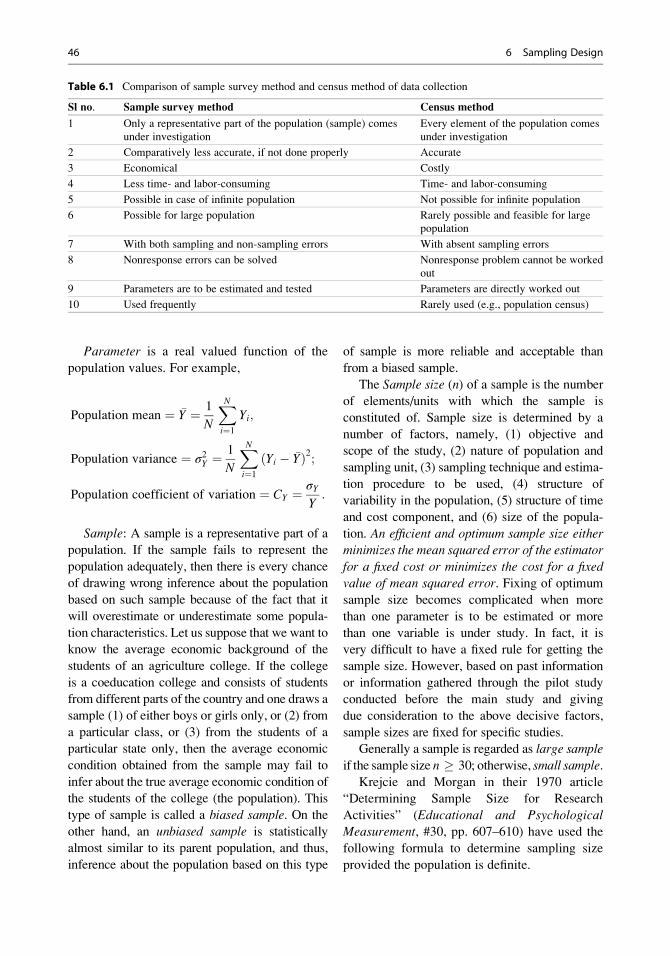
Parameter is a real valued function of the

population values. For example,

Population mean ¼ �Y ¼ 1

N

XNi¼1

Yi;

Population variance ¼ σ2Y ¼ 1

N

XNi¼1

Yi � �Yð Þ2;

Population coefficient of variation ¼ CY ¼ σYY:

Sample: A sample is a representative part of a

population. If the sample fails to represent the

population adequately, then there is every chance

of drawing wrong inference about the population

based on such sample because of the fact that it

will overestimate or underestimate some popula-

tion characteristics. Let us suppose that we want to

know the average economic background of the

students of an agriculture college. If the college

is a coeducation college and consists of students

from different parts of the country and one draws a

sample (1) of either boys or girls only, or (2) from

a particular class, or (3) from the students of a

particular state only, then the average economic

condition obtained from the sample may fail to

infer about the true average economic condition of

the students of the college (the population). This

type of sample is called a biased sample. On the

other hand, an unbiased sample is statistically

almost similar to its parent population, and thus,

inference about the population based on this type

of sample is more reliable and acceptable than

from a biased sample.

The Sample size (n) of a sample is the number

of elements/units with which the sample is

constituted of. Sample size is determined by a

number of factors, namely, (1) objective and

scope of the study, (2) nature of population and

sampling unit, (3) sampling technique and estima-

tion procedure to be used, (4) structure of

variability in the population, (5) structure of time

and cost component, and (6) size of the popula-

tion. An efficient and optimum sample size eitherminimizes the mean squared error of the estimator

for a fixed cost or minimizes the cost for a fixed

value of mean squared error. Fixing of optimum

sample size becomes complicated when more

than one parameter is to be estimated or more

than one variable is under study. In fact, it is

very difficult to have a fixed rule for getting the

sample size. However, based on past information

or information gathered through the pilot study

conducted before the main study and giving

due consideration to the above decisive factors,

sample sizes are fixed for specific studies.

Generally a sample is regarded as large sample

if the sample size n � 30; otherwise, small sample.

Krejcie and Morgan in their 1970 article

“Determining Sample Size for Research

Activities” (Educational and PsychologicalMeasurement, #30, pp. 607–610) have used the

following formula to determine sampling size

provided the population is definite.

Table 6.1 Comparison of sample survey method and census method of data collection

Sl no. Sample survey method Census method

1 Only a representative part of the population (sample) comes

under investigation

Every element of the population comes

under investigation

2 Comparatively less accurate, if not done properly Accurate

3 Economical Costly

4 Less time- and labor-consuming Time- and labor-consuming

5 Possible in case of infinite population Not possible for infinite population

6 Possible for large population Rarely possible and feasible for large

population

7 With both sampling and non-sampling errors With absent sampling errors

8 Nonresponse errors can be solved Nonresponse problem cannot be worked

out

9 Parameters are to be estimated and tested Parameters are directly worked out

10 Used frequently Rarely used (e.g., population census)

46 6 Sampling Design

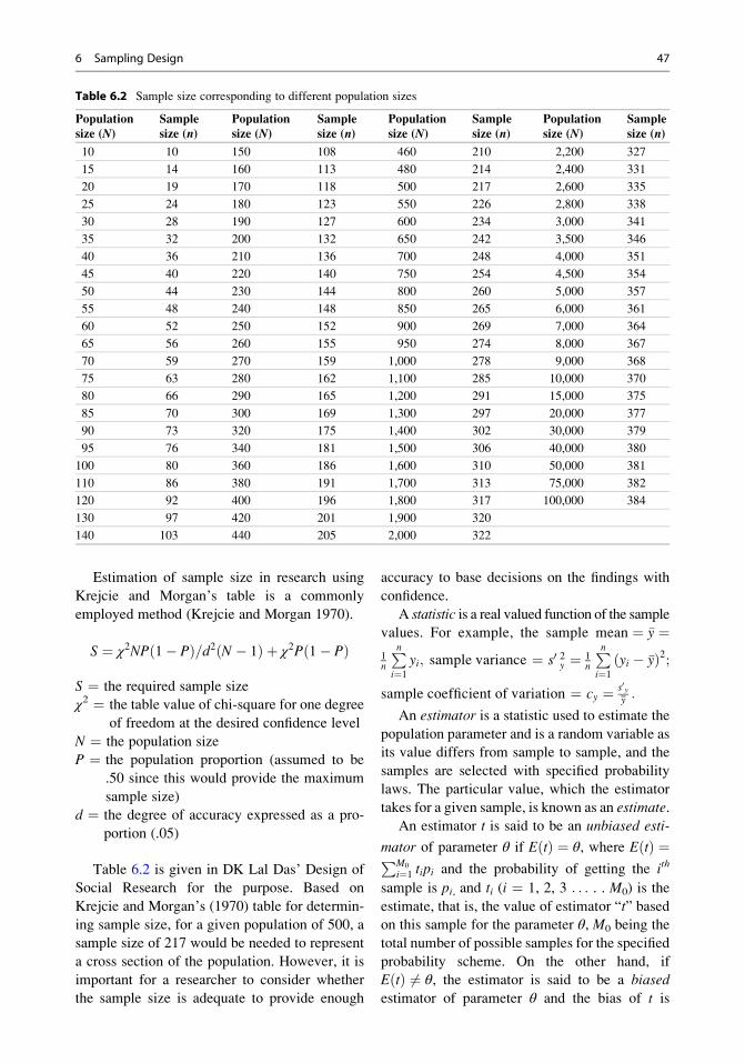
Estimation of sample size in research using

Krejcie and Morgan’s table is a commonly

employed method (Krejcie and Morgan 1970).

S ¼ χ2NP 1� Pð Þ=d2 N � 1ð Þ þ χ2P 1� Pð Þ

S ¼ the required sample size

χ2 ¼ the table value of chi-square for one degree

of freedom at the desired confidence level

N ¼ the population size

P ¼ the population proportion (assumed to be

.50 since this would provide the maximum

sample size)

d ¼ the degree of accuracy expressed as a pro-

portion (.05)

Table 6.2 is given in DK Lal Das’ Design of

Social Research for the purpose. Based on

Krejcie and Morgan’s (1970) table for determin-

ing sample size, for a given population of 500, a

sample size of 217 would be needed to represent

a cross section of the population. However, it is

important for a researcher to consider whether

the sample size is adequate to provide enough

accuracy to base decisions on the findings with

confidence.

A statistic is a real valued function of the sample

values. For example, the sample mean ¼ �y ¼1n

Pni¼1

yi; sample variance ¼ s0 2y ¼ 1n

Pni¼1

yi � �yð Þ2;

sample coefficient of variation ¼ cy ¼ s0yy :

An estimator is a statistic used to estimate the

population parameter and is a random variable as

its value differs from sample to sample, and the

samples are selected with specified probability

laws. The particular value, which the estimator

takes for a given sample, is known as an estimate.

An estimator t is said to be an unbiased esti-

mator of parameter θ if EðtÞ ¼ θ, where EðtÞ ¼PM0

i¼1 tipi and the probability of getting the ith

sample is pi, and ti (i ¼ 1, 2, 3 . . . . . M0) is the

estimate, that is, the value of estimator “t” basedon this sample for the parameter θ, M0 being the

total number of possible samples for the specified

probability scheme. On the other hand, if

EðtÞ 6¼ θ, the estimator is said to be a biased

estimator of parameter θ and the bias of t is

Table 6.2 Sample size corresponding to different population sizes

Population

size (N)Sample

size (n)Population

size (N)Sample

size (n)Population

size (N)Sample

size (n)Population

size (N)Sample

size (n)

10 10 150 108 460 210 2,200 327

15 14 160 113 480 214 2,400 331

20 19 170 118 500 217 2,600 335

25 24 180 123 550 226 2,800 338

30 28 190 127 600 234 3,000 341

35 32 200 132 650 242 3,500 346

40 36 210 136 700 248 4,000 351

45 40 220 140 750 254 4,500 354

50 44 230 144 800 260 5,000 357

55 48 240 148 850 265 6,000 361

60 52 250 152 900 269 7,000 364

65 56 260 155 950 274 8,000 367

70 59 270 159 1,000 278 9,000 368

75 63 280 162 1,100 285 10,000 370

80 66 290 165 1,200 291 15,000 375

85 70 300 169 1,300 297 20,000 377

90 73 320 175 1,400 302 30,000 379

95 76 340 181 1,500 306 40,000 380

100 80 360 186 1,600 310 50,000 381

110 86 380 191 1,700 313 75,000 382

120 92 400 196 1,800 317 100,000 384

130 97 420 201 1,900 320

140 103 440 205 2,000 322

6 Sampling Design 47

given as BðtÞ ¼ EðtÞ � θ. The difference

between estimate ti based on the ith sample and

parameter θ, that is, (ti � θ), may be called the

error of the estimate.

The mean squared error (MSE). The MSE of

an estimator t of θ is MðtÞ ¼ E t� θð Þ2 ¼ PMo

i¼1

piðti � θÞ2 ¼ VðtÞ þ BðtÞ½ �2; where V(t) (the

variance of t) is defined as E t� EðtÞ½ �2 ¼PMo

i¼1 pi½ti � EðtÞ�2.Given two estimators t1 and t2 for the popula-

tion parameter θ, the estimator t1 is said to be

more efficient than t2 if MSE(t1)<MSE(t2).

The selection of proper method to obtain a

representative sample is of utmost importance.

The selection of sample is oriented to answer the

following major queries:

(a) To select a representative part (sample) of the

population under interest

(b) To fix the size of the sample

(c) To ensure good quality of information and

subsequent inference

(d) To estimate parameters, minimizing errors

towards valid inferences about the population

Once the purpose and objective of the study

is fixed, one has to prepare a suitable sampling

plan to fulfill the objective of the study. The

basic components of sampling plans are:

(a) Definition of population and sampling units

(b) Preparation of sampling frame

(c) Scope of study area or domain

(d) Time period allowed

(e) Amount of cost permissible

(f) Coverage, that is, type of information (quali-

tative or quantitative) to be collected

(g) Type of parameters to be estimated

(h) Sampling design

(i) Selection of sample and collection of data

through trained investigators

All the above steps aim at reducing the sam-

pling error at a given cost within limited resources.

6.1 Errors in Sample Survey

There are mainly two types of errors associated

with estimates worked out from the sample:

(a) sampling error and (b) non-sampling error.

(a) Sampling Error: If we use different samples,

drawn following exactly the same way

from the same population, it will be found

that the estimates from each sample differ

from the other even if the same question-

naires, instructions, and facilities are pro-

vided for the selection of all the samples.

This difference is termed as sampling

error.

(b) Non-sampling Error: Non-sampling errors

are attributed mainly to differential behav-

ior of respondents as well as interviewers.

Thus, difference in response, difficulties

in defining, difference in interpretations,

and inability in recalling information and

so on are the major sources of non-sampling

errors.

6.2 Selection of Sample(Sampling Technique)

Depending upon the nature and scope of the

investigation and the situations under which the

study is being carried out, appropriate sampling

technique is being chosen. Available sampling

techniques can broadly be categorized into two

categories: (a) probability sampling and (b) non-

probability sampling. Probability sampling helps

researchers to estimate the extent to which the

sample statistics are likely to adhere to the popu-

lation parameters. Different types of sampling

techniques available are:

Probability sampling Non-probability sampling

1) Simple random sampling 1) Quota sampling

2) Varying probability sampling 2) Judgment sampling3) Stratified sampling 3) Purposive sampling4) Systematic sampling 4) Snowball sampling5) Cluster sampling 5) Accidental sampling6) Multistage sampling7) Multiphase and double sampling8) Sampling on two occasions9) Inverse sampling10) Sampling technique for rapid assessment (STRA)

48 6 Sampling Design

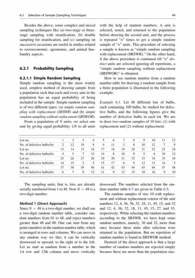
Besides the above, some complex and mixed

sampling techniques like (a) two-stage or three-

stage sampling with stratification, (b) double

sampling for stratification, and (c) sampling on

successive occasions are useful in studies related

to socioeconomic, agronomic, and animal hus-

bandry aspects.

6.2.1 Probability Sampling

6.2.1.1 Simple Random SamplingSimple random sampling is the most widely

used, simplest method of drawing sample from

a population such that each and every unit in the

population has an equal probability of being

included in the sample. Simple random sampling

is of two different types: (a) simple random sam-pling with replacement (SRSWR) and (b) simple

random sampling without replacement (SRSWOR).

From a population of N units, we select one

unit by giving equal probability 1/N to all units

with the help of random numbers. A unit is

selected, noted, and returned to the population

before drawing the second unit, and the process

is repeated “n” times to get a simple random

sample of “n” units. This procedure of selecting

a sample is known as “simple random sampling

with replacement (SRSWR).” On the other hand,

if the above procedure is continued till “n” dis-

tinct units are selected ignoring all repetitions, a

“simple random sampling without replacement

(SRSWOR)” is obtained.

How to use random number from a random

number table for drawing a random sample from

a finite population is illustrated in the following

example.

Example 6.1. Let 48 different lots of bulbs,

each containing 100 bulbs, be studied for defec-

tive bulbs, and the following figures give the

number of defective bulbs in each lot. We are

to draw two random samples of 10 lots: (1) with

replacement and (2) without replacement.

The sampling units, that is, lots, are already

serially numbered from 1 to 48. Now N ¼ 48 is a

two-digit number.

Method 1 (Direct Approach)

Since N ¼ 48 is a two-digit number, we shall use

a two-digit random number table, consider ran-

dom numbers from 01 to 48, and reject numbers

greater than 48 and 00. One can start from any

point (number) in the random number table, which

is arranged in rows and columns. We can move in

any random way we like; it can be vertically

downward or upward, to the right or to the left.

Let us start at random from a number in the

1st row and 12th column and move vertically

downward. The numbers selected from the ran-

dom number table 6.7 are given in Table 6.3:

The random samples of size 10 with replace-

ment and without replacement consist of the unit

numbers 12, 4, 36, 36, 32, 18, 11, 45, 15, and 32

and 12, 4, 36, 32, 18, 11, 45, 15, 27, and 33,

respectively. While selecting the random numbers

according to the SRSWR, we have kept some

random numbers, namely, 36 and 32, more than

once because these units after selection were

returned to the population. But no repetition of

random number is found in SRSWOR method.

Demerit of the direct approach is that a large

number of random numbers are rejected simply

because these are more than the population size.

Lot no. 1 2 3 4 5 6 7 8 9 10 11 12

No. of defective bulbs/lot 2 12 10 8 9 11 3 8 10 12 7 9

Lot no. 13 14 15 16 17 18 19 20 21 22 23 24

No. of defective bulbs/lot 4 5 7 12 14 8 10 0 5 6 10 12

Lot no. 25 26 27 28 29 30 31 32 33 34 35 36

No. of defective bulbs/lot 14 15 2 5 15 17 8 9 12 13 14 5

Lot no. 37 38 39 40 41 42 43 44 45 46 47 48

No. of defective bulbs/lot 6 7 8 12 11 9 12 15 18 16 9 10

6.2 Selection of Sample (Sampling Technique) 49

Method 2 (Remainder Approach)

To reduce time and labor, the commonly used

“remainder approach” is employed to avoid the

rejection of random numbers. The greatest two-

digit number, which is a multiple of 48, is 96, and

we consider two-digit numbers from 01 to 96,

rejecting the numbers greater than 96 and 00.

By using two-digit random numbers as above, we

prepare Table 6.4.

The randomsamples of size 10with replacement

andwithout replacement consist of the variety num-

bers 12, 4, 36, 32, 36, 32, 47, 15, 30, and 18 and 12,

4, 36, 32, 47, 15, 30, 18, 46, and 11, respectively.

In the direct approach, as many as 22 random

numbers were selected to obtain a random sam-

ple of ten only. On the contrary, only 12 random

numbers were sufficient in the second “remain-

der approach” to draw the sample of 10. Thus,

with the help of the remainder approach, one can

save time as well as labor in drawing a definite

simple random sample.

If a sample of n units is drawn from a population

of N units with SRSWR, then there are Nn ordered

possible samples and the probability of getting any

sample is P(s) ¼ 1/Nn. If a sample is drawn with

SRSWOR, then there are NCnð Þ unordered possiblesamples and PðsÞ ¼ 1= NCnð Þ. It is further to be

noted that the probability of getting ith unit at rth

draw is P [irð Þ ¼ 1=N; i ¼ 1, 2, 3, . . ., N and

r ¼ 1, 2, 3, . . ., n for both SRSWR and SRSWOR.

In case a sample of n units is drawn from a

population of N units with SRSWR and the sam-

ple values are (y1, y2, y3, . . ., yn), then the sample

mean y ¼ 1n

Pni¼1

yi is an unbiased estimator of the

population mean �Y; that is; Eð�yÞ ¼ �Y, and a

sampling variance of the sample mean, that is,

Vð�yÞ is equal to σ2

n where σ2 is the population

variance. It is also observed that the sample mean

square (s2) is an unbiased estimator of the popu-

lation variance, that is Eðs2Þ ¼ σ2 where

s2 ¼ 1n�1

Pni¼1

ðyi � �yÞ2. Thus, the standard error

of the sample mean is given by SEð�yÞ ¼ σffiffin

p and

the estimated SEð�yÞ ¼ sffiffin

p :

For SRSWOR Eð�yÞ ¼ �Y; Vð�yÞ ¼ N � n

N � 1

σ2

n

¼ N � n

N

S2

n

¼ ð1� f Þ S2

n;E s2

� � ¼ S2

Table 6.3 Selection of random numbers for SRSWR and

SRSWOR scheme using direct method

Random numbers taken

from the table 6.7

Selected random

numbers

SRSWR SRSWOR

12 12 12

4 04 4

36 36 36

80 – –

36 36 –

32 32 32

95 — —

63 – –

78 — —

18 18 18

94 — —

11 11 11

87 — —

45 45 45

15 15 15

32 32 –

71 — —

77 – –

55 – –

95 – —

27 – 27

33 – 33

— means random number drawn from random number

table is more than 48.

Table 6.4 Selection of random numbers for SRSWR and

SRSWOR scheme using remainder approach

Random

numbers

Remainder when

divided by 48

Selected random

numbers

SRSWR SRSWOR

12 12 12 12

4 04 04 4

36 36 36 36

80 32 32 32

36 36 36 –

32 32 32 –

95 47 47 47

63 15 15 15

78 30 30 30

18 18 18 18

94 46 – 46

11 11 – 11

50 6 Sampling Design

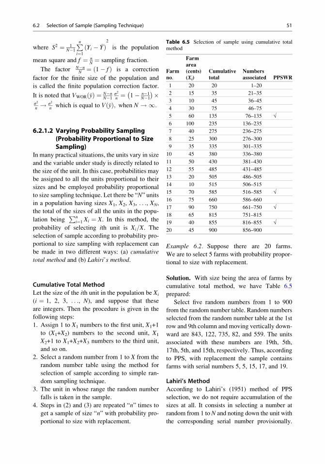
where S2 ¼ 1N�1

Pni¼1

Yi � �Yð Þ2

is the population

mean square and f ¼ nN ¼ sampling fraction:

The factor N�nN ¼ ð1� f Þ is a correction

factor for the finite size of the population and

is called the finite population correction factor.

It is noted that VWORð�yÞ ¼ N�nN�1

σ2

n ¼ 1� n�1N�1

� ��σ2

n ! σ2

n which is equal to Vð�yÞ; when N ! 1:

6.2.1.2 Varying Probability Sampling(Probability Proportional to SizeSampling)

In many practical situations, the units vary in size

and the variable under study is directly related to

the size of the unit. In this case, probabilities may

be assigned to all the units proportional to their

sizes and be employed probability proportional

to size sampling technique. Let there be “N” unitsin a population having sizes X1, X2, X3, . . ., XN,

the total of the sizes of all the units in the popu-

lation beingPn

i¼1 Xi ¼ X. In this method, the

probability of selecting ith unit is Xi=X. The

selection of sample according to probability pro-

portional to size sampling with replacement can

be made in two different ways: (a) cumulative

total method and (b) Lahiri’s method.

Cumulative Total Method

Let the size of the ith unit in the population be Xi

(i ¼ 1, 2, 3, . . ., N), and suppose that these

are integers. Then the procedure is given in the

following steps:

1. Assign 1 to X1 numbers to the first unit, X1+1

to (X1+X2) numbers to the second unit, X1

X2+1 to X1+X2+X3 numbers to the third unit,

and so on.

2. Select a random number from 1 to X from the

random number table using the method for

selection of sample according to simple ran-

dom sampling technique.

3. The unit in whose range the random number

falls is taken in the sample.

4. Steps in (2) and (3) are repeated “n” times to

get a sample of size “n” with probability pro-

portional to size with replacement.

Example 6.2. Suppose there are 20 farms.

We are to select 5 farms with probability propor-

tional to size with replacement.

Solution. With size being the area of farms by

cumulative total method, we have Table 6.5

prepared:

Select five random numbers from 1 to 900

from the random number table. Random numbers

selected from the random number table at the 1st

row and 9th column and moving vertically down-

ward are 843, 122, 735, 82, and 559. The units

associated with these numbers are 19th, 5th,

17th, 5th, and 15th, respectively. Thus, according

to PPS, with replacement the sample contains

farms with serial numbers 5, 5, 15, 17, and 19.

Lahiri’s Method

According to Lahiri’s (1951) method of PPS

selection, we do not require accumulation of the

sizes at all. It consists in selecting a number at

random from 1 to N and noting down the unit with

the corresponding serial number provisionally.

Table 6.5 Selection of sample using cumulative total

method

Farm

no.

Farm

area

(cents)

(Xi)

Cumulative

total

Numbers

associated PPSWR

1 20 20 1–20

2 15 35 21–35

3 10 45 36–45

4 30 75 46–75

5 60 135 76–135 √6 100 235 136–235

7 40 275 236–275

8 25 300 276–300

9 35 335 301–335

10 45 380 336–380

11 50 430 381–430

12 55 485 431–485

13 20 505 486–505

14 10 515 506–515

15 70 585 516–585 √

16 75 660 586–660

17 90 750 661–750 √18 65 815 751–815

19 40 855 816–855 √20 45 900 856–900

6.2 Selection of Sample (Sampling Technique) 51

Another random number is then chosen from 1 to

M, where M is the maximum of the sizes of the N

units or some convenient number greater than the

maximum size. If the second random number is

smaller or equal to the size of the unit provision-

ally selected, the unit is selected into the sample.

If not, the entire procedure is repeated until a unit

is finally selected. For selecting a sample of n

units with PPSWR, the above procedure is

repeated till “n” units are selected.

Example 6.3. Let there be ten farms having farm

sizes of X1 to X10 as given below. We are to select

four farms with PPSWR according to Lahiri’s

method (Table 6.6).

In this example, N ¼ 10, M ¼ 90. First, we

have to select a random number from 1 to 10 and

a second random number from 1 to 90. Referring

to the random number table, the pair is (8, 23).

Here, 23 < X8 ¼ 27. Hence, the 8th unit is

selected in the sample. We choose another pair,

which is (2, 48). Here, 48 < X2 ¼ 50. Thus, the

2nd unit is selected in the sample. We choose

another pair, which is (7, 55). Here, 55 > X7

¼ 34. So the pair (7, 55) is rejected. Choosing

two pairs, we can have (10, 70) and (6, 38). Here,

the 10th and 6th units are selected in the sample.

Hence, the sample consists of farms with serial

numbers 8, 2, 10, and 6.

PPS sampling takes care of the heterogeneity

in the population as well as the varying sizes of

the population units/elements. Thus, it uses ancil-

lary information in the form of size of units. This

will help us in getting more efficient estimator of

the population.

A random number can also be generated from

the function menu of MS Excel following the

method given below. Assume that we want tohave 20 random numbers between 1 and 900.

It may be noted that in this process, the

random number changes as we change the

Table 6.6 Selection of sample using PPSWR (Lahiri’s

method)

Sl. no. of farms Farm area (cent) (Xi)

Farm

selected

1 76

2 50 √3 30

4 26

5 40

6 50 √

7 34

8 27 √9 60

10 90 √

Step 1: Click on Formulas as shown above in any Excel spreadsheet to get the following screen.

52 6 Sampling Design

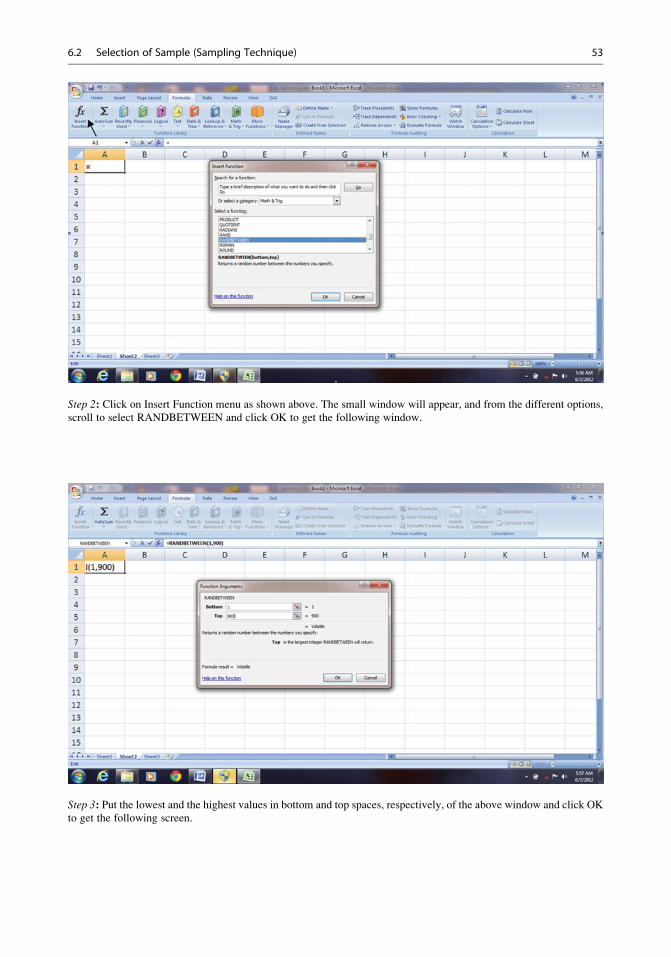
Step 3: Put the lowest and the highest values in bottom and top spaces, respectively, of the above window and click OK

to get the following screen.

Step 2: Click on Insert Function menu as shown above. The small window will appear, and from the different options,

scroll to select RANDBETWEEN and click OK to get the following window.

6.2 Selection of Sample (Sampling Technique) 53

Step 5: The above random number generated may contain repetitions; repetitions are allowed in SRSWR, but to get

distinct random numbers for SRSWOR, discard the repetitive ones and take only the distinct random numbers.

Step 4: The first random number is generated. Click on the right lower corner of the first cell, hold it, and drag it to more

than 20 cells to get random numbers as given below.

54 6 Sampling Design

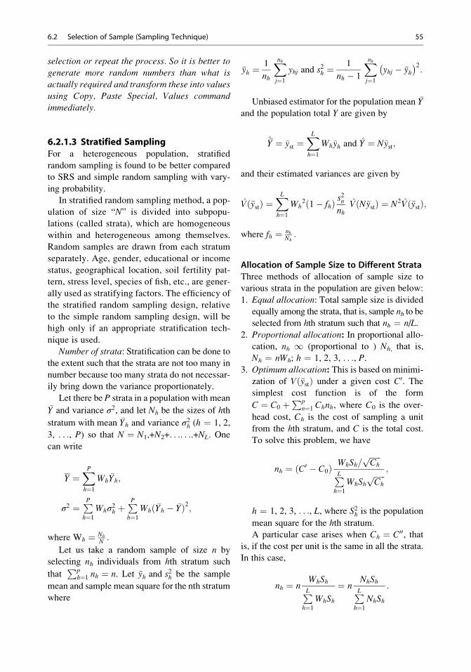
selection or repeat the process. So it is better togenerate more random numbers than what is

actually required and transform these into valuesusing Copy, Paste Special, Values command

immediately.

6.2.1.3 Stratified SamplingFor a heterogeneous population, stratified

random sampling is found to be better compared

to SRS and simple random sampling with vary-

ing probability.

In stratified random sampling method, a pop-

ulation of size “N” is divided into subpopu-

lations (called strata), which are homogeneous

within and heterogeneous among themselves.

Random samples are drawn from each stratum

separately. Age, gender, educational or income

status, geographical location, soil fertility pat-

tern, stress level, species of fish, etc., are gener-

ally used as stratifying factors. The efficiency of

the stratified random sampling design, relative

to the simple random sampling design, will be

high only if an appropriate stratification tech-

nique is used.

Number of strata: Stratification can be done to

the extent such that the strata are not too many in

number because too many strata do not necessar-

ily bring down the variance proportionately.

Let there be P strata in a population with mean�Y and variance σ2, and let Nh be the sizes of hth

stratum with mean �Yh and variance σ2h (h ¼ 1, 2,

3, . . ., P) so that N ¼ N1,+N2+. . .. . ..+NL. One

can write

Y ¼XPh¼1

Wh�Yh;

σ2 ¼ PPh¼1

Whσ2h þPPh¼1

Wh�Yh � �Yð Þ2;

where Wh ¼ Nh

N :

Let us take a random sample of size n by

selecting nh individuals from hth stratum such

thatPp

h¼1 nh ¼ n. Let �yh and s2h be the sample

mean and sample mean square for the nth stratum

where

�yh ¼1

nh

Xnhj¼1

yhj and s2h ¼1

nh � 1

Xnhj¼1

yhj � �yh� �2

:

Unbiased estimator for the population mean �Y

and the population total Y are given by

�Y ¼ �yst ¼XLh¼1

Wh�yh and Y ¼ N�yst;

and their estimated variances are given by

V �ystð Þ ¼XLh¼1

Wh2 1� fhð Þ s

2n

nhV N�ystð Þ ¼ N2V �ystð Þ;

where fh ¼ nhNh:

Allocation of Sample Size to Different Strata

Three methods of allocation of sample size to

various strata in the population are given below:

1. Equal allocation: Total sample size is divided

equally among the strata, that is, sample nh to be

selected from hth stratum such that nh ¼ n/L.

2. Proportional allocation: In proportional allo-

cation, nh 1 (proportional to ) Nh, that is,

Nh ¼ nWh; h ¼ 1, 2, 3, . . ., P.

3. Optimum allocation: This is based on minimi-

zation of Vð�ystÞ under a given cost C0. Thesimplest cost function is of the form

C ¼ C0 þPp

n¼1 Chnh, where C0 is the over-

head cost, Ch is the cost of sampling a unit

from the hth stratum, and C is the total cost.

To solve this problem, we have

nh ¼ C0 � C0ð Þ WhSh=ffiffiffiffiffiffiCh

pPLh¼1

WhShffiffiffiffiffiffiCh

p ;

h ¼ 1, 2, 3, . . ., L, where S2h is the population

mean square for the hth stratum.

A particular case arises when Ch ¼ C00, thatis, if the cost per unit is the same in all the strata.

In this case,

nh ¼ nWhShPL

h¼1

WhSh

¼ nNhShPL

h¼1

NhSh

:

6.2 Selection of Sample (Sampling Technique) 55

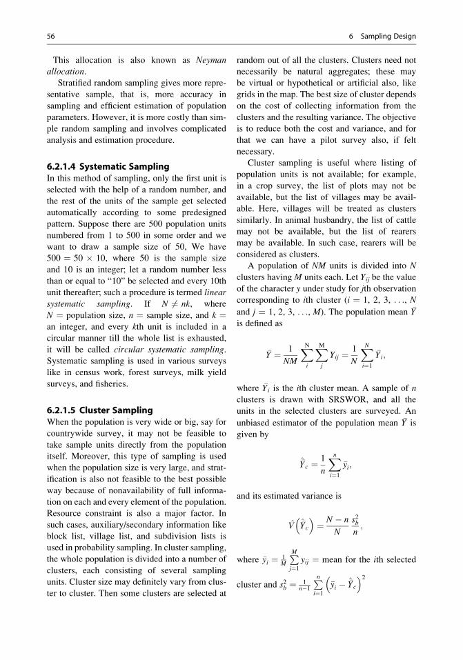
This allocation is also known as Neymanallocation.

Stratified random sampling gives more repre-

sentative sample, that is, more accuracy in

sampling and efficient estimation of population

parameters. However, it is more costly than sim-

ple random sampling and involves complicated

analysis and estimation procedure.

6.2.1.4 Systematic SamplingIn this method of sampling, only the first unit is

selected with the help of a random number, and

the rest of the units of the sample get selected

automatically according to some predesigned

pattern. Suppose there are 500 population units

numbered from 1 to 500 in some order and we

want to draw a sample size of 50, We have

500 ¼ 50 � 10, where 50 is the sample size

and 10 is an integer; let a random number less

than or equal to “10” be selected and every 10th

unit thereafter; such a procedure is termed linear

systematic sampling. If N 6¼ nk, where

N ¼ population size, n ¼ sample size, and k ¼an integer, and every kth unit is included in a

circular manner till the whole list is exhausted,

it will be called circular systematic sampling.Systematic sampling is used in various surveys

like in census work, forest surveys, milk yield

surveys, and fisheries.

6.2.1.5 Cluster SamplingWhen the population is very wide or big, say for

countrywide survey, it may not be feasible to

take sample units directly from the population

itself. Moreover, this type of sampling is used

when the population size is very large, and strat-

ification is also not feasible to the best possible

way because of nonavailability of full informa-

tion on each and every element of the population.

Resource constraint is also a major factor. In

such cases, auxiliary/secondary information like

block list, village list, and subdivision lists is

used in probability sampling. In cluster sampling,

the whole population is divided into a number of

clusters, each consisting of several sampling

units. Cluster size may definitely vary from clus-

ter to cluster. Then some clusters are selected at

random out of all the clusters. Clusters need not

necessarily be natural aggregates; these may

be virtual or hypothetical or artificial also, like

grids in the map. The best size of cluster depends

on the cost of collecting information from the

clusters and the resulting variance. The objective

is to reduce both the cost and variance, and for

that we can have a pilot survey also, if felt

necessary.

Cluster sampling is useful where listing of

population units is not available; for example,

in a crop survey, the list of plots may not be

available, but the list of villages may be avail-

able. Here, villages will be treated as clusters

similarly. In animal husbandry, the list of cattle

may not be available, but the list of rearers

may be available. In such case, rearers will be

considered as clusters.

A population of NM units is divided into N

clusters having M units each. Let Yij be the value

of the character y under study for jth observation

corresponding to ith cluster (i ¼ 1, 2, 3, . . ., N

and j ¼ 1, 2, 3, . . ., M). The population mean �Y

is defined as

�Y ¼ 1

NM

XNi

XMj

Yij ¼ 1

N

XNi¼1

�Yi;

where �Yi is the ith cluster mean. A sample of n

clusters is drawn with SRSWOR, and all the

units in the selected clusters are surveyed. An

unbiased estimator of the population mean �Y is

given by

�Yc ¼ 1

n

Xni¼1

�yi;

and its estimated variance is

V �Yc

� �¼ N � n

N

s2bn;

where �yi ¼ 1M

PMj¼1

yij ¼ mean for the ith selected

cluster and s2b ¼ 1n�1

Pni¼1

�yi � �Yc

� �2

56 6 Sampling Design

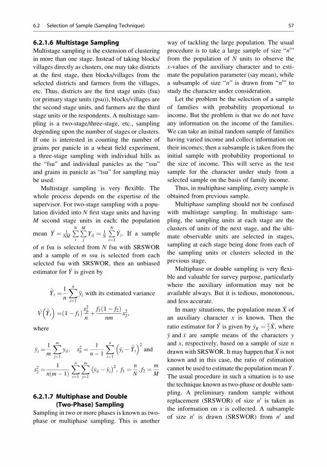
6.2.1.6 Multistage SamplingMultistage sampling is the extension of clustering

in more than one stage. Instead of taking blocks/

villages directly as clusters, one may take districts

at the first stage, then blocks/villages from the

selected districts and farmers from the villages,

etc. Thus, districts are the first stage units (fsu)

(or primary stage units (psu)), blocks/villages are

the second stage units, and farmers are the third

stage units or the respondents. A multistage sam-

pling is a two-stage/three-stage, etc., sampling

depending upon the number of stages or clusters.

If one is interested in counting the number of

grains per panicle in a wheat field experiment,

a three-stage sampling with individual hills as

the “fsu” and individual panicles as the “ssu”

and grains in panicle as “tsu” for sampling may

be used.

Multistage sampling is very flexible. The

whole process depends on the expertise of the

supervisor. For two-stage sampling with a popu-

lation divided into N first stage units and having

M second stage units in each; the population

mean �Y ¼ 1NM

PNi

PMj

Yij ¼ 1N

PNi¼1

�Yi. If a sample

of n fsu is selected from N fsu with SRSWOR

and a sample of m ssu is selected from each

selected fsu with SRSWOR, then an unbiased

estimator for �Y is given by

�Yt ¼ 1

n

Xni¼1

yi with its estimated variance

V �Yt

� �¼ð1� f1Þ s

2b

nþ f1ð1� f2Þ

nms22,

where

�yi ¼1

m

Xmj¼1

yij; s2b ¼1

n� 1

Xni¼1

�yi � �Yt

� �2

and

s22 ¼1

nðm� 1ÞXni¼1

Xmj¼1

yij � �yi� �2

; f1 ¼ n

N; f2 ¼ m

M

6.2.1.7 Multiphase and Double(Two-Phase) Sampling

Sampling in two or more phases is known as two-

phase or multiphase sampling. This is another

way of tackling the large population. The usual

procedure is to take a large sample of size “n0”from the population of N units to observe the

x-values of the auxiliary character and to esti-

mate the population parameter (say mean), while

a subsample of size “n” is drawn from “n0” to

study the character under consideration.

Let the problem be the selection of a sample

of families with probability proportional to

income. But the problem is that we do not have

any information on the income of the families.

We can take an initial random sample of families

having varied income and collect information on

their incomes; then a subsample is taken from the

initial sample with probability proportional to

the size of income. This will serve as the test

sample for the character under study from a

selected sample on the basis of family income.

Thus, in multiphase sampling, every sample is

obtained from previous sample.

Multiphase sampling should not be confused

with multistage sampling. In multistage sam-

pling, the sampling units at each stage are the

clusters of units of the next stage, and the ulti-

mate observable units are selected in stages,

sampling at each stage being done from each of

the sampling units or clusters selected in the

previous stage.

Multiphase or double sampling is very flexi-

ble and valuable for survey purpose, particularly

where the auxiliary information may not be

available always. But it is tedious, monotonous,

and less accurate.

In many situations, the population mean �X of

an auxiliary character x is known. Then the

ratio estimator for �Y is given by �yR ¼ �y�x�X, where

�y and �x are sample means of the characters yand x, respectively, based on a sample of size n

drawnwith SRSWOR. It may happen that �X is not

known and in this case, the ratio of estimation

cannot be used to estimate the population mean �Y.The usual procedure in such a situation is to use

the technique known as two-phase or double sam-

pling. A preliminary random sample without

replacement (SRSWOR) of size n0 is taken as

the information on x is collected. A subsample

of size n0 is drawn (SRSWOR) from n0 and

6.2 Selection of Sample (Sampling Technique) 57

information on y is measured. The ratio estimator

for �Y based on double sampling is given by

�yRd ¼�y

�x�x0;

where �x and �y are subsample means of x and y,

respectively, and �x0 is the sample mean in the first

sample. It is noted that �yRd is biased and the

estimator of V �yRdð Þ to the first-order approxima-

tion is given by

V �yRdð Þ ¼ 1

n0� 1

N

� �s2y þ

1

n� 1

n0

� �

s2y þ R2s2x � 2Rsyx

� �

where R ¼ �y

�x; syx ¼ 1

n� 1

Xni¼1

yi � �yð Þ xi � �xð Þ

6.2.1.8 Sampling in Two OccasionsIn agriculture, plant characters are commonly

measured at different growth stages of the crop.

For example, tiller number in rice may be

measured at 30, 60, 90, and 120 days after trans-

planting or at the tillering, flowering, and harve-

sting stages. If suchmeasurements are made on the

same plants at all stages of observation, the

resulting data may be biased because plants that

are subjected to frequent handling may behave

differently from others. In this situation, if sam-

pling on successive occasions is done according to

a specific rule, with partial replacement of sam-

pling units, it is known as rotation sampling.

On the first occasion, a SRSWOR sample “s”

of size “n” is selected from a population of “N”units; on the second occasion, a SRSWOR sam-

ple “s1” of “m” units from “s” and a SRSWOR

sample “s2” of “u” (¼ n � m) units from the

(N � n) units in the population not included in

“s” are selected. The estimate for the population

mean �Y2 on the second occasion is given by

�Y2 ¼ W�y2n þ ð1�WÞ�y02mwhere �y2n ¼

Ps2

y2iu and �y02m ¼ �y2m � b �y1m�ð

�y1nÞ are the simple mean for �Y2 based on the

replaced (unmatched) portion and the regression

estimator for �Y2 based on the matched portion,

respectively, b being the sample regression

coefficient of y2 on y1 based on matched part of

s1, W being a constant, and �y1h ¼Ps

y1in ; �yhm ¼P

s1

yhi=m; ðh ¼ 1; 2ÞThe alternatives to the above scheme are the

schemes based on (1) complete matching (i.e.,

retaining the sample of the first occasion to the

second occasion completely) or (2) complete

replacement (i.e., drawing a single independent

sample at the second occasion and taking the

sample mean as the estimator of Y2 in both

cases). The partial matching procedure is better

than the other two procedures; for all practical

purposes, one should retain 25–30% units at the

second occasion for the gain in the efficiency.

6.2.1.9 Inverse SamplingInverse sampling is generally used for the esti-

mation of a rare population and is a method of

sampling in which the drawing of a sample unit

continues until certain specified conditions

dependent on the results of those drawings have

been fulfilled, for example, until a given number

of individuals of specified type have emerged.

For example, if we want to draw a sample of

population affected by pox disease in which at

least “k” has been affected by “chicken pox,”

while doing so, we do not know about the exact

size of the sample because unless and otherwise

we have “k” number of persons affected by

chicken pox, the drawing will continue and the

sample size will go on increasing. Thus, though

costly and time and labor- consuming, this sam-

pling gives due weightage to rare elements in the

population.

Let P denote the proportion of units in the

population possessing the rare attribute under

study. Therefore, NP number of units in the

population will possess the rare attributes. To

estimate P, units are drawn one by one with

SRSWOR. Sampling is discontinued as soon as

the number of units in the sample possessing the

rare attribute (a predetermined number, m) is

reached. Let us denote by n the number of units

required to be drawn in the sample to obtain m

units possessing the rare attribute. An unbiased

estimator of P is given by

58 6 Sampling Design

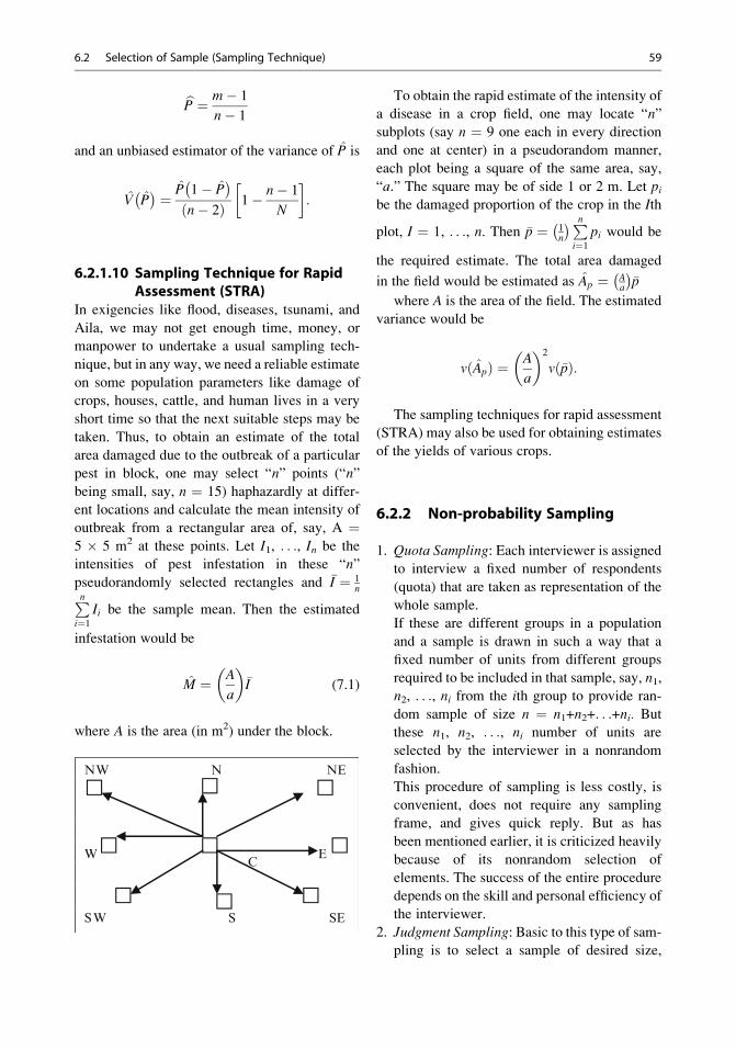
bP ¼ m� 1

n� 1

and an unbiased estimator of the variance of P is

V P� � ¼ P 1� P

� �ðn� 2Þ 1� n� 1

N

:

6.2.1.10 Sampling Technique for RapidAssessment (STRA)

In exigencies like flood, diseases, tsunami, and

Aila, we may not get enough time, money, or

manpower to undertake a usual sampling tech-

nique, but in any way, we need a reliable estimate

on some population parameters like damage of

crops, houses, cattle, and human lives in a very

short time so that the next suitable steps may be

taken. Thus, to obtain an estimate of the total

area damaged due to the outbreak of a particular

pest in block, one may select “n” points (“n”

being small, say, n ¼ 15) haphazardly at differ-

ent locations and calculate the mean intensity of

outbreak from a rectangular area of, say, A ¼5 � 5 m2 at these points. Let I1, . . ., In be the

intensities of pest infestation in these “n”

pseudorandomly selected rectangles and �I ¼ 1nPn

i¼1

Ii be the sample mean. Then the estimated

infestation would be

M ¼ A

a

� ��I (7.1)

where A is the area (in m2) under the block.

NW N NE

WC

E

SW S SE

To obtain the rapid estimate of the intensity of

a disease in a crop field, one may locate “n”

subplots (say n ¼ 9 one each in every direction

and one at center) in a pseudorandom manner,

each plot being a square of the same area, say,

“a.” The square may be of side 1 or 2 m. Let pibe the damaged proportion of the crop in the Ith

plot, I ¼ 1, . . ., n. Then �p ¼ 1n

� �Pni¼1

pi would be

the required estimate. The total area damaged

in the field would be estimated as Ap ¼ Aa

� ��p

where A is the area of the field. The estimated

variance would be

vðApÞ ¼ A

a

� �2

vð�pÞ:

The sampling techniques for rapid assessment

(STRA) may also be used for obtaining estimates

of the yields of various crops.

6.2.2 Non-probability Sampling

1. Quota Sampling: Each interviewer is assignedto interview a fixed number of respondents

(quota) that are taken as representation of the

whole sample.

If these are different groups in a population

and a sample is drawn in such a way that a

fixed number of units from different groups

required to be included in that sample, say, n1,

n2, . . ., ni from the ith group to provide ran-

dom sample of size n ¼ n1+n2+. . .+ni. Butthese n1, n2, . . ., ni number of units are

selected by the interviewer in a nonrandom

fashion.

This procedure of sampling is less costly, is

convenient, does not require any sampling

frame, and gives quick reply. But as has

been mentioned earlier, it is criticized heavily

because of its nonrandom selection of

elements. The success of the entire procedure

depends on the skill and personal efficiency of

the interviewer.

2. Judgment Sampling: Basic to this type of sam-

pling is to select a sample of desired size,

6.2 Selection of Sample (Sampling Technique) 59

giving priority to the purpose of the study, and

the elements of the sample are selected in such

a way so as to fulfill the objective of the study.

This method is the simplest but may lead to

biased and inefficient sample depending upon

the efficiency of the investigator.

3. Purposive Sampling: The selection of elements

to be included in the sample is entirely made on

the basis of the choice of the researcher.

Though easy to operate, it gives hardly a repre-

sentation of the parent population and as such

the results are biased and unsatisfactory.

4. Snowball Sampling: In researches, particularlyin the field of social studies, related to sensitive

issues like drug abuse and HIV victims in

which the respondents are very much hesitant

because of social taboos, reasons, or otherwise,

this type of sampling is very useful. In this type

of study, the researcher finds out initially one or

two or a few respondents for the study purpose

and then takes the help of these respondents to

find more and more respondents on specific

aspects. This is because of the fact that this

type of respondents may be hesitant to present

themselves when approached by a stranger

rather than a fellow friend. Thus, in this type

of studies, size of sample goes on increasing as

one getsmore andmore number of respondents.

5. Accidental Sampling: This type of sampling is

mostly used in evaluative types of research

studies. Suppose one wants to know the extent

of adoption of a particular technology, say, birth

control program/hybrid rice technology in a

certain community. In this method of selecting

the respondents, the researchers/interviewers

take information from the respondents who hap-

pen to meet the researchers first, and in the

process, the researchers may take information

from the first 100 respondents whom the

researchers/interviewers have met and who are

willing to share information. Samples collected

in this process are subject to biasness, and the

only way to overcome the bias is to conduct

parallel studies.

6.3 Execution of the Sampling Plan

A good sampling plan is an “essential” condition

for the study to be undertaken, but it is

not sufficient to have a good sample leading to

efficient and accurate estimation of the population

parameter. It is necessary to have a “good” sam-

pling plan suitable for the study followed by the

“efficient execution” of the sampling plan. A

“good” sampling plan, if not executed properly,

may give “bad” (unreliable, inaccurate) results,

leading to wastage of entire time, energy, and

money used for the investigation. For the efficient

execution of the sampling plan, the investigator

responsible for the data collection must possess

the necessary qualifications. They must be prop-

erly trained before the data collection. They must

be taught how to handle the equipment and to

make correct observations and measurements and

note them down carefully. A proper supervision of

the fieldwork is a must, and scrutiny and editing of

the collected data is essential. Precautions must be

taken to identify the sample units, in specifying the

units(s) of measurements at various stages, and to

minimize the error in recording the data. Pilot

survey may be undertaken to select the suitable

sampling plan among the alternative plans. An

efficient execution of sampling plan cannot only

reduce both the sampling and non-sampling errors

but also helps in reducing the cost of the study.

60 6 Sampling Design

Table 6.7 Random number table

00–04 05–09 10–14 15–19 20–24 25–29 30–34 35–39 40–44 45–49

00 54463 22662 65905 70639 79365 67382 29085 69831 47058 08186

01 15389 85205 18850 39226 42249 90669 96325 23248 60933 26927

02 85941 40756 82414 02015 13858 78030 16269 65978 01385 15345

03 61149 69440 11286 88218 58925 03638 52862 62733 33451 77455

04 05219 81619 10651 67079 92511 59888 84502 72095 83463 75577

05 41417 98326 87719 92294 46614 50948 64886 20002 97365 30976

06 28357 94070 20652 35774 16249 75019 21145 05217 47286 76305

07 17783 00015 10806 83091 91530 36466 39981 62481 49177 75779

08 40950 84820 29881 85966 62800 70326 84740 62660 77379 90279

09 82995 64157 66164 41180 10089 41757 78258 96488 88629 37231

10 96754 17675 55659 44105 47361 34833 86679 23930 53249 27083

11 34357 88040 53364 71726 45690 66334 60332 22554 90600 71113

12 06318 37403 49927 57715 50423 67372 63116 48888 21505 80182

13 62111 52820 07243 79931 89292 84767 85693 73947 22278 11551

14 47534 09243 67879 00544 23410 12740 02540 54440 32949 13491

15 98614 75993 84460 62846 59844 14922 48730 73443 48167 34770

16 24856 03648 44898 09351 98795 18644 39765 71058 90368 44104

17 96887 12479 80621 66223 86085 78285 02432 53342 42846 94771

18 90801 21472 42815 77408 37390 76766 52615 32141 30268 18106

19 55165 77312 83666 36028 28420 70219 81369 41943 47366 41067

20 75884 12952 84318 95108 72305 64620 91318 89872 45375 85436

21 16777 37116 58550 42958 21460 43910 01175 87894 81378 10620

22 46230 43877 80207 88877 89380 32992 91380 03164 98656 59337

23 42902 66892 46134 01432 94710 23474 20423 60137 60609 13119

24 81007 00333 39693 28039 10154 95425 39220 19774 31782 49037

25 68089 01122 51111 72373 06902 74373 96199 97017 41273 21546

26 20411 67081 89950 16944 93054 87687 96693 87236 77054 33848

27 58212 13160 06468 15718 82627 76999 05999 58680 96739 63700

28 70577 42866 24969 61210 76046 67699 42054 12696 93758 03283

29 94522 74358 71659 62038 79643 79169 44741 05437 39038 13163

30 42626 86819 85651 88678 17401 03252 99547 32404 17918 62880

31 16051 33763 57194 16752 54450 19031 58580 47629 54132 60631

32 08244 27647 33851 44705 94211 46716 11738 55784 95374 72655

33 59497 04392 09419 89964 51211 04894 72882 17805 21896 83864

34 97155 13428 40293 09985 58434 01412 69124 82171 59058 82859

35 98409 66162 95763 47420 20792 61527 20441 39435 11859 41567

36 45476 84882 65109 96597 25930 66790 65706 61203 53634 22557

37 89300 69700 50741 30329 11658 23166 05400 66669 48708 03887

38 50051 95137 91631 66315 91428 12275 24816 68091 71710 33258

39 31753 85178 31310 89642 98364 02306 24617 09609 83942 22716

40 79152 53829 77250 20190 56535 18760 69942 77448 33278 48805

41 44560 38750 83635 56540 64900 42915 13953 79149 18710 48805

42 68328 83378 63369 71381 39564 05615 42451 64559 97501 65747

43 46939 38689 58625 08342 30459 85863 20781 09284 26333 91777

44 83544 86141 15707 96256 23068 13782 08467 89469 93842 55349

45 91621 00881 04900 54224 46177 55309 17852 27491 89415 23466

46 91621 00881 04900 54224 46177 55309 17852 27491 89415 23466

47 55751 62515 21108 80830 02263 29303 37204 96926 30506 09808

48 85156 87689 954963 88842 00664 55017 55539 17771 69448 87530

49 07521 56898 12236 60277 39102 62315 12239 07105 11844 01117

6.3 Execution of the Sampling Plan 61

Collection of Data 7

Research is a process of knowing the unknown

things for the betterment of humanity. In the

process, explorations of the different sources of

information are carried out by a researcher to

expose the so long unexposed truth. Thus, infor-

mation is the prerequisite for achieving the

objectives of any research program. Information

may be qualitative or quantitative/numerical.

Data refers to different kinds of numerical infor-

mation. In any research program, a researcher is

always in search of a suitable mechanism/process

for the collection of information. Thus, data col-

lection plays a vital role in any research program.

Depending upon the research design, in particu-

lar, the objective of a research program and the

types of information required are fixed. The next

task is data collection. Depending upon the

sources of information, data may be (1) primary

or (2) secondary.

1. Primary Data

Primary data are those data which are col-

lected by a researcher afresh and for the first

time with specific research objectives in mind.

Thus, primary data are original in nature.

2. Secondary Data

Secondary data are those data which are col-

lected by someone, an agency, an organization,

etc., but are being used by some other users. So

secondary data are not collected by a user

himself/herself; rather the user is using the

information generated by some other users.

Weather data is the primary data to the depart-

ment of meteorology, as a part of their manda-

tory duties, but when this meteorological

information is used by any researcher as an

auxiliary or supportive information to facilitate

the findings of a research program, then this

data becomes secondary. Secondary informa-

tion might have undergone a thorough statisti-

cal process to some extent. But primary data

are raw in nature; that’s why sometimes these

are known as raw data, which definitely require

processing. As a result, the methods of collec-

tion of these two types of data differ signifi-

cantly. In case of primary data, the method for

collection is required, whereas in secondary

data, it requires a mere compilation.

7.1 Methods of Collectionof Primary Data

As it has already been mentioned, the primary

data are original in nature and collected with

specific objectives in mind. Thus, the methods of

the collection of primary data play a vital role in a

research process. It requires an efficient planning

and execution. Depending upon the type of a

research design, primary data may be obtained

from experimental fields or through a survey

type of study. Experiment is an investigation to

explore the hidden fact under the objectives. On

the other hand, in a descriptive type of research,

the information is collected through a sample sur-

vey technique or a census survey method from the

existing area under study. Among the several

methods of collection of primary data, the follow-

ing methods are mostly used: (a) observation

P.K. Sahu, Research Methodology: A Guide for Researchers in Agricultural Science,Social Science and Other Related Fields, DOI 10.1007/978-81-322-1020-7_7, # Springer India 2013

63

method, (b) interview method, (c) questionnairemethod, (d) schedule method, and (e) other

methods.

7.1.1 Observation Method

In an observation method, data can be collected

from structured experiments as well as from

descriptive research studies. Though it is com-

monly used in behavioral/social sciences, it has

also an ample application in experimental

sciences. The power of observation in a scientific

research program may lead to an icebreaking dis-

covery. Observation is a planned, carefully and

thoughtfully selected method of data collection.

A scientific method of observation can result accu-

rate findings and conclusions. In observation, a

researcher can observe the elements under study

even without asking anything. If observation is

taken accurately, then subjective bias may also

get reduced. While applying the observation

method of data collection, a researcher should

keep in mind (a) what to observe, (b) how

observations are required to be noted, (c) how toensure the accuracy of the information, and so on.

Observations can be of two kinds: (a) structured

observation and (b) unstructured observation. In astructured observation, the definition of units to be

observed, the style of observation, the method of

recording, the standardization of condition of data

collection and selection of the pertinent data of

observation, etc., are all settled well ahead of

data collection. On the other hand, when data

collection takes place without the above

characteristics thought/settled in advance, then

the process is known as unstructured observations.

Generally the structured observation process is

used in a descriptive type of studies, whereas the

unstructured observations are mostly used in an

exploratory type of research.

Depending upon the participation or nonpar-

ticipation of a researcher/investigator/enumera-

tor, the observation methods of data collection

can again be divided into participant and non-participant methods. In a participant method of

observation, the observer (i.e., the researcher/the

investigator/enumerator) acts as a member of a

group in which he/she shares his/her experiences.

Thus, in the participant method, the added advan-

tage is that the observer can extract information

which were not thought earlier but may be found

suitable while discussing. Nonparticipant obser-

vation method of data collection leads the

observer to record the feelings/experiences of

others maybe without disclosing the identity. As

such, this method is also known as disguisedobservation. In a disguised method of observa-

tion, participants are free to exchange their

experiences without being cautious by the pres-

ence of an investigator. But in the process, the

investigator may not be in a position to ask for

any additional explanation or experience arising

out of discussion. Both participant and nonpar-

ticipant observation methods are applicable in

social as well as experimental studies.

Observation methods of data collection may

again be grouped into controlled and uncon-

trolled observations. When observations are

recorded in accordance with the prearranged

plans of the observer, which involves experimen-

tal procedures, the observation is known as con-

trolled observation. On the other hand, in an

uncontrolled observation, the observations take

place in normal natural orders, without requiring

any preplan for the recording of the observations.

In social sciences, particularly in the studies of

human behavior, uncontrolled observations pro-

vide natural and complete behavior of the human

being/society. These are mostly applicable in an

exploratory type of a research study. Control

observation mostly takes place in laboratory or

field experiments.

7.1.2 Interview Method

This is one of the most common methods of data

collection, particularly in social and behavioral

sciences. Oral communication is the main theme

behind such method. Different questions, some-

times called stimuli are presented, to the

respondents to record their responses. Interviews

can broadly be classified into three categories:

personal interview, telephonic interview, and

chatting.

64 7 Collection of Data

7.1.2.1 Personal InterviewIn a personal interview method of data collection,

a researcher or an interviewer generally asks some

questions and notes down the respondent’s

responses, while in a direct personal interview

method, an interviewer collects the information

directly from the respondent. This is compara-

tively easy, and data collection takes place then

and there. But, in some cases, it may not be

possible to contact directly the person concerned

due to various reasons; in such cases, indirect oral

examinations can be conducted and of course

followed by cross-examinations from other

persons who have sufficient knowledge about the

problem under investigation. An indirect method

of interview is mostly useful if respondents are

high profile in nature or are members of the com-

mission and committee appointed by the govern-

ment for specific investigations.

A personal interview can again be structured

and unstructured. As usual, a structured personal

interview is concerned with the use of a set of

predetermined questions with standardized tech-

nique of data recording. These are mostly useful

in descriptive and experimental type of research

studies. An unstructured personal interview

method is characterized by a freestyle approach

of an investigator for getting the answers to

questions as per situations the investigator finds

them suitable. In this process, the investigator has

a greater freedom to include and exclude some of

the answers and also to inquire some relevant

supplementary questions if he/she found them

suitable. The unstructured personal interview

method depends greatly on the capability of an

interviewer for its success. In an exploratory type

of research or a formulative type of studies, an

unstructured personal interview is mostly useful.

Interview is a method of exposing the hidden

factors at the heart of the respondent. The skill

and capability of an interviewer greatly

influence the outcome of an interview. In many

of the situations, a specific and skilled interviewer

is required to conduct the process. As such

interviews can further be classified into three

categories: (a) focus interview, (b) clinical

interview, and (c) nondirective interviews. In a

focus interview methods, an interviewer is free

to design and prepare a sequence of questions.

Mostly this is a conversation-based interview in

which an interviewer concentrates in getting infor-

mation from the respondent about the subject in

which the respondent has enough experience.

Clinical interview is concerned with the recording

of information about the feelings and opinions of

individuals about their experiences in their own

lives, whereas in a nondirective interviewmethod,

information on a particular aspect is recorded

from the respondents. In this method, the work

of an interviewer is to stimulate the respondent to

go on talking about his/her feelings, beliefs, and

experiences on a particular aspect.

Merits and Demerits of Personal Interview

Though a personal interview is an excellent

method of data collection, particularly in the

field of social studies and behavioral sciences, it

has certain advantages and weaknesses. There is a

saying that “if there is a challenge, then face it.”

A personal interview method of data collection is

such an activity which inspires researchers not

only face the challenges of solving burning prob-

lem of the society but also collect the information

for the purpose. Though a personal interview

method is a challenging task to an interviewer or

a researcher, it has still the following advantages:

1. More and more information at a greater depth

could be obtained.

2. By overcoming the resistance, if any, during

the recording of information, an interviewer

or researcher can lead to yield a perfect infor-

mation bank.

3. Flexibility is the beauty of a personal inter-

view method.

4. The factors of nonresponse, nonreturned, and

ill response can be minimized.

5. Because of greater interactions, an inter-

viewer develops a greater confidence on

human behavior.

6. With the help of charisma, greater acceptabil-

ity, and capability, newer dimension of

research may also be worked out.

7.1 Methods of Collection of Primary Data 65

7. Both the interviewer and respondent become

further educated.

8. Misinterpretation could be avoided.

In spite of the above strengths, there are also

certain weaknesses of a personal interview

method of data collection:

1. It is very expensive and time consuming, par-

ticularly when the area of study is big.

2. The whole method of a personal interview

depends on the quality of an interviewer.

As such for a big study, one needs to employ

a number of interviewers, wherein they differ

among themselves and thereby causing

differences in the quality of information.

3. Nonresponse from potential respondents like

higher officials in the government/private

machineries is one of the major problems

with this type of interview.

4. The presence of an interviewer may overstim-

ulate or may cause shyness to the respondent,

thereby hampering the quality of the data.

5. Selecting, providing training, and supervising

an interviewer are the challenging tasks of a

researcher.

Criteria for Better Interviewing

1. An interviewer should be selected carefully;

only those persons who are well acquainted

and honest and have the intelligence to cap-

ture the essence of the interview should be

selected for this purpose.

2. A selected interviewer should be trained ade-

quately so that there would be no ambiguity

arises in understanding the questions and the

expected responses.

3. An interviewer should be well behaved, hon-

est, sincere, hard working, and impartial.

Interviewing is an art of extracting the inner

heart of the respondent.

4. An interviewer must enjoy the confidence and

faith of the respondent.

5. An interviewer’s approach must be friendly,

courteous, conversational, and unbiased.

6. An interviewer should refrain from asking

undesirable and unwarranted questions.

7. An interviewer should always try to create an

atmosphere of mutual understanding, belief,

and faith.

7.1.2.2 Telephonic InterviewWith the advancement of communication

technology, telephonic interview is gaining

momentum. An interviewer should contact a

respondent over a telephone. Telephonic methods

of interviews include phone calls, SMS, and

emails. Respondents are asked to provide a suitable

time slot duringwhich they could be talked over the

telephone. During the interview, questions are

asked and responses may be noted or recorded;

the process facilitates the interview of the

respondents at different places at different times.

Short message service (SMS) andmultimediames-

sage service (MMS) are also used for interviewing

over telephones, and an interview may also be

conducted through emails. Questionnaires can be

sent as an email attachment to which the respon-

dent replied. Like the other methods, a telephonic

interviewing method has merits and demerits.

Merits1. It is faster than any conventional method

of personal interviewing or data collections

through questionnaires or schedules.

2. It is cost-efficient.

3. It is easily manageable, no questions of train-

ing or supervising the field staff, etc.

4. People located at distant places over the

world may be contacted for the purpose of

the interview.

5. It is lesser time consuming than the other

methods.

6. Telephonic interview can be recorded.

Demerits

1. All intended respondents may not have a tele-

phone connection.

2. Sometimes it is difficult to collect the tele-

phone numbers of all potential respondents.

3. Respondents may refuse to response without

facing the interviewers.

66 7 Collection of Data

4. If the survey is comprehensive in nature and

requires much time, the method may not be a

suitable one.

5. For a telephonic interview, questions must be

short and to the point; this may prove some-

times difficult to handle.

6. Time provided to answer the question is com-

paratively limited.

7.1.2.3 ChattingWith the increasing use of Internet facilities,

chatting has become the most popular way of

communicating among people. Various common

interest groups have come into existence, taking

advantage of the facilities. Simply chatting or

video chatting helps more than one person, sit-

ting at distant places all over the world, to com-

municate their ideas, thoughts, and beliefs

instantly. This type of interviewing, particularly

the video chatting, is as good as personal

interviewing method of data collection. As

such, the competence of an interviewer not only

over the subject under study but also the commu-

nication technology plays a great role on the

successful completion of a process. This type of

interviewing is very fast and has almost all the

merits of telephonic methods of data collection.

One of the most demerits of this method is that

each and every respondent is required to be a

member of the group for which an interview is

to be conducted. The disturbances during the

conversations or chatting may cause additional

problems in this method. However, with the

advancement of technology, this type of

interviewing is bound to gain momentum day

by day. In business and corporate sectors, this

type of interviewing is highly appreciated. In

many corporate sectors, employers recruit their

employees through telephonic or chatting

interviewing methods.

7.1.3 Questionnaire Method

One of the most conventional methods of data

collection, particularly in wider areas having big

inquiries, is the questionnaire method of primary

data collection. In this method, a questionnaire is

prepared befitting to the objective of the study

and sent generally by post to the respondents

with a request to answer the questionnaires.

Nowadays, questions are also sent via an email

attachment using Internet facilities. The

respondents are expected to read the questions

and answer them. During the framing of the

questionnaire, the questions may be set in a

sequential order. The researcher sets the

questions in such a way that the respondent can

have an idea about the logical sequences and

chronology of the questions. This is known as

structured questionnaire. The questionnaire can

also be nonstructured, that is, following no

sequence. This may lead to problems in under-

standing the questions by the respondent.

Questionnaires may be disguised or nondisguised

in nature. In a disguised questionnaire method,

the objective of the questionnaire is not clearly

spelt out, whereas in a nondisguised question-

naire method, the objective of the study is made

clear to the respondent. Like other methods of

collecting information, a questionnaire method

has also certain advantages and disadvantages.

The success of this method, though, depends on

the ability of a researcher to frame the

questionnaires and the cooperation from the

respondent. The following are some of the merits

and demerits of questionnaire method:

Merits

1. Most useful in comprehensive study.

2. Interviewer’s biases are reduced.

3. In the absence of an interviewer, the answers

of the respondents are free in nature.

4. Sufficient times are provided to the

respondent.

5. Questionnaire can be sent to any phone num-

ber of respondents in any part of the world.

Demerits1. This method of data collection does not apply

to uneducated or illiterate respondents.

2. It is time consuming.

3. Lengthy questionnaires may bore the respon-

dent and thereby reducing the number of

responses.

7.1 Methods of Collection of Primary Data 67

4. Postal delay may lead to ill response.

5. The response of the respondent may not be

accurate.

6. The possibility of getting more information

like that of an interview method is reduced.

For a data collection method to be successful,

researchers dealing with the questionnaire should

pay attention to the following features: (1)

introducing letter, (2) the size of the questionnaires,

(3) sequence of questions, (4) simplicity, (5) clarity,

(6) nonpersonal, and (7) pretesting.

Each and every questionnaire should reach to

the respondent with a request from the researcher

in a very humble approach clearly mentioning

the need for the study and the help needed from

the respondent. The size of the questionnaire is a

matter of great concern. In the present and fast-

moving world, time is precious to each and every

one. If one gets very lengthy questionnaire, the

respondent gets bored. The question should be

kept as minimal as possible. Repetitions and

unnecessary questions should be avoided.

Questions should be framed in a logical sequence

so that both the respondent and the researcher

become very much clear about each other with

respect to the objective of the study vis-a-vis the

questions framed. Questions should be framed in

a free-flowing sequence. If the sequencing of the

questions is such that the respondent may get

confused, then their immediate reflection will

be in how to answer the questions. Simplicity in

language and communication is the art of fram-

ing a good questionnaire. A researcher should

communicate to the respondent in a very simple

and sober manner using simple language. The

simpler the language, the easier is the way to

reach the respondent. Any ambiguous question

should be avoided. Question should be very short,

simple, and informative. Clarity in the nature of

questioning is the most important factor in getting

an actual response. The degree of clarity of the

questions asked and their wordings are the most

important things. Questions should be easily

understood; it should convey only one message at

a time. The researcher should try to avoid asking

any personal questions which may make the

respondent hesitant in answering those questions.

Questions related to personal income, income tax

paid, sale tax paid, and extramarital relationship

should be avoided. Asking personal information

greatly influences the overall response of the

respondent. As such, personal questions if at all

required to be asked should be placed at the end of

the questionnaire. Instructions in filling out the

questionnaire will provide an additional advantage

to the respondent and may encourage him/her to

respond positively to the request of the researcher.

The researcher should clearly clarify the code,

groups, or other special notations used in the

questionnaire. A declaration on the part of the

researcher stating that the information provided

by the respondent should be kept confidential and

should not be used for other purposes other than

the purpose mentioned in the study without prior

permission from the respondent may encourage

the respondents in providing feedback to the

questionnaires. For comprehensive and big stud-

ies, pretesting of questionnaire is essential.

Pretesting of questionnaire means application of

the questionnaire to a small group of respondents

before it is being used for the main study. This is

also known as pilot survey. There are several

advantages of a pilot survey. The researcher can

modify or adjust, incorporate some new questions,

and delete some unwanted or nonresponsive

questions based on the feedback from the pilot

survey.

7.1.4 Schedule Method

Themethod of data collection through a schedule is

almost similar to that method of data collection

through questionnaires with a slight difference,

that is, an enumerator or a researcher prepares

a list of questions and takes it to the respondents to

fill them in during the process/time of interviewing.

While the questionnaires are being filled in by the

respondents themselves, the schedule is most likely

to be filled in by an enumerator or investigator. The

added advantage of data collection through sched-

ule is that the enumerator or investigator clarifies or

explains the questions which seem to be difficult to

answer by the respondent. The success of this

68 7 Collection of Data

method of data collection depends on the capability

of the enumerator. The enumerator should be

trained in such a way so that he/she becomes com-

petent enough about the objective of the project and

his/her duties. Though this method is time and

resource consuming, a good, qualified, and capable

enumerator can deliver wonderful information even

beyond the scope of the research studies (Table 7.1).

7.1.5 Other Methods of DataCollection

Besides the above methods, there are other

methods also for data collection particularly in the

field of social, economic, psychometric, business,

etc., studies. Among the different methods, (1)

projective method of data collection, (2) warranty

card method, (3) audit method, (4) consumer

panels, (5) mechanical device method, (6) depthinterview method, (7) content analysis method, and

(8) PRA method are important.

7.1.5.1 Projective Method of DataCollection

It is mostly used in psychological studies to project

the feelings, behaviors, and understanding of the

respondents on a particular aspect. It is an indirect

method of interview in which a respondent is put

in a situation wherein information about his/her

personality and inner mind is extracted con-

sciously by an interviewer but unconsciously by

him. This method is mostly used in situations

where the respondents are unwilling to respond

to direct questions—this might be because of the

fact that they have no clear-cut idea, opinion, and

thought of feelings or situations where direct

questioning is undesirable. There are different

methods of projective techniques: (a) word associ-ation test, (b) sentence completion test, (c) story

completion test, (d) verbal projection test, (e) pic-

torial technique, (f) play technique, (g) quiz, (h)sociometry, etc.

In a word association test, the number of

disjoint words is provided to the respondent,

and a response is sought about the first thought

or word that the individual associates with each

word. The interviewer notes the response, pro-

motional expressions, etc., to judge the attitude

of the respondents.

Instead of providing a list of words, a list of

incomplete sentences is provided to the

respondents with the request to complete this.

Analysis of the replies serves as an indicator for

the conception of the respondent about the sub-

ject and also the attitude towards it. Both the

word testing and sentence completion are quick

and easy to use but may not be easy to analyze

Table 7.1 Differences between the questionnaire and schedule

Slno. Questionnaire Schedule

1 Sent through mail Carried by an enumerator or investigator

2 Filled in by the respondent Filled in by an enumerator or the enumerator helps the

respondent in filling in

3 No manpower is required Trained enumerator or investigators are required

4 Cheaper or cost-effective Costly

5 No questions of supervision is required Enumerator or investigators are required to be

supervised

6 Has more nonresponse Has comparatively low nonresponse

7 Respondent’s identify is unknown Identity of respondent is fixed

8 May be time-consuming Can be completed within a given time frame

9 No personal contact (in general) Personal contact is established

10 Risk of misinformation or more wrong

information is seen

Quality of information depends on the quality of the

enumerator

11 Not applicable for illiterate May be applicable for illiterate

12 Worldwide collection of information is possible Worldwide collection of information is not possible

7.1 Methods of Collection of Primary Data 69

numerically. Moreover, the entire success of

word association and sentence completion test

depends on the championship of the interviewer.

A story completion test is one step ahead of a

word association and sentence completion test.

A part of the story is provided to the respondent

and asked to complete the same. In the process,

the intention, thought, feelings, and the attitude

of the respondent towards the subject of the story

are recorded and analyzed.

In a verbal projection method, respondents are

requested to comment on the subject about the

feelings of others. For example, the question may

be asked why people get married. From the

answer to the question, the feelings of the

people about marriage are being noted through

the respondents.

In a pictorial technique, pictures of different

forms, types, and subjects in series are presented

to respondents, and the responses are recorded

and analyzed to draw the personality structure

and attitude of the respondents. There are differ-

ent methods of pictorial techniques; among

these, the important are (a) thematic appreciationtest (TAT), (b) Rosenzweig test, (c) Rorschach

test, (d) Holtzman inkblot test (HIT), and

(e) Tomkins–Horn picture arrangement test.A Play technique is the simplest form of under-

standing the inner feelings and the attitudes of the

younger. In this method, different types of dolls

(different races, different genders, different

dresses, different religions, etc.) depending upon

the subject of study are provided to the children or

younger persons with the request to arrange these.

The arrangements made by the respondents are

the reflection of the state of mind, feelings, and

attitude towards the society.

The different types of short questions are

framed to test memorization and analytical abil-

ity of the respondents, supposing that the memo-

rization capability and analytical ability are

related to the likings, dislikings, and inner

feelings of the respondents. It relates to answer-

ing the research problem: what are the subject

areas in which people are interested in?

The motives of the respondents are studied

to trace the flow of information and examine

the ways in which new ideas are diffused.

Sociograms are constructed to categorize the

respondent into innovators, leaders, early

adopters, laggards, etc.

7.1.5.2 Warranty Card MethodIn market and business research, the warranty

card method is mostly used. It is our common

experience that when the consumers purchase

any durable items, the post card (or in different

form) size of information sheet is provided to the

consumer to collect information not only about

the product but also about certain other points of

business interest. Analyzing the feedback from

the consumer, the efficiency of the business

house could be enhanced. Analyzing the feed-

back forms, the feelings, the attitude of the

consumers, their expectations or discontent,

etc., can be obtained.

7.1.5.3 Audit MethodThere are different audit methods to know the

attitudes of the consumers. Distributor or store

audit method and pantry audit methods are mostly

used in market and business research. Distributors

or manufacturers get the retail stores audited

through a salesman at a regular time interval.

The information collected is used to assess the

market size, market share, seasonality and cyclical

behavior, trend, and so on of a particular item or a

group of items. Thus, the process of auditing the

retail stores by a distributor or a manufacturer is

known as auditing method of data collection.

Auditing is generally followed at an interval of

time for a long period. In the process, one can

have an idea about the impact of promotional

program (if any) taken during the period of

investigations. Auditing can also be made to esti-

mate the consumption pattern of the consumers—

known as pantry audit method. In a pantry audit

method, an investigator collects the information

on the types and quantities consumed of different

commodities at different points of time and at

different places. The same thing can also be

obtained from the respondents. This type of pantry

audit method of data collection can also be panel

as well as one time. These methods give the

70 7 Collection of Data

investigators huge amount of information maybe

through questionnaires, personal interviews, or

other methods. The only demerit is that personal

preferences of the consumers may not be

identified in this method or the effect of sale

promotional activities may not be measured

accurately.

7.1.5.4 Consumer PanelsA consumer panel method is a specialized type of

pantry audit method. In this data collection

method, the consumers or a set of consumers are

studied on a regular basis. The assumption or the

understanding of this method is that a selected

consumer will maintain a daily detail record of

his/her consumption, and the same could be made

available to researchers as, and when, necessary.

The consumer panel method of data collection

may be transitory or continuing. In a transitory

consumer panel method, information on the

consumers’ consumption details is taken before

and after basis. That is, the information is taken

from the selected consumer before introducing a

particular phenomenon (sales promotional scheme

like 20 % extra in biscuit packets of particular

brand, etc.) and again after the occurrence of a

particular phenomenon. Generally, consumers are

not aware about the promotional scheme so long

these are not introduced in the market. Thus, the

effect of such phenomenon would be measured

with such method of data collection. On the other

hand, a continuing consumer panel is generally set

up to study the consumer behaviors on particular

aspects over a period of time. Like the market

survey of consumers’ good, in studies like televi-

sion/radio viewership/listeners, care must be taken

so that consumer panels selected for that purpose

must represent the whole consumer community.

7.1.5.5 Mechanical Device MethodAs the name suggests, this is amethod of collecting

data through mechanical devices. Mechanical

devices like camera, psychogalvanometer, motion

picture camera, and audiometer are the principal

devices used for general purposes. In agriculture,

the instruments like leaf area meter and seed

counter are in use to get information on particular

aspects of interest.

7.1.5.6 Depth Interview MethodA special type of interviewing to get data is the

depth interview method. Generally, this type of

method is used to unearth the motives and desires

of the respondents. Thus, this technique is more

on psychological than mechanical one. The suc-

cess of this method depends on the skills of an

interviewer and the endurance of the respondents

to reply to the queries, as most of depth

interviews involve considerable time. The depth

interviews may be projective or non-projective in

nature depending upon the objective and the type

of questions.

7.1.5.7 Content Analysis MethodIt has already been mentioned that during the

formulation of the subject matter of research

studies, related documents are essential in the

whole process. A researcher is to study and ana-

lyze the content of the documents (books,

journals, magazines, Internet resources, etc.) to

facilitate the whole research process. The content

analysis may be a qualitative as well as quantita-

tive one.

7.1.5.8 PRA and RRA MethodThis method is mostly used under two situations,

particularly in social sciences, when a researcher

does not have a complete idea about the problems

faced by the people and/or when information is

needed quickly. The purpose of this method is to

get an understanding and complexity of the prob-

lem rather than of getting absolutely accurate

data. In this method, people participate in sharing

their views, action–interaction takes place, and

information is recorded.

7.2 Collection of Secondary Data

Secondary data are available only if required

to be collated or compiled. Generally, secondary

data are available from different sources like the

7.2 Collection of Secondary Data 71

government/private/industrial/business/research/

voluntary organizations. These are generally

found in journals, booklets, books, monograms,

technical reports, etc. In India, each and every

state government and central government along

with their different establishments publishes dif-

ferent data on various aspects. Before utilizing

any secondary data, a researcher should be very

much careful about the originality or authenticity

of the data. In many of the cases, it is found that

the data on the same aspect in various organiza-

tions has been reported in different ways. So the

reliability, accuracy, and adoptability of the data

are the most important features. The sources

of secondary data may be under published or

unpublished. The published data are generally

available from various publications of the

central/provincial/local bodies, publications of

different international bodies or organizations,

technical/scientific/trade journal, and books/

monographs/magazines/newspaper published by

various government/nongovernment/business/

voluntary establishments. Reports and documents

prepared by different research scholars, univer-

sities, and establishments also serve as good

sources of secondary data. Among the unpub-

lished sources of information are diaries, letters,

biographies, autobiographies, and other relevant

unpublished documents.

Before using a secondary data, a researcher

must be careful whether to use or not to use

the available secondary data. This can be judged

on the basis of parameters like reliability, suit-

ability, and adequacy. Reliability refers to

the characteristic features of the sources of

information. A researcher should be clear about

the following essential points: (1) who collected

the data, (2) where the data was collected, (3)

what were the methods of data collection,(4) were the required methods followed properly,

(5) what is the time of data collection, and

(6) were the data collected at the desired levelof accuracy? A researcher must be aware about

the fact that whether the secondary data available

are suitable for the present research purpose.

That means the adoptability of the data must

be verified under the given situations. The

original objective, scope, and nature of data

collection must be scrutinized thoroughly.

7.3 Case Study

Case study refers to an in-depth study on various

qualitative and quantitative aspects of a particular

community, social unit, institution, etc. The main

emphasis of this type of study is to study the units

under considerations vertically rather than hori-

zontally. For intensive investigation, this type of

method of data collection is generally used. Min-

ute details of the selected unit are studied inten-

sively. Being exhaustive and intensive in nature, a

case study method enables a researcher to under-

stand fully the behavioral pattern of the concerned

unit. Understanding the relationship of a social

unit with the social factors and the forces involved

in the surrounding environment is the major aim

of case studies.

7.4 Criteria for Selectionsof Appropriate Methodof Data Collection

So far, we have discussed the different methods of

collections of primary and secondary data. Among

the competitive methods of data collection, a

researcher must optimally select the method for

a specific research program. In doing so, a

researcher is required to follow the following

aspects of a research program: (1) the nature,scope, and objective of the study, (2) availability

of fund, (3) availability of time, (4) availability of

technical person, and (5) precision required.

7.4.1 Nature, Scope, and Objectiveof the Study

The nature, scope, and objective of a study

decide the type of information required for the

purpose. Whether a research program is

72 7 Collection of Data

exploratory, descriptive, etc., in nature decides

the type of data collection method. The objective

and scope of the study guide whether to use the

primary data or secondary data. If secondary data

are to be used, then what are the sources, what is

the reliability of, and at what accuracy they have

been collected, all these things should be criti-

cally examined before taking any decision in this

regard. If primary data are to be recorded, then

what type of data is needed, qualitative or quan-

titative; does it require assistance from experts or

sophisticated instrument, etc.?

7.4.2 Availability of Fund

Financial resource is a pivotal point or lifeline of

any good or bad research program. Depending

upon the availability of fund, research projects

are exhaustive/intensive. In developing countries,

where financial resources are one of the major

constraints in conducting good research work,

the guardians generally advise “try to do, what-

ever you can do within the limited resources,

don’t hanker for that which is not available

at your disposal.” When funds are available,

a researcher is at his/her liberty to frame a

research process; otherwise, he/she has to keep

in mind the available resources at his/her dis-

posal. If resources are available, one can make

the program exhaustive/intensive, make use of

sophisticated instrument, can take help from

technical experts, and also can minimize the

time required or otherwise.

7.4.3 Availability of Time

As discussed already, the different methods of

data collection require different time periods for

a successful completion. A researcher must be

aware about the time period allowed to fulfill the

objective of the study. A researcher must always

make an endeavor to complete the data collection

within the shortest possible time period at his/her

disposal, keeping in mind the financial resources

available for the purpose.

7.4.4 Availability of Technical Person

While discussing the different methods of data

collection, it is noted that some methods of data

collection require the help from the experts.

In a schedule/observation/interview and other

methods of data collection, the quality of the

data depends greatly on the understanding of

the subject/questions of the enumerator/investi-

gator, behavior, intellectuality, and training

taken by the enumerator. One cannot use highly

sophisticated instrument for data collection in the

absence of a highly trained expert in recording

and retrieving the data from the sophisticated

instruments.

7.4.5 Precision Required

Methods of data collection are greatly influenced

by the precision required for the study. For exam-

ple, length data can be taken with the help of

screw gauge, slide calipers, centimeter scales, or

tape. All these are coming under an experimental

and observational data collection method. Now,

the question is, to which one should one apply?

Clearly, the precision with which the above

instruments work is different, and a researcher

needs to desire which technique or which method

he/she should apply. Similarly, the different

methods of data collection, may it be primary

or secondary, have different levels of precision

or accuracy. A researcher is to desire the best

methods of data collection befitting to the objec-

tive of a research program commensurating

with the available resources and the given

time frame.

7.4 Criteria for Selections of Appropriate Method of Data Collection 73

Processing and Analysis of Data 8

8.1 Processing of Information

The information/data collected/collated either

from primary or secondary sources at the initial

stage is known as raw data. Raw data is nothing

but the observation recorded from individual

units. Raw data, particularly the primary data,

can hardly speak anything unless and otherwise

arranged in order or processed. Data are

required to be processed and analyzed as per

the requirement of a research problem outlined.

Working with data starts with the scrutiny of

data; sometimes it is also known as editing of

data. There are several steps to follow before a

set of data is put under analysis befitting with

the objectives of a particular research program.

Though the order of the steps are not unique and

may change according to the need and objective

of a study, the following steps are generally

followed: (1) scrutiny/editing of data, (2) arrange-

ment of data, (3) coding of data, (4) classification

of data, and (5) presentation of data. The first

three steps, that is, scrutiny, arrangement, and cod-

ing of data may interchange the order depending

upon the situation. If the number of observations is

few, one can go for scrutiny at the first stage;

otherwise, it is better to arrange the data in ascend-

ing or descending order. We shall demonstrate the

whole procedure by taking the following example.

Example 8.1. The following table gives data on

the yield (q/ha) of paddy of 130 varieties.

15.50 25.50 26.50 24.50 28.50 29.50 26.50 53.50 46.50 43.50 77.50 63.50 51.50

24.80 12.80 21.80 23.80 25.80 27.80 58.80 80.80 24.80 33.80 77.80 74.80 70.80

18.00 19.00 22.00 21.00 23.00 26.00 40.00 68.00 20.00 30.00 83.00 55.00 80.00

20.00 21.00 22.00 27.00 28.00 26.00 41.00 37.00 61.00 68.00 78.00 39.00 51.00

19.00 28.00 27.00 26.00 29.00 30.00 68.00 48.00 33.00 38.00 23.00 66.00 37.00

23.50 32.50 15.50 17.50 18.50 19.50 87.50 29.50 18.50 65.50 45.50 64.50 44.50

17.50 16.50 19.50 22.50 23.50 21.50 57.50 66.50 52.50 60.50 51.50 56.50 80.50

19.00 21.00 23.00 25.00 27.00 24.00 36.00 74.00 32.00 23.00 80.00 16.00 45.00

20.00 20.00 21.00 22.00 23.00 24.00 59.00 39.00 71.00 20.00 46.00 30.00 19.00

20.00 24.00 25.00 26.00 27.00 28.00 41.00 30.00 49.00 70.00 85.00 27.00 24.00

P.K. Sahu, Research Methodology: A Guide for Researchers in Agricultural Science,Social Science and Other Related Fields, DOI 10.1007/978-81-322-1020-7_8, # Springer India 2013

75

Slide 8.2: Step 2 showing the sorting of data in Excel data sheet

Slide 8.1: Step 1 showing the entry or the transformation of data to Excel data sheet

76 8 Processing and Analysis of Data

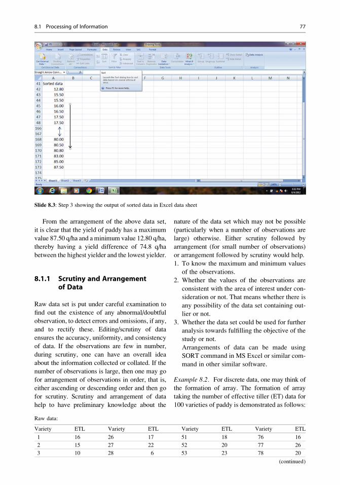
From the arrangement of the above data set,

it is clear that the yield of paddy has a maximum

value 87.50 q/ha and a minimum value 12.80 q/ha,

thereby having a yield difference of 74.8 q/ha

between the highest yielder and the lowest yielder.

8.1.1 Scrutiny and Arrangementof Data

Raw data set is put under careful examination to

find out the existence of any abnormal/doubtful

observation, to detect errors and omissions, if any,

and to rectify these. Editing/scrutiny of data

ensures the accuracy, uniformity, and consistency

of data. If the observations are few in number,

during scrutiny, one can have an overall idea

about the information collected or collated. If the

number of observations is large, then one may go

for arrangement of observations in order, that is,

either ascending or descending order and then go

for scrutiny. Scrutiny and arrangement of data

help to have preliminary knowledge about the

nature of the data set which may not be possible

(particularly when a number of observations are

large) otherwise. Either scrutiny followed by

arrangement (for small number of observations)

or arrangement followed by scrutiny would help.

1. To know the maximum and minimum values

of the observations.

2. Whether the values of the observations are

consistent with the area of interest under con-

sideration or not. That means whether there is

any possibility of the data set containing out-

lier or not.

3. Whether the data set could be used for further

analysis towards fulfilling the objective of the

study or not.

Arrangements of data can be made using

SORT command in MS Excel or similar com-

mand in other similar software.

Example 8.2. For discrete data, one may think of

the formation of array. The formation of array

taking the number of effective tiller (ET) data for

100 varieties of paddy is demonstrated as follows:

Slide 8.3: Step 3 showing the output of sorted data in Excel data sheet

Raw data:

Variety ETL Variety ETL Variety ETL Variety ETL

1 16 26 17 51 18 76 16

2 15 27 22 52 20 77 26

3 10 28 6 53 23 78 20

(continued)

8.1 Processing of Information 77

From the arrangement of the above data set on

the number of effective tier per hill (ETL) of 100

varieties of paddy, it is clear that the ETL has a

minimum value 4 and a maximum value 26;

thereby having a range of 26 � 4 ¼ 22 number

of ETL among the varieties of paddy under con-

sideration. After the formation of data, it takes

the following shape (Tables 8.1 and 8.2).

It is found from the array that there are four

varieties having ETL 4 numbers per hill; one

(continued)

Variety ETL Variety ETL Variety ETL Variety ETL

4 11 29 8 54 9 79 21

5 12 30 16 55 13 80 19

6 13 31 12 56 14 81 7

7 14 32 13 57 8 82 9

8 7 33 14 58 7 83 14

9 8 34 7 59 9 84 22

10 9 35 8 60 13 85 23

11 10 36 11 61 7 86 14

12 11 37 17 62 8 87 26

13 14 38 9 63 11 88 18

14 16 39 10 64 24 89 20

15 18 40 12 65 16 90 19

16 20 41 18 66 4 91 17

17 7 42 17 67 6 92 9

18 8 43 16 68 5 93 10

19 4 44 8 69 6 94 12

20 6 45 6 70 7 95 23

21 15 46 4 71 10 96 20

22 8 47 16 72 11 97 21

23 12 48 22 73 4 98 12

24 15 49 26 74 8 99 10

25 16 50 21 75 12 100 18

Slide 8.4: Step 1 showing the entry or the transformation of data to Excel data sheet

78 8 Processing and Analysis of Data

variety is having 5 ETL per hill, five varieties is

having ETL six, and so on. This formation of array

is done with the help of SORT key in Microsoft

Excel computer package as shown above in case of

example with the yield of paddy. Otherwise, con-

ventionally we may take help of the tally marking.

Process for tally marking is presented below

(Table 8.3).

8.1.2 Coding of Data

Sometimes the information collected may be

qualitative in nature like male/female, black/yel-

low/white/green, determinate/indeterminate, and

educated/illiterate. Coding refers to the process

of assigning numerals or other symbols to the

responses so that these could be categorized.

Coding should be made in such a way that these

are nonoverlapping and all the observations are

categorized in one of the categories framed for

the purpose. That means the coding should

be made in such a way that categories are exclu-

sive and exhaustive in nature. Generally, the

numerical information does not require coding.

Coding helps researchers in understanding the

data in a more meaningful way.

8.1.3 Classification/Grouping

While dealing with a huge number of

observations, it is sometimes very difficult to

have a concise idea about the information col-

lected. So the first idea comes to mind, that is, to

have a logical classification (formation of

groups) in accordance with some common char-

acteristic(s)/classification or grouping, may be

one of the solutions.

The first question in classification comes

to mind is, how many classes one should make?There is no hard-and-first rule as to fix the num-

ber of classes. However, a general guideline as

given below is followed while making the

classes:

(a) Classes should bewell defined and exhaustive.

(b) Classes should not be overlapping.

(c) Classes should be of equal width as far as

possible.

(d) The number of classes should not be too few

or too many.

(e) Classes should be devoid of an open-ended

limit.

(f) Classes should be framed in such a way that

each and every class should have some

observation.

Table 8.1 ETL data arranged in ascending order

ETL

4 7 8 9 11 13 15 16 19 22

4 7 8 9 11 13 15 17 19 22

4 7 8 10 11 13 15 17 20 22

4 7 8 10 12 13 16 17 20 23

5 7 8 10 12 14 16 17 20 23

6 7 8 10 12 14 16 18 20 23

6 7 9 10 12 14 16 18 20 24

6 8 9 10 12 14 16 18 21 26

6 8 9 11 12 14 16 18 21 26

6 8 9 11 12 14 16 18 21 26

Table 8.2 Summary of ETL data arranged in ascending order

From the above array, one can have the following summary:

ETL 4 5 6 7 8 9 10 11 12 13 14 15 16 17 18 19 20 21 22 23 24 26

Frequency 4 1 5 7 9 6 6 5 7 4 6 3 8 4 5 2 5 3 3 3 1 3

Table 8.3 Tally marking and formation of frequency distribution of ETL data

ETL 4 5 6 7 8 9 10 11 12 13 14 15 16 17 18 19 20 21 22 23 24 26

Tally marks //// / //// //// // //// //// //// / //// / //// //// // //// //// / /// //// /// //// //// // //// /// /// /// / ///

Frequency 4 1 5 7 9 6 6 5 7 4 6 3 8 4 5 2 5 3 3 3 1 3

8.1 Processing of Information 79

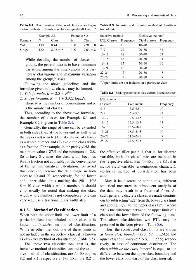
While deciding the number of classes or

groups, the general idea is to have minimum

variations among the observations of a par-

ticular class/group and maximum variation

among the groups/classes.

Following the above guidelines and the

formulae given below, classes may be formed.

1. Yule formula: K ¼ 2.5 � N1/4

2. Sturge formula: K ¼ 1 + 3.322 log10N,where N is the number of observations and K

is the number of classes.

Thus, according to the above two formulae,

the number of classes for Example 8.1 and

Example 8.2 is given in Table 8.4.

Generally, the range of date can be extended

in both sides (i.e., at the lower end as well as at

the upper end) so as to (1) make the no. of classes

as a whole number and (2) avoid the class width

as a fraction. For example, in the paddy yield, the

maximum value is 87.5 and the minimum is 12.8.

So to have 8 classes, the class width becomes

9.33, a fraction not advisable for the convenience

of further mathematical calculation. To avoid

this, one can increase the data range in both

sides to 10 and 90, respectively, for the lower

and upper sides, thus making the (90 � 10)/

8 ¼ 10 class width a whole number. It should

emphatically be noted that making the class

width whole number is not compulsory; one can

very well use a fractional class width also.

8.1.3.1 Method of ClassificationWhen both the upper limit and lower limit of a

particular class are included in the class, it is

known as inclusive method of classification.

While in other methods one of these limits is

not included in the respective class, it is known

as exclusive method of classification (Table 8.5).

The above two classifications, that is, the

inclusive method of classification and the exclu-

sive method of classification, are for Examples

8.2 and 8.1, respectively. For Example 8.2 of

the effective tiller per hill, that is, for discrete

variable, both the class limits are included in

the respective class. But for Example 8.1, that

is, for yield variable (a continuous character),

exclusive method of classification has been

used.

May it be discrete or continuous, different

statistical measures in subsequent analysis of

the data may result in a fractional form. As

such, generally discrete classes are made continu-

ous by subtracting “d/2” from the lower class limit

and adding “d/2” to the upper class limit, where

“d” is the difference between the upper limit of a

class and the lower limit of the following class.

The above classification wrt ETL may be

presented in the form given in Table 8.6.

Thus, the constructed class limits are known

as lower class boundary (3.5, 6.5, . . .,24.5) andupper class boundary (6.5, 9.5, . . ., 27.5), respec-

tively, in case of continuous distribution. The

class width or the class interval is equal to the

difference between the upper class boundary and

the lower class boundary of the class interval.

Table 8.4 Determination of the no. of classes according to

the twomethods of classification for example data 8.1 and 8.2

Formula

Example 8.1 Example 8.2

N Class N Class

Yule 130 8.44 ¼ 8 100 7.91 ¼ 8

Struge 130 8.02 ¼ 8 100 7.64 ¼ 8

Table 8.5 Inclusive and exclusive method of classifica-

tion of data

Inclusive method Exclusive methoda

ETL Classes Frequency Yield classes Frequency

4–6 10 10–20 16

7–9 22 20–30 54

10–12 18 30–40 14

13–15 13 40–50 11

16–18 17 50–60 10

19–21 10 60–70 10

22–24 7 70–80 8

25–27 3 80–90 7

aUpper limits are not included in a particular class

Table 8.6 Making continuous classes fromdiscrete classes

ETL classes

Discrete Continuous Frequency

4–6 3.5–6.5 10

7–9 6.5–9.5 22

10–12 9.5–12.5 18

13–15 12.5–15.5 13

16–18 15.5–18.5 17

19–21 18.5–21.5 10

22–24 21.5–24.5 7

25–27 24.5–27.5 3

80 8 Processing and Analysis of Data

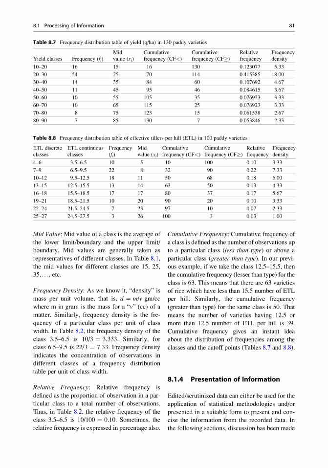
Mid Value: Mid value of a class is the average of

the lower limit/boundary and the upper limit/

boundary. Mid values are generally taken as

representatives of different classes. In Table 8.1,

the mid values for different classes are 15, 25,

35,. . ., etc.

Frequency Density: As we know it, “density” is

mass per unit volume, that is, d ¼ m/v gm/cc

where m in gram is the mass for a “v” (cc) of a

matter. Similarly, frequency density is the fre-

quency of a particular class per unit of class

width. In Table 8.2, the frequency density of the

class 3.5–6.5 is 10/3 ¼ 3.333. Similarly, for

class 6.5–9.5 is 22/3 ¼ 7.33. Frequency density

indicates the concentration of observations in

different classes of a frequency distribution

table per unit of class width.

Relative Frequency: Relative frequency is

defined as the proportion of observation in a par-

ticular class to a total number of observations.

Thus, in Table 8.2, the relative frequency of the

class 3.5–6.5 is 10/100 ¼ 0.10. Sometimes, the

relative frequency is expressed in percentage also.

Cumulative Frequency: Cumulative frequency of

a class is defined as the number of observations up

to a particular class (less than type) or above a

particular class (greater than type). In our previ-

ous example, if we take the class 12.5–15.5, then

the cumulative frequency (lesser than type) for the

class is 63. This means that there are 63 varieties

of rice which have less than 15.5 number of ETL

per hill. Similarly, the cumulative frequency

(greater than type) for the same class is 50. That

means the number of varieties having 12.5 or

more than 12.5 number of ETL per hill is 39.

Cumulative frequency gives an instant idea

about the distribution of frequencies among the

classes and the cutoff points (Tables 8.7 and 8.8).

8.1.4 Presentation of Information

Edited/scrutinized data can either be used for the

application of statistical methodologies and/or

presented in a suitable form to present and con-

cise the information from the recorded data. In

the following sections, discussion has been made

Table 8.7 Frequency distribution table of yield (q/ha) in 130 paddy varieties

Yield classes Frequency (fi)Mid

value (xi)Cumulative

frequency (CF<)

Cumulative

frequency (CF�)

Relative

frequency

Frequency

density

10–20 16 15 16 130 0.123077 5.33

20–30 54 25 70 114 0.415385 18.00

30–40 14 35 84 60 0.107692 4.67

40–50 11 45 95 46 0.084615 3.67

50–60 10 55 105 35 0.076923 3.33

60–70 10 65 115 25 0.076923 3.33

70–80 8 75 123 15 0.061538 2.67

80–90 7 85 130 7 0.053846 2.33

Table 8.8 Frequency distribution table of effective tillers per hill (ETL) in 100 paddy varieties

ETL discrete

classes

ETL continuous

classes

Frequency

(fi)Mid

value (xi)Cumulative

frequency (CF<)

Cumulative

frequency (CF�)

Relative

frequency

Frequency

density

4–6 3.5–6.5 10 5 10 100 0.10 3.33

7–9 6.5–9.5 22 8 32 90 0.22 7.33

10–12 9.5–12.5 18 11 50 68 0.18 6.00

13–15 12.5–15.5 13 14 63 50 0.13 4.33

16–18 15.5–18.5 17 17 80 37 0.17 5.67

19–21 18.5–21.5 10 20 90 20 0.10 3.33

22–24 21.5–24.5 7 23 97 10 0.07 2.33

25–27 24.5–27.5 3 26 100 3 0.03 1.00

8.1 Processing of Information 81

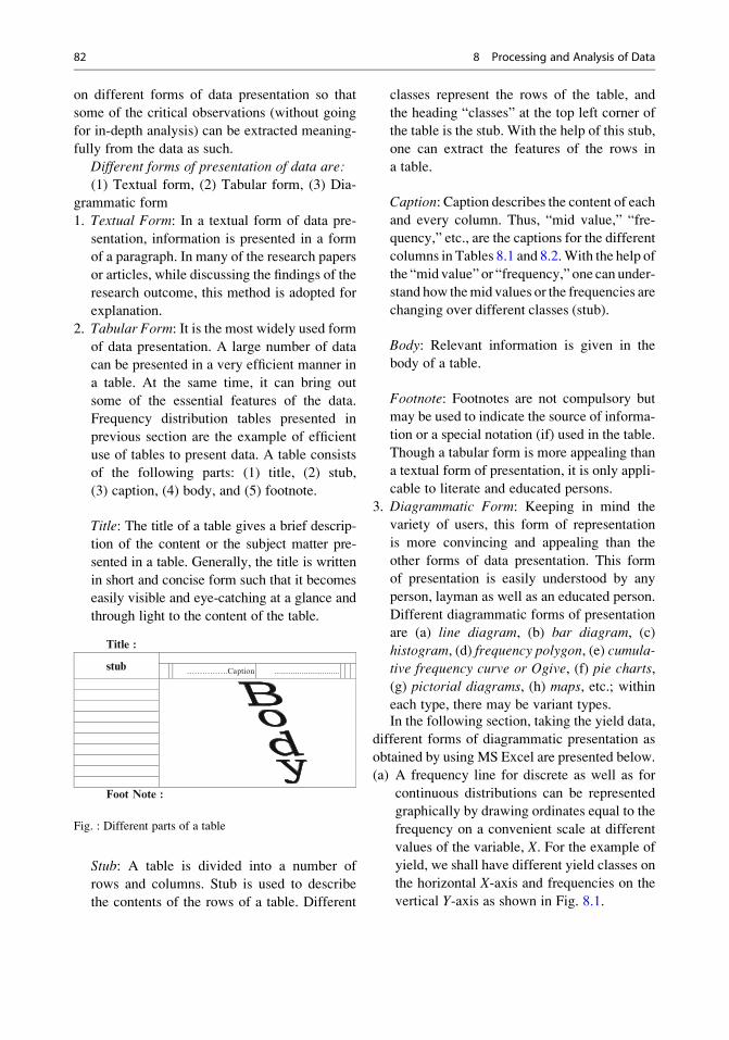
on different forms of data presentation so that

some of the critical observations (without going

for in-depth analysis) can be extracted meaning-

fully from the data as such.

Different forms of presentation of data are:

(1) Textual form, (2) Tabular form, (3) Dia-

grammatic form

1. Textual Form: In a textual form of data pre-

sentation, information is presented in a form

of a paragraph. In many of the research papers

or articles, while discussing the findings of the

research outcome, this method is adopted for

explanation.

2. Tabular Form: It is the most widely used form

of data presentation. A large number of data

can be presented in a very efficient manner in

a table. At the same time, it can bring out

some of the essential features of the data.

Frequency distribution tables presented in

previous section are the example of efficient

use of tables to present data. A table consists

of the following parts: (1) title, (2) stub,

(3) caption, (4) body, and (5) footnote.

Title: The title of a table gives a brief descrip-tion of the content or the subject matter pre-

sented in a table. Generally, the title is written

in short and concise form such that it becomes

easily visible and eye-catching at a glance and

through light to the content of the table.

Title :

Foot Note :

stub …………….Caption ...............................

Fig. : Different parts of a table

Stub: A table is divided into a number of

rows and columns. Stub is used to describe

the contents of the rows of a table. Different

classes represent the rows of the table, and

the heading “classes” at the top left corner of

the table is the stub. With the help of this stub,

one can extract the features of the rows in

a table.

Caption: Caption describes the content of each

and every column. Thus, “mid value,” “fre-

quency,” etc., are the captions for the different

columns in Tables 8.1 and 8.2.With the help of

the “mid value” or “frequency,” one can under-

stand how themid values or the frequencies are

changing over different classes (stub).

Body: Relevant information is given in the

body of a table.

Footnote: Footnotes are not compulsory but

may be used to indicate the source of informa-

tion or a special notation (if) used in the table.

Though a tabular form is more appealing than

a textual form of presentation, it is only appli-

cable to literate and educated persons.

3. Diagrammatic Form: Keeping in mind the

variety of users, this form of representation

is more convincing and appealing than the

other forms of data presentation. This form

of presentation is easily understood by any

person, layman as well as an educated person.

Different diagrammatic forms of presentation

are (a) line diagram, (b) bar diagram, (c)

histogram, (d) frequency polygon, (e) cumula-

tive frequency curve or Ogive, (f) pie charts,(g) pictorial diagrams, (h) maps, etc.; within

each type, there may be variant types.In the following section, taking the yield data,

different forms of diagrammatic presentation as

obtained by using MS Excel are presented below.

(a) A frequency line for discrete as well as for

continuous distributions can be represented

graphically by drawing ordinates equal to the

frequency on a convenient scale at different

values of the variable, X. For the example of

yield, we shall have different yield classes on

the horizontal X-axis and frequencies on the

vertical Y-axis as shown in Fig. 8.1.

82 8 Processing and Analysis of Data

(b) Bar diagram: Instead of drawing a line join-

ing the class frequencies, one represents

the frequencies in the form of bars. In bar

diagrams, equal bases on a horizontal

(or vertical) line are selected, and rectangles

are constructed with length proportional to

the given frequencies on a suitably chosen

scale. The bars should be drawn at equal

distances from one another (Fig. 8.2).

A more complicated form of bar diagrams is

the clustered column/bar, stacked column

and bar, and 100% stacked column/bar dia-

gram. In clustered bar diagrams, values of

the same item for different categories are

compared. While in a stacked column,

the proportions of the values across the

categories are shown. In 100% stacked bar,

a comparison of each category is made in

such a way to make the following example.

With the help of educational status data of

five different blocks, let us demonstrate these

graphs in Table 8.9, Figs. 8.3 and 8.4.

(c) Histogram: Histogram is almost similar to

that of a bar diagram for discrete data; the

only thing is that the reflection of nonexistence

of any gap between two consecutive classes is

also reflected by leaving no gap between two

consecutive bars. Continuous grouped data are

usually represented graphically by a histo-

gram. The rectangles are drawn with bases

corresponding to the true class intervals and

with heights proportional to the frequencies.

With all the class intervals equal, the areas of a

rectangle also represent the corresponding

frequencies. If the class intervals are not all

equal, then the heights are to be suitably

adjusted to make the area proportional to the

frequencies (Fig. 8.5).

(d) Frequency Polygon: If the midpoints of the

top of the bars in histogram are joined by

straight lines, then a frequency polygon is

Table 8.9 Educational status data (%) of five different

blocks

Block Illiterate School Graduation

Post

graduation

Block1 23.7 34.6 18.0 23.7

Block2 13.2 42.2 23.8 20.8

Block3 18.0 33.0 30.0 19.0

Block4 19.3 14.0 34.0 32.7

Block5 26.5 29.5 24.0 20.0

Fig. 8.1 Line diagram

Fig. 8.2 Rice yield data

and its corresponding bar

diagram

8.1 Processing of Information 83

obtained. To complete the polygon, it is cus-

tomary to join the extreme points at each end

of the frequency polygon to the midpoints of

the next higher and lower class intervals on a

horizontal line (class axis here). For the pur-

pose, generally two hypothetical classes, one

before the lowest actual class and another at

the last of the highest actual class, are added

with zero observation in both cases so that

the frequency line diagram completes a

bounded area with horizontal X-axis as

shown below (Fig. 8.6):

(e) Pie Chart: The basic idea behind the forma-

tion of a pie diagram is to take the whole

frequencies in 100% and present it in a circle

with 360� angle at the center. In the fre-

quency distribution table, ordinary frequency

or relative frequency can effectively be used

Fig. 8.3 Stacked bar

diagram of educational

status of five blocks

Fig. 8.4 Clustered bar

diagram of educational

status of five blocks

Fig. 8.5 Yield frequency

histogram of 130 varieties

of paddy

84 8 Processing and Analysis of Data

in the form of a pie diagram. Thus, for exam-

ple, the yield data following a pie chart is

prepared with class frequencies (Fig. 8.7).

The advantage of pie diagram is that differ-

ent characteristics measured in different units

and or under different situations can be

compared with the help of this diagram.

Moreover, along with other diagrammatic

data presentation, this method is also appeal-

ing to both illiterate and educated persons.

Taking the example of an expenditure

pattern of two groups of people, pie diagram

could be used for comparison (Table 8.10

and Fig. 8.8).

(f) Cumulative Frequency Curve (Ogive):

Partitioning the whole data set can verywell be made with the help of a cumulative

frequency graph, also known as OGIVE. It is

of two different types, that is, “less than type”

and “more than equal to type.” For “less than

type,” one plots the points with the upper

boundaries of the classes as abscissa and the

corresponding cumulative frequency as

ordinates. The points are joined by a freehand

smooth curve. For “more than equal to type”

one plots the points with the lower

boundaries of the classes as abscissas and

the corresponding cumulative frequencies as

ordinates. Then, the points are joined by a

freehand smooth curve (Fig. 8.9).

Fig. 8.6 Yield frequency

polygon and histogram of

130 varieties of paddy

Fig. 8.7 Pie diagram of

yield frequency for 130

varieties of paddy

Table 8.10 Expenditure pattern of two groups of people

Expenditure (Rs) Group-1 Group-2

Food 1,800 1,600

Housing 6,500 4,500

Clothing 4,000 3,400

Education 1,250 1,650

Medical 800 500

Others 650 350

Total 15,000 12,000

8.1 Processing of Information 85

Fig. 8.8 Pie diagram showing the expenditure pattern of two groups of people

Fig. 8.9 Different forms of cumulative frequency graphs (Ogives)

86 8 Processing and Analysis of Data

(g) Pictorial Diagram: To make the information

lively and easy to understand by any user,

sometimes information is presented in picto-

rial forms. Instead of a bar diagram or line

diagram or pie chart, one can use pictures in

the diagrams. Let us take the example of the

no. of particular insects per hill of 100 varieties

of paddy; the frequencies can be represented

with suitably scaled figure. If we assume that

each insect represents four similar insects,

then the frequency distribution can be

represented in the following forms (Fig. 8.10):

This type of pictorial representation is easy to

understand even by the layman and is more

eye-catching. But the problem with this type

of representation is that if the number of

figures does not exactly match with the fre-

quency, then some of the drawings are to be

kept incomplete like classes 4–7 and 10–13.

(h) Maps: Statistical maps are generally used to

represent the distribution of particular

parameters like a forest area in a country,

paddy-producing zone, different mines

located at different places in a country, rain-

fall pattern, population density, etc. The map

shown in Fig. 8.11 gives the rainfall distribu-

tion during 1-6-12 to 25-7-12 for the whole

of India. The essence of a pictorial diagram

or map lies in their acceptability to a wide

range of users including the illiterate people.

This type of data representation is easily

conceived by any person, but utmost care

should be taken to make the statistical map

true to the sense and scale, etc.

It should clearly be noted that all types of

presentation are not suitable for all types of

data, at all situations, and to all users. The appro-

priate type of presentation is to be decided on the

basis of the type of information, the objective of

the presentation, and the person concerned for

whom the presentation is basically meant.

8.2 Analysis of Data

Once after the processing and data presentation,

it is now imperative for a researcher to explain

and describe the nature of the research in a

deeper sense. In the first attempt, the researcher

tries to explain/describe the nature of the infor-

mation through measures of central tendency,

measures of dispersion, measures of asymmetry,

etc., taking one variable at a time—known as

univariate analysis. In his/her next endeavor,

he/she tries to find out the association among

the variables—which are coming under either

bivariate (taking two variables at a time) or

multivariate analysis (taking more than two

variables at a time). Once after completion of

the description (through univariate/bivariate/

Class Frequency Pictures

3.5 - 6.5 12

6.5 - 9.5 21

9.5 -12.5 18

12.5-15.5 13

15.5-18.5 16

18.5-21.5 11

21.5-24.5 9

Fig. 8.10 Pictorial

presentation of a frequency

distribution of the no. of

insect per hill

8.2 Analysis of Data 87

Fig. 8.11 Pictorial presentation of rainfall distribution in India (Source: India meteorological department; http://www.

google.com.in, accessed on 18-8-12)

88 8 Processing and Analysis of Data

multivariate analysis), the researcher tries to

infer or draw conclusion about the population

characteristics from the sample behaviors studied

so far through inferential statistics. In the

following few sections, we shall discuss the

descriptive statistics up to bivariate levels.

Multivariate and inferential statistics will be

taken up in the subsequent chapters.

In an attempt to summarize the information/

data, a researcher is always in search of certain

value(s) that can represent a set of information

given in a big table or otherwise. Thus, we

are always in search of such a measure, which

can describe the inherent characteristics of a

given set of information. Generally, a researcher

is in search of the two types of measures, one to

find out the central value around which the

observations are supposed to lie and another

measure for the spread/dispersion/scatteredness

of the observations.

8.2.1 Measures of Central Tendencyand Locations

Given a set of data, we are in search of a

typical value below and above which the

observations tend to cluster around. Thus, the

tendency of the observations to cluster around

a central value is known as central tendency.

Sometimes, researchers want to have an idea

about specific locations below and above which

there is a certain percentage of population.

For example, one may be interested in knowing

the 50th percentile value, that is, the value below

and above which there are half the population,

or the 3rd quartile value, that is, the value below

which there are 75% of the population and so on.

That means we are in search of certain locational

values.

According to Yule, a good measure should

have the following characteristics:

(a) It should be defined rigidly without any

ambiguity

(b) It should be based on all observations

(c) It should be easy to calculate

(d) It should be easy to understand

(e) It should be readily acceptable to mathemati-

cal treatments

(f) It should be the least influenced by sampling

fluctuations

The Different Measures of Central TendencyAre:

(a) Mean

(b) Median

(c) Mode

(d) Midpoint average, etc.

Analysis of data

Descriptive Statistics Inferential Statistics

Estimation

Univariate Bivariate Multivariate Parametric

Interval estimation Nonparametric

Central tendency Simple Correlation Multiple correlationDispersion Simple Regression Partial CorrelationAsymmetry Association of Attributes Multiple RegressionIndex No Two way ANOVA etc. Path analysisTime series Multiple Discriminant AnalysisOne way ANOVA etc. Canonical Analysis

Factor analysis/ Cluster analysis etc.

Point estimation

Testing of Hypothesis

8.2 Analysis of Data 89

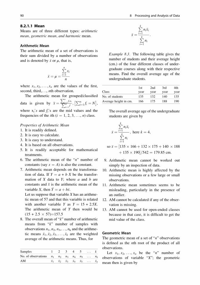
8.2.1.1 MeanMeans are of three different types: arithmetic

mean, geometric mean, and harmonic mean.

Arithmetic Mean

The arithmetic mean of a set of observations is

their sum divided by a number of observations

and is denoted by �x or μ, that is,

�x ¼ μ ¼Pni¼1

xi

n

where x1; x2; . . . ; xn are the values of the first,

second, third,. . ., nth observation.

The arithmetic mean for grouped/classified

data is given by x ¼Pn

i¼1fixiPn

i¼1f;Pn

i¼1 fi ¼ N� �

,

where xi’s and fi’s are the mid values and the

frequencies of the ith (i ¼ 1, 2, 3, . . ., n) class.

Properties of Arithmetic Mean

1. It is readily defined.

2. It is easy to calculate.

3. It is easy to understand.

4. It is based on all observations.

5. It is readily acceptable for mathematical

treatments.

6. The arithmetic mean of the “n” number of

constants (say x ¼ A) is also the constant.

7. Arithmetic mean depends on the transforma-

tion of data. If Y ¼ a + b X be the transfor-

mation of X data to Y; where a and b are

constants and x is the arithmetic mean of the

variable X, then �Y ¼ aþ b�x:Let us suppose that variable X has an arithme-

tic mean of 57 and that this variable is related

with another variable Y as Y ¼ 15 + 2.5X.The arithmetic mean of Y then would be

(15 + 2.5 � 57)¼157.5

8. The overall mean of “k” number of arithmetic

means from “k” number of samples with

observations n1, n2, n3,. . ., nk and the arithme-

tic means �x1; �x2; �x3; . . . ; �xk are the weighted

average of the arithmetic means. Thus, for

�x ¼Pki¼1

ni�xi

Pki¼1

ni

:

Example 8.3. The following table gives the

number of students and their average height

(cm.) of the four different classes of under-

graduate courses along with their respective

means. Find the overall average age of the

undergraduate students.

The overall average age of the undergraduate

students are given by

�x ¼Pki¼1

ni�xi

Pki¼1

ni

; here k ¼ 4;

so �x ¼ ½135� 166þ 132� 175þ 140 � 188

þ 135� 190�=542 ¼ 179:85 cm:

9. Arithmetic mean cannot be worked out

simply by an inspection of data.

10. Arithmetic mean is highly affected by the

missing observations or a few large or small

observations.

11. Arithmetic mean sometimes seems to be

misleading, particularly in the presence of

an outlier.

12. AM cannot be calculated if any of the obser-

vation is missing.

13. AM cannot be used for open-ended classes

because in that case, it is difficult to get the

mid value of the class.

Geometric Mean

The geometric mean of a set of “n” observations

is defined as the nth root of the product of all

observations.

Let x1, x2, . . ., xn be the “n” number of

observations of variable “X”; the geometric

mean then is given by

Samples 1 2 3 4 5 . . . k

No. of observations n1 n2 n3 n4 n5 . . . nkAM �x1 �x2 �x3 �x4 �x5 . . . �xn

Class

1st

year

2nd

year

3rd

year

4th

year

No. of students 135 132 140 135

Average height in cm. 166 175 188 190

90 8 Processing and Analysis of Data

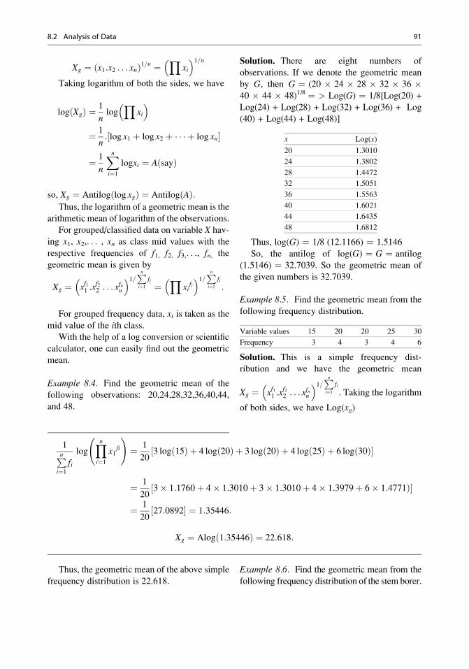
Xg ¼ ðx1:x2 . . . xnÞ1=n ¼Y

xi

� �1=nTaking logarithm of both the sides, we have

logðXgÞ ¼ 1

nlog

Yxi

� �¼ 1

n: log x1 þ log x2 þ . . .þ log xn½ �

¼ 1

n

Xni¼1

logxi ¼ AðsayÞ

so, Xg ¼ Antilogðlog xgÞ ¼ AntilogðAÞ:Thus, the logarithm of a geometric mean is the

arithmetic mean of logarithm of the observations.

For grouped/classified data on variable X hav-

ing x1, x2,. . . , xn as class mid values with the

respective frequencies of f1, f2, f3,. . ., fn, the

geometric mean is given by

Xg ¼ xf11 :xf22 . . . xfnn

� �1=Pni¼1

fi ¼Y

xifi

� �1=Pni¼1

fi:

For grouped frequency data, xi is taken as the

mid value of the ith class.

With the help of a log conversion or scientific

calculator, one can easily find out the geometric

mean.

Example 8.4. Find the geometric mean of the

following observations: 20,24,28,32,36,40,44,

and 48.

Solution. There are eight numbers of

observations. If we denote the geometric mean

by G, then G ¼ (20 � 24 � 28 � 32 � 36 �40 � 44 � 48)1/8 ¼ > Log(G) ¼ 1/8[Log(20) +

Log(24) + Log(28) + Log(32) + Log(36) + Log

(40) + Log(44) + Log(48)]

x Log(x)

20 1.3010

24 1.3802

28 1.4472

32 1.5051

36 1.5563

40 1.6021

44 1.6435

48 1.6812

Thus, log(G) ¼ 1/8 (12.1166) ¼ 1.5146

So, the antilog of log(G) ¼ G ¼ antilog

(1.5146) ¼ 32.7039. So the geometric mean of

the given numbers is 32.7039.

Example 8.5. Find the geometric mean from the

following frequency distribution.

Variable values 15 20 20 25 30

Frequency 3 4 3 4 6

Solution. This is a simple frequency dist-

ribution and we have the geometric mean

Xg ¼ xf11 :xf22 . . . xfnn

� �1=Pni¼1

fi. Taking the logarithm

of both sides, we have Log(xg)

1Pni¼1

fi

logYni¼1

x1fi

!¼ 1

203 logð15Þ þ 4 logð20Þ þ 3 logð20Þ þ 4 logð25Þ þ 6 logð30Þ½ �

¼ 1

203� 1:1760þ 4� 1:3010þ 3� 1:3010þ 4� 1:3979þ 6� 1:4771Þ½ �

¼ 1

2027:0892½ � ¼ 1:35446:

Xg ¼ Alog 1:35446ð Þ ¼ 22:618:

Thus, the geometric mean of the above simple

frequency distribution is 22.618.

Example 8.6. Find the geometric mean from the

following frequency distribution of the stem borer.

8.2 Analysis of Data 91

Solution. From the given information, we make

the following table:

Xi Frequency(fi) Log (Xi) fi. Log (xi)

5 14 0.69897 9.78558

6 18 0.77815 14.0067

7 23 0.84509 19.4370

8 16 0.90309 14.4494

9 11 0.95424 10.4966

10 19 1 19.0000

11 4 1.04139 4.16556

Thus; logðGÞ ¼ 1Pni¼1

fi

f1Xni¼1

logðxiÞ ¼ 91:340

105

¼ 0:869

G ¼ Alogð0:869Þ ¼ 7:396:

Properties1. It is rigidly defined.

2. It is not so easy to calculate or understand the

physical significance.

3. It takes care of all observations.

4. Mathematical treatments are not as easy as in

the case of arithmetic mean.

If G1, G2, . . ., Gk are the geometric means of

the samples having n1, n2, . . ., nk numbers of

the observations, then the combined geomet-

ric mean is given by

G ¼ðGn11 :G

n22 . . .Gnk

k Þ1=Pki¼1

ni ¼Yki¼1

G1=Pki¼1

ni

i

or log G ¼ 1P1i¼1

ni

Xki¼1

ni log½Gi�:

5. If all observations are equal to a constant, say

A, then the geometric mean is also equal to A.6. Geometric mean is not influenced very much

by the inclusions of a few large or small

observations unlike the arithmetic mean.

7. Geometric mean can’t be calculated if any of

the observation is zero.

8. GM is useful in the construction of index

numbers.

9. As GM gives greater weights to smaller items,

it is useful in economic and socioeconomic

data.

Harmonic Mean

The harmonic mean of a set of “n” observations

is the reciprocal of the arithmetic mean of the

reciprocals of the observations.

Let x1,x2, . . . , xn be the n number of

observations. So the arithmetic mean of the

reciprocals of the observations is

Pni¼1

1xi

n . Hence,

the harmonic mean, HM ¼ nPni¼1

1xi

.

For grouped data:Let x1, x2,. . .,xn be the mid values of the “n”

number of classes with the respective frequencies

of f1, f2, f3,. . ., fn; then, the harmonic mean is

given by

Pni¼1 fiPn

i¼1 fi=xi:

Example 8.7. Find the harmonic mean of the

following observations: 15,20,25,30,35,40,45,

and 50.

Solution. Here, the number of observations is 8.

So their harmonic mean is given by

HM ¼ nPni¼1

1

xi

¼ 8P8i¼1

1

xi

¼ 8

1

15þ 1

20þ 1

25þ 1

30þ 1

35þ 1

40þ 1

45þ 1

50

¼ 8

0:2857¼ 28:00:

Example 8.8. Find the harmonic mean from the

following frequency distribution.

No of insect 4.5–5.5 5.5–6.5 6.5–7.5 7.5–8.5 9.5–10.5 10.5–11.5 11.5–12.5

Frequency 14 18 23 16 11 19 4

92 8 Processing and Analysis of Data

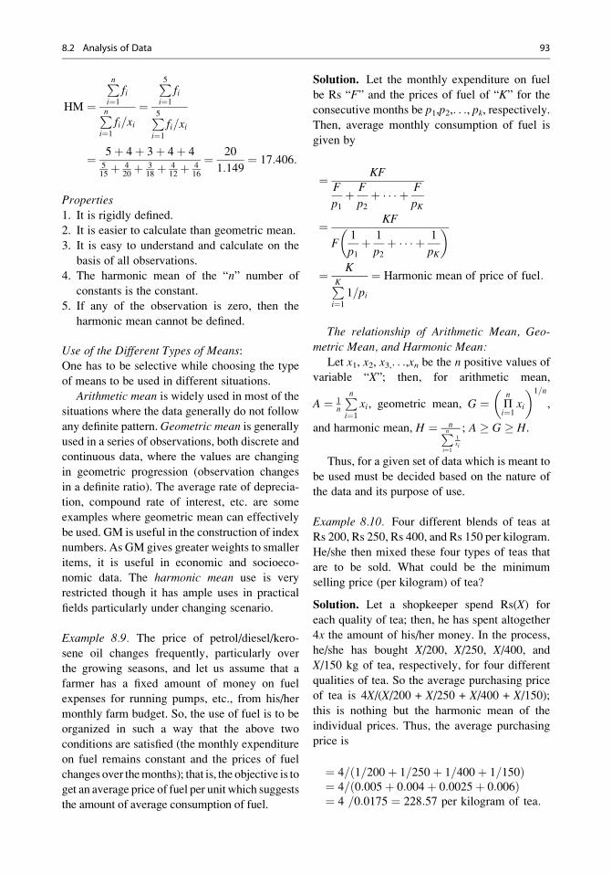
HM ¼Pni¼1

fi

Pni¼1

fi=xi

¼P5i¼1

fi

P5i¼1

fi=xi

¼ 5þ 4þ 3þ 4þ 4515þ 4

20þ 3

18þ 4

12þ 4

16

¼ 20

1:149¼ 17:406:

Properties

1. It is rigidly defined.

2. It is easier to calculate than geometric mean.

3. It is easy to understand and calculate on the

basis of all observations.

4. The harmonic mean of the “n” number of

constants is the constant.

5. If any of the observation is zero, then the

harmonic mean cannot be defined.

Use of the Different Types of Means:One has to be selective while choosing the type

of means to be used in different situations.

Arithmetic mean is widely used in most of the

situations where the data generally do not follow

any definite pattern. Geometric mean is generally

used in a series of observations, both discrete and

continuous data, where the values are changing

in geometric progression (observation changes

in a definite ratio). The average rate of deprecia-

tion, compound rate of interest, etc. are some

examples where geometric mean can effectively

be used. GM is useful in the construction of index

numbers. As GM gives greater weights to smaller

items, it is useful in economic and socioeco-

nomic data. The harmonic mean use is very

restricted though it has ample uses in practical

fields particularly under changing scenario.

Example 8.9. The price of petrol/diesel/kero-

sene oil changes frequently, particularly over

the growing seasons, and let us assume that a

farmer has a fixed amount of money on fuel

expenses for running pumps, etc., from his/her

monthly farm budget. So, the use of fuel is to be

organized in such a way that the above two

conditions are satisfied (the monthly expenditure

on fuel remains constant and the prices of fuel

changes over themonths); that is, the objective is to

get an average price of fuel per unit which suggests

the amount of average consumption of fuel.

Solution. Let the monthly expenditure on fuel

be Rs “F” and the prices of fuel of “K” for the

consecutive months be p1,p2,. . ., pk, respectively.

Then, average monthly consumption of fuel is

given by

¼ KFF

p1þ F

p2þ � � � þ F

pK

¼ KF

F1

p1þ 1

p2þ � � � þ 1

pK

� �

¼ KPKi¼1

1 pi=

¼ Harmonic mean of price of fuel:

The relationship of Arithmetic Mean, Geo-

metric Mean, and Harmonic Mean:

Let x1, x2, x3,. . .,xn be the n positive values of

variable “X”; then, for arithmetic mean,

A ¼ 1n

Pni¼1

xi, geometric mean, G ¼ Πn

i¼1xi

� �1=n

,

and harmonic mean, H ¼ nPni¼1

1xi

; A � G � H.

Thus, for a given set of data which is meant to

be used must be decided based on the nature of

the data and its purpose of use.

Example 8.10. Four different blends of teas at

Rs 200, Rs 250, Rs 400, and Rs 150 per kilogram.

He/she then mixed these four types of teas that

are to be sold. What could be the minimum

selling price (per kilogram) of tea?

Solution. Let a shopkeeper spend Rs(X) for

each quality of tea; then, he has spent altogether

4x the amount of his/her money. In the process,

he/she has bought X/200, X/250, X/400, and

X/150 kg of tea, respectively, for four different

qualities of tea. So the average purchasing price

of tea is 4X/(X/200 + X/250 + X/400 + X/150);

this is nothing but the harmonic mean of the

individual prices. Thus, the average purchasing

price is

¼ 4= 1=200þ 1=250þ 1=400þ 1=150ð Þ¼ 4= 0:005þ 0:004þ 0:0025þ 0:006ð Þ¼ 4 =0:0175 ¼ 228:57 per kilogram of tea:

8.2 Analysis of Data 93

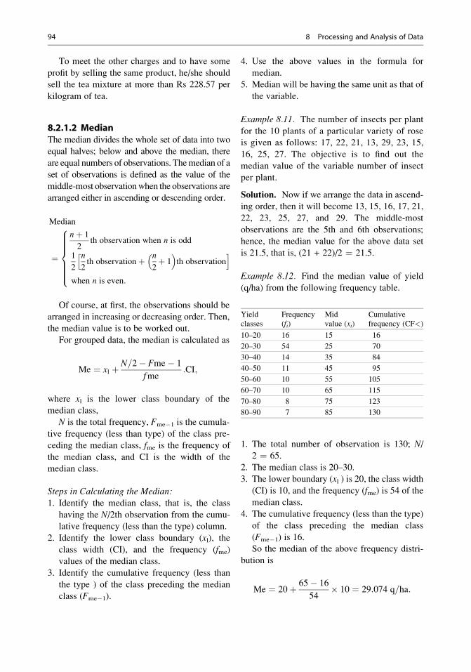
To meet the other charges and to have some

profit by selling the same product, he/she should

sell the tea mixture at more than Rs 228.57 per

kilogram of tea.

8.2.1.2 MedianThe median divides the whole set of data into two

equal halves; below and above the median, there

are equal numbers of observations. Themedian of a

set of observations is defined as the value of the

middle-most observationwhen the observations are

arranged either in ascending or descending order.

Median

¼

nþ 1

2th observation when n is odd

1

2

n

2th observationþ n

2þ 1

� �th observation

h iwhen n is even:

8>>>>><>>>>>:Of course, at first, the observations should be

arranged in increasing or decreasing order. Then,

the median value is to be worked out.

For grouped data, the median is calculated as

Me ¼ xl þ N=2� Fme� 1

fme:CI;

where xl is the lower class boundary of the

median class,

N is the total frequency, Fme�1 is the cumula-

tive frequency (less than type) of the class pre-

ceding the median class, fme is the frequency of

the median class, and CI is the width of the

median class.

Steps in Calculating the Median:

1. Identify the median class, that is, the class

having the N/2th observation from the cumu-

lative frequency (less than the type) column.

2. Identify the lower class boundary (xl), the

class width (CI), and the frequency (fme)

values of the median class.

3. Identify the cumulative frequency (less than

the type ) of the class preceding the median

class (Fme�1).

4. Use the above values in the formula for

median.

5. Median will be having the same unit as that of

the variable.

Example 8.11. The number of insects per plant

for the 10 plants of a particular variety of rose

is given as follows: 17, 22, 21, 13, 29, 23, 15,

16, 25, 27. The objective is to find out the

median value of the variable number of insect

per plant.

Solution. Now if we arrange the data in ascend-

ing order, then it will become 13, 15, 16, 17, 21,

22, 23, 25, 27, and 29. The middle-most

observations are the 5th and 6th observations;

hence, the median value for the above data set

is 21.5, that is, (21 + 22)/2 ¼ 21.5.

Example 8.12. Find the median value of yield

(q/ha) from the following frequency table.

1. The total number of observation is 130; N/

2 ¼ 65.

2. The median class is 20–30.

3. The lower boundary (xl ) is 20, the class width

(CI) is 10, and the frequency (fme) is 54 of the

median class.

4. The cumulative frequency (less than the type)

of the class preceding the median class

(Fme�1) is 16.

So the median of the above frequency distri-

bution is

Me ¼ 20þ 65� 16

54� 10 ¼ 29:074 q=ha:

Yield

classes

Frequency

(fi)Mid

value (xi)Cumulative

frequency (CF<)

10–20 16 15 16

20–30 54 25 70

30–40 14 35 84

40–50 11 45 95

50–60 10 55 105

60–70 10 65 115

70–80 8 75 123

80–90 7 85 130

94 8 Processing and Analysis of Data

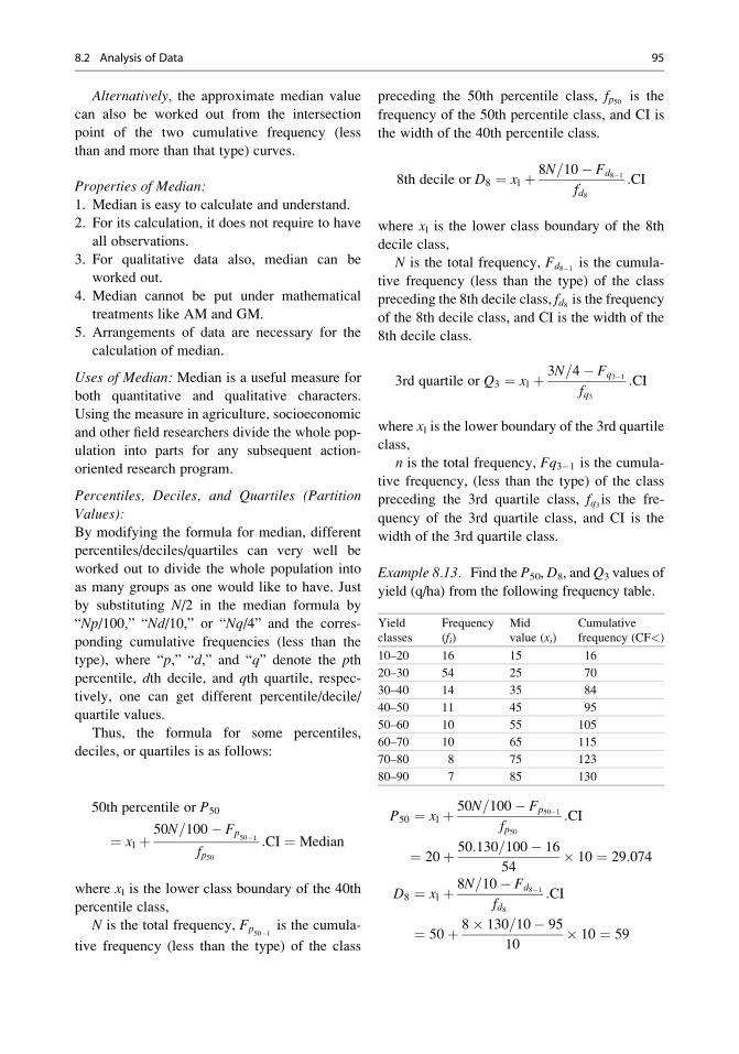
Alternatively, the approximate median value

can also be worked out from the intersection

point of the two cumulative frequency (less

than and more than that type) curves.

Properties of Median:

1. Median is easy to calculate and understand.

2. For its calculation, it does not require to have

all observations.

3. For qualitative data also, median can be

worked out.

4. Median cannot be put under mathematical

treatments like AM and GM.

5. Arrangements of data are necessary for the

calculation of median.

Uses of Median: Median is a useful measure for

both quantitative and qualitative characters.

Using the measure in agriculture, socioeconomic

and other field researchers divide the whole pop-

ulation into parts for any subsequent action-

oriented research program.

Percentiles, Deciles, and Quartiles (Partition

Values):

By modifying the formula for median, different

percentiles/deciles/quartiles can very well be

worked out to divide the whole population into

as many groups as one would like to have. Just

by substituting N/2 in the median formula by

“Np/100,” “Nd/10,” or “Nq/4” and the corres-

ponding cumulative frequencies (less than the

type), where “p,” “d,” and “q” denote the pth

percentile, dth decile, and qth quartile, respec-

tively, one can get different percentile/decile/

quartile values.

Thus, the formula for some percentiles,

deciles, or quartiles is as follows:

50th percentile or P50

¼ xl þ50N=100� Fp

50�1

fp50:CI ¼ Median

where xl is the lower class boundary of the 40th

percentile class,

N is the total frequency, Fp50�1

is the cumula-

tive frequency (less than the type) of the class

preceding the 50th percentile class, fp50 is the

frequency of the 50th percentile class, and CI is

the width of the 40th percentile class.

8th decile or D8 ¼ xl þ 8N=10� Fd8�1

fd8:CI

where xl is the lower class boundary of the 8th

decile class,

N is the total frequency, Fd8�1is the cumula-

tive frequency (less than the type) of the class

preceding the 8th decile class, fd8 is the frequency

of the 8th decile class, and CI is the width of the

8th decile class.

3rd quartile or Q3 ¼ xl þ 3N=4� Fq3�1

fq3:CI

where xl is the lower boundary of the 3rd quartileclass,

n is the total frequency, Fq3�1 is the cumula-

tive frequency, (less than the type) of the class

preceding the 3rd quartile class, fq3 is the fre-

quency of the 3rd quartile class, and CI is the

width of the 3rd quartile class.

Example 8.13. Find the P50, D8, and Q3 values of

yield (q/ha) from the following frequency table.

Yield

classes

Frequency

(fi)Mid

value (xi)Cumulative

frequency (CF<)

10–20 16 15 16

20–30 54 25 70

30–40 14 35 84

40–50 11 45 95

50–60 10 55 105

60–70 10 65 115

70–80 8 75 123

80–90 7 85 130

P50 ¼ xl þ 50N=100� Fp50�1

fp50:CI

¼ 20þ 50:130=100� 16

54� 10 ¼ 29:074

D8 ¼ xl þ 8N=10� Fd8�1

fd8:CI

¼ 50þ 8� 130=10� 95

10� 10 ¼ 59

8.2 Analysis of Data 95

Q3 ¼ xl þ 3N=4� Fq3�1

fq3:CI

¼ 50þ 3� 130=4� 95

10� 10 ¼ 52:5

Thus, from the above results, one can find that

50% (P50) plants have 29.074 q/ha or less yield,

75% (Q3) plants have 52.5 q/ha or less yield,

and 80% (D8) plants 59 q/ha or less yield.

8.2.1.3 ModeThe mode of a variable is defined as the value of

the observation having a maximum frequency.

Example 8.14. The number of accidents per day

on a specific road is given below:

15, 8, 7, 15, 10, 12, 13, 9, 10, 15, 8, 9, 10,

13,9,12, 10, 8, 10, and 7. Find the mode of the

number of accidents per day.

No. accidents per day 7 8 9 10 12 13 15

Frequency 2 3 3 5 2 2 3

From the above arrangement, it is found that

the maximum frequency is for the 10 accidents

per day. Hence, the mode is 10.

From a grouped/classified frequency distribu-

tion, the mode cannot be worked out as above.

The mode from a grouped frequency distribution

is calculated with the help of the following

formula:

Mo ¼ xl þ fmo � fmo�1

fmo � fmo�1ð Þ þ fmo � fmoþ1ð Þ :CI;

where xl is the lower class boundary of the modal

class,

fme�1 is the frequency of the class preceding the

modal class,

fmo is frequency of the modal class,

fme+1 is the frequency of the class following the

modal class, and

CI is the width of the modal class.

Steps in Calculating the Mode:

1. Identify the modal class, that is, the class

having the maximum observation from the

frequency column.

2. Identify the lower class boundary (xl), the

class width (CI), and the frequency (fmo)

values of the modal class.

3. Identify the frequency of the class preceding

the modal class (fm�1) and also the frequency

of the class following the modal class (fm+1).4. Use the above values in the formula for mode.

5. Mode will be having the same unit as that of

the variable.

Example 8.15. Find the P50, D8, and Q3 values

of yield (q/ha) from the following frequency

table.

Yield

classes

Frequency

(fi)Mid value

(xi)Cumulative

frequency (CF<)

10–20 16 15 16

20–30 54 25 70

30–40 14 35 84

40–50 11 45 95

50–60 10 55 105

60–70 10 65 115

70–80 8 75 123

80–90 7 85 130

1. The total number of observation is 130.

2. The modal class is 20–30.

3. The lower class boundary (xl) is 20, the classwidth (CI) is 10, and the frequency (fm) is 54

of the modal class.

4. The frequency of the class preceding the

modal class (fm�1) is 16 and the frequency

of the class following the modal class (fm+1)

is 14.

So the mode of the above frequency distribu-

tion is

Mo ¼ 20þ 54� 16

ð54� 16Þ þ ð54� 14Þ � 10

¼ 24:87 q=ha:

96 8 Processing and Analysis of Data

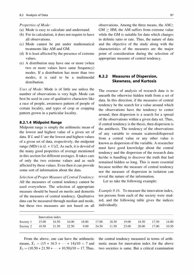
Properties of Mode:

(a) Mode is easy to calculate and understand.

(b) For its calculation, it does not require to have

all observations.

(c) Mode cannot be put under mathematical

treatments like AM and GM.

(d) It is least affected by the presence of extreme

values.

(e) A distribution may have one or more (when

two or more values have same frequency)

modes. If a distribution has more than two

modes, it is said to be a multimodal

distribution.

Uses of Mode: Mode is of little use unless the

number of observations is very high. Mode can

best be used in case of qualitative characters like

a race of people, awareness pattern of people of

certain locality, and types of crop or cropping

pattern grown in a particular locality.

8.2.1.4 Midpoint RangeMidpoint range is simply the arithmetic mean of

the lowest and highest value of a given set of

data. If L and U are the lowest and highest values

of a given set of data, respectively, the midpoint

range (MDr) is (L + U)/2. As such, it is devoid ofthe many good properties of average mentioned

in this section for different averages. It takes care

of only the two extreme values and as such

affected by these values. Even then it can provide

some sort of information about the data.

Selection of Proper Measure of Central Tendency:

All the measures of central tendency cannot be

used everywhere. The selection of appropriate

measure should be based on merits and demerits

of the measures of central tendency. Qualitative

data can be measured through median and mode,

but these two measures are not based on all

observations. Among the three means, the AM�GM � HM, the AM suffers from extreme value

while the GM is suitable for data which changes

in definite ratio or rate. Thus, the nature of data

and the objective of the study along with the

characteristics of the measures are the major

point of consideration during the selection of

appropriate measure of central tendency.

8.2.2 Measures of Dispersion,Skewness, and Kurtosis

The essence of analysis of research data is to

unearth the otherwise hidden truth from a set of

data. In this direction, if the measures of central

tendency be the search for a value around which

the observations have the tendency to center

around, then dispersion is a search for a spread

of the observations within a given data set. Thus,

if central tendency is the thesis, then dispersion is

the antithesis. The tendency of the observations

of any variable to remain scattered/dispersed

from a central value or any other value is

known as dispersion of the variable. A researcher

must have good knowledge about the central

tendency and the dispersion of the research data

he/she is handling to discover the truth that had

remained hidden so long. This is more essential

because neither the measure of central tendency

nor the measure of dispersion in isolation can

reveal the nature of the information.

Let us take the following example:

Example 8.16. To measure the innovation index,

ten persons from each of the society were stud-

ied, and the following table gives the indices

individually.

From the above, one can have the arithmetic

means, �X1 ¼ (15 + 16.5 + � � � + 14)/10 ¼ 7 and�X2 ¼ (10.50 + 21.50 + � � � + 10.50)/10¼ 17. Thus,

the central tendency measured in terms of arith-

metic mean for innovation index for the above

two societies is same. But a critical examination

Innovation index

Society 1 15.00 16.50 16.00 18.00 17.00 18.50 19.00 18.50 17.50 14.00

Society 2 10.50 21.50 22.50 9.00 24.50 11.50 23.00 20.00 17.00 10.50

8.2 Analysis of Data 97

of the data reveals that in society 1, the innovation

remains in between 14 and 19; on the other hand,

in society 2 it remains between 9 and 24.5. Thus,

the innovation indices are more dispersed in soci-

ety 2 than in society 1, in spite of having the same

average performance for both the societies. Thus,

from the above results, two conclusions can be

drawn: (a) the maximum innovation potentiality

and innovation variability of society 1 is less than

in society 2 and (b) given a better attention, people

in society 2 can be better innovative by attaining

its full potentiality.

Measures of Dispersion: Like the measures of

central tendency, there is a need to have measures

for dispersion also. In fact, different measures of

dispersions are available in the theory of statistics.

Before going into the details on the discussion of

the different measures of dispersion, let us try to

examine the characteristics of a good measure of

dispersion. There should not be any ambiguity in

defining a measure; it should be clear and rigid in

definition. Unless a measure is convincing, that is,

easily understood and applicable by the user, it is

of least importance. For further application of a

measure, it should be put easily under mathemati-

cal treatments. In order to reflect the true nature of

the data, a good measure should try to take care of

all the observations, and it should lay equal impor-

tance to each and every observation without being

affected by the extreme values.

8.2.2.1 Absolute Measures of DispersionThe absolute measures of dispersion have the

units according to those of variables, but relative

measures are pure number; as such are unit-free

measures. Thus, unit-free measures can be used

to compare distributions of different variables

measured in different units.

(a) Range: A range of a set of observations is the

difference between the maximum value and

the minimum value of a set of data. Thus,

Rx ¼ Xmax–Xmin is the range of variable “X”for a given set of observations. In the above

example, the ranges for two societies are

19�14 ¼ 5 and 24.5�9 ¼ 15.5, respec-

tively, for society 1 and society 2.

Uses of Range: Range can be used in any

type of continuous or discrete variables.

Range has its uses in the field of stock market

(daily variation), in meteorological forecast-

ing, in statistical quality control, etc.

Advantages and Disadvantages of Range:1. Range is rigidly defined and can be calcu-

lated easily.

2. Though range is not based on all the

observations, it cannot be worked out if

there are missing values.

3. Range is very much affected by sampling

fluctuations.

In spite of all these drawbacks, range is

being used in many occasions only because

of its simplicity and of having a first-hand

information on the variation of the data.

(b) Mean Deviation: The mean deviation of var-

iable “X” (x1, x2, x3,� � �, xn) about any arbi-

trary point “A” is defined as the mean of the

absolute deviation of the different values of

the variable from the arbitrary point “A” and

is denoted as MDA ¼ 1n

Pni¼1

Xi � A, 1Pn

i¼1fi�Pn

i¼1 fi Xi � Aj j for grouped data.

Similarly, instead of taking the deviation

from the arbitrary point “A,” one can take the

deviation from the arithmetic mean, median,

or mode also. Actually, the mean deviation of

variable “X” is defined as the mean of the

absolute deviation of different values of the

Measures of dispersion

Absolute measure Relative measuresa) Rangeb) Mean deviationc) Quartile deviationd) Standard deviatione) Moments

a) Coefficient of quartile deviationb) Coefficient mean deviationc) Coefficient of variation

98 8 Processing and Analysis of Data

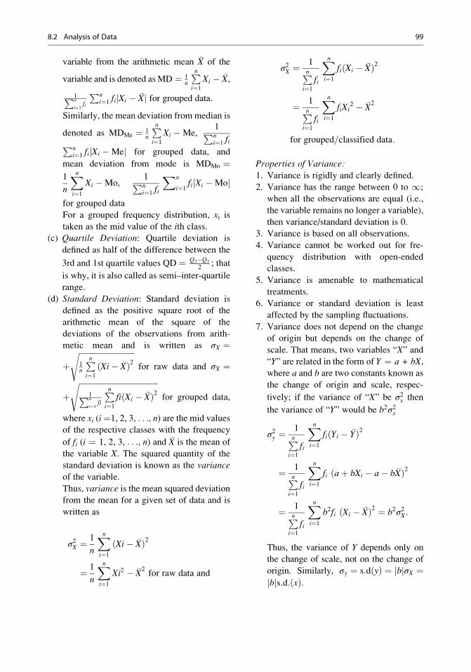
variable from the arithmetic mean �X of the

variable and is denoted asMD ¼ 1n

Pni¼1

Xi � �X,

1Pn

i¼1fi

Pni¼1 fi Xi � �Xj j for grouped data.

Similarly, the mean deviation from median is

denoted as MDMe ¼ 1n

Pni¼1

Xi �Me,1Pni¼1 fiPn

i¼1 fi Xi �Mej j for grouped data, and

mean deviation from mode is MDMo ¼1

n

Xni¼1

Xi �Mo,1Pni¼1 fi

Xn

i¼1fi Xi �Moj j

for grouped data

For a grouped frequency distribution, xi istaken as the mid value of the ith class.

(c) Quartile Deviation: Quartile deviation is

defined as half of the difference between the

3rd and 1st quartile values QD ¼ Q3�Q1

2; that

is why, it is also called as semi–inter-quartile

range.

(d) Standard Deviation: Standard deviation is

defined as the positive square root of the

arithmetic mean of the square of the

deviations of the observations from arith-

metic mean and is written as σX ¼

þffiffiffiffiffiffiffiffiffiffiffiffiffiffiffiffiffiffiffiffiffiffiffiffiffiffiffiffiffi1n

Pni¼1

Xi� �Xð Þ2s

for raw data and σX ¼

þffiffiffiffiffiffiffiffiffiffiffiffiffiffiffiffiffiffiffiffiffiffiffiffiffiffiffiffiffiffiffiffiffiffiffiffiffiffiffiffiffi

1Pn

i¼1fi

Pni¼1

fiðXi � �XÞ2s

for grouped data,

where xi (i¼1, 2, 3, . . ., n) are the mid values

of the respective classes with the frequency

of fi (i ¼ 1, 2, 3, . . ., n) and �X is the mean of

the variable X. The squared quantity of the

standard deviation is known as the variance

of the variable.

Thus, variance is the mean squared deviation

from the mean for a given set of data and is

written as

σ2X ¼ 1

n

Xni¼1

ðXi� �XÞ2

¼ 1

n

Xni¼1

Xi2 � �X2for raw data and

σ2X ¼ 1Pni¼1

fi

Xni¼1

fiðXi � �XÞ2

¼ 1Pni¼1

fi

Xni¼1

fiXi2 � �X

2

for grouped=classified data:

Properties of Variance:

1. Variance is rigidly and clearly defined.

2. Variance has the range between 0 to 1;

when all the observations are equal (i.e.,

the variable remains no longer a variable),

then variance/standard deviation is 0.

3. Variance is based on all observations.

4. Variance cannot be worked out for fre-

quency distribution with open-ended

classes.

5. Variance is amenable to mathematical

treatments.

6. Variance or standard deviation is least

affected by the sampling fluctuations.

7. Variance does not depend on the change

of origin but depends on the change of

scale. That means, two variables “X” and

“Y” are related in the form of Y ¼ a + bX,where a and b are two constants known as

the change of origin and scale, respec-

tively; if the variance of “X” be σ2x then

the variance of “Y” would be b2σ2x

σ2y ¼1Pn

i¼1

fi

Xni¼1

fi Yi � �Yð Þ2

¼ 1Pni¼1

fi

Xni¼1

fi aþ bXi � a� b �Xð Þ2

¼ 1Pni¼1

fi

Xni¼1

b2fi Xi � �Xð Þ2 ¼ b2σ2X:

Thus, the variance of Y depends only on

the change of scale, not on the change of

origin. Similarly, σy ¼ s:dðyÞ ¼ bj jσX ¼bj js:d:ðxÞ:

8.2 Analysis of Data 99

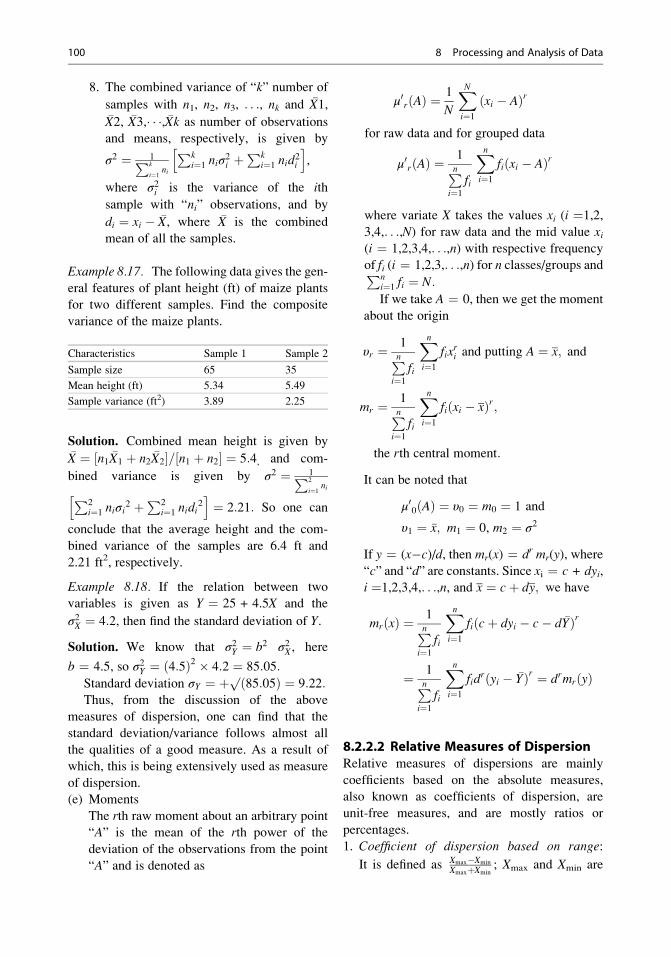
8. The combined variance of “k” number of

samples with n1, n2, n3, . . ., nk and �X1,�X2, �X3,� � �, �Xk as number of observations

and means, respectively, is given by

σ2 ¼ 1Pk

i¼1ni

Pki¼1 niσ

2i þ

Pki¼1 nid

2i

h i,

where σ2i is the variance of the ith

sample with “ni” observations, and by

di ¼ xi � �X, where �X is the combined

mean of all the samples.

Example 8.17. The following data gives the gen-

eral features of plant height (ft) of maize plants

for two different samples. Find the composite

variance of the maize plants.

Solution. Combined mean height is given by�X ¼ n1 �X1 þ n2 �X2½ �= n1 þ n2½ � ¼ 5:4, and com-

bined variance is given by σ2 ¼ 1P2

i¼1niP2

i¼1 niσi2 þP2

i¼1 nidi2

h i¼ 2:21: So one can

conclude that the average height and the com-

bined variance of the samples are 6.4 ft and

2.21 ft2, respectively.

Example 8.18. If the relation between two

variables is given as Y ¼ 25 + 4.5X and the

σ2X ¼ 4:2, then find the standard deviation of Y.

Solution. We know that σ2Y ¼ b2 σ2X, here

b ¼ 4.5, so σ2Y ¼ 4:5ð Þ2 � 4:2 ¼ 85:05:

Standard deviation σY ¼ þp85:05ð Þ ¼ 9:22:

Thus, from the discussion of the above

measures of dispersion, one can find that the

standard deviation/variance follows almost all

the qualities of a good measure. As a result of

which, this is being extensively used as measure

of dispersion.

(e) Moments

The rth raw moment about an arbitrary point

“A” is the mean of the rth power of the

deviation of the observations from the point

“A” and is denoted as

μ0rðAÞ ¼1

N

XNi¼1

ðxi � AÞr

for raw data and for grouped data

μ0rðAÞ ¼1Pn

i¼1

fi

Xni¼1

fiðxi � AÞr

where variate X takes the values xi (i ¼1,2,

3,4,. . .,N) for raw data and the mid value xi(i ¼ 1,2,3,4,. . .,n) with respective frequency

of fi (i ¼ 1,2,3,. . .,n) for n classes/groups andPni¼1 fi ¼ N:

If we take A ¼ 0, then we get the moment

about the origin

υr ¼ 1Pni¼1

fi

Xni¼1

fixri and putting A ¼ x; and

mr ¼ 1Pni¼1

fi

Xni¼1

fi xi � xð Þr;

the rth central moment:

It can be noted that

μ00ðAÞ ¼ υ0 ¼ m0 ¼ 1 and

υ1 ¼ �x; m1 ¼ 0, m2 ¼ σ2

If y ¼ (x�c)/d, then mr(x) ¼ dr mr(y), where

“c” and “d” are constants. Since xi ¼ c + dyi,i ¼1,2,3,4,. . .,n, and x ¼ cþ dy; we have

mrðxÞ ¼ 1Pni¼1

fi

Xni¼1

fiðcþ dyi � c� d �YÞr

¼ 1Pni¼1

fi

Xni¼1

fidrðyi � �YÞr ¼ drmrðyÞ

8.2.2.2 Relative Measures of DispersionRelative measures of dispersions are mainly

coefficients based on the absolute measures,

also known as coefficients of dispersion, are

unit-free measures, and are mostly ratios or

percentages.

1. Coefficient of dispersion based on range:

It is defined as Xmax�Xmin

XmaxþXmin; Xmax and Xmin are

Characteristics Sample 1 Sample 2

Sample size 65 35

Mean height (ft) 5.34 5.49

Sample variance (ft2) 3.89 2.25

100 8 Processing and Analysis of Data

the maximum and minimum values of

variable “X.”2. Coefficient of dispersion based on quartile

deviation: It is defined asQ3�Q1

2Q3þQ1

2

¼ Q3�Q1

Q3þQ1

3. Coefficient of dispersion based on mean

deviation from mean / median / mode / arbi-

trary point: This measure is given byMD mean=median=mode etc:

Mean=Median=Mode

4. Coefficient of dispersion based on standard

deviation: It is defined as σX�X, where σX and

�X are the standard deviation and arithmetic

mean of variable “X,” respectively. The

more widely used and customary coefficient

of dispersion based on standard deviation is

the “coefficient of variation (CV)” σX�X� 100:

8.2.2.3 Skewness and KurtosisNeither the measure of central tendency nor the

measure of dispersion alone is sufficient to

extract the inherent characteristics of a given set

of data. We need to combine both these measures

together. We can come across with a situation

where two frequency distributions have the same

measures of central tendency as well as measure

of dispersion but they differ widely in their

nature.

Example 8.20. Given below are the two fre-

quency distributions for a number of nuts per

bunch with respective means as 12.62 and 12.11

and standard deviations as 3.77 and 3.484, respec-

tively. Thus, both the distributions have almost the

same measure of central tendency as well as mea-

sure of dispersion. But a close look at the graphs

drawn for the two frequency distributions shows

that they differ widely in nature (Fig. 8.12).

Along with the measures of dispersion and

central tendency, there should be certain

measures which can provide the exact picture of

the given data set. Skewness and kurtosis talk

about the nature of the frequency distribution.

The skewness of a frequency distribution is

the departure of the frequency distribution from

symmetricity.

A frequency distribution is either symmetric

or asymmetric/skewed. Again an asymmetric/

skewed distribution may be positively skewed or

negatively skewed.

Example 8.21. Let us take the example of the

panicle length in three different varieties of

paddy. The frequency distributions and the

corresponding graphical representations are

given in Figs. 8.13, 8.14, and 8.15.

Among the different measures, the measures

based on moments are mostly used and are given

asffiffiffiβ

p1 ¼ γ1 ¼ m3ffiffiffiffi

m32

p , wherem3 andm2 are the 3rd

and 2nd central moments, respectively. It may be

noted that all the measures of skewness have no

units; these are pure numbers and equal to zero

when the distribution is symmetric. Further, it is

to be noted that β1 ¼ m23

m32

� 0. The sign offfiffiffiβ

p1

depends on the sign of m3.

Kurtosis refers to the peakedness of a frequency

distribution.While skewness refers to the horizon-

tal property of the frequency distribution, kurtosis

refers to the vertical nature of the frequency distri-

bution. According to the nature of peak, a distribu-

tion is leptokurtic, mesokurtic, or platykurtic in

nature. Kurtosis is measured in terms of β2 ¼ m4

m22

,

where m4 and m2 are the 4th and 2nd central

moments, respectively. If β2>3, β2 ¼ 3, the distri-

bution ismesokurtic, and if β2 < 3, the distribution

is platykurtic. In the case of a normal distribution

mentioned in Chap. 6, if this is taken as standard,

the quantity β2 � 3 measures the what is known

as excess of kurtosis. If β2 > 3, the distribution

is leptokurtic, and β2 ¼ 3, the distribution is

Symmetric Asymmetric / Skewed

Frequency distribution

Positively skewed Negatively skewed

8.2 Analysis of Data 101

Fig. 8.12 (a) Graphical presentation of a no. of nuts per plant in 179 plants of coconut, (b) Graphical presentation of a

no. of nuts per plant in 159 plants of coconut

Fig. 8.13 Graphical presentation of a symmetric distribution

mesokurtic, and the distribution is platykurtic in

nature. It can be shown that β2 � 1þ β1.

Example 8.22. The frequency distribution of the

length of the leaflet of the three varieties of tube

rose flower is given in Figs. 8.16, 8.17 and 8.18.

It is clear from the corresponding figures that the

three distributions vary widely with respect to the

peakedness of the frequency graph.

A leptokurtic distribution means an aggrega-

tion of more observations (frequency) in a par-

ticular class or a couple of classes. Mesokurtic

distribution follows the general norm that at the

lower classes, there are a fewer number of

frequencies, and as the class value increases,

the number of observations (frequency) also

increases then reaches to the peak, and as the

class value increases further, the number of

observations (frequency) decreases. On the

other hand, in a platykurtic distribution, a good

number of classes have almost the same higher

observations and thereby, forming a platelike

structure at the top of the frequency distribution.

Thus, to know the nature of the data, the

measures of central tendency and measures of

dispersion along with skewness and kurtosis of

the frequency distribution are essential.

With the help of the following example, we

shall demonstrate how these analyses could be

taken up using SAS 9.3.

Example 8.23. The following table gives the

yield attributing characters along with the yield

for 37 varieties. We are to summarize the data in

terms of the different measures of dispersion,

central tendency, skewness, and kurtosis.

Fig. 8.14 Graphical presentation of a positively skewed distribution

Fig. 8.15 Graphical presentation of a negatively skewed distribution

8.2 Analysis of Data 103

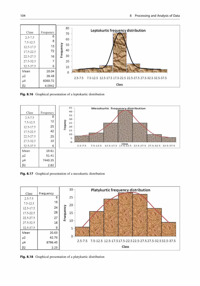
Fig. 8.16 Graphical presentation of a leptokurtic distribution

Fig. 8.17 Graphical presentation of a mesokurtic distribution

Fig. 8.18 Graphical presentation of a platykurtic distribution

104 8 Processing and Analysis of Data

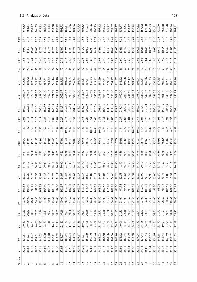
SLNo

X1

X2

X3

X4

X5

X6

X7

X8

X9

X10

X11

X12

X13

X14

X15

X16

X17

X18

X19

Y

132.34

151.81

140.47

21.23

162.67

107.88

23.20

31.33

9.47

149.37

7.55

2.01

195.77

1663.67

313.38

1.93

1.93

9.96

9.49

345.85

229.85

140.71

140.95

20.33

150.00

104.49

23.20

33.17

8.87

144.04

7.82

2.11

222.68

1675.33

298.72

1.93

2.45

14.50

9.45

354.41

332.38

138.77

144.30

18.63

146.00

93.17

22.23

33.33

9.00

145.20

7.90

2.14

219.74

1672.33

302.74

1.90

2.44

15.45

9.33

358.12

438.33

138.31

140.06

17.67

156.33

92.60

22.93

34.50

8.73

141.57

7.67

2.15

228.32

1587.33

263.92

1.57

2.59

15.63

7.93

341.39

537.81

140.23

135.62

18.70

153.67

103.54

23.07

33.50

8.77

133.96

7.72

2.15

207.93

1621.00

277.86

1.53

2.40

13.75

7.73

323.82

635.02

132.90

128.79

18.47

143.00

108.60

23.33

29.00

9.03

145.32

7.97

2.27

189.59

1629.00

267.74

1.34

2.41

13.37

6.91

369.82

732.25

136.10

123.41

19.93

130.00

108.25

23.13

30.33

9.70

149.08

7.80

2.12

161.48

1657.33

264.72

1.72

2.45

13.76

8.44

373.14

832.56

137.11

116.18

18.87

143.67

100.95

23.73

28.17

9.47

133.45

7.83

2.08

146.38

1621.67

241.44

1.74

2.25

12.26

7.98

353.28

934.10

147.68

125.74

19.67

153.00

98.60

24.13

30.33

9.67

132.12

7.88

2.08

162.86

1634.33

253.30

1.95

2.74

15.22

8.94

350.18

10

37.05

153.77

123.49

19.10

160.00

100.17

24.07

30.00

9.23

137.06

8.58

2.27

184.37

1702.67

263.88

1.77

2.74

15.05

8.18

394.78

11

43.70

161.64

124.89

19.07

166.33

112.08

27.57

25.93

10.30

147.31

10.19

2.73

239.65

1785.67

286.02

1.77

2.73

14.98

8.67

489.41

12

41.96

160.23

114.79

19.60

143.67

107.01

26.27

24.83

10.23

135.48

9.17

2.40

237.48

1693.00

284.65

1.86

2.20

11.29

8.54

416.26

13

38.29

144.75

115.58

20.03

143.00

107.58

26.63

26.17

9.80

129.08

8.97

2.52

201.06

1609.00

276.24

1.74

2.47

12.21

8.01

384.56

14

33.84

155.17

117.81

19.33

157.00

102.07

25.27

24.83

9.17

130.27

7.72

2.16

178.28

1496.00

294.98

1.67

2.29

11.29

7.76

327.73

15

34.56

148.67

119.07

16.67

164.33

116.45

25.87

24.50

9.33

130.48

8.55

2.43

188.79

1511.67

288.41

1.32

2.33

11.52

6.68

363.85

16

32.46

156.00

121.01

20.10

162.67

115.48

25.50

22.50

9.07

138.49

8.38

2.25

202.79

1547.33

307.51

1.44

2.05

10.52

7.22

371.94

17

34.01

156.99

138.86

21.83

144.00

117.92

25.07

27.40

9.10

151.50

10.06

2.54

216.33

1662.67

316.73

1.42

2.66

14.93

7.46

505.86

18

34.58

162.46

145.61

23.90

149.33

104.79

25.17

29.67

9.20

144.95

10.46

2.60

220.73

1685.33

313.12

1.49

2.58

14.54

7.77

502.73

19

34.22

166.22

153.17

22.73

155.67

108.22

24.67

33.83

9.07

150.81

10.01

2.56

208.66

1738.67

288.29

1.85

3.05

17.96

9.29

495.12

20

33.13

162.80

143.02

23.10

144.00

109.56

24.03

30.60

8.93

131.19

8.64

2.34

168.35

1668.33

247.84

1.55

2.40

13.12

7.58

359.93

21

34.27

168.36

135.34

21.20

163.33

115.47

23.13

26.50

11.93

132.39

7.50

1.98

131.32

1711.33

239.02

2.07

2.19

12.33

8.40

325.47

22

31.85

163.56

129.03

20.53

154.67

102.78

24.60

29.00

12.87

117.91

7.89

2.02

117.85

1653.00

234.97

1.81

2.02

10.43

7.41

298.67

23

29.36

160.86

129.24

21.17

193.67

99.50

20.80

37.60

12.50

117.78

7.99

2.11

158.37

1701.67

211.97

2.13

2.38

12.65

8.86

299.57

24

35.01

154.62

140.06

21.53

171.00

90.33

22.53

42.50

9.50

129.01

8.64

2.37

218.03

1692.00

244.12

1.66

2.60

13.66

8.31

356.87

25

35.71

161.44

145.13

22.40

181.00

98.85

21.87

36.73

9.67

131.64

8.67

2.62

263.96

1764.00

289.06

1.87

2.88

15.42

9.13

372.53

26

38.24

159.29

144.58

19.73

161.67

93.00

24.57

37.50

10.57

140.35

9.84

2.84

223.82

1744.67

312.47

1.96

2.65

14.10

9.53

453.42

27

35.36

147.69

144.01

21.93

182.33

104.51

24.37

36.50

10.87

135.28

10.06

2.70

216.55

1747.33

289.87

1.71

2.53

13.53

8.67

450.74

28

33.81

139.24

145.32

22.97

178.00

105.69

23.20

34.50

9.90

137.24

10.00

2.45

197.75

1698.67

286.04

1.49

2.02

10.29

7.83

449.22

29

34.44

139.44

146.65

22.63

193.00

112.40

23.90

29.50

8.50

155.76

8.94

2.08

238.45

1624.00

333.34

1.39

2.01

10.28

7.65

457.62

30

36.05

151.53

154.25

23.53

194.00

103.77

24.10

31.17

8.73

149.60

8.58

2.25

236.20

1542.33

306.56

1.79

2.04

10.45

8.28

420.00

31

37.34

157.67

151.84

21.63

195.33

102.57

24.90

33.50

10.90

161.70

8.42

2.20

232.85

1582.33

291.33

1.76

2.05

10.76

8.12

442.93

32

33.13

151.16

143.56

24.53

191.00

98.26

25.00

29.50

11.03

135.25

7.69

2.20

203.45

1588.33

250.95

2.15

1.80

9.63

7.10

331.91

33

30.20

144.68

133.70

21.73

176.00

95.76

22.50

35.83

10.50

140.91

6.96

1.94

154.35

1611.00

277.85

1.89

2.00

10.19

7.25

321.00

34

30.26

140.64

119.93

21.93

178.67

94.23

20.77

37.67

9.30

128.65

7.12

2.13

159.38

1601.00

286.54

1.89

1.99

10.35

7.28

283.70

35

31.27

141.59

123.96

19.37

180.67

105.51

18.00

35.33

8.93

133.87

6.65

1.91

205.68

1648.00

302.31

1.74

2.23

12.42

8.15

276.98

36

33.17

150.82

131.18

18.80

178.67

107.36

17.37

31.17

9.23

143.59

6.68

1.92

206.11

1634.00

306.61

2.08

2.12

11.87

9.09

300.94

37

32.15

151.23

137.13

22.37

179.67

112.17

20.13

30.83

8.90

143.36

6.83

1.81

203.41

1650.33

304.86

2.12

2.15

11.52

9.27

295.61

8.2 Analysis of Data 105

1. Analysis Through MS Excel

If one wants to perform the above analyses

using MS Excel software, then one should

follow the following steps:

Step 1: Go to Data Analysis submenu of Data

in MS Excel. Select Descriptive Statistics

as shown below.

Step 2: Provide the input range and the output

range (where the output is to be placed up

on analysis), and tick on to Summary

Statistics as shown below.

Slide 8.5: Step 1 showing the entry or the transformation of data to Excel data sheet and Data Analysis menu selection

Slide 8.6: Step 2 showing the selection of appropriate menus in Descriptive Data Analysis menu of MS Excel

106 8 Processing and Analysis of Data

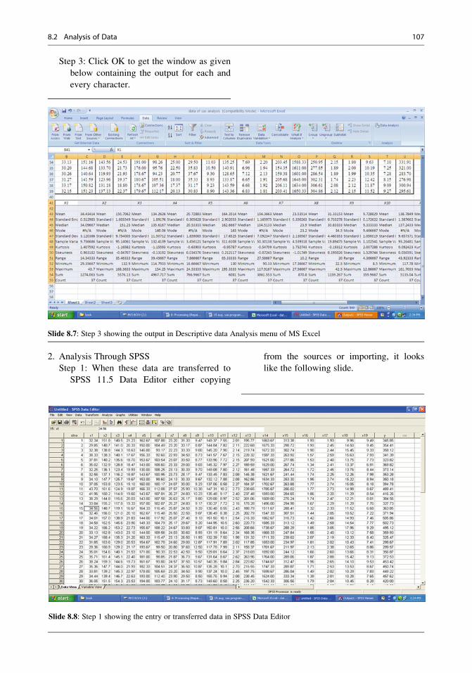
Step 3: Click OK to get the window as given

below containing the output for each and

every character.

2. Analysis Through SPSS

Step 1: When these data are transferred to

SPSS 11.5 Data Editor either copying

from the sources or importing, it looks

like the following slide.

Slide 8.7: Step 3 showing the output in Descriptive data Analysis menu of MS Excel

Slide 8.8: Step 1 showing the entry or transferred data in SPSS Data Editor

8.2 Analysis of Data 107

Step 2: Go to Analysis menu followed by

Descriptive Statistics and Descriptive as

shown below.

Step 3: Select the variable for which one

wants the Descriptive Statistics and then

click on to Option menu as shown below.

Slide 8.9: Step 2 showing the selection of appropriate Data Analysis menu in SPSS analysis

Slide 8.10: Step 3 showing the selection of appropriate variables for Analysis menu in SPSS

108 8 Processing and Analysis of Data

Step 4: From Options, select the required

measures as shown below and click on to

Continue.

Step 5: Click on to OK as given below to get

the output.

Slide 8.11: Step 4 showing the selection of appropriate Analysis submenu of SPSS

Slide 8.12: Step 4 showing the appropriate command to get the output in Analysis submenu of SPSS

8.2 Analysis of Data 109

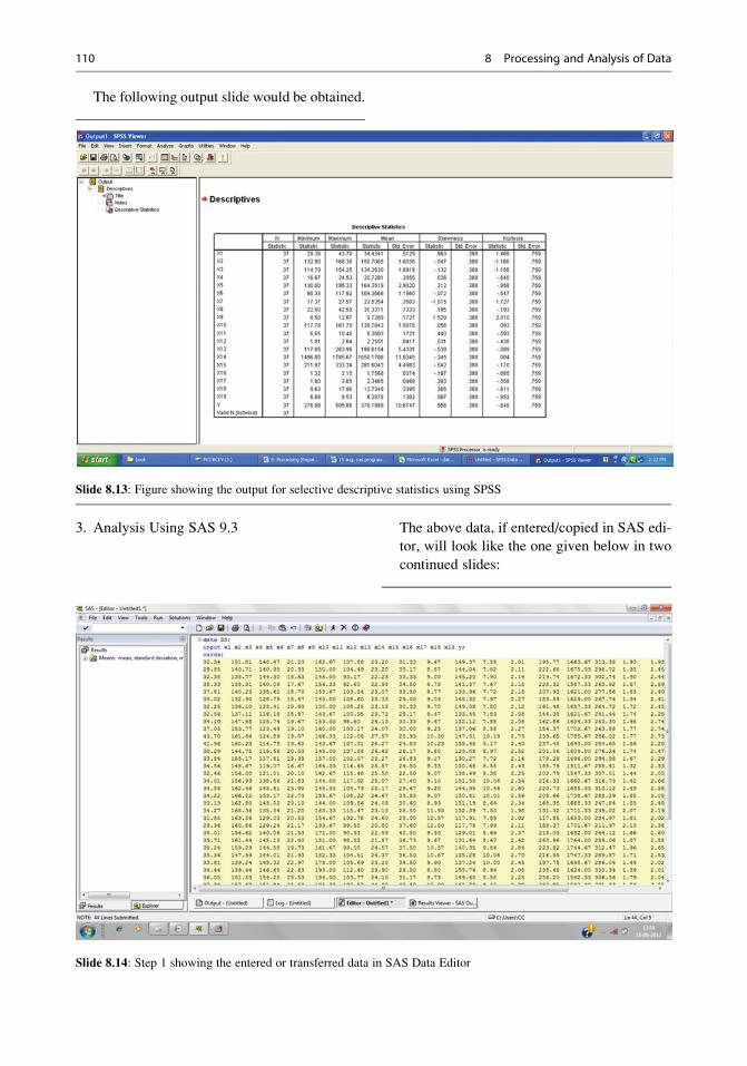
The following output slide would be obtained.

3. Analysis Using SAS 9.3 The above data, if entered/copied in SAS edi-

tor, will look like the one given below in two

continued slides:

Slide 8.13: Figure showing the output for selective descriptive statistics using SPSS

Slide 8.14: Step 1 showing the entered or transferred data in SAS Data Editor

110 8 Processing and Analysis of Data

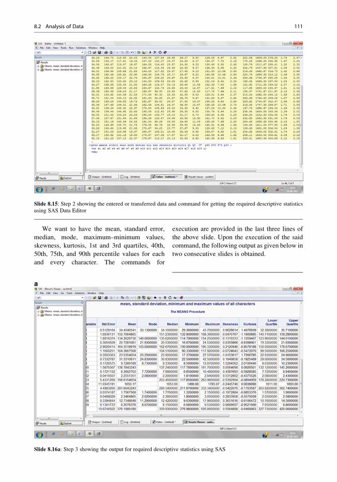
We want to have the mean, standard error,

median, mode, maximum–minimum values,

skewness, kurtosis, 1st and 3rd quartiles, 40th,

50th, 75th, and 90th percentile values for each

and every character. The commands for

execution are provided in the last three lines of

the above slide. Upon the execution of the said

command, the following output as given below in

two consecutive slides is obtained.

Slide 8.15: Step 2 showing the entered or transferred data and command for getting the required descriptive statistics

using SAS Data Editor

Slide 8.16a: Step 3 showing the output for required descriptive statistics using SAS

8.2 Analysis of Data 111

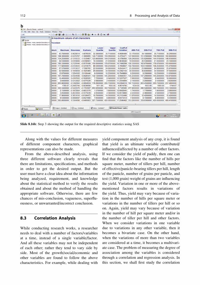
Along with the values for different measures

of different component characters, graphical

representations can also be made.

From the above-described analysis, using

three different software clearly reveals that

there are limitations, specifications, and methods

in order to get the desired output. But the

user must have a clear idea about the information

being analyzed, requirement, and knowledge

about the statistical method to verify the results

obtained and about the method of handling the

appropriate software. Otherwise, there are few

chances of mis-conclusion, vagueness, superflu-

ousness, or unwarranted/incorrect conclusion.

8.3 Correlation Analysis

While conducting research works, a researcher

needs to deal with a number of factors/variables

at a time, instead of a single variable/factor.

And all these variables may not be independent

of each other; rather they tend to vary side by

side. Most of the growth/social/economic and

other variables are found to follow the above

characteristics. For example, while dealing with

yield component analysis of any crop, it is found

that yield is an ultimate variable contributed/

influenced/affected by a number of other factors.

If we consider the yield of paddy, then one can

find that the factors like the number of hills per

square meter, number of tillers per hill, number

of effective/panicle-bearing tillers per hill, length

of the panicle, number of grains per panicle, and

test (1,000 grain) weight of grains are influencing

the yield. Variation in one or more of the above-

mentioned factors results in variations of

the yield. Thus, yield may vary because of varia-

tion in the number of hills per square meter or

variations in the number of tillers per hill or so

on. Again, yield may vary because of variation

in the number of hill per square meter and/or in

the number of tiller per hill and other factors.

When we consider variations in one variable

due to variations in any other variable, then it

becomes a bivariate case. On the other hand,

when the variations of more than two variables

are considered at a time, it becomes a multivari-

ate case. The problem of measuring the degree of

association among the variables is considered

through a correlation and regression analysis. In

this section, we shall first study the correlation

Slide 8.16b: Step 3 showing the output for the required descriptive statistics using SAS

112 8 Processing and Analysis of Data

and then go for the study of the form of the

association, that is, the regression analysis.

The simplest and widely used measure of

correlation is the measure of Karl Pearson’s

correlation coefficients. Correlation coefficient

measures the degree of closeness of the linearassociation between any two variables and is

given as

rxy ¼ Cov x;yð Þsx:sy , where (x1,y1), (x2,y2), (x3,y3),. . .,

(xn,yn) are n pairs of observations and

ðiÞ Cov x; yð Þ ¼ 1

n

Xni¼1

xi � �xð Þ yi � �yð Þ ¼ Sxy

ðiiÞ s2x ¼1

n

Xni¼1

xi � �xð Þ2 and

ðiiiÞ s2y ¼1

n

Xni¼1

yi � �yð Þ2

Thus, rxy ¼1n

Pni¼1

xiyi��x�yffiffiffiffiffiffiffiffiffiffiffiffiffiffiffiffiffiffiffiffiffiffiffiffiffiffiffiffiffiffiffiffiffiffiffiffiffiffiffiffiffiffiffiffiffiffiffiffi1n

Pni¼1

xi2��x2

� �1n

Pni¼1

yi2��y2

� �s :

It may be noted that we have considered

two variables x and y irrespective of their

dependency.

Properties of Correlation Coefficient:

1. The correlation coefficient between any two

variables is independent of change of origin

and scale in value but depends on the signs

of scales.

Let us consider (x1,y1), (x2,y2), (x3,y3),. . .,

(xn,yn), the n pairs of observations for the two

characters x and y having the means �x and �y

and the variances S2x and S2y . We take another

two variables such that, xi ¼ aþ bui and yi ¼cþ dvi ) x ¼ aþ bu and y ¼ cþ dv, and

S2x ¼ b2S2u and S2y ¼ d2S2v ; i ¼ 1,2,3,. . .,n

and a, b, c, and d are constants, and a and c

are changes of origin and b and d are changes

of scale.

So,

Cov x; yð Þ ¼ 1

n

Xi

ðxi � �xÞðyi � �yÞ

¼ bdCov u; vð Þ:

Thus, the correlation coefficient between x

and y becomes

rxy ¼ Cov x; yð ÞffiffiffiffiffiffiffiffiffiffiS2x :S

2y

q ¼ b:d

bj j: dj j :ruv:

Thus, the numerical value of rxy and ruv are the

same. But, the sign of ruv depends on the sign

of b and d. If both b and d are of the same sign,

then rxy ¼ ruv; on the other hand, if b and d are

of the opposite signs, then rxy ¼ �ruv.

2. The correlation coefficient rxy lies between

�1 and +1, that is, � 1 � rxy � þ1.

3. The correlation coefficient between x and yis same as the correlation coefficient between

y and x.

4. Being a ratio, a correlation coefficient is a

unit-free measure. So, it can be used to compare

the degree of the linear association between

the different pairs of the variables.

5. The two independent variables are uncorre-

lated, but the converse may not be true. Let

us consider the following two variables:

Therefore, rxy ¼ Cov x;yð ÞSx:Sy

¼1n

Pni¼1

xiyið Þ��x:�y

Sx:Sy¼

19:0�0:60

9

Sx:Sy¼ 0:

Clearly, the relationship is y ¼ x2 between xand y. Thus, the zero correlation coefficient

between the two variables does not necessarily

mean that the variables are independent.

x �4 �3 �2 �1 0 1 2 3 4P

x ¼ 0

y 16 9 4 1 0 1 4 9 16P

y ¼ 60

xy �64 �27 �8 �1 0 1 8 27 64P

xy ¼ 0

8.3 Correlation Analysis 113

Examples 8.24. Given below are the plant height

(cm) and the no. of fruits per plant in eight varieties

of lady fingers. Find out whether the height and the

weight of the boys are correlated or not.

At first, we calculate the following quantities:

�x ¼ 1

8

X8i¼1

xi ¼208; �y ¼ 1

8

X8i¼1

yi ¼72:

We have

ðiÞ Cov x; yð Þ ¼ 1

n

Xni¼1

xi � �xð Þ yi � �yð Þ ¼ 1

8

Xni¼1

xiyi � �x�y ¼ 3

ðiiÞ s2x ¼1

n

Xni¼1

xi � �xð Þ2 ¼ 1

n

Xni¼1

xi2 � �x2

!¼ 5:143

ðiiiÞ s2y ¼1

n

Xni¼1

yi � �yð Þ2 ¼ 1

n

Xni¼1

yi2 � �y2

!¼ 6:286

rxy ¼1n

Pni¼1

xiyi � �x�yffiffiffiffiffiffiffiffiffiffiffiffiffiffiffiffiffiffiffiffiffiffiffiffiffiffiffiffiffiffiffiffiffiffiffiffiffiffiffiffiffiffiffiffiffiffiffiffiffiffiffiffiffiffiffiffiffiffiffiffiffiffiffi1n

Pni¼1

xi2 � �x2� �

1n

Pni¼1

yi2 � �y2� �s

¼ 3ffiffiffiffiffiffiffiffiffiffiffiffiffiffiffiffiffiffiffiffiffiffiffiffiffiffiffiffiffiffi5:143ð Þ 6:286ð Þp ¼ 0:527:

So the correlation coefficient between the

height and weight of 8 boys of class nine is 0.603.

Example 8.25. Using the same problem given in

Example 8.21, we shall try to get the correlation

coefficients among the variables using MS Excel,

SPSS, and SAS as shown in the following slides:

(a) Using MS Excel software

Height (X) 205 206 208 207 209 207 210 212

No of fruit (Y) 70 71 75 68 75 71 72 74

Slide 8.17: Step 1 showing the entered or transferred data and selection of Correlation Analysis menu in MS Excel work

sheet

114 8 Processing and Analysis of Data

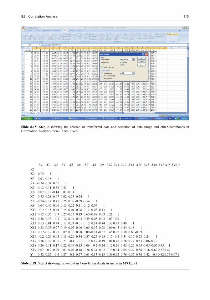
Slide 8.18: Step 2 showing the entered or transferred data and selection of data range and other commands in

Correlation Analysis menu in MS Excel

X1 X2 X3 X4 X5 X6 X7 X8 X9 X10 X11 X12 X13 X14 X15 X16 X17 X18 X19 YX1 1X2 0.22 1

X3 -0.03 0.18 1X4 -0.24 0.34 0.61 1X5 -0.13 0.11 0.38 0.43 1X6 0.07 0.19 -0.14 0.01 -0.14 1X7 0.55 0.28 -0.07 0.02 -0.33 0.24 1X8 -0.24 -0.14 0.47 0.25 0.39 -0.69 -0.54 1X9 -0.04 0.45 -0.06 0.13 0.22 -0.11 0.12 0.07 1X10 0.2 -0.15 0.49 0.15 0.04 0.26 0.11 -0.08 -0.43 1X11 0.52 0.36 0.3 0.27 -0.13 0.19 0.65 -0.08 0.03 0.21 1X12 0.58 0.33 0.2 0.12 -0.14 0.03 0.59 0.03 0.02 0.07 0.9 1X13 0.53 0.01 0.44 0.11 0.24 -0.01 0.12 0.14 -0.44 0.52 0.43 0.48 1X14 0.23 0.35 0.27 0.19 -0.07 -0.06 -0.05 0.37 0.28 0.00 0.45 0.44 0.18 1X15 0.12 -0.12 0.27 0.09 0.13 0.28 0.00 -0.11 -0.57 0.65 0.22 0.18 0.63 -0.09 1X16 -0.2 0.26 0.05 0.18 0.29 -0.34 -0.37 0.27 0.45 -0.17 -0.4 -0.31 -0.17 0.28 -0.24 1X17 0.36 0.22 0.07 -0.21 -0.4 -0.1 0.19 0.17 -0.19 0.01 0.48 0.58 0.27 0.53 -0.06 -0.12 1X18 0.26 0.11 0.17 -0.22 -0.44 -0.13 0.06 0.2 -0.24 0.12 0.36 0.43 0.26 0.53 -0.05 -0.05 0.95 1X19 0.07 0.2 0.29 0.01 0.02 -0.18 -0.26 0.34 0.02 0.19 0.04 0.05 0.29 0.58 0.16 0.62 0.37 0.42 1Y 0.52 0.25 0.4 0.27 -0.1 0.27 0.61 -0.13 -0.13 0.56 0.92 0.76 0.52 0.36 0.42 -0.4 0.42 0.35 0.07 1

Slide 8.19: Step 3 showing the output in Correlation Analysis menu in MS Excel

8.3 Correlation Analysis 115

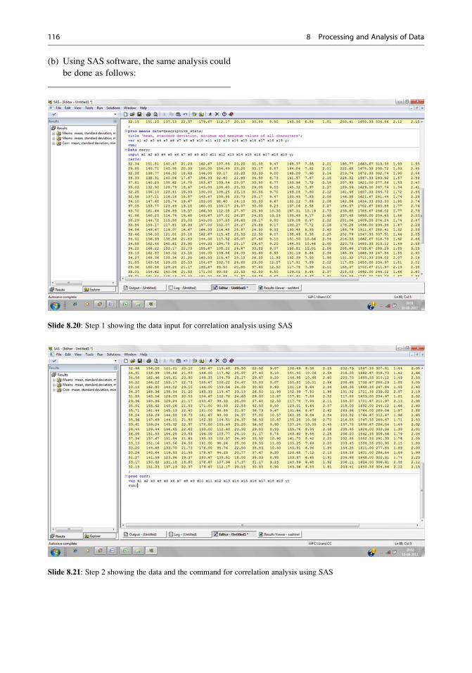
(b) Using SAS software, the same analysis could

be done as follows:

Slide 8.20: Step 1 showing the data input for correlation analysis using SAS

Slide 8.21: Step 2 showing the data and the command for correlation analysis using SAS

116 8 Processing and Analysis of Data

The following is the output of the same

analysis through SPSS.

Slide 8.22: Step 3 showing the SAS output for correlation analysis

Slide 8.23: Data imputed for correlation analysis through SPSS

8.3 Correlation Analysis 117

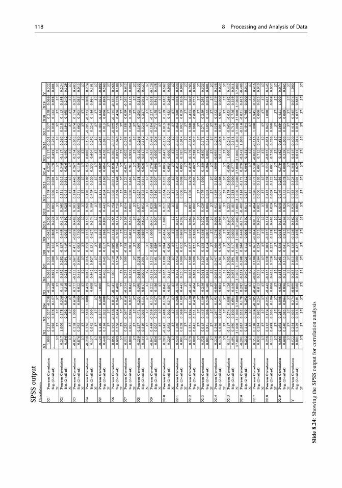
Slide8.24:ShowingtheSPSSoutputforcorrelationanalysis

118 8 Processing and Analysis of Data

Significance of the Values of Correlation

Coefficients:1. A positive correlation coefficient between any

two variables means both the variables move

in the same direction.

2. A negative correlation between any two

variables means if there is an increase or

decrease in one variable, then there will be a

decrease/increase, respectively, in the other

variables.

3. As the numerical value of correlation coeffi-

cient approaches 1, the degree of linear asso-

ciation becomes more and more intense

(Fig. 8.19).

Correlation Coefficient of Bivariate FrequencyDistribution:

Let the two variables X and Y have a joint fre-

quency distribution as follows (Table 8.11):where

Xni¼

Xmj¼1

fij ¼Xni¼1

fi: ¼Xmj¼1

f:j ¼ N:

From the data given in Table 8.11, we shall

calculate the means and variances using the mar-

ginal frequencies and the corresponding mid

values of the classes. The covariance between

the variables will be calculated by taking cell

frequencies and the corresponding mid values

y y y

0 0

0 x x

y

x x

y

(rxy > 0, say 0.8)

(rxy = +1) (rxy = −1)

(rxy < 0, say -0.6) (rxy = 0)0 0

Fig. 8.19 Graphical presentation of different types of correlation coefficient

Table 8.11 Bivariate frequency distribution table

Mid value Mid value (y)

Total(x) y1 y2 y3 . . . yj . . . ym

x1 f11 f12 f13 . . . . . . . . . f1m f1.x2 f21 f22 f23 . . . . . . . . . f2m f2.x3 f31 f32 f33 . . . . . . . . . f3m f3.. . . . . . . . . . . . . . . . . . . . . . . . . . .

xi . . . . . . . . . fij . . . f1m f1.. . . . . . . . . . . . . . . . . . . . . . . . . . .

xn fn1 fn2 fn3 . . . . . . . . . fnm fn.Total f.1 f.2 f.3 . . . f.j f.m

Pi

Pj fij ¼ N

8.3 Correlation Analysis 119

of different class combinations of variables Xand Y. Marginal frequency refers to the total

frequencies of each and every class of the two

variables under consideration. Thus, the mar-

ginal frequency corresponding to the mid value

yj is f.j and that for xi is fi.. So,

x ¼ 1

N

Xni¼1

fi::xið Þ; y ¼ 1

N

Xmj¼1

f:j:yj

:

Similarly,

S2x ¼ 1

N

Xni¼1

fi::x2i � �x2; S2y ¼ 1

N

Xmj¼1

f:j:y2j � �y2

and

Cov x; yð Þ ¼ 1

N

Xi;j

fijxiyj � �x:�y ¼ Sxy:

Example 8.26. The following table gives the

bivariate frequency distribution of the plant

height and the no. of insects per plant. Using

the information, find the correlation coefficient

between the plant height and the no. of insects

per plant.

Height

No. of insects per plant

1–3 3–5 5–7 7–9 9–11 11–13

10–20 0 1 0 0 0 0

20–30 1 2 0 0 0 0

30–40 0 3 2 1 0 0

40–50 1 3 2 1 1 0

50–60 2 2 3 1 0 0

60–70 0 1 2 2 2 0

70–80 0 2 3 3 1 0

80–90 0 1 4 3 2 1

Solution.

�x ¼ 1

N

Xni¼1

fi::xið Þ ¼ 15þ 75þ 210þ . . .þ 935½ �=78 ¼ 3165=53 ¼ 59:716

Similarly,

�y ¼ 1

N

Xmj¼1

f:j:yj ¼ 8þ 60þ . . .þ 12½ �=78 ¼ 324=53 ¼ 6:113

S2x ¼ 1

N

Xni¼1

fi::x2i � �x2 ¼ 209525=53� 59:716ð Þ2 ¼ 387:301

Height

No. of insects per plant

Mid value (x1)

1–3 3–5 5–7 7–9 9–11 11–13

Mid value(x2)

fi. fi.xi fi.xi2

xiPmj¼1

fijyj2 4 6 8 10 12

10–20 15 0 1 0 0 0 0 1 15 225 60

20–30 25 1 2 0 0 0 0 3 75 1,875 250

30–40 35 0 3 2 1 0 0 6 210 7,350 1,120

40–50 45 1 3 2 1 1 0 8 360 16,200 1,980

50–60 55 2 2 3 1 0 0 8 440 24,200 2,090

60–70 65 0 1 2 2 2 0 7 455 29,575 3,380

70–80 75 0 2 3 3 1 0 9 675 50,625 4,500

80–90 85 0 1 4 3 2 1 11 935 79,475 7,140

Total (f.j) 4 15 16 11 6 1 53 3165 209,525 20,520

f.jyj 8 60 96 88 60 12 324 Check

f :jyj2 16 240 576 704 600 144 2,280

yjPni¼1

fijxi360 2,860 6,120 5,960 4,200 1,020 20,520

120 8 Processing and Analysis of Data

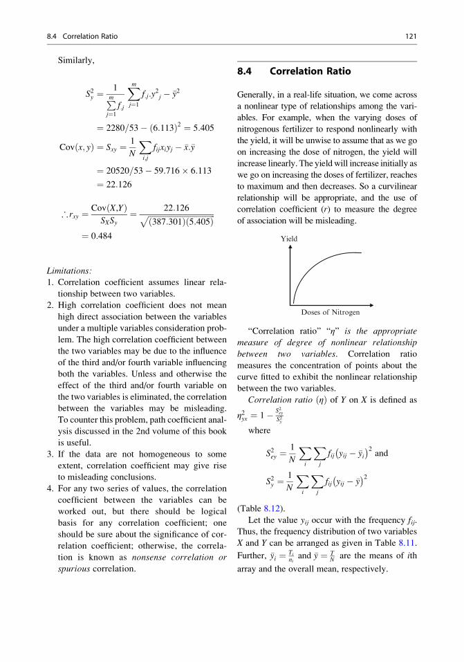
Similarly,

S2y ¼1Pm

j¼1

f:j

Xmj¼1

f:j:y2j � �y2

¼ 2280=53� 6:113ð Þ2 ¼ 5:405

Cov x; yð Þ ¼ Sxy ¼ 1

N

Xi;j

fijxiyj � �x:�y

¼ 20520=53� 59:716� 6:113

¼ 22:126

;rxy ¼ CovðX,YÞSXSy

¼ 22:126ffiffiffiffiffiffiffiffiffiffiffiffiffiffiffiffiffiffiffiffiffiffiffiffiffiffiffiffiffiffiffiffiffiffiffið387:301Þð5:405Þp¼ 0:484

Limitations:

1. Correlation coefficient assumes linear rela-

tionship between two variables.

2. High correlation coefficient does not mean

high direct association between the variables

under a multiple variables consideration prob-

lem. The high correlation coefficient between

the two variables may be due to the influence

of the third and/or fourth variable influencing

both the variables. Unless and otherwise the

effect of the third and/or fourth variable on

the two variables is eliminated, the correlation

between the variables may be misleading.

To counter this problem, path coefficient anal-

ysis discussed in the 2nd volume of this book

is useful.

3. If the data are not homogeneous to some

extent, correlation coefficient may give rise

to misleading conclusions.

4. For any two series of values, the correlation

coefficient between the variables can be

worked out, but there should be logical

basis for any correlation coefficient; one

should be sure about the significance of cor-

relation coefficient; otherwise, the correla-

tion is known as nonsense correlation or

spurious correlation.

8.4 Correlation Ratio

Generally, in a real-life situation, we come across

a nonlinear type of relationships among the vari-

ables. For example, when the varying doses of

nitrogenous fertilizer to respond nonlinearly with

the yield, it will be unwise to assume that as we go

on increasing the dose of nitrogen, the yield will

increase linearly. The yieldwill increase initially as

we go on increasing the doses of fertilizer, reaches

to maximum and then decreases. So a curvilinear

relationship will be appropriate, and the use of

correlation coefficient (r) to measure the degree

of association will be misleading.

Yield

Doses of Nitrogen

“Correlation ratio” “η” is the appropriatemeasure of degree of nonlinear relationship

between two variables. Correlation ratio

measures the concentration of points about the

curve fitted to exhibit the nonlinear relationship

between the two variables.

Correlation ratio ηð Þ of Y on X is defined as

η2yx ¼ 1� S2eyS2y

where

S2ey ¼1

N

Xi

Xj

fij yij � �yi 2

and

S2y ¼1

N

Xi

Xj

fij yij � �y 2

(Table 8.12).

Let the value yij occur with the frequency fij.Thus, the frequency distribution of two variables

X and Y can be arranged as given in Table 8.11.

Further, �yi ¼ Tini

and �y ¼ TN are the means of ith

array and the overall mean, respectively.

8.4 Correlation Ratio 121

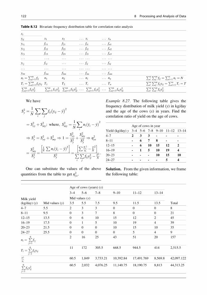
We have

S2y ¼1

N

Xi

Xj

fij yij � �y 2

¼ S2ey þ S2my; where; S2my ¼

1

N

Xi

ni �yi � �yð Þ2

) S2y ¼ S2ey þ S2my ) 1 ¼ S2eyS2y

þ S2myS2y

) η2yx

¼ S2myS2y

¼1N

Pni �yi � �yð Þ2

h iS2y

¼P Ti

2

ni� T

N

2h iPi

Pj

fijy2ij � T2

N

:

One can substitute the values of the above

quantities from the table to get η2yx.

Example 8.27. The following table gives the

frequency distribution of milk yield (y) in kg/day

and the age of the cows (x) in years. Find the

correlation ratio of yield on the age of cows.

Yield (kg/day) y

Age of cows in year

3–4 5–6 7–8 9–10 11–12 13–14

4–7 2 3 3 - - -

8–11 - 6 7 8 - -

12–15 - 6 10 15 12 2

16–19 - 1 5 10 19 4

20–23 - - - 10 15 10

24–27 - - - - 5 4

Solution. From the given information, we frame

the following table:

Milk yield

(kg/day) (y) Mid values (y)

Age of cows (years) (x)

3–4 5–6 7–8 9–10 11–12 13–14

Mid values (x)

3.5 5.5 7.5 9.5 11.5 13.5 Total

4–7 5.5 2 3 3 0 0 0 8

8–11 9.5 0 3 7 8 0 0 21

12–15 13.5 0 6 10 15 12 2 45

16–19 17.5 0 1 5 10 19 4 39

20–23 21.5 0 0 0 10 15 10 35

24–27 25.5 0 0 0 0 5 4 9

ni ¼P6j¼1

fij2 16 25 43 51 20 157

Ti ¼P6j¼1

fijyij11 172 305.5 668.5 944.5 414 2,515.5

T2i

ni60.5 1,849 3,733.21 10,392.84 17,491.769 8,569.8 42,097.122

P6j¼1

fijy2ij

60.5 2,032 4,076.25 11,140.75 18,190.75 8,813 44,313.25

Table 8.12 Bivariate frequency distribution table for correlation ratio analysis

xix1 x2 . . . xi . . . xnyij

yi1 f11 f21 . . . fi1 . . . fn1yi2 f12 f22 . . . fi2 . . . fn2yi3 f13 f23 . . . fi3 . . . fn3. . . . . .. . . . . . . . . . . . . . . .

yij f1j . . . . . . fij . . . fnj

. . . . . . . . . . . . . . . . . . . . .

yim f1m f2m . . . fim . . . fnm

ni ¼Pm

j¼1 fij n1 n2 . . . ni . . . nnPn

i

Pmj fij ¼

Pni¼1 ni ¼ N

Ti ¼Pm

j¼1 fijyij T1 T2 . . . Ti . . . TnPn

i

Pmj fijyij ¼

Pni¼1 Ti ¼ TPm

j¼1 fijy2ij

Pmj¼1 f1jy

21j

Pmj¼1 f2jy

22j

. . .Pm

j¼1 fijy2ij

. . .Pm

j¼1 fnjy2nj

Pni

Pmj fijy

2ij

122 8 Processing and Analysis of Data

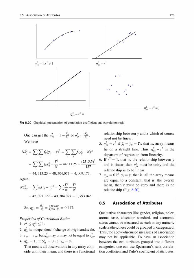
One can get the η2yx ¼ 1� S2eyS2y

or η2yx ¼S2myS2y.

We have

NS2y ¼Xi

Xj

fijðyij � �yÞ2 ¼Xi

Xj

fijy2ij � N�y2

¼Xi

Xj

fijy2ij �

T2

N¼ 44313:25� ð2515:5Þ2

157

¼ 44; 313:25� 40; 304:077 ¼ 4; 009:173:

Again;

NS2my ¼Xi

nið�yi � �yÞ2 ¼X T2

i

ni� T2

N

¼ 42; 097:122� 40; 304:077 ¼ 1; 793:045:

So, η2yx ¼S2myS2y

¼ 1;793:0454;009:173 ¼ 0:447.

Properties of Correlation Ratio:

1. r2 � η2yx � 1.

2. η2yx is independent of change of origin and scale.

3. rxy ¼ ryx, but η2yx may or may not be equal to η2xy.

4. η2yx ¼ 1; if S2ey ¼ 0 i:e: yij ¼ �yi.

That means all observations in any array coin-

cide with their mean, and there is a functional

relationship between y and x which of course

need not be linear.

5. η2yx ¼ r2 if �yi ¼ yij ¼ Yi; that is, array means

lie on a straight line. Thus, η2yx � r2 is the

departure of regression from linearity.

6. If r2 ¼ 1, that is, the relationship between y

and is linear, then η2yx must be unity and the

relationship is to be linear.

7. ηyx ¼ 0 if �yi ¼ �y; that is, all the array means

are equal to a constant, that is, the overall

mean, then r must be zero and there is no

relationship (Fig. 8.20).

8.5 Association of Attributes

Qualitative characters like gender, religion, color,

aroma, taste, education standard, and economic

status cannot be measured as such in any numeric

scale; rather, these could begrouped or categorized.

Thus, the above-discussed measures of association

may not be applicable. To have an association

between the two attributes grouped into different

categories, one can use Spearman’s rank correla-

tion coefficient andYule’s coefficient of attributes.

Fig 8.20 Graphical presentation of correlation coefficient and correlation ratio

8.5 Association of Attributes 123

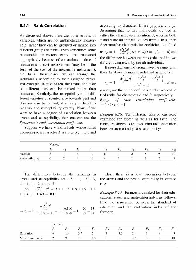
8.5.1 Rank Correlation

As discussed above, there are other groups of

variables, which are not arithmetically measur-

able, rather they can be grouped or ranked into

different groups or ranks. Even sometimes some

measurable characters cannot be measured

appropriately because of constraints in time of

measurement, cost involvement (may be in the

form of the cost of the measuring instrument),

etc. In all these cases, we can arrange the

individuals according to their assigned ranks.

For example, in case of tea, the aroma and taste

of different teas can be ranked rather than

measured. Similarly, the susceptibility of the dif-

ferent varieties of scented rice towards pest and

diseases can be ranked; it is very difficult to

measure the susceptibility exactly. Now, if we

want to have a degree of association between

aroma and susceptibility, then one can use the

Spearman’s rank correlation coefficient.Suppose we have n individuals whose ranks

according to a character A are x1,x2,x3, . . .,xn and

according to character B are y1,y2,y3, . . ., yn.Assuming that no two individuals are tied in

either the classification mentioned, wherein both

x and y are all integral values from 1 to n, then

Spearman’s rank correlation coefficient is defined

as rR ¼ 1� 6P

d2in n2�1ð Þ , where di i ¼ 1; 2; . . . ; nð Þ are

the difference between the ranks obtained in two

different characters by the ith individual.

If more than one individual have the same rank,

then the above formula is redefined as follows:

rR ¼ 1�6P

d2i þ pðp2�1Þ12

þ qðq2�1Þ12

n on n2 � 1ð Þ , where

p and q are the number of individuals involved in

tied ranks for characters A and B, respectively.

Range of rank correlation coefficient:� 1 � rR � þ1.

Example 8.28. Ten different types of teas were

examined for aroma as well as for taste. The

ranks are shown as follows. Find the association

between aroma and pest susceptibility:

The differences between the rankings in

aroma and susceptibility are �3, �1, �3, �3,

4, �1, 1, �2, 1, and 7.

So,Pn

i¼1 d2i ¼ 9 + 1 + 9 + 9 + 16 + 1 +

1 + 4 + 1 + 49 ¼ 100

) rR ¼ 1�6:P10i¼1

d2i

10 10� 1ð Þ ¼ 1� 6:100

10:99¼ 1� 20

33¼ 13

33:

Thus, there is a low association between

the aroma and the pest susceptibility in scented

rice.

Example 8.29. Farmers are ranked for their edu-

cational status and motivation index as follows.

Find the association between the standard of

education and the motivation index of the

farmers:

Farmers

F1 F2 F3 F4 F5 F6 F7 F8 F9 F10

Education 6 10 3.5 5 7 3.5 2 1 9 8

Motivation index 2 9 7 4.5 6 1 4.5 3 8 10

Variety

T1 T2 T3 T4 T5 T6 T7 T8 T9 T10

Aroma: 3 1 6 7 8 4 2 5 9 10

Susceptibility: 6 2 9 10 4 5 1 7 8 3

124 8 Processing and Analysis of Data

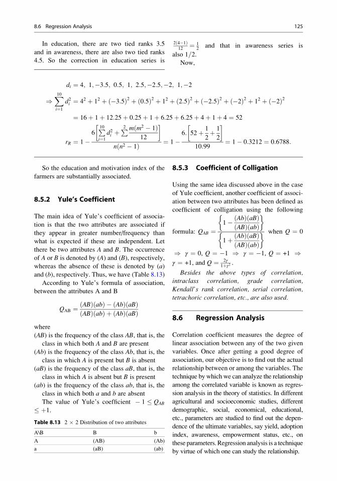
In education, there are two tied ranks 3.5

and in awareness, there are also two tied ranks

4.5. So the correction in education series is

2 4�1ð Þ12

¼ 12

and that in awareness series is

also 1=2.

Now,

di ¼ 4; 1;�3:5; 0:5; 1; 2:5;�2:5;�2; 1;�2

)X10i¼1

d2i ¼ 42 þ 12 þ �3:5ð Þ2 þ 0:5ð Þ2 þ 12 þ 2:5ð Þ2 þ �2:5ð Þ2 þ �2ð Þ2 þ 12 þ �2ð Þ2

¼ 16þ 1þ 12:25þ 0:25þ 1þ 6:25þ 6:25þ 4þ 1þ 4 ¼ 52

rR ¼ 1�6P10i¼1

d2i þP2 m m2 � 1ð Þ

12

� �n n2 � 1ð Þ ¼ 1�

6: 52þ 1

2þ 1

2

� �10:99

¼ 1� 0:3212 ¼ 0:6788:

So the education and motivation index of the

farmers are substantially associated.

8.5.2 Yule’s Coefficient

The main idea of Yule’s coefficient of associa-

tion is that the two attributes are associated if

they appear in greater number/frequency than

what is expected if these are independent. Let

there be two attributes A and B. The occurrence

of A or B is denoted by (A) and (B), respectively,whereas the absence of these is denoted by (a)

and (b), respectively. Thus, we have (Table 8.13)

According to Yule’s formula of association,

between the attributes A and B

QAB ¼ ðABÞðabÞ � ðAbÞðaBÞðABÞðabÞ þ ðAbÞðaBÞ

where

(AB) is the frequency of the class AB, that is, theclass in which both A and B are present

(Ab) is the frequency of the class Ab, that is, the

class in which A is present but B is absent

(aB) is the frequency of the class aB, that is, the

class in which A is absent but B is present

(ab) is the frequency of the class ab, that is, theclass in which both a and b are absent

The value of Yule’s coefficient � 1 � QAB

� þ1.

8.5.3 Coefficient of Colligation

Using the same idea discussed above in the case

of Yule coefficient, another coefficient of associ-

ation between two attributes has been defined as

coefficient of colligation using the following

formula: QAB ¼1� ðAbÞðaBÞ

ðABÞðabÞ �

1þ ðAbÞðaBÞðABÞðabÞ

� when Q ¼ 0

) γ ¼ 0, Q ¼ �1 ) γ ¼ �1, Q ¼ +1 )γ ¼ +1, and Q ¼ 2γ

1þγ2 .

Besides the above types of correlation,intraclass correlation, grade correlation,

Kendall’s rank correlation, serial correlation,

tetrachoric correlation, etc., are also used.

8.6 Regression Analysis

Correlation coefficient measures the degree of

linear association between any of the two given

variables. Once after getting a good degree of

association, our objective is to find out the actual

relationship between or among the variables. The

technique by which we can analyze the relationship

among the correlated variable is known as regres-

sion analysis in the theory of statistics. In different

agricultural and socioeconomic studies, different

demographic, social, economical, educational,

etc., parameters are studied to find out the depen-

dence of the ultimate variables, say yield, adoption

index, awareness, empowerment status, etc., on

these parameters. Regression analysis is a technique

by virtue of which one can study the relationship.

Table 8.13 2 � 2 Distribution of two attributes

A\B B b

A (AB) (Ab)

a (aB) (ab)

8.6 Regression Analysis 125

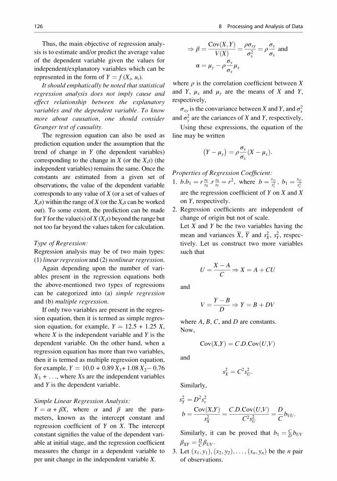
Thus, the main objective of regression analy-

sis is to estimate and/or predict the average value

of the dependent variable given the values for

independent/explanatory variables which can be

represented in the form of Y ¼ f (Xi, ui).

It should emphatically be noted that statisticalregression analysis does not imply cause and

effect relationship between the explanatory

variables and the dependent variable. To knowmore about causation, one should consider

Granger test of causality.

The regression equation can also be used as

prediction equation under the assumption that the

trend of change in Y (the dependent variables)

corresponding to the change in X (or the Xis) (theindependent variables) remains the same. Once the

constants are estimated from a given set of

observations, the value of the dependent variable

corresponds to any value of X (or a set of values of

Xis) within the range of X (or the Xis can be worked

out). To some extent, the prediction can be made

forY for the value(s) ofX (Xis) beyond the range but

not too far beyond the values taken for calculation.

Type of Regression:Regression analysis may be of two main types:

(1) linear regression and (2) nonlinear regression.

Again depending upon the number of vari-

ables present in the regression equations both

the above-mentioned two types of regressions

can be categorized into (a) simple regressionand (b) multiple regression.

If only two variables are present in the regres-

sion equation, then it is termed as simple regres-

sion equation, for example, Y ¼ 12.5 + 1.25 X,

where X is the independent variable and Y is the

dependent variable. On the other hand, when a

regression equation has more than two variables,

then it is termed as multiple regression equation,

for example, Y ¼ 10.0 + 0.89 X1+ 1.08 X2� 0.76

X3 + . . ., where Xs are the independent variables

and Y is the dependent variable.

Simple Linear Regression Analysis:

Y ¼ α + βX, where α and β are the para-

meters, known as the intercept constant and

regression coefficient of Y on X. The intercept

constant signifies the value of the dependent vari-

able at initial stage, and the regression coefficient

measures the change in a dependent variable to

per unit change in the independent variable X.

) β ¼ Cov X; Yð ÞVðXÞ ¼ ρσxy

σ2x¼ ρ

σyσx

and

α ¼ μy � ρσyσx

μx

where ρ is the correlation coefficient between X

and Y, μx and μy are the means of X and Y,

respectively,

σxy is the convariance between X and Y, and σ2xand σ2y are the cariances of X and Y, respectively,

Using these expressions, the equation of the

line may be written

Y � μy ¼ ρ

σyσx

X � μxð Þ:

Properties of Regression Coefficient:

1. b:b1 ¼ r sYsX:r sX

sY¼ r2, where b ¼ sxy

s2x; b1 ¼ sxy

s2y

are the regression coefficient of Y on X and Xon Y, respectively.

2. Regression coefficients are independent of

change of origin but not of scale.

Let X and Y be the two variables having the

mean and variances X, Y and s2X, s2Y , respec-

tively. Let us construct two more variables

such that

U ¼ X � A

C) X ¼ Aþ CU

and

V ¼ Y � B

D) Y ¼ Bþ DV

where A, B, C, and D are constants.

Now,

CovðX,YÞ ¼ C:D:CovðU,VÞand

s2X ¼ C2s2U:

Similarly,

s2Y ¼ D2s2v

b ¼ CovðX,YÞs2X

¼ C:D:CovðU,VÞC2s2U

¼ D

CbVU:

Similarly, it can be proved that b1 ¼ CD bUV

βXY ¼ DC βUV :

3. Let x1; y1ð Þ; x2; y2ð Þ; . . . ; xn; ynð Þ be the n pair

of observations.

126 8 Processing and Analysis of Data

Now, the total sum of squares (y)

TSS ¼Xni¼1

yi � �yð Þ2 ¼Xni¼1

yi � y_ þ y

_ � �y� �2

¼Xni¼1

ðyi � y_Þ2 þ

Xni¼1

ðy_ � �yÞ2;

where y_is the estimate of Y

¼ Residual sum of squares þRegression sum of squares

¼ RSSþ RgSS

;TSS ¼ RSSþ RgSS ) 1 ¼ RSS

TSSþ RgSS

TSS

¼ RSS

TSSþ r2:

Now, we observe thatRgSS

TSS¼ r2 and

RSSTSS

¼ 1� r2:

If we get the calculated value of r2 as 0.55,

we mean that 55% variations are explained by

the regression line, and the remaining 45%

variations are unexplained (Table 8.14).

Example 8.30. The following table gives the

panicle length (X in cm) and the corresponding

yield (Y in q/ha) of paddy in ten different

varieties to find out the degree of linear associa-

tion between the yield and the panicle length of

paddy and to find out the linear relationship of

yield on the panicle length of paddy.

X 18 20 20 22 22 25 26 28 35 40

Y 14 14 15 15 16 18 17 20 22 21

Solution. Let us make the following table:

X Y X2 Y2 XY

18 14 324 196 252

20 14 400 196 280

20 15 400 225 300

22 15 484 225 330

22 16 484 256 352

25 18 625 324 450

26 17 676 289 442

28 20 784 400 560

35 22 1,225 484 770

40 21 1,600 441 840

Mean 25.6 17.2

Variance 44.84 7.76

Covariance 17.28

Correlation coefficient 0.926

We have a no. of observations “n” ¼10, and

the mean and variances and covariance are cal-

culated as per the formula given in Chap. 3. So

the correlation coefficient between the yield and

the panicle length is given by r ¼ Cov(X,Y)/sd

(X).sd(Y). Now, the regression equation of yield

(Y) on the panicle length (X) is given by

ðY � YÞ ¼ byxðX � XÞ

) ðY � 17:2Þ ¼ CovðX:YÞs2X

ðX � 25:6Þ

¼ 17:28

44:84ðX � 25:6Þ

¼ 0:385ðX � 25:6Þ ¼ 0:385x� 9:865

) Y ¼ 17:2þ 0:385X � 9:865

) Y ¼ 7:335þ 0:385X:

Example 8.31. The following data give the num-

ber of insects per hill (X) and the corresponding

yield (Y) of nine different varieties of rice. Work

out the linear relationship between the yield and

the number of insects per hill.

Variety V1 V2 V3 V4 V5 V6 V7 V8 V9

X 16 16 22 23 24 24 25 28 29

Y 55 54 48 47 45 40 44 37 40

Table 8.14 Comparison between the correlation coeffi-

cient and the regression coefficient

Sl

no. Correlation coefficient Regression coefficient

1 Correlation coefficient

(rXY) measures the degree

of linear association

between any two given

variables

Regression coefficient

(bXY ; bYX) measures the

change in dependent

variable due to per unit

change in independent

variable when the

relation is linear

2 Correlation coefficient

does not consider the

dependency between the

variables

One variable is

dependent on the other

variable

3 Correlation coefficient is

a unit-free measure

Regression coefficient

(bXY ; bYX) has the unitdepending upon the units

of the variables under

consideration

4 Correlation coefficient is

independent of the

change of origin and

scale

Regression coefficient

(bXY ; bYX) does notdepend on the change of

origin but depends on the

change of scale

5 � 1 � rXY � þ1 bXY ; bYX does not have

any limit

8.6 Regression Analysis 127

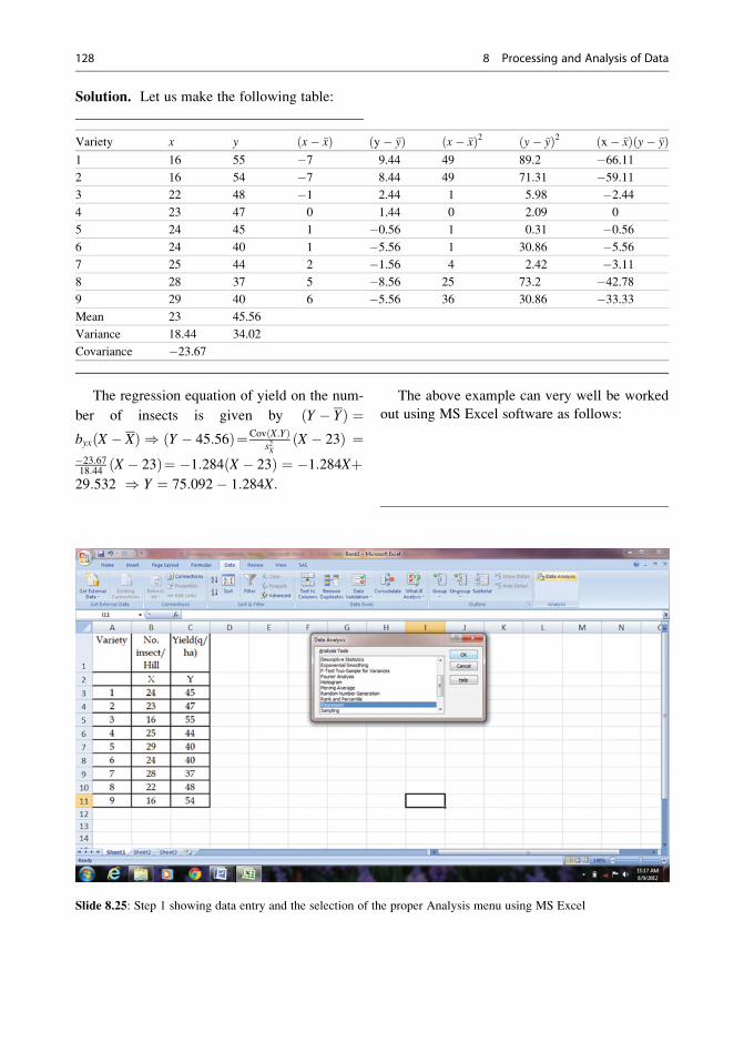
Solution. Let us make the following table:

The regression equation of yield on the num-

ber of insects is given by ðY � YÞ ¼byxðX � XÞ ) ðY � 45:56Þ¼CovðX:YÞ

s2X

ðX � 23Þ ¼�23:6718:44 ðX � 23Þ¼ �1:284ðX � 23Þ ¼ �1:284Xþ29:532 ) Y ¼ 75:092� 1:284X:

The above example can very well be worked

out using MS Excel software as follows:

Variety x y x� �xð Þ y� �yð Þ x� �xð Þ2 y� �yð Þ2 x� �xð Þ y� �yð Þ1 16 55 �7 9.44 49 89.2 �66.11

2 16 54 �7 8.44 49 71.31 �59.11

3 22 48 �1 2.44 1 5.98 �2.44

4 23 47 0 1.44 0 2.09 0

5 24 45 1 �0.56 1 0.31 �0.56

6 24 40 1 �5.56 1 30.86 �5.56

7 25 44 2 �1.56 4 2.42 �3.11

8 28 37 5 �8.56 25 73.2 �42.78

9 29 40 6 �5.56 36 30.86 �33.33

Mean 23 45.56

Variance 18.44 34.02

Covariance �23.67

Slide 8.25: Step 1 showing data entry and the selection of the proper Analysis menu using MS Excel

128 8 Processing and Analysis of Data

Slide 8.26: Step 2 showing data and the selection of proper data range and other submenus in regression analysis using

MS Excel

Slide 8.27: Step 3 showing the output generated in regression analysis using MS Excel

8.6 Regression Analysis 129

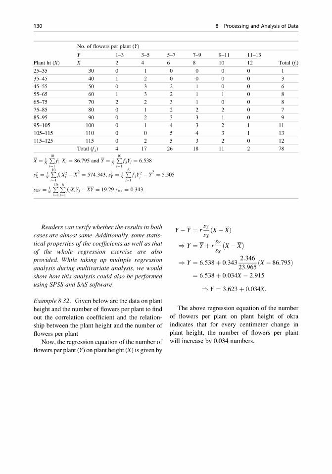
Readers can verify whether the results in both

cases are almost same. Additionally, some statis-

tical properties of the coefficients as well as thatof the whole regression exercise are also

provided. While taking up multiple regression

analysis during multivariate analysis, we wouldshow how this analysis could also be performed

using SPSS and SAS software.

Example 8.32. Given below are the data on plant

height and the number of flowers per plant to find

out the correlation coefficient and the relation-

ship between the plant height and the number of

flowers per plant

Now, the regression equation of the number of

flowers per plant (Y) on plant height (X) is given by

Y � Y ¼ rsYsX

ðX � XÞ

) Y ¼ Y þ rsYsX

X � X

) Y ¼ 6:538þ 0:3432:346

23:965ðX � 86:795Þ

¼ 6:538þ 0:034X � 2:915

) Y ¼ 3:623þ 0:034X:

The above regression equation of the number

of flowers per plant on plant height of okra

indicates that for every centimeter change in

plant height, the number of flowers per plant

will increase by 0.034 numbers.

No. of flowers per plant (Y)

Plant ht (X)

Y 1–3 3–5 5–7 7–9 9–11 11–13

Total (fi)X 2 4 6 8 10 12

25–35 30 0 1 0 0 0 0 1

35–45 40 1 2 0 0 0 0 3

45–55 50 0 3 2 1 0 0 6

55–65 60 1 3 2 1 1 0 8

65–75 70 2 2 3 1 0 0 8

75–85 80 0 1 2 2 2 0 7

85–95 90 0 2 3 3 1 0 9

95–105 100 0 1 4 3 2 1 11

105–115 110 0 0 5 4 3 1 13

115–125 115 0 2 5 3 2 0 12

Total (f.j) 4 17 26 18 11 2 78

X ¼ 1N

P10i¼1

fi: Xi ¼ 86:795 and Y ¼ 1N

P10i¼1

f:jYj ¼ 6:538

s2X ¼ 1N

P10i¼1

fi:X2i � X

2 ¼ 574:343, s2Y ¼ 1N

P6j¼1

f:jY2j� Y

2 ¼ 5:505

sXY ¼ 1N

P10i¼1

P6j¼1

fijXiYj � XY ¼ 19:29 rXY ¼ 0.343.

130 8 Processing and Analysis of Data

Formulation and Testing of Hypothesis 9

The main objective of the researchers is to study

the population behavior to draw the inferences

about the population, and in doing so, in most

of the cases the researcher uses sample

observations. As samples are part of the popula-

tion, there are possibilities of difference in sample

behavior from that of population behavior. Thus,

the process/technique is of knowing accurately

and efficiently the unknown population behavior

from the statistical analysis of the sample behav-

ior—known as statistical inference.

Problems in statistical inference:

(a) Estimation: Scientific assessment of the pop-

ulation characters from sample observations.

(b) Testing of hypothesis: Some information or

some hypothetical values about the popula-

tion parameter may be known or available

but it is required to be tested how far these

information or hypothetical values are

acceptable or not acceptable in the light of

the information obtained from the sample

supposed to have been drawn from the

same population.

9.1 Estimation

Let (x1, x2, x3, . . ., xn) be a random sample drawn

from a population having density f(x/θ) where θis an unknown parameter. Estimation is the prob-

lem of estimating the value θ with the help of thesample observations. There are mainly two types

of estimation, namely, point estimation and

interval estimation.

9.1.1 Point Estimation

Suppose x1, x2, x3, . . ., xn is a random sample

from a density f(x/θ), where θ is an unknown

parametric. Let t be a function of x1, x2, x3, . . .,

xn and is used to estimate θ, then t is called a

point estimator of θ. Among the many estimators

based on sample observations, a good estimator

is one which is (a) unbiased, (b) consistent, and

(c) efficient and sufficient.The details of these properties and their esti-

mation procedures are beyond the scope of this

book.

9.1.2 Interval Estimation

In contrast to the point estimation method, in

interval estimation, we are always in search of a

probability statement about the unknown para-

meter θ of the population from which the sample

has been drawn. If x1, x2, x3, . . ., xn be a random

sample drawn from a population, we shall be

always in search of two functions u1 and u2such that the probability of θ remains in the

interval (u1, u2) is given by a value say 1 � α.Thus, P u1 � θ � u2ð Þ ¼ 1� α. This type of

interval, if exists, is called confidence interval

P.K. Sahu, Research Methodology: A Guide for Researchers in Agricultural Science,Social Science and Other Related Fields, DOI 10.1007/978-81-322-1020-7_9, # Springer India 2013

131

for the parameter θ. u1 and u2 are known as

confidence limits and 1 � α is called the confi-

dence coefficient.

9.2 Testing of Hypothesis

A statistical hypothesis is an assertion about the

population distribution of one or more random

variables belonging to a particular population.

In other words statistical hypothesis is a state-

ment about the probability distribution of popu-

lation characteristics which are to be verified on

the basis of sample information. On the basis of

the amount of information provided by a hypoth-

esis, a statistical hypothesis is either (1) simple or(2) composite. Given a random variable from a

population, a simple hypothesis is a statistical

hypothesis which specifies all the parameters of

the probability distribution of the random vari-

able; otherwise it is a composite hypothesis. For

example, if we say that the height of the Indian

population is distributed normally with mean 5.60

and variance 15.6, then it is a simple hypothesis.

On the other hand, if we say that (1) the height of

the Indian population is distributed normally

with mean 5.60 or (2) the height of the Indian

population is distributed normally with variance

15.6 is composite in nature. Because to specify

the distribution of height which is distributed

normally, we require two information on mean

and variance of the population. Depending upon

the involvement or noninvolvement of the popu-

lation parameter in the statistical hypothesis, it is

again divided into parametric or nonparametric

hypothesis, and corresponding tests are either

parametric test or nonparametric test. Thus, astatistical hypothesis μ ¼ μ0 is a parametric

hypothesis, but testing whether a time series

data is random or not, that is, to test “the series

is random,” is a nonparametric hypothesis.

Any unbiased/unmotivated statistical asser-

tion (hypothesis) whose validity is to be tested

for possible rejection on the basis of sample

observations is called null hypothesis. And the

statistical hypothesis which contradicts the null

hypothesis is called the alternative hypothesis.

For example, against the null hypothesis

H0: μ ¼ μ0, (1) μ 6¼ μ0, (2) μ > μ0, and

(3) μ < μ0 are the alternative hypotheses.In testing of hypothesis, a test statistic is a

function of sample observations whose computed

value when compared with the probability distri-

bution, it follows, leads us to take final decision

with regard to acceptance or rejection of null

hypothesis.

9.2.1 Qualities of Good Hypothesis

1. Hypothesis should be clearly stated.

2. Hypothesis should be precise and stated in

simple form as far as possible.

3. Hypothesis should state the relationships

among the variables.

4. Hypothesis should be in the form of being

tested.

5. Hypothesis should be such that it can be tested

within the research area under purview.

Critical region: Let a random sample x1, x2,x3, . . ., xn be represented by a point x in n-dimen-

sional sample spaceΩ and ω being a subset of the

sample space, defined according to a prescribed

test such that it leads to the rejection of the null

hypothesis on the basis of the given sample if the

corresponding sample point x falls in the subset

ω; the subset ω is known as the critical region of

the test. As it rejects the null hypothesis, it is also

known as the zone of rejection. The complemen-

tary region to the critical region of the sample

space, that is, ω0 or ω, is known as the region ofacceptance. Two boundary values of the critical

region are also included in the region of

acceptance.

Errors in decision: In statistical inference,

drawing inference about the population parame-

ter based on sample observation may lead to the

following situations, and out of the four

situations in two situations, one can commit

errors. (Table 9.1)

9.2.2 Level of Significance

The probability of committing type I error (α) iscalled the level of significance. If the calculated

132 9 Formulation and Testing of Hypothesis

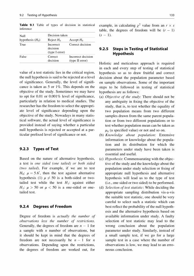
value of a test statistic lies in the critical region,

the null hypothesis is said to be rejected at α level

of significance. Generally, the level of signifi-

cance is taken as 5 or 1%. This depends on the

objective of the study. Sometimes we may have

to opt for 0.01 or 0.001% level of significance,

particularly in relation to medical studies. The

researcher has the freedom to select the appropri-

ate level of significance depending upon the

objective of the study. Nowadays in many statis-

tical software, the actual level of significance is

provided instead of saying whether a particular

null hypothesis is rejected or accepted at a par-

ticular prefixed level of significance or not.

9.2.3 Types of Test

Based on the nature of alternative hypothesis,

a test is one sided (one tailed) or both sided

(two tailed). For example, if we are to test

H0: μ ¼ 5:60, then the test against alternative

hypothesis (1) μ 6¼ 50 is a both-sided or two-

tailed test while the test H1: against either

H1: μ > 50 or μ < 50 is a one-sided or one-

tailed test.

9.2.4 Degrees of Freedom

Degree of freedom is actually the number of

observations less the number of restrictions.

Generally, the degrees of freedom are n � 1 for

a sample with n number of observations, but

it should be kept in mind that the degrees of

freedom are not necessarily be n � 1 for n

observations. Depending upon the restrictions,

the degrees of freedom are worked out, for

example, in calculating χ2 value from an r � s

table, the degrees of freedom will be (r � 1)

(s � 1).

9.2.5 Steps in Testing of StatisticalHypothesis

Holistic and meticulous approach is required

in each and every step of testing of statistical

hypothesis so as to draw fruitful and correct

decision about the population parameter based

on sample observations. Some of the important

steps to be followed in testing of statistical

hypothesis are as follows:

(a) Objective of the study: There should not be

any ambiguity in fixing the objective of the

study, that is, to test whether the equality of

two population means from two different

samples drawn from the same parent popula-

tion or from two different populations or to

test whether population mean can be taken as

μ0 (a specified value) or not and so on.

(b) Knowledge about population: Extensive

information or knowledge about the popula-

tion and its distribution for which the

parameters under study have been taken is

essential and useful.

(c) Hypothesis: Commensurating with the objec-

tive of the study and the knowledge about the

population under study selection or fixing of

appropriate null hypothesis and alternative

hypothesis will lead us to the type of test

(i.e., one sided or two sided) to be performed.

(d) Selection of test statistic: While deciding the

appropriate sampling distribution vis-a-vis

the suitable test statistic, one should be very

careful to select such a statistic which can

best reflect the probability of the null hypoth-

esis and the alternative hypothesis based on

available information under study. A faulty

selection of test statistic may lead to the

wrong conclusion about the population

parameter under study. Similarly, instead of

a small sample test, if we go for a large

sample test in a case where the number of

observations is low, we may lead to an erro-

neous conclusion.

Table 9.1 Table of types of decision in statistical

inference

Null

hypothesis (H0)

Decision taken

Reject H0 Accept H0

True Incorrect

decision

(type I error)

Correct decision

False Correct

decision

Incorrect decision

(type II error)

9.2 Testing of Hypothesis 133

(e) Selection of level of significance: Depending

upon the objective of the study, type of param-

eter, type of study object, precision required,

etc., the appropriate level of significance is

required to be decided. Selection of suitable

level of significance (i.e., the region of rejec-

tion) is a must before the testing of hypothesis

actually takes place.

(f) Critical values: Depending upon the type of

test (one sided or both sided), test statistic,

and its distribution, level of significance

values separating the zone of rejection and

the zone of acceptance are to be worked out

from the table of specific corresponding dis-

tribution. Critical region should be selected in

such a way that its power be maximum. A test

is significant (i.e., rejection of null hypo-

thesis) or not significant (acceptance of null

hypothesis) depending upon the values of the

calculated value of the test statistic and the

table value of the statistic at prefixed level of

significance. Fault in selection of the critical

values may lead to a wrong conclusion.

(g) Calculation of test statistic: From the given

information, one needs to accurately calcu-

late the value of the test statistic under null

hypothesis.

(h) Comparison of calculated value of the statis-

tic at prefixed level of significance with that

of the corresponding table value.

(i) Decision with respect to rejection or accep-

tance of null hypothesis.

(j) Drawing conclusion in line with the questions

put forward in the objective of the study.

9.3 Statistical Test Based onNormal Population

1. Test for specified value of population mean

with known population variance

2. Test for specified value of population mean

with unknown population variance

3. Test of significance for specified population

variance with known population mean (μ)4. Test of significance for specified popula-

tion variance with unknown population

mean (μ)

5. Test of equality of two population variances

from two normal populations with known

population means

6. Test of equality of two population variances

from two normal populations with unknown

population means

7. Test for equality of two population means

with known variances

8. Test for equality of two population means

with equal but unknown variance

9. Test for equality of two population means

with unequal and unknown variances—

Fisher–Berhans problem

10. Test equality of two population means under

the given condition of unknown population

variances from a bivariate normal population-

paired t-test

11. Test for significance of population correla-

tion coefficient, that is, H0: ρ ¼ 0 against

H1: ρ 6¼ 0

12. Test for equality of two population variances

from a bivariate normal distribution

13. Test for specified values of intercept and

regression coefficient in a simple linear

regression

14. Test for significance of the population multi-

ple correlation coefficient

15. Test for significance of population partial

correlation coefficient

The above tests are few to maintain but are

not exhaustive.

A. Tests Based on a Normal Population

Depending upon the type of test (i.e., one

sided or both sided) and the level of signifi-

cance, the limiting values of the critical

regions (i.e., region of acceptance and region

of rejection) under standard normal probabil-

ity curve are given as follows (Table 9.2):

Table 9.2 Critical values under standard normal

probability curve

Type of test

Level of

significance

α ¼ 0.05

Level of

significance

α ¼ 0.01

Both-sided test 1.960 2.576

One sided (left tailed) �1.645 �2.330

One sided (right tailed) 1.645 2.330

134 9 Formulation and Testing of Hypothesis

1. Test for Specified Values of Population Mean

with Known Population Variance from aNormal Population

To test H0: μ ¼ μ0 against the alternative

hypotheses H1: ð1Þ μ 6¼ μ0; ð2Þ μ> μ0; andð3Þ μ< μ0 with known population variance σ

2.

The test statistic under the given null

hypothesis is

τ ¼ x� μ0σ=

ffiffiffin

p ;

where x is the sample mean and this τ followsa standard normal distribution.

Conclusion:

(a) For H1: μ 6¼ μ0, reject H0 if the calculated

value of τj j< τα=2, where τα=2 is the table

value of τ at upper α=2 level of significance

(e.g., 1.96 or 2.576 at 5 or 1% level of signif-

icance, respectively); otherwise accept it.

(b) For H1: μ> μ0, reject H0 if the calculated

value of τ> τα, where τα is the table value

of τ at upper α level of significance (e.g.,

1.645 or 2.33 at 5 or 1% level of signifi-

cance, respectively); otherwise accept it.

(c) For H1: μ< μ0, reject H0 if the calculated

value of τ> τ1�α, where τ1�α is the table

value of τ at lower α level of significance

(e.g., �1.645 or �2.33 at 5 or 1% level

of significance, respectively); otherwise

accept it.

Example 9.1. A random sample drawn from

ten students of a college found that the average

weight of the students is 45 kg. Test whether

this average weight of the students be taken as

50 kg at 1% level of significance or not, given

that the weight of the students follows a nor-

mal distribution with variance 9 kg2.

Solution. Given that (1) the population is nor-

mal with variance 9, (2) sample mean (x) is 45and (3) population hypothetical mean is 50.

To test H0: Population mean μ ¼ 50 against

H1: μ 6¼ 50.

This is a both-sided test. As the sample has

been drawn from a normal population with

known variance, the appropriate test statistic

will be

τ ¼ x� μ0σX=

ffiffiffin

p :

For this problem,

τ ¼ 45� 50ffiffiffiffiffiffiffiffiffiffi9=10

p ¼ �5

0:949¼ �5:269:

From the table of the standard normal variate,

we have τ0:01ð¼ 2:576Þ � τj jcal ð¼ 5:269Þ. So

the test is significant at 1% level of significance.

Hence, we reject the null hypothesis, that is,

H0: μ ¼ μ0. So the average student weight is

not 50 kg.

2. Test for Specified Value of Population Meanwith Unknown Population Variance from a

Normal Population

To test H0: μ ¼ μ0 against the alternative

hypotheses H1: ð1Þ μ 6¼ μ0; ð2Þ μ> μ0; andð3Þ μ< μ0 with unknown population

variance σ2.The test statistic under the given null hypothesis

is t ¼ x� μ0 s=ffiffiffin

pð Þ= , where (n � 1) is the

degrees of freedom, and x and s2 are the

sample mean and sample mean square,

s2 ¼ 1n�1

Pni¼1

xi� xð Þ2 (an unbiased estimator

of population variance σ2).Conclusion(a) For H1: μ 6¼ μ0, reject H0 if the calculated

value of t> tα=2;n�1 or cal t< tð1�αÞ=2;n�1 ¼�tα=2;n�1 i:e: cal tj j> tα

2;n�1 where tα=2;n�1

is the table value of t at upper α=2 level ofsignificance with (n � 1) d.f.; otherwise

accept it.

(b) For H1: μ> μ0, reject H0 if the calculated

value of t> tα;n�1, where τα;n�1 is the table

value of t at upper α level of significance

with (n � 1)d.f.; otherwise accept it.

(c) For H1: μ< μ0, reject H0 if the calculated

value of t< t1�α;n�1, where t1�α;n�1 is the

table value of t at lower α level of signifi-

cance with (n � 1)d.f.; otherwise accept it.

9.3 Statistical Test Based on Normal Population 135

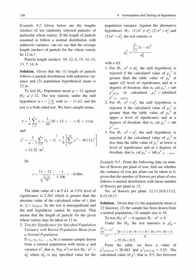
Example 9.2. Given below are the lengths

(inches) of ten randomly selected panicles of

particular wheat variety. If the length of panicle

assumed to follow a normal distribution with

unknown variance, can we say that the average

length (inches) of panicle for the wheat variety

be 12 in.?

Panicle length (inches): 10, 12, 6, 15, 14, 13,

13, 7, 14, 6

Solution. Given that the (1) length of panicle

follows a normal distribution with unknown var-

iance and (2) population hypothetical mean is

12 in.

To test H0: Population mean μ ¼ 12 against

H1: μ 6¼ 12. The test statistic under the null

hypothesis is t ¼ x�μs=ffiffin

p with (n � 1) d.f. and the

test is a both-sided test. We have sample mean,

x ¼ 1

n

Xni¼1

xi ¼ 1

1010þ 12þ � � � þ 6½ � ¼ 11 in:

and

s2 ¼ 1

n� 1

Xni¼1

xi � xð Þ2

¼ 1

9

X101

xi2 � 10:ð11Þ2

" #

¼ 12:22 in2:

So

t ¼ 11� 12ffiffiffiffiffiffiffiffi12:2210

q ¼ �1

1:106¼ �0:904:

The table value of t at 9 d.f. at 2.5% level of

significance is 2.262 which is greater than the

absolute value of the calculated value of t, thatis, tj j< t0:025;9. So the test is nonsignificant and

the null hypothesis cannot be rejected. That

means that the length of panicle for the given

wheat variety may be taken as 12 in.

3. Test for Significance for Specified Population

Variance with Known Population Mean from

a Normal PopulationIf x1, x2, x3,. . ., xn be a random sample drawn

from a normal population with mean μ and

variance σ2, that is, N(μ; σ2) to test H0 : σ2 ¼σ20 where σ20, is any specified value for the

population variance. Against the alternative

hypotheses H1: ð1Þ σ2 6¼ σ20; ð2Þ σ2 > σ2

0; and

ð3Þ σ2 < σ20, the test statistic is

χ2n ¼Pni¼1

ðxi � μÞ2

σ20

with n d.f.

1. For H1 : σ2 6¼ σ20, the null hypothesis is

rejected if the calculated value of χn2 is

greater than the table value of χn2 at

upper α/2 level of significance and at ndegrees of freedom, that is, cal χn

2 > tab

χ2α/2,n or calculated χn2 < tabulated

χ2 (1 � α)/2,n.

2. For H1 : σ2 > σ20, the null hypothesis is

rejected if the calculated value of χn2 is

greater than the table value of χn2 at

upper α level of significance and at n

degrees of freedom, that is, cal χn2 > tab

χ2 α,n.

3. For H1 : σ2 < σ20, the null hypothesis is

rejected if the calculated value of χn2 is

less than the table value of χn2 at lower α

level of significance and at n degrees of

freedom, that is, cal χn2 < tab χ2 (1 � α),n.

Example 9.3. From the following data on num-

ber of flowers per plant of rose, find out whether

the variance of rose per plant can be taken as 6,

given that the number of flowers per plant of rose

follows a normal distribution with mean number

of flowers per plant as 12.

No. of flowers per plant: 12,11,10,9,13,12,

8,15,16,13

Solution. Given that (1) the population mean is

12 (known), (2) the sample has been drawn from

a normal population, (3) sample size is 10.

To test H0: σ2 ¼ 6 against H1 : σ2 6¼ 6.

Under the H0, the test statistics is χ210 ¼Pni¼1

xi�μð Þ2

σ2 ¼ ½0þ1þ4þ9þ1þ0þ16þ9þ16þ1�6

¼ 57=6¼ 9:5:

From the table, we have a value of

χ20.025,10 ¼ 20.483 and χ20.975,10 ¼ 3.25. The

calculated value of χ2, that is, 9.5, lies between

136 9 Formulation and Testing of Hypothesis

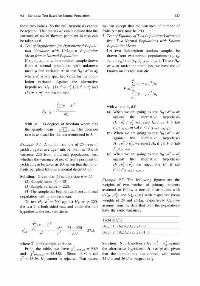
these two values. So the null hypothesis cannot

be rejected. That means we can conclude that the

variance of no. of flowers per plant in rose can

be taken as 6.

4. Test of Significance for Hypothetical Popula-tion Variance with Unknown Population

Mean from a Normal PopulationIf x1, x2, x3,. . ., xn be a random sample drawn

from a normal population with unknown

mean μ and variance σ2 to test H0 : σ2 ¼ σ20where σ2

0is any specified value for the popu-

lation variance. Against the alternative

hypotheses H1: ð1Þ σ2 6¼ σ20; ð2Þ σ2 > σ2

0; and

ð3Þ σ2 < σ20, the test statistic,

χ2ðn�1Þ ¼Pni¼1

ðxi � xÞ2

σ20

with (n � 1) degrees of freedom where x is

the sample mean ¼ 1n

Pni¼1 xi. The decision

rule is as usual for the test mentioned in 3.

Example 9.4. A random sample of 25 trees of

jackfruit gives average fruits per plant as 40 with

variance 220 from a normal population. Test

whether the variance of no. of fruits per plant of

jackfruit can be taken as 200 given that the no. of

fruits per plant follows a normal distribution.

Solution. Given that (1) sample size n ¼ 25.

(2) Sample mean x ¼ 40ð Þ.(3) Sample variance ¼ 220.

(4) The sample has been drawn from a normal

population with unknown mean.

To test H0: σ2 ¼ 200 against H1: σ2 6¼ 200,

the test is a both-sided test, and under the null

hypothesis, the test statistic is

χ224 ¼Pni¼1

xi � xð Þ2

σ2¼ nS2

σ2¼ 25� 220

200¼ 27:5;

where S2 is the sample variance.

From the table, we have χ20.995,24 ¼ 9.89

and χ20.005,24 ¼ 45.558. Since 9.89 < cal

χ2 < 45.56, H0 cannot be rejected. That means

we can accept that the variance of number of

fruits per tree may be 200.

5. Test of Equality of Two Population Variances

from Two Normal Populations with Known

Population MeansLet two independent random samples be

drawn from two normal populations (x1, x2,x3,. . ., xn1 ) and (y1, y2, y3,. . ., yn2 ). To test H0:

σ21 ¼ σ22 under the condition, we have the of

known means test statistic

F ¼Pn1i¼1

ðxi � μ1Þ2=n1Pn2i¼1

ðyi � μ2Þ2=n2

with n1 and n2 d.f.

(a) When we are going to test H0 : σ21 ¼ σ22against the alternative hypothesis

H1 : σ21 6¼ σ22, we reject H0 if cal F > tab

Fα=2;ðn1;n2Þ or cal F < Fð1�α=2Þ;ðn1;n2Þ:(b) When we are going to test H0 : σ21 ¼ σ22

against the alternative hypothesis

H1 : σ21 > σ22, we reject H0 if cal F > tab

Fα=2;ðn1;n2Þ.(c) When we are going to test H0 : σ21 ¼ σ22

against the alternative hypothesis

H1 : σ21 < σ22, we reject the H0 if cal

F < Fð1�α=2Þ;ðn1;n2Þ:

Example 9.5. The following figures are the

weights of two batches of primary students

assumed to follow a normal distribution with

(N μ1; σ21

� �and N μ2; σ

22

� �with respective mean

weights of 24 and 26 kg, respectively. Can we

assume from the data that both the populations

have the same variance?

Yield in t/ha

Batch 1: 16,18,20,22,24,30

Batch 2: 19,22,23,27,29,31,33

Solution. Null hypothesis H0 : σ21 ¼ σ22 against

the alternative hypothesis H1 : σ21 6¼ σ22, given

that the populations are normal with mean

24 t/ha and 26 t/ha, respectively.

9.3 Statistical Test Based on Normal Population 137

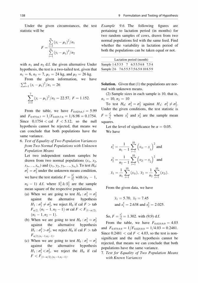
Under the given circumstances, the test

statistic will be

F ¼Pn1i¼1

ðxi � μ1Þ2=n1Pn2i¼1

ðyi � μ1Þ2=n2

with n1 and n2 d.f. the given alternative Under

hypothesis, the test is a two-tailed test, given that

n1 ¼ 6, n2 ¼ 7, μ1 ¼ 24 kg, and μ2 ¼ 26 kg.

From the given information, we haveP6i¼1 ðxi � μ1Þ2=n1 ¼ 26

X7i¼1

ðyi � μ1Þ2=n2 ¼ 22:57; F ¼ 1:152:

From the table, we have F0.025;6,7 ¼ 5.99

and F0:975;6;7 ¼ 1 F0:025;7;6

� ¼ 1 6:98= ¼ 0:1754:

Since 0.1754 < cal F < 5.12, so the null

hypothesis cannot be rejected, that means we

can conclude that both populations have the

same variance.

6. Test of Equality of Two Population Variances

from Two Normal Populations with Unknown

Population MeansLet two independent random samples be

drawn from two normal populations (x1, x2,

x3,. . ., xn1 ) and (y1, y2, y3,. . ., yn2 ). To test H0:

σ21 ¼ σ22 under the unknown means condition,

we have the test statistic F ¼ S21

S22

with (n1 � 1,

n2 � 1) d.f. where S21 & S22 are the sample

mean square of the respective populations.

(a) When we are going to test H0 : σ21 ¼ σ22against the alternative hypothesis

H1 : σ21 6¼ σ22, we reject H0 if cal F > tab

Fα=2; ðn1 � 1; n2 � 1Þ or cal F < Fð1�α=2Þ;ðn1 � 1; n2 � 1Þ:

(b) When we are going to test H0 : σ21 ¼ σ22against the alternative hypothesis

H1 : σ21 > σ22, we reject H0 if cal F > tab

Fα=2;ðn1�1;n2�1Þ.(c) When we are going to test H0 : σ21 ¼ σ22

against the alternative hypothesis

H1 : σ21 < σ22, we reject the H0 if cal

F < Fð1�α=2Þ;ðn1�1;n2�1Þ:

Example 9.6. The following figures are

pertaining to lactation period (in months) for

two random samples of cows, drawn from two

normal populations fed with the same feed. Find

whether the variability in lactation period of

both the populations can be taken equal or not.

Lactation period (month)

Sample 1 4.5 3 5 7 6.5 5.5 6 8 7.5 4

Sample 2 6 7 6.5 5.5 7.5 6.5 8 10 8.5 9

Solution. Given that (1) the populations are nor-

mal with unknown means.

(2) Sample sizes in each sample is 10, that is,

n1 ¼ 10, n2 ¼ 10

To test H0: σ21 ¼ σ22 against H1: σ21 6¼ σ22.Under the given conditions, the test statistic is

F ¼ s21

s22

where s21 and s22 are the sample mean

squares.

Let the level of significance be α ¼ 0.05.

We have

s21 ¼1

n1 � 1

X10i¼1

x1i � �x1

� �2and

s22 ¼1

n2 � 1

X10i¼1

x2i � �x2

� �2and

x1 ¼ 1

n1

X10i¼1

ðx1iÞ; x2 ¼ 1

n2

X10i¼1

ðx2iÞ:

From the given data, we have

x1 ¼ 5:70; x2 ¼ 7:45

and s21 ¼ 2:638 and s22 ¼ 2:025:

So, F ¼ s21

s22

¼ 1:302: with (9,9) d.f.

From the table, we have F0.025;9,9 ¼ 4.03

and F0:975;9;9 ¼ 1 F0:025;9;9

� ¼ 1 4:03= ¼ 0:2481:

Since 0.2481 < cal F < 4.03, so the test is non-

significant and the null hypothesis cannot be

rejected, that means we can conclude that both

populations have the same variance.

7. Test for Equality of Two Population Means

with Known Variances

138 9 Formulation and Testing of Hypothesis

To test the H0: μ1 ¼ μ2 for (x1, x2, x3,. . ., xn1 )and (y1, y2, y3,. . ., yn2 ) two independent

random samples drawn from two normal

populations N μ1; σ21

� �and N μ2; σ

22

� �, respec-

tively, and under the condition of known

variances σ21 and σ22, the test statistic is

τ ¼ x� yffiffiffiffiffiffiffiffiffiffiffiffiffiffiffiσ21n1

þ σ22n2

s ;

when τ is in a standard normal variate.

Example 9.7. The following data are pertaining

to grain yield of two varieties of paddy under the

same management. If the grain yield follows a

normal distribution with known variances 36 and

64, respectively, for two varieties test whether

these two varieties differ significantly with

respect to grain yield (q/ha).

(Grain yield q/ha)

Variety A: 25, 30, 31, 35, 24, 14, 32, 25, 29, 31, 30

Variety B: 30, 32, 28, 36, 42, 18 ,16 , 20 , 22, 40

Solution. Assumption: grain yield follows a

normal distribution. Population variances are

known. Let the level of significance be α ¼ 0.05.

So the null hypothesis is H0: μA ¼ μB (under

known population variances) against alternative

hypothesis H1 : μA 6¼ μB.Under the given condition, the test statistic is

τ ¼ A�Bffiffiffiffiffiffiffiffiffiffiffiffiffiffiffiffiσ2An1

þ σ2Bn2

s which follows as a standard

normal variate.

From the sample observations, we have nA ¼ 11

and nB ¼ 10 and A ¼ 27:82 and B ¼ 28:4

τ ¼ 27:82� 28:4ffiffiffiffiffiffiffiffiffiffiffiffiffi3611þ 64

10

q ¼ �0:58ffiffiffiffiffiffiffiffiffiffiffiffiffiffiffiffiffiffiffiffiffiffiffi3:277þ 6:4

p ¼ �0:58ffiffiffiffiffiffiffiffiffiffiffi9:677

p

¼ �0:58

3:109¼ �0:186:

We know that at α ¼ 0.05, the value of

τα=2 ¼ 1:96, as the calculated τj j< 1:96. So we

cannot reject the null hypothesis. We conclude

that the varieties do not differ significantly with

respect to grain yield.

8. Test for Equality of Two Population Means

with Equal but Unknown Variance

To test the H0: μ1 ¼ μ2 against H1 : μ1 6¼ μ2for (x1, x2, x3,. . ., xn1 ) and (y1, y2, y3,. . ., yn2 )

two independent random samples drawn

from two normal populations N μ1; σ21

� �and

N μ2; σ22

� �, respectively, under the condition

that σ21 ¼ σ22 ¼ σ2 (unknown). The test statis-tic under the given H0 is

t ¼ x� y

s

ffiffiffiffiffiffiffiffiffiffiffiffiffiffiffi1

n1þ 1

n2

r

with (n1 + n2 � 2) degrees of freedom where

s2 ¼ ðn1�1Þs2xþðn2�1Þs2yn1þn2�2

and s2x and s2y are the

sample mean squares for two samples,

respectively.

If the calculated absolute value of t is greaterthan the table value of t at upper α 2= level of

significance and at (n1 þ n2 � 2) d.f., then the

test is significant and the null hypothesis is

rejected; that means the two population means

are unequal.

Note: This test statistic is known as two-

sample t statistic or Fisher’s t statistic. Before

performing the test we are to test first

H0 : σ21 ¼ σ22 by F-test as already discussed.

If it is accepted, then we perform t-test statis-

tic; otherwise not. In that situation we perform

the following test.

Example 9.8. Given below are the two samples

about the vase life of two varieties of tuberose. Is it

possible to draw inference that the vase life of

variety A is more than that of the variety B, assum-

ing that vase life behaves like a normal population?

Sample

size

Sample

mean

Sample mean

square

Variety A 7 72 h 36 h2

Variety B 8 64 h 25 h2

Solution. H0: Both the varieties of tuberose

have the same vase life, that is, H0: μ1 ¼ μ2against the alternative hypothesis, H1: Variety

9.3 Statistical Test Based on Normal Population 139

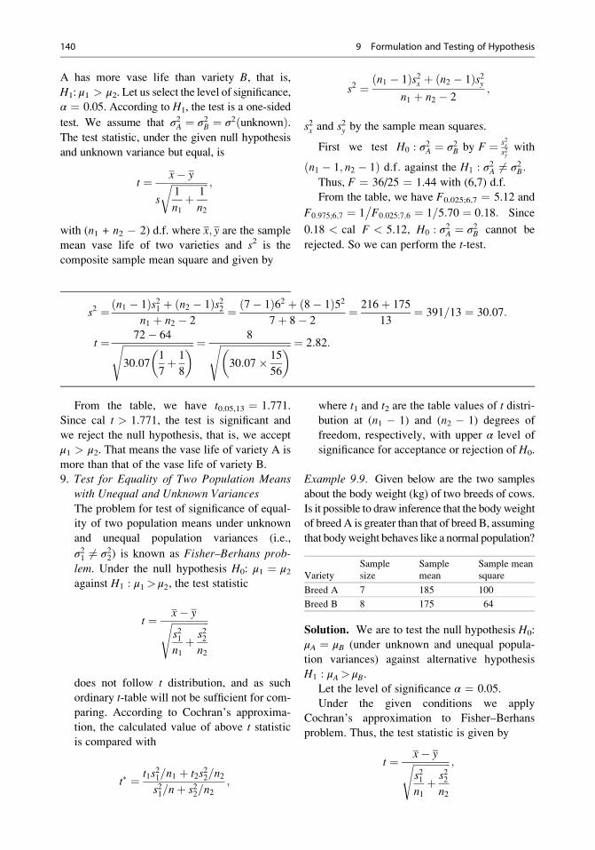
A has more vase life than variety B, that is,

H1: μ1 > μ2. Let us select the level of significance,α ¼ 0.05. According to H1, the test is a one-sided

test. We assume that σ2A ¼ σ2B ¼ σ2ðunknownÞ.The test statistic, under the given null hypothesis

and unknown variance but equal, is

t ¼ x� y

s

ffiffiffiffiffiffiffiffiffiffiffiffiffiffiffi1

n1þ 1

n2

r ;

with (n1 + n2 � 2) d.f. where x; y are the sample

mean vase life of two varieties and s2 is the

composite sample mean square and given by

s2 ¼ ðn1 � 1Þs2x þ ðn2 � 1Þs2yn1 þ n2 � 2

;

s2x and s2y by the sample mean squares.

First we test H0 : σ2A ¼ σ2B by F ¼ s2xs2y

with

ðn1 � 1; n2 � 1Þ d:f: against the H1 : σ2A 6¼ σ2B:Thus, F ¼ 36/25 ¼ 1.44 with (6,7) d.f.

From the table, we have F0.025;6,7 ¼ 5.12 and

F0:975;6;7 ¼ 1 F0:025;7;6

� ¼ 1 5:70= ¼ 0:18: Since

0.18 < cal F < 5.12, H0 : σ2A ¼ σ2B cannot be

rejected. So we can perform the t-test.

s2 ¼ðn1 � 1Þs21 þ ðn2 � 1Þs22n1 þ n2 � 2

¼ ð7� 1Þ62 þ ð8� 1Þ527þ 8� 2

¼ 216þ 175

13¼ 391=13 ¼ 30:07:

t ¼ 72� 64ffiffiffiffiffiffiffiffiffiffiffiffiffiffiffiffiffiffiffiffiffiffiffiffiffiffiffiffiffi30:07

1

7þ 1

8

� s ¼ 8ffiffiffiffiffiffiffiffiffiffiffiffiffiffiffiffiffiffiffiffiffiffiffiffiffiffiffiffiffi30:07� 15

56

� s ¼ 2:82:

From the table, we have t0.05,13 ¼ 1.771.

Since cal t > 1.771, the test is significant and

we reject the null hypothesis, that is, we accept

μ1 > μ2. That means the vase life of variety A is

more than that of the vase life of variety B.

9. Test for Equality of Two Population Means

with Unequal and Unknown Variances

The problem for test of significance of equal-

ity of two population means under unknown

and unequal population variances (i.e.,

σ21 6¼ σ22) is known as Fisher–Berhans prob-

lem. Under the null hypothesis H0: μ1 ¼ μ2against H1 : μ1 > μ2, the test statistic

t ¼ x� yffiffiffiffiffiffiffiffiffiffiffiffiffiffiffis21n1

þ s22n2

s

does not follow t distribution, and as such

ordinary t-table will not be sufficient for com-

paring. According to Cochran’s approxima-

tion, the calculated value of above t statistic

is compared with

t� ¼ t1s21=n1 þ t2s

22=n2

s21=nþ s22=n2;

where t1 and t2 are the table values of t distri-

bution at (n1 � 1) and (n2 � 1) degrees of

freedom, respectively, with upper α level of

significance for acceptance or rejection of H0.

Example 9.9. Given below are the two samples

about the body weight (kg) of two breeds of cows.

Is it possible to draw inference that the bodyweight

of breed A is greater than that of breed B, assuming

that bodyweight behaves like a normal population?

Variety

Sample

size

Sample

mean

Sample mean

square

Breed A 7 185 100

Breed B 8 175 64

Solution. We are to test the null hypothesis H0:

μA ¼ μB (under unknown and unequal popula-

tion variances) against alternative hypothesis

H1 : μA > μB.Let the level of significance α ¼ 0.05.

Under the given conditions we apply

Cochran’s approximation to Fisher–Berhans

problem. Thus, the test statistic is given by

t ¼ x� yffiffiffiffiffiffiffiffiffiffiffiffiffiffiffis21n1

þ s22n2

s ;

140 9 Formulation and Testing of Hypothesis

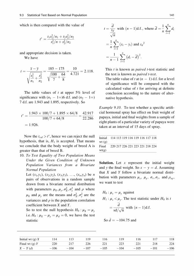
which is then compared with the value of

t� ¼ t1s21=n1 þ t2s

22=n2

s21=nþ s22=n2

and appropriate decision is taken.

We have

t ¼ x� yffiffiffiffiffiffiffiffiffiffiffiffiffiffiffis21n1

þ s22n2

s ¼ 185� 175ffiffiffiffiffiffiffiffiffiffiffiffiffiffiffiffiffiffi100

7þ 64

8

r ¼ 10

4:721¼ 2:118:

The table values of t at upper 5% level of

significance with (n1 � 1¼)6 d.f. and (n2 � 1¼)

7 d.f. are 1.943 and 1.895, respectively. So

t� ¼ 1:943� 100=7þ 1:895� 64=8

100=7þ 64=8¼ 42:917

22:286

¼ 1:926:

Now the tcal > t�, hence we can reject the null

hypothesis, that is, H1 is accepted. That means

we conclude that the body weight of breed A is

greater than that of breed B.

10. To Test Equality of Two Population Means

Under the Given Condition of UnknownPopulation Variances from a Bivariate

Normal Population

Let (x1,y1), (x2,y2), (x3,y3), . . ., (xn,yn) be npairs of observations in a random sample

drawn from a bivariate normal distribution

with parameters μX; μy; σ2X; σ

2y and ρ where

μX and μy are the means and σ2X; σ2y are the

variances and ρ is the population correlation

coefficient between X and Y.So to test the null hypothesis H0 : μX ¼ μyi:e:H0 : μX � μy ¼ μd ¼ 0, we have the test

statistic

t ¼ dsdffiffiffin

pwith ðn� 1Þd:f:; where d ¼ 1

n

Xni¼1

di

¼ 1

n

Xni¼1

ðxi � yiÞ and sd2

¼ 1

n� 1

Xni¼1

di � d� �2

:

This t is known as paired t-test statistic and

the test is known as paired t-test.The table value of t at (n � 1) d.f. for α level

of significance will be compared with the

calculated value of t for arriving at definite

conclusion according to the nature of alter-

native hypothesis.

Example 9.10. To test whether a specific artifi-

cial hormonal spray has effect on fruit weight of

papaya, initial and final weights from a sample of

eight plants of a particular variety of papaya were

taken at an interval of 15 days of spray.

Solution. Let x represent the initial weight

and y the final weight. So x � y ¼ d. Assuming

that X and Y follow a bivariate normal distri-

bution with parameters μx; μy; σx; σy; and ρxy,

we want to test

H0 : μx ¼ μy against

H1 : μx < μy: The test statistic under H0 is t

¼ d

sd=ffiffiffin

p with ðn� 1Þd:f:

So �d ¼ �104:75 and

Initial wt (g) X 114 113 119 116 119 116 117 118

Final wt (g) Y 220 217 226 221 223 221 218 224

X � Y (d) �106 �104 �107 �105 �104 �105 �101 �106

Initial

wt (g)

114 113 119 116 119 116 117 118

Final

wt(g)

220 217 226 221 223 221 218 224

9.3 Statistical Test Based on Normal Population 141

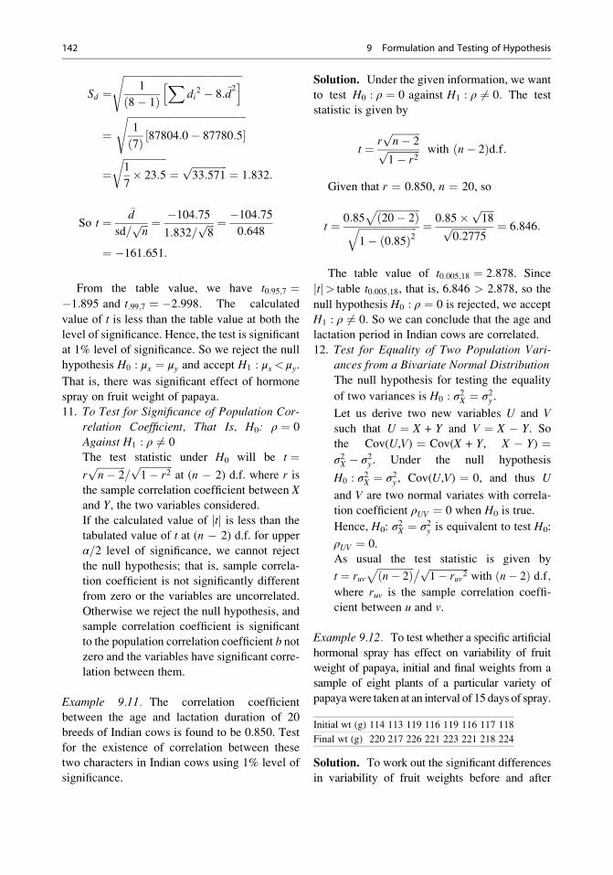
Sd ¼ffiffiffiffiffiffiffiffiffiffiffiffiffiffiffiffiffiffiffiffiffiffiffiffiffiffiffiffiffiffiffiffiffiffiffiffiffiffiffiffiffiffiffiffiffiffiffi

1

ð8� 1ÞX

di2 � 8:�d

2h is

¼ffiffiffiffiffiffiffiffiffiffiffiffiffiffiffiffiffiffiffiffiffiffiffiffiffiffiffiffiffiffiffiffiffiffiffiffiffiffiffiffiffiffiffiffiffiffiffi1

ð7Þ 87804:0� 87780:5½ �s

¼ffiffiffiffiffiffiffiffiffiffiffiffiffiffiffiffiffi1

7� 23:5

r¼

ffiffiffiffiffiffiffiffiffiffiffiffiffiffi33:571

p¼ 1:832:

So t ¼�d

sd=ffiffiffin

p ¼ �104:75

1:832=ffiffiffi8

p ¼ �104:75

0:648

¼ �161:651:

From the table value, we have t0:95;7 ¼�1:895 and t:99;7 ¼ �2:998: The calculated

value of t is less than the table value at both the

level of significance. Hence, the test is significant

at 1% level of significance. So we reject the null

hypothesis H0 : μx ¼ μy and accept H1 : μx < μy.

That is, there was significant effect of hormone

spray on fruit weight of papaya.

11. To Test for Significance of Population Cor-

relation Coefficient, That Is, H0: ρ ¼ 0

Against H1 : ρ 6¼ 0

The test statistic under H0 will be t ¼rffiffiffiffiffiffiffiffiffiffiffin� 2

p=ffiffiffiffiffiffiffiffiffiffiffiffiffi1� r2

pat (n � 2) d.f. where r is

the sample correlation coefficient between X

and Y, the two variables considered.

If the calculated value of tj j is less than the

tabulated value of t at (n � 2) d.f. for upper

α 2= level of significance, we cannot reject

the null hypothesis; that is, sample correla-

tion coefficient is not significantly different

from zero or the variables are uncorrelated.

Otherwise we reject the null hypothesis, and

sample correlation coefficient is significant

to the population correlation coefficient b not

zero and the variables have significant corre-

lation between them.

Example 9.11. The correlation coefficient

between the age and lactation duration of 20

breeds of Indian cows is found to be 0.850. Test

for the existence of correlation between these

two characters in Indian cows using 1% level of

significance.

Solution. Under the given information, we want

to test H0 : ρ ¼ 0 against H1 : ρ 6¼ 0: The test

statistic is given by

t ¼ rffiffiffiffiffiffiffiffiffiffiffin� 2

pffiffiffiffiffiffiffiffiffiffiffiffiffi1� r2

p with ðn� 2Þd:f:

Given that r ¼ 0.850, n ¼ 20, so

t ¼ 0:85ffiffiffiffiffiffiffiffiffiffiffiffiffiffiffiffiffið20� 2Þpffiffiffiffiffiffiffiffiffiffiffiffiffiffiffiffiffiffiffiffiffiffiffi

1� ð0:85Þ2q ¼ 0:85� ffiffiffiffiffi

18pffiffiffiffiffiffiffiffiffiffiffiffiffiffi

0:2775p ¼ 6:846:

The table value of t0:005;18 ¼ 2:878. Since

tj j> table t0:005;18, that is, 6.846 > 2.878, so the

null hypothesis H0 : ρ ¼ 0 is rejected, we accept

H1 : ρ 6¼ 0: So we can conclude that the age and

lactation period in Indian cows are correlated.

12. Test for Equality of Two Population Vari-

ances from a Bivariate Normal DistributionThe null hypothesis for testing the equality

of two variances is H0 : σ2X ¼ σ2y .

Let us derive two new variables U and V

such that U ¼ X + Y and V ¼ X � Y. So

the Cov(U,V) ¼ Cov(X + Y, X � Y) ¼σ2X � σ2y . Under the null hypothesis

H0 : σ2X ¼ σ2y , Cov(U,V) ¼ 0, and thus U

and V are two normal variates with correla-

tion coefficient ρUV ¼ 0 when H0 is true.

Hence, H0: σ2X ¼ σ2y is equivalent to test H0:

ρUV ¼ 0.

As usual the test statistic is given by

t ¼ ruvffiffiffiffiffiffiffiffiffiffiffiffiffiffiffiðn� 2Þp ffiffiffiffiffiffiffiffiffiffiffiffiffiffiffiffi

1� ruv2p�

with ðn� 2Þ d:f;where ruv is the sample correlation coeffi-

cient between u and v.

Example 9.12. To test whether a specific artificial

hormonal spray has effect on variability of fruit

weight of papaya, initial and final weights from a

sample of eight plants of a particular variety of

papayawere taken at an interval of 15 days of spray.

Initial wt (g) 114 113 119 116 119 116 117 118

Final wt (g) 220 217 226 221 223 221 218 224

Solution. To work out the significant differences

in variability of fruit weights before and after

142 9 Formulation and Testing of Hypothesis

spraying, the null hypothesis would be H0 : σx ¼σy against H0 : σx 6¼ σy. This is equivalent to test

ρuv ¼ 0 where u and v are x + y and x � y,

respectively. The test statistic for the same will be

t ¼ ruvffiffiffiffiffiffiffiffiffiffiffiffiffiffiffiffi1� ruv2

p ffiffiffiffiffiffiffiffiffiffiffin� 2

pwith ðn� 2Þ d:f:

We have

;ruv ¼P

uv� nuvffiffiffiffiffiffiffiffiffiffiffiffiffiffiffiffiffiffiffiffiffiffiffiffiffiffiffiffiffiffiffiffiffiffiffiffiffiffiffiffiffiffiffiffiffiffiffiffiffiffiffiffiffiffiPu2 � nu2

� � Pv2 � nv2

� �q ¼ �0:4647:

Thus, t ¼ �0:4647ffiffiffiffiffiffiffiffiffiffiffi8� 2

pffiffiffiffiffiffiffiffiffiffiffiffiffiffiffiffiffiffiffiffiffiffiffiffiffiffiffiffiffiffiffi1� ð�0:4647Þ2

q ¼ �1:2855 at 6 d:f:

From the table we get t0:025;6 ¼ 2:447. Thus,

the observed value of tj j is less than the table

value. That is, tcalj j< ttab. So we cannot reject the

null hypothesis of equality of variances.

13. Test for Significance and Regression Coeffi-cient in a Simple Linear Regression.

To test the H0: b ¼ 0, we have the test sta-

tistic t ¼ b SEðbÞ= with n � 1 d.f.: if the

calculated value of H � tabðn�1Þ d:f: at α2level of significance, then it cannot be

rejected; otherwise t is rejected.

Example 9.13. The relation between yield and

expenditure on plant protection measure was

found to be Y ¼ 15.6 + 0.8 PP with standard

error estimates for the intercept and the regres-

sion coefficients being 6.2 and 0.625, respec-

tively, from ten varieties of paddy. Test for

significance of regression coefficient of plant

protection.

Solution. To rest the H0: b ¼ 0 the test statistic

is t ¼ b SEðbÞ= ¼ 0:8 0:625= ¼ 1:28. The table

value of t statistic at 5% level of significance is

greater than the table value. Hence, the test is

nonsignificant and the null hypothesis cannot

be rejected. We conclude that population regres-

sion coefficient may be zero.

14. Test for Significance of the PopulationMultiple Correlation Coefficients

Let there be p variables ðx1; x2; . . . xpÞfollowing a p-variate normal distribution and

the multiple correlation of x1 on x2; x3; . . . xpbe given by ρ12:34;...p and the corresponding

sample multiple correlation coefficient being

R1:2;3;...p based on a random sample of size n.

The problem is to test whether the population

multiple correlation is zero or not, that is, to

test H0 : ρ1:2;3;...;p ¼ 0 against the alternative

hypothesis H1 : ρ1: 2; 3;...;p > 0. Under H0 the

test statistic is

F ¼ R21:23...p ðp� 1Þ=

1� R21:23...p

� � ðn� pÞ=

with ðp� 1; n� pÞd:f:

If cal F>Fα; p�1;n�p, then H0 is rejected, else

it is accepted}.

It is noted that in this problem, alternative

hypothesis is always one sided (right)

because ρ12: 3;4;...;p cannot be negative.

Example 9.14. In a yield component analysis,

the relationship of yield with five-yield compo-

nent was worked out for 20 plants. The multiple

correlation coefficients were found to be 0.98.

Test for significance of multiple correlation

coefficients.

X : 114 113 119 116 119 116 117 118

Y : 220 217 226 221 223 221 218 224

U ¼ (X + Y): 334 330 345 337 342 337 335 342

V ¼ (X � Y): �106 �104 �107 �105 �104 �105 �101 �106

9.3 Statistical Test Based on Normal Population 143

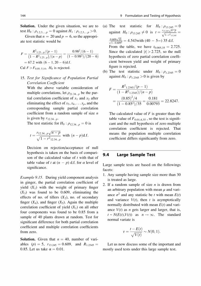
Solution. Under the given situation, we are to

test H0 : ρ1:2;3;...;p ¼ 0 against H1 : ρ1:2;3;...;p > 0.

Given that n ¼ 20 and p ¼ 6, so the appropri-

ate test statistic would be

F ¼ R21:23...p ðp� 1Þ=

1� R21:23...p

� � ðn� pÞ=¼ 0:982 ð6� 1Þ=

1� 0:982ð Þ ð20� 6Þ=

¼ 67:2 with ð6� 1; 20� 6Þd:f:Cal F>F0:05; 5;14; H0 is rejected:

15. Test for Significance of Population Partial

Correlation Coefficient

With the above variable consideration of

multiple correlations, let ρ21:34...p be the par-

tial correlation coefficient of x1 and x2 after

eliminating the effect of x3; x4; . . . xp, and the

corresponding sample partial correlation

coefficient from a random sample of size n

is given by r12:34...p.

The test statistic for H0 : ρ12:34...p ¼ 0 is

t ¼ r12:34...pffiffiffiffiffiffiffiffiffiffiffin� p

pffiffiffiffiffiffiffiffiffiffiffiffiffiffiffiffiffiffiffiffiffiffiffiffiffi1� r212:34...p

p with ðn� pÞd:f:

Decision on rejection/acceptance of null

hypothesis is taken on the basis of compari-

son of the calculated value of t with that of

table value of t at (n � p) d.f. for α level of

significance.

Example 9.15. During yield component analysis

in ginger, the partial correlation coefficient of

yield (X1) with the weight of primary finger

(X3) was found to be 0.609, eliminating the

effects of no. of tillers (X2), no. of secondary

finger (X4), and finger (X5). Again the multiple

correlation coefficient of yield (X1) on all other

four components was found to be 0.85 from a

sample of 40 plants drawn at random. Test for

significant difference for both partial correlation

coefficient and multiple correlation coefficients

from zero.

Solution. Given that n ¼ 40, number of vari-

ables (p) ¼ 5, r13:245 ¼ 0:609; and R1:2345 ¼0:85. Let us take α ¼ 0:01.

(a) The test statistic for H0 : ρ13:245 ¼ 0

against H0 : ρ13:245 6¼ 0 is t ¼ r13:245ffiffiffiffiffiffin�p

pffiffiffiffiffiffiffiffiffiffiffiffiffiffi1�r213:245

p ¼0:609

ffiffiffiffi35

pffiffiffiffiffiffiffiffiffiffiffiffiffiffi1�0:6092

p ¼ 4:543with (40 � 5¼) 35 d.f.

From the table, we have t0.005,35 ¼ 2.725.

Since the calculated tj j> 2:725, so the null

hypothesis of zero partial correlation coeffi-

cient between yield and weight of primary

figure is rejected.

(b) The test statistic under H0 : ρ1:2345 ¼ 0

against H0 : ρ1:2345 > 0 is given by

F ¼ R21:2345 ðp� 1Þ=

1� R21:2345ð Þ ðn� pÞ=

¼ ð0:85Þ2 4=

1� 0:852ð Þ 35=¼ 0:181

0:00793¼ 22:8247:

The calculated value of F is greater than the

table value of F0.01;4,35 , so the test is signifi-

cant and the null hypothesis of zero multiple

correlation coefficient is rejected. That

means the population multiple correlation

coefficient differs significantly from zero.

9.4 Large Sample Test

Large sample tests are based on the followings

facets:

1. Any sample having sample size more than 30

is treated as large.

2. If a random sample of size n is drawn from

an arbitrary population with mean μ and vari-

ance σ2 and any statistic be t with mean E(t)

and variance V(t), then t is asymptotically

normally distributed with mean E(t) and vari-

ance V(t) as n gets larger and larger, that is,

t ~ N(E(t),V(t)) as n ! 1. The standard

normal variate is

τ ¼ t� EðtÞffiffiffiffiffiffiffiffiffiVðtÞp Nð0; 1Þ:

Let us now discuss some of the important and

mostly used tests under this large sample test.

144 9 Formulation and Testing of Hypothesis

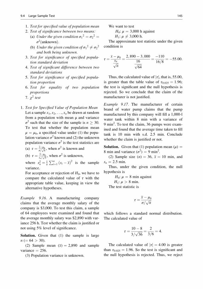
1. Test for specified value of population mean

2. Test of significance between two means:

(a) Under the given condition σ12 ¼ σ22 ¼σ2ðunknownÞ.

(b) Under the given condition of σ12 6¼ σ22

and both being unknown.

3. Test for significance of specified popula-tion standard deviation

4. Test of significant difference between two

standard deviations5. Test for significance of specified popula-

tion proportion

6. Test for equality of two populationproportions

7. χ2 test

1. Test for Specified Value of Population Mean

Let a sample x1, x2, . . ., xn be drawn at random

from a population with mean μ and variance

σ2 such that the size of the sample is n 30.

To test that whether the population mean

μ ¼ μ0, a specified value under (1) the popu-

lation variance σ2 known and (2) the unknownpopulation variance σ2 is the test statistics are

(a) τ ¼ x�μ0σ=ffiffin

p , when σ2 is known and

(b) τ ¼ x�μ0sn=ffiffin

p , when σ2 is unknown,

where s2n ¼ 1n

Pni¼1 xi � xð Þ2 is the sample

variance.

For acceptance or rejection of H0, we have to

compare the calculated value of τ with the

appropriate table value, keeping in view the

alternative hypotheses.

Example 9.16. A manufacturing company

claims that the average monthly salary of the

company is $3,000. To test this claim, a sample

of 64 employees were examined and found that

the average monthly salary was $2,890 with var-

iance 256 h. Test whether the claim is justified or

not using 5% level of significance.

Solution. Given that (1) the sample is large

n (¼ 64 > 30).

(2) Sample mean (x) ¼ 2,890 and sample

variance ¼ 256.

(3) Population variance is unknown.

We want to test

H0: μ ¼ 3,000 h against

H1: μ 6¼ 3,000 h.

The approximate test statistic under the given

condition is

τ ¼ x� μ0snffiffiffin

p¼ 2; 890� 3; 000

16ffiffiffiffiffi64

p¼ �110

16=8¼ �55:00:

Thus, the calculated value of τj j, that is, 55.00,is greater than the table value of τ0:025 ¼ 1:96;

the test is significant and the null hypothesis is

rejected. So we conclude that the claim of the

manufacturer is not justified.

Example 9.17. The manufacturer of certain

brand of water pump claims that the pump

manufactured by this company will fill a 1,000-l

water tank within 8 min with a variance of

9 min2. To test the claim, 36 pumps were exam-

ined and found that the average time taken to fill

tank is 10 min with s.d. 2.5 min. Conclude

whether the claim is justified or not.

Solution. Given that (1) population mean (μ) ¼8 min and variance (σ2) ¼ 9 min2.

(2) Sample size (n) ¼ 36, x ¼ 10 min, and

sn ¼ 2.5 min.

Thus, under the given condition, the null

hypothesis is

H0: μ ¼ 8 min against

H1: μ > 8 min.

The test statistic is

τ ¼ x� μ0σ=

ffiffiffin

p

which follows a standard normal distribution.

The calculated value of

τ ¼ 10� 8

3=ffiffiffiffiffi36

p ¼ 2

3=6¼ 4:

The calculated value of τj j ¼ 4:00 is greater

than τ0:025 ¼ 1:96. So the test is significant and

the null hypothesis is rejected. Thus, we reject

9.4 Large Sample Test 145

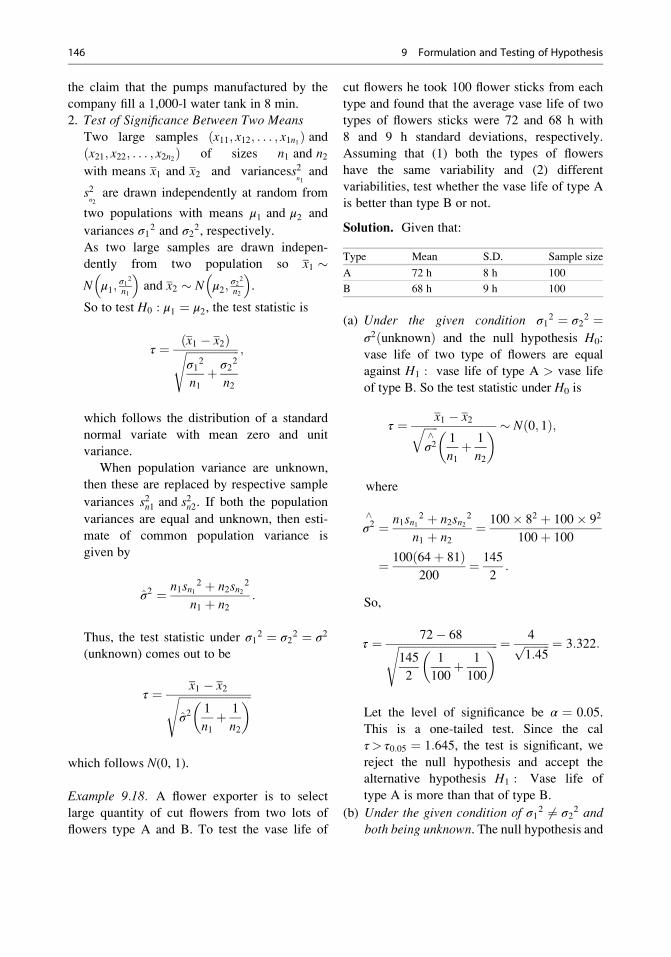
the claim that the pumps manufactured by the

company fill a 1,000-l water tank in 8 min.

2. Test of Significance Between Two Means

Two large samples x11; x12; . . . ; x1n1ð Þ andx21; x22; . . . ; x2n2ð Þ of sizes n1 and n2with means x1 and x2 and variancess2

n1and

s2n2

are drawn independently at random from

two populations with means μ1 and μ2 and

variances σ12 and σ22, respectively.As two large samples are drawn indepen-

dently from two population so x1 N μ1;

σ12

n1

� �and x2 N μ2;

σ22

n2

� �.

So to test H0 : μ1 ¼ μ2, the test statistic is

τ ¼ x1 � x2ð Þffiffiffiffiffiffiffiffiffiffiffiffiffiffiffiffiffiffiffiσ12

n1þ σ22

n2

s ;

which follows the distribution of a standard

normal variate with mean zero and unit

variance.

When population variance are unknown,

then these are replaced by respective sample

variances s2n1 and s2n2. If both the population

variances are equal and unknown, then esti-

mate of common population variance is

given by

σ2 ¼ n1sn12 þ n2sn2

2

n1 þ n2:

Thus, the test statistic under σ12 ¼ σ22 ¼ σ2

(unknown) comes out to be

τ ¼ x1 � x2ffiffiffiffiffiffiffiffiffiffiffiffiffiffiffiffiffiffiffiffiffiffiffiffiffiffiσ2

1

n1þ 1

n2

� s

which follows N(0, 1).

Example 9.18. A flower exporter is to select

large quantity of cut flowers from two lots of

flowers type A and B. To test the vase life of

cut flowers he took 100 flower sticks from each

type and found that the average vase life of two

types of flowers sticks were 72 and 68 h with

8 and 9 h standard deviations, respectively.

Assuming that (1) both the types of flowers

have the same variability and (2) different

variabilities, test whether the vase life of type A

is better than type B or not.

Solution. Given that:

Type Mean S.D. Sample size

A 72 h 8 h 100

B 68 h 9 h 100

(a) Under the given condition σ12 ¼ σ22 ¼σ2ðunknownÞ and the null hypothesis H0:

vase life of two type of flowers are equal

against H1 : vase life of type A > vase life

of type B. So the test statistic under H0 is

τ ¼ x1 � x2ffiffiffiffiffiσ2^

q1

n1þ 1

n2

� Nð0; 1Þ;

where

σ2^¼ n1sn1

2 þ n2sn22

n1 þ n2¼ 100� 82 þ 100� 92

100þ 100

¼ 100ð64þ 81Þ200

¼ 145

2:

So,

τ ¼ 72� 68ffiffiffiffiffiffiffiffiffiffiffiffiffiffiffiffiffiffiffiffiffiffiffiffiffiffiffiffiffiffiffiffiffiffiffiffi145

2

1

100þ 1

100

� s ¼ 4ffiffiffiffiffiffiffiffiffi1:45

p ¼ 3:322:

Let the level of significance be α ¼ 0.05.

This is a one-tailed test. Since the cal

τ> τ0:05 ¼ 1:645, the test is significant, we

reject the null hypothesis and accept the

alternative hypothesis H1 : Vase life of

type A is more than that of type B.

(b) Under the given condition of σ12 6¼ σ22 andboth being unknown. The null hypothesis and

146 9 Formulation and Testing of Hypothesis

the alternative hypothesis remain the same,

that is,

H0 : Vase life of two types of flowers are same:

H1 : Vase life of type A> vase life of type B;

that is; H0 : μ1 ¼ μ2H1 : μ1 > μ2:

Let the level of significance be α ¼ 0.05;

being a one-sided test, the critical value is

1.645 for standard normal variate τ. The teststatistic is

τ ¼ �x1 � �x2ffiffiffiffiffiffiffiffiffiffiffiffiffiffiffiffiffiffiffiffiffisn1

2

n1þ sn2

2

n2

s Nð0; 1Þ:

Thus,

τ ¼ 72� 68ffiffiffiffiffiffiffiffiffiffiffiffiffiffiffiffiffiffiffiffiffi64

100þ 81

100

r ¼ 4ffiffiffiffiffiffiffiffi145

100

r ¼ 4ffiffiffiffiffiffiffiffiffi1:45

p

¼ 4

1:204¼ 3:322:

Since the cal τ> 1:645, so the test is

significant, we reject the null hypothesis

and accept the alternative hypothesis H1 :

vase life of type A is more than that of type

B.

3. Test for Significance of Specified Population

Standard DeviationLet (x1, x2, . . ., xn) be a large sample of size n

drawn randomly from a population with vari-

ance σ2. The sampling distribution of the sam-

ple s.d. sn follows an approximately normal

distribution with mean E snð Þ ¼ σ and vari-

ance V snð Þ ¼ σ2

2n as the sample size n tends to

infinity. Thus, as n ! 1; sn N σ; σ2

2n

� �.

Our objective is to test H0 : σ ¼ σ0:

To test the above null hypothesis, we have the

following approximate test statistic

τ ¼ sn � σ0ffiffiffiffiffiσ202n

r

which is a standard normal variate with mean

zero and variance unity.

For acceptance or rejection of H0, we have to

compare the calculated value of τ with the

appropriate table value keeping in view the

alternative hypotheses.

Example 9.19. To test the variability in vase life

of a cut flower, a sample of 100 cut flowers gives

s.d. 8.5 h. Can we conclude that the vase life of

the cut flower has the variability of 65 h2?

Solution. Given that the sample is large of size

(n) 100. The population variance is assumed to

be 65 h2, and s.d. of the sample is 8.5 h. Under

the given condition, the null hypothesis is the

population s.d. ¼ ffiffiffiffiffi65

ph.

That is, H0 : σ ¼ 8:06 against H1 : σ0 6¼ 8:06.

The test statistic for the above null hypothesis is

τ ¼ sn � σ0ffiffiffiffiffiσ2

0

2n

r ¼ 8:5� 8:06ffiffiffiffiffiffiffiffiffiffiffiffiffiffiffiffiffiffiffiffi65

ð2� 100Þr ¼ 0:44

0:57¼ 0:77:

Let the level of significance be α ¼ 0.05, and

the corresponding critical value of τ (standard

normal variate) is 1.96. So the calculated value

of τj j < tabulated value of τ (1.96). The test is

nonsignificant and the null hypothesis cannot be

rejected. Hence, the population variance of vase

life of the cut flower under consideration can

be taken as 65 h2.

4. Test of Significant Difference Between TwoStandard Deviations

Let us draw two independent samples x11;ðx12; . . . ; x1n1Þ and x21; x22; . . . ; x2n2ð Þ of sizes

n1 and n2 with means x1; x2 and variance sn12;

sn22 from two populations with variances σ12

and σ22, respectively.For a large sample, both sn1 and sn2 are

distributed as sn1 N σ1,σ12

2n1

� �and sn2

N σ2,σ22

2n2

� �.

Now, E sn1�sn2ð Þ ¼ Eðsn1Þ � Eðsn2Þ ¼ σ1�σ2and

SE sn1 � sn2ð Þ ¼ffiffiffiffiffiffiffiffiffiffiffiffiffiffiffiffiffiffiffiffiffiffiffiffiV sn1 � sn2ð Þ

p¼

ffiffiffiffiffiffiffiffiffiffiffiffiffiffiffiffiffiffiffiffiσ212n1

þ σ222n2

s:

9.4 Large Sample Test 147

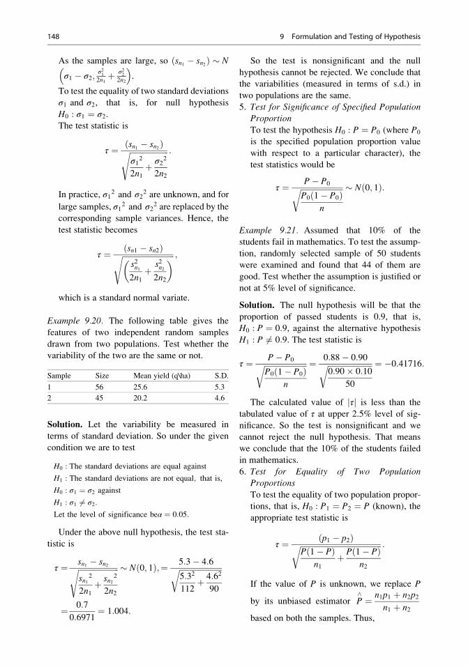
As the samples are large, so sn1 � sn2ð Þ N

σ1 � σ2;σ21

2n1þ σ2

2

2n2

� �.

To test the equality of two standard deviations

σ1 and σ2, that is, for null hypothesis

H0 : σ1 ¼ σ2.The test statistic is

τ ¼ sn1 � sn2ð Þffiffiffiffiffiffiffiffiffiffiffiffiffiffiffiffiffiffiffiffiσ12

2n1þ σ22

2n2

s :

In practice, σ12 and σ22 are unknown, and for

large samples, σ12 and σ22 are replaced by thecorresponding sample variances. Hence, the

test statistic becomes

τ ¼ sn1 � sn2ð Þffiffiffiffiffiffiffiffiffiffiffiffiffiffiffiffiffiffiffiffiffiffiffiffiffiffiffis2n12n1

þ s2n22n2

� s ;

which is a standard normal variate.

Example 9.20. The following table gives the

features of two independent random samples

drawn from two populations. Test whether the

variability of the two are the same or not.

Sample Size Mean yield (q\ha) S.D.

1 56 25.6 5.3

2 45 20.2 4.6

Solution. Let the variability be measured in

terms of standard deviation. So under the given

condition we are to test

H0 : The standard deviations are equal against

H1 : The standard deviations are not equal; that is,

H0 : σ1 ¼ σ2 against

H1 : σ1 6¼ σ2:

Let the level of significance beα ¼ 0:05:

Under the above null hypothesis, the test sta-

tistic is

τ ¼ sn1 � sn2ffiffiffiffiffiffiffiffiffiffiffiffiffiffiffiffiffiffiffiffiffisn1

2

2n1þ sn2

2

2n2

s Nð0; 1Þ;¼ 5:3� 4:6ffiffiffiffiffiffiffiffiffiffiffiffiffiffiffiffiffiffiffiffiffiffi5:32

112þ 4:62

90

r

¼ 0:7

0:6971¼ 1:004:

So the test is nonsignificant and the null

hypothesis cannot be rejected. We conclude that

the variabilities (measured in terms of s.d.) in

two populations are the same.

5. Test for Significance of Specified PopulationProportion

To test the hypothesis H0 : P ¼ P0 (where P0

is the specified population proportion value

with respect to a particular character), the

test statistics would be

τ ¼ P� P0ffiffiffiffiffiffiffiffiffiffiffiffiffiffiffiffiffiffiffiffiffiffiP0ð1� P0Þ

n

r Nð0; 1Þ:

Example 9.21. Assumed that 10% of the

students fail in mathematics. To test the assump-

tion, randomly selected sample of 50 students

were examined and found that 44 of them are

good. Test whether the assumption is justified or

not at 5% level of significance.

Solution. The null hypothesis will be that the

proportion of passed students is 0.9, that is,

H0 : P ¼ 0:9, against the alternative hypothesis

H1 : P 6¼ 0:9. The test statistic is

τ ¼ P� P0ffiffiffiffiffiffiffiffiffiffiffiffiffiffiffiffiffiffiffiffiffiffiP0ð1� P0Þ

n

r ¼ 0:88� 0:90ffiffiffiffiffiffiffiffiffiffiffiffiffiffiffiffiffiffiffiffiffiffiffi0:90� 0:10

50

r ¼ �0:41716:

The calculated value of τj j is less than the

tabulated value of τ at upper 2.5% level of sig-

nificance. So the test is nonsignificant and we

cannot reject the null hypothesis. That means

we conclude that the 10% of the students failed

in mathematics.

6. Test for Equality of Two Population

Proportions

To test the equality of two population propor-

tions, that is, H0 : P1 ¼ P2 ¼ P (known), the

appropriate test statistic is

τ ¼ p1 � p2ð ÞffiffiffiffiffiffiffiffiffiffiffiffiffiffiffiffiffiffiffiffiffiffiffiffiffiffiffiffiffiffiffiffiffiffiffiffiffiffiffiffiffiffiPð1� PÞ

n1þ Pð1� PÞ

n2

r :

If the value of P is unknown, we replace P

by its unbiased estimator P^ ¼ n1p1 þ n2p2

n1 þ n2based on both the samples. Thus,

148 9 Formulation and Testing of Hypothesis

τ ¼ p1 � p2ð ÞffiffiffiffiffiffiffiffiffiffiffiffiffiffiffiffiffiffiffiffiffiffiffiffiffiffiffiffiffiffiffiffiffiffiffiffiffiffiffiffiffiffiffiffiP^

1� P^�

1

n1þ 1

n2

� s :

Example 9.22. From two large samples of 500

and 600 of electric bulbs, 30 and 25%, respec-

tively, are found to be defective. Can we con-

clude that the proportions of defective bulbs are

equal in both the lots?

Solution. Under the given condition, the null

hypothesis isH0 : P1 ¼ P2 against the alternative

hypothesis H1 : P1 6¼ P2.

That means there exists no significant differ-

ence between the two proportions against the

existence of significant difference.

Let the level of significance be α ¼ 0.05,

and the test statistic for the above null

hypothesis is

τ ¼ p1 � p2ð ÞffiffiffiffiffiffiffiffiffiffiffiffiffiffiffiffiffiffiffiffiffiffiffiffiffiffiffiffiffiffiffiffiffiffiffiffiffiffiffiffiPð1� PÞ 1

n1þ 1

n2

� s ; where P ¼ n1p1 þ n2p2n1 þ n2

¼ 500� 0:3þ 600� 0:25

500þ 600¼ 3

11

nτ ¼ 0:3� 0:25ð Þffiffiffiffiffiffiffiffiffiffiffiffiffiffiffiffiffiffiffiffiffiffiffiffiffiffiffiffiffiffiffiffiffiffiffiffiffiffiffiffiffiffiffiffi3

11� 8

11

1

500þ 1

600

� s ¼ 0:05

0:02697¼ 1:8539:

Since the calculated value of τj j is less thanthe tabulated value of τ (1.96), we have to

accept the null hypothesis and conclude that

proportions of damaged bulbs are equal in both

the lots.

7. χ2 TestThe χ2 test is one of the most important

and widely used tests in testing of hypo-

thesis. It is used both in parametric and in

nonparametric tests. Some of the impor-

tant uses of χ2 test are testing equality of

proportions, testing homogeneity or signifi-

cance of population variance, test for good-

ness of fit, tests for association between

attributes, etc.

(a) χ2 Test for Equality of k(2) Population

ProportionsLet X1,X2,X3, . . ., Xk be independent ran-

dom variables with Xi ~ B(ni,Pi), i ¼ 1, 2,

3, . . ., k; k 2. The random variable

Xki¼1

Xi � niPiffiffiffiffiffiffiffiffiffiffiffiffiffiffiffiffiffiffiffiffiffiffiffiffiniPið1� PiÞ

p( )2

is distributed as χ2 with k d.f. as n1, n2, n3,. . ., nk ! 1.

To test H0 : P1 ¼ P2 ¼ P3 ¼ � � � ¼ Pk ¼P ðknownÞ against all alternatives, the

test statistic is

χ2 ¼Xki¼1

xi � niPffiffiffiffiffiffiffiffiffiffiffiffiffiffiffiffiffiffiffiffiffiffiniPð1� PÞp

( )2

with k d:f:;

and if cal χ2 > χ2α;k; we reject Ho:

In practice P will be unknown. The unbi-

ased estimate of P is

P ¼ x1 þ x2 þ � � � þ xkn1 þ n2 þ � � � þ nk

: Then the statistic

χ2 ¼Xki¼1

xi � niPffiffiffiffiffiffiffiffiffiffiffiffiffiffiffiffiffiffiffiffiffiffiniPð1� PÞ

q0B@

1CA

2

is asymptotically χ2 with (k � 1) d.f.

If cal χ2 > χ2α;k�1, we reject H0 : P1 ¼P2 ¼ P3 ¼ � � � ¼ Pk ¼ P ðunknownÞ.

9.4 Large Sample Test 149

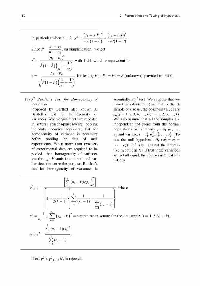
In particular when k ¼ 2; χ2 ¼ x1 � n1P� �2n1P 1� P� � þ x2 � n2P

� �2n2P 1� P� � :

Since P ¼ x1 þ x2n1 þ n2

, on simplification; we get

χ2 ¼ p1 � p2ð Þ2

P 1� P� � 1

n1þ 1

n2

� with 1 d:f: which is equivalent to

τ ¼ p1 � p2ffiffiffiffiffiffiffiffiffiffiffiffiffiffiffiffiffiffiffiffiffiffiffiffiffiffiffiffiffiffiffiffiffiffiffiffiffiffiffiffiP 1� P� � 1

n1þ 1

n2

� s for testing H0 : P1 ¼ P2 ¼ P ðunknownÞ provided in test 6:

(b) χ2 Bartlett’s Test for Homogeneity ofVariances

Proposed by Bartlett also known as

Bartlett’s test for homogeneity of

variances. When experiments are repeated

in several seasons/places/years, pooling

the data becomes necessary; test for

homogeneity of variance is necessary

before pooling the data of such

experiments. When more than two sets

of experimental data are required to be

pooled, then homogeneity of variance

test through F statistic as mentioned ear-

lier does not serve the purpose. Bartlett’s

test for homogeneity of variances is

essentially a χ2 test. We suppose that we

have k samples (k > 2) and that for the ith

sample of size ni , the observed values are

xij (j ¼ 1, 2, 3, 4, . . ., ni; i ¼ 1, 2, 3, . . ., k).We also assume that all the samples are

independent and come from the normal

populations with means μ1; μ1; μ1; . . . ;μk and variances σ21; σ

22; σ

23; . . . ; σ

2k . To

test the null hypothesis H0 : σ21 ¼ σ22 ¼� � � ¼ σ2k ¼ σ2; sayð Þ against the alterna-

tive hypothesis H1 is that these variances

are not all equal, the approximate test sta-

tistic is

χ2k�1 ¼Pki¼1

ðni � 1Þloges2

si2

�

1þ 1

3ðk � 1ÞXki¼1

1

ðni � 1Þ �1Pk

i¼1

ðni � 1Þ

8>>><>>>:

9>>>=>>>;

26664

where

s2i ¼1

ni � 1

Xnij¼1

xij � xi� �2 ¼ sample mean square for the ith sample ði ¼ 1; 2; 3; . . . kÞ,

and s2 ¼Pki¼1

ðni � 1ÞðsiÞ2

Pki¼1

ðni � 1Þ:

If cal χ2 > χ2α;k�1;H0 is rejected.

150 9 Formulation and Testing of Hypothesis

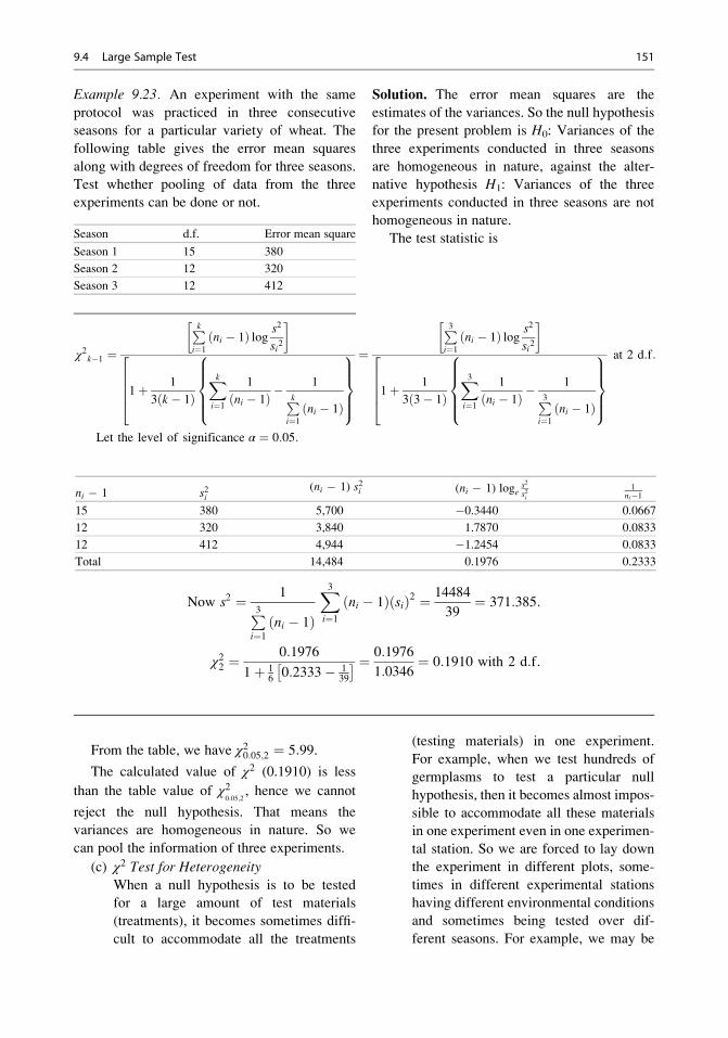
Example 9.23. An experiment with the same

protocol was practiced in three consecutive

seasons for a particular variety of wheat. The

following table gives the error mean squares

along with degrees of freedom for three seasons.

Test whether pooling of data from the three

experiments can be done or not.

Season d.f. Error mean square

Season 1 15 380

Season 2 12 320

Season 3 12 412

Solution. The error mean squares are the

estimates of the variances. So the null hypothesis

for the present problem is H0: Variances of the

three experiments conducted in three seasons

are homogeneous in nature, against the alter-

native hypothesis H1: Variances of the three

experiments conducted in three seasons are not

homogeneous in nature.

The test statistic is

χ2k�1 ¼Pki¼1

ðni � 1Þ log s2

si2

�

1þ 1

3ðk � 1ÞXki¼1

1

ðni � 1Þ �1Pk

i¼1

ðni � 1Þ

8>>><>>>:

9>>>=>>>;

26664

¼P3i¼1

ðni � 1Þ log s2

si2

�

1þ 1

3ð3� 1ÞX3i¼1

1

ðni � 1Þ �1P3

i¼1

ðni � 1Þ

8>>><>>>:

9>>>=>>>;

26664

at 2 d:f:

Let the level of significance α ¼ 0:05:

Now s2 ¼ 1P3i¼1

ðni � 1Þ

X3i¼1

ðni � 1ÞðsiÞ2 ¼ 14484

39¼ 371:385:

χ22 ¼0:1976

1þ 160:2333� 1

39

� ¼ 0:1976

1:0346¼ 0:1910 with 2 d:f:

From the table, we have χ20:05;2 ¼ 5:99.

The calculated value of χ2 (0.1910) is less

than the table value of χ20:05;2

, hence we cannot

reject the null hypothesis. That means the

variances are homogeneous in nature. So we

can pool the information of three experiments.

(c) χ2 Test for HeterogeneityWhen a null hypothesis is to be tested

for a large amount of test materials

(treatments), it becomes sometimes diffi-

cult to accommodate all the treatments

(testing materials) in one experiment.

For example, when we test hundreds of

germplasms to test a particular null

hypothesis, then it becomes almost impos-

sible to accommodate all these materials

in one experiment even in one experimen-

tal station. So we are forced to lay down

the experiment in different plots, some-

times in different experimental stations

having different environmental conditions

and sometimes being tested over dif-

ferent seasons. For example, we may be

ni � 1 s2i(ni � 1) s2i (ni � 1) loge

s2

s2i1

ni�1

15 380 5,700 �0.3440 0.0667

12 320 3,840 1.7870 0.0833

12 412 4,944 �1.2454 0.0833

Total 14,484 0.1976 0.2333

9.4 Large Sample Test 151

interested to test the Mendel’s monohybrid

cross ratio (1:2:1) of F1 generation under

different experiments using χ2 test. Now

the question is whether all these informa-

tion from different experiments testing the

same null hypothesis can be pooled/added

to test for the theoretical ratio. χ2 test

for heterogeneity of variances based on

additive property of χ2 variates can be

used here.

Let us suppose we have p experimental

setup providing χ12; χ2

2; χ32; . . . χp

2 each

with (k � 1) d.f. The individual χ2 values

from p setup are added to get χs2 with

p(k � 1) d.f. Then a χ2 value known as

χp2 is calculated from the pooled sample

of all the p experiments with (k � 1) d.f.

Now the heterogeneity χ2 is calculated

as χh2 ¼ χs

2 � χp2 with p k � 1ð Þ�f

k � 1ð Þg ¼ p� 1ð Þ k � 1ð Þ d.f.Decisions are taken by comparing the cal-

culated value of χ2 with table value of χ2

at upper level of significance with (p � 1)

(k � 1) degrees of freedom.

Example 9.24. Three sets of experiments were

conducted at three different places, and the fol-

lowing information are collected to check

whether the data follow Mendel’s monohybrid

cross ratio of 1:2:1 or not.

Places

Fruit shape

Long Medium Small

Place A 70 120 60

Place B 45 70 30

Place C 15 25 20

Solution. Under the given conditions, we are to

test (1) the validity of monohybrid cross ratio

with respect to fruit shape in all the three places

separately and (2) whether we can pool the χ2

values from different location to judge the valid-

ity of monohybrid cross ratio for fruit shape for

the given population.

1. The null hypothesis for the first problem is

H0: The ratio of different fruit shape in F1

generation follow 1:2:1 ratio in each

location against the alternative hypothesis

H1: The ratio of different fruit shape in F1

generation does not follow 1:2:1 ratio in

each location.

Under the given null hypothesis, the test

statistic is

χ22 ¼X3i¼1

ðObs� ExpÞ2Exp

for each place:

Let the level of significance be α ¼ 0.05.

The χ22 value for each place are:

Place χ2 value d.f.

Place A 1.2 2

Place B 3.276 2

Place C 1.666 2

The χ22 table value at 5% level of signifi-

cance is 5.991. In all the places, the χ2

value obtained is less than the table value

of χ20:05;2 , so we can conclude that in all the

places, the null hypothesis cannot be

rejected. That means the experimental F1

generation data follow the theoretical ratio

1:2:1.

2. Our next objective is to work out the χ2

value for pooled data, that is, 130:215:110

:: long:medium:small and to test whether

homogeneity of variances is true for the

whole experiment or not. Thus, the null

hypothesis is that H0: Homogeneity of var-

iance exists against the alternative hypo-

thesis that homogeneity of variance does

not exist.

Let the level of significance be α ¼ 0.05.

The calculated value of χ2p for whole data is

3.426, and the sum of all the χ2 values

obtained in different places is 6.142.

Thus,

χh2 ¼ χs

2 � χp2with p� 1ð Þ k � 1ð Þ d:f:

¼ 6:142� 3:426 with 2� 2 ¼ 4 d:f:

¼ 2:715:

At 0.05 level of significance, the tabulated

χ2 value at 4 d.f. is 9.488. So the calculated

152 9 Formulation and Testing of Hypothesis

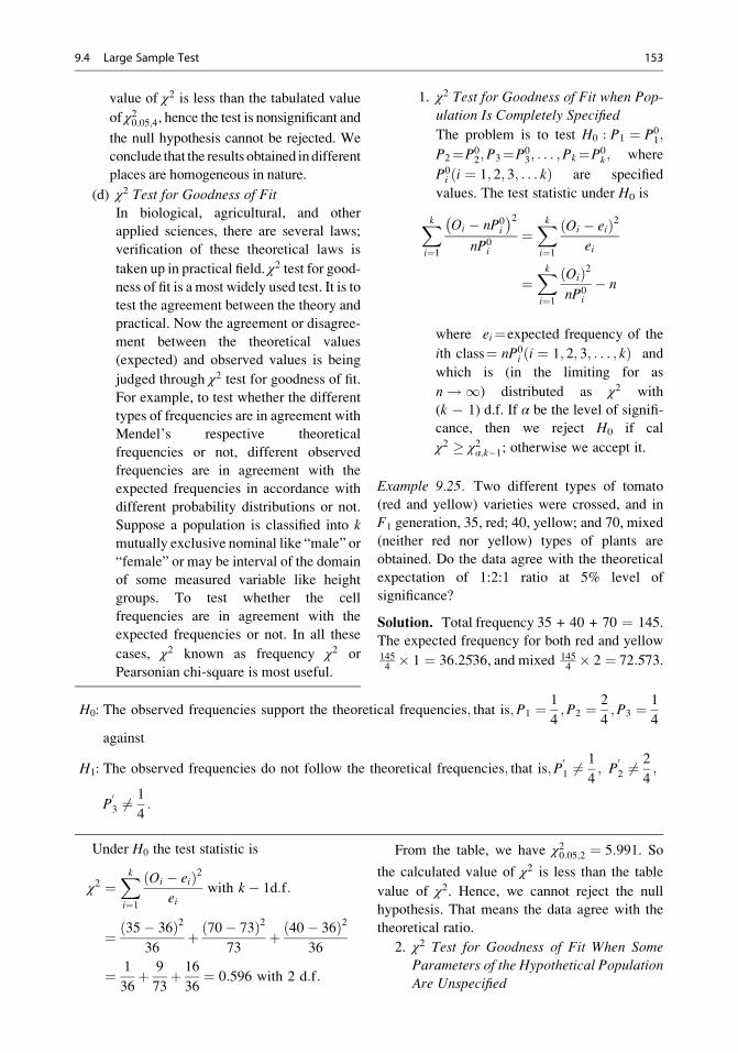
value of χ2 is less than the tabulated value

of χ20:05;4, hence the test is nonsignificant and

the null hypothesis cannot be rejected. We

conclude that the results obtained indifferent

places are homogeneous in nature.

(d) χ2 Test for Goodness of FitIn biological, agricultural, and other

applied sciences, there are several laws;

verification of these theoretical laws is

taken up in practical field. χ2 test for good-ness of fit is a most widely used test. It is to

test the agreement between the theory and

practical. Now the agreement or disagree-

ment between the theoretical values

(expected) and observed values is being

judged through χ2 test for goodness of fit.For example, to test whether the different

types of frequencies are in agreement with

Mendel’s respective theoretical

frequencies or not, different observed

frequencies are in agreement with the

expected frequencies in accordance with

different probability distributions or not.

Suppose a population is classified into kmutually exclusive nominal like “male” or

“female” or may be interval of the domain

of some measured variable like height

groups. To test whether the cell

frequencies are in agreement with the

expected frequencies or not. In all these

cases, χ2 known as frequency χ2 or

Pearsonian chi-square is most useful.

1. χ2 Test for Goodness of Fit when Pop-ulation Is Completely Specified

The problem is to test H0 : P1 ¼ P01;

P2¼P02;P3¼P0

3; . . . ;Pk¼P0k ; where

P0i ði ¼ 1; 2; 3; . . . kÞ are specified

values. The test statistic under H0 is

Xki¼1

Oi � nP0i

� �2nP0

i

¼Xki¼1

Oi � eið Þ2ei

¼Xki¼1

Oið Þ2nP0

i

� n

where ei¼expected frequency of the

ith class¼ nP0i ði ¼ 1; 2; 3; . . . ; kÞ and

which is (in the limiting for as

n ! 1) distributed as χ2 with

(k � 1) d.f. If α be the level of signifi-

cance, then we reject H0 if cal

χ2 χ2α;k�1; otherwise we accept it.

Example 9.25. Two different types of tomato

(red and yellow) varieties were crossed, and in

F1 generation, 35, red; 40, yellow; and 70, mixed

(neither red nor yellow) types of plants are

obtained. Do the data agree with the theoretical

expectation of 1:2:1 ratio at 5% level of

significance?

Solution. Total frequency 35 + 40 + 70 ¼ 145.

The expected frequency for both red and yellow1454� 1 ¼ 36:25~36, and mixed 145

4� 2 ¼ 72:5~73.

H0: The observed frequencies support the theoretical frequencies; that is;P1 ¼ 1

4;P2 ¼ 2

4;P3 ¼ 1

4

against

H1: The observed frequencies do not follow the theoretical frequencies; that is;P01 6¼

1

4; P

02 6¼

2

4;

P03 6¼

1

4:

Under H0 the test statistic is

χ2 ¼Xki¼1

Oi � eið Þ2ei

with k � 1d:f:

¼ 35� 36ð Þ236

þ 70� 73ð Þ273

þ 40� 36ð Þ236

¼ 1

36þ 9

73þ 16

36¼ 0:596 with 2 d:f:

From the table, we have χ20:05;2 ¼ 5:991. So

the calculated value of χ2 is less than the table

value of χ2. Hence, we cannot reject the null

hypothesis. That means the data agree with the

theoretical ratio.

2. χ2 Test for Goodness of Fit When Some

Parameters of the Hypothetical Population

Are Unspecified

9.4 Large Sample Test 153

An observed frequency distribution in a

sample may often be supposed to arise

from a true binomial, Poisson, normal, or

some other known type of distribution in

the population. In most cases in practice,

the hypothesis that we want to test is H0:

The sample has been drawn from a parent

population of certain type.

This hypothesis may be tested by compar-

ing the observed frequencies in various

classes with those which would be given

by the assumed theoretical distribution.

Usually the parameters of this distribution

may not be known but will have to be

estimated from the sample. The test statis-

tic under H0 is

χ2 ¼Xki¼1

ðOi � eiÞ2ei

¼Xki¼1

ðOi � nPiÞ2nP0

which is χ2 distribution with (k � s � 1)

d.f. where s(<k � 1) is the number of

parameters of this distribution to be

estimated from the sample and Pi is the

estimated probability that a single item in

the sample falls in the ith class which is a

function of the estimated parameters. We

reject H0 if cal χ2 > χ2α;k�s�1, and otherwise

we accept it.

Example 9.26. While analyzing a set of data

following frequency (observed and expected) are

obtained by a group of students. Test whether the

data fitted well with the expected distribution

or not.

Class Observed frequency Expected frequency

2–4 2 1

4–6 4 7

6–8 26 28

8–10 60 56

10–12 62 58

12–14 29 31

14–16 4 9

16–18 4 1

Solution.

H0: The data fit well with the theoretical expec-

tation against

H1: The data do not fit well with the theoretical

expectation.

Let the level of significance be α ¼ 0.05. The

test statistic is given by

χ2 ¼Xni¼1

Oi � Eið Þ2Ei

at ðk � 2� 1Þ d:f:

¼ 14:896 at 5 d:f:

Class Obs. Exp. (Obs. � exp.)2/exp.

1 2 1 1

2 4 7 1.285714

3 26 28 0.142857

4 60 56 0.285714

5 62 58 0.275862

6 29 31 0.129032

7 4 9 2.777778

8 4 1 9

From the table, we have χ20:05;5 ¼ 11:07, that

is, the calculated value of χ2 is greater than the

table value of χ2. So the test is significant and thedata do not fit well with the expected distribution.

(e) χ2 Test for Independence of AttributesA large number of statistical theories are

available which deal with quantitative

characters. χ2 test is one of the few avail-

able statistical tools dealing with qualita-

tive characters (attributes). χ2 test for

independence of attributes work out the

association or independence between the

qualitative characters like color, shape,

and texture which cannot be measured

but grouped. χ2 test for independence of

attributes helps in finding the dependence

or independence between such qualitative

characters from their joint frequency

distribution.

Let us suppose two attributes A and B

grouped into r (A1, A2, . . ., Ar) and

154 9 Formulation and Testing of Hypothesis

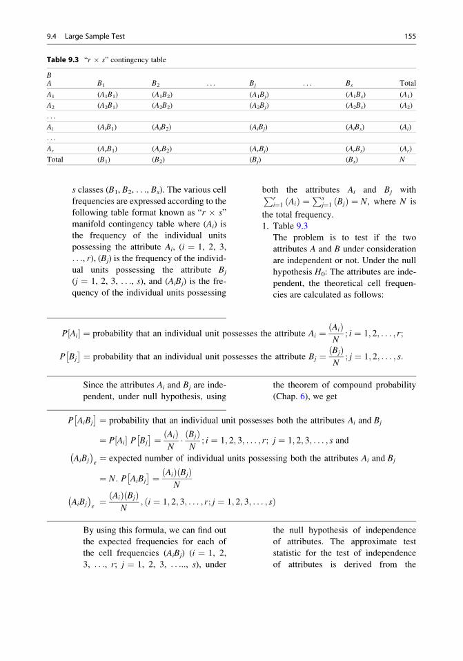
s classes (B1, B2, . . ., Bs). The various cell

frequencies are expressed according to the

following table format known as “r � s”

manifold contingency table where (Ai) is

the frequency of the individual units

possessing the attribute Ai, (i ¼ 1, 2, 3,

. . ., r), (Bj) is the frequency of the individ-

ual units possessing the attribute Bj

(j ¼ 1, 2, 3, . . ., s), and (AiBj) is the fre-

quency of the individual units possessing

both the attributes Ai and Bj withPri¼1 ðAiÞ ¼

Psj¼1 ðBjÞ ¼ N, where N is

the total frequency.

1. Table 9.3

The problem is to test if the two

attributes A and B under consideration

are independent or not. Under the null

hypothesis H0: The attributes are inde-

pendent, the theoretical cell frequen-

cies are calculated as follows:

P Ai½ � ¼ probability that an individual unit possesses the attribute Ai ¼ ðAiÞN

; i ¼ 1; 2; . . . ; r;

P Bj

� ¼ probability that an individual unit possesses the attribute Bj ¼ ðBjÞN

; j ¼ 1; 2; . . . ; s:

Since the attributes Ai and Bj are inde-

pendent, under null hypothesis, using

the theorem of compound probability

(Chap. 6), we get

P AiBj

� ¼ probability that an individual unit possesses both the attributes Ai and Bj

¼ P Ai½ � P Bj

� ¼ ðAiÞN

� ðBjÞN

; i ¼ 1; 2; 3; . . . ; r; j ¼ 1; 2; 3; . . . ; s and

AiBj

� �e¼ expected number of individual units possessing both the attributes Ai and Bj

¼ N: P AiBj

� ¼ ðAiÞðBjÞN

AiBj

� �e¼ ðAiÞðBjÞ

N; i ¼ 1; 2; 3; . . . ; r; j ¼ 1; 2; 3; . . . ; sð Þ

By using this formula, we can find out

the expected frequencies for each of

the cell frequencies (AiBj) (i ¼ 1, 2,

3, . . ., r; j ¼ 1, 2, 3, . . ..., s), under

the null hypothesis of independence

of attributes. The approximate test

statistic for the test of independence

of attributes is derived from the

Table 9.3 “r � s” contingency table

BB1 B2 . . . Bj . . . Bs TotalA

A1 (A1B1) (A1B2) (A1Bj) (A1Bs) (A1)

A2 (A2B1) (A2B2) (A2Bj) (A2Bs) (A2)

. . .

Ai (AiB1) (AiB2) (AiBj) (AiBs) (Ai)

. . .

Ar (ArB1) (ArB2) (ArBj) (ArBs) (Ar)

Total (B1) (B2) (Bj) (Bs) N

9.4 Large Sample Test 155

χ2 test for goodness of fit as given

below:

χ2 ¼Xri¼1

Xsj¼1

AiBj

� �o� AiBj

� �e

n o2

AiBj

� �e

264

375

¼Xri¼1

Xsj¼1

fij � eij� �2

eij: χ2ðr�1Þðs�1Þ

where

fij ¼ observed cell frequency of ith

row and jth column combination and

eij ¼ expected cell frequency of ith rowand jth column combination.

2. “2 � 2” χ2 TestUnder the special case, the r � s con-tingency table becomes a 2 � 2 con-

tingency table, in which both the

attributes are classified into two groups

each. The test of independence of

attributes can be performed in the sim-

ilar way as in the case of r � s contin-gency table. Moreover, the value of

χ2 can also be calculated directly from

the observed frequency table. Let us

suppose we have the following 2 � 2

contingency Table 9.4 as given below:

The formula for calculating χ2 value is

χ2 ¼ Nðad � bcÞ2ðaþ cÞðbþ dÞðaþ bÞðcþ dÞ χ2ð2�1Þð2�1Þ χ21:

Now comparing the table value of χ2 at1 degree of freedom at a prefixed αlevel of significance with the calcu-

lated value of χ2, one can arrive at a

definite conclusion about the indepen-

dence of the two attributes.

Yates’s CorrectionValidity of the χ2 depends on the con-

dition that the expected frequency in

each cell should be sufficiently large;

generally the expected frequency is

required to be at least five. One can

overcome the problem of lower cell

frequency by coalescing or merging

consecutive rows or columns. In

doing so, one has to compromise with

the basic concept of the classification

of the particular subject on hand. In a

2 � 2 table, the possibility of merging

cell frequencies is ruled out, rather we

adopt Yates’s corrected formula for

χ2 as given below:

χ21 ¼ad � bcj j � N

2

� �2N

ðaþ bÞðcþ dÞðaþ cÞðbþ dÞ ;

where N is the total frequency and a, b,

c, and d are as usual.

Example 9.27. The following table gives the

frequency distribution of education standard

and type occupation for 280 persons. Test

whether the type of occupation is independent

of education standard or not.

Cultivation Teaching

Govt.

service Others

HS 65 5 12 8

Graduation 35 25 15 10

Postgraduation 25 40 25 15

Solution. Under the given condition

H0: Educational standard and occupation are

independent against

H1: Educational standard and occupation are not

independent.

Under the given H0, the test statistic is

χ2ð3�1Þð3�1Þ ¼Xri¼1

Xsj¼1

AiBj

� �o� AiBj

� �e

n o2

AiBj

� �e

264

375

¼Xri¼1

Xsj¼1

fij � eij� �2

eij:

Table 9.4 “2 � 2” contingency table

Attribute B

Attribute A B1 B2 Total

A1 a b a + b

A2 c d c + d

Total a + c b + d a + b + c + d ¼ N

156 9 Formulation and Testing of Hypothesis

Let the level of significance be α ¼ 0.05

We calculate the expected frequencies as

follows:

P AiBj

� ¼ probability that an individual unit possesses both the attributes Ai and Bj

¼ P Ai½ � P Bj

� ¼ ðAiÞ

N� ðBjÞN

; i ¼ 1; 2; 3; . . . ; r; j ¼ 1; 2; 3; . . . ; s; and

AiBj

� �e¼ expected number of individual units possessing both the attributes Ai and Bj

¼ N: P AiBj

� ¼ ðAiÞðBjÞN

:

As follows:

The expected frequencies are as follows:

Cultivation Teaching

Govt.

service Others

HS 40.1786 22.50 16.7143 10.6071

Graduation 37.9464 21.25 15.7857 10.0178

Postgraduation 46.8750 26.25 19.500 12.3750

So,

χ26 ¼Xri¼1

Xsj¼1

fij � eij� �2

eij¼ ð65� 40:1786Þ2

401786

þ ð5� 22:5Þ222:5

þ � � � þ ð15� 12:375Þ212:375

¼ 51:3642:

The table value of χ20:05;6 ¼ 12:592 is less than

the calculated value of χ2 . Hence, the test is

significant and the null hypothesis is rejected.

We can conclude that the two attributes, educa-

tional standard and the type of occupation, are

not independent of each other.

Example 9.28. The following table is pertaining

to classification of rice varieties classified into

grain shape and aroma. Test whether the taste

and aroma are independent of each other or not.

Grain shape

Aroma Long Dwarf

Aromatic 40 50

Nonaromatic 45 65

Solution. To test H0: Taste and aroma are inde-

pendent of each other against the alternative

hypothesis H1: Grain shape and aroma are not

independent of each other. The test statistic

follows a χ2 distribution with 1 d.f. Let the

level of significance be 0.05.

So

χ2 ¼ ðad � bcÞ2Nðaþ bÞðcþ dÞðaþ cÞðbþ dÞ :

We don’t have to go for Yates’s correction.

From the above given information, we have

χ2 ¼ ð40� 65� 50� 45Þ220090� 110� 85� 115

¼ 0:2532:

The calculated value of χ2 is less than the

tabulated value of χ20:05;1 (3.84). So the test is

Groups Cultivation Teaching Govt. service Others Total

HS ¼ 90 � 125/280 ¼ 90 � 70/280 ¼ 90 � 52/280 ¼ 90 � 33/280 90

Graduation ¼ 85 � 125/280 ¼ 85 � 70/281 ¼ 85 � 52/281 ¼ 85 � 33/281 85

Postgraduation ¼ 105 � 125/280 ¼ 105 � 70/282 ¼ 105 � 52/282 ¼ 105 � 33/282 105

Total 125 70 52 33 280

9.4 Large Sample Test 157

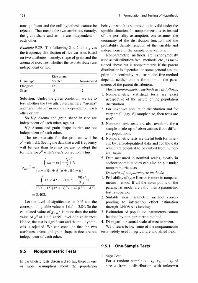
nonsignificant and the null hypothesis cannot be

rejected. That means the two attributes, namely,

the grain shape and aroma are independent of

each other.

Example 9.29. The following 2 � 2 table gives

the frequency distribution of rice varieties based

on two attributes, namely, shape of grain and the

aroma of rice. Test whether the two attributes are

independent or not.

Rice aroma

Grain type Scented Non-scented

Elongated 15 30

Short 3 42

Solution. Under the given condition, we are to

test whether the two attributes, namely, “aroma”

and “grain shape” in rice are independent of each

other or not.

So H0: Aroma and grain shape in rice are

independent of each other, against

H1: Aroma and grain shape in rice are not

independent of each other.

The test statistic for the problem will be

χ2 with 1 d.f. Seeing the data that a cell frequencywill be less than five, so we are to adopt the

formula for χ2 with Yates’s correction. Thus,

χcorr:2 ¼

ad � bcj j � N

2

� 2

N

ðaþ bÞðcþ dÞðaþ cÞðbþ dÞ

¼15� 42� 30� 3j j � 90

2

� 2

90

ð30þ 15Þð15þ 3Þð3þ 42Þð30þ 42Þ¼ 8:402:

Let the level of significance be 0.05 and the

corresponding table value at 1 d.f. is 3.84. So the

calculated value of χcorr:2 is more than the table

value of χ2 at 1 d.f. at 5% level of significance.

Hence, the test is significant and the null hypoth-

esis is rejected. We can conclude that the two

attributes, aroma and grain shape in rice, are not

independent of each other.

9.5 Nonparametric Tests

In parametric tests discussed so far, there is one

or more assumption about the population

behavior which is supposed to be valid under the

specific situation. In nonparametric tests instead

of the normality assumption, one assumes the

continuity of the distribution function and the

probability density function of the variable and

independence of the sample observations.

Nonparametric methods are synonymously

used as “distribution-free” methods, etc., as men-

tioned above but is nonparametric if the parent

distribution is dependent on some general assum-

ption like continuity. A distribution-free method

depends neither on the form nor on the para-

meters of the parent distribution.

Merits nonparametric methods are as follows:

1. Nonparametric statistical tests are exact

irrespective of the nature of the population

distribution.

2. For unknown population distribution and for

very small (say, 6) sample size, then tests are

useful.

3. Nonparametric tests are also available for a

sample made up of observations from differ-

ent populations.

4. Nonparametric tests are useful both for inher-

ent by ranked/qualified data and for the data

which are potential to be ranked from numer-

ical figure.

5. Data measured in nominal scales, mostly in

socioeconomic studies can also be put under

nonparametric tests.

Demerits of nonparametric methods:

1. Probability of type II error is more in nonpara-

metric method. If all the assumptions of the

parametric model are valid, then a parametric

test is superior.

2. Suitable non parametric method corres-

ponding to interaction effect estimation

through ANOVA is lacking.

3. Estimation of population parameters cannot

be done by non-parametric method.

4. Disregard the actual scale of measurement.

We discuss below some of the nonparametric

tests widely used in agriculture and allied field.

9.5.1 One-Sample Tests

1. Sign TestFor a random sample x1, x2, x3, . . . xn of

size n from a distribution with unknown

158 9 Formulation and Testing of Hypothesis

median θ, we are to test H0: θ ¼ θ0 against

the alternative hypotheses ð1Þ θ 6¼ θ0;ð2Þ θ> θ0; and ð3Þθ< θ0.If θ0 be the median, then there will be equal

number of observations below and above the

value θ0. We denote the observations greater

than the θ0 with plus (+) signs and the

observations smaller than θ0 with minus (�)

signs and ignore the sample values equal to

the median. Let item be r plus (+) sign and

minus signs. Such that r + s ¼ m � n. Distri-

bution of r given r + s ¼ m is binomial with

probability ½. Thus, the above null hypothesis

becomes equivalent to testing H0: P ¼ 1/2,

where P ¼ P(x > θ0). One-tailed cumulative

binomial probabilities are given in Table A.9.

For H1: θ 6¼ θ0 the critical region for α

level of significance is given by r � r0α=2 and

r rα=2 where r0α=2 and rα=2 are the largest

and smallest integer such thatPr

0α=2

r¼0

m

r

!m

� α=2 andPm

r¼α=2

m

r

!1

2

� m

�

α=2. For H1: θ> θ0, the critical region for

α level of significance is given by r rα;where rα is the smallest integer such thatPm

r¼rα

m

r

!12

� �m � α: For H1: θ< θ0, the

critical region for ^α level of significance is

given by r � r0α where r

0α is the larger integer

such thatPm

r¼0

m

r

!1

2

� � α:

Example 9.30. Test whether the median long

jump (θ) of a group of students is 10 ft or not at

5% level of significance from the following data

on long jumps.

Long jumps (feet): 11.2, 12.2, 10.0, 9, 13,

12.3, 9.3, 9.8, 10.8, 11, 11.6, 10.6, 8.5, 9.5, 9.8,

11.6, 9.7, 10.9, 9.2, 9.8

Solution. Let us first assign the signs to each of

the given observations as follows:

There are 10 (¼ r) plus (+) signs and 9 (¼ s)

minus (�) signs, and one observation is equal to

the median value and discarded. This r is a bino-

mial variate with parameter (m ¼ r + s ¼20 � 1 ¼ 19) and P(¼ 1/2). Thus, testing of

H0 : θ ¼ 10 ft against H1 : θ 6¼ 10 ft is equiva-

lent to testing of H0: P ¼ ½ against H1: P 6¼ 1/2.

The critical region for α ¼ 0.05 (two-sided

test) is r rα=2 and r � r0α=2 where r is the num-

ber of plus signs and rα=2 and r0α=2 are the smallest

and largest integer, respectively, such thatP19

rα=2

19

x

!1

2

� 19

� α=2 andPr0

α=2

0

19

x

!1

2

� 19

� α=2.From the table we get r0:025 ¼ 14 and r00:025 ¼

4 for 19 distinct observations at p ¼ 1=2. For

this example we have 4/r ¼ 10 < 14, which

lies between 4 and 14, so we cannot reject the

null hypothesis at 5% level of significance, that

is, we conclude that the median of the long jump

can be taken as 10 ft.

[If total number of signs, that is, plus (+) signs

plus the minus (�) signs (i.e., r + s ¼ m), is

greater than 25, that is, m ¼ r + s > 25, then

normal approximation to binomial may be used,

and accordingly the probability of r or fewer

success will be tested with the statistic

τ ¼ r � rþs2ffiffiffiffiffiffi

rþs4

q ¼r�s2ffiffiffiffiffiffirþs

p2

¼ r � sffiffiffiffiffiffiffiffiffiffir þ s

p .]

2. Test of Randomness(a) One Sample Run Test

In socioeconomic or time series analysis,

the researchers often wants to know

whether the data point or observations

have changed following a definite pattern

or in a haphazard manner. One-sample run

test is used to test the hypothesis that a

sample is random. In other form, run test

is used to test the hypothesis that the given

sequence/arrangement is random.

A run is a sequence of letters (signs) of the

same kind bounded by letters (signs) of

Long jump 10 9 11.2 12.2 10 9 13 12.3 10.8 11 9.3 9.8

Signs � � + + � � + + + + � �Long jump 8.5 9.5 11.6 10.6 8.5 9.5 9.8 11.6 9.2 9.8 9.7 10.9

Signs � � + + � � � + � + � �

9.5 Nonparametric Tests 159

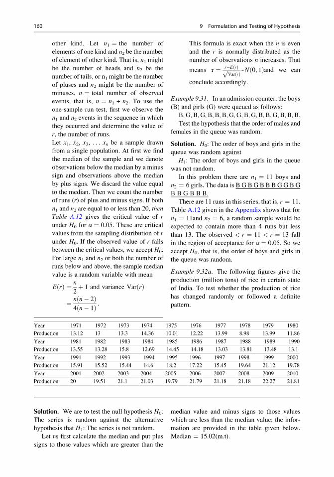
other kind. Let n1 ¼ the number of

elements of one kind and n2 be the number

of element of other kind. That is, n1 might

be the number of heads and n2 be the

number of tails, or n1 might be the number

of pluses and n2 might be the number of

minuses. n ¼ total number of observed

events, that is, n ¼ n1 + n2. To use the

one-sample run test, first we observe the

n1 and n2 events in the sequence in which

they occurred and determine the value of

r, the number of runs.

Let x1, x2, x3, . . . xn be a sample drawn

from a single population. At first we find

the median of the sample and we denote

observations below the median by a minus

sign and observations above the median

by plus signs. We discard the value equal

to the median. Then we count the number

of runs (r) of plus and minus signs. If both

n1 and n2 are equal to or less than 20, then

Table A.12 gives the critical value of runder H0 for α ¼ 0:05: These are critical

values from the sampling distribution of r

under H0. If the observed value of r fallsbetween the critical values, we accept H0.

For large n1 and n2 or both the number of

runs below and above, the sample median

value is a random variable with mean

EðrÞ ¼ n

2þ 1 and variance VarðrÞ

¼ nðn� 2Þ4ðn� 1Þ :

This formula is exact when the n is even

and the r is normally distributed as the

number of observations n increases. That

means τ ¼ r�EðrÞffiffiffiffiffiffiffiffiffiffiVarðrÞ

p~Nð0; 1Þand we can

conclude accordingly.

Example 9.31. In an admission counter, the boys

(B) and girls (G) were queued as follows:

B, G, B, G, B, B, B, G, G, B, G, B, B, G, B, B, B.

Test the hypothesis that the order of males and

females in the queue was random.

Solution. H0: The order of boys and girls in the

queue was random against

H1: The order of boys and girls in the queue

was not random.

In this problem there are n1 ¼ 11 boys and

n2 ¼ 6 girls. The data is B G B G B B B G G B G

B B G B B B.

There are 11 runs in this series, that is, r ¼ 11.

Table A.12 given in the Appendix shows that for

n1 ¼ 11and n2 ¼ 6, a random sample would be

expected to contain more than 4 runs but less

than 13. The observed < r ¼ 11 < r ¼ 13 fall

in the region of acceptance for α ¼ 0:05. So we

accept H0, that is, the order of boys and girls in

the queue was random.

Example 9.32a. The following figures give the

production (million tons) of rice in certain state

of India. To test whether the production of rice

has changed randomly or followed a definite

pattern.

Solution. We are to test the null hypothesis H0:

The series is random against the alternative

hypothesis that H1: The series is not random.

Let us first calculate the median and put plus

signs to those values which are greater than the

median value and minus signs to those values

which are less than the median value; the infor-

mation are provided in the table given below.

Median ¼ 15.02(m.t).

Year 1971 1972 1973 1974 1975 1976 1977 1978 1979 1980

Production 13.12 13 13.3 14.36 10.01 12.22 13.99 8.98 13.99 11.86

Year 1981 1982 1983 1984 1985 1986 1987 1988 1989 1990

Production 13.55 13.28 15.8 12.69 14.45 14.18 13.03 13.81 13.48 13.1

Year 1991 1992 1993 1994 1995 1996 1997 1998 1999 2000

Production 15.91 15.52 15.44 14.6 18.2 17.22 15.45 19.64 21.12 19.78

Year 2001 2002 2003 2004 2005 2006 2007 2008 2009 2010

Production 20 19.51 21.1 21.03 19.79 21.79 21.18 21.18 22.27 21.81

160 9 Formulation and Testing of Hypothesis

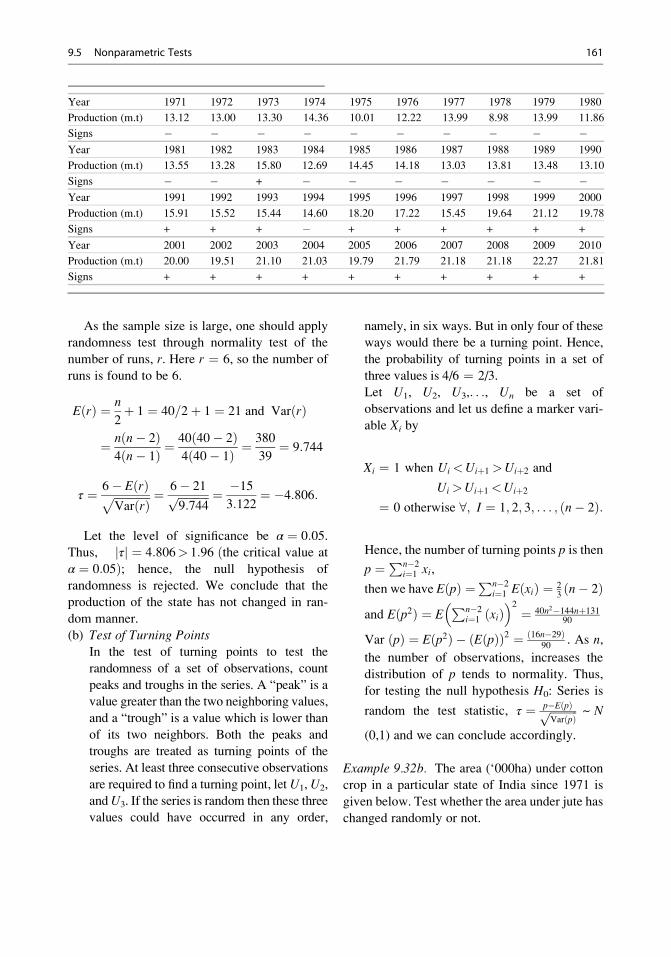
As the sample size is large, one should apply

randomness test through normality test of the

number of runs, r. Here r ¼ 6, so the number of

runs is found to be 6.

EðrÞ ¼ n

2þ 1 ¼ 40=2þ 1 ¼ 21 and VarðrÞ

¼ nðn� 2Þ4ðn� 1Þ ¼

40ð40� 2Þ4ð40� 1Þ ¼ 380

39¼ 9:744

τ ¼ 6� EðrÞffiffiffiffiffiffiffiffiffiffiffiffiffiVarðrÞp ¼ 6� 21ffiffiffiffiffiffiffiffiffiffiffi

9:744p ¼ �15

3:122¼ �4:806:

Let the level of significance be α ¼ 0:05.

Thus, τj j ¼ 4:806> 1:96 ðthe critical value at

α ¼ 0:05Þ; hence, the null hypothesis of

randomness is rejected. We conclude that the

production of the state has not changed in ran-

dom manner.

(b) Test of Turning PointsIn the test of turning points to test the

randomness of a set of observations, count

peaks and troughs in the series. A “peak” is a

value greater than the two neighboring values,

and a “trough” is a value which is lower than

of its two neighbors. Both the peaks and

troughs are treated as turning points of the

series. At least three consecutive observations

are required to find a turning point, let U1, U2,

andU3. If the series is random then these three

values could have occurred in any order,

namely, in six ways. But in only four of these

ways would there be a turning point. Hence,

the probability of turning points in a set of

three values is 4/6 ¼ 2/3.

Let U1, U2, U3,. . ., Un be a set of

observations and let us define a marker vari-

able Xi by

Xi ¼ 1 when Ui <Uiþ1 >Uiþ2 and

Ui >Uiþ1 <Uiþ2

¼ 0 otherwise 8; I ¼ 1; 2; 3; . . . ; n� 2ð Þ:

Hence, the number of turning points p is then

p ¼Pn�2i¼1 xi,

then we have EðpÞ ¼Pn�2i¼1 EðxiÞ ¼ 2

3ðn� 2Þ

and E p2ð Þ ¼ EPn�2

i¼1 ðxiÞ� �2

¼ 40n2�144nþ13190

Var ðpÞ ¼ E p2ð Þ � EðpÞð Þ2 ¼ ð16n�29Þ90

. As n,

the number of observations, increases the

distribution of p tends to normality. Thus,

for testing the null hypothesis H0: Series is

random the test statistic, τ ¼ p�EðpÞffiffiffiffiffiffiffiffiffiffiVarðpÞ

p ~ N

(0,1) and we can conclude accordingly.

Example 9.32b. The area (‘000ha) under cotton

crop in a particular state of India since 1971 is

given below. Test whether the area under jute has

changed randomly or not.

Year 1971 1972 1973 1974 1975 1976 1977 1978 1979 1980

Production (m.t) 13.12 13.00 13.30 14.36 10.01 12.22 13.99 8.98 13.99 11.86

Signs � � � � � � � � � �Year 1981 1982 1983 1984 1985 1986 1987 1988 1989 1990

Production (m.t) 13.55 13.28 15.80 12.69 14.45 14.18 13.03 13.81 13.48 13.10

Signs � � + � � � � � � �Year 1991 1992 1993 1994 1995 1996 1997 1998 1999 2000

Production (m.t) 15.91 15.52 15.44 14.60 18.20 17.22 15.45 19.64 21.12 19.78

Signs + + + � + + + + + +

Year 2001 2002 2003 2004 2005 2006 2007 2008 2009 2010

Production (m.t) 20.00 19.51 21.10 21.03 19.79 21.79 21.18 21.18 22.27 21.81

Signs + + + + + + + + + +

9.5 Nonparametric Tests 161

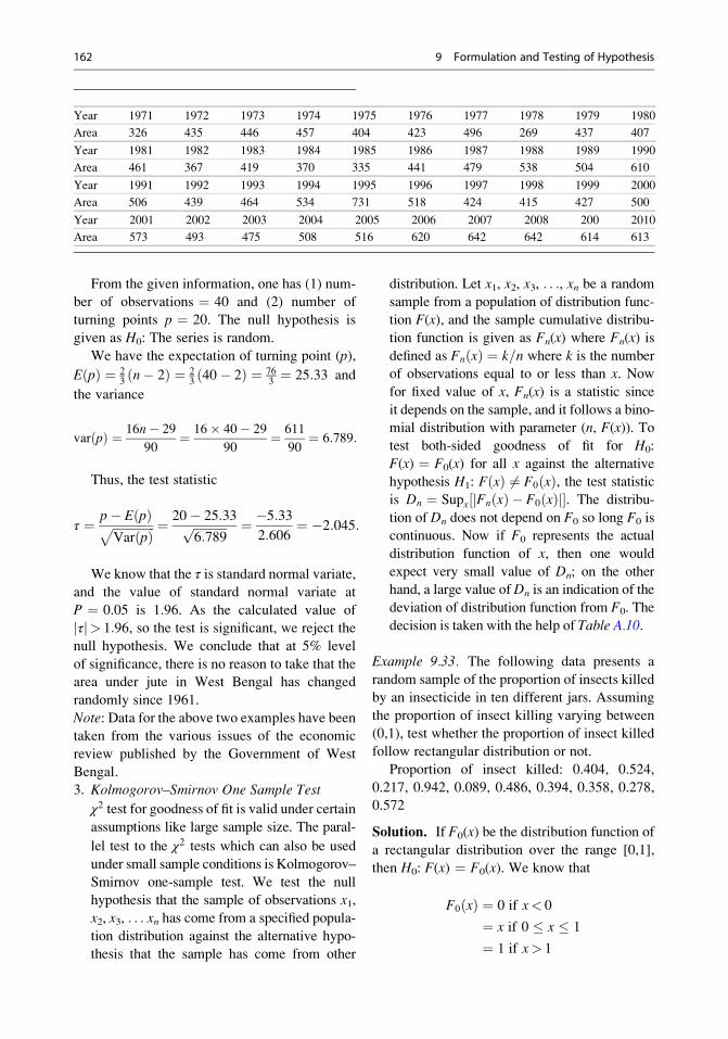
From the given information, one has (1) num-

ber of observations ¼ 40 and (2) number of

turning points p ¼ 20. The null hypothesis is

given as H0: The series is random.

We have the expectation of turning point (p),

EðpÞ ¼ 23ðn� 2Þ ¼ 2

3ð40� 2Þ ¼ 76

3¼ 25:33 and

the variance

varðpÞ ¼ 16n� 29

90¼ 16� 40� 29

90¼ 611

90¼ 6:789:

Thus, the test statistic

τ ¼ p� EðpÞffiffiffiffiffiffiffiffiffiffiffiffiffiffiVarðpÞp ¼ 20� 25:33ffiffiffiffiffiffiffiffiffiffiffi

6:789p ¼ �5:33

2:606¼ �2:045:

We know that the τ is standard normal variate,

and the value of standard normal variate at

P ¼ 0.05 is 1.96. As the calculated value of

τj j> 1:96, so the test is significant, we reject the

null hypothesis. We conclude that at 5% level

of significance, there is no reason to take that the

area under jute in West Bengal has changed

randomly since 1961.

Note: Data for the above two examples have been

taken from the various issues of the economic

review published by the Government of West

Bengal.

3. Kolmogorov–Smirnov One Sample Test

χ2 test for goodness of fit is valid under certainassumptions like large sample size. The paral-

lel test to the χ2 tests which can also be used

under small sample conditions is Kolmogorov–

Smirnov one-sample test. We test the null

hypothesis that the sample of observations x1,

x2, x3, . . . xn has come from a specified popula-

tion distribution against the alternative hypo-

thesis that the sample has come from other

distribution. Let x1, x2, x3, . . ., xn be a random

sample from a population of distribution func-

tion F(x), and the sample cumulative distribu-

tion function is given as Fn(x) where Fn(x) is

defined as FnðxÞ ¼ k n= where k is the number

of observations equal to or less than x. Now

for fixed value of x, Fn(x) is a statistic since

it depends on the sample, and it follows a bino-

mial distribution with parameter (n, F(x)). To

test both-sided goodness of fit for H0:

F(x) ¼ F0(x) for all x against the alternative

hypothesis H1: FðxÞ 6¼ F0ðxÞ, the test statistic

is Dn ¼ Supx FnðxÞ � F0ðxÞj j½ �. The distribu-

tion of Dn does not depend on F0 so long F0 is

continuous. Now if F0 represents the actual

distribution function of x, then one would

expect very small value of Dn; on the other

hand, a large value ofDn is an indication of the

deviation of distribution function from F0. The

decision is taken with the help of Table A.10.

Example 9.33. The following data presents a

random sample of the proportion of insects killed

by an insecticide in ten different jars. Assuming

the proportion of insect killing varying between

(0,1), test whether the proportion of insect killed

follow rectangular distribution or not.

Proportion of insect killed: 0.404, 0.524,

0.217, 0.942, 0.089, 0.486, 0.394, 0.358, 0.278,

0.572

Solution. If F0(x) be the distribution function of

a rectangular distribution over the range [0,1],

then H0: F(x) ¼ F0(x). We know that

F0ðxÞ ¼ 0 if x< 0

¼ x if 0 � x � 1

¼ 1 if x> 1

Year 1971 1972 1973 1974 1975 1976 1977 1978 1979 1980

Area 326 435 446 457 404 423 496 269 437 407

Year 1981 1982 1983 1984 1985 1986 1987 1988 1989 1990

Area 461 367 419 370 335 441 479 538 504 610

Year 1991 1992 1993 1994 1995 1996 1997 1998 1999 2000

Area 506 439 464 534 731 518 424 415 427 500

Year 2001 2002 2003 2004 2005 2006 2007 2008 200 2010

Area 573 493 475 508 516 620 642 642 614 613

162 9 Formulation and Testing of Hypothesis

for a rectangular distribution. We make the

following table:

x F0(x) Fn(x) FnðxÞ � F0ðxÞj j0.089 0.089 0.1 0.011

0.217 0.217 0.2 0.017

0.278 0.278 0.3 0.022

0.358 0.358 0.4 0.042

0.394 0.394 0.5 0.106

0.404 0.404 0.6 0.196

0.486 0.486 0.7 0.214

0.524 0.524 0.8 0.276

0.572 0.572 0.9 0.328

0.942 0.942 1.0 0.058

Let the level of significance α ¼ 0.05.

From the table we get for n ¼ 10 the critical

value of K–S statistic Dn at 5% level of signifi-

cance is 0.409. Thus, the calculated value of

Dn ¼ Supx

FnðxÞ � F0ðxÞj j½ � ¼ 0:328 < the table

value 0.409, so we cannot reject the null hypoth-

esis. That means we conclude that the given

sample is from the rectangular parent distribu-

tion. This example is due to Sahu (2007).

4. The Median Test

Synonymous to that of the parametric test to

test whether two samples have been taken

from the same population or not, the median

test is also used to test whether two groups

have been taken from the same population

or not. Actually in the median test, the null

hypothesis tested is that whether two sets of

scores differ significantly between them or

not. Generally it is used to test whether there

exists any significant difference between the

experimental group and the control group or

not. If the two groups have been drawn at

random from the same population, it is quite

obvious that half of the frequencies will lie

above and below the median. The whole pro-

cess is given stepwise:

(a) Arrange the ranks/scores of both the

group units taken together.

(b) A common median is worked out.

(c) Scores of each group are then divided into

two subgroups: (a) those above the com-

mon median and (b) those below the com-

mon median; generally the ranks equal to

the medians are ignored.

(d) These frequencies are then put into 2 � 2

contingency table.

(e) χ2 value is obtained using the usual

norms.

(f) The decision rule is the same as that was

for χ2 test.

Example 9.34. The following table gives the

scores of two groups of students. Test whether

the two groups could be taken as one or not.

Solution. Under the given condition, we can go

for median test to test the equality of two groups

with respect to their scores.

Taking both the groups as one can have the

following arrangement:

From the above arrangements, we have the

median score as the average of the 12th and 13th

ordered observation, that is, (8 + 9)/2 ¼ 8.5.

Now a 2 � 2 contingency table is prepared

as follows:

Below Above

Group1 (a) 5 (b) 7

Group2 (c) 7 (d) 5

Group

Students

1 2 3 4 5 6 7 8 9 10 11 12

Group 1 9 8 12 6 8 9 5 10 9 7 11 10

Group2 8 11 4 9 7 3 10 9 5 6 12 8

3 4 5 5 6 6 7 7 8 8 8 8 9 9 9 9 9 10 10 10 11 11 12 12

9.5 Nonparametric Tests 163

X21 ¼

ðad � bcÞ2Nðaþ bÞðaþ cÞðbþ dÞðcþ dÞ

¼ 24� 24

12� 12� 12¼ 0:66:

From this 2 � 2 contingency table using the

formula, the calculated value of χ2 ¼ 0.66 < the

table value of χ2 ¼ 3.841 at 5% level of signifi-

cance. So we have no reason to reject the null

hypothesis that the two groups have come from

the same population, that is, the two groups do

not differ.

5. The Mann–Whitney U-Test

Analogous to the parametric t-test, the

Mann–Whitney U-test is aimed at determin-

ing whether two independent samples have

been drawn from the same population or not.

This test does not require any assumption

except that the continuity. Steps involved in

the process are given below:

(a) Rank the data of both the samples taking

them as one sample from low to high

(generally low ranking is given to low

value and so on).

(b) For tied ranks take the average of the

ranks for each of the tied values (e.g.,

if 4th, 5th, 6th, and 7th places are having

the same value, then each of these

identical values would be assigned ((4 +

5 + 6 + 7)/4¼) 5.5 rank).

(c) Find the sum of the ranks of both the

samples separately (say, R1 and R2,

respectively, for 1st and 2nd sample).

(d) Calculate U ¼ n1 � n2 þ n1ðn1þ1Þ2

� R1,

where n1 and n2 are the sizes of the 1st and2nd sample, respectively.

(e) If both n1 and n2 are sufficiently large

(>8), the sampling distribution of U can

be approximated to a normal distribution

and usual critical values could be used to

arrive at the conclusion. On the other

hand, if the sample sizes are small, then

the significance test can be worked out as

per the table values of the Wilcoxon’s

unpaired distribution.

Example 9.35. The following table gives the

scores in mathematics of two groups of students.

Using Mann–Whitney U-test, can you say that

these two groups of students are the same at 5%

level of significance, that is, they have come

from the same population?

Solution. Using the above information we get

the following table:

Given that n1 ¼ 12 and n2 ¼ 10, so

U ¼ n1 � n2 þ n1ðn1 þ 1Þ2

� R1

¼ 12:10þ 12ð12þ 1Þ2

� 143:5

¼ 120þ 78� 143:5 ¼ 54:5:

Since both n1 and n2 are greater than 8, so

normal approximation can be used with mean

μU ¼ n1 � n2=2 ¼ 60ð Þ and variance

σ2U ¼ n1 � n2 þ n1ðn1 þ n2 þ 1Þ12

¼ 12:10þ 12ð12þ 10þ 1Þ12

¼ 120þ 23

¼ 143 and σU ¼ 11:958:

Group

Students

1 2 3 4 5 6 7 8 9 10 11 12

Group A 59 48 52 45 32 56 98 78 70 85 43 80

Group B 39 45 55 87 36 67 96 75 65 38

164 9 Formulation and Testing of Hypothesis

At 5% level of significance, the critical value

of Z the standard normal variate is 1.96.

So the upper and lower confidential limits are

μU þ 1:96σU ¼ 60þ 1:96� 11:958¼ 83:438 and μU � 1:96σU¼ 60� 1:96� 11:958 ¼ 36:562:

As the observed value is within the accep-

tance zone, one can accept the null hypothesis

to conclude that the two groups of students have

come from the same population.

By calculating U using R2, one get the value

of U as

U ¼ n1 � n2 þ n2ðn2 þ 1Þ2

� R2

¼ 12:10þ 10ð10þ 1Þ2

� 109:5

¼ 120þ 55� 109:5 ¼ 65:5

which is also within the zone of acceptance. So it

does not matter how we are calculating the U

value, the inference remains the same.

6. The Kruskal–Wallis Test

The Kruskal–Wallis test is used to compare

the average performance of many groups,

analogous to the one-way analysis of variance

in parametric method. But unlike the para-

metric method, it does not require the assump-

tion that the samples have come from normal

populations. This test is mostly an extension

of the Mann–Whitney U-test; difference is

that here more than two groups are compared,

and the test statistic is approximated to χ2 withthe stipulation that none of the groups should

have less than five observations. The steps for

this test are given below:

(a) Rank the data of all the samples taking them

as one sample from low to high (generally

low ranking is given to lowvalue and so on).

(b) For tied ranks take the average of

the ranks for each of the tied values

(e.g., if 4th, 5th, 6th, and 7th places are

having the same value then each of

these identical values would be assigned

(4 + 5 + 6 + 7)/4¼ 5.5 rank).

Original score Ordered score

Unified rank

Rank

Group Score Group Score Group A Group B

A 59 A 32 1 1

A 48 B 36 2 2

A 52 B 38 3 3

A 45 B 39 4 4

A 32 A 43 5 5

A 56 A 45 6.5 6.5

A 98 B 45 6.5 6.5

A 78 A 48 8 8

A 70 A 52 9 9

A 85 B 55 10 10

A 43 A 56 11 11

A 80 A 59 12 12

B 39 B 65 13 13

B 45 B 67 14 14

B 55 A 70 15 15

B 87 B 75 16 16

B 36 A 78 17 17

B 67 A 80 18 18

B 96 A 85 19 19

B 75 B 87 20 20

B 65 B 96 21 21

B 38 A 98 22 22

Total 253 143.5 109.5

9.5 Nonparametric Tests 165

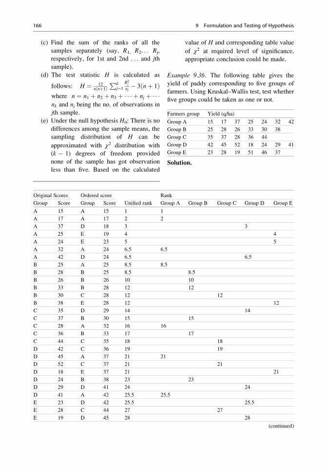
(c) Find the sum of the ranks of all the

samples separately (say, R1, R2. . . Rj,

respectively, for 1st and 2nd . . . and jth

sample).

(d) The test statistic H is calculated as

follows: H ¼ 12nðnþ1Þ

Pkj¼1

R2j

nj� 3ðnþ 1Þ

where n ¼ n1 þ n2 þ n3 þ � � � þ nj þ � � �nk and nj being the no. of observations in

jth sample.

(e) Under the null hypothesis H0: There is no

differences among the sample means, the

sampling distribution of H can be

approximated with χ2 distribution with

(k � 1) degrees of freedom provided

none of the sample has got observation

less than five. Based on the calculated

value of H and corresponding table value

of χ2 at required level of significance,

appropriate conclusion could be made.

Example 9.36. The following table gives the

yield of paddy corresponding to five groups of

farmers. Using Kruskal–Wallis test, test whether

five groups could be taken as one or not.

Farmers group Yield (q/ha)

Group A 15 17 37 25 24 32 42

Group B 25 28 26 33 30 38

Group C 35 37 28 36 44

Group D 42 45 52 18 24 29 41

Group E 23 28 19 51 46 37

Solution.

Original Scores Ordered score

Unified rank

Rank

Group Score Group Score Group A Group B Group C Group D Group E

A 15 A 15 1 1

A 17 A 17 2 2

A 37 D 18 3 3

A 25 E 19 4 4

A 24 E 23 5 5

A 32 A 24 6.5 6.5

A 42 D 24 6.5 6.5

B 25 A 25 8.5 8.5

B 28 B 25 8.5 8.5

B 26 B 26 10 10

B 33 B 28 12 12

B 30 C 28 12 12

B 38 E 28 12 12

C 35 D 29 14 14

C 37 B 30 15 15

C 28 A 32 16 16

C 36 B 33 17 17

C 44 C 35 18 18

D 42 C 36 19 19

D 45 A 37 21 21

D 52 C 37 21 21

D 18 E 37 21 21

D 24 B 38 23 23

D 29 D 41 24 24

D 41 A 42 25.5 25.5

E 23 D 42 25.5 25.5

E 28 C 44 27 27

E 19 D 45 28 28

(continued)

166 9 Formulation and Testing of Hypothesis

H ¼ 12

nðnþ 1ÞXkj¼1

R2j

nj� 3ðnþ 1Þ

¼ 12

31ð31þ 1Þ 925:75þ 1218:375þ 1881:8þ 2489:143þ 1700:167½ � � 3ð31þ 1Þ

¼ 12

31� 328215:235½ � � 3ð32Þ ¼ 99:378� 96 ¼ 3:378:

As all the groups have five or more

observations, so H is distributed as χ2 with

(5 � 1¼)4 d.f. The table value of χ2 at 5%

level of significance and 4 d.f. is 9.488 which is

greater than the calculated value, so we cannot

reject the null hypothesis of equality of means of

five farmers groups.

7. The McNemar TestJust like to that of paired t-test, McNemar test

is applicable for related samples, particularly

concerned with nominal data. Initially when

the subjects are categorized into two groups,

treatment is applied and again the responses

are recorded and subjects are grouped. This

test is used to record whether there has been

any significant change in grouping due to

treatment or not.

After treatment

Before treatment Disliked Liked

Liked a b

Disliked c d

Where a, b, c, and d are the respective cell

frequencies. Clearly a + d is the change in

response due to treatment whereas b + c

does not indicate any change. Thus, under

normal situation one can expect equal proba-

bility of changes in either direction; that

means one should go for testing H0: P

(a) ¼ P(d) against the alternative H1: P

(a) 6¼ P(b), and the appropriate test statistic

is χ21 ¼ a� dj j � 1ð Þ2 ðaþ dÞ= .

Example 9.37. Eight hundred farmers were asked

about the effectiveness of SRI (system rice inten-

sification); then these farmers were demonstrated

the practice. The following table gives the

responses before and after the demonstration.

Examine whether the demonstration has got any

impact on farmers’ attitude towards SRI or not.

After demonstration

Before demonstration Disliked Liked

Liked 125 225

Disliked 75 375

Solution. Under the given condition, we are to

test H0: P(like, dislike) ¼ P(dislike, like) against

H1: P(like, dislike) 6¼ P(dislike, like). The

appropriate test statistic is χ21 ¼ a� dj j � 1ð Þ2=ðaþ dÞ; here a ¼ 125, d ¼ 375, so the

χ21 ¼a� dj j � 1ð Þ2ðaþ dÞ ¼ 125� 375j j � 1ð Þ2

ð125þ 375Þ

¼ 249ð Þ2ð500Þ ¼ 124:002:

(continued)

Original Scores Ordered score

Unified rank

Rank

Group Score Group Score Group A Group B Group C Group D Group E

E 51 E 46 29 29

E 46 E 51 30 30

E 37 D 52 31 31

Rj 80.5 85.5 97 132 101

nj 7 6 5 7 6

R2j

nj

925.75 1218.375 1881.8 2489.143 1700.167

9.5 Nonparametric Tests 167

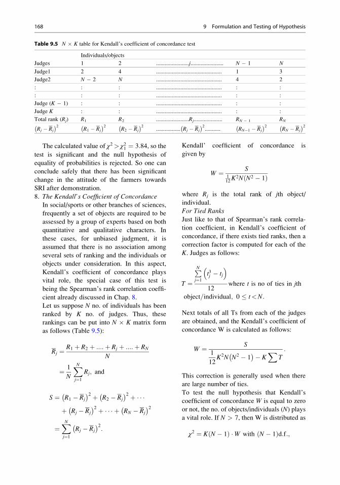
The calculated value of χ2 > χ21 ¼ 3:84, so the

test is significant and the null hypothesis of

equality of probabilities is rejected. So one can

conclude safely that there has been significant

change in the attitude of the farmers towards

SRI after demonstration.

8. The Kendall’s Coefficient of ConcordanceIn social/sports or other branches of sciences,

frequently a set of objects are required to be

assessed by a group of experts based on both

quantitative and qualitative characters. In

these cases, for unbiased judgment, it is

assumed that there is no association among

several sets of ranking and the individuals or

objects under consideration. In this aspect,

Kendall’s coefficient of concordance plays

vital role, the special case of this test is

being the Spearman’s rank correlation coeffi-

cient already discussed in Chap. 8.

Let us suppose N no. of individuals has been

ranked by K no. of judges. Thus, these

rankings can be put into N � K matrix form

as follows (Table 9.5):

Rj ¼ R1 þ R2 þ ::::þ Rj þ ::::þ RN

N

¼ 1

N

XNj¼1

Rj; and

S ¼ R1 � Rj

� �2 þ R2 � Rj

� �2 þ � � �þ Rj � Rj

� �2 þ � � � þ RN � Rj

� �2¼XNj¼1

Rj � Rj

� �2:

Kendall’ coefficient of concordance is

given by

W ¼ S112K2N N2 � 1ð Þ

where Rj is the total rank of jth object/

individual.

For Tied Ranks

Just like to that of Spearman’s rank correla-

tion coefficient, in Kendall’s coefficient of

concordance, if there exists tied ranks, then a

correction factor is computed for each of the

K. Judges as follows:

T ¼

PNj¼1

t3j � tj

� �12

where t is no of ties in jth

object=individual; 0 � t<N:

Next totals of all Ts from each of the judges

are obtained, and the Kendall’s coefficient of

concordance W is calculated as follows:

W ¼ S1

12K2N N2 � 1

� �� KX

T:

This correction is generally used when there

are large number of ties.

To test the null hypothesis that Kendall’s

coefficient of concordance W is equal to zero

or not, the no. of objects/individuals (N) plays

a vital role. If N > 7, then W is distributed as

χ2 ¼ KðN � 1Þ �W with ðN � 1Þd:f:;

Table 9.5 N � K table for Kendall’s coefficient of concordance test

Judges

Individuals/objects

1 2 .......................j....................... N � 1 N

Judge1 2 4 .............................................. 1 3

Judge2 N � 2 N .............................................. 4 2

: : : .............................................. : :

: : : .............................................. : :

Judge (K � 1) : : .............................................. : :

Judge K : : .............................................. : :

Total rank (Rj) R1 R2 .......................Rj.................... RN � 1 RN

Rj � Rj

� �2R1 � Rj

� �2R2 � Rj

� �2................. Rj � Rj

� �2........... RN�1 � Rj

� �2RN � Rj

� �2

168 9 Formulation and Testing of Hypothesis

and the conclusion is drawn accordingly. But

if the N � 7, then a table has been prepared

for different critical values of S associated

with W. If the observed S the value shown

in table, then H0: K sets of ranking are inde-

pendent may be rejected at the particular level

of significance.

Example 9.38. In a heptathlon event, eight

athletes were judged by six judges, and the fol-

lowing table shows the rank provided by each

judge to all the athletes. Test whether the judges

independently worked or not.

Judges

Athletes

1 2 3 4 5 6 7 8

Ranks

Judge 1 2 4 3 5 7 8 1 6

Judge 2 3 2 4 5 6 7 1 8

Judge 3 4 3 5 6 7 8 2 1

Judge 4 5 4 3 7 6 8 2 1

Judge 5 4 5 6 8 7 3 2 1

Judge 6 6 4 8 7 5 1 3 2

Solution. There are six sets of ranking for eight

objects. Kendall’s coefficient of concordance can

very well be worked out followed by the test of

H0:W ¼ 0. For this purpose we make the follow-

ing table:

Judges

Athletes

1 2 3 4 5 6 7 8

Judge 1 2 4 3 5 7 8 1 6

Judge 2 3 2 4 5 6 7 1 8

Judge 3 4 3 5 6 7 8 2 1

Judge 4 5 4 3 7 6 8 2 1

Judge 5 4 5 6 8 7 3 2 1

Judge 6 6 4 8 7 5 1 3 2

Total rank (Rj) 24 22 29 38 38 35 11 19

Rj � Rj

� �2 9 25 4 121 121 64 256 64

Rj ¼ R1 þ R2 þ � � � þ R8

8¼ 1

N

XNj¼1

Rj ¼ 27:

S ¼ R1 � Rj

� �2 þ R2 � Rj

� �2 þ � � � þ R8 � Rj

� �2¼ 24� 24ð Þ2 þ 22� 27ð Þ2 þ � � � þ 19� 27ð Þ2¼ 664:

W ¼ S1

12K2N N2 � 1

� � ¼ 664

1

12� 62 � 8 82 � 1

� � ¼ 0:439:

As N > 7, we can use the approximate χ2 ¼KðN � 1Þ �W with ðN � 1Þd:f: Here N ¼ 8,

K ¼ 6, and W ¼ 0.439, χ2 ¼ KðN � 1Þ �W ¼6� ð8� 1Þ � 0:439 ¼ 18:438; table value of

χ20:05;9 ¼ 16:919< χ2cal. Thus, the null hypothesis

of independence of judgment is rejected, and we

conclude that W is significant at 5% level of

significance.

9.5.2 Two-Sample Test

1. Paired-Sample Sign TestThe sign test for one sample mentioned above

can be easily modified to apply to sampling

from a bivariate population. Let a random

sample of n pairs (x1,y1), (x2,y2), (x3,y3), . . .,

(xn,yn) be drawn from a bivariate population.

Let di ¼ xi � yi (i ¼ 1, 2, 3, . . ., n). It is

assumed that the distribution function of dif-

ference, di, is also continuous. We want to test

H0: Med(D) ¼ 0, that is, P(D > 0) ¼ P(D< 0) ¼ 1 2= . It is to be noted that Med(D) is

not necessarily equal to Med (X) – Med(Y), so

that H0 is not that Med(X) ¼ Med(Y), but theMed(D) ¼ 0. Like the one-sample sign test,

we assign plus (+) and minus (�) signs to the

difference values which are greater and lesser

than zero, respectively. We perform the one-

sample sign test as given in the previous sec-

tion and conclude accordingly.

Example 9.39. Ten students were subjected to

physical training. Their body weights before and

after the training were recorded as given below.

Test whether there is any significant effect of

training on body weight or not.

9.5 Nonparametric Tests 169

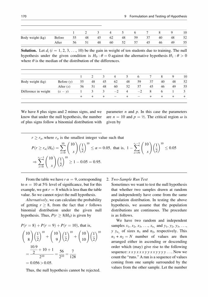
Solution. Let di (i ¼ 1, 2, 3, . . ., 10) be the gain in weight of ten students due to training. The null

hypothesis under the given condition is H0 : θ ¼ 0 against the alternative hypothesis H1 : θ > 0

where θ is the median of the distribution of the differences.

We have 8 plus signs and 2 minus signs, and we

know that under the null hypothesis, the number

of plus signs follow a binomial distribution with

parameter n and p. In this case the parameters

are n ¼ 10 and p ¼ ½. The critical region ω is

given by

r rα;where rα is the smallest integer value such that

Pðr rα=H0Þ ¼X10x¼0

10

x

!1

2

� 10

� α ¼ 0:05; that is; 1�Xrα�1

x¼r0

10

x

!1

2

� 10

� 0:05

)Xrα�1

x¼0

10

x

!1

2

� 10

1� 0:05 ¼ 0:95:

From the table we have r α ¼ 9, corresponding

to n ¼ 10 at 5% level of significance, but for this

example, we got r ¼ 8 which is less than the table

value. So we cannot reject the null hypothesis.

Alternatively, we can calculate the probabilityof getting r 8, from the fact that r follows

binomial distribution under the given null

hypothesis. Thus, P(r 8/H0) is given by

P r ¼ 8ð Þ þ P r ¼ 9ð Þ þ P r ¼ 10ð Þ, that is,10

8

!1

2

� 10

þ 10

9

!1

2

� 10

þ 10

10

!1

2

� 10

¼10:9

2þ 10þ 1

210¼ 56

210¼ 7

128

¼ 0:056> 0:05:

Thus, the null hypothesis cannot be rejected.

2. Two-Sample Run Test

Sometimes we want to test the null hypothesis

that whether two samples drawn at random

and independently have come from the same

population distribution. In testing the above

hypothesis, we assume that the population

distributions are continuous. The procedure

is as follows.

We have two random and independent

samples x1, x2, x3, . . ., xn1 and y1, y2, y3, . . .,

y yn1 of sizes n1 and n2, respectively. This

n1 + n2 ¼ N number of values are then

arranged either in ascending or descending

order which (may) give rise to the following

sequence: x x y x x x y y x x y y y y . . .. Now we

count the “runs.” A run is a sequence of values

coming from one sample surrounded by the

values from the other sample. Let the number

1 2 3 4 5 6 7 8 9 10

Body weight (kg) Before 55 48 45 62 48 59 37 40 48 52

After 56 51 48 60 52 57 45 46 49 55

1 2 3 4 5 6 7 8 9 10

Body weight (kg) Before (y) 55 48 45 62 48 59 37 40 48 52

After (x) 56 51 48 60 52 57 45 46 49 55

Difference in weight (x � y) 1 3 3 �2 4 �2 8 6 1 3

+ + + � + � + + + +

170 9 Formulation and Testing of Hypothesis

of runs in total n1+ n2 ¼ N arranged

observations be r. Number of runs r is

expected to be very high if the two samples

are thoroughly mixed; that means the two

samples are coming from the identical

distributions, otherwise the number of runs

will be very small. Table for critical values

of r for given values of n1 and n2 are provided

in Table A.10 (Appendix) for both n1 and n2less than 20. If the calculated r value is greaterthan the critical value of run for a given set of

n1 and n2, then we cannot reject the null

hypothesis; otherwise any value of calculated

r is less than or equal to the critical value of r

for a given set n1 and n2, the test is significant

and the null hypothesis is rejected.

For large n1 and n2 (say, >10) or any one of

them is greater than 20, the distribution of r is

asymptotically normal with

EðrÞ ¼ 2n1n2N

þ 1 and VarðrÞ

¼ 2n1n2ð2n1n2 � NÞN2ðN � 1Þ ;

and we can perform an approximate test sta-

tistic as

τ ¼ r � EðrÞffiffiffiffiffiffiffiffiffiffiffiffiffiVarðrÞp Nð0; 1Þ:

Example 9.40. Two independent samples of 9

and 8 plants of coconuts were selected randomly,

and the number of nuts per plant was recorded.

On the basis of nut characters, we are to decide

whether the two samples came from the same

coconut population or not.

Solution. Null hypothesis is H0: Samples have

come from identical distribution against the

alternative hypothesis that they have come from

different populations.

We arrange the observations as follows:

The value of r counted from the above table is

11 and the table value of r corresponding to 9 and

8 is 5. Thus, we cannot reject the null hypothesis

of equality of distributions. Hence, we conclude

that the two samples have been drawn from the

same population.

3. Two-Sample Median Test

The test parallel to equality of two means test

in parametric procedure is the two-sample

median tests in nonparametric method. The

objective of this test is to test that the two

independent samples drawn at random having

the same or different sample sizes are from

identical distributions against the alternative

hypotheses that they have different location

parameters (medians).

Let us draw two random independent samples

of sizes n1 and n2 from two populations. Make

an ordered combined sample of size n1 +

n2 ¼ N and get the median (θ) of the com-

bined sample. Next, we count the number of

observations below and above the estimated

median value θ for all the two samples, which

can be presented as follows (Table 9.6):

Sample Plant 1 Plant 2 Plant 3 Plant 4 Plant 5 Plant 6 Plant 7 Plant 8 Plant 9

Sample 1 140 135 85 90 75 110 112 95 100

Sample 2 80 125 95 100 112 90 105 108

Nut/plant 75 80 85 90 90 95 95 100 100

Sample 1 2 1 1 2 1 2 1 2

Nut/plant 105 108 110 112 112 125 135 140

Sample 2 2 1 1 2 2 1 1

9.5 Nonparametric Tests 171

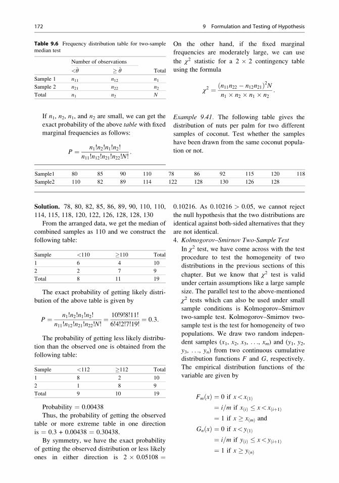
If n1, n2, n1, and n2 are small, we can get the

exact probability of the above table with fixedmarginal frequencies as follows:

P ¼ n1!n2!n1!n2!

n11!n12!n21!n22!N!:

On the other hand, if the fixed marginal

frequencies are moderately large, we can use

the χ2 statistic for a 2 � 2 contingency table

using the formula

χ2 ¼ ðn11n22 � n12n21Þ2Nn1 � n2 � n1 � n2

:

Example 9.41. The following table gives the

distribution of nuts per palm for two different

samples of coconut. Test whether the samples

have been drawn from the same coconut popula-

tion or not.

Solution. 78, 80, 82, 85, 86, 89, 90, 110, 110,

114, 115, 118, 120, 122, 126, 128, 128, 130

From the arranged data, we get the median of

combined samples as 110 and we construct the

following table:

Sample <110 110 Total

1 6 4 10

2 2 7 9

Total 8 11 19

The exact probability of getting likely distri-

bution of the above table is given by

P ¼ n1!n2!n1!n2!

n11!n12!n21!n22!N!¼ 10!9!8!11!

6!4!2!7!19!¼ 0:3:

The probability of getting less likely distribu-

tion than the observed one is obtained from the

following table:

Sample <112 112 Total

1 8 2 10

2 1 8 9

Total 9 10 19

Probability ¼ 0.00438

Thus, the probability of getting the observed

table or more extreme table in one direction

is ¼ 0.3 + 0.00438 ¼ 0.30438.

By symmetry, we have the exact probability

of getting the observed distribution or less likely

ones in either direction is 2 � 0.05108 ¼

0.10216. As 0.10216 > 0.05, we cannot reject

the null hypothesis that the two distributions are

identical against both-sided alternatives that they

are not identical.

4. Kolmogorov–Smirnov Two-Sample Test

In χ2 test, we have come across with the test

procedure to test the homogeneity of two

distributions in the previous sections of this

chapter. But we know that χ2 test is valid

under certain assumptions like a large sample

size. The parallel test to the above-mentioned

χ2 tests which can also be used under small

sample conditions is Kolmogorov–Smirnov

two-sample test. Kolmogorov–Smirnov two-

sample test is the test for homogeneity of two

populations. We draw two random indepen-

dent samples (x1, x2, x3, . . ., xm) and (y1, y2,

y3, . . ., yn) from two continuous cumulative

distribution functions F and G, respectively.

The empirical distribution functions of the

variable are given by

FmðxÞ ¼ 0 if x< xð1Þ¼ i=m if xðiÞ � x< xðiþ1Þ¼ 1 if x xðmÞ and

GnðxÞ ¼ 0 if x< yð1Þ¼ i=m if yðiÞ � x< yðiþ1Þ¼ 1 if x yðnÞ

Table 9.6 Frequency distribution table for two-sample

median test

Number of observations

Total<θ θ

Sample 1 n11 n12 n1Sample 2 n21 n22 n2Total n1 n2 N

Sample1 80 85 90 110 78 86 92 115 120 118

Sample2 110 82 89 114 122 128 130 126 128

172 9 Formulation and Testing of Hypothesis

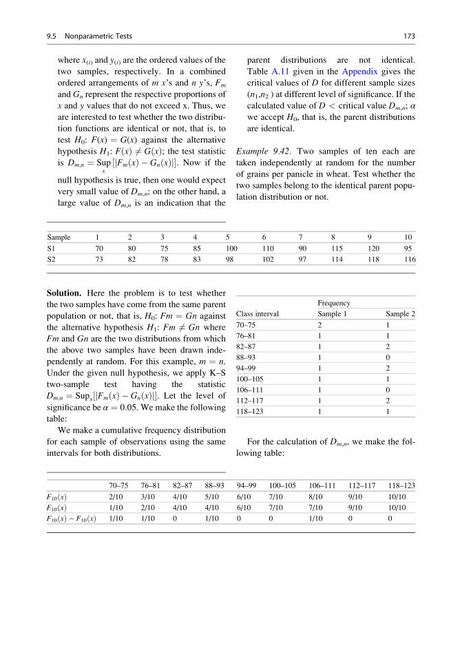
where x(i) and y(i) are the ordered values of the

two samples, respectively. In a combined

ordered arrangements of m x’s and n y’s, Fm

and Gn represent the respective proportions of

x and y values that do not exceed x. Thus, we

are interested to test whether the two distribu-

tion functions are identical or not, that is, to

test H0: F(x) ¼ G(x) against the alternative

hypothesis H1: FðxÞ 6¼ GðxÞ; the test statistic

is Dm;n ¼ Supx

FmðxÞ � GnðxÞj j½ �. Now if the

null hypothesis is true, then one would expect

very small value of Dm,n; on the other hand, a

large value of Dm,n is an indication that the

parent distributions are not identical.

Table A.11 given in the Appendix gives the

critical values of D for different sample sizes

(n1,n2 ) at different level of significance. If the

calculated value of D < critical value Dm,n; αwe accept H0, that is, the parent distributions

are identical.

Example 9.42. Two samples of ten each are

taken independently at random for the number

of grains per panicle in wheat. Test whether the

two samples belong to the identical parent popu-

lation distribution or not.

Solution. Here the problem is to test whether

the two samples have come from the same parent

population or not, that is, H0: Fm ¼ Gn against

the alternative hypothesis H1: Fm 6¼ Gn where

Fm and Gn are the two distributions from which

the above two samples have been drawn inde-

pendently at random. For this example, m ¼ n.

Under the given null hypothesis, we apply K–S

two-sample test having the statistic

Dm;n ¼ Supx FmðxÞ � GnðxÞj j½ �. Let the level of

significance be α ¼ 0:05. We make the following

table:

We make a cumulative frequency distribution

for each sample of observations using the same

intervals for both distributions.

Class interval

Frequency

Sample 1 Sample 2

70–75 2 1

76–81 1 1

82–87 1 2

88–93 1 0

94–99 1 2

100–105 1 1

106–111 1 0

112–117 1 2

118–123 1 1

For the calculation of Dm,n, we make the fol-

lowing table:

Sample 1 2 3 4 5 6 7 8 9 10

S1 70 80 75 85 100 110 90 115 120 95

S2 73 82 78 83 98 102 97 114 118 116

70–75 76–81 82–87 88–93 94–99 100–105 106–111 112–117 118–123

F10ðxÞ 2/10 3/10 4/10 5/10 6/10 7/10 8/10 9/10 10/10

F10ðxÞ 1/10 2/10 4/10 4/10 6/10 7/10 7/10 9/10 10/10

F10ðxÞ � F10ðxÞ 1/10 1/10 0 1/10 0 0 1/10 0 0

9.5 Nonparametric Tests 173

Appendix

Table A.1 Table of random numbers

00–04 05–09 10–14 15–19 20–24 25–29 30–34 35–39 40–44 45–49

00 54463 22662 65905 70639 79365 67382 29085 69831 47058 08186

01 15389 85205 18850 39226 42249 90669 96325 23248 60933 26927

02 85941 40756 82414 02015 13858 78030 16269 65978 01385 15345

03 61149 69440 11286 88218 58925 03638 52862 62733 33451 77455

04 05219 81619 10651 67079 92511 59888 84502 72095 83463 75577

05 41417 98326 87719 92294 46614 50948 64886 20002 97365 30976

06 28357 94070 20652 35774 16249 75019 21145 05217 47286 76305

07 17783 00015 10806 83091 91530 36466 39981 62481 49177 75779

08 40950 84820 29881 85966 62800 70326 84740 62660 77379 90279

09 82995 64157 66164 41180 10089 41757 78258 96488 88629 37231

10 96754 17676 55659 44105 47361 34833 86679 23930 53249 27083

11 34357 88040 53364 71726 45690 66334 60332 22554 90600 71113

12 06318 37403 49927 57715 50423 67372 63116 48888 21505 80182

13 62111 52820 07243 79931 89292 84767 85693 73947 22278 11551

14 47534 09243 67879 00544 23410 12740 02540 54440 32949 13491

15 98614 75993 84460 62846 59844 14922 48730 73443 48167 34770

16 24856 03648 44898 09351 98795 18644 39765 71058 90368 44104

17 96887 12479 80621 66223 86085 78285 02432 53342 42846 94771

18 90801 21472 42815 77408 37390 76766 52615 32141 30268 18106

19 55165 77312 83666 36028 28420 70219 81369 41843 41366 41067

20 75884 12952 84318 95108 72305 64620 91318 89872 45375 85436

21 16777 37116 58550 42958 21460 43910 01175 87894 81378 10620

22 46230 43877 80207 88877 89380 32992 91380 03164 98656 59337

23 42902 66892 46134 01432 94710 23474 20423 60137 60609 13119

24 81007 00333 39693 28039 10154 95425 39220 19774 31782 49037

25 68089 01122 51111 72373 06902 74373 96199 97017 41273 21546

26 20411 67081 89950 16944 93054 87687 96693 87236 77054 33848

27 58212 13160 06468 15718 82627 76999 05999 58680 96739 63700

28 70577 42866 24969 61210 76046 67699 42054 12696 93758 03283

29 94522 74358 71659 62038 79643 79769 44741 05437 39038 13163

30 42626 86819 85651 88678 17401 03252 99547 32404 17918 62880

31 16051 33763 57194 16752 54450 19031 58580 47629 54132 60631

32 08244 27647 33851 44705 94211 46716 11738 55784 95374 72655

33 59497 04392 09419 89964 51211 04894 72882 17805 21896 83864

34 97155 13428 40293 09985 58434 01412 69124 82171 59058 82859

35 98409 66162 95763 47420 20792 61527 20441 39435 11859 41567

36 45476 84882 65109 96597 25930 66790 65706 61203 53634 225571

37 89300 69700 50741 30329 11658 23166 05400 66669 48708 03887

38 50051 95137 91631 66315 91428 12275 24816 6809 71710 33258

39 31753 85178 31310 89642 98364 02306 24617 09607 83942 22716

40 79152 53829 77250 20190 56535 18760 69942 77448 33278 48805

41 44560 38750 83750 56540 64900 42912 13953 79149 18710 68618

42 68328 83378 63369 71381 39564 05615 42451 64559 97501 65747

43 46939 38689 58625 08342 30459 85863 20781 09284 26333 91777

44 83544 86141 15707 96256 23068 13782 08467 89469 93469 55349

45 91621 00881 04900 54224 46177 55309 17852 27491 89415 23466

46 91896 67126 04151 03795 59077 11848 12630 98375 52068 60142

47 55751 62515 21108 80830 02263 29303 37204 96926 30506 09808

48 85156 87689 95493 88842 00664 55017 55539 17771 69448 87530

49 07521 56898 12236 60277 39102 62315 12239 07105 11844 01117

174 9 Formulation and Testing of Hypothesis

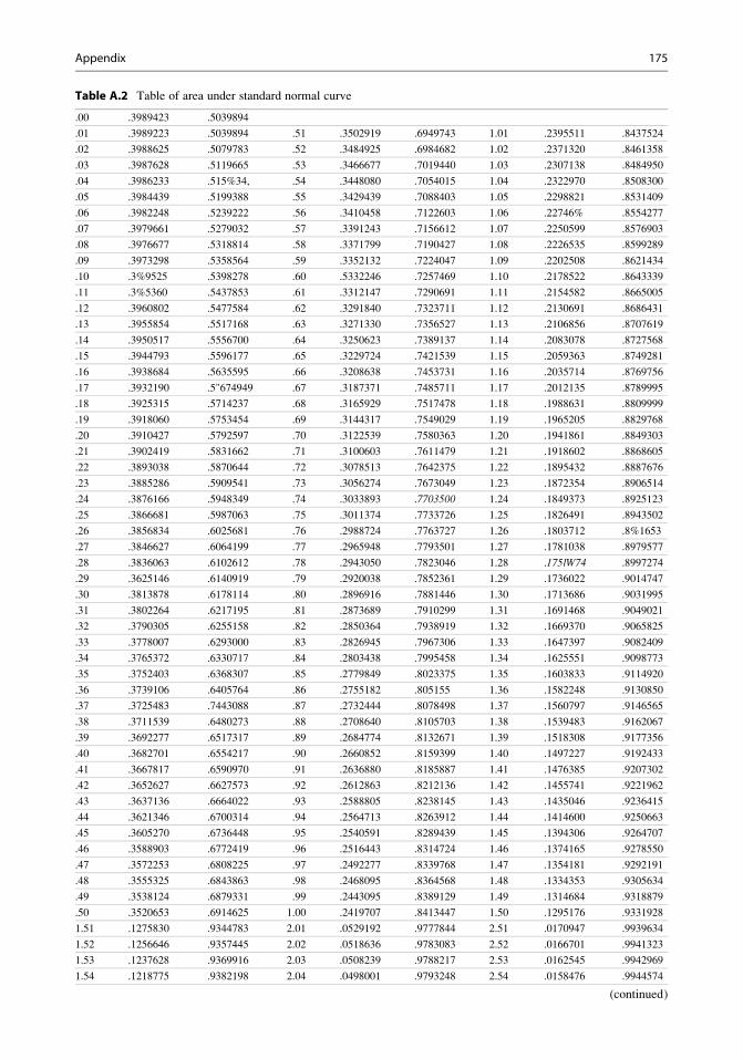
Table A.2 Table of area under standard normal curve

.00 .3989423 .5039894

.01 .3989223 .5039894 .51 .3502919 .6949743 1.01 .2395511 .8437524

.02 .3988625 .5079783 .52 .3484925 .6984682 1.02 .2371320 .8461358

.03 .3987628 .5119665 .53 .3466677 .7019440 1.03 .2307138 .8484950

.04 .3986233 .515%34, .54 .3448080 .7054015 1.04 .2322970 .8508300

.05 .3984439 .5199388 .55 .3429439 .7088403 1.05 .2298821 .8531409

.06 .3982248 .5239222 .56 .3410458 .7122603 1.06 .22746% .8554277

.07 .3979661 .5279032 .57 .3391243 .7156612 1.07 .2250599 .8576903

.08 .3976677 .5318814 .58 .3371799 .7190427 1.08 .2226535 .8599289

.09 .3973298 .5358564 .59 .3352132 .7224047 1.09 .2202508 .8621434

.10 .3%9525 .5398278 .60 .5332246 .7257469 1.10 .2178522 .8643339

.11 .3%5360 .5437853 .61 .3312147 .7290691 1.11 .2154582 .8665005

.12 .3960802 .5477584 .62 .3291840 .7323711 1.12 .2130691 .8686431

.13 .3955854 .5517168 .63 .3271330 .7356527 1.13 .2106856 .8707619

.14 .3950517 .5556700 .64 .3250623 .7389137 1.14 .2083078 .8727568

.15 .3944793 .5596177 .65 .3229724 .7421539 1.15 .2059363 .8749281

.16 .3938684 .5635595 .66 .3208638 .7453731 1.16 .2035714 .8769756

.17 .3932190 .5"674949 .67 .3187371 .7485711 1.17 .2012135 .8789995

.18 .3925315 .5714237 .68 .3165929 .7517478 1.18 .1988631 .8809999

.19 .3918060 .5753454 .69 .3144317 .7549029 1.19 .1965205 .8829768

.20 .3910427 .5792597 .70 .3122539 .7580363 1.20 .1941861 .8849303

.21 .3902419 .5831662 .71 .3100603 .7611479 1.21 .1918602 .8868605

.22 .3893038 .5870644 .72 .3078513 .7642375 1.22 .1895432 .8887676

.23 .3885286 .5909541 .73 .3056274 .7673049 1.23 .1872354 .8906514

.24 .3876166 .5948349 .74 .3033893 .7703500 1.24 .1849373 .8925123

.25 .3866681 .5987063 .75 .3011374 .7733726 1.25 .1826491 .8943502

.26 .3856834 .6025681 .76 .2988724 .7763727 1.26 .1803712 .8%1653

.27 .3846627 .6064199 .77 .2965948 .7793501 1.27 .1781038 .8979577

.28 .3836063 .6102612 .78 .2943050 .7823046 1.28 .175lW74 .8997274

.29 .3625146 .6140919 .79 .2920038 .7852361 1.29 .1736022 .9014747

.30 .3813878 .6178114 .80 .2896916 .7881446 1.30 .1713686 .9031995

.31 .3802264 .6217195 .81 .2873689 .7910299 1.31 .1691468 .9049021

.32 .3790305 .6255158 .82 .2850364 .7938919 1.32 .1669370 .9065825

.33 .3778007 .6293000 .83 .2826945 .7967306 1.33 .1647397 .9082409

.34 .3765372 .6330717 .84 .2803438 .7995458 1.34 .1625551 .9098773

.35 .3752403 .6368307 .85 .2779849 .8023375 1.35 .1603833 .9114920

.36 .3739106 .6405764 .86 .2755182 .805155 1.36 .1582248 .9130850

.37 .3725483 .7443088 .87 .2732444 .8078498 1.37 .1560797 .9146565

.38 .3711539 .6480273 .88 .2708640 .8105703 1.38 .1539483 .9162067

.39 .3692277 .6517317 .89 .2684774 .8132671 1.39 .1518308 .9177356

.40 .3682701 .6554217 .90 .2660852 .8159399 1.40 .1497227 .9192433

.41 .3667817 .6590970 .91 .2636880 .8185887 1.41 .1476385 .9207302

.42 .3652627 .6627573 .92 .2612863 .8212136 1.42 .1455741 .9221962

.43 .3637136 .6664022 .93 .2588805 .8238145 1.43 .1435046 .9236415

.44 .3621346 .6700314 .94 .2564713 .8263912 1.44 .1414600 .9250663

.45 .3605270 .6736448 .95 .2540591 .8289439 1.45 .1394306 .9264707

.46 .3588903 .6772419 .96 .2516443 .8314724 1.46 .1374165 .9278550

.47 .3572253 .6808225 .97 .2492277 .8339768 1.47 .1354181 .9292191

.48 .3555325 .6843863 .98 .2468095 .8364568 1.48 .1334353 .9305634

.49 .3538124 .6879331 .99 .2443095 .8389129 1.49 .1314684 .9318879

.50 .3520653 .6914625 1.00 .2419707 .8413447 1.50 .1295176 .9331928

1.51 .1275830 .9344783 2.01 .0529192 .9777844 2.51 .0170947 .9939634

1.52 .1256646 .9357445 2.02 .0518636 .9783083 2.52 .0166701 .9941323

1.53 .1237628 .9369916 2.03 .0508239 .9788217 2.53 .0162545 .9942969

1.54 .1218775 .9382198 2.04 .0498001 .9793248 2.54 .0158476 .9944574

(continued)

Appendix 175

Table A.2 (continued)

1.55 .1200090 .9394292 2.05 .0487920 .9798178 2.55 .0154493 .9946139

1.56 .1181573 .9406201 2.06 0477996 .9803007 2.56 .0150596 .9947664

1.57 .1163225 .9417924 2.07 .0468226 .9807738 2.57 ~0146782 .9949151

1.58 .1145048 .9429466 2.08 .0458611 .9812372 2.58 .0143051 .9950600

1.59 .1127042 .9440826 2.09 .0449148 .9816911 2.59 .0139401 .9952012

1.60 .1109208 .9452007 2.10 .0439836 .9821356 2.60 .0135830 .9953388

1.61 .1091548 .9463011 2.11 .0430674 .9825708 2.61 .0132337 .9954729

1.62 .1074061 .9473839 2.12 .0421661 .9829970 2.62 .0128921 .9956035

1.63 .1056748 .9484493 2.13 .0412795 .9834142 2.63 .0125581 .9957308

1.64 .1039611 .9494974 2.14 .0404076 .9838226 2.64 .0122315 .9958547

1.65 .1022649 .9505285 2.15 .0395500 .9842224 2.65 .0119122 .9959754

1.66 .1005864 .9515428 2.16 .0387069 .9846137 2.66 .0116001 .9960930

1.67 .0989255 9525403 2.17 .0378779 .9849966 2.67 .0112951 .9962074

1.68 .0972823 .9535213 2.18 .0370629 .9853713 2.68 .0109969 .9963189

1.69 .0956568 .9544860 2.19 .0362619 .9857379 2.69 .0107056 .9964274

1.70 .0940491 .9554345 2.20 .0354746 .9860966 2.70 .0104209 .9965330

1.71 .0924591 .9563671 2.21 .0347009 .9864474 2.71 .0101428 .9966358

1.72 .0908870 .9572838 2.22 .0339408 .9867906 2.72 .0098712 .9967359

1.73 .0893326 .9581849 2.23 .0331939 .9871263 2.73 .0096058 .9968333

1.74 .0877961 .9590705 2.24 .0324603 .9874545 2.74 .0093466 .9969280

1.75 .0862773 .9599408 2.25 .0317397 .9877755 2.75 .0090936 .9970202

1.76 .0847764 .9607961 2.26 .0310319 .9880894 2.76 .0068465 .9971099

1.77 .0832932 .9616364 2.27 .0303370 .9883962 2.77 .0086052 .9971972

1.78 .0818278 .9624620 2.28 .02%546 .9886962 2.78 .0083697 .9972821

1.79 .0803801 .9632730 2.29 .0289647 .9889893 2.79 .0081398 .9973646

1.80 .0789502 .9640697 2.30 .0283270 .9892759 2.80 .0079155 .9974449

1.41 .0775379 .9648521 2.31 .0276816 .9895559 2.81 .0076965 .9975229

1.82 .0761433 .9656205 2.32 .0270481 .98982% 2.82 .0074829 .9975983

1.83 .0741663 .9663750 2.33 .0264265 .9900969 2.83 .0072744 .9976726

1.84 .()1.34068 .9671159 2.34 .0258166 .9903581 2.84 .0070711 .9977443

1.85 .0720649 4678432 2.35 .0252182 .9906153 2.85 .0068728 .9978140

1.86 .0707404 .9685572 2.36 .0246313 .9908625 2.86 .0066793 .9978818

1.87 .0694333 .9692581 2.37 .0240556 .9911060 2.87 .0064907 .9979476

1.83 .0681436 .9699460 2.38 .4234910 .9913437 2.88 .0063067 .9980116

1.89 .0668711 .9706210 2.39 .0229374 .9915758 2.89 .0061274 .998073J~

1.90 .0656158 9712834 2.40 .0223945 .9918025 2.90 .0059525 .9981342

1.91 .0643777 .9719334 2.41 .0218624 .9920237 2.91 .0057821 .9981929

1.92 .0631566 .9725711 2.42 .0213407 .9922397 2.92 .0056160 .9982498

1.93 .0619524 .9731966 2.43 .0208294 .9924506 2.93 .0054541 .9983052

1.94 .0607652 .9738102 2.44 .0203284 .9926564 2.94 .0052963 .9983589

1.95 4595947 .9744119 2.45 4198374 9928572 2.95 .0051426 .9984111

1.% .0584409 .9750021 2.46 .0193563 .9930531 2. % .0049929 .9984618

1.97 .0573038 .9755808 2.47 .0188850 .9932443 2.97 .0048470 .9985110

1.98 .0561831 .9761482 2.48 .0184233 .9934309 2.98 .0047050 .9985583

1.99 .0550789 9767045 2.49 .0179711 .9936128 2.99 .0045666 .9986051

2.00 .0539910 .9772499 2.50 .0175283 .9937903 3.00 .0044318 .9986501

176 9 Formulation and Testing of Hypothesis

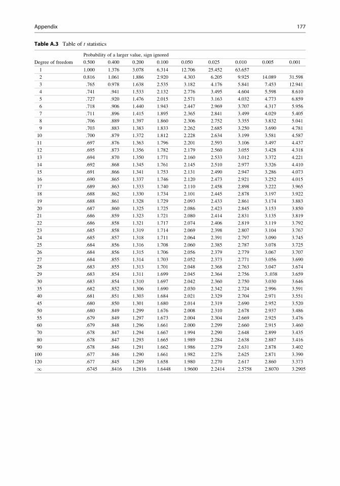
Table A.3 Table of t statistics

Degree of freedom

Probability of a larger value, sign ignored

0.500 0.400 0.200 0.100 0.050 0.025 0.010 0.005 0.001

1 1.000 1.376 3.078 6.314 12.706 25.452 63.657

2 0.816 1.061 1.886 2.920 4.303 6.205 9.925 14.089 31.598

3 .765 0.978 1.638 2.535 3.182 4.176 5.841 7.453 12.941

4 .741 .941 1.533 2.132 2.776 3.495 4.604 5.598 8.610

5 .727 .920 1.476 2.015 2.571 3.163 4.032 4.773 6.859

6 .718 .906 1.440 1.943 2.447 2.969 3.707 4.317 5.956

7 .711 .896 1.415 1.895 2.365 2.841 3.499 4.029 5.405

8 .706 .889 1.397 1.860 2.306 2.752 3.355 3.832 5.041

9 .703 .883 1.383 1.833 2.262 2.685 3.250 3.690 4.781

10 .700 .879 1.372 1.812 2.228 2.634 3.199 3.581 4.587

11 .697 .876 1.363 1.796 2.201 2.593 3.106 3.497 4.437

12 .695 .873 1.356 1.782 2.179 2.560 3.055 3.428 4.318

13 .694 .870 1.350 1.771 2.160 2.533 3.012 3.372 4.221

14 .692 .868 1.345 1.761 2.145 2.510 2.977 3.326 4.410

15 .691 .866 1.341 1.753 2.131 2.490 2.947 3.286 4.073

16 .690 .865 1.337 1.746 2.120 2.473 2.921 3.252 4.015

17 .689 .863 1.333 1.740 2.110 2.458 2.898 3.222 3.965

18 .688 .862 1.330 1.734 2.101 2.445 2.878 3.197 3.922

19 .688 .861 1.328 1.729 2.093 2.433 2.861 3.174 3.883

20 .687 .860 1.325 1.725 2.086 2.423 2.845 3.153 3.850

21 .686 .859 1.323 1.721 2.080 2.414 2.831 3.135 3.819

22 .686 .858 1.321 1.717 2.074 2.406 2.819 3.119 3.792

23 .685 .858 1.319 1.714 2.069 2.398 2.807 3.104 3.767

24 .685 .857 1.318 1.711 2.064 2.391 2.797 3.090 3.745

25 .684 .856 1.316 1.708 2.060 2.385 2.787 3.078 3.725

26 .684 .856 1.315 1.706 2.056 2.379 2.779 3.067 3.707

27 .684 .855 1.314 1.703 2.052 2.373 2.771 3.056 3.690

28 .683 .855 1.313 1.701 2.048 2.368 2.763 3.047 3.674

29 .683 .854 1.311 1.699 2.045 2.364 2.756 3..038 3.659

30 .683 .854 1.310 1.697 2.042 2.360 2.750 3.030 3.646

35 .682 .852 1.306 1.690 2.030 2.342 2.724 2.996 3.591

40 .681 .851 1.303 1.684 2.021 2.329 2.704 2.971 3.551

45 .680 .850 1.301 1.680 2.014 2.319 2.690 2.952 3.520

50 .680 .849 1.299 1.676 2.008 2.310 2.678 2.937 3.486

55 .679 .849 1.297 1.673 2.004 2.304 2.669 2.925 3.476

60 .679 .848 1.296 1.661 2.000 2.299 2.660 2.915 3.460

70 .678 .847 1.294 1.667 1.994 2.290 2.648 2.899 3.435

80 .678 .847 1.293 1.665 1.989 2.284 2.638 2.887 3.416

90 .678 .846 1.291 1.662 1.986 2.279 2.631 2.878 3.402

100 .677 .846 1.290 1.661 1.982 2.276 2.625 2.871 3.390

120 .677 .845 1.289 1.658 1.980 2.270 2.617 2.860 3.373

1 .6745 .8416 1.2816 1.6448 1.9600 2.2414 2.5758 2.8070 3.2905

Appendix 177

Table A.4 Table of F statistic (5% level of significance)

n1

1 2 3 4 5 6 8 12 24 1n2

1 161.40 199.50 215.70 224.60 230.20 234.00 238.90 243.90 249.00 254.30

2 18.51 19.00 19.16 19.25 19.30 19.33 19.37 19.41 19.45 19.50

3 10.13 9.55 9.28 9.12 9.01 8.94 8.84 8.74 8.64 8.53

4 7.71 6.94 6.59 6.39 6.26 6.16 6.04 5.91 5.77 5.63

5 6.61 5.79 5.41 5.19 5.05 4.95 4.82 4.68 4.53 4.36

6 5.99 5.14 4.76 4.53 4.39 4.28 4.15 4.00 3.84 3.67

7 5.59 4.74 4.35 4.12 3.97 3.87 3.73 3.57 3.41 3.23

8 5.32 4.46 4.07 3.84 3.69 3.58 3.44 3.28 3.12 2.93

9 5.12 4.26 3.86 3.63 3.48 3.37 3.23 3.07 2.90 2.71

10 4.96 4.10 3.71 3.48 3.33 3.22 3.07 2.91 2.74 2.54

11 4.84 3.98 3.59 3.86 3.20 3.09 2.95 2.79 2.61 2.40

12 4.75 3.88 3.49 3.26 3.11 3.00 2.85 2.69 2.50 2.30

13 4.67 3.80 3.41 3.18 3.02 2.92 2.77 2.60 2.42 2.21

14 4.60 3.74 3.34 3.11 2.96 2.85 2.70 2.53 2.35 2.13

15 4.54 3.68 3.29 3.06 2.90 2.79 2.64 2.48 2.29 2.07

16 4.49 3.63 3.24 3.01 2.85 2.74 2.59 2.42 2.24 2.01

17 4.45 3.59 3.20 2.96 2.81 2.70 2.55 2.38 2.19 1.96

18 4.41 3.55 3.16 2.93 2.77 2.66 2.51 2.34 2.15 1.92

19 4.38 3.52 3.13 2.90 2.74 2.63 2.48 2.31 2.11 1.88

20 4.35 3.49 3.10 2.87 2.71 2.60 2.45 2.28 2.08 1.84

21 4.32 3.47 3.07 2.84 2.68 2.57 2.42 2.25 2.05 1.81

22 4.30 3.44 3.05 2.82 2.66 2.55 2.40 2.23 2.03 1.78

23 4.28 3.42 3.03 2.80 2.64 2.53 2.38 2.20 2.00 1.76

24 4.26 3.40 3.01 2.78 2.62 2.51 2.36 2.18 1.98 1.73

25 4.24 3.38 2.99 2.76 2.60 2.49 2.34 2.16 1.96 1.71

26 4.22 3.37 2.98 2.74 2.59 2.47 2.32 2.15 1.95 1.69

27 4.21 3.35 2.96 2.73 2.57 2.46 2.30 2.13 1.93 1.67

28 4.20 3.34 2.95 2.71 2.56 2.44 2.29 2.12 1.91 1.65

29 4.18 3.33 2.93 2.70 2.54 2.43 2.28 2.10 1.90 1.64

30 4.17 3.32 2.92 2.69 2.53 2.42 2.27 2.09 1.89 1.62

40 4.03 3.23 2.84 2.61 2.45 2.34 2.18 2.00 1.79 1.51

60 4.00 3.16 2.76 2.52 2.37 2.25 2.10 1.92 1.70 1.39

120 3.92 3.07 2.68 2.45 2.29 2.17 2.02 1.83 1.61 1.25

1 3.84 2.99 2.60 2.37 2.21 2.09 1.94 1.75 1.52 1.00

178 9 Formulation and Testing of Hypothesis

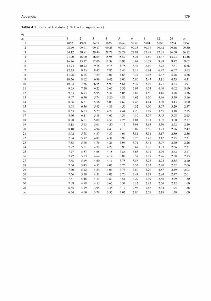
Table A.5 Table of F statistic (1% level of significance)

n1

1 2 3 4 5 6 8 12 24 1n2

1 4052 4999 5403 5625 5764 5859 5981 6106 6234 6366

2 98.49 99.01 99.17 99.25 99.30 99.33 99.36 99.42 99.46 99.50

3 34.12 30.81 29.46 28.71 28.24 27.91 27.49 27.05 26.60 26.12

4 21.20 18.00 16.69 15.98 15.52 15.21 14.80 14.37 13.93 13.46

5 16.26 13.27 12.06 11.39 10.97 10.67 10.27 9.89 9.47 9.02

6 13.74 10.92 9.78 9.15 8.75 8.47 8.10 7.72 7.31 6.88

7 12.25 9.55 8.45 7.85 7.46 7.19 6.84 6.47 6.07 5.65

8 11.26 8.65 7.59 7.01 6.63 6.37 6.03 5.67 5.28 4.86

9 10.56 8.02 6.99 6.42 6.06 5.80 5.47 5.11 4.73 4.31

10 10.04 7.56 6.55 5.99 5.64 5.39 5.06 4.71 4.33 3.91

11 9.65 7.20 6.22 5.67 5.32 5.07 4.74 4.40 4.02 3.60

12 9.33 6.93 5.95 5.41 5.06 4.82 4.50 4.16 3.78 3.36

13 9.07 6.70 5.74 5.20 4.86 4.62 4.30 3.96 3.59 3.16

14 8.86 6.51 5.56 5.03 4.69 4.46 4.14 3.80 3.43 3.00

15 8.68 6.36 5.42 4.89 4.56 4.32 4.00 3.67 3.29 2.87

16 8.53 6.23 5.29 4.77 4.44 4.20 3.89 3.55 3.18 2.75

17 8.40 6.11 5.18 4.67 4.34 4.10 3.79 3.45 3.08 2.65

18 8.28 6.01 5.09 4.58 4.25 4.01 3.71 3.37 3.00 2.57

19 8.18 5.93 5.01 4.50 4.17 3.94 3.63 3.30 2.92 2.49

20 8.10 5.85 4.94 4.43 4.10 3.87 3.56 3.23 2.86 2.42

21 8.02 5.78 4.87 4.37 4.04 3.81 3.51 3.17 2.80 2.36

22 7.94 5.72 4.82 4.31 3.99 3.76 3.45 3.12 2.75 2.31

23 7.88 5.66 4.76 4.26 3.94 3.71 3.41 3.07 2.70 2.26

24 7.82 5.61 4.72 4.22 3.90 3.67 3.36 3.03 2.66 2.21

25 7.77 5.57 4.68 4.18 3.86 3.63 3.32 2.99 2.62 2.17

26 7.72 5.53 4.64 4.14 3.82 3.59 3.29 2.96 2.58 2.13

27 7.68 5.49 4.60 4.11 3.78 3.56 3.26 2.93 2.55 2.10

28 7.64 5.45 4.57 4.07 3.75 3.53 3.23 2.90 2.52 2.06

29 7.60 5.42 4.54 4.04 3.73 3.50 3.20 2.87 2.49 2.03

30 7.56 5.39 4.51 4.02 3.70 3.47 3.17 2.84 2.47 2.01

40 7.31 5.18 4.31 3.83 3.51 3.29 2.99 2.66 2.29 1.80

60 7.08 4.98 4.13 3.65 3.34 3.12 2.82 2.50 2.12 1.60

120 6.85 4.79 3.95 3.48 3.17 2.96 2.66 2.34 1.95 1.38

1 6.64 4.60 3.78 3.32 3.02 2.80 2.51 2.18 1.79 1.00

Appendix 179

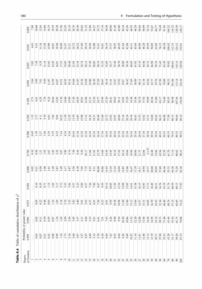
Table

A.6

Table

ofcumulativedistributionofw2

Degree

offreedom

Probabilityofgreater

value

0.995

0.990

0.975

0.950

0.900

0.750

0.500

0.250

0.100

0.050

0.025

0.010

0.005

1....

....

....

....

0.02

0.10

0.45

1.32

2.71

3.84

5.02

6.63

7.88

20.01

0.02

0.05

0.10

0.21

0.58

1.39

2.77

4.61

5.99

7.38

9.21

10.60

30.07

0.11

0.22

0.35

0.58

1.21

2.37

4.11

6.25

7.81

9.35

11.34

12.84

40.21

0.30

0.48

0.71

1.06

1.92

3.36

5.39

7.78

9.49

11.14

13.28

14.86

50.41

0.55

0.83

1.15

1.61

2.67

4.35

6.63

9.24

11.07

12.83

15.09

16.75

60.68

0.87

1.24

1.64

2.20

3.45

5.35

7.84

10.64

12.59

14.45

16.81

18.55

70.99

1.24

1.69

2.17

2.83

4.25

6.35

9.04

12.02

14.07

16.01

18.48

20.28

81.34

1.65

2.18

2.73

3.49

5.07

7.14

10.22

13.36

15.51

17.53

20.09

21.96

91.73

2.09

2.70

3.33

4.17

5.90

8.34

11.39

14.68

16.92

19.02

21.67

23.59

10

2.16

2.56

3.25

3.94

4.87

6.74

9.34

12.55

15.99

18.31

20.48

23.21

25.19

11

2.60

3.05

3.82

4.57

5.58

7.58

10.34

13.70

17.28

19.68

21.92

24.72

26.76

12

3.07

3.57

4.40

5.23

6.30

8.44

11.34

14.85

18.55

21.03

23.34

26.22

28.30

13

3.57

4.11

5.01

5.89

7.04

9.30

12.34

15.98

I9.81

22.36

24.74

27.69

29.82

14

4.07

4.66

5.63

6.57

7.79

10.17

13.34

17.12

21.06

23.68

26.12

29.14

31.32

15

4.60

5.23

6.27

7.26

8.55

11.04

14.34

18.25

22.31

25.00

27.49

30.58

32.80

16

5.14

5.81

6.91

7.96

9.31

11.91

15.34

19.37

23.54

26.30

28.85

32.00

34.27

17

5.70

6.41

7.56

8.67

I0.09

12.79

16.34

20.49

24.77

27.59

30.19

33.41

35.72

18

6.26

7.01

8.23

9.39

10.86

13.68

17.34

21.60

25.99

28.87

31.53

34.81

37.16

19

6.84

7.63

8.91

10.12

11.65

14.56

18.34

22.72

27.20

30.14

32.85

36.19

38.58

20

7.43

8.26

9.59

10.85

12.44

15.45

19.34

23.83

28.41

31.41

34.17

37.57

40.00

21

8.03

8.90

10.28

11.59

13.24

16.34

20.34

24.93

29.62

32.67

35.48

38.93

41.40

22

8.64

9.54

10.98

12.34

14.04

17.24

21.34

26.04

30.11

33.92

36.78

40.29

42.80

23

9.26

10.20

11.69

13.09

14.85

18.14

22.34

27.14

32.01

35.I7

38.08

41.64

44.18

24

9.89

10.86

12.40

13.85

15.66

19.04

23.34

28.24

33.20

36.42

39.36

42.98

45.56

25

10.52

11.52

13.12

14.61

16.47

19.94

24.34

29.34

34.38

37.65

40.65

44.31

46.93

26

11.16

12.20

13.84

15.38

17.29

20.84

25.34

30.43

35.56

38.89

41.92

45.64

48.29

27

11.81

12.88

14.57

16.15

18.11

21.75

26.34

31.53

36.74

40.11

43.19

46.96

49.64

28

12.46

13.56

15.31

16.93

18.94

22.66

27.34

32.62

37.92

41.34

44.46

48.28

50.99

29

13.12

14.26

16.05

17.71

19.77

2.1.57

28.34

33.71

39.09

42.56

45.72

49.59

52.34

30

13.79

14.95

16.79

18.49

20.60

24.48

29.34

34.80

40.26

43.77

46.98

50.89

53.67

40

20.71

22.16

24.43

26.51

29.05

33.66

39.34

45.62

51.80

55.76

59.34

63.69

66.77

50

27.99

29.71

32.36

34.76

37.69

42.94

49.33

56.33

63.17

67.50

71.42

76.15

79.49

60

35.53

37.48

40.48

43.19

46.46

52.29

59.33

66.98

74.40

79.08

83.30

88.38

91.95

70

43.28

43.44

48.76

51.74

55.33

61.70

69.33

77.58

85.53

90.53

95.02

100.42

104.22

80

51.17

53.54

57.15

60.39

64.28

71.14

79.33

88.13

96.58

101.88

106.63

112.33

116.32

90

59.20

61.75

65.65

69.13

73.29

80.62

89.33

98.64

107.56

113.14

118.14

124.12

128.30

100

67.33

70.06

74.22

77.93

82.36

90.13

99.33

09.14

118.50

124.34

129.56

135.81

140.17

180 9 Formulation and Testing of Hypothesis

Table A.7 Table of critical values of simple and partial correlation coefficients

d.f

Two-sided

5% 1% 0.1%

1 .969 .988 .988

2 .960 .900 .900

3 .878 .959 .911

4 .811 .917 .974

5 .754 .875 .951

6 .707 .834 .925

7 .606 .798 .898

8 .632 .765 .872

9 .602 .735 .847

10 .576 .708 .823

11 .553 .684 .801

12 532 .661 .780

13 .514 .041 .760

14 .497 .623 .742

15 .482 .606 .725

16 468 .590 .708

17 .456 .575 .093

18 .444 .561 .679

19 .433 .549 .065

20 .423 .537 .652

21 .413 .526 .640

22 .404 .615 .629

23 .396 .505 .618

24 .388 .496 .607

25 .381 .487 .697

26 .374 .478 .588

27 .367 .470 .578

28 .361 .463 .570

29 .355 .456 .562

30 .349 .449 .654

40 .304 .393 .490

50 .273 .354 .443

60 .250 .325 .408

70 .232 .302 .380

80 .117 .283 .357

100 .196 .254 .321

160 .159 .208 .263

200 .138 .181 .230

260 .124 .162 .206

300 .113 .146 .188

Appendix 181

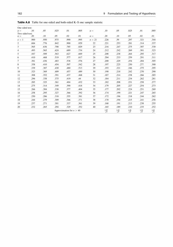
Table A.8 Table for one-sided and both-sided K–S one sample statistic

One sided test:

α ¼ .10 .05 .025 .01 .005 α ¼ .10 .05 .025 .01 .005

Two sided test:α ¼ .20 .10 .05 .02 .01 α ¼ .20 .10 .05 .02 .01

n ¼ 1 .900 .950 .975 .990 .995 n ¼ 21 .226 .59 .297 .321 .344

2 .684 .776 .842 .900 .929 22 .221 .253 .281 .314 .337

3 .565 .636 .708 .785 .829 23 .216 .247 .275 .307 .330

4 .493 .565 .624 .689 .734 24 .212 .242 .269 .301 .323

5 .447 .509 .563 .627 .669 25 .208 .238 .264 .295 .317

6 .410 .468 .519 .577 .617 26 .204 .233 .259 .291 .311

7 .381 .436 .483 .538 .576 27 .200 .229 .254 .284 .305

8 .358 .410 .454 .507 .542 28 .197 .225 .250 .27? .300

9 .339 .387 .430 .480 .513 29 .193 .221 .246 .275 .295

10 .323 .369 .409 .457 .489 30 .190 .218 .242 .270 .290

11 .308 .352 .391 .437 .468 31 .187 .214 .238 .266 .285

12 .296 .338 .375 .419 .44 32 .184 .211 .234 .262 .281

13 .285 .325 .361 .404 .432 33 .182 .208 .231 .258 .277

14 .275 .314 .349 .390 .418 34 .179 .205 .227 .254 .273

15 .266 .304 .338 .377 .404 35 .177 .202 .224 .251 .269

16 .258 .295 .327 .366 .392 36 .174 .199 .221 .247 .265

17 .250 .286 .318 .355 .381 37 .172 .196 .218 .244 .262

18 .244 .279 .309 .346 .371 38 .170 .194 .215 .241 .258

19 .237 .271 .301 .337 .361 39 .168 .191 .213 .238 .255

20 .232 .265 .294 .329 .352 40 .165 .189 .210 .235 .252

Approximation for n > 40 1:07ffiffin

p 1:22ffiffin

p 1:36ffiffin

p 1:52ffiffin

p 1:63ffiffin

p

182 9 Formulation and Testing of Hypothesis

Table A.9 Critical values for K–S two-sample test statistic

This table gives the values of Dþm; n; a and Dm; n; a for which a P Dþ

m; n Dþm; n; a

n ofor some selected values of

N1 ¼ smaller sample size, N2 ¼ larger sample size, and a

One sided test: α ¼ .10 .05 .025 .01 .005Two sided test: α ¼ .20 .10 .05 .02 .01

N1 ¼ 1 N2 ¼ 9 17/18

10 9/10

N1 ¼ 2 N2 ¼ 3 5/6

4 3/4

5 4/5 4/5

6 5/6 5/6

7 5/7 6/7

8 3/4 7/4 7/8

9 7/9 8/9 8/9

10 7/10 4/5 9/10

N1 ¼ 3 N2 ¼ 4 3/4 3/4

5 2/3 4/5 4/5

6 2/3 2/3 5/6

7 2/3 5/7 6/7 6/7

8 5/8 3/4 3/4 7/8

9 2/3 2/3 7/9 8/9 8/9

10 3/5 7/10 4/5 9/10 9/10

12 7/12 2/3 3/4 5/6 11/12

N1 ¼ 4 N2 ¼ 5 3/5 3/4 4/5 4/5

6 7/12 2/3 3/4 5/6 5/6

7 17/28 5/7 3/4 6/7 6/7

8 5/8 5/8 3/4 7/8 7/8

9 5/9 2/3 3/4 7/9 8/9

10 11/20 13/20 7/10 4/5 4/5

12 7/12 2/3 2/3 3/4 5/6

16 9/1 5/8 11/16 3/4 13/16

N1 ¼ 5 N2 ¼ 6 3/5 2/3 2/3 5/6 5/6

7 4/7 23/35 5/7 29/35 6/7

8 11/20 5/8 27/40 4/5 4/5

9 5/9 3/5 31/45 7/9 4/5

10 1/2 3/5 7/10 7/10 4/5

15 8/15 3/5 2/3 77/15 11/15

20 1/2 11/20 3/5 7/10 3/4

N1 ¼ 6 N1 ¼ 7 23/42 4/7 29/42 5/7 5/6

8 1/2 7/12 2/3 3/4 3/4

9 1/2 5/9 2/3 13/18 7/9

10 1/2 17/30 19/30 7/10 1/15

12 1/2 7/12 7/12 2/3 3/4

18 4/9 5/9 11/18 2/3 2/3

(continued)

Appendix 183

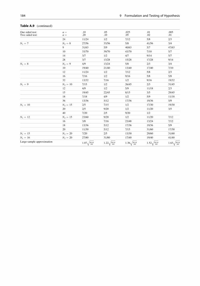
Table A.9 (continued)

One sided test: α ¼ .10 .05 .025 .01 .005Two sided test: α ¼ .20 .10 .05 .02 .01

24 11/24 1/2 7/12 5/8 2/3

N1 ¼ 7 N2 ¼ 8 27/56 33/56 5/8 41/56 3/4

9 31/63 5/9 40/63 5/7 47/63

10 33/70 39/70 43/70 7/10 5/7

14 3/7 1/2 4/7 9/14 5/7

28 3/7 13/28 15/28 17/28 9/14

N1 ¼ 8 N2 ¼ 9 4/9 13/24 5/8 2/3 3/4

10 19/40 21/40 13/40 17/40 7/10

12 11/24 1/2 7/12 5/8 2/3

16 7/16 1/2 9/16 5/8 5/8

32 13/32 7/16 1/2 9/16 19/32

N1 ¼ 9 N2 ¼ 10 7/15 1/2 26/45 2/3 31/45

12 4/9 1/2 5/9 11/18 2/3

15 19/45 22/45 8/15 3/5 29/45

18 7/18 4/9 1/2 5/9 11/18

36 13/36 5/12 17/36 19/36 5/9

N1 ¼ 10 N2 ¼ 15 2/5 7/15 1/2 17/30 19/30

20 2/5 9/20 1/2 11/20 3/5

40 7/20 2/5 9/20 1/2

N1 ¼ 12 N2 ¼ 15 23/60 9/20 1/2 11/20 7/12

16 3/8 7/16 23/48 13/24 7/12

18 13/36 5/12 17/36 19/36 5/9

20 11/30 5/12 7/15 31/60 17/30

N1 ¼ 15 N2 ¼ 20 7/20 2/5 13/30 29/60 31/60

N1 ¼ 16 N2 ¼ 20 27/80 31/80 17/40 19/40 41/40

Large-sample approximation 1:07ffiffiffiffiffiffiffimþnmn

q1:22

ffiffiffiffiffiffiffimþnmn

q1:36

ffiffiffiffiffiffiffimþnmn

q1:52

ffiffiffiffiffiffiffimþnmn

q1:63

ffiffiffiffiffiffiffimþnmn

q

184 9 Formulation and Testing of Hypothesis

Table A.10 Table for critical values of r in run test

n2

2 3 4 5 6 7 8 9 10 11 12 13 14 15 16 17 18 19 20n1

2 2 2 2 2 2 2 2 2 2

3 2 2 2 2 2 2 2 2 2 3 3 3 3 3 3

4 2 2 2 3 3 3 3 3 3 3 3 4 4 4 4 4

5 2 2 3 3 3 3 4 4 4 4 4 4 4 5 5 5

6 2 2 3 3 3 3 4 4 4 4 5 5 5 5 5 5 6 6

7 2 2 3 3 3 4 4 5 5 5 5 5 6 6 6 6 6 6

8 2 3 3 3 4 4 5 5 5 6 6 6 6 6 7 7 7 7

9 2 3 3 4 4 5 5 5 6 6 6 7 7 7 7 8 8 8

10 2 3 3 4 5 5 5 6 6 7 7 7 7 8 8 8 8 9

11 2 3 4 4 6 5 6 6 7 7 7 8 8 8 9 9 9 9

12 2 2 3 4 4 5 6 6 7 7 7 8 8 8 9 9 9 10 10

13 2 2 3 4 5 5 6 6 7 7 8 8 9 9 9 10 10 10 10

14 2 2 3 4 5 5 6 7 7 8 8 9 9 9 10 10 10 11 11

15 2 3 3 4 5 6 6 7 7 8 8 9 9 10 10 11 11 11 12

16 2 3 4 4 5 6 6 7 8 8 9 9 10 10 11 11 11 12 12

17 2 3 4 4 5 6 7 7 8 9 9 10 10 11 11 11 12 12 13

18 2 3 4 6 5 6 7 8 8 9 9 10 10 11 11 12 12 13 13

19 2 3 4 5 6 6 7 8 8 9 10 10 11 11 12 12 13 13 13

20 2 3 4 5 6 6 7 8 9 9 10 10 11 12 12 13 13 13 14

n2

2 3 4 5 6 7 8 9 10 11 12 13 14 15 16 17 18 19 20n1

2

3

4 9 9

5 9 10 10 11 11

6 9 10 11 12 12 13 13 13 13

7 11 12 13 13 14 14 14 14 15 15 15

8 11 12 13 14 14 15 15 16 16 16 16 17 17 17 17 17

9 13 14 14 15 16 16 16 17 17 18 18 18 18 18 18

10 13 14 15 16 16 17 17 18 18 18 19 19 19 20 20

11 13 14 15 16 17 17 18 19 19 19 20 20 20 21 21

12 13 14 16 16 17 18 19 19 20 20 21 21 21 22 22

13 15 16 17 18 19 19 20 20 21 21 22 22 23 23

14 15 16 17 18 19 20 20 21 22 22 23 23 23 24

15 15 16 18 18 19 20 21 22 22 23 23 24 24 25

16 17 18 19 20 21 21 22 23 23 24 25 25 25

17 17 18 19 20 21 22 23 23 24 25 25 26 26

18 17 18 19 20 21 22 23 24 25 25 26 26 27

19 17 18 20 21 22 23 23 24 25 26 26 27 27

20 17 18 20 21 22 23 24 25 25 26 27 27 28

For one sample and two sample run test any value of r equal to or smaller than the value shown in Table A.12 is

significant at 0.05 level. For one sample run test, any value of r greater than or equals to the values shown in

Table A.12A is also significant at 0.05 level

Appendix 185

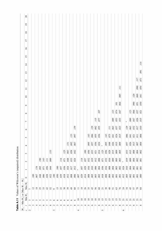
Table

A.11

Values

ofWilcoxon’s

(unpaired)distribution

Ws�Min

Ws

½�o

rMax

Wl�W

l½

�s

lMin

Ws

Max

Wl

01

23

45

67

89

10

11

12

13

14

15

16

17

18

19

20

22

37

33

12

.100

43

18

.067

.134

53

25

.048

.095

.190

63

33

.086

.071

.143

73

42

.028

.056

.111

83

52

.022

.044

.089

.133

32

69

.100

36

15

.050

.100

46

22

.029

.057

.114

56

30

.018

.036

.071

.125

66

39

.012

.024

.048

.083

.131

76

49

.008

.017

.033

.058

.092

.133

86

60

.006

.012

.024

.042

.067

.097

.139

42

10

11

.007

a

310

18

.029

.057

.114

410

26

.014

.029

.057

.100

510

35

.008

.016

.032

.056

.095

.143

610

45

.005

.010

.019

.033

.057

.086

.129

710

56

.003

.006

.012

.021

.036

.055

.082

.115

810

68

.002

.004

.008

.014

.024

.036

.055

.077

.107

53

15

21

.018

.036

.071

.125

a

415

30

.008

.016

.032

.056

.095

.143

515

40

.004

.008

.016

.028

.048

.075

.111

615

51

.002

.004

.009

.015

.026

.041

.063

.089

.123

715

63

.001

.003

.005

.009

.015

.024

.037

.053

.074

.101

815

76

.001

.002

.003

.005

.009

.015

.023

.033

.047

.064

.085

.111

63

21

24

.012

.024

a

421

34

.005

.010

.019

.033

.057

.086

.129

a

521

45

.002

.004

.009

.015

.026

.041

.063

.089

.123

621

57

.001

.002

.004

.008

.013

.021

.032

.047

.066

.090

.120

721

70

.001

.001

.002

.004

.007

.011

.017

.026

.037

.051

.069

.090

.117

821

84

.000

.001

.001

.002

.004

.006

.010

.015

.021

.030

.041

.054

.071

.091

.114

74

28

38

.003

.006

.012

.021

.036

.055

a

528

50

.001

.003

.005

.009

.015

.024

.037

.053

.074

.101

628

63

.001

.001

.002

.004

.007

.011

.017

.026

.037

.051

.069

.090

.117

728

77

.000

.001

.001

.002

.003

.006

.009

.013

.019

.027

.036

.049

.064

.082

.104

828

92

.000

.000

.001

.001

.002

.003

.005

.007

.010

.014

.020

.027

.036

.047

.060

.076

.095

.116

84

36

42

.002

.004

.008

.014

a

536

55

.001

.002

.003

.005

.009

.015

.023

.033

.047

.064

a

636

69

.000

.001

.001

.002

.004

.006

.010

.015

.021

.030

.041

.054

.071

.091

.114

736

84

.000

.000

.001

.001

.002

.003

.005

.007

.010

.014

.020

.027

.036

.047

.060

.076

0.95

.116

836

100

.000

.000

.000

.001

.001

.001

.002

.003

.005

.007

.010

.014

.019

.025

.032

.041

0.52

.065

.080

.097

.117

aIndicates

that

thevalueat

headofthiscolumn(andthose

values

that

arelarger

arenotpossible

forthegiven

values

ofsandlin

thisrow)

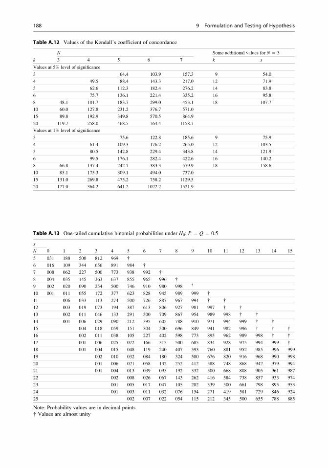
Table A.13 One-tailed cumulative binomial probabilities under H0: P ¼ Q ¼ 0.5

x

0 1 2 3 4 5 6 7 8 9 10 11 12 13 14 15N

5 031 188 500 812 969 {

6 016 109 344 656 891 984 {

7 008 062 227 500 773 938 992 {

8 004 035 145 363 637 855 965 996 {

9 002 020 090 254 500 746 910 980 998 {

10 001 011 055 172 377 623 828 945 989 999 {

11 006 033 113 274 500 726 887 967 994 { {

12 003 019 073 194 387 613 806 927 981 997 { {

13 002 011 046 133 291 500 709 867 954 989 998 { {

14 001 006 029 090 212 395 605 788 910 971 994 999 { {

15 004 018 059 151 304 500 696 849 941 982 996 { { {

16 002 011 038 105 227 402 598 773 895 962 989 998 { {

17 001 006 025 072 166 315 500 685 834 928 975 994 999 {

18 001 004 015 048 119 240 407 593 760 881 952 985 996 999

19 002 010 032 084 180 324 500 676 820 916 968 990 998

20 001 006 021 058 132 252 412 588 748 868 942 979 994

21 001 004 013 039 095 192 332 500 668 808 905 961 987

22 002 008 026 067 143 262 416 584 738 857 933 974

23 001 005 017 047 105 202 339 500 661 798 895 953

24 001 003 011 032 076 154 271 419 581 729 846 924

25 002 007 022 054 115 212 345 500 655 788 885

Note: Probability values are in decimal points

{ Values are almost unity

Table A.12 Values of the Kendall’s coefficient of concordance

k

N Some additional values for N ¼ 3

3 4 5 6 7 k s

Values at 5% level of significance

3 64.4 103.9 157.3 9 54.0

4 49.5 88.4 143.3 217.0 12 71.9

5 62.6 112.3 182.4 276.2 14 83.8

6 75.7 136.1 221.4 335.2 16 95.8

8 48.1 101.7 183.7 299.0 453.1 18 107.7

10 60.0 127.8 231.2 376.7 571.0

15 89.8 192.9 349.8 570.5 864.9

20 119.7 258.0 468.5 764.4 1158.7

Values at 1% level of significance

3 75.6 122.8 185.6 9 75.9

4 61.4 109.3 176.2 265.0 12 103.5

5 80.5 142.8 229.4 343.8 14 121.9

6 99.5 176.1 282.4 422.6 16 140.2

8 66.8 137.4 242.7 383.3 579.9 18 158.6

10 85.1 175.3 309.1 494.0 737.0

15 131.0 269.8 475.2 758.2 1129.5

20 177.0 364.2 641.2 1022.2 1521.9

188 9 Formulation and Testing of Hypothesis

Analysis of Varianceand Experimental Designs 10

In Chap. 9, a discussion has been made as to how

two sample means can be compared using τ or

t-test. Problem arises when one wants to compare

more than two populations at a time. One of the

possible solutions to this problem is to take mC2

no. of pairs of samples and test these using the

τ or t-test as applicable. Another important pro-

cedure is to use the analysis of variance tech-

nique. The analysis of variance technique, in

short ANOVA, is a powerful technique used in

the field of agriculture, social science, business,

education, medicine, and several other fields.

Using this tool the researcher can draw inference

about the samples whether these have been

drawn from the same population or they belong

to different populations. Using this technique

the researcher can establish whether a no. of

varieties differ significantly among themselves

with respect to their different characteristics

like yield, susceptibility to diseases and pests,

nutrient acceptability, and stress tolerance and

efficiency of different salesmen; for example,

one can compare different plant protection

chemicals, different groups of people with

respect to their innovativeness, and different

drugs against a particular disease, different

programs of poverty reduction, performances of

different business houses, and so on.

In statistical studies variability and measures

of variability are the major focal points of atten-

tion. The essence of ANOVA lies in partitioning

the variance of a set of data into a number of

components associated with the type, classifica-

tion, and nature of data. Analysis of variance is a

systematic approach of partitioning the variance

of a variable into assignable and non-assignable

parts. Through ANOVA one can investigate one

or more factors (variety, type of irrigation, fertil-

izer doses, social groups, business houses, etc.)

with varying levels (e.g., five or six varieties at a

time; three or more irrigation types; different

levels of NPK; social groups like innovators,

early adopters, early majority, late majority, and

laggards; more than one business house) that are

hypothesized to influence the dependent variable.

Depending upon the nature, type, and classifica-

tion of data, the analysis of variance is developed

for one-way classified data, two-way classified

data with one observation per cell, two-way clas-sified data with more than one observation per

cell, etc. Before taking up the analysis of vari-

ance in detail, let us discuss about linear model,

which is mostly being used in the analysis of

variance.

10.1 Linear Models

Taken observation on any dependent variable Y,

yi can be assumed as yi ¼ αi þ ei, where αi is itstrue value and ei is the error part, which may be

because of chance factor. This αi again may be

the linear combination of m unknown quantities

γ1; γ2; . . . ; γm asαi ¼ ai1γ1 þ ai2γ2 þ � � � þ aimγm,where aij (j ¼ 1, 2, . . ., m) is the constant and take

the values 0 or 1.

Thus, yi ¼ ai1γ1 þ ai2γ2 þ � � � þ aimγm þ ei.

P.K. Sahu, Research Methodology: A Guide for Researchers in Agricultural Science,Social Science and Other Related Fields, DOI 10.1007/978-81-322-1020-7_10, # Springer India 2013

189

If aij ¼ 1 for a particular value of j and for

all i, then γj is termed general mean or general

effect. A linear model in which all the γj’s are

unknown constants (known as parameters) is

termed fixed effect model. On the other hand,

a linear model in which γj’s are random variables

excepting the general mean or general effect is

known as variance component model or random

effect model. A linear model in which at least one

γj is a random variable and at least one γj is a

constant (other than general effect or general

mean) is called a mixed effect model.

Assumptions in Analysis Variance

The analysis of variance is based on following

assumptions:

1. The effects are additive in nature.

2. The observations are independent.

3. The variable concerned must be normally

distributed.

4. Variances of all populations from which

samples have been drawn must be the same.

In other words, all samples should be drawn

from normal populations having common

variance with the same or different means.

The interpretation of analysis of variance is

valid only when the assumptions are met. A larger

deviation from these assumptions affects the

level of significance and the sensitivity of F- andt-test. Two independent factors are said to be

additive in nature if the effect of one factor

remains constant over the levels of the other fac-tor. On the contrary when the effects of one factor

remain constant by a certain percentage over the

levels of other factors, then the factors are multi-plicative or nonadditive in nature. The models

for additive and multiplicative effects may be

presented as follows:

yij ¼ μþ αi þ βj þ eij additive modelð Þyij ¼ μþ αi þ βj þ ðαβÞij þ eij multiplicative modelð Þ

The second assumption is related to the error

associated with the model. Precisely, this

assumption means that the errors should be inde-

pendently and identically distributed with mean

0 and constant (σ2) variance.Several normality test procedures are avail-

able in the literature. However, the nature of the

functional relationship between the mean and

the variance may help us in identifying whether

a distribution is normal or non-normal. Homo-

geneity of error variance is one of the important

assumptions in the analysis of variance. In prac-

tice we may not get exactly equal (homosce-

dastic) variances. The variances can be tested

for homogeneity through Hartley’s test or

Bartlett’s test.

10.2 One-Way ANOVA

In one-way analysis of variance, different

samples for only one factor are considered. That

means the whole data set comprised several

groups with many observations based on one

factor as shown below:

Let yi1; yi2; yi3; . . . yini be a random sample

from an N μi; σ2ð Þ population and i ¼ 1, 2, 3, 4,

. . ., k. The random samples are independent.

Suppose there are n ¼ Pki¼1

ni observations yij

(i ¼ 1, 2, 3, . . .., k; j ¼ 1, 2, 3, 4, . . ., ni),

which are grouped into k classes in the following

way (Table 10.1):

If we consider the fixed effect model, then it

can be written as yij ¼ μi þ eij, where μi is a fixedeffect due to ith class and eijs are independently

N 0; σ2ð Þ. This μi can be regarded as the sum of

two components, namely, μ, the overall mean,

and a component due to the specific class. Thus,

we can write

μi ¼ μþ αi:

Thus; the mathematical model will be

yij ¼ μþ αi þ eij;

Table 10.1 One-way classification of data

1 2 . . . . . . . . . . .i. . . . . . . . . . k

y11 y21 yi1 yk1y12 y22 yi2 yk2: : : :

j : yij yjk: : : :

y1n1 y2n2 yini yknk

190 10 Analysis of Variance and Experimental Designs

where

yij ¼ response due to jth observation of ith

group,

μ ¼ general mean effect,

αi ¼ additional effect due to ith class group,

eij ¼ errors component associated with jth obser-

vation of ithclass group and are i.i.d.N

(0,σ2),

Xki¼1

niαi ¼ 0:

We want to test the equality of the population

means, that is,

H0 : α1 ¼ α2 ¼ α3 ¼ � � � ¼ αk ¼ 0 against the

alternative hypothesis

H1 : All α’s are not equal:

Let the level of significance chosen be equal

to 0.05.

yij ¼ �y00 þ ð�yi0 � �y00Þ þ ðyij � �yi0Þ;where �yi0 ¼ mean of the ith group=class,

�y00 ¼ grand mean,

;yij � �y00 ¼ ð�yi0 � �y00Þ þ ðyij � �yi0Þ:

Squaring and taking sum for both the sides over i and j; we haveXi

Xj

ðyij � �y00Þ2 ¼Xi

Xj

ð�yi0 � �y00Þ þ ðyij � �yi0Þ� �2

¼Xi

Xj

ð�yi0 � �y00Þ2 þXi

Xj

ðyij � �yi0Þ2 þ 2Xi

Xj

ð�yi0 � �y00Þðyij � �yi0Þ

¼Xi

Xj

ð�yi0 � �y00Þ2 þXi

Xj

ðyij � �yi0Þ2 þ 2Xi

ð�yi0 � �y00ÞXj

ðyij � �yi0Þ

¼Xi

nið�yi0 � �y00Þ2 þXi

Xj

ðyij � �yi0Þ2 ,Xj

ðyij � �yi0Þ ¼ 0

" #

SSðTotalÞ ¼ SSðclass=groupÞ þ SSðerrorÞ,TSS ¼ CSSþ ErSS:

Thus, the total sum of squares is partitioned

into sum of squares due to classes/groups and

sum of squares due to error.

n � 1 d.f. is attributed to SS(total) or TSS

because it is computed from the n quantities of

the form ðyij � �yÞwhich is subjected to one linearconstraint

Pj

ðyij � �yiÞ ¼ 0; i ¼ 1; 2; 3; ::::; k.

Similarly, (k � 1) d.f. is attributed to CSS sincePi

nið�yi0 � �y00Þ ¼ 0. Finally ErSS will have

(n � k) d.f. since it is based on quantities which

are subjected to k linear constraintsPjð�yij � �yiÞ ¼ 0; i ¼ 1; 2; 3; . . . ; k. It is to be

noted that CSS and ErSS add up to TSS and the

corresponding d.f. is also additive. Dividing SS

by their respective d.f., we will get the respective

mean sum of squares, that is, MSS due to class

and error. Thus,

CMS ¼ CSS

k � 1¼ mean sum of squares due to class=group,

ErMS ¼ ErSS

n� k¼ mean sum of squares due to error:

10.2 One-Way ANOVA 191

Since eij are independently and normally

distributed with zero mean and common variance

σ2, the test statistic under H0 is given by

F ¼ CSS

σ2� 1

k � 1

� �� ErSS

σ2� 1

n� k

� �¼ CMS

ErMS;

which has an F distribution with (k � 1) and

(n � k) d.f. If the calculated value of F >

Fα;k�1;n�k, then H0 is rejected; otherwise, it is

accepted.

So we have Table 10.2 as the following

ANOVA table.

For all practical purposes, the various sums of

squares are calculated using the following short-

cut formulae:

G ¼ Grand total ¼Xki¼1

Xnij¼1

yij;

Correction factor ðCFÞ ¼ n�y2 ¼ G2

n;where n ¼

Xki¼1

ni;

Total sum of squares ðTSSÞ¼

Xi

Xj

ðyij � �yÞ2

¼Xi

Xj

y2ij � n�y2 ¼Xi

Xj

y2ij � CF

Class sum of squares ðCSSÞ¼

Xi

niα2i¼

Xnið�yi � �yÞ2 ¼

Xi

ni�y2i� n�y2

¼Xi

ni

Pjyij

ni

0B@

1CA

2

� CF ¼Xki¼1

y2i0ni

� CF

where yi0 ¼Xj

yij is the sum of observations

for ith class;; Error sum of squares ðErSSÞ ¼ TSS� CSS:

Example 10.1. The following figures give pani-

cle lengths (cm) of 30 hills of 4 local cultivars of

rice. Test (1) whether the panicle lengths of all

the four varieties are equal or not and (2) the

variety having the best panicle length.

Variety 1 Variety 2 Variety 3 Variety 4

12.5 13.2 11.5 14.5

13.4 13.2 11.6 14.2

12.6 13.4 11.7 14.3

12.8 12.9 11.8 14.2

12.9 13.7 12.2 14.6

12 13.8 11 15.2

12.2 11.9 15.6

13 15.5

12.4

Solution. We are to test whether all the varieties

are equal or not w.r.t. the panicle length, that is,

to test the null hypothesis

H0 : α1 ¼ α2 ¼ α3 ¼ α4 ¼ 0 against the

H1 : α0s are not all equal,

where αi is the effect of ith ði ¼ 1,2,3,4Þ variety:This is a fixed effect model and can be

written as

yij ¼ μþ αi þ eij:

From the above information, we calculate the

following quantities:

Variety Variety 1 Variety 2 Variety 3 Variety 4

Total(yi0) 113.8 80.2 97.2 102.6

GT ¼ 12:5þ 13:4þ 12:6þ � � � þ 15:2þ 15:6

þ 15:5 ¼ 393:8

CF ¼ GT2 n= ¼ 393:82 30= ¼ 5169:281

TSS ¼ 12:52 þ 13:42 þ 12:62 þ � � � þ 15:22

þ 15:62 þ 15:52 � CF ¼ 43:9387

SS Varietyð Þ ¼ 113:802

9þ 80:202

6þ 97:2

8

2

þ 118:1

7

2

� CF ¼ 26:46597

ErSS ¼ TSS� SS Varietyð Þ ¼ 5:2686

ANOVA for one-way analysis of variance

Source of variation d.f. SS MS F

Variety (between) 3 26.4659 8.8219 13.1274

Error (within) 26 17.4728 0.6720

Total 29 43.9387

The table value of F0.05;3,26 ¼ 2.975, that is,

Fcal > Ftab. So the test is significant at 5% level

of significance and we reject the null hypothesis.

Thus, we can conclude that the panicle lengths of

all the four varieties are not equal.

Table 10.2 ANOVA table for one-way classification of

data

Sources of

variation (SOV) d.f. SS MS F-ratio

Class/group k � 1 CSS MSC MSC/

ErMS

Error n � k ErSS ErMS

Total n � 1 TSS

192 10 Analysis of Variance and Experimental Designs

The next task is to find out which pair of

variety differs significantly and which is the

best or worst variety. To compare the schools,

we calculate the means (�yi) of the observations of

four schools and the means are arranged in

decreasing order. Thus, we get

Variety V4 V2 V1 V3

Mean (�yi) 14.66 13.37 12.64 12.15

Now we find the critical difference (CD) (also

known as the least significant difference (LSD))

value at α/2 level of significance, which is calcu-

lated as

ffiffiffiffiffiffiffiffiffiffiffiffiffiffiffiffiffiffiffiffiffiffiffiffiffiffiffiffiffiMSE

1

riþ 1

rj

� �s� t0:025;err:df:

¼ffiffiffiffiffiffiffiffiffiffiffiffiffiffiffiffiffiffiffiffiffiffiffiffiffiffiffiffiffiffi0:672

1

riþ 1

rj

� �s� t0:025;26:

¼ffiffiffiffiffiffiffiffiffiffiffiffiffiffiffiffiffiffiffiffiffiffiffiffiffiffiffiffiffiffi0:672

1

riþ 1

rj

� �s� 2:056

where ri and rj are the number of observations of the

two schools in comparison. Thus, for comparing the

schools, we have the following critical difference

and mean difference values among the schools:

It is found from the above table that not all the

values of the mean differences are greater than

the respective critical difference values, except

the first two pairs. Among the four varieties,

variety 4 has significantly the best panicle length

(14.657 cm).

The above analysis could be done using the

data analysis module of MS Excel, as given

below in a stepwise manner.

Step 1: Arrange the data in Ms Excel workout as

shown below:

CD/LSD values Mean difference

CD(0.05) (variety 1–variety 2) 0.888 Difference between variety 1 and variety 2 0.72

CD(0.05) (variety 1–variety 3) 0.818 Difference between variety 1 and variety 3 0.494

CD(0.05) (variety 1–variety 4) 0.849 Difference between variety 1 and variety 4 2.012

CD(0.05) (variety 2–variety 3) 0.910 Difference between variety 2 and variety 3 1.467

CD(0.05) (variety 2–variety 4) 0.938 Difference between variety 2 and variety 4 1.29

CD(0.05) (variety 3–variety 4) 0.872 Difference between variety 3 and variety 4 2.507

Slide 10.1: Arrangement of one-way classified data in MS Excel work sheet

10.2 One-Way ANOVA 193

Step 2: Go to Data menu and then Data Analysis

add-in and select ANOVA: Single Factor as

shown above.

Step 3: Select the input range and click the

appropriate boxes as shown above. Also select a

cell when the output is to be written. Click OK to

get the following output:

Slide 10.2: Selection of data range and other appropriate fields in analysis of one-way classified data using MS Excel

Slide 10.3: Data along with output of analysis of one-way classified data using MS Excel

194 10 Analysis of Variance and Experimental Designs

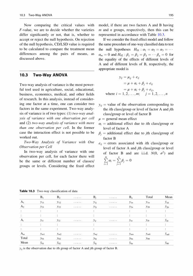
Now comparing the critical values with

F-value, we are to decide whether the varieties

differ significantly or not, that is, whether to

accept or reject the null hypothesis. On rejection

of the null hypothesis, CD/LSD value is required

to be calculated to compare the treatment mean

differences among the pairs of means, as

discussed above.

10.3 Two-Way ANOVA

Two-way analysis of variance is the most power-

ful tool used in agriculture, social, educational,

business, economics, medical, and other fields

of research. In this analysis, instead of consider-

ing one factor at a time, one can consider two

factors in the same experiment. Two-way analy-

sis of variance is of two types: (1) two-way anal-

ysis of variance with one observation per celland (2) two-way analysis of variance with more

than one observation per cell. In the former

case the interaction effect is not possible to be

worked out.

Two-Way Analysis of Variance with OneObservation per Cell

In two-way analysis of variance with one

observation per cell, for each factor there will

be the same or different number of classes/

groups or levels. Considering the fixed effect

model, if there are two factors A and B having

m and n groups, respectively, then this can be

represented in accordance with Table 10.3.

If we consider the fixed effect model and follow

the same procedure of one-way classified data to test

the null hypotheses H01 : α1 ¼ α2 ¼ α3 ¼ � � �αm ¼ 0 and H02 : β1 ¼ β2 ¼ β3 ¼ � � � βn ¼ 0 for

the equality of the effects of different levels of

A and of different levels of B, respectively, the

appropriate model is

yij ¼ μij þ eij

¼ μþ αi þ βj þ eij

¼ μþ αi þ βj þ eij;where i ¼ 1; 2; . . . ;m; j ¼ 1; 2; . . . ; n

yij ¼ value of the observation corresponding to

the ith class/group or level of factor A and jthclass/group or level of factor B

μ ¼ general mean effect

αi ¼ additional effect due to ith class/group or

level of factor A

βj ¼ additional effect due to jth class/group of

factor B

eij ¼ errors associated with ith class/group or

level of factor A and jth class/group or level

of factor B and are i.i.d. N(0, σ2) andPmi¼1

αi ¼Pnj¼1

βj ¼ 0

Table 10.3 Two-way classification of data

B1 B2 . . .. . . Bj . . .. . . Bn Total Mean

A1 y11 y12 . . .. . . y1j . . .. . . y1n y1o �y10A2 y21 y22 . . .. . . y2j . . .. . . y2n y20 �y20: : : : : : :

: : : : : : :

Ai yi1 yi2 . . .. . . yij . . .. . . yin yi0 �yi0: : : : : : :

: : : : : : :

Am ym1 ym2 . . .. . . ymj . . .. . . ymn ym0 �ym0Total y01 y02 . . .. . . y0j . . .. . . y0n y00Mean �y01 �y02 . . .. . . �y0j . . .. . . �y0n �y00

yij is the observation due to ith group of factor A and jth group of factor B.

10.3 Two-Way ANOVA 195

and

μ ¼ �y00;

αi ¼ �yi0 � �y00;

βj ¼ �y0j � �y00;

with �y00 ¼1

mn

Xi;j

yij; �yi0 ¼1

n

Xj

yij; �y0j ¼1

m

Xi

yij:

Thus, yij ¼ �y00 þ �yi0 � �y00ð Þ þ �y0j � �y00

� �þ

yij � �yi0 � �y0j þ �y00

� �. (The product terms van-

ish because of assumption of independence.)

Xi

Xj

yij � �y00 2 ¼ n

Xi

�yi0 � �y00ð Þ2

þ mXj

�y0j � �y00

� �

þXi

Xj

yij � �yi0 � �y0j þ �y00

� �2

or SS totalð Þ ¼ SS factor Að Þ þ SS factor Bð Þ þ SS errorð Þor TSS ¼ SS Að Þ þ SS Bð Þ þ ErSS:

The corresponding partitioning of the total d.f.

is as follows:

mn� 1 ¼ m� 1ð Þ þ n� 1ð Þ þ m� 1ð Þ n� 1ð Þ:Hence, the test statistic under H01 is given by

F ¼ SSðAÞσ2

:1

m� 1

� �� ErSS

σ2:

1

ðm� 1Þðn� 1Þ� �

¼ MSðAÞErMS

which follows F distribution with [(m � 1),

(m � 1)(n � 1)] d.f.

Thus, the null hypothesis H01 is rejected

at α level of significance if

F ¼ MSðAÞErMS

> Fα; ðm� 1Þ; ðm� 1Þðn� 1Þd:f:

Similarly the test statistics underH02 is given by

F ¼ MSðBÞErMS

withα; ðm� 1Þ; ðm� 1Þðn� 1Þ d:f:

For practical purposes the various sums of

squares are calculated using the following

formulae:

G ¼ grand total ¼Xmi¼1

Xnj¼1

yij;

Correction factor ðCFÞ ¼ G2

mn;

Total sum of squares ðTSSÞ ¼Xi

Xj

ðyij � �y00Þ2

¼Xi

Xj

y2ij � CF;

Sum of squares ðAÞ ¼ SS ðAÞ

¼ nXi

ð�yi0 � �y00Þ2 ¼ nXi

�y2i0� m�y2

00

" #

¼ nXi

Pnj¼1

�yij

n

0BB@

1CCA

2

� nm�y200¼ 1

n

Xi

y2i0 � CF,

where; yi0 ¼Xnj¼1

yij is the sum of observations

for ith level of factor A:

Sum of squares ðBÞ ¼ SS ðBÞ¼ m

Xj

�y0j � �y00

� �2

¼ 1

m

Xj

y20j � CF,

where y0j ¼Xmi¼1

yij is the sum of observations

for jth level of factor B;

ErSS ¼ TSS� SS ðAÞ � SS ðBÞ

Dividing this SSs by their respective degrees

of freedom, we will get the corresponding mean

sum of squares, that is, mean sum of squares due

to classes and error mean sum of squares.

We have Table 10.4 as the ANOVA table for

two-way classification with one observation per

cell.

196 10 Analysis of Variance and Experimental Designs

Example 10.2. The following table gives the

milk produced (liter/day) by four breeds of

cows under five different feeds. Analyze the

data to find out the best feed and best breed of

cow with respect to production of milk.

Feed

Breed

Breed A Breed B Breed C Breed D

Feed 1 17 10.6 47 30

Feed 2 19 10.8 46 28

Feed 3 21 10.9 45.5 29

Feed 4 23 11.2 48 25

Feed 5 25 11.3 45 26

Solution. Under the given condition we are to

analyze the data per the two-way ANOVA with

one observation per cell to test the null

hypotheses:

H01 :α1 ¼ α2 ¼ α3 ¼ α4 ¼ α5 ¼ 0 against

H11 :α’s are not all equal and

H02 :β1 ¼ β2 ¼ β3 ¼ β4 ¼ 0 against

H12 :β’s are not all equal:

The appropriate model to test the above is

yij ¼ μþ αi þ βj þ eij, where i ¼ 5, j ¼ 4

yij ¼ value of the observation corresponding to

the ith feed and jth breed

μ ¼ general mean effect

αi ¼ additional effect due to the ith feed

βj ¼ additional effect due to the jth breed

eij ¼ errors associated with the ith feed and jth

breed

For the purpose let us frame the following

table:

Total number of observations¼ N¼mn¼ 20,

G ¼ 17:0þ 10:6þ 47:0þ � � � þ 11:3þ 45þ 26 ¼ 529:3

CF ¼ G2 N= ¼ 529:32 20= ¼ 14007:92

TSS ¼ 17:02 þ 10:62 þ 47:02 þ � � � þ 11:32 þ 452 þ 262 � CF ¼ 3388:27

FSS ¼ SS Feedð Þ ¼ 104:62

4þ 103:82

4þ 106:4

4

2

þ 107:2

4

2

þ 107:3

4

2

� 14007:92 ¼ 2:498

BrSS ¼ SS Breedð Þ ¼ 1052

5þ 54:82

5þ 231:5

5

2

þ 138

5

2

� 14007:92 ¼ 3324:934

ErSS ¼ TSS� FSS� BrSS ¼ 60:834

Table 10.4 ANOVA table for two-way classification of data

SOV d.f. SS MS F

Factor A m � 1 SS(A) AMS ¼ SS(A)/(m � 1) AMS/ErMS

Factor B n � 1 SS(B) BMS ¼ SS(B)/(n � 1) BMS/ErMS

Error (m � 1)(n � 1) ErSS ErMS ¼ ErSS/(m � 1)(n � 1)

Total mn � 1 TSS

Feed

Breed

Total MeanBreed A Breed B Breed C Breed D

Feed 1 17 10.6 47 30 104.6 26.15

Feed 2 19 10.8 46 28 103.8 25.95

Feed 3 21 10.9 45.5 29 106.4 26.6

Feed 4 23 11.2 48 25 107.2 26.8

Feed 5 25 11.3 45 26 107.3 26.825

Total (y0j) 105 54.8 231.5 138 529.3 26.465

Mean �y0j

� �21 10.96 46.3 27.6

10.3 Two-Way ANOVA 197

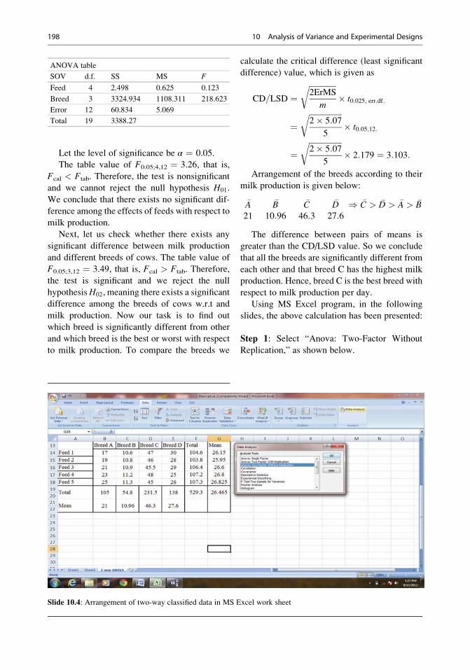
ANOVA table

SOV d.f. SS MS F

Feed 4 2.498 0.625 0.123

Breed 3 3324.934 1108.311 218.623

Error 12 60.834 5.069

Total 19 3388.27

Let the level of significance be α ¼ 0.05.

The table value of F0.05;4,12 ¼ 3.26, that is,

Fcal < Ftab. Therefore, the test is nonsignificant

and we cannot reject the null hypothesis H01.

We conclude that there exists no significant dif-

ference among the effects of feeds with respect to

milk production.

Next, let us check whether there exists any

significant difference between milk production

and different breeds of cows. The table value of

F0.05;3,12 ¼ 3.49, that is, Fcal > Ftab. Therefore,

the test is significant and we reject the null

hypothesisH02, meaning there exists a significant

difference among the breeds of cows w.r.t and

milk production. Now our task is to find out

which breed is significantly different from other

and which breed is the best or worst with respect

to milk production. To compare the breeds we

calculate the critical difference (least significant

difference) value, which is given as

CD=LSD ¼ffiffiffiffiffiffiffiffiffiffiffiffiffiffi2ErMS

m

r� t0:025; err:df:

¼ffiffiffiffiffiffiffiffiffiffiffiffiffiffiffiffiffi2� 5:07

5

r� t0:05;12:

¼ffiffiffiffiffiffiffiffiffiffiffiffiffiffiffiffiffi2� 5:07

5

r� 2:179 ¼ 3:103:

Arrangement of the breeds according to their

milk production is given below:

�A21

�B10:96

�C46:3

�D27:6

) �C > �D > �A > �B

The difference between pairs of means is

greater than the CD/LSD value. So we conclude

that all the breeds are significantly different from

each other and that breed C has the highest milk

production. Hence, breed C is the best breed with

respect to milk production per day.

Using MS Excel program, in the following

slides, the above calculation has been presented:

Step 1: Select “Anova: Two-Factor Without

Replication,” as shown below.

Slide 10.4: Arrangement of two-way classified data in MS Excel work sheet

198 10 Analysis of Variance and Experimental Designs

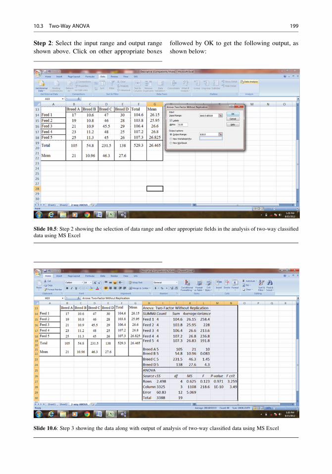
Step 2: Select the input range and output range

shown above. Click on other appropriate boxes

followed by OK to get the following output, as

shown below:

Slide 10.5: Step 2 showing the selection of data range and other appropriate fields in the analysis of two-way classified

data using MS Excel

Slide 10.6: Step 3 showing the data along with output of analysis of two-way classified data using MS Excel

10.3 Two-Way ANOVA 199

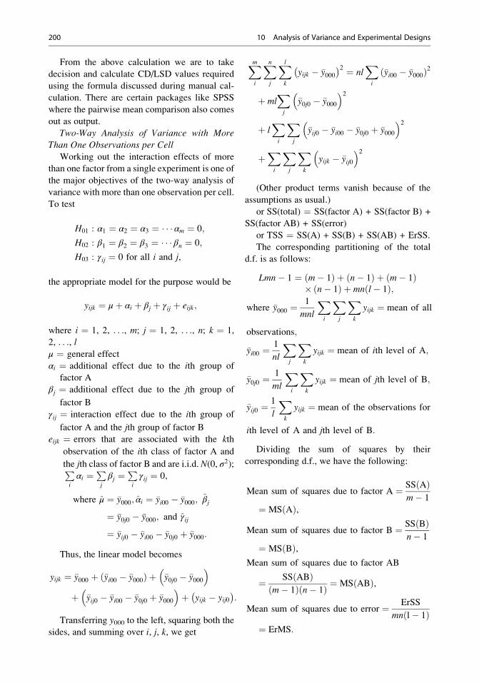
From the above calculation we are to take

decision and calculate CD/LSD values required

using the formula discussed during manual cal-

culation. There are certain packages like SPSS

where the pairwise mean comparison also comes

out as output.

Two-Way Analysis of Variance with More

Than One Observations per Cell

Working out the interaction effects of more

than one factor from a single experiment is one of

the major objectives of the two-way analysis of

variance with more than one observation per cell.

To test

H01 : α1 ¼ α2 ¼ α3 ¼ � � � αm ¼ 0;

H02 : β1 ¼ β2 ¼ β3 ¼ � � � βn ¼ 0;

H03 : γij ¼ 0 for all i and j,

the appropriate model for the purpose would be

yijk ¼ μþ αi þ βj þ γij þ eijk;

where i ¼ 1, 2, . . ., m; j ¼ 1, 2, . . ., n; k ¼ 1,

2, . . ., l

μ ¼ general effect

αi ¼ additional effect due to the ith group of

factor A

βj ¼ additional effect due to the jth group of

factor B

γij ¼ interaction effect due to the ith group of

factor A and the jth group of factor B

eijk ¼ errors that are associated with the kth

observation of the ith class of factor A and

the jth class of factor B and are i.i.d. N(0, σ2);Pi

αi ¼Pj

βj ¼Pi

γij ¼ 0,

where μ ¼ �y000; αi ¼ �yi00 � �y000; βj

¼ �y0j0 � �y000; and γij

¼ �yij0 � �yi00 � �y0j0 þ �y000:

Thus, the linear model becomes

yijk ¼ �y000 þ �yi00 � �y000ð Þ þ �y0j0 � �y000

� �þ �yij0 � �yi00 � �y0j0 þ �y000

� �þ yijk � yij0

:

Transferring y000 to the left, squaring both the

sides, and summing over i, j, k, we get

Xmi

Xnj

Xl

k

yijk � �y000 2 ¼ nl

Xi

�yi00 � �y000ð Þ2

þ mlXj

�y0j0 � �y000

� �2

þ lXi

Xj

�yij0 � �yi00 � �y0j0 þ �y000

� �2

þXi

Xj

Xk

yijk � �yij0

� �2

(Other product terms vanish because of the

assumptions as usual.)

or SS(total) ¼ SS(factor A) + SS(factor B) +

SS(factor AB) + SS(error)

or TSS ¼ SS(A) + SS(B) + SS(AB) + ErSS.

The corresponding partitioning of the total

d.f. is as follows:

Lmn� 1 ¼ m� 1ð Þ þ n� 1ð Þ þ m� 1ð Þ� n� 1ð Þ þ mn l� 1ð Þ;

where �y000 ¼1

mnl

Xi

Xj

Xk

yijk ¼ mean of all

observations;

�yi00 ¼1

nl

Xj

Xk

yijk ¼ mean of ith level of A;

�y0j0 ¼1

ml

Xi

Xk

yijk ¼ mean of jth level of B;

�yij0 ¼1

l

Xk

yijk ¼ mean of the observations for

ith level of A and jth level of B:

Dividing the sum of squares by their

corresponding d.f., we have the following:

Mean sum of squares due to factor A ¼ SSðAÞm� 1

¼ MSðAÞ,

Mean sum of squares due to factor B ¼ SSðBÞn� 1

¼ MSðBÞ,Mean sum of squares due to factor AB

¼ SSðABÞðm� 1Þðn� 1Þ ¼ MSðABÞ,

Mean sum of squares due to error ¼ ErSS

mnðl� 1Þ¼ ErMS:

200 10 Analysis of Variance and Experimental Designs

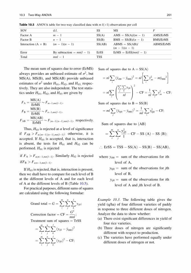
The mean sum of squares due to error (ErMS)

always provides an unbiased estimate of σ2, butMS(A), MS(B), and MS(AB) provide unbiased

estimates of σ2 under H01, H02, and H03, respec-

tively. They are also independent. The test statis-

tics under H01, H02, and H03 are given by

FA ¼ MSðAÞErMS

� Fm�1;mnðl�1Þ;

FB ¼ MSðBÞErMS

� Fn�1;mnðl�1Þ;

FAB ¼ MSðABÞErMS

� Fðm�1Þðn�1Þ;mnðl�1Þ; respectively:

Thus, H03 is rejected at α level of significance

if FAB > Fα;ðm�1Þðn�1Þ;mnðl�1Þ; otherwise, it is

accepted. If H03 is accepted, that is, interaction

is absent, the tests for H01 and H02 can be

performed. H01 is rejected

if FA > Fα;m�1;mnðl�1Þ: Similarly H02 is rejected

ifFB > Fα;n�1;mnðl�1Þ:

IfH03 is rejected, that is, interaction is present,

then we shall have to compare for each level of B

at the different levels of A and for each level

of A at the different levels of B (Table 10.5).

For practical purposes, different sums of squares

are calculated using the following formulae:

Grand total ¼ G ¼Xmi

Xnj

Xl

k

yijk;

Correction factor ¼ CF ¼ G2

mnl;

Treatment sum of squares ¼ TrSS

¼Xmi

Xnj

Xl

k

ðyijk � �y000Þ2

¼Xmi

Xnj

Xl

k

ðyijkÞ2 � CF;

Sum of squares due to A ¼ SSðAÞ

¼ nlXi

ð�yi00 � �y000Þ2 ¼ nlXi

�y2i00� m�y000

2

" #

¼ nlXi

Pj

Pk

yijk

nl

0B@

1CA

2

� CF ¼ 1

nl

Xi

y2i00� CF;

Sum of squares due to B ¼ SSðBÞ¼ ml

Xj

ð�y0j0 � �y000Þ2 ¼1

ml

Xi

y20j0 � CF;

Sum of squares due to ðABÞ

¼Xmi

Xnj

y2ij0

l� CF� SS ðAÞ � SS ðBÞ;

; ErSS ¼ TSS� SSðAÞ � SSðBÞ � SSðABÞ;

where yi00 ¼ sum of the observations for ith

level of A,

y0j0 ¼ sum of the observations for jth

level of B,

yij0 ¼ sum of the observations for ith

level of A and jth level of B:

Example 10.3. The following table gives the

yield (q/ha) of four different varieties of paddy

in response to three different doses of nitrogen.

Analyze the data to show whether:

(a) There exist significant differences in yield of

four rice varieties.

(b) Three doses of nitrogen are significantly

different with respect to production.

(c) The varieties have performed equally under

different doses of nitrogen or not.

Table 10.5 ANOVA table for two-way classified data with m l(>1) observations per cell

SOV d.f. SS MS F

Factor A m � 1 SS(A) AMS ¼ SS(A)/(m � 1) AMS/ErMS

Factor B n � 1 SS(B) BMS ¼ SS(B)/(n � 1) BMS/ErMS

Interaction (A � B) (m � 1)(n � 1) SS(AB) ABMS ¼ SS(AB)/

(m � 1)(n � 1)

ABMS/ErMS

Error By subtraction ¼ mn(l � 1) ErSS ErMS ¼ ErSS/mn(l � 1)

Total mnl � 1 TSS

10.3 Two-Way ANOVA 201

Doses

of N Variety 1 Variety 2 Variety 3 Variety 4

N1 13.0 17.0 15.5 20.5

13.4 17.5 15.6 20.8

13.5 17.4 15.5 20.4

N2 14.0 18.0 16.2 24.5

14.2 18.5 16.1 25.6

14.6 18.9 16.3 25.0

N3 25.0 22.0 18.5 32.0

24.8 22.5 18.6 32.5

24.3 22.3 18.7 32.0

Solution. The problem can be visualized as the

problem of two-way analysis of variance with

three observations per cell. The linear model is

yijk ¼ μþ αi þ βj þ γij þ eijk;

where

αi is the effect of ith level of nitrogen; i ¼ 3;

βj is the effect of jth level of variety; j ¼ 4;

γij is the interaction effect of ith level of nitrogen

and jth level of variety:

Wewant to test the following null hypotheses:

H01 : α1 ¼ α2 ¼ α3 ¼ 0 against H11 : α’s are not

all equal,

H02 : β1 ¼ β2 ¼ β3 ¼ β4 ¼ 0 against H12 : β’s

are not all equal,

H03 : γij’s ¼ 0 for all i; j against H13 : γij’s are

not all equal:

Let the level of significance be α ¼ 0.05.

Let us construct the following table of totals

(yij):

Total number of observations ¼ mnl ¼ 3� 4� 3 ¼ 36 ¼ N

G ¼ 13:0þ 17þ 15:5þ � � � þ 22:3þ 18:7þ 32: ¼ 715:2;

CF ¼ GT2 N= ¼ 715:22 36= ¼ 14208:64,

TSS ¼ 13:02 þ 172 þ 15:52 þ � � � þ 22:32 þ 18:72 þ 322 � CF ¼ 975:52;

NSS ¼ 200:12

12þ 221:92

12þ 293:20

12

2

� CF ¼ 395.182,

VSS ¼ 156:82

9þ 174:102

9þ 151:00

9

2

� CF ¼ 472.131,

SS ðN� VÞ ¼ 1=3 39:92 þ 51:92 þ 46:62 þ � � � þ 66:802 þ 55:802 þ 96:52� �� CF� NSS� VSS ¼ 106:04,

ErSS ¼ TSS� NSS� VSS� SS N� Vð Þ ¼ 975:52� 395:182� 472:131� 106:04 ¼ 2:17:

Nitrogen Variety 1 Variety 2 Variety 3 Variety 4 Total (yi00) Mean

N1 39.90 51.90 46.60 61.70 200.10 16.675

N2 42.80 55.40 48.60 75.10 221.90 18.492

N3 74.10 66.80 55.80 96.50 293.20 24.433

Total(y0j0) 156.800 174.100 151.000 233.300 715.200

Mean 17.422 19.344 16.778 25.922 19.867

202 10 Analysis of Variance and Experimental Designs

ANOVA table for two-way analysis of

variance with three observations per cell

SOV d.f. SS MS F

Variety 3 472.131 157.377 1743.253

Nitrogen 2 395.182 197.591 2188.698

Interaction

(V � N)

4 106.041 17.673 195.767

Error 24 2.167 0.090

Total 26 975.520

Let the level of significance be α ¼ 0.05.

The table value of F0.05;2,24 ¼ 3.40,

F0.05;3,24 ¼ 3.01, and F0.05;6,24 ¼ 2.51, that is,

Fcal > Ftab, in all the cases, that is, nitrogen,

variety, and nitrogen � variety interaction. So

the tests are significant and we reject the null

hypotheses and conclude that there exists signifi-

cant difference among the effects of doses of

nitrogen, varieties, and their interactions with

respect to the yield of paddy.

Now, we are interested in identifying the best

nitrogen, the best variety, and the nitrogen �variety combination providing the best yield.

To accomplish this task, we calculate the crit-

ical difference (CD)/LSD values for nitrogen,

variety, and interaction separately as follows:

CD0:05ðNitrogenÞ ¼ffiffiffiffiffiffiffiffiffiffiffiffiffi2MSE

l� v

r� t0:025; err:d:f:

¼ffiffiffiffiffiffiffiffiffiffiffiffiffiffiffiffiffiffiffiffi2� 0:073

3� 4

r� t0:025;18:

¼ffiffiffiffiffiffiffiffiffiffiffiffiffiffiffiffiffiffiffiffi2� 0:090

3� 4

r� 2:064 ¼ 0:252;

CD0:05ðVarietyÞ ¼ffiffiffiffiffiffiffiffiffiffiffiffiffi2MSE

r � t

r� t0:025;err:d:f:

¼ffiffiffiffiffiffiffiffiffiffiffiffiffiffiffiffiffi2� 0:09

3� 3

r� t0:025;18:

¼ffiffiffiffiffiffiffiffiffiffiffiffiffiffiffiffiffi2� 0:09

3� 3

r� 2:064 ¼ 0:292;

CD0:05ðTr:� VÞ ¼ffiffiffiffiffiffiffiffiffiffiffiffiffi2MSE

r

r� t0:025; err:d:f:

¼ffiffiffiffiffiffiffiffiffiffiffiffiffiffiffiffiffiffiffiffi2� 0:090

3

r� t0:025;18:

¼ffiffiffiffiffiffiffiffiffiffiffiffiffiffiffiffiffiffiffiffi2� 0:090

3

r� 2:064 ¼ 0:505:

Comparing the three nitrogen means provided

in the table of treatment totals, one can find that

the difference between any two nitrogen means is

greater than the corresponding critical difference

value 0.252. So we can conclude that nitrogen

doses significantly differ among themselves

with respect to yield of paddy and the nitrogen

dose giving significantly the highest yield

(24.433q/ha) is treatment N3.

As far as the response of four varieties of

paddy is concerned, it is found that the difference

between any two variety means is greater than

the critical difference value 0.292. Thus, the

varieties differ significantly among themselves

with respect to yield. Among the varieties, vari-

ety 4 has produced significantly the highest yield,

so this is the best variety.

After identifying the best variety and the best

treatment separately, our task is now to identify

the best nitrogen � variety combination for

yield of paddy from the above information. Let

us construct the following table of average inter-

action values of nitrogen and variety.

Mean table of N � V

Nitrogen

Variety

1

Variety

2

Variety

3

Variety

4

N1 13.300 17.300 15.533 20.567

N2 14.267 18.467 16.200 25.033

N3 24.700 22.267 18.600 32.167

From the above table, it can be seen that the

difference between any two combinations is

more than the corresponding critical difference

value for nitrogen � variety interaction (0.505),

so all the combinations produce significantly dif-

ferent yields of paddy. Among the nitrogen �variety combinations, it is noticed that variety

4–nitrogen 3 combination produced the highest

yield; hence, this is the best combination,

followed by V4N2, which is at par with V1N3.

Thus, from the analysis we draw the following

conclusions:

1. The treatments differ significantly among them-

selves and the best treatment is treatment T3.

2. The varieties differ significantly among

themselves and the best variety is V2.

3. Treatment T3 along with variety V1, produces

significantly higher yield than any other

combination.

Let us try to know how the above analysis of

variance could be done with MS Excel program

10.3 Two-Way ANOVA 203

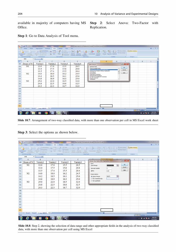
available in majority of computers having MS

Office.

Step 1: Go to Data Analysis of Tool menu.

Step 2: Select Anova: Two-Factor with

Replication.

Step 3: Select the options as shown below.

Slide 10.7: Arrangement of two-way classified data, with more than one observation per cell in MS Excel work sheet

Slide 10.8: Step 2, showing the selection of data range and other appropriate fields in the analysis of two-way classified

data, with more than one observation per cell using MS Excel

204 10 Analysis of Variance and Experimental Designs

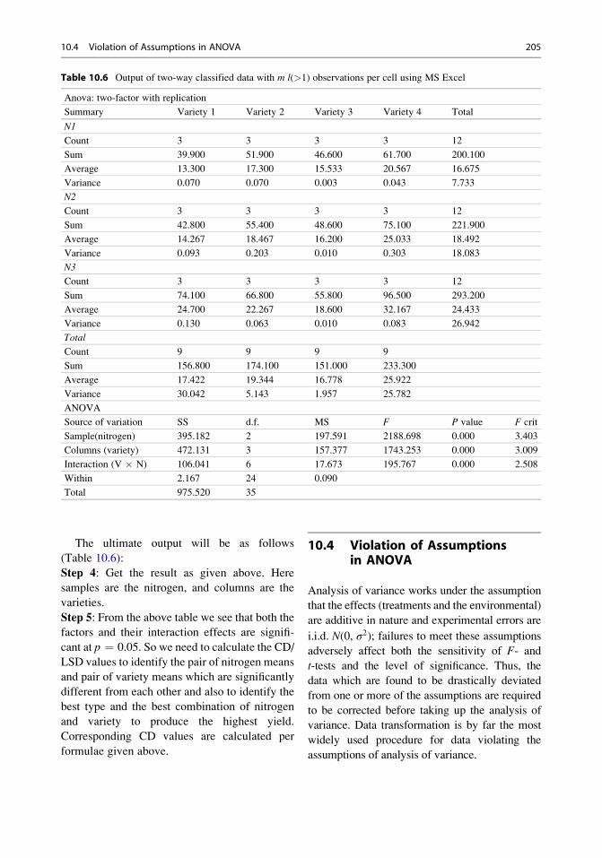
The ultimate output will be as follows

(Table 10.6):

Step 4: Get the result as given above. Here

samples are the nitrogen, and columns are the

varieties.

Step 5: From the above table we see that both the

factors and their interaction effects are signifi-

cant at p ¼ 0.05. So we need to calculate the CD/

LSD values to identify the pair of nitrogen means

and pair of variety means which are significantly

different from each other and also to identify the

best type and the best combination of nitrogen

and variety to produce the highest yield.

Corresponding CD values are calculated per

formulae given above.

10.4 Violation of Assumptionsin ANOVA

Analysis of variance works under the assumption

that the effects (treatments and the environmental)

are additive in nature and experimental errors are

i.i.d. N(0, σ2); failures to meet these assumptions

adversely affect both the sensitivity of F- and

t-tests and the level of significance. Thus, the

data which are found to be drastically deviated

from one or more of the assumptions are required

to be corrected before taking up the analysis of

variance. Data transformation is by far the most

widely used procedure for data violating the

assumptions of analysis of variance.

Table 10.6 Output of two-way classified data with m l(>1) observations per cell using MS Excel

Anova: two-factor with replication

Summary Variety 1 Variety 2 Variety 3 Variety 4 Total

N1

Count 3 3 3 3 12

Sum 39.900 51.900 46.600 61.700 200.100

Average 13.300 17.300 15.533 20.567 16.675

Variance 0.070 0.070 0.003 0.043 7.733

N2

Count 3 3 3 3 12

Sum 42.800 55.400 48.600 75.100 221.900

Average 14.267 18.467 16.200 25.033 18.492

Variance 0.093 0.203 0.010 0.303 18.083

N3

Count 3 3 3 3 12

Sum 74.100 66.800 55.800 96.500 293.200

Average 24.700 22.267 18.600 32.167 24.433

Variance 0.130 0.063 0.010 0.083 26.942

Total

Count 9 9 9 9

Sum 156.800 174.100 151.000 233.300

Average 17.422 19.344 16.778 25.922

Variance 30.042 5.143 1.957 25.782

ANOVA

Source of variation SS d.f. MS F P value F crit

Sample(nitrogen) 395.182 2 197.591 2188.698 0.000 3.403

Columns (variety) 472.131 3 157.377 1743.253 0.000 3.009

Interaction (V � N) 106.041 6 17.673 195.767 0.000 2.508

Within 2.167 24 0.090

Total 975.520 35

10.4 Violation of Assumptions in ANOVA 205

10.4.1 Data Transformation

Among the different types of transformation

generally used to make the data corrected for

analysis of variance, logarithmic transformation,

square root transformation, and angular

transformation are widely used.

10.4.1.1 Logarithmic TransformationThe number of plant insects, number of egg

mass per unit area, number of larvae per unit

area, etc., are typical examples wherein variance

is proportional to the mean and logarithmic trans-

formation can be used effectively. The procedure

is to take simply the logarithm of each and

every observation and carry out the analysis of

variance following the usual procedure with the

transformed data. However, if in the data set

small values (less than 10) are recorded, then

instead of taking log(x), it will be better to take

log(x + 1). The final results or inference should

be drawn on the basis of transformed mean

values and on the basis of calculations made

through transformed data. However, while

presenting the mean table, it will be appropriate

to recalculate the means by taking the antilog of

the transformed data. In practice, the treatment

means are calculated from the original data

because of simplicity of calculations, but statis-

tically the procedure of converting transformed

mean to original form is more appropriate.

If there is a mismatch in the two procedures,

then the procedure of converting the transformed

mean with the help of the antilog is preferred

over the other procedure.

Example 10.4. The following data give the

number of fruit set after the application of eight

different hormonal treatments in jackfruit. Use

suitable transformation and analyze the data

using the suitable model.

Solution. Because this experiment is related

with count data, violation of the assumption of

ANOVA is suspected and the analysis of the data

is required to be made on the basis of the

transformed data. The appropriate transforma-

tion would be logarithmic transformation.

The following table presents the transformed

data. It may be noted that as some of the

observations are below 10, we apply log(X + 1)

transformation instead of log(X).

Hormone Replication 1 Replication 2 Replication 3 Replication 4

H1 2 9 8 2

H2 4 5 6 3

H3 5 7 12 6

H4 3 11 8 13

H5 19 26 15 22

H6 24 34 24 27

H7 3 1 1 5

H8 15 11 13 15

Hormone H1 H2 H3 H4 H5 H6 H7 H8

Replication 1 0.4771 0.6990 0.7782 0.6021 1.3010 1.3979 0.6021 1.2041

Replication 2 1.0000 0.7782 0.9031 1.0792 1.4314 1.5441 0.3010 1.0792

Replication 3 0.9542 0.8451 1.1139 0.9542 1.2041 1.3979 0.3010 1.1461

Replication 4 0.4771 0.6021 0.8451 1.1461 1.3617 1.4472 0.7782 1.2041

Average 0.7271 0.7311 0.9101 0.9454 1.3246 1.4468 0.4956 1.1584

206 10 Analysis of Variance and Experimental Designs

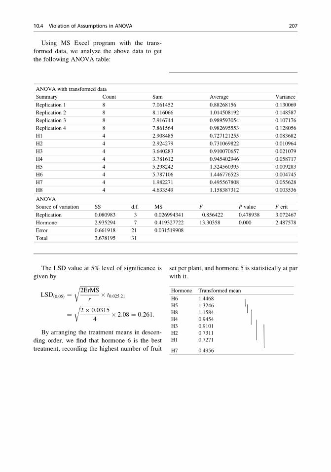
Using MS Excel program with the trans-

formed data, we analyze the above data to get

the following ANOVA table:

The LSD value at 5% level of significance is

given by

LSDð0:05Þ ¼ffiffiffiffiffiffiffiffiffiffiffiffiffiffi2ErMS

r

r� t0:025;21

¼ffiffiffiffiffiffiffiffiffiffiffiffiffiffiffiffiffiffiffiffiffiffi2� 0:0315

4

r� 2:08 ¼ 0:261:

By arranging the treatment means in descen-

ding order, we find that hormone 6 is the best

treatment, recording the highest number of fruit

set per plant, and hormone 5 is statistically at par

with it.

Hormone Transformed mean

H6 1.4468

H5 1.3246

H8 1.1584

H4 0.9454

H3 0.9101

H2 0.7311

H1 0.7271

H7 0.4956

ANOVA with transformed data

Summary Count Sum Average Variance

Replication 1 8 7.061452 0.88268156 0.130069

Replication 2 8 8.116066 1.014508192 0.148587

Replication 3 8 7.916744 0.989593054 0.107176

Replication 4 8 7.861564 0.982695553 0.128056

H1 4 2.908485 0.727121255 0.083682

H2 4 2.924279 0.731069822 0.010964

H3 4 3.640283 0.910070657 0.021079

H4 4 3.781612 0.945402946 0.058717

H5 4 5.298242 1.324560395 0.009283

H6 4 5.787106 1.446776523 0.004745

H7 4 1.982271 0.495567808 0.055628

H8 4 4.633549 1.158387312 0.003536

ANOVA

Source of variation SS d.f. MS F P value F crit

Replication 0.080983 3 0.026994341 0.856422 0.478938 3.072467

Hormone 2.935294 7 0.419327722 13.30358 0.000 2.487578

Error 0.661918 21 0.031519908

Total 3.678195 31

10.4 Violation of Assumptions in ANOVA 207

Let us examine the analysis of the aboveproblem without transforming the data using MS

Excel and following the steps discussed above.

The LSD value at 5% level of significance

with original data is given by

LSDð0:05Þ ¼ffiffiffiffiffiffiffiffiffiffiffiffiffiffi2ErMS

r

r� t0:025;21

¼ffiffiffiffiffiffiffiffiffiffiffiffiffiffiffiffiffiffiffiffiffiffi2� 11:067

4

r� 2:08 ¼ 4:893:

By arranging the treatment means in

descending order, we find that hormone 6 is the

best treatment, recording the highest number of

fruit set per plant, and all other hormonal effects

are statistically different with it. Thus, the con-

clusion on the basis of original data clearly

differs from that of transformed data.

Hormone Original average

H6 27.25

H5 20.5

H8 13.5

H4 8.75

H3 7.5

H1 5.25

H2 4.5

H7 2.5

10.4.1.2 Square Root TransformationFor count data consisting of small whole

numbers and percentage data where the data

ranges either between 0 and 30% or between 70

and to 100%, that is, the data in which the vari-

ance tends to be proportional to the mean, the

square root transformation is used. Data obtained

from counting rare events like the number of

death per unit time, the number of infested leaf

per plant, the number of call received in a tele-

phone exchange, or the percentage of infestation

(disease or pest) in a plot (either 0–30% or

70–100%) are examples where square root trans-

formation can be useful before taking up analysis

of variance to draw a meaningful conclusion or

inference. If most of the values in a data set are

small (<10) coupled with the presence of

0 values, instead of usingffiffiffix

ptransformation, it

is better to useffiffiffiffiffiffiffiffiffiffiffiffiffiffiffiffiffiffiðxþ 0:5Þp

. Then analysis of

variance to be conducted with the transformed

data and the mean table should be made from

the transformed data instead of taking the mean

from the original data because of the facts stated

earlier.

ANOVA with original data

Summary Count Sum Average Variance

H1 4 21 5.2500 14.2500

H2 4 18 4.5000 1.6667

H3 4 30 7.5000 9.6667

H4 4 35 8.7500 18.9167

H5 4 82 20.5000 21.6667

H6 4 109 27.2500 22.2500

H7 4 10 2.5000 3.6667

H8 4 54 13.5000 3.6667

Replication 1 8 75 9.3750 74.5536

Replication 2 8 104 13.0000 125.4286

Replication 3 8 87 10.8750 47.5536

Replication 4 8 93 11.6250 85.6964

ANOVA

Source of variation SS d.f. MS F P value F crit

Hormone 2100.21875 7 300.0313 27.1105 0.0000 2.4876

Replication 54.84375 3 18.2813 1.6519 0.2078 3.0725

Error 232.40625 21 11.0670

Total 2387.46875 31

208 10 Analysis of Variance and Experimental Designs

Example 10.5. The following information

pertains to the number of insects per 20 insects

that remained alive after the application of six

different insecticides. Analyze the data to work

out the most efficient insecticide.

Solution. Information given in this problem is

in the form of small whole numbers, so violation

of assumption of ANOVA is suspected.

Hence, a square root transformation will be

appropriate before taking up the analysis of

variance.

So from the given data table, we first make the

following table by taking the square roots of the

given observations. It may be noted that the data

set contains small whole number (<10); instead

offfiffiffiffiX

p, we have taken

ffiffiffiffiffiffiffiffiffiffiffiffiffiffiffiffiffiffiffiðX þ 0:5Þp.

Using MS Excel (as described in the previous

example) with the transformed data, we analyze

the above data to get the following ANOVA

table:

Insecticides Replication 3 Replication 2 Replication 1 Replication 4

I1 3 5 1 3

I2 6 3 2 3

I3 6 7 5 5

I4 3 4 4 5

I5 9 8 7 8

I6 10 9 12 11

Insecticides Replication 1 Replication 2 Replication 3 Replication 4

I1 1.22474487 1.58113883 1.87083 1.58114

I2 1.58113883 2.34520788 2.12132 2.12132

I3 1.58113883 2.738612788 2.54951 2.54951

I4 1.22474487 2.34520788 2.12132 2.54951

I5 2.12132034 3.535533906 3.08221 2.91548

I6 3.53553391 2.549509757 3.24037 3.39116

Insecticides Replication 1 Replication 2 Replication 3 Replication 4 Average

I1 1 2 3 2 2

I2 2 5 4 4 3.75

I3 2 7 6 6 5.25

I4 1 5 4 6 4

I5 4 12 9 8 8.25

I6 12 6 10 11 9.75

10.4 Violation of Assumptions in ANOVA 209

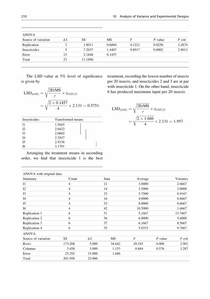
The LSD value at 5% level of significance

is given by

LSDð0:05Þ ¼ffiffiffiffiffiffiffiffiffiffiffiffiffiffi2ErMS

r

r� t0:025;21

¼ffiffiffiffiffiffiffiffiffiffiffiffiffiffiffiffiffiffiffiffiffiffi2� 0:1457

4

r� 2:131 ¼ 0:5751:

Insecticides Transformed means

I1 1.5645

I2 2.0422

I3 2.0602

I4 2.3547

I5 2.9136

I6 3.1791

Arranging the treatment means in ascending

order, we find that insecticide 1 is the best

treatment, recording the lowest number of insects

per 20 insects, and insecticides 2 and 3 are at par

with insecticide 1. On the other hand, insecticide

6 has produced maximum input per 20 insects.

LSDð0:05Þ ¼ffiffiffiffiffiffiffiffiffiffiffiffiffiffi2ErMS

r

r� t0:025;21

¼ffiffiffiffiffiffiffiffiffiffiffiffiffiffiffiffiffiffiffiffi2� 1:686

4

r� 2:131 ¼ 1:957:

ANOVA with original data

Summary Count Sum Average Variance

I1 4 12 3.0000 2.6667

I2 4 14 3.5000 3.0000

I3 4 23 5.7500 0.9167

I4 4 16 4.0000 0.6667

I5 4 32 8.0000 0.6667

I6 4 42 10.5000 1.6667

Replication 1 6 31 5.1667 15.7667

Replication 2 6 36 6.0000 5.6000

Replication 3 6 37 6.1667 8.5667

Replication 4 6 35 5.8333 9.7667

ANOVA

Source of variation SS d.f. MS F P value F crit

Rows 173.208 5.000 34.642 20.545 0.000 2.901

Columns 3.458 3.000 1.153 0.684 0.576 3.287

Error 25.292 15.000 1.686

Total 201.958 23.000

ANOVA

Source of variation d.f. SS MS F P value F crit

Replication 3 1.8011 0.6004 4.1221 0.0256 3.2874

Insecticides 5 7.2037 1.4407 9.8917 0.0002 2.9013

Error 15 2.1848 0.1457

Total 23 11.1896

210 10 Analysis of Variance and Experimental Designs

Arranging the treatment means in ascending

order, we find that insecticide 1 is the best insec-

ticide treatment, recording the lowest number of

insects per 20 insects, and insecticides 2 and 4

are at par with insecticide 1. On the other hand,

insecticide 6 has retained insect weeds per 20

insects. But with transformed data I1, I2, and I3

are at par.

Insecticide Average

I1 3.0000

I2 3.5000

I4 4.0000

I3 5.7500

I5 8.0000

I6 10.5000

10.4.1.3 Angular TransformationData on proportions/percentages arising out of

count data require angular transformation or the

arcsine transformation. It may be noted emphati-

cally that the percentage data (e.g., percentage of

carbohydrate, protein, and sugar; percentage of

marks; and percentage of infections) which are

not arising out of count data mn � 100

should

not be put under arcsine transformation. More-

over, all the percentage data arising out of count

data need not be subjected to arcsine transforma-

tion before analysis of variance:

(a) For percentage data ranging either between

0 and 30% or 70 and 100% but not both, the

square root transformation should be used.

(b) For percentage data ranging between 30 and

70%, no transformation is required.

(c) Percentage data which overlaps the above

two situations should only be put under arc-

sine transformation.

Thus, a data set having 0 to more than 30%,

less than 70–100%, and 0–100% should be put

under arcsine transformation.

The values of 0% should be substituted by 14n

and the values of 100% by 100� 14n , where n is

the number of counts on which percentages are

worked out before transformation of data follow-

ing arcsine rule of transformation. The essence

of arcsine transformation is to convert the

percentage data into angles measured in degrees,

that is, to transform 0–100% data into 0–90�

angles. The actual procedure is to convert the

percentage data into proportions and transform

it into sin�1 ffiffiffip

p, where p is the percentage data

measured in proportions. Ready-made tables are

available for different percentage values with

their corresponding transformed values. How-

ever, in MS Excel with the following functional

form, a percentage data can be directly converted

to arcsine transformed data.

¼ degrees (asin(sqrt(p/100))), where p is the

percentage value.

Analysis of variance is taken up on the

transformed data and inferences are made

accordingly with the transformed means. How-

ever, to get original means retransformation of

transformed means is preferred over the means

from original data because of the fact stated

earlier.

Example 10.6. The following table gives the

germination percentage of eight varieties of

wheat in a field trial with three replications.

Analyze the data to find out the best variety

w.r.t. germination.

Variety

Replication

3

Replication

1

Replication

2

V1 62 55 48

V2 28 23 32

V3 70 75 72

V4 85 86 88

V5 92 90 95

V6 18 15 17

V7 20 16 18

V8 68 65 66

Solution. From the given information it is clear

that (a) the data can be analyzed per the analysis

of two-way classified data and (b) the data relates

to percentage data arising out of count data and

the percentage ranges from 15 to 95%. Thus,

there is a chance of heterogeneous variance.

So we opt for arcsine transformation before

taking up the analysis of variance.

10.4 Violation of Assumptions in ANOVA 211

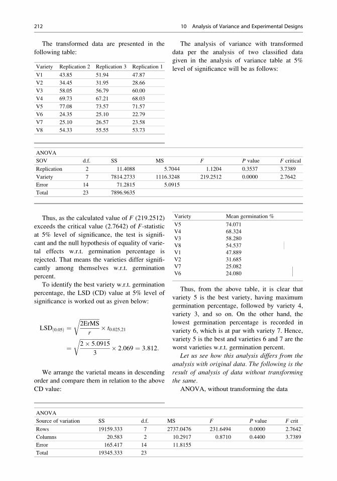
The transformed data are presented in the

following table:

Variety Replication 2 Replication 3 Replication 1

V1 43.85 51.94 47.87

V2 34.45 31.95 28.66

V3 58.05 56.79 60.00

V4 69.73 67.21 68.03

V5 77.08 73.57 71.57

V6 24.35 25.10 22.79

V7 25.10 26.57 23.58

V8 54.33 55.55 53.73

The analysis of variance with transformed

data per the analysis of two classified data

given in the analysis of variance table at 5%

level of significance will be as follows:

Thus, as the calculated value of F (219.2512)

exceeds the critical value (2.7642) of F-statisticat 5% level of significance, the test is signifi-

cant and the null hypothesis of equality of varie-

tal effects w.r.t. germination percentage is

rejected. That means the varieties differ signifi-

cantly among themselves w.r.t. germination

percent.

To identify the best variety w.r.t. germination

percentage, the LSD (CD) value at 5% level of

significance is worked out as given below:

LSDð0:05Þ ¼ffiffiffiffiffiffiffiffiffiffiffiffiffiffi2ErMS

r

r� t0:025;21

¼ffiffiffiffiffiffiffiffiffiffiffiffiffiffiffiffiffiffiffiffiffiffi2� 5:0915

3

r� 2:069 ¼ 3:812:

We arrange the varietal means in descending

order and compare them in relation to the above

CD value:

Variety Mean germination %

V5 74.071

V4 68.324

V3 58.280

V8 54.537

V1 47.889

V2 31.685

V7 25.082

V6 24.080

Thus, from the above table, it is clear that

variety 5 is the best variety, having maximum

germination percentage, followed by variety 4,

variety 3, and so on. On the other hand, the

lowest germination percentage is recorded in

variety 6, which is at par with variety 7. Hence,

variety 5 is the best and varieties 6 and 7 are the

worst varieties w.r.t. germination percent.

Let us see how this analysis differs from the

analysis with original data. The following is theresult of analysis of data without transforming

the same.

ANOVA, without transforming the data

ANOVA

SOV d.f. SS MS F P value F critical

Replication 2 11.4088 5.7044 1.1204 0.3537 3.7389

Variety 7 7814.2733 1116.3248 219.2512 0.0000 2.7642

Error 14 71.2815 5.0915

Total 23 7896.9635

ANOVA

Source of variation SS d.f. MS F P value F crit

Rows 19159.333 7 2737.0476 231.6494 0.0000 2.7642

Columns 20.583 2 10.2917 0.8710 0.4400 3.7389

Error 165.417 14 11.8155

Total 19345.333 23

212 10 Analysis of Variance and Experimental Designs

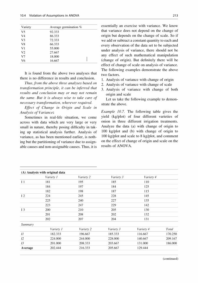
It is found from the above two analyses that

there is no difference in results and conclusion.

Thus, from the above three analyses based ontransformation principle, it can be inferred that

results and conclusion may or may not remain

the same. But it is always wise to take care ofnecessary transformation, wherever required.

Effect of Change in Origin and Scale in

Analysis of Variance:Sometimes in real-life situation, we come

across with data which are very large or very

small in nature, thereby posing difficulty in tak-

ing up statistical analysis further. Analysis of

variance, as has been mentioned earlier, is noth-

ing but the partitioning of variance due to assign-

able causes and non-assignable causes. Thus, it is

essentially an exercise with variance. We know

that variance does not depend on the change of

origin but depends on the change of scale. So if

we add or subtract a constant quantity to each and

every observation of the data set to be subjected

under analysis of variance, there should not be

any effect of such mathematical manipulation

(change of origin). But definitely there will be

effect of change of scale on analysis of variance.

The following examples demonstrate the above

two factors.

1. Analysis of variance with change of origin

2. Analysis of variance with change of scale

3. Analysis of variance with change of both

origin and scale

Let us take the following example to demon-

strate the above.

Example 10.7. The following table gives the

yield (kg/plot) of four different varieties of

onion in three different irrigation treatments.

Analyze the data (a) with change of origin to

100 kg/plot and (b) with change of origin to

100 kg/plot and scale to 8 kg/plot, and comment

on the effect of change of origin and scale on the

results of ANOVA.

Variety Average germination %

V5 92.333

V4 86.333

V3 72.333

V8 66.333

V1 55.000

V2 27.667

V7 18.000

V6 16.667

(A) Analysis with original data

Variety 1 Variety 2 Variety 3 Variety 4

I 1 181 195 185 110

184 197 184 125

182 198 187 115

I 2 224 245 228 145

225 240 227 135

223 247 229 142

I 3 200 210 205 130

201 208 202 132

202 207 204 131

Summary

Variety 1 Variety 2 Variety 3 Variety 4 Total

I1 182.333 196.667 185.333 116.667 170.250

I2 224.000 244.000 228.000 140.667 209.167

I3 201.000 208.333 203.667 131.000 186.000

Average 202.444 216.333 205.667 129.444

(continued)

10.4 Violation of Assumptions in ANOVA 213

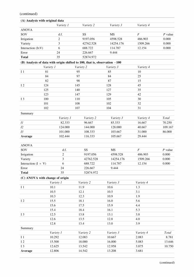
(A) Analysis with original data

Variety 1 Variety 2 Variety 3 Variety 4

ANOVA

SOV d.f. SS MS F P value

Irrigation 2 9197.056 4598.528 486.903 0.000

Variety 3 42762.528 14254.176 1509.266 0.000

Interaction (IxV) 6 688.722 114.787 12.154 0.000

Error 24 226.667 9.444

Total 35 52874.972

(B) Analysis of data with origin shifted to 100, that is, observation �100

Variety 1 Variety 2 Variety 3 Variety 4

I 1 81 95 85 10

84 97 84 25

82 98 87 15

I 2 124 145 128 45

125 140 127 35

123 147 129 42

I 3 100 110 105 30

101 108 102 32

102 107 104 31

Summary

Variety 1 Variety 2 Variety 3 Variety 4 Total

I1 82.333 96.667 85.333 16.667 70.250

I2 124.000 144.000 128.000 40.667 109.167

I3 101.000 108.333 103.667 31.000 86.000

Average 102.444 116.333 105.667 29.444

ANOVA

SOV d.f. SS MS F P value

Irrigation 2 9197.056 4598.528 486.903 0.000

Variety 3 42762.528 14254.176 1509.266 0.000

Interaction (I � V) 6 688.722 114.787 12.154 0.000

Error 24 226.667 9.444

Total 35 52874.972

(C) ANOVA with change of origin

Variety 1 Variety 2 Variety 3 Variety 4

I 1 10.1 11.9 10.6 1.3

10.5 12.1 10.5 3.1

10.3 12.3 10.9 1.9

I 2 15.5 18.1 16.0 5.6

15.6 17.5 15.9 4.4

15.4 18.4 16.1 5.3

I 3 12.5 13.8 13.1 3.8

12.6 13.5 12.8 4.0

12.8 13.4 13.0 3.9

Summary

Variety 1 Variety 2 Variety 3 Variety 4 Total

I 1 10.292 12.083 10.667 2.083 8.781

I 2 15.500 18.000 16.000 5.083 13.646

I 3 12.625 13.542 12.958 3.875 10.750

Average 12.806 14.542 13.208 3.681

(continued)

(continued)

From the above analyses the following points

may be noted:

1. F-ratios and the significance level do not

change under the above three cases.

2. Mean values change in the second and third

cases.

3. Sumof squares andmean sum of squares values

do not change in the first and second cases.

4. As error mean square remains the same in the

first and second cases, critical difference

values also remain the same.

Thus, with the change of origin and/or scale,the basic conclusion from ANOVA does not

change, but while comparing the means, care

should be taken to adjust the mean values andthe critical difference values accordingly.

10.5 Experimental Reliability

Reliability of experimental procedure, in its

simplest form, can be verified with the help of

coefficient of variations. The coefficient of vari-

ation is defined as

CV ¼ S:D

Grand Mean� 100:

Here the positive square root of error mean

square in analysis of variance is taken as an

estimate of the standard deviation. Thus, from

the table of analysis of variance, one can work

out the CV% as follows:

CV ¼ffiffiffiffiffiffiffiffiffiffiffiffiErMS

p

Grand Mean� 100:

Now the question is, what should be the range

or the value of CV% for the information from an

experiment to be taken reliable? There is no hard

and fast rule to determine the cutoff value of CV

% for an experiment is reliable; it depends on the

condition of the experiment (laboratory condi-

tion, field condition, etc.), type of materials/

treatments tested in the experiment, desired pre-

cision from the experiment, etc. Generally the

CV% should be less in experiments conducted

under laboratory conditions compared to field

experiments. Similarly CV% also depends on

the type of field crop, size and shape of experi-

mental units, etc. However, by and large, a CV%

less than 20% is regarded as an indication for the

reliability of the experiments. If the CV value is

more than 20%, there is a need to verify the

experimental procedure and need for emphasis

on the reduction of experimental error.

10.6 Comparison of Means

The F-test in analysis of variance indicates the

acceptance or the rejection of the null hypothesis.

The F-test in analysis of variance can be signi-

ficant even if only one pair of means among

several pairs of means is significant. If the nullhypothesis is rejected, we need to find out the

means which are significantly different from

each other and resulting the significance ofF-test. Thus, comparison of treatment means

becomes essential. The comparison of treatment

means can be done either through pair compari-son or through group comparison. In group com-

parison, two or more than two treatment means

are involved in the process. Under the group

comparison there are between-group compari-

son, within-group comparison, trend compari-

son, and factorial comparison. Pair comparison

is the simplest and most commonly used method.

(C) ANOVA with change of origin

Variety 1 Variety 2 Variety 3 Variety 4

ANOVA

SOV d.f. SS MS F P value

Irrigation 2 143.704 71.852 486.903 0.000

Variety 3 668.164 222.721 1509.266 0.000

Interaction (I � V) 6 10.761 1.794 12.154 0.000

Error 24 3.542 0.148

Total 35 826.171

(continued)

10.6 Comparison of Means 215

In the following section we will discuss pair

comparison.

10.6.1 Pair Comparison

Quite a good number of test procedures are

available for the purpose of comprising pair of

treatment means. Among the methods the leastsignificant difference test (LSD), also known as

critical difference (CD) test; student Newman–Keuls test, Duncan multiple range test (DMRT),

and Tukey’s honestly significant difference test

are commonly used. Again, among the four test

procedures, the CD and the DMRT are mostly

used.

10.6.1.1 CD/LSD TestThe essence of LSD test is to provide a single

value at specified level of significance which

serves as the limiting value of significant or non-

significant difference between two treatment

means. Thus, two treatment means are declared

significantly different at the specified level of

significance if the difference between the treat-

ment means exceeds the LSD/CD value; other-

wise they are not.

Calculation of LSD Values

LSD ¼ standard error of difference between two

treatment means under comparison multiplied by

the table value of t distribution at error degrees of

freedom with specific level of significance.

Thus, for both-sided tests LSDα=CDα ¼SEðdifferenceÞ � tα

2;error d:f .

The standard error of difference is calculated as

SEd ¼ffiffiffiffiffiffiffiffiffiffiffiffiffiffiffiffiffiffiffiffiffiffiffiffiffiffiffiffiffiffiffiffiErMS

1

riþ 1

ri0

� �s;

where ri and ri0 are the replications/number of

observations for the ith and the i0th treatment

under comparison. For ri ¼ ri0 (in case of designs

like RBD LSD), the CD values are calculated as

CDd ¼ffiffiffiffiffiffiffiffiffiffiffiffiffiffi2ErMS

r

r� tα

2;error d:f :

The LSD/CD test is most appropriate for

comparing planned pair; in fact it is not advisable

to use LSD for comparing all possible pairs of

means. When the number of treatment is large,

the number of possible pair of treatment means

increases rapidly, and thereby, increasing the prob-

ability of significance of at least one pair of means

will have the difference exceeding the LSD value.

As a result LSD test is used only when the F-testfor treatment effects is significant and the number

of treatments is not too many, preferably less than

six. LSD test is best used in comparing the control

treatment with that of the other treatments.

10.6.1.2 Duncan Multiple Range TestIn the experiment, very large numbers of treat-

ment means are compared in number, as has been

mentioned already, and thus, the LSD test is

not suitable. The fact that LSD can be used

only when the F-test is significant in the analysisof variance has prompted the use of Duncan

multiple range test. Duncan multiple range test

can be used irrespective of the significance ornonsignificance of the F-test in the analysis of

variance. The essence of Duncan multiple range

test calculation is that instead of using standard

error of difference between the two means, we

use standard error of mean in this case. The

standard error of mean is multiplied by rp valuesfor different values of p (the number of treatment

means involved in the comparison) from the sta-

tistical tables for significant studentized ranges at

p ¼ 2, 3, . . ., t treatments with different error

degrees of freedom.

Thus, if SEm ¼ffiffiffiffiffiffiffiffiffiErMSr

q, then rp � SEm gives

us Rp value. This Rp is subtracted from the largest

mean arranged in either ascending or descend-

ing order. All the means less than the above

subtracted values are declared as significantly

different from the largest mean. Other treatments

whose values are larger than the above differ-

ence, these are compared with appropriate Rp

values depending upon the number of treatment

means to be compared. That means for three

means to be compared with R3, two means

remain to be compared with R2 and so on. Let

us demonstrate the procedure with the help of

the following example.

216 10 Analysis of Variance and Experimental Designs

Example 10.8. Five treatments were used to test

the superiority measured in terms of harvest

index. The following information is noted. Find

out the best treatment using DMRT.

Treatment means are as follows: 2.6, 2.1, 2.5,

1.0, and 1.2

ErMS ¼ 0.925, error d.f. ¼ 21, no. of

observations per mean is 5.

Solution. Five treatment means are 2.6, 2.1, 2.5,

1.0, and 1.2 with error mean square ¼ 0.925;

replication, 5; and error degrees of freedom¼ 21.

At the first instance, arrange the mean in

descending order, that is, 2.6, 2.5, 2.1, 1.2,

and 1.0.

So the SEm ¼ffiffiffiffiffiffiffiffiffiffiffiffiErMS

5

r¼

ffiffiffiffiffiffiffiffiffiffiffi0:925

5

r¼ 0:43:

The Rp values for different p values at error

degrees of freedom ¼ 21 are read from the

studentized range table and are as follows:

p Rp (0.05) Rp

2 2.94 2.94 � 0.43 ¼ 1.26

3 3.09 3.09 � 0.43 ¼ 1.329

4 3.18 3.18 � 0.43 ¼ 1.367

5 3.24 3.24 � 0.43 ¼ 1.39

From the largest mean (t1) 2.6, we subtract the

Rp value for the largest p ¼ 5, that is, 1.39, to get

2.6 � 1.39 ¼ 1.21.

Declare all the mean values which are less

than this difference value as significantly differ-

ent from the largest mean. In this case t4 and t5are significantly different from t1.

The difference between treatments t1 and t2 is2.6 � 2.1 ¼ 0.5. Since there are three treatment

means not declared significantly different from

t1, we are to compare the above difference with

R3 value, that is, R3 ¼ 1.329. The difference is

less than the R3 value. So these treatments are not

different significantly. Thus, the conclusion is

that t1, t2, and t3 are statistically at par while t4and t5 are also statistically at par. The largest

treatment mean is for treatment t1. In the next

few sections, some basic and complex experi-

mental designs have been discussed.

10.7 Completely RandomizedDesign (CRD)

Among all experimental designs, completely

randomized design (CRD) is the simplest one

where only two principles of design of experi-

ments, that is, replication and randomization,

have been used. The principle of local control is

not used in this design. CRD is being analyzed as

per the model of one-way ANOVA. The basic

characteristic of this design is that the whole

experimental area (1) should be homogeneous

in nature and (2) should be divided into as many

numbers of experimental units as the sum of the

number of replications of all the treatments. Let us

suppose there are five treatments A, B, C, D, and

E replicated 5, 4, 3, 3, and 5 times, respectively,

then according to this design, we require the

whole experimental area to be divided into 20

experimental units of equal size. Under labora-

tory condition, completely randomized design is

the most accepted and widely used design.

AnalysisLet there be t number of treatments with r1, r2,

r3, . . ., rt number of replications, respectively, in

a completely randomized design. So the model

for the experiment will be yij ¼ μþ αi þ eij,

i ¼ 1, 2, 3, . . ., t; j ¼ 1, 2, . . ., ri,

where

yij ¼ response corresponding to the jth observa-

tion of the ith treatment

μ ¼ general effect

αi ¼ additional effect due to the ith treatment

andP

riαi ¼ 0

eij ¼ errors that are associated with the jth obser-

vation of the ith treatment and are i.i.d.N(0, σ2)Assumption of the Model

The above model is based on the assumptions

that the effects are additive in nature and the

error components are identically, independently

distributed as normal variate with mean zero and

constant variance.

Hypothesis to Be TestedH0 : α1 ¼ α2 ¼ α3 ¼ � � � ¼ αi ¼ � � � ¼ αt ¼ 0

against the alternative hypothesis

H1 : All α0s are not equal

10.7 Completely Randomized Design (CRD) 217

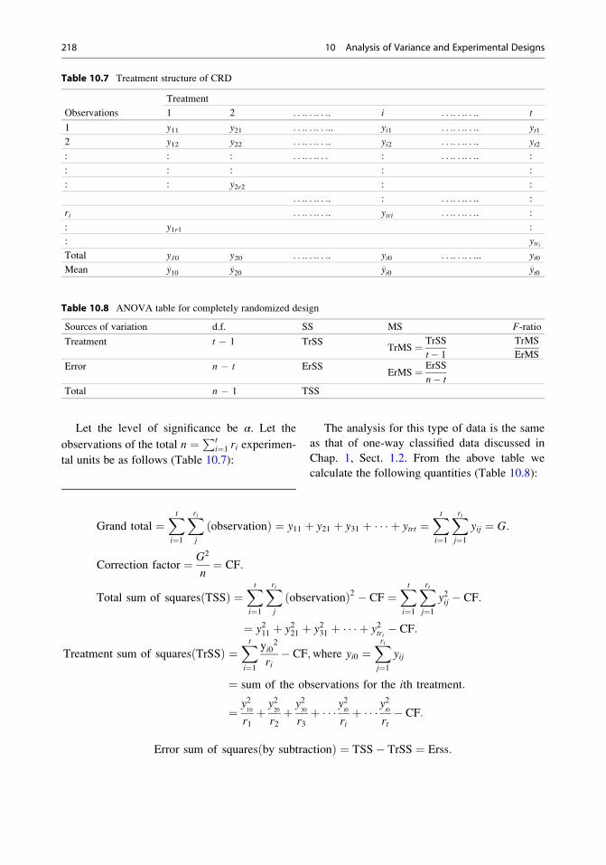
Let the level of significance be α. Let the

observations of the total n ¼ Pti¼1 ri experimen-

tal units be as follows (Table 10.7):

The analysis for this type of data is the same

as that of one-way classified data discussed in

Chap. 1, Sect. 1.2. From the above table we

calculate the following quantities (Table 10.8):

Grand total ¼Xt

i¼1

Xrij

observationð Þ ¼ y11 þ y21 þ y31 þ � � � þ ytrt ¼Xt

i¼1

Xrtj¼1

yij ¼ G:

Correction factor ¼ G2

n¼ CF:

Total sum of squares TSSð Þ ¼Xt

i¼1

Xrij

observationð Þ2 � CF ¼Xt

i¼1

Xrtj¼1

y2ij � CF:

¼ y211 þ y221 þ y231 þ � � � þ y2trt � CF:

Treatment sum of squares TrSSð Þ ¼Xt

i¼1

yi02

ri� CF;where yi0 ¼

Xrij¼1

yij

¼ sum of the observations for the ith treatment:

¼ y210

r1þ y2

20

r2þ y2

30

r3þ � � � y

2i0

riþ � � � y

2t0

rt� CF:

Error sum of squares by subtractionð Þ ¼ TSS� TrSS ¼ Erss:

Table 10.7 Treatment structure of CRD

Observations

Treatment

1 2 . . .. . .. . .. i . . .. . .. . .. t

1 y11 y21 . . .. . .. . ... yi1 . . .. . .. . .. yt12 y12 y22 . . .. . .. . .. yi2 . . .. . .. . .. yt2: : : . . .. . .. . . : . . .. . .. . .. :

: : : : :

: : y2r2 : :

. . .. . .. . .. : . . .. . .. . .. :

ri . . .. . .. . .. yiri . . .. . .. . .. :

: y1r1 :

: ytrtTotal y10 y20 . . .. . .. . .. yi0 . . .. . .. . ... yt0Mean �y10 �y20 �yi0 �yt0

Table 10.8 ANOVA table for completely randomized design

Sources of variation d.f. SS MS F-ratio

Treatment t � 1 TrSSTrMS ¼ TrSS

t� 1

TrMS

ErMSError n � t ErSS

ErMS ¼ ErSS

n� tTotal n � 1 TSS

218 10 Analysis of Variance and Experimental Designs

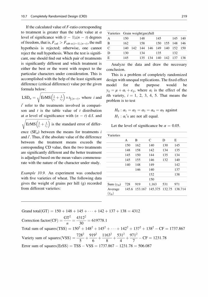
If the calculated value of F-ratio correspondingto treatment is greater than the table value at αlevel of significance with (t � 1),(n � t) degreesof freedom, that is, Fcal > Ftab α;ðt�1Þ;ðn�tÞ, the nullhypothesis is rejected; otherwise, one cannot

reject the null hypothesis. When the test is signifi-

cant, one should find out which pair of treatments

is significantly different and which treatment is

either the best or the worst with respect to the

particular characters under consideration. This is

accomplished with the help of the least significant

difference (critical difference) value per the given

formula below:

LSDα ¼ffiffiffiffiffiffiffiffiffiffiffiffiffiffiffiffiffiffiffiffiffiffiffiffiffiffiffiffiffiErMS 1

riþ 1

ri0

� �r�tα

2;ðn�tÞ, where i and

i0 refer to the treatments involved in compari-

son and t is the table value of t distribution

at α level of significance with (n � t) d.f. andffiffiffiffiffiffiffiffiffiffiffiffiffiffiffiffiffiffiffiffiffiffiffiffiffiffiffiffiffiErMS 1

riþ 1

ri0

� �ris the standard error of differ-

ence (SEd) between the means for treatments iand i0. Thus, if the absolute value of the differencebetween the treatment means exceeds the

corresponding CD value, then the two treatments

are significantly different and the better treatment

is adjudged based on the mean values commensu-

rate with the nature of the character under study.

Example 10.9. An experiment was conducted

with five varieties of wheat. The following data

gives the weight of grains per hill (g) recorded

from different varieties:

Varieties Grain weight(gm)/hill

A 150 148 145 145 140

B 162 158 150 155 148 146

C 140 142 144 146 149 140 152 150

D 130 134 135 132

E 145 135 134 140 142 137 138

Analyze the data and draw the necessary

conclusion.

This is a problem of completely randomized

design with unequal replications. The fixed effect

model for the purpose would be

yij ¼ μþ αi þ eij, where αi is the effect of the

ith variety, i ¼ 1, 2, 3, 4, 5. That means the

problem is to test

H0 : α1 ¼ α2 ¼ α3 ¼ α4 ¼ α5 against

H1 : αi0s are not all equal:

Let the level of significance be α ¼ 0.05.

Varieties

A B C D E

150 162 140 130 145

148 158 142 134 135

145 150 144 135 134

145 155 146 132 140

140 148 149 142

146 140 137

152 138

150

Sum (yi0) 728 919 1,163 531 971

Average�yi0ð Þ

145.6 153.167 145.375 132.75 138.714

Grand total GTð Þ ¼ 150þ 148þ 145þ � � � þ 142þ 137þ 138 ¼ 4312

Correction factor CFð Þ ¼ GT2

n¼ 43122

30¼ 619778:1

Total sum of squares TSSð Þ ¼ 1502 þ 1482 þ 1452 þ � � � þ 1422 þ 1372 þ 1382 � CF ¼ 1737:867

Variety sum of squares VSSð Þ ¼ 7282

5þ 9192

6þ 11632

8þ 5312

4þ 9712

7� CF ¼ 1231:78

Error sum of squares ErSSð Þ ¼ TSS� VSS ¼ 1737:867� 1231:78 ¼ 506:087

10.7 Completely Randomized Design (CRD) 219

ANOVA

SOV d.f. SS MS F

Variety 4 1231.780 307.945 15.212

Error 25 506.087 20.243

Total 29 1737.867

The table value of F0.05;4,25 ¼ 4.18.

Thus, F(cal) > F(tab)0.05;4,25, so the test is sig-nificant and reject the null hypothesis of equality of

grain weight per hill. We conclude that there exist

significant differences among the five varieties of

wheat with respect to grain weight per hill.

So, the next objective is to find out the

varieties which differ significantly among them-

selves and the variety/varieties having signifi-

cantly the highest weight per hill.

To compare the varieties we calculate the

critical difference value, which is given asffiffiffiffiffiffiffiffiffiffiffiffiffiffiffiffiffiffiffiffiffiffiffiffiffiffiffiffiffiffiMSE

1

riþ 1

ri0

� �s� t0:025; err:d:f:

¼ffiffiffiffiffiffiffiffiffiffiffiffiffiffiffiffiffiffiffiffiffiffiffiffiffiffiffiffiffiffiffiffiffiffi20:243

1

riþ 1

ri0

� �s� t0:025;25:

¼ffiffiffiffiffiffiffiffiffiffiffiffiffiffiffiffiffiffiffiffiffiffiffiffiffiffiffiffiffiffiffiffiffiffi20:243

1

riþ 1

ri0

� �s� 2:06;

where ri and ri0 are the number of observations of

the two varieties under comparison. Thus, for

comparing the varieties, we have the following

critical difference and mean difference values

among the varieties:

Comparison

CD

(0.05)

values

Mean

difference

yi0 � yi00j j Conclusion

(Variety

A–variety B)

5.612 7.567 Varieties are

different

(Variety

A–variety C)

5.284 0.225 Varieties are

the same

(Variety

A–variety D)

6.217 12.85 Varieties are

different

(Variety

A–variety E)

5.427 6.886 Varieties are

different

(Variety

B–variety C)

5.006 7.792 Varieties are

different

(Variety

B–variety D)

5.983 20.417 Varieties are

different

(Variety

B–variety E)

5.156 14.452 Varieties are

different

(Variety

C–variety D)

5.676 12.625 Varieties are

different

(Variety

C–variety E)

4.797 6.661 Varieties are

different

(Variety

D–variety E)

5.809 5.964 Varieties are

different

Thus, variety B is the variety giving signifi-

cantly the highest grain weight per hill followed

by variety A and variety C, which are statistically

at par.

Slide 10.9: Step 1 showing the data input for analysis of CRD using SAS

220 10 Analysis of Variance and Experimental Designs

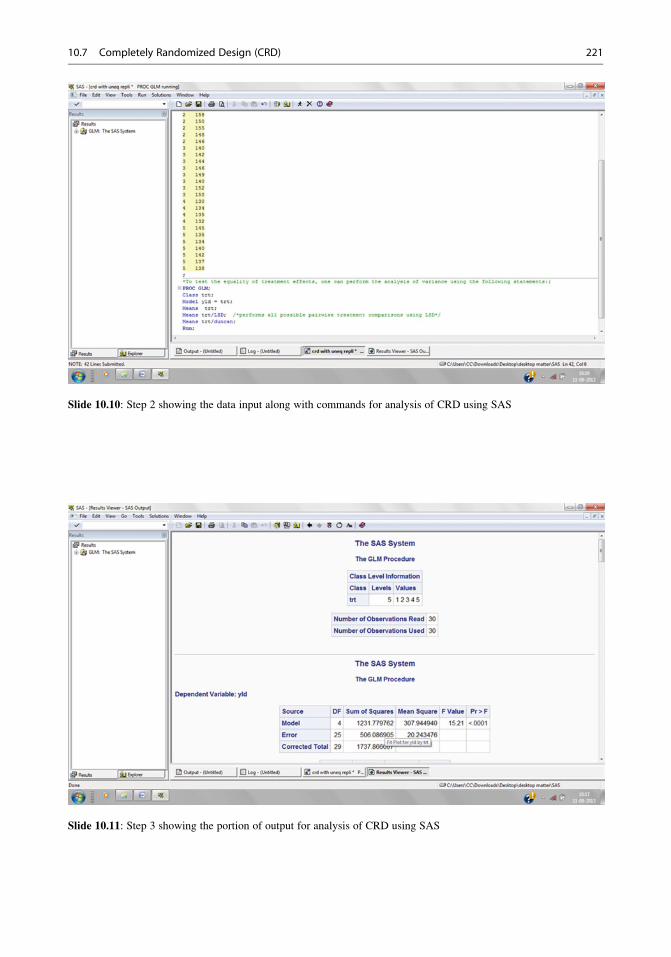
Slide 10.10: Step 2 showing the data input along with commands for analysis of CRD using SAS

Slide 10.11: Step 3 showing the portion of output for analysis of CRD using SAS

10.7 Completely Randomized Design (CRD) 221

Slide 10.12: Step 3 showing the portion of output for analysis of CRD using SAS

Slide 10.13: Step 3 showing the portion of output for analysis of CRD using SAS

222 10 Analysis of Variance and Experimental Designs

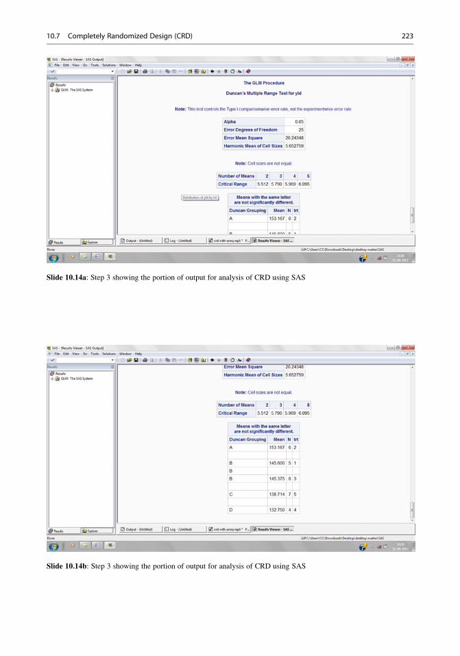
Slide 10.14a: Step 3 showing the portion of output for analysis of CRD using SAS

Slide 10.14b: Step 3 showing the portion of output for analysis of CRD using SAS

10.7 Completely Randomized Design (CRD) 223

Example 10.10. Seven varieties of wheat were

tested for yield using CRD with 5 plots per

variety. The following table gives the yields of

grain in quintal per acre. Test whether the 7

varieties differ significantly with respect to

yield or not.

Solution. The statement shows that the experi-

mentwas laid out in completely randomized design

with seven varieties each replicated five times.

The model for the purpose is yij ¼ μþ αiþ eij,

i ¼ 7, j ¼ 5

where

yij ¼ jth observation for the ith variety

μ ¼ general effect

αi ¼ additional effect due to the ith variety

eij ¼ errors that are associated with jth obser-

vation in the ith variety and are i.i.d. N(0, σ2)So the problem is to test

H0 : α1 ¼ α2 ¼ α3 ¼ α4 ¼ α5 ¼ α6 ¼ α7 against

H1 : αi’s are not all equal:

Let the level of significance be α ¼ 0.05.

Let us construct the following table:

A B C D E F G

18 19 17 18 21 20 19

14 19.5 15 14 21.5 16 13

16 20 14 19 22 17 17

17 22 20 21 23 19 18

15 18 16 14 22 15 14

Total (yi0) 80 98.5 82 86 109.5 87 81

Average (�yi0) 16 19.7 16.4 17.2 21.9 17.4 16.2

Grand total GTð Þ ¼ 18þ 14þ 16þ � � � þ 17þ 18þ 14 ¼ 624:00

Correction factor CFð Þ ¼ GT2

n¼ 6242

35¼ 11125:03

Total sum of squares TSSð Þ ¼ 182 þ 142 þ 162 þ � � � þ 172 þ 182 þ 142 � CF ¼ 268:471

Variety sum of squares VSSð Þ ¼ 802

5þ 98:52

5þ 822

5þ 862

5þ 109:52

5þ 87:002

5þ 81:002

5� CF ¼ 143:471

Error sum of squares ErSSð Þ ¼ TSS� VSS ¼ 268:471� 143:471 ¼ 125:00

ANOVA

SOV d.f. SS MS F

Variety 6 143.471 23.912 5.356

Error 28 125.000 4.464

Total 34 268.471

The table value of F0.05;6,28 ¼ 2.45.

Thus, F(cal) > F(tab)0.05;6,28, so the test is

significant and we reject the null hypothesis of

equality of yields.

Variety A Variety B Variety C Variety D Variety E Variety F Variety G

18 19 17 18 21 20 19

14 19.5 15 14 21.5 16 13

16 20 14 19 22 17 17

17 22 20 21 23 19 18

15 18 16 14 22 15 14

224 10 Analysis of Variance and Experimental Designs

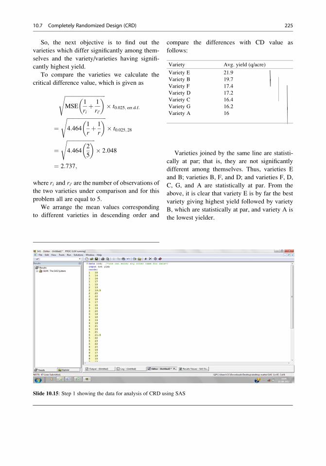
So, the next objective is to find out the

varieties which differ significantly among them-

selves and the variety/varieties having signifi-

cantly highest yield.

To compare the varieties we calculate the

critical difference value, which is given as

ffiffiffiffiffiffiffiffiffiffiffiffiffiffiffiffiffiffiffiffiffiffiffiffiffiffiffiffiffiffiMSE

1

riþ 1

ri0

� �s� t0:025; err:d:f:

¼ffiffiffiffiffiffiffiffiffiffiffiffiffiffiffiffiffiffiffiffiffiffiffiffiffiffiffiffiffi4:464

1

rþ 1

r

� �s� t0:025; 28

¼ffiffiffiffiffiffiffiffiffiffiffiffiffiffiffiffiffiffiffiffiffi4:464

2

5

� �s� 2:048

¼ 2:737;

where ri and ri0 are the number of observations of

the two varieties under comparison and for this

problem all are equal to 5.

We arrange the mean values corresponding

to different varieties in descending order and

compare the differences with CD value as

follows:

Variety Avg. yield (q/acre)

Variety E 21.9

Variety B 19.7

Variety F 17.4

Variety D 17.2

Variety C 16.4

Variety G 16.2

Variety A 16

Varieties joined by the same line are statisti-

cally at par; that is, they are not significantly

different among themselves. Thus, varieties E

and B; varieties B, F, and D; and varieties F, D,

C, G, and A are statistically at par. From the

above, it is clear that variety E is by far the best

variety giving highest yield followed by variety

B, which are statistically at par, and variety A is

the lowest yielder.

Slide 10.15: Step 1 showing the data for analysis of CRD using SAS

10.7 Completely Randomized Design (CRD) 225

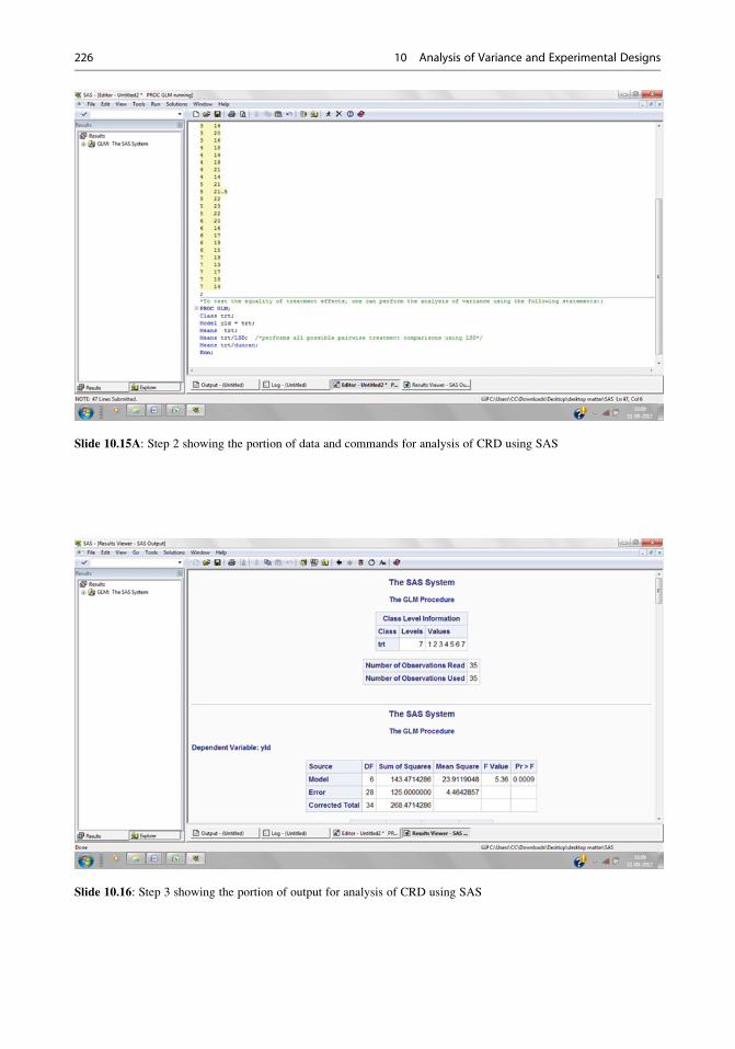
Slide 10.15A: Step 2 showing the portion of data and commands for analysis of CRD using SAS

Slide 10.16: Step 3 showing the portion of output for analysis of CRD using SAS

226 10 Analysis of Variance and Experimental Designs

Slide 10.17: Step 3 showing the portion of output for analysis of CRD using SAS

Slide 10.18: Step 3 showing the portion of output for analysis of CRD using SAS

10.7 Completely Randomized Design (CRD) 227

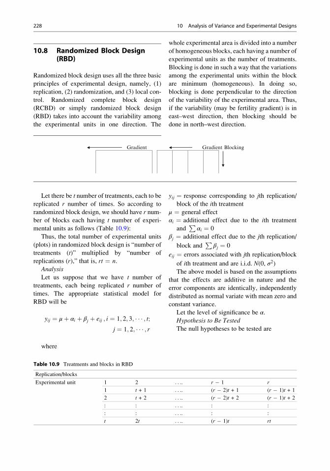
10.8 Randomized Block Design(RBD)

Randomized block design uses all the three basic

principles of experimental design, namely, (1)

replication, (2) randomization, and (3) local con-

trol. Randomized complete block design

(RCBD) or simply randomized block design

(RBD) takes into account the variability among

the experimental units in one direction. The

whole experimental area is divided into a number

of homogeneous blocks, each having a number of

experimental units as the number of treatments.

Blocking is done in such a way that the variations

among the experimental units within the block

are minimum (homogeneous). In doing so,

blocking is done perpendicular to the direction

of the variability of the experimental area. Thus,

if the variability (may be fertility gradient) is in

east–west direction, then blocking should be

done in north–west direction.

Let there be t number of treatments, each to be

replicated r number of times. So according to

randomized block design, we should have r num-

ber of blocks each having t number of experi-

mental units as follows (Table 10.9):

Thus, the total number of experimental units

(plots) in randomized block design is “number of

treatments (t)” multiplied by “number of

replications (r),” that is, rt ¼ n.Analysis

Let us suppose that we have t number of

treatments, each being replicated r number of

times. The appropriate statistical model for

RBD will be

yij ¼ μþ αi þ βj þ eij ; i ¼ 1; 2; 3; � � � ; t;j ¼ 1; 2; � � � ; r

where

yij ¼ response corresponding to jth replication/

block of the ith treatment

μ ¼ general effect

αi ¼ additional effect due to the ith treatment

andP

αi ¼ 0

βj ¼ additional effect due to the jth replication/

block andP

βj ¼ 0

eij ¼ errors associated with jth replication/block

of ith treatment and are i.i.d. N(0, σ2)The above model is based on the assumptions

that the effects are additive in nature and the

error components are identically, independently

distributed as normal variate with mean zero and

constant variance.

Let the level of significance be α.Hypothesis to Be TestedThe null hypotheses to be tested are

Gradient Gradient Blocking

Table 10.9 Treatments and blocks in RBD

Replication/blocks

Experimental unit 1 2 . . .. r � 1 r

1 t + 1 . . .. (r � 2)t + 1 (r � 1)t + 1

2 t + 2 . . .. (r � 2)t + 2 (r � 1)t + 2

: : . . .. : :

: : . . .. : :

t 2t . . .. (r � 1)t rt

228 10 Analysis of Variance and Experimental Designs

H0 :ð1Þ α1 ¼ α2 ¼ � � � ¼ αi ¼ � � � ¼ αt ¼ 0;

ð2Þ β1 ¼ β2 ¼ � � � ¼ βj ¼ � � � ¼ βr ¼ 0

against the alternative hypotheses

H1 :ð1Þ α’s are not equal,

ð2Þ β’s are not equal:

Let the observations of these n ¼ rt units be

as follows (Table 10.10):

The analysis of this design is the same as that

of two-way classified data with one observation

per cell discussed in Chap. 1, Sect. 4.2.3.2.

From the above table, we calculate the follow-

ing quantities (Table 10.11):

Grand total ¼Xi;j

yij ¼ y11 þ y21 þ y31 þ � � � þ ytr ¼ G

Correction factor ¼ G2

rt¼ CF

Total sum of squares TSSð Þ ¼Xi;j

yij2 � CF ¼ y211 þ y221 þ y231 þ � � � þ y2tr � CF

Treatment sum of squares TrSSð Þ ¼Pti¼1

yi02

r� CF ¼ y2

10

rþ y2

20

rþ y2

30

rþ � � � y

2i0

rþ � � � y

2t0

r� CF

Replication sum of squares RSSð Þ ¼

Prj¼1

y0j2

t� CF ¼ y2

01

tþ y2

02

tþ y2

03

tþ � � �

y20j

tþ � � � y

20r

t� CF

Error sum of squares by subtractionð Þ ¼ TSS� TrSS� RSS

Table 10.10 Summary of observations from RBD

Replications/blocks

Treatments 1 2 . . .. j . . .. r Total Mean

1 y11 y12 . . .. y1j . . .. y1r y10 �y102 y21 y22 . . .. y2j . . .. y2r y20 �y20: : : : : : : : :

i yi1 yi2 . . .. yij . . .. yir yi0 �yi0: : : : : : : : :

t yt1 yt2 . . .. ytj . . .. ytr yt0 �yt0Total y01 y02 . . .. y0j . . .. y0r y00Mean �y01 �y02 . . .. �y0j . . .. �y0r

Table 10.11 ANOVA table for RBD

SOV d.f. SS MS F-ratioTabulated

F (0.05)

Tabulated

F (0.01)

Treatment t � 1 TrSSTrMS ¼ TrSS

t� 1

TrMS

ErMSReplication

(block)

r � 1 RSSRMS ¼ RSS

r � 1

RMS

ErMS

Error (t � 1)

(r � 1)

ErSSErMS ¼ ErSS

ðt� 1Þðr � 1ÞTotal rt � 1 TSS

10.8 Randomized Block Design (RBD) 229

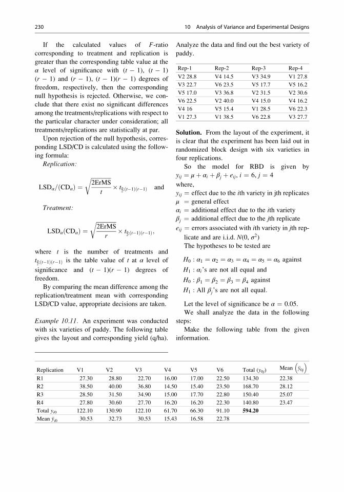
If the calculated values of F-ratiocorresponding to treatment and replication is

greater than the corresponding table value at the

α level of significance with (t � 1), (t � 1)

(r � 1) and (r � 1), (t � 1)(r � 1) degrees of

freedom, respectively, then the corresponding

null hypothesis is rejected. Otherwise, we con-

clude that there exist no significant differences

among the treatments/replications with respect to

the particular character under consideration; all

treatments/replications are statistically at par.

Upon rejection of the null hypothesis, corres-

ponding LSD/CD is calculated using the follow-

ing formula:

Replication:

LSDα=ðCDαÞ ¼ffiffiffiffiffiffiffiffiffiffiffiffiffiffi2ErMS

t

r� tα

2;ðt�1Þðr�1Þ and

Treatment:

LSDαðCDαÞ ¼ffiffiffiffiffiffiffiffiffiffiffiffiffiffi2ErMS

r

r� tα

2;ðt�1Þðr�1Þ;

where t is the number of treatments and

tα2;ðt�1Þðr�1Þ is the table value of t at α level of

significance and (t � 1)(r � 1) degrees of

freedom.

By comparing the mean difference among the

replication/treatment mean with corresponding

LSD/CD value, appropriate decisions are taken.

Example 10.11. An experiment was conducted

with six varieties of paddy. The following table

gives the layout and corresponding yield (q/ha).

Analyze the data and find out the best variety of

paddy.

Rep-1 Rep-2 Rep-3 Rep-4

V2 28.8 V4 14.5 V3 34.9 V1 27.8

V3 22.7 V6 23.5 V5 17.7 V5 16.2

V5 17.0 V3 36.8 V2 31.5 V2 30.6

V6 22.5 V2 40.0 V4 15.0 V4 16.2

V4 16 V5 15.4 V1 28.5 V6 22.3

V1 27.3 V1 38.5 V6 22.8 V3 27.7

Solution. From the layout of the experiment, it

is clear that the experiment has been laid out in

randomized block design with six varieties in

four replications.

So the model for RBD is given by

yij ¼ μþ αi þ βj þ eij, i ¼ 6, j ¼ 4

where,

yij ¼ effect due to the ith variety in jth replicates

μ ¼ general effect

αi ¼ additional effect due to the ith variety

βj ¼ additional effect due to the jth replicate

eij ¼ errors associated with ith variety in jth rep-

licate and are i.i.d. N(0, σ2)The hypotheses to be tested are

H0 : α1 ¼ α2 ¼ α3 ¼ α4 ¼ α5 ¼ α6 against

H1 : αi’s are not all equal and

H0 : β1 ¼ β2 ¼ β3 ¼ β4 against

H1 : All βj’s are not all equal:

Let the level of significance be α ¼ 0.05.

We shall analyze the data in the following

steps:

Make the following table from the given

information.

Replication V1 V2 V3 V4 V5 V6 Total (y0j)Mean �y0j

� �R1 27.30 28.80 22.70 16.00 17.00 22.50 134.30 22.38

R2 38.50 40.00 36.80 14.50 15.40 23.50 168.70 28.12

R3 28.50 31.50 34.90 15.00 17.70 22.80 150.40 25.07

R4 27.80 30.60 27.70 16.20 16.20 22.30 140.80 23.47

Total yi0 122.10 130.90 122.10 61.70 66.30 91.10 594.20

Mean �yi0 30.53 32.73 30.53 15.43 16.58 22.78

230 10 Analysis of Variance and Experimental Designs

Calculate the following quantities:

CF ¼ G2

n¼ 594:202

6� 4¼ 14711:40167;

TSS ¼X

Obs:2 � CF ¼ 27:32 þ 28:82 þ � � � þ 16:22 þ 22:32 � 14711:40167

¼ 16156:72� 14711:40167 ¼ 1445:318;

RSS ¼ 1

6

X4j¼1

y20j � CF ¼ 1

6134:32 þ 168:72 þ 150:42 þ 140:82� �� 14711:40167

¼ 88940:98

6� 14711:40167 ¼ 112:095;

TrSS ¼ 1

4

X6i¼1

y2i0� CF ¼ 1

4122:12 þ 130:92 þ 122:12 þ 61:72 þ 66:32 þ 91:12� �� 14711:40167

¼ 63453:42

4� 14711:40167 ¼ 1151:953;

ErSS ¼ TSS� RSS� TrSS ¼ 1445:318� 112:095� 1151:953 ¼ 181:27;

where TSS, RSS, TrSS, and ErSS are the total,

replication, treatment, and error sum of squares,

respectively.

Construct the ANOVA table as given below.

ANOVA

SOV d.f. SS MS F

Replication 3 112.095 37.365 3.091935

Variety 5 1151.953 230.3907 19.06471

Error 15 181.270 12.08467

Total 23 1445.318

The table value of F0.05;3,15 ¼ 3.29 and

F0.05;5,15 ¼ 2.90. Thus, we find that the test

corresponding to replication is not significant,

but the test corresponding to the effect of

varieties is significant. So the null hypothesis of

equality of replication effects cannot be rejected;

that means there is no significant difference

among the effects of the replications; they are

statistically at par. On the other hand, the null

hypothesis of equality of varietal effect is

rejected; that means there exist significant

differences among the varieties. So we are to

identify the varieties, which varieties are signifi-

cantly different from each other, and the best

variety.

Calculate critical difference value at α ¼ 0.05

using the following formula:

CD0:05ðVarietyÞ ¼ffiffiffiffiffiffiffiffiffiffiffiffiffi2MSE

r

r� t0:025;err:d:f:

¼ffiffiffiffiffiffiffiffiffiffiffiffiffiffiffiffiffiffiffiffiffiffi2� 12:085

4

r� t0:025;15

¼ffiffiffiffiffiffiffiffiffiffiffiffiffiffiffiffiffiffiffiffiffiffi2� 12:085

4

r� 2:131 ¼ 5:238:

Arrange the varietal mean values in descending

order and compare the difference between any

two treatment mean differences with that of the

critical difference value. If the critical difference

value be greater than the difference of two varietal

means, then the treatments are statistically at par;

there exists no significant difference among the

means under comparison.

Variety Mean yield (bushels/acre)

V2 32.725

V1 30.525 difference < CD(0.05)

V3 30.525

V6 22.775

V5 16.575

V4 15.425 difference < CD(0.05)

Variety 2 is the best variety having highest

yield, but variety 1 and variety 3 are also at par

with that of variety 2. Variety 6 is significantly

different from all other varieties. Variety 5 and

variety 4 are statistically at par and are the lowest

yielders among the varieties.

10.8 Randomized Block Design (RBD) 231

Slide 10.20: Step 2 showing a portion of output for RBD analysis using SAS

Slide 10.19: Step 1 showing data input and commands for RBD analysis using SAS

232 10 Analysis of Variance and Experimental Designs

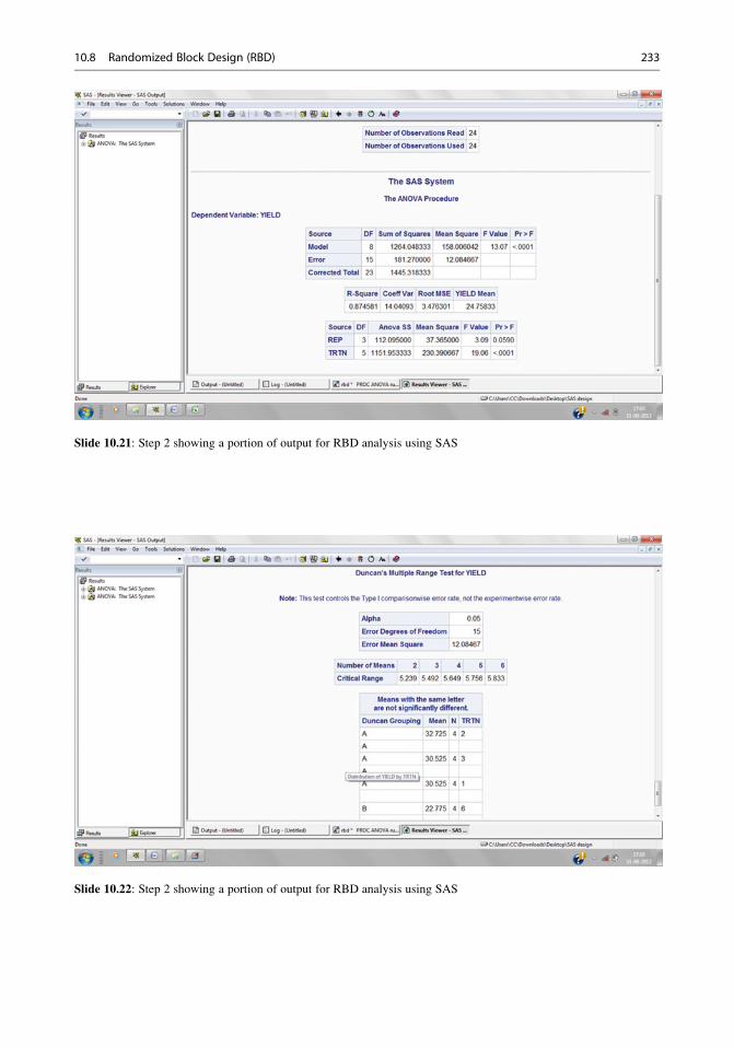
Slide 10.22: Step 2 showing a portion of output for RBD analysis using SAS

Slide 10.21: Step 2 showing a portion of output for RBD analysis using SAS

10.8 Randomized Block Design (RBD) 233

10.9 Latin Square Design (LSD)

LSD is a design in which known sources of

variation in two perpendicular directions, that

is, north to south and east to west or south to

north and west to east, could be taken into con-

sideration. In this type of field, we require fram-

ing of blocks into perpendicular directions which

take care of the heterogeneity in both directions.

A Latin square is an arrangement of treatments

in such a way that each treatment occurs once

and only once in each row and each column.

If t is the number of treatments, then the total

number of experimental units needed for this

design is t � t. These t2 units are arranged in

t rows and t columns. This type of experiments

is rare in laboratory condition but can be

conducted or useful in field conditions or green-

house conditions. The two perpendicular sources

of variations in greenhouse may be the difference

among the rows of the plot and their distances

from the greenhouses.

So while selecting an LSD design, an experi-

menter faces two problems: how to maintain the

minimum replication and how to accommodate

the maximum number of treatments in the

experiment. This makes the LSD design’s appli-

cability limited in field experimentations. The

number of treatments in LSD design should gen-

erally lie in between four and eight. All these

limitations have resulted in the limited use of

Latin square design in spite of its high potential-

ity for controlling experimental errors.

Analysis

Let there be t treatments, so there should be

t rows and t columns. So we need a field of t� texperimental units. The appropriate statistical

model for the analysis of the information from a

t� t LSD can be given as follows:

yijk ¼ μþ αi þ βj þ υk þ eijk; i ¼ j ¼ k ¼ t

Where

μ ¼ general effect

αi ¼ additional effect due to the ith treatment

andP

αi ¼ 0

βj ¼ additional effect due to the jth row andPrj ¼ 0

υk ¼ additional effect due to the kth treatment

andP

ck ¼ 0

eijk ¼ errors that are associated with the ith treat-

ment in the jth row and the kth column and are

i.i.d. N(0, σ2)

Slide 10.23: Step 2 showing a portion of output for RBD analysis using SAS

234 10 Analysis of Variance and Experimental Designs

Hypothesis to Be Tested

H0 : ð1Þ α1 ¼ α2 ¼ � � � ¼ αi ¼ � � � ¼ αt ¼ 0;

ð2Þ β1 ¼ β2 ¼ � � � ¼ βj ¼ � � � ¼ βt ¼ 0;

ð3Þ γ1 ¼ γ2 ¼ � � � ¼ γk ¼ � � � ¼ γt ¼ 0

against

H1 :ð1Þ α’s are not equal,

ð2Þ β’s are not equal,

ð3Þ γ’s are not equal:

Analysis

From least square estimates; we haveXXi; j; k

Xðyijk � �y000Þ2 ¼ t

Xi

ð�yi00 � �y000Þ2 þ tXj

ð�y0j0 � �y000Þ2 þ tXk

ð�y00k � �y000Þ2

þXi; j; k

ðyijk � �yi00 � �y0j0 � �y00k þ 2�y000Þ2;

TSS ¼ Tr SSþ RSSþ CSSþ ErSS,

where

μ ¼ �y000; αi ¼ �yi00 � �y000; βj ¼ �y0j0 � �y000;

γk ¼ �y00k � �y000;

�y000 ¼ mean of all t2 observations,

�yi00 ¼ mean of t observations from ith treatment,

�y0j0 ¼ mean of t observations from jth row,

�y00k ¼ mean of t observations from kth column:

Various sums of squares are calculated using

the following formulae (Table 10.12):

Grand total ¼X

ði;j;kÞ2Dyijk ¼ G

Correction factor ¼ ðGÞ2t2

¼ CF

Total sum of squares TSSð Þ ¼X

ði;j;kÞ2Dyijk

2 � CF

Treatment sum of squares TrSSð Þ ¼Pti¼1

yi002

t� CF

¼ y2100

tþ y2

200

tþ y2

300

tþ � � � y

2i00

tþ � � � þ y2

t00

t� CF

Row sum of squares RSSð Þ ¼

Ptj¼1

y0j02

t� CF

¼ y2010

tþ y2

020

tþ y2

030

tþ � � �

y20j0

tþ � � � þ y2

0t0

t� CF

Column sum of squares CSSð Þ ¼Ptk¼1

y00k2

t� CF

¼ y2001

tþ y2

002

tþ y2

003

tþ � � � y

200k

tþ � � � þ y2

00t

t� CF

Error sum of squares by subtractionð Þ¼ TSS� TrSS� RSS� CSS

Table 10.12 ANOVA table for LSD

Sources of variation d.f. SS MS F-ratio

Treatment t � 1 TrSSTrMS ¼ TrSS

t� 1

TrMS

ErMSRow t � 1 RSS

RMS ¼ RSS

t� 1

RMS

ErMSColumn t � 1 CSS

RMS ¼ CSS

t� 1

CMS

ErMSError (t � 1)(t � 2) ErSS

ErMS ¼ ErSS

ðt� 1Þðt� 2ÞTotal t2 � 1 TSS

10.9 Latin Square Design (LSD) 235

The null hypotheses are rejected at α level of

significance if the calculated values of F-ratio

corresponding to treatment or row or column

are greater than the corresponding table values

at the same level of significance with the same

(t � 1), (t � 1)(t � 2) degrees of freedom,

respectively. When any one of the three null

hypotheses is rejected, then LSD for treatments/

rows/columns is calculatedffiffiffiffiffiffiffiffiffiffi2ErMS

t

q� tα

2;ðt�1Þðt�2Þ,

where tα2;ðt�1Þðt�2Þ is the table value of t at α level

of significance with (t � 1)(t � 2) degrees of

freedom.

If the absolute value of the difference between

any pair of means of row/column/treatment is

more than the critical difference value, as calcu-

lated above, then the row/column/treatment

means are significantly different from each

other; otherwise, they are not.

Example 10.12. Five varieties of wheat were

tested using the Latin square design. The follow-

ing information pertains to the yield data (q/ha)

along with the layout of the above experiment.

Analyze the data and find out the best variety.

Layout along with yield data (q/ha)

D 34.0 A 19.1 E 21.1 B 32.0 C 37.2

E 16.2 B 33.1 A 19.0 C 34.3 D 28.1

C 30.6 E 28.5 B 33.1 D 35.8 A 19.2

A 25.8 C 26.1 D 41.7 E 23.7 B 39.9

B 39.3 D 24.6 C 36.1 A 21.3 E 19.4

Solution. The model for LSD is yijk ¼μþ αi þ βj þ γk þ eijk, i ¼ j ¼ k ¼ 5

where

yijk ¼ effect due to the ith variety in the jth row

and the kth column

μ ¼ general effect

αi ¼ additional effect due to the ith variety,Pi

αi ¼ 0

βj ¼ additional effect due to the jth row,Pj

βj ¼ 0

γk ¼ additional effect due to the kth column,Pk

γk ¼ 0

eijk ¼ errors that are associated with the ith

variety in the jth row and kth column and are

i.i.d. N(0, σ2)The hypotheses to be tested are

H0 : α1 ¼ α2 ¼ α3 ¼ α4 ¼ α5,

β1 ¼ β2 ¼ β3 ¼ β4 ¼ β5;

γ1 ¼ γ2 ¼ γ3 ¼ γ4 ¼ γ5against

H1 : αi’s are not all equal,

βj’s are not all equal,

γk’s are not all equal:

Let the level of significance be α ¼ 0.05.

Make the following two tables from the given

information:

C1 C2 C3 C4 C5 Total ðy0j0Þ Average ð�y0j0ÞR1 34 19.1 21.1 32 37.2 143.4 28.68

R2 16.2 33.1 19 34.3 28.1 130.7 26.14

R3 30.6 28.5 33.1 35.8 19.2 147.2 29.44

R4 25.8 26.1 41.7 23.7 39.9 157.2 31.44

R5 39.3 24.6 36.1 21.3 19.4 140.7 28.14

Total y00kð Þ 145.9 131.4 151 147.1 143.8 719.2

Average �y00kð Þ 29.18 26.28 30.2 29.42 28.76

236 10 Analysis of Variance and Experimental Designs

Calculate the following quantities:

CF ¼ G2

t� t¼ 719:202

5� 5¼ 20689:9;

TSS ¼X

Obs:2 � CF ¼ 34:02 þ 19:12 þ � � � þ 21:32 þ 19:42 � 20689:9 ¼ 1385:91;

RSS ¼ 1

5

X5j¼1

y20j0� CF ¼ 1

5143:42 þ 130:72 þ � � � þ 140:72� �� 20689:9456 ¼ 74:498;

CSS ¼ 1

5

X5k¼1

y200k � CF ¼ 1

5145:92 þ 131:42 þ � � � þ 143:802� �� 20689:9456 ¼ 44:178;

VSS ¼ 1

5

X5i¼1

y2i00� CF ¼ 1

5104:42 þ 177:42 þ � � � þ 108:92� �� 20689:9456 ¼ 947:146;

ErSS ¼ TSS� RSS� CSS� VSS ¼ 1385:914� 74:498� 44:178� 947:146 ¼ 320:091;

where TSS, RSS, CSS, VSS, and ErSS are the

total, row, column, variety, and error sum of

squares, respectively.

Construct the ANOVA table as given below.

ANOVA

SOV d.f. SS MS F

Row 4 74.498 18.625 0.698

Column 4 44.178 11.045 0.414

Variety 4 947.146 236.787 8.877

Error 12 320.091 26.674

Total 24 1385.914

The table value of F0.05;4,12 ¼ 3.26. Thus, we

find that the calculated values of F are less,

except for variety, than the corresponding table

value. So the tests for row and columns are non-

significant. We conclude that neither the row

effects nor the column effects are significant.

But the effects of varieties are significant.

So we are to identify the best variety.

Calculate CD(0.05) using the following

formula:

CD0:05ðVarietyÞ ¼ffiffiffiffiffiffiffiffiffiffiffiffiffiffiffiffiffiffiffi2�MSE

t

r� t0:025; err: d:f:

¼ffiffiffiffiffiffiffiffiffiffiffiffiffiffiffiffiffiffiffiffiffiffi2� 26:674

5

r� t0:025;12

¼ffiffiffiffiffiffiffiffiffiffiffiffiffiffiffiffiffiffiffiffiffiffi2� 26:674

5

r� 2:179

¼ 7:118:

Arrange the varietal mean values in descen-

ding order and compare the difference between

any two treatment mean differences with that of

the critical difference value. If the critical differ-

ence value is greater than the difference of two

varietal means, then the treatments are statisti-

cally at par; there exists no significant difference

among the means under comparison.

Varieties

A B C D E

25.8 39.3 30.6 34 16.2

19.1 33.1 26.1 24.6 28.5

19 33.1 36.1 41.7 21.1

21.3 32 34.3 35.8 23.7

19.2 39.9 37.2 28.1 19.4

Total ðyiooÞ 104.4 177.4 164.3 164.2 108.9

Average ð�yiooÞ 20.88 35.48 32.86 32.84 21.78

10.9 Latin Square Design (LSD) 237

Variety Avg. yield (q/ha)

B 35.48

C 32.86

D 32.84

E 21.78

A 20.88

Variety B is the best variety having the highest

yield but variety C and variety D are also at par

with that of variety B. Variety A and E are signifi-

cantly different from the other three varieties and

are also statistically at par with variety A as the

lowest yielders among the varieties.

Slide 10.25: Step 2 showing portion of data entry and commands for LSD analysis using SAS

Slide 10.24: Step 1 showing data entry and portion of commands for LSD analysis using SAS

238 10 Analysis of Variance and Experimental Designs

The above analysis can also be done usingSAS statistical software. The following few slides

present the data entry, command syntax, and theoutput for the same.

Slide 10.26: Step 3 showing portion of output for LSD analysis using SAS

Slide 10.27: Step 3 showing portion of output for LSD analysis using SAS

10.9 Latin Square Design (LSD) 239

Slide 10.28: Step 3 showing portion of output for LSD analysis using SAS

Slide 10.29: Step 3 showing portion of output for LSD analysis using SAS

240 10 Analysis of Variance and Experimental Designs

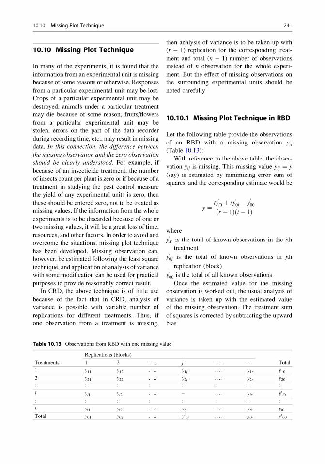
10.10 Missing Plot Technique

In many of the experiments, it is found that the

information from an experimental unit is missing

because of some reasons or otherwise. Responses

from a particular experimental unit may be lost.

Crops of a particular experimental unit may be

destroyed, animals under a particular treatment

may die because of some reason, fruits/flowers

from a particular experimental unit may be

stolen, errors on the part of the data recorder

during recording time, etc., may result in missing

data. In this connection, the difference between

the missing observation and the zero observation

should be clearly understood. For example, if

because of an insecticide treatment, the number

of insects count per plant is zero or if because of a

treatment in studying the pest control measure

the yield of any experimental units is zero, then

these should be entered zero, not to be treated as

missing values. If the information from the whole

experiments is to be discarded because of one or

two missing values, it will be a great loss of time,

resources, and other factors. In order to avoid and

overcome the situations, missing plot technique

has been developed. Missing observation can,

however, be estimated following the least square

technique, and application of analysis of variance

with some modification can be used for practical

purposes to provide reasonably correct result.

In CRD, the above technique is of little use

because of the fact that in CRD, analysis of

variance is possible with variable number of

replications for different treatments. Thus, if

one observation from a treatment is missing,

then analysis of variance is to be taken up with

(r � 1) replication for the corresponding treat-

ment and total (n � 1) number of observations

instead of n observation for the whole experi-

ment. But the effect of missing observations on

the surrounding experimental units should be

noted carefully.

10.10.1 Missing Plot Technique in RBD

Let the following table provide the observations

of an RBD with a missing observation yij(Table 10.13):

With reference to the above table, the obser-

vation yij is missing. This missing value yij ¼ y

(say) is estimated by minimizing error sum of

squares, and the corresponding estimate would be

y ¼ ty0i0 þ ry

00j � y

000

ðr � 1Þðt� 1Þ

where

y0i0 is the total of known observations in the ith

treatment

y00j is the total of known observations in jth

replication (block)

y000 is the total of all known observations

Once the estimated value for the missing

observation is worked out, the usual analysis of

variance is taken up with the estimated value

of the missing observation. The treatment sum

of squares is corrected by subtracting the upward

bias

Table 10.13 Observations from RBD with one missing value

Treatments

Replications (blocks)

Total1 2 . . .. j . . .. r

1 y11 y12 . . .. y1j . . .. y1r y102 y21 y22 . . .. y2j . . .. y2r y20: : : : : : : :

i yi1 yi2 . . .. – . . .. yir y0 i0: : : : : : : :

t yt1 yt2 . . .. ytj . . .. ytr yt0Total y01 y02 . . .. y00j . . .. y0r y000

10.10 Missing Plot Technique 241

B ¼y00j � t� 1ð Þy

h i2t t� 1ð Þ :

The degrees of freedom for both total and error

sum of squares are reduced by one in each case.

The treatment means are compared with the mean

having missing value and no missing value using

the formula for standard error of difference as

SEd ¼ffiffiffiffiffiffiffiffiffiffiffiffiffiffiffiffiffiffiffiffiffiffiffiffiffiffiffiffiffiffiffiffiffiffiffiffiffiffiffiffiffiffiffiffiffiffiffiffiffiffiffiffiffiErMS

r2þ t

ðr � 1Þðt� 1Þ� �s

:

Example 10.13. An experiment with six

varieties of onion was conducted using RBD

with four replications. The following table gives

the layout and data pertaining to yield (t/ha) from

the experiment. Analyze the data and find out the

best variety of onion.

Rep-1 Rep-2 Rep-3 Rep-4

V1 17.8 V2 23.8 V3 27.9 V4 15.5

V5 19.2 V3 26.7 V5 19.7 V6 23.5

V2 23.6 V5 V2 23.5 V3 26.8

V4 16.2 V6 22.5 V4 15.0 V2 24.0

V6 22.3 V4 16 V1 18.5 V5 19.4

V3 27.7 V1 17.3 V6 22.8 V1 18.5

As per the given information, the appropriate

model is given by yij ¼ μþ αi þ βj þ eijwhere i ¼ 6, j ¼ 4

yij ¼ effect due to the ith variety in jth replicates

μ ¼ general effect

αi ¼ additional effect due to the ith variety

βj ¼ additional effect due to the jth replicate

eij ¼ errors that are associated with the ith vari-

ety in the jth replicate and are i.i.d. N(0, σ2)The hypotheses to be tested are

H0 : α1 ¼ α2 ¼ α3 ¼ α4 ¼ α5 ¼ α6;

β1 ¼ β2 ¼ β3 ¼ β4against

H1 : αi’s are not all equal,

βj’s are not all equal:

Let the level of significance be α ¼ 0.05.

We shall analyze the data in the following steps:

Make the following table from the given

information.

Variety Rep-1 Rep-2 Rep-3 Rep-4 Total

V1 17.8 17.3 18.5 18.5 72.10

V2 23.6 23.8 23.5 24 94.90

V3 27.7 26.7 27.9 26.8 109.10

V4 16.2 16 15 15.5 62.70

V5 19.2 X 19.7 19.4 58.30

V6 22.3 22.5 22.8 23.5 91.10

Total 126.80 106.30 127.40 127.70 488.20

The estimate of the missing value is given by

yij ¼ X ¼ rR0 þ tT0 � G0

ðr � 1Þðt� 1Þwhere

X ¼ estimate of the missing value

R0 ¼ total of available entries of the replication

having the missing observation

T0 ¼ total of available entries of the treatment

having the missing observation

G0 ¼ total of available entries in the whole

design

For this problem X ¼ rR0 þ tT0 � G0

ðr � 1Þðt� 1Þ ¼4� 106:3þ 6� 58:3� 488:2

ð4� 1Þð6� 1Þ ¼ 19:12.

Now, G ¼ G0 + X ¼ 488.2 + 19.12 ¼ 507.32

Total of variety five ¼ 58.30 + X ¼ 77.42

Total of replication four ¼ 106.30 + X ¼ 125.42

Now we proceed for usual analysis of vari-

ance is taken up with the estimated values of the

missing observation.

CF ¼ GT2

n¼ 507:322

6� 4¼ 10723.90,

TSS ¼X

Obs:2 � CF ¼ 18:52 þ 19:72 þ � � �þ 19:122 þ 17:32 � 10723:90 ¼ 363:20;

RSS ¼ 1

6

X4j¼1

R2j� CF ¼ 1

6127:42 þ 127:72�

þ126:82 þ 106:32�� 10723:90 ¼ 0.51,

TrSS ¼ 1

4

X6i¼1

V2i� CF ¼ 1

472:12 þ 94:92�

þ109:12 þ 62:72 þ 77:422 þ 91:12�

� 10723:90 ¼ 359:00:

The TrSS is an overestimate and has to be

corrected by subtracting from a quantity (bias)

242 10 Analysis of Variance and Experimental Designs

B ¼ ½R0 � ðt� 1ÞX�2tðt� 1Þ

¼ ½106:30� ð6� 1Þ19:12�26ð6� 1Þ ¼ 3:816

Corrected TrSS ¼ TrSS� B

¼ 359:00� 3:816 ¼ 355:18;

ErSS ¼ TSS� RSS� TrSS correctedð Þ¼ 363:20� 0:51� 355:18 ¼ 7:50;

where TSS, RSS, TrSS, and ErSS are the total,

replication, treatment, and error sum of squares,

respectively.

Construct the ANOVA table as given

below with the help of the above sum of squares

values.

ANOVA

SOV d.f. SS MS F

Replication 3 0.51 0.17 0.31733

Variety 5 359.00 71.80 272.38

Error 14 3.69 0.2636

Total 22 363.20

Variety

(corrected)

5 355.18 71.036 132.51

Error 14 7.506 0.5361

Let the level of significance be α ¼ 0.05.

Thus, one can find that the varietal effects

differ significantly among themselves. So we

are to calculate the CD values for comparing

the treatment means.

The treatment means having no missing value

are compared by usual CD value given as

CD0:05 ¼ffiffiffiffiffiffiffiffiffiffiffiffiffiffi2ErMS

r

r� t0:025; error df

¼ffiffiffiffiffiffiffiffiffiffiffiffiffiffiffiffiffiffiffiffiffiffi2� 0:5361

4

r� t0:025;14

¼ffiffiffiffiffiffiffiffiffiffiffiffiffiffiffiffiffiffiffiffiffiffi2� 0:5361

4

r� 2:145 ¼ 1:110:

The treatment means are compared with the

mean having missing values using the formula

for standard error of difference as

SEd ¼ffiffiffiffiffiffiffiffiffiffiffiffiffiffiffiffiffiffiffiffiffiffiffiffiffiffiffiffiffiffiffiffiffiffiffiffiffiffiffiffiffiffiffiffiffiffiffiffiffiffiffiffiffiErMS

r2þ t

ðr � 1Þðt� 1Þ� �s

¼ffiffiffiffiffiffiffiffiffiffiffiffiffiffiffiffiffiffiffiffiffiffiffiffiffiffiffiffiffiffiffiffiffiffiffiffiffiffiffiffiffiffiffiffiffiffiffiffiffiffiffiffiffiffiffiffi0:2636

42þ 6

ð4� 1Þð6� 1Þ� �s

¼ 0:398:

Thus, to compare the variety having missing

value (V5) with the other varieties having no

missing value, SEd � t0.025,14 ¼ 0.398 � 2.145

¼ 0.854.

Variety Average yield

V3 27.28

V2 23.73

V6 22.78

V5 19.36

V1 18.03

V4 15.68

From the table of means it is clear that variety

V3 is the highest yielder followed by V2, V6, and

so on.

10.10.2 Missing Plot Technique in LSD

For a missing observation in t � t Latin square,

let it be denoted by yijk and let T0, R0, C0, and G0

be the total of available observations (excluding

the missing value) of ith treatment, jth row, kth

column, and all available observations, respec-

tively; then the least square estimate for the

missing value is given by

y ¼ tðT0 þ R0 þ C0Þ � 2G0

ðt� 1Þðt� 2Þ :

Once the estimated value for the missing obser-

vation is worked out, the usual analysis of variance

is taken up with the estimated value of the missing

observation. The treatment sum of squares is to be

corrected by subtracting the upward biased

B ¼ t� 1ð ÞT 0 þ R0 þ C0 � G0½ �2t� 1ð Þ t� 2ð Þ½ �2 :

The degrees of freedom for both total and

error sum of squares is reduced by one in each

case. The treatment means are compared with the

10.10 Missing Plot Technique 243

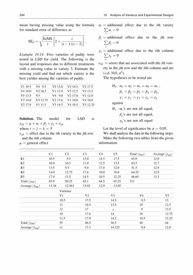
mean having missing value using the formula

for standard error of difference as

SEd ¼ffiffiffiffiffiffiffiffiffiffiffiffiffiffiffiffiffiffiffiffiffiffiffiffiffiffiffiffiffiffiffiffiffiffiffiffiffiffiffiffiffiffiffiffiffiffiffiffiffiffiffiffiffiErMS

t2þ t

ðt� 1Þðt� 2Þ� �s

:

Example 10.14. Five varieties of paddy were

tested in LSD for yield. The following is the

layout and responses due to different treatments

with a missing value in variety 3. Estimate the

missing yield and find out which variety is the

best yielder among the varieties of paddy.

V1 10.5 V4 9.5 V5 13.0 V3 14.5 V2 17.5

V4 10.0 V2 16.5 V1 11.0 V5 12.5 V3 13.5

V5 13.5 V3 V4 9.0 V2 17.0 V1 12.0

V3 14.0 V5 12.75 V2 17.6 V1 10.0 V4 10.0

V2 17.9 V1 11.5 V3 14.5 V4 10.5 V5 12.25

Solution. The model for LSD is

yijk ¼ μþ αi þ βj þ γk þ eijkwhere i ¼ j ¼ k ¼ 5

yijk ¼ effect due to the ith variety in the jth row

and the kth column

μ ¼ general effect

αi ¼ additional effect due to the ith varietyPiαi ¼ 0

βj ¼ additional effect due to the jth rowPj

βj ¼ 0

γk ¼ additional effect due to the kth columnPk

γk ¼ 0

eijk ¼ errors that are associated with the ith vari-

ety in the jth row and the kth column and are

i.i.d. N(0, σ2).The hypotheses to be tested are

H0 : α1 ¼ α2 ¼ α3 ¼ α4 ¼ α5 ,

β1 ¼ β2 ¼ β3 ¼ β4 ¼ β5;

γ1 ¼ γ2 ¼ γ3 ¼ γ4 ¼ γ5against

H1 : αi’s are not all equal,

βj’s are not all equal,

γk’s are not all equal:

Let the level of significance be α ¼ 0.05.

We shall analyze the data in the following steps:

Make the following two tables from the given

information.

C1 C2 C3 C4 C5 Total ðy0j0Þ Average ð�y0j0ÞR1 10.5 9.5 13.0 14.5 17.5 65.0 13.0

R2 10.0 16.5 11.0 12.5 13.5 63.5 12.7

R3 13.5 V3 9.0 17.0 12.0 51.5 12.9

R4 14.0 12.75 17.6 10.0 10.0 64.35 12.9

R5 17.9 11.5 14.5 10.5 12.25 66.65 13.3

Total y00kð Þ 65.9 50.25 65.1 64.5 65.25 311

Average �y00kð Þ 13.18 12.563 13.02 12.9 13.05

Varieties

V1 V2 V3 V4 V5

10.5 17.5 14.5 9.5 13

11 16.5 13.5 10 12.5

12 17 y 9 13.5

10 17.6 14 10 12.75

11.5 17.9 14.5 10.5 12.25

Total ðyi00Þ 55 86.5 56.5 49 64

Average ð�yi00Þ 11 17.3 14.125 9.8 12.8

244 10 Analysis of Variance and Experimental Designs

y ¼ X ¼ tðR0 þ C0 þ T0Þ � 2G0

ðt� 1Þðt� 2Þ¼ 5ð51:5þ 50:25þ 56:5Þ � 2� 311

ð5� 1Þð5� 2Þ ¼ 14:104

where

X ¼ estimate of the missing value

R0 ¼ total of available entries of the row having

the missing observation

T0 ¼ total of available entries of the variety V3

having the missing observation

C0 ¼ total of available entries of the column

having the missing observation

G0 ¼ total of available entries in the whole design

Now, G¼ G0 + X ¼ 311 + 14.104 ¼ 325.104

Total of variety three ¼ 56.5 + X ¼ 70.604

Total of row three ¼ 51.5 + X ¼ 65.604

Total of column two ¼ 50.25 + X ¼ 64.354

Calculate the following quantities:

CF ¼ G2

t� t¼ 325:1042

5� 5¼ 4227:704;

TSS ¼X

Obs:2 � CF ¼ 10:52 þ 9:52 þ � � � þ 10:52 þ 12:252 � 4227:704 ¼ 176.7634,

RSS ¼ 1

5

X5j¼1

y20j0� CF ¼ 1

5652 þ 63:52 þ � � � þ 66:652� �� 4227:704 ¼ 1:151531,

CSS ¼ 1

5

X5k¼1

y200k � CF ¼ 1

565:92 þ 64:3542 þ � � � þ 65:252� �� 4227:704 ¼ 0:309531,

VSS ¼ 1

5

X5i¼1

y2i00� CF ¼ 1

5552 þ 86:52 þ 70:6042 þ 492 þ 642� �� 4227:704 ¼ 170:1305,

ErSS ¼ TSS� RSS� CSS� VSS ¼ 176:7634� 1:151531 � 0:309531� 170:1305 ¼ 5:171792

where TSS, RSS, CSS, VSS, and ErSS are the

total, row, column, variety, and error sum of

squares, respectively.

The upward bias is calculated as follows:

B ¼ G0 � R0 � C0 � ðt� 1ÞT0ð Þ2ðt� 1Þðt� 2Þ½ �2

¼ 311� 51:5� 50:25� ð5� 1Þ56:3ð Þ2ð5� 1Þð5� 2Þ½ �2 ¼ 1:948:

Construct the ANOVA table as given below

using the above values:

ANOVA

SOV d.f. SS MS F

Row 4 1.152 0.288 <1

Column 4 0.309 0.077 <1

Variety 4 170.131

Error 11 5.172

Total 23 176.763

Variety

(corrected)

168.182 42.046 64.957

Error 7.120 0.647

The table value of F0.05;4,11 ¼ 3.36. Thus, we

find that the calculated values of F are less than

the corresponding table value, except for variety.

So the tests for row and columns are nonsignifi-

cant. We conclude that neither the row effects

nor the column effects are significant. But the

effects of varieties are significant. So we are to

identify the best variety.

To compare the varietal means involving no

missing value, the CD(0.05) is calculated using

the following formula:

CD0:05ðVarietyÞ ¼ffiffiffiffiffiffiffiffiffiffiffiffiffiffiffiffiffiffiffi2�MSE

t

r� t0:025; err:df:

¼ffiffiffiffiffiffiffiffiffiffiffiffiffiffiffiffiffiffi2�MSE

5

r� t0:025;11

¼ffiffiffiffiffiffiffiffiffiffiffiffiffiffiffiffiffiffiffiffiffiffiffiffiffiffiffi2� 0:647286

5

r� 2:201 ¼ 1:12;

and

to compare the varietal means with variety 3,

involving missing value, the CD(0.05) is calcu-

lated using the following formula:

10.10 Missing Plot Technique 245

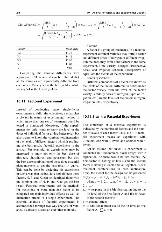
CD0:05ðVarietyÞ ¼ffiffiffiffiffiffiffiffiffiffiffiffiffiffiffiffiffiffiffiffiffiffiffiffiffiffiffiffiffiffiffiffiffiffiffiffiffiffiffiffiffiffiffiffiffiffiffiffiffiffiffiffiffiMSE

t2þ t

ðt� 1Þðt� 2Þ� �s

� t0:025; err:df: ¼ffiffiffiffiffiffiffiffiffiffiffiffiffiffiffiffiffiffiffiffiffiffiffiffiffiffiffiffiffiffiffiffiffiffiffiffiffiffiffiffiffiffiffiffiffiffiffiffiffiffiffiffiffiMSE

t2þ t

ðt� 1Þðt� 2Þ� �s

� t0:025;11

¼ffiffiffiffiffiffiffiffiffiffiffiffiffiffiffiffiffiffiffiffiffiffiffiffiffiffiffiffiffiffiffiffiffiffiffiffiffiffiffiffiffiffiffiffiffi0:647286

52þ 5

4� 3

� �s� 2:201 ¼ 1:231:

Variety Mean yield

V2 17.30

V3 14.12

V5 12.80

V1 11.00

V4 9.80

Comparing the varietal differences with

appropriate CD values, it can be inferred that

all the varieties are significantly different from

each other. Variety V2 is the best yielder, while

variety V4 is the lowest yielder.

10.11 Factorial Experiment

Instead of conducting many single-factor

experiments to fulfill the objectives, a researcher

is always in search of experimental method in

which more than one set of treatments could be

tested or compared. Moreover, if the experi-

menter not only wants to know the level or the

doses of individual factor giving better result but

also wants to know the combination/interaction

of the levels of different factors which is produc-

ing the best result, factorial experiment is the

answer. For example, an experimenter may be

interested to know not only the best dose of

nitrogen, phosphorus, and potassium but also

the best dose combination of these three essential

plant nutrients to get the best result in guava.

This can be done by designing his experiment

in such a way that the best levels of all these three

factors, N, P, and K, can be identified along with

the combination of N, P, and K to get the best

result. Factorial experiments are the methods

for inclusions of more than one factor to be

compared for their individual effects as well as

interaction effects in a single experiment. The

essential analysis of factorial experiments is

accomplished through two-way analysis of vari-

ance, as already discussed and other methods.

Factors

A factor is a group of treatments. In a factorial

experiment different varieties may form a factor

and different doses of nitrogen or different irriga-

tion methods may form other factors in the same

experiment. Here variety, nitrogen (irrespective

dose), and irrigation schedule (irrespective of

types) are the factors of the experiment.

Levels of Factors

Different components of a factor are known as

the levels of the factor. Different varieties under

the factor variety form the level of the factor

variety; similarly doses of nitrogen, types of irri-

gation, etc., are the levels of the factors nitrogen,

irrigation, etc., respectively.

10.11.1 m � n Factorial Experiment

The dimension of a factorial experiment is

indicated by the number of factors and the num-

ber of levels of each factor. Thus, a 3 � 4 facto-

rial experiment means an experiment with

2 factors, one with 3 levels and another with 4

levels.

Let us assume that an m� n experiment is

conducted in a randomized block design with rreplication. So there would be two factors: the

first factor is having m levels and the second

factor is having n levels and, all together, m� ntreatment combinations in each replication.

Thus, the model for the design can be presented

as yijk ¼ μþ αi þ βj þ αβð Þij þ γk þ eijk

where i ¼ 1, 2, . . ., m; j ¼ 1, 2, . . ., n; k ¼ 1,

2, . . ., ryijk ¼ response in the kth observation due to the

ith level of the first factor A and the jth level

of the second factor B

μ ¼ general effect

αi ¼ additional effect due to the ith level of first

factor A,P

αi ¼ 0

246 10 Analysis of Variance and Experimental Designs

βj ¼ additional effect due to the jth level of B,Pβj ¼ 0

αβð Þij ¼ interaction effect of the ith level of

the first factor and the jth level of B,Pi

αβð Þij ¼Pj

αβð Þij ¼ 0

γk ¼ additional effect due to the kth replicate,Pγk ¼ 0

eijk ¼ error component associated with the

ith level of the first factor and the jth level of

B in kth replicate and eijk ~ i.i.d. N(0, σ2)We have the following hypotheses for m � n

factorial experiment in RBD to be tested:

H01 : α1 ¼ α2 ¼ . . . ¼ αi ¼ . . . ¼ αm ¼ 0;

H02 : β1 ¼ β2 ¼ . . . ¼ βj ¼ . . . ¼ βn ¼ 0;

H03 : γ1 ¼ γ2 ¼ . . . ¼ γk ¼ . . . ¼ γr ¼ 0;

H04 : All αβð Þijs are equal

against the alternative hypotheses

H11 : All α’s are not equal,

H12 : All β’s are not equal,

H13 : All γ’s are not equal,

H14 : All ðαβÞ’s are not equal:

Let the level of significance be 0.05.

We calculate the following quantities from the

table:

Grand total ðGÞ ¼Xmi¼1

Xnj¼1

Xr

k¼1

yijk

Correction factor CFð Þ ¼ G2

mnr

TSS ¼Xmi¼1

Xnj¼1

Xr

k¼1

y2ijk � CF

RSS ¼ 1

mn

Xr

k¼1

y2ook � CF;

where y00k ¼Xmi

Xnj

yijk ¼ kth replication total:

Let us make the following table for calculating

other sums of squares (Tables 10.15 and 10.16).

TrSS ¼ 1

r

Xmi¼1

Xnj¼1

y2ij0 � CF;

where yij0 ¼Xr

k¼1

yijk

ErSS ¼ TSS� RSS� TrSS;

SS Að Þ ¼ 1

nr

Xmi¼1

y2i00 � CF

SS Bð Þ ¼ 1

mr

Xnj¼1

y20j0 � CF;

SS ABð Þ ¼ TrSS� SSðAÞ � SSðBÞ

If the cal. F (for A) > F0.05;(m�1), (r�1)(mn�1)

then H01 is rejected. This means the main effects

Table 10.14 Plot-wise observations from factorial RBD experiment

B Replication 1 Replication 2 Replication r

A b1 b2 . . .bj. . . bn b1 b2 . . .bj. . . bn . . . b1 b2 . . .bj. . . bn

a1 y111 y121 y1j1 y1n1 y112 y122 y1j2 y1n2 . . . y11r y12r y1jr y1nra2 y211 y221 y2j1 y2n1 y212 y222 y2j2 y2n2 . . . y21r y22r y2jr y2nr. . . . . .. . .

: : : . . .. . .

: : : . . .. . .

ai yi11 yi21 yij1 yin1 yi12 yi22 yij2 yin2 yi1r yi2r yijr yinr: : : :

: : : :

am ym11 ym21 ymj1 ymn1 ym12 ym22 ymj2 ymn2 ym1r ym2r ymjr ymnr

10.11 Factorial Experiment 247

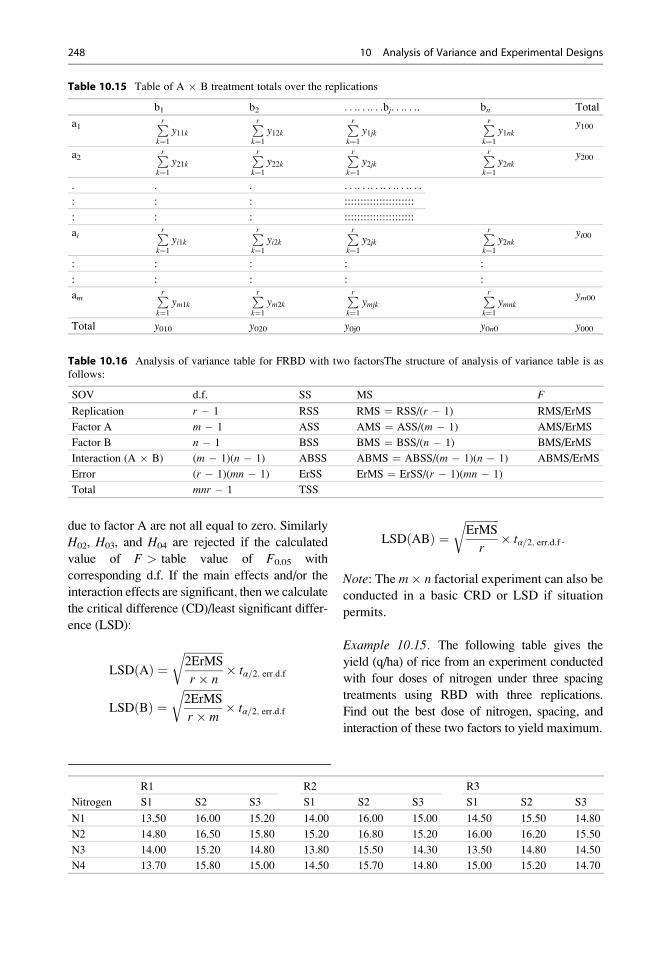
due to factor A are not all equal to zero. Similarly

H02, H03, and H04 are rejected if the calculated

value of F > table value of F0.05 with

corresponding d.f. If the main effects and/or the

interaction effects are significant, then we calculate

the critical difference (CD)/least significant differ-

ence (LSD):

LSD Að Þ ¼ffiffiffiffiffiffiffiffiffiffiffiffiffiffi2ErMS

r � n

r� tα=2; err:d:f

LSD Bð Þ ¼ffiffiffiffiffiffiffiffiffiffiffiffiffiffi2ErMS

r � m

r� tα=2; err:d:f

LSD ABð Þ ¼ffiffiffiffiffiffiffiffiffiffiffiffiErMS

r

r� tα=2; err:d:f :

Note: The m� n factorial experiment can also be

conducted in a basic CRD or LSD if situation

permits.

Example 10.15. The following table gives the

yield (q/ha) of rice from an experiment conducted

with four doses of nitrogen under three spacing

treatments using RBD with three replications.

Find out the best dose of nitrogen, spacing, and

interaction of these two factors to yield maximum.

Table 10.15 Table of A � B treatment totals over the replications

b1 b2 . . .. . .. . .bj. . .. . .. bn Total

a1 Prk¼1

y11kPrk¼1

y12kPrk¼1

y1jkPrk¼1

y1nky100

a2 Prk¼1

y21kPrk¼1

y22kPrk¼1

y2jkPrk¼1

y2nky200

. . . . . .. . .. . .. . .. . .. . .

: : : ::::::::::::::::::::::

: : : ::::::::::::::::::::::

ai Prk¼1

yi1kPrk¼1

yi2kPrk¼1

y2jkPrk¼1

y2nkyi00

: : : : :

: : : : :

am Prk¼1

ym1kPrk¼1

ym2kPrk¼1

ymjkPrk¼1

ymnkym00

Total y010 y020 y0j0 y0n0 y000

Table 10.16 Analysis of variance table for FRBD with two factorsThe structure of analysis of variance table is as

follows:

SOV d.f. SS MS F

Replication r � 1 RSS RMS ¼ RSS/(r � 1) RMS/ErMS

Factor A m � 1 ASS AMS ¼ ASS/(m � 1) AMS/ErMS

Factor B n � 1 BSS BMS ¼ BSS/(n � 1) BMS/ErMS

Interaction (A � B) (m � 1)(n � 1) ABSS ABMS ¼ ABSS/(m � 1)(n � 1) ABMS/ErMS

Error (r � 1)(mn � 1) ErSS ErMS ¼ ErSS/(r � 1)(mn � 1)

Total mnr � 1 TSS

R1 R2 R3

Nitrogen S1 S2 S3 S1 S2 S3 S1 S2 S3

N1 13.50 16.00 15.20 14.00 16.00 15.00 14.50 15.50 14.80

N2 14.80 16.50 15.80 15.20 16.80 15.20 16.00 16.20 15.50

N3 14.00 15.20 14.80 13.80 15.50 14.30 13.50 14.80 14.50

N4 13.70 15.80 15.00 14.50 15.70 14.80 15.00 15.20 14.70

248 10 Analysis of Variance and Experimental Designs

Solution. From the given information it is clear

that the experiment is an asymmetrical (4 � 3)

factorial experiment conducted in randomized

block design, so the appropriate statistical

model for the analysis will be

yijk ¼ μþ αi þ βj þ γk þ αβð Þij þ eijk, where

i ¼ 4; j ¼ 3; k ¼ 3

yijk ¼ response in the kth replicate due to the

ith level of the first factor (variety) and the

jth level of the second factor (seed rate)

μ ¼ general effect

αi ¼ additional effect due to the ith level of the

first factor (nitrogen),P

αi ¼ 0

βj ¼ additional effect due to the jth level of the

second factor (spacing),P

βj ¼ 0

γk ¼ additional effect due to the kth replicate,Pγk ¼ 0

αβð Þij ¼ interaction effect of the ith level of the

first factor (nitrogen) and the jth level of

the second factor (spacing),Pi

αβð Þij ¼Pj

αβð Þij ¼ 0

eijk ¼ error component associated with the ith

level of the first factor (nitrogen), the jth

level of the second factor (spacing), and the

kth replicates and eijk ~ N(0, σ2)Hypothesis to Be Tested

H0 : α1 ¼ α2 ¼ α3 ¼ α4 ¼ 0;

β1 ¼ β2 ¼ β3 ¼ 0;

γ1 ¼ γ2 ¼ γ3 ¼ 0;

All αβð Þij’s are equal

against

α’s are not all equal;

βj’s are not all equal;

γ’s are not all equal;

All αβð Þij’s are not equal:

Let the level of significance be 0.05.

From the given data table, let us calculate the

following quantities:

Grand total GTð Þ ¼X4i¼1

X3j¼1

X3k¼1

yijk ¼ 541:300

Correction factor CFð Þ ¼ GT2

4:3:3¼ 541:32

36¼ 8139:047

TSS ¼X4i¼1

X3j¼1

X3k¼1

y2ijk � CF

¼ 8162:810� 8139:047 ¼ 23:763

RSS ¼ 1

v:s

X3k¼1

y2ijk� CF

¼ 180:32 þ 180:82 þ 180:22

12� 8139:047

¼ 0:017

From the above table first let us form the

following table and from the table get the

following quantities:

TrSS¼ 1

3

X4i¼1

X3j¼1

y2ij0�CF

¼ 422þ47:52þ45:02þ�� �þ45:52þ43:62

3

�8139:047¼ 20:296

Table of totals

Spacing

Nitrogen

N1 N2 N3 N4 Total Average

S1 42.0 46.0 41.3 43.2 172.5 14.4

S2 47.5 49.5 45.5 46.7 189.2 15.8

S3 45.0 46.5 43.6 44.5 179.6 15.0

Total 134.5 142.0 130.4 134.4

Average 14.9 15.8 14.5 14.9

10.11 Factorial Experiment 249

ErSS ¼ TSS� TrSS� RSS ¼ 23:763� 20:296� 0:017 ¼ 3:449

SS ðNitrogenÞ ¼ 1

3:3

X4i¼1

y2i00 � CF ¼ 134:52 þ 142:02 þ 130:42 þ 134:42

9� 8139:047 ¼ 7:816

SS ðSpacingÞ ¼ 1

4:3

X3j¼1

y20j0 � CF ¼ 172:52 þ 189:22 þ 179:62

12� 8139:047 ¼ 11:70

SS ðNSÞ ¼ TrSS� SS ðNitrogenÞ � SS ðSpacingÞ ¼ 20:296� 7:816� 11:706 ¼ 0:773

Now we make the following analysis of variance table with the help of the above quantities:

It is clear from the above table that all the

effects of variety as well as the spacing are sig-

nificant at 1% level of significance. But the rep-

lication interaction effects of nitrogen and

spacing are not significant even at 5% (desired

level of significance) level of significance.

To find out which dose of nitrogen and which

spacing have maximum yield potentiality, we are

to calculate the critical difference values for

nitrogen and spacing effects separately using

the following formulae:

CD0:01 Nitrogenð Þ ¼ffiffiffiffiffiffiffiffiffiffiffiffiffiffi2ErMS

r:s

rt0:005; err:d:f

¼ffiffiffiffiffiffiffiffiffiffiffiffiffiffiffiffiffiffiffiffi2� 0:157

3� 3

r2:819 ¼ 0:527;

CD0:01 Spacingð Þ ¼ffiffiffiffiffiffiffiffiffiffiffiffiffiffi2ErMS

r:n

rt0:005; err:d:f

¼ffiffiffiffiffiffiffiffiffiffiffiffiffiffiffiffiffiffiffiffi2� 0:157

3� 4

r2:819 ¼ 0:456:

Table of averages

Yield (q/ha)

Variety

N2 15.78

N1 14.94

N4 14.93

N3 14.49

Seed rate

S2 15.77

S3 14.97

S1 14.38

Nitrogen N2 has recorded significantly the

highest yield compared to other doses of nitro-

gen. The difference of means between any two

varieties for the rest three varieties (N1, N3, N4)

is not greater than the critical difference value;

they are statistically at par. There exists no

significant difference among the nitrogen doses

N1, N3, and N4. On the other hand, spacing S2

is the best plant density for getting maximum

yield of paddy followed by S3 and S1. So far

ANOVA

Table value of FSOV d.f. MS MS F-ratio

Replication 3 � 1 ¼ 2 0.017 0.009 0.055 F0:05;2;22 ¼ 3:44 F0:01;2;22 ¼ 5:72

Treatment 12 � 1 ¼ 11 20.296 1.845 11.768 F0:05;11;22 ¼ 2:27 F0:01;11;22 ¼ 3:19

Nitrogen 4 � 1 ¼ 3 7.816 2.605 16.617 F0:05;3;22 ¼ 3:05 F0:01;3;22 ¼ 4:82

Spacing 3 � 1 ¼ 2 11.707 5.854 37.333 F0:05;2;22 ¼ 3:44 F0:01;2;22 ¼ 5:72

NS 3 � 2 ¼ 6 0.773 0.129 0.821 F0:05;6;22 ¼ 2:55 F0:01;6;22 ¼ 3:76

Error 35 � 2 � 11 ¼ 22 3.449 0.157

Total 36 � 1 ¼ 35 23.763

250 10 Analysis of Variance and Experimental Designs

about the interaction effect of nitrogen and

spacing is concerned, no significant difference

is recorded among the different treatment

combinations.

The above analysis can also be done usingSAS statistical software. The following few slides

present the data entry, the command syntax, andthe output for the same:

Slide 10.30: Step 1 showing data entry for two-factor factorial RBD analysis using SAS

Slide 10.31: Step 2 showing portion of data entry and commands for two-factor factorial RBD analysis using SAS

10.11 Factorial Experiment 251

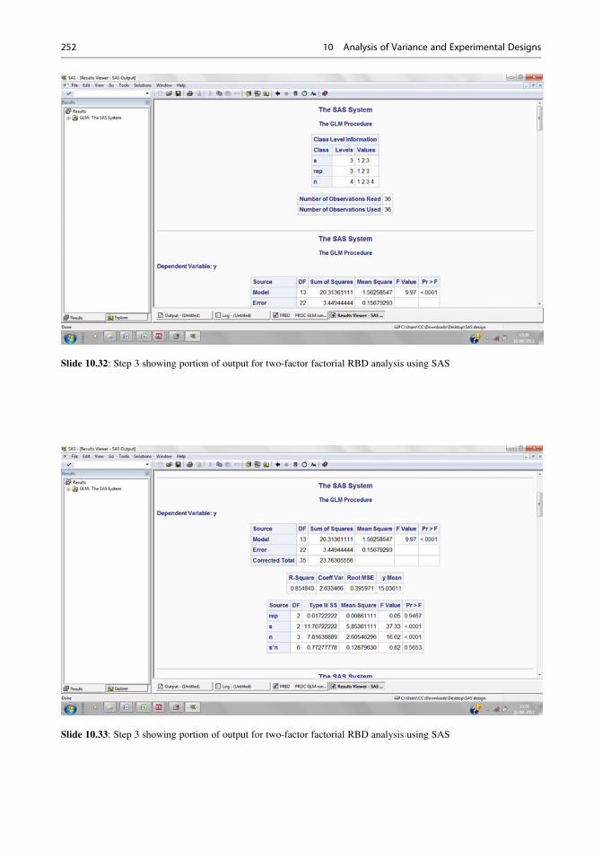
Slide 10.32: Step 3 showing portion of output for two-factor factorial RBD analysis using SAS

Slide 10.33: Step 3 showing portion of output for two-factor factorial RBD analysis using SAS

252 10 Analysis of Variance and Experimental Designs

10.11.2 m � n � p FactorialExperiment

In an m � n � p three-factor factorial experi-

ment, three factors are tested of which the first,

second, and third factors are at m, n, and p levels,

respectively; the efficacy of levels of different

factors separately and the interactions of the

levels of different factors are worked out. A

three-factor factorial experiment can be designed

in a CRD, RBD, or LSD fashion. But the problem

with LSD is that even at the lowest level of three-

factor factorial experiment, that is, 23 factorial

experiment, we require to get a plot of 8 � 8

experimental area, and any factor having a level

more than two in a three-factor factorial experi-

ment requires at least a plot of 12� 12 number of

experimental units. In reality most of the times, it

becomes difficult to get such a plot and impossi-

ble when the levels of any factor increase beyond

this three-level limit. Thus, three-factor and

more-than-three-factor factorial experiments are

generally conducted in CRD or RBD design.

Let us take the following examples of 2 � 3 � 4

FRBD.

Example 10.16. The following table gives the

yield (q/ha) from a field experiment of paddy

with three doses of phosphate fertilizer and four

doses of nitrogen in two types of irrigation in a

randomized block design. Analyze the data to

find out the best dose of phosphate, the best

dose of nitrogen, the best irrigation, and the

best interaction effects among the factors.

Solution. The experiment is an asymmetrical

(2 � 3 � 4) factorial experiment conducted in

randomized block design, so the appropriate

statistical model for the analysis will be

yijkl ¼ μþ αi þ βj þ αβð Þij þ γk þ ðαγÞikþðβγÞjk þ ðαβγÞijk þ δl þ eijkl, where i ¼ 2;

j ¼ 3; k ¼ 4; l ¼ 3

yijkl ¼ response in the lth replicate due to the ith

level of irrigation, the jth level of phosphate,

and the kth level of nitrogen

μ ¼ general effect

Slide 10.34: Step 3 showing portion of output for two-factor Factorial RBD analysis using SAS

10.11 Factorial Experiment 253

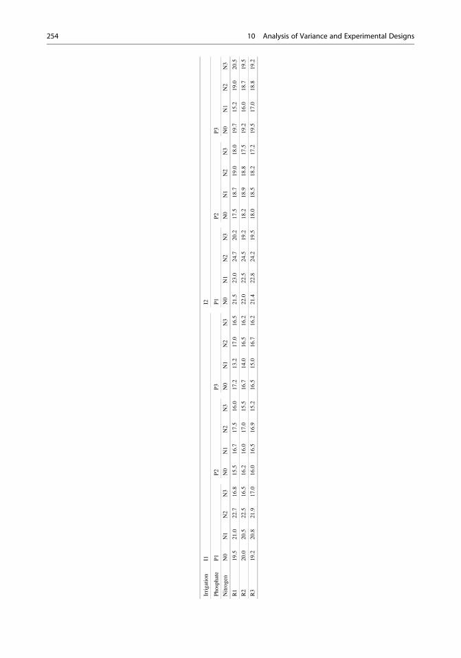
Irrigation

I1I2

Phosphate

P1

P2

P3

P1

P2

P3

Nitrogen

N0

N1

N2

N3

N0

N1

N2

N3

N0

N1

N2

N3

N0

N1

N2

N3

N0

N1

N2

N3

N0

N1

N2

N3

R1

19.5

21.0

22.7

16.8

15.5

16.7

17.5

16.0

17.2

13.2

17.0

16.5

21.5

23.0

24.7

20.2

17.5

18.7

19.0

18.0

19.7

15.2

19.0

20.5

R2

20.0

20.5

22.5

16.5

16.2

16.0

17.0

15.5

16.7

14.0

16.5

16.2

22.0

22.5

24.5

19.2

18.2

18.9

18.8

17.5

19.2

16.0

18.7

19.5

R3

19.2

20.8

21.9

17.0

16.0

16.5

16.9

15.2

16.5

15.0

16.7

16.2

21.4

22.8

24.2

19.5

18.0

18.5

18.2

17.2

19.5

17.0

18.8

19.2

254 10 Analysis of Variance and Experimental Designs

αi ¼ additional effect due to the ith level of

irrigation,P

αi ¼ 0

βj ¼ additional effect due to the jth level of

phosphate,P

βj ¼ 0

γk ¼ additional effect due to the kth level of

nitrogen,P

γk ¼ 0

αβð Þij ¼ interaction effect of the ith level of irri-

gation and the jth level of phosphate,Pi

αβð Þij ¼Pj

αβð Þij ¼ 0

αγð Þik ¼ interaction effect of the ith level of

irrigation and the kth level of nitrogen,Pi

αγð Þik ¼Pk

αγð Þik ¼ 0

βγð Þjk ¼ interaction effect of the jth level of

phosphate and the lth level of nitrogen,Pj

βγð Þjk ¼Pk

βγð Þjk ¼ 0;

αβλð Þijk ¼ interaction effect of the ith level of

irrigation, the jth level of phosphate, and

the kth level of nitrogen,Pi

αβλð Þijk ¼Pj

αβλð Þijk ¼Pk

αβλð Þijk ¼ 0

δl ¼ additional effect due to the lth replication,Pδl ¼ 0

eijkl ¼ error component associated with the lth

replicate due to the ith level of irrigation and

the jth level of phosphate and the kth level of

nitrogen and eijkl ~ i.i.d. N(0, σ2)Hypothesis to Be Tested

H0 : α1 ¼ α2 ¼ 0;

β1 ¼ β2 ¼ β3 ¼ 0;

γ1 ¼ γ2 ¼ γ3 ¼ γ4 ¼ 0;

δ1 ¼ δ2 ¼ δ3 ¼ 0;

All interaction effects ¼ 0 against

H1 : All α’s are not equal,

All β’s are not equal,

All γ’s are not equal,

All δ’s are not equal;

All interaction effects are not equal.

Let the level of significance be 0.05.

From the given data table, let us calculate the

following quantities:

Grand total GTð Þ ¼X2i¼1

X3j¼1

X4k¼1

X3l¼1

yijkl ¼ 1331:4

Correction factor CFð Þ ¼ GT2

2:3:4:3¼ 1331:42

72

¼ 24619:805

TSS ¼X2i¼1

X3j¼1

X4k¼1

X3l¼1

y2ijkl� CF ¼ 461:767

RSS ¼ 1

m:n:p

X3l¼1

y2000l

� CF

¼ 446:62 þ 442:22 þ 442:22

24� 24619:805

¼ 0:500:

From the above table first let us form the

following tables and from the table get the fol-

lowing quantities:

Table of totals for irrigation � nitrogen

Nitrogen

Irrigation

I1 I2 Total Average

N0 156.800 177.000 333.800 18.544

N1 153.650 172.600 326.250 18.125

N2 168.700 185.900 354.600 19.700

N3 145.900 170.800 316.700 17.594

Total 625.050 706.300

Average 17.363 19.619

Table of totals for irrigation � phosphate

Phosphate

Irrigation

I1 I2 Total Average

P1 238.350 265.500 503.850 20.994

P2 195.000 218.500 413.500 17.229

P3 191.700 222.300 414.000 17.250

Total 625.050 706.300

Average 17.363 19.619

SS ðIrrigationÞ ¼ 1

n:p:r

X2i¼1

y2iooo

� CF

¼ 625:052 þ 706:32

3:4:3

� 24619:805¼ 91:688

10.11 Factorial Experiment 255

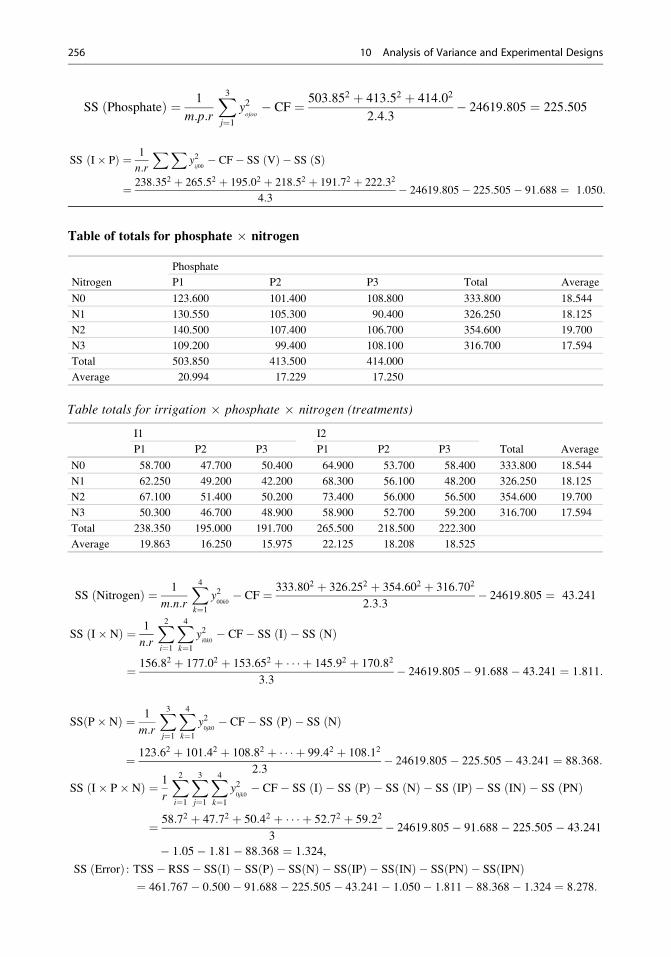
SS ðPhosphateÞ ¼ 1

m:p:r

X3j¼1

y2ojoo

� CF ¼ 503:852 þ 413:52 þ 414:02

2:4:3� 24619:805 ¼ 225:505

SS ðI� PÞ ¼ 1

n:r

XXy2ij00

� CF� SS ðVÞ � SS ðSÞ

¼ 238:352 þ 265:52 þ 195:02 þ 218:52 þ 191:72 þ 222:32

4:3� 24619:805� 225:505� 91:688 ¼ 1:050:

Table of totals for phosphate � nitrogen

Table totals for irrigation � phosphate � nitrogen (treatments)

SS ðNitrogenÞ ¼ 1

m:n:r

X4k¼1

y200k0

� CF ¼ 333:802 þ 326:252 þ 354:602 þ 316:702

2:3:3� 24619:805 ¼ 43:241

SS ðI� NÞ ¼ 1

n:r

X2i¼1

X4k¼1

y2i0k0

� CF� SS ðIÞ � SS ðNÞ

¼ 156:82 þ 177:02 þ 153:652 þ � � � þ 145:92 þ 170:82

3:3� 24619:805� 91:688� 43:241 ¼ 1:811:

SSðP� NÞ ¼ 1

m:r

X3j¼1

X4k¼1

y20jk0

� CF� SS ðPÞ � SS ðNÞ

¼ 123:62 þ 101:42 þ 108:82 þ � � � þ 99:42 þ 108:12

2:3� 24619:805� 225:505� 43:241 ¼ 88:368:

SS ðI� P� NÞ ¼ 1

r

X2i¼1

X3j¼1

X4k¼1

y20jk0

� CF� SS ðIÞ � SS ðPÞ � SS ðNÞ � SS ðIPÞ � SS ðINÞ � SS ðPNÞ

¼ 58:72 þ 47:72 þ 50:42 þ � � � þ 52:72 þ 59:22

3� 24619:805� 91:688� 225:505� 43:241

� 1:05� 1:81� 88:368 ¼ 1:324,

SS Errorð Þ : TSS� RSS� SS Ið Þ � SS Pð Þ � SS Nð Þ � SS IPð Þ � SS INð Þ � SS PNð Þ � SS IPNð Þ¼ 461:767� 0:500� 91:688� 225:505� 43:241� 1:050� 1:811� 88:368� 1:324 ¼ 8:278:

I1 I2

Total AverageP1 P2 P3 P1 P2 P3

N0 58.700 47.700 50.400 64.900 53.700 58.400 333.800 18.544

N1 62.250 49.200 42.200 68.300 56.100 48.200 326.250 18.125

N2 67.100 51.400 50.200 73.400 56.000 56.500 354.600 19.700

N3 50.300 46.700 48.900 58.900 52.700 59.200 316.700 17.594

Total 238.350 195.000 191.700 265.500 218.500 222.300

Average 19.863 16.250 15.975 22.125 18.208 18.525

Nitrogen

Phosphate

P1 P2 P3 Total Average

N0 123.600 101.400 108.800 333.800 18.544

N1 130.550 105.300 90.400 326.250 18.125

N2 140.500 107.400 106.700 354.600 19.700

N3 109.200 99.400 108.100 316.700 17.594

Total 503.850 413.500 414.000

Average 20.994 17.229 17.250

256 10 Analysis of Variance and Experimental Designs

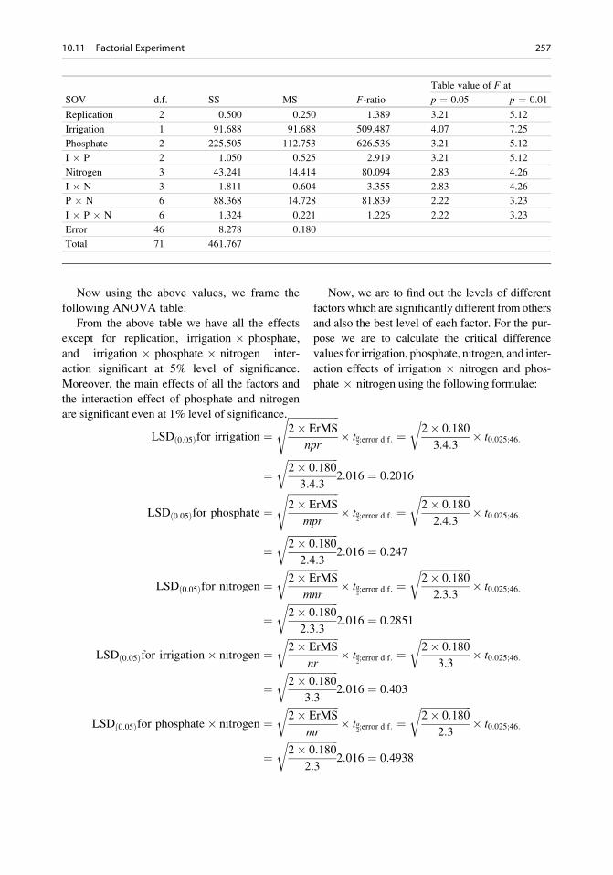
Now using the above values, we frame the

following ANOVA table:

From the above table we have all the effects

except for replication, irrigation � phosphate,

and irrigation � phosphate � nitrogen inter-

action significant at 5% level of significance.

Moreover, the main effects of all the factors and

the interaction effect of phosphate and nitrogen

are significant even at 1% level of significance.

Now, we are to find out the levels of different

factorswhich are significantly different fromothers

and also the best level of each factor. For the pur-

pose we are to calculate the critical difference

values for irrigation, phosphate, nitrogen, and inter-

action effects of irrigation � nitrogen and phos-

phate � nitrogen using the following formulae:

LSDð0:05Þfor irrigation ¼ffiffiffiffiffiffiffiffiffiffiffiffiffiffiffiffiffiffiffiffi2� ErMS

npr

s� tα

2;error d:f: ¼

ffiffiffiffiffiffiffiffiffiffiffiffiffiffiffiffiffiffiffiffi2� 0:180

3:4:3

r� t0:025;46:

¼ffiffiffiffiffiffiffiffiffiffiffiffiffiffiffiffiffiffiffiffi2� 0:180

3:4:3

r2:016 ¼ 0:2016

LSDð0:05Þfor phosphate ¼ffiffiffiffiffiffiffiffiffiffiffiffiffiffiffiffiffiffiffiffi2� ErMS

mpr

s� tα

2;error d:f: ¼

ffiffiffiffiffiffiffiffiffiffiffiffiffiffiffiffiffiffiffiffi2� 0:180

2:4:3

r� t0:025;46:

¼ffiffiffiffiffiffiffiffiffiffiffiffiffiffiffiffiffiffiffiffi2� 0:180

2:4:3

r2:016 ¼ 0:247

LSDð0:05Þfor nitrogen ¼ffiffiffiffiffiffiffiffiffiffiffiffiffiffiffiffiffiffiffiffi2� ErMS

mnr

r� tα

2;error d:f: ¼

ffiffiffiffiffiffiffiffiffiffiffiffiffiffiffiffiffiffiffiffi2� 0:180

2:3:3

r� t0:025;46:

¼ffiffiffiffiffiffiffiffiffiffiffiffiffiffiffiffiffiffiffiffi2� 0:180

2:3:3

r2:016 ¼ 0:2851

LSDð0:05Þfor irrigation� nitrogen ¼ffiffiffiffiffiffiffiffiffiffiffiffiffiffiffiffiffiffiffiffi2� ErMS

nr

r� tα

2;error d:f: ¼

ffiffiffiffiffiffiffiffiffiffiffiffiffiffiffiffiffiffiffiffi2� 0:180

3:3

r� t0:025;46:

¼ffiffiffiffiffiffiffiffiffiffiffiffiffiffiffiffiffiffiffiffi2� 0:180

3:3

r2:016 ¼ 0:403

LSDð0:05Þfor phosphate� nitrogen ¼ffiffiffiffiffiffiffiffiffiffiffiffiffiffiffiffiffiffiffiffi2� ErMS

mr

r� tα

2;error d:f: ¼

ffiffiffiffiffiffiffiffiffiffiffiffiffiffiffiffiffiffiffiffi2� 0:180

2:3

r� t0:025;46:

¼ffiffiffiffiffiffiffiffiffiffiffiffiffiffiffiffiffiffiffiffi2� 0:180

2:3

r2:016 ¼ 0:4938

SOV d.f. SS MS F-ratio

Table value of F at

p ¼ 0.05 p ¼ 0.01

Replication 2 0.500 0.250 1.389 3.21 5.12

Irrigation 1 91.688 91.688 509.487 4.07 7.25

Phosphate 2 225.505 112.753 626.536 3.21 5.12

I � P 2 1.050 0.525 2.919 3.21 5.12

Nitrogen 3 43.241 14.414 80.094 2.83 4.26

I � N 3 1.811 0.604 3.355 2.83 4.26

P � N 6 88.368 14.728 81.839 2.22 3.23

I � P � N 6 1.324 0.221 1.226 2.22 3.23

Error 46 8.278 0.180

Total 71 461.767

10.11 Factorial Experiment 257

Table of means

Yield (q/ha) LSD(0.05)

Irrigation

I2 19.619 0.2016I1 17.363Phosphate

P1 20.994 0.247P3 17.250P2 17.229

Nitrogen

N2 19.700 0.2851N0 18.544N1 18.125N3 17.594

Irrigation � nitrogen(I � N)

I2N2 20.656 0.403I2N0 19.667I2N1 19.178I2N3 18.978I1N2 18.744I1N0 17.422I1N1 17.072I1N3 16.211

Phosphate � nitrogen (P � N)

P1N2 23.417 0.494P1N1 21.758P1N0 20.600P1N3 18.200P3N0 18.133P3N3 18.017P2N2 17.900P3N2 17.783P2N1 17.550P2N0 16.900P2N3 16.567P3N1 15.067

From the above table we have the following

conclusions:

1. I2 irrigation is significantly better than the I1

irrigation.

2. Phosphate P1 is the best one and P2 and P3 are

statistically at par.

3. All the doses of nitrogen are significantly

different from each other and the best dose

of nitrogen is N2.

4. Among the interaction effects of irrigation

and nitrogen, I2N2 is the best followed by

I2N0 and so on.

5. Among the interaction effects of variety and

nitrogen, P1N2 is the best followed by P1N1,

P1N0, and so on.

10.12 Incomplete Block Design

As the number of factors or levels of factors or

both increase, the number of treatment combina-

tion increases, and it becomes very difficult to

accommodate all the treatments in a single block.

As a result the idea of incomplete blocks comes

under consideration. Each replication is now

being constituted of a number of blocks which

can accommodate a part of the total treatments.

Thus, the blocks are incomplete in the sense

that they do not contain/accommodate all the

treatments in each of them. In the process a

complete block equivalent to a complete replica-

tion changes to a replication of number of incom-

plete blocks. Thus, in an incomplete block

design, blocks are no longer equivalent to

replication.

10.12.1 Split Plot Design

The simplest of all incomplete block designs

involving two factors is the split plot design.

In field experiment certain factors like type of

irrigation, tillage, drainage, and weed manage-

ment require comparatively larger size of plots

for convenience of the treatments compared to

the other factors. Thus, factorial experiments

involving these factors along with other factors

require different sizes of experimental plots in

the same experiment. In split plot design, each

and every replication is divided into the number

of blocks as the number of levels of the factors

requiring higher plot size and lesser precision,

the main plot factor. Each and every block is

constituted of as many numbers of experimental

units as the levels of the other factors which

require lesser plot size compared to the main plot

factor and higher precision. The subplot effects

and the interaction effects of subplot factors are

more precisely estimated in split plot design com-

pared to the main plot effects.

258 10 Analysis of Variance and Experimental Designs

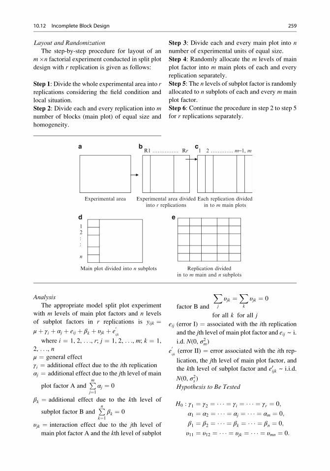
Layout and RandomizationThe step-by-step procedure for layout of an

m�n factorial experiment conducted in split plot

design with r replication is given as follows:

Step 1: Divide the whole experimental area into rreplications considering the field condition and

local situation.

Step 2: Divide each and every replication into mnumber of blocks (main plot) of equal size and

homogeneity.

Step 3: Divide each and every main plot into nnumber of experimental units of equal size.

Step 4: Randomly allocate the m levels of main

plot factor into m main plots of each and every

replication separately.

Step 5: The n levels of subplot factor is randomly

allocated to n subplots of each and every m main

plot factor.

Step 6: Continue the procedure in step 2 to step 5

for r replications separately.

Analysis

The appropriate model split plot experiment

with m levels of main plot factors and n levels

of subplot factors in r replications is yijk ¼μþ γi þ αj þ eij þ βk þ υjk þ e

0ijk

where i ¼ 1, 2, . . ., r; j ¼ 1, 2, . . ., m; k ¼ 1,

2, . . ., nμ ¼ general effect

γi ¼ additional effect due to the ith replication

αj ¼ additional effect due to the jth level of main

plot factor A andPmj¼1

αj ¼ 0

βk ¼ additional effect due to the kth level of

subplot factor B andPnk¼1

βk ¼ 0

υjk ¼ interaction effect due to the jth level of

main plot factor A and the kth level of subplot

factor B and

Xj

υjk ¼Xk

υjk ¼ 0

for all k for all j

eij (error I) ¼ associated with the ith replication

and the jth level of main plot factor and eij ~ i.

i.d. N(0, σ2m)

e0ijk(error II) ¼ error associated with the ith rep-

lication, the jth level of main plot factor, and

the kth level of subplot factor and e0ijk ~ i.i.d.

N(0, σ2s )Hypothesis to Be Tested

H0 : γ1 ¼ γ2 ¼ � � � ¼ γi ¼ � � � ¼ γr ¼ 0;

α1 ¼ α2 ¼ � � � ¼ αj ¼ � � � ¼ αm ¼ 0;

β1 ¼ β2 ¼ � � � ¼ βk ¼ � � � ¼ βn ¼ 0;

υ11 ¼ υ12 ¼ � � � ¼ υjk ¼ � � � ¼ υmn ¼ 0:

R1 …………… Rr 1 2 …………. m−1, m

1 ……………

Experimental area Experimental area dividedinto r replications

Each replication dividedin to m main plots

12::

n

Main plot divided into n subplots Replication dividedin to m main and n subplots

a

d e

b c

10.12 Incomplete Block Design 259

H1 : γ’s are not all equal,

α’s are not all equal,

β’s are not all equal,

υ’s are not all equal:

Let the level of significance be 0.05

(Table 10.17).

The step-by-step procedure for the computa-

tion of different sums of squares and mean sum

of squares is given as follows:

1. Grand total ¼ Pri¼1

Pmj¼1

Pnk¼1

yijk ¼ GT:

2. Correction factor ðCFÞ ¼ GT2

mnr :

3. Total MS ¼ Pri¼1

Pmj¼1

Pnk¼1

y2ijk � CF:

4. Work out the sum of squares due to the main

plot factor and the replication. For the pur-

pose, the following table of totals is required

to be framed (Table 10.18):

where yij0 ¼Pnk¼1

yijk

TSS (Table 10.18) ¼ 1n

Pri

Pmj

y2ij0 � CF,

Replication SS ¼ 1mn

Pri¼1

y2i00 � CF,

SS(A) ¼ 1nr

Pmj¼1

y20j0 � CF, SS Error I ¼ TSS

ðTable 10:18Þ � RSS� SSðAÞ.5. Work out the sum of squares due to the sub-

plot factor and interaction. For the purpose,

the following table of totals is required to the

formed (Table 10.19):

Note: In both tables the totals for main factor

A at different levels will be the same.

TSS ðTable 10:19Þ ¼ 1

r

Xmj¼1

Xnk¼1

y20jk � CF;

SS Bð Þ ¼ 1

mr

Xnk¼1

y200k � CF

SS ABð Þ ¼ TSS ðTable 10:19Þ � SS ðAÞ� SS ðBÞ; SS Error IIð Þ

¼ TSS� RSS� SS Að Þ� SS Error Ið Þ � SS Bð Þ � SS ABð Þ:

Mean sum of squares is calculated by dividing

the sum of squares by the corresponding

degrees of freedom.

Table 10.17 ANOVA for split plot design

SOV d.f. MS MS F-ratio Table value of F

Replication r � 1 RMS RMS RMS/Er.MS I

Main plot factor(A) m � 1 MS(A) MS(A) MS(A)/Er.MS I

Error I (r � 1) (m � 1) Er.MS(I) Er.MS I

Subplot factor(B) (n � 1) MS(B) MS(B) MS(B)/Er.MS II

Interaction (A � B) (m � 1) (n � 1) MS(AB) MS(AB) MS(AB)/Er.MS II

Error II m (n � 1) (r � 1) Er.MS II Er.MS II

Total mnr � 1

Table 10.18 Table totals for main plot � replication

a1 a2 . . .. . . aj . . .. . . am Total Mean

R1 y110 y120 . . .. . . y1j0 . . .. . . y1m0 y100 �y100R2 y210 y220 . . .. . . y2j0 . . .. . . y2m0 y200 �y200: : : : : : : :

Ri yi10 yi20 . . .. . . yij0 . . .. . . yim0 yi00 �yi00: : : : : : : :

Rr yr10 yr20 . . .. . . yrj0 . . .. . . yrm0 yr00 �yr00Total y010 y020 . . .. . . y0j0 . . .. . . y0m0 y000 �y000Mean �y010 �y020 �y0j0 �y0m0

260 10 Analysis of Variance and Experimental Designs

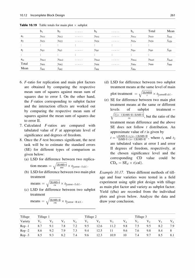
6. F-ratio for replication and main plot factors

are obtained by comparing the respective

mean sum of squares against mean sum of

squares due to error I. On the other hand,

the F-ratios corresponding to subplot factor

and the interaction effects are worked out

by comparing the respective mean sum of

squares against the mean sum of squares due

to error II.

7. Calculated F-ratios are compared with

tabulated value of F at appropriate level of

significance and degrees of freedom.

8. Once the F-test becomes significant, the next

task will be to estimate the standard errors

(SE) for different types of comparison as

given below:

(a) LSD for difference between two replica-

tion means ¼ffiffiffiffiffiffiffiffiffiffiffiffiffi2ErMS-I

mn

q� tα

2;error�I d:f:.

(b) LSD for difference between two main plot

treatment

means ¼ffiffiffiffiffiffiffiffiffiffiffiffiffi2ErMS-I

rn

q� tα

2;error�I d:f:.

(c) LSD for difference between two subplot

treatment

means ¼ffiffiffiffiffiffiffiffiffiffiffiffiffiffi2ErMS-II

rm

q� tα

2;error�II d:f:.

(d) LSD for difference between two subplot

treatment means at the same level of main

plot treatment ¼ffiffiffiffiffiffiffiffiffiffiffiffi2ErMSII

r

q� tα

2;errorII d:f:.

(e) SE for difference between two main plot

treatment means at the same or different

levels of subplot treatment ¼ffiffiffiffiffiffiffiffiffiffiffiffiffiffiffiffiffiffiffiffiffiffiffiffiffiffiffiffiffiffiffiffiffiffiffiffiffiffi2½ðn�1ÞErMS-IIþErMS-I�

rn

q, but the ratio of the

treatment mean difference and the above

SE does not follow t distribution. An

approximate value of t is given by

t ¼ t1ErMS-Iþt2ðn�1ÞErMS-IIErMS-Iþðn�1ÞErMS-II , where t1 and t2

are tabulated values at error I and error

II degrees of freedom, respectively, at

the chosen significance level and the

corresponding CD value could be

CDα ¼ SEd � tðcalÞ.

Example 10.17. Three different methods of till-

age and four varieties were tested in a field

experiment using split plot design with tillage

as main plot factor and variety as subplot factor.

Yield (t/ha) are recorded from the individual

plots and given below. Analyze the data and

draw your conclusion.

Table 10.19 Table totals for main plot � subplot

b1 b2 . . .. . . bk . . .. . . bn Total Mean

a1 y011 y012 . . .. . . y01k . . .. . . y01n y010 �y010a2 y021 y022 . . .. . . y02k . . .. . . y02n y020 �y020: : : : : : : :

aj y0j1 y0j2 . . .. . . y0jk . . .. . . y0jn y0j0 �y0j0

: : : : : : : :

am y0m1 y0m2 . . .. . . y0mk . . .. . . y0mn y0m0 �y0m0Total y001 y002 . . .. . . y00k . . .. . . y00n y000 �y000Mean �y001 �y002 �y00k �y00n

Tillage Tillage 1 Tillage 2 Tillage 3

Variety V1 V2 V3 V4 V1 V2 V3 V4 V1 V2 V3 V4

Rep -1 8.7 9.1 7.8 7.2 9.5 12.6 11.2 9.8 7.5 9.5 8.2 7.9

Rep -2 8.6 9.2 7.9 7.3 9.4 12.5 11 9.6 7.6 9.8 8.4 8

Rep -3 8.5 9.3 8.2 7.4 9.6 12.3 10.9 10 7.4 9.7 8.5 8.1

10.12 Incomplete Block Design 261

For the above experiment, the appropriate

model is

yijk¼μþ γi þ αj þ eij þ βk þ υjk þ eijk, i ¼ 3,

j ¼ 3, k ¼ 4,

where

μ ¼ general effect

γi ¼ additional effect due to the ith replication

αj ¼ additional effect due to the jth level of main

plot factor, tillage, andP3j¼1

αj ¼ 0

βk ¼ additional effect due to the kth level of

subplot factor, variety, andP4k¼1

βk ¼ 0

υjk ¼ interaction effect due to the jth level of

main plot factor (tillage) and the kth level

of subplot factor (variety) andP3j¼1

υjk ¼P4k¼1

υjk ¼ 0

eij (error I) ¼ error associated with the ith

replication and the jth level of tillage and

eij ~ i.i.d. N(0, σ2m)

e0ijk(error II) ¼ error associated with the ith repli-

cation, the jth level of tillage, and the kth level of

subplot factor (variety) and eijk ~ i.i.d. N(0, σ2s )Hypothesis to Be Tested

H0 : γ1 ¼ γ2 ¼ γ3 ¼ 0;

α1 ¼ α2 ¼ α3 ¼ 0;

β1 ¼ β2 ¼ β3 ¼ β4 ¼ 0;

υ0s are all equal to zero:

H1 : α’s are not all equal,

γ’s are not all equal,

β’s are not all equal,

υ’s are not all equal:

Let the level of significance be 0.05.

Grand total ¼X3i¼1

X3j¼1

X4k¼1

yijk ¼ GT ¼ 8:7þ 9:1þ � � � þ 8:5þ 8:1 ¼ 328:20

Correction factor ðCFÞ ¼ GT2

mnr¼ 328:202

3:4:3¼ 2992:09

Total SS ¼X3i¼1

X3j¼1

X4k¼1

y2ijk � CF ¼ 8:72 þ 9:12 þþ � � � þ 8:52 þ 8:12 � 2992:09 ¼ 75:87

Table I Table of totals for tillage � replication

Tillage

Replication

R1 R2 R3 Total

T1 32.800 33.000 33.400 99.20

T2 43.100 42.500 42.800 128.40

T3 33.100 33.800 33.700 100.60

Total 109.000 109.300 109.900 328.20

Average 36.3333 36.43333 36.6333

TSS Table 1ð Þ ¼ 1

n

Xr

i¼1

Xmj¼1

y2ij0 � CF

¼ 45:37

SS ðError IÞ ¼ TSS ðTable IÞ � RSS� SS ðPÞ¼ 45:37� 45:207� 0:035 ¼ 0:128:

Replication SS ¼ 1

mn

Xr

i¼1

y2i00 � CF

¼ 1

3:4

X3i¼1

y2i00 � CF

¼ 1092 þ 109:32 þ 109:92

12� 2992:09

¼0:035

SS ðtillageÞ ¼ 1

nr

Xmj¼1

y20j0 � CF

¼ 1

4:3

X3j¼1

y20j0 � CF

¼ 99:22 þ 128:42 þ 100:62

12� 2992:09

¼ 45:207

262 10 Analysis of Variance and Experimental Designs

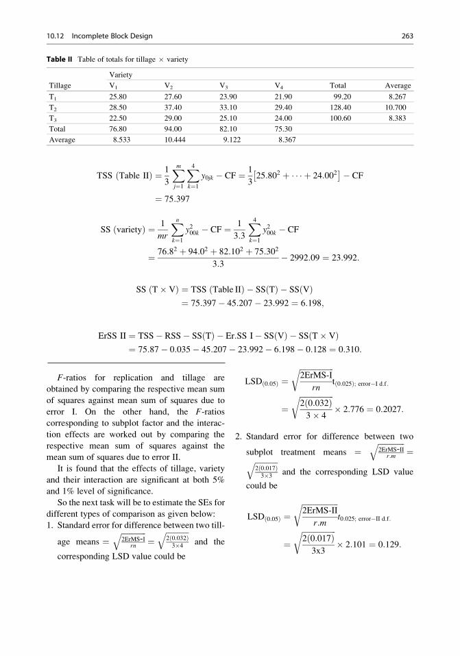
TSS Table IIð Þ ¼ 1

3

Xmj¼1

X4k¼1

y0jk � CF ¼ 1

325:802 þ � � � þ 24:002� �� CF

¼ 75:397

SS ðvarietyÞ ¼ 1

mr

Xnk¼1

y200k � CF ¼ 1

3:3

X4k¼1

y200k � CF

¼ 76:82 þ 94:02 þ 82:102 þ 75:302

3:3� 2992:09 ¼ 23:992:

SS ðT� VÞ ¼ TSS ðTable IIÞ � SSðTÞ � SSðVÞ¼ 75:397� 45:207� 23:992 ¼ 6:198;

ErSS II ¼ TSS� RSS� SS Tð Þ � Er:SS I� SS Vð Þ � SS T� Vð Þ¼ 75:87� 0:035� 45:207� 23:992� 6:198� 0:128 ¼ 0:310:

F-ratios for replication and tillage are

obtained by comparing the respective mean sum

of squares against mean sum of squares due to

error I. On the other hand, the F-ratioscorresponding to subplot factor and the interac-

tion effects are worked out by comparing the

respective mean sum of squares against the

mean sum of squares due to error II.

It is found that the effects of tillage, variety

and their interaction are significant at both 5%

and 1% level of significance.

So the next task will be to estimate the SEs for

different types of comparison as given below:

1. Standard error for difference between two till-

age means ¼ffiffiffiffiffiffiffiffiffiffiffiffiffi2ErMS-I

rn

q¼

ffiffiffiffiffiffiffiffiffiffiffiffi2ð0:032Þ3�4

qand the

corresponding LSD value could be

LSDð0:05Þ ¼ffiffiffiffiffiffiffiffiffiffiffiffiffiffiffiffiffiffi2ErMS-I

rn

rtð0:025Þ; error�I d:f:

¼ffiffiffiffiffiffiffiffiffiffiffiffiffiffiffiffiffiffi2ð0:032Þ3� 4

r� 2:776 ¼ 0:2027:

2. Standard error for difference between two

subplot treatment means ¼ffiffiffiffiffiffiffiffiffiffiffiffiffiffi2ErMS-II

r:m

q¼ffiffiffiffiffiffiffiffiffiffiffiffi

2ð0:017Þ3�3

qand the corresponding LSD value

could be

LSDð0:05Þ ¼ffiffiffiffiffiffiffiffiffiffiffiffiffiffiffiffiffiffiffi2ErMS-II

r:m

rt0:025; error�II d:f:

¼ffiffiffiffiffiffiffiffiffiffiffiffiffiffiffiffiffiffi2ð0:017Þ

3x3

r� 2:101 ¼ 0:129:

Table II Table of totals for tillage � variety

Tillage

Variety

V1 V2 V3 V4 Total Average

T1 25.80 27.60 23.90 21.90 99.20 8.267

T2 28.50 37.40 33.10 29.40 128.40 10.700

T3 22.50 29.00 25.10 24.00 100.60 8.383

Total 76.80 94.00 82.10 75.30

Average 8.533 10.444 9.122 8.367

10.12 Incomplete Block Design 263

3. Standard error for difference between two tillage

means at the same or different level of subplot

treatment ¼ffiffiffiffiffiffiffiffiffiffiffiffiffiffiffiffiffiffiffiffiffiffiffiffiffiffiffiffiffiffiffiffiffiffiffiffiffiffiffiffiffiffiffiffiffiffiffiffiffiffiffiffiffiffiffiffiffi2½ðn� 1ÞErMS-IIþ ErMS-I�

rn

r¼ffiffiffiffiffiffiffiffiffiffiffiffiffiffiffiffiffiffiffiffiffiffiffiffiffiffiffiffiffiffiffiffiffiffiffiffiffiffiffiffiffiffiffiffiffiffiffiffi

2½ð4� 1Þ 0:017þ 0:032�3:4

r¼ 0:1386, but the

ratio of the treatment mean difference and the

above SE does not follow t distribution, and the

approximate value of t is given by

t ¼ t1ErMS-Iþ t2ðn� 1Þ ErMS-II

ErMS-Iþ ðn� 1Þ ErMS-II¼

ð2:776Þ ð0:032Þ þ ð2:101Þ ð4� 1Þ 0:017ð0:032Þ þ ð4� 1Þ ð0:017Þ ¼

2:361, where t1 ¼ t0.025,4 value and t2 ¼t0.025,18 value and the corresponding

CD value could be LSDð0:05Þ ¼ SEd�tðcalÞ ¼ 0:1386 �2:361 ¼ 0:327.

Table of mean comparison

Average LSD(0.05)

Tillage

T2 10.700 0.2027

T3 8.383

T1 8.267

VarietyV2 10.444 0.129

V3 9.122

V1 8.533

V4 8.367

T � VT2V2 12.467 0.227

T2V3 11.033 and 0.324

T2V4 9.800

T3V2 9.667

T2V1 9.500

T1V2 9.200

T1V1 8.600

T3V3 8.367

T3V4 8.000

T1V3 7.967

T3V1 7.500

T1V4 7.300

Thus, second tillage is the best, which is

significantly superior to the other two tillages.

The two methods of tillage, namely, T3 and T1,

are statistically at par. So far as the effect of

variety is concerned, maximum yield of ginger

is obtained from variety V2 followed by V3,

V1, and V4. All the varieties are significantly

different from each other with respect to yield

of ginger. The interaction of the method of

tillage and the varieties has significantly dif-

ferent effects from each other; the interac-

tion effects which are not significantly

different have been put under the same lines.

Variety in combination with tillage T2V2 has

produced significantly higher yield than any

other combination, followed by P2V3, P2V4,

and so on.

The above analysis can also be done using

SAS statistical software. The following few slidespresent the data entry, command syntax, and the

output for the same:

10.12.2 Strip Plot Design

In split plot design, if both the factors require a

large plot like that in the main plot factor, then it

may not be possible in split plot design. Strip

plot design is the solution. In agricultural field

experimentation with factors like different

methods of irrigation, different methods of pest

control, different methods of mulching, differ-

ent methods of plowing, etc., require larger plot

size for convenience of management. In

experiments involving these factors, strip plot

design may become very useful. In strip plot

design each replication is divided into the num-

ber of horizontal rows and the number of verti-

cal columns equals to the number of levels of

factor 1 and factor 2, respectively, or vice versa.

ANOVA table for 3 � 4 split plot experiment Table value of F

SOV d.f. MS MS F-ratio p ¼ 0.05 p ¼ 0.01

Replication 3 � 1 ¼ 2 0.035 0.018 0.545 6.94 18.00

Main Plot Factor(P) 3 � 1 ¼ 2 45.207 22.603 704.519 6.94 18.00

Error I (3 � 1) (3 � 1) ¼ 4 0.128 0.032

Subplot factor(V) (4 � 1) ¼ 3 23.992 7.997 464.366 3.16 5.09

Interaction (P � V) (3 � 1) (4 � 1) ¼ 6 6.198 1.033 59.978 2.66 4.01

Error II 3 (4 � 1) (3 � 1) ¼ 18 0.310 0.017

Total 3.3.4 � 1 ¼ 35 75.87'

264 10 Analysis of Variance and Experimental Designs

The factor assigned to the horizontal rows is

called horizontal factor and the factor assigned

to the vertical column is called the verticalfactor. Thus, horizontal factor and vertical fac-

tor always remain perpendicular to each other.

This does not necessarily mean that the shapeand/or size of horizontal strips and vertical

strips will be the same. The smallest plot in

strip plot design is the intersection plot and

in strip plot design, the interaction effects

Slide 10.35: Step 1 showing data entry for split plot data analysis using SAS

Slide 10.36: Step 2 showing a portion of data entry and commands for split plot data analysis using SAS

10.12 Incomplete Block Design 265

Slide 10.37: Step 3 showing a portion of output for split plot data analysis using SAS

Slide 10.38: Step 3 showing a portion of output for split plot data analysis using SAS

266 10 Analysis of Variance and Experimental Designs

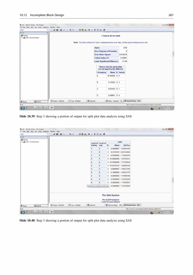
Slide 10.39: Step 3 showing a portion of output for split plot data analysis using SAS

Slide 10.40: Step 3 showing a portion of output for split plot data analysis using SAS

10.12 Incomplete Block Design 267

between the two factors are measured with

higher precision than either of the two factors.

Randomization and Layout

Like split plot design, the randomization and

allocation of the two factors in strip plot design

is done in two steps. First, n horizontal factors

are randomly allocated to n horizontal strips.

Next the m levels of factor B are distributed

among the m vertical strips independently and

randomly. The procedure of randomization is

repeated for each and every replication indepen-

dently. The ultimate layout of an m� n strip

plot design in r replication is given in

(Table 10.20):

Analysis

The analysis of strip plot design is performed in

three steps: (a) analysis of horizontal factor

effects, (b) analysis of vertical factor effects,

and (c) analysis of interaction factor effects.

Statistical Model

yijk ¼ μþ γi þ αj þ eij þ βk þ e0ik þ ðαβÞjkþ e00ijk

where i ¼ 1, 2, . . ., r; j ¼ 1, 2, . . ., m; k ¼ 1, 2,

. . ., n

μ ¼ general effect

γi ¼ additional effect due to the ith replication

αj ¼ additional effect due to the jth level of

vertical factor A andPmj¼1

αj ¼ 0

βk ¼ additional effect due to the kth level of

horizontal factor B andPnj¼1

βk ¼ 0

ðαβÞjk ¼ interaction effect due to the jth level of

factor A and the kth level of factor B andPj

ðαβÞjk ¼Pk

ðαβÞjk ¼ 0 r

eij (error I) ¼ error associated with the ith repli-

cation and the jth level of vertical factor A and

~eik ~ i.i.d. N(0, σ21)

Table 10.20 Layout of m � n strip plot design

1 …………… ….r 12:::::

n

A) Whole experimental B) Experimental area dividedin to r replications

C) Each replication divided intom horizontal rows

1 ………………… 1……..

………………...12::::

nD) Each replication divided in m vertical columns

E) Whole experimental area n ´ mhorizontal and vertical rows

n-1

n-1

268 10 Analysis of Variance and Experimental Designs

e0ik(error II) ¼ error associated with the ith level

of replication and the kth level of horizontal

factor B and e0ij~ i.i.d. N(0, σ22 )

e00ijk (error III) ¼ error associated with the ith

replication, the jth level of vertical factor A,

and the kth level of horizontal factor B and eijk~ i.i.d. N(0, σ23 )

Hypothesis to Be Tested

H0 :γ1 ¼ γ2 ¼ � � � ¼ γi ¼ � � � ¼ γr ¼ 0;

α1 ¼ α2 ¼ � � � ¼ αj ¼ � � � ¼ αm ¼ 0;

β1 ¼ β2 ¼ � � � ¼ βk ¼ � � � ¼ βn ¼ 0;

αβð Þ11 ¼ αβð Þ12 ¼ � � � ¼ αβð Þjk ¼ � � �¼ αβð Þmn ¼ 0:

H1 :γ’s are not all equal;

α’s are not all equal,

β’s are not all equal,

ðαβÞ’s are not all equal:

Let the level of significance be 0.05.

First we construct the three two-way

tables of totals for (a) replication � horizontal

factor, (b) replication � vertical factor, and (c)

horizontal � vertical factor. The step-by-step

procedure for computation of different sums of

squares and mean sums of squares is given as

follows:

1. Grand total ¼ Pri¼1

Pmj¼1

Pnk¼1

yijk ¼ G:

2. Correction factor ðCFÞ ¼ G2

mnr :

3. Total MS ¼ Pri¼1

Pmj¼1

Pnk¼1

y2ijk � CF:

4. Work out the sum of squares due to the

vertical factor A and the replication.

Table 10.21 (table of totals) is required to be

framed.

where

yij0 ¼Xnk¼1

yijk

TSS Table Ið Þ ¼ 1

n

Xr

i¼1

Xmj¼1

y2ij0 � CF

Replication SS ¼ 1

mn

Xr

i¼1

y2i00 � CF

SS Að Þ ¼ 1

nr

Xmj¼1

y20j0 � CF

SS Error Ið Þ ¼ TSSðTable IÞ � RSS� SSðAÞ

5. Work out the sum of squares due to the hori-

zontal factor B and the replication.

Table 10.22 (table of totals) is required to be

framed.

TSS ðTable IIÞ ¼ 1

m

Xr

i¼1

Xnk¼1

y2i0k � CF

SS Bð Þ ¼ 1

mr

Xnk¼1

y200k � CF

SS Error IIð Þ ¼ TSSðTable IIÞ � RSS� SSðBÞ

Table 10.21 Table of totals for replication � vertical factor A

a1 a2 . . .. . . aj . . .. . . am Total Mean

R1 y110 y120 . . .. . . y1j0 . . .. . . y1m0 y100 �y100R2 y210 y220 . . .. . . y2j0 . . .. . . y2m0 y200 �y200: : : : : : : :

Ri yi10 yi20 . . .. . . yij0 . . .. . . yim0 yi00 �yi00: : : : : : : :

Rr yr10 yr20 . . .. . . yrj0 . . .. . . yrm0 yr00 �yr00Total y010 y020 . . .. . . y0j0 . . .. . . y0m0 y000 �y000Mean �y010 �y020 �y0j0 �y0m0

10.12 Incomplete Block Design 269

6. Work out the sum of squares due to vertical

factor A and horizontal factor B interaction.

Table 10.23 (table of totals) is required to be

formed.

TSS Table IIIð Þ ¼ 1

r

Xmj¼1

Xnk¼1

y20jk � CF

SS ABð Þ ¼ TSSðTable IIIÞ � SSðAÞ � SSðBÞ

SS Error IIIð Þ ¼ TSS� RSS� SS Að Þ� SS Bð Þ � SS ABð Þ � ErSS I

� ErSS II

Mean sum of squares is calculated by dividing

the sum of squares by the corresponding

degrees of freedom (Table 10.24).

7. F-ratios for replication and vertical factor

effects are obtained by comparing the replica-

tion mean sum of squares against the mean

sum of squares due to error I. On the other

hand, the F-ratios corresponding to horizontal

factor and interaction between horizontal and

vertical factors are worked out by comparing

the respective mean sum of squares against

the mean sum of squares due to error II and

error III, respectively.

8. Calculated F-ratios are compared with

tabulated value of F at appropriate level of

significance and degrees of freedom.

9. Once the F-test becomes significant, our next

task will be to estimate the SEs for different

types of comparison as given below:

(a) Standard error for difference between two

replication means ¼ffiffiffiffiffiffiffiffiffiffiffiffiffi2ErMS-I

mn

qand the

corresponding LSD value will be

LSDα ¼ffiffiffiffiffiffiffiffiffiffiffiffiffi2ErMS-I

mn

q� tα

2;error�I d:f:.

(b) Standard error for difference between two

vertical plot treatment means ¼ffiffiffiffiffiffiffiffiffiffiffiffiffi2ErMS-I

rn

qand the corresponding LSD value will be

LSDα ¼ffiffiffiffiffiffiffiffiffiffiffiffiffi2ErMS-I

rn

q� tα

2;error�I d:f:.

(c) Standard error for difference between

two horizontal plot treatment

Table 10.22 Table of totals for replication � horizontal factor B

b1 b2 . . .. . . bk . . .. . . bn Total Mean

R1 y101 y102 . . .. . . y10k . . .. . . y10n y100 �y100R2 y201 y202 . . .. . . y20k . . .. . . y20n y200 �y200: : : : : : : :

Ri yi01 yi02 . . .. . . yi0k . . .. . . yi0n yi00 �yi00: : : : : : : :

Rr yr01 Yr02 . . .. . . yr0k . . .. . . yr0n yr00 �yr00Total y001 y002 . . .. . . y00kj . . .. . . y00nm y000 �y000Mean �y001 �y002 �y00k �y00n

Table 10.23 Table of totals for vertical factor A � horizontal factor B

b1 b2 . . .. . . bk . . .. . . bn Total Mean

a1 y011 y012 . . .. . . y01k . . .. . . y01n y010 �y010a2 y021 y022 . . .. . . y02k . . .. . . y02n y020 �y020: : : : : : : :

aj y0j1 y0j2 . . .. . . y0jk . . .. . . y0jn y0j0 �y0j0

: : : : : : : :

am y0m1 y0m2 . . .. . . y0mk . . .. . . y0mn y0m0 �y0m0Total y001 y002 . . .. . . y00k . . .. . . y00n y000 �y000Mean �y001 �y002 �y00k �y00n

270 10 Analysis of Variance and Experimental Designs

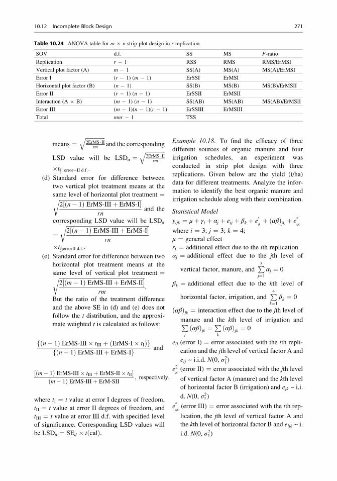
means ¼ffiffiffiffiffiffiffiffiffiffiffiffiffiffi2ErMS-II

rm

qand the corresponding

LSD value will be LSDα ¼ffiffiffiffiffiffiffiffiffiffiffiffiffiffi2ErMS-II

rm

q�tα

2; error�II d:f:.

(d) Standard error for difference between

two vertical plot treatment means at the

same level of horizontal plot treatment ¼ffiffiffiffiffiffiffiffiffiffiffiffiffiffiffiffiffiffiffiffiffiffiffiffiffiffiffiffiffiffiffiffiffiffiffiffiffiffiffiffiffiffiffiffiffiffiffiffiffiffiffiffiffiffiffiffiffiffiffi2 ðn� 1Þ ErMS-IIIþ ErMS-I½ �

rn

rand the

corresponding LSD value will be LSDα

¼ffiffiffiffiffiffiffiffiffiffiffiffiffiffiffiffiffiffiffiffiffiffiffiffiffiffiffiffiffiffiffiffiffiffiffiffiffiffiffiffiffiffiffiffiffiffiffiffiffiffiffiffiffiffiffiffiffiffiffiffi2 ðn� 1Þ ErMS-IIIþ ErMS-I½ �

rn

r�tα

2;errorII d:f:.

(e) Standard error for difference between two

horizontal plot treatment means at the

same level of vertical plot treatment ¼ffiffiffiffiffiffiffiffiffiffiffiffiffiffiffiffiffiffiffiffiffiffiffiffiffiffiffiffiffiffiffiffiffiffiffiffiffiffiffiffiffiffiffiffiffiffiffiffiffiffiffiffiffiffiffiffiffiffiffiffiffiffi2 ðm� 1Þ ErMS-IIIþ ErMS-II½ �

rm

r.

But the ratio of the treatment difference

and the above SE in (d) and (e) does not

follow the t distribution, and the approxi-

mate weighted t is calculated as follows:

ðn� 1Þ ErMS-III� tIII þ ðErMS-I� tIÞf gðn� 1Þ ErMS-IIIþ ErMS-If g and

ðm� 1Þ ErMS-III� tIII þ ErMS-II� tII½ �ðm� 1Þ ErMS-IIIþ ErM-SII

; respectively;

where tI ¼ t value at error I degrees of freedom,

tII ¼ t value at error II degrees of freedom, and

tIII ¼ t value at error III d.f. with specified level

of significance. Corresponding LSD values will

be LSDα ¼ SEd � tðcalÞ.

Example 10.18. To find the efficacy of three

different sources of organic manure and four

irrigation schedules, an experiment was

conducted in strip plot design with three

replications. Given below are the yield (t/ha)

data for different treatments. Analyze the infor-

mation to identify the best organic manure and

irrigation schedule along with their combination.

Statistical Model

yijk ¼ μþ γi þ αj þ eij þ βk þ e0jkþ ðαβÞjk þ e

00ijk

where i ¼ 3; j ¼ 3; k ¼ 4;

μ ¼ general effect

ri ¼ additional effect due to the ith replication

αj ¼ additional effect due to the jth level of

vertical factor, manure, andP3j¼1

αj ¼ 0

βk ¼ additional effect due to the kth level of

horizontal factor, irrigation, andP4k¼1

βk ¼ 0

ðαβÞjk ¼ interaction effect due to the jth level of

manure and the kth level of irrigation andPj

ðαβÞjk ¼Pk

ðαβÞjk ¼ 0

eij (error I) ¼ error associated with the ith repli-

cation and the jth level of vertical factor A and

eij ~ i.i.d. N(0, σ21)

e2jk(error II) ¼ error associated with the jth level

of vertical factor A (manure) and the kth level

of horizontal factor B (irrigation) and ejk ~ i.i.

d. N(0, σ22 )

e00ijk(error III) ¼ error associated with the ith rep-

lication, the jth level of vertical factor A and

the kth level of horizontal factor B and eijk ~ i.

i.d. N(0, σ23 )

Table 10.24 ANOVA table for m � n strip plot design in r replication

SOV d.f. SS MS F-ratio

Replication r � 1 RSS RMS RMS/ErMSI

Vertical plot factor (A) m � 1 SS(A) MS(A) MS(A)/ErMSI

Error I (r � 1) (m � 1) ErSSI ErMSI

Horizontal plot factor (B) (n � 1) SS(B) MS(B) MS(B)/ErMSII

Error II (r � 1) (n � 1) ErSSII ErMSII

Interaction (A � B) (m � 1) (n � 1) SS(AB) MS(AB) MS(AB)/ErMSII

Error III (m � 1)(n � 1)(r � 1) ErSSIII ErMSIII

Total mnr � 1 TSS

10.12 Incomplete Block Design 271

Hypothesis to Be Tested

H0 :γ1 ¼ γ2 ¼ γ3 ¼ 0;

α1 ¼ α2 ¼ α3 ¼ 0;

β1 ¼ β2 ¼ β3 ¼ β4 ¼ 0;

αβð Þ11 ¼ αβð Þ12 ¼ � � � ¼ αβð Þjk ¼ � � �¼ αβð Þ34 ¼ 0:

H1 :γ’s are not all equal;

α’s are not all equal,

β’s are not all equa,

ðαβÞ’s are not all equal:

Let the level of significance be 0.05.

First we construct three two-way tables of

totals for replication � manure, replication �irrigation, and manure � irrigation. The step-

by-step procedure for computation of different

sums of squares and mean sum of squares is

given as follows:

1. Grand total =P3i¼1

P3j¼1

P4k¼1

yijk ¼ GT ¼ 11:2þ10:2þ � � � þ 12:4þ 10:7 ¼ 434:6:

2. Correction factor ðCFÞ ¼GT2

3:4:3¼ 434:62

36¼ 5246:488:

3. Work out the sum of squares due to vertical

factor A and replication. The following table

of totals is required to be framed:

TSS Table Ið Þ ¼ 1

4

X3i¼1

X3j¼1

y2ij0 � CF

¼ 5279:09� 5246:588 ¼ 32:502

Replication SS ¼ 1

3:4

X3i¼1

y2i00 � CF

¼ 144:22 þ 145:42 þ 1452

12

� 5246:588¼ 0:062

SS Að Þ ¼ 1

4:3

X3j¼1

y20j0 � CF

¼ 1462 þ 158:22 þ 130:42

12� 5246:588

¼ 32:362

SS Error Ið Þ ¼ TSS ðTable IÞ � RSS� SS ðAÞ¼ 32:502� 0:062� 32:362¼ 0:078

4. Work out the sum of squares due to horizontal

factor B and replication. The following table

of totals is required to be framed:

Horizontal plot

(irrigation)

Vertical plot (manure)

M1 M2 M3

I1 I2 I3 I4 I1 I2 I3 I4 I1 I2 I3 I4

R1 11.2 10.2 14.5 12.3 11.8 10.9 16.2 13.5 11 9.5 12.5 10.6

R2 11.3 10.5 14.6 12.5 11.9 10.8 16.5 13.8 10.9 9.8 12 10.8

R3 11.5 10.4 14.2 12.8 11.6 10.7 16.6 13.9 10.5 9.7 12.4 10.7

Table I Table of totals for replication � manure

M1 M2 M3 Total Average

R1 48.200 52.400 43.600 144.200 12.017

R2 48.900 53.000 43.500 145.400 12.117

R3 48.900 52.800 43.300 145.000 12.083

Total 146.000 158.200 130.400

Average 12.167 13.183 10.867

272 10 Analysis of Variance and Experimental Designs

(Table II) ErSS II ¼ 13

P3i¼1

P4k¼1

y2i0k � CF

¼ 342 þ 30:62 þ � � � þ 43:22 þ 37:42

3� 5246:588

¼ 83:416

SS Bð Þ ¼ 1

3:3

X4k¼1

y200k � CF

¼ 101:72 þ 92:52 þ 129:52 þ 110:92

9

� 5246:588¼ 83:212

ErSS II ¼ 1

3

X3i¼1

X4k¼1

y2i0k � CF� SS ðIrrg:Þ

¼ 342 þ 30:62 þ � � � þ 43:22 þ 37:42

3

�5246:588� 83:212 ¼ 0:204:

5. Work out the sum of squares due to vertical

factor and horizontal factor interaction. The

following table of totals is required to be

framed:

Table 3 Table of totals for irrigation � manure

SSðM� IÞ ¼ 1

r

Xmj¼1

Xnk¼1

y20jk � CF� SSðAÞ � SSðBÞ

¼ 342 þ 35:32 þ 32:42 þ � � � þ 41:22 þ 32:12

3� 5246:588� 32:362� 83:212 ¼ 10:644

Error III ¼ TMS� RMS�MS Að Þ �MS Bð Þ �MS ABð Þ � ErMS-I� ErMS-II

¼ 127:112� 0:062� 32:362� 83:212� 10:644� 0:078� 0:204

¼ 0:549:

Table 2 Table of totals for replication � irrigation

I1 I2 I3 I4 Total Average

R1 34.000 30.600 43.200 36.400 144.200 12.017

R2 34.100 31.100 43.100 37.100 145.400 12.117

R3 33.600 30.800 43.200 37.400 145.000 12.083

Total 101.700 92.500 129.500 110.900

Average 11.300 10.278 14.389 12.322

M1 M2 M3 Total Average

I1 34.0 35.3 32.4 101.700 11.300

I2 31.1 32.4 29.0 92.500 10.280

I3 43.3 49.3 36.9 129.500 14.389

I4 37.6 41.2 32.1 110.900 12.322

Total 146.000 158.200 130.400

Average 12.167 13.183 10.867

10.12 Incomplete Block Design 273

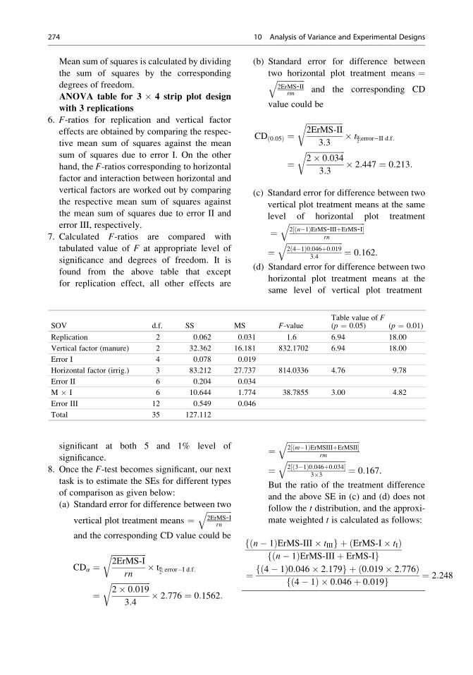
Mean sum of squares is calculated by dividing

the sum of squares by the corresponding

degrees of freedom.

ANOVA table for 3 � 4 strip plot design

with 3 replications

6. F-ratios for replication and vertical factor

effects are obtained by comparing the respec-

tive mean sum of squares against the mean

sum of squares due to error I. On the other

hand, the F-ratios corresponding to horizontalfactor and interaction between horizontal and

vertical factors are worked out by comparing

the respective mean sum of squares against

the mean sum of squares due to error II and

error III, respectively.

7. Calculated F-ratios are compared with

tabulated value of F at appropriate level of

significance and degrees of freedom. It is

found from the above table that except

for replication effect, all other effects are

significant at both 5 and 1% level of

significance.

8. Once the F-test becomes significant, our next

task is to estimate the SEs for different types

of comparison as given below:

(a) Standard error for difference between two

vertical plot treatment means ¼ffiffiffiffiffiffiffiffiffiffiffiffiffi2ErMS-I

rn

qand the corresponding CD value could be

CDα ¼ffiffiffiffiffiffiffiffiffiffiffiffiffiffiffiffiffiffi2ErMS-I

rn

r� tα

2; error�I d:f:

¼ffiffiffiffiffiffiffiffiffiffiffiffiffiffiffiffiffiffiffiffi2� 0:019

3:4

r� 2:776 ¼ 0:1562:

(b) Standard error for difference between

two horizontal plot treatment means ¼ffiffiffiffiffiffiffiffiffiffiffiffiffiffi2ErMS-II

rm

qand the corresponding CD

value could be

CDð0:05Þ ¼ffiffiffiffiffiffiffiffiffiffiffiffiffiffiffiffiffiffiffi2ErMS-II

3:3

r� tα

2;error�II d:f:

¼ffiffiffiffiffiffiffiffiffiffiffiffiffiffiffiffiffiffiffiffi2� 0:034

3:3

r� 2:447 ¼ 0:213:

(c) Standard error for difference between two

vertical plot treatment means at the same

level of horizontal plot treatment

¼ffiffiffiffiffiffiffiffiffiffiffiffiffiffiffiffiffiffiffiffiffiffiffiffiffiffiffiffiffiffiffiffiffiffiffiffiffiffiffi2½ðn�1ÞErMS-IIIþErMS-I�

rn

q¼

ffiffiffiffiffiffiffiffiffiffiffiffiffiffiffiffiffiffiffiffiffiffiffiffiffiffiffiffiffi2ð4�1Þ0:046þ0:019

3:4

q¼ 0:162.

(d) Standard error for difference between two

horizontal plot treatment means at the

same level of vertical plot treatment

¼ffiffiffiffiffiffiffiffiffiffiffiffiffiffiffiffiffiffiffiffiffiffiffiffiffiffiffiffiffiffiffiffiffiffiffiffiffi2½ðm�1ÞErMSIIIþErMSII�

rm

q¼

ffiffiffiffiffiffiffiffiffiffiffiffiffiffiffiffiffiffiffiffiffiffiffiffiffiffiffiffiffiffi2½ð3�1Þ0:046þ0:034�

3�3

q¼ 0:167.

But the ratio of the treatment difference

and the above SE in (c) and (d) does not

follow the t distribution, and the approxi-

mate weighted t is calculated as follows:

fðn� 1ÞErMS-III� tIIIg þ ðErMS-I� tIÞfðn� 1ÞErMS-IIIþ ErMS-Ig

¼ fð4� 1Þ0:046� 2:179g þ ð0:019� 2:776Þfð4� 1Þ � 0:046þ 0:019g ¼ 2:248

SOV d.f. SS MS F-valueTable value of F(p ¼ 0.05) (p ¼ 0.01)

Replication 2 0.062 0.031 1.6 6.94 18.00

Vertical factor (manure) 2 32.362 16.181 832.1702 6.94 18.00

Error I 4 0.078 0.019

Horizontal factor (irrig.) 3 83.212 27.737 814.0336 4.76 9.78

Error II 6 0.204 0.034

M � I 6 10.644 1.774 38.7855 3.00 4.82

Error III 12 0.549 0.046

Total 35 127.112

274 10 Analysis of Variance and Experimental Designs

and

½ðm� 1ÞErMS-III� tIII þ ErMS-II� tII�ðm� 1ÞErMS-IIIþ ErMS-II

¼ ½ð3� 1Þ � 0:046� 2:179þ 0:034� 2:447�ð3� 1Þ � 0:046þ 0:034

¼ 2:251;

where tI ¼ t0.025,4 ¼ 2.776, tII ¼ t0.025,6¼ 2.447, and tIII ¼ t0.025,12 ¼ 2.179.

Corresponding CD values could be

CD ð0:05Þ ¼ SEd � tcal.Thus, the critical difference value to com-

pare two vertical plot treatment means at

the same level of horizontal plot treat-

ment is CDð0:05Þ ¼ SEd � tcal ¼ 0:162

�2:248 ¼ 0:364, and the critical differ-

ence value to compare two horizontal

plot treatment means at the same level of

vertical plot treatment is CDð0:05Þ ¼SEd� tcal ¼ 0:167� 2:251 ¼ 0:376.

Manure

Yield

(t/ha) Irrigation

Yield

(t/ha)

M2 13.183 I3 14.389

M1 12.167 I4 12.322

M3 10,867 I1 11.300

I2 10.280

Comparing the treatment means it can be

concluded that manure 2 is the best

among the manures and irrigation sched-

ule 3 is the best irrigation schedule. Simi-

larly by using appropriate critical

difference values as mentioned above,

one can find out the best manure at a

particular irrigation level and vice versa

(Table 10.25).

10.12 Incomplete Block Design 275

Table

10.25

Table

fortransform

edvalues

ofpercentages

asarcsine

ffiffiffiffiffiffiffiffiffiffiffiffiffiffiffiffi

ffiffiffiffiffiffiffipercentage

p

Percent(%

)Transform

edPercent(%

)Transform

edPercent(%

)Transform

edPercent(%

)Transform

edPercent(%

)Transform

ed

0.0

0.00

4.1

11.68

8.2

16.64

12.3

20.53

16.4

23.89

0.1

1.81

4.2

11.83

8.3

16.74

12.4

20.62

16.5

23.97

0.2

2.56

4.3

11.97

8.4

16.85

12.5

20.70

16.6

24.04

0.3

3.14

4.4

12.11

8.5

16.95

12.6

20.79

16.7

24.12

0.4

3.63

4.5

12.25

8.6

17.05

12.7

20.88

16.8

24.20

0.5

4.05

4.6

12.38

8.7

17.15

12.8

20.96

16.9

24.27

0.6

4.44

4.7

12.52

8.8

17.26

12.9

21.05

17.0

24.35

0.7

4.80

4.8

12.66

8.9

17.36

13

21.13

17.1

24.43

0.8

5.13

4.9

12.79

9.0

17.46

13.1

21.22

17.2

24.50

0.9

5.44

5.0

12.92

9.1

17.56

13.2

21.30

17.3

24.58

1.0

5.74

5.1

13.05

9.2

17.66

13.3

21.39

17.4

24.65

1.1

6.02

5.2

13.18

9.3

17.76

13.4

21.47

17.5

24.73

1.2

6.29

5.3

13.31

9.4

17.85

13.5

21.56

17.6

24.80

1.3

6.55

5.4

13.44

9.5

17.95

13.6

21.64

17.7

24.88

1.4

6.80

5.5

13.56

9.6

18.05

13.7

21.72

17.8

24.95

1.5

7.03

5.6

13.69

9.7

18.15

13.8

21.81

17.9

25.03

1.6

7.27

5.7

13.81

9.8

18.24

13.9

21.89

18

25.10

1.7

7.49

5.8

13.94

9.9

18.34

14

21.97

18.1

25.18

1.8

7.71

5.9

14.06

10.0

18.43

14.1

22.06

18.2

25.25

1.9

7.92

6.0

14.18

10.1

18.53

14.2

22.14

18.3

25.33

2.0

8.13

6.1

14.30

10.2

18.63

14.3

22.22

18.4

25.40

2.1

8.33

6.2

14.42

10.3

18.72

14.4

22.30

18.5

25.47

2.2

8.53

6.3

14.54

10.4

18.81

14.5

22.38

18.6

25.55

2.3

8.72

6.4

14.65

10.5

18.91

14.6

22.46

18.7

25.62

2.4

8.91

6.5

14.77

10.6

19.00

14.7

22.54

18.8

25.70

2.5

9.10

6.6

14.89

10.7

19.09

14.8

22.63

18.9

25.77

2.6

9.28

6.7

15.00

10.8

19.19

14.9

22.71

19.0

25.84

2.7

9.46

6.8

15.12

10.9

19.28

15.0

22.79

19.1

25.91

2.8

9.63

6.9

15.23

11.0

19.37

15.1

22.87

19.2

25.99

2.9

9.80

7.0

15.34

11.1

19.46

15.2

22.95

19.3

26.06

3.0

9.97

7.1

15.45

11.2

19.55

15.3

23.03

19.4

26.13

276 10 Analysis of Variance and Experimental Designs

3.1

10.14

7.2

15.56

11.3

19.64

15.4

23.11

19.5

26.21

3.2

10.30

7.3

15.68

11.4

19.73

15.5

23.18

19.6

26.28

3.3

10.47

7.4

15.79

11.5

19.82

15.6

23.26

19.7

26.35

3.4

10.63

7.5

15.89

11.6

19.91

15.7

23.34

19.8

26.42

3.5

10.78

7.6

16.00

11.7

20.00

15.8

23.42

19.9

26.49

3.6

10.94

7.7

16.11

11.8

20.09

15.9

23.50

20.0

26.57

3.7

11.09

7.8

16.22

11.9

20.18

16.0

23.58

20.1

26.64

3.8

11.24

7.9

16.32

12.0

20.27

16.1

23.66

20.2

26.71

3.9

11.39

8.0

16.43

12.1

20.36

16.2

23.73

20.3

26.78

4.0

11.54

8.1

16.54

12.2

20.44

16.3

23.81

20.4

26.85

20.5

26.92

24.6

29.73

28.7

32.39

32.8

34.94

36.9

37.41

20.6

26.99

24.7

29.80

28.8

32.46

32.9

35.00

37.0

37.46

20.7

27.06

24.8

29.87

28.9

32.52

33.0

35.06

37.1

37.52

20.8

27.13

24.9

29.93

29.0

32.58

33.1

35.12

37.2

37.58

20.9

27.20

25.0

30.00

29.1

32.65

33.2

35.18

37.3

37.64

21.0

27.27

25.1

30.07

29.2

32.71

33.3

35.24

37.4

37.70

21.1

27.35

25.2

30.13

29.3

32.77

33.4

35.30

37.5

37.76

21.2

27.42

25.3

30.20

29.4

32.83

33.5

35.37

37.6

37.82

21.3

27.49

25.4

30.26

29.5

32.90

33.6

35.43

37.7

37.88

21.4

27.56

25.5

30.33

29.6

32.96

33.7

35.49

37.8

37.94

21.5

27.62

25.6

30.40

29.7

33.02

33.8

35.55

37.9

38.00

22.0

27.69

25.7

30.46

29.8

33.09

33.9

35.61

38.0

38.06

21.7

27.76

25.8

30.53

29.9

33.15

34.0

35.67

38.1

38.12

21.8

27.83

25.9

30.59

30.0

33.21

34.1

35.73

38.2

38.17

21.9

27.90

26.0

30.66

30.1

33.27

34.2

35.79

38.3

38.23

22.0

27.97

26.1

30.72

30.2

33.34

34.3

35.85

38.4

38.29

22.1

28.04

26.2

30.79

30.3

33.40

34.4

35.91

38.5

38.35

22.2

28.11

26.3

30.85

30.4

33.46

34.5

35.97

38.6

38.41

22.3

28.18

26.4

30.92

30.5

33.52

34.6

36.03

38.7

38.47

22.4

28.25

26.5

30.98

30.6

33.58

34.7

36.09

38.8

38.53

22.5

28.32

26.6

31.05

30.7

33.65

34.8

36.15

38.9

38.59

22.6

28.39

26.7

31.11

30.8

33.71

34.9

36.21

39.0

38.65

22.7

28.45

26.8

31.18

30.9

33.77

35.0

36.27

39.1

38.70

(continued)

10.12 Incomplete Block Design 277

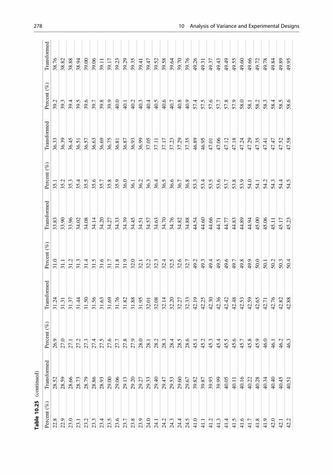
Table

10.25

(continued)

Percent(%

)Transform

edPercent(%

)Transform

edPercent(%

)Transform

edPercent(%

)Transform

edPercent(%

)Transform

ed

22.8

28.52

26.9

31.24

31.0

33.83

35.1

36.33

39.2

38.76

22.9

28.59

27.0

31.31

31.1

33.90

35.2

36.39

39.3

38.82

23.0

28.66

27.1

31.37

31.2

33.96

35.3

36.45

39.4

38.88

23.1

28.73

27.2

31.44

31.3

34.02

35.4

36.51

39.5

38.94

23.2

28.79

27.3

31.50

31.4

34.08

35.5

36.57

39.6

39.00

23.3

28.86

27.4

31.56

31.5

34.14

35.6

36.63

39.7

39.06

23.4

28.93

27.5

31.63

31.6

34.20

35.7

36.69

39.8

39.11

23.5

29.00

27.6

31.69

31.7

34.27

35.8

36.75

39.9

39.17

23.6

29.06

27.7

31.76

31.8

34.33

35.9

36.81

40.0

39.23

23.7

29.13

27.8

31.82

31.9

34.39

36.0

36.87

40.1

39.29

23.8

29.20

27.9

31.88

32.0

34.45

36.1

36.93

40.2

39.35

23.9

29.27

28.0

31.95

32.1

34.51

36.2

36.99

40.3

39.41

24.0

29.33

28.1

32.01

32.2

34.57

36.3

37.05

40.4

39.47

24.1

29.40

28.2

32.08

32.3

34.63

36.4

37.11

40.5

39.52

24.2

29.47

28.3

32.14

32.4

34.70

36.5

37.17

40.6

39.58

24.3

29.53

28.4

32.20

32.5

34.76

36.6

37.23

40.7

39.64

24.4

29.60

28.5

32.27

32.6

34.82

36.7

37.29

40.8

39.70

24.5

29.67

28.6

32.33

32.7

34.88

36.8

37.35

40.9

39.76

41.0

39.82

45.1

42.19

49.2

44.54

53.3

46.89

57.4

49.26

41.1

39.87

45.2

42.25

49.3

44.60

53.4

46.95

57.5

49.31

41.2

39.93

45.3

42.30

49.4

44.66

53.5

47.01

57.6

49.37

41.3

39.99

45.4

42.36

49.5

44.71

53.6

47.06

57.7

49.43

41.4

40.05

45.5

42.42

49.6

44.77

53.7

47.12

57.8

49.49

41.5

40.11

45.6

42.48

49.7

44.83

53.8

47.18

57.9

49.55

41.6

40.16

45.7

42.53

49.8

44.89

53.9

47.24

58.0

49.60

41.7

40.22

45.8

42.59

49.9

44.94

54.0

47.29

58.1

49.66

41.8

40.28

45.9

42.65

50.0

45.00

54.1

47.35

58.2

49.72

41.9

40.34

46.0

42.71

50.1

45.06

54.2

47.41

58.3

49.78

42.0

40.40

46.1

42.76

50.2

45.11

54.3

47.47

58.4

49.84

42.1

40.45

46.2

42.82

50.3

45.17

54.4

47.52

58.5

49.89

42.2

40.51

46.3

42.88

50.4

45.23

54.5

47.58

58.6

49.95

278 10 Analysis of Variance and Experimental Designs

42.3

40.57

46.4

42.94

50.5

45.29

54.6

47.64

58.7

50.01

42.4

40.63

46.5

42.99

50.6

45.34

54.7

47.70

58.8

50.07

42.5

40.69

46.6

43.05

50.7

45.40

54.8

47.75

58.9

50.13

42.6

40.74

46.7

43.11

50.8

45.46

54.9

47.81

59.0

50.18

42.7

40.80

46.8

43.17

50.9

45.52

55.0

47.87

59.1

50.24

42.8

40.86

46.9

43.22

51.0

45.57

55.1

47.93

59.2

50.30

42.9

40.92

47.0

43.28

51.1

45.63

55.2

47.98

59.3

50.36

43.0

40.98

47.1

43.34

51.2

45.69

55.3

48.04

59.4

50.42

43.1

41.03

47.2

43.39

51.3

45.74

55.4

48.10

59.5

50.48

43.2

41.09

47.3

43.45

51.4

45.80

55.5

48.16

59.6

50.53

43.3

41.15

47.4

43.51

51.5

45.86

55.6

48.22

59.7

50.59

43.4

41.21

47.5

43.57

51.6

45.92

55.7

48.27

59.8

50.65

43.5

41.27

47.6

43.62

51.7

45.97

55.8

48.33

59.9

50.71

43.6

41.32

47.7

43.68

51.8

46.03

55.9

48.39

60.0

50.77

43.7

41.38

47.8

43.74

51.9

46.09

56.0

48.45

60.1

50.83

43.8

41.44

47.9

43.80

52.0

46.15

56.1

48.50

60.2

50.89

43.9

41.50

48.0

43.85

52.1

46.20

56.2

48.56

60.3

50.94

44.0

41.55

48.1

43.91

52.2

46.26

56.3

48.62

60.4

51.00

44.1

41.61

48.2

43.97

52.3

46.32

56.4

48.68

60.5

51.06

44.2

41.67

48.3

44.03

52.4

46.38

56.5

48.73

60.6

51.12

44.3

41.73

48.4

44.08

52.5

46.43

56.6

48.79

60.7

51.18

44.4

41.78

48.5

44.14

52.6

46.49

56.7

48.85

60.8

51.24

44.5

41.84

48.6

44.20

52.7

46.55

56.8

48.91

60.9

51.30

44.6

41.90

48.7

44.26

52.8

46.61

56.9

48.97

61.0

51.35

44.7

41.96

48.8

44.31

52.9

46.66

57.0

49.02

61.1

51.41

44.8

42.02

48.9

44.37

53.0

46.72

57.1

49.08

61.2

51.47

44.9

42.07

49.0

44.43

53.1

46.78

57.2

49.14

61.3

51.53

45.0

42.13

49.1

44.48

53.2

46.83

57.3

49.20

61.4

51.59

61.5

51.65

65.6

54.09

69.7

56.60

73.8

59.21

77.9

61.96

61.6

51.71

65.7

54.15

69.8

56.66

73.9

59.28

78.0

62.03

61.7

51.77

65.8

54.21

69.9

56.73

74.0

59.34

78.1

62.10

61.8

51.83

65.9

54.27

70.0

56.79

74.1

59.41

78.2

62.17

61.9

51.88

66.0

54.33

70.1

56.85

74.2

59.47

78.3

62.24

(continued)

10.12 Incomplete Block Design 279

Table

10.25

(continued)

Percent(%

)Transform

edPercent(%

)Transform

edPercent(%

)Transform

edPercent(%

)Transform

edPercent(%

)Transform

ed

62.0

51.94

66.1

54.39

70.2

56.91

74.3

59.54

78.4

62.31

62.1

52.00

66.2

54.45

70.3

56.98

74.4

59.60

78.5

62.38

62.2

52.06

66.3

54.51

70.4

57.04

74.5

59.67

78.6

62.44

62.3

52.12

66.4

54.57

70.5

57.10

74.6

59.74

78.7

62.51

62.4

52.18

66.5

54.63

70.6

57.17

74.7

59.80

78.8

62.58

62.5

52.24

66.6

54.70

70.7

57.23

74.8

59.87

78.9

62.65

62.6

52.30

66.7

54.76

70.8

57.29

74.9

59.93

79.0

62.73

62.7

52.36

66.8

54.82

70.9

57.35

75.0

60.00

79.1

62.80

62.8

52.42

66.9

54.88

71.0

57.42

75.1

60.07

79.2

62.87

62.9

52.48

67.0

54.94

71.1

57.48

75.2

60.13

79.3

62.94

63.0

52.54

67.1

55.00

71.2

57.54

75.3

60.20

79.4

63.01

63.1

52.59

67.2

55.06

71.3

57.61

75.4

60.27

79.5

63.08

63.2

52.65

67.3

55.12

71.4

57.67

75.5

60.33

79.6

63.15

63.3

52.71

67.4

55.18

71.5

57.73

75.6

60.40

79.7

63.22

63.4

52.77

67.5

55.24

71.6

57.80

75.7

60.47

79.8

63.29

63.5

52.83

67.6

55.30

71.7

57.86

75.8

60.53

79.9

63.36

63.6

52.89

67.7

55.37

71.8

57.92

75.9

60.60

80.0

63.43

63.7

52.95

67.8

55.43

71.9

57.99

76.0

60.67

80.1

63.51

63.8

53.01

67.9

55.49

72.0

58.05

76.1

60.73

80.2

63.58

63.9

53.07

68.0

55.55

72.1

58.12

76.2

60.80

80.3

63.65

64.0

53.13

68.1

55.61

72.2

58.18

76.3

60.87

80.4

63.72

64.1

53.19

68.2

55.67

72.3

58.24

76.4

60.94

80.5

63.79

64.2

53.25

68.3

55.73

72.4

58.31

76.5

61.00

80.6

63.87

64.3

53.31

68.4

55.80

72.5

58.37

76.6

61.07

80.7

63.94

64.4

53.37

68.5

55.86

72.6

58.44

76.7

61.14

80.8

64.01

64.5

53.43

68.6

55.92

72.7

58.50

76.8

61.21

80.9

64.09

64.6

53.49

68.7

55.98

72.8

58.56

76.9

61.27

81.0

64.16

64.7

53.55

68.8

56.04

72.9

58.63

77.0

61.34

81.1

64.23

64.8

53.61

68.9

56.10

73.0

58.69

77.1

61.41

81.2

64.30

64.9

53.67

69.0

56.17

73.1

58.76

77.2

61.48

81.3

64.38

65.0

53.73

69.1

56.23

73.2

58.82

77.3

61.55

81.4

64.45

280 10 Analysis of Variance and Experimental Designs

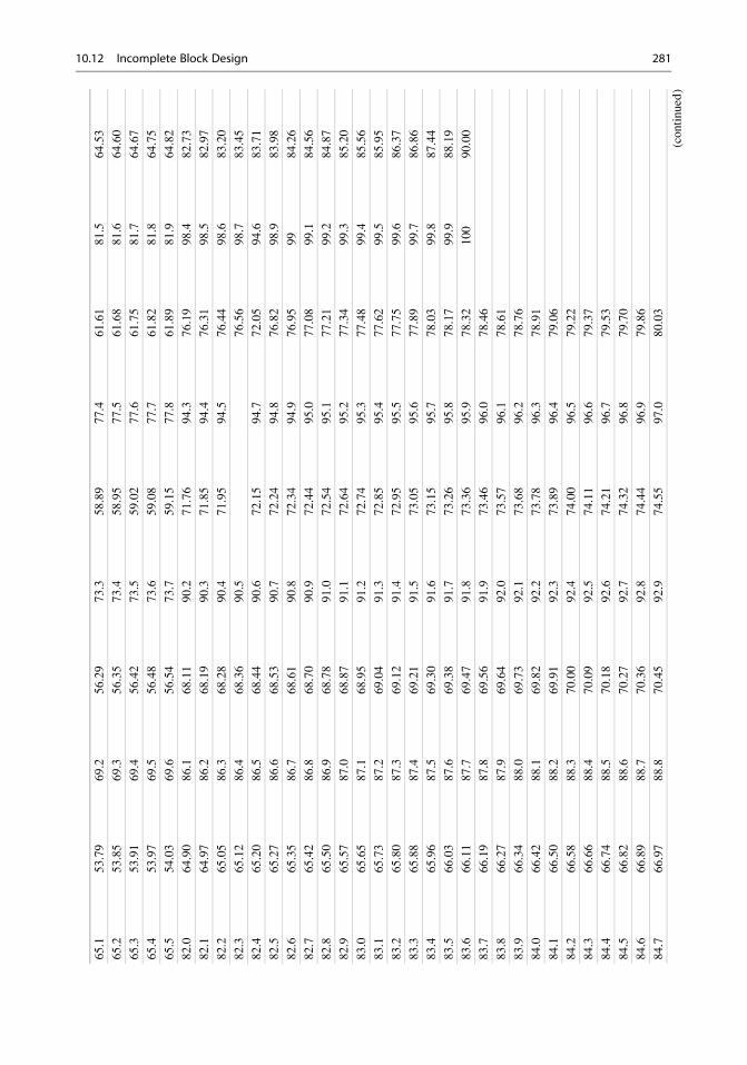
65.1

53.79

69.2

56.29

73.3

58.89

77.4

61.61

81.5

64.53

65.2

53.85

69.3

56.35

73.4

58.95

77.5

61.68

81.6

64.60

65.3

53.91

69.4

56.42

73.5

59.02

77.6

61.75

81.7

64.67

65.4

53.97

69.5

56.48

73.6

59.08

77.7

61.82

81.8

64.75

65.5

54.03

69.6

56.54

73.7

59.15

77.8

61.89

81.9

64.82

82.0

64.90

86.1

68.11

90.2

71.76

94.3

76.19

98.4

82.73

82.1

64.97

86.2

68.19

90.3

71.85

94.4

76.31

98.5

82.97

82.2

65.05

86.3

68.28

90.4

71.95

94.5

76.44

98.6

83.20

82.3

65.12

86.4

68.36

90.5

76.56

98.7

83.45

82.4

65.20

86.5

68.44

90.6

72.15

94.7

72.05

94.6

83.71

82.5

65.27

86.6

68.53

90.7

72.24

94.8

76.82

98.9

83.98

82.6

65.35

86.7

68.61

90.8

72.34

94.9

76.95

99

84.26

82.7

65.42

86.8

68.70

90.9

72.44

95.0

77.08

99.1

84.56

82.8

65.50

86.9

68.78

91.0

72.54

95.1

77.21

99.2

84.87

82.9

65.57

87.0

68.87

91.1

72.64

95.2

77.34

99.3

85.20

83.0

65.65

87.1

68.95

91.2

72.74

95.3

77.48

99.4

85.56

83.1

65.73

87.2

69.04

91.3

72.85

95.4

77.62

99.5

85.95

83.2

65.80

87.3

69.12

91.4

72.95

95.5

77.75

99.6

86.37

83.3

65.88

87.4

69.21

91.5

73.05

95.6

77.89

99.7

86.86

83.4

65.96

87.5

69.30

91.6

73.15

95.7

78.03

99.8

87.44

83.5

66.03

87.6

69.38

91.7

73.26

95.8

78.17

99.9

88.19

83.6

66.11

87.7

69.47

91.8

73.36

95.9

78.32

100

90.00

83.7

66.19

87.8

69.56

91.9

73.46

96.0

78.46

83.8

66.27

87.9

69.64

92.0

73.57

96.1

78.61

83.9

66.34

88.0

69.73

92.1

73.68

96.2

78.76

84.0

66.42

88.1

69.82

92.2

73.78

96.3

78.91

84.1

66.50

88.2

69.91

92.3

73.89

96.4

79.06

84.2

66.58

88.3

70.00

92.4

74.00

96.5

79.22

84.3

66.66

88.4

70.09

92.5

74.11

96.6

79.37

84.4

66.74

88.5

70.18

92.6

74.21

96.7

79.53

84.5

66.82

88.6

70.27

92.7

74.32

96.8

79.70

84.6

66.89

88.7

70.36

92.8

74.44

96.9

79.86

84.7

66.97

88.8

70.45

92.9

74.55

97.0

80.03

(continued)

10.12 Incomplete Block Design 281

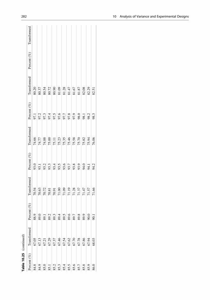
Table

10.25

(continued)

Percent(%

)Transform

edPercent(%

)Transform

edPercent(%

)Transform

edPercent(%

)Transform

edPercent(%

)Transform

ed

84.8

67.05

88.9

70.54

93.0

74.66

97.1

80.20

84.9

67.13

89.0

70.63

93.1

74.77

97.2

80.37

85.0

67.21

89.1

70.72

93.2

74.88

97.3

80.54

85.1

67.29

89.2

70.81

93.3

75.00

97.4

80.72

85.2

67.37

89.3

70.91

93.4

75.11

97.5

80.90

85.3

67.46

89.4

71.00

93.5

75.23

97.6

81.09

85.4

67.54

89.5

71.09

93.6

75.35

97.7

81.28

85.5

67.62

89.6

71.19

93.7

75.46

97.8

81.47

85.6

67.70

89.7

71.28

93.8

75.58

97.9

81.67

85.7

67.78

89.8

71.37

93.9

75.70

98.0

81.87

85.8

67.86

89.9

71.47

94.0

75.82

98.1

82.08

85.9

67.94

90.0

71.57

94.1

75.94

98.2

82.29

86.0

68.03

90.1

71.66

94.2

76.06

98.3

82.51

282 10 Analysis of Variance and Experimental Designs