A Dynamic Politico-Economic Modelof Intergenerational Contracts

Francesco Lancia and Alessia Russo1

March 3rd, 2014

Abstract

This paper proposes a dynamic politico-economic theory of intergenerational government spend-

ing. We embed a repeated voting system in an overlapping generations model with human capital

accumulation. The aim is to study how democratic institutions settle intergenerational disagree-

ment over the allocation of the public budget. We characterize the Markov-perfect equilibrium of

the voting game, as well as its welfare properties. We find that (i) the political empowerment of

elderly agents acts as a disciplining mechanism for adults, so as to provide durable public invest-

ments; (ii) high elderly-targeted transfers do not necessarily dampen public investments; and (iii)

a high degree of intergenerational disagreement over the allocation of the public budget leads to

high growth. The equilibrium can reproduce some salient features of intergenerational accounting

in the U.S.

Keywords: Human capital, intergenerational contract, intergenerational disagreement, Markov-

perfect equilibrium, repeated voting, social planner.

JEL Classification: D72, E62, H23, H30, H53.

1Francesco Lancia, University of Vienna, Email: francesco.lancia@univie.ac.at. Alessia Russo, University of Oslo, Email:alessia.russo@econ.uio.no. We are grateful for valuable comments from Graziella Bertocchi, Marco Bassetto, Roland Ben-abou, Michele Boldrin, Alejandro Cunat, Vincenzo Denicolo, Bard Harstad, David K. Levine, Anirban Mitra, Nicola Pavoni,Karl Schlag, Paolo Siconolfi, Kjetil Storesletten, and Fabrizio Zilibotti. We also thank the seminar participants at the NBERSummer Institute Meeting in Income Distribution and Macroeconomics, the 2011 SED Annual Meeting in Ghent, theNSF/NBER/CEME Conference in Mathematical Economics and General Equilibrium Theory in New York, the XV Work-shop on Macroeconomic Dynamics in Vigo, the 2nd Conference on Recent Development in Macroeconomics in Mannheim,and 8th Workshop on Macroeconomic Theory in Pavia, as well as the seminar participants at the Bank of Italy, ETH in Zurichand the Universities of Bologna, Louvain, Milan, Modena, Napoli, Oslo, and Vienna for useful discussions. All errors are ourown.

Why should I care about future generations? What have they done for me?” (Groucho Marx)

1 IntroductionThe challenges involved in sustaining intergenerational welfare programs are prominent in the

current political debate. In modern societies, electoral campaigns often serve as a battleground,

with opposing parties fiercely defending their positions by either promising more generous pub-

lic spending or arguing the financial unsustainability of public programs. Such political disputes pit

young against old and taxpayers against recipients, especially when balanced-budget restrictions ap-

ply. Accordingly, it becomes crucial to explore (i) how democratic institutions settle intergenerational

disagreement over the allocation of public budgets; and (ii) the extent to which the current welfare

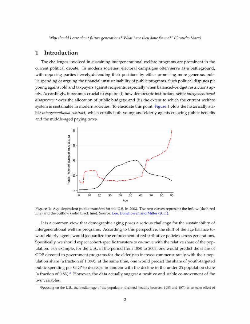
system is sustainable in modern societies. To elucidate this point, Figure 1 plots the historically sta-

ble intergenerational contract, which entails both young and elderly agents enjoying public benefits

and the middle-aged paying taxes.

010

2030

40Pu

blic

Tra

nsfe

rs (U

nits

of 1

000

U.S

. $)

0 10 20 30 40 50 60 70 80 90Age

Figure 1: Age-dependent public transfers for the U.S. in 2003. The two curves represent the inflow (dash redline) and the outflow (solid black line). Source: Lee, Donehower, and Miller (2011).

It is a common view that demographic aging poses a serious challenge for the sustainability of

intergenerational welfare programs. According to this perspective, the shift of the age balance to-

ward elderly agents would jeopardize the enforcement of redistributive policies across generations.

Specifically, we should expect cohort-specific transfers to co-move with the relative share of the pop-

ulation. For example, for the U.S., in the period from 1980 to 2003, one would predict the share of

GDP devoted to government programs for the elderly to increase commensurately with their pop-

ulation share (a fraction of 1.089); at the same time, one would predict the share of youth-targeted

public spending per GDP to decrease in tandem with the decline in the under-25 population share

(a fraction of 0.85).2 However, the data actually suggest a positive and stable co-movement of the

two variables.2Focusing on the U.S., the median age of the population declined steadily between 1955 and 1970 as an echo effect of

2

.05

.055

.06

.065

Shar

e of

GD

P

1980 1984 1988 1992 1996 2000 2004Year

Panel (a)

.041

.042

.043

.044

.045

Shar

e of

GD

P

1980 1984 1988 1992 1996 2000 2004Year

Panel (b)

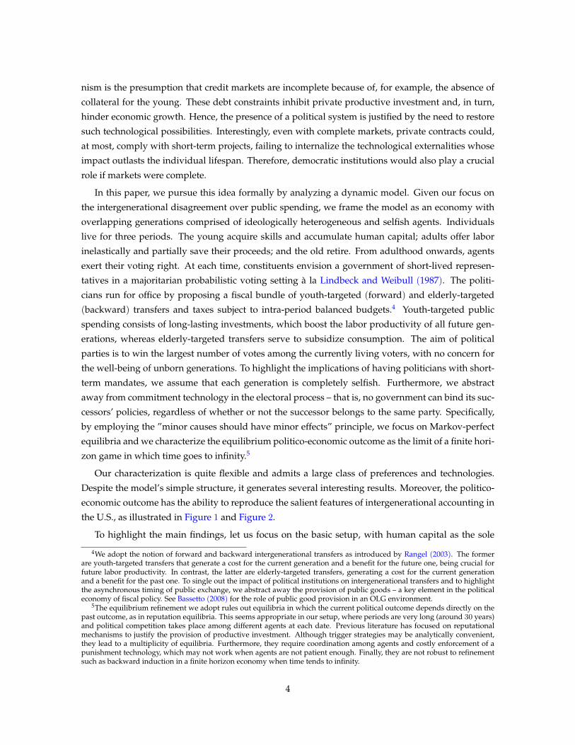
Figure 2: Cohort-specific public inflow for the U.S. in the period 1980-2003. Panel (a) plots the GDP-ratioof public spending for social security and health case. Panel (b) plots the GDP-ratio of public spending foreducation. Source: Lee, Donehower, and Miller (2011).

As Figure 2 highlights, while public spending on the elderly (including Social Security and health

care) has grown by a factor of 1.196, public spending for the young (including education) has grown

by a factor of 1.06. The scope of this study is to provide a tractable dynamic politico-economic theory

of intergenerational government spending that addresses this seeming puzzle.

Our main idea is driven by the following observation. In a graying society, elderly constituents

show a large propensity to vote and form a single-minded voting block, which makes them an in-

creasingly prized electoral group.3 Insofar as the political imbalance in favor of elderly voters trans-

lates into a large claim over future production, both youth-targeted and elderly-targeted government

spending can be simultaneously implemented as an outcome of the electoral competition. The in-

tuition is the following. Forward-looking voters anticipate that they will peddle their political influence

when they are old and that will be rewarded for the sacrifices they made as adults. Therefore, they provide

youth-targeted public spending, requiring that it be durable and productive. This simple argument can

explain the counter-intuitive simultaneous co-movement of age-targeted public spending and also

the difference from what is expected solely from shifts in the demographic structure. The proposed

mechanism merits two additional qualifications. First, the expected political power assigned to future

elderly constituents also implies a commensurate claim on public spending by current elders, which

may compromise the strategic channel previously highlighted. We show that crowding-out (-in)

effects of elderly-targeted spending on youth-targeted programs ultimately depend on primitives

of the model, such as the intertemporal elasticity of substitution. Second, underlying the mecha-

the baby boom and began to increase in the 1970s. At the same time, the fraction of the elderly – people aged 65+ – inthe population steadily increased, whereas the fraction of youths – people under the age of 25 – in the population steadilydecreased (Source: U.N.). The simultaneous variation in both the median age and the relative cohort size had an impactboth on the financial solvency of the public system – since the share of recipients increased, while the share of contributorsdecreased – and on the outcome of the voting competition – as the population aged, so did the voters.

3As Galasso and Profeta (2004) report, in some countries, the elderly have a higher turnout rate at elections in comparisonto the young and to adults. For example, in the U.S., the turnout rate among those aged 60-69 is twice as high as amongthe young (19-29 years). Furthermore, according to Mulligan and Xala-i-Martin (1996), while young citizens disperse theirpolitical interests among different and often contrasting issues, their older counterparts are likely to target fewer programs,such as Social Security and Medicare, while making their voting decisions.

3

nism is the presumption that credit markets are incomplete because of, for example, the absence of

collateral for the young. These debt constraints inhibit private productive investment and, in turn,

hinder economic growth. Hence, the presence of a political system is justified by the need to restore

such technological possibilities. Interestingly, even with complete markets, private contracts could,

at most, comply with short-term projects, failing to internalize the technological externalities whose

impact outlasts the individual lifespan. Therefore, democratic institutions would also play a crucial

role if markets were complete.

In this paper, we pursue this idea formally by analyzing a dynamic model. Given our focus on

the intergenerational disagreement over public spending, we frame the model as an economy with

overlapping generations comprised of ideologically heterogeneous and selfish agents. Individuals

live for three periods. The young acquire skills and accumulate human capital; adults offer labor

inelastically and partially save their proceeds; and the old retire. From adulthood onwards, agents

exert their voting right. At each time, constituents envision a government of short-lived represen-

tatives in a majoritarian probabilistic voting setting a la Lindbeck and Weibull (1987). The politi-

cians run for office by proposing a fiscal bundle of youth-targeted (forward) and elderly-targeted

(backward) transfers and taxes subject to intra-period balanced budgets.4 Youth-targeted public

spending consists of long-lasting investments, which boost the labor productivity of all future gen-

erations, whereas elderly-targeted transfers serve to subsidize consumption. The aim of political

parties is to win the largest number of votes among the currently living voters, with no concern for

the well-being of unborn generations. To highlight the implications of having politicians with short-

term mandates, we assume that each generation is completely selfish. Furthermore, we abstract

away from commitment technology in the electoral process – that is, no government can bind its suc-

cessors’ policies, regardless of whether or not the successor belongs to the same party. Specifically,

by employing the ”minor causes should have minor effects” principle, we focus on Markov-perfect

equilibria and we characterize the equilibrium politico-economic outcome as the limit of a finite hori-

zon game in which time goes to infinity.5

Our characterization is quite flexible and admits a large class of preferences and technologies.

Despite the model’s simple structure, it generates several interesting results. Moreover, the politico-

economic outcome has the ability to reproduce the salient features of intergenerational accounting in

the U.S., as illustrated in Figure 1 and Figure 2.

To highlight the main findings, let us focus on the basic setup, with human capital as the sole

4We adopt the notion of forward and backward intergenerational transfers as introduced by Rangel (2003). The formerare youth-targeted transfers that generate a cost for the current generation and a benefit for the future one, being crucial forfuture labor productivity. In contrast, the latter are elderly-targeted transfers, generating a cost for the current generationand a benefit for the past one. To single out the impact of political institutions on intergenerational transfers and to highlightthe asynchronous timing of public exchange, we abstract away the provision of public goods – a key element in the politicaleconomy of fiscal policy. See Bassetto (2008) for the role of public good provision in an OLG environment.

5The equilibrium refinement we adopt rules out equilibria in which the current political outcome depends directly on thepast outcome, as in reputation equilibria. This seems appropriate in our setup, where periods are very long (around 30 years)and political competition takes place among different agents at each date. Previous literature has focused on reputationalmechanisms to justify the provision of productive investment. Although trigger strategies may be analytically convenient,they lead to a multiplicity of equilibria. Furthermore, they require coordination among agents and costly enforcement of apunishment technology, which may not work when agents are not patient enough. Finally, they are not robust to refinementsuch as backward induction in a finite horizon economy when time tends to infinity.

4

payoff-relevant state variable. In this stylized economy, the unique source of disagreement among

cohorts lies in the difference in lifespan. Elderly voters aim to maximize the current benefits, whereas

adult constituents also are concerned about next-period wealth. None of them has a personal inter-

est in fostering the stock of human capital in society. Nevertheless, our model predicts that the

existence of a Markov-perfect equilibrium, which attains a growth-enhancing intergenerational contract,

does not require pre-commitment through the establishment of institutions that outlive the current govern-

ment and bind future decision-makers. In a probabilistic voting framework and in the absence of storage

technologies, expected consumption possibilities are related solely to the generations’ prospects for

democratically claiming part of future production via transfers. Accordingly, the empowerment of the

elderly cohort acts as a credible disciplining device for adults to provide public investments. When the relative

political clout of the elderly is large enough, the political outcome entails a self-enforcing intergen-

erational contract with both forward and backward transfers activated in equilibrium. Clearly, the

redistributive scheme works only if the cost of providing forward transfers is at least compensated

by the expected benefit of receiving backward transfers when old. At high values of intertemporal

elasticity of substitution, the model predicts a hump-shaped relationship between the political influ-

ence of elderly voters – and, in turn, the amount of enforced backward transfers – and the provision

of productive transfers – and, in turn, the attained rate of economic growth.

Remarkably, the existence of a growth-enhancing intergenerational contract hinges on the absence

of commitment technology. If the current government invested too little, then the future officeholder

would necessarily punish the generations that were alive under the former government. Indeed,

given the strategic complementarity between human capital and backward transfers, lacking pro-

ductive investments would restrict the public budget possibilities of future constituents. The less the

former government cares for future generations, the harsher the punishment will be. Therefore, it is

the expected punishment that disciplines all governments and discourages them from underinvest-

ment.

When a private storage technology is available, an additional source of intergenerational dis-

agreement arises, which is rooted in the difference in ownership of productive factors, as well as in

the source of income. As a measure of the technological complementarity among assets, the elas-

ticity of factor substitution is also interpreted as a proxy for economic disagreement between workers

and retirees. From this perspective, less complementarity among assets exacerbates the conflict of

interest between different owners of the factors of production. We show that the greater the degree

of economic disagreement over government spending, the lower is the economic growth. Intuitively, when

productive assets are technologically closer complements, the rate of return on physical capital turns

out to be more responsive to a variation of the intergenerational transfers, through a simultaneous

adjustment of both physical and human capital. The increase of the interest rate due to a positive

variation of forward and backward transfers depresses the present value of next-period backward

transfers as internalized by current adults. As a consequence, less economic disagreement implies

a smaller amount of enforced backward transfers and – through their weaker disciplinary valence –

poorer productive investments. Ultimately, this leads to lower economic growth. This effect appears

5

only in overlapping generation economies with long-lasting productive spending – a novelty in the

literature. Furthermore, this finding provides new fundamentals to the theory, which recognizes the

link between the elasticity of substitution in technology and economic growth (Klump and De La

Grandville, 2000).

Finally, we contrast the results with an environment in which intergenerational transfers are del-

egated to a benevolent social planner who attaches independent decaying weights to all future gen-

erations. We emphasize the case of a small open economy in which the electoral competition among

short-term-mandate policy-makers plunges the economy into the efficient allocation. The outcome

hinges on the absence of pecuniary externalities. Indeed, in a closed economy, in which productive

assets are complements, the interdependence of the political wedges via price precludes the possibil-

ity of attaining the efficient allocation via democratic institutions.

Our theoretical mechanism involves two fundamental aspects: (i) the nature of short-term agree-

ments among politicians and current living voters – i.e., the absence of commitment; and (ii) the

prospect of follow-up intergenerational contracts, which serves as a disciplining device to implement

current policies. Clearly, there are many extensions that fit into this setting. Prominent examples of

forward transfers are government decisions on how much to invest in the public infrastructure or

in environmental preservation and R&D. Similar to human capital investments, these programs en-

tail a transfer to future generations that is financed through taxes paid by current generations and

whose benefits are long-lasting. Future compensation through backward transfers can take the form

of pension, health assistance, and, generally, elderly-targeted public good provision.

2 Related LiteratureThis paper augments the literature on dynamic politico-economic models with overlapping gen-

erations that incorporates forward-looking decision makers in a multidimensional policy space (Kru-

sell, Quadrini, and Rıos-Rull, 1997). Previous literature has highlighted altruism (Tabellini, 1991),

public good provision (Bassetto, 2008; Hassler, Storesletten, and Zilibotti, 2007; and Song, Storeslet-

ten, and Zilibotti, 2012), and reputation mechanisms (Bellettini and Berti Ceroni, 1999; and Rangel,

2003) to justify the emergence of an intergenerational contract. While recognizing the theoretical rel-

evance of these channels, we emphasize the role played purely by political institutions and strategic

incentives: The willingness of each adult generation to transfer wealth to the elderly and the young

hinges on its beliefs that the same thing will happen in the subsequent time period via an established

and effective institution, such as democratic voting.

Adopting an approach similar to ours, recent works have developed models of Social Security

in a repeated voting environment. We focus, in particular, on the contributions by Azariadis and

Galasso (2002), Forni (2005), and Gonzalez-Eiras and Niepelt (2008), which are based largely on the

pioneering work of Grossman and Helpman (1998). Unlike in our case, most of their findings exhibit

indeterminacy in equilibrium. Moreover, they have focused only on backward transfers, whereas our

theory recognizes the fundamental link between productive and redistributive public spending as a

social-policy-package deal.

6

Closer in spirit to our work are Gonzalez-Eiras and Niepelt (2012) and Chen and Song (2013). Un-

like in our study, the former analyze a richer demographic environment with elastic labor supply and

endogenous retirement age. Despite this complexity, they find an analytical solution of the Markov-

perfect equilibrium. This comes at the cost of some simplifying assumptions on the parametric form

of preferences and technologies. In the studied case of log-preferences and Cobb-Douglas produc-

tion, strategic effects are mute, and the crowding in of backward transfers on productive investments

is an equilibrium outcome only if the retirement decision is endogenous. As a main departure, we

elucidate contingencies of crowding in and crowding out in the two-sided welfare program for more

flexible preferences and technologies and point out the role of political institutions instead of de-

mographic aging. Chen and Song (2013) develop a dynamic theory of Social Security with sole

private investments in human capital to figure out the puzzling negative correlation between wage

inequality and the size of government. The main prediction is that a larger level of human capital

corresponds to a lower amount of backward transfers. Abstracting from issues of inequality, our

model encompasses the authors’ mechanism as a particular case: With exogenous prices, positive

transfers to the elderly reduce the level of physical capital, which, in turn, increases future payroll

taxes, exactly as human capital does in their framework.

To the best of our knowledge, none of the existing papers have provided an implicit character-

ization of the general-equilibrium politico-economic outcome and posited implications in terms of

welfare analysis, as we do here.6

The remainder of the paper is organized as follows. Section 3 describes the model’s environment.

Section 4 discusses the social planner’s allocation and provides the criterion for the welfare compar-

ison. Section 5 introduces the equilibrium concept. Section 6 presents the main results. Section 7

describes two analytical examples. Section 8 illustrates the quantitative experiments. Finally, Section

9 concludes. All proofs are contained in the Appendix.

3 The ModelConsider an overlapping generation (OLG) economy inhabited by an infinite number of ideolog-

ically heterogeneous agents, living up to three periods: young, adult, and old. i ∈ a, o labels the

adult and elderly cohorts, respectively. Agents of different ages differ in their wealth holdings. Time

is discrete, indexed by t, and runs from zero to infinity. The population grows at a constant rate ν−1;

thus, the mass of the adult generation born at time t− 1 and living at time t is equal to N t−1t = νtN0.

At each time, two short-lived parties, denoted by ιt ∈ Lt,Rt, run for office by proposing a political

platform to maximize the probability of winning the election without commitment to future policies.

6Battaglini and Coate (2007) have explored how pork-barrel spending affects the overall size of government and distortsinvestment in public capital goods. They have focused on the efficiency of the steady-state level of taxation and allocationof the public budget. Unlike us, they have studied an environment in which infinite-living agents make policy decisions bylegislative bargaining.

7

3.1 Households

An agent j born at time t− 1 and living at time t evaluates consumption and ideology according

to the following additive intertemporal (non-altruistic) utility function:

u (cat ) + ςaj,ιt + βEιt[u(cot+1

)+ ςoj,ιt+1

](1)

where β ∈ (0, 1) is the individual discount factor, and Eιt [·] is the expectation operator, which is

conditional on the political platform implemented by the current incumbent party. The random

variable ςij,ιt summarizes the utility derived by agent j belonging to cohort i at time t from political

factors that are orthogonal to consumption (to be discussed later in more detail).

Assumption 1 (Utility) The function u : R+ → R+ is twice continuously differentiable, strictly increasing

and concave, and it satisfies the usual Inada conditions.

cat denotes the consumption at time t when adult, and cot+1 represents the consumption at time

t+ 1 when old. In the first period of life, individuals do not consume. When young, agents spend all

of their time endowment in acquiring skills if productive forward transfers, fιt , are publicly provided,

without having access to private credit markets. In the absence of government intervention, the

debt constraint faced by the young would inhibit human capital formation.7 As adults, individuals

inelastically supply labor and use their income, wtht, taxed at a flat rate, zιt , for consumption and

saving, st. When old, agents retire and consume their total income equal to the sum of savings

capitalized at a gross rate of return Rt+1 and the backward transfers, bιt , that their children pass to

them in the form of a PAYGO system. Thus, the individual budget constraints for the adult and

elderly agents are, respectively, as follows:

cat + st ≤ (1− zιt)wtht (2)

cot+1 ≤ Rt+1st + bιt+1 (3)

At the initial time t = 0, the economy is endowed with an exogenous amount of physical and

human capital, k0, h0. Hence, the budget constraint of the initial adult agent is equal to ca0 =

(1− zι0)w0h0 − s0, whereas the budget constraint of the initial elderly agent is co0 = R0k0 + bι0 .

3.2 Technology

At each time t, the economy produces a single homogeneous private good, Yt ≡ ytN t−1t , combin-

ing aggregate physical capital, Kt ≡ ktN t−1t , which depreciates fully after one period, and aggregate

human capital, Ht ≡ htN t−1t , according to the following technology (expressed in per-capita units):

yt = Θ (kt, ht)

7The debt constraint faced by the young – which is familiar in the literature of self-enforcing contracts – can be motivatedby several factors. For example, Kehoe and Levine (2001) show that debt constraints arise due to the inalienability of cer-tain types of assets, primarily human capital. In this scenario, as in Boldrin and Montes (2005), the presence of a politicalsystem is justified by the need to finance the provision of public spending, which would otherwise preclude the young fromaccumulating human capital.

8

Assumption 2 (Production) The function Θ : R2+ → R+ exhibits a constant return to scale, and it is

strictly monotonic increasing and weakly concave in each of the two inputs with Θ (0, ht), Θ (kt, 0) ≥ 0 and

Θkt,ht , Θht,kt ≥ 0.

By Assumption 2, it follows that yt = htΘ(ktht, 1)≡ htϑ

(kt

)and, in turn, yt = ϑ

(kt

), where

yt and kt refer to the per-efficiency units of the final good and the physical capital, respectively. The

inverse demand functions for factor prices are Θkt = ϑkt and Θht = ϑ(kt

)− ktϑkt . The elasticity

of factor substitution is denoted by ζ. The human capital of an adult born at time t is produced

according to a technology, which combines forward transfers, fιt , and parental human capital, ht, as

complementary factors:

ht+1 = Φ (fιt , ht)

Assumption 3 (Human Capital) The function Φ : R2+ → R+ exhibits a constant return to scale, and it is

strictly monotonic increasing and strictly concave in each of the two inputs with Φ (0, ht), Φ (fιt , 0) ≥ 0 and

Φfιt ,ht , Φht,fιt > 0.

By Assumption 3, a higher level of knowledge attained by one generation reduces the cost of the

next generation to achieve the same level. Furthermore, ht+1 = htΦ(fιtht, 1)≡ htϕ

(fιt

), where fιt

denotes the per-efficiency units of productive transfers. It follows that the growth rate of human

capital is equal to ht+1

ht= ϕ

(fιt

). The marginal impact of forward transfers and parental human

capital on human capital production are Φfιt = ϕfιtand Φht = ϕ

(fιt

)− fιtϕfιt , respectively.8

3.3 Fiscal Constitution

At each date, short-term-mandate governments, democratically elected by their constituents, use

their fiscal authority to transfer income across different age groups. The transfers simultaneously

serve the political scope of the elected representatives and the economic needs of their constituents.

We assume that politicians are prevented from borrowing. Thus, the public balance must hold in

every period, which implies the following:

zιtwthtNt−1t = bιtN

t−2t + fιtN

tt (4)

where the collection zιt , bιt , fιt represents the age-targeted fiscal bundle.9 At each time t, Eq. (4)

reduces the multidimensionality of the political platform to a bi-dimensional plan bιt , fιt, where

the fiscal feasibility conditions require that bιt ∈[0, bt

]and fιt ∈

[0, ft

]with bt ≡ νwtht and ft ≡

8For clarity of exposition, we adopt the following notation. Let xt = x (qt, pt) and pt = p (qt) be functions of the variable

qt. Then, xqt ≡ ∂xt∂qt

and xqt,qt ≡ ∂2xt∂qt∂qt

denote the first and second partial derivative, respectively. Furthermore, dxtdqt

≡∂xt∂qt

+ ∂xt∂pt

∂pt∂qt

represents the total derivative.9In the national accountability of many countries, taxes are transfer-targeted. Social Security contributions cover the bene-

fits of elderly agents, whereas income taxes cover public spending, such as human capital investment. However, in a frame-work with inelastic labor supply and a balanced budget, such an alternative formulation would not compromise the results.

Indeed, Eq. (4) would be equivalent to modeling two separate government budgets, as zbιtwtht =bιtν

and zfιtwtht = νfιt ,where zbιt is the Social Security contribution, and zfιt is the income tax rate.

9

wthtν . The non-negativity constraint for backward transfers can be justified by either the ever-binding

participation constraint of elderly voters or the ability of the older generation to manage an active

lobby group. Suppose that elderly agents were required to pay transfers to future generations. Then,

they would default on their obligations, and the economy would revert to intergenerational autarky.

Definition 1 (Intergenerational Contract) An intergenerational contract is a mutual political agreement

that simultaneously enforces backward and forward transfers.

4 Social Planner AllocationBefore describing the outcome under political competition, we characterize the efficient alloca-

tion implemented by a benevolent social planner who chooses the sequence cat , cot , ft, kt+1, ht+1∞t=0

to maximize the discounted utility of all generations.10 Following Farhi and Werning (2007), the

planner attaches geometrically decaying Pareto weight, δ ∈ (0, 1), to the discounted utility of each

dynasty. Varying δ yields all the allocation possibilities on the Pareto frontier. Given the initial level

of physical and human capital, the sequential formulation of the social planner’s problem is as fol-

lows:

maxcat ,cot+1,ft,ht+1,kt+1∞

t=0

∞∑t=0

δt(u (cat ) + βu

(cot+1

))+β

δu (co0)

subject to the aggregate resource constraint and human capital technology:

cat +cotν

+ νkt+1 + νft −Θ (kt, ht) ≤ 0, ∀t(κtδt

)ht+1 − Φ (ft, ht) ≤ 0, ∀t

(%t+1δ

t+1)

where (κtδt) and(%t+1δ

t+1)

are the associated Lagrangian multipliers. Removing the functional

arguments for expositional clarity, the first-order conditions of the Lagrangian are equal to:

cat : ucat = κt

cot : νβucot = κtδ

ft : νκt = %t+1δΦft

ht+1 : %t+1 = κt+1Θht+1+ %t+2δΦht+1

kt+1 : νκt = κt+1δΘkt+1

together with the transversality conditions – i.e., limt→∞

κtδtkt+1 = 0 and limt→∞

%t+1δt+1ht+1 = 0. Elim-

inating the multipliers from the first-order conditions, the following wedges for the optimal alloca-

tions must be satisfied:

0 = ucat − βΘkt+1ucot+1

(5)

10Gonzalez-Eiras and Niepelt (2008) show that in the absence of binding non-negativity constraints on tax rates, tax distor-tions, and intragenerational inequality, the Ramsey policy with full commitment supports the social planner allocation.

10

Eq. (5) describes the conventional consumption-savings Euler condition and, in turn, the optimal

accumulation of physical capital. The social planner chooses kt+1 to equate the marginal cost in

terms of forgone consumption to the discounted marginal benefits of savings.

0 = νβucot − δucat (6)

The second condition captures the intra-temporal redistribution wedge between the current adult

and elderly cohorts. The social planner is concerned for future generations and does not redistribute

resources from unborn generations to current ones. Thus, the redistributive wedge is entirely de-

termined by the Pareto weight. At each time, the utility of the elderly generation is weighted νβδ ,

reflecting the social planner’s bias toward either adult (δ > νβ) or elderly (δ < νβ) agents. In the

special case with dynastic discounting – that is, if the planner’s weights reflect the discount factor

of the household as well as the cohort size – the optimal policy aims at equalizing the per-capita

consumption of all cohorts in each period.

0 = Φft −Θkt+1

Θht+1

(1− εt+1) (7)

Finally, Eq. (7) describes the productive wedge where εt+1 ≡ νΘkt+1

ΦftΦht+1

Φft+1denotes the intergener-

ational externalities of human capital expressed as a fraction of the cost of investment. Specifically,

it quantifies the impact of productive spending on the utility of adults in terms of current cost and

discounted marginal benefits, through the channels of parental human capital. Despite the infinite

persistence of the productive investment, only the current and subsequent periods matter directly.

Hence, Eq. (7) can be viewed as resulting from a variational (two-period) problem. In other words,

let us think of our variational argument as follows: given the state variables kt, ht and kt+2, ht+2,let us vary kt+1, ht+1 through the controls ft to obtain the highest possible utility.

Definition 2 (Social Planner Allocation) Given the initial conditions k0, h0, the social planner alloca-

tion is defined as a sequencecat , c

ot , ft, kt+1, ht+1

∞t=0

such that for all t ≥ 0, Eqs. (5), (6), and (7), jointly

with the transversality conditions, are satisfied.

5 Politico-Economic EquilibriumWe characterize the politico-economic equilibrium of the economy as a subgame perfect equilib-

rium. Within each time period, the sequence of moves is as follows:

i. A new generation of young people is born.

ii. Before the realization of the ideological shocks among voters, office-seeking candidates demo-

cratically compete by proposing their political platforms.

iii. All uncertainty is realized, and agents vote for their preferred candidates.

iv. The winning candidate implements the proposed political platform.

11

v. Agents save and firms hire workers and rent capital.

vi. The older generation dies; the young and adult generations age and become adult and old, re-

spectively.

Within a given period, the sequential politico-economic game can be viewed as Stackelberg, and

it is solved by backward induction. This procedure entails the standard fixed-point problem, which

nests two interdependent parts. First, given policies, adults determine the individual savings level

and firms produce the homogeneous final good (competitive economic equilibrium). Second, to

maximize the probability of winning the election, short-lived office-seeking politicians promise vot-

ers an age-targeted fiscal bundle (politico-economic equilibrium). We assume that all expectations

about subsequent events are correct and that all promises are honored. The fixed-point problem

requires consistency of the laws of motion for policies that underlie the competitive economic equi-

librium with the political selection.

5.1 Competitive Economic Equilibrium

In a competitive economic equilibrium, each adult individual j chooses her lifetime consumption,

taking factor prices and fiscal policies as given. Maximizing Eq. (1) subject to individual budget

constraints, Eqs. (2) and (3), and the feasibility constraints, cat ≥ 0, cot+1 ≥ 0, and st ≥ 0, yields the

standard Euler condition for savings:

ucat ≥ βEιt[Rt+1ucot+1

](8)

Resulting from Eq. (8), the equilibrium private savings is defined as the functional equation st =

S(Iιt , kt+1, bιt+1

), with Iιt ≡ wtht − νfιt −

bιtν . Hence, conditional on the current and next-period

political platforms, S (·) maps the after-tax earnings for adults and the aggregate savings into the

optimal individual savings. Under full depreciation, the level of saving completely determines the

dynamics of physical capital.

Firms produce in a perfectly competitive environment. They choose the level of inputs to maxi-

mize profits – i.e., maxkt,ht

[Θ (kt, ht) − wtht − Rtkt]. Firms’ optimality and market clearing imply that

factor prices are given by the marginal productivity of each factor:

wt = Θht (9)

Rt = Θkt (10)

Definition 3 (Competitive Economic Equilibrium) Given the initial conditions k0, h0 and the sequence

of policies bιt , fιt∞t=0, a competitive economic equilibrium is defined as a sequence of allocations cat , cot , kt+1, ht+1∞t=0

and factor prices wt, Rt∞t=0 such that for all t ≥ 0:

i. The allocation solves the maximization problem of adults – i.e., Eq. (8) is satisfied;

ii. The factor prices are consistent with the profit maximization of firms – i.e., Eqs. (9) and (10) are satisfied;

12

iii. The market for the private good clears – i.e., cat +cotν + νfιt + νkt+1 = Θ (kt, ht);

iv. The market for physical capital clears – i.e.:

νkt+1 = S(Iιt , kt+1, bιt+1

)(11)

The indirect utility of any individual belonging to the adult and elderly cohorts is, respectively,

equal to:

Waιt≡ u

(Ca(kt, ht, kt+1, bιt , f ιt

))+βEιt

[u(Co(kt+1, ht+1, bιt+1

))](12)

and

Woιt≡ u

(Co(kt, ht, bιt

))(13)

where the individual consumption levels, cat = Ca (kt, ht, kt+1, bιt , fιt) ≡ Iιt − νkt+1 and cot+1 =

Co(kt+1, ht+1, bιt+1

)≡ νRt+1kt+1 + bιt+1

, are obtained by plugging Eqs. (9), (10), and (11) into Eqs.

(2) and (3). When taxation and public spending are precluded, intergenerational autarky yields

Wt ≡ maxstu (cat ) + βu

(cot+1

)| It = wth0.

Definition 4 (Equilibrium Feasible Allocation) Given the initial conditions k0, h0, an equilibrium fea-

sible allocation is a sequence of competitive economic equilibrium allocations cat , cot , kt+1, ht+1∞t=0, factor

prices wt, Rt∞t=0, and policies bιt , fιt∞t=0 that satisfy the balanced budget constraint, Eq. (4), and the

fiscal feasibility conditions at each time t.

5.2 Electoral Competition

In this section, we describe how short-lived office-seeking parties interact in electoral compe-

titions. Public policies are chosen through a repeated voting system according to majority rule.

The young have no political power. The utility derived from political factors, ςij,ιt , embeds two

components: an idiosyncratic ideological bias, σij , and an aggregate ideological bias, η. Formally,

ςij,ιt =(σij + η

)Iιt , where Iιt is an indicator function such that IRt = 1 and ILt = 0. A zero value of

ςij,ιt indicates the neutrality of voters’ ideology, whereas a positive value reveals that an individual

j prefers the candidate belonging to party Rt to the candidate’s opponent. Precisely, the random

variable σij reflects the voters’ opinions about the candidate’s positions (e.g., civil rights, pro-market

rules, religious issues) and personal characteristics (e.g., honesty, leadership, trustworthiness). As

it is drawn from cohort-specific distributions, individuals belonging to the same cohort may vote

differently. The additional random variable η measures the average candidates’ popularity. Thus,

individuals belonging to different cohorts may support the same party. For simplicity, we assume

both shocks to be i.i.d. over time and uniformly distributed with densities σi and η, respectively.

By modeling the political mechanism as a probabilistic voting model a la Lindbeck and Weibull

(1987) – adapted to an OLG environment with intergenerational transfers – at each time t, the parties

propose the same political platform in equilibrium. No candidate is able to change current policies

to obtain a net gain in the number of votes. Hence, they set policies so that the marginal effect on the

13

probability of being (re)elected of the last unit invested is actually zero.11 Using Eqs. (12) and (13),

the equilibrium political platform maximizes a weighted sum of the adult and elderly voters’ utility

as follows:

νWat (kt, ht, kt+1, bt, ft, bt+1) + φWo

t (kt, ht, bt) (14)

The parameter φ ≡ σo

σa ∈ [0,∞) has a structural interpretation: it is a synthetic measure that captures

the political clout – or single-mindedness – of voters belonging to the elderly cohort relative to the

adult cohort. In the limit, when φ approaches infinity, the dictatorship of old agents shapes the insti-

tutional process. The elderly cohort forms a single-minded ideological block, ready to compromise

their partisan loyalties in return for particularistic benefits. When φ = 0, the opposite holds. That

is, the adults hold the only relevant ideological position in the political competition.12 As Eq. (14)

displays, the adoption of a probabilistic voting framework acknowledges not only political factors,

but also demographic characteristics. The pure mass effect is summarized by the relative cohort size,

which weights the indirect utility of each generation.

5.3 Markov-Perfect Equilibrium

We now characterize the subgame perfect equilibrium of the intergenerational voting game. At

each time t, the implementation of a political platform induces dynamic linkages of policies across

periods through the evolution of the asset variables. Fully rational voters internalize such dynamic

effects, which influence their strategic position over time. In principle, the construction of policies

contingent on alternative histories and enforced by reputation mechanisms allows for multiple sub-

game perfect equilibria. We rule out such mechanisms and focus instead on differentiable stationary

Markov policies as equilibrium refinement.13 The payoff-relevant state variables for the political can-

didates are the assets held by the pivotal constituents at each time – i.e., physical and human capital.

In a probabilistic voting environment, when voters condition their strategies on those assets, the

intergenerational contract is enforced and sustained even in a finite-horizon economy. Thus, the

equilibrium characterized here corresponds to the limits of a finite-horizon game. The objects we

are interested in are the intergenerational policy rules and the rules governing the evolution of both

physical and human capital.

Definition 5 (Markov-Perfect Equilibrium) Given the initial conditions k0, h0, a Markov-perfect equi-

librium is an equilibrium feasible allocation such that, for each t ≥ 0, the differentiable policy rules B :

R+ × R+ →[0, bt

]and F : R+ × R+ →

[0, ft

]and the private decision rule K : R+ × R+ → R+ satisfy

the following points:11Probabilistic voting has been extensively studied both theoretically and empirically. Stromberg (2008) adopts this type of

electoral competition to study presidential races in the U.S. and shows the suitability of the model in explaining candidates’behavior. An explicit microfoundation of the probabilistic voting game is provided in the supplementary material in AppendixB.

12An alternative interpretation of φ is in terms of effectiveness of intergenerational political power. On the one hand, itreflects the existence of formal institutions committed to guaranteeing active and passive political participation (i.e., candidacyage, electoral rules, lobby power, voting enfranchisement). On the other hand, it measures how informal institutions alter theage-cohorts’ representativeness (i.e., civil society, clientelism, corruption, social norms, culture).

13Markov perfectness implies that outcomes are history-dependent only on the fundamental state variables. The stationarypart is introduced to focus on equilibrium policy rules that do not depend on calendar time. The differentiable part is aconvenient requirement to avoid the multiplicity of equilibrium outcomes and to give clear positive predictions.

14

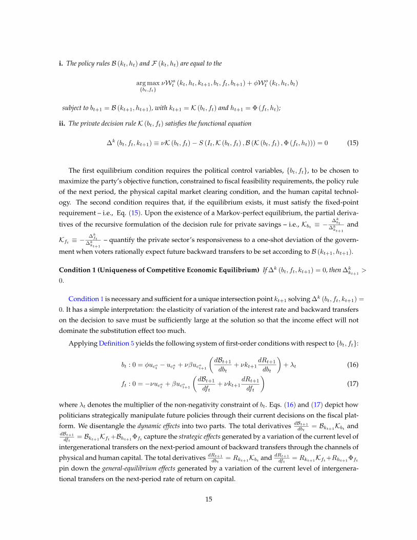
i. The policy rules B (kt, ht) and F (kt, ht) are equal to the

arg maxbt,ft

νWat (kt, ht, kt+1, bt, ft, bt+1) + φWo

t (kt, ht, bt)

subject to bt+1 = B (kt+1, ht+1), with kt+1 = K (bt, ft) and ht+1 = Φ (ft, ht);

ii. The private decision rule K (bt, ft) satisfies the functional equation

∆k (bt, ft, kt+1) ≡ νK (bt, ft)− S (It,K (bt, ft) ,B (K (bt, ft) ,Φ (ft, ht))) = 0 (15)

The first equilibrium condition requires the political control variables, bt, ft, to be chosen to

maximize the party’s objective function, constrained to fiscal feasibility requirements, the policy rule

of the next period, the physical capital market clearing condition, and the human capital technol-

ogy. The second condition requires that, if the equilibrium exists, it must satisfy the fixed-point

requirement – i.e., Eq. (15). Upon the existence of a Markov-perfect equilibrium, the partial deriva-

tives of the recursive formulation of the decision rule for private savings – i.e., Kbt ≡ −∆kbt

∆kkt+1

and

Kft ≡ −∆kft

∆kkt+1

– quantify the private sector’s responsiveness to a one-shot deviation of the govern-

ment when voters rationally expect future backward transfers to be set according to B (kt+1, ht+1).

Condition 1 (Uniqueness of Competitive Economic Equilibrium) If ∆k (bt, ft, kt+1) = 0, then ∆kkt+1

>

0.

Condition 1 is necessary and sufficient for a unique intersection point kt+1 solving ∆k (bt, ft, kt+1) =

0. It has a simple interpretation: the elasticity of variation of the interest rate and backward transfers

on the decision to save must be sufficiently large at the solution so that the income effect will not

dominate the substitution effect too much.

Applying Definition 5 yields the following system of first-order conditions with respect to bt, ft:

bt : 0 = φucot − ucat + νβucot+1

(dBt+1

dbt+ νkt+1

dRt+1

dbt

)+ λt (16)

ft : 0 = −νucat + βucot+1

(dBt+1

dft+ νkt+1

dRt+1

dft

)(17)

where λt denotes the multiplier of the non-negativity constraint of bt. Eqs. (16) and (17) depict how

politicians strategically manipulate future policies through their current decisions on the fiscal plat-

form. We disentangle the dynamic effects into two parts. The total derivatives dBt+1

dbt= Bkt+1

Kbt anddBt+1

dft= Bkt+1

Kft+Bht+1Φft capture the strategic effects generated by a variation of the current level of

intergenerational transfers on the next-period amount of backward transfers through the channels of

physical and human capital. The total derivatives dRt+1

dbt= Rkt+1Kbt and dRt+1

dft= Rkt+1Kft+Rht+1Φft

pin down the general-equilibrium effects generated by a variation of the current level of intergenera-

tional transfers on the next-period rate of return on capital.

15

According to Eq. (16), the solution for the backward transfers features three components: (i) the

direct effect on the individual consumption of redistributing resources from tax-payers to tax recip-

ients; (ii) the expected benefits on the consumption of the next-period elderly voters; and (iii) the

tightness of the fiscal constraint relative to the non-negativity of backward transfers. Eq. (17) yields

the trade-off for the current adults between public investments and private savings. On the one

hand, an increase in the total fiscal burden raises the opportunity cost of saving. On the other hand,

the sacrifices suffered by the current taxpayers will be rewarded by higher next-period consumption

through an adjustment of backward transfers and a positive variation in the market interest rate.

6 Intergenerational ContractsIn this section, we characterize the Markov-perfect equilibrium under two headings. To highlight

the main mechanism at work, the first analyzes the basic setup with human capital as the sole payoff-

relevant state variable. The second adds physical capital to the analysis and discusses how elderly

voters’s private wealth alters the politico-economic outcome.

6.1 Human Capital

In this context, we abstract away the general-equilibrium effects via prices, and we isolate the

institutional channel of political competition as the sole determinant of the emergence of a growth-

enhancing intergenerational contract.14 The absence of physical capital destroys the dynamic link-

ages across backward policies. Assuming interior solutions, the redistributive wedge is determined

entirely by the political clout of currently living voters. The equilibrium condition described by Eq.

(16) boils down to the following:

0 = φucot − ucat (18)

Agents’ consumption turns out to be a constant share of the total outcome. The higher the degree

of elderly voters’ relative single-mindedness – i.e., the larger the φ – the lower will be the marginal

rate of intergenerational substitution,ucotucat

, which measures the consumption tightness among agents.

Thus, elderly voters’ bigger relative political clout implies a larger share of public resources devoted to backward

transfers and, in turn, a more unbalanced distribution of consumption in their favor. At the same time, Eq.

(17) collapses to the following:

0 = −νucat + βucot+1Bht+1

Φft (19)

According to Eq. (19), the marginal cost of current taxation borne by adults will be offset by the

marginal benefits of larger next-period consumption. Expected consumption possibilities are related

to the generations’ prospect of democratically claiming part of the future returns of current public

investments via backward transfers.

Proposition 1 (Political Empowerment) An intergenerational contract is enforced if and only if φ > 0,

and it satisfies Bht > 0 and Fht > 0.14The absence of a general-equilibrium effect can be derived as an equilibrium outcome in the context of small open

economies. The link between strategic effects and international capital mobility is further explored in Section 7.1, wherewe provide analytical solutions of the equilibrium policy rules.

16

The proof for the result is the following. In the absence of physical capital, elderly agents have

no private wealth, and bt = 0 whenever φ = 0 for each date t. This implies that Bht+1= 0 and,

by inspecting Eq. (19), there is no productive investment – i.e., ft = 0. In contrast, suppose that

φ > 0 and ft = 0; then, from Eq. (18), bt > 0 for each period t. This cannot be an equilibrium,

as ft = 0 and, in turn, ht+1 = 0 implies bt+1 = 0. The second part of the Proposition hinges on

the forward-looking behavior of constituents and on Assumption 3: accordingly, the sole way to

maximize the voters’ utility entails a positive equilibrium relation between human capital and both

sides of intergenerational transfers. Thus, in equilibrium, backward and forward transfers become

increasing functions of the stock of human capital.

The discontinuity of the mapping F (ht) at φ = 0 highlights the dramatic impact of democratic

institutions in settling intergenerational disagreements and, in turn, enforcing intergenerational con-

tracts. Although our economy encompasses the well-known median voter framework as a degener-

ative case of political competition, Proposition 1 stresses a new neat prediction: when elderly agents

are disempowered – i.e., φ = 0 – voters fail to support productive and durable public spending,

although a growth-enhancing technology is at their disposal. Thus, the economy reverts to inter-

generational autarky. In contrast, if the elderly constituents actively participate in the public debate,

then they will extract a political rent in the form of backward transfers by exerting their electoral in-

fluence. At the same time, adult voters will support productive policies, as they are entitled to grab

a larger share of the next-period production.

In our model, the agents’ concern for future backward transfers is key to enforcing the intergen-

erational contract, given the lack of intergenerational altruism. Therefore, the existence of a Markov-

perfect equilibrium that attains a growth-enhancing intergenerational contract does not require pre-

commitment through the establishment of an institution that outlives the current government and

binds future decision-makers. Rather, the empowerment of the elderly cohort acts as the sole disciplining

mechanism for adults to support public investments.15

6.1.1 Political Power and Growth

In view of Proposition 1, the two redistributive sides of the intergenerational contract are strongly

interrelated. To investigate the nature of such a link, let ρ+ ≡ φBht+1

Bht+1

,φ and ρ− ≡ucot+1

ucot

ddφ

(φucotucot+1

)denote the elasticities of the variation of φ, respectively, on the marginal impact of human capital on

backward transfers and on the marginal rate of substitution between the current and next-period

elderly cohort, weighted by the relative political clout of the elderly voters.

Proposition 2 (Single-Mindedness and Growth) dftdφ≥ (<) 0 if and only if ρ+≥ (<) ρ−.

Proof (See Appendix).15In an OLG economy inhabited by finitely lived players, the assumption of a three-period lifespan might appear unnec-

essarily restrictive. In a more general framework with T periods, the working-age cohorts would support human capitalinvestment to increase their future wealth, just as they were willing to accumulate physical capital in the presence of storagetechnology. These incentives arise irrespective of the implemented voting mechanism that assigns political voice to differentgenerations (see Chen and Song, 2013). Although the extension of the model to a T -period setting would partially under-mine the quantitative impact of the strategic channel, our mechanism remains in place from a qualitative perspective. Indeed,before retiring, the working-aged still have incentives to politically support forward transfers to offspring and increase rentopportunities after retiring.

17

An increase in φ has a two-fold impact on the intergenerational contract. On the one hand, it

alters the distribution of consumption in favor of the current elderly constituents: a higher degree

of elderly voters’ relative single-mindedness positively affects the amount of enforced backward

transfers and, in turn, the consumption level of retirees, measured by ρ−. On the other hand, it

improves the future political ability of current adults to extract an electoral rent – in the form of social

insurance – generated by current public investments, quantified by ρ+. Proposition 2 predicts that

if the latter effect prevails, then the larger φ, the more resources are allocated to growth-enhancing

technology. Therefore, as long as redistribution is crucial to reaching social consensus for growth-oriented

policies, higher redistribution of public resources may enhance growth. From this perspective, our theory

reconciles the existing literature’s contrasting conclusions, which have emphasized a relation of both

strategic complementarity and substitutability between intergenerational welfare programs.16

To further qualify the properties of the equilibrium policy rules, Figure 3 graphs forward transfers

against backward transfers, as captured by a variation of φ, for two different levels of intertemporal

elasticity of substitution.17

0 0.2 0.4 0.60.04

0.05

0.06

0.07

0.08Panel (a): GDP-share of f

GDP-share of b0 0.2 0.4 0.6

0.04

0.06

0.08

0.1

0.12Panel (b): GDP-share of f

GDP-share of b

Figure 3: Intergenerational redistribution and economic growth. Panels (a) and (b) plot the equilibrium relationbetween B (ht) and F (ht) in per-efficiency units, when the inverse of the intertemporal elasticity of substitutionacquires the values 0.7 and 2, respectively.

Two observations can be made. First, when agents’ utility is less responsive to changes in con-

sumption, the model predicts a hump-shaped relationship between the provision of backward and

forward transfers and, in turn, the rate of economic growth. Indeed, at low levels of elderly single-

mindedness, an increase in φ induces a variation in ρ+ that offsets the variation in ρ−. The overall

effect reverses at high levels of the relative political clout of elderly constituents (Panel (a)). Second,

16Following the pioneering work of Becker and Murphy (1988), Rangel (2003) emphasizes how voters support publicinvestment because a trigger strategy links investment spending to the future provision of public pensions. Furthermore,Gonzalez-Eiras and Niepelt (2012) have documented the boost of the GDP share of Social Security transfers and public in-vestment as a response to a large increase in the retirement age. In contrast, recent politico-economic models of growth(Alesina and Rodrick, 1994; Persson and Tabellini, 1994; and Azzimonti, 2011) have suggested that political disagreementover the composition of public expenditures leads to extensive redistribution, which depresses growth. As long as partiescompete to retain power via the democratic process, politicians tend to be endogenously short-sighted, and the economyexperiences underinvestment in productive assets.

17Appendix B provides the quantitative framework to replicate Figure 3.

18

the model also predicts that a higher curvature of utility over consumption implies a monotonically

decreasing relation between sustainable public investments and pro-elderly spending (Panel (b)).

6.2 Physical Capital

When a private storage technology is available, the definition of property rights on produc-

tion inputs creates divergent economic interests among cohorts, straining intergenerational coop-

eration. Furthermore, the general-equilibrium effects may add to the analysis and shape the politico-

economic outcome in tandem with the strategic effects. Nevertheless, we show that the core re-

sults of an economy with sole human capital still characterize an environment with savings. As in

Proposition 1, if φ > 0, then an intergenerational contract exists. By contrast, the following remark

acknowledges the case with φ = 0.

Remark 1 (Indeterminacy) When φ = 0, there exists a continuum of undetermined intergenerational con-

tracts.

In the case of adults’ dictatorship, the marginal utility of middle-aged voters is invariant to

changes in the fiscal bundle since agents privately respond through an automatic adjustment of sav-

ings decisions. Therefore, indeterminacy affects the equilibrium outcome. A way to break down

indeterminacy is to introduce some degree of commitment. This is what probabilistic voting does.18

When φ > 0, the political sustainability of the intergenerational contract – either in the presence

or in the absence of general-equilibrium effects – does not rely on self-fulfilling expectations of fu-

ture agreements, but on politico-economic fundamentals that are payoff-relevant state variables for

future constituents. The equilibrium policies directly affect the marginal utility of current elderly

agents and, in turn, the marginal rate of intergenerational substitution. Therefore, the enforced inter-

generational transfers uniquely pin down the consumption level of the old cohort.

Proposition 3 (Necessary Condition) In any intergenerational contract enforced as a Markov-perfect equi-

librium, the dynamic effects of forward transfers are larger than the dynamic effects of backward transfers.

Proof (See Appendix).

Proposition 3 reveals the intertemporal structural relations among policies, which guarantee the

simultaneous enforcement of forward and backward transfers via democratic elections. The sum of

the marginal impacts of public investments on next-period backward benefits and prices is required

to be larger than the sum of the marginal impacts generated by current backward transfers. By con-

trast, if dBt+1

dft+ νkt+1

dRt+1

dftwere smaller or equal to dBt+1

dbt+ νkt+1

dRt+1

dbt, then to maximize the voters’

utility, it would be sufficient to support intergenerational cooperation over backward transfers with-

out investments.18The literature has proposed alternative ways to break down indeterminacy. For example, Azariadis and Galasso (2002)

have established a fiscal constitution, which allows generations to use veto power. However, a general critique asks why asociety that can agree on sophisticated constitutional constraints is not able to agree on the efficient outcome in the first place.Closer to the spirit of this paper are Bassetto (2008) and Gonzalez-Eiras and Niepelt (2008). Whereas the former deals withindeterminacy by assuming that policies are the outcome of a bargaining process, the latter obtains a unique politico-economicequilibrium by modeling political competition with probabilistic voting. We adopt a solution similar to that of Gonzalez-Eirasand Niepelt, and we obtain a unique Markov-perfect equilibrium in a multidimensional state space.

19

To highlight how the dynamic effects influence the enforced intergenerational contract, we rewrite

the political first-order conditions in per-efficiency units by adopting the notation introduced in Sec-

tion 3.2. The state space conveniently reduces to a one-dimensional space, with kt as the state vari-

able. Assuming an interior solution, an envelope argument implies that Eq. (16) now reads as

follows:

0 = φucot −

1− νϕtRt+1

Bkt+1Kbt︸ ︷︷ ︸

Sbt

−

Gbt︷ ︸︸ ︷ν2 kt+1

Rt+1Rkt+1

Kbt

ucat = 0 (20)

where Sbt and Gbt denote, respectively, the strategic and the general-equilibrium effects in per-efficiency

units, generated by bt. Eq. (20) yields the political redistributive wedge, where Υt ≡ 1 − Sbt − Gbtrepresents the endogenous political weight of adult voters as internalized by politicians. A change

in the ratio Υtφ spawns relevant implications in terms of intergenerational inequality. Formally,

higher (lower) endogenous political weight of adult relative to elderly voters corresponds to a higher

(lower) marginal rate of intergenerational substitution and, in turn, to a more skewed distribution of

consumption in favor of the adult (elderly) cohort. Suppose, for example, that Gbt = 0 because of the

negligible impact of assets on prices; then the following Proposition holds.

Proposition 4 (Strategic Substitutability) When the general-equilibrium effects are mute, the Markov-

perfect equilibrium satisfies Bkt+1< 0.

Proof (See Appendix).

When pecuniary externalities are absent, Proposition 4 establishes a decreasing relation between

elderly-targeted transfers and asset variables. Note that, if φ = 0, then Bkt+1= −νR and multi-

ple stationary equilibria – indexed by a free parameter – emerge, consistent with Remark 1. In this

context, the equilibrium policies are obtained as the maximization of adults’ life-cycle utility. The

middle-aged face a trade-off between a more generous next-period Social Security – as measured

by Sbt – and a more effective self-insurance through private savings. In equilibrium, this scheme

prompts a strategic substitutability between public subsidies and private assets. When φ > 0, the

backward policies are set so as to maximize adults’ life-cycle utility in tandem with current elderly

voters’ short-term gains. This additional component weakens the initial trade-off. However, it does

not overturn the substitutability relation between private savings and backward transfers. This out-

come departs from the complementarity result obtained by Grossman and Helpman (1998) for high

levels of elderly political weight, and it hinges on the nonlinearity of voters’ preference.

When the channel of prices is activated, voters also anticipate the general-equilibrium effects

induced by backward policies. By Condition 1, intergenerational transfers have an unambiguous

depressive impact on the accumulation of the asset variable that boosts the rate of return on capital.

Therefore, Gbt is non-negative and partially offsets the strategic benefits via policies. As will be quan-

tified in Section 8 – depending on the intertemporal elasticity of substitution – such a counteracting

force may alter the strategic substitutability relation between private savings and social insurance.

20

We will also document that the magnitude of enforced backward transfers depends negatively on

the degree of complementarity among productive assets.

We conclude this section by taking a closer look at the intergenerational externalities associated

with productive investments. Combining Eqs. (16) and (17) with the equilibrium response of the

saving rate to a variation of current policies – Kbt and Kft – yields the political productive wedge:

0 = ϕft −Rt+1

wt+1(1− εt+1) (21)

where εt+1 ≡ 1 − νϕtwt+1

Rt+1

φucot(It+ϕt

bt+1Rt+1

)ucat−Itφucot

quantifies the human capital externalities in the

politico-economic equilibrium, expressed as a fraction of the cost of investment.19 Eq. (21) illustrates

an interesting property. When εt+1 > 0, office-seeking politicians internalize, at least to some ex-

tent, the inter-temporal externalities generated by current forward transfers. Due to the overlapping

demographic structure and the presence of parental human capital, politicians evaluate the utility

of current living voters, anticipating the expectation of future generations over policies that will be

credibly proposed by future governments. An inspection of Eq. (21) shows that, ceteris paribus,

larger expected backward transfers correspond to greater εt+1 – that is, to a stronger internalization

of the human capital externalities through the channel of rent extraction. It leads to more disci-

plined politicians and to higher economic growth. However, as the amount of enforceable backward

transfers is called into question by technological complementarity, so is its disciplinary impact on

enforceable forward transfers. We return to this point in Section 8.

To sum up: for our theory to apply, the following two fundamental elements of the model must

be identified: (i) the prospect of follow-up intergenerational contracts, which serves as a disciplining device

to implement current policies; and (ii) the nature of short-term agreements among politicians and current

constituents – i.e., the absence of commitment. To clarify the role of commitment, suppose that policy-

makers were able to sign binding long-term agreements with current living voters. Because repre-

sentatives run for office with the aim of being elected following the current political campaign, the

intergenerational contract they may commit to will be, at most, a two-period agreement. In the best

scenario, they will promise current adults that they will fully expropriate the next-period generation

and use the proceeds to subsidize current adults’ consumption when they are old. As a consequence,

the amount of pledgeable income devoted to productive investment would be such that the marginal

rate of transformation equals the opportunity cost of savings, disregarding the effects of externalities

associated with forward transfers. In contrast, in a politico-economic equilibrium without commit-

ment, εt+1 may differ from zero and attain higher economic growth.

19When εt+1 = 0, Eq. (21) is equivalent to the necessary condition of a competitive equilibrium with no credit marketconstraints, where the young can borrow money at the market interest rate.

21

7 Illustrative ExamplesWe now explore the properties of the politico-economic equilibrium under two different economic

environments by providing analytical solutions of the equilibrium policy rules and inspecting their

welfare properties. In the first case, we examine a small open economy. The negligible impact of

domestic capital formation on the world interest rate implies the absence of general-equilibrium ef-

fects. In the second case, we focus on a closed economy. The lack of international capital mobility

gives rise to general-equilibrium effects via prices. We emphasize that democratic institutions en-

force an efficient intergenerational contract when the sole strategic effects influence the economic

system. In both examples, the Markov-perfect equilibrium is obtained as the limit of a finite-horizon

equilibrium whose characteristics do not significantly depend on the time horizon, as long as it is

long enough. We parameterize (i) the preferences over private consumption as the logarithmic type,

u (c) = log (c); and (ii) the human capital and the final good technologies as the Cobb-Douglas form,

ht+1 = Ahθt f1−θt and yt = Bkαt h

1−αt , respectively, with α, θ ∈ (0, 1), and the factor productivity

parameters A, B ≥ 1.

7.1 Small Open Economy

Capital is perfectly mobile. We denote the (exogenous) world interest rate by R and the workers’

per-efficiency wage byw. In a competitive equilibrium, kt =(αBR

) 11−α ht andw = (1− α)B

(αBR

) α1−α .

Hence, the world interest rate uniquely pins down the ratio of the factors of production. According

to Eq. (17), the political productive wedge collapses to dBt+1

dft= νR. Furthermore, from Eq. (16), the

endogenous weight that politicians attach to adults simplifies to Υt+1 = 1 − νRdBt+1

dbt. Proposition 3

predicts that dBt+1

dft> dBt+1

dbt– that is, the strategic effect generated by a variation on current public

investment in the next-period backward benefits is required to be larger than the strategic linkage

between the two successive backward policies.

Lemma 1 (Human Capital Externality) Let m : R+ → R+ be a differentiable single-valued mapping

m(ψ(j)) ≡(AθνR ψ(j) + wA(1−θ)

R

) 1θ

with ψ(1) ≡(wA(1−θ)(φ+αβ(φ+ν))

R(1+αβ)(φ+ν)

) 1θ

as the initial condition. For R >

Aνθ, the first-order nonlinear equation ψ(j+1) = m(ψ(j)) has a unique, locally stable, fixed point equal to ψ.20

Proof (See Appendix).

The fixed point ψ analytically quantifies the human capital externalities as internalized by policy-

makers when proposing their welfare programs. A natural comparative statics is that ψ is decreasing

in the market interest rate. This is intuitive since higher a return of private assets discourages agents

from supporting intergenerational welfare schemes. Furthermore, in the limit, when the share of

parental human capital θ approaches zero, human capital externalities vanish. Let R (φ) ≡ φ+νββ ϕ

denote the implicit net return of Social Security in equilibrium, where ϕ is the economy growth rate.

Using Lemma 1, the following Proposition holds.

20The subscript in the parentheses denotes the number of iterations.

22

Proposition 5 (Equilibrium in a Small Open Economy) WhenR = R (φ), there exists a unique Markov-

perfect equilibrium characterized by the following set of policy functions and laws of motion for the state vari-

ables:

i. bt = B (kt, ht) = − ν2R(1+β)φ+ν(1+β)kt + φν

φ+ν(1+β)

(w + νθ

1−θψ)ht;

ii. ft = F (ht) = ψht;

iii. kt+1 = Rβφ+νβkt +

βR(w−νψ)(φ+ν(1+β))−φ(βR+νAψ1−θ)(w+ θν1−θψ)

νR(1+β)(φ+νβ) ht;

iv. ht+1 = Aψ1−θht.

Proof (See Appendix).

When R = R (φ), agents are indifferent between individual savings and Social Security. The

Markov-perfect equilibrium delivers intergenerational transfers, the strategic effects of which are not

mute. At each time, politicians can influence future policies by varying capital formation through

the current fiscal platform. Consistent with Proposition 4, backward transfers turn out to be a non-

increasing linear function of physical capital and an increasing linear function of human capital. The

equilibrium predictions for forward transfers are easily illustrated. Assumption 3 reveals that the

sole way to maximize the utility of adult constituents requires a positive relation between human

capital and forward transfers. Since the political preferences of the old do not depend on productive

spending, physical capital retained by elderly constituents is not a payoff-relevant state variable for

forward-oriented policies. Moreover, public investments are not influenced by the degree of single-

mindedness among cohorts. This result is an application of Proposition 2 to a small open economy.

Under perfect capital mobility, adults privately respond to a reassessment of relative political clout

by optimally reallocating consumption over time through an automatic adjustment of savings deci-

sions. Inasmuch as the borrowing constraint does not bind, voters always freely allocate their wealth

holdings. Finally, the rate of economic growth amounts to ϕ = Aψ1−θ, and the long-term solution

converges to the balanced growth path in one period.21

Note that there can be no intergenerational contracts with R > R (φ). In this circumstance, voters

would replace social insurance with self-insurance through private saving, accumulating an ever-

increasing stock of physical capital. As elderly agents become richer, they would be required to

use part of their proceeds to subsidize the consumption of future generations, thereby violating the

feasibility constraint of backward transfers. In contrast, it is possible that R < R (φ). In this context,

there exists a unique stationary equilibrium in which the government taxes a share of the adults’

income and uses the proceeds to provide forward transfers and to subsidize the consumption of

elderly agents.

21The introduction of distortionary capital taxation and credit market frictions compromises the costless adjustment of in-dividual saving decisions to a reassessment of political power. In this case, the amount of forward transfers would be affectedby the voters’ ideological distribution. Assessing the relative impact of capital taxation and stricter borrowing constraints onthe equilibrium intergenerational contract is left to future research.

23

Proposition 6 (Equilibrium in a Small Open Economy) WhenR < R (φ), there exists a unique Markov-

perfect equilibrium characterized by the following set of policy functions and laws of motion for the state vari-

ables:

i. bt = B (ht) = νwφφ+ν(1+β(1−θ))ht;

ii. ft = F (ht) = wβ(1−θ)φ+ν(1+β(1−θ))ht;

iii. ht+1 = A(

β(1−θ)φ+ν(1+β(1−θ))

)1−θht.

Proof (See Appendix).

When the implicit net return of Social Security is larger than the world interest rate, voters substi-

tute private savings with public transfers, and, in turn, the economy converges to zero private assets

after one period, whereas human capital accumulates progressively. Hence, intergenerational trans-

fers are not a function of physical capital, and politics fosters economic growth by means of human

capital formation at the rate ϕ = A(

β(1−θ)φ+ν(1+β(1−θ))

)1−θ.

To evaluate political performance, we compare the Markov-perfect equilibrium with the social

planner allocation as described in Definition 2. Let R (δ) ≡ νδ ϕ denote the optimal implicit net return

of Social Security, where ϕ is the efficient growth rate.

Proposition 7 (Efficiency in a Small Open Economy) There always exists a pair of political and welfare

weights φ, δ and market interest rate R such that the Markov-perfect equilibrium coincides with the social

planner allocation.

Proof (See Appendix).

Proposition 7 draws an interesting result. In a small open economy, there always exists a config-

uration of feasible weights such that both office-seeking politicians and the social planner attain an

implicit return of Social Security that corresponds to the market interest rate – i.e.,R = R (φ) = R (δ).

Thus, bt = bt. In this scenario, the inefficient accumulation of human capital may potentially be the

sole concern for political distortion. Nevertheless, as the government fully rewards the generations

for the sacrifices borne by adults via backward transfers, it succeeds, through democratic competi-

tion, in implementing efficient long-term productive investment – namely, ft = ft. Our result relates

to Barro (1974), in which altruistic motives and gifts/bequests are replaced by the political empower-

ment of elderly agents and backward transfers, respectively. In a similar fashion, in an OLG economy

populated by selfish agents, current generations act essentially as though they were infinite-lived, as

long as they are linked to future generations by a chain of operative intergenerational transfers.

Note that the optimal implicit return of pensions is determined entirely by the welfare weight.

This feature has a counterintuitive implication. For example, consider the case with δ sufficiently

large: We might have a configuration where the optimal allocation reverts to intergenerational au-

tarky, whereas the politico-economic equilibrium sustains intergenerational cooperation. Although

24

the social planner has concerns for future generations, R might be so high that the implicit return

of Social Security promised by the social planner falls short of the market interest rate. Thus, the

economy reverts to intergenerational autarky. Conversely, in the political setting, φ might be high

enough to have backward transfers at least as profitable as private assets and intergenerational co-

operation enforced as equilibrium outcome. Generalizing, there exists a range of high (low) welfare

weights such that the implicit net return of Social Security is lower (higher) in the optimal alloca-

tion than in the corresponding Markov-perfect equilibrium, implying a lower (higher) amount of

intergenerational transfers.

7.2 Closed Economy

Suppose that access to the international capital market is precluded. Then, in a competitive equi-

librium, Rt = αBkα−1t h1−α

t and wt = (1− α)Bkαt h−αt . We show that there exists a unique inter-

generational contract enforced as a Markov-perfect equilibrium of the voting game, whose delivered

policy rules are linear functions of the final production.

Proposition 8 (Equilibrium in a Closed Economy) When φ ≥ φ ≡ αν(1+β(1−θ(1−α)))1−α , there exists a

unique Markov-perfect equilibrium characterized by the following set of policy functions and laws of motion

for the state variables:

i. bt = B (kt, ht) = ν(φ−α(φ+ν(1+β(1−(1−α)θ))))φ+ν(1+β(1−(1−α)θ)) yt;

ii. ft = F (ht, kt) = β(1−θ)(1−α)φ+ν(1+β(1−(1−α)θ))yt;

iii. kt+1 = αβ(1+αβ)φ+αβ(φ+ν(1+β(1−(1−α)θ)))yt;

iv. ht+1 = A(

Bβ(1−θ)(1−α)φ+ν(1+β(1−θ(1−α)))

)1−θkα(1−θ)t h

1−α(1−θ)t .

Proof (See Appendix).

As long as φ ≥ φ, both backward and forward transfers are financed through flat taxes paid by

the middle-aged cohort. Unlike the previous case, adult constituents now internalize the strategic

effect in concert with the general-equilibrium effect. Therefore, they finance the current investment

in human capital anticipating the induced variation on both the next-period rate of return on private

savings and the amount of backward transfers. In view of Proposition 8, intergenerational transfers

are increasing functions of the asset variables. Under logarithmic preferences, private saving and So-

cial Security act as complementary factors, flipping the strategic substitutability relation highlighted

in Proposition 4. The Markov-perfect equilibrium converges to a balanced growth path at the rate

ϕ = A(χ1−α

ξα

) 1−θ1−αθ

, with ξ ≡ ABφ+αβ(φ+ν(1+β(1−θ(1−α))))

αβ(1+αβ) and χ ≡ Bβ(1−θ)(1−α)φ+ν(1+β(1−θ(1−α))) , whose asso-

ciated return on capital is equal to ϑk = αB(ξχ1−θ) 1−α

1−αθ . Note that the larger the relative political

clout of elderly voters, the lower is the economic growth rate. When the physical capital supply is not

perfectly elastic – so that it cannot frictionlessly adjust to individual changes in consumption – and

individual preferences are logarithmic, the main insight of Proposition 2 still applies. In Section 8, we

25

will run some numerical experiments to show that a higher intertemporal elasticity of substitution

actually overturns this negative relation.

Finally, when φ < φ, there can be no intergenerational contracts. In this scenario, the equilibrium

fiscal bundle would entail elderly agents subsidizing adults’ consumption and productive invest-

ment in human capital, thereby violating the fiscal feasibility condition. Intergenerational autarky is,

then, the equilibrium regime.

As our focus is on the scope of government and the equilibrium tax rate is constant over time, we

perform a welfare comparison by fixing the degree of relative political power such that the size of

government, as the outcome of electoral competition, and the optimal tax rate coincide for any given

level of welfare weight. Using this procedure, we can easily evaluate political performance, which is

established in the following Proposition.

Proposition 9 (Efficiency in a Closed Economy) There exists a real mapping Ψ (δ), such that if φ =

Ψ (δ), then office-seeking politicians and the social planner implement the same tax rate – i.e., zt = zt. In

this parametric configuration, the Markov-perfect equilibrium implements too generous backward transfers

and too low forward transfers over GDP compared to the optimal allocations – i.e., btyt >btyt

, and ftyt< ft

yt.

Proof (See Appendix).

For any Pareto weight, the government – as compared to an infinite-lived social planner – pro-

vides a larger amount of backward transfers and a meager level of forward transfers. The source

of inefficiency hinges on the presence of factor complementarity in production and the absence of

perfect capital mobility. Suppose that a government were required to provide the efficient level of

productive investments, associated with a given welfare weight. Simple algebra shows that an ap-

propriate reassignment of intergenerational political weights would be sufficient to achieve this goal.

However, in this political configuration, the amount of backward transfers would be inefficiently low.

In contrast, suppose that politics also fostered the optimal redistribution. This political announce-

ment would be not credible, as the high level of forward transfers would boost the market interest

rate and depress the implicit net return of next-period backward benefits. Therefore, current living

voters would not perceive the optimal amount of Social Securities as the most profitable option. In

sum, the sole adjustment of φ is not sufficient to simultaneously correct the redistribution and pro-

ductive wedges in the presence of pecuniary externalities. This is fundamentally different from what

occurs in a small open economy, in which wedges are not interdependent via prices.

The long-term convergence reflects similar sources of inefficiency. In balanced growth, the social

planner allocation attains ϕ = A(χ1−α

ξα

) 1−θ1−αθ

and ϑk = αB(ξχ1−θ

) 1−α1−αθ

, with ξ ≡ AB

ναδ and χ ≡

δB(1−θ)(1−α)ν(1−δθ) . Clearly, the social planner allocation is dynamically efficient for any level of δ, whereas

the politico-economic equilibrium is dynamically efficient only in a subset of φ – i.e., for large enough

φ. Moreover, the balanced-growth levels of physical capital and forward transfers are, on the one

hand, increasing functions of the welfare weight and converge to zero when δ approaches to zero,

and, on the other hand, decreasing functions of the political clout of the elderly and converge to

zero when φ reaches infinity. These structural properties imply that in the long run, the Markov-

26

perfect equilibrium can never replicate the social planner allocation for any parametric configuration

of (φ, δ). That is, there always exists a fiscal policy that would make everyone better off by increasing

growth and transfers to the old – at the expense of current output.

8 Quantitative AnalysisIn view of the example economies, the properties of the Markov-perfect equilibrium are heavily

affected by restrictions on both preferences and technologies. Therefore, it is worth illustrating the

features of the model for a more general setup. In this section, we consider the instantaneous utility

function to be of the CRRA form, c1−σt −11−σ , where σ > 0 measures the inverse of the intertemporal

elasticity of substitution; and the final good technology to be of the two-factor CES production type,

B(αk

1εt + (1− α)h

1εt

)ε, with ζ ≡ ε

ε−1 ≥ 1 quantifying the elasticity of factor substitution. Under the

suggested parametric configuration, a full analytical characterization of the Markov-perfect equilib-

rium is not available; therefore we must resort to numerical analysis. The computational strategy

adopts a standard projection method with Chebyshev collocation to approximate the policy func-

tions K (kt, ht), B (kt, ht), and F (kt, ht), exploiting the equilibrium conditions (15), (16), and (17).

We adopt a calibrated version of the model consistent with key features of U.S. intergenerational ac-

counting to run some numerical experiments. We aim to provide quantitative support to the follow-

ing statements: (i) crowding in of backward transfers on public investments emerges in an economy

with high intertemporal elasticity of substitution – i.e., small σ; and (ii) the Markov-perfect solution

supports an intergenerational contract that generates stronger economic growth, the higher is the

degree of economic disagreement – i.e., the larger ζ. Table 1 summarizes the parameters.

Parameter Value Description Source

Population growth rate 1.008530 ν World Population Prospect

Physical capital’s share of output 0.2815 α Piketty and Saez (2003)

Individual discount factor 0.97830 β Calibration

Factor productivity of human capital output 3.145 A Calibration

Relative political power of elderly voters 0.7041 φ Calibration

Parental human capital’s share of output 0.8014 θ Calibration

Elasticity of factors substitution 1 ζ Sensitivity

Intertemporal elasticity of substitution 1/2 1/σ SensitivityTable 1: Calibration.

We take one period in the model to correspond to 30 years in the data. In the benchmark case, the elas-

ticity of factor substitution is set equal to one, whereas the intertemporal elasticity of substitution is

fixed to 1/2. B is normalized to unity. Based on Piketty and Saez (2003), the share of physical capital,

estimated from the post-war U.S. data, is set to 0.2815. The population growth rate is assumed to be

stationary at ν = 1.0085, as in the 2003 U.S. economy.22 To calibrate the parameters β, A, φ, and θ,

22Demographic data are taken from Population Division of the Department of Economic and Social Affairs of the UnitedNations Secretariat, World Population Prospects.

27

we impose the following model restrictions. First, we fix the GDP-shares of backward transfers and

public investment in 2003 at the values 0.0614 and 0.045, respectively.23 Second, as in Trabandt and

Uhlig (2011), the annualized interest rate is set at 4%. Finally, we fix the balanced growth path by

pooling data from 1985 to 2003 at the value 1.01.24 Matching these moments jointly yields β = 0.513,

A = 3.145, φ = 0.7041, and θ = 0.8014. Despite the simplicity of the model, our calibrated political

economy has the ability to generate plausible values. For example, the annual discount factor cor-

responds to 0.978. Moreover, the calibrated φ appears consistent with the notion that old and adult

voters have approximately the same per-capita influence. The numerical algorithm is described in

Appendix B.

0.01 0.03 0.050.01

0.02

0.03

0.04

0.05Panel (a): Next-period Capital

0.01 0.03 0.050.02

0.03

0.04

0.05Panel (b): GDP-share of f

0.01 0.03 0.050.03

0.07

0.11

0.15Panel (c): GDP-share of b

0.01 0.03 0.050.01

0.03

0.05

0.07Panel (d): Next-period Capital

Capital0.01 0.03 0.05

0.03

0.035

0.04

0.045Panel (e): GDP-share of f

Capital0.01 0.03 0.050

0.05

0.1

0.15Panel (f): GDP-share of b

Capital

Figure 4: Equilibrium policy functions.

Figure 4 plots the equilibrium policy functions K (·), F (·), and B (·), for the benchmark case

(Panels (a) , (b) , and (c)) and for the counterfactual case with σ = 0.7 (Panels (d) , (e) , and (f)). The

two curves in each panel represent the policies under the baseline calibration (solid black line) and

under a level of φ equal to 1 (dotted red line). Consider, first, the dynamics of the asset variable. As

23The intergenerational accountability data source is Lee, Donehower, and Miller (2011). Backward transfers include publictransfer inflows for Social Security and health care, whereas forward transfers regard public transfer inflows for education.

24Like Gonzales-Eiras and Niepelt (2012), we adopt the average annual multifactor productivity growth rate as calculatedby OECD.

28

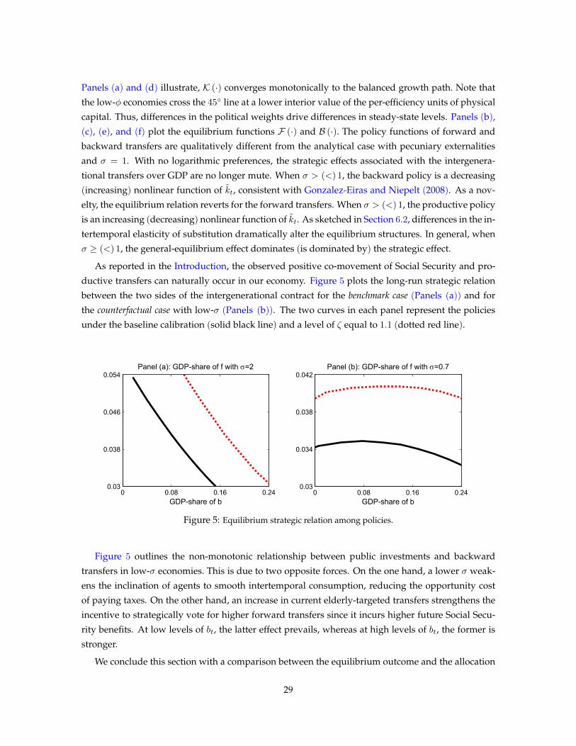
Panels (a) and (d) illustrate, K (·) converges monotonically to the balanced growth path. Note that

the low-φ economies cross the 45 line at a lower interior value of the per-efficiency units of physical

capital. Thus, differences in the political weights drive differences in steady-state levels. Panels (b),

(c), (e), and (f) plot the equilibrium functions F (·) and B (·). The policy functions of forward and

backward transfers are qualitatively different from the analytical case with pecuniary externalities

and σ = 1. With no logarithmic preferences, the strategic effects associated with the intergenera-

tional transfers over GDP are no longer mute. When σ > (<) 1, the backward policy is a decreasing

(increasing) nonlinear function of kt, consistent with Gonzalez-Eiras and Niepelt (2008). As a nov-

elty, the equilibrium relation reverts for the forward transfers. When σ > (<) 1, the productive policy

is an increasing (decreasing) nonlinear function of kt. As sketched in Section 6.2, differences in the in-

tertemporal elasticity of substitution dramatically alter the equilibrium structures. In general, when

σ ≥ (<) 1, the general-equilibrium effect dominates (is dominated by) the strategic effect.

As reported in the Introduction, the observed positive co-movement of Social Security and pro-

ductive transfers can naturally occur in our economy. Figure 5 plots the long-run strategic relation

between the two sides of the intergenerational contract for the benchmark case (Panels (a)) and for

the counterfactual case with low-σ (Panels (b)). The two curves in each panel represent the policies

under the baseline calibration (solid black line) and a level of ζ equal to 1.1 (dotted red line).

0 0.08 0.16 0.240.03

0.038

0.046

0.054

GDP-share of b

Panel (a): GDP-share of f with =2

0 0.08 0.16 0.240.03

0.034

0.038

0.042

GDP-share of b

Panel (b): GDP-share of f with =0.7

Figure 5: Equilibrium strategic relation among policies.

Figure 5 outlines the non-monotonic relationship between public investments and backward

transfers in low-σ economies. This is due to two opposite forces. On the one hand, a lower σ weak-

ens the inclination of agents to smooth intertemporal consumption, reducing the opportunity cost

of paying taxes. On the other hand, an increase in current elderly-targeted transfers strengthens the

incentive to strategically vote for higher forward transfers since it incurs higher future Social Secu-

rity benefits. At low levels of bt, the latter effect prevails, whereas at high levels of bt, the former is

stronger.

We conclude this section with a comparison between the equilibrium outcome and the allocation

29

implemented by the social planner with dynastic welfare weight. Table 2 reports the results.

Variables Markov-perfect equilibrium Social Planner allocation

z 0.1474 0.2154

f 0.0445 0.0936

b 0.0614 0.0612

k 0.0333 0.0210

Table. 2: Steady-state comparison.

Both the political parties and the benevolent government implement strictly positive intergenera-

tional transfers. Compared to the policy chosen by the social planner, the GDP-share of public in-

vestments in the politico-economic equilibrium are 52% lower. This translates into smaller size of

government and under-investment in durable goods. Furthermore, the politico-economic equilib-

rium features larger Social Security benefits and over-accumulation of the asset variable.

8.1 Economic Disagreement and Intergenerational Contracts

As noted in Section 6, the degree of technological complementarity among assets quantitatively

influences the sustenance of intergenerational contracts. The introduction of physical capital gener-

ates a further source of disagreement related to pure economic factors, which adds to the intergen-

erational disagreement rooted in the difference in lifespan. The novel comparative statics carried

out in this section are, then, with respect to the elasticity of factor substitution, ζ, which can also be

interpreted as a measure of economic disagreement between workers and capitalists.

As shown in Figure 5, ζ does not alter the equilibrium relation between public transfers. Specifi-

cally, substitutability among backward and forward transfers still holds at low intertemporal elastic-

ity of substitution, and non-monotonicity is preserved in the opposite case. Nevertheless, a variation

of intergenerational economic disagreement has significant repercussions for the size of government,

as the following Proposition points out.

Proposition 10 (Economic Disagreement and Intergenerational Contracts) A higher elasticity of sub-

stitution among productive factors and, in turn, a higher economic disagreement correspond to a larger amount

of intergenerational transfers, and, in turn, higher economic growth.

The intuition behind this result is best conveyed graphically. Figure 6 plots the steady-state level

of backward transfers over GDP (Panel (a)) and the economic growth rate (Panel (b)) as a function

of the relative political power of elderly agents, when ζ acquires the values 1 (solid black line) and

1.1 (dotted red line).

In view of Proposition 10, high-ζ economies are characterized by more generous backward trans-

fers and higher economic growth compared to low-ζ economies.25 For the benchmark calibration, an

increase in economic disagreement by 10% leads to an increase in both the investment-to-GDP ratio25This claim provides a new fundamental to the theory, which recognizes the link between the elasticity of factor substitu-

tion and the rate of economic growth. In particular, it can be interpreted as a microfoundation of the conjecture by Klumpand De La Grandville (2000). Specifically, we add the channel of voting to conclude that countries with higher elasticity of

30

0.7 0.9 1.1 1.30.02

0.1

0.18

0.26Panel (a): GDP-share of b

Elderly voters` relative single-mindedness0.7 0.9 1.1 1.3

1.2

1.26

1.32

1.38Panel (b): Per-capita growth rate

Elderly voters` relative single-mindedness

Figure 6: Intergenerational disagreement and public expenditures.

and pension benefit-to-GDP ratio of 8.6% and 114%, respectively. The result is driven by the follow-

ing intuition. When productive inputs are technologically closer substitutes, the rate of return on

savings turns out to be less responsive to a positive variation of intergenerational transfers, through

the contraction of the asset variable. As a consequence, the interest rate falls and the present value

of the next-period backward transfers rises. The overall economic adjustment translates into a larger

endogenous political weight attached to the adults, Υt, with the following consequences: a distribu-

tion of consumption more skewed in favor of adult voters and a bigger amount of enforced backward

policies. Surprisingly, it is the strategic incentive of the middle-aged that fosters Social Security. Indeed,

under a weak general-equilibrium effect, adults anticipate that the sole way to maximize life-cycle in-

come is to replace private saving with public insurance schemes. As a consequence, larger backward

transfers prompt – through their disciplinary valence – the provision of higher public investments.

9 ConclusionsIn this paper, we propose a novel mechanism that enforces a growth-enhancing intergenerational

contract, given the lack of commitment technology, reputation mechanisms, and altruism. Embed-

ding a repeated probabilistic voting setup in a standard OLG model with human capital accumula-

tion, we find that the empowerment of elderly constituents is key to enforcing forward productive

transfers. As an equilibrium outcome, intergenerational government expenditures may be either

strategic complements or strategic substitutes, depending on the fundamentals of the model, such as

the intertemporal elasticity of substitution.

The power of this mechanism lies in the ability of short-lived institutions to generate long-term

growth. In our institutional environment, the sacrifices borne by the current constituents will be cred-

ibly, and at least partially, rewarded by future constituents. Two fundamental features of the model

drive our results: (i) the nature of short-term agreements among politicians and voters; and (ii) the

substitution will always experience, other things being equal, a higher income per capita, as they devote more resources topublic investment.

31

prospect of follow-up intergenerational contracts, which serve as disciplining devices to implement

current policies.

In this paper, we have assumed that the government runs a balanced budget and does not have

access to financial credit markets. In a theoretical environment in which the operating budget is

used to finance both durable goods – i.e., forward transfers – and non-durable goods – i.e., backward

transfers – balanced-budget restrictions necessarily generate distortions in the provision of public

spending. Indeed, voters have incentives to pay solely for the services they receive from the govern-

ment but do not have the same incentives to optimally finance durable goods, the benefits of which

have a long-lasting impact. This finding implies that it would be fair to ask voters to share the fiscal

burden by using debt financing, which, in turn, would alleviate the inefficiency due to the under-

investment in productive assets. Assessing the relative impact of government indebtedness on the

equilibrium intergenerational contracts is left to future research.

32

10 Appendix A

Proof of Proposition 2: Let us restate the political first-order conditions, Eqs. (18) and (19), as

Ω (ft, φ) ≡ Φft − νβ

φucotucot+1

1Bht+1

. Applying the implicit function theorem yields dftdφ = − Ωφ

Ωft, where

Ωft ≡ Φft,ft +Φftνβ

φucotucot+1

(Bht+1,ht+1

B2ht+1

+ucot+1

,cot+1

ucot+1

)and Ωφ ≡ − ν

β

(1

Bht+1

ddφ

(φucotucot+1

)−

φucotucot+1

Bht+1,φ

B2ht+1

).

Assumptions 1 and 2 guarantee the negativity of Ωft . As a result, dftdφ ≥ (<) 0 if and only if Ωφ ≥ (<) 0.

Let us denote ρ+ ≡ φBht+1

Bht+1

,φ and ρ− ≡ucot+1

ucot

ddφ

(φucotucot+1

). Hence, Ωφ ≥ (<) 0 if and only if

ρ− ≤ (>) ρ+.

Proof of Proposition 3: Denote µt ≡ucotucat

. Assuming interior bt and combining Eqs. (8), (16), and

(17), yields dBt+1

dbt+ νkt+1

dRt+1

dbt= 1−φµt

ν2

(dBt+1

dft+ νkt+1

dRt+1

dft

)with dBt+1

dft+ νkt+1

dRt+1

dft= Rt+1 > 0.

Since dBt+1

dbt+ νkt+1

dRt+1

dbt≥ 0, then φµt ∈ [0, 1]. Moreover, 1−φµt

ν2 ≤ 1 directly implies 0 ≤ dBt+1

dbt+

νkt+1dRt+1

dbt< dBt+1

dft+ νkt+1

dRt+1

dft.

Proof of Proposition 4 Let us adopt the notation in per-efficiency units as introduced in Section

3.2. Recall that It = wt − 1ν bt − νft and µt ≡

ucotucat

. Furthermore, Dt ≡ It +ϕtbt+1

Rt+1denotes the present

value of after-tax lifetime income. The derivatives of Dt with respect to policies are equal to Dbt=

− 1ν + ϕt

R2t+1

(Bkt+1

Rt+1 − bt+1Rkt+1

)Kbt and Dft

= −ν+ ϕtR2t+1

(Bkt+1

Rt+1 − bt+1Rkt+1

)Kft+ϕft

bt+1

Rt+1.

For any separable additive utility function, using the Euler condition for savings, we obtain:

νϕtkt+1 = It − Ξt+1Dt (22)

where Ξt+1 ≡ u−1c (βRt+1)Rt+1

1+u−1c (βRt+1)Rt+1

. Hence, the equilibrium response of the saving rate to a variation in

bt and ft is, respectively, equal to:

Kbt = − 1− Ξt+1

ν2ϕt

(1 + Dt

νϕtΞkt+1

+

(Bkt+1

− bt+1

Rkt+1

Rt+1

)Ξt+1

νRt+1

) (23)

and

Kft = −(1− Ξt+1)

(1 +

ϕftνϕt

It

)ϕt

(1 + Dt

νϕtΞkt+1

+

(Bkt+1

− bt+1

Rkt+1

Rt+1

)Ξt+1

νRt+1

) (24)

Therefore, the relative adjustment of capital due to a variation in policies is asKbtKft

= ϕtν(νϕt+ϕft It)

.

Plugging Eq. (22) into the individual budget constraints yields the individual consumption levels

cat = Ξt+1Dt and cot+1 = (1− Ξt+1)Rt+1Dt, such that cat +cot+1

Rt+1= Dt. The political first-order

conditions, Eqs. (16) and (17), read now as:

0 = φucot + ucat

(−1 +

νϕtRt+1

Bkt+1Kbt − ν

(ϕtbt+1

Rt+1−cot+1

Rt+1

)Rkt+1

Rt+1Kbt

)(25)

33

and

0 = −ν +1

Rt+1

(ϕft bt+1 + ϕtBkt+1

Kft)−

(ϕtbt+1

Rt+1−cot+1

Rt+1

)Rkt+1

Rt+1Kft (26)

Plugging Eq. (23) into Eq. (25), after algebraic manipulation, we obtain:

Bkt+1= − νRt+1 (1− φµt)

νϕt (1− φµtΞt+1)

(νϕt + DtΞkt+1

)(27)

− 1

νϕt (1− φµtΞt+1)

((1− Ξt+1)

2Dt − ϕt (1− φµtΞt+1)

bt+1

Rt+1

)νRkt+1

where the first line captures the strategic effect, whereas the second line highlights the general-

equilibrium effect. Disregarding the general-equilibrium component, Eq. (27) simplifies to Bkt+1=

−νR 1−φµt1−φΞµt

. Therefore, since φµt ∈ [0, 1], then the marginal impact of kt+1 on backward transfer

is always negative – i.e., Bkt+1< 0. As a further implication, using Eqs. (24), (26), and (27) yields

ϕft = νϕtφucot(

It+ϕtbt+1Rt+1

)ucat−Itφucot

, which describes the political productive wedge as reported in Eq.

(21).

Proof of Lemma 1: The resolution strategy involves two steps. First, starting from a sufficiently

large and finite date T , we compute the first-order conditions for intergenerational transfers, and

we solve by backward induction for each time T − j with j = 0, 1, ..., T , subject to (i) the Euler

condition for saving, (ii) the fiscal feasibility conditions, and (iii) the policy rules of future periods.

Second, we recursively determine the conditions for the existence of the fixed points. For notational

purpose, let IT−j = whT−j − νfT−j − bT−jν for ∀j denote the disposable income of adults, with

w = B (1− α)(αBR

) α1−α .

First Step (First-Order Conditions): At the terminal date T , adults have a one-period temporal hori-

zon. Hence, sT = 0. Eq. (14) reduces to νu (CaT ) + φu (CoT ), where CaT ≡ IT and CoT ≡ νRkT + bT . It

immediately follows that fT = 0. The first-order condition for bT turns out to be CaT

CoT= 1

φ . Standard

algebra implies that:

bT = − ν2R

φ+ νkT +

φνw

φ+ νhT (28)

Combining Eq. (28) and the Euler condition for savings (for period T − 1) yields kT = αβ(φ+ν)ν(φ+αβ(φ+ν))

IT−1. At time T − 1, the agents born at time T − 2 have two-period lifespan. Hence, the politi-

cal objective function is ν(u(CaT−1

)+ βu (CoT )

)+ φu

(CoT−1

), where CoT−1 ≡ νRkT−1 + bT−1. The

optimal saving decision and the policy rules for period T provide CaT−1 ≡φ

φ+αβ(φ+ν)IT−1 and

CoT ≡φαβR

φ+αβ(φ+ν)IT−1 + φνwφ+νhT . The first-order conditions with respect to fT−1 and bT−1 yield

ΦfT−1= R(1+αβ)(φ+ν)

w(φ+αβ(φ+ν)) and CaT−1

CoT−1= 1+αβ

φ+αβ(φ+ν) , respectively. Let ψ(1) ≡(wA(1−θ)(φ+αβ(φ+ν))

R(1+αβ)(φ+ν)

) 1θ

,

where the subscript in parentheses denotes the number of iterations. Under the human capital Cobb-

Douglas function, we obtain the following:

fT−1 = ψ(1)hT−1 (29)

34

and

bT−1 = − ν2R (1 + αβ)

φ+ ν (1 + αβ)kT−1 +

φν

φ+ ν (1 + αβ)

(w − νψ(1)

)hT−1 (30)

Substituting these expressions into the Euler condition for savings (for period T − 2) yields kT−1 =β(φ+ν(1+αβ))

ν(φ+β(φ+ν(1+αβ)))IT−2 −φ(w−νψ(1))

R(φ+β(φ+ν(1+αβ)))hT−1.

Starting from period T − 2 onwards, the political objective function is structurally equivalent to

the political objective function for period T − 1. Combining Eqs. (29), (30), and the level of physical

capital, kT−1, yields the expressions for CaT−2 ≡φ

φ+β(φ+ν(1+αβ))W(1) and CoT−1 ≡φβR

φ+β(φ+ν(1+αβ))W(1),

with W(1) = IT−2 + νR

(w − νψ(1)

)hT−1. The first-order conditions for fT−2 and bT−2 are ΦfT−2

=R

w−νψ(1)and C

aT−2

CoT−2= 1+β

φ+β(φ+ν(1+αβ)) , respectively. Solving for the intergenerational transfers, we get:

fT−2 = ψ(2)hT−2 (31)

and

bT−2 = − ν2R (1 + β)

φ+ ν (1 + β)kT−2 +

φν

φ+ ν (1 + β)

(w +

νθ

1− θψ(2)

)hT−2 (32)

where ψ(2) ≡(A(1−θ)(w−νψ(1))

R

) 1θ

. Plugging Eqs. (31) and (32) into the Euler condition for savings

(for period T − 3) yields kT−2 = β(φ+ν(1+β))ν(1+β)(φ+νβ)IT−3 − φ

R(φ+νβ)(1+β)

(w + νθ

1−θψ(2)

)hT−2.

Replicating the procedure developed at period T − 2, the consumption levels for period T − 3 are

CaT−3 ≡φ

(1+β)(φ+βν)W(2) and CoT−2 ≡φβR

(1+β)(φ+νβ)W(2), with W(2) = IT−3 + νR

(w + νθ

1−θψ(2)

)hT−2.

The first-order conditions for the intergenerational transfers – i.e., ΦfT−3= R

w+ νθ1−θψ(2)

and CaT−3

CoT−3=

1+βφ+β(φ+ν(1+αβ)) – imply:

fT−3 = ψ(3)hT−3 (33)

and

bT−3 = − (1 + β) ν2R

φ+ ν (1 + β)kT−3 +

φν

φ+ ν (1 + β)

(w +

νθ

1− θψ(3)

)hT−3 (34)

where ψ(3) = m(ψ(2)

)≡(νAθR ψ(2) + wA(1−θ)

R

) 1θ

. Combining Eqs. (33), (34), and the optimal saving

(for period T − 4) yields kT−3 = β(φ+ν(1+β))ν(1+β)(φ+νβ)IT−4− φ

R(φ+νβ)(1+β)

(w + νθ

1−θψ(3)

)hT−3. Thus, CaT−4 ≡

φ(1+β)(φ+βν)W(3) and CoT−3 ≡

φβR(1+β)(φ+νβ)W(3), with W(3) = IT−4 + ν

R

(w + νθ

1−θψ(3)

)hT−3. The first-

order conditions for fT−4 and bT−4 are ΦfT−4= R

w+ νθ1−θψ(3)

and CaT−4

CoT−4= 1

φ+βν , respectively. It is

straightforward to show that the resulting policy rules are structurally equivalent to Eqs. (33) and

(34) and that, from now on, the first-order conditions for intergenerational transfers are equal to

those of period T − 4.

Second Step (Fixed-Point): The Markov-perfect equilibrium exists if and only if the limit for j → ∞

of the series ψ(j+1) = m(ψ(j)) ≡(AθνR ψ(j) + wA(1−θ)

R

) 1θ

exists and is finite, with ψ(1) as the initial

condition. The differentiable single-valued function m(ψ(j)) satisfies m (0) > 0, mψ(j)> 0, and

mψ(j),ψ(j)> 0. Let ψ ≡ 1

θ

((RAν

) 11−θ − w(1−θ)

ν

)denote the value of ψ(j) such that mψ(j)

(ψ) = 1. The

35

corresponding value of the series evaluated at ψ is m(ψ) ≡(RAν

) 11−θ . For R > Aνθ, we get m(ψ) < ψ.

Hence, the first-order nonlinear equation ψ(j+1) = m(ψ(j)) supports two solutions with ψ1 ≤ ψ2,

where ψ1 is the unique, locally stable fixed-point. Henceforth, ψ1 ≡ ψ. By the implicit function

theorem, ψθ < 0, ψR < 0, ψA > 0, and ψν < 0.

Proof of Proposition 5: Under Lemma 1, the Markov-perfect equilibrium is given by:

ft = ψht (35)

and

bt = − ν2R (1 + β)

φ+ ν (1 + β)kt +

φν

φ+ ν (1 + β)

(w +

νθ

1− θψ

)ht (36)

Hence, the laws of motion for asset variables are ht+1 = ϕht, with ϕ = Aψ1−θ, and kt+1 = Rβφ+νβkt +

βR(w−νψ)(φ+ν(1+β))−φ(βR+νϕ)(w+ θν1−θψ)

ν(φ+νβ)(1+β)R ht. The argument in the text establishes that R ≤ R (φ) ≡φ+νββ ϕ. If R = R (φ), then physical and human capital grow at the same rate. Hence, Eqs. (35)

and (36) are Markov-perfect equilibrium and the economy is at the balanced growth path with k =(αβB

ϕ(φ+νβ)

) 11−α

.

Proof of Proposition 6: If R < R (φ), the physical capital converges to zero after one period.

We follow the logic of Lemma 1 to characterize the Markov-perfect equilibrium in an environment

with sole human capital. At the terminal date T , Eq. (14) reduces to νu (CaT ) + φu (CoT ), where

CaT ≡ whT − fT − bTν and CoT ≡ bT . It immediately follows that fT = 0 and bT = φν

ν+φwhT . At

time T − 1, the political objective function is as ν(u(CaT−1

)+ βu (CoT )

)+ φu

(CoT−1

), where CaT−1 ≡

whT−1 − fT−1 − bT−1

ν and CoT−1 ≡ νRkT−1 + bT−1. Standard algebra implies:

fT−1 =β (1− θ)

φ+ ν (1 + β (1− θ))whT−1 (37)

and

bT−1 =φν

φ+ ν (1 + β (1− θ))whT−1 (38)

Under the adopted parametric form, it is straightforward to show that policies converge after one-

period recursion. Hence, we conclude that for a generic time t, the equilibrium policies are as in Eqs.

(37) and (38). The dynamic of human capital is equal to ht+1 = ϕht, with ϕ ≡ A(

β(1−θ)φ+ν(1+β(1−θ))

)1−θ.

Proof of Proposition 7: We separate the proof in two steps. First, we characterize the social

planner’ s short- and long-run solutions. Second, we state the efficient properties of the Markov-

perfect equilibrium, as reported in Propositions 5 and 6.

First Step (Efficient allocation): Let us guess and verify that the optimal policy rules are structurally

equivalent to Eqs. (35) and (36). If the guesses are the equilibrium, then they must simultaneously

satisfy the first-order conditions – i.e., Eqs. (6) and (7). Under the human capital Cobb-Douglas

function,Φht+1

Φft+1= θ

1−θft+1

ht+1. Hence, the optimal first-order condition for forward transfers reduces

36

to Φft − Rw

(1− ν

RΦftΦht+1

Φft+1

)= 0. Using the guess ft = ψht yields ψ =

(νθAR ψ + A(1−θ)w

R

) 1θ

,

whose zero is equal to the politico-economic solution – i.e., ψ = ψ. As a result, ht+1 = ϕht,

with ϕ ≡ Aψ1−θ. Under the guess bt = π1kt + π0ht, the optimal saving decision is as kt+1 =βR

π1+νR(1+β)

(wht−νft − bt

ν

)− π0

π1+νR(1+β)ht+1. Plugging the guesses and the dynamics of physical

and human capital into Eq. (6), we get:

bt = − νδR (π1 + νR (1 + β))

(δ + β)π1 + νR (β + δ (1 + β))kt +

νβ (νϕπ0 + (π1 + νR) (w−νψ))

(δ + β)π1 + νR (β + δ (1 + β))ht

Solving for undetermined coefficients yields π1, π0 =−νδR(1+β)

δ+β , νβR(1−δ)(w−νψ)(δ+β)(R−νϕ)

. Hence, the

optimal dynamics for physical capital is equal to kt+1 = Rδν kt + (w−νψ)(Rδ−νϕ)

ν(R−νϕ) ht. If R = R (δ) ≡ νδϕ,

then physical and human capital grow at the same rate and the economy converge to the balanced

growth path after one-period with k = w−νψν(νϕ−R) . By contrast, ifR < R (δ), then the efficient allocation

is characterized by human capital as the sole asset variable. In this context, Eqs. (6) and (7) reduce tocatcot

= δνβ and cot+1

cat= Φftβ

(Θht+1

+ νΦht+1

Φft+1

), respectively. Guessing and verifying that bt = πbht and

ft = πfht and solving for undetermined coefficients, we get bt = wνβ(1−δ)(1−δθ)(δ+β)ht and ft = wδ(1−θ)

ν(1−δθ) ht.

Hence, the optimal dynamics of human capital is equal to ht+1 = ϕht, with ϕ ≡ A(wδ(1−θ)ν(1−δθ)

)1−θ.

Second Step (Efficiency vs Markov-perfect): Taking the inverse function of R = R (φ) and R = R (δ)

yields φ = Λ (R) ≡ β(

RAψ1−θ − ν

)and δ = Λ (R) ≡ ν

RAψ1−θ, respectively. Lemma 1 shows thatψR <

0 and, in turn, ΛR = ψ−(1−θ)RψRAψ2−θ > 0 and ΛR = νAψ1−θ

R2

((1−θ)RψR−ψ

ψ

)< 0 for any R > Aνθ. Hence,

there always exists a level of the market interest rate, denoted by R∗, such that Λ (R∗) = Λ (R∗).

In this case, ft = ft and bt = bt. We distinguish four parametric areas corresponding to different

configurations of political and optimal allocations: (i) if φ > Λ (R) and δ > Λ (R), then R (δ) <

R < R (φ). This implies that the Markov-perfect equilibrium enforces an intergenerational contract

with only human capital, as stated in Proposition 6, whereas the social planner allocation reverts to

intergenerational autarky; (ii) if φ < Λ (R) and δ < Λ (R), then R (φ) < R < R (δ) and the opposite

occurs – namely, the political outcome induces intergenerational autarky, and the optimal allocation

sustains positive intergenerational transfers as a function of the sole human capital; (iii) if φ < Λ (R)

and δ > Λ (R), thenR > max R (φ) , R (δ) and autarky is the unique outcome in both scenarios; and

(iv) if φ > Λ (R) and δ < Λ (R), then R < min R (φ) , R (δ). In this circumstance, intergenerational

cooperation is enforced in both the Markov-perfect equilibrium and the social planner allocation.

When φ = Ψ (δ) ≡ ν(β−δ(β−δ(1+β−θ−βθ)))δ(1−δ) , it is straightforward to show that zt

ht= zt

ht. Then, the

following inequalities apply: btht− bt

ht= −νw(1+β)(1−θ)δ2

(δ+β)(1−δθ) < 0 and ftht− ft

ht= w(1+β)(1−θ)δ2

ν(δ+β)(1−δθ) > 0.

Proof of Proposition 8: The resolution strategy follows the logic of the proof of Lemma 1. Recall

that IT−j ≡ (1− α) yT−j − νfT−j − bT−jν , with j = 0, 1, ..., T . In the last period, CaT ≡ IT and

CoT ≡ ναyT + bT . As fT = 0, the first-order condition with respect to bT collapses to CaT

CoT= 1

φ . Solving

for backward transfers yields:

bT =ν (φ− α (φ+ ν))

φ+ νyT (39)

37

Plugging Eq. (39) into the Euler condition for savings (for period T − 1), we get kT = αβ(φ+ν)ν(φ+αβ(φ+ν))IT−1.

It follows that at time T − 1, CaT−1 ≡φ

φ+αβ(φ+ν)IT−1, CoT−1 ≡ ναyT−1 + bT−1, and CoT = νφφ+ν yT . Ap-

plying the envelope condition, the first-order conditions for interior fT−1 and bT−1 are ΦfT−1=

RTwT

(1+αβ)(φ+ν)φ+αβ(φ+ν) and C

aT−1

CoT−1= 1+αβ

φ+αβ(φ+ν) , respectively. As the technology is Cobb-Douglas, the policy

rules are equal to:

fT−1 =β (1− θ) (1− α)

φ+ ν (1 + β (1− (1− α) θ))yT−1 (40)

and

bT−1 =ν (φ− α (φ+ ν (1 + β (1− (1− α) θ))))

φ+ ν (1 + β (1− (1− α) θ))yT−1 (41)

Combining Eqs. (40), (41), and the Euler condition on savings (for period T − 2) yields kT−1 =αβ(φ+ν(1+β(1−(1−α)θ)))

ν(φ+αβ(φ+ν(1+β(1−(1−α)θ))))IT−2. Thus, we obtain the individual consumption levels CoT−2 ≡ ναyT−2+

bT−2, CaT−2 ≡φ

φ+αβ(φ+ν(1+β(1−(1−α)θ)))IT−2, and CoT−1 = νφφ+ν(1+β(1−(1−α)θ))yT−1. At time T − 2,

proceeding as in the previous period, the first-order conditions for fT−2 and bT−2 are ΦfT−2=

RT−1

wT−1

(1+αβ)(φ+ν(1+β(1−(1−α)θ)))φ+αβ(φ+ν(1+β(1−(1−α)θ))) and C

aT−2

CoT−2= 1+αβ

φ+αβ(φ+ν(1+β(1−(1−α)θ))) . It is straightforward to show

that the policy rules are identical to those of period T−1 and the individual consumption amounts to

CaT−2 = νφ(1+αβ)(φ+αβ(φ+ν(1+β(1−(1−α)θ))))(φ+ν(1+β(1−(1−α)θ)))yT−2 and CoT−2 = νφ

φ+ν(1+β(1−(1−α)θ))yT−2. Due

to the specific parameterization, the policies converge after two periods of recursion. We conclude

that for a generic time t and φ ≥ φ ≡ αν(1+β(1−θ(1−α)))1−α , the equilibrium policies are given by Eqs.

(40) and (41). Furthermore, the transition laws of human and physical capital are, respectively:

ht+1 = A

(Bβ (1− θ) (1− α)

φ+ ν (1 + β (1− θ (1− α)))

)1−θ

kα(1−θ)t h

1−α(1−θ)t

and

kt+1 =αβ (1 + αβ)

φ+ αβ (φ+ ν (1 + β (1− (1− α) θ)))Bkαt h

1−αt

Finally, in balanced growth, we obtain k =(

1ξ

) 11−αθ

(1χ

) 1−θ1−αθ

and f =(

1ξ

) α1−αθ

(χ)1−α1−αθ , where

ξ ≡ ABφ+αβ(φ+ν(1+β(1−(1−α)θ)))

αβ(1+αβ) and χ ≡ βB(1−θ)(1−α)φ+ν(1+β(1−(1−α)θ)) . Hence, the growth rate and associated

rental price of capital are ϑk = αB(ξχ1−θ) 1−α

1−αθ and ϕ = A(χ1−α

ξα

) 1−θ1−αθ

, respectively.

Proof of Proposition 9: The resolution strategy mirrors the logic of the proof of Proposition 7.

First Step (Efficient allocation): Let guess ft = πfyt and bt = πbyt. If the guesses are the equilibrium,

then they must simultaneously satisfy the first-order conditions – i.e., Eqs. (6) and (7). Plugging the

guesses into Φft −Φkt+1

Φht+1

(1− ν

Φkt+1Φft

Φht+1

Φft+1

)= 0 and cat

cot= δ

νβ yields:

bt =ν((αν + πb) (β (1− νπf )− α (δ + β))− νδα2β

)πb (δ + β) + να (β + δ (1 + β))

yt

and

ft =β ((1− θ) (1− α) + νθπf ) (ν (1− α)− πb)

ν (νβ ((1− θ) (1− α) + νθπf ) + αν (1 + β) + πb)yt

38

Solving for undetermined coefficients, we get πb, πf =ν(β(1−α)−δ(β+α(1−θδ(1+β))))

(δ+β)(1−θδ) , δ(1−θ)(1−α)ν(1−δθ)

.

Hence, the optimal dynamics for physical and human capital are equal to kt+1 = αδν yt and ht+1 =

A(δ(1−θ)(1−α)B

ν(1−δθ)

)1−θkα(1−θ)t h

1−α(1−θ)t , respectively. As a result, k =

(BAαδν

) 11−αθ

(ν(1−δθ)

δB(1−θ)(1−α)

) 1−θ1−αθ

in the long-run. Furthermore, the efficient growth rate and rental price of capital are equal to ϕ =

A(χ1−θ

ξα

) 1−α1−αθ

and ϑk = αB(ξχ1−θ

) 1−α1−αθ

, with ξ ≡ AB

ναδ and χ ≡ δB(1−θ)(1−α)

ν(1−δθ) , respectively.

Second Step (Efficiency vs Markov-perfect): Using the equilibrium policy rules and the efficient al-

location into Eq. (4) yields the equilibrium and optimal tax rates, z = (1−α)(φ+νβ(1−θ(1−α)))−αν(1+β)φ+ν(1+β(1−θ(1−α)))

and z = (1−α)(β+δ(1−θ)(δ+β))−δ(β+α(1−δθ(1+β)))(1−δθ)(δ+β) . Note that z and z are positive only if φ > φ and δ <

δ ≡ α+β−√

(α+β)2−4αθβ(1−α)(1+β)

2αθ(1+β) , respectively. In the feasible space (φ, δ), it is straightforward to

show that z ≥ (<) z if and only if φ ≤ (>) Ψ (δ), where

Ψ (δ) ≡ ν

δ

(1− α) (1− θ) (β + δ) (β − δ (1 + β (1 + αθ)))− β (1− δ) (1− αθδ) (1 + β (1− θ (1− α)))

δ (1− α (1− θ (1 + β)))− (1 + αβ)

Moreover, for φ = Ψ (δ), the following inequalities hold: btyt −btyt

= ν(1−θ)(1−α)(1+β)(1+αβθ)δ2

(1−δθ)(1+αβ)(β+δ) > 0 andftyt− ft

yt= − (1−θ)(1−α)(1+β)(1+αβθ)δ2

ν(1−δθ)(1+αβ)(β+δ) < 0.

39

References[1] Alesina, A., and Rodrick, D., 1994. Distributive Politics and Economic Growth, The Quarterly

Journal of Economics, 109 (2), 465-490.

[2] Azariadis, C., and Galasso, V., 2002. Fiscal Constitutions, Journal of Economic Theory, 103 (2),

255-281.

[3] Azzimonti, M., 2011. Barriers to Investment in Polarized Societies, American Economic Review,

101 (5), 2182-2204.

[4] Barro, R., 1974. Are Government Bonds Net Wealth?, Journal of Political Economy, 82 (6), 1095-

1117.

[5] Bassetto, M., 2008. Political Economy of Taxation in an Overlapping-Generations Economy, Re-

view of Economic Dynamics, 11 (1), 18-43.

[6] Battaglini, M., and Coate, S., 2007. Inefficiency in Legislative Policy-Making: A Dynamic Anal-

ysis, American Economic Review, 97 (1), 118-149.

[7] Becker, G., and Murphy, K., 1988. The Family and the State, Journal of Law and Economics, 31 (1),

1-18.

[8] Bellettini, G., and Berti Ceroni, C., 1999. Is Social Security Really Bad for Growth?, Review of

Economic Dynamics, 2 (4), 796-819.

[9] Boldrin, M. and Montes, A., 2005. The Intergenerational State Education and Pension, Review of

Economic Studies, 72 (3), 651-664.

[10] Chen, K., and Song, M.. Markovian Social Security in Unequal Societies, Scandinavian Journal of

Economics, forthcoming.

[11] Farhi, E., and Werning, I., 2007. Inequality and Social Discounting, Journal of Political Economy,

115, 365-402.

[12] Forni, L., 2005. Social Security as Markov Equilibrium in OLG Models, Review of Economic Dy-

namics, 8 (1), 178-194.

[13] Galasso, V., and Profeta, P., 2004. Lessons for an Aging Society: the Political Sustainability of

Social Security Systems, Economic Policy, 19 (38), 63-115.

[14] Gonzalez-Eiras, M., and Niepelt, D., 2008. The Future of Social Security, Journal of Monetary

Economics, 55(2), 197-218.

[15] Gonzalez-Eiras, M., and Niepelt, D., 2012. Aging, Government Budgets, Retirement, and

Growth, European Economic Review, 56 (1), 97-115.

40

[16] Grossman, G. M., and Helpman, E., 1998. Intergenerational Redistribution with Short-lived

Government, Economic Journal, 108, 1299-1329.

[17] Hassler, J., Storesletten, K., and Zilibotti, F., 2007. Democratic Public Good Provision, Journal of

Economic Theory, 133 (1), 127-151.

[18] Kehoe, T. J., and Levine, D. K., 2001. Liquidity Constrained Markets versus Debt Constrained

Markets, Econometrica, 69 (3), 575-598.

[19] Klump, R., and de La Grandville, O., 2000. Economic Growth and the Elasticity of Substitution:

Two Theorems and Some Suggestions, American Economic Review, 90 (1), 282-291.

[20] Krusell, P., Quadrini, V. and Rıos-Rull, J. V., 1997. Politico-Economic Equilibrium and Economic

Growth, Journal of Economic Dynamics and Control, 21 (1), 243-272.

[21] Lancia, F., and Russo, A., 2011. A Dynamic Politico-Economic Model of Intergenerational Con-

tracts, unpublished manuscript, universita di Modena.

[22] Lee, R., Donehower, G., and Miller, T., 2011. The changing shape of the economic lifecycle in

the United States, 1960 to 2003, Ch. 15 in Population Aging and the Generational Economy: A Global

Perspective, eds. Edward Elgar, 313-326.

[23] Lindbeck, A., and Weibull, J.W., 1987. Balanced-budget redistribution as the outcome of political

competition, Public choice, 52, 273-297.

[24] Mulligan, C. B., and Xala-i-Martin, X., 1999. Gerontocracy, Retirement, and Social Security,

NBER Working Papers 7117.

[25] Persson, T. and Tabellini, G., 1994. Is Inequality Harmful for Growth?, American Economic Review,

84 (3), 600-621.

[26] Piketty, T., and Saez, E., 2003. Income inequality in the United States, 1913–1998, Quarterly Jour-

nal of Economics, 118 (1), 1-39.

[27] Rangel, A., 2003. Forward and Backward Intergenerational Goods: Why is Social Security Good

for Environment?, American Economic Review, 93, 813-834.

[28] Song, Z., Storesletten, K., and Zilibotti, F., 2012. Rotten Parents and Disciplined Children: A

Politico-Economic Theory of Public Expenditure and Debt, Econometrica, 80 (6), 2785-2804.

[29] Stromberg, D., 2008. How the Electoral College Influences Campaigns and Policy: The Proba-

bility of Being Florida, American Economic Review, 98 (3), 769-807.

[30] Tabellini, G., 1991. The Politics of Intergenerational Redistribution, Journal of Political Economy,

99 (2), 335-57.

[31] Trabandt, M., and Uhlig, H., 2011. The Laffer Curve Revisited, Journal of Monetary Economics, 58,

305-327.

41

11 Appendix B (Not For Publication)In this Appendix, we provide some supplementary material. Section B.1 presents the politico-

economic microfoundation of the model. Section B.2 shows the details of the numerical strategy.

Finally, Section B.3 provides the quantitative framework to replicate Figure 3 in Section 6.1.

B.1. PROBABILISTIC VOTING MODEL

The political equilibrium discussed in the paper has an explicit microfoundation in terms of the

voting model based on Lindbeck and Weibull (1987), applied to a dynamic voting setting in an OLG

environment with intergenerational transfers. The electoral competition takes place between two

office-seeking candidates, L and R. Parties and voters move sequentially. First, parties announce

their political platform constrained to the per-period balanced budget and fiscal feasibility. As the

election takes place each time, the candidates cannot credibly commit to future policies. Second,

voters belonging to cohort i ∈ a, o choose the preferred candidate based on the fiscal announce-

ments and their ideology. Agents vote for party Rt as long as the idiosyncratic ideological bias, σij ,

is larger than the difference in the indirect utility achieved from voting for any alternative platforms,

net of the aggregate shock η. It implies that σij ≥ σi (kt, ht) ≡(WiLt −W

iRt)− η, where σi (kt, ht)

identifies the swing voters of each cohort – that is, the voter who is indifferent between the two

parties. We assume that σij is drawn from a symmetric and cohort-specific uniform distribution on[− 1

2σi ,1

2σi

]. Similarly, the i.i.d. random variable η is uniformly distributed in the support

[− 1

2η ,1

2η

].

The assumption of uniform distribution is for simplicity.26 Conditional on η, the share of voters

belonging to cohort i and supporting party Rt is equal to λit ≡ 12 − σi

(WiLt −W

iRt − η

). Under

majoritarian rule, party Rt wins the election if and only if it obtains the largest share of votes – that

is, N t−1t λat +N t−2

t λot >12

(N t−1t +N t−2

t

). This implies that η must be larger than the threshold level

η (kt, ht) ≡ σo

σa+σo

(WoLt −W

oRt)

+ ν σa

σa+σo

(WaLt −W

aRt). Hence, the objective function of party Rt

– i.e., maxbRt ,fRt

Pr (ηt ≥ η (kt, ht)) – simplifies to:

maxbRt ,fRt

1

2− ηη (kt, ht) (B.1.1)

Likewise, for party Lt, the objective function – i.e., maxpLt

Pr (ηt ≤ η (kt, ht)) – collapses to maxbLt ,fLt

12 +

ηη (kt, ht). To prove that the two parties’ platforms converge in equilibrium to the same fiscal policy

maximizing the weighted average utility of adults and the elderly, we adopt a backward procedure.

Let us consider a two-period economy. In period 2, the political maximization program for partyR2

– described in Eq. (B.1.1) – simplifies to:

maxbR2

,fR21

2− η

(σo

σa + σo(WoL2−Wo

R2

)+ ν

σa

σa + σo(WaL2−Wa

R2

))(B.1.2)

26See Banks and Duggan (2005) for a generalization.

42

As in the last period, adults have no future, so thenWaι2 is equal to u

(Caι2). Hence, Eq. (B.1.2) reduces

to maxbR2

,fR2νu(CaR2

)+ σo

σau(CoR2

). In the same spirit, the political objective function for partyL2 turns

out to be maxbL2 ,fL2

νu(CaL2

)+ σo

σau(CoL2

). It follows that, in equilibrium, office-seeking parties propose

the same platform – that is, bL2= bR2

and fL2= fR2

. Replicating the same argument at date 1, the

maximization program for partyR1 is as:

maxbR1

,fR11

2− η

(σo

σa + σo(WoL1−Wo

R1

)+ ν

σa

σa + σo(WaL1−Wa

R1

))(B.1.3)

whereWaι1 is equal to u

(Caι1)

+ Πι1

(WoR2

+ σoj,2 + η)

+ (1−Πι1)WoL2

, with Πι1 ≡ 12 − ηη (k2, h2; ι1)

defined as the probability of R2 being elected, conditional on the incumbent party ι1. As bL2 = bR2 ,

fL2 = fR2 andWiL2

=WiR2

, it follows that ΠL1 = ΠR1 = 12 . Hence, the maximization program given

by Eq. (B.1.3) reduces to maxbR1

,fR1ν(u(CaR1

)+ βu

(CoR2

))+ σo

σau(CoR1

). Replicating the same argu-

ment for partyL1 the objective turns out to be maxbL1 ,fL1

ν(u(CaL1

)+ βu

(CoL2

))+ σo

σau(CoL1

). Therefore,

in period 1, both candidates propose the same platform. The platforms of the two candidates con-

verge in equilibrium to the same fiscal policy that maximizes a weighted utility of current adults and

the elderly:

maxbt,ft

ν (u (Ca (ft, bt, ht, kt+1)) + βu (Co (Bt+1, kt+1))) +σo

σau (Co (bt, kt))

We conclude by noting that under the assumption of Markov-perfect equilibria, the probabilistic

voting outlined in this Appendix applies equally to both static and dynamic models.

B.2. NUMERICAL ALGORITHM

In this section, we provide a detailed description of the numerical strategy adopted for the compu-

tation of the Markov-perfect equilibria. To derive the three unknown functions K (kt, ht), B (kt, ht),

and F (kt, ht) that solve the Eqs. (15), (16), and (17), we follow a standard projection method with n-

order Chebyshev polynomials. Within the class of orthogonal polynomials, the Chebyshev method

stands out for its efficiency in approximating smooth functions.27 Due to CRRA form of preferences,

the two-dimensional state Markov-perfect equilibrium can be conveniently reduced to an equilib-

rium defined in a one-dimensional state space,[kmin, kmax

]⊆ R+, with kt belonging to such a

space. Therefore, the computation will involve solving a system of 3 × n non-linear equations. We

approximate the functions for saving and backward and forward transfers as K(k;a)

=n∑i=1

aiθi

(k)

,

B(k;d

)=

n∑i=1

diθi

(k)

, and F(k; e)

=n∑i=1

eiθi

(k)

, where a = (a1, ..., an), d = (d1, ..., dn), and

e = (e1, ..., en) are the vectors of unknown coefficients, and θi

(k)

is the Chebyshev polynomial

that forms the basis for the approximation. As the Chebyshev polynomials are defined in the in-

27For a complete characterization of their properties and a rigorous exposition of projection techniques, see Judd(1992, 1998).

43

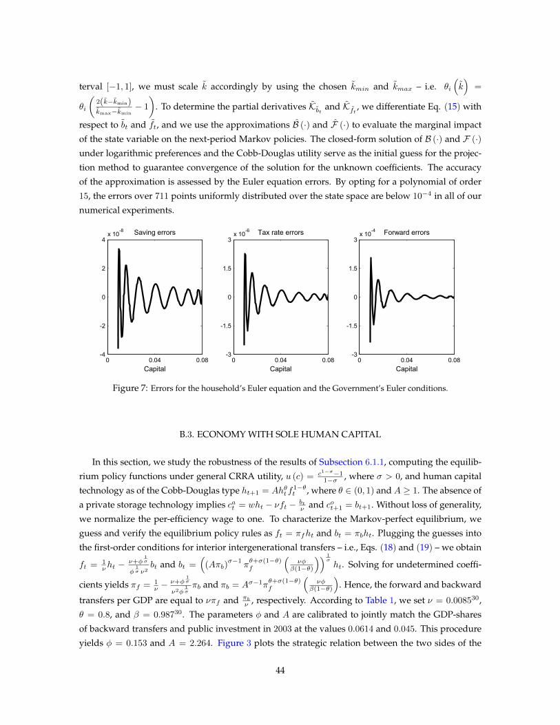
terval [−1, 1], we must scale k accordingly by using the chosen kmin and kmax – i.e. θi

(k)

=

θi

(2(k−kmin)kmax−kmin

− 1

). To determine the partial derivatives Kbt and Kft , we differentiate Eq. (15) with

respect to bt and ft, and we use the approximations B (·) and F (·) to evaluate the marginal impact

of the state variable on the next-period Markov policies. The closed-form solution of B (·) and F (·)under logarithmic preferences and the Cobb-Douglas utility serve as the initial guess for the projec-

tion method to guarantee convergence of the solution for the unknown coefficients. The accuracy

of the approximation is assessed by the Euler equation errors. By opting for a polynomial of order

15, the errors over 711 points uniformly distributed over the state space are below 10−4 in all of our

numerical experiments.

0 0.04 0.08-4

-2

0

2

4x 10

-8 Saving errors

Capital0 0.04 0.08

-3

-1.5

0

1.5

3x 10

-6 Tax rate errors

Capital0 0.04 0.08

-3

-1.5

0

1.5

3x 10

-4 Forward errors

Capital

Figure 7: Errors for the household’s Euler equation and the Government’s Euler conditions.

B.3. ECONOMY WITH SOLE HUMAN CAPITAL

In this section, we study the robustness of the results of Subsection 6.1.1, computing the equilib-

rium policy functions under general CRRA utility, u (c) = c1−σ−11−σ , where σ > 0, and human capital

technology as of the Cobb-Douglas type ht+1 = Ahθt f1−θt , where θ ∈ (0, 1) and A ≥ 1. The absence of

a private storage technology implies cat = wht − νft − btν and cot+1 = bt+1. Without loss of generality,

we normalize the per-efficiency wage to one. To characterize the Markov-perfect equilibrium, we

guess and verify the equilibrium policy rules as ft = πfht and bt = πbht. Plugging the guesses into

the first-order conditions for interior intergenerational transfers – i.e., Eqs. (18) and (19) – we obtain

ft = 1νht −

ν+φ1σ

φ1σ ν2

bt and bt =(

(Aπb)σ−1

πθ+σ(1−θ)f

(νφ

β(1−θ)

)) 1σ

ht. Solving for undetermined coeffi-

cients yields πf = 1ν −

ν+φ1σ

ν2φ1σπb and πb = Aσ−1π

θ+σ(1−θ)f

(νφ

β(1−θ)

). Hence, the forward and backward

transfers per GDP are equal to νπf and πbν , respectively. According to Table 1, we set ν = 0.008530,

θ = 0.8, and β = 0.98730. The parameters φ and A are calibrated to jointly match the GDP-shares

of backward transfers and public investment in 2003 at the values 0.0614 and 0.045. This procedure

yields φ = 0.153 and A = 2.264. Figure 3 plots the strategic relation between the two sides of the

44

intergenerational contract for the benchmark case with σ = 0.7 (Panel (a)) and for the counterfactual

case with σ = 2 (Panel (b)).

References[1] Banks, J. S., and Duggan J., 2005. Probabilistic voting in the spatial model of elections: The

theory of office-motivated candidates, Social choice and strategic decisions, 15-56.

[2] Judd, K., 1992. Projection Methods for Solving Aggregate Growth Models, Journal of Economic

Theory, 58, 410-452.

[3] Judd, K., 1998. Numerical Methods in Economics, The MIT Press.

45