J Heuristics (2006) 12: 211–233

DOI 10.1007/s10732-006-5905-1

A decomposition heuristics for the container ship stowageproblem

Daniela Ambrosino · Anna Sciomachen · Elena Tanfani

Submitted in May 2004 and accepted by Anthony Cox in October 2005 after 2 revisionsC© Springer Science + Business Media, LLC 2006

Abstract In this paper we face the problem of stowing a containership, referred to as the

Master Bay Plan Problem (MBPP); this problem is difficult to solve due to its combinatorial

nature and the constraints related to both the ship and the containers. We present a decom-

position approach that allows us to assign a priori the bays of a containership to the set of

containers to be loaded according to their final destination, such that different portions of

the ship are independently considered for the stowage. Then, we find the optimal solution of

each subset of bays by using a 0/1 Linear Programming model. Finally, we check the global

ship stability of the overall stowage plan and look for its feasibility by using an exchange

algorithm which is based on local search techniques. The validation of the proposed approach

is performed with some real life test cases.

Keywords Stowage plan . Heuristic algorithm . Local search . 0/1 linear programming

1. Introduction and problem definition

In this paper we deal with the ship planning problem. The stowage of a containership is one

of the problems that has to be solved on a daily basis by any company which manages a

container terminal (Thomas, 1989). In the past stowage plans for containers were performed

by the Captain of the ship; today, as a consequence of containerisation, the maritime terminal

has to decide the stowage of containers following the instructions coming from the maritime

company holding the ship and taking into account different interrelated terminal requirements

(see Atkins, 1991).

This work has been developed within the research area: “The harbour as a logistic node” of the Italian Centreof Excellence on Integrated Logistics (CIELI) of the University of Genoa, Italy

D. Ambrosino · A. Sciomachen (�) · E. TanfaniDepartment of Economics and Quantitative Methods (DIEM), University of Genova, Via Vivaldi 5,16126 Genova, Italye-mail: sciomach@economia.unige.it

Springer

212 J Heuristics (2006) 12: 211–233

Formally, the stowage planning problem, known as the Master Bay Plan Problem (MBPP),

consists in determining how to stow a given set C of n containers of different type into a

set S of m available locations of a containership, respecting some structural and opera-

tional constraints, related to both the containers and the ship; the goal is the minimisa-

tion of the loading time of all containers. In fact, while the turnaround time of a ship in-

cludes the time for berthing, unloading, loading and departure, the major activities affecting

the turnaround time are the unloading and loading processes, and, in particular, loading

is the more difficult and sensitive to the efficiency of the operations process (Imai et al.,

2002).

In the MBPP each container c ∈ C must be stowed in a location l ∈ S of the ship. Note that

the l-th location is actually addressed by indices i, j, k representing, respectively: the bay

(i), that gives its position related to the cross section of the ship (counted from bow to stern),

the row ( j), that gives its position related to the horizontal section of the corresponding bay

(counted from centre to outside), and the tier (k) that gives its position related to the vertical

section of the corresponding bay (counted from bottom to top). We will denote by I , J and K ,

respectively, the set of bays, rows and tiers of the ship, and by b, r and s their corresponding

cardinality.

The objective function is expressed in terms of the sum of time tlc required for loading

a container c, ∀c ∈ C , in location l, ∀l ∈ S, such that L = ∑lc tlc. However, when two or

more quay cranes are used for the loading operations the objective function is given by the

maximum over the minimum loading time (Lq ) for handling all containers in the corre-

sponding ship partition by each quay crane q , that is L = maxQC {Lq}, where QC is the set of

available quay cranes. Note that the time for handling a container by a quay crane depends,

as we will see later, on the row and the tier address in the ship and the type of quay crane

used.

The main constraints that must be considered for the stowage planning process for an

individual port are related to the structure of the ship and focused on the size, type, weight,

destination and distribution of the containers to be loaded.

Size of containers. Usually, as in this paper, set C of containers is considered as the union

of two subsets, T and F , consisting, respectively, of 20 and 40 feet containers, such that

T ∩ F = ∅ and T ∪ F ≡ C . Standard locations are generally thought for dry 20 feet

containers and referred to as one Twenty Equivalent Unit (TEU) location. Containers of

40 feet (denoted by 40’) require two contiguous locations of 20 feet (denoted by 20’). Note

that according to a practice adopted by the majority of maritime companies, bays with even

number are used for stowing 40’ containers and correspond to two contiguous odd bays,

that are used for the stowage of 20’ containers. Consequently, if a 40’ container is stowed

in an even bay (for instance bay02) the locations of the same row and tier corresponding

to two contiguous odd bays (e.g. bay01 and bay03) are not anymore available for stowing

containers of 20’.

Type of containers. Different types of containers can usually be stowed in a containership,

such as standard, carriageable, reefer, out of gauge and hazardous.

The location of reefer containers is defined by the ship coordinator (who has a global vision

of the trip), so that we know their exact position. This is generally near power points in

order to maintain the required temperature during transportation. Hazardous containers are

also assigned by the harbour-master’s office which authorises their loading. In particular,

hazardous containers cannot be stowed either in the upper deck or in adjacent locations.

They are considered in the same way as 40’ containers. Note that, for the definition of

Springer

J Heuristics (2006) 12: 211–233 213

the stowage plan we consider only dry and dry high cube containers, having exterior

dimensions conforming to ISO standards of 20 and 40 feet long, either 8 feet 6 inches or

9 feet 6 inches high and 8 feet depth.

Weight of containers. The standard weight of an empty container ranges from 2 to 3.5 tons,

while the maximum weight of a full container to be stowed in a containership ranges from

20–32 and 30–48 tons for 20’ and 40’ containers, respectively. The weight constraints force

the weight of a stack of containers to be less than a given tolerance value. In particular the

weight of a stack of 3 containers of 20’ and 40’ cannot be greater than an a priori established

value, say MT and MF respectively. Moreover, the weight of a container located in a tier

cannot be greater than the weight of the container located in a lower tier having the same

row and bay and, as it is always required for security reasons, both 20’ and 40′ containers

cannot be located over empty locations.

Destination of containers. A good general stowing rule suggests to load first (i.e. in the lower

tiers) those containers having as destination the final stop of the ship and load last those

containers that have to be unloaded first.

Distribution of containers. Such constraints, also denoted stability constraints, are related to

a proper weight distribution in the ship. In particular, we have to verify different kinds of

equilibrium, namely: (a) horizontal equilibrium, that is the weight on the right side of the

ship, including the odd rows of the hold and upper deck, must be equal (within a given

tolerance, say Q1) to the weight on the left side of the ship; (b) cross equilibrium, that is

the weight on the stern must be equal (within a given tolerance, say Q2) to the weight on

the bow; (c) vertical equilibrium, that is the weight on each tier must be greater or equal

than the weight on the tier immediately over it. Let us denote by L and R, respectively,

the set of rows belonging to the left /right side of the ship and by A and P , respectively,

the sets of anterior and posterior bays of the ship. In Sections 5 and 6 we will see how

the horizontal ship stability constraint impacts on the total loading time by increasing the

optimal value.

The description of the entire problem in the form of an optimisation problem is given in

Ambrosino et al. (2004).

The MBPP is a NP-complete combinatorial optimisation problem (see. e.g. Avriel et al.

(2000) that connect the MBPP to the colouring of circle graphs problem).

Many interesting approaches for solving container loading problems that have some com-

monalties with the MBPP have been presented in the recent literature (see, e.g., Bischoff

and Mariott (1990), Bischoff and Ratcliff (1995), Bortfeldt and Gehring (2001), Davies and

Bischoff (1999), Eley (2002), Gehring et al. (1990), Gehring and Bortfeldt (1997) among

others).

The first attempt to derive some rules for determining good container stowage plans is

reported in Ambrosino and Sciomachen (1998), where a constraint satisfaction approach is

used for defining and characterising the space of feasible solutions. Wilson and Roach (1999,

2000) divide the container stowage process into two sub-processes, at a strategic and tactical

planning level, respectively. In particular, they use branch and bound algorithms for solving

the problem of assigning generalized containers to a bays’ block in a vessel; in the second step

they find a detailed plan which assigns specific positions or locations in a block to specific

containers by a tabu search algorithm. Wilson et al. (2001) present a computer system for

generating solutions for the decomposed stowage pre-planning problem illustrated in a case

study, using a genetic algorithm (GA) approach in order to generate automatically strategic

stowage plans and explore the application of artificial intelligence to cargo stowage problems.

Springer

214 J Heuristics (2006) 12: 211–233

Dubrovsky et al. (2002) use a GA for minimizing the number of container movements in the

stowage planning problem, while being able to include with appropriate constraints some

ship stability criteria; the authors significantly reduce the search space using a compact and

efficient encoding scheme.

Avriel and Penn (1993) and Avriel et al. (1997) focus on stowage planning considering the

problem of minimising the number of unproductive shifts (temporary unloading and reloading

of container at a port before their destination ports in order to access containers below them

for unloading). Martin et al. (1988) develop a heuristic algorithm that in solving the planning

problem takes into account the transtainer quay cranes, with the aim of minimising their global

longitudinal movement time and the total number of shifts in the successive ports. Sciomachen

and Tanfani (2003) present a heuristic method for the MBPP based on its connection to the

three dimensional bin packing problem.

Integer Linear Programming models for solving the MBPP have been proposed in Botter

and Brinati (1992) and Imai et al. (2002); however, due to many simplified assumptions,

they are not suitable for real life large scale applications. Ambrosino et al. (2004) give a 0/1

Linear Programming model and solve it by performing a preprocessing heuristic algorithm.

Here, we present a three phase algorithm for defining stowage plans with the aim of

minimising the total loading time of the containers on the ship and satisfying weight, size and

stability constraints, related to weight’ distribution. In the first phase, denoted main branching

tree, we split the ship into different portions and associate containers with different subsets

of bays without specifying their actual position. Successively, we find the optimal way for

loading containers into each partition of the ship by solving a 0/1 Linear Programming model.

Note that in this way the search for the location of each container is limited to a portion of

the ship and therefore the space of the solutions is reduced. Finally, we check and remove

possible unfeasibilities of the global solution due to the cross and horizontal stability of the

ship by performing some local search exchanges.

Note that in the present approach we assume that the ship starts its journey in the port

for which we are studying the problem, and successively visits a given number of other

ports where only unloading operations are allowed, that is we are only concerned with the

loading problem at the first port. However, note that in all the following ports visited by

the ship the same loading process holds provided that only the available locations would

be considered. Moreover we assume that the number of containers to load on board is not

greater than the number of available locations; this means that we are not concerned with the

problem of selecting some containers to be loaded among all, and we will verify a priori the

capacity of the ship related to the maximum weight and size available for all containers to be

loaded.

The proposed bay assignment algorithm is described in Section 2; Section 3 reports the

0/1 Linear Programming model related to each portion of the ship; Section 4 describes how

we make the overall solution feasible with respect to the stability conditions of the ship. An

application of our algorithm is given in Section 5 by solving a sample problem step by step,

and a validation of the approach based on some real life test cases is reported in Section 6.

Finally, some conclusions are given in Section 7.

2. The bay assignment algorithm

In this section we will show how to split set I into different partitions, in order to be able

to solve separately the loading problem for each portion of the ship, independently on its

stability conditions, that will be verified successively. Other decomposition approaches have

Springer

J Heuristics (2006) 12: 211–233 215

been presented in the literature with the same aim of reducing the complexity of the overall

problem (Wilson and Roach, 1999, 2001).

The bay partitioning procedure proposed here is based on a main branching tree, consisting

of the following four steps. In particular, our bay assignment algorithm can be applied when

b ≥ 6; this choice for b allows at least two quay cranes working in parallel.

Step 1 (Sorting C). We split set C into p subsets Ch , h = 1, . . . , p, where p > 1 is

the number of different ports visited by the ship, such that c ∈ Ch if and only if

dc = h, ∀ h = 1, . . . , p, where dc denotes the destination port of containerc, ∀ c ∈ C.

Note that, as it is also in our referring terminal operative scenario, the number of

ports to be visited by a ship is generally p ≤ 10. Moreover, it is assumed that

p < b, i.e. the number of bays is usually greater than the number of ports to be

visited.

All containers are hence grouped together according to their destination, such that⋃h=1,...,p Ch = C and Cg∩ Ch = ∅, ∀ h �= g, h, g = 1, . . . , p. Let h = 1 denote the

first destination of the ship, h = 2 the second destination, and so on. We then sort Cin such a way that Ch < Cg if and only if h < g. Elements belonging to C1 are hence

containers to be unloaded first.

Step 2 (Sizing Ch , h = 1, . . . , p). For each subset of containers Ch, h = 1, . . . , p, we com-

pute the corresponding TEUs, denoted by τ h ; that is τ h is the number of TEUs

corresponding to those 20’ and 40’ containers that belong to Ch , h = 1, . . . , p .At the end of this step we hence know the size of each subset of containers

Ch , h = 1,. . . , p.

Step 3 (Partitioning I ). We associate subset Ch , h = 1, . . . , p, with bays i ∈ I , depending

on the value of p and the size of Ch , and generate subset ICh of all bays devoted to

the stowage of container c, ∀ c ∈ Ch . Let N (ICh ) be the number of TEUs belonging

to ICh .

In particular, we first assign the central bay of the ship, namely bay b/2�, to

C1, where b/2� denotes the smallest integer number greater than b/2 and C1 is the

subset of containers to be unloaded first; consequently, we initialise IC1= { b/2�}

and compute N (IC1).

At each decision node of the main branching tree the feasibility of the assignment

is checked as follow. If τ 1, that is the number of TEUs of the containers belonging to

C1, is less, within a given TEUs tolerance, than N (IC1), the assignment is accepted,

since no further bay is required for loading the whole set C1. In this case, we start

with the search of the bays for loading containers belonging to C2; otherwise, we

assign to C1 also bay ( b/2� + 3), update IC1= { b/2�, ( b/2� + 3)} and N (IC1

),

and check the feasibility of the assignment. If τ 1 is still greater thanN (IC1) we go

ahead by adding to IC1bay ( b/2� − 3) in the left side. In the search for feasibility we

continuously add, alternatively at their right and left side, the bays that are externals

and contiguous to those that have been already chosen, i.e. ( b/2� + 4), ( b/2� − 4),

( b/2� + 5), etc; when there is not any more available bay in the considered direction,

we choose the nearest bay to the centre of the ship, until N (IC1) > τ 1 and accept the

current assignment. We denote by δ1 the residual number of TEUs belonging to IC1

such that δ1 = N (IC1)−τ 1.

Successively, we assign bay (�b/2� + 1) to C2, initialise IC2and check the feasi-

bility of the assignment as before by computing N (IC2); we then jump two or more

bays, alternatively, at the right and left side searching for a free bay to assign to

C2. When IC2is large enough for loading all containers of C2 the current node is

Springer

216 J Heuristics (2006) 12: 211–233

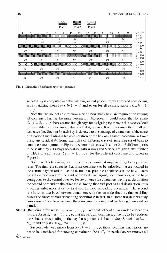
Fig. 1 Examples of different bays’ assignments

selected, δ2 is computed and the bay assignment procedure will proceed considering

set C3, starting from bay (�b/2� − 1) and so on for all existing subsets Ch, h = 1,

. . . , p.

Note that we are not able to know a priori how many bays are required for stowing

all containers having the same destination. Moreover, it could occur that for some

Ch, h = 2, . . . , p there are not enough bays for assigning τh ; then, in this case we look

for available locations among the residual δh−1 ones. It will be shown that in all our

test cases (see Section 6) each bay is devoted to the stowage of containers of the same

destination thus finding a feasible solution of the bay assignment procedure without

using any residual δh . Some examples of different ways of assigning set of bays to

containers are reported in Figure 1, where instances with either 2 or 3 different ports

to be visited by a 14 bays hold-ship, with 4 rows and 5 tiers, are given; the number

of TEUs of each subset Ch, h = 1, . . . , 3, for the different cases are also given in

Figure 1.

Note that this bay assignment procedure is aimed at implementing two operative

rules. The first rule suggests that those containers to be unloaded first are located in

the central bays in order to avoid as much as possible unbalances in the bow—stern

weight distribution after the visit at the first discharging port; moreover, in the bays

contiguous to the central ones we locate on one side containers having as destination

the second port and on the other those having the third port as final destination, thus

avoiding unbalances after the first and the next unloading operations. The second

rule is to let two bays between containers with the same destination, thus enabling

easier and faster container handling operations; in fact, in a “three transtainers quay

complement” two bays between the transtainers are required for letting them work in

parallel.

Step 4 (Reducing S for subset Ch, h = 1, . . . , p). We split set S of all m available locations

into p subsets SCh , h = 1, . . . , p, that identify all locations li jk having as bay address

the values corresponding to the bays’ assignments defined in Step 3, such that li jk ∈SCh if and only if i ∈ ICh , ∀h = 1, . . . , p.

Successively, we remove from SCh , h = 1, . . . , p, those locations that a priori are

not to be considered for stowing container c, ∀c ∈ Ch . In particular, we remove all

Springer

J Heuristics (2006) 12: 211–233 217

locations in odd bays for 40’ containers and those in even bays for 20′ ones, since

they cannot be considered in any feasible solution (see Section 1).

We denote by S̄Ch the set of really available locations for stowing containers be-

longing to Ch , and by Th and Fh , the sets of 20′ and 40′ containers of Ch , respectively,

such that Th ∪ Fh ≡ Ch . In practice, in this step we initially assign SCh to S̄Ch and

remove from it location li jk if any of the following conditions is satisfied:

if (Fh �= ∅) then for (i ∈ O; c ∈ Fh ; ∀ j, k)S̄Ch := S̄Ch \{li jk};if (Th �= ∅) then for (i ∈ E ; c ∈ Th ; ∀ j, k)S̄Ch := S̄Ch \{li jk},

where O and E denote, respectively, the set of bays with odd and even number.

It can be easily noted that the time complexity of the overall algorithm is bounded by a

quadratic polynomial function in the number of bays; in particular, the worst case complexity

is O(pb2) due to Step 3.

3. A 0/1 model for the optimal stowage of each ship partition

The procedure presented above allows us to do not consider the destination constraints that

are active combinatorial ones and strongly affect the computational time (Wilson and Roach,

1999). In particular, remember that the destination constraints force containers stowed in the

highest tiers to be unloaded first and hence from an operative point of view they are very

important; in fact, without considering the unloading port some containers loaded last could

be necessarily moved for enabling the unloading operations of some others, thus causing

the so called “empty moves” and increasing the turnaround time. Some interesting results

based on the reduction of the number of restows and/or empty moves are given in Avriet

et al. (1997) and Botter and Brinati (1992), where a binary decision model is given that is

explosive in the resolution step; Dubrovsky et al. (2002) use an efficient genetic algorithm

for minimizing container movements and, finally, in Imai et al. (2002) stability conditions

are given in the objective function of an assignment model together with the minimization

of re-handles.

Now we introduce a 0/1 Linear Programming model aimed at finding the optimal way for

stowing containers in each partition S̄Ch , h = 1, . . . , p, of the ship. Note that by considering

only a single partition of the ship, a part from the already mentioned destination constraints,

also the cross equilibrium constraints, as they have been described in Section 1, are not

included. The decision variables are:

xi jkc ={

1 if in location li jk ∈ S̄Ch is stowed container c ∈ Ch

0 otherwise

For a better reading of the model we need the following additional notation: wc, weight of

container c ∈ Ch ; ti jkc, time for stowing a container c ∈ Ch in location li jk ∈ S̄Ch ; note that

ti jkc includes both the time for lifting container off the quay and the time for putting it into

the assigned location.

MinL S̄Ch=

∑i jk

∑c

ti jkcxi jkc (1)

Springer

218 J Heuristics (2006) 12: 211–233∑i jk

xi jkc = 1 ∀c (2)

∑c

xi jkc ≤ 1 ∀i, j, k (3)

∑c∈Th

xi+1 jkc +∑c∈Fh

xi jkc ≤ 1 ∀i, j, k (4)

∑c∈Th

xi−1 jkc +∑c∈Fh

xi jkc ≤ 1 ∀i, j, k (5)

∑c∈Th

wcxi jkc +∑c∈Th

wcxi jk+1c +∑c∈Th

wcxi jk+2c ≤ MT ∀i, j, k = 1, . . . , |K | − 2 (6)

∑c∈Fh

wcxi jkc +∑c∈Fh

wcxi jk+1c +∑c∈Fh

wcxi jk+2c ≤ M F ∀i, j, k = 1, . . . , |K | − 2 (7)

∑c

wcxi jkc −∑

c

wcxi jk+1c ≥ 0 ∀i, j, k = 1, . . . , |K | − 1 (8)

−Q ≤∑

i, j∈L ,k,c

wcxi jkc −∑

i, j∈R,k,c

wcxi jkc ≤ Q (9)

xi jkc ∈ {0, 1} ∀i, j, k∀c (10)

(1) is the objective function aimed at minimising the total stowage time of partition S̄Ch ; it

is expressed in terms of the sum of time ti jkc required for loading container c, ∀ c∈ Ch ,in

location li jk , ∀li jk ∈ S̄Ch .

Relations (2)–(3) are the well known assignment constraints forcing each con-

tainer to be stowed in one ship location and each location to have at most one

container.

As we have already said in Section 1, 40’ containers can be stowed only in even bays

and 20’ containers in odd bays; in our model (4) and (5) make unfeasible the stowage of 20’

containers in those odd bays that are contiguous to even locations already chosen for stowing

40’ containers.

The weight constraints (6) and (7) say that each stack of three 20’ and 40’ containers

cannot exceed some tolerance values MT and MF, respectively, that usually correspond to

45 and 66 tons. Constraints (8) force heavier containers to be put not over lighter ones; (8)

also avoid to stow both 20’ and 40’ containers over empty locations.

Constraint (9) is the horizontal equilibrium requiring that the weight on the right side must

be equal, within a given tolerance Q to the weight on the left side of each portion of the ship.

Finally, (10) defines the binary decision variables of the problem.

The optimal stowage plan x∗ of the whole ship is given by x∗ = {x∗C1

∪ . . . x∗Ch

. . . ∪ x∗C p

},where x∗

Chis the optimal solution of model (1)–(10) for ship partition S̄Ch , h = 1, . . . , p. Note

that in Avriel and Penn (1993) a 0/1 Linear Programming model is given for the stowage of

a single rectangular bay, knowing in advance, as in our case, the number of containers to be

loaded.

If from step 2 of Section 2 we have S̄Ch ∩ S̄Cg �= ∅ for some h, g = 1, . . . , p, g < h, that

is, some residual δg is used for stowing containers belonging to Ch , then we first solve model

(1)–(10) for S̄Ch , thus avoiding to load in the lowest tiers of a bay devoted both to Ch and Cg

containers to be unloaded first; then, before solving the model for partition S̄Cg we remove

Springer

J Heuristics (2006) 12: 211–233 219

from S̄Cg those locations li jk ∈ S̄Ch ∩ S̄Cg in which containers belonging to Ch have been

already assigned in the optimal solution x∗Ch

.

It is opportune to observe that following the decomposition approach given in Section 2 we

derive the number of bays to assign to each destination port on the basis of the real number

of containers to be loaded on board and hence their size and weight are implicitly taken

into account also considering the effective given TEUs tolerance (see Section 2); in all our

experimentations we never found unfeasible solutions with respect to constraints (2)–(9);

however, if an unfeasible solution would be found then the involved containers would be

removed from their corresponding partition S̄Ch and put a priory to another one according to

the residual TEUs δh, h = 1, . . . , p.

Model (1)–(10) has been implemented in MPL and solved for each bay partition up to

optimality by using the commercial software CPLEX 7.0 (see Table 3, Section 6). Note

that, the unfeasibility due to the horizontal and cross equilibrium of the whole ship will be

checked in the last phase of the resolution approach, here below presented. In fact, even if

the horizontal equilibrium is satisfied in a partition S̄Ch the global equilibrium of the ship

could be violated, as we will see in Sections 5 and 6.

4. An exchange algorithm for the stability conditions

In the last phase we check the stability of the ship and verify both its horizontal and

cross equilibrium. In particular, the horizontal stability condition requires, as it has been

done with constraint (9) in each portion S̄Ch , h = 1, . . . , p, that the weight on the right

side must be equal, within a given tolerance Q1, to the weight on the left side of

the ship; the cross stability condition requires that the weight on the stern must be

equal, within a given tolerance Q2, to the weight on the bow. Such conditions can be

expressed by constraints (11) and (12):

−Q1 ≤∑

i, j∈L ,k

∑c

wcx∗i jkc −

∑i, j∈R,k

∑c

wcx∗i jkc ≤ Q1 (11)

−Q2 ≤∑

i∈A, j,k

∑c

wcx∗i jkc −

∑i∈P, j,k

∑c

wcx∗i jkc ≤ Q2 (12)

where x∗i jkc are all variables set to 1 in the optimal solution of partition S̄Ch , h = 1, . . . , p.

Let η(x∗) be the left-right unbalance, that is the difference between the weight

on the left and right side of the ship in the optimal current solution x∗, given

by η(x∗) = |∑i, j∈L ,k

∑c wcx∗

i jkc − ∑i, j∈R,k

∑c wcx∗

i jkc|; analogously, let χ (x∗) be the

anterior-posterior unbalance, that is the difference between the weight on the anterior

and posterior bays of the ship in the optimal current solution x∗, given by χ (x∗) =|∑i∈A, j,k

∑c wcx∗

i jkc − ∑i∈P, j,k

∑c wcx∗

i jkc|; then, we compute the horizontal and cross

stability violations, respectively σ1 (x∗) and σ2 (x∗), as:

σ1(x∗) = max(η(x∗) − Q1, 0) (13)

σ2(x∗) = max(χ (x∗) − Q2, 0) (14)

Following (13) and (14) the global ship stability unfeasibility is hence given by:

σ (x∗) = σ1(x∗) + σ2(x∗) (15)

Springer

220 J Heuristics (2006) 12: 211–233

We propose some exchanges for making feasible solution x∗ obtained at the end of the

second phase whenever σ (x∗) > 0, that is if the ship stability is violated. In particu-

lar, we change the locations of some containers that are currently stowed in bays be-

longing to ICh in order to reduce the unfeasibility value (15) and possibly obtaining a

solution that satisfies constraints (11) and (12), without violating constraints of model

(1)–(10).

More precisely, we consider side, cross and bay exchanges among containers as they are

defined as follows.

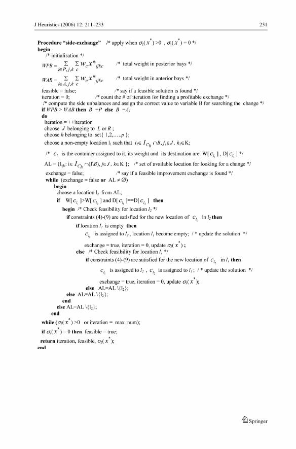
Definition 1. In a side-exchange a container c belonging to C is moved from its current

location l ∈ A ∩ L (or, analogously l ∈ A ∩ R) and put in a location, say f , such that

f ∈ P ∩ L( f ∈ P ∩ R). f can be either empty or filled with a container g ∈ C ; in this last

case g is moved from f and put in location l, that is the original location of container c (and

vice versa).

Note that Definition 1 implies that by performing one side-exchange we either move one

container or exchange the location between two containers from the anterior to posterior part

of the ship (or vice versa) without changing the side, that can be either the sea or the quay

one.

Definition 2. In a cross-exchange a container c belonging to C is moved from its current

location l ∈ A ∩ L (or, analogously, l ∈ A ∩ R) and put in a location, say f , such that

f ∈ P ∩ R(l ∈ P ∩ L). f can be either empty or filled with a container g ∈ C ; in this last

case g is moved from f and put in location l, that is the original location of container c (and

vice versa).

Note that Definition 2 implies that by performing one cross-exchange we either move one

container or exchange the location between two containers from the anterior to posterior part

of the ship (or vice versa) while changing the side, that is from the sea side to the quay one

(or vice versa).

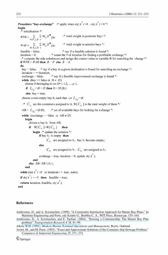
Definition 3. In a bay-exchange a whole stack of containers belonging to C is moved from

its current bay address i ∈ I ∩ A (or, analogously, i ∈ I ∩ P) and located in bay, say e,

such that e ∈ I ∩ P(i ∈ I ∩ A) in the same position as far as their row and tier addresses.

All rows and tiers at bay e can be empty or filled with a stack of containers; in this last case,

such containers are moved from e and located in the same order at bay i .

Note that Definition 3 implies that by performing one bay-exchange we move either one

or two whole stacks of containers and put them, as they are stowed in the current bay, in

a different part of the ship, i.e. from the anterior to the posterior part of the ship (and vice

versa).

Of course, any of the above exchange is performed if and only if the new defined location

of all containers does not violate constraints (4)–(9). Moreover, we perform the exchanges

only among containers having the same destination, that is to say we exchange containers

considering only subsets ICh , h = 1, . . . , p.

Usually an exchange is performed if the difference between the objective function values

of the current and the new solution is in favour of the last one. In our case, we apply a

local search not for improving the current solution but for obtaining feasibility in terms of

Springer

J Heuristics (2006) 12: 211–233 221

constraints (4)–(9) and (11)–(12). For this reason we consider as cost θ of an exchange the

difference between the related global stability value (15), that is:

θ = σ (x∗)′ − σ (x∗) (16)

where x∗′denotes the solution obtained from x∗ after an exchange of containers. Note that

if θ < 0 we have a profitable exchange, since this implies that some unfeasibility has been

removed. The cost given in (16) can be in some sense viewed as a penalty function for

obtaining feasibility in terms of ship stability as it is proposed in Dubrovsky et al. (2002).

As in any local search algorithm the definition of the neighbourhood and the strategy

used during the search are relevant factors. Moreover, the sequence of the defined moves

influences the “feasibility” process.

Here above, we have defined three moves (side-exchange, cross-exchange and bay-

exchange), respectively, in Definitions 1, 2 and 3. The best sequence of moves that we

perform for eliminating unfeasibility is reported in the following c-like procedure, while the

scheme of procedures “cross exchange”, “bay exchange”, and “side exchange” are reported

in the Appendix. It can be easily observed that the time complexity of the exchange algorithm

is of the order of br4

.

Note that we randomly chose a container for starting the search of a profitable exchange

(of course in the Anterior/Posterior or Right/Left part of the ship, in accordance with the

existing unfeasibility) and we operate the first profitable exchange found during the search.

Since we have defined as a profitable exchange a move such that σ (x∗) < 0, we accept also a

move that reduces σ1(x∗) whilst increases σ2(x∗). The search ends as soon as either a feasible

solution is found (i.e. σ1 (x∗) = σ2(x∗) = 0) or when after a certain number of iterations we

are not able to find a change for reducing σ1(x∗) or/and σ2(x∗). In this last case the algorithm

returns “No feasible solution found with respect to constraints (4)–(9), (11) and (12)”. As

we will show in Section 6, in our experiments we obtain a feasible solution in all instances

considered.

Springer

222 J Heuristics (2006) 12: 211–233

Table 1 Input data of the sample problem

Containers characteristics

Weight

Destination n Size n Light Medium Heavy TEUs

1 47 20 38 15 20 3 56

40 9 2 4 3

2 38 20 32 13 18 1 44

40 6 1 3 2

3 34 20 28 10 16 2 40

40 6 1 3 2

119 42 64 13 140

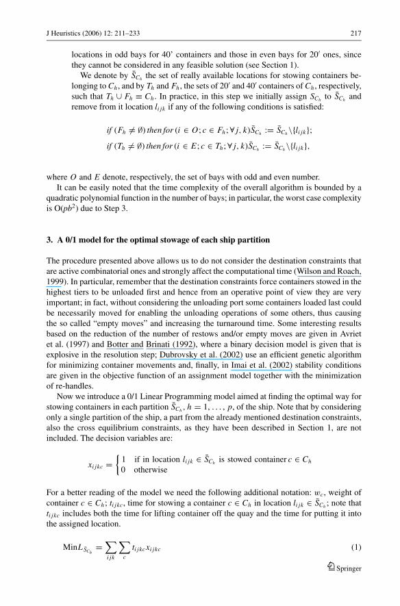
Fig. 2 The bay plan configuration of the sample problem

5. A sample problem

To give an idea of how the proposed three phase algorithm works, let us present a simple

case study concerning a 168 TEUs containership, in which we have to stow 119 standard

containers, split into 20 and 40 feet. The weight of the containers ranges from 5 to 15

tons (light containers), 15 to 25 tons (medium containers) and more than 25 tons (heavy

containers); 3 different ports have to be visited by the ship (see Table 1).

The ship consists of 14 odd bays, namely 1, 3, 5, . . . , 27 (originating seven even bays,

namely 2, 6, . . . , 26), 4 rows and 3 tiers (2 in the hold and 1 in the upper deck) and has a

maximum capacity of 1800 tons; the maximum horizontal and cross weight tolerance is fixed

to 20 and 35 tons, respectively.

By applying the assignment algorithm for the bays presented in Section 2, we

obtain subsets ICh , h = 1, 2, 3, given by: IC1= {1, 2, 3, 13, 14, 15, 25, 26, 27}, IC2

={5, 6, 7, 17, 18, 19}, IC3

= {9, 10, 11, 21, 22, 23}.The resulting bay plan configuration is shown in Figure 2. We can see that there

is a “two bays” distance between containers having the same destination; in this way

the handling time can be possibly reduced by letting the available quay cranes working

in parallel.

Then, by using model (1)–(10) we solve the loading problem for each ship partition SCh ,

h = 1, 2, 3. Note that the formulation of the problem related to the first ship partition SC1

Springer

J Heuristics (2006) 12: 211–233 223

requires 5076 variables and 2459 constraints, while for SC2and SC3

we have, respectively,

2736 variables and 1358 constraints, and 2448 variables and 1258 constraints. The objective

function values, that is the loading times, are (in minutes): L∗C1

= 108’ 6”, L∗C2

= 87’ 48”,

L∗C3

= 79’ 6”. The optimal solutions are obtained on a PC Pentium II by using MPL (Maximal

Software, 2000) and Cplex 7.0; the corresponding computational times are C PU ∗C1

= 1’ 04”,

C PU ∗C2

= 23.94”, C PU ∗C3

= 17.13”. The global solution x∗ = {x∗C1

∪ . . .x∗Ch

. . . ∪ x∗C p

}, that

gives the final stowage plan of the ship, is reported in Figure 3, where rows are denoted R01,

R04, R02, R01 and R03, while the tiers in the hold are Tier 02 and Tier 04 and that in the

upper deck is Tier 82.

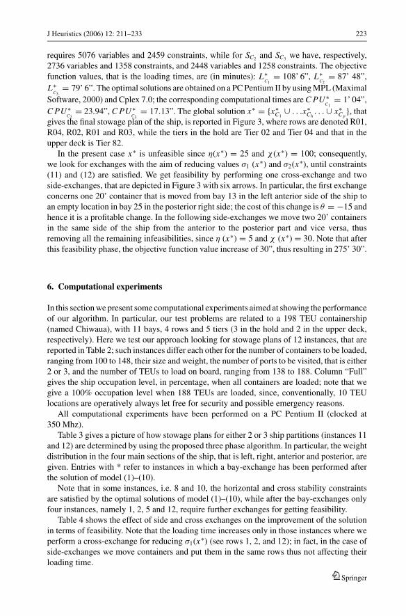
In the present case x∗ is unfeasible since η(x∗) = 25 and χ (x∗) = 100; consequently,

we look for exchanges with the aim of reducing values σ1 (x∗) and σ2(x∗), until constraints

(11) and (12) are satisfied. We get feasibility by performing one cross-exchange and two

side-exchanges, that are depicted in Figure 3 with six arrows. In particular, the first exchange

concerns one 20’ container that is moved from bay 13 in the left anterior side of the ship to

an empty location in bay 25 in the posterior right side; the cost of this change is θ = −15 and

hence it is a profitable change. In the following side-exchanges we move two 20’ containers

in the same side of the ship from the anterior to the posterior part and vice versa, thus

removing all the remaining infeasibilities, since η (x∗) = 5 and χ (x∗) = 30. Note that after

this feasibility phase, the objective function value increase of 30”, thus resulting in 275’ 30”.

6. Computational experiments

In this section we present some computational experiments aimed at showing the performance

of our algorithm. In particular, our test problems are related to a 198 TEU containership

(named Chiwaua), with 11 bays, 4 rows and 5 tiers (3 in the hold and 2 in the upper deck,

respectively). Here we test our approach looking for stowage plans of 12 instances, that are

reported in Table 2; such instances differ each other for the number of containers to be loaded,

ranging from 100 to 148, their size and weight, the number of ports to be visited, that is either

2 or 3, and the number of TEUs to load on board, ranging from 138 to 188. Column “Full”

gives the ship occupation level, in percentage, when all containers are loaded; note that we

give a 100% occupation level when 188 TEUs are loaded, since, conventionally, 10 TEU

locations are operatively always let free for security and possible emergency reasons.

All computational experiments have been performed on a PC Pentium II (clocked at

350 Mhz).

Table 3 gives a picture of how stowage plans for either 2 or 3 ship partitions (instances 11

and 12) are determined by using the proposed three phase algorithm. In particular, the weight

distribution in the four main sections of the ship, that is left, right, anterior and posterior, are

given. Entries with * refer to instances in which a bay-exchange has been performed after

the solution of model (1)–(10).

Note that in some instances, i.e. 8 and 10, the horizontal and cross stability constraints

are satisfied by the optimal solutions of model (1)–(10), while after the bay-exchanges only

four instances, namely 1, 2, 5 and 12, require further exchanges for getting feasibility.

Table 4 shows the effect of side and cross exchanges on the improvement of the solution

in terms of feasibility. Note that the loading time increases only in those instances where we

perform a cross-exchange for reducing σ1(x∗) (see rows 1, 2, and 12); in fact, in the case of

side-exchanges we move containers and put them in the same rows thus not affecting their

loading time.

Springer

224 J Heuristics (2006) 12: 211–233Ta

ble

2In

stan

ces

of

the

con

tain

ersh

ipn

amed

Ch

iwau

a

Co

nta

iner

char

acte

rist

ics

Siz

eW

eig

ht

Des

tin

atio

n

Inst

ance

TE

Us

n2

0’

%4

0’

%L

igh

t%

Med

ium

%H

eav

y%

1%

2%

3%

%F

ull

113

81

00

62

62

,00

38

38

,00

46

46

,00

50

50

,00

44

,00

47

47

,00

53

53

,00

00

73

,40

216

51

20

75

62

,50

45

37

,50

52

43

,33

64

53

,33

43

,33

55

45

,83

65

54

,17

00

87

,77

317

01

30

90

69

,23

40

30

,77

60

46

,15

66

50

,77

43

,08

62

47

,69

68

52

,31

00

90

,43

417

51

30

85

65

,38

45

34

,62

58

44

,62

68

52

,31

43

,08

62

47

,69

68

52

,31

00

93

,09

518

01

40

10

07

1,4

34

02

8,5

76

24

4,2

97

45

2,8

64

2,8

66

14

3,5

77

95

6,4

30

09

5,7

4

618

01

50

12

08

0,0

03

02

0,0

07

04

6,6

77

65

0,6

74

2,6

76

54

3,3

38

55

6,6

70

09

5,7

4

718

51

30

75

57

,69

55

42

,31

60

46

,15

66

50

,77

43

,08

62

47

,69

68

52

,31

00

98

,40

818

51

40

95

67

,86

45

32

,14

58

41

,43

78

55

,71

42

,86

65

46

,43

75

53

,57

00

98

,40

918

81

48

10

87

2,9

74

02

7,0

36

64

4,5

97

85

2,7

42

,70

71

47

,97

77

52

,03

00

10

0,0

10

18

61

35

84

62

,22

51

37

,78

59

43

,70

72

53

,33

42

,96

60

44

,44

75

55

,56

00

98

,94

11

185

14

09

56

7,8

64

53

2,1

46

24

4,2

97

35

2,1

45

3,5

75

03

5,7

14

02

8,5

75

03

8,4

69

8,4

0

12

188

14

81

08

72

,97

40

27

,03

68

45

,95

76

51

,35

42

,70

50

33

,78

50

33

,78

48

36

,92

10

0,0

Springer

J Heuristics (2006) 12: 211–233 225

Table 3 Weight configuration and corresponding unfeasibilities of optimal ship partition solutions afterbay-exchanges

CPU* L* Weight distribution

INSTANCE 1Tot.right Tot.left bay5/7* bay13* bay19/21*

C1 00.54,9 1.48.36 310 325 125 185 325Tot.right Tot.left bay1/3 bay9/11 bay15/17

C2 00.29,5 2.03.06 380 400 350 210 220Tot.right Tot.left Tot.ant Tot.post

C1+C2 01.24,4 3.51.42 690 725 685 730σ 1,2 15 10

INSTANCE 3Tot.right Tot.left bay5/7* bay13* bay19/21

C1 01.21,6 2.25,42 365 350 155 285 275Tot.right Tot.left bay1/3 bay9/11* bay15/17*

C2 02.01,0 2.40.30 495 510 335 355 315Tot.right Tot.left Tot.ant Tot.post

C1+C2 03.22,6 5.06.12 860 860 845 875σ 1, 2 0 0

INSTANCE 5Tot.right Tot.left bay5/7 bay13 bay19/21

C1 02.21,5 2.23.06 370 370 305 125 310Tot.right Tot.left bay1/3 bay9/11* bay15/17*

C2 1.52,2 3.04.30 455 450 295 280 330Tot.right Tot.left Tot.ant Tot.post

C1+C2 04:13.7 5:27:36 825 820 880 765σ 1,2 0 80

INSTANCE 7Tot.right Tot.left bay5/7* bay13 bay19/21*

C1 02.26,0 2.27.18 360 355 240 110 365Tot.right Tot.left bay1/3 bay9/11* bay15/17*

C2 00.42,5 2.38.54 510 495 375 245 385Tot.right Tot.left Tot.ant Tot.post

C1+C2 03.08,5 5.06.12 870 850 860 860σ 1, 2 0 0

INSTANCE 9Tot.right Tot.left bay5/7 bay13 bay19/21

C1 02.15,3 2.32.48 360 375 165 250 320Tot.right Tot.left bay1/3 bay9/11 bay15/17

C2 01:30,7 2.43.06 425 425 315 300 235Tot.right Tot.left Tot.ant Tot.post

C1+C2 03:46,0 5.15.54 785 800 780 805σ 1, 2 0 0

INSTANCE 11Tot.right Tot.left bay9/11* bay19/21*

C1 00:28,4 1.56.30 290 300 210 280Tot.right Tot.left bay5/7 bay13

C2 01.14,2 1.34.24 220 235 225 230Tot.right Tot.left bay1/3 bay15/17

C3 02.15,4 1.57.00 270 265 315 220Tot.right Tot.left Tot.ant Tot.post

C1+C2+C3 03.57,9 5.27.54 780 800 750 730σ 1, 2 0 0

(Continued on the next page)

Springer

226 J Heuristics (2006) 12: 211–233

Table 3 (Continued)

CPU* L* Weight distribution

INSTANCE 2

Tot.right Tot.left bay5/7 bay13 bay19/21

C1 00.41,6 2.06.30 360 380 355 120 265

Tot.right Tot.left bay1/3 bay9/11* bay15/17*

C2 01.20,0 2.30.36 465 480 315 190 440

Tot.right Tot.left Tot.ant Tot.postC1+C2 02.01,6 4.37.06 825 860 860 825

σ 1, 2 15 0

INSTANCE 4

Tot.right Tot.left bay5/7* bay13 bay19/21*

C1 00.47,3 2.23.48 365 380 230 175 340

C2 01.12,0 2.40.30 510 495 375 275 355

Tot.right Tot.left Tot.ant Tot.postC1 + C2 01.59,3 5.04.18 875 875 880 870

σ 1, 2 0 0

INSTANCE 6

Tot.right Tot.left bay5/7 bay13 bay19/21

C1 01:59,3 2.33.12 395 380 230 175 340

Tot.right Tot.left bay1/3 bay9/11* bay15/17*

C2 03.15,4 3.18.48 470 475 340 285 320

C1+C2 05.14,7 5.52.00 865 855 855 835

σ 1, 2 0 0

INSTANCE 8

Tot.right Tot.left bay5/7 bay13 bay19/21

C1 00.38.8 2.31.36 390 385 365 150 280

Tot.right Tot.left bay1/3 bay9/11 bay15/17

C2 02.40,2 2.55.24 465 485 280 240 430

Tot.right Tot.left Tot.ant Tot.postC1+C2 03.19,0 5.27.00 855 870 885 860

σ 1, 2 0 0

INSTANCE 10

Tot.right Tot.left bay5/7 bay13 bay19/21

C1 02.17,5 2.46.06 390 410 265 180 355

Tot.right Tot.left bay1/3 bay9/11 bay15/17

C2 03.54,3 2.58.18 430 415 255 315 275

Tot.right Tot.left Tot.ant Tot.postC1 + C2 06.11,8 5.44.24 820 825 835 810

σ 1, 2 0 0

INSTANCE 12

Tot.right Tot.left bay9/11 bay19/21

C1 01.30,5 1.56.54 275 255 240 290

Tot.right Tot.left bay5/7 bay13

C2 02.38,4 1.56.54 260 270 255 275

Tot.right Tot.left bay1/3 bay15/17

C3 02.04,1 1.51.48 255 270 295 230

Tot.right Tot.left Tot.ant Tot.postC1+C2+C3 06.13,0 5.45.36 515 540 790 795

σ 1, 2 5 0

Springer

J Heuristics (2006) 12: 211–233 227

Fig. 3 Stowage plan of the sample problem and representation of side and cross exchanges

Table 5 reports the comparison between the optimal solutions obtained by solving the

exact 0/1 Linear Programming model for the MBPP reported in Ambrosino et al. (2004)

(column LP) and the solutions obtained by using the present algorithmic approach (column

BA).

The comparison is based on two main indicators, that is the total loading time L (in hours,

minutes and seconds) and the computational time CPU (in minutes and seconds). Note that

in the case of our algorithm both L and CPU values related to the final solutions are given

by the sum of the corresponding values of each ship partition, such that L∗ = ∑ph=1 LCh and

CPU* = ∑ph=1 C PUCh .

Springer

228 J Heuristics (2006) 12: 211–233

Table 4 Improvement of the horizontal and cross stability violations after the exchange algorithm

Loading time (L)

(h.mm.ss) σ1 σ2

After cross After cross After cross

Model After bay- and side- Model After bay- and side- Model After bay- and side-

Instance (1)–(10) exchanges exchanges (1)–(10) exchanges exchanges (1)–(10) exchanges exchanges

1 3.51.42 3.51.42 3:52.12 15 15 0 320 10 0

2 4.37.06 4.37.06 4.38.54 15 15 0 500 0 0

3 5.06.12 5.06.12 5.06.12 0 0 0 115 0 0

4 5.04.18 5.04.18 5.04.18 0 0 0 355 0 0

5 5.27.36 5.27.36 5.27.36 0 0 0 180 80 0

6 5.52.00 5.52.00 5.52.00 0 0 0 0 0 0

7 5.06.12 5.06.12 5.06.12 0 0 0 495 0 0

8 5.27.00 5.27.00 5.27.00 0 0 0 0 0 0

9 5.15.54 5.15.54 5.15.54 0 0 0 120 0 0

10 5.44.24 5.44.24 5.44.24 0 0 0 125 0 0

11 5.27.54 5.27.54 5.27.54 0 0 0 0 0 0

12 5.45.36 5.45.36 5.46.06 5 5 0 0 0 0

Average 5.13.50 5.13.50 5.14.04 3 3 0 184 8 0

Table 5 Comparison of the loading time and the computational time betweenour solutions and the optimal ones

Loading time (L) CPU(h.mm.ss) (mm.ss,0)

Instance LP BA �% LP BA �%

1 3.46.54 3.52.12 2,34 03.25,0 01.34,8 53,76

2 4.32.36 4.38.54 2,31 08.28,4 02.11,9 74,06

3 5.01.48 5.06.12 1,46 10.32,4 03.33,1 66,30

4 5.00.36 5.04.18 1,23 03.33,7 02.09,8 39,26

5 5.24.24 5.27.36 0,99 10.08,2 04.24,0 56,59

6 5.48.12 5.52.00 1,09 14.27,5 05.25,0 62,54

7 5.03.06 5.06.12 1,02 11.02,0 03.19,0 69,94

8 5.24.00 5.27.00 0,93 15.38,3 03.29,1 77,72

9 5.13.18 5.15.54 0,83 05.52,8 03.56,1 33,08

10 5.43.48 5.44.24 0,17 13.32,1 06.21,9 52,98

11 5.25.12 5.27.54 0,83 14.53,6 04.08,3 72,21

12 5.45.36 5.46.06 0,14 13.17,6 06.23,2 51,96

Average 5.10.48 5.14.04 1,05 10.24,3 03.54,7 59,20

Springer

J Heuristics (2006) 12: 211–233 229

Table 6 Main information and results about a real scale instance

Containers characteristics

Weight

Destination n Size n Light Medium Heavy TEUs

1 100 20 70 30 20 20 130

40 30 10 10 10

2 120 20 90 40 20 30 150

40 30 15 10 5

3 80 20 60 20 20 20 100

40 20 5 5 10

300 300 42 64 13 380

Ship

Characteristics LP Model BA Algorithm

L CPU L CPU

Bays Rows Tiers TEUs Variables Contraints (hh.mm.ss) (hh.mm.ss,0) (hh.mm.ss) (hh.mm.ss,0)

17 6 6 612 356.400 4.257 − > 60.00.00,0 11.15.43 00.30.40,3

See the goodness of our solutions that are on the average about 1.05% greater than the

optimal values and, in the worst case, only 2.34%. Moreover, note the impressive reduction of

the CPU time of our approach, that is up to 59.20%. Even if in absolute terms the above CPU

time reduction is not significant, when considering larger instances it becomes noticeable. A

large amount of numerical experiments have been carried out in this direction with various

patterns of containers and different sizes of ships; unfortunately, we were not able to find

optimal values LP as for the instances given in Table 5. To get an idea of the explosive CPU

time required for solving the MBPP up to optimality Table 6 reports some information about

a large real case instance for which we were not able to find any integer solution in more

than 60 hours of CPU time; of course for this instance we cannot prove the goodness of the

solution but starting from the results given in Table 5 we believe that the optimality gap is

very tight.

7. Conclusions

In this paper we have presented a three phase algorithm for the MBPP, that is based on a

partitioning procedure that splits the ship into different portions and assigns them to containers

on the basis of their destination. The proposed solution method has very good performances

in terms of both solution quality and computational time. Looking at the given results, we

believe that the proposed approach is particularly suitable for determining stowage plans

of large size containerships, also considering the possibility of exploiting the potential of

commercial software, as Cplex, for solving up to the optimality single bay partitions of the

ship. Moreover, our algorithm enables the loading operations of each portion of the ship to

be performed in parallel thus minimising the loading time of the containership and hence

improving the competitiveness of maritime terminals.

Springer

230 J Heuristics (2006) 12: 211–233

Appendix

Springer

J Heuristics (2006) 12: 211–233 231

Springer

232 J Heuristics (2006) 12: 211–233

References

Ambrosino, D., and A. Sciomachen. (1998). “A Constraints Satisfaction Approach for Master Bay Plans.” InMaritime Engineering and Ports, eds Sciutto G., Brebbia C. A., WIT Press, Boston pp. 155–164.

Ambrosino, D., A. Sciomachen, and E. Tanfani. (2004). “Stowing a Containership: The Master Bay Planproblem.” Transportation Research A 38, 81–99.

Atkins W.H. (1991). Modern Marine Terminal Operations and Management, Boyle, Oakland.Avriel, M., and M. Penn. (1993). “Exact and Approximate Solutions of the Container ship Stowage Problem.”

Computers & Industrial Engineering 25, 271–274.

Springer

J Heuristics (2006) 12: 211–233 233

Avriel, M., M. Penn, N. Shpirer, and S. Witteboon. (1997). ”Stowage Planning for Container Ships to Reducethe Number of Shifts.” Annals of Operations Research 76, 55–71.

Avriel, M., and M. Penn, and N. Shpirer. (2000). “Container ship Stowage Problem: Complexity and Connec-tion to the Colouring of Circle Graphs.” Discrete Applied Mathematics 103, 271–279.

Bischoff, E.E., and M.D. Mariott. (1990). ”A Comparative Evaluation of Heuristics for Container Loading.”European Journal of Operational Research 44, 267–276.

Bischoff, E.E. and M.S.W. Ratcliff. (1995). “Issues on the Development of Approaches to Container loading.”International Journal of Management Science 23(4), 377–390.

Bortfeldt, A., and H. Gehring. (2001). “A Hybrid Genetic Algorithm for the Container Loading Problem.”European Journal of Operational Research 131(1), 143–161.

Botter, R.C., and M.A. Brinati. (1992). “Stowage Container Planning: A Model for Getting an OptimalSolution.” IFIP Transactions B B-5, 217–229.

Davies, A.P., and E.E. Bischoff. (1999). “Weight Distribution Considerations in Container Loading.” EuropeanJournal of Operational Research 114, 509–527.

Dubrovsky, O., G. Levitin, and M. Penn. (2002). ”A Genetic Algorithm with Compact Solution Encoding forthe Container ship Stowage Problem.” Journal of Heuristics 8, 585–599.

Eley, M. (2002). “Solving Container Loading Problems by Block Arrangment.” European Journal of Opera-tional Research 141, 393–409.

Gehring, M., and A. Bortfeldt. (1997). “A Genetic Algorithm for Solving Container Loading Problem.”International Transactions of Operational Research 4, 5/6, 401–418.

Gehring, M., M. Menscher, and A. Meyer. (1990). ”Computer-based Heuristic for Packing Pooled ShipmentContainers.” European Journal of Operational Research 44, 277–288.

Imai, A., E. Nishimura, S. Papadimitriu, and K. Sasaki. (2002). “The Containership Loading Problem.”International Journal of Maritime Economics 4, 126–148.

Martin, JR., SU. Randhawa, and ED.McDowell. (1988). ”Computerized Containership Load Planning: AMethodology and Evaluation.” Computers & Industrial Engineering 14, 429–440.

Sciomachen, A., and E. Tanfani. (2003). “The Master Bay Plan Problem: A Solution Method Based on itsConnection to the Three Dimensional bin Packing Problem.” IMA Journal of Management Mathematics14(3), 251–269.

Thomas, B.J. (1989). Management of Port Maintenance: A Review of Current Problems and Practices.H.M.S.O, London.

Wilson, I.D. and P. Roach. (1999). ”Principles of Combinatorial Optimisation Applied to Container-shipStowage Planning.” Journal of Heuristics 5, 403–418.

Wilson, I.D. and P. Roach. (2000). “Container Stowage Planning: A Methodology for Generating ComputerisedSolutions.” Journal of the Operational Research Society 51(11), 248–255.

Wilson, I.D., P.A. Roach, and J.A. Ware. (2001). “Container Stowage Pre-planning: Using Search to GenerateSolutions, a Case Study.” Knowledge-Based Systems 14, 3–4, 137–145.

Springer