A Dataset for Provident Vehicle Detection at Night

Sascha Saralajew,*, 1 Lars Ohnemus,*, 2 Lukas Ewecker,*, 2 Ebubekir Asan,*, 2 Simon Isele,2 and Stefan Roos2

Abstract— In current object detection, algorithms requirethe object to be directly visible in order to be detected. Ashumans, however, we intuitively use visual cues caused bythe respective object to already make assumptions about itsappearance. In the context of driving, such cues can be shadowsduring the day and often light reflections at night. In this paper,we study the problem of how to map this intuitive humanbehavior to computer vision algorithms to detect oncomingvehicles at night just from the light reflections they cause bytheir headlights. For that, we present an extensive open-sourcedataset containing 59 746 annotated grayscale images out of346 different scenes in a rural environment at night. In theseimages, all oncoming vehicles, their corresponding light objects(e. g., headlamps), and their respective light reflections (e. g.,light reflections on guardrails) are labeled. In this context, wediscuss the characteristics of the dataset and the challenges inobjectively describing visual cues such as light reflections. Weprovide different metrics for different ways to approach thetask and report the results we achieved using state-of-the-artand custom object detection models as a first benchmark. Withthat, we want to bring attention to a new and so far neglectedfield in computer vision research, encourage more researchersto tackle the problem, and thereby further close the gap betweenhuman performance and computer vision systems.

I. INTRODUCTION

© 2021 IEEE. Personal use of this material is permitted. Permission from IEEE must be obtained for all other uses, in any current or future media,including reprinting/republishing this material for advertising or promotional purposes, creating new collective works, for resale or redistribution to serversor lists, or reuse of any copyrighted component of this work in other works.

Object detection is one of the most popular and best studiedfields in computer vision. One reason is that object detectionis essential to several applications, for example, autonomousdriving and surveillance cameras. Currently, State-Of-The-Art(SOTA) object detection is performed by Neural Networks(NNs) and the target is to predict Bounding Boxes (BBs)that describe the position of visible objects. Thereby, a notnegligible restriction is the visibility assumption in formof direct sight to objects (ignoring systems that combinedetection and tracking to deal with occluded objects). Incontrast, in certain situations, human perception is capable toreason about the position of objects without direct visibility—for instance, by considering the illumination changes in anenvironment at daylight (e. g., in form of shadow movements).When driving a car at night, a similar human ability becomesa key feature for safe and anticipatory driving: The ability toreliably detect light reflections in the environment caused bythe mandatory headlamps of other road participants. Buildingon this ability, drivers can predict other vehicles and theirposition, in the sense where the object will occur in the future,even though they are not in direct sight.

*Authors contributed equally.1Bosch Center for Artificial Intelligence, Renningen, and Leibniz Univer-

sity Hannover, Institute of Product Development, Hannover, both Germany.The research was performed during employment at Dr. Ing. h.c. F. PorscheAG. sascha.saralajew@bosch.com

2Dr. Ing. h.c. F. Porsche AG, Weissach, Germany. {lars.ohnemus1,lukas.ewecker, ebubekir.asan}@porsche.de

Fig. 1. Annotation of light artifacts with KPs (dots) and the correspondinginferred saliency maps (colored areas represent the saliency of one KP).3

Motivated by the aforementioned human provident behaviorand the discrepancy to SOTA object detection, we providewith this paper all the tools needed to boost “ordinary” vehicledetection at night to provident vehicle detection such thatconsumer products can take advantage of this ability soon. Tothis end, we introduce and publish4 an annotated image datasetcontaining 346 different sequences with 59 746 annotatedgrayscale images in total captured at two different exposures.Each image is equipped with several annotations—in form ofKeyPoints (KPs)—that describe the position of other vehiclesand all their produced light instances (effects). Exemplary, weuse this dataset to train several machine learning models todetect light reflections that might serve as baselines for futureresearch. In order to properly evaluate object detectors onthe proposed dataset, we discuss commonly used evaluationmetrics in object detection and propose specially craftedmetrics for the dataset. Beyond the presented applicationof provident vehicle detection at night, the structure of thedataset is carefully designed such that it will be useful forother investigations as well (e. g., object tracking at night,transfer learning between different image exposure cycles).

The outline of the paper is as follows: In the next section,we discuss related work. Following this, we describe theannotation methodology and the challenges in annotatinglight reflections. With these insights, Section IV explains theprocess of creating the Provident Vehicle Detection at Night(PVDN) dataset. Afterwards, Section V shows the versatilityof our annotation strategy by extending the dataset withsaliency- and BB-representations. To analyze the performanceof detectors on the dataset, we craft evaluation metrics inSection VI. After that, we present benchmark models trainedon the dataset and finish with a conclusion and discussion.

3All images are brightness adjusted, cropped to the region of interest, andbest viewed when printed in color.

4https://www.kaggle.com/saralajew/provident-vehicle-detection-at-night-pvdn

arX

iv:2

105.

1323

6v2

[cs

.CV

] 1

1 A

ug 2

021

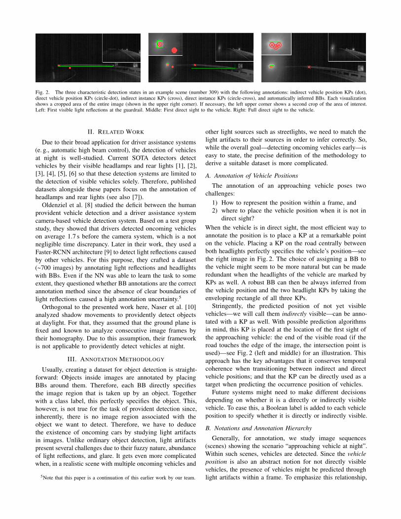
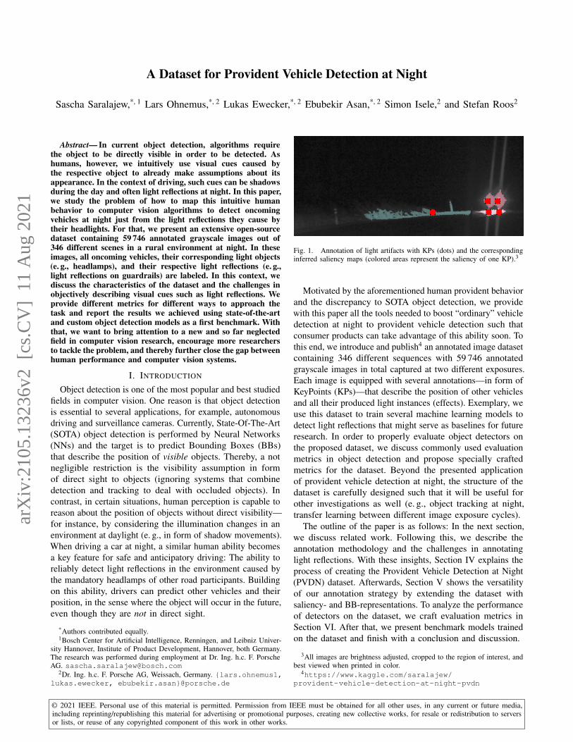
Fig. 2. The three characteristic detection states in an example scene (number 309) with the following annotations: indirect vehicle position KPs (dot),direct vehicle position KPs (circle-dot), indirect instance KPs (cross), direct instance KPs (circle-cross), and automatically inferred BBs. Each visualizationshows a cropped area of the entire image (shown in the upper right corner). If necessary, the left upper corner shows a second crop of the area of interest.Left: First visible light reflections at the guardrail. Middle: First direct sight to the vehicle. Right: Full direct sight to the vehicle.

II. RELATED WORK

Due to their broad application for driver assistance systems(e. g., automatic high beam control), the detection of vehiclesat night is well-studied. Current SOTA detectors detectvehicles by their visible headlamps and rear lights [1], [2],[3], [4], [5], [6] so that these detection systems are limited tothe detection of visible vehicles solely. Therefore, publisheddatasets alongside these papers focus on the annotation ofheadlamps and rear lights (see also [7]).

Oldenziel et al. [8] studied the deficit between the humanprovident vehicle detection and a driver assistance systemcamera-based vehicle detection system. Based on a test groupstudy, they showed that drivers detected oncoming vehicleson average 1.7 s before the camera system, which is a notnegligible time discrepancy. Later in their work, they used aFaster-RCNN architecture [9] to detect light reflections causedby other vehicles. For this purpose, they crafted a dataset(~700 images) by annotating light reflections and headlightswith BBs. Even if the NN was able to learn the task to someextent, they questioned whether BB annotations are the correctannotation method since the absence of clear boundaries oflight reflections caused a high annotation uncertainty.5

Orthogonal to the presented work here, Naser et al. [10]analyzed shadow movements to providently detect objectsat daylight. For that, they assumed that the ground plane isfixed and known to analyze consecutive image frames bytheir homography. Due to this assumption, their frameworkis not applicable to providently detect vehicles at night.

III. ANNOTATION METHODOLOGY

Usually, creating a dataset for object detection is straight-forward: Objects inside images are annotated by placingBBs around them. Therefore, each BB directly specifiesthe image region that is taken up by an object. Togetherwith a class label, this perfectly specifies the object. This,however, is not true for the task of provident detection since,inherently, there is no image region associated with theobject we want to detect. Therefore, we have to deducethe existence of oncoming cars by studying light artifactsin images. Unlike ordinary object detection, light artifactspresent several challenges due to their fuzzy nature, abundanceof light reflections, and glare. It gets even more complicatedwhen, in a realistic scene with multiple oncoming vehicles and

5Note that this paper is a continuation of this earlier work by our team.

other light sources such as streetlights, we need to match thelight artifacts to their sources in order to infer correctly. So,while the overall goal—detecting oncoming vehicles early—iseasy to state, the precise definition of the methodology toderive a suitable dataset is more complicated.

A. Annotation of Vehicle Positions

The annotation of an approaching vehicle poses twochallenges:

1) How to represent the position within a frame, and2) where to place the vehicle position when it is not in

direct sight?When the vehicle is in direct sight, the most efficient way toannotate the position is to place a KP at a remarkable pointon the vehicle. Placing a KP on the road centrally betweenboth headlights perfectly specifies the vehicle’s position—seethe right image in Fig. 2. The choice of assigning a BB tothe vehicle might seem to be more natural but can be maderedundant when the headlights of the vehicle are marked byKPs as well. A robust BB can then be always inferred fromthe vehicle position and the two headlight KPs by taking theenveloping rectangle of all three KPs.

Stringently, the predicted position of not yet visiblevehicles—we will call them indirectly visible—can be anno-tated with a KP as well. With possible prediction algorithmsin mind, this KP is placed at the location of the first sight ofthe approaching vehicle: the end of the visible road (if theroad touches the edge of the image, the intersection point isused)—see Fig. 2 (left and middle) for an illustration. Thisapproach has the key advantages that it conserves temporalcoherence when transitioning between indirect and directvehicle positions; and that the KP can be directly used as atarget when predicting the occurrence position of vehicles.

Future systems might need to make different decisionsdepending on whether it is a directly or indirectly visiblevehicle. To ease this, a Boolean label is added to each vehicleposition to specify whether it is directly or indirectly visible.

B. Notations and Annotation Hierarchy

Generally, for annotation, we study image sequences(scenes) showing the scenario “approaching vehicle at night”.Within such scenes, vehicles are detected. Since the vehicleposition is also an abstract notion for not directly visiblevehicles, the presence of vehicles might be predicted throughlight artifacts within a frame. To emphasize this relationship,

Scen

eLe

vel

Vehicle 1 Vehicle N

Fram

eLe

vel

Predicted position PositionIn

stan

ceLe

vel

indirect1

indirect2

indirect3

direct2

direct1

indirect1

indirect2

Fig. 3. Hierarchy of different entities used for the PVDN dataset. Thestructure allows for multiple vehicles each having a single (predicted) position.The vehicles are observed through a variable number of instances.

we denote any form of light artifacts as an instance of thevehicle. The “human” approach to predict and detect vehiclesat night spans three hierarchical semantic levels. On thetop level—the scene level—the aim is to predict and locateoncoming vehicles. This usually uses both temporal andspatial features. While the consideration of consecutive framesallows the driver to increase the detection certainty, oncomingvehicles can be detected using isolated, single images only. Onthis frame level, the vehicles have to be located. As instancesbuild up the knowledge about vehicles, they are placed onthe lowest semantic level, the instance level. The instancesare essential because, for not directly visible vehicles, theyare the only features available to infer the vehicles’ positions.Fig. 3 shows the hierarchy that implies two requirements fora suitable annotation strategy:

1) vehicle positions and their instances must be annotated;2) annotations should be coherent over multiple frames to

capture the temporal characteristics.While the second requirement can be enforced by assigningIDs to each annotated entity, the annotation of vehiclepositions and instances requires further investigations.

C. Annotation of Instances

We split the annotations in the same way we did for thevehicle position. Instances can be both direct (headlights) orindirect (halos, reflections), see Fig. 2. While direct instancesare well-specified, the total number and size of the indirectinstances cannot be specified objectively. The headlights mightbounce and be reflected multiple times, leaving instances ofvarious strengths all around the image.

1) Lessons learned of BB annotations: Oldenziel et al. [8]used BBs to represent light reflections, as already stated inSection II, and noticed a strong tendency of the detectortowards False Positive (FP) detections. We hypothesize, thatthis was mainly caused by two reasons: First, only thestrongest light artifact was annotated to represent a vehicle.Even if this assumption resulted in an objective annotationstrategy, it seemed to confuse the system as the intensityof the strongest instance is always dependent on the entirescenario. Thus, a lot of predictions might be True Positives(TPs) but were considered FPs due to the missing annotationsof weaker instances. Second, the metric used for evaluatingpredictions—the Intersection over Union (IoU)—is sensibleto size variations between ground truth and predictions. While

this is usually desired for object detection, it requires a well-specified, objective ground truth. However, on many occasions,both the ground truth and the prediction could be consideredcorrect while still giving a small IoU. This poses the question:Is it possible to objectively specify BBs? To address this, weperformed a small experiment, tasking multiple experts toannotate the same indirect instance with BBs. The resultsshow that on average the experts’ BBs only overlapped with amedian IoU of 59.4% for the indirect instance. This effect iseven worse for direct instances, resulting in a median IoU ofjust 52.0%. For a more detailed discussion of the annotationexperiment, see Appendix I.

2) KP annotations based on saliency: Based on theprevious discussion, it is clear that a proper annotation strategyshould not insinuate the existence of perfect annotations andtherefore leading to false conclusions on the real problem.Thus, a suitable strategy has to be flexible enough to allowfor variations while still describing the situation properly.Simply put, the annotation strategy should be guided by thelocal light intensity because this is the only available featureto judge the existence of instances. In real life, such locallight intensities or locally salient regions attract the attentionof drivers, and the goal of the annotation process is to mimicthis attention behavior.

An approach to this attention behavior is to mark points ofhigh visual saliency by KPs without proclaiming a boundary,see Fig. 2. With these KPs carefully placed in salient regions,we have markers for human attention—similar to datasetsusing eye-fixation points as descriptors of visual saliency [11].This annotation approach captures the top-down aspect ofhuman attention [12], which is goal-driven (detect oncomingvehicles). After the annotation, we can use the KPs to checkfor intensity stimuli that lead the annotators to the decision toplace a KP in this region, which corresponds to a bottom-upor stimuli-based saliency approach [12]. Such a bottom-upsaliency approach can be realized by comparing the pixelintensities of the surrounding area with the intensity value atthe KP. Usually, the intensity values in the surrounding areaare on average slightly lower than the KP intensity becausethe annotators intuitively look at the most salient point first—the intensity maximum. In Fig. 1 we show an example wherethe salient region was inferred from the KP (see Section Vfor further details about the saliency inference). Using thisapproach, we can specify entire instances without statingground-truth borders but rather suggestions of interestingimage regions. Additionally, the approach is fairly robust tovariations in the KP placement.

This annotation strategy applies to direct and indirectinstances. For direct instances, the KP is placed centrallywithin the headlight cone, see Fig. 2. To distinguish betweenboth instance types, we add a Boolean label. Additionally,it is worth noting, that this strategy is efficient to carry outsince only one point per instance has to be annotated.

IV. THE PVDN DATASET

The PVDN dataset is derived from a test group studyperformed to analyze provident vehicle detection skills of

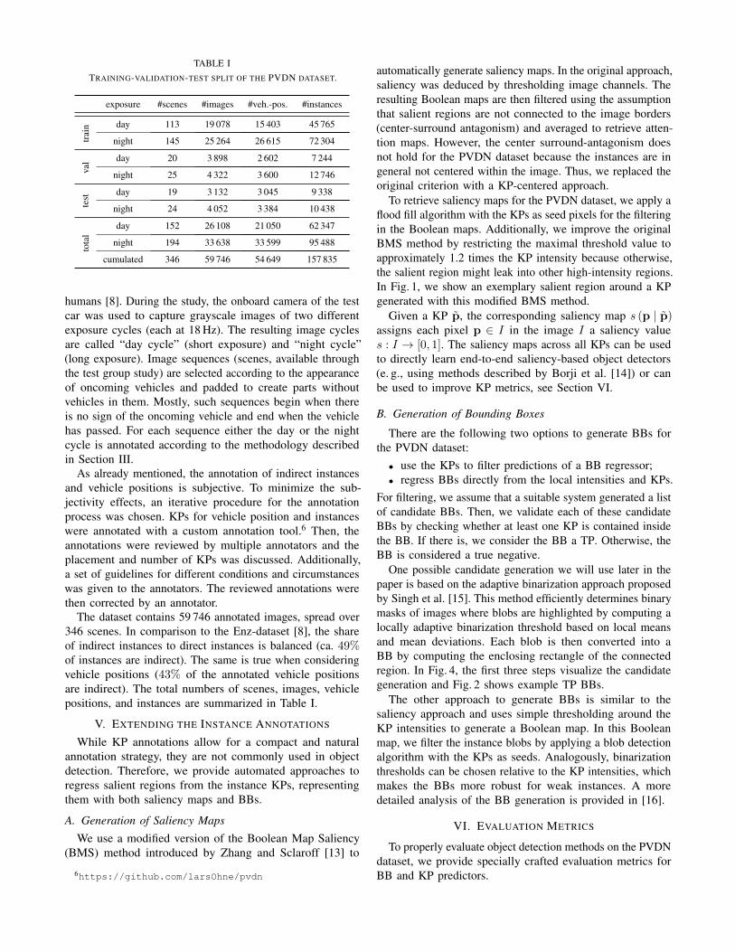
TABLE ITRAINING-VALIDATION-TEST SPLIT OF THE PVDN DATASET.

exposure #scenes #images #veh.-pos. #instances

trai

n day 113 19 078 15 403 45 765

night 145 25 264 26 615 72 304

val day 20 3 898 2 602 7 244

night 25 4 322 3 600 12 746

test day 19 3 132 3 045 9 338

night 24 4 052 3 384 10 438

tota

l

day 152 26 108 21 050 62 347

night 194 33 638 33 599 95 488

cumulated 346 59 746 54 649 157 835

humans [8]. During the study, the onboard camera of the testcar was used to capture grayscale images of two differentexposure cycles (each at 18 Hz). The resulting image cyclesare called “day cycle” (short exposure) and “night cycle”(long exposure). Image sequences (scenes, available throughthe test group study) are selected according to the appearanceof oncoming vehicles and padded to create parts withoutvehicles in them. Mostly, such sequences begin when thereis no sign of the oncoming vehicle and end when the vehiclehas passed. For each sequence either the day or the nightcycle is annotated according to the methodology describedin Section III.

As already mentioned, the annotation of indirect instancesand vehicle positions is subjective. To minimize the sub-jectivity effects, an iterative procedure for the annotationprocess was chosen. KPs for vehicle position and instanceswere annotated with a custom annotation tool.6 Then, theannotations were reviewed by multiple annotators and theplacement and number of KPs was discussed. Additionally,a set of guidelines for different conditions and circumstanceswas given to the annotators. The reviewed annotations werethen corrected by an annotator.

The dataset contains 59 746 annotated images, spread over346 scenes. In comparison to the Enz-dataset [8], the shareof indirect instances to direct instances is balanced (ca. 49%of instances are indirect). The same is true when consideringvehicle positions (43% of the annotated vehicle positionsare indirect). The total numbers of scenes, images, vehiclepositions, and instances are summarized in Table I.

V. EXTENDING THE INSTANCE ANNOTATIONS

While KP annotations allow for a compact and naturalannotation strategy, they are not commonly used in objectdetection. Therefore, we provide automated approaches toregress salient regions from the instance KPs, representingthem with both saliency maps and BBs.

A. Generation of Saliency Maps

We use a modified version of the Boolean Map Saliency(BMS) method introduced by Zhang and Sclaroff [13] to

6https://github.com/larsOhne/pvdn

automatically generate saliency maps. In the original approach,saliency was deduced by thresholding image channels. Theresulting Boolean maps are then filtered using the assumptionthat salient regions are not connected to the image borders(center-surround antagonism) and averaged to retrieve atten-tion maps. However, the center surround-antagonism doesnot hold for the PVDN dataset because the instances are ingeneral not centered within the image. Thus, we replaced theoriginal criterion with a KP-centered approach.

To retrieve saliency maps for the PVDN dataset, we apply aflood fill algorithm with the KPs as seed pixels for the filteringin the Boolean maps. Additionally, we improve the originalBMS method by restricting the maximal threshold value toapproximately 1.2 times the KP intensity because otherwise,the salient region might leak into other high-intensity regions.In Fig. 1, we show an exemplary salient region around a KPgenerated with this modified BMS method.

Given a KP p, the corresponding saliency map s (p | p)assigns each pixel p ∈ I in the image I a saliency values : I → [0, 1]. The saliency maps across all KPs can be usedto directly learn end-to-end saliency-based object detectors(e. g., using methods described by Borji et al. [14]) or canbe used to improve KP metrics, see Section VI.

B. Generation of Bounding Boxes

There are the following two options to generate BBs forthe PVDN dataset:

• use the KPs to filter predictions of a BB regressor;• regress BBs directly from the local intensities and KPs.

For filtering, we assume that a suitable system generated a listof candidate BBs. Then, we validate each of these candidateBBs by checking whether at least one KP is contained insidethe BB. If there is, we consider the BB a TP. Otherwise, theBB is considered a true negative.

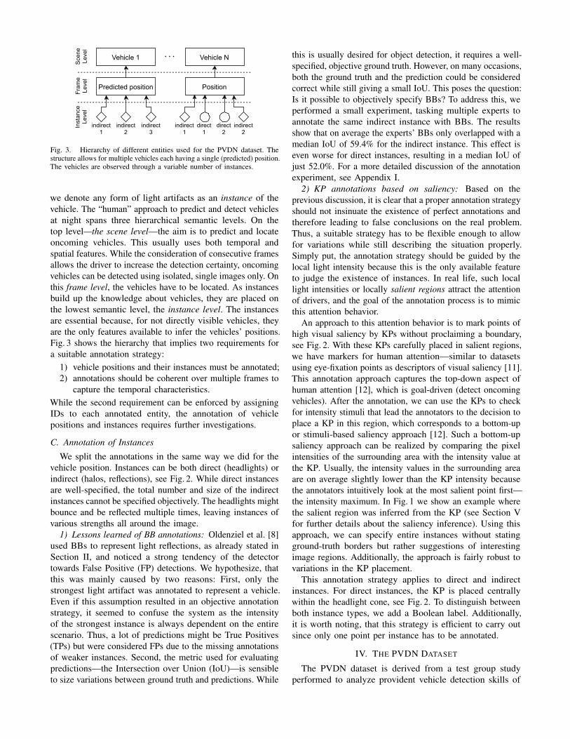
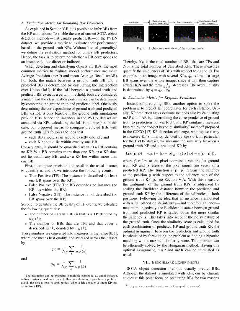
One possible candidate generation we will use later in thepaper is based on the adaptive binarization approach proposedby Singh et al. [15]. This method efficiently determines binarymasks of images where blobs are highlighted by computing alocally adaptive binarization threshold based on local meansand mean deviations. Each blob is then converted into aBB by computing the enclosing rectangle of the connectedregion. In Fig. 4, the first three steps visualize the candidategeneration and Fig. 2 shows example TP BBs.

The other approach to generate BBs is similar to thesaliency approach and uses simple thresholding around theKP intensities to generate a Boolean map. In this Booleanmap, we filter the instance blobs by applying a blob detectionalgorithm with the KPs as seeds. Analogously, binarizationthresholds can be chosen relative to the KP intensities, whichmakes the BBs more robust for weak instances. A moredetailed analysis of the BB generation is provided in [16].

VI. EVALUATION METRICS

To properly evaluate object detection methods on the PVDNdataset, we provide specially crafted evaluation metrics forBB and KP predictors.

A. Evaluation Metric for Bounding Box PredictorsAs explained in Section V-B, it is possible to infer BBs from

the KP annotations. To enable the use of current SOTA objectdetection methods—that usually predict BBs—on the PVDNdataset, we provide a metric to evaluate their performancebased on the ground truth KPs. Without loss of generality,7

we define the evaluation method for binary BB predictors.Hence, the task is to determine whether a BB corresponds toan instance (either direct or indirect).

When detecting and classifying objects via BBs, the mostcommon metrics to evaluate model performance are meanAverage Precision (mAP) and mean Average Recall (mAR).For both, the match between a ground truth BB and apredicted BB is determined by calculating the Intersectionover Union (IoU). If the IoU between a ground truth andpredicted BB exceeds a certain threshold, both are considereda match and the classification performance can be determinedby comparing the ground truth and predicted label. Obviously,determining the correspondence of ground truth and predictedBBs via IoU is only feasible if the ground truth annotationsprovide BBs. Since the instances in the PVDN dataset areannotated via KPs, calculating the IoU is not possible. In thiscase, our proposed metric to compare predicted BBs withground truth KPs follows the idea that

• each BB should span around exactly one KP, and• each KP should lie within exactly one BB.

Consequently, it should be quantified when a) a BB containsno KP, b) a BB contains more than one KP, c) a KP doesnot lie within any BB, and d) a KP lies within more thanone BB.

First, to compute precision and recall in the usual manner,to quantify a) and c), we introduce the following events:

• True Positive (TP): The instance is described (at leastone BB spans over the KP);

• False Positive (FP): The BB describes no instance (noKP lies within the BB);

• False Negative (FN): The instance is not described (noBB spans over the KP).

Second, to quantify the BB quality of TP events, we calculatethe following quantities:

• The number of KPs in a BB b that is a TP, denoted bynK (b);

• The number of BBs that are TPs and that cover adescribed KP k, denoted by nB (k).

These numbers are converted into measures in the range [0, 1],where one means best quality, and averaged across the datasetby

qK =1

NB

∑b

1

nK (b)

andqB =

1

NK

∑k

1

nB (k).

7The evaluation can be extended to multiple classes (e. g., direct instance,indirect instance, and no instance). However, defining it as a binary problemavoids the task to resolve ambiguities (when a BB contains a direct KP andan indirect KP).

Input image Binarization viadynamic thresholding Region proposals Classification of each

region proposal

Fig. 4. Architecture overview of the custom model.

Thereby, NB is the total number of BBs that are TPs andNK is the total number of described KPs. These measuresquantify the uniqueness of BBs with respect to b) and d). Forexample, in an image with several KPs, qk is low if a largeBB spans over the whole image, since it will then captureseveral KPs and the term 1

nK(b) decreases. The overall qualityis determined by q = qK · qB .

B. Evaluation Metric for Keypoint Predictors

Instead of predicting BBs, another option to solve theproblem is to predict KP coordinates for each instance. Usu-ally, KP prediction tasks evaluate methods also by calculatingmAP and mAR but determining the correspondence of groundtruth to prediction not via IoU but a KP similarity measure.Inspired by the “object keypoint similarity” method8 proposedin the COCO [17] KP detection challenge, we propose a wayto measure KP similarity, denoted by kps (·, ·). In particular,for the PVDN dataset, we measure the similarity between aground truth KP and a predicted KP by

kps (p, p) = exp (−‖p− p‖E · |s (p | p)− s (p | p)|) ,

where p refers to the pixel coordinate vector of a groundtruth KP and p refers to the pixel coordinate vector of apredicted KP. The function s (p | p) returns the saliencyat the position p with respect to the saliency map of theground truth KP p, see Section V-A. With this measure,the ambiguity of the ground truth KPs is addressed byscaling the Euclidean distance between the predicted andground truth KP by the difference of the saliencies at bothpositions. Following the idea that an instance is annotatedwith a KP placed on its intensity—and therefore saliency—maximum objectively, the Euclidean distance between groundtruth and predicted KP is scaled down the more similarthe saliency is. This takes into account the noisy nature ofthe ground truth. Once the similarity score is calculated foreach combination of predicted KP and ground truth KP, theoptimal assignment between the prediction and ground truthis calculated by formulating the problem as finding a bipartitematching with a maximal similarity score. This problem canbe efficiently solved by the Hungarian method. Having thisoptimal assignment, mAP and mAR can be calculated asusual.

VII. BENCHMARK EXPERIMENTS

SOTA object detection methods usually predict BBs.Although the dataset is annotated with KPs, our benchmarkstudies at this point focus on predicting BBs for two reasons.

8https://cocodataset.org/#keypoints-eval

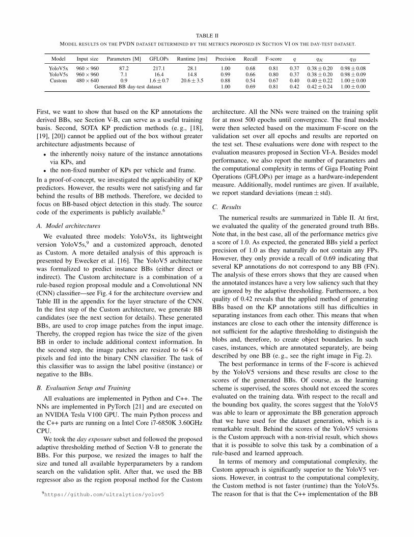
TABLE IIMODEL RESULTS ON THE PVDN DATASET DETERMINED BY THE METRICS PROPOSED IN SECTION VI ON THE DAY-TEST DATASET.

Model Input size Parameters [M] GFLOPs Runtime [ms] Precision Recall F-score q qK qB

YoloV5x 960× 960 87.2 217.1 28.1 1.00 0.68 0.81 0.37 0.38± 0.20 0.98± 0.08YoloV5s 960× 960 7.1 16.4 14.8 0.99 0.66 0.80 0.37 0.38± 0.20 0.98± 0.09Custom 480× 640 0.9 1.6± 0.7 20.6± 3.5 0.88 0.54 0.67 0.40 0.40± 0.22 1.00± 0.00

Generated BB day-test dataset 1.00 0.69 0.81 0.42 0.42± 0.24 1.00± 0.00

First, we want to show that based on the KP annotations thederived BBs, see Section V-B, can serve as a useful trainingbasis. Second, SOTA KP prediction methods (e. g., [18],[19], [20]) cannot be applied out of the box without greaterarchitecture adjustments because of

• the inherently noisy nature of the instance annotationsvia KPs, and

• the non-fixed number of KPs per vehicle and frame.In a proof-of-concept, we investigated the applicability of KPpredictors. However, the results were not satisfying and farbehind the results of BB methods. Therefore, we decided tofocus on BB-based object detection in this study. The sourcecode of the experiments is publicly available.6

A. Model architectures

We evaluated three models: YoloV5x, its lightweightversion YoloV5s,9 and a customized approach, denotedas Custom. A more detailed analysis of this approach ispresented by Ewecker et al. [16]. The YoloV5 architecturewas formalized to predict instance BBs (either direct orindirect). The Custom architecture is a combination of arule-based region proposal module and a Convolutional NN(CNN) classifier—see Fig. 4 for the architecture overview andTable III in the appendix for the layer structure of the CNN.In the first step of the Custom architecture, we generate BBcandidates (see the next section for details). These generatedBBs, are used to crop image patches from the input image.Thereby, the cropped region has twice the size of the givenBB in order to include additional context information. Inthe second step, the image patches are resized to 64× 64pixels and fed into the binary CNN classifier. The task ofthis classifier was to assign the label positive (instance) ornegative to the BBs.

B. Evaluation Setup and Training

All evaluations are implemented in Python and C++. TheNNs are implemented in PyTorch [21] and are executed onan NVIDIA Tesla V100 GPU. The main Python process andthe C++ parts are running on a Intel Core i7-6850K 3.60GHzCPU.

We took the day exposure subset and followed the proposedadaptive thresholding method of Section V-B to generate theBBs. For this purpose, we resized the images to half thesize and tuned all available hyperparameters by a randomsearch on the validation split. After that, we used the BBregressor also as the region proposal method for the Custom

9https://github.com/ultralytics/yolov5

architecture. All the NNs were trained on the training splitfor at most 500 epochs until convergence. The final modelswere then selected based on the maximum F-score on thevalidation set over all epochs and results are reported onthe test set. These evaluations were done with respect to theevaluation measures proposed in Section VI-A. Besides modelperformance, we also report the number of parameters andthe computational complexity in terms of Giga Floating PointOperations (GFLOPs) per image as a hardware-independentmeasure. Additionally, model runtimes are given. If available,we report standard deviations (mean± std).

C. Results

The numerical results are summarized in Table II. At first,we evaluated the quality of the generated ground truth BBs.Note that, in the best case, all of the performance metrics givea score of 1.0. As expected, the generated BBs yield a perfectprecision of 1.0 as they naturally do not contain any FPs.However, they only provide a recall of 0.69 indicating thatseveral KP annotations do not correspond to any BB (FN).The analysis of these errors shows that they are caused whenthe annotated instances have a very low saliency such that theyare ignored by the adaptive thresholding. Furthermore, a boxquality of 0.42 reveals that the applied method of generatingBBs based on the KP annotations still has difficulties inseparating instances from each other. This means that wheninstances are close to each other the intensity difference isnot sufficient for the adaptive thresholding to distinguish theblobs and, therefore, to create object boundaries. In suchcases, instances, which are annotated separately, are beingdescribed by one BB (e. g., see the right image in Fig. 2).

The best performance in terms of the F-score is achievedby the YoloV5 versions and these results are close to thescores of the generated BBs. Of course, as the learningscheme is supervised, the scores should not exceed the scoresevaluated on the training data. With respect to the recall andthe bounding box quality, the scores suggest that the YoloV5was able to learn or approximate the BB generation approachthat we have used for the dataset generation, which is aremarkable result. Behind the scores of the YoloV5 versionsis the Custom approach with a non-trivial result, which showsthat it is possible to solve this task by a combination of arule-based and learned approach.

In terms of memory and computational complexity, theCustom approach is significantly superior to the YoloV5 ver-sions. However, in contrast to the computational complexity,the Custom method is not faster (runtime) than the YoloV5s.The reason for that is that the C++ implementation of the BB

generation is not highly optimized. To put this into numbers,from the total computation time on average only 2.5 ms arerequired to compute the classification outputs of the CNNper image (including data loading to the GPU).10

Overall, our results show that a) it is possible to detectoncoming vehicles based on their light reflections and b)based on the KP annotations BBs can be generated that canserve as training data.

Finally, a rationale for the design of the Custom approach:We used the Custom method together with a tracking andplausibility algorithm to test prototype driver assistancefunctions in a test car. For that, we ran the Custom approachtogether with all the other applications (receiving inputs,sending outputs, etc.) in real time (faster than 18 Hz). Theusage of a shallow CNN together with a rule-based BBgenerator has the advantage to be more transparent. Therefore,the model behavior and, especially, exceptional cases canbe better understood, analyzed, and interpreted making theapproach easier to validate and verify.

VIII. CONCLUSION AND OUTLOOK

Based on the work of Oldenziel et al. [8], we presenteda thoroughly designed image dataset including evaluationmetrics and benchmark results to investigate the problem ofprovident vehicle detection at night. In general, the task toprovidently detect objects based on visual cues is a promisingnew research direction to bring object detection towardshuman performance. With the presented work here and theopen-sourcing of all data and code, we hope to provide theresearch community a jump start.

The annotation of light artifacts is challenging comparedto ordinary object annotation due to the lack of clear objectboundaries. We tackled this difficulty by an annotationapproach based on placing KPs in salient regions and methodsto automatically extend the base annotations to saliency mapsor BBs. Even if we showed in a set of benchmark experimentsthat automatically generated BBs can be used to train SOTAobject detectors such that they detect light reflections, thegeneration approach and their inherent quality is of coursea limiting factor. Since we already provided an evaluationmetric for KP detectors, we plan to develop KP and saliencydetection methods to overcome this limiting factor.

Besides, we annotated the vehicle positions so that thePVDN dataset provides ground truth for several researchfields:

• Time estimation: Time until vehicle appearance;• Tracking: Track instances and vehicles across scenes;• Transfer learning: Transfer methods to different exposure

cycles or weather conditions (snow, rain, fog, etc.);• Learning with label noise: Design methods that properly

handle the KP or generated annotations.

We are looking forward to all the upcoming results.

10Note that the computational complexity of the Custom approach is notconstant as the runtime of the proposal generation depends on the numberof positive values in the Boolean map.

REFERENCES

[1] A. López, J. Hilgenstock, A. Busse, R. Baldrich, F. Lumbreras, andJ. Serrat, “Nighttime vehicle detection for intelligent headlight control,”in Advanced Concepts for Intelligent Vision Systems, ser. Lecturenotes in Computer Science, J. Blanc-Talon, S. Bourennane, W. Philips,D. Popescu, and P. Scheunders, Eds. Springer, 2008, pp. 113–124.

[2] P. Alcantarilla, L. Bergasa, P. Jiménez, I. Parra, D. Fernández, M.A.Sotelo, and S.S. Mayoral, “Automatic lightbeam controller for driverassistance,” Machine Vision and Applications, pp. 1–17, 2011.

[3] S. Eum and H. G. Jung, “Enhancing light blob detection for intelligentheadlight control using lane detection,” IEEE Transactions on IntelligentTransportation Systems, vol. 14, no. 2, pp. 1003–1011, 2013.

[4] D. Juric and S. Loncaric, “A method for on-road night-time vehicleheadlight detection and tracking,” in 2014 International Conferenceon Connected Vehicles and Expo (ICCVE), 2014, pp. 655–660.

[5] P. Sevekar and S. B. Dhonde, “Nighttime vehicle detection forintelligent headlight control: A review,” in Proceedings of the 20162nd International Conference on Applied and Theoretical Computingand Communication Technology (iCATccT), 2016, pp. 188–190.

[6] R. K. Satzoda and M. M. Trivedi, “Looking at vehicles in the night:Detection and dynamics of rear lights,” IEEE Transactions on IntelligentTransportation Systems, vol. 20, no. 12, pp. 4297–4307, 2019.

[7] C. J. Rapson, B.-C. Seet, M. A. Naeem, J. E. Lee, M. Al-Sarayreh, andR. Klette, “Reducing the pain: A novel tool for efficient ground-truthlabelling in images,” in 2018 International Conference on Image andVision Computing New Zealand (IVCNZ), 2018, pp. 1–9.

[8] E. Oldenziel, L. Ohnemus, and S. Saralajew, “Provident detection ofvehicles at night,” in 2020 IEEE Intelligent Vehicles Symposium (IV),2020, pp. 472–479.

[9] S. Ren, K. He, R. Girshick, and J. Sun, “Faster R-CNN: Towardsreal-time object detection with region proposal networks,” in Advancesin Neural Information Processing Systems 28, 2015, pp. 91–99.

[10] F. M. Naser, “Detection of dynamic obstacles out of the line of sightfor autonomous vehicles to increase safety based on shadows,” Master’sthesis, MIT, Boston, 2019.

[11] A. Borji and L. Itti, “CAT2000: A large scale fixation dataset forboosting saliency research,” arXiv:1505.03581 [cs.CV], 2015.

[12] L. Itti and A. Borji, “Computational models: Bottom-up and top-downaspects,” arXiv:1510.07748 [cs.CV], 2015.

[13] J. Zhang and S. Sclaroff, “Saliency detection: A boolean map approach,”in 2013 IEEE International Conference on Computer Vision, 2013, pp.153–160.

[14] A. Borji, M. Cheng, H. Jiang, and J. Li, “Salient object detection: Abenchmark,” IEEE Transactions on Image Processing, vol. 24, no. 12,pp. 5706–5722, 2015.

[15] T. R. Singh, S. Roy, O. I. Singh, T. Sinam, and K. M. Singh, “Anew local adaptive thresholding technique in binarization,” IJCSIInternational Journal of Computer Science Issues, vol. 8, no. 6, pp.271–277, 2011.

[16] L. Ewecker, E. Asan, L. Ohnemus, and S. Saralajew, “Providentvehicle detection at night for advanced driver assistance systems,”arXiv preprint arXiv:2107.11302 [cs.CV], 2021.

[17] T.-Y. Lin, M. Maire, S. Belongie, J. Hays, P. Perona, D. Ramanan,P. Dollár, and C. L. Zitnick, “Microsoft COCO: Common objects incontext,” in European Conference on Computer Vision. Springer,2014, pp. 740–755.

[18] S.-E. Wei, V. Ramakrishna, T. Kanade, and Y. Sheikh, “Convolutionalpose machines,” in Proceedings of the IEEE Conference on ComputerVision and Pattern Recognition (CVPR), 2016, pp. 4724–4732.

[19] K. Sun, B. Xiao, D. Liu, and J. Wang, “Deep high-resolutionrepresentation learning for human pose estimation,” in Proceedings ofthe IEEE/CVF Conference on Computer Vision and Pattern Recognition(CVPR), 2019, pp. 5693–5703.

[20] F. Zhang, X. Zhu, H. Dai, M. Ye, and C. Zhu, “Distribution-awarecoordinate representation for human pose estimation,” in Proceedings ofthe IEEE/CVF Conference on Computer Vision and Pattern Recognition(CVPR), 2020, pp. 7093–7102.

[21] A. Paszke, S. Gross, F. Massa, A. Lerer, J. Bradbury, G. Chanan,T. Killeen, Z. Lin, N. Gimelshein, L. Antiga, A. Desmaison, A. Kopf,E. Yang, Z. DeVito, M. Raison, A. Tejani, S. Chilamkurthy, B. Steiner,L. Fang, J. Bai, and S. Chintala, “PyTorch: An imperative style, high-performance deep learning library,” in Advances in Neural InformationProcessing Systems 32, 2019, pp. 8024–8035.

APPENDIX IBOUNDING BOX ANNOTATION CONSISTENCY

Usually, BB annotations created by experts for object de-tection can be considered as objective ground truth. However,for instances, this ground truth is subjective. To study thissubjectiveness, we compared the BB annotations for directand indirect instances across several annotators. The resultsconfirm the following hypothesis: BB annotations vary to anot negligible extent between different annotators or even forthe same annotator between different frames.

A. Experiment Setup

To study the annotation consistency, seven experts weretasked to annotate the same scene with BBs. Thereby, theannotation inconsistency that might be observed is two-fold:First, some experts might decide to not annotate an instancebecause it is too weak or cannot be separated from anotherinstance. Second, after the experts agreed on the existence ofan instance, the actual size and position of the BB are alsosubject to the subjective behavior of the annotators.

We decided to only study the subjectivity of the BBplacement. This decision was made to reduce the evaluationcomplexity of the experiment while still emphasizing theoverall problem. This led to the following experiment setup:

1) Two instances (one direct, one indirect) were selectedfor annotation. The participants were shown an exampleimage to clarify the annotation targets.

2) The experts annotate the scene (number 15) from startto end using BBs.

3) The resulting annotations are evaluated with appropriatemetrics.

B. Evaluation Metrics

For evaluation, annotated BBs were collected from allN experts. To explain the evaluation scheme, we willfocus on the consistency of all BBs B = {b1, . . . , bN} ={(p1,1,p1,2) , . . . , (pN,1,pN,2)} for an instance in one frame.Metrics are calculated for the direct and indirect instancesseparately and then averaged over all frames. A BB isdescribed by its upper-left corner pi,1 and its lower-rightcorner pi,2. Rect (bi) defines the set of all points inside theBB bi. Drawing from common object detection metrics, theIoU can be used to compress the position and size variations ofBBs into a scalar value. This is usually done by comparing apredicted BB to a ground truth BB. Since this is not applicablefor our purpose, we compare the expert annotations to themean BB b, specified as the average over all annotations:

b = (p1, p2) =

(1

N

N∑i=1

pi,1,1

N

N∑i=1

pi,2

).

Using this as a reference, the IoU values to all BBs arecalculated:

IoU(bi, b

)=

∣∣Rect (bi) ∩ Rect(b)∣∣∣∣Rect (bi) ∪ Rect

(b)∣∣ .

Assuming, that all annotations are drawn from the samedistribution, we can infer the statistics and therefore the

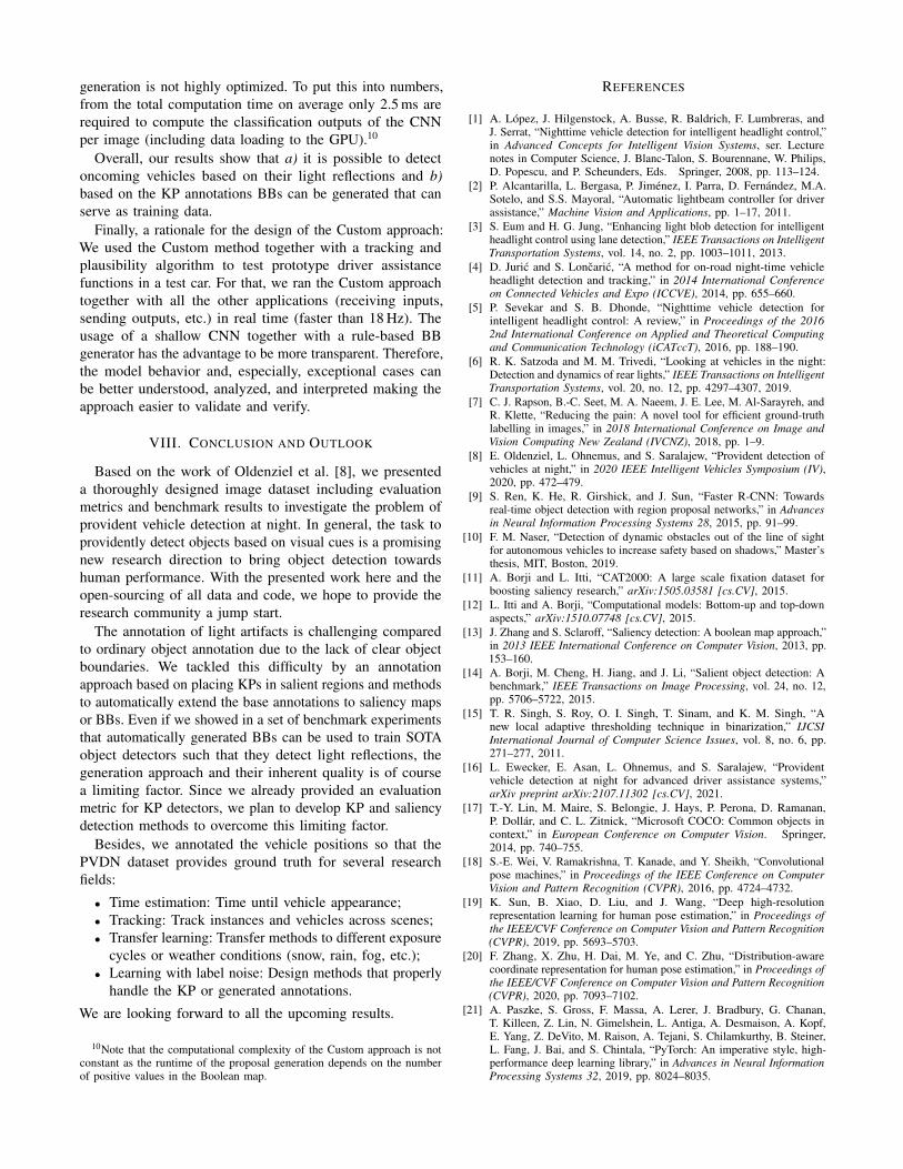
0.0 0.2 0.4 0.6 0.8 1.0IoU to mean bounding box

0

2

4

6

8

10

Freq

uenc

y

IndirectDirect

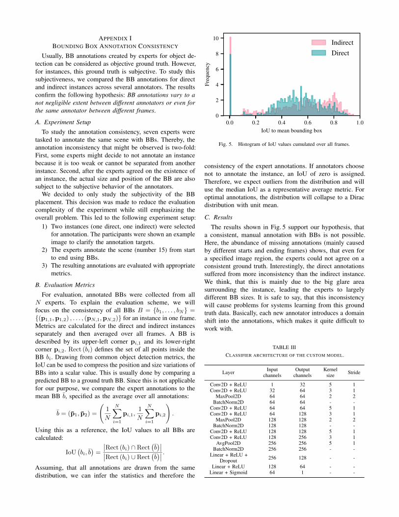
Fig. 5. Histogram of IoU values cumulated over all frames.

consistency of the expert annotations. If annotators choosenot to annotate the instance, an IoU of zero is assigned.Therefore, we expect outliers from the distribution and willuse the median IoU as a representative average metric. Foroptimal annotations, the distribution will collapse to a Diracdistribution with unit mean.

C. Results

The results shown in Fig. 5 support our hypothesis, thata consistent, manual annotation with BBs is not possible.Here, the abundance of missing annotations (mainly causedby different starts and ending frames) shows, that even fora specified image region, the experts could not agree on aconsistent ground truth. Interestingly, the direct annotationssuffered from more inconsistency than the indirect instance.We think, that this is mainly due to the big glare areasurrounding the instance, leading the experts to largelydifferent BB sizes. It is safe to say, that this inconsistencywill cause problems for systems learning from this groundtruth data. Basically, each new annotator introduces a domainshift into the annotations, which makes it quite difficult towork with.

TABLE IIICLASSIFIER ARCHITECTURE OF THE CUSTOM MODEL.

Layer Inputchannels

Outputchannels

Kernelsize Stride

Conv2D + ReLU 1 32 5 1Conv2D + ReLU 32 64 3 1

MaxPool2D 64 64 2 2BatchNorm2D 64 64 - -

Conv2D + ReLU 64 64 5 1Conv2D + ReLU 64 128 3 1

MaxPool2D 128 128 2 2BatchNorm2D 128 128 - -

Conv2D + ReLU 128 128 5 1Conv2D + ReLU 128 256 3 1

AvgPool2D 256 256 5 1BatchNorm2D 256 256 - -

Linear + ReLU +Dropout 256 128 - -

Linear + ReLU 128 64 - -Linear + Sigmoid 64 1 - -