3 A COMPUTER MODEL FOR INVESTIGATING

THE FREQUENCY DOMAIN CHARACTER1 STICS

ASSOCIATED WITH THE CUMULANT METHOD OF

POWER SYSTEM SIMULATION

A Thes i s Presen ted t o

The Facu l ty of t h e Col lege of Engineer ing and Technology

Ohio U n i v e r s i t y

I n P a r t i a l F u l f i l l m e n t

of t h e Requirements of t h e Degree

Master of Sc ience

Somphop - Poshakrishna, - November, 1985

ACKNOWLEDGEMENT

I would l i k e t o exp res s my s i n c e r e s t g r a t i t u d e t o my adv i so r ,

D r . Br ian Manhire, f o r h i s h e l p f u l d i r e c t i o n and p a t i e n c e which con t r ibu ted

t o t h e complet ion of t h i s t h e s i s . I b e l i e v e t h i s work i s a r e s u l t of h i s

s t r o n g encouragement.

I would l i k e t o thank t o t h e members of my t h e s i s committee,

D r . E r n s t Bre i t enbe rge r , D r . Butch H i l l and D r . Nasser J a l e e l l , f o r t h e i r

sugges t ions and c a r e f u l reviewing of t h i s t h e s i s .

F i n a l l y , I would a l s o l i k e t o exp res s my deep a p p r e c i a t i o n t o

my mother whose emot iona l , s p i r i t u a l and f i n a n c i a l suppor t have been wi th

me through a l l my academic endeavors.

TABLE OF CONTENTS

Page

ACKNOWLEDGEMENT . . . . . . . . . . . . . . . . . . . . . . . . i

. . . . . . . . . . . . . . . . . . . . . . . . LIST OF FIGURES i v

. . . . . . . . . . . . . . . . . . . . . . . . LIST OF TABLES

Chapter

1 . INTRODUCTION . . . . . . . . . . . . . . . . . . . . . 1

2 . OVERVIEW OF PROBABILISTIC SIMULATION . . . . . . . . . 5

2 . 1 I n t r o d u c t i o n . . . . . . . . . . . . . . . . . . . 5

2 . 2 P r o b a b i l i s t i c S imula t ion . . . . . . . . . . . . . 6

. . . . . . . . . . . . . . . . . . 3 . THE CUMULANTMETHOD 16

. . . . . . . . . . . . . . . . . . . 3 . 1 I n t r o d u c t i o n 16

3 . 3 The R e l a t i o n s h i p be tween Actua l P r o b a b i l i t y Dens i ty Funct ion and s t a n d a r d i z e d . . . . . . . . . . . P r o b a b i l i t y Dens i ty Funct ion 28

3 . 4 Some L i m i t a t i o n s of t h e Cumulant Method . . . . . 29

3 . 5 Computational Procedure t o C a l c u l a t e t h e Cumulant Represen t a t i on of a . . . . . . . . . . . P r o b a b i l i t y Dens i ty f u n c t i o n 30

3 . 6 Computational Procedure t o e v a l u a t e t h e Equ iva l en t Load Dura t ion Curve u s ing . . . . . . . . . . . . . . . t h e Cumulant Method 31

. . . . . . . . . . . . . 4 . FOURIER STUDIES OF CONVOLUTION 3 3

. . . . . . . . . . . . . . . . . . . 4 . 1 I n t r o d u c t i o n 3 3

. . . . . 4 . 2 Motiva t ion f o r Frequency Domain S t u d i e s 3 3

Page

4 .4 Four i e r Transform of Cumulant Represen t a t i on of a P r o b a b i l i t y Dens i ty Funct ion . . . . . . . . . . . . . . . . . 37

4.5 Computational Procedure t o Evalua te t h e F o u r i e r Transform of Cumulant r e p r e s e n t a t i o n of P r o b a b i l i t y Dens i ty F u n c t i o n . . . . . . . . . . . . . . . . . . . . . 4 1

5 . SOME EXPERIMENTAL RESULTS . . . . . . . . . . . . . . . 42

5 .1 I n t r o d u c t i o n . . . . . . . . . . . . . . . . . . . 42

5.2 S o u r c e o f D a t a . . . . . . . . . . . . . . . . . . 43

5 .3 Computer S imula t ion R e s u l t s . . . . . . . . . . . 48

6 . CONCLUSIONS. . . . . . . . . . . . . . . . . . . . . . 63

REFERENCES . . . . . . . . . . . . . . . . . . . . . . . . . . 65

APPENDIX

A. De r iva t ion of t h e F o u r i e r Transform of t h e Cumulant Represen t a t i on of P r o b a b i l i t y Dens i ty Funct ions . . . . . . . . . . . . . . . . . . . 68

8. Load P r o b a b i l i t y Dens i ty Funct ion(pdf ) Eva lua t ion P r o g r a m . . . . . . . . . . . . . . . . . . . . . . . . 72

C . An Outages pdf Eva lua t ion Program . . . . . . . . . . . 75

D . A Cumulant (GCA S e r i e s ) Represen t a t i on of pdf Eva lua t ionProg ram . . . . . . . . . . . . . . . . 78

E . An Equiva len t Load Dura t ion Curve Eva lua t ion . . . . . . . . . . . . . . . . . . . . . . P r o g r a m . . 82

F. A Program which Evalua tes t h e F o u r i e r Transform of a d i s c r e t e pdf . . . . . . . . . . . . . . 87

G . A Program which Eva lua t e s t h e F o u r i e r Transform of Cumulants (GCA S e r i e s ) Represen t a t i on of a pdf . . . . . . . . . . . . . . . . 89

LIST OF FIGURES

Page F igure

2.2.1 Chronologica l . Load Dura t ion . and I n v e r t e d Load Dura t ion Curves . . . . . . . . . . . 7

Normalized I n v e r t e d Load Curves ( A l l U n i t s Ava i l ab l e ) . . . . . . . . . . . . . . . 9

Normalized I n v e r t e d Load Curves ( Unit 4 fo rced o u t ) . . . . . . . . . . . . . . . 9

E f f e c t i v e P l a n t Loading Curve . . . . . . . . . . . 10

P r o b a b i l i t y I n t e r p r e t a t i o n of ILDC . . . . . . . . 15

A Linea r System . . . . . . . . . . . . . . . . . . 21

Chronologica l Load . . . . . . . . . . . . . . . . 49

Load P r o b a b i l i t y D i s t r i b u t i o n . . . . . . . . . . . 50

Outages P r o b a b i l i t y D i s t r i b u t i o n . . . . . . . . . 51

Cumulant Curve F i t t i n g of I n v e r t e d Load Dura t ion Curve (ILDC) . . . . . . . . . . . . . . . 53

Cumulant Curve F i t t i n g of Complement of Generator Outages (CGO) . . . . . . . . . . . . 54

Cumulant Represen t a t i on of Equiva len t Load Dura t ion Curve . . . . . . . . . . . . . . . . 55

F o u r i e r Transform of Actua l P r o b a b i l i t y D i s t r i b u t i o n . . . . . . . . . . . . . . . . . . . 56

F o u r i e r Transform of Normal D i s t r i b u t i o n . . . . . 58

F o u r i e r Transform of 6 Cumulants GCA s e r i e s . . . . 59

F o u r i e r Transform of Normal D i s t r i b u t i o n (one 400 MW u n i t ) . . . . . . . . . . . . . . . . . 61

Page

5.3.1 1 Four i e r Transform of 6 Cumulants GCA S e r i e s ( o n e 4 0 0 M W u n i t ) . . . . . . . . . . . . . 6 2

LIST OF TABLES

Table Page

4 . 3 . 1 Some Theorems of F o u r i e r Transform . . . . . . . . 36

5 . 2 . 1 Weekly Peak i n P e r c e n t of Annual Peak . . . . . . . 44 5 . 2 . 2 Dai ly Peak Load i n P e r c a n t of Weekly

Peak . . . . . . . . . . . . . . . . . . . . . . . 45

5 . 2 . 3 Hourly Peak Load i n Pe rcen t of Da i ly Peak . . . . . . . . . . . . . . . . . . . . . . . 46

5 .2 .4 Genera t ing Un i t R e l i a b i l i t y Data . . . . . . . . . 47

CHAPTER 1

INTRODUCTION

C a l c u l a t i o n of r e l i a b i l i t y indexes and product ion

c o s t i n g a r e two impor tan t problems i n power system p lanning . Among

t h e a n a l y t i c l y based techniques used have been F o u r i e r s e r i e s [ I ] and

more r e c e n t l y t h e cumulant method [2-71 . Since i t s i n t r o d u c t i o n , t h e

cumulant method has r ec i eved inc reased a t t e n t i o n i n s imu la t i ng t h e

o p e r a t i o n of power systems because i t i s computa t iona l ly f a s t and

s imp le . However, t h e r e a r e s e v e r a l s i t u a t i o n s t h a t may degrade t h e

r e s u l t s of t h e cumulant method [ 8 ] . The a b i l i t y t o i d e n t i f y t h e s e

s i t u a t i o n s a p r i o r i i s h i g h l y d e s i r a b l e .

A fundamental requirement of t h i s i d e n t i f i c a t i o n i s the

unders tanding of mathematical concepts a s s o c i a t e d w i t h t h e cumulant

method and t h e n a t u r e of i t s e r r o r s . Because t h i s method i s intima-

t e l y l i n k e d t o convo lu t ion , and convolu t ion i s t ransformed t o t h e

r e l a t i v e l y s imple concept of m u l t i p l i c a t i o n of F o u r i e r t r ans fo rms , i t

i s be l i eved t h a t a s t u d y of t h e frequency domain may r e v e a l t h e

unde r ly ing mathematical concep t s a s s o c i a t e d w i t h t h e e r r o r s i t u a t i o n s

mentioned p rev ious ly [ 9 ] . The primary g o a l of t h i s t h e s i s i s t o deve-

l o p so f tware s u i t a b l e f o r use i n a f requency domain s tudy of t h e

cumulant method w i t h emphasis on i t s mathematical and computa t iona l I

a s p e c t s . While t h e primary focus of t h i s t h e s i s i s on t h e com-

p u t a t i o n a l and mathematical a s p e c t s of t h e cumulant method, some

background m a t e r i a l i s inc luded f o r completeness .

Th i s t h e s i s i s organized a s fo l l ows . Chapter 2 provides

a g e n e r a l overview of p r o b a b i l i s t i c s imu la t i on . I t d e s c r i b e s t h e

b a s i c Baler iaux method a s w e l l a s i l l u s t r a t e s t h e procedure used t o

o b t a i n t h e e q u i v a l e n t load d u r a t i o n curve (ELDC). The purpose of

Chapter 2 i s t o provide t h e r e a d e r w i th a g e n e r a l p i c t u r e of t h e

eng inee r ing problem w i t h which t h i s t h e s i s i s u l t i m a t e l y a s s o c i a t e d .

Much more d e t a i l can be found i n t h e r e f e r e n c e m a t e r i a l inc luded i n

t h i s t h e s i s .

Chapter 3 cove r s t h e cumulant method of p r o b a b i l i s t i c

s imu la t i on . I t p r e s e n t s t h e method's mathematics i n d e t a i l . A f t e r

g i v i n g a n overview of computa t iona l procedures used i n t h e method, a

b r i e f d i s c u s s i o n of some of i t s l i m i t a t i o n s a r e g iven .

Chapter 4 deve lops t h e a lgo r i t hms a s s o c i a t e d w i t h t h e

proposed F o u r i e r s t u d i e s of t h e cumulant method. It s t a r t s by

b r i e f l y i n t r o d u c i n g F o u r i e r a n a l y s i s inc luded convo lu t ion theorems.

Then us ing F o u r i e r a n a l y s i s a d e r i v a t i o n of t h e F o u r i e r t ransform of

t h e Gram C h a r l i e r series (GCA) a s s o c i a t e d w i th t h e method i s g iven .

F i n a l l y , computa t iona l procedures f o r t h i s F o u r i e r t ransform a s we l l

a s t h e a c t u a l F o u r i e r t ranform of t h e p r o b a b i l i t y f u n c t i o n be ing pre-

s e n t e d by t h e GCA s e r i e s i s presen ted .

Chapter 5 d e s c r i b e s some exper imenta l r e s u l t s r e l a t e d

t o t h e t e s t i n g and v a l i d a t i o n of t h e a lgo r i t hms presen ted i n t h e pre-

v i o u s c h a p t e r .

Chapter 6 c o n t a i n s conc lus ions .

Appendix A p r e s e n t s t h e d e r i v a t i o n of F o u r i e r t ransform

of cumulant r e p r e s e n t a t i o n of a p r o b a b i l i t y d e n s i t y f u n c t i o n ( p d f ) .

Appendix B i s a computer program t o c a l c u l a t e load pdf

from IEEE t e s t d a t a .

Appendix C i s a computer program t o c a l c u l a t e outage

pd f s from IEEE t e s t d a t a .

Appendix D i s a computer program t o e v a l u a t e t h e GCA

r e p r e s e n t a t i o n of a pdf.

Appendix E i s a computer program t o c a l c u l a t e t h e

e q u i v a l e n t l oad d u r a t i o n curve from load and outage pd f s of appendix

B and C .

Appendix F Is a computer program t o c a l c u l a t e F o u r i e r

t r ans fo rm of a d i s c r e t e pdf. I t ou tpu t s e r v e s a s a benchmark f o r eva-

l u a t i n g t h e frequency domain r e s u l t s .

Appendix G i s a computer program t o c a l c u l a t e F o u r i e r

t r ans fo rm of GCA series r e p r e s e n t a t i o n of a pdf based on t h e der iva-

t i o n g i v e n i n Appendix A. The ou tpu t of t h i s program i s compared w i t h

that of Appendix F.

CHAPTER 2

OVERVIEW OF PROBABILISTIC SIMULATION

2 .1 I n t r o d u c t i o n

The f i r s t p r o b a b i l i s t i c s imu la t i on approach was deve-

loped i n Belgium by Baler iaux and Jamoulle i n 1967 [ l o ] . S ince i t s

i n t r o d u c t i o n , a c o n s i d e r a b l e amount of advancement i n t h e probabi-

l i s t i c s i m u l a t i o n a r e a has been made. Th i s advancement has been d r i -

ven by s i g n i f i c a n t i n c r e a s e s i n t h e complexi ty of t h e power systems

whose o p e r a t i o n i s t o be s imula ted .

D i g i t a l computers have been used i n power system s i n c e

t h e l a t e 1950's . The e a r l i e s t a p p l i c a t i o n w a s t h e s i m u l a t i o n of power

system o p e r a t i o n [ l l ] .

The end of e r a of cheap energy had r e s u l t e d i n t h e use

of new and s o p h i s t i c a t e d t echno log ie s . The cho ices between poten-

t i a l l y complex mixes of u n i t s w i t h h igh c a p i t a l c o s t and low

o p e r a t i n g c o s t and u n i t s having low c a p i t a l c o s t and h igh o p e r a t i n g

c o s t r e q u i r e t h e u se of computer models.

T h i s c h a p t e r is concerned wi th t h e concep t s of probabi-

l i s t i c s imu la t i on . More s p e c i f i c a l l y , i t d i s c u s s e s t h e b a s i c

Ba le r i aux method a s w e l l a s i l l u s t r a t e s t h e procedure t o o b t a i n t h e

e q u i v a l e n t l oad d u r a t i o n cu rves a s s o c i a t e d w i t h t h e method.

2.2 P r o b a b i l i s t i c S imula t ion

P r o b a b i l i s t i c s i m u l a t i o n i s a load d u r a t i o n technique

which i n c l u d e s t h e e f f e c t s of g e n e r a t i n g u n i t f o r ced outages [ I ] . The

b a s i c i d e a of p r o b a b i l i s t i c s i m u l a t i o n i s t h e u se of p r o b a b i l i t y

d i s t r i b u t i o n s t o d e s c r i b e t h e system loads and gene ra t i ng u n i t f o r ced

ou tages .

P r o b a b i l i s t i c s i m u l a t i o n o f f e r s f a s t computation w i t h

r ea sonab le accuracy. The load d u r a t i o n curve which forms i t s b a s i s i s

i l l u s t r a t e d i n F igure 2.2.1. I n F igure 2.2 .l . a , t h e ch rono log ica l

system load curve i s ob ta ined from hour ly load d a t a over a per iod of

t ime.(week, month, year ) The load d u r a t i o n curve i s ob ta ined by

a r r a n g i n g t h e ch rono log ica l system of load from Figure 2.2.1.a i n t o

dec reas ing o r d e r of magnitude a s shown i n Figure 2.2 .l .b. The

i n v e r t e d l oad d u r a t i o n curve (ILDC) i n F igure 2 . 2 . l . c i s ob ta ined by

r e v e r s i n g t h e o r d i n a t e and a b s c i s s a of t h e load d u r a t i o n curve . I f

t h e o r d i n a t e is normalized t o t h e number of hours be ing cons ide red ,

t h e n t h e o r d i n a t e r e p r e s e n t s t h e p r o b a b i l i t y t h a t t h e load i s g r e a t e r

t han o r equa l t o t h e cor responding a b s c i s s a va lue . The shaded a r e a

on each curve r e p r e s e n t s a p a r t i c u l a r p o r t i o n of t h e t o t a l l oad

energy served by t h e g e n e r a t i o n f o r t h e time per iod being cons idered .

I n t h e Ba le r i aux framework of p r o b a b i l i s t i c s i m u l a t i o n , l o a d i s

modelled a s a random v a r i a b l e and t i m e i s no t t r e a t e d e x p l i c i t l y

F i g u r e 2 . 2 . 1 C h r o n o l o g i c a l L o a d , Load D u r a t i o n , and I n v e r t e d Load D u r a t i o n C u r v e s

Load t Peak Load

Minimum Load j$j&J$&$J$ t ' ' ' V

Tlne (!'curs) G a) C h r o n o l o g ~ c s i S y ~ t s ~ Laad

Load (IN) A

Peak Load - ST = Tocal nwnber oE

Minrmum Load - - - - - - - - -

Tine (Hours) fi b) Load Durat ion C ~ r v e

Time 4 Hours DT

I * Loaa X l n l ~ s k ~ Loaa ? e i , (XU)

C) I n v e r t e d Load Duracion Curve

S o u r c e : From EPRI EA-1411 p p . 2 - 2 .

.

[ 1 2 ] . The e f f e c t s of g e n e r a t o r fo rced outages a r e inc luded by way of

t h e concept of e q u i v a l e n t l oad [13 ] . Equiva len t load c o n s i s t s of con-

sumer demand ( load ) p l u s fo rced outages of p l a n t ( o u t a g e s ) . The load

and ou tages a r e random v a r i a b l e s ; t h e i r sum i s a random v a r i a b l e

whose p r o b a b i l i t y d i s t r i b u t i o n i s ob ta ined by convolving t h e probabi-

l i t y d i s t r i b u t i o n s of t h e components [ l l ] . Symbol ica l ly ,

E = L + O 2 . 2 . 1

where E i s e q u i v a l e n t l oad

L i s consumer load

0 i s g e n e r a t i n g c a p a c i t y on outage

I n o r d e r t o u se t h e method e f f e c t i v e l y , two b a s i c

assumptions a r e r e q u i r e d . F i r s t , ou tage occur rences a r e independent

of l o a d , and second, ou tage occur rences are independent of o t h e r

ou tages .

F igu re s 2.2.2 through 2.2.4 i l l u s t r a t e t h e t h r e e fun-

damental mathematical o p e r a t i o n s used i n p r o b a b i l i s t i c s imu la t i on ,

namely i n t e g r a t i o n , convo lu t ion and i m p l i c i t l y , t h e r e p r e s e n t a t i o n of

e q u i v a l e n t load curve by mathematical f u n c t i o n s .

I n F igure 2.2.2 i l l u s t r a t e s t h e ILDC of s e v e r a l thermal

u n i t s loaded under t h e curve by way of a l oad ing o r d e r . The energy

gene ra t ed by each u n i t e q u a l s t o t h e a r e a under t h e ILDC spanned by

each u n i t times t h e t o t a l number of hours i n t h e pe r iod (DT) (assume

a l l g e n e r a t i n g u n i t s are 100% a v a i l a b l e ) . For example, t h e energy

Figure 2.2.2 Normalized Inverted Load Curve (All Units Available)

Source : From EPRI EA-1411 pp.2-3.

I 0 i 3 T )

P r o n ~ c i l i t v ( P C )

! 0

(Load Ln Yi )

Figure 2.2.3 Normalized Inverted Load Curve (Unit 4 Forced out)

Source : From EPRI EA-1411 pp.2-3.

10 (DT

Probability (PU)

UnlL Unit Unkt UniL Uni t Uni t Uni t Uni t Uni t 1 h . t 1 . 2 1 4 5 6 7 8 9 1 0 7

I n s t a l l e d Capac i ty

F i g u r e 2.2.4 E f f e c t i v e Plant Loading Curve

Source : From EPRI EA-1411 pp .2 -7 .

I n s t a l l e d Capac i ty + Peak Load

demand f o r u n i t 7 (D7) i s expressed by

where F(x) i s t h e ILDC

E i s t h e energy se rved by u n i t 7 , i n t h i s c a s e , E7 i s 7

equa l t o D7 because no u n i t below u n i t 7 f a i l s . Th i s c o n d i t i o n i s

g e n e r a l l y no t t r u e i n r e a l power system o p e r a t i o n where each u n i t has

a p r o b a b i l i t y of f a i l u r e ( f o r c e d outages r a t e ) . I f we a s s i g n t o

each g e n e r a t o r a p r o b a b i l i t y of being o u t of s e r v i c e ( a v a i l a b l e a t 0

MW) and c a l l t h i s q , t hen t h e p r o b a b i l i t y of being i n s e r v i c e ( p )

must be 1-q s o t h a t pi-q-1.

F i g u r e 2 . 2 . 3 shows u n i t 4 fo rced o u t . The expected

energy demand f o r any u n i t above u n i t 4 i s

DI = Demand energy on u n i t I g i v e n u n i t 4 i s a v a i l a b l e

+ Demand energy on u n i t I g iven u n i t 4 i s fo rced o u t (where I > 4 ) .

The expected energy demand f o r u n i t 7 i s

where

The G(x) i s t h e e q u i v a l e n t load r e s u l t i n g from t h e

system load and outages of u n i t 4 . It can be shown t h a t t h i s G(x)

r e s u l t s from t h e convo lu t ion of t h e outage p r o b a b i l i t y d e n s i t y func-

t i o n s ( p d f s ) of u n i t 4 w i t h p r o b a b i l i t y f u n c t i o n a s s o c i a t e d w i th t h e

ILDC ( F ( x ) ) i n F igure 2.2.2 [ 9 ] . As can be seen , u n i t s below u n i t

4 i n l oad ing o r d e r a r e une f f ec t ed by t h e fo rced outage e f f e c t s of u n i t

4 . Thus F(x) i s t h e e q u i v a l e n t load curve f o r u n i t below u n i t 4 i n

l oad ing o r d e r .

The prev ious d i s c u s s i o n assumes a l l bu t one of t h e

g e n e r a t i n g u n i t s a r e 100% a v a i l a b l e . I f more t han one u n i t a r e no t

100% a v a i l a b l e m u l t i p l e e q u i v a l e n t load cu rves a r e r equ i r ed . For

example, assume each u n i t i n F igure 2.2.4 has a f o r c e outage r a t e of

q i ( i = l , 2 , 3 , . . . . . , l o ) and c a p a c i t y c i ( i = l , 2 , 3 , . . . . . , l o ) , t hen t h e

expec ted energy f o r each u n i t i s computed a s fo l l ows .

Uni t 1

The energy demand on u n i t 1 i s ob ta ined from t h e a r e a

under ILDC f o r t h e time pe r iod being cons idered and

The expected energy se rved by u n i t 1 i s

Now t h e c u r r e n t e q u i v a l e n t l oad curved F(x) i s modified

(by way of convolu t ion) t o r e f l e c t t h e fo rced outage e f f e c t s of u n i t

1. The r e s u l t i n g i s

Unit 2

The new e q u i v a l e n t l oad curve f o r u n i t 2 i s Fl(x) and

t h e energy demand on u n i t 2 i s

and t h e energy se rved by u n i t 2 i s

The c u r r e n t e q u i v a l e n t l oad curve Fl(x) i s modif ied t o

r e f l e c t t h e f o r c e d outage e f f e c t s of u n i t 2 . Resu l t i ng i n

The above convo lu t ion equa t ion i s r epea t ed u n t i l a l l

u n i t s have been cons ide red . The g e n e r a l r e s u l t f o r any i n t e r m e d i a t e

u n i t I i s

and

where

Th i s s e q u e n t i a l procedure r e s u l t s i n m u l t i p l e equiva-

l e n t l oad cu rves a s shown i n F igure 2 . 2 . 4 . Each u n i t has i t s own

e q u i v a l e n t load curve . The shaded a r e a i n F igure 2 .2 .4 r e p r e s e n t s

system unserved energy. The f i n a l ( r i g h t most) e q u i v a l e n t load curve

e v a l u a t e d a t t h e i n s t a l l e d c a p a c i t y i s t h e p r o b a b i l i t y t h a t t h e

e q u i v a l e n t l oad e q u a l s o r exceeds t h e i n s t a l l e d c a p a c i t y of t h e

system. T h i s o r d i n a t e i s c a l l e d t h e system loss-of- load p r o b a b i l i t y .

I n power system s i m u l a t i o n , t h e ou tage c a p a c i t y proba-

b i l i t y d i s t r i b u t i o n s a r e developed from i n p u t d a t a a s s o c i a t e d wi th

t h e f a i l u r e r a t e s of t h e g e n e r a t i n g u n i t s . The p r o b a b i l i t y d i s t r i b u -

t i o n of t h e l o a d i s e x t r a c t e d from ILDC by normal iz ing i t s o r d i n a t e .

The r e l a t i o n s h i p between t h e ILDC, t h e cumulat ive p r o b a b i l i t y func-

t i o n of t h e l oad and t h e p r o b a b i l i t y d e n s i t y f u n c t i o n of t h e load a r e

shown i n f i g u r e 2 .2 .5 .

CHAPTER 3

THE CUMULANT METHOD

3.1 I n t r o d u c t i o n

The cumulant method i s t h e most r e c e n t advancement i n

t h e p r o b a b i l i s t i c s imu la t ion a r e a . I t i s both reasonably a c c u r a t e

and i s economical of computer t ime. The cumulant method has two

h i g h l y d e s i r a b l e c h a r a c t e r i s t i c s f o r p r o b a b i l i s t i c s imu la t ion . F i r s t ,

i t can be used t o d e s c r i b e a p r o b a b i l i t y d i s t r i b u t i o n f o r t h e t o t a l

and p a r t i a l ou tages of each gene ra t ing u n i t ; second, as w i l l be shown

i n t h i s c h a p t e r , t h e cumulants of t h e system 's numerous equ iva l en t

l oad curves ( d e s c r i b e d i n Chapter 2) can be obta ined by simply adding

t h e corresponding i n d i v i d u a l p l a n t cumulants and load cumulants [5].

T h i s second p rope r ty i s perhaps t h e most s i g n i f i c a n t b e n e f i t of t h e

method s i n c e i t t ransforms t h e most computa t iona l ly i n t e n s i v e p o r t i o n

of t h e s imu la t ion , i . e . , convolu t ion , t o s imple a d d i t i o n of r e a l

numbers[l3] .

I n t h e p a s t , us ing convolu t ion i n p r o b a b i l i s t i c simu-

l a t i o n has had some l i m i t a t i o n s i n terms of accuracy and com-

p u t a t i o n a l speed. For example, i n o r d e r t o o b t a i n t h e gene ra t ion

system outage c a p a c i t y t a b l e , i t w i l l t ake q u i t e long t ime. On t h e

o t h e r hand, t h e cumulant method o f f e r s a f a s t e r method t o o b t a i n

t h e ou tages t a b l e [ 5 ] .

There a r e some q u e s t i o n s on how and when t h e cumulant

method may be e f f e c t i v e l y used. Some s t u d i e s show t h a t t h e accuracy

of t h e cumulant method appears t o be a c c e p t a b l e f o r some l a r g e

systems (more t han 10,000 MW of i n s t a l l e d c a p a c i t y ) [ 3 ] , f o r sma l l e r

systems t h e r e s u l t s i s not comple t ly s a t i s f a c t o r y . [8 ,14 ,15 ] . The

f a c t o r s t h a t appear t o i n f l u e n c e t h e accuracy of t h e cumulant method

a r e l oad l e v e l , r e l a t i v e s i z e s and fo rced outage r a t e s of gene ra t i ng

u n i t s [ 6 ] .

I n t h e remainder of t h i s c h a p t e r , t h e mathematical d e t a i l s

of t h e cumulant method inc lud ing t h e computa t iona l procedure used t o

o b t a i n e q u i v a l e n t l oad d u r a t i o n curve (ELDC) w i l l be p re sen t ed .

3 . 2 Cumulant Mathematics

The cumulant method r e p r e s e n t s a g iven frequency func-

t i o n ( p r o b a b i l i t y d e n s i t y f u n c t i o n ) a s an or thogonal s e r i e s whose

terms c o n s i s t of t h e normal f requency f u n c t i o n and i t s d e r i v a t i v e s

[ 1 6 ] . Cumulants a r e a f u n c t i o n of t h e c e n t r a l moments (moment about

t h e mean) a s s o c i a t e d w i t h t h e p r o b a b i l i t y f u n c t i o n .

Given a random v a r i a b l e x w i t h pdf f ( x ) . The f i r s t

moment about t h e o r i g i n (mean) i s de f ined by

and moment of o r d e r r about an a r b i t a r y po in t a i s

I f a i s t h e mean, t h e second moment about t h e mean

( r = 2 ) i s t h e va r i ance . The t h i r d moment about t h e mean c a p t u r e s

skewness (asymmetry) and ' t h e f o u r t h moment about t h e mean cap tu re s

k u r t o s i s (peakedness-of t h e d i s t r i b u t i o n ) .

The F o u r i e r i n t e g r a l of f ( x ) i s g iven by

where j = C i

l e t Q = -w

t hen t h e c h a r a c t e r i s t i c f u n c t i o n of f ( x ) i s g iven by

l e t t = j&

then t h e moment g e n e r a t i n g f u n c t i o n of f ( x ) i s g iven by

m(t) = ~ ( j ~ ) l ~ ~ = ~

00

etxf (x) dx = I*

t x The Maclaurin series expansion of e y i e l d s

and on s u b s t i t u t i n g 3 . 2 . 6 i n t o 3 . 2 . 5

where

Reca l l i ng equa t ion 3 . 2 . 2 when t h e a r b i t r a r y p o i n t a i s

equa l t o z e r o , equa t ion 3 . 2 . 2 becomes

Th i s i s so c a l l e d t h e moment about t h e o r i g i n . The r e l a t i o n s h i p s bet-

ween moments about t h e o r i g i n and moments t he mean a r e

The cumulant gene ra t ing f u n c t i o n c ( t ) i s de f ined by

e C( t, = rn(t) 3.2.11

When c ( t ) can b e e x p a n d e d i n term of Maclaurin s e r i e s a s

2 c ( t ) = c0+c1t+lc t +..... - 2 2

t h e cn a r e c a l l e d t h e cumulants of t h e pdf f ( x ) and

By us ing equa t ion 3.2.11 i n conjunct ion wi th 3.2.7, 3.2.10, 3.2.12,

and 3.2.13. The cumulants of t h e pdf i n terms of moments about t h e

mean a r e

Figu re 3.2.1 A l i n e a r system

The mathematical p r i n c i p l e s of t h e cumulant method

which t ransforms convo lu t ion t o t r i v i a l numerical a d d i t i o n can be

d e r i v e d by us ing w e l l known concepts a s s o c i a t e d w i th t h e g e n e r i c

l i n e a r system i n t h e f i g u r e 3.2.1.

The l i n k a g e t o p r o b a b i l i s t i c s i m u l a t i o n i s made by

assuming t h a t t h e l o a d pdf ( u ( t ) ) i s t h e i n p u t t o a system. The

g e n e r a t o r ou t ages ( h ( t ) ) i s assumed t o be r ep re sen t ed by t h e impulse

r e sponse of t h e l i n e a r system. Under t h e s e assumptions t h e ELDC

( x ( t ) ) i s then t h e ou tpu t response of t h e l i n e a r system and i s

ob ta ined by convolving t h e load pdf u ( t ) and g e n e r a t o r ou tages h ( t ) .

R e c a l l t h a t i n t h e frequency domain, t h e response can be c a l c u l a t e d

by m u l t i p l y i n g F o u r i e r t ransforms .

Now, i t w i l l be shown t h a t t h e cumulant method t r ans -

forms convo lu t ion t o t r i v i a l numerical a d d i t i o n [ 1 7 ] . From F igu re

3.2 . l , t h e ou tpu t response i s

where * deno te s convo lu t ion

The moment g e n e r a t i n g f u n c t i o n m(t) i s r e l a t e d t o t h e

F o u r i e r t ransform by equa t ions3 .2 .3 and 3.2.5. The re fo re

x( t ) 'h ( t )*u( t ) -gh( jw) . yU( jw) 3.2.16

t h e n

x ( t ) = h ( t ) * u ( t ) - mh(t ) . mu(t) 3.2.17

where mx(t) , m ( t ) and m ( t ) a r e t h e moment g e n e r a t i n g f u n c t i o n s of h u

x ( t ) , h ( t ) , and u ( t ) r e s p e c t i v e l y . Reca l l i ng e q u a t i o n 3.2.11

making t h e s u b s t i t u t i o n y i e l d s

e cX( t ) = ech( t, ecu( t,

= e ( ch( t>+cu( t )

hence

Equat ion 3.2.19 shows t h a t whenever t h e moment

g e n e r a t i n g f u n c t i o n s a r e m u l t i p l i e d ( convo lu t ion ) , t h e i r a s s o c i a t e d

cumulants a r e added.

The Gram C h a r l i e r s e r i e s of type A (GCA) i s used t o

r e p r e s e n t t h e p r o b a b i l i t y f u n c t i o n s f o r l o a d and e q u i v a l e n t l oad .

Th i s o r thogona l s e r i e s u l t i l i z e s a s t anda rd normal d i s t r i b u t i o n ( z e r o

mean and u n i t y s t anda rd d e v i a t i o n ) and i t s d e r i v a t i v e s .

The s t anda rd normal d i s t r i b u t i o n i s g i v e n by

and

t h e s u c c e s s i v e d e r i v a t i v e s of a ( t ) w i t h r e s p e c t t o t a r e r e l a t e d by

t h e Chebyshev Hermite polynomials a s fo l l ows

D a ( t ) = -t a ( t )

where H,(t) i s t h e Chebyshev Hermite polynomial of o r d e r r .

The f i r s t seven polynomials a r e

The GCA s e r i e s can be expanded i n a s e r i e s of d e r i v a t i -

ves of s tandard normal d i s t r i b u t i o n . Symbolical ly ,

m

f ( t ) = 2 d jHj ( t ) a ( t ) j=O

mul t ip ly ing 3.2 .22 by Hr( t ) and i n t e g r a t i n g from - w t o w g i v e s

and t h e impor tan t or thogonal proper ty i s

0 , m#n Hm( t)Hn( t ) a ( t ) d t = /" 3.2 .24

-00 n!, m=n

s u b s t i t u t e 3 .2 .24 i n t o 3.2 .23 y i e l d s

By us ing equa t ion 3 . 2 . 2 1 and 3 . 2 . 2 4 , t h e f i r s t seven c o e f f i c i e n t s

a r e

where

where

and

dl = ml (mean)

In t roduc ing t h e s t anda rd measure v a r i a b l e

a i s t h e s t anda rd d e v i a t i o n

An impor tan t proper ty of t h e s t anda rd measure v a r i a b l e

i s t h a t t h e new random v a r i a b l e s always has zero mean and u n i t y

s t anda rd d e v i a t i o n . It can be seen t h a t t h e moment about t h e mean and

t h e moment about t h e o r i g i n i s i d e n t i c a l because mean i s t h e o r i g i n .

For t h e s t anda rd measure v a r i a b l e ' s moments (denoted by t h e primed

v a r i a b l e ) t hen

The h ighe r o r d e r s t anda rd cumulants (Kn) a r e r e l a t e d t o t h e h ighe r

o r d e r cumulants ( c,) by

The c o e f f i c i e n t s of t h e GCA i n equa t ion 3.2.26 a f t e r s u b s t i t u t i n g

ml=O and m -1 become 2-

The c o e f f i c i e n t s of t h e GCA s e r i e s can be ob ta ined by

comparing equa t ion 3.2.14 wi th equat ion 3.2.30 and 3.2 -31. The

r e s u l t s a r e

F i n a l l y , t h e GCA series expansion i n terms of f i r s t s i x

s t anda rd cumulants i s

The cumulat ive p r o b a b i l i t y f u n c t i o n of s i s

and t h e complementary cumulat ive p r o b a b i l i t y o r ELDC of s i s

For a g iven load l e v e l t , us ing e q u a t i o n 3.2.28, 3.2.31

and 3.2.36 a r e t h e exp re s s ions f o r t h e o r d i n a t e s on t h e i n v e r t e d load

d u r a t i o n curve o r e q u i v a l e n t l oad d u r a t i o n curve .

3.3 The R e l a t i o n s h i p between A c t u a l P r o b a b i l i t y D e n s i t y F u n c t i o n and

S t a n d a r d i z e d P r o b a b i l i t y D e n s i t y F u n c t i o n

L e t f ( t ) be t h e a c t u a l pdf

and g ( s ) b e t h e s t a n d a r d i z e d pdf

where

and

from

t h e n

0 = s t a n d a r d d e v i a t i o n

According t o t h e o r y of p r o b a b i l i t y

E q u a t i o n 3.3.1 and 3.3.2 are e q u a l

s u b s t i t u t i o n of 3.3.3 i n t o 3.3 .4 y i e l d s

comparing b o t h s i d e s of e q u a t i o n 3.3 .5 y i e l d s

observe from e q u a t i o n 3.3.6 t h a t t h e d i f f e r e n c e between t h e a c t u a l

pdf and t h e s t anda rd i zed pdf i s 1 . Thi s means t h a t t h e magnitude of - d

s t a n d a r d i z e d pdf w i l l d e c r e a s e by t h e f a c t o r 1 . - Q

3.4 Some L i m i t a t i o n s of t h e Cumulant Method

A s d i s c u s s e d p rev ious ly , t h e Gram C h a r l i e r ( t y p e A)

s e r i e s used i n t h e cumulant method i s based on a normal d i s t r i b u t i o n

and i t s d e r i v a t i v e s . Although i n many a p p l i c a t i o n s normal i ty can

o f t e n be a r ea sonab le assumption, one can not use i t u n c r i t i c a l l y . The

p u b l i c a t i o n of r e c e n t s t u d i e s r e l a t e d t o t h e cumulant method show

some s i t u a t i o n s which may g e n e r a t e problems [ 3 , 8 ] :

1. A s m a l l number of u n i t s i n t h e power system

2 . Systems which i n c l u d e u n i t s having a low fo rced

ou tage r a t e .

3 . Systems having r e l a t i v e l y d i f f e r e n t s i z e d of

g e n e r a t i n g u n i t s .

The above s i t u a t i o n s can g ive r ise t o a very skewed

d i s t r i b u t i o n t h u s t h e normal approximation w i l l be i n e x a c t . The

skewness tends t o l e s s e n i f t h e number of u n i t s i n t h e system i s

l a r g e o r u n i t f o r ced outage r a t e ~ a r e h i g h ~ b u t i t i s always p r e s e n t i n

some degree . The cumulant method o f f e r s a n approach t o t h e problem of

n e a r normal i ty . The cumulant method w i l l be e s p e c i a l l y u s e f u l when

pdf i s c l o s e t o a normal d i s t r i b u t i o n . T h e a p r i o r i i d e n t i f i c a t i o n of

t h o s e c a s e s where i t would be s a f e t o use cumulant method w i t h reaso-

n a b l e accuracy would be u s e f u l .

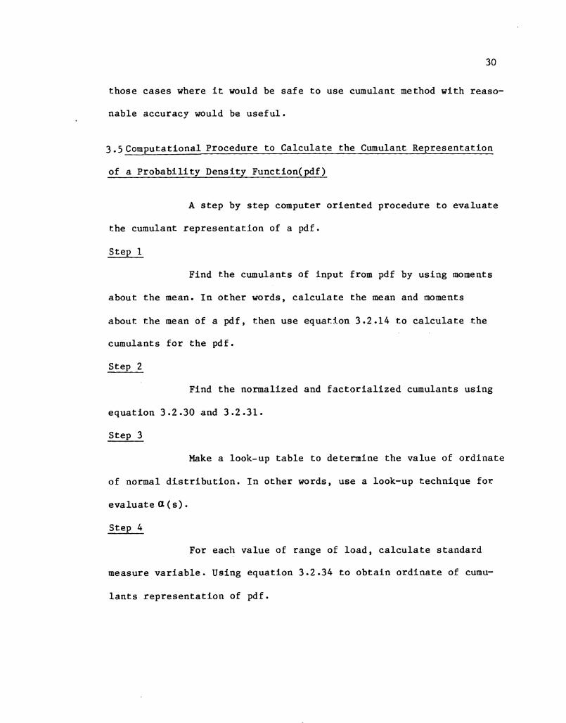
3 .5Computa t iona l Procedure t o C a l c u l a t e t h e Cumulant Represen t a t i on

of a P r o b a b i l i t y Dens i ty Funct ion(pdf )

A s t e p by s t e p computer o r i e n t e d procedure t o e v a l u a t e

t h e cumulant r e p r e s e n t a t i o n of a pdf.

S tep 1

Find t h e cumulants of i n p u t from pdf by us ing moments

about t h e mean. I n o t h e r words, c a l c u l a t e t h e mean and moments

abou t t h e mean of a pdf , t hen use equa t ion 3 . 2 . 1 4 t o c a l c u l a t e t h e

cumulants f o r t h e pdf .

S t ep 2

Find t h e normalized and f a c t o r i a l i z e d cumulants u s ing

e q u a t i o n 3 . 2 . 3 0 and 3 . 2 . 3 1 .

Step 3

Make a look-up t a b l e t o de te rmine t h e va lue of o r d i n a t e

of normal d i s t r i b u t i o n . I n o t h e r words, u se a look-up t echn ique f o r

e v a l u a t e CX ( s ) . Step 4

For each va lue of range of l o a d , c a l c u l a t e s t anda rd

measure v a r i a b l e . Using equa t ion 3 . 2 . 3 4 t o o b t a i n o r d i n a t e of cumu-

l a n t s r e p r e s e n t a t i o n of pdf .

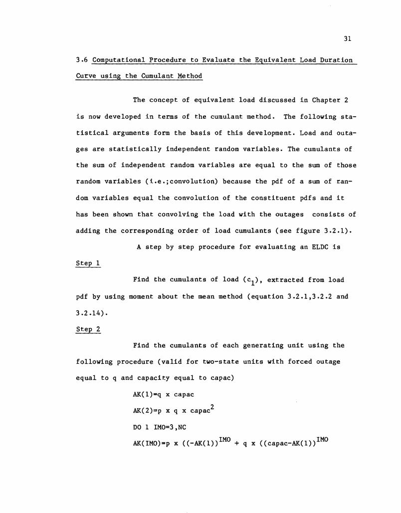
3.6 Computational Procedure t o Eva lua t e t h e Equiva len t Load Dura t ion

Curve u s ing t h e Cumulant Method

The concept of e q u i v a l e n t load d i scus sed i n Chapter 2

i s now developed i n terms of t h e cumulant method. The fo l l owing s t a -

t i s t i c a l arguments form t h e b a s i s of t h i s development. Load and outa-

g e s a r e s t a t i s t i c a l l y independent random v a r i a b l e s . The cumulants of

t h e sum of independent random v a r i a b l e s a r e equa l t o t h e sum of t hose

random v a r i a b l e s ( i . e . ; c o n v o l u t i o n ) because t h e pdf of a sum of ran-

dom v a r i a b l e s equa l t h e convolu t ion of t h e c o n s t i t u e n t pd f s and i t

has been shown t h a t convolving t h e load wi th t h e ou tages c o n s i s t s of

adding t h e cor responding o r d e r of load cumulants ( s e e f i g u r e 3.2.1).

A s t e p by s t e p procedure f o r e v a l u a t i n g an ELDC i s

S tep 1

Find t h e cumulants of l oad ( c l ) , e x t r a c t e d from load

pdf by us ing moment about t h e mean method ( equa t ion 3.2.1,3.2.2 and

S t ep 2

Find t h e cumulants of each g e n e r a t i n g u n i t u s ing t h e

fo l l owing procedure ( v a l i d f o r two-state u n i t s w i th fo rced outage

e q u a l t o q and c a p a c i t y equa l t o capac)

AK(l)=q x capac

AK(2)=p x q x capac 2

DO 1 IMO=3 ,NC

AK(IMO)=p x ((-AK(1))IM0 + q x ((capac-AK(1)) I M O

1 CONTINUE

where AK(N) = Moment o r d e r N abou t t h e mean

NC = Number of cumulants

t hen us ing equa t ion 3 . 2 . 1 4 , o b t a i n t h e outage cumulants of each

g e n e r a t i n g u n i t . Adding t h e outage cumulants of i n d i v i d u a l u n i t s t o

form t h e ( t o t a l ) system ou tages (ou t age t a b l e ) .

S t ep 3

Find t h e cumulants of ELDC by adding t h e corresponding

cumulants of l oad and outages .

S t ep 4

Find t h e normalized and f a c t o r i z e d cumulants u s ing

e q u a t i o n 3 . 2 . 3 0 and 3 . 2 . 3 1 . Note i n equa t ion 3 . 2 . 3 1 a i s t h e square

r o o t of second cumulant of system load and outages .

S t ep 5

Make a look-up t a b l e t o de te rmine t h e v a l u e of o r d i n a t e

of normal d i s t r i b u t i o n and t h e a r e a under normal d i s t r i b u t i o n curve.

S tep 6

For each va lue of l o a d , c a l c u l a t e s t anda rd measure

v a r i a b l e s and Hermite of h ighe r o r d e r a s s o c i a t e d w i t h s t anda rd

measure v a r i a b l e . Using e q u a t i o n 3 . 2 . 3 6 t o o b t a i n t h e o r d i n a t e va lue

on e q u i v a l e n t load and r e p e a t u n t i l reaching d e s i r a b l e l oad l e v e l .

CHAPTER 4

FOURIER STUDIES OF CONVOLUTION

4.1 I n t r o d u c t i o n

I n Chapter 3 , t h e f requency domain r e p r e s e n t a t i o n s of

p r o b a b i l i t y d e n s i t y f u n c t i o n s were developed. Mul t ip ly ing t h e f r e -

quency domain ( F o u r i e r t ransforms) cor responds t o convolving t h e i r

a s s o c i a t e d p r o b a b i l i t y d i s t r i b u t i o n s and thus t h e frequency domain

concept of bandwidth can be a p p l i e d t o t h e convolu t ion . Th i s chap te r

p r e s e n t s t h e F o u r i e r a n a l y s i s r equ i r ed t o c a l c u l a t e t h e F o u r i e r

t r ans fo rm of pd f s germane t o p r o b a b i l i s t i c s i m u l a t i o n a s w e l l a s t h e

F o u r i e r t ransform of t h e i r cumulant r e p r e s e n t a t i o n s ( i n c l u d e d up t o

f i r s t s i x cumulants ) . The r e s u l t of t h e F o u r i e r s t u d i e s used t o test

t h e computer codes a l s o shed some new l i g h t on how t h e cumulant

method may be s t u d i e d i n t h e frequency domain.

4.2 Mot iva t ion f o r Frequency Domain S t u d i e s

From t h e s t a n d p o i n t of t h e cumulant method, t h e essen-

t i a l i n fo rma t ion ob ta ined from t h e frequency domain i s bandwidth. I n

t h i s c o n t e x t , bandwidth i s t h e range of f r equenc i e s t h a t a F o u r i e r

t r ans fo rm has a magnitude p o s i t i v e of a t l e a s t some ( u s e r s p e c i f i e d )

l e v e l . A s mentioned i n Chapter 3 , cumulant method i s an approxima-

t i o n . The q u e s t i o n a s s o c i a t e d w i t h u s ing t h e cumulant method i s t h a t

by adding more terms (cumulants) how does t h e method's accuracy

improve? C u r r e n t l y , many u t i l i t i e s u se 6 o r less cumulants i n t h e i r

cumulant models [ 1 7 ] . One p o s s i b l e way t o s tudy t h e accuracy of t h i s

method i s t o compare t h e bandwidth of a GCA s e r i e s ' t ransform f o r a

d i f f e r e n t number of cumulants.

I n Chapter 5 of t h i s t h e s i s , 2 cumulants (normal

d i s t r i b u t i o n ) and 6 cumulants GCA s e r i e s w i l l be compared i n f r e -

quency domain of l o a d , ou tages and e q u i v a l e n t load f o r IEEE endorsed

d a t a .

4.3 F o u r i e r Ana lys i s

An a r b i t a r y f u n c t i o n f ( t ) might c o n s i s t of completely

d i f f e r e n t a n a l y t i c p i e c e s i n v a r i o u s p a r t s of t h e t a x i s . Th i s func-

t i o n can be expressed by

Th i s e q u a t i o n i s v a l i d f o r every t. The q u a n t i t y F(w) i s g iven by

and i s c a l l e d a s t h e F o u r i e r i n t e g r a l o r F o u r i e r t r ans fo rm of f ( t )

[ 1 8 ] . Equat ion 4 . 3 . 2 i s v a l i d i n t h e c a s e of cont inuous f u n c t i o n . I n

t h e c a s e of d i s c r e t e f u n c t i o n r e p r e s e n t e d a s a row of n D i r ac d e l t a

f u n c t i o n s

t h e i n t e g r a l o p e r a t i o n becomes summation. Equat ion 4.3.2 becomes

t h e n-terms s e r i e s ( F o u r i e r polynomial w i t h unevenly space pe r iods )

The f u n c t i o n F(w) i s i n g e n e r a l complex

A(w), t h e ampl i tude of f ( t ) f o r each w , i s c a l l e d t h e F o u r i e r .

spectrum of f ( t ) and @ (w) i s c a l l e d phase ang le . Table 4.3.1 shows

some theorems t h a t can be d e r i v e d from equat ions4 .3 .1 and 4.3.2. The

d e t a i l s of t h e s e theorems can be found i n any common r e f e r e n c e on

F o u r i e r t ransforms . I n t h i s s e c t i o n , t h e convo lu t ion theorem w i l l be

d i s c u s s e d i n d e t a i l .

Given two f u n c t i o n f l ( t ) and f (t). The convo lu t ion of 2

f l ( t ) and f 2 ( t ) i s g i v e n by

on t h e above equa t ion can be w r i t t e n i n t h e form

and i t can be s e e n t h a t f l ( t ) * f ( t ) = f 2 ( t ) * f l ( t ) 2

Table 4.3.1 Some Theorems of Fourier Transform

A . Linearity

B. Symmetry

C. Time Scaling

D. Time Shifting

E . Frequency Shifting

F. Time Differentiation

G. Frequency Differentiation

H. Conjugate Functions

alfl( t)+a2f 2( t)-alF1(w)+a2F2(w)

F(t) 2Tf(-w)

f(at) 1 F w

- l a l (a>

f(t-to) C3 F(w)e - jwto

ejwtOf ( t) U F(wwO)

- dnf - (jw)"~(w) dt"

(-jt)"f(t) dn~(w) dwn

f*( t) F*(w)

1. Time Convolution

I f f l ( t ) f i 3 F (w) and f (t)<-SF (w) 1 2 2

t hen

changing t h e o r d e r of i n t e g r a t i o n , y i e l d s

From time s h i f t i n g theorem ( t a b l e 4 .3 . I ) , equa t ion 4.3.8 becomes

t h e r e f o r e

2 . Frequency Convolut ion

From t h e r e s u l t of 4.3.10 i n con junc t ion wi th t h e use of

symmetry theorem (Table 4.3.1). I t can be shown t h a t

4.4 F o u r i e r Transform of Cumulant Represen t a t i on of a P r o b a b i l i t y

Dens i ty Funct ion

The Gram C h a r l i e r ( t y p e A) series used i n cumulant

method i s a cont inuous f u n c t i o n . Examination of t h e d e r i v a t i o n of

t h e F o u r i e r t r a n s f o r m of t h i s s e r i e s i s n e c e s s a r y i n o r d e r t o e x t e n d

cumulant s t u d i e s i n t o t h e f requency domain*

R e c a l l i n g e q u a t i o n 3 . 2 . 3 4

where t -u l ( s t a n d a r d measure v a r i a b l e )

s '- d

K n = c n n k 3 ( s t a n d a r d i z e d cumulan t s ) ?=

cn= nth cumulant

L

u ( s ) = +e-; ( s t a n d a r d normal d i s t r i b u t i o n ) 2-77

and f i r s t s e v e n Chebyshev Hermite po lynomia l s a r e

l e t

The r e l a t i o n s h i p between f ( t ) and g ( s ) d e s c r i b e d i n Sec t ion 3 . 3 i s

t h e r e f o r e

app ly ing t i m e s h i f t i n g theorem y i e l d s

a s i n c e Q k 0

t he re f o r e 'J1 - j-w F(w) = e a G(wa)

f i n a l l y ,

Equat ion 4 . 4 . 9 shows t h a t t h e F o u r i e r t r ans fo rm of f ( t )

i s r e l a t e d t o t h e F o u r i e r t ransform of g(s ) by e n l a r g i n g ( s c a l i n g )

t h e magnitude of a n g u l a r f requency by a f a c t o r of 6 .

The d e t a i l s of F o u r i e r t ransform of cumulant represen-

t a t i o n of pdf i s d e r i v e d i n Appendix A and t h e r e s u l t shown h e r e

3 4 G(w)= a ( w ) [ l + l K3(- jw) + 1 K4(- jw) + - - 6 24

5 6 -

2 1 Kg(-jw) + 1 (K6+10K3 )(- jw) ] 4.4.10 - 120 7 20

o r i n g e n e r a l

where

The r e s u l t of equa t ions4 .4 .10 and 4.4.11 a r e e x a c t l y

t h e same except Hr(s) i n GCA s e r i e s i s r ep l aced by (- jw)r.

The f i n a l s t e p i s t o s u b s t i t u t e w by w a i n t o equa t ion

4.4.10 o r 4.4.11 t h e i r F o u r i e r t ransform of cumulants r e p r e s e n t a t i o n

of pdf can be ob t a ined .

4.5 Computational Procedure t o Eva lua t e t h e F o u r i e r Transform of

Cumulant R e ~ r e s e n t a t i o n of P r o b a b i l i t v Dens i ty Funct ion

I n S e c t i o n 4 .4 , t h e F o u r i e r t ransform of cumulant

r e p r e s e n t a t i o n of a pdf was presen ted . The computa t iona l procedure t o

e v a l u a t e t h e magnitude (spectrum) of t h i s F o u r i e r t ransform i s a s

fo l l ows :

Step 1

Find t h e cumulants of load ( o r ou tages) u s ing t h e

moment about t h e mean method ( s e e s e c t i o n 3 .5) .

S t ep 2

Find t h e normalized and f a c t o r i z e d cumulants ( s e e sec-

t i o n 3 .5 ) .

S t ep 3

For a g i v e n range of f requency , use e q u a t i o n 4.4.10 o r

4.4.11 t o f i n d F o u r i e r t ransform of t h e cumulant r e p r e s e n t a t i o n (GCA

s e r i e s ) of t h e pdf .

CHAPTER 5

SOME EXPERIMENTAL RESULTS

5.1 I n t r o d u c t i o n

I n t h i s c h a p t e r , t h e F o u r i e r t ransforms developed i n

t h e prev ious c h a p t e r , t o g e t h e r w i th t h e cumulant method's mathema-

t i c s of c h a p t e r 2 , a r e used t o develop s i x computer programs namely

1. Load p r o b a b i l i t y d e n s i t y f u n c t i o n ( p d f ) e v a l u a t i o n

program.

2 . An ou tages pdf e v a l u a t i o n program.

3 . A cumulants (GCA s e r i e s ) r e p r e s e n t a t i o n of pdf eva-

l u a t i o n program.

4 . An e q u i v a l e n t load d u r a t i o n curve e v a l u a t i o n

program.

5. A program which e v a l u a t e s t h e F o u r i e r t ransform of a

d i s c r e t e pdf.

6 . A program which e v a l u a t e s t h e F o u r i e r t ransform of

cumulants (GCA s e r i e s ) r e p r e s e n t a t i o n of a pdf.

The computer programs a r e g iven i n Appendix B-G. When

used t o s t u d y l o a d p r o b a b i l i t y d i s t r i b u t i o n s , t h e s e programs a r e a b l e

t o p roces s hou r ly l oad d a t a f o r a per iod of up t o 4 weeks. The d a t a

used i s taken from t h e IEEE RELIABILITY TEST SYSTEM [ 1 9 ] . The r e s u l t s

p re sen ted i n t h i s c h a p t e r both v a l i d a t e t he model a s w e l l a s

i l l u s t r a t e some of t h e p r i n c i p l e s g iven i n prev ious chap te r s .

A l l computer programs have been implemented on t h e Ohio

Un ive r s i t y Vax 111750 computer u s ing t h e VMS o p e r a t i n g system.

Graph ica l r e s u l t s were obta ined us ing t h e EPRIPLTR ( fo rmer ly FLIPPER)

i n t e r a c t i v e p l o t t i n g program developed by Dr.Brian Manhire a s p a r t of

a r e s e a r c h p r o j e c t conducted by Ohio Univers i ty f o r t he E l e c t r i c Power

Research I n s t i t u t e (EPRI) i n 1983.

5.2 Source of Data

The load and gene ra t ing system d a t a used i n t h i s t h e s i s

was developed us ing t h e 1EEE.RELIABILITY TEST SYSTEM [ 1 9 ] . The load

d a t a c o n s i s t s of l oads f o r 4 weeks on a per u n i t b a s i s , expressed i n

ch rono log ica l f a sh ion . A s shown i n Tables 5.2 .l, 5.2.2 and 5.2.3.

The annual peak load f o r t h e t e s t system i s 2,850 MW. To o b t a i n hour ly

load i n MW, t h e hour ly per u n i t loads of Tables 5.2 .l, 5.2.2 and 5.2.3

a r e m u l t i p l i e d by t h i s base annual peak load .

Table 5.2.4 shows t h e Generat ing system. It con ta ins 32

u n i t s , ranging from 12 t o 400 MW. The loading o r d e r used i n t h i s the-

sis is from t h e l a r g e s t u n i t s i z e t o s m a l l e s t u n i t s i z e and was

a r b i t r a r i l y s e l e c t e d .

Table 5 . 2 . 1 Weekly Peak Load i n Percent o f Annual Peak

Week Peak Load

Monday

Tuesday

Wednesday

Thursday

F r i d a y

S a t u r d a y

Sunday

Peak Load I I

T a b l e 5.2.2 D a i l y Peak Load i n P e r c e n t of Weekly Peak

I

Table 5.2.3 Hourly Peak Load i n Pe rcen t of D a i l y Peak

Hour

1 12-1 A.M.

i 1-2

Winter Weeks ,

Weekday

6 7 6 3

Weekend

78 7 2

6 6 6 8

6 4 6 5 66 7 0 80 8 8 9 0 9 1 90 88 8 7

60 I 2-3 3-4 1 59

4-5 I

I 5-6 6-7

. 7-8 8 -9 9-10

I

10-1 1 I I 11-noon ' noon-1 P.M.

1-2 1 2-3

5 9 60 7 4 86 9 5 96 96 9 5 9 5 9 5 9 3 1 3-4

4-5 1 5-6

6-7 1 7-8 8-9 9-10

10-11 11-12

9 4 9 9

100 100

96 91 83 7 3 63

87 9 1

100 99 97 9 4 9 2 87 8 1

Table 5 . 2 . 4 Generating Unit R e l i a b i l i t y Data

5.3 Computer S imula t ion R e s u l t s

The load d a t a g iven i n Sec t ion 5.2 i s used i n conjunc-

t i o n w i t h t h e computer program i n Appendix B t o compute t h e hour ly

l o a d s shown i n F igure 5.3.1. Note t h a t f o r t h e s e loads t h e r e i s more

demand on weekdays than weekends and t h a t t h e h i g h e s t demand i s on

Tuesday between 5-7 PM. The maximum (peak) l oad i s 2,850 MW.

I n t h i s s e c t i o n 2 , cumulants (normal d i s t r i b u t i o n ) and

6 cumulant GCA s e r i e s pdf r e p r e s e n t a t i o n a r e compared i n va r ious

a s p e c t s . F igu re 5.3.2 shows t h e a c t u a l , normal d i s t r i b u t i o n and 6

cumulant GCA r e p r e s e n t a t i o n s of t h e load pdf . Note t h a t t h e a c t u a l

pdf i s not uniformly d i s t r i b u t e d . A s can be seen i n t h e f i g u r e

5.3.2 .b, t h e normal d i s t r i b u t i o n does not c a p t u r e a s much informat ion

as t h e 6 cumulant GCA s e r i e s . Also, no te t h a t cumulants y i e l d nega-

t i v e p r o b a b i l i t y . The s tudy of Barton and Denis [20] shows t h a t i f

cumulants above f o u r t h a r e neg lec t ed , t h e GCA s e r i e s w i l l no t y i e l d

nega t ive p r o b a b i l i t y .

Figure 5.3.3 shows t h e outage pdf of a c t u a l , normal

d i s t r i b u t i o n and 6 cumulant GCA d i s t r i b u t i o n s . The a c t u a l outage pdf

h a s t h r e e very l a r g e s p i k e s a t 0 , 20 and 400 MW which because of

t h e i r l a r g e magnitude a r e not shown i n t h e c o r r e c t s c a l e i n t h e

f i g u r e . The outage cumulants a r e e x t r a c t e d from outage pdf (by

convo lu t ion ) . Due t o t h e low forced outage r a t e of i n d i v i d u a l u n i t ,

t h e d i s t r i b u t i o n r i s e s t o a very skewed d i s t r i b u t i o n . The cumulant

Consumer Demand (MW)

P I 4: 30 1 w a lkse 2kn &. m &I. 2s hse $875 d4. a

Chronologica l Time (Hours)

F i g u r e 5.3.1 Chronolog ica l Load

p r o b a b i l i t y ( x l ~ - 3 )

i

--

a .Actual D i s c r e t e pdf

P r o b a b i l i t y ( x 1 0 - ~ ] I

Normal d i s t r i b u t i o n

b. Normal D i s t r i b u t i o n VS cumulants t (MW) P

Figu re 5 . 3 . 2 Load P r o b a b i l i t y D i s t r i b u t i o n Represented by 2 and 6 cumulants

.Actual D i s c r e t e pdf

F igu re 5 . 3 . 3 Outage P r o b a b i l i t y D i s t r i b u t i o n

p r o b a b i l i t y 1 Cumulants

4 R b

1 Normal D i s t r i b u t i o n

-

b

w * s 1:zs k 4 an 7i.3 &a l k m *la

b .Normal D i s t r i b u t i o n VS Cumulants t(MW)

method shows t h e a b i l i t y t o c a p t u r e skewness, where a s t h e normal

d i s t r i b u t i o n does n o t . Note t h a t t h e r e a r e many s p i k e s i n t h e a c t u a l

outage pdf ove r 1,200 MW b u t t h e magnitude i s very sma l l ( i . e . ;

beyond t h e c a p a b i l i t y of t h e p l o t t i n g program) .

The ILDC i s ob ta ined by i n t e g r a t i n g t h e pdf from t h e

maximum a b s c i s s a t o t h e minimum a b s c i s s a a s shown i n F igure 5.3.4

where i t i s c l e a r t h a t t h e cumulant method poor ly r e p r e s e n t s t h e

ILDC. The a c t u a l peak load i s 2,850 MW where a s t h e cumulant f i t i nd i -

c a t e s a peak of approximately 3,300 MW. The p r a c t i c a l s i g n i f i c a n c e of

t h i s a d d i t i o n a l l oad might produce d i s t o r t e d r e s u l t s f o r example i n

t h e de t e rmina t ion of loss-of- load p r o b a b i l i t y (LOLP). Th i s d i s t o r t i o n

could weak havoc i n an LOLP d r i v e n maintenance schedul ing a lgor i thm.

F i g u r e 5.3.5 shows t h e cumulant curve f i t of t h e

complement of t h e g e n e r a t o r ou tages . Again t h e i n e x a c t n e s s of t h e

cumulant method can be observed i n t h i s f i g u r e .

F igu re 5.3.6 shows t h e cumulant r e p r e s e n t a t i o n of t h e

e q u i v a l e n t l o a d d u r a t i o n curve (ELDC) which was gene ra t ed by t h e com-

p u t e r program i n appendix E . I t i n c l u d e s t h e l oad cumulants p l u s t h e

sum of a l l of t h e outage cumulants of t h e supply system.

F i g u r e 5.3.7 shows F o u r i e r t ransforms of t h e a c t u a l

d i s c r e t e p r o b a b i l i t y d i s t r i b u t i o n s developed from t h e a c t u a l d a t a .

The computer program t o de te rmine F o u r i e r t ransform of d i s c r e t e pro-

b a b i l i t y d i s t r i b u t i o n i n d e t a i l i s g i v e n i n Appendix F. Th i s program

Cumulant s

ILDC

F igu re 5.3.4 Cumulant Curve F i t t i n g of I n v e r t e d Load Dura t ion Curve (ILDC)

Probabi li ty m

A

A m 1h.m h m t k m

Figure 5 . 3 . 5 Cumulant Curve F i t t i n g of Complement of Generator t(MW)

Outages ( CGO)

P r o b a b i l i t y

F i g u r e 5.3.6 Cumulant R e p r e s e n t a t i o n of t h e E q u i v a l e n t Load Dura t ion Curve

a . Load ( x 1 0 - ~ rad/MW)

I I 1 I I 1 i -2 .o 0 .o 2 .o

b. Outages ( x l d 2 r a d / ~ J )

c . Equivalent Load ( x 1 0 - ~ rad/MW)

Figure 5 . 3 . 7 Fourier Transform of Actual Probabil ity Distribution

was a p p l i e d t o bo th l oad and outages , t h e r e s u l t of which a r e shown

i n F igu re s 5.3.7.a and 5.3.7.b r e s p e c t i v e l y . F igu re 5.3.7.c shows

e q u i v a l e n t l oad ' s ( l o a d convolved w i t h ou tages) F o u r i e r t ransform

which was ob t a ined by t h e m u l t i p l i c a t i o n of f i g u r e 5.3.7 .a and

5.3.7.b i n t h e frequency domain. R e c a l l t h a t convolving i n MW ( t ime)

domain cor responds t o mu l t i p ly ing i n t h e frequency domain. Note t h a t

t h e magnitude of t h e e q u i v a l e n t l o a d ' s F o u r i e r t ransform a s a r e s u l t

of i s supressed by t h i s m u l t i p l i c a t i o n of t h e load and outage

t r a n s forms.

F igu re 5.3.8 and 5.3.9 show t h e F o u r i e r t ransform of

t h e normal d i s t r i b u t i o n and 6 cumulant GCA d i s t r i b u t i o n of load

r e s p e c t i v e l y . The F o u r i e r t ransform of t h e normal d i s t r i b u t i o n of

l oad and outages a s po in ted o u t i n Chapter 4 a r e normally shaped,

t h u s t h e e q u i v a l e n t l o a d i s a l s o normally shaped. The F o u r i e r t r ans -

form of 6 cumulant r e p r e s e n t a t i o n of t h e load pdf has a s i d e lobe . By

comparing f i g u r e s 5.3.7 w i t h 5.3.8 and 5.3.9 confirm t h a t bo th t h e

normal d i s t r i b u t i o n and cumulants do no t c a p t u r e a l l t h e in format ion

p re sen t ed i n t h e a c t u a l d a t a . By comparing f i g u r e s 5.3.8 and 5.3.9,

i t i s c l e a r t h a t t h e bandwidth of t h e 6 cumulant r e p r e s e n t a t i o n i s

l a r g e r t han t h a t of normal d i s t r i b u t i o n i n a l l c a s e s . The term band-

wid th is used l o o s e l y h e r e t o r e p r e s e n t any c o n s i s t a n t measure of t h e

f requency range of a F o u r i e r t ransform 's magnitude. For example, t h e

"ha l f power po in t s " a r e o f t e n used i n e l e c t r i c a l eng inee r ing [Zl]. I n

t h e con tex t p resen ted h e r e , t h e concept of bandwidth i s r e q u i r e d

0 .o a . Load

Figure 5.3.8 Fourier ~ransfo& of Normal Distribution

-

b. Outages

0.0 c . Equiva len t Load

Figure 5 - 3 -9 Four i e r Transform of 6 Cumulants GCA Series

6 0

r a t h e r than i t ' s s p e c i f i c mathematical d e f i n i t i o n . The bandwidth of

ou tages is l a r g e r than load because of t h e smal l v a r i a t i o n i n

g e n e r a t i n g system outages r e l a t i v e t o t h e v a r i a t i o n of load ( i . e . ;

t h e s t anda rd d e v i a t i o n of gene ra t ing system 's outages i s lower than

t h a t of t h e l o a d ) . However, when comparing t h e F o u r i e r t ransform of

e q u i v a l e n t l oad f o r a l l c a s e s ( a c t u a l , normal and GCA), t h e asso-

c i a t e d m u l t i p l i c a t i o n of t h e load and outage t ransforms seems t o

sugges t t h a t t h e load t ransform dominates over t he outage t ransform

by way of i t s narrow bandwidth.

Th i s becomes even more e v i d e n t , when t h e load i s con-

volved wi th a s i n g l e u n i t ' s ou tages r a t h e r than t h e e n t i r e outage

t a b l e a s shown i n F igure 5.3.9. For example, i n o r d e r t o i l l u s t r a t e

t h e dominance of t h e load t ransform over outages t ransform, t h e 400

MW u n i t w i th f o r c e outage r a t e of 0.12 i s used ( i n s t e a d of t h e e n t i r e

g e n e r a t i n g systems ou tages ) a s shown i n F igure 5.3.10 (normal

d i s t r i b u t i o n ) and 5.3.11 (curnulants). For both approximations, t h e

outage t ransform has a much l a r g e r bandwidth than load t ransform.

Thus, when t h e s e two t ransforms a r e m u l t i p l i e d t o o b t a i n t h e t rans-

form of t h e equ iva l en t l o a d , equ iva l en t l oad i s dominated by t h e

shape of l oad t ransform r a t h e r than outage t ransform. Another obser-

v a t i o n i s t h a t , cumulant r e p r e s e n t a t i o n has a l a r g e r bandwidth than

normal d i s t r i b u t i o n f o r both load and outages.

a . Load ( x 1 0 - ~ r a d /MW)

0 .o b. Outage

2 .o (xloW2 r a d /MW)

c . Equiva len t Load ( x 1 0 - ~ rad/MW)

F i g u r e 5.3.10 Four i e r Transform of Normal D i s t r i b u t i o n (one 400 MW u n i t )

a . Load r ad /MW)

0 .o 4

-2 .o 0 .o 2 .o b. Outage (x10-~ rad/MW)

1 .o-

0 .o i 4

-2 .o 0 .o 2 .o c . Equiva len t Load

( x 1 0 - ~ tad/MW) F igu re 5.3.1 1 F o u r i e r Trans f o m of 6 Cumulants GCA S e r i e s

(one 400 MW u n i t )

CHAPTER 6

CONCLUSIONS

This t h e s i s has s u c c e s s f u l l y developed computer codes

s u i t a b l e f o r u se i n s tudying t h e cumulant method i n t h e frequency

domain. The 2 cumulants(norma1 d i s t r i b u t i o n ) and a 6 cumulants Gram

C h a r l i e r s e r i e s r e p r e s e n t a t i o n of pd f s were compared. The r e s u l t s of

t h e s e s t u d i e s can be summarized a s fo l lows:

1. The cumulant method u t i l i z e d t h e GCA expansion, a

F o u r i e r t r ans fo rm of t h i s expansion i s obta ined by s imply r e p l a c i n g

t h e Hermite polynomials i n t h e MW domain exp re s s ion of o r d e r r (Hr)

by (- jw)r . The g e n e r a l v e r s i o n of t h e t r ans fo rma t ion desc r ibed i n

S e c t i o n 4.4 can be used t o implement a r e c u r s i v e approach which is

capable of being expanded t o i n c l u d e any number of cumulants.

2 . I n power system a p p l i c a t i o n s , t h e bandwidth i n t h e

f requency domain of t h e ou t ages i s g e n e r a l l y l a r g e r t han t h a t of t h e

l oad . Th i s i s because t h e v a r i a t i o n ( r ange i n MW) of t h e outage i s

v i r t u a l l y always s m a l l e r t han t h a t of t h e l o a d .

3 . The bandwidth of a cumulants r e p r e s e n t a t i o n (GCA

s e r i e s ) i s l a r g e r t han t h a t of i t s cor responding normal d i s t r i b u t i o n .

Th i s r e i n f o r c e s ( i n t h e frequency domain) t h e a l r e a d y e s t a b l i s h e d

f a c t t h a t cumulants can c a p t u r e more informat ion than t h e

corresponding normal d i s t r i b u t i o n .

4. To o b t a i n equ iva l en t l oad (convolving t h e load w i t h

o u t a g e s ) , t h e l oad can tend t o dominate t h e shape of equ iva l en t load

( r a t h e r t han t h e outages) .

The l i m i t e d frequency domain s t u d i e s presented i n t h i s

t h e s i s show some i n t e r e s t i n g r e s u l t s from a new viewpoint . Car r ied

f u r t h e r , t h i s viewpoint may r e v e a l new a s p e c t s of t h e cumulant

methods' computat ional c h a r a c t e r i s t i c s which could l e a d t o improve-

ments i n t h e method. For example, perhaps 6 cumulants could be used

t o r e p r e s e n t l o a d , wi th only 2 cumulants being s u f f i c i e n t t o repre-

s e n t an i n d i v i d u a l u n i t ' s ou tages .

REFERENCES

B. Manhire, P r o b a b i l i s t i c S imula t ion of M u l t i p l e Energy S torage

Devices f o r Product ion Cost C a l c u l a t i o n s , EPRI EA-1411 (May 1980).

J .P . S t r eme l , "Product ion Cos t ing f o r Long-range Genera t ion

Expansion P lanning S t u d i e s , " IEEE Transac t ions on Power Apparatus

and Systems, PAS-101 (March 1983) : 526-536.

J .P. S t r eme l , " S e n s i t i v i t y Study of t h e Cumulant Method of

C a l c u l a t i n g Genera t ion System R e l i a b i l i t y , " IEEE Transac t ions on

Power Apparatus and Systems, PAS-100 (February-1981) : 711-713.

John S t remel and John Dickson, "The Cumulant Method f o r Product ion

Cos t ing : Eva lua t ion & Sugges t ion f o r P r a c t i t i o n e r , " proceeding

of t h e Conference on E l e c t r i c System Expansion Analys i s , Columbus,

Ohio, 5-6 March 1981.

J .P . S t remel e t . a l . , " P r o d u c t i o n Cos t ing Using t h e Cumulant Method

of Represent ing t h e Equiva len t Load Curve," IEEE Transac t ions on

Power Apparatus and Systems, PAS-99 (SeptIOct 1980) : 1947-1956.

H. Durun, "A Recursive Approach t o t h e Cumulant Method of C a l c u l a t i n g

R e l i a b i l i t y and P roduc t ion Cos t , " IEEE Transac t ions on Power

Apparatus and Systems, PAS-104 (January 1985) : 82-90.

W. Bayless and R.T. J e n k i n s , "More than You r e a l l y Need t o know

about t h e Cumulant Method t o do S imula t ion and Expansion S t u d i e s , "

proceeding of t h e conference on E l e c t r i c System Expansion Analys i s ,

Columbus, Ohio, 5-6 March 1981.

8 . D . J . Levy and E.P. Kahn, "Accuracy of t h e Edgeworth Approximation

f o r LOLP C a l c u l a t i o n s i n Small Power Systems," IEEE Transac t ions

on Power Apparatus and Systems, PAS-101 ( A p r i l 1982) : 986-996.

9 . B. Manhire, Department of E l e c t r i c a l and Computer Engineer ing

Ohio U n i v e r s i t y , Athens, Ohio. In t e rv i ew , September 1985.

1 0 . H. Bale r i aux , E. Jamoul le , and F r . Linard de Guer tech in ,

"S imula t ion de 1' e x p l o i t a t i o n d ' un parc de machines

thermiques de product ion d ' e l e c t r i c i t e couple a des

s t a t i o n s d e pompage," Review E. ( e d i t i o n SBRE) v , No.7 (1967) :

3-24.

11. R.R. Booth, "The ABC of p r o b a b i l i s t i c S imula t ion Overview and

H i s t o r i c a l I n t r o d u c t i o n , " paper p re sen t ed a t t h e symposium on

Load Management and T a r i f f s , The U n i v e r s i t y of New South Wales,

Sydney, A u s t r a l i a , 15 November 1983.

12 . M. Caramanis e t . a l . , " P r o b a b i l i s t i c Product ion Cos t ing : An

I n v e s t i g a t i o n of A l t e r n a t i v e Algori thms," I n t e r n a t i o n a l J o u r n a l

of E l e c t r i c Power and Energy Systems, 5 , No.2 (1983) : 75-76.

13 . B. Manhire, " An Overview of S e l e c t e d Supply S ide Models f o r t h e i r

Genera t ion System Expansion P lanning w i t h Emphasis on t h e i r

P r o b a b i l i s t i c S imula t ion Product ion Cos t ing methodology, "

Department of E l e c t r i c Power Engineer ing , The Un ive r s i t y of New

South Wales, Sydney, A u s t r a l i a , J u l y 1984.

14 . R.A. Smith, R.D. S h u l t z , and T.M. Sweet, " Cumulant Method

Equ iva l en t Load Curve C a l c u l a t i o n Performance f o r small Genera t ion

Systems," IEEE Transac t ions on Power Apparatus and System, PAS-102

(May 1983) : 1302-1307.

15 . R . B i l l i n g t o n and G. Hamoud, Discuss ion of "Accuracy of t h e

Edgeworth Approximation f o r LOLP. C a l c u l a t i o n s i n Small Power

System," IEEE Transac t ions on Power Apparatus and Systems,

PAS-101 ( A p r i l 1982) : 995-996.

16 . M.G. Kendal l and A. S t u a r t , The Advanced Theory of

S t a t i s t i c s , 3 Vols (New York : MacMillan, 1977) , 1.

17 . E l e c t r i c Genera t ion Expansion Analys i s System, EPRI EL-2561

(1982) .

18 . A. Papou l i s , The F o u r i e r I n t e g r a l and I t s App l i ca t i ons , (New York :

M c G r a w H i l l Book I n c . , 1962)

19. "IEEE R e l i a b i l i r y T e s t System," IEEE Transac t ions on Power

Apparatus and Systems, PAS-98 (November 1979) : 2047-2053.

20. D.E. Barton and K.E. Dennis, "The Condi t ions under which

Gram C h a r l i e r and Edgeworth a r e P o s i t i v e D e f i n i t e and Unimodal,"

Biometr ika 39 (1952) : 425.

21. R . J . Mayhan, Discrete-Time and Continuous-Time L inea r Systems,

(Addison-Wesley Pub l i sh ing Company., 1984).

Appendix A

Der iva t ion of t h e F o u r i e r Transform of t h e Cumulant Represen t a t i on

of P r o b a b i l i t y Dens i ty Funct ions

R e c a l l i n g equa t ion 3.2.34

and equa t ion 4.4.2

s u b s t i t u t e A.2 i n t o A . l g i v e s

2 + - 1 K ~ ( s4-6s +3) a ( s ) 2 4

3 + 1 K5(s5-10s +15s) a ( s ) - 120

from t h e w e l l k n o w n r e l a t i o n ( f requency d i f f e r e n t i a t i o n )

and

where

s u s t i t u t e t he above equa t ion i n con junc t ion wi th equat ion A . 4 r e s u l t

i n

3 G(w) = a(w) [l+l K ~ ( - j w ) +_I K4(- jw)

4 - 6 2 4

Next the F o u r i e r t ransform of cumulants r e p r e s e n t a t i o n

of pdf i s developed. The same r e s u l t can be obta ined by us ing GCA

expansion

from

and

from t h e F o u r i e r t ransform theorem

us ing e q u a t i o n A . 9 and A . 1 0 i n A.7 y i e l d s

where

Equat ion A . 6 and A . l l a r e F o u r i e r t ransform of t h e 6

cumulant r e p r e s e n t a t i o n of t h e pdf .

Appendix B

~ t x x t t x x ~ ~ * ~ t r r t ~ t ~ x x t t t x x * x x ~ ~ x * x x c f t x t y v z ~ ~ ~ ~ r * ~ ~ ~ ~ t ~ ~ x ~ x x x t ~ r ~ ~ ~ ~ ~ ~ * s r x C LOAD F K O P A P I L I T Y DENS1 TY F U h l C T I O N E V A L U A T I O K F KOGF kY $

C : i: t ~ * * # x * * X * L ~ x * Y x z x x f x X P X Y ~ * * x * r * x * * * * ~ 1 : * * * x * * x * * * * % * # * * * x f * * * Y * * * * * * * ~ ~ ~ ~

~ 4 ~ t ~ ~ t t * ~ ~ * ~ ~ ~ ~ t ~ ~ t t ~ ~ x ~ t ~ ~ ~ ~ ~ ~ ~ x ~ ~ ~ ~ r * ~ t x z ~ ~ ~ x ~ t x x ~ ~ t ~ ~ ~ ~ + ~ ~ ~ ~ ~ r * ~ ~ x x x ~ ~ X

L' I H F U T LlATA f F F C r I E E E K E A L I A P I L I T Y TEST SVSTE, I FcGI1 LEE} 4 5 TO 5 2 k

*

OUTFYT Df iTA t F f i O E A P I L I T Y D E N S I T i F U N C T I O N OF L O A D 4 -

b * i C C l X X 4 * X f l X X * * t * X X * ~ ~ t X X * * ~ ~ X X x t t t t r 4 L X X ~ * * t ~ X X X ~ X t X Y X ~ t t t ~ ~ t ~ ~ ~ ~ * ~ x X A ~ rn .,

COf" t iON'cCFh L D / A F E " h I WEEi L < ' 1 I t : IAILLf ( 7 ) r Hub 1lY ( ~ A J ~ H W h N l l ( 2 4 1 ~ t l 0 L E E h r Xt.lOilAY I rJOLIOUF

COPlflON/CF DF/CHKONO t 1 0 0 0 ) r I H t i A X 9 F l l F L l I ( ? o c ~ O ) C A L L AF f lFL1. STOF END

C C % ~ ~ X X t X f ~ X X X X * t ~ ~ X 1 : t X X ~ C ~ ~ 6 ~ C X L f X X 1 : X C * L ~ # t ~ * X ~ f * $ * Y * Y X X ~ X * X ~ X # * ~ Y Y ~ Y ~ * ~ 9

L 6 L O C h DATA OF LOAD X C X ~ ~ Y X X X X X Y ~ X X X t ~ X X 1 : ~ ~ X X ~ ~ C ~ X : ~ 1 . C X X ~ X X X X ~ 1 : ~ X C C X ~ X 1 : ~ t ~ $ ~ X ~ ~ u + * $ ~ ~ ~ v ~ ~ v k u ~ ~ C

BLOCK D A T A COtiMOEI/F'CPb,LIl/ 'AFEAkr WEEKLY( /? , L I A I L Y ! 7 ) r hWI. , i lY(24) t H U b N i l < 2 , 1 ) -NOI:EEF> 1

LNODAY r NOHOUF; DATA A F E A K / 2 8 5 C 4 , 0 / DATA W E E ? ~ L Y / C 4 . 2 * 9 7 . 0 , 1 0 0 , 0 1 9 5 + 2 ~ ' DATA DAILY/?3.0~100.:?E.r96+194.177~175~/ DATA H W k D Y / t 7 . ~ 5 3 . r t ~ 0 . ~ 5 ? ~ 1 ~ 9 . 1 5 0 0 ~ ~ 4 ~ 1 S t t 1 9 ~ ~ 1 ? S + ~ ? 5 + r ~ ~ ~ 1 ~ ~ . ~

~ ~ 5 , ~ 9 3 ~ ~ ? 4 t 9 ? 9 . r 1 0 0 . 9 1 C ~ 0 ~ 9 ? 5 ~ 1 9 1 ~ 9 E 3 3 r 7 3 ~ r 5 3 ~ ~ ~ DATA H W K N D / 7 3 . r 7 2 ~ r 6 8 . ~ 5 ~ C C r S 4 , r 5 5 5 ~ S S S r 7 O O ~ S ~ 3 . r S 3 + r ? O . ~ ? l ~ r ' ~ ~ 3 ~ ~

#88+r87+,87~191+~100+90?+197.994+r?2.937.~32 6 , '

UATA NOWEEF> 9 NOLIAY r NOHOUF:/'4 I 7 9 24,' E N 11

T,: -'!c A > , -

I S Y H E . i S THE I S T H E I S 'HE I S T t ! C T C , .. T ii E v c - k

- . ? -- > . . - F E.; i

u

C OUTPUT X C P I! F L D I S THE P R O E A P I L Y D E N S I T Y F U N C T I C N OF L O A D X C X C * x * * L x * * x * X ~ x * L * x x * * t * * * * x x * x * * x * . 1 t ' X x * * * C * x x * * * * x x # * L * * * * * t # * * z * x x * * x z *

SLIE:F:OUTINE APDFLII ~OMMc7N/CFDF!CHF:OIIO: 1009) , IHMAX .F'T;FLLI ( 3 0 3 5 C O M ~ O ~ . I / F C F ~ ; L ~ l i A P E A I . , I J ~ ~ I ~ L Y ! 4 ) ,:tAIL.f ! 7 i . l i !J?.DY ( 2 4 J .HWI.,?III(Z?' *

' ~ ~ I O U E E ~ ; , t t o r l ; l f . ~ i ~ . t ; i ) ' : ~ ~.~j-q~r!l~[:f) ILl-!;,; , 7 : , . ; . * : -- , I 1 ;- ? < I - - , . - . H i , ; C t i f C :

1 ~ ~ ~ A F ~ = ~ I O E E Z ~ , ~ . P ! ~ ~ I * A ' : 4 i ldr i9 -i:; TMW=IFIX(APEACSl,~2~ ;rFEAb,=AF'EAK; lCC(!! .!$, (2

n 1" I ~ E E I - I r * ! r 2 TIIAY = l 7 t4ClLlA :ICI z o I Y I I L ' F , = I ~ ~ ~ O H c l ~ ! CHFO=I?HhJ+: TEMF=AF EAhC1IAIL.Y (1:lAY )XWEEE LY ( IWEEh J

C c * * * X * * * * * * * * * * * * * * x . z * x t ~ * . . t * t x x 1 : * t . l i x ~ f J : * * % $ 8 * * * $ * t % ? ? < l i r $ ~ % t * t ~ ~ k # k k ~ + ? v C CHECh IF IT IS A WEEhDtA- OR UEE4ENK' 9 C * * * * * * * * * * * * * * * * * * * * * * * * 1 : * * * * * C * * V t * * * * * # * ~ * ~ * * Y * * ~ l * * l i * = % ~ ? ? ~ t ' ~ w * ~ ~ " ~ F b

IF(IDAY.GT.5) GO TO ? O CHF:ONO(ICHRO)=TEMPXHWhDY(IHOUF.) SO TO 30

4 0 CHRONO(ICHKO)=TEkP*HWhNII'IHOUR) 3 0 CONTIt4UE 2 0 CONTINUE 10 CONTINUE

DO 45 I=lrIHMAX Wh1TEtlr33)11CHR0NOd)

2 3 F O R M A T ~ ~ X ~ ' H O U R S = ' . I ~ I ~ X P ' L O A I I IN MW='rF15.7) 45 CONTINUE

C ~ * * t t * t * * * * t ~ * ~ ~ ~ t * * * ~ * ~ * * ~ ~ t ~ ~ * ~ * ~ * t ~ ~ * ~ x ~ ~ ~ ~ ~ ~ ~ ~ ~ t ~ ~ ~ ~ t ~ w ~ t t * ~ ~ ~ ~ ~ ~ * ~ ~ * C FIND THE F'ROPABILTY IlEElSITY FUNCTION OF LOAD .w C * * * * * * * * * * * * * * * * * * * * * * * * * $ S * * * * * * ~ * * . z * * * * ~ ~ ~ * * u Y 4 * ' t * Y * * v u ~ C L

DO 100 J H O U R = ~ P I M W 100 ICOUNT(JHOUR)=O

D O 110 J H O U R = ~ P I H H A X ILOAD(JHOUR)=IFIX(CHRONO~JHOUF:~) INDEX=ILOAII (JHOUR) ICOUNT( INDEXj=ICOUNT( IbJLIEX) tl

110 CONTINUE HflAX=FLOAT(IHhAX) DO 115 JCOUNT=l r IhW COUNT=FLOAT! ICOUNT JCOUNT I )

F'IIF,II (JCOLINT) =C:JUIIT/ HHt?i. 115 CONTINUE

DO 130 1=1000r?G00 WRITE(2rl35jlrPDFLn!J)

135 F O R M A T ( ~ X P ' M W = ' ~ I ~ ~ C Z . ~ ' P ~ I F LOAT1= rE15+7) 130 CONTINUE

F:ETURN EN rl

Appendix C

P - C X * X * * * C * ~ # ~ L * * * * ' ~ Y * X Y X C * X X X C I Y ~ * + Y I ~ Y X ~ Y * ~ ~ ~ t * * # I r * t , + * a * * - * # * ~ * + p & p , + $ k * * -

t C At4 OUTAGES F K O F A P I L I T Y D E N S I T f FUPICTION E l J i l l U i i i I l l r J F F CGhAn $ P e C X ~ ~ C ~ Y ~ C X C C * C C C C X I # X * * ~ Y ~ : X * X I ~ ~ : X X X * ~ Y X X * * * # ~ ~ ~ % ~ ~ ~ * ~ ~ ~ Y ~ Y ~ * ? ~ ~ ~ ~ Y ~ * ~ * * * ~ L,

P

C C Y X X t * x C t l l t r * d C * b C C f ~ ~ % ~ ~ * ~ X 1 x ~ x X ~ t ? ? X * ? ~ ~ ~ ? ? % ~ x ? ~ X Y # f r t ~ X % ~ ~ ~ k ~ ~ ~ ~ ? t ~ ~ r

A u IP!FUT [ l&TA * :: FFnh I E E E K E L I A b I L I T Y T E Z T S t S T E H FFOfl I E E b 4 5 TO 52 K P * C L, OIJTFUT DATA %

C F h O P k b I L I T Y D E N S I T Y F U N C T I O N OF A L L GEP'EKATOk 0 l lT1>GE5 # P - x C ~ X I X ~ Y ~ L ~ Y ~ * ~ * X * * ~ ~ ~ C * ~ X ~ ~ ~ X X C X Y * % Y Y ~ X ~ * # ~ ~ * * ? ~ ~ ~ ~ ? Y Y ~ ~ Y Y * * ~ I ~ ~ * ~ ~ ~ $ * ~ ~ ~ L

C ~ C ~ ~ C ~ ~ / F E N E K A / N O U M I T ( ~ ) I C ~ F ~ C ( ~ ) ~ F O U T R ( ~ ) . N O G E N i -G iL C O h C L l T "TOF E N :

P L

C * * Y L Y % ~ * ~ * * ~ * * * * * * * x * * * * * * * * * X X X Z * f * ~ X t x * * * * * * * x * * * C * x X * ~ * * % t t * t ~ X X * x * * * I: E L O C b , I I A T A nF GEPIERATORS I C Y * C t 6 C ~ k l X < X Y X * X $ X ~ * 1 : * b b C * ~ X # X Y # Y L * * ' c * X * # * * % t ~ ~ Y * t Y * v X X * * * X ~ * Y # * % ~ Y ~ ~ Y ~ ~ - u

ELOC? KlATA C 1 7 f l @ Q / G E N E K A / N G U N I T ( 9 ) y C A F A C ( 9 ) r F O U T K ( 0 ) I b!@GEN G A T A f l U U N I T / 2 r l * 3 r 4 r 3 ~ 4 * & 1 4 ~ 5 , ~ ~ { I T G CAFOC/4C~0.~3'50+r197.~15~. ~ 100. r75+ 150. I ~ C J . fl:.,' LIATA ~ O ~ T K , ' , 1 2 r . O ~ r , 0 ~ ~ ~ 0 4 ~ ~ 0 4 ~ ~ 0 1 , ~ ~ G l l . l , ~ : 'A75 NOGEN/o, L- :I L'

P ~ ~ * ~ ~ ~ ~ ~ ~ ~ t ~ ~ ~ ~ * ~ ~ ~ * x ~ ~ x ~ * * ~ ~ x x ~ x ~ x x x t ' c r ~ ~ * t ~ * ~ * ~ t ~ ~ ~ + t * ~ * + ~ ~ ~ ~ ~ ~ v ~ r ~ ~ ~ ~ C TWI; S U P h O U T I N E F F E F A k E ORTA FOF. C O N V O L U T I O k t 1C.k C t X C t C * I C * * * % * * * * * * * * * * * * X * ~ * * # X C i : ? X * X # ~ * * * * % # * % # X C * * C W f Y F * * * ? ? ~ ? + . ! " * *

9 9 9 NCOUNT=(IX2(2)f:Yi(Nl))!IAMINt: 3 3 FOKflAT(5Xv'NC3UNTft2f,1-'

CALL C O N V O L ( I X 1 v I % 2 v Y I v Y 2 r N ~ ~ E I 2 ~ I X C O t 4 v Y C O N ~ N C @ I J E ! T v I ~ ~ ~ I ~ ~ ~ DO 3 0 IXY=l.NCOUNT IXl(IXY)=IXCON(IXY) Yl!IXY)=YCON(IXYj

3 0 CONTINUE N 1 =NCOUN T

2 0 CONTINUE 10 CONTINUE

NCOUtIT=tlCOUNTtI DO 4 Q b C3UPT=l rr4C"UNT IF(YCCIN(bi31INT).EO0[ .O) GO TO 50 I%%CON=IXCCII.l( h C 0 l i h l - CON=YCON(b,COUNT WF 1 T E i 3 ~ 3 9 1 IXYl3iJN. ;, r

39 FOKMAT(2Yv'X v12*TA, I ~ t ? > , - ~ 50 CONTINUE 40 CONTINUE

KETULEI EN 11

C C x x * * * * x * x * * * Y X # * * x x * ~ C C * ~ * X r X ~ * . t * k * C X i : * ~ ~ ~ r ~ * ~ " ~ Y Y Y ~ " ~ Y ~ ~ ~ ~ ~ ~ k # ~ x x ~ * * * x c THIS SUHKOUTINE nnr E C O N ~ O L JTION x C ~ X ~ X $ X X $ X * X # X X X L L f X ~ 1 * $ 1 : X t t $ : $ : * X ~ ~ t Y f X t X X # C # * X ~ ~ % % X ~ X X K # ~ ~ ~ % t * t Y t Y ~ % Y * ~ ~ ~ P

SURKOUTINE CONVOL(IXl,I'3, (1, Y 2 ~ N 1 9 N 2 v IXCOt4v'fCONvEiCC1JNT~ IAMIbl) KIIMENSION I Y 1 ( 5 0 0 0 ~ ~ I ~ ~ 2 ~ r Y l ( 5 C ~ 0 0 j ~ Y f ( 2 ) ~ I 1 . C 0 N ( ~ 0 G C ) v ~ C 0 N ( ~ 0 0 L ~ DO 10 I=29N? IX2(1)=-IX2(Ij

10 CONTINUE DO 3 0 I=lrNCOUNT RETEtfF =O. 0 IF(I.GT.1) GO TO 7 " YCON(I)=Y1(I)ff?(I) GO TO 30

70 DO 60 JXX=l,N2 6 0 IXXJXX)=:X3JYX)tI?~IN

30 30 Jh=l?Nl DO 40 JJ=lvNZ T ~ R = F L O A T ( I X ~ ( J ~ ) - I X ~ ( J J ) J TERF = A P S ( TKK) IF(TEflF ,LT,0001) GO TO 5 0 GO TO 4 C

59 LETEMF = i1 (Jh) 8"" J') t F ETEIF GO TO 30

40 CONTINUE 30 T ' 3 N T I V . I I J -

YCON~I)=;ETEni IYC@N(I J = I - ! & ; A P I l l

.? ' 1 3 ' I T I t I U E L C - ) * f

c L

Appendix D

z : t : . C i . i ( # I : k i Y i i ( ' k ' t i ' i C ! t C K A C * * f i ' i I c t i . . t 1 V t . . i ! . + X ) : X C t . * ~ t : 9 t t . , t . . C . i $ # t ~ ~ ~ . ~ , + $ ~ r r , ~ ~ : $ , ~ ~ r b x:

.; SUhUi;i:'i; R E F f . E ~ E \ : T l i T I ~ f ! ' JF Z F ' C E A E I i I T ' ! i , E f ! ; I 7 : i y : ! C T ~ g f ) - L.

L, E i > A ~ 2 A T : C l N ?F,r!G;:Ac X b * C t - Y t C i k . t * C Y k . ) X X I * t # C X $ k P h t x ~ f C f r C X . t ~ : x I . C A X L . ) X X $ . A : X . C ~ ~ . $ L ~ ~ X X ~ . C L L L C C ~ X . ~ C * ~ Z C $ - ?. L,

2 L ; i k 1 t f k i i t ' C C f . % X ; i r f ~ C . K f C t f i C X ' t t . l Y C t $ * + . X i S i ~ b b i . C . k C C : I ( L . k f k X C M h t . X . 1 C f L . C C : C f C . k k X f X m L, i b ! C ' i T TIAT;, t C C'F:CiFAP I L I T ' f T I I S T F : I P U T I O ~ ! X

8' 3 IJ T F I_' T 11 (1 T :I X

?. u C " p j ~ J L j f l T ' ~ REERE3C:dTO': '? t i C.F r ' T , Q ? ; r R I L : T Y [ ! E : i S i i ' f K

7 ! J ' i t T : C i b I S I n L, t C f C . K X # % # $ X ' * , $ $ * * f X % % f X . # * X # f # 8 * t t C l k * X X f ' f : . * % * . % # : # & * # * b * * # * * k * X 8 # * ' * k Kg k * f # * . X K K 1 ?. b

: i I r : E ' { $ I O N A ( & ) , A h < i j , A F , ! j ) - H ( ; > 1 U ( P \ t i ' t . ' * ? F i L 0 1 ' , i ! ! ? O C O ) . F " i F i 3gjt)c:'.

C C S E p { < j) . h p 3 C [ ? ( J O l j ) ALP!,+?,( ' @ > I : , , . AF,E i ; ( 70fiC , E L : C ,iI:.'>) , ts; .-,)QC :(;,T,; 'ZF.EFci-5; 4 0 0 . rJ,'triC,'b,,', U / ' 6 , i C ' . O ; ' r i F ' D F , ' : ; c 3 , 7 A f , , ' s . % O . 9.' v F.h/ 1 D I ~ E : I S L 9 N . X N O R < 1 0 0 0 ) 1 Y t J O K ' ? , 3 C C :

r. L,

C K $ C ~ : C # ' C X . ~ ~ . $ . r t . L C . C t t A . C X ' t t t t ' C + f % f * r ~ t # t C ~ I ' ~ : X $ X X : ' C ~ ~ $ : ~ C ~ C ~ C * X ~ # * C ~ ? : X $ * X x L < * C % C C A L C U L A T E Ci 'nC;i: , r iTt CF i t J P ! J T CIAT;, C C $ , C * f $ * f + # f C ; k q r $ I : $ K . c l % : f ' t , i : f t C,k.f C : C % ' L $ t X . t . C i ' r I C % l t f b . C t t t t C k T X . ? C k . C ' i t # C # * X i * * X Y ?.

:CU:l,NFT." F : E : ; t . ! : ? l l l ; c l F '

: 1 O FJF4AT(?X.IJ,i%,E2'2.7:, 11 : F O ? ; ~ A T ( ~ X , I ~ ? : ~ ? Y E : ~ + ~ ,

PCF ( b , k \ ) = F , t\L.':,:Ll <I, l .> ! = ? L O { , T < : ;., h. = I.. '., 4. i

1 0 6 C O ~ 1 T i f i l J : - >,i. - - h v - 1 , - 1 1 1 ,

Eli) izc? I ? l E , ' i f < = : r t,h ~ { ! A = A L O A D I I r iE . : i i j X F ' : I i ! I ' . 'EAPr: 3 , % 1; = l J ( 1 ;r+zJrg

1 2 0 C O N T I N U E 30 1 3 0 I ? I O = 7 9 ? 4 C TI0 1413 I = i . h K ! J ( I f i O j = ! J ( i h C : > + ' > F I ) * : , ' : . I ~ A D : I ; - I I { l ) i C . C I M 1 3 :

1 4 3 C U N T I N U L : C O I I T I N U E :

C!:)=u(l: - . L ( ~ > = I J < ~ ' I

;(3\=u(:: c : , a j = , j ( A ) - !. :$: j , . : : ;%L!<,:

C . 5 : : ' J r = ) - I p:?$J 2 ; ? l J ( . - g ; e , z l j t L - , , - l:,.,>ilJ * : J { : : - - ; c . , , K : ' f : ~ . % : . : :!*:,':.;< , ?:'Kk:

D O I66 J=Iil,-1 FAC=FAC*J

160 CONTINUE Ak(Ij=C(I) '(FAC~(STIIC$I))

150 CONTINUE DO 70 1-lrNC WKITE(6,7S)IrAR(I)

-,c / cl FOKMAT(SX?'HODIFIEIl CUMULPf'T OR[EK't2Y,I7r'~'rEl5.?) 7 0 CONTINUE

C * * d * * * * * * * * x * t x t ~ ~ x i t 1 : ~ t 1 : t ~ f 1 ~ f x 1 : 1 x X : r ~ x ~ ~ ~ ~ ~ ~ ~ ? ~ ~ ~ ~ ~ ? ~ ~ ~ r ? ? ~ ~ ~ x ? ~ ~ r ~ ~ ~ ~ C MAkE LUOh UP T?BLE X C Y * X * X * X ~ X * ~ * ~ * X ~ ~ ~ ~ X I X ~ Y ~ ~ ~ Y C X * $ : X X ~ ~ X ~ ~ ~ Y Y ~ Y * ~ Y * Y * Y * ~ Y ~ ~ ~ Y ~ % ~ $ ~ ~ % Y ? ~ * ~ ~

CALL k L F S T F ( k H S C i A L F q A , A K E A , I S > STEF=S,OCSTL/2OO,O FI=3,1415?2t P I E = ~ O ~ ~ . O / S O K T ( , " . O X F ' I ) / S T : I DO 200 I=lr401 TUSIG={ tCKEhM-C'l) ) , SSII)XX2 Z=EXP(-O.ZXTUSIG> YNOK(I)=FIE1EXF(-0.5XTUSIG' XNOR!I)=CfiEAM T=CKEAtl S=!T-C(l))/STL SSS(I)=S S=S*S S=SORT (S) CHECK=S*1000.0+1,0 INDEX=IFIX(CHECh) DIFF=CHECh-FLOAT(1NnEX) IF(DIFF+NE+O) GO TO i?O3 GO TO 1000

1100 DIFF=DIFF*10.0 IDIFF=IFIY(DIFF) DIFF=FLOAT(IDIFF >/10030,0 INAIlW=It4tlEX+l S L O P E = ( A L F H A ( I N A D V ~ A A L F ' H A INDEX))/'l. A F S = A L P H A ( I N D E X ) t S L O F ' E X [ I I F F TEMP=(ALPHA(INDEY)+AFS;tIIIFF/',O AkCHI=AfiEA( INDEX) tTE3F

1000 CONTINUE AFS-ALPHA(1NDEX) ARCHI=AREA(INDEX) IF(SSS!I)+LT+O) GO TO 1200 ARCHI=O.S+AKCH: GO TO 1300

1200 AKCHI=0.5-AKCH: 1300 CONTINUE

CALL FIEF IITE 5 . h + FJ,? I EL[IC'I\=(~,O+AK Z j Y P ( ? \ , t , : t & F 4 ) C H ' 4 ) 2 4 . 1 * +AF;,=,.cH :', 1; . + c r i : , A 4 r . * ; - _ ) t : ~ ::, XI,'^ f ' 7 : x , ? X ' N C ~ ~ : yE.4i"<:3:C* .. ' 1 I C T E i

" 9 - * C S r l T : .'I,: :lo 1;:- : - : . d J :

WKITE\S.1111 Y P J C F ' : ) YE-TC ! :I01 FOPMAT12F10+7' 1 CONTINUE

;TO: EN1

C ~ ~ # ~ $ n + a t y + ~ + * $ ~ t & f * t ' i ~ $ x + ~ ~ t t ~ x r i t b ~ " ' * P + * ~ + ' ~ * * ~ * * * ~ , i ~ l t r - = - , - I - - - - _ . - - - -. .. - - - - - < - - , - . - .--i

~ t r v X r C X k t + C * t X t t x t X . x $ ~ C r . Y % r c $ i t , * ' j r k + + $ - c - r - - t * - - - " v . + e b u * r x i X * ~ r C * t ' P L.

C SUHKOUTINE HEKhITE!SrL!rHC; SUFFOUTINE HEc,MIIE( S I A - ~ ~ C ) DIMENSION H(0:tJC) H(O)=l.C

Htl)=S DO 10 I=29NC H(I)=S*H(I-1)-FLOAT(1-l)XH(I-2)

1 0 CONTINUE RETURN E ?! TI

C C 1 : * * * * * * * * * * * * * * * * * * : C t * l : * * * t * X * * * X * * * * * * % t X 1 ! % t i t t * t t t t . t . k $ l * * * * * * * t X X X C h t f ~ t t C THIS SUBROUTINE IS TO CALCULATE t4ORMAL DISTRIHUTION AND AREA t C UNDER NORMAL DISTRIBUTION CURVE f C * * * * * * * * * * * * * * * t f $ . 1 : f f * . r * X * f * f S * * * * * * * * * * * * * * * ~ # * * * * * * * * * ~ * * * * % * * * * * * * # * y . r * ~ C C SUBROUTINE A L F S T F ( A B S C 9 A L P H A r k R E A 9 L l S i

SUBROUTINE A L F S T F ( A B S C P A L P H A I A R E P I C I S ) DIMENSION A H S C ( 7 0 0 0 ) ~ A L P H A ( ? O O O ) ~ A F : E A ~ 7 0 0 0 ) DATA NOPNTS/70OG/rPIi3~1115926/~S/0+0~' DS=7,0/FLOAT!NOFNTS) INDXDO=NOPNTS+1 COEF=l+O/SnRT(2+OrFIj DO 10 INLIEX=l 9 INDXDC ABSC( INDEX)=DS$FLOAT( INrlEX-1) A L P H A ( I N l l E X ) = C O E F * E X F ' ( - S * S t . S ) S=StTIS

1 0 CONTINUE AREA(l)=O+O CONST=O. 0 DO 2 9 INDEX=2?INDXDO INADV=INDEX+ 1 AREA ( INDEX)= (ALPHA( INTIEX) +ALPHA( iE4ALIV) > # l l S / 2 . OtCONST CONST=AREA(INDEX>

2 0 CONTINUE RETURN EN[:

Appendix E

C * * * x * * t * * x * * x x x * t * * x * x * * * * x r * * * * * x g * * * x * r r t r t f * y * x ~ x r ~ v * t x * ~ ~ g x ~ C * C AN E Q U I V A L E N T L O A D DUKATIOFI CUK'JE E V A L U A T I D N FROGKAh C C %

L * C INF'IJT DATA X C L O A D F R O H A H I L I T Y D I S T R I B U T I O N L C GENEKATOR DATA INCLUDEII C f i P A C I T Y ? N U M R E K OF U N I T S * P b AND F O k C E OUTAGES KATE ,Y

C N F D F IS THE TOTAL NUhPEf i OF T P F F r l F OF L O ~ D 4 C X C OUTFUT I l A T A x C E Q U I V A L E N T LOAD CURVE COORDINATE X C * C x X * x * x * x x x * x X X x * t * * ? ( * x x x X X * x X x x x * X * x x x * x * * x * * x * x * * * x ~ * * * x * * * * x * * C

COPflON/GENE3A/NOUNIT(9) t C A P A C ( 9 ) t FOt ITK : 7) - FJOGFN D I H E N S I O N A ( ~ ) ~ A ~ ( ~ ) ~ A R ( ~ ) ~ H ( ~ ) ~ U ~ ~ ~ ~ C ~ ~ ~ I A L O A ~ I ~ ~ ~ ? O O ~ ~ P ~ ~ F ~ ~ O O O ~ I

t C G E N ( ~ ) ~ A H S C ( ~ ~ ~ ~ ) ~ A L F ' H A ~ ~ O O G ~ I F : F , E A ( ~ G O O ~ ~ E L ~ ~ C ! ~ ~ @ ~ ~ ~ S S S ~ ~ G O O ~ I l A T A N C / 6 / r U / 6 t 0 + O / r N F ' D F / 1 5 6 3 / t A h / ' S X O -0,'

C * x t * ~ * * * x * x * * * * x x * * * * * * * x r t ~ ? X ~ t t * * x * * * ~ * x * x * ~ * * * * x * x * * ~ * Y ? Y ~ * * x c CUMULANT OF GENERATO' x c ~ * r x * * * x C x x * x x * * C * x x x x * 1 : * * x * r x x x x x x * * x * a * x t ~ t t t ~ t ~ * * ~ ~ r $ * ~ v t ~ t ~ ~

D O 10 I G E N = l t N O G E N F = 1 . 0 - F O U T R ( I G E N 1 C A F ' A = C A P A C f I G E N ' C A L L CUMGEN( F v CAF'A t CGEN) NN=? IOUNIT ( I G E N ) W F ' I T E ( 6 v 4 0 )

4 o F O R M A T ( 5 x , 'cunul A N T OF GEIIERATOF"/ P 5 x t ' O F D E K ' 9 9 x t ' C L ~ P L I L ~ ~ N T ~ ' DO 5 0 I = l r N C W ~ I T E ! ~ ~ ~ O ) I I C G F N ( I )

5 0 F O R K A T ( S X P I ? ~ ~ X ~ E ~ ~ . ? ) 5 0 C O N T I N U E

DO 25 I C O U = l r N C Ah(ICoU)=Ah'ICOU'tFLOaT(r!r~~*CGEN(ICoU)

2 5 C O N T I N U E 1 0 C O N T I N U E

DO 2 J I = l t N C WF I T E ' S , Y ) A - ( i - 7 -, F O R B A T ( 5 f v E I 5 . " - L - b C O t I i I l J l J E

C

: $ Y f * * I * Y * * X * * * r ~ * l k 1 t s ~ r " * + t I : + t $ t Y $ 1 t I ' k t ? K t K t * " 4 + ' t - * * t i * < : * k t + # x b < - r

CUnULANT OF LEA; 1 C * x ~ * * * * x * * * * * * * * * * x C t X X f X * K * X * * # X I t t % X X 4 4 * x u ~ ~ ~ ~ ~ ~ ~ * * K * * . ~ * v * v ~ * b * " i " x C

30 1 0 0 l C H = l t N F f I F K E A [ l ( 2 . : 1 3 1 I * i D F ( i C P

1 1 0 F O C M A T t a X v T ' . 1 4 ' r F ! 7 , - : - , , ; - d -c - { T r

. . > A " ) - ' T : + E l

:(O 1 ; 0 l t t E A F I = ! 9 f + F [IF SUH=ALOAD( I M E A N ) * F :IF I I M E A A i ) U ( l ~ = t J ( l , t S U f 7

1 2 0 CONTI tdUE DO 1 3 0 I M O = Z t N C DO 1 4 0 I = l t N F ' T l F

U(ItlO)=U(IHo) +PIIF( I)*( (ALOA[t(I)-l.I(l) )##IMO) 140 CONTINUE 130 CONTINUE

C(l)=U<1) C(2)=U(2) C(3)=U(3) C(4)=U(4)-3.O*U(?)~U(?) C(5)=U(5)-10*0*U(3)*U(2) C ( O ) = U ( ~ ) - ~ ~ ~ ~ X U ( ~ ) X U ~ Z ~ - ~ O ~ ~ ~ C U ( ~ ) $ ~ O ~ O X ~ U ~ ? ~ ~ ~ ~ ~ WRITE(br53)

5 3 FORHAT(5Xr 'CUMULANT OF L O A D r / 5:lr 'ORTIER' 7 4X r 'cl~MlJLi1l4T ' )

DO 5 4 I=lrNC W R I T E ( L T ~ ~ ) I I C ( I )

5 5 F O R M A T ( ~ X ? I Z ~ ~ X I E ~ ~ , ~ ) 5 4 CONTINUE

C C ~ * X * * * ~ * * * * $ * * * * * * * * X ~ * X ~ t V f t * : ( l * X X ~ Z Y Y t f $ X t : C t % t ~ f I b * ~ ~ ~ ~ ~ . w ~ ~ n x % d ~ ~ r . ? : r x i C ALlflING THE C0RF:ESF'ONDIbIG CUElJLAdTS 't: C * * t * * * * * * * * * * * * * * * * * * * : C * * C X * * * * * * k : C Y * Y * * # Y * * * * * * * % * K ; t # t ~ t ~ ; ~ * * % t ~ t # % * f % * C

ao 4 5 I = ~ , N C AG(I)=AK(I)tC(I)

4 5 CONTINUE STD=SQRT(&K(2)) AR(l)=AK(l) AR(?)=AK(2) DO 150 I=3,NC FAC=1* 0 DO 160 J=Irl?-.I FAC=FAC%J

160 CONTINUE A R ( I ) = A K ( I ) i ( F A C * ( S T r i * X I ) j

150 CONTINUE DO 70 1-1 7NC WRITE(6?75)IrAR(I)

75 FORMAT(5X~'HODIFIED CUHULANT ORItER'12XrI2r'='?E15t7) 7 0 CONTINUE

C C * * t * * * * * * * x * * * * * * * * * * x * L * * * * * * * * * * * t X t ~ x * ~ ~ X ~ ~ K * * * * * * * * * * * * x ~ t ~ ~ f ~ ~ * x ~ x * C HAKE LODK UP TABLE d ~ * * t * * * * * * * * * * * * * * * * * * * * * * * * * * * * * * * * * * * * * x * * * * * * * # * * * t # t * ~ ~ t * t # % * ~ t ~ * : ~ * * L

CALL R L F S T F ! A B S C I A L P H A ? A R E A ? I I S ) DO 200 I=lr500 T=lO.OXFLOAT(I) S=(T-AR(1) )/'ST11 CALL HERflITE(SvH9NC) sssr I ) = Y S=S*E; c ,-9NRT{.T - I

C HE 1: :. : '2 r 1 :I i'f + ;. Ii{r~E,<.=i F:~: < ; -L !c , . ! - I j It~~~=::~{E[&-!-l ,, t I,,lJl[::' I F < ~ I I F F + N F , < I / r;,; T C J !:or: GO TCI 1009

1100 IIIFF=:IIF!~$~~~.!~ ITIIFF-IFIX(DTFT 1

DIFF=FiOAT( It11 F F ' / :OCOO. ( l -. i~ fi rt 61 = I * I rl= t I - L ( j f ' E 7 ;<[.rb!;4< y ; J i 4 : 1: A L . 1 8 , . - - & 8 : ? ~ : I E X ) ) / I . i;,C$=;,LF,~A( I f j L c : < > +:,: :-,FT 4 [;I:- F

TEHF'=(ALF,HA ( IN~IF,:; ti:^: IFF ";: . C ARCHI=AREA( INDEX) tTEilP

1000 CONTIP:!.:E AFS-ALf'tIA (INTIEX) ARCHI=AREA(INDEX)

I F ( S S S ( I ) , L T . O ) GO T O 1 2 0 0 A R C H I - 0 , S t A R C H I GO TO 1 3 0 0

1 2 0 0 A R C H I = 0 + 5 - A R C H : 1 3 0 0 C O N T I N U E

C S t * X * i t * t t t # X $ t $ $ * ~ * * * ~ ~ 1 : * X ~ X * ' 1 : Y Y ~ ' C f ' X t C X . Y ~ % ~ : C f t f X t t t t . " ~ k 1 : d X C C C Y * 1 : X X t 1 t Z X C E O U A T I O N FOR E O U I V A L E K T LOAD DURATION CURVE 1: C ~ * b t X t * L X l t b * L * $ * f l * * * X X Y t X 1 X f X C X 1 : Y i X X X Y ? t Y t : 1 : + 3 ~ K X : ~ . * ; f # * e ? T : % Z ~ $ * X t t t t t # X %

ELDC(I)-1.0-ARCHIt!AR~3iCH~2)/SSGtkF:(4)LH(2~;'?4.O X + A R ( 5 ) * H ( 4 ) / 1 7 0 ~ + ( ~ R ~ ~ 5 ) t l ~ ~ j O X A F ~ ~ ~ i i t : A F : ( 3 ) ~ C H I : ~ : , ' ~ X + ~ ? , ~ t , ; F 3

W R I T E ( ~ ~ ~ ~ O ) T I E L D C ( I ) 1 9 0 F O R M A T ( 2 F 1 0 . 3 ) 2 0 6 C O N T I N U E

STOF' EN 11

L

~ t ~ t * ~ * * t x * ~ a ~ ~ * * ~ t * ~ : * t ~ t * ~ ~ t * * ~ * r ~ ~ * * * ~ ~ ~ ~ * : ~ ~ t t ~ t t t v ~ * r v * ~ + ~ t ~ ~ ~ ~ ~ r ~ ~ $ C HLOCh D A T A FOR GEr4EKATOK C C X ~ L * * ~ ~ ~ * ~ * ~ ~ ~ ~ ~ ~ L L ~ X ~ ~ Y Y Y ~ T X X Y ~ ~ X Y ~ ~ ~ X ~ ~ ~ ~ ~ ~ * ~ * X * ~ * ~ * * ~ ~ ~ ~ ~ * Y ~ ~ ~ ~ ~ * ~ ~ * C

PLOCh DATA COf lMON/GENERk/NOUNIT ( 9 ) rCCiFAC ( 9 ) qF3IJTK ( 9 I r NOGEN DATA N O U N I T / ? ~ l r 3 r 4 v 3 * 4 , 0 1 4 ~ 5 / DATA C A P A C / 4 0 0 + ~ 3 5 0 , r 1 ~ i + t l ~ " J " J ~ 1 O 0 O v 7 ~ , r Z j j ~ 2 ~ + ~ 1 2 ~ ~ DATA F O U T F i / . l ? r . o c ! r , 0 5 , . 0 4 , + 0 4 , + 0 2 , . 0 t v .1v .OZ',' DATA N O G E N / 9 / EN 11 -

C l * * * * * * * * * L * * * * * * * * * ~ * * * * * t * * * * X X * X X * * * ~ * ~ X * ~ * ~ * t * X * * * Y ? * + + " * * * * * * K f Y +* C; T H I S SUHF 'OUTINE CALCL'L ATE THE CUHULANT I7F GEIIEEATrJF, t C * * * * * * X * * * * * * * * * * * * * * * * * * * * t * X X * * C * * # * f 4 * t ~ X ? ' ~ v Y * ~ t t ~ * Y * ~ ~ ~ Y * * # 4 % ~ * ~ ~ t L

C S U B R O U T I N E CUPIGEN S U B R O U T I N E C U H G E N ( F ' r C A F ' A C t C G E N ) D I M E N S I O N A ( 6 ) p A K ( n i r C G E N ( 6 ) DATA N C / 6 / r A / 6 * 0 . 0 J ' n = 1 .o-F' A ( ? ) = F ' * Q A K ( l ) = R * C A P A C A k ( 2 ) = i ' t C 7 * C A F ' A C * C A F ' A C no 10 1 n o = 3 , ~ c A K ( I H O ) = P * ~ ( - A h ~ l ~ ) t Y I H O ~ t C ! X : ( ( C A F A C - C . i . i . i l ~ ) * ~ I H ~ ~

1 0 C O N T I N U E C G E N ( l ) = A K ( l ) C G E N ( > = A K ( 2 ) C G E N ( 3 ) = A k l 3 > C G E N ( 4 ) = A b : ( - ? j - 3 . 0 X A b ( 2 ) t A b : 2 ) C G E N ! Z ~ - A K ( 5 ~ - 1 O . O C & ~ , f ? ; X A h ! ? ) : 2 G E ? 4 < , 7 ) = A h ( b : 8 - 1 ? . ) # A t ( i ' ~ % ' . r ~ i ~ ) - l ~ ~ , C A F , 3 7 j k , ' , f , : ~ > 4 T ~ . : , * , ' , - : ) * % , ? I z,ETIJF:;; :: tJ 11

~ : ~ r . ~ t t t ~ ~ ~ x ~ # ~ z $ x ~ f # % ~ ~ ~ c k # i v t . ? t t ; ? * ~ ~ ~ r t * + : t . r - ? ? + v ~ , * - : t . t * + - r

j_ ~ 9 1 5 SLIE~F,IJII:IEIE IS - 2 I:AI.C;IL~;TE ~ E F ~ I T E :;c i : : : .~ f : i I-F,: :F. c $ t m k k t X X x x t i i t x * ~ l : t s x ~ ~ # I * ~ r c ~ t ~ ~ Y r ~ ~ t ~ C X C L V ! ! ~ + Y ~ Y ? ~ ~ r d b ? ' ~ $ 4 t ~ z r ~ k x t k ~ * 4

C C SUE,ECIUTINE H E F : f i I T E " . C r N C '

TepF , ! - ! ' lT I> !E q F c 3 1 - E ,; . I + , . J C L ~ : ; y F ( i s : [ , ~ l I J , , I : [

9( ,.,' - 1 . i

i i < l , = S a0 l o I=:.Nc H ( I ) = S X H t I - 1 ) - F L O A T ( : - l l t H ( I - 2 )

1 0 CONTINLIE RETURN E N 11

C c * * * * * * * * t * * * t * * * * * * x ; C . c * * * * t * t x x * ; r * x x t * x . ~ * * * * : ~ ~ t * * * a * ; C x * * * * * * * * x * ~ ~ : ~ x ~ x ~ . c C T H I S S U B R O U T I N E I S TO C A L C U L A T E NORMAL D I S T R I E U T I O N A N D i

C AREA UNDER NORHAL D I S T R I B U T I O N C 2 R V E J: C S S * X * * * * ~ ~ * * ~ * ~ ~ ~ X * X * P * * * X * X * * ~ ~ * ~ : * ~ ~ * X ~ * * * * * * ~ ~ # X * * ~ * ~ ~ ~ * * * ~ * X X X * X * * ~ * * ~ C C S U B R O U T I N E A L F S T F

S U B R O U T I N E A L F S T F ( A B S C I A L F ' H A I A R E A * ~ . I S ) L I I M E N S I O N A H S C ( ~ @ O G ~ ~ ~ ~ L F ' I ~ A ( ~ G G G ~ P A F ' E A ( ~ G ~ G ; ~ D A T A N O P N T S / 7 0 0 O / ~ F I . / 3 . 1 4 1 5 9 2 6 t t t 6 ~ ' O ~ 0 , ' D S = 7 , 0 / F L O A T ( N O F N T S j I t4DXDO=NOF'NTS+ 1 C O E F - 1 . O / S O R T ( Z . O . K F I , DO 10 I N D E X = l y I N D X t I U AHSC ( I N t l E X != : ISXFLOAT! I N r l E Y - 1 I

A L P H A ( I E l I l E X ) = C ; S E F U F : X F ' : - C X C C . 5 ) S=S+DS

1 0 C O N T I N U E A R E A ( l ) = O * O CONST=O + 0 DO 20 I N D E X = 2 , INL IX I IO I N A D V = I N C i E X f 1 AREA ( I N D E X ) = ( A L F H A ( I t J C I E X ) + A L P H A ( 1NAI:IV) ! ,t:ClS/'2. 3 t C O N S T CONST=AREA ( I N D E X 3

2 0 C O N T I N U E R E T U R N EN11

Appendix F

i l C 4 1 X C X Y # $ 4 t X # h X t ~ C * Y I # 4 C C ? * A t t t * L t # i X S $ X * t # 4 4 % b ~ $ % * k t $ V * * $ + * t k k f * i + + * * k % L F E k I i f * i U T P A T A F L U ? ' I L F ; t , * t # ~ Y X * 4 * * * * * f * X * * * * * * k . i ; t ~ * * * * * * * i X t * I * ~ ~ ~ ~ * ~ ~ ~ ~ * * ~ + ~ r ~ + * * i ~ * * * # k ~ * ~ * * f ~ *

:IC 5 I = l - N h E A D ( 2 , ; , t , T ? F D F : I t,L OF, I l ( ! ) = F L O A T 8 b T - F ? h i l A T ' 6 ~ r I J ~ 1 4 X ~ E 1 5 . :

v " U F M k T ( 7 X q : 3 r t / q C 2 C . : c C O N T I N U E

:ALL E O U c I t 8 i TtFri'i, - r L l , ' l S T O L EN11

r

C ~ * # ~ # # # * # * f # # * # % # X $ t C k * h ~ d * $ t ~ t R $ k k k * * # * k k * # k * * * * + $ $ * 7 * * k * k T # # k * % ~ 6 t ~ k $ 6 (. rti:: ~ L ~ ~ ~ I ~ ~ J T I N E 1; 1): 7 4 1 E -21- : ? E L T: ;:I;-- C U K , ? ,jr i - ! ~ L T ; ; - A ~ + + * * * * * t t ~ * * * * Y ~ * * C * L * ~ 1 * I * * * # * * ~ t 4 X * I t + * t ~ * ~ * m r + * R t % ~ ~ i ~ + * + * + t 4 * * ~ * * ~ + ~

Appendix G

C FDF IS THE FROFAPILITY ~ t I C T ~ I b V T I S N t?F IYFUT L u ALOnLl IS THE h b C S I 3 5 A FI33ilCIATETl WITri F I t F 'I C N IS THE TOTAL NIJMPER OF FTlF O R ALOfiIl X " u *

OUTFIJT DATA t. F O I " ICK TF F I t l = - O F L1 OF CIIE!ILAt.I' 'r

L * $ ~ ~ K ~ X X ~ * X t f t t X * X ' c X X ~ * . t X + * h t h X X ~ * k X X ~ X ~ * ~ ~ 4 T U X X ~ ~ ~ ~ 4 K X $ ~ * X ~ X * * X * i ? t ~ :

C DIflENSION U ( t ) ~ C ( 6 ~ ~ A L O A D ~ 4 0 0 0 ) ~ F ' L l F ( ! O O O ) DATA NC/t/qU/t*O .Or'

C C t t $ $ X * * * S Y * * X * * * f * * * * * * t t * * * X * * * * * d * t R L * ~ * X * * % 1 : f t 1 : t % X Z X 6 t t X X X ~ * X * * ~ X * * * f * C N flUST SPECIFIED BY THE USER * C * * * * * * * * * * * * * * * * * * * * * * * * * * * * * * ' C * t * * * * * * ~ * * * * * * * * * * * * * * * * * * x * : * * t t ? f ~ ~ 8 : C C

DATA N/1563/ C C * * X * * * * * * * * * * * * * * * * * * * * * * * t * * * * * * * * t t z t % % t * * * * * * * * * * ~ * * * t * f * * Y ~ * Y * ~ : * t * C READ INPUT DATA FROH FILE 3 1 C * * * * * * * * * * * * * * * * * * * * * * t * * * * * * * * * * * * 1 * * * * * * % * ~ % % t ~ ~ % t ~ * ? * * ? ~ ~ ~ * * * * * # * ~ * x

DO 100 ICHslrN READ(3rlll)I?PDF(ICH)

110 FORMAT(6Xr14~14X,€15.7) 111 FORflAT(7X~14,6XrE2@,7)

ALOAD(ICH)=FLOAT(I) 100 CONTINUE

C C * * * * * * * * * * * * * * * * * x * * * * * * * * * * * * * * * * * * * * * * * * * * * * * * * * * * * * * * ~ * * * * Y t * ~ ~ : ~ * t * C CUHULANT AND MOMENT ABOUT THE MEAN P C * * t * * * * * * * * * * * * * X * * * * * * * * * * * * * * * * * * * * * * * * * * * * * t * : " * * ~ t * ~ * t * t * ~ 8 * z t z t * * * C

D O 120 IUEAN=lrN S U M = A L O A D ( I M E A N ) * P D F ( I M E A N ) U(l)=U(1)tSUH

120 CONTINUE D O 130 IflO=2,NC D O 140 I=lrN U ( I ~ 0 ) = U ( I f l O ) + P D F ( I ) ~ ~ ~ A L O A I I ~ I ~ - U ~ l ) ) t X I M O ~

140 CONTINUE 130 CONTINUE

C(l)=U(l) C(2)=U(2) C(3)=U(3) C(4)=U(4)-3,0tU(2~*U(2) C(5)=U(5)-10.@*U(3)*U(2) C ( 6 ) = U ( 6 ) - 1 5 ~ 0 ~ U ( 4 ) t U ~ 2 ~ - 1 O O 0 ~ U i 3 ~ ~ C U ~ 3 j t 3 0 + @ ~ ~ ~ J ~ 2 ~ ~ ~ ~ ~ WRITE(6953)

5 3 F O R ~ ~ A T ( ~ X ~ ' C U ~ ~ U L A N T ' / ~ X ? ' O F : I I E F : ' Y ~ X ~ ' C U M U L A N T ' ) DO 54 I=lrNC WRITE(6,55)IrC(I)

5 5 FORflAT(8X~12~8XrE15+7) 5 4 CONTINUE

CALL FOCHPDF(C) STOP END

ir

C * * % Y * * * $ * * * L * * * * * * * X X * * X * * X * C * I * X % * Y u C $ * * * * * * * * ~ w * * * ~ ~ * x * * * ~ * * Y ~ Y ~ ' ~ ~ * * C THIS SLIWFc71JTII.IE Ic TO YALE k FULIFIEF: TFANSFOFH L7F Cllf4~ILA):T X C * * Y * * * * * * * * * * * * * * * X * * X . C * 1 : X * $ C * V * C C C X Y t t * u * * * + ~ t * * * * x Y ~ u ~ * + ~ C ~ ~ * ~ ~ Y " ~ ' Y * C

SUBFOUTINE F O C R F D F ( 2 U Y ) . - 7 r . [ l l ~ ! = t i ~ y c p 4 r ( l - t - ) . d l 2 ,r:':-' , - > .- , O h , F L E n C - J ' , _J;,T 'J * - IL , r - KlkTA W0(1)/0,02' ;TD=SORT ( CllM (: ) )

WKITE(SIIO)~UY !)r;TD 10 FOkMAT(5Y. 'i*EiirJ'.i10.3r5Xr S T A t 4 I l 4 F f l I z E S ' I A T T ~ N ' . F l ? . 3 )

CUM(3)=CUfl(3)/tSTD**Z' CUM(4)=ZU3(3/ (CTDt*4) CUHr;)=CUH(5 ~ / 1 5 T D t x S r U M ( 4 ) = C L l f i ( ( o ' , ' ! 3 T I t 4 t o L1'=CUfl(? ) 0 . : 114=c?lM! 4 ) 24.0 K15=CUM(5)/120,0 I I S = ( C U M ( 6 ) t l G . O T C U f l ( 3 ) 1 : C U M ! 3 ~ ~ , ' 0 . 0 STEP=W0(1)/100+3 DO 30 I=21201 WO(I)=WO(I-1)-STEP

20 CONTINUE DO 30 k=lv?Ol RFRE=WO(h)*STD R3=RFRES*3 R4=R3*RFRE RS=R4XRFRE R6=RS#RFRE CJW3=CklPLX(O*?R3) CJW4=CHPLX(R4rC,O) CJWS=-l.OtCMPLX(O.*M) CJW6=-l+O*CMPLX(R6?0+0) WRITE(6r78)CJW3,CJW'??CJW5?CJW6

78 FORMAT(8E15.7) Z=EXP(-OaStRFREtRFRE) F T = Z * ( l + O + D 3 * C J W 3 + D 4 ~ C J W 4 t I ! 5 * C J W 5 f f ~ S L C J W 5 ) FHAG(K)=CAHS(FT) F 2 (k) =Z

3 0 CONTINUE DO 6 0 h=lr201 TEHP=WO(K)*100.0 WRITE(~~SO)TEMPYFMAG(~)

5 0 FORMAT(2F10+31 6 0 CONTINUE

DO 70 I=19201 TEflP=WO(I)X100+0 W R I T E ( ~ ~ S O ) T E H F I F ~ ( I )

70 CONTINUE RETURN END