
A computational and perceptual account of motion lines
14
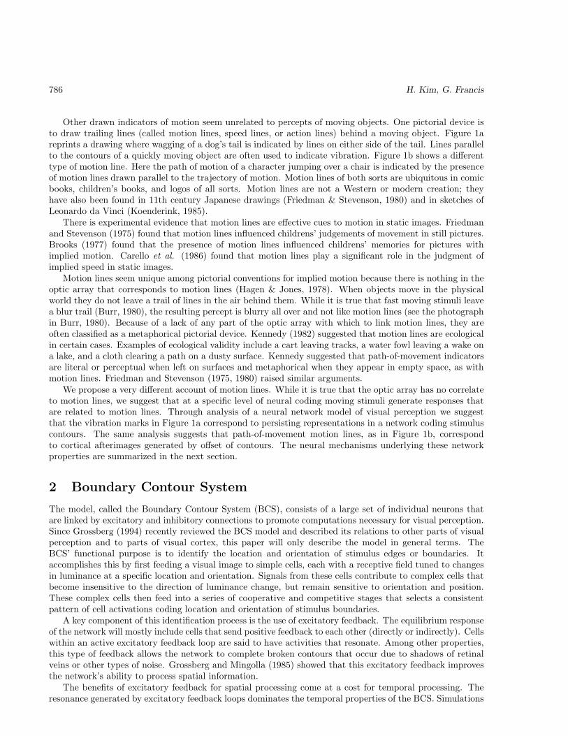
Perception, 1998, volume 27, pages 785–797 This formatted manuscript was created by the second author and does not correspond exactly to the manuscript published in the journal. References to page numbers should refer to the published article. A computational and perceptual account of mo- tion lines Hyungjun Kim, Gregory Francis Department of Psychological Sciences, Purdue University, 1364 Psychological Sciences Building, West Lafayette, IN 47907-1364, USA; e-mail: [email protected] Received 21 April 1997, in revised form 7 May 1998 Abstract. To indicate motion in a static drawing, artists often include lines trailing a moving object. The use of these motion lines is notable because they do not seem to be related to anything in the optic array. We analyze the dynamic behavior of a neural network model for contour detection and show that it generates trails of oriented responses behind moving stimuli. The properties of the oriented response trails are shown to correspond to motion lines. The model generates trails of different orientations depending on the speed and length of the movement, and thereby predicts different uses of two types of motion lines. The model further predicts that motion lines should bias real motion in some situations. An experiment relating motion lines to ambiguous motion percepts demonstrates that motion lines contribute to motion percepts. 1 Introduction Many cues convey an impression of movement in static images. Even without seeing literal movement a viewer can have the sense of seeing a snapshot of something that was moving. Some cues to motion in static images arise from their correlation with true moving objects. For example, a snapshot of a child jumping in midair conveys a strong sense of motion because the viewer knows that masses must be pulled back down toward the ground by the Earth’s gravity (Freyd, 1992). Likewise, when objects move they can take postural positions very different from objects that are nonmoving. Friedman and Stevenson (1975) and Carello, Rosenblum, and Grosofsky (1986) demonstrated that such posture cues influence judgments of implied motion in static images. (a) (b) Figure 1: Examples of motion lines. (a) When lines are drawn on either side of an object and have the same orientation as the object, the impression is that the object is moving rapidly back and forth. (Reprinted from Where’s Spot? by E. Hill, 1980.) (b) When lines are drawn to one side of an object and have an orientation orthogonal to the object, the impression is that the object is moving along a path indicated by the lines. Cues such as posture and position also contribute to the impression that the creature is moving. (Reprinted from The foot book by Dr. Seuss, 1968.)
Transcript of A computational and perceptual account of motion lines

Perception, 1998, volume 27, pages 785–797This formatted manuscript was created by the second author and does not correspond exactly to the
manuscript published in the journal. References to page numbers should refer to the published article.
A computational and perceptual account of mo-tion linesHyungjun Kim, Gregory FrancisDepartment of Psychological Sciences, Purdue University, 1364 Psychological Sciences Building,West Lafayette, IN 47907-1364, USA; e-mail: [email protected] 21 April 1997, in revised form 7 May 1998
Abstract. To indicate motion in a static drawing, artists often include lines trailing a moving object. Theuse of these motion lines is notable because they do not seem to be related to anything in the optic array. Weanalyze the dynamic behavior of a neural network model for contour detection and show that it generatestrails of oriented responses behind moving stimuli. The properties of the oriented response trails are shownto correspond to motion lines. The model generates trails of different orientations depending on the speedand length of the movement, and thereby predicts different uses of two types of motion lines. The modelfurther predicts that motion lines should bias real motion in some situations. An experiment relating motionlines to ambiguous motion percepts demonstrates that motion lines contribute to motion percepts.
1 Introduction
Many cues convey an impression of movement in static images. Even without seeing literal movement aviewer can have the sense of seeing a snapshot of something that was moving. Some cues to motion instatic images arise from their correlation with true moving objects. For example, a snapshot of a childjumping in midair conveys a strong sense of motion because the viewer knows that masses must be pulledback down toward the ground by the Earth’s gravity (Freyd, 1992). Likewise, when objects move they cantake postural positions very different from objects that are nonmoving. Friedman and Stevenson (1975)and Carello, Rosenblum, and Grosofsky (1986) demonstrated that such posture cues influence judgments ofimplied motion in static images.
(a) (b)
Figure 1: Examples of motion lines. (a) When lines are drawn on either side of an object and have the sameorientation as the object, the impression is that the object is moving rapidly back and forth. (Reprintedfrom Where’s Spot? by E. Hill, 1980.) (b) When lines are drawn to one side of an object and have anorientation orthogonal to the object, the impression is that the object is moving along a path indicated bythe lines. Cues such as posture and position also contribute to the impression that the creature is moving.(Reprinted from The foot book by Dr. Seuss, 1968.)
786 H. Kim, G. Francis
Other drawn indicators of motion seem unrelated to percepts of moving objects. One pictorial device isto draw trailing lines (called motion lines, speed lines, or action lines) behind a moving object. Figure 1areprints a drawing where wagging of a dog’s tail is indicated by lines on either side of the tail. Lines parallelto the contours of a quickly moving object are often used to indicate vibration. Figure 1b shows a differenttype of motion line. Here the path of motion of a character jumping over a chair is indicated by the presenceof motion lines drawn parallel to the trajectory of motion. Motion lines of both sorts are ubiquitous in comicbooks, children’s books, and logos of all sorts. Motion lines are not a Western or modern creation; theyhave also been found in 11th century Japanese drawings (Friedman & Stevenson, 1980) and in sketches ofLeonardo da Vinci (Koenderink, 1985).
There is experimental evidence that motion lines are effective cues to motion in static images. Friedmanand Stevenson (1975) found that motion lines influenced childrens’ judgements of movement in still pictures.Brooks (1977) found that the presence of motion lines influenced childrens’ memories for pictures withimplied motion. Carello et al. (1986) found that motion lines play a significant role in the judgment ofimplied speed in static images.
Motion lines seem unique among pictorial conventions for implied motion because there is nothing in theoptic array that corresponds to motion lines (Hagen & Jones, 1978). When objects move in the physicalworld they do not leave a trail of lines in the air behind them. While it is true that fast moving stimuli leavea blur trail (Burr, 1980), the resulting percept is blurry all over and not like motion lines (see the photographin Burr, 1980). Because of a lack of any part of the optic array with which to link motion lines, they areoften classified as a metaphorical pictorial device. Kennedy (1982) suggested that motion lines are ecologicalin certain cases. Examples of ecological validity include a cart leaving tracks, a water fowl leaving a wake ona lake, and a cloth clearing a path on a dusty surface. Kennedy suggested that path-of-movement indicatorsare literal or perceptual when left on surfaces and metaphorical when they appear in empty space, as withmotion lines. Friedman and Stevenson (1975, 1980) raised similar arguments.
We propose a very different account of motion lines. While it is true that the optic array has no correlateto motion lines, we suggest that at a specific level of neural coding moving stimuli generate responses thatare related to motion lines. Through analysis of a neural network model of visual perception we suggestthat the vibration marks in Figure 1a correspond to persisting representations in a network coding stimuluscontours. The same analysis suggests that path-of-movement motion lines, as in Figure 1b, correspondto cortical afterimages generated by offset of contours. The neural mechanisms underlying these networkproperties are summarized in the next section.
2 Boundary Contour System
The model, called the Boundary Contour System (BCS), consists of a large set of individual neurons thatare linked by excitatory and inhibitory connections to promote computations necessary for visual perception.Since Grossberg (1994) recently reviewed the BCS model and described its relations to other parts of visualperception and to parts of visual cortex, this paper will only describe the model in general terms. TheBCS’ functional purpose is to identify the location and orientation of stimulus edges or boundaries. Itaccomplishes this by first feeding a visual image to simple cells, each with a receptive field tuned to changesin luminance at a specific location and orientation. Signals from these cells contribute to complex cells thatbecome insensitive to the direction of luminance change, but remain sensitive to orientation and position.These complex cells then feed into a series of cooperative and competitive stages that selects a consistentpattern of cell activations coding location and orientation of stimulus boundaries.
A key component of this identification process is the use of excitatory feedback. The equilibrium responseof the network will mostly include cells that send positive feedback to each other (directly or indirectly). Cellswithin an active excitatory feedback loop are said to have activities that resonate. Among other properties,this type of feedback allows the network to complete broken contours that occur due to shadows of retinalveins or other types of noise. Grossberg and Mingolla (1985) showed that this excitatory feedback improvesthe network’s ability to process spatial information.
The benefits of excitatory feedback for spatial processing come at a cost for temporal processing. Theresonance generated by excitatory feedback loops dominates the temporal properties of the BCS. Simulations

Motion lines 787
Reset signal
time
time
time
time
On responseOffset response
Tonicinput
PhasicOn−input
A Yij0
Figure 2: At stimulus offset, a gated dipole circuit produces a transient rebound of activity in the non-stimulated opponent pathway. When the pathways code opposite orientations, offset of a horizontal inputleads to a rebound of vertical activity. Dashed lines with circle terminators indicate inhibition, solid arrowsindicate excitation, boxes indicate transmitter gates. The plot next to each cell or gate schematizes thesignal strength over time as a horizontal input is applied and removed. Offset of the horizontal input leadsto a rebound of activity in the vertical pathway.
in Francis, Grossberg and Mingolla (1994) demonstrated that, if left unchecked, resonating signals can lastfor hundreds of simulated milliseconds. To prevent resonating signals from lasting indefinitely, internalprocesses in the network automatically speed disappearance of persisting neural signals. Francis et al.(1994) identified two mechanisms embedded in the BCS design that reset activities in the feedback loop.One is lateral inhibition, and the other is a reset mechanism that inhibits persisting signals. The propertiesof lateral inhibition account for and predict many characteristics of visual masking, including effects on visualpersistence (Francis et al., 1994; Francis, 1996a), temporal integration (Francis, 1996b), and metacontrastmasking (Francis, 1997).
The reset mechanism derives from a different set of mechanisms. Figure 2 schematizes separate pathwayssensitive to the same position in visual space but perpendicular orientations. These pathways competevia reciprocal inhibition from lower levels to higher levels. Feeding this competition are inputs gated byhabituative transmitters. Along with signals from external stimuli, each input pathway receives a tonic sourceof activity, and all output signals are rectified. This combination of rectification, opponent competition,habituative transmitter gates, and tonic input creates a gated dipole circuit. At the offset of stimulation, agated dipole circuit generates a transient rebound of activity in the previously non-stimulated pathway.
The time plot next to each cell or gate describes the dynamics of this circuit. In the case shown, thesharp increase and then decrease of the time plot at the lower right of Figure 2 indicates that an externalinput stimulates the horizontal pathway. In response to the stronger signal being transmitted to the nextlevel, the amount of transmitter in the gate inactivates, or habituates, during stimulation and then rises backtoward the baseline level upon stimulus offset. Notice that the inactivation and reactivation of transmitteroccurs more slowly than changes in the activities of the neural cells. Each slowly habituating transmittermultiplies, or gates, the more rapidly varying signal in its pathway, thereby yielding net overshoots and

788 H. Kim, G. Francis
undershoots at input onset and offset, respectively. During stimulation, the horizontal channel wins therectified opponent competition against the vertical channel as indicated in the top right time plot. However,upon offset of the stimulation to the horizontal channel, the input signal returns to the baseline level but thehorizontal transmitter gate remains habituated below its baseline value. As a result, shortly after stimulusoffset, the gated tonic input in the horizontal channel has a net signal below the baseline level. Meanwhile,the vertical pathway maintains the baseline response at all cells and gates before the opponent competition.Thus, when the horizontal channel is below the baseline activity, after stimulus offset, the vertical channelwins the rectified opponent competition and produces a rebound of activity as shown in the top left timeplot. As the horizontal transmitter gate recovers from its habituated state, the rebound signal in the verticalchannel weakens and finally disappears. The duration of the transient rebound thus matches the recoveryrate of the transmitter from habituation.
The top level of the gated dipole circuit contributes to another circuit that determines the locationand orientation of stimulus boundaries using positive feedback. In these neural circuits, an orientationallysensitive cell is excited by cells of the same orientation sensitivity and inhibited by cells of the orthogonalorientation sensitivity. Thus, the rebound generated by the gated dipole circuit inhibits any persistingactivity generated by the oriented edges of the stimulus.
The properties of reset signals explain why persistence of static stimuli varies inversely with stimulusluminance and duration (e.g., Bowen, Pola & Matin, 1974), and why the persistence of illusory contours isgreater and differently affected by stimulus duration than luminance contours (Meyer and Ming, 1988). Ineach case, stimuli that produce a strong response among oriented cells feeding into the gated dipole generatea strong reset signal at stimulus offset. The strong reset signal greatly reduces persistence. Weaker stimuli(smaller luminance, shorter duration, fewer luminance contours) produce weaker reset signals at stimulusoffset, thereby allowing persisting neural signals to last longer. Details of these model properties are inFrancis et al. (1994).
Signals in the BCS are insensitive to direction of contrast, and thereby are similar to concepts of visualform. Groupings of BCS activities can be recognized as corresponding to specific shapes, without requiringassociated percepts of brightness or color (Grossberg & Mingolla, 1985). The boundary signals in the BCSinteract with a complementary system called the Feature Contour System (FCS), which codes brightnessand color information. Activities in the FCS diffuse across surfaces until constrained by boundaries fromthe BCS (Grossberg & Todorovic, 1988).
Francis and Grossberg (1996) noted that the properties of a type of afterimage support the existence ofreset signals used in the BCS. MacKay (1957) reported an orientation afterimage that appears after viewinga set of radial lines, passing through a common center point , for several seconds and then looking at a blankscreen. The afterimage consists of a perceived wavy circular form. Similarly, viewing a set of concentricoutline circles produces a radially organized afterimage. The afterimage often does not include brightnessor color, but conveys only an impression of form or shape. Francis and Grossberg simulated the BCS modeland showed that the spatial organization of rebound signals generated by the offset of stimuli of this sortare grouped together to produce these types of orientation afterimages.
3 Motion lines
In this section we analyze the dynamic responses of the BCS to moving stimuli. We show that the BCS’srepresentation of contours corresponds to various types of motion lines. In the model, a moving stimulusgenerates a trail of responses among orientationally tuned cells. We suggest that some unspecified mechanismof the visual system interprets these patterns of oriented activities as cues to motion. A nonmoving stimuluswith drawn motion lines will excite many of the same cells. Thus, motion lines convey an impression ofmotion in a static image by tapping in to systems that are tuned to those cues for motion.
3.1 Vibration marks and persistence
While the mechanisms described in the previous section shorten the duration of persisting signals in the BCS,a fast moving stimulus will leave a trail of persisting responses that code the orientation of the stimulus.

Motion lines 789
Figure 3: A simulation demonstrating persistence of oriented responses in the model. The stimulus was avertically oriented bar that moved two pixels to right, four pixels to the left, and then two pixels to the rightto stop in the center of the image plane. Movement of the bar leaves a trail of persisting vertical signals thatare similar to the vibration marks in Figure 1a.
Figure 3 summarizes a simulation that shows this effect. The equations governing the simulations aredescribed in the Appendix. In the simulation a (4×6 pixel) luminous bar started at the middle of the imageplane and then shifted two pixels to right, four pixels to the left, and then two pixels to the right, so thatit ended at the same place it started. The bar moved quickly, relative to the dynamics of the equations;spending one time unit at each pixel location. Figure 3 shows the responses of all cells when the bar reachesits resting place.
This snapshot demonstrates significant temporal-spatial interactions. The strongest responses outlinethe edges of the stimulus, when it was shifted one pixel to the left of center. These responses are persistingrepresentations. The responses to the bar at the center, where it is physically located, have not, at the timeof the snapshot, grown as strong as the persisting responses. Signals to the left and right of the center arealso persisting responses that coded the vertical edges of the stimulus.
We propose that the type of motion lines used in Figure 1a to indicate vibration correspond to thepersisting representations of contour information in the BCS. Significantly, we note that motion lines usedto indicate short, quick movements like in Figure 1a utilize lines that have the same local orientation as themoving stimulus. This characteristic is consistent with the proposal that such motion lines schematize thepersisting oriented responses generated by quickly moving stimuli.
It should be noted that the persisting representations in Figure 3 do not directly correspond to blurredpercepts generated by fast moving stimuli. In the general theory, percepts of smeared brightness mustcorrespond to FCS activities, as the BCS activities do not code brightness percepts. This distinction isemphasized because one could imagine a model-neutral explanation that hypothesizes that vibration marksare schematic drawings of blur. While the model predicts that blur is strongly associated with movingstimuli that generate persisting BCS responses, it further suggests that the vibration marks are schematicsof the BCS responses and not the blur per se. This model property explains why cues for vibration consistof drawn lines instead of smears of color, which would seem better representations of perceived blur.
3.2 Path-of-movement lines and reset signals
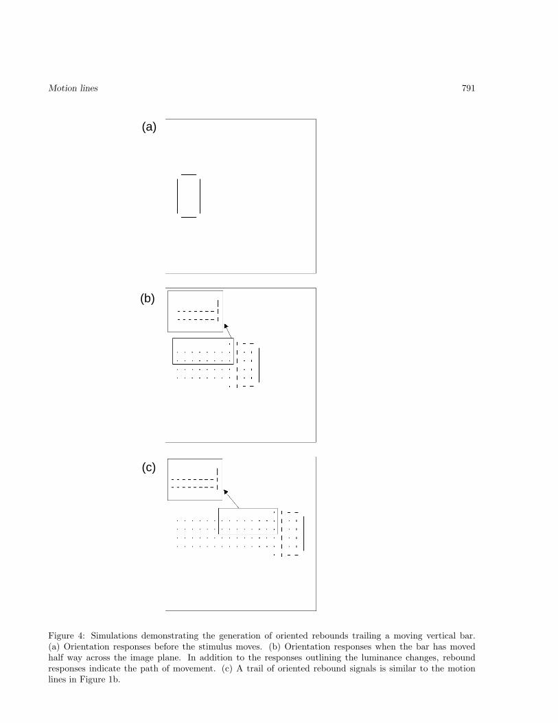
Figure 4 shows responses generated by the model simulation when the bar stimulus moves across the imageplane more slowly (4 time units per pixel) than in Figure 3. Figure 4a shows the responses generated bythe bar before any movement. The oriented signals outline the bar luminance edges. Figure 4b shows

790 H. Kim, G. Francis
the oriented responses after the bar has moved halfway across the image plane. In addition to the strongresponses along the luminance edges, rebound signals produce a trail of responses at the previous locationsof the bar. The inset magnifies the responses in the indicated box to better show the orientation sensitivityof the cell responses. In the inset, the vertical lines represent persisting responses from vertical cells thatresponded to the moving vertical edge. The horizontal responses correspond to the reset signals generatedin the gated dipole circuit at the offset of the vertical response. Figure 4c shows the responses when the barhas moved all the way across the image plane. A long trail of horizontal orientation afterimages remains.
The reset signal trail contains information about the stimulus’ movement. The relative strength ofresponses within a trail provides information about the direction of motion. Close inspection of the inset inFigure 4c shows that the oriented responses decrease in magnitude with separation from the stimulus edge.This occurs because reset signals farther away from the stimulus have had more time to decay. The speedof a stimulus is partly coded by the length of its reset signal trail. As comparison of Figures 5a (fast) and b(slow) indicates, a faster stimulus leaves a longer reset signal trail because it moves a greater distance beforethe signals decay away. The length of the trail can also be influenced by the luminance of the stimulus, withmore luminous stimuli producing stronger afterimages and longer trails.
Figure 5c shows the responses from a horizontal cross-section of reset signal responses generated by thefast and slow moving stimuli in Figures 5a and b. Responses are plotted at the time that the trailing edgeof the stimulus moves off position 13 to position 14 as it translates across the image plane. The dashed lineindicates a fixed threshold that was applied to the responses for producing Figures 5a and b. The reboundresponses generated by the fast stimulus remain above the threshold during the movement of the bar, whilethe responses generated by the slow stimulus have decayed below threshold for the small pixel locations(where the movement started).
The key difference between the responses of the fast and slow stimuli is the time necessary to traversethe image plane. The fast stimulus remains at each pixel location for 4 time units, while the slow stimulusremains at each pixel location for 8 time units. As a result, it takes the slow stimulus twice as long to moveacross the image plane. Thus, the rebound signal generated by the slow stimulus at pixel 1 has decayedfor twice as long as the signal generated by the fast stimulus at the same location. This time differencegenerally means that the response from the fast stimulus is larger than the response from the slow stimulus.An exception is at pixel 13, which is the position each stimulus just moved off. Here, the response from thefast stimulus is smaller because of two factors. First, there remains some persisting activity in the verticalpathway, which limits the response in the horizontal pathway. Such persisting activity has decayed at pixel12, which explains why the strength of the rebound is stronger at pixel 12 than at pixel 13 for the faststimulus. Second, the slower stimulus remains at each pixel position for twice as long as the fast stimulus.As a result it more fully habituates the transmitter gates in the gated dipole, and generates a strongerrebound at stimulus offset. Thus, the initial strength of the rebound is larger for the slow stimulus than forthe fast stimulus. This advantage is quickly eroded, though, as the responses from the slow stimulus decaybefore the stimulus moves very far.
The spatial layout of the reset signal trail suggests the path of movement of the stimulus. In Figure 5dthe vertical bar moves from the lower left to the upper middle to the lower right. The distribution of resetsignals indicates the trajectory of the bar. As the inset shows, the pattern of oriented responses in the resetsignal trail include both vertical and horizontal signals. The horizontal (vertical) signals correspond to resetsignals generated by the vertical (horizontal) edges of the stimulus.
We propose that the type of motion lines used in Figure 1b to indicate path of movement correspond tothe trail of reset signals generated in the BCS by a moving stimulus. Consistent with this hypothesis is theobservation that path-of-movement motion lines are drawn with orientations that are generally orthogonalto the orientation of the moving stimulus.
4 Motion lines and motion percepts
We suggest that motion lines tap into neural mechanisms that treat trailing contour signals as cues to motion.Such contour trails are created, in the model circuits, in response to moving stimuli. If such trails are cues toperceived motion it is reasonable to wonder why artists’ rendering of motion lines do not convey a percept of
Motion lines 791
(a)
(b)
(c)
Figure 4: Simulations demonstrating the generation of oriented rebounds trailing a moving vertical bar.(a) Orientation responses before the stimulus moves. (b) Orientation responses when the bar has movedhalf way across the image plane. In addition to the responses outlining the luminance changes, reboundresponses indicate the path of movement. (c) A trail of oriented rebound signals is similar to the motionlines in Figure 1b.

792 H. Kim, G. Francis
(a) (b)
(d)(c)
Figure 5: Simulations demonstrating rebounds generated by a moving vertical bar. (a) Rebounds generatedby a fast moving bar. (b) When the moving bar travels at half the speed, it leaves a shorter trail because therebounds decay further before the bar reaches the end of the image plane. (c) Rebound responses along across section of the image plane for the fast and slow stimulus. (d) When the bar moves from the lower leftto the upper middle to the lower right of the display it leaves a path of orientation rebounds that indicatesits trajectory.

Motion lines 793
(a)
(b)
Frame 1 Frame 2 Frame 3 Frame 4
Frame 1 Frame 2 Frame 3 Frame 4
Figure 6: A schematic of the stimuli used in the experiment. On the monitor, the stimuli were white onblack (a) The standard bistable motion display. When set in a continual loop, observers generally reportseeing horizontal or vertical motion. (b) When motion lines are added to the display the model predicts thatobservers should see clockwise rotation of the dots. On the monitor the motion lines were more numerousand thinner.
true motion, rather than an implication or understanding of motion, as is typically observed. We suspect theanswer consists of at least two parts. First, from a model-neutral point of view, there may be many differentcontributions to motion percepts. We hypothesize that for real moving objects, motion lines contribute to,but do not solely determine, the accompanying motion percept. In a static image with drawn motion lines,the other cues to motion are absent, and cues for stationarity may conflict with the implications of motionlines.
Second, the model proposes a distinct difference between drawn motion lines and oriented trails gen-erated by moving stimuli in the BCS. As mentioned previously, the BCS interacts with a complementarysystem called the FCS, whose activities code information on brightness, color, and other surface properties.The oriented trails (especially those generated by reset signals) are unlikely to correspond with any FCSrepresentations, as the color and brightness of a moving stimulus is trapped by the boundaries of the stim-ulus itself. In contrast, the motion lines used to imply motion in a static drawing necessarily generate bothBCS orientational and FCS brightness responses. The extra responses in the FCS may preclude the BCSorientational information from acting as a strong cue to motion.
4.1 Experiment
Despite these caveats, the model generally predicts that motion lines should influence percepts of real movingobjects. We tested whether path-of-movement motion lines biased motion percepts in an ambiguous motiondisplay. When presented with the repeating sequence of frames in Figure 6a, observers report seeing apparentmotion between the dots in Frame 1 and the dots in Frame 3. Observers’ percepts tend to be of two types.Either they consist of vertical movement for both the left and right dots, or they consist of horizontalmovement for both the top and bottom dots. These are mutually exclusive percepts, observers report seeingeither vertical or horizontal, but not both at once. The percepts are often bistable, with frequent changesbetween horizontal and vertical motion directions. Although they are reported less frequently, it is alsopossible to see the dots moving in clockwise or counterclockwise directions.
The experiment explores how the presence of motion lines biases observers to report motion directions

794 H. Kim, G. Francis
0
25
50
75
100
NO ML ML
BK
HK
YC
Per
cent
age
of ti
me
repo
rt cl
ockw
ise
Figure 7: Percentage of time observers reported seeing clockwise rotation of the dots. For the no motionline condition, clockwise rotation was rare. For the motion line condition, clockwise rotation was frequentlyobserved.
consistent with the directions implied by the motion lines. We designed ambiguous motion displays to includemotion lines that, if used, would disambiguate the overall motion organization.
4.1.1 Methods
ObserversThree observers with normal or corrected to normal vision participated in three sessions each. One observerwas an author, the other two were naive to the purpose of the study.DisplayAll stimuli were presented on a Silicon Graphics Indy computer. Figure 6 demonstrates the type of stimuliused in all the experiments. Figure 6a schematizes the standard stimulus. Frame 1 included two dots onopposite corners of an imaginary square. Frames 2 and 4 were blank screens. Frame 3 included two dots onopposite corners of an imaginary square, but the corners not used in Frame 1. The frames were presentedin a loop so that frame 1 appeared right after frame 4. The percept was of dots moving, usually back andforth either horizontally or vertically.
The dots were circles with a radius of 1.08 deg. The center-to-center distance of a dot from frame 1 toframe 2 was 5.56 deg. The dots had a luminance 52 cd/m2 and the background was 0.06 cd/m2. Each framewas presented for 150 milliseconds.
The motion line stimulus is schematized in Figure 6b. It was identical to the standard stimulus exceptmotion lines were added to various frames. Frame 1 added motion lines to the left and right sides of thedots, thereby implying horizontal movement. Frame 2 added motion lines to the top and bottom sides ofthe dots, thereby implying vertical movement. Motion lines were also added in all positions for frames 2and 4. Each set of motion lines consisted of nine lines, with a length of 5.40 deg, thickness of 0.077 deg, andluminance of 5 cd/m2.ProceduresIn each trial, an observer viewed a repeating sequence of images in Figure 6a or b for thirty seconds. Theobserver noted, by keypresses, whenever the percept changed to or from clockwise motion. The computerkept track of the time that an observer saw clockwise motion. Observers first went through five practicetrials each with and without motion lines. Data was then gathered from ten trials without motion lines andten trials with motion lines; which were randomly mixed as the observer went through a testing session.
4.1.2 Results
Figure 7 plots the percentage of time that each observer reported seeing clockwise motion for each stimulustype. Observers rarely reported clockwise motion for the stimulus without motion lines, but often reportedclockwise motion for the stimulus with motion lines. We interpret the data as evidence that motion linesbias observers’ percepts of moving stimuli. Motion lines can contribute to percepts of motion.

Motion lines 795
Per
cent
age
of ti
me
repo
rt c
lock
wis
e
0
25
50
75
100
NO ML ML
BK
HK
YC
0
25
50
75
100
NO ML ML
BK
HK
YC
PRO
CON
Figure 8: Asking observers to try to force the dots to move clockwise (PRO) or not clockwise (CON) hasno effect on the frequency of observing clockwise motion. This suggests that the influence of motion lines isnot due to cognitive factors that could bias ambiguous percepts.
Exactly how motion lines contribute to motion percepts is not resolved by the previous finding. Forexample, the neural network model described here suggests that motion lines act as cues to motion andthe visual system, in responding to those cues, is biased toward a particular interpretation of an otherwiseambiguous motion display. An alternative account is that the motion lines are processed as metaphors formotion direction and through attentional processes the observer forces the ambiguous motion signals togroup in particular ways. It is indeed true that with sufficient practice one can “mentally” bias the perceivedtype of motion to be vertical or horizontal. With a bit more effort it is also possible to force the percept tobe of clockwise motion.
Thus, the experimental data support the idea that motion lines influence percepts of ambiguous motiondisplays, but it is not clear whether the mechanisms underlying such influence are perceptual or attentional.To try to disentangle perceptual and attentional effects, we asked subjects to participate in two more sessionsof the experiment. The methods and procedures were exactly the same as before, except observers whereasked to try to force the dots to move in a particular manner. In the second session observers were asked totry to make the dots move clockwise. In the third session observers were asked to try to make the dots notmove clockwise. We refer to these sessions as PRO and CON, respectively.
We reasoned that if motion lines simply resulted in increased attentional biases for clockwise motion, thenhaving observers mentally apply such attentional biases should cause the differences between the no-motionline and motion line conditions to disappear. If a difference remains, then it is more plausible that the effectof motion lines is not exclusively the result of attentional biases. Such a result would lend credence to theperceptual account we have offered. Likewise, if observers actively try to not see clockwise motion, but therestill remains a significant percept of such motion for the motion line display, this is evidence that motionlines directly contribute to motion percepts.
Figure 8 plots the data for the two sessions. The results are essentially the same as in Figure 7, withattentional bias hardly effecting the percentages of reported clockwise percepts. These findings suggest thatattentional biases are not responsible for the increased frequency of perceiving clockwise motion for themotion line display.
In a less formal study, we have changed the design of the motion lines so that they indicate counter-clockwise, vertical, or horizontal motion. The results are essentially unchanged, with high frequency of seeing

796 H. Kim, G. Francis
the motion direction implied by the motion lines. As a whole then, the experimental data demonstrate thatmotion lines do contribute to motion percepts and are not limited to implied motion in static images.Moreover, the effects of motion lines on the ambiguous display suggest that they are not simply workingthrough attentional biases, as a metaphorical explanation of motion lines would imply. The results areconsistent with the proposed hypothesis that motion lines are one of many cues to motion generated by realmoving objects, and that the visual system is tuned to detect the motion line cue.
5 Conclusions
By analyzing the behavior of a neural network in response to moving stimuli, we have shown that the modelprovides a computational and perceptual explanation of motion lines. Since the model has already accountedfor a wide variety of psychophysical and neural data on motion, brightness, texture segmentation, figure-ground separation, and dynamic vision, the new account of motion lines links aspects of picture perceptionto a large literature of visual perception in general.
Although we suggest that motion lines have a computational and perceptual basis, this does not precludeinfluences from metaphorical interpretations of images. Kennedy (1982) convincingly argues for a metaphor-ical interpretation of many aspects of picture perception, and we suspect they play a role in motion linesas well. However, both computational and experimental analyses suggest that there is a strong perceptualcomponent that guides the interpretation of motion lines in static images as cues to motion.
We anticipate that an analysis of motion lines and neural mechanisms tuned to detect motion lines ascues to motion will improve our understanding of motion perception in general. For example, McBeath,Shaffer and Kaiser (1995) noted in a discussion of object tracking that stimuli do not leave observabletrajectories behind them as they move. In contrast, our analysis of the neural network model suggeststhat a moving object can, under the proper circumstances, leave a trail of signals that provide informationabout the object’s trajectory. The trajectory trail could be processed by the spatial analyzing parts of thevisual system to predict future paths of the object. The link between spatial and motion aspects of visualperception would tie together areas of perception that have previously been considered distinct.
References
Bowen, R., Pola, J., & Matin, L. (1974). Visual persistence: Effects of flash luminance, duration and energy.Vision Research, 14, 295–303.
Brooks, P. (1977). The role of action lines in children’s memory for pictures. Journal of Experimental ChildPsychology, 23, 98–107.
Burr, D. (1980). Motion smear. Nature, 284, 164–165.
Carello, C., Rosenblum, L., & Grosofsky, A. (1986). Static depiction of movement. Perception, 15, 41–58.
Francis, G. (1996a). Cortical dynamics of lateral inhibition: Visual persistence and ISI. Perception &Psychophysics, 58, 1103–1109.
Francis, G. (1996b). Cortical dynamics of visual persistence and temporal integration. Perception & Psy-chophysics, 58, 1203–1212.
Francis, G. (1997). Cortical dynamics of lateral inhibition: Metacontrast masking. Psychological Review,104, 572–594.
Francis, G. & Grossberg, S. (1996). Cortical dynamics of boundary segmentation and reset: Persistence,afterimages and residual traces. Perception, 25, 543-567.
Francis, G., Grossberg, S., & Mingolla, E. (1994). Cortical dynamics of binding and reset: Control of visualpersistence. Vision Research, 34, 1089-1104.

Motion lines 797
Freyd, J. (1992). Five hunches about perceptual processes and dynamic representations. In D. Meyer &S. Kornblum (Eds.). Attention and Performance XIV. Synergies in experimental psychology, artificialintelligence, and cognitive neuroscience. Cambridge, MA: The MIT press.
Friedman, S. & Stevenson, M. (1975). Developmental changes in the understanding of implied motion intwo-dimensional pictures. Child Development, 46, 773-778.
Friedman, S. & Stevenson, M. (1980). Perception of movement in pictures. In M. A. Hagen (Ed.). Theperception of pictures (Vol. 1. pp. 225-255). New York: Academic Press.
Grossberg, S. (1994). 3-D vision and figure-ground separation by visual cortex. Perception & Psychophysics,55, 48-120.
Grossberg, S. & Mingolla, E. (1985). Neural dynamics of perceptual grouping: Textures, boundaries, andemergent segmentations. Perception & Psychophysics, 38, 141-171.
Grossberg, S. & Todorovic, D. (1988). Neural dynamics of 1-D and 2-D brightness perception: A unifiedmodel of classical and recent phenomena. Perception and Psychophysics, 43, 241–277.
Hagen, M. & Jones, R. (1978). Cultural effects on pictorial perception: How many words is one picturereally worth? In R. Walk & H. Pick, Jr. (Eds.). Perception and experience, (pp 171–212). New York:Plenum.
Hill, E. (1980). Where’s Spot? New York: C. P. Putnam & Sons.
Kennedy, J. (1982). Metaphor in picture. Perception, 11, 589-605.
Koenderink, J. J. (1985). Space, form, and optical deformations. In D. Ingle, M. Jeannerod, & D. Lee(Eds.). Brain Mechanisms and Spatial Vision (pp. 31-58). Dordrecht: Martinus Nijhoff Publishers.
MacKay, D. (1957). Moving visual images produced by regular stationary patterns. Nature, 180, 849-850.
McBeath, M. K., Shaffer, D. M. & Kaiser, M. K. (1995). How baseball outfielders determine where to runto catch fly balls. Science, 268, 569–573.
Meyer, G. & Ming, C. (1988). The visible persistence of illusory contours. Canadian Journal of Psychology,42, 479-488.
Seuss, Dr. (1968). The foot book. New York: Random House.
Appendix
In the simulations, a 4× 6 pixel bar on a 20× 14 image plane was filtered by oriented detectors that fed intoa gated dipole circuit. The orientation detectors were identical to Levels 1–4 in Grossberg and Todorovic(1988) and are not described here. The output of Level 4, Yijk, codes the response of an oriented cell atposition (i, j) in the pixel plane that is tuned to orientation k. For our simulations we used only two cellorientations: horizontal, k = 0, and vertical, k = 1. The Yijk values were recalculated for every change inthe position of the moving bar stimulus.
At each pixel location, these values fed into a gated dipole competition across orientation. Each cell inthe gated dipole (see Figure 2), at each pixel position, obeyed a differential equation. The activity of thefirst cell obeyed the equation:
dVijk
dt= −Vijk + Yijk + A, (1)
where −Vijk indicates passive decay and A indicates a constant source of input to each pathway. Activitythen passed through a habituating gate that obeyed a differential equation of the form:
dTijk
dt= B (C − Tijk − TijkVijk) . (2)

798 H. Kim, G. Francis
The term C−Tijk indicates a production process whereby the amount of transmitter grows toward the valueC. The term −TijkVijk models how transfer of information to the next level uses a proportion of availabletransmitter. The entire equation was multiplied by B << 1, to indicate that the dynamics of the transmitterwas much slower than the dynamics of neural activities.
The next level received the gated flow of activation. Cells at this level obeyed equations of the form
dWijk
dt= −Wijk + TijkVijk. (3)
The final level received excitatory input from the same pathway and inhibitory input from the orthogonalpathway. Thus, a horizontal cell obeyed an equation of the form
dZij0
dt= −Zij0 + Wij0 −Wij1. (4)
Each Zijk was compared to a threshold of 0.1 and any values above the threshold were used to produceFigures 3, 4 and 5.
In all simulations A = 1, B = 0.001 and C = 1. All equations were integrated using Euler’s method witha step size of 0.0001. The (arbitrarily coded) intensity of the bar was 9 on a background of 4.5.