A Behavior-Based System For Off-Road Navigation

D. Langer, J. K. Rosenblatt, and M. Hebert

The Robotics InstituteCarnegie Mellon University

Pittsburgh PA 15213

Abstract

In this paper, we describe a core system for autonomous navigation in outdoor natural ter-rain. The system consists of three parts: a perception module which processes range images toidentify untraversable regions of the terrain, a local map management module which main-tains a representation of the environment in the vicinity of the vehicle, and a planning modulewhich issues commands to the vehicle controller. Our approach is to use the concept of “earlytraversability evaluation,” in which the perception module decides which parts of the terrainare traversable as soon as a new image is taken, and on the use of a behavior-based architec-ture for generating commands to drive the vehicle. We argue that our approach leads to arobust and efficient navigation system. We illustrate our approach by an experiment in whicha vehicle travelled autonomously for one kilometer through unmapped cross-country terrain.The system used in this experiment can be viewed as a core navigation system in that othermodules, such as a map navigation module, can be easily added to the system.

1 Introduction

Autonomous navigation missions through unmapped open terrain are critical in many applications ofoutdoor mobile robots. To successfully complete such missions, a mobile robot system needs to beequipped with reliable perception and navigation systems capable of sensing the environment, of buildingenvironment models, and of planning safe paths through the terrain. In that respect, autonomous cross-country navigation imposes two special challenges in the design of the perception system. First, theperception must be able to deal with very rugged terrain. This is in contrast to more conventional mobilerobot systems which operate in simpler structured environments. Second, the perception system must beable to reliably process a large number of data sets over a long period of time. For example, even arelatively short navigation mission of a few kilometers may require processing thousands of images.Furthermore, because manual rescue of the vehicle from a serious failure is impossible, the perceptionsystem must be able to process a large number of images without any errors, or, at least, the system mustbe able to identify and correct for errors in time to avoid catastrophic failure of the vehicle. Although thebasic computer vision and planning technologies exist and have been demonstrated in the laboratory,achieving such a level of reliability is still a significant challenge.

Several approaches have been proposed to address these problems. Autonomous traverse of ruggedoutdoor terrain has been demonstrated as part of the ALV [17] and UGV [16] projects. JPL’s Robby usedstereo vision [15] as the basis of its perception system and has been demonstrated over a 100 m traverse

2

in outdoor terrain. Other efforts include: France’s VAP project which is also based on stereo vision [6];the MIT rovers which rely on simple sensing modalities [1]; and several Japanese efforts[11].

In this paper, we argue that relatively simple algorithms for obstacle detection and local map building aresufficient for cross-country navigation. Furthermore, when used in the context of a behavior-basedarchitecture, these algorithms are capable of controlling the vehicle at significantly faster speeds thanwould be possible with a system that planned an optimal path through a detailed, high-resolution terrainmap. Moreover, we argue that an accurate map is not necessary because the vehicle can safely traverserelatively large variations of terrain surface.

The underlying principle of this work was to keep things as uncomplicated as possible. We opted for asimple yet effective system rather than using more complex methods which often look good on paper yetproduce problems in the field.

To illustrate our approach, we will describe a set of perception and navigation modules which constitutethe core of a cross-country navigation system. The goal of this system is to enable the vehicle to travelthrough unmapped rugged terrain at moderate speeds, typically two to three meters per second. Wearranged the system modules in a self-contained navigation system which we demonstrated on a onekilometer path through unmapped open terrain. In the next sections, we will use this result as the mainreference to illustrate our approach and to discuss the system performance and the implementation detailsof each module.

The perception and navigation system was developed as part of the Unmanned Ground Vehicle (UGV)project. The support vehicle is a retrofitted HMMWV capable of cross-country navigation (Figure 1). Thesensor is the Erim laser range finder which acquires 64x256 range images at 2 Hz. An estimate of vehicleposition can be obtained at all times by combining readings from an INS system and from encoders.

Figure 2 shows a high level view of the architecture of the system. A perception module computes a listof untraversable regions and sends the region description to a local map management module. The localmap module is responsible for gathering information from the perception module over time and formaintaining a consistent model of the terrain around the vehicle. (We will elaborate on the description ofthe perception and local map modules in Sections 2 and 3, respectively.) The description of theuntraversable regions is sent by the local map module to a planning module at regular intervals.Untraversable regions are terrain features such as high slopes, ditches, or tall objects over which thevehicle cannot drive safely.

Based on a set of driving behaviors, the planning module generates arcs which steer the vehicle such thatit remains clear of the untraversable regions. (We describe the planning module in detail in Section 4.)The three logical modules, perception, local map, and arc generation constitute the core of the system.Although it is divided into three logical units, the core system is implemented as a decentralized set ofseven software modules. The software modules exchange information using the TCX communicationsystem [5].

In order to be used in a real mission, this core system must be embedded in a larger navigation system soas to carry out a specific task. As will be explained in Section 4, the planning module is capable ofarbitration between the steering directions generated by an external module and the steering directionsgenerated by the core navigation system. For example, the external module can be a module that forces

3

the vehicle to drive to a specific goal point or to follow a specific direction. We will show in Section 5 anexample in which an additional module drives the vehicle through a set of intermediate goal points.

2 Perception

The range image processing module takes a single image as input and produces a list of regions which areuntraversable. The initial stage of image filtering resolves the ambiguity due to the maximum range of thescanner, and removes outliers due to effects such as mixed pixels and reflections from specular surfaces(see [7] for a complete description of these effects). After image filtering, the (x,y,z) location of everypixel in the range image is computed in a coordinate system relative to the current vehicle position. Thecoordinate system is defined so that thez axis is vertical with respect to the ground plane, and they axis ispointing in the direction of travel of the vehicle. It is convenient to center the coordinate at the point usedas the origin for vehicle control, in this case between the two rear wheels, rather than at the origin of thesensor. The transformation takes into account the orientation of the vehicle read from an INS system. Thepoints are then mapped into a discrete grid on the (x,y) plane. Each cell of the grid contains the list of the(x,y,z) coordinates of the points which fall within the bounds of the cell inx andy. The size of a cell in thecurrent system is 20 cm in bothx and y. The choice of the grid resolution is based on the angularresolution of the sensor, in this case 0.5o, and on the size of terrain features which need to be detected,20cm in the case of the HMMWV.

2.1. Terrain classification algorithm

The terrain classification as traversable or untraversable is first performed in every cell individually. Thecriteria used for the classification are:

• the height variation of the terrain within the cell,

• the orientation of the vector normal to the patch of terrain contained in the cell,

• and the presence of a discontinuity of elevation in the cell.

To avoid frequent erroneous classification, the first two criteria are evaluated only if the number of pointsin the cell is large enough. In practice, a minimum of five points per cell is used. Once individual cells areclassified, they are grouped into regions and sent to the local map maintainer. It is necessary to use a slopecriterion instead of a simple test on elevation for two reasons. First, the vehicle has limitations on the typeof slopes on which it can drive independently of any elevation discontinuity. Second and mostimportantly, a test on absolute elevation would be very unreliable due to the potentially high variation ofelevation from the near range to the far range of the field of view. Also, a small error in the estimation ofvehicle pitch may induce a large error in the elevation at the far range of the field of view.

• For every range pixelp = (ρ, row, col):

• Convertp to a 3-D pointP = [x y z] with respect to the vehicle position at the time the imagewas taken.

• Compute the location of the cellC which containsP.

• Add P to the list of points inC.

4

• For every non-empty cellC:

• Compute the elevation statistics:hmin, hmax, σh, and the slopev by doing a weighted least-squares estimation using the list of points in C.

• If hmin - hmax andv are outside of the acceptable bounds for the current vehicle configuration interms of undercarriage and tipover constraints, classify the cell as untraversable.

• Send the list of untraversable cells to the local map manager along with the pose of the vehicleat the time the image was taken.

In general, the density of points in the map is not uniform. As a result, many cells of the map may end upbeing empty. A dense map without these gaps could be produced by first interpolating the map. Thiswould be necessary in order to evaluate slope by using a neighborhood of each of the grid points.However, with the algorithm above, it is not necessary to interpolate the map because slope is evaluatedat each cell individually without using its neighborhood. All that is required in order to compute the slopeat a given cell is that enough data points fall in that cell. As result, the slopes cannot be evaluated at thosecells of the map which have low or no data content. This is acceptable assuming that the data acquisitionprocessing are fast enough compared to the speed of the vehicle so that the regions of the map withinsufficient data can be covered in subsequent images. Although this solution relies on fast perceptionrate, it is in practice preferable to interpolating the map for two reasons. First, interpolation does increasethe computation time substantially, thus increasing reaction time and map update time. Second, theinterpolation may smooth out important local details of the terrain which are left untouched in ouralgorithm.

2.2. Example

Figure 3 shows an example of terrain classification at one position along the path of Figure 8. A videoimage of the terrain is shown in Figure 3 (a); the corresponding range image is shown in Figure 3 (b). Inthis example, a large part of the terrain on the left side of the vehicle is untraversable because of eitherhigh slope or high elevation.

Figure 3 (c) shows the grid built internally by the perception module. The (x,y) plane is the referenceground plane and z is vertical. Thez value displayed at each element of the grid is the highest elevation ofthe set of data points within that cell. The scaling factors in (x,y) and inz are different so that the height ofthe hill on the left is exaggerated in this display. The elevation varies by approximately one meter acrossthe terrain in this example.

Figure 3 (d) shows the result of the terrain classification. The points that are classified as obstaclesbecause they are part of an untraversable region of the terrain are indicated by non-zero values, the rest ofthe terrain is set to zero. The cells in the region indicated by the labelA are not classified as obstaclesbecause the terrain slope within these cells is still within the bounds of the slopes on which the vehiclecan travel. The cells in the regions indicated by the labelB are not all classified as untraversable becausethe number of data points within each of these cells is not sufficient.

It is clear from this example that the portions of the grid that are not visible are not reported to the localmap manager because only the untraversable cells are explicitly detected. This can occur for two reasons:insufficient density of data points at long range or occlusions from other parts of the terrain. The former

5

occurs only at long range and the timing of the system is adjusted so that new scans of the same area aretaken before the vehicle reaches that area. Specifically, assuming that a minimum ofn points per cell isnecessary with cells of sizel meters on the side, a cell on a the ground will have a number of data pointstoo small when it is a range greater than , where h is the height of the sensor above theground andθ is the angular field of view of a single pixel. Withl = 40cm,n = 3, andθ = 0.01,R isapproximately 6.5m. At a speed of 3m/s, three scans of this cell will be taken before the vehicle reachesit, using the current image acquisition rate of 2Hz. This result corresponds to the worst case of the groundplane because cells on slanted surfaces have a higher density of points. This analysis shows that the cellswith insufficient data are processed on time provided that vehicle speed is properly tuned to the sensingrate.

Cells with insufficient data due to occlusions occur because of the presence of obstacles. The arcgeneration module steers the vehicle away from the obstacles, and, just as before, the cells in an occludedarea are scanned before the vehicle reaches this area. Based on this analysis and the fact that maintainingthe traversable cells in the local would degrade performance appreciably, we decided not to representexplicitly the traversable regions.

2.3. Performance and limitations

The range image processing module is efficient because it does not build a dense, high-resolution map ofthe terrain, and because each image is processed individually without any terrain matching and merging.Specifically, the range processing algorithms run at 200 ms/image on Sparc II workstations.

Although the image acquisition time (500 ms) is effectively the main limitation because it is over twicethe processing time, we have put the emphasis on the efficiency of the processing for two reasons. First,faster processing translates to lower latency between the time an object appears in the field of view of therange image and the time it is placed in the local map, irrespective of the image acquisition time. Second,the slow image acquisition is specific to the scanner that was available to us for the experiments reportedin this paper. We believe that efficient processing is needed for the next generation of faster sensors withwhich we are experimenting.

In practice, terrain features of size 30cm are detected at a range of ten meters when vehicle speed is 2 m/s. By comparison, the maximum range of the scanner in its first ambiguity interval is 18 m with aseparation of one meter between pixels at that range. More than the range resolution, the reason for thelimited detection range is mainly the angular resolution of the scanner which limits the number of pixelsmeasured on a given object.

Several problems can lead to occasional misclassification of the terrain. The first problem is the presenceof terrain regions with poor reflectance characteristics, such as water. In practice, such points can beremoved from the image during the initial filtering phase. However, the missing data creates large gaps inthe map in which the terrain cannot be classified. This problem can really be solved only with the help ofadditional sensors suitable for terrain typing.

The second problem is the presence of vegetation in typical natural outdoor environments. This problemcan manifest itself in several ways. Dense vegetation appears as an obstacle in the range image, causingthe vehicle to come to a stop even when the underlying terrain is traversable. Sparse vegetation also

R hl( ) nθ( )⁄=

6

causes the detection of spurious obstacles at short range from the sensor. Obviously there is no solution tothis problem using the laser range finder alone. Additional sensing, such as millimeter wave radar, or adifferent type of range sensing, such as passive stereo may help.

3 .Local Map Management

The purpose of the local map module is to maintain a list of the untraversable cells in a region around thevehicle. In the current system, the local map module is a general purpose module called Ganesha [9].Ganesha uses a 2-D grid-based representation of the local map. In this system, the active map extendsfrom 0 to 20 meters in front of the vehicle and 10 meters on both sides. Each grid cell has a resolution of

which was found to provide sufficient accuracy for navigation functions as it is small withrespect to vehicle size and large with respect to sensor resolution. This module is general purpose in thatit can take input from an arbitrary number of sensor modules and it does not use any explicit knowledgeof the algorithms used in the sensor processing modules.

3.1. Overview

The core of Ganesha is a single loop shown in Figure 4. At the beginning of the loop, the current positionof the vehicle is read and the coordinates of all the cells in the map with respect to the vehicle arerecomputed. Cells that fall outside the bounds of the active region are discarded from the map. The nextstep in the loop is to get obstacle cells from the perception modules, and then to place them in the localmap using the position of the vehicle at the time the sensor data was processed. The sensing position hasto be used in this step because of the latency between the time a new image is taken, and the time thecorresponding cells are received by the map module, typically on the order of 300ms.

After new cells are placed in the map, internal cell attributes are updated. Cell attributes include thenumber of times a cell has been previously observed and a flag that indicates whether it is inside thecurrent field of view of the sensor. Finally, Ganesha sends the list of current obstacle cells in its map tothe planning system. At the end of each loop, Ganesha waits before starting a new iteration in order tokeep a constant loop cycle time.

3.2. Map scrolling

All the coordinates are maintained in Ganesha relative to the vehicle. In particular, vehicle position andorientation are kept constant in the map. At every iteration, Ganesha reads from the positioning system aposition (x,y) and a headingϕ. Assuming that the local map is currently expressed with respect to vehicleposeP1 = (x1, y1, ϕ1) and the new vehicle pose read from the controller isP2 = (x2,y2,ϕ2), Ganesha firstcomputes the relative transformationP = P2P1

-1 and then transform every cell (xm1, ym

1) of the currentmap to its new location with respect to the vehicle poseP2: (x

m2, ym

2) = P (xm1, ym

1).

It is important to note that Ganesha deals only withrelative transformations from one vehicle position toanother. Therefore, Ganesha relies on the relative accuracy of the vehicle positioning system, not on theabsolute accuracy of the global positions. Assuming that the maximum error on the positioning system ofk% of distance travelled under normal conditions.Assuming Ganesha maintains aL meter deep map, themaximum error in the position of a map object occurs when an object that was added when it was at a

0.4 0.4× m2

7

distanceL from the vehicle is now about to disappear from the map after the vehicle has travelled adistance L. In that case, the error in the position of the cell is at mostkL because it is the relative errorbetween two vehicle positions separated byL. In our case,k < 1% andL = 20m, and the error is therefore20cm which is below the 40cm resolution of the Ganesha grid. The estimate ofk is based on experimentalwork with the vehicle controller as reported in [20]. Based on these numbers, the accuracy of thepositioning system is sufficient to provide enough relative accuracy for the Ganesha map to be updatedcorrectly.

The fact that the relative accuracy of the positioning system is sufficient for this resolution of the Ganeshagrid and for our vehicle does not preclude the use of other sources of position information. For example,we could imagine using 3-D landmark or feature tracking in the range images in order to refine theposition estimates. However, this type of visual positioning should be separate a process of whichGanesha uses the output in the form of periodical position updates. In particular, vehicle position fromvisual registration should not be part of this system.

Because the map module deals only with a small number of terrain cells instead of a complete model andthe number of obstacle cells is small compared to the number of traversable cells, the map update is fast.In practice, the update rate can be as fast as 50 ms on a SparcII workstation. Because of the fast updaterate, this approach is very effective in maintaining an up-to-date local map at all times. One lastadvantage of Ganesha’s design is that the module does not need to know the details of the sensing part ofthe system because it uses only information from early terrain classification. In fact, the only sensor-specific information known to the map module is the sensor field of view which is used to check forconsistency of terrain cells between images as described below.

3.3. Error correction

The perception module may produce occasional false positive detection because of noise in the image, forexample, which would affect the path of the vehicle. This problem is solved by the map maintainer whichmaintains a history of the observations. Specifically, an untraversable map cell which is not consistentacross images is discarded from the local map if it is not reported by the perception module asuntraversable in the next overlapping images. Because the terrain classification is fast compared to thespeed of the vehicle, many overlapping images are taken during a relatively short interval of distancetravelled. As a result, an erroneous cell is deleted before the vehicle starts altering its path significantly toavoid it.

DECAY ALGORITHM

3.4. Field of view management

A severe limitation of any navigation system is the limited field of view of the sensor, in this case 80o.The problem with the limited field of view is that if the vehicle turns too sharply it may drive into a regionthat falls outside of the region covered by the previous images. Specifically, the minimum possibleturning radius that would keep the entire vehicle within the area swept by the sensor’s FOV is given by:

rmin w 2⁄ mc c m2 1+++=

8

With the current parameters of the current laser range finder, the minimum possible turning radius is thenrmin ~ 17.25 m.

In order to address the field of view constraint, we introduced a new mechanism in Ganesha to explicitlyrepresent fields of view. The idea is to add artificial obstacles in the map, the FOV obstacles, whichrepresent the bounds on the sensor field of view at every recorded position as shown in Figure 5. TheFOV obstacles are generated at the two outermost boundary points of the field of view polygon. Sinceadding FOV obstacles every time a new position is read might be too expensive and is not necessary, theyare added at one meter intervals.

The FOV cells are first hidden which means that they do not affect the behavior of the vehicle undernormal operating conditions. A hidden FOV obstacle occupies a map cell and is transformed with vehiclemotion just like the regular obstacle cells, but is not sent to the planner and thus not considered anobstacle by the avoidance behavior. A hidden obstacle is converted to an active obstacle when it comesclose to the vehicle. Currently this is done when the FOV obstacle is less than one meter from the front ofthe vehicle (Figure 5). Active FOV obstacles are treated just like any other regular obstacle. Thismechanism ensures that the vehicle can still make sharp turns (Figure 5(a)), but will be prevented fromsteering into a path that falls into a locally unmapped area (Figure 5(b)).

Using FOV obstacles is a simple and effective way of dealing with the field of view constraint. It has theadvantage that it has no effect on the behavior of the vehicle in normal operation and the increase incomputation time in Ganesha is negligible as only a few artificial obstacles are used. Another advantageis that the FOV objects mechanism is completely transparent to the rest of the system. In particular, theplanning system does not have any knowledge of the way the field of view is handled in Ganesha. As aresult, different sensors with different fields of view may be used without any modification of the planner.

Because FOV obstacles increase the amount of computation in Ganesha, one could be tempted tomaintain a representation of the traversable area rather than the untraversable area. In reality, thisapproach would degrade performance: Because the FOV obstacles are inserted every meter, there are onthe order of 2L FOV cells in the Ganesha at any given time, whereL = 20m is the depth of the grid. At thesame time, there are on the orderL2/c2 empty cells in the grid, wherec = 40cm is the resolution of thegrid. Therefore, even in cluttered terrain, it would always considerably less efficient to transform thetraversable cells instead of the combination of untraversable cells and the FOV cells. The situation isworse in the case of a flat terrain in which the map update would beL/2c2 = 66 times slower.

4 Planning

Once obstacles have been detected by the terrain evaluation modules and the local map has been updatedby Ganesha, the next step is to use this map to generate commands that steer the vehicle around theseobstacles. This is done within the framework of the Distributed Architecture for Mobile Navigation(DAMN).

DAMN is a behavior-based architecture similar in some regards to reactive systems such as theSubsumption Architecture [2]. In contrast to more traditional centralized AI planners that build a worldmodel and plan an optimal path through it, a behavior-based architecture consists of specialized task-achieving modules that operate independently and are responsible for only a very narrow portion of

9

vehicle control, thus avoiding the need for sensor fusion. A distributed architecture has severaladvantages over a centralized one, including greater reactivity, flexibility, and robustness [19].However, one important distinction between this system and purely reactive systems is that, while anattempt is made to keep the perception and planning components of a behavior as simple as possiblewithout sacrificing dependability, they can and do maintain internal representations of the world (e.g.Ganesha’s local map). Brooks has argued that “the world is its own best model” [3], but this assumes thatthe vehicle’s sensors and the algorithms which process them are essentially free of harmful noise and thatthey can not benefit from evidence combination between consecutive scenes. In addition, disallowing theuse of internal representations requires that all environmental features of immediate interest are visible tothe vehicle sensors at all times. This adds unnecessary constraints and reduces the flexibility of thesystem.Figure 6 shows the organization of the DAMN system in which individual behaviors such as roadfollowing or obstacle avoidance send preferred steering directions to the command arbitration modulewhich combines these inputs into a single steering direction and speed command. We describe the use ofDAMN in the context of the cross-country navigation system only and we refer the reader to [20] for adescription of other systems built around DAMN in the context of road following.

4.1. The arbiter

The role of the architecture is to decide which behaviors should be controlling the vehicle at any giventime. In the Subsumption Architecture, this is achieved by having priorities assigned to each behavior; ofall the behaviors issuing commands, the one with the highest priority is in control and the rest areignored. In order to allow multiple considerations to affect vehicle actions concurrently, DAMN insteaduses a scheme where each behavior votes for or against each of a set of possible vehicle actions [18]. Anarbiter then performscommand fusion to select the most appropriate action.

More precisely, each behavior generates a vote between -1 and +1 for every possible steering command.A vote of -1 indicates that the behavior recommends that the vehicle should not execute the command,because the vehicle would encounter an obstacle, for example. A vote of +1 indicates that the behaviorhas no objection to that steering command, because there is no obstacle nearby. The votes generated bythe behavior are only recommendations to the arbiter. The arbiter computes for each steering command alinear combination of the votes from all the behaviors. The coefficients of the sum reflect the relativepriorities of the behaviors. The steering command with the highest vote is send to the vehicle controller.

In the current implementation, the set of steering commands is the set of 15 arcs shown in Figure 7.Although other combinations of arcs can be used, we limit ourselves to the configuration which we usedin the cross-country navigation experiments at the time of this writing.

The arbiter computes the turn command to be sent to the controller as follows:

1. Compute the weighted sum of the votes received from each active behavior (each behavior hasan associated weight between 0 and 1)

2. Normalize the votes by dividing by the sum of the weights for all active behaviors; thus the nor-malized weighted sums lie between -1 and +1, as each behavior is constrained to vote withinthat range.

3. The arc with the maximum vote is found and is used as the command. The three cases are:

10

• If there is a single arc with the maximum value, then its value is used.

• If there is a series of consecutive turn choices with the maximum value, then the aver-age of the curvatures is used (curvature is the inverse of turn radius).

• If there exist multiple non-consecutive arcs with the same maximum value, then thelarger series of arcs is used. If there are multiple series of arcs with the same maximumvalue and of the same size, then one is chosen arbitrarily.

In addition to steering, speed is also controlled by the arbiter. The commanded speed is decided based onthe commanded turn radius. A maximum speed is set for the vehicle, and this value is simply multipliedby the normalized weighted sum of the votes for the chosen turn radius; the result is the speed commandissued.

The voting and arbitration scheme described above bears some obvious similarities to Fuzzy Logicsystems [22] [10]. Fuzzy Logic is typically used within the framework of rule-based systems, as in [12],but behavior-based systems are generally procedural in nature and do not readily lend themselves to theuse of if-then rules. In [21], an architecture is described which proposes to extend DAMN by using FuzzyLogic, but in doing so it restricts each behavior to having a uniquely determined desired steering directionwhich is then voted for using a fuzzy membership set. The scheme described here is more general in thatit allows for an arbitrary distribution of votes. For example, the obstacle avoidance behavior describedbelow independently evaluates each of the proposed steering directions, whereas forcing it to choose,albeit fuzzily, a single heading would necessarily restrict the overall decision-making process. Oneadvantage of using fuzzy sets in lieu of the discrete sets used in DAMN is that the output is continuous,thus yielding smoother control. Current work on DAMN will provide command interpolation, which isanalogous to defuzzification, but using assumptions on the nature of the votes received that are morereasonable for this domain.

4.2. The obstacle behavior

Within the framework of DAMN, behaviors that provide the task-specific knowledge for controlling thevehicle must be defined. Each behavior runs completely independently and asynchronously, providingvotes to the arbiter each at its own rate and according to its own time constraints. The arbiter periodicallysums all the latest votes from each behavior and issues commands to the vehicle controller.

The most important behavior for vehicle safety is the obstacle avoidance behavior. In order to decide inwhich directions the vehicle may safely travel, this behavior receives a list of current obstacles, invehicle-centered coordinates, and evaluates each of the possible arcs.

If a trajectory is completely free of any neighboring obstacles, then the obstacle avoidance behavior votesfor travelling along that arc. If an obstacle lies in the path of a trajectory, the behavior votes against thatarc, with the magnitude of the penalty proportional to the distance from the obstacle. In order to avoidbringing the vehicle unnecessarily close to an obstacle, the behavior also votes against those arcs thatresult in a near miss, although the evaluation is not as unfavorable as for those trajectories leading to adirect collision.

More precisely, the obstacle avoidance behavior uses the following algorithm: If there is no obstaclealong or near an arc for at least Lmax meters, then the vote for that turn radius is +1. If an obstacle appears

11

Lmax meters away, then the vote becomes 0. If an obstacle on the path isLmin meters away or less, thenthe vote is -1. For obstacles of an intermediate distance, the value is linearly interpolated between 0 and -1. The voting algorithm in the obstacle avoidance behavior is summarized below:

• for each turn radius choice:

• if no obstacle lies along the arc (or near it, see below), then set the vote to be 1.0

• if an obstacle lies at a distance greater thanLmax, then set the vote to be 1.0

• if an obstacle lies along the arc at a distance less thanLmin, then set the vote to be -1.0

• otherwise, set the vote to be: , whereLobs isthe distance between the obstacle and the current vehicle position.

This algorithm will vote against any turn radii that lead to a direct collision with a detected obstacle.However, it is also desirable to avoid coming unnecessarily close to an obstacle. For this reason, if an arcmisses an obstacle, then the distanceLmiss by which it misses is used to set the vote as follows:

• compute the vote as if a collision were imminent, using the obstacle distance in the algorithmdescribed above

• add to this value the quantitykmiss . Lmiss, and take the smaller of that sum and 1.0

The set of values used in the experiments reported in this paper is:Lmin = 5.0,Lmax = 20.0, andkmiss =0.5.

4.3. Additional behaviors

Once the ability of the vehicle to avoid collisions is ensured, it is desirable to provide the vehicle with theability to reach certain destinations; theGoal Seeking behavior provides this capability. This fairly simplebehavior uses pure pursuit to direct the vehicle toward a series of user-specified goal points. The outcomeof the pure pursuit algorithm is a desired turn radius; this is transformed into a series of votes by applyinga gaussian whose peak is at the desired turn radius and which tapers off as the difference between thisturn radius and a prospective turn command increases.

Various other auxiliary behaviors that do not achieve a particular task but issue votes for secondaryconsiderations may also be used. These include theDrive Straight behavior, which simply favors going inwhatever direction the vehicle is already heading at any given instant, in order to avoid sudden andunnecessary turns; and theMaintain Turn behavior, which votes against turning in directions opposite tothe currently commanded turn, and which helps to avoid unnecessary oscillations in steering.

5 Experimental Results

In order to illustrate and evaluate the performance of the system, we conducted a series of runs of thenavigation system on our testbed vehicle in natural terrain. We now discuss those experiments in the nextSections. Starting with a description of a one kilometer run, we then analyze the operation of the arbiterand of the behaviors on data collected in a real run and we conclude with an discussion of the limitations

1.0– Lobs Lmin–( ) Lmax Lmin–( )⁄+

12

of the system and of its failure modes.

5.1. System example

Figure 8 and Figure 9 show a typical run of the perception and navigation system. Figure 8 (a) shows theenvironment in which this experiment takes place. The terrain includes hills, rocks, and ditches. Thewhite line superimposed on the image of the terrain shows the approximate path of the vehicle throughthis environment. The path was drawn manually for illustrative purpose. Figure 8 (b) shows the actualpath recorded during the experiment projected on the average ground plane. In addition to the path,Figure 8 (b) shows the obstacle regions as black dots and the intermediate goal points as small circles.

In this example, the vehicle completed a one kilometer loop without manual intervention at an averagespeed of 2 m/s. The input to the system was a set of 10 waypoints separated by about one hundred meterson average. Except for the waypoints, the system does not have any previous knowledge of the terrain.Local navigation is performed by computing steering directions based on the locations of untraversableregions in the terrain found in the range images. An estimated 800 images were processed during thisparticular run.

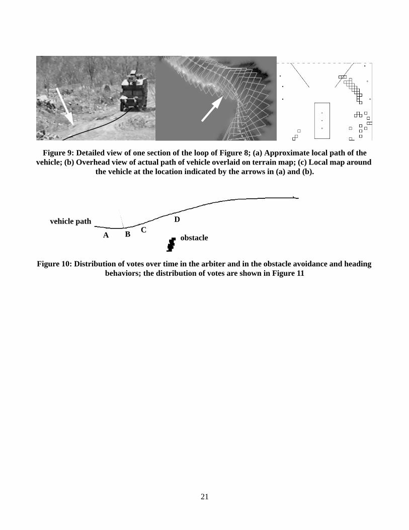
Figure 9 (a) shows a close-up view of one section of the loop of Figure 9. The black lines show theapproximate paths followed by the vehicle in this section. Figure 9 (b) shows the elevation map obtainedby pasting together the images taken along the path. The grey polygons are the projections of the fields ofview on the ground, the curved grey line is the path of the vehicle on the ground, and the grey dotsindicate locations at which images were taken. In this case, the images are separated by approximatelytwo meters.

Finally, Figure 9 (c) shows the local map which is maintained at all time around the vehicle. The squarescorresponds to 40x40 cm patches of terrain classified as untraversable regions or obstacles. These localmaps are computed from the positions shown in Figure 9 (a) and Figure 9 (b) by the white arrows.

In this experiment, the core system is configured with two behaviors: the obstacle avoidance behavior andthe goal seeking behavior. The obstacle avoidance behavior receives a new description of the local mapfrom Ganesha every 100ms. The arbiter combines the votes from the two behaviors and issues a newdriving command every 100ms. The goal points are on average 100 meters apart and the goal seekingbehavior switches goals whenever it comes within eight meters of the current target goal point. Theweights are 0.8 for the obstacle avoidance behavior and 0.2 for the seek goal behavior.

5.2. Arbiter performance

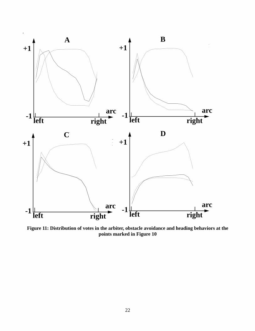
In order to analyze the performance of the arbiter more closely, we recorded additional data on a simplepath around a single obstacle. The result of this experiment is shown in Figure 10 and Figure 11.

The lower part of Figure 10 shows the path of the vehicle, shown as a black line, around a set of obstaclepoints, shown as black dots. In this example, the vehicle was controlled by the steering commands issuedby the arbiter. In this experiment, the arbiter was receiving votes from two behaviors, the obstacleavoidance behavior described above, and a heading behavior which forces the vehicle to follow aconstant heading.

13

Figure 11 shows the distribution of votes at five points of interest along the path, indicated by capitalletters in Figure 10. Each graph depicts the votes issued for each turn choice by the obstacle avoidanceand heading behaviors, as well as the weighted sum of these votes as computed by the arbiter. Thehorizontal axis of each graph shows the possible turn radius choices encoded from -8 m to +8 m.

At point A, the obstacle is first reported and the obstacle avoidance behavior generates high votes for theleft turns to go around the obstacle and inhibits the right turns with negative votes, as shown by the solidline in the graph. At the same time, the heading behavior’s vote distribution is relatively flat around thestraight direction since the vehicle is currently headed in the desired direction; this is shown by thedashed line in the graph. Because of the small relative weight of the heading behavior, the combined votedistribution in the arbiter, shown as a thicker solid line in the graph, is dominated by the votes receivedfrom the obstacle avoidance behavior; a left turn is therefore commanded.

At point B, the obstacle is still close to the vehicle and the votes distributions are similar to the ones atA,thus maintaining the vehicle to the left of the obstacle. At pointC, the obstacle avoidance behavior is stillvoting in favor of a sharp left turn, but the votes for the softer left turns is now not as low as it was atA orB, since the vehicle is now clearing the obstacles. At the same time, the heading behavior is starting toshift its votes towards turning right in order to bring the vehicle back to the target heading. The summedvotes are still at a maximum for a left turn because of the greater weight of the obstacle avoidancebehavior’s votes, and so the arbiter continues to steer the vehicle well clear of the obstacles.

By the time the vehicle has reached pointD, it is just passing the obstacles, so that the obstacle avoidancebehavior is now only disallowing extreme right or left turns because of the field of view constraints. Theheading behavior is now able to have more influence over the chosen turn direction, and a right turn isnow executed so that the desired vehicle heading is restored. Note that between pointsC andD, there is atransition period where the turn radius chosen by the arbiter is neither the hard left favored by theobstacle avoidance behavior nor the medium right favored by the heading behavior. Instead, as turnsother than hard left become acceptable to the obstacle avoidance behavior, and as the distribution of votesfrom the heading behavior shift further to the right, the vehicle is commanded to make ever softer leftturns, and eventually turns to the right.

As can be seen in the graph of the commanded turn radius in Figure 10, the arbiter exhibits the desiredbehavior. Namely, rather than abruptly switching modes from avoiding obstacles to following a heading,the arbiter generates a smooth and steady transition as the situation gradually changes.

5.3. Limitations and failure modes

A fundamental limitation of the system is its inability of dealing with dead-ends such as a closed corridorwith a depth greater than the field of view of the sensor. Because the system deals only with a localrepresentation of the terrain, it is incapable of dealing with this type of situations of a more global nature.In particular, in the experiment of 5.2 it is clear that the vehicle can easily run into a dead-end situation byusing the simple goal-seeking behavior, which is why multiple intermediate goal points are used ratherthan a signle global goal. If fact, this is by far the most common failure mode of the system. Thislimitation can be addressed by adding to the system another behavior which uses knowledge about theglobal representation of the terrain in order to plan appropriate vehicle paths. In this approach, theperception, local map, and obstacle avoidance modules are responsible for local navigation, while the

14

other modules are responsible for global navigation.

As mentioned earlier, the speed of the vehicle is in large part limited by the maximum range of the sensorand by the image acquisition rate which introduces a minimum 500ms latency between the time an objectenters the field of view of the sensor and the time the corresponding image is fully acquired. The effectivesteering radius of the vehicle is limited by the 80o horizontal field of view of the sensor. The detectionrange is limited by the angular resolution of the scanner. These three limitations can be addressed only byusing other sensors. We investigating the use of fast single-scan laser range finders and of passive stereo.

Because the system is implemented as a distributed system communicating through the standard Unixnetwork facilities, there are no guarantees on the delays involved in sending messages between themodules. In practice, these delays are compounded into a significant latency between the time an objectappears in the field of view of the sensor and the time a steering command is actually executed by thecontroller. Although the latency varies, we have observed latency as high as one or two seconds. Thisproblem is being addressed by combining the modules in a way that is more suitable to predictablescheduling, and by porting the system to a real-time operating system.

6 Conclusion

We have presented a navigation system based on early evaluation of terrain traversability. We havedemonstrated this system in a one kilometer traverse of unmapped cross-country terrain. This experimentdemonstrates: the robustness of the approach; its ability to accommodate additional driving behaviors inaddition to the basic obstacle avoidance behaviors, such as driving toward intermediate goal points; andits ability to compensate for constraints imposed by the sensing system, such as the limited field of viewof the sensor. This is achieved by: reducing the amount of computation required by the perceptionsystem; simplifying local map management and path planning; hiding the details of sensing from all themodules except perception; and avoiding the problems caused by merging multiple terrain maps usinginaccurate position estimates.

The drawback of this approach is that an error in the perception system may propagate unchallengedthrough the system because only the perception module has access to the sensor data. This problem isaddressed by using a fast reactive path planner and a simple perception algorithm with fast cycle timerelative to vehicle speed, both of which allow the system to correct quickly for occasional perceptionerrors, and by incorporating a history mechanism in the local map manager which eliminates falsepositive detection.

The main limitations of the system are the limited range and speed of the sensor, the non-real-time natureof the system which is implemented on conventional Unix workstations using standard networkingprotocol, and the poor performance of perception on certain types of environments, such as vegetation.To address the first limitation, we have conducted preliminary experiments with a passive stereo system,and we are planning to experiment with a fast, single-line range sensor. These new sensor modalities willimprove both acquisition rate and maximum range. To address the second limitation, we are planning onporting the critical parts of the system to a real time operating system and to combine parts of the system,such as perception and local map management into a single module with better control over scheduling.We feel that the third class of problems, due to poor reflectivity of surfaces and vegetation, can beaddressed only by adding other specialized sensors.

15

In addition to research on the cross-country navigation system proper, we are continuing the developmentof the DAMN architecture. In particular, we are developing new approaches to speed which involve aseparate speed arbiter and we are investigating ways for the arbiter to interpolate between the referenceset of arcs based on the vote distributions from the behaviors. These two improvements will lead tosmoother control in both speed and steering.

Acknowledgments

The UGV project is supported by ARPA under contracts DACA76-89-C-0014 and DAAE07-90-C-R059,and by the National Science Foundation under NSF Contract BCS-9120655. Julio Rosenblatt issupported by a Hughes Research Fellowship. The authors wish to thank Jay Gowdy, Bill Ross, JimMoody, Jim Frazier, George Mueller, and Mike Blackwell for their help in the cross-country navigationexperiments. Many thanks to Dave Payton for the advice and support he has provided over the years inthe development of the planning system.

References

[1]R. Brooks and A. Flynn. Fast, Cheap, and Out of Control: A Robot Invasion of the Solar System.J.British Interplanetary Society, 42(10):478-485, 1989.

[2]R. Brooks, A., A Robust Layered Control System for a Mobile Robot, IEEE Journal of Robotics andAutomation vol. RA-2, no. 1, pp. 14-23, Apr 1986.

[3]R. Brooks. Intelligence Without Reason. Proc. IJCAI’93. 1993.[4]B. Brummit, R. Coulter, A. Stentz. Dynamic Trajectory Planning for a Cross-Country Navigator. In

Proc. of the SPIE Conference on Mobile Robots, 1992.[5]C. Fedor. TCX, Task Communications User’s Manual. Internal Report, The Robotics Institute, Carn-

egie Mellon, 1993.[6]G. Giralt and L. Boissier. The French Planetary Rover VAP: Concept and Current Developments. In

Proc. IEEE Intl. Workshop on Intelligent Robots and Systems, pp. 1391-1398, Raleigh, 1992.[7]M. Hebert, E. Krotkov. 3D Measurements from Imaging Laser Radars.Image and Vision Computing

10(3), April 1992.[8]Keirsey, D.M., Payton, D.W. and Rosenblatt, J.K., “Autonomous Navigation in Cross-Country Ter-

rain,” in Image Understanding Workshop, Cambridge, MA, April, 1988.[9]D. Langer and C. Thorpe. Sonar based Outdoor Vehicle Navigation and Collision Avoidance. InProc.

IROS ‘92. 1992.[10]C. Lee, Fuzzy Logic in Control Systems: Fuzzy Logic Controller -- Parts I & II, IEEE Transactions on

Systems, Man and Cybernetics, Vol 20 No 2, March/April 1990[11]T. Iwata and I. Nakatani. Overviews of the Japanese Activities on Planetary Rovers. InProc. 43rd

Congress Intl. Astronautical Federation, Washington, D.C., 1992.[12]H. Kamada, S. Naoi, T. Gotoh, A Compact Navigation System Using Image Processing and Fuzzy

Control, IEEE Southeastcon, New Orleans, April 1-4, 1990[13]A. Kelly, T. Stentz, M. Hebert. Terrain Map Building for Fast Navigat ion on Rugged Outdoor Terrain.

In Proc. of the SPIE Conference on Mobile Robots, 1992.[14]I.S. Kweon.Modeling Rugged Terrain by Mobile Robots with Multiple Sensors.Ph.D. thesis, Robotics

Institute, Carnegie Mellon University, January, 1991.[15]L. H. Matthies. Stereo Vision for Planetary Rovers: Stochastic Modeling to Near Real-Time Imple-

16

mentation.International Journal of Computer Vision, 8:1, 1992.[16]E. Mettala. Reconnaissance, Surveillance and Target Acquisition Research for the Unmanned Ground

Vehicle Program. InProc. Image Understanding Workshop, Washington, D.C., 1993.[17]K. Olin, D.Y. Tseng. “Autonomous Cross-Country Navigation”.IEEE Expert, 6(4), August 1991.[18]D.W. Payton, J.K. Rosenblatt, D.M. Keirsey. Plan Guided Reaction.IEEE Transactions on Systems

Man and Cybernetics, 20(6), pp. 1370-1382, 1990.[19]J.K. Rosenblatt and D.W. Payton. A Fine-Grained Alternative to the Subsumption Architecture for

Mobile Robot Control. inProc. of the IEEE/INNS International Joint Conference on Neural Networks,Washington DC, vol. 2, pp. 317-324, June 1989.

[20] C. Thorpe, O. Amidi, J. Gowdy, M. Hebert, D. Pomerleau,.Integrating Position Measurement andImage Understanding for Autonomous Vehicle Navigation. Proc.Workshop on High Precision Naviga-tion, Springer-Verlag Publisher, 1991.

[21]J. Yen, N. Pfluger, A Fuzzy Logic Based Robot Navigation System, AAAI Fall Symposium, 1992.[22]Zadeh, Lotfi A., “Outline of a New Approach to the Analysis of Complex Systems and Decision Pro-

cesses”, IEEE Transactions on Systems, Man and Cybernetics, Vol 3 No 1, January 1973

17

Figure 1: The testbed vehicle

.

Figure 2: Architecture of the perception and navigation system

cameras

laser range finder

Local Map ManagerArc Generation

Perception: Laser Range FinderVehicle Controller

Goal PointsIntermediate

Terrain Evaluation

18

Figure 3: Example of terrain classification

Figure 4: Main loop in Ganesha

y: 3.5 mx: -7.5 m to 7.5 m

z: 0 to 1.0 m B

A

(c) Elevation map from the range image of (a).

A

B

(d) Terrain classification on the map of (c);

to 14.5 m

non-zero values indicate obstacle regions.(b) Range image of the terrain shown in (a).

(a) A section of terrain from the path of Figure 2.

Update cellpositions in map

Place new cellsin map

Update attributesof map cells Wait

Vehicle positionNew objects fromperception +Correspondingvehicle position

Loop delayPlanning module

19

Figure 5: Use of FOV obstacles to limit turning radius

Figure 6: Behavior-based architecture; solid lines indicate the behaviors used in the cross-countrysystem

hidden

active

obstacle

MAINTAINHEADING

AVOIDOBSTACLES

PATHTRACKING

COMMANDARBITRATION

ANNOTATEDMAPS

GOALSEEKING

ROADFOLLOWING

STEERING RADIUS+SPEED

20

Figure 7: Set of possible turning radii in DAMN for the cross-country navigation system

Figure 8: A loop through natural terrain

8.0m

13.0m

25.0m

50.0m

100.0m

200.0m400.0m

∞

8.0m

13.0m

25.0m

50.0m

100.0m200.0m

400.0m

400

met

ers

(b) Exact path of vehicle: the obstacle regionsare shown as black dots; the intermediate goal

points are shown as small circles.

(a) Camera view of terrain with approximatepath superimposed.

21

Figure 9: Detailed view of one section of the loop of Figure 8; (a) Approximate local path of thevehicle; (b) Overhead view of actual path of vehicle overlaid on terrain map; (c) Local map around

the vehicle at the location indicated by the arrows in (a) and (b).

Figure 10: Distribution of votes over time in the arbiter and in the obstacle avoidance and headingbehaviors; the distribution of votes are shown in Figure 11

A B CD

E

vehicle path

obstacle

22

.

Figure 11: Distribution of votes in the arbiter, obstacle avoidance and heading behaviors at thepoints marked in Figure 10

A

arbiter

obstacles

heading

Vote

Radius

-1.00

-0.90

-0.80

-0.70

-0.60

-0.50

-0.40

-0.30

-0.20

-0.10

-0.00

0.10

0.20

0.30

0.40

0.50

0.60

0.70

0.80

0.90

1.00

1.10

-6.00 -4.00 -2.00 0.00 2.00 4.00 6.00

A+1

-1left right

arc

B

arbiter

obstacles

heading

Vote

Radius

-1.00

-0.90

-0.80

-0.70

-0.60

-0.50

-0.40

-0.30

-0.20

-0.10

-0.00

0.10

0.20

0.30

0.40

0.50

0.60

0.70

0.80

0.90

1.00

1.10

-6.00 -4.00 -2.00 0.00 2.00 4.00 6.00

B+1

-1left right

arc

C

arbiter

obstacles

heading

Vote

Radius

-1.00

-0.90

-0.80

-0.70

-0.60

-0.50

-0.40

-0.30

-0.20

-0.10

-0.00

0.10

0.20

0.30

0.40

0.50

0.60

0.70

0.80

0.90

1.00

1.10

-6.00 -4.00 -2.00 0.00 2.00 4.00 6.00

C+1

-1left right

arc

D

arbiter

obstacles

heading

Vote

Radius

-1.00

-0.90

-0.80

-0.70

-0.60

-0.50

-0.40

-0.30

-0.20

-0.10

-0.00

0.10

0.20

0.30

0.40

0.50

0.60

0.70

0.80

0.90

1.00

1.10

-6.00 -4.00 -2.00 0.00 2.00 4.00 6.00

D+1

-1left right

arc