
690222.pdf - RWTH Publications
223
“Non-local Denoising and Unsupervised Quantitative Analysis in Scanning Transmission Electron Microscopy” Von der Fakult¨ at f¨ ur Mathematik, Informatik und Naturwissenschaften der RWTH Aachen University zur Erlangung des akademischen Grades eines Doktors der Naturwissenschaften genehmigte Dissertation vorgelegt von Master of Science Niklas Mevenkamp aus Duisburg Berichter: Professor Dr. Benjamin Berkels Professor Dr. Wolfgang Dahmen Associate Professor Peter G. Binev, Ph.D. Tag der m¨ undlichen Pr ¨ ufung: 11.04.2017 Diese Dissertation ist auf den Internetseiten der Universit ¨ atsbibliothek online verf ¨ ugbar.
-
Upload
khangminh22 -
Category
Documents
-
view
0 -
download
0
Transcript of 690222.pdf - RWTH Publications

“Non-local Denoising and Unsupervised Quantitative Analysisin Scanning Transmission Electron Microscopy”
Von der Fakultat fur Mathematik, Informatik und Naturwissenschaften der RWTHAachen University zur Erlangung des akademischen Grades eines Doktors derNaturwissenschaften genehmigte Dissertation
vorgelegt von
Master of Science
Niklas Mevenkamp
aus Duisburg
Berichter: Professor Dr. Benjamin BerkelsProfessor Dr. Wolfgang DahmenAssociate Professor Peter G. Binev, Ph.D.
Tag der mundlichen Prufung: 11.04.2017
Diese Dissertation ist auf den Internetseiten der Universitatsbibliothek online verfugbar.


iii
Abstract
Modern scanning transmission electron microscopes (STEM) provide atomic reso-lution images of inorganic materials. Atom positions and other information extractedfrom such images are key ingredients in the understanding of the relation betweenmicroscopic material structure and macroscopic material properties. Unfortunately,in certain applications, the ability to obtain this information is severely obstructedby low signal-to-noise ratios of the acquired images. These result from restrictionson the electron dose (exposure time) due to potential beam damage. Aiming at re-solving this deciency, we propose an eective denoising strategy that is specicallytailored to the special structure of atomic-resolution crystal images. It is based on thenon-local denoising principle and uses the block-matching and 3D ltering algorithm(BM3D) by Dabov et al. [39] as a starting point. We employ an adaptive piecewiseperiodic block-matching strategy that exploits the crystal geometry - accounting fortypical irregularities such as dislocations, crystal interfaces and image distortion - andprovides ecient and truly non-local denoising. The required crystal geometry infor-mation is extracted from the noisy raw image in an unsupervised fashion. To this end,we present novel real-space algorithms for accurate unit cell extraction and crystalsegmentation. Furthermore, we analyze the noise behavior of experimental high-angleannular dark-eld (HAADF)-STEM images and show that a simple additive Gaussianwhite noise model is not suitable for low-dose images. Instead, we propose to employa more complex mixed Poisson-Gaussian noise model which results in a much bettert and present an unsupervised algorithm to estimate the required noise parametersfrom a given raw image. Then, the generalized Anscombe transform [93] is used forvariance-stabilization, which enables the use of BM3D for noise removal. Results onboth articial and real experimental single-shot HAADF-STEM images are presentedwhich show that the proposed method signicantly improves the visual quality and,more importantly, the precision of detected atom positions. We also present an exten-sion of the method to series of images including a coupling of non-local denoising withnon-rigid image alignment. An evaluation based on experimental images reveals thatcompared to plain averaging of an aligned image stacks the number of frames requiredto obtain a high SNR reconstruction can be signicantly reduced. Also, we show thatthis way state-of-the-art precisions can be obtained using less than ten frames. Besidesthis, we propose an extension of our denoising method to spectral data and present verypromising results on an electron energy loss spectroscopy dataset. Finally, we presenta multi-modal and multi-scale similarity measure intended for joint denoising of STEMand spectral data. Using a jointly acquired dataset consisting of an HAADF-STEMimage and an energy-dispersive X-ray scan, we demonstrate that extreme gains in SNRare achievable without noticeably sacricing spatial resolution.


Acknowledgements
First and foremost I would like to express my sincerest gratitude to my advisor, Prof.Dr. Benjamin Berkels, for his never-ending support and patience, for sharing his extensiveknowledge on applied mathematics, in particular on image processing, as well as some sub-tleties of C++ programming, and for expertly managing the balance between giving methe freedom to explore my ideas and keeping me in line with our initial goals - in short:for creating an environment that has made the journey towards this dissertation an utterlyexciting and enjoyable one. Thank you.
The data and issues that became the driving force of this thesis are based on Prof. Dr.Paul M. Voyles' and Dr. Andrew B. Yankovich's outstanding research in scanning trans-mission electron microscopy. I am most grateful for their open and inspiring collaboration,for sharing and explaining their images and experiments, and, at the core, for their genuineinterest in mathematical models and techniques.
I am greatly indebted to my co-advisor, Prof. Dr. Wolfgang Dahmen, as well as to Prof.Dr. Peter Binev for initiating this project, for fruitful discussions and invaluable advice.Their distinguished research and their unique ability to grasp the mathematical essence ofchallenges arising in other scientic elds are truly inspiring. I would also like to thank Peterfor inviting me to the BIRS workshop in Ban, Canada, which gave rise to a multitude ofquestions and ideas that have signicantly inuenced my further path.
Thanks are also due to Dr. Martial Duchamp for introducing me to spectral imagingand especially for contributing his knowledge and sharing his work on EELS and EDXspectroscopy, the latter of which was the foundation for developing the multi-scale andmulti-modal similarity measure presented in Chapter 7.
I am also indebted to Prof. Dr. Joachim Mayer for supporting this project and especiallyfor bringing it to my attention while I was still working as a student assistant at the centralfacility for electron microscopy of the RWTH Aachen.
In addition, I thank Dr. Ronny Bergmann for providing insights into the properties ofthe Fourier transform, as well as Mark Kärcher and Eduard Bader for productive discussionson model order reduction and principal component analysis.
Finally, I thank my parents and my partner for their limitless support, for keeping mehealthy, cheerful and optimistic, thereby providing the very fundamentals for my work.
v


Contents
Abstract iii
Acknowledgements v
List of Figures ix
List of Tables xv
List of symbols xvii
Introduction xxi
1 Electron micro- and spectroscopy 1
1.1 Scanning transmission electron microscopy . . . . . . . . . . . . . . . . . . . . 11.2 Hyper-spectral imaging . . . . . . . . . . . . . . . . . . . . . . . . . . . . . . 5
2 Non-local image denoising 9
2.1 Introduction . . . . . . . . . . . . . . . . . . . . . . . . . . . . . . . . . . . . . 92.2 Digital images . . . . . . . . . . . . . . . . . . . . . . . . . . . . . . . . . . . . 92.3 Linear and non-linear local ltering . . . . . . . . . . . . . . . . . . . . . . . . 112.4 Patch-based non-local ltering . . . . . . . . . . . . . . . . . . . . . . . . . . 142.5 Numerical results . . . . . . . . . . . . . . . . . . . . . . . . . . . . . . . . . . 222.6 Non-local regularization for crystal images . . . . . . . . . . . . . . . . . . . . 262.7 Conclusions . . . . . . . . . . . . . . . . . . . . . . . . . . . . . . . . . . . . . 27
3 Periodicity analysis and unit cell extraction 29
3.1 Introduction . . . . . . . . . . . . . . . . . . . . . . . . . . . . . . . . . . . . . 293.2 Crystal images as periodic functions . . . . . . . . . . . . . . . . . . . . . . . 303.3 Reciprocal unit cell estimation . . . . . . . . . . . . . . . . . . . . . . . . . . 323.4 Extracting unit cells in real-space . . . . . . . . . . . . . . . . . . . . . . . . . 423.5 Numerical results . . . . . . . . . . . . . . . . . . . . . . . . . . . . . . . . . . 533.6 Conclusions . . . . . . . . . . . . . . . . . . . . . . . . . . . . . . . . . . . . . 55
4 Feature-based crystal image segmentation 57
4.1 Introduction . . . . . . . . . . . . . . . . . . . . . . . . . . . . . . . . . . . . . 574.2 Variational image segmentation . . . . . . . . . . . . . . . . . . . . . . . . . . 584.3 Region indicators for structural segmentation . . . . . . . . . . . . . . . . . . 754.4 Handling irregular regions . . . . . . . . . . . . . . . . . . . . . . . . . . . . . 874.5 Numerical results . . . . . . . . . . . . . . . . . . . . . . . . . . . . . . . . . . 904.6 Conclusions . . . . . . . . . . . . . . . . . . . . . . . . . . . . . . . . . . . . . 101
vii

viii CONTENTS
5 Noise modeling and parameter estimation 103
5.1 Introduction . . . . . . . . . . . . . . . . . . . . . . . . . . . . . . . . . . . . . 1035.2 Poisson and mixed Poisson-Gaussian noise . . . . . . . . . . . . . . . . . . . . 1045.3 Variance stabilization . . . . . . . . . . . . . . . . . . . . . . . . . . . . . . . 1105.4 Unsupervised noise parameter estimation . . . . . . . . . . . . . . . . . . . . 1155.5 p-Values: generalizing the method noise . . . . . . . . . . . . . . . . . . . . . 1315.6 Conclusions . . . . . . . . . . . . . . . . . . . . . . . . . . . . . . . . . . . . . 142
6 HAADF-STEM image reconstruction 145
6.1 Adaptive piecewise periodic block-matching . . . . . . . . . . . . . . . . . . . 1456.2 Extension to stacks of images . . . . . . . . . . . . . . . . . . . . . . . . . . . 1476.3 Quantitative atom detection . . . . . . . . . . . . . . . . . . . . . . . . . . . . 1526.4 Numerical results . . . . . . . . . . . . . . . . . . . . . . . . . . . . . . . . . . 1566.5 Conclusions . . . . . . . . . . . . . . . . . . . . . . . . . . . . . . . . . . . . . 169
7 Spectral and multi-modal denoising 171
7.1 Non-local denoising of spectral data . . . . . . . . . . . . . . . . . . . . . . . 1717.2 Adaptation to power-law EELS signals . . . . . . . . . . . . . . . . . . . . . . 1727.3 Multi-modal non-local denoising . . . . . . . . . . . . . . . . . . . . . . . . . 1737.4 Numerical results . . . . . . . . . . . . . . . . . . . . . . . . . . . . . . . . . . 1757.5 Conclusions . . . . . . . . . . . . . . . . . . . . . . . . . . . . . . . . . . . . . 189
Conclusions 191
Bibliography 193

List of Figures
1.1 Illustration of the image acquisition process in high-angle annular dark-eld scan-ning transmission electron microscopy . . . . . . . . . . . . . . . . . . . . . . . . 2
1.2 Exemplary HAADF-STEM image: gallium nitride crystal at 29 million timesmagnication; image courtesy of Paul M. Voyles . . . . . . . . . . . . . . . . . . 3
1.3 Gallium arsenide crystal at dierent dwell times; images courtesy of Paul M.Voyles . . . . . . . . . . . . . . . . . . . . . . . . . . . . . . . . . . . . . . . . . 4
1.4 Electron energy loss spectroscopy at micron scale; data courtesy of MartialDuchamp . . . . . . . . . . . . . . . . . . . . . . . . . . . . . . . . . . . . . . . . 5
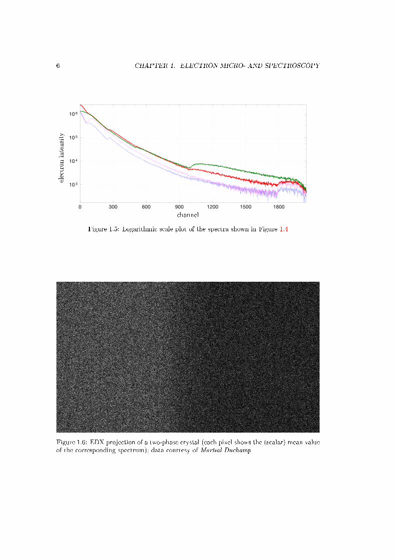
1.5 Logarithmic scale plot of the spectra shown in Figure 1.4 . . . . . . . . . . . . . 61.6 EDX projection of a two-phase crystal (each pixel shows the (scalar) mean value
of the corresponding spectrum); data courtesy of Martial Duchamp . . . . . . . 61.7 Mean EDX spectra of the two materials visible in Figure 1.6 (left: dotted red;
right: solid blue) . . . . . . . . . . . . . . . . . . . . . . . . . . . . . . . . . . . . 71.8 Individual EDX spectra corresponding to Figure 1.6 for a few selected pixels . . 7
2.1 Illustration of the block-matching and 3D ltering procedure. . . . . . . . . . . . 182.2 Comparison of dierent denoising methods for a natural image (Aachen cathe-
dral); from left to right: noise-free image (V = [0, 255]), image aected by AGWN(top: σ = 25, bottom: σ = 40), estimates retrieved by moving averages, bilateralltering, non-local means, BM3D . . . . . . . . . . . . . . . . . . . . . . . . . . 23
2.3 Comparison of the method noise for the image and algorithms in Figure 2.2 . . 242.4 Comparison of dierent denoising methods for a periodic image (bricks); from left
to right: noise-free image (V = [0, 255]), image aected by AGWN (top: σ = 25,center: σ = 40, bottom: σ = 60), estimates retrieved by moving averages,bilateral ltering, non-local means, BM3D . . . . . . . . . . . . . . . . . . . . . 25
2.5 Comparison of the method noise for the image and algorithms in Figure 2.4 . . 25
3.1 Articial crystal lattice images; top row: ideal crystals (from left to right: Bumps3,HexVacancy, SingleDouble, Nc3Nm); bottom row: same images plus Gaus-sian noise with a standard deviation of 50% of the maximum intensity . . . . . . 40
3.2 Fourier transformed crystal images (cf. Figure 3.1); top row: noisefree case; bot-tom row: Gaussian noise case. The Fourier transform is shifted such that F [g]0,0is in the center of the image (cf. (3.48)) and the center peak is removed. . . . . 41
3.3 Unit cells (blue) and crystal lattices (red) of the articial crystals (cf. Figure 3.1)estimated in reciprocal space (cf. Algorithm 56); top row: noisefree case; bottomrow: Gaussian noise case . . . . . . . . . . . . . . . . . . . . . . . . . . . . . . . 41
ix

x List of Figures
3.4 Top row: experimentally acquired HAADF-STEM images (from left to right:GaN, Si, Series1, Series03); bottom row: unit cells (blue) and crystal lat-tices (red) estimated in reciprocal space (cf. Algorithm 56); images courtesy ofP. M. Voyles . . . . . . . . . . . . . . . . . . . . . . . . . . . . . . . . . . . . . . 42
3.5 Left: articial crystal lattice (magenta dots) with a motif of size two (a ma-genta/blue dot pair is a motif copy); right: normalized energy (3.53) for ~v1 =t(cosα, sinα)T , ~v2 = 0 as a function of t with α = −61.95 (green vector) . . . . 44
3.6 Illustration of the set of points Pδ(p) that are projected onto the line `δ(p) . . . 46
3.7 Left: hex lattice with vacancies, vectors Tαi~eαi , i = 1, . . . , 5 (blue, purple, green,red, cyan), unit cell (purple/red box); right: psd for δ ∈ [0, π] . . . . . . . . . . . 47
3.8 Unit cells (blue) and crystal lattices (red) of the articial crystal images (cf.Figure 3.1) estimated in real-space (cf. Algorithm 76 + local renement); toprow: noisefree case; bottom row: Gaussian noise case . . . . . . . . . . . . . . . 54
3.9 Periodicity energies (cf. (3.72)) for α = 45 (diagonal lattice direction) for thenoisefree (blue crossed) and Gaussian noise (red dotted) Bumps3 image in Fig-ure 3.1 . . . . . . . . . . . . . . . . . . . . . . . . . . . . . . . . . . . . . . . . . 55
3.10 Unit cells (blue) and crystal lattices (red) of the experimental HAADF-STEMimages (cf. Figure 3.4) estimated in real-space (cf. Algorithm 76 + local rene-ment) . . . . . . . . . . . . . . . . . . . . . . . . . . . . . . . . . . . . . . . . . . 55
4.1 Segmentations of selected mosaics from the Prague ICPR2014 contest. The rstcolumn shows the original image, the second the ground truth and the remainingcolumns the results by SegTexCol, FSEG [154], VRA-PMCFA and PCA-MS
with TxtMerge post-processing (TM). . . . . . . . . . . . . . . . . . . . . . . . . 92
4.2 Segmentations of the rst three mosaics from the Outex_US_00000 test suite.The rst column shows the original image, the second the ground truth and theremaining columns the results by FSEG [154], clustering, FSEG∗, FSEG∗-TMand Algorithm 147. . . . . . . . . . . . . . . . . . . . . . . . . . . . . . . . . . . 93
4.3 Segmentation of synthetic multi-grain crystals without (left) and with (right)noise, computed by the proposed method using local power spectrum based fea-tures (cf. Denition 132) and visualized as boundary curves (red). . . . . . . . . 95
4.4 Segmentation of multi-phase crystals, computed by the proposed method usinglocal power spectrum based features (cf. Denition 132) and visualized as bound-ary curves (red); images courtesy of Paul M. Voyles (top & middle) and DaesungPark (bottom). . . . . . . . . . . . . . . . . . . . . . . . . . . . . . . . . . . . . 96
4.5 Two-stage segmentation of a two-phase crystal image into two dierent phasesand an irregular boundary region in-between; from left to right: input image,bottom region indicator, top region indicator, minimum indicator function (cf.(4.152)), resulting segmentation visualized as boundary curves (red) . . . . . . . 97
4.6 Left: projection of a multi-spectral dataset consisting of 5 ROI and an irregularregion (the background); right: 3 ROI partially segmented by hand; data courtesyof Rohit Bhargava (University of Illinois Urbana Champaign) . . . . . . . . . . . 97
4.7 ROI membership after plain clustering (left) and subspace clustering (right) ofall spectra of the manually segmented ROI . . . . . . . . . . . . . . . . . . . . . 98
4.8 Indicator functions of the rst 3 ROI and the corresponding labeling function,including an irregular region (black), overlayed with manual segmentation bound-aries (blue) . . . . . . . . . . . . . . . . . . . . . . . . . . . . . . . . . . . . . . . 98

List of Figures xi
4.9 From left to right: 1) minimum indicator function (cf. (4.152)) based on 4 (top)and 5 (bottom) ROI; 2) estimate subset of ROI #4 (top) and #5 (bottom)(cf. (4.154)); region indicator based on 4-th (top) and 5-th (bottom) subspace;labeling function for 4 (top) and 5 (bottom) ROI and an irregular region (black),overlayed with manual segmentation boundaries (blue) . . . . . . . . . . . . . . 99
4.10 Labeling functions of the 5 ROI and an unknown region (black) after alternatingiterative renements of subspaces and segmentation (cf. Algorithm 147), over-layed with manual segmentation boundaries (blue) . . . . . . . . . . . . . . . . . 99
4.11 From top to bottom: 5 dierent ROI; from left to right for each ROI: threeselected (mean subtracted) spectra, mean spectrum, eigenvectors of the subspace;the x-axis represents the channels of the spectra in each graph . . . . . . . . . . 100
5.1 Numerically estimated variance of Anscombe transformed Poisson distributedrandom variables (red solid) and asymptotic limit (blue dashed) . . . . . . . . . 111
5.2 Inverse Ansombe transformation . . . . . . . . . . . . . . . . . . . . . . . . . . . 1135.3 Bias of the dierent inverse Anscombe transformations . . . . . . . . . . . . . . 1135.4 Numerically estimated mean value of Anscombe transformed Poisson random
variables versus the asymptotical approximation in (5.43) . . . . . . . . . . . . . 1145.5 Sample mean-variance pairs (cyan cross marks) of the level sets extracted from
the noisy Aachen cathedral image (cf. Figure 2.2) corrupted by AGWN withσ = 25 (left) and σ = 40 (right), estimated noise standard deviation (greendash-dotted line) and ground truth (blue dashed line); parameters used: alvl =10, nlvl = 100, slvl = 64 and np = (11, 11) . . . . . . . . . . . . . . . . . . . . . . 123
5.6 Aachen cathedral image scaled to range [50, 200] and aected by mixed Poisson-Gaussian noise with the following parameters (from left to right): (α, σ, µ) =(1.5, 25, 100), (0.1, 1,−250), (10, 500, 1000) . . . . . . . . . . . . . . . . . . . . . 124
5.7 Sample mean-variance pairs of the level sets extracted from the noisy Aachencathedral image (α = 1.5, σ = 25, µ = 100) in Figure 5.6 and linear variancefunctions; parameters used: alvl = 10, nlvl = 100, slvl = 64, np = (17, 17) . . . . 124
5.8 Articial HAADF-STEM image (λ ∈ (0, 6]) including scan line distortions with-out shot noise (left) and with mixed Poisson-Gaussian noise (right) of parametersα = 100, σ = 10, µ = 1000; images courtesy of Paul M. Voyles . . . . . . . . . . 126
5.9 Sample mean-variance pairs of the level sets extracted from the noisy simulatedHAADF-STEM image in Figure 5.8 and linear variance functions; parametersused: alvl = 1, nlvl = 1000, slvl = 64 and np = (17, 17) (left), np = (51, 1) (right) 126
5.10 Experimental HAADF-STEM images (left: CMS-GaAs, right: gallium nitride);images courtesy of Paul M. Voyles . . . . . . . . . . . . . . . . . . . . . . . . . . 127
5.11 Sample mean-variance pairs of the level sets extracted from the noisy experimen-tal HAADF-STEM images in Figure 5.10 and linear variance functions; param-eters used: alvl = 1, nlvl = 1000, slvl = 64, np = (51, 1) . . . . . . . . . . . . . . 127
5.12 Level sets (red dots mark the center points of the patches) extracted from thenoisy Aachen cathedral image in Figure 5.6 for two selected reference coordi-nates . . . . . . . . . . . . . . . . . . . . . . . . . . . . . . . . . . . . . . . . . . 128
5.13 Level set (red dots mark the center points of the patches) extracted from thegallium nitride image in Figure 5.10 for a selected reference coordinate (left) andthe corresponding stack of patches (right) . . . . . . . . . . . . . . . . . . . . . . 128
5.14 Sample mean-variance pairs of the level sets extracted from the HAADF-STEMimage in Figure 5.8 and linear variance functions; parameters used: α = 200, σ =50, µ = 1000, alvl = 1, nlvl = 1000, slvl = 64, np = (51, 1) . . . . . . . . . . . . . . 129

xii List of Figures
5.15 Estimated mean value deviations for the level sets in Figure 5.14 based on therespective ground truth values . . . . . . . . . . . . . . . . . . . . . . . . . . . . 132
5.16 Sample mean-variance pairs (cyan cross marks) as in Figure 5.14 (same parame-ters used) and corrected sample mean-variance pairs (golden cross marks) usingthe α∆i from Figure 5.15; tted linear variance functions are based on the cor-rected sample mean-variance pairs. . . . . . . . . . . . . . . . . . . . . . . . . . 132
5.17 Inverse images (cf. Denition 201) for dierent lters and the noisy Aachencathedral image in Figure 2.2 aected by AGWN with σ = 25 (top), σ = 40(bottom) . . . . . . . . . . . . . . . . . . . . . . . . . . . . . . . . . . . . . . . . 140
5.18 Left: Poisson noise instance of the Aachen cathedral image from Figure 2.2(rescaled to [10, 50]); center: Anscombe transformed image; right: inverse imagebased on the ground truth . . . . . . . . . . . . . . . . . . . . . . . . . . . . . . 140
5.19 Estimates, method noise and inverse images for dierent lters and the Poissonnoise instance of the Aachen cathedral from Figure 5.18 . . . . . . . . . . . . . 141
5.20 Inverse histograms (cf. Denition 204) for the Poisson noise instance of theAachen cathedral from Figure 5.18 based on the ground truth (top left) andthe moving averages (top right), Bilateral lter (bottom left) and BM3D (bottomright) estimates . . . . . . . . . . . . . . . . . . . . . . . . . . . . . . . . . . . . 142
5.21 From left to right: Pinwheel galaxy NGC 4414 (rescaled to [2, 10]), Poissonnoise instance, Anscombe transformed image, inverse image based on the groundtruth . . . . . . . . . . . . . . . . . . . . . . . . . . . . . . . . . . . . . . . . . . 142
5.22 Estimates, method noise and inverse images for dierent lters and the Poissonnoise instance of the Pinwheel galaxy from Figure 5.21 . . . . . . . . . . . . . 143
5.23 Left: mixed Poisson-Gaussian noise instance of the Aachen cathedral imagefrom Figure 5.6 (α = 1.5, µ = 100, σ = 25); center: generalized Anscombetransformed image; right: inverse image based on the ground truth . . . . . . . 143
5.24 Estimates, method noise and inverse images for dierent lters and the MPGnoise instance of the Aachen cathedral from Figure 5.23 . . . . . . . . . . . . . 144
6.1 Articial crystal images (silicon and gallium nitride) with perfect lattice, simu-lated scan line distortions and dierent simulated electron doses (increasing fromtop to bottom for each crystal); from left to right: ground truth, ground truthcorrupted with MPG noise, BM3D estimate, π-BM3D estimate . . . . . . . . . . 158
6.2 Articial silicon crystal image with a dislocation, simulated scan line distortionsand dierent simulated electron doses (increasing from top to bottom); from leftto right: ground truth, ground truth corrupted with MPG noise, BM3D estimate,π-BM3D estimate . . . . . . . . . . . . . . . . . . . . . . . . . . . . . . . . . . . 159
6.3 Top: experimental HAADF-STEM images of a gallium arsenide crystal acquiredusing dierent dwell times (increasing from left to right); center: BM3D esti-mates; bottom: π-BM3D estimates . . . . . . . . . . . . . . . . . . . . . . . . . 161
6.4 Visual comparison of the denoising performance of π-BM3D when using dierentnoise models based on the experimental gallium arsenide HAAF-STEM imagewith a dwell time of t = 5µs from Figure 6.3 . . . . . . . . . . . . . . . . . . . . 162
6.5 Articial two-phase crystal image (top region: gallium arsenide, bottom region:cobalt-manganese-silicon (CMS) system) with simulated scan line distortions anddierent simulated electron doses (increasing from top to bottom); red rectangleindicates the window used for atom position related quantication . . . . . . . . 163
6.6 Denoising of experimental HAADF-STEM images of a real instance of the two-phase crystal from Figure 6.5 acquired using dierent dwell times . . . . . . . . 164

List of Figures xiii
6.7 Denoising of experimental HAADF-STEM images of multi-phase crystals; redrectangles indicate the windows used for atom position related quantication . . 165
6.8 First ve images of two experimentally and sequentially acquired series of HAADF-STEM images . . . . . . . . . . . . . . . . . . . . . . . . . . . . . . . . . . . . . 166
6.9 Average registered images of the gallium nitride image series from Figure 6.8using non-rigid alignment (from left to right: using the rst 1, 2, 4 images) . . . 167
6.10 Average precision (mean over 10 similar series using an increasing oset for therst image) of the gallium nitride image series from Figure 6.8 after averaging thenon-rigidly aligned images (NR), as well as the π-NR-BM3D estimates (BM3D) 167
6.11 Average registered images of the silicon image series from Figure 6.8 using non-rigid alignment (from left to right: using the rst 1, 2, 4, 8 images) . . . . . . . 168
6.12 Average (mis-)detection fraction (mean over 10 similar series using an increasingoset for the rst image) of the silicon image series from Figure 6.8 after averagingthe non-rigidly aligned images (NR), as well as the π-NR-BM3D estimates; atomcenters are initialized using Algorithm 221 . . . . . . . . . . . . . . . . . . . . . 168
6.13 Average precision (mean over 10 similar series using an increasing oset for therst image) of the silicon image series from Figure 6.8 after averaging the non-rigidly aligned images (NR), as well as the π-NR-BM3D estimates (BM3D);dashed lines indicate that the atom centers were initialized manually, otherwiseAlgorithm 221 was used . . . . . . . . . . . . . . . . . . . . . . . . . . . . . . . . 169
7.1 HAADF-STEM image acquired simultaneously with the EDX scan shown inFigure 1.6 . . . . . . . . . . . . . . . . . . . . . . . . . . . . . . . . . . . . . . . 174
7.2 Mean values of all spectra (projection) of the EELS dataset corresponding toFigures 1.4 and 1.5 . . . . . . . . . . . . . . . . . . . . . . . . . . . . . . . . . . 176
7.3 Comparison between selected channels of the noisy and denoised EELS datasetfrom Figure 7.2 . . . . . . . . . . . . . . . . . . . . . . . . . . . . . . . . . . . . 176
7.4 Sample mean-variance pairs of the level sets extracted from the EELS datasetin Figure 7.2 and estimated linear variance functions; the left plot uses only thelatter half of the channels while the right plot uses all channels . . . . . . . . . . 176
7.5 Comparison between selected spectra of the noisy (dash-dotted line) and denoised(solid line) EELS dataset from Figure 7.2 . . . . . . . . . . . . . . . . . . . . . . 177
7.6 Comparison between channel j = 1700 of an articial dataset (top) and its BM3Destimates using the standard L2-distance (center) and the power-law normalizedsimilarity measure (bottom) . . . . . . . . . . . . . . . . . . . . . . . . . . . . . 178
7.7 Comparison of projected intensities as a function of the vertical spatial coordinate(x1 = 25 is xed) between the ground truth and the BM3D estimates obtainedwith the standard L2-distance and the power-law normalized similarity measure 179
7.8 Comparison between selected recovered spectra (blue: without bump; red: withbump) of the articial dataset in Figure 7.6 using the BM3D lter with the stan-dard L2-distance (solid line) and the power-law normalized similarity measure(dashed line); . . . . . . . . . . . . . . . . . . . . . . . . . . . . . . . . . . . . . 179
7.9 Comparison between channel j = 1700 of an articial dataset (top) and its NLMestimates using the standard L2-distance (center) and the power-law normalizedsimilarity measure (bottom) . . . . . . . . . . . . . . . . . . . . . . . . . . . . . 180
7.10 Comparison between selected recovered spectra (blue: without bump; red: withbump) of the articial dataset in Figure 7.9 using the NLM lter with the stan-dard L2-distance (solid line) and the power-law normalized similarity measure(dashed line); . . . . . . . . . . . . . . . . . . . . . . . . . . . . . . . . . . . . . 181

xiv List of Figures
7.11 EELS projection (left) and complementary HAADF-STEM image (right) of the2nd Vaso dataset . . . . . . . . . . . . . . . . . . . . . . . . . . . . . . . . . . 181
7.12 Comparison between selected channels of the noisy and denoised EELS datasetfrom Figure 7.11 . . . . . . . . . . . . . . . . . . . . . . . . . . . . . . . . . . . . 181
7.13 Comparison between selected spectra of the noisy (dash-dotted line) and denoised(solid line) EELS dataset from Figure 7.11 . . . . . . . . . . . . . . . . . . . . . 182
7.14 Projection of an experimentally acquired EDX map (top left) and its multi-modalnon-local means estimate (top right); experimentally acquired HAADF-STEMimage (bottom left) and its multi-modal BM3D estimate (bottom right) . . . . . 183
7.15 Comparison between individual recovered spectra (gold and cyan dotted) andthe mean spectra over the entire respective material (red and blue solid) for theEDX map shown in Figure 7.14 . . . . . . . . . . . . . . . . . . . . . . . . . . . 184
7.16 Individual channels (j = 40, 100, 138, 318) corresponding to peaks in Figure 7.15;left: noisy; right: multi-modal non-local means reconstruction . . . . . . . . . . 185
7.17 Individual channels (j = 338, 795, 914, 1019) corresponding to peaks in Fig-ure 7.15; left: noisy; right: multi-modal non-local means reconstruction . . . . . 186
7.18 From top to bottom: projection of an articial EDX map and a complementaryHAADF-STEM image; from left to right: ground truth, ground truth aectedby Poisson (EDX) and mixed Poisson-Gaussian (HAADF-STEM) noise, multi-modal non-local reconstruction . . . . . . . . . . . . . . . . . . . . . . . . . . . . 187
7.19 Similarity measures evaluated for a selected reference pixel (red) for the datasetin Figure 7.18; from left to right: HAADF-STEM based L2-similarity measure(cf. Denition 15), resampled EDX based similarity measure (cf. Denition 234),multi-scale and multi-modal similarity measure (cf. Denition 235) . . . . . . . 188
7.20 Individual channels (j = 100, 138) corresponding to two dierent peaks of themean spectra; left: ground truth; right: multi-modal non-local means reconstruc-tion . . . . . . . . . . . . . . . . . . . . . . . . . . . . . . . . . . . . . . . . . . . 188
7.21 Comparison between individual recovered spectra (gold and cyan dotted) andthe ground truth spectra (red and blue solid) for two dierent atomic columnsin the EDX map shown in Figure 7.18 . . . . . . . . . . . . . . . . . . . . . . . . 189

List of Tables
2.1 PSNR before and after denoising the Aachen cathedral image (cf. Figure 2.2)aected by AGWN with dierent lters . . . . . . . . . . . . . . . . . . . . . . . 24
2.2 PSNR before and after denoising the bricks image (cf. Figure 2.4) aected byAGWN with dierent lters . . . . . . . . . . . . . . . . . . . . . . . . . . . . . 26
3.1 Dierence between the unit cells detected in reciprocal space (cf. Algorithm 56)(third column) or real-space (cf. Algorithm 76 + local renement) (fourth col-umn) and the closest unit cell of the true lattice for the crystals shown in Fig-ure 3.1 . . . . . . . . . . . . . . . . . . . . . . . . . . . . . . . . . . . . . . . . . 56
4.1 Color texture segmentation on the Prague ICPR2014 contest dataset with un-known number of segments (cf. http://mosaic.utia.cas.cz). Bold facehighlights the best, a star the second-best value in each column, and indicatesthat no corresponding publication could be found at the time of writing. . . . . 91
4.2 Gray-scale texture segmentation comparison on the Outex_US_00000 test suitewith known number of segments. Bold face highlights the best, a star the second-best result in each column. . . . . . . . . . . . . . . . . . . . . . . . . . . . . . . 94
5.1 Relative errors in the estimated variance parameters a, b for the estimation methodproposed by [53] and our method for the Aachen cathedral image aected bymixed Poisson-Gaussian noise of dierent parameters . . . . . . . . . . . . . . . 125
5.2 Comparison of the PSNRs after denoising the MPG instance of the Aachencathedral image (cf. Figure 5.23) with dierent lters; results use dierent noiseparameters: ground truth (top row) and estimated (bottom row) . . . . . . . . . 125
5.3 Results of the µ and σ parameter estimation based on the method of moments(cf. (5.80) and Remark 192). ∗ uses nlvl = 500, alvl = 4. . . . . . . . . . . . . . . 129
6.1 Quantitative analysis of the articial HAADF-STEM images shown in Figures 6.1and 6.2 with a comparison between vanilla and π-BM3D; atom centers are ini-tialized using Algorithm 220 . . . . . . . . . . . . . . . . . . . . . . . . . . . . . 160
6.2 Quantitative analysis of the experimental gallium arsenide crystal images shownin Figure 6.3; atom centers are initialized using Algorithm 221 . . . . . . . . . . 161
6.3 Quantitative analysis of the articial two-phase crystal images shown in Fig-ure 6.5; ρ+, ρ−, Fidelity & Precision refer to a window within the bottom phase(indicated by the red rectangle in the top left image of Figure 6.5) . . . . . . . . 164
6.4 Quantitative analysis of the experimental three-phase crystal images shown inFigure 6.7; for SrRuO3-BaTiO3-SrTiO3, ρ+, ρ− & Precision refer to a windowwithin the bottom phase; for CMS and GaAs they refer to a window within therespective phase in the CMS-GaAs; windows are indicated in red in Figure 6.7 . 166
xv


List of symbols
A Anscombe transformation
BM3D Block-matching and 3D ltering algorithm
BU Bravais lattice spanned by the basis U
C∗i (S; f) ith cluster of S after clustering the function values f(S)
Ck(S; f) Tuple of clusters of S after clustering the function values f(S)
C(α, λ, µ, σ) Mixed Poisson-Gaussian distribution with scaling factor α, Poisson mean λ,Gaussian mean µ and standard deviation σ
δ Dirac delta distribution
distL2(x,y) (Normalized) Euclidean distance between the vectors x,y
~eα Vector of unit length and angle α with the x-axis
E [X|H] Expectation of the random variable X under the assumption H
FT (g) Feature extractor acting on the image g with the feature map T
FMPGα,λ,µ,σ Mixed Poisson-Gaussian cumulative distribution function with parameters
α, λ, µ, σ
fMPGα,λ,µ,σ Mixed Poisson-Gaussian probability distribution function with parameters
α, λ, µ, σ
Fw Discrete non-linear lter with weights w
FGµ,σ Gaussian cumulative distribution function with parameters µ, σ
fGµ,σ Gaussian probability distribution function with parameters µ, σ
F Continuous Fourier transformation
F Discrete Fourier transformation
F|·| Modulus of the discrete Fourier transformation
FPλ Poisson cumulative distribution function with parameter λ
fPλ Poisson probability distribution function with parameter λ
G Generalized Anscombe transformation
xvii

xviii List of symbols
Γ0(X) Space of proper convex functionals over the vector space X
g Continuous image
g Discrete image
g Denoised version of an image
I Discrete pixel index set
LH Discrete linear lter with kernel matrix H
M Total number of pixels within the respective image
MNF (z) Method noise of the lter F w.r.t. the (noisy) image z
NLM Non-local means lter
N (µ, σ) Normal distribution with mean µ and standard deviation σ
|u|BV(Ω) Continuous total variation semi-norm
|u|BV(X)
Discrete total variation semi-norm
np Total number of pixels in a patch (mostly used for non-local means)
Bin Discrete n1 × n2 neighborhood with top-left corner at pixel i
N in Discrete n1 × n2 centralized neighborhood around the pixel i
(n1, n2 must be odd)
Ω Continuous image domain
Partk(S) Set of all partitions of the set S into k subsets
P(λ) Poisson distribution with mean λ
P(S) Power set of the set S
Pr (A|H) Probability of the event A under the assumption H
PS(x) Projection of the point x onto the set S
proxJ Proximal mapping of the functional J
psd Projective standard deviation
psdpeak Set of angles with peak projective standard deviations
PSNR (g; g) Peak signal-to-noise ratio of the estimate image g (w.r.t. its ground truth g)
Tα Fundamental period of the crystal image in the direction ~eα
Tα Set of all periods of the crystal image in the direction ~eα
ΘH Heaviside function
U Unit cell of a crystal (basis of the Bravais lattice)
Var [X|H] Variance of the random variable X under the assumption H

List of symbols xix
V∠C Set of estimated lattice vector angle candidates of the crystal C
V∠C Set of lattice vector angles of the crystal C
~v Lattice vector
XT Dirac comb with period T > 0
XU Bravais lattice of Dirac distributions spanned by the basis U ∈ Rd
ΥHT Hard-thresholding operator
z Noisy version of an image

Introduction
This thesis focuses on mathematical image processing techniques for specic electronmicroscopy applications. The wavelength of electrons is signicantly shorter than that ofvisible light. Therefore, electron microscopes allow for much larger magnications than lightmicroscopes. Accordingly, since their invention in 1931 by Max Knoll and Ernst Ruska [80],electron microscopes have opened new possibilities in the investigation of material structures.Owing to advances in resolution over the past few decades, it has been found that slightdeviations in the arrangement of atoms, especially near the interfaces between crystals, mayhave a signicant impact on material properties at the macroscopic scale (e.g. thermal andelectric conductivity) [143, 159]. Accordingly, an important aspect of materials science isto quantify atom positions and other related measures (e.g. intensity) from given electronmicrographs. Increasing the precision with which these measures can be estimated improvesthe ability to understand the relation between irregularities in the microscopic materialstructure and macroscopic material properties [67, 70]. Great advances have been madein this regard already. For instance, Schmid et al. [128] reported a precision of around15 pm for a single-shot image. Yankovich et al. [153] were the rst to report sub-picometerprecision for a series of images using a non-rigid alignment technique. While these workshave proven to be very useful in practice, in many applications a major problem remains:beam damage. The electrons used by the microscope to produce an image interact with theobserved material and may thereby cause the material itself to change during the acquisitionprocess. This eect is highly undesirable since it prohibits the observation of the material inits original state. Unfortunately, decreasing the exposure to dampen the beam damage alsodecreases the signal-to-noise ratio (SNR) of the acquired image. The extent of this eectmay vary depending on the beam sensitivity of the material. Organic samples are especiallyvulnerable [13], but even for certain inorganic materials beam damage becomes noticeablewhen acquiring high SNR images [46,65].
The aim of this thesis is to investigate whether denoising algorithms may serve as a toolto enhance the ability to perform high precision atom detection in the presence of severenoise, which would expand such analyses to more beam sensitive materials. Inherently, animportant property for a suitable denoising algorithm in this context is the preservationof ne details. It has been found that simple methods, such as moving averages [66] orGaussian ltering do not perform very well in this regard. Therefore, we will investigate theperformance of a more powerful class of methods, namely the non-local denoising methods[26]. Their most distinctive feature is that they search for similar objects in images whichthey average in order to obtain higher SNR approximations of the corresponding image parts.This works better the more identical, or at least similar, objects appear within a given image.Given sucient self-similarity within the image, non-local denoising approaches have provento be capable of substantially increasing the SNR while maintaining a sharp representationof ne image details. The materials of interest in our applications typically consist of justa few elements and thus the corresponding electron microscopy images at atomic scale
xxi

xxii Introduction
contain many identical atoms that appear numerous times within the entire image. Thisis an ideal situation for non-local averaging. Still, there are some open challenges. First ofall, most available methods are designed to remove purely Gaussian noise, which neglectssignal dependence of the noise variance - an important aspect in a low electron dose setting.Furthermore, classical non-local denoising approaches limit the search for similar objectsto local neighborhoods in order to maintain a feasible computational complexity. However,crystal images typically require the search of comparably large parts of the image in order tovisit a suitable number of instances of the unit cell, i.e. the smallest structure of the crystalthat contains all of its constituents. Thus, another challenge lies in the adaptation of thesimilarity search to the special structure that is typically encountered in crystal images.
As mentioned before, the main focus of this thesis is the adaptation of non-local denoisingmethods to the special properties of electron microscopy images of crystals, such as crystalsymmetry and interfaces between dierent crystals. Since these geometric properties haveto be acquired before they can be exploited, we devote a signicant part of this work to thedevelopment of unsupervised and highly accurate methods for their analysis. In particular,we treat the segmentation of crystal images into the dierent materials, as well as theestimation of unit cell dimensions.
This thesis is arranged as follows. In Chapter 1, we describe the image modalities and ef-fects inherent to electron microscopy and briey comment on the possibilities and challengesposed by the recent advances in high-resolution electron spectroscopy. In Chapter 2, we in-troduce the concepts of local ltering and non-local denoising. In Chapter 3, we proposea novel unsupervised and accurate method for unit cell extraction from crystal images. InChapter 4, we introduce the concept of variational image segmentation and propose a novelmethod for unsupervised crystal segmentation, including an extension to spectral images.In Chapter 5, we recall complex noise models suitable for low-light imaging and propose anovel unsupervised method for noise model parameter estimation. In Chapter 6, we formal-ize the adaptation of the non-local similarity search to crystal images and investigate theperformance of the resulting method in the context of both single-shot images and seriesof images. In Chapter 7, we discuss the application of the non-local denoising frameworkto spectral datasets and show that the combination of the information in jointly acquiredelectron micrographs and spectral data leads to astonishing results.
We would like to point out that the image noise analysis framework presented in Chap-ter 5 is very generic and might therefore be of interest in other low-light imaging applicationsas well. In view of this, the chapter was written in a way that allows it to be understoodmostly independent of the rest of the thesis. In particular, it has its own introduction andconclusions. The same goes for Chapters 3 and 4 which focus on crystal geometry analysis.
Most of the methods that were developed during the work on this thesis have alreadybeen published. In the following, they are listed in chronological order. The integrationof the adaptive periodic similarity search into non-local means was presented at the 19thInternational Symposium on Vision, Modeling and Visualization in 2014 and publishedin [103]. Its integration into BM3D (as well as Poisson noise related adaptations that are nottreated in this thesis) were published in [102] following a workshop at the Ban InternationalResearch Station in 2015. Furthermore, the unit cell extraction algorithm was presented atthe 37th German Conference on Pattern Recognition in 2015 and published in [99]. Theunsupervised crystal segmentation framework was presented at the IEEE Winter Conferenceon Applications of Computer Vision in 2016 and published in [101]. Additionally, summariesof the methods and results on both experimentally acquired electron microscopy images andspectral datasets were published in [16,100].

Chapter 1
Electron micro- and spectroscopy
In this chapter, we describe the image formation process in scanning transmission electronmicroscopy (STEM), as well as relevant issues resulting from the technique, such as scan linedistortion and the relation between beam damage and signal-to-noise ratio. Furthermore,we give examples for quantities of interest to material scientists that might be extractedfrom such micrographs. The fact that intensity noise has become a limiting factor for theaccuracy with which such quantities can be estimated in practice will serve as a motivationfor the denoising method that will be constructed throughout the remainder of this thesis.
Furthermore, we will briey comment on challenges and opportunities in spectral andmulti-modal imaging.
1.1 Scanning transmission electron microscopy
The main idea behind STEM is to measure the interaction of electrons with solid matter.More precisely, a focused electron beam is shot (typically orthogonally) at the surface ofa very thin specimen (typically just a few atoms thick). Specimens observed with thistechnique are typically solid crystals which are aligned such that the electron beam is parallelto one of the symmetry axes.
The following description of the image acquisition process focuses on high-angle annu-lar dark-eld scanning electron microscopy (HAADF-STEM). The following description isillustrated in Figure 1.1. There, an annulus detector beneath the specimen counts electronsarriving within a certain interval of scattering angles. These angles depend on the inter-action of the beam electrons with the Coulomb eld generated by the atoms within thecrystal, i.e. depending on the distance to and the type of nearby atoms, the beam electronsscatter at smaller or larger angles before eventually leaving the material at the opposite sidetowards the detector. Electrons arriving during a certain exposure time are quantized andtransformed into a digital intensity. The word scanning in scanning transmission electronmicroscopy refers to the sequential process used to acquire the entire image. Given a certainstep length and direction, imagine a regular grid projected onto the specimen's surface ata particular region of interest. Each pixel in the resulting digital image then correspondsto the measurement of electrons arriving at the annulus detector when the beam is keptstationary at the center point of the corresponding cell within the regular grid. In-betweenmeasurements, the beam is moved from one cell to the next within each row and uponarriving at the end of the row it is moved all the way back to the rst cell of the next row,until the entire grid has been scanned.
1

2 CHAPTER 1. ELECTRON MICRO- AND SPECTROSCOPY
Incident Electron Beam(Rastering Probe)
Nanoprobe(0.1-1.0 nm)
Specimen(thickness: 10-50 nm)
High-Angle AnnularDark-Field Detector
Contrast ~ Z2
Raster(e.g. 256x256 px)
Digital STEMimage
quantization
Figure 1.1: Illustration of the image acquisition process in high-angle annular dark-eldscanning transmission electron microscopy
In order to get a better idea of how such an electron micrograph might look like, pleaserefer to Figure 1.2. It shows a gallium nitride crystal at 29 million times magnication. Atthis magnication, we can clearly see the individual atomic columns (the white blobs).
A particularly interesting property of the HAADF modality is the relation between theimage intensity at a given pixel and the mean atomic number of the column of atoms atthat position. Whereas this relation is typically approximated by the power law I ∼ Z2,where Z is the mean atomic number [117], it was recently shown that the exponent may varydepending on the collection angle and typical values are rather between 1.2 and 1.8 [145].
Looking at the image in Figure 1.2 it also becomes very apparent that the sequentialacquisition technique leads to substantial distortions. Ideally, each atomic column shouldbe represented by a smooth function (approximately Gaussian in shape) within the image.However, we can see distinct shifts of the scan lines that vary irregularly across the dierentrows. This eect is caused by environmental disturbances during the acquisition process thatlead to a visible movement of the specimen due to the large magnication. Since all pixels areacquired sequentially, a movement of the object in-between measurements manifests itself asdistortions in the image. There are dierent sources for these distortions (e.g. acoustic andelectro-magnetic) that result in random vibrations at certain high frequencies, as well as low

1.1. SCANNING TRANSMISSION ELECTRON MICROSCOPY 3
Figure 1.2: Exemplary HAADF-STEM image: gallium nitride crystal at 29 million timesmagnication; image courtesy of Paul M. Voyles

4 CHAPTER 1. ELECTRON MICRO- AND SPECTROSCOPY
161 µs 81 µs 40 µs 20 µs
10 µs 5 µs 3 µs 1 µs
Figure 1.3: Gallium arsenide crystal at dierent dwell times; images courtesy of Paul M.Voyles
frequency movements (e.g. due to thermal gradients) that result in approximately linearlyvarying shifts, also called sample drift. For a thorough discussion of these distortions, aswell as a method for correcting them approximately, see [72].
Finally, let us point out the property of electron microscopy that is most relevant forthis thesis, namely the relation between exposure time (also called dwell time) and beamdamage. In general, the interaction of the electron beam with the specimen may causethe specimen's material to change physically. In order to retrieve images of a specimen inits original state, it is very important to avoid such a transformation. How much energy(i.e. exposure time) can be applied before this eect becomes non-negligible depends on thebeam sensitivity of the material. For organic materials this is typically very low. Sincethe exposure time dictates the signal-to-noise ratio (SNR), this leads to an extremely lowupper bound for the achievable SNR. Let us point out that decreasing the exposure timealso has one positive eect, namely decreasing the magnitude of the aforementioned scanline distortions.
In this thesis, we mostly regard metals, which have a signicantly lower beam sensitivitythan organic material. However, even in this context there exist relevant applications wherethe SNR is the limiting factor for the accuracy of the desired analyses [15, 110]. As anillustration, Figure 1.3 shows experimental HAADF-STEM images of a gallium arsenidecrystal over a range of dwell times. As we can see, towards the lower end (t ≤ 5 µs), itbecomes very hard to distinguish the individual atoms in each pair. At such poor SNRstypical analysis methods for the identication of the atom locations or intensities are likelyto fail entirely. The fact that for certain materials the SNR cannot be increased beyond thislevel on the experimental side creates a need for suitable denoising methods on the softwareside to enhance the image quality prior to the actual analysis. This will be the main focusof this thesis.

1.2. HYPER-SPECTRAL IMAGING 5
0 300 600 900 1200 1500 1800
400000
800000
1.2·10 6
1.6·10 6
2·106
2.4·10 6
channel
electron
intensity
projection
Figure 1.4: Electron energy loss spectroscopy at micron scale; data courtesy of MartialDuchamp
1.2 Hyper-spectral imaging
Due to the aforementioned relation between the image contrast and the atomic number inHAADF-STEM, it is generally possible to quantify the chemical composition of a materialusing this technique [82, 118]. However, in some cases the dierence in image contrastbetween dierent elements or mixtures might be close to or even smaller than the noise levelwhich makes such a quantication unreliable or even impossible in practice [96].
An alternative, or an addition, to electron microscopy is given by electron spectroscopy.Dierent techniques have been developed, among which we will treat electron energy lossspectroscopy (EELS) and energy-dispersive X-ray spectroscopy (EDX) in particular. Al-though these experimental techniques typically lead to a lower spatial resolution thanHAADF-STEM, they provide signicantly more information regarding the chemical com-position. More precisely, for each pixel both techniques yield an entire spectrum whosecomponents resolve the energy of the electron (or X-ray) arriving at the detector. Due tothe unique relation between elements and characteristic energy levels this additional infor-mation signicantly enhances accuracy with which chemical compositions can be quantied.Both techniques complement each other in the sense that peaks in EELS spectra are sharpestfor low atomic numbers [1] and EDX is most sensitive to heavier elements [56].
Again, in order to illustrate the typical shape of these modalities, let us look at someexamples. Figure 1.4 shows a few selected EELS spectra extracted at certain positions(right), as well as the map of (scalar) mean values of the spectra over the entire imagedomain (left). The spectra do not look particularly noisy, but this is only due to the power-law trend of the signal. Looking at log-scaled versions of the same signals in Figure 1.5, wesee that the SNR in the last components is actually not very high. In fact, this is a casewhere established methods for the quantication of the atomic composition do not yielddesirable results.
Now let us turn towards EDX. For a two-phase crystal, Figure 1.6 shows the correspond-ing map of the (scalar) mean values of individual X-ray spectra over the image domain.Figure 1.7 shows the mean spectra corresponding to the two dierent materials (left andright). In this case, the projection (mean values of each spectrum) only allows to roughly
6 CHAPTER 1. ELECTRON MICRO- AND SPECTROSCOPY
0 300 600 900 1200 1500 1800
10 3
10 4
10 5
10 6
channel
electron
intensity
Figure 1.5: Logarithmic scale plot of the spectra shown in Figure 1.4
Figure 1.6: EDX projection of a two-phase crystal (each pixel shows the (scalar) mean valueof the corresponding spectrum); data courtesy of Martial Duchamp

1.2. HYPER-SPECTRAL IMAGING 7
0 300 600 900 1200 1500 18000
0.015
0.03
0.045
0.06
0.075
0.09 mean spectrum (left)
mean spectrum (right)
channel
averagenumberof
X-rays
Figure 1.7: Mean EDX spectra of the two materials visible in Figure 1.6 (left: dotted red;right: solid blue)
0 300 600 900 1200 1500 18000
0.15
0.3
0.45
0.6
0.75
0.9(72, 55)
(312, 74)
(324, 311)
(648, 139)
channel
numberof
X-rays
Figure 1.8: Individual EDX spectra corresponding to Figure 1.6 for a few selected pixels
dierentiate between the two materials (brighter on the left and darker on the right). Themean spectra of the materials show clearly separated peaks at dierent channels (energies).Figure 1.8 shows exemplary spectra extracted at dierent pixels. Unfortunately, they haveso few signal that only individual channels contain one count whereas the rest is zero. Thisis representative for the entire dataset, which obviously impedes any kind of analysis on apixel-wise basis. Please note that this is an extreme case and datasets with such low SNRwould be discarded in practice. In spite of this, in Chapter 7 we will show that by usinga multi-modal approach even such data can be enhanced to a point where it is useful forreconstruction.


Chapter 2
Non-local image denoising
In this chapter, we will formalize the denition of (digital) images and recall establishedconcepts of linear, local and, more importantly, non-local lters for intensity noise reduction.Concerning the latter ones, we will particularly focus on non-local means (NLM) [2628]and block-matching and 3D ltering (BM3D) [38, 39]. A brief numerical comparison ofstandard methods will be presented in order to motivate the focus on the non-local principle.Furthermore, we will introduce the notion of a piecewise periodic similarity search, whichadapts non-local averaging methods to the special properties of crystal images. This willserve as a basis for the following chapters.
2.1 Introduction
Noise suppression was among the rst applications in digital image processing. Earlyapproaches were based on linear lters, such as the moving averages lter [66] or the Gaussianlter. While these lters are fast and easy to employ, they suer from certain drawbacks,most notably introducing blur and smearing out edges. In view of this, more elaboratemethods have been developed that aim at using the image information in oder to adapt thedenoising process, such as anisotropic diusion [120] and the bilateral lter [139]. In 2005,Buades et al. [26] revolutionized the eld of image denoising with their observation thatnatural images typically contain lots of self-similar image parts, which led to their inventionof a patch-based non-local averaging method, the non-local means (NLM) lter. One yearlater, the concept was rened by Dabov et al. [38], resulting in the block-matching and 3Dltering (BM3D) algorithm. Today, a decade later, it is still considered the gold standardin digital image denoising [29,74,98].
2.2 Digital images
Let us begin with a formal denition of images and begin by establishing the notationused for images as continuous objects.
Denition 1 (Mathematical image).An image is a mapping from a domain Ω ⊂ R2 to a range V ∈ Rm:
g : Ω ⊂ R2 → V (2.1)
Typical image ranges are gray-scale (m = 1) and color (m = 3). For hyper-spectralimaging, the dimension of the image range depends on the spectral resolution of the mea-
9

10 CHAPTER 2. NON-LOCAL IMAGE DENOISING
surement device. This leads us to the fact that digital images are generally discrete objects.For the scope of this thesis, we restrict digital images to regular two-dimensional grids.
Denition 2 (Digital image).LetM1,M2 ∈ N denote the number of pixels in horizontal and vertical direction, respectively.Then, the corresponding pixel index set is dened as
I := 1, . . . ,M1 × 1, . . . ,M2 . (2.2)
Furthermore, denoting with ai, bi ∈ R, i = 1, 2 the center points of the corner pixels wedene the horizontal and vertical pixel sizes as hi := bi−ai
Miand the corresponding regular
two-dimensional grid as
X :=(xj)j∈I , x
j :=(xj
1, xj
2
), x
j
i := ai + (ji −1
2)hi . (2.3)
Given a continuous image g ∈ L1(Ω) and a sampling function, φ : R2 → R with φ ≥ 0and´R2 φ(x) dx = 1, we dene the resulting digital image as
g ∈ VM1×M2 , g := (gj)j∈I , gj :=
ˆΩ
g(y)φ(xj − y) dy , j ∈ I . (2.4)
Throughout the thesis we will generally use the notation i = (i1, i2), M = (M1,M2) fortwo-dimensional indices and sizes and i = i1 + M1(i2 − 1) for linearized indices, as well asM = M1 ·M2 for total sizes (e.g. all pixels). For a set of indices S ⊂ I, we will use thenotation gS := (gi)i∈S to refer to the corresponding subset of image values. These will beconsidered as a matrix or the corresponding linearized vector, depending on the context.
Beyond loss of information due to the convolution and quantization, digital images aretypically aected by various sources of noise inherent to the imaging process. As an example,think of the typical low quality of pictures taken with smart phone cameras in low-lightenvironments (e.g. outside at dusk). As in many applications dealing with stochastics, themost studied type of noise distribution in image processing is the normal distribution.
Denition 3 (Normal distribution [64]).For µ ∈ R and σ > 0 the function
fGµ,σ : R→ [0, 1] , x 7→ 1√2πσ2
exp
− (x− µ)2
2σ2
, (2.5)
is called normal distribution or Gaussian distribution.
Remark 4 (Normal distribution).The function in (2.5) is a probability density function (PDF). Its cumulative distributionfunction (CDF) is given by
FGµ,σ : R→ [0, 1] , x 7→ˆ x
−∞fGµ,σ(x) dx =
1
2
(1 + erf
(x− µ√
2σ2
)), (2.6)
where erf denotes the error function, which is dened as
erf(x) :=1√π
ˆ x
−xe−t
2
dt . (2.7)

2.3. LINEAR AND NON-LINEAR LOCAL FILTERING 11
In case a digital image is regarded as a sequence of random variables of the form
Zi = Gi +Hi, Hi∼N (0, σ) , (2.8)
we say the image Z is aected by additive Gaussian white noise (AGWN).Here, the notation H∼N (µ, σ) states that H is a normally distributed random variable.
It has expectation E [H] = µ and variance Var [H] = σ2. Furthermore, the probability of Htaking a value x ∈ R is given by
Pr (H = x|H∼N (µ, σ)) = fGµ,σ(x) , (2.9)
and the probability of H taking a value less than or equal to x ∈ R is given by
Pr (H ≤ x|H∼N (µ, σ)) = FGµ,σ(x) . (2.10)
A specic manifestation of the random variable will be denoted with small letters, i.e.zi = gi + ηi. Here, G could be a random variable, but in most cases we consider it a xedground truth that is related to the properties of all objects and the lighting in the scene.
As indicated before, the vast majority of image denoising methods are (or were originally)designed to remove AGWN. In line with this, for the remainder of this chapter, we willassume that the objective is to remove AGWN from the given image. The adaptation todierent types of noise, especially a mixed Poisson-Gaussian noise model, that is more suitedto electron micrographs, will be covered in Chapter 5.
2.3 Linear and non-linear local ltering
In this section, we briey discuss the concept of linear ltering and recall its limitations.These can be overcome to a certain extent by local non-linear lters. Examples given in thissection are the median and bilateral lter.
In the continuous setting, linear ltering can be represented as the convolution of theimage with a certain lter function or kernel.
Denition 5 (Convolution [24]).For 1 ≤ p, q ≤ ∞ with 1
p + 1q = 1, let g ∈ Lp
(Rd;R
), h ∈ Lq
(Rd;R
). Then,
(g ∗ h)(x) :=
ˆRdg(y)h(x− y) dy , (2.11)
is called convolution of g with h. Here, h is called lter function or lter kernel.
The earliest and simplest lter for denoising is constructed by averaging all values in alocal neighborhood.
Denition 6 (‖ · ‖p-balls).For 1 ≤ p ≤ ∞, r > 0 and x ∈ Rd, we denote with
Bpr (x) :=y ∈ Rd : ‖x− y‖p < r
. (2.12)
the ball of radius r around x with respect to the p-norm.
Example 7 (Moving averages [24]).Given a radius r > 0, the lter function
hMA :=1
Vol (B2r (0))
χB2r(0) (2.13)

12 CHAPTER 2. NON-LOCAL IMAGE DENOISING
is called moving averages. This yields
(g ∗ hMA)(x) =1
Vol (B2r (0))
ˆB2r(x)
g(y) dy . (2.14)
The term local lter is used when the lter kernel has a local support, as is the case forthe moving averages lter. In order to formulate the discretization of lters with localizedkernels, it is useful to dene discrete square local neighborhoods.
Denition 8 (Discrete square local neighborhoods).For n ∈ N2 with n1, n2 odd we denote with
Nni :=
i+ j : j ∈ −n1−1
2 , . . . , n1−12 × −
n2−12 , . . . , n2−1
2 , (2.15)
an n1 × n2 neighborhood centralized at i.
With this, discrete linear lters can be formulated as follows.
Denition 9 (Discrete convolution [24]).For ease of notation, let us assume V = R. Then, for g ∈ RM1×M2 and n ∈ N2 with n1, n2
odd, H ∈ Rn1×n2 we dene the following discretization of (2.11)
(LH(g))i :=∑j∈Nni
gjHi−j . (2.16)
Please note that here the indexing of the lter kernel matrix H runs through −ni−12 ,
. . . , ni−12 for i = 1 (rows) and i = 2 (columns). Filter kernels designed for the purpose of
denoising images are normalized (i.e. the sum of their entries equals one). Furthermore, letus point out that this expression requires an extension of the discretized image beyond itsboundary. Common types of extension are: periodic, zero, constant, symmetric.
Also, note that this discretization is consistent with the continuous setting in the sensethat it follows from piecewise constant interpolation in the case of a localized continuouslter kernel. Let us now recall the discretized moving averages lter kernel.
Example 10 (Discrete moving averages [24]).The discrete analog of (2.13) is given by
HMA :=1
n1n21n1×n2 , (2.17)
where 1m×n denotes the m× n matrix containing ones in all entries.
As mentioned before, the simplicity of this lter on the one hand promotes its popularitybut on the other hand brings along certain drawbacks, as demonstrated by the followingtheorem.
Theorem 11 (Properties of the convolution [24]).Let 1 ≤ r ≤ ∞, k ∈ N. Then
g ∈ Lr(Rd), h ∈ Ck(Rd)⇒ g ∗ h ∈ Ck(Rd) , (2.18)
holds. Furthermore, for p > 1 and q =(
1− 1p
)−1
,
g ∈ Lp(Rd), h ∈ Lq(Rd)⇒ g ∗ h ∈ C(Rd) , (2.19)
holds.

2.3. LINEAR AND NON-LINEAR LOCAL FILTERING 13
The main consequence of this theorem is that linear ltering of images yields a continuousobject. In other words: when processing an image with a linear lter, it is not possible toretain sharp edges. This is a severe drawback of linear lters, as it infers the loss of importantinformation.
In view of this it suggests itself to turn towards non-linear lters. Closely related tothe moving averages lter is the median lter, which replaces the local mean by the localmedian.
Denition 12 (Median lter [24]).The median lter is dened as
Fmedian(g)j := mediangNnj
. (2.20)
The median lter is much more robust to outliers than the moving averages lter, whichmakes it especially useful for impulsive noise (some pixels have entirely random values, othersare unaected). However, despite its non-linearity, it does not perform well at retaining edgesor important structures in images either. This is mainly due to the fact that the median lteralso treats all intensities in the local neighborhood equally and disregards their similarityto the reference pixel at the center. A more modern lter that addresses exactly this issue,is the bilateral lter.
Similar to how the moving averages lter was identied as a linear lter through its kernelfunction, we will see that the bilateral lter can be identied as a kernel-based non-linearlter and can therefore be dened solely through its kernel function as follows.
Example 13 (Bilateral lter [139]).Let hi : R → R be an image intensity based distance function and hd : Rd → R with´Rd hd(x) dx = 1 a point distance function. Then, the non-linear lter with kernel
kbil [g] (x, y) := hd(x− y)hi(g(x)− g(y)) , (2.21)
is called bilateral lter.
The most common choice for hi, hd are Gaussian functions.We see that in contrast to the linear lter, non-linear lter kernels may combine the
knowledge of pixel positions and the corresponding image intensities and may thus dependexplicitly on the image intensities. The resulting non-linear lter reads as follows:
Fk [g] (x) :=
ˆΩ
g(y)k [g] (x, y) dy , (2.22)
where
k [g] (x, y) := k [g] (x, y)
/ˆΩ
k [g] (x, z) dz , (2.23)
denotes the normalized kernel function. The discretization of the non-linear lter leads to asimilar notation as the discrete linear lter.
Given a discrete image g, pixel-wise evaluation of the lter kernel yields weights w(g)i,jfor i, j ∈ I, which induce a discrete non-linear lter in terms of the normalized weightedaverage
Fw (g)i :=∑j∈I
giw(g)i,j , (2.24)
14 CHAPTER 2. NON-LOCAL IMAGE DENOISING
where
w(g)i,j := w(g)i,j
/∑k∈I
w(g)i,k . (2.25)
The bilateral lter has been found to preserve edges quite well [24]. However, there isstill room for improvement, since, like the moving averages lter, it only regards a localneighborhood around the reference pixel to determine a new estimate intensity. This bringsus to the concept of the signicantly more powerful, yet also computationally more costly,non-local lters.
2.4 Patch-based non-local ltering
In the following we recall the denitions of non-local means and block-matching and3D ltering, as well as the most important theoretical aspects of patch-based non-localaveraging.
2.4.1 Non-local means
The core idea of the bilateral lter is to compute a weighted average of image intensities,where the weights depend on 1) the similarity between intensities and 2) the spatial distancebetween the corresponding pixels. The latter factor is based on the assumption that for agiven pixel similar image intensities are typically found in its vicinity. While this assumptionis true for images that consist mostly of homogeneous regions with a few edges, it quicklybreaks in scenarios like smooth gradients or high-frequency patterns (e.g. textures). Espe-cially the latter are very hard to reconstruct, since noise distributions typically manifestthemselves as high-frequency patterns too.
In that case, the only hope for getting an accurate estimate is to retrieve multiple samplesof the same (or a similar) pattern with dierent instances of noise. Finding such self-similarimage parts is the core idea behind non-local averaging strategies. This idea was rstconceived by Buades et al. [26] and led to the development of the non-local means lter.Its denition is similar to the bilateral lter. However, the spatial factor within the lterkernel was dropped in favor of a non-local search for similar image intensities. Therefore,the comparison between image intensities was extended to entire neighborhoods around therespective pixels. This allows one to measure the similarity of local patterns.
For images following the AGWN model in (2.8), one can show that a Gaussian scaledEuclidean distance is an optimal similarity measure between neighborhoods.
Remark 14 (Similarity measure for AGWN neighborhoods [26]).For n ∈ N2 with n1, n2 odd and v ∈ Rn1×n2 let
‖v‖22,a :=∑j∈Nn0
(fG0,a(j)vj
)2
, (2.26)
denote the Gaussian kernel weighted Euclidean distance. Here, fG0,a is as dened in (2.5)and the indexing of the vectors is analogous to that of the kernel matrix in (2.16).
Then, given a random image z = g +H following the AGWN noise model (cf. (2.8)),one can prove that
E[‖zNni − zNnj ‖
22,a
]= ‖gNni − gNnj ‖
22,a + 2σ2 . (2.27)
2.4. PATCH-BASED NON-LOCAL FILTERING 15
In other words: choosing the weighted Euclidean distance of neighborhoods guarantees thatthe most similar pixels to i ∈ I in the ground truth g are also expected to be the most similarpixels to i in the noisy image z.
This observation, in combination with the previous arguments, led Buades et al. to theinvention of the non-local means lter, which is a kernel-based non-linear lter where thekernel is dened through the similarity of Gaussian neighborhoods around the regardedpixels.
The non-local means (NLM) lter [26] is the non-linear lter induced by the followinglter kernel
kNLM [g] (x, y) := exp
−´R2 f
G0,a(z)|g(x+ z)− g(y + z)|2 dz
h2
, (2.28)
where a > 0 denes the scale of the neighborhoods and h > 0 is called lter parameter.Obviously, for this denition the image g is required to be extended to R2.Please note that in contrast to the bilateral lter, the non-local means lter does not
truncate the weights outside of a local neighborhood of the reference point. Again, let usstress that for xed x ∈ Ω, the kernel function of non-local means may take large positivevalues for any y ∈ Ω, solely based on the similarity of the local structure of the image aroundboth points.
Since all point pairs within the entire image are possible candidates for weighted aver-aging, this algorithm has the requirement to truncate weights for dissimilar points. Thisis achieved by the exponential function in (2.28) which leads to a rapid decay of the ker-nel as the integral expression increases. The lter parameter h can be used to adjust themagnitude of this decay. Typically, it is chosen in relation to the standard deviation of theadditive Gaussian white noise. In [28] it was proposed to choose h ≈ 0.35σ.
In order to discretize the non-local means lter, one typically replaces the Gaussianweighted integral over the entire image with a piecewise constant trunction, i.e. with discretesquare neighborhoods (cf. Denition 8). For xed np ∈ N2 with np
1 , np2 odd, let us introduce
the short notation Pi := Nnp
i for image patches that are used in the context of the NLMalgorithm.
In line with this, the Gaussian weighting may be entirely neglected (cf. [28]). Thesimilarity measure is then dened as a simple normalized Euclidean distance.
Denition 15 (L2 similarity measure).For vectors in Rn, we dene the L2 similarity measure as
distL2(u, v) : Rn × Rn → R≥0, (u, v) 7→ 1
n‖u− v‖22 . (2.29)
With this, we can formulate the following discretization of (2.28).
Denition 16 (Discrete pixelwise non-local means (NLM) [26]).The discrete non-local means lter is the discrete non-linear lter induced by the weights
wNLM(g)i,j := exp
−distL2(gPi , gPj )
h2
. (2.30)
Please note that similar to the linear lters, this denition requires an extension of theimage beyond its boundary. For ease of implementation, we chose to disregard the imageboundary when computing NLM and to crop the corresponding estimates instead.

16 CHAPTER 2. NON-LOCAL IMAGE DENOISING
Buades et al. proved a consistency theorem for NLM that guarantees optimal recon-struction on the basis of neighborhood information [26]. The result only requires a fewassumptions on increasing self-similarity as the regarded images grow in size. Most notably,in contrast to any other denoising method available at the time of its invention, NLM doesnot make any regularity assumptions on the ground truth G. Since the exact formulationof the theorem, and especially its assumptions, is rather technical, we limit ourselves to aparaphrased summary of the core result. For the exact details, please refer to [26].
Remark 17 (Consistency of the NLM lter [26]).Given a noisy version of an image, the non-local means lter converges to the function ofthe neighborhood around a given pixel that minimizes the mean square error to the expectedimage intensity at that pixel.
Please note that this is only an asymptotical result in the sense that the number ofavailable neighborhoods for comparison goes to innity. Therefore, in practice it might bepossible to improve the mean square error by modifying the algorithm. For instance, inaccordance with (2.27) it has been suggested to modify the weights in order to truncate thecontribution of dierences below those expected due to the noise variance.
Given an estimate of the noise standard deviation σ > 0, the weights in (2.30) may bereplaced with [28]
wNLM(g)i,j := exp
−maxdistL2(gPi , gPj )− 2σ2, 0
h2
. (2.31)
Furthermore, the denoising performance of NLM can be improved by denoising entirepatches instead of only their central pixels. This allows for an aggregation of all denoisedpatches into a single estimate for the noisy image.
Denition 18 (Discrete patchwise non-local means (NLM) [28]).The non-local means based patch estimate is dened as
Ei(g)Pi :=
∑j∈I gPjwNLM(g)i,j∑j∈I wNLM(g)i,j
,
Ei(g)j := 0 ∀j ∈ I \ Pi .(2.32)
The corresponding aggregation of all patch estimates forms the following patchwise non-localmeans lter
NLMP(g)i :=
∑j∈I Ej(g)i∑j∈I χPj (i)
. (2.33)
This formulation will be particularly useful to compare non-local means to a more in-volved non-local averaging method that is also based on aggregation of patch estimates andwill be presented in the next section.
Finally, let us comment on the computational cost associated with non-local meansltering.
Remark 19 (Computational complexity of non-local means).The full pixelwise non-local means requires O(M2np) time (arithmetic operations) and O(M)space (memory size). The same holds for the patchwise version, although it might appearto have O(M3np) time complexity, due to the double sum resulting from the substitutionof (2.32) into (2.33). However, an ecient implementation runs through all coordinates

2.4. PATCH-BASED NON-LOCAL FILTERING 17
i ∈ I, calculates the corresponding denoised patch Ei(g) and adds its entries to an estimatebuer at the locations Pi while also adding ones to the corresponding entries in a separateweight buer. Obviously, this requires O(M2) operations. The nal result is then given bycomponent-wise division of the estimate buer by the weight buer.
The quadratic time complexity of NLM is too large for most applications. A commonremedy for this is the replacement of I with a local search window NNS
i in (2.24), (2.25),(2.32) and (2.33), where NS M . Then, the time complexity reduces to O(MNSn
p).
2.4.2 Block-matching and 3D ltering
In the following, we will discuss an extension of non-local means that uses transformdomain ltering of similar patches in order to increase the quality of the patch estimatescompared to plain averaging. It was invented by Dabov et al. in 2006 and the authors namedit block-matching and 3D ltering (BM3D) [39].
To simplify the understanding of the description of the BM3D algorithm throughout thissection, please refer to the according illustration in Figure 2.1.
For this section, we will choose a dierent convention for the denition of patches and,in line with [39], call them blocks:
Bnx :=x+ j : j ∈ 0, . . . , n1 − 1 × 0, . . . , n2 − 1
, (2.34)
For n ∈ N2 the resulting n1 × n2 block is associated with the pixel index x as its top-leftcorner.
Please note that due to the amount of indices required to describe the dierent partsof the BM3D lter, we use x, y when referring to block corners and j to refer to indices ofpixels within a block.
In particular, in the context of the BM3D algorithm we will x a certain block sizenb ∈ N2 and use the short notation Bx := B
nb
x .Please note that blocks do not use centralized neighborhoods and thus allow for even
block sizes. This is benecial in practice as most transforms used in signal analysis (e.g.Fourier, wavelets) have fast implementations that are most ecient if the signal length isa power of two. Thus, applying such transforms to square blocks of size nb = (2n, 2n) forsome n ∈ N is benecial. Another dierence in notation compared to the previous section isthat here the anchor of the block is the top-left corner (instead of the center as in NLM).This follows the convention chosen by Dabov et al. However, please note that the particularchoice of the anchor is irrelevant as long as a patch (or block) based non-local denoisingstrategy is pursued instead of a pixel-wise one (cf. Denition 16 vs. Denition 18).
The rst ingredient of BM3D consists of searching for a set of similar blocks for eachgiven reference block.
Denition 20 (Block-matching).Let τ > 0 be some threshold. Then, for x ∈ I the set of indices of matched blocks is denedas
S′x(g) :=y ∈ I : distL2(gBx , gBy ) < τ
. (2.35)
Corresponding to this, we dene the ordered tuple Sx(g) that fullls
distL2(gBx , gBS′x(g)i) ≤ distL2(gBx , gBS′x(g)j
) < τ (2.36)

18 CHAPTER 2. NON-LOCAL IMAGE DENOISING
2) denoise each column of m
atched blocks (e.g. average along indicated direction)
3) aggregate denoised blocks at original positions and average overlapping parts
for each reference block:
reference block
reference block
1) find blocks similar to the reference
overlap
Figure 2.1: Illustration of the block-matching and 3D ltering procedure.

2.4. PATCH-BASED NON-LOCAL FILTERING 19
for 1 ≤ i ≤ j ≤ Nx(g), where Nx(g) := #(S′x(g)
), as well as the corresponding short
notation for the matched blocks
Bkx(g) := BSx(g)k , k = 1, . . . , Nx(g) . (2.37)
The second step in the BM3D method is to stack all matched blocks into a 3D tensor.
Denition 21 (Block stacking).Given an estimate g of the image g (possibly g = g in case no estimate is available), foreach reference index x ∈ I, the 3D stack of matched 2D blocks is dened as
Bx(g; g)j,k :=(gBkx(g)
)j, j ∈ nb, k = 1, . . . , Nx(g) . (2.38)
Here, Bx(g; g) is a third order tensor of dimension nb1 × nb
2 ×Nx(g). Also, please notethat the image values are extracted from the rst argument, whereas the block-matching isperformed with respect to the second argument.
The reason for implementing an option to perform the similarity search and to copyimage values to the 3D tensor from dierent images will become apparent later, when wediscuss an outer iteration that renes the estimate of the noisy image.
The main new ingredient in BM3D compared to NLM is the ltering of these blockstacks in a transformed domain. The idea is to choose a transform that leads to a commonsparse representation of all matched blocks. Regularizing such a transformed stack leads tosuperior noise suppression while retaining ne details that occur within the majority of thematched blocks [75].
For proper denoising, transformations along the lines mentioned above need to fullltwo criteria: 1) an inverse transformation must exist in order to be able to transform theregularized stack back to the original image intensity domain and 2) the transform mustnot manipulate the noise power of the block stacks. Both properties are fullled by theclass of unitary transformations, i.e. bijective transformations of the form T : Rd 7→ Rd with〈T x, T x〉 = 〈x, y〉 for all x, y ∈ Rd.
Typical unitary transformations used in practice are the discrete cosine transform (DCT)and dierent types of discrete wavelet transforms (DWT) (e.g. using the Haar-wavelet orbiorthogonal wavelet bases).
Now, we require suitable lters in order to manipulate the block stacks after applicationof such a unitary transform with the objective to reduce noise while preserving importantdetails. Utilizing a sparse representation of the block stack this can be achieved by shrinkingor thresholding small (and thus negligible) coecients. Accordingly, we will refer to suchlters as coecient shrinkage operators. Dabov et al. proposed to combine two dierentlters in an outer iteration, namely: 1) hard-thresholding and 2) Wiener ltering (whichrequires an initial estimate of the ground truth).
Denition 22 (Hard-thresholding operator [39]).Let θ be some thresholding parameter. Then, the scalar hard-thresholding operator is denedas
ΥHT : R→ R, u 7→
u, |u| > θ
0, else. (2.39)
The multi-dimensional version is dened through component-wise application.

20 CHAPTER 2. NON-LOCAL IMAGE DENOISING
Denition 23 (Wiener lter [39]).Let σ > 0 be an estimate of the noise standard deviation. Then, the Wiener lter is denedas
ΥWie : R× R→ R, (u, v) 7→ |v|2
|v|2 + σ2u . (2.40)
The multi-dimensional version is dened through component-wise application.
Here, v is supposed to be an estimate of the value u.Given a specic unitary transform, as well as a lter, transform domain ltering is
described by the following three step procedure: 1) transformation, 2) ltering, 3) inversetransformation.
More precisely, given a unitary transform T , an estimate g of the image g and a referencepixel index x ∈ I, the transform domain ltering of the corresponding 3D stack of matchedblocks Bx(g) can be written as [39]:
Bx(g; g,Υ) :=(T −1 Υ T
) (Bx(g; g),Bx(g; g)
). (2.41)
Additionally, we x a short notation for the denoised blocks as objects of the same sizeas the image (using zero extension) analogous to (2.32):
Ekx(g; g,Υ)y :=
Bx(g; g,Υ)y−x,k , if y − x ∈ nb ,
0 , else .(2.42)
Since the notation Bx(g; g,Υ)y−x,k is rather complicated, we remind the reader of Def-inition 21 at this point.
Here, T(Bx(g; g),Bx(g; g)
):=
(T(Bx(g; g)
), T(Bx(g; g)
)). This construction is
needed since the Wiener lter requires two block stacks: one with the noisy image values andone with the initial estimate image values. In contrast to that, the hard-thresholding oper-ator only takes one argument. In such cases we set Υ
(Bx(g; g),Bx(g; g)
):= Υ
(Bx(g; g)
).
In the following, we will particularly use Bx(g; g,ΥHT) and Bx(g; g,ΥWie).Before we come to the nal step, namely the aggregation of all block estimates (similar
to (2.33)), let us point out the following: while plain averaging of all matched (or similar)blocks (or patches) leads to the same estimate for any block (or patch) in the group, thetransform domain ltering in (2.41) yields Nx(g) dierent block estimates. Although theywill be rather similar in practice, due to the expected sparse representation of matchedblocks, Dabov et al. proposed to use all of these estimates for aggregation, not only the onecorresponding to the reference index.
As mentioned before, the main advantage of transform domain ltering over plain aver-aging is that the expected high correlation along the stack direction after block matchingallows for a sparse representation of the resulting block stack, which in turn helps to preservene details during its regularization. In line with this, Dabov et al. argued that sparsity ofthe transformed and ltered block stacks should be promoted and proposed to exchange thesimilarity measure based weights with sparsity based ones.
Denition 24 (Sparsity based weights [39]).The weight corresponding to the hard-thresholding operator is dened as the reciprocal of thenumber of non-zero coecients after thresholding the transformed block stack:
ωHTx (g) := #
((j, k) ∈ I(x, g) :
(ΥHT T
)(Bx(g; g))j,k 6= 0
)−1
, (2.43)

2.4. PATCH-BASED NON-LOCAL FILTERING 21
where I(x, g) := 1, . . . , nb1 × 1, . . . , nb
2 ×Nx(g).The weight corresponding to the Wiener lter is dened as the inverse of the sum of
squared lter coecients (weighted with the estimate noise standard deviation):
ωWiex (g) := σ−2‖ΥWie
x (1nb1×n
b2×Nx(g), T
(Bx(g; g)
))‖−2
2 . (2.44)
Here, 1nb1×n
b2×Nx(g) denotes the matrix containing ones in all entries that has the same
size as the estimate block stack. Please note that the same weight is assigned to all blocksin a stack.
Finally, we can formulate the block matching and 3D ltering method.
Algorithm 25 Block matching and 3D ltering [39]Given a coecient shrinkage operator Υ as in Denitions 22 and 23,corresponding weightsω as in Denition 24, as well as an estimate g of the noisy image g (possibly g = g), ageneric iteration of the BM3D lter is dened as
BM3D(g; g,Υ, ω)x :=
∑y∈I ωy(g)
∑Ny(g)
k=1 Eky(g; g,Υ)x∑y∈I ωy(g)
∑Ny(g)
k=1 χBkx(g)(x). (2.45)
The nal BM3D lter (as dened in [39]) consists of an initial hard-thresholding iterationand a subsequent Wiener ltering iteration:
BM3D(g) := BM3D(g; BM3D(g; g,ΥHT, ωHT),ΥWie, ωWie) . (2.46)
Although BM3D seems signicantly more complicated than NLM at rst glance, theformula of the generic BM3D iteration looks similar to that of patch-based NLM. The onlydierence is that for BM3D there is an extra sum over all matched blocks
∑Nx(g)k=1 and an
additional weight ωy(g). However, the main dierence between both algorithms lies in thedenition of the block estimate: NLM computes a weighted average of all patches using thepatch similarity as weight, whereas BM3D performs a transform domain ltering.
Let us nalize the discussion on the BM3D algorithm with some remarks on its compu-tational complexity.
Remark 26 (Computational complexity of BM3D).The complexity of BM3D is similar to NLM in the sense that all possible pixel pairs have to beprocessed. However, processing of the block estimates for a given reference block Bx requiresmore than a simple convex-combination of all blocks, namely a forward and inverse unitarytransformation of the entire block stack. Given an image g, let N := maxx∈I Nx(g). Then,this cost is O((Nnb) log(Nnb)) in case a fast transform is used (e.g. DCT)). Thus, the overalltime complexity is O(M2nb +MNnb log(Nnb)). The space complexity is O(M +Nnb).
Similar to NLM, in practice one typically replaces I in (2.35) with a local search window.Furthermore, to reduce the cost of transform domain ltering, in addition to the thresholdθ in (2.35), which imposes only an implicit restriction on N, one additionally introducesan explicit restriction by replacing Nx with minNx, N3D, where M N3D ∈ 2N (e.g.N3D ∈ 16, 32).
A further performance gain is often realized by reducing the processed set of referencecoordinates I in (2.45) with
Iref := i ∈ I : i1, i2 ≡ 1 (mod nstep), (2.47)
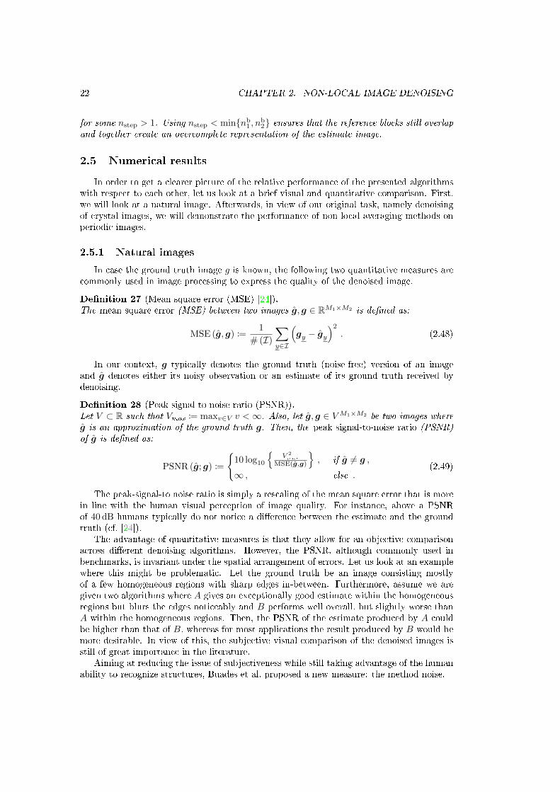
22 CHAPTER 2. NON-LOCAL IMAGE DENOISING
for some nstep > 1. Using nstep < minnb1 , n
b2 ensures that the reference blocks still overlap
and together create an overcomplete representation of the estimate image.
2.5 Numerical results
In order to get a clearer picture of the relative performance of the presented algorithmswith respect to each other, let us look at a brief visual and quantitative comparison. First,we will look at a natural image. Afterwards, in view of our original task, namely denoisingof crystal images, we will demonstrate the performance of non-local averaging methods onperiodic images.
2.5.1 Natural images
In case the ground truth image g is known, the following two quantitative measures arecommonly used in image processing to express the quality of the denoised image.
Denition 27 (Mean square error (MSE) [24]).The mean square error (MSE) between two images g, g ∈ RM1×M2 is dened as:
MSE (g, g) :=1
# (I)
∑y∈I
(gy − gy
)2
. (2.48)
In our context, g typically denotes the ground truth (noise-free) version of an imageand g denotes either its noisy observation or an estimate of its ground truth received bydenoising.
Denition 28 (Peak signal-to-noise ratio (PSNR)).Let V ⊂ R such that Vmax := maxv∈V v <∞. Also, let g, g ∈ VM1×M2 be two images whereg is an approximation of the ground truth g. Then, the peak signal-to-noise ratio (PSNR)of g is dened as:
PSNR (g; g) :=
10 log10
V 2max
MSE(g,g)
, if g 6= g ,
∞ , else .(2.49)
The peak-signal-to noise ratio is simply a rescaling of the mean square error that is morein line with the human visual perception of image quality. For instance, above a PSNRof 40 dB humans typically do not notice a dierence between the estimate and the groundtruth (cf. [24]).
The advantage of quantitative measures is that they allow for an objective comparisonacross dierent denoising algorithms. However, the PSNR, although commonly used inbenchmarks, is invariant under the spatial arrangement of errors. Let us look at an examplewhere this might be problematic. Let the ground truth be an image consisting mostlyof a few homogeneous regions with sharp edges in-between. Furthermore, assume we aregiven two algorithms where A gives an exceptionally good estimate within the homogeneousregions but blurs the edges noticeably and B performs well overall, but slightly worse thanA within the homogeneous regions. Then, the PSNR of the estimate produced by A couldbe higher than that of B, whereas for most applications the result produced by B would bemore desirable. In view of this, the subjective visual comparison of the denoised images isstill of great importance in the literature.
Aiming at reducing the issue of subjectiveness while still taking advantage of the humanability to recognize structures, Buades et al. proposed a new measure: the method noise.

2.5. NUMERICAL RESULTS 23
σ=
25σ
=40
g z LHMA(z) Fwbil
(z) NLM (z) BM3D (z)
Figure 2.2: Comparison of dierent denoising methods for a natural image (Aachen cathe-dral); from left to right: noise-free image (V = [0, 255]), image aected by AGWN (top:σ = 25, bottom: σ = 40), estimates retrieved by moving averages, bilateral ltering, non-local means, BM3D
Denition 29 (Method noise).Let z = g + η be an image where η is an instance of white noise, i.e. the correspondingrandom distributions all have zero mean and the same variance. Furthermore, let F be somelter. Then,
MNF (z) := z − F (z) , (2.50)
is called method noise.
Given an ideal lter, MNF (z) should look like white noise. Please note that due tothe subtraction in (2.50), the method noise is only applicable in case of additive noisedistributions.
Figure 2.2 shows a comparison of the four methods discussed in this chapter, namely:moving averages, bilateral ltering, non-local means and BM3D. All results for non-localmeans presented in this and the next chapter are based on its pixel-wise implementa-tion. For moving averages, we use a lter kernel size of n = (7, 7). The discrete bi-lateral lter uses the same kernel size, its spatial Gaussian hd has standard deviation7 and its intensity Gaussian has standard deviation 2σ, where σ is the standard devia-tion of the Gaussian noise applied to the respective ground truth image. The NLM re-sults are based on its pixel-wise implementation with the default parameters suggested athttp://www.ipol.im/pub/art/2011/bcm_nlm/. BM3D also uses the default pa-rameters and transformations employed in its published implementation http://www.cs.tut.fi/~foi/GCF-BM3D/. Please note however, that all results presented here wereproduced with our own implementations of the algorithms in C++, which are available athttps://github.com/nmevenkamp/nonLocalDenoising.
The comparison in Figure 2.2 shows that while all regarded methods signicantly reducethe noise, moving averages also signicantly blurs the entire image. As expected, the bilaterallter performs much better in this regards, although the edges (especially at the bricks andwindows) are not as sharp as in the non-local estimates. BM3D clearly outperforms NLMin terms of visual quality.
These ndings are reected by the quantitative results in Table 2.1.Finally, let us look at the comparison of the method noise in Figure 2.3. Apparently,
very clear structure remains for both the moving averages and bilateral lter, although for

24 CHAPTER 2. NON-LOCAL IMAGE DENOISING
Noise level PSNRσ Input moving averages bilateral lter NLM BM3D25 20.4006 23.7709 24.9996 26.9886 28.601440 16.5656 23.3188 23.2823 24.3500 26.3668
Table 2.1: PSNR before and after denoising the Aachen cathedral image (cf. Figure 2.2)aected by AGWN with dierent lters
σ=
25σ
=40
MNLHMA(z) MNFwbil
(z) MNNLM (z) MNBM3D (z)
Figure 2.3: Comparison of the method noise for the image and algorithms in Figure 2.2
the latter, the edges are less pronounced. The method noise of NLM and BM3D containssignicantly less structure. Here, BM3D performs slightly better upon close comparison.Overall, it is apparent that there is more structure in the method noise of all methods forσ = 40 than for σ = 25.
2.5.2 Periodic images
As expressed by the consistency result in Remark 17, neighborhood-based non-localaveraging strategies perform better the more samples of each detail are available in anygiven image. As mentioned in [26], the prime example for this are periodic images. In orderto motivate our focus on non-local means (or BM3D) for the reconstruction of electronmicrographs of crystals, let us perform the same analysis as in Section 2.5.1, but using aperiodic image as the input. Here, we use a natural image of a brick wall.
Looking at the results in Figures 2.4 and 2.5 and Table 2.2 we observe similar aspects asthose discussed in Section 2.5.1, only that now the gain in performance when using non-localaveraging methods instead of local ones is much larger. Furthermore, comparing the PSNRvalues in Tables 2.1 and 2.2 with each other, our expectation that the absolute performanceof the non-local methods should be better on the periodic bricks image in Figure 2.4 than onthe Aachen cathedral image Figure 2.2 is conrmed. Please note that both the quantitativeand visual comparison yield a noticeable gain when using BM3D instead of NLM.

2.5. NUMERICAL RESULTS 25
σ=
25σ
=40
σ=
60
g z LHMA(z) Fwbil
(z) NLM (z) BM3D (z)
Figure 2.4: Comparison of dierent denoising methods for a periodic image (bricks); fromleft to right: noise-free image (V = [0, 255]), image aected by AGWN (top: σ = 25,center: σ = 40, bottom: σ = 60), estimates retrieved by moving averages, bilateral ltering,non-local means, BM3D
σ=
25σ
=40
σ=
60
MNLHMA(z) MNFwbil
(z) MNNLM (z) MNBM3D (z)
Figure 2.5: Comparison of the method noise for the image and algorithms in Figure 2.4
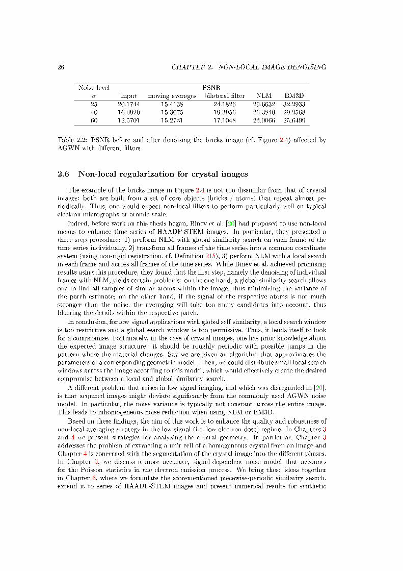
26 CHAPTER 2. NON-LOCAL IMAGE DENOISING
Noise level PSNRσ Input moving averages bilateral lter NLM BM3D25 20.1744 15.4138 24.1826 29.6632 32.293340 16.0920 15.3675 19.3956 26.3840 29.256860 12.5701 15.2731 17.1048 23.0066 25.6499
Table 2.2: PSNR before and after denoising the bricks image (cf. Figure 2.4) aected byAGWN with dierent lters
2.6 Non-local regularization for crystal images
The example of the bricks image in Figure 2.4 is not too dissimilar from that of crystalimages: both are built from a set of core objects (bricks / atoms) that repeat almost pe-riodically. Thus, one would expect non-local lters to perform particularly well on typicalelectron micrographs at atomic scale.
Indeed, before work on this thesis began, Binev et al. [20] had proposed to use non-localmeans to enhance time series of HAADF-STEM images. In particular, they presented athree-step procedure: 1) perform NLM with global similarity search on each frame of thetime series individually, 2) transform all frames of the time series into a common coordinatesystem (using non-rigid registration, cf. Denition 215), 3) perform NLM with a local searchin each frame and across all frames of the time series. While Binev et al. achieved promisingresults using this procedure, they found that the rst step, namely the denoising of individualframes with NLM, yields certain problems: on the one hand, a global similarity search allowsone to nd all samples of similar atoms within the image, thus minimizing the variance ofthe patch estimate; on the other hand, if the signal of the respective atoms is not muchstronger than the noise, the averaging will take too many candidates into account, thusblurring the details within the respective patch.
In conclusion, for low-signal applications with global self-similarity, a local search windowis too restrictive and a global search window is too permissive. Thus, it lends itself to lookfor a compromise. Fortunately, in the case of crystal images, one has prior knowledge aboutthe expected image structure: it should be roughly periodic with possible jumps in thepattern where the material changes. Say we are given an algorithm that approximates theparameters of a corresponding geometric model. Then, we could distribute small local searchwindows across the image according to this model, which would eectively create the desiredcompromise between a local and global similarity search.
A dierent problem that arises in low-signal imaging, and which was disregarded in [20],is that acquired images might deviate signicantly from the commonly used AGWN noisemodel. In particular, the noise variance is typically not constant across the entire image.This leads to inhomogeneous noise reduction when using NLM or BM3D.
Based on these ndings, the aim of this work is to enhance the quality and robustness ofnon-local averaging strategy in the low signal (i.e. low electron dose) regime. In Chapters 3and 4 we present strategies for analyzing the crystal geometry. In particular, Chapter 3addresses the problem of extracting a unit cell of a homogeneous crystal from an image andChapter 4 is concerned with the segmentation of the crystal image into the dierent phases.In Chapter 5, we discuss a more accurate, signal-dependent noise model that accountsfor the Poisson statistics in the electron emission process. We bring these ideas togetherin Chapter 6, where we formulate the aforementioned piecewise-periodic similarity search,extend it to series of HAADF-STEM images and present numerical results for synthetic
2.7. CONCLUSIONS 27
and experimental images. Finally, Chapter 7 treats the extension of NLM and BM3D tohyper-spectral imaging and also demonstrates how exploiting the dierent properties ofspectral and HAADF-STEM images can lead to astonishing results, when combining bothin a multi-modal lter.
2.7 Conclusions
In this chapter, we have laid the foundation for the understanding of local and non-localaveraging concepts for image denoising. In particular, we presented the non-local means(NLM) and block-matching and 3D ltering (BM3D) algorithms. A theoretical result onthe optimal performance of non-local lters was recalled and experimental results wereprovided that support the claim of the non-local concept outperforming local averagingstrategies, most signicantly in the case of rich self-similarity. We summarized that due totheir periodic nature, non-local averaging is expected to work particularly well for electronmicrographs of crystals. Finally, we pointed at two major problems whose investigationwill be the main subject of this thesis, namely: 1) low-signal electron micrographs deviatesignicantly from the AGWN noise model and 2) neither local nor global similarity searchis optimal for low-signal crystal images.
Summarizing, the core aspects of this thesis are:
1) mixed Poisson-Gaussian noise model estimation,
2) unsupervised crystal geometry analysis,
3) piecewise periodic block-matching,
4) hyper-spectral and multi-modal averaging.

Chapter 3
Periodicity analysis and unit cell
extraction
In this chapter, we discuss techniques for the unsupervised analysis of the structure ofperiodic images. We focus on the context of crystal images, but most of the content appliesto general periodic functions in 1D and 2D.
We open the chapter with an introduction to the problem of periodicity analysis ingeneral, and crystal geometry analysis in particular. After that, we give a mathematicaldenition of a crystal and discuss the relation between crystal images and periodic functions.Then, two practical approaches for the automated analysis of periodic images are discussed.The rst, and more classical one, is based on Fourier analysis, while the second relies onenergy minimization in real-space.
With the exception of Section 3.3 the content of this chapter was published in [99]. Letus point out that the denition of unit cells and the corresponding notation deviate fromthose in [99].
3.1 Introduction
Analyzing and classifying the properties of crystalline structures is a fundamental issuein various elds, such as biology, chemistry and materials science [31,63,76,146]. One of themajor properties in this context is the symmetry of the crystal, which is often inferred fromdiraction patterns, e.g. from X-rays [79] or electrons [149]. Most commonly, one analyzesthe Bragg reections [23], i.e. the lattice vectors of the crystal are related to the positions ofpeaks in the Fourier transformed crystal image. This relation serves as a basis for a variousimage processing techniques designed for crystal geometry analysis or for removing artifacts(noise, distortions) from crystal images [78].
Recently, novel real-space methods have proposed, which have proven to be very powerfulfor dierent tasks, such as grain segmentation [21], crystal defect localization [47], noisereduction [102] and sample drift correction [127]. The common nature of these methodsis the exploitation of information about the crystal geometry in real-space, i.e. the directlattice angles or vectors. Unfortunately, these methods either require the crystal latticeparameters to be provided manually, or rely on Fourier-based techniques which were shownto be the limiting factor for the performance in some cases. In short, entirely unsuperviseduse of these otherwise automated methods is generally not possible at present.
Within the context of sample drift correction, Sang and LeBeau proposed a novel real-space method for lattice angle estimation. They introduced the so-called projective standard
29
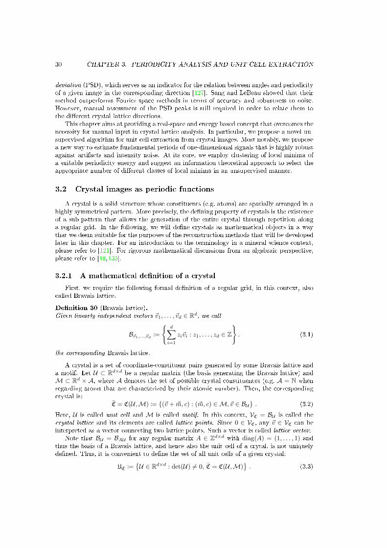
30 CHAPTER 3. PERIODICITY ANALYSIS AND UNIT CELL EXTRACTION
deviation (PSD), which serves as an indicator for the relation between angles and periodicityof a given image in the corresponding direction [127]. Sang and LeBeau showed that theirmethod outperforms Fourier space methods in terms of accuracy and robustness to noise.However, manual assessment of the PSD peaks is still required in order to relate them tothe dierent crystal lattice directions.
This chapter aims at providing a real-space and energy based concept that overcomes thenecessity for manual input in crystal lattice analysis. In particular, we propose a novel un-supervised algorithm for unit cell extraction from crystal images. Most notably, we proposea new way to estimate fundamental periods of one-dimensional signals that is highly robustagainst artifacts and intensity noise. At its core, we employ clustering of local minima ofa suitable periodicity energy and suggest an information theoretical approach to select theappropriate number of dierent classes of local minima in an unsupervised manner.
3.2 Crystal images as periodic functions
A crystal is a solid structure whose constituents (e.g. atoms) are spatially arranged in ahighly symmetrical pattern. More precisely, the dening property of crystals is the existenceof a sub-pattern that allows the generation of the entire crystal through repetition alonga regular grid. In the following, we will dene crystals as mathematical objects in a waythat we deem suitable for the purposes of the reconstruction methods that will be developedlater in this chapter. For an introduction to the terminology in a mineral science context,please refer to [121]. For rigorous mathematical discussions from an algebraic perspective,please refer to [48,135].
3.2.1 A mathematical denition of a crystal
First, we require the following formal denition of a regular grid, in this context, alsocalled Bravais lattice.
Denition 30 (Bravais lattice).Given linearly independent vectors ~v1, . . . , ~vd ∈ Rd, we call
B~v1,...,~vd :=
d∑i=1
zi~vi : z1, . . . , zd ∈ Z
. (3.1)
the corresponding Bravais lattice.
A crystal is a set of coordinate-constituent pairs generated by some Bravais lattice anda motif. Let U ⊂ Rd×d be a regular matrix (the basis generating the Bravais lattice) andM ⊂ Rd × A, where A denotes the set of possible crystal constituentes (e.g. A = N whenregarding atoms that are characterized by their atomic number). Then, the correspondingcrystal is:
C = C(U ,M) := (~v + ~m, c) : (~m, c) ∈M, ~v ∈ BU . (3.2)
Here, U is called unit cell and M is called motif. In this context, VC = BU is called thecrystal lattice and its elements are called lattice points. Since 0 ∈ VC, any ~v ∈ VC can beinterpreted as a vector connecting two lattice points. Such a vector is called lattice vector.
Note that BU = BAU for any regular matrix A ∈ Zd×d with diag(A) = (1, . . . , 1) andthus the basis of a Bravais lattice, and hence also the unit cell of a crytal, is not uniquelydened. Thus, it is convenient to dene the set of all unit cells of a given crystal:
UC :=U ∈ Rd×d : det(U) 6= 0, C = C(U ,M)
. (3.3)

3.2. CRYSTAL IMAGES AS PERIODIC FUNCTIONS 31
In the crystallography literature, one often nds denitions of unit cells that allow multi-plying any of the basis vectors with an integer, resulting in an increase of the size of the unitcell. To compensate for this (i.e. to ensure that the same crystal is generated), the otherwisemissing lattice points are simply transferred to the motif. In that context, one encountersthe term primitive unit cell, which denes the smallest possible unit cells generating a givencrytal.
Here, we only allow motifsM⊂ Rd ×A with the smallest possible number of elementssuch that the corresponding crystal C can still be generated by a Bravais lattice, i.e. ∃U ∈Rd×d with C = C(U ,M). Given this setting, the denition of unit cells in (3.3) coincideswith the notion of primitive unit cells. In [99], exactly these types of unit cells were identiedas primitive.
While in [99] we distinguished between primitive and ordinary unit cells, we found thatfor the purposes of this work this is not necessary. Thus, in favor of a more concise andless confusing notation, here we restrict ourselves to the notion of crystals and unit cells asintroduced in (3.2) and (3.3).
Finally, let us remark that shortest and linearly independent lattice vectors always forma unit cell. This property will be important for the methods discussed later in this chapter.
Remark 31 (Shortest linearly independent lattice vectors form a unit cell).Let d = 2 and C = C(U ,M) ⊂ R2 × A be a crystal. Furthermore, let ~v1, ~v2 ∈ VC linearlyindependent such that
‖~v1‖2 + ‖~v2‖2 ≤ ‖~u1‖2 + ‖~u1‖2 ∀ ~u1, ~u2 ∈ UC . (3.4)
Then BU = BU , i.e. U is a unit cell of the crystal C.
3.2.2 Modeling projected crystals as periodic functions
In order to bridge the gap between crystals as highly ordered sets of position-constituentpairs and periodic functions, let us rst dene what a periodic function is.
Denition 32 (Periodic function).A function g ∈ L1(Rd) is periodic if there exist linearly independent vectors ~v1, . . . , ~vd, suchthat
g(x+ ~v) = g(x) ∀~v ∈ B~v1,...,~vd . (3.5)
We say that the function g is ~v1, . . . , ~vd-periodic. In case dimV = 1, the smallest v > 0such that (3.5) holds, is called fundamental period of the function g.
In this work, we concentrate on the setting where three-dimensional crystals are pro-jected onto a two-dimensional plane, in particular images acquired in electron micro- andspectroscopy. First, let us assume that the modality of electron micrographs or multispectralimages retains a unique identication of the constituents of the crystal. Now let C ⊂ R3×Abe a crystal, ~v1, ~v2, ~v3 be a unit cell of C and let us assume that the projection is alignedwith ~v3. Then the resulting electron micrograph or multispectral image is ~v1, ~v2-periodic.
Note that in the real-world setting both the actual sample of the crystal and the pro-jection plane are bounded, typically in a way which prohibits receiving a periodic functionsimply by extending the nite image to R2 with periodic boundary conditions. Furthermore,due to the acquisition noise (spatial distortions and shot noise) discussed in Chapter 1, thediscrete raw image g cannot be expected to fulll (3.5). Despite these errors, crystal imageshave an underlying periodic structure and, in the following, we discuss how to estimatethe corresponding unit cells in an unsupervised and robust manner, despite the presence ofmoderate spatial distortions and possibly severe shot noise.

32 CHAPTER 3. PERIODICITY ANALYSIS AND UNIT CELL EXTRACTION
3.3 Reciprocal unit cell estimation
In the following we present a practical method for periodicity analysis that is based onpeak nding in Fourier space and the fact that there is a direct relation between a Bravaislattice in Fourier or reciprocal space and the lattice of the actual crystal, also called directlattice.
In order to motivate the usage of the reciprocal space, let us briey bring to mind whya simple peak nding technique for unsupervised lattice vector extraction is not feasible inpractice on the crystal image itself. In Section 6.3, we will discuss an algorithm for ndingthe atom centers in HAADF-STEM images in the presence of moderate noise. However,there is no trivial way to decide which atoms belong to the same unit cell and which do not.Thus, the task of identifying the lattice points among all tted atom centers, and thereforealso the task of nding lattice vectors, is non-trivial.
In the following we will show that in Fourier space, this task becomes much easier. Inparticular, we show that the Fourier transform maps periodic functions to sums of Diracdistributions. Furthermore, we will show that the Fourier transform maps Bravais lattices,represented as periodic sums of Dirac distributions, to Bravais lattices.
3.3.1 The Fourier transform for tempered distributions
In the following, let us dene the Fourier transform for L1-functions. Furthermore,we will regard extensions of the Fourier transform to L2-functions and nally tempereddistributions. The latter is required in order to study the eect of the Fourier transform onthe aforementioned Dirac distributions.
Denition 33 (Fourier transform [24]).Let g ∈ L1(Rd)b and ω ∈ Rd. Then, the Fourier transformation of g at ω is dened as
F [g](ω) :=
ˆRdg(x)e−iω·x dx , (3.6)
and the mappingF : L1(Rd)→ C(Rd), g 7→ F [g] (3.7)
is called Fourier transform.
Please note that this denition diers from that in [24] by a factor of 1(2π)d/2
, whichaccordingly aects all following statements. This scaling, as well as a possible factor of 2πin the argument of the exponential function, is merely a question of preference and variesacross the literature.
Remark 34 (Linearity and continuity of the Fourier transform [24]).F is linear and continuous.
In order to extend the Fourier transform to L2, we need to introduce the Schwartz space,characterized by the property that all derivatives of its functions are rapidly decreasing andthat it is dense in Lp for 1 ≤ p <∞.
Denition 35 (Schwartz space [24]).
S(Rd) :=
g ∈ C∞(Rd) : sup
x∈Rd|xα ∂β
∂xβg(x)| <∞ ∀α, β ∈ Nd
, (3.8)
is called Schwartz space and g ∈ S(Rd) is called Schwartz function.

3.3. RECIPROCAL UNIT CELL ESTIMATION 33
Lemma 36 (The Schwartz space is dense in Lp [119]).For 1 ≤ p <∞ S(Rn) is dense in Lp(Rn).
Now we recall the theorem that extends the Fourier transform to L2.
Theorem 37 (Fourier transform for L2 functions [24]).The Fourier transform is a continuous and bijective mapping of S(Rd) onto itself and thefollowing inversion formula holds:
F−1[F [g]](x) = g(x) =
ˆRdF [g](ω)eix·ω dω . (3.9)
Furthermore, there is exactly one continuous operator F : L2(Rd) → L2(Rd) that extendsthe Fourier transform onto S(Rn) and fullls
‖g‖2 = ‖F [g]‖2 ∀g ∈ L2(Rd) . (3.10)
This operator is bijective and its inverse is a continuous extension of F−1 from S(Rd) toL2(Rd). Note that the integrals in (3.6) and (3.9) do not necessarily exist for L2 functions.Nevertheless, they are are meaningful in the sense that the integrals over B2
R(0) converge toF [g] (or F−1[g]) in L2 for R→∞.
At this point, let us recall some important properties of the Fourier transform.
Lemma 38 (Elementary Fourier transform properties [24]).Let g ∈ L1(Rd) and for y ∈ Rd let
Ty : L1(Rd)→ L1(Rd), g 7→ (x 7→ g(y + x)) ,
My : L1(Rd)→ L1(Rd), g 7→(x 7→ eix·yg(x)
).
(3.11)
Furthermore, for A ∈ Rd×d regular let
DA : L1(Rd)→ L1(Rd), g(·) 7→ g(A·) . (3.12)
Then
F [Ty[g]] = My[F [g]] , (3.13)
F [My[g]] = T−y[F [g]] , (3.14)
and
F [DA[g]] =1
|detA|DA−T [F [g]] . (3.15)
hold. Furthermore,
F [F [g]] = D− 1[g] . (3.16)
Applying F−1 to both sides directly implies
F [g] = F−1[D− 1[g]] ⇔ F−1[g] = F [D− 1[g]] . (3.17)
We will also require the Poisson summation formula for Schwartz functions.

34 CHAPTER 3. PERIODICITY ANALYSIS AND UNIT CELL EXTRACTION
Theorem 39 (Poisson summation formula [24,134]).Let g ∈ S(Rd). Then ∑
~n∈ZdF [g](~n) =
∑~n∈Zd
g(~n) , (3.18)
holds.Please note that in [24] the statement and proof are only given for the case d = 1.
However, for d ∈ N with d > 1 the statement still holds and the proof is analogous.
Furthermore, we require the following modulated version that results from (3.15). Al-though it is a known formula, we give its proof for the convenience of the reader.
Remark 40 (Modulated Poisson summation formula).Let g ∈ S(Rd) and A ∈ Rd×d be regular. Then∑
~n∈ZdF [g](A~n) =
1
|detA|∑~n∈Zd
g(A−T~n) . (3.19)
holds.
Proof. Replacing A with A−T in (3.15) and using elementary properties of the determinantyields
DA[F [g]] = |detA−T |F [DA−T [g]] =1
|detA|F [DA−T [g]] . (3.20)
Using Theorem 39 we therefore receive∑~n∈Zd
F [g](A~n) =1
|detA|∑~n∈Z
F [DA−T [g]](~n) =1
|detA|∑~n∈Z
DA−T [g](~n) . (3.21)
Finally, let us introduce the space of tempered distributions as the dual of the Schwartzspace and extend the Fourier transform to this space.
Denition 41 (Tempered distribution [24,134]).Let
S∗(Rd) :=T : S(Rd)→ C : T linear and continuous
, (3.22)
denote the dual space of S(Rd). Then, T ∈ S∗(Rd) is called tempered distribution.
Remark 42 (Regular tempered distributions [24,134]).Any g ∈ L1(Rd) induces a tempered distribution
Tg[h] :=
ˆRdg(x)h(x) dx ∀h ∈ S(Rd) . (3.23)
Such tempered distributions are called regular.
Denition 43 (Fourier transform for tempered distributions [24]).For T ∈ S∗(Rd) the Fourier transform is dened as
(F [T]) [g] := T[F [g]] ∀g ∈ S(Rd) . (3.24)
The inverse is dened analogously.

3.3. RECIPROCAL UNIT CELL ESTIMATION 35
By this denition the Fourier transform becomes a bijective mapping of S∗(Rd) ontoitself. Note that for L1(Rd) functions Denition 43 is consistent with Denition 33 inthe following sense. Let g ∈ L1(Rd). Then g induces a tempered distribution Tg andin alignment with the equivalence between the inducing function and its distribution it isnatural to interpret F [Tg] as TF [g]. In fact, analogous to the Fourier convolution theorem,one can show that [24]
TF [g][h] = Tg[F [h]] = F [Tg][h] ∀h ∈ S(Rd) . (3.25)
3.3.2 The Fourier transform of a periodic function
Before we discuss the relation between reciprocal and direct lattice, let us analyze why thetask of estimating lattice vectors is expected to be signicantly easier in reciprocal space thanin direct space. In particular, we show that the Fourier transform of any periodic functionis a sum of Dirac distributions positioned at multiples of the fundamental frequency.
In order to show this, we need to introduce the Fourier series representation for periodicfunctions, as well as a uniform convergence statement.
Theorem 44 (Fourier series [24,134]).Let T > 0 and g ∈ L2(R) be T -periodic. Then, for ω0 = 1
T
g|[0,T ] =∑n∈Z〈g, eω0
n 〉[0,T ]eω0n , (3.26)
holds, whereeω0n : R→ C : x 7→ e2πinω0x , (3.27)
and for a, b ∈ R and g, h ∈ L2([a, b])
〈g, h〉[a,b] :=
ˆ b
a
g(x)h(x) dx . (3.28)
Note that the denition of the Fourier series in [24] is formulated for 2π-periodic func-tions. However, using the substitution h(x) = g( T2πx) one transforms 2π-periodic functionsinto T -periodic functions, which yields the above formulation of the Fourier series.
Lemma 45 (Uniform convergence of the Fourier series [55,134]).Let T > 0 and g ∈ C1(R) be T -periodic. Then, the Fourier series of g converges uniformly.
Furthermore, let us dene the Dirac distribution.
Denition 46 (Dirac distribution [24,134]).For x ∈ Rd the Dirac distribution (centered at x) is dened as
δx[g] := g(x) ∀g ∈ S(Rd) . (3.29)
The Dirac distribution is a tempered distribution. The following result on the Fouriertransform of the Dirac distribution is an immediate consequence of Denition 43.
Lemma 47 (The Fourier transform of the Dirac distribution [24,134]).Let n ∈ Z, ω0 ∈ Rd \ 0 and g ∈ S(Rd). Then
(F [δnω0 ]) [g] =
ˆRdg(x)e−inω0·x dx = T
D− 1[eω0/2πn ]
[g] . (3.30)

36 CHAPTER 3. PERIODICITY ANALYSIS AND UNIT CELL EXTRACTION
Thus, F [δnω0] is regular and induced by D− 1[eω0
n ]. Furthermore, using (3.17), we receive
F[Teω0
n
]= F−1
[TD− 1[e
ω0n ]
]= δ2πnω0
. (3.31)
Theorem 48 (The Fourier transform of a periodic function).Let T > 0 and g ∈ S(R) be T -periodic. Then, for ω0 = 1
T ,
F [Tg] =∑n∈Z〈g, eω0
n 〉[0,T ]δ2πnω0 . (3.32)
holds. This also implies F [g](ω) = 0 for all ω ∈ (0, ω0) and thus
ω0 = min ω ∈ R \ 0 : F [g](ω) 6= 0 . (3.33)
Proof. Using Theorem 44 we receive
F [Tg][h] =
ˆR
ˆR
∑n∈Z〈g, eω0
n 〉[0,T ]eω0n (x)e−iωx dω h(x) dx . (3.34)
According to Lemma 45 the Fourier series converges uniformly and thus summation andintegration may be interchanged here:
F [Tg][h] =∑n∈Z〈g, eω0
n 〉[0,T ]
ˆR
ˆReω0n (x)e−iωx dω h(x) dx
=∑n∈Z〈g, eω0
n 〉[0,T ]
(F[Teω0
n
])[h] .
(3.35)
Finally, using (3.31) concludes the proof.
This means that the Fourier transform of (suitably smooth) periodic functions is discretewith impulses at integer multiples of the fundamental frequency. Please note that thefactor 2π within the frequencies accounts for the missing factor 2π in the exponent of theexponential function within the denition of the Fourier transform in Denition 33.
As mentioned earlier, in practice crystal images are bounded and typically not exactlyperiodic on their support. Even if this were the case, noise eects would lead to most,if not all, Fourier frequencies being non-zero. Nevertheless, in practice one observes thatdespite the nite frequency resolution, the reciprocal lattice points are conned to very smallneighborhoods, or even individual pixels. Furthermore, their intensity is signicantly largerthan that of all frequencies that are not (roughly) an integer multiple of the fundamentalfrequency. Thus, in practice it is much easier to locate Bravais lattice points in reciprocalspace than in direct space.
3.3.3 The Fourier transform of a Bravais lattice
In the following, we will conrm that the Fourier transform of a Bravais lattice is againa Bravais lattice. As mentioned earlier, for this purpose we model the Bravais lattice as asum of Dirac distributions centered at the lattice points. This leads us to the denition ofthe Dirac comb.
Denition 49 (Dirac comb).Let d = 1 and T > 0. Then, the distribution
XT :=∑n∈Z
δnT , (3.36)

3.3. RECIPROCAL UNIT CELL ESTIMATION 37
is called Dirac comb. In case d ∈ N, d > 1, we extend the denition analogously. Let d ∈ Nand A ∈ Rd×d be regular. Then
XA :=∑~n∈Zd
δA~n . (3.37)
The Dirac comb yields a representation of a Bravais lattice in terms of a tempereddistribution. Using Remark 40, we can easily show that the Fourier transform maps aBravais lattice to a Bravais lattice and that, in case d = 1, the fundamental period of thetransformed Dirac comb is the inverse of the fundamental period of the original Dirac comb:
Lemma 50 (The Fourier transform of the Dirac comb).Let d ∈ N and A ∈ Rd×d be regular. Then,
F [XA] =1
|detA|XA−T . (3.38)
In particular, for d = 1 and T > 0, this reads
F [XT ] =1
TX 1
T. (3.39)
Proof. Let g ∈ S(Rd) be arbitrary. Then, using Remark 40, we receive:
(F [XA]) [g] = XA [F [g]] =∑~n∈Zd
δA~n [F [g]] =∑~n∈Zd
F [g](A~n)
=1
|detA|∑~n∈Zd
g(A−T~n) =1
|detA|∑~n∈Zd
δA−T ~n[g]
=1
|detA|XA−T [g] .
(3.40)
Note that due to (3.17) and B−A = BA for A ∈ Rd×d regular, Lemma 50 also holds whenreplacing F with F−1. This means that unit cells can be converted from reciprocal spaceto direct space and vice versa by inverting and transposing the corresponding matrices.
In the crystallography literature, the above relation is typically stated explicitly ford ∈ 2, 3. Let us cite the most popular case, d = 3. Let ~v1, ~v2, ~v3 ∈ R3 be linearlyindependent. Then, the corresponding reciprocal lattice vectors are given by [138]:
~u1 =~v2 × ~v3
~v1 · (~v2 × ~v3), ~u2 =
~v1 × ~v3
~v2 · (~v1 × ~v3), ~u3 =
~v1 × ~v2
~v3 · (~v1 × ~v2). (3.41)
Since (~u1, ~u2, ~u3) = (~v1, ~v2, ~v3)−T holds for this expression, it is equivalent to Lemma 50 ford = 3.
3.3.4 Extracting unit cells from the DFT
In the following, we complete the method for lattice vector estimation in reciprocal space.Therefore, we dene the discrete Fourier transform and derive explicit formulas for the directlattice vectors in dependence of peak positions localized in discrete Fourier space.

38 CHAPTER 3. PERIODICITY ANALYSIS AND UNIT CELL EXTRACTION
Denition 51 (Discrete Fourier transform (DFT) [24]).Let d = 1, M ∈ N and g ∈ CM . Then, the Fourier transform of the discrete series g isdened as
F(g)k :=1
M
M∑n=1
gne−2πi(n−1) k−1
M for k = 1, . . . ,M . (3.42)
Now let d = 2, M1,M2 ∈ N and g ∈ CM1×M2 . Then, the Fourier transform of the discreteimage g is dened as
F(g)kl =1
M1M2
M1∑m=1
M2∑n=1
gm,ne−2πi(n−1) k−1
M1 e−2πi(m−1) l−1M2 . (3.43)
We see that in the discrete one-dimensional Fourier transform, the frequencies are sam-pled evenly spaced on the interval [0, 2π]. This means that the discrete Fourier transformis constructed based on the assumption that the provided function values are also sam-pled evenly and that they represent one period of the function (though not necessarily afundamental one).
In order to extract reciprocal lattice vectors from the discrete Fourier transform, we willnow have to discuss 1) how peaks can be extracted and 2) how the corresponding indices canbe mapped to meaningful lattice vector components. In the following, let d = 2,M1,M2 ∈ Nand g ∈ CM1×M2 .
Denition 52 (Power spectrum).The power spectrum of g is dened as
F|·|(g)i := |F(g)i| . (3.44)
Using the power spectrum, let us dene the peak extraction method.
Denition 53 (Set of power spectrum peaks).Let θ ∈ [0, 1] and p ∈ N. Then
Fpeak(g) :=i ∈ I : F|·|(g)i > maxθFmax(g), F|·|(g)j ∀j ∈ N i
p
, (3.45)
denotes the set of indices corresponding to peaks in the power spectrum of g. Here,
Fmax[g] := maxj∈IF|·|(g)j . (3.46)
Due to the periodicity of the exponential function the exponent x ∈ [π, 2π) is equivalentto x − 2π in (3.43). The latter representation (using [−π, π) as the base interval) is moreconvenient in our context since it allows a direct interpretation of orientations around theorigin in 2D. Thus, in order to represent the reciprocal lattice vectors in terms of fractions(frequencies) of the period (image size), we map the index domain 1, . . . ,M1×1, . . . ,M2to [− 1
2 ,12 )2. Using the Heaviside function, we can infer the following denition of the discrete
reciprocal lattice vectors.
Denition 54 (Heaviside function).The Heaviside function is dened as
ΘH(x) : R→ 0, 1, x 7→
0, x < 0
1, x ≥ 0. (3.47)

3.3. RECIPROCAL UNIT CELL ESTIMATION 39
Denition 55 (Discrete reciprocal lattice vector).For indices (k, l) ∈ I, the corresponding reciprocal lattice vector is dened as
~u(i) :=
(i1 − 1
M1−ΘH
(i1 − 1− M1
2
),i2 − 1
M2−ΘH
(i2 − 1− M2
2
))T. (3.48)
Here, the quotient ij−1Mj
maps the indices ij from 1, . . . ,Mj to [0,1) for j = 1, 2 and
then the Heaviside function shifts the interval [ 12 , 1) to [− 1
2 , 0), which nally yields the range[−1
2 ,12 ).
Using these denitions, we can nally state the method for extracting unit cells in recip-rocal space.
Algorithm 56 Estimating a unit cell via the reciprocal latticeWe estimate the reciprocal lattice as
VFg :=~u(j) : j ∈ Fpeak[g]
. (3.49)
Note that if the mean value of g is non-zero, then F [g]0,0 6= 0 and thus ~u(0, 0) = (0, 0)T ∈VFg . Based on the conversion rule for continuous periodic functions in Lemma 50, as well asRemark 31, we propose to estimate a unit cell of the direct lattice as follows:
U∗FFT := (~v1, ~v2) ∈
(arg min
(~u1,~u2)∈VFg \(0,0)‖~u1‖2 + ‖~u2‖2
)−T. (3.50)
While this method is motivated by Theorem 48 and Lemma 50, we have not treated thetransfer of the continuous theory to the discrete setting. However, it is expected that theconversion rules (3.41) and (3.50) are also valid in the discrete setting - up to errors dueto the discretization of both the image and the Fourier transform - and indeed, they arecommonly used in the literature [123,150] in both the continuous and discrete setting.
3.3.5 Numerical results and limitations
In the following, let us investigate the performance of the unit cell extraction techniquebased on reciprocal peak nding. We will only perform a qualitative investigation here. Aquantitative evaluation will be presented later, in Section 3.4, where the reciprocal-space unitcell estimation method will be compared to its competitor, namely the real-space method.
We regard four dierent articial crystal images constructed by sampling motifs madeup of a few Gaussian bells over perfect Bravais lattices (cf. Figure 3.1). We will also test themethod on Gaussian noise aected versions of these images, where the standard deviationis equal to 50% of the maximum image intensity.
For each of the four articial images, Figure 3.2 shows the corresponding Fourier trans-forms. The top row shows those corresponding to the noisefree images and the bottomrow those corresponding to the Gaussian noise case. Note that the Fourier transform wasshifted here, such that F [g]0,0 is in the center of the image (cf. (3.48)). Furthermore, sinceF [g]0,0 is typically very large, we set it to zero (which is equivalent to subtracting the meanvalue of the image) in order to enhance the discrete gray scale contrast for the remainingcoecients. As expected, the Fourier transforms consist of distinct and strongly localizedpeaks. Furthermore, we see that the Fourier transforms of the noisefree and Gaussian noise

40 CHAPTER 3. PERIODICITY ANALYSIS AND UNIT CELL EXTRACTION
Figure 3.1: Articial crystal lattice images; top row: ideal crystals (from left to right:Bumps3, HexVacancy, SingleDouble, Nc3Nm); bottom row: same images plus Gaus-sian noise with a standard deviation of 50% of the maximum intensity
degraded images are very similar to each other in terms of the positions and contrast of thepeaks.
Figure 3.3 shows the unit cells (blue) estimated using (3.50) with p = 3 and θ = 0.05(noisefree), θ = 0.005 (Gaussian noise), as well as the corresponding Bravais lattices (red).Note that the origin of each Bravais lattice shown in the following was aligned manually withthe center of an atom. First of all, in the noisefree case, the estimated unit cells are correctup to a fraction of the inter-atomic distance. However, this error is large enough that theestimated crystal lattice deviates signicantly from the actual lattice after a few periods,especially for the Nc3Nm image. This is due to the limited frequency resolution of thediscrete Fourier transform. Let us now look at the noise robustness of the method. For theHexVacancy and SingleDouble images the estimated unit cell remains unchanged whenadding Gaussian noise. However, both for the Bumps3 and Nc3Nm the estimated unitcell is wrong. In both cases, the length of the horizontal lattice vectors is an integer fractionof the corresponding fundamental period, which is an indicator for the noise dominating thepeaks corresponding to the actual fundamental frequencies.
The four test images regarded so far are based on perfect Bravais lattices. Let us nowlook at a few results on actual experimental HAADF-STEM images to see how the methodcopes with the image distortions discussed in Chapter 1. Figure 3.4 shows four HAADF-STEM images of dierent materials, as well as the corresponding estimated unit cells (blue)and crystal lattices (red). Since the intensities of the raw STEM images are oset by alarge number, we subtracted the minimum image intensity from all pixels before applyingthe reciprocal peak nding. Then, p = 3 and θ = 0.05 was used in all cases. The result issimilar to the articial setting, namely the unit cells are recognized correctly in the majorityof the cases, but there is a non-negligible error in the lattice vectors. Also, the methodfails to recognize the unit cell correctly for the GaN example. Please note that neitherin this case, nor for the synthetic images above, tuning the parameter θ could alleviate theproblem.

3.3. RECIPROCAL UNIT CELL ESTIMATION 41
Figure 3.2: Fourier transformed crystal images (cf. Figure 3.1); top row: noisefree case;bottom row: Gaussian noise case. The Fourier transform is shifted such that F [g]0,0 is inthe center of the image (cf. (3.48)) and the center peak is removed.
Figure 3.3: Unit cells (blue) and crystal lattices (red) of the articial crystals (cf. Figure 3.1)estimated in reciprocal space (cf. Algorithm 56); top row: noisefree case; bottom row:Gaussian noise case

42 CHAPTER 3. PERIODICITY ANALYSIS AND UNIT CELL EXTRACTION
Figure 3.4: Top row: experimentally acquired HAADF-STEM images (from left to right:GaN, Si, Series1, Series03); bottom row: unit cells (blue) and crystal lattices (red)estimated in reciprocal space (cf. Algorithm 56); images courtesy of P. M. Voyles
In conclusion, reciprocal peak nding turns out to be a very powerful method for unitcell estimation given its simplicity. However, it lacks accuracy due to the limited frequencyresolution of the discrete Fourier transform. While accuracy with which the peaks in thepower spectrum may be increased beyond the pixel resolution of the image [41, 131], theissue of possibly detecting spurious peaks due to intensity noise or image distortions, whichlead to completely wrong lattice vectors, remains.
3.4 Extracting unit cells in real-space
In the following, let us discuss a structurally very dierent method for unit cell estima-tion. In contrast to the previous method, it is based entirely on real-space computations andallows to overcome, or at least greatly improve on the issues of the reciprocal-space method.
In this context, we only analyze the crystal lattice. Thus, it is convenient to introducethe following notation for unit cells and crystal lattices that is only dependent on latticevectors and disregards the motif.
Denition 57 (Unit cells based on generating lattice vectors).LetM0 = (0, 0) denote the trivial motif. Then, for linearly independent vectors ~v1, ~v2 ∈ R2
we dene
U~v1,~v2 := UC(~v1,~v2,M0), V~v1,~v2 := VC(~v1,~v2,M0) . (3.51)
Now, let us introduce an energy that measures the dierence between a given image andits values at nearby lattice points in dependence of the lattice vectors.
Denition 58 (Periodicity energy).For Ω ⊂ R2 let g ∈ L2(Ω). Furthermore, let
Uadmiss ⊂
(~v1, ~v2) ∈ R2×2 : ~v1, ~v2 linearly independent
(3.52)

3.4. EXTRACTING UNIT CELLS IN REAL-SPACE 43
be an admissible set of pairs of linearly independent vectors. Then, for (~v1, ~v2) ∈ Uadmiss wedene the energy
Eπ(~v1, ~v2) :=∑
(z1,z2)∈Z
ˆΩUadmiss
(g(x)− g(x+ z1~v1 + z2~v2))2
dx , (3.53)
where Z := (1, 0)T , (0, 1)T , (1, 1)T and
ΩUadmiss:= x ∈ Ω : x+ U~z ∈ Ω ∀~z ∈ Z ∀U ∈ Uadmiss . (3.54)
Note that here the admissible set of lattice vectors is only used in order to make ΩUadmiss
independent of the energy's arguments. We will discuss later how this admissible set can bechosen in practice.
In an ideal setting, unit cells can be characterized as roots of this energy.
Lemma 59 (Unit cells are roots of the periodicity energy).Let (~v1, ~v2) ∈ Uadmiss and g ∈ L2(Ω) be ~v1, ~v2-periodic. Then,
U~v1,~v2 ∩ Uadmiss = (~u1, ~u2) ∈ Uadmiss : Eπ(~u1, ~u2) = 0 =: E0π , (3.55)
holds. Recalling Remark 31 this also implies
arg min(~u1,~u2)∈E0
π
(‖~u1‖2 + ‖~u2‖2) ∈ U~v1,~v2 . (3.56)
Unfortunately, this characterization is of little use in practice, since intensity noise, imagedistortions and crystal defects lead to the energy Eπ being non-zero except for the trivialsolution (which is neither in Uadmiss nor a candidate for a unit cell) and thus E0
π = ∅.Nevertheless, due to the regularity imposed by the integral in (3.53), ∇Eπ(~v1, ~v2) = 0
typically still holds for ~v1, ~v2 ∈ U~v1,~v2∩Uadmiss. Unfortunately, the reverse implication doesnot hold generally. Figure 3.5 illustrates a counter-example. In this case, there are two typesof local minima associated with the ∼ 60 symmetry axis: one of larger energy correspondingto the spacing between neighboring atoms and one of lower energy corresponding to twicethe spacing. Only the latter leads to a valid unit cell.
Another issue with a straight-forward minimization of Eπ is that ∇Eπ(~v1, ~v2) = 0 implies∇Eπ(~u1, ~u2) = 0 for all ~u1, ~u2 ∈ U~v1,~v2 ∩ Uadmiss. Thus, there is no guarantee that localminima correspond to unit cells. Since gradient-based iterative optimization will get stuckat the nearest local minimum, this means a good initialization strategy is required.
In the following, we discuss an initialization strategy that eliminates both problems. Itconsists of a two-step procedure that estimates 1) candidate lattice vector angles and 2)the corresponding fundamental periods. From all resulting candidates, the nal unit cellestimate is again selected via Remark 31. Finally, we will briey comment on how theresulting approximate unit cell can be rened iteratively.
3.4.1 Estimating lattice vector angles
As a start, let us formalize what a lattice vector angle is.
Denition 60 (Lattice vector angle).For α ∈ R let ~eα := (cosα, sinα)T denote the vector of unit length whose angle to the x-axisis α mod 2π. Furthermore, let C ⊂ Rd ×A be a crystal. Then,
V∠C :=
α ∈ [−π2 ,
π2 ) : ∃t ∈ (0,∞) : t~eα ∈ VC
, (3.57)
is the set of lattice vector angles.

44 CHAPTER 3. PERIODICITY ANALYSIS AND UNIT CELL EXTRACTION
0 20 40 60 80 100 1200.0
0.2
0.4
0.6
0.8
1.0
t
EHt
Hcos
Α,s
inΑ
L,0LT
Figure 3.5: Left: articial crystal lattice (magenta dots) with a motif of size two (amagenta/blue dot pair is a motif copy); right: normalized energy (3.53) for ~v1 =t(cosα, sinα)T , ~v2 = 0 as a function of t with α = −61.95 (green vector)
In other words: an angle is a lattice vector angle if and only if the unit vector pointingin the corresponding direction can be scaled such that it becomes a lattice vector. Notethat analogous to Denition 57 we will also use the notation V∠
~v1,~v2for linearly independent
vectors ~v1, ~v2 ∈ R2 in the following.Let us remark that for any non-trivial crystal, there exists a countable innity of lattice
vector angles and an uncountable innity of angles that are not lattice vector angles.
Remark 61 (Characterization of lattice vector angles).For d > 1, C ⊂ Rd ×A let U ∈ UC. Furthermore, let us dene
∠−π2U :=
−π2 ,(U)−1
1,2
(U)−12,2
∈ Q
∅ , else(3.58)
Then
V∠C =
arctan
(−
(U)−11,1 − q(U)−1
2,1
(U)−11,2 − q(U)−1
2,2
): q ∈ Q
∪ ∠
−π2U . (3.59)
In particular, V∠C is countably innite and [−π2 ,
π2 ] \ V∠
C is uncountably innite.
Proof. For α ∈ (−π2 ,π2 ) let us set ~x := (U)−1~eα. Since ~x 6= 0 let us assume without loss of
generality that x2 6= 0. Then α ∈ V∠C if and only if
∃~z ∈ Z2 ∃t ∈ (0,∞) : t~eα = U~z ,⇔ ∃t ∈ (0,∞) : t~x ∈ Z2 ,
⇔ x1/x2 ∈ Q ,
⇔ ∃q ∈ Q :((U)−1
1,1 − q(U)−12,1
)cosα+
((U)−1
1,2 − q(U)−12,2
)sinα = 0 ,
⇔ ∃q ∈ Q : α = arctan
(−
(U)−11,1 − q(U)−1
2,1
(U)−11,2 − q(U)−1
2,2
).
(3.60)
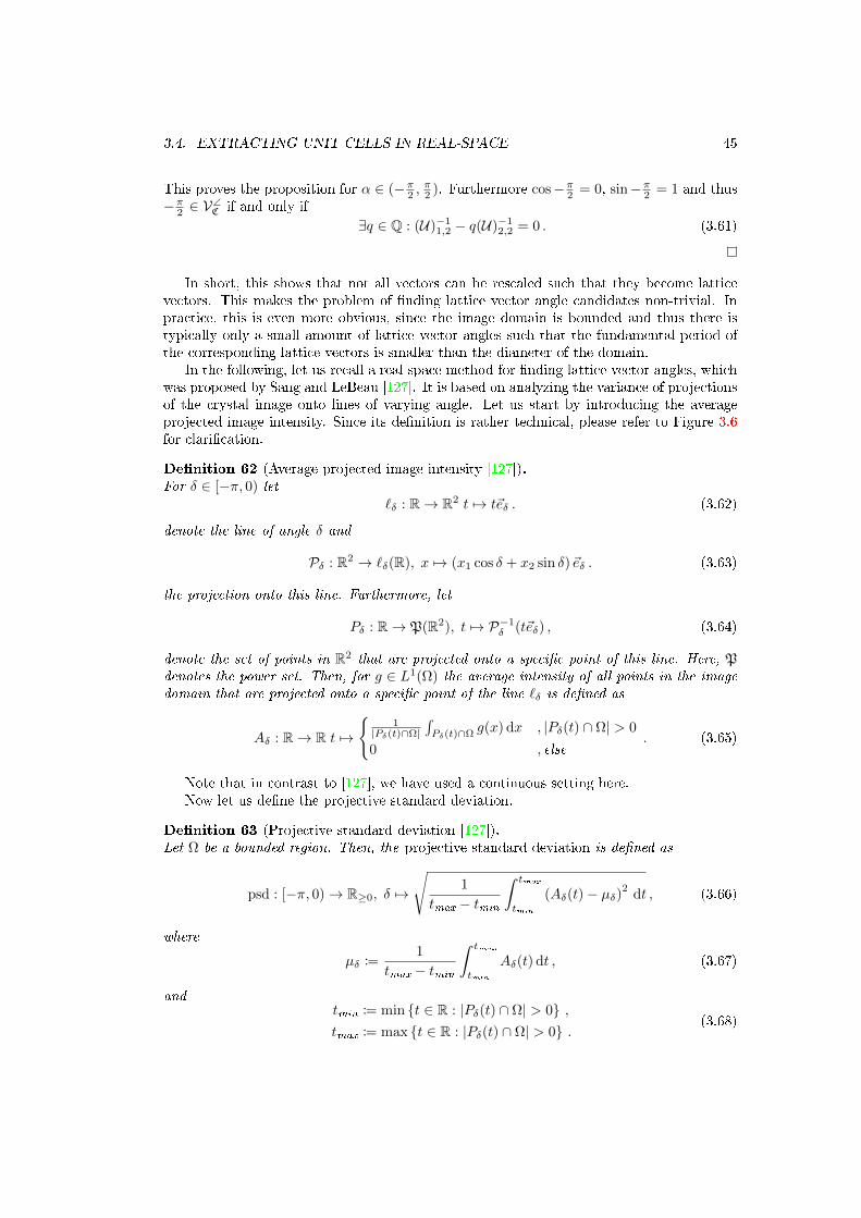
3.4. EXTRACTING UNIT CELLS IN REAL-SPACE 45
This proves the proposition for α ∈ (−π2 ,π2 ). Furthermore cos−π2 = 0, sin−π2 = 1 and thus
−π2 ∈ V∠C if and only if
∃q ∈ Q : (U)−11,2 − q(U)−1
2,2 = 0 . (3.61)
In short, this shows that not all vectors can be rescaled such that they become latticevectors. This makes the problem of nding lattice vector angle candidates non-trivial. Inpractice, this is even more obvious, since the image domain is bounded and thus there istypically only a small amount of lattice vector angles such that the fundamental period ofthe corresponding lattice vectors is smaller than the diameter of the domain.
In the following, let us recall a real-space method for nding lattice vector angles, whichwas proposed by Sang and LeBeau [127]. It is based on analyzing the variance of projectionsof the crystal image onto lines of varying angle. Let us start by introducing the averageprojected image intensity. Since its denition is rather technical, please refer to Figure 3.6for clarication.
Denition 62 (Average projected image intensity [127]).For δ ∈ [−π, 0) let
`δ : R→ R2 t 7→ t~eδ . (3.62)
denote the line of angle δ and
Pδ : R2 → `δ(R), x 7→ (x1 cos δ + x2 sin δ)~eδ . (3.63)
the projection onto this line. Furthermore, let
Pδ : R→ P(R2), t 7→ P−1δ (t~eδ) , (3.64)
denote the set of points in R2 that are projected onto a specic point of this line. Here, Pdenotes the power set. Then, for g ∈ L1(Ω) the average intensity of all points in the imagedomain that are projected onto a specic point of the line `δ is dened as
Aδ : R→ R t 7→
1
|Pδ(t)∩Ω|´Pδ(t)∩Ω
g(x) dx , |Pδ(t) ∩ Ω| > 0
0 , else. (3.65)
Note that in contrast to [127], we have used a continuous setting here.Now let us dene the projective standard deviation.
Denition 63 (Projective standard deviation [127]).Let Ω be a bounded region. Then, the projective standard deviation is dened as
psd : [−π, 0)→ R≥0, δ 7→
√1
tmax − tmin
ˆ tmax
tmin
(Aδ(t)− µδ)2dt , (3.66)
where
µδ :=1
tmax − tmin
ˆ tmax
tmin
Aδ(t) dt , (3.67)
andtmin := min t ∈ R : |Pδ(t) ∩ Ω| > 0 ,tmax := max t ∈ R : |Pδ(t) ∩ Ω| > 0 .
(3.68)

46 CHAPTER 3. PERIODICITY ANALYSIS AND UNIT CELL EXTRACTION
Figure 3.6: Illustration of the set of points Pδ(p) that are projected onto the line `δ(p)
Again this denition follows the continuous setting in contrast to the discrete denitiongiven in [127].
According to [127], if the projective standard deviation has a distinct peak at a certainangle, this is a strong indicator that this angle shifted by 90 is a lattice vector angle. Themain reasoning behind this is two-fold: 1) as suggested earlier (cf. Section 3.2.2), projectinga periodic structure onto a hypersurface that is orthogonal to any of its lattice vectors,again yields a periodic structure (of lower dimension); 2) in the 2D→ 1D case, the resultingperiodic signal has the highest variance among all other signals retrieved by projecting alongother directions. Note that this eect will be stronger for lattice vectors that are part ofunit cells (i.e. the ones we are interested in), since those result in the clearest overlap of theminimum and maximum image intensities, and thus the highest variance.
Based on these considerations, let us summarize the method for nding lattice vectorangles.
Algorithm 64 Lattice vector angle estimation [127]
Let Ω ⊂ R2 be a bounded region, ~v1, ~v2 ∈ R2 be linearly independent and g ∈ L1(Ω) be~v1, ~v2-periodic. Furthermore, let us denote with psdpeak the set of distinct peaks in theprojective standard deviation (a 1D variant of (3.45)). Then, we propose to estimate theset of relevant lattice vector angles as
V∠g :=
δ + π
2 : δ ∈ psdpeak
. (3.69)
Unlike in Section 3.3.4, we put aside here the exact denition of the method in thediscrete case, as the translation of integrals into sums etc. is straight-forward. For moreinformation, please refer to [127].
Please note that the projective standard deviation itself does not allow any conclusionson whether lattice vector angles correspond to lattice vectors forming a unit cell. To clarifythis, please regard the example shown in Figure 3.7. In that case, the two most prominent
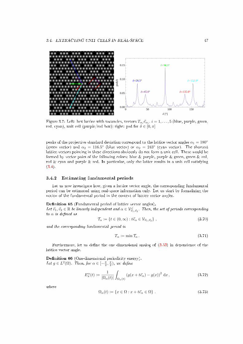
3.4. EXTRACTING UNIT CELLS IN REAL-SPACE 47
0 50 100 1500.00
0.05
0.10
0.15
∆ @°Dps
dH∆
L
∆=90.0°
∆=26.5° ∆=153.0°
∆=135.0°∆=45.0°
Figure 3.7: Left: hex lattice with vacancies, vectors Tαi~eαi , i = 1, . . . , 5 (blue, purple, green,red, cyan), unit cell (purple/red box); right: psd for δ ∈ [0, π]
peaks of the projective standard deviation correspond to the lattice vector angles α1 = 180
(green vector) and α2 = 116.5 (blue vector) or α2 = 243 (cyan vector). The shortestlattice vectors pointing in these directions obviously do not form a unit cell. These would beformed by vector pairs of the following colors: blue & purple, purple & green, green & red,red & cyan and purple & red. In particular, only the latter results in a unit cell satisfying(3.4).
3.4.2 Estimating fundamental periods
Let us now investigate how, given a lattice vector angle, the corresponding fundamentalperiod can be estimated using real-space information only. Let us start by formalizing thenotion of the fundamental period in the context of lattice vector angles.
Denition 65 (Fundamental period of lattice vector angles).Let ~v1, ~v2 ∈ R be linearly independent and α ∈ V∠
~v1,~v2. Then, the set of periods corresponding
to α is dened as
Tα := t ∈ (0,∞) : t~eα ∈ V~v1,~v2 , (3.70)
and the corresponding fundamental period is
Tα := min Tα . (3.71)
Furthermore, let us dene the one-dimensional analog of (3.53) in dependence of thelattice vector angle.
Denition 66 (One-dimensional periodicity energy).Let g ∈ L2(Ω). Then, for α ∈ [−π2 ,
π2 ), we dene
Eαπ (t) :=1
|Ωα(t)|
ˆΩα(t)
(g(x+ t~eα)− g(x))2
dx , (3.72)
where
Ωα(t) := x ∈ Ω : x+ t~eα ∈ Ω . (3.73)

48 CHAPTER 3. PERIODICITY ANALYSIS AND UNIT CELL EXTRACTION
Analogous to Lemma 59, we can conclude that in an ideal setting the fundamental periodcoincides with the smallest non-trivial root of this energy.
Lemma 67 (Fundamental periods as roots of the periodicity energy).Let Ω ⊂ R2 be a bounded domain, ~v1, ~v2 linearly independent and g ∈ L2(Ω) ~v1, ~v2-periodic.Furthermore, let α ∈ V∠
g . Then
Tα = min((Eαπ )−1(0) \ 0
). (3.74)
Again, this characterization is not useful, because due to distortions, noise, as well aserrors in the estimated lattice vector angle, the assumptions in Lemma 67 are far frombeing fullled in practice. Nevertheless, as mentioned earlier, the smoothness introducedby integration typically leads to periods of a lattice vector angle being local minimizers of(3.72).
Denition 68 (Local minimizers of the one-dimensional periodicity energy).The set of isolated local minimizers of (3.72) is dened as
Sα = t ∈ (0,∞) : ∃δ > 0 : ∀s ∈ [t− δ, t+ δ] \ t : Eαπ (t) < Eαπ (s) . (3.75)
Unfortunately, as mentioned before and as illustrated in Figure 3.5, the set of localminimizers may also contain lengths that are not periods of the lattice vector angle, i.e.possibly (minSα) 6= Tα. Thus, it is essential to have a criterion that reliably discriminatesthe desired local minima in Sα, i.e. those corresponding to actual periods of the lattice vectorangle, from all others.
In order to construct such a criterion, let us postulate a few milder assumptions that aretypically fullled in practice, except if the noise or the distortions are extreme.
Assumption 69 (Assumption about local minimizers of the periodicity energy).Let us assume that the following assumptions are fullled in practice up to unavoidable errorsfrom noise, distortions and discretization:
(a) Eαπ is periodic and its fundamental period is equal to Tα
(b) Integer multiples of Tα are local minimizers of Eαπ
(c) arg mint∈Sα Eαπ (t) is an integer multiple of Tα
(d) maxt∈Tα |Eαπ (t)− 1#(Tα)
∑t′∈Tα E
απ (t′)| < mint∈Tα,t′∈Sα\Tα |Eαπ (t)− Eαπ (t′)|
In this context, Tα ⊂ Sα denotes the set of all local minimizers of Eαπ that are integer multi-ples of the fundamental frequency (see (b)). Additionally, we assume that (d) holds exactly,as it already takes into account deviations between energies of dierent local minimizers.
Assumption 69 (d) ensures that minimizers corresponding to an integer multiple of thefundamental frequency can be distinguished from other local minimizers in terms of therabsolute energy. Please note that in an ideal setting, Assumptions 69 (a) to 69 (d) can beinferred from (3.5).
Building on Assumption 69, the core part of the fundamental period recovery will consistof clustering. Thus, let us dene the k-means clustering problem.

3.4. EXTRACTING UNIT CELLS IN REAL-SPACE 49
Denition 70 (The k-means clustering problem [151]).For k ∈ N let S ⊂ Rd be some point set and f ∈ C(Rd). Furthermore, let
Partk(S) :=
(C1, . . . , Ck) ∈ (P(S))
k:
k⋃l=1
Cl = S ∧ Cl, Cm = ∅ ∀l 6= m
(3.76)
denote the set of all partitions of S into k pairwise disjoint sets. Then, the k-means clusteringproblem is given by nding the partition that minimizes the variances of all (function valuesof the) subsets of the partition members:
Ck(S; f) = (C∗1 (S; f)), . . . , C∗k(S; f)) ∈ arg min(C1,...,Ck)∈Partk(S)
k∑l=1
∑x∈Cl
(f(x)− µl(Cl))2 , (3.77)
where
µl(Cl) :=1
# (Cl)
∑x∈Cl
f(x) . (3.78)
Although the k-means clustering problem is NP-hard, ecient algorithms for its ap-proximate solution exist. Both Lloyd's [88] and MacQueen's [89] algorithms are extremelypopular and thus either is often simply referred to as the k-means algorithm, although otherstrategies exist [10]. In the following, we will denote with Ck(S; f) the solution computedby such an approximate solver of the k-means clustering problem.
Finally, we are able to infer a strategy for recovering the fundamental period.
Lemma 71 (Recovering the fundamental period through clustering).Let
k := # (Eαπ (t) : t ∈ Sα ∩ (0, Tα]) , (3.79)
denote the number of dierent isolated local minimizers of Eαπ that are less than or equal tothe fundamental period. Let us stress that this does not count two local minimizers twice incase they have the same energy. Furthermore, without loss of generality, let Ck(Sα;Eαπ ) benumbered such that
arg mint∈Sα
Eαπ (t) ∈ C∗1 (Sα;Eαπ ) . (3.80)
Then, assuming that Assumption 69 is valid, the fundamental period is given as
Tα = minC∗1 (Sα;Eαπ ) . (3.81)
Proof. Assumption 69 (a) implies that there are at most # (Sα ∩ (0, Tα)) classes of localminimizers since the periodicity of Eαπ ensures that all local minimizers corresponding tot > Tα have to be equal in energy to one of the local minimizers with t ≤ Tα. Of course, thenumber of classes might be smaller since multiple local minimizers with t < Tα might happento have the same energy. However, this case is already covered by the denition of k in (3.79)since the set cardinality counts equal energies only once. Assumptions 69 (b) and 69 (d)imply that all integer multiples of the fundamental frequency (including Tα itself) are locatedin the same cluster. Assuming (without loss of generality) that the clusters Ck(Sα;Eαπ ) arenumbered such that (3.80) holds, Assumption 69 (c) implies that C∗1 (Sα;Eαπ ) is the clustercontaining these integer multiples of the fundamental frequency, i.e. C∗1 (Sα;Eαπ ) ⊂ Tα. Asmentioned before, this includes Tα itself, i.e. Tα ∈ C∗1 (Sα;Eαπ ) and thus (3.81) follows fromthe fact that Tα ≤ t for all t ∈ Tα.

50 CHAPTER 3. PERIODICITY ANALYSIS AND UNIT CELL EXTRACTION
Solving the clustering problem in Denition 70 requires a-priori knowledge of the numberof classes. Unfortunately, the denition of k in (3.79) already requires the knowledge of thefundamental period and is therefore of no use in practice. Let us stress that choosing thenumber of classes properly is crucial in this context: on the one hand, if k is too small, itmay happen that t ∈ C∗1 (Sα;Eαπ ) for t < Tα; on the other hand, if k is too large, it mayhappen that Tα /∈ C∗1 (Sα;Eαπ ). In both cases, the fundamental period would be estimatedincorrectly and possibly with a large error.
To resolve this issue, we propose a method that robustly selects the correct number ofclasses k in an unsupervised manner. We base this approach on X-means by Pelleg andMoore [116], which uses a Bayesian information criterion (BIC) assuming identical sphericalGaussian distributions of all clusters to select the most appropriate value of k. We areaware of a similar extension of k-means, called G-means [61], which outperforms X-means,especially in higher dimensions. However, the latter approach is not suitable for our context,where the number of data points # (Sα) is small.
In contrast to [116], we base the selection process for the number of classes on Akaike'sinformation criterion (AIC) [2, 3] instead of BIC. With this decision, we follow a discussionin [30] that points out theoretical and practical advantages of AIC over BIC. Most notably,it enables the evaluation of actual model likelihoods. We will later see that this allows us toidentify ambiguous cases and resolve them through additional information in our context.Before we address the issue of choosing the right number of classes in the clustering problem(3.77), let us start by introducing AIC and the decision strategy it infers. Please note thatdue to our context, we only discuss AIC in the one-dimensional setting.
Let S = x1, . . . , xn ⊂ R denote a set, from now on interpreted as data. Furthermore, letM1, . . . ,Mnmodel
be dierent parametrized models for the data and for k ∈ 1, . . . , nmodel letPk be the space of admissible parameters ofMk. For x ∈ Rn,Mk induces point probabilitiesP (x|Mk(θ)) in dependence of the chosen model parameters θ ∈ Pk. Then, the log-likelihoodof the dataset given the model and a certain choice of the model parameters θ ∈ Pk, isdened as
L (S|Mk(θ)) := log
n∏j=1
P (xj |Mk(θ)) =
n∑j=1
logP (xj |Mk(θ)) , (3.82)
and withLk(S) := max
θ∈PkL (S|Mk(θ)) , (3.83)
we dene the maximum log-likelihood of the set S given the model Mk over all admissibleparameters. The maximizing parameter
θ = arg maxθ∈Pk
L (S|Mk(θ)) , (3.84)
is called maximum likelihood estimator. Finally, Akaike's information criterion is dened as
AICk(S) = −2Lk(S) + 2pk , (3.85)
where pk denotes the number of free parameters of the model, i.e. those that that cannotbe inferred from other parameters.
It turns out that this denition allows for an easy expression of the likelihood of themodels given the data as well.
Lemma 72 (Model likelihoods based on AIC [2,3, 30]).The likelihood of the model Mk given the data S ⊂ Rn is
L(Mk|S) = exp (AICkmin(S)−AICk(S))/2 , (3.86)

3.4. EXTRACTING UNIT CELLS IN REAL-SPACE 51
wherekmin = arg min
k∈1,...,nmodelAICk(S) . (3.87)
In particular, L(Mkmin |S) = 1.
Given a set of models M1, . . .Mnmodel, AIC suggests to choose Mkmin
. However, if thereare models whose likelihoods are not signicantly less than one, they cannot be discardedwith condence. In such a case, additional knowledge might be used to choose the bestmodel among all seemingly equivalent ones.
With this, let us come back to the problem of choosing the right number of classes inclustering problems. In order to apply AIC, we need to model the dataset S. The only priorknowledge available is that S may be split into an unknown number of clusters. Assumingthat at least an upper bound nmodel ∈ N for the number of plausible classes is known, letus generate nmodel models M1, . . . ,Mnmodel
such that the model Mk assumes that the datais made up of k classes. Since no further information on the distribution of the data insideeach cluster is known, we follow the approach in [116] and assume Gaussian distributions.In contrast to [116], however, we will not assume that the standard deviation is identical forall clusters.
Remark 73 (Modeling the number of classes in clustering problems).Let S = x1, . . . , xn ⊂ R be some dataset and f ∈ C(R) be some function and let Mf
k
denote the model representing the (function values of the) dataset as k normally distributed
clusters. Then, Mfk can be characterized by the following probability distribution
P (xj |Mfk (θ)) =
n(j)
n
1√2πσ2
(j)
exp
−(f(xj)− µ(j))
2
2σ2(j)
, (3.88)
and the corresponding model parameters are
θ = (n1, . . . , nk−1, µ1, . . . , µk, σ1, . . . , σk) . (3.89)
Here, nl, µl, σl denote the number of points, mean value and standard deviation of the lth
cluster and
(j) := minl ∈ 1, . . . , k | |f(xj)− µl|2 ≤ |f(xj)− µm|2 ∀l 6= m , (3.90)
represents the cluster membership, i.e. xj is a member of the (j)th cluster. Usually thisrelation is unique. Please note that nk can be inferred explicitly from n1, . . . , nk−1 as nk =∑k−1l=1 nl. Thus, the number of free parameters is pk = 3k − 1 in this case.
We would like to point out that this denition can be extended to higher dimensions ina straight-forward manner. Thus, it might be of use in a wider range of applications and isnot restricted to the clustering of energies, as done here.
The explicit expression of the point probabilities (3.88) allows us to derive the corre-sponding maximum likelihood estimators, as well as the maximum log-likelihood of themodel Mf
k for k = 1, . . . , nmodel.
Lemma 74 (Maximum likelihood of the clustering models).Let S = x1, . . . , xn ⊂ R be a dataset, f ∈ C(R) be a function and k ∈ 1, . . . , nmodel bexed. Furthermore, let the maximum likelihood estimator
θ := (n1, . . . , nk−1, µ1, . . . , µk, σ1, . . . , σk) , (3.91)
52 CHAPTER 3. PERIODICITY ANALYSIS AND UNIT CELL EXTRACTION
denote the maximum likelihood estimator of the model Mfk . Given C∗1 (S; f), . . . , C∗k(S; f),
the solution of the corresponding clustering problem (cf. (3.77)), θ may be estimated as [116]:
nl ≈ # (C∗l (S; f)) ,
µl ≈1
nl
∑x∈C∗l (S;f)∗
f(x) ,
σl ≈
√√√√ 1
nl
∑x∈C∗l (S;f)
(f(x)− µl)2 .
(3.92)
Furthermore, the maximum log-likelihood of the set S given the model Mfk is
Lk(S) =
k∑l=1
[nl log
nln− 1
2nl(log(2πσ2
l
)+ 1)]
. (3.93)
Proof. Combining (3.82) to (3.84) and (3.88) yields
Lk(S) =
n∑j=1
log
[n(j)
n(2πσ2
(j))− 1
2 exp
−|f(xj)− µ(j)|2
2σ2(j)
],
=
k∑l=1
nl lognln− 1
2nl log(2πσ2
l )− nl2σ2
l nl
∑x∈C∗l (S;f)
(f(x)− µl)2 ,
=
k∑l=1
nl lognln− 1
2nl log(2πσ2
l )− 1
2nl .
(3.94)
The expressions in (3.94) are not exact equations since the clustering problem in (3.77)neither accounts for non-uniform prior probabilities of the clusters (ratio between the numberof elements), nor for non-uniform cluster variances. In spite of this, in our one-dimensionalcontext, using k-means yields very good results. However, we would like to stress that inhigher dimensions the anisotropy of clusters might cause signicant problems. In that case,we suggest to turn towards clustering algorithms based on Gaussian mixture models andexpectation-maximization [152].
Now we have everything at hand to compute (3.86) and (3.87) in the context of our prob-lem to choose the right number of classes for clustering local minimizers of the periodicityenergy (3.72). Hence, we can now summarize an according decision strategy.
Algorithm 75 Unsupervised choice of the number of classes in Lemma 71
Let τ > 0 be some threshold such that all models MEαπk with L(M
Eαπk |Sα) > τ may be
regarded as valid. Then, we propose to choose the optimal number of classes for clusteringin Lemma 71 as
k∗ := mink ∈
1, . . . , 1
2# (Sα)
: L(MEαπk |Sα) > τ
. (3.95)
The upper bound of the number of classes stems from the assumption that in order toanalyze the periodicity of the image, its domain should at least be twice as large as its

3.5. NUMERICAL RESULTS 53
fundamental period and thus each cluster should contain at least two elements. Choosingthe model assuming the least classes among all valid models is motivated by the fact thatthis increases the probability that Tα is assigned to the same cluster as arg mint∈Sα E
απ (t).
Note that we use τ = 0.1 for all experiments presented in this work. According to ourexperience, the decision process is not very sensitive to this particular choice.
3.4.3 Selecting a unit cell among all candidates
In the previous sections, we discussed how to retrieve
1) a set of candidate lattice vector angles V∠g (cf. Algorithm 64)
2) for each α ∈ V∠g the corresponding fundamental period Tα (cf. Lemma 71)
Let us now summarize the method we propose for selecting the nal unit cell estimate.
Algorithm 76 Estimating unit cells in real-spaceLet
Vg :=Tα~eα : α ∈ V∠
g
, (3.96)
denote the set of candidate lattice vectors retrieved by estimating lattice vector angles(cf. Algorithm 64) and their corresponding fundamental periods (cf. Lemma 71). Then,according to Remark 31 we propose to select an estimate for a unit cell as follows:
U∗real := (~v1, ~v2), ~v1 := arg min~u∈Vg
‖~u‖2, ~v2 := arg min~u∈Vg\~v1
‖~u‖2 . (3.97)
3.4.4 Local renement of the unit cell
While Algorithm 76 is a good approximation of a unit cell, the sequential strategy of rstestimating lattice vector angles and then the corresponding fundamental frequencies allowsfor an accumulation of errors. Still, the initial guess provided by Algorithm 76 should begood enough to guarantee convergence of an iterative gradient based minimization techniqueto the correct solution when applied to the energy in (3.53). Note that discretizing (3.53)leads to a sum of squares, which allows for Gauss-Newton type algorithms to be used fornumerical optimization. Furthermore, let us point out that in practice the initial guessprovided by Algorithm 76 is usually so close to the optimal solution that the admissible setin (3.54) can be replaced with
Ωε := x ∈ Ω : x+ (~v1, ~v2)~z ± ε~z′ ∈ Ω ∀~z, ~z′ ∈ Z , (3.98)
where typically ε is at most three times the pixel size.
3.5 Numerical results
In the following, we perform a visual inspection of the performance of the real-spacemethod for unit cell estimation based on the same articial and experimental images thatwere used in Section 3.3.5. Note that, like in Section 3.3.5, the origin of illustrated Bravaislattices (red) was aligned manually with the center of an atom in all cases presented in thefollowing. Furthermore, we provide a quantitative comparison of both methods based onthe knowledge of the true geometry of the articial lattices.

54 CHAPTER 3. PERIODICITY ANALYSIS AND UNIT CELL EXTRACTION
Figure 3.8: Unit cells (blue) and crystal lattices (red) of the articial crystal images (cf.Figure 3.1) estimated in real-space (cf. Algorithm 76 + local renement); top row: noisefreecase; bottom row: Gaussian noise case
Figure 3.8 shows the estimated unit cells (blue) and crystal lattices (red) for the articialtest images (cf. Figure 3.1). Except for the noisy Bumps3 image, all unit cells are correct.On the one hand, this already implies an improvement over the reciprocal-space method,which also failed to recognize a unit cell in the Nc3Nm case. On the other hand, thisshows that even the carefully designed clustering may fail in extreme situations. Moreprecisely, the error is due to the local minima of the periodicity energy Eαπ , α = 45 notsatisfying Assumption 69 (d) due to the noise and the small dierence between the localminima belonging to the fundamental period and those belonging to one third and two thirdsof the fundamental period (cf. Figure 3.9). Please note that we deliberately constructedthis example as a particularly challenging case for unit cell recognition and that it is ofsmall concern for real-world applications. Finally, we would like to point out that a visualcomparison of the lattices in Figures 3.3 and 3.8 reveals that the real-space method has anoticeably higher accuracy. This will be conrmed by the quantitative evaluation at the endof this section.
Let us now look at the performance of the real-space unit cell estimation technique onthe experimental HAADF-STEM images (previously shown in Figure 3.4). The unit cells(blue) and crystal lattices (red) estimated by the proposed real-space method are shown inFigure 3.10. Comparing both gures, we see that the real-space method gives the correctresult in all cases. Most notably, it correctly identies a unit cell in the GaN image, wherethe reciprocal-space method failed. Furthermore, the overall accuracy of the unit cellsestimated in reciprocal-space is surpassed signicantly by that of the unit cells estimated inreal-space.
Finally, let us regard the quantitative evaluation shown in Table 3.1. For each of thearticial crystal images (cf. Figure 3.1) (noisefree and aected by Gaussian noise) and bothproposed methods (reciprocal- and real-space) it gives the Euclidean distance between theestimated unit cell and the best-approximation among all true unit cells of the correspondingcrystal. First of all, we observe a very large error for the noisy Nc3Nm image when using

3.6. CONCLUSIONS 55
0 20 40 60 80 100 1200
0.25
0.5
0.75
1
1.25
1.5Gaussian noise
noisefree
t
Eα π
(t)
Figure 3.9: Periodicity energies (cf. (3.72)) for α = 45 (diagonal lattice direction) for thenoisefree (blue crossed) and Gaussian noise (red dotted) Bumps3 image in Figure 3.1
Figure 3.10: Unit cells (blue) and crystal lattices (red) of the experimental HAADF-STEMimages (cf. Figure 3.4) estimated in real-space (cf. Algorithm 76 + local renement)
the reciprocal-space method, as well as for the Bumps3 image when using either method.This was expected, since we had already visually conrmed that the methods fail to recognizea unit cell at all in the respective cases. Moreover, we see that among the remaining cases,there is only a single one where the reciprocal-space method is more accurate than the real-space one. In all other cases, the real-space method's accuracy is at least twice as good asthat of the reciprocal-space technique. Most notably, except for the (rather delicate) noisyBumps3 image, the real-space yields sub-pixel accuracy in all cases.
Please note that for the sake of demonstrating the benets of the real-space method, weused the full real-space framework including the local renement. However, we would like topoint out that the local renement can of course also be applied to the unit cells estimatedin reciprocal space and we expect a similar overall accuracy in case the initial guess is notmuch more than a pixel away from the solution.
3.6 Conclusions
In this chapter, we proposed two distinct methods for the unsupervised estimation ofunit cells in crystal images. The rst is based on extracting peaks from the power spectrum

56 CHAPTER 3. PERIODICITY ANALYSIS AND UNIT CELL EXTRACTION
σmax g−min g Crystal ‖U∗FFT − PU(U∗FFT)‖2 ‖U∗real − PU(U∗real)‖2
0
Bumps3 1.6364 1.2475 × 10⁻⁵
SingleDouble 0.6000 9.8073 × 10⁻⁶
HexVacancy 0.5143 1.6476 × 10⁻⁵
Nc3Nm 1.9793 0.0609
0.5
Bumps3 20.1538 20.4219SingleDouble 0.6000 0.3636HexVacancy 0.5143 0.6068Nc3Nm 24.4461 0.3591
Table 3.1: Dierence between the unit cells detected in reciprocal space (cf. Algorithm 56)(third column) or real-space (cf. Algorithm 76 + local renement) (fourth column) and theclosest unit cell of the true lattice for the crystals shown in Figure 3.1
of the given image and an explicit relation between the corresponding reciprocal latticeand the desired direct lattice. The second combines a real-space lattice angle estimationmethod proposed by Sang & LeBeau [127] with a novel real-space method for estimatingfundamental periods. The latter is done by locally minimizing a suitable periodicity energy.This involves the problem of selecting the local minimum corresponding to the fundamentalperiod among multiple other local minima of possibly similar energy. We presented a solutionto this problem via clustering. In this context, building on X-means, an improved strategyfor selecting the most suitable number of clusters in an unsupervised manner was proposed.It is based on a data model allowing dierent variances for each cluster, as well as modellikelihoods derived from AIC.
Results on articial and experimental HAADF-STEM images demonstrate that bothproposed methods for unit cell estimation are suitable for real-world applications. However,the real-space method shows higher robustness against noise and image distortions, as wellas increased accuracy.

Chapter 4
Feature-based crystal image
segmentation
In this chapter, we will present a novel technique for multi-phase segmentation of imagesinto dierent structures described by high-dimensional features. The focus will be on theapplication of most interest to this work, namely crystal segmentation. However, we will alsocover the segmentation of textures, EELS spectral data, as well as sub-space segmentationin the context of multi-spectral biological data.
The chapter opens with an introduction to image segmentation and the practical rele-vance of segmentation by structure. Then, the Mumford-Shah model for image segmentationis introduced, followed by a discussion on numerical optimization for such types of varia-tional problems, most importantly, recalling the Chambolle-Pock algorithm. We continueby introducing the notion of high-dimensional local features for structure or pattern recog-nition and discuss how this can be integrated into the multi-phase segmentation framework,including proper initialization of features. Furthermore, we propose some ideas on how tohandle heterogeneous background that does not t within the Mumford-Shah setting, aswell as how to nd additional regions in the case that not all desired regions can be ini-tialized. We nish the chapter with a numerical evaluation of the proposed method on 1)exemplary HAADF-STEM crystal images, 2) the Prague texture segmentation benchmarkand 3) multi-spectral EELS and biological data.
The methods proposed in Section 4.3 of this chapter were published in [101].
4.1 Introduction
Image segmentation is one of the fundamental tasks in image processing. Its objectiveis to decompose an image into disjoint regions, such that each region has a dierent, yetroughly homogeneous structure (in a suitable sense). As we will see later, the diculty of thisproblem increases signicantly when more than two regions are sought. In order to clarifythe setting (two regions versus three or more regions), the term multi-phase segmentationis typically reserved for the case that more than two regions are sought.
Image segmentation has been studied thoroughly and the literature oers a wide rangeof dierent concepts for its solution. Examples are fuzzy region competition [85], contourdetection [8], random walks [36] and Markov random elds [86], just to name a few. Dueto the richness of dierent methods we refrain from giving a comprehensive list here, butrefer the interested reader to review articles on this topic, e.g. [69, 142]. In this work, we
57

58 CHAPTER 4. FEATURE-BASED CRYSTAL IMAGE SEGMENTATION
will focus on variational image segmentation, which is based on the famous Mumford-Shahmodel [108].
The simplest and best understood type of image segmentation problems is the division ofimages into regions based on their gray or color intensities [35]. More complex is the problemof segmenting images based on their local structure. This problem is under highly activeresearch due to the vast variety of relevant applications, ranging from texture segmentation[122] over scene segmentation [130] to a multitude of tissue recognition tasks in medicalimaging, e.g. blood vessels [54], bones [71] and tumors [57].
Structure classication is typically done by analyzing local image properties such as theimage intensity, position and orientation of edges, or frequency spectrum [137]. Within thecontext of texture segmentation, the most successful structure analysis tool is arguably theGabor lter [148]. The ability to discriminate structures is often improved by combiningmultiple lters of the same type, but with dierent parameters, or of dierent type (e.g.intensity, Laplacian-of-Gaussian) in so-called local spectral histograms [87]. A thoroughlystudied alternative is given by the class of linear transforms, such as wavelet transforms [34],the (short-time) Fourier transform [11], as well as the (more recent) Stockwell transform[44]. We will later see that localized Fourier transforms perform very well at discriminatingdierent crystal geometries in images, which is due to the properties discussed in Chapter 3.
On the one hand, complex structures are often described by a high-dimensional set ofparameters. On the other hand, in many image segmentation applications, the number ofsought regions, and thus the number of structure categories of interest, is small. There-fore, in many cases, it is expected that suitable lower-dimensional representations of localstructures suce for an assignment to the regions of interest. This requires techniques fordimensionality reduction, which is an immensely broad topic [141] with applications in verydierent areas of research. The most widely used techniques in this context are cluster-ing [113] and principal component analysis (PCA) [73] (as well as its related variants, suchas singular value decomposition (SVD)). These two concepts are related to each other in thesense that the relaxed solution of k-means can be expressed as principal components [43].In the context of variational image segmentation, PCA has been used before, both for di-mension reduction [112] and to increase the contrast of color-texture indicators in naturalimages [62].
Finally, let us point out that structure-based segmentation is of great importance inmaterials science, namely for crystal analysis. Although there exist sophisticated methodswith a large degree of automation [17,21,47], they 1) only cope with changes in the crystalorientation and 2) require prior knowledge of a unit cell. In this chapter, we will presenta method that, like the aforementioned ones, is based on a Mumford-Shah type functional,but through the use of dierent indicators eliminates the existing problems, allowing fortruly unsupervised segmentation of complex crystal images.
4.2 Variational image segmentation
In this section, we discuss the general concept of variational problems. We have alreadyseen one in Section 3.4, which was tied to the functional in (3.53). Here, we focus on vari-ational image segmentation. We begin with a denition of the term variational problemand then recall important theoretical aspects on the existence and characterization of min-imizers. Furthermore, we discuss how solutions can be obtained in practice via numericaloptimization. Finally, we introduce the two- and multi-phase Mumford-Shah model for im-age segmentation. We will see that whereas the two-phase case leads to an eciently solubleconvex optimization problem, the multi-phase case turns out to be quite dicult.

4.2. VARIATIONAL IMAGE SEGMENTATION 59
4.2.1 The generic and classical variational problem
To start o, let us formulate what is exactly meant by the term variational problem.Let (X, ‖ · ‖) be a normed vector space, M ⊂ X and J : M → R. Then, the followingminimization problem
nd y∗ ∈M s.t. J [y∗] ≤ J [y] ∀y ∈M . (4.1)
is often called variational problem in the context of the calculus of variations.As we see, variational problems are essentially classical optimization problems. The
major dierence is that innite-dimensional admissible sets and spaces are allowed (andtypically used). To get a better impression of the setting, let us also dene the classicalformulation of variational problems, which is restricted to a special integral form and certainconditions on the objective functional.
Let Ω ⊂ Rd be a bounded region with piecewise smooth boundary and
f : Ω× R× Rd → R, (x, y, ξ) 7→ f(x, y, ξ) (4.2)
continuous and continuously dierentiable with respect to the second and third variable.Furthermore, let
J : C1(Ω)→ R, y 7→ J [y] :=
ˆΩ
f(x, y(x),∇y(x)) dx . (4.3)
Then the variational problem corresponding to f (or J) is
nd y∗ ∈ arg miny∈C1(Ω)
J [y] . (4.4)
Now it is important to note that some of the theory used in classical (nite-dimensional)optimization is, in general, not valid in innite-dimensional spaces. Thus, in the following,we recall the most important propositions regarding necessary and sucient conditions forthe existence, uniqueness and characterization of global and local minimizers.
4.2.2 Necessary and sucient conditions for minimizers
A very central mathematical object for the characterization of minimizers of variationalproblems is the Gâteaux dierential, which provides an innite-dimensional analog of thegradient.
Denition 77 (Gâteaux dierential [24]).Let X be a vector space, D ⊂ X open and J : D → R. Furthermore, let ε0 > 0 and y, z ∈ Xbe such that y + εz ∈ D for all ε ≤ ε0. Then, if the following limit exists
〈J ′[y], z〉 := limε→0
J [y + εz]− J [y]
ε, (4.5)
it is called Gâteaux dierential of J at y in the direction z. Moreover, if X is normed and
J ′[y] : X → R, z 7→ 〈J ′[y], z〉 , (4.6)
is linear and continuous, then J is called Gâteaux dierentiable at y and J ′[y] is calledGâteaux derivative (or rst variation) of J at y.

60 CHAPTER 4. FEATURE-BASED CRYSTAL IMAGE SEGMENTATION
Note that for X = Rn, J ∈ C1(D), we receive 〈J ′[y], z〉 = ∇J(y) ·z for all z ∈ Rn. Thus,the Gâteaux dierential is consistent with the classical derivative in nite dimensions. Nowwe can directly formulate a necessary condition for global and local minimizers.
Theorem 78 (Necessary condition for global and local extrema [24]).Let (X, ‖ · ‖) be a normed vector space, M ⊂ X and J : M → R. Furthermore, let y∗ ∈ Mbe a solution of (4.1), ε0 > 0 and z ∈ X such that y∗ + εz ∈ M for all ε ≤ ε0. Then, if〈J ′[y∗], z〉 exists, the following necessary condition holds
〈J ′[y∗], z〉 = 0. (4.7)
(4.7) also holds in case y∗ in the interior of M is a local minimum of J and 〈J ′[y∗], z〉 exists.
In the case of the classical variational problem in (4.4), this necessary condition canbe reformulated in terms of a boundary value problem, i.e. a system of partial dierentialequations with a prescribed boundary condition.
Theorem 79 (Euler-Lagrange equation [24]).Let Ω ⊂ Rd be a bounded region with a piecewise smooth boundary, J, f as in (4.2) and (4.3)and y∗ ∈ C1(Ω) be a solution of (4.4). Also, let y∗ ∈ C2(Ω) and f ∈ C2. Then y∗ solves
∂yf (x, y∗(x),∇y∗(x))− divx (∇ξf (x, y∗(x),∇y∗(x))) = 0 ∀x ∈ Ω ,
∇ξf (x, y∗(x),∇y∗(x)) · ν = 0 ∀x ∈ ∂Ω .(4.8)
Here, ν is the normal on ∂Ω. (4.8) is called Euler-Lagrange equation of (4.4). The secondequation is also called natural boundary condition.
As the major tool for proving this theorem is a very deep result itself (and thus alsocalled fundamental lemma), let us recall it briey.
Lemma 80 (Fundamental lemma (in the calculus of variations) [24]).Let Ω ⊂ Rn be a non-empty domain and y ∈ L1
loc(Ω). Then, the following propositions are
equivalent:
(i) y = 0 almost everywhere in Ω ,
(ii)´
Ωy(x)φ(x) dx = 0 for all φ ∈ C∞0 (Ω) .
This lemma shows how integral expressions induced by testing J with directions z ∈ Xcan be transformed into point-wise expressions for the integrand f in (4.2).
Now let us have a look at sucient conditions for minimizers. It turns out that, asin classical optimization, necessary conditions are also sucient in the case that both theobjective functional and the admissible set are convex.
Lemma 81 (Sucient conditions for minimizers of (4.1) and (4.4) [24]).Let X be a normed vector space, M ⊂ X convex, U an open neighborhood of M and J :U → R Gâteaux dierentiable and convex. Furthermore, let y∗ ∈M with 〈J ′[y∗], z〉 = 0 forall z ∈ X. Then y∗ solves (4.1).
Furthermore, given that f ∈ C2 has the form given in (4.2) and is convex in its secondand third argument, as well as that y∗ ∈ C2(Ω) be a solution of the Euler-Lagrange (4.8).Then y∗ solves (4.4). Moreover, if f is strictly convex in its second and third argument, thesolution of (4.4) is unique.

4.2. VARIATIONAL IMAGE SEGMENTATION 61
Finally, let us recall that the uniqueness of minimizers is also granted in the generalconvex case.
Theorem 82 (Uniqueness of minimizers of strictly convex functionals [24]).Let X be a vector space, M ⊂ X convex and J : M → R strictly convex. Then there existsat most one global minimizer of J over M .
4.2.3 Existence of minimizers
Let us recall one of the fundamental tools used in the calculus of variations to prove theexistence of minimizers of functionals, namely the so-called direct method of the calculus ofvariations. In order to formulate it, we need to dene (lower) semicontinuity.
Denition 83 (Lower semicontinuity [24]).Let X be a topological space and J : X → R∪∞. Then J is lower semicontinuous (l.s.c.)if and only if
J [u] ≤ lim infn→∞
J [un] , (4.9)
holds for all convergent sequences (un)n∈N ⊂ X, u ∈ X with limn→∞ un = u.
Assumption 84 (Direct method (in the calculus of variations)).Let X be a topological vector space and J : X → R. Furthermore, assume that
(a) there exists (un)n∈N ⊂ X such that limn→∞ J [un] = infu∈X J [u] > −∞ ,
(b) there exists (unk)k∈N ⊂ X and u∗ ∈ X such that limk→∞ unk = u∗ ,
(c) J is lower semicontinuous .
Lemma 85 (Direct method (in the calculus of variations) [24]).Let X be a topological vector space and J : X → R. Then, given that Assumptions 84 (a)to 84 (c) hold, u∗ in Assumption 84 (b) solves (4.1).
Proof. Let J
:= infu∈X J [u]. Then
J≤ J [u∗] ≤ lim inf
k→∞J [unk ] = lim
k→∞J [unk ] = lim
n→∞J [un] = J
. (4.10)
The existence of a convergent subsequence is often inferred through the boundedness ofthe minimizing sequence. However, in innite-dimensional spaces this implication does notgenerally hold. Fortunately, there is a dierent notion of convergence which resolves thisproblem for a relevant class of spaces. Before we treat this, we reformulate Lemma 85 usingthe following assumptions, which are more suitable for the following discussion:
Assumption 86 (Direct method (using sequential compactness)).Let X be a normed vector space, J : X → R, c→ a convergence criterion and assume that
(a) J is bounded below ,
(b) (J [un])n∈N bounded ⇒ (un)n∈N bounded for all (un)n∈N ⊂ X ,
(c) B‖·‖1 (0) = u ∈ X : ‖u‖ < 1 is sequentially compact (w.r.t.
c→) ,
(d) J is lower semicontinuous (w.r.t.c→) .

62 CHAPTER 4. FEATURE-BASED CRYSTAL IMAGE SEGMENTATION
Lemma 87 (Direct method (using sequential compactness) [24]).Let X be a normed vector space, J : X → R and
c→ be some convergence criterion. Thengiven that Assumptions 86 (a) to 86 (d) hold, there exists a solution u∗ ∈ X of (4.1).
Proof. Assumption 86 (a) implies J
:= infu∈X J [u] > −∞. Thus, there exists a minimizingsequence (un)n∈N ⊂ X. This implies Assumption 84 (a), as well as the boundedness of(J [un])n∈N. Now, due to Assumption 86 (b), (un)n∈N is also bounded. Noting that As-sumption 86 (c) implies that any bounded sequence in X has a subsequence that convergesin X, we receive Assumption 84 (b). Together with Assumption 86 (d) all conditions ofLemma 85 are met.
The boundedness of the functional of interest from below is obviously the most funda-mental necessary condition for the existence of a minimizer and typically easy to prove. Theboundedness of the minimizing sequence with respect to the norm can also often be proveddirectly using some sort of relation between the functional value and its argument. Asmentioned before, proving the sequential compactness of the closed unit ball within innite-dimensional spaces is more delicate. This leads us to the notion of weak convergence, whichis based on dual spaces.
Denition 88 (Topological dual space [24]).Let X a topological vector space (over a eld F). Then
X ′ := u : X → F : u linear and continuous , (4.11)
is called the topological or continuous dual space of X.
Based on the context, X ′ is often simply referred to as dual space. We follow thisconvention in this chapter. The dual space X ′ induces the following operator norm:
|||u′||| := sup‖u‖≤1
|〈u′, u〉| , u′ ∈ X ′ . (4.12)
Denition 89 (Weak convergence [24]).Let X be a normed vector space. Then, a sequence (un)n∈N ⊂ X is convergent to u ∈ X inthe weak topology if and only if
〈u′, un〉 → 〈u′, u〉 ∀u′ ∈ X ′ . (4.13)
We also say (un)n∈N ⊂ X converges weakly to x ∈ X and denote this by un u. Further-more, a sequence (u′n)n∈N ⊂ X ′ is convergent to u′ ∈ X ′ in the weak-* topology if and onlyif
〈u′n, u〉 → 〈u′, u〉 ∀u ∈ X . (4.14)
Analogously, we also say (u′n)n∈N ⊂ X ′ convereges weakly−∗ to u′ ∈ X ′ and denote this by
u′n∗ u′.
Please note that these convergence criteria give rise to corresponding notions of weak(-*)sequential compactness and weak(-*) lower semicontinuity. Furthermore, note that weakconvergence is weaker than convergence with respect to the norm (strong convergence),since the latter implies the former. In contrast to that, weak semicontinuity is stronger than(strong) semicontinuity, since it requires (4.9) to hold for more sequences.
Now, let us recall a very important result on weak-* sequential compactness of certainspaces that, as we will see later, also applies to the function space employed in the Mumford-Shah model.

4.2. VARIATIONAL IMAGE SEGMENTATION 63
Theorem 90 (On separability and weak-* sequential compactness of unit balls [4]).Let X be a separable normed vector space (i.e. X has a countable dense subset). Then
B|||·|||1 (0) = u′ ∈ X ′ : |||u′||| < 1 ⊂ X ′ , (4.15)
is weakly-* sequentially compact.
Later, we will also need an analog result for weak sequential compactness, that holds forreexive Banach spaces, which we will dene now.
Denition 91 (Reexivity [4]).Let X be a normed vector space. Then, X is called reexive if and only if X and X ′′ areisomorphic with respect to the isometry
JX : X → X ′′ , x 7→ (x′ 7→ 〈x′, x〉) . (4.16)
Theorem 92 (On reexivity and weak sequential compactness of unit balls [4]).Let X be a reexive Banach space. Then
B‖·‖1 (0) = u ∈ X : ‖u‖ < 1 ⊂ X , (4.17)
is weakly sequentially compact.
4.2.4 Numerical minimization of variational problems
In the following, we recall three concepts for numerical optimization of variational prob-lems, namely gradient descent, gradient ow and primal-dual methods. Let us begin withthe most straight-forward method: the gradient descent.
Algorithm 93 The gradient descent method [14]
Let J ∈ C1(Rd) and u0 ∈ Rd. Then, nding a solution u : [0, T ] → Rd of the ordinarydierential equation
d
dtu(t) = −∇J(u(t)) ∀t ∈ (0, T ) ,
u(0) = u0 ,(4.18)
in order to obtain a minimizer of J is called gradient descent method.
Lemma 94 (Validity of the gradient descent method [14]).Let J ∈ C1(Rd), u0 ∈ Rd and u : R≥0 → Rd be the solution of (4.18). Then,
J(u(t)) ≤ J(u0) ∀t ∈ [0, T ) . (4.19)
The above inequality is strict, if ∇J(u0) 6= 0.
Now let us look at a generalization of the gradient descent method to innite dimensionalspaces, namely the gradient ow method.

64 CHAPTER 4. FEATURE-BASED CRYSTAL IMAGE SEGMENTATION
Algorithm 95 The gradient ow method [14]Let H be a Hilbert space with scalar product g : H × H → R and J : H → R Gateauxdierentiable on H. Furthermore, note that according to the Riesz representation theorem,there exists an isomorphism
A : H → H ′, u 7→ Au, s.t. g(u, v) = 〈Au, v〉 ∀u, v ∈ H . (4.20)
Using this, we dene the gradient of J with respect to g as
gradgJ [u] := A−1J ′[u] for u ∈ H . (4.21)
Finally, for u0 ∈ H, the gradient ow method consists in nding a solution u : [0, T ] → Hof the ordinary dierential equation
∂tu(t) = −gradgJ [u(t)] = −A−1J ′[u(t)] ∀t ∈ (0, T ) ,
u(0) = u0 .(4.22)
We see that the gradient ow is similar to the gradient descent, except that in the gradientow, the scalar product g inuences the descent direction. One may take advantage of thisfact by choosing g such that it favors desired minimizers. For instance, in case one desiressmoothness of minimizers, one may choose a scaled H1-scalar product (cf. [136]).
In practice, one may use forward Euler discretization to solve the ODEs of the gradientdescent (or gradient ow) method. However, one has to choose the step size carefully, sinceconvergence is not guaranteed for all step sizes. A popular step size control mechanism isthe so-called Armijo rule (cf. [9]).
Now let us investigate a theoretically more involved strategy for minimizing functionalsbased on the proximal mapping. Before we introduce this map, let us prepare the theorythat will grant its well-denedness. First, we introduce the eective domain and epigraph,through which we dene the space of closed proper convex functions.
Denition 96 (Eective domain and epigraph [24]).Let X be a vector space and J : X → R∞. Then,
dom(J) := u ∈ X : J [u] <∞ , (4.23)
is called eective domain of J and
epi(J) := (u, t) ∈ X × R : J [u] ≤ t , (4.24)
is called epigraph of J . Furthermore, let us denote the set of closed proper convex functionson X with
Γ0(X) := J : X → R∞ : J convex, dom(J) 6= ∅, epi(J) closed . (4.25)
This allows us to formulate the following result.
Theorem 97 (Weak lower semicontinuity of closed proper convex functionals [4, 24]).Let X be a Banach space and J ∈ Γ0(X). Then, J is weakly lower semicontinuous and forany t ∈ R
u ∈ X : J [u] ≤ t , (4.26)
is weakly sequentially closed.

4.2. VARIATIONAL IMAGE SEGMENTATION 65
Now, we can dene the proximal mapping.
Theorem 98 (Proximal mapping [125]).Let X be a reexive Banach space and J ∈ Γ0(X). Then the mapping
proxJ : X → X, v 7→ arg minu∈X
(J [u] +
1
2‖u− v‖2
), (4.27)
is well-dened and called proximal mapping.
The proof of the existence of a unique minimizer of
pv[u] := J [u] +1
2‖u− v‖2 , (4.28)
in (4.27) and thus the well-denedness of the proximal mapping can be done via the directmethod (cf. Lemma 85). It relies mainly on the weak lower semicontinuity of J and theweak sequential closedness of the super-level set
u ∈ X : pv[u] ≤ pv[z] (4.29)
for z ∈ dom(J) that are granted by Theorem 97. The uniqueness of the minimizer followsfrom the fact that pv is strictly convex on the convex set dom(J).
In the following, let us recall some important properties of the proximal mapping thatwill lead to a practical algorithm for nding minimizers of functionals. First, however, weneed to dene the subdierential.
Denition 99 (Subgradient and subdierential [24]).Let X be a normed vector space and J : X → R∞ be convex. Then u′ ∈ X ′ is calledsubgradient of J at u ∈ X if and only if
J [u] + 〈u′, v − u〉 ≤ J [v] ∀v ∈ X . (4.30)
Furthermore, we denote with
∂J [u] := u′ ∈ X ′ : u′ fullls (4.30) , (4.31)
the subdierential of J at u.
Lemma 100 (The proximal mapping, subdierential & minimizers [106,124]).Let J ∈ Γ0(X), τ > 0, u, u∗ ∈ X. Then,
(a) u∗ ∈ arg minv∈X J [v]⇔ u∗ = proxτJ [u∗] ,
(b) u ∈ u∗ + τ∂J [u∗]⇔ u∗ = proxτJ [u] ,
(c) proxτJ [u] = (1+τ∂J)−1
[u] ,
(d) u∗ ∈ ∂J [u]⇔ u = proxτJ [u+ τu∗] .
From now on, let us regard the nite-dimensional setting, i.e. the minimization problem(4.1) after domain discretization. Then, using Lemma 100 (a) we can directly motivate theproximal point method.

66 CHAPTER 4. FEATURE-BASED CRYSTAL IMAGE SEGMENTATION
Algorithm 101 Proximal point method [124]
Let J ∈ Γ0(Rd), u0 ∈ Rd and τ > 0. Then, the iteration
uk+1 := proxτJ(uk) , (4.32)
is called proximal point method.
In case the functional consist of a dierentiable part, this may be generalized to theproximal gradient method.
Algorithm 102 Proximal gradient method [125]
Let J = G + H, where G ∈ C1(Rd) ∩ Γ0(Rd) and H ∈ Γ0(Rd). Furthermore, let u0 ∈ Rdand (τk)k∈N ⊂ R>0. Then, the iteration
uk+1 := proxτkH(uk − τk∇G(uk)
)(4.33)
is called proximal gradient method.
Please note that for G = 0, H = J the proximal gradient method reduces to the proximalpoint method and for G = J,H = 0 it reduces to the gradient descent method.
Convergence (at linear rate) of the proximal gradient method (and thus also of theproximal point and gradient descent methods) can be proven, given that the gradient of thedierentiable part of the functional is Lipschitz continuous.
Theorem 103 (Linear convergence of the proximal gradient method [32]).Let J , G, H be as in Algorithm 102. Additionally, let ∇G be Lipschitz continuous withconstant L, τmin ∈ (0, 1
L ] and τk ∈ [τmin,1L ]. Then, given that there exists a minimizer u∗
of J , the proximal gradient method converges and
0 ≤ J(uk)− J(u∗) ≤ 1
2kτmin‖u0 − u∗‖22 = O( 1
k ) , (4.34)
holds.
Using the Fenchel conjugate, we can nally formulate a primal-dual method that isparticularly suited for a wide range of image processing related variational problems, wherethe functional may be split into a data term and a (total-variation based) regularizer, whichapplies also to the Mumford-Shah functional, as we will see later.
Denition 104 (Fenchel conjugate [24]).Let X be a Banach space and J : X → R∞ be proper (i.e. dom(J) 6= ∅). Then,
J∗ : X ′ → R∞, u′ 7→ supu∈X
(〈u′, u〉 − J [u]) (4.35)
is called Fenchel conjugate or dual functional of J .
Theorem 105 (Fenchel-Moreau [12]).Let X be a Hilbert space and J : X → R∞ be proper (i.e. dom(J) 6= ∅). Then, the followingare equivalent:
1. J is lower semicontinuous and convex ,
4.2. VARIATIONAL IMAGE SEGMENTATION 67
2. J = J∗∗ .
Let G ∈ Γ0(Rn), H ∈ Γ0(Rm) and A : Rn → Rm be linear. Furthermore, let
J(u) := G(u) +H(Au) , u ∈ Rn . (4.36)
Then, the primal problem (4.1) can be expressed equivalently as the following primal-dualproblem
infv∈Rn
J(v) = infv∈Rn
supr∈Rm
(〈Av, r〉+G(v)−H∗(r)) , (4.37)
and, for u ∈ Rn, p ∈ Rm, the necessary conditions for optimality are
Au ∈ ∂H∗(p) ,
−ATp ∈ ∂G(u) .(4.38)
which, according to Lemma 100 (d) is equivalent to
p = proxσH∗ (p+ σAu) ,
u = proxτG(u− τATp
).
(4.39)
for τ, σ > 0.Finally, this motivates the primal-dual method, also named Chambolle-Pock algorithm
after the authors who rst proposed it [32].
Algorithm 106 Primal-dual method [32]
Given initial values u0 = u0 ∈ Rn,p0 ∈ Rm and θ ∈ [0, 1], the primal dual method reads asfollows
pk+1 = proxσH∗(pk + σAuk
),
uk+1 = proxτG(uk − τATpk+1
),
uk+1 = uk+1 + θ(uk+1 − uk) .
(4.40)
The stopping criteria used in this work are
‖uk+1 − uk‖2 < εCP , (4.41)
for some εCP > 0, as well as an upper bound for the number of iterations, i.e. k ≤ kCPmax.
Please note that in the literature, the Chambolle-Pock algorithm is often formulatedusing the so-called resolvent operator (1+τ∂J)
−1 instead of the proximal mapping proxτJ .The justication for this is given by Lemma 100 (c).
4.2.5 The two-phase Mumford-Shah model
Now that we have the relevant theory at hand, let us return to our original goal ofsegmenting images into pairwise disjoint homogeneous (in a suitable sense) regions. Forthis section, let us assume that the number of desired regions is equal to two. Then, givensuitable indicator functions f1, f2 : Ω→ R≥0, i.e. for x ∈ Ω, i.e. fl(x) measures how well thepoint x ts into the region Ωl (a smaller value corresponds to a better t), a straight-forwardapproach to segmentation is
Ω∗1 := x ∈ Ω : f1(x) < f2(x) , Ω∗2 := Ω \ Ω∗1 . (4.42)
68 CHAPTER 4. FEATURE-BASED CRYSTAL IMAGE SEGMENTATION
However, in practice, the region indicators are typically not perfectly reliable and thus sucha solution will be subject to signicant noise. In order to promote connectedness of regions,or, in other words, regularity of the segments, it is benecial to penalize the perimeter ofthe regions Ω1,Ω2. This leads to the two-phase Mumford-Shah model.
Given a bounded domain Ω ⊂ Rd let
UMS(Ω) := O′ ⊂ Ω : O′measurable, Per(O,Ω) <∞ , (4.43)
where Per(O,Ω) denotes the perimeter of the set O in Ω (cf. [5]). Then, given f1, f2 ∈ L1(Ω)with f1, f2 ≥ 0 almost everywhere in Ω and λ > 0, for O ∈ UMS(Ω), the minimizationproblem associated with the energy
EMS[O] :=
ˆOf1(x) dx+
ˆΩ\O
f2(x) dx+ λPer(O,Ω) , (4.44)
is called two-phase Mumford Shah model [108].In its current form, this problem does not t within the context of variational optimiza-
tion, since the argument of the energy in (4.44) are sets, not functions. This can be alleviatedby replacing the sets with their corresponding characteristic functions. This would resultin a straight-forward reformulation of the integral expressions. However, in order to seehow the perimeter can be equivalently expressed using characteristic functions, we have tointroduce the space of functions of bounded variation, and, in particular, the correspondingtotal variation semi-norm.
Denition 107 (Total variation and functions of bounded variation [5]).Let Ω ⊂ Rd be a bounded domain and u ∈ L1(Ω). Furthermore, let
P :=p ∈ C∞c (Ω,Rd) : ‖‖p‖2‖L∞ ≤ 1
. (4.45)
Then, the total variation is dened as
|u|BV(Ω) := supp∈P
ˆΩ
u(x) div p(x) dx . (4.46)
The space of functions of bounded (total) variation is dened as
BV(Ω) :=u ∈ L1(Ω) : |u|BV(Ω) <∞
. (4.47)
Remark 108 (Bounded variation norm [5]).The following expression denes a norm on BV(Ω)
‖u‖BV(Ω) := ‖u‖L1(Ω) + |u|BV(Ω) . (4.48)
Naturally, it is referred to as the bounded variation norm.
The total variation is a generalization of the size of the gradient for non-dierentiablefunctions. In particular, the total variation of a characteristic function measures the size ofits jump set, or, in other words, the perimeter of the corresponding domain, which is exactlywhat we had required earlier.
Lemma 109 (Representing the perimeter through the total variation [5]).Let Ω ⊂ Rd be a bounded domain and u ∈ C1(Ω). Then
|u|BV(Ω) =
ˆΩ
‖∇u(x)‖2 dx . (4.49)

4.2. VARIATIONAL IMAGE SEGMENTATION 69
Furthermore, for a measurable set O ⊂ Ω,
|χO|BV(Ω) = Per(O,Ω) . (4.50)
Nikolova, Esedoglu and Chan proposed to reformulate the Mumford-Shah problem asa variational problem over BV as follows. First, the integration over the set O (and itscomplement) in (4.44) are extended to the entire domain Ω and instead truncated by multi-plication of the integrands with a characteristic function (and one minus the characteristicfunction), respectively. Then, in order to retrieve a convex problem, the constraint that theadmissible functions must have values in 0, 1 is relaxed to the set [0, 1]. Fortunately, itcan be proven that this relaxation does not aect the solution of the problem:
Lemma 110 (The Nikolova-Esedoglu-Chan model [33]).For u ∈ BV(Ω; [0, 1]), the minimization problem associated with the functional
JNEC[u] :=
ˆΩ
u(x)f1(x) + (1− u(x))f2(x) dx+ λ|u|BV(Ω) , (4.51)
is called Nikolova-Esedoglu-Chan model. The corresponding admissible set is
UNEC := BV(Ω; [0, 1]) . (4.52)
Furthermore, for c ∈ [0, 1),
u∗ ∈ arg minu∈UNEC
JNEC[u]⇒ x ∈ Ω : u(x) > c ∈ arg minO∈UMS(Ω)
EMS[O] . (4.53)
As mentioned earlier, the advantage of this problem is that it is convex and thus a globalminimizer can be obtained eciently using the primal-dual method in Algorithm 106. Inorder to prove the existence of a minimizer we require the following theorems.
Theorem 111 (The unit ball in BV is weakly-* sequentially compact [5]).Let Ω ⊂ Rd be a bounded domain. Then BV(Ω) is the dual space of a separable normedvector space. Thus, according to Theorem 90, the unit ball in BV(Ω) is weakly-* sequentiallycompact.
Theorem 112 (Weak lower semicontinuity of the total variation on L1(Ω) [5]).Let Ω ⊂ Rd be a bounded domain and (un)n∈N ⊂ L1(Ω) weakly convergent to u ∈ L1(Ω).Then,
|u|BV(Ω) ≤ lim infn→∞
|un|BV(Ω) . (4.54)
Lemma 113 (Weak-* lower semicontinuity of JNEC on BV(Ω)).Let Ω ⊂ Rd be a bounded domain. Then, JNEC is weakly-* lower semicontinuous on BV(Ω).
Proof. Let (un)n∈N ⊂ BV(Ω) be weakly-* convergent to u ∈ BV(Ω). Then, (un)n∈N alsoconverges strongly to u in L1 (cf. [5]). Also, there exists a subsequence (unk)k∈N with
limk→∞
‖unkf1 + (1− unk)f2‖L1 = lim infn→∞
‖uf1 + (1− u)f2‖L1 . (4.55)
Since (unk)k∈N also converges strongly in L1, there exists a subsequence (again denoted with(unk)k∈N) that converges pointwise almost everywhere to u [4]. Thus, Fatou's lemma yields
‖uf1 + (1− u)f2‖L1(Ω) =
ˆΩ
lim infk→∞
(unk(x)f1(x) + (1− unk(x))f2(x)) dx ,
≤ lim infk→∞
‖unkf1 + (1− unk)f2‖L1(Ω) ,
= limk→∞
‖unkf1 + (1− unk)f2‖L1(Ω)
= lim infn→∞
‖unf1 + (1− un)f2‖L1(Ω)
(4.56)

70 CHAPTER 4. FEATURE-BASED CRYSTAL IMAGE SEGMENTATION
Combining this with Theorem 112, we nally receive
JNEC[u] = ‖uf1 + (1− u)f2‖L1(Ω) + λ|u|BV(Ω)
≤ lim infn→∞
‖unf1 + (1− un)f2‖L1(Ω) + λ lim infn→∞
λ|un|BV(Ω)
= lim infn→∞
JNEC[un] .
(4.57)
Finally, we can put together a proof for the existence of a minimizer of the Nikolova-Esedoglu-Chan functional.
Lemma 114 (Existence of a minimizer of JNEC).There exists u∗ ∈ BV(Ω; [0, 1]) such that
JNEC[u∗] = infu∈UNEC
JNEC[u∗] . (4.58)
Proof. Since f1, f2 ≥ 0 almost everywhere, the restriction to functions of bounded variationwith range [0, 1] obviously makes JNEC bounded below by zero, i.e. Assumption 86 (a).Furthermore, for u ∈ UNEC, we have
‖u‖BV(Ω) = ‖u‖L1(Ω) + |u|BV(Ω) ,
≤ ‖1‖L1(Ω) +1
λ
(ˆΩ
uf1 + (1− u)f2 dx+ λ|u|BV(Ω)
),
= |Ω|+ 1
λJNEC[u] .
(4.59)
This implies Assumption 86 (b). Furthermore, Assumptions 86 (c) and 86 (d) follow fromTheorem 111 and Lemma 113 respectively. Thus, all requirements of Lemma 87 are fullled,which yields the existence of a minimizer according to the direct method.
In the following, let us rephrase the Nikolova-Esedoglu-Chan functional in terms of theoperator splitting in (4.36) and compute the resulting proximal mappings in (4.40). First ofall, we have to discretize the functional. Let us begin with the discretization of the | · |BV(Ω)
semi-norm, as this will be required more than once throughout this chapter. In this context,we return to the notation for the discrete setting that was introduced in Denition 2.
Let u be a discretization of u according to the image grid X. Furthermore, let
K : RM → RM×2 , (4.60)
denote the corresponding discrete gradient operator using forward dierences, i.e.
(Ku)j,1 :=
uj1+1,j2
−ujh1
if j1 < M1 ,
0 else ,,
(Ku)j,2 :=
uj1,j2+1−uj
h2if j2 < M2 ,
0 else ,,
(4.61)
Furthermore, let us denote with
Ph :=p ∈ RM×2 : ‖pj‖2 ≤ 1 ∀j ∈ I
. (4.62)

4.2. VARIATIONAL IMAGE SEGMENTATION 71
the admissible set of the discretized dual variable (cf. (4.45)). Here, for p ∈ RM×2, pj ∈ R2
denotes the vector selected from the row corresponding to the linearized version of the 2Dindex j ∈ I (cf. Denition 2).
Using integration by parts, in accordance with (4.46), we can then discretize | · |BV(Ω):
|u|BV(X)
:= supr∈Ph〈Ku, r〉 . (4.63)
Here, for q, r ∈ RM×2, the corresponding scalar product is
〈q, r〉 :=∑j∈I〈qj , rj〉 . (4.64)
Now let us discretize the entire Nikolova-Esedoglu-Chan functional.Let f1,f2 ∈ RM be piecewise constant discretizations of f1, f2. Then, the corresponding
discretization of JNEC is
JNEC(u) := 〈u,f1〉+ 〈1−u,f2〉+ λ|u|BV(X)
. (4.65)
The corresponding discretization of the admissible set (cf. (4.52)) is
UNECh :=
u ∈ RM : 0 ≤ uj ≤ 1 ∀j ∈ I
. (4.66)
Now let us investigate how this nite-dimensional functional can be represented as in(4.36) and how eciently computable representations of the corresponding proximal map-pings in (4.40) can be obtained. In order to express these, we need to dene the indicatorfunction.
Denition 115 (Indicator function [24]).Let Ω ⊂ Rd. Then, we denote with
δΩ(x) :=
0, if x ∈ Ω ,
+∞ else ,(4.67)
the indicator function of the set Ω.
In the following, we will also require the following properties of the indicator function.
Lemma 116 (Convexity of the indicator function [24]).Let P ⊂ Rd. Then, δP is convex if and only if P is convex.
Lemma 117 (Lower semicontinuity of the indicator function [4]).Let P ⊂ Rd. Then, δP is lower semicontinuous if and only if P is closed.
Lemma 118 (Fenchel conjugate of the indicator function).Let P ⊂ Rd be a closed convex set and
H : Rd → R∞ , q 7→ supr∈Rd〈q, r〉 − δP (r) . (4.68)
Then, H∗ = δP .
Proof. Since P is closed convex, Lemmas 116 and 117 imply that δP is convex and lowersemicontinuous. Thus, Theorem 105 implies that δP = (δP )
∗∗. From the denition of theFenchel conjugate in Denition 104 we immediately receive (δP )
∗= H. Together, this
concludes the proof.
72 CHAPTER 4. FEATURE-BASED CRYSTAL IMAGE SEGMENTATION
Also, let us note the following convenient property of the indicator function.
Remark 119 (The indicator function in optimization problems [24]).Let Ω ⊂ Rd, f ∈ C1(Rd) be convex and infx∈Ω f(x) <∞. Then
arg minx∈Ω
f(x) = arg minx∈Rd
f(x) + δΩ(x) . (4.69)
Now, we can summarize the ingredients required to implement the Chambolle-Pock al-gorithm (cf. Algorithm 106) for the Nikolova-Esedoglu-Chan functional.
Remark 120 (The Chambolle-Pock algorithm for JNEC).Let f1,f2 ∈ RM be piecewise constant discretizations of f1, f2 and
G(u) :=1
λ(〈u,f1〉+ 〈1−u,f2〉) + δUNEC
h(u) ,
H(q) := supr∈RM×2
〈q, r〉 − δPh(r) .(4.70)
Then,arg minu∈UNEC
h
JNEC(u) = arg minu∈RM
G(u) +H(Ku) , (4.71)
and the proximal mappings in (4.40) are given by
proxτG (u) = PUNECh
(u− τ
λ(f1 − f2)
), (4.72)
proxσH∗ (p) = PPh(p) . (4.73)
Proof. (4.71) follows directly from the construction of J and Remark 119. Since Ph is closedand convex, Lemma 118 implies H∗ = δPh and we receive
proxσH∗ (p) = arg minr∈RM×2
1
2‖p− r‖22 + σδPh(r) = arg min
r∈RM×2
1
2‖p− r‖22 + δPh(r) . (4.74)
Using Remark 119 we conclude that proxσH∗ (p) computes the orthogonal projection of ponto Ph, which yields (4.73). Furthermore, we have
PUNECh
(u− τ
λ(f1 − f2)
)= arg minv∈UNEC
h
1
2‖u− τ
λ(f1 − f2)− v‖22
= arg minv∈UNEC
h
1
2‖u− v‖22 − 〈u− v,
τ
λ(f1 − f2)〉+
τ
2λ‖f1 − f2‖22
= arg minv∈UNEC
h
1
2‖u− v‖22 +
τ
λ
(〈v,f1〉+ 〈v,1−f2〉 − 〈u,f1 − f2〉 − 〈1,f2〉+
1
2‖f1 − f2‖22
)Dropping all terms that are independent of v and using Remark 119, we receive
PUNECh
(u− τ
λ(f1 − f2)
)= arg min
v∈RM
1
2‖u− v‖22 + τG(v) = proxτG (u) , (4.75)
which is (4.72).
Please note that the projection in (4.72) and (4.73) are trivial to compute: one simplydivides by the point-wise maximum of the norm of the corresponding vectors and one.
Summarizing the above, we have derived an ecient algorithm for the Mumford-Shahtype variational two-phase image segmentation problem with generic region indicators. Inparticular, the algorithm is guaranteed to converge to a global optimum whose existence isalso guaranteed.

4.2. VARIATIONAL IMAGE SEGMENTATION 73
4.2.6 The multi-phase Mumford-Shah model
Now let us investigate the extension of the aforementioned ideas to multiple regions ofinterest. In this case, the Mumford-Shah model takes an analog form.
Given a bounded domain Ω ⊂ Rd, let
UMSk (Ω) :=
(O′1, . . . ,O′k) ∈ Partk(Ω) : O′l ∈ UMS(Ω) for l = 1, . . . , k
. (4.76)
Then, given λ > 0, f1, . . . , fk ∈ L1(Ω) with fl ≥ 0 almost everywhere in Ω for l = 1, . . . , k,for (O1, . . .Ok) ∈ UMS
k (Ω), the minimization problem associated with the energy
EMS[O1, . . .Ok] :=
k∑l=1
ˆOlfl(x) dx+ λPer(Ol,Ω)
, (4.77)
is called multi-phase Mumford Shah model [108].Unfortunately, it is known that the discrete counter-part of the multi-phase Mumford-
Shah model, namely the Pott's model, is NP-hard [22]. Thus, there is little hope of ndinga proof for a thresholding theorem similar to (4.53) for any convex relaxation. Nevertheless,a convex relaxation similar to the Nikolova-Esedoglu-Chan model can be formulated formultiple regions as well and is also both eciently soluble via the Chambolle-Pock algorithmand, in practice, a suciently sharp approximation of the multi-phase Mumford-Shah model.
The minimization problem associated with the functional
JZach[u] :=
k∑l=1
ˆΩ
fl(x)ul(x) dx+ λ|ul|BV(Ω)
, (4.78)
is called Zach's convex relaxation of the multi-phase Mumford-Shah model [155]. The cor-responding admissible set is dened as
UZach :=
u ∈ BV(Ω; [0, 1])k :
k∑l=1
ul = 1 almost everywhere in Ω
. (4.79)
The existence of a minimizer, as well as the convexity of the minimization problemassociated with JZach can be proven analogous to Lemma 114.
Lemma 121 (Existence of a minimizer of JZach).There exists u∗ ∈ UZach such that
JZach[u∗] = infu∈UZach
JZach[u∗] . (4.80)
Furthermore, this problem is convex and thus any local minimizer is also a global minimizer.
The discretization is also straight-forward.Let f1, . . . ,fk ∈ RM be piecewise constant discretizations of f1, . . . fk. Then, the corre-
sponding discretization of JZach is
JZach(u) :=
k∑l=1
〈ul,f l〉+ λ|ul|BV(X)
. (4.81)
The corresponding discretized version of the admissible set is (cf (4.79))
UZachh :=
u ∈
(RM
)k: (ul)j ≥ 0 ∀j ∈ I ∀l ∈ 1, . . . , k,
k∑l=1
(ul)j = 1 ∀j ∈ I
. (4.82)

74 CHAPTER 4. FEATURE-BASED CRYSTAL IMAGE SEGMENTATION
In order to convert a minimizer of JZach to a segmentation, we use the following labelingfunction.
Denition 122 (Segment index labeling function).For u ∈ UZach
h the segment index labeling function is dened as:
`(u)j := min
(arg maxl=1,...,k
(ul)j
), j ∈ I . (4.83)
Here, the min expression is used to ensure uniqueness in case two or more indicators havethe same value at any pixel.
Furthermore, we receive the following analog of Remark 120 for solving Zach's convexi-cation eciently using the Chambolle-Pock algorithm.
Remark 123 (The Chambolle-Pock algorithm for JZach).Let f1, . . . ,fk ∈ RM be piecewise constant discretizations of f1, . . . fk. Furthermore, let
G(u) :=1
λ
k∑l=1
〈ul,f l〉+ δUZachh
,
H(q) := supr∈(RM×2)k
〈q, r〉 − δPh(r) ,
(4.84)
where the discretized version of the admissible set of the dual variable is given as (cf. (4.62))
Ph :=p ∈
(RM×2
)k: ‖(pl)j‖2 ≤ 1 ∀j ∈ I ∀l ∈ 1, . . . , k
. (4.85)
which corresponds to applying the dual formulation of the total variation to each vector ulindividually. Then,
arg minu∈UZach
h
JZach(u) = arg minu∈(RM )k
G(u) +H(Ku) , (4.86)
and the proximal mappings in (4.40) are given by
proxτG (u) = PUZachh
(u− τ
λf), (4.87)
proxσH∗ (p) = PPh(p) . (4.88)
Proof. Analogous to the proof of Remark 120.
Please note that here the projection in (4.88) can still be computed in a trivial mannersimilar to that in (4.73). While the projection in (4.87) is harder to obtain, there still existsan ecient algorithm that requires at most O(k) iterations (cf. [104]).
Let Ubin := UZach ∩ (BV(Ω; 0, 1))k. Then, as mentioned before, it is very unlikely thatthere exists a thresholding theorem along the lines of
u ∈ arg minv∈UZach
JZach[v] ,
⇒(
(PUbin(u))l > 0
)kl=1∈ arg min
(O1,...,Ok)∈UMSk (Ω)
EMS[O1, . . . ,Ok] ,(4.89)

4.3. REGION INDICATORS FOR STRUCTURAL SEGMENTATION 75
as this would imply P = NP. Nevertheless, the two energies are still related in the sensethat if a solution of Zach's convexication turns out to be binary, i.e. it has values in 0, 1,the corresponding level-sets are also a solution of the Mumford-Shah problem. Furthermore,in case the solution is not binary, the gap between the optimal Zach and Mumford-Shahfunctional values can be quantied as follows.
Lemma 124 (Energy gap of Zach's convexication).Let u∗ ∈ UZach be a minimizer of JZach and assume that a minimizer O∗ ∈ UMS
k (Ω) of EMS
exists. Then
0 ≤ JZach [PUbin(u∗)]− EMS[O∗] ≤ JZach [PUbin
(u∗)]− JZach[u∗] . (4.90)
Proof. Since u∗ ∈ UZach and O∗ ∈ UMSk (Ω) are global minimizers of JZach and EMS respec-
tively, we receive
JZach[u∗] = infu∈UZach
JZach[u] ≤ JZach
[(χO∗l
)kl=1
],
= EMS[O∗] = infO∈UMS
k (Ω)EMS[O] ≤ EMS
[((PUbin
(u∗))l > 0)kl=1
],
= JZach [PUbin(u∗)] .
(4.91)
Subtracting JZach [PUbin(u∗)] from both sides results in
JZach[u∗]− JZach [PUbin(u∗)] ≤ EMS[O∗]− JZach [PUbin
(u∗)] ≤ 0 . (4.92)
Now, multiplying with minus one yields (4.90).
4.3 Region indicators for structural segmentation
In the following, we discuss the design of region indicators suitable for segmenting imagesbased on local structure, such as texture or spectral informations. In particular, we proposea novel strategy for unsupervised crystal segmentation. The description of this method, aswell as the corresponding numerical results were published in [101].
4.3.1 Piecewise constant scalar region indicators
Before we look at the notion of features and structure, let us recall the general ideaof segmenting an image into regions of (roughly) homogeneous intensity. Among the rstapplications was the corresponding two-phase segmentation, where the task is to separate ascalar image into fore- and background. For this, the following indicators are used:
For Ω ⊂ R2, g ∈ L2(Ω), let c1, c2 ∈ R be estimates of the mean fore- and backgroundintensity of g. Then, g can be segmented into its foreground O and background Ω \O usingthe following indicators in (4.44) (or (4.51)):
fl(x) := (g(x)− cl)2, l = 1, 2 . (4.93)
In case the fore- and background intensities are unknown, they can be determined easily,at least for a xed guess of the level set function in the Nikolova-Esedoglu-Chan model.
For xed λ > 0 and u ∈ UNEC such that neither u ≡ 0 nor u ≡ 1 on Ω, the functional
J [c1, c2] :=
ˆΩ
u(x)(g(x)− c1)2 + (1− u(x))(g(x)− c2)2 dx+ λ|u|BV(Ω) , (4.94)

76 CHAPTER 4. FEATURE-BASED CRYSTAL IMAGE SEGMENTATION
is strictly convex and its unique minimizer is
c∗1 =
(ˆΩ
u(x)g(x) dx
)/(ˆΩ
u(x) dx
),
c∗2 =
(ˆΩ
(1− u(x))g(x) dx
)/(ˆΩ
1− u(x) dx
).
(4.95)
Thus, a solution of the two-phase piecewise constant scalar image segmentation problemcan be approximated by alternating between minimizing JNEC with the indicators in (4.93)as in Remark 120 and recomputing the mean fore- and background values as in (4.95).Fortunately, in the scalar two-phase case, such this alternating strategy typically yields theglobal minimizer in practice, except for very special cases.
4.3.2 Indicators based on local features
Finally, let us turn to our initial goal, namely identifying regions based on their structure.First of all, let us elaborate on what the notion of structure means in our context. On theone hand, it expresses that region membership cannot be decided based upon the imagevalues at individual pixels alone, but must take into account the relation between the valuesat nearby locations. On the other hand, it should suce to take into account all (or some)pixel values in a neighborhood that is suciently large, but signicantly smaller than theentire image domain. In other words, there should be some kind of (more or less strictly)spatially repetitive pattern that governs the value of the image in each region of interest.
Based on these considerations, let us dene the notion of a feature extractor for structurecharacterization. Since we are particularly interested in features as vector-valued objects, itis convenient to turn directly to the discrete setting.
Denition 125 (Feature extractor for structure characterization).For some odd local window size n ∈ N, a feature dimension m ∈ N, and a suitable featuremapping, i.e. a mapping
T : V n×n → Rm , (4.96)
from set of (neighboring) image values to features, we call
FT (g) :=(T(gNni
))j∈I∈ Rm×M , (4.97)
the corresponding feature extractor. Here, n denes the size of regions that are still consid-ered to be local.
Given such a feature extractor, the corresponding region indicator can be dened anal-ogously to (4.93).
Let m ∈ N be odd and T be a suitable feature mapping and c1, . . . , ck ∈ Rm be estimatesof the mean features corresponding to the desired regions (I∗1 , . . . , I∗k) ∈ Partk(I). Then,the following region indicator may be used in (4.81) to nd these regions:
(fl)i := ‖FT (g)i − cl‖22 . (4.98)
Note that we can also formulate an alternating minimization strategy for updating themean features in multi-phase segmentation.
4.3. REGION INDICATORS FOR STRUCTURAL SEGMENTATION 77
Let u0 be a minimizer of the discretized Zach energy JZach (cf. (4.81)) using the featurebased region indicator in (4.98). Then, the mean features can be rened iteratively by alter-nating between the following update rule and recomputing the corresponding segmentation
ct+1l :=
∑j∈I FT (g)j
(utl
)j
/∑j∈I
(utl
)j, if
∑j∈I
(utl
)j> 0 ,
0 , else .(4.99)
Here, c0l := cl, l = 1, . . . , k and for t > 0 the level set functions ut are given as the resultof applying the Chambolle-Pock algorithm (cf. Remark 123) to the discretized Zach energyusing the region indicators with updated mean features ct.
Now we are faced with two problems, namely 1) how to design a suitable feature extrac-tor for a given application, and 2) how to retrieve an initial guess of the mean features of thedesired regions. Concerning the former task, we will elaborate on certain conditions to befullled by the feature extractor in the remainder of this section and discuss state-of-the-artexamples for two applications: texture (cf. Section 4.3.3) and crystal segmentation (cf. Sec-tion 4.3.4). Concerning the latter task, we will present an ecient and robust initializationstrategy for the mean features based on principal component analysis and clustering (cf.Section 4.3.5).
In order to get a better understanding of what makes a feature extractor suitable forimage segmentation by structure, let us look at the following property.
Remark 126 (Region discrimination quotient).Let g be an image that contains k ∈ N dierent and non-empty structural regions (I∗1 , . . . , I∗k) ∈Partk(I). Furthermore, let T be feature mapping and n ∈ N be an odd local window sizesuch that
I∗l :=j ∈ I∗l : Nn
j ⊂ I∗l6= ∅ for l = 1, . . . , k . (4.100)
Then, the corresponding region discrimination quotient is dened as
Ξ(F(g)) :=
maxl=1,...,k
maxj,h∈I∗l
‖FT (g)j −FT (g)h‖22
minl,l′=1,...,k
l6=l′
minj∈I∗l ,h∈I
∗l′
‖FT (g)j −FT (g)h‖22. (4.101)
This quantity measures the quotient between the maximum (true) intra- and minimum inter-class distance of features. A goal in designing suitable feature extractors should be to min-imize Ξ. In particular, Ξ ≤ 1 is desirable, although often not achievable due to the loosedenition of structure that often gives rise to signicant outliers in practice. Another, morerelaxed criterion is that the quotient between the maximum intra- and minimum inter classvariance is smaller than one:
ξ(FT (g)) :=
maxl=1,...,k
1
#(I∗l )2
∑j,h∈I∗l
‖FT (g)j −FT (g)h‖22
minl,l′=1,...,k
l6=l′
1
#(I∗l )#(I∗l′)
∑j∈I∗l ,h∈I
∗l′
‖FT (g)j −FT (g)h‖2. (4.102)
Please not that 0 ≤ ξ(F(g)) ≤ Ξ(FT (g)).
In the following, let us investigate state-of-the-art examples of feature extractors fordierent applications.

78 CHAPTER 4. FEATURE-BASED CRYSTAL IMAGE SEGMENTATION
4.3.3 A feature extractor for texture discrimination
As a start, let us look at texture segmentation, which is arguably the most thoroughlystudied type of structural segmentation. In the context of image processing, a textureconsists in a more or less strictly repetitive spatial arrangement of the gray or color valuesof an image. The operators for texture characterization proposed in the literature fall intotwo main classes, namely 1) local spectral histograms (using a suitable bank of lters) and2) localized linear transforms. Since we will later see the use of a localized linear transformin the context of crystal segmentation, let us focus on local spectral histograms here.
First, we recall the denition of the histogram.
Denition 127 (Histogram).The mapping
Hnbin: RM1×M2 → Rnbin , g 7→
1
# (I)
∑j∈I
ˆ zi+1
zi
dδgj (z)
nbin
i=1
(4.103)
is called histogram. Here, nbin ∈ N is the number of bins and
z1 ≤ · · · ≤ znbin+1 ∈ R (4.104)
are the bounds of the histogram bins. Often, they are distributed equidistantly over the rangeof the input, i.e.
zi :=
(1− i− 1
nbin
)minj∈I
gj +i− 1
nbinmaxj∈I
gj , i = 1, . . . , nbin + 1 . (4.105)
As in Chapter 2, a lter is a mapping from the space of images of a certain size ontoitself. However, in the context of spectral histograms, the purpose of a lter is not todenoise the image, but to uncover structural aspects of the image (e.g. edges with specicorientations) while possibly suppressing unimportant aspects (e.g. low-frequency intensityvariations). Furthermore, lters used in this context are typically linear lters, i.e. discreteconvolutions (cf. Denition 9).
The following are examples of popular lters used in the context of texture classication.For convenience, we will dene the discrete kernels only.
Example 128 (Intensity lter).The lter with kernel
H1 := 1 ∈ R1×1 , (4.106)
is called intensity lter. It is useful in case textures can be discriminated (partly) by theirmean image intensity.
Example 129 (Laplacian of Gaussian lter [132]).The Laplacian of Gaussian lter kernel is the result of applying the Laplace operator to theGaussian kernel (cf. (2.5)). More precisely, for σ > 0 and n ∈ N
HLoG :=
(− 1
πσ4
(1− x2 + y2
2σ2
)exp
−x
2 + y2
2σ2
)nx,y=−n
, (4.107)
is called Laplacian of Gaussian lter. This lter highlights edges.

4.3. REGION INDICATORS FOR STRUCTURAL SEGMENTATION 79
Example 130 (Gabor lter [97]).For σ, ψ, λ, γ > 0, θ ∈ [0, 2π] and n ∈ N
HGabor :=
(1
2πσ2exp
− x
2(x, y) + γ2y2(x, y)
2σ2
cos (2πλx(x, y) + ψ)
)nx,y=−n
, (4.108)
is called Gabor lter. Here,
x(x, y) := x cos θ + y sin θ, y(x, y) := −x sin θ + y cos θ . (4.109)
This Gabor lter is also used for edge detection.
While the Laplacian of Gaussian and the Gabor lter have a similar structure, the Gaborlter has more degrees of freedom. Furthermore, the Gabor lter has a similar structureas mathematical representations developed for the human visual system [95] and has beenfound to work particularly well for texture representation and discrimination [148].
Now let us combine histograms with lters, creating so-called local spectral histograms.
Denition 131 (Local spectral histogram [87]).Let n ∈ N odd, nbin ∈ N, nker ∈ N and H1, . . . ,Hnker
be a set of lter kernels (also calledlter bank). Then, the feature extractor FTSH
(g) corresponding to the mapping
TSH : Rn×n → Rnkernbin , h 7→ ((HnbinLHi
) (h))nker
i=1 , (4.110)
is called local spectral histogram.
Note that the feature dimension of local spectral histograms is m = nker · nbin.Combining the variational segmentation algorithm in Remark 123 with this feature ex-
tractor one can obtain state-of-the-art results in texture segmentation, as we will show inSection 4.5.1.
4.3.4 A feature extractor for crystal segmentation
The fully unsupervised analysis of crystal geometry in HAADF-(S)TEM images is stillunder active research. Current state-of-the-art methods, such as the ones by Berkels etal. [17], Boerdgen et al. [21] and Elsey and Wirth [47], rely on the prior knowledge ofthe unit cell of the observed crystal. A remedy to this problem is given by combiningthese methods with the unsupervised unit cell extraction technique presented in Chapter 3.However, the structure of the aforementioned methods implies yet another restriction: theyare only applicable to images of materials that are composed of crystals whose unit cells arerotated versions of a single reference unit cell. This setting is called grain segmentation.
For example, the methods presented in [17, 21] are based on the multi-phase Mumford-Shah model using
fl(x) :=1
N
N∑k=1
d (g(x), g(x+Mαl~vk)) , (4.111)
as the region indicator, where g is the crystal image, N ∈ N, ~v1, . . . , ~vN ∈ R2 are latticevectors of the reference crystal, α1, . . . , αk ∈ [0, 2π] are the estimated rotations of the crystalin each segment, Mαl ∈ R2×2 denotes the orthogonal rotation matrix corresponding to theangle αl and d is a suitable image intensity distance function.
In the following, we propose a novel method for crystal segmentation that 1) eliminatesthe requirement of knowing the unit cell of a reference crystal and 2) is applicable to crystalimages composed of arbitrary crystals. Therefore, we suggest to combine the Mumford-Shahmodel with the following feature extractor.

80 CHAPTER 4. FEATURE-BASED CRYSTAL IMAGE SEGMENTATION
Denition 132 (Local power spectrum).Let F|·| be as in (3.44) and n ∈ N be odd. Then, the feature extractor FTFFT
(g) correspondingto the mapping
TFFT : Rn×n → Rn×n, h 7→ F|·|(h) . (4.112)
is called local power spectrum.
Note that the feature dimension of the local power spectrum is m = n2.A relation between this feature extractor and methods based on indicators as in (4.111)
is that FTFFT(g) automatically encodes the stencilMαl~vk in the form of the Bragg reections
in the power spectrum.Now let us convince ourselves that this extractor is suitable for the discrimination of
dierent crystals and, in fact, for the segmentation of any type of piecewise periodic image.
Remark 133 (Optimality of FTFFT(g) for periodicity discrimination).
Let (I∗1 , . . . , I∗k) ∈ Partk(I) be such that gI∗l is (n, 0)T , (0, n)T -periodic for each l = 1, . . . , k,i.e.
gi = gi1+nz1,i2+nz2 ∀i ∈ I∗l ∀z ∈ Z2 : i1 + nz1, i2 + nz2 ∈ I∗l for l = 1, . . . , k . (4.113)
Furthermore, we assume that gI∗l6= gI∗m
∀l 6= m. Then, the feature extractor FTFFT(g) is
translation invariant inside I∗l for l = 1, . . . , k and thus
ξ(FTFFT(g)) = Ξ(FTFFT
(g)) = 0 , (4.114)
holds.
Proof. Let l ∈ 1, . . . , k and k ∈ I∗l be arbitrary. Then, using a discrete analog of (3.13)(cf. [42]), for any i ∈ I∗l , we receive
FTFFT(g)i = TFFT
(gNni
)= F|·|
(Ti−k
(gNnk
))=
∣∣∣∣(Mi−kF(gNnk
))j
∣∣∣∣j∈I
= F|·|(gNnk
)= FTFFT
(g)k .(4.115)
Here, the discrete translation operator Tk for bounded neighborhoods Nnk assumes periodic
boundary conditions and shifts the pixels within the neighborhood accordingly.
Of course, the ideal assumptions made in this remark do not hold in practice. However,to some extent, artifacts in the frequency domain are handled very well by the perimeterregularization of the variational image segmentation framework. Indeed, we will show inSection 4.5.2 that for suciently large local window sizes (covering at least one unit cell ofthe local crystal), the local power spectrum based feature extractor performs extremely wellunder experimental conditions and copes both with moderate lattice distortions and withsubstantial intensity noise.
Please note that crystal images are usually not at all periodic at the boundary and thusTFFT cannot be dened in a reasonable way there. To this end, we propose to compute asegmentation on the interior (excluding the boundary region) and extending it constantlytowards the boundary region.

4.3. REGION INDICATORS FOR STRUCTURAL SEGMENTATION 81
4.3.5 Initialization via dimension reduction and clustering
In the following, we propose a method for retrieving an initial guess of the mean featuresthat is required to compute the region indicators (cf. (4.98)).
In the context of scalar images, Brown et al. [25] proposed to approximate the mean gray-values for each segment via k-means clustering (cf. Denition 70). In the general settingwhere mean values (either scalar or multi-dimensional) of the regions are sought, this isequivalent to minimizing a discretized version of the multi-phase Mumford-Shah energy (cf.(4.77)) with λ = 0 and the corresponding mean value based indicator (cf. (4.98)) with respectto both the regions O1, . . . ,Ok and the mean values c1, . . . , ck. Unfortunately, in the contextof segmentation by structure, the feature dimension tends to be very high (m > 100). Insuch high dimensions, k-means clustering is likely to converge slowly or to get stuck atundesired local minima. However, in many applications with high-dimensional datasets themajority of the dimensions are of marginal relevance for certain relationships and simplycause a masking of the essential clusters due to noise [113]. To alleviate this issue, dierentapproaches for clustering a suitable lower-dimensional representation of the data have beenproposed [81]. Here, we propose to perform dimension reduction and decorrelation viaprincipal component analysis (PCA) prior to clustering. In the following, we will simplydenote the system or data matrix with A. In our particular application, A will always beequal to FT (g).
Remark 134 (Principal component analysis (PCA) [115]).Let m ≤ n ∈ N, A ∈ Rm×n and
µ :=1
n
n∑j=1
A−,j , 1µ := (µ, . . . ,µ) ∈ Rm×n . (4.116)
Then, the positive semi-denite matrix
Σ := (A− 1µ)(A− 1µ)T ∈ Rm×m , (4.117)
is called covariance matrix of A. Since Σ is symmetric, in case rank (A) = m, the spectraltheorem implies that an eigendecomposition of Σ exists:
Σ = UΛU−1 . (4.118)
Here,
Λ := diag(λ1, . . . , λm) ∈ Rm×m , (4.119)
where λ1 ≥ · · · ≥ λn ≥ 0 are the eigenvalues of Σ and U ∈ Rm×m is an orthogonal matrixcontaining the linearly independent orthonormal eigenvectors of Σ, also called principalcomponents in this context. For r ≤ m, let
U (r) := (U−,j)j=1,...,r . (4.120)
Then, replacing the original data A with the uncorrelated and (possibly) lower-dimensionalvariables
α(r) :=(U (r)
)T(A− 1µ) (4.121)
is called principal component analysis (PCA). In particular, this coordinate transformationmaximizes the variance of the dataset in the direction of the principal components.

82 CHAPTER 4. FEATURE-BASED CRYSTAL IMAGE SEGMENTATION
A variety of equivalent concepts exist, with dierent terms being used depending on theeld, e.g. Karhunen-Loève transform in signal processing [77], proper orthogonal decompo-sition (POD) in mechanical engineering [18] and simply eigenvalue decomposition (EVD)in linear algebra. Another related concept, that allows for a decomposition of the featurematrix itself, is singular value decomposition.
Remark 135 (Singular value decomposition (SVD) [40]).Letm ≤ n ∈ N and A ∈ Rm×n. Then, there exist orthogonal matrices U ∈ Rm×m, V ∈ Rn×nand a (non-square) diagonal matrix
Σ := diag(σ1, . . . , σp) ∈ Rm×n , (4.122)
such thatA = U ΣV T . (4.123)
Here, p = minm,n and σ1 ≥ · · · ≥ σp ≥ 0 are called singular values of A and the
columns of U , V are called left and right singular vectors of A, respectively. Accordingly, thedecomposition in (4.123) is called singular value decomposition (SVD).
Let us formally state the relation between principal component analysis and singularvalue decomposition.
Remark 136 (Relation between PCA and SVD [40]).Let m ≤ n ∈ N with n > m and A ∈ Rm×n with rank (A) = m and assume that A iscolumn-wise mean-centralized (otherwise replace A with A− 1µ). Then, the eigenvectors ofAAT coincide with the left singular vectors of A and the singular values of A are the rootsof the eigenvalues of AAT , i.e. for U , λ1, . . . , λm as in Remark 134 and U , σ1, . . . , σm asin Remark 135, the following holds
U = U , λi = σ2i for i = 1, . . . ,m . (4.124)
Thus, in case A is column-wise mean-centralized, PCA and SVD are equivalent.
Proof. The desired result can be directly inferred from the following equation
UΛU−1 = Σ = AAT = U ΣV T V ΣT UT = U ΣΣT U−1 . (4.125)
Now let us come back to our original goal, the clustering of features in a suitable lower-dimensional space. Before combining PCA with k-means clustering, let us mention a thirdingredient required for a robust initialization. Yuan et al. [154] observed that when clusteringthe PCA coecients corresponding to local spectral histograms of textures, k-means is likelyto get stuck in local minima that are located in-between the desired clusters. This is dueto spectral histograms extracted near an interface between two regions residing between themean features of the respective regions in feature space. Yuan et al. proposed to remediatethis issue by regarding only features with a low spatial nite dierence during clustering.The authors refer to this property as low edge-ness.
Denition 137 (Low edge-ness).Let T be some feature mapping. Furthermore, let h ∈ N be the nite dierence stencil size.With this let us dene the set of pixel indices whose nite dierence stencil is still insidethe domain, i.e.
Ih :=j : (j1 ± h, j2), (j1, j2 ± h) ∈ I
. (4.126)

4.3. REGION INDICATORS FOR STRUCTURAL SEGMENTATION 83
Then, the local edge-ness indicator of the features FT (g)j, j ∈ I is dened as
ζj := ‖FT (g)j1+h,j2 −FT (g)j1−h,j2‖22 + ‖FT (g)j1,j2+h −FT (g)j1,j2−h‖22 . (4.127)
Accordingly, the mean edge-ness is dened as
ζµ :=1
# (Ih)
∑j∈Ih
ζj (4.128)
and, nally, given τedge ∈ (0, 1), the set of indices whose features are of low edge-ness isdened as
Z :=j ∈ Ih : ζj ≤ τedge · ζµ
. (4.129)
We propose to set h := n−12 .
Finally, let us summarize the initialization strategy for the mean features of the regionsof interest in (4.98).
Algorithm 138 Initialization based on PCA and low edge-ness k-means clustering
Let T be some feature mapping. Furthermore, let k ≤ r ≤ m and α(r) ∈ Rr×M be the PCAcoecient representation of the feature matrix A = FT (g) using an eigenvector basis of sizer. In accordance with Denition 137, we dene the corresponding set of PCA coecientsbelonging to features of low edge-ness:
α(r) :=(α
(r)j
)j∈Z
. (4.130)
Furthermore, let us denote with
γ(r) := meanCk(α(r);1) ∈ Rr×k , (4.131)
the corresponding clusters means (cf. Denition 70). Then, an initial approximation for themean features in (4.98) is given by
cl := U (r)γ(r)l + µ ∈ Rm×k . (4.132)
4.3.6 PCA-based region indicator
The intention behind reducing the dimension of the features prior to clustering wasto get rid of irrelevant dimensions that mask the important clusters and to reduce thecomputational complexity of k-means. Indeed, given a suitable feature extractor, i.e. onethat has a low region discrimination quotient (cf. Remark 126), there should only be a few(roughly k) directions of high variance in the feature space. Thus, the same few numberof principal components should suce to represent the data well enough for any furtherprocessing. Accordingly, for all results presented in Section 4.5 we use r = k.
Beyond this, we propose to employ the dimension reduction we have at hand now withinthe region indicator (cf. (4.98)) as well, as this will provide additional labeling noise sup-pression.

84 CHAPTER 4. FEATURE-BASED CRYSTAL IMAGE SEGMENTATION
Denition 139 (PCA-based region indicator).Let α(r) ∈ Rr×M and γ(r) ∈ Rr×k be as in Algorithm 138. Then, given k ≤ r ≤ m wedene the PCA-based region indicator(
f(r)l
)j
:= ‖α(r)j − γ
(r)l ‖
22 , j ∈ I, l = 1, . . . , k . (4.133)
The error introduced by this replacement, and thus also the error in the delity term ofthe clustering objective function (cf. (3.77)), can be quantied using the singular values ofthe feature matrix.
Remark 140 (Error bound for the PCA-based region indicator).For the PCA-based region indicator in Denition 139 the following error bound holds:∣∣∣∣(fl)j − (f (r)
l
)j
∣∣∣∣ ≤ 4
m∑i=r+1
λi . (4.134)
In particular, in case r = m, both indicators coincide.
Proof. First let us prove the case r = m. Let Σ = UΛU−1 be the eigenvalue decomposition ofthe covariance matrix corresponding to the (mean-centralized) feature matrix A := FT (g)−1µ. Then, since U = U (m) is orthonormal, we receive(
f(m)l
)j
= ‖αj − γl‖22 = ‖Uαj − Uγl‖22 . (4.135)
Using (4.121) and (4.132) with r = m yields f (m)l = f l. Now let us prove the error
bound for r < m. Therefore, let U := (U−,j)mj=r+1, Σ ∈ R(m−r)×M with Σi,i+r = σi+r
for i = 1, . . . ,m − r and zero in all other entries. Accordingly, let us dene α := UTA,γl := UT cl. Since cl are the mean features, they reside within the convex hull of the featureset and thus there exists x ∈ Rn with ‖x‖1 ≤ 1 such that γl = UTAx. Hence
‖γl‖22 = ‖UTAV V Tx‖22 = ‖UT V V Tx‖22 ≤ ‖Σ‖22 · ‖x‖22 ≤ ‖Σ‖22 · ‖x‖21 ≤m∑
i=r+1
σ2i . (4.136)
The same inequality holds for ‖αj‖22, since αj = UA~ej , where ~ej is the j−th canonical basisvector of RM . Using the already proven result for r = m, we can now conclude the proof asfollows:
0 = (fl)j −(f
(m)l
)j
= (fl)j −[(f
(r)l
)j
+ ‖αj − γl‖22]
(4.137)
Thus, we nally receive∣∣∣∣(fl)j − (f (r)l
)j
∣∣∣∣ ≤ ‖αj − γl‖22 ≤ 2‖αj‖22 + 2‖γl‖22
≤ 4
m∑i=r+1
σ2i = 4
m∑i=r+1
λi .
(4.138)
Please note that the error bound in (4.134) can be computed without calculating all meigenvalues of the covariance matrix.

4.3. REGION INDICATORS FOR STRUCTURAL SEGMENTATION 85
Remark 141 (Ecient computation of the reduced region indicator error bound).The error bound in (4.134) can be computed equivalently as
m∑i=r+1
λi = ‖A‖2F −r∑i=1
λi =
m∑i=1
M∑j=1
|Aij |2 −r∑i=1
λi . (4.139)
This is of particular importance when deation type algorithms are used to estimate therst k ≤ r m eigenvectors of the covariance matrix eciently in an iterative fashion,since such algorithms deliver the corresponding eigenvalues without signicant additionalcomputational cost.
Finally, let us point out that when using PCA-based region indicator in (4.133), it makessense to perform the update of the mean values (cf. (4.99)) in the same lower-dimensionalspace.
Remark 142 (PCA-based update of mean features).Updating the mean features analogous to (4.99) with respect to the basis transformation U (r)
(cf. Remark 134) results in the following iterative renement:
(γ
(r)l
)t+1:=
∑j∈I α
(r)j
(utl
)j
/∑j∈I
(utl
)j, if
∑j∈I
(utl
)j> 0 ,
0 , else .
(4.140)
Please note that using (4.132), for r = m, this yields
γt+1l =
(γ
(m)l
)t+1= UT
(ct+1l − µ
), (4.141)
and thus this denition is indeed consistent with (4.99).
4.3.7 Subspace-based region indicator
The feature based region indicator discussed in the previous section (cf. (4.98) and (4.133))promotes the assignment of features to the nearest cluster center. This works well in appli-cations where cluster centers are clearly separated. As we had seen in the previous chapter,in Remark 73, a more complex representation of the data might help to distinguish clus-ters more robustly in case they do not follow identical Gaussian distributions. Here, wewould like to propose a dierent kind of extension of the data model and incorporate it intothe region indicator function, namely one based on subspace clustering, a generalization ofprincipal component analysis:
Algorithm 143 Subspace clustering [144]
Letm, k ∈ N, µl ∈ Rm, dl ∈ 1, . . . ,m, and Ul ∈ Rm×dl with rank (Ul) = dl for l = 1, . . . , k.Furthermore, let us dene the corresponding ane subspaces
Sl :=µl + Uly : y ∈ Rdl
. (4.142)
Furthermore, let n ∈ N and X = xjnj=1 be a dataset, where each point xj ∈ Rm is drawnfrom either of the subspaces S1, . . . Sk - in practice we will allow for additional noise, i.e. xjis in fact drawn from a suitable probability distribution centered around the correspondingsubspace.Then, the task of nding values for the unknown parameters k, µ1, . . . ,µk, d1, . . . , dk,U1, . . . , Uk that t best to the observed data X, as well as an assignment of each data pointto its best-tting subspace, is called subspace clustering problem.
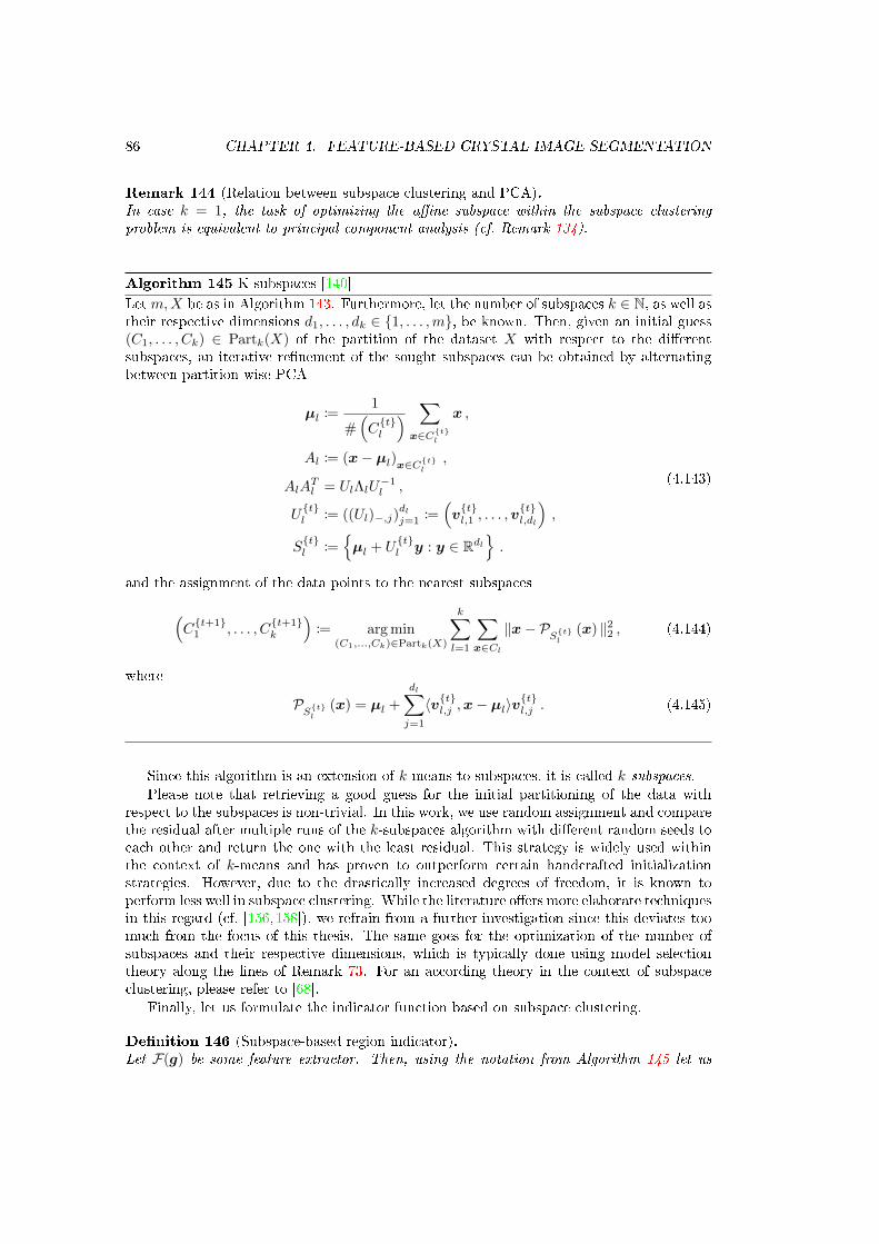
86 CHAPTER 4. FEATURE-BASED CRYSTAL IMAGE SEGMENTATION
Remark 144 (Relation between subspace clustering and PCA).In case k = 1, the task of optimizing the ane subspace within the subspace clusteringproblem is equivalent to principal component analysis (cf. Remark 134).
Algorithm 145 K-subspaces [140]Letm,X be as in Algorithm 143. Furthermore, let the number of subspaces k ∈ N, as well astheir respective dimensions d1, . . . , dk ∈ 1, . . . ,m, be known. Then, given an initial guess(C1, . . . , Ck) ∈ Partk(X) of the partition of the dataset X with respect to the dierentsubspaces, an iterative renement of the sought subspaces can be obtained by alternatingbetween partition-wise PCA
µl :=1
#(Ctl
) ∑x∈Ctl
x ,
Al := (x− µl)x∈Ctl ,
AlATl = UlΛlU
−1l ,
Utl := ((Ul)−,j)
dlj=1
:=(vtl,1 , . . . ,v
tl,dl
),
Stl :=
µl + U
tl y : y ∈ Rdl
.
(4.143)
and the assignment of the data points to the nearest subspaces
(Ct+11 , . . . , C
t+1k
):= arg min
(C1,...,Ck)∈Partk(X)
k∑l=1
∑x∈Cl
‖x− PStl
(x) ‖22 , (4.144)
where
PStl
(x) = µl +
dl∑j=1
〈vtl,j ,x− µl〉vtl,j . (4.145)
Since this algorithm is an extension of k-means to subspaces, it is called k-subspaces.Please note that retrieving a good guess for the initial partitioning of the data with
respect to the subspaces is non-trivial. In this work, we use random assignment and comparethe residual after multiple runs of the k-subspaces algorithm with dierent random seeds toeach other and return the one with the least residual. This strategy is widely used withinthe context of k-means and has proven to outperform certain handcrafted initializationstrategies. However, due to the drastically increased degrees of freedom, it is known toperform less well in subspace clustering. While the literature oers more elaborate techniquesin this regard (cf. [156, 158]), we refrain from a further investigation since this deviates toomuch from the focus of this thesis. The same goes for the optimization of the number ofsubspaces and their respective dimensions, which is typically done using model selectiontheory along the lines of Remark 73. For an according theory in the context of subspaceclustering, please refer to [68].
Finally, let us formulate the indicator function based on subspace clustering.
Denition 146 (Subspace-based region indicator).Let F(g) be some feature extractor. Then, using the notation from Algorithm 145 let us

4.4. HANDLING IRREGULAR REGIONS 87
dene the following subspace-based region indicator
(fl)j := ‖F(g)j − PSl(F(g)j
)‖22 . (4.146)
We would like to point out that the subspaces may also be rened iteratively as an outeriteration between the variational segmentation using the subspace-based region indicatorand principal component analysis of the segments resulting from the thresholded level-setfunctions.
4.3.8 Summary and nal remarks
In the following, let us make some nal remarks regarding the proposed method forsegmenting images by structure and summarize the nal algorithm.
Compared to its direct competitor, namely factorization-based texture segmentation(FSEG) by [154], the proposed method has the major advantage that it is not tied to theuse of spectral histograms as the feature extractor. The exibility of using generic featureextractors allows the proposed method to be employed in multiple applications, such ascrystal segmentation and hyper-spectral image segmentation.
Please note that the use of certain feature extractors (e.g. the one in Denition 132) leadto a high deviation of features at region boundaries from the mean features of the surroundingregions of interest. In particular, in case k > 2 it is possible that the feature at a boundarybetween two regions Ω∗1,Ω
∗2 is more similar to the mean feature of a third region Ω∗3 than
it is to Ω∗1 or Ω∗2 itself. Thus, the region indicators in (4.98) cannot necessarily identifyregions correctly within a distance of n−1
2 to boundaries between segments. However, theregularization of the level-set functions in the Mumford-Shah model remediates this problemfor practical purposes. In applications where the regularization alone does not work wellenough, we suggest to combine several feature extractors of the same type with decreasingwindow sizes.
Finally, let us point out that the proposed method inherits typical limitations of seg-mentation method based on local windows. Most importantly, regions can only be detectedreliably in case they are at least somewhat larger than the local window size n × n. Fur-thermore, some convention for the denition of features near the image boundary has tobe implemented, where the local windows leave the support of the image. Finally, pleasenote that the proposed method inherently enforces region boundaries to approach the im-age boundary orthogonally. This is due to the natural boundary conditions in the Euler-Lagrange equation (cf. (4.8)) corresponding to (4.78). However, this eect can be reducedin practice by extending the image with ghost cells using a zero boundary extension of theindicator functions.
The proposed method is summarized in Algorithm 147 . Please note that all numericalexperiments presented in this chapter use tmax = 3 outer iterations (for the renement of themean features). The low edge-ness threshold parameter in (4.129) is chosen as τedge = 0.5(Table 4.1), τedge = 0.25 (Table 4.2, Figure 4.2) and τedge = 1.0 (Figures 4.3 and 4.4).
4.4 Handling irregular regions
In image segmentation applications with complex objects and modalities it might occurthat for certain regions no suitable indicator function can be designed. This might havedierent reasons, for instance: 1) the corresponding mean values (or subspaces) cannot beestimated, 2) the region does not fulll the homogeneity property, 3) the existence of certainhomogeneous regions is unknown, i.e. k is chosen too small.
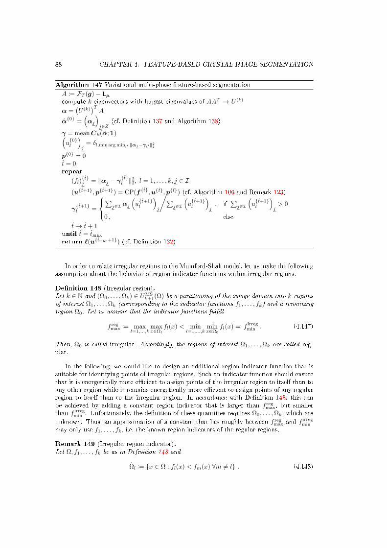
88 CHAPTER 4. FEATURE-BASED CRYSTAL IMAGE SEGMENTATION
Algorithm 147 Variational multi-phase feature-based segmentationA := FT (g)− 1µcompute k eigenvectors with largest eigenvalues of AAT → U (k)
α =(U (k)
)TA
α0 =(αj
)j∈Z
(cf. Denition 137 and Algorithm 138)
γ = meanCk(α;1)(u0l
)j
= δl,min arg minl′ ‖αj−γl′‖22
p0 = 0t = 0repeat
(fl)tj = ‖αj − γtl ‖22, l = 1, . . . , k, j ∈ I
(ut+1,pt+1) = CP(ft,ut,pt) (cf. Algorithm 106 and Remark 123)
γt+1l =
∑j∈I αj
(ut+1l
)j
/∑j∈I
(ut+1l
)j, if
∑j∈I
(ut+1l
)j> 0
0 , elset→ t+ 1
until t = tmaxreturn `(utmax+1) (cf. Denition 122)
In order to relate irregular regions to the Mumford-Shah model, let us make the followingassumption about the behavior of region indicator functions within irregular regions.
Denition 148 (Irregular region).Let k ∈ N and (Ω0, . . . ,Ωk) ∈ UMS
k+1(Ω) be a partitioning of the image domain into k regionsof interest Ω1, . . . ,Ωk (corresponding to the indicator functions f1, . . . , fk) and a remainingregion Ω0. Let us assume that the indicator functions fulll
f regmax := max
l=1,...,kmaxx∈Ωl
fl(x) < minl=1,...,k
minx∈Ω0
fl(x) =: f irregmin . (4.147)
Then, Ω0 is called irregular. Accordingly, the regions of interest Ω1, . . . ,Ωk are called reg-ular.
In the following, we would like to design an additional region indicator function that issuitable for identifying points of irregular regions. Such an indicator function should ensurethat it is energetically more ecient to assign points of the irregular region to itself than toany other region while it remains energetically more ecient to assign points of any regularregion to itself than to the irregular region. In accordance with Denition 148, this canbe achieved by adding a constant region indicator that is larger than f reg
max, but smallerthan f irreg
min . Unfortunately, the denition of these quantities requires Ω0, . . . ,Ωk, which areunknown. Thus, an approximation of a constant that lies roughly between f reg
max and f irregmin
may only use f1, . . . , fk, i.e. the known region indicators of the regular regions.
Remark 149 (Irregular region indicator).Let Ω, f1, . . . , fk be as in Denition 148 and
Ωl := x ∈ Ω : fl(x) < fm(x) ∀m 6= l . (4.148)

4.4. HANDLING IRREGULAR REGIONS 89
Furthermore, for r > 0 let xminl be a solution of
arg minx∈Ωl
fl(x)
s. t. B∞r (x) ⊂ Ωl
. (4.149)
Additionally, for ε > 0 let us dene
f0 := maxl=1,...,k
maxx∈B∞r (xmin
l )fl(x) + ε . (4.150)
Then, for suciently small r and Ωl as in Denition 148 we receive xminl ∈ Ωl and also
B∞r (xminl ) ⊂ Ωl, which implies f0 ≤ f reg
max (for ε = 0). On the other hand, if r is chosensuciently large, the variance of fl due to noise and uctuations in color (or structure) ofthe regarded region of interest will be covered over the region B∞r (xmin
l ) and thus f regmax − f0
will be small (for ε = 0). Hence, given a reasonable choice of r and for ε > 0 suciently
small, f regmax < f0 < f irreg
min holds and f0 serves as an indicator function for irregular regions.
Please note that in practice, when using feature-based region indicators, the minimumof each indicator will typically reside within the interior of the region of interest and thusthe constraint in (4.149) can often be omitted without noticeably changing the outcome ofthe segmentation.
Now, the additional region indicator from (4.150) can be integrated into the variationalmulti-phase segmentation framework as follows.
Denition 150 (Extension of JZach by an Irregular region).Let f0 as in Remark 149. Then, the following functional may be used to extend Zach's convexrelaxation of the multi-phase Mumford-Shah model (cf. (4.78)) by an additional level-setfunction for an irregular region:
J irregZach
[(ul)
kl=0
]:= JZach
[(ul)
kl=1
]+ f0
ˆΩ
u0(x) dx+ λ|u0|BV(Ω) . (4.151)
Please note that J irregZach has exactly the same form as JZach and can therefore be discretized
and optimized in the same manner.An entirely dierent idea for nding irregular regions is to perform a two-stage segmen-
tation as follows.
Algorithm 151 Two-stage approach for nding irregular regionsWe dene
f regmin(x) := min
l=1,...,kfl(x) . (4.152)
Now let Ω∗1, . . . ,Ω∗k denote the optimal sets after thresholding the solution of the multi-phase
Zach functional (cf. (4.78)) corresponding to the indicator functions f1, . . . , fk. Furthermore,let u be the minimizer of the two-phase Nikolova-Esedoglu-Chan model (cf. Lemma 110)corresponding to the indicator functions
f1(x) :=
(f reg
min(x)−maxy∈Ω
f regmin(y)
)2
,
f2(x) :=
(f reg
min(x)−miny∈Ω
f regmin(y)
)2
.
(4.153)
Then, setting Ω0 :=x ∈ Ω : u(x) ≤ 1
2
and Ωl := Ω∗l \Ω0 yields a partitioning of the domain
Ω into the regions of interest Ωl, l = 1, . . . , k and an irregular region Ω0.

90 CHAPTER 4. FEATURE-BASED CRYSTAL IMAGE SEGMENTATION
Note that using the region indicators in (4.153) within the two-phase segmentation frame-work is equivalent to segmenting the image f reg
min into fore- and background, where the meanforeground (and background) intensity is set to the minimum (and maximum) intensity ofthe image.
Using similar ideas as the ones above, let us propose a strategy for nding the meanvalue or subspace of additional regions of interest:
Algorithm 152 Estimation of mean-values / subspaces of additional ROIFor r > 0 we approximate a subset of an additional ROI as
Ωmax := B∞r (arg maxx∈Ω
f regmin(x)) . (4.154)
Given that additional ROI consist of image parts that are least well represented by themean values / subspaces of the currently dened ones, and for a reasonable choice of r, themean-value or subspace of an additional ROI can now be estimated as the mean value ofthe input over Ωmax or through the principal component analysis of the data inside Ωmax.
4.5 Numerical results
In the following, let us present numerical results that demonstrate the performance ofthe variational segmentation framework when using the features discussed in Sections 4.3.3and 4.3.4 within their respective applications, namely: texture and crystal segmentation.Moreover, we will show exemplary segmentations of a hyper-spectral image from a biologicalapplication.
The numerical experiments presented in this section use the following regularizationparameters: λ = 0.01 (Table 4.1), λ = 0.005 (Table 4.2 and Figure 4.2) and λ = 25 (Fig-ure 4.4). Furthermore, for the Chambolle-Pock algorithm (cf. (4.40)) we use the followingparameters for all experiments: σ = τ = 1
8 , θ = 0.7, εCP = 0.001, kCPmax = 10000.
4.5.1 Texture segmentation
Let us begin by comparing the proposed method for texture segmentation with estab-lished state-of-the-art methods in that domain. As test data we use the Prague ICPR2014texture segmentation benchmark [59] (http://mosaic.utia.cas.cz/icpr2014/) andthe Outex_US_00000 test suite of the Outex texture database (http://www.outex.oulu.fi).
The more popular of the two benchmarks is the Prague ICPR2014 contest dataset. Itconsists of 80 colored textural mosaics with dierent numbers of segments (3− 12). It wasdesigned as an unsupervised segmentation contest and thus the number of segments for eachimage has to be estimated by the algorithm. A crude estimate can be retrieved from thesingular values of the feature matrix as follows:
k := min
k′ :
1
m
m∑i=k′+1
λi < ω
. (4.155)
for some hand-tuned ω > 0. Here, we use ω = 0.05. However, in our experience, even forwell-tuned values of ω this estimate is far from being precise on all images. Please note thatthis is probably not only due to the nature of the estimate, but rather also due to the natureof the dataset, which contains textures that deviate greatly from our denition of a texture,

4.5. NUMERICAL RESULTS 91
Method CS ↑ OS ↓ US ↓ ME ↓ NE ↓ O ↓ C ↓ CA ↑ CO ↑ CC ↑VRA-PMCFA 75.32 *11.95 *9.65 4.57 *4.63 4.51 8.87 83.50 88.16 90.73PCA-MS+TM *72.27 18.33 9.41 4.19 3.92 *7.25 6.44 *81.13 *85.96 91.24
FSEG [154] 69.18 14.69 13.64 5.13 *4.63 9.25 12.55 78.22 84.44 87.38SegTexCol 61.19 1.92 27.02 9.33 9.05 15.17 12.12 71.69 81.16 76.34MW3AR8 [60] 53.66 51.40 14.21 *5.54 6.33 19.86 84.27 70.15 75.41 89.36RS 46.02 13.96 30.01 12.01 11.77 35.11 29.91 58.75 68.89 69.30Deep Brain [52] 36.20 41.87 53.87 7.38 9.06 47.53 99.56 49.97 62.62 70.08
Table 4.1: Color texture segmentation on the Prague ICPR2014 contest dataset with un-known number of segments (cf. http://mosaic.utia.cas.cz). Bold face highlightsthe best, a star the second-best value in each column, and indicates that no correspondingpublication could be found at the time of writing.
namely a locally recurring pattern (cf. Figure 4.1, row 3). In particular, for plausible valuesof ω the number of segments is often over-estimated on this dataset. To counter this, wedecided to employ a post-processing algorithm for texture merging proposed by Yuan etal. [154].
For this benchmark, we transformed the images to Lab color space and combined localspectral histograms with 11 bins, window sizes n = 31, 61 (stacked with weights 0.8 and 0.2respectively), intensity lters on all three channels and Gabor lters of kernel sizes n = 5, 7and orientations θ = 0, 1
2π,14π,−
14π on the lightness channel.
The results of the benchmark in terms of mean segmentation quality with respect todierent quantities (cf. [59]) are shown in Table 4.1. We see that our method producesa larger over-segmentation (OS) than the other best-ranked methods. We believe this tobe correlated with a stronger over-estimation of the number of segments. In contrast tothis, our method yields the best under-segmentation (US), which we think indicates a goodcoverage of all ground truth segments. With respect to the measures correct segmentation(CS), omission error (O), class accuracy (CA) and correct assignment (CO) our methodperforms second-best. Most notably, according to all other presented meaures (in total halfof them) our method performs better than all competitors.
Figure 4.1 displays exemplary segmentations of the relevant methods (CS > 60) onselected input images.
We would like to point out that while the winning algorithm of the Prague ICPR2014contest, namely VRA-PMCFA, succeeds in resolving ne boundary features, it producesnoticeable labeling noise. In contrast to that, our method smooths region boundaries, thussmearing out details of the true boundary geometry, in favor of suppressing labeling noise.In summary, both methods perform well in texture segmentation, but it depends on therequirements of the application which of the two might be more suitable.
As pointed out before, the Prague dataset (despite being popular) has some major draw-backs. First of all, it contains textures that are not robustly classiable with localized fea-tures (as seen in Figure 4.1, row 3). Furthermore, many of the texture have very distinctcolors and some of them might even be separated by using mainly the intensity lter. Inview of these issues, let us now look at the Outex benchmark, which contains histogram-equalized, gray-value textures that are much closer to our denition of textures, yet veryhard to distinguish with simple intensity-based methods. Unfortunately, there is no databaseof published results for the Outex_US_00000 test suite. Thus, we can only compare resultsfor methods with a published implementation.

92 CHAPTER 4. FEATURE-BASED CRYSTAL IMAGE SEGMENTATION
Input GT SegTexCol FSEG VRA-PMCFA
PCA-MS
+TM
Figure 4.1: Segmentations of selected mosaics from the Prague ICPR2014 contest. The rstcolumn shows the original image, the second the ground truth and the remaining columnsthe results by SegTexCol, FSEG [154], VRA-PMCFA and PCA-MS with TxtMerge post-processing (TM).

4.5. NUMERICAL RESULTS 93
Input GT FSEG Clustering FSEG∗ FSEG∗-TMAlgorithm 147
Figure 4.2: Segmentations of the rst three mosaics from the Outex_US_00000 test suite.The rst column shows the original image, the second the ground truth and the remainingcolumns the results by FSEG [154], clustering, FSEG∗, FSEG∗-TM and Algorithm 147.
The code for VRA-PMCFA is not published (neither is the exact algorithm), but it makesheavy use of color information anyways and thus is not a good candidate for comparisonon the Outex dataset. Fortunately, the code of FSEG [154], the second best competitor(and thus the best published one) is available at http://web.ornl.gov/~jiy/FSEG_contest.zip. It is also a particularly good candidate for a comparison since it is similarto our framework.
For this benchmark, we used the same local spectral histograms as above (the lightnesschannel is already given by the gray-values here), except that we omitted the intensity ltersand added another Gabor lter of kernel size n = 9.
Here, we compare the results of our proposed method to both plain clustering of thesefeatures and dierent versions of FSEG [154]:
FSEG: xed number of segments (segn = 5)
FSEG∗: uses the same features as our method
FSEG∗-TM: TxtMerge post-processing is deactivated
Please note that deactivating the TxtMerge post-processing makes sense in this case,because the number of segments is known.
Figure 4.2 shows three exemplary texture mosaics from the Outex_US_00000 test suite,as well as the ground truth segmentations and the results retrieved from FSEG, clustering,FSEG∗, FSEG∗-TM and Algorithm 147. Comparing the results visually, we see that theproposed method provides a good compromise between delity and artifact suppression(holes, missing regions).
Now let us turn to the quantitative comparison shown in Table 4.2. While FSEG∗-TM performs best in terms of correct segmentation (CS), and FSEG∗ with respect to theomission error (O), our method ranks highest in all of the remaining quantitative measures.Furthermore, we see that compared to plain clustering there is a signicant benet of both
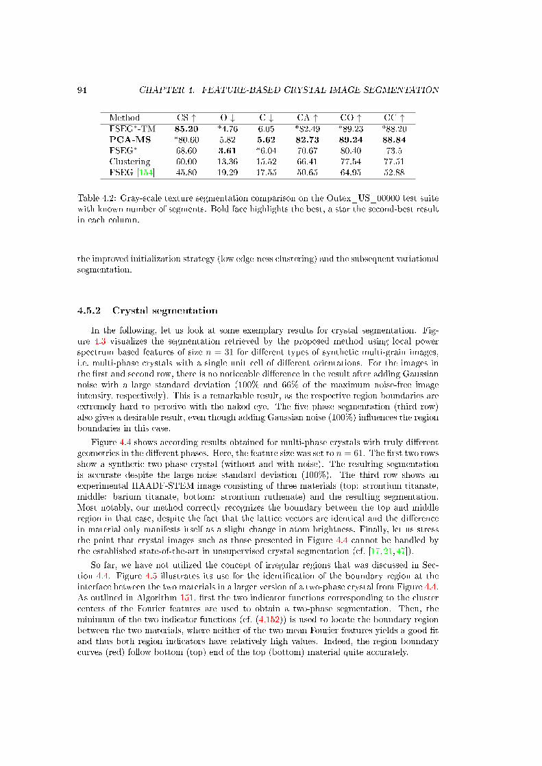
94 CHAPTER 4. FEATURE-BASED CRYSTAL IMAGE SEGMENTATION
Method CS ↑ O ↓ C ↓ CA ↑ CO ↑ CC ↑FSEG∗-TM 85.20 *4.76 6.05 *82.49 *89.23 *88.20PCA-MS *80.60 5.82 5.62 82.73 89.24 88.84
FSEG∗ 68.60 3.61 *6.04 70.67 80.40 73.5Clustering 60.00 13.36 15.52 66.41 77.54 77.51FSEG [154] 45.80 19.29 17.55 50.65 64.95 52.88
Table 4.2: Gray-scale texture segmentation comparison on the Outex_US_00000 test suitewith known number of segments. Bold face highlights the best, a star the second-best resultin each column.
the improved initialization strategy (low edge-ness clustering) and the subsequent variationalsegmentation.
4.5.2 Crystal segmentation
In the following, let us look at some exemplary results for crystal segmentation. Fig-ure 4.3 visualizes the segmentation retrieved by the proposed method using local powerspectrum based features of size n = 31 for dierent types of synthetic multi-grain images,i.e. multi-phase crystals with a single unit cell of dierent orientations. For the images inthe rst and second row, there is no noticeable dierence in the result after adding Gaussiannoise with a large standard deviation (100% and 66% of the maximum noise-free imageintensity, respectively). This is a remarkable result, as the respective region boundaries areextremely hard to perceive with the naked eye. The ve phase segmentation (third row)also gives a desirable result, even though adding Gaussian noise (100%) inuences the regionboundaries in this case.
Figure 4.4 shows according results obtained for multi-phase crystals with truly dierentgeometries in the dierent phases. Here, the feature size was set to n = 61. The rst two rowsshow a synthetic two-phase crystal (without and with noise). The resulting segmentationis accurate despite the large noise standard deviation (100%). The third row shows anexperimental HAADF-STEM image consisting of three materials (top: strontium titanate,middle: barium titanate, bottom: strontium ruthenate) and the resulting segmentation.Most notably, our method correctly recognizes the boundary between the top and middleregion in that case, despite the fact that the lattice vectors are identical and the dierencein material only manifests itself as a slight change in atom brightness. Finally, let us stressthe point that crystal images such as those presented in Figure 4.4 cannot be handled bythe established state-of-the-art in unsupervised crystal segmentation (cf. [17, 21,47]).
So far, we have not utilized the concept of irregular regions that was discussed in Sec-tion 4.4. Figure 4.5 illustrates its use for the identication of the boundary region at theinterface between the two materials in a larger version of a two-phase crystal from Figure 4.4.As outlined in Algorithm 151, rst the two indicator functions corresponding to the clustercenters of the Fourier features are used to obtain a two-phase segmentation. Then, theminimum of the two indicator functions (cf. (4.152)) is used to locate the boundary regionbetween the two materials, where neither of the two mean Fourier features yields a good tand thus both region indicators have relatively high values. Indeed, the region boundarycurves (red) follow bottom (top) end of the top (bottom) material quite accurately.

4.5. NUMERICAL RESULTS 95
Figure 4.3: Segmentation of synthetic multi-grain crystals without (left) and with (right)noise, computed by the proposed method using local power spectrum based features (cf.Denition 132) and visualized as boundary curves (red).
4.5.3 Sub-space segmentation
We would like to close the presentation of results with an outlook towards hyper-spectralsegmentation using subspace-based region indicators. Figure 4.6 shows a biological hyper-spectral image, where each pixel consists of a vector of length greater than 1400. Accordingto the experimentalists, it is expected to contain 5 regions of interest and a background.The right image in Figure 4.6 shows three such regions that were partially and manuallysegmented by an expert.
In order to assess whether the PCA-based region indicator (cf. (4.133)) is suitable for thisdataset or indeed the extension to subspaces is required, we performed both plain clusteringand subspace clustering of the spectra of the manually segmented ROI. The results of thisare shown in Figure 4.7. Assuming that the manual segmentation is somewhat accurate,the fact that the geometry of the ROI changes completely after plain clustering is a strongindicator that indeed the PCA-based region indicator is not suitable here. In contrast to this,we see that the subspace clustering roughly retains the geometry of the manually segmentedROI.
Figure 4.8 shows the segmentation result of the proposed method using the subspace-based region indicator, where the subspaces were obtained by performing principal compo-nent analysis on the vectors belonging to the manually segmented regions, respectively and
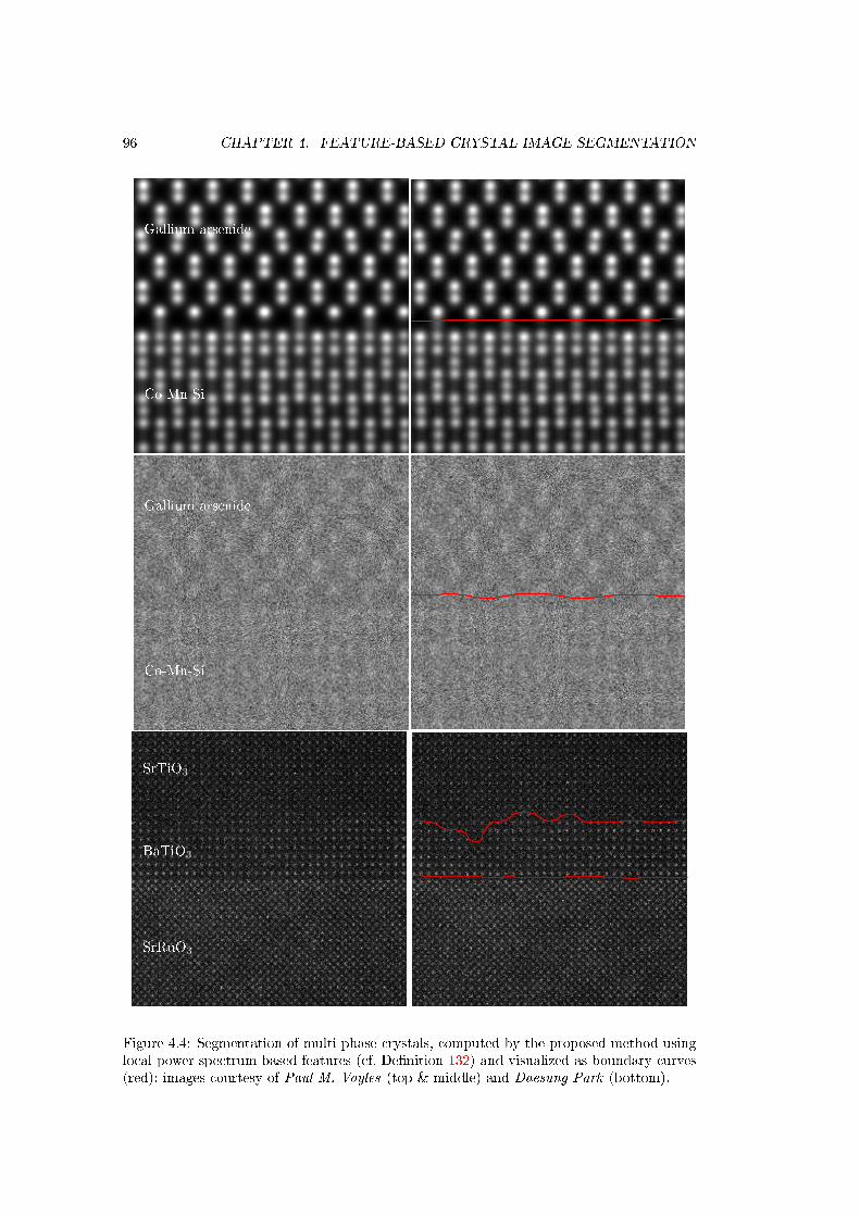
96 CHAPTER 4. FEATURE-BASED CRYSTAL IMAGE SEGMENTATION
Co-Mn-Si
Gallium arsenide
Co-Mn-Si
Gallium arsenide
SrRuO3
BaTiO3
SrTiO3
Figure 4.4: Segmentation of multi-phase crystals, computed by the proposed method usinglocal power spectrum based features (cf. Denition 132) and visualized as boundary curves(red); images courtesy of Paul M. Voyles (top & middle) and Daesung Park (bottom).

4.5. NUMERICAL RESULTS 97
g f1 f2 f regmin boundary curves
Figure 4.5: Two-stage segmentation of a two-phase crystal image into two dierent phasesand an irregular boundary region in-between; from left to right: input image, bottom regionindicator, top region indicator, minimum indicator function (cf. (4.152)), resulting segmen-tation visualized as boundary curves (red)
Figure 4.6: Left: projection of a multi-spectral dataset consisting of 5 ROI and an irregularregion (the background); right: 3 ROI partially segmented by hand; data courtesy of RohitBhargava (University of Illinois Urbana Champaign)

98 CHAPTER 4. FEATURE-BASED CRYSTAL IMAGE SEGMENTATION
Figure 4.7: ROI membership after plain clustering (left) and subspace clustering (right) ofall spectra of the manually segmented ROI
f1 f2 f3 `
Figure 4.8: Indicator functions of the rst 3 ROI and the corresponding labeling function,including an irregular region (black), overlayed with manual segmentation boundaries (blue)
each segmentation includes a background based on the irregular region indicator conceptformulated in Denition 150.
The process of adding estimating subspaces for the fourth and fth ROI is illustratedin Figure 4.9, including the corresponding minimum indicator function (cf. (4.152)), theestimate of a subset of the new ROI based on the strategy outlined in Algorithm 152 andthe resulting new indicator functions and segmentations.
Furthermore, Figure 4.10 shows the change in the segmentation through the iterative re-nement of all subspaces by recomputing the principal component analysis on the respectiveregions after variational segmentation (cf. (4.140)).
The nal estimates of the eigenvector bases of the subspaces of all ROI, as well as the

4.5. NUMERICAL RESULTS 99
ROI#4
ROI#5
f regmin Ωmax f4/5 `
Figure 4.9: From left to right: 1) minimum indicator function (cf. (4.152)) based on 4 (top)and 5 (bottom) ROI; 2) estimate subset of ROI #4 (top) and #5 (bottom) (cf. (4.154));region indicator based on 4-th (top) and 5-th (bottom) subspace; labeling function for 4 (top)and 5 (bottom) ROI and an irregular region (black), overlayed with manual segmentationboundaries (blue)
t = 1 t = 2 t = 3
Figure 4.10: Labeling functions of the 5 ROI and an unknown region (black) after alternatingiterative renements of subspaces and segmentation (cf. Algorithm 147), overlayed withmanual segmentation boundaries (blue)

100 CHAPTER 4. FEATURE-BASED CRYSTAL IMAGE SEGMENTATIONl
=1
-0.1
-0.08
-0.06
-0.04
-0.02
0
0.02
0.04
0.06
0.08
0 200 400 600 800 1000 1200 1400 1600-0.2
0
0.2
0.4
0.6
0.8
1
1.2
0 200 400 600 800 1000 1200 1400 1600-0.1
-0.05
0
0.05
0.1
0.15
0.2
0 200 400 600 800 1000 1200 1400 1600
l=
2
-0.15
-0.1
-0.05
0
0.05
0.1
0.15
0.2
0 200 400 600 800 1000 1200 1400 1600-0.2
0
0.2
0.4
0.6
0.8
1
1.2
0 200 400 600 800 1000 1200 1400 1600-0.15
-0.1
-0.05
0
0.05
0.1
0.15
0 200 400 600 800 1000 1200 1400 1600
l=
3
-0.25
-0.2
-0.15
-0.1
-0.05
0
0.05
0.1
0.15
0.2
0.25
0 200 400 600 800 1000 1200 1400 1600-0.2
0
0.2
0.4
0.6
0.8
1
1.2
0 200 400 600 800 1000 1200 1400 1600-0.2
-0.15
-0.1
-0.05
0
0.05
0.1
0.15
0.2
0 200 400 600 800 1000 1200 1400 1600
l=
4
-0.6
-0.5
-0.4
-0.3
-0.2
-0.1
0
0.1
0.2
0 200 400 600 800 1000 1200 1400 1600-0.2
0
0.2
0.4
0.6
0.8
1
1.2
0 200 400 600 800 1000 1200 1400 1600-0.2
-0.15
-0.1
-0.05
0
0.05
0.1
0.15
0.2
0 200 400 600 800 1000 1200 1400 1600
l=
5
-0.3
-0.25
-0.2
-0.15
-0.1
-0.05
0
0.05
0.1
0 200 400 600 800 1000 1200 1400 1600-0.2
0
0.2
0.4
0.6
0.8
1
1.2
0 200 400 600 800 1000 1200 1400 1600-0.2
-0.15
-0.1
-0.05
0
0.05
0.1
0.15
0.2
0 200 400 600 800 1000 1200 1400 1600
gj µl vl,1,vl,2,vl,3
Figure 4.11: From top to bottom: 5 dierent ROI; from left to right for each ROI: threeselected (mean subtracted) spectra, mean spectrum, eigenvectors of the subspace; the x-axisrepresents the channels of the spectra in each graph
respective mean spectra and selected input spectra for each ROI are plotted in Figure 4.11.Please note that there was no ground truth available for this dataset at the time of writing
and therefore the subspace-based segmentation proposed in this work should be seen as anidea, rather than an established method. This applies especially to the strategies of ndinggood estimates for the subspaces of all ROI, as this is a very delicate topic that requiresfurther research. However, the comparison between plain clustering and subspace clusteringof the manually segmented ROI convinced us that the general approach of subspace-basedsegmentation is very promising for these kinds of datasets.

4.6. CONCLUSIONS 101
4.6 Conclusions
In this chapter, we introduced the concept of variational optimization of functionalswith innite-dimensional arguments, as well as the most important theorems on the exis-tence, uniqueness and numerical approximation of solutions. Furthermore, two-phase andmulti-phase variational segmentation frameworks based on this theory were recalled. Themain novelty proposed in this chapter is the extension of these frameworks to structuraland hyper-spectral segmentation, using high-dimensional local features to capture structureand principal component analysis for dimension and noise reduction. The proposed methodachieves state-of-the-art performance on the popular Prague texture segmentation bench-mark. Most important for this thesis is the resulting algorithm for unsupervised crystalsegmentation, which opens new possibilities, namely segmenting multi-phase crystals gener-ated by a set of truly dierent unit cells in an automated fashion. Finally, we gave an outlooktowards hyper-spectral segmentation applications, where distances to the mean feature of aregion of interest might not be sucient for robust region discrimination. To this end, weproposed to employ region indicators measuring the distances of spectra to the subspacesof the regions of interest. We presented results on a biological dataset that indicate theusefulness of this ansatz.
The source code of the PCA-based variational segmentation method discussed in thischapter, including executables reproducing the results presented in [101], is available online:http://nmevenkamp.github.io/pcams.


Chapter 5
Noise modeling and parameter
estimation
In this chapter we discuss intensity dependent noise models, namely Poisson noise anda mixed model consisting of a scaled Poissonian and a Gaussian random variable. Further-more, we present a generic framework for unsupervised tuning of the corresponding modelparameters based on a modied block-matching strategy. Using experimental HAADF-STEM images, we demonstrate that the mixed noise model is much more accurate thaneither additive Gaussian white noise or plain Poisson noise. Finally, we recall strategiesfor adapting AGWN based denoising methods to non-additive, intensity dependent noisemodels.
5.1 Introduction
Some natural random phenomena, such as diusion, are known to inherently follow aGaussian distribution. Furthermore, the central limit theorem states that under certainconditions, the sum, or an iteration, of a number of random variables converges to theGaussian distribution as the number goes to innity [7]. Due to this fact, a variety of randomprocesses can be approximated well by Gaussian distributions. Moreover, due its simplicityand being the limit of many dierent probability distributions, the Gaussian distribution isoften used as an approximation in case no information about a certain random process isknown (except for its mean and variance) [115].
Despite this trend, there are certainly situations where assuming a Gaussian distributionleads to signicant errors. Within the context of image processing, examples are astronomyand magnetic resonance imaging. In astronomy, the amount of light detected by the tele-scope is often so weak that a major source of variance in the measured intensity is due tothe random emission of light by the observed star. This is referred to as shot noise, whichfollows a Poisson distribution when neglecting the photon bunching eect [107]. In mag-netic resonance imaging (MRI), noise has been found to follow a Rician distribution [58].Gudbjartsson and Patz found that by using the previously widely accepted Gaussian noisedistribution, the noise power would often be underestimated by about 60%.
The noise characteristics in low-dose electron microscopy should be similar to that of low-light astronomy, as both are aected by the random emission of electrons (or photons), aswell as the noise in the electronic sensor. Thus, we expect it to behave - at least in part - likea Poisson random variable. However, as mentioned before, when regarding the exact physicalprocesses (e.g. photon bunching in thermal light), not even the electron counting statistics
103

104 CHAPTER 5. NOISE MODELING AND PARAMETER ESTIMATION
will be exactly Poissonian. Modeling exactly the distribution of random contributions withinthe digital sensor is even more complicated. Thus, in favor of practicability, the goal of thischapter is to nd a noise model that is 1) suciently accurate, 2) simple enough thatit allows for unsupervised parameter tuning solely based on the noisy data, 3) employablewithin common denoising methods that were originally designed for additive Gaussian whitenoise.
In the context of generic CCD/CMOS sensor based image acquisition, Foi et al. [53]proposed to use a mixed Poisson-Gaussian noise model (MPG), which leads to a noisevariance that is an ane function of the true image intensity. Most notably, they showedthat considering a more complicated noise model, that takes into account various scalingsand Gaussian contributions at the dierent stages of the acquisition process, leads to thesame linear variance model. Foi et al. also proposed an algorithm for estimating the noisemodel parameters from natural images.
Furthermore, Mäkitalo and Foi [133] investigated the estimation and inversion of suit-able variance stabilization transforms (VST) utilized for the employment of AGWN baseddenoising algorithms on data with non-AGWN noise distributions. In particular, they in-vestigated the generalized Anscombe transform [133], which is an extension of the originalAnscombe transform [6] to the MPG setting.
In this chapter, we present experimental analyses that support the validity of the MPGnoise model under HAADF-STEM and EELS experimental conditions. However, we ndthat the core assumption of the parameter estimation algorithm proposed by Foi et al. [53]is not valid in atomic-scale electron microscopy. To circumvent this issue, we propose adierent, more generic strategy based on modied non-local block-matching. Another con-tribution in this chapter is the theoretical analysis of errors arising in this context. Further-more, we propose a method to estimate the mean and variance of the Gaussian distributionwithin the MPG model separately, which is, to the best of our knowledge, not covered inthe literature so far. Finally, we discuss a novel framework for the evaluation of the qualityof denoised images that is similar to, but more general than, the method noise (cf. Deni-tion 29). In particular, the new framework applies to all probability distributions with acontinuous CDF. We also cover a modied alternative for the case of discrete probabilitydistributions. Since its practical use requires the evaluation of the CDF, we propose ex-pressions that approximate the PDF and CDF of the MPG model numerically and provecorresponding error bounds. Moreover, we prove a Berry-Esseen bound for the MPG normalapproximation.
5.2 Poisson and mixed Poisson-Gaussian noise
Let us begin by dening the Poisson distribution and recalling its relation to the Gaussiandistribution.
Denition 153 (Poisson distribution [64]).The probability density function of the Poisson distribution with parameter λ > 0 is denedas
fPλ (k) :=λke−k
k!, k ∈ N0 . (5.1)
Note that the Poisson distribution is a discrete density, since it is only dened for non-negative integers.

5.2. POISSON AND MIXED POISSON-GAUSSIAN NOISE 105
Remark 154 (Cumulative distribution function of the Poisson distribution [64]).The cumulative distribution function of the Poisson distribution is
FPλ (x) := e−λbxc∑i=0
λi
i!, x ∈ R≥0 . (5.2)
Due to the integer part in the summation limit, it is discontinuous on R.
Analogous to Denition 3, the notation P∼P(λ) states that P is a Poisson distributedrandom variable. Its expectation and variance are equal: E [P ] = Var [P ] = λ. Furthermore,Pr (P = k|P∼P(λ)) can be interpreted as the probability of observing k occurrences of anevent over a time span during which the event occurs λ times on average and in case eachevent is independent of the preceding one.
Now we would like to show that the Poisson distribution converges to the Gaussiandistribution. For this, we require the fact that the sum of Poisson distributed randomvariables is also Poisson distributed.
Remark 155 (Sum of Poisson distributions).For λ1, λ2 > 0 let P1∼P(λ1), P2∼P(λ2) be independent random variables. Then,
P := P1 + P2∼P(λ1 + λ2) . (5.3)
Proof.Pr (P1 + P2 = k|P1∼P(λ1), P2∼P(λ2)))
=
∞∑l=0
Pr (P1 = l|P1∼P(λ1)) Pr (P2 = k − l|P2∼P(λ2)) ,
=
k∑l=0
λl1e−l
l!
λk−l2 e−(k−l)
(k − l)!=e−k
k!
k∑l=0
(k
l
)λl1λ
k−l2 ,
=(λ1 + λ2)ke−k
k!,
=Pr (P = k|P∼P(λ1 + λ2)) .
(5.4)
Now let us recall a version of the aforementioned central limit theorem.
Theorem 156 (Central limit theorem [64]).Let (Xi)i∈N be a sequence of independent and identically distributed (i.i.d.) random variableswith E [X1] = µ and Var [X1] = σ2. Note that due to the identical distribution of the Xi thisimplies E [Xi] = µ and Var [Xi] = σ2 for all i ∈ N. This way of dening properties of i.i.d.random variables will be used throughout this chapter. Furthermore, let Sn :=
∑ni=1Xi and
Fn(z) := Pr
(Sn − nµ√
nσ≤ z). (5.5)
Then, for all z ∈ Rlimn→∞
Fn(z) = FG0,1(z) . (5.6)
holds.

106 CHAPTER 5. NOISE MODELING AND PARAMETER ESTIMATION
A direct consequence of the central limit theorem is that the Poisson distribution con-verges to the normal distribution as the mean goes to innity.
Remark 157 (Convergence of the Poisson distribution [83]).Let (Pi)i∈N be i.i.d. random variables with P1∼P(1). Then, due to Remark 155, for λ ∈ N,Sλ :=
∑λi=1∼P(λ). In this setting, Theorem 156 reads
limλ→∞
Pr
(Sλ − λ√
λ≤ z)
= FG0,1(z) ∀z ∈ R . (5.7)
Due to the scaling properties of the Gaussian distribution, we can reformulate this as
limλ→∞
FPλ (z)− FGλ,√λ(z) = 0 ∀z ∈ R , (5.8)
i.e. the Poisson distribution approaches the Gaussian distribution as the mean value in-creases.
Furthermore, the following theorem yields an error bound for nite λ.
Theorem 158 (The Berry-Esseen theorem [19,49]).Let (Xn)n∈N and Fn be as in Theorem 156. Additionally, let ρ = E
[|X1 − µ|3
]<∞. Then,
there exists 0 < C <∞ such that
supz∈R
∣∣Fn(z)− FG0,1(z)∣∣ ≤ Cρ√
nσ2. (5.9)
To our knowledge, the best value for C (resulting in the sharpest bound) currently known isC = 0.4748 [129]. This value cannot be improved much further, since a lower bound is given
by C ≥√
10+26√
2π≥ 0.4097 [50].
Remark 159 (The Berry-Esseen bound for the Poisson Normal approximation [84,111]).Let (Pi)i∈N be as in Remark 157. Then, ρ = E
[|X1 − µ|3
]= 1. Thus, in this case Theo-
rem 158 reads
supz∈R
∣∣∣∣Pr
(Sλ − λ√
λ≤ z)− FG0,1(z)
∣∣∣∣ ≤ C√λ∀λ ∈ N . (5.10)
This result can be extended to λ ∈ R and the rescaling of the Gaussian distribution yields
supz∈R
∣∣∣FPλ (z)− FGλ,√λ(z)∣∣∣ ≤ C√
λ∀λ ∈ R . (5.11)
For small mean values the Poisson distribution deviates signicantly from the Gaussiandistribution. Therefore, as we mentioned earlier, an imaging noise model that seeks to beaccurate under low-light (or low electron dose) conditions, needs to account for Poissondistributed portions of the noise. A simple model that regards both a Poisson distributedcontribution and a Gaussian one is the following.
Denition 160 (Mixed Poisson-Gaussian (MPG) distribution [133]).For α, λ > 0, µ ∈ R, σ ≥ 0 and P∼P(λ), H∼N (µ, σ), the random variable Z = αP +H issaid to follow the mixed Poisson-Gaussian (MPG) distribution.
We use the short notation C∼C(λ, α, µ, σ) to express that C follows the MPG distribu-tion.

5.2. POISSON AND MIXED POISSON-GAUSSIAN NOISE 107
Given the ground truth g of a digital image, for Pi∼P(gi) and Hi∼N (µ, σ), we say that
Z = αP +H , (5.12)
is aected by mixed Poisson-Gaussian noise (MPG).Please note that the Gaussian distribution is only dened for σ > 0. However, for σ = 0,
H is simply not regarded as a random variable, but as the constant H = µ in this context.
Remark 161 (Mean and variance of the MPG distribution [133]).The mean and variance of the MPG distribution are given by
E [Z] = αλ+ µ , (5.13)
Var [Z] = α2λ+ σ2 = αE [Z] + σ2 − αµ . (5.14)
As mentioned in [53], the parameters of the mixed Poisson-Gaussian noise model can berelated to parameters in digital sensor based image acquisition as follows: λ is the averagerate of photons / electrons hitting the detector; α is the gain by which the measured countis multiplied (e.g. proportional to the ISO in modern digital cameras); µ is the pedestal,a constant that is added to all intensities; σ is the standard deviation of thermal andelectromagnetic noise within the sensor.
The probability density and cumulative distribution function of MPG can be computedvia convolution:
Remark 162 (PDF and CDF of the mixed Poisson-Gaussian distribution).The probability density function and the cumulative distribution function of the mixed Poisson-Gaussian distribution are given by
fMPGλ,α,µ,σ(z) =
∑k∈N0
fPλ (k)fGµ,σ(z − αk) , (5.15)
FMPGλ,α,µ,σ(z) =
∑k∈N0
fPλ (k)FGµ,σ(z − αk) . (5.16)
Since these probability functions contain an innite sum, their denition is not usefulin practice. In order to approximate them with sucient accuracy using reasonably manyoperations, we will use two approximations: 1) the similarity of the Poisson distribution toa Gaussian distribution for large λ, 2) the fast decay of the Poisson PDF for small λ.
First, let us show how the mixed Poisson-Gaussian distribution can be approximated bya single Gaussian distribution for large λ. Therefore, we need the following lemma.
Lemma 163 (Linear combination of Gaussian distributions [37]).Let n ∈ N, a0, . . . , an ∈ R with ai 6= 0 for some i ∈ 1, . . . , n. Furthermore, for µi ∈ R,σi > 0 let Xi∼N (µi, σi) be independent random variables for i = 1, . . . , n. Then, thefollowing holds
a0 +
n∑i=1
aiXi∼N (µ, σ) , (5.17)
where
µ = a0 +
n∑i=1
aiµi ,
σ =
√√√√ n∑i=1
a2iσ
2i .
(5.18)

108 CHAPTER 5. NOISE MODELING AND PARAMETER ESTIMATION
Since the stochastic convergence of random variables also implies the stochastic conver-gence of their sum to the sum of their limits, combining Remark 157 and Lemma 163 yieldsthe following result.
Remark 164 (Convergence of the mixed Poisson-Gaussian distribution).Let α, σ > 0, µ ∈ R. Then
limλ→∞
FMPGλ,α,µ,σ(z)− FG
αλ+µ,α√λ+σ
(z) = 0 ∀z ∈ R . (5.19)
It can be shown easily that the Berry-Esseen bound from Remark 159 is also valid forthe mixed Poisson-Gaussian distribution:
Remark 165 (Berry-Esseen bound for the MPG normal approximation).For λ, α, σ > 0, µ ∈ R let C∼C(λ, α, µ, σ). Then
supz∈R
∣∣∣FMPGλ,α,µ,σ − FGαλ+µ,α
√λ+σ
(z)∣∣∣ ≤ C√
λ. (5.20)
Proof. Let P∼P(λ), H1∼N (µ, σ), Z∼N (αλ+ µ, α√λ+ σ) and H2∼N (λ,
√λ). Then
supz∈R
∣∣∣FMPGλ,α,µ,σ − FGαλ+µ,α
√λ+σ
(z)∣∣∣ (5.21)
= supz∈R|Pr (αP +H1 ≤ z)− Pr (Z ≤ z)| (5.22)
= supz∈R
∣∣∣∣ˆR
Pr
(P ≤ z − y
α
)Pr (H1 = y)− Pr
(H2 ≤
z − yα
)Pr (H1 = y) dy
∣∣∣∣ (5.23)
= supz∈R
∣∣∣∣ˆR
(FPλ
(z − yα
)− FG
λ,√λ
(z − yα
))fGµ,σ(y) dy
∣∣∣∣ (5.24)
≤ˆR
supz∈R
∣∣∣FPλ (z)− FGλ,√λ(z)∣∣∣ fGµ,σ(y) dy ≤ C√
λ(5.25)
This yields an approximation of FMPGλ,α,µ,σ in case λ is large. In case λ is small, we can
truncate the sums in Remark 162 to approximate the MPG distribution numerically. Inorder to prove bounds that can be used in practice, we require the concept of the inversecumulative distribution function for discrete random variables:
Denition 166 (Inverse CDF of discrete random variables).For θ ∈ Rm let D(θ) be a discrete probability distribution with values in N0 and FD(θ) be thecorresponding CDF. Then, its inverse is dened as
F−1
D(θ): [0, 1]→ N0 , x 7→ mink ∈ N0 : FD(θ)(k) ≥ x . (5.26)
Now let us formulate and prove the aforementioned bounds.
Remark 167 (Numerical approximation of the PDF and CDF for MPG).For a suciently small error bound ε < 0, i.e. at least ε < 1, let
kεmin :=(FPλ)−1
( 12ε) + 1 (5.27)
kεmax :=(FPλ)−1
(1− 12ε) . (5.28)
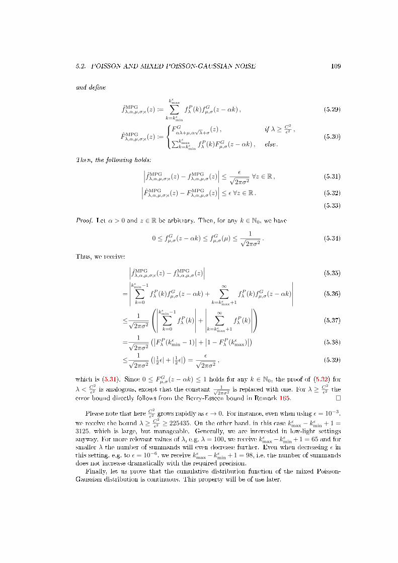
5.2. POISSON AND MIXED POISSON-GAUSSIAN NOISE 109
and dene
fMPGλ,α,µ,σ;ε(z) :=
kεmax∑k=kεmin
fPλ (k)fGµ,σ(z − αk) , (5.29)
FMPGλ,α,µ,σ;ε(z) :=
FGαλ+µ,α
√λ+σ
(z) , if λ ≥ C2
ε2 ,∑kεmax
k=kεminfPλ (k)FGµ,σ(z − αk) , else .
(5.30)
Then, the following holds:∣∣∣fMPGλ,α,µ,σ;ε(z)− fMPG
λ,α,µ,σ(z)∣∣∣ ≤ ε√
2πσ2∀z ∈ R , (5.31)∣∣∣FMPG
λ,α,µ,σ;ε(z)− FMPGλ,α,µ,σ(z)
∣∣∣ ≤ ε ∀z ∈ R . (5.32)
(5.33)
Proof. Let α > 0 and z ∈ R be arbitrary. Then, for any k ∈ N0, we have
0 ≤ fGµ,σ(z − αk) ≤ fGµ,σ(µ) ≤ 1√2πσ2
. (5.34)
Thus, we receive: ∣∣∣fMPGλ,α,µ,σ;ε(z)− fMPG
λ,α,µ,σ(z)∣∣∣ (5.35)
=
∣∣∣∣∣∣kεmin−1∑k=0
fPλ (k)fGµ,σ(z − αk) +
∞∑k=kεmax+1
fPλ (k)fGµ,σ(z − αk)
∣∣∣∣∣∣ (5.36)
≤ 1√2πσ2
∣∣∣∣∣∣kεmin−1∑k=0
fPλ (k)
∣∣∣∣∣∣+
∣∣∣∣∣∣∞∑
k=kεmax+1
fPλ (k)
∣∣∣∣∣∣ (5.37)
=1√
2πσ2
(∣∣FPλ (kεmin − 1)∣∣+∣∣1− FPλ (kεmax)
∣∣) (5.38)
≤ 1√2πσ2
(| 12ε|+ |
12ε|)
=ε√
2πσ2, (5.39)
which is (5.31). Since 0 ≤ FGµ,σ(z − αk) ≤ 1 holds for any k ∈ N0, the proof of (5.32) for
λ < C2
ε2 is analogous, except that the constant 1√2πσ2
is replaced with one. For λ ≥ C2
ε2 theerror bound directly follows from the Berry-Esseen bound in Remark 165.
Please note that here C2
ε2 grows rapidly as ε→ 0. For instance, even when using ε = 10−3,
we receive the bound λ ≥ C2
ε2 ≥ 225435. On the other hand, in this case kεmax − kεmin + 1 =3125, which is large, but manageable. Generally, we are interested in low-light settingsanyway. For more relevant values of λ, e.g. λ = 100, we receive kεmax−kεmin + 1 = 65 and forsmaller λ the number of summands will even decrease further. Even when decreasing ε inthis setting, e.g. to ε = 10−6, we receive kεmax− kεmin + 1 = 98, i.e. the number of summandsdoes not increase dramatically with the required precision.
Finally, let us prove that the cumulative distribution function of the mixed Poisson-Gaussian distribution is continuous. This property will be of use later.

110 CHAPTER 5. NOISE MODELING AND PARAMETER ESTIMATION
Remark 168 (Continuity of the CDF of the mixed Poisson-Gaussian distribution).Let α, λ > 0, µ ∈ R and σ ≥ 0. Then FMPG
λ,α,µ,σ ∈ C(R).
Proof. Let us dene
fn(z) :=
n∑k=0
fPλ (k)FGµ,σ(z − αk) . (5.40)
Since z 7→ FGµ,σ(z − αk) is a continuous mapping for any k ∈ N0, fn is also continuous foreach n ∈ N. Furthermore, comparing with Remark 162, we obviously nd limn→∞ fn(z) =FMPGλ,α,µ,σ(z) for all z ∈ R. Thus, it suces to show that the sequence (fn)n∈N is uniformly
convergent in order to receive the required continuity of FMPGλ,α,µ,σ.
Analogous to the proof in Remark 167, we receive
an := supz∈R
∣∣fn(z)− FMPGλ,α,µ,σ(z)
∣∣ ≤ ∣∣1− FPλ (n)∣∣ . (5.41)
Since FPλ is a cumulative distribution function, we receive limn→∞ FPλ (n) = 1 and thuslimn→∞ an = 0.
5.3 Variance stabilization
In view of our goal to apply AGWN methods to images aected by MPG, it wouldbe most desirable to have a normalizing transformation, i.e. one that transforms MPG toa Gaussian distribution. Unfortunately, this cannot be achieved exactly [45]. A weakerrequirement would be that of variance-stabilization, i.e. transforming MPG such that thevariance is independent of the mean value (and thus also constant throughout the observedimage). As Efron et al. showed, there is also no transformation that achieves this exactly [45].However, for plain Poisson noise, as well as MPG, there exist approximate transformationsthat achieve very good variance-stabilization. We will recall these, as well as their inversetransformations in this section.
5.3.1 Forward and inverse Anscombe transformation
Let us rst regard the case of plain Poisson noise. In this context, the most commonlyused variance-stabilizing transformation is the Anscombe transformation.
Denition 169 (The Anscombe transformation [6]).For k ∈ N, the Anscombe transformation is dened as
A(k) := 2
√k +
3
8. (5.42)
It has the following properties.
Remark 170 (Moments of the Anscombe transformed Poisson distribution [6]).Let λ > 0 and P∼P(λ). Then, up to terms of higher order in 1
λ ,
E [A(P )] ∼ 2
√λ+
3
8− 1
4√λ, (5.43)
Var [A(P )] ∼ 1 +1
16λ2. (5.44)
holds.

5.3. VARIANCE STABILIZATION 111
0 0,8 1,6 2,4 3,2 4 4,80
0,2
0,4
0,6
0,8
1
1,2
numerically approximated stabilized variance
asymptotic limit
λ
Var
[A(P
)|P∼P
(λ)]
Figure 5.1: Numerically estimated variance of Anscombe transformed Poisson distributedrandom variables (red solid) and asymptotic limit (blue dashed)
As we see, asymptotically, the Anscombe transformation leads to a constant variance asthe mean of the Poisson distribution increases. Salmon et al. noted that the approximation isgood for λ ≥ 3 [126]. This can be veried experimentally by sampling mean values (λi)
ni=1 ⊂
(0, 5] and and for each generating a large number of random values (ρ(i)j )j=1m (Poisson
distributed with mean λi) using a suitable random number generator. Then, the variance ofthe corresponding Anscombe transformed values can be estimated via the unbiased samplevariance
σ2i :=
1
m− 1
m∑j=1
(λi − ρ(i)j )2 . (5.45)
The resulting values for n = 102 and m = 106 are shown in Figure 5.1. Indeed, the samplevariance approaches 1 as λi increases, but it deviates signicantly from 1 for λi < 3. Pleasenote that this numerically approximated result deviates signicantly from the asymptoticexpression in (5.44). However, the latter is only used to prove the convergence of the variancetowards one and is not reliable for small λ.
Apart from stabilizing the variance, the Anscombe transform also alters the mean values.This manipulation would have to be reverted after denoising a transformed image in orderto retrieve an estimate of the desired mean values of the original noisy image. The obviousway is to use the algebraic inverse of the Anscombe transform. Unfortunately, this does notlead to a desirable result, since it introduces a bias.
Remark 171 (Algebraic inverse Anscombe transformation [6]).Let us denote with
A−1alg(ζ) :=
(ζ
2
)2
− 3
8(5.46)
the algebraic inverse of A. Then, for arbitrary λ > 0 and P∼P(λ)
A−1alg (E [A(P )]) 6= E [P ] = λ . (5.47)
holds.

112 CHAPTER 5. NOISE MODELING AND PARAMETER ESTIMATION
The bias can be removed asymptotically using a small correction.
Remark 172 (Asymptotically unbiased inverse Anscombe transformation [6]).Let
A−1asym(ζ) :=
(ζ
2
)2
− 1
8. (5.48)
denote the asymptotically unbiased inverse Anscombe transformation. Its name is justiedby the following equation:
limλ→∞
∣∣A−1asym (E [A(P )|P∼P(λ)])− λ
∣∣ = 0 . (5.49)
However, this correction leads to a signicant bias for small values, roughly λ < 3, ascan be seen in Figure 5.3.
Mäkitalo and Foi showed a way to eliminate the bias completely in theory, as well as anapproach to do so with arbitrary accuracy in practice.
Remark 173 (Exact unbiased inverse Anscombe transformation [90]).For λ > 0 let
AE(λ) := E [A(P )|P∼P(λ)] =
∞∑k=0
A(k)λke−λ
k!, (5.50)
Then, exact unbiasedness of an inverse Anscombe transformation can be achieved by invert-ing (5.50) in the following sense:
A−1(ζ) := λ s.t. AE(λ) = ζ . (5.51)
Unfortunately, no explicit expression for this inversion can be derived. However, su-ciently accurate and practical approximations have been derived. For instance, Mäkitalo andFoi [91] proposed a closed-form approximation. Here, we follow another approach proposedby Mäkitalo and Foi [92] that is based on numerical approximation and interpolation.
Since the asymptotically unbiased inverse can be used for large ζ, it is sucient to approx-imate the inversion (5.51) on a bounded interval. This approximation can be precomputed
once independent of the given data. For instance, for a sequence (λi)ni=1 ⊂ [2
√38 , λmax] we
may precompute ζi := AE(λi) and dene a piecewise linear approximation:
A−1(ζ) :=
0 , if ζ ≤ 2
√38 ,
λi + (ζ−ζi)·(λi+1−λi)ζi+1−ζi , if ζi+1 ≤ ζ ≤ ζi for i ∈ 1, . . . , n− 1 ,(
ζ2
)2
− 18 , if ζ > ζn .
(5.52)
Following the advice of Mäkitalo and Foi, we use a non-linear grid instead of evenlyspaced λi. The values used in this work are
λi := a1 ∗ i2 + a2 ∗ i+ a3 (5.53)
with a1 = 2.778× 10⁻⁶, a2 = −5.556× 10⁻⁶, a3 = 2.778× 10⁻⁶ and N = 30000. Thisyields λN ≈ 2500. The values ζi = AE(λi) were approximated by truncating the sum in(5.50) at k = 103. In Figure 5.2 the dierent inverse transformations are compared to eachother and Figure 5.3 shows the corresponding bias (cf. (5.49)). Furthermore, now that wehave the numerical approximation AE(λi) of the expected value of Anscombe transformedPoisson random variables at hand, we may compare it to the algebraic approximation from(5.43). The corresponding plot in Figure 5.4 conrms the expected asymptotical behavior.

5.3. VARIANCE STABILIZATION 113
0 0.8 1.6 2.4 3.2 4 4.80
0.8
1.6
2.4
3.2
4
4.8algebraic inverse
asymptotically unbiased inverse
exact unbiased inverse
λ
A−
1(E
[A(P
)|P∼P
(λ)]
)
Figure 5.2: Inverse Ansombe transformation
0.8 1.6 2.4 3.2 4 4.8
0
0.045
0.09
0.135
0.18
0.225 algebraic inverse
asymptotically unbiased inverse
exact unbiased inverse
λ
∣ ∣ A−1(E
[A(P
)|P∼P
(λ)]
)−λ∣ ∣
Figure 5.3: Bias of the dierent inverse Anscombe transformations
5.3.2 Generalized Anscombe Transformation
Now let us investigate how variance-stabilization can be achieved for the mixed Poisson-Gaussian noise model. It turns out that for this setting there also exists a pair of forwardand inverse transformation - only that due to the more complex noise model it requires theknowledge of the noise characteristics.
Denition 174 (Generalized Anscombe transformation [133]).The transformation
Gα,σ,µ(z) :=
2α
√αz + 3
8α2 + σ2 − αµ , if z > − 3
8α−σ2−αµα ,
0 , else ,(5.54)
is called generalized Anscombe transformation (GAT).

114 CHAPTER 5. NOISE MODELING AND PARAMETER ESTIMATION
0 0,8 1,6 2,4 3,2 4 4,80
0,6
1,2
1,8
2,4
3
3,6
4,2 asymptotical approximation
machine precision approximation
λ
E[A
(P)|P∼P
(λ)]
Figure 5.4: Numerically estimated mean value of Anscombe transformed Poisson randomvariables versus the asymptotical approximation in (5.43)
Remark 175 (Consistency of the generalized Anscombe transform).For α = 1, σ = µ = 0 the Poisson and mixed Poisson-Gaussian noise models coincide.Accordingly, we receive G1,0,0 = A.
For the discussion of the inverse transformation, it is useful to simplify (5.54) through avariable transformation.
Remark 176 (Reformulation of the generalized Anscombe transformation).Let us dene the variable transformation
z =z − µα
, σ =σ
α. (5.55)
Then, (5.54) becomes
Gσ(z) :=
2√z + 3
8 + σ2 , if z > − 38 − σ
2 ,
0 , else ,(5.56)
which satises G σα
( z−µα ) = Gα,σ,µ(z) for all z ∈ R.
Using this representation, Mäkitalo and Foi found a simple expression that yields areasonably accurate approximation of an exact unbiased inverse transformation of the gen-eralized Anscombe transformation.
Remark 177 (Unbiased inverse generalized Anscombe transformation [93]).Let
G−1
σ (ζ) := A−1(ζ)− σ2 , (5.57)
where A−1 is the exact unbiased inverse of the plain Anscombe transformation (cf. (5.51)).Denoting with G−1
σ an exact unbiased inverse of the generalized Anscombe transformation,

5.4. UNSUPERVISED NOISE PARAMETER ESTIMATION 115
the bias introduced by the approximation (5.57) has the following asymptotical behavior:
G−1σ (ζ) = G−1
σ (ζ) +O(ζ−4) for large ζ , (5.58)
G−1σ (ζ) = G−1
σ (ζ) +O(σ−2) for large σ , (5.59)
G−1σ (ζ) = G−1
σ (ζ) +O(σ2) for small σ . (5.60)
Furthermore, the global error of the bias is bounded by∥∥∥G−1
σ
(E[Gσ(C)|C∼C(λ, α, µ, σ)
])− λ∥∥∥∞
= 0.047 . (5.61)
Here, along the lines of (5.55), we used C = C−µα , λ = λ−µ
α .Please note that this inverse maps to the transformed variable space, i.e. z instead of z.
Finally, applying the inverse of the variable transformation (cf. (5.55)) yields the followinginverse that maps back to the original variable space.
Remark 178 (Original formulation of the unbiased inverse GAT [93]).The approximate unbiased inverse of the GAT from (5.57) can be reformulated as
G−1
α,σ,µ(ζ) := α
(A−1(ζ)− σ2
α2
)+ µ , (5.62)
which maps back to the original (untransformed) variable space. Since the expectation is alinear operator, ane transformations do not cause any bias. Therefore this reformulationfullls the same bias asymptotic and error bound as in Remark 177.
5.3.3 Combining variance-stabilization and AGWN lters
With the variance-stabilization framework at hand, the extension of denoising algorithmsdesigned for the removal of additive Gaussian white noise becomes straight-forward.
Algorithm 179 VST-AGWN based denoisingLet z be a noisy image following any noise distribution with a corresponding suitablevariance-stabilizing transformation FVST (e.g. FVST = A for Poisson noise and FVST = Gfor mixed Poisson-Gaussian noise) and F σ be a lter designed to estimate the mean valuesof an image corrupted by AGWN of standard deviation σ. Then, one may use the followingformula to estimate the mean values of z:
EF σ,FVST(z) :=
(F−1
VST F 1 FVST
)(z) . (5.63)
5.4 Unsupervised noise parameter estimation
In the following, let us discuss a framework for the unsupervised estimation of the pa-rameters required to calculate the forward and inverse generalized Anscombe transform.The main idea, proposed by Foi et al. [53], is based on approximating sets of pixels that arelikely to have the same mean value. Although these sets will, in practice, neither containpixels with exactly the same intensity nor exactly the same underlying mean value, we will,in accordance with [53], refer to them as level sets. These can be used to estimate sample

116 CHAPTER 5. NOISE MODELING AND PARAMETER ESTIMATION
means and variances. Since the true variance of any random variable is a function of itstrue mean, one can then use parameter tting, e.g. least squares, to retrieve a guess of themodel parameters. However, depending on the form of the variance function in dependenceof the noise model parameters, there might not be a unique solution, as is the case forMPG. Fortunately, at least for the purpose of variance-stabilization, it turns out that forMPG a variable transformation yields both a unique solution and the required informationfor forward and inverse transformation using the GAT. Furthermore, for MPG we present amethod of moments framework that can be used to estimate the remaining noise parameters.
5.4.1 Level set based noise parameter estimation
Let us begin by formalizing the idea of noise model parameter tting under the assump-tion that the aforementioned level sets are already at hand. How those can be retrieved inan unsupervised manner will be discussed in the next section.
Remark 180 (Level sets and sample mean-variance estimates).For λ ∈ R, θ ∈ Rd let D(λ, θ) be a probability distribution and f ∈ C
(R× Rd
)be such that
Var [X|X∼D(λ, θ)] = f (E [X|X∼D(λ, θ)] , θ) . (5.64)
Now let g ∈ RM and θ∗ ∈ Rd be xed and Zi∼D(gi, θ∗). Furthermore, given a particular
observation z of Z, disjoint sets S1, . . . , Snlvl⊂ 1, . . . ,M are, in our context, considered
as level sets, in case the corresponding sample estimates of the mean and variance
mi :=1
# (Si)
∑j∈Si
zj (5.65)
vi :=1
# (Si)− 1
∑j∈Si
(zj −mi)2 . (5.66)
are suciently accurate.
Given this setting, Foi et al. proposed the following estimator for the model parameters(although they posed it in the specic MPG setting, which we formulate as an example).
Remark 181 (Least squares estimator [53]).Given the setting of Remark 180, an estimate of the model parameters θ can be retrievedthrough (non-) linear regression:
θLS ∈ arg minθ∈Rd
nlvl∑i=1
(f(mi, θ)− vi)2 . (5.67)
Please note that (5.67) can be solved with standard methods such as normal equationsor QR decomposition in case it is linear and the Gauÿ-Newton method or the Levenberg-Marquardt algorithm in case it is non-linear. For a description of these algorithms, see, forinstance, [40].
Furthermore, please note that depending on the form of the variance function in de-pendence of the parameters and the mean, f , it might happen that (5.67) does not have aunique solution, as we will see in the following examples for the purely Gaussian and themixed Poisson-Gaussian noise model.

5.4. UNSUPERVISED NOISE PARAMETER ESTIMATION 117
Example 182 (Least squares estimator for Gaussian noise).For µ ∈ R and σ > 0 and θ = σ, let D(µ, θ) = N (µ, σ) be the probability distribution of theGaussian noise model. Then, (5.64) becomes
f(x;σ) = σ2 , (5.68)
and
σLS :=1
nlvl
nlvl∑i=1
vi . (5.69)
is the unique solution of (5.67).
Example 183 (Least squares estimator for MPG).For λ, α > 0, µ ∈ R, σ ≥ 0 and θ = (α, µ, σ), let D(λ, θ) = C(λ, α, µ, σ) be the probabilitydistribution of the mixed Poisson-Gaussian noise model. Then, according to (5.14), (5.64)becomes
f(x; (α, µ, σ)) = αx+ σ2 − αµ . (5.70)
Unfortunately, if (α∗, µ∗, σ∗) is a solution of (5.67) for this function, then, for any t ≥ 0,
(α∗, µ∗ − 2σ∗t+t2
α∗ , σ∗ + t) is also a solution. Thus, (5.67) has innitely many solutions.
In oder to circumvent the issue of non-uniqueness, let us remark that, at least in thecontext of variance-stabilization of the MPG model, neither the forward nor the inversegeneralized Anscombe transformation from (5.54) and (5.57) actually require the knowledgeof µ and σ separately.
Remark 184 (Reformulation of the forward and inverse GAT).The forward and inverse generalized Anscombe transformations from (5.54) and (5.62) canbe expressed equivalently using just two parameters. Let us dene the variable transformation
a = α , b = σ2 − αµ . (5.71)
Then, (5.54) becomes
Ga,b(z) :=
2a
√az + 3
8a2 + b , if z > − 3
8a−ba ,
0 , else .(5.72)
Furthermore, (5.62) becomes
G−1
a,b(ζ) := aA−1(ζ)− b
a. (5.73)
Now, the required parameters (a, b) can be obtained as in Example 183, but applyingthe variable transformation from (5.71) to (5.70).
Remark 185 (Reformulation of the least squares estimator for MPG).Applying the variable transformation from (5.71) to (5.70) yields:
f(x; (a, b)) = ax+ b . (5.74)
Please note that for this f , (5.67) is a linear least squares problem.
Foi et al. also proposed a renement of the estimator in Remark 181 using a maximum-likelihood approach [53]. However, here we focus on a renement based on optimizedvariance-stabilization, which ts better to our context.
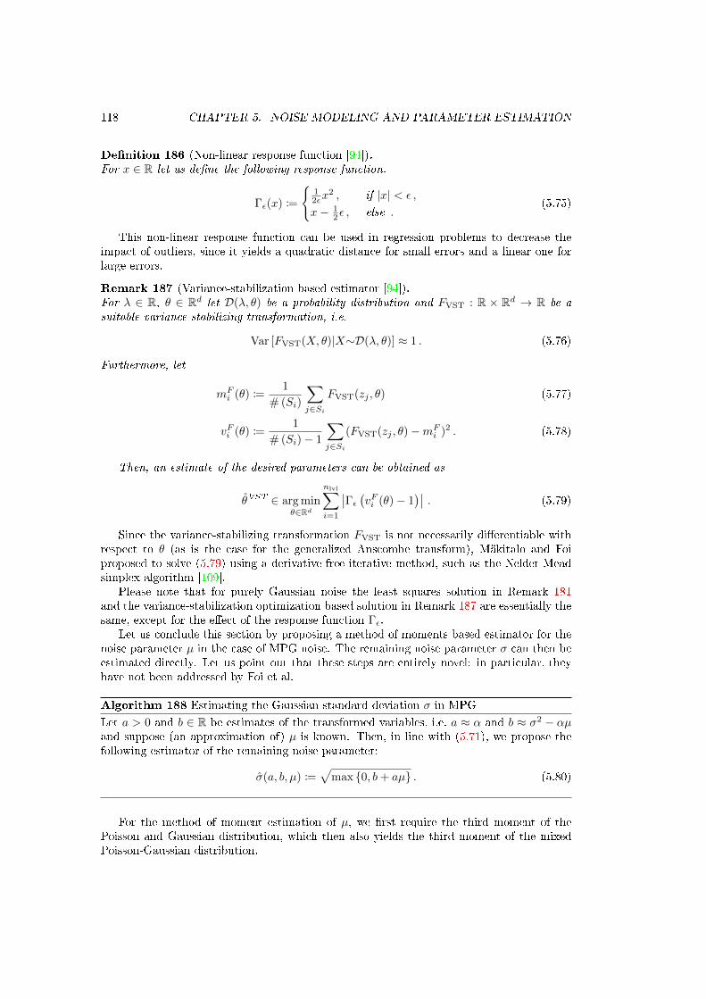
118 CHAPTER 5. NOISE MODELING AND PARAMETER ESTIMATION
Denition 186 (Non-linear response function [94]).For x ∈ R let us dene the following response function.
Γε(x) :=
12εx
2 , if |x| < ε ,
x− 12ε , else .
(5.75)
This non-linear response function can be used in regression problems to decrease theimpact of outliers, since it yields a quadratic distance for small errors and a linear one forlarge errors.
Remark 187 (Variance-stabilization based estimator [94]).For λ ∈ R, θ ∈ Rd let D(λ, θ) be a probability distribution and FVST : R × Rd → R be asuitable variance-stabilizing transformation, i.e.
Var [FVST(X, θ)|X∼D(λ, θ)] ≈ 1 . (5.76)
Furthermore, let
mFi (θ) :=
1
# (Si)
∑j∈Si
FVST(zj , θ) (5.77)
vFi (θ) :=1
# (Si)− 1
∑j∈Si
(FVST(zj , θ)−mFi )2 . (5.78)
Then, an estimate of the desired parameters can be obtained as
θVST ∈ arg minθ∈Rd
nlvl∑i=1
∣∣Γε (vFi (θ)− 1)∣∣ . (5.79)
Since the variance-stabilizing transformation FVST is not necessarily dierentiable withrespect to θ (as is the case for the generalized Anscombe transform), Mäkitalo and Foiproposed to solve (5.79) using a derivative-free iterative method, such as the Nelder-Meadsimplex algorithm [109].
Please note that for purely Gaussian noise the least squares solution in Remark 181and the variance-stabilization optimization based solution in Remark 187 are essentially thesame, except for the eect of the response function Γε.
Let us conclude this section by proposing a method of moments based estimator for thenoise parameter µ in the case of MPG noise. The remaining noise parameter σ can then beestimated directly. Let us point out that these steps are entirely novel: in particular, theyhave not been addressed by Foi et al.
Algorithm 188 Estimating the Gaussian standard deviation σ in MPGLet a > 0 and b ∈ R be estimates of the transformed variables, i.e. a ≈ α and b ≈ σ2 − αµand suppose (an approximation of) µ is known. Then, in line with (5.71), we propose thefollowing estimator of the remaining noise parameter:
σ(a, b, µ) :=√
max 0, b+ aµ . (5.80)
For the method of moment estimation of µ, we rst require the third moment of thePoisson and Gaussian distribution, which then also yields the third moment of the mixedPoisson-Gaussian distribution.

5.4. UNSUPERVISED NOISE PARAMETER ESTIMATION 119
Remark 189 (Third centralized moment of the Poisson distribution [157]).Let λ > 0 and P∼P(λ). Then
E[(P − E [P ])
3]
= E [P ] . (5.81)
Remark 190 (Third centralized moment of the Gaussian distribution [114]).Let σ > 0, µ ∈ R and H∼N (µ, σ). Then
E[(H − E [H])
3]
= 0 . (5.82)
Remark 191 (Third centralized moment of MPG).Let λ, α > 0, µ ∈ R, σ ≥ 0 and C∼C(λ, α, µ, σ). Then
E[(C − E [C])
3]
= α2 (E [C]− µ) . (5.83)
Proof. Let P∼P(λ) and H∼N (µ, σ). Then, due to the additivity of the third centralizedmoment, we receive
E[(C − E [C])
3], = E
[(αP +H − E [αP +H])
3], (5.84)
= E[(αP − E [αP ])
3]
+ E[(H − E [H])
3], (5.85)
= α3E[(P − E [P ])
3]
= α3E [P ] . (5.86)
Now the result follows from (5.13).
Now let us derive a least squares t for the parameter µ along the lines of Remark 181,but using the third centralized moment of the mixed Poisson-Gaussian distribution thistime.
Remark 192 (Method of moments estimator of the Gaussian mean µ in MPG).Let g, Z,z and Si,mi, vi, i = 1, . . . , nlvl be as in Remark 180, where Zj∼C(gj , α, µ, σ) forj ∈ I. Furthermore, let a > 0 and b ∈ R be estimates of the transformed variables, i.e.
a ≈ α and b ≈ σ2 − αµ. Furthermore, let
γi :=1
# (Si)
∑j∈Si
(zj −mi)3 , (5.87)
the sample-based estimator of the third centralized moment. Then, based on (5.83) andanalogous to Remark 181, we propose to use the following least squares estimator for theGaussian mean:
µLS ∈ arg minµ∈R
nlvl∑i=1
(γi − α2(mi − µ)
)2. (5.88)
The unique solution is given by
µLS =1
nlvl
nlvl∑i=1
mi −1
α2γi . (5.89)

120 CHAPTER 5. NOISE MODELING AND PARAMETER ESTIMATION
Proof. Let
L(µ) :=1
2
nlvl∑i=1
(γi − α2(mi − µ)
)2. (5.90)
Then
L′(µ) = α2nlvl∑i=1
γi − α2(mi − µ) . (5.91)
Solving L′(µ) = 0 with basic operations concludes the proof.
5.4.2 Finding sets of observations with a similar mean
The parameter estimation discussed in the previous section was built around the knowl-edge of level sets suitable for estimating pairs of mean and variance (cf. (5.65) and (5.66)).Here, we would like to discuss available algorithms for this purpose and propose a new one.Please note that now we return to the setting of two-dimensional images.
Alongside with the ideas discussed in the previous section, Foi et al. proposed a strategyto retrieve the level sets. The details of the algorithm are rather technical. Thus, for aprecise denition, please refer to [53]. The main aspects of the method can be summarizedas follows.
Algorithm 193 Estimating level sets based on a smoothness set [53]Given a noisy image z, the strategy for nding level sets proposed by Foi et al. can besummarized as follows:
1) set g := LH(z) using a suitable smoothing lter kernel H ,
2) estimate a set Ismooth =j ∈ I : j does not belong to an edge
,
3) dene an equidistant sampling g1, . . . , gnlvlof the range V ,
4) dene Si :=j ∈ Ismooth : |gj − gi| ≤ ∆i
.
5) discard any Si with # (Si) < 2
Please note that there is no requirement for the level sets to be connected. Beyond thesesteps, the level sets are somehow modied in order to be disjoint (the details of this are notmentioned in [53]).
While this strategy was found to work considerably well for natural images, it has certaindrawbacks. First of all, the choice of ∆i might aect the sample variance. More importantly,the method in Algorithm 193 assumes a piecewise homogeneous image model. In particular,it assumes that away from edges linear ltering yields a reasonably accurate estimate ofthe mean value. This assumption is not met, for instance, in case of smooth gradients thatmay also appear in natural images. More importantly, in view of our context, let us pointout that atomic-scale electron micrographs typically have large gradients almost everywhere(due to the high contrast between atoms and void). Therefore, the method described inAlgorithm 193 is not suitable for our purpose. On a more general level, let us remindourselves that regularity assumptions, as the ones made in Algorithm 193, are not in linewith the non-local averaging principle we pursuit (cf. Remark 17).
In the following, let us propose a remedy for the aforementioned deciencies that is morein line with the non-local principle. We base our strategy solely on the assumption that

5.4. UNSUPERVISED NOISE PARAMETER ESTIMATION 121
image details are larger than the resolution of the image. In order to formalize this, let usintroduce the following notation for a patch without its central pixel:
Pi :=i+ j : j ∈ −n1−1
2 , . . . , n1−12 × −
n2−12 , . . . , n2−1
2 \ i , i ∈ I . (5.92)
Let g be a noise-free image (ground truth) image. Then, given a reasonably large patchsize, we assume that for any i, j ∈ I the following holds
distL2(gPi , gPj ) is small ⇒ |gi − gj |2 is small . (5.93)
This allows us to approximate level sets as follows.
Algorithm 194 Non-local similarity search based level set estimationGiven a reference coordinate i ⊂ I and a set of matching candidates S ⊂ I, in line with(2.30), let us measure the accuracy of t as follows:
disti(S) :=∑j∈S
distL2(gPi , gPj ) . (5.94)
Then, for xed slvl ∈ N, we estimate the corresponding level set as
S′i := arg minS⊂I,#(S)=slvl
disti(S) , (5.95)
which is the set of the slvl best matching coordinates according to the L2 similarity measure,disregarding the dierence of the centers of the patches.
Please note that, as stated before, the sets in (5.95) are not level sets in the strictmathematical sense (since the included pixels do not have the same intensities), but anapproximation of a set of pixel with the same expected value.
Furthermore, note that we deliberately disregard the centers of the patches for the sim-ilarity search here as this avoids introducing a bias to the similarity of the noise instanceswithin the level sets - and therefore also avoids an according bias of the sample variances.Furthermore, note that S′i can be computed in O (M(np + slvl)) by performing a globalsimilarity search and then selecting the slvl patches with the smallest distance.
Here, on the one hand, the parameter slvl should be chosen large enough to ensure areasonably small error of the sample variance (cf. (5.66)). On the other hand, it must bechosen small enough that there are at least slvl occurrences of the image detail at i withinthe rest of the image. Ensuring the latter condition is not a trivial task when regardedindividually for each reference coordinate. Fortunately, it is not necessary to do so for everypossible reference coordinate, since typically the number of level sets required to retrieve areliable estimate of the model parameters is much smaller than the number of pixels, i.e.nlvl M . Furthermore, it is typically safe to assume that the image contains a large amountof details that occur at least slvl times for a reasonable choice of slvl, e.g. slvl ∈ [32, 64].
Besides this, it is important that the reference coordinates are selected such that theresulting sample means span the majority of the image range V . This is to ensure a goodaccuracy of the tted variance model across all mean values. Since we do not assumethe reliability of a linear lter based estimate anywhere, we cannot reliably predict whichcoordinate is best suited as the reference for a given mean value. Therefore, we will employan adaptive sampling strategy.

122 CHAPTER 5. NOISE MODELING AND PARAMETER ESTIMATION
Together, these two aspects lead us to the following strategy for the global selection ofreference coordinates.
Algorithm 195 Global selection of level setsFor alvl ∈ N we dene an initially enlarged number of level sets:
nlvl↑ := alvlnlvl . (5.96)
Also, let z denote the noisy image and g := LHMA(z) an estimate of z based on moving
averages with a small kernel (e.g. n = (3, 3)).We suggest to use the minimum and maximum estimated image intensities to determine therst two reference coordinates:
ref1 := arg minj∈I
gj ,
ref2 := arg maxj∈I\ref1
gj .(5.97)
In the following we outline an adaptive strategy to select refi+1 based on the sample meansm1, . . . ,mi. First, we bring them into ascending order, receiving mi
1 ≤ · · · ≤ mii and we
denote with
nik := #(j ∈ I : gj ∈
[mik, m
ik+1
]\
ref1, . . . , refi)
, k = 1, . . . , i− 1 , (5.98)
the number of intensity values in the moving averages estimate that lie between each of thesample means (excluding previously used reference coordinates). This allows us to dene
m(1, . . . , i) :=mik∗ + mi
k∗+1
2, k∗ := arg max
k=1,...,i−1
nik≥1
|mik+1 − mi
k| , (5.99)
the center point of the largest interval between two neighboring (i.e. consecutive in ascendingorder) sample means among the rst i selected reference coordinates, which contains at leastone estimated image intensity (that has not been used as a reference coordinate yet).Then, in favor of sampling the entire image range as evenly as possible, we propose to selectthe remaining reference coordinates adaptively as follows:
refi+1 := arg minj∈I\ref1,...,refi
|gj − m(1, . . . , i)| . (5.100)
Finally, the reference coordinates for the actual noise model parameter t are selected asthe nlvl ones with the best accuracy of t:
I∗ref := arg minI′⊂
ref1,...,refnlvl
↑#(I′)=nlvl
∑i∈I′
disti(S′i) . (5.101)
For the context of HAADF-STEM imaging, we recommend the following two modica-tions to Algorithms 194 and 195:
(i) for a suitable n ∈ N, set np = (n, 1) ,
(ii) set alvl = 1 .

5.4. UNSUPERVISED NOISE PARAMETER ESTIMATION 123
40 60 80 100 120 140 160
250
500
750
1000
1250
1500
1750samples
least squares fit
ground truth
mi
v i
20 40 60 80 100 120 140 160
600
1200
1800
2400
3000
3600
4200samples
least squares fit
ground truth
mi
v i
Figure 5.5: Sample mean-variance pairs (cyan cross marks) of the level sets extracted fromthe noisy Aachen cathedral image (cf. Figure 2.2) corrupted by AGWN with σ = 25 (left)and σ = 40 (right), estimated noise standard deviation (green dash-dotted line) and groundtruth (blue dashed line); parameters used: alvl = 10, nlvl = 100, slvl = 64 and np = (11, 11)
Using blocks of vertical size equal to one adapts the block-matching to the scan-line dis-tortions inherent to scanning acquisition (cf. Chapter 1) and has been found to drasticallyincrease the accuracy of the noise parameter estimates. Please see Figure 5.9 (which will bediscussed later in detail) for a comparison that reveals how signicant this eect is. Pleasenote that reducing the vertical block size component must be somehow compensated byincreasing the horizontal one, in oder to achieve a comparable noise robustness of the patchsimilarity measure.
Less importantly, but still worth mentioning, we found that atomic-scale images typicallycontain more than enough samples for any reference coordinate such that the optimizationin (5.101) is not required. Even if a unique feature (such as a single dislocation) happensto be chosen as a reference coordinate, this just produces one or a few outliers which cantypically be handled by the t in (5.79), especially when tting an ane function, such asfor MPG.
5.4.3 Numerical results: noise parameter estimation
Let us begin with an experimental verication of the proposed noise parameter estimationframework on the basis of purely additive Gaussian white noise. Figure 5.5 shows the samplemeans and variances gathered from the Aachen cathedral image (cf. Figure 2.2) corruptedby AGWN with σ = 25 (left) and σ = 40 (right). Obviously, the standard deviation isexpected to be over-estimated to some degree, since the mean values of the pixels in acertain level set will never coincide exactly. Still, with about 7.7% relative error the resultσ = 26.9188 is useful in practice. Please note that for higher standard deviations smalluctuations in the underlying mean values will have less relative inuence on the samplevariance. Indeed, the result for the σ = 40 case is σ = 41.8391, which yields a relative errorof about 4.6%. In order to assess the eect of the error in the estimated noise standarddeviation on the denoising estimate, we applied the BM3D lter from Algorithm 25 to theAachen cathedral image and compared the PSNR when using the true standard deviationversus the estimated one. This yields a dierence of 0.1832 dB for σ = 25 and 0.0634 dB forσ = 40, which is rather small.
Now we come to the more interesting part: analyzing mixed Poisson-Gaussian noise.Again, let us rst regard a natural image, namely the Aachen cathedral from Figure 2.2.In Figure 5.6, it is shown with randomly generated MPG noise using three dierent sets ofparameters.

124 CHAPTER 5. NOISE MODELING AND PARAMETER ESTIMATION
Figure 5.6: Aachen cathedral image scaled to range [50, 200] and aected by mixed Poisson-Gaussian noise with the following parameters (from left to right): (α, σ, µ) = (1.5, 25, 100),(0.1, 1,−250), (10, 500, 1000)
200 225 250 275 300 325
700
1050
1400
1750
2100
2450 samples
least squares fit
VST optimization fit
ground truth
mi
v i
Figure 5.7: Sample mean-variance pairs of the level sets extracted from the noisy Aachencathedral image (α = 1.5, σ = 25, µ = 100) in Figure 5.6 and linear variance functions;parameters used: alvl = 10, nlvl = 100, slvl = 64, np = (17, 17)

5.4. UNSUPERVISED NOISE PARAMETER ESTIMATION 125
Ground truth Algorithm 193 [53] Proposed method
α σ µ a b |a−a||a|
|b−b||b|
|a−a||a|
|b−b||b|
1.5 25 100 1.5 475 0.3754 0.2741 0.0212 0.1699
0.1 1 -250 0.1 26 0.2798 0.2599 0.1836 0.1870
10 500 1000 10 2.4 · 105 0.1425 0.0060 0.1419 0.0035
Table 5.1: Relative errors in the estimated variance parameters a, b for the estimationmethod proposed by [53] and our method for the Aachen cathedral image aected bymixed Poisson-Gaussian noise of dierent parameters
a b LHMAF kbil F kNLM
BM3D1.5 475 27.5101 28.2037 30.0259 31.8074
1.46817 555.683 27.5103 28.1783 30.1915 31.7233
Table 5.2: Comparison of the PSNRs after denoising the MPG instance of the Aachencathedral image (cf. Figure 5.23) with dierent lters; results use dierent noise parameters:ground truth (top row) and estimated (bottom row)
Figure 5.7 shows the result of the mixed Poisson-Gaussian noise analysis for the Aachencathedral image with noise parameters α = 10, σ = 25, µ = 100. As we can see, thevariance-stabilization optimization based estimate is slightly better than the least squaresestimate, but both have a noticeable constant oset.
In order to evaluate the accuracy of the proposed estimates, let us compare them to theresults retrieved by the method published in [53]. For the dierent choices of the groundtruth parameters, Table 5.1 shows the resulting relative errors in the two variance parame-ters. The results indicate that our patch similarity based approach of estimating level setsis consistent with, or even superior to the method proposed by Foi et al. [53].
In this context, it is also interesting to analyze how the error within the noise parameterestimation aects the PSNR after denoising. The corresponding comparison is given inTable 5.2. The results indicate that the error introduced by the noise parameter estimationis very small.
Now let us turn towards HAADF-STEM imaging and investigate the eect of the scanline distortions on the sample variance of the level sets. The left image in Figure 5.8shows a simulated image without shot noise but including horizontal distortions. The rightimage in the same gure shows the corresponding image after corruption with MPG noiseof the parameters α = 100, σ = 10, µ = 1000, i.e. a = 100, b = −99900. Furthermore,Figure 5.9 shows the corresponding plots of the sample mean and variance pairs in the samefashion as Figure 5.7. The following parameters were used: alvl = 1, nlvl = 1000, slvl = 64.The dierence between the two plots is that for the left the block size np = (17, 17) wasused, whereas for the right, the block size np = (51, 1) was used. The results conrmour expectation that reducing the vertical component of the block size to one signicantlyreduces the estimation error.
In order to assess whether the linear variance model does actually seem plausible forHAADF-STEM imaging, let us also perform the noise parameter estimation for two ex-perimental images. For the electron micrographs shown in Figure 5.10, the correspondingsample mean-variance pairs and tted linear variance models are shown in Figure 5.11. Inour view, the goodness of t of the linear model is sucient to support the validity of the

126 CHAPTER 5. NOISE MODELING AND PARAMETER ESTIMATION
Figure 5.8: Articial HAADF-STEM image (λ ∈ (0, 6]) including scan line distortions with-out shot noise (left) and with mixed Poisson-Gaussian noise (right) of parameters α = 100,σ = 10, µ = 1000; images courtesy of Paul M. Voyles
1120 1200 1280 1360 1440 1520 1600
10000
20000
30000
40000
50000
60000
70000sample (mean, variance)
least squares fit
VST optimization fit
ground truth
mi
v i
1120 1200 1280 1360 1440 1520 1600
10000
20000
30000
40000
50000
60000
70000
80000sample (mean, variance)
least squares fit
VST optimization fit
ground truth
mi
v i
Figure 5.9: Sample mean-variance pairs of the level sets extracted from the noisy simulatedHAADF-STEM image in Figure 5.8 and linear variance functions; parameters used: alvl = 1,nlvl = 1000, slvl = 64 and np = (17, 17) (left), np = (51, 1) (right)
mixed Poisson-Gaussian noise model. In particular, let us point out that the data indicatesvery clearly that neither a plain Poisson (a = 1 and b = 0), nor a plain Gaussian model(a = 0) is plausible. Besides these two extremes, one could also assume a scaled and con-stantly shifted Poisson distribution (a > 0, b 6= 0, σ = 0). Indeed, the idea of performingan ane transformation to HAADF-STEM images in order to conform its intensities to aPoisson distribution has been put forward, but is not yet very common, in the materialsscience community. Please note that our proposed method could be used to approximatesuch an ane transformation (using b
a = µ for σ = 0). However, we believe that accountingfor an additional source of noise, namely the Gaussian part, yields a more realistic model.
Figures 5.12 and 5.13 show exemplary level sets extracted from the Aachen cathedralimage in Figure 5.6 and the gallium nitride HAADF-STEM image in Figure 5.10. In thelatter case, we also show the (one-dimensional) patches stacked on top of each other.
Finally, we would like to present the results of the µ parameter estimation based on the

5.4. UNSUPERVISED NOISE PARAMETER ESTIMATION 127
Figure 5.10: Experimental HAADF-STEM images (left: CMS-GaAs, right: gallium nitride);images courtesy of Paul M. Voyles
2450 2800 3150 3500 3850 4200160000
240000
320000
400000
480000
560000
640000 samples
least squares fit
VST optimization fit
mi
v i
4550 4900 5250 5600 5950 6300 6650
80000
120000
160000
200000
240000
280000
320000samples
least squares fit
VST optimization fit
mi
v i
Figure 5.11: Sample mean-variance pairs of the level sets extracted from the noisy exper-imental HAADF-STEM images in Figure 5.10 and linear variance functions; parametersused: alvl = 1, nlvl = 1000, slvl = 64, np = (51, 1)
method of moments approximation in Remark 192. For the dierent Aachen cathedralimages and the HAADF-STEM image they are shown in Table 5.3. Obviously, the relativeaccuracy in σ is much worse than in the plain Gaussian noise model, which is not surprisingdue to the increased complexity of the mixed Poisson-Gaussian noise model. The relativeaccuracy of µLS is quite good in two cases, but rather poor in the rest of the cases. Despitethe fact that the third moment estimator is much more sensitive to outliers than the secondmoment (variance) estimator, this aspect of noise estimation should be investigated furtherin future. Let us stress again that for the purpose of variance stabilization the individualestimation of µ and σ is not required.

128 CHAPTER 5. NOISE MODELING AND PARAMETER ESTIMATION
Figure 5.12: Level sets (red dots mark the center points of the patches) extracted from thenoisy Aachen cathedral image in Figure 5.6 for two selected reference coordinates
Figure 5.13: Level set (red dots mark the center points of the patches) extracted fromthe gallium nitride image in Figure 5.10 for a selected reference coordinate (left) and thecorresponding stack of patches (right)

5.4. UNSUPERVISED NOISE PARAMETER ESTIMATION 129
Image λ range α µ µLS σ σ(a, b, µLS)Aachen cathedral [50,200] 1.5 100 26.6798 25 26.6798Aachen cathedral [50,200] 0.1 -250 -268.167 1 0Aachen cathedral [50,200] 10 1000 2.1872 · 106 500 26.6798Aachen cathedral∗ [50,200] 10 1000 43480 500 909.798HAADF-STEM (0,6] 100 1000 956.72 10 0
Table 5.3: Results of the µ and σ parameter estimation based on the method of moments(cf. (5.80) and Remark 192). ∗ uses nlvl = 500, alvl = 4.
1200 1350 1500 1650 1800 1950 21000
60000
120000
180000
240000
300000
360000 samples
least squares fit
VST optimization fit
ground truth
mi
v i
Figure 5.14: Sample mean-variance pairs of the level sets extracted from the HAADF-STEMimage in Figure 5.8 and linear variance functions; parameters used: α = 200, σ = 50, µ =1000, alvl = 1, nlvl = 1000, slvl = 64, np = (51, 1)
5.4.4 On the ill-posedness of noise parameter estimation in
HAADF-STEM
As presented above, we found that the noise parameter estimation described above worksquite well for both natural images and atomic-scale electron micrographs (articial andexperimental). However, in the case of articial electron micrographs, we were also able toconstruct cases where the estimated parameters had signicant errors. An extreme exampleis shown in Figure 5.14.
In the following, we would like to argue that this is not a deciency of the estimationalgorithm, but rather due to the problem being ill-conditioned. Arguments supportingthis claim are that the underlying ground truth of an atomic-scale electron micrograph isnowhere locally constant. This means that even very small errors in the assignment of pixelsto according level sets can lead to large dierences in the underlying mean values. Let alonethe fact that due to the nite pixel size technically there might not even exist two pixels inthe image that have the same underlying mean intensity.
Let us analyze how such errors aect the sample variance and to which degree theestimated parameters could be improved through an appropriate correction (if available).As an approximation for this scenario, let us assume that the observations in each level

130 CHAPTER 5. NOISE MODELING AND PARAMETER ESTIMATION
set do not belong to a common and xed mean value. Instead, we introduce an additionalvariation, in the form of a uniform random distribution of the Poisson mean values. Thisgives the following result.
Lemma 196 (Variance of a mean-randomized MPG random variable).For λ, α > 0, µ ∈ R and σ ≥ 0, let C = αP +H ∈ C(λ, α, µ, σ). Furthermore, for a ≤ b ∈ Rlet U (a, b) denote the uniform probability distribution, i.e.
Pr (X = x|X∼U (a, b)) =
1b−a , if a ≤ x ≤ b ,0 , else .
(5.102)
Now, let 0 < ∆ < 2λ and P∆∼P(U∆), where U∆∼U(λ− 1
2∆, λ+ 12∆), as well as C∆ :=
αP∆ +H. Then,
E[C∆]
= E [C] , (5.103)
Var[C∆]
= Var [C] +1
12α2∆2 . (5.104)
Proof. First of all, we immediately receive
E[C∆]
=1
∆
ˆ λ+12
λ− 12
αz + µdz = αλ+ µ = E [C] (5.105)
which is (5.103).Furthermore, using Cy∼C(y, α, µ, σ) and Py∼P(y) for y > 0, we have
E[(C∆)2
]=
ˆRz2Pr
(C∆ = z
)dz
=
ˆRz2
ˆ λ+12∆
λ− 12∆
Pr(Cy = z|U∆ = y
)Pr(U∆ = y
)dy dz
=1
∆
ˆ λ+12∆
λ− 12∆
ˆRz2Pr (αPy +H = z) dz − (αy + µ)2 dy
+1
∆
ˆ λ+12∆
λ− 12∆
(αy + µ)2 dy
=1
∆
ˆ λ+12∆
λ− 12∆
Var [αPy +H] dy +1
∆
ˆ λ+12∆
λ− 12∆
αy + µ)2 dy
=1
∆
ˆ λ+12∆
λ− 12∆
α2y + σ2 dy +1
∆
ˆ λ+12∆
λ− 12∆
(αy + µ)2 dy
=α2λ+ σ2 +1
∆
ˆ λ+12∆
λ− 12∆
α2y2 + 2αyµ+ µ2 dy
=Var [C] + (αλ+ µ)2 +1
12α2∆2
(5.106)

5.5. p-VALUES: GENERALIZING THE METHOD NOISE 131
This nally gives
Var[C∆]
=E[(C∆)2
]− E
[C∆]2
=Var [C] + (αλ+ µ)2 +1
12α2∆2 − (αλ+ µ)2
=Var [C] +1
12α2∆2
(5.107)
which concludes the proof.
Furthermore, let us point out that given a suitably regularized version of the level sets,there is a simple estimator for α∆.
Remark 197 (Maximum-likelihood estimator for α∆).For a sample size m ∈ N, λ > 0, 0 < ∆ < 2λ, let Ui∼U
(λ− 1
2∆, λ+ 12∆)i.i.d. random
variables for i = 1, . . . ,m. Furthermore, for α > 0 and µ ∈ R, let a = α(λ − 12∆) + µ,
b = α(λ + 12∆) + µ. Then, for the (actually observed) random variables Xi := αUi + µ,
we have Xi∼U (a, b). Furthermore, given an observation x of X, the maximum-likelihoodestimators of the parameters a, b are given as [37]:
a = mini=1,...,m
xi , b = maxi=1,...,m
xi . (5.108)
Thus, an appropriate estimate for α∆ = b− a is given by b− a = maxi xi −mini xi.
Unfortunately, despite applying various kinds of regularization strategies prior to esti-mating the α∆i for the level sets, we were unable to design an algorithm that consistentlyimproved the resulting noise variance parameter estimates in an articial setting where thetrue error could be computed. Nevertheless, we would like to point out that performing thenoise parameter estimation on the noisy data, but using the ground truth data to estimatethe ∆i for each level set, can indeed signicantly boost the accuracy of the resulting esti-mate. Figure 5.15 shows the ∆i retrieved in this way for the example from Figure 5.14. Itturns out that the deviation in λ is actually quite large (within [0.5, 5]). Furthermore, wesee that it varies for the dierent mean values, which is plausible, since the variation of theintensity in the ground truth also depends on the intensity itself (atoms are approximatelyresembled by Gaussian bells).
In Figure 5.16, we have repeated the noise parameter estimation from Figure 5.14,but based on the corrected sample variances retrieved by applying the correction fromLemma 196 with the corresponding deltas shown in Figure 5.15. As we see, the t ismuch closer to the ground truth than in Figure 5.14. Quantitatively, the nal (variancestabilization optimization based) t without correction has a relative error of 0.258 in a and0.372 b, whereas the corrected t only yields a relative error of 0.006 in a and 0.073 b.
5.5 p-Values: generalizing the method noise
In the previous part of this chapter, we discussed how more general noise models can beintegrated into denoising frameworks that were designed for additive Gaussian white noise.In this regard, let us also consider the corresponding quality measures. In Section 2.5.1 wediscussed two dierent ones: the quantitative peak signal-to-noise ratio, which is indepen-dent of the noise model and thus remains unchanged in the setting of this chapter; and themethod noise, which is tailored to the AGWN model and cannot be directly extended tonon-additive noise distributions.

132 CHAPTER 5. NOISE MODELING AND PARAMETER ESTIMATION
1200 1350 1500 1650 1800 1950 2100
100
200
300
400
500
600
700
800
mi
α∆i
Figure 5.15: Estimated mean value deviations for the level sets in Figure 5.14 based on therespective ground truth values
1200 1350 1500 1650 1800 1950 2100
60000
120000
180000
240000
300000
360000 sample (mean,variance)
corrected sample (mean,variance)
least squares fit
VST optimization fit
ground truth
mi
v i
Figure 5.16: Sample mean-variance pairs (cyan cross marks) as in Figure 5.14 (same pa-rameters used) and corrected sample mean-variance pairs (golden cross marks) using theα∆i from Figure 5.15; tted linear variance functions are based on the corrected samplemean-variance pairs.

5.5. p-VALUES: GENERALIZING THE METHOD NOISE 133
In the case a variance-stabilizing transformation is employed, as in our context, an al-ternative is to compute the method noise in the transformed domain.
Denition 198 (Variance-stabilization based method noise).Let z be a noisy image following any noise distribution with a corresponding suitable variance-stabilizing transformation FVST and F σ be a lter designed to remove additive Gaussianwhite noise of standard deviation σ. Then, in the style of Algorithm 179, the followinganalog of the method noise can be used to assess the denoising performance:
MNVSTF σ (z) := FVST(z)− (F 1 FVST) (z) . (5.109)
Here, we would like to propose an entirely dierent alternative based on a similar conceptas inverse transform sampling. The idea is to transform the noisy input image such that itbecomes a uniform distribution under the hypothesis that the denoised image contains thecorrect mean values. Otherwise, the transformed noisy image would also show structure inthe form of clusters of very bright or dark values, such as the method noise. The advantageof the new quality measure is that it applies well to a much wider range of probabilitydistributions.
5.5.1 p-values for continuous random processes
Let us begin with the denition of p-values.
Denition 199 (p-value [51]).For λ ∈ R and θ ∈ Rm let D(λ, θ) be a probability distribution and FD(λ,θ) denote thecorresponding cumulative distribution function. Then, the probability of observing a valuez, or a more extreme one, under the null hypothesis that the observed values are distributedaccording to D(λ, θ), is given by
pD(λ,θ)(z) := 2 minFD(λ,θ)(z), 1− FD(λ,θ)(z)
, (5.110)
and called the corresponding p-value.
For these p-values one can derive the following lemma.
Lemma 200 (Uniform distribution of p-values of continuous random variables [51]).Let λ, θ, D(λ, θ) and FD(λ, θ) be as in Denition 199. Then, if FD(λ,θ) is additionallycontinuous, the following holds:
Y∼D(λ, θ)⇒ pD(λ,θ)(Y )∼U (0, 1) . (5.111)
Proof. Let us rst regard p(z) := FD(λ,θ)(z). Then we have
p(z) = FD(λ,θ)(z) = Pr (Y ≤ z|Y∼D(λ, θ))
= Pr(FD(λ,θ)(Y ) ≤ FD(λ,θ)(z)|Y∼D(λ, θ)
),
= Pr(p(Y ) ≤ FD(λ,θ)(z)|Y∼D(λ, θ)
),
(5.112)
since FD(λ,θ) is monotone and continuous. In particular, this means that
Pr(FD(λ,θ)(Y ) ≤ FD(λ,θ)(z)|Y∼D(λ, θ)
)= FD(λ,θ)(z) (5.113)
holds for any z ∈ R. Thus, we also receive
Pr (p(Y ) ≤ x|Y∼D(λ, θ)) = x , (5.114)

134 CHAPTER 5. NOISE MODELING AND PARAMETER ESTIMATION
for all x ∈ [0, 1], which is nothing else than the cumulative distribution function of U (0, 1).Thus,
Y∼D(λ, θ)⇒ p(Y )∼U (0, 1) . (5.115)
Now letU∗ := 2 minU , 1− U, where U∼U (0, 1) . (5.116)
Then, for z ∈ [0, 1]
Pr (U∗ ≤ z) = Pr(
minU , 1− U ≤ z
2
)= Pr
(U ≤ z
2
)+ 1− Pr
(U ≤ 1− z
2
)= z
(5.117)
This yields U∗∼U (0, 1), which concludes the proof.
This lemma can be used to dene a quality measure that is similar to the method noise.
Denition 201 (Inverse image: p-values based quality measure for denoising).For λ ∈ R and θ ∈ Rm let D(λ, θ) be a probability distribution with E [X] = λ for X∼D(λ, θ),and FD(λ,θ) the corresponding CDF. Now let Zj∼D(λj , θ) for j ∈ I be independent random
variables and z ∈ RM1×M2 be an instance of Z. Then, given a suitable image denoisingoperator F : RM1×M2 → RM1×M2 , i.e. F (z) ≈ E [Z] = λ, we call
D−1F (z)i := pD(F (z)i,θ)(zi) , (5.118)
the inverse image.
Now, from Lemma 200 it follows that D−1F (z)∼U (0, 1) if indeed F (z) ≈ E [Z]. Oth-
erwise, D−1F (z) will deviate from a uniform distribution. In particular, we can interpret
deviations in D−1F (z) from a uniform distribution as follows:
(i) Clusters of too bright values (near 1) indicate that the corresponding observationshave abnormally high probabilities, which indicates that the corresponding estimatedmean values are too near to the noisy observations. In other words: regularization inthese areas was most likely too weak.
(ii) Clusters of too dark values (near 0) indicate that the corresponding observations haveabnormally low probabilities, which indicates that the corresponding estimated meanvalues are too far away from the noisy observations. In other words: the regularizationin these areas was either too strong, or simply produced some kind of artifact.
Please note that Denition 201 is directly applicable to Gaussian and MPG noise (cf.Remark 168).
Although we had thoroughly discussed earlier that the MPG noise setting is suitable forour context, and thus the above analysis is sucient for our purposes, its extension to othernoise distributions might be of use in other applications. Unfortunately, Lemma 200 cannotbe applied to discrete random processes, such as Poisson noise, since the correspondingcumulative distribution functions are not continuous. For the Poisson distribution, we expectasymptotic convergence of the corresponding p-values to a uniform distribution as the meangoes to innity, since the Poisson distribution with parameter λ converges to the Gaussiandistribution (cf. Remark 157). Nevertheless, for purely Poisson processes with low meanvalues, the above concept has to be modied in order to be useful.

5.5. p-VALUES: GENERALIZING THE METHOD NOISE 135
5.5.2 P-values for discrete random processes
The major dierence between p-values based on continuous and discrete random variablescan be understood easily by inverting the above concept: if U∼U (0, 1) and F−1
D(θ) exists,
then F−1D(θ)(U)∼D(θ). This fact is used in inverse transform sampling to generate random
numbers following a given continuous probability distribution based on a uniform randomnumber generator. Similarly, one can also generate random numbers following a discreteprobability distribution D(θ), but since the classical inverse function of the correspondingcumulative distribution function does not exist, one has to use the generalized inverse fromDenition 166.
Then F−1
D(θ)(U)∼D(θ). In the continuous case, we could use the p-values to map back from
Y∼D(θ) to p(Y )∼U (0, 1). In the discrete case, there is no way to create a bijective mappingthat goes back from Y∼D(θ) ∈ N0 to [0, 1]. Furthermore, for arbitrary (xk)k∈N0
⊂ [0, 1] thevalues xY do not follow a discrete uniform distribution. However, there is a choice for xkthat will ensure the expected value E [xY ] to coincide with that of the uniform distributionon [0, 1]:
Lemma 202 (Uniform expected value of modied discrete p-values).For λ ∈ R and θ ∈ Rm let D(λ, θ) be a discrete probability distribution with values in N0
and FD(λ,θ) the corresonding CDF. Furthermore, let
p(k) =1
2
(FD(λ,θ)(k) + FD(λ,θ)(k − 1)
). (5.119)
Then, the following holds:
E[p(Y )|Y∼D(λ, θ)
]=
1
2. (5.120)
Proof. Using the short notation F := FD(λ,θ), we receive:
E[p(Y )
∣∣∣Y∼D(λ, θ)]
=
∞∑k=−∞
p(k)Pr(Y = k|Y∼D(λ, θ)
)=
∞∑k=−∞
F (k) + F (k − 1)
2(F (k)− F (k − 1))
=1
2
∞∑k=−∞
F (k)2 − F (k − 1)2
=1
2lim
m→−∞
(limn→∞
n∑k=m
F (k)2 − F (k − 1)2
)
=1
2
(limn→∞
F (n))2
− 1
2
(lim
m→−∞F (m− 1)
)2
=1
2.
(5.121)
Still, the random variable p(Y ) does not follow a (discrete) uniform distribution. Toachieve this, it is required to introduce an additional random variable.
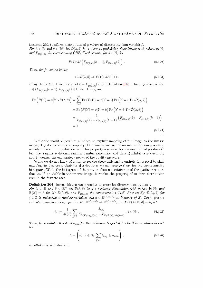
136 CHAPTER 5. NOISE MODELING AND PARAMETER ESTIMATION
Lemma 203 (Uniform distribution of p-values of discrete random variables).For λ ∈ R and θ ∈ Rm let D(λ, θ) be a discrete probability distribution with values in N0
and FD(λ,θ) the corresonding CDF. Furthermore, for k ∈ N0 let
P (k)∼U(FD(λ,θ)(k − 1), FD(λ,θ)(k)
). (5.122)
Then, the following holds:
Y∼D(λ, θ)⇒ P (Y )∼U (0, 1) . (5.123)
Proof. For x ∈ [0, 1] arbitrary, let k = F−1
D(λ,θ)(x) (cf. Denition 166). Then, by construction
x ∈ (FD(λ,θ)(k − 1), FD(λ,θ)(k)] holds. This gives
Pr(P (Y ) = x
∣∣∣Y∼D(λ, θ))
=
∞∑i=0
Pr(P (Y ) = x
∣∣Y = i)
Pr(Y = i
∣∣∣Y∼D(λ, θ))
= Pr(P (Y ) = x
∣∣Y = k)
Pr(Y = k
∣∣∣Y∼D(λ, θ))
=1
FD(λ,θ)(k)− FD(λ,θ)(k − 1)
(FD(λ,θ)(k)− FD(λ,θ)(k − 1)
)= 1.
(5.124)
While the modied p-values p induce an explicit mapping of the image to the inverseimage, they do not share the property of the inverse image for continuous random processes,namely to be uniformly distributed. This property is ensured for the randomized p-values P ,but they require additional random number generation and thus 1) inhibit reproducibilityand 2) weaken the explanatory power of the quality measure.
While we do not know of a way to resolve these deciencies entirely for a pixel-to-pixelmapping for discrete probability distributions, we can resolve them for the correspondinghistogram. While the histogram of the p-values does not retain any of the spatial structurethat would be visible in the inverse image, it retains the property of uniform distributioneven in the discrete case.
Denition 204 (Inverse histogram: a quality measure for discrete distributions).For λ ∈ R and θ ∈ Rm let D(λ, θ) be a probability distribution with values in N0 andE [X] = λ for X∼D(λ, θ), and FD(λ,θ) the corresponding CDF. Now let Zj∼D(λj , θ) for
j ∈ I be independent random variables and z ∈ RM1×M2 an instance of Z. Then, given a
suitable image denoising operator F : RM1×M2 → RM1×M2 , i.e. F (z) ≈ E [Z] = λ, let
hi :=1
# (I)
∑j∈I
δi,zj
FD(F (z)j ,θ)(i)− FD(F (z)j ,θ)(i−1)
, i ∈ N0 . (5.125)
Then, for a suitable threshold nmin for the minimum (expected / actual) observations in eachbin,
h =
hi : i ∈ N0,∑j∈I
δi,zj ≥ nmin
, (5.126)
is called inverse histogram.
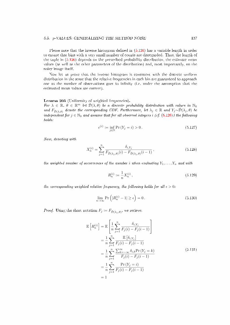
5.5. p-VALUES: GENERALIZING THE METHOD NOISE 137
Please note that the inverse histogram dened in (5.126) has a variable length in orderto ensure that bins with a very small number of counts are disregarded. Thus, the length ofthe tuple in (5.126) depends on the prescribed probability distribution, the estimate meanvalues (as well as the other parameters of the distribution) and, most importantly, on thenoisy image itself.
Now let us prove that the inverse histogram is consistent with the discrete uniformdistribution in the sense that the relative frequencies in each bin are guaranteed to approachone as the number of observations goes to innity (i.e. under the assumption that theestimated mean values are correct).
Lemma 205 (Uniformity of weighted frequencies).For λ ∈ R, θ ∈ Rm let D(λ, θ) be a discrete probability distribution with values in N0
and FD(λ,θ) denote the corresponding CDF. Furthermore, let λj ∈ R and Yj∼D(λj , θ) be
independent for j ∈ N0 and assume that for all observed integers i (cf. (5.126)) the followingholds:
c(i) := infj∈N
Pr (Yj = i) > 0 . (5.127)
Now, denoting with
X(i)n =
n∑j=1
δi,YjFD(λj ,θ)
(i)− FD(λj ,θ)(i− 1)
, (5.128)
the weighted number of occurrences of the number i when evaluating Y1, . . . , Yn and with
R(i)n :=
1
nX(i)n , (5.129)
the corresponding weighted relative frequency, the following holds for all ε > 0:
limn→∞
Pr(|R(i)n − 1| ≥ ε
)= 0 . (5.130)
Proof. Using the short notation Fj := FD(λj ,θ), we recieve:
E[R(i)n
]= E
1
n
n∑j=1
δi,YjFj(i)− Fj(i− 1)
=
1
n
n∑j=1
E[δi,Yj
]Fj(i)− Fj(i− 1)
=1
n
n∑j=1
∑∞k=−∞ δi,kPr (Yj = k)
Fj(i)− Fj(i− 1)
=1
n
n∑j=1
Pr (Yj = i)
Fj(i)− Fj(i− 1)
= 1
(5.131)

138 CHAPTER 5. NOISE MODELING AND PARAMETER ESTIMATION
Using aj := (Fj(i)− Fj(i− 1))−1, we also receive:
Var[R(i)n
]=
1
n2Var
[X(i)n
]=
1
n2Var
n∑j=1
ajδi,Yj
=
1
n2
n∑j=1
a2jVar
[δi,Yj
]+∑j 6=l
ajalCov[δi,Yj , δi,Yl ]
.
(5.132)
For the variance Var[δi,Yj
]we receive the following:
Var[δi,Yj
]= E
[δ2i,Yj
]− E
[δi,Yj
]2=
∞∑k=−∞
δ2i,kPr (Yj = k)−
( ∞∑k=−∞
δi,kPr (Yj = k)
)2
= Pr (Yj = i)− (Pr (Yj = i))2
(5.133)
Since the Yj are pairwise independent, the covariance Cov[δi,Yj , δi,Yl ] is zero:
Cov[δi,Yj , δi,Yl ] = E[δi,Yjδi,Yl
]− E
[δi,Yj
]E [δi,Yl ]
=
∞∑k=−∞
δi,kδi,kPr (Yj = k, Yl = k)− Pr (Yj = i) Pr (Yl = i)
= Pr (Yj = i, Yl = i)− Pr (Yj = i) Pr (Yl = i)
= 0
(5.134)
Together this yields:
Var[R(i)n
]=
1
n2
n∑j=1
Pr (Yj = i)− (Pr (Yj = i))2
(F (i)− F (i− 1))2
=1
n2
n∑j=1
Pr (Yj = i)− (Pr (Yj = i))2
(Pr (Yj = i))2
=1
n2
n∑j=1
[1
Pr (Yj = i)− 1
]
≤ 1
n2
n∑j=1
[1
c(i)− 1
]
=(c(i))−1 − 1
n
(5.135)
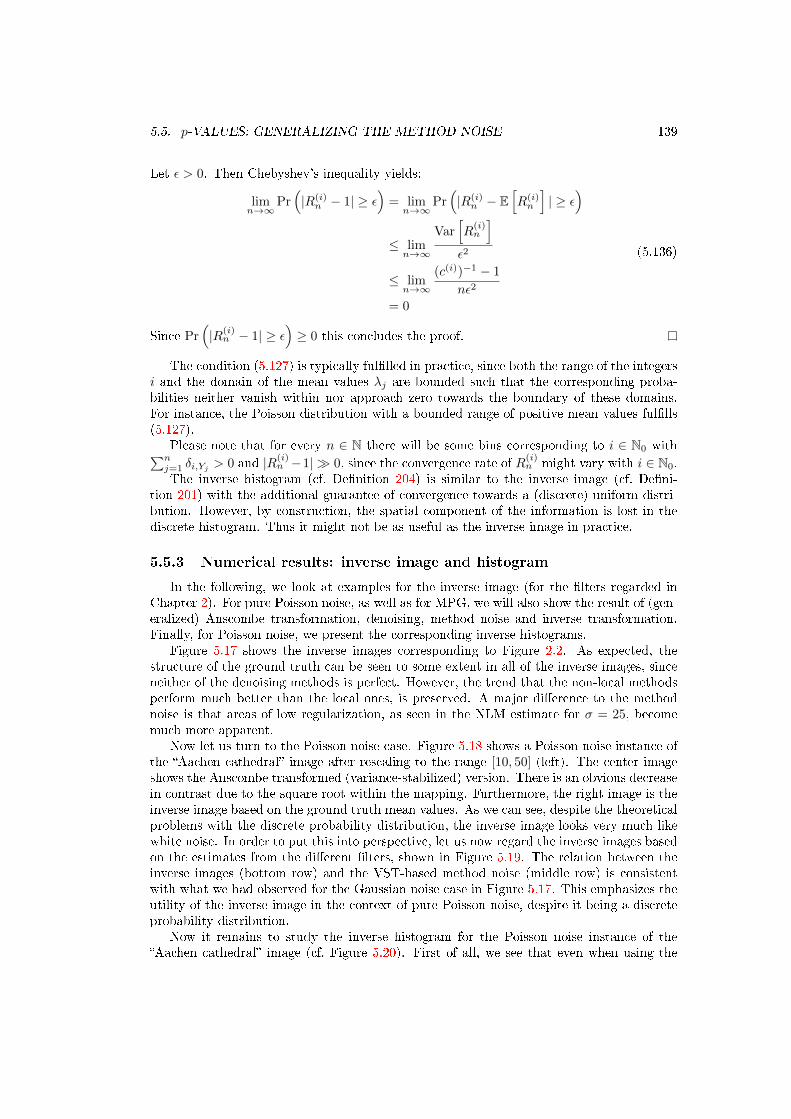
5.5. p-VALUES: GENERALIZING THE METHOD NOISE 139
Let ε > 0. Then Chebyshev's inequality yields:
limn→∞
Pr(|R(i)n − 1| ≥ ε
)= limn→∞
Pr(|R(i)n − E
[R(i)n
]| ≥ ε
)≤ limn→∞
Var[R
(i)n
]ε2
≤ limn→∞
(c(i))−1 − 1
nε2
= 0
(5.136)
Since Pr(|R(i)n − 1| ≥ ε
)≥ 0 this concludes the proof.
The condition (5.127) is typically fullled in practice, since both the range of the integersi and the domain of the mean values λj are bounded such that the corresponding proba-bilities neither vanish within nor approach zero towards the boundary of these domains.For instance, the Poisson distribution with a bounded range of positive mean values fullls(5.127).
Please note that for every n ∈ N there will be some bins corresponding to i ∈ N0 with∑nj=1 δi,Yj > 0 and |R(i)
n −1| 0, since the convergence rate of R(i)n might vary with i ∈ N0.
The inverse histogram (cf. Denition 204) is similar to the inverse image (cf. Deni-tion 201) with the additional guarantee of convergence towards a (discrete) uniform distri-bution. However, by construction, the spatial component of the information is lost in thediscrete histogram. Thus it might not be as useful as the inverse image in practice.
5.5.3 Numerical results: inverse image and histogram
In the following, we look at examples for the inverse image (for the lters regarded inChapter 2). For pure Poisson noise, as well as for MPG, we will also show the result of (gen-eralized) Anscombe transformation, denoising, method noise and inverse transformation.Finally, for Poisson noise, we present the corresponding inverse histograms.
Figure 5.17 shows the inverse images corresponding to Figure 2.2. As expected, thestructure of the ground truth can be seen to some extent in all of the inverse images, sinceneither of the denoising methods is perfect. However, the trend that the non-local methodsperform much better than the local ones, is preserved. A major dierence to the methodnoise is that areas of low regularization, as seen in the NLM estimate for σ = 25, becomemuch more apparent.
Now let us turn to the Poisson noise case. Figure 5.18 shows a Poisson noise instance ofthe Aachen cathedral image after rescaling to the range [10, 50] (left). The center imageshows the Anscombe transformed (variance-stabilized) version. There is an obvious decreasein contrast due to the square root within the mapping. Furthermore, the right image is theinverse image based on the ground truth mean values. As we can see, despite the theoreticalproblems with the discrete probability distribution, the inverse image looks very much likewhite noise. In order to put this into perspective, let us now regard the inverse images basedon the estimates from the dierent lters, shown in Figure 5.19. The relation between theinverse images (bottom row) and the VST-based method noise (middle row) is consistentwith what we had observed for the Gaussian noise case in Figure 5.17. This emphasizes theutility of the inverse image in the context of pure Poisson noise, despite it being a discreteprobability distribution.
Now it remains to study the inverse histogram for the Poisson noise instance of theAachen cathedral image (cf. Figure 5.20). First of all, we see that even when using the

140 CHAPTER 5. NOISE MODELING AND PARAMETER ESTIMATIONσ
=25
σ=
40
D−1LHMA
(z) D−1F kbil
(z) D−1F kNLM
(z) D−1BM3D(z)
Figure 5.17: Inverse images (cf. Denition 201) for dierent lters and the noisy Aachencathedral image in Figure 2.2 aected by AGWN with σ = 25 (top), σ = 40 (bottom)
z A(z) D−1GT(z)
Figure 5.18: Left: Poisson noise instance of the Aachen cathedral image from Figure 2.2(rescaled to [10, 50]); center: Anscombe transformed image; right: inverse image based onthe ground truth

5.5. p-VALUES: GENERALIZING THE METHOD NOISE 141
estimate
methodnoise
inverseimage
LHMAF kbil F kNLM
BM3D
Figure 5.19: Estimates, method noise and inverse images for dierent lters and the Poissonnoise instance of the Aachen cathedral from Figure 5.18
ground truth values (top left), there is a noticeable deviation from uniformity, despite thefact that we disregarded alls bins with less than nmin = 1000 elements. However, the inversehistogram still shows very clearly that the moving averages estimate (top right) is of lowquality. Furthermore, the BM3D estimate (bottom right) is closer to uniformity than theBilateral lter estimate (bottom left), which preserves the order of accuracy of the lterssuggested by the PSNR, method noise and the inverse image. In summary: as expected,due to the loss of spatial information, the inverse histogram is not as useful for analyzingthe strengths and weaknesses of certain lters as the inverse image, but it may still assist aquantitative comparison in case no ground truth is available.
As we mentioned in the introduction to this chapter, the Poisson statistics within im-age acquisition become most apparent under low light conditions. In view of this, let usregard the same analysis as presented in Figures 5.18 and 5.19, but for an image with muchlower average counts per pixel. In favor of a more authentic example, we chose an image ofthe pinwheel galaxy NGC 4414 and rescaled it to the range [2, 10]. The ground truth, aPoisson noise instance, variance-stabilized and ground truth based inverse image are shownin Figure 5.21. The estimate, VST-based method noise and inverse image for the dierentlters is given in Figure 5.22. Due to the decreased signal-to-noise ratio of the input, theoverall quality of the estimates is worse than in the Aachen cathedral example. Inter-estingly, there is very few structure in the method noise and inverse image of the movingaverages lter (comparably to BM3D). This is probably due to the fact that that there areno sharp edges in the image. Also the mediocre performance of the non-local lters can be
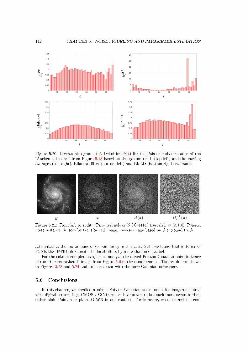
142 CHAPTER 5. NOISE MODELING AND PARAMETER ESTIMATION
12 18 24 30 36 420
0.25
0.5
0.75
1
1.25
1.5
1.75
i
hGT
i
12 18 24 30 36 420
8
16
24
32
40
48
i
hMA
i
12 18 24 30 36 420
0.25
0.5
0.75
1
1.25
1.5
1.75
i
hBilateral
i
12 18 24 30 36 420
0.25
0.5
0.75
1
1.25
1.5
1.75
i
hBM3D
i
Figure 5.20: Inverse histograms (cf. Denition 204) for the Poisson noise instance of theAachen cathedral from Figure 5.18 based on the ground truth (top left) and the movingaverages (top right), Bilateral lter (bottom left) and BM3D (bottom right) estimates
g z A(z) D−1GT(z)
Figure 5.21: From left to right: Pinwheel galaxy NGC 4414 (rescaled to [2, 10]), Poissonnoise instance, Anscombe transformed image, inverse image based on the ground truth
attributed to the low amount of self-similarity in this case. Still, we found that in terms ofPSNR the BM3D lter beats the local lters by more than one decibel.
For the sake of completeness, let us analyze the mixed Poisson-Gaussian noise instanceof the Aachen catheral image from Figure 5.6 in the same manner. The results are shownin Figures 5.23 and 5.24 and are consistent with the pure Gaussian noise case.
5.6 Conclusions
In this chapter, we recalled a mixed Poisson-Gaussian noise model for images acquiredwith digital sensors (e.g. CMOS / CCD), which has proven to be much more accurate thaneither plain Poisson or plain AGWN in our context. Furthermore, we discussed the con-

5.6. CONCLUSIONS 143
estimate
methodnoise
inverseimage
LHMA F kbil F kNLM BM3D
Figure 5.22: Estimates, method noise and inverse images for dierent lters and the Poissonnoise instance of the Pinwheel galaxy from Figure 5.21
z G(z) D−1GT(z)
Figure 5.23: Left: mixed Poisson-Gaussian noise instance of the Aachen cathedral imagefrom Figure 5.6 (α = 1.5, µ = 100, σ = 25); center: generalized Anscombe transformedimage; right: inverse image based on the ground truth

144 CHAPTER 5. NOISE MODELING AND PARAMETER ESTIMATIONestimate
methodnoise
inverseimage
LHMAF kbil
F kNLMBM3D
Figure 5.24: Estimates, method noise and inverse images for dierent lters and the MPGnoise instance of the Aachen cathedral from Figure 5.23
cept of variance-stabilization, in particular, the (generalized) Anscombe transformation for(mixed) Poisson(-Gaussian) noise, which allows a subsequent processing of standard denois-ing methods designed for additive noise. Inverse transforms, including a bias correction, leadto a nal estimate of the noise-free image under mixed noise conditions. In particular, weproposed a reformulation of the forward and inverse generalized Anscombe transformationthat allows for parameter estimation solely based on mean-variance pairs. We complementedthis approach with a method of moments estimator that yields the remaining noise parame-ters. In this context, we also proposed a novel algorithm for level set estimation based on amodied non-local block-matching strategy. In contrast to the method proposed in [53], ouralgorithm does not rely on regularity assumptions about the input image. Instead, it followsthe non-local paradigm discussed in Chapter 2. Results were presented that support the va-lidity and accuracy of the MPG noise model and the corresponding unsupervised parameterestimation in the context of HAADF-STEM imaging. We commented on the ill-posedness ofsample variance estimation in HAADF-STEM imaging and provided a relation between thedeviation of the true Poisson mean values in each level set and the corresponding error inthe sample variances. Finally, we proposed a novel quality measure for denoising methods,which we termed inverse image, that is similar to the method noise, but extends directlyto any noise distribution with a continuous cumulative distribution function. Since thisexcludes the Poisson distribution, we also provided an alternative in the form of the inversehistogram, which can be applied to discrete probability distributions with values in N0.

Chapter 6
HAADF-STEM image reconstruction
In this chapter, we discuss a novel modication of the BM3D denoising method thatadapts it to characteristics of atomic-scale crystal images. In particular, we thoroughlyanalyze the behavior of our method on dierent articial and experimental HAADF-STEMimages, as well as two dierent series of images. All raw images in this chapter (includingthe ground truths of the articial ones) courtesy of Paul M. Voyles.
6.1 Adaptive piecewise periodic block-matching
At the end of Chapter 2, we had introduced the idea of piecewise periodic block-matchingas a compromise between local and global block-matching that is tailored to the specicgeometry of crystal images. Within the context of Poisson noise and single image recon-struction, we have already published this concept in [103] (for non-local means) and [102](for BM3D), although in a more simple form than it will be treated here.
In Chapters 3 and 4, we discussed how the crystal geometry, i.e. labeling of the dierentcrystals and lattice vectors of each crystal can be retrieved from a given noisy crystal image.Now that we have this information at hand, let us formalize the algorithm for the piecewiseperiodic block-matching.
Let us begin with a straight-forward denition without any adaptiveness. This requiresthe rounding operator.
Denition 206 (Rounding operator).For r ∈ R let
drc :=
sign (r)
(|r|+ 1
2
), r ∈ 1
2 + Z ,arg mini∈Z |r − i| , else ,
(6.1)
denote the rounding operator.
Please note that the denition for r ∈ 12 + Z is a matter of preference, since j =
arg mini∈Z |r−i| does not have a unique solution in that case. For multi-dimensional objectsthe rounding operator acts component-wise.
145

146 CHAPTER 6. HAADF-STEM IMAGE RECONSTRUCTION
Algorithm 207 Piecewise periodic block-matching
Let ` ∈ 0, 1, . . . , kM1×M2 be a labeling function that assigns to each pixel the correspondingcrystal phase, or an irregular phase (if existent), e.g. the boundary region between to crystals(cf. Section 4.4). With this, let us dene
Ix :=y ∈ I : `y = `x
. (6.2)
Furthermore, let U1, . . . ,Uk denote unit cells corresponding to the respective crystals. Then,we dene the following piecewise periodic search grid
Iπx :=
⌈U`x~n
⌋: ~n ∈ Z2
∩ Ix , if `x > 0 ,
Ix , else .(6.3)
Please note that for any pixel within the irregular region, we suggest to simply perform aglobal search within the irregular region.Given a threshold τ > 0, analogous to Denition 20, we dene the corresponding set ofmatched blocks as
Sπx (g) :=y ∈ Iπx : distL2(gBx , gBy ) < τ
. (6.4)
As we had seen in Section 3.5, even when using a very accurate technique to estimatethe lattice vectors, errors become noticeable when far away from the reference point. Thus,we propose to enhance Algorithm 207 by introducing adaptiveness based on evaluating thesimilarity measure locally around the periodic search grid points.
Denition 208 (Adaptive periodic search stencil).Let I, ` and U1, . . . ,Uk be as in Algorithm 207. Furthermore, let us dene
Z := (1, 0)T , (−1, 0)T , (0, 1)T , (0,−1)T . (6.5)
Then, given a local search window size nl ∈ N2, we dene the following locally adaptiveperiodic search stencil:
πnl (x, y)
:=ln
l (x, y +
⌈U`y~z
⌋): ~z ∈ Z
, (6.6)
where
lnl (x, y)
:= arg miny′∈Nn
ly
distL2(gBx , gBy′ ) . (6.7)
Here, the arg min expression causes a reset of the coordinates to the locally best-matchingones. This grants robustness against errors in the lattice vector estimates, as well as defor-mations of the crystal or the image itself.

6.2. EXTENSION TO STACKS OF IMAGES 147
Algorithm 209 Adaptive piecewise periodic similarity searchIn a recursive manner, we assemble the entire adaptive periodic search grid for a givenreference coordinate:
Iπ,1x := x , (6.8)
Iπ,kx :=
⋃y∈Iπ,k−1
x
πnl (x, y)\
⋃y∈Iπ,k−1
x
Nnl
y
, k = 2, 3, . . . . (6.9)
Here, subtracting the set of local neighborhoods around the previous coordinates is done inorder to avoid visiting the same coordinate (up to local renement) more than once (e.g. bystepping back and forth between lattice points).Now, we can replace (6.3) with
Iπ,nl
x :=
⋃∞k=1 Iπ,kx ∩ Ix , if `x > 0 ,
Ix , else .(6.10)
Again, this leads to the following analogous denition of the set of adaptively and piecewiseperiodically matched blocks
Sπ,nl
x (g) :=y ∈ Iπ,n
l
x : distL2(gBx , gBy ) < τ. (6.11)
Although (6.10) theoretically contains a union over an innite number of sets, due tothe nite size of Ix, there is an upper bound on how many locally adaptive periodic searchstencils can be added before any further stencil will lie outside the domain. In order toapproximate this set eciently in practice, we propose the following recursive algorithm.
In order to promote shorter paths from the reference coordinate to the coordinateswithin the adaptive periodic search grid, we propose to use a queue as the data structureQx. This ensures that all coordinates corresponding to the local periodic stencil of thereference coordinate will be processed before their respective children and so on.
6.2 Extension to stacks of images
In HAADF-STEM imaging, often an entire series of frames is acquired one after the otherwhile keeping the beam grid as stationary as possible over the same region. The intentionis to increase the available information while keeping the local concentration of the electrondose at an acceptable level (by letting heat and energy dissipate until the next measurementof the same pixel is taken). Furthermore, reducing the acquisition time per image alsoreduces the magnitude of scan line distortions. In Section 2.6, we had mentioned the workby Binev et al. that addressed the application of non-local means to a series of HAADF-STEM images, employing image alignment techniques to allow for a direct similarity searchacross the dierent frames.
In this section, we would like to discuss an analogous idea that aims at extending theabove adaptive piecewise periodic similarity search to stacks of similar crystal images. Letus begin by formulating conditions for the similarity between the dierent frames of such aseries.
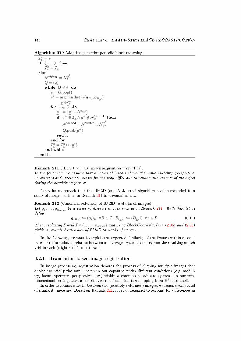
148 CHAPTER 6. HAADF-STEM IMAGE RECONSTRUCTION
Algorithm 210 Adaptive piecewise periodic block-matchingIπx = ∅if `x = 0 then
Iπx = Ixelse
N visited = Nnl
x
Q = (x)while Q 6= ∅ do
y = Q.pop()y∗ = arg min
y′∈Nnl
y
distL2(gBx , gBy′ )
for ~z ∈ Z do
y+ =⌈y∗ + U`x~z
⌋if y+ ∈ Ix ∧ y+ /∈ N visited
x then
N visited = N visited ∪Nnl
y+
Q.push(y+)end if
end for
Iπx = Iπx ∪ y∗end while
end if
Remark 211 (HAADF-STEM series acquisition properties).In the following, we assume that a series of images shares the same modality, perspective,parameters and specimen, but its frames may dier due to random movements of the objectduring the acquisition process.
Next, let us remark that the BM3D (and NLM etc.) algorithm can be extended to astack of images such as in Remark 211 in a canonical way.
Remark 212 (Canonical extension of BM3D to stacks of images).Let g1, . . . , gnseries
be a series of discrete images such as in Remark 211. With this, let usdene
g(B,i) := (gi)B ∀B ⊂ I, B(x,i) := (Bx, i) ∀x ∈ I . (6.12)
Then, replacing I with I ×1, . . . , nseries and using BlockCoords(x, i) in (2.35) and (2.45)yields a canonical extension of BM3D to stacks of images.
In the following, we want to exploit the expected similarity of the frames within a seriesin order to formulate a relation between an average crystal geometry and the resulting searchgrid in each (slightly deformed) frame.
6.2.1 Translation-based image registration
In image processing, registration denotes the process of aligning multiple images thatdepict essentially the same specimen but captured under dierent conditions (e.g. modal-ity, focus, aperture, perspective, etc.) within a common coordinate system. In our two-dimensional setting, such a coordinate transformation is a mapping from R2 onto itself.
In order to compare the t between two (possibly deformed) images, we require some kindof similarity measure. Based on Remark 211, it is not required to account for dierences in

6.2. EXTENSION TO STACKS OF IMAGES 149
modality in our context. Thus, a simple L2-distance could be used, as was done throughoutthe previous chapters. However, in image registration, it is more common to use the closelynormalized related cross-correlation.
Denition 213 (Normalized cross-correlation [105]).Let Ω ⊂ R2. Then, the normalized cross-correlation (NCC) energy of g, h ∈ L2(Ω) is denedas
ENCC [g, h] :=
ˆΩ
g(x)− g√1|Ω|‖g − g‖L2(Ω)
h(x)− h√1|Ω|‖h− h‖L2(Ω)
dx . (6.13)
where g, h ∈ R denote the mean values of the respective images.
The NCC satises ENCC [g, h] ∈ [−1, 1] for all g, h ∈ L2(Ω) with ENCC [g, h] = 1 if andonly if g = αh + β for some α > 0, β ∈ R. In this sense the negative NCC is minimal fortwo perfectly overlapping images while disregarding dierences in global illumination.
The most commonly used coordinate transformation for image registration within theelectron microscopy community is the translation.
Denition 214 (Translation-based image registration functional [105]).Let Ω ⊂ R2 be a domain and g1, . . . , gnseries
∈ L2(Ω) be a series of images as in Remark 211.Then, using deformations φv : R2 → R2, x 7→ x + v and corresponding translation vectorsvi ∈ R2 for i = 2, . . . , nseries, we refer to
Eregisλ [(vi)
nseriesi=2 ] :=
nseries∑i=2
−ENCC [gi φvi , g1] . (6.14)
as translation-based image registration functional.
The above functional can be used to align multiple images with each other by translatingeach by an individual vector in R2. As this leaves the relative positions of all pixels withineach image unchanged, it is sometimes referred to as a rigid registration. However, mostdenitions of rigid deformations also allow for rotations (which we do not consider here).
Please note that the above formulation requires an extension of the images gi beyond theirsupport Ω. In practice, we use a constant extension in normal direction. Furthermore, letus point out that the minimization with respect to the dierent vi can be entirely decoupledhere.
6.2.2 Non-rigid image registration
Due to the distortions arising from the sequential acquisition of individual pixels inSTEM (cf. Chapter 1), signicant deformations might occur within each image and, moreimportantly, these deformations might deviate from one frame to the next within the series.In order to account for this, Berkels et al. [15] proposed a multi-stage approach for robustnon-rigid registration in the context of crystal images. Their approach is embedded in avariational framework (cf. Chapter 4) and based on the following energy.
Denition 215 (Non-rigid image registration functional [105]).Let Ω ⊂ R2 be a domain and g1, . . . , gnseries
∈ L2(Ω) be a series of images as in Remark 211.Furthermore, let λ > 0 be a regularization parameter. Then, using deformations φi ∈H1(Ω;R2) for i = 1, . . . , nseries, we refer to
Eregisλ [(φi)
nseriesi=1 , g] :=
nseries∑i=1
−ENCC [gi φi, g] +λ
2‖∇φi − 1‖2L2(Ω) , (6.15)

150 CHAPTER 6. HAADF-STEM IMAGE RECONSTRUCTION
as non-rigid image registration functional.
The above functional can be used to align all images with an (unknown) mean image ofthe series and allows for non-rigid deformations.
In practice, we alternate between the minimization with respect to the deformations andthe minimization with respect to the mean image and use g = g1 for the initialization.
Please note that this energy is a generalization of the one in (6.14), in the sense thatxing g = g1 and restricting the admissible set of deformations to translations yields thesame minimizers for both energies.
This general form of the variational non-rigid registration has been thoroughly studiedin the literature [105]. However, in the context of aligning crystal images it requires specialtreatment, because the global minimizer cannot be obtained eciently and there exist avariety of undesirable local minimizers, similar to the periodicity analysis problem discussedin Chapter 3. These arise from the fact that due to the periodicity of the crystal, two imagesmight align reasonably well when shifted by any integer multiple of the lattice vectors. Inorder to circumvent this issue, Berkels et al. proposed a multi-stage approach that employssubsequent minimization from low to high resolutions and from adjacent frames to the wholeseries [15]. Their approach is based on the assumption that the displacement between twosubsequent frames will, under typical conditions, be smaller than half a period of the crystal,which resolves the aforementioned problem.
6.2.3 Deformed adaptive piecewise periodic block-matching
In order to extend the piecewise periodic block-matching technique outlined in Section 6.1to stacks of images in a canonical way, we would require the labeling function and unit cellsfor all images of the series. On the one hand, this is computationally rather costly. On theother hand, in view of the desire to extend the periodic block-matching for each referencecoordinate to the entire series, it lends itself to take advantage of the image alignmenttechniques that were briey outlined in the previous section.
Once a proper registration of the series is at hand, we might as well determine onesegmentation of the average crystal, as well as the corresponding unit cells, and assign themto all individual images by composition with the respective inverse deformation. In order toformulate this, let us turn to the discrete setting.
Denition 216 (Mean aligned image).Let X be a discrete domain and g1, . . . , gnseries
∈ RM1×M2 be a series of discrete images as in
Remark 211. Furthermore, for i = 1, . . . , nseries let φi be deformations such that gi φi ≈ gholds in a suitable notion (cf. Denitions 214 and 215), where g is the approximate mean
of the series. Also, let φ−1i denote the corresponding approximate inverse deformations, i.e.
g φ−1i ≈ gi. Moreover, let
X ′ :=⋂
i=1,...,nseries
φ−1i (X) , (6.16)
denote the common support of all deformed images. With this, we dene the mean alignedimage as
meanregis
((gi)
nseries
i=1 ,(φi
)nseries
i=1
):=
(1
nseries
nseries∑i=1
gi φi
)|X′
. (6.17)

6.2. EXTENSION TO STACKS OF IMAGES 151
Denition 217 (Mean labeling function and unit cells).Let X, gi, φi, φ
−1i be as in Denition 216. Then, we denote with ¯, U1, . . . , Uk the labeling
function for the dierent crystal regions within the mean aligned image (cf. Denition 216)and the corresponding unit cells, respectively. Also, we dene the following labeling functionscorresponding to the individual images gi:
`i :=(
¯ φ−1i
)|φi(X′)
. (6.18)
Using the deformations, the mean labeling function, as well as the mean unit cells, wepropose to extend the adaptive piecewise periodic block-matching to the entire series asfollows: for each reference coordinate we determine its region membership based on thedeformed mean labeling function in (6.18). In case the coordinate belongs to the irregularregion, we perform block-matching with respect to all coordinates that belong to the irregularregion (within all frames). Otherwise, we perform a modied version of the adaptive periodicblock-matching by replacing the stencil in (6.6) with a deformed one and adding stepstowards the adjacent frames.
Denition 218 (Deformed locally adaptive periodic search stencil).Let Z, nl be as in Denition 208 and ¯, U i, φ−1
i be as in Denition 217. Then, we denethe following analog of (6.6):
πnl
φ
(x, y, i
):=(ln
l(x,⌈φ−1i
(φi(y) + U (`i)x~z
)⌋), i)
: ~z ∈ Z
∪(lx(nl,⌈(φ−1i+j φi
)(y)⌋), i+ j
): j ∈ −1, 1
∩ I × 1, . . . , nseries .
(6.19)
Here, the reference coordinate is rst mapped to the common coordinate system of the alignedseries, then the steps along the symmetry axes of the average crystal are applied and nallythe result is mapped back to the coordinate system of the individual frame. Additionally, thereference coordinate is mapped to the coordinate system of the two adjacent frames (exceptat the beginning and end of the series, where only one adjacent frame exists).
Using the formalism outlined in Remark 212, and replacing (6.6) with (6.19), we receivean extension of the locally adaptive, piecewise periodic block-matching to stacks of imagesthat employs deformation to account for the specimen movement between the acquisitionof subsequent frames. Let us summarize the numerical construction of the correspondingindex set in the fashion of Algorithm 210:

152 CHAPTER 6. HAADF-STEM IMAGE RECONSTRUCTION
Algorithm 219 Deformed adaptive piecewise periodic block-matchingIπ(x,i) = ∅if (`i)x = 0 then
Iπ(x,i) = I(x,i)
else
N visited = Nnl
x × iQ = ((x, i))while Q 6= ∅ do
(y, j) = Q.pop()y∗ = arg min
y′∈Nnl
y
distL2(gB(x,j), gB(y′,j)
)
for ~z ∈ Z do
y+ =⌈φ−1j
(φj(y
∗) + U (`i)x~z)⌋
if (y+, j) ∈ I(x,i) ∧ (y+, j) /∈ N visited then
N visited = N visited ∪(Nnl
y+ × j)
Q.push((y+, j)
)end if
end for
if j > 1 then
N visited = N visited ∪(Nnl
(φ−1j−1φj)(y)
× j − 1)
Q.push(((
φ−1j−1 φj
)(y), j − 1
))end if
if j < nseries then
N visited = N visited ∪(Nnl
(φ−1j+1φj)(y)
× j + 1)
Q.push(((
φ−1j+1 φj
)(y), j + 1
))end if
Iπ(x,i) = Iπ(x,i) ∪ (y∗, j)
end while
end if
6.3 Quantitative atom detection
As mentioned in the introduction, the position and intensity of atomic columns in crystalimages are key quantities for the analysis of material properties in materials science and inthis context the precision with which these can be determined is of great importance. Inview of this, let us discuss an algorithm that estimates the centers, shapes and intensitiesof atoms in a given crystal image.
A good model for an ideal atom in HAADF-STEM images is given by a Gaussian bell.Thus, the core part of the algorithm is to t Gaussian bells locally to individual atoms.However, for this we require at least an initial guess of the center of each atom within theimage. In the following, we propose two distinct ways to receive such initial guesses.
The rst method is based on two-phase segmentation of the crystal image in its fore-ground (atoms) and background (void).

6.3. QUANTITATIVE ATOM DETECTION 153
Algorithm 220 Estimating initial atom centers based on two-phase segmentationLet g be a crystal image and ` be a labeling function retrieved from the two-phase segmen-tation of g into its fore- and background using the maximum and minimum image intensityas initial mean values (cf. Section 4.2.5). Furthermore, let
I1, . . . , InA ⊂ I , (6.20)
denote the pairwise disjoint connected components of the foreground setj ∈ I : `j = 1
. (6.21)
Then, an initial guess of the atom centers may be retrieved from the geometric centers ofthe respective connected components:
ci :=1
# (Ii)∑j∈Ii
j . (6.22)
For the special case of pairs of atoms, such as in the gallium arsenide crystal image inFigure 1.3, we propose to estimate two geometric centers per connected component basedon the manual specication of the approximate angle α of the line connecting the two centers,as well as their separation d:
c±1i := ci ±
d
2~eα . (6.23)
Another, more direct method is to successively nd the largest peak within the image,mask all pixels in a reasonably sized neighborhood around it and proceed with the nextpeak, until the intensity of all non-masked pixels is below a certain threshold.
Algorithm 221 Estimating initial atom centers based on peak nding
Let g be a crystal image, ρ ∈ N2 and θ ∈[minj∈I gj ,maxj∈I gj
). Furthermore, let
Iθ :=j ∈ I : gj > θ
, (6.24)
denote the set of all pixels whose intensity is above the threshold θ. Then, an initial guessof the atom centers may be retrieved from the following recursive denition:
c1 := arg maxj∈Iθ
gj , (6.25)
ci := arg maxj∈Iθ\
⋃i−1j=1N
ρ
cj
gj , i = 2, 3, . . . . (6.26)
Here, i runs until Iθ \⋃i−1j=1N
ρ
cj= ∅.
Finally, let us formalize the optimization problem of tting Gaussian bells locally at eachapproximate atom center.

154 CHAPTER 6. HAADF-STEM IMAGE RECONSTRUCTION
Denition 222 (Two-dimensional Gaussian bell).Let
fbellc,IG,σ,θ,γ(x) := IG · e
ξ1(‖diag(σ−1
1 ,σ−12 )(x−c)‖2
2−ξ2(x1−c1)(x2−c2)
)+ γ , (6.27)
denote a two-dimensional Gaussian bell, where
ξ1 := − 1
2(1− θ2), (6.28)
ξ2 := 2θ
σ1σ2. (6.29)
The parameters can be interpreted as follows: c is its center, IG its intensity, σ its size(two-dimensional, elliptic), θ its rotation and γ its constant oset (to account for imageintensity within background).
Denition 223 (Least-squares energy for a sum of 2D Gaussian bells).Given a crystal image g, an initial guess dcc ∈ I for an atom center, as well as its approx-imate radius rA ∈ N, we dene the following functional:
F bell(c, IG,σ, θ, γ) :=1
2
∑j∈N rAdcc
(gj − fbell
c,IG,σ,θ,γ(j))2
. (6.30)
The above functional measures the local t between the Gaussian bells and the atomsin the crystal image.
Algorithm 224 Rening atom centers through local Gaussian bell ttingDenoting with
Imin := minj∈N rAdcc
gj , Imax := maxj∈N rAdcc
gj , Imean :=1
2(Imin + Imax) , (6.31)
the minimum, maximum and mean value of the image within the patch around the initialatom center, we propose to initialize x with
c = c , IG = 12 (Imax − Imin) , σ = ( 1
2rA,12rA) , θ = 0 , γ = Imin . (6.32)
We recommend to restrict the set of feasible parameters to
Ubellh := N rA−1
dcc × [Imax − Imean, Imax − Imin]× (0, rA)2 × R× [Imin, Imax] . (6.33)
This yields the following rened atom center estimator
c∗ ∈ arg miny∈Ubell
h
F bell(y) , (6.34)
which can be obtained using a suitable constrained non-linear least squares solver (e.g.combining Levenberg-Marquardt with a box projector).
Please note that the renement of atom centers can be extended to pairs of atoms as inAlgorithm 220 by using a sum of two Gaussian bell functions (cf. (6.27)) within the targetfunctional, as well as using a rectangular patch for the local tting that is adjusted to theapproximate dimensions of the atom pairs within the image. Noting that the constant oset

6.3. QUANTITATIVE ATOM DETECTION 155
can be merged into one parameter for the sum of the Gaussian bells, this results in a similarconstrained non-linear least squares problem as in (6.34), only with dim
(Ubellh
)= 13 instead
of dim(Ubellh
)= 7.
6.3.1 Quantitative quality measures related to atom detection
In this section, we would like to introduce quantitative measures related to atom detec-tion. Let us emphasize that the goal here is not to analyze the performance of the atomdetection method itself, but the entire reconstruction pipeline. In particular, we will usethe quantitative measures formulated in the following to compare the accuracy of detectedatom centers when using noisy micrographs versus using denoised ones.
The detectability of the atomic columns in the noisy and denoised images can be as-sessed by the fraction of atoms detected in the ground truth, which could be matched to acorresponding atom detected in the observed image.
Denition 225 (Detection fraction).Given a crystal image, let cgt
i ∈ [1,M1] × [1,M2], i = 1, . . . , ngtA denote the (approximate)
true atom positions (e.g. manually determined, or determined based on a noise-free versionof the crystal image and the methods described above. Moreover, let
∆cmin := mini,j=1,...,n
gtA
i6=j
∣∣cgti − c
gtj
∣∣ , (6.35)
denote the corresponding shortest inter-atomic distance. Furthermore, let c∗i ∈ [1,M1] ×[1,M2], j = 1, . . . , nA denote the positions detected from the observed image (e.g. the noisyor denoised version). Then, the detection fraction is dened as
ρ+
(cgt, c∗
):=
#(D+
(cgt, c∗
))ngtA
, (6.36)
where
D+(cgt, c∗
):=
i ∈ 1, . . . , ngt
A : minj=1,...,nA
∣∣∣cgti − c
∗j
∣∣∣ < 1
2∆cmin
. (6.37)
Please note that the detection fraction is invariant under slight errors within the groundtruth atom positions, i.e. errors that are much smaller than ∆cmin.
As a complementary measure, let us dene the fraction of atoms detected from theobserved image that could not be matched to any of the atoms detected within the groundtruth.
Denition 226 (Misdetection fraction).Given the setting of Denition 225, the misdetection fraction is dened as
ρ−(cgt, c∗
):=
nA −#
(j ∈ 1, . . . , nA : min
i=1,...,ngtA
∣∣∣cgti − c∗j
∣∣∣ < 12∆cmin
)nA
. (6.38)
Whereas, in combination, these two measures give a good indication about the overallrobustness of the atom detection process, they do not provide any information about itsactual accuracy. In view of this, let us introduce the delity, the root mean square of thedistances between the (approximate) ground truth and detected atom positions.

156 CHAPTER 6. HAADF-STEM IMAGE RECONSTRUCTION
Denition 227 (Fidelity).Given the setting of Denition 225, the delity is dened as
Fidelity(cgt, c∗
):=
√√√√ 1
#(D+
(cgt, c∗
)) ∑i∈D+(cgt,c∗)
minj=1,...,nA
∣∣∣cgti − c
∗j
∣∣∣2. (6.39)
Note that the delity only regards distances between correctly identied atoms (in thesense of Denition 225).
The above three measures require either a reasonably accurate manual specication ofthe ground truth atom positions or knowledge of the underlying noise-free image. Let usstress that in this work we will not use the actual ground truth atom positions (e.g. froma molecular dynamics simulation) for this purpose, but the ones detected from articialnoise-free images.
Since we would also like to evaluate experimental images, where no ground truth is avail-able (and thus at least the delity cannot be evaluated), let us introduce another measurethat copes with less restricting assumptions: the precision. Here, one exploits the fact thatan ideal crystal should be perfectly periodic. Thus, given an image part far away from anyirregularities or region boundaries, the deviation of the inter-atomic distances of the atomcenters detected in that part may serve as an indicator for their accuracy.
Denition 228 (Precision).Let c∗i , i = 1, . . . , nA be atom positions detected within an image part where the crystal isexpected to be perfectly periodic. Furthermore, let ~v1, ~v2 be an approximate unit cell of thecrystal (e.g. manually specied or estimated using the methods described in Chapter 3) andfor δprec > 0 let
∆prec1/2
:=‖ci − cj‖2 : i, j = 1, . . . , nA, i 6= j, ‖cicj − ~v1/2‖2 < δprec
, (6.40)
where AB denotes the vector connecting two points A,B ∈ R2. Then, the precision is denedas
Precision (c) :=
√√√√ 2∑i=1
1
# (∆preci )
∑d∈∆prec
i
d2 . (6.41)
Let us point out that both the precision and the delity are intended to only measurethe error within reasonable approximations of the atom centers (i.e. disregarding thosethat are too far o to be interpreted uniquely as an approximation of any ground truthposition). Thus, we encourage to regard both the delity and precision together with the(mis-)detection fraction whenever possible in order to assess their validity and signicance.
6.4 Numerical results
In the following, we evaluate the performance of the proposed adaptive piecewise periodicblock-matching. For a clear separation between dierent methods, we will refer to classicalBM3D as introduced in Chapter 2 as vanilla BM3D or simply BM3D (in tables) and to ourproposed modied BM3D method as π-BM3D. For the analysis, we will use a range of crystalimages with dierent properties: articial with ground truth available and experimentallyacquired, high to low electron doses, as well as single and multi-phase crystals. Also, weconsider both single-shot images and image series. For each of those we will analyze thePSNR (cf. Denition 28) and delity (cf. Denition 227) (if a ground truth is available), as

6.4. NUMERICAL RESULTS 157
well as the (mis-) detection fraction (cf. Denitions 225 and 226), as well as the precision(cf. Denition 228) (except for non-periodic crystals). In case no ground truth is available,the (mis-) detection fractions are calculated based on the atoms detected in the π-BM3Destimate after carefully checking manually that all atoms were detected correctly.
6.4.1 Single-shot HAADF-STEM images
Let us begin by analyzing the performance of the BM3D on single-shot HAADF-STEMimages.
In [102], we had conducted an evaluation using simulated ground truth images for threedierent crystals: silicon, gallium nitride and silicon with a single dislocation. However, inthat publication we had used the Poisson model to generate articial pixel intensity noise.The analysis presented in Chapter 5 revealed that this model is too simplistic and doesnot t very well with the noise observed in actual experimental HAADF-STEM images. Inplace of this, we had introduced a more complex mixed Poisson-Gaussian noise model (cf.Denition 160). Here, we would like to present the same analysis that was performed in [102]but using the more general MPG noise model instead of the Poisson one. Since, in contrastto the Poisson model, the MPG model requires the knowledge of corresponding parameters,we additionally employ the noise analysis framework discussed in Chapter 5, i.e. even forthe synthetic images, we use the estimated noise parameters instead of the ground truthvalues for variance-stabilization in all presented cases. Another dierence is that here weuse a block size of nb = (32, 32) instead of nb = (16, 16), which was used in [102].
Figure 6.1 shows the silicon and gallium nitride crystal images (from left to right: groundtruth pixel intensities with simulated scan line distortions, ground truth intensities corruptedwith MPG noise, BM3D estimates, π-BM3D estimates). A visual inspection conrms thatapplying the BM3D lter signicantly reduces the noise (as we had already observed inChapter 2). As mentioned in [102], a local search is not ideal for crystal images because theself-similar objects, namely the atoms, are spread throughout the entire image. Accordingly,we observe noticeable artifacts (smearing of the atoms and asymmetric shapes) within thevanilla BM3D estimates (3rd column in Figure 6.1), especially for the lowest SNR galliumnitride crystal image. The π-BM3D estimates do not show these artifacts and generallyappear to be of a higher visual quality. When comparing either of the non-local estimatesto their ground truths, we see that in addition to reducing the intensity noise in all pixels,the BM3D ltering also reduces scan line distortions, which manifests itself in more roundedatoms. While we believe that this eect stems from the sparsication achieved by the unitarytransforms mentioned in Section 2.4.2, this requires further investigation.
Figure 6.2 shows silicon crystal images with a dislocation at dierent electron doses (thearrangement is the same as in Figure 6.1). Here we do not observe such a large dierencebetween the adaptive periodic and local block-matching, which is most likely caused bythe higher density of atoms that allows even the local search to nd several similar blocks.Furthermore, around the dislocation the π-BM3D estimates (4th column) also contain a fewartifacts. This is because due to their rotation, atoms around the dislocation are uniquewithin the image and thus the true non-local similarity search does not yield more informa-tion than a local search.
The above ndings due to a visual inspection of the results are supported by the quanti-tative analysis shown in Table 6.1. As expected, applying the BM3D lter yields a signicantincrease in PSNR and except for the silicon dislocation images the PSNR is increased by1-2 dB when using the adaptive periodic similarity search instead of the local one. Pleasenote that although it might be counterintuitive that the PSNR of the noisy images decreaseswith increasing dose, this is caused by the higher variance of the Poisson part, as well as the

158 CHAPTER 6. HAADF-STEM IMAGE RECONSTRUCTION0.79
C/cm
21.57
C/cm
27.85
C/cm
21.54
C/cm
23.85
C/cm
2
g z BM3D (z) π-BM3D (z)
Figure 6.1: Articial crystal images (silicon and gallium nitride) with perfect lattice, sim-ulated scan line distortions and dierent simulated electron doses (increasing from top tobottom for each crystal); from left to right: ground truth, ground truth corrupted withMPG noise, BM3D estimate, π-BM3D estimate

6.4. NUMERICAL RESULTS 159
2.81
C/c
m2
5.68
C/c
m2
28.47
C/c
m2
g z BM3D (z) π-BM3D (z)
Figure 6.2: Articial silicon crystal image with a dislocation, simulated scan line distortionsand dierent simulated electron doses (increasing from top to bottom); from left to right:ground truth, ground truth corrupted with MPG noise, BM3D estimate, π-BM3D estimate
larger value of the denominator due to the overall increased intensity. Furthermore, usingthe π-BM3D estimates, we receive optimal or near optimal values for the detection andmisdetection fractions on all images. In contrast, when using the raw images (or the vanillaBM3D estimate), the detection misses up to 48% (or 14%) of the atoms, respectively. Whilethe misdetection fraction is also nearly optimal in all cases for the vanilla BM3D estimates,using the raw images may lead to signicant misdetections (up to 11%). Most notably, boththe delity and precision are increased up to a factor of 4 by applying π-BM3D to atomdetection. With respect to delity and precision π-BM3D also clearly outperforms vanillaBM3D. Please note that the delity is improved by π-BM3D even for the silicon dislocationimages, which indicates that the adaptivity within the periodic block-matching is able tocope with large-scale deviations from perfect periodicity as those introduced by the disloca-tion. It is worth noting that for the silicon crystal image we achieved atom detection with aprecision below 3 pm, which is well below other state-of-the-art results presented for single-shot images in the literature. However, this result should be interpreted cautiously, sincewe used articial images here that are unable to capture all eects of actual experimentalimages.
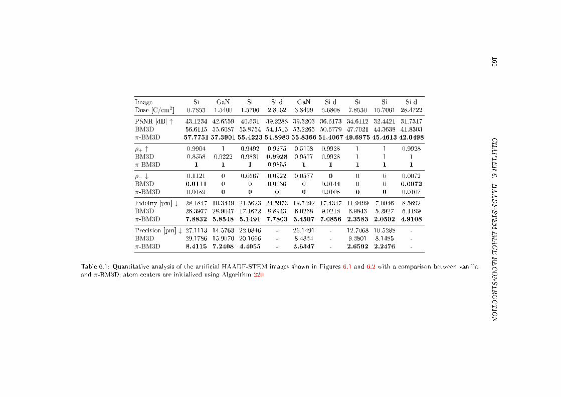
160CHAPTER6.HAADF-STEM
IMAGERECONSTRUCTION
Image Si GaN Si Si d GaN Si d Si Si Si dDose [C/cm2] 0.7853 1.5400 1.5706 2.8062 3.8499 5.6808 7.8530 15.7061 28.4722
PSNR [dB] ↑ 43.1234 42.6559 40.631 39.2288 39.3203 36.6173 34.6112 32.4421 31.7317BM3D 56.6115 55.6087 53.8754 54.1515 53.2265 50.6779 47.7021 44.3638 41.8303π-BM3D 57.7751 57.3901 55.4223 54.8983 55.8366 51.4067 49.6975 45.4613 42.0498
ρ+ ↑ 0.9904 1 0.9492 0.9275 0.5158 0.9928 1 1 0.9928BM3D 0.8558 0.9222 0.9831 0.9928 0.9577 0.9928 1 1 1π-BM3D 1 1 1 0.9855 1 1 1 1 1
ρ− ↓ 0.1121 0 0.0667 0.0922 0.0577 0 0 0 0.0072BM3D 0.0111 0 0 0.0036 0 0.0144 0 0 0.0072
π-BM3D 0.0189 0 0 0 0 0.0108 0 0 0.0107
Fidelity [pm] ↓ 28.1847 10.3449 21.5623 24.5973 19.7492 17.4347 11.9499 7.0946 8.5692BM3D 26.3977 28.9047 17.1672 8.8943 6.0268 9.0218 6.9843 5.2927 6.1199π-BM3D 7.8832 5.8548 5.1491 7.7803 3.4507 7.0856 2.3583 2.0502 4.9108
Precision [pm] ↓ 27.1113 14.5763 22.0846 - 26.1491 - 12.7068 10.5288 -BM3D 29.1786 15.9070 20.1666 - 8.4834 - 9.3801 8.1485 -π-BM3D 8.4115 7.2408 4.4055 - 3.6347 - 2.6592 2.2476 -
Table 6.1: Quantitative analysis of the articial HAADF-STEM images shown in Figures 6.1 and 6.2 with a comparison between vanillaand π-BM3D; atom centers are initialized using Algorithm 220

6.4. NUMERICAL RESULTS 161
zBM3D(z
)π-B
M3D(z
)
1 µs 3µs 5µs 10 µs 20µs 40µs 81µs
Figure 6.3: Top: experimental HAADF-STEM images of a gallium arsenide crystal acquiredusing dierent dwell times (increasing from left to right); center: BM3D estimates; bottom:π-BM3D estimates
In view of this, let us now perform a similar analysis on a set of experimentally acquiredHAADF-STEM images. The top row in Figure 6.3 shows a set of gallium arsenide crystalimages acquired using dierent electron doses (increasing from left to right). The centerand bottom row show the corresponding BM3D and π-BM3D estimates, respectively. Wecan conrm our ndings from the articial experiments above that the visual quality isdrastically increased by non-local ltering (with the standard algorithm only for t > 5 µs)and that the adaptive periodic similarity search reduces artifacts and signicantly increasesthe image quality compared to local block-matching. Furthermore, we can conrm theprevious observation that the non-local ltering reduces scan line distortions. Table 6.2shows the quantitative analysis for this dataset. As mentioned earlier, we cannot analyzethe PSNR and delity due to the missing ground truth information. However, the results forthe (mis-) detection fractions and the precision are in line with those observed in Table 6.1.
In Chapter 5, we showed results which indicated that a purely Gaussian noise model doesnot yield a good t for the actual noise variance in experimental HAADF-STEM images.Now that we have a powerful denoising method at hand, let us further investigate the impactof using the more general MPG noise model. Figure 6.4 shows a side-by-side comparison
t [µs] ρ+ ↑ BM3D π-BM3D ρ− ↓ BM3D π-BM3D Prec. [px] ↓ BM3D π-BM3D
1 0.5588 0.6471 1 0.6299 0.0571 0 4.8184 2.4383 1.6493
3 0.6525 0.8390 1 0.4726 0.0294 0 4.8732 1.8331 0.9460
5 0.7288 1 1 0.4756 0 0 4.5027 1.6639 0.5470
10 0.8362 0.9483 1 0.3071 0 0 3.1043 1.2396 0.7253
20 0.8448 1 1 0.3636 0 0 3.2870 1.1922 0.7230
40 0.8966 1 1 0.0370 0 0 1.0363 0.8610 0.6285
81 0.9322 0.9831 1 0 0 0 0.9123 0.8985 0.7052
Table 6.2: Quantitative analysis of the experimental gallium arsenide crystal images shownin Figure 6.3; atom centers are initialized using Algorithm 221

162 CHAPTER 6. HAADF-STEM IMAGE RECONSTRUCTION
Gaussian noise model MPG noise model
Figure 6.4: Visual comparison of the denoising performance of π-BM3D when using dierentnoise models based on the experimental gallium arsenide HAAF-STEM image with a dwelltime of t = 5µs from Figure 6.3
of the π-BM3D estimates of the gallium arsenide image with a dwell time of t = 5µs fromFigure 6.3, when using a purely Gaussian noise model (left) and the MPG noise modelwith variance-stabilization via the generalized Anscombe transformation. As expected, thedierence between the two noise models is signicant. In particular, the lack of a signaldependent part within the purely Gaussian noise model causes a signicantly lower noisereduction near the atoms.
Since purely periodic crystals are of little interest in the context of atomic scale HAADF-STEM imaging, let us now look at both articial and experimental multi-phase crystals. Forthis scenario we proposed to use adaptive piecewise periodic block-matching based on thesegmentation approach described in Chapter 4. Figure 6.5 shows simulated images of atwo-phase material with gallium arsenide at the top and a cobalt-manganese-silicon (CMS)system at the bottom. Again, dierent electron doses (increasing from top to bottom)were simulated using the same MPG noise parameters. The quantitative analysis for theseimages is shown in Table 6.3. Due to aperiodicity of the gallium arsenide crystal within therst three rows of atomic columns near the interface (the atom pairs are slightly rotatedclockwise and counter-clockwise in an alternating fashion), as well as the small image section,we chose to conne the atomic center related analysis to a window (indicated in red in thetop left image of Figure 6.5) within the bottom (CMS) material here. Despite the increasedcomplexity of the structure of the raw images, we still observe a signicant increase inPSNR when using the adaptive piecewise periodic block-matching. Furthermore, we observeartifacts in the form of smeared out atoms in the π-BM3D estimate only for the imagewith the lowest electron dose (top row) and in this case the blurring is much worse forthe vanilla BM3D estimate. Moreover, π-BM3D consistently and signicantly improves allatom position related measures. It is interesting to note that the precision of the π-BM3Destimate of the high electron dose image is worse than that of the medium dose image,which is unexpected since the ground truth is perfectly periodic within the bottom phase.

6.4. NUMERICAL RESULTS 163
g z BM3D (z) π-BM3D (z)
Figure 6.5: Articial two-phase crystal image (top region: gallium arsenide, bottom region:cobalt-manganese-silicon (CMS) system) with simulated scan line distortions and dierentsimulated electron doses (increasing from top to bottom); red rectangle indicates the windowused for atom position related quantication
However, the π-BM3D estimate of the medium dose image also contains signicantly lessscan line distortion, which is most likely due to a dierent in the estimated noise parametersand the cause for the behavior of the precision.
Again, we would like to complement these ndings with analyses on actual experimentalHAADF-STEM images. Figure 6.6 shows real counterparts of the images in Figure 6.5.Unfortunately, because barely one period of the CMS material is visible in the bottomphase a precision analysis would not be very meaningful in this case. Still, the visual qualityimprovement achieved by π-BM3D is signicant. While, as expected, the increase in imagequality is slightly lesser around the material interface it is still noticeable compared to theraw image.
Figure 6.7 shows experimental HAADF-STEM images of two multi-phase crystals. Theone in the top row is the three-phase crystal previously shown in Figure 4.4. It revealed thatwhile there are two clearly separate regions with a horizontal interface in the center, the topregion actually consists of two dierent materials (strontium titanate and barium titanate)with very similar HAADF-STEM intensities. Looking at the π-BM3D estimate (top right)the separation now becomes more clear to the naked eye. The bottom crystal image showsthe same CMS-GaAs material as in Figure 6.6 but at higher resolution and with a largerimage section. Table 6.4 shows the results of the atom center based quantitative analysis
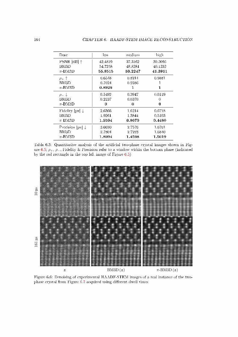
164 CHAPTER 6. HAADF-STEM IMAGE RECONSTRUCTION
Dose low medium high
PSNR [dB] ↑ 42.4819 37.3162 30.5095BM3D 54.7258 48.8281 40.1252π-BM3D 55.8515 50.2247 41.3911
ρ+ ↑ 0.6548 0.8214 0.9881BM3D 0.7024 0.9286 1π-BM3D 0.8929 1 1
ρ− ↓ 0.5492 0.3947 0.0119BM3D 0.2237 0.0370 0π-BM3D 0 0 0
Fidelity [px] ↓ 2.6366 1.6214 0.6718BM3D 1.9261 1.3844 0.5103π-BM3D 1.5594 0.8670 0.4480
Precision [px] ↓ 3.6680 2.7576 1.6701BM3D 2.7804 2.7223 1.6840π-BM3D 1.8094 1.4598 1.5019
Table 6.3: Quantitative analysis of the articial two-phase crystal images shown in Fig-ure 6.5; ρ+, ρ−, Fidelity & Precision refer to a window within the bottom phase (indicatedby the red rectangle in the top left image of Figure 6.5)
10µs
161µs
z BM3D (z) π-BM3D (z)
Figure 6.6: Denoising of experimental HAADF-STEM images of a real instance of the two-phase crystal from Figure 6.5 acquired using dierent dwell times
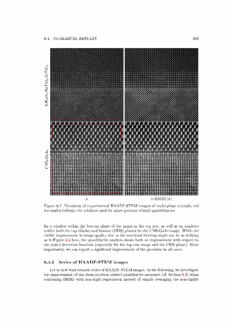
6.4. NUMERICAL RESULTS 165
SrRuO
3-BaT
iO3-SrTiO
3CMS-GaA
s
z π-BM3D (z)
Figure 6.7: Denoising of experimental HAADF-STEM images of multi-phase crystals; redrectangles indicate the windows used for atom position related quantication
for a window within the bottom phase of the image in the top row, as well as on windowswithin both the top (GaAs) and bottom (CMS) phases for the CMS-GaAs image. While thevisible improvement in image quality due to the non-local ltering might not be as strikingas in Figure 6.6 here, the quantitative analysis shows both an improvement with respect tothe (mis-) detection fractions (especially for the top row image and the CMS phase). Moreimportantly, we can report a signicant improvement of the precision in all cases.
6.4.2 Series of HAADF-STEM images
Let us now turn towards series of HAADF-STEM images. In the following, we investigatethe improvement of the atom position related quantitative measures (cf. Section 6.3) whencombining BM3D with non-rigid registration instead of simply averaging the non-rigidly

166 CHAPTER 6. HAADF-STEM IMAGE RECONSTRUCTION
Image / region ρ+ ↑ ρ− ↓ Precision [pm] ↓SrRuO3-BaTiO3-SrTiO3 0.9990 0.2018 47.2607π-BM3D 1 0 16.9276
GaAs 1 0 11.6145π-BM3D 1 0 4.9174
CMS 0.9139 0.0057 25.0472π-BM3D 1 0 12.9135
Table 6.4: Quantitative analysis of the experimental three-phase crystal images shown inFigure 6.7; for SrRuO3-BaTiO3-SrTiO3, ρ+, ρ− & Precision refer to a window within thebottom phase; for CMS and GaAs they refer to a window within the respective phase in theCMS-GaAs; windows are indicated in red in Figure 6.7
gallium
nitride
silicon
z1 z2 z3 z4 z5
Figure 6.8: First ve images of two experimentally and sequentially acquired series ofHAADF-STEM images
aligned images as proposed in [153]. We will denote the latter algorithm with NR. Theformer will be denoted with π-NR-BM3D and consists of the following three stage approach:1) translation registration (with integer shifts) of the raw images and application of BM3Dusing the deformed adaptive piece-wise periodic block-matching, 2) non-rigid registrationof the estimates from 1) and processing of the raw images with BM3D using the deformedadaptive piece-wise periodic block-matching (cf. Section 6.2.3), 3) nal non-rigid registrationand averaging of the estimates from 2).
For the following evaluation, we use series of experimentally acquired HAADF-STEMimages of two dierent materials: gallium nitride and silicon. For each of these, Figure 6.8shows the rst ve sequentially acquired images. Comparing the two series, we see that thehigher SNR of the gallium nitride image, which is owing to a longer exposure, is tied tostronger scan line distortions. This eect was mentioned previously in Chapter 1.
For the gallium nitride series, Figure 6.9 compares the NR estimates with those obtainedfrom the π-NR-BM3D method described above. Please note that for nseries = 1 no registra-tion is performed at all and thus the NR estimate is equal to the raw image in that case.In order to investigate the eect of increasing the number of available images, we show theresulting average images when using the rst 1, 2, and 4 images of the series. All resulting

6.4. NUMERICAL RESULTS 167
NR
π-N
R-B
M3D
nseries = 1 nseries = 2 nseries = 4
Figure 6.9: Average registered images of the gallium nitride image series from Figure 6.8using non-rigid alignment (from left to right: using the rst 1, 2, 4 images)
1 2 3 4 5 6 7
4
6
8
10
12
14 mean x-precision (pi-NR-BM3D)
mean y-precision (pi-NR-BM3D)
mean x-precision (NR)
mean y-precision (NR)
nseries
averageprecision[pm]
Figure 6.10: Average precision (mean over 10 similar series using an increasing oset for therst image) of the gallium nitride image series from Figure 6.8 after averaging the non-rigidlyaligned images (NR), as well as the π-NR-BM3D estimates (BM3D)
averages were aligned and cropped to a common support using translation-based registrationfor improved comparability. First of all, we notice that the π-NR-BM3D averages appear tohave a much higher SNR even when using just a single image and that the SNR does notincrease noticeable when increasing the number of images. This is due to the eective BM3Ddenoising that we already observed for the single-shot images above. In contrast to that,however, we expect that the additional averaging over multiple images will reduce imagedistortions, such as the previously mentioned scan line distortions, which should improveatom center precision.

168 CHAPTER 6. HAADF-STEM IMAGE RECONSTRUCTIONN
Rπ-N
R-B
M3D
nseries = 1 nseries = 2 nseries = 4 nseries = 8
Figure 6.11: Average registered images of the silicon image series from Figure 6.8 usingnon-rigid alignment (from left to right: using the rst 1, 2, 4, 8 images)
2 4 6 8 10 12
0
0,15
0,3
0,45
0,6
0,75
0,9
1,05detection fraction (pi-NR-BM3D)
detection fraction (NR)
misdetection fraction (pi-NR-BM3D)
misdetection fraction (NR)
ideal detection fraction
nseries
average(m
is-)detectionfraction
Figure 6.12: Average (mis-)detection fraction (mean over 10 similar series using an increasingoset for the rst image) of the silicon image series from Figure 6.8 after averaging thenon-rigidly aligned images (NR), as well as the π-NR-BM3D estimates; atom centers areinitialized using Algorithm 221
Figure 6.10 compares the precision of both methods on the gallium nitride series (cf. Fig-ure 6.8). The precision was evaluated on the image section shown in Figure 6.9 for allregistered mean images. In order to better understand the trend of the precision with anincreasing number of images, we averaged all precision values over ten similar series in eachcase, using an increasing oset (in steps of size one) for the rst image. Furthermore, in con-trast to the evaluation of the single-shot images above, we present the individual precisionsin horizontal (x-precision) and vertical (y-precision) direction here, i.e. the square roots ofthe two sums in (6.41) are calculated separately. The graph in Figure 6.10 reveals two majordierences between the proposed π-NR-BM3D method and plain non-rigid alignment : 1)π-NR-BM3D leads to a signicant improvement of both the x- and y-precision (x-precisionis reduced by more than a factor of two); 2) the improvement of the precision with an in-creasing number of images is less with π-NR-BM3D than with plain non-rigid alignment.In either case, a diminishing improvement with an increasing number of images is expected.Both observations are in line with the visual comparison. For all regarded averages boththe detection and misdetection fraction have optimal, or very close to optimal values.

6.5. CONCLUSIONS 169
2 4 6 8 10 12
0,4
0,8
1,2
1,6
2
2,4 x-prec. (pi-NR-BM3D)
y-prec. (pi-NR-BM3D)
x-prec. (NR)
y-prec. (NR)
x-prec. (pi-NR-BM3D, manual init)
y-prec. (pi-NR-BM3D, manual init)
x-prec. (NR, manual init)
y-prec. (NR, manual init)
nseries
averageprecision[px]
Figure 6.13: Average precision (mean over 10 similar series using an increasing oset forthe rst image) of the silicon image series from Figure 6.8 after averaging the non-rigidlyaligned images (NR), as well as the π-NR-BM3D estimates (BM3D); dashed lines indicatethat the atom centers were initialized manually, otherwise Algorithm 221 was used
For the silicon image series, Figure 6.11 shows the registered mean images when using therst 1-8 images for both regarded methods. Due to the much lower SNR of the raw images,the improvement in visual image quality by the π-NR-BM3D method is even more apparentin this case. In fact, the SNR of the raw images are poor enough that there is a signicantquantitative dierence between the detection and misdetection fractions of the NR averagesand those computed using π-NR-BM3D, as shown in Figure 6.12. While the π-NR-BM3Dbased averages yield near optimal detection fractions and optimal misdetection fractions,the averages obtained by plain non-rigid alignment exhibit both a high misdetection fractionthat barely approaches an optimal value when using the maximum number of regardedimages and a low detection fraction that does not signicantly increase with the number ofregarded images. This shows that the proposed combination of non-local denoising and non-rigid registration is especially valuable for low dose imaging, where both the SNR per imageand the number of available images is limited. In order to nalize the quantitative analysis,let us also regard the average precisions for this case, which are shown in Figure 6.13. In viewof the poor (mis-)detection fractions of the average images retrieved by the NR method, wealso consider the precisions obtained when manually initializing the atom centers (dashedlines). We observe the same trend of the precision with respect to the number of imagesas in the gallium nitride case above. Most notably, in either case, the precisions obtainedfrom the NR estimates are surpassed by those obtained from the π-NR-BM3D estimates bya factor of 2− 3.
6.5 Conclusions
In this chapter, we have formalized an adaptive piecewise-periodic block-matching strat-egy for non-local denoising frameworks that is tailored to the special properties of crystalimages. In particular, we investigated its use within the BM3D algorithm. It was demon-strated that together, the adaptivity and the segmentation approach incorporated into the

170 CHAPTER 6. HAADF-STEM IMAGE RECONSTRUCTION
method are able to handle complex material structures, including dislocations and interfacesbetween grains, as well as entirely dierent materials. We showed that the proposed block-matching strategy outperforms local block-matching in this context, especially at low SNRand yields a signicant increase in both PSNR, as well in visual image quality. Using thenovel denoising procedure, we were able to obtain unprecedented precision in atom detectionfor single-shot HAADF-STEM images. Most notably, we showed that our method provideshigh atom detectability (in terms of the (mis-)detection fraction) and high precision evenfor images acquired with very small electron doses. In view of this, we encourage the use ofπ-BM3D for applications in which dose limitations otherwise prohibit a proper quantitativeanalysis.
In addition to this, we proposed an extension of the technique to series of images byapplying periodic search stencils within the common coordinate system given by deforma-tions from non-rigid registration. The best precision reported in the literature for alignedstacks of images is due to Yankovich et al. [153] who applied non-rigid registration to aseries of 512 sequentially acquired images. In that case, more than 200 images were requiredto reach sub-picometer precision. While we were not able to present superior results interms of the absolute precision itself here, we did present results that indicate a signicantimprovement over the state-of-the-art in a setting where only a few images are available.In particular, by utilizing our proposed non-local denoising framework in addition to thenon-rigid alignment, we were able to improve the precision by a factor of two to three. Thisalso drastically improved the actual detectability of the atoms (in terms of (mis-)detectionfraction) for the very low SNR silicon images. It still remains to show that sub-picometerprecision can be achieved with the novel combination of non-local denoising and non-rigidregistration. However, this will most likely require the usage of many more input imagesand thus drastically increase the overall computational cost.
Overall, these ndings support our initial claim that non-local denoising is a very usefultool for low-dose electron microscopy.

Chapter 7
Spectral and multi-modal denoising
In this chapter, we would like to extend our ideas presented in the previous chapter tospectral images. First, we introduce the canonical extension of BM3D to spectral images.Then, we discuss modications that improve the performance in the context of power-law signals, which are typically encountered in electron energy loss spectroscopy (EELS).Finally, we propose a multi-scale and multi-modal block similarity measure that aims tocombine the advantages of HAADF-STEM (high spatial resolution) and EDX spectroscopy(high resolution of the atomic composition), while overcoming limitations due to extremelylow signal-to-noise within the EDX map. All raw data in this chapter courtesy of MartialDuchamp.
7.1 Non-local denoising of spectral data
Let us begin by describing the notion of a spectral image.
Remark 229 (Spectral image).A spectral image is an image g ∈ VM1×M2 as in Denition 2. Its specifc characteristic isthat V = (R>0)
nc , where nc is large. Typically nc ∈ 2N and nc ≥ 1024.
The general extension of the non-local means and block-matching and 3D ltering meth-ods described in Sections 2.4.1 and 2.4.2 to spectral images is rather straight-forward. Whenextracting blocks from the image (cf. Denition 20), one extracts the entire spectrum ateach position of the bock, yielding a three-dimensional object. The L2-similarity measure(cf. Denition 15) is dened in a canonical way as for the two-dimensional blocks, namelysumming the squared dierences over all positions and channels. In other words, in termsof the L2-similarity measure, the spectral blocks are regarded as long vectors.
Stacking the spectral blocks (cf. Denition 21) yields a four-dimensional object. Thus,for the transform domain ltering, one has to extend the unitary transform from three tofour dimensions (possibly choosing a dierent transform for the spectral dimension thanthe other dimensions). Since the ltering operators (cf. Denitions 22 and 23) are appliedcomponent-wise, their extension is straight-forward as well.
Compared to gray-scale images, spectral images typically contain signicantly more in-formation within each pixel. Thus, in case the signal-to-noise ratio of the measured spectraldata is not extremely low, one might reduce the block size to 1. Then, the similarity measuresimply compares individual spectra and stacks the most similar ones into a two-dimensionaltensor. In that case, no unitary transform for the block plane is required. However, keepin mind that while this will eectively denoise the individual spectra, there will be very
171
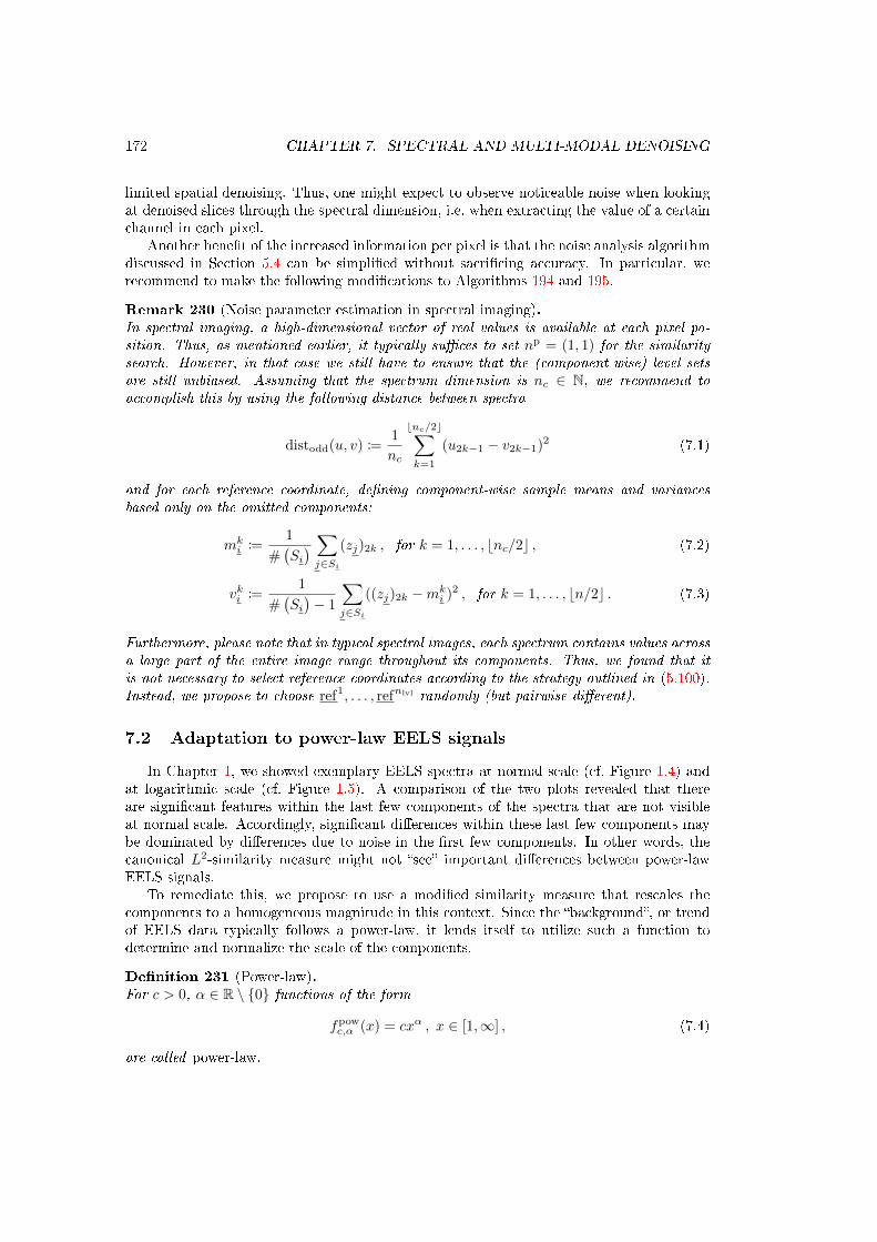
172 CHAPTER 7. SPECTRAL AND MULTI-MODAL DENOISING
limited spatial denoising. Thus, one might expect to observe noticeable noise when lookingat denoised slices through the spectral dimension, i.e. when extracting the value of a certainchannel in each pixel.
Another benet of the increased information per pixel is that the noise analysis algorithmdiscussed in Section 5.4 can be simplied without sacricing accuracy. In particular, werecommend to make the following modications to Algorithms 194 and 195.
Remark 230 (Noise parameter estimation in spectral imaging).In spectral imaging, a high-dimensional vector of real values is available at each pixel po-sition. Thus, as mentioned earlier, it typically suces to set np = (1, 1) for the similaritysearch. However, in that case we still have to ensure that the (component-wise) level setsare still unbiased. Assuming that the spectrum dimension is nc ∈ N, we recommend toaccomplish this by using the following distance between spectra
distodd(u, v) :=1
nc
bnc/2c∑k=1
(u2k−1 − v2k−1)2 (7.1)
and for each reference coordinate, dening component-wise sample means and variancesbased only on the omitted components:
mki :=
1
#(Si) ∑j∈Si
(zj)2k , for k = 1, . . . , bnc/2c , (7.2)
vki :=1
#(Si)− 1
∑j∈Si
((zj)2k −mki )2 , for k = 1, . . . , bn/2c . (7.3)
Furthermore, please note that in typical spectral images, each spectrum contains values acrossa large part of the entire image range throughout its components. Thus, we found that itis not necessary to select reference coordinates according to the strategy outlined in (5.100).Instead, we propose to choose ref1, . . . , refnlvl randomly (but pairwise dierent).
7.2 Adaptation to power-law EELS signals
In Chapter 1, we showed exemplary EELS spectra at normal scale (cf. Figure 1.4) andat logarithmic scale (cf. Figure 1.5). A comparison of the two plots revealed that thereare signicant features within the last few components of the spectra that are not visibleat normal scale. Accordingly, signicant dierences within these last few components maybe dominated by dierences due to noise in the rst few components. In other words, thecanonical L2-similarity measure might not see important dierences between power-lawEELS signals.
To remediate this, we propose to use a modied similarity measure that rescales thecomponents to a homogeneous magnitude in this context. Since the background, or trendof EELS data typically follows a power-law, it lends itself to utilize such a function todetermine and normalize the scale of the components.
Denition 231 (Power-law).For c > 0, α ∈ R \ 0 functions of the form
fpowc,α (x) = cxα , x ∈ [1,∞] , (7.4)
are called power-law.

7.3. MULTI-MODAL NON-LOCAL DENOISING 173
Fitting such a power-law to a given spectrum in the least-squares sense yields an explicitexpression.
Remark 232 (Explicit least squares power-law t [147]).Let n ∈ N and (xi, yi)
ni=1 be a set of data points with xi ≥ 1 and yi > 0 for all i = 1, . . . , n.
Then, the least squares power-law t is given by
(cLS, αLS) ∈ arg min(c,α)∈(0,∞)×R\0
1
2
n∑i=1
(fpowc,α (xi)− yi)2 . (7.5)
The unique solution of this problem can be expressed explicitly as
αLS =n∑ni=1 lnxi ln yi − (
∑ni=1 lnxi) (
∑ni=1 ln yi)
n∑ni=1 ln2 xi − (
∑ni=1 lnxi)
2 , (7.6)
cLS = exp
∑ni=1 ln yi − αLS
∑ni=1 lnxi
n
. (7.7)
We propose to modify the similarity measure in the context of power-law EELS signalsby normalizing all spectra with the power-law tted to the reference signal.
Denition 233 (Power-law normalized similarity measure).Let g ∈
(Rnc>0
)M1×M2be an EELS scan whose spectra roughly follow a power-law as in De-
nition 231 (except for the distinctive peaks related to the atomic composition). Furthermore,
for i ∈ I let cLSi , αLSi be the solution of (7.5) for x =(j,(gi)j
)ncj=1
. Then, we dene the
following power-law normalized version of the L2-similarity measure (cf. Denition 15):
distpow(gBi , gBj ) :=1
nbnc
∑k∈Bi
nc∑l=1
(gk)l −(gk−i+j
)l
fpow
cLSk ,αLSk(l)
2
. (7.8)
Here, nb ∈ N denotes the number of pixels per block.
When processing EELS scans containing spectra that follow a power-law with the non-local lters described in Section 2.4, we propose to replace the L2-similarity measure (cf.Denition 15) with the above normalized measure.
Please note that in case the (generalized) Anscombe transform is applied to the inputimage prior to denoising in order to achieve variance-stabilization (cf. Algorithm 179), thepower-law functions have to be processed using the same transformation as well.
7.3 Multi-modal non-local denoising
In the following, we would like to propose a multi-scale and multi-modal similarity mea-sure for non-local denoising that combines the benets of HAADF-STEM and hyper-spectralimaging. In Figures 1.6 to 1.8, we showed an EDX dataset with mean spectra containingvery detailed information about the atomic composition of the material. Unfortunately, thesignal-to-noise ratio of the dataset is extremely low and thus impedes the assessment ofthis information at the given resolution. However, it is possible to simultaneously acquire acomplementary HAADF-STEM image (cf. Figure 7.1) of much higher SNR.
While the EDX scan may contain enough instances of every spectrum to obtain a reason-able reconstruction via non-local averaging, the poor SNR prohibits accurate block-matching

174 CHAPTER 7. SPECTRAL AND MULTI-MODAL DENOISING
Figure 7.1: HAADF-STEM image acquired simultaneously with the EDX scan shown inFigure 1.6
at the given resolution. In contrast, the HAADF-STEM image allows for accurate block-matching. Assuming a pixel-wise correlation between both modalities - as is the case inour context due to the simultaneous acquisition of both scans - it lends itself to utilize theinformation about self-similarity within the HAADF-STEM image and apply it to the EDXscan. However, this is problematic because the HAADF-STEM modality does not guaran-tee a unique mapping to the EDX modality. In other words, there might be two dierentmaterials that result in the same HAADF-STEM intensities but dierent EDX maps.
In order to circumvent this issue, we propose to combine the information from bothmodalities. In particular, we propose to compensate the poor SNR of the EDX scan byresampling it to a lower spatial and spectral resolution within the similarity search.
Denition 234 (Resampled EDX similarity measure).
For an image g ∈(Rnc≥0
)M1×M2
with nc = ar · nrc for ar, nr
c ∈ N, let
g(nr
c)i :=
1
ar
lar∑j=(l−1)ar+1
(gi)j
nrc
l=1
, i ∈ I , (7.9)
denote the resampled version of g (with respect to its spectral components). Here, we call ar
resample factor. Then, we dene the following similarity measure:
distr(gBi , gBj ) :=1
nrc
∥∥∥∥∥∥ 1
nb
∑k∈Bi
g(nr
c)k − 1
nb
∑k∈Bj
g(nr
c)k
∥∥∥∥∥∥2
2
. (7.10)
The above measure compares the average downsampled spectra in favor of increasingthe signal-to-noise ratio of the blocks prior to comparison.

7.4. NUMERICAL RESULTS 175
Now, the idea is to compensate this loss in spatial resolution by utilizing the high-resolution HAADF-STEM information. The key property for this to work properly is thatthe HAADF-STEM similarity measure is more sensitive to coordinate changes than theresampled EDX similarity measure. Simply put, the HAADF-STEM similarity measureensures that all atomic columns within similar blocks are at the same relative positions andthe EDX similarity measure ensures that they also have the same atomic composition.
To this end, we propose to employ the following normalized convex combination of bothsimilarity measures.
Denition 235 (Multi-scale & multi-modal similarity measure).Let g ∈ RM1×M2 be an HAADF-STEM image with suciently high SNR for robust block-
matching (e.g. as most of the images shown in Section 6.4). Furthermore, let h ∈(Rnc≥0
)M1×M2
be a jointly acquired EDX scan and f = (g,h) denote the combined multi-modal image.Then, we dene the following similarity measure:
distmm(fBi ,fBj ) := c1distL2(gBi , gBj )
distL2(gBi , 0)+ c2
distr(hBi ,hBj )
distr(hBi , 0), (7.11)
where c1, c2 ∈ [0, 1] with c1 + c2 = 1.
Given g,h as above, and in case that the SNR of h is much lower than that of g, wepropose to use the above normalized multi-scale and multi-modal similarity measure for thecombined image.
7.4 Numerical results
In the following, we provide numerical results for non-local denoising of dierent exper-imental EELS datasets and investigate the performance of the proposed multi-modal andmulti-scale block-matching method for both articial and experimental pairs of EDX andHAADF-STEM datasets.
7.4.1 Electron energy loss spectroscopy
Let us begin with the EELS dataset that was previously shown in Figures 1.4 and 1.5.Figure 7.2 shows the corresponding map of the mean values of all spectra in the scan (theEELS projection). As mentioned earlier, it follows the power-law scaling discussed in Sec-tion 7.2. Here, we use BM3D with default parameters, except for the following modications:1) replacement of the L2-similarity measure (cf. Denition 15) with the power-law normal-ized one (cf. Denition 233), 2) post-processing of each individual spectrum with a 1Dbilateral lter and 3) multiplied the noise standard deviation after generalized Anscombetransformation by the factor 2. The latter two steps were done in order to further increasethe regularity of the resulting EELS spectra. All results for EELS datasets presented in thissection use a block size of nb = (1, 1).
Figure 7.3 compares selected channels of the measured EELS spectra with those obtainedby the non-local denoising. Especially for the last channels (j = 1600, 2000), where the initialSNR is quite small, we see a substantial increase in quality due to the reconstruction, whilethe edges due to boundaries between dierent materials seem to be retained quite well.
Please note that we performed the noise analysis (cf. Remark 230) on the latter halfof the components of all spectra only, since otherwise the large deviations in the matched

176 CHAPTER 7. SPECTRAL AND MULTI-MODAL DENOISING
Figure 7.2: Mean values of all spectra (projection) of the EELS dataset corresponding toFigures 1.4 and 1.5
400
800
1200
1600
2000
j (z)j (BM3D(g))j
Figure 7.3: Comparison between selected channels of the noisy and denoised EELS datasetfrom Figure 7.2
350 700 1050 1400 1750 2100
3500
7000
10500
14000
17500
21000sample (mean, variance)
least squares fit
VST optimization fit
mi
v i
200000 400000 600000 800000 1·106 1.2·10 6 1.4·10 60
1·107
2·107
3·107
4·107
5·107
6·107
7·107
8·107
sample (mean, variance)
least squares fit
VST optimization fit
mi
v i
Figure 7.4: Sample mean-variance pairs of the level sets extracted from the EELS datasetin Figure 7.2 and estimated linear variance functions; the left plot uses only the latter halfof the channels while the right plot uses all channels

7.4. NUMERICAL RESULTS 177
0 300 600 900 1200 1500 1800
10 3
10 4
10 5
10 6spectrum #1 (noisy)
spectrum #2 (noisy)
spectrum #3 (noisy)
spectrum #1 (denoised)
spectrum #2 (denoised)
spectrum #3 (denoised)
channel
electron
intensity
Figure 7.5: Comparison between selected spectra of the noisy (dash-dotted line) and denoised(solid line) EELS dataset from Figure 7.2
spectra in the rst few components led to extreme outliers in the variance sample estimates,as seen in Figure 7.4.
Figure 7.5 compares a few selected spectra before and after non-local denoising at loga-rithmic scale. The result is consistent with Figure 7.3 in the sense that the signal to noiseratio is improved signicantly, especially for the latter components and that the edges inthe spectra are retained.
Looking at the gold dashed graph in Figure 7.5, we see a very signicant outlier in one ofthe channels. Such hot pixels appear sparsely throughout the entire dataset. In this work,we applied a pre-processing step to remove these outliers before any further processing (noiseanalysis, non-local ltering, etc.). The outlier removal is based on an initial noise analysis,receiving a rough estimate for the variance parameters. Then, the generalized Anscombetransform is applied to the data, receiving a dataset of expected variance roughly equal toone in each entry (cf. Chapter 5). Afterwards, each entry in each spectrum that deviatesmore than six standard deviations from the median of a local neighborhood is replaced bythe respective median.
While this experimental dataset clearly demonstrated the possible performance of non-local denoising for EELS datasets, it is not well suited to investigate the eect of the power-law normalized similarity measure. This is because we do not know where (or whether atall) this data set contains any occurrences of spectra that are similar in the channels oflarge magnitude but dier signicantly in certain channels of much smaller magnitude. Tocircumvent this issue, we added an artifact signal consisting of a Gaussian bump of standarddeviation with mean value at the channel j = 1700 to every other spectrum. Figure 7.6shows the channel j = 1700 of the articial dataset, as well as the corresponding estimatesretrieved from BM3D with the standard L2- and the power-law normalized similarity mea-sure. Although not very prominent, we see a decrease in contrast between the spectra withand without bump when using the standard L2-distance. This eect can be seen moreclearly when looking at Figure 7.7, which plots the projected intensities as a function of the

178 CHAPTER 7. SPECTRAL AND MULTI-MODAL DENOISINGarticialraw
data
dis
t L2
dis
t pow
Figure 7.6: Comparison between channel j = 1700 of an articial dataset (top) and itsBM3D estimates using the standard L2-distance (center) and the power-law normalizedsimilarity measure (bottom)
vertical spatial coordinate (the horizontal coordinate is xed in the center) for the groundtruth and the two dierent BM3D estimates. When directly comparing recovered spectrawith and without the Gaussian bump, as well as with and without the similarity measureadaptation, this dierence becomes more apparent, as seen in Figure 7.8. The graph clearlyshows that intensities in the spectrum with (without) the Gaussian bump are underesti-mated (overestimated) when using the standard L2-similarity measure. This is caused by amixing of spectra with and without the bump.
Whereas the dierence between using the standard L2 and the power-law normalizedsimilarity measure was not very large when using BM3D, it becomes even more apparentwhen using non-local means instead, since then the estimate is simply the weighted meanvalue of all regarded spectra. Looking at Figures 7.9 and 7.10, which give the same infor-mation as Figures 7.6 and 7.8, just using NLM instead of BM3D for the estimation, wesee that the dierence between the channels (cf. Figure 7.9) becomes much more apparent.Also, comparing the plotted spectra in Figure 7.10 shows a very signicant mixing of thespectra with and without the bump. Interestingly, in this case the NLM estimate based onthe power-law normalized similarity measure has a lower SNR than that of the L2-distancebased one, which is likely due to the dierent scaling of the similarity measures that hasmore inuence on the estimate in NLM than in BM3D, because BM3D uses sparsity insteadof block similarity as a weight during the nal averaging.
Based on these ndings we strongly recommend to use the power-law normalized similar-ity measure for EELS datasets that follow a power-law trend in order to prevent undesiredmixing of actually dierent spectra.
Now we would like to present results for another EELS dataset that was acquired at

7.4. NUMERICAL RESULTS 179
0 10 20 30 40 50 60250
500
750
1000
1250
1500
1750
2000ground truth
L2 similarity measure
adapted similarity measure
i2
meanspectralintensity
Figure 7.7: Comparison of projected intensities as a function of the vertical spatial coordinate(x1 = 25 is xed) between the ground truth and the BM3D estimates obtained with thestandard L2-distance and the power-law normalized similarity measure
1620 1665 1710 1755 1800 1845 1890
10 3
spectrum without bump - adapted similarity measure
spectrum with bump - adapted similarity measure
spectrum without bump - L2 similarity measure
spectrum with bump - L2 similarity measure
channel
electron
intensity
Figure 7.8: Comparison between selected recovered spectra (blue: without bump; red: withbump) of the articial dataset in Figure 7.6 using the BM3D lter with the standard L2-distance (solid line) and the power-law normalized similarity measure (dashed line);

180 CHAPTER 7. SPECTRAL AND MULTI-MODAL DENOISINGarticialraw
data
dis
t L2
dis
t pow
Figure 7.9: Comparison between channel j = 1700 of an articial dataset (top) and its NLMestimates using the standard L2-distance (center) and the power-law normalized similaritymeasure (bottom)
atomic scale. Figure 7.11 shows the corresponding projected spectral map as well as acomplementary HAADF-STEM image. Furthermore, Figure 7.12 compares a few selectednoisy channels with their respective estimates retrieved from non-local denoising.
Additionally, Figure 7.13 compares a few selected noisy spectra from the dataset withtheir respective estimates. Please note that this dataset was already given to us in a pre-processed form, which is why the spectra do not follow a power-law trend. Accordingly, weapplied vanilla BM3D together with the automated mixed Poisson-Gaussian noise estimationand generalized Anscombe transformation.
The results show that the non-local denoising substantially reduces the noise withinthe individual channels while retaining important local details such as the bright region inthe channel j = 1400 in Figure 7.12. Furthermore, distinct peaks within the individualspectra are retained while the overall smoothness of the signals is signicantly improved (cf.Figure 7.13).
7.4.2 Joint denoising of EDX and HAADF-STEM data
In the following, we would like to present results for non-local denoising with the multi-modal and multi-scale similarity measure in Denition 235 in the context of combined EDXand HAADF-STEM imaging. As mentioned in Section 1.2 and seen in Figure 1.8, the EDXdata at hand only contains a few counts in some of the channels and is zero everywhere else.In view of this, we choose the following setting for the combined reconstruction.
First, the noise distribution of the EDX signals is assumed to be purely Poissonian andhence the Anscombe transform (cf. Denition 169) is used. Second, we found that transform

7.4. NUMERICAL RESULTS 181
1620 1665 1710 1755 1800 1845 1890
10 3
spectrum without bump - adapted similarity measure
spectrum with bump - adapted similarity measure
spectrum without bump - L2 similarity measure
spectrum with bump - L2 similarity measure
channel
electron
intensity
Figure 7.10: Comparison between selected recovered spectra (blue: without bump; red:with bump) of the articial dataset in Figure 7.9 using the NLM lter with the standardL2-distance (solid line) and the power-law normalized similarity measure (dashed line);
Figure 7.11: EELS projection (left) and complementary HAADF-STEM image (right) ofthe 2nd Vaso dataset
114
0020
48
j (z)j (BM3D(g))j
Figure 7.12: Comparison between selected channels of the noisy and denoised EELS datasetfrom Figure 7.11

182 CHAPTER 7. SPECTRAL AND MULTI-MODAL DENOISING
0 300 600 900 1200 1500 1800
0
200
400
600
800
1000
1200spectrum #1 (noisy)
spectrum #1 (denoised)
spectrum #2 (noisy)
spectrum #2 (denoised)
spectrum #3 (noisy)
spectrum #3 (denoised)
channel
electron
intensity
Figure 7.13: Comparison between selected spectra of the noisy (dash-dotted line) and de-noised (solid line) EELS dataset from Figure 7.11
domain ltering does not give desirable results for the EDX signals. This is most likely dueto the extremely low counts per channel which result in the Anscombe transformed datadeviating signicantly from a Gaussian distribution. Thus, an NLM-based block estimatemight be more suitable for the EDX spectra. In view of this, we use the following com-bination of BM3D, NLM here. For each reference block, we perform the following steps:1) block-matching with respect to the multi-scale and multi-modal similarity measure inDenition 235; 2) reduction of the set of regarded blocks to the N3D blocks with smallest(multi-modal) block distance; 3) computation of the block stack estimate of the HAADF-STEM modality based on BM3D; 4) computation of the NLM-based weighted average blockof the EDX modality (using the multi-modal block distance for the weights); 5) aggregationof the block estimates within the respective modalities. A benet of this procedure is thatwe can ensure the estimate EDX signals to be convex combinations of existing signals in thedataset. Thus, as long as the multi-modal similarity measure yields negligibly small valuesfor pairs of blocks containing atom columns of a dierent composition, we can guaranteethat the method will not introduce any artifacts (such as mixing of dierent materials), orat least be as good in that regard as the local averaging methods that are commonly usedby material scientists. Please note that we still use the mixed Poisson-Gaussian noise modeland the generalized Anscombe transformation to preprocess the HAADF-STEM image. Fur-thermore note that the truncation introduced by the BM3D-like block-matching eectivelyresults in reduction of the sum in (2.32) to the N3D most similar patches for the NLM-basedblock estimate of the EDX spectra. All results presented here regard the N3D = 256 mostsimilar blocks and a (spatial) block size of nb = (16, 16)T .
Let us begin by analyzing the performance of the proposed method on the EDX datasetshown in Figures 1.6 to 1.8. For this dataset, we set the coecients of the convex combinationin (7.11) to c1 = c2 = 0.5, the resample factor of the spectral channels in (7.9) to ar = 8 andused a local search window of size NS = (201, 201)T . Figure 7.14 shows the reconstructedEDX projection map next to the measured one. The quality improvement due to the multi-modal non-local denoising is very signicant. Most notably, individual atomic columns arerecognizable in the reconstruction, which was not the case at all in the measured data.

7.4. NUMERICAL RESULTS 183
EDXprojection
HAADF-STEM
Experimentally acquired Multi-modal non-local reconstruction
Figure 7.14: Projection of an experimentally acquired EDX map (top left) and its multi-modal non-local means estimate (top right); experimentally acquired HAADF-STEM image(bottom left) and its multi-modal BM3D estimate (bottom right)
This is a rst indicator for the proposed technique being able to recover the desired EDXspectra at atomic resolution. We would like to stress that this is impossible to achieve withexisting methods in such a low SNR setting. Furthermore, let us point out that upon closeinspection, the denoised EDX projection reveals inhomogeneities in the right half that werenot visible within the projection of the experimentally acquired EDX map.
Although not as interesting in this context, for the sake of completeness, Figure 7.14 alsoshows the reconstructed HAADF-STEM images next to the measured one.
Let us now convince ourselves that the reconstruction did not introduce any artifactsand that the recovered spectra are in line with the mean spectra for the two segments wehad shown in Figure 1.7. The corresponding comparison is shown in Figure 7.15. Obviously,the regularity of the recovered spectra is not as high as the one of the mean spectra. Thisis not surprising when considering that the mean spectra are based on entire halves of thescan (each 400 x 300 pixels), whereas the non-local estimates are only based on at mostN3D = 256 spectra. Still, the peaks that are important for the analysis of the atomiccomposition are clearly visible and coincide very well with those of the mean spectra, whichis remarkable given that the measured spectra are zero almost everywhere.
In order to better understand at the eect of the non-local denoising on the spatialresolution of the reconstruction, as well as the corresponding potential for the reconstruc-tion of the atomic composition of the material, let us now look at Figures 7.16 and 7.17,which show individual channels corresponding to peaks in Figure 7.15 before and after thereconstruction. First of all, we can clearly see that while the experimentally acquired chan-nels are mostly zero except for individual pixels, the reconstructed ones show clearly visibledistributions. In particular, the aforementioned inhomogeneity within the right materialis visible at the channel level (cf. j = 138, 318, 338, 795). While the spatial resolution ofthe individual suces to make out individual atomic columns in some regions, it does seemto be lower than in the projection. It is unclear how large the actual error of the spatial

184 CHAPTER 7. SPECTRAL AND MULTI-MODAL DENOISING
0 150 300 450 600 750 900 10500
0.015
0.03
0.045
0.06
0.075
0.09
0.105 individual recovered spectrum (left)
individual recovered spectrum (right)
mean spectrum (left)
mean spectrum (right)
channel
averagenumberof
X-rays
Figure 7.15: Comparison between individual recovered spectra (gold and cyan dotted) andthe mean spectra over the entire respective material (red and blue solid) for the EDX mapshown in Figure 7.14
distributions within individual channels is and thus the usefulness of this information forpractical applications has to be further investigated by material scientists.
Although in the HAADF-STEM image in Figure 7.14 the signal for the right material isvery weak, this dataset does not serve as an example to test whether our proposed method isactually able to distinguish correctly between atomic columns that have the same HAADF-STEM image intensity but dierent EDX spectra despite an extremely low SNR in the EDXmap. In order to support our claim, we constructed an articial dataset where the groundtruth HAADF-STEM image consists of a periodic pattern of exactly identical Gaussianfunctions, which is shown in Figure 7.18. The ground truth EDX map was dened byscaling the mean EDX spectra from Figure 1.7 with the HAADF-STEM intensities andassigning the two dierent spectra to groups of neighboring atomic columns in an alternatingfashion. The articial noisy measurements for this dataset were created by applying Poissonnoise to the EDX map. Accordingly, the individual noisy spectra are similar to those seenin Figure 1.8, i.e. they contain 1-3 counts in a few channels while all other channels areequal to zero. For the HAADF-STEM image, we applied mixed Poisson-Gaussian noise andchose the parameters such that the resulting image looks similar to the experimental one inFigure 7.14.
The last row in Figure 7.18 shows the corresponding reconstructions from the multi-modal non-local denoising. Here, we used c1 = 0.2, c2 = 0.8 in (7.11). A more carefulchoice of these parameters was required in this case due to the existence of pixels with equalHAADF-STEM modality but dierent EDX modalities. Furthermore, we use a resamplefactor of ar = 8, as well as a global search window. While the regions belonging to thedierent mean spectra are clearly visible in the noisy EDX projection map, the individualatomic columns cannot be distinguished. In the multi-modal non-local reconstruction onthe other hand, these are clearly visible. Most notably, in terms of the mean values of thespectra, the material membership was retained at the atomic resolution, despite the factthat this information is not included in the HAADF-STEM image at all.
In order to understand this mechanism better, let us compare the individual HAADF-

7.4. NUMERICAL RESULTS 185
4010
013
831
8
j (z)j (F kNLM(z))j
Figure 7.16: Individual channels (j = 40, 100, 138, 318) corresponding to peaks in Fig-ure 7.15; left: noisy; right: multi-modal non-local means reconstruction

186 CHAPTER 7. SPECTRAL AND MULTI-MODAL DENOISING338
795
914
1019
j (z)j (F kNLM(z))j
Figure 7.17: Individual channels (j = 338, 795, 914, 1019) corresponding to peaks in Fig-ure 7.15; left: noisy; right: multi-modal non-local means reconstruction

7.4. NUMERICAL RESULTS 187
EDXprojection
HAADF-STEM
Ground truth Noisy Multi-modalnon-local reconstruction
Figure 7.18: From top to bottom: projection of an articial EDX map and a complementaryHAADF-STEM image; from left to right: ground truth, ground truth aected by Poisson(EDX) and mixed Poisson-Gaussian (HAADF-STEM) noise, multi-modal non-local recon-struction
STEM and EDX similarity measures with the multi-modal one (cf. Figure 7.19). The imagesshow clearly that the similarity measure based on the HAADF-STEM information identiesthe atomic column positions but not the relation to the two mean spectra. In contrastto that, the similarity measure based on the EDX information identies the relation tothe two mean spectra but the atomic resolution is lost completely. Finally, the combinedmulti-modal similarity measure correctly assigns the smallest distances to pixels that bothbelong to the same relative position to the atomic columns and the correct underlying meanspectrum.
In line with Figures 7.16 and 7.17, let us also compare the ground truth and estimateEDX data for two channels where the dierent materials have distinct peaks (j = 100, 138).For the articial dataset, these are shown in Figure 7.20. As in the experimental data,we see that the spatial resolution within the individual channels is lower than in the EDXprojection. In fact, having the ground truth at hand, we can clearly see that while theboundary between the dierent materials is retained quite well within the channels, theydenitely exhibit certain artifacts within the individual atoms. This reinforces the conclusionthat the inuence of the proposed method on the spatial resolution of individual channelsshould be investigated further in the future.
Let us conclude this analysis by regarding individual spectra extracted from the centersof two atoms belonging to dierent mean spectra in order to verify that there is no (ornegligible) mixing of the dierent spectra in the reconstruction. This comparison is shownin Figure 7.21. The result is similar to that in Figure 7.15, i.e. there is a good agreementbetween the ground truth and recovered spectra (considering the extremely low SNR of thenoisy EDX map) and no noticeable artifacts or mixing of the distinct peaks is observed.

188 CHAPTER 7. SPECTRAL AND MULTI-MODAL DENOISING
HAADF-STEM EDX Multi-modal
Figure 7.19: Similarity measures evaluated for a selected reference pixel (red) for the datasetin Figure 7.18; from left to right: HAADF-STEM based L2-similarity measure (cf. Deni-tion 15), resampled EDX based similarity measure (cf. Denition 234), multi-scale andmulti-modal similarity measure (cf. Denition 235)
100
138
j (g)j (F kNLM(z))j
Figure 7.20: Individual channels (j = 100, 138) corresponding to two dierent peaks of themean spectra; left: ground truth; right: multi-modal non-local means reconstruction

7.5. CONCLUSIONS 189
0 150 300 450 600 750 900 10500
0.015
0.03
0.045
0.06
0.075
0.09
individual recovered spectrum (composition #1)
individual recovered spectrum (composition #2)
ground truth spectrum (composition #1)
ground truth spectrum (composition #2)
channel
averagenumberof
X-rays
Figure 7.21: Comparison between individual recovered spectra (gold and cyan dotted) andthe ground truth spectra (red and blue solid) for two dierent atomic columns in the EDXmap shown in Figure 7.18
7.5 Conclusions
In this chapter, we discussed the extension of non-local denoising to spectral image data.In particular, we proposed a modied similarity measure for electron energy loss spectroscopydatasets that follow a power-law trend. We demonstrated the importance of this modicationin order to prevent mixing of spectra belonging to dierent materials. Numerical results ontwo dierent experimental datasets were presented that illustrate the performance of non-local denoising methods in the context of high-dimensional hyper-spectral data. In contrastto established local averaging, the non-local methods are able to substantially increase theSNR without noticeably reducing the spatial resolution.
Furthermore, we looked at an extremely noisy EDX dataset containing only a few countsin individual channels and being zero elsewhere. For such data local averaging would drasti-cally reduce the spatial resolution in order to achieve acceptable SNR and non-local averag-ing methods would fail to recognize similarity between associated spectra. To alleviate this,we took advantage of the comparably high SNR and spatial resolution of a simultaneouslyacquired HAADF-STEM image. More precisely, we proposed a multi-scale and multi-modalsimilarity measure, which enabled us to obtain a high quality reconstruction of the EDXmap without sacricing spatial resolution, thus overcoming the unavoidable limitations ofestablished denoising techniques in this context.

Conclusions
In this thesis, we presented an eective denoising strategy for atomic-scale electron mi-crographs of crystals.
Due to their power in scenarios with rich image self-similarity, as is the case for crys-tal images, we use non-local denoising methods, in particular NLM and BM3D, as a basisfor eective noise reduction. In the context of crystal images, classical block-matching ap-proaches encounter two major problems: 1) global block-matching leads to restrictingly highcomputational complexity, 2) considering too many similar blocks is prone to create blur(and thus reducing spatial resolution). To alleviate these issues, we proposed a novel adap-tive piece-wise periodic similarity search strategy that accounts for the special structure ofcrystal images and is compatible with complex geometries, such as dislocations and materialinterfaces.
In order to obtain the geometrical information required for our approach, we inventednovel unsupervised approaches for unit cell extraction and crystal segmentation. In line withpreviously existing Fourier based methods, our real-space energy based unit cell extractionalgorithm has proven to be extremely robust to noise, but results in a higher accuracy. In thecontext of crystal segmentation, existing approaches rely on prior knowledge of the latticevectors and are restricted to rotations of the unit cell (grain boundaries). Combining Fouriertransform based region descriptors, PCA and the Mumford-Shah image segmentation model,we were able to eliminate these restrictions. Furthermore, we showed results that indicate avery good performance of the proposed crystal segmentation method for complex geometries(interfaces between entirely dierent crystals) in the presence of severe noise.
While these two algorithms may be used entirely on their own for the purpose of highlyaccurate unsupervised crystal analysis, our main goal was to employ them within the afore-mentioned adaptive piece-wise periodic similarity search. In this regard, we presented nu-merical experiments on articial and real experimental crystal images of dierent electrondoses. The proposed method consistently achieved a signicant improvement of the PSNRcompared to standard BM3D (with a local search) (by up to 2.5 dB) and, of course, evenmore compared to the noisy input images (up to 15 dB). Furthermore, in case of the lowerSNR images, the modied non-local denoising approach noticeably increases both the detec-tion and misdetection fractions, i.e. the overall ability to automatically detect atom centerscorrectly at all. More importantly, compared to analyzing the raw images, our proposedmethod improves both the delity (for articial images), as well as the precision of the de-tected atom centers by up to a factor of 8. We would like to point out that for articialexperiments we observed the delity to be of the same magnitude as the precision, whichindicates that the proposed denoising procedure does not introduce artifacts that aectatom positions noticeably with respect to the ground truth. On an experimentally acquiredsingle-shot HAADF-STEM image, we achieved a precision of about 5 pm, which, to the bestof our knowledge, surpasses the state-of-the-art [128] by more than a factor of 3.
Furthermore, we discussed a combination of the adaptive piece-wise periodic similarity
191

192 Conclusions
search with non-rigid image registration and presented results that showed an improvementof the precision over plain non-rigid alignment for small image series (4-8 images) by afactor of 2-3. Using a low SNR silicon image series as an example, we also demonstratedthat the atom detectability in terms of (mis-)detection fraction can be improved signicantlyby merging these two frameworks.
The above mentioned NLM and BM3D algorithms are designed to remove additive Gaus-sian white noise. However, we presented results which indicate that the more general mixedPoisson-Gaussian noise model is more suited for experimental HAADF-STEM images. Inorder to adapt the denoising methods to this noise distribution, we follow the approachin [93] and use the generalized Anscombe transformation for variance-stabilization. In thiscontext, we designed an unsupervised parameter estimation method for both Gaussian andmixed Poisson-Gaussian noise models. The generality of the proposed algorithm allowsits use in other settings than electron microscopy, such as natural images acquired withconsumer-grade digital cameras. In this context, we were able to present results that indi-cate state-of-the-art performance of our noise analysis method.
Finally, we presented the application of BM3D to spectral microscopy data; in particular,EELS and joint HAADF-STEM & EDX scans. Overall, the conducted experiments indicatethat the rich spectral information in each pixel allows for very eective non-local denoising,even when reducing the block size to one. In view of the possibly large scale dierencesbetween peaks in EELS spectra, we proposed to replace the Euclidean block distance witha power-law normalized one and presented results that show how this adapted similaritymeasure helps to prevent the creation of artifacts. We also discussed the adaptation ofthe non-local denoising framework to joint HAADF-STEM and spectral imaging. In thiscontext, we proposed a multi-modal and multi-resolution similarity measure that exploitsthe advantages of both modalities, namely high spatial resolution and SNR in the HAADF-STEM image and high sensitivity with respect to the chemical composition in the EDXscan. Our experiments indicate that the resulting method is able to reconstruct EDX spec-tra containing extremely few signal (below 0.01 − 0.1 average counts per channel) withoutnoticeable sacricing spatial resolution within the projection - the usefulness of the spatialinformation contained within individual channels has to be further investigated by materialscientists. Most notably, an experiment on articial data conrmed that our method cor-rectly separates dierent EDX spectra (of a similarly low signal as mentioned before) evenin case their HAADF-STEM modalities are identical.

Bibliography
[1] C. C. Ahn. Transmission electron energy loss spectrometry in materials science andthe EELS atlas. John Wiley & Sons, 2006.
[2] H. Akaike. A new look at the statistical model identication. Automatic Control,IEEE Transactions on, 19(6):716723, 1974.
[3] H. Akaike. Likelihood of a model and information criteria. Journal of econometrics,16(1):314, 1981.
[4] H. W. Alt. Lineare Funktionalanalysis: Eine anwendungsorientierte Einführung.Springer-Verlag, 2012.
[5] L. Ambrosio, N. Fusco, and D. Pallara. Functions of bounded variation and freediscontinuity problems. Oxford Mathematical Monographs. Oxford University Press,New York, 2000.
[6] F. J. Anscombe. The transformation of Poisson, binomial and negative-binomial data.Biometrika, 35(3/4):246254, 1948.
[7] A. Araujo and E. Giné. The central limit theorem for real and Banach valued randomvariables, volume 431. Wiley New York, 1980.
[8] P. Arbelaez, M. Maire, C. Fowlkes, and J. Malik. Contour detection and hierarchicalimage segmentation. IEEE Trans. Pattern Anal. Mach. Intell., 33(5):898916, May2011.
[9] L. Armijo. Minimization of functions having Lipschitz continuous rst partial deriva-tives. Pacic Journal of mathematics, 16(1):13, 1966.
[10] D. Arthur and S. Vassilvitskii. k-means++: The advantages of careful seeding. InProceedings of the eighteenth annual ACM-SIAM symposium on Discrete algorithms,pages 10271035. Society for Industrial and Applied Mathematics, 2007.
[11] J. Barba and J. Gil. An iterative algorithm for cell segmentation using short-timeFourier transform. J. Microsc., 184(2):127132, 1996.
[12] H. H. Bauschke and P. L. Combettes. Convex analysis and monotone operator theoryin Hilbert spaces. Springer Science & Business Media, 2011.
[13] M. Beer, J. Frank, K.-J. Hanszen, E. Kellenberger, and R. Williams. The possibilitiesand prospects of obtaining high-resolution information (below 30 Å) on biologicalmaterial using the electron microscope. Quarterly reviews of biophysics, 7(02):211238, 1974.
[14] B. Berkels. Joint methods in imaging based on diuse image representations. PhDthesis, Universitäts-und Landesbibliothek Bonn, 2010.
[15] B. Berkels, P. Binev, D. A. Blom, W. Dahmen, R. C. Sharpley, and T. Vogt. Optimizedimaging using non-rigid registration. Ultramicroscopy, 138:4656, 2014.
193

194 BIBLIOGRAPHY
[16] B. Berkels and N. Mevenkamp. Denoising of atomic-scale images based on automaticgrain segmentation, unsupervised primitive unit cell extraction and periodic block-matching. In Microscopy and Microanalysis, volume 22 (Supplement S3), pages 14041405, 2016.
[17] B. Berkels, A. Rätz, M. Rumpf, and A. Voigt. Extracting grain boundaries andmacroscopic deformations from images on atomic scale. J. Sci. Comput., 35(1):123,2008.
[18] G. Berkooz, P. Holmes, and J. L. Lumley. The proper orthogonal decomposition inthe analysis of turbulent ows. Annual review of uid mechanics, 25(1):539575, 1993.
[19] A. C. Berry. The accuracy of the Gaussian approximation to the sum of independentvariates. Transactions of the american mathematical society, 49(1):122136, 1941.
[20] P. Binev, F. Blanco-Silva, D. Blom, W. Dahmen, P. Lamby, R. Sharpley, andT. Vogt. High-quality image formation by nonlocal means applied to high-angleannular dark-eld scanning transmission electron microscopy (HAADFSTEM). InModeling Nanoscale Imaging in Electron Microscopy, pages 127145. Springer, 2012.
[21] M. Boerdgen, B. Berkels, M. Rumpf, and D. Cremers. Convex relaxation for grainsegmentation at atomic scale. In R. Koch, A. Kolb, and C. Rezk-Salama, editors,Vision, Modeling, and Visualization (2010). The Eurographics Association, 2010.
[22] Y. Boykov, O. Veksler, and R. Zabih. Fast approximate energy minimization via graphcuts. IEEE Transactions on Pattern Analysis and Machine Intelligence, 23(11):12221239, Nov 2001.
[23] W. L. Bragg. The determination of parameters in crystal structures by means ofFourier series. In Proceedings of the Royal Society of London A: Mathematical, Physicaland Engineering Sciences, volume 123, pages 537559. The Royal Society, 1929.
[24] K. Bredies and D. Lorenz. Mathematische Bildverarbeitung. Vieweg+ Teubner,4(6):12, 2011.
[25] E. S. Brown, T. F. Chan, and X. Bresson. Convex formulation and exact global solu-tions for multi-phase piecewise constant Mumford-Shah image segmentation. Technicalreport, DTIC Document, 2009.
[26] A. Buades, B. Coll, and J.-M. Morel. A review of image denoising algorithms, with anew one. Multiscale Modeling & Simulation, 4(2):490530, 2005.
[27] A. Buades, B. Coll, and J.-M. Morel. Image denoising methods. a new nonlocalprinciple. SIAM review, 52(1):113147, 2010.
[28] A. Buades, B. Coll, and J.-M. Morel. Non-local means denoising. Image ProcessingOn Line, 1, 2011.
[29] H. C. Burger, C. J. Schuler, and S. Harmeling. Image denoising: Can plain neuralnetworks compete with BM3D? In Computer Vision and Pattern Recognition (CVPR),2012 IEEE Conference on, pages 23922399. IEEE, 2012.
[30] K. P. Burnham and D. R. Anderson. Multimodel inference understanding AIC andBIC in model selection. Sociological methods & research, 33(2):261304, 2004.
[31] R. Cava, H. Ji, M. Fuccillo, Q. Gibson, and Y. Hor. Crystal structure and chemistryof topological insulators. Journal of Materials Chemistry C, 1(19):31763189, 2013.
[32] A. Chambolle and T. Pock. A rst-order primal-dual algorithm for convex problemswith applications to imaging. J. Math. Imaging Vision, 40(1):120145, 2011.

BIBLIOGRAPHY 195
[33] T. F. Chan, S. Esedoglu, and M. Nikolova. Finding the global minimum for binaryimage restoration. In IEEE International Conference on Image Processing 2005, vol-ume 1, pages I121. IEEE, 2005.
[34] D. Charalampidis and T. Kasparis. Wavelet-based rotational invariant roughness fea-tures for texture classication and segmentation. IEEE Transactions on Image Pro-cessing, 11(8):825837, Aug 2002.
[35] H.-D. Cheng, X. Jiang, Y. Sun, and J. Wang. Color image segmentation: advancesand prospects. Pattern recognition, 34(12):22592281, 2001.
[36] M. D. Collins, J. Xu, L. Grady, and V. Singh. Random walks based multi-imagesegmentation: Quasiconvexity results and GPU-based solutions. In Proceedings of theIEEE Conference on Computer Vision and Pattern Recognition (CVPR), Providence,Rhode Island, June 2012.
[37] H. Cramér. Mathematical Methods of Statistics, volume 9. Princeton university press,2016.
[38] K. Dabov, A. Foi, V. Katkovnik, and K. Egiazarian. Image denoising with block-matching and 3D ltering. Proc. SPIE, 6064:60641460641412, 2006.
[39] K. Dabov, A. Foi, V. Katkovnik, and K. Egiazarian. Image denoising by sparse 3-Dtransform-domain collaborative ltering. Image Processing, IEEE Transactions on,16(8):20802095, 2007.
[40] W. Dahmen and A. Reusken. Numerik für Ingenieure und Naturwissenschaftler.Springer-Verlag, 2006.
[41] X. Dai, H. Xie, H. Wang, C. Li, Z. Liu, and L. Wu. The geometric phase analysismethod based on the local high resolution discrete Fourier transform for deformationmeasurement. Measurement Science and Technology, 25(2):025402, 2014.
[42] L. Debnath and F. A. Shah. Wavelet transforms and their applications. Springer,2002.
[43] C. Ding and X. He. K-means clustering via principal component analysis. In ICML,2004.
[44] S. Drabycz, R. G. Stockwell, and J. R. Mitchell. Image texture characterization usingthe discrete orthonormal S-transform. J. Digit. Imaging, 22(6):696708, 2009.
[45] B. Efron et al. Transformation theory: How normal is a family of distributions? TheAnnals of Statistics, 10(2):323339, 1982.
[46] R. Egerton. Control of radiation damage in the TEM. Ultramicroscopy, 127:100108,2013.
[47] M. Elsey and B. Wirth. Fast automated detection of crystal distortion and crystaldefects in polycrystal images. Multiscale Modeling & Simulation, 12(1):124, 2014.
[48] P. Engel. Geometric crystallography: an axiomatic introduction to crystallography.Springer Science & Business Media, 2012.
[49] C.-G. Esseen. On the Liapouno limit of error in the theory of probability. Almqvist& Wiksell, 1942.
[50] C.-G. Esseen. A moment inequality with an application to the central limit theorem.Scandinavian Actuarial Journal, 1956(2):160170, 1956.
[51] W. J. Ewens and G. R. Grant. Statistical methods in bioinformatics: an introduction.Springer Science & Business Media, 2006.
[52] P. F. Felzenszwalb and D. P. Huttenlocher. Ecient graph-based image segmentation.Int. J. Comput. Vision, 59(2):167181, Sept. 2004.

196 BIBLIOGRAPHY
[53] A. Foi, M. Trimeche, V. Katkovnik, and K. Egiazarian. Practical PoissonianGaussiannoise modeling and tting for single-image raw-data. IEEE Transactions on ImageProcessing, 17(10):17371754, 2008.
[54] M. M. Fraz, P. Remagnino, A. Hoppe, B. Uyyanonvara, A. R. Rudnicka, C. G. Owen,and S. A. Barman. Blood vessel segmentation methodologies in retinal imagesasurvey. Comput. Methods Programs Biomed., 108(1):407433, 2012.
[55] C. Gasquet and P. Witomski. Fourier analysis and applications: ltering, numericalcomputation, wavelets, volume 30. Springer Science & Business Media, 2013.
[56] J. Goldstein, D. E. Newbury, P. Echlin, D. C. Joy, A. D. Romig Jr, C. E. Lyman,C. Fiori, and E. Lifshin. Scanning electron microscopy and X-ray microanalysis: atext for biologists, materials scientists, and geologists. Springer Science & BusinessMedia, 2012.
[57] N. Gordillo, E. Montseny, and P. Sobrevilla. State of the art survey on MRI braintumor segmentation. Magnetic resonance imaging, 31(8):14261438, 2013.
[58] H. Gudbjartsson and S. Patz. The Rician distribution of noisy MRI data. Magneticresonance in medicine, 34(6):910914, 1995.
[59] M. Haindl and S. Mike. Unsupervised image segmentation contest. In Pattern Recog-nition (ICPR), 2014 22nd International Conference on, pages 14841489, Aug 2014.
[60] M. Haindl, S. Mikes, and P. Pudil. Unsupervised hierarchical weighted multi-segmenter. In J. A. Benediktsson, J. Kittler, and F. Roli, editors, Multiple ClassierSystems, volume 5519 of Lecture Notes in Computer Science, pages 272282. SpringerBerlin Heidelberg, 2009.
[61] G. Hamerly and C. Elkan. Learning the k in k-means. In In Neural InformationProcessing Systems, page 2003. MIT Press, 2003.
[62] Y. Han, X.-C. Feng, and G. Baciu. Variational and PCA based natural image seg-mentation. Pattern Recognition, 46(7):19711984, 2013.
[63] M. A. Hanson, C. B. Roth, E. Jo, M. T. Grith, F. L. Scott, G. Reinhart, H. Desale,B. Clemons, S. M. Cahalan, S. C. Schuerer, et al. Crystal structure of a lipid Gproteincoupled receptor. Science, 335(6070):851855, 2012.
[64] N. Henze. Stochastik für Einsteiger, volume 6. Springer, 1997.
[65] L. Hobbs. Radiation damage in electron microscopy of inorganic solids. Ultrami-croscopy, 3:381386, 1978.
[66] R. H. Hooker. Correlation of the marriage-rate with trade, 1901.
[67] L. Houben, A. Thust, and K. Urban. Atomic-precision determination of the recon-struction of a 90 tilt boundary in YBa2Cu3O7-δ by aberration corrected HRTEM.Ultramicroscopy, 106(3):200214, 2006.
[68] K. Huang, Y. Ma, and R. Vidal. Minimum eective dimension for mixtures of sub-spaces: A robust GPCA algorithm and its applications. In Computer Vision andPattern Recognition, 2004. CVPR 2004. Proceedings of the 2004 IEEE Computer So-ciety Conference on, volume 2, pages II631. IEEE, 2004.
[69] D. E. Ilea and P. F. Whelan. Image segmentation based on the integration of colourtexture descriptorsa review. Pattern Recognition, 44(10):24792501, 2011.
[70] C.-L. Jia, K. W. Urban, M. Alexe, D. Hesse, and I. Vrejoiu. Direct observation ofcontinuous electric dipole rotation in ux-closure domains in ferroelectric Pb (Zr, Ti)O3. Science, 331(6023):14201423, 2011.
BIBLIOGRAPHY 197
[71] R. Jia, S. J. Mellon, S. Hansjee, A. Monk, D. Murray, and J. A. Noble. Automaticbone segmentation in ultrasound images using local phase features and dynamic pro-gramming. In 2016 IEEE 13th international symposium on biomedical imaging (ISBI),pages 10051008. IEEE, 2016.
[72] L. Jones and P. D. Nellist. Identifying and correcting scan noise and drift in the scan-ning transmission electron microscope. Microscopy and Microanalysis, 19(04):10501060, 2013.
[73] N. Kambhatla and T. K. Leen. Dimension reduction by local principal componentanalysis. Neural Comput., 9(7):14931516, 1997.
[74] D. Karimi and R. K. Ward. Patch-based models and algorithms for image processing:a review of the basic principles and methods, and their application in computed to-mography. International Journal of Computer Assisted Radiology and Surgery, pages113, 2016.
[75] Y. Katznelson. An introduction to harmonic analysis. Cambridge University Press,2004.
[76] K. Kimoto, T. Asaka, X. Yu, T. Nagai, Y. Matsui, and K. Ishizuka. Local crystalstructure analysis with several picometer precision using scanning transmission elec-tron microscopy. Ultramicroscopy, 110(7):778782, 2010.
[77] M. Kirby and L. Sirovich. Application of the Karhunen-Loeve procedure for thecharacterization of human faces. IEEE Transactions on Pattern analysis and Machineintelligence, 12(1):103108, 1990.
[78] A. Klug. Image analysis and reconstruction in the electron microscopy of biologicalmacromolecules. Chemica Scripta, 14:245256, 19781979.
[79] H. P. Klug, L. E. Alexander, et al. X-ray diraction procedures, volume 2. Wiley NewYork, 1954.
[80] M. Knoll and E. Ruska. Das Elektronenmikroskop. Zeitschrift für Physik, 78(5-6):318339, 1932.
[81] H.-P. Kriegel, P. Kröger, and A. Zimek. Clustering high-dimensional data: A surveyon subspace clustering, pattern-based clustering, and correlation clustering. ACMTrans. Knowl. Discov. Data, 3(1):1:11:58, Mar. 2009.
[82] O. L. Krivanek, M. F. Chisholm, V. Nicolosi, T. J. Pennycook, G. J. Corbin, N. Dellby,M. F. Murtt, Z. S. Szilagyi, M. P. Oxley, S. T. Pantelides, et al. Atom-by-atomstructural and chemical analysis by annular dark-eld electron microscopy. Nature,464(7288):571574, 2010.
[83] J. A. Lane. The central limit theorem for the Poisson shot-noise process. Journal ofapplied probability, pages 287301, 1984.
[84] J. A. Lane. The Berry-Esseen bound for the Poisson shot-noise. Advances in appliedprobability, pages 512514, 1987.
[85] F. Li, M. K. Ng, T. Y. Zeng, and C. Shen. A multiphase image segmentation methodbased on fuzzy region competition. SIAM J. Imaging Sci., 3(3):277299, 2010.
[86] J. Li, J. M. Bioucas-Dias, and A. Plaza. Spectralspatial hyperspectral image seg-mentation using subspace multinomial logistic regression and Markov random elds.IEEE Transactions on Geoscience and Remote Sensing, 50(3):809823, March 2012.
[87] X. Liu and D. Wang. Image and texture segmentation using local spectral histograms.Trans. Img. Proc., 15(10):30663077, Oct. 2006.

198 BIBLIOGRAPHY
[88] S. Lloyd. Least squares quantization in PCM. IEEE transactions on informationtheory, 28(2):129137, 1982.
[89] J. MacQueen. Some methods for classication and analysis of multivariate observa-tions. In Proceedings of the fth Berkeley symposium on mathematical statistics andprobability, volume 1, pages 281297. Oakland, CA, USA., 1967.
[90] M. Makitalo and A. Foi. On the inversion of the Anscombe transformation in low-countPoisson image denoising. In 2009 International Workshop on Local and Non-LocalApproximation in Image Processing, pages 2632. IEEE, 2009.
[91] M. Makitalo and A. Foi. A closed-form approximation of the exact unbiased inverseof the Anscombe variance-stabilizing transformation. IEEE transactions on imageprocessing, 20(9):26972698, 2011.
[92] M. Makitalo and A. Foi. Optimal inversion of the Anscombe transformation in low-count Poisson image denoising. IEEE Transactions on Image Processing, 20(1):99109,2011.
[93] M. Makitalo and A. Foi. Optimal inversion of the generalized Anscombe transforma-tion for Poisson-Gaussian noise. IEEE transactions on image processing, 22(1):91103,2013.
[94] M. Mäkitalo and A. Foi. Noise parameter mismatch in variance stabilization, withan application to PoissonGaussian noise estimation. IEEE Transactions on ImageProcessing, 23(12):53485359, 2014.
[95] S. Marcelja. Mathematical description of the responses of simple cortical cells. JOSA,70(11):12971300, 1980.
[96] G. Martinez, S. Van Aert, A. De Backer, A. Rosenauer, and J. Verbeeck. Atomic scalequantication of chemical composition using model-based HAADF STEM. In 15thEuropean Microscopy Congress, 2012.
[97] R. Mehrotra, K. R. Namuduri, and N. Ranganathan. Gabor lter-based edge detection.Pattern recognition, 25(12):14791494, 1992.
[98] C. A. Metzler, A. Maleki, and R. G. Baraniuk. BM3D-AMP: A new image recov-ery algorithm based on BM3D denoising. In Image Processing (ICIP), 2015 IEEEInternational Conference on, pages 31163120. IEEE, 2015.
[99] N. Mevenkamp and B. Berkels. Unsupervised and accurate extraction of primitiveunit cells from crystal images. In German Conference on Pattern Recognition, pages105116. Springer, 2015.
[100] N. Mevenkamp and B. Berkels. Non-local averaging in EM: decreasing the requiredelectron dose in crystal image reconstruction without losing spatial resolution. InEuropean Microscopy Congress, 2016.
[101] N. Mevenkamp and B. Berkels. Variational multi-phase segmentation using high-dimensional local features. In 2016 IEEE Winter Conference on Applications of Com-puter Vision, pages 19, 2016.
[102] N. Mevenkamp, P. Binev, W. Dahmen, P. M. Voyles, A. B. Yankovich, and B. Berkels.Poisson noise removal from high-resolution STEM images based on periodic blockmatching. Advanced Structural and Chemical Imaging, 1(1):1, 2015.
[103] N. Mevenkamp, A. B. Yankovich, P. M. Voyles, and B. Berkels. Non-local means forscanning transmission electron microscopy images and Poisson noise based on adaptiveperiodic similarity search and patch regularization. In J. Bender, A. Kuijper, T. vonLandesberger, H. Theisel, and P. Urban, editors, Vision, Modeling & Visualization.The Eurographics Association, 2014.
BIBLIOGRAPHY 199
[104] C. Michelot. A nite algorithm for nding the projection of a point onto the canonicalsimplex of Rn. J. Optim. Theory Appl., 50(1):195200, 1986.
[105] J. Modersitzki. Numerical methods for image registration. Oxford University Press onDemand, 2004.
[106] J.-J. Moreau. Proximité et dualité dans un espace Hilbertien. Bulletin de la Sociétémathématique de France, 93:273299, 1965.
[107] B. Morgan and L. Mandel. Measurement of photon bunching in a thermal light beam.Physical Review Letters, 16(22):1012, 1966.
[108] D. Mumford and J. Shah. Optimal approximations by piecewise smooth functions andassociated variational problems. Commun. Pure Appl. Math., 42(5):577685, 1989.
[109] J. A. Nelder and R. Mead. A simplex method for function minimization. The computerjournal, 7(4):308313, 1965.
[110] V. Ortalan, A. Uzun, B. C. Gates, and N. D. Browning. Direct imaging of single metalatoms and clusters in the pores of dealuminated HY zeolite. Nature nanotechnology,5(7):506510, 2010.
[111] A. Papoulis. High density shot noise and Gaussianity. Journal of Applied Probability,pages 118127, 1971.
[112] B. Parker and D. D. Feng. Variational segmentation and PCA applied to dynamicPET analysis. In Pan-Sydney Area Workshop on Visual Information Processing, 2003.
[113] L. Parsons, E. Haque, and H. Liu. Subspace clustering for high dimensional data: Areview. SIGKDD Explor. Newsl., 6(1):90105, 2004.
[114] J. K. Patel and C. B. Read. Handbook of the normal distribution, volume 150. CRCPress, 1996.
[115] K. Pearson. On lines and planes of closest t to systems of points in space. The London,Edinburgh, and Dublin Philosophical Magazine and Journal of Science, 2(11):559572,1901.
[116] D. Pelleg and A. W. Moore. X-means: Extending k-means with ecient estimation ofthe number of clusters. In Proceedings of the Seventeenth International Conference onMachine Learning, ICML '00, pages 727734, San Francisco, CA, USA, 2000. MorganKaufmann Publishers Inc.
[117] S. Pennycook. Structure determination through Z-contrast microscopy. Advances inimaging and electron physics, 123:173206, 2002.
[118] S. Pennycook and D. Jesson. High-resolution Z-contrast imaging of crystals. Ultrami-croscopy, 37(1):1438, 1991.
[119] M. C. Pereyra and L. A. Ward. Harmonic analysis: from Fourier to wavelets, vol-ume 63. American Mathematical Soc., 2012.
[120] P. Perona and J. Malik. Scale-space and edge detection using anisotropic diusion.IEEE Transactions on pattern analysis and machine intelligence, 12(7):629639, 1990.
[121] A. Putnis. An introduction to mineral sciences. Cambridge University Press, 1992.
[122] T. R. Reed and J. H. DuBuf. A review of recent texture segmentation and featureextraction techniques. CVGIP: Image understanding, 57(3):359372, 1993.
[123] J. R. Reimers. Computational methods for large systems: electronic structure ap-proaches for biotechnology and nanotechnology. John Wiley & Sons, 2011.
[124] R. T. Rockafellar. Monotone operators and the proximal point algorithm. SIAMjournal on control and optimization, 14(5):877898, 1976.

200 BIBLIOGRAPHY
[125] R. T. Rockafellar. Convex analysis. Princeton university press, 2015.
[126] J. Salmon, Z. Harmany, C.-A. Deledalle, and R. Willett. Poisson noise reduction withnon-local PCA. Journal of mathematical imaging and vision, 48(2):279294, 2014.
[127] X. Sang and J. M. LeBeau. Revolving scanning transmission electron microscopy: Cor-recting sample drift distortion without prior knowledge. Ultramicroscopy, 138(0):2835, 2014.
[128] H. Schmid, E. Okunishi, T. Oikawa, and W. Mader. Structural and elemental analysisof iron and indium doped zinc oxide by spectroscopic imaging in Cs-corrected STEM.Micron, 43(1):4956, 2012.
[129] I. Shevtsova. On the absolute constants in the BerryEsseen type inequalities foridentically distributed summands. arXiv preprint arXiv:1111.6554, 2011.
[130] N. Silberman and R. Fergus. Indoor scene segmentation using a structured lightsensor. In Computer Vision Workshops (ICCV Workshops), 2011 IEEE InternationalConference on, pages 601608. IEEE, 2011.
[131] J. O. Smith. Mathematics of the discrete Fourier transform (DFT): with audio appli-cations. Julius Smith, 2007.
[132] G. Sotak and K. L. Boyer. The Laplacian-of-Gaussian kernel: a formal analysis and de-sign procedure for fast, accurate convolution and full-frame output. Computer Vision,Graphics, and Image Processing, 48(2):147189, 1989.
[133] J.-L. Starck, F. D. Murtagh, and A. Bijaoui. Image processing and data analysis: themultiscale approach. Cambridge University Press, 1998.
[134] E. M. Stein and G. Weiss. Introduction to Fourier analysis on Euclidean spaces (PMS-32), volume 32. Princeton university press, 2016.
[135] T. Sunada. Topological Crystallography: With a View Towards Discrete GeometricAnalysis, volume 6. Springer Science & Business Media, 2012.
[136] G. Sundaramoorthi, A. Yezzi, and A. C. Mennucci. Sobolev active contours. Interna-tional Journal of Computer Vision, 73(3):345366, 2007.
[137] C. Tai, X. Zhang, and Z. Shen. Wavelet frame based multiphase image segmentation.SIAM J. Imaging Sci., 6(4):25212546, 2013.
[138] D. Thompson. The reciprocal lattice as the Fourier transform of the direct lattice.American Journal of Physics, 64(3):333334, 1996.
[139] C. Tomasi and R. Manduchi. Bilateral ltering for gray and color images. In ComputerVision, 1998. Sixth International Conference on, pages 839846. IEEE, 1998.
[140] P. Tseng. Nearest q-at to m points. Journal of Optimization Theory and Applications,105(1):249252, 2000.
[141] L. J. van der Maaten, E. O. Postma, and H. J. van den Herik. Dimensionality reduc-tion: A comparative review. JMLR, 10(1-41):6671, 2009.
[142] S. R. Vantaram and E. Saber. Survey of contemporary trends in color image segmen-tation. J. Electron. Imaging, 21(4):040901104090128, 2012.
[143] M. Varela, A. R. Lupini, K. v. Benthem, A. Y. Borisevich, M. F. Chisholm, N. Shibata,E. Abe, and S. J. Pennycook. Materials characterization in the aberration-correctedscanning transmission electron microscope. Annu. Rev. Mater. Res., 35:539569, 2005.
[144] R. Vidal, Y. Ma, and S. S. Sastry. Generalized principal component analysis. SpringerPublishing Company, Incorporated, 1st edition, 2016.

BIBLIOGRAPHY 201
[145] Z. Wang, Z. Li, S. Park, A. Abdela, D. Tang, and R. Palmer. Quantitative Z-contrastimaging in the scanning transmission electron microscope with size-selected clusters.Physical Review B, 84(7):073408, 2011.
[146] Z. Wang, Y. Song, H. Shi, Z. Wang, Z. Chen, H. Tian, G. Chen, J. Guo, H. Yang,and J. Li. Microstructure and ordering of iron vacancies in the superconductor sys-tem Ky Fex Se2 as seen via transmission electron microscopy. Physical Review B,83(14):140505, 2011.
[147] E. W. Weisstein. Least squares tting. 2002.
[148] T. P. Weldon, W. E. Higgins, and D. F. Dunn. Ecient Gabor lter design for texturesegmentation. Pattern Recognition, 29(12):20052015, 1996.
[149] D. B. Williams and C. B. Carter. The transmission electron microscope. Springer,1996.
[150] H.-S. P. Wong and D. Akinwande. Carbon nanotube and graphene device physics.Cambridge University Press, 2011.
[151] J. Wu. Advances in K-means clustering: a data mining thinking. Springer Science &Business Media, 2012.
[152] M.-S. Yang, C.-Y. Lai, and C.-Y. Lin. A robust EM clustering algorithm for Gaussianmixture models. Pattern Recognition, 45(11):39503961, 2012.
[153] A. B. Yankovich, B. Berkels, W. Dahmen, P. Binev, S. Sanchez, S. Bradley, A. Li,I. Szlufarska, and P. M. Voyles. Picometre-precision analysis of scanning transmissionelectron microscopy images of platinum nanocatalysts. Nature communications, 5,2014.
[154] J. Yuan, D. Wang, and A. M. Cheriyadat. Factorization-based texture segmentation.IEEE Transactions on Image Processing, 24(11):34883497, Nov 2015.
[155] C. Zach, D. Gallup, J. Frahm, and M. Niethammer. Fast global labeling for real-time stereo using multiple plane sweeps. In 13th International Fall Workshop Vision,Modeling, and Visualization 2008, VMV 2008, pages 243252, 2008.
[156] A. A.-K. Zaringhalam. Nonlinear least squares in Rn. Acta Appl Math, 107:325337,2009.
[157] D. Zelterman. Discrete distributions: applications in the health sciences. John Wiley& Sons, 2005.
[158] T. Zhang, A. Szlam, Y. Wang, and G. Lerman. Hybrid linear modeling via localbest-t ats. International journal of computer vision, 100(3):217240, 2012.
[159] A. Ziegler, J. C. Idrobo, M. K. Cinibulk, C. Kisielowski, N. D. Browning, and R. O.Ritchie. Interface structure and atomic bonding characteristics in silicon nitride ce-ramics. Science, 306(5702):17681770, 2004.