602 - Overview Report Lower Mainland Housing Prices.pdf

Cullen Commission of Inquiry into Money Laundering in BC

1

Overview Report: Lower Mainland Housing Prices

A. Scope of Overview Report 1. This overview report attaches research and commentary on changing residential real estate prices in Canada in the 2010’s, with a focus on housing prices in the Lower Mainland of BC. B. Appendices CMHC Reports

a. Appendix A Canada Mortgage and Housing Corporation (“CMHC”), Housing Market Insight - Vancouver CMA - Date Released - March 2016 (Ottawa: CMHC, March 2016).

b. Appendix B Canada Mortgage and Housing Corporation (“CMHC”), Housing Market Insight - Vancouver CMA - Date Released – May 2017 (Ottawa: CMHC, May 2017).

c. Appendix C Canada Mortgage and Housing Corporation (“CMHC”), Housing Market Insight - Vancouver CMA - Date Released – October 2016 (Ottawa: CMHC, October 2016).

d. Appendix D Canada Mortgage and Housing Corporation (“CMHC”), Housing Market Insight - Vancouver CMA - Date Released – Fall 2019 (Ottawa: CMHC, Fall 2019).

e. Appendix E CMHC, Examining Escalating House Prices in Large Canadian Metropolitan Centres (Ottawa: CMHC, 24 May 2018).

f. Appendix F CMHC, Research Insight: Impact of Credit Unions and Mortgage Finance Companies on the Canadian Mortgage Market (Ottawa: CMHC, August 2018).

g. Appendix G CMHC, Housing Market Outlook Special Edition – Spring 2020: Canada’s Major Markets (Ottawa: CMHC, 27 April 2020).


2

h. Appendix H CMHC, Housing Market Outlook Special Edition – Summer 2020: Canada’s Major Markets (Ottawa: CMHC, 5 June 2020).

i. Appendix I CMHC, Housing Research Report: Supply Constraints Increased Prices of Apartment Condominiums in Canadian Cities (Ottawa: CMHC, 2 November 2020).

j. Appendix J CMHC, The State of Homebuying in Canada: 2019 CMHC Mortgage Consumer Survey (Ottawa: CMHC, 5 November 2020). BC Real Estate Association Reports

k. Appendix K British Columbia Real Estate Association (“BCREA”), Market Intelligence Report – April 4, 2018: Careful What You Wish For: The Economic Fallout of Housing Price Shocks (Vancouver: BCREA, 4 April 2018).

l. Appendix L BCREA, Market Intelligence Report – July 2019: The Impact of the B20 Stress Test on BC Home Sales in 2018 (Vancouver: BCREA, July 2019).

m. Appendix M BCREA, Market Intelligence Report – March 2020: Estimating the Impacts of the Speculation and Vacancy Tax (Vancouver: BCREA, March 2020).

n. Appendix N BCREA, Foreign Buyer Tax Presentation Slides (Vancouver: BCREA, undated). Academic and government reports

o. Appendix O Wendell Cox, “Housing Affordability and the Standard of Living in Vancouver,” Frontier Centre for Public Policy: Policy Series, No. 164, June 2014, https://www.fcpp.org/posts/housing-affordability-and-the-standard-of-living-in-vancouver

p. Appendix P Andy Yan, Housing Affordability, Global Networks, and Local Transportation in Vancouver, (Vancouver: CDIC presentation, October 2019).

https://www.fcpp.org/posts/housing-affordability-and-the-standard-of-living-in-vancouver


3

q. Appendix Q Department of Finance Canada, Backgrounder: An Affordable Place to Call Home (Ottawa: Government of Canada, 19 March 2019).

r. Appendix R Stephen Punwasi, “How A Little Money Laundering Can Have A Big Impact On Real Estate Prices” (24 April 2019), Better Dwelling, online: <https://betterdwelling.com/how-a-little-money-laundering-can-have-a-big-impact-on-real-estate-prices/#_>

s. Appendix S Josh Gordon, “Solving Wozny’s Puzzle: Foreign ownership and Vancouver’s “de-coupled” housing market” (Vancouver: School of Public Policy, Simon Fraser University, 18 June 2019).

t. Appendix T David Ley, “A regional growth ecology, a great wall of capital and a metropolitan housing market,” Urban Studies Journal, (UK: Sage, November 2019).

u. Appendix U Josh Gordon, “Solving puzzles in the Canadian housing market: foreign ownership and de-coupling in Toronto and Vancouver” (Vancouver: Routledge Taylor & Francis Group, 9 November 2020).

v. Appendix V Somerville, T., Wang, L., & Yang, Y. “Using Purchase Restrictions to Cool Housing Markets: A Within-Market Analysis.” Journal of Urban Economics 115 (2020).

w. Appendix W Somerville, T. & Pavlov, A. “Immigration, Capital Flows and Housing Prices.” Real Estate Economics 48, no. 3 (2020): 915-949.

x. Appendix X Somerville, T. & Pavlov, A. “Analyzing the Impact of Foreign Investment on Real Estate Markets.” Public Sector Digest (Fall 2016): 23-29.

y. Appendix Y Somerville, T., Bulan, L., & Mayer, C. “Irreversible Investment, real options, and competition: Evidence from Real Estate Development.” Journal of Urban Economics 65, no. 3 (2009): 237-251.


4

z. Appendix Z Somerville T, & Swan, K. Are Canadian Housing Markets Overpriced? (2008)

aa. Appendix AA Somerville, T. & Mayer, C. “Government Regulation and Changes in the Affordable Housing Stock.” Federal Reserve Bank of New York Economic Policy Review 9, no. 2 (2003): 45-67.

Appendix A

Appendix B

Appendix C

Appendix D

Appendix E

Examining Escalating House Prices in Large Canadian Metropolitan Centres

Appendix E

3

E x a m i n i n g E s c a l a t i n g H o u s e P r i c e s i n L a r g e C a n a d i a n M e t ro p o l i t a n C e n t r e s

Executive SummaryThe Minister of Families, Children and Social Development asked CMHC to study the causes of rapidly rising home prices in major metropolitan centres across Canada since 2010. In fulfilling this task, we have performed advanced, data-driven quantitative and statistical analyses, and engaged with stakeholders and government partners. This report elaborates on our analytical results. We concentrate in our analysis on the period of escalating home prices from 2010 until 2016, prior to the imposition of policies by provincial governments.

AnAlysisCities across Canada show marked differences in the growth of their prices. While Toronto and Vancouver showed large and persistent increases in prices, there was only modest price growth in Montréal. Despite softer local economic conditions, home prices in oil-dependent Calgary and Edmonton ended the period slightly higher.

Examining the path of house price growth requires looking at both supply and demand. We started our work by looking at conventional demand factors. Patterns of economic and population growth together with lower mortgage rates do indeed explain a substantial part of price changes in Canadian cities. Incorporating supply takes our analysis further. As the U.S. economists Ed Glaeser and Joseph Gyourko pointed out, “High prices always and everywhere reflect the intersection of strong demand and limited supply.” We found that over the last seven years overall, the supply response of new housing in Toronto and Vancouver was weaker than might have been expected given the upsurge in demand.

Sources: CREA MLS®, real estate boards.

$0

$200,000

$400,000

$600,000

$800,000

$1,000,000

Canada Vancouver Calgary Edmonton Montréal Toronto

First quarter of 2010 Second quarter of 2016

Average Seasonally Adjusted Price of a Home on Canada’s Multiple Listing Service (MLS®)

Appendix E

4


The Demand Side of Housing To examine variations in local market conditions, we undertook statistical analyses to determine the extent to which rising home prices are consistent with by the economic forces that are conventionally associated with upward price movements—including higher disposable incomes,1 positive population growth2 and low mortgage rates. These fundamental factors tend to increase the attractiveness of (or the demand for) homeownership. Against the backdrop of local variations, we found that these fundamentals are at work in Canada. Taken together, they play a large part in long-term house price growth across Canada’s major markets. The following two charts show the difference in actual price increases in Vancouver and Toronto as compared to the predicted performance. The model does a reasonable job in predicting prices in Vancouver, but less so in Toronto.

While house prices increased by 48 per cent in Vancouver over the 2010-16 period, those conventional economic factors played a part in nearly 75 per cent of this increase according to our estimates. Meanwhile, prices increased by 40 per cent in Toronto, of which 40 per cent is accounted for by conventional demand-side factors. Since the Minister asked us to explain price increase since 2010, we only used data up until 2010 when forecasting prices to 2016.

Source: Actual prices from CREA MLS®; predicted prices from CMHC calculations.

- 100,000 200,000 300,000 400,000 500,000 600,000 700,000 800,000 900,000

1988

1989

1990

1991

1992

1993

1994

1995

1996

1997

1998

1999

2000

2001

2002

2003

2004

2005

2006

2007

2008

2009

2010

2011

2012

2013

2014

2015

2016

Prices ($)Average House Prices in Vancouver

Predicted Prices Actual Prices

- 100,000 200,000 300,000 400,000 500,000 600,000 700,000 800,000 900,000

1988

1989

1990

1991

1992

1993

1994

1995

1996

1997

1998

1999

2000

2001

2002

2003

2004

2005

2006

2007

2008

2009

2010

2011

2012

2013

2014

2015

2016

Prices ($)Average House Prices in Toronto


Real Average Prices From 1988 to 2016; Predicted Prices From 2010 to 2016

1 In oil-dependent provinces, changes in disposable income are closely tied to changes in oil prices, which therefore influences the amount of income available for households to spend on housing.

2 Canada’s economy continues to attract a high level of immigrants, as new targets for immigration are set by the federal government. Immigration has tended to be two to three times greater than the level of natural population growth (births less deaths), particularly in Vancouver and Toronto. This provides a boost to local housing requirements, which in turn necessitates further housing supply.

Appendix E

5


While our analyses showed that these fundamental factors helped account for much of the price growth, there was a portion of the gap that remained unexplained, but particularly for Vancouver and Toronto. We investigated the data for additional key factors that could explain the elevated activity levels. We found that there had been a shift in the distribution of sales toward high-end homes, with almost all the growth in prices for these properties coming from more expensive, single-detached units. This suggests that looking at different points in the income distribution is just as important as studying how income levels evolve across the distribution.

Higher income levels at the upper end of the distribution would enable high-income households to purchase bigger and more luxurious homes, while also allowing others greater access to mortgage financing. But more complex urbanization forces may also be at work. Outside the resource sector, high-paying jobs tend to be increasingly located in large cities. Many of those who hold these jobs—in industries such as financial services, advanced technology development or healthcare—benefit from being in close proximity to others in similar jobs. As well, businesses locate their workplaces where they can access these pools of talent—in major metropolitan centres. Consequently, disposable income among some groups is rising more rapidly in certain cities.

Moreover, these trends reinforce the role of larger cities in attracting highly educated professionals from both other parts of Canada and abroad, thereby providing even a further boost to the demand for housing. Although our statistical analyses corroborate these effects, more detailed data on the drivers of growth in economic fundamentals in these areas would assist in developing a keener understanding of these events.

As a next step, we introduced proxies for investor and speculative activity, and found that they also contributed to house price increases since 2010, but to a lesser extent than traditional economic factors. If the number of housing starts is much higher than the rate of household formation, we argue that this difference was likely financed by investors. To measure speculative activity, we used a “price acceleration” metric as a signal for excess optimism for real estate.

We were not entirely satisfied with these proxies, so we have developed additional data sources. While being of great value over coming years, these data will not cast much light on history unfortunately.

Firstly, we worked with Statistics Canada to develop detailed data on rental income from properties held by individual investors. These data highlighted to us the significant extent to which Canadians purchase properties to enhance their incomes. It also suggested to us that these investors may have played a critical role in increasing the supply of new housing in Canada. Although further analysis is needed, we therefore caution that actions curtailing investors’ interest in financing new housing construction could impact long-term housing supply adversely.

Secondly, we have introduced a new survey to examine the motivations and behaviour of new homebuyers. Concern has been expressed in many countries that when home prices rise rapidly, homebuyers’ hopes for future home price appreciation may become too optimistic. To develop a gauge for this, our survey delves deeper into the home-buying process as well. We are very grateful to Canadians who responded to our survey. While Canadians’ expectations of house price growth over the long term appears high, it is in line with recent historical experience. But our survey highlights concerns that some of those caught up in bidding wars risk overpaying.

A persistent challenge in understanding demand for housing in Canada is the extent of foreign investment. We have supported Statistics Canada in their efforts to bring better data to bear on this question while filling short-term data gaps ourselves. Ontario and British Columbia have also started collecting data on the flow of foreign investment. It remains difficult to quantify the impact of foreign investment, however. The comprehensive data released by Statistics Canada in late 2017 suggest that non-residents account for 3.4 per cent of residential properties in Toronto, and 4.9 per cent in Vancouver. Non-resident owners, however, tend to own proportionately more condominium apartments than single-detached housing. As discussed below, however, prices of single-detached housing have increased proportionately more than those of condominium apartments.

Appendix E

6


While official data on the stock and flow of foreign investment appear low, it is possible that upsurges of foreign investment at market peaks could alter expectations of domestic homebuyers on the price they should pay for housing, and encourage domestic speculators. Our new Homebuyers Motivation Survey shows that 52 per cent of the buyers who purchased a home recently in Toronto and Vancouver believed that foreign buyers were having an influence on home prices in those centres. Actions taken by the Provinces to curtail foreign investment could therefore have been timely to reduce excessive short-term spikes in house prices.

The Supply Side of HousingClearly stronger demand for housing should ultimately increase the supply of housing, as higher prices will encourage development and redevelopment of land. We first took a close look at the data. These suggest that the composition of housing starts has evolved over time, reflecting a greater tendency toward the supply of condominium apartments rather than single-detached homes, particularly in pricier cities such as Vancouver and Toronto.

There are a number of reasons that could account for the slower pace of growth in the supply response for single-detached homes. First, in areas where the supply of land is constrained for geographic or policy reasons, favourable economic conditions and population growth will lead to higher land prices. As land becomes more expensive, developers will prefer building either more expensive homes or denser housing types, such as condominiums.

These market forces have moved in tandem with municipal and provincial policies encouraging increased housing density. Higher density has come to be seen by them as a desirable trait which mitigates the health, environmental and economic costs of unmanaged growth. Density lowers adverse pollution and GHG emissions, and lowers the cost of providing infrastructure, for instance. As discussed above, by promoting increased levels of innovation higher density also holds out the prospect of increased productivity gains as well. While urban growth boundaries may have contributed to higher land prices, the desirable outcome from such price increases is greater housing density. Critical to ensuring such density is facilitating redevelopment of under-utilized land.

Given the importance of constraints on the supply side of the market, we examined several metrics, including geography and regulations, but our results did not clearly isolate any particular restraining factor. Geographic constraints were found to be relevant, but it is also difficult to separate their effect from regulation. We found that supply responses to price increases in Toronto and Vancouver were proportionately weaker than the responses in other cities, which is consistent with corresponding regulation and geographic characteristics.

Vancouver Toronto

Source: CMHC.

-

5,000

10,000

15,000

20,000

25,000

2004-2006 2014-2016

Units

-

5,000

10,000

15,000

20,000

25,000

2004-2006 2014-2016

Units

Condominium Apartments Single-detached Condominium Apartments Single-detached

Average Housing Starts in Toronto and Vancouver

Source: CMHC based on data from Statistics Canada, Conference Board of Canada, Canadian Real Estate Association, and CMHC. OLS panel refers to separately estimating a stock-�ow model with a demand equation and a supply equation in a panel; SUR panel simultaneously estimating the model in a panel; SUR time series simultaneously estimating the model by CMA; and 2SLS time series simultaneously estimating the model using instrument variables by CMA.

0

0.5

1.0

1.5

2.0

2.5

Calgary Edmonton Montréal Toronto Vancouver Group Mean

OLS Panel SUR Panel SUR Time Series2SLS Time Series Model Average

Estimated Long-Run Supply Elasticity of Housing Starts from Different Models

Appendix E

7


Supply constraints are not only important in determining the type of homes on the market, but can also influence expectations of future price gains. Weaker supply responses mean that strengthening demand will be met by expectations of further appreciation in house prices rather than by a supply response to accommodate that increased demand and bring prices back down. As such, the supply responsiveness found here is highly correlated with the finding of price acceleration in CMHC’s Housing Market Assessment, indicating the presence of speculative activity.

In our consultations with many municipalities, we found general agreement that the state of housing supply is not well understood. We believe therefore that CMHC should work with provincial and municipal partners to develop a better understanding of how the supply side operates. While reducing the uncertainty of the planning process could yield substantial gains, we also believe it is appropriate for all levels of government to make fuller use of the full range of policy options to address negative externalities of development and encourage density.

The overall challenge, we believe, is to combat urban sprawl and increase the densification of our cities. We believe that municipalities have been constrained in the types of policies they can use in the face of the numerous affordability, infrastructure and environmental challenges that they face. Overcoming these challenges can be fostered through coordinated use of a wider suite of policy instruments by all levels of government. While there is a role for the federal government to introduce policies to help municipalities overcome their challenges, ensuring policy coherence requires close coordination between all levels of government.

Densification, however, needs to increase the supply of all types of housing; preserving enclaves of single-detached housing will likely only serve to increase wealth inequality and not meet the housing needs of a growing population. It is particularly imperative that the process of redeveloping land within the borders of Canadian cities occur efficiently and promote change in the form of local neighbourhoods. While many Canadians fear increased density, we found evidence that high-density communities can be made in low-rise structures through partnerships between developers and local communities and government.

We present policy options for consideration. We fully recognize that this is the beginning of a process of improving the functioning of Canadian housing markets. We also recognize that we have much work to do on improving our own data and the availability of data to researchers. We will work with all partners to improve data and learn more about the operation of the housing market.

While official data on the stock and flow of foreign investment appear low, it is possible that upsurges of foreign investment at market peaks could alter expectations of domestic homebuyers on the price they should pay for housing, and encourage domestic speculators. Our new Homebuyers Motivation Survey shows that 52 per cent of the buyers who purchased a home recently in Toronto and Vancouver believed that foreign buyers were having an influence on home prices in those centres. Actions taken by the Provinces to curtail foreign investment could therefore have been timely to reduce excessive short-term spikes in house prices.

The Supply Side of HousingClearly stronger demand for housing should ultimately increase the supply of housing, as higher prices will encourage development and redevelopment of land. We first took a close look at the data. These suggest that the composition of housing starts has evolved over time, reflecting a greater tendency toward the supply of condominium apartments rather than single-detached homes, particularly in pricier cities such as Vancouver and Toronto.

There are a number of reasons that could account for the slower pace of growth in the supply response for single-detached homes. First, in areas where the supply of land is constrained for geographic or policy reasons, favourable economic conditions and population growth will lead to higher land prices. As land becomes more expensive, developers will prefer building either more expensive homes or denser housing types, such as condominiums.

These market forces have moved in tandem with municipal and provincial policies encouraging increased housing density. Higher density has come to be seen by them as a desirable trait which mitigates the health, environmental and economic costs of unmanaged growth. Density lowers adverse pollution and GHG emissions, and lowers the cost of providing infrastructure, for instance. As discussed above, by promoting increased levels of innovation higher density also holds out the prospect of increased productivity gains as well. While urban growth boundaries may have contributed to higher land prices, the desirable outcome from such price increases is greater housing density. Critical to ensuring such density is facilitating redevelopment of under-utilized land.

Given the importance of constraints on the supply side of the market, we examined several metrics, including geography and regulations, but our results did not clearly isolate any particular restraining factor. Geographic constraints were found to be relevant, but it is also difficult to separate their effect from regulation. We found that supply responses to price increases in Toronto and Vancouver were proportionately weaker than the responses in other cities, which is consistent with corresponding regulation and geographic characteristics.

Vancouver Toronto

Source: CMHC.

-

5,000

10,000

15,000

20,000

25,000

2004-2006 2014-2016

Units

-

5,000

10,000

15,000

20,000

25,000

2004-2006 2014-2016

Units

Condominium Apartments Single-detached Condominium Apartments Single-detached

Average Housing Starts in Toronto and Vancouver


0

0.5

1.0

1.5

2.0

2.5



Estimated Long-Run Supply Elasticity of Housing Starts from Different Models

Appendix E

8


WhAt We PlAn to DoHelping Canadians meet their housing needs is an important responsibility that falls to all levels of government. Housing is also connected to other government priorities, such as action on climate change, social inclusiveness, economic growth and macroeconomic stability. Federal collaboration with all partners is therefore needed to develop and coordinate a cohesive policy framework.

The federal government, through CMHC, can play a facilitating role in this regard, including addressing important data and analytical gaps to help cities better anticipate and respond to strong demand.

With this in mind, CMHC will continue to address data and information gaps. We have consulted regularly with stakeholders for several years, and worked with other stakeholders and government partners on gaps that we cannot address on our own. Some of the gaps we have already helped to fill include data on the degree of foreign ownership of condominiums in large Canadian cities, turnover rates in rental markets, and the prices and square footage of newly-built condominiums.

In our consultations, we have also encountered common problems faced by cities across Canada. We believe therefore that CMHC should develop an analytical and research framework on housing and urban economics with input from municipal and provincial governments.

The Government of Canada, with the help of CMHC, will continue to work with governments at all levels to:

• Fill key data and analytical gaps in housing that restrict our ability to predict housing market forces and anticipate changing needs;

• Share new information broadly to promote analysis and new ideas from a community of interest;

• Better understand the underlying factors that limit housing supply in high-priced markets, and support more timely and flexible ways to respond to those challenges; and

• Monitor both demand- and supply-side policies that are implemented in Canada and around the world, to measure their effectiveness in responding to rising house prices.

Appendix E

9


ContentsExecutive Summary 3

What We Plan to Do 8

1 Introduction 171.1 What has Happened to Home Prices? 17

1.2 Why Should We be Concerned about Rising Home Prices? 18

1.3 The Influence of Global Mega Trends on Housing Markets 18

1.4 Summary of Analysis 19

2 Laying Out the Facts and Framework for Understanding Housing Markets 202.1 What is the Framework for Thinking about the Housing Market? 20

2.2 Laying out the facts: Patterns and Facts we are Trying to Explain 22

2.3 What was the Strategy for Analyzing the Causes of Higher Home Prices? 30

2.4 What were Some of the Challenges in Undertaking Analysis? 30

Chapter appendix: Distribution of price increases 31

3 Econometric Approaches to Housing Prices 353.1 Introduction 35

3.2 Understanding housing prices in Canada: a historical perspective 36

3.3 A stock-flow model 37

3.4 A general discussion on econometric methodologies 38

3.5 Data 39

3.6 Econometric model 40

3.7 Conclusion 46

4 What Are the Drivers for Demand? 474.1 Introduction 47

4.2 Fundamental Factors Driving Home Prices 47

4.3 Economic Growth in Cities 48

4.4 Financial Flows 54

4.5 Conclusions, and Limits to Demand-Side Explanations 59

5 Results From CMHC Model Estimation 605.1 Introduction 60

5.2 Core Data and Results 61

5.3 CMHC Modelling 63

5.4 Extension 1: Examining the Links Between House Prices and Income and Wealth Inequality 68

5.5 Extension 2: Examining the Implications of Credit Expansion 70

5.6 Extension 3: Examining the Importance of Local Conditions 73

5.7 Conclusion 74

Appendix E

10


6 The Supply Side of Housing 756.1 Introduction 75

6.2 The conceptual Framework 76

6.3 Data gaps 86

6.4 Macro data on supply responses in Canada 86

6.5 Housing supply elasticities 88

6.6 Macroeconomic Consequences of Land Supply 93

6.7 Market Dynamics 94

6.8 Conclusion 94

7 Closing the Gap: Results from CMHC Model Estimation (panel data approach) 967.1 Introduction 96

7.2 Additional Data 97

7.3 Empirical Analysis 101

7.4 Chapter Conclusion 108

8 Who are the Domestic Investors in Canada’s Housing Market? 1098.1 Introduction 109

8.2 Data and data sources 110

8.3 Basic facts and trends 111

8.4 Surging Activity from Female Taxfilers 114

8.5 Toronto Immigrants Investing More 115

8.6 Life Cycle Patterns Continue to Shape the Market 117

8.7 Trends in total investment 119

8.8 Top Decile Earners report the Largest Share of Rental Income 120

8.9 Conclusion 121

9 Exploring Canadian Homebuyers’ Behaviours and Expectations: An Application of Behavioural Economics 1229.1 Introduction 122

9.2 What is behavioural economics? 122

9.3 Surveying homebuyers 123

9.4 Survey results 125

9.5 Conclusion 130

9.6 Appendix 130

10 Density and Urban Sprawl 13210.1 Introduction 132

10.2 Municipal and provincial policy action 133

10.3 How do we see density? 134

10.4 What is happening to population density in Canada’s largest cities? 145

10.5 International data from the OECD 156

10.6 Data gaps 157

Appendix E

11


10.7 Implications of densification for land prices 158

10.8 Conclusion 160

10.9 Appendix: GIS Methodology 160

11 Agglomeration Economics, Income and Wealth Inequality, and Housing 16211.1 Introduction 162

11.2 Economics and cities 163

11.3 Skills and wages 164

11.4 Household choices on housing characteristics and location 165

11.5 Have trends changed? 165

11.6 Housing 167

11.7 Risks 168

12 Market Failures in the Supply-Side of Housing 16912.1 The government role in housing 169

12.2 Why should governments try to affect housing supply? 171

12.3 Why should the federal government be interested in housing supply? 173

12.4 What is the range of policy options available to achieve these objectives? 173

12.5 What are the risks from policy action? 175

12.6 Risks of over- or under-building are asymmetric for governments 178

12.7 Coordination across governments 179

12.8 Data on supply 180

13 What is the Overall Picture in Canada on Housing Supply? 18113.1 Introduction 181

13.2 The structure of policies in Canada 183

13.3 Actions in other countries to increase supply 192

13.4 Conclusion 193

14 Affordable Homeownership in High-Priced Markets: Policy Tools 19514.1 Introduction: Why Should Governments Care About High-Priced Markets? 195

14.2 Policy Objectives 196

14.3 What Measures Have Already Been Taken? 197

14.4 Dealing with Housing Market Fundamentals 198

14.5 Improving Market Response 202

14.6 Preserving Economic Stability 203

14.7 Conclusion and Policy Summary 206

15 Conclusions and Next Steps 208Acknowledgments 209

References 210

Appendix E

12


List of FiguresAverage Seasonally Adjusted Price of a Home on Canada’s Multiple Listing Service (MLS®) 3

Real Average Prices From 1988 to 2016; Predicted Prices From 2010 to 2016 4

Average Housing Starts in Toronto and Vancouver 6

Estimated Long-Run Supply Elasticity of Housing Starts from Different Models 7

Figure 1: Average Price of a Home 17

Figure 2: The Stock of Housing in Large Canadian Cities, 2016 22

Figure 3: Median price Growth by Dwelling Type (2010-2016) 23

Figure 4: Market Share for Homes Worth $1 Million or more 24

Figure 5: Average Annualized Price Changes, by housing type, by price range 25

Figure 6: Total Annual Housing Starts 26

Figure 7: Toronto housing starts (units) 26

Figure 8: Vancouver Housing Starts (units) 26

Figure 9: Ratio of Multiple Starts to Single Starts 27

Figure 10: House price, population, income and mortgage rate, Canada, 1921-2016 36

Figure 11: Employment shock 42

Figure 12: Population shock 43

Figure 13: Thresholds of top 1 per cent total incomes by geography (2014) 50

Figure 14: Number of patents per census division, 2013 50

Figure 15: Average annual growth in populations, CMAs and Canada 53

Figure 16: Interest rates and mortgage rates in Canada, 1990-2016 54

Figure 17: Share of total credit, by type of credit 56

Figure 18: House Prices and Long-Term Trends 62

Figure 19: Accounting for price changes by CMA, 2010-2016 66

Figure 20: Actual average price for Vancouver, 1988 to 2016; predicted price from 2010 to 2016 67

Figure 21: Actual average price for Toronto, 1988 to 2016; predicted price from 2010 to 2016 67

Figure 22: Gini coefficient, income including capital gains 68

Figure 23: Shapley value decomposition for demand model with income inequality 69

Figure 24: Total new households and new housing starts, 1987 to 2020, Vancouver 77

Figure 25: Employment patterns by province, in construction 78

Figure 26: Increases in Apartment Building Construction Costs 78

Figure 27: Apartment Construction Costs and Prices for Select Cities, 2005Q1=100 79

Figure 28: The Fraser Institute’s Regulatory Index, select cities, 2016 81

Figure 29: Zoning for the City of Vancouver 83

Appendix E

13


Figure 30: Zoning rules for the City of Toronto 83

Figure 31: Land Prices per square feet, by city 84

Figure 32: Land Prices as percentage of total house prices, by city 85

Figure 33: Shares of components of residential investment and their totals in GDP 87

Figure 34: Employment patterns by province in real estate industries 87

Figure 35: Estimated Long-Run Supply Elasticity of Housing Starts from Different Models 88

Figure 36: Estimates of the long-run price-elasticity of new housing supply 90

Figure 37: Estimates of the speed of new housing supply response to the long-run disequilibrium 91

Figure 38: Housing starts and household formation 98

Figure 39: The stock of privately owned rental apartments 99

Figure 40: Price acceleration metric 100

Figure 41: Shapley value decomposition of the model to explain forecasting errors with regulation constraint 102

Figure 42: Shapley value decomposition of the model to explain forecasting errors with geographic constraint 103

Figure 43: Shapley value decomposition of the long-run equation, 1988-2016 106

Figure 44: Shapley value decomposition of the Error-Correction model 107

Figure 45: Taxfiler data in Canada, by CMA, 2014 111

Figure 46: Share of Taxfilers Reporting Rent Relative to All Taxfilers, by CMA 111

Figure 47: Growth in the number of taxfilers, and in the number of taxfilers reporting rental income, by CMA 112

Figure 48: Change in Gross Rental Income of Taxfilers 112

Figure 49: Change in the number of rental taxfilers 113

Figure 50: Average Gross Rental Income Reported by Taxfilers 113

Figure 51: Rental Taxfilers by gender, 2014 114

Figure 52: Total Taxfiler Population 115

Figure 53: Rental Taxfiler Population 116

Figure 54: Average Gross Rental Income, 2014 116

Figure 55: Taxfiler Population Shares, Canada, 2014 117

Figure 56: Rental Taxfiler Growth, 2010-2014 118

Figure 57: 2010-2014 Growth of Taxfilers 65 and older 118

Figure 58: Taxfiler Shares of the Rental Market, 2014 119

Figure 59: Investment income by type, 2006-2014, Vancouver 119

Figure 60: Investment income by type, 2006-14, Toronto 120

Figure 61: Average rental income by decile 120

Figure 62: Total Gross Rental Income Shares by Decile, 2014 121

Figure 63: Sold price-to-list price ratio, Vancouver CMA Average 125

Appendix E

14


Figure 64: Population and population density, select Canadian cities 145

Figure 65: Maps of population density 148

Figure 66: Regional land use designations in Metro Vancouver 153

Figure 67: Greater Golden Horseshoe Growth Plan Area 153

Figure 68: Population density by Census Tract, and cubic estimation 154

Figure 69: Changes in population-density relationships, large Canadian cities 155

Figure 70: Population density of 281 metropolitan areas in OECD, Canadian cities in red 157

Figure 71: Annual Completions-to-Demolitions Ratio 158

Figure 72: Average House Price per Bedroom, City of Vancouver, 2016, all dwelling types 159

Figure 73: Share of first-time buyers using family assistance 167

Figure 74: Vancouver housing starts, shares by intended market (%) 168

Figure 75: Summary of Land Sales Points for Single-Family New Home Projects Opened in the GTA 190

Figure 76: Low and Medium Density Residential Land Sales Transactions in the GTA 190

Figure 77: Low- and medium-density residential land sales transactions in Vancouver 191

Figure 78: Summary of Land Sales Points for Single-Family New Home Projects Opened in Vancouver CMA 191

Appendix E

15


List of TablesTable 1: Stylized facts, and their implications for explanations of higher home prices 29

Table 2: Average price increase, by distribution, by building type, Vancouver and Toronto 32

Table 3: Separate OLS estimation and SUR estimation 41

Table 4: First-stage regression 43

Table 5: SUR and IV estimation results 44

Table 6: IV estimation in an ECM 45

Table 7: Separate OLS and SUR estimation in an ECM 46

Table 8: Total permanent immigrants, and number of immigrants admitted through the Business Immigration Program 54

Table 9: Changes from 2010 to 2016 in house prices, fundamental factors, and predicted prices 62

Table 10: Johansen Test of Cointegration 64

Table 11: Regression Results from the Workhorse Model 65

Table 12: House prices and residential mortgage credit 70

Table 13: SVAR results 72

Table 14: Variance decomposition of house prices in Canada using SVAR (percentage) 72

Table 15: Variance decomposition of house prices in Canada using VECM (percentage) 73

Table 16: Estimation results of demand equations, by CMA, 1992Q1 to 2016Q2 89

Table 17: Estimation results of supply equations by CMA, 1992Q1-2016Q2 90

Table 18: Estimation results of demand equations by CMA using Instrumental Variables, 1992Q1-2016Q2 91

Table 19: Estimation results of supply equations by CMA using Instrumental Variables, 1992Q1-2016Q2 92

Table 20: Geography and regulation constraint on the supply of land 97

Table 21: Results of panel data analysis with regulation constraint 102

Table 22: Panel data analysis with geographic constraint 103

Table 23: Panel data analysis to explain forecasting errors with different measures of speculation and investment demand 104

Table 24: Panel-data result of the long-run equation using full-sample data 105

Table 25: A panel data analysis of EC model 107

Table 26: Purchasing price of dwelling types across CMAs 124

Table 27: Buyer experience and purchase price 124

Table 28: Purchase price in a tight market 126

Table 29: Allocating scarce resources 126

Table 30: How much households spend when they spend too much 127

Appendix E

16


Table 31: Social influences and the home purchase 127

Table 32: Social influences and buyer experience 128

Table 33: What influences price growth in my city 128

Table 34: Price expectations across cities 129

Table 35: Estimating population-density relationships for large Canadian cities 147

Table 36: Population density of select metropolitan areas 156

Table 37: Identifying Central Business Districts (CBDs) 160

Table 38: Policy solutions to externalities that affect sustainability adversely 175

Table 39: Summary of Findings, Government Charges Study, by Greater Metropolitan Area 188

Appendix E

17


1 IntroductionHome prices in select Canadian centres have escalated rapidly over recent years. After describing these price increases, this chapter outlines why these increases matter. Their immediate effect is to place at risk the ability of Canadians to access properties that meet their needs and respect their capacity to pay. But, as experience of the last recession attests, rising home prices also place growth in Canadians’ living standards at risk through higher debt levels. Such a potential for housing markets to affect the rest of the economy suggests the scale that housing has reached in the economy. But housing also cannot be examined in isolation from the rest of the economy. A range of global changes, from flows of capital to greater concern about the environment, are changing decisions by homeowners and policymakers that influence our communities.

In this report, we generally report data until the end of 2016. There are a few reasons for this. First, we only have annual data to that point. Secondly, our research endeavour was concentrated on examining the period of price growth in Canada, and not the policy reactions that happened in late 2016 and 2017. We do not purport to examine or evaluate policy actions taken. Since price changes in 2017 were influenced by these policies, we would not want this analysis to be portrayed as an evaluation of those policies.

For ease of exposition in this report, we refer to the areas examined as Montréal, Toronto, Edmonton, Calgary and Vancouver. Our analysis relates to the wider economic areas that contain these cities, which Statistics Canada calls Census Metropolitan Areas (CMAs). Our analysis does not pertain to the city administrations, such as the Ville de Montréal, the City of Toronto and so forth, unless specifically referenced. Again, for Vancouver, our analysis relates to the wider Metro Vancouver area. Indeed, one of the challenges in this report has been inconsistent reporting of data because of differences in definitions of geographic areas.

1.1 WhAt hAs hAPPeneD to home Prices?Figure 1 shows the change in average home prices from 2010 to 2016. Prices in Toronto and Vancouver increased markedly, while prices increased more consistently in Montréal. This figure masks the ups and downs of home prices for Calgary and Edmonton following changes in the price of oil. Prices in the Greater Toronto and Greater Vancouver areas increased the average price for all of Canada, as these geographies account for such a large part of total home sales in the country.

Sources: CREA MLS®, real estate boards. All data for CMAs.

$0

$200,000

$400,000

$600,000

$800,000

$1,000,000

Canada Vancouver Calgary Edmonton Montréal Toronto

First quarter of 2010 Second quarter of 2016

Figure 1: Average Price of a Home

Appendix E

18


1.2 Why shoulD We be concerneD About rising home Prices?

The core mandates of CMHC are to facilitate access to housing, and contribute to the stability of the financial system. These objectives are important because by both meeting the basic human need of shelter and by lowering risks to rising living standards, Canadians’ well-being is improved and preserved over the long term. Home prices that increase too rapidly risk damaging this prospect by taking housing beyond Canadians’ capacity to pay, and by creating risks to the financial system.

Having access to shelter is a core necessity, whether households choose to own or rent their homes. But Canadians want to ensure they enjoy other aspects of well-being as well, including other goods and services. So Canadian households are concerned that the cost of their homes does not become an undue burden.

The rise of the financial importance of the housing market in the economy over the last few decades has equally increased risks to the wider economy if turbulence were to strike it. This risk became very apparent in the last recession, particularly in the U.S. and some European markets. Higher home prices drive households to incur more debt to buy a home. This debt creates a vulnerability, as continuing to service debt is difficult in the event of a job loss if the economy turns down. Faltering economic growth can snowball into a larger economic contraction because such a large share of households’ income would go to meeting debt payments, curtailing their other expenditures.

Rising prices can have wider effects as well. In a globalizing economy, driven by technological change, much innovation activity now originates in cities. Limiting cities’ capacity to expand their pools of those talented workers who generate the new ideas and products of tomorrow also limits growth in productivity and overall living standards in the wider economy over the long-term.

The analysis presented in the rest of this document explores in detail why home prices have increased. Clearly, local decisions are important, but these decisions are not isolated from what is happening in the wider global scene.

1.3 the influence of globAl megA trenDs on housing mArkets

While households make decisions on their place to live based on all sorts of local circumstances, these circumstances are tethered to global changes. Prices of homes in resource-abundant provinces have been whipsawed by first the hopes of ever-increasing demand for commodity exports to China, and then by increased competition from the development of new oil-extraction technologies. And as the importance of global trends continues to grow, their influence on Canadian housing markets are unlikely to wane.3

These global trends include:

• increased global economic inter-linkages. The rise of large developing economies is altering trade patterns. As discussed above, these trends can help parts of Canada, such as when the demand for resources from Western Canada was strong, boosting property prices there;

• increased global financial flows. The rise of large developing economies increased the supply of global savings (Bernanke, 2005). With increased openness to financial flows, this pool of savings can find its way to anywhere in the world, including Canadian real estate. There has also been an indirect impact by lowering global real interest

3 Englund and Ioannides (1997) found there was a high degree of similarity of house prices across countries for the years 1970-1992; that is, even prior to the onset of the recent upswing of globalization.

Appendix E

19


rates, encouraging further direct investment in financial assets, including by Canadians. As housing is increasingly seen by many as a financial asset, Canadians bought more real estate for themselves;

• technology changes. Technology is having widespread impacts on our daily lives. Oftentimes, new technology is developed in leading cities, and such innovation will play a greater part in raising living standards. Experience shows that highly skilled and educated workers will be more productive, generating more ideas, if they locate close together. Already, global innovation hubs like San Francisco and Boston are attracting highly talented workers who earn high incomes, driving home prices higher in those cities. Indeed, some argue that the major beneficiaries of technology change are property owners in those cities! Enabling talent to co-locate without driving up home prices holds out the prospect of driving long-term productivity growth. Technology will also have more direct impacts on housing. Consumers are moving their purchases online leading to less need for land-intensive retailers and parking lots, suggesting that increased amounts of land could be available for housing;

• global environmental challenges. Rising concerns about both local pollution and global climate change are leading to a range of policy actions. A sizable source of emissions is transportation, so actions to curtail its use will encourage households to live either closer to their place of work (in city centres in many cases) or in areas with convenient access to public transit; and

• Aging population. The effect of changing demographics also highlights how complicated the effects of these changes can be to predict. An aging population will cause more households to shift to dwellings requiring less efforts for home maintenance, likely leading to more demand for apartments, but it will also alter the total pool of savings, in turn influencing interest rates and hence the ability to purchase housing.

The push and pull of these forces can also influence policy choices, as different levels of government react to their own particular challenges. Environmental and technological changes suggest that policies should encourage households to live closer to city centres, and increase density. At the same time, limiting development in city centres could lead to higher home prices and attract speculative capital, creating risks for the entire economy.

1.4 summAry of AnAlysisThe analyses in the following chapters take several perspectives on house price growth across Canadian cities. While there remain important data gaps, it shows that there are many reasons why demand for housing has increased—including low mortgage rates and strong economic growth that has also attracted workers from other places. While some of these elements may be common across cities, they can have different effects across cities. As well as the complexity of modern cities, a key reason for this is that the supply response in terms of new construction can differ in each. If this response to higher prices is rapid then price growth is unlikely to remain high. In this regard, policies that lower the efficiency of redeveloping land into new and denser homes will limit housing wealth to the few while creating economic risks through higher debt levels for many.

Appendix E

20


2 Laying Out the Facts and Framework for Understanding Housing Markets

chAPter objectives:• Outline a simple framework for the initial economic analysis of the housing market.

• Discuss stylized facts on large Canadian housing markets that will guide our analysis.

key finDings:• Price increases have tended to be greater for more expensive single-detached housing, rather

than for condominium apartments.

• Supply responses have been proportionately greater for condominium apartments than for single-detached housing.

• Investor demand for condominium apartments has increased. In turn, this increase lifts the supply of rental properties, but these units tend to be more expensive than units from existing purpose-built rentals. There appears to be a wider prevalence of mortgage helpers as well.

2.1 WhAt is the frAmeWork for thinking About the housing mArket?

In this section, we outline a basic framework regarding the economics of housing. The framework shows how the intertwining of buildings, geography and demography plays a part in understanding the economic analysis of housing markets. This framework is then used to organize our analysis of basic facts obtained from the data in Section 2.2. This framework will be enhanced further in the following chapters.

2.1.1 Households’ Decisions about a Place to LiveHousing is different from many other goods and services obtained in the marketplace, as everyone has a basic need for shelter. This is not a choice, as households cannot do without shelter. Nevertheless individual tastes, circumstances and the capacity to purchase housing services differ. Households have different demands for characteristics that they would like in a home (space, location, quality, number of amenities, physical mobility, transport links, etc.), and they need to make decisions on these based on what they can afford just as they do for all commodities and services.

A key early decision on housing is whether to buy or to rent. Rental has advantages in terms of not committing large amounts of savings, but ownership can be a form of insurance against future rent increases in high growth markets (Sinai and Souleles, 2005). Rental may also be more appropriate for some, and increasingly so in the modern economy, if workers have to or want to be mobile between jobs that may be located in different cities. Purchasing a home tends to tie them to a particular location (Blanchflower and Oswald, 2013). Rental properties may also be more convenient for seniors, and a means of releasing equity from their homes. Other key decisions include location as well as the size and quality of the building. Being close to the workplace lowers commuting time, while larger homes are attractive as a household size grows with the number of children.

Appendix E

21


These decisions have become more complicated over recent decades as real estate moved to having two roles: as mentioned, it provides the space to meet the needs and wants of households for shelter, but it has also developed to be a financial asset since households commit such large amounts of money to these physical assets.4 Hence, the decisions households make about owning their home also rests on their capacity to make a substantial commitment of capital. They make these decisions based on their view of future incomes (including their future geographical mobility). Other elements that enter their calculation include—how mortgage rates, interest rates and property taxes evolve; the alternative uses to which the cash used to buy a home can be put; the risks from owning; maintenance costs; and any future capital gains from higher prices.5

2.1.2 The Market for Physical SpaceTaking the sum of households’ decisions on shelter choices across their local communities will be reflected in the performance of the local housing market. Because of the number of factors that can affect households differently, the local housing market then reflects the ebb and flow of desires and incomes both over its population and over time. Among the goods and services that people buy, housing tends to be unique because there are so many differences in housing characteristics, and their match to the wants and needs of households. Hence, examining housing has to be done at a finer level than at the level of the whole economy. Different segments of society need to be looked at separately, and housing markets in different locales have their own features, but they are still influenced by fundamental long-term trends.

2.1.2.1 DemographicsAn example of some large-scale trends that will influence the housing market to an ever greater extent is the aging of society. An older population may want to live in smaller units that are easier to maintain, within easy walking distance of shops, and that can be afforded on a fixed-income basis. Collectively, this may lead to a shift away from single-detached homes toward apartment living. Already demographic trends toward smaller household size are influencing the patterns of housing.

2.1.2.2 Economic TrendsSimilarly, different patterns of economic growth at the aggregate level influence housing markets. Booming oil prices drove house prices in Alberta, Saskatchewan and Newfoundland & Labrador, while developing services industries contribute to the economies of Quebec and Ontario.

These patterns of demand move at different paces. They change slowly in the case of aging, but rapidly and unpredictably in the case of commodity markets. Whichever the case, they come face-to-face with a housing stock that is slow to change. The stock of buildings is not repeatedly knocked down to meet the changing needs of society, but adjusts slowly as builders supply new structures. These changes can lead to mismatches between demand and supply as markets transition.

2.1.2.3 The Stock of HousingChoices made by households over many generations affect, and are affected by, the stock of available housing. Figure 2 shows that there are large differences in the stock of housing across Canadian cities. Calgary and Edmonton tend to have more single-detached homes whereas other cities tend to have denser housing. Toronto has more high-rises, while Montréal has proportionately more low-rise structures, with Vancouver in between. This pattern is in turn reflected in the dwelling and population densities of cities. In turn, these patterns have impacts on population and dwelling densities, which are examined in greater detail in Chapter 10.

4 For initial analysis of these two roles, see DiPasquale and Wheaton (1992). 5 This expresses the economists’ description of the user cost of housing. See, for example, Gyourko and Sinai (2002), Poterba (1984),

OECD (2005) and ECB (2003).

Appendix E

22


2.1.3 Financial LinksAlthough housing has been linked strongly with wider economic trends, perhaps the most profound development affecting the housing market over the last few decades is their increased inter-linkage with financial markets. This evolution has created linkages between financial asset markets and the market for physical space.

The scale of these assets has grown to such a magnitude that any disruption in the housing market can now have large impacts, and pose risks to macroeconomic stability. Indeed, a prominent U.S. economist has argued that “housing is the business cycle” (Leamer, 2007). Risks can go either way, with even local housing markets susceptible to changes in the global economy.

2.2 lAying out the fActs: PAtterns AnD fActs We Are trying to exPlAin

2.2.1 What do the Data Show?The conceptual framework laid out in the previous section suggests that many aspects need to be considered when explaining the level and growth of house prices. This section highlights some of the more salient facts that motivate our analysis. In other words, what are the key generally accepted truths — stylized facts — about Canadian housing markets, which our explanations of rising home prices have to be consistent with? These facts are summarized at the end of this section alongside the challenges they pose to the interpretation of movements in Canada’s housing markets. First we draw on the work of many analysts at CMHC who have examined Canada’s housing markets and published their analysis in the Housing Market Assessment and the Housing Market Outlook.

Source: Statistics Canada, CMHC calculations. Occupied Housing Stock by Structure Type, 2016

Other single-attached houseMovable dwelling

Apartment detached duplexFive or more storeys

Single-detached houseSemi-detached house

Less than �ve storeys

Row house

Edmonton Calgary Toronto Montréal Vancouver

0%

10%

20%

30%

40%

50%

60%

70%

80%

90%

100%

Figure 2: The Stock of Housing in Large Canadian Cities, 2016

Appendix E

23


2.2.1.1 What has Happened to Prices?Recent economic signposts point to sustained demand in Canada’s housing markets as well as regional shifts in home buying patterns. Between 2010 and 2016, the national average price of a home on Canada’s Multiple Listing Service (MLS®) rose from about a third of a million dollars to nearly a half. Demographic fundamentals underpinning these shifts include an aging population, high urban density in major cities, and the changing composition of households in Canada (Figure 1).

Despite this, the overall picture for Canada’s housing market clouds regional differences, as the first key stylized fact suggests. These differences evolve against the backdrop of wide variations in economic growth patterns and local market conditions. Therefore, statistics for Canada’s major census metropolitan areas (CMAs) provide a better indication of the state of the housing market than would be the case with provincial or national level data.

KEY STYLIZED FACT 1: The Canadian housing market differs by CMA

Our first objective, therefore, was to look at price patterns across those key large Canadian centres: Vancouver, Calgary, Edmonton, Toronto and Montréal. The story unfolds with Canada’s local housing markets continuing to see accelerating price growth in Toronto and Vancouver—enough to offset the effects of weaker activity in other major metropolitan centres. Among the major CMAs, Toronto and Vancouver continued to set the pace of growth over the period, but conditions remained softer elsewhere. From 2010 to 2016, prices surged 67 per cent to over $700,000 in Toronto, and by 60 per cent to nearly $1 million in Vancouver.

Elsewhere in Canada, trends remained mixed. Montréal prices rose 20 per cent over the period. And the picture in Toronto and Vancouver stands in marked contrast to the slowdown that hit Calgary and Edmonton. Housing activity in the oil-dependent centres has been weighed down by the downturn in crude oil markets that kept house prices below 2014 peak levels. Between 2010 and 2014, prices had jumped almost 17 per cent in Calgary and 15 per cent in Edmonton, before declining from the second half of 2014.

2.2.1.2 Price Increases have Differed within Canadian Housing MarketsA closer look at the numbers reveals that aggregate price measures also tend to mask the range of homeownership options available to buyers across home types. Over the 2010-16 period, price growth has not been uniform across home types, and while single-detached prices have shown the strongest price response, condominium apartment prices have also moved higher.

Sources: CREA MLS®, real estate boards. * Average of price growth for each month from, 2016 over 2010. Data for Montréal include all condominium apartments and single-family homes.

-10% 0%

10% 20% 30% 40% 50% 60% 70% 80% 90%

100%

Vancouver Calgary Edmonton Toronto Montréal

Condominium Apartments Single-Detached

Figure 3: Median price Growth by Dwelling Type (2010-2016*)

Appendix E

24


Across the Greater Toronto area, the price gap between single-detached homes and condominium apartments continued to grow over the 2010-16 period. In 2016, the median price of single-detached homes was more than double that of condominium apartments. Over the period, the median price of single-detached homes and condominium apartments surged 69 per cent and 26 per cent, respectively.

A similar story holds for the Vancouver market. The price gap between home types continued to widen over the 2010-16 period, with single-detached home prices gaining ground at a faster pace than condominium apartments—over four-and-a-half times the rate. The median price of single-detached homes nearly doubled over the period, while condominium prices advanced at a still-strong 20 per cent.

KEY STYLIZED FACT 2: higher prices in Vancouver and Toronto have been driven largely by higher single-detached home pricesThe boost in single-detached home prices can be partially attributed to a combination of factors—including strong housing demand, low resale home inventories and a limited supply of land for new development in major metropolitan centres.

2.2.2 Sales Profile ShiftingThe gap between average and median home prices has also increased, suggesting a shift in the distribution of sales toward high-end housing markets over the 2010 to 2016 period. In fact, Canada’s market for million-dollar homes continued to pick up steam, with almost all of the growth in the number of homes sold over $1 million coming from single-detached homes. While we concentrate on this metric here, a more sophisticated analysis of the data is presented in the chapter appendix. Note that this chart, and in many of the following charts, data may sometimes be suppressed for some CMAs because of the absence of sufficient data because of the limited number of observations (e.g., there are not enough homes above a million dollars in Edmonton to provide a robust estimate of shift in this chart).

Across the Greater Toronto area, price growth has pushed the share of homes selling over the million-dollar mark to 17 per cent in 2016, up from a modest 3 per cent in 2010. Almost all of the growth in the number of homes sold over $1 million were for single-detached homes, which saw prices grow nearly 70 per cent over the period. These gains come as no surprise, given that the average selling price for single-detached homes in Toronto’s 416 area code has been above the $1 million mark since early 2015, thereby pricing out many potential buyers.

The Vancouver market also strengthened, with single-detached homes costing over $1 million accounting for 35 per cent of sales in 2016, compared with 14 per cent in 2010. Over the same period, prices for single-detached homes that cost over $1 million nearly doubled.

Meanwhile, the million-dollar market for homes in Calgary and Montréal showed little or no movement over the period. In 2016, the shares of high-end homes sold in these cities remained at 3 per cent and 2 per cent, respectively.

Sources: CREA MLS®, real estate boards. Data for the �rst two quarters of 2010 and 2016.

0%

10%

20%

30%

40%

Toronto Vancouver Montréal Calgary

2010 2016

Figure 4: Market Share for Homes Worth $1 Million or more

Appendix E

25


This was enough to lift overall prices in Canada’s high-end sales market by a solid 10 per cent over the 2010-16 period. Figure 5 illustrates the pace of home price appreciation. When the top bracket group is removed from the data, the pace of price growth for single-detached homes declines to nearly 4 per cent.

Over the period, high-end million-dollar homes in major markets outside of Calgary and Edmonton posted the largest gains. Top-bracket single-detached homes posted growth of 12 per cent in Toronto (versus 8 per cent across remaining segments), 11 per cent in Vancouver (versus 7 per cent), and a somewhat slower 9 per cent in Montréal (versus 2 per cent). The top bracket comprises mostly single-detached homes.

KEY STYLIZED FACT 3: higher prices in Vancouver and Toronto have been driven by more expensive properties

2.2.3 New Home Market Sending Mixed MessagesRising prices and tight resale market conditions created increased demand in the new home market. But what was the reaction from the supply side of new housing? The following analyses show that supply of new housing has tended to be for condominium apartments rather than for single-detached housing, despite greater price increases for single-detached housing (Stylized Fact 2 above). For this we look at CMHC’s Starts and Completions Survey. In this survey a start has a precise definition: the beginning of construction work on a building, usually when the concrete has been poured for the whole of the footing around the structure, or an equivalent stage where a basement will not be part of the structure (CMHC, 2017c).

KEY STYLIZED FACT 4: There is an increase in the supply of condominium apartments relative to single-detached homesTrends in supply were mixed. Looking at the total market, Toronto led the way, with total housing starts averaging 37,300 units annually over the 2010-16 period. Meanwhile, Vancouver starts climbed to new consecutive highs through the first three quarters of 2016, while averaging 19,800 units per year over the period. Elsewhere, total starts averaged 19,500 units in Montréal, 12,500 units in Edmonton and 11,900 units in Calgary. (See Figure 6.)

These numbers represent the total number of starts, and unsurprisingly, Toronto has more starts since it is a larger city. In order to compare apples to apples, these numbers can be corrected in a number of ways, usually by correcting for population differences. Here we concentrate on separating starts into those for condominium apartments and those for single-detached housing.

Looking at these data shows how the types of starts evolved over time, with housing markets in Toronto and Vancouver reflecting a greater tendency towards the supply of condominium apartment units. Unlike the single-detached sector, supply of condominiums is not limited and units are available at various price points, which appeals to first-time homebuyers.

Source: CMHC calculations using the PSAD database. Note: Price ranges based on property sold between March 2016 and February 2017.

0%

2%

4%

6%

8%

10%

12%

14%

<$1M =>$1M Total <$1M =>$1M Total <$1M =>$1M TotalVancouver Toronto Montréal

Single-Detached All Other Types

Figure 5: Average Annualized Price Changes, by housing type, by price range

Appendix E

26


In very broad strokes, condominium apartment starts in Toronto have been on an upward trend for about two decades. More recently, the condominium apartment market in Toronto has shown marked strength. Altogether, condominium apartments represented 31 per cent of starts in 2001, 40 per cent in 2010, and 47 per cent in 2016.

A slightly different picture appears in Vancouver with a consistently higher level of apartment starts than starts for single-detached homes. The pace of starts exceeded its 20-year average in 7 of the past 10 years, and continues to see a growing share of total starts with 25 per cent of starts in 2001, 38 per cent in 2010, and 45 per cent in 2016.

Source: CMHC.

VancouverCalgaryEdmontonTorontoMontréal

-

10,000

20,000

30,000

40,000

50,000

60,000

1990

1991

1992

1993

1994

1995

1996

1997

1998

1999

2000

2001

2002

2003

2004

2005

2006

2007

2008

2009

2010

2011

2012

2013

2014

2015

2016

Figure 6: Total Annual Housing Starts

Source: CMHC.

1990

1991

1992

1993

1994

1995

1996

1997

1998

1999

2000

2001

2002

2003

2004

2005

2006

2007

2008

2009

2010

2011

2012

2013

2014

2015

2016

14,000

12,000

10,000

8,000

6,000

4,000

2,000

-

Condominium Apartment starts Single-Detached starts

Figure 8: Vancouver Housing Starts (units)

Source: CMHC.

1990

1991

1992

1993

1994

1995

1996

1997

1998

1999

2000

2001

2002

2003

2004

2005

2006

2007

2008

2009

2010

2011

2012

2013

2014

2015

2016

30,000

25,000

20,000

15,000

10,000

5,000

0

Condominium Apartment starts Single-Detached starts

Figure 7: Toronto housing starts (units)

Appendix E

27


Meanwhile, single-detached starts in Canada’s major centres remained generally flat over the 2010-16 period. Single starts in Toronto reflected a decreasing share of total starts, at only about 30 per cent of construction totals in 2016, down from 34 per cent in 2010. Quarterly figures for the Vancouver market suggest similar conditions, with single-detached starts ranging from 30 per cent in 2010 to 19 per cent in 2016. Elsewhere, total housing starts remained relatively stable in Montréal, and generally strong market conditions boosted total starts in Edmonton and Calgary.

The multiple-to-single-starts-ratio is a summary indicator of whether supply is tightening in the single-detached market relative to the condominium market. The generally rising ratio observed in Toronto and Vancouver were the result of sustained growth in starts of condominium apartments, suggesting that their continued evolution plays a predominant role in overall activity. (Figure 9.)

The 2016 ratio was well above historical norms in all five CMAs. The ratio for Montréal has increased significantly over recent years. In 2012, Montréal changed its zoning regulations on height to encourage construction of high-rise residential units to replace vacant lands or parking lots (Ville-Marie, 2011). Since 2012, in the Arrondissement de Ville-Marie (where downtown Montréal is located), 37 condominium high-rise apartments were started.

2.2.4 Rent, Investor Demand, and ‘Mortgage Helpers’The focus of this report is on homeownership, but some additional insights can be gained from looking at the rental market as well. Moreover, rental and ownership are becoming increasingly intertwined through investors buying condominiums to rent in the secondary rental market. According to CMHC’s Rental Market Survey, about one quarter of the condominium apartments in Vancouver and one-third in Toronto are occupied by renters.

The combination of low rental vacancy rates and strong home price appreciation motivated investment in the secondary condominium apartment rental market, particularly in the most expensive homeownership markets of Toronto and Vancouver. Although it has been suggested that these properties are held for speculative purposes, our analysis of the data suggests that this represents a relatively small proportion of the market. In contrast, our data in Chapter 8 suggest that longer-term domestic investors are large in number.

There are significant costs involved in holding property (Realosophy, 2017). Based on tax advice we have received from EY, there needs to be a reasonable expectation of profit in order to deduct these costs for tax purposes; properties cannot be loss-making forever in order to claim tax benefits. Moreover, an investor cannot continually refinance a property for the sole purpose of always having a mortgage charge to deduct from gross income. Hence, to receive the tax benefits of deducting costs, properties have to be rented out.

Source: CMHC. Calculations based on CMHC's Survey of Starts and Completions.

Calgary

EdmontonVancouverTorontoMontréal

0

1

2

3

4

5

6

7

8

1988

1989

1990

1991

1992

1993

1994

1995

1996

1997

1998

1999

2000

2001

2002

2003

2004

2005

2006

2007

2008

2009

2010

2011

2012

2013

2014

2015

2016

Figure 9: Ratio of Multiple Starts to Single Starts

Appendix E

28


Also on this front is the emergence of mortgage helpers: dwelling units that have been created within a larger principal residence. This trend makes pricier homes more affordable by enabling homebuyers and investors to qualify for bigger mortgages. This is especially true in the case of Vancouver where single-detached homes average well over $1 million. In fact, the majority of new single-detached homes started in the city have some form of mortgage helper—for every ten single-detached homes started in 2014, there were approximately eight mortgage helpers started alongside (Housing Market Outlook, Fall 2014).

The mortgage helper trend is also favoured in other cities and is expected to continue over the next few years. In order to maximize the return on investment in an environment of high land costs, particularly in central areas zoned exclusively for single-detached homes, developers are building larger single-detached homes. These starts often incorporate one or more secondary suites or laneway homes, effectively converting single-detached homes into low-density, multiple-family zones.

These trends could affect home prices, but it is difficult to know how exactly. While investor demand for condominiums has increased, their supply has increased as well, so condominium prices have not increased proportionately. Estimating the impact of mortgage helpers on home prices is much more difficult: on the one hand they may enable a household to buy a home, but some of the debates surrounding Airbnb suggest that they could lower house prices as well.6

KEY STYLIZED FACT 5: There is increasing investor demand for properties that is supplying higher-quality rental properties to the market

Another phenomenon that has garnered significant attention is the impact of foreign ownership. Statistics Canada published data in late 2017. These data and survey data from CMHC (which are both on the stock of foreign investment in housing) and data on the flow of investment now gathered in British Columbia and Toronto together suggest a relatively low share of foreign investment. It remains possible, however, that foreign investment could be influencing Canadians’ expectations of future house prices, particularly if foreign investors are concentrated on higher- priced properties, as CMHC and Statistics Canada data suggest. Indeed, our survey of homebuyers’ motivations (Chapter 9) support the view that Canadians perceive foreign investment as an important factor in driving up home prices. Such arguments are somewhat more speculative, and will need to be analyzed further.

Another concern among Canadians is that foreign investors may be using Canadian real estate to avoid tax liabilities. In further advice from EY, foreign buyers have a legal obligation to pay taxes in Canada on income flow as well as capital gains realized on the disposition of properties held here. While improper paperwork and data recording may help tax evasion, such practices remain illegal. The Canada Revenue Agency monitors non-compliance in the real estate sector (Government of Canada, 2017).

2.2.5 What do we learn from these stylized facts?Typically, the boost in single-detached home prices can be partially attributed to strong housing demand because of higher income growth, combined with low resale home inventories and a limited supply of land for new development. Single-detached homes attract move-up buyers with families in need of additional square footage. On the other hand, condominiums are typically more affordable, closer to workplaces and urban amenities, and favoured by downsizing empty-nesters. In general, therefore, this pattern of price changes could reflect rising income growth, possibly as families become richer or larger, and moving from condominiums to single-detached units.

So what are we to make of these five stylized facts? This is explored further in Table 1. One of the key lessons is that any robust explanation of higher home prices will have to take into account: i) household income differences; ii) that the properties whose prices have gone up the most have been more expensive ones; iii) relative differences in the supply of condominiums and single-detached homes; and iv) will need, to some degree, a city-by-city explanation.

6 See an assessment of Airbnb’s impact in New York in Shepphard and Udell (2016).

Appendix E

29


A critical distinction, however, is that while the prices of more expensive, single-detached properties have gone up the most, the supply response has mostly been for apartment condominiums that generally have lower price points.

These stylized facts may, however, hide some more general trends. Lower interest rates, for example, increase the affordability of housing across the country. If prospects for economic growth are stronger in Toronto or Vancouver, or supply conditions are tighter in some cities, then the common element of lower interest rates will have differing impacts across cities.

2.2.6 These facts highlight differences with other countriesWhile the rest of the document tries to bring our analysis of a range of factors to be consistent with these facts, it is worth pausing to suggest that these stylized facts for Canada highlight some important distinctions with the experiences of other countries. Stylized facts 2 and 3 suggest that more expensive homes are the ones going up in price in Vancouver and Toronto. This is an important distinction with U.S. experience prior to last recession. In that case, large price increases were more predominant at the low- to middle-end of the market (Landvoigt et al., 2015 and Mian and Sufi, 2014).

Caution should be taken in drawing too many inferences from the abundance of recent U.S. research on the housing market prior to the last recession.7 Another example of an international difference is that, according to The Economist, prices for apartments have gone up much more in Sweden than have houses, again a different pattern to Vancouver’s.8

Table 1: Stylized facts, and their implications for explanations of higher home prices

key styliZeD fAct chAllenge PoseD to conventionAl exPlAnAtions PotentiAl imPlicAtion

1: the canadian housing market differs by cmA

1. There is a need to go beyond conventional explanations, such as the impact of lower interest rates, because impacts differ by CMA.

1. Need to examine local conditions, e.g., local supply and demand conditions, local amenities, local geography, etc.

2: higher prices in vancouver and toronto have been driven by more expensive properties

1. Home prices are unlikely to be driven by the average new immigrant, as their average income is below an average Canadian-born citizen’s. It is unclear whether immigration through programs targeting business people is sufficiently large in scale.

2. Explanations that do not take distributional implications or household heterogeneity into account will be difficult to reconcile with this.

1. Could be driven by the rise in income and wealth inequality, and by economic growth.

2. Suggests shortage of supply of expensive properties.

3: higher prices in vancouver and toronto have been driven by higher prices for single-detached properties compared to condominiums

1. Difficult to reconcile with arguments on investor-driven demand for housing as a driving force for higher prices. Historically Canadians tended to rent apartments, and condo prices have not been appreciating as much as prices for detached houses.

1. Suggests higher-income households moving out of condominiums and purchasing single-detached homes.

2. Suggests shortage of supply of single-detached homes, but not of condominiums.

4: there is an increase in the supply of condominiums relative to single-detached homes

1. That there is purely a demand effect at work, otherwise prices would increases to a similar extent for both types of dwelling.

1. That returns on producing single-detached homes are lower than for condominiums.

5: there is increasing investor demand for properties that is supplying higher-quality rental properties to the market

1. Again, difficult to reconcile with the price of single-detached housing increasing.

1. Shortage of supply in the purpose-built higher-quality rental market.

2. Normal effects of lower interest rates.

7 Indeed, it is possible that the analysis of Poterba (1984, 1991) looking back to the 1970s is more relevant to the current Canadian situation.

8 http://www.economist.com/news/finance-and-economics/21677671-house-prices-sweden-continue-soar-regulators-despair-home-where November 7, 2015

Appendix E

http://www.economist.com/news/finance-and-economics/21677671-house-prices-sweden-continue-soar-regulators-despair-home-where

30


2.3 WhAt WAs the strAtegy for AnAlyZing the cAuses of higher home Prices?

In this analysis, the bar for the analysis was high. We were asked not only what factors could influence house prices, but also which were the most important. We approached this challenge by pursuing multiple lines of evidence to gain a greater understanding of what is happening to home prices across Canadian cities. Our main approach—discussed in Chapter 3—was to examine the macroeconomic relationship between average home prices in a city with variables such as interest rates, population flows and disposable income. We also undertook additional steps to look at the impact of increased credit supply. We found that these variables played a sizable role in explaining home prices in Canada. We also found, however, that an important gap remained, including the need to delve deeper into the supply side of housing.

To assess what factors could explain that remaining gap between the price predicted by our model and the actual change in price, we adopted a battery of approaches. Those factors that could impact the demand for housing are discussed in Chapter 4 and evaluated statistically in Chapter 5, while those that could affect the supply side or for which we only have limited data are explored in Chapter 6 and 7.

2.4 WhAt Were some of the chAllenges in unDertAking AnAlysis?

The task of analyzing the effect of these factors proved challenging for several reasons. First, although the analysis pursued here was based on microeconomic theory, there is no settled theoretical model that explains all aspects of house prices in every city.

In their review of the intense macroeconomic research on housing since the crisis, for instance, Piazzesi and Schneider (2016) state that “A major outstanding puzzle is the volatility of house prices—including but not only over the recent boom-bust episode”. In some cases there are theoretical structures that could have been used, but they suggested particular forms of data that are lacking in Canada.

Dupuis and Zheng (2010) examine Canadian housing markets at the national and provincial levels; their approach, however, requires data on the stock of housing, for which there is no robust annual data at the CMA level. CMHC is working to address this problem, and indeed we have developed a close proxy for the work in this report.

Data gap: Stock of housing

Prices are the focus of our analysis. Many insights can be gained from having lengthy historical and detailed data on the prices of different types of dwelling. Lengthy data are also necessary for statistical robustness. This is an important data gap that has hindered, to some extent, these analyses. We are also concerned that this data gap may be exacerbated as households bypass traditional realtors to undertake transactions, so that the quality of data sources may decline in the future.

Appendix E

31


Data gap: Historical price data series with a sufficient number of time periods for statistical analysis

Over the course of our analyses, we have adapted measures supplied by the Canadian Real Estate Association (CREA) database in order to better integrate with geographical boundaries reported at the CMA level. More specifically, municipalities that are considered part of Greater Metropolitan Areas, as defined under Real Estate Boards, do not fall within Statistics Canada’s Census Metropolitan Areas (CMAs) boundaries.

Although geographical boundaries can be similar, they are not exactly the same. Both CMHC and Statistics Canada report their measures based on CMA-level boundaries. In contrast, CREA defines respective boundaries in terms of Greater Metropolitan Areas. This is the case particularly for Vancouver.

Data gap: lack of consistency across reported geographic boundaries

Other relevant data gaps for prices include:

1. The extent of homeowners’ efforts to improve the quality of their homes through renovation. Renovations will increase the price of a home, but that higher price comes from improved quality rather than from general market conditions. Adjusting for quality may lower house price increases over time. Separating such price differences would give a more precise understanding of underlying market conditions; and

2. Suggestions that, to appeal to investors of condominium units, average sizes of condominiums have declined over time. Hence, quality-adjusting condominium prices may lead to a higher trend over time.

Data gap: Complete indexing of quality in home prices

From a statistical perspective, we are also inherently limited in Canada by the relatively small number of cities in Canada compared to the U.S. Establishing statistical robustness is easier with a larger number of observations, as is afforded by the sheer number of cities in the U.S.

chAPter APPenDix: Distribution of Price increAsesImportant information that could help explain the evolution of home prices is contained in the distribution of prices. To this end, we have explored transaction data from Teranet for Ontario and Alberta, JLR for Montréal, and Landcor for British Columbia. For simplicity of exposition, we present data for 2008, 2012 and 2016. We look at the distribution of prices for single houses and apartments, and for the total (which would also include other housing types such as row houses).

In our preliminary analysis, we looked at two approaches to looking at price changes: 1) pooling all record-level data for a city, and 2) applying the Case-Shiller weighted repeat-sales price-index method to estimate the house price between their two sale periods. In the first approach, there are different types of houses being sold each year. The Case-Shiller method controls for different types of houses being sold so that house quality is maintained. In principle, the Case-Shiller approach means that the distribution of houses will be kept the same over time. In our final results, however, we did not find significant differences between the two approaches. Consequently, because the sample size is large enough, we concentrate on results from the first approach.

Based on these data, we undertook kernel density estimation to examine whether the patterns of home prices have changed over time. Our results are presented in the following pages. The clearest implication of the data is that the distributions of prices for single-detached homes in both Toronto and Vancouver have shifted to the right. As a result, the distribution of prices for all properties has also shifted to the right. Distributions of prices have been relatively constant in Calgary and Edmonton, although the medians did fall back after the collapse in the oil price.

Appendix E

32


Table 2 shows further analysis of the raw data, including the average annual price growth at various points in the distribution of home prices, by type of dwelling, for both Toronto and Vancouver. The increases in prices have been relatively constant across dwelling type, although increasing by somewhat more at the top end of the distribution for apartments in Vancouver. A more striking feature of the data is that the price distribution of single homes has gone up more than the distribution of apartment prices. In technical jargon, this suggests that singles and apartments are not perfect substitutes.

Table 2: Average price increase, by distribution, by building type, Vancouver and Toronto

DWelling tyPeAverAge AnnuAl Price groWth, 2008-2016

10th Percentile meDiAn 90th Percentile

toronto Single 9.0% 9.0% 9.3%

Apartment 5.7% 5.6% 6.1%

Total 7.0% 8.6% 9.8%

vancouver Single 9.3% 8.8% 10.7%

Apartment 0.4% 2.3% 3.9%

Total 2.3% 7.2% 10.4%

Source: CMHC calculations based on Teranet, JLR and Landcor.

Toronto Single-Detached Prices Vancouver Single-Detached Prices

Toronto Condominium Apartment Prices Vancouver Condominium Apartment Prices

Appendix E

33


Toronto All Property Prices Vancouver All Property Prices

Montréal Single-Detached Prices Calgary Single-Detached Prices

Montréal Condominium Apartment Prices Calgary Condominium Apartment Prices

Appendix E

34


Montréal All Property Prices Calgary All Property Prices

Edmonton Single-Detached Prices Edmonton Condominium Apartment Prices

Edmonton All Property Prices

Appendix E

35


3 Econometric Approaches to Housing Prices

chAPter objectives:• Discuss modelling and estimation approach with associated strengths and weaknesses.

• Present and estimate standard stock-flow model to study housing prices of the five CMAs.

• Highlight similarity of results across estimation methods.

• Construct instrumental variables (IV) to identify real disposable income and young adult population, addressing potential endogeneity problem. IV estimation suggests that housing prices are explained by income, young-adult population, mortgage rate, and local amenities.

key finDings:• The parsimonious specification adopted in this study is robust because the cointegration estimation

is consistent with long time-series data.

• We therefore believe that city-level estimation of macro trends is broadly robust.

3.1 introDuctionIn this chapter, we explore the general approach to econometric estimation of housing prices in Canada. Although a variety of econometric methods are available in theory, we are in fact constrained by the availability of data and the questions we pose. For our analysis, we were asked specifically to look at what happened to price levels in several Canadian cities over time (not growth rates). Note also that extending to more CMAs imposes more constraints from the availability of data. By statistical standards, we are therefore inherently constrained to look at a relatively small number of CMAs but for which we have a relatively long period of observations (also known in the jargon as small N and large T).

This structure of the data generally drives us to adopt ‘time-series’ methods of estimation as opposed to ‘panel-data’ approaches (where there may be a much larger number of observations but generally shorter time periods). For many years, CMHC has published the results of its Housing Market Assessment (HMA) based on the time-series method. In future, the new Canadian Housing Statistics Program from Statistics Canada holds out the prospect of moving to panel-data approaches. New technologies also suggest that more ‘big-data’ approaches could also be used. Building up a sufficient data history will take time, however, so using time-series methods remain indispensable.

Despite the time-series approach being the main estimation method that we can implement practically at the moment, we prepared this chapter to establish its credibility and robustness, and to prepare the ground for analysis in the remainder of this report. However, as a robustness check, main results from panel analysis are reported as well.

Notably, we start by looking at the history of housing price data in Canada. Indeed, if there is a price as old as the hills, it is the housing price! We examine the statistical properties of basic estimation techniques. We then develop a comprehensive approach to look at both the supply and demand of housing simultaneously, and establish the robustness of our approach by using panel-data techniques to the extent we can. This gives us confidence that a simplified version of these models do provide valid results, and we use this approach in the remainder of our report.

Appendix E

36


3.2 unDerstAnDing housing Prices in cAnADA: A historicAl PersPective

Historical records on house prices can show some key characteristics to consider when making econometric modelling choices. Through revisiting old publications, we collected almost a century of historical data on housing prices and some related indicators. Figure 10 shows home prices, disposable income per capita, mortgage rates, and population in Canada. When relevant, data are corrected for inflation.

Various data sets are used to construct the historical house prices. Home-price data for Canada between 1921 and 1949 are from Firestone (1951).9 These data points are not the actual sales price, but rather the estimated replacement value. Price data from 1956 to 1980 are from Annual Reports (1977, 1980) of the Canadian Real Estate Association (CREA). Note that prices from 1956 to 1975 cover all MLS® transactions. The breakdown to residential properties was only made available from 1975. Price data for MLS® residential property from 1980 to 2016 are provided by CREA.

CMHC published several reports studying historical housing prices. Firestone (1951) provides a detailed analysis for the period 1921 to 1949. Miron and Clayton (1987) studies housing prices for the period 1945 to 1985, while the Report of Renter to Buyer (1998) provides some analysis for the period of 1970 to 1997. This report focuses on the 2010-2016 period, but historical data are largely used.

Figure 10 illustrates several key features to consider when modelling Canadian housing markets:

1. Home prices in Canada exhibit a distinct upward trend. Similar to the study of economic output (GDP), it is of central importance to distinguish the long-run trend from short-run fluctuations when studying house prices. The long-run trend in house prices is likely determined by real factors such as income, population, and the mortgage rate, while the short-run fluctuations are more likely affected by expectations, demand shifts, and some temporary shocks;

Data sources: Statistics Canada, CMHC, and CREA. For illustrative purposes, real housing price, population, and real disposable income are rebased so that the value in 1957 is 100, and real mortgage rate is augmented a thousand fold.

1921

1924

1927

1930

1933

1936

1939

1942

1945

1948

1951

1954

1957

1960

1963

1966

1969

1972

1975

1978

1981

1984

1987

1990

1993

1996

1999

2002

2005

2008

2011

2014

500

400

300

200

100

0

-100

Index or Interest RateReal housing price index 1957=100

Real mortgage rate *1,000

Population 1957=100

Real disposable income per capita index 1957=100

Figure 10: House price, population, income and mortgage rate, Canada, 1921-2016

9 Data points are from Table 18 on page 99 of Firestone (1951).

Appendix E

37


2. There is a long-run relation between home prices and population, income, and mortgage rates. Incorporating house prices into a real business cycle model, such as in Iacoviello (2005), and allowing positive population growth shows that, in the long run, the growth of home prices can be affected by income, population, and mortgage rates when the supply of land is fixed. Moreover, that these variables share a common trend implies that cointegration exists. Consequently, cointegration analysis is the major approach used in this report while population, income, and mortgage rate are used to explain housing prices in the long run;

3. Housing prices fluctuate around the trend, and any deviation too far from fundamental variables often indicates overvaluation. Unlike housing prices in the U.S., there are no hump-shaped price adjustments of more than thirty per cent in Canadian housing prices. This may result from the combination of the unique adjustment process in Canadian housing markets and macroprudential policies; and

4. The deviation of housing prices from the fundamental variables seems to have increased since 2010. Before the urbanization rate reached 76 per cent in the early 1970s, housing prices moved in tandem with fundamental variables. As a rule of thumb from developed countries’ experiences, when a country’s urbanization reaches 75 per cent, it is a turning point for the end of “big cycles” in housing prices. It is also the point where the peak is reached for the compound annual growth rate of housing prices. Between 1980 and 2000, housing prices fluctuated within the bands of disposable income and population. Since 2004, housing prices have departed from the higher band of disposable income, and the deviation has become larger, especially since 2010. In fact it is the largest deviation we have ever observed since 1921. This observation shows why focusing on the period between 2010 and 2016 is of central importance.

Though historical data series are shorter for the five major CMAs in Canada, these key features still hold. To reflect these main characteristics, we use cointegration analysis to study the long-run trend in housing prices, and Error-Correction Models (ECM) allowing for disequilibrium in housing markets, to study the short-run fluctuations. In addition, we present a stock-flow model as our analytical framework to capture some unique characteristics of housing markets. This model serves also as a starting point for econometric estimations.

3.3 A stock-floW moDelThe housing market is fairly unique with several important characteristics to consider when modelling it. Firstly, houses are very durable: a house can last for decades or centuries. Thus, one of the key determinants of housing supply is the stock of existing houses. In Canada, housing starts represent only 1.4 per cent of the total housing stock in 2016, and home sales represent 3.8 per cent.

Second, houses are dual: a house is a consumption good, as well as a capital good. As a consumption good, the use of real estate matters, while as a capital good, the ownership of real estate is important. The market for the use of real estate is the property market, similar to markets for other goods and services, while the market for the ownership of real estate is similar to asset or capital markets.

Analyzing the housing market therefore requires looking at both stocks and flows. The standard theory of the stock-flow model is as follows. In the property market, demand comes from the occupiers or users of space, whether they be tenants or owners. In contrast, the supply of housing is given by the asset market, consisting mainly of the housing stock, and the cost for the use of housing is rent. The demand for space depends on rents, income levels, the number of households, etc. In the asset market, the price of houses depends on how many households wish to own units, and how many units are available for ownership. The willingness to own a unit is jointly determined by the expected stream of rents or rent-to-price ratio, and alternative expected returns.

Let denote the stock of house units, the real price level of housing, and the vector of exogenous variables affecting demand for housing services (or the use of housing). Equilibrium in the property market is obtained when demand for housing services, , is equal to supply, , as expressed by

Appendix E

38


The housing stock slowly expands and gradually depreciates. New development is costly, time-consuming, and subject to supply constraints (e.g., regulatory and/or geographic constraints, labour costs). The supply of new real estate assets comes from construction, , which depends on the price of those assets relative to the replacement or construction costs, . How construction reacts to price changes is determined by construction bottlenecks, scarcity of land, and other impediments to development. Let denote the depreciation rate of the stock of houses. The stock of house units evolves according to the law of motion as follows:

The standard stock-flow model that has been largely estimated in the literature consists of a system of two equations (1) and (2) (see below). While most studies simultaneously estimate both equations, some studies estimate a single reduced-form equation derived from them. Equating equation (1) and (2) does tend to create confusion, however. Some studies consider as the demand for housing, while is seen as supply, but this approach is somewhat problematic because the demand is for both existing and new houses, while is the supply of new houses solely. is equal to only at the steady state when depreciation is equal to completions. In this case, the general-equilibrium equation (when ) is:

Otherwise it would be:

Thus, without imposing steady sate, equation (4) is the general-equilibrium equation derived from (1) and (2).

3.4 A generAl Discussion on econometric methoDologies

The existing literature provides three main approaches to estimating a stock-flow model:

1. Estimate a stock-flow model simultaneously with a demand equation and a flow equation, e.g., Case (1986), DiPasquale and Wheaton (1994), and Caldera and Johansson (2013);

2. Estimate a single demand equation by controlling for supply factors such as starts, housing stock, and construction costs, e.g., Mankiw and Weil (1989), Hilber and Vermeulen (2016), and Monnet and Wolf (2017); and

3. Estimate a Structural Vector Autoregression (SVAR) or Vector Error Correction Model (VECM) framework (Tsatsaronis and Zhu, 2004).

Each approach has its own strengths and weaknesses. The first approach requires data on housing stock, construction costs, and housing starts. Studying the dynamics of housing prices in a macro framework requires yearly or quarterly data, but some data can only be found from Censuses that are gathered at lower frequency. For instance, housing stock by CMA in Canada is only available from the Census with an interval of five years. Estimating a demand equation by controlling for supply factors—the second approach—is an alternative if some variables are not available.

Nevertheless, the common issue with both approaches is the simultaneous-equation bias that may arise if housing prices feed back to income and population structures. One way to solve the endogeneity problem is to identify some exogenous shocks or to use Instrumental Variables (IV). Identifying exogenous shocks is desirable but the challenge remains of determining whether they are really exogenous. Another option is to use structural VARs or Vector Error Correction methods (SVAR or VECM). Their advantage is that they solve the simultaneous equation bias without seeking IVs, but a weakness is that they require identification hypotheses.

Appendix E

39


Our modelling strategy consists of adopting the appropriate approach considering the main characteristics of housing markets. Canadian CMA housing prices exhibit long-run relationships with these three fundamental variables: disposable income, young-adult population, and mortgage rates. Cointegration regression is the natural best choice for our analysis in this instance, as it exploits these long-run relationships between fundamental variables. Statistically, the cointegration estimation is consistent if the number of periods is large, and we have a panel with a small but large . Meanwhile we should note that cointegration regression limits the number of variables in the regression because variables have to be cointegrated to be included; adding more variables risks causing multicollinearity issues. Model selection has to be carefully conducted, and a parsimonious specification is preferred to deliver reliable results.

Having said this, we conduct robustness checks in three ways. First, we estimate the stock-flow model simultaneously by constructing housing stock series. Second, we address the endogeneity problem on personal disposable income and young-adult population using IVs. Lastly, we highlight the issues with the validity of the overidentification test for the exogeneity of IVs. These analyses show that the parsimonious specification we adopt in subsequent analysis is robust.

3.5 DAtAData on demand factors are discussed at greater length in the next chapter. Here we concentrate on discussing data on supply factors. Housing starts and completions are available back to 1972. They are surveyed monthly by CMHC for CMAs with populations of over 50,000, and quarterly for centres with populations below that.

Statistics Canada provides several series on construction costs. Residential construction costs are estimated in the New Housing Price Index (NHPI). In their method, Statistics Canada surveys selling prices of new single homes, semi-detached homes, and row houses. Weights are estimated for the house component and the land component with the house component referring to construction costs. (Non-residential construction costs are constructed by asking builders directly about the costs of building, including material costs and labour costs.) Statistics Canada also provides the construction union wage index, computed from collective bargaining contracts negotiated in the construction sector.

Because residential construction costs are computed in the NHPI, they exhibit similar trends and dynamics. In general, construction costs declined during the 1980s, increased in the 2000s, but declined after 2008. As a component of construction costs, construction union wage index shows a similar trend to disposable income. While directly collected from builders, non-residential construction costs show trends similar to those of residential construction costs.

Data on housing stock by CMA are limited in Canada with no quarterly or yearly series. Censuses provide some measures of housing stock with an interval of five years. We construct housing stock series by combining census, completions, conversions and demolitions data. More specifically, the stock is constructed with the following inventory accumulation equation, using a base (starting) level of the housing stock provided by the 2011 Census.

where is housing stock for a CMA at time , completed residential units, converted residential units, and demolished residential units. The prior three

Censuses (2001, 2006 and 2011) provided two measures of private dwellings: total private dwellings and private dwellings occupied by usual residents. And all previous Censuses only had measures of occupied dwellings, which were exactly equal to the total number of households. As a supply-side measure, we used the total private dwellings, which include both occupied and vacant units. The constructed stock is validated by previous Census data.

Appendix E

40


3.6 econometric moDelTo take into account the feedback between demand and supply in housing markets, we estimate the stock-flow model using the Seemingly Unrelated Regression (SUR) approach as follows.

3.6.1 SUR estimationFor the demand equation, we use the following form:

where represents housing price of CMA at time , real personal disposable income, young-adult populations of 24 to 35 years old; is real 5-year mortgage rate,

total population, and housing stock. Except for mortgage rate, all other variables are in logarithms. Thus, is the ratio of population on housing stock, a control variable to capture the size effect of houses such as the decline in average household size over many years, and is CMA-level fixed effects to capture local amenities.

Our supply-flow equation takes the form:

where, represents housing starts, construction costs, and sales. All of these variables are in logarithms. Lagged variables are used to capture the decision process for housing starts based on information from the previous period (results are robust when contemporary variables are used instead). The sample period is from 1992Q1 to 2016Q2. The starting year is chosen from 1992Q1 because Census data in 1991 are used to construct IVs, and some data points in 1991 are dropped when converting yearly data to quarterly data (See more details in the next subsection).

3.6.2 ResultsFor comparison purposes, we estimate the stock-flow model with the simple Ordinary Least Squares (OLS) and the Seemingly Unrelated Regression (SUR) approach. Heteroscedasticity and arbitrary serial correlation in the residuals are corrected. However, the t-statistics do not differ from the ones based on regular OLS standard errors.

The main results from separate OLS estimation and SUR estimation are reported in Table 3. Several observations can be made:

1. Long-run explanatory variables have signs as expected. Housing prices are positively correlated with income and the young-adult population, but negatively related to real mortgage rate. Housing starts positively depend on lagged housing prices and sales, but negatively on lagged construction costs;

2. The long-run estimated elasticities are very similar between the OLS estimation and SUR estimation, and are in the range of the existing literature; and

3. There is no multicollinearity, a common concern when estimating a reduced-form of the stock-flow model.

Appendix E

41


Table 3: Separate OLS estimation and SUR estimation(Dependent variables are logged real average MLS house price for demand-stock equation and logged total housing starts for supply-flow equation, 1992Q1-2016Q2, five CMAs)

inDeP. vAriAble PRICE (OLS) HOUSING STARTS (OLS) PRICE (SUR) HOUSING STARTS (SUR)

Income 1.55*** (18.49)

1.56*** (18.86)

Population 25-34 0.72*** (11.89)

0.70*** (12.27)

Mortgage rate -0.02*** (-6.09)

-0.02*** (-6.61)

Lagged house price 0.65*** (5.69)

0.74*** (6.58)

Lagged construction costs -1.61*** (-5.99)

-1.66*** (-6.34)

Lagged sales 1.05*** (15.92)

1.04*** (16.13)

Lagged population to housing stock ratio

-3.91*** (-11.67)

2.00** (2.32)

-3.85*** (-12.44)

2.34** (2.74)

CMA fixed effects Yes Yes Yes Yes

Sample period 1992Q1 2016Q2

1992Q2 2016Q2

1992Q1 2016Q2

1992Q1 2016Q2

R-squared 0.94 0.82 0.94 0.82

Sources: Statistics Canada, Conference Board of Canada, and CMHC. Note: t-statistics are reported in parentheses. * Significant at the 10 per cent** Significant at the 5 per cent*** Significant at the 1 per cent

A common second approach is to estimate a single demand equation by controlling for supply factors. In the previous specification, we employ lagged price and lagged housing stock in the flow equation to avoid contemporaneous endogeneity issue because housing starts could feedback to affect house prices. If we assume, however, they are determined simultaneously within the system, then housing stock and price could be treated as endogenous variables.

Solving the system of simultaneous equations, we obtain the housing price equation as follows:

The main issue when estimating the above equation is multicollinearity. In our data, construction costs are highly correlated with income and housing starts. The resulted multicollinearity may inflate other estimates. We do not pursue this approach further. Simultaneous estimation of the stock-flow model allows us to take into account supply factors without causing multicollinearity.

Appendix E

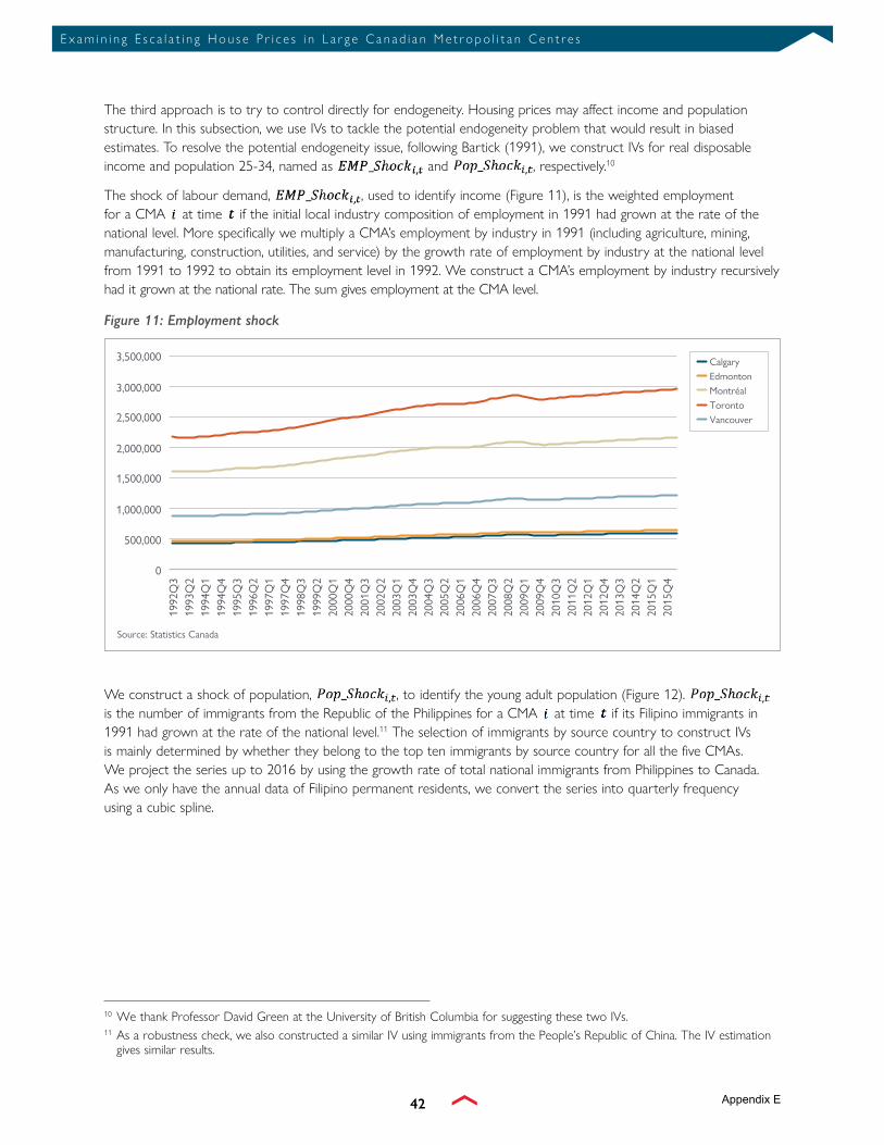
42


The third approach is to try to control directly for endogeneity. Housing prices may affect income and population structure. In this subsection, we use IVs to tackle the potential endogeneity problem that would result in biased estimates. To resolve the potential endogeneity issue, following Bartick (1991), we construct IVs for real disposable income and population 25-34, named as and , respectively.10

The shock of labour demand, , used to identify income (Figure 11), is the weighted employment for a CMA at time if the initial local industry composition of employment in 1991 had grown at the rate of the national level. More specifically we multiply a CMA’s employment by industry in 1991 (including agriculture, mining, manufacturing, construction, utilities, and service) by the growth rate of employment by industry at the national level from 1991 to 1992 to obtain its employment level in 1992. We construct a CMA’s employment by industry recursively had it grown at the national rate. The sum gives employment at the CMA level.

We construct a shock of population, , to identify the young adult population (Figure 12). is the number of immigrants from the Republic of the Philippines for a CMA at time if its Filipino immigrants in 1991 had grown at the rate of the national level.11 The selection of immigrants by source country to construct IVs is mainly determined by whether they belong to the top ten immigrants by source country for all the five CMAs. We project the series up to 2016 by using the growth rate of total national immigrants from Philippines to Canada. As we only have the annual data of Filipino permanent residents, we convert the series into quarterly frequency using a cubic spline.

1992

Q3

1993

Q2

1994

Q1

1994

Q4

1995

Q3

1996

Q2

1997

Q1

1997

Q4

1998

Q3

1999

Q2

2000

Q1

2000

Q4

2001

Q3

2002

Q2

2003

Q1

2003

Q4

2004

Q3

2005

Q2

2006

Q1

2006

Q4

2007

Q3

2008

Q2

2009

Q1

2009

Q4

2010

Q3

2011

Q2

2012

Q1

2012

Q4

2013

Q3

2014

Q2

2015

Q1

2015

Q4

3,500,000

3,000,000

2,500,000

2,000,000

1,500,000

1,000,000

500,000

0

Calgary

Vancouver

EdmontonMontréalToronto

Source: Statistics Canada

Figure 11: Employment shock

10 We thank Professor David Green at the University of British Columbia for suggesting these two IVs.11 As a robustness check, we also constructed a similar IV using immigrants from the People’s Republic of China. The IV estimation

gives similar results.

Appendix E

43


Before proceeding to IV estimation, we conduct weak instrument tests. We use robust Wald Test to test the joint significance of our instrumental variables in the first-stage equation. Results are reported in Table 4. Instruments are significantly correlated with income and young-adult population. The F-statistics for the weak instrument test in the first stage equations are much larger than the critical values suggested by Stock and Yogo (2005). Our instruments are strong.

Table 4: First-stage regression

inDeP. vAriAble REAL DISPOSABLE INCOME POPULATION 25-34

Employment shock 0.54*** (7.45)

-0.17*** (-2.74)

Population shock 0.02 (1.3)

0.1*** (7.33)

Mortgage Rate 0.004*** (2.87)

0.01*** (6.65)

Lagged construction costs 0.005 (0.14)

-0.01 (-0.21)

Lagged house price 0.12*** (8.85)

-0.05*** (-4.18)

Lagged sales 0.03***(3.35)

0.3***(-5.45)

Lagged population to housing stock ratio 0.15*(1.84)

1.51***(11.42)

CMA fixed effects Yes Yes

Weak instrument test (Robust F-Statistic) 71.68 28.95

Sample period 1996Q12016Q2

1996Q12016Q2

R-squared 0.91 0.99

Source: Statistics Canada, Conference Board of Canada, and CMHC. Note: t-statistics are reported in parentheses. * Significant at the 10 per cent.** Significant at the 5 per cent.*** Significant at the 1 per cent.

Calgary

Vancouver

EdmontonMontréalToronto

Source: Statistics Canada

1991

Q4

1992

Q3

1993

Q2

1994

Q1

1994

Q4

1995

Q3

1996

Q2

1997

Q1

1997

Q4

1998

Q3

1999

Q2

2000

Q1

2000

Q4

2001

Q3

2002

Q2

2003

Q1

2003

Q4

2004

Q3

2005

Q2

2006

Q1

2006

Q4

2007

Q3

2008

Q2

2009

Q1

2009

Q4

2010

Q3

2011

Q2

2012

Q1

2012

Q4

2013

Q3

2014

Q2

2015

Q1

2015

Q4

600,000

500,000

400,000

300,000

200,000

100,000

0

Figure 12: Population shock

Appendix E

44


The main results from IV estimation are reported in Table 5, together with the previous results estimated from simple SUR (from Table 3). All the coefficients have the expected signs with simple SUR and IV estimation. Compared to the simple SUR, IV estimation produces smaller coefficients for income, but larger coefficients for young-adult population. Other long-run coefficients are quite similar. The IV results suggest that housing prices in the five CMAs are explained by real disposable income, young-adult population, mortgage rates, and fixed effects. Lastly, the magnitude of coefficients with both estimations is in the range generally found in the literature.

Table 5: SUR and IV estimation results

inDeP. vAriAble PRICE (SUR) HOUSING STARTS (SUR) PRICE (IV) HOUSING START (IV)

Income 1.56***(18.86)

0.98***(4.62)

Population 25-34 0.70***(12.27)

1.57***(9.41)

Mortgage rate -0.02***(-6.61)

-0.02***(-4.28)

Lagged house price 0.74***(6.58)

0.65***(5.70)

Lagged construction costs -1.66***(-6.34)

-1.60***(-5.99)


1.05***(15.92)

Lagged population to housing stock ratio (lagged)

-3.85***(-12.44)

2.34**(2.74)

-4.92***(-10.83)

2.00**(2.32)



1992Q12016Q2

1992Q12016Q2

1992Q12016Q2

R-squared 0.94 0.82 0.91 0.82

Sources: Statistics Canada, Conference Board of Canada, and CMHC. Note: t-statistics are reported in parentheses.* Significant at the 10 per cent.** Significant at the 5 per cent.*** Significant at the 1 per cent.

Several precautions are required, however, when interpreting the IV results. First of all, the over-identification test suggests that IVs may not be exogenous. The Sargan statistic is marginally larger than the corresponding chi-squared critical value at 1 per cent level, which rejects the null that instruments are uncorrelated with error terms or instruments are exogenous. In other words, while our instruments are strong, they may be invalid because of possible correlations with error terms. One may advance that the validity of instruments is of concern because each CMA in our analysis is relatively large and important for the national level.

On the other hand, we are not convinced that the over-identification tests are applicable to our study. The main reason, overlooked by the literature, is that the Sargan statistic is computed when there is a risk of running spurious regressions. More specifically, we regress the residuals from the Two-Stage Least Squares (2SLS), I(0) if there is cointegration, on exogenous variables in level that are I(1).

Appendix E

45


Second, there is no evidence that the predicted variable using the IV approach are cointegrated with housing prices. While there is no theory to support the existence of cointegration between these predicted variables and housing prices, Table 6 also shows that the error correction term (ECT) in the short-run regression or in the error-correction model (ECM) is not significant, indicating the lack of cointegration between predicted variables and housing prices. In addition, IVs become weak when instrumenting the short-run equation with variables in first difference.

Because of these uncertainties, IV estimation results seem to suggest income, young-adult population, and mortgage rates explain housing prices in the long run, but further research efforts are required on overidentification tests with cointegration to validate the IV estimation results.

Table 6: IV estimation in an ECM

inDeP. vAriAble PRICE (IV) HOUSING START (IV)

Price ECT 0.01(0.299)

∆Income 0.34***(6.13)

∆Population 25-34 0.72(1.13)

∆Mortgage rate 0.49(0.68)

Supply ECT -0.31***(10.14)

∆Lagged house price 0.36***(6.13)

0.75**(2.36)

∆Lagged construction costs 1.18**(1.88)

∆Lagged sales 0.50***(7.14)

CMA fixed effects Yes Yes


1992Q12016Q2

R-squared -0.08 0.27

Sources: Statistics Canada, Conference Board of Canada, and CMHC. Note: t-statistics are reported in parentheses. * Significant at the 10 per cent.** Significant at the 5 per cent.*** Significant at the 1 per cent.

Appendix E

46


Lastly, contrary to the IV estimation results, simple OLS and SUR estimations on short-run model confirm the existence of cointegration between housing prices, income, young adult population, and mortgage rate, as shown in Table 7. Results from OLS and SUR estimations are quite similar. Thus results from separate OLS estimation of a simple demand equation are robust.

Table 7: Separate OLS and SUR estimation in an ECM

inDeP. vAriAble PRICE(OLS) HOUSING START(OLS) PRICE(SUR) HOUSING START (SUR)

Price ECT -0.03**(-3.08)

-0.03***-3.31

∆Lagged price 0.32***(7.42)

0.26**(6.20)

∆Income 0.09(1.60)

0.07(1.25)

∆Population 25-34 0.65***(3.00)

0.73***(3.37)

∆Mortgage Rate 0.005***(4.11)

0.004***(3.62)

Supply ECT -0.32***(-10.17)

-0.31***(-10.27)

∆Lagged house price 0.78***(2.40)

0.61**(1.96)

∆Lagged construction costs 1.23*(1.96)

0.80(1.30)

∆Lagged sales 0.50***(7.25)

0.50***(7.52)


Sample Period 1992Q22016Q2

1992Q22016Q2

1992Q22016Q2

1992Q22016Q2

R-squared 0.17 0.28 0.13 0.27

Sources: Statistics Canada, Conference Board of Canada, and CMHC. Note: t-statistics are reported in parentheses. * Significant at the 10 per cent.** Significant at the 5 per cent.*** Significant at the 1 per cent.

3.7 conclusionIn this chapter, we presented almost a century of data on house prices, mortgage rates, population, and income. The historical data demonstrate some important characteristics of house prices in Canada, and also highlight its large deviation from fundamental variables since 2010. We provided a theoretical framework to study housing prices of the five CMAs. The stock-flow model was presented, and the strengths and weaknesses of different estimation methods were discussed. We simultaneously estimated a stock-flow model. The results are quite similar with separate OLS and SUR estimation.

To tackle the potential endogeneity problem, we constructed instruments to identify real disposable income and young-adult population. The results seem to support that housing prices of the five CMAs are explained by income, young adult population, mortgage rates, and fixed effects. While over-identification tests cast doubt over the validity of instruments as exogenous variables, the validity of the test itself is uncertain because of the existence of cointegration, an econometric question requiring further research. We therefore view the parsimonious specification used in the rest of this report as reliable because the cointegration estimation is consistent with long time-series data (large T).

Appendix E

47


4 What Are the Drivers for Demand?

chAPter objectives:• List factors that influence the demand for homes, and explain how Canadian and global trends

are changing these factors.

• Look at different aspects of the “real” economy on housing (population flows, industrial activity, commodity production, etc.).

• Because of the absence of detailed data at the CMA level, explore what is happening in the economies of Canadian cities based on available — albeit disparate — data, while remaining consistent with the stylized facts of Chapter 2.

• Look at the impacts of the financial economy on housing (interest rates, the availability of credit, etc.).

key finDings:• There is a wide array of factors that could be explaining higher home prices. These require evaluation

using more sophisticated statistical tools, which are used in Chapter 5.

• While the statistical analyses concentrate on average levels of key variables, it is likely that the distribution of these variables is becoming more important in understanding our cities, including the distribution of income, industries and locations.

4.1 introDuctionWhile households are influenced by their own circumstances in deciding whether to buy a home, as described in Chapter 2, they are also impacted by wider dynamics affecting the broad swathe of the economy, such as overall economic growth or lower interest rates. This chapter outlines briefly these economic factors that influence demand for housing, some of them driven by the global changes described in Chapter 1. This chapter also highlights important changes in the patterns of some of these variables across Canadian cities. Concentrating on average levels of these variables may mask the importance of their distribution—the distribution of incomes may be as important as the average level of income in explaining the evolution of prices, for example. As discussed in Chapter 6, these patterns of increasing demand can combine with different supply responses to lead to variation in the local responses of house prices. Since homes are seen as a financial asset, changes in financial markets are also discussed.

4.2 funDAmentAl fActors Driving home PricesTraditionally, the fundamental factors for driving home prices higher include growth in disposable income and population, and lower interest rates. These are the core building blocks of our Workhorse model to account for home price growth, which will be elaborated on in the next chapter. In our analysis of this model, we have gained many insights into what has driven home prices, but we also feel that some elements are missing from that model. This chapter elaborates on what those might be.

Appendix E

48


4.3 economic groWth in cities

4.3.1 Income and Employment GrowthGrowth rates of the economy and employment are central variables influencing growth in house prices. A stronger economy with more jobs enables more of those who work to purchase suitable, bigger homes. But experience around the world suggests that the types of industries in cities also matter.

Some large cities tend to have a concentration of service or manufacturing industries that have particularly potent impacts on productivity and employment growth. In particular, information technology and financial services industries have powerful agglomeration effects, which means that other businesses benefit from co-locating with them. Firms benefit from being close to other firms that provide specialized inputs, or having access to a pool of specialized talent. Barr documents how over many decades the financial services industry remained on Wall Street while the population found housing further up the island of Manhattan. It was only after a significant period of elevated costs that a second business district in midtown Manhattan developed (Barr, 2016).

This effect may be becoming more important globally. Chapter 1 discussed some of the global changes that are taking place, one of which is the increasing pace of technological change. Industries that develop these new technologies tend to be concentrated in key cities such as San Francisco and Boston in the U.S., so technology change is having profound impacts directly on these cities. Another industry experiencing similar concentration is financial services, which tended to become concentrated in London and New York. As the importance of industries such as these has become greater, and commensurately higher salaries are paid, cities where these industries are located tend to have high home prices. This may be happening, albeit to a smaller extent, in Canadian cities.

Academics have laid out the path of what can happen to households (and hence homes) with technology change (Black and Henderson (1999) and Puga (2010)). Because of their access to highly skilled workers, breakthrough innovation tends to be located in cities. This innovation drives higher wages because of productivity and agglomeration gains in these cities—growing businesses attract businesses that supply them, for example.

This growth not only increases income levels of residents in particular cities, but also leads to the migration of domestic and international workers to those cities. This ‘selection effect’ can amplify the impact on local income levels, as those individuals who are attracted to growing industries in those cities can be more highly educated, and thus earn higher wages (Behrens et al., 2014). Significant wealth may be created that affords even greater opportunity to buy larger homes. These patterns have been explored for the U.S. in Enrico Moretti’s The New Geography of Jobs, but he finds that this pattern is not reflected in all cities (Moretti, 2012). Indeed, he finds that some cities cannot take advantage of the opportunities afforded by technology, and fall behind. The question broached in this section is whether similar trends promoting growth and wealth are manifesting themselves in Canada, and particularly in our large cities.

Another implication of the trend is that attracting highly paid workers will tend to increase inequality over time. Such income (and wealth) inequality could lead to higher home prices because of the greater ability of richer households to pay for homes, the greater ability to borrow in order to pay for homes, and the greater desire to purchase more “housing services”.

In the U.S., van Nieuwerburgh and Weil (2010) find that the distribution of house price increases matches the increase in wage dispersion. They look at the impact of different economic growth patterns when workers can move between cities and there are sluggish housing supply responses. The dispersion of productivity differences across cities and abilities across individuals lead to greater dispersion of house prices across cities. High-ability individuals will move to cities with increasing demand and increase property prices there.

Appendix E

49


Similar analysis emerges in Gyourko et al. (2013). As the aggregate number of high-income individuals increases across the United States, prices in ‘superstar cities’ increase. In turn, this increases inequality further as low-income individuals move out of expensive cities. “Mere [U.S.] population growth forces residency in preferred cities and towns effectively to be auctioned off to the highest bidder, with existing landowners in those places benefitting from the rise in prices.” Their data suggest that as much as two-thirds of the growth in dispersion in house prices can be explained by the increase in high-income households at the national level.

The rise in income and wealth has a self-reinforcing effect through the housing market. Those fortunate enough to have homes in fast-growing cities benefit from both higher incomes there, and higher property prices that increases their wealth. This tendency has morphed into the ongoing debate about income inequality. Thomas Piketty gained fame for drawing attention to the increased concentration of wealth, but has been criticized for neglecting to mention that much of that wealth is concentrated in housing (Piketty, 2014). Rognlie (2015), for example, shows that the share of net income generated by housing has risen in all seven large developed economies (Canada, France, Germany, Japan, Italy, U.K. and U.S.) since data became available. La Cava (2016) further finds that the long-run rise in housing capital income share is “fully concentrated in states that face housing supply constraints.” Joseph Stiglitz notes that some greater wealth can be transformed into productive capital: “The most important source of the disparity between the growth of wealth and the growth of productive capital is the growth in the value of land” (Stiglitz, 2016a).

4.3.2 What are the Patterns of Economic and Population Flows in Canada?

Canada as a whole has benefited from strong economic and employment growth over the last two decades, affording Canadians the opportunity to buy a home. Economic growth rates have differed across regions because of differences in the industrial structure. Rapid growth in commodity prices promotes growth in rural Canada and in cities where such resources predominate, such as from the impact of oil in Alberta, Saskatchewan and Newfoundland & Labrador.

4.3.2.1 Average Income and its DistributionWhile there is much data available for provinces, there are limited economic data at the CMA level in Canada.12 Hence, this section draws inferences about what is happening in Canadian cities from disparate data sources and from available academic research in Canada. Notable insights are gained from the papers of Mike Veall and his various coauthors on the distribution of incomes in Canada (e.g., Veall, 2012). Some of these findings include, for example, Murphy and Veall’s (2016) research showing that the national surge in top incomes from 1982 to 2010 can be disproportionately attributed to cities, with two cities—Calgary and Toronto—contributing more than half.

Data gap: Detailed economic statistics by CMA (particularly on the industrial and economic output side)The pattern may have changed for the period under study here. Figure 13 shows this result at work. The figure shows the level of income required to be in the top 1 per cent for cities in Canada, including inside and outside Census Metropolitan Areas (CMAs). Clearly there is a significant level of income in some Canadian cities that enables some to purchase expensive homes.

These data suggest that the local economy—notably, the types of industries in the local economy—can have an impact on the distribution of income in a CMA. Fortin and Lemieux (2015) examine Canadian labour data at the provincial level from 1997 and 2013. They found that the faster increase in the level of wages and the decline in wage dispersion in Newfoundland & Labrador, Saskatchewan and Alberta are a major difference between provinces. Moreover, they found that these trends are accounted for by growth in the extractive resources sectors, which benefited less-educated and younger workers the most.

12 The importance of cities suggests that Statistics Canada’s efforts to produce GDP statistics by CMA are to be welcomed (Statistics Canada, 2014).

Appendix E

50


Given the importance of resource industries in those provinces, we would expect the same pattern to hold for Calgary and Edmonton. In addition, given their statement about income inequality, we would not expect much dispersion in price increases in those cities—all prices for different types of properties are likely to rise in tandem. The flip side of this observation is that those markets are likely to display much tighter links to any cycles in commodity prices.

As discussed above, technology changes could also be an important driver of income growth, but the gains from inventing technology may accrue to a small number of people and firms. A source of data on this is the location of where patents are granted. Figure 14 shows the distribution of patents across regions of Canada in 2013. The region with the greatest number of patents generated is Toronto, followed by Vancouver and Montréal. The fact that most regions have close to zero patents indicates how concentrated innovative activity is, a pattern reflected in other countries as well (CCA, 2013). And again, this pattern is likely to reflect where higher earnings for the skilled workers and firms that produce patents are located.

Source: Statistics Canada (CANSIM Table 204-0002).

Troi

s-Ri

vièr

es, Q

C

Ott

awa-

Gat

inea

u, Q

C

Sagu

enay

, QC

Sher

broo

ke, Q

C

St. C

atha

rines

-Nia

gara

, ON

Non

-CM

A a

nd n

on-C

A

Thun

der

Bay,

ON

Win

dsor

, ON

Qué

bec,

QC

Sain

t Jo

hn, N

B

Gre

ater

Sud

bury

, ON

Osh

awa,

ON

Win

nipe

g, M

B

Lond

on, O

N

All

CA

Hal

ifax,

NS

Vict

oria

, BC

Kitc

hene

r-C

ambr

idge

-Wat

erlo

o, O

N

Mon

tréa

l, Q

C

Can

ada

Regi

na, S

K

Ham

ilton

, ON

Sask

atoo

n, S

K

Vanc

ouve

r, BC

Ott

awa-

Gat

inea

u, O

N

All

CM

As

St. J

ohn'

s, N

L

Edm

onto

n, A

B

Toro

nto,

ON

Cal

gary

, AB

$0$50

$100$150$200$250$300$350$400$450$500Thousands

Figure 13: Thresholds of top 1 per cent total incomes by geography (2014)

Source: OECD.

0

100

200

300

400

500

600

700

800Number of Patents

Census division, ordered by number of patents

Figure 14: Number of patents per census division, 2013

Appendix E

51


Turning to other data, Labour Force Survey data on employment can also provide insight on what is happening in Canadian cities. Employment in manufacturing increased by 14 per cent in Vancouver since the beginning of 2010, compared to a 17-per-cent increase in overall employment in Vancouver. Employment in information, culture and recreation increased by 30 per cent. Employment increases in manufacturing are rare given heightened competition with low-cost sources of manufactured goods in Asia. Therefore, a rise in manufacturing employment suggests that the goods being produced are high-end products in perhaps communication equipment or pharmaceuticals.

Labour Force Survey data also show that employment in finance, insurance, real estate, rental and leasing increased by 20 per cent in Toronto since early 2010, compared to the total increase in employment of 10 per cent. The results above suggest that if particularly high-paying industries are located in a CMA then there is likely to be a high level of income in that CMA as well, creating the capacity in that CMA to buy bigger and better homes. Another factor at work is what is happening within those industries.

Looking at the wage profile of industries gives some indication of underlying economic trends at work, but disentangling what is going on is more challenging. Rising wages over time suggest a need for more skills to work in that industry. Within industries, jobs for those with fewer skills became less prevalent. In the financial services industry, for example, there were proportionately more jobs that would be classified as occupations requiring high skill levels than ten years previously (see survey in ab Iorwerth, 2016).13

There have been differing patterns of wage growth across the Canadian population, and these differences in trends will affect Canadian cities differently depending on the prevalence of certain occupations and industries in those cities. Morissette et al. (2013) look at these trends in detail for Canada up to 2011. This paper also finds that pay rates grew substantially in the resource sector. There were also substantial increases in the financial services industry, which were associated with upskilling in that industry as well. Murphy and Veall (2016) found that the top 5 per cent of all wage earners working in the Finance & Insurance industry in Calgary earned over 40 per cent of the wages in that industry.

These patterns of income growth in cities have been captured in a range of analysis conducted by Statistics Canada, although their data predate some of the recent technology changes. Beckstead et al. (2010) explore urban-rural wage differences. Earnings in large metropolitan areas in 2000 were 25-per-cent higher than rural counterparts (and recall the difference between CMAs and non-CMAs in Figure 13). Up to a half of the difference between urban and rural earnings is explained by a greater number of skilled workers being in cities than in rural areas. They also find strong evidence of higher productivity among skilled workers if they co-locate in cities (i.e., of agglomeration effects).

Brown and Scott (2012) look at the location choices of people moving jobs in Canada. Degree-holders are more likely to move to locations that are specialized in their industry, and they are willing to move longer distances. They find this “consistent with specialized workers seeking out thicker labor markets.” Brown and Newbold (2012) found that in-migrants to Toronto received an immediate jump in earnings, exceeding what they would have obtained had they stayed where they were or moved to another city.

Although imprecise, and sometimes somewhat dated, all these analyses point to substantial gains from moving to larger Canadian cities, and that these gains are increasing over time. This leads to incentives for population movements.

13 Aled ab Iorwerth, 2016, “Financial Services Intermediation, and its Role in Economic Growth and Stability”, mimeo, Department of Finance Canada.

Appendix E

52


4.3.2.2 Population FlowsDemographic fundamentals suggest steady population growth, fuelled by natural increases as well as international arrivals. Canada’s population profile indicates annual growth averaging nearly 1.1 per cent between 2010 and 2016, in line with the 20-year national average of 1 per cent.

Figure 15 shows average population growth rates across CMAs in Canada, and for Canada as a whole since 2001 as well as since 2010. Cities that experienced booming economies from higher resource prices, and larger cities tended to show large population growth. Of the five cities we concentrate on in this report, only Montréal had population growth below the Canadian average. CMAs that showed strong population growth, both above the Canadian average and at a higher pace since 2010, included some areas surrounding Vancouver and Toronto such as Barrie, Kelowna, Abbotsford-Mission and Kitchener-Cambridge-Waterloo.

This population growth comes from natural changes through births and deaths, in- and out-migration from the rest of Canada, and net immigration from the rest of the world. There has been an on-going shift in immigration policy over the past fifteen years, aimed at helping to improve outcomes for new immigrants. Immigration has tended to be two to three times greater than the level of natural population growth (births less deaths) in Montréal, Toronto and Vancouver. All three cities have tended to show net out-migration to the rest of the country. By contrast, the composition of population growth in Calgary and Edmonton has been split relatively equally, with in-migration from the rest of Canada occasionally exceeding net immigration inflows and natural growth, particularly for Edmonton.14

These data again suggest that large cities are pulling people in, as they respond to incentives to move there. But, while coarse data such as these give some indication of potential pressures on housing prices, they must be treated with caution. Immigrants, on average, tend to have lower labour income than native-born Canadians, and thus may not immediately put upward pressure on house prices.15 Immigrant incomes are lowest on entry and then rise rapidly with the time spent in Canada, especially for economic immigrants. Homeownership rates increase along with incomes, and the overall homeownership rate for immigrants ends up being similar to that of non-immigrants. Geographic differences in the homeownership rates of immigrants further obscure the impact that immigrants may have on house prices. For instance, in the Vancouver CMA, the immigrant homeownership rate is five percentage points higher than the rate for native-born Canadians while in Montréal, it is five percentage points lower.

Another potential impact of immigrants is the wealth that they bring with them, giving them the opportunity to buy homes, and put upward pressure on home prices, but there do not appear to be robust data on this issue, although Statistics Canada is now producing data on non-resident owners of residential properties (Gellatly and Morissette, 2017). It is also important to bear in mind that, although some immigrants may have such wealth, many other immigrants do not: older research by Zhang (2003) found that wealth among recent immigrants in 1999 was lower than for native-born Canadians, but the distribution of wealth of immigrants who arrived between 1976 and 1985 was similar to that of Canadians by birth.

14 Data in this paragraph draw on CMHC analysis of Statistics Canada (051-0057).15 Skuterud and Clarke (2013) review evidence on immigrants’ performance in the Canadian labour markets.

Appendix E

53


Pavlov and Somerville (2016) finds a price premium in Vancouver neighbourhoods favoured by immigrant investors. There was a significant drop in that price premium following the announcement to cancel the Immigrant Investor Program in 2012. The drop in the price premium persisted while the flow of immigrants through the program faded out. Two years after that, the premium had returned to those neighbourhoods, possibly because many of the would-be immigrant investors would also qualify under programs like the Provincial Nominee Program. The authors did not find evidence that the price premium had spread to other neighbourhoods or market segments, possibly because of the relatively small size of the Immigrant Investor Program (Table 8).

Source: Statistics Canada (CANSIM Tables 051-0056 and 051-0001).

-0.5% 0.0% 0.5% 1.0% 1.5% 2.0% 2.5% 3.0% 3.5%

Thunder Bay, ONSaguenay, QCSaint John, NB

Greater Sudbury, ONSt. Catharines-Niagara, ON

Windsor, ONPeterborough, ONTrois-Rivières, QC

Kingston, ONHamilton, ON

London, ONBrantford, ON

Victoria, BCQuébec, QC

Halifax, Nova ScotiaMontréal, Quebec [24462]

Winnipeg, ManitobaCanada

Sherbrooke, QCKitchener-Cambridge-Waterloo, ON

Guelph, ONAbbotsford-Mission, BC

Ottawa-Gatineau, ON/QCMoncton, NB

Vancouver, BCSt. John's, NL

Regina, SKOshawa, ONToronto, ONKelowna, BC

Barrie, ONSaskatoon, SK

Edmonton, ABCalgary, AB

Average Annual Growth Rate

2010-16 2001-16

Figure 15: Average annual growth in populations, CMAs and Canada

Appendix E

54


Table 8: Total permanent immigrants, and number of immigrants admitted through the Business Immigration Program

TOTAL PERMANENT IMMIGRANTS, 2007-2011

BUSINESS IMMIGRATION PROGRAM (BIP), 2007-2011

Canada 1,265,601 12,402

Atlantic 33,280 124

Ontario 546,620 4,527

Manitoba 67,463 37

Saskatchewan 31,811 25

Alberta 135,689 347

British Columbia 203,365 7,317

Territories 1,620 -

Note that Québec has a separate immigration policy. Source: CIC, Evaluation of the Federal Business Immigration Program (2014).

4.4 finAnciAl floWsThis section starts by looking at the conventional determinants of financial flows: interest rates and credit availability. These are the powerful forces influencing housing markets. But another lesson from the last financial crisis is that even small segments of housing markets can push up prices. Piazzesi and Schneider (2009) explain how a small number of optimistic buyers can push up prices, for instance. Consequently, we outline the arguments why investors, both foreign and domestic, in properties could push up housing prices, and how having different beliefs about future house price gains could develop into a bubble.

4.4.1 Interest RatesMortgage rates have been trending down over many years (Figure 16). This trend makes it easier for a household to buy a home. With lower interest rates for all Canadians collectively, this would increase total demand for housing and for credit—a trend that happened in most developed economies.


Rate (%)

0

2

4

6

8

10

12

14

16

1990

1991

1992

1993

1994

1995

1996

1997

1998

1999

2000

2001

2002

2003

2004

2005

2006

2007

2008

2009

2010

2011

2012

2013

2014

2015

2016

Bank rate Chartered bank - conventional mortgage: 5 year

Figure 16: Interest rates and mortgage rates in Canada, 1990-2016

16 Technical discussion for the U.S. in Hamilton et al. (2016).

Appendix E

55


In making decisions about whether to purchase a home with a mortgage, households must have one eye on the future of interest rates. Over recent years, expectations regarding the trajectory of future interest rates have likely declined, possibly encouraging greater borrowing. There has been much debate over whether low interest rates are a temporary phenomenon, reflecting perhaps the debt overhang from the last recession as households continue to rebuild their balance sheets, or whether there are longer-term structural issues at play. This latter concern has been dubbed ‘secular stagnation’ by Harvard economist Larry Summers.

The Governor of the Bank of Canada outlined three reasons why interest rates have stayed low in line with the decline in the real neutral rate (Poloz, 2016).16 Firstly, there may have been a decline in the potential growth rate of the economy, mainly driven by an aging population that lowers growth in the labour force. Secondly, there may be rising global savings rates while investment remains subdued (usually associated with the ‘savings glut’ hypothesis of the former head of the Federal Reserve, Ben Bernanke (Bernanke, 2005)). And thirdly, a slower pace of technological change may be weakening potential world economic growth (associated with an economist at Northwestern University, Robert Gordon).

While low interest rates make financial assets more attractive, they could also lead to more savings being necessary to obtain a given level of income retirement. This “hunt for yield” could encourage investment in ownership of properties to obtain income, putting upward pressure on home prices, or that low interest rates (at close to zero) may have non-linear effects on asset prices (Hubbard and Mayer, 2009).

4.4.2 Credit AvailabilityWhile lower interest rates will encourage purchases of homes and increased credit in the economy, the amount of credit in the economy could also increase because of financial innovation (Wachter, 2015). Financial institutions would want to increase credit to households if they found it more profitable, or believed that mortgage lending is more secure than lending to firms.

Interest rates are also only one element limiting people’s ability to borrow; there are other conditions that financial institutions attach to receiving those loans (Stiglitz, 2016b). Over the last decade, it transpired that in the U.S. those conditions had become too lax, and excessive borrowing pushed up property prices. Favilukis et al. (2016) took a look at the lessons of the U.S. housing crisis prior to the last recession. They found that relaxation of credit constraints accounted for nearly two-thirds of the increase in the price-to-rent ratio. In the U.S., Favara and Imbs (2015) found similar results.

For the U.S., Mian and Sufi (2009) find that house price growth had been greater in areas where more individuals had been shut out previously from credit markets. Financial liberalization had eased their credit constraints. Chambers et al. (2009) found that the most important factor (56 to 70 per cent) explaining homeownership rates in the U.S. from 1994 to 2005 was the introduction of new mortgage products; demographics only accounted for 16 to 31 per cent of the change.

The latest research argues, however, that there was an across-the-board increase in debt (Adelino et al., 2016). Mortgage originations increased for borrowers across all income and creditworthiness levels. In turn, borrowers defaulting on bigger mortgages were responsible for a greater dollar amount in defaults. These results suggest that debt among all income groups should be of concern to governments, and not just among those with low income.

Appendix E

56


To the extent that financial institutions do not fully bear the burden of debt defaults, there may be incentives for banks to lend excessively to households. As noted by Beck et al. (2012), there is a global trend for banks to rely on lending to households for a greater part of their lending. Data show that this trend holds in Canada as well, with lending to households now more important for Canadian banks than lending to firms (Figure 17). Residential mortgages rose from 20 per cent of total credit in 1969 to 37 per cent in 2015 while other forms of household credit have remained relatively unchanged.

While patterns in Canada are different from the U.S. in that the lending system is more tightly regulated and homeowners have greater amounts of equity in their homes, concern remains over the role of credit because of its historical role in aggravating crises. Jordá et al. (2015), for example, analyze the role of interest rates and credit in driving house price booms and busts. Using data spanning 140 years of modern economic history in the advanced economies, they showed that loose monetary conditions lead to booms in real estate lending and house price bubbles.

Setting interest rates too low will tend to increase overall asset prices, and encourage households to purchase those assets. In turn, Wachter and Herring (2003) explored relationships between real estate bubbles and banking crises.

4.4.3 Income Inequality (financial effects)In reviewing the impacts of the last recession, Piazzesi and Schneider (2016) suggest that one of the key insights from the new post-crisis macroeconomic literature on housing is that heterogeneity of households matters. Models with heterogeneous households and frictions introduce powerful new amplification and propagation mechanisms. In particular, they provide more scope for effects of shocks to the financial sector, which have become important in accounts of post-war U.S. history, to propagate throughout the economy.

Because of this effect, the role of credit in different segments of the population—rather than its overall level—becomes important. Landvoigt et al. (2015) find, for example, that cheaper credit at the low end of the market was a major driver of home prices in San Diego. Krueger et al. (2016) find that wealth inequality can significantly amplify the impact of an aggregate shock if a sufficiently large fraction of households have little net wealth. Although there is limited historical data in Canada on wealth inequality, monitoring the evolving patterns of wealth may yield insights into the housing market, and to any risks that are in it.


Share of Total Credit

0%

10%

20%

30%

40%

50%

60%

70%

80%

1969

1971

1973

1975

1977

1979

1981

1983

1985

1987

1989

1991

1993

1995

1997

1999

2001

2003

2005

2007

2009

2011

2013

2015

Residential mortgage credit Consumer credit Business credit

Figure 17: Share of total credit, by type of credit

Appendix E

57


4.4.4 Investment in buy-to-rent housingLower interest rates, the prospect of capital gains from rising property prices, and income from renting out properties can make owning real estate attractive to investors. In the short term, such investments could put upward pressure on home prices, particularly if there is no supply response. Quantifying this impact is challenging because data on foreign and domestic investment activity is sparse. New research on the scale of domestic investment in the buy-to-rent market is discussed in Chapter 8.

Haughwout et al. (2011) explore this issue in the U.S., although they face data challenges there as well. They classify investors into three types: those who buy properties in order to rent; those who buy properties as a vacation or future retirement home; and those who buy properties to flip the house, hoping for capital gain. After mining debt data, they estimate that the investor proportion increased from 20 per cent of the market in 2000, to a peak of nearly 35 per cent in 2006 in the U.S. They also found that investors were more prominent in the markets that experienced the greatest “bubble” conditions. The authors conclude that the large influx of investors is likely to have amplified the upward pressure on house prices during the boom.

As the savings for such investment can come from anywhere, the housing market in Canada cannot be examined in isolation from global changes, including the international flows of capital (see Chapter 1.) Lower global interest rates and large pools of savings could increase direct investment by foreigners in Canadian property. Inflows of foreign capital are not restricted to the housing market, however. There has been an upsurge of foreign investment in Canadian debt, which would push Canadian interest rates down, and encourage Canadians to invest in higher-risk equity and housing investments as well. But Favilukis et al. (2013) argue that “changes in international capital flows played, at most, a small role driving house price movements in this episode [prior to 2008] and that, instead, the key causal factor was a financial market liberalization and its subsequent reversal that took place in many countries largely independently of international capital flows.” There has, however, been a significant upswing in foreign investment overall in Canada since 2010, so it is certainly possible that some of those funds have entered the housing market.

At this stage, we have not undertaken comprehensive research to evaluate the impact of foreign investment on housing prices, mainly because these data were not available. New data from Statistics Canada became available shortly before the publication of this report at the end of 2017, and we look forward to analyzing these data in 2018. The absence of such data prior to a policy change, however, makes it difficult statistically to evaluate the impact of the change in policy.

The new data from Statistics Canada, reported in Gellatly and Morissette (2017), show that non-residents owned 3.4 per cent of all residential properties in Toronto, and 4.9 per cent in Vancouver. The non-resident ownership share was more prevalent for condominium apartments (at 7 to 8 per cent) than for single-detached housing (at 2 to 3 per cent). Although we do not have historical data to correlate changes in foreign ownership with increases in housing prices, the prevalence of the stock of non-resident investment in condominium apartments makes it difficult to state that foreign investment is a major causal factor in driving prices higher, given that the prices of condominium apartments declined relative to single-detached homes.

With the introduction of taxes on foreign investment in housing by both British Columbia and Ontario, additional data have become available on the flow of foreign investment.

After Ontario introduced its non-residential speculation tax, individuals who are not citizens or permanent residents of Canada, or foreign corporations, accounted for 3.2 per cent of home purchases across the Greater Golden Horseshoe Region between May 27 and August 18 of 2017, down from 4.7 per cent in the month to May 26 (Ontario, 2017b). For Toronto, the comparable numbers had dropped from 7.2 per cent to 5.6 per cent.

Appendix E

58


It is difficult to evaluate the impact of foreign investment based on these numbers. At first blush, the shares of both the stock and the flow appear to be low. Nevertheless, they represent incremental demand to purchases by Canadians, and will therefore have played a role in pushing prices higher. As discussed in the previous section, short-term bursts of concentrated buying could be sufficient to spark broader price increases. As discussed below, it is also possible that the potential role of foreign investment has fed into expectations of domestic homebuyers regarding future demand. In this regard, the introduction of policies to curtail foreign investment may have played an important role in curtailing excessive optimism.

4.4.5 Differences in Price ExpectationsIn making their decisions to invest in homes (as discussed in Chapter 2), a critical factor that would encourage households to make a purchase is optimistic expectations about the path of future home prices. Hopes of future gains effectively lower the cost of purchasing a house today. While differences in opinions about valid prices are omnipresent in market economies, it appears that expectations about home prices can be subject to fads, and bouts of extreme optimism or pessimism. Shiller (2007) went as far as suggesting that other factors beyond psychology were irrelevant in explaining house price increases over the last decade in the U.S., and Granziera and Kozicki (2012) examined the development of bubbles in the U.S. when expectations of future prices are not fully rational.

That such an important decision can reflect more psychological forces means that house prices in the overall market can also become subject to collective mania. The risk then is compounded when irrational expectations by one segment of the population spills over onto others. Shiller (2007) has defined bubbles as: “a feedback mechanism operating through public observations of price increases and public expectations of future price increases. The feedback can also be described as a social epidemic, where certain public conceptions and ideas lead to emotional speculative interest in the markets, and therefore to price increases; these, then, serve to reproduce those public conceptions and ideas in more people.” As these different viewpoints play out, and if a significant part of the population moves to having exuberant expectations, then cycles in housing prices become extended (Burnside et al., 2016).

Much of the focus in explaining rising prices in the Vancouver market, for example, is the influence of foreign investors. Despite the absence of any concrete evidence, Angus Reid (2015) reports that 64 per cent of those living in Vancouver believed that “foreigners investing in the real estate market” is one of the “main causes of high housing prices in Vancouver”. It is possible that the narrative around foreign investment in Vancouver with an endless flow of funds has created a compelling story encouraging residents to enter the market. The actual size of foreign investment in Vancouver would therefore not matter if the narrative were compelling enough to alter households’ beliefs, and therefore encourage exuberant expectations of future prices.

The role of expectations can be important in housing markets, as they can reverse quickly. Head and Lloyd-Ellis (2016) show explicitly how a shift in expectations magnifies the effect of a given reduction in interest rates for 11 Canadian metro areas. The effects, relative to cases in which interest rates are expected to revert to their mean relatively quickly, are substantial.

It is hard to measure speculation in the housing market, but a survey developed in the U.S. by Karl Case and Robert Shiller has proved to be an interesting reference point (e.g., Case and Shiller, 2003). To this effect, CMHC developed a similar survey in Canada, and its results are explored in Chapter 9.

Appendix E

59


4.4.6 Consumption Wealth EffectsIt has been argued that since housing is such an important part of household wealth, changes in the perceived value of their home would change household consumption patterns, and also encourage some households to use gains from appreciating house prices to invest further in housing.

There is debate about this effect. Buiter (2010) and Carney (2011) share the view that a rise in house prices today means that the cost of housing increases tomorrow as well; hence, there should be no impact on consumption since households realize that the cost of housing has gone up as well. By contrast, Calomiris et al. (2013) suggest this argument is not as valid, however, when looking at those who have limited capacity to borrow—they may be housing rich but cash-flow poor—and those who can cash out of the housing market. In this case, rising home prices enables people to borrow more, or makes them richer when they cash out. Abdallah and Lastrapes (2013) find that spending in those U.S. states with greater opportunity for home-equity borrowing is more responsive to housing demand shocks. These wealth effects are particularly pronounced at peaks and troughs in housing cycles, exacerbating cycles.

There is limited capacity to link data on home prices, wealth and consumption patterns in Canada. Instead, CMHC has undertaken preliminary analysis of debt patterns in Vancouver and Toronto. In particular, we parse the data according to whether consumers have a mortgage or not. A first limitation of the data is that we do not know if those who do not have a mortgage own a house or not: they may have paid the mortgage off. The data do suggest, however, that growth in non-mortgage credit has been greater for those without a mortgage than for those with a mortgage. If the majority of homeowners have a mortgage, then this finding would suggest that they are not increasing non-housing credit significantly in response to home price gains in order to boost consumption. In fact, there is some evidence that non-mortgage debt is being reduced in response to higher prices.

Other analysis by CMHC of Equifax data looks at the share of consumers with more than one mortgage. It is possible that another mortgage has been taken out to increase consumption, but also to invest in other property. Since 2014, the share of consumers with more than one mortgage has risen from 4.5 per cent to 4.9 per cent in Vancouver, and from 3.3 per cent to 3.7 per cent in Toronto. The proportion for Toronto is lower than the Canadian average.

4.5 conclusions, AnD limits to DemAnD-siDe exPlAnAtions

Many of the arguments in this chapter could play a role in accounting for house price increases, and are explored further in Chapter 5, but they have been questioned (Shiller (2007) and Mayer (2007) debated the importance of psychological factors, for example).

Another counter-argument is developed in Glaeser et al. (2013), which found that lower interest rates can only explain one-fifth of the rise in U.S. house prices from 1996 to 2006. The core of their argument is that prices are more likely to rise when the supply response is limited, and consequently cities with more restricted land supply may be more prone to bubbles. The usual way that bubbles deflate is when supply of the factor thought to be in short supply actually materializes, but if supply is thought to be restricted, then people may be more willing to believe that prices can only go up. Glaeser et al. (2008) show that price run-ups in U.S. cities during the 1980s were more prevalent in cities with smaller supply responses. Park and Xiao (2010) look at the impact of restrictive land supply leading to a bubble in Seoul, Republic of Korea.

These arguments motivate us to look at the supply side of housing in Chapter 7.

Appendix E

60


5 Results From CMHC Model Estimation

chAPter objectives:• Outline the approach taken in the identification of key contributors to long-term trends in house prices.

• Report on the contribution of those key factors to both long-term price trends as well as changes in house prices since 2010.

key finDings:• Macroeconomic variables—including population trends, interest rates and disposable incomes—play an

important role in accounting for the steady rise in house prices witnessed in Canada’s major centres. Nevertheless, there remains a gap between predicted and actual prices.

• In an extension of the Workhorse model, we examine one additional factor that could account for this gap—the role of higher income and wealth inequality across major metropolitan centres in Canada. We find that changes in these factors play an important role in explaining accelerating house price growth in urban locations.

• We also examine the role of greater credit supply for national home prices. We find that growth in credit increases house prices, but not vice versa.

• The Canadian housing market is marked by significant regional contrasts. For this reason, we analyze local variations underpinning each CMA in order to fully understand market dynamics.

5.1 introDuctionThis Chapter elaborates on long-run house price trends across major centres in Canada. The Workhorse model specification explores the historical relationship between house prices and fundamental factors—including income, the young-adult population, and mortgage rates. After carefully specifying the model and performing model-selection procedures, we conclude that fundamentals do play a sizable role in accounting for the long-term upward movement in house prices.

Additional factors reflecting local conditions may also be required in order to provide a complete picture. We evaluate one such factor—the impact of income and wealth inequality—and, while we cannot always precisely identify its magnitude, we find that it largely explains growth in home prices.

As house prices tend to fluctuate around an upward trend, studying house prices in Canada requires a dynamic perspective using macroeconomic tools. In this chapter, the approach we follow first identifies the key factors behind long-run trends in house prices, and follow with the determinants of short-run fluctuations in the next chapter.

Appendix E

61


5.2 core DAtA AnD resultsPrior to explaining our methodology, we outline the data underlying fundamental factors and highlight the key results output from our modelling. Table 9 shows the core data used for the macroeconomic modelling, the pattern of price increases we are trying to explain, and the price changes predicted by the model over the period from 2010 to 2016.

As is standard in the literature, we approximate the impact of first-time homebuyers—who represent incremental demand to the market—by the 25- to 34-year-old population. Because of the increase in home prices, however, it is possible that first-time homebuyers in Toronto and Vancouver may be better represented by an older demographic. We will examine this issue further in future research.

A look at economic fundamentals suggests that housing activity in Edmonton was linked to the strongest drivers among the five CMAs. Despite the negative impacts of the recent shock in oil prices, market activity in the CMA was boosted by a solid 29.7-per-cent increase in the size of the young-adult population and 15.2 per cent in disposable income. This was followed by Calgary with growth of 21.4 per cent in the young-adult population and 15.5 per cent in disposable income. Gains in Vancouver were more moderate, with still healthy growth of 9 per cent in the young-adult population and 11.5 per cent in disposable income. Results in Toronto were mixed, with a drop of 1 per cent in disposable income, but decent growth of 11.6 per cent in the young-adult population. Montréal continued to strengthen, but at a slower pace, posting gains of 4 per cent in the young-population and 4.6 per cent in disposable income.

While the fall in nominal mortgage rates was uniform across Canada, we use mortgage rates adjusted for local differences in consumer price inflation, so that our model captures such variations in mortgage rates across these cities. This pattern of change in economic fundamentals provides clearer indication of prices predicted by the model.

Table 9 offers a foretaste of our modelling results. Price changes predicted by the model are reported in the bottom row of the table, with actual changes in house prices over the 2010-16 period reported in the penultimate row. After adjusting for inflation, actual house prices increased by 48 per cent in Vancouver, by 41 per cent in Toronto, and 11 per cent in Montréal, while remaining nearly flat in Calgary and Edmonton. Figure 18 illustrates the long-term trends in home prices across Canada’s major census metropolitan areas.

Model results show that house price growth in the five CMAs (Vancouver, Toronto, Montréal, Calgary, and Edmonton) was largely explained by fundamentals, but significant regional differences played out against this backdrop. Over two thirds of price growth in Vancouver was explained by fundamentals, while only one third was explained by these factors in Toronto. Meanwhile, the Workhorse Model over-predicts price growth in Montréal, Calgary, and Edmonton. A different modelling approach was pursued by Head and Lloyd-Ellis (2016), but they also reached very similar conclusions.

While price increases in Vancouver have been largely supported by economic fundamentals, a more puzzling result points to the state of the Toronto market, where fundamentals have not been as strong. In interpreting the results for Calgary and Edmonton, it is important to bear in mind that the model was estimated using data prior to 2010. Therefore, the recent volatility in oil prices was not captured in the data. This issue is discussed further in Section 5.5.

It is important to note that the model is being placed under the heavy burden of forecasting prices six years into the future. In this sense, the relative accuracy obtained for price predictions underscores the conclusion that the empirical specification is robust.

Appendix E

62


Table 9: Changes from 2010 to 2016 in house prices, fundamental factors, and predicted prices (All variables, except population, are deflated by CPI at CMA level.)

vAriAble VANCOUVER TORONTO MONTRéAL CALGARy EDMONTON

Disposable income 11.5% -1% 4.6% 15.5% 15.2%

Population 25-34 9% 11.6% 4% 21.4% 29.7%

Mortgage rate -229 BP -161 BP -120 BP -224 BP -195 BP

MLS® average price 48% 41% 11% 0.4% 0.11%

Predicted price 36% 16% 19% 7% 22%

Note: BP stands for basis points. Sources: Statistics Canada, CREA, Institut de la Statistique du Québec, Québec Federation of Real Estate Boards, Conference Board of Canada, CMHC calculations.

Sources: CMHC calculations based on Canadian Real Estate Association, Québec Federation of Real Estate Boards.Notes: Hodrick-Prescott Filter applied to obtain trends.

Figure 18: House Prices and Long-Term Trends

Appendix E

63


5.3 cmhc moDellingTo account for price increases over the 2010-16 period, we first evaluate model selection. This section describes our approach to determine the appropriate model—which, in turn, resulted in the adoption of the ‘Workhorse model’ as our baseline specification.

Factor identification follows a modified out-of-sample forecasting approach of Wheaton and Nechayev (2008).17 First, we estimate the Workhorse model using historical data prior to 2010. Second, we forecast house prices over the 2010-16 period. Finally, we assess the extent to which movements in the price of resale homes are explained by fundamentals over the period. This last step is based on the Shapley value decomposition (Shorrocks, 2013), which attributes the change in the variable of interest to each underlying factor. Hence, the method suggests the following multi-step approach:

1. Adopt a particular modelling structure (several can be evaluated);

2. Regress house prices on fundamentals and evaluate statistical properties using data through to 2010;

3. Evaluate the economic significance of these factors;

4. Forecast the equation over the 2010-16 period to assess the collective role of these variables in accounting for price growth, as well as recover forecasting errors; and

5. Regress forecasting errors on idiosyncratic factors.

In this section we concentrate on the first four steps (the fifth is discussed in greater detail in Chapter 6). In summary, this sequence of steps suggests that model specification is formed on the basis of economic theories, statistical properties are determined on a range of tests, and economic significance is based on the Shapley Value decomposition. Even if a factor shows statistical significance, it will be discarded if Shapley Value decomposition show its contribution to explaining house prices is negligible. This rigorous model specification process aims at minimizing the presence of potential biases.

5.3.1 Step 1: Modelling StructureWe are interested in explaining CMA-specific house prices on an inflation-adjusted basis. In the model, key independent variables include real personal disposable income per capita, the young-adult population aged 25-34 years old, and real five-year fixed mortgage rates. More formally, our Workhorse model is specified as:

where

: natural logarithm of real house prices;

: natural logarithm of real personal disposable income per person;

: natural logarithm of the young-adult population aged 25-34 years old;

: real five-year fixed mortgage rate;

: control vector of leads and lags; and

: Error term.

17 An alternative approach would have been the user-cost model of Hubbard and Mayer (2009), but this approach is a bottom-up approach and requires much more data. See also Himmelberg, Mayer and Sinai (2005), and Brown et al.(2011) for Australia.

Appendix E

64


5.3.2 Step 2: Estimation and Statistical PropertiesWe estimated demand over the period from 1988 to 2009 following Stock and Watson(1993)’s Autoregressive Distributed Lag (ARDL) model of cointegrated variables, which adds lags and leads of independent variables as control variables. The specification is statistically sound if variables are integrated of order one and cointegrated; otherwise, there is likely to be a spurious relationship (Granger and Newbold, 1974).

Over the period, model results indicate that real house prices, real disposable income per capita, and CMA-adjusted mortgage rates are integrated of order one, while the young-adult population is integrated of order two, at the margin. Generally, population is integrated of order one, but this statistical property also tends to be sensitive to sample sizes. As the analysis below suggests, incorporating growth rates for the young-adult population would seem statistically appealing at first glance; however, its explanatory power is practically negligible. Therefore, our model incorporates young-adult population levels, instead of growth rates, thereby reflecting greater economic significance, rather than unstable statistical properties.

Detection of cointegrating relationships was performed using Engle-Granger tests (Engle and Granger, 1987) as well as Johansen tests ( Johansen, 2000). The interpretation of Johansen Tests is conducted sequentially. More specifically, the existence of a cointegration equation first requires the rejection of the null hypothesis of cointegration, and subsequently the non-rejection of the null hypothesis that there is at most one cointegration equation.

Results presented in Table 10 reveal that house prices are cointegrated with real disposable income, young-adult population, and mortgage rates, thereby supporting the conclusion that the specification is statistically reliable. Note that despite variations in trend and lag intervals, cointegration test results generally hold. It is also important to note that we abstract from non-linear cointegration as in Park and Phillips (2001), largely owing to the lack of evidence of non-linear relations between variables.

Table 10: Johansen Test of Cointegration

hyPothesiZeD no. of coint. eq. VANCOUVER TORONTO MONTRéAL CALGARy EDMONTON

Number of coint. eq. at the 5% level 1* 1* 1* 1* 1*

None 47.47 63.63 62.96 61.83 61.17

Critical value 5% 47.86 47.86 47.86 47.86 47.86

At most 1 18.44 25.45 21.25 19.95 16.30

Critical value 5% 29.80 29.80 29.80 29.80 29.80

Lags interval 3 3 3 3 3

Linear deterministic trend Yes Yes Yes Yes Yes

Note: Trace test indicates 1 cointegration equation at the 5% level.

Appendix E

65


Because the model is not stationary, statistical references based on standard OLS methodologies will be biased (Hamilton, 1994). For this reason, we estimate the baseline specification using Dynamic Ordinary Least Squares (DOLS) (Stock and Watson,1993), as it corrects the model by making it variance-stationary. The results from the estimation are reported in Table 11.

Table 11: Regression Results from the Workhorse Model(Dependant variable is the log of real house price, Dynamic OLS with 2 leads and 2 lags, 1988Q1-2009Q4)

inDeP. vAriAble VANCOUVER TORONTO MONTRéAL CALGARy EDMONTON

Income 1.42***(2.51)

1.33***(2.82)

3.00***(9.57)

1.32*(1.77)

2.24***(3.31)

Population 25-34 1.98***(3.45)

2.72***(3.63)

2.14***(5.50)

1.77***(3.22)

2.42***(5.48)

Mortgage rate -0.04*(1.49)

-0.02(-1.42)

-0.02(-1.21)

-0.02(-1.16)

-0.10***(-5.75)

Constant -26.51***(2.53)

-37.79***(-5.85)

-46.05***(-6.39)

-22.64***(-3.99)

-39.19***(-4.98)

R-squared 0.91 0.88 0.95 0.96 0.94

S.E. of regression 0.07 0.06 0.06 0.06 0.08

Note: t-statistics are reported inside of parentheses. * Significant at the 10 per cent.** Significant at the 5 per cent.*** Significant at the 1 per cent.

Interpretation is straightforward with double-log models. A look at how fundamentals affect house prices in Vancouver suggests that an increase of one per cent in income raises house prices by 1.42 per cent; an increase of one per cent in young-adult population increases house prices by 1.98 per cent; and a decrease of one per cent in mortgage rate raises house prices by 4 per cent. The magnitudes of these coefficients tend to be similar across the other major CMAs, but generally, an increase of one per cent in income would increase house prices by 3 per cent in Montréal, while a decrease of 1 per cent in mortgage rates would increase house prices in Edmonton by 10 per cent.

5.3.3 Step 3: Accounting For Price ChangesThe importance of variables included in the model is evaluated using the Shapley decomposition method (Shorrocks, 2013).18 While the decomposition confirms the importance of key variables in explaining the model, the method also pointed to weakness when the specification incorporated young-adult population in terms of growth rates. This result allowed us to modify the model so that it captured young-adult population levels, rather than growth rates, thus improving its explanatory power overall.

A closer look at the numbers reveals the extent to which movements in the price of homes can be explained by individual fundamental factors. (See Figure 19.) In Vancouver, for example, home prices rose by 48 per cent over the 2010-16 period. Of this increase, 16 per cent was attributed to the rise in real disposable income, 11 per cent to higher levels of the young-adult population, 9 per cent to lower mortgage rates, and the remaining 12 per cent to unobserved factors.19

18 Shapley value is a decomposition method that is theoretically sound. In game theory, the Shapley value is a way to fairly distribute the total gains of a game to players by considering all possible coalitions between players. It is applied to identify how much a particular regressor contributes to the overall explanation of variation in a model. Calculating the Shapley value for a model of pregressors requires the computation of 2p models.

19 The contribution is computed by the combination of Shapely value decomposition and the comparison between the actual price changes and the price changes predicted by the model. Thus, if the model underpredicts price increases, the unexplained part is positive, while negative if the model overpredicts price increases.

Appendix E

66


Results also highlight the importance of accounting for local contrasts when performing price growth attribution analyses (Section 4.4.) In particular, the base case Workhorse model underpredicts price increases in Toronto and Vancouver, while overpredicting gains in Calgary, Edmonton and Montréal. Later on in this chapter and in the next, we turn our attention to competing hypotheses that support the factors explaining heterogeneity, considering local contrasts in income distributions as well as opportunities to increase the supply of housing. It is important to note, however, that these hypotheses are not necessarily mutually exclusive.

Actual price change: 48%, Vancouver, 2010-16 Actual price change: 40%, Toronto, 2010-16

Actual price change: 11%, Montréal, 2010-16

Actual price change: 0.1%, Edmonton, 2010-16

Actual price change: 0.4%, Calgary, 2010-16

Source: CMHC calculations.

0%

5%

10%

15%

20%

25%

30%

Real personaldisposable

income

Young adult population

Realmortgage

rate

Unexplainedprice change

0%2%4%6%8%

10%12%14%16%18%


income

Young adultpopulation

Realmortgage

rate



income


Realmortgage

rate



income


Realmortgage

rate



income


Realmortgage

rate


16.36%

10.85%

8.52%

12.15%

5.04%8.09%

3.22%

23.84%

-10.00%

-5.00%

0.00%

5.00%

10.00%

15.00%

-8%

-6%

-4%

-2%

0%

2%

4%12.63%

1.13%

4.97%

-7.80%

3.13%2.01% 1.83%

-6.61%

-25%-20%-15%-10%-5%0%5%

10%15% 11.96%

4.77% 5.45%

-22.08%

Figure 19: Accounting for price changes by CMA, 2010-2016

Appendix E

67


5.3.4 Step 4: In-Sample ForecastingOnce the model becomes well-specified, the main question that arises is to what extent model fundamentals explain house prices over the 2010-16 period. To answer this question, the estimated relations between house prices and fundamental factors are subsequently used to predict house prices over the period. Noteworthy is that no structural breaks have been detected among model variables over the period.

This analysis is illustrated in Figure 20 and Figure 19. (Recall that actual and predicted changes over the 2010-16 period were previously displayed in Table 9.) Once again, the model was first estimated using data from Q1 1988 to Q4 2009. Next, we generated a forecast based on the estimates from the previous stage through to Q1 2016, using actual data on interest rates, the young-adult population and disposable income. Forecasting errors represent the gap between actual house prices and predicted prices.

Source: Actual prices from CREA, MLS®.

Prices ($)

-100,000

100,000

300,000

500,000

700,000

900,000

1988

1989

1990

1991

1992

1993

1994

1995

1996

1997

1998

1999

2000

2001

2002

2003

2004

2005

2006

2007

2008

2009

2010

2011

2012

2013

2014

2015

2016


Figure 21: Actual average price for Toronto, 1988 to 2016; predicted price from 2010 to 2016

Source: Actual prices from CREA, MLS®.

Prices ($)

-

200,000

400,000

600,000

800,000

1,000,000

1988

1989

1990

1991

1992

1993

1994

1995

1996

1997

1998

1999

2000

2001

2002

2003

2004

2005

2006

2007

2008

2009

2010

2011

2012

2013

2014

2015

2016


Figure 20: Actual average price for Vancouver, 1988 to 2016; predicted price from 2010 to 2016

Appendix E

68


Overall, signs suggest that fundamentals largely explain movements in house prices across Canada’s major cities. The model accounts for nearly a third of the price increase seen in Toronto and over two-thirds of the growth experienced in Vancouver. (As mentioned previously, economic fundamentals were weaker in Toronto.) Meanwhile, the model overestimates house price predictions in Montréal by 8 per cent. And in line with the strong fundamentals seen in Calgary and Edmonton, predicted house price growth is higher than actual house price growth in these cities.

Generally, overprediction suggests that additional developments emerging locally, and that are affecting the market today, were not foreseen in 2010 (e.g. the expansion of the financial services industry in Toronto, and oil-price shocks to resource-based Calgary and Edmonton).

5.4 extension 1: exAmining the links betWeen house Prices AnD income AnD WeAlth inequAlity

As explored previously in Chapter 3, income and wealth inequality could play an important role in explaining accelerating house price growth in urban locations associated with more favourable living conditions. With a growing number of higher income families, more households are willing and able to afford the premium charged for larger homes that are conveniently located. Therefore, house prices in these cities tend to rise faster, especially when land supply is subject to geographic and regulatory constraints.

Source: Statistics Canada.

0.540

0.560

0.580

0.600

0.620

0.640

0.660

1995 1996 1997 1998 1999 2000 2001 2002 2003 2004 2005 2006 2007 2008 2009 2010 2011 2012 2013

0.500

0.520

0.540

0.560

0.580

0.600

0.620

0.640

0.660

1995 1996 1997 1998 1999 2000 2001 2002 2003 2004 2005 2006 2007 2008 2009 2010 2011 2012 2013

Montréal Calgary Edmonton

Canada Toronto Vancouver

Figure 22: Gini coefficient, income including capital gains

Appendix E

69


Statistics Canada has provided CMA-level data on the Gini Coefficient for the 1995 to 2013 period. Since the latest data were available only through to the end of 2013, our model does not incorporate any recent movements in this measure.

The Gini Coefficient is a standard measure of inequality that reflects income trends reported in tax filings. In order to explore potential growth in wealth inequality, our analyses probed returns originating from capital income. It is important to note that capital income is a broad-based indicator representing income from realized capital gains—such as the sale of real-estate properties or closing a position in stocks and other asset classes—rather than unrealized capital gains. Moreover, as there is no tax on capital gains from the sale of primary residences, this measure does not include capital gains from selling homes.

Figure 22 suggests that income inequality in Toronto and Vancouver has been on the rise since 1995. Income inequality remained nearly flat in Montréal. In Calgary and Edmonton inequality has trended down steadily since 2006. Similar patterns have also been observed when capital gains were excluded from this measure.

Once validated as an economically significant metric through Shapley decompositions, these inequality metrics are incorporated as part of the forecast reflecting the period from 2010 onward.20 Figure 23 confirms that income

inequality has been an important factor in accounting for house price increases in Canada’s largest centres over the 1995 to 2013 period.

From 2010 to 2013, average home prices in Toronto advanced by 17.5 per cent (the latest data we have for the Gini coefficient is to 2013). Meanwhile, the Workhorse model suggests a 12 per cent jump in prices over the same period, and if we include the Gini Coefficient, price levels are forecast to increase by 16.4 per cent. The results for Vancouver suggest correlation between the rise in income and the rise in income inequality. Because of this multicollinearity property observed between income and income inequality, inclusion of the Gini Coefficient leads to overpredicted price growth, underscoring the importance of incorporating distributional aspects into the model. In addition, changes in income inequality do not contribute to house price gains in Calgary, Edmonton, and Montréal. Income inequality has eased in Calgary and Edmonton since 2007, while in Montréal it has remained relatively flat since 1995.

20 Results of Shapley value decomposition for Montréal, Calgary, and Edmonton are available upon request.


Vancouver Toronto

Real personal disposable

income


Real Mortgage

rate

Ginicoe�cient

Real personal disposable

income


Real Mortgage

rate

Ginicoe�cient

0%5%

10%15%20%25%30%35%40%

0%5%

10%15%20%25%30%35%40%

27.03%

17.32% 19.24%

36.42%

19.22%

33.63%

13.26%

33.89%

Figure 23: Shapley value decomposition for demand model with income inequality

Appendix E

70


5.5 extension 2: exAmining the imPlicAtions of creDit exPAnsion

Studying the impact of credit supply may be hindered by endogeneity originating from potential reverse causality—credit supply changes tend to affect house price changes, while at the same time, house price changes tend to affect credit supply. Solving simultaneous-equation bias has been a long-standing challenge in economics, and this section takes multiple approaches to address this issue. In order to study the relationship between mortgage credit levels and house prices, we concentrate our analyses on estimation results from fitting a Structural Vector Autoregressive model (SVAR).21 We first look at a “naïve” OLS approach, and we subsequently adopt a vector error correction model (VECM) to account for common trends.

Results indicate that both the impact and interaction of residential mortgage credit levels on house prices are quantitatively important. A one-standard-deviation shock to residential credit supply generates an increase of 4 to 7 basis points in the growth rate of house prices. Alternatively, a one-unit shock to residential credit supply is associated with an increase in the range of 1 to 2 units in the growth rate of house prices. We also find that impacts are persistent and generally last through more than six quarters.

5.5.1 Initial ApproachWe estimate models in the presence and absence of error correction terms. Results indicate that growth in mortgage credit affects growth in prices. (Table 12.) Although Granger Causality Tests do not reject exogeneity (results not shown), concerns over endogeneity are still not allayed. For example, the sign of the coefficient estimate for the growth of young-adult population is negative, while we would expect the effect of young-adult population to run in the opposite direction.

Table 12: House prices and residential mortgage credit(Dependent variable is growth rate of real house prices of Canada, 1999-2016, Dynamic OLS with 1 lag)

inDeP. vAriAble MODEL WITHOUT ERROR CORRECTION

MODEL WITH ERROR CORRECTION

∆Residential credit 0.79(4.63)

1.95(4.26)

∆Income 0.15(1.33)

0.30(2.31)

∆Population 25-34 -0.48(-0.41)

-4.57(-2.72)

Error Correction Term -0.34(-3.14)

Constant -0.004(-1.37)

0.02(2.68)

R-squared 0.19 0.43

S.E. of regression 0.01 0.01

Source: CMHC calculations

21 To overcome this “simultaneous equation bias”, Favara and Imbs (2015) exploit natural experiments from the different implementation of the deregulation process in the U.S., and construct a control group and treatment group. The effects of credit supply on house prices are simply the treatment effect. The lack of a similar deregulation process in Canada limits the application of the same study.

Appendix E

71


5.5.2 Structural VARIn order to account for simultaneous-equation bias, we fit a Structural VAR specification to the data. In the following structure, price is dependent on credit, while at the same time, credit is dependent on price. The following three-equation system is characterized by a set of covariates that allows for contemporaneous reverse causality:

where

: Real house price growth rates for Canada;

: Residential credit growth rates for Canada;

: Real personal disposable income per person growth rates for Canada;

: Young-adult population (25-34 years) growth rates;

: Set of control variables in lags;

, , and : Error terms and economic shocks, where : house price shock; : residential mortgage credit shock; : income shock.

In matrix form, we have

where,

: 3X3 matrix, i=0,…,k;

: 3X1 vector characterizing endogenous variables, such as , , and ;

: 3X3 matrix;

: 3X1 vector controlling for observed heterogeneity;

: 3X1 vector of error terms or shocks;

The vector of error terms satisfies the following properties:

• , every error term has mean zero;

• , the contemporaneous covariance matrix of error terms is diagonal, which means the structural shocks are not correlated; and

• , there is no serial correlation in individual error terms.

Appendix E

72


In this system, we have six equations but nine unknowns; accordingly, the identification strategy requires three hypotheses. Since contemporaneous changes in house prices and residential credit supply are not expected to affect income, we impose the following assumption: . In addition, we restrict , as contemporaneous changes in income are assumed to not affect residential credit supply.

Table 13: SVAR results(Dependent variable is the growth rate of repeat sale house prices in real terms in Canada, 2000-2016, SVAR with 4 lags)

inDeP. vAriAble ∆HOUSE PRICE ∆RESIDENTIAL CREDIT

∆Residential credit 1.03(3.27)

∆Income 0.14(1.38)

∆Population 25-34 -0.65(-1.08)

-0.09(-2.72)

∆house price -0.01(-0.40)

Log likelihood 679.34


Results from the SVAR model confirm that growth in residential mortgage credit affects house prices significantly; however, growth in house prices do not affect mortgage credit significantly. Taking into account possible simultaneous equation bias, estimates suggest that an increase of one per cent in the growth rate of residential mortgage rates raises the growth rate of house prices by 1.03 per cent.

Variance decomposition (Table 14) shows that residential mortgage credit explains between 30 and 40 per cent of the variation in house prices, depending on the lag length from the shock.

Table 14: Variance decomposition of house prices in Canada using SVAR (percentage)

PerioD S.E. HOUSE PRICES MORTGAGE CREDIT INCOME

1 0.009 100 0.00 0.00

4 0.014 67.37 31.44 1.19

8 0.014 65.33 33 1.67

16 0.015 60.03 38.43 1.53

20 0.016 57.89 40.62 1.49


Appendix E

73


22 The results are robust using total credit rather than residential mortgage credit.

5.5.3 Robustness Check: Vector Error Correction model (VECM) ApproachThe above SVAR structure does not account for the possibility of common trends among variables (unlike in the CMHC-HMA model where variables are I(1).) In particular, Johansen tests indicate a cointegration relation at 8 per cent. Consequently, we explore a Vector Error Correction model (VECM) that considers the possibility of such common trends. The VECM approach is essentially an extension of the SVAR method, but with the addition of an error correction term.

Compared with SVAR, accounting for the cointegration relation resulted in the reduction of the contribution of mortgage credit shocks to variations in house prices. The contribution of mortgage credit ranges from 18 per cent to 23 per cent, but remains an important factor.22

Table 15: Variance decomposition of house prices in Canada using VECM (percentage)

PerioD S.E. HOUSE PRICES MORTGAGE CREDIT INCOME

1 0.009 100 0.00 0.00

4 0.013 80.50 18.02 1.48

8 0.013 77.48 18 4.52

16 0.014 73.65 21.54 4.82

20 0.014 72.65 22.56 4.80


5.6 extension 3: exAmining the imPortAnce of locAl conDitions

In the above modelling structure, a very parsimonious approach is taken. Clearly, this approach does not reflect the rich set of factors that explain local variations in house price changes. To this end, additional econometric work was undertaken to highlight how knowledge at the local level can further our understanding of housing market dynamics.

Oil prices, for instance, describe one such factor, and it plays an important role in the local economies of resource-based Calgary and Edmonton. To explore this relationship, we incorporated oil prices into the set of covariates specified in the Workhorse model. Results exhibit some subtleties. Under the forecasting procedure laid out in Section 4.3, results suggest that accounting for oil prices did not improve predictive power. (Recall, however, that model estimation was initially based on data through to 2010—prior to the recent vicissitudes in the oil market.) In contrast, estimating the model with the inclusion of oil prices over the full period (from 1988 to 2016) generates predictions of lower price levels, thereby closing the gap between predicted and actual prices. This suggests the model can be sensitive to new economic developments.

Appendix E

74


Another factor that can be added to the regional specification is the terms of trade. The terms of trade (ratio of export prices to import prices) are strongly correlated with the real exchange rate. Regionally, the terms of trade are strongly correlated with house prices in Calgary and Edmonton, but less so in Vancouver, Toronto, and Montréal, especially since 2009.

Including the terms of trade in a regression requires caution for two reasons:

1. The terms of trade are strongly correlated with personal disposable income in Montréal, Calgary, and Edmonton. This fact suggests the possible presence of multicollinearity in the model, which would make the results difficult to interpret;

2. The terms of trade are strongly correlated with the real exchange rate. Hence, the effects of the depreciation of the Canadian dollar on house prices may differ across cities. For instance, the weaker Canadian dollar would make Vancouver, Toronto, and Montréal more attractive housing markets to foreign buyers. However, the lower value of the Canadian dollar was due largely to tumbling world oil prices; hence, the impact of the ratio on oil-producer CMAs, such as Calgary and Edmonton, would be more likely negative.

Including the terms of trade in the regression for Vancouver gives a positive relation, and as such it will underestimate fundamental prices forecast by the model. For Calgary, the terms of trade are strongly correlated with personal disposable income, thereby causing multicollinearity problems.

To explain long-run trends in house prices, we opt for a parsimonious specification that balances the trade-off between overfitting the model and its predictive power. As specified, the key fundamentals in the model—disposable income, young-adult population, and mortgage rates—largely explain the long-run trends seen in the five CMAs. Even though the inclusion of additional variables into the specification can slightly increase the R-squared, it can also undermine the predictive power of the model.

5.7 conclusionWe undertook a macroeconomic approach to examine the drivers behind the steady rise in house prices witnessed in Canada’s major centres. Through a rigorous process of empirical specification and model selection, we identify the key economic fundamentals—disposable income, young-adult population, and mortgage rates—explaining long-run trends in these markets.

These factors are largely responsible for the upward movement in the price of resale homes, accounting for over two-thirds of the growth experienced in Vancouver, while over-predicting prices in Montréal, Calgary, and Edmonton. However, the fundamentals support only a third of the price increases in Toronto.

These findings are well supported by actual changes in fundamental factors. Despite the negative impact of tumbling world oil prices, Calgary and Edmonton experienced the strongest increases in the young-adult population as well as disposable income among the 5 CMAs. This was followed by more modest increases in Vancouver, Toronto, and Montréal.

The Canadian housing market is marked by significant regional contrasts. For this reason, modelling efforts take into account the local variations underpinning each CMA. The plunge in oil prices illustrates one such event in terms of its contribution to the modelling specification of oil-dependent regions.

Nevertheless, in this chapter we focus primarily on long-term trends, opting for a parsimonious specification that balances the trade-off between overfitting the model and its predictive power. (Overfitting may artificially inflate R-squared values while undermining its predicting power.) Other factors—such as income distribution, supply constraints, investment-driven demand, speculation, residential mortgage credit, and CMA characteristics—will be studied in detail in the following chapters.

Appendix E

75


6 The Supply Side of Housing

chAPter objectives:• Analyze separately the roles of construction and land in determining the supply response of new

homes to the demand pressures discussed in Chapter 4.

• Discuss restrictions on land supply by geography, policy and landowners.

• Outline policy trade-offs in increasing land available for development, and macroeconomic risk from restricting land supply.

key finDings:• There is no evidence that there are construction cost pressures, in terms of higher labour or material

costs, pushing home prices higher. An increased share of the economy is taken by ownership transfer costs (federal and provincial taxes, land development costs, etc.).

• Higher land prices indicate a scarcity of land, which can be curtailed by geography, government policy and decisions of landowners. In combination with economic and population growth, these have likely contributed to higher land prices. Higher land prices would lead to either increased densification of cities and/or higher home prices. Intensification will be more likely if the process of redevelopment and rezoning operates efficiently.

• Differences in the ease of increasing supply across Canadian cities imply that responses to macroeconomic events will differ among them. As the share of land value in the total price of a building rises, inter-linkages between home prices and macroeconomic variables will increase, creating the potential for greater volatility where land supply is restricted.

6.1 introDuctionWhile the previous two chapters laid out how various forces increase demand for housing, this chapter explores the supply side of housing. In well-functioning markets, rising prices signal that more supply is required.

The supply side of housing reflects not only the physical construction of homes, but also the economics of land that homes are built on. While constructing new homes is akin to a manufacturing process, the value of land captures the value of being close to places of work, transit and good schools, and being far from pollution or noise. In turn, the magnitude of land values and its tradability have made it closer to being a financial asset, and hence more sensitive to macroeconomic variables.

Since the cost of constructing a standardized home has not grown as rapidly as home prices, rising home prices mean that a greater part of the price of a property is made up by the price of land. Change in this asset value can have far reaching consequences for home prices and the types of homes that are built. As a very rough rule of thumb, land prices form roughly 30 per cent of the value a new building sold, so as the value of land rises, so should the value of the structure built on it. Higher land values give incentives to economize on land, and this leads to higher-value properties being built—either more expensive single-detached homes, or denser multi-storey buildings. As cities expand in size, land may not be available for construction because of physical features such as geography, restrictions imposed by government, or decisions by landowners. Anticipation of such future shortages will drive land prices higher today.

Unfortunately, to date there has been little analysis of data in Canada on many of the factors that would enable us to form a robust view of housing supply in Canada. Therefore, in this chapter and the next we examine this issue from multiple perspectives to try to build an understanding of what is happening. We start by laying out the conceptual framework for understanding the supply side of housing.

Appendix E

76


6.2 the concePtuAl frAmeWorkThis section discusses the economics of building new homes. While market dynamics are important in determining the direction of the housing market, they are first attenuated by unavoidable physical realities.

The obvious physical constraint is that development is curtailed by terrain. Land may be too steep to build upon, for instance. Obviously, the value of underwater land close to the shore where high-priced buildings are concentrated would be highly valuable if it could be built upon! These geographical constraints limit the supply response to price changes, and Saiz (2010) in the U.S. finds that most areas in which housing supply are found to be inelastic (i.e., are less responsive to price changes) are constrained by geography. But, as Davidoff (2016) pointed out, supply constraints in terms of mountains and oceans can also be attractive places to live, and be correlated with greater demand; this again argues for looking at both demand and supply.

Another reality of housing supply is that it takes time to plan and build new homes, and develop land to allow construction. Consequently, there is an inherently slow rate of adjustment to prices in the housing sector relative to other industries. Equally, there are lag times if builders want to demolish old houses to build new ones, particularly if they need to assemble different lots in order to build a larger structure. Hence, changing the stock of housing to match uncertain changes in demand is inherently slow. To the extent that this tends to be more difficult, prices will need to rise even further to encourage turnover in the stock of housing. Increasing the uncertainty faced by homebuilders risks lengthening this process further.

The value of a structure reflects its building costs plus the value of the land it sits on, but the economic issues involved in each need to be considered separately. While housing construction is similar to a manufacturing process, the value of land is more closely associated with the value of conventional financial assets—therefore, different economic forces are at play. Moreover, while the economics of construction are generally similar across the country, the greater importance of land in the overall value of buildings in high-priced markets means that the same economic forces across the country can have different effects across cities.

6.2.1 The Economics of ConstructionIn deciding whether to build new houses, homebuilders make judgments on several factors—including the cost of construction materials and hiring skilled workers. These costs weigh against the expected present value of the houses they will build. The choice to build involves significant risk given the time it takes to build new structures, although builders will also pre-sell many to secure their operations. Hence, builders will have to base their decisions on prices they expect to obtain many months, if not years, into the future. These expectations are based on a whole raft of variables including population dynamics, conditions in financial markets, and the evolution of government policies. Figure 24 shows, for example, how housing starts may lead or lag the formation of new households.

As with manufacturing, higher input costs faced by the construction industry would tend to lead to either lower profits or higher prices for new homes.23 It is therefore possible—in theory—that the recent rise in home prices could be explained by either the construction industry restricting supply of new houses in order to push up prices and profitability, or by the fact that material and labour costs could also be rising. In our following analysis, we find no evidence to support these hypotheses.24

23 Performance could also be boosted by improving productivity, but this is difficult. Analysis of data in Statistics Canada (383-0029) shows that labour productivity in the construction industry increased by 5 per cent between 1997 and 2015 while it increased by 25 per cent in the overall business sector. McKinsey recently reported that the productivity of the worldwide construction industry had lagged that of other industries for decades (McKinsey, 2017).

24 U.S. research has shown that differences in construction activity are not as important as regulation, geography etc., in explaining differences in housing construction costs across cities (Gyourko and Saiz, 2006).

Appendix E

77


These hypotheses can be explored using data from Statistics Canada. While the data reflect the construction industry province-wide rather than at particular cities of interest, they are still informative given the relatively easy movement of workers and capital — both within the sector and the province. The data paint a broad picture of an industry that has not expanded supply significantly, but that at the same time does not appear to have been under substantial pressure to do so because of the following key findings:

• The increase in the number of workers employed in the construction industry has been relatively modest in provinces where house price growth has been strong; (Panel A, Figure 25.)

• Compared to other provinces, wages in British Columbia and Ontario have not increased much more rapidly in the construction industry relative to other industries; (Panel B, Figure 25.)

• There has been no large-scale differential rise in construction costs for apartments across Canadian cities, as shown in Figure 26.25 While higher growth in costs in Calgary and Edmonton pushed up prices with the resource boom until 2008, the rise in construction costs in Vancouver and Toronto since 2010 has not been out of line with that of other cities (recall that these do not include the cost of land);

• Data comparing the costs of building apartments with apartment prices suggest that the latter have risen relatively more rapidly (Figure 27); and

• Statistics Canada data show that the ratio of operating profit to operating revenues in Canada’s overall construction industry (i.e., residential and non-residential construction) has remained relatively constant over the past decade, at around 6 per cent.26

In provinces experiencing rapid growth in home prices, the lack of significant increases in construction sector employment or wages suggests a limited supply response. In an industry that seems to have limited barriers to entry, the construction industry could have expanded employment significantly to meet incremental demand through increasing supply, given the opportunities afforded by higher home prices. If such an expansion had been held back by a shortage of skilled labour, then wages would likely have risen — however, this outcome did not seem to happen.

25 Construction costs here include costs of materials, labour and equipment, provincial sales taxes where applicable, and contractors’ overhead and profit. The costs of land, land assembly, design and development, as well as real estate fees, are excluded. Value added taxes such as the federal goods and services tax and the harmonized sales tax are excluded (Statistics Canada: http://www.statcan.gc.ca/daily-quotidien/161108/dq161108b-eng.htm).

26 Analysis based on Statistics Canada (187-0001)

Source: CMHC. Notes: Data for 2016-forward re�ect high scenario forecasts of new households. New households include migrant �ows. This data does not re�ect demolitions and conversions.

0

5

10

15

20

25

3019

87

1988

1989

1990

1991

1992

1993

1994

1995

1996

1997

1998

1999

2000

2001

2002

2003

2004

2005

2006

2007

2008

2009

2010

2011

2012

2013

2014

2015

2016

2017

F

2018

F

2019

F

'000s New Housing Starts Total New Households

Figure 24: Total new households and new housing starts, 1987 to 2020, Vancouver

Appendix E

http://www.statcan.gc.ca/daily-quotidien/161108/dq161108b-eng.htm

78


Another possibility—given a shift in the composition of demand—is that construction companies that build single-detached homes would not have the required skills to start building apartment high-rises. Over time, however, these skills could be acquired, thereby implying that such limitation is more likely to be a temporary phenomenon. Moreover, the evidence on the rate of high-rise construction presented in Chapter 2 suggests that there has been a ready supply of such buildings.

Source: CMHC calculations based on Statistics Canada data (CANSIM Table 327-0044).

Average annual growth rate

0% 1% 2% 3% 4% 5% 6% 7%

Montréal

Toronto

Calgary

Edmonton

Vancouver

Q1, 2010 to Q4, 2016 Q1, 2003 to Q4, 2009

Figure 26: Increases in Apartment Building Construction Costs

Sources: CMHC calculations based on Statistics Canada data (SEPH and CANSIM 281-0063).

A. Employment in Constructionas a Share of Total Employment

2016 2010 2016 2010

B. Wage Di�erential of ConstructionRelative to Industrial Aggregate

0.0% 2.0% 4.0% 6.0% 8.0% 10.0% 12.0%

Quebec

Ontario

Alberta

British Columbia

Quebec

Ontario

Alberta

British Columbia

$- $50 $100 $150 $200 $250 $300 $350

Figure 25: Employment patterns by province, in construction

Appendix E

79


6.2.2 Regulations and constructionUrban growth is becoming an increasing feature of economies as many leading industries co-locate in leading cities, as described in Chapter 3. Cities attract more workers from rural areas and immigrants from overseas. In turn, rising incomes lead to greater demand for more and better housing.

But there are policy challenges from this growth as well. While market forces will lead builders to meet rising housing demand, policymakers are confronted with a range of other challenges. As discussed in greater detail in Chapter 12, these challenges include increased congestion, the need to fund and build more infrastructure, whether transit, water supply or new schools, a larger environmental footprint from pollution and greenhouse gases, and concerns over the

Calgary

Vancouver

Toronto

Montréal

Sources: Statistics Canada (CANSIM Table 327-0044) and MLS® HPI Apartment. Notes: There is no HPI index for Edmonton. The Apartment Building Construction Price Index measures changes in contractors' selling prices of a representative apartment building. The index relates to both general and trade contractors' work and excludes the cost of land, land assembly, design, development and real estate fees.

Apartment Construction Building Index MLS HPI Apartment

0

0.5

1.0

1.5

2.0

2.5

0

0.5

1.0

1.5

2.0

2.5

2005 2006 2007 2008 2009 2010 2011 2012 2013 2014 2015 2016

2005 2006 2007 2008 2009 2010 2011 2012 2013 2014 2015 2016

2005 2006 2007 2008 2009 2010 2011 2012 2013 2014 2015 2016

2005 2006 2007 2008 2009 2010 2011 2012 2013 2014 2015 2016

0

0.5

1.0

1.5

2.0

2.5

0

0.5

1.0

1.5

2.0

2.5

Figure 27: Apartment Construction Costs and Prices for Select Cities, 2005Q1=100

Appendix E

80


increase in home prices.27 To address these challenges, regulations are imposed by city planners themselves, but they also implement priorities set by other levels of government. These are discussed in greater detail in Chapter 12, but we give some brief highlights here.

Despite the importance of efficient policy design, as advocated by the OECD (Andrews et al. 2011), local governments have been limited in the set of policy instruments they deploy, notably to limiting the supply of land. Hence, for example, addressing climate-change implications of cities is highly complex, and many cities around the world have adopted urban growth boundaries (UGBs), but road tolls and carbon taxes are likely to be more efficient policies (Brueckner, 2007; Anas, 2013). Similarly, researchers have argued that development charges could be structured more appropriately to meet planning objectives (summarized in Baumeister, 2012). In turn, regulations on land supply can have significant negative effects.

In other countries, researchers have found links between tighter regulations and higher home prices. For the U.S., some of the leading research papers include Glaeser et al. (2005), Glaeser et al. (2006), and Mayer and Somerville (2000). Because of the complexity of regulation (Glaeser and Ward, 2009), researchers in the U.S. have surveyed municipalities to try to get a keener understanding of regulatory structures, and summarized results in the Wharton Residential Land Use Regulatory Index (Gyourko et al., 2008). Undertaking this effort in Canada would help understand the challenges faced by planners.

For England, Hilber and Vermeulen (2016) looked at the same issues. In relation to England’s affordability challenge, their findings point to “the English planning system as an important causal factor behind the crisis”. Moreover, they find: regulatory constraints have a substantive positive impact on the house price-earnings elasticity, the effect of constraints due to scarcity of developable land is largely confined to highly urbanised area, uneven topography has a quantitatively less meaningful impact, and the effects of supply constraints are greater during boom than bust periods.

Home prices have risen significantly in Auckland, New Zealand, and New Zealand’s Productivity Commission found that a “major contributor to this price growth has been insufficient supply of land that is ready for housing … Land now makes up 50 per cent of the total value of property in many high-growth New Zealand cities and around 60 per cent of Auckland property” (NZPC, 2015). The Productivity Commission said the following elements caused this shortfall of land: costly rules and restrictions, insufficiently responsive infrastructure provision, a sluggish planning system, and incentives to oppose the growth of cities. Research at the central bank concluded that “Supply conditions – which are influenced by a range of regulatory and geographic factors – are a key determinant of housing market outcomes. Low housing supply responsiveness can result in volatile house price inflation and increases in house prices that appear to be semi-permanent” (Watson, 2013).

Quantifying regulations is hard. Some U.S. academics have resorted to using Google searches for “zoning rules” as a measure of their intensity, with the argument being that more intense regulations will lead to more searches for this term (Gyourko and Saiz, 2006). Another option is a deep dive on regulations in a particular city, but it took the researchers two years to detail the regulatory structure in Boston (Glaeser et al., 2006). Researchers have developed the Wharton Residential Land Use Regulatory Index. This captures the result of a survey of U.S. municipalities on the characteristics of the regulatory process (Gyourko et al., 2008).

Unfortunately, there is no direct analogue to the Wharton Index mentioned above. We found two major studies on measuring land-use regulations across cities in Canada. Realpac (2012)’s survey covers several Canadian cities. It collected information from municipal staff on land development application fees and processing times, infrastructure charges, parkland dedication, and density bonusing and density transfers. The lack of aggregation and uniform measures hampered our use of this survey.

27 Combes et al. (2016) evaluate these costs, where they determine cost to be the share of housing and transport in household expenditure. They find that a 10 per cent increase in the population of a small city generates a cost to the residents of 0.4 per cent while a similar increase in the population of a city the size of Paris would increase costs by 1 per cent. They argue that these costs are quite small, and the costs are smaller if housing supply were allowed to increase (this would lower the cost of housing).

Appendix E

81


The Survey of Land-Use Regulation by the Fraser Institute covered 48 municipalities (Green et al., 2016). It collected information from homebuilders and developers (i.e., not from municipalities) on five sub-indices to capture the main dimensions of the land-use regulation: approval timelines: time from filing to the date when construction is allowed; Cost and fees: regulatory compliance costs and fees per dwelling unit built; Council and community: the effect of local council and community groups on residential development; Timeline uncertainty: the effect of uncertainty in approval timelines on residential development; and Rezoning prevalence: the percentage of residential development projects that require rezoning approval. We make use of these data in the next chapter.

Analysis of the index shows that Toronto is the most regulated city. This was followed by Vancouver, Edmonton, Calgary and Montréal. The index also indicated that approval times are longest in Toronto. On the other hand, approval times are shortest in Montréal. Compliance costs and fees are highest in Toronto. Meanwhile, Montréal has the lowest costs and fees.28 In terms of the percentage of projects that requires rezoning, the share is highest in Vancouver. In comparison, the share is lowest in Montréal. Calgary has the highest time uncertainty and Edmonton the least.

We use these data in our statistical tests of factors associated with higher home prices in the next chapter. We stress that we use these data as experimental indicators, as the number of firms in the Fraser Institute’s survey is small, and these do not represent any data from the municipalities themselves. In addition, we have heard that the greatest concern among homebuilders is over uncertainty associated with regulation as oppose to the levels of fixed fees.

28 These data do not conform to the analysis in REALPAC (2015) on fees and taxes. This reflects the lack of consensus of the scale of fees, and motivates our proposed analysis on the extent of development fees.

Land-use regulation index Average approval time lines (months)

Costs and fees, per unit

Degree of opposition from council and community groups Degree of uncertainty on approval timelines

Percentage of projects requiring rezoning

Source: CMHC calculations based on Green et al. (2016).

0.002.004.006.008.00

10.0012.0014.0016.0018.00

$0.00$5,000.00

$10,000.00$15,000.00$20,000.00$25,000.00$30,000.00$35,000.00$40,000.00$45,000.00$50,000.00

52.00%54.00%56.00%58.00%60.00%62.00%64.00%66.00%

0.00 0.50 1.00 1.50 2.00 2.50 3.00 3.50 4.00

0.000.501.001.502.002.503.003.504.00

-4-3-2-10123

Vancouver Toronto Calgary Montréal Edmonton Vancouver Toronto Calgary Montréal Edmonton



Figure 28: The Fraser Institute’s Regulatory Index, select cities, 2016

Appendix E

82


6.2.3 The Economics of LandLand prices are high in city centres because businesses find it valuable to be close to one another. There are various benefits from locating business in these settings—including access to a greater number of service providers, a larger pool of skilled workers, interacting with and monitoring competitors, and being in closer proximity to affluent consumers and large transport hubs, such as airports. Central locations are also at the centre of transit hubs that bring workers to their place of employment.

As discussed in Chapter 3, these forces can be particularly pronounced if city growth is driven by certain industries—such as the high-tech industry in Silicon Valley or the financial services industry in New York—where the value of co-locating is high. In short, businesses are willing and able to pay for central locations; as a result, the price of land is high in city centres. As these cities grow, so will the value of land surrounding city centres.

This trend is widespread in cities around the world, and is reflected in research by economic historians. Knoll et al. (2017) find that land prices accounted for 80 per cent of the rise in global house prices since the Second World War, probably reflecting the wider use of cars enabling households to locate further from city centres and raising the value of swathes of land further out in the suburbs. These trends are part and parcel of city growth. Similarly, after estimating the separate value of land and of structures in the U.S., Davis and Heathcote (2007) estimate that the inflation-adjusted price of residential land nearly quadrupled since 1970, while the real price of structures increased cumulatively by only 33 per cent.

Although there is housing in city centres, they tend to be smaller, more expensive units. Housing tends to be found further out from central locations, largely because of lower land prices associated with locations away from the downtown core. Land prices fall the further away from city centres, but land can be made more valuable away from commercial centres as well, by increasing access to local amenities or services. Not only may proximity to a pleasant public park raise the value of land, but so may a good local school. Indeed, the efforts of city planners to make their cities more livable can increase land prices!

Transit, land, the locations of work and housing are all brought together in this framework.29 As the cost of commuting to work—both financially and in terms of pure time—is lessened the closer home is to the place of work, the higher land values become. With limited infrastructure, workers live closer to downtown, pushing up land prices there. As pointed out by Arnott and Stiglitz (1979), higher transportation costs will tend to be associated with higher land values in city centres. Further out, being near a station for public transit would also raise land value. Having access to an extensive transit network lowers the imperative of living close to the place of work, and tends to lead to a more even distribution of land prices.

The spread of economic growth from city centres leads to rising land values in neighbouring areas, changing the incentives to build different types of homes, and giving incentives to demolish older single-storey houses to replace them with more expensive homes. As land becomes more valuable, the more value the building on that land must have. The price of land may increase so much that there is an incentive to incur the costs of combining many lots and rip down all structures in order to build multi-storey buildings: adding storeys to buildings economizes on the cost of land. Other forms of denser housing are also possible, as explored in Chapter 10. Over time, and with unabated market forces, single-detached homes only become available further out from city centres. The maps of zoning rules in Toronto and Vancouver (Figure 29 and Figure 30) suggest, however, that significant single-detached housing remains close to the centres of Toronto and Vancouver, which in turn also suggests that the process of densification is not operating efficiently (Lauster, 2016).

29 As is done in the classic Alonso-Muth-Mills model of urban growth, based on their research in the 1960s. The story outlined above is clearly over-simplified compared to the complex realities of modern cities, but the essential dynamics remain unchanged, as examined by Henderson and Mitra (1996).

Appendix E

83


Source: City of Vancouver (2017)

Figure 29: Zoning for the City of Vancouver

Source: Toronto City Planning (2014)

Figure 30: Zoning rules for the City of Toronto

Appendix E

84


6.2.3.1 Land pricesWhile some land price data are currently available, care has to be practised with these data as the precise location of the land and their characteristics are not clear. Land prices may be recorded from sales of empty lots, as is done by companies such as MCAP (2017). Such prices tend to be location specific, however, as well as sporadic with significant time lags between transactions. Alternatively, econometric techniques can be used to estimate land prices from the value of homes to reflect the actual value of raw land underlying these homes. In principle, the value of land estimated from such hedonic techniques should be related to the value of undeveloped land on the outskirts of cities, after correcting for distance and the availability of infrastructure.

To find out what was happening to land prices in Canadian cities, we obtained data for the cities of Montréal and Vancouver, but obtaining long-dated land-price data for Toronto was not possible from public sources. Consequently, we attempted to estimate land prices for Toronto using hedonic methods. Further refinements of this method will be needed, however. Figure 31 shows the evolution of land prices in Toronto, Montréal and Vancouver over the past decade. While land prices in Montréal have remained relatively constant, land prices in Vancouver and Toronto have risen markedly.30 The pattern of increasing land prices in Toronto reflects patterns in MCAP (2017).

As mentioned, the value of a home can be thought of as the value of the land plus the value of the structure put on it. Figure 32 shows that land prices are a major part of the value of homes in Vancouver and Toronto, but much less so than in Montréal. This pattern captures multiple effects. First of all, it reflects that there is more density in Montréal overall, so that the value of the structure in Montréal is much higher. Structures in Montréal are more likely to be row housing or low-rise apartment buildings. Secondly, the data reflect that appreciating value of homes has been capitalized into land. Finally, it could reflect a shortage of developable land.

Sources: JLR, Landcor, MPAC calculations by CMHC

Vancouver Montréal Toronto

0

50

100

150

200

250

300

350

400

450

500

2006 2007 2008 2009 2010 2011 2012 2013 2014 2015 2016

$ per sq. ft.

Figure 31: Land Prices per square feet, by city

30 These estimates are reflected roughly in the MCAP analysis that shows land prices increasing in the GTA since around 2014.

Appendix E

85


As discussed above, with continued economic and population growth, the availability of land to be built upon declines. When the land supply will have been exhausted, its price will obviously be high, but investors will also anticipate such higher future prices and buy land now. Capozza and Helsley (1989) show how this growth premium can easily account for half the average price of land in rapidly growing cities. This is also the logic behind Nathanson and Zwick (2017), which argues that controls by the U.S. federal government on land areas around Las Vegas — even if not binding today — creates a risk that they will be binding in future, and therefore generated an incentive to speculate in land during the 2000s run-up in home prices. A further implication of this argument is that debate over the availability of land may be more concisely resolved by looking at the evolution of land prices as both are so intimately linked.

6.2.3.2 Land availabilityThe amount of land available varies across cities for many of reasons:

1. Geographical constraints vary. In some cities, such as in the Canadian Prairies, there are no obvious physical limits to the land available to be built up. In other cases—the lakeshore in Toronto or the Burrard Peninsula in Vancouver—water is the obvious limit to land supply;

2. Government policies may restrict land supply. First of all, land may be zoned for particular types of dwellings: Figure 29 and Figure 30 showed that large areas of the cities of Toronto and Vancouver are zoned for single-family dwellings. Secondly, many cities around the world regulate the amount of land available for developing new homes. These Urban Growth Boundaries (UGB) produce limits to the physical spread of cities to prevent urban sprawl (as discussed at greater length in Chapter 10); and

3. Land owners may delay developing land as it may have even higher values in the future. Not developing land today has an “option time value”: not building today leaves the option open of building tomorrow when pricier structures can be built.

Clearly, as some cities expand they will run into these limits to their growth, and the price of land will rise. This means that the value of land can become disproportionately higher in cities where construction is constrained compared to cities that can expand freely. Deaton and Vyn (2010), used agricultural land prices and found that Greenbelt legislation affected farmland prices with a greater effect closer to the GTA. Vyn (2012) suggests that land prices beyond the greenbelt have increased, supporting the argument of a leapfrog effect whereby construction jumps over the greenbelt and therefore generates even longer commutes. For Vancouver, Eagle et al. (2015) find that landowners paid 19 per cent less for the typical improved farmland parcel within the Agricultural Land Reserve (ALR) versus that outside it.

Source: JLR, Landcor, MPAC calculations by CMHC. Data are for respective cities, not CMAs.

Vancouver Montréal Toronto

0102030405060708090

100

2006 2007 2008 2009 2010 2011 2012 2013 2014 2015 2016

%

Figure 32: Land Prices as percentage of total house prices, by city

Appendix E

86


6.3 DAtA gAPs

6.3.1 Land availabilityA central implication of the above analysis is that the availability and price of land and its regulation are critical to understanding housing dynamics in Canada. Unfortunately, there is a lack of comprehensive data on either land prices or its availability, as discussed further in Chapter 10. The Province of Ontario requires that there be at least a 3 year supply of short-term land at all times. Academics at Ryerson University have, however, criticized the incomplete reporting of land supply within the GTA (Clayton and Amborski, 2017).

Determining the importance of land in Canada would require detailed geographic data on:

1. The physical availability of land. We make an attempt at this in the next chapter;

2. Serviced land, i.e., for which there is provision of water and sewage; and

3. Land that is accessible by transit.

Moreover, a breakdown of land by availability for single-detached housing versus denser types of housing would be informative.

6.3.2 Land pricesFor economists, the price of land is a central indicator of how well the housing market is functioning, as land prices indicate how well the supply side of the market is operating (Glaeser and Gyourko, 2017).31 Land prices are affected by regulations, the availability of urban amenities and speculative land hoarding. As pointed out by Cheshire and Sheppard (1993), even vacant land prices will vary by neighbourhood location and the mix of public goods and services provided.

The impacts of regulation can be examined by movements in land prices. Excessive regulation on redevelopment sites, for example, could force the devaluation of land because such restrictions could make it more difficult to build denser structures (Turner et al., 2014). On the other hand, limiting construction of such structures holds back overall housing supply, leading to higher land prices (Kok et al., 2014). Disentangling these effects requires detailed, time-series data on land prices as well as on land-use regulations.

Unfortunately, no accessible and robust land data exist in Canada. A complementary approach to land valuation is gathering detailed data on how much land is available for houses to be built on and that have easy access to the required infrastructure to support housing. Again, such data are not easily accessible to researchers, so resolving some of the housing supply debates is difficult (Neptis (2016) and Malone Given Parsons (2017)). As noted by Knaap (2004), “[w]hile most communities generally agree that Smart Growth goals are laudable, they often find they lack the necessary tools to make sophisticated, well-founded land use decisions that are likely to stand the test of time.”—and accurate monitoring of land use is critical in this regard.

6.4 mAcro DAtA on suPPly resPonses in cAnADAWhat has been the supply response to higher home prices in Canada? Figure 33 shows the shares of various components of residential investment and their totals, back to the early 1980s. It provides several insights into the experience of Canada in the housing market. The data suggest in general, that over recent years there has been more economic activity proportionately in the existing home market rather than in constructing new homes.

First, the late 1980s was a period associated with a housing-price boom and a construction boom as well, as the share of new residential construction reached almost 4 per cent of GDP (Figure 33). The lingering effects of the early 1990 recession led to an over-supply of housing in the 1990s, which had a lasting effect on the construction sector with limited investment in new homes throughout the 1990s. Now, Canada overall is not experiencing the same type of construction boom.

31 In principle, the key ratio also incorporates construction costs but is relatively constant in real terms in Canada.

Appendix E

87


Second, the chart shows Statistics Canada data for ownership transfer costs, which include: real estate commissions, land transfer taxes, legal costs (fees paid to notaries, surveyors, experts, etc.), and file review costs (inspection and surveying) (Statistics Canada, 2008). These have now reached 1.8 per cent, double their level in the early 1980s, and higher than their level of 1.4 per cent of GDP at the height of the boom in the late 1980s. These data are not available at the provincial or more local level.

Incidentally, and thirdly, there is a significant rise in renovation expenditures, and are now higher proportionately by a quarter than at the end of the 1980s. As homeowners spend on or renovate their homes, the price of that home will rise. The growth in prices for existing homes is likely overstated without correcting for this type of quality change.

Similar to the data in Figure 25 for the construction industry, Figure 34 shows employment and wage data for industries linked to real-estate activity. In this case, there are more obvious pressure points in the labour market. Employment in this industry has grown in Ontario and British Columbia relative to other industries, while wages have also grown strongly, particularly in British Columbia. These patterns suggest that workers have moved into the real-estate industry, attracted by the higher earnings it offers.


0%

1%

2%

3%

4%

5%

6%

7%

8%

9%

1981

1982

1983

1984

1985

1986

1987

1988

1989

1990

1991

1992

1993

1994

1995

1996

1997

1998

1999

2000

2001

2002

2003

2004

2005

2006

2007

2008

2009

2010

2011

2012

2013

2014

2015

2016

Share of new residential construction in GDP Share of total residential structures in GDPShare of ownership transfer costs in GDP Share of renovations in GDP

Figure 33: Shares of components of residential investment and their totals in GDP

Sources: CMHC calculations based on Statistics Canada data (CANSIM Table 281-0063). Note: real estate includes �rms primarily engaged in renting and leasing of real estate, managing real estate for others, acting as intermediaries in the sale and/or rental of real estate, and appraising real estate.

A. Employment in Real Estate as Share of Total Employment

B. Wage Di�erential of Real Estate Relative to Industrial Aggregate

2016 2010 2016 2010

0.0% 0.5% 1.0% 1.5% 2.0% 2.5%

Quebec

Ontario

Alberta

British Columbia

-$120 -$70 -$20 $30 $80

Quebec

Ontario

Alberta

British Columbia

Figure 34: Employment patterns by province in real estate industries

Appendix E

88


6.5 housing suPPly elAsticitiesA key concept that emerges from this report is the responsiveness of supply to prices. This concept can be analyzed more formally through the idea of a housing supply elasticity; in other words, what is the percentage change in the stock of housing for any given percentage change in prices. While researchers have investigated this concept in the U.S., there appears to be limited research on it in Canada. Our analysis shows sharp differences across cities in Canada.

We utilize the stock-flow simultaneous-equation models developed earlier in the report (Chapter 3) but on a city-by-city basis. We estimate, simultaneously, an equation for housing demand and an equation for housing starts. We use a variety of statistical methodologies. Before discussing two approaches in detail, we highlight Figure 35, which gives the estimated supply elasticities from all the methods we used. In general, the supply responsiveness in Toronto and Vancouver have been proportionately weaker than in other cities.

Our benchmark model to examine the relationship between housing supply and prices is as follows. The long-run equation for house prices and starts take the following forms:

where is the long-run elasticity of new housing supply. The short-run equation for prices and starts take the form:

In these equations, and are the error correction terms in house prices and housing starts equations respectively.


0

0.5

1.0

1.5

2.0

2.5



Figure 35: Estimated Long-Run Supply Elasticity of Housing Starts from Different Models

Appendix E

89


These short- and long-run equations for both demand and supply are estimated on a CMA-by-CMA basis. Results are shown in Table 16 and Table 17. The value of interest is in the first data row of Panel A in Table 17, and graphically in Figure 36. Figure 37 shows the rate of adjustment in each CMA. As a robustness check, we also produce results estimated using Instrumental Variables (Table 18 and Table 19).

Table 16: Estimation results of demand equations, by CMA, 1992Q1 to 2016Q2

Panel A: Long-run house price equations by CMA

inDeP. vAriAble CALGARy EDMONTON MONTRéAL TORONTO VANCOUVER

Real Disposable Income 0.83***(6.56)

0.73***(5.63)

1.64***(12.54)

2.13***(20.33)

2.09***(19.48)

5-year Real Mortgage Rate -0.02***(-4.25)

-0.01***(-3.14)

-0.02***(-4.60)

-0.01***(-4.13)

-0.01*(-1.70)

Population aged 25-34 1.16***(13.89)

0.99***(11.20)

1.41***(11.08)

2.49***(19.81)

1.62***(12.19)

Population/Housing Stock -3.10***(-7.60)

-5.35***(-10.17)

-4.18***(-6.44)

-0.29(-0.67)

-4.34***(-7.86)

R-squared 0.94 0.92 0.96 0.96 0.95

Source: CMHC. Note: t-statistics are reported in parentheses. * Significant at the 10 per cent.** Significant at the 5 per cent.*** Significant at the 1 per cent.

Panel B: Short-run house price equations by CMA


Lagged House Price (Diff.) 0.39***(4.53)

0.37***(4.33)

-0.10(-1.17)

0.17*(1.76)

0.16*(1.76)

Real Disposable Income (Diff.) -0.02(-0.26)

0.11(1.09)

0.10(0.71)

0.57***(2.95)

0.18***(1.36)

5-year Real Mortgage Rate (Diff.)

0.004**(2.02)

0.003(1.49)

0.003**(2.17)

0.003(1.43)

0.01***(3.31)

Population aged 25-34 (Diff.) 0.42(0.98)

0.84**(2.27)

3.47***(6.10)

2.19***(3.13)

0.02(0.03)

Lagged ECT -0.06**(-2.57)

-0.05**(-2.15)

-0.10***(-4.82)

-0.12***(-3.02)

0.006(1.25)

R-squared 0.26 0.25 0.32 0.22 0.16


Appendix E

90


Table 17: Estimation results of supply equations by CMA, 1992Q1-2016Q2

Panel A: Long-run housing starts equations by CMA


Lagged House Price 0.94***(3.60)

2.15***(7.62)

2.10***(11.85)

0.35*(1.81)

0.22*(1.68)

Lagged Population/ Housing Stock

2.77**(2.24)

7.22***(4.64)

19.52***(6.28)

16.04***(10.00)

-13.67***(-8.41)

Lagged Construction costs -2.74***(-5.25)

-5.09***(-7.50)

-2.50***(-2.82)

0.47(1.26)

-0.10(-0.29)


1.56***(11.57)

0.78***(10.68)

0.40***(2.78)

0.58***(6.83)

R-squared 0.76 0.80 0.82 0.73 0.51


Panel B: Short-run housing starts equations by CMA


Lagged House Price (Diff.) 0.47(0.78)

2.12***(2.75)

-0.10(-0.11)

1.53**(2.24)

0.90*(1.88)

Lagged construction costs (Diff.)

-1.75(-1.60)

-2.88**(-2.15)

0.77(0.38)

6.07***(3.25)

3.33***(3.50)

Lagged sales (Diff.) 0.78***(6.26)

0.79***(4.13)

0.46***(2.61)

0.32**(2.36)

0.12(1.12)

Lagged ECT -0.52***(-6.25)

-0.38***(-5.31)

-0.08**(-2.28)

-0.22***(-4.03)

-0.31***(-5.36)

R-squared 0.41 0.33 0.10 0.23 0.31



0.0

0.5

1.0

1.5

2.0

2.5

Toronto Vancouver Calgary Edmonton Montréal

Figure 36: Estimates of the long-run price-elasticity of new housing supply

Appendix E

91


Table 18: Estimation results of demand equations by CMA using Instrumental Variables, 1992Q1-2016Q2



Real Disposable Income 0.54*(1.88)

0.69***(5.07)

2.44***(17.95)

2.49***(16.92)

2.32***(18.97)

5-year Real Mortgage Rate -0.02***(-3.27)

-0.01***(-3.11)

-0.01***(-4.74)

-0.01***(-2.63)

-0.0004(-0.07)

Population aged 25-34 1.41***(8.12)

1.08***(11.50)

1.92***(16.35)

2.23***(13.25)

1.53***(10.16)

Population/Housing Stock -3.92***(-7.53)

-5.73***(-10.70)

-0.42(-0.60)

-0.46(-0.91)

-3.31***(-6.05)

R-squared 0.96 0.94 0.97 0.97 0.98




Lagged House Price (Diff.) 0.30**(2.09)

0.34***(3.74)

0.03(0.30)

0.54***(2.78)

0.28**(2.34)

Real Disposable Income (Diff.) 0.98**(2.41)

0.38(1.11)

0.47(1.10)

-0.97*(-1.94)

1.27*(1.86)

5-year Real Mortgage Rate (Diff.)

0.003(1.00)

0.0008(0.25)

0.003(1.07)

0.009***(2.82)

0.01**(2.51)

Population aged 25-34 (Diff.) 0.47(0.79)

0.10(0.43)

1.48***(3.66)

-0.22(-0.37)

0.29(0.83)

Lagged ECT -0.03(-0.95)

-0.02(-1.03)

-0.06*(-1.86)

-0.06(-0.80)

-0.10**(-2.11)

R-squared 0.31 0.21 0.17 0.17 0.27



0.00

0.10

0.20

0.30

0.40

0.50

0.60

Toronto Vancouver Calgary Edmonton Montréal

Figure 37: Estimates of the speed of new housing supply response to the long-run disequilibrium

Appendix E

92


Table 19: Estimation results of supply equations by CMA using Instrumental Variables, 1992Q1-2016Q2



Lagged House Price 0.93***(3.67)

2.22***(7.84)

2.11***(12.06)

0.52***(2.72)

0.28**(2.11)

Lagged Population/ Housing Stock

2.31*(1.90)

7.46***(4.77)

20.82***(6.71)

16.22***(10.36)

-12.66***(-7.71)

Lagged Construction costs -2.77***(-5.44)

-5.33***(-7.81)

-2.34***(-2.70)

0.18(0.49)

-0.27(-0.79)


1.59***(11.70)

0.83***(11.91)

0.36**(2.57)

0.62***(7.00)

R-squared 0.75 0.80 0.82 0.73 0.53




Lagged House Price (Diff.) 0.33(0.54)

2.01***(2.61)

-0.04(-0.05)

1.45**(2.11)

0.93*(1.93)

Lagged construction costs (Diff.)

-2.03*(-1.86)

-2.86*(-2.12)

0.63(0.31)

5.79***(3.06)

3.57***(3.81)

Lagged sales (Diff.) 0.81***(6.49)

0.79***(4.15)

0.50**(2.80)

0.31**(2.19)

0.15(1.36)

Lagged ECT -0.52***(-6.28)

-0.38***(-5.35)

-0.09***(-2.69)

-0.18***(-3.43)

-0.32***(-5.67)

R-squared 0.41 0.34 0.09 0.22 0.33


Appendix E

93


6.6 mAcroeconomic consequences of lAnD suPPly

As discussed in Chapter 2, the value of homes has increased to a scale where changes in their values can have macroeconomic consequences, as was experienced in the last recession of 2007-09. This chapter has further argued that an important component of home prices is—in certain cities—the value of land. Clearly, the value of land and limits in its supply can also therefore have macroeconomic consequences. In particular, limits on land supply lead to greater house-price volatility and macroeconomic risk.

In cities where expansion of housing has been relatively easy, construction costs are a greater proportion of the value of the home. As these construction costs change relatively little, prices in these cities tend to be more stable. By contrast, restrictions on supply in many cities act to increase home prices in the face of continuing increases in demand, with the higher prices reflecting higher land values. Consequently, home prices become affected more by financial conditions than by construction costs, and the value of property becomes more volatile and prone to speculative interest.

These risks have been reflected in recent U.S. research. Kiyotaki et al. (2011) finds that in an economy where the share of land in the value of real estate is large, housing prices respond more to changes in interest rates. Glaeser et al. (2014) reports that prices of property in coastal markets in the U.S. are highly volatile. And a series of relevant results were recorded for the U.S. in Davis and Heathcote (2007). They find, for instance, that the price of land is more than three times as volatile as the price of structures at business-cycle frequencies. Consequently, in cities where most of the value of housing is accounted for by land (San Francisco, Boston), changes in demographics, interest rates or the tax treatment of housing have larger effects on house prices in regions where land’s share is high, whereas prices should largely reflect construction costs where land is cheap. Glaeser et al. (2008) look at the different responses across U.S. cities to house price increases. In cities with more elastic supply responses, price increases are smaller and there are fewer bubbles since construction responds more to prices in these cities.

Another way of looking at this issue is through the experience of various U.S. cities in the years leading up to the recession. Mayer (2011) classifies U.S. cities according to their histories. The first set of cities he describes as “cyclical”, which includes superstar cities that continually attract new workers and businesses. These have strong boom-bust cycles with strong price volatility, and includes the ‘superstar’ cities such as San Francisco, Boston, Los Angeles and New York. Secondly, there are “steady” markets where normally there is little house-price appreciation except in response to much lower interest rates with house prices driven by construction costs and local demand. This category would include cities such as Atlanta, Chicago, Denver and Detroit. Thirdly there are “Recent boomers”, which had price growth above historic norms and that can quickly look like bubble markets, such as Las Vegas, Phoenix, and parts of Florida and southern California.

This history lends itself to the description of how speculation enters these housing markets in Malpezzi and Wachter (2005). A key difference across these cities described by Mayer is the responsiveness of supply. In constrained areas such as San Francisco or New York, there will be limited additional construction, so house prices can seem like a sure bet. These prices then spill over to neighbouring cities as households move out of more expensive cities, driving up their prices as well. One mechanism by which this arises is explored in Chinco and Mayer (2016). Price increases may rise sufficiently in a market to attract investors from other cities or countries. They find a 10 percentage point rise in a city’s fraction of sales to out-of-town second house buyers was associated with a 6 percentage points increase in house prices. These outside investors, however, are less well informed of the market than local investors, and were notably less successful than local buyers in timing their exit from the market in Las Vegas and other “boom” markets.

Appendix E

94


As higher prices reach the recent-boomer cities, supply is more likely to respond as they are not typically land-constrained markets. As Robert Shiller has pointed out, asset purchasers at the height of cycles may not anticipate fully the supply responses. This supply response may not come in cyclical markets but it will happen in the recent-boomer cities, and this creates risk. So while households build up debt in the face of higher prices in recent-boomer markets, construction companies are also building more supply that will eventually bring down prices leaving households with high debt levels and lower home prices. This spike in construction will ultimately leave an oversupply lasting many years before it is absorbed, as observed in Ireland and Spain. The risk is therefore heightened by booms in core cities spreading to areas with higher elasticities of supply (see also Case and Shiller (2003) and Mian and Sufi (2014)).

The obvious question is whether this story of contagion is at work in Canada. Our analysis shows that higher prices in Toronto and Vancouver are spreading to other parts of Ontario and British Columbia. But are Toronto and Vancouver closer to San Francisco or New York, or to Atlanta and Chicago? Are Hamilton and Abbotsford-Mission closer to Denver and Detroit, or to Phoenix and Las Vegas? This concern gives added impetus to the importance of examining the supply side of housing.

We have also examined statistically the extent of spillovers from the large Canadian cities to their neighbours, following the methodology of Pesaran and Yamagata (2011). Generally, a shock to Toronto house price spills over to other CMAs according to their distance from Toronto. The responses of Peterborough, St. Catharines-Niagara and London to the shock to Toronto Prices are more pronounced than the responses of some closer CMAs like Hamilton, Guelph, Brantford and Barrie. However, a spatial propagation operates at all horizons from Toronto to Oshawa, London, Kingston, Windsor, Sudbury, Ottawa and Thunder Bay in this order. In British Columbia, the shock to Vancouver house price propagates temporally and spatially to other CMAs. Victoria seems to be affected more than Abbotsford-Mission which is the closest CMA to Vancouver.32

6.7 mArket DynAmicsDemographic and economic dynamics are combined in the life-cycle models of households. Traditionally, households borrow when young to buy a more affordable home, and then buy a larger home when they are wealthier, before paying back their debt before retiring and dissaving. Another factor at work when couples grow older is that the size of their family grows with children. Aggregated over households, this dynamic leads to a flow of people between rental property to condominium and to single-detached home, which reflects not only higher incomes with greater work experience but also larger family size. Much as these dynamics affect the aggregate amount of savings in the economy, they also affect the stock of housing. One of the concerns that we have heard during the course of our work is that the average size of new condominiums is declining as they are built to meet the needs of investors who intend to rent them out. In the absence of historical data on square footage of condominiums, we cannot verify this claim, however.

6.8 conclusionThe arguments and evidence gathered in this chapter suggest that rising home prices reflect rising land values. These values are likely the result of limits in the supply of land. This rise in land values is changing incentives on the type of dwellings to be built, with greater attention generally focussed on multi-unit structures. Over time, there will likely be a growing trend to convert detached homes into denser structures. Whether such an outcome is desirable depends on judgments on prioritizing policy objectives.

32 Greater detail is provided in CMHC (2017a) and CMHC (2017b).

Appendix E

95


APPenDix A. stAtionArity tests (Decision bAseD on ADf, PP AnD ers unit root tests). vAriAble is i(1) At 5%. sAmPle 1992q1-2016q2

INTERCEPT ONLy INTERCEPT AND TREND

ADF PP ERS ADF PP ERSHouse price

Calgary Yes Yes Yes Yes Yes Yes

Edmonton Yes Yes Yes Yes Yes Yes

Montréal Yes Yes Yes 10% No Yes No

Toronto Yes Yes Yes 10% Yes Yes Yes

Vancouver Yes Yes Yes Yes Yes Yes

Per capita income

Calgary Yes Yes Yes I(0) I(0) I(0)

Edmonton Yes Yes Yes I(0) I(0) I(0)

Montréal Yes Yes Yes Yes Yes Yes

Toronto Yes Yes Yes Yes Yes Yes

Vancouver Yes Yes Yes Yes I(0) Yes

5-year mortgage rate

Calgary Yes Yes Yes Yes I(0) Yes

Edmonton Yes Yes Yes Yes I(0) Yes

Montréal Yes Yes Yes Yes I(0) Yes

Toronto Yes Yes Yes Yes I(0) Yes

Vancouver Yes Yes Yes Yes I(0) Yes

Housing stock

Calgary I(2) Yes I(2) I(2) Yes I(2)

Edmonton I(2) Yes I(2) I(2) Yes I(2)

Montréal I(0) Yes I(2) I(2) Yes I(2)

Toronto I(2) Yes I(2) I(2) Yes I(2)

Vancouver I(0) Yes I(2) I(2) Yes I(2)

Population 25-34

Calgary I(2) I(2) I(2) I(0) I(0) Yes

Edmonton I(2) I(2) I(2) Yes I(2) Yes

Montréal I(2) I(2) I(2) I(2) I(2) I(2)

Toronto I(2) I(2) I(2) I(2) I(2) I(2)

Vancouver I(2) I(2) Yes I(2) I(2) I(0)

Housing starts

Calgary I(0) I(0) Yes Yes Yes Yes




Vancouver Yes Yes I(0) Yes Yes Yes

Construction costs

Calgary Yes Yes Yes Yes Yes Yes




Vancouver Yes Yes Yes Yes 10% Yes I(0)

Appendix E

96


7 Closing the Gap: Results from CMHC Model Estimation (panel data approach)

chAPter objectives:• Explore additional factors potentially accounting for price increases in Canada’s largest cities, and seek

further reasons explaining the gap between actual and predicted prices. What makes the gap for some cities larger than for others?

• Develop proxies for additional factors that could influence house prices. Currently, there is a lack of comprehensive historical and recent data on the extent of developable land supply.

• Examine these additional factors in the context of short-term fluctuations. Some of the effects may not be observable at all stages of the cycle, but may become exaggerated at peaks and troughs.

key finDings:• While other potential elements are found to play a role, differences in land supply available for new

homes are found to be the most significant factor explaining price fluctuations. This result requires careful interpretation, as it may indicate a shift in the composition of supply toward condominiums.

• Other potential explanations such as investor demand and speculative activity appear to have more limited impacts on prices over the long term.

7.1 introDuctionWe undertook a two-step approach in our econometric analyses of price trends across Canada’s major metropolitan centres. Our first step, described in Chapter 4, used the Workhorse model to estimate the price forecast for 2016 based on historical data through to 2010, and subsequently compared these predicted prices to actual prices. Here, we dig further into the second stage, which examines additional factors that could account for the divergence between actual and predicted prices.

Because of data limitations, our analytical approach takes proxies of particular variables that we think might be influencing prices. Consequently, this approach requires the careful interpretation of results. We follow this procedure with respect to three variables of interest—including factors influencing supply, an initial proxy for investor interest in real-estate properties, and speculation. In turn, we would expect the model to suggest house price growth in response to certain events—specifically in the form of supply restrictions (but possibly more so during a boom period); macroeconomic changes favouring investor demand for properties; and speculation at the height of the market.

Appendix E

97


While we report on the average effects of these factors over a period of many years, we would expect stronger impacts during cyclical peaks. As a result, these variables are also introduced to a model that captures a higher degree of volatility in house price patterns using the full sample from 1988 to 2016 as a further robustness check.

7.2 ADDitionAl DAtA

7.2.1 Measuring Supply ConstraintsOur analyses were limited by a lack of robust historical data on the supply of developable or serviced land. To address this issue, we gathered Fraser Institute’s index of regulation and a measure of developable land, based on geographic indicators.

To examine the geographic constraints facing the five cities, we constructed a measure of the share of land that is “developable” following the approach from Saiz (2010). To compute this share, we first chose a point located in the downtown area of a city. We then constructed a radius of 50 km from this point. Within this circle, wetlands, lakes, rivers, and other internal water bodies are considered as non-developable lands. Land steeper than 15 per cent was also excluded. The share of developable land is calculated as the total area within the 50 km radius minus the total area of non-developable land over the total area (Table 20). The data show that the share of land unconstrained by geography is low in Toronto, and even lower in Vancouver. In contrast, there are few geographic barriers to development in the other cities.

Saiz (2010) also suggests that geographically-constrained cities tend to have higher regulatory constraints. This pattern is reflected in Canada as well (Table 20). The impact of regulatory and geographic constraints can be summarized as follows:

• Vancouver and Toronto are subject to the highest levels of land supply constraints, in terms of both geography and regulation;

• Montréal and Edmonton are not supply-constrained in geography or regulation; and

• Calgary is supply-constrained in regulation, but not in geography.

Table 20: Geography and regulation constraint on the supply of land

cmA DEVELOPABLE LAND SHARE REGULATION CONSTRAINT INDEx

Vancouver 34.08% 2.25

Toronto 54.81% 2.50

Montréal 88.26% -3.61

Calgary 94.56% 1.07

Edmonton 96.18% -3.51

Note: Regulation constraint is a simple sum of demeaned measures of average approval timelines, timeline uncertainty, costs and fees, frequency of rezoning, and council and community opposition. It is read as a z-score (the number of standard deviations from the mean). A large number means high constraint.

7.2.2 Measuring Investment Demand for PropertiesWe also develop a general proxy for investor demand in the housing market, following Wheaton and Nechayev (2008). For this measure, we take the difference between the supply of new home units and household formation — if the number of housing starts is much higher than the rate of household formation, we conclude this increment to be financed by investors. Alternatively, builders may have been constructing units based on speculation, i.e., if you build it, they will come. This is more likely, however, in the single-detached than in the multi-family segment where pre-sale

Appendix E

98


targets need to be reached prior to obtaining financing approval. For the current analysis, we use province-level data for household formation. Figure 38 indicates the gap between housing starts and household formation was positive during both 2002 and 2007 in the four provinces—British Columbia, Ontario, Quebec, and Alberta. The gap has remained positive in British Columbia since 2008, while it has become negative in Ontario, Quebec, and Alberta since 2013.

British Columbia

Ontario

Quebec

Alberta

Sources: Statistics Canada, CMHC.

Household Formation Housing Starts

0102030405060

1972

19

73

1974

19

75

1976

19

77

1978

19

79

1980

19

81

1982

19

83

1984

19

85

1986

19

87

1988

19

89

1990

19

91

1992

19

93

1994

19

95

1996

19

97

1998

19

99

2000

20

01

2002

20

03

2004

20

05

2006

20

07

2008

20

09

2010

20

11

2012

20

13

2014

20

15

2016

010203040506070

1972

19

73

1974

19

75

1976

19

77

1978

19

79

1980

19

81

1982

19

83

1984

19

85

1986

19

87

1988

19

89

1990

19

91

1992

19

93

1994

19

95

1996

19

97

1998

19

99

2000

20

01

2002

20

03

2004

20

05

2006

20

07

2008

20

09

2010

20

11

2012

20

13

2014

20

15

2016

020406080

100120140160

1972

19

73

1974

19

75

1976

19

77

1978

19

79

1980

19

81

1982

19

83

1984

19

85

1986

19

87

1988

19

89

1990

19

91

1992

19

93

1994

19

95

1996

19

97

1998

19

99

2000

20

01

2002

20

03

2004

20

05

2006

20

07

2008

20

09

2010

20

11

2012

20

13

2014

20

15

2016

0

20

40

60

80

100

1972

19

73

1974

19

75

1976

19

77

1978

19

79

1980

19

81

1982

19

83

1984

19

85

1986

19

87

1988

19

89

1990

19

91

1992

19

93

1994

19

95

1996

19

97

1998

19

99

2000

20

01

2002

20

03

2004

20

05

2006

20

07

2008

20

09

2010

20

11

2012

20

13

2014

20

15

2016

Figure 38: Housing starts and household formation

Appendix E

99


As an alternative measure of investor demand in the housing market, we also look at the number of privately owned rental units. This measure reflects the sum of purpose-built and condominium apartment rental units. While this metric is specifically aimed at the rental sector (rather than homeownership), we use it as a crude indicator of investor demand since sentiment toward private property is likely correlated with this variable. Figure 39 shows that privately owned rental units in all five CMAs have been trending up since 2010, although levels and growth rates differ.

Source: CMHC.

Montréal Calgary

Edmonton

Vancouver Toronto

120,000 125,000 130,000 135,000 140,000 145,000 150,000 155,000 160,000 165,000 170,000

2007

2008

2009

2010

2011

2012

2013

2014

2015

300,000

320,000

340,000

360,000

380,000

400,000

420,000

2007

2008

2009

2010

2011

2012

2013

2014

2015

400,000 420,000 440,000 460,000 480,000 500,000 520,000 540,000 560,000 580,000 600,000

2007

2008

2009

2010

2011

2012

2013

2014

2015

30,000

35,000

40,000

45,000

50,000

55,00020

07

2008

2009

2010

2011

2012

2013

2014

2015

60,000 62,000 64,000 66,000 68,000 70,000 72,000 74,000 76,000 78,000 80,000

2007

2008

2009

2010

2011

2012

2013

2014

2015

Figure 39: The stock of privately owned rental apartments

Appendix E

100


7.2.3 Measuring SpeculationCMHC’s HMA framework contains a ‘price acceleration’ metric to detect rapid growth in house prices that may signal excess optimism for real state (Phillips et al., 2015). Researchers at the Federal Reserve Bank of Dallas have also applied a similar method to monitor housing markets for episodes of excessive exuberance.

Figure 40 shows historical estimates of the price acceleration indicator, which takes on the value of 1 if there is price acceleration and zero otherwise. Recent price acceleration was detected in Vancouver and Toronto, while there was no such sign in Montréal, Calgary, or Edmonton. (Note that as part of the decision rules of the HMA framework, the indicator continues to reflect price acceleration for 3 years after it was last detected.)

Sources: CMHC analysis using data from CREA and the Quebec Federation of Real Estate Boards.Note: The indicator equals “1” when price acceleration is detected, “0” when it is not.

Montréal

Calgary

Edmonton

Vancouver

Toronto

0

1

2

1988

1989

1990

1991

1992

1993

1994

1995

1996

1997

1998

1999

2000

2001

2002

2003

2004

2005

2006

2007

2008

2009

2010

2011

2012

2013

2014

2015

2016

0

1

2

1988

1989

1990

1991

1992

1993

1994

1995

1996

1997

1998

1999

2000

2001

2002

2003

2004

2005

2006

2007

2008

2009

2010

2011

2012

2013

2014

2015

2016

0

1

2

1988

1989

1990

1991

1992

1993

1994

1995

1996

1997

1998

1999

2000

2001

2002

2003

2004

2005

2006

2007

2008

2009

2010

2011

2012

2013

2014

2015

2016

0

1

2

1988

1989

1990

1991

1992

1993

1994

1995

1996

1997

1998

1999

2000

2001

2002

2003

2004

2005

2006

2007

2008

2009

2010

2011

2012

2013

2014

2015

2016

0

1

2

1988

1989

1990

1991

1992

1993

1994

1995

1996

1997

1998

1999

2000

2001

2002

2003

2004

2005

2006

2007

2008

2009

2010

2011

2012

2013

2014

2015

2016

Figure 40: Price acceleration metric

Appendix E

101


7.3 emPiricAl AnAlysisRecall that in Chapter 4 we evaluated the role of traditional fundamental factors—including disposable income, the size of the young-adult population, and mortgage rates. In the present analysis, we extend the framework to reflect additional factors—including supply constraints, investor demand for real estate properties, an indicator for speculation, and a CMA dummy controlling for the identity of each CMA. We also examine inter-related effects. We use two approaches to look at supply constraints: firstly, we use the Fraser Institute’s measure of regulation, and then we use a geographic constraint developed by CMHC.

In this step, we conduct panel-data analysis where the key dependent variable represents the forecast error estimating the gap between actual and predicted prices (generated in Chapter 4). This forecast error is entered separately for each CMA , where denotes a specific CMA—Vancouver, Toronto, Montréal, Calgary, or Edmonton. The starting econometric model is as follows:

where,

: forecasting error for CMA at time from our Workhorse model;

: fixed effect;

: year trend;

: interaction term between Fraser Institute’s index of regulation and MLS® average house prices;

: investor demand, defined as the difference between housing starts and household formation or, alternatively, as privately-owned rental apartments;

: price acceleration dummy or the market sentiment index; and

: error term.

Motivated by the previous chapter’s discussion on the potential interaction between supply constraints and speculation, we also include an interaction effect between these two variables. The interaction term ( ) captures the idea that the effects of constraints on supply vary across house-price cycles (Gyourko et al., 2008). Effectively, the constraint will be ‘more binding’ when house prices are high. Statistically, it introduces time variation into the regulation-constraint variable, which is measured over a year.

The results show statistically significant estimates for the effect of supply constraints as well as CMA dummies on increasing average prices. (Table 21.) Although weaker, there is evidence that investor demand and speculation for real estate are also increasing prices. The interaction term between regulation constraints and speculation has a significant effect on housing prices, suggesting that the impact of speculation on prices increases with the degree of regulation constraints, or that the impact of regulation constraints on house prices is more pronounced when there is speculation. This could indicate that speculation is more likely to occur in inefficient markets that are supply-constrained, as conditions prevent price deviations from readjusting. When the regulation constraint is interacted with investor demand for real estate properties, the term is not statistically significant.

Appendix E

102


Altogether, 72 per cent of the forecast errors can be explained by covariates—including CMA dummy, year dummy, regulation constraints, investor demand, and speculation. The regulation term is the key predictor of forecasting errors in different specifications. The positive coefficient of regulation constraints implies that house prices move up higher over the national cycle in more supply-constrained markets. The impact of regulation constraints on house prices is larger if there is speculation.

Table 21: Results of panel data analysis with regulation constraint(Dependent variable = forecasting errors, 2010-2016, 5 CMAs)

inDeP. vAriAble MODEL (1) MODEL (2) MODEL (3) MODEL (4)

Regulation constraint 0.18***(6.41)

0.18***(6.35)

0.17***(6.02)

0.12***(4.14)

Investment demand 0.88***(2.86)

0.80**(2.43)

0.54*(1.69)

Speculation 6.70(0.72)

-277***(-3.56)

REG*Speculation 0.35***(3.67)

Fixed effect Yes Yes Yes Yes

year trend -2.66*(-2.50)

-1.07(-0.91)

-1.33(-1.08)

-3.58*(-2.71)

R-squared 0.70 0.72 0.72 0.75

Note: t-statistics are reported in parentheses. * Significant at the 10 per cent.** Significant at the 5 per cent.*** Significant at the 1 per cent.

The explanatory contribution of each variable is shown in Figure 41. The fixed effect accounts for 36 per cent of the forecasting errors, while the interaction term between regulation constraints and national house prices accounts for 30 per cent. Speculation and investor demand for properties account for 5 per cent of the forecasting errors.


35.59%

1.62%

29.55%

3.72%1.55%

0%

10%

20%

30%

40%

Fixed E�ects Year Dummy Regulation Constraint Speculation Investment Demand

Figure 41: Shapley value decomposition of the model to explain forecasting errors with regulation constraint

Appendix E

103


We now turn to using the geographic metric. Recall that there is an inverse relationship between the geographic constraint and the regulatory index. Hence, when we replace the regulatory constraint with the geographic constraint, we obtain a negative coefficient—the less developable land available, the higher the average price. Moreover, according to Table 22, the negative coefficient of geographic constraint implies that house prices move much more over the national cycle in more geographically-constrained markets. Again, the impact of geographic constraints on house prices is larger if there is speculation. Both investor demand for real estate and speculation affect house prices significantly, and the impact of speculation is increasing when geographically-constrained.

Table 22: Panel data analysis with geographic constraint(Dependent variable = forecasting errors, 2010-2016, 5 CMAs)


Geographic constraint -0.59***(-2.75)

-0.87***(-4.15)

-0.87***(-4.16)

-0.88***(-4.32)


1.25***(3.41)

1.24***(3.46)

Speculation 18.65*(1.91)

-126**(-2.30)

GEO*Speculation 0.84***(2.68)


year trend 2.07(0.91)

7.39*(3.01)

6.63*(4.48)

-3.58*(-2.71)

R-squared 0.62 0.67 0.68 0.70


In this formulation, 70 per cent of the forecasting errors can be explained by covariates—including geographic constraints, CMA dummy, investor demand, and speculation. Of this proportion, 43 per cent was accounted for by the CMA dummy, 17 per cent by geographic constraints, 5 per cent by speculation, and 2 per cent by investor demand. (See Figure 42.) The effect of geographic constraints is lower than regulatory constraints, but interestingly this smaller effect is reflected in the higher share explained by the fixed effect. (See Figure 41.)


0

0.1

0.2

0.3

0.4

0.5

Fixed e�ect Year dummy Geographic constraint Speculation Investment demand

42.61%

1.75%

16.99%

4.71%2.01%

Figure 42: Shapley value decomposition of the model to explain forecasting errors with geographic constraint

Appendix E

104


The above results are robust to different measures of speculation and investor demand for real estate properties. For illustrative purposes, we show regression results with regulation constraints using different measures of speculation and investor demand. (See Table 23.)

Table 23: Panel data analysis to explain forecasting errors with different measures of speculation and investment demand(Dependent variable = forecasting errors, 2010-2016, 5 CMAs)



0.22***(7.15)

0.21***(6.32)

0.16***(3.91)

Privately owned rental property 0.51***(4.80)

0.45***(4.12)

0.50***(3.91)

Market sentiment index 1.11*(1.89)

1.21**(2.09)

REG*SENTIMENT 0.001**(2.18)


year trend -2.66***(-2.50)

-8.12***(-5.77)

-7.87***(-5.63)

-8.67***(-6.09)

R-squared 0.70 0.75 0.76 0.77

Note: t-statistics are reported in parentheses. * Significant at the 10 per cent level.** Significant at the 5 per cent level.*** Significant at the 1 per cent level.

To summarize:

• Chapter 4 showed that fundamental factors—such as disposable income, young-adult population, and mortgage—largely explain long-run trends in house prices in Vancouver, Montréal, Calgary, and Edmonton. However, these factors explain only one-third of the house price trends in Toronto; and

• Various combinations of covariates—including CMA-dummy, regulatory restrictions on land use, geographic constraints on land supply, investor demand for real-estate properties, and speculation—explain more than 70 per cent of the forecasting errors over the 2010-16 period. Among these factors, the most important contributors are the CMA dummy and regulation/geographic constraints of land use, while speculation and investor demand account for approximately 5 per cent of the forecast errors according to the model. The results are robust to different measures of speculation and investor demand for properties.

7.3.1 Alternative Modelling Approach: Robustness CheckThe approach adopted in this study allows us to study the contribution of regional characteristics to explaining local-level house prices over the period from 2010 onward. To further test the validity of this approach, in this section we adopt an alternative approach that tests statistical significance over the entire sample from 1988 to 2016.

We conduct this robustness check in the following two ways:

1. Conduct panel-data analysis of the determinants of long-run house prices; and

2. Undertake analysis in an error correction model to study the determinants of short-run fluctuations in house prices.

Appendix E

105


7.3.2 Explaining Long-Run House Prices with the Full SampleThe formal presentation of the modified demand model is as follows:

where

: natural logarithm of real house prices in CMA

: fixed effect

: year dummy

: natural logarithm of real personal disposable income per person

: natural logarithm of young-adult population aged 25-34 years old

: real 5-year fixed mortgage rates;

: control variables in leads and lags;

: error term.

Under the specification using the full sample, results show that the CMA dummy, disposable income, young-adult population, and mortgage rates significantly affect long-run house prices. (See Table 24.) In particular, an increase of one per cent in real disposable income raises house prices by 1.16 per cent; an increase of one per cent in the young-adult population increases house prices by 0.37 per cent; and a decrease of 100 basis points in real mortgage rates raises house prices by one per cent.

Table 24: Panel-data result of the long-run equation using full-sample data(Dependent variable = real house prices in natural logarithm, 1988-2016, 5 CMAs)

inDeP. vAriAble MODEL

Income 1.79***(23.61)

Population 25-34 0.56***(9.77)

Mortgage rate -0.02***(-6.72)

Fixed effect Yes

R-squared 0.92

Note: t-statistics are reported in parentheses.* Significant at the 10 per cent.** Significant at the 5 per cent.*** Significant at the 1 per cent.

The combination of CMA dummy and fundamental factors explains 92 per cent of the price variation among the five CMAs. Of this proportion, results from the Shapley value decomposition indicate that 49 per cent of the variation is accounted for by the CMA dummy, 21 per cent by disposable income, 10.5 per cent by young-adult population, and 11.32 per cent by real mortgage rates. (See Figure 43.)

Appendix E

106


7.3.3 Error-Correction ModelTo explain short-run fluctuations in house prices, we adopt an Error-Correction Model. The essential argument here is that many of the additional factors that could account for high prices may only occur at the peak or trough of the housing market—investor demand will not be uniform throughout the business cycle, for instance, but may tend to exacerbate cyclical upswings, and will therefore impact shorter term fluctuations.

The formal presentation of the model is as follows:

where

: growth rate of house prices from the previous quarter

: fixed effect

: year dummy

: error-correction term

: interaction term of regulation constraint index and growth rate of MLS® average of house prices for Canada

: investor-driven demand, defined as the difference between housing starts and household formation

: price acceleration dummy or consumer confidence index (the percentage of people that think it is a good time to purchase a house or other durable goods)

: growth rate of real personal disposable income per person

: growth rate of young-adult population

: change in real 5-year fixed mortgage rates

: includes control variables in leads and lags

: Error term.


0%

10%

20%

30%

40%

Fixed E�ects Year Dummy Income Young-Adult Population Mortgage Rates

34.56%

13.78%

27.62%

16.24%

3.98%

Figure 43: Shapley value decomposition of the long-run equation, 1988-2016

Appendix E

107


The impact of regulation constraints on the growth rate of house prices is significant in the model. Results are robust in various specifications. The error-correction term is significant in various specifications, indicating the existence of long-run relations between house prices and fundamental factors. The negative coefficient of -0.06 implies that the half-life of a shock to price growth is 11 quarters. The half-life is approximated by , where is the coefficient of the error-correction term. It takes five and a half years for prices to adjust back to fundamental levels. Both investor demand for real estate properties and speculation affect growth of house prices significantly.

The model explains 33 per cent of growth variation in house prices. Of this proportion, the Shapley value decomposition shows that 3 per cent is accounted for by the error correction term, 19 per cent by regulation constraints interacting with the national average price, 4 per cent by fundamental factors, 4 per cent by investor demand for properties, and 3 per cent by speculation. The results are robust to different measures of speculation. (See Figure 44.)

Table 25: A panel data analysis of error-correction model(Dependent variable = growth rate of real house prices, 1988-2016, 5 CMAs)



0.07***(8.43)

0.07***(8.52)

0.07***(8.52)

Error correction term -0.05***(-4.20)

-0.07***(-5.36)

-0.08***(-5.54)

∆Income 0.10*(1.83)

0.11**(2.04)

0.11**(2.13)

∆Population 25-34 1.27***(3.84)

1.59***(4.75)

1.51***(4.47)

∆Mortgage rate -0.05***(-4.20)

0.002**(2.19)

0.002**(2.16)


0.0006***(5.12)

Speculation 0.004(1.47)

CMA Fixed effect Yes Yes Yes Yes

year Fixed effect Yes Yes Yes Yes

Constant -0.01(-1.01)

-0.007*(-0.75)

-0.005*(-0.51)

-0.009(-0.89)

R-squared 0.32 0.38 0.40 0.40



0%

5%

10%

15%

20%

25%

Error Correction Term Fundamental Variables Regulatory Constraints Investment Demand Speculation

3.05%4.36%

19.15%

3.68% 2.97%

Figure 44: Shapley value decomposition of the Error-Correction model

Appendix E

108


7.4 chAPter conclusionThis chapter identifies and tests the determinants of short-run fluctuations of house prices across Canada’s major metropolitan centres—Vancouver, Toronto, Montréal, Calgary, and Edmonton—over the 2010-16 period. The results show that 70 per cent of forecasting errors unexplained by traditional fundamental factors (i.e., income, young-adult population, and mortgage rates) are in turn explained by other factors—such as CMA dummy, land-use regulation/geographic constraints, investor demand for properties, and speculation. In general, however, any gap between predicted and actual prices tends to be associated with supply restrictions.

The results using the full sample from 1988 to 2016 are robust to various specifications. In particular, the Error-Correction model reveals that house prices share long-run relations with fundamental factors (i.e. income, young-adult population, and mortgage rate), and that the error-correction term contributes significantly to explaining price fluctuations. Furthermore, Shapley value decomposition results show that the CMA dummy and geographic constraints on land use are the most important factors explaining price fluctuations.

Appendix E

109


8 Who are the Domestic Investors in Canada’s Housing Market?

chAPter objectives:• Examine the extent of investment by individual Canadian taxfilers in the housing market, at least partially,

for the purpose of generating rental income. Such income could also come from renting spare bedrooms or basements.

• Explore the characteristics of investors.

key finDings:• Around 5 per cent of Canadian taxfilers obtain income from rental property. Of these, half are from the

five cities covered in this report. By comparison, this proportion was only 40 per cent for the overall taxfiling population.

• While the number of taxfilers reporting rental income is increasing, the average income from rent is declining.

• There appears to have been an increase in total rental income relative to fixed income generated by investments such as bonds. This would be consistent with lower interest rates and investors switching away from bonds towards housing in the “search for yield.”

8.1 introDuctionIn our earlier models, we adopted a battery of approaches to assess what fundamental factors could explain house price growth in Canada’s major markets. Taken together, our results indicated that, although conventional fundamentals helped account for price growth, there was a portion of the gap between predicted prices and actual price changes that remained unexplained, particularly for Vancouver and Toronto.

In this section, we examine another factor that could impact the demand for housing—investor interest in rental markets. Statistics that depict movements along the rental income distribution, such as the proportion of taxfilers entering or exiting rental markets from one year to the next, provide indirect, but important, new evidence to help understand the role of investors in influencing house prices.

We concentrate in this chapter on examining the extent of individuals’ direct investment in property for rental. We also document recent trends. Unfortunately, these data do not go back far enough in time to apply the methods used elsewhere in this report to examine house prices.

Appendix E

110


8.2 DAtA AnD DAtA sourcesRental market investment activity has many implications. To this end, we have developed new time series data using the Longitudinal Administrative Databank (LAD) to examine the dynamics of Canadian taxfilers and identify patterns characterizing investment in Canada’s largest housing markets. The data therefore consist of information on the flow of funds, not the stock.

The LAD is a 20 per cent Bernoulli sample of the T1 Family File (T1FF) and is constructed by Statistics Canada using information from individual income tax records and other administrative sources. The T1FF covers all persons from census families and persons not in census families who completed a T1 income tax return. The LAD also contains information from the Longitudinal Immigration Database (IMDB), which covers immigrants who landed between 1980 and 2015 and provides information on their key characteristics at landing.

However, the LAD is not a simple random sample of the T1FF population—only those with an SIN are eligible to be sampled into the LAD. This sampling rule ensures individuals can be tracked over time with a reliable identifier. Also important to note is that the data should be interpreted in the context of living taxfilers—not the whole population, as not all individuals file income tax returns and a small share of taxfilers die each year.

All dollar figures are expressed in nominal terms, and to prevent our analyses from becoming skewed, the entire sample is trimmed of extreme outliers at the upper tail of distributions and across individual characteristics. The population of the LAD is estimated by scaling the number of records by a factor of 5, and prior to release, the data are subjected to stringent non-disclosure practices, including statistical dominance tests, estimate rounding, and the addition of unbiased random noise using disturbance weights. The unit of analysis in this study is individual taxfilers since LAD weights are available only at the individual- rather than at the household-level.

The LAD now spans 34 years, from 1982 to 2015, and contains a wide variety of demographic variables, as well as investment and non-investment income sources. But the current LAD sample does not allow us to generate statistics that provide direct evidence on housing investment activity. Consequently, CMHC worked with Statistics Canada to establish a record linkage between the LAD and the Statement of Real Estate Rentals (T776). Hence, we are the first to use administrative tax data to conduct rental market analyses in Canada.

The T776 data are available at Statistics Canada from 2000 and currently reflect both bar code returns and EFILE information. However, the sample is restricted to 2006 and subsequent years since information from bar code tax records is not available for prior years. The T776 linkage file contains only those records that match LAD record SINs, and each filer may submit up to six T776 forms due to electronic tax filing limitations. As such, data on individual rental properties may not always be complete, and therefore we report estimates of the minimum number of rental properties, which may not always represent the full size of their portfolios.

A final point is that identified partnership records are removed, and we calculate gross rental income shares, since gross rent, as reported in the T1FF, cannot be interpreted directly. Gross rent is one of the key measures used in this chapter to determine the scale of investment activity in Canada’s major centres.

Appendix E

111


8.3 bAsic fActs AnD trenDsThis section provides a broad statistical portrait of rental market dynamics in Canada’s five largest metropolitan centres. It describes panels of rental taxfilers—that is, populations reporting rental income—and presents trends from 2010 to 2014, a period of significant house price growth. Estimates by total income decile, age and sex are used to examine patterns, as are comparisons between immigrant and Canadian-born taxfilers.

Nationally, 27.4 million taxfilers reported income in 2014, up 5.2 per cent from 2010. Among the census metropolitan areas (CMAs), Toronto had the highest share of Canadians filing tax returns, followed by Montréal and Vancouver. In line with underlying demographics, the share of taxfilers was lower in Calgary and Edmonton. (See Panel A of Figure 45.)

Similarly, the proportion of filers reporting gross rental income in 2014 tended to follow patterns consistent with those of the Canadian population. Toronto (18.9 per cent), Montréal (13.7 per cent) and Vancouver (9.3 per cent) had the highest shares of rental taxfilers, while these shares were lower in Calgary (4.4 per cent) and Edmonton (3.3 per cent). Overall, the five CMAs combined accounted for 49 per cent of rental taxfilers in Canada, which was above the share of the country’s total taxfilers, at 42 per cent. (See Panel B of Figure 45.)

In relative terms, the share of rental filers as a proportion of the total number of taxfilers increased across the country, although trends varied greatly from one city to another. In Canada as a whole, 5.5 per cent of taxfilers reported rental income in 2014, compared with 7.4 per cent in Vancouver, 6.7 per cent in Montréal, and 6.3 per cent in both Toronto and Calgary. Edmonton had the lowest share (5.1 per cent) among the cities. (See Figure 46.)

Source: Longitudinal Administrative Databank (LAD), Statistics Canada, CMHC Calculations

2006 2010 2014

Montréal

Toronto

Edmonton

Calgary

Vancouver

Canada

0% 1% 2% 3% 4% 5% 6% 7% 8%

Figure 46: Share of Taxfilers Reporting Rent Relative to All Taxfilers, by CMA

Panel A: Tax�lers by CMA


Panel B: Where tax�lers report rent

Rest of Canada 58%

Montréal11%

Toronto16%

Edmonton4%

Calgary4%

Vancouver7%

Rest of Canada 51%

Montréal14%

Toronto19%

Vancouver9%

Edmonton3%

Calgary4%

Figure 45: Taxfiler data in Canada, by CMA, 2014

Appendix E

112


Regional variations were also observed on the growth rates of taxfilers. Over the 2006 to 2010 period, the number of rental taxfilers grew at the fastest pace in the Prairie CMAs of Alberta. (See Panel A of Figure 47.) The shares climbed approximately 60 per cent in both Calgary and Edmonton, about three times the rate for Canada (22 per cent).

This pattern changed over the 2010-2014 period, when there was less difference among the CMAs in terms of growth in the number of taxfilers reporting rent. With the exception of Montréal, growth ranged from 26 per cent in both Vancouver and Toronto to 36 per cent in Calgary. (See Panel B of Figure 47.)

In 2014, Canadians reported over $23 billion in total rental income; this represented approximately 2 per cent of total income reported by Canadians in that year. Among the CMAs, total gross rental income was highest in in Toronto ($4.4 billion) and Montréal ($4 billion), followed by Vancouver ($2.5 billion). In contrast, taxfilers in Calgary and Edmonton had the lowest total gross rental income ($1 billion and $0.8 billion, respectively).

As Figure 48 shows, total gross rent declined in 2011 before bouncing back in 2012. With the exception of Edmonton, where total rent remained essentially flat, the decline was also widespread across CMAs, with the largest decreases in Toronto (-18 per cent), Vancouver and Montreal (both -13 per cent).

0% 10% 20% 30% 40%

Vancouver

Calgary

Edmonton

Toronto

Montréal

0% 10% 20% 30% 40% 50% 60%

Vancouver

Calgary

Edmonton

Toronto

Montréal


Panel A: 2006 to 2010, CMAs Panel B: 2010 to 2014, CMAs

Total Tax�lers Rental Tax�lersTotal Tax�lers Rental Tax�lers

Figure 47: Growth in the number of taxfilers, and in the number of taxfilers reporting rental income, by CMA


2014 2013 2012 2011 2010 2009 2008

Percentage Change-20% -10% 0% 10% 20% 30% 40% 50% 60%

Canada

Vancouver

Toronto

Montréal

Figure 48: Change in Gross Rental Income of Taxfilers

Appendix E

113


Despite the 2011 decline in gross rent, there were steady increases in the number of taxfilers reporting rent. (See Figure 49.) Every CMA in the study posted taxfiler growth above 5 per cent, except for Montréal. Altogether, the data confirm a sharp increase in the number of small-scale investors reporting rental income over the period.

Such a pattern occurred against the backdrop of expanded use of mortgage helpers—that is, dwelling units that have been created within a larger principal residence. This trend makes pricier homes more affordable by enabling homebuyers and investors to qualify for bigger mortgages, in line with escalating home prices in Canada’s major metropolitan centres.

Overall, the average rental income reported by Canadian taxfilers was estimated at $18,165 in 2009. The average decreased to $14,991 in 2011 and rose to $15,456 in 2012. However, this growth was still not enough to offset the declines in average rent that occurred over the period. (See Figure 50.) Again, the decline in average rental income, coupled with the increase in the number of rental taxfilers, suggests that a greater number of smaller units, basements or spare bedrooms are being rented out.

At the regional level, taxfilers in Montréal reported the highest average rent in 2014 ($19,539), followed by those in Vancouver ($17,666), Edmonton ($15,783) and Calgary ($15,665). The lowest average rental income was reported in Toronto ($15,721), which is somewhat low for a city with higher levels of income and wealth.

0

50,000

100,000

150,000

200,000

250,000

300,000

201420132012201120102009200820072006



Tax�lers

Figure 49: Change in the number of rental taxfilers


25,000

($)

20,000

15,000

10,000

5,000

-Canada Vancouver Toronto

2007 2008 2009 2010 2011 2012 2013 2014

Figure 50: Average Gross Rental Income Reported by Taxfilers

Appendix E

114


8.4 surging Activity from femAle tAxfilers During the 1980s, the increase in the share of female taxfilers—the share they represent of the total taxfiler population—was the largest observed in Canada. In particular, there have been slightly more female than male taxfilers since 1984, marking a reversal of trends according to LAD data.

Nonetheless, the sex structure of the rental taxfiler population in 2010 was similar across all five CMAs, with more males than females reporting rental income. The rental share composed of males ranged from 51 per cent in Vancouver to 54 per cent in Montréal. (See Panel A of Figure 51.)

However, this differential in taxfiler shares has since been reduced, as growth has been more rapid for females than males during the 2010-2014 period. The number of female taxfilers reporting rent in Canada rose 22 per cent to 706,775 in 2014, with the largest gains in Toronto (30 per cent) and Vancouver (28 per cent). In contrast, the rate was relatively lower among male taxfilers, at 23 per cent in both cities. Overall, the difference in rental shares that existed between male and female taxfilers prior to 2010 had largely disappeared by 2014.

Despite an increasingly female population, there were still differences in average rental income reported between the two groups. In 2014, for example, female taxfilers reported an average of $14,221 in gross rental income, while male taxfilers reported an average 1.2 times that of females, at $16,726—a gap that could at least be partially explained by a growing market share of smaller rental units, such as less expensive basement apartments.

At the same time, the difference in average reported rent was also evident also across the CMAs. Among female taxfilers, average rent ranged from $14,082 in Edmonton to $16,922 in Vancouver, a difference of $2,840. (See Panel B of Figure 51.) For males, the difference in rental income reported was even larger. Taxfilers in Montréal reported on average $21,224 in gross rent, nearly 28 per cent more than the average reported in Calgary, for example.


Panel A: Number Panel B: Average Rental Income

160,000

Tax�lers

140,000

120,000

100,000

80,000

60,000

40,000

20,000

-

25,000

($)

20,000

15,000

10,000

5,000

-

2010

2014

2010

2014

2010

2014

2010

2014

2010

2014


VancouverCanada Calgary Edmonton Toronto Montréal

F M F M

Figure 51: Rental Taxfilers by gender, 2014

Appendix E

115


8.5 toronto immigrAnts investing moreThis section provides new evidence on the distribution of taxfiling immigrants as well as variations across the five major metropolitan centres covered in this report.

In 2014, over 4.8 million immigrants filed taxes in Canada, accounting for about 18 per cent of the country’s total taxfiler population. The term immigrant is used here to refer to individuals that have, at any point in their lives, been landed immigrants or permanent residents. In that same year, their share ranged from 20 per cent in both Montréal and Edmonton to 37 per cent in Vancouver and 41 per cent in Toronto.

The 2010-2014 panel of taxfiling immigrants grew 44 per cent over the period in Canada. In contrast, Canadian-born taxfilers contributed slightly negatively over the period, marking the first time that the LAD data has recorded a smaller number of taxfilers (starting in 2011).

Population growth among taxfiling immigrants varied significantly across the five CMAs in the study. In relative terms, Edmonton, Calgary and Montréal were among the cities with the highest growth rates. However, a large part of this variation is attributable to population size differences. And while, in absolute terms, the number of immigrant taxfilers increased in each CMA, they grew fastest in Toronto. (See Figure 52.) Vancouver had the second-largest increase in the number of immigrants.

Since 2010, a growing share of immigrants have reported rental income in Canada’s housing markets. Rental taxfiling rates for immigrants increased nationally, from 18 per cent in 2010 to 23 per cent in 2014. Among the CMAs, Toronto and Vancouver had the highest proportions of immigrant taxfilers reporting rent in 2014, followed by Calgary. Rental taxfiling rates were lower in both Edmonton and Montréal, somewhat below the national rate.


2010 2014

3,000,000

Tax�lers

2,500,000

2,000,000

1,500,000

1,000,000

500,000

-


Imm

igra

nt

Non

-imm

igra

nt

Imm

igra

nt

Non

-imm

igra

nt

Imm

igra

nt

Non

-imm

igra

nt

Imm

igra

nt

Non

-imm

igra

nt

Imm

igra

nt

Non

-imm

igra

nt

Figure 52: Total Taxfiler Population

Appendix E

116


The figures for Toronto, Canada’s largest housing market, provide new evidence on the evolution of investment activity over the past few years. For the first time in 2012, the share of immigrant rental taxfilers in Toronto (50.1 per cent)—the share they represent of the total taxfiler population reporting rental income—exceeded the share of Canadian-born taxfilers (49.9 per cent). The share has since remained elevated relative to historical levels, increasing to 52.4 per cent in 2013 and to 53.5 per cent in 2014. (See Figure 53.)

This trend toward more immigrant than Canadian-born rental taxfilers in Toronto occurred against the backdrop of an increasingly immigrant population. However, this explains some—but not all—of the differences in rent reporting rates between the two groups of taxfilers. If economic incentives have shifted differentially, then part of the divergent trends in rental investment could be traced to other demand side factors, such as the strength and diversity of Toronto’s labour market, which attracts young adults seeking post-secondary education or employment.

On average, Canadian-born taxfilers reported higher rental income than immigrant taxfilers in each of the CMAs in 2014. (See Figure 54.) Montréal and Toronto reported the highest rental averages. Perhaps surprisingly, taxfiling immigrants in Toronto reported the lowest average rent.


2010 2014Tax�lers


Imm

igra

nt

Non

-imm

igra

nt

Imm

igra

nt

Non

-imm

igra

nt

Imm

igra

nt

Non

-imm

igra

nt

Imm

igra

nt

Non

-imm

igra

nt

Imm

igra

nt

Non

-imm

igra

nt

180,000160,000140,000120,000100,00080,00060,00040,00020,000

-

Figure 53: Rental Taxfiler Population



25,000

Tax�lers

20,000

15,000

10,000

5,000

-

Immigrant Non-immigrant

Figure 54: Average Gross Rental Income, 2014

Appendix E

117


8.6 life cycle PAtterns continue to shAPe the mArket

From 2011 to 2014, Canada registered the largest increases in the proportion of taxfilers aged 65 and over since the 1993 tax year. This acceleration of taxfiler aging is the result of the first baby boomers reaching the age of 65 in 2011.

As a result of the rapid growth in the number of seniors, 2012 marked the first time that more seniors filed income taxes than taxfilers aged 45 to 54. In particular, the share of senior taxfilers increased from 22 per cent in 2010 to 24 per cent in 2014. The corresponding numbers for 45- to 54-year-olds declined from 22 per cent to 20 per cent during the period, as people who reached these ages are smaller in number than the baby boomers. Meanwhile, the share was unchanged for taxfilers under 25, at 12 per cent. By comparison, Canada’s overall taxfiler population grew by 5 per cent over the same period. (See Figure 55.)

Trends in the proportions of rental taxfilers are also shifting towards those aged 65 and older. Across groups, growth in the number of seniors reporting rent became stronger than that for other age groups over the 2010-2014 period. (See Figure 56.)

Outside of Montréal, our estimates suggest that rental taxfiler growth tends to be strongest for those aged 65 and older, ranging from 36 per cent in Edmonton to 50 per cent in Calgary. Generally, taxfilers aged 55 to 64 had the second-largest increase among the CMAs, with growth between 26 per cent in Vancouver and 40 per cent in Calgary. While still reasonably high, growth was slowest among the younger group of taxfilers aged 25 to 34. Increases for this age group ranged from 22 per cent in Toronto and 23 per cent in Vancouver to 37 per cent in both Prairie CMAs.


under 25 12%65 & older

21%

45-5418%

25-34 16%

55-6417%

35-4416%

Figure 55: Taxfiler Population Shares, Canada, 2014

Appendix E

118


As Figure 57 shows, in addition to a growing portion of the taxfiler population aged 65 and older, there were also proportionately more seniors reporting rental income in 2014. This suggests that, aside from population aging, other factors can also have an impact on changes in the number of rental taxfilers.

Although growth patterns varied with age, the age composition of the rental taxfiler population is relatively uniform across Canada’s largest metropolitan centres. With the exception of Montréal (which shows less dissaving with age), rental market profiles followed an inverted U-shaped pattern over the life-cycle. In other words, rental investment tracked taxfiler earnings in this cross-section of the data, with rising rates from the 20s until the 40s and steadily declining rates at older ages over the period of dissaving toward retirement. (See Figure 58.)


Montréal

Toronto

Edmonton

Calgary

Vancouver

Canada

0% 10% 20% 30% 40% 50% 60%

Tax�lers GrowthRental Tax�lers Growth

Figure 57: 2010-2014 Growth of Taxfilers 65 and older



25-3

4

35-4

4

45-5

4

55-6

4

65 &

old

er

25-3

4

35-4

4

45-5

4

55-6

4

65 &

old

er

25-3

4

35-4

4

45-5

4

55-6

4

65 &

old

er

25-3

4

35-4

4

45-5

4

55-6

4

65 &

old

er

25-3

4

35-4

4

45-5

4

55-6

4

65 &

old

er

60%

50%

40%

30%

20%

10%

0%

Figure 56: Rental Taxfiler Growth, 2010-2014

Appendix E

119


Generally, younger taxfilers will not have had the time to accumulate enough savings for down payments, causing them to delay investment. Further, younger taxfilers now study longer, begin their careers later and delay family formation. As such, borrowing constraints may be more binding for this age group, and this is particularly true during periods of rising house prices.

As expected, rental investment increases with both age and income (discussed in the next section). And while the current picture corroborates the life-cycle theory, it should be noted that the slope of the curve is shifting at the top end of the distribution, as the oldest group of taxfilers experience the strongest gains in their relative market shares. This indicates that higher rates of investment across succeeding age cohorts may be suggestive of trends in the underlying structure of housing markets.

8.7 trenDs in totAl investmentIn line with theory, the investment horizon decision depends on how taxfilers choose to distribute their savings over the life-cycle. There are potentially strong incentives for taxfilers to invest as economic circumstances change, and they may relate to the opportunity cost of capital. For example, if there is an increase in the expected capital gains from owning a rental property, then there would be an increased incentive to invest, independent of its relative cost.

And this seems to be the case, beginning in the 2010 to 2014 period, as financial markets for fixed income products (such as bonds) perform relatively poorly while house values appreciate. (See Figure 59 and Figure 60.) As a result, some might enter the housing market, not only for consumption purposes but also to improve investment returns as housing market conditions improve.


3,000,000,000

($)

2,500,000,000

2,000,000,000

1,500,000,000

1,000,000,000

500,000,000

-2006 2007 2008 2009 2010 2011 2012 2013 2014

Fixed Income Products - Vancouver Gross Rent - Vancouver

Figure 59: Investment income by type, 2006-2014, Vancouver



25-3

4

35-4

4

45-5

4

55-6

4

65 &

old

er

25-3

4

35-4

4

45-5

4

55-6

4

65 &

old

er

25-3

4

35-4

4

45-5

4

55-6

4

65 &

old

er

25-3

4

35-4

4

45-5

4

55-6

4

65 &

old

er

25-3

4

35-4

4

45-5

4

55-6

4

65 &

old

er

35%

30%

25%

20%

15%

10%

5%

0%

Tax�lers Growth Rental Tax�lers Growth

Figure 58: Taxfiler Shares of the Rental Market, 2014

Appendix E

120


8.8 toP Decile eArners rePort the lArgest shAre of rentAl income

This section examines the trend in rental income reporting by income decile groups. Total income deciles are derived based on the total income ranking for the entire Canadian population living in private households. Total income refers to the sum of a taxfiler’s before-tax income excluding capital gains, and modified by Statistics Canada’s Income Statistics Division (ISD).

Average rent reported by Canadian taxfilers from both bottom and top deciles were generally lower in 2014 relative to 2010. (See Figure 61.) The top decile had the largest decline in average rent in Canada, followed by the bottom decile, while taxfilers from the middle deciles reported moderate increases.

Even though the average rent reported by the top decile declined, total rent gradually increased with income. The share of gross rent held by the top decile in Canada has declined from 35 per cent in 2010 to 31 per cent in 2014, nearly 7 percentage points below the peak of 37 per cent in 2009. Despite this, the top decile still retained a significant portion of the rental market in Canada. Furthermore, the top three deciles combined accounted for nearly 58 per cent of the total market in 2014. Top decile shares were generally the same across most CMAs, at around 31 per cent, but significantly higher in the Prairies, at 47 per cent in both Calgary and Edmonton. (See Figure 62.)


2010 2014$50,000

$40,000

$30,000

$20,000

$10,000

$00 9 0 9 0 9 0 9 0 9

Vancouver Calgary MontréalEdmonton Toronto

Figure 61: Average rental income by decile


6,000,000,000

($)

5,000,000,000

4,000,000,000

3,000,000,000

2,000,000,000

1,000,000,000

-2006 2007 2008 2009 2010 2011 2012 2013 2014

Fixed Income Products - Toronto Gross Rent - Toronto

Figure 60: Investment income by type, 2006-14, Toronto

Appendix E

121


8.9 conclusionResults from this chapter suggest that rising home prices attract small-scale rental investors into Canada’s major markets. Clearly, there is greater investor interest in the housing market, but now individuals also tend to rent out some of their housing in order to increase affordability. It is also possible that many of these investors have effectively generated demand for builders and developers to construct more housing. In this regard, investors could be effectively encouraging more supply rather than increasing demand.

There is more work to be done on the impacts of rental investment on housing markets. For one thing, we have not distinguished among the different types of rental investors. For another, we have focused entirely on the taxfiler perspective of rental market dynamics. No comparative analysis has been presented between groups of taxfiling investors. Finally, it is unclear whether the observed heterogeneity derives from underlying differences in property characteristics or from some other reason altogether. Understanding these different trends and the extent to which they impact housing markets is a promising direction for future research, and we leave this work to a different project in the future.


VancouverCanada Calgary MontréalEdmonton Toronto

50%

45%

40%

35%

30%

25%

20%

15%

10%

5%

0%

0 1 2 3 4 5 6 7 8 9

Figure 62: Total Gross Rental Income Shares by Decile, 2014

Appendix E

122


9 Exploring Canadian Homebuyers’ Behaviours and Expectations: An Application of Behavioural Economics

chAPter objectives:• Review perspectives of behavioural economics on housing.

• Introduce survey results conducted by CMHC on homebuyers’ behaviours and motivations conducted in Montréal, Toronto and Vancouver.

• Identify next steps.

key finDings:• In Vancouver, 53 per cent of respondents who purchased an apartment condominium experienced

participating in a bidding war.

• About 45 per cent of respondents in Toronto and Vancouver reported exceeding their purchase budget.

• Homebuyers’ long-term price expectations are in line with past market returns.

• No homebuyers believe the value of their home will decline in the next twelve months.

9.1 introDuctionSo far, we have mentioned several times the influence that expectations of future house price changes might have on investors’ and homebuyers’ decisions to purchase a house. Here we examine expectations more directly through a survey developed by CMHC.

The behaviour of U.S. homebuyers prior to the last recession was prescient in signalling sentiment in the housing market. Some of these insights were garnered through a survey done by Robert Shiller and Karl Case. In our efforts to further understand Canadian housing markets, CMHC has harnessed and refined their insights to develop our own survey of Canadians’ behaviours and motivations.

To ensure the validity of this survey, we identified new homebuyers (who had purchased a home in the prior 12 months), and invited them to participate in an online survey. We are very grateful to the more than two thousand Canadians who participated in this effort. As a result, we have established a sufficiently large sample size to be able to draw a statistically sound analysis.

9.2 WhAt is behAviourAl economics?Behavioural economics roots its key concepts in the traditional texts of classical economics. Loss aversion, overconfidence and self-control were recognized by Adam Smith as key mechanisms explaining human behaviour. These concepts are now being revisited through the well-known works of Richard Thaler and Daniel Kahneman.

Appendix E

123


Behavioural economics is now establishing itself as a suitable framework to analyze housing markets. So-called sentiment indices are often used to test the efficacy of economic indicators in forecasting exercises. Marcato and Nanda (2016) found sentiment in real estate conveys information to help predict changes in real estate returns. Citing investment decisions as the main area of application, such findings could also prove useful to understand potential risks to the housing system. They find predictability of prices is due to future price expectations that cannot be explained by conventional fundamental drivers.

Case and Shiller (2003) implemented a survey to provide detailed descriptive analyses on homebuyer expectations, and found that expectations played a role in the house price boom and decline in California. Homeowners may feel overconfident about the returns to real estate, providing an explanation why markets deviate from their predicted values, particularly at market peaks or troughs. Their empirical contribution is the basis of the present chapter in which we report findings on key decisions of homebuyers in the homebuying process in Montréal, Toronto and Vancouver. This chapter introduces the survey results in a descriptive fashion. Further research will be undertaken to model homebuyers’ behaviours through an econometric framework.

Drawing on more recent work by Case, Shiller, and Thompson (2012) we focus on:

• The concept of overconfidence by examining price expectations among homebuyers in the short and long term;

• How social pressures—friends and family, real estate industry experts and media—influence homebuyers; and

• The concept of self-control through questions relating ability to respect a purchasing budget and to participate in a bidding war.

The results show long-term homebuyers’ expectations in Vancouver, Toronto, and Montréal are in line with past price growth. In the short-term, none of the respondents believed the value of their home would decline in the next twelve months.

Purchasing a property involves synthesizing information from various sources. Respondents reported being influenced by friends and family and realtors to much greater extent than being influenced by government and media. First-time homebuyers reported being more influenced than repeat buyers.

Homebuyers in Toronto and Montréal who reported experiencing a bidding war spent a premium of $125,000 and $43,000, respectively, on their home purchase. Vancouver is an exception. Bidding wars occurred to a greater degree for apartment condominiums, where prices are lower than the median.

9.3 surveying homebuyers The questionnaire was designed to survey the attitudes and behaviours of homebuyers. As such, this approach provides a novel approach to understanding homebuyers’ motivations in the purchase of a home. The results probe the concepts of loss aversion, self-control and overconfidence.

9.3.1 The Questionnaire The questionnaire includes six different sections:

1. The homebuyer profile: To establish a demographic portrait of the respondents

2. The type of home purchase: To characterize the home by price, location, tenure, and physical characteristics

3. Constraints faced during the home purchase process: To identify how individuals relate to local market conditions

4. The presence of external influences: To identify and measure the degree to which social groups influenced homebuyer’s behaviours

5. The view on price movements: To measure a respondent’s assessment and outlook of past and future home prices

6. The opinion on other investment vehicles: To compare how alternative investment vehicles are evaluated

Appendix E

124


9.3.2 What does the survey sample look like?This section gives brief summary statistics on who responded to the survey in Vancouver, Toronto, and Montréal. Table 26 provides highlights on regional differences. Patterns align with what might be expected with higher values in Toronto and Vancouver compared to Montréal, and the value of single-detached housing being higher than apartments.

Table 26: Purchasing price of dwelling types across CMAs

SINGLE-DETACHED SEMI-DETACHED TOWNHOUSE LOW RISE APARTMENT

HIGH RISE APARTMENT

Vancouver

Mean $1,335,001 $918,290 $610,267 $452,323 $601,433

Median $1,154,940 $827,000 $555,000 $401,111 $515,000

Standard deviation $696,017 $407,475 $265,052 $224,731 $364,644

Number of observations 206 19 93 183 164

Toronto

Mean $1,016,472 $833,837 $596,161 $526,066 $461,256

Median $872,500 $750,000 $573,442 $527,000 $406,206



Montréal

Mean $392,780 $466,415 $388,143 $286,280 $338,940

Median $329,000 $355,035 $330,000 $245,000 $305,000



Source: CMHC HBMS

Repeat buyers hold more equity in real estate and earn more than first-time homebuyers. Their greater ability to pay enables them to pay more for homes, such as single-detached homes. Table 27 demonstrates first-time homebuyers spent less.

Table 27: Buyer experience and purchase price

MEAN STANDARD DEVIATION MEDIAN

Overall sample

Not first time homebuyers, n=1277 $692,784 $535,954 $540,000

First time homebuyers, n=946 $455,236 $316,283 $365,000

Vancouver



Toronto



Montréal



Source: CMHC HBMS

Appendix E

125


9.4 survey results

9.4.1 Self-ControlBondt and Thaler (1985) shows investors tend to overvalue an investment when they were exposed to “good news” stories and undervalue it during “bad news” stories. Overreacting to data indicates evidence of lack of what behavioural economists call self control. Housing markets share similarities with the example above. Like financial investors, households must synthesize information from various sources to form their opinion about how much housing to consume. Popular phrases such as “it’s a sellers’ market” or “you can’t miss out” colour how people think about real estate and most importantly informs how they are expected to behave in market transactions.

In this section, we provide a key area where households overreact to the information: whether or not households reported being in a bidding war. A bidding war may arise because of perceived necessity of owning a home, but it could also be a time of high pressure where choices become more impulsive. Circumstances for the would-be buyers could be opaque, non-transparent and could incite mispricing.

Sellers and their representatives prepare the sale of the property with calculated expectations. Subtle cues promoting the sale as “no presentation of offers” until a given time are sufficient hints to make potential buyers aware of a bidding war. In addition, properties listed 5-10 per cent below “perceived” market value also tend to attract many interested parties who believe they’ve found a discount.

The Vancouver market showcases an example where sellers failed to adjust the sale price of their property to reflect long term market value. For much of the period covering 2005 to 2015, the sale price to list price ratio reverted to 0.98. For most of 2015, however, the ratio exceeded 1.00 across most submarkets in the Greater Vancouver market which suggests an increase in competition among would-be buyers, likely leading to an increase in the number of bidding wars.

Unlike classic open auctions, households participating in a bidding war are only somewhat aware of the number of participants because would-be buyers can only keep track of the number of bids at the time of submission, and more bids can enter between that time and the time the presentation of offers closes. Only the seller and their representative are aware of the number of participants. Therefore, the lack of information incentivizes would-be buyers to be impulsive and exaggerate their offer; it is thus no surprise the sale price in a bidding war tends to exceed substantially the asking price.

0.940.950.960.970.980.99

11.01

1.02

2005 2006 2007 2008 2009 2010 2011 2012 2013 2014 2015 2016

Source: Real Estate Board of Greater Vancouver MLS®

Figure 63: Sold price-to-list price ratio, Vancouver CMA Average

Appendix E

126


Households participating in a bidding war are also unaware of the prices offered by rival parties, as the information is kept confidential until the end of the presentation of offers. Rather than reflecting the marginal value of the home, the selling price instead reflects what one buyer is willing to pay. Once the sale price is realized and the information is made available to the public, this price becomes an additional reference point to the public. Consequently, in a market, where supply is constrained and demand is strong, bidding wars act as a combustible to propel sale prices.

Table 28 reports summary statistics comparing homebuyers who experienced a bidding war versus those who have not. In both Toronto and Montréal, homebuyers paid more for a property. The case is different in Vancouver where the trend is reversed. The upper end of the market in Vancouver is likely accessible to only a few homebuyers, making it less likely to attract multiple bidders.

Table 28: Purchase price in a tight market

VANCOUVER TORONTO MONTRéAL

MEAN MEDIAN MEAN MEDIAN MEAN MEDIAN

Not in a bidding war $870,614 $651,600 $702,319 $599,900 $360,304 $309,100

Number of observations 312 219 870

Experienced a bidding war $744,209 $605,000 $814,545 $725,000 $436,999 $352,000

Number of observations 371 284 182

Source: CMHC HBMS

The distribution of sales by purchase price provides evidence to this hypothesis where buyers not experiencing a bidding war who purchased in the upper 25th percentile of the market spent on a median price of $1,100,000 whereas those who experienced a bidding war spent $902,000. In Vancouver, bidding wars are especially concentrated in apartment condominiums; 53 per cent of buyers experienced a bidding war compared to lower percentages in Toronto and Montréal.

Therefore, while Toronto and Montréal markets experience bidding wars because of overall market conditions—due to low supply of homes for sale or preference for certain areas—which tend to push up prices across many price segments of the market, the case of Vancouver bucks this trend. Buyers experiencing bidding wars seem to find themselves purchasing apartment condominiums to a greater extent. Overall, this points to an area of the market showing particular tightness, where buyers tend to be first-time homebuyers and older households.

One of the consequences of experiencing a bidding war is that households may be unable to respect their purchase budget. Table 29 reports summary statistics on households’ self-reported assessment of whether they respected their purchase budget or not. In the two most expensive markets, approximately 47 per cent of households reported paying more than planned on their home purchase. Probing further into the behaviour of households, it is unclear whether there is any evidence to suggest that experiencing a bidding war increases the likelihood of households spending more than they initially planned. Those who reported spending more than planned, however, generally purchased a more expensive property than those who reported respecting their budget.

Table 29: Allocating scarce resources


Share who said:

I paid less than I planned 6.37% 5.84% 10.95%

I paid about what I planned 44.30% 44.06% 62.76%

I paid more than I planned 46.96% 47.89% 24.00%

I didn't have any budget 2.37% 2.21% 2.29%

Observations 675 497 1,050

Source: CMHC HBMS

Appendix E

127


Table 30 reports summary statistics for those who reported exceeding their budget. There is a clear link between overspending and purchase price. Homebuyers who reported exceeding their budget the most also paid the highest median price for their purchase.

Table 30: How much households spend when they spend too much


over budget by…. mean sD median mean sD median mean sD median

Less than 5% $715,195 $421,162 $630,000 $939,408 $526,234 $797,412 $352,210 $140,913 $319,000

More than 5% but less than 10%

$702,070 $382,263 $600,000 $787,587 $424,362 $695,000 $403,044 $224,835 $343,000

More than 10% $918,974 $555,833 $750,000 $874,003 $532,628 $803,535 $490,951 $287,980 $389,033

On budget, n=340 $765,737 $636,084 $580,950 $697,645 $412,219 $601,000 $355,596 $237,063 $299,000

in a bidding war and over budget by...

Less than 5% $568,358 $277,084 $510,000 $1,078,857 $543,589 $1,005,000 $404,431 $189,857 $355,000

More than 5% but less than 10%

$679,166 $272,512 $555,000 $791,554 $418,590 $694,500 $436,454 $234,847 $381,250

More than 10% $872,552 $522,775 $726,000 $876,139 $402,394 $832,500 $575,846 $372,517 $480,000

Source: CMHC HBMS

9.4.2 Social Influences A key tenet of behavioural economics is that cognitive bias—arising from social pressure and influences—shapes human behaviour. For instance, research has shown that small-scale investors tend to follow the recommendations of their financial advisors without taking into account the interests the financial advisor affiliation serves, making them subject to persuasion. Buying a property is no different. Would-be buyers have to synthesize a lot of information during the purchase process. Realtors, media, family and friends have interests spanning beyond the interests of homebuyers. And respondents recognize such differences with 90 per cent of respondents believing realtors are either optimistic or very optimistic about the real estate market. This section reports survey results on what social groups influence homebuyers.

Social networks, such as family, friends and realtors tend to be very influential (Table 31). There is still a significant percentage (37.16 per cent), however, who reported realtors have no influence on their purchasing decision. A closer look shows 60 per cent of respondents in Montréal reported realtors have no influence on their purchase decision. Most respondents reported the media and government did not have much influence.

Table 31: Social influences and the home purchase

FAMILy AND FRIENDS REALTORS BUILDERS MEDIA GOVERNMENT

No influence 26.16% 37.16% 78.02% 64.98% 76.23%

Very little influence 12.41% 20.09% 11.83% 17.51% 13.67%

Some influence 30.45% 29.84% 7.37% 13.85% 7.82%

A lot of influence 30.98% 12.91% 2.78% 3.66% 2.29%

Source: CMHC HBMS

Appendix E

128


The social group exerting the most influence on the respondents’ purchase decision is friends and family (Table 32). This was true across the three urban centres surveyed. In Toronto and Vancouver, approximately 65 per cent of respondents reported friends and family have some or a lot of influence on their home purchase while approximately 50 per cent of respondents in Montréal reported friends and family have some or a lot of influence. These findings stand in stark contrast to Montréal respondents where 30 per cent reported that friends and family have no influence at all on their purchase decision.

The impact of social groups was particularly obvious when looking at first-time homebuyers and repeat buyers.

Table 32: Social influences and buyer experience

FAMILy AND FRIENDS REALTORS MEDIA GOVERNMENT

FIRST TIME

REPEAT BUyER

FIRST TIME

REPEAT BUyER

FIRST TIME

REPEAT BUyER

FIRST TIME

REPEAT BUyER

No influence 16.50% 33.41% 32.26% 41.00% 59.01% 69.47% 68.67% 81.90%

Very little influence 10.15% 14.13% 19.44% 20.62% 20.17% 15.42% 18.12% 10.32%

Some influence 31.92% 29.12% 33.33% 26.94% 16.95% 11.57% 10.37% 5.87%

A lot of influence 41.33% 23.34% 14.96% 11.45% 3.86% 3.54% 2.84% 1.90%

Source: CMHC HBMS

Overall, first-time homebuyers report all social groups have more influence on their decision than repeat buyers. First-time homebuyers have less experience going through the purchase process and typically rely on their immediate surroundings. Family and friends, for instance, play a significant role for first-time homebuyers, 73 per cent reported they have some influence or a lot of influence on them. Realtors also play an influential role, with 48 per cent of first-time homebuyers having reported they have some or a lot of influence.

When looking at media and government influence, the percentages taper off sharply for both first-time homebuyers and repeat buyers. In addition, 58 per cent of respondents reported the tone of messages from the media to be either pessimistic or very pessimistic while 43 per cent reported government messages to be either pessimistic or very pessimistic. Messaging from friends, family, and realtors may reinforce homebuyers’ established beliefs.

9.4.3 What do people believe is driving home prices?It is quite common to hear about factors impacting price growth. While these stories tend to be location specific, they also become accepted as common knowledge. Table 33 reports summary statistics on the level of influences of each factor

Table 33: What influences price growth in my city?

NO INFLUENCE

VERy LITTLE INFLUENCE

SOME INFLUENCE

A LOT OF INFLUENCE

Employment growth 5.86% 18.39% 48.00% 27.74%

Population growth 2.25% 7.32% 44.16% 46.27%

My city is attractive 1.79% 5.06% 30.85% 62.30%

Lack of buildable land 6.01% 12.41% 35.17% 46.41%

City hall is too slow to approve zoning changes

12.24% 29.28% 38.44% 20.04%

Not in my backyard 16.55% 39.51% 33.26% 10.68%

Foreign investors 3.69% 10.94% 33.25% 52.12%

Local speculators 3.14% 13.16% 46.00% 37.70%

Source: CMHC HBMS

Appendix E

129


Foreign investors in the Canadian market have received an abundant amount of press lately. It is not surprising 52 per cent of respondents believe foreign investors have a lot of influence on price growth. In each of the three markets, 80 per cent of respondents believe foreign investors have some or a lot of influence on home prices. In Vancouver, 69 per cent of respondents believe foreign investors have a lot of influence on price growth. Interestingly, foreign investors and local speculators are both felt to be equally influential in affecting house prices (combining some and a lot of influence).

What stands out, however, is that city attractiveness is the factor reported to be impacting growth the most, even more than foreign investors. Respondents recognize that the city where they live is a significant population draw, which exerts pressures on price. On the other hand, fewer respondents reported land supply as having a lot of influence on price growth. This trend is observable in all three cities too. In a nutshell, respondents ascribe more influence on price to strong demand than a lack of supply.

NIMBYism is perceived as exerting much less influence than expected. Respondents may live in newer subdivisions where proposals for densification are not being considered. Contentious proposals also tend to garner a lot of press, but they typically trigger a strong position only among those impacted directly.

9.4.4 OverconfidenceA long-standing empirical result is that future price expectations influence how homebuyers value their property in the present. Homebuyers consider price growth as being important to their purchase. Case and Shiller (2006) argue expectations played a central role in producing California’s price boom, signifying to consumer overconfidence in the real estate market. The direction goes both ways in fact. By 2008, with the housing collapse well under way, Case and Shiller (2010) found respondents then mostly expected declines in future home prices. Examining how overconfident or pessimistic homebuyers are about prospects of price growth is a cornerstone of this study.

The survey provides some preliminary indication to test whether price expectations are being formed rationally (Table 34). One approach to rational-thinking suggests homebuyers would need to be aware of and incorporate all readily available information to form rational price expectations. The survey results show homebuyers were aware of the price changes in their cities over the previous 12 months, indicating that they had up-to-date knowledge of their market after their home purchase. This is in line with the results of Case and Shiller. In addition, our results show price-growth expectations for the next ten years (the ‘long term’) are roughly in line with actual price movements over the previous ten years. While not conclusive, this could be suggestive of backward-looking price expectations as opposed to forward looking, rational expectations. Backward-looking expectations implies slower reactions to changes in the marketplace.

Table 34: Price expectations across cities


Median future price growth expectation – 10 year

7% 7% 5%

Median future price growth expectation – 12 month

10% 8% 5%

Median estimated price growth – prior 12 months

10% 13% 5%

Actual price change, year-over-year, MLS®HPI composite from September 2017

11% 12% 5%

Average annual growth in SML® HPI composite 2006-2016

6% 7% 4%

Sources: CMHC HBMS, CREA

Appendix E

130


While roughly 22 per cent of respondents felt that a price drop of 5 per cent or more was likely or very likely over the next 12 months, no respondents expected negative price growth in the value of their home over that same period. The results show a strong correlation between the perceived likelihood of a price drop over the next 12 months and the estimates of price growth over the long run (i.e., the next 10 years). The relationship is much weaker when looking at estimates of price growth over the short run. One interpretation of these results is that homebuyers are able to incorporate risk into their purchase decision in the long run. In the short run, however, buyers fail to incorporate risk in their purchase decisions. This leads to an overestimation of current values during periods of elevated market risk.

9.5 conclusionHomebuyers consider various sources of information to form their opinions about purchasing a home. The survey was a first attempt in Canada to better understand and describe their behaviours. The results show half of recent homebuyers reported exceeding their purchase budget. As detailed above, two explanations provide potential solutions as to why this behaviour arises. First, homebuyers who report having participated in a bidding war are twice as likely to spend more than planned compared to those who have not participated in a bidding war. Second, not a single homebuyer reported that their property could depreciate over the next 12 months, which suggests there is a short-term risk of miscalculations. In the long term, however, homebuyers’ price expectations are in line with past market returns. Crucially, unlike the views of homeowners in the U.S. prior to the last recession, the survey results show homebuyers in Canada’s largest cities demonstrate a much more sober outlook on the future of real estate prices.

The descriptive statistics presented above are the beginning of a larger project by CMHC that will seek to model homebuyers’ choices and to identify the causal mechanisms informing their house-purchase decisions in the short term.

9.6 APPenDix

The Questionnaire The questionnaire included six different sections. The first sections aimed to screen respondents to ensure the questionnaire was filled out by the homeowners. Respondents who lived at the address but are not owners (observations = 105) answered an abridged version focused exclusively on opinions about the real estate market. Surveying homebuyers about their opinions and views entails these views are likely to change over time. The real estate market is the subject of much conversation in the media and has often been a focal point of discussion by elected officials. Therefore, it was important to survey homebuyers who purchased a house in a time horizon we found acceptable. In the end, we succeeded in having the bulk of respondents purchasing within a twelve month period preceding the administration of the questionnaire. The screening part of the questionnaire provided both a purchase date, defined as a date where an offer was accepted by the seller, and a sale date, defined as the date when the transaction was closed.

In addition, a few warm-up questions with binary outcomes framed the screening section: such as whether the property was a condominium, whether the homebuyer was a first-time homebuyer, whether the property was purchased before delivery.33 Finally, a question describing the property concluded the screening section.

33 Condominium units are usually pre-sold and delivered months or years after the initial purchasing contract is ratified. This is an additional check to assess time of purchase and attitudinal context, as a homebuyer who decided to buy in 2015, let’s say, must have done so with different information than someone who purchased in mid-2017.

Appendix E

131


In the following section, titled “The Purchase”, respondents were asked to report factual information about their home purchase, as well as to provide a subjective assessment of their decision. Respondents were asked the price paid for the property, whether or not they respected their budget and by how much they derogated in percentage terms. Respondents were asked if they participated in a bidding war as well.

Respondents were then asked three questions regarding their assessment of the purchase—whether they bought when they felt ready; whether they bought in the area they wanted; and finally whether they bought a house appropriately sized for them.

The section called “Motivation” asks respondents to rank the level of influence exerted by certain groups on the respondents’ home purchase. Another question sought to validate the level of influence by asking respondents how they perceive the attitudes of these groups vis-à-vis the real estate market.

In the section titled “Current Views”, respondents were asked to conduct an assessment of the value of their home, according to perceived recent changes in the market. Following this, respondents were asked about their outlook on home prices over a one and ten year horizon.

The final section, “Market Sentiment” presentsed a number of statements respondents answered along a Likert scale, with a five point range of strongly disagree to strongly agree (or not likely at all to very likely). Some of the questions sought to gauge the level of confidence of respondents by asking them to contrast different investment vehicles. Other questions assessed the likelihood of further price growth or price decline in the real estate market in a given time period. Finally, the questionnaire closed with a query on standard demographic data such as income, household size, and age group of the respondent.

Survey administrationWe defined a survey sample of 30,000 households equally distributed in the Census Metropolitan Area of Vancouver, Toronto and Montréal. The sample was selected randomly from a property database recording residential transactions. A survey invitation was mailed to the residential address where the transaction occurred on September 8th. Respondents were provided two weeks to access a CMHC website which hosted the questionnaire. Once the respondent agreed to take the survey, the respondent was redirected to a third-party provider responsible for handling electronic data collection. The online survey period remained active until October 13th. Starting September 21st, the third party provider conducted interviews with the survey sample in order to increase the response rate. This approach faced some limitations because far fewer individuals have landlines. The third party made up to four attempts to reach the household. In the end, 2,251 owners and 105 non-owners filled out the survey. The responses were strongest in Montréal with 1059 surveys completed, followed by Vancouver with 685 surveys completed and finally Toronto with 507 surveys completed.

Appendix E

132


10 Density and Urban Sprawl

chAPter objectives:• Explore patterns in population density, and compare different patterns across Canadian cities.

• Examine how density can be made livable.

key finDings:• Montréal, Toronto and Vancouver are following patterns of increasing densification,

and Toronto and Vancouver have reversed the trends toward sprawl over the last decade.

• Because of limited data, it is unclear if the process of densification is meeting its potential. Our limited data for Vancouver suggests that the redevelopment and new building processes are not meeting what Canadians want.

10.1 introDuctionOver the past few decades, cities around the world have faced increased urban sprawl. Sprawl, the expansion of homes away from city centres into car-dependent communities, has been a low-cost and rapid way to supply housing in order to satisfy growing populations, particularly after the Second World War (Baum-Snow, 2007; Kopecky and Suen, 2010). Today, sprawl tends to be associated with greater motor vehicle use, increased GHGs emissions, air pollution, and longer commuting times. Sprawl also poses the risk of damaging wildlife habitats and affecting water systems by increasing the impermeability of land. Furthermore, sprawl tends to generate demand for infrastructure that municipalities in tight fiscal positions could find challenging to supply. As a result of these factors, municipal and provincial governments across Canada have chosen to combat urban sprawl using their planning processes to restrict the locations of employment and land development.

It is beyond the scope of this research to undertake a thorough analysis of urban sprawl, and some have expressed skepticism that concerns surrounding its potential impacts have already been thoroughly evaluated (see discussion in Glaeser and Kahn (2004) and in Duranton and Puga (2015)). Sprawl could also reflect choices made by households to obtain more space as family size or income grows. Nevertheless, in this report we presume that sprawl has an overall negative effect on households and the economy. Defining the appropriate level of population density in urban centres remains a difficult task, and its optimal degree may differ by industrial structure as arguments in the next chapter suggest.

In this chapter, we document the evolution of population density in the five major metropolitan centres covered in this report. Although a crude metric in terms of spatial development comparisons, density does give some indication of how these cities evolved between 1991 and 2016. It is a slow-moving indicator because, compared to other goods and assets in the economy, the stock of housing changes slowly, with new buildings adding only marginally to the stock each year.

Appendix E

133


Data in this chapter indicate that Montréal has consistently experienced compact development, whereas Calgary and Edmonton tended to be more sprawled. Meanwhile, Vancouver and Toronto started to reverse the sprawl in their cities over the 2006 to 2016 period. In Toronto, Vancouver and Montréal, a key element of these policies has been the introduction of urban growth boundaries (UGBs). In Vancouver, the Agricultural Land Reserve (ALR) has existed since 1973. In Ontario, the Growth Plan was introduced in 2006. In Montréal, the Plan métropolitain d’aménagement et de développement (PMAD) was established in 2011.

Higher density through restricting land supply does not have to lead to higher home prices if the following conditions hold:

• the process of land redevelopment is fast and efficient; or there is a large supply of either serviced land or land that could be redeveloped within the greenbelt; and,

• the provision of new residential structures meets household quality standards (for example, number of bedrooms or floor space).

Determining whether these conditions hold is limited by the paucity of data. However, according to the crude proxies that we have developed, many Vancouver homes are disproportionately demolished in order to be replaced by more expensive ones containing the same number of families. There also appears to be a sizable price gap when moving from 2- to 3-bedroom homes, suggesting that there is a shortage of 3-bedroom homes. We do not have data for Toronto on this issue, but we suspect that this is happening there as well.

10.2 municiPAl AnD ProvinciAl Policy Action

To address problems of urban sprawl, local governments from around the world have pursued a planning approach variously called “smart growth”, “new urbanism” or related terms. This approach was developed in reaction to the process of urban sprawl as described above, and primarily aimed at reducing automobile dependence. As such, their response concentrated on designing walkable neighbourhoods, public transit systems and greater integration of different land uses at the neighbourhood level.

These policies are reflected in city planning in some Canadian cities. For example, Metro Vancouver’s goals include creating a compact urban area, supporting a sustainable economy, protecting the environment, responding to climate change impacts, developing complete communities, and supporting sustainable transportation choices (Metro Vancouver, 2017). Similarly in Ontario, the guiding principles include supporting complete communities, prioritizing intensification, providing flexibility to capitalize on new economic opportunities, supporting affordable housing, improving integration of land use planning with infrastructure, recognizing diversity of communities, protecting heritage and hydrological systems, protecting agricultural areas, conserving cultural heritage, and integrating climate change considerations (Ontario, 2017).

Clearly these statements reflect many desirable objectives, and those living in more compact cities will reap the benefits. Ensuring the livability of our cities is vital, but as Richard Florida says, “we have to do density right” (Florida, 2017). The costs of failing to achieve livability can be painful to see, engendering the pushback against soulless cities captured in Jane Jacobs’ Death and Life of Great American Cities (1961).34

34 For Canadian examples, see Natrasony and Alexander (2005).

Appendix E

134


10.3 hoW Do We see Density?Many Canadians probably feel an instinctive dislike for increased density, associating it with poor-quality tower blocks. In turn, this probably reinforces community opposition to redevelopment of under-used land sites. Architects and planners have taken these concerns on board, and are increasingly turning to smaller low-rise structures to increase density. The famed English architect, Richard Rogers, highlighted in his presentation how increased density does not necessarily mean increased height (Rogers, 2016).

To understand these opportunities in the Canadian context, we commissioned Urban Strategies to highlight some case studies of under-used land can be converted to highly livable space. Five of their case studies are highlighted on the next few pages, and the entire document will be published separately.

The case studies provide an overview of recent developments, as well as of projects in advanced planning stages, demonstrating innovative approaches to increasing and diversifying the housing supply in Toronto and Vancouver, including the supply of affordable homes. The focus is on projects where existing land uses were converted or intensified to yield an urban residential or mixed-use form. For example, they include shopping centres and industrial sites transformed into mixed-use, mixed-tenure new communities, and the general urbanization of underused sites in transit hubs and corridors. Although each of the projects is unique, they shed light on the future possibilities for reuse and redevelopment projects that address housing issues in both inner-city and suburban contexts.

Since it is widely recognized that it is not sustainable to meet housing demand largely through low-density development at the edges of cities, strategic intensification will continue to be a primary means of increasing housing supply. Downtowns, suburban centres, and transit corridors are obvious priority areas for housing growth. In addition, significantly increasing density through context-sensitive developments in existing lower-density residential areas is a strategy that cities should continue to explore.

Cities can also create housing where none was initially contemplated, as in Toronto’s West Don Lands. Former industrial and commercial sites generally, as well as under-utilized parking lots, should always be considered for residential conversion. Vancouver’s Olympic Village illustrates a large-scale conversion of a former industrial site into a mixed-use neighbourhood. In Toronto, Weston Common is not only creating 370 new rental units on a former parking lot, but also making a better use of the empty podium space in an adjacent building by creating a community hub for arts and culture. These developments also demonstrate that, beyond just increasing the supply of housing, infill and intensification projects of any significance should be accompanied by usable, well-designed open spaces at grade, commercial amenities where appropriate, and other facilities that benefit the wider area. In addition, multi-purpose rooftop amenity space, like that of the 60 Richmond project in Toronto, will become increasingly common.

Appendix E

135


cAse stuDies

Etobicoke, City of Toronto, ON

DESCRIPTION

From the initial idea in 2010, to the final masterplan in 2013, the Humbertown regeneration has gone through a rigorous process of reviews and refinements. The final masterplan proposes five mixed-use buildings, and adds 604 residential units of which 160 are retirement units. Given that it is a high-density regeneration project in a mature neighbourhood, Humbertown was initially met with strong community concerns. The approval process spanned three years and involved six comprehensive reviews, as well as a mediation by the Ontario Municipal Board. In the end, the project was scaled down from high-rise residential towers to mid-rise buildings. Nonetheless, the project retained the original idea of a dense urban community, and introduced relative affordability in the area. The project proposed the idea of a ‘Humbertown Mix’, which involves introducing a mix of uses on the site to animate the area around the clock. A key aspect of this idea is the flexible use of the central parking space to accommodate both retail and community uses, which leads to active uses of the area beyond traditional retail hours. Other community services and amenities are integrated into the site such as a daycare, and a generous mix of public spaces including a community garden, a parkette, and an elevated pedestrian connection throughout the site. While the project has not yet been realized, it presents important lessons on how an older retail plaza can be reimagined into an intensified, mixed-use development.

Humbertown MasterplanCredit: LGA Architectural Partners, Scott Torrance Landscape Architect Inc., Kirkor Architects, and DoHere Digital

HUMBERTOWN

CONTEXT

• Humbertown is located in an affluent suburban community in Etobicoke on the west side of Toronto.

• It is currently a shopping centre, built in 1956, which has not physically changed in 50 years.

• The shopping mall is nested inside a predominantly low-rise mature neighbourhood, with detached single family homes.

• The mall buildings are nearing the end of their lifecycle, and there are extensive parking lots.

• The site was acquired in 2006 and was the subject of a design competition to introduce residential use and reimagine it as a vibrant mixed-use community.

KEY FEATURES

• 604 residential units added to a previously commercial site

• Flexible open space in the centre that doubles as parking and a village square

• Mix of uses to activate the site round-the-clock

• Mix of housing types, from one, two, and three-bedroom units to townhouses

• Most of existing surface parking replaced by underground parking directly connected to the shopping mall

HUMBERTOWN

Residential Addition to Commercial | Pre-Construction

Appendix E

136


HUMBERTOWN

The SiteCredit: Urban Strategies Inc.

Site PlanCredit: Urban Strategies Inc.

Humbertown, 1959Credit: City of Toronto Archives

PROJECT INFORMATION

DeveloperTridel First Capital

ArchitectLGA Architectural PartnersKirkor ArchitectsScott Torrance Landscape Architect Inc.

TenureCondominium

Land Area36,373 sq. m

Gross Floor Area (GFA)54,059 sq. m (residential)74,896 sq. m (total)

Height9-12 storeys

Density (Residential)2.06 FSI

Number of Units604

Range of Unit Types 1 bedroom 2 bedroom3 bedroomTownhouse

Unit Price RangeTBD

Percentage of Units Below Market RateInformation not available

Length of Approval Process23 Months

Type of Application(s)Zoning By-law Amendment

ParkingSurface: 42 (commercial)Underground: 1,610 (residential and commercial)

Proposed Underground Retail ParkingCredit: LGA Architectural Partners, Kirkor Architects and DoHere Digital

Appendix E

137


35 WABASH AVENUECity of Toronto, ON

Residential Densification | Under Construction

DESCRIPTION

35 Wabash is a townhouse and condominium project currently under construction on a vacant site previously occupied by a two-storey industrial building demolished in 2010. The project represents an appropriate form of low-rise residential intensification on an underutilized site. It is well-served by municipal infrastructure, community facilities and other services. The four-storey building is a hybrid of stacked townhouses and an apartment building, with two-storey units accessed from an internal corridor, and street-level access for the ground-level units facing Wabash Avenue. Each of the 60 one-, two-, and three- bedroom townhouses and flats has either a private backyard or a rooftop terrace. 30 units are located on the ground and second floors, of which 20 are two-storey units, three are single-storey units on the ground floor, and seven are single-storey units on the second floor. The remaining 32 units are two-storeys, located on the third and fourth floors. With units up to 151 square metres in size, many of the split-level suites provide family-friendly housing in an urban market largely dominated by smaller condos. The building offers 64 square metres of shared indoor amenity space on the ground floor, and 60 square metres of shared outdoor amenity terrace. The building incorporates a brick frame that provides a contemporary interpretation of historic warehouse designs. It also reflects the industrial heritage of the area with extensive glazing throughout the front façade along Wabash Avenue. The project won the BILD Award for mid-rise buildings in 2016 for its excellence and innovation in design and construction. The building is an example of optimizing a site with medium-density, family friendly development, within a low-rise neighborhood.

South Façade Credit: Zinc Development

35 WABASH AVENUE

CONTEXT

• Site is located near the eastern edge of the low-rise Roncesvalles neighbourhood in the west end of Toronto.

• Immediate surroundings include Sorauren Avenue Park, future Wabash Community Centre, Sorauren Park Town Square, and a live-work building to the north.

• The area is generally characterized as a residential neighbourhood, but the site is located within an area in transition from light industrial towards residential uses.

KEY FEATURES

• 4 storey low rise apartment building

• 60 units with either a private backyard or rooftop terrace

• Building design reflects former industrial character of the area

• Includes 64 square metres of shared indoor amenity space and 60 square metres of shared outdoor amenity terrace

Appendix E

138


PROJECT INFORMATION

DeveloperZinc Developments Inc.

ArchitectRaw Design Inc.

TenureCondominium


Gross Floor Area (GFA)6,832 sq. m (residential)

Height4 storeys

Density (Residential)2.66 FSI

Number of Units60

Range of Unit Types 1 Bedroom (23%)2 Bedroom (47%)3+ Bedroom (30%)

Unit Price Range$400 - $600/ sq. ft

Percentage of Units Below Market RateN/A

Length of Approval Process2015-2016

Type of Application(s)Zoning By-law Amendment Site Plan Approval

ParkingUnderground: 68

The SiteCredit: Nearmap

View of a Private Rooftop TerraceCredit: Raw Design

35 WABASH AVENUE

35 Wabash Proposed Rendering Credit: RAW Design

Appendix E

139


CLIFFORD KORMAN

BES / B.ARCH / OAA / MRAIC / MAIBC / OPPI / RPP / MCIP / NCARB / AIA / AAA

STEVEN KIRSHENBLATT

BES / B.ARCH / OAA / MRAIC / MAIBC / LEED AP

CARLOS ANTUNES

B.TECH (ARCH) / M.ARCH / OAA / MRAIC

DAVID BUTTERWORTH

BA (HONS) ARCH / DIP ARCH (OXFORD) / OAA / ARB / RIBA / MRAIC

BRENT WHITBY

BES / M.ARCH / OAA / MAA / AAA / MRAIC

20 Martin Ross Ave Toronto ON M3J 2K8 TEL 416 665 6060 kirkorarchitects.com

WORLD ON YONGEMARKHAM | ONTARIO

WORLD ON YONGEMarkham, ON

Residential Addition to Commercial | Built

DESCRIPTION

World on Yonge is a mixed-use development built on the site of the former Hy&Zel's plaza in the Town of Markham. It is an example of a mixed use intensification of an outdated retail plaza in a suburban community. The project is located on existing transportation corridors and includes residential, office, hotel and retail uses. The Official Plan and Zoning by-law Amendment applications were filed in 2006. Initially, the community was resistant to the application, especially regarding the building heights and future traffic impacts. The applications were refused by the City, and subsequently, the developer appealed the decision to the Ontario Municipal Board (OMB). After significant modifications to the proposed development, the site plan application was eventually approved by the board in 2009. The building height was reduced and the project committed to LEED Silver standards along with adding more green spaces within the site. World on Yonge offers 1,223 market rate residential units across four, mixed-use high-rise buildings with retail at grade, and a 20 storey office and hotel complex. The site is serviced by three privately owned roads with public access, and contains two publicly accessible parks, one internal and the other facing south. The project won the Building Industry and Land Development (BILD) Award in 2011.

World on Yonge Credit: Kirkor Architects

WORLD ON YONGE

CONTEXT

• The site is situated at 7161 and 7171 Yonge Street, at the edge of Town of Markham where it meets the City of Vaughn and the City of Toronto boundaries.

• The site is located just blocks north of Steeles Ave and offers close proximity to Highways 407, 404, 400, and Highway 7.

KEY FEATURES

• Mixed use development with office, residential, hotel and retail amenities

• 1,223 residential units

• Includes two publicly accessible parks, one internal and the other facing south

• BILD Award, 2011

Appendix E

140


PROJECT INFORMATION

DeveloperLiberty Developments

ArchitectKirkor Architects

TenureMixed Use


Gross Floor Area (GFA)Residential: 103,000 sq. mOffice: 16,890 sq. mCommercial: 21,896 sq. mHotel: 21,371 sq. mTotal: 163,157 sq. m

HeightBuilding A1 & A2: 34 FloorsBuilding B1 & B2: 27 Floors & 22 FloorsBuilding C: 20 Floors

Density (Residential)N/A

Number of Units1,223

Range of Unit Types 1 Bedroom 2 Bedroom 3 Bedroom

Unit Price RangeN/A

Percentage of Units Below Market Rate40%

Length of Approval Process2006 - 2009

Type of Application(s)Zoning By-law Amendment Site Plan Approval

ParkingUnderground: 2,408


View of the Landscape Courtyad and RetailCredit: Kirkor Architects

View from Yonge StreetCredit: Kirkor Architects

WORLD ON YONGE

Site PlanCredit: Kirkor Architects

Appendix E

141


DESCRIPTION

Plans are underway to redevelop the Oakridge Centre, an auto-oriented shopping centre from the 1950s, into a new mixed-use community where retail, residential, office, transit, and amenities are seamlessly integrated. In 2014, after two years of public consultation involving over 30,000 community members, Council approved the rezoning of the 115,335 square metre Oakridge Centre site for a comprehensive redevelopment up to 4.6 million square feet. The proposed development is comprised of 11 residential towers and three mid-rise buildings, above two floors of retail and service uses. It will be home to a diverse mix of residents in 2,914 dwelling units, including 290 social housing units and 290 secured market rental housing units. The development will also include 168,059 square metres of commercial space, a 36,422 square metre rooftop park, and a 6,503 square meter civic centre. The civic centre will comprise a community centre, an expanded library, a seniors' centre, and a 69-space childcare facility. Construction on the project was set to begin in 2016 with full completion of all phases by 2024. However, in late 2015, the project’s proponents identified key constraints to moving forward, including the presence of an aquifer and the need to accommodate the continuous operation of the shopping mall during a multi-phased construction. The proponents are currently seeking a new rezoning that would reduce the previously approved residential and commercial densities by 20%.

Site PlanCredit: Henriquez Partners Architects

OAKRIDGE SHOPPING CENTRE

CONTEXT

• Oakridge Centre is located in the centre of the City of Vancouver at the intersection of Cambie Street and 41st Avenue.

• Oakridge Centre, developed in 1956, was the first auto-oriented shopping centre in Vancouver.

• The site is at the intersection of the Canada Line and high frequency bus service on 41st Avenue.

KEY FEATURES

• A comprehensive mixed-use development including retail and service, office, and residential uses

• 11 residential towers and three mid-rise buildings over two floors of retail and service uses

• A total of 2,914 residential units, including 290 social housing units and 290 secured market rental housing units

• A Civic Centre comprised of a community centre, Oakridge Seniors Centre, a library, and a 69-space childcare

• 36,422 square metre rooftop park

OAKRIDGE SHOPPING CENTRE REDEVELOPMENTCity of Vancouver, BC

Residential Addition to Commercial | Pre- Construction

Appendix E

142


OAKRIDGE SHOPPING CENTRE


Tower HeightsCredit: Henriquez Partners Architects

The Centre CourtCredit: Ivanhoe Cambridge/Westbank

PROJECT INFORMATION

DeveloperIvanhoe CambridgeWestbank

ArchitectHenriquez Partners ArchitectsStantec ArchitectureGensler

TenureCondominium and Rental


Gross Floor Area (GFA)Residential: 25,641 sq. m Commercial Space: 168,059 sq. m Civic Centre: 6,503 sq. m

HeightResidential Towers: 17-44 storeys Mid-rise Buildings: 9-13 storeys

Density (Residential)3.71 FAR

Number of Units2,914 (total)

Range of Unit Types Studio1 Bedroom2 Bedroom3 Bedroom

Unit Price Range (Propsed rental rate) Studio: $3751 Bedroom: $375 - $5402 Bedroom: $570 3 Bedroom: $660

Percentage of Units Below Market Rate20%

Length of Approval ProcessFebruary 2014 - Ongoing

Type of Application(s)Zoning By-law Amendment

ParkingCommercial: 5400Residential: 1570

The Entrance PromenadeCredit: Ivanhoe Cambridge/Westbank

Appendix E

143


City of Surrey, BC

DESCRIPTION

Surrey is a city located to the southeast of Vancouver. While largely suburban, in the last 15 years the city has started to develop an identifiable downtown. Now called the Surrey City Centre, this large-scale development was enabled by the master plan initiated by the City of Surrey. The original City Centre plan was completed in 1991, and updated in 2006 when the City realized that the document’s assumptions about the downtown context and development were no longer relevant. A transit plan is also a key part of the master plan, with a strong focus on multi-modal street design that facilitates both pedestrian and cyclist movements. In terms of existing and planned transit, Surrey City Centre is connected to downtown Vancouver by a SkyTrain. A future at-grade rapid train system has also been proposed, which will connect Surrey City Centre to major regional destinations. When completed, Surrey City Centre will become a hub for high density housing, employment, culture, and entertainment. The new City Centre plan is written to address three phases, and will guide development in the area for the next 30 years. The final phase, which is now complete, features refinements to the plan, as well as implementation strategies for servicing and financing. Currently located in the City Centre are a university, a hospital, civic and historic districts, as well as a new innovative business sector. Over time, the City Centre has become a diverse area, with new immigrants, students, and young professionals, along with established residents of all ages, calling it their home. Along with adding density, green infrastructure and open spaces have been introduced to the City Centre. There are greenways, planted boulevards, and rain gardens. Visual and physical access to the surrounding natural features have been maintained, including fish bearing creeks, riparian areas, and views to the North Shore mountains. The momentum is in place for Surrey’s downtown development, and will continue with the guidance of the renewed vision presented by the Surry City Centre plan.

Surrey City CentreCredit: City of Surrey

SURREY CITY CENTRE

CONTEXT

• Surrey City Centre is located in northern Surrey, which is a part of Metro Vancouver that sits between the Fraser River and the U.S. border.

• It is designated as the region’s second metropolitan centre in the Metro Vancouver 2040 Regional Growth Strategy.

• The site is connected to the SkyTrain Expo Line, and a future Light Rail Transit network. It is also in close proximity to two international airports, Vancouver and Abbotsford.

• A new light rail transit network is proposed and will connect Surrey City Centre with Guildford, Newton, and Langley.

KEY FEATURES

• Build density and mixed use

• Transit oriented development

• Encourages housing diversity with a full spectrum of tenures including ownership and rental, as well as supportive and social housing

• Range of unit sizes including larger family units and smaller units for singles, students, and seniors that are typically more affordable

SURREY CITY CENTRE

Residential Densification | Under Construction

Appendix E

144


PROJECT INFORMATION

DeveloperMaster Plan by City of Surrey - Developer selection through proposal calls

ArchitectVarious/TBD

TenureMixed Tensure/Mixed Use

Land Area540 hectares

Gross Floor Area (GFA)TBD

Height2-36 storeys

Density (Residential)High-rise residential 5.5 FARMid-rise to high-rise 3.5 FARLow-rise to mid-rise 1.5 FAR

Number of UnitsCapacity between 50,000 - 70,000Exact number of units TBD

Range of Unit Types TBD

Unit Price RangeTBD

Percentage of Units Below Market RateTBD

Length of Approval ProcessOngoing

Type of Application(s)N/A

ParkingN/A

SURREY CITY CENTRE

Intensification of NeighbourhoodsCredit: City of Surrey

Surrey City Centre Masterplan AreaCredit: City of Surrey

The Commercial CoreCredit: City of Surrey

Appendix E

145


10.4 WhAt is hAPPening to PoPulAtion Density in cAnADA’s lArgest cities?

The population density of a city will reflect densification efforts by governments and the choices of households and firms. Data can be generated on patterns of population density to see how cities evolve in response. Bertaud and Malpezzi (2003) show how cities in market-based economies generally follow a pattern of high population density around central business districts and low density as households live farther away from city centres. But this pattern is violated in cities that were centrally planned, such as Moscow or Brasilia, or cities facing other influences, such as the impact of apartheid on Cape Town’s development.

Although the concept of population density seems straightforward enough—the amount of population per unit area—its practical implementation is complex and needs to be treated with care. Two immediate challenges are:

1. What is the unit area? Should the unit measure be defined as a metropolitan area, the area within commuting distances, or the area defined by government or political boundaries?

2. Should the area metric be defined as gross or net? That is, should it correspond to the actual physical surface area or its total value reduced by the area of land that will not (or cannot) be developed, such as parkland, marshlands, wetlands, protected areas, roads, etc.

The first is addressed using Statistics Canada’s concept of Census Metropolitan Areas (CMAs), but it is important to note that their boundaries can change over time to reflect demographic or economic changes. Later in this chapter we use OECD data that employs a different geographic definition in order to improve international comparability; hence, results differ. Because of data availability, the second point is addressed through the use of gross area in this analysis, and this important data gap is also raised in Section 10.6.

Figure 64 shows Statistics Canada data on population and population density for the five key cities analyzed in this report. The data suggest that the population in each city has increased over the 2006 to 2016 period. Meanwhile population density increases also occurred in all these cities except Montréal, where there was a small decline. The largest difference between the cities is seen in Edmonton and Calgary on the one hand, and Vancouver, Montréal and Toronto on the other. This is because the Prairie cities have expanded horizontally in response to population growth, whereas the other three cities have expanded vertically over time. Given the different approaches to development of these two groups, the remainder of this chapter focuses primarily on Toronto, Montréal and Vancouver. Potential reasons for these differences are discussed in the subsequent chapters.

Source: Statistics Canada (2017)

Edmonton

Calgary

Vancouver

Montréal

Toronto

Edmonton

Calgary

Vancouver

Montréal

Toronto

Population Population density per square kilometre0 1,500,000 3,000,000 4,500,000 6,000,000 200 400 600 800 1,0000

2006 2011 2016 2006 2011 2016

Figure 64: Population and population density, select Canadian cities

Appendix E

146


The following analysis looks at how Montréal, Vancouver and Toronto evolved from 1991 to 2016 using three different approaches.35 First, we look at maps that depict population density changes in the three cities. Second, we examine density changes graphically by distances from the Central Business District (CBD), and lastly we look at a basic statistical approach that estimates changes in population density.

Figure 65 shows maps comparing densities in 1991 and 2016. The Vancouver maps show higher population concentrations within areas defined by the Urban Containment Boundary. (See Figure 66.) Similarly in Toronto, growth in population density is concentrated in areas designated by the Ontario Growth Plan. (See Figure 67.) (The methodology for constructing the maps is in the Chapter Appendix).

Figure 68 shows the estimated relationship between density and distances from Central Business Districts (CBDs). A cubic spline is added for illustrative purposes. For each Census Tract, the data clearly show that areas closer to downtown have higher densities. But the data also show that there are many areas close to downtown with lower densities. In the case of Vancouver, this trend may reflect protected areas; but it could also be explained by single-detached housing.

To understand the evolution of population density, the statistical approach estimates a simple relationship between population density and distance from CBDs. Despite its simplicity, the approach does yield some important insights, which we explore further in Table 35. The table fits a curve to population density by Census Tract for each of the five cities.36 Interpretation of the data can be done by looking at the following elements:

1. The intercept, which indicates ideal levels of population density at the centre of the CBD (at kilometre 0);

2. The slope, which shows how rapidly population density declines as a function of greater distances from CBD areas (the percentage decline in population density for each kilometre travelled away from the CBD); and

3. The R2 measure, which shows how well distance from CBD areas explains population density.

Generally, cities experiencing compact development tend to show high density levels in CBD areas (high intercept), rapid density declines with distance (large slope), and variations in travelled distance explaining a large share of density (high R2). These patterns are shown graphically in panels A, B and C of Figure 69. Table 36 also shows that the number of Census Tracts increases over time as they split into two or more Census Tracts (usually when their population exceeds 10,000) or the CMA expands.

This more granular data show that population density in the city centre of Toronto has just jumped ahead of Montréal levels. The growth seen in Toronto may be driven by increased construction of condominiums in the city’s core. The data also suggest:

• Montréal is the most compact city. It has high, but declining levels of population density in the CBD. Distance from CBD areas largely explains the pattern of development;

• Both Calgary and Edmonton have low-density CBDs, which have been in decline in recent years. Distance is not a good explanatory factor of the city structure, i.e., the cities are relatively sprawled; and

• Toronto and Vancouver had tended to sprawl across their regions. However, between the 2006 and 2016 Census data, both cities have experienced a reversal in this trend.

35 Older analysis and other approaches are available in Bunting et al. (2006) and Filion et al. (2010). 36 The fitted curve is where is population density in Census Tract , is distance from the Central Business

District to census tract , is an exponential function, and and are estimated parameters. Other approaches are discussed in McMillen (2010).

Appendix E

147


Table 35: Estimating population-density relationships for large Canadian cities

nAme of cmA yEAR NUMBER OF CENSUS TRACTS INTERCEPT (S0) SLOPE (b) GOODNESS OF FIT (R2)Montréal 1991 749 12545.37 0.0813 0.33109

1996 769 12537.31 0.08226 0.34356

2001 862 12723.64 0.08348 0.36531

2006 878 12720.66 0.0827 0.37658

2011 921 12800.57 0.08318 0.39343

2016 970 13249.94 0.08408 0.41898

Toronto 1991 812 10008.79 0.05701 0.2826

1996 813 10228.37 0.05444 0.26038

2001 932 10912.63 0.05012 0.2215

2006 1003 10671.86 0.04775 0.22596

2011 1088 11357.76 0.04637 0.19827

2016 1151 13317.12 0.05453 0.21163

Calgary 1991 153 3408.87 0.05101 0.10393

1996 153 3351.66 0.04852 0.09756

2001 193 3348.28 0.03626 0.07013

2006 203 3507.48 0.0448 0.10589

2011 248 3380.66 0.0337 0.07117

2016 253 3507.64 0.02914 0.0601

Edmonton 1991 195 3081.59 0.05028 0.17162

1996 196 2866.19 0.04504 0.16426

2001 211 3087.6 0.04796 0.1792

2006 229 3195.45 0.05153 0.17934

2011 252 3301.66 0.0524 0.19073

2016 272 3344.84 0.04662 0.19724

Vancouver 1991 299 8330.04 0.10463 0.28621

1996 299 8667.81 0.09463 0.27821

2001 387 8786.74 0.0711 0.27926

2006 410 9287.96 0.07025 0.27143

2011 457 9682.21 0.06082 0.2398

2016 478 10585.69 0.06671 0.24465

Sources: CMHC calculations based Statistics Canada Census data

Appendix E

148


Source: CMHC calculations based Statistics Canada (2017a)

Figure 65: Maps of population density

Appendix E

149



Figure 65: Maps of population density (cont’d)

Appendix E

150




Appendix E

151




Appendix E

152




Appendix E

153


Source: Metro Vancouver (2016)

Figure 66: Regional land use designations in Metro Vancouver

Source: Ontario Municipal A�airs (2015) and Statistics Canada (2016).

Figure 67: Greater Golden Horseshoe Growth Plan Area

Appendix E

154


Source: CMHC calculations based on Statistics Canada Census data

Figure 68: Population density by Census Tract, and cubic estimation

Appendix E

155


Source: CMHC calculations based on Statistics Canada Census data

Figure 68: Population density by Census Tract, and cubic estimation (cont’d)

Sources: CMHC calculations based on Statistics Canada Census data

A. Population density in Central Business District (s0)

B. Rate of decline in population density (b)

C. Goodness of �t (R2)

CalgaryEdmontonMontréalTorontoVancouver



1991 1996 2001 2006 2011 2016

1991 1996 2001 2006 2011 2016

1991 1996 2001 2006 2011 2016

14,000

12,000

10,000

8,0006,000

4,000

2,000

0

0.12

0.10

0.08

0.06

0.04

0.02

0

0.450.400.350.300.250.200.150.100.05

0

Figure 69: Changes in population-density relationships, large Canadian cities

Appendix E

156


10.5 internAtionAl DAtA from the oecDIn Regions at a Glance, the OECD publishes detailed analyses as part of its efforts to further understand how regions and cities contribute to national economic growth and well-being (OECD, 2016a). To enhance international comparability, the OECD introduced common definitions of urban areas based on geographic data provided by member countries (OECD, 2011). Well-being is covered by various indicators ranging from income and jobs, through the environment and civic engagement, to health and housing. Clearly, there is scope to dig deeper into these data and draw on international experience to develop greater understanding for policymaking.

However, OECD data also illustrate the challenges of international comparisons and standardization. Table 36 data from the OECD shows a different ranking for Canadian cities’ population-density rankings from Figure 64, which was based on Statistics Canada data, because the OECD has adjusted Canadian data to facilitate international comparison (OECD, 2016b).

Table 36 also suggests that the population densities of Canadian cities are quite low compared to those of some other leading international cities: obviously, cities around the world reflect a wide pattern of different histories, ages and development stages. This is illustrated in Figure 70, which shows population densities for the 281 largest metropolitan areas in the OECD database with Canadian cities shown in red. As discussed in Section 10.2 above, the data suggest that some of the cities considered highly livable, such as Barcelona, also have high population densities.

Table 36: Population density of select metropolitan areas

RANk (OUT OF 281 METROPOLITAN AREAS) metroPolitAn AreA

POPULATION DENSITy (PERSONS PER kM2)

1 Seoul Incheon 5338.72

4 Tokyo 4181.17

5 Mexico City 3999.52

6 The Hague 3054.86

7 Barcelona 2824.24

20 London 1791.85

23 New York 1691.35

60 Paris 995.74

140 Vancouver 489.7

144 Toronto 482.02

154 Melbourne 439.49

165 Montréal 400.85

167 Sydney 395.83

253 Calgary 113.61

271 Edmonton 64.77

Source: OECD

Appendix E

157


10.6 DAtA gAPs

10.6.1 Population densityAt the gross level, the data examined in the previous section provide a reasonably accurate population density picture across Canadian cities. For a more detailed analysis, however, densities at the net level would be required. Hess and Sorensen (2015) show that space occupied by parks and streets have been trending higher in Toronto over recent decades. And so a different picture emerges: net densities did not decline over time by as much as gross densities. As Hess et al. (2007) argue, “Consistent, region-wide definitions and data are needed to develop a detailed understanding of existing trends in population and jobs density, land use, development patterns, and housing issues.”

Analysis would be simplified by maintaining the size of Census Tracts. Currently, Census Tracts are re-defined or occasionally split, which makes time-series or panel-data analysis challenging (Martin et al., 2002).

10.6.2 Multiple indicators of urban growthSo far in this chapter, population density has been the main metric analyzed. But there are multiple other ways of looking at how cities evolve, including land-use mix and accessibility, the mix of housing types and street system connectivity (Hess and Sorensen, 2015). Bento et al. (2005), for example, suggests that an integrated approach has to be taken to reduce automobile use. While individual factors—population centrality, jobs-housing balance, city shape, and road density—make some contribution to car use, it is only their combined effects that has an impact so that changing from the characteristics of Atlanta to the characteristics of Boston lowers annual vehicle miles travelled by 25 per cent.

Source: OECDNotes: Canadian cities, ranked by population density, are Vancouver, Toronto, Montréal, Hamilton, Québec, Calgary, Ottawa-Gatineau, Edmonton and Winnipeg.

Population density (persons per km2)

6,000

5,000

4,000

3,000

2,000

1,000

0

City, ranked by population density

Figure 70: Population density of 281 metropolitan areas in OECD, Canadian cities in red

Appendix E

158


Clifton et al. (2008) argue that although data are being made available to economists, transportation and urban planners, and designers to work together, there are still so many disparate measures operationalizing the same constructs that standardization in operational definitions and measurement protocols would be necessary to advance urban research.

Population density should not be interpreted exclusively from the economic perspective presented here. As noted by Knaap et al. (2007), there is scope for a significant expansion in quantitative research that focuses on patterns of urban form. This would also include residential and pedestrian proximity to commercial uses, land use mix, and street network patterns.

10.7 imPlicAtions of DensificAtion for lAnD Prices

Higher density and concentration of housing in city centres, all else equal, will tend to raise land prices. So, as discussed in Chapter 6, the price of underlying land is critical to understanding the evolution of home prices.

High land prices give incentives to construct higher-value structures on that land. Ideally, this should mean providing additional units of housing (increasing density) rather than more expensive single-detached homes. It is, at the moment, difficult to obtain data on how lands are redeveloped, but CMHC has modified its Starts and Completions Survey to gather data on conversions and demolitions to develop an understanding of this phenomenon.

A proxy for what is happening is to use the building permits data from Statistics Canada. A permit is required for each completion and demolition. If there is a ratio of one completion for every demolition then it is likely that one single-detached home is being replaced with a larger single-detached home; a high ratio would indicate increased densification as, say, one single-detached home is replaced by condominium buildings. The data in Figure 71 suggest that the rate of densification is relatively high in Toronto and Montréal whereas it is much lower in Vancouver.

Source: Statistics Canada, CMHC, calculations by CMHC

Ratio

Montréal Toronto Vancouver

2007 2008 2009 2010 2011 2012 2013 2014 2015 2016

80

70

60

50

40

30

20

10

0

Figure 71: Annual Completions-to-Demolitions Ratio

Appendix E

159


As discussed in the introduction to this chapter, it is not necessary that home prices increase as a result of imposing constraints on land, but the imperative to densify could be counter to what households want. As incomes rise, economic analysis suggests that demand for private space will also increase (it is income elastic). Analysis in England suggests, for example, that income elasticities for internal space and for gardens are relatively high (Cheshire and Sheppard, 1998). Rouwendal and van der Straaten (2008) look at data for Dutch cities and find that willingness to pay for parks and public gardens increases with income, although not as fast as that for private residential space. As incomes rise in general, competition for space will increase leading to greater demand for single-detached housing if other forms of housing to not meet households’ wants.

As households grow older with higher incomes and larger families, they are also likely to want to move to larger, perhaps 3-bedroom homes. It appears, however, that there is a gap in the market in moving from 2- to 3-bedroom homes, notably because there are relatively few 3-bedroom condominiums. Figure 72 shows the prices of dwellings in the City of Vancouver divided by the number of bedrooms (dwellings include all types of housing including single-detached and apartments). In a market without any frictions, one would expect to see a relatively constant number. The data suggest, however, a sharp jump when increasing in size from a 2-bedroom dwelling with an extra $100,000 required for an extra bedroom. This suggests a shortage of 3-bedroom dwellings, and a substantial willingness to pay for 3-bedroom units. In general, there appears to be a shortage of adequate dwelling space for some households in Vancouver. Although we do not have comparable data for Toronto, we suspect that the same pattern is occurring there.

Source: BC Assessment

$700,000

$600,000

$500,000

$400,000

$300,000

$200,000

$100,000

$01 2 3 4

Number of bedrooms5 6 7

Figure 72: Average House Price per Bedroom, City of Vancouver, 2016, all dwelling types

Appendix E

160


10.8 conclusionThis chapter has reviewed population density over recent decades in the five major centres discussed in this report. Toronto and Vancouver have changed their development strategy, and are now moving toward more compact forms of development. Montréal has been the more compact city in Canada for some time.

Increased density creates challenges, however, as homebuyers may perceive denser cities as less livable. Our commissioned study from Urban Strategies suggests that this is now always the case if innovative design is followed. Nevertheless, data from Vancouver suggest that there remain challenges in ensuring adequate supply of what Canadian households want. We emphasize that this is not a challenge for Vancouver alone, but is widespread in cities around the world.

10.9 APPenDix: gis methoDology

Population density calculationPopulation counts by Census Tract (CT) were obtained from the Census Datasets download page for each census year available. They included catalog item numbers: 95F0171X, 95F0183XDB, 93F0050XCB2001011, 94-575-XCB2006005, 98-311-XCB2011010 and 98-400-X2016005.

Census Tract boundary files were obtained from the Boundary files download page for each census year available. CT boundary files for previous years were obtained by request from GEO Help.

“There are two types of boundary files: cartographic and digital. Cartographic boundary files portray the geographic areas using only the major land mass of Canada and its coastal islands. Digital boundary files portray the full extent of the geographic areas, including the coastal water area. The boundary files use the Lambert conformal conic projection. Boundary files using geographic projection (latitude and longitude coordinates) are available upon request.”

The boundary files received were of mixed type and had different (sometimes absent) coordinate systems. They were standardised to represent the Cartographic boundary and all were transformed to an Albers Equal Area projected coordinate system to ensure an accurate calculation of area using a linear unit (metres).

The population counts were then joined to the boundary files and the population density was calculated based on the square metres area of each CT, then brought to a density of population per square kilometre.

Census Tract distance from Central Business DistrictThe distance from each CT to the CMA’S CBD was obtained by converting each CT boundary polygon to a point representing its centre (constrained within). Current CBD locations were determined from crowd-sourced information (i.e. wikipedia) as illustrated below; they were not adjusted to reflect movement in time for previous years. Straight-line (as the crow flies) distance was calculated in the GIS. The same coordinate system as specified above was used for distance calculations. Even if it is not optimized for distance calculation, that coordinate system is global enough (across Canada) and the CMAs are close enough in latitude between the standard parallels that distance distortion to distance should not be significant. The resulting population-density-over-distance was then plotted for each census year for which the data was prepared.

Table 37: Identifying Central Business Districts (CBDs)

CMA LONGITUDE LATITUDE STREET LOCATION

Vancouver -123.1222 49.2798 Granville St. between Smithe St. & Nelson St.

Calgary -114.0632 51.0446 Centre St. South at 9 Ave SW

Edmonton -113.4904 53.5462 103a Ave NW at 100 St. NW

Toronto -79.3817 43.6519 Queen St. W at Bay St.

Montréal -73.5674 45.5019 Boul. René-Lévesque O. at University St.

Appendix E

http://www12.statcan.gc.ca/datasets/Index-eng.cfm

http://www12.statcan.gc.ca/census-recensement/2011/geo/bound-limit/bound-limit-eng.cfm

mailto:statcan.geohelp-infogeo.statcan%40canada.ca?subject=

161


Starts Density calculationHousing construction starts (see definitions below) were extracted from the standard tables published by CMHC in the Housing Market Information Portal for the years 2012 to 2016. The data were extracted at the CT level and the count of new units for the 5 year period was summed from the 5 individual years’ tables. This operation was done for two categories: All Intended Markets, and Apartment only. The 5 year unit counts were joined to the 2016 CT boundary file to obtain their area and distance from the CBD. The starts density was calculated on a unit per square kilometre. The 5 year unit starts-density-over-distance was then plotted against the 2011 population-density-over-distance. Absolute unit counts by CT were also plotted against their distance from each CMA’s CBD.

Survey DefinitionsFor the purposes of the Starts and Completions Survey, a dwelling unit is defined as a structurally separate set of self-contained living premises with a private entrance from outside the building or from a common hall, lobby, or stairway inside the building. Such an entrance must be one that can be used without passing through another separate dwelling unit.

For the purposes of the Starts and Completions Survey, a start is defined as the beginning of construction work on a building, usually when the concrete has been poured for the whole of the footing around the structure, or an equivalent stage where a basement will not be part of the structure.

Appendix E

https://www03.cmhc-schl.gc.ca/hmiportal/

162


11 Agglomeration Economics, Income and Wealth Inequality, and Housing

chAPter objectives:• Review international research evidence on economic changes within cities. So far, the report has concentrated

on city- or CMA-level analysis, but economic research on what happens within cities has been limited in Canada.

• Examine the role of housing-related research within a broader analysis of urban economics.

• Discuss research on possible interactions between multiple facets of global cities’ recent histories including economic development, rising home prices and increasing inequality.

• Highlight the increasing fluidity of choices by businesses and households, and stress that housing systems and choices will need to become more flexible in response.

key finDings:• Agglomeration economies are powerful, so city sizes may be too small. But these forces are also highly

localized within cities, so dispersing economic activity of some industries across a city may curtail economic growth.

• These changes are likely generating significant wealth and increasing income inequality. Using such wealth to preserve existing housing systems is likely to increase house price pressures, increasing wealth inequality further.

• Incomplete understanding of these changes leads to risks when designing policy.

11.1 introDuctionSo far, this report has concentrated on housing at the city (or CMA) level, but understanding some of the forces at play and their impacts requires digging deeper within our cities. Choices on housing are also contingent on structural trends in the wider economy that interact with cities’ spatial dynamics. Further research on these critical issues will have to turn to more microeconomic analysis, and place study of housing within a broader research agenda on urban economics.

As discussed in Chapter 4, cities have become hotbeds of innovation, attracted highly skilled workers, experienced greater inequality and seen rising home prices. These trends appear inter-linked but are not yet entirely understood.37 This chapter gives some highlights of the newest academic research on what is happening within cities, drawing mostly on international research.

37 Duranton and Puga (2014) concludes that little is known about the details of these spatial patterns of decentralized employment, for instance.

Appendix E

163


Unfortunately, there is limited academic research in Canada on these topics, perhaps because detailed and robust economic data on and within cities are sparse. So we caution that what happens in other countries may not be happening here.38 Because of differences between Canadian and U.S. cities—Canadian cities have maintained dynamic city centres compared to urban blight in some U.S. cities, for instance—forming such policy advice in Canada requires new research. This chapter therefore suggests areas of pressing research requirements in Canada, highlighting policy risks absent such information.

11.2 economics AnD cities39

Successful cities are driven by powerful agglomeration economies. The phenomenon of agglomeration economies captures the myriad interactions in cities that make them productive. These include the pool of rich talent available in cities that fosters competition for job places, the happenstance interactions between different designers and engineers, the easy spread of information, and so on.40 These economies are potent: they are at the core of the financial districts driving development of New York and London, and the success of Silicon Valley in California. Although these are the best-known examples, strong agglomeration effects are at the core of modern cities.

Indeed, the the goal of many cities is to harness these forces to create dynamic clusters of innovation. Innovation hubs have attracted aspiring youth to come together to build new technologies that can create outsized gains to their creators. Working together and collaborating on these projects heighten the importance of face-to-face contact in some instances. Some types of agglomeration economies may be becoming more important. Grieser et al. (2016), for example, finds that riskier and more complex industries experience the greatest gains from knowledge spillovers. The presence of industry risk or complexity tends to lead to the clustering of firms’ headquarters and their value-added activities such as research and innovation. Co-locating with related firms facilitates communication and the sharing of private information. Dense urban structures facilitate face-to-face interaction and knowledge sharing, reducing project uncertainty, which is more important for more complex industries in relatively more uncertain environments.

Firms can obtain substantial benefits from agglomeration economies. But these benefits may be under-supplied in a completely free market since firms have no incentive to generate these agglomeration benefits, and newly arriving firms can free-ride, benefiting from the existing pool of talent created. This suggests that governments have a role in supporting businesses in these clusters, such as by supporting higher education. Critically, it also suggests that cities can be too small.41 Ahrend et al. (2017) finds that labour productivity increases with city size, and that cities affect economic performance beyond their boundaries.

Agglomeration economies can differ by industry, and hence their benefits to the local economy can vary depending on a city’s industrial structure. Face-to-face contact in some financial and business services is imperative, so these industries’ agglomeration economies are highly localized, close to Wall Street or Bay Street, for example. Close proximity may not be as critical in the high-tech industry, so there is a bit more sprawl to Silicon Valley, while in Calgary and Edmonton, firms related to the oil and gas industries require considerable land, so the agglomeration effects are even more spread out, as discussed in the previous chapter. Ahlfeldt et al. (2015) take advantage of both detailed data for Berlin and the natural experiment of the reunification of the city to assess carefully the extent of agglomeration forces, taking into account the presence of local amenities, and finds that production externalities are substantial but highly localized.

38 Research such as Beach (2016) found differences in the patterns of inequality between Canada and the U.S., for instance, and it is probable that local dynamics of immigrant behaviour in Canada differs from the U.S.

39 As discussed briefly in Chapter 5, economists have a basic framework for examining the economics of city structure (the Alonso-Muth-Mills model). Much of the discussion here draws on that basic framework with some recent advancements in the theoretical literature.

40 These agglomeration economies are reviewed in numerous articles such as Glaeser (1998) and Rosenthal and Strange (2004).41 The downside of cities, such as congestion, will be looked at in the next chapter.

Appendix E

164


As well as access to ideas and workers, Glaeser (1998) argues that firms make choices on locations based on land costs and savings in transport costs for inputs and outputs. With products becoming more virtual than physical, transport cost savings may not be as important as they once were, so manufacturing plants have tended to move away from cities. Companies that use land intensively (big-box retailers with large parking lots or large manufacturing plants) are also likely to move away from city centres with high land costs—to decentralize—while service industries with intense face-to-face contact where ideas can be communicated are likely to remain centralized. Glaeser and Kahn (2001) finds that industries that have more skilled workers and that are more IT-intensive tend to be centralized. Hence, employment patterns have changed with some jobs remaining downtown and others migrating to the suburbs (Niu et al., 2015). Baum-Snow (2017) finds that these forces are working at very local levels (i.e., at areas smaller than a CMA). Businesses in some industries, notably financial services, are being drawn to city centres while retailers will move to be close to consumers. Other businesses are moving outward to the suburbs to economize on land costs. Rossi-Hansberg et al. (2009) looks at local U.S. data to show that city centres are becoming management and administrative hubs. Production plants are increasingly moving out to the suburbs where land prices are lower, which has implications for employment and travel patterns as well.

These patterns perhaps help explain the results of Behrens and Bougna (2015) who look at the location pattern of Canadian manufacturing industries. Manufacturing in Canada is less centralized than in other countries, and has become even less so. Again, their findings show that patterns differ by industry, with some industries like machinery, and computer and electronic manufacturing highly localized while wood products and petroleum and coal products are not. Their data are limited to manufacturing, and do not cover the service industry. In Toronto, the Canadian Urban Institute found that “[t]he head offices, publishing firms, and engineering companies have largely moved out to suburban areas, sometimes elsewhere in the City of Toronto, but mostly in the ‘905’ region. For the most part, what remains are businesses in or affiliated with the financial services sector” (CUI, 2011).

Data and research gap: An important data and research gap in Canada, hence, is detailed analysis of the evolution of places of employment by industry, and their effect on household location decisions.

11.3 skills AnD WAgesAgglomeration economies means that firms can pay higher wages in cities. De La Roca and Puga (2017) outline three reasons why firms are willing to pay higher wages in larger cities: 1) there are agglomeration economies that are associated with larger cities; 2) workers who are more productive choose to locate in bigger cities; and 3) there are dynamic learning economies that enable workers to accumulate valuable experience in larger cities. Using Spanish data, they find that the first and third effects are the most important. So, when workers move to another region, they retain what they have learned. In U.S. data, Baum-Snow and Pavan (2013) also find limited evidence for the second channel.

The extent to which there are higher wages can depend on the prevalence of particular industries. If there is a greater presence of some industries with strong agglomeration economies then wages are higher and more dispersed. This is more likely to be the case in larger cities with more exposure to the financial services or high-tech industries. Breau et al. (2014) looks at the links between incomes of Canadians and a proxy for innovation, and finds that more innovative cities have a more unequal distribution of earnings. Using U.S. data, Brinkman (2014) finds that while demand for skill had increased within most industries, finance and professional services industries in particular had increasingly concentrated their high-skilled workers into large cities.

Appendix E

165


11.4 householD choices on housing chArActeristics AnD locAtion

Households obviously make location choices as well as businesses. They will tend to choose housing close to their place of work to minimize commuting time, but they also value amenities and the characteristics of their homes. The amount of income a household earns will affect these choices. Higher income households may want larger homes with better interior finishing, more bedrooms and gardens, and be able to pay for accessing amenities, short-hand for access to quality schools or to local parks, nightlife, retail and cultural centres, sporting events, live performances, and so on (Rosen (1979) and Roback (1982)). In economic jargon, demand for housing size, characteristics and amenities is income elastic.

These demands also influence in which cities people choose to live as well. They may move to cities with better mountain and lake views or with closer access to outdoor pursuits (Davidoff, 2016). The presence of desirable amenities draws people to these centres, and further increases provision of amenities in these locales. The increased number of high-income earners in city centres makes it economic to increase provision of niche amenities as market size increases. Glaeser et al., 2001) argues that cities are important not only for production but also as centres of consumption.

These household choices are all conditional on the local economy, which is influenced by the wider economic forces described above. Changing agglomeration dynamics and firm choices affect their employees’ choices of where to live through a variety of factors from increasing incomes and changing tolerance for commuting times (Anas et al., 1998). So, for example, the sprawl of housing in Edmonton and Calgary may reflect the greater sprawl of industry and jobs in those cities: in general, Gleaser and Kahn (2001) finds a high correlation between industry and housing sprawls in U.S. cities. Although density is valued in all cases, the practical scale or metric of density varies by industry. These findings may help explain the different patterns of sprawl in Canadian cities found in Chapter 10.

How these choices by firms and households are reflected in cities’ structures is also contingent on local circumstance and history. Albouy et al. (2013) compares Canadian cities to see how the contribution of productivity and amenities differ. Victoria yields the highest quality of life, followed by other CMAs in British Columbia (Vancouver, Kelowna and Abbotsford), and then Toronto, Calgary and Montréal. Turning to productivity — the output per hour worked — Toronto ranks highest followed by Calgary, Oshawa, Vancouver and Ottawa-Hull. Combining these effects, they find that the most valuable CMA per hectare is Vancouver, followed by Victoria, Toronto, Calgary, Kelowna and Montréal.

11.5 hAve trenDs chAngeD?But, the trends in agglomeration and amenities are not constant. They evolve with changes in the global economy, and how households, businesses and governments react. The development of new technologies has had profound impacts on our economy and society, and not least on our cities, through changing patterns of income and wealth.

Many U.S. cities have become rejuvenated with new sources of economic growth, such as Pittsburgh (Andes et al., 2017). New life can also be local with gentrification of many formerly destitute areas, such as in Washington, D.C. Higher-income households move into low-cost neighbourhoods and renovate buildings, and once a critical mass is reached, the value of all homes in the area will increase. Edlund et al. (2015) argue that the reduced tolerance of commuting by high-income households has driven many to live in the city centre. Also likely to play a part is rising incomes, which increases the opportunity cost of commuting.

Appendix E

166


Baum-Snow and Hartley (2017) look at patterns of change in U.S. cities. While the population had been moving out of downtown until 2000, college graduates and high-income households have then returned to city centres while those without college degrees have continued to leave. There are improved job opportunities for city centres, but they also find that the valuations of amenities in downtown neighbourhoods had increased. Notably, there are different income elasticities of demand for downtown amenities.

Couture and Handbury (2017) argues that non-tradable services are rising in importance for the young and college educated. These generate socializing opportunities with other young professionals (homophily), but there is also a role played by delayed family formation, rising incomes and improvements in the quality and diversity of non-tradable services. In their model, these changing preferences of young professionals for non-tradable services like restaurants, bars, gyms, and beauty salons account for between 50 to 80 per cent of their growth near city centres. In turn, Couture (2017) argues that the main benefit of density is indeed this variety available that yields higher consumption.

Cities have always been centres of positive agglomeration effects leading to higher relative wages there. Has this become more potent? Moretti (2013) found that relative demand had increased in key cities for skilled workers. Baum-Snow and Pavan (2013) finds that the relationship between city size and inequality has strengthened in U.S. data over the previous three decades. Baum-Snow and Pava (2017) use U.S. data to show that “skill groups and industries disproportionately located in larger cities experienced larger increases in their wage dispersion in larger cities than in smaller cities”. In turn, Baum-Snow et al. (2017) finds that the link between agglomeration economies and high skills have tightened in the U.S. over the last three decades. Clearly, the combination of rising incomes in cities relative to rural areas, and increased dispersion of income within cities will together lead to increased inequality in the country overall.

While much of our discussion so far has focused on what happens to those with high levels of skills, there is also a risk of a downside to those with fewer skills or who are affected adversely by technological change. In some cases, technologies have obviated the need for face-to-face contact: freelance contractors can now work on software in cheaper parts of a city or indeed in a different country without a need for local residence. Technology and the market economy have also fragmented companies. Businesses no longer feel the need to hire permanent workers and the ‘gig economy’ has grown in importance. In the gig-economy, or the sharing economy, workers complete short-term contracts with no guarantee of long-term pay (Kobie, 2017). An important difference perhaps, is that tasks that are easily contractible can be outsourced whereas others where a much higher degree of trust is required remain located in city centres.

As pointed out by Behrens and Robert-Nicoud (2014a) those who cannot adjust to technological change also tend to be concentrated in cities. U.S. research has tended to find that cities attract migrants disproportionately from the top and bottom end of the income distribution. Kristian Behrens and Frédéric Robert-Nicoud further argue that “[l]arge cities are more unequal than the nations that host them [...] because large cities disproportionately reward talented superstars and disproportionately ‘fail’ the least talented. Cities should thus be the primary focus of policies to reduce inequality and its adverse consequences for society.” (Robert-Nicoud and Behrens, 2014b).

Collectively, these forces make cities the locus of rising inequality. It is not clear that these forces have been as prevalent in Canada overall as in the U.S. because of growth in the largely rural resource sector, at least until 2014. It appears that the spatial distribution of inequality within cities in Canada is little researched.42

42 Reviews of the increased inequality in Canada include Fortin et al. (2012), Beach (2016) and Veall (2012). Inequality differences across cities is in Canada is discussed in Bolton and Breau (2012) and Murphy and Veall (2015).

Appendix E

167


11.6 housingThe structural dynamics discussed above lead to fluidity in demand for housing across housing types and locations within cities. Unfortunately, the time lags in changing the stock of housing and the long-lived nature of housing mean that changing forces in the economy are more readily reflected in changing prices of housing rather than in changing quantities. Moretti (2013) finds that skilled workers have seen increased demand for their skills in U.S. cities, but housing costs have also increased so that the rise in inequality is markedly smaller when incomes are measured in real rather than nominal terms.43 In other words, the rich have not gained as much as thought because their housing costs have gone up so much. Such forces can be reinforced if communities value maintaining the vision of their community rather than accommodating changing needs. A key risk therefore is that housing costs deter households from moving to cities or discourage them from staying, thereby depriving the economy of agglomeration benefits of larger cities. Hsieh and Moretti (2015) estimate the importance of city growth in the U.S. to overall economic growth, and estimate that there are substantial costs of regulations that inhibit growth of those cities.

Opposition to local redevelopment curtails supply of new homes, ultimately driving up the price of existing homes if demand continues apace. This dynamic leads to further impacts on patterns of wealth inequality described above, since the wealth of existing residents increases. Such wealth can be transferred to the children of existing residents as well, through parental contributions to children’s mortgage down payments and acting as co-signees. Figure 73 shows that an increasing proportion of first-time homebuyers are using assistance from their families to buy a home.

These trends come together with housing in analysis such as Diamond (2016). In the U.S., the wage gap in favour of those with college degrees has increased, resulting in highly educated workers moving to cities that already have a high level of skilled workers. Those cities also experience rapid wage growth and substantially higher housing costs. While lowering wage gains in real terms, these cities also experienced greater amenity gains in terms of more restaurants and bars, improved air quality and lowered crime rates. So we see a combination of high wages—driven by productivity—and high amenities. In combination, this increased desirability of living in cities leads to higher home prices.

Notes: Parental assistance includes both gifting of down payments and acting as co-signees. Source: CMHC

40%

35%

30%

25%

20%

15%

10%

5%

MontréalToronto Vancouver

0%2000 2001 2002 2003 2004 2005 2006 2007 2008 2009 2010 2011 2012 2013 2014 2015 2016

Figure 73: Share of first-time buyers using family assistance

43 Hence, at the national level in the U.S., the overall rise in inequality based on real wages has been less than the increase based on nominal wages.

Appendix E

168


In turn, as households with large incomes and wealth congregate in large cities, and the value of their homes grow significantly, they may also be reluctant to put the value of their housing asset at risk by accommodating change in the local population. In U.S. data, Lens and Monkkonen (2016) find that land use regulations, notably density restrictions and more independent reviews for project approval, increase income segregation by community.

Lower-skilled workers relocate to more affordable, lower-amenity areas. These are not the only adverse effects on workers as hinted at above. Technology change happening in parallel increases the fragility of work so the absence of long-term jobs makes it difficult to obtain long-term credit, and the need to potentially move from one part of a city to another makes long-term housing impractical. This raises the importance of a fully functioning rental market, and explains why the City of Vancouver has actively re-zoned small-family zoned land to multi-unit districts in recent years, supporting growth in purpose-built units with Vancouver seeing strong gains in purpose-built rental starts since 2012 (Figure 74).

Those from other parts of the country, whatever their skill levels, find it harder to access the local housing market, and therefore would be less likely to consider moving to a high-priced city. Ganong and Shoag (2017) argues that incomes in poorer U.S. states had traditionally been converging to richer states’, as less skilled workers move to the richer states, boosting wage growth in poorer states. This convergence has slowed in recent decades, as housing costs in richer states increased. Convergence with states without restrictive housing policies continued apace: low skilled workers are moving to states with high incomes net of housing costs.

11.7 risksThis chapter highlights how Canadians’ choices on housing are driven by all sorts of other trends in the economy. These trends are based on theory and the experience of other countries. Because of the absence of detailed research on these in Canada, we can only summarize risks in making policy.

The importance of agglomeration economies to modern cities could mean that constraining city size (in terms of population) will lead to large economic costs. This will constrain job creation and higher wages. These agglomeration effects are not well understood, however, but evidence seems to suggest that they are highly localized—at a scale smaller than a CMA. Consequently, policies to disperse employment across a CMA may also lead to lower growth. Restricting housing growth will likely lead to less mobility, which again will have economic costs.

Source: CMHC Starts and Completions Survey. Data for 2017 is for the �rst half of the year.

100

80

60

40

20

0

Condo Purpose-Built Rental Other

1990

1991

1992

1993

1994

1995

1996

1997

1998

1999

2000

2001

2002

2003

2004

2005

2006

2007

2008

2009

2010

2011

2012

2013

2014

2015

2016

2017

Figure 74: Vancouver housing starts, shares by intended market (%)

Appendix E

169


12 Market Failures in the Supply-Side of Housing

chAPter objectives:• Review role of governments on the supply side of housing.

• Examine governments’ overall objectives, and how policies could be designed to implement those policies.

kEy FINDINGS:• Structures of some policy instruments may not be aligned with governments’ objectives, and not all

policy tools are utilized.

• Implementing a broader set of policy instruments would require close coordination across all levels of government.

An earlier chapter showed differences in supply elasticities across large Canadian cities. This chapter tries to explore why that might be the case. Given that there are differences across Canadian cities (and a limited number), we are cannot undertake aggregate statistical analyses. Instead, we draw inferences based on academic research.

Some of the issues raised in this chapter are partly summarized in a recent article in the Houston Chronicle by Paul Krugman, shortly after Hurricane Harvey hit that city:

“Houston’s sprawl gave the city terrible traffic and outsized pollution footprint even before the storm. When the rains came, the vast paved-over area meant that rising waters had nowhere to go. So is Houston’s disaster a lesson in the importance of urban land-use regulation, of not letting developers build whatever they want, wherever they want? Yes, but. To understand that ‘but’, consider the different kind of disaster taking place in San Francisco. Where Houston has long been famous for its virtual absence of regulations on building, greater San Francisco is famous for its NIMBYism — that is, the power of ‘not in my backyard’ sentiment to prevent new housing construction. The Bay Area economy has boomed in recent years, mainly thanks to Silicon Valley, but very few new housing units have been added. [...] We should have regulation that prevents clear hazards, like exploding chemical plants in the middle of residential neighbourhoods, preserves a fair amount of open land, but allows housing construction. In particular, we should encourage construction that takes advantage of the most effective mass transit technology yet devised: the elevator. [...] One thing is clear: How we manage urban land is a really important issue, with huge impacts on American lives.” (Krugman, 2017)

12.1 the government role in housingThe overall goal of governments is to maximize Canadians’ well-being through improving living standards, health, shelter, safety and security. Improving living standards is critical, as it provides resources to improve the other aspects of well-being. Key to higher living standards is a greater number of jobs, and more output being produced by each of those jobs. Two additional elements buttress well-being: financial stability and fair outcomes. Financial stability ensures money flows to where it can contribute most to economic output while greater inequality risks lowering growth in consumption, and even imperils support for policies that sustain growth in living standards.

Appendix E

170


Housing can play a prominent role in growing living standards over time. While housing in and of itself is not a productive asset, a flexible housing system fosters mobility of workers. Facilitating such easy movement is critical to making sure that Canadians obtain the greatest rewards for their skills, and that those skills are fully deployed.

Facilitating access to workers and enabling businesses to co-locate together foster the powerful agglomeration economies discussed in the previous chapter. Consequently, employment density can be correlated with economic growth (Ciccone and Hall, 1996) while housing density can lower the tax burden on productive activity.

A poorly working housing system can also damage living standards. The last recession showed how excessive debt related to housing placed the whole economy at risk. While Canada largely escaped the damage experienced by the U.S., our current high debt levels make the economy vulnerable when the next global crisis strikes, if not even contributing to it.

The substantial fallout from a housing-driven financial crisis means that ensuring a financially sound and flexible housing system takes on greater importance. While safeguarding all aspects of well-being is important, the potential cost of a financial crisis—which also risks damaging governments’ capacity to address health, environmental and other social challenges—means primacy has to be given to preventing the housing system from introducing undue risks to the economy.

Those high home prices can also drive other sources of instability as well. International evidence suggests that the rise in house prices is intimately tied to rising wealth inequality, as discussed in the last chapter. House prices that increase because of undue restrictions on supply suggest that resources will be diverted away from more productive activities. Rewards come to those fortunate to have been long-term landowners rather than from hard work, innovation and effort.

Housing also plays a role in determining environmental damage as well (Box 12.1). Poorly insulated houses with old heating or cooling equipment can lead to higher GHG emissions, so preserving them and curtailing supply of new housing will increase harmful emissions. And housing located far from places of employment is associated with increased car use.

Box 12.1: Environmental policy and housingHousing can have multiple environmental impacts. First of all, the insulation of the house and the efficiency of the heating and cooling equipment in a home influence the amount of energy consumed. If the energy consumed is generated by burning fossil fuels then greenhouse gases will be generated. The location of housing can also influence transportation choices. Housing far from the place of work or without easy access to mass transit would encourage car use and increase associated greenhouse gases and air pollutants. Glaeser and kahn (2010) show in U.S. data that restricting development in areas with generally low GHG emissions will push development to areas with high GHG emissions. Central city residences are associated with lower levels of emissions relative to suburbs. Allowing increased density in city centres will therefore generally lower Canada’s GHG emissions.

Addressing this location aspect is far more challenging, however, as housing is locked in once it is built. Planning policies encourage appropriate location of housing, but has no further effect once housing is built. To provide continued incentives to lower emissions requires policies such as carbon or road pricing to economize on car use, encourage location of future housing closer to workplaces (Avin et al., 2014). Molloy and Shan (2013) find that a 10 per cent increase in gas prices leads to a 10 per cent decline in construction in locations with a long average commute relative to other locations, but to no significant change in house prices (the supply response prevents the change in housing demand from capitalizing in home prices). Anas (2013) shows that fuel taxes are particularly potent at concentrating jobs and population in the central city. Planning alone does not provide incentives to improve automotive efficiency or encourage the adoption of electric vehicles.

Appendix E

171


Ensuring that housing plays its role in improving well-being therefore requires looking at every way in which it can affect well-being. This requires careful judgment of the myriad ways in which the private sector and governments manage housing’s contribution to the economy. Box 12.2 suggests a handful of indicators that could be monitored at the CMA level to evaluate the impacts of housing on the local economy. Unfortunately there is limited reporting of these data at the CMA level and, as noted in a previous chapter, land price data are hard to come by in Canada.

12.2 Why shoulD governments try to Affect housing suPPly?

Private landowners, developers and builders play the leading role in developing and building the houses that Canadians want. While all governments help ensure that housing needs are met, the affordability of market-provided homes will be achieved ultimately by across-the-board increases in housing supply. Down the line, increasing supply of new housing will eventually lead to more housing for poorer households as richer households move from older to newer homes, a process known as filtering (Rosenthal, 2014). But, the social benefits of each type of housing may differ from their private benefits, so the mix of housing provided by the market may not fit what would benefit society as a whole.

While the private sector is a powerful force to improve living standards, governments help by addressing shortcomings in market outcomes. These market failures are particularly prevalent in the housing sector and the urban environment because of physical proximity.44 Market failures mean that targeted government policies in the housing market can improve well-being (Henderson (2009) and Burge and Ihlanfeldt (2013)).

From the perspective of economics, the primary role of government is to address market failures such as externalities. The incentive to skimp on safety features (such as fireproofing, which led to a negative externality on other buildings) led to the development of building codes. The key characteristic of public goods is that individuals cannot be excluded from them, and that consumption by one person does not reduce others’ consumption of it, so they tend to be under-provided. Examples include the provision of robust and accurate data on housing so that market participants can make sound decisions. There can also be land-based public goods, such as parks and preserving historic locations.

Box 12.2: Indicators of well-beingA pulse-check of housing markets could be done using a small number of aggregate indicators. key metrics—at the CMA level—should be:

• Strong growth in GDP per capita, to capture growth in living standards;

• Declining emissions of GHGs;

• Increased population density; and

• Limited growth in land values to capture an efficient housing market (Glaeser and Gyourko, 2017).

44 Rossi-Hansberg et al. (2010) used data from an urban revitalization project to estimate that housing externalities fell by half approximately every 1,000 feet. An initial dollar of home improvement would generate between $2 and $6 in land value by way of externalities.

Appendix E

172


Coordination failures can occur if the market is allowed to operate freely: a factory owner may want to put a polluting plant next to a residential area in order to be close to its workers, so municipal planners restrict what can be done on different lands. Similarly, there are challenges in providing public infrastructure, as infrastructure needs to be provided when and where new houses are built. Again municipal planners coordinate this process so that infrastructure can be built in tandem and in close proximity to new housing.

As individuals move to the city to purchase a new house, whether from other parts of the country or internationally, they may put upward pressure on current infrastructure. These congestion externalities could come in the form of increased pressure on local transport, infrastructure such as sewerage, classroom size, etc.

Associated with congestion externalities are environmental externalities. Incremental population growth will tend to increase car use, and therefore increase local air pollutants such as ozone, and emissions of global concern such as greenhouse gases. Combes et al. (2016) try to estimate the cost of increasing city population.

Some of these externalities can become intertwined, as in the case of public infrastructure (roads, water infrastructure, etc.). Because these projects can benefit all, they can be public goods and therefore need support of governments. But, as Charles Tiebout (1956) pointed out, these local public goods can be subject to congestion. With congestion, pricing of externalities can be introduced such as road pricing that can, in turn, be used to pay for infrastructure.

While thorough discussion of appropriate financing of public infrastructure is beyond the scope of this analysis, ready availability of public infrastructure such as water supply and local roads (servicing) is critically important to housing supply. Traditionally, significant infrastructure was built by municipalities with the upfront capital costs then recovered later from developers through development fees on the construction of new homes. Significant delays in the system mean, however, that there are also significant risks to municipalities if the eventual growth in the local economy is insufficient to repay the initial capital outlay, saddling municipalities with significant debts.45

As well as taking action to prevent or curtail negative potential outcomes from an unrestrained market, it is also important to recognize that the market could under-provide as well, or that there are positive externalities. As discussed in the previous chapter, there is large potential for the wider economy from co-locating skilled workers, leading firms and their supporting industries in cities.

Curtailing growth of cities, or making property too expensive, will deprive the economy from these wider benefits.46 The OECD estimates that estimates that just over half of Canada’s GDP growth comes from the fifth of the most dynamic regions in terms of GDP growth rates. The importance of these regions is greater in Canada than all bar four countries in the OECD (OECD, 2016a). Moreover, attempting to curtail firms’ behaviour as they seek to benefit from these agglomeration economies—by forcing firms to be close to where their workers live rather than to each other—could be costly (Bertaud, 2004).

45 The dynamics of this are complex, and are explored in the Spanish context in Hortas-Rico (2014). In that context, municipalities must rely on upper-tier governments for increased grants to cover the capital costs.

46 Growth here should be interpreted in terms of economic activity and population, and not in terms of geographical area.

Appendix E

173


12.3 Why shoulD the feDerAl government be interesteD in housing suPPly?

Addressing some of these market failures is more appropriate at the federal level. First of all, GHGs are of national if not global concern, and consequently efficient policy responses are best coordinated at the national level because the adverse impacts spill over provincial borders. Given that policies to address climate change should be implemented to lower economy-wide costs by equating marginal abatement costs across emission sources, setting policies at the local level could be costly. Failure by past federal government to introduce carbon pricing encouraged local governments to take action through increased regulation and land planning, but these are not the most appropriate and efficient policy tools to lower GHG emissions.

Secondly, agglomeration economics in business have the potential to generate spillover benefits that can extend to the whole country, much as developments in Silicon Valley benefit the United States if not the world. While the federal government has a key role to play in curtailing environmental damage, it has a commensurate role in promoting agglomeration benefits.47

A third concern for the federal government is the core market failure highlighted in many countries in the last recession when households had excessive debts.48 When house prices deviate too much from their long-term fundamentals, it risks causing excessive speculation and debt. Growing demand will always drive up prices, but in normal (elastic) markets, this would encourage more supply so prices revert to previous levels. If supply is restricted, an upward trend in prices can foment speculative exuberance, as there is no corrective mechanism.49 Consequently, there is a clear federal interest in an efficient housing supply system so that supply responds to demand changes preventing excessive debt.

12.4 WhAt is the rAnge of Policy oPtions AvAilAble to Achieve these objectives?

There are a wide range of potential policy instruments that could be used to address the externalities outlined above. These will be discussed here at a more conceptual level; their extent in Canada is discussed in the next chapter. We concentrate on potential policies, and do not discuss legal or institutional restraints (in Canada, land use generally falls under provincial jurisdiction). The standard options for dealing with market failures are:

• Regulation;

• Taxes, fees and subsidies; and

• Compensation through negotiation.

47 Sánchez and Andrews (2011) show how mobility is higher in countries with more responsive housing supply.48 Technical consideration of this market failure is laid out in Bianchi and Mendoza (2017) and Hanson et al. (2011). Highly leveraged

financial firms, especially those that rely primarily on short-term debt, are forced to dump assets simultaneously when hit with a common shock, and that these firms do not properly take into account the problems that this fire-selling creates when picking their initial capital structures.

49 For discussion linking housing supply elasticity with bubbles, see Glaeser et al. (2008), which was criticized by Davidoff (2013). Such criticisms seem to be overcome in the works of Nathanson and Zwick (2017) and Ihlanfeldt and Mayock (2014).

Appendix E

174


Extensive zoning and planning controls are the most common approaches used by municipal and provincial governments. Taxes and fees could also be used to discourage certain forms of housing development. Thirdly, compensation could be transferred from those who gain to those who suffer from change (Coase, 1960). Municipalities can employ a mixture of these policies; their current planning process could be seen as a combination of regulation and compensation; municipalities try to intermediate between the development process and compensating existing residents.

The types of taxes and fees imposed by municipalities on housing currently are, broadly, property taxes and development fees (next chapter). Property taxes are based on the value of homes, and development fees are levied on new construction to pay for expanded infrastructure stock. Since development fees are one-off fees on new development, they target one-off increases in spending on infrastructure, notably land servicing.50

With the range of market failures facing cities in particular, it is unclear that the appropriate mix of these policies has been reached across Canadian governments (Table 38). The main policy tool of municipalities has been through planning regulation, which they use when attempting to address a range of market failures. While there may be justifiable reasons to be concerned about urban sprawl, for instance, relying on planning alone may not always be appropriate. Indeed, as discussed in the next Chapter, some of the tax and fee structures imposed by municipalities may in fact promote sprawl (Blais, 2010).51 Song and Zenou (2009) show how lower property taxes in suburbs, for example, can encourage urban sprawl. The structure of these fees could be examined to see whether fees should be imposed to discourage some of the negative externalities discussed above. An approach implemented in Albuquerque in the U.S. was to have zone-based development fees by varying the fee across geographic zones to account for different costs of adding infrastructure. Burge et al. (2013) found that this approach increased density in centrally located areas and lowered it at the fringe. There was risk of spillovers onto neighbouring municipalities, however, which suggested that a regional approach should be used.

There are important differences between regulation and various types of fees. First, fees raise revenues for the government whereas regulations create economic rents that could go, in this case, to the owners of land.52 This revenue-recycling effect can be large if revenues are used to correct other market failures (Bento et al., 2009).

Secondly, development fees and land-use regulations are static in the sense that once the building has been put in place, there is no further incentive to change behaviour. Consequently, these are not suitable policies when ongoing incentives for change are required, such as a continuing incentive to lower GHG emissions. Carbon pricing, for instance, would give an ongoing incentive to economize on fossil fuels.

Thirdly, the geographical distribution of policies has to be considered. To tackle the problems of road congestion, for example, requires a policy that covers the entire region covering most transportation choices. Higher development fees or regulations in a part of a region will not affect congestion in another.

Fourthly, imprecise targeting of policies can lead to adverse effects.53 This concern is exacerbated if there is inadequate data or research to identify and quantify the market failure precisely. In other countries, even policies to protect environmentally sensitive areas through regulation have been criticized for being inefficient. Clearly, the objective of improving environmental outcomes is desirable, but the policy approach may not be appropriate. A sizable part of England has been set aside for a greenbelt, but a third of this greenbelt is covered by intensive industrial agriculture, which is not necessarily beneficial to the environment (Cheshire, 2016). Similar arguments have brewed in British Columbia, as reviewed by Condon et al (2011).

50 Discussion here draws on Gregory Burge and Keith Ihlanfeldt (2013).51 In a meta-analysis of research, Stevens (2017) suggests, for example, that compact development has a statistically significant

negative effect on driving but that the effect is small.52 Distribution consequences are complex, as analyzed in Bento and Franco (2006).53 Bento et al. (2014), for example, look at the impact of allowing single-occupant low-emission vehicles in high-occupancy vehicle

lanes. Although this encouraged adoption of such vehicle, the beneficial impact was far outweighed by the congestion impacts.

Appendix E

175


Table 38: Policy solutions to externalities that affect sustainability adversely

ExTERNALITy THREATENING URBAN SUSTAINABILITy TIME SPAN GEOGRAPHIC

ExTENTPREFERRED

POLICy OPTION(S)

Incompatible land use (separation of polluting plans from housing)

Immediate and over time Local Usage-based zoning

Local public goods (parklands, wetlands, etc.)

Over time Local Local development fees

Congestion Immediate and over time Region Regional-based development fees; Road pricing

Need to improve infrastructure Immediate and over time Local/region Regional-based development fees

Environmental damage Immediate and over time Local/regional/national National policies for pollutants with wide reach

Source: adapted from Burge and Ihlanfeldt (2013)

12.5 WhAt Are the risks from Policy Action?In meeting their goals of improving well-being, governments run risks because of incomplete knowledge of the economy. Here we focus on risks particular to housing supply, which could offset or reinforce each other. Bertaud and Malpezzi (2001) outlined a detailed methodology for looking at the total impacts of taxes and regulation, and conclude that “land use regulations, each of which is seemingly reasonable and innocuous in isolation, can when taken together impose larger taxes on developers and ultimately, consumers.” These concerns are portrayed here as risks rather than definite costs: although there is international evidence to validate the existence of these risks, there are limited Canadian data to quantify them.

Adverse impacts of decision delay In our consultations, some builders suggested that they did not see property taxes and development fees as major barriers because they are certain and fixed.54 Instead, a major concern for them is uncertainty and delay in the regulatory process, which can be particularly important in delaying irreversible investment such as housing.55 Significant delays can lead to investment being abandoned.

Lengthy delay also implies that the land has to be held through the approval process, tying up large amounts of capital without a clear return, increasing the cost of the investment. The opportunity cost of holding capital will likely be capitalized in the value of land (ultimately necessitating more expensive structures to be built in order for the project to be profitable). Since financial institutions will be reluctant to lend given this uncertainty, taking land through the development process is often only open to well-financed large companies, and therefore risks cartelizing the development industry (Dowall, 1982). We have heard that the number of landowners in the GTA is quite small, but are unable to substantiate this.

54 This does not mean that there are no adverse general-equilibrium effects. For example, Quigley and Swoboda (2006), in turn, argue that the restricting development in one area has knock-on impacts outside it as land prices are increased elsewhere.

55 Bar-Ilan and Strange (1996) discuss how lags between the time of starting and investment and finishing it (e.g., in building a power plant) could lead to over-investment because firms do not want to risk losing out on periods of high demand.

Appendix E

176


Forecasting errors on demand and supplyThe time to build infrastructure means that planning for infrastructure and its location has to be done long before actual demand materializes. Although difficult to avoid in practice, forecast mistakes will have real resource consequences if demand falls short. In particular, forecasting patterns of employment over time and location appears to be particularly difficult. The previous chapters outlined how economic forces are changing our cities, so making predictions based on limited data is becoming even harder.

Growth in the number of dwellings in the City of Vancouver itself has been outpacing growth plan projections, in some cases quite significantly, each year for the past 5 years. But municipalities like Richmond, North Vancouver, White Rock and New Westminster have been adding new households more rapidly than anticipated. For the most part, these higher growth areas tend to be closer to key employment centres. Alternatively, areas that have been experiencing slower than anticipated growth include Burnaby, Surrey, Coquitlam, Pitt Meadows, Port Moody, and Port Coquitlam. Thus far in the growth timeline, the underlying assumption in the Growth Strategy report of populations growing faster in suburbs to the east has not materialized.

To evaluate risks in Toronto, we contracted with the Canadian Centre for Economic Analysis (CANCEA) to evaluate risks involved in long-term growth projections in Ontario (CANCEA, 2017). Risks include, among others, changes in labour force participation rates, location preferences, types of housing stock, the mix of industries and their land use, and so forth. According to most of their simulations, Toronto will end up with considerably higher population and number of jobs than envisaged in current plans (Ontario, 2017a). Within the GTHA, there is again considerable uncertainty where population and jobs will be. Some GTHA regions could undershoot, and some could overshoot current plans. In all cases, the resulting density would be very sensitive to the amount of developable land, particularly for regions with significant greenbelt coverage.

A common approach when attempting to judge the appropriate balance between supply and demand is to compare trends in the formation of new households with the number of houses constructed. This approach is based on demographic rather than economic methods. In balanced well-functioning markets and over the short term such an approach is generally valid. But, if there is an increasing trend in incomes that raises effective demand—richer households will demand larger and more spacious homes—then such methods will lead to a gap between what is provided and what is demanded (Cheshire, 2009).

Box 12.3 discusses further challenges in assessing whether there is an appropriate balance between supply and demand. Because of these factors, it is difficult to judge empirically whether there is “adequate supply”; rising home prices suggest there is not. If new supply does not meet what Canadians want, they will pay more for the existing supply in the resale market that does.

Appendix E

177


Zoning rules can create large economic rentsZoning policy effectively give government the right to control new housing when a change in zoning is required. Municipalities use that control to ensure that the new development conforms to long-term plans and meets livability requirements. Rezoning of land will see an ‘uplift’ in the value of land since the land can then be used to build a higher-value structure. Determining who gets that land-value uplift is contentious, particularly because of its scale; is it the landowner, the builder, the local community, the municipality and/or the ultimate purchaser of housing units? Solving this problem is difficult. On the one hand, ensuring that the local community obtains some benefit would facilitate construction process; on the other hand, taking too much of the land uplift could discourage the project from being initiated because of heightened risk for the builder. Lengthy battles over the sharing of land uplift risk delaying increased housing supply.

Box 12.3: Determining whether there is sufficient supplyA critical challenge when assessing the adequate quantity of housing supply is determining what exactly is ‘adequate’. Lags in the system imply that decisions on what to build today will be done based on projections of expected demand several years into the future. Since supply necessarily has to be forward looking, judging supply by comparing to historical supply (such as based on CMHC housing completion rates) is likely to prove inadequate, particularly as past housing supply may have been too low. Comparing housing supply to population and demographic projections could also prove to be incomplete:

1. Housing markets have frictions so there are always some households moving and could therefore be in possession of two houses. If growth in housing supply were to only just match population growth, housing markets would be illiquid;

2. Completions, which are a measure of gross housing supply, could be misleading if there is a large number of demolitions. Data in Chapter 10 suggest that the rate of demolitions was particularly high in Vancouver;

3. An important factor driving demand for housing is increased income and wealth, so not accounting for income growth may mean that the projected supply of housing does not meet the wants of Canadians; and

4. High housing costs will imply that population and population growth are too low because households have been deterred from moving to the area (Monkkonen, 2016). So, in high housing cost areas, projected population growth is too low.

These concerns suggest that housing supply plans need to be constantly monitored and updated.

Appendix E

178


Lack of transparency on future supply could drive speculationIn analyzing bubbles in the stock market or housing, Ed Glaeser (2013) notes that one of the key mistakes made by speculators is that they underestimate the supply response. In financial markets, uncertainty and doubt over underlying facts lead to disagreement about true values, which in turn gives rise to speculation. It has long been argued that short-term inelastic supply can lead to speculative bubbles, but new research highlights the importance of uncertain future supply on speculation as well (Nathanson and Zwick, 2017). Las Vegas was surrounded by federal lands, but it was uncertain whether permission could be obtained to build on them. Builders, developers and investors perceived future land supply shortages and therefore bought land anticipating higher future prices, pushing land prices up much earlier than when land availability might be exhausted. This argument highlights the critical importance of land price data and of examining policies in a dynamic context.

Having transparent and complete data on supply could lower such speculative practices. Gao et al. (2015) explore further how lack of knowledge about supply elasticities can lead to mistakes by households and investors because they misinterpret what an increase in the price of housing means. Although not explored in their paper, it is possible that this would lead to excessive optimism about the state of the local economy, and therefore to house prices becoming increasingly detached from fundamentals.

12.6 risks of over- or unDer-builDing Are Asymmetric for governments

As supply and demand adjust for most goods and services, market imbalances are quickly resolved. It is far more difficult to restore balance in housing because of the long lags between realizing demand exists and the new homes being ready for occupying. Prediction mistakes lead to either too much or too little supply where the extent of that mis-match can be influenced both by a range of policies by all levels of government. Policy processes therefore need careful weighting of risks of under- and over-supply.

Over-supply will lead to hardship for builders and developers, as happened in Canada during the 1990s following over-building in the late 1980s. Over-building has broader economic costs as well since resources will be tied up in empty homes and housing estates, as was observed in Ireland and Spain following their building frenzy before the last recession. Lags in the time to build new homes and to pass through the approval process could ultimately lead to over-building, and DeCoster and Strange (2012) point out that builders may be subject to the herding and psychological biases (leading over-building) that were discussed for consumers in Chapter 9. Having a large (elastic) supply response could therefore lead to real resource costs through over-building in boom times, although Glaeser et al. (2017) point out that housing bubbles tend to be shorter and fewer in housing markets with more elastic supply.

Under-supply risks creating macro systemic risks, which are of particular concern to the federal government. Glaeser et al. (2008) argues that price booms tend to be concentrated in regions with inelastic supply. This concern is heightened since—in an economy showing long-term positive economic and population trends—it seems to take more time to correct under-supply than to correct over-supply. Moreover, given the positive externalities referred to above, it is likely that city sizes are, from a national perspective, too small.

There are, however, risks to municipal governments from over-building. In anticipation of future economic and population growth, municipalities spend money to improve infrastructure. If employment gains do not materialize then municipalities will be saddled with excessive debts. At present, it seems that the only means by which municipalities can regulate future supply is through the planning system; they can lengthen approval times if they are concerned that they cannot recover large upfront spending on infrastructure.

On the balance of risks, and taking a national perspective, it would seem appropriate to attach less risk to over-building relative to under-building at the moment. Short-term over-building will yield long-term benefits if the population continues to grow. But the risk in either case comes from any fallout on the financial system. Over-building could be induced by excessive lending to developers, but reforms in the late 1990s appear to have corrected for this.

Appendix E

179


The greater challenge is to curtail lending when house prices are increasing, and there is under-building. Glaeser (2017b) argues that the larger costs of real estate bubbles come from financial dislocation rather than from overbuilding: “curtailing investment in real estate directly can be difficult and even harmful. Larger welfare gains could be realized from ensuring that the financial system faces less risk from potential real estate downturns.”56

12.7 coorDinAtion Across governmentsEach level of government is limited in its actions. A local municipality risks losing households and businesses to other regions if its policies are too onerous, which suggests that policy action should be taken at a higher level of government (including metro, provincial and federal). Unfortunately, higher levels of government do not have the understanding of local issues and concerns to always address local concerns, suggesting policies should be made at a more local level. There is no clear and obvious answer to this dilemma other than increasing information flow and policy coordination between levels of government.

With significant risks coming from the housing market, developing new structures and policies to address this dilemma is imperative. As argued by the New Zealand Productivity Commission, there is a greater need for balance between local and national interests in the planning system: “The planning system needs to recognise that both central and local governments have an interest in the growth of cities, and ensure prompt and credible responses to increases in the demand for housing” (NZPC, 2015).

Solving these coordination problems requires the cooperation of all levels of government. While the federal government has not taken significant action over the past few decades to address climate change, municipal and provincial governments have taken action to develop more compact urban spaces. By developing livable communities in downtown areas and curtailing urban sprawl, they acted to lower GHGs and local air pollution, and protect species in protected areas. Higher levels of government have access to a wider range of policy instruments, such as road pricing and carbon taxes, so action on these by other levels of government would have afforded greater flexibility to municipal governments in their response to local concerns. An example of cooperation between municipalities and a national government is given for England in Box 12.4.

This situation also then suggests that a more holistic strategy should be deployed. Metro Vancouver, for example, calls for “the federal government and the province and their agencies to develop a formal mechanism to collaborate with Metro Vancouver, TransLink, municipalities, and the private sector on a regional economic strategy to retain and attract investment and employment to the region” (p.26, Metro Vancouver, 2017).

Box 12.4: England’s New Home BonusTo attempt to unlock bottlenecks in housing supply, and to overcome NIMByism, England introduced a New Homes Bonus in 2011, a transfer from the national to municipal governments to encourage housing supply. It is based on the amount of extra property tax (Council Tax) revenue raised for new-build homes, conversions and long-term empty homes brought back into use. There is also an extra payment for providing affordable homes (Wilson et al. (2017) and DCLG (2014)). Total payments were £1.23bn. The incentive structure embodied in that policy addresses concerns through incentivising municipalities to increase incremental supply, but it has been criticized in England as being too small and therefore unlikely to provide a sufficient impetus to supply (Hilber, 2015). The English program is proportional to property tax revenue generated from incremental supply.

56 Clearly, there are limits as overbuilding of durable capital such as housing, depriving capital from productive sectors and leading to a demand-driven recession (Rognlie et al. (2017).

Appendix E

180


12.8 DAtA on suPPlyTo determine whether risks outlined above are a reality and their extent depends on a wide range of data. Although much of these data reside with municipalities, those data may not be reported publicly or may not be in a form that sheds light on risks. Data that would be particularly relevant may be more aggregated, or would relate more to government process (such as length of time to pass through approval processes).

From our analysis and discussions with some municipalities, we found that:

• There is limited availability of data on supply, including on government processes, which many municipalities recognize and struggle with;

• Some provinces and/or municipalities pursue a range of policies without reporting regularly on their impacts; and

• Municipal government have limited resources (and incentives) to collect and disseminate relevant data.

A review of Ontario’s planning rules, led by David Crombie, noted that “[m]unicipalities emphasized the need for more technical and financial support to comply with the requirements of the plans” and their recommendations included: “Developing a comprehensive monitoring program [... and ...] Creating an oversight forum to monitor and report on implementation and deliver public education about the four plans” (MMAH, 2015).57 In our consultations with municipalities, some have also indicated a need for increased cooperation and development of a research agenda to address pressing needs in their communities.

57 The four plans include the Growth Plan for the Greater Golden Horseshoe, the Greenbelt Plan, the Oak Ridges Moraine Conservation Plan and the Niagara Escarpment Plan

Appendix E

181


13 What is the Overall Picture in Canada on Housing Supply?

chAPter objectives:• Explore policy approaches toward housing supply, including the availability of land, and the structure

of fees and taxes, and examine uncertainty in regulation.

• Summarize policy approaches adopted in other countries to improve housing supply.

key finDings:• The data on the availability of developable land supply in Toronto are unclear, but there is limited land

available for new homes in Vancouver. In either case, however, redevelopment of existing lands will become more important, and help achieve densification objectives. It is therefore imperative that the process of redevelopment operate efficiently. CMHC is participating in a new Data and Evidence Working Group that was established this year as part of Ontario’s Fair Housing Plan.

• The structure of fees by charged cities does not appear to be penalizing low-density development or being a progressive tax on wealth.

• Other countries, notably England, are trying to change their policies to encourage increased housing supply. This challenge of increasing both housing supply and density is a worldwide challenge, however.

13.1 introDuctionThis chapter reviews some of the policies on the supply side of housing for Canada. Analysis is based on available data and reports, newly commissioned reports, and discussions with related parties. Because of the incredible complexity of these systems, we do not attempt a comprehensive discussion but concentrate only on salient points. In addition, the terminology in this area is complex and specific, so we have tried to use more general language to ease communication.

We draw a distinction between Edmonton and Calgary on the one hand, and Toronto, Vancouver and Montréal on the other. The latter three cities are adopting more compact forms of development, and are therefore more comparable. Analysis in this chapter is focused on these three cities. This is not to say that valuable lessons could not be learned from the two Albertan cities; we believe that some aspects of the planning approval processes work relatively efficiently there.

To oversimplify, new homes can come from 1) taking raw land, usually agricultural land, and building completely new homes, or 2) tearing down old housing or industrial structures and replacing them with homes. Importantly, many planners anticipate that much future housing supply will come from the second option. A further key distinction for raw lands is whether the land is serviced or not: whether there is provision of roads, water and sewerage pipes, schools, electricity lines, etc. In this regard, redeveloping existing land will cost less since much of the infrastructure is already there (although it may need to be enlarged or renovated as well).

Appendix E

182


This typology leads to different government processes. On the one hand, it appears that the planning process can happen relatively quickly if there is no rezoning in building new homes, and there is servicing. On the other hand, the process can be complex, uncertain and lengthy if rezoning is required, notably through the appeals process. If infrastructure provision is required, then the process can be lengthier still. The facility with which these processes occur, however, could vary by jurisdiction (we have no data to check this).

In general, policies for new developments are set directly by the provinces while redevelopment and rezoning falls within the purview of the municipal governments. Hence, when there is a change in the purpose for which land is used, agreement of municipal government is required. In addition, it appears that these rezoning processes and the associated fees charged, where applicable in certain municipalities, must work by negotiation without pre-set fees in British Columbia and Ontario; with pre-set fees, the policies would be considered taxes and thereby regulated by the provinces.

The evidence provided to support these observations comes from a variety of sources, including theoretical considerations from the previous chapter. We have also reviewed any outstanding documents and analysis that have been published. We have talked to some municipalities and provinces, and to those in the building and development industries. These sources generally align with the arguments presented here, but further data would be invaluable. We rely, for example, on anecdotal experience on the length of time to pass through government approval processes because there is an absence of data from government agencies on these.

In this chapter, we report on some available facts within the control of municipalities and provinces that might influence the supply of homes. These include:

• Land availability (because some cities limit the total land area that can be developed);

• Development fees, property taxes and other charges; and

• Regulations and changes in them.

The challenges facing Canadian cities are not unique. The supply responsiveness of new housing has been criticized as being too low in the Netherlands. Box 13.1 summarizes high-level themes from a report on the supply side there. There have also been numerous reports in England on the supply of housing, such as Barker Review (2004, 2006).

Developing data and understanding of the supply side of housing for Canada has proven difficult for us. Some of the challenges include:

• Opaque processes understood only by specialists;

• Limited data on various aspects of supply;

• Lack of common understanding of key issues and terms;

• Data that are sometimes available, but only in forms accessible to researchers and/or are not available over time; For example, detailed data on current zoning rules are only available in the form accessible to GIS researchers (and no historical data are available);

• Other critical data are debated, such as data on the availability of land in the GTA; and

• Lack of data on time taken for approval process, although there are commitments in Ontario to pursue this topic further in 2018.

The following outlines our attempts to understand the processes, but cannot be guaranteed to be entirely accurate or comprehensive because of the sheer complexity of processes.

Appendix E

183


13.2 the structure of Policies in cAnADA

13.2.1 What are the policy frameworks in place in Canada?The OECD has developed a typology to compare planning systems across countries (OECD, 2015). Firstly, the OECD notes that only Canada and a few other countries (Australia, Belgium, Chile and the U.S.)58 do not have national policy and perspectives on planning. Other countries delegate many decisions to municipal or regional levels, but general guidance, vision, or performance criteria are developed in most other countries at the national level. The OECD advocates an integrated approach across at least three levels of government with national governments setting an overall vision for urban policy, but effective policy requires collaboration and coordinating across all levels. An example of a governance structure to promote a national urban policy in the Federal State of Austria is in Box 13.2.

Secondly, the OECD looks at the planning philosophies adopted. It characterizes Canadian planning policy as following 1) a comprehensive integrated approach (concentrating on spatial co-ordination rather than economic development), and 2) urbanism (concentrating on issues of urban design, townscapes and building control). A sub-category of urbanism is new urbanism, which aims at walkable neighbourhoods, mixed-use development and sustainable communities with healthy living conditions. Unlike other countries, the approach of regional economic planning is not adopted in Canada.

For Toronto and Vancouver, these types of planning have been reflected in Metro Vancouver’s Metro 2040: Shaping Our Future (Metro Vancouver 2017a), and planning in Toronto reflects the Ontario Places to Grow – Growth Plan for the Greater Golden Horseshoe (Ontario, 2017a). The OECD typology is reflected in the Growth Strategy for Vancouver: “The Regional Growth Strategy is intended to support a sustainable economy and a number of its strategies are important in contributing to that goal. However, it is important to recognize that this is a Regional Growth Strategy concerned primarily with land use and transportation and not an economic development strategy.”59

These philosophies are in turn reflected in, for example, performance indicators with the relative absence of economic indicators such as land and home prices. This description of policy has wider policy implications, specifically the absence of economic analysis of the supply side. Indeed, economists in the U.K. have gone as far as suggesting that the effect of high land prices should be included explicitly into the planning process (Cheshire and Sheppard, 2005).

58 Note that this does not reflect all federal countries (e.g., Austria, Germany)59 p.25, Metro Vancouver (2017a)

Box 13.1: Potential reform in the NetherlandsThe Netherlands has been criticized as a country with a low elasticity of supply. Vermeulen and Rouwendal (2007) state that “we do not find any evidence that housing supply is responsive to prices.” As a result, the Dutch government asked its advisory body for policy advice, which are summarized in Boelhouwer and Hoekstra (2009).

It is difficult to translate conditions from one country to another, particularly in a commodity as localized as housing, but the focus of attention in the Dutch report may be relevant. As well as criticizing subsidies to demand, it focused on: the availability of land, misplacing of housing whereby housing construction was concentrated in areas with relatively low economic growth and house prices, concern that the quality improvements in new housing demanded by government to benefit society as a whole were not paid for by the government but by new homebuyers, and concern over time spent in approval processes.

Appendix E

184


13.2.2 Is land available? Chapter 10 argued that one of the key indicators of how well housing markets are functioning is the price of land. A complementary, but subsidiary, metric is the quantity of land available for development. Given that increased importance will be laid on redevelopment and infill construction, it is less clear that obtaining more greenfield land is necessary. There is debate in Ontario, however, on how much of such land is available, notably of serviced land (Clayton, 2015). So key starting questions are: is there land available to build upon; where is that land, and is that land ready to be built upon with appropriate regulation and servicing?

a) Assessing available land in TorontoIn a report written in April, 2015, the Neptis Foundation compared and contrasted the implementation of policies to slow urban expansion. It noted that “The [Ontario] Growth Plan’s performance indicators report contains less data and is less robust than Metro Vancouver’s performance indicators report. It has little land-based data and contains mostly aggregated statistics. There is no information on the amount of land that has been urbanized or designated for urbanization since the time the plan came into effect, a basic metric that would indicate whether the plan is succeeding in its primary goal to reduce expansion at the urban edge. In contrast, Metro Vancouver’s performance indicators report tracks several land-based metrics including detailed information on the total amount of land being added to or taken out of industrial use or mixed employment areas, a measure related to the region’s overall strategy for protecting the industrial land base.” (p. 32, Burchfield and Kramer (2015)).

In Vancouver, Metro Vancouver reports annually on an extensive number of indicators including detailed inventories of land use. For 2011, it estimated that there were 7,850 hectares that remained largely undeveloped.60 Two thirds of that land was in Langley and Surrey to the east of Metro Vancouver, and south of the Fraser River. Although there does not appear to be significant greenfield land available, it is clear where they are.

For Onatrio, the Neptis Foundation estimated that 107,000 hectares of land had been set aside by the municipalities of the Greater Golden Horseshoe to accommodate growth to 2031. About half of that land, 56,200 hectares, is located in the Greater Toronto and Hamilton Area (GTHA). This land is the “designated Greenfield Area”, which is land made available by the Government of Ontario for housing and employment outside the existing urbanized area of the region’s cities and towns.61 These data were gathered from satellites (Neptis, 2016). A drawback of this approach is that it is unclear 1) whether it captures gross or net lands available (as discussed in Chapter 10), and/or 2) whether servicing is available. Given the location of these areas in the Neptis report, it seems unlikely that servicing is available.

Box 13.2: National Urban Policy in AustriaAustria is a country with a federal government. It developed the Austrian Spatial Development Concept (ÖREk) in 2011 to provide strategic guidance to steer spatial planning and development at the national, Länder and municipal level. Its main objectives include compact and polycentric settlement structures, the development of infrastructure, regional development and the management of population growth. It is a participatory process with members at multiple levels of government. It emphasises coherence between multiple levels of government and fosters cooperation between them in the development and implementation of spatial strategies.

Sources: OECD (2017) and ÖROk (2015)

60 It is unclear whether land is serviced or not. Details are on p.34 of Metro Vancouver (2015b).61 Performance indicators for the Greater Golden Horseshoe were published in Ontario (2015).

Appendix E

185


In contrast, the consultancy group Malone Given Parsons estimates that 17,200 hectares remain in vacant Greenfield Areas to accommodate residential growth. They aggregate their data from local analysis (Malone Given Parsons, 2017). Moreover, they concentrate on the net amount of land (after deducting parkland, marshlands, etc.) as discussed in Chapter 10. They also argue that the available land is not serviced and remote, concerns also raised by Amborski (2016).

The amount of land available therefore is not clear. Consequently, it is unclear whether housing supply could be increased on these lands in the near future because of the absence of servicing. And, as discussed in prior chapters, this could be leading to speculation in land. Unfortunately, we have no data to examine this claim.

b) Assessing available land in VancouverLand in the Metro Vancouver region has been assigned to one of six regional land-use designations. They are intended to reflect municipal and regional commitments and aspirations. Two potential sources of land within these designations is the ALR and greenfield land (which is within the general urban designation).

As discussed in Chapter 10, a significant proportion of the Vancouver region is set aside for agricultural use. In the Vancouver CMA, the ALR accounts for about 21 per cent of the total land cover. In Metro Vancouver as of 2015, 32 per cent of total land area (90,497 ha62) has been designated by the Metro Vancouver regional growth strategy as land within the Urban Containment Boundary (UCB). Between 2011 and 2015, 72 ha were added to the urban containment area as a result of changing land use designations for individual parcels.

Within the UCB, there were 7,490 ha remaining for ‘greenfield’ development as of 2015 constituting 11 per cent of total land area marked as ‘general urban’. Between 2011 and 2015, 411 ha (5.5 per cent) of remaining land were absorbed to development, accommodating 14 per cent of regional dwelling unit growth within the same period (Metro Vancouver, 2015). All of the remaining land is located in 6 municipalities. Surrey and Langley Township have over 2,000 ha each available for greenfield development, Maple Ridge and West Vancouver have just under 1,500 ha each, with West Vancouver’s lands having limited development potential, and Coquitlam and Tsawwassen have less than 1000 ha still to be developed.

c) Employment landsTraditionally, industrial plants may have created large amounts of pollution or noise. Consequently, lands where these plants were located were kept separate from lands for homes; lands became zoned either for industrial use or for housing. With technological changes around the world, some of the plants on industrial lands have closed. What to do with those lands poses difficult challenges: should they be retained as industrial lands in the hope that new industrial plants come back, or should they be remediated at great cost and transformed into land for housing? As discussed in Chapter 11, fundamental technological and economic change suggest that large-scale land-intensive manufacturing is unlikely to return to city centres.

Montréal has made a clear decision that industrial lands need to be redeveloped for housing, and it estimates that there is sufficient land for future housing through such redevelopment.63 It has recently redeveloped Griffintown, for instance (pp. 234-235, City of Montréal, 2004). By contrast, it seems that there is more caution in Toronto and Vancouver; indeed it seems that they see protecting employment lands as an important goal. Metro Vancouver states its challenge: “Given the ongoing pressure to convert industrial lands to other uses and the limited industrial land base, protecting the region’s industrial land supply is imperative to accommodate the growing economy and employment.” (Metro Vancouver, 2015). The City of Toronto’s consultations led it to establish key directions to: promote office space on rapid transit, preserve the City’s Employment Areas for business and economic activities, and accommodate the growth of the retail and institutional sectors to serve the growing population of the City and the Region.

62 For comparison, this is almost 50 per cent more than the total Agricultural Land Reserve (ALR), which now stands at 60,893 ha.63 CMM (2015) notes, for example, how important redevelopment is to accommodating growth.

Appendix E

186


In the wider Toronto area, there appears to be no aggregate publicly available data on the amount of employment land available or are in a format ready to disseminate. For the Metro Vancouver region, maps are provided in Metro Vancouver (2015).

In Vancouver, lands used for the port underpin economic linkages between Canada and economies on the other side of the Pacific Ocean. But equally, industrial lands that had been used for sawmills and the CP rail yards were transformed through a variety of means to provide land for Expo 86, and were then transformed over the subsequent 20 years into the current Vancouver metropolis north of False Creek (Business Vancouver, 2016).

Determining which view on preserving employment lands is more appropriate would be facilitated by greater detail on the type of employment by location: is employment in central Toronto and Vancouver more likely to be service industries with manufacturing leaving, or could some manufacturing plants remain? Moreover, this is also a critical question with respect to land set aside for retailing: with the advent of online shopping, will the amount of land devoted to retailing and associated parking decline with more housing put in its place?

Forecasting these dynamics is difficult. They not only rely on anticipating technological and global changes that could continue to reduce the scale of manufacturing, but also the impact of rising land prices on location choices of business. Higher land prices would encourage land-intensive firms to relocate. Data on employment locations are available from the Census of Canada. Blais (2017) uses some of these data for regions of Toronto, but it is unclear if there has been widespread analysis of these data across Canada. Sweet et al. (2017) examines some employment trends using data from InfoCanada. Consequently, further research is required on this topic.

13.2.3 Fees and taxesWe first give a brief and stylized summary of taxes and fees used currently in Canada’s large cities. Then we provide high-level estimates of the extent and pattern of these fees.

13.2.3.1 What are the taxes and fees in place?Taxes and fees are used to achieve multiple government objectives. Property taxes are a tax on housing wealth, and higher property prices should be reflected in higher property tax revenues (also allowing local governments to recover some of their expenditures on local infrastructure and amenities). Increasing property taxes, and increasing them proportionately more for higher-valued property, would be equivalent to a progressive tax on wealth. Some households may struggle to pay higher property taxes, however, as they have significant capital tied in their homes but do not have much income, such as older households. Other taxes used are land transfer taxes, a tax imposed when a property is sold, but increasing them would likely discourage mobility.

As discussed in the previous chapter, development fees are levied on new housing to provide funding to cover costs induced by growth. Additional housing will imply additional infrastructure costs and more congestion; development fees are intended to cover these costs. They are intended to only cover incremental costs.

A particularly important form of future housing supply is likely to be rezoning of employment land or existing housing or industrial structures into denser housing structures, also known as infill.64 Infill housing will also generally be lower cost as much of the infrastructure exists (although some, such as pipes, may need to be upgraded for a larger population). Rezoning of property to, for example, allow higher density will increase the value of the associated land (leading to higher property tax revenues). Municipalities may try to capture that land uplift through a variety of means that, for simplicity, we will follow Moore (2013) and call density for benefit agreements (DBA). The fees gathered through this process are variously called Community Amenity Contributions (CACs) in British Columbia (BC, 2014) or “Section 37”

64 The development of vacant lots or portions of vacant lots in established urban areas. A vacant lot may have been vacant historically, created by a severance, or result from demolition, fire and/or some other means.

Appendix E

187


in Ontario,65 and are subject, in many cases, to negotiation. Hence, these are not the same as density bonusing or inclusionary zoning, which are more predictable and systematic, used in Montréal and in the U.S. Mattinson (2015) argues that the process in Vancouver is technocratic while the process in Toronto falls under the control of local councillors.

DBAs could come in the form of direct financial contributions in exchange for rezoning permission, or contribution in lieu such as additional affordable housing, parkland, day care, public art or contributions to other social objectives. Exacting these payments is usually done through negotiation, which leads to uncertain outcomes and delay. Moore (2013) finds that DBAs in Vancouver are used to redistribute wealth while they are used to provide visually desirable amenities in Toronto.

While development fees are broadly governed by the provinces, DBAs fall within the purview of municipalities. Provinces establish guidelines on their use, and also recognize risks: the guide from British Columbia states “how CACs, if not handled carefully, can potentially decrease the supply of new housing and lead to increases in housing prices” (BC, 2014). In its consultation document in 2013, the Province of Ontario noted “the application of section 37 (Density Bonusing) has sometimes been characterized as being ad hoc or unstructured. As well, questions have been raised about whether the payments are being used for the intended purpose and whether the appropriate accountability and reporting measures are in place” (Ontario, 2013).

While the objectives of these schemes are laudable, DBAs risk introducing uncertainty for developers and altering the type of housing built. Additional costs can either be direct through demanding provision of below-market-price affordable housing or indirect through uncertainty in the negotiating process. In turn, developers may react by increasing the finish of their proposed new structure so that the resulting housing is priced higher. Although we have no evidence to support this claim, we believe that profit margins are greater for more expensive homes so there is a risk that increased supply would be diverted to more expensive homes. Hence, while agreement to provide more affordable housing might keep the average price of housing down, the shortage of relatively low-priced denser housing structures (the ‘missing middle’) may have been exacerbated. It is also possible that risks may lead to the project being foregone entirely. These concerns are not addressed in the only available study that we found of their impacts (Coriolis, 2014).

Given the economic logic laid out in the previous chapter, the basis for levying these charges is not entirely clear, and as discussed in the Dutch case in Box 13.1. If densification is seen as a social benefit (because of arguments laid out in the previous chapter), then based on the logic of the last chapter, academics argue that there should not be a significant levy against it.

13.2.3.2 What do the data show on taxes and fees overall?We commissioned Altus Group to provide estimates of government fees (explicit and implicit) in Toronto, Vancouver and Montréal. Blais (2010) argues that the structure of fees provides implicit encouragement to sprawl. While development fees are higher for single-detached housing than for condos, they do not increase as much as the increased floor-space required for such structures. The main reason for this is that the demands placed by single-detached housing for incremental servicing is proportionately less than for new dense structures such as a condominium. Development fees are intended to recover incremental infrastructure costs. In other words, the structure of the charges is not well targeted to address urban sprawl.

In our consultations with builders, their concerns tend to focus on the costs, length and uncertainties related to the approval process. In Durham Region, development charges increased at an average rate of 7.3 per cent per year between 2004-2017 while in York Region, the increase was about 11 per cent. Charges for townhomes grew slightly slower, while those for small apartments rose slightly faster in both regions. Lower-tier municipalities had additional development charges. The cost of studies is also a concern. In Hamilton, an application for subdivision can require potentially 13 reports (environmental assessments, traffic, drainage etc.).

65 After Section 37 of the Ontario Planning Act, 1990 (Ontario, 2017c).

Appendix E

188


Altus was asked to estimate fees according by various scenarios (Table 39). First of all, they were asked to look at fees for new developments (i.e., from undeveloped land) and from redevelopment (i.e., that required rezoning). Secondly, they were asked to develop their estimates according to different density scenarios. In their work, these were classified as low‐density development (single-detached units), medium‐density development (traditional freehold townhouses), and high-density development (condominium apartment building). These results represent rough averages in the respective CMAs, as not all lower-tier municipalities were surveyed. Moreover, a number of assumptions had to be made in undertaking this analysis, and results should therefore be treated as indicative.

Table 39 records the data in terms of 1) the actual dollar-level of fees, 2) as a share of the average price of such a unit, and 3) in terms of fees per unit area of land taken up. These data do not include any federal charges relating to new housing (such as GST) or that could be applied (such as mortgage insurance). Moreover, they do not include DBA charges for Toronto because fees were too uncertain to be quantified, but do include DBA charges for Vancouver (recall that these are relevant when comparing redevelopment scenarios).

Findings from the table include:

• Charges are meaningfully higher in Toronto compared to Vancouver, and then considerably higher than in Montréal. After taking the value of property into account, charges are very roughly comparable in Toronto and Vancouver, but meaningfully lower in Montréal;

• The charges are highest in absolute value for low-density developments;

• In the GTA, charges are lower for redevelopment than for new development (but the data do not include DBA charges), but are higher in Vancouver. Charges are roughly equivalent in Montréal;

• To the extent that homes form an important part of the distribution of wealth, fees based on the value of property are slightly progressive in Montréal, roughly neutral in Vancouver but regressive in Toronto; and

• Denser developments have higher fees proportional to area in Toronto, flat-to-declining in Vancouver, and flat in Montréal.

It would appear, based on this evidence, that the structure of fees, at the margin, are not targeted to address concerns of increasing density and any adverse distributional impacts of rising wealth inequality. The charges do not appear to reflect the possibility of lower infrastructure costs associated with redevelopment.

Table 39: Summary of Findings, Government Charges Study, by Greater Metropolitan Area

DENSITy:

NEW DEVELOPMENT SCENARIO REDEVELOPMENT SCENARIO

LOW MEDIUM HIGH LOW MEDIUM HIGH

Average Charges per Unit Dollars per Unit

Greater Toronto 100,900 80,400 62,800 58,500 57,900 56,300

Greater Vancouver 86,700 48,500 23,200 105,800 63,300 31,400

Greater Montréal 18,100 12,800 7,100 18,500 12,900 7,100

Average Charges per Square Foot Dollars per Square Foot

Greater Toronto 40 45 70 23 32 63

Greater Vancouver 35 27 26 42 35 35

Greater Montréal 7 7 8 7 7 8

Average Charges as % of Sales Price Per cent

Greater Toronto 7.4 9.6 11.1 4.2 6.9 10.0

Greater Vancouver 3.6 4.9 3.5 4.0 5.4 4.5

Greater Montréal 3.0 3.1 2.6 3.1 3.2 2.6

Source: Altus Group Economic Consulting

Appendix E

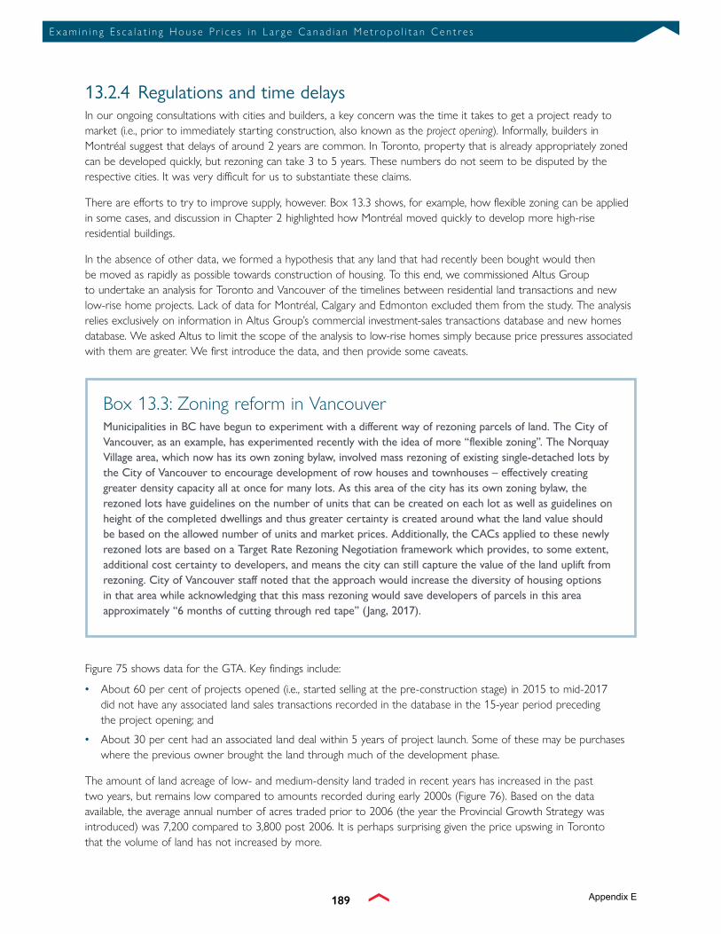
189


13.2.4 Regulations and time delaysIn our ongoing consultations with cities and builders, a key concern was the time it takes to get a project ready to market (i.e., prior to immediately starting construction, also known as the project opening). Informally, builders in Montréal suggest that delays of around 2 years are common. In Toronto, property that is already appropriately zoned can be developed quickly, but rezoning can take 3 to 5 years. These numbers do not seem to be disputed by the respective cities. It was very difficult for us to substantiate these claims.

There are efforts to try to improve supply, however. Box 13.3 shows, for example, how flexible zoning can be applied in some cases, and discussion in Chapter 2 highlighted how Montréal moved quickly to develop more high-rise residential buildings.

In the absence of other data, we formed a hypothesis that any land that had recently been bought would then be moved as rapidly as possible towards construction of housing. To this end, we commissioned Altus Group to undertake an analysis for Toronto and Vancouver of the timelines between residential land transactions and new low-rise home projects. Lack of data for Montréal, Calgary and Edmonton excluded them from the study. The analysis relies exclusively on information in Altus Group’s commercial investment-sales transactions database and new homes database. We asked Altus to limit the scope of the analysis to low-rise homes simply because price pressures associated with them are greater. We first introduce the data, and then provide some caveats.

Figure 75 shows data for the GTA. Key findings include:

• About 60 per cent of projects opened (i.e., started selling at the pre-construction stage) in 2015 to mid-2017 did not have any associated land sales transactions recorded in the database in the 15-year period preceding the project opening; and

• About 30 per cent had an associated land deal within 5 years of project launch. Some of these may be purchases where the previous owner brought the land through much of the development phase.

The amount of land acreage of low- and medium-density land traded in recent years has increased in the past two years, but remains low compared to amounts recorded during early 2000s (Figure 76). Based on the data available, the average annual number of acres traded prior to 2006 (the year the Provincial Growth Strategy was introduced) was 7,200 compared to 3,800 post 2006. It is perhaps surprising given the price upswing in Toronto that the volume of land has not increased by more.

Box 13.3: Zoning reform in VancouverMunicipalities in BC have begun to experiment with a different way of rezoning parcels of land. The City of Vancouver, as an example, has experimented recently with the idea of more “flexible zoning”. The Norquay Village area, which now has its own zoning bylaw, involved mass rezoning of existing single-detached lots by the City of Vancouver to encourage development of row houses and townhouses – effectively creating greater density capacity all at once for many lots. As this area of the city has its own zoning bylaw, the rezoned lots have guidelines on the number of units that can be created on each lot as well as guidelines on height of the completed dwellings and thus greater certainty is created around what the land value should be based on the allowed number of units and market prices. Additionally, the CACs applied to these newly rezoned lots are based on a Target Rate Rezoning Negotiation framework which provides, to some extent, additional cost certainty to developers, and means the city can still capture the value of the land uplift from rezoning. City of Vancouver staff noted that the approach would increase the diversity of housing options in that area while acknowledging that this mass rezoning would save developers of parcels in this area approximately “6 months of cutting through red tape” (Jang, 2017).

Appendix E

190


Results are broadly similar for each of the five regions in the GTA, with the exception of the City of Toronto, where relatively more land deals occurred closer to the launch date. Interestingly, within the city of Toronto the split was more even: 50 per cent projects that started selling between 2015 to mid-2017 had land transactions associated with them in the past 5-years. However, it must be kept in mind that the amount of single-family development in the City of Toronto is limited. It also points to the fact that servicing is more readily accessible in built-up areas of the City of Toronto and therefore any delays associated with servicing will be more pronounced in some 905 areas where brand new servicing and zoning is required.

Key findings for Vancouver (Figure 77 and Figure 78) include:

• About 60 per cent of all projects opened in 2015 to mid-2017 had an associated land deal within 5 years of project launch. Again, some of these may be purchases where the previous owner brought the land through much of the development phase.

• The results for Surrey, where the largest number of projects has occurred, were broadly similar to the overall market results.

Unlike in Toronto, the amount of low- and medium-density land traded in recent years in Vancouver has been steady and on an upward trend. This could signify a potential increase in land available for single-family project launches going forward.

Source: Altus Group

Ratio of number of land dels in each timeframe to number of projects launched during 2015 to mid 2017

75%

60%

45%

30%

15%

0%

60%

4% 7%

32%

No transaction in previous 15 years prior to launch

11-15 years prior to launch



Figure 75: Summary of Land Sales Points for Single-Family New Home Projects Opened in the GTA

Source: Altus Group

15,000

12,000

9,000

6,000

3,000

02000 2001 2002 2003 2004 2005 2006 2007 2008 2009 2010 2011 2012 2013 2014 2015 2016 2016

1st half2017

1st half

6,914

3,008

8,447

11,464

8,287

5,408

3,701

5,937

4,259

1,422

3,312

5,110 4,705

2,549 2,1453,499

5,154

2,3983,145

Acres Medium Density (Acres)Low Density (Acres)Total Area (Acres)

Figure 76: Low and Medium Density Residential Land Sales Transactions in the GTA

Appendix E

191


While the analysis has provided some interesting new evidence, caution needs to be used in interpreting the information and understanding its limitations. In particular, the reasons why a significant portion of new projects launched do not have land transactions within the past 15 years may be based on a variety of reasons including:

• The long lead times needed to take land through to the point of being “build ready”;

• Servicing constraints in some municipalities that may have delayed land development;

• Non-land related factors related to planning applications and approvals processes that may have affected project start; and

• Cases where very large tracts of land were purchased many years ago, with the intent that they would be gradually developed over time by the proponent to maintain business over the long term.

In addition, the analysis has only been undertaken for a relatively short period of time (projects launched in 2015 through mid-2017).

Source: Altus Group

Acres Medium Density (Acres)Low Density (Acres)Total Area (Acres)

2000 2001 2002 2003 2004 2005 2006 2007 2008 2009 2010 2011 2012 2013 2014 2015 2016 20161st half

20171st half

608 670

1,278 1,304

1,966 1,8422,229

1,275

588271

636

1,157935 880 1,026 1,092

2,124

1,118669

5,000

4,000

3,000

2,000

1,000

0

Figure 77: Low- and medium-density residential land sales transactions in Vancouver

100%

80%

120%

60%

40%

20%

0%

Source: Altus Group

Ratio of number of land dels in each timeframe to number of projects launched during 2015 to mid 2017

% of projects launched in 2015 to mid 2017 that had at least 1 associated land deal during the timeframe

No transaction in previous15 years prior to launch

11-15 yearsprior to launch



29% 29%

6% 5%

17%12%

109%

60%

Figure 78: Summary of Land Sales Points for Single-Family New Home Projects Opened in Vancouver CMA

Appendix E

192


Approval delays are only a subset of explanations for the delays as demonstrated by the Altus findings. The overall time line for the majority of recent projects spanning 15 years in the GTA may also be associated with land hoarding. Our extensive discussions with the building community have suggested otherwise. Developers have been quick to dismiss land hoarding, as there is no incentive to pass on high profits available now in favour an uncertain future. The lower time span associated with projects in Vancouver compared to the GTA could suggest that servicing delays are playing a key role in delaying projects coming on to the market. In Vancouver, most low-rise developments have taken place within built-up areas where services are already in place. Similarly, zoning is also likely to be already in place in urban cores compared to some 905 areas in the GTA where new servicing needs to be provided.

13.3 Actions in other countries to increAse suPPly

In this section we briefly review some policies adopted in other countries aimed at increasing supply. We do not advocate for any policy, but highlight some innovations that have been introduced in other countries.

Some countries have tried to move from a regulatory approach to a fee-based approach in order to: increase the degree of certainty that builders and developers face; increase transparency of the overall process that is currently difficult to understand; provide more tools for municipalities to control the timing and type of supply; and provide revenues for local governments to address infrastructure needs. Burge and Ihlanfeldt (2006) finds that development fees can increase construction rates by reducing exclusionary regulations and increasing the percentage of proposed projects receiving local government approval. In the Canadian context, such a policy change was also proposed by Slack (2002). The U.K. has attempted to move away from DBAs (called Section 106 there) and toward development fees (called the Community Infrastructure Levy) (Wales, 2015).

Development fees are intended to cover only the costs from new development. They are not intended currently to address any market failure from urban sprawl of single-detached housing. In exchange for greater planning certainty and diminished regulation, Burge et al. (2013) argues development fees could be raised substantially for construction of single-detached houses. Such a system could also provide incentives to builders to address the ‘missing middle’ by building more row houses, stacked apartments, etc.

In theory, economists argue a land tax would be a more efficient than the current property taxes, and indeed was an important source of taxation in many of the provinces in Western Canada at the onset of the twentieth century (Dixon, 1914). A property tax is levied on both the land and the structure built on it. Hence, a land-only tax removes taxation from the structure; it does not penalize land improvement. A land tax encourages the construction of higher-valued structures on the land through replacing single-detached with multi-family housing, effectively lowering the per-household tax burden. A land tax would also discourage both speculation in land and hoarding of land as the carrying costs of vacant land would be increased. Moreover, it would address distributional concerns as it would be a progressive tax on wealth.

Land taxes have been proposed as an efficient form of taxation, but are rarely applied today.66 Municipalities in Denmark levy a tax on land value of between 1.6 per cent and 3.4 per cent. A review of Australia’s tax system recommended the introduction of a graduated land tax (with no tax on agricultural land), but argued that zoning, planning and development approval policies and infrastructure charges should first be reviewed to ensure they do not unnecessarily reduce housing supply (Australia, 2010).

66 Skaburskis and Tomalty (1997) provide a history of the idea in Canada.

Appendix E

193


After determining that England has a problem of housing supply (after the Barker Reviews cited in the chapter introduction), the Joseph Rowntree Foundation commissioned a survey of supply-side policies conducted elsewhere in the world (Rowntree Foundation, 2013). Its survey covered 11 countries (excluding Canada). Box 13.4 shows a typology of supply policies used in other countries.

Some of these policies have been used in Canada, such as inclusionary zoning and growth management. The Rowntree report also notes that careful design and implementation of many of these policies are required. Importing a policy from another country would be difficult as the institutional circumstances in England would have to be thoroughly understood first, such as the growing tendency in England for developers to buy ‘options to buy’ land rather than purchasing land outright. Some of the policies come in a range of varieties: land-value capture is a goal of many municipal policies, but the most efficient policy from the economic perspective of a land tax is rarely applied.

One of the options that does not seem to have been used by Canadian governments is land assembly. With many plots having single-detached housing on them, a denser housing development would require purchasing several houses, combining the lots, changing the zoning rules, and building a new dense property structure. Land assembly is the process of combining the lots in order to be ready for development. This process is time consuming and risky, as some of the homeowners may hold out for a higher bid on their land to capture most of the land uplift.67

An option in this context is for local government to undertake the land assembly. Single-detached housing could be bought at market price and/or ‘expropriated’ in law at market price: zoning rules would then be changed, and the resulting assembled land sold to private developers at market price for building of dense structures. By paying market price and then using its legal power of expropriation at market price, municipal government would prevent the hold-up problem. By reselling the land after re-zoning, it would capture the land uplift. A problem with this approach is the need for large amounts of capital.

13.4 conclusionThis chapter has reviewed policies on supply. Unfortunately, there is little public data to understand fully what is happening. While there are concerns about the availability of land, more informative data would be on the price of land. Ultimately, increased densification will come about through efficient processes or redevelopment and rezoning. We believe, however, that there are significant delays in these.

It does not appear as if the fee structure on housing is set to encourage densification nor to be a progressive tax on wealth. Consequently, builders and developers can face incentives at the margin to construct large single-detached homes on greenfield land. Further research is required to understand fully what the impact of maintaining employment lands will be on local employment and housing prices. These challenges are not unique to Canada, and many cities around the world are grappling with the problem.

67 Brooks and Lutz (2016) find that ‘to-be-assembled land’ trades at a 15-40 per cent premium in Los Angeles, suggesting that significant frictions prevent assembly.

Appendix E

194


Box 13.4: Typology of policies to address housing supply used in select countries

1. growth management Growth management boundaries are used by most countries to prevent urban sprawl, but successful management requires planners to be pro-active in monitoring and adjusting land supply.

2. land assembly Land assembly is the process of combining several plots to form single plots so that, for example, a larger structure can be built. This can be problematic because of hold-outs. In countries such as Germany and the Netherlands, municipal governments have bought land. In the Netherlands, the municipality buys land through compulsory purchases based on current land values, provides needed infrastructure, and then sells the land back to developers to recover costs of infrastructure provision.

3. infrastructure provision Some governments ensure that infrastructure is place prior to planned development.

4. compensation and incentives Compensation could be used to offset local resistance.

5. land value capture There is a wide variety of schemes to capture land uplift. Notably in New Zealand there is a land tax. Such a tax gives an incentive to develop land to its highest value use but the uplift in the value of the land is captured by the government.

Source: Adapted from p.5, Whitehead et al. (2013)

Appendix E

195


14 Affordable Homeownership in High-Priced Markets: Policy Tools

chAPter objectives:• Examine what governments can do to address the challenges to homeownership affordability posed

by high-priced housing markets.

• Identify strategic policy tools aimed at addressing those challenges.

key finDings:• High priced markets, even if largely supply side driven, fuel higher indebtedness of borrowers who take

on larger loans relative to income to enter the market.

• Proposed Federal support for affordable ownership falls into three key areas:

• Supporting land use planning with improved data, modelling and analysis

• Improving housing development approval processes

• Remaining vigilant on housing-related risks to economic stability

14.1 introDuction: Why shoulD governments cAre About high-PriceD mArkets?

Our analysis has found that key factors on both the demand and supply side of housing have contributed to the increase in prices since 2010 in some housing markets in Canada. Demand-side factors such as population and income growth and a low interest rate environment explain much of the recent price growth in Canada’s major urban centres. For cities such as Toronto and Vancouver, however, other factors also appear to be at play. Speculation and investor demand are certainly part of the story, a natural outcome when there are perceptions of persistent land and housing shortages. Supply-side challenges including land supply and zoning regulation also emerge as factors that contribute particularly to high-priced markets.

But are elevated house prices in high-priced markets a challenge or market failure that warrants government intervention? The answer to that question varies depending on one’s interest in the housing market. Homeowners generally benefit from consistent growth in the value of their homes. This is important because for many Canadians their home is their most important asset. Housing markets, however, are not immune from price corrections driven by external economic shocks. High priced markets, whether supply or demand driven, fuel higher indebtedness both from borrowers who take on larger loans relative to income to enter the market and homeowners who take advantage of these higher prices to extract equity. Both increase vulnerabilities of higher household debt and in turn help drive even higher prices. Macroprudential policy has a role to play both in reducing demand side pressures on prices, and in ensuring that the lending that is taking place in these markets is prudent and doesn’t create broader systemic risks which could crystalize in the event of an economic shock, higher interest rates, or a rapid fall in house prices.

Appendix E

196


As discussed in previous chapters, housing markets tend to be much less flexible (or elastic in economic terms) than most other markets. When the demand for most consumer goods rises, it typically does not take long for suppliers to respond with additional production. Creating additional dwelling units to respond to unanticipated increases in housing demand typically involves production times measured in years, not weeks. Greenfield building sites need to have infrastructure in place to respond quickly to increased demand, but maintaining an emergency supply of serviced land is expensive: just-in-time land inventory lowers carrying costs for municipalities and developers. Navigation through rezoning and other approvals processes, as well as the securing and scheduling of materials and skilled labour, and actual building of the dwellings take time. Government investment in data, modelling, planning and scenario tools can provide insight into the future of markets and help citizens gain a better sense of the longer term consequences of current decisions.

Canada is not alone in experiencing these challenges. CMHC conducted a thorough review of the measures that have been implemented in Canada and in other countries to gain a better understanding of what governments can do to address the issue of rising home prices. These measures range from those that were designed to mitigate some of the demand drivers affecting house prices, to those focused on helping specific groups overcome higher costs. The results are mixed and difficult to interpret, given the challenge of measuring impacts on housing markets that are subject to a wide range of market forces. Certainly, no one simple measure emerges as an obvious candidate for addressing the challenges posed by high-priced markets, and some are more likely to do harm than good. We offer our policy options to stimulate further public discussion.

14.2 Policy objectivesCurrent federal government policy goals for the housing sector are well-aligned with objectives of other levels of government: promoting access to affordable housing options, while maintaining financial market and economic stability. Housing markets work best when there is a home available for every household, and housing prices reflect the underlying cost of land and construction.

14.2.1 Promoting Balance in Housing MarketsSound housing market policy outcomes are fundamentally dependent on ensuring that the supply of dwellings is balanced with the number of households needing shelter. Given long lead times needed to create increased housing supply, forecasting housing demand accurately is vitally important as excesses and shortfalls can generate significant price instability. Planners and developers need to anticipate what households will need (or want) and what they can afford. Some components of demand are reasonably predictable: natural population growth and age composition, and housing preferences based on historical standards. Less predictable components are economic growth, job growth, migration, and wage growth in a region, particularly three to ten years in the future, as required by housing development lead times.

14.2.2 Maintaining Financial Market and Economic StabilityWhile the goal of ensuring Canadians have access to affordable housing is extremely important, the federal government also plays a key role in managing the risk of collapse in the financial sector like the one that triggered the Great Recession in the US. Recent federal government interventions have focused on limiting credit flows to the housing sector in the interest of financial stability. The changes have made it more difficult for Canadians to over-extend themselves and qualify for loans they may not be able to service in the event of a shock. Addressing these issues reduces demand-side pressures, helps maintain more balanced housing markets, supports price moderation and reduces the risk of a long and severe recession exacerbated by high levels of consumer debt. Housing markets that are out of balance create transfers of wealth, but they don’t create better economic and social outcomes. Promoting balanced housing markets serves both access and stability objectives.

Appendix E

197


14.2.3 Related Public Policy ObjectivesHousing affordability is part of a range of policy objectives that shape development of urban environments. By shaping our population centres and hubs of economic activity and growth, regional land planning and use has great influence on productivity and prosperity, environmental impact, and the nature of our society. Municipal and regional plans must simultaneously address multiple objectives including:

• Promotion of economic growth in ways that reduce economic inequality;

• Respect for the environment through reduced greenhouse gas emissions, and preservation of sensitive areas, agriculture and recreational spaces; and

• Promotion of social inclusion and opportunity for all in society.

Arriving at an overall regional or municipal plan that address each of these policy objectives to the satisfaction of citizens and several levels of government that provide funding to support those plans is not an easy task. Without data and tools to provide sound information and support evidence-based decisions, the task becomes even more challenging.

14.3 WhAt meAsures hAve AlreADy been tAken?Government measures aimed at addressing the challenges of high-priced housing markets tend to focus on the specific drivers affecting either housing demand or supply. This report has highlighted a number of factors on the demand-side that play an important role in accounting for the rapid rise in house prices in Canada’s major centres, including macroeconomic variables such as migration trends and growing population, low interest rates, and rising disposable incomes.

14.3.1 Recent Demand-Side Initiatives in Mortgage FinanceThe Government of Canada has taken steps to address vulnerabilities associated with high household debt and market imbalances, strengthen the prudential framework for lenders, manage risks, and mitigate factors that could potentially be fuelling more speculative investments. In the last two years, these steps have included:

• Introducing more stringent debt-servicing eligibility thresholds for borrowers seeking government-backed insured mortgages. These changes reduce risk to borrowers and the financial system by making them less vulnerable to economic shocks such as a sudden increase in interest rates. But they also mean that some Canadians, particularly in high priced markets where higher debt servicing ratios are more common, may need to wait longer to enter the housing market, save more for a down payment, or settle on a smaller home (all of which puts downward pressure on house prices);

• Increasing the amount of capital that federally-regulated lenders and mortgage insurers must hold against exposures in high priced markets to make them less vulnerable to a significant correction in market prices. Depending on how institutions choose to reflect the additional costs, these changes could increase the cost of mortgages in high-priced housing markets, thereby reducing market demand;

• Tightening the rules on the capital gains exemption for the sale of a primary residence, to ensure that permanent non-residents are not eligible for the exemption on any part of a gain from the disposition of a residence; and

• Changes to residential mortgage underwriting guidelines of Office of the Superintendent of Financial Institutions to require stress testing against higher interest rates to help manage financial risks of federally regulated lenders. This change extends measures to the uninsured space that have been effective in reducing loan to income ratios in the insured mortgage space. These changes may also result in some borrowers with uninsured mortgages having to either delay purchases or consider a smaller mortgage and lower priced home. Borrowers in high priced markets with higher debt service ratios are more likely to be affected by these changes.

These changes moderate demand in ways that yield other public policy benefits, such as greater stability in housing markets, the financial sector, and the economy and improve the fairness and integrity of our tax system.

Appendix E

198


14.3.2 Government Initiatives to Increase Housing SupplyThrough the National Housing Strategy (NHS), federal and provincial/territorial governments’ commitments on affordable housing focus support on those areas of greatest need and impact. NHS consultations revealed that a majority of Canadians support a vision for housing where all Canadians have housing that meets their needs, and which they can afford. Affordable housing is a cornerstone of sustainable, inclusive communities, and an economy where all can prosper and thrive.

Our review of demand pressures in this report noted that global cities tend to attract high-skill, high-wage workers who have the means to bid up prices when housing is scarce. The appropriate policy response is clearly not to discourage the growth of good jobs, but to recognize that housing price growth makes it difficult for the less advantaged to find affordable housing. The government reinforced its commitment to housing in the NHS with a $40 billion plan under the NHS that will strengthen the middle class, fuel our economy and give more Canadians across the country a place to call home. Increases in the supply of assisted housing and other forms of affordable housing will help address issues related to income disparities and the housing challenges of the less advantaged, and relieve some demand pressure in high priced housing markets.

14.4 DeAling With housing mArket funDAmentAlsGrowth in housing prices has been driven by economic fundamentals of job and population growth generating increased housing demand from a growing, increasingly wealthy population. Supply has not kept pace. Economic growth has become more concentrated in large urban centres with a ready supply of talent and attractive, livable environments. Our analysis suggests that land supply restrictions such as land-use regulation, restrictive zoning, and geographic constraints are factors that help explain price fluctuations in high-priced markets relative to other markets. Some of the effect of land restriction may be psychological, instilling in buyer’s minds that land resources are limited even if land supply is adequate to meet expected demand for many years. Research has found that markets with inelastic land supply—whether because of geography or regulatory constraint—are more volatile and more prone to speculation.68

Supply-side measures are policies that can directly or indirectly increase the supply of homes, or respond more quickly to housing shortages as signalled by rising prices. The factors that give rise to supply constraints are complex, and the solutions may not be readily apparent. The impact of land regulation and urban plans—including such factors as rezoning restrictions, density limits, development fees and the time it takes to approve new supply—warrant closer scrutiny. Collaborative investments in standardized data collection, improved modelling and cost-benefit analysis can help citizens and decision-makers understand longer term consequences of current decisions and processes.

14.4.1 Improved Information and Support for Land Use Planning“When it comes to public policy decisions, what I believe in, for every city, is cost-benefit analysis. I believe that about high-speed rail, and I believe that about land-use planning. The ultimate question is: whatever our argument is for saying “no”, can we plausibly put down numbers that tell us that, in this neighbourhood, the benefits of preventing a development are high enough that we don’t want it to happen?”

– Edward Glaeser 69

68 Stephen Malpezzi and Susan M. Wachter, 2005. “The role of speculation in real estate cycles,” Journal of Real Estate Literature 13, 143-164, 2005.

69 Simon Jenkins, “The trials and triumphs of the city: Edward Glaeser in conversation,” The Guardian, 21 May 2015, www.theguardian.com/cities/2015/may/21/what-are-cities-doing-so-right-and-so-wrong-the-experts-go-head-to-head?CMP=share_btn_link

Appendix E

http://www.theguardian.com/cities/2015/may/21/what-are-cities-doing-so-right-and-so-wrong-the-experts-go-head-to-head?CMP=share_btn_link

199


A key observation throughout this Report has been the absence of some of the essential data, analysis and modelling needed to understand and act on housing market dynamics. These gaps complicate housing planning and contribute to housing supply inelasticity. This observation was consistently heard in the NHS consultation process as well as in other consultations and discussions CMHC organized or attended over the past 18 months. Even in the most responsive markets, housing supply takes time to bring to market. Better data on demand and supply factors, and realistic modelling of delivery on new supply would support improved warning systems of imbalances in various market segments.

Regional planners in major urban areas have to consider not just the need for dwellings, but also how the type and density of their housing supply will affect the livability and sustainability of their economic region and its sub-communities. Creating plans that generate buy-in from all key stakeholders is challenging and time-consuming. It is also necessary. The regional plans in other global cities like Auckland, New Zealand, Portland, Oregon, and the San Francisco Bay Area—each facing challenges similar to those in Toronto and Vancouver—also consider the complexity and trade-offs of fostering affordable homeownership and rental solutions along with other key social and economic objectives.

While housing needs are highly diverse in terms of both size and location, our consultations suggest that current efforts to estimate future demand often focus on basic counts of dwelling units. While young families may be able to afford to buy an average condominium, it may not have the features they need, such as enough bedrooms or being close enough to parks, schools or public transit. Investment in information would support demand projections that are well-identified in terms of size and affordability, lessen the uncertainty inherent in planning, and allow supply to respond in a timely and appropriate manner to underlying demand.

The National Housing Strategy consultations suggested that CMHC is in a unique position to develop the research and data-gathering capacity needed to fill these data gaps. For instance, CMHC recently worked with several property management companies to expand its Condominium Apartment Survey in order to bring clarity to the prevalence of foreign ownership in the Canadian housing market. This is an example of the benefits of a coordinated, multi-level approach to data gathering and analysis. It also highlights the lack of standardization in many key housing market concepts, as the survey results differed from those of previous studies on foreign ownership due to differences in the definition of foreign residents, sample size, geographic coverage and housing type. All levels of government would benefit from continuing partnerships and working housing industry stakeholders to establish common information standards for understanding housing market dynamics.

Another opportunity is this area is for the federal government to facilitate through CMHC the development of urban modelling and planning platforms that provide an economic region perspective of land use and transportation infrastructure, and support a region-wide perspective of housing market demand and supply balance (see box). Current regional and municipal data on zoning changes, development approvals, and the timing of anticipated supply are needed to run such models, and would represent a significant in-kind contribution of data that are currently either not publicly available or with varied definitions and formats or both. If the pilot confirms the value of such models, ongoing federal government funding would offer value by supporting a network of users across the country, as well as stimulate greater academic and research interest in urban decision-making in Canada simply by making better data available.

The value of these microsimulation models and the associated incentive to fuel them with up-to-date data goes well beyond dealing with issues associated with high-priced housing markets. Such models also support ex-ante and ex-post evaluation of shared government infrastructure investments in housing under the NHS, and in transportation and other municipal infrastructure proposals under programs of the Canada Infrastructure Bank.

Options available to the federal government include:

• Encouraging provinces, regions, and cities to pursue more integrated, comprehensive infrastructure planning and decision making at the economic region level; and

• Using funds announced in Budget 2017 to support collaborative investment in comprehensive data collection and urban planning tools to provide clearer insight into the costs and benefits of land use decisions, and stimulate more informed public debate.

Appendix E

200


Policy tool: Microsimulation modelsregional microsimulation models are uniquely positioned to provide key insights into the canadian housing market and support effective policy development aimed at market stability and access. in their application to urban development, microsimulation models can simulate complex relationships among fast-moving real estate markets, municipal and provincial policies, and federal investments to create policy scenarios that estimate an array of social, economic and environmental outcomes. the government of canada should consider a role in enhancing research programs and working at all levels of government to put these evidence-based tools directly into the hands of decision makers, and provide a basis for more informed public discourse on planning decisions.

municipal planning organizations across the united states (e.g. san francisco, seattle, houston), europe (e.g. Paris, Zurich) and in other parts of the world (e.g. johannesburg) have already turned to microsimulation models of both land use and traffic in order to strengthen decision making on local housing issues.

And, increasing access for canadian cities would:

1. generate new insights by linking market, municipal, provincial and federal data2. better prioritize investments in affordable housing3. leverage outputs from statistics canada’s canadian housing statistics Program4. facilitate city-level performance tracking5. strengthen participatory democracy

the government of canada (through cmhc) has committed to working with urbansim (university of california – berkeley) and the constituent governments of metro vancouver to implement a pilot microsimulation model for the vancouver region, in anticipation of support for similar models for other canadian cities. While typically custom microsimulation models are resource-intensive to build—requiring large investments in both it and subject-matter expertise across statistics, computer programming, machine learning, and big data—leveraging this open source platform would provide a fast, cost-effective solution for any canadian economic region. this platform would also allow for ongoing collaboration with the research community to continuously improve the underlying behavioural models.

further, widespread adoption of a standardized platform by municipal and provincial governments could act as incentive for all jurisdictions to actively engage in supplying the most up-to-date data. As a policy tool, accessible microsimulation models have the ability to inform and democratize policy debates and counter nimbyism with yimbyism (yes in my backyard).

Appendix E

201


14.4.2 Market Incentives to Encourage SupplyOur analysis indicates that many Canadian regions, including Vancouver and Toronto, focus on zoning and regulation as primary tools to shape development rather than economic incentives such as well-defined taxes, levies, or subsidies to shape developer and citizen behaviour. For example, rather than land use restrictions regions could impose highway use or parking levies to encourage more dense development around urban cores.

The City of Vancouver has recently moved in this direction with its dwelling vacancy tax. Where excessive speculation or land hoarding is removing the supply of land or dwellings from active markets, additional taxes on vacant lands or empty dwellings can encourage a more efficient use of the existing supply. Florida, California, Illinois and Michigan have all enacted vacant property registration ordinances that require individuals to register—and often pay additional fees on—vacant land. These measures are designed to incent owners to put vacant properties to more productive uses. Similarly, local councils in France were given discretionary power to impose a tax on under-developed land to reflect the higher per-capita infrastructure and transport costs associated with servicing low-density development, discourage urban sprawl, and increase the provision of new homes. In some areas that are zoned for higher densities, the tax is mandatory.

Effectively-applied taxes could also reduce incentives to hold land purely for capital appreciation purposes. Further, including sunset clauses on development approvals can help stream new housing onto markets more quickly and help to deal with developer incentives to avoid bringing new supply online in competition with one another.


• Work with provinces and regions to pursue policies based on market incentives to shape development, rather than a system of zoning restrictions and regulations and lengthy negotiations to overcome them.

14.4.3 Direct Government Support of Housing Supply and AccessThe NHS provides opportunities for the federal government to assist in making non-government lands ready for housing development. While both Ontario and British Columbia already recognize the benefits of utilizing surplus industrial land (see text box on Vancouver’s Portico development for an example), the federal government could contribute further to the remediation of brownfield sites in these high-priced markets by, for example, playing a role in the assessment phase to increase the land supply that could be used for residential development. Such support would, of course, recognize that all necessary precautions must be taken to ensure that any contamination is safely remediated.

Beyond the existing support for homeowners, the Government of Canada is exploring ways to facilitate access to mortgage loan insurance for borrowers who are more challenging to qualify, such as self-employed individuals. Today’s job market requires many Canadians to adopt alternative means of generating income, including by running their own businesses. Approximately 15% of Canadians are self-employed and may have difficulty accessing financing to buy a home, since their income sources may vary or be less predictable than those of salaried borrowers. To address this issue, the federal government is examining if there are barriers to housing finance for self-employed borrowers and options to expand access to mortgage loan insurance.


• Increasing supply of affordable housing and extending existing programs to more Canadians as described in the National Housing Strategy to offer families more choice in housing and reduce market pressures on timing home purchase decisions.

Appendix E

202


14.5 imProving mArket resPonseAs cities grow and consume available land supply, market pressures and incentives develop to repurpose already developed land to higher valued uses. Converting land from one use to another almost always inspires heated debate as some interests line up with existing use and other see greater value in the proposed use. As with broader land use planning, individual project proposals also need to be judged on a cost-benefit basis, including impacts of the project not proceeding, and finding ways to compensate in some form those whose welfare would be significantly compromised when a new development goes forward.

Resistance to rezoning areas in the urban core that are currently zoned for detached, single-family homes makes it difficult to achieve required densities in areas near urban cores and transportation hubs. Other inefficiencies, including excessive design specifications and intra-regional variations in codes and requirements, also appear to slow development approvals. Further investigation is required to provide an exact diagnosis of the issues, but it is clear that municipalities in affected regions need to harmonize their regulations, adjust zoning for denser development and streamline their processes, particularly for affordable development, to support more responsive supply.

Portico – Vancouver, British Columbiathe Portico development transformed an underused brownfield (the former Pacific Press site) into a higher density, mixed-use, infill development that is pedestrian- and transit-friendly. located in the fairview district of vancouver, at the base of the granville street bridge, Portico is a gateway to the city core. the fairview district consists of mostly low-and high-rise condominium and rental apartment buildings and a large number of commercial and industrial buildings. At 118 dwelling units per hectare, Portico’s residential density is more than double that of the entire fairview community, at 52.2 dwelling units per hectare. moreover, the city of vancouver (like the city of toronto) does not have a significant supply of greenfield land, so growth is largely accommodated through redevelopment and infill. housing opportunities have been created by rezoning some areas that were traditionally industrial and commercial to allow for residential development. With regard to this community’s connection to transit, city council approved significant road network modifications to re-establish the former street grid, linking it back to the surrounding community. the changes also provided opportunities for new public open space amenities.

Appendix E

203


Optimal uses of land change as cities grow, yet current processes seem to restrict supply by giving undue control to narrow interests. Options available to the federal government include:

• Working with provinces and regions on developing forward-looking, housing data and market modelling to better anticipate housing market imbalances in both rental and ownership markets based on projected demand and expected or modeled housing supply;

• Examining financial incentives that would reward cities and economic regions that encourage denser, mixed-use urban development;

• Developing modelling tools to counter NIMBYism and support more informed debate on how specific development proposals may affect neighbourhood character, real estate pricing, and other urban goals.

14.6 Preserving economic stAbilityChallenges in coping with basic underlying economic growth in our cities have led to consequences and risks that also need to be managed. Rising prices, low interest rates, and slow supply responsiveness accelerate demand and generate incentives to extend excessive levels of credit, and opportunities to speculate on land and housing with relatively low carrying costs. These contribute to land and housing cost escalation that impedes long term economic growth and citizen welfare. Rising prices attract speculative investment, domestic and foreign, though the foreign component has been challenging to measure in Canadian markets.

Price increases have also made housing much more capital intensive, and lead to questions of whether there are opportunities to adapt conventional notions of homeownership and mortgage arrangements to emerging market realities. We owe it to Canadians to ensure that innovative and viable mortgage products come to market to provide greater homebuyer choices on the amount of risk they take on, including opportunities to share that risk with lenders or other institutions at mutually acceptable prices.

14.6.1 Macroprudential VigilenceAs noted above, the federal government has taken actions affecting mortgage credit to promote longer term economic stability. Ongoing monitoring of housing markets and debt levels, and taking additional action if necessary, remains a key role for the government.


• Continue to monitor vulnerabilities and intervene if necessary to maintain financial system and economic stability via mortgage insurance “sandbox” rules and other measures.

14.6.2 Innovation in Mortgage OptionsMuch recent academic literature has focused on improving mortgage contracts to incent parties to act in ways that promote better private and social outcomes. Some of this literature is directed toward the fact that housing costs represent a large fraction of disposable incomes, and disruptions in housing or housing finance markets can trigger significant swings in consumer spending on other goods. Structuring mortgage contracts to adapt payments to changing market conditions is one way to spread the risk from borrowers to lenders and investors. While innovation in this area is in the early stages, the overall objective is to reduce the volatility of housing and housing finance markets, and introduce macroprudential characteristics and market-stabilizing measures into mortgage contracts.

Appendix E

204


Current policy does permit innovation in this area through CMHC’s Flexibilities for Affordable Housing Programs.70 These programs allow for creative solutions in alternative forms of down payment and supporting rent-to-own options where the sponsor supports prospective homebuyers while they save for a down payment or enhance their credit ratings and capacity to borrow.

The challenge in mortgage innovation is in developing products that all sides of the transaction find attractive given expectations on future home prices. Relatively few episodes of significant and long-term price declines in Canada likely have most homebuyers willing to take on downside risks and unwilling to pay for others to absorb those risks. More research is required, but CMHC is committed to further investigating the potential of adjusting mortgage contracts to improve economic stability and increase long-term economic growth.

14.6.3 Purchase Support ProgramsA number of jurisdictions provide various forms of assistance to help individuals and families purchase their first home. This is especially tempting in markets that have experienced high price growth, or where housing affordability has become a challenge. But programs such as the down payment assistance plan recently implemented by the B.C. government, which are designed to facilitate or subsidize demand, are not recommended unless backed by an aligned increase in dwelling supply. Without measures to increase the responsiveness of housing supply, most of the assistance afforded by these programs will end up in the hands of sellers and real estate agents through higher prices, adding to house price inflation pressures. Further, at the federal level, costs of such programs would likely involve transfers from residents of low cost to high cost housing areas that are difficult to justify, and would exacerbate tendencies to concentrate wealth and opportunity in a few regions. Under current conditions, current resources devoted to demand support programs would be better used to resolve supply issues, such as finding ways to address lengthy approval processes.


• Providing no additional support programs for homeownership in high priced, supply-constrained markets (notably including first time homebuyers) and discourage provinces / territories from doing the same.

14.6.4 SpeculationDemand for housing is partly influenced by its value as a vehicle for capital appreciation. Sustained increases in house prices generate expectations for further gains, causing house prices to be increasingly driven by their perceived value as financial assets rather than their “use value” as residential accommodation. While investment that supports an additional supply of rental accommodation is helpful, speculation that effectively removes dwellings from supply, particularly in low vacancy markets, can create further imbalance in housing markets. Investment in rental units by small investors does not remove dwellings from supply, and offers additional rental stock for those without the inclination or financial means to own their homes.

Drawing on the experiences of international jurisdictions, the federal government could further analyze the suitability of taxing transactions to discourage speculative demand. For example, Hong Kong charges a special stamp duty on residential properties that are resold within 24 to 36 months. Such measures could complement the recent change that requires the declaration of a principal residence to claim the capital gain exemption on the sale of a primary home.

Our analysis has found that investor demand and speculative activity (both domestic and foreign), as measured by currently available data, have had a limited measured impact on prices. This not to say that speculation is of no concern. While investors look for opportunities for returns where demand is growing and supply is fixed or slow to respond, increased speculation is more likely to amplify the impact of persistent market imbalances rather than

70 Details are available at: https://www.cmhc-schl.gc.ca/en/inpr/afhoce/upload/65950_EN_W_ACC.pdf

Appendix E

https://www.cmhc-schl.gc.ca/en/inpr/afhoce/upload/65950_EN_W_ACC.pdf

205


serve as a key cause. Although policy measures aimed at purely speculative demand that doesn’t serve to increase supply could mitigate those effects, current evidence suggests they are not likely to have a substantial impact on affordability in high-priced markets like Toronto and Vancouver.

Restricted supply in the face of rising demand creates opportunities for speculation in housing markets in forms that can reduce the availability of housing for participants in the local economy by buyers who leave dwellings vacant, rarely occupied, competing with local hotels for short-term visitors, or delay approved development in expectation of higher future prices. This reduction or delay in dwelling supply is not typically anticipated in regional or municipal development plans. Measures restricting these activities are implemented by provincial or municipal governments.

Federal government support in this area should focus on continued efforts for better data on the beneficial ownership of land and incenting land use that recognizes the importance of land in housing and economic development.


• Working with provinces and municipalities to evaluate approval “sunset” clauses to prevent private land-banking.

14.6.5 Measures Targeting Foreign OwnershipCanada is an open economy that welcomes foreign investment to spur economic growth and create jobs. Media stories have created a sense that non-resident purchases of real estate have played a significant role in price appreciation, particularly in Vancouver, and recent data indicates that foreign buying accounts for roughly one in ten home purchases in some municipalities or districts. Comprehensive data to consistently measure this source of demand and supply has only recently begun to be collected. This improvement in data collection is welcome for a variety of reasons, including better understanding of the size and trends in non-resident purchases of Canadian real estate.

Foreign investment in residential real estate can introduce instability into local housing markets, especially if the investments are concentrated in relatively limited areas and are purely speculative in the sense of sequestering supply from the market. Foreign investment can be subject to disruptively rapid increases or withdrawals based on factors outside the housing market such as changes in exchange rates and political or regulatory changes in the country of origin. Both registration and taxation of non-resident purchases create an opportunity to monitor foreign investment trends, and give regional planners more insight into whether non-resident activity is a significant supply or demand factor in local real estate markets. The beneficial ownership of land is often obscured by use of numbered companies, and concentration of land ownership has been difficult to monitor. Real estate lending by Canadian financial institutions supported by foreign incomes and wealth is not well understood.

Improved monitoring and awareness does not necessarily mean greater restriction or regulation. If foreign developers invest in housing projects that support more affordable housing in Canada, should we treat such investment differently than Canadian firms with similar projects? In a market with significant shortages of affordable dwellings, restrictions on foreign investment seem counterproductive as long as dwellings are occupied.

Australia and New Zealand have chosen to require foreigners who wish to purchase residential property to apply for a purchase permit and limit purchases to new supply, to leverage foreign investment to encourage new construction. New Zealand also requires non-residents to register real estate purchases, but it doesn’t currently restrict purchases. These registration mechanisms can help improve data on foreign real estate investment activity and inform local planning scenarios, while also creating mechanisms to implement restrictions if the activity proves to be excessively disruptive.


• Continue to work with provinces and Statistics Canada to improve data and monitoring of real estate transactions, land ownership, and foreign capital flows.

Appendix E

206


14.7 conclusion AnD Policy summAryHelping Canadians meet their housing needs is an important responsibility that can benefit from public discussion and collaboration across all levels of government. Housing is clearly interconnected with other government priorities such as economic growth and macroeconomic stability. Federal collaboration with all partners is therefore needed to develop and coordinate a cohesive policy framework. There is a strong temptation in some housing markets to provide greater assistance to those on the margins of homeownership. However, policies that encourage such demand risk adding to house price pressures, generating extra profits to suppliers without triggering supply, and exposing vulnerable people to excessive financial risk. Strategic policy tools that are aimed at addressing elevated house prices should therefore focus instead on ways to improve the responsiveness of supply.

The Government of Canada has few policy levers at its disposal to directly target supply challenges, particularly on a region-by-region basis. Consultations for the National Housing Strategy suggest that increasing the supply of rental housing could ease some of the pressure to own posed by low vacancy rates and high rental costs. But there is also an opportunity for the federal government to work with provincial and municipal partners to better understand the challenges that give rise to an unresponsive supply and drive price appreciation. This approach would enable governments at all levels to develop an effective and cohesive policy framework to better understand and support solutions to affordability challenges. There is also a potential to leverage investments in mass transit and other infrastructure to help alleviate supply challenges.

The federal government, through CMHC, can play a key facilitating role by stimulating discussion and addressing important data and analytical gaps to improve the capacity of cities to better anticipate—and respond to—strong demand. This could include developing more granular analyses of the growth and nature of housing demand and supply, model housing market scenarios, and develop knowledge base of best practices for addressing housing market supply challenges.

In addition to addressing gaps in information, analysis and knowledge, there is also an opportunity for governments, industry, and housing advocates to work together to better understand how policies around zoning, densification (including overcoming resistance), land development, transportation, infrastructure, environment and other housing-related activities can help achieve outcomes that more effectively meet the evolving demand for living space in globally-attractive cities like Vancouver and Toronto.

The policy options for the federal government summarized below are intended to stimulate broad policy discussion across all levels of government, housing advocates, industry, academia, and the general public:

land use Planning: Urban land is a scarce resource that must be efficiently and responsibly managed, recognizing significant externalities associated with land use decisions. Options available to the federal government include:

• Encouraging provinces, regions, and cities to pursue more integrated, comprehensive infrastructure planning and decisions at the regional level;

• Using funds announced in Budget 2017 to support investment in comprehensive data collection and planning tools to provide clearer insight into the costs and benefits of land use decisions, and stimulate more informed public debate; and

• Examining financial incentives to reward cities and economic regions that promote denser, mixed-use urban development.

Appendix E

207


housing Development and Approval Processes: Optimal uses of land change as cities grow, yet current processes seem to restrict supply by giving undue control to narrow interests. Options available to the federal government include:

• Working with provinces and regions on developing forward-looking housing data and market modelling to better anticipate short to medium term housing market imbalances in both rental and ownership markets based on projected demand and expected or modelled housing supply;

• Increasing supply of affordable rental housing as described in the National Housing Strategy to offer households more choice in housing and reduce market pressures to rush purchase decisions; and

• Working with provinces and regions to increase supply and further identify and address bottlenecks in development approval processes, including:

• Pursuing policies based on market incentives to shape development, rather than on a system of zoning restrictions and regulations and lengthy negotiations to overcome them;

• Evaluating approval “sunset” clauses to prevent private land-banking; and

• Developing modelling tools to counter NIMBYism and support more informed debate on how specific development proposals may affect neighbourhood character, real estate pricing, and other urban goals.

speculation and the role of credit: Rising prices, historically low interest rates, and slow supply response generate incentives to extend excessive levels of credit and opportunities to speculate on land and housing. Options available to the federal government include:

• Continuing to monitor vulnerabilities and intervening if necessary to maintain financial system and economic stability via mortgage insurance “sandbox” and other measures;

• Providing no additional support programs for homeownership in high priced, supply-constrained markets (notably including first time homebuyers) and discourage provinces / territories from doing the same; and

• Using funds announced in Budget 2017 to work with provinces and Statistics Canada to improve data and monitoring of real estate transactions, land ownership, and foreign capital flows. The beneficial ownership of land is often obscured by use of numbered companies, and concentration of land ownership has been difficult to monitor. Real estate lending by Canadian financial institutions supported by foreign incomes and wealth is not well understood.

Appendix E

208


15 Conclusions and Next StepsThis report has outlined several reasons for escalating home prices in high-priced housing markets. Traditional fundamental factors—such as economic growth, low mortgage rates and population flows—play important roles in accounting for higher home prices. CMHC has been monitoring these fundamental drivers of house price growth through our Housing Market Assessment (HMA) to ensure that Canadians are not subjected to undue vulnerability from the housing sector, a vulnerability heightened by what happened in several other countries during the last recession.

This report is a further step in developing new tools to enhance our capacity to monitor and understand the Canadian housing market. Since new vulnerabilities can arise, we need to be constantly on our toes to watch out for new warning signs that may lead to housing and financial market imbalances.

Our analysis has reinforced our interest in understanding how credit growth can encourage growth in house prices. But it also highlighted to us that we need a deeper understanding of how changes in the global economy—whether they are changing demand for resources, or promoting financial services and high-technology industries—are affecting growth in our cities.

We also found that changes on the supply side of housing play a role in explaining changing price patterns. Our cities are evolving toward denser housing, increases in the price of land, concerns about the environment, and changing living patterns with households wanting to be close to leisure and entertainment amenities in city centres as well as to their workplaces. Our work highlights our need to develop a keener understanding of supply dynamics in cities. In this report, we used what metrics were available to us to understand the supply side of the market, but we understand that more could be done.

Consequently, CMHC will continue to take steps to improve the use and availability of data. This effort will not only serve to help us improve our analyses, but will hopefully also foster deeper interest by academics and researchers to understand the dynamics of the housing market and their inter-linkages with the wider economy. We have, for instance, been hampered by the absence of historical and detailed price data, and we will take steps to publish work we do to develop these time-series data. Creating historical data sets would also attract research students to work on housing-related research. In addition, CMHC has started to publish annual estimates of conversions and demolitions, but we will also estimate annual historical data on the stock of housing.

We heard during our engagement with key stakeholders of challenges in understanding many aspects of modern cities. Improved research will both need and enable more data, make the housing market more transparent, and lessen concerns regarding risks coming from this market. Our work has highlighted the importance of land prices to understanding market dynamics in large cities, but there is not a scientifically sound index of land prices available currently. Developing such indices is not just a matter of gathering data, it also requires ensuring that they are based on sound statistical principles. Several projects have been directly animated by the work done for this report. But we cannot rely on CMHC work alone.

We benefited directly from comments provided on our report by academics, but we also need to foster independent academic and external research. Data provision will help, but we will also directly encourage more research and collaboration with academics. We will establish a working paper series to publish more advanced internal research undertaken by CMHC to make it available and open to scrutiny by academics. We also need to see how we can set the groundwork with academics for the exciting technologies that could further extend our understanding of the housing market, such as the prospect of using visual data to understand how our communities work.

During this work, we have strengthened already strong partnerships at the federal level with the Bank of Canada, the Department of Finance and Statistics Canada. Since housing has attained such a prominent part of the Canadian financial system, we will build on these relationships with other levels of government.

Appendix E

209


AcknoWleDgmentsWe would like to thank many academics, market participants and government officials for their time in providing advice for this document. We also presented some research results at CMHC seminars in Toronto, Montréal and Vancouver, and at the Canadian Economics Association meetings in Antigonish, Nova Scotia held in June of 2017.

In particular, we would like to thank the following academics who provided detailed comments. We benefitted from their comments, recognizing that many disagreed with some aspects of the report. Although we will endeavour to address many additional comments they raised, we continue to struggle with inadequate data.

Thanks to:

Professor David Amborski, Ryerson University, Toronto, Ontario.

Professor Kristian Behrens, Université du Québec à Montréal, Montréal, Québec.

Dr. Frank A. Clayton, Ryerson University, Toronto, Ontario.

Associate Professor Thomas Davidoff, University of British Columbia, Vancouver, British Columbia.

Professor François Des Rosiers, Université Laval, Laval, Québec.

Assistant Professor Josh Gordon, Simon Fraser University, Vancouver, British Columbia.

Associate Professor Joshua Gottlieb, University of British Columbia, Vancouver, British Columbia.

Professor David Green, University of British Columbia, Vancouver, British Columbia.

Professor Allen Head, Queen’s University, Kingston, Ontario.

Professor J. Rhys Kesselman, Simon Fraser University, Vancouver, British Columbia.

Associate Professor Nathanael Lauster, University of British Columbia, Vancouver, British Columbia.

Professor David Ley, University of British Columbia, Vancouver, British Columbia.

Professor Huw Lloyd-Ellis, Queen’s University, Kingston, Ontario.

Associate Professor Jim MacGee, Western University, Ontario.

Professor Duncan Maclennan, University of St. Andrews, St. Andrews, Scotland.

Professor James McKellar, York University, Toronto, Ontario.

Professor Leo Michelis, Ryerson University, Toronto, Ontario.

Associate Professor Tsur Somerville, University of British Columbia, Vancouver, British Columbia.

Appendix E

210


referencesAled ab Iorwerth, 2016, “Financial Services Intermediation, and its Role in Economic Growth and Stability”, mimeo, Department of Finance Canada.

Chadi S. Abdallah and William D. Lastrapes, 2013, “Evidence on the Relationship Between Housing and Consumption in the United States: A State-Level Analysis”, Journal of Money, Credit and Banking Vol. 45, Iss. 4, June, pp. 559-590.

Manuel Adelino, Antoinette Schoar and Felipe Severino, 2016, “Loan Originations and Defaults in the Mortgage Crisis: the Role of the Middle Class”, Review of Financial Studies Vol. 29, Iss. 7, July, pp. 1635-1670.

Gabriel M. Ahlfeldt, Stephen J. Redding, Daniel M. Sturm, Nikolaus Wolf, 2015, “The Economics of Density: Evidence from the Berlin Wall”, Econometrica, Vol. 83, Iss. 6, November, pp. 2127-2189.

Rüdiger Ahrend, Alexander C. Lembcke, and Abel Schumann, 2017, “The Role of Urban Agglomerations in Economic and Productivity Growth”, International Productivity Monitor, No. 32, Spring, pp. 160-178.

David Albouy, Fernando Leibovici and Casey Warman, 2013, “Quality of Life, Firm Productivity, and the Value of Amenities Across Canadian Cities”, Canadian Journal of Economics, Vol. 46, No. 2, May, pp.379-411.

David Amborski, 2016, “Affordable Housing and Land Supply Issues in the Greater Toronto Area (GTA)”, Policy report Centre for Urban Research & Land Development, November 4.

Scott Andes, Mitch Horowitz, Ryan Helwig and Bruce Katz, 2017, “Capturing the Next Economy: Pittsburh’s Rise as a Global Innovation City”, Anne T. and Robert M. Bass Initiative on Innovation and Placemaking.

Robert A.Androkovich, 2013, “British Columbia’s agricultural land reserve: Economic, legal and political issues” Land Use Policy, Vol. 30, No. 1, 365-372.

Angus Reid, 2015, “Lotusland Blues: One-in-five Metro Vancouverites Experience Extreme Housing & Traffic Pain; Most Of Them Think Of Leaving”, Angus Reid Institute of Public Interest Research, posted June 18, 2015, http://angusreid.org/vancouver-real-estate/.

Alex Anas, 2013. “The Location Effects of Alternative Road-Pricing Policies”, Chapter 6 in Infrastructure and Land Policies, eds. Ingram, Gregory K. and Karin L. Brandt. Cambridge, MA: Lincoln Institute of Land Policy.

Alex Anas, Richard Arnott and Kenneth A. Small, 1998, “Urban Spatial Structure”, Journal of Economic Literature, Vol. 36, No. 3, September, pp. 1426-1464.

Dan Andrews, Aida Caldera Sánchez and Åsa Johansson, 2011, “Housing Markets and Structural Policies in OECD Countries”, OECD Economics Department Working Paper No. 836.

Richard J. Arnott and Joseph E. Stiglitz, 1979, “Aggregate Land Rents, Expenditure on Public Goods, and Optimal City Size”, Quarterly Journal of Economics, Vol. 93, No. 4, November, pp. 471-500.

Australia, 2010, Australia’s Future Tax System. Available at: http://taxreview.treasury.gov.au/content/FinalReport.aspx?doc=html/Publications/Papers/Final_Report_Part_1/index.htm

Uri Avin, Timothy F. Welch, Gerrit Knaap, Fred Ducca, Sabyasachee Mishra, Yuchen Cui, and Sevgi Erd, 2017, Even Smarter Growth? Land Use Policy Impact On Transportation And Emissions In Maryland, undated. Available at: http://smartgrowth.umd.edu/assets/documents/research/even_smarter_growth_dc_paris_symp.pdf

Avner Bar-Ilan and William C. Strange, 1996, “Investment Lags”, American Economic Review, Vol. 86, No. 3, June, pp. 610-622.

Barker Review, 2004, Review of Housing Supply: Delivering Stability: Securing our Future Housing Need London: HM Treasury

Appendix E

http://angusreid.org/vancouver-real-estate/

http://taxreview.treasury.gov.au/content/FinalReport.aspx?doc=html/Publications/Papers/Final_Report_Part_1/index.htm

http://smartgrowth.umd.edu/assets/documents/research/even_smarter_growth_dc_paris_symp.pdf

211


Barker Review, 2006, Barker Review of Land Use Planning, London: HM Treasury.

Jason M. Barr, 2016, Building the Skyline: The Birth and Growth of Manhattan’s Skyscrapers New York, NY: Oxford University Press.

Timothy J. Bartik, (1991), Who Benefits from State and Local Economic Development Policies? Kalamazoo, MI: W.E. Upjohn Institute for Employment Research.

Nathaniel Baum-Snow, 2007, “Did Highways Cause Suburbanization?”, Quarterly Journal of Economics, Vol. 122, No. 2, May, pp. 775-805.

________________, 2017, “Urban Transport Expansions, Employment Decentralization, and Spatial Scope of Agglomeration Economies”, mimeo, University of Toronto.

Nathaniel Baum-Snow and Daniel Hartley, 2017, “Accounting for Central Neighbourhood Change, 1980-2010”, mimeo, University of Toronto.

Nathaniel Baum-Snow and Ronni Pavan, 2013, “Inequality and City Size”, Review of Economics and Statistics, Vol 95, Iss. 5, December, pp. 1535-1548.

Mia Baumeister, 2012, “Development Charges Across Canada: An Underutilized Growth Management Tool?”, Institute of Municipal Finance and Governance papers no. 9. Available at: http://www.munkschool.utoronto.ca/imfg/uploads/201/imfg_no.9_online_june25.pdf

BC (British Columbia), 2014, “Community Amenity Contributions: Balancing Community Planning, Public Benefits and Housing Affordability”, Victoria, BC: Ministry of Community, Sport and Cultural Development. Available at: http://www.cscd.gov.bc.ca/lgd/intergov_relations/library/CAC_Guide_Full.pdf

Charles M. Beach, 2016, “Changing Income Inequality: A Distributional Paradigm for Canada”, Canadian Journal of Economics, Vol. 49, Iss. 4, November, pp. 1229-1292.

Thorsten Beck, Berrak Büyükkarabacak, Felix K. Rioja and Neven T. Valev, 2012, “Who Gets the Credit? And Does It Matter? Household vs. Firm Lending Across Countries”, B.E. Journal of Macroeconomics, Vol. 12, Iss. 1 (Contributions), Article 2.

Desmond Beckstead, W. Mark Brown, Yusu Guo, and K. Bruce Newbold, 2010, “Cities and Growth: Earnings Levels Across Urban and Rural Areas: The Role of Human Capital”, Statistics Canada: The Canadian Economy in Transition Series.

Kristian Behrens, Gilles Duranton and Frédéric Robert-Nicoud, 2014, “Productive Cities: Sorting, Selection and Agglomeration”, Journal of Political Economy, Vol. 122, No. 3, pp. 507-553.

Kristian Behrens and Théophile Bougna, 2015, “An anatomy of the geographical concentration of Canadian manufacturing industries”, Regional Science and Urban Economics, Vol. 51, March, pp. 47-69

Kristian Behrens and Frédéric Robert-Nicoud, 2014a, “Survival of the Fittest in Cities: Urbanisation and Inequality”, Economic Journal, Vol. 124, Iss.581, December, pp. 1371-1400.

_________________, 2014b, “Urbanization Makes the World More Unequal”, Voxeu.org, Available at: http://voxeu.org/article/inequality-big-cities

Antonio M. Bento, Maureen L. Cropper, Ahmed Mushfiq Mobarak and Katja Vinha, 2005, “The Effects of Urban Spatial Structure on Travel Demand in the United states”, Review of Economics and Statistics, Vol. 87, No. 3, August, pp. 466-478.

Antonio M. Bento and Sofia F. Franco, 2006, “The Efficiency and Distributional Impacts of Alternative Anti-Sprawl Policies”, Journal of Urban Economics, Vol. 59, No. 1, pp. 121-141.

Appendix E

http://www.munkschool.utoronto.ca/imfg/uploads/201/imfg_no.9_online_june25.pdf

http://www.cscd.gov.bc.ca/lgd/intergov_relations/library/CAC_Guide_Full.pdf

http://voxeu.org/article/inequality-big-cities

212


Antonio Bento, Daniel Kaffine, Kevin Roth and Matthew Zaragoza-Watkins, 2014, “The Effects of Regulation in the Presence of Multiple Unpriced Externalities: Evidence from the Transportation Sector”, American Economic Journal: Economic Policy, Vol. 6, No. 3, August, pp. 1-29.

Ben S. Bernanke, 2005, “Global Savings Glut and the U.S. Current Account Deficit”, speech in Richmond, Virginia. Available at: https://www.federalreserve.gov/boardDocs/Speeches/2005/200503102/

Alain Bertaud, 2004, “The Spatial organization of Cities: Deliberate Outcome or Unforeseen Consequence?” Available at: http://alain-bertaud.com/images/AB_The_spatial_organization_of_cities_Version_3.pdf

Alain Bertaud and Stephen Malpezzi, 2001, “Measuring the Costs and benefits of urban Land Use Regulation: A Simple Model with an Application to Malaysia”, Journal of Housing Economics, Vol. 10, pp. 393-418.

Alain Bertaud and Stephen Malpezzi, 2003, “The Spatial Distribution of Population in 48 World Cities: Implications for Economies in Transition”, mimeo. Available at: http://alain-bertaud.com/AB_Files/Spatia_%20Distribution_of_Pop_%2050_%20Cities.pdf

Javier Bianchi and Enrique G. Mendoza, 2017, “Optimal Time-Consistent Macroprudential Policy”, Journal of Political Economy, forthcoming.

Duncan Black and Vernon Henderson, 1999, “A Theory of Urban Growth”, Journal of Political Economy, Vol. 107, No. 2, pp. 252-284.

Pamela Blais, 2010, Perverse Cities: Hidden Subsidies, Wonky Policy and Urban Sprawl Vancouver, Toronto: UBC Press.

________________, 2017, “The Tor-York West Megazone: A Profile”, Toronto: Neptis Foundation. Available at: http://www.neptis.org/publications/tor-york-west-megazone-profile

David G. Blanchflower and Andrew J. Oswald, 2013, “The Danger of High Homeownership: Greater Unemployment”, The CAGE-Chatham House Series, No. 10, October.

Peter Boelhouwer and Joris Hoekstra, 2009, “Towards a Better Balance on the Dutch Housing Market? Analysis and Policy Propositions”, International Journal of Housing Policy, Vol. 9, No. 4, pp. 457-475.

Kenyon Bolton and Sébastien Breau, 2011, “Growing Unequal? Changes in the Distribution of Earnings Across Canadian Cities”, Urban Studies, Vol. 49, Iss. 6, May, pp. 1377-1396.

Jeffrey Brinkman,2014, “The Supply and Demand of Skilled Workers in Cities and the Role of Industry Composition”, Federal Reserve Bank of Philadelphia Working Paper, No. 14-32.

Sébastien Breau, Dieter F. Kogler and Kenyon C. Bolton, 2014, “On the Relationship Between Innovation and Wage Inequality: New Evidence from Canadian Cities”, Economic Geography, Vol. 90, No. 4, pp. 351-373.

Leah Brooks and Byron Lutz, 2016, “From Today’s City to Tomorrow’s City: An Empirical Investigation of Urban Land Assembly”, American Economic Journal: Economic Policy, Vol. 8, No. 3, August, pp. 69-105.

Rayna Brown, Rob Brown, Ian O’Connor, Gregory Schwann, 2011, “The Other Side of Housing Affordability: The User-Cost of Housing in Australia”, Economic Record Vol. 87, Iss. 279, pp. 558-574.

W. Mark Brown and K. Bruce Newbold, 2012, “Cities and Growth: Moving to Toronto – Income Gains Associated with Large metropolitan Labour Markets”, Statistics Canada: The Canadian Economy in Transition Series.

W. Mark Brown and Darren M. Scott, 2012, “Cities and Growth: Human Capital Location Choice: Accounting for Amenities and Thick labour Markets”, Statistics Canada: The Canadian Economy in Transition Series.

Appendix E

https://www.federalreserve.gov/boardDocs/Speeches/2005/200503102/

http://alain-bertaud.com/images/AB_The_spatial_organization_of_cities_Version_3.pdf

http://alain-bertaud.com/AB_Files/Spatia_%20Distribution_of_Pop_%2050_%20Cities.pdf

http://www.neptis.org/publications/tor-york-west-megazone-profile

213


Jan K. Brueckner, 2000, “Urban Sprawl: Diagnosis and Remedies”, International Regional Science Review, Vol. 32, No., 2, April, pp. 160-171.

Jan K. Brueckner, 2007, “Urban Growth Boundaries: An Effective Second-best Remedy for Unpriced Traffic Congestion”, Journal of Housing Economics Vol. 16, Iss. 3-4, November, pp. 263-273.

Willem H. Buiter, 2010. “Housing wealth isn’t wealth,” Economics - The Open-Access, Open-Assessment E-Journal, Vol. 4, No. 22, pp. 1-29.

T. Bunting, P Filion and H. Priston, 2002, “Density Gradients in Canadian Metropolitan Regions, 1971-1996: Differential Patterns of Central Area and Suburban Growth and Change”, Urban Studies, Vol. 39, No. 13, pp. 2531-2552.

Marcy Burchfield and Anna Kramer, 2015, Growing Pains: Understanding the new Reality of Population and Dwelling Patterns In The Toronto and Vancouver Regions Toronto: Neptis Foundation.

Gregory Burge and Keith Ihlanfeldt, 2006, “Impact Fees and Single-Family Home Construction”, Journal of Urban Economics, Vol. 60, pp. 284-306.

___________________, 2013, “Promoting Sustainable Land development Patterns through Impact Fee Programs”, Cityscape, Vol. 15, No. 1, pp. 83-105.

Gregory S. Burge, Trey L. Trosper, Arthur C. Nelson, Julian C. Juergensmeyer, and James C. Nicholas, 2013, “Can Development Impact Fees Help Mitigate Urban Sprawl?”, Journal of the American Planning Association, Vol. 79, No. 3, pp. Summer, 235-248.

Craig Burnside, Martin Eichenbaum and Sergio Rebelo, 2016, “Understanding Booms and Busts in housing Markets”, Journal of Political Economy, Vol. 124, No. 4, pp. 1088-1147.

Business Vancouver, 2016, “The EXPO Effect: How Expo 86 Changed Vancouver”. Available at: https://www.biv.com/article/2016/4/expo-effect-how-expo-86-changed-vancouver/

Caldera S. A. and Johansson A., 2013, “The price responsiveness of housing supply in OECD countries”, Journal of Housing Economics, Vol. 22(3), pp213-249.

Charles W. Calomiris, Stanley D. Longhofer and William Miles, 2013, “The Housing Wealth Effect: The Crucial Roles of Demographics, Wealth Distribution and Wealth Shares,” Critical Finance Review, Vol. 2, No. 1, July , pp. 49-99.

CANCEA (Canadian Centre for Economic Anaylsis), 2017, “Exploring Places to Grow Divergence Risk”, project prepared for CMHC.

Dennis R. Capozza and Robert W. Helsley, 1989, “The Fundamentals of Land Prices and Urban Growth”, Journal of Urban Economics, Vol. 26, pp. 295-306.

Mark Carney, 2011, “Housing in Canada”, speech at Vancouver Board of Trade, 15 June. Available at: http://www.bankofcanada.ca/2011/06/housing-in-canada/

Karl E. Case, 1986, “The Market for Single-Family Homes in the Boston Area”, New England Economic Review, May/June, pp. 38-48.

Karl Case and Robert J. Shiller, 2003, “Is There a Bubble in the Housing Market?”, Brookings Papers on Economic Activity 2, pp. 299-362.

Karl Case, K., Robert J. Shiller and Anne Thompson (2012) “What Have They Been Thinking? Homebuyer Behaviour in Hot and Cold Markets”, Brookings Papers on Economic Activity, Vol. 45, No. 2, Fall, pp. 265-315.

Appendix E

https://www.biv.com/article/2016/4/expo-effect-how-expo-86-changed-vancouver/

http://www.bankofcanada.ca/2011/06/housing-in-canada/

214


CCA (Council of Canadian Academies), 2013, The State of Industrial R&D in Canada Ottawa: Council of Canadian Academies.

CMM (Communauté Métropolitaine de Montréal), 2015, “Perspective Grand Montréal : Projections Démographiques: 221,000 Nouveaux Ménages attendus dans le Grand Montréal pour la Période 2016-3031”, Bulletin de la Communauté Métropolitaine de Montréal, no. 29, November. Available at: http://cmm.qc.ca/fileadmin/user_upload/periodique/29_Perspective.pdf

Matthew Chambers, Carlos Garriga and Don E. Schlagenhauf, 2009, “Accounting for Changes in the Homeownership Rate”, International Economic Review, Vol. 50, Iss. 3, August, pp. 677-726.

Paul Cheshire, 2009, “Urban Containment, housing Affordability and Price Stability – Irreconcilable Goals”, SERC Policy Paper No. 4.

___________, 2016, “Land Market Regulation: Market Versus Policy Failures”, presentation on Macroeconomic Implications of Housing Markets, ECFIN-B1-Workshop. 30th November.

Paul Cheshire and Stephen Sheppard, 1995, “On the Price of Land and the Value of Amenities”, Economica, Vol. 42, May, pp. 247-267

_____________________, 1998, “Estimating the Demand for Housing, Land, and Neighbourhood Characteristics”, Oxford Bulletin and Economics and Statistics, Vol. 60, No. 3, August, pp. 357-382.

_____________________, 2005, “The Introduction Of Price Signals Into Land Use Planning Decision-Making : A Proposal”, Urban Studies, Vol. 42, Iss. 4, pp. 647 -663.

Alex Chinco and Christopher Mayer, 2016, “Distant Speculators and Asset Bubbles in the Housing Market”, Review of Financial Studies Vol. 29, No. 2, pp. 486-522.

CIC (Citizenship and Immigration Canada), 2014, “Evaluation of the Federal Business Immigration Program”, Ottawa: Government of Canada.

Antonio Ciccone and Robert E. Hall, 1996, “Productivity and the Density of Economic Activity”, American Economic Review, Vol. 86, No. 1, March, pp. 54-70.

City of Montréal, 2004, Master Plan. Available at: http://ville.Montréal.qc.ca/portal/page?_pageid=2762,3099656&_dad=portal&_schema=PORTAL

City of Vancouver, 2017, Zoning data package. Available at: http://data.vancouver.ca/datacatalogue/zoning.htm

Andrew Clarke and Mikal Skuterud, 2013, “Why Do Immigrant Workers in Australia Perform Better Than Those in Canada? Is it the Immigrants or Their Labour Markets?”, Canadian Journal of Economics Vol. 46, No. 4, November, pp. 1431-1462.

Frank Clayton, 2015, “Why is There a Shortage of New Ground-Related Housing in the GTA”, Policy Commentary, Centre for Urban Research and Land Development, Ryerson University.

Kelly Clifton, Reid Ewing, Gerrit-Jan Knaap and Yan Song, 2008, “Quantitative Analysis of Urban Form: A Multidisciplinary Review”, Journal of Urbanism, Vol. 1, No. 1, March, pp. 27-45.

CMHC (Canada Mortgage and Housing Corporation), 2016, Housing Market Insight: Canada – Foreign ownership Ottawa: CMHC.

_____________________, 2017a, Housing Market Insight: GTA House Price Spillovers to Surrounding Centres Ottawa: CMHC.

Appendix E

http://cmm.qc.ca/fileadmin/user_upload/periodique/29_Perspective.pdf

http://ville.montreal.qc.ca/portal/page?_pageid=2762,3099656&_dad=portal&_schema=PORTAL

http://data.vancouver.ca/datacatalogue/zoning.htm

215


_____________________, 2017b, Housing Market Insight: Spill-over effects from Vancouver City are strongest in Richmond and the North Shore Ottawa: CMHC.

___________________, 2017c, Housing Market Information Portal: Starts & Completions Survey Methodology. Available at: https://www03.cmhc-schl.gc.ca/hmip-pimh/en/TableMapChart/ScsMasMethodology

CUI (Canadian Urban Institute), 2011, “The New Geography of Office Location and the Consequences of Business as Usual in the GTA”, Report prepared for the Toronto Office Coalition, March 18.

Pierre-Philippe Combes, Gilles Duranton and Laurent Gobillon, 2011, “The Identification of Agglomeration Economies”, Journal of Economic Geography, pp. 253-266.

________________, 2016, “The Costs of Agglomeration: Land Prices in French Cities”, IZA Discussion Paper No. 7027. http://ftp.iza.org/dp7027.pdf.

Patrick M. Condon, Kent Mullinix, Arthur Fallick, and Mike Harcourt, 2010, Agriculture on the edge: strategies to abate urban encroachment onto agricultural lands by promoting viable human-scale agriculture as an integral element of urbanization. International Journal of Agricultural Sustainability, 8(1-2), p. 108.

Coriolis Consulting, 2014, CAC Policy and Housing Affordability: Review for the City of Vancouver. Available at: http://vancouver.ca/files/cov/CAC-coriolis-consultancy-final-report-december-2014.pdf

Victor Couture, 2017, “Valuing the Consumption benefits of Urban Density”, mimeo, University of California, Berkeley.

Victor Couture and Jessie Handbury, 2017, “Urban revival in America, 2000 to 2010”, mimeo, University of California, Berkeley.

Thomas Davidoff, 2013, “Supply Elasticity and the Housing Cycle of the 2000s”, Real Estate Economics, Vol. 41, Iss. 4, Winter, pp. 793-813.

___________, 2016, “Supply Constraints Are Not Valid Instrumental Variables for Home Prices Because They Are Correlated With Many Demand Factors” Critical Finance Review, Vol. 6.

Morris A. Davis and Jonathan Heathcote, 2007, “The Price and Quantity of Residential Land in the United States”, Journal of Monetary Economics, Vol. 54, Iss. 8, November, pp. 2595-2620.

Werner F.M. De Bondt and Richard Thaler, 1985, “Does the Stock Market Overreact,” The Journal of Finance, 40, 3, pp. 793-805.

DCLG (Department for Communities and Local Government), 2014, “Evaluation of the New Homes Bonus”, London, U.K.: HM Government.

Gregory DeCoster and William C. Strange, 2011, “Developers, Herding, and Overbuilding”, Journal of Real Estate Finance and Economics, Vol. 44, Nos. 1 & 2, 2012.

James Deaton and Richard J. Vyn, 2010, “The Effect of Strict Agricultural Zoning on Agricultural Land Values: The Case of Ontario’s Greenbelt”, American Journal of Agricultural Economics, pp. 141-155.

Rebecca Diamond, 2016, “The Determinants and Welfare Implications of U.S. Workers’ Diverging Location Choices by Skill: 1980-2000”, American Economic Review, Vol. 106, No. 3, March, pp. 479-524

Denise DiPasquale and William C. Wheaton, 1992, “The Markets for Real Estate Assets and Space: A Conceptual Framework”, Real Estate Economics, Vol. 20, Iss. 2, June, pp. 181-198.

________________, 1994, “Housing Market Dynamics and the Future of Housing Prices”, Journal of Urban Economics, Vol. 35, pp.1-27.

Appendix E

https://www03.cmhc-schl.gc.ca/hmip-pimh/en/TableMapChart/ScsMasMethodology

http://ftp.iza.org/dp7027.pdf

http://vancouver.ca/files/cov/CAC-coriolis-consultancy-final-report-december-2014.pdf

216


F.J. Dixon, 1914, “The Progress of Land Value Taxation in Western Canada”, Proceedings of the Annual Conference on Taxation under the Auspices of the National Tax Association, Vol. 8 (September 8 TO 11, 1914), pp. 405-415.

David E. Dowall, 1982, “The Suburban Squeeze: Land-Use Policies in the San Francisco Bay Area”, Cato Journal, Vol. 2, No. 3, Winter, pp. 709-738.

David Dupuis and Yi Zheng, 2010, “A Model of Housing Stock for Canada”, Bank of Canada Working Paper, No. 2010-19.

Gilles Duranton and Diego Puga, 2015, “Urban Land Use”, in Gilles Duranton, J. Vernon Henderson and Wiliam C. Strange, 2015, Handbook of Regional and Urban Economics, Edition 1, volume 5, Chapter 8, pp. 467-560.

ECB (European Central Bank), 2003, “Structural Factors in the EU Housing Market”.Available at: https://www.ecb.europa.eu/pub/pdf/other/euhousingmarketsen.pdf?b8be7fdbf18641fc7b8cce7e84a57721

Eagle, A. J., Eagle, D. E., Stobbe, T. E., & van Kooten, G. C. (2014). Farmland protection and agricultural land values at the urban-rural fringe: British Columbia’s agricultural land reserve. American Journal of Agricultural Economics, 97(1), 282-298.

Lena Edland, Cecilia Machado and Maria Sviaschi, 2015, “Bright Minds, Big Rent: Gentrification and the Rising Returns to Skill”, IZA Discussion Paper, No. 9502.

Rober F. Engle and C. W. J. Granger, 1987, “Co-Integration and Error Correction: Representation, Estimation, and testing”, Econometrica, Vol. 55, No. 2, pp. 251-276.

Peter Englund and Yoannis Ioannides, 1997, “House Price Dynamics: An International Empirical Perspective”, Journal of Housing Economics, Vol. 6, pp. 119-136.

Giovanni Favara and Jean Imbs, 2015, “Credit Supply and the Price of Housing”, American Economic Review, March, Vol. 105, No. 3, pp. 958-992.

Jack Favilukis, David Kohn, Sydney C. Ludvigson, Stijn Van Nieuwerburgh, 2013, “International Capital Flows and House Prices: Theory and Evidence”, pp. 235-299 in Edward L. Glaeser and Todd Sinai, eds., “Housing and the Financial Crisis”, NBER and University of Chicago Press.

____________________, 2016, “Macroeconomic Effects of Housing Wealth, Housing Finance, and Limited Risk-Sharing in General Equilibrium” Journal of Political Economy, forthcoming.

Pierre Filion, Trudi Bunting, Dejan Pavlic and Paul Langlois, 2010, “Intensification and sprawl: Residential Density trajectories in Canada’s Largest Metropolitan Regions”, Urban Geography, Vol. 31, No. 4, pp. 541-569.

Firestone, O.J. (1951), “Residential Real Estate in Canada”, University of Toronto Press.

Richard Florida, 2017, “Two Takes on the Fate of Future Cities”, Citylab. Available at: https://www.citylab.com/equity/2017/04/two-takes-on-the-fate-of-future-cities/521907/

Nicole M. Fortin and Thomas Lemieux, 2015, “Changes in Wage Inequality in Canada: An Interprovincial Perspective”, Canadian Journal of Economics Vol. 48, Iss. 2, May, pp. 682-713.

Nicole Fortin, David A. Green, Thomas Lemieux, Kevin Milligan and W. Craig Riddell, 2012, “Canadian Inequality: Recent Developments and Policy Options”, Canadian Public Policy, Vol. 38, No. 2, June, pp. 121-145.

William Fulton, 1996, The New Urbanism: Hope or Hype for American Communities? Lincoln Institute of Land Policy.

Peter Ganong and Daniel Shoag, 2017, “Why Has Regional Income Convergence in the U.S. Declined?”, NBER Working Paper No. 23609.

Appendix E

https://www.ecb.europa.eu/pub/pdf/other/euhousingmarketsen.pdf?b8be7fdbf18641fc7b8cce7e84a57721

https://www.citylab.com/equity/2017/04/two-takes-on-the-fate-of-future-cities/521907/

217


Zhenyu Gao, Michael Sockin and Wei Xiong, 2015, “Learning about the Neighbourhood: Supply Elasticity and Housing Cycles”, mimeo, Department of Economics, Princeton. Available at: https://www.princeton.edu/~wxiong/papers/Housing.pdf

Edward L. Glaeser, 1998, “Are Cities Dying?”, Journal of Economic Perspectives, Vol. 12, No. 2, Spring, pp. 139-160.

_________, 2007, “The Economics Approach to Cities”, National Bureau of Economic Research, Working Paper No. 13696.

_________, 2013, “A Nation of Gamblers: Real Estate Speculation and American History.” American Economic Review, Vol. 103, No. 3, May, pp. 1-42.

_________, 2017, “The Economic Implications of Housing Supply”, Journal of Economic Perspectives, forthcoming.

_________, 2017b, “Real Estate Bubbles and urban Development”, Asian Development Review, Vol. 34, No. 2, pp. 114-151.

Edward L. Glaeser, Joshua D. Gottlieb and Joseph Gyourko, 2013, “Can Cheap Credit Explain the Housing Boom?” in Edward L. Glaeser and Todd Sinai, eds., Housing and the Financial Crisis, NBER Conference, Chicago: University of Chicago Press.

Edward L. Glaeser, Joseph Gyourko, Eduardo Morales and Charles G. Nathanson, 2014, “Housing Dynamics: An Urban Approach”, Journal of Urban Economics, Vol. 81, May, pp. 45-56.

Edward L. Glaeser, Joseph Gyourko and Albert Saiz, 2008, “Housing Supply and Housing Bubbles”, Journal of Urban Economics, Vol. 64, Iss. 2, September, pp. 198-217.

Edward L. Glaeser, Joseph Gyourko and Raven E. Saks, 2005, “Why Have Housing Prices Gone Up?”, American Economic Review, May, Vol. 95, No. 2, pp. 329-333.

_________________________, 2006, “Urban Growth and Housing Supply”, Journal of Economic Geography, Vol. 6, pp. 71-89.

Edward L. Glaeser and Matthew E. Kahn, 2001, “Decentralized Employment and the Transformation of the American City”, Brookings-Wharton Papers on Urban Affairs, pp. 1-63.

__________________, 2004, “Sprawl and urban growth,” in J. V. Henderson and J. F. Thisse, eds., Handbook of Regional and Urban Economics, Edition 1, volume 4, chapter 56, pp. 2481-2527, Elsevier

______________________, 2010, “The Greenness of Cities: Carbon Dioxide Emissions and Urban Development”, Journal of Urban Economics, Vol. 67, No. 3, May, pp. 404-418.

Edward L. Glaeser, Jed Kolko and Albert Saiz, 2001, “Consumer City”, Journal of Economic Geography, Vol. 1, Iss. 1, January, pp. 27-50.

Edward L. Glaeser, Scott Duke Kominers, Michael Luca and Nikhil Naik, 2015, “Big Data and Big Cities: The Promises and Limitations of Improved Measures of Urban Life”, NBER Working Paper No. 21778.

Edward L. Glaeser and Bryce A. Ward, 2009, “The Causes and Consequences of Land Use Regulation: Evidence from Greater Boston”, Journal of Urban Economics, Vol. 65, pp. 265-278.

Government of Canada, 2017, “How Does the Canada Revenue Agency address Non-Compliance in the Real Estate Sector”, https://www.canada.ca/en/revenue-agency/programs/about-canada-revenue-agency-cra/compliance/does-canada-revenue-agency-address-non-compliance-real-estate-sector.html

Appendix E

https://www.princeton.edu/~wxiong/papers/Housing.pdf

https://www.canada.ca/en/revenue-agency/programs/about-canada-revenue-agency-cra/compliance/does-canada-revenue-agency-address-non-compliance-real-estate-sector.html

https://www.canada.ca/en/revenue-agency/programs/about-canada-revenue-agency-cra/compliance/does-canada-revenue-agency-address-non-compliance-real-estate-sector.html

218


C. W. J. Granger and P. Newbold, 1974, “Spurious Regressions in Econometrics”, Journal of Econometrics, Vol. 2, pp. 111-120.

Eleonora Granziera and Sharon Kozicki, 2012, “House Price dynamics: Fundamentals and Expectations”, Bank of Canada Working Paper 2012-12.

Kenneth P. Green, Josef Filipowicz, Steve Lafleur and Ian Herzog, 2016, “The Impact of Land-Use Regulation on Housing Supply in Canada”, Vancouver: Fraser Institute.

William Grieser, Gonzalo Maturana and Santiago Truffa, 2016, “Clustering to Coordinate: Who Benefits from Knowledge Spillovers?” Available at SSRN: https://ssrn.com/abstract=2851588

Huseyin Gulen and Mihai Ion, 2016, “Policy Uncertainty and Corporate Investment”, Review of Financial Studies, Vol. 29, no. 3, pp. 523-564.

Joseph Gyourko, Christopher Mayer and Todd Sinai, 2013, “Superstar Cities”, American Economic Journal: Economic Policy, 5(4), pp. 167-199.

Joseph Gyourko and Albert Saiz, 2006, “Construction Costs and the Supply of Housing Structure”, Journal of Regional Science, Vol. 46, No. 4, pp. 661-680.

Joseph Gyourko, Albert Saiz, and Anita Summers, 2008, “A New Measure of the Local Regulatory Environment for Housing Markets: The Wharton Residential Land Use Regulatory Index”, Urban Studies Vol. 45, March, pp. 693-729.

Joseph Gyourko and Todd Sinai, 2002, “The Spatial Distribution of Housing-Related Ordinary Income Tax Benefits”, Real Estate Economics, Vol. 31, No. 4, pp. 527-57

James D. Hamilton, 1994, Time Series Analysis Princeton: Princeton University Press.

James D. Hamilton, Ethan S. Harris, Jan Hatzuis, Kenneth D. West, 2016, “The Equilibrium Real Funds Rate: Past, Present and Future”, mimeo, University of California, San Diego.

Samuel G. Hanson, Anil K. Kashyap and Jeremy C. Stein, 2011, “A Macroprudential Approach to Financial Regulation”, Journal of Economic Perspectives, Vol. 25, No. 1, pp. 3-28

Andrew Haughwout, Donghoon Lee, Joseph Tracy and Wilbert van der Klaauw, 2011, “Real estate Invesstors, the Leverage Cycle, and he Housing Market Crisis”, Federal Reserve Bank of New York Staff Reports, No. 514, September.

Allen Head and Huw Lloyd-Ellis, 2016, “Has Canadian House Price Growth Been Excessive?”, Canadian Journal of Economics, Vol. 49, No. 4, November, pp. 1367-1400.

J. Vernon Henderson, 2009, “The Effect of Residential Land Market Regulations on Urban Welfare” in Somik V. Lall, Mila Freire, Belinda Yuen, Robin Rajack and Jean-Jacques Helluin, eds., Urban Land Markets: Improving Land Management for Successful Urbanization Dordrecht: Springer.

J. Vernon Henderson and Arindam Mitra (1996). “The New Urban Landscape: Developers and Edge Cities”, Regional Science and Urban Economics, Vol. 26, Iss. 6, December, pp. 613-643.

Richard Herring and Susan Wachter, 2003, “Bubbles in Real Estate Markets,” in Asset Price Bubbles: The Implications for Monetary, Regulatory, and International Policies, eds., W. Hunter, G. Kaufman, and M. Pomerleano. Cambridge, MA: MIT Press.

Paul Hess and André Sorensen, 2015, “Compact, Concurrent, and Contiguous: Smart Growth and 50 Years of Residential Planning in the Toronto Region”, Urban Geography, Vol. 36, No. 1, pp. 127-151.

Paul Hess, André Sorensen and Kate Parizeau, 2007, “Urban Density in the Greater Golden Horseshow”, Centre for Urban and Community Studies, University of Toronto, Research Paper 209.

Appendix E

https://ssrn.com/abstract=2851588

219


Christian Hilber, 2015, “U.K. Housing and Planning Policies: the Evidence from Economic research”, Centre for Economic Performance. Available at: http://cep.lse.ac.uk/pubs/download/EA033.pdf

Christian Hilber and Wouter Vermeulen, 2016, “The Impact of Supply Constraints on House Prices in England”, Economic Journal, Vol. 126, pp. 358-405.

Harles Himmelberg, Christopher Mayer and Todd Sinai, 2005, “Assessing High House Prices: Bubbles, Fundamentals and Misperceptions”, Journal of Economic Perspectives Vol. 19, No. 4, Fall, pp. 67-92.

Sean Holly, M.Hashem Pesaran, Takashi Yamagata (2011), “Spatial and Temporal Diffusion of House Prices in the UK”, Journal of Urban Economics, Vol. 69, pp. 2-23.

Miriam Hortas-Rico, 2014, “Urban Sprawl and Municipal budgets in Spain: A Dynamic Panel Data Analysis”, Papers in Regional Science, Vol. 93, No. 4, November, pp. 843-864.

Cheng-Tai Hsieh and Enrico Moretti, 2015, “Why Do Cities Matter? Local Growth and Aggregate Growth”, NBER Working Paper 21154.

R. Glenn Hubbard and Christopher J. Mayer, 2009, “The Mortgage Market Meltdown and House Prices”, B.E. Journal of Economic Analysis and Policy, Vol. 9, Iss. 3, Article 8.

Matteo Iacoviello, 2005, “House prices, borrowing constraints, and monetary policy in the business cycles”, American Economic Review, 95(3): 740-764.

Keith Ihlanfeldt and Tom Mayock, 2014, “Housing Bubbles and Busts: the Role of Supply Elasticity”, Land Economics, Vol. 90, No. 1, February, pp. 79-99.

Òscar Jordá, Moritz H.P. Schularick and Alan M. Taylor, 2015. “Betting the House,” Journal of International Economics, Vol. 96(S1), pp. S2-S18

Nobuhiro Kiyotaki, Alexander Michaelides and Kalin Nikolov, 2011, “Winners and Losers in Housing Markets”, Journal of Money, Credit and Banking, Vol. 43, No. 2-3, March-April, pp. 255-296.

Gerrit J. Knaap, 2004, “Monitoring Land and Housing Markets: An Essential Tool for Smart Growth”, report prepared for National Centre for Housing and the Environment, Washington, DC.

Gerrit-Jan Knaap, Yan Song and Zorica Nedovic-Budic, 2007, “Measuring Patterns of Urban Development: New Intelligence for the War on Sprawl”, Local Environment: the International Journal of Justice and Sustainability, Vol. 12, Iss. 3, pp. 239-257.

Katharina Knoll, Moritz Schularick and Thomas Steger, 2017, “No Price Like Home Global House Prices, 1870-2012”, American Economic Review, Vol. 107, No. 2, February, pp. 331-353.

Nicole Kobie, 2017, “What if the Gig Economy and Why is it Controversial?”, Wired, Tuesday, 11 July.

Nils Kok, Paavo Monkkonen and John M. Quigley, 2014, “Land Use Regulations and the Value of Land and Housing: An Intra-Metropolitan Analysis”, Journal of Urban Economics, Vol. 81, pp. 136-148.

Karen A. Kopecky and Richard M.H. Suen, 2010, “A Quantitative Analysis of Suburbanization and the Diffusion of the Automobile”, International Economic Review, Vol. 51, no. 4, November, pp. 1003-1037.

Dirk Krueger, Kurt Mitman and Fabrizio Perri, 2016, “Macroeconomics and Household Heterogeneity”, NBER Working Paper No. 22319.

Paul Krugman, 2017, “Bad policy helped fuel catastrophe of Harvey”, Houston Chronicle, September 6.

Appendix E

http://cep.lse.ac.uk/pubs/download/EA033.pdf

220


Brent Jang, 2017, “Norquay Rezoning a Glipmse of the Future”, Globe and Mail. March 26. Available at: https://beta.theglobeandmail.com/news/british-columbia/norquay-rezoning-a-glimpse-of-the-future/article8282868/?ref=http://www.theglobeandmail.com&

Søren Johansen, 2000, “modelling of Cointegration in the Vector Autoregressive model”, Economic modelling, Vol. 17, pp. 359-373.

Gianni La Cava, 2016, “Housing Prices, Mortgage Interest Rates and the Rising Share of Capital Income in the United States”, Reserve Bank of Australia Research Discussion Paper – 2016-04.

Tim Landvoigt, Monika Piazessi and Martin Schneider, 2015, “The Housing Market(s) of San Diego”, American Economic Review, Vol. 106, No. 4, pp. 1371-1407.

Nathaneal Lauster, 2016, The Death and Life of the Single-Family House: Lessons from Vancouver on Building a Livable City, Philadelphia: Temple University Press.

Edward E. Leamer, 2007, “Housing is the Business Cycle”, Proceedings - Economic Policy Symposium - Jackson Hole, Federal Reserve Bank of Kansas City, pp. 149-233.

Michael C. Lens and Paavo Monkkonen, 2016, “Do Atrict Land Use Regulations Make Metropolitan Areas More Segregated by Income?’, Journal of the American Planning Association, Vol. 82, Iss. 1 pp. 6-21.

David C. Ling, Joseph T.L. Ooi, and Thao T.T. Le, 2015, “Explaining House Price Dynamics: Isolating the Role of Nonfundamentals”, Journal of Money, Credit and Banking, Vol. 47, No. 1, pp. 87- 129.

Malone Given Parsons, 2017, “Getting the Growth Plan Right”. Available at: http://www.mgp.ca/wp-content/uploads/2017/04/Getting-the-Growth-Plan-Right-March-2017.pdf

N. Gregory Mankiw and David N. Weil, 1989, “The baby boom, the baby bust, and the housing market”, Regional Science and Urban Economics, Vol. 19, No. 2, May, pp. 235-258.

Christopher J. Mayer and C. Tsuriel Somerville, 2000, “Land Use Regulation and New Construction”, Regional and Urban Economics, Vol. 30, Iss. 6, pp. 639-662.

Stephen Malpezzi and Susan Wachter, 2005, “The Role of Speculation in Real Estate Cycles”, Journal of Real Estate Literature, Vol. 13, No. 2, pp. 141-164.

Marcato, G. and A.Nanda (2016) “Information Content and Forecasting Ability of Sentimental Indicators: Case of Real Estate Market”, Journal of Real Estate Research, 38, 2, 165-203.

David Martin, Danny Dorling and Richard Mitchell, 2002, “Linking Censuses Through Time: Problems and Solutions”, Area, Vol. 34, No. 1, March, pp. 82-91.

Adam Mattinson, 2015, “Density benefit Incentives in Metro Vancouver: Lessons for the Greater Golden Horseshoe”, Ryerson University, Centre for Urban Research and Land Development, Policy Report, November.

Christopher Mayer, 2007, “Commentary: understanding Recent Trends in House Prices and Homeownership”, Proceedings - Economic Policy Symposium - Jackson Hole, Federal Reserve Bank of Kansas City, pp. 125-137.

____________, 2011, “Housing Bubbles: A Survey”, Annual Review of Economics, Vol. 3, pp. 559-77.f

MCAP, 2017, “Lot Value and High-Rise Land Value Reports”. Available at: https://www.mcap.com/development-finance/land-value-report

McKinsey, 2017, Reinventing Construction: A Route to Higher Productivity, McKinsey Global Institute.

Daniel P. McMillen, 2010, “Issues in Spatial Data Analysis”, Journal of Regional Science, Vol. 50, No. 1, pp. 119-141

Appendix E

https://beta.theglobeandmail.com/news/british-columbia/norquay-rezoning-a-glimpse-of-the-future/article8282868/?ref=http://www.theglobeandmail.com&

https://beta.theglobeandmail.com/news/british-columbia/norquay-rezoning-a-glimpse-of-the-future/article8282868/?ref=http://www.theglobeandmail.com&

http://www.mgp.ca/wp-content/uploads/2017/04/Getting-the-Growth-Plan-Right-March-2017.pdf

https://www.mcap.com/development-finance/land-value-report

221


Mark Merante and Keren Mertens Horn, 2016, “Is Home Sharing driving Up Rents? Evidence from Airbnb in Boston”, Department of Economics, University of Massachusetts Boston Working Paper 2016-03.

Metro Vancouver, 2014b, Status of Metro Vancouver Agricultural Land Reserve with Respect to Farming – Map of the Month.

___________, 2015, Industrial Lands Inventory: Summary report. Available at: http://www.metrovancouver.org/services/regional-planning/PlanningPublications/PPEIndustrialLandsInventorySummaryReport.pdf

___________, 2015b, Annual Report. Available at: http://www.metrovancouver.org/services/regional-planning/PlanningPublications/MV_2040_Progress_toward_Shaping_our_Future_2015_Annual_Report.pdf

___________, 2016, Land Use data. Version of December 8, 2016. Available from http://www.metrovancouver.org/data

___________, 2017a, Metro Vancouver 2040: Shaping Our Future: Regional Growth Strategy. Vancouver: Greater Vancouver Regional District Board. Updated to July 28, 2017.

___________, 2017b, Metro 2040 Goals. Available at: http://www.metrovancouver.org/services/regional-planning/metro-vancouver-2040/goals/Pages/default.aspx

Atif Mian and Amir Sufi, 2009, “The Consequences of Mortgage Credit Expansion: Evidence from the U.S. Mortgage Default Crisis”, Quarterly Journal of Economics, Vol. 124(4), pp. 14449-1496.

_________________, 2014, House of Debt: How They (and You) Caused the Great Recession and How We Can Prevent it from Happening Again, Chicago: University of Chicago Press.

Atif Mian, Kamalesh Rao and Amir Sufi, 2013, “Household Balance Sheets, Consumption, and the Economic Slump”, Quarterly Journal of Economics, Vol. 128, No. 4, pp. 1687-1726.

Raven Molloy and Hui Shan, 2013, “The Effect of Gasoline Prices on Household Location”, Review of Economics and Statistics, Vol. 95, No. 4, October, pp. 1212-1221,

Monnet E. and Wolf C., 2017, “Demographic cycles, migration and housing investment”, Journal of Housing Economics, Vol. 38, pp. 38-49.

Aaron A. Moore, 2013, “Trading Density for Benefits: Section 37 Agreements in Toronto”, Institute on Municipal Finance and Governance Perspectives, No. 2.

Enrico Moretti, 2012, The New Geography of Jobs, Houghton Mifflin Harcourt

________, 2013. “Real Wage Inequality.” American Economic Journal: Applied Economics, Vol. 5, No. 1, January, pp 65-103.

René Morissette, Garnett Picot and Yuqian Lu, 2013, “The Evolution of Canadian Wages Over the Last Three Decades” Statistics Canada, Analytical Studies Branch Research Paper Series.

MMAH (Ministry of Municipal Affairs and Housing), 2015, Planning for Health, Prosperity and Growth in the Greater Golden Horseshoe: 2015-2041, Toronto: Government of Ontario.

Brian Murphy and Michael R. Veall, 2016, “A Tale of Two Cities? The Surge of Top Incomes at the City Level in Canada” in K. G. Banting, R. Chaykowski and S. F, Lehrer (editors), Thinking Outside the Box: Essays in Honour of Tom Courchene, McGill-Queen’s University Press, pp. 347-363.

Charles G. Nathanson and Erick Zwick, 2017, “Arrested Development: Theory and Evidence of Supply-Side Speculation in the Housing Market”, mimeo, University of Chicago.

Appendix E

http://www.metrovancouver.org/services/regional-planning/PlanningPublications/PPEIndustrialLandsInventorySummaryReport.pdf

http://www.metrovancouver.org/services/regional-planning/PlanningPublications/PPEIndustrialLandsInventorySummaryReport.pdf

http://www.metrovancouver.org/services/regional-planning/PlanningPublications/MV_2040_Progress_toward_Shaping_our_Future_2015_Annual_Report.pdf

http://www.metrovancouver.org/services/regional-planning/PlanningPublications/MV_2040_Progress_toward_Shaping_our_Future_2015_Annual_Report.pdf

http://www.metrovancouver.org/data

http://www.metrovancouver.org/services/regional-planning/metro-vancouver-2040/goals/Pages/default.aspx

222


Shawn M. Natrasony and Don Alexander, 2005, “The Rise of Modernism and the Decline of Place: the Case of Surrey City Centre, Canada”, Planning Perspectives, Vol. 20, Iss. 4, pp. 413-433.

Neptis Foundation, 2016, “No Shortage Of Land For Homes In The Greater Toronto And Hamilton Area”. Available at: http://www.neptis.org/publications/no-shortage-land-homes-greater-toronto-and-hamilton-area

Stijn van Nieuwerburgh and Pierre-Olivier Weil, 2010, “Why Has House Price Dispersion Gone Up?”, Review of Economic Studies, Vol. 77, pp. 1567-1606.

Denver V. Nixon and Lenore Newman, 2016, “The Efficacy And Politics Of Farmland Preservation Through Land Use Regulation: Changes In Southwest British Columbia’s Agricultural Land Reserve” Land Use Policy, 59, 227-240.

Yi Niu, Chengri Deng and Gerrit-Jan Knaap, 2015, “Employment Centres and Agglomeration Economies: Foundations of a Spatial Economic Development Strategy”, Economic Development Quarterly, Vol. 29, Iss. 1, February, pp. 14-22.

NZPC (New Zealand Productivity Commission),2015, “Using Land for Housing”, Cut to the Chase. Available at: https://www.productivity.govt.nz/sites/default/files/using-land-for-housing-4%20page%20Cut%20to%20the%20Chase,%20PDF,%20198Kb.pdf

OECD (Organization of Economic Cooperation and Development), 2005, “Recent House Price Developments: The Role of Fundamentals”. Available at: https://www.oecd.org/eco/monetary/35756053.pdf

____________, 2011, OECD Regional Typology, Paris: OECD.

___________, 2015, “Developing and Inventory and Typology of Land-Use Planning Systems and policy Instruments in OECD countries”, Working Party on Integrating Environmental and Economic Policies.

____________, 2016a, OECD Regions at a Glance, 2016 Paris: OECD.

____________, 2016b, Functional Urban Areas in OECD Countries: Canada Paris: OECD

____________, 2017, National Urban Policy in OECD Countries Paris: OECD.

Ontario, 2013, Development Charges in Ontario: Consultation Document. Available at: http://www.mah.gov.on.ca/AssetFactory.aspx?did=10253

_______, 2015, Performance Indicators for the Growth Plan for the Greater Golden Horseshoe, 2006. Government of Ontario: Ministry of Municipal Affairs and Housing. Available at: http://www.mah.gov.on.ca/AssetFactory.aspx?did=10849

_______, 2017a, Growth Plan for the Greater Golden Horseshoe, 2017 Toronto: Government of Ontario.

_______, 2017b, “New Data Shows Decrease in Non-Resident Home Purchases”, Ministry of Finance news release, September 14.

_______, 2017c, Height and Density Bonusing. Available at: http://www.mah.gov.on.ca/Page6845.aspx

ÖROK (Austrian Conference on Spatial Planning), 2015, ÖROK: Goals and Organization. Available at: http://www.oerok.gv.at/fileadmin/Bilder/1.Reiter-Uber_die_Oerok/OEROK-Geschaefststelle/OEROK_Folder_EN.pdf

Joon Y. Park and Peter C.B. Phillips, 2001, “Nonlinear Regressions With Integrated Time Series”, Econometrica, Vol. 69, pp. 117-161.

Andrey Pavlov and Tsur Somerville, 2016, “Immigration and Real Estate Returns”, mimeo, Simon Fraser University.

Appendix E

http://www.neptis.org/publications/no-shortage-land-homes-greater-toronto-and-hamilton-area

https://www.productivity.govt.nz/sites/default/files/using-land-for-housing-4%20page%20Cut%20to%20the%20Chase,%20PDF,%20198Kb.pdf

https://www.productivity.govt.nz/sites/default/files/using-land-for-housing-4%20page%20Cut%20to%20the%20Chase,%20PDF,%20198Kb.pdf

https://www.oecd.org/eco/monetary/35756053.pdf

http://www.mah.gov.on.ca/AssetFactory.aspx?did=10253

http://www.mah.gov.on.ca/AssetFactory.aspx?did=10849

http://www.mah.gov.on.ca/Page6845.aspx

http://www.oerok.gv.at/fileadmin/Bilder/1.Reiter-Uber_die_Oerok/OEROK-Geschaefststelle/OEROK_Folder_EN.pdf

223


Efthymios Pavlidis, Alisa Yusupova, Ivan Paya, David Peel, Enrique Martínez-García, Adrienne Mack, and Valerie Grossman (2013): “Monitoring Housing Markets for Episodes of Exuberance - An Application of the Phillips et al. (2013) GSADF test on the Dallas Fed International House Price Database,” Federal Reserve Bank of Dallas, Working paper No. 165.

Peter C. Phillips, Shu-Ping Shi, and Jun Yu, 2015, “Testing for Multiple Bubbles: Historical Episodes of Exuberance and Collapse in the S&P 500”, International Economic Review, Vol. 56, No. 4, pp. 1043-1078.

Monika Piazzesi and Martin Schneider, 2016, “Housing and Macroeconomics”, forthcoming in John Taylor and Haral Uhlig, eds., Handbook of Macroeconomics.

Thomas Piketty, 2014, Capital in the Twenty-First Century Cambridge, MA: Harvard University Press

Stephen S. Poloz, 2016, “Living with Lower for Longer”, presentation to Association des économistes québécois, the Cercle finance du Québec and CFA Québec, September, 2016.

James M. Poterba, 1984, “Tax Subsidies to Owner-Occupied Housing: An Asset-Market Approach”, Quarterly Journal of Economics, November, pp. 729-752.

__________, 1991, “House Price Dynamics: The Role of Tax Policy and Demography”, Brookings Paper on Economic Activity Vol. 2, pp. 143-203.

Diego Puga, 2010, “The Magnitude and Causes of Agglomeration Economies”, Journal of Regional Science, Vol. 50, No. 4, pp. 203-219.

John M. Quigley and Aaron M. Swoboda, 2007, “The Urban Impacts of the Endangered Species Act: A General Equilbrium Analysis”, Journal of Urban Economics, Vol. 61, pp. 299-318.

Realosophy, 2017, “How investor Demand for Houses is Driving Up Prices in the Greater Toronto Area”. Available at: https://realosophyrealty.blob.core.windows.net/static/InvestorDemandHouses.pdf

RealPac, 2012, 2012: Canada-Wide Development Process Survey Report Toronto: Real Property Association of Canada.

Jennifer Roback, 1982, “Wages, Rents and the Quality of Life,” Journal of Political Economy, Vol. 90, No. 6, December, pp. 1257–1278.

Jorge de la Roca and Diego Puga, 2017, “Learning by Working in Big Cities”, Review of Economics Studies, Vol. 84, Iss. 1, January, pp. 106-142.

Matthew Rognlie, 2015, “Deciphering the Fall and Rise in the Net Capital Share: Accumulation or Scarcity?”, Brookings Papers on Economic Activity, Spring, pp. 1-69.

Matthew Rognlie, Andrei Shleifer and Alp Simsek, 2017, “Investment Hangover and the Great Recession, American Economic Review, forthcoming.

Richard Rogers, 2016, “Urban Land Institute Europe Conference”, presentation 3 February, Paris. Available at: http://europeconference.uli.org/wp-content/uploads/sites/93/2016/02/Richard-Rogers-Presentation.compressed.pdf

Sherwin Rosen, 1979, “Wage-Based Indexes of Urban Quality of Life” in Peter Mieszkowski and Mahlon Straszheim, eds., Current Issues in Urban Economics, Baltimore: Johns Hopkins University Press.

Stuart S.Rosenthal, 2014, “Are Private Markets and Filtering a Viable Source of Low-Income Housing? Estimates from a “Repeat Income” Model”, American Economic Review, Vol. 104, No. 2, February, pp. 687-706.

Stuart S. Rosenthal and William C. Strange, 2004, Evidence on the Nature and Sources of Agglomeration Economies in J.V.Henderson & J.F. Thisse, eds, Handbook of Urban and Regional Economics, Issue 4, Amsterdam: Elsevier, pp. 2119-2172.

Appendix E

https://realosophyrealty.blob.core.windows.net/static/InvestorDemandHouses.pdf

http://europeconference.uli.org/wp-content/uploads/sites/93/2016/02/Richard-Rogers-Presentation.compressed.pdf

224


Esteban Rossi-Hansberg, Pierre-Daniel Sarte, and rayomnd Owens III, 2009, “Firm Fragmentation and Urban Patterns”, International Economic Review, Vol. 50, No. 1, February, pp. 143-186.

_______________________, 2010, “Housing Externalities”, Journal of Political Economy, Vol. 118, no. 3, pp. 485-535

Jan Rouwendal and J. Willemijn van der Straaten, 2008, “The Costs and Benefits of Providing Open Space in Cities”, Tinbergen Institute Discussion Paper 2008-001/3

Albert Saiz, 2010, “The Geographic Determinants of Housing Supply”, Quarterly Journal of Economics, Vol. 125, No. 3, pp. 1253-1296.

Aida Caldera Sánchez and Dan Andrews, 2011, “Residential Mobility and Public Policy in OECD Countries”, OECD Journal: Economic Studies, Volume 2011, pp. 185-206

Stephen Shepard and Andrew Udell, 2016, “Do Airbnb Properties Affect House Prices?”, Williams College Working Paper.

Robert J. Shiller, 2007, “Understanding Recent Trends in House Prices and Homeownership”, Proceedings - Economic Policy Symposium - Jackson Hole, Federal Reserve Bank of Kansas City, pp. 89-123.

Anthony F. Shorrocks, 2013, “Decomposition Procedure for Distributional Analysis: A Unified Framework Based on the Shapley value”, Journal of Economic Inequality, Vol. 11, No.1, pp. 99-126.

Todd Sinai and Nicholas S. Souleles, 2005, “Owner-Occupied Housing as a Hedge Against Rent Risk”, Quarterly Journal of Economics, May, pp. 763-789.

Andrejs Skaburskis and Ray Tomalty, 1997, “Land Value Taxation and Development Activity: The Reaction of Toronto and Ottawa Developers, Planners, and Municipal Finance Officials”, Canadian Journal of Regional Science, Vol. 20, No. 3, Autumn, pp. 401-417.

Enid Slack, 2001, “Municipal Finance and the Pattern of Urban Growth”, C.D. Howe Institute Commentary, February.

Yan Song and Yves Zenou, 2009, “How do Differences in Property Taxes Within Cities Affect Urban Sprawl?”, Journal of Regional Science, Vol. 49, No. 5, pp. 801-831.

Joseph E. Stiglitz, 2016a, “New Theoretical Perspectives on the Distribution of Income and Wealth Among Individuals,” in Inequality and Growth: Patterns and Policy, Volume I: Concepts and Analysis, Kaushik Basu and Joseph E. Stiglitz (eds.), IEA Conference Volume No. 156-I, Houndmills, UK and New York: Palgrave Macmillan.

Joseph E. Stiglitz, 2016b, “The Theory of Credit and Macro-economic Stability”, forthcoming, in Development Policy in a Globalised World: Recent Trends, Theories and Lessons, Essays in Honor of Deepak Nayyar, Ananya Ghosh Dastidar, Rajeev Malhotra and Vivek Suneja (eds.), Routledge.

Statistics Canada, 2008, Guide to the Income and Expenditure Accounts Ottawa: Statistics Canada.

__________, 2014 “Metropolitan Gross Domestic Product: Experimental Estimates, 2001 to 2009” Ottawa: Statistics Canada.

__________, 2016, “The Changing Landscape of Canadian Metropolitan Areas”, Ottawa: Statistics Canada.

__________, 2017a, “Boundary Files”, Ottawa: Statistics Canada. Available at: http://www12.statcan.gc.ca/census-recensement/2011/geo/bound-limit/bound-limit-eng.cfm

Mark R. Stevens, 2017, “Does Compact Development Make People Drive Less?”, Journal of the American Planning Association, Vol. 83, No. 1, Winter, pp. 7-18.

Appendix E

http://www12.statcan.gc.ca/census-recensement/2011/geo/bound-limit/bound-limit-eng.cfm

225


James H. Stock and Mark W. Waston, 1993, “A Simple Estimator of Cointegrating Vectors in Higher Order Integrated Systems”, Econometrica, Vol. 61, No. 4, pp. 783-820.

James H. Stock and Motohiro Yogo, 2005, “Testing for Weak Instruments in Linear IV Regression”, pp. 80-108, in Donald W.K. Andrews, James H. Stock and Thomas J. Rothenberg, eds., Identification and Inference for Econometric Models: Essays in Honor of Thomas Rothenberg New York: Cambridge University Press.

Matthis N. Sweet, Bronson Bullivant and Pavlos S. Kanaroglou, 2017, “Are Major Canadian City-regions Monocentric, Polycentric, or Dispersed?”, Urban Geography, Vol. 38, No. 3, pp. 445-471.

Charles M. Tiebout, 1956, “A Pure Theory of Local Expenditures.”, Journal of Political Economy, Vol. 64, October, pp. 416-424.

Toronto City Planning, 2014, Zoning By-law. Available at: https://www1.toronto.ca/wps/portal/contentonly?vgnextoid=5a9923e69b4a6410VgnVCM10000071d60f89RCRD

Tsatsaronis Kostas and Zhu Haibin, 2004, “What drives housing price dynamics: cross-country evidence”, BIS Quarterly Review, March, pp. 65-78.

Matthew A. Turner, Andrew Haughwout and Wilbert van der Klaauw, 2014, “Land Use Regulation and Welfare”, Econometrica, Vol. 82, Iss. 4, July, pp. 1241-1404.

Michael R. Veall, “Top Income Shares in Canada: Recent Trends and Why They Might Matter”, Presidential Address to the Canadian Economics Association, Canadian Journal of Economics, November, 2012, pp. 1247-42.

Wouter Vermeulen and Jan Rouwendal, 2007, “Housing Supply in the Netherlands”, CPB Discussion Paper, No. 87.

Ville-Marie, 2011, Cadre de Révision des hauteurs et Densités du Centre Ville Ville-Marie Montréal.

Richard J. Vyn, 2012, “Examining the Evidence of the Leapfrog Effect in the Context of Strict Agricultural Zoning”, Land Economics, Vol. 88, No.3, pp. 457-477.

Susan Wachter, 2015, “The Housing and Credit Bubbles in the United States and Europe: A Comparison”, Journal of Money Credit and Banking Vol. 47, No. 1, March-April, pp. 37-42.

Susan Wachter and Richard Herring, 2003, “Bubbles in Real Estate Markets”, in George Kaufman, ed., Asset Price Bubbles: Implications for Monetary, Regulatory, and International Policies, Cambridge: MIT Press, pp. 217-230.

Wales, 2015, Planning – Section 106 Agreements, Quick Guide. Available at: http://www.assembly.wales/Research%20Documents/QG15-007-Planning-Section%20106%20agreements/QG15-007.pdf

Elizabeth Watson, 2013, “A Closer Look at Some of the Supply and Demand Factors Influencing Residential Property Markets”, Reserve Bank of New Zealand, Analytical Notes, AN 2013/11

William C. Wheaton and Gleb Nechayev, 2008, “The 1998-2005 Housing ‘Bubble’ and the Current ‘Correction’: What’s Different This Time?”, Journal of Real Estate Research, Vol. 30, No.1, pp. 1-26.

Wendy Wilson, Chris Murphy and Cassie Barton, 2017, “The New Homes Bonus (England)”, Briefing Paper, House of Commons Library.

Qin Xiao and Donghyun Park, 2010, “Seoul Housing Prices and the Role of Speculation”, Empirical Economics, Vol. 38, No. 3, 619-644.

Christine Whitehead, Sarah Monk, Gemma Burgess and Connie Tang, 2013, International Review of Land Supply and Planning Systems York: Joseph Rowntree Foundation

Xuelin Zhang, 2003, “The Wealth position of Immigrant Families in Canada”, Statistics Canada, Analytical Studies Branch research paper series.

Appendix E

https://www1.toronto.ca/wps/portal/contentonly?vgnextoid=5a9923e69b4a6410VgnVCM10000071d60f89RCRD

http://www.assembly.wales/Research%20Documents/QG15-007-Planning-Section%20106%20agreements/QG15-007.pdf

cmhc.ca©2018, Canada Mortgage and Housing CorporationProduced by CMHC 02-05-18

Appendix E

http://www.cmhc.ca

http://www.youtube.com/CMHCca

https://www.facebook.com/cmhc.schl

http://www.linkedin.com/company/canada-mortgage-and-housing-corporation

http://www.twitter.com/CMHC_ca

Appendix F

THE RESEARCHUnregulated mortgage finance companies (MFCs) are originating a growing number of residential mortgages. At the same time, federal regulation now allows for the expansion of credit unions beyond their provincial markets. The goal of this research is to provide a greater level of understanding of the risks and impacts stemming from credit union and MFC business models and activities in the Canadian mortgage market.

PROJECT OVERVIEWTo conduct this research, CMHC commissioned a survey of representatives of large MFCs along with a review of financial reports, regulatory filings and relevant publications. Beyond this, analysis of available and relevant financial and economic data was used in the development of this report.

KEY FINDINGS• MFCs and credit unions accounted for 17% of the mortgage

market in 2016.

• Credit unions tend to have local market expertise that allowsthem to extend mortgages to borrowers deemed higher riskby other lenders.

• Both credit unions and MFCs exhibit strong risk managementpractices; as well, despite being unregulated, MFCs tend to aligntheir practices with OSFI guidelines to ensure they can maintainbusiness relations with regulated banks.

• MFCs and credit unions are not increasing risk to the mortgagemarket with delinquency rates below those of other lenders.

• The 2016 regulatory changes have limited MFCs’ ability tocompete and serve certain segments of the market, mostnoticeably homeowners refinancing and homebuyers seekingproperties over $1 million in value.

IMPLICATIONS FOR THE HOUSING INDUSTRYPresently, both MFCs and credit unions present minimal risk to the Canadian mortgage market. As these organizations continue to modernize and adjust to new market conditions and regulations, CMHC will continue to monitor their impact and risk.

0 5 10 15 20 25 30 35 40

66+

51-65

41-50

31-40

Under 31

Mortgage �nance companies

Small credit unions

Mid-tier credit unions

Large credit unions

Big 5

Source: Deloitte

Impact of Credit Unions and Mortgage Finance Companies on the Canadian Mortgage Market

Research Insight August 2018

Figure 1: Age Distribution of Residential Mortgage Origination by Lender Type, 2016

MFCs originated 58% of their residential mortgage volume from homebuyers younger than 41, and credit unions originated the largest portion of their volume (36-42%) from those older than 50.

Fast Facts• Three types of institutions dominate the Canadian

mortgage industry: Schedule 1 chartered banks, creditunions and MFCs.

• These institutions represent 91% of outstanding credit.

• MFCs have a disproportionate volume of youngerhomebuyers, largely driven through mortgage brokers.

• Credit unions have historically served older homebuyersand small business owners.

Appendix F

cmhc.ca

Research Insight: Impact of Credit Unions and Mortgage Finance Companies on the Canadian Mortgage Market

August 2018

FURTHER READINGFull report – Impact of Credit Unions and Mortgage Finance Companies on the Canadian Mortgage Market (https://eppdscrmssa01.blob.core.windows.net/cmhcprodcontainer/sf/project/archive/research_2/impact_of_credit_unions_w.pdf)

Project Managers: Richard Gabay and Michael Oram Housing Finance Canada Mortgage and Housing Corporation

Consultant: Deloitte

Although this information product reflects housing experts’ current knowledge, it is provided for general information purposes only. Any reliance or action taken based on the information, materials and techniques described is the responsibility of the user. Readers are advised to consult appropriate professional resources to determine what is safe and suitable in their particular case. Canada Mortgage and Housing Corporation assumes no responsibility for any consequence arising from use of the information, materials and techniques described.

©2018, Canada Mortgage and Housing CorporationPrinted in CanadaProduced by CMHC 09-08-18

Appendix F

https://www.cmhc-schl.gc.ca/

https://eppdscrmssa01.blob.core.windows.net/cmhcprodcontainer/sf/project/archive/research_2/impact_of_credit_unions_w.pdf

https://eppdscrmssa01.blob.core.windows.net/cmhcprodcontainer/sf/project/archive/research_2/impact_of_credit_unions_w.pdf

Research Insight: Impact of Credit Unions and Mortgage Finance Companies on the Canadian Mortgage Market

August 2018

A1

ALTERNATIVE TEXT AND DATA FOR FIGURES

Figure 1: Age Distribution of Residential Mortgage Origination by Lender Type, 2016

Lender TypeAge

Under 31 31-40 41-50 51-65 66+

Big 5 13 27 28 27 6Large credit unions 13 26 26 28 8Mid-tier credit unions 11 22 25 32 10Small credit unions 12 22 25 32 10Mortgage finance companies 21 37 24 16 3

Source: Deloitte

Appendix F

Appendix G

Housing Market OutlookSPECIAL EDITION – SPRING 2020

Appendix G

HOUSING MARKET OUTLOOK – SPECIAL EDITION – SPRING 2020

2

SOLD

Highlights

1 The forecasts and historical data included in this document reflect information available as of April 27, 2020.

Date Released: Spring 20201

Total Housing Starts2020

MLS®

Sales2020

147,100

109,500

450,500

416,000

Average MLS® Price2020

$518,400

$493,200

The housing outlook is subject to unprecedented

uncertainty due to the pandemic.

“Following large declines in2020, housing starts, sales and prices are expected to

start to recover by mid-2021 as pandemic containment

measures are lifted and economic conditions gradually improve. Sales and prices are likely to remain below their pre-COVID-19 levels by the

end of our forecast horizon in 2022. The precise timing and

speed of the recovery is highly uncertain because the virus’s

future path is not yet known.”–Bob DuganChief Economist

HIGH

LOW

HIGH

LOW

HIGH

LOW

Appendix G


3

Highlights

2 As Canada’s housing authority, we have a heightened responsibility to provide reliable, evidence-based outlooks on the impacts of the pandemic. This special edition of the Housing Market Outlook presents forecasts for the National and Provincial level. We will release outlooks for major city-level housing markets in the following weeks.

• The national and provincial economic outlook is subject toconsiderable risk given the rapid evolution of COVID-19,the speed at which the global economy and financialmarkets are reacting, and the unprecedented uncertaintysurrounding the severity and duration of the pandemic.

• Canada will see a historic recession in 2020 with significantfalls in indicators of the housing market. This outcomereflects measures to contain the pandemic to protectpublic health, and cutbacks in economic activity. Theglobal reach of the pandemic lowered demand for oil,aggravating global excess supply, and resulted in falling oilprices, which will exacerbate declines in the economiesof Canada’s oil-producing provinces.

• Following declines in 2020, housing starts, sales andprices are expected to start to recover by mid-2021as the pandemic recedes. Sales and prices are still likelyto remain below their pre-COVID-19 levels by the endof 2022 (the forecast horizon). The precise timing andduration of the recovery is highly uncertain becausethe virus’s future path is not yet known.

High degree of forecast uncertainty reflects the unprecedented nature of the COVID-19 pandemic The health, social and economic impacts of COVID-19 continue to be felt around the world, creating unprecedented declines in employment, incomes and migration, while increasing stresses in financial markets. In order to confront the threat to health and well-being, necessary containment shutdowns across Canada have resulted in job losses and a substantial rise in unemployment. Severe declines in oil prices exacerbated impacts on labour markets while imposing additional downward pressures on Canada’s oil-exporting provinces. This special edition of the Housing Market Outlook presents forecasts of the potential ranges for housing starts, sales and prices for Canada and the provinces until the end of the forecast horizon in 20222. Given the rapid evolution of COVID-19, the speed at which the economy and financial markets are evolving, and the unprecedented uncertainty surrounding the potential severity and duration of the pandemic, economic outlooks are currently subject to considerable risk. As such, our outlook incorporates a wider range of plausible scenarios for housing indicators than we normally publish.

OverviewOur range of potential scenarios indicates that Canada could see declines in output, employment and immigration exceeding those observed during the recession of 2008-2009. These declines will in turn drive large falls in housing starts and sales in 2020. House prices will be lower than recent levels by the end of the year. The downturn in economic and housing activity will be aggravated in the oil-producing provinces of Alberta, Saskatchewan and (to a lesser extent) Newfoundland & Labrador, as the negative impacts of falling oil-sector investment and employment, following the recent decline in oil prices, are expected to continue throughout 2020.

According to our forecast range, Canada’s housing markets could start to rebound by the end of the first half of 2021, once the unprecedented medical emergency abates sufficiently to allow containment measures to be relaxed, and consumer and business confidence to recover. However, the exact timing and length of the economic recovery cannot currently be forecast with any degree of certainty since exceptional fiscal and monetary policy measures are being undertaken. Unfortunately, a more severe and sustained recession could also emerge if the pandemic were not contained, delaying recovery. The high uncertainty regarding the path of the pandemic is reflected in our wider forecast ranges. Provincial forecasts are subject to similar variability, although Alberta and Saskatchewan are likely to experience more prolonged downturns due to the additional negative impacts on output and employment from lower oil prices.

Housing startsOur forecasts indicate that lower economic activity, together with recent provincial measures to contain the virus have slowed residential construction activity in many provinces, particularly in Quebec and Ontario. These trends will drive a decline in national housing starts in 2020, leaving the level of housing starts at historic lows in the second and third quarters of 2020. Housing starts are expected to begin to recover in the first half of 2021 as economic conditions improve.

Appendix G


4

However, the duration and strength of the recovery in housing starts (and residential construction generally) is highly uncertain due to factors that are difficult to predict based on past experience. For example, the speed with which construction activity could return to pre-COVID-19 levels will depend on the ability of the building industry to adapt to distancing protocols and other containment measures. In addition, uncertainty regarding the course of the pandemic situation could impact adversely the confidence of builders and homebuyers in future economic growth thus further delaying recovery compared to past downturns. This uncertainty is reflected in the broad range for our housing starts forecast. Housing starts will likely see a decline of 51% to 75% in 2020 from pre-COVID-19 levels before starting to recover by the second half of 2021. Housing starts are not expected to rebound to pre-COVID-19 levels by the end of the forecast horizon (Figure 1).

Existing home salesLarge declines in employment and household disposable income will cause large reductions in demand for existing homes in 2020, despite the impact of monetary stimulus which is expected to keep nominal borrowing rates low. Sales are likely to register a decline in the range of 19% to 29% from their pre-COVID levels before beginning to recover in late 2020. Our forecasts indicate that sales are not likely to recover to pre-COVID-19 levels by the end of the forecast horizon (Figure 2). As is the case for new construction, the outlook for sales is subject to a high degree of uncertainty regarding the path of recovery in the existing home market in a context of social

distancing and related containment measures, and the path of confidence of buyers and sellers in the context of a pandemic.

Existing home pricesOur forecasts indicate that the average MLS® price will decline by 9% to 18% from its pre-COVID-19 levels before beginning to recover in the first half of 2021, reflecting the negative outlook for impacts on income and employment. Our forecast for average prices reflects different potential outcomes for price growth that could see price levels return to their pre-COVID-19 levels by the end of the forecast horizon but could also see price levels remain below pre-COVID-19 levels throughout this period.

0

50,000

100,000

150,000

200,000

250,000

300,000

2018 2019 2020(F) 2021(F) 2022(F)

Units, SAARForecast range

Figure 1: Canada Starts

Source: CMHC, (F) Forecasts by CMHC, Seasonally adjusted annual rates (SAAR)

Units, SAAR Forecast range

Figure 2: Canada MLS® Sales

Source: CREA, (F) Forecasts by CMHC, Seasonally adjusted annual rates (SAAR)

320,000

370,000

420,000

470,000

520,000

2018 2019 2020(F) 2021(F) 2022(F)

Forecast range

Figure 3: Canada MLS® Average Price

Source: CREA, (F) Forecasts by CMHC

420,000

440,000

460,000

480,000

500,000

520,000

540,000

560,000

2018 2019 2020(F) 2021(F) 2022(F)

$

Appendix G


5

Provincial summaryOur provincial forecasts (see Figures 4 to 33) indicate that the outlooks for housing indicators in Alberta and Saskatchewan are more heavily weighted to the downside than for other provinces. As a result, the lower end of the range indicates the potential decline from pre-COVID-19 levels is greatest in Alberta (for starts, sales and price levels) and Saskatchewan. This reflects additional pressure on housing markets in these oil-producing provinces from negative economic impacts of lower oil prices. The range of forecasts for Manitoba indicates that this province is likely to see smaller declines in housing indicators than the other Prairie provinces over the forecast horizon, reflecting the absence of similar direct impacts from lower oil prices.

The outlook is broadly similar with respect to the range of declines that could be expected among the most populous provinces of Ontario, Quebec and British Columbia in 2020 and 2021 from pre-COVID-19 levels. There are some notable differences. British Columbia is likely to see relatively smaller declines in housing starts in 2020 and 2021 than are Quebec and Ontario. However, Ontario is likely to see larger declines in sales and prices in 2020 than are B.C. and Quebec.

The Atlantic provinces will see relatively smaller declines in housing indicators as economic conditions are expected to decline modestly, compared to other regions, before starting to recover.


Figure 4: British Columbia Starts


0

10,000

20,000

30,000

40,000

50,000

60,000

2018 2019 2020(F) 2021(F) 2022(F)


Figure 5: British Columbia MLS® Sales


56,00061,00066,00071,00076,00081,00086,00091,00096,000

2018 2019 2020(F) 2021(F) 2022(F)

Forecast range

Figure 6: British Columbia MLS® Average Price


580,000

620,000

660,000

700,000

740,000

780,000

2018 2019 2020(F) 2021(F) 2022(F)

$

Appendix G


6


Figure 7: Alberta Starts


05,000

10,00015,00020,00025,00030,00035,00040,000

2018 2019 2020(F) 2021(F) 2022(F)


Figure 8: Alberta MLS® Sales


24,00029,00034,00039,00044,00049,00054,00059,00064,000

2018 2019 2020(F) 2021(F) 2022(F)

Forecast range

Figure 9: Alberta MLS® Average Price


280,000

300,000

320,000

340,000

360,000

380,000

400,000

2018 2019 2020(F) 2021(F) 2022(F)

$


Figure 10: Saskatchewan Starts


0

1,000

2,000

3,000

4,000

2018 2019 2020(F) 2021(F) 2022(F)


Figure 11: Saskatchewan MLS® Sales


7,200

8,200

9,200

10,200

11,200

12,200

2018 2019 2020(F) 2021(F) 2022(F)

Forecast range

Figure 12: Saskatchewan MLS® Average Price


$

210,000

230,000

250,000

270,000

290,000

2018 2019 2020(F) 2021(F) 2022(F)

Appendix G


7


Figure 13: Manitoba Starts


0

2,000

4,000

6,000

8,000

10,000

2018 2019 2020(F) 2021(F) 2022(F)


Figure 14: Manitoba MLS® Sales


11,200

12,000

12,800

13,600

14,400

15,200

16,000

2018 2019 2020(F) 2021(F) 2022(F)

Forecast range

Figure 15: Manitoba MLS® Average Price


$

240,000

260,000

280,000

300,000

2018 2019 2020(F) 2021(F) 2022(F)


Figure 16: Ontario Starts


0

20,000

40,000

60,000

80,000

100,000

2018 2019 2020(F) 2021(F) 2022(F)


Figure 17: Ontario MLS® Sales


120,000

140,000

160,000

180,000

200,000

220,000

240,000

2018 2019 2020(F) 2021(F) 2022(F)

Forecast range

Figure 18: Ontario MLS® Average Price


500,000

550,000

600,000

650,000

700,000

2018 2019 2020(F) 2021(F) 2022(F)

$

Appendix G


8


Figure 19: Quebec Starts


0

20,000

40,000

60,000

80,000

2018 2019 2020(F) 2021(F) 2022(F)


Figure 20: Quebec Centris® Sales

Source: QPAREB by Centris®, (F) Forecasts by CMHC, Seasonally adjusted annual rates (SAAR)

72,00077,00082,00087,00092,00097,000

102,000107,000112,000

2018 2019 2020(F) 2021(F) 2022(F)

$Forecast range

Figure 21: Quebec Centris® Average Price

Source: QPAREB by Centris®, (F) Forecasts by CMHC

300,000

320,000

340,000

360,000

2018 2019 2020(F) 2021(F) 2022(F)


Figure 22: New Brunswick Starts


1,000

2,000

3,000

4,000

5,000

6,000

2018 2019 2020(F) 2021(F) 2022(F)


Figure 23: New Brunswick MLS® Sales


7,200

7,700

8,200

8,700

9,200

9,700

10,200

2018 2019 2020(F) 2021(F) 2022(F)

Forecast range

Figure 24: New Brunswick MLS® Average Price


$

165,000

170,000

175,000

180,000

185,000

190,000

2018 2019 2020(F) 2021(F) 2022(F)

Appendix G


9


Figure 25: Nova Scotia Starts


3,000

3,500

4,000

4,500

5,000

5,500

6,000

6,500

2018 2019 2020(F) 2021(F) 2022(F)


Figure 26: Nova Scotia MLS® Sales


9,60010,10010,60011,10011,60012,10012,60013,10013,600

2018 2019 2020(F) 2021(F) 2022(F)

Forecast range

Figure 27: Nova Scotia MLS® Average Price


$

220,000

230,000

240,000

250,000

260,000

270,000

280,000

2018 2019 2020(F) 2021(F) 2022(F)


Figure 28: Prince Edward Island Starts


0

500

1,000

1,500

2,000

2018 2019 2020(F) 2021(F) 2022(F)


Figure 29: Prince Edward Island MLS® Sales


1,4001,5001,6001,7001,8001,9002,0002,1002,200

2018 2019 2020(F) 2021(F) 2022(F)

Forecast range

Figure 30: Prince Edward Island MLS® Average Price


$

200,000

220,000

240,000

260,000

280,000

2018 2019 2020(F) 2021(F) 2022(F)

Appendix G


10

Sign UpGet the latest findings directly in your inbox

cmhc.ca/researchnewsletter

Stay InformedGet more housing market publications and reports

cmhc.ca/housingmarketinformation

Additional Resources


Figure 31: Newfoundland and Labrador Starts


0

400

800

1,200

1,600

2,000

2,400

2018 2019 2020(F) 2021(F) 2022(F)


Figure 32: Newfoundland and Labrador MLS® Sales


3,200

3,400

3,600

3,800

4,000

4,200

4,400

2018 2019 2020(F) 2021(F) 2022(F)

Forecast range

Figure 33: Newfoundland and Labrador MLS® Average Price


$

210,000

220,000

230,000

240,000

250,000

260,000

2018 2019 2020(F) 2021(F) 2022(F)

SUBSCRIBE BROWSE

Appendix G

https://www.cmhc-schl.gc.ca/en/cmhc-enewsletters/housing-research/subscribe?utm_medium=report&utm_source=housing-market-outlook&utm_campaign=Spring%202020%20special%20edition&utm_content=english

https://www.cmhc-schl.gc.ca/en/data-and-research?utm_medium=report&utm_source=housing-market-outlook&utm_campaign=Spring%202020%20special%20edition&utm_content=english


11

Appendix AMethodology for forecast rangesThis edition of Housing Market Outlook incorporates forecast ranges for housing variables. However, all analyses and forecasts of market conditions continue to be conducted using the full range of quantitative and qualitative tools currently available. The range provides a relatively precise guidance to readers on the outlook while recognizing the small random components of the relationship between

the housing market and its drivers. In this special edition of the Housing Market Outlook, the forecast range includes an upper and lower bound established by a set of economic and demographic scenarios. It provides precision and direction for forecasts of housing variables, given a specific set of assumptions for the market conditions and underlying economic fundamentals.

Appendix BDefinitions and methodology

New Home MarketHistorical home starts numbers are collected through CMHC’s monthly Starts and Completions Survey. Building permits are used to determine construction sites and visits confirm construction stages. A start is defined as the beginning of construction on a building, usually when the concrete has been poured for the whole of the structure’s footing, or an equivalent stage where a basement will not be part of the structure.

Resale MarketHistorical resale market data in the summary tables of the Housing Market Outlook Reports refers to residential transactions through the Multiple Listings Services (MLS®) as reported by The Canadian Real Estate Association (CREA). In Quebec, this data is obtained by the Centris® listing system via the Quebec Professional Association of Real Estate Brokers (QPAREB).

MLS® (Centris® in the province of Quebec) Sales: Refers to the total number of sales made through the Multiple Listings Services in a particular year.

MLS® (Centris® in the province of Quebec) Average Price: Refers to the average annual price of residential transactions through the Multiple Listings Services.

Forecast range

2018 2019 2020(F) 2021(F) 2022(F)

(F) Forecasts

Appendix G


12

CMHC helps Canadians meet their housing needs. Canada Mortgage and Housing Corporation (CMHC) has been helping Canadians meet their housing needs for more than 70 years. As Canada’s authority on housing, we contribute to the stability of the housing market and financial system, provide support for Canadians in housing need, and offer unbiased housing research and advice to Canadian governments, consumers and the housing industry. Prudent risk management, strong corporate governance and transparency are cornerstones of our operations.

For more information, visit our website cmhc.ca or follow us on Twitter, LinkedIn, Facebook, Instagram and YouTube.

You can also reach us by phone at 1-800-668-2642 or by fax at 1-800-245-9274.

Outside Canada call 613-748-2003 or fax to 613-748-2016.

Canada Mortgage and Housing Corporation supports the Government of Canada policy on access to information for people with disabilities. If you wishto obtain this publication in alternative formats, call 1-800-668-2642.

©2020 Canada Mortgage and Housing Corporation. All rights reserved. CMHC grants reasonable rights of use of this publication’s content solely for personal, corporate or public policy research, and educational purposes. This permission consists of the right to use the content for general reference purposes in written analyses and in the reporting of results, conclusions, and forecasts including the citation of limited amounts of supporting data extracted from this publication. Reasonable and limited rights of use are also permitted in commercial publications subject to the above criteria, and CMHC’s right to request that such use be discontinued for any reason.

Any use of the publication’s content must include the source of the information, including statistical data, acknowledged as follows:

Source: CMHC (or “Adapted from CMHC,” if appropriate), name of product, year and date of publication issue.

Other than as outlined above, the content of the publication cannot be reproduced or transmitted to any person or, if acquired by an organization, to users outside the organization. Placing the publication, in whole or part, on a website accessible to the public or on any website accessible to persons not directly employed by the organization is not permitted. To use the content of this CMHC publication for any purpose other than the general reference purposes set out above or to request permission to reproduce large portions of, or the entire content of, this CMHC publication, please send a Copyright request to the Housing Knowledge Centre at [email protected]. Please provide the following information: Publication’s name, year and date of issue.

Without limiting the generality of the foregoing, no portion of the content may be translated from English or French into any other language without the prior written permission of Canada Mortgage and Housing Corporation.

The information, analyses and opinions contained in this publication are based on various sources believed to be reliable, but their accuracy cannot be guaranteed. The information, analyses and opinions shall not be taken as representations for which Canada Mortgage and Housing Corporation or any of its employees shall incur responsibility.

6150

0 2

1-05

-20

Appendix G

https://www.cmhc-schl.gc.ca




https://www.instagram.com/cmhc_schl/




A1

Alternative text and data for figuresFigure 1: Canada Starts

Quarter

Forecast range (Units, SAAR)

Upper bound Lower bound2020(F) Q2 110,341 60,2842020(F) Q3 101,492 51,4352020(F) Q4 167,471 117,4142021(F) Q1 195,277 145,2192021(F) Q2 202,638 152,5812021(F) Q3 210,286 160,2292021(F) Q4 209,061 159,0032022(F) Q1 215,918 165,8612022(F) Q2 214,104 164,0472022(F) Q3 212,992 162,9342022(F) Q4 211,967 161,910


Figure 2: Canada MLS® Sales

Quarter


Upper bound Lower bound2020(F) Q2 458,470 416,914 2020(F) Q3 422,278 376,396 2020(F) Q4 412,217 361,559 2021(F) Q1 421,649 365,718 2021(F) Q2 436,218 374,465 2021(F) Q3 439,528 371,348 2021(F) Q4 441,871 366,594 2022(F) Q1 448,810 365,697 2022(F) Q2 455,977 371,507 2022(F) Q3 465,737 384,375 2022(F) Q4 477,866 403,294


Figure 3: Canada MLS® Average Price

QuarterForecast range ($)



Figure 4: British Columbia Starts

Quarter




Figure 5: British Columbia MLS® Sales

Quarter




Figure 6: British Columbia MLS® Average Price




Appendix G


A2

Figure 7: Alberta Starts

Quarter




Figure 8: Alberta MLS® Sales

Quarter




Figure 9: Alberta MLS® Average Price




Figure 10: Saskatchewan Starts

Quarter


Upper bound Lower bound2020(F) Q2 1,016 5472020(F) Q3 920 4512020(F) Q4 1,858 1,3892021(F) Q1 1,976 1,5072021(F) Q2 2,097 1,6282021(F) Q3 2,181 1,7122021(F) Q4 2,002 1,5332022(F) Q1 2,246 1,7772022(F) Q2 2,333 1,8642022(F) Q3 2,371 1,9022022(F) Q4 2,450 1,981


Figure 11: Saskatchewan MLS® Sales

Quarter




Figure 12: Saskatchewan MLS® Average Price




Appendix G


A3

Figure 13: Manitoba Starts

Quarter




Figure 14: Manitoba MLS® Sales

Quarter




Figure 15: Manitoba MLS® Average Price




Figure 16: Ontario Starts

Quarter




Figure 17: Ontario MLS® Sales

Quarter




Figure 18: Ontario MLS® Average Price




Appendix G


A4

Figure 19: Quebec Starts

Quarter




Figure 20: Quebec Centris® Sales

Quarter



Source: QPAREB by Centris®, (F) Forecasts by CMHC, Seasonally adjusted annual rates (SAAR)

Figure 21: Quebec Centris® Average Price



Source: QPAREB by Centris®, (F) Forecasts by CMHC

Figure 22: New Brunswick Starts

Quarter




Figure 23: New Brunswick MLS® Sales

Quarter




Figure 24: New Brunswick MLS® Average Price




Appendix G


A5

Figure 25: Nova Scotia Starts

Quarter




Figure 26: Nova Scotia MLS® Sales

Quarter




Figure 27: Nova Scotia MLS® Average Price




Figure 28: Prince Edward Island Starts

Quarter


Upper bound Lower bound2020(F) Q2 472 1842020(F) Q3 500 2122020(F) Q4 1,055 7672021(F) Q1 1,579 1,2912021(F) Q2 1,499 1,2112021(F) Q3 1,473 1,1852021(F) Q4 1,469 1,1812022(F) Q1 1,480 1,1912022(F) Q2 1,495 1,2072022(F) Q3 1,515 1,2272022(F) Q4 1,537 1,249


Figure 29: Prince Edward Island MLS® Sales

Quarter




Figure 30: Prince Edward Island MLS® Average Price




Appendix G


A6

Figure 31: Newfoundland and Labrador Starts

Quarter


Upper bound Lower bound2020(F) Q2 508 3992020(F) Q3 622 5122020(F) Q4 857 7482021(F) Q1 834 7242021(F) Q2 741 6312021(F) Q3 714 6052021(F) Q4 692 5822022(F) Q1 679 5702022(F) Q2 662 5522022(F) Q3 645 5352022(F) Q4 631 522


Figure 32: Newfoundland and Labrador MLS® Sales

Quarter




Figure 33: Newfoundland and Labrador MLS® Average Price




Appendix G

Appendix H

Housing Market OutlookSPECIAL EDITION – SUMMER 2020CANADA’S MAJOR MARKETS

Appendix H

HOUSING MARKET OUTLOOK – SPECIAL EDITION – SUMMER 2020

2

Highlights

1 The forecasts and historical data included in this document reflect information available as of June 5th, 2020.

Date Released: Summer 20201

• Necessary actions to prevent the spread of COVID-19 have had severe short-term impacts on economic conditions in Canada’s major urban centres. Sales and construction have dropped. House prices will likely fall because of uncertainty over the economy’s path.

• It will be easier to work from home in some industries, which will make some cities more resilient. Exposure to the energy industry will lead to significant risks for Calgary and Edmonton.

• Lower immigration and less mobility within Canada coupled with an overhang of buildings under construction could lead to vacancy rates increasing in the rental market. Any such spike is likely to be short-lived as demand for rental continues to grow in the medium term.

• The precise timing and speed of the recovery in major markets is highly uncertain and will vary considerably.

The housing outlook is subject to unprecedented uncertainty

due to the pandemic.

“COVID-19 has had unprecedented impacts on Canada’s urban centres. Short-term

uncertainty will lead to severe declines in sales activity and in new construction. As the virus is overcome, cities will bounce back but there is significant uncertainty with respect

to the path and timing of the recovery.”–Aled ab IorwerthDeputy Chief Economist

Appendix H


3

National Economic and Public Health ContextAled ab Iorwerth, Chief Spokesperson – Deputy Chief Economist

Building on the release of CMHC’s Housing Market Outlook on May 27th, which provided housing forecasts for Canada and the Provinces, this report provides projections for housing activity in Canada’s largest urban centres: Vancouver, Calgary, Edmonton, Toronto, Ottawa and Montreal (see Table 1 for a summary of the outlook in these centres).

Measures to limit the spread of COVID-19 and protect Canadians’ health are contributing to a significant interruption in economic activity. Despite the swift response by federal and provincial governments to limit this economic fallout, adverse impacts on many aspects of the housing system risk being large. More than three million Canadians lost their jobs in March and April according to Statistics Canada, but a limited rebound appears to have started in May. The Canada Emergency Response Benefit, which gives financial support to employed and self-employed Canadians who are directly affected by COVID-19, had received eight and a quarter million unique applicants by May 26, 2020.

For Canada’s three largest Census Metropolitan Areas (CMAs), there were steep initial employment declines of 18% in Montreal, 17% in Vancouver and 15% in Toronto, and employment declined for the province of Alberta by more than 15%, according to Statistics Canada. According to the latest Labour Force Survey from Statistics Canada, employment started to increase from April to May in all provinces apart from Ontario.

Such large employment and income declines, coupled with uncertainty over the future trajectory of the virus, will lower demand for housing. Necessary health measures will also affect the housing market directly through, for instance, making purchasers reluctant to look for a new home thereby putting downward pressure on the volume of sales. For similar reasons, housing starts will fall sharply as construction decisions are delayed and builders work to protect employees’ safety on worksites. House prices will fall as well and are unlikely to recover over the horizon of this report.

2 For a list of essential services see: https://www2.gov.bc.ca/gov/content/safety/emergency-preparedness-response-recovery/covid-19-provincial-support/essential-services-covid-19.3 The 2019 CMHC forecast for total starts was 22,500 to 24,800 in 2020 for the Vancouver CMA.

Statistics Canada data show that employment losses resulting from the pandemic are greater for those with a temporary job and lower-income households, households that typically rent. In this report we attempt to report on the rental sector given its critical importance in these times. Doing so is fraught with difficulty, however, as falling immigration will curtail demand but fewer short-term rentals could make more units available for longer-term rental.

Significant uncertainty remains for both the economy and the housing market. Rapid elimination of the virus and a resurgence in global trade will clearly be of benefit while further waves of the virus will put negative pressure on the economy.

Canada’s Major MarketsVancouverBraden Batch, Senior Analyst – Economics and Eric Bond, Senior Specialist – Market Analysis

New housing starts already in decline from record peak

Housing starts in the Vancouver CMA will contract significantly in the immediate future. The response to the pandemic has thus far resulted in a partial shutdown of the economy, but one that allows construction to proceed2. Nonetheless, new construction will be challenged by reduced migration both from other parts of Canada and abroad, loss of household income due to increased unemployment, and increased uncertainty regarding the long-run economic impacts of the pandemic affecting confidence in initiating new housing units. Directly preceding the pandemic, however, the Vancouver CMA had registered a new historical peak for housing starts in the first half of 2019 and had begun to trend lower. With an elevated number of units under-construction, the industry had been operating at or near capacity. The effect of the pandemic will deepen a decline in construction activity that was already in progress3. Following the immediate shock to the economy, we expect housing starts to begin recovery by the end of 2020 to a pace in-line with household formation and economic growth of the region.

Appendix H

https://www2.gov.bc.ca/gov/content/safety/emergency-preparedness-response-recovery/covid-19-provincial-support/essential-services-covid-19


4

The immediate effect of the pandemic is a reversal and a delay of a sales recovery

We expect that resale market sales will contract and remain low for the balance of 2020 and begin to recover in 2021. A price decline will occur, but it will take place more gradually over the next two years before showing some recovery late in 2022. Resale activity in the Vancouver CMA has been largely suspended in the first few months of the pandemic, with major declines in both sales and new listings already observed. Unlike new construction, sales activity had been recovering prior to the onset of the pandemic from a recent low point reached in 2018/2019. The effect of the pandemic will delay this recovery. Average house prices will decline with weaker household budgets and the uncertain nature of the economic reopening. In addition, the uneven impact on buyers at different levels of income will result in a change to the share of condominium and single detached sales, creating additional uncertainty for the path of the average price decline.

Rental demand is more directly impacted than ownership demand

To some degree, the Vancouver ownership markets are less exposed to the impacts of rising unemployment and a closed border, while the rental market is more sensitive to the shock. Real estate buyers tend to be older than renters, therefore they are less likely to have lost their employment as a result of the economic shutdown. The brunt of job losses has so far been borne by younger employees who are less likely to have the accumulated savings necessary to buy. The same is true of population growth in the Vancouver CMA, which is largely driven by the influx of young migrants, most of whom are immigrants to Canada. The immediate decline in migration to Vancouver is expected to reduce rental demand directly. A rising vacancy rate from historical lows is a possibility in the near term, since with recent elevated purpose-built rental starts; there will be an increased supply of rental units coinciding with a fall in demand.


Figure 1: Vancouver Starts


2018 2019 2020(F) 2021(F) 2022(F)0

10,000

20,000

30,000

40,000


Figure 2: Vancouver MLS® Sales

Sources: CREA, (F) Forecasts by CMHC, Seasonally adjusted annual rates (SAAR)

2018 2019 2020(F) 2021(F) 2022(F)

16,000

20,000

24,000

28,000

32,000

36,000

40,000

$ Forecast range

Figure 3: Vancouver MLS® Average Price

Sources: CREA, (F) Forecasts by CMHC

2018 2019 2020(F) 2021(F) 2022(F)

700,000750,000800,000850,000900,000950,000

1,000,0001,050,000

Appendix H


5

CalgaryTaylor Pardy, Senior Analyst – Economics

New construction set to decline sharply in 2020, gradually improve through 2022

The unprecedented measures taken to address the COVID-19 pandemic will be reflected in a significantly slower pace of new construction in the Calgary CMA over the course of this year4. The global nature of the pandemic, restrictions to protect public health, and their impact on demand for oil and gas, will result in economic challenges in the near term5. In turn, this will result in a significant decline in the pace of new construction in the range of 43% to 64% in 2020.

While pandemic restrictions are in place, some of the key sources of population growth in the Calgary CMA will be slowed significantly. Natural population growth and intraprovincial migration into the Calgary area will likely remain net-positive, but reduced immigration and interprovincial migration will result in a reduction in demand for new housing units, particularly in 2020. Prior to the pandemic, inventories of completed and unsold new homes were elevated, which may place additional downward pressure on new construction in the short- term as builders look to sell off inventory before starting new projects6. Looking forward to 2021 and 2022, the pace of new construction should improve gradually as pandemic restrictions ease, economic activity improves, and population flows resume.

Resale activity will slow significantly in response to employment conditions and household budgets

Significant declines in employment and household disposable incomes will result in lower demand for existing homes this year. Despite favourable borrowing conditions, existing home sales are likely to decline 13% to 27% in 2020, as households adjust to a period of uncertainty. Similar to new construction, sales activity should gradually recover in 2021 and 2022 as employment conditions improve.

4 There were 575 housing starts in the Calgary CMA in April 2020. This compares with approximately 970 total housing starts on average in the month of April over the past 5 years (https://www03.cmhc-schl.gc.ca/hmip-pimh/en#TableMapChart/0140/3/Calgary). May 25, 2020.

5 In 2018, oil and gas products represented approximately 70% of the Province of Alberta’s exports (https://export.alberta.ca/export-tool/). May 25, 2020.6 Housing Market Assessment 2020Q1 – Calgary CMA (https://assets.cmhc-schl.gc.ca/sites/cmhc/data-research/publications-reports/housing-market-assessment/2020-q01/housing-

market-assessment-calgary-68597-2020-q01-en.pdf?rev=6363c146-fd5e-431b-bd17-b95a883769b6). May 25, 2020.

The MLS® average home price should continue its previous downward trajectory and be 2.5% to 12% lower in 2020 as weaker economic conditions impact households’ budgets. In contrast with new construction and existing home sales, prices historically tend to take longer to adjust to changes in market conditions and thus there is a higher degree of uncertainty regarding the magnitude of the decline in the price forecast. Looking ahead, we anticipate that the MLS® average home price will continue declining throughout most of the forecast horizon before stabilizing by the end of 2022 as economic conditions gradually improve.

Migration patterns will determine the path of the vacancy rate

Net migration, from all sources, has historically been a key driver of population growth and rental demand in the Calgary CMA. Near-term immigration and interprovincial migration will be negatively impacted by the pandemic. This will result in significantly reduced rental demand. At the same time, a large number of new rental units are anticipated to complete and be brought to market over the next few years, while some existing units previously used as short-term rentals may also add to the supply of long-term rental units in the near-term. The combined effect of a decline in demand and increase in supply could be a higher vacancy rate in the Calgary CMA over the next two years.

Appendix H

https://www03.cmhc-schl.gc.ca/hmip-pimh/en#TableMapChart/0140/3/Calgary

https://export.alberta.ca/export-tool/

https://assets.cmhc-schl.gc.ca/sites/cmhc/data-research/publications-reports/housing-market-assessment/2020-q01/housing-market-assessment-calgary-68597-2020-q01-en.pdf?rev=6363c146-fd5e-431b-bd17-b95a883769b6

https://assets.cmhc-schl.gc.ca/sites/cmhc/data-research/publications-reports/housing-market-assessment/2020-q01/housing-market-assessment-calgary-68597-2020-q01-en.pdf?rev=6363c146-fd5e-431b-bd17-b95a883769b6


6

EdmontonChristian Arkilley, Senior Analyst – Economics

Construction of new homes to decrease in 2020 as demand weakens

Edmonton’s housing starts are projected to decline in 2020 before gradually increasing in 2021. The pandemic and oil price shock will have a negative impact on Edmonton’s economy, as the CMA relies heavily on the oil industry as a major source of employment. As job losses increase, real personal disposable income will fall and the demand for new homes is expected to weaken, which will then affect the supply of new homes in the Edmonton CMA. In addition, new construction will also be impacted by the elevated inventory of completed and unsold homes, which reached historically high levels in 2019 and accounts for more than half of all unsold homes in Alberta. Reduced migration inflows as a result of the pandemic could also affect population growth and contribute to a short-term decrease in housing starts in Edmonton in 2020. Newly completed units, combined with existing inventories, are expected to deter further construction activities as demand takes time to adjust to supply in 2021.

Resale transactions to decline on weakening fundamentals

Resale activity in Edmonton is expected to decline in 2020 due to pandemic restrictions and the oil price shock. Since the third quarter of 2019, sales have been declining and are expected to continue this path until mid-2021. The economic impact is anticipated to restrain job growth and limit consumer spending, causing housing demand to move lower. Overall, average home prices have been trending downwards in the Edmonton CMA since mid-2017. Due to the uncertainties around oil prices and trajectory of the regional economy, average home prices are estimated to continue to decrease until 2022. As restrictions are eased, paving the way for population growth and labour market improvements, home prices are projected to begin gradually picking up in 2022; however, prices are not expected to be back to pre-COVID-19 levels within the forecast period.


Figure 5: Calgary MLS® Sales


2018 2019 2020(F) 2021(F) 2022(F)0

4,0008,000

12,00016,00020,00024,00028,000

$ Forecast range

Figure 6: Calgary MLS® Average Price


2018 2019 2020(F) 2021(F) 2022(F)250,000

300,000

350,000

400,000

450,000

500,000

Figure 4: Calgary Starts

2018 2019 2020(F) 2021(F) 2022(F)



0

4,000

8,000

12,000

16,000

20,000

Appendix H


7

Increased rental supply with softening demand will result in an increase in the vacancy rate

The demand for rental units is likely to decline in Edmonton because of the slower than expected growth in key demographics such as the population of young adults (aged 25-34 years) and international migrants. The imposition of travel restrictions is projected to affect international and interprovincial migration, which will restrain the demand for rental units in Edmonton. On the supply side, there will be more rental units entering the market in both the purpose-built and condominium segments as the elevated number of units currently under construction complete over the next two years. The projected increases in supply with few or no additions to demand are likely to lead to increases in vacancy rates in Edmonton in 2020 and 2021.

TorontoDana Senagama, Senior Specialist – Market Analysis

Housing Starts to Rebound in 2021

Total housing starts are likely to drop in 2020 before rebounding next year. Strong pre-construction sales across the Toronto CMA (particularly from mid-2019 onwards where typically over 80% of units are sold) owing to a more robust and diverse economy, will ensure that Toronto’s recovery will be slightly stronger than that of the rest of Ontario in 2021 and 2022. Supply chain disruptions due to border closures and global lockdowns will curtail some starts activity throughout 2020. Moreover, labour shortages resulting from the pandemic (particularly if construction sites employ temporary foreign workers) will curtail some starts activity this year.

Resale sales and price to rebound in 2022

Home sales in the Greater Toronto Area (GTA) will decline for the rest of this year, and then start to recover by 2021 Q1 and show growth throughout 2022. A labour market with a heavy concentration of “office-based” companies will enable a greater number of employees to work remotely in the event that the pandemic drags on (and prolongs lockdowns) possibly ensuring business continuity and minimal interruption to receiving income. Short-term job losses will occur primarily in the retail and hospitality industries, which typically employ lower paid workers. Based on their average income level, these groups are more likely to rent than own.


Figure 8: Edmonton MLS® Sales


2018 2019 2020(F) 2021(F) 2022(F)0

4,000

8,000

12,000

16,000

20,000

24,000

$ Forecast range

Figure 9: Edmonton MLS® Average Price


2018 2019 2020(F) 2021(F) 2022(F)200,000

250,000

300,000

350,000

400,000


Figure 7: Edmonton Starts


2018 2019 2020(F) 2021(F) 2022(F)0

4,000

8,000

12,000

16,000

Appendix H


8

Therefore, the negative impact to the homeownership market will likely be less severe but with a downside risk that sales will not return to pre-COVID levels in the forecast period.

Average house prices were on an upward trajectory during the time period leading up to the provincial lockdown in mid-March. They will decline throughout the remainder of this year and into 2021. Homeowners, particularly those owning ground-oriented homes (single and semi-detached and townhomes), will choose to keep listings off the market to wait and see how market conditions develop. Lower mortgage rates, mortgage deferrals and fiscal stimulus packages will likely ensure that many homeowners are able to meet their monthly mortgage payments and thus remain in the homeownership market. However, anticipated increases in the supply of condominium apartments will lead to softening prices next year. Increased listings because of moderating short-term rental demand (due to both regulatory and pandemic effects on short-term rentals) will force some investors to list their units up for sale. More units could also sit on the market longer as more buyers wait on the sidelines due to loss of jobs/income and wanted assistance in 2021. A significant number of condominium units under construction (54,000 units currently) will make its way to the resale pool and will further increase supply. The upside risk to the forecast is a milder price correction with sustained resilience in the ground-oriented home market (detached and townhomes) and persistent demand for more affordable condominium apartment units. The downside risk to the forecast is a more severe and prolonged adjustment to the pandemic that will have far reaching economic consequences.

Vacancy rate and rent growth to ease

Anticipated increases in supply, in terms of higher completions in primary rental units and more rental condominium apartments entering the secondary market should ease rent growth and vacancy rates in a historically tight rental market. Short-term job losses, which will likely persist mainly in the service and hospitality industries and typically employ lower-salaried workers, are more likely to affect renters. An uncertain job market will likely affect millennials that are looking to enter the job market. As a result, they may now delay their entry into the rental market and stay at home with parents and/or choose co-sharing living arrangements, thus reducing demand for rental units. Prolonged effects of the pandemic, such as border and airport closures, will reduce net migration inflows – particularly immigration which has been a key driver of rental demand in the GTA.


Figure 11: Toronto MLS® Sales


2018 2019 2020(F) 2021(F) 2022(F)50,00055,00060,00065,00070,00075,00080,00085,00090,00095,000

100,000

$ Forecast range

Figure 12: Toronto MLS® Average Price


2018 2019 2020(F) 2021(F) 2022(F)700,000

750,000

800,000

850,000

900,000

950,000


Figure 10: Toronto Starts


2018 2019 2020(F) 2021(F) 2022(F)0

10,000

20,000

30,000

40,000

50,000

Appendix H


9

Ottawa7

Anne-Marie Shaker, Senior Analyst – Economics

Housing starts to rebound by 2022

Housing starts are expected to trend lower over the remainder of 2020 due to the unprecedented uncertainty surrounding the COVID-19 pandemic, but also partly due to the high level of under construction inventory where scarce labour and equipment may already be deployed. Starts activity should gradually increase from the second half of 2021 but are expected to remain lower than pre-pandemic levels. The uncertain outlook regarding the free movement of labour (both domestically and internationally) and migration will dampen housing demand and reduce the need for new housing starts. While economic recovery commences and net migration prompts population growth and household formation, starts will remain relatively stable in 2022, but still unlikely to reach pre-COVID levels.

Over the forecast horizon, the composition of housing starts is not expected to change drastically, as the shift toward more multi-unit8 starts, a trend that began during the early part of this decade, is here to stay given rising single-detached home prices.

Sales and prices to remain muted over the forecast horizon

The uncertain outlook for job recovery and immigration will dampen demand for resale homes into the latter half of 2021. As the economy recovers, resale market activity should trend higher in 2022 but will remain in a range below the 2019 historical peak. Prices will continue to trend lower, under both optimistic and pessimistic scenarios in 2021, on weaker demand for homeownership due to job and income losses. As demand slowly recovers in 2022, it is anticipated that price growth will recommence due to supply constraints. The number of new listings entering the market had been on a downward trend since 2016, a trend that is unlikely to reverse by 2022, especially given fewer new home starts.

7 Includes the Ontario section of the Census Metropolitan Area only.8 Multi-unit dwelling types include: Semi-detached homes, row homes (also known as townhomes) and apartments (both rental and condo).9 It takes an average of 25 months for apartment structures (condominium and purpose-built) to be completed in the Ottawa Census Metropolitan Area.

Last year, Ottawa existing home sales recorded a historical high while prices in the early months of 2020, just prior to the crisis, were growing at double-digit rates, compared to the same time a year earlier. As the crisis began to unfold in March 2020, sales plummeted by half and listings followed suit, so that prices continued to grow, albeit at a slower rate. The Ottawa market remained in sellers’ market territory in April as listings continued to fall short of demand.

Rental market conditions to see little change

Prior to the pandemic, steady population growth fueled by rising net migration levels, an aging population and students (domestic and international) continued to support demand for rentals while supply was rising at a slower pace. These conditions held the purpose-built vacancy rate below two percent since 2017. Over the course of 2020, demand for rental accommodation could be tempered by universities offering online courses (including to international students), lower net migration, and some elderly reluctant to move in the current restrictive environment. However, as normalcy slowly resumes over the forecast horizon, demand for rental housing should remain robust given the uncertain repercussions of job and income losses, which may delay the transition into homeownership for some households.

On the supply side, year-to-date to April, there were 2,481 purpose-built rental apartments under construction to be completed9 roughly by the end of 2022 easing some of the supply pressures that existed before the onset of the pandemic. A reprieve on the supply side could also come from some short-term rental units being added back into the long-term rental universe. On balance, rental market conditions could see little change over the forecast horizon from pre-pandemic with some potential upward pressure on the already low vacancy rate.

Appendix H


10

MontrealFrancis Cortellino, Senior Specialist – Market Analysis

Starts to decline sharply in mid-2020, then rebound

The various pandemic-related health measures have slowed real estate activity in Greater Montréal, including the elevated rate of housing starts seen until just recently.

After coming to a standstill in April, construction is expected to rebound by the end of the year, as many projects (having gone through the financing conditions, pre-sale and building permit stages prior to the crisis) should start up soon.

Rental apartment starts have driven construction in recent years and should continue to do so over the forecast horizon. This market segment will benefit from a slowdown in homeownership due to weaker demand from first-time buyers. In other words, slower sales of new condominiums and, to a lesser extent, freehold units (single-family dwellings) will moderate residential construction in these market segments.

Overall, depending on the pace at which economic and demographic conditions recover and affect demand for new housing, starts could return to the levels observed in the last two years by 2022.

Sales and prices to recover gradually by 2022

The weaker economic context will cause the record levels of activity seen in the Montréal resale market prior to the pandemic to fall. Following record numbers of Centris® sales in 2018 and 2019, data from the first quarter of 2020 showed the Montréal market continuing its ascent to new highs.

Housing demand will be weaker as a result of the negative impacts of the crisis on employment and incomes, which will continue to affect household confidence. Continued low mortgage rates will nevertheless help support demand.

On the other hand, as the economy recovers and employment gains strengthen, resales will gradually increase after a mid-2020 low and approach 2019 levels by 2022.

In addition, prior to the pandemic, the all-time low number of properties for sale on the market, combined with high sales, had created market conditions (sales-to-listings ratio) that strongly favoured sellers. As a result, prices rose sharply.


Figure 14: Ottawa MLS® Sales


2018 2019 2020(F) 2021(F) 2022(F)8,000

10,000

12,000

14,000

16,000

18,000

20,000

$ Forecast range

Figure 15: Ottawa MLS® Average Price


2018 2019 2020(F) 2021(F) 2022(F)300,000

350,000

400,000

450,000

500,000

550,000


Figure 13: Ottawa Starts


2018 2019 2020(F) 2021(F) 2022(F)0

2,000

4,000

6,000

8,000

10,000

12,000

Appendix H


11

Because of the scarce supply before the crisis, market conditions are not expected to change drastically, even if demand is weaker and the housing supply increases.

Therefore, even though prices10 could decline significantly in the coming months, as economic and demographic conditions become more favourable, prices are still expected to trend slightly higher by 2022 and could even exceed their pre-pandemic levels.

Vacancy rate to be highly dependent on migration

Approximately 10,000 new rental units will arrive on the market in 202011, a record not seen in many years. Some short-term rental units could also move into the long-term supply, thereby adding to the number of new apartments. This growth in supply will ease pressure on the rental market.

As well, as mentioned above, demand for rental housing will be supported by a slowdown in homeownership, but overall, this demand will continue to be heavily dependent on net migration.

If net migration declines dramatically, the rental market is expected to ease. Otherwise, the Montréal vacancy rate should remain under 2%.

10 Seasonally adjusted.11 Projected rental apartment completions (excluding seniors’ housing) from July 2019 to June 2020.


Figure 17: Montreal Centris® Sales

Sources: QPAREB by Centris®, (F) Forecasts by CMHC, Seasonally adjusted annual rates (SAAR).

2018 2019 2020(F) 2021(F) 2022(F)30,000

40,000

50,000

60,000

$ Forecast range

Figure 18: Montreal Centris® Average Price

Sources: QPAREB by Centris®, (F) Forecasts by CMHC

2018 2019 2020(F) 2021(F) 2022(F)340,000

380,000

420,000

460,000


Figure 16: Montreal Starts


2018 2019 2020(F) 2021(F) 2022(F)0

10,000

20,000

30,000

40,000

Appendix H


12

Table 1 - Canadian Major Centres Forecast Summary

2018 20192020(F) 2021(F) 2022(F)

(L) (H) (L) (H) (L) (H)

Vancouver

Total Starts 23,404 28,141 11,925 17,710 15,290 23,475 16,050 24,060

MLS ® Sales 33,057 33,535 27,290 29,515 25,590 29,800 27,100 32,370

MLS ® Average Price ($) 966,866 923,195 892,790 918,555 827,760 889,455 809,215 888,580

Calgary

Total Starts 10,971 11,909 4,300 6,745 7,375 10,945 9,200 12,771

MLS® Sales 20,534 20,938 15,300 18,380 15,130 19,965 17,680 22,130

MLS® Average Price ($) 460,619 443,254 390,400 432,800 341,700 411,000 335,300 399,800

Edmonton

Total Starts 10,038 10,720 4,020 6,400 6,115 9,075 7,630 10,590

MLS® Sales 18,486 18,524 13,380 16,550 10,760 16,040 11,550 16,970


Toronto

Total Starts 41,107 30,462 16,880 22,660 25,315 33,340 29,590 37,935

MLS® Sales 78,477 88,223 76,000 82,000 69,000 79,000 72,000 85,000


Ottawa

Total Starts 7,539 7,782 4,800 6,500 5,500 7,600 5,800 8,200

MLS® Sales 17,699 18,882 14,200 16,100 12,800 15,100 13,400 16,700


Montreal

Total Starts 25,000 25,112 14,000 20,200 19,000 25,750 17,500 25,000

Centris® Sales 46,695 51,329 46,500 49,600 43,500 48,500 43,500 51,500

Centris® Average Price ($) 384,713 408,401 405,000 422,800 392,000 425,000 398,000 442,000

Muliple Listing Service ® (MLS®) is a registered trademark of the Canadian Real Estate Association (CREA).QPAREB by Centris®. The Centris ® system contains all the listings of Quebec Real Estate Board.Sources: CMHC (Starts and Completions Survey, Market Absorption Survey), Statistics Canada, CREA, Centris, CMHC, (F) Forecasts by CMHC (2020-2022)The forecasts included in this document are based on information available as of June 5th, 2020. (L) = Low end of range. (H) = High end of range.

Appendix H

HOUSING MARKET OUTLOOK –SPECIAL EDITION – SUMMER 2020

13

Sign UpGet the latest findings directly in your inbox

cmhc.ca/researchnewsletter

Stay InformedGet more housing market publications and reports

cmhc.ca/housingmarketinformation

Additional Resources

SUBSCRIBE BROWSE

CMHC Market Insights Report Contributors

Aled ab Iorwerth, Chief Spokesperson Deputy Chief Economist

VANCOUVERNATIONAL CONTEXT VANCOUVER

Eric Bond Senior Specialist, Market Analysis

Braden T. Batch Senior Analyst, Economics

Christian Arkilley Senior Analyst, Economic

Dana Senagama Senior Specialist, Market Analysis

Anne-Marie Shaker Senior Analyst, Economics

Francis Cortellino Senior Specialist, Market Analysis

Taylor Pardy Senior Analyst, Economics

OTTAWA MONTREALEDMONTON

CALGARY

TORONTO

Appendix H

https://www.cmhc-schl.gc.ca/en/data-and-research?utm_medium=report&utm_source=housing-market-outlook&utm_campaign=Summer%202020%20special%20edition&utm_content=english

https://www.cmhc-schl.gc.ca/en/cmhc-enewsletters/housing-research/subscribe?utm_medium=report&utm_source=housing-market-outlook&utm_campaign=Summer%202020%20special%20edition&utm_content=english


14

Appendix AMethodology for forecast rangesThis edition of Housing Market Outlook incorporates forecast ranges for housing variables. However, all analyses and forecasts of market conditions continue to be conducted using the full range of quantitative and qualitative tools currently available. The range provides a relatively precise guidance to readers on the outlook while recognizing the small random components of the relationship between

the housing market and its drivers. In this special edition of the Housing Market Outlook, the forecast range includes an upper and lower bound established by a set of economic and demographic scenarios. It provides precision and direction for forecasts of housing variables, given a specific set of assumptions for the market conditions and underlying economic fundamentals.

Appendix BDefinitions and methodologyNew Home MarketHistorical home starts numbers are collected through CMHC’s monthly Starts and Completions Survey. Building permits are used to determine construction sites and visits confirm construction stages. A start is defined as the beginning of construction on a building, usually when the concrete has been poured for the whole of the structure’s footing, or an equivalent stage where a basement will not be part of the structure.

Resale MarketHistorical resale market data in the summary tables of the Housing Market Outlook Reports refers to residential transactions through the Multiple Listings Services (MLS®) as reported by The Canadian Real Estate Association (CREA). In Quebec, this data is obtained by the Centris® listing system via the Quebec Professional Association of Real Estate Brokers (QPAREB).

MLS® (Centris® in the province of Quebec) Sales: Refers to the total number of sales made through the Multiple Listings Services in a particular year.

MLS® (Centris® in the province of Quebec) Average Price: Refers to the average annual price of residential transactions through the Multiple Listings Services.

Forecast range

2018 2019 2020(F) 2021(F) 2022(F)

(F) Forecasts

Appendix H


15

CMHC helps Canadians meet their housing needs. Canada Mortgage and Housing Corporation (CMHC) has been helping Canadians meet their housing needs for more than 70 years. As Canada’s authority on housing, we contribute to the stability of the housing market and financial system, provide support for Canadians in housing need, and offer unbiased housing research and advice to Canadian governments, consumers and the housing industry. Prudent risk management, strong corporate governance and transparency are cornerstones of our operations.

For more information, visit our website cmhc.ca or follow us on Twitter, LinkedIn, Facebook, Instagram and YouTube.



Canada Mortgage and Housing Corporation supports the Government of Canada policy on access to information for people with disabilities. If you wishto obtain this publication in alternative formats, call 1-800-668-2642.







6150

0 2

0200

512-

001

Appendix H

https://www.cmhc-schl.gc.ca






mailto:[email protected]


A1

Alternative text and data for figuresFigure 1: Vancouver Starts (Units, SAAR)

Quarter Historical data2020 Q1 18,612

Quarter

Forecast rangeUpper bound

Lower bound

2020(F) Q2 15,960 9,0902020(F) Q3 15,338 7,4142020(F) Q4 20,914 12,5842021(F) Q1 22,352 14,2522021(F) Q2 23,400 15,3582021(F) Q3 24,016 15,7212021(F) Q4 24,136 15,8342022(F) Q1 24,210 16,2812022(F) Q2 23,977 15,9932022(F) Q3 23,987 15,8702022(F) Q4 24,070 16,047


Figure 2: Vancouver MLS® Sales (Units, SAAR)


Quarter


Lower bound

2020(F) Q2 30,227 27,547 2020(F) Q3 27,867 24,909 2020(F) Q4 27,608 24,342 2021(F) Q1 28,591 24,985 2021(F) Q2 29,715 25,734 2021(F) Q3 30,257 25,861 2021(F) Q4 30,619 25,766 2022(F) Q1 31,226 25,868 2022(F) Q2 31,877 26,368 2022(F) Q3 32,687 27,362 2022(F) Q4 33,697 28,810


Figure 3: Vancouver MLS® Average Price ($)


Quarter


Lower bound



Figure 4: Calgary Starts (Units, SAAR)


Quarter


Lower bound

2020(F) Q2 6,828 1,778 2020(F) Q3 5,647 970 2020(F) Q4 7,766 4,197 2021(F) Q1 9,355 5,787 2021(F) Q2 10,368 6,799 2021(F) Q3 11,862 8,293 2021(F) Q4 12,188 8,619 2022(F) Q1 13,006 9,437 2022(F) Q2 12,826 9,258 2022(F) Q3 12,675 9,107 2022(F) Q4 12,576 9,008


Figure 5: Calgary MLS® Sales (Units, SAAR)


Quarter


Lower bound



Figure 6: Calgary MLS® Average Price ($)


Quarter


Lower bound



Appendix H


A2

Figure 7: Edmonton Starts (Units, SAAR)


Quarter


Lower bound

2020(F) Q2 4,926 1,638 2020(F) Q3 4,182 894 2020(F) Q4 6,440 3,481 2021(F) Q1 7,758 4,798 2021(F) Q2 8,597 5,638 2021(F) Q3 9,836 6,877 2021(F) Q4 10,107 7,147 2022(F) Q1 10,785 7,826 2022(F) Q2 10,636 7,677 2022(F) Q3 10,511 7,552 2022(F) Q4 10,429 7,470


Figure 8: Edmonton MLS® Sales (Units, SAAR)


Quarter


Lower bound



Figure 9: Edmonton MLS® Average Price ($)


Quarter


Lower bound



Figure 10: Toronto Starts (Units, SAAR)


Quarter


Lower bound



Figure 11: Toronto MLS® Sales (Units, SAAR)


Quarter


Lower bound



Figure 12: Toronto MLS® Average Price ($)


Quarter


Lower bound



Appendix H


A3

Figure 13: Ottawa Starts (Units, SAAR)


Quarter


Lower bound



Figure 14: Ottawa MLS® Sales (Units, SAAR)


Quarter


Lower bound



Figure 15: Ottawa MLS® Average Price ($)


Quarter


Lower bound



Figure 16: Montreal Starts (Units, SAAR)


Quarter


Lower bound



Figure 17: Montreal Centris® Sales (Units, SAAR)


Quarter


Lower bound


Sources: QPAREB by Centris®, (F) Forecasts by CMHC, Seasonally adjusted annual rates (SAAR)

Figure 18: Montreal Centris® Average Price ($)


Quarter


Lower bound


Sources: QPAREB by Centris®, (F) Forecasts by CMHC

Appendix H

Appendix I

HOUSING RESEARCH REPORTSupply Constraints Increased Prices of Apartment Condominiums in Canadian Cities

Appendix I

This study was conducted for Canada Mortgage and Housing Corporation (CMHC) under Part IX of the National Housing Act. The analysis, interpretations and recommendations are those of the consultant and do not necessarily reflect the views of CMHC.

CMHC helps Canadians meet their housing needs.Canada Mortgage and Housing Corporation (CMHC) has been helping Canadians meet their housing needs for more than 70 years. As Canada’s authority on housing, we contribute to the stability of the housing market and financial system, provide support for Canadians in housing need, and offer unbiased housing research and advice to Canadian governments, consumers and the housing industry. Prudent risk management, strong corporate governance and transparency are cornerstones of our operations.

For more information, visit our website at www.cmhc.ca or follow us on Twitter, LinkedIn, Facebook, Instagram and YouTube.

You can also reach us by phone at 1-800-668-2642 or by fax at 1-800-245-9274. Outside Canada call 613-748-2003 or fax to 613-748-2016.

Canada Mortgage and Housing Corporation supports the Government of Canada policy on access to information for people with disabilities. If you wish to obtain this publication in alternative formats, call 1-800-668-2642.

Appendix I

https://www.cmhc-schl.gc.ca/en/index.cfm

https://www.twitter.com/cmhc_ca

https://www.linkedin.com/company/canada-mortgage-and-housing-corporation



https://www.youtube.com/cmhcca

i

Executive Summary

Since the end of the US Financial Crisis, housing affordability concerns rose in some of Canada’s major

cities. Prices increased rapidly in cities like Toronto and Vancouver in the last decade. However,

unaffordable housing itself is not a market failure. When the price of housing is similar to the cost of

producing more of it, the market is operating properly and housing prices cannot decrease by adding

more supply. If prices are above the cost to provide additional units, the market has failed. Market

failure has several possible causes. Among them are supply constraints, regulatory and non-regulatory,

and a lack of competition. To differentiate between these major causes, the analysis must establish

whether suppliers can respond to higher prices by building more units. If they cannot, then it is apparent

they are constrained in some way.

In the Toronto and Vancouver Census Metropolitan Areas (CMAs), prices per square foot of new

condominium units are much higher than the cost per square foot to provide more of them. Further,

the number of new units initiated has little relation to the price of new units in previous years. Supply

constraints, and not market power, are constraining construction and increasing the price of apartment

condominiums in Toronto and Vancouver. This is not true for the Montreal CMA.

When CMAs are broken down into their subdivisions, it becomes apparent that the constraints most

bind in the central city. This is true in Montreal, where the price to cost ratio in the central city is above

the threshold indicative of an unconstrained market while Laval is not. Such a result suggests that the

city’s height limit may push up costs in the central city and induce sprawl.

In terms of overall frictions, Canadian cities experience relatively low constraints compared to their

peers. It is possible to attenuate loss of affordability due to supply constraints if the constraints can

be reduced in the near-term.

Appendix I

ii

Résumé Depuis la fin de la crise financière aux États-Unis, les préoccupations relatives à l’abordabilité du

logement ont pris de l’ampleur dans quelques grandes villes canadiennes. Les prix ont augmenté

rapidement dans des villes comme Toronto et Vancouver au cours de la dernière décennie. Cependant,

l’inabordabilité du logement en soi n’est pas un échec du marché. Lorsque le prix d’un logement est

proche de son coût de production, le marché fonctionne correctement, et l’augmentation de l’offre ne

fera pas diminuer le prix des logements. Si le prix d’un logement dépasse son coût de production, alors

le marché a échoué. Plusieurs causes peuvent expliquer les défaillances du marché. Parmi elles figurent

les contraintes liées à l’offre, qu’elles soient règlementaires ou non, et le manque de concurrence. Pour

différencier ces causes majeures, notre analyse doit établir si les fournisseurs peuvent réagir aux prix

plus élevés en construisant plus de logements. S’ils ne le peuvent pas, il est alors évident qu’ils sont

contraints, d’une certaine manière.

Dans les régions métropolitaines de recensement (RMR) de Toronto et de Vancouver, le prix par pied

carré des logements en copropriété neufs est beaucoup plus élevé que le coût de production par pied

carré. En outre, la relation entre le nombre de mises en chantier et les prix observés sur le marché du

neuf les années précédentes est ténue. Ce sont les contraintes liées à l’offre, et non les forces du

marché, qui limitent la construction et font augmenter le prix des appartements en copropriété à

Toronto et à Vancouver. Ce n’est cependant pas le cas dans la RMR de Montréal.

Lorsque les RMR sont subdivisées par quartier, il devient évident que les contraintes sont plus

importantes dans la partie centrale de la ville. C’est le cas à Montréal, où le rapport prix-coût dans le

centre de la ville dépasse le seuil indiquant la présence de contraintes sur le marché, alors que ce n’est

pas le cas à Laval. Ce résultat semble indiquer que la limite de hauteur de la ville peut faire augmenter

les coûts dans le centre de la ville et provoquer l’étalement urbain.

En ce qui concerne les frictions dans leur ensemble, les villes canadiennes subissent relativement peu

de contraintes par rapport aux villes étrangères. Lorsqu’il est possible de réduire, à court terme, les

contraintes liées à l’offre, il est également possible d’atténuer la détérioration que subit l’abordabilité

en raison de ces contraintes.

Appendix I

Société canadienne d’hypothèques et de logement Canada Mortgage and Housing Corporation

schl.ca

La SCHL fera traduire le document sur demande.

Pour recevoir une copie traduite de ce document, veuillez envoyer un courriel ou remplir la partie ci-dessous et la retourner à l’adresse suivante :

Centre du savoir sur le logement Société canadienne d’hypothèques et de logement 700, chemin Montréal Ottawa (Ontario) K1A 0P7

Titre du rapport :

Je demande que ce rapport soit disponible en français.

Nom :

* Courriel :

* No de téléphone :

Adresse : rue app.

ville province code postal

* Obligatoire

Appendix I


https://www.cmhc-schl.gc.ca/fr

Table of Contents Executive Summary ........................................................................................................................................ i

Résumé .......................................................................................................................................................... ii

Supply Constraints increased prices of apartment condominiums in Canadian Cities ................................. 1

Brief Methodology ..................................................................................................................................... 2

Results ........................................................................................................................................................ 4

Responsiveness .......................................................................................................................................... 6

Conclusion .................................................................................................................................................. 7

Bibliography ................................................................................................................................................... 9

Figures and Tables ....................................................................................................................................... 11

Appendix 1: Data and Methodology ............................................................................................................ 22

Methods ................................................................................................................................................... 22

Data .......................................................................................................................................................... 23

Construction Costs ............................................................................................................................... 23

Sale Prices and Characteristics ............................................................................................................ 25

Appendix I

1

Supply Constraints increased prices of apartment condominiums

in Canadian Cities This Report is a simplified version of a section from a forthcoming larger project. It reports less detailed

versions of the Methodology and data. When the project reaches a more complete state, a working

paper will become available. Data and Methodological points will be contained in an appendix

Since the end of the US financial crisis, concerns over the affordability of housing in some of Canada’s

major cities have been rising. This is especially true in Vancouver and Toronto, two cities that have seen

rapid price increases in the last decade (Canada Mortgage and Housing Corporation 2018). Price growth

in Vancouver has been especially strong in the last five years. However, housing that is considered

unaffordable to many is not a failure of the housing market per se (Glaeser and Gyourko 2003).

Economists believe that a change from an equilibrium reached in a competitive market cannot make

someone better off without making someone else worse off1. Competitive markets are ones where

companies and consumers can enter and leave at will. Further, they are markets where a few companies

cannot dominate the market. A hallmark of a competitive market is prices are equal to the cost of

providing more of that resource. Stated differently, prices are equal to marginal costs.

If prices are equal to marginal costs suppliers cannot reduce the price of units by supplying more units

in a sustainable way, as the units would be selling for less than it costs to create them. Marginal costs

increase as more units are produced; the marginal cost of buildings increase when they get taller

(Canada Mortgage and Housing Corporation 2017) (See also table 1). Accommodating lots of demand

will increase the marginal cost of supplying units. Thus, prices may still be unaffordable to many people

in a market that is operating efficiently. Prices may be high in these cities even if prices are equal to

marginal costs. If this is the case, there is room for various levels of government to build housing they

deem affordable. Individual wages in Toronto and Vancouver are above average for Canada (Statistics

Canada 2019) and Canadian cities consistently rank among the world’s most pleasant cities to live (The

Economist Intelligence Unit 2019), two things that increase housing demand in those cities.

If the prices are much greater than marginal costs, supply frictions or market power2 exist. Supply

friction or market power prevent the market from reaching the efficient outcome of a competitive

1 This is the First Welfare Theorem of Economics. The technical definition of the First Welfare Theorem states that the equilibrium outcome of a competitive market is weakly Pareto Efficient. A weakly Pareto efficient outcome is one where a change in outcome cannot make someone better off without making someone else worse off 2 Market power is a situation where one or a few firms are large enough to set the price in the market to some degree. A firm that is a monopoly is an example of a firm with market power.

Appendix I

2

market. Removal of the supply friction or removing the market power will allow the market to reduce

prices by increasing supply of units to the market equilibrium level. The price of an apartment unit may

be higher than the cost to produce the unit for many reasons. One form of frictions are supply

constraints such as regulation or geographic constraints. Regulation can increase the cost of housing in

a variety of ways (Gyourko and Molloy, Regulation and Housing Supply 2015) and reduce overall social

welfare (Albouy and Ehrlich 2018). Height limits and zoning bylaws are two types of regulation that can

constrain supply. Geographic constraints like mountains and oceans can increase prices over marginal

costs as they prevent builders from building in certain areas of the city (Saiz 2010). They may even

increase prices when they do not bind (Nathanson and Zwick 2018). On the other hand, prices may be

elevated over cost due to an inability to meet strong demand no matter how responsive suppliers are to

customer demand (Davidoff, 2013). Further, many things considered as constraints, like oceans and

mountains, can be thought of as amenities themselves. Simply considering them a constraint to building

and not a feature that affects demand is an incomplete or improper treatment of the feature rendering

inaccurate analysis (Davidoff, 2015).

Thus, this analysis must accomplish two tasks if it wants to establish whether a supply constraint

or market power in apartment construction is causing affordability issues, and differentiate between

the two. First, it must show that new units sell for a price much higher than what they cost to build,

establishing that an increase in supply could reduce prices in the long run. Second, we must show the

builders are unable to respond easily to changes in prices to differentiate the supply constraint from

the existence of an oligopoly. Oligopolists will still build more units if prices increase, while supply

constraints prevent the amount supplied to increase in response to higher selling prices in the market.

Results of this analysis suggest that the marginal cost of producing new apartment units is far below

the average price per square meter that they sell for in Vancouver and Toronto, whereas this is not the

case for Montreal. Builders in Toronto and Vancouver do not respond to past changes in prices for new

units by building more units while builders in Montréal do. Supply constraints, and not market power,

are constraining construction and increasing the price of apartment condominiums in Toronto

and Vancouver.

Brief Methodology The methodology of this report follows closely the methods deployed by Glaser, Gyourko and Saks

(2005). In a well-functioning market without market power, they argue, the price of a housing unit will

be equivalent to its average cost of production. In the long run, the average cost of production is equal

Appendix I

3

to the marginal cost of production. A difference between price and cost will erode as new builders enter

the market to provide new supply and compete on price. Competition will continue to add supply and

push down prices until prices are equal to marginal costs. This report’s methodology relies on the free

entry of firms to compete. If a few firms can exercise market power in multifamily unit construction by

doing only lucrative work and keeping other firms out then prices can remain above costs indefinitely,

as these firms produce less than what a competitive market would. This allows them to capture

consumer surplus and a higher profit than a competitive market would allow. That behavior is indicative

of monopolies and oligopolies in a particular industry.

Average costs for multi-family apartment buildings are hard to determine. Land sales in Canada are

infrequent and development fees can vary greatly from project to project within a city. Marginal costs,

however, are much easier to observe. The marginal cost of producing a multifamily unit is simply the

cost of building another floor of units, and estimated with available industry data.

Data for the costs of new multi-family units is typically an average cost of construction for a specific type

of building at a specific height. A description of converting between average and marginal cost is in the

appendix. The final number for marginal cost for the city is the cost suggested by the marginal cost of

the highest floor covered by the range of floors provided, 24. This creates a measure that is less likely

to suggest that supply constraints exist when they do not, as marginal costs tend to increase as a

building gets taller.

Unlike Toronto and Vancouver, Montreal’s new units tend not to be high rises. In fact, the majority

of new apartments built in Montreal are low-rise buildings: As demonstrated in Figure 2, 89% of

apartments completed in Montreal where height information exists were three stories or shorter,

according to the CMHC Starts and Completions Survey. Thus, for Montreal the height level for a marginal

unit will be four stories. Such an extreme cut off at a low building height suggests that Montreal’s

variable height limit, which bans buildings that block the view of Mount Royal, with some exceptions

(Ville de Montreal n.d.), may bind.

We compare the estimated marginal costs to the sale prices3 of units by dividing the sale price of units

by the marginal cost of a unit. This creates a measure of potential supply constraints in a given city for

the given year. If the value is exactly one, then prices are equal to marginal costs. A ratio below one

3 We use two measures of price, the MLS® HPI benchmark price for an apartment and the recorded sale price of apartments that are less than five years old.

Appendix I

4

suggests that prices are below marginal cost. A ratio above one suggests that prices are above marginal

costs. This is not to say that a market with a ratio above one is operating inefficiently. The price of the

unit must accommodate things that the marginal cost does not cover to allow builders to break even or

make a small profit, like land. However, builders in Canada typically follow a rule of thumb: the cost of

land should not be more than a third of the total project4. Thus, markets that have a ratio below 1.3 are

markets where this methodology cannot detect a friction. These guidelines roughly line up with the

boundaries for a “flexibly supplied city” when Glaeser and Gyourko investigated a similar methodology

for single detached homes (Glaeser and Gyourko, 2018).

See the Appendix for details on data sources and definitions.

Results When evaluating the price to cost ratios using the HPI Apartment Benchmark Price, an immediate

difference between Vancouver and the other two cities is apparent. At no point between 2005 and 2018

is the ratio for Vancouver below one. Toronto and Montreal both start the period with the benchmark

price per square-foot lower than the marginal cost of construction. In Montreal, the ratio fluctuates

around one for the entire sample, a value that suggests that housing prices are in line with marginal

costs of construction.

In the early period of the sample prices grew in line with or slightly faster than the cost of construction.

Unlike the cost of construction that continues to grow slowly over the entire period, price per square

foot growth accelerates in all three cities at the end of the sample. The growth in prices overall is far

more volatile than the growth in the cost of construction, suggesting a strong change in demand in this

period has driven the increase in the difference between prices and costs. Since the actual cost of

construction has changed slowly, the high price volatility cannot be due to changes in marginal costs.

While Toronto and Montreal continue to have prices close to the cost of production by this measure,

Vancouver’s ratio grows in excess of 1.3. In the last year of the sample, units in Vancouver sell for 1.77

times more than the cost of goods and labour for an additional floor of units. The ratio of price to sales

had grown by 20 percentage points each year.

4 Several members of various chapters of CHBA and BILD, the national association of homebuilders and developers in Canada, suggested that they follow such a rule of thumb, and American homebuilders follow a similar rule (Glaeser and Gyourko, 2018).

Appendix I

5

When considering only the prices of new units, the picture changes dramatically for Toronto. When the

HPI is the price measure, Toronto exhibits a stable ratio of sale price to marginal cost of below one until

2015. However, when the prices of units built five years or less prior to sale is the price measure,

the ratio of price to marginal cost consistently increases throughout the sample. It starts around .8

in 2005 and increases steadily to 1.66 in 2018. Using a benchmark price masks what prices builders are

actually considering when making price decisions. Montreal also exhibits a higher ratio than it does with

the HPI, but it remains below 1.33, the threshold suggested for a healthy market. Toronto and

Vancouver, on the other hand, are above the 1.33 threshold.

Condominium apartment markets in Toronto and Vancouver are not delivering efficient outcomes.

Vancouver’s has been persistent, with a ratio close to or above 1.3 for the majority of the sample when

new units are considered. Toronto’s on the other hand is recent.

A potential issue that arises when selecting the proper price measures is the location of the units

themselves. Including units at the edge of the CMA in an analysis of the main city will reduce the value

of the price to marginal cost ratio. This mainly becomes an issue where a large number of units are in

different municipalities than the core cities. The municipalities have different laws that affect permitting

and construction, even if they may not change the way prices change relative to the distance one has to

commute to the central city (Glaeser and Ward 2009). Including these units will distort the analysis if we

believe the different municipalities operate as different cities with different centers and different

regulations. This is an ecology fallacy. This is not a question with a clear-cut answer. If the municipalities

serve as places for people to live and commute into the city center, it is reasonable to include the

outlying municipalities in the sample analyzed, even if the regulations are different. Determining

whether the municipalities are significantly different from each other is outside the scope of this report,

we will present results from the City of Montreal and the City of Vancouver5 and their major

municipalities for 2018 and mapped in figure 6.

Within Vancouver, most of the new multifamily units sold were not within the city of Vancouver,

but in other municipalities. In 2018, Burnaby and Richmond specifically. Richmond is Vancouver’s

immediate neighbor to the south, and not surprisingly, Richmond and the City of Vancouver have similar

5 Results are not presented for Toronto, as the vast majority of units in the sample are in the City of Toronto and an ecology fallacy is unlikely to arise.

Appendix I

6

price to marginal costs ratios, 1.71 and 1.89. Both of which are similar to that as the CMA as a whole.

Burnaby however has a lower but elevated ratio of 1.45.

When we consider just the city of Montreal, the ratio rises from just at the edge of the flexibly supplied

city line to 1.49 while Laval has a ratio of 1.1. This suggests that prices are higher than marginal costs in

the central city. Montreal’s height limit may bind, which would cause sprawl out of the central city and

into the suburbs. Sprawl results in increased price over building costs as land in prime areas can serve

less people and becomes more expensive, a theoretical prediction of binding height limits (Bertaud and

Brueckner 2005).

To determine if we have observed supply side frictions in Canada’s major cities, we must determine

if builders can react to changes in demand indicated by increasing prices.

Responsiveness There are many ways to measure how responsive builders are to prices in general. A complete

treatment that fits into this extensive literature is outside the scope of this analysis. The simple measure

for responsiveness is a scatterplot comparing lagged prices by one year6 to current starts and permits.

Builders use past prices of new units to guide the amount of units they prepare to build. Quantity and

price are determined at the same time, and thus changes in price will cause changes in quantities and

vice versa. However, past prices are pre-determined; a change in permits or starts today cannot change

prices yesterday. The assumption applied in the previous sections suggests that if a constraint impeding

new construction is the reason that prices are above costs, then developers are not able respond to

price changes. If this is the case, the relationship between past prices and current starts should be weak

or non-existent. If it is the case that builders increase current building after seeing prices go up, the price

above cost situation is either transitory, due to exceptionally strong demand, or due to market power

structure like an oligopoly.

Choice of price measure for the responsiveness exercise is crucial. The choice of price measure greatly

affects the slope of the line of best fit. Apartments built in the last five years was selected as the

measure of choice as these prices are the prices that developers receive when they sell units, hence

are what they use to plan. Other measures, like benchmark prices take into account very old buildings.

6 This analysis were performed with lag lengths of two and three years, but did not alter the interpretation of the analysis. Those results are omitted.

Appendix I

7

Choosing the price of units built in the last five years is least likely to commit an ecology fallacy,

or to compare unlike populations. Including the price and features of old buildings with the cost of

constructing new ones by using the HPI in the comparison, on the other hand, very likely commits an

ecology fallacy. Old buildings have features are likely not relevant to the present builders; old homes

have depreciated due to use and do not have the same amenities that new buildings do. Unfortunately,

the sale price data for individual municipalities was too variable in number of observations year over

year to allow for a stable analysis. Thus, responsiveness can only be tested at the CMA level. For results

of this analysis, see table 3 and figure 7.

In Vancouver and Toronto, the relationship between new units and past prices is almost non-existent.

Vancouver’s relationship is weakly negative with a very low R2 while the relationship in Toronto

is almost flat with an R2 of zero. It is clear that response from past prices to current construction

is very weak, indicative of some sort of supply restriction. Meanwhile, in Montreal a robust positive

relationship exists with an R2 of 47%. This suggests that builders in Montreal are able to respond to price

changes. Combined with the previous analysis, the only market that currently has a price to cost ratio

indicative of a normally functioning market, Montreal, is the only market where developers are able

to respond to price signals. This suggests that supply constraints have muted supply responses in

Vancouver and Toronto while existing supply constraints in Montreal, like its height limit, do not bind

new construction.

Conclusion

This report compares the prices of new housing units in three of Canada’s largest cities to the costs to

produce an additional unit. The marginal cost of producing new apartments unit is far below the average

price per square meter that they sell for in Vancouver and Toronto. This is not the case for Montreal

as a whole. If a market friction preventing new supply from entering the market is causing the large

difference between marginal costs and sale prices, we would expect to find a weak relationship or no

relationship between past sale prices and current starts or permits. Again, this is observed in Toronto

and Vancouver, while there is a strong positive relationship between past prices and starts in Montreal.

Supply constraints are increasing the price of units in Toronto and Vancouver. Unfortunately, this

method is unable to identify what is the cause of the friction. Identifying the source of the constraint

is the subject of future research.

In terms of absolute frictions, Canadian cities experience relatively low frictions compared to their

peers. Recently, researchers in Australia (Kendal and Tulip 2018) and New Zealand (Lees 2017)

Appendix I

8

conducted similar analysis and found larger frictions in the cities of Auckland and Sydney than any city

in Canada. In 2016, Sydney had a price to cost ratio of 1.85 while Auckland’s was 3.5. Meanwhile, no city

in Canada had a price to cost ratio reach 1.85, let alone sale prices over three times the marginal cost of

construction. It is possible to attenuate the loss of affordability due to supply constraints if policy makers

rectify them in the near-term.

Appendix I

9

Bibliography Albouy, D., and G. Ehrlich. 2018. "Housing Productivity and the Social Cost of Land-Use Restrictions."

Journal of Urban Economics 101-120.

Bertaud, Alain, and J.K Brueckner. 2005. "Analyzing building-height restrictions: predicted impacts and

welfare costs." Regional Science and Urban Economics 35 (2): 109-125.

Canada Mortgage and Housing Corporation. 2018. Examining Escalating House Prices in Large Canadian

Metropolitan Centres. Research Report, Ottawa, Ontario: Canada Mortgage and Housing

Corporation.

Canada Mortgage and Housing Corporation. 2017. The Economics of New Purpose-Built Rental Housing

Development in Selected Canadian Markets. Research Report, Ottawa, Ontario: Canada

Mortgage and Housing Corporation.

Canadian Real Estate Association. 2019. "MLS Home Price Index: Methodology." Canadian Real Estate

Association. 06. Accessed 11 15, 2019. https://www.crea.ca/wp-

content/uploads/2019/06/HPI_Methodology-1.pdf.

Davidoff, Thomas. 2015. Supply Constraints are Not Valid Instruments for Home Prices Because They Are

Correlated with Many Demand Factors. Vancouver, British Columbia, May 28.

Davidoff, Thomas. 2013. "Supply Elasticity and the Housing Cycle of the 2000s." Real Estate Economics

41 (4): 343-358.

Glaeser, E., and B. Ward. 2009. "The causes and consequences of land use regulation: Evidence from

Greater Boston." Journal of Urban Economics 65: 265-278.

Glaeser, Edward, and Joseph Gyourko. 2018. "The Economic Implications of Housing Supply." Journal of

Economic Perspectives 32 (1): 3-30.

Glaeser, Edward, Joseph Gyourko, and Raven Saks. 2005. "Why is Manhattan so Expensive? Regulation

and the Rise in Housing Prices." Journal of Law and Economics 48 (2): 331-369.

Glaeser, EL, and J Gyourko. 2003. "The Impact of Building Restrictions on Housing Affordability.’."

Economic Policy Review 9 (2): 21-39.

Gyourko, Joseph, Albert Saiz, and Anita Summers. 2008. "A New Measure of the Local Regulatory

Environment for Housing Markets: The Wharton Residential Land Use Regulatory Index." Urban

Studies 45 (3): 693-729.

Gyourko, Joseph, and Raven Molloy. 2015. "Regulation and Housing Supply." In Handbook of Regional

and Urban Economics, by Gilles Duranton, Vernon Henderson and William Strange, 1289-1337.

North Holland: Elsevier.

Kendal, Ross, and Peter Tulip. 2018. The Effect of Zoning on Housing Prices. Research Discussion Paper,

Economic Research Department, Reserve Bank of Australia, Canberra: Reserve Bank of Australia.

Lees, K. 2017. Quantifying the impact of land use regulation: Evidence from New Zealand. Report for

Superu, Ministerial Social Sector Research Fund, Wellington: Sense Partners.

Appendix I

10

Nathanson, C. G., and E. Zwick. 2018. "Arrested Development: Theory and Evidence of Supply‐Side

Speculation in the Housing Market." The Journal of Finance.

Saiz, Albert. 2010. "The Geographic Determinants of Housing Supply." Quarterly Journal of Economics

1253-1296.

Statistics Canada. 2019. Statistics Canada. Table 18-10-0005-01 Consumer Price Index, annual average,

not seasonally adjusted. Accessed 11 15, 2019.

https://www150.statcan.gc.ca/t1/tbl1/en/tv.action?pid=1810000501.

—. 2019. Table 11-10-0239-01 Income of individuals by age group, sex and income source, Canada,

provinces and selected census metropolitan areas. 11 15. Accessed 11 15, 2019.

https://www150.statcan.gc.ca/t1/tbl1/en/tv.action?pid=1110023901.

The Economist Intelligence Unit. 2019. The Global Livability Index 2019. Accessed 09 24, 2019.

https://www.eiu.com/public/topical_report.aspx?campaignid=liveability2019.

Ville de Montreal. n.d. Ville de Montreal - Master Plan. Accessed 10 16, 2019.

http://ville.montreal.qc.ca/portal/page?_pageid=2762,3101387&_dad=portal&_schema=PORTA

L.

Wikimedia Foundation. 2019. "List of tallest buildings in Montreal." Wikipedia. October 12. Accessed

October 16, 2019. https://en.wikipedia.org/wiki/List_of_tallest_buildings_in_Montreal.

—. 2019. "List of Tallest Buildings in Vancouver." Wikipedia. October 10. Accessed October 16, 2019.

https://en.wikipedia.org/wiki/List_of_tallest_buildings_in_Vancouver.

Appendix I

11

Figures and Tables Table 1: Construction Costs per Square Foot (Canadian Dollars) for each city, 2018

Montreal Toronto Vancouver

Average Cost Marginal Cost Average Cost Marginal Cost Average Cost Marginal Cost

RS Means: Apartments in each City

1-3 Story $ 283.35 $ 286.20 $ 297.94 $ 300.34 $ 281.37 $ 284.31

4-7 Story $ 293.32 $ 289.52 $ 306.79 $ 315.43 $ 291.56 $ 300.61

8-24 Story $ 357.53 $ 371.87 $ 477.23 $ 354.87 $ 450.41

Atlus : Apartments in Each City†

Lower Bound Upper Bound Lower Bound Upper Bound Lower Bound Upper Bound

Up to 6 Story (Hybrid) $ 198.90 $ 251.55 $ 228.15 $ 310.05 $ 257.40 $ 339.30

Up to 12 Story $ 216.45 $ 286.65 $ 251.55 $ 327.60 $ 292.50 $ 368.55

13-39 Story $ 234.00 $ 327.60 $ 251.55 $ 339.30 $ 310.05 $ 380.25

40-60 Story $ 257.40 $ 345.15 $ 274.95 $ 362.70 $ 315.90 $ 409.50

60+ n/a n/a $ 321.75 $ 386.10 $ 374.40 $ 432.90

Sources: RS Means Corporation and Altus Group Marginal cost reported is the marginal cost for the top floor of the group except for Montreal's 4-7 story marginal cost, which is the marginal cost for the 4th floor.

†Altus group data adjusted to add in "soft costs" omitted in their reporting for which RS Means includes a 17% allowance.

Appendix I

12

Mean25th

PercentileMedian

75th

PercentileN (Count) Mean

25th

PercentilMedian

75th

PercentilN (Count) Mean

25th

PercentilMedian

75th

PercentilN (Count)

City 287 208 269 350 21773 466 353 454 567 95640 681 490 605 730 29633

Rest of CMA 188 151 178 215 18000 355 267 346 431 27149 444 333 423 517 49564

By Year, CMA

2005 184 143 172 212 1818 263 233 272 319 8012 366 272 325 416 5082

2006 192 147 177 220 2215 261 235 274 318 5815 400 290 352 453 5055

2007 202 153 185 226 3139 296 259 304 357 9842 447 339 402 503 6509

2008 209 157 191 239 3339 296 259 303 370 5316 482 356 435 550 7501

2009 226 165 204 254 3176 315 278 332 397 6075 489 376 457 562 8283

2010 241 175 218 283 3205 373 315 367 448 9673 572 379 480 632 5244

2011 251 182 230 291 2923 426 348 408 490 10842 536 364 476 622 4910

2012 255 185 235 299 2775 435 366 418 499 6687 521 369 468 561 5023

2013 259 192 240 301 2459 498 393 448 520 7454 533 376 465 591 4985

2014 270 196 250 320 2372 461 389 435 509 10179 572 416 555 680 5303

2015 295 205 267 344 2353 526 449 516 581 12582 554 424 514 627 6134

2016 313 214 288 374 2384 567 476 558 651 15374 648 442 564 713 3940

2017 347 224 304 427 2551 619 484 585 718 11898 659 514 587 696 5401

2018 384 237 340 500 2094 791 656 784 938 3040 771 582 670 804 5827

Source: BC Assessments, LANDCOR, Terranet, Centris, CMHC Calculations


Table 2: Distribution of Price per Square Foot, Units Built in the Last Five Years

By City, In Canadian Dollars

Appendix I

13

Table 3: Lagged Price Coefficient from Regression on Apartment Starts


Coefficient 48625 -3919 -8497

t-statistic 2.95* -0.14 -0.52

R Squared 0.46 0.01 0.03

Observations 12 12 12

*: Relationship is significant at the 5% significance level Sources: BC Assessments, LANDCOR, Terranet, Centris, CMHC Data and Calculations

Appendix I

14

Figure 1: Sale prices, HPI Benchmark Price and average price of new units. (Index: 2005 = 100)

Sources: Canadian Real Estate Association, BC Assessments, LANDCOR, Terranet, Centris

Figure 2: Cumulative Distribution of Completed Apartments in Montreal, 2006 to 2018

Source: CMHC Data and Calculations

Appendix I

15

Figure 3: Comparison of Sale Prices and Construction Costs: Montreal (HPI: Top, New Units: Bottom)

Sources: Centris, CMHC Data and Calculations

0.00

0.20

0.40

0.60

0.80

1.00

1.20

1.40

1.60

1.80

2.00

$-

$100.00

$200.00

$300.00

$400.00

$500.00

$600.00

$700.00

$800.00

$900.00

$1,000.00

2005 2006 2007 2008 2009 2010 2011 2012 2013 2014 2015 2016 2017 2018

Rat

io

$

Sale Price, Recent Units, per Sqft (Left Axis) Apartment Cost per Sqft (Left Axis)

Wedge (Right Axis)

Appendix I

16

Figure 4: Comparison of Sale Prices and Construction Costs: Toronto (HPI: Top, New Units: Bottom)

Sources: Terranet, CMHC Data and Calculations

0.00

0.20

0.40

0.60

0.80

1.00

1.20

1.40

1.60

1.80

2.00

$-

$100.00

$200.00

$300.00

$400.00

$500.00

$600.00

$700.00

$800.00

$900.00

$1,000.00

2005 2006 2007 2008 2009 2010 2011 2012 2013 2014 2015 2016 2017 2018

Rat

io

$

Apartment HPI per Sqft (Left Axis) Apartment Cost per Sqft (Left Axis) Wedge (Right Axis)

0.00

0.20

0.40

0.60

0.80

1.00

1.20

1.40

1.60

1.80

2.00

$-

$100.00

$200.00

$300.00

$400.00

$500.00

$600.00

$700.00

$800.00

$900.00

$1,000.00

2005 2006 2007 2008 2009 2010 2011 2012 2013 2014 2015 2016 2017 2018

Rat

io

$


Wedge (Right Axis)

Appendix I

17

Figure 5: Comparison of Sale Prices and Construction Costs: Vancouver (HPI: Top, New Units: Bottom)

Sources: BC Assessments, LANDCOR, Statistics Canada, CMHC Calculations

0.00

0.20

0.40

0.60

0.80

1.00

1.20

1.40

1.60

1.80

2.00

$-

$100.00

$200.00

$300.00

$400.00

$500.00

$600.00

$700.00

$800.00

$900.00

$1,000.00

2005 2006 2007 2008 2009 2010 2011 2012 2013 2014 2015 2016 2017 2018

Rat

io

$

Apartment HPI per Sqft (Left Axis) Apartment Cost per Sqft (Left Axis) Wedge (Right Axis)

0.00

0.20

0.40

0.60

0.80

1.00

1.20

1.40

1.60

1.80

2.00

$-

$100.00

$200.00

$300.00

$400.00

$500.00

$600.00

$700.00

$800.00

$900.00

$1,000.00

2005 2006 2007 2008 2009 2010 2011 2012 2013 2014 2015 2016 2017 2018

Rat

io

$


Wedge (Right Axis)

Appendix I

18

Figure 6: Maps of Price to Marginal cost in municipalities within the Vancouver and Montreal CMAs.

2018.

Appendix I

19

Montreal

Municipality Wedge Effect

Montreal 1.63

Laval 1.11 Longueuil 0.80

Vancouver

Municipality Wedge Effect

Vancouver 1.89 Richmond 1.71

Burnaby 1.45

Surrey 1.20

North Vancouver 1.77

Sources: BC Assessments, LANDCOR, Statistics Canada, Centris, CMHC Calculations

Appendix I

20

Figure 7: Responsiveness of new units to prices

A: Montreal Apartment Construction Starts, Changes in Lagged New Prices, 2006 to 2018

B: Toronto Apartment Construction Starts, Changes in Lagged New Prices, 2006 to 2018

2007

2008

2009 2010

2011

2012

2013

2014

2015

20162017

2018

0

5000

10000

15000

20000

25000

30000

35000

-0.15 -0.1 -0.05 0 0.05 0.1 0.15

Ap

artm

ent

Star

ts

Real Price Change (t-1)

Appendix I

21

C: Vancouver Apartment Construction Starts, Changes in Lagged New Prices, 2006 to 2018

Sources: BC Assessments, LANDCOR, Terranet, Centris, CMHC Data and Calculations

2007 2008

2009

2010

2011

2012

2013 2014

2015

2016

2017

2018

0

2000

4000

6000

8000

10000

12000

14000

16000

18000

20000

-0.15 -0.1 -0.05 0 0.05 0.1 0.15 0.2

Ap

artm

ent

Star

ts

Real Price Change (t-1)

Appendix I

22

Appendix 1: Data and Methodology

Methods The methodology of this report follows closely the methods deployed by Glaser, Gyourko and Saks

(2005). Instead of documenting and collecting information on regulation in each of the three cities

studied, like the Wharton Residential Land Index in the US (Gyourko, Saiz and Summers, A New Measure

of the Local Regulatory Environment for Housing Markets: The Wharton Residential Land Use Regulatory

Index 2008), they invoke a neo-classical equilibrium argument to detect the presence of supply

constraints. In a well-functioning market without market power, the price of a housing unit will be

equivalent to its average cost of production. In the long run, the average cost of production is equal to

the marginal cost of production. A difference between price and cost will erode with free entry to the

housing market; i.e. new builders will enter the market to provide new supply and compete on price.

The new competition will continue to enter and push down prices until prices are equal to marginal

costs.

This report’s methodology relies on the free entry of firms to compete. If there are a few firms that

can exercise market power, monopolies or oligopolies, in multifamily unit construction then prices

can remain above costs indefinitely as the firms will produce less than a competitive market would

to earn extra normal profits.

Average costs for multi-family apartment buildings are hard to determine. Land sales in Canada are

infrequent and development fees can vary greatly from project to project. Marginal costs, however,

are much easier to observe. The marginal cost of producing a multifamily unit is simply the cost of

building another floor of units. These costs are easily estimated with available industry data. This is

because the cost of building up is a function of construction materials and labour, no additional land

or fees are required.

Data for the costs of new multi-family units is typically an average cost of construction for a specific type

of building at a specific height. To convert this into a marginal cost, we can fit a cost curve to these data

and retrieve the estimated cost at a particular floor. We fit a quadratic function to the cost data, the

simplest curve that allows marginal cost to vary with building height as applied in Glaeser, Gyourko and

Saks (2005). We fit this curve by interpolating a relationship through each data point provided by RS

Means7. Then, the final number for marginal cost for the city is the cost suggested by the marginal cost

7 The only fact that requires verifications is the estimated cost curve is the correct shape. We have applied a framework based off the neo-classical model of the firm, and this asserts that cost curves are increasing over their

Appendix I

23

of the highest floor covered by the range of floors provided by RS Means, 248. Unlike Toronto and

Vancouver, Montreal’s new units are not high rises. In fact, the majority of new apartments built in

Montreal are low-rise buildings: As demonstrated in figure 2 89% of apartments completed in Montreal

where height information exists were three stories or shorter, according to the CMHC Starts and

Completions Survey. Thus, for Montreal the height level for a marginal unit will be four stories.

Costs are then compared to the sale prices of units by dividing the sale price of units by the marginal

cost of a unit. This creates a unit less measure of potential supply constraints in a given city for the given

year. If the value is exactly one, then prices are equal to marginal costs. A ratio below one suggests that

prices are below marginal cost. A ratio above one suggests that prices are above marginal costs. This is

not to say that a market with a ratio above one is operating inefficiently. The price of the unit must

accommodate things that the marginal cost does not cover, like land. However, builders in Canada

typically follow the following rule of thumb: the cost of land should not be more than a third of the total

project. Thus, markets that have a ratio below 1.3 are markets where this methodology cannot detect

a friction. These guidelines line up with the boundaries for a “flexibly supplied city” when Glaeser and

Gyourko investigated a similar methodology for single detached homes (Glaeser and Gyourko, 2018).

Data

Construction Costs In Canada, both RS Means and Atlus provide Construction cost data for residential apartment buildings.

RSMeans is a construction cost database created by Gorridan. The company collects the cost for labour,

materials, and services related to the construction of a building. Their data does not include land or

domain. Given that we are fitting a parabola to our data, we have to confirm that both the first and second derivative are positive from the range of [1,25]. The curve’s slope is increasing and not levelling off also visually confirms the proper shape of the curve. 8 A concern of this type of analysis is whether the estimated cost curve represents the city itself. Chief among them is that RS means only provided cost estimates for buildings that are up to and including 24 stories tall. Outside of Toronto, skyscrapers are quite rare in Canada. In fact, at the time of writing, buildings that are shorter than 30 stories are included in the list of the 50 tallest buildings in Vancouver (Wikimedia Foundation 2019) and Montreal (Wikimedia Foundation 2019) on Wikipedia. For these cities, if the extreme end of the height distribution is near where our cost curve ends the rest of the distribution is likely well covered. In the case of Toronto, our RS Means average costs fall within the cost bands provided by Atlus for taller buildings, assuaging this concern for a city that has taller buildings. Further, as figure A suggests, the mean new Canadian buildings is no more than 20 stories, within our cost curve. Montreal’s low average does complicate interpretation of the supply friction, as many of the apartments are likely not high-rises unlike Toronto or Vancouver. Using a high floor’s marginal cost may be making the measure too conservative and obscuring market frictions that really exist. However, due to the existence of very tall buildings in Montreal, it is not obvious that large buildings are impossible either. Choosing a low floor will make Montreal’s results more likely to suggest a market is not a flexibly supplied market. Caution is of utmost importance with rejecting a null hypothesis when considering Montreal.

Appendix I

24

permitting costs, but does include a profit margin of 17% for the builders included. Industry consultation

suggests that this margin is reasonable. RSMeans provides an estimate for the cost per square foot to

construct a new building of six varying styles and three different height profiles. The height ranges are

1-3 stories, 4-7 stories and 8-24 stories. We take the simple average of all six styles of building at each

height to generate an average cost of that height profile.

Further, the RSMeans data is per square foot of built space. To make the RSMeans data conformable

with sale prices, which are set to make the project must at least breakeven, the cost per square-foot

must scale by the non-livable spaces in the building. Non-livable space includes things like the fire

escapes, elevators, amenity spaces, and any other communal space. RSMeans refers to this adjustment

as converting gross space to net space. RSMeans suggests that the ratio of net floor space to gross floor

space is .64, so we adjust up the RS Means cost data by 1.56. For the year 2018, Table 1 reports the

adjusted average and marginal cost for each CMA.

Altus also reports per square cost estimate range for several building heights. Like the RSMeans data,

Altus do not include land costs in their estimates. However, unlike the RSMeans costs they report as

costs for net floor space. Further, they do not include the soft costs that the RSMeans data accounts for.

RSMeans includes factors to scale the RSmeans prices to be conformable with the Altus prices. Altus

reports an average for all types of construction at roughly 20 story intervals. However, when the RS

Means data are made conformable with the Altus data, they tend to fall near or above the upper range

of the Altus ranges for each city. Given the indirect nature of the analysis, a conservative measure for

cost is desirable. Conservative in this context means that it will generate a result with a lower value of

the ratio, making it less likely to report that a market has frictions. Industry consultations suggest that

the Altus numbers can be low, so the RSMeans numbers coming in on the high end also bodes well for

their accuracy.

In 2015, RSMeans changed the six styles of building that they reported in Canada. This change occurred

to reflect more accurately the types of buildings that built in Canada. Since the RSMeans data is

meaningfully different from 2007 to 2014, we back cast the data for those years using a historical

building price index provided by RSMeans. Specifically, we multiply the last year of data by the inverse

of the inflation rate from between that year and the previous year. The construction costs are adjusted

to real prices with the all items CPI for each Census Metropolitan Area (CMA) (Statistics Canada 2019).

The CPI is rebased so that 2018 is the base year. Adjusting the price data uses the same method.

Appendix I

25

Sale Prices and Characteristics This analysis uses two sources for sale price data: The MLS® HPI Benchmark Apartment Price9 for each

CMA and data retrieved from our CMHC’s Property Sales and Assessment Database (PSAD). The HPI

Benchmark for prices is a monthly price series that uses a hybrid of the Case-Shiller and hedonic

regression methods to assess the price of a typical condominium unit in a particular city as predicted by

the average size and characteristics (Canadian Real Estate Association 2019). Since the price is monthly

and our construction cost data is annual, we aggregate the price series.

PSAD aggregates data from British Columbia Assessments, and LANDCOR for British Columbia, and

Terranet for Ontario. These data include the unit selling and a set of property characteristics such as

price, size, and age. The data for Montreal that we have internally does not cover all required

information, so we purchased data for Montreal from Centris. To build a useable data set, we removed

observations without a sale price, with more than ten bedrooms or bathrooms, larger than 10,000

square meters, or duplicate entries. Then, we trimmed the dataset to remove further outliers by

excluding the top and bottom 1% priced entries. We then collect the average size of units for units in the

area. This is used to convert the HPI Benchmark price into a per square foot measure to compare it to

the construction costs. PSAD and the HPI conform since their underlying datasets are essentially

identical, residential transactions within the specified real estate area, which is usually similar to the

CMA definition. The HPI methodology also uses a similar data cleaning methodology to our own.

One deficiency of using the benchmark price is that it includes buildings that have existed for many

years. This is of concern when new buildings have different characteristics than older buildings. One

noted difference is that new units tend to be smaller than units built before the year 2000 are. When

considering the difference between the marginal costs of units, it is worth considering the prices when

only new units are included, as builders build and make profit from new units. Further, old units have

depreciated, reducing their overall value while new units have not. Builders do not inherently care about

depreciation when building new units. Thus, we use the PSAD database to calculate the average price

and size of apartment units built at most five years before the date they sold.

9 MLS® is a registered trademark of the Canadian Real Estate Association

Appendix I

26

Figure A: Average Stories per building

Source: CMHC Data and Calculations

0

5

10

15

20

25

2006 2007 2008 2009 2010 2011 2012 2013 2014 2015 2016 2017 2018


Appendix I

cmhc.ca

Appendix I

http://www.cmhc.ca






2019CMHC Mortgage Consumer Survey

The State of Homebuying in Canada:

What You’ll Find InsideThe homebuying process: focusing on affordability ....................................................................... 9

Finding answers: where Canadians get information about buying a home .........................11

Markets on the move: rising uncertainty ..........................................................................................12

The cost of homeownership: keeping an eye on the bottom line ........................................14

Changing the rules: the mortgage qualification “stress test” ...................................................16

Mortgages 101: interest rates and buyer optimism .....................................................................17

Cutting costs: mortgages and consumer debt ...............................................................................18

Why buy: homebuyer attitudes and behaviours ................................................................................... 19

The homebuyer experience: mortgage lenders and brokers ....................................................20

By the Numbers: Mortgage Renewals and Refinancing in 2019 ...............................................22

CMHC Helps Canadians Meet Their Housing Needs ................................................................24

2019 MORTGAGE CONSUMER SURVEY3

Overview Every year, CMHC carries out an in-depth survey of Canadians across the country to find out their thoughts, attitudes and behaviours about homeownership and the process of buying a home. The findings are then brought together to create the CMHC Mortgage Consumer Survey.

This year, we had 1,385 first-time and repeat homebuyers take part in the online survey. The interviews included people in every region of the country in both English and French. The 2 requirements were that participants:

• were the prime decision-makers in their households • had all undertaken a mortgage transaction in the past 18 months

This highlights the findings of the 2019 Mortgage Consumer Survey. It offers key insights into the current state of homebuying, homeownership and mortgage lending in Canada.

Respondent Pro�le

8%Row house

17%Apartment/Condo

9%Semi-detached

63%Single-detached

COMMUNITY DESCRIPTION

Respondent Pro�le

REGION

18%PRAIRIES 37%

ONTARIO

25%QUEBEC

47%FIRST-TIME

BUYER

53%REPEATBUYER

7%ATLANTIC

13%BC

MORTGAGE CONSUMER SEGMENT

4 2019 MORTGAGE CONSUMER SURVEY

Respondent Pro�le

REGION

18%PRAIRIES 37%

ONTARIO

25%QUEBEC

47%FIRST-TIME

BUYER

53%REPEATBUYER

7%ATLANTIC

13%BC

MORTGAGE CONSUMER SEGMENT

GEN

DER

AG

EED

UC

AT

ION

MARITAL STATUS

17% Single

71% Married/Common Law

TOTAL

FIRST-TIME BUYER

REPEAT BUYER

11% Divorced/Separated/Widowed

23% Single



11% Single



0%

10%

20%

30%

40%

50%

60%

18-24 25-34 35-44 45-54 55-64 65+

Total

4

34

2325

2117

9

23

13

3

21

9

2

16

53

17

7

<1

First-time buyer

Repeat buyer

TOTAL

14% HIGH SCHOOL OR LESS

17% POST GRADUATION

32% COLLEGE

37% UNIVERSITY

FIRST-TIME BUYERS


16% POST GRADUATION

26% COLLEGE

44% UNIVERSITY

REPEAT BUYERS


17% POST GRADUATION

36% COLLEGE

30% UNIVERSITY

61% FEMALE

39% MALE

LANGUAGE

76% of survey participants responded in English

24% of survey participants responded in French



EMPLOYMENT

HOUSEHOLD INCOME

0%Employed Self-employed Retired Unemployed Homemaker Student Other

20%

40%

60%

80%

100%

74

513

86

3 3 32 422 2 33 311 0

63

6

23

Total

First-time buyer

Repeat buyer

0%Less than $45,000 $45,000 - $60,000 $60,000 - $105,000 More than $105,000 Prefer not to say

10%

20%

30%

40%

911

8

12 12 129 9 10

33

28

3736

40

33Total

First-time buyer

Repeat buyer


AT A GLANCE: Top 10 Highlights for 2019 Affordability continues to be the most important factor for many Canadians when it comes to buying a home.


81%

of buyers said their current home meets their needs.

35% of buyers recognize the value of using a real estate agent – up from 28% in 2018.

60% of buyers spent the maximum amount they could afford in 2019 – down from 78% in 2018.

STRESS TEST

65%

of buyers said they believe the new mortgage qualification “stress test” will keep more Canadians from taking on a mortgage they can’t afford.

32% of homebuyers don’t expect interest rates to rise in the next year – up from just 20% in 2018.

23%

of buyers said their current level of debt is higher than they were expecting.

33%

of buyers didn’t have a monthly budget before buying a home.

87%

of homebuyers feel confident that buying a home is a sound long-term investment.

47% of purchasers were first-time homebuyers in 2019 – a significant decrease from 56% in 2018.

56%

201847%

2019

TOP HOMEBUYER “MUST-HAVES” WERE EITHER

80% 73% 67%

price/ affordability

number of rooms

proximity to public transit

92019 MORTGAGE CONSUMER SURVEY

The homebuying process: focusing on affordability The old real estate adage tells us that the 3 most important things to look for in a property are “location, location, location.” For the majority of Canadians who bought a home over the past year, the most important factors affecting their decision were price and affordability.

FIRST-TIME HOMEBUYERS

When asked to name their top 3 “must-haves” in a home, more than 66% of the buyers who took part in the survey said either: • price / affordability (80%) • number of rooms (73%) • proximity to public transit (67%)

The highest proportion of first-time homebuyers live in ONTARIO and are between 18-34 YEARS OLD The percentage of homebuyers

who were first-time buyers decreased from 56% in 2018 to 47% in 2019

Percentage of first-time buyers who had rented with family and friends before buying a home increased from 28% in 2018 to 44% in 2019

Percentage of first-time buyers who were renting on their own before buying a home decreased from 39% in 2018 to 23% in 2019

Percentage of first-time buyers who rented for 10+ years before buying a home increased from 22% in 2018 to 31% in 2019

Exactly 33% of buyers pointed to affordability as their single biggest need, a slight increase over 2018. A full 80% of buyers said finding a home they could afford was a necessity.



“About 8 out of 10 buyers agree that their current home meets their needs.”

When it came to homebuying “wants,” buyers singled out a wider range of features, such as:

• buying a brand new home • looking for a fixer-upper • proximity to shopping, restaurants

and entertainment

There was a significant decrease in the percentage of buyers who listed a move-in-ready home as their most important “want.” Only 6% of homebuyers wanted a turnkey house in 2019. That’s barely half of the 11% of buyers who were looking for a move-in ready home in 2018.

It’s also notable that most homebuyers said the type of neighbourhood was more of a “want” (56% of buyers) than a “need” (44%).

“WANTS” VS. “NEEDS”

Price/A�ordability 20%

27%

33%

40%

42%

44%

46%

47%

80%

73%

67%

60%

56%

54%

53%

58%

Number of rooms

Proximity to public transit

Number of bathrooms

Proximity to daycare/schools

Proximity to work

Condition of home (i.e. move-in-ready)

Type of home (i.e. single, condo)

Proximity to family/friends 49%

50%

52%

53%

56%

58%

63%

73%

51%

50%

48%

47%

42%

37%

27%

44%

Overall living space of house

Outdoor space

Proximity to nature/outdoor spaces

Type of neighbourhood

Proximity to shopping/restaurants/entertainment

Fixer-upper (home needing renovations)

Newly-built home

NEEDWANT


Finding answers: where Canadians get information about buying a homeNearly half (47%) of all homebuyers used both online and offline resources to gather information about mortgages or buying a home. The other half divided almost equally between those who used only online sources (30%) and those who did all their research offline (23%).

The most frequently consulted online sources were the websites of mortgage brokers (21% of buyers) and lenders (45%). Many buyers also went online to compare interest rates (87%) or use a mortgage calculator (82%).

The use of social media to gather information was surprisingly limited – 68% of buyers didn’t rely on any social media platforms when doing their research.

On average, half of buyers contacted both mortgage lenders and brokers to learn about mortgage options. Most buyers contacted up to 3 lenders and 2 mortgage brokers for information or advice.

TREND ANALYSIS: WHERE DO HOMEBUYERS GATHER THEIR INFORMATION?

Significant decrease in the use of lender websites

Significant increase in use of real estate listing websites

of buyers (29%) used social media to gather mortgage-related information

ONLY 1/3

66%

2018

22%

2018

45%

2019

36%

2019


Markets on the move: rising uncertaintyWhile buyers might have had a variety of attitudes this year in terms of their wants, needs and sources of information, what many of them shared was a clear increase in uncertainty about the homebuying process.

For nearly half (47%) of all homebuyers, the main causes of concern were: • unforeseen housing costs • living with home expenditures • paying too much for a home

In all, 42% of 2019 buyers said they felt concerned or were uncertain about the process of buying a home. This is a noticeable jump over the 37% of buyers who said the same in 2018.

Perhaps because of this uncertainty, 78% of buyers interacted with a real estate agent to help guide them through the process. That’s a significant increase over the 61% of buyers who used an agent in 2018.

There was a strong increase in buyers’ perceptions of the value of working with a real estate agent. The percentage of homebuyers who recognized the value of using an agent rose from 28% in 2018 to 35% this year. Some of the key reasons buyers highlighted for this trend were an appreciation for the advice they received from their agent and their agent’s attentiveness to their specific needs.

More than 82% of all buyers also interacted with a lawyer in 2019, compared to 53% of buyers the previous year. That’s an increase of more than 50% in a single year.

“2019 saw a strong increase in buyers’ perceptions of the value of working with a real estate agent, rising from 28% of buyers in 2018 to 35% of homebuyers this year.”



of buyers received recommendations for real estate agents from their family members

INTERACTION WITH DIFFERENT PEOPLE

REFERRALS AND RECOMMENDATIONS

ONE THIRD OF BUYERS received recommendations to use mortgage lenders (33%), mortgage brokers (33%) and real estate agents (35%)

of buyers received recommendations for mortgage lenders from their family members

of buyers received recommendations for mortgage brokers from real estate agents

23% 32%

34%

LAWYER 82% (2019) 53% (2018)

FRIEND 46% (2019) 29% (2018)

REAL ESTATE AGENT 78% (2019) 61% (2018)

MORTGAGE APPRAISER 33% (2019) 17% (2018)

MORTGAGE LENDER 74% (2019) 53% (2018)

FINANCIAL PLANNER 27% (2019) 14% (2018)

FAMILY MEMBER 67% (2019) 47% (2018)

COLLEAGUE FROM WORK 22% (2019) 11% (2018)

HOME INSPECTOR 62% (2019) 44% (2018)

HOME BUILDER 21% (2019) 15% (2018)

MORTGAGE BROKER 49% (2019) 36% (2018)



The cost of homeownership: keeping an eye on the bottom line One of the biggest stories of 2019 was the dramatic decrease in the number of homebuyers who chose to spend the maximum amount they could afford on their home. This suggests that many Canadians may be shying away from the “house-rich, cash-poor” approach of past years.

In 2018, 78% of homebuyer – that’s more than 3 out of every 4 buyers – bought the highest-priced home they could afford. In 2019, that number fell to just 60%. Only 18% of all Canadians who bought a home last year spent less than they could have afforded.

Nearly one third of buyers spent $300,000 to $499,000 on their home purchase in 2019. Only around 1 in 5 buyers spent more than $500,000.

On average, buyers were equally divided between the 3 down payment categories: more than 20%, 20% and less than 20%. Half of the buyers who put down less than 20% cited a lack of funds as the main reason (53%). This was followed by a desire to keep some of their funds for other expenses (27%) and wanting to be comfortable at their current debt level (14%).

One third of the buyers (30%) who put down 20% or more said they did so to avoid paying mortgage loan insurance. Others wanted to reduce the amount of interest they had to pay (28%) and pay down their mortgage as soon as possible (26%).


“One of the biggest stories of 2019 was the dramatic decrease in the number of homebuyers who spent the maximum amount they could afford.”

Approximately 1 in 5 buyers took less than 2 years to save for their down payment. Nearly half (47%) of all buyers received advice on the amount of their down payment. Further, 45% of buyers turned to a mortgage lender for advice, followed by family members (33%) and mortgage brokers (29%).

Buyers were also savvier about preparing for unexpected or “hidden costs.” More than half (56%) of homebuyers discussed the possibility of unexpected costs with their mortgage professionals in 2019, compared to just 48% in 2018.

A third (33%) of all buyers surveyed also ended up having to pay some of those costs this year, compared to just 25% of buyers in 2018. This included expenses like home repairs, legal fees and adjustments.

BY THE NUMBERS: SAVING VS. SPENDING

52% of homebuyers paid what they had planned in 2019

55% of homebuyers paid what they had planned in 2018

20182019

ONE IN FOUR buyers (24%) in 2019 were involved in a bidding war

Equity from previous home and savings outside of a Registered Retirement Savings Plan (RRSP) are the main down payment sources

• Increase in % of buyers with a less than 20% down payment (33% in 2019 compared to 26% in 2018)

• Increase in % of buyers who didn’t have enough saved for a larger down payment (53% in 2019 vs. 49% in 2018)

INCREASE

DECREASE in % of buyers saving funds for other expenses (27% in 2019 compared to 34% in 2018)



59%

76%

60%

59%

Changing the rules: the mortgage qualification “stress test” This was also more than a full year since the new federal mortgage qualification rules, or “stress test,” came into effect. The majority (59%) of homebuyers surveyed were aware of the new rules. Among all buyers aware and not aware of the new rules, more than three-quarters (76%) said the changes had little or no impact on their decision to buy a home. This number is down slightly from 80% in 2018, but still represents a healthy majority of homebuyers.

Most of those buyers impacted by the new rules were still able to buy a home by making other compromises. This included things like buying a smaller (52%) or less expensive home (61%), cutting back on other expenses (60%), or dipping deeper into their savings (59%) to come up with a larger down payment.

Interestingly, nearly 2 out of every 3 respondents (65% of all the homebuyers surveyed) felt the new “Stress Test” rules would help keep more Canadians from taking on a mortgage they can’t afford in the future.

“65% of homebuyers felt the new “stress test” rules would help keep more Canadians from taking on a mortgage they can’t afford.”

THE “STRESS TEST” EFFECT

of homebuyers were aware of the latest mortgage qualification rules “stress test” (compared to 52% in 2018)

said the new rules had no impact on their decision to buy a home

61% of homebuyers who were impacted by the stress test reacted by purchasing a smaller or less expensive home (compared to 47% in 2018)

reduced their other non-essential expenses (compared to 56% in 2018)

dipped into their savings to increase their down payment (compared to 44% in 2018)


Mortgages 101: interest rates and buyer optimism Mortgage rates were up in 2019. Consumer optimism was also on the rise. More buyers were betting that interest rates wouldn’t rise again anytime soon.

In 2019, for example, 43% of buyers negotiated a mortgage with an interest rate between 3% to 3.499%. In 2018, 32% paid between 2.5% to 2.999%. When asked about the future, 32% of buyers in 2019 said they don’t expect interest rates to rise next year. This number is considerably higher in comparison to the 20% of buyers who made the same prediction in 2018.

Nearly half of 2019 buyers (47%) used a mortgage broker to negotiate their mortgage, a slight increase from 45% in 2018. Of those who arranged a mortgage through a financial institution (lender), about half (45%) worked with a mortgage specialist at their bank, up significantly from 37% in 2018.

Currently, nearly 7 in 10 buyers in Canada have a fixed mortgage rate. More than 6 in 10 buyers chose 5 years as the renewal term for their mortgage but half of all buyers surveyed said they would consider a longer renewal term. Over 30% would pay up to 1% higher, if the option was available to them. Half of current buyers have an amortization period of 25 years, but 7 in 10 said they would have preferred a longer amortization.

Similar to 2018, the majority of buyers this year (76%) obtained a mortgage only – as opposed to a home equity line of credit (HELOC) (5%) or a combination of a mortgage loan and a HELOC (17%). Nearly half (46%) of the buyers purchased mortgage insurance.

Fewer buyers were aware that they could include renovation costs as part of their mortgage. In total, just 63% of homebuyers said they were aware of this option in 2019. That’s down slightly from 69% in 2018.

HELOCS* VS. TRADITIONAL MORTGAGES

*HELOC (home equity line of credit) is a type of loan where you can borrow up to a pre-determined limit any time you like. You can borrow money, pay it back and borrow it again without needing to get a new loan.

Decrease in buyers planning to use their HELOC for home improvements

Decrease in buyers planning to use their HELOC as a safety or emergency fund

Less buyers are obtaining a HELOC to have more control over the amount borrowed (24% in 2019 vs. 44% in 2018)

More buyers are obtaining a HELOC due to a recommendation by their bank, lawyer or broker (26% in 2019 vs. 11% in 2018)

56%

201848%

2019

43%

201837%

2019



Cutting costs: mortgages and consumer debt Consumer debt continues to be a significant challenge in nearly every part of the country. The impact of those debts also continued to spill over into the mortgage markets.

In total, around 23% of homebuyers in 2019 said their current level of debt is higher than they were expecting. This number is up from 19% of buyers in 2018.

In addition, 59% of buyers reduced their non-essential expenditures since owning a home. Among those, the most common area where they chose to cut back was on entertainment (66%), vacations (55%) and food (44%). About a quarter of the homebuyers surveyed (26%) applied for a tax credit or rebate with their purchase.

On average, 1 in 5 buyers listed car loans and groceries as their biggest monthly expenses (after their mortgage). Surprisingly, a third (33%) of all buyers said they did not have a monthly budget in place before they bought their home. Nearly two thirds incorporated a financial buffer to plan for the future.

A third (33%) of all buyers did not have a monthly budget in place before they bought their home. More than two thirds (69%) operate on a monthly budget as a homeowner.

PAYING THE BILLS

Among those having difficulties maintaining the schedule of payments for some of their existing debt obligations since starting their mortgage, more than half (53%) said these difficulties are related to their current mortgage, unexpected spending related to their home purchase (45%), a decrease in household income (34%), and credit cards debts (73%).


Nearly half of homebuyers make monthly mortgage payments

of buyers in 2019 didn’t have difficulty maintaining the schedule of payments for some of their existing debt obligations since starting their mortgage

About one third of buyers make higher mortgage payments than the minimum amount required

86%

46%

32%

Why buy: homebuyer attitudes and behavioursThe vast majority of homebuyers in 2019 had a positive attitude towards the idea of buying a home.

Close to 9 out of 10 buyers were “happy” (47%) or “excited” (39%) about buying a home. However, 34% of buyers surveyed also said that buying a home made them feel “stressed.” Another 10% said the whole process left them feeling “frustrated.”

A total of 87% of the buyers surveyed were confident in the long-term financial prospects of homeownership, and their future ability to make their mortgage payments. Other signs of steady consumer confidence in Canada’s housing markets included: • 32% of buyers are paying more than their minimum mortgage payments • most buyers were consistent in their monthly budgets both before and after

buying a home • most homebuyers (61%) set aside a “buffer” for possible higher expenses

in the future

More than 6-in-10 homebuyers (63%) plan to renovate in the next 5 years. Similar to last year, the top reason is to customize the home to meet their needs and preferences (56%). The expected renovation cost is approximately $18,000. The majority plan to finance their renovations from savings.

CONSUMER SENTIMENT ABOUT HOMEOWNERSHIP

47%HAPPY

34%STRESSED

29%CONFIDENT

12%NEUTRAL

9%FEARFUL

39%EXCITED

30%OPTIMISTIC

28%ANXIOUS

10%FRUSTRATED



Most homebuyers were generally satisfied with their experience with their lenderor mortgage broker. Many also said they would recommend their real estate professional to friends and family members, or use them again the next time they bought a home.

For buyers who got their mortgage through a lender, roughly 79% were satisfied with their choice of lender. Close to 71% said they would likely use the same lender again for their next mortgage transaction. The most common reasons buyers gave for choosing a lender were the interest rate offered (80% of buyers) and the level of service they received (80%).

Results from this year’s survey show that lender loyalty among first-time buyers has increased slightly at 54% compared to 52% one year ago. Loyalty among repeat buyers has decreased slightly at 72% compared to 75% in 2018. On average, buyers in the 35-44 age group tended to be the least loyal. The main reasons buyers gave for switching or staying with their lender were to get a better interest rate.

Buyers who used a mortgage broker, on the other hand, said they did so either to get a better interest rate (61% of buyers), to save time (52%), or because of the advice (50%) they received.

A total of 77% of buyers who used a broker said their mortgage broker gave them advice on rates and terms. Seventy-five percent said they were offered advice on choosing a mortgage they could afford.

Most of the buyers surveyed were satisfied with their brokers and/or would likely recommend them to others (76% and 69% respectively).

Nearly three quarters (73%) of buyers agree it is important to discuss face-to-face with their mortgage professionals. However, half would feel comfortable using more technology to arrange their next mortgage transaction (i.e. their mortgage renewal). There is a significant decrease in the comfort level of managing the entire homebuying process and mortgage transaction without having to meet with a mortgage professional (38% in 2019 compared to 45% in 2018).

The homebuyer experience: mortgage lenders and brokers

46% Almost half of the buyers said their brokers followed up with them after they bought their home.

35% Only about a third of all the homebuyers surveyed were contacted by their mortgage lender after their transaction was completed.

OTHER FINANCIAL PRODUCTS

LENDERS The percentage of buyers who were offered other financial products by their lenders decreased from 46% in 2018 to 34% in 2019

MORTGAGE BROKERS The percentage of buyers who were offered other financial products by their brokers decreased from 47% in 2018 to 27% in 2019

LENDERS More than three-quarters of buyers (77%) were offered mortgage life insurance

MORTGAGE BROKERS 80% of buyers were offered mortgage life insurance

LENDERS Two-thirds (67%) of buyers were offered a line of credit

MORTGAGE BROKERS More than half of buyers (53%) were offered a line of credit


By the Numbers: Mortgage Renewals and Refinancing in 2019 Although this year’s survey focused on first-time homebuyers, a number of mortgage renewers and refinancers were also surxveyed on select aspects of the mortgage transaction to better understand their thoughts, attitudes and behaviours.

RENEWALS

83%

67%

of people who renewed their mortgage through a broker in 2019 were satisfied with their overall experience

of renewers who used a mortgage broker did so because they wanted to get the best rate or deal

78% of people who renewed their mortgage through a lender in 2019 were satisfied with their overall experience

54% of renewers who used a lender did so because they had received excellent service

39% of renewers researched information both online and offline in 2019, compared to 42% in 2018

only 36% of renewers used social media to get mortgage advice in 2019 (down from 39% in 2018)



REFINANCING

85%

69%

of people who refinanced their mortgage through a broker in 2019 were satisfied with their overall experience

69% of refinancers who used a mortgage broker did so to get the best mortgage rate or deal

of people who refinanced their mortgage through a lender in 2019 were satisfied with their overall experience

of refinancers who used a lender did so because they had received excellent service

78% 54%

PLAN TO RENOVATE

61% of refinancers survey in 2019 indicated they were currently renovating their home, compared to only 23% in 2018

FIRST-TIME vs. REPEAT

52% of refinancers in 2019 said it was their first time refinancing

TOP REASONS FOR REFINANCING

reconcile debt (34%); fund home improvements (27%)

NO. OF YEARS SINCE PURCHASE OF CURRENT HOME

55% refinanced their home more than 10 years after their purchase



CMHC Helps Canadians Meet Their Housing NeedsCanada Mortgage and Housing Corporation (CMHC) has been helping Canadians meet their housing needs for more than 70 years. As Canada’s authority on housing, we contribute to the stability of the housing market and financial system, provide support for Canadians in housing need, and offer unbiased housing research and advice to Canadian governments, consumers and the housing industry. Prudent risk management, strong corporate governance and transparency are cornerstones of our operations.

For more information, visit our website at www.cmhc.ca or follow us on Twitter, LinkedIn, Facebook, Instagram and YouTube.



Canada Mortgage and Housing Corporation supports the Government of Canada policy on access to information for people with disabilities. If you wish to obtain this publication in alternative formats, call 1-800-668-2642.


https://twitter.com/CMHC_ca

https://www.linkedin.com/company/canada-mortgage-and-housing-corporation/



https://www.youtube.com/user/CMHCca







SO4017546 05-11-19

www.cmhc.ca


Appendix K

Market Intelligence April 4, 2018

BCREA Economics

Careful What You Wish For The Economic Fallout of Housing Price Shocks

10% Home Price Shock

$70,000 Average Equity Loss

Economic Growth Slips to 1.5%

26,000 Jobs Forfeited

10,000 Fewer Housing Starts

Unemployment Rate at 6%

$1.8 billion Forgone Retail Sales

Over $3 billion loss to Economy



Economic Growth Falls to 0.8%



Unemployment Rate at 6.5%


Nearly $5 billion loss to Economy



Economy in Recession (-0.5%)



Unemployment Rate at 7.5%


Over $8 billion loss to Economy

The desire of some well-meaning British Columbians for government to

drive down the price of homes through demand-side policy may sound

practical at first blush. However, when you consider the broad and deep

economic toll that a negative shock to home prices would exact on both

homeowners and renters, it quickly becomes apparent that such an

approach is at best, a mug’s game. BCREA Economics analysis* shows that

even a relatively modest negative price shock will produce significant

consequences to the BC economy.

Nearly 70 per cent of British Columbian households own their home. A

relatively minor 10 per cent negative shock to home prices would

extinguish $90 billion of their wealth, or $70,000 of the average home

owner’s equity. While some may see this as a paper loss, it will have a

significant impact on the economy, as declining household wealth reins in

consumer spending. Retail sales would suffer, with an estimated $1.8

billion in forgone revenue in the first year after the shock.

Home construction activity would fall dramatically. Home builders would

cut back production 25 per cent; that’s 10,000 fewer housing starts in the

first year alone. A negative price shock would markedly slow the expansion

of the housing stock, creating even more critical housing supply problems

down the road.

Across the economy, a negative home price shock will slow growth. Tens of

thousands of jobs will be forfeited. The unemployment rate will shoot up. A

10 per cent negative price shock will slow real GDP growth to 1.5 per cent

from a baseline of 2.7 per cent. That’s $3 billion in lost activity. If home

prices fell 35 per cent, a level some activists are championing, the BC

economy would collapse into recession. The average home owner would

have lost $245,000 in equity, housing starts would fall by half, 64,000 jobs

would be forfeited – sending the unemployment rate to 7.5 per cent with

$4.4 billion in forgone retail sales and a colossal $8 billion loss to GDP in the

first year.

This analysis does not account for the negative impact on provincial tax

revenues, expanding deficits, ballooning debt and credit downgrade risks.

*Based on simulations using BCREA’s econometric model of the BC economy augmented

by a housing Vector Autoregression model.

Appendix K

Market Intelligence April 4, 2018

BCREA Economics

First Year of Shock

Decline of Average Home Prices

Baseline 10% 20% 35%

Housing Starts (000s) 37,600 27,600 24,000 18,900

Retail Sales Growth (%) 6.0 3.8 2.7 0.7

Retail Sales Growth ($ billions) 5.0 3.2 2.3 0.6

Unemployment Rate 4.9 6.0 6.5 7.5

Total Unemployment (000s) 130.4 158.5 171.7 198.1

Employment Growth (%) 1.8 0.7 0.2 -0.8

Employment Growth (000s of Jobs) 44 18.0 4.0 -20.0

Real GDP Growth (%) 2.7 1.5 0.8 -0.5

Decline of Average Home Prices

Impact Compared to Baseline (Year 1) 10% 20% 35%

Housing Starts (000s) (10,000) (13,600) (18,700)

Retail Sales Growth (%) (2.2) (3.3) (5.3)

Unemployment Rate 1.1 1.6 2.6

Employment (000s) (26.2) (40.0) (64.3)

Real GDP (1.2) (1.9) (3.1)

Cameron Muir, Chief Economist,

[email protected]; 604.742.2780

Brendon Ogmundson, Economist,

[email protected];

604.742.2796

Appendix K

Appendix L

1

ECONOMICS Market Intelligence

The Impact of the B20 Stress Test on BC Home Sales in 2018

Summary Findings:

• The decline in home sales in 2018 was largely due to market factors like interest rates andaffordability

• Without the stress test, home sales in BC would have been about 7,500 sales —or 10%higher—in 2018

• Approximately $500 million in BC economic activity was lost due the B20 stress test

Home sales across Canada plummeted to start 2018. The near-coincident implementation of several new federal and provincial housing policies designed to temper BC housing demand has given rise to competing explanations for what ultimately caused the downturn. Was it the B20 mortgage stress test? Higher interest rates? The provincial speculation tax or the expansion of the foreign buyers’ tax?

In this Market Intelligence, we will attempt to provide some insight into the causes of the 2018 housing market slowdown.

Isolating the Impact of the B20 Mortgage Stress Test

The coordinated decline in Canadian home sales, which began immediately after the implementation of B20, makes that policy a natural place to look as we investigate the cause of the housing downturn. The fact that so many Canadian markets saw home sales drop sharply to start 2018 indicates a common factor driving that decline.

Many markets in BC experienced a much deeper and more prolonged decline in home sales than in other Canadian markets, perhaps pointing to provincial polices weighing down sales over and above the impact of the stress test alone. However, when we look at markets across Canada, it appears that the outsized decline in BC may have more to do with relatively stretched affordability in BC compared to the rest of the country. Expensive markets in other areas, most notably those near Toronto, also experienced significant declines in 2018.

July 2019

Appendix L

2

July 2019 BCREA Market Intelligence

Methodology

The ideal way to identify causation in economics is to use a controlled experiment, in which impacts can be compared between a test group subject to the new policy and a control group that is not. Unfortunately, such experiments in macroeconomics are rare. Since B20 applies across all Canadian markets, we do not have a suitable control group to use as a baseline for comparison. As a next best solution, we can instead use econometric modelling to estimate a baseline of home sales if the stress test had not been implemented.

Using BCREA’s workhorse forecasting modeli, we estimate a 2018 baseline of BC home sales of 90,500 units, a decline of roughly 13,000 units from 2017. This decline was driven by market forces such as rising interest rates, deteriorating affordability and a slowing economy. Given that home sales in 2018 were 78,346, this means that factors outside of those explicitly controlled for in the model need to explain about 12,000 additional lost sales.

Isolating the share of sales lost due to the stress test is a challenging task. To do so, we employed both our own forecasting model and a model of sales fundamentals developed by the Bank of Canada ii.

Specifically, we tried to isolate the impact of the stress test using 5 different shock specifications. These include incorporating B20 as a shock to an affordability index, a shock to the cost of borrowing, a policy dummy variable and a shock to a macroprudential policy indexiii both by itself and interacted with mortgage ratesiv. We then compared dynamic simulations from these models to our estimated baseline.

We estimate the lost sales due to B20 in 2018 to be a range of 5,300 to 11,500 units, with an average of 7,500 units. On average, we estimate that B20 accounted for about 30% of the total downturn in BC home sales observed in 2018 and cost the province approximately $500 million in spin-off activity related to MLS® home salesv.

Appendix L

3

July 2019 BCREA Market Intelligence

Notes and References: i BCREA’s workhorse forecasting model uses a vector error-correction framework in which sales, listings and prices are determined jointly based on a long-run equilibrium relationship and changes in other factors such as interest rates and employment growth. ii Taylor Webley, “Fundamental Drivers of Existing Home Sales in Canada,” Bank of Canada Staff Discussion Paper, December 2018. iii This index was constructed based on the IMF’s integrated Macroprudential Policy (iMaPP) database, found here. iv The methodology here is similar to Aastveit et al., “Economic uncertainty and the effectiveness of monetary policy,” Norges Bank Research Working Paper, June 2013. v Lost economic activity is derived from estimates of spin-off activity resulting from each MLS sale, found here.

For more information, please contact: Brendon Ogmundson, Chief Deputy Economist [email protected]; 604.742.2796

Kellie Fong, Economist [email protected]; 778.357.0831

Additional economics information is available on BCREA’s website at: www.bcrea.bc.ca. To sign up for

BCREA news releases by email visit: www.bcrea.bc.ca/news-and-publications/publications/manage-

subscriptions.

Appendix L

https://www.elibrary-areaer.imf.org/Macroprudential/Pages/Home.aspx

https://www.elibrary-areaer.imf.org/Macroprudential/Pages/Home.aspx

https://www.crea.ca/wp-content/uploads/2017/10/Altus-Report-2017_E_Final4.pdf

https://www.crea.ca/wp-content/uploads/2017/10/Altus-Report-2017_E_Final4.pdf





file:///C:/Users/lcook/AppData/Local/Microsoft/Windows/Temporary%20Internet%20Files/Content.Outlook/V6GDEJX4/www.bcrea.bc.ca

file:///C:/Users/lcook/AppData/Local/Microsoft/Windows/Temporary%20Internet%20Files/Content.Outlook/V6GDEJX4/www.bcrea.bc.ca

http://www.bcrea.bc.ca/news-and-publications/publications/manage-subscriptions




Appendix M

ECONOMICS Market Intelligence

Estimating the Impacts of the Speculation and Vacancy Tax Summary Findings:

• While all BC markets experienced sharp declines since 2018, the Speculation andVacancy tax (SVT) is estimated to have reduced home sales in taxable regions inBC by an additional 12.5 per cent compared to non-taxable regions. Growth in homeprices since 2018 is estimated to be 5 per cent lower in taxable regions in BCcompared with non-taxable regions due to the SVT.

• However, these impacts effectively disappear if Metro Vancouver markets areexcluded from the analysis, suggesting the impact of the SVT has been limited toMetro Vancouver.

• A recovery of home sales is underway around the province, and without addressingsignificant supply issues, any progress made toward improved affordability looks tobe short-lived.

• The SVT’s impact on the rental market also appears to be more material in MetroVancouver, where there was a record increase in rental supply, yet it is not possibleto disentangle this from impacts of the Empty Homes Tax and short-term rentalregulations that were implemented around the same time.

Introduction

Since 2018, several housing policies designed to dampen demand and household indebtedness have been implemented by federal, provincial and municipal governments. These include the federal government’s revised

Guideline B-20, generally referred to as the mortgage stress test, the increase and expansion of the province’s Foreign Buyer

Tax (FBT), and the new Speculation and Vacancy Tax (SVT). This period also coincided with interest rates gradually rising from very low levels.

Given the concurrent implementation of these measures, it is difficult to isolate each policy’s impact on the housing

1 In a previous study, BCREA Economics estimated that B-20, along with rising interest rates and strainedaffordability, accounted for as much as 85 per cent of the

market.1 While this report focuses on the impact of the SVT, the provincial government also increased the FBT rate from 15 to 20 per cent and expanded the geographic scope of the taxable regions. While foreign transactions have declined, that downtrend occurred well before Budget 2018 and was likely prompted by external factors such as tighter capital controls by the Chinese government in 2017 (Figure 1).

Given there is considerable overlap between the SVT and FBT regions, our estimated impacts could be viewed as

decline in 2018 home sales. BCREA Market Intelligence - https://www.bcrea.bc.ca/wp-content/uploads/the-impact-of-the-b20-stress-test-on-bc-home-sales-in-2018.pdf

March 2020

Appendix M

https://www.bcrea.bc.ca/wp-content/uploads/the-impact-of-the-b20-stress-test-on-bc-home-sales-in-2018.pdf

https://www.bcrea.bc.ca/wp-content/uploads/the-impact-of-the-b20-stress-test-on-bc-home-sales-in-2018.pdf

2

March 2020 BCREA Market Intelligence

capturing the combined impacts of the province’s Budget 2018 policy measures.

Figure 1: Non-Resident Purchase of

Residential Properties

The Speculation and Vacancy Tax

The SVT is part of the BC government’s

30-Point Plan for housing announced inFebruary 2018.2 The impetus for the SVT,according to the provincial government, isto discourage housing speculation and toencourage people with vacant homes toconvert them to long-term rentals.

The annual tax targets foreign and domestic owners of residential properties in designated taxable regions of BC3 who do not pay provincial taxes, and satellite families who declare less than 50 per cent of their household income for Canadian tax purposes. In 2019, a 2 per cent tax rate was applied to the assessed value of properties owned by foreign owners and satellite families, and 0.5 per cent for Canadian citizens or permanent residents (e.g., an owner who pays taxes in another province).

According to the provincial government, the “…tax only applies in urban housing

2 Homes for B.C. - https://www.bcbudget.gov.bc.ca/2018/homesbc/2018_homes_for_bc.pdf 3 With some exceptions, the tax generally applies to municipalities within the Capital Regional District (e.g., Victoria, Saanich, Sooke, Sidney, etc.), Metro Vancouver Regional District, Abbotsford-Mission, Chilliwack, Kelowna, Nanaimo and Lantzville.

markets hardest hit by the crisis,”4 and exemptions from paying the tax range from vacation properties owned by British Columbians to situations related to death and health.5

As of September 2019, data from the BC Ministry of Finance shows that 9,350 owners of residential properties in the province paid the SVT, which represents about 0.5 per cent of total residential properties in the province. Of these, 78 per cent were in Metro Vancouver where 31 per cent were foreign owners, 19 per cent were satellite families, and the remaining half were a mix of BC residents and other Canadians (Figure 2).

Revenue from the tax was $115 million for the 2018-19 fiscal year, higher than what the province expected.6 The province intends to use the revenue to support affordable housing initiatives.

Figure 2: Share of SVT Payors by Type of

Owner and Region

Impacts on the Rental Market

As stated earlier, one of the province’s

intentions with the SVT is to encourage

4 BC government news release - https://news.gov.bc.ca/releases/2018FIN0009-000501 5 Full list of exemptions can be found here: https://www2.gov.bc.ca/gov/content/taxes/speculation-vacancy-tax/exemptions-speculation-and-vacancy-tax 6 Speculation and Vacancy Tax Technical Briefing - https://news.gov.bc.ca/files/SVT_Consultation_All.pdf

Appendix M

https://www.bcbudget.gov.bc.ca/2018/homesbc/2018_homes_for_bc.pdf

https://www.bcbudget.gov.bc.ca/2018/homesbc/2018_homes_for_bc.pdf

https://news.gov.bc.ca/releases/2018FIN0009-000501

https://www2.gov.bc.ca/gov/content/taxes/speculation-vacancy-tax/exemptions-speculation-and-vacancy-tax

https://www2.gov.bc.ca/gov/content/taxes/speculation-vacancy-tax/exemptions-speculation-and-vacancy-tax

https://news.gov.bc.ca/files/SVT_Consultation_All.pdf

3


the conversion of vacant homes into long-term rentals. Data from the Canada Mortgage and Housing Corporation7 shows that, between 2018 and 2019, a record number of condominium rentals was added in Metro Vancouver. Although we cannot determine the exact number of newly completed units versus the conversion of vacant units to long-term rentals, we do know that the number of units added to the rental market in 2019 exceeds the net additions to the condominium universe (Figure 3). This suggests that at least some existing units in Metro Vancouver were converted to long-term rentals.8

Despite the increase in supply, strong demand in Metro Vancouver kept the rental vacancy rate unchanged at 0.3 per cent in 2019 (Figure 4). In recent years, population growth in the younger cohort (between 15 and 34 years old) who tend to be renters has surged. In 2018, this cohort grew by 2.6 per cent, an increase not seen since 1996 (Figure 5).

Figure 3: Change in the Number of Units

in the Condominium Rental Universe

7 CMHC, Rental Market Report - https://www.cmhc-schl.gc.ca/en/data-and-research/data-tables/rental-market-report-data-tables

Figure 4: Rental Vacancy Rates of the

Three Largest Paying SVT Regions

Nonetheless, the impact of the SVT on the rental market in Metro Vancouver is particularly difficult to disentangle from the impacts of the Empty Homes Tax (EHT) and short-term rental regulations that were implemented around the same time.

Figure 5: Growth in Population by Age

Cohort in Metro Vancouver

According to City of Vancouver data on the EHT, 787 homes were declared unoccupied in 2019. This was about a 15 per cent decline compared to the previous year and 30 per cent lower than in 2017 when the number of declared vacant

8 CMHC reported that this is particularly true in the Burrard Peninsula area in downtown Vancouver, where 2,996 units were added to the rental market, while only 318 were new units.

Appendix M

https://www.cmhc-schl.gc.ca/en/data-and-research/data-tables/rental-market-report-data-tables



4


properties stood at 1,131.9 However, the decline in the number of homes declared as vacant does not fully explain the increase in the condominium rental universe between 2018 and 2019 in Metro Vancouver (Figure 3), suggesting that other factors were at play.

The next largest SVT-paying region was Victoria, which reported a decline in the vacancy rate between 2018 and 2019 from 0.4 per cent to 0.3 per cent (Figure

4). Reasons for the decline likely have more to do with economic fundamentals than policy, given the change in the condominium rental universe was negligible during this period (Figure 3). Census data shows that there has been a slow shift from home ownership toward the rental market in Victoria, which likely has been exacerbated by an increasingly unaffordable housing market in the region. As well, Victoria continues to attract young workers who tend to be renters, placing further upward pressure on demand.

In contrast, the vacancy rate doubled in Kelowna between 2018 and 2019 from 0.6 per cent to 1.2 per cent (Figure 4). During this period, there was a surge in newly completed rentals and condos, adding much supply to the rental market. Also, unlike Metro Vancouver and Victoria, Kelowna has a higher share of SVT properties owned by BC residents and other Canadians who tend to own recreational and retirement properties (Figure 2). To be exempt from the SVT, such properties need to be rented for at least six months in the calendar year.

9 Mortgage Broker News - https://www.mortgagebrokernews.ca/news/vancouvers-empty-homes-tax-is-working--city-officials-326143.aspx

Estimating the Impact of the SVT on Home Sales and Prices

As a first step in analyzing the impact of the SVT on ownership markets, we looked at the change in MLS® sales and average prices from 2017 to 2019 across 76 sub-markets in BC, separating those sub-markets into two groups – SVT regions where the SVT applies and non-SVT regions where it does not.

While the trend in market performance between SVT and non-SVT regions was broadly similar, as Table 1 shows, sales and average price declines were larger in SVT regions. On average, sales in SVT regions declined 29 per cent while those in non-taxable regions were down about 20 per cent in the post-2018 Budget period. Average prices increased 1.2 per cent in SVT regions and were up 7.3 per cent in non-SVT regions.

We further confirm a distinction in market performance between SVT and non-SVT regions using a machine learning algorithm called k-means clustering.10 Specifically, we apply an unsupervised learning algorithm (e.g., the data is not pre-classified as SVT or non-SVT) to sort the regions into clusters based on their similarity in market performance.

Table 1: Comparing SVT and Non-SVT

Markets (Post 2018 Budget)

MLS® Data % Change Sales Avg. Prices

SVT -29.5% 1.2% Non-SVT -20.3% 7.3% Cluster Analysis % Change Sales Avg. Prices

Cluster 1 (SVT) -31.5%

0.1%

Cluster 2 (Non-SVT) -19.3% 7.8%

10 This is an algorithm that groups data into clusters by minimizing within-group variation. In this analysis, it attempts to find clusters of markets whose change in sales and average prices are as similar as possible.

Appendix M

https://www.mortgagebrokernews.ca/news/vancouvers-empty-homes-tax-is-working--city-officials-326143.aspx

https://www.mortgagebrokernews.ca/news/vancouvers-empty-homes-tax-is-working--city-officials-326143.aspx

5


As shows in Table 1 and Figure 6, despite some false positives, the algorithm does a good job of sorting the data into clusters that very much resemble the actual SVT and non-SVT regions.11

Of note, the algorithm has a difficult time differentiating SVT and non-SVT markets that are geographically adjacent. For example, market performance is very similar in Nanaimo, an SVT region, and Parksville, a non-SVT region. The algorithm sorts both markets into the non-SVT cluster. Similarly, the Central Okanagan, an SVT region, and Penticton, a non-SVT region, were both sorted into the SVT cluster.

Figure 6: Cluster Analysis

11 Outlier markets such as Kitimat were excluded from this analysis.

Overall, the data seems to show a clear distinction between the market performance of SVT and non-SVT regions. However, we need to remember that the SVT was announced and implemented during a period of material changes to housing and macroeconomic policy, including the B-20 mortgage stress test and rising interest rates.

Therefore, to measure the impact of the SVT, we must try to control for the impact of confounding policies in our analysis.

Appendix M

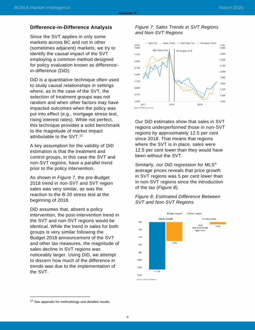
6


Difference-in-Difference Analysis

Since the SVT applies in only some markets across BC and not in other (sometimes adjacent) markets, we try to identify the causal impact of the SVT employing a common method designed for policy evaluation known as difference-in-difference (DiD).

DiD is a quantitative technique often used to study causal relationships in settings where, as in the case of the SVT, the selection of treatment groups was not random and when other factors may have impacted outcomes when the policy was put into effect (e.g., mortgage stress test, rising interest rates). While not perfect, this technique provides a solid benchmark to the magnitude of market impact attributable to the SVT.12

A key assumption for the validity of DiD estimation is that the treatment and control groups, in this case the SVT and non-SVT regions, have a parallel trend prior to the policy intervention.

As shown in Figure 7, the pre-Budget 2018 trend in non-SVT and SVT region sales was very similar, as was the reaction to the B-20 stress test at the beginning of 2018.

DiD assumes that, absent a policy intervention, the post-intervention trend in the SVT and non-SVT regions would be identical. While the trend in sales for both groups is very similar following the Budget 2018 announcement of the SVT and other tax measures, the magnitude of sales decline in SVT regions was noticeably larger. Using DiD, we attempt to discern how much of the difference in trends was due to the implementation of the SVT.

12 See appendix for methodology and detailed results.

Figure 7: Sales Trends in SVT Regions

and Non-SVT Regions

Our DiD estimates show that sales in SVT regions underperformed those in non-SVT regions by approximately 12.5 per cent since 2018. That means that regions where the SVT is in place, sales were 12.5 per cent lower than they would have been without the SVT.

Similarly, our DiD regression for MLS® average prices reveals that price growth in SVT regions was 5 per cent lower than in non-SVT regions since the introduction of the tax (Figure 8).

Figure 8: Estimated Difference Between

SVT and Non-SVT Regions

Appendix M

7


We also estimated the DiD regressions excluding Metro Vancouver to gauge whether our results held up for markets where the tax applies, but where there were relatively few SVT payors.

Estimating the same regression but for a data sample that excludes Metro Vancouver, we found that the impact of the SVT on home sales was close to zero and not statistically significant. The impact of the SVT on home price growth was an estimated negative 0.6 per cent.

Conclusions

Our estimates show that tax measures introduced in Budget 2018 compounded the already significantly negative effects on home sales and average prices from other policy measures, particularly the B-20 stress test. While B-20 is still the dominant causal factor in the broad market slowdown that occurred in 2018 and 2019, markets in which the SVT was levied underperformed non-SVT regions by a significant margin. However, these results seem to be confined to Metro Vancouver markets with negligible difference in market performance

between SVT and non-SVT markets on Vancouver Island and in the Okanagan.

The combined effect of federal and provincial measures may have successfully arrested the rapid acceleration of home prices that occurred before 2018. However, a recovery of home sales is underway around the province, and without addressing significant supply issues, any progress made toward improved affordability looks to be short-lived.

Moreover, while the SVT, the City of Vancouver’s Empty Homes Tax and short-term rental regulations may have encouraged more units to be added to the rental stock, particularly in Metro Vancouver, vacancy rates remain extremely low and as a result rental rates continue to rise.

Perhaps the impact of the SVT will be felt longer term, as tax revenues are allocated to affordable housing and other projects needed to address the supply side of provincial housing. For now, it appears that the SVT, along with other recently enacted housing policies, provided an ultimately temporary salve to the issue of housing affordability.

Appendix M

8


Appendix: Methodology and Results To estimate the impact of the SVT on sales and prices in SVT regions, we estimated the following standard difference-in-difference regression for our outcome variables Yi (sales or prices in each market i) on Tax status Ti=0 for non-SVT markets, Ti=1 for SVT markets, a time dummy variable ti where t=0 for the time period before the SVT and t=1 for the period after the SVT, and an interaction term to capture the impact of the SVT:

Yi = α + β1Ti + β2ti + δ(Ti ∗ ti) + εi

Where, α = constant term

β1 = Treatment group specific effect (average permanent difference between treatment group (SVT markets) and control group (non-SVT markets)

β2 = Time trend common to SVT and non-SVT markets

δ = Estimated impact of the SVT

εi = random, unobserved error term

The regressions were estimated in natural logs, so the coefficient of interest, δ, can be interpreted as a percent change in sales or prices due to the SVT.

The coefficient δ, which measures the impact of the SVT, reported below with t -statistics in brackets. Note: the regressions are in natural logs, so the reported impact is calculated as 𝑒𝛿 − 1.

Table 1: Estimated Impact on Sales and Prices – Whole Sample

Outcome Variable δ (t-statistic)

Estimated Impact, 𝑒𝛿 − 1 %

Sales -0.133 (-1.96)* -12.5%

Prices -0.052 (-2.719)* -5.0%

*Statistically significant at the 5% level

Table 2: Estimated Impact on Sales and Prices – Excluding Metro Vancouver Markets

Outcome Variable δ (t-statistic)

Estimated Impact, 𝑒𝛿 − 1 %

Sales 0.002 (0.468)** 0.2%

Prices -0.006 (-10.758)* -0.6%

*Statistically significant at the 5% level **Not statistically significant

Appendix M

Appendix N

What Caused the 2018 Sales Decline?

0% 50% 100%

Affordability Index

Mortgage Rate Shock

MacroPrudential Shock

MacroPrudential x Interest Rate Shock

B20 Dummy Variable

Average

B20

Affordability/Interest Rates/Economic Conditions

OtherModel

Share of Decline in Home Sales Source: BCREA Economics

• Based on research conducted by theBCREA Economics department, themajority of the decline in home salessince the beginning of 2018 is due to acombination of strained affordability,slowing economic growth, risinginterest rates and the B20 stress test

• A smaller share of the decline,between 15-20%, is due to otherfactors including provincial policymeasures

• As the next slides show – the share ofhouseholds subject to new provincialtaxes are not large enough to explainthe decline in sales observed since theend of 2017

Appendix N

Who Pays the Speculation Tax?

0 1,000 2,000 3,000 4,000 5,000

Non-Resident "Empty"

Canadian and "Empty"

"Satellite" Family0.17% of BC Households

0.21% of BC Households

Households

0.24% of BC Households

• According to provincial data,only 11,783 households paidthe speculation tax.

• That number includes:• 4,261 foreign owners• 3,060 “Satellite” families• 1,519 Canadians outside

of BC• 2,362 BC residents

Source: Ministry of FinanceAppendix N

Speculation Tax in Perspective

0

100,000

200,000

300,000

400,000

500,000

600,000

700,000

800,000

900,000

Total ResidentOwned andOccupied

Investor Owned,Rented

Non-Resident,Vacant

Sattelite Family

Non Resident

Resident

Households• Putting the speculation tax inperspective - the overwhelmingmajority of households in BC areResidents who occupy their homes

• Another significant share ofowners are residents and non-residents who rent their units

• A very small share of totalhouseholds (<0.5%) are non-resident owners who leave theirunits vacant or households whoseprimary breadwinner earns morethan 50% of household incomeoutside of BC – so called “SatelliteFamilies”

Source: Statistics Canada; Ministry of FinanceAppendix N

Facts about Foreign Buyers

Regional District% Non-Resident Share of Transactions (2017)

% Non-Resident Share of Transactions (2018)

Nanaimo 4.4% 1.8%

Capital Region 4.3% 2.0%

Metro Vancouver 3.6% 3.0%

Central Okanagan 1.8% 1.0%

Fraser Valley 1.4% 0.9%

All BC 3.3% 2.4%

• Foreign buyers accounted for 3.3 percent of all provincial residentialtransactions in 2018 and 3.6 per cent inMetro Vancouver in 2017 prior to theincrease and expansion of the foreignbuyer tax in February of 2018

• The Share of foreign transactionsdeclined to 2.4 per cent in BC and 3 percent in Metro Vancouver in 2018

• That decline was primarily the result ofa continued trend of falling foreigntransactions since the original foreignbuyers tax implemented in 2016, andthe imposition of more strict capitalcontrols by the Chinese government in2017

Source: DataBCAppendix N

Foreign Resident Transactions (BC)

0

100

200

300

400

500

600

2017 2018 2019

Source: Data BC

Units

China Tightens Capital ControlsBC Expands FBT

Appendix N

1,500

2,000

2,500

3,000

3,500

4,000

4,500

Jan

-15

Mar

-15

May

-15

Jul-

15

Sep

-15

No

v-1

5

Jan

-16

Mar

-16

May

-16

Jul-

16

Sep

-16

No

v-1

6

Jan

-17

Mar

-17

May

-17

Jul-

17

Sep

-17

No

v-1

7

Actual No-Foreign Tax Scenario

Fear in the market caused sales to overshoot to the downside

Sales rebounded to baseline no-tax projection

Impact of 2016 Foreign Buyer Tax on Vancouver Sales

Source: BCREA Economics

Unit Sales• The original 2016 foreign buyer taxexacerbated an already slowingmarket

• Analysis by the BCREA Economicsdepartment at the time of the taxillustrates that much of the initialreaction to the tax was the resultof the impact on marketexpectations which caused sales toovershoot to the downside.

• However, sales and prices quicklyrecovered to where BCREAprojected they would have beenunder a no-tax scenario.

Appendix N

Appendix O

1F C P P P O L I C Y S E R I E S N O . 1 6 4 • J U N E 2 0 1 4 • H O U S I N G A F F O R D A B I L I T Y A N D T H E S TA N D A R D O F L I V I N G I N VA N C O U V E R

POLICY SERIESFRONTIER CENTRE FOR PUBLIC POLICY © 2 0 1 4

Housing Affordability and the Standard of Living in Vancouver

Wendell Cox

POLICYSERIESPOLICYSERIESF R O N T I E R C E N T R E F O R P U B L I C P O L I C Y

N O . 1 6 4 • J U N E 2 0 1 4

Appendix O



The Frontier Centre for Public Policy is an independent, non-profit organization that undertakes research and education in support of economic growth and social outcomes that will enhance the quality of life in our communities. Through a variety of publications and public forums, the Centre explores policy innovations required to make the prairies region a winner in the open economy. It also provides new insights into solving important issues facing our cities, towns and provinces. These include improving the performance of public expenditures in important areas like local government, education, health and social policy. The author of this study has worked independently and the opinions expressed are therefore their own, and do not necessarily reflect the opinions of the board of the Frontier Centre for Public Policy.

Copyright © MMXIV by the Frontier Centre for Public Policy.

Date of First Issue: June 2014.

Reproduced here with permission of the author. Any errors or omissions and the accuracy and completeness of this paper remain the responsibility of the author.

ISSN 1491-78

FRONTIER CENTRE FOR PUBLIC POLICY

MB: 203-2727 Portage Avenue, Winnipeg, Manitoba Canada R3J 0R2 Tel: 204-957-1567 Email: [email protected]

SK: 2353 McIntyre Street, Regina, Saskatchewan Canada S4P 2S3 Tel: 306-352-2915 Email: [email protected]

AB: Ste. 603, 734-7th Avenue SW, Calgary, Alberta Canada T2P 3P8 Tel: 587-930-2289 Email: [email protected]

I d e a s f o r a b e t t e r t o m o r r o ww w w . f c p p . o r g

Wendell Cox is principal of Wendell Cox Consultancy (Demographia), a St. Louis-based (Missouri-Illinois) international public policy firm. He is an expert in land-use and transportation policy and is co-author of the “Demographia International Housing Affordability Survey,” which has examined metropolitan areas in Canada, Australia, Ireland, New Zealand, the United Kingdom and the United States since 2004 and will cover 10 nations in its 10th edition (2014).

The Frontier Centre for Public Policy sponsors the “Survey” in Canada.

About the author

He has written and spoken widely on the role of housing affordability in the standard of living and in poverty reduction, including national speaking tours of Australia and during numerous international presentations.

He is author of War on the Dream: How Anti-sprawl Policy Threatens the Quality of Life and the co-author with Richard Vedder of The Wal-Mart Revolution: How Big-Box Stores Benefit Consumers, Workers, and the Economy. In addition to these books, he has been a frequent book chapter contributor and is the author of a regular column in www.newgeography.com.

Cox is also the author of the widely cited “Demographia World Urban Areas,” which is the only compendium of population, land area and population density for all known urban areas (population centres) of 500,000 or more people.

He was a visiting professor for nine years at the Conservatoire national des arts et métiers, a Paris university. He has a BA in Government from California State University, Los Angeles, and an MBA from Pepperdine University in Los Angeles. Mayor Tom Bradley appointed him to three terms on the Los Angeles County Transportation Commission, which was the top policy body in both highways and transit in the largest county in the United States. He was appointed by then Speaker of the United States House of Representatives Newt Gingrich to the Amtrak Reform Council to fulfill the unexpired term of New Jersey Governor Christine Todd Whitman when she resigned from the Council.

He was an invited participant in a forum sponsored by Calgary Transit in 1999.

Wendell Cox is a senior fellow at the Frontier Centre for Public Policy.

Appendix O



Table of ContentsTitle Page

Housing Affordability and the Standard of Living in Vancouver

Wendell Cox

Executive Summary 4

1. Focusing on priorities 9

2. The Regional Growth Strategy 11

3. Housing affordability in Vancouver 12

4. Urban containment and higher house costs 20

5. Transportation in Vancouver 25

6. Mobility and the standard of living 33

7. Sustainability 35

8. Overall economic impact 40

9. Evaluation 43

Recommendations 44

Appendix A 46

Appendix B 49

Endnotes 51

Note to reader: Endnotes and some words in this document may appear in blue and underlined. When e-reading, these links will directly access relevant online

websites or documents using your associated browser. Endnotes’ numerals will directly link to the appropriate reference at the end of this document.

FCPP Policy Series No. 148 • December 2012

POLICY SERIES FRONTIER CENTRE© 2 0 1 2

FOR PUBLIC POLICY

FCPP Policy Series No. 164 • June 2014

Appendix O



Executive SummaryThe average household can no longer afford a home in the average price range. Housing is so expensive in Vancouver that an additional annual income of between $22,000 and $40,000 is required for the average house, compared to other major metropolitan areas (Toronto, Montreal, Ottawa, Calgary and Edmonton). Most people are priced out of the market for the average house and have to accept lower-cost housing, which is generally smaller and can be of lower quality. Moreover, Vancouver has the highest house prices relative to income in the New World (Canada, Australia, New Zealand and the United States).

The principal cause of this difference is likely Vancouver’s urban containment land-use policies. Unusually high house prices occur when such policies are strongly enforced. The same policies have also been instrumental in making Vancouver’s traffic congestion the worst in North America (worse than Los Angeles) and third worst in the high-income world.

Focusing on Priorities: Over the past two centuries, the world has become urban, as people have moved to the cities to better their lives. The very purpose of cities is to facilitate a higher standard of living for residents and to reduce poverty.

Consistent with this, the domestic public policy priority of most governments is the betterment of people by facilitating a higher standard of living and reducing poverty.

Yet, the dominant strain of urban planning, which is urban containment policy, works against the aspirations of households and against the fundamental policy priority of a better standard of living. Urban containment policy (also called “compact city policy,” “smart growth” “livability” and other terms) seeks to limit or prohibit development on or beyond the urban fringe. By creating an imbalance of demand over supply for residential land, house prices are driven up, breaking their historic and fundamental nexus with household income. The increase in housing costs, the largest component of household budgets, reduces discretionary income, which translates into a lower standard of living and more poverty.

There are few, if any, places where this loss of housing affordability and reduction in the standard of living is more evident than in Vancouver.

There is a need to focus on the fundamental priority of improving the standard of living and reducing poverty (Section 1).

The Regional Growth Strategy: Metro Vancouver, through its Regional Growth Strategy, drafted under the provisions of British Columbia law and policy, oversees land and transportation policy in the Vancouver metropolitan area. A principal feature of the Regional Growth Strategy is an urban containment boundary that bans urbanization on most of the land that is appropriate for development; therefore, comparatively little land is available for the expanding urban area.

Regional authorities are attempting to minimize automobile use and, thus, regional policy favours the expansion of transit. These policies have resulted in a higher

Appendix O



market share for transit, but automobiles continue to account for the vast majority of travel in the Vancouver metropolitan area.

Regional policy has also sought to avoid urban sprawl and to preserve agricultural land. These objectives are consistent with British Columbia law and policy. However, housing affordability and economic development, also objectives of British Columbia law and policy, have received insufficient attention. Housing affordability has deteriorated substantially in this environment (Section 2).

Housing Affordability and the Standard of Living in Vancouver: Vancouver has by far the highest housing costs in Canada. In2013, Vancouver’s housing affordability was the worst among the 85 major metropolitan areas in Canada, the United Kingdom, Australia, Ireland, New Zealand, Singapore and the United States. In 2011, the average existing house price in Vancouver was from 65 per cent to 275 per cent higher than in the other major metropolitan areas. The differences in household income are far more modest .

Vancouver’s houses prices were not always unaffordable. As late as 1971, housing affordability was better in the Vancouver metropolitan area than in the Toronto metropolitan area, and it was only slightly worse than in the other four major metropolitan areas (Calgary, Edmonton, Montréal and Ottawa). By comparison, there is little variation in household income among these major metropolitan areas.

The impact of unaffordable housing on the standard of living is illustrated by the additional income that would have been available to Vancouver households if the price to income ratio were the same as those in other major metropolitan areas. At the price to income ratios in the other areas, the average Vancouver household purchasing the average-priced house (detached, semi-detached or apartment) would have needed from $22,000 to $31,000 more income in 2010. Similarly, the average-income household would have needed between $29,000 and $40,000 more at the price to income ratios of the other major metropolitan areas.

Higher amounts spent on housing result in less discretionary income for households. This is money not available for purchasing other goods and services, which would create more employment and economic growth, other things being equal. This has resulted in a lower standard of living for Vancouver residents than would be the case if housing affordability had been retained (Section 3).

Urban Containment and the Standard of Living: Vancouver’s excessive housing costs relative to income are consistent with the economic literature that associates urban containment policy with higher housing costs. There is an economic consensus that, other things being equal, scarcity drives up prices. Urban containment boundaries drive up the price of housing by creating an imbalance between demand and supply in which the supply of land is severely restricted. There is considerable research on this issue (Appendix A).

At the same time, there is also evidence that lower-income households pay a heavy price in higher housing costs because of urban containment policy.

In short, the higher housing costs relative to income typical of urban containment

Appendix O



policy, other things being equal, tend to reduce the standard of living and increase poverty by reducing household discretionary income (Section 4).

Transportation in Vancouver: As part of its urban containment policies, Vancouver has made substantial improvements to public transit. The most important is the SkyTrain system, which is one of the most successful rail systems developed in North America in recent decades. There have been transit market share increases, though the automobile continues to be the most-used form of travel in the Vancouver area.

The transit improvements have been concentrated in areas in and near the core of the metropolitan area, including downtown and the Vancouver Metro Core. Downtown and the core have by far the most favourable environments in the area for transit ridership increases. Metro Vancouver projects that the overwhelming majority of new employment will be outside of downtown and the Vancouver Metro Core.

Local officials hope to facilitate substantial transit ridership increases in the future. The areas in which new jobs will be concentrated are far less amenable to transit use, principally because the density and coverage of transit routes make most commutes by transit impractical. Given this reality, it could be difficult for transit to maintain its present market share in Vancouver, and the share of travel by automobile could increase.

Moreover, Vancouver has recently emerged as having the worst traffic congestion in North America and the third worst out of more than 120 metropolitan areas in Canada, Western Europe, Australia, New Zealand and the United States). This increase in traffic congestion is consistent with the results of urban containment policies, which seek higher densities and fail to increase roadway capacity consistent with the demand. Further, greater traffic congestion is associated with more local air pollution, which has negative health effects (Section 5).

Mobility and the Standard of Living: Greater mobility, which is the ability of residents to commute to the maximum number of jobs in the metropolitan area in a specific period (such as 30 minutes), improves economic growth. Transit, cycling and walking are appropriate for many; however, these modes are unable to compete with the automobile in providing quick and comprehensive mobility throughout the metropolitan area. Further, access to an automobile improves the mobility and standard of living of low-income households (Section 6).

Sustainability: Sustainability is a principal underlying justification of the Regional Growth Strategy

Perhaps the most important concern of urban containment policy is the reduction of greenhouse gas (GHG) emissions. Yet, recent research indicates that urban containment policy is an ineffective and expensive means of reducing GHG emissions. Moreover, regional planning efforts around the world routinely fail to subject their strategies to an economic metricProgress in automobile fuel efficiency that will result in substantial reductions of GHG emissions even while driving continues to increase is anticipated. Similarly, substantial decreases have been made in GHG emissions from detached housing. At the same time, research indicates that GHG emissions per capita are higher from the high-rise residential buildings that are favoured in the

Appendix O



Regional Growth Strategy.

There is also concern about local food production and its importance to the food security of the Vancouver metropolitan area. In fact, local agricultural production provides comparatively little of Vancouver’s food, and local food objectives do not necessarily improve the standard of living of consumers or people involved in agricultural production. Finally, urbanization does not represent a threat to Canadian agriculture. The nation has taken out of production more land than the total area of the entire Maritime provinces, a far greater amount than all of the urbanization that has occurred since the coming of European settlement. At the same time, agricultural production has increased markedly (Section 7).

Overall Economic Impact: Not surprisingly, the reduction in household discretionary income associated with urban containment has also led to less-robust metropolitan area growth. Research findings that show this has been published in the United Kingdom, continental Europe and the United States.

There are also concerns about the impact on the national economy. The Bank of Canada has expressed apprehension about rising household debt and rising house prices. These matters were also a factor in the downgrading of most major Canadian banks by international rating agencies in 2012. The longer-term potential for higher interest rates that would put even more pressure on household budgets heightens this concern. However, despite its mandate to maintain economic stability through its inflation target, house prices are largely beyond the ability of the Bank of Canada to control, because of the much stronger influence of metropolitan and provincial land-use policies in driving up prices. .

At the same time, Vancouver has already reached the price to income ratio equal to those in the 11 “ground zero” metropolitan areas in the United States that were responsible for three-quarters of the US house-price losses that set off the international Great Recession (Section 8).

Evaluation: Vancouver’s urban containment policies have drastically reduced the amount of land available for development, with the predictable consequences of higher house prices, less household discretionary income and a lower standard of living. This is inconsistent with Vancouver’s reputation as one of the world’s most liveable cities. Vancouver’s intense traffic congestion is also inconsistent with this reputation.

Regional policy places insufficient emphasis on the principal priority of improving the standard of living and reducing poverty. This focus needs correcting and requires reforms (Section 9).

Recommendations: Vancouver’s urban containment policies, which have little potential for improving the environment while imposing great cost, need to be reformed. The metropolitan area should seek to return to broad-based prosperity in which the average household and lower-income households can have the same standard of living as the other major metropolitan areas. There is a need to put people first in Vancouver land-use policy. Improving the standard of living and reducing poverty need to be the principal objectives.

Appendix O



The province of British Columbia should give clear direction to Metro Vancouver to place housing affordability and economic development as its principal policy priorities. The urban containment boundary should be substantially expanded. Further, Metro Vancouver should subject all of its strategies to an economic metric that measures the cost per tonne of GHG emissions reduction. Jurisdictions in the Lower Mainland should also implement public facility finance options that can improve housing affordability (Section 10).

“The metropolitan area should seek to return to broad-based prosperity in which the average household and lower-income households can have the same standard of living as the other major metropolitan areas.

Appendix O



1. Focusing on prioritiesThroughout history, people have moved to cities for better lives. Cities offered better opportunities because households could expect to enjoy greater discretionary incomes than in rural areas, and there were greater opportunities for upward economic mobility. Cities are economic entities. Former World Bank principal urban planner Alain Bertaud (2004) noted that: Large labor markets are the only raison d’être of large cities.1 The very purpose of cities is to facilitate a higher standard of living for residents and to reduce poverty. In a more recent paper, he continued:

“Increasing mobility and affordability are the two main objectives of urban planning. These two objectives are directly related to the overall goal of maximizing the size of a city’s labor market, and therefore, its economic prosperity.”2

Yet, urban containment policy, which is the dominant strain in contemporary urban planning, works against the economics of cities — the aspirations of households and their standard of living. People have advocated for urban containment policy for at least seven decades.3 Urban containment is also called “smart growth,” “compact city policy,” “growth management,” “liveability,” and “densification” among other terms. Along with other restrictions, urban containment seeks to limit the expansion of urban areas (suburbanization or pejoratively called “urban sprawl”) by severely restricting or prohibiting development on, or beyond the urban fringe (See Box 1, next page).

A related element of urban containment policy is to limit the use of the automobile4

by transferring demand to transit, cycling or walking.

Economic principle holds that other things being equal, a scarcity in the supply of a product will tend to influence its price upwardly. This is true of land for urban development—policies that severely restrict the availability of land are associated with higher and rising house prices. Economists Richard Green and Stephen Malpezzi summarize the issue: “When the supply of any commodity is restricted, the commodity’s price rises. To the extent that land-use, building code, housing finance, or any other type of regulation is binding, it will worsen housing affordability.”5

The higher prices associated with urban containment policy have broken the historical connection between house prices and household incomes (Appendix B).

Since housing is the largest item in household budgets,6 more expensive housing reduces discretionary incomes, the money left over after taxes and funds needed for necessities. Less discretionary income means a lower standard of living and higher rates of poverty.7

The house price increases have occurred across the spectrum of metropolitan areas with urban containment policies, from the most vibrant to those that have experienced significant industrial decline (such as Liverpool and Glasgow). There are few places where housing affordability has deteriorated as severely as in Vancouver.8

Appendix O



Moreover, Vancouver has recently emerged as having the worst traffic congestion in North America and the third worst out of more than 120 metropolitan areas in Canada, Western Europe, Australia, New Zealand and the United States. This increase in traffic congestion is consistent with the results of urban containment policies, which seek higher densities and fail to increase roadway capacity consistent with the demand. Further, greater traffic congestion is associated with more local air pollution, which has negative health effects (Section 5.4).

As is indicated in Urban Policy: A Time for a Paradigm Shift,9 there is a need to focus on the fundamental objectives of maintaining or improving the standard of living and reducing poverty. The focus of this report is land-use and related policy and its effect on the standard of living in the Vancouver metropolitan area.

Urban Expansion in Context

Cities grow geographically as they add population. This has been the case since the first cities arose. The extent of this spatial expansion has become greater as cities have grown exponentially and transportation technology has improved. This expansion is related to people’s desire for better lives (Section 1). This report does not argue that urban expansion (urban sprawl) is inherently wealth generating; however, it certainly has been associated with an unprecedented expansion of affluence and the reduction of poverty. Virtually all of the largest cities in the world have expanded at least as rapidly as they have added population (see “Dispersion in the World’s Largest Urban Areas”10). Urban expansion is not a Canadian or U.S. phenomenon. It can be witnessed from Atlanta, with the world’s lowest major urban area density, to London, Paris, Tehran, Lagos, Jakarta, Shanghai and even to Dhaka, with the world’s highest urban densities.

Urban containment policy seeks to slow, stop or even reverse this organic expansion. Nonetheless, New York University professor and urban planner Shlomo Angel advises in Planet of Cities coming to terms with urban expansion.11 He urges the abandonment of artificial limits on urban expansion and population growth (such as urban containment boundaries) and advocates for programs that improve economic development and the quality of life. He decries the notion that “cities should simply be contained and enclosed by greenbelts or impenetrable urban growth boundaries” as “uninformed and utopian” because it makes sustainability “an absolute end that justifies all means to attain it.” This perspective is substantially at odds with Vancouver policies.

BOX 1

Appendix O



2. The Regional Growth StrategyAs The Vancouver metropolitan area’s land-use policy is framed by Metro Vancouver, which adopted its present plan in 2011 (the Regional Growth Strategy). This is the latest in a series of plans that stretch back more than 40 years.12

One of the most important policy initiatives in the planning process was the designation of the Agricultural Land Reserve (ALR), which severely limits urban expansion into developable land outside the existing urban area. The ALR and other land on which development is prohibited have been referred to as the “Green Zone,” which is delineated by an urban containment boundary (Chart 1). The developable area inside the urban containment boundary remains similar to that of a 1996 map published by the Metro Vancouver predecessor Greater Vancouver Regional District (Chart 2).

Metro Vancouver has implemented strategies to increase travel by transit, walking and cycling in the metropolitan area and has sought to discourage automobile use. Yet, the automobile remains the dominant form of personal transportation.

Urban Containment BoundaryFrom Regional Growth Plan

CHART 1

Future Growth Plans (1996)From Regional Growth Plan

CHART 2

Vancouver’s urban containment policy generally follows the philosophy of the British Town and Country Planning Act 1947, which required limiting the extent of urban areas and permitting limited development in rural areas. Other major metropolitan areas have implemented similar policies, with some of the early followers being Sydney, Australia, and Portland, Oregon, with much of Australia and New Zealand following in recent years.

These policy directions are consistent with some provisions of existing provincial law and policy.13 This includes objectives to avoid urban sprawl, preserve agricultural

Appendix O



land, “minimize the use of automobiles and encourage walking, bicycling and the efficient use of public transit.” However, the same set of policies includes housing affordability and economic development objectives, which have received, at best, secondary treatment in the Regional Growth Strategy and its predecessor plans.

3. Housing affordability in VancouverVancouver has by far the most expensive housing among the major metropolitan areas (populations over 1,000,000). In 2011, average existing house prices (all listed and sold housing) in Vancouver were from 65 per cent to 275 per cent higher than in the other major metropolitan areas.14 By comparison, the differences in household income were far more modest (Chart 3).15 The result is a substantial disconnection of historical and fundamental relationship between house prices and household income in Vancouver.

In the 10th Annual Demographia International Housing Affordability Survey, Vancouver had the most expensive housing in 2013 among the 85 major metropolitan areas of Canada, Australia, Ireland, New Zealand, Singapore, the United Kingdom and the United States.16

Average Owned House Price & Household IncomeMajor Metropolitan Areas (2011)

CHART 3

$800,000

$700,000

$600,000

$500,000

$400,000

$300,000

$200,000

$100,000

0

Ave

rage

Pri

ce

Calgary Edmonton Montreal Ottawa ON Ottawa QC Toronto Vancouver

Average House Price (MLS) Average Household IncomeSource: National Household Survey and CMHC.

Appendix O



3.1 Housing affordability in Vancouver

Vancouver’s housing costs relative to income have not always been more expensive than other metropolitan areas. As late as 1971, the Census of Canada reported that the price of the average detached house in the Vancouver metropolitan area was 3.9 times the median household income. Toronto was more expensive, and five other major metropolitan areas had a price to income ratio of 3.5, somewhat below that of Vancouver.

In the subsequent four decades, the price to income ratio (median multiple17) in Vancouver has increased to 10.3. The house price increases have escalated significantly since 2005. By comparison, from1971 to 2005, the median multiple remained relatively constant in the other major metropolitan areas, indicating stability in the housing market. Since that time, however, house prices have escalated in the other metropolitan areas, especially with the preparation and adoption of urban containment plans (Chart 4).18

Median MultipleVancouver CMA Compared (1971-2012)

CHART 4

12

10

8

6

4

2

0 Med

ian

Hous

e Pr

ice/

Med

ian

Hous

ehol

d In

com

e

1971 2000 2012 I I I I I I I I I I I I I I I I I I I I I I I I I I I I I I I I I I I I I I I I I I I I

Vancouver 5 Other Major Metropolitan AreasSource: From 1971 Census and the Demographia International Housing Affordability Survey.

Appendix O



The average detached house in Vancouver was approaching double Toronto’s detached-house price (2012). Vancouver’s detached housing average price was at least 2.5 times that of the other four major metropolitan areas (Chart 5). Worse, between 2004 and 2012, the median price of a detached house rose nearly four times that of the median household income (Chart 6, next page). These differences are not the result of construction costs (Section 4).

New Detached House PricesMajor Metropolitan Areas (2012)

CHART 5

$1,250,000

$100,000

$750,000

$500,000

$250,000

0

Ave

rage

Pri

ce


Average House Price (MLS) MedianSource: CMHC (No data for QC).

Appendix O



With these price pressures, many households are unable to afford detached housing. This has led to a declining relative volume of detached housing construction, and Vancouver had the smallest share of new detached housing among the major metropolitan areas between 2006 and 2011.19 The urban planning literature sometimes implies that higher density, multi-family housing can be readily substituted among households that prefer detached housing.20 However, for many households, higher density housing is not an adequate substitute for a detached house with a yard, especially for households with children.

Income and New Detached House PricesVancouver CMA (July 2004-2012)

CHART 6

100%

90%

80%

70%

60%

50%

40%

30%

20%

10%

0%

Perc

enta

ge c

hang

e fr

om J

uly

2004

2004 2005 2006 2007 2008 2009 2010 2011 2012 I I I I I I I I I I I I I I I I I I I I I I I I I I I I I I I I I I I I I I I I I I I I I I I I I I I I I I I I I I I I I I I I I I I I I I I I I I I I I I I I I I I I I I I I I I I I I I

Median Price New Detached Houses Median Household IncomeSource: CMHC and Estimated from Statistics Canada.

Appendix O



The extent of Vancouver’s detached-house-cost escalation is illustrated in Chart 7, which compares the 2012 median detached-house price in Vancouver with those in Edmonton and the Bellingham metropolitan area21 (across the United States’ border from the Vancouver metropolitan area) and Dallas-Fort Worth, which is the fastest-growing metropolitan area with more than 5 million people in the high-income world. These comparisons show that Vancouver’s median detached-house price is double that of Edmonton’s, three times that of Bellingham’s and more than 4.5 times that of Dallas-Fort Worth’s. Despite the huge difference in house prices among the metropolitan areas, there is comparatively little difference in household income.

Detached House Prices and IncomeVancouver and Major Metropolitan Areas Medians (2012)

CHART 7

$800,000

$700,000

$600,000

$500,000

$400,000

$300,000

$200,000

$100,000

0

Med

ian

Pric

e

Vancouver Edmonton Bellingham U.S. Dallas-Fort Worth U.S.

House Price Median Household IncomeSource: Estimated from NHS and CMHC data, and Demographia International Housing Affordability Survey.

Appendix O



3.2 Housing affordability assessment by 3.2 Metro Vancouver

Metro Vancouver confirms Vancouver’s housing affordability problem. Generally, housing is affordable when housing costs are less than 30 per cent of gross household income. By this standard, most of the Vancouver metropolitan area house sales between 2007 and 2011 were unaffordable. In the area reported upon by the Greater Vancouver Real State Board, between 67 per cent and 73 per cent of sales transactions in each year were unaffordable. The Fraser Valley Real Estate Board reports on parts of the Vancouver and Abbotsford metropolitan areas. Its data indicate that between 2007 and 2011, 56 per cent to 60 per cent of sales transactions were unaffordable in each year.22

Vancouver’s high housing prices also extended to households that rented. Metro Vancouver notes that the number of apartments renting for $750 or less monthly declined 57 per cent between 2007 and 2011.23

3.3 Vancouver housing prices: 3.2 Their impact on the standard of living

Vancouver’s high housing costs relative to income result in lower discretionary income and a lower standard of living. The following examples estimate the differences in discretionary income for the average Vancouver household if Vancouver house prices were as low relative to income as they are in the other major metropolitan areas.

Appendix O



Example 1Average-priced Existing House (2011): The average-income Vancouver household cannot afford the average-priced existing house (includes all housing types).24 The cost of other necessities (food, clothing, transportation, health care, taxes and Canada pension fund) and the mortgage25 would exceed the average household income by approximately $1,000. This is in stark contrast with the housing affordability (price to income ratio) in the other five major metropolitan areas. If Vancouver’s existing houses were similarly priced relative to income in the other major metropolitan areas, the average household would have from $22,000 (Toronto price to income ratio) to $31,000 (Montréal and Ottawa, Québec-portion price to income ratios) left over to spend on other goods and services or to save (Chart 8).26 The additional discretionary income would not only improve the standard of living of the households, but the additional purchases the household could make would create jobs and improve the economy and savings rates would be higher. At present house prices, Vancouver households have a lower standard of living than they would have if the price to income ratio replicated those of the other major metropolitan areas.

The average Vancouver household is priced out of the market for the average-priced existing house.

Estimated Discretionary IncomeAverage Income Purchasing Existing House (2011)

CHART 8

$30,000

$25,000

$20,000

$15,000

$10,000

$5,000

0

-$5,000

Dis

cret

iona

ry I

ncom

e


Note: Prices and discretionary spending adjusted to Vancouver levels.

Appendix O



Example 2Average-priced New Detached House (2011): The average-priced new house is also beyond the financial capability of the average income Vancouver household (2011).27 The cost of other necessities (food, clothing, transportation, health care, taxes and Canada pension fund) and the mortgage28 would exceed the average household income by approximately $18,000. This contrasts with the situation for average income households in the other five major metropolitan areas. If the price to income ratios in the other five metropolitan areas were applied in Vancouver, the average household would have from $29,000 (Toronto price to income ratio) to $40,000 (Calgary price to income ratio) left over (Chart 9,).29 As in the case of the existing house, the additional discretionary income would not only improve the standard of living of the household, but the additional purchases the household could make would create jobs and improve the economy, and savings rates would be higher.

Estimated Discretionary IncomeAverage Income Purchasing New Detached House (2011)

CHART 9

$30,000

$25,000

$20,000

$15,000

$10,000

$5,000

0

-$5,000

-$10,000

-$15,000

-$20,000

Dis

cret

iona

ry I

ncom

e


Note: Prices and discretionary spending adjusted to Vancouver levels.

Appendix O



4. Urban containment and higher 4. house costsVancouver’s excessive housing costs are consistent with the economic literature that associates urban containment with rising housing costs relative to income. There is an economic consensus that other things being equal, scarcity tends to drive up prices (whether the good or service is land, gasoline or any other).

Perhaps the earliest evaluation of urban containment policy was The Containment of Urban England, which was a five-year project by a team of academics led by urbanologist Sir Peter Hall (1973) of University College, London, England. The subject of this early 1970s work was the housing market as it had evolved since the enactment of the Town and Country Planning Act 1947. Hall et al. found that “perhaps the biggest single factor of the 1947 planning system is that it failed to check the rise in land prices which is probably the largest and most potent element of Britain’s postwar inflation.” The results are characterized as being inconsistent “with the objective of providing cheap owner-occupied housing.” Moreover, Hall et al. note that the planning system has imposed the greatest burdens on lower-income households

Former governor of the Reserve Bank of New Zealand Donald Brash wrote in an introduction to the “4th Annual Demographia International Housing Affordability Survey,” “The affordability of housing is overwhelmingly a function of just one thing, the extent to which governments place artificial restrictions on the supply of residential land.”30

In reports commissioned by the Blair government, former Bank of England Monetary Policy Committee member Kate Barker wrote of a strong relationship between unaffordable housing prices and urban containment policy.31

A New Zealand government report by Arthur Grimes (2007), former chairman of the Board of the Reserve Bank of New Zealand, attributed the loss of housing affordability in the nation’s largest urban area, Auckland, on urban containment policies. In another report (2009), he found that per acre prices just inside Auckland’s urban growth boundary were 10 times that of comparable land on the other side of the boundary.

London School of Economics professor Paul Cheshire concluded from his research that urban containment policy is irreconcilable with housing affordability.32 Given the importance of housing affordability in household budgets, this means that urban containment policy is incompatible with maintaining or improving the standard of living.

The literature documenting the relationship between urban containment policy and house-price increases is reviewed in more detail in Appendix A.

Fundamentals of the Housing Market: For decades, there has been a fundamental relationship between house prices and household income. This relationship, which is indicated by a 3.0 times (or less) ratio between median house prices and median

Appendix O



household income has predominated in Canada, the United Kingdom, Australia, Ireland, New Zealand and the United States (Appendix B).33

Generally, the fundamental connection between house prices and household income has been retained in the metropolitan areas that are not governed by strong urban containment policy or by government policies that create land scarcity. On the other hand, the connection between house prices and household income has been substantially broken only where there are strong urban containment policies. All of the major metropolitan areas with seriously unaffordable or severely unaffordable housing (median multiples above 4.0) in the 10th Annual Demographia International Housing Affordability Survey have strong urban containment policies34 or other strong land rationing policies.35 Conversely, none of the major metropolitan areas with liberal land-use policies has seriously unaffordable or severely unaffordable housing. In other words, serious and severely unaffordable housing is strongly associated with urban containment policy.

One of Ireland’s most respected economists, Colm McCarthy of University College, Dublin, described how adoption of urban containment policies not only undermined the fundamentals of the housing market, but also led to Ireland’s destructive bubble and bust (and one of the most significant economic reversals suffered by any nation in decades).36

“Ireland passed its first major piece of land-use planning legislation in 1963, modelled on the UK’s Town and Country Planning Act of 1947. The intentions were laudable, to restrict the construction of unwelcome developments and to empower local authorities to take a more active role in shaping the built environment.

…Our old friend, the Law of Unintended Consequences, began to impact from the mid-Seventies onwards as house prices in Dublin began to diverge from the national average.

…Before land-use zoning came along, house-builders extended the city by buying up farms on the city’s edge and building at whatever densities the market would support. But as more and more lands were withdrawn from the buildable stock by the planners, prices began to rise and the house-builders moved further away from the city proper.”

McCarthy noted that urban containment policies had been adopted with good intentions. The impact, however, has been disastrous.

Urban Containment and Housing Affordability in Vancouver: Consistent with the international experience, Vancouver’s urban containment boundary creates a scarcity of developable land that is far more expensive than before. Vancouver’s high developer and home builder fees and levies have also likely contributed to the escalation of house prices relative to income (Box 2, page 24). At the same time, Vancouver’s construction costs are not much different from those of other large metropolitan areas (Chart 10, next page).

Much, if not all of the difference is in land and regulatory costs.

Appendix O



Construction Cost IndexMajor Metropolitan Areas (2010)

CHART 10

1.20

1.0

0.80

0.60

0.40

0.20

0.00

Cons

truc

tion

Cos

ts C

ompa

red

wit

h N

atio

nal


Source: R.S. Means.

Vancouver’s land-use policies are associated with higher house prices, as the analysis above indicates. This results in higher housing costs and, thus, less discretionary income for households. Similarly, housing costs are higher for low-income households, which leads to greater poverty. Vancouver’s land-use policies are producing effects that undermine the economic well-being of people by reducing the standard of living and increasing poverty, as higher house prices reduce discretionary income.

The Social Costs of Higher House Prices: The consequences of urban containment on housing affordability and, thus, the standard of living for low-income households go well beyond the data cited for Vancouver.

This is evident in Portland, one of the international leaders in urban containment policies. House-price increases have been substantial, though less than in Vancouver.37 Portland’s median multiple rose from the national standard of 3.0 in 1995 to 4.8 in 2013.

However, Portland’s low-income households have experienced a greater loss of housing affordability than the average resident in the metropolitan area average. This is indicated by an analysis of postal codes with poverty rates of 50 per cent or more above average. Owned housing rose in value (median multiple, using values) approximately 75 per cent more in the higher-poverty areas than overall in the metropolitan area. The cost of rented housing (adjusted for incomes) rose nearly three times as much in high-poverty areas.

Appendix O



When comparing 2000 and 2010 census data, The Oregonian (the metropolitan daily newspaper) noted that ethnic diversity was on the decline in some denser Portland neighbourhoods.38 The greater rise in housing costs in higher-poverty areas indicates that the social costs of urban containment are even more burdensome for low-income households than are the additional costs imposed on households with average incomes.

Related research by Guanyu Zheng for the New Zealand Productivity Commission found that the higher prices generated by Auckland’s urban growth boundary were more severe for lower-cost housing: “…when the supply of land on the urban periphery is restricted, the price of available residential land rises and new builds tend to be larger and more expensive houses.”39

California, which has the U.S. highest housing cost adjusted poverty rate best illustrates the potential for social and economic consequences. This, combined with its highest housing costs relative to income, is stark testimony to the economic and social costs of urban containment policy.

In this connection, economist Anthony Downs wrote: “Higher prices then reflect a pure social cost because the efficiency of society’s resource allocations has decreased.”40 This means that if households have to pay more for their basic living expenses, such as housing, they will have a lower standard of living.

House Price Increases Likely to Continue: In the absence of reforms to urban containment policy, house-price increases relative to income seem likely to continue in Vancouver.

Appendix O



BOX 2

Government-imposed costs, fees and levies Before home builders can commence construction, raw land is converted into fin-ished lots. This is usually a principal task of the land developer, who arranges (and pays for) the local streets and utilities, such as sewage, electricity and natural gas lines. The finished land is purchased by home builders, the price of which includes the roads and utilities put in place by the developer. The street and utility improve-ments are turned over to the municipality and utility system owners.Government-imposed charges are an important element of new-house costs. These charges include provincial sales taxes, the GST and land transfer taxes as well as transaction fees and infrastructure fees (sometimes called development levies). In addition to the expense of preparing the land for construction, developers are also responsible for the public service levies and fees (sometimes called impact fees) paid to municipalities to offset the cost of off-site municipal improvements, which include infrastructure fees (for streets outside the subdivision and for utilities) and land dedication fees (such as for parks). Generally, these fees are a flat rate per unit of housing, by type of unit (such as single-detached, semi-detached, townhouse, apartment or condominium).According to the Canada Mortgage and Housing Corporation (CMHC), these fees are very high in the Vancouver metropolitan area The total government-imposed charg-es per new detached house in 2009 were estimated at $151,000 in the City of Van-couver,41 $109,000 in Surrey and $95,000 in Burnaby. In comparison, the national average was $59,000. The higher government-imposed charges in the Vancouver area are related to the much higher new-house costs. There are equity concerns about funding public facilities through up front charges on developers, which are routinely included in lot prices charged to home builders and home purchasers.42 Economic literature indicates that these charges are associated with both higher new-house costs and higher existing-house costs, all things being equal.43 In effect, new-home buyers pay for the new infrastructure, while existing home-owners and multi-family housing owners receive a windfall from the higher values induced by the development charges. At the same time, buyers of new houses, con-dominiums and rental units must pay for public facilities in advance, while existing owners are permitted to pay their shares of such expenditures over time. Other public facility financing methods are available that would permit owners of homes and multi-unit buildings to pay the attributable costs on a pay as you go basis. These include municipal debt instruments and user fees. Reliance on such instruments could reduce the pressure of higher housing costs, both in the new and existing stock, and lead to improved housing affordability.

Appendix O



5. Transportation in VancouverAn important part of the strategies of Metro Vancouver and its predecessor agencies has been to discourage automobile use while diverting the demand for driving to transit, walking and cycling. Public expenditures have generally favoured transit expansion in preference to providing additional roadway capacity. This has produced a considerable increase in TransLink ridership. However, automobile use has also continued to increase.

The most important transit improvement has been SkyTrain, which opened in 1985. This automated rail system that operates as a high quality Metro (subway, underground or elevated) by virtue of its complete grade separation carries approximately 400,000 weekday trips and has been the model for other systems, such as in Bangkok’s (also called SkyTrain). Among the many new rail systems that have opened in North America since 1960, SkyTrain has achieved greater ridership than all but the Montréal Metro and the Washington Metro.

Transit ridership in the Vancouver metropolitan area now ranks tenth among the metropolitan areas of North America, with the top nine having much larger populations. Transit in Vancouver performs much more strongly than transit does in well-regarded U.S. cities, carrying more than double the ridership of much larger Seattle and 3.5 times the ridership of similarly sized Portland.44

Yet, automobile use has continued to increase, and Vancouver remains largely suburban (Box 3).

BOX 3

Vancouver: A Suburban Metropolitan Area Queen’s University research indicates that even after four decades of urban contain-ment policy, Vancouver’s urban form and transport differ little from those of other metropolitan areas, none of which has a long history of urban containment policy. Despite efforts to discourage automobile use and with perhaps some of the most substantial transit improvements in North America, the Vancouver metropolitan area continues to be overwhelmingly suburban and exurban. A team led by Dr. David Gordon examined metropolitan areas using factors such as density and work-trip travel mode, and they classified census tracts as “active core” (walkable), “transit suburbs,” “auto suburbs” or (auto) “exurbs.” Vancouver was the least suburban and exurban, though not by much. The other five major metropolitan areas ranged from 75 per cent suburban or exurban (Toronto and Montréal) to 84 per cent suburban and exurban (Calgary). Vancouver was 73 per cent suburban or exurban (Chart 11, next page).

Appendix O



Distribution of 2011 PopulationMajor Census Metropolitan Areas - By Core/Suburban/Exurban

CHART 11

Shar

ed P

opul

atio

n

Source: David Gordon, et al, Queen’s University.

Calgary Edmonton Montreal Ottawa Toronto Vancouver

5%11%

4%13%

3% 6%

3%

13% 11% 11% 12% 11% 16%

12% 14% 11% 14%12%

67%72%65%72%66%80%

Exburban Transit Suburbs

Auto Suburbs Active Core

100%

90%

80%

70%

60%

50%

40%

30%

20%

10%

0%

5.1 Aggressive transit ridership increases However, there are difficulties with transit in Vancouver. According to an efficiency report commissioned by TransLink, costs have been rising at a greater rate than inflation and ridership.45 More recent information from TransLink indicates efficiency improvements. However, delivering full value in increased transit ridership and fair revenue have been an intractable problem in the transit industry for decades, as was indicated in “Improving the Competitiveness of Metropolitan Areas.”46

TransLink hopes that the share of all trips by transit, walking and cycling in the metropolitan area will rise from 27 per cent in 2011 to 50 per cent in 2045. There has been an increase from 19 percent since 1985, when Sky Train opened.47 This would require a substantial escalation in the market shares of transit, walking and cycling, from an eight percentage point increase over 26 years to a 23 percentage point increase over 34 years.

TransLink acknowledges the difficulty of this task: “Clearly our current trajectory will not bring us to the 50% target ….” (Emphasis in original.)48

Appendix O



5.2 Transit and the Vancouver metro coreIn announcing the adoption of the Regional Growth Strategy in 2011, Metro Vancouver noted that 40 per cent of the office development between 1990 and 2006 had been downtown, with the balance in regional centres in the rest of the area.49 Transit’s strength is service to downtown, both in Vancouver and across Canada. In 2006, more than 40 per cent of morning transit trips were to the downtown area, well above its 13 per cent share of regional employment.50

Regional Growth Strategy projections indicate that only 10 per cent of employment growth from 2006 to 2041 will be in the Vancouver Metro Core (Chart 12). This will reduce the share of employment in the Metro Core, which is where transit is the most successful in the metropolitan area.

Transit is most effective where destinations are concentrated, which means downtown or the urban core, whether in Vancouver, Montréal, Paris or London. Passengers can often walk from their homes to access transit and travel directly to the core, where they exit within walking distance of their destinations (such as in downtown). In suburban areas, transit is often not accessible by walking from the residence, while travel to destinations other than downtown can require time-consuming transfers.

The principal strength of transit in the downtown market is that it can provide virtually direct door-to-door service to the Vancouver Metro Core. As a result, the large increases in transit ridership over the past quarter-century have occurred as system expansions focused on the central area, especially the Vancouver Metro Core and in the rest of the City of Vancouver, Burnaby and New Westminster. Indeed, this is where adding new transit capacity makes the most sense. There is greater demand and it is possible to deliver more-frequent bus service to support the trunk line service provided by SkyTrain.

Share of Employment GrowthVancouver Metropolitan Area (2006-2041)

CHART 12

Source: Regional Growth Strategy.

RegionalCentres

24%

Elsewhere76%

Metro Core10%

Appendix O



Transit cannot effectively compete with the automobile for trips between suburban locations, because it generally cannot provide door-to-door mobility throughout the metropolitan area. Door-to-door travel is the strength of the automobile. In Vancouver, the vast majority of commute trips have a destination outside of the Vancouver Metro Core. Even so, the automobile can also be an effective means of mobility for people working in the core, which is illustrated by the fact that there was more work-trip travel by car than transit to the Vancouver Metro Core in 2006 (49 per cent versus 34 per cent).51

5.3 Commuting to areas outside of the 5.3 Vancouver metro coreMetro Vancouver projects that 90 per cent of job growth to 2041 will be outside of the Metro Core, where the environment for increasing transit use is less favourable. Metro Vancouver hopes to continue its transit market-share increases by focusing jobs in the regional centres (such as Surrey, Burnaby and Richmond) that will have more-frequent transit service. In addition, more jobs will be sought along a “frequent transit network,” with new employment expected near busy transit stops.

Yet, Metro Vancouver figures indicate that in 2006, more than two decades after receiving high-quality SkyTrain service, the regional centres in Burnaby and New Westminster continued to have work-trip destination automobile market shares near or above the metropolitan area average.

The more-suburban areas are substantially different from downtown and core area transit markets. A British Columbia Ministry of Transportation/Greater Vancouver Transportation Authority report on the Vancouver metropolitan area described this reality.52

“The predominant suburb-to-downtown commuting that some other cities experience no longer exists in this region, and has not for quite some time. Instead, people travel from everywhere to everywhere. The majority of trips begin and end somewhere in the outer municipalities (either within one outer municipality or in adjacent outer municipalities.)”

Transit’s difficulties outside downtowns and the dense urban cores are summarized by the Transport Association of Canada:53 ”Outside Central Areas, sustainable travel modes—walking, cycling, and transit—have been used for only a small portion of daily trips; they appear to remain unfeasible or not cost- or time-effective compared with automobile use.” (Emphasis added.)

Gains from increasing densities in centres outside the Vancouver Metro Core are unlikely to increase transit ridership or reduce automobile use. Research by Statistics Canada concludes that high densities far from the core are unlikely to reduce automobile use.

“Above 10 kilometres from the city centre, however, the impact of neighbourhood density on automobile use dwindles until it almost vanishes.

Appendix O



If the effects of other factors are kept constant, the predicted probability that a person living in a medium- or high-density neighbourhood made all trips by car was not statistically different from that of a person living in a low-density neighbourhood.”54 (Author’s emphasis.)

Attempting to increase market share outside these central areas results in diminishing returns in passengers per kilometre and in greater expense.

Walking and Cycling: Finally, unlike the transit market-share increases that have occurred, the share of commuting by walking and cycling has changed little.55 Moreover, walking and cycling are less prevalent to the regional centres than to the Vancouver Metro Core. The smaller walking and cycling shares to areas outside the Metro Core result in higher automobile market shares (Chart 13). This illustrates the fact that these modes rely on very high employment densities that can be reached quickly from nearby areas of high residential density. This is principally a downtown phenomenon. Walking and cycling are not practical for most because of geographical constraints, trip chaining (such as stops for dropping children at daycare facilities), weather and personal travel preferences. Moreover, the broad adoption of cycling and walking for commuting would likely have negative economic consequences because of the resulting economic Balkanization of the metropolitan area (Section 6).

Commute Mode to Work Location Vancouver Metropolitan Area (2006)

CHART 13

Surrey Metro Centre

Richmond City Centre

New West Minister City Centre

Burnaby-Metrotown

Maple Ridge City Centre

Lonsdale City Centre

Langley City Centre

Coquitlam City Centre

Vancouver Metro Core

0% 10% 20% 30% 40% 50% 60% 70% 80% 90% 100%

Walk Transit Automobile Source: RGS Urban Centre Descriptions.

Appendix O



Transit’s Travel Time Disadvantage: Furthermore, virtually across the country (Chart 14), transit tends to suffer from a substantial travel time disadvantage compared with the automobile (Chart 14). Even after Vancouver’s substantial transit improvements, the average 2011 transit commute took 40.9 minutes one-way, more than 1.5 times the average drive-alone commute time. As the economic research indicates, shorter work-trip travel times are an important contributor to job creation and economic growth in metropolitan areas (Section 6). Moreover, no metropolitan area in the high-income world has seriously considered development of a transit system that would provide service that is competitive with the automobile throughout its urban expanse, not least because it is economically infeasible.56

Automobile Market Shares Could Increase: In fact, it could be challenging for transit to maintain its present market share in Vancouver, while the share of travel by automobile could increase. Further, TransLink’s potential for significant transfer of demand from cars is made even more daunting by a challenging funding environment.57

Work-trip Travel Time by ModeMajor Metropolitan Areas (2011)

CHART 14

50

45

40

35

30

25

20

15

10

0

One

-way

Min

utes

Canada Toronto Montreal Vancouver Ottawa Calgary Edmonton

Drive Alone Transit Source: National Household Survey.

Appendix O



5.4 Traffic CongestionHigher densities, such as those sought by the Regional Growth Strategy, are associated with greater traffic congestion and more-intense local air pollution.

In a widely cited study, Reid Ewing of the University of Utah, and the University of California, Berkeley’s Robert Cervero reported only a minimal relationship between higher density and less driving per capita.58 In a meta-analysis of nine studies that examined the relationship between higher density and per household or per capita car travel, they found that for each 1 per cent higher density, there is only 0.04 per cent less vehicle travel per household (or per capita). This would mean that 10 per cent higher density (10 per cent more people) would result in an increase of 9.6 per cent in total driving. In other words, driving increases nearly as much as density.

The relationship between higher densities and greater traffic congestion is obvious. As a defined area increases its number of households, traffic volumes must increase unless both the existing residents and the new residents drive far fewer miles on average than those who lived in the area before the densification. Alternatively, if the existing residents continue to drive the same distances, increased traffic volumes could be avoided only if the new residents do not drive at all. Because there is more traffic in the same geographic area, there is likely to be more traffic congestion and then roadway travel will slow and GHG emissions will increase.

Research by the Rand Corporation and others documents the relationship between higher densities and greater traffic congestion.59

Vancouver, Most-congested Metropolitan Area in North America: According to international traffic ratings, Vancouver suffers from serious traffic congestion. According to data from Tom Tom,60 Vancouver had the worst traffic congestion in North America out of 59 rated metropolitan areas. In the latest data, Vancouver has displaced Los Angeles as the most congested, with travel taking 36 per cent longer due to traffic congestion (Chart 15, next page).61 This result may be surprising, since Los Angeles has long had the worst traffic congestion,62 has approximately six times the population of Vancouver and is denser.63

Among 122 metropolitan areas in the high-income world (Canada, Western Europe, Australasia and the United States) for which data were developed by Tom Tom, Vancouver has the third-worst traffic congestion (Chart 16, next page).64

Without policy reforms that match the capacity of roads to automobile and commercial truck demand, traffic congestion is likely to get worse from the increases in automobile travel (Section 5.3).

Air Pollution Health Effects of High Density: Greater congestion inevitably means a greater intensity of air pollution emissions along the more-congested freeways, arterials and boulevards. Greater traffic congestion increases exposure to the health risks of air pollution in the immediate area, with negative health consequences.65 As population densities continue to rise under the Regional Growth Strategy, it can be expected that traffic congestion will become more intense, and the resulting localized air pollution will also be more intense.

Appendix O



Vancouver

Los Angeles

San Fransisco

Seattle

Honolulu

Washington

Toronto

San Jose

New York

Portland

Montreal

Traffic Congestion in North AmericaMost-congested Metropolitan Areas (2013 Q2)

CHART 15

0% 5% 10% 15% 20% 25% 30% 35% 40% Excess Travel Time Due to Congestion

Source: Tom Tom Traffic Index (59 Rated).

Marseille

Palermo

Vancouver

Rome

Paris

Stockholm

Los Angeles

Sydney

Brisbane

Auckland

San Francisco

Christchurch

Lyon

Nice

Stuttgart

Hamburg

London

Perth

Adelaide

Honolulu

Seattle

Berlin

Melbourne

Wellington

High Income World Traffic CongestionMost-congested Metropolitan Areas (2013 Q2)

CHART 16

0% 10% 20% 30% 40% 50% Excess Travel Time Due to Congestion

Canada W. Europe U.S. Source: Tom Tom Traffic Index (122 Rated).

Australia New Zealand

Appendix O



6. Mobility and the standard of livingVancouver’s transportation policies and its traffic congestion could retard economic growth.

The economic literature generally associates stronger urban area economic growth and job creation with the ability of workers to access the maximum number of jobs in a short travel time. For decades, this assumption was a principle of transport planning. Projects are routinely evaluated, at least in part, based on the amount of time that they will save users.

Prud’homme and Lee (1998) examine the productivity of cities and relate it to the effective size of labour markets. The labour market is defined both in terms of employers and employees and is measured by the number of jobs in the metropolitan area that can either

(1) Be accessed in a particular period of time (such as 30 minutes) by workers (employee point of view) or;

(2) Be accessed by the labour force in relation to the work location (enterprise point of view).

Further, research by Cervero indicated a strong relationship between higher journey to work travel speeds and employee productivity.66

“… average commute speed—reflecting the provision of transportation infrastructure – most strongly influenced labor productivity in the San Francisco Bay Area, with an elasticity of around 0.10—every 10 percent increase in commuting speed was associated with a one percent increase in worker output, all else being equal.” (Author’s emphasis.)

Similar results were found by Hartgen and Fields for U.S. urban areas67 and for international urban areas by this author.68 The economic advantages of personal mobility extend to lower-income households (Box 4, next page).

Metro Vancouver’s efforts to encourage people to live where they can access their employment by walking or rapid transit are likely to be ineffective and could lead to a less productive metropolitan area. The Vancouver metropolitan area is a labour market. As Bertaud indicated, large labour markets are the only reason for large cities to exist. Efforts to Balkanize cities can succeed only by compromising their economic growth, reducing the standard of living and increasing poverty. According to Bertaud:

“Cities’ economic efficiency requires, therefore, avoiding any spatial fragmentation of labor markets. In simpler terms, it means that all the locations where jobs are offered should—at least potentially—be physically accessible from the place of residence of all households within about an hour travel time. This requirement should be borne in mind when evaluating alternative urban shapes. Any type of spatial organization implying that residence and jobs should be matched individually—i.e. that workers need to have a good access only

Appendix O



to their current job location—contradicts our premises that large competitive labor markets are efficient and that this efficiency alone justifies the complexity and high operating costs of large cities.”69

People live where they like and commute to the jobs that best suit them. Many who live in the Vancouver Metro Core will have jobs that are close by and may walk to work. Others will choose to live in the farther reaches of White Rock or Langley and commute long distances to work, more often than not by car. Work location is not the principal determinant of residential location. Canada Post change of address data indicates that only 22 per cent of residential moves were for work-related reasons in 2012.70 (A more complete discussion of this subject is found in Urban Policy: A Time for a Paradigm Shift.)71

Virtually across the nation, door-to-door work-trip travel times by automobile are considerably shorter than work trips by transit (Section 5.3).72 Walking and bicycling are inherently more limited than cars in their ability to access employment in metropolitan areas. The automobile maximizes mobility, which leads to greater economic growth throughout the modern metropolitan area.

Vancouver is likely to facilitate a better standard of living for residents if commute travel times are minimized and the transportation system permits ready access to employment throughout the metropolitan area regardless of residential location.

BOX 4

Mobility for low-income households The role of the automobile in providing mobility for lower-income households is often underestimated. Research on the mobility opportunities of lower-income households parallels the more general findings above. In research published by the Brookings Institution, Waller and Blumenberg noted the importance of automobile access for lower-income workers.73

“Even in cities with good transit service, transit travel times, on average, far exceed automobile travel times because of walking to and from stops, waits at stops and for transfers, and frequent vehicle stops along the way. These slower travel speeds are especially difficult for parents who must ‘trip chain,’ make stops for child care or shop along the commute.”

They suggested, “Given the strong connection between cars and employment out-comes, auto ownership programs may be one of the more promising options and one worthy of expansion.”They further suggested, “Those workers fortunate to have access to automobiles can reach many employment opportunities within a reasonable commute time re-gardless of where they live.”Raphael and Rice find substantial advantages in employment outcomes for people with cars compared with those without cars.74

Appendix O



7. SustainabilityA principle goal of the Regional Growth Strategy and previous regional plans has been environmental sustainability. Yet, as the discussion below indicates, the sustainability strategies of urban containment policy produce little benefit at an exorbitant cost.

7.1 Greenhouse Gas EmissionsUrban containment policy, which is largely favoured in urban planning, generally recommends higher densities, opposes detached housing and seeks to transfer travel demand from cars to transit, is of long standing. This thrust stretches back to at least the British Town and Country Planning Act 1947. It encompassed later initiatives, especially in the 1970s in Vancouver, Sydney, Australia and Portland.

In more recent years, these initiatives were strengthened by the concern for reducing GHG emissions. It was generally thought that GHG emissions could be substantially reduced by substituting higher-density housing for detached housing and by discouraging automobile use.

Urban Containment: An Ineffective Strategy for Reducing GHG Emissions: The expectation that urban containment policy would contribute substantially to the objective of reducing GHG emissions has proven to be disappointing. Comprehensive studies indicate that the potential reduction is not only minimal, but it is also prohibitively expensive. Based on their research of urban containment (smart growth) policies in the United Kingdom, Hargreaves, Mitchell and Namdeo concluded:75

“Smart growth[76] principles should not unquestioningly promote increasing levels of compaction on the basis of reducing energy consumption without also considering its potential negative consequences. In many cases, the potential socioeconomic consequences of less housing choice, crowding, and congestion may outweigh its very modest CO2 reduction benefits.”

The most important reviews in the United States have also indicated that the GHG emissions reductions from urban containment policies are generally small and much less than the gains from improved fuel economy.77

Limitations of Strategies to Reduce Driving: Urban containment policy generally seeks to reduce automobile travel, which, as noted above, is an ineffective strategy for reducing GHG emissions. Even the apparent gains can be illusory. There is an assumption of a virtual one-to-one relationship between kilometres of automobile travel and GHG emissions. In fact, as travel speeds slow and congestion increases, as has occurred in Vancouver, fuel economy suffers. The reduction in GHG emissions can be significantly less than the reduction in driving. This substantially reduces the potential for GHG emission reductions from strategies to reduce vehicle kilometres of travel.

Appendix O



Transport Canada research indicates that the greater fuel consumption in congested traffic can result in GHG emissions that are more than 70 per cent higher per kilometre than emissions in free-flow traffic.78 Thus, strategies that rely on reducing travel can have a much less significant effect on GHG emission reduction than planned because of the greater congestion that occurs in higher-density areas (Section 5.4).

The Economic Metric: Achievement of GHG emissions reductions objectives relies on cost effective approaches. Spending more than necessary not only compromises the ability to reduce GHG emissions, but can also retard economic growth and job creation, reducing discretionary incomes and increasing poverty.

McKinsey & Company estimated that GHG emissions sufficient to achieve the Intergovernmental Panel on Climate Change (IPCC) recommended reduction rates to 2030 could be achieved at an average cost of minus $9 per tonne, with a range of minus $250 to plus $116.79

GHG emissions can be reduced by the purchase of carbon credits, with each credit reducing GHG emissions by one tonne. Consumers can purchase carbon credits to offset the GHG emissions from air travel. The cost per tonne of GHG emissions reduction is approximately $13.80

Urban containment is a costly strategy for reduction of GHg emissions. The cost of reducing GHG emissions through transit alternatives is estimated at $1,000 per tonne,81 and the additional housing costs incurred to reduce GHG emissions are estimated at nearly $20,000 per tonne in the United States.82 Obviously, such exorbitant expenditures are not only unnecessary, but could also seriously delay economic growth and increase poverty. Regional planning agencies virtually never subject their urban containment strategies to the cost per tonne metric. Inevitably, the result is economic disruption, especially to households where the standard of living is reduced by the higher costs of housing. Thus, urban containment policy is not only ineffective and unnecessary, but also inappropriate by virtue of its likely associated economic damage.

Making Personal Mobility Sustainable: Meanwhile, new government regulations are projected to reduce GHG emissions much more, even as driving continues to increase. Similar regulations, already adopted in the United States, are expected to yield huge GHG emissions reductions from automobiles, even as driving continues to increase substantially (Chart 17, next page). The EPA and the California Air Resources Board programs are expected to reduce GHG emissions at a cost of less than zero. Two Obama administration regulatory actions were adopted to improve light-vehicle fuel efficiency between 2017 and 2025. Under each of these regulations, the EPA estimates that the cost per GHG emission tonne removed would be approximately minus $200 by 2040 and minus $300 by 2050.83 Based upon more-conservative driving volumes, other sources project even greater savings. Moreover, these projections assume no regulatory actions to improve GHG emissions after 2025, though such improvements are likely. Importantly, these gains are to be achieved cost-free in Canada—the vehicle operating cost savings are projected to exceed the additional cost of the regulations.84

Appendix O



Further regulations are likely, and there is considerable potential for other technological advances to improve automobile fuel efficiency beyond current projections. A New York University research report indicates the potential progress: “The advent of a new generation of automobiles—cars that do not harm the physical environment—represents a major turning point in urban mobility.”85 Door-to-door automobile transportation, which plays such a large role in job creation and economic growth, is due for huge improvements in its environmental footprint (Section 5.3).

An example of a technological improvement that could materially improve automobile emissions is the automated car, also called the self driving car. One study suggested that fuel economy could be improved by from 13 per cent to 25 per cent. These improvements are in addition to the already projected GHG emissions reductions.86

There may be even more substantial progress in the future. The California Air Resources Board (CARB) is working toward an objective that would have 87 percent of the light vehicle fleet be zero emission vehicles 2050, and 100 percent in the following decade.87 GHG emissions from cars could become virtually a thing of the past.

Housing GHGs: The often-asserted premise is that very dense housing is associated with reduced GHG emissions. Much of the research, however, excludes common GHG emissions (from elevators, common-area lighting, space heating, air conditioning, vertical pumping of water, etc.) in large multi-unit buildings, usually because data

U.S.: Driving and GHG EmissionsFrom Light-duty Vehicles - 2010-2040

CHART 17

50%

40%

30%

20%

10%

0%

-10%

-20%

-30%

-40%

-50%

Perc

enta

ge C

hang

e

I I I I I I I I I I I I I I I I I I I I I I I I I I I I I I I I I 2010 2020 2030 2040

Driving GHG Emissions Additional ImprovementsSource: U.S. Department of Energy. Canadian projections for similar fuel efficency standards not yet available.

Appendix O



are not available. Research in Sydney found that townhouses and detached housing produce fewer GHG emissions per capita than higher density housing does when common GHG emissions are included.88

Improvements have been made in reducing GHG emissions from lower-density housing. According to the Canadian Home Builders’ Association, the residential sector has experienced a 5 per cent net reduction in GHG emissions since 1990, while overall GHG emissions have risen 18 per cent. This improvement in housing GHG emissions occurred despite a substantial increase in housing units and an increase in average new-house size.89

Rational Sustainability Policy: Sustainability policy needs to be economically rational. All policies intended to address sustainability should be subjected to a rigorous cost metric to avoid exorbitant public expenditures that can result in a lower standard of living and greater poverty (and that can reduce public support for GHG emissions reductions programs). Fortunately, there are alternatives for achieving far greater reductions in GHG emissions at lower costs such as the improved automobile fuel economy measures noted above.

McKinsey & Company and The Conference Board found that in the United States, where driving per capita is greater and large urban area densities are lower, sufficient GHG emission reductions can be achieved without reducing driving or living in denser housing.90

7.2 AgricultureConcern about the previously mentioned Agricultural Land Reserve is misplaced. Katz finds that local agricultural production provides comparatively little of Vancouver’s food. The family farms that ALR was intended to protect have been disappearing in the Fraser Valley.91 According to Pierre Desrochers and Hiroko Shimizu, the benefits of local food production do not necessarily improve the lives of consumers or people dependent on agricultural production (in Canada or beyond).92

Neither Vancouver nor any other major metropolitan area is self-sufficient with respect to much of what it consumes, whether food, construction materials, cars or other products. The standard of living is improved by relying on producers, local and distant, to supply the metropolitan areas at the lowest possible cost, regardless of the geographical source.

Further, Canadian agriculture is very healthy. As indicated in Urban Policy: A Time for a Paradigm Shift,93 the reduction in Canadian farmland has far exceeded the total urbanization in the four centuries of European settlement. The agricultural land that has been taken out of production exceeds the total land area (Chart 18, next page) of the Maritime provinces (New Brunswick, Nova Scotia and Prince Edward Island). Yet, agricultural productivity has improved substantially. Moreover, urban land areas are very small compared to agricultural lands. The total urban land area is approximately 3 per cent of the combined agricultural and urban land area. Urbanization is not a threat to agricultural production or the supply of rural land.

Appendix O



http://diymaps.net/userimages/569308.gif

Agricultural Land Taken Out of ProductionFROM PEAK LAND: EQUAL TO LAND IN MARITIMES

Figure 29

Agriculture Land Taken Out of ProductionFrom Peak Land - Equal to Land in Maritimes

CHART 18

Source: http://diymaps.net/userimages/569308.gif.

Urbanization poses no threat to agricultural production. Indeed, as in Europe and the United States, Canada’s agricultural subsidy program provides incentives to farm more land than is needed. New York University professor Shlomo Angel has shown that worldwide there are adequate reserves of cultivatable land sufficient to feed the planet in perpetuity.94

Appendix O

http://diymaps.net/userimages/569308.gif



8. Overall economic impactNot surprisingly, reducing discretionary income can be expected to have a negative effect on metropolitan economies and the national economy.

8.1 Impact on metropolitan economiesHousing costs are important to the competitiveness of metropolitan economies. A metropolitan area with inordinately higher house prices relative to income will be at a competitive disadvantage with others, other things being equal. Fewer people are likely to move to the area, and businesses may leave or not relocate to the area because the high housing prices make it difficult to recruit staff at competitive compensation rates. A growing body of literature documents the competitive disadvantages of urban containment policy.

An econometric analysis concluded that there is an association between the more restrictive housing supply limitations from more-strict land-use regulation in the Randstad (Amsterdam-Rotterdam-The Hague-Utrecht and the surrounding areas) and slower economic growth.95

U.S. Federal Reserve Board economist Raven Saks found that employment growth is 20 per cent less than expected in U.S. metropolitan areas that have stronger land-use policies.96

After the collapse of the housing market, the U.S. Congress commissioned a report on the causes of the financial crisis. A U.S. Financial Crisis Inquiry Commission minority report identified four hypotheses as possible causes of the U.S. housing bubble. One of these hypotheses involved strong land-use restrictions. The report stated:

“Land use restrictions. In some areas, local zoning rules and other land use restrictions, as well as natural barriers to building, made it hard to build new houses to meet increased demand resulting from population growth. When supply is constrained and demand increases, prices go up.”97 (Emphasis in original. Author’s italics.)

Urban containment policy has also been associated with higher commercial development costs98 and higher retail prices.99

Obviously, these broader economic consequences would reduce discretionary income, undermine the standard of living and lead to greater poverty (other things being equal).

Appendix O



8.2 Impact on the national economyConcern that a housing bubble may be developing has been expressed. This is an ominous prospect in view of the disastrous impact of the U.S. housing bubble on its economy. Canadian house prices relative to income increased more between 2004 and 2012 than they did in the United States, Australia or New Zealand. The increase was more than 50 per cent relative to household income; however, the effect on household budgets had been masked to some degree by historically low interest rates.

Today’s lower mortgage interest rates seem likely to be a temporary phenomenon. RBC Global Asset Management chief economist Eric Lascelles said:100

“Of course, rock-bottom interest rates won’t last forever, and the key change on the horizon is higher borrowing costs via the Bank of Canada.”

Higher interest rates could result in substantial increases in mortgage payments. Younger households are likely to have greater financial constraints, especially with many facing substantial student loan debt. The high student loan debts would make home purchases more difficult and are another reason for seeking improved housing affordability.

The escalating house prices have also caught the attention of the Bank of Canada101 among others. More recently, most of the largest banks have had credit rating downgrades by international credit rating agencies, at least in part out of concern for their inordinately large exposure to huge levels of mortgage debt.

The concern has spread to the Organisation for Economic Co-operation and Development (OECD), which has noted that housing in Canada is overvalued. Yet, prices are still rising (as they are in Norway, New Zealand and to a lesser extent, Sweden). “Economies in this category are most vulnerable to the risk of a price correction—especially if borrowing costs were to rise or income growth were to slow.”102

Former federal finance minister Jim Flaherty noted that the Bank of Canada is unlikely to be able to raise interest rates in order to slow house-price escalation and that a housing bubble could “destabilize the economy.”

The Bank of Canada has a monetary policy objective of keeping “inflation near 2 per cent.”103 Even if the Bank were in a position to raise interest rates substantially, the brake on house prices would likely beineffective. House prices are not rising principally because of normal market forces in urban containment markets, of which Vancouver is the ultimate; the increases relative to incomes are principally the result of provincial and metropolitan urban containment policy.104

Appendix O



San Francisco

San Jose

Los Angeles

San Diego

Vancouver

Riverside-San Bernardino

Miami

Sacramento

Las Vegas

Washington, D.C.

Tampa-St. Petersburg

Phoenix

8.3 Vancouver house price ratios reach U.S. 8.3 bubble levelsVancouver’s house prices have already reached the critically high levels that precipitated the housing bust in the United States and the international Great Recession.105 In the United States, 11 major metropolitan markets, comprising just 28 per cent of the owned housing stock, accounted for 73 per cent of the house-value losses before the Lehman Brothers’ bankruptcy, which is generally accepted as the point at which the Great Recession began. Vancouver’s median multiple of 10.3 (2013) is already well above the population-weighted peak median multiple of 7.7 in these ground zero U.S. markets (Chart 20, page 50).106 However, this does not necessarily mean that Vancouver house prices are going to suffer a catastrophic decline.

However, the problem is not limited to Vancouver. Various metropolitan areas are mimicking Vancouver’s policies. In less than a decade, substantial house-price increases have occurred (such as in Toronto, Ottawa and Calgary). Vancouver-like house-cost escalation in other metropolitan areas could not only reduce the standard of living and increase poverty, but could also destabilize the national economy. Government, Bank of Canada and international credit rating agency concern about house-price escalation is warranted.

Vancouver and U.S. Bubble MarketsComparison of Median Multiples at Peak

CHART 19

0 2 4 6 8 10 12 Median Multiple

Source: Demographia International Housing Surveys.

Appendix O



9. Evaluation Thus, the land-use policies of Metro Vancouver and its predecessors have significantly reduced the land available for urban development. Consistent with economic theory and the experience elsewhere, the resulting scarcity in land supply has been accompanied by an increase in housing costs relative to income. In Vancouver’s case, the house-price increase has been among the largest for which international data are available.

This has reduced the discretionary income of Vancouver residents, most significantly among those who live in poverty. The result is a lower standard of living and a greater intensity of poverty. At the same time, Vancouver has developed the worst traffic congestion in North America and, its congestion is among the worst in the high-income world, exceeding levels in much larger cities. Consistent with the economic literature, it is likely that this has exacted a toll.

Having some of the worst housing affordability and traffic congestion in the world seems inconsistent with Vancouver’s reputation as one of the world’s most liveable cities. Given Vancouver’s physical setting, this reputation is not surprising. Certainly, for those with enough money, such as expatriates working for large international corporations, people able to afford homes in multiple countries and others of substantial means, Vancouver rightly earns this reputation. However, for the average household, the first principle of liveability is affordability. Because of its far higher housing costs, the standard of living available to the average Canadian household is simply beyond reach in Vancouver.

This results from misplaced priorities that have been insufficiently focused on housing affordability. Rather than seeking the principal priority of economic well-being, public policy in the Vancouver metropolitan area has targeted such aspects as the urban form and the way people travel. The pursuit of these secondary priorities might be appropriate if they did not undermine the principal priority of improving the standard of living and reducing poverty. Nevertheless, they have. This is most evident in the enormously higher prices that residents pay for housing in Vancouver.

Unless Vancouver’s urban containment policy is reformed, it will be increasingly difficult for many younger households to remain in Vancouver, and others will be deterred from moving there. The exceptions will be those fortunate enough to obtain quality housing through inheritance. With the continuing scarcity of land for development, it would not be surprising if Vancouver house prices continue their upward climb relative to income, just as they have done over the last decade and before.

Appendix O



10. RecommendationsAs noted in Section 6, urban containment policy is incapable of producing material sustainability results, despite its huge costs. The consequences of a reduced standard of living and higher levels of poverty far outweigh any gains. The Vancouver metropolitan area should restore the broad-based prosperity for average and low-income households that exists in other major metropolitan areas and which once existed in Vancouver.

This would require reordering priorities that put people first. People are more important than the urban form, and they are more important than local agricultural production, especially in a world that supplies most of the metropolitan area’s needs from afar. Moreover, people are a higher priority than the mode of travel, especially when encouraging Balkanization and slower travel modes (such as transit for most trips, walking and cycling) would reduce mobility, which is associated with a lower standard of living.

The principal priority of urban policy in the Vancouver metropolitan area should be the well-being of people. This means maximizing the standard of living and minimizing poverty. Other urban policies are secondary.

In this regard, the following recommendations are offered:

• The province of British Columbia should enact sufficient legislation or regulation to direct Metro Vancouver to address housing affordability and economic development as the principal urban objectives. This should include the establishment of housing affordability improvement standards for each type of owned and rented housing, which should be reported upon on an annual basis. Other objectives, such as the urban form and the manner in which people travel, should be secondary.

• Metro Vancouver should focus primarily on improving the standard of living and eradicating poverty by establishing and monitoring affordability improvement standards.

• Metro Vancouver should take immediate steps to liberalize the housing market. This should include a substantial expansion of the urban containment boundary and a roll back of the ALR.

• Metro Vancouver should develop estimates for the impact cost per ton of GHG emissions reduction from its strategies to better inform future policy choices.

• Metro Vancouver and the municipalities should implement public facility financing options that could improve housing affordability. For example:

• Bonding for Fees and Levies: Governments could issue bonds to finance levies and fees.107 This would improve housing affordability by reducing initial sale prices, which is also likely to lead to more-modest existing house-price increases.108

• User fees should fully fund all government-financed utilities.

• Special Districts: Following models being implemented in New Zealand and already operating in California, Colorado and Texas, governments could establish special housing districts or utility districts that offer self-contained public services and utilities.109 Governments, or private developers under the supervision of governments, might sponsor them. New residents in such districts would pay the public facility debt.

Appendix O



• Local authorities should adopt transportation policies that maximize mobility between virtually all locations in the urban portion of the metropolitan area. These strategies should seek to minimize commute travel times throughout the metropolitan areas, regardless of the mode of travel. This would improve the prospects for economic growth and job creation in the Vancouver metropolitan area.

Appendix O



Appendix A: Summary of economic research:Urban containment and house pricesA principal purpose of urban containment policy is to stop the expansion of urban areas (referred to as “urban sprawl”110). This is accomplished by prohibiting development outside so-called urban growth boundaries111 or other restrictions that confine new development to much smaller areas than before.

A.1 The association between urban containment A.1 and higher housing costsEconomic principle holds that, other things being equal, a scarcity in the supply of a product will tend to influence its price upwardly. The same thing is true of land for urban development—policies that severely restrict the availability of land are associated with higher and rising house prices.112

This results in significant rationing of land, which like rationing of any good or service, leads to artificially higher land prices, which increases house prices. Economists Richard Green and Stephen Malpezzi summarize the issue: Economists Richard Green and Stephen Malpezzi summarize the issue:

“When the supply of any commodity is restricted, the commodity’s price rises. To the extent that land—use, building codes, housing finance, or any other type of regulation is binding, it will worsen housing affordability.”113

Urban containment policy is also strongly associated with higher costs of living, principally due to the resulting higher housing costs relative to incomes. The association between urban containment policies and higher relative house prices is strongly documented in the economic literature.

Housing constitutes the largest share of household budgets. House price differentials are significant between Canada’s major metropolitan areas and are a principal element of cost of living differences.

Appendix O



A.2 Economic researchA limited sampling of the research that indicates an association between urban containment and higher house prices follows.

According to Brookings Institution economist Anthony Downs, the housing affordability problem occurs from the failure to maintain a “competitive land supply.” Downs notes that more urban growth boundaries can convey monopolistic pricing power on sellers of land if sufficient supply is not available, which, all things being equal, is likely to raise the price of land and the housing that is built on it.114

“If a locality limits to certain sites the land that can be developed within a given period, it confers a preferred market position on those sites... If the limitation is stringent enough, it may also confer a monopolistic power on the owners of those sites, permitting them to raise land prices substantially.”

In any policy that seeks to control or direct growth, it is important for jurisdictions to ensure that there is a sufficient supply of competitively priced lands so that their policies do not retard housing affordability. This point was made in a Brookings Institution policy analysis by a team led by urban containment advocate Arthur C. Nelson of the University of Utah, who associated higher house prices in California with such policies. He wrote, “... [T]he housing price effects of growth management policies depend heavily on how they are designed and implemented. If the policies serve to restrict land supplies, then housing price increases are expected.” (Emphasis in original.)

Based on their research on the association between urban containment policy and house prices, Quigley and Raphael (University of California, Berkeley) noted:

“Indeed, many cities complicate and add costs to the process of building new housing. Perhaps the most extreme barriers to new housing come in the form of explicit growth controls. Municipal growth control measures may take the form of moratoria on new developments, urban growth boundaries beyond which development is severely curtailed, or open space requirements intended to preserve undeveloped land.”115

Economic research also identifies slower than expected economic growth in metropolitan areas with urban containment policies. Urban containment policy has been associated with higher commercial development costs116 and higher retail prices.117

World Bank Economist Steven Mayo indicated, “House prices in cities with stricter regulatory policies rose 30 to 60 per cent relative to less restrictively regulated cities over a 15-year period.” He further noted,

“Relative shifts in housing costs are in some cases equivalent to doubling potential residents’ combined federal and state income tax, creating powerful disincentives for moving and for the functioning of labor markets. These and similar findings suggest that systematic policy mistakes have been made, that their costs have been high, and that it is time for a general change in thinking about the aims and instruments of land and housing policy.”118

Appendix O



In additional research, Richard Green of the University of Wisconsin, along with Steven Malpezzi and Stephen Mayo performed an econometric analysis of 44 U.S. metropolitan areas and found that heavily regulated metropolitan areas always had constrained housing supplies (which would lead to higher prices).119

Glaeser, Gottlieb and Gyourko characterized their research as indicating that markets with stronger land-use regulation experienced larger house-price increases during the housing bubble.120 They said, “…one of the policy implications … is that in some regions more restrictive building environments exacerbated the bubble in housing prices.”

Other strategies of urban containment policy have similar effects. Infill requirements limit the number of houses that can be developed on or beyond the urban fringe, creating upward pressure on prices. Building moratoria limit the amount of housing that can be built, similarly leading to higher house prices than would otherwise be expected.

Regrettably, the housing affordability consequences were rarely, if ever, considered by government agencies as they imposed urban containment policy. However, the impact was clearly predictable from economic theory, and the files of Metro Vancouver’s predecessor contained analysis that raised housing affordability concerns when the 1976 Livable Region Strategic Plan was adopted.121

As in Auckland, urban containment has been associated with huge differences in the price of equivalent and adjacent land. In Portland,122 there are virtually across the road differences in raw land costs of at least 10 times. The London, U.K., area has even greater disparities.123 In a normal market, the price differentials would be minimal.

Dartmouth University professor William Fischel cites studies in the United Kingdom and Korea associating stronger land-use policy with housing affordability losses.124

Greater Attraction of Property Investors (Also referred to as “speculators”): As urban containment policy increases house prices, additional property investors are drawn in by the prospect of quick and substantial profits. These market participants are pejoratively called “speculators” or “flippers.” These additional buyers further increase demand relative to supply. The house-cost escalation typical of urban containment policy thus feeds on itself by attracting this additional speculative demand, raising house prices even more. As a result, housing markets with urban containment policies tend to have more-volatile price fluctuations.125 The role of additional investors was substantial in driving up house prices during the housing bubble.126

A.3 Urban containment policy and housing A.3 affordability: The experienceCalifornia has experienced the most significant house-price escalation in the United States. As late as 1970, California house prices were within the 3.0 median multiple standard, with a ratio of prices to income similar to that of the rest of the nation. However, at about that time, significant housing regulations were adopted in many parts of California, and house prices relative to income began to rise substantially above those in the rest of the country.

Appendix O



Some urban planning analysts, such as Bernard Frieden of the Massachusetts Institute of Technology, were expressing concern about California’s planning-related increases in house prices in the late 1970s and early 1980s.127 In a study focusing on the San Francisco Bay Area, David Dowall of the University of California, Berkeley, noted in 1984,128 “But now the costs of this policy are also becoming clear: wherever stringent land-use controls have come up against burgeoning demand for housing, land and home prices have skyrocketed.”

Fischel found that by 1990, California house prices had escalated well ahead of the rest of the nation. He found that the higher prices could not be explained by higher construction cost increases, demand, the quality of life, amenities, the property tax reform initiative (Proposition 13), land supply or water issues. He associated the higher prices with the expansion of land-use restrictions.129

Appendix B: Measuring housing affordabilityHousing costs are the largest share of household budgets, which makes housing affordability an important economic and public policy issue.

There are various methods for measuring housing affordability. One of the most frequently used is the median multiple, which is the median existing-house price divided by the median household income. This measure has been widely used, including by the World Bank, the United Nations and the OECD. Median multiple housing affordability categories are now often used.130

Housing Affordability Rating Catagories Rating Median Multiple

Severely Unaffordable 5.1 & Over

Seriously Unaffordable 4.1 to 5.0

Moderately Unaffordable 3.1 to 4.0

Affordable 3.0 & Under

There has been a long-term relationship between house prices and household income. Generally, it has been a median multiple range of 2.0 to 3.0, which was typical in the metropolitan areas of Canada, Australia, New Zealand, the United States, Ireland and the United Kingdom for most of the period since World War II. Figure 20 from the Reserve Bank of Australia, the central bank, shows housing affordability at or below the median multiple of 3.0 into the late 1980s and early 1990s in each nation.

Appendix O



Housing affordability was the rule across Canada as late as the middle 2000s. In 2004, Calgary’s median multiple was 3.0. Ottawa’s was 2.9 and Montréal had a median multiple of 3.1. In 2005, Edmonton’s median multiple was 2.8. Since then, substantial house-price escalation has occurred, contributing to concerns raised by the federal government, the Bank of Canada, the OECD and international credit rating agencies (Section 8.2).

Ratio Ratio

6 6

5 5

4 4

3 3

2 2

1 1

0 0

House Price to Income Ratios*CHART 20

Canada United Kingdom Australia

U.S. Ireland New Zealand

I I I I I I I I I I I I I I I I I I I I I 1987 1990 1995 2000 2005 2007

* Various combinations of median and mean measures of house prices and incomes uses depending on availablilty.

Sources: ABS; BIS; Bureau of Economic Analysis; Central Statistics Office Ireland; Communications and Local Government (UK); National Statistics website; OECD; REIA; Reserve Bank of New Zealand; Statistics Canada; Statistics New Zealand; Thomson Financial.

Chart Source: Reserve Bank of Australia.

Appendix O



Endnotes 1. Bertaud, Alain (2002), “The Spatial Organization of Cities: Deliberate Outcome or Unforeseen

Consequence?” Available online at http://www-wds.worldbank.org/external/default/WDSContentServer/WDSP/IB/2004/02/13/000265513_20040213120824/Rendered/INDEX/wdr27864.txt.

2. Alain Bertaud (2014), Cities as Labor Markets, Marron Institute on Cities and the Urban Environment, New York University, http://marroninstitute.nyu.edu/sites/default/files/%20Cities%20As%20Labor%20Markets.pdf.

3. Much of current urban planning theory can be traced to the British Town and Country Planning Act 1947. 4. Throughout this report, the generic term “automobile” denotes automobiles, sport utility vehicles and

personal trucks (all of these may also be called “light vehicles” or “personal vehicles”). 5. Green, R.K. and S. Malpezzi. (2003). A Primer on U.S. Housing Markets and Housing Policy. Urban

Institute Press, p. 146. 6. http://www.statcan.gc.ca/tables-tableaux/sum-som/l01/cst01/famil130a-eng.htm. 7. Discretionary income is gross income minus taxes, mandatory payments and necessities (such as

housing, clothing, transportation and health). 8. The term “Vancouver” is used to denote the Vancouver metropolitan area (census metropolitan area),

except where designated differently (such as the “city of Vancouver”). 9. Cox, Wendell (2013), “Urban Policy: A Time for a Paradigm Shift,” Frontier Centre for Public Policy.

Available online at https://www.fcpp.org/search/content/paradigm%20shift. 10. Cox, Wendell (2013), “Dispersion in the World’s Largest Urban Areas.” Available online at http://www.

newgeography.com/content/003468-dispersion-worlds-largest-urban-areas. 11. Shlomo, Angel (2012), Planet of Cities, Lincoln Institute of Land Policy. Available online at http://www.

lincolninst.edu/pubs/2094_Planet-of-Cities. 12. Including plans drafted by Metro Vancouver predecessors. 13. “Regional Growth Strategies: An Explanatory Guide (2006),” British Columbia Ministry of Community

Services. Available online at http://www.cscd.gov.bc.ca/lgd/intergov_relations/library/RGS_Explanatory_Guide_2005.pdf.

14. The Ottawa CMA, formally called the Ottawa-Gatineau CMA, is divided between Ontario and Quebec. In the some of the figures (charts) below, separate data is provided for the provincial components of the CMA.

15. Estimated from the National Household Survey for 2010, with 2011 income estimated by change in provincial earnings from 2010 to 2011.

16. “10th Annual Demographia International Housing Affordability Survey: 2014.” Available online at http://www.demographia.com/dhi.pdf.

17. Median house price divided by median household income. 18. Especially in Toronto and Calgary. A shortage of land has also developed inside the Montreal agricultural

limit, which has led to higher prices in that metropolitan area. 19. Calculated from 2006 Census and 2011 National Household Survey data. 20. Phillips, J. and E. Goodstein, “Growth Management and Housing Prices: The Case of Portland,

Oregon,” Contemporary Economic Policy, Vol. 18. Available online at http://onlinelibrary.wiley.com/doi/10.1111/j.1465-7287.2000.tb00030.x/abstract;jsessionid=3F931C91A37ED7A508706B27612E8460.d03t02?deniedAccessCustomisedMessage=&userIsAuthenticated=false.

21. The Bellingham metropolitan area, consisting of Whatcom County, has a population of over 200,000 and is located across the international border from the Vancouver and Abbotsford metropolitan areas.

22. “Metro Vancouver Housing Data Book” (2014). Available online at http://www.metrovancouver.org/planning/development/housingdiversity/HousingDataBookDocuments/MV_Housing_Data_Book.pdf.

23. Ibid. 24. Vancouver average house price for 2011 from Canada Mortgage and Housing Corporation. House prices

at other metropolitan area levels are based upon the relationship of their price to income ratio compared with Vancouver’s. The 2011 income is estimated from the National Household Survey, adjusted upward to reflect the increase in average British Columbia earnings.

25. Mortgage assumptions: 10 per cent down payment, 4 per cent interest rate, 25-year amortization. 26. In all cases, the cost of necessities is held constant at the British Columbia household spending rate,

which is estimated from the “Survey of Household Spending” and is available online at http://www23.statcan.gc.ca/imdb/p2SV.pl?Function=getSurvey&SDDS=3508&Item_Id=64678&lang=en.

Appendix O

http://www-wds.worldbank.org/external/default/WDSContentServer/WDSP/IB/2004/02/13/000265513_20040213120824/Rendered/INDEX/wdr27864.txt




http://www.statcan.gc.ca/tables-tableaux/sum-som/l01/cst01/famil130a-eng.htm

https://www.fcpp.org/search/content/paradigm%20shift

http://www.newgeography.com/content/003468-dispersion-worlds-largest-urban-areas

http://www.newgeography.com/content/003468-dispersion-worlds-largest-urban-areas

http://www.lincolninst.edu/pubs/2094_Planet-of-Cities


http://www.cscd.gov.bc.ca/lgd/intergov_relations/library/RGS_Explanatory_Guide_2005.pdf

http://www.cscd.gov.bc.ca/lgd/intergov_relations/library/RGS_Explanatory_Guide_2005.pdf

http://www.demographia.com/dhi.pdf


http://onlinelibrary.wiley.com/doi/10.1111/j.1465-7287.2000.tb00030.x/abstract;jsessionid=3F931C91A37ED7A508706B27612E8460.d03t02?deniedAccessCustomisedMessage=&userIsAuthenticated=false



http://www.metrovancouver.org/planning/development/housingdiversity/HousingDataBookDocuments/MV_Housing_Data_Book.pdf

http://www.metrovancouver.org/planning/development/housingdiversity/HousingDataBookDocuments/MV_Housing_Data_Book.pdf

http://www23.statcan.gc.ca/imdb/p2SV.pl?Function=getSurvey&SDDS=3508&Item_Id=64678&lang=en




27. Vancouver average house price for 2012 from the Canada Mortgage and Housing Corporation (CHMC). House prices at other metropolitan area levels are based upon the relationship of their price to income ratio compared with Vancouver’s.

28. Mortgage assumptions: 10 per cent down payment, 4 per cent interest 25-year amortization. 29. In all cases, the cost of necessities is held constant at the British Columbia household spending rate,

which is estimated from “Survey of Household Spending” and is available online at http://www23.statcan.gc.ca/imdb/p2SV.pl?Function=getSurvey&SDDS=3508&Item_Id=64678&lang=en.

30. Brash, Donald, Introduction to the “4th Annual Demographia International Housing Affordability Survey.”

31. Barker, Kate, “Barker Review of Housing Supply – Final Report – Recommendations” (2004). Available online at http://webarchive.nationalarchives.gov.uk/+/http:/www.hm-treasury.gov.uk/consultations_and_legislation/barker/consult_barker_index.cfm#report.

32. Cheshire, Paul, “Urban Containment, Housing Affordability and Price Stability – Irreconcilable Goals” (2009), Spatial Economics Research Centre. Available online at http://www.spatialeconomics.ac.uk/textonly/SERC/publications/download/sercpp004.pdf.

33. Cox, Wendell, “10th Annual Demographia International Housing Affordability Survey.” Available online at http://www.demographia.com/dhi.pdf.

34. Cox, Wendell, “Annual Demographia International Housing Affordability Survey.” Available online at http://www.demographia.com/dhi.pdf. (2005 through 2013 editions)

35. This is indicated by Phoenix and Las Vegas, which have strong land use policies, the effect of which is exacerbated by government ownership of most land that can be developed on the periphery. Land auctions by governments (the federal government in Las Vegas and Arizona government in Phoenix) released land at rates well below demand, resulting in six to 10 times price escalation per hectare during the housing bubble (see Wendell Cox, Phoenix Land Market Analysis, http://www.demographia.com/db-phxland.pdf. and Wendell Cox, Las Vegas Land Market Analysis, http://www.demographia.com/db-lvland.pdf).

36. McCarthy, Colm, “Land Zoning Helped the ‘Bubble’ Form,” Independent, November 2013. Available online at http://www.independent.ie/irish-news/colm-mccarthy-land-zoning-helped-the-bubble-form-29741063.html.

37. It is also likely that Portland’s housing affordability losses have been moderated by the less stringent regulatory environment in the portion of the metropolitan area located in the state of Washington (principally Clark County, where the City of Vancouver, Washington is located). Traditional new housing continues to be developed in this part of the metropolitan area, which is without the severe restrictions that exist in the Oregon portion of the metropolitan area. This may be part of the reason that the share of population growth in the Washington part of the metropolitan area has been greater since 1990 than before 1990.

38. Hannah-Jones, Nikole, “In Portland’s Heart, 2010 Census Shows Diversity Dwindling,” The Oregonian, April 30, 2011. Available online at http://www.oregonlive.com/pacific-northwest-news/index.ssf/2011/04/in_portlands_heart_diversity_dwindles.html.

39. Zheng, G. (‎2013), “The Effect of Auckland’s Metropolitan Urban Limit on Land Prices,” New Zealand Productivity Commission. Available online at http://www.productivity.govt.nz/sites/default/files/research-note-mar-13-auckland-mul.pdf.

40. Downs Anthony (1994), New Visions for Metropolitan America, Brookings Institution Press and Lincoln Land Institute, p. 38.

41. This is more than the median price of a detached home in the Atlanta metropolitan area ($143,300 in the second quarter of 2013, according to the U.S. National Association of Realtors. (Atlanta is one of the fastest-growing metropolitan areas in the high-income world, having added 3,000,000 residents between 1980 and 2010. Atlanta has an average house size of 2,300 square feet, the highest in the United States according to the United States Census Bureau’s American Housing Survey, and one of the largest lot sizes.)

42. This is under normal circumstances. A developer is not likely to proceed with a project unless a competitive return on investment can be made, which includes covering the government-imposed charges. Developers may not be able to recoup all of these costs when land prices fall. However, this is unusual in urban containment markets, unless, as happened in the United States, there is a serious housing bust.

43. Ihlanfeldt, Keith R. and Timothy M. Shaughnessy, “An Empirical Investigation of the Effects of Impact Fees on Housing and Land Markets.” Available online at http://www.impactfees.com/publications percent20pdf/Ihlanfeldt_Shaughnessy.pdf.

44. “Transit Ridership Report: Second Quarter 2013,” American Public Transportation Association. Available online at http://www.apta.com/resources/statistics/Documents/Ridership/2013-q2-ridership-APTA.pdf.

Appendix O



http://webarchive.nationalarchives.gov.uk/+/http:/www.hm-treasury.gov.uk/consultations_and_legislation/barker/consult_barker_index.cfm#report

http://webarchive.nationalarchives.gov.uk/+/http:/www.hm-treasury.gov.uk/consultations_and_legislation/barker/consult_barker_index.cfm#report

http://www.spatialeconomics.ac.uk/textonly/SERC/publications/download/sercpp004.pdf

http://www.spatialeconomics.ac.uk/textonly/SERC/publications/download/sercpp004.pdf



http://www.demographia.com/db-phxland.pdf

http://www.demographia.com/db-phxland.pdf

http://www.demographia.com/db-lvland.pdf

http://www.demographia.com/db-lvland.pdf

http://www.independent.ie/irish-news/colm-mccarthy-land-zoning-helped-the-bubble-form-29741063.html

http://www.independent.ie/irish-news/colm-mccarthy-land-zoning-helped-the-bubble-form-29741063.html

http://www.oregonlive.com/pacific-northwest-news/index.ssf/2011/04/in_portlands_heart_diversity_dwindles.html

http://www.oregonlive.com/pacific-northwest-news/index.ssf/2011/04/in_portlands_heart_diversity_dwindles.html

http://www.productivity.govt.nz/sites/default/files/research-note-mar-13-auckland-mul.pdf

http://www.productivity.govt.nz/sites/default/files/research-note-mar-13-auckland-mul.pdf

http://www.impactfees.com/publications percent20pdf/Ihlanfeldt_Shaughnessy.pdf

http://www.impactfees.com/publications percent20pdf/Ihlanfeldt_Shaughnessy.pdf

http://www.apta.com/resources/statistics/Documents/Ridership/2013-q2-ridership-APTA.pdf



45. “TransLink Efficiency Review” (2012). Available online at http://www.caw111.com/TranslinkEfficiencyReview-Mar2012.pdf.

46. Cox, Wendell (2012), “Improving the Competitiveness of Metropolitan Areas,” Frontier Centre for Public Policy. Available online at http://www.fcpp.org/posts/improving-the-competitiveness-of-metropolitan-areas.

47. Estimated from Figure 1, “Regional Transportation Strategy: Strategic Framework” (2013), TransLink. Available online at http://www.translink.ca/~/media/documents/plans_and_projects/regional_transportation_strategy/rts_strategic_framework_07_31_2013.ashx.

48. “Regional Transportation Strategy: Strategic Framework” (2013), TransLink. Available online at http://www.translink.ca/~/media/documents/plans_and_projects/regional_transportation_strategy/rts_strategic_framework_07_31_2013.ashx.

49. “New Regional Land-use Plan for Metro Vancouver Approved” (2011), Metro Vancouver media release. Available online at http://www.metrovancouver.org/mediaroom/Media percent20Releases/2011-07-29-NewRegionalLandUsePlanForMVApproved.pdf.

50. Calculated from data in the Transportation Association of Canada’s “Urban Transportation Indicators Fourth Survey.” Available online at http://tac-atc.ca/sites/tac-atc.ca/files/site/doc/resources/report-uti-survey4.pdf. Downtown Vancouver is approximately two-thirds smaller in land area than is the Vancouver Metro Core as defined in the Regional Growth Strategy.

51. Metro Vancouver urban centre profiles. 52. British Columbia Ministry of Transportation and Greater Vancouver Transportation Authority, “2004

Greater Vancouver Trip Diary Survey,” p. 15. Available online at http://www.pmh1project.com/Policy%20Planning%20%20Reports/Trip_Diary_Summary-TransLink.pdf.

53. Transportation Association of Canada 2010, “Urban Transportation Indicators Fourth Survey.” Available online at http://tac-atc.ca/sites/tac-atc.ca/files/site/doc/resources/briefing-uti-4.pdf.

54. Turcotte, Martin, “Life in Metropolitan Areas: Dependence on Cars in Urban Neighbourhoods,” Statistics Canada. Available online at http://www.statcan.gc.ca/pub/11-008-x/2008001/article/10503-eng.pdf.

55. In 1996, 6.7 per cent of commuters walked or cycled to work, while in 2011 the number had increased to only 7.5 per cent. (The 1996 Census was the first that compiled work-trip travel-mode data.)

56. Ziv, Jean-Claude and Wendell Cox (2007), “Megacities and Affluence: Transport and Land-use Considerations,” Transportation Research Board. Available online at http://trid.trb.org/view.aspx?id=890075.

57. “Regional Transportation Strategy: Strategic Framework (2013),” TransLink. Available online at http://www.translink.ca/~/media/documents/plans_and_projects/regional_transportation_strategy/rts_strategic_framework_07_31_2013.ashx.

58. Ewing, R. and R. Cervero, “Travel and the Built Environment: A Meta-Analysis,” Journal of the American Planning Association, Volume 76, Issue 3, 2010.

59. Sorensen, Paul and Martin Wachs, Endy Y. Min, Aaron Kofner, Liisa Ecola, Mark Hanson, Allison Yoh, Thomas Light and James Griffin (2008), “Moving Los Angeles: Short-term Policy Options for Improving Transportation,” Rand Corporation. Available online at http://www.rand.org/content/dam/rand/pubs/monographs/2008/RAND_MG748.pdf; Wendell Cox, “Urban Travel and Urban Population Density,” Journeys. Available online at http://ltaacademy.gov.sg/doc/J12 percent20Nov-p19Cox_Urban percent20Travel percent20and percent20Urban percent20Population percent20Density.pdf.

60. A supplier of automobile navigation systems (global positioning systems). Available online at http://www.tomtom.com/en_gb/.

61. “Tom Tom Traffic Index.” Available online at http://www.tomtom.com/en_gb/trafficindex/. 62. The Texas Transportation Institute has measured traffic congestion in U.S urban areas since 1982.

Los Angeles has had the worst traffic congestion in 27 of the 30 intervening years. In the early 1980s, Houston had the worst traffic congestion for three years, but roadway expansion has improved Houston’s relative standing. According to Tom Tom, Houston now ranks 18th in traffic congestion in North America (excess travel time of 22 per cent, more than one-third less than Vancouver) despite having added more than three million people (more than the population of the Vancouver metropolitan area. Larger and faster-growing Dallas-Fort Worth is rated even better among North American metropolitan areas, with the 37th worst traffic congestion and an excess travel time of 16 percent, less than one-half that of Vancouver.

63. The 2010 Census indicated a population density of 2,702 per square kilometre for the Los Angeles built-up urban area compared with the 1,856 per square kilometre in the Vancouver built-up urban area (population centre). The Texas A&M Transportation Institute has been measuring traffic congestion in major U.S. urban areas for 30 years. In 23 of these, Los Angeles has had the worst traffic congestion. “2012 Annual Mobility Report,” Texas A&M Transportation Institute. Available online at http://mobility.tamu.edu/ums/.

Appendix O

http://www.caw111.com/TranslinkEfficiencyReview-Mar2012.pdf

http://www.caw111.com/TranslinkEfficiencyReview-Mar2012.pdf

http://www.fcpp.org/posts/improving-the-competitiveness-of-metropolitan-areas

http://www.fcpp.org/posts/improving-the-competitiveness-of-metropolitan-areas

http://www.translink.ca/~/media/documents/plans_and_projects/regional_transportation_strategy/rts_strategic_framework_07_31_2013.ashx





http://www.metrovancouver.org/mediaroom/Media percent20Releases/2011-07-29-NewRegionalLandUsePlanForMVApproved.pdf

http://www.metrovancouver.org/mediaroom/Media percent20Releases/2011-07-29-NewRegionalLandUsePlanForMVApproved.pdf

http://tac-atc.ca/sites/tac-atc.ca/files/site/doc/resources/report-uti-survey4.pdf

http://tac-atc.ca/sites/tac-atc.ca/files/site/doc/resources/report-uti-survey4.pdf

http://www.pmh1project.com/Policy%20Planning%20%20Reports/Trip_Diary_Summary-TransLink.pdf

http://www.pmh1project.com/Policy%20Planning%20%20Reports/Trip_Diary_Summary-TransLink.pdf

http://tac-atc.ca/sites/tac-atc.ca/files/site/doc/resources/briefing-uti-4.pdf

http://www.statcan.gc.ca/pub/11-008-x/2008001/article/10503-eng.pdf

http://trid.trb.org/view.aspx?id=890075





http://www.rand.org/content/dam/rand/pubs/monographs/2008/RAND_MG748.pdf

http://www.rand.org/content/dam/rand/pubs/monographs/2008/RAND_MG748.pdf

http://ltaacademy.gov.sg/doc/J12 percent20Nov-p19Cox_Urban percent20Travel percent20and percent20Urban percent20Population percent20Density.pdf

http://ltaacademy.gov.sg/doc/J12 percent20Nov-p19Cox_Urban percent20Travel percent20and percent20Urban percent20Population percent20Density.pdf

http://www.tomtom.com/en_gb/

http://www.tomtom.com/en_gb/

http://www.tomtom.com/en_gb/trafficindex/

http://mobility.tamu.edu/ums/



64. Despite Vancouver’s intense traffic congestion, transit commute times are considerably longer than automobile commute times (Section 5.3).

65. Cox, Wendell (2011), “Smart Growth (Livability), Air Pollution and Public Health,” New Geography. Available online at http://www.newgeography.com/content/002462-smart-growth-livability-air-pollution-and-public-health.

66. Cervero, R. (2000), “Efficient Urbanization: Economic Performance and the Shape of the Metropolis,” Lincoln Institute of Land Policy. Available online at http://www.lincolninst.edu/pubs/dl/88_CERVEWEB.pdf.

67. Hartgen, David T. and M. Gregory Fields, “Gridlock and Growth: The Effect of Traffic Congestion on Regional Economic Performance,” Reason Foundation. Available online at http://reason.org/news/show/gridlock-and-growth-the-effect.

68. Cox, Wendell (2004), “Public Transport Competitiveness: Implications for Emerging Urban Areas,” Transport Research Board. Available online at http://trid.trb.org/view.aspx?id=899905.

69. Bertaud, Alain (2004), “The Spatial Organization of Cities: Deliberate Outcome or Unforeseen Consequence?” Available online at http://alain-bertaud.com/images/AB_The_spatial_organization_of_cities_Version_3.pdf.

70. “Moving Trends: 1 in 5 Canadians Moves Because of Work” (2012), Canada Post news release. Available online at http://www.canadapost.ca/cpo/mc/aboutus/news/pr/2012/2012_moving_trends.jsf.

71. Cox, Wendell (2013), “Urban Policy: A Time for a Paradigm Shift,” Frontier Centre for Public Policy. Available online at http://www.fcpp.org/files/1/PS151_UrbanPolicy_JL03F2.pdf.

72. Transit commutes are longer than automobile commutes in every major metropolitan area of the nation. In 2007, the average transit work-trip travel time in metropolitan areas with more than one million residents was 88 per cent longer than the average work-trip travel time for people driving alone. Calculated from American Community Survey Data. See “Demographia Journey to Work Data United States: 2007.” Available online at http://www.publicpurpose.com/ut-commute2007.pdf.

73. Blumenberg, Evelyn and Margy Waller (2003), “The Long Journey to Work: A Federal Transportation Policy for Working Families,” Brookings Institution. Available online at http://www.brookings.edu/research/reports/2003/07/transportation-waller.

74. Raphael, Steven and Lorien Rice (2000), “Car Ownership, Employment and Earnings,” University of California. Available online at http://ist-socrates.berkeley.edu/~raphael/cars1.pdf.

75. Echenique, Marcial and Anthony Hargreaves, Gordon Mitchell and Anil Namdeo, “Growing Cities Sustainably: Does Urban Form Really Matter?” Journal of the American Planning Association, Vol. 78, Issue 2, 2012. Available online at http://www.tandfonline.com/doi/abs/10.1080/01944363.2012.666731#preview.

76. Smart growth is a virtual synonym for urban containment policy. 77. Cox, Wendell (2011), “Reducing Greenhouse Gases from Personal Mobility: Opportunities and

Possibilities,” Reason Foundation. Available online at http://reason.org/files/reducing_greenhouse_gases_mobility_development.pdf and Alan Pisarski (2009), “ULI Moving Cooler Report: Greenhouse Gases, Exaggerations and Misdirections,” New Geography. Available online at http://www.newgeography.com/content/00932-uli-moving-cooler-report-greenhouse-gases-exaggerations-and-misdirections.

78. Calculated from data from Transport Canada. (2006). The Cost of Urban Congestion in Canada. Available online at http://www.adec-inc.ca/pdf/02-rapport/cong-canada-ang.pdf.

79. The original figures are in 2006 euros and converted here to 2013$. See McKinsey & Company. (2010). “Impact of the Financial Crisis on Carbon Economics: Version 2.1 of the Global Greenhouse Gas Abatement Cost Curve.” Available online at http://www.mckinsey.com/~/media/McKinsey/dotcom/client_service/Sustainability/cost curve PDFs/ImpactFinancialCrisisCarbonEconomicsGHGcostcurveV21.ashxs.

80. See http://www.terrapass.com/shop/. 81. U.S. Department of Energy (2013), “Effects of the Built Environment on Transportation: Energy

Use, Greenhouse Gas, Emissions and other Factors.” Available online at http://www.nrel.gov/docs/fy13osti/55634.pdf.

82. Cox, Wendell (2011), “Reducing Greenhouse Gases from Personal Mobility: Opportunities and Possibilities,” Reason Foundation. Available online at http://reason.org/files/reducing_greenhouse_gases_mobility_development.pdf.

83. U.S. Environmental Protection Agency. “Regulatory Impact Analysis: Final Rulemaking for 2017-2025 Light-duty Vehicle Greenhouse Gas Emission Standards and Corporate Average Fuel Economy Standards.” Available online at http://www.epa.gov/otaq/climate/documents/420r12016.pdf. Also see “Final Rulemaking to Establish Light-duty Vehicle Greenhouse Gas Emission Standards and Corporate

Appendix O

http://www.newgeography.com/content/002462-smart-growth-livability-air-pollution-and-public-health

http://www.newgeography.com/content/002462-smart-growth-livability-air-pollution-and-public-health

http://www.lincolninst.edu/pubs/dl/88_CERVEWEB.pdf

http://www.lincolninst.edu/pubs/dl/88_CERVEWEB.pdf

http://reason.org/news/show/gridlock-and-growth-the-effect

http://reason.org/news/show/gridlock-and-growth-the-effect




http://www.canadapost.ca/cpo/mc/aboutus/news/pr/2012/2012_moving_trends.jsf

http://www.fcpp.org/files/1/PS151_UrbanPolicy_JL03F2.pdf

http://www.publicpurpose.com/ut-commute2007.pdf

http://www.brookings.edu/research/reports/2003/07/transportation-waller

http://www.brookings.edu/research/reports/2003/07/transportation-waller

http://ist-socrates.berkeley.edu/~raphael/cars1.pdf

http://www.tandfonline.com/doi/abs/10.1080/01944363.2012.666731#preview

http://www.tandfonline.com/doi/abs/10.1080/01944363.2012.666731#preview

http://reason.org/files/reducing_greenhouse_gases_mobility_development.pdf


http://www.newgeography.com/content/00932-uli-moving-cooler-report-greenhouse-gases-exaggerations-and-misdirections



http://www.adec-inc.ca/pdf/02-rapport/cong-canada-ang.pdf

http://www.mckinsey.com/~/media/McKinsey/dotcom/client_service/Sustainability/cost curve PDFs/ImpactFinancialCrisisCarbonEconomicsGHGcostcurveV21.ashxs



http://www.terrapass.com/shop/

http://www.nrel.gov/docs/fy13osti/55634.pdf

http://www.nrel.gov/docs/fy13osti/55634.pdf



http://www.epa.gov/otaq/climate/documents/420r12016.pdf



Average Fuel Economy Standards Regulatory Impact Analysis.” Available online at http://www.epa.gov/otaq/climate/regulations/420r10009.pdf.

84. Environment Canada, “Regulating Greenhouse Gas Emissions from Light-duty Vehicles (2017-2025).” Available online at http://www.ec.gc.ca/default.asp?lang=En&n=56D4043B-1&news=1F13DA8A-EB01-4202-AA6B-9E1E49BBD11E.

85. Moss, Mitchell and Hugh O’Neill, “Urban Mobility in the 21st Century: A Report for the NYU BMW i Project on Cities and Sustainability” (2012). Available online at http://wagner.nyu.edu/files/rudincenter/NYU-BMWi-Project_Urban_Mobility_Report_November_2012.pdf.

86. https://www.enotrans.org/wp-content/uploads/wpsc/downloadables/AV-paper.pdf. 87. California Air Resources Board, Public Hearing to Consider Advanced Clean Cars Program, http://www.

arb.ca.gov/board/books/2012/012612/12-1-2pres.pdf. 88. Cox, Wendell (2009), “Greenhouse Gas Emissions and Reality: Residential Emissions,” New Geography.

Available online at http://www.newgeography.com/content/00728-greenhouse-gas-emissions-and-reality-residential-emissions.

89. Canadian Home Builder’s Association (2013), Recognizing Success: Energy Efficiency, Energy Use and Greenhouse Gas Emission Performance in Canadian Homes: 1990–2010, Available online at http://www.chba.ca/uploads/policy%20archive/2013/Recognizing%20Success%20-%202012.pdf.

90. Cox, Wendell (2012), “California Declares War on Suburbia ll: The Cost of Radical Densification,” New Geography. Available online at http://www.newgeography.com/content/002781-california-declares-war-suburbia-ii-the-cost-radical-densification.

91. Fraser Institute (2009), “BC’s Agricultural Land Reserve a Costly Failure Responsible for the Most Expensive Housing Costs in North America.” Available online at http://www.fraserinstitute.org/publicationdisplay.aspx?id=12138&terms=census.

92. Desrochers, Pierre and Hiroku Shimizu, The Locavore’s Dilemma: In Praise of the 10,000-mile Diet, Public Affairs, NY: New York. See http://www.amazon.com/The-Locavores-Dilemma-Praise-000-mile/dp/1586489402.

93. Cox, Wendell (2013), “Urban Policy: A Time for a Paradigm Shift,” Frontier Centre for Public Policy. Available online at http://www.fcpp.org/files/1/PS151_UrbanPolicy_JL03F2.pdf.

94. Angel, Shlomo (2012), Planet of Cities, Lincoln Institute of Land Policies. Available online at http://www.lincolninst.edu/pubs/2094_Planet-of-Cities.

95. Vermeulen, W. and J. van Ommeren (2008), “Does Land-use Planning Shape Regional Economies?” Tinbergen Institute. Available online at http://papers.tinbergen.nl/08004.pdf.

96. Saks, R.E. (2005), Job Creation and Housing Construction: Constraints on Metropolitan Area Employment Growth, Federal Reserve Board.

97. U.S. Financial Crisis Inquiry Commission (2011), “Final Report of the National Commission on the Causes of the Financial and Economic Crisis in the United States.” Available online at http://www.gpo.gov/fdsys/pkg/GPO-FCIC/pdf/GPO-FCIC.pdf.

98. Cheshire, P.C. and C. Hilber (2008), “Office Space Supply Restrictions in Britain: The Political Economy of Market Revenge,” Economic Journal, 118 (529). Available online at http://eprints.lse.ac.uk/4372/.

99. Lewis, B., M. Ballek, C. Craig, V. Harris, B. Levi, H. Mullings, I. Osborne, S. Anthony, D. Bugrov, J. Kondo, V. Palmade, J. Remes, S. Fidler, N. Lovegrove and M. Baily (1998), “Driving Productivity and Growth in the U.K. Economy. Available online at http://www.mckinsey.com/insights/mgi/research/productivity_competitiveness_and_growth/driving_productivity_and_growth_in_the_uk_economy.

100. Lascelles, Eric (2011), “Canada’s Debt Threat.” Available online at http://www.rbcgam.com/investment-insights/research-publications/_assets-custom/pdf/rbcgam-economic-compass-canadas-debt-threat-201107.pdf.

101. Macklem, Tiff (2013), W. Edmund Clark Distinguished Lecture, Bank for International Settlements. Available online at http://www.bis.org/review/r130111d.pdf.

102. Organisation for Economic Co-operation and Development, “Focus on House Prices.” Available online at http://www.oecd.org/eco/outlook/focusonhouseprices.htm.

103. Bank of Canada, “What is Monetary Policy?” Available online at http://www.bankofcanada.ca/about/what-we-do/what-is-monetary-policy/.

104. Reserve Bank of New Zealand Deputy Governor Grant Spencer recently told a parliamentary committee that the monetary policy tools available to his central bank were not sufficient to restrain the growth of house prices in Auckland, which has a strong urban containment policy. See MSN NZ, Money, “RBNZ’s Tool Kit Won’t Stop Housing Bubble.” Available online at http://money.msn.co.nz/businessnews/national/8626288/rbnzs-tool-kit-wont-stop-housing-bubble.

Appendix O

http://www.epa.gov/otaq/climate/regulations/420r10009.pdf

http://www.epa.gov/otaq/climate/regulations/420r10009.pdf

http://www.ec.gc.ca/default.asp?lang=En&n=56D4043B-1&news=1F13DA8A-EB01-4202-AA6B-9E1E49BBD11E

http://www.ec.gc.ca/default.asp?lang=En&n=56D4043B-1&news=1F13DA8A-EB01-4202-AA6B-9E1E49BBD11E

http://wagner.nyu.edu/files/rudincenter/NYU-BMWi-Project_Urban_Mobility_Report_November_2012.pdf

http://wagner.nyu.edu/files/rudincenter/NYU-BMWi-Project_Urban_Mobility_Report_November_2012.pdf

https://www.enotrans.org/wp-content/uploads/wpsc/downloadables/AV-paper.pdf

http://www.arb.ca.gov/board/books/2012/012612/12-1-2pres.pdf

http://www.arb.ca.gov/board/books/2012/012612/12-1-2pres.pdf

http://www.newgeography.com/content/00728-greenhouse-gas-emissions-and-reality-residential-emissions

http://www.newgeography.com/content/00728-greenhouse-gas-emissions-and-reality-residential-emissions

http://www.chba.ca/uploads/policy%20archive/2013/Recognizing%20Success%20-%202012.pdf

http://www.chba.ca/uploads/policy%20archive/2013/Recognizing%20Success%20-%202012.pdf

http://www.newgeography.com/content/002781-california-declares-war-suburbia-ii-the-cost-radical-densification

http://www.newgeography.com/content/002781-california-declares-war-suburbia-ii-the-cost-radical-densification

http://www.fraserinstitute.org/publicationdisplay.aspx?id=12138&terms=census

http://www.fraserinstitute.org/publicationdisplay.aspx?id=12138&terms=census

http://www.amazon.com/The-Locavores-Dilemma-Praise-000-mile/dp/1586489402

http://www.amazon.com/The-Locavores-Dilemma-Praise-000-mile/dp/1586489402

http://www.fcpp.org/files/1/PS151_UrbanPolicy_JL03F2.pdf



http://papers.tinbergen.nl/08004.pdf

http://www.gpo.gov/fdsys/pkg/GPO-FCIC/pdf/GPO-FCIC.pdf

http://www.gpo.gov/fdsys/pkg/GPO-FCIC/pdf/GPO-FCIC.pdf

http://eprints.lse.ac.uk/4372/

http://www.mckinsey.com/insights/mgi/research/productivity_competitiveness_and_growth/driving_productivity_and_growth_in_the_uk_economy


http://www.rbcgam.com/investment-insights/research-publications/_assets-custom/pdf/rbcgam-economic-compass-canadas-debt-threat-201107.pdf



http://www.bis.org/review/r130111d.pdf

http://www.oecd.org/eco/outlook/focusonhouseprices.htm

http://www.bankofcanada.ca/about/what-we-do/what-is-monetary-policy/

http://www.bankofcanada.ca/about/what-we-do/what-is-monetary-policy/

http://money.msn.co.nz/businessnews/national/8626288/rbnzs-tool-kit-wont-stop-housing-bubble

http://money.msn.co.nz/businessnews/national/8626288/rbnzs-tool-kit-wont-stop-housing-bubble



105. Canada suffered much less than many countries in the Great Recession. In part, this is due to Canada’s strong banking sector, which is routinely ranked the best in the world. This is in contrast with the United States, where the latest rankings place its banking sector at 58 out of 148 nations. Schwab, Klaus, “The Global Competitiveness Report: 2013-2014” (2013), World Economic Forum. Available online at http://www3.weforum.org/docs/WEF_GlobalCompetitivenessReport_2013-14.pdf.

106. Cox, Wendell (2011), “The Housing Crash and Smart Growth,” National Center for Policy Analysis. Available online at http://www.ncpa.org/pdfs/st335.pdf.

107. Additional options are described in Canadian Home Builder’s Association (2012), Basic Urban Infrastructure for Canada: Evidence and Issues, http://www.chba.ca/uploads/Urban_Council/June2012/Tab%203%20-%20Infrastructure%20Evidence%20and%20Issues%20Synthesis,%20May,%202012.pdf and Canada Mortgage and Housing Corporation, “Government-imposed Charges on New Housing in Canada.” Available online at https://www03.cmhc-schl.gc.ca/catalog/productDetail.cfm?cat=150&itm=7&lang=en&fr=1364224781452.

108. Less price escalation in new housing is likely to moderate cost escalation in the existing housing stock.109. Cox, Wendell (2013), “‘Unblocking Constipated Planning’ in New Zealand,” New Geography. Available

online at http://www.newgeography.com/content/003950-unblocking-constipated-planning-new-zealand (New Zealand); Bort, Daniel C. (2006), “An Introduction to California-Mello Roos, Community Facilities Districts,” Orrick. Available online at http://www.orrick.com/Events-and-Publications/Documents/1180.pdf (California); Allen, J.B. and D.M. Oliver, Jr. “Texas Municipal Utility Districts: An Infrastructure Financing System.” Available online at http://westten.com/docs/texas-municipal-utility-districts-an-infrastructure-financing-system.pdf (Texas) and Highlands Ranch Metro District (2014), Welcome to Highlands Ranch Colorado! Available online at http://highlandsranch.org/.

110. “Urban sprawl” has become a pejorative term. Yet it is also poorly defined. For example, “urban sprawl” has been applied to the worlds large urban areas, from the most dense, Dhaka, Bangladesh (http://www.newgeography.com/content/003004-evolving-urban-form-dhaka) to the least dense, Birmingham, Alabama, at 500 per square kilometer (see Demographia World Urban Areas, http://demographia.com/db-worldua.pdf).

111. An urban growth boundary can be called by varying names, such as an urban limit, or an urban service boundary. The euphemism “growth areas” is also used.

112. Gross income, minus taxes and necessities (such as housing, food, clothing and transportation).113. R. K Green and S. Malpezzi (2003), A Primer on U.S. Housing Markets and Housing Policy, Urban

Institute Press, p. 146. 114. Downs, Anthony (1994), New Visions for Metropolitan America, Brookings Institution Press and Lincoln

Land Institute, p. 38.115. Quigley, John M. and Steven Raphael, “Is Housing Unaffordable? Why Isn’t It More Affordable?”

Journal of Economic Perspectives – Volume 18, Number 1 – Winter 2004. Available online at http://urbanpolicy.berkeley.edu/pdf/QRJEP04PB.pdf.

116. Cheshire, P.C. and C. Hilber (2008), “Office Space Supply Restrictions in Britain: The Political Economy of Market Revenge,” Economic Journal, 118 (529). Available online at http://eprints.lse.ac.uk/4372/.

117. Lewis, B. and M. Ballek, C. Craig, V. Harris, B. Levi, H. Mullings, I. Osborne, S. Anthony, D. Bugrov, J. Kondo, V. Palmade, J. Rames, S. Fidler, N. Lovegrove and M. Baily (1998), “Driving Productivity and Growth in the U.K. Economy,” McKinsey Global Institute. Available online at http://www.mckinsey.com/insights/mgi/research/productivity_competitiveness_and_growth/driving_productivity_and_growth_in_the_uk_economy.

118. Mayo, S.K. (1997), “Effects of Land and Housing Policies on Market Performance,” Land Lines, May 1997, Volume 9, Number 3. Available online at http://www.lincolninst.edu/pubs/483_Effects-of-Land-and-Housing-Policies-on-Market-Performance-.

119. Green, R.K., S. Malpezzi and S.K. Mayo (2005), “Metropolitan-specific Estimates of the Price Elasticity of Supply of Housing, and Their Sources,” American Economic Review, Vol. 95(2). Available online at https://www.aeaweb.org/articles.php?doi=10.1257/000282805774670077.

120. Glaeser, E.L., J. Gottlieb and J. Gyourko (2010), “Did Credit Market Policies Cause the Housing Bubble?” Harvard Kennedy School. Available online at http://patrick.net/contrib/GlaeserGFCPaper2010.pdf.

121. O’Toole, Randal (2007), “Unlivable Strategies: The Greater Vancouver Regional District and The Livable Region Strategic Plan,” Fraser Institute. Available online at http://www.fraserinstitute.org/WorkArea/DownloadAsset.aspx?id=4276.

122. Cox, Wendell (2010), “Property Values 11 Times Higher across Portland’s Urban Growth Boundary,” New Geography. Available online at http://www.newgeography.com/content/001808-property-values-11-times-higher-across-portlands-urban-growth-boundary.

Appendix O

http://www3.weforum.org/docs/WEF_GlobalCompetitivenessReport_2013-14.pdf

http://www.ncpa.org/pdfs/st335.pdf

http://www.chba.ca/uploads/Urban_Council/June2012/Tab%203%20-%20Infrastructure%20Evidence%20and%20Issues%20Synthesis,%20May,%202012.pdf



https://www03.cmhc-schl.gc.ca/catalog/productDetail.cfm?cat=150&itm=7&lang=en&fr=1364224781452

https://www03.cmhc-schl.gc.ca/catalog/productDetail.cfm?cat=150&itm=7&lang=en&fr=1364224781452

http://www.newgeography.com/content/003950-unblocking-constipated-planning-new-zealand

http://www.newgeography.com/content/003950-unblocking-constipated-planning-new-zealand

http://www.orrick.com/Events-and-Publications/Documents/1180.pdf

http://www.orrick.com/Events-and-Publications/Documents/1180.pdf

http://westten.com/docs/texas-municipal-utility-districts-an-infrastructure-financing-system.pdf

http://westten.com/docs/texas-municipal-utility-districts-an-infrastructure-financing-system.pdf

http://highlandsranch.org/

http://www.newgeography.com/content/003004-evolving-urban-form-dhaka

http://demographia.com/db-worldua.pdf

http://demographia.com/db-worldua.pdf

http://urbanpolicy.berkeley.edu/pdf/QRJEP04PB.pdf

http://urbanpolicy.berkeley.edu/pdf/QRJEP04PB.pdf

http://eprints.lse.ac.uk/4372/




http://www.lincolninst.edu/pubs/483_Effects-of-Land-and-Housing-Policies-on-Market-Performance-

http://www.lincolninst.edu/pubs/483_Effects-of-Land-and-Housing-Policies-on-Market-Performance-

https://www.aeaweb.org/articles.php?doi=10.1257/000282805774670077

http://patrick.net/contrib/GlaeserGFCPaper2010.pdf

http://patrick.net/contrib/GlaeserGFCPaper2010.pdf

http://www.fraserinstitute.org/WorkArea/DownloadAsset.aspx?id=4276

http://www.fraserinstitute.org/WorkArea/DownloadAsset.aspx?id=4276

http://www.newgeography.com/content/001808-property-values-11-times-higher-across-portlands-urban-growth-boundary

http://www.newgeography.com/content/001808-property-values-11-times-higher-across-portlands-urban-growth-boundary



123. Barker, K. (2004), “Review of Housing Supply: Delivering Stability: Securing Our Future Housing Needs: Final Report –Recommendations.” Available online at http://webarchive.nationalarchives.gov.uk/+/http:/www.hm-treasury.gov.uk/consultations_and_legislation/barker/consult_barker_index.cfm; Barker, K. (2006), “Barker Review of Land-use Planning: Final Report Recommendations.” Available online at https://www.gov.uk/government/publications/barker-review-of-land-use-planning-final-report-recommendations.

124. Fischel, William A., “Comment by William A Fischel” in “The Link between Growth Management and Housing Affordability: The Academic Evidence,” in Anthony Downs, ed., (2004), Growth Management and Affordable Housing: Do They Conflict? Brookings Institution Press.

125. Glaeser, E.L. and Joseph Gyourko, Rethinking Federal Housing Policy: How to Make Housing Plentiful and Affordable, Aei Press, 2008, p.78.

126. Haughwout, Andrew, Donghoon Lee, Joseph Tracy and Wilbert van der Klaauw (2011). “Real Estate Investors, the Leverage Cycle, and the Housing Market Crisis,” Federal Reserve Bank of New York. Available online at http://www.ny.frb.org/research/staff_reports/sr514.pdf. See also Glaeser, E.L. and Joseph Gyourko, Rethinking Federal Housing Policy: How to Make Housing Plentiful and Affordable, Aei Press, 2008.

127. Frieden, Bernard J. (1979), The Environmental Protection Hustle, MIT Press.128. Dowall, David. E. (1984), The Suburban Squeeze: Land Conversion and Regulation in the San

Francisco Bay Area, University of California Press, p. 1. Available online at http://www.amazon.com/The-Suburban-Squeeze-Conversion-Development/dp/0520049683.

129. Fischel, William A. (1998), Regulatory Takings: Law, Economics, and Politics, Harvard University Press.130. From the “Demographia International Housing Affordability Survey (2005 to 2013).” Available online at

http://www.demographia.com/dhi.pdf.

Appendix O

http://webarchive.nationalarchives.gov.uk/+/http:/www.hm-treasury.gov.uk/consultations_and_legislation/barker/consult_barker_index.cfm

http://webarchive.nationalarchives.gov.uk/+/http:/www.hm-treasury.gov.uk/consultations_and_legislation/barker/consult_barker_index.cfm

https://www.gov.uk/government/publications/barker-review-of-land-use-planning-final-report-recommendations

https://www.gov.uk/government/publications/barker-review-of-land-use-planning-final-report-recommendations

http://www.ny.frb.org/research/staff_reports/sr514.pdf

http://www.amazon.com/The-Suburban-Squeeze-Conversion-Development/dp/0520049683

http://www.amazon.com/The-Suburban-Squeeze-Conversion-Development/dp/0520049683




For more see

www.fcpp.orgI deas fo r a Bet te r Tomor row

Further Reading

April 2014

Housing Affordability and the Standard of Living in Calgary

By Wendell Cox

http://www.fcpp.org/posts/housing-affordability-and-the-standard-of-living-in-calgary

December 2013

Housing Affordability and the Standard of Living in Regina

By Wendell Cox

http://www.fcpp.org/posts/housing-affordability-and-the-standard-of-living-in-regina

December 2013

Housing Affordability and the Standard of Living in Saskatoon

By Wendell Cox

https://www.fcpp.org/posts/housing-affordability-and-the-standard-of-living-in-saskatoon

Appendix O

http://www.fcpp.org



https://www.fcpp.org/posts/housing-affordability-and-the-standard-of-living-in-saskatoon

Appendix P

The Housing Affordability, Global

Networks, and Local Transportation in

Vancouver

Andy [email protected] / @ayan604

Simon Fraser University City ProgramOctober 2019

Appendix P

Source: Statistics Canada, 2016 Census; US Census Bureau, 2016 American Community Survey (1 Year Estimate)Purchasing Power Parity Adjusted into 2016 US Dollars using Statistics Canada PPPAnalysis by Andy Yan, Community Data Science @ the SFU City Program

Top 25 Highest Median Housing Values by Metropolitan Areas (Population > 500,000 pop) in Canada and the United States, 2016Purchasing Power Parity into US Dollars

$-

$100,000

$200,000

$300,000

$400,000

$500,000

$600,000

$700,000

$800,000

$900,000

$1,000,000

Metro Vancouver$672,000 / #3

Appendix P

$-

$20,000

$40,000

$60,000

$80,000

$100,000

$120,000

Top 51 Highest Median Household Incomes by Metropolitan Areas (Population > 500,000) in Canada and the United States, 2016Purchasing Power Parity into US Dollars

Metro Vancouver$61,036 / #50

Source: Statistics Canada, 2016 Census; US Census Bureau, 2016 American Community Survey (1 Year Estimate)Purchasing Power Parity Adjusted into 2016 US Dollars using Statistics Canada PPPAnalysis by Andy Yan, Community Data Science @ the SFU City Program

Appendix P

Top 25 Highest Affordability Index (Median Housing Values/Median Household Incomes)by Metropolitan Areas (Population > 500,000) in Canada and the United States, 2016

Source: Statistics Canada, 2016 Census; US Census Bureau, 2016 American Community Survey (1 Year Estimate)Purchasing Power Parity Adjusted into 2016 Canadian Dollars Using 2015 Statistics Canada PPPAnalysis by Andy Yan, Community Data Science @ the SFU City Program

4.5

4.5

4.7

4.9

4.9

4.9

5.0

5.0

5.0

5.1

5.1

5.3

5.5

5.6

5.7

5.9

7.0

7.4

7.6

8.2

8.2

8.3

8.3

8.8

11.0

0.0 2.0 4.0 6.0 8.0 10.0 12.0

Calgary CMA

Kitchener - Cambridge - Waterloo CMA

Bridgeport-Stamford-Norwalk, CT Metro

Denver-Aurora-Lakewood, CO Metro

Montréal CMA

Fresno, CA Metro

Seattle-Tacoma-Bellevue, WA Metro

Boston-Cambridge-Newton, MA-NH Metro

Portland-Vancouver-Hillsboro, OR-WA Metro

Modesto, CA Metro

Miami-Fort Lauderdale-West Palm Beach, FL Metro

Stockton-Lodi, CA Metro

Riverside-San Bernardino-Ontario, CA Metro

Hamilton CMA

Sacramento--Roseville--Arden-Arcade, CA Metro

New York-Newark-Jersey City, NY-NJ-PA Metro

Oxnard-Thousand Oaks-Ventura, CA Metro

San Diego-Carlsbad, CA Metro

Santa Rosa, CA Metro

Urban Honolulu, HI Metro

San Francisco-Oakland-Hayward, CA Metro

Toronto CMA

San Jose-Sunnyvale-Santa Clara, CA Metro

Los Angeles-Long Beach-Anaheim, CA Metro

Vancouver CMA

Appendix P

Median Household Incomes and Median Housing Values in Selected Canadian Metropolitan Areas, 2016

Data Source: Statistics Canada, 2016 CensusAnalysis by Andy Yan, Community Data Science @ the SFU City Program

$-

$20,000

$40,000

$60,000

$80,000

$100,000

$120,000

$- $100,000 $200,000 $300,000 $400,000 $500,000 $600,000 $700,000 $800,000 $900,000

Med

ian

Hou

seho

lds

Tota

l Inc

ome

in 2

015

Median Value (Owner Estimated) of Dwellings in 2015

Vancouver

Toronto

Victoria

CalgaryEdmonton

Oshawa

Hamilton

Ottawa-Gatineau

Kitchener-Cambridge-Waterloo

Canada - Nationwide

MontrealSt. Catharine's-Niagara

Halifax

London Quebec

Appendix P

Median Household Incomes and Median Housing Values in Selected Canadian Metropolitan Areas, 1991


$-

$20,000

$40,000

$60,000

$80,000

$100,000

$120,000

$0 $100,000 $200,000 $300,000 $400,000 $500,000 $600,000 $700,000 $800,000 $900,000

Med

ian

Hou

seho

lds

Tota

l Inc

ome

(in 2

015$

)

Median Value (Owner Estimated) of Dwellings (in 2015$)

Toronto

Ottawa

VancouverWaterloo

Hamilton

Calgary

Canada

Montreal

Winnipeg/Quebec City

ReginaHalifax

Appendix P

Average Home Prices in Greater VancouverJanuary 1995 – August 2019

$-

$200,000

$400,000

$600,000

$800,000

$1,000,000

$1,200,000

$1,400,000

$1,600,000

$1,800,000

$2,000,00019

9519

9519

9619

9619

9719

9719

9819

9819

9919

9920

0020

0020

0120

0120

0220

0220

0320

0320

0420

0420

0520

0520

0620

0620

0720

0720

0820

0820

0920

0920

1020

1020

1120

1120

1220

1220

1320

1320

1420

1420

1520

1520

1620

1620

1720

1720

1820

1820

1920

19

Detached Attached Apartments (Condos)

Source: Globe and Mail, Greater Vancouver Real Estate BoardAnalysis by Andy Yan, Community Data Science @ the SFU City Program

Appendix P

Median Household Incomes in the City of Vancouver and Metro Vancouver, 1991-2016

All incomes have been inflation indexed to the 2016 CensusData Source: 1991, 2001, 2006, 2011, and 2016 Canadian Censuses

Analysis by Andy Yan, Community Data Science @ the SFU City Program

1991 1996 2001 2006 2011 2016City of Vancouver $55,164 $51,475 $55,844 $56,220 $61,158 $65,327Metro Vancouver $68,154 $63,669 $66,360 $65,648 $69,042 $72,662

$-

$10,000

$20,000

$30,000

$40,000

$50,000

$60,000

$70,000

$80,000

Appendix P

2016 Median Employment Incomes for 25-64 year olds with Bachelor degrees or Above for Canada’s 10 Largest Metropolitan Areas

Source: Statistics Canada, 2016 Census of Population, Statistics Canada Catalogue no. 98-400-X2016254Analysis by Andy Yan, Community Data Science @ the SFU City Program

.

$87,668 $82,728

$80,449 $77,259 $76,277

$72,918 $68,356 $67,849 $67,677 $66,445

$-

$10,000

$20,000

$30,000

$40,000

$50,000

$60,000

$70,000

$80,000

$90,000

$100,000

Calgary Ottawa -Gatineau

Edmonton Hamilton Kitchener -Cambridge -

Waterloo

Toronto Québec Montréal Vancouver Winnipeg

Appendix P

Total Property Values forSingle Family Home (RS) DistrictsCity of Vancouver

2006

Data Source: City of Vancouver Open Data CatalogueProperty values are based on BC Assessment dataInflation adjusted from Assessment base to 2015 baseMap by Andy Yan, SFU CIty Program

19%All RS Properties with

Total AssessmentsOver $1 million

Broadway Knig

ht S

t

Mai

n St

Gra

nville

St

Dun

bar S

t

41st Ave

Total BC Assessment Property ValuesLand + Improvement Values

Over $1 millionBelow $1 millionNon-RS Property/Data Unavailable Appendix P

Total Property Values for Single Family Home (RS) DistrictsCity of Vancouver

2017 99.7%All RS Properties with

Total AssessmentsOver $1 million

Broadway Knig

ht S

t

Mai

n St

Gra

nville

St

Dun

bar S

t

41st Ave

Total BC Assessment Property ValuesLand + Improvement Values

Over $1 millionBelow $1 millionNon-RS Property/Data Unavailable

Data Source: City of Vancouver Open Data CatalogueProperty values are based on BC Assessment dataAnalysis and Map by Andy Yan, SFU CIty Program

Appendix P

Total Assessment Values for Single Family Residential Properties in Metro Vancouver

2014

Total Single Family Residential Property Assessment(Land + Improvement)

More than $1 MillionLess than $999,999Non-Single Family ResidentialAgricultural, Conservation, or Rural Designated AreaMunicipal Boundary

Total Assessment Values are derived from the assessment made in July of the previous year.

Maps are based on nominal assessment values and have been edited for clarity, consistency, and analysis.

Map by Andy Yan, Community Data Science @ SFU City ProgramData Sources: BC Assessment,Integrated Cadastral Information Society,Statistics Canada, Metro Vancouver

23%of Single Family

Residential Properties in Metro Vancouver

over $1 million

Appendix P

Total Assessment Values for Single Family Residential Properties in Metro Vancouver

2018

Total Single Family Residential Property Assessment(Land + Improvement)

More than $1 MillionLess than $999,999Non-Single Family ResidentialAgricultural, Conservation, or Rural Designated AreaMunicipal Boundary

Total Assessment Values are derived from the assessment made in July of the previous year.

Maps are based on nominal assessment values and have been edited for clarity, consistency and analysis.

Map by Andy Yan, Community Data Science @ SFU City ProgramData Sources: BC Assessment,Integrated Cadastral Information Society,Statistics Canada, Metro Vancouver

73%of Single Family


over $1 million

Appendix P

Population Growth and Average 5-Year Residential Mortgage Ratein Metro Vancouver, 1981 to 2019

Source: Bank of Canada and Statistics CanadaAnalysis by Andy Yan, Community Data Science @ the SFU City Program

0.0%

2.0%

4.0%

6.0%

8.0%

10.0%

12.0%

14.0%

16.0%

18.0%

20.0%

0

500,000

1,000,000

1,500,000

2,000,000

2,500,000

Population Interest Rate

Appendix P

Source: City of Vancouver ArchivesAppendix P

Source: Vancouver Economic Commission, 2011Appendix P

Canadians Abroad

Source: Asia Pacific Foundation of Canada, 2011Appendix P

29%

41%

1986 – 1,266,150

2016 – 2,426,235

Source: Statistics Canada, 1986 and 2016 Census

Immigrant Population in Metro Vancouver, 1986 - 2016

Source: Statistics Canada, 2016 Census and US Census, 2015 American Community SurveyAnalysis by Andy Yan, Community Data Science @ the SFU City Program

Immigrant Percentages by Canadian and US Selected MetrosToronto – 46%Los Angeles – 34%San Francisco – 30%New York – 29%Calgary – 29%Montreal – 23%Seattle – 17%Portland – 13%

Appendix P

Selected Asian Groups by Selected Metropolitan Area in Canada and United States, 2015/16

Source: Statistics Canada, 2016 Census and 2015 American Community SurveyAnalysis by: Andy Yan, Community Data Science @ SFU City Program

0%

10%

20%

30%

40%

50%

60%

70%

80%

90%

100%

Vancouver Toronto Montreal New York Los Angeles San Francisco Seattle Portland

Chinese South Asian Filipino Korean Southeast Asian Japanese Other Groups

Appendix P

Strait Times (Singapore) February 15, 2018

Appendix P

Ownership Patterns of Single Family Home Sales on Selected West Side Neighborhoods in the City of Vancouver: A Case Study (Nov 2015)

Source: BC Land Titles, City of Vancouver, and Statistics CanadaAnalysis by Andy Yan

LegendSale Price

$1.25 m - $2 m

$2 m - $3 m

$3 m- $4 m

$4 m - $5 m

$5 m - $9.1 mNon Single Family Residents / Data Unavailable

• 172 Westside Single Family Homes Sale Transactions as listed by the Multiple Listing Service in the West Point Grey, Dunbar, and University Endowment Land neighborhoods (West of Alma Street)

• All detached home sales from August 2014 to February 2015 (Six months)

• Total Study Dwelling Value: $525 million• Average Study Sale Price: $3.05 million (Canadian)

> Average 2015 City of Vancouver Single Family Home Total Assessment Value: $1.5 m

• Median Study Sale Price: $2.64 million> Median 2015 City of Vancouver Single Family Home

Total Assessment Value: $1.1 m

Appendix P

Mortgages on Title

• 32 properties (18%) held no mortgage

• 140 properties (82%) held a mortgage

Data Source: BC Land TitlesAnalysis by Andy Yan

Mortgage, 82%

No Mortgage, 18%

34

61

19 13 13

10

12

43 3

0

10

20

30

40

50

60

70

80

$1.25m to $2m $2m to $3m $3m to $4m $4m to $5m Over $5 m

Distribution of Property Prices of Study Population by Price Category and Mortgage Presence

Mortgage No Mortgage

Appendix P

Holders of Mortgages

• 140 properties (82% of totalstudy) held a mortgage

> 69 percent of mortgages were heldby either CIBC, HSBC, or Bank ofMontreal


CIBC28%

HSBC25%

Bank of Montreal

16%

Bank of Nova Scotia

8%

Royal Bank of Canada

8%

Vancity5%

Toronto Dominion

4%

Other6%

Appendix P

Non-Anglicized Chinese Name Analysis by Property Value

88%

94%

78%

56%

57%

66%

13%

6%

22%

38%

34%

30%

5%

9%

5%

Over $5 m

$4m to $5m

$3m to $4m

$2m to $3m

$1.25m to $2m

Total Study Population

Non-Anglicized Chinese Name Other Names Corporation


Number of Units

172

44

73

23

16

16

Appendix P

Surname Analysis by LendersWith More than 5 units + Excluding Corporations


33 Units

38 Units

11 Units

21 Units

6 Units

11 Units

7 Units

28 Units

Total Number of Properties

50%

14%

18%

50%

81%

82%

84%

94%

50%

86%

82%

50%

19%

18%

16%

6%

No Mortgage Present

Vancity

Bank of Nova Scotia

Toronto Dominion

Bank of Montreal

Royal Bank of Canada

CIBC

HSBC

Non-Anglicized Chinese Name Other Names

Appendix P

Self Declared Buyer’s Occupations of All Registered Owners on Title

• 228 Individual Buyers on Title for 174 Properties

> 8 Corporate Owners


Homemaker/Housewife23%

Businessperson18%

Manager4%Student

4%Self Employed

4%

Retired3%

Other44%

Top 10 Occupations of Buyers

Number

Homemaker/Housewife 52Businessperson 42Manager 10Self Employed 8Student 8Retired 7Accountant 5Realtor 5Physician 4Other 87Total 228

Appendix P

https://betterdwelling.com/cibc-kills-foreign-income-program-makes-buying-canadian-real-estate-harder/

Appendix P

Bank of China (Canada) Residential Mortgage Disclosures

Appendix P

Percentage of Non-Owner Occupied Condominium Apartments in Metro Vancouver by Municipality and the City of Toronto, 2018

49%

46%

37% 37% 37%36% 35%

33%31% 31% 30% 30%

28% 27% 27%

23% 23% 23%21%

38%

0%

5%

10%

15%

20%

25%

30%

35%

40%

45%

50%

Source: Statistics Canada. Table 46-10-0029-01 Property use of residential properties, by property type and residency ownership, https://www150.statcan.gc.ca/t1/tbl1/en/tv.action?pid=4610002901Data was not available for municipalities of Anmore, Belcarra, Bowen Island, and Lions Bay.Chart by Andy Yan, Community Data Science @ the SFU City Program

Residency ownership is defined as follows: A property is classified as resident owned when the majority of owners are defined as residents. Conversely, a property is classified as non-resident owned when the majority of owners are defined as non-residents. When there is an equal number of resident and non-resident owners for the same property, the property is classified as resident owned.

Appendix P

https://www150.statcan.gc.ca/t1/tbl1/en/tv.action?pid=4610002901

19.5%

11.1%10.3%

9.0%8.3% 7.9%

5.7% 5.4% 4.9% 4.9% 4.5% 4.1%3.2% 3.1% 3.0% 2.9% 2.9% 2.8% 2.7%

6.6%

0.0%

2.0%

4.0%

6.0%

8.0%

10.0%

12.0%

14.0%

16.0%

18.0%

20.0%

Percentage of Condominium Apartments Owned by Non-Residents by Municipality in Metro Vancouver and City of Toronto, 2018

Statistics Canada and CMHC both define a non-resident homeowner (often expressed as a "foreign homeowner") as an individual whose principal residence is outside of Canada. "Foreign ownership," in this case, technically refers to the non-Canadian residency of the legal owner of the property, irrespective of the owner's citizenship. It should be noted that this definition would classify Canadian citizens whose primary residence is outside of Canada as a "non-resident."

Source: Statistics Canada. Table 46-10-0027-01 Residency participation of residential properties, by property type and period of construction, provinces of Nova Scotia, Ontario and British ColumbiaNote: Data for Belcarra, Anmore, Bowen Island, and Lions Bay are unavailable.Chart by Andy Yan, Community Data Science @ the SFU City Program

Appendix P


Distribution of Total Population in MetroVancouver, 2016and Public Transportation Network

Agricultural Land Reserve

Population per Hectacre0 - 10

10 - 25

25 - 50

50 - 100

100 - 481


Appendix P

Transit Oriented Development (Skytrain)in Metro Vancouver

Data Source: Statistics Canada, 2016 Census; TranslinkAnalysis by Andy Yan, Community Data Science @ the SFU City Program

21% of all new housing in

Metro Vancouver from 2006 to 2016 was built

within 400 metres(~1,300 feet) radius of a

Skytrain Station (Pre-Evergreen Line)

Appendix P

Main Modes of Commuting for the Employed Labour Force (Aged 15 year age and Over) in Metro Vancouver and Selected US Metros

Metro VancouverSeattle-Tacoma-

Bellevue, WAMetro Area

Portland-Vancouver-

Hillsboro, OR-WAMetro Area

San Francisco-Oakland-

Hayward, CAMetro Area

Los Angeles-LongBeach-Anaheim,CA Metro Area

San Diego-Carlsbad, CAMetro Area

Minneapolis-St.Paul-Bloomington,

MN-WI MetroArea

New York-Newark-JerseyCity, NY-NJ-PA

Metro Area Other Means (Taxicab, motorcycle, or other means) 1% 1% 1% 2% 1% 2% 1% 1% Bicycle 2% 1% 2% 2% 1% 1% 1% 1% Walked 7% 4% 3% 5% 3% 3% 2% 6% Public transportation (excluding taxicab) 20% 10% 7% 18% 5% 3% 5% 33% Car, truck, or van 69% 83% 86% 72% 90% 91% 91% 59%

69%

83% 86%

72%

90% 91% 91%

59%

20%

10% 7%

18%

5% 3% 5%

33%

0%

10%

20%

30%

40%

50%

60%

70%

80%

90%

100%

Source: Statistics Canada, 2016 Census; US Census Bureau, 2016 American Community Survey (1 Year Estimate)Analysis by Andy Yan, Community Data Science @ the SFU City Program

Appendix P

% Employed Labour Force (Aged 15 years and Over) where Public Transit is the Main Mode for Commuting by Industryin Metro Vancouver


8%9%

11%12%13%

14%18%18%18%

20%20%20%

21%24%24%24%

25%27%

28%28%

33%

0% 5% 10% 15% 20% 25% 30% 35%

Agriculture, forestry, fishing and huntingConstruction

Transportation and warehousingWholesale trade

ManufacturingReal estate and rental and leasing

Public administrationHealth care and social assistance

Educational servicesOther services (except public administration)

Arts, entertainment and recreationAll Industries - Regionwide

UtilitiesFinance and insurance

Retail tradeManagement of companies and enterprises

Administrative and support, waste management and remediation…Mining, quarrying, and oil and gas extraction

Information and cultural industriesProfessional, scientific and technical services

Accommodation and food services

Appendix P

% Employed Labour Force (Aged 15 years and Over) where Public Transit is the Main Mode for Commuting by Gender in Metro Vancouver


18%

25%

20%

0%

5%

10%

15%

20%

25%

30%

Male Workers Female Workers Overall Population

Appendix P

Data Source: Statistics Canada. Table 11-10-0223-01 Household spending by household income quintile, Canada, regions and provincesAnalysis by Andy Yan, Community Data Science @ SFU City Program

% Household Spending by Expenditures Category in British Columbia, 2017

Appendix P


Appendix P

Average 25 Year Transportation Costs with 2% Compounding Inflation

$563,755

$530,593 $530,593

$497,431 $497,431 $497,431

$464,269 $464,269 $464,269 $464,269 $446,713

$431,107 $431,107

$397,945

$364,783 $364,783

$331,621

$298,459

$-

$100,000

$200,000

$300,000

$400,000

$500,000

$600,000

Source: Metro Vancouver and Statistics Canada and 2% per annum inflation rateCalculations by Andy Yan, SFU City Program Appendix P

97.8%

89.0%

78.3%73.7%

67.5%

61.1%

43.1%

22.4%

15.9%11.7%

5.6% 4.8%1.5% 0.3%

99.4% 99.7% 98.2% 98.4% 99.5% 98.6%

91.7%96.6%

84.5% 84.6%

98.6%

90.5% 88.4%

73.1%

0.0%

10.0%

20.0%

30.0%

40.0%

50.0%

60.0%

70.0%

80.0%

90.0%

100.0%

More than $1 million More than $1 million with Transportation Costs

Percentage of Selected Municipalities in Metro Vancouver for Single Family Properties Over $1 million + Amortized 25 Year Annual Average Transportation Costs, 2016

Data Source: BC Assessment with calculations from data from Metro Vancouver and Statistics Canada with 2% per annum inflation rateAnalysis by: Andy Yan, SFU City Program

Appendix P

43%of Single Family


over $1 million

$1 Million Single Family Residential Properties in Metro Vancouver, 2016

Map by Andy Yan, SFU City ProgramData Sources: BC Assessment,Integrated Cadastral Information Society,Statistics Canada, Metro Vancouver

LegendTotal Single Family Residential Property Assessment (Land+Improvement)

More than $1 Million

Less than $1 Million

Non-Single Family ResidentialAgricultural, Conservation, or Rural Designated AreaMunicipal Boundary

Appendix P

92%of Single Family

Residential Properties

in Metro Vancouverover $1 million

Map by Andy Yan, SFU City ProgramData Sources: BC Assessment,Integrated Cadastral Information Society,Statistics Canada, Metro Vancouver

$1 Million Single Family Residential Properties with Amortized Transportation Costs (25 years) in Metro Vancouver, 2016

LegendTotal Single Family Residential Property Assessment (Land+Improvement)

More than $1 Million

Less than $1 Million

Non-Single Family ResidentialAgricultural, Conservation, or Rural Designated AreaMunicipal Boundary

Appendix P

Daily Transportation Costs

25 year TransportationMortgage

Appendix P

Centre for Neighborhood Technologies H+T (Chicago)

Appendix P

Market Ownership, Market Rental, and Non-Market Rental Housing Unit Completions in the City of Vancouver, 2009-2018

2009 2010 2011 2012 2013 2014 2015 2016 2017 2018Citywide10 YearAverage

Temporary Modular Housing - - - - - - - - 40 404 -Non-Market Rental (Social & Supportive

Housing) - - 413 254 269 408 336 125 164 527 258

Market Rental 413 207 229 370 699 940 792 810 1,270 2,494 822Market Ownership 3,496 3,540 2,512 3,745 3,630 4,424 2,716 4,012 4,182 4,862 3,712

-

1,000

2,000

3,000

4,000

5,000

6,000

7,000

8,000

9,000

Source: 2019 City of Vancouver Housing Data BookAnalysis by Andy Yan, Community Data Science @ the SFU City Program

Appendix P

3%1%

5%

24%

44%

23%

10%13%

16%

20%

25%

15%

0%

5%

10%

15%

20%

25%

30%

35%

40%

45%

50%

Shelter(<$15k/year)

Minimum Wage($15-30k/year)

Living Wage ($30K-50k/year)

Middle Income($50-$80k/year)

Professional ($80-150k/year)

High Income(>$150k/year)

% Total of 2 year (Jan 2017 - Dec 2018) CoV Housing Units Approved by Income Band% of Total Households in the City of Vancouver by Income Band

% Total of 2 year (Jan 2017-Dec 2018) CoV Housing Units Approved by Income Bands vs. % Total of Households in the City of Vancouver by Income Bands

Sources: Statistics Canada, 2016 Census; City of VancouverCompiled by: Andy Yan, Community Data Science @ SFU City Program

Approved Housing Units n = 15,406 units Households in CoV n = 283,930

Appendix P

Appendix P

Transit Oriented Displacement / Transit Oriented Gentrification - Metrotown

Image and Data Source: Craig E Jones, UBC Geography, SCARP Housing Research Collaborative

931 Purpose Built Rental Units lostfrom Oct 2010 to Oct 2018

Metrotown Station

Patterson Station

PattersonStation

Appendix P

Appendix P

Appendix

Appendix P

Further Readings on Global Capital and Investment in Residential Real Estate

1. Badarinza, C., & Ramadorai, T. (2015, April 24). Home Away From Home? Foreign Demand and London House Prices. Retrieved 23 2015, August, from http://papers.ssrn.com/sol3/papers.cfm?abstract_id=2353124

2. Cityspaces Consulting. (2009). Vancouver Condominium Rental Study. Retrieved August 18, 2014, from http://vancouver.ca/docs/policy/housing-role-rented-condo-stock.pdf.

3. Ley, D. (2011). Millionaire Migrants Trans-Pacific Life Lines. London: Wiley-Blackwell.4. Ley, D., & Titchener, J. (2001). Immigration, Globalisation, and House Prices in Canada's Gateway Cities. Housing

Studies , 199-223.5. Li, W. & Dymski, G. “Financial Globalization and Cross-Border Co-Movements of Money and Population: Foreign

Bank Offices in Los Angeles.” Environment & Planning A 36(2): 213-240 6. Li, W., Lo, L., & Oberle, A. (2014). The embeddedness of bank branch networks in immigrant gateways. The

Canadian Geographer, 48-62.7. Li, W., Oberle, A., & Dymski, G. (2007, April). Metropolis British Columbia: Centre of Excellence for Research on

Immigration and Diversity. Retrieved from Global Banking and Finance Services to Immigrants in Canada and the United States: http://mbc.metropolis.net/assets/uploads/files/wp/2007/WP07-06.pdf

8. Mitchell, K. (2004). Crossing the Neoliberal Line: Pacific Rim Migration and the Metropolis. Philadelphia : Temple University.

9. Moos, M., & Skaburskis, A. (2010). The Globalization of Urban Housing Markets: Immigration and Changing Housing Demand in Vancouver. Urban Geography , 724-749.

10. Surowiecki, J. (2014, May 26). Real Estate Goes Global. New Yorker .11. Walks, A., & Clifford, B. (2015). The political economy of mortgage securitization and the neoliberalization of

housing policy in Canada. Environment and Planning A , 1-19.12. Yan, A. (2013, March 21). Foreign Investment in Vancouver's Real Estate Market. Retrieved August 2015, 23, from

BTAworks Foreign Investment in Vancouver Real Estate Slide Presentation at SFU Woodwards: http://www.slideshare.net/ayan_bta/btaworks-foreign-investment-in-vancouver-real-estate

13. Yan, A. (2009). Ownership, Occupancy, and Rentals: An Indicative Sample Study of Condominiums in Downtown Vancouver. Vancouver: BTAworks.

14. Yu, H. (2009). Global migrants and the New Pacific Canada. International Journal , 1011-1026. Appendix P

http://papers.ssrn.com/sol3/papers.cfm?abstract_id=2353124

http://vancouver.ca/docs/policy/housing-role-rented-condo-stock.pdf

http://mbc.metropolis.net/assets/uploads/files/wp/2007/WP07-06.pdf

http://www.slideshare.net/ayan_bta/btaworks-foreign-investment-in-vancouver-real-estate

• Follows the Name Analysis methodology commonly used in Public Health, Political Science and Asian American Studies from the United States

• Based on the insights from three papers:> Choi, B. C., Hanley, A. J., Holowaty, E. J., & Dale, D. (1993). Use of Surnames to Identify Individual of Chinese Ancestry.

American Journal of Epidemiology, 723-734.> Lauderdale, D. S., & Kestenbaum, B. (2000). Asian American Ethnic Identification by Surname. Population Research and

Policy Review, 283-300.> Mateos, P. (2007). A Review of Name-based Ethnicity Classification Methods and their Potential in Population Studies.

Population, Space, and Place, 243-263.

• Identifies “Non-Anglicized Chinese” names: Wong San Fung or Li Xian (example names) but excludes ethnic Chinese names like Andrew Shui-Him Yan unless otherwise stated.

• With an assumption that a non-Anglicized suggest a newer immigrant whereas an Anglicized Chinese name is someone who has spent a much longer amount of time in Canada or multi-generational Canadian of Chinese single origin or mixed decent.

• There may be some mis-categorization as an Anglicized Chinese name could be someone who is a new immigrant and a non-Anglizied Chinese name could be a locally born citizen, but after an external review, we feel this is minimal

Name Analysis Methodology

Appendix P

Appendix Q

An Affordable Place to Call Home Every Canadian deserves a safe and affordable place to call home.

Yet for too many hard-working Canadians, especially for young people, it feels like an impossibility. There aren’t enough houses for people to buy, or apartments for people to rent. That makes finding a good place to live too expensive—beyond what many people can afford.

The measures in Budget 2019 plan to increase the supply of housing, because it is the most effective way to address affordability in the long run. Also, Budget 2019 proposes to crack down on the people who break the rules—who evade taxes or use real estate for money laundering—making housing less affordable for the people who need it.

And to help more middle class families find an affordable home today, Budget 2019 is offering new, targeted support for first-time home buyers, and taking steps to address lack of housing supply and make the housing market more fair.

Improving Affordability Today: Support for First-Time Home Buyers

To help make homeownership more affordable for first-time home buyers, Budget 2019 introduces the First-Time Home Buyer Incentive.

• The Incentive would allow eligible first-time home buyers who have the minimum downpayment for an insured mortgage to apply to finance a portion of their home purchasethrough a shared equity mortgage with Canada Mortgage and Housing Corporation (CMHC).

• It is expected that approximately 100,000 first-time home buyers would be able to benefitfrom the Incentive over the next three years.

• Since no ongoing payments would be required with the Incentive, Canadian families wouldhave lower monthly mortgage payments. For example, if a borrower purchases a new$400,000 home with a 5 per cent down payment and a 10 per cent CMHC shared equitymortgage ($40,000), the borrower’s total mortgage size would be reduced from $380,000 to$340,000, reducing the borrower’s monthly mortgage costs by as much as $228 per month.Terms and conditions for the First-Time Home Buyer Incentive would be released by CMHC.

• CMHC would offer qualified first-time home buyers a 10 per cent shared equity mortgagefor a newly constructed home or a 5 per cent shared equity mortgage for an existing home.This larger shared equity mortgage for newly constructed homes could help encourage thehome construction needed to address some of the housing supply shortages in Canada,particularly in our largest cities.

Appendix Q

2

• The First-Time Home Buyer Incentive would include eligibility criteria to ensure that the program helps those with legitimate needs while ensuring that participants are able to afford the homes they purchase. The Incentive would be available to first-time home buyers with household incomes under $120,000 per year. At the same time, participants’ insured mortgage and the Incentive amount cannot be greater than four times the participants’ annual household incomes.

Budget 2019 also proposes to increase the Home Buyers’ Plan withdrawal limit from $25,000 to $35,000, providing first-time home buyers with greater access to their Registered Retirement Savings Plan savings to buy a home.

Working Together: Increasing Housing Supply Through Partnerships and Targeted Investments

In some of Canada’s largest cities, many lower income and middle class Canadians are struggling to find, maintain and afford a good place to live. Where housing supply is limited and new housing construction is not keeping up with demand, the cost to purchase or rent housing has risen to the point of unaffordability for many families. Increasing housing supply will help ensure that housing prices grow at a more moderate pace, keeping homeownership or renting more affordable for more Canadians and keeping markets accessible for future generations.

To help more Canadians find a good, affordable place to live, Budget 2019 proposes to:

• Help build 42,500 new housing units across Canada, with a particular focus in areas of low rental supply, through an expanded Rental Construction Financing Initiative. Budget 2019 makes available an additional $10 billion in financing over nine years, extending the program until 2027–28.

• Invite communities and other groups to propose initiatives that break down barriers limiting new housing. This new Housing Supply Challenge will run through the Impact Canada Initiative, with funding of $300 million.

• Get the best advice to increase housing supply that meets Canadians’ needs by supporting the recently announced Expert Panel on the Future of Housing Supply and Affordability, jointly established by the Government and the Province of British Columbia. CMHC will invest $4 million over two years to support the Panel’s work, and $5 million over two years for state-of-the-art housing supply modelling and related data collection.

Appendix Q

3

Increasing Fairness: Strengthening Rules and Compliance in Canada’s Housing Market

Buying a home is often the single largest investment Canadian families will make in their lifetime. To protect this investment and help keep the real estate market accessible and fair, Budget 2019 includes measures to tackle tax non-compliance and money laundering in the housing market. These include:

• Creating four new dedicated real estate audit teams at the Canada Revenue Agency to monitor transactions in the real estate sector. These teams will focus on high-risk areas, notably in British Columbia and Ontario.

• Strengthening the enforcement framework by improving monitoring of private sector partners and collaborating with government leads in order to deter financial crime in real estate, including mortgage fraud and money laundering.

• Exploring opportunities to improve data sharing on real estate purchases between the federal government and British Columbia to inform enforcement efforts on tax compliance and anti-money laundering. As part of this initiative, the Government will provide up to $1 million to Statistics Canada starting in 2019–20 to conduct a comprehensive federal data needs assessment to further streamline data sharing and monitoring of purchases of Canadian real estate.

Delivering on Canada’s First National Housing Strategy

In 2017, the Government launched the country’s first-ever National Housing Strategy—a $40 billion, 10-year plan to help Canadians access housing that meets their needs and that they can afford.

Since announcing the Strategy:

• The National Housing Co-Investment Fund has been launched, which is expected to help build 60,000 new units and repair or renew 240,000 existing units of affordable and community housing.

• Seven provinces and territories have signed bilateral housing agreements under the new multilateral Housing Partnership Framework. These agreements will see more than $7.7 billion in new federal funding flow to provinces and territories over the next decade, to support the stock of community housing and address regional priorities.

Appendix Q

Appendix R

8/13/2020 How A Little Money Laundering Can Have A Big Impact On Real Estate Prices | Better Dwelling

https://betterdwelling.com/how-a-little-money-laundering-can-have-a-big-impact-on-real-estate-prices/#_ 1/51

How A Little Money LaunderingCan Have A Big Impact On RealEstate Prices

A P R I L 2 4 , 2 0 1 9

Money laundering in Canadian real estate is a widely accepted fact of

life these days, but the impact isn’t. Government and academics are

still debating how much money is needed to distort a market. The

truth is, not a whole lot is required to distort any asset market. This is

a problem the stock market has been dealing with since the 1920s,

and the reason it’s so highly regulated.

The key to understanding how laundering impacts prices, is

understanding the marginal buyer. If you understand how prices are

set, it doesn’t take long to see it’s not the amount of money that’s the

issue. Price distortions can be the result of capital velocity, and the

intention of the marginal buyer.

Squad Goal: Money LaunderingFirst, let’s clarify laundering. Money laundering is the process of

making illegally-gained proceeds appear legit. Those proceeds can be

from monstrous activity, like fentanyl traf�cking. Sometimes it’s less

nefarious, like earned income evading a country’s arbitrary capital

controls. All of it is illegal however, and is people are trying to hide it.

There’s a few ways to do it – but the all follow the same basic process.

Money laundering is usually done in three phases – placement,

layering, and integration. Placement is the introduction of cash into a

legitimate system. Layering is conducting multiple transactions

through multiple accounts, to obfuscate a trail. Integration is working

the money back into the legit system. Properly laundered money

should be extremely dif�cult to tell from legitimate business.

One last time, the goal is clean money. Parking cash long term in

assets is not typical – these aren’t investors. That said, the layering

process usually involves moving cash around very quickly. Fast

moving cash often leaves a wake, especially if it’s moving through real

estate. To understand why, you need to understand a few concepts –

marginal buyers, money laundering, and sales comps.

C A N A DA

|I N S T I T U T I O N S A B O U T

Appendix R

https://betterdwelling.com/how-a-little-money-laundering-can-have-a-big-impact-on-real-estate-prices/

https://betterdwelling.com/category/canada/

https://betterdwelling.com/about/



Marginal Buyers Be Cray, CrayThe marginal buyer is an important part of any asset market,

especially fast moving ones. This is the person(s) or company that’s

willing to pay the most for an asset. They are a small percent of the

potential buyer pool, but the ones that actually buy the assets. The

competition between marginal buyers is key to asset price escalation.

Every market has one on the way up, but skill and motive determine

how healthy the outcome is.

If the marginal buyer is a rational investor, they’re thinking about

liquidity. They’re restrained in their bidding price, because they need

to be able to make a pro�t. Rational consideration helps to keep a

market sane. If the buyer isn’t bound by rationale or logic, things start

to get sloppy.

A cannabis company making $20 million a year in revenue fetching

close to the valuation of GM? An investment condo that produces

negative cash �ow? The buyers of these things aren’t making rational

decisions. It doesn’t mean they can’t make money, but they are playing

a game of greater fool. You’re hoping that the next buyer is more

irrational than you – whether you know that’s the plan or not. When

you have an in�ux of irrational money, it’s hard to �gure out what’s

real.

The Objective Of Money LaunderingWhen you buy an asset, whether a home or an oz of pink kush, you try

to get the best value for your time and money. You want a deal. The

seller is trying to extract the maximum price they can get from you,

without driving you away. They don’t want you to get a great deal. The

balance of interests go back and forth, and is a fundamental part of a

functioning market. Opposing interests help balance things, plus or

minus a dash of exuberance.

If you are money laundering, that’s not the case. The objective is to

move as much cash, as fast as possible. This often involves large

assets, and the bigger the price – the better. Especially if there’s a

recurring payment component. Both the seller and the money

laundering buyer want the highest acceptable price.

Sellers often feel somewhere between a genius and a lottery winner

when they �nd this buyer. Competition between interests align, and

there’s minimal friction preventing prices from going higher. The

seller assumes their master negotiation skills prevailed. The money

laundering buyer gets to move more money than they were asking for.

The buyer seems “irrational,” but that’s just the market. Real estate

agents without a clue, begin to rationalize and normalize this

behavior. There’s no more land is a popular explanation.

Understanding How Real Estate Prices Are BornWe all know how prices are born. When a homeowner �nds a selling

agent they love, they go into a quiet backroom, make a few strokes,

and boom! The multiple listing service spits out the comparables,

a.k.a. your comps. Comps are a fancy way of saying what has sold

around you, like the neighbor’s house. These numbers are then used

to establish a baseline price, which a selling agent tries to push higher.

No comps in your neighborhood? No problem, we’ll use the

neighborhood next door. Eventually, the arbitrary line disappears that

separates the pricing in neighborhoods. This is when you hear dumb

things, like “Shaughnessy Heights adjacent.” This spreads like a virus,

from one neighborhood to the next.


Appendix R




Vancouver Real Estate Prices OverheatingA time-lapse of real estate sales in the City of Vancouver. Herd behavior

can be observed in clusters, as people pay over or under the list price –

based on whether other people are doing it.

Source: Better Dwelling.

Poisoning The Comp SystemSmarter real estate agents can already spot the problem here. Let’s

look at an example, say you’re shopping for a home in Anyplace, BC.

You’re watching the homes in the neighborhood climb at an average

of 5% from last year. You �nd a place you’re ready to put on offer on,

do some research, and come up with an offer. All of a sudden, a money

launderer shows up, and offers the owner 10% over ask for a “quick

close.” You’re not too worried, your agent told you the place a few

doors down is going to be on the market next week.

Unfortunately, the new place now uses the home owned by the

money launder as a comp. Now the ask is 10% more than you were

expecting, because the marginal buyer set the price down the street.

Someone else bites, and buys it before it “goes too high.” Now the

money launderer’s buy was just validated in the system. But wait –

there’s more.

Remember, the goal of laundering isn’t to buy a house, it’s to clean the

money. They list the home again, let’s say another 10 points higher

than bought. Bonus points if they can turn it into a wash trade, and sell

it to another associated launderer. A regular family shopping down

the street uses your washing machine as a comp for their buy.

Behavior typically only seen in the frothiest of asset bubbles, can

surface quickly. Exuberant buyers, both illicit and legit, compete and

drive prices higher.

Driving Exuberance In Canadian Real EstateAn index of exuberance Canadian real estate buyers are demonstrating, in

relation to pricing fundamentals. Once above the critical threshold is

breached, buyers are no longer using fundementals. Instead they resort to

market momentum, and the possiblity of reward is justi�cation enough.

Vancouver Real Estate Buyers Demonstrating HerVancouver Real Estate Buyers Demonstrating Her……


Appendix R

https://www.youtube.com/watch?v=RBy42L3zsp4




Source: Federal Reserve Bank of Dallas, Better Dwelling.

Now in this example, just a few sales would have helped to push the

comps up to 21% higher. There would also be hundreds of sales

validating the price movements in between. Each time the launder

injects capital, they inject a new marginal buyer. The whole time,

Boomers are stoking the coals on this �re, explaining this is “earned

equity.” If you want your own, you need to work as hard as they did.

Standing by as each irrational player enters the market is exhausting

work. Boomers also had to save uphill for a down payment… both

ways, in the snow or something.

“It Wasn’t That Much Money”Still think a small amount of money can’t in�uence prices? Clearly

you’re not familiar with another asset class – stocks. CNBC host Jim

Cramer once ranted that his fund could manipulate stock prices with

as little as $5 million. Nav Singh Sarao, spoo�ng just $170 million

worth of orders, set off events that led to the DJIA losing $1 trillion in

just a few minutes. Note: the orders were spoofed – meaning he only

had a fraction of the money. More formally, academics determined

traders can use less than $500,000 to raise a stock price 1%, by

targeting the bottom half of the liquidity spectrum.

Smack That Ask: It’s Not What You Pay, It’sWhat You Think People Will PayAn example of Dynamic Layering, the spoo�ng technique used by Nav

Singh Sarao. The lower dots are bids placed, that only sometimes execute

as a trade. Free markets can’t effectively determine if participants are

executing trades in good faith – required for natural price balance.

Source: US Department of Justice.

Each of the situations are different, but have two common things –

in�uence and intent. While not that much money, each example

precipitated events that had a big impact. The actual trades weren’t so

important, so much as in�uencing volatility. Setting the marginal

buyer de�nitely counts as an event that in�uences market direction.

Canada Critical Values

1984

Q3

1985

Q4

1987

Q1

1988

Q2

1989

Q3

1990

Q4

1992

Q1

1993

Q2

1994

Q3

1995

Q4

1997

Q1

1998

Q2

1999

Q3

2000

Q4

2002

Q1

2003

Q2

2004

Q3

2005

Q4

2007

Q1

2008

Q2

2009

Q3

2010

Q4

2012

Q1

2013

Q2

2014

Q3

2015

Q4

2017

Q1

2018

Q2

-3

-2

-1

0

1

2

3

4

5

Inde

x


Appendix R

https://youtu.be/gMShFx5rThI?t=23

https://www.jstor.org/stable/42002571




Each one of these events are also easily mistaken for an accident,

which conceals intent. Fat �nger, trade algo gone wild, and/or eager

market buyer. Each one of these situations could have been caused by

regular, everyday occurrences. Now it’s unlikely that money

laundering is focusing on systematic trading of homes to in�ate

prices. It could however, be one of the times an unintentional

destabilization of a market is just a side effect.

Velocity may also be playing a large roll here. When cash goes into

one house, it’s eventually sold. That cash likely gets pumped through

multiple transactions for the purposes of layering. That means more

houses are being bought with the money, and pro�ts. More

sophisticated operations also have combine layering with an

integration platform. Bonus points if the integration platform is

registered with FINTRAC. That way the integration platform is also in

charge of submitting suspicious transaction reports.

Combine this with an opaque comp system with closed data, and it’s

really hard to catch. The chances of buyers being able to do their own

due diligence on a property buy is virtually nil. Closed systems also

mean no wide scale analysis of the transaction. There’s very little way

for anyone outside of regulators to actually be able to determine it.

Where’s The Money At?While Canadian cities are debating whether dirty money impacts

prices, the rest of the world made up its mind. Transparency

International UK found a signi�cant correlation between shell

companies, and elevated prices. London for instance, has 87,000

homes owned by anonymous companies. According to Christoph

Trautvetter of Netzwerk Steuergerechtigkeit, the estimated impact

from dirty money in London is 20% of the price increases.

London, UK Average Home Sale PriceThe average sale price of a London, UK home. The estimate removes the

20% of annual gains attributed to the in�uence of money laundering. The

number also assumes no laundering was done prior to 2008. LOL.

Source: HM Land Registry (UK), Better Dwelling.

Avg. price Est Avg. w/o money laundering

Jan

2008

Jun

2008

Nov

200

8Ap

r 200

9Se

p 20

09Fe

b 20

10Ju

l 201

0D

ec 2

010

May

201

1O

ct 2

011

Mar

201

2Au

g 20

12Ja

n 20

13Ju

n 20

13N

ov 2

013

Apr 2

014

Sep

2014

Feb

2015

Jul 2

015

Dec

201

5M

ay 2

016

Oct

201

6M

ar 2

017

Aug

2017

Jan

2018

Jun

2018

Nov

201

8

200,000

250,000

300,000

350,000

400,000

450,000

500,000

UK

Pou

nds


Appendix R




There’s a similar setup brewing in Canada, politicians are just a little

less willing to look into it. Transparency International Canada found

50,000+ Greater Toronto homes bought by companies without

known bene�cial ownership. Even worse, $20 billion of the funds

used were not subject to any anti-money laundering checks. In

Vancouver, local politicians are still claiming money laundering is over

exaggerated. Meanwhile, in European Parliament, Vancouver is

literally being used as an example of opaque ownership distorting

home prices.

Money Laundering Through Commodities Is OldNews, The Velocity Is NewLaundering money through real estate is far from new, but the

velocity and volume is. Traditionally, launderers would buy, hold, and

sometimes even rent the places out. The lack of scrutiny in real

estate transactions, has always made it a prime landing spot. Every

city has a few well known families connected to local mobs, that just

happen to be in real estate. The impact to home prices are minimal

when the volume is low and slow.

Treating real estate like a global commodity market makes it fast and

high volume. The real estate industry in Canada encourages foreign

capital. In fact, Canadian banks openly helped clients with

“placement,” obfuscating deposit trails. The faster you can place, the

faster prices rise, and the more they welcome foreign capital – the

easier the wash.

This has always been an issue stock markets have had to deal with.

Equity is issued, arti�cial volume in�ates prices, and launderers

liquidate to unsuspecting victims. Equity markets have increased

ownership transparency on larger exchanges, making it more dif�cult.

However, it’s still common, especially on European and Asian stock

exchanges. Treating real estate like a stock market encourages the

same type of laundering, without the transparency.

Fun fact: The now defunct Vancouver Stock Exchange was popular with

money launderers. It was so popular, Forbes called Vancouver the “Scam

Capital of The World” in 1989. The Coordinated Law Enforcement Unit in

British Columbia warned the government of organized crime on the

exchange as early as 1974. Those warnings were largely ignored. Are you

also sensing a pattern here?

Money laundering is not the sole reason for much higher prices, but it

fans the �ames. Low interest rates and easy lending allow regular

families to provide liquidity. If a launderer can’t get clean cash, they

don’t transact. There’s no appeal without house horny buyers

overbidding comps, or rapidly �ipping.

Money laundering investors however, can in�uence the direction of

the market. A real estate market is only as good as its last comp, set by

the marginal buyer. If that marginal buyer was laundering money, they

have motivation to overpay. Regular households buying into this,

provide comp validation, and liquidity. Most households never

consider where their liquidity is going to come from.

Like this post? Like us on Facebook for the next one in your feed.

C A N A D I A N R E A L E S TAT E M O N E Y L AU N D E R I N G TO RO N TO R E A L E S TAT E

VA N C O U V E R R E A L E S TAT E


Appendix R

https://betterdwelling.com/billions-in-toronto-real-estate-bought-anonymously-with-funds-of-unknown-origin/

https://www.europarl.europa.eu/cmsdata/161086/TAX3%20Verbatim%205%20February%202019_OR.pdf

https://www.curbed.com/2018/8/10/17674584/money-laundering-real-estate-paul-manafort-trial

https://eurasiangroup.org/files/Typologii%20EAG/WGTYP_2013_4_eng_copy0.pdf

https://scamcouver.files.wordpress.com/2012/04/scam-capital.pdf

http://asperchairwp.bryan-schwartz.com/wp-content/uploads/images/stories/Asper/Conferences/2003_Dirty_Money/Papers/10_Money_Laundering_Through_Securities.pdf

https://www.facebook.com/betterdwelling

https://betterdwelling.com/tag/canadian-real-estate/

https://betterdwelling.com/tag/money-laundering/

https://betterdwelling.com/tag/toronto-real-estate/

https://betterdwelling.com/tag/vancouver-real-estate/


Appendix S

Solving Wozny’s Puzzle

Foreign ownership and Vancouver’s “de-coupled” housing market

Josh Gordon

School of Public Policy, Simon Fraser University

June 18, 2019

Appendix S

1

1. Wozny’s Puzzle

Vancouver has been struggling with a major housing affordability problem in recent years. Housing

affordability is typically measured by the relationship between house prices and local incomes. If

housing prices are high relative to incomes, then a city is considered to have an affordability

problem. This is usually captured in a ratio: the average house price to average household income

ratio – or the “price to income ratio”, for short.1

The price to income ratio is useful because it can tell us whether the average house price is beyond

the reach of an average household. There is a limit to the amount banks are willing to lend buyers

relative to their incomes, and this sets a range for what each household can afford. With low interest

rates today, that range is usually between about 3 and 5 times a household income, depending on the

down payment available, as well as a few other factors (property taxes, existing debt, etc.). Indeed,

for most Canadian cities, that is the range for their house price to income ratios: for example,

Calgary sits at 3.9, Montreal at 4.1, and Ottawa at 3.5.

Vancouver is an outlier in this respect. In early 2019, its ratio sat at roughly 11.4. The nearest other

Canadian city was Toronto at 8.9. Clearly, the two cities have major housing affordability challenges,

especially Vancouver.

None of this is news to Vancouverites, nor Torontonians. But what may be news is that these extreme

ratios are not evenly found across each metropolitan region: certain parts of those cities have much higher

price to income ratios than others. This was the interesting finding of the late Richard Wozny, a

former consultant to developers in Vancouver. He presented this result in an April 2017 report titled

Low Incomes and High House Prices in Metro Vancouver.

Wozny had seen enough after years of being an insider in Vancouver’s real estate market, and he

wanted to sound the alarm over a unique pattern he had seen emerge: some of the areas of

Vancouver with the lowest average incomes had some of the highest housing prices, while some of

the areas with the highest average incomes had among the lowest housing prices.

This was completely backwards. We would normally expect that higher income areas would have

higher house prices, since the residents of those areas could afford bigger mortgages. Indeed, in any

typical North American housing market, this is what we find: the wealthy buy in the expensive areas,

and those with lower incomes buy in less expensive areas. In short, we should see a strong positive

correlation between housing prices and household incomes by sub-area in an urban region. Yet in

Vancouver, the correlation was virtually non-existent. Figure 1 shows this unique pattern for 2016.

In fact, if the outlier of West Vancouver is removed, then the correlation is actually negative. As

Wozny (p. 1) put it: “This market cannot even support a proper supply and demand equation.”

The upshot of this peculiar pattern was that parts of Vancouver had, and continue to have,

extremely high price to income ratios. This was the conclusion Wozny hammered home in the 2017

1 Other measures take a slightly different approach, but those measures correlate very strongly with the price to income measure. The “housing affordability measure” developed by the Royal Bank of Canada, for example, calculates what proportion of an average income would go towards an average price house, subject to the typical mortgage rate at the time, a 20 percent down payment, and various maintenance costs and taxes. Across Canadian cities, the RBC measure correlates with a standard price-to-income ratio at around r = 0.98 (i.e., nearly perfectly).

Appendix S

2

report – the key chart of which is reproduced here, in Figure 2. Whereas for most Canadian cities

the price to income ratio for detached houses hovers between 3 and 5, in some Vancouver

municipalities the ratio was over 20. And in the City of Vancouver and West Vancouver, the ratio

has been over 30 in recent years.

Something has clearly been amiss, then, in the Vancouver real estate market. In his report, Wozny

did not really attempt to explain this strange pattern, except to note that it suggested that a

substantial amount of income was not being properly declared to Canadian tax authorities. This

hinted at the idea that much of the “de-coupling” of prices and incomes he documented was due to

foreign ownership – since foreign income might be more easily concealed from the tax authorities –

however that claim was never made explicit. Wozny also noted that varying rates of elderly

households, where income may no longer coincide with previous purchasing power, could not

account for the massive divergence between municipalities in their ratios.

The pattern Wozny identified has thus remained something of a puzzle. And it is a crucial puzzle

when it comes to understanding Vancouver’s affordability problem: a big part of what drives the

outlier status of Vancouver in price to income ratio comparisons among Canadian cities is the major

de-coupling found in a few municipalities, such as Burnaby, Richmond, City of Vancouver and West

Vancouver. If we can understand and account for these extreme ratios, then we will have a much

better sense of the causes of Vancouver’s affordability crisis. (And the same is arguably true for

Toronto.)

Figure 1: Vancouver’s strange housing market, 2016

Source: REBGV; Canada Revenue Agency. Uses data from Wozny (2017).

Burnaby

Langley Maple Ridge

Richmond

City of Vancouver

West Vancouver

R² = 0.0066

0

0.5

1

1.5

2

2.5

3

3.5

4

50 60 70 80 90 100 110 120

Dea

tch

ed h

ou

se p

rice

, in

mil

lio

ns

CA

D

Average household income, in thousands

Appendix S

3

Figure 2: Radical de-coupling in Metro Vancouver real estate, 2008-2016

Source: REBGV; Canada Revenue Agency. Reproduces chart in Wozny (2017).

This report seeks to account for these extreme ratios. It is important, then, to step back and grasp

which factors could not account for this pattern, or are very unlikely to do so. Consider a few factors

that have been offered up in the housing debate to account for Vancouver’s affordability woes:

development charges and other “supply constraints”, lax mortgage lending, and low interest rates.

None of these causal factors could plausibly explain the divergence in ratios between municipalities.

If lax mortgage lending or interest rate differences were driving the divergence, then we would

expect that mortgage lending policy and interest rates varied sharply across municipalities. But the

idea that Burnaby has a different mortgage lending regime than Surrey, say, or has much lower

interest rates, is implausible and not supported by any available evidence.

The idea that development charges or restrictions (e.g., permit times) could account for the pattern

is similarly implausible. Development charges do not typically apply to building (or rebuilding) a

detached house, which is the most that could be at play given that almost none of the municipalities can

build any net new detached houses (due to the Agricultural Land Reserve). Thus it’s hard to see how

0

5

10

15

20

25

30

35P

rcie

to

in

com

e ra

tio

fo

r d

etac

hed

ho

use

s

2008 2013 2016

Appendix S

4

development charges could have a substantial effect on detached house prices.2 Differing permit

times are also unlikely to have any substantial effect: buyers are not going to pay massively more if

the permit time for a new build is 6 months instead of 3. In fact, it is unlikely to be a significant

factor at all.

In short, some of the common refrains in the debate are of no use in understanding one of the key

empirical patterns in the Vancouver housing market.

What might account for the divergence then? If substantial amounts of foreign money were used to

purchase housing, then that might generate such a pattern, since the declared Canadian incomes of

this international elite might have little relationship to buyers’ purchasing power. In this case, the

municipalities with the highest levels of foreign buying would see the highest price to income ratios,

while those with least foreign buying would experience the lowest ratios.

This has in fact long been my suspicion, based on my own research and the work of David Ley and

others.3 For some time, however, this has had to remain a hunch, or an inference, based on what we

knew to that point. Thanks to new Statistics Canada housing data, it no longer needs to remain a

hunch – it can now be compellingly documented.

2. Foreign ownership and de-coupling

Consider the typical pattern of a “satellite family”. A wealthy businessperson earns abroad, while the

rest of the family resides in Canada, yet the family does not declare their global income in Canada

for tax purposes. This would mean that a family with a low declared Canadian income might live in a

multimillion dollar mansion.

This particular situation would represent “de-coupling” on steroids. The house price to (domestic)

income ratio of that one house would be massive. Suppose they declared $20,000 – which is actually

close to the typical gross declared income of those who entered through the Investor Immigration

Program (IIP)4 – and they lived in a $2 million house, which is the average house value in Vancouver

of IIP families.5 In that case, the ratio would be a whopping 100. It’s fairly easy to see how that

situation, multiplied over many households, could start to generate a high price to income ratio.

But the impact of foreign ownership is likely more complicated, and subtle, than that. That is

because when it comes to a housing market, we must distinguish between “stock” and “flow”. The

“stock” refers simply to the ownership patterns of all existing housing. “Flow”, on the other hand,

2 They don’t typically have an impact on condo prices either, but that’s a different debate. See Coriolis (2014) “CAC Policy and Housing Affordability: Review for the City of Vancouver.” Available at: https://vancouver.ca/files/cov/CAC-coriolis-consultancy-final-report-december-2014.pdf. 3 See e.g., David Ley (2017) “Global China and the making of Vancouver’s residential property market.” International Journal of Housing Policy 17(1): 15-34; and Markus Moos and Andrejs Skaburskis (2010) “The Globalization of Urban Housing Markets: Immigration and Changing Housing Demand in Vancouver.” Urban Geography 31 (6): 724-749. 4 See pages 52-53 of Citizenship and Immigration Canada (2014) Evaluation of the Federal Business Immigration Program. Available at: https://www.canada.ca/content/dam/ircc/migration/ircc/english/pdf/pub/e2-2013_fbip.pdf. 5 See for example Guy Gellatly and Rene Morissette (2019) Immigrant ownership of residential properties in Toronto and Vancouver, Statistics Canada. The figures in that document relate to detached houses, and the figures are even higher: the average assessed value for detached houses owned by investor immigrants in Metro Vancouver is roughly $3.2 million. When condos are also considered, the average drops to around $2 million.

Appendix S

https://vancouver.ca/files/cov/CAC-coriolis-consultancy-final-report-december-2014.pdf

https://www.canada.ca/content/dam/ircc/migration/ircc/english/pdf/pub/e2-2013_fbip.pdf

5

refers to the participants in the housing market at a particular moment in time – usually the present.

This is relevant because the current proportion of buyers using foreign money might matter more

than the overall ownership patterns, since the price for an asset is determined by the demand and

supply conditions in the present, not demand and supply in the past. So a surge in buying by wealthy

individuals might send prices skyrocketing in the present, even if they only represent a modest share

of the total ownership picture.

A hypothetical example may help to illustrate the point. Suppose that there are 10,000 houses in a

community. Every year, around 200 houses are bought and sold. If we did a “census” of ownership

and found that 5 percent of houses were owned by non-residents, then we might be tempted to

think that foreign ownership was not driving changes in the housing market. But 5 percent of 10,000

houses is 500. So if we started at a 3 percent ownership share five years ago (i.e., 300 houses), then

the “flow” of non-resident buying would be significant. That would entail the purchase of 200

houses by non-resident buyers over five years (500 – 300), or 40 houses every year. So moving from

the 3 percent ownership share to 5 percent share would mean that non-resident buyers were 20

percent of the buyer pool over those years (40/200 = 20 percent).

In fact, we already know that the “stock” data understates the “flow” data, because recent data from

Statistics Canada shows this. To take one example, the share of condos owned by non-residents in

Burnaby in 2018 was about 12.5 percent – however the share of condos that were built in 2016-17

that were owned by non-residents was 25 percent. The latter figure is the closest we have to “flow”

data, and it shows roughly double the rate of non-resident participation than the “stock” data

suggests. This share of non-resident buying is likely to have a significant impact on housing prices,

as economic studies attest. Chinco and Mayer (2015) found, for instance, that for each extra percent

share of out-of-town buyers, prices were predicted to rise nearly 2 percent the next year in American

cities during their 2000s housing boom.6

The influential role played by these buyers is partly a product of the fact that they are typically the

buyers willing to pay the most (the so-called “marginal buyer”). This means that their purchases set

new “benchmarks” in the market, which affect the buying and selling behavior of other market

participants.

Moreover, their purchasing will have potent “knock-on effects” in the market. To see this, consider

the purchase of a detached house on Vancouver’s westside by a buyer using substantial foreign

wealth. In this case, perhaps the house is bought for $4 million, and it was owned by a longtime

resident, who purchased it in the 1980s for $250,000. So, all of a sudden, that longtime resident is

now a very wealthy person: that $3.75 million capital gain is tax-free. What happens next? Suppose

that the longtime owner is a grandmother who wants to downsize. First, she takes some of the

money and buys a pricey condo in Kits, pushing up prices in that segment – she is now “setting the

pace” in that market. Next, she generously shares some of her windfall with her three children and

their spouses, who live in East Vancouver. Two of the couples choose to move up in the market,

using their newfound money to purchase at a higher price than they could have otherwise, even

6 See Alex Chinco and Chris Mayer (2015) “Misinformed speculators and mispricing in the housing market”, The Review of Financial Studies 29(2): 486-522.

Appendix S

6

though they stay in the same neighborhood. The house prices in that neighborhood are then pushed

up. One of the couples also has a 27 year old son and a 25 year old daughter, both looking to get

into the market. The windfall gets shared with them, too, in the form of down payment help. Now

they can purchase well beyond what they otherwise could have (or simply get into the market at all).

All of a sudden, one expensive house purchase has turned into five other house purchases, all

transacted at higher prices than would have otherwise occurred.7 Now repeat that process a few

thousand times in the span of a couple of years. Your housing market is going to quickly become

divorced from local earning power: it will reflect the purchasing power of wealthy buyers abroad,

and cease to match local incomes.

You can thereby arrive at a radically de-coupled housing situation, and this will be witnessed most

intensely in the areas that are most affected by foreign-sourced buying – in part because some of the

“up-market” moves done by those with access to a “windfall boost” may happen within their

existing municipalities (e.g., the children in the example above), where they have established social

communities and/or career connections.

In sum, if a significant share of existing purchases – the “flow” – is made by those with foreign

wealth then house prices will reflect the purchasing power of these foreign-sourced buyers, even if

the “stock” of foreign ownership is modest. And this decoupling of house prices will be most

pronounced in the areas affected by foreign ownership.

3. Examining the hypothesis

If the above is true, then we should see a strong (positive) relationship between the degree of de-

coupling (i.e., high price to income ratios) and levels of foreign ownership in a municipality. Do we

find this? Yes, we do. In fact, the relationship is extremely strong.

To test the hypothesis, I looked at the non-resident ownership data generated by Statistics Canada

and CMHC through the Canada Housing Statistics Program (CHSP). The measure I present below

defines non-resident ownership as a situation where there is at least one individual on title that has

an address abroad as their primary residence (i.e., they do not typically reside in the country).8 Non-

resident ownership is not exactly the same thing as foreign ownership. Foreign ownership is best

defined as “ownership primarily based on foreign income or wealth”, and this is distinct from

residency. Nevertheless, non-resident ownership usually entails foreign ownership, since non-

resident owners are likely to be using foreign money to purchase or maintain ownership – otherwise

they’d be working and living in Canada. So these data are still informative in relation to foreign

ownership. That said, non-residency doesn’t capture all foreign ownership, because resident owners

may be using foreign income or wealth too, as in a “satellite family”, yet the breadwinner may not be

listed on title. So the “non-resident ownership” figures from the CHSP are likely conservative in

7 This in fact understates the case, since those who sell their units at higher prices to the buyers with “windfall equity” (i.e., the children) now have more in the bank that they can take to their next purchase. So the knock-on effects are even broader than the five transactions in this hypothetical case. 8 There is another possible definition in the CHSP: properties are considered non-resident owned only if a majority of owners on title have a primary residence abroad. These definitions are very similar, clearly. The one I use produces estimates of non-resident ownership that are slightly higher than the other definition, however they correlate extremely closely (r = 0.98). The conclusions presented below therefore do not change materially if we use a different definition.

Appendix S

7

terms of the overall amount of foreign ownership, properly defined. The data are also limited since it

only describes the ownership “stock” in 2017.

Despite these limitations, these data are useful for current purposes because they are likely to reflect

longstanding patterns of foreign buying (i.e., where those with foreign money are most likely to

purchase housing). As a result, the figures for non-resident ownership can be taken as reliable

proxies for the relative amount of foreign buying taking place in different municipalities.

The second type of data that we need is that found in Figure 2, which measures the price to income

ratio in different municipalities. The variation that we see in “de-coupling” in Figure 2 is what we are

trying to explain here (i.e., it is our dependent variable). This data was gathered by Wozny from the

Canada Revenue Agency, for household income, and the Real Estate Board of Greater Vancouver,

for house prices. I have reproduced his charts here, and stick to using the years he selected for his

analysis.9

So, what does the relationship between these variables look like? The relationship between foreign

ownership and de-coupling is depicted in Figure 3 for 2016. The correlation is 0.96. (1 is a perfect

correlation, 0 is the absence of any correlation.) This is a remarkably strong relationship: the vast

majority of the variation in price to income ratios can be accounted for by foreign ownership.10

Figure 3: Non-resident ownership vs. “de-coupling” in 2016, Metro Vancouver

9 Using household income figures from the Census did not change the results significantly. The charts use Wozny’s data. 10 If we run a simple regression of these two variables, the R squared is 0.93 – which means that 93 percent of the variation in de-coupling is “explained” or “predicted” by foreign ownership, in a simple linear model. The relationship is statistically significant at α = 0.001.

Burnaby

Maple Ridge

Pitt Meadows

Richmond

City of Vancouver West Van

y = 357.57x - 2.2469R² = 0.9291

0

5

10

15

20

25

30

35

0% 2% 4% 6% 8% 10% 12%

Pri

ce t

o i

nco

me

rati

o, d

etac

hed

ho

use

s, 2

016

Non-resident ownership share, detached houses, 2018

Appendix S

8

A common rejoinder is that “correlation is not causation”, but that is unlikely to be a valid critique

here. We have a good causal theory for the relationship to exist, and there does not seem to be any

other plausible contending factors that might account for the pattern, as noted above.11 Indeed the

strength of this relationship is striking; it is rare in social science research to see a relationship this

strong. This is compelling evidence that when it comes to the extreme “de-coupling” seen in the

Vancouver housing market, foreign ownership is the primary culprit.

It is also telling to look at the relationship in 2013. Figure 4 does this. Here again the relationship is

extremely strong. What is different, though, is the slope of the predicted linear relationship. Put

simply, in 2013 the share of foreign ownership predicts less extreme price to income ratios than in

2016 (Figure 3). What this suggests is that the “flow” of foreign money was less pronounced in 2013

than it was in 2016. In both years, the relative amount of foreign ownership (or foreign interest)

accounts very well for the price to income ratios; however, in 2016, foreign interest drove the ratios

to unprecedented levels, since Vancouver was experiencing a surge in foreign buying during that

period. Indeed, this matches up with the empirical evidence.12

Figure 4: Non-resident ownership vs. “de-coupling” in 2013, Metro Vancouver

11 Differing patterns of elderly households, for example, don’t account well for the variation. We might think that areas with a larger elderly population might have higher price to income ratios, because the incomes of elderly households might be relatively low compared to their purchasing power in the past. A simple regression on de-coupling that included both elderly and non-resident ownership share found that only the latter was statistically significant. 12 See Josh Gordon (2017) “Housing price lunacy moves east”, Inroads, No. 41 (Summer/Fall 2017): 25-37. We would

also expect that as foreign buying slowed, then the slope will drop again, which we may be able to soon test.

Burnaby

Maple Ridge

Pitt Meadows

Richmond

City of Vancouver

West Van

y = 202.84x - 0.0541R² = 0.9134

0

5

10

15

20

25

0% 2% 4% 6% 8% 10% 12%

Pri

ce t

o i

nco

me

rati

o, d

etac

hed

ho

use

s, 2

013


Appendix S

9

Using the CHSP data, we can also see other corroborative evidence: we can look at the current state

of the detached housing market in different municipalities as foreign buying has slowed in the past

two years, due to policy measures (e.g., the Foreign Buyer Tax, Speculation and Vacancy Tax, etc.)

and to limits on capital flight imposed by China, previously the primary source of foreign buying. If

foreign money has been playing a big role in the market, then we would expect that the softest

detached markets would be those found in the areas traditionally most exposed to foreign demand.

Do we see this? Yes, again we do.

Figure 5 shows this by plotting the foreign ownership share in 2017 against the state of the detached

housing market in early 2019, as captured by the sales-to-active listings ratio. The sales-to-active

listings ratio is widely used in real estate circles, since it is seen as an indicator of future price trends.

It compares monthly sales with the amount of listings for sale in that month. In other words, it

furnishes analysts with a simple indicator that relates supply (inventory/active listings) to demand

(sales). Typically, below 0.12, a market is considered a buyer’s market, with prices falling – i.e., low

sales, high inventory – while above 0.20 constitutes a seller’s market, with prices rising – i.e, high

sales, low inventory. The markets that have been most exposed to foreign buying are the deepest in

buyer’s market territory, despite (still) low interest rates and low unemployment, which should

otherwise support a buoyant market. This is yet more evidence of the central role played by foreign

buying in the Vancouver housing market.

Figure 5: State of detached market in early 2019 vs. non-resident ownership, select cities

Source: REBGV; CHSP.

Burnaby

Langley

Richmond

Surrey

Westside Vancouver

West Van

R² = 0.8721

0.00

0.02

0.04

0.06

0.08

0.10

0.12

0.14

0.16

0.18

0% 2% 4% 6% 8% 10% 12%

Sal

es t

o a

ctiv

e li

stin

gs

rati

o,

det

ach

ed m

ark

et,

2019

Q1


Appendix S

10

In the face of all this evidence, a skeptic might reply: “Well sure, you’ve found the relationship in

Vancouver, but it might be spurious – maybe there’s something else driving that relationship.” As

explained above, this is highly unlikely, given the strength of the relationship and the absence of any

plausible alternative factors. But another piece of evidence might be invoked to convince the

skeptic: data for the same relationship in Toronto, another market that has been subject to strong

foreign demand in recent years.13 Does the Toronto market display the same pattern, with foreign

ownership shares associated with higher price to income ratios? Yes, it does. Figure 6 shows this.

The relationship is somewhat weaker (r = 0.76) than in Vancouver, likely due to the weaker relative

influence of foreign ownership in Toronto, but the connection remains strong and unmistakable.

The City of Toronto is also an outlier.14 If the City of Toronto is removed from the scatterplot, the

correlation increases to r = 0.88.

Figure 6: Non-resident ownership vs. “de-coupling” in detached houses, Greater Toronto

Source: CHSP; Statistics Canada.

13 We could consider this a test of the theory’s “external validity”, to use social science jargon. There is strong evidence for the hypothesis in Vancouver (i.e., “internal validity”), but if we can show the same relationship holding in another context, then this provides extra confidence in the theory. 14 This may reflect amalgamation, which has the effect of pooling many lower income renters (who typically live in apartments) with higher income detached homeowners, thus boosting the price to income ratio. This will happen in all municipalities, but it may be more pronounced in City of Toronto due to amalgamation and the density of the city (relative rarity of detached houses). Detached houses in the City of Toronto may also be considered to have significant rezoning potential, which will boost land values – again pushing up the price to income ratio relative to other municipalities.

MarkhamMissisauga

Oakville

Orangeville

Richmond Hill

City of Toronto

y = 246.41x + 2.391R² = 0.6058

0

2

4

6

8

10

12

14

16

0% 1% 2% 3% 4% 5%

Pri

ce t

o i

nco

me

rati

o, d

etac

hed

ho

use

s, 2

017

/20

15


Appendix S

11

Note also that the shares of non-resident ownership are lower than in Metro Vancouver (the x-axis).

These relatively low figures have been used in the debate to discredit the notion that foreign

ownership is playing a big role in the Toronto market. What Figure 6 shows, however, is that even

modest amounts of overall foreign ownership – as proxied by “stock” figures based on “residency”

– can be very powerful in accounting for a substantial divergence in price-to-income ratios. This is

likely because both the “stock” figures significantly understate the “flow” figures, and because non-

resident buying is a decent proxy of the much more influential phenomenon of “residents” using

foreign money in housing purchases.

Another way of making the point is as follows: if foreign demand is playing as small a role as some

pundits maintain, then how do we account for these strong relationships? Until these pundits offer

up a compelling alternative account, then there is very strong evidence that foreign ownership is

having a major impact.

Lastly, I should simply note that this document has focused on detached houses to keep the story

simple, and to try to illuminate the most extreme examples of “de-coupling”. Foreign ownership has

also affected the condo market, however. It has done so in part by pushing some higher-income

Vancouverites, who might otherwise have bought a detached house, to buy a condo, or by fostering

the “windfall boosts” described above, which serve to push up condo prices. But its impact is also

reflected in differing price to income ratios for condo prices across municipalities, which accords to

the same logic spelled out earlier. As Figure 7 shows, using Wozny’s reference year again (2016), the

correlation between price to income ratios for condos and non-resident ownership shares remains

strong (r = 0.75). With the outlier of West Vancouver removed, the correlation is r = 0.88.

Figure 7: Non-resident ownership vs. “de-coupling” in the condo market, Metro Vancouver

Burnaby

Coquitlam

Maple Ridge

Pitt Meadows

Richmond

City of VancouverWest Van

R² = 0.5672

0

1

2

3

4

5

6

7

8

9

10

0% 2% 4% 6% 8% 10% 12% 14% 16%

Pri

ce t

o i

nco

me

rati

o, co

nd

os,

20

16

Non-resident ownership share, condos, 2018

Appendix S

12

4. Moving forward

Some in the housing debates in Toronto and Vancouver have sought to downplay the role of

foreign demand or ownership. We now have reliable data from the Government of Canada and it is

telling us plainly that foreign ownership has been central to “de-coupling” and thereby central to

housing unaffordability in Toronto and Vancouver.

We should be thankful that this data has been gathered, so that we can cut through some of the

misinformation that has surrounded the topic. Those who have cited modest “stock” figures for

foreign or non-resident ownership, in order to allege its “minimal role”, have been leading us astray.

If foreign ownership or demand was truly playing such a minor role, then the relationships

uncovered in this report simply would not exist. The likelihood of these strong correlations – in two

cities, no less – existing just by “chance” is not plausible.

The question then is “what next?” My hope in writing this document is partly to support the views

of most Torontonians and Vancouverites, who have long recognized the prominent role of foreign

demand or foreign ownership in their housing markets. What is needed is an evidence-based

discussion about how to move forward towards affordability.

Another hope is that this document will prompt a rethink among the leadership of the CMHC. The

leadership of the organization has got this issue consistently wrong, as their own data now shows.

The report that they released in 2018, Examining escalating home prices in large Canadian metropolitan

centres, was gravely flawed, and its conclusions highly misleading. Moving forward, they should

distance themselves from its conclusions, especially their misplaced emphasis on supply-side factors.

Lastly, this document is testament to Richard Wozny’s instincts and character. He saw what was

going on and how it threatened the long-term social and economic viability of Metro Vancouver,

and he saw how the existing policy framework harmed especially young Vancouverites. He spoke

up, and risked alienating long-time colleagues in doing so. We should be thankful for his candor and

insight, we need more of that today.

Appendix S

Appendix T

Article

Urban Studies1–19� Urban Studies Journal Limited 2020Article reuse guidelines:sagepub.com/journals-permissionsDOI: 10.1177/0042098019895226journals.sagepub.com/home/usj

A regional growth ecology, a greatwall of capital and a metropolitanhousing market

David LeyUniversity of British Columbia, Canada

AbstractIn a narrative framed by Harvey Molotch’s growth machine thesis, this article examines the globa-lisation of property in gateway cities, and its contribution to house price inflation in Vancouver,the least affordable market in North America. In response to a floundering British Columbia (BC)economy, a favourable investment and immigration climate welcomed capital and invited capital-ists to re-locate their economic skills. Substantial funds flowed to Vancouver from the buoyantAsia Pacific, from distant investors and wealthy immigrants. Capital flows were facilitated by apowerful growth coalition, as the provincial government benefited significantly from these funds,and held a common interest with a vigorous trans-Pacific property industry. Supporting thisgrowth coalition, the deregulation of private institutions and the under-resourcing of public agen-cies working in the capital/real estate nexus provided an ecology favourable to the ‘animal spirits’of the market, including real estate opportunism and money laundering. Such a growth ecology,exacerbating severe unaffordability, may exist in other globally networked cities, though relationsare rarely so well developed and so powerful in their effects.

Keywordsderegulation, globalisation of property, growth machine, unaffordable housing, Vancouver

Received November 2019; accepted November 2019

• Harvey Molotch

/“ ”

Appendix T

https://uk.sagepub.com/en-gb/journals-permissions

https://doi.org/10.1177/0042098019895226

journals.sagepub.com/home/usj

http://crossmark.crossref.org/dialog/?doi=10.1177%2F0042098019895226&domain=pdf&date_stamp=2020-01-27

Cheap and available investment capital andthe globalisation of property markets havecontributed to a new centrality for housingin both national and global economies(Aalbers and Christophers, 2014; Bardhanet al., 2012; Lowe, 2011). Authors havenoted the commodification and financialisa-tion of housing that have occurred withheightened liquidity, among both corporateand individual investors (Aalbers, 2016;Fields, 2018). For private equity firms,insurance companies, sovereign wealth enti-ties, pension funds and wealthy private fami-lies, global investment in property as assethas become popular and usually profitable(Rogers and Koh, 2017). For homeowners,inflated residential value provides a pensionfund and a source of equity withdrawal(Smith and Searle, 2008). Piketty’s analysisof the relations between income and wealth-generation in shaping long-term inequalityhas brought new attention to the seminalcontribution of property to household andbusiness wealth portfolios (Piketty, 2014).

While recent low interest rates and creditavailability benefit in principle propertyinvestment everywhere, in practice there is adistinctive geography to the scale of housingcommodification (Hamnett and Reades,2019; Martin, 2011). Global portfolio invest-ment, variably supplemented by wealthmigration, have together brought a ‘wall ofcapital’ (Aalbers, 2016) to bear uponselected gateway cities like London, NewYork, San Francisco, Hong Kong andSydney. These portals to global flows ofcapital and labour have become honey-potsfor national and global property investors(Fernandez et al., 2016; Gallent et al., 2017;Moos and Skaburskis, 2010; Rogers andKoh, 2017). The result of extensive invest-ment capital chasing finite housing stock has

been a dramatic rise in residential unafford-ability in gateway cities, with housing costsrunning far ahead of local wage increases(Carpenter and Hutton, 2019; Gallent et al.,2017). In the past 15 years, Mainland Chinahas emerged as a source of corporate and indi-vidual investment plus wealth migration intothe real estate of gateway cities, especiallythose located around the Pacific Rim, follow-ing earlier flows from Hong Kong and Taiwan(Ley, 2010, 2017; Liu and Gurran, 2017).

Of course, such global impacts are notthe only ones re-shaping these unaffordableresidential markets. A fuller interpretationwould include the withdrawal of senior gov-ernments from affordable housing produc-tion, and the policies of local government,such as rent control in New York andSan Francisco, and sustainable growth mod-els, like transit-oriented development orVancouver’s ‘ecodensity’ (Quastel, 2009).Important too are various building restric-tions affecting supply such as London’sgreen belt or undevelopable ocean frontagein other cities. There are also demand sub-markets not considered here, includingyoung adults (Moos, 2014), or less resourcedrecent immigrants, increasingly appearing inassessments of urban poverty. The objectiveof this article is narrower, to analyse the glo-balisation and subsequent unaffordability ofthe housing market in the mid-sized gatewaycity of Vancouver, Canada, by examiningagents, agencies and institutions propelling aproperty-seeking growth coalition operatingin a heavily deregulated regional context.

Here Harvey Molotch’s long-establishedgrowth machine thesis will provide a usefultheoretical heuristic. An enterprising trans-Pacific real estate sector and the neoliberalBritish Columbia provincial governmentlubricated an integrated network of capital

Corresponding author:

David Ley, Geography, University of British Columbia, 1984 West Mall, Vancouver, BC V6T1Z2, Canada.

Email: [email protected]

2 Urban Studies 00(0)

Appendix T

and migration flows that together shapedVancouver property as a global asset. Sincethe global financial crisis, Vancouver home-ownership has been the least affordable ofany city in North America (Cox andPavletich, 2019). Restricted access to owner-ship and rental units indicates a mismatch ofhousing and labour markets, with seriousproblems of crowding, homelessness, house-hold mortgage debt, long commutes, labourshortages in key sectors and out-migration(Carpenter and Hutton, 2019; Gordon,2019; Vancity, 2015; Walks, 2013).

A growth coalition, noted Molotch, needsbesides an alliance of property interests andgovernment, complicit and complacent institu-tional partners to establish a growth-orientedeconomy and culture around the nexus of capi-tal and property. We will see how some privatesector agencies have taken advantage of dereg-ulation to cut professional and sometimes legalcorners in the pursuit of profit, thereby acceler-ating the market momentum. Meanwhile, pub-lic watchdogs and ancillary institutions findthemselves without the capacity and sometimesthe creativity to manage the scale and dyna-mism of the growth challenges they confront.A detailed examination in Vancouver identifiescovert processes accompanying deregulationrarely addressed in urban theory, includingmoney laundering, property-related tax eva-sion and real estate opportunism, that likelyinflate housing markets in other deregulatedgateway cities. Deregulation, both at themacro-economic level and in the everydayrules of economic culture, facilitates a realm ofhot property where ‘animal spirits’ may prevail(Akerlof and Shiller, 2009).

Theorising a growth ecology

Urban regime theory has been identified as‘a dominant paradigm in the field of urbanpolitics and policy’ (Mossberger and Stoker,2001: 810). In his seminal work, ClarenceStone (1989) examined the collaboration of

public- and private-sector groups in govern-ing Atlanta, aiming for a ‘middle ground’between the voluntarism of political pluralismand a structuralism that overstated the role ofeconomic forces (Stone, 1993: 2). Morerecently, Rachel Weber (2015: 23–37), in hercelebrated study of redevelopment in down-town Chicago, has similarly steered betweenwhat she identifies as demand-side traditionsproceeding from neoclassical economics (e.g.Muth, 1975) and supply-led emphases on cap-ital and capitalists (e.g. Harvey, 1989). Insteadshe presents an interpretation that is histori-cally contingent and institutionally complex.Such work proceeds from case studies andinductive method (Mossberger and Stoker,2001), providing frameworks and conceptsrather than testable theory. This tradition ofempirically thick concept development enga-ging both institutions and contexts matchesthe objectives of this article.

Stone identified four different types ofurban regimes; later authors suggested oth-ers. A common US model is the develop-ment regime highlighting collaborationbetween market and political interests in thepursuit of economic development; Stonelocated some stability in this regime in gov-erning Atlanta over more than four decades.Identification of a development regime wasanticipated by Harvey Molotch’s earlier the-sis of an urban growth machine, a coalitionof decision-makers from the property sectorand government who define the task ofurban politics as the promotion and achieve-ment of growth and development (Loganand Molotch, 1987; Molotch, 1976, 1993,1999). Like Stone and Weber, Molotch’swork was empirically thick and institution-ally complex, representing ‘an agency-centered localism’ (Jonas and Wilson, 1999:5) within the conditions of a broader politi-cal economy (Logan and Molotch, 1987). Inthis structuration-like model (Molotch,1993), ‘The very essence of locality is itsoperation as a growth machine’ (Molotch,

Ley 3

Appendix T

1976: 310). However, though powerful, agrowth machine’s efforts were not determi-nistic. There was work to do in forging apopular consensus, with an ideological edgeto the machine’s successful reproduction.The task was to promote ‘the common senseof growth as a solution’ in urban policy(Molotch, 1993: 36). In his earlier work,Molotch (1976) wrote hopefully of an emer-ging countercoalition that could undercutthe boosterism of the growth machine. Butlater he was less optimistic:

The growth machine system has a stayingpower enhanced by long-term institutionalpresence, by the mundane timidity of thoseunaware of the common path that would bet-ter serve them, and by vested interests alert tothe advantages of maintaining what is in place.(Molotch, 1993: 49)

Our interpretation of the making ofVancouver’s unaffordable housing market willwork with Molotch’s thesis of a growthmachine with its focus on urban property rela-tions. We will identify the chief partners in agrowth coalition, an energetic trans-Pacificreal estate industry and a free-market provin-cial government that consistently invitedunrestrained capital flows, permitting specula-tive investment in the Vancouver propertymarket. Around the coalition was a broaderinstitutional ecology of both private sectorinterests and public sector agencies that have,wittingly and unwittingly, through deregula-tion and the relaxing of due diligence, createda favourable business environment. Molotchacknowledged the role of such a supportingcast including the media, notably metropolitannewspapers (Molotch, 1976). However, in theVancouver case investigative journalism hasfuelled the rise of a critical local consciousnesschallenging the growth machine.

Empirical sources for this study include acomprehensive critical reading of this investi-gative journalism, plus review of analyticalreports by government, professional and

business organisations and NGOs. Whereavailable, income, housing and immigrationstatistics are employed, as well as other admin-istrative data, including information on capitalflows, tax audits and money laundering fromgovernment and compliance agency reports.Of course, in institutional practices, muchactivity is not transparent; a good deal is delib-erately concealed (German, 2019). Even harddata like income statistics need contextualgrounding in a situation where tax evasion ispervasive (Site Economics, 2017). Ourapproach, then, is closer to the ethnographer’spractice of thick description, using both quali-tative material and descriptive statistics, withqualitative sources necessarily becoming pro-minent in revealing institutional practices. Weaim to provide a narrative of the institutionsinvolved in developing and cultivating agrowth imperative that favoured propertyinvestment and contributed significantly to anunaffordable housing market.

Molotch’s perspective on growth coalitionshas achieved considerable longevity and geo-graphical and conceptual extension, includinguse in international assessments of majorurban development and large infrastructureprojects (e.g. Lauermann and Vogelpohl, 2017;Mboumoua, 2017); a spate of recent publica-tions has employed the growth machine con-cept to assess land dynamics in Chinese cities(e.g. Sun, 2019; Zhang, 2014). A geographi-cally nearer extension is to Canada where, likethe US, there is a federal system with signifi-cant decentralisation of powers. Decentralisedauthority lies primarily with the middle, pro-vincial level of governance, with local adminis-trations frequently defined as ‘creatures of theprovince’.

From the national to the global:Creating a trans-Pacific propertymarket

By the 1980s, a nation-centred economicparadigm in Canada was in crisis, especially


Appendix T

for British Columbia’s natural resource-basedeconomy (Barnes et al., 1992), manifestingeconomic recession, serious unemploymentand a rapidly inflating national debt. Inresponse, the upscaling of neoliberal policy tothe global level brought open borders in trade,including the FTA (ratified in 1988) andNAFTA (ratified in 1993), and in 1989 found-ing membership of the Asia-Pacific EconomicCooperation (APEC) forum. Cross-borderflows of labour were expedited by raisingnational immigration targets, and by introdu-cing an Investor stream to Canada’s BusinessImmigration Program (BIP) in 1986, anattempt to entice wealthy global entrepreneursto immigrate and deploy their expertise andcapital to stimulate local economies. The larg-est and wealthiest Investor group gathered inVancouver (Ley, 2010; Ware et al., 2010). Aparallel border-opening initiative by the BCgovernment was Expo ’86, a world’s fair heldin Vancouver to showcase tourism, immigra-tion and investment opportunities, especiallyto the growth region of the Asia Pacific. Inan act of symbolic significance, in 1988 theprovincial government sold the large Exposite, an attractive waterfront adjoining down-town, to a Hong Kong development syndi-cate led by Li Ka-shing, the colony’swealthiest businessperson (Olds, 2001). Thisland privatisation was shortly followed bythe federal government’s elimination of socialhousing programmes in 1994.

Senior governments thus established apolicy context that welcomed market-basedglobalisation and introduced a turn to theAsia Pacific, innovations that would lead tothe transformation of Vancouver’s housingmarket (Ley and Tutchener, 2001; Moos andSkaburskis, 2010). The Expo sale promptedstrong trans-Pacific flows of capital andmigrants (Ley, 2010: 67–73). While precisedata are unavailable, even in the early 1990sbanks were estimating annual transfers ofCA$2–$4 billion to Canada from HongKong alone (Mitchell, 2004). Wealth

migration through the BIP accelerated andwas dominated by ‘Greater China’: first‘reluctant exiles’ (Skeldon, 1994) from HongKong and Taiwan in the 1990s concerned byChina’s geopolitical ambitions, then arrivalsfrom Mainland China after 2000. Wealthymigrants moved rapidly into homeownershipand purchased additional investment proper-ties (Hiebert, 2017; Ley, 2010). Indeed,income derived from real estate and rentalleasing was by far the largest revenue sourcein Canada for investor immigrants (CIC,2014: Table 5.6). Major housing marketimpacts occurred in a metropolis where popu-lation growth is driven primarily by immigra-tion, with net domestic migration minimal ornegative (Ley, 2017). Business immigrantswere millionaires; in the mid-1990s, provincialgovernment data revealed that individualinvestor immigrants to BC could access onaverage liquid capital of around CA$2.25 mil-lion. Including the entrepreneur stream of theBIP, some CA$35–$40 billion were availablefor property-seeking business immigrants inGreater Vancouver from 1988 to 1997 (Ley,2010). Moreover, 1980–2012 BIP arrivals,though a minority of all immigrants, still com-prised some 200,000 people, large enough tomake a significant housing impact on a 2001metropolitan population of 2 million.

Besides wealth migration, separate,though related, price inflation came fromforeign buyers, primarily based in the AsiaPacific. From the late 1980s, Vancouverproperty was regularly marketed at propertyfairs in Hong Kong, Singapore, Taipei,Seoul and later in Shanghai and Beijing.Recently, online marketing, permitting vir-tual home visits, has vastly expanded theaccess of off-shore buyers to global property(Rogers, 2016); Juwai, a Shanghai- andHong Kong-based platform, links investorsin Greater China to a global online inven-tory of 2.8 million properties. The financialplanning of Mainland high net-worth indi-viduals (HNWIs) is regularly monitored by

Ley 5

Appendix T

wealth management companies. In 2016,over 70% of HNWI respondents surveyed inChina had already made overseas propertypurchases, almost a quarter of them inCanada (FT, 2016). The Hurun consultancynoted that for some years Vancouver wasthe most popular Canadian location forChinese property investment, and third glob-ally behind Los Angeles and San Francisco(Hurun Report, 2014).

The federal government’s CanadianHousing Statistics Program (CHSP) attemptsto enumerate more comprehensively the roleof immigrants and non-resident investors inthe housing market by linking cross-cuttingadministrative databases. Table 1 extractsnew CHSP data showing an ownership profilefor resident and non-resident owners inVancouver’s Census Metropolitan Area(CMA) (Gellatly and Morissette, 2017, 2019).Residents include both the Canadian-bornplus immigrants with a primary home inCanada; non-residents have their primarydwelling outside Canada. For detachedhouses and condominiums, non-resident-owned dwellings reveal significantly higherassessed values than resident-owned dwellings(45% and 30% respectively) (Gellatly andMorissette, 2017). This distinction confirmsthe well-resourced economic status of over-seas investors. Recent immigrant owners, resi-dent in Canada, and arriving between 2009and 2016, owned detached houses with anaverage assessed value of CA$2.3 million inVancouver (Table 1), a differential 55%above Canadian-born residents. A full 68%of these recent immigrants arrived fromChina (Gellatly and Morissette, 2019).Sub-dividing this population further by immi-gration class, among the wealthiest cohort –investor immigrant owners landing throughboth the federal and Quebec programmes –91% of detached properties were held byinvestor immigrants originating in China.Their properties had an average value of overCA$3 million, over twice the value of houses

with Canadian-born owners. Here then is aprofile of wealth migration and non-residentinvestment with significant economic capacityto impact a local housing market.

An important remaining question is theextent of homeownership by non-residents.They prefer newer property in central muni-cipalities (Bond and Nanowski, 2019). In2018, non-resident owners (comprising bothsole and joint owners with a Canadian part-ner) held 15–18% of condominium unitsbuilt between 2001 and 2017 in the City ofVancouver, with even higher numbers in theadjacent suburbs of Richmond and Burnaby.For detached houses in the City ofVancouver, non-resident sole and joint own-ership ranged from 9 to 14% for completionsbetween 2001 and 2017 (Yan, 2019). Non-resident investment does not exhaust the roleof off-shore capital, for wealthy immigrantowners are also importing capital accumu-lated elsewhere (Ley, 2010). Such impacts aresubstantial at the margin in an alreadyexpensive market. Relevant is an Americanstudy reporting that an extra 1% in out-of-town purchasers in tight markets led to apredicted rise of 2% in urban house pricesthe next year (Chinco and Mayer, 2015).

The combined effects of wealth migrationand off-shore investment have supported avibrant transnational real estate industry (Ley,2017). A notable ethnic Chinese company isRoyal Pacific Realty, founded in 1994, and by2015 the largest independent realty firm inGreater Vancouver with 1200 staff, and resi-dential sales in 2014 equal to 18% of all trans-actions by value in the Real Estate Board ofGreater Vancouver (REBGV) region (RoyalPacific Realty, 2015). Its founder, a HongKong immigrant, started out sellingVancouver detached homes in Hong Kongand Taiwan, and the firm’s business modelhas favoured more expensive neighbourhoodspopular with investors and wealthy immi-grants. Developers are also buoyed by thismarket. Westbank, one of Vancouver’s largest


Appendix T

residential developers, has five offices in AsiaPacific selling Vancouver property.

While the major concentration of trans-Pacific capital is concentrated in the City ofVancouver and its inner suburbs, price infla-tion has diffused throughout the metropoli-tan area. The mean regional price ofdetached houses had reached CA$1.6 mil-lion by the end of 2017, and over CA$2.5million in the City itself (REBGV, 2017).Vancouver, like other gateway cities,received an investment surge coinciding withsubstantial capital flight from Chinabetween mid-2014 and the end of 2016. Netinvestment outflows of US$676 billion leftChina in 2015, with an estimated CA$600billion more in 2016 (IIF, 2016). A signifi-cant fraction of this capital exodus enteredselected global real estate markets. Juwai(2017) enumerated US$180 billion in out-bound real estate investment from privateand institutional Mainland sources in 2015and 2016. The volume of Vancouver homesales hit a record in 2015 and, signalling anasset bubble, detached house prices in theleast affordable city in North Americasurged another 39% from July 2015 to July2016 (REBGV, various issues). Vancouver’sMayor Robertson, a former denier of therole of off-shore investment capital, reversed

his position after visiting Sydney and NewYork: ‘We’re among a group of big citiesthat have attracted billions of dollars each ininvestment . it’s hit us like a ton of bricks’(Fumano, 2017a). The great wall of capitalhad arrived.

The REBGV’s residential re-sale marketalone was worth CA$38.6 billion in 2015,three times the combined sales from estab-lished BC staples of forestry, oil, gas andmining (O’Brien, 2015). Powerful vestedinterests with political heft in property devel-opment, construction and sales exist behindthese large numbers, interests advanced vig-orously by such entities as the BC RealEstate Association, the Urban DevelopmentInstitute, a pro-development lobbyist, andconstruction unions. Substantial materialinterests are defended and promoted by thereal estate sector, one arm of Molotch’sgrowth machine.

Shaping a growth coalition: Thepolitical arm

In January 2017, the shenanigans of politicalfundraising in British Columbia reached theNew York Times (Levin, 2017). Ministers ofthe free-market Liberal Party, in office since2001, were present and available for

Table 1. Assessed house value by ownership groups, Vancouver CMA, 2017.

Owner group Average assessed value of detached houses (CA$)

Non-residents 2,275,900Residents 1,568,100

Canadian-born residents 1,512,400All immigrant residents 1,767,500Recent immigrant residents (2009–2016) 2,336,200

From ChinaFederal investors 3,270,400Quebec investors 3,343,900Provincial nominees 2,835,400Skilled workers 1,831,200Other immigration classes 1,955,200

Source: Compiled from Gellatly and Morissette (2017, 2019).

Ley 7

Appendix T

‘conversation’ at private fundraising dinnerswhere invitation was by donation; with theBC Premier present, the cost could exceedCA$10,000 a plate. Unlimited gift-giving tothe Party was permitted, including dona-tions by foreign companies. The Premierreceived an annual salary top-up, reachingCA$50,000, from Party contributions. Whenthese practices were challenged as introdu-cing conflicts of interest, no infringementwas found by the provincial Conflict ofInterest Commissioner; both he and hisDeputy Minister son were contributors tothe Liberal Party (Levin, 2017).

Half of the top 20 contributors to theparty over the previous decade were in prop-erty development, rising to eight out of thetop 10 in the boom year of 2016 (Hoekstra,2017). Such close links between the LiberalParty and the development sector forged thebasis for a growth coalition. The investmentcapital that flowed so freely across thePacific and boosted the profits of the prop-erty sector was regarded as an unqualifiedbenefit by the Liberal government. TheParty held that rising home equity by home-owners through price inflation was right andgood, offering a merited asset to those wiseenough to invest in BC real estate. Propertytaxes filled municipal and provincial coffers,while the property transfer tax, charged onreal estate transactions, provided an addedwindfall. Forecast revenues from propertytransfer rose during the 2016 housing boomto CA$1.49 billion, or 3.2% of all provincialrevenues, and were updated to CA$2.2 billionby the boom’s peak (British Columbia, 2016).

There has been deliberation about directcollusion between the BC Government andthe real estate industry during the Liberals’17-year term of office (2001–2017), a periodcoinciding with rapid property inflation. Apast-president of the Real Estate Institute ofCanada reflected critically on ‘the incestuousrelationship between the real estate anddevelopment industry and career politicians

in this province’ (McCarthy, 2016). TheLiberal Party’s chief fundraiser during the2014–2016 boom was Bob Rennie, owner ofa leading company selling Vancouver-areacondominiums. Besides close relationships,there were also common objectives. The roleof investors and business immigrants, forexample, not only inflated the housing mar-ket, meeting development industry goals,but also brought tax revenues and stipulatedimmigration fees to the provincial treasury;each investor immigrant was obliged to postan interest-free loan of CA$800,000 in a pro-vincial fund for five years. Both governmentand industry also shared a naturalised viewof the innate wisdom of the market, and ‘thecommon sense of growth’ (Molotch, 1993:36). Departures from free enterprise havebeen small and grudging. When asked if hisgovernment would join other administra-tions with red-hot housing markets andintroduce cooling measures, the Minister ofFinance replied, ‘If by cool you mean actu-ally reduce the value of people’s major asset,their home, clearly we’re not interested intaking that step’ (Jang, 2016). Indeed, fromthe Minister’s perspective, high residentialprices were a sign of a robust economy: ‘It’sa challenge that virtually every other juris-diction would like to have, because it is achallenge that is associated with a growingeconomy’ (Hager, 2016a). Here is the ideolo-gical harmony Molotch identified within thegrowth machine.

The role of government in the growthcoalition, besides ideological affirmation,has been to keep global money flowing intothe province. Several tools have beenemployed to achieve this end. First, immi-gration policy has been used strategically toimport investment capital through the BIP.However, in the late 1990s it became evidentthat wealth migration was associated withunder-reporting of global incomes in taxreturns. The federal government announcedlegislation to check tax avoidance and


Appendix T

evasion by enforcing the disclosure of globalassets (Ley, 2013). Dissent and vigorous lob-bying emerged in British Columbia, fromboth the centre-left New Democratic gov-ernment and also private sector organisa-tions. The united voice of business andpolitical interests protested that greater for-eign asset disclosure would upset a statusquo where off-shore capital benefited bothconstituencies in the growth coalition. Theimportant thing was not inaccurate taxreporting, but to keep the money flowing.

A second tool to ensure continuing capi-tal flows has been regular trade tours to AsiaPacific to prime the investment pump. Astriking insight followed freedom of infor-mation access to government briefing notesfor a 2015 trade mission to China by thePremier (Cooper, 2017). For meetings withdevelopers and other wealthy investors inHong Kong and Guangzhou, briefing notesstressed a ‘master narrative’ of openness toforeign investment dating from the 1988Expo sale to Li Ka-shing’s consortium.Notes for Hong Kong anticipated meeting‘. an intimate group of long-standing inves-tors and donors in the Vancouver economy.Many of these investors have real estateholdings in Vancouver worth several billiondollars’ (Cooper, 2017). But such off-shoreinvestment in the Vancouver market hadreceived energetic denials by the same BCgovernment in Canada. Earlier in 2015, theMayor of Vancouver had written to thePremier requesting action to block the com-modification of Vancouver housing by ‘theworld’s wealthiest citizens, with people park-ing their money in Vancouver real estatesimply for profit. I firmly believe that hous-ing should not be treated solely as an invest-ment commodity’ (Robertson, 2015). Inresponse, the Premier denied a significantrole for foreign investment, citing the BCReal Estate Association (BCREA), the voiceof BC’s realtors and an integral member ofthe growth machine. In terms of foreign

investment, the BCREA’s chief economistopined that ‘It doesn’t make any sense to bedesigning solutions to a problem that wehave no evidence exists’ (BCREA, 2015;Lee, 2015). Denial of foreign investment inBritish Columbia, however, morphed intocelebration of such investment during thetrade mission in China, where briefing noteslauded the government’s ‘progressive andopen-minded’ sale of the Expo site to HongKong interests as having ‘paved the way forthe influx of capital that followed’ (cited inCooper, 2017).

A paucity of data also aided the growthmachine. The provincial government hadterminated collecting information on thecitizenship of property purchasers in the1990s, allowing the growth coalition to rejecta foreign buyer narrative as mere ‘anecdote’.Another discursive tactic was to close downdiscussion with the charge, employed forexample by Liberal fundraiser Bob Rennie,that racism is ‘a huge undercurrent’ in sucha narrative (Rennie, cited in Young, 2015).This offsetting challenge has been persis-tently used by construction firms and theirpolitical allies for 30 years (Fung, 2016).

A supportive chorus:Opportunistic private enterpriseand struggling public agencies

As noted earlier, Harvey Molotch observedthat government and the property sector didnot act alone, but were enabled in an urbangrowth ecology by a supporting cast of pri-vate and public institutions. Less attentionhas been paid to these growth partners, anda contribution of this article is to interprethow housing investment and price inflationwere enhanced by the failure of public agen-cies and the opportunism of private institu-tions. Pursuing this objective, we examinetwo private sector and two public sectorentities: the banks and the Real EstateCouncil of BC on the one hand, and the

Ley 9

Appendix T

Canada Revenue Agency (CRA) and theanti-money-laundering Financial Transactionsand Reports Analysis Centre (FINTRAC) onthe other. Both public agencies are tasked withtracing unreported capital flows, notablyaround the nexus of real estate.

Spreading the margins: The banks

Canadian banks promoted their mortgageportfolio by loosening due diligence onsome financial transactions. As part of itsmandate to ensure financial security, theSuperintendent of Financial Institutions senta stern warning to Canadian mortgage provi-ders that they must verify customer incomes,especially when they involve uninsured mort-gages and a foreign paper trail (Kiladze,2016). Risk management, barriers to moneylaundering and anti-terrorism compliancerequired full disclosure of income sources.Nonetheless, reports appeared that banks inVancouver were giving preferential loanterms to foreign home-purchasers withoutfull disclosure, effectively practising deregu-lation for non-Canadian clients (Tomlinson,2016a). At one bank, international studentswho could put down cash for 35–50% of ahouse price needed to provide no furtherfinancial evidence to qualify for an uninsuredloan. In a wealthy part of Vancouver, nineforeign students, with no documentedincome source, received CA$57 million inmortgage money for home purchase fromthree Canadian banks (Hager, 2016b).

Such easy credit access facilitated realestate investment and speculation. A loanofficer at one bank confirmed that access tomortgage financing was ‘very lenient’ to for-eign applicants, and that he had seen thesefunds used for property flipping, by ‘manypeople . many times’ (Tomlinson, 2016a).Such speculation was ‘a very big share of themortgage market . it’s out of control’(Tomlinsin, 2016a: A1). The deregulatedloan behaviour of the banks aggravated

house price inflation by extending to off-shore applicants and recent arrivals liberallending privileges unavailable to Canadians.

The banks have also helped foreignnationals to transmit capital in a mannerprohibited in China, though not in Canada.Each Chinese citizen has been limited toexporting US$50,000 a year to an overseasaccount. However, by amalgamating thepermitted allowances of individual familyand friends, that figure may be multiplied.In a process revealed in court cases and con-firmed by banks, collaborators in China actas proxies for an originator in Canada bywiring their own allocation to Canadianaccounts, or by identifying funds as permit-ted tourist spending in Canada. There, thetransmissions are consolidated into a singlebank account, available for real estate pur-chase. The origin of funds may be opaque,and banks are obligated to report suspicioustransactions to FINTRAC, the Canadiananti-money-laundering agency. However, afreedom of information request showed thatin 96% of suspicious cases the banks accom-modated the transfer, and very rarely didFINTRAC pass on case details submittedby the banks to police (Tomlinson, 2015).

Consequences of deregulation: The RealEstate Council of BC (RECBC)

The provincial government deregulated theRECBC in 2005, freeing it to self-managethe professional conduct of BC realtors andto ensure consumer protection. The removalof an arms-length regulator, however,opened the door to opportunistic activities.A serious failing of the Council becameinordinate slackness in monitoring moneylaundering exposure, an endemic risk inhigh-priced markets. FINTRAC has beencritical of realtors’ non-reporting of residen-tial sales, observing ‘deficiencies in mostaspects of the real estate sector’s complianceprograms that render it more vulnerable of


Appendix T

being used by criminals to launder illicitfunds’ (FINTRAC, 2016: 2). While realestate brokerages are legally required toreport suspicious or large cash transactions,FINTRAC received only seven such reportsfrom Vancouver realtors over a four-yearperiod. A compliance review showed signifi-cant or very significant deficiencies in 55 outof 80 BC real estate companies visited, preci-pitating serious risk levels. Among basicdeficiencies, ‘Attempts to verify sources ofmoney were found to be inadequate ornon-existent’ (Tomlinson, 2016a), as well asa failure to secure proper identification fromclients. Such basic failings blocked attemptsto locate the sources of cash funds or theidentity of buyers.

The Canadian Real Estate Associationresponded pugnaciously to these charges,accusing FINTRAC of confusing guidelinesand of creating extra work for their mem-bers. The impasse remained evident a yearlater when I attended a consultation on realestate practice. Agents were disparaging ofFINTRAC documents’ – ‘incomprehensiblelegalese’ – and its assessment of deficientreporting. FINTRAC was concerned with‘minutiae’ and ‘trivialisation’; it was a ‘blackhole’ that never replied to realtors’ queries.Whether these complaints were legitimate ornot, the communication failures theyrevealed provided a substantial opening forirregular real estate activities.

A second failing of deregulation was tol-erance of unprofessional behaviour, includ-ing the practice of shadow flipping, orselling assignments as they are innocuouslycalled in the industry (Tomlinson, 2016b).Shadow flipping inflates home pricesthrough repeated short-term selling amonginvestors before an existing transaction haslegally closed, conducted usually without theknowledge of the initial seller. Complaintsby sellers and anxious, ethical realtors toRECBC were fruitless. With growing mediaexposure and public displeasure, the BC

government established an investigatorypanel and declared a crackdown on shadowflipping. The panel found weak governancestandards in the Council, inadequate moni-toring of the conduct of agents and insuffi-cient response to complaints. Penalties forinfringements were minimal. Compliancewith reporting standards for money launder-ing risks was poor. Castigating the Council,the Province’s top financial regulatordeclared, ‘The issues . in your sector of lateare affecting many areas of the financial sec-tor that we regulate and creating many otherrisks’ (Cooper, 2016). A past-president ofthe Real Estate Institute of Canada observedthat the Council’s deregulation had brought‘a systemic failure of ethics and standardsand a culture too focused on fees – not ser-vice’ (McCarthy, 2016).

Following the scathing report, the RealEstate Council’s self-regulation was removedin 2016 and it was reconstituted as a publicentity with new leadership and an overseeingSuperintendent of Real Estate. Disciplinaryfines were raised from a maximum of onlyCA$10,000 per infringement to CA$250,000going forward. The new Council met withreal estate practitioners in a broad consulta-tion. Sentiments I heard expressed at roundtables by practitioners ranged from embar-rassment to contrition, to denial of pastunprofessional practices. A seasoned profes-sional declared that ‘there are not one ortwo bad apples among real estate agents inthe Vancouver area, but hundreds, maybe athousand’. He was not contradicted aroundthe table.

However, shadow flipping was too profit-able to be eliminated so readily. There is,according to Vancouver’s Planning Director,a ‘very extreme level of speculative invest-ment in real estate, primarily in high-endcondominiums’ (Fumano, 2017b). Thecrackdown on assignments was directed atexisting homes, leaving untouched a lucrativebusiness in flipping pre-sales of

Ley 11

Appendix T

condominium units before construction iscomplete and formal ownership registrationoccurs, a common practice in speculativemarkets that significantly raises prices. Pre-build assignment contracts, allowing (illeg-ally) untaxed short-term price gains throughrepeated sales ‘off the books’, are popularamong ‘friends and relatives’ of the develo-per, including real estate agents with a suc-cessful record of multiple sales (Gold, 2017).Indeed, lending institutions require a propor-tion of pre-sales before construction beginsin order for the developer to secure a loan.Guaranteed pre-sales to dependable clientshave become part of financial practice.

An investigation of six condominiumtowers showed the presence of several dozenrealtors among early pre-sale buyers(Tomlinson, 2018). Other pre-sale purchasershad no Canadian address or a foreignaddress; some units were bought by num-bered companies. The average gross profitbetween initial pre-sale and eventual pur-chase by an end user was CA$145,000. Onerealtor acknowledged that through privilegedaccess to a project in suburban Burnaby heand his clients had bought 120 units pre-sale;most of the units were flipped, with profits,he claimed, reaching CA$300,000–400,000.The inflationary price lift was passed on toend users.

The Financial Transactions and ReportsAnalysis Centre of Canada (FINTRAC)

Money laundering in high-priced residentialreal estate is common; according toAustralia’s detection agency, ‘money launder-ing through real estate – both residential andcommercial – can be relatively uncomplicated,requiring little planning or expertise. Largesums of illicit funds can be concealed andintegrated into the legitimate economythrough real estate’ (AUSTRAC, 2015: 5).Canada’s federal agency, FINTRAC, hasmonitoring and detection powers, but

enforcement is the responsibility of the police.The vulnerability of Canadian real estate hasbeen assessed by Transparency International(TI) and the Financial Action Task Force(FATF), international agencies concernedwith evaluating financial security measures.FATF observed, in assessing Canada’scompliance, that ‘The real estate sector ishighly vulnerable to ML [money laundering],including international ML activities’ (FATF,2016: 16).

The use of shell companies and trusts,and nominee or surrogate ownership, con-ceals the beneficiary owner of property andis a tool commonly employed for tax evasionand real estate money laundering. Canada’sperformance was ‘either ‘‘weak’’ or ‘‘veryweak’’’ in seven of the ten G20 recommenda-tions on beneficial ownership, including avery weak ranking on ‘the roles and respon-sibilities of financial institutions and busi-nesses and professions’ (TI, 2016: 12).Moreover, a major reporting loophole fol-lowed a 2015 decision of the Supreme Court,absolving lawyers from reporting on suspi-cious property transactions, in deference toclient confidentiality, so that ‘The legal pro-fession in Canada is especially vulnerable tomisuse’ (FATF, 2016: 15). In addition (as wehave seen), FINTRAC data show high non-compliance among realtors in reporting sus-picious transactions. Together these failingscreate a perfect environment for moneylaundering. An earlier FATF report hadidentified Canadian real estate as ‘highly vul-nerable to money laundering . notablyfrom Asia . particularly in Vancouver’(cited in TI, 2016: 27).

FINTRAC and the police have failed intheir joint mandate. FATF’s detailed reportcriticised the significant under-estimation ofthe risks of money laundering: ‘law enforce-ment results are not commensurate with themoney laundering risk, and asset recovery islow’ (FATF, 2016: 3). Diversion of policecapacity to anti-terrorism and other


Appendix T

priorities has created understaffing inaddressing money laundering; BC’s anti-money-laundering unit was allocated 25police officers, but contained 14 vacancies in2018 with the rest re-allocated to otherassignments (German, 2019). These vulner-abilities have encouraged Vancouver’s inclu-sion in networks of ‘opaque’ capital flows.High-priced neighbourhoods in Vancouverand two suburbs, Richmond and WestVancouver, contain disproportionate num-bers of addresses included in the PanamaPapers’ database of off-shore tax havenaccounts, sites that correlate with move-ments of undocumented capital and moneylaundering (Young, 2016a). TransparencyInternational also revealed that almost halfof the 100 most expensive houses in metro-politan Vancouver were purchased by shellcompanies, trusts or nominees, concealingbeneficial ownership. The report observed,‘Anonymous companies and trusts are thegetaway cars of financial crime’ (TI, 2016:6). Indeed, such is the state of deregulationand enforcement failure that MossackFonseca, source of the Panama Papers, mar-keted Canada as an attractive nation to setup shell companies. An applicant needs lessidentification in British Columbia to set up acompany than to secure a library card (TI,2016).

The Canada Revenue Agency (CRA)

Richard Wozny, a land economist, observeda counterfactual in the relationship betweendeclared incomes and house prices in GreaterVancouver: lower house prices were locatedin self-declared higher income municipalities,while higher house prices were located in cen-tral municipalities with reportedly low tax-able incomes, core areas of wealth migration(Gordon, 2019). Wozny outlined the conse-quences of the asymmetry between pricesand incomes: ‘(Fair) tax payers are subsidis-ing house prices for those who

inappropriately report low incomes, enablingthem to reallocate resources from taxation topaying higher house prices’ (Site Economics,2017: 3). Besides increasing available per-sonal finance for housing, the taxation short-fall led to an infrastructure deficit, andgrowth that was not paying for itself. Herewe see realised Molotch’s (1993) observationof the growth machine’s socialisation of costsagainst its personalisation of gains.

A serious issue of non-compliance withCanadian tax reporting among wealthyimmigrants prompted foreign assets disclo-sure legislation in 1999. But the urgency oflegislation has been lost in the weakness ofenforcement. Ian Young’s insight into theinternal culture of the CRA, Canada’s taxcollection and enforcement agency, in themid-1990s showed that while the tax author-ity knew about tax avoidance and evasionimplications when immigrants ‘with minimaldeclared income’ owned very expensivehousing, it failed to follow up (Young,2016b). Retired staff declared that CRAmanagers were unwilling to commitresources to a time-consuming complianceinvestigation with potentially intractableoverseas money trails. By 2016, in responseto significant media attention and publicpressure, the CRA finally initiated a broadcompliance investigation of high-end homebuyers, committing dozens of auditors sup-ported by a substantial budget increase. Butnote the sequence of events, with mediapressure triggering CRA response; earlier, in2015, only one successful audit of high-endbuyers had been completed. Moreover, areluctance to audit immigrant files wasseemingly also shaped by cultural fears. Anauditor within the CRA stated that manage-ment had been aware of tax avoidanceimplications of a property speculation casein the courts, but had not acted: ‘they werescared of being racist . I can confirm thisfact, based on meetings held’ (Curry, 2016).

Ley 13

Appendix T

The CRA took an unusually proactivestep to speak back to its critics. Recognisingthat its failure to address tax evasion hadbecome a cause celebre, the agency took outhalf-page newspaper advertisements to tellits story. A first advertisement, ‘Catchingthe crooks’, was addressed especially to theCRA’s mission against misreporting of off-shore funds by Canadian residents; a seconddiscussed the investigative tools and punish-ments for convictions for off-shore tax eva-sion and tax avoidance. The Agencyrecognised the size of its challenge as it item-ised the many types of tax evasion related toreal estate, including under-reporting of glo-bal income; undeclared profits from pre-sales flipping; unreported goods and servicestaxes and foreign buyer taxes on propertysales; and unreported capital gains on a sec-ond home. As Wozny observed, lower taxpayment freed up additional resources forproperty purchase. However, with theiradditional auditing capacity, CRA resultssteadily improved. From April to December2018 real estate-related audits in BritishColumbia collected CA$141 million in delin-quent taxes, or CA$100,000 per file, farexceeding the average of CA$17,000 inOntario, and indicative of the scale ofproperty-related tax evasion (Wood, 2019).

Conclusion

We have examined the agents and institu-tions contributing to the commodification ofhousing in a gateway city, and shaping aglobalised residential market beyond theaffordable reach of local residents. In aprovince seeking to rejuvenate its economy,a growth coalition of regional neoliberal pol-iticians and property interests constructedan ecology highly favourable to investmentand accumulation in Vancouver real estate.While there may have been collusionbetween the members of this growth

machine, their common commitment tokeeping investment capital flowing may alsohave led to convergence without collusion.The naturalisation of growth meant that, asMolotch (1993) anticipated, there was noaccounting of the public cost, in this case inhousing affordability, from the private gainsof a globalised housing market.

While the provincial government and theproperty sector were key players in securingand sustaining capital investment inVancouver real estate, a particular insight ofthe growth machine thesis is to look beyondthis collaboration to a broader ecology ofrelevant agencies and institutions operatingin a deregulated environment, whose (in)ac-tion added to the growth momentum.Deregulation weakened the institutionalcapacity of public monitors, while freeinglibertarian spirits among private sector par-ticipants. The legal, real estate and bankingsectors, in their own contexts, turned a blindeye to compliance regulations by failing toreport questionable real estate transactions.They were, however, alert to opportunitiesto turn a profit through such dubious activi-ties as shadow flipping or by providing gen-erous mortgage terms to foreign studentsand other local proxies fronting for investorswishing to conceal their status as beneficialowners. In each instance, the consequencewas to liberate more frothy capital for use inreal estate investment. Opaque transactionsaround the capital/real estate nexus aggra-vated inflationary pressures, destabilisinglocal communities and contributing signifi-cantly to a dysfunctional housing marketfrom the perspective of a local workforce.The key theoretical point is that each failureof institutional due diligence removed a bar-rier against a ‘wall’ of capital, licit and illicit,from flooding the Vancouver market. Themarket was wide open to gaming, and gam-ing most certainly occurred. Vancouver andits high-value residential neighbourhoods


Appendix T

feature disproportionately in the PanamaPapers as destinations for funds from anon-ymous companies, many based in off-shoretax havens. Only in hindsight is the extent ofmoney laundering through Vancouver realestate becoming evident (German, 2019).

The weakness of Canada’s public moni-tors had been apparent to internationalfinancial security agencies like the FinancialAction Task Force for some years. The lim-ited capacity of FINTRAC and CRA led toneglect in tracing concealed capital flowsthrough a challenging overseas paper trail.The police, the enforcement arm ofFINTRAC, effectively dissolved their entireBC anti-money-laundering unit by failing tofill vacancies and dispersing officers to othertasks. The CRA, while aware of the risks ofproperty-related tax evasion and avoidance,was under-resourced to pursue the complextask of following up off-shore paper trails.Such institutional failures evoke the pessi-mism of Molotch’s (1993) assessment of thedurability of a growth coalition and theimprobability of a resistant countercoalition.

It would take another article to discussresistance to this growth machine, but wehave seen that investigative journalism usingfreedom of information requests consistentlypried open critical knowledge, while publicpressure caused the re-regulation of the RealEstate Council. Moreover, and counteringsomewhat Molotch’s pessimism, in a 2017election the provincial Liberal Party wasdefeated primarily because of its mishand-ling of the housing file. The new governmenthas rushed to re-regulate the housing mar-ket, introducing cooling measures andexposing money laundering. The federal gov-ernment has empowered monitoring agen-cies. With additional staff, CRA audits in2018 assessed CA$141 million in property-related tax delinquencies in British Columbiain eight months. The average metropolitanprice for all types of residential units fell byalmost 10% in the 12 months to July 2019

(REBGV, 2019), led by properties in expen-sive neighbourhoods.

But even with this cooling, overall five-yearinflation remained at 55%, and the averageprice for all units was still CA$1 million.Without a major correction, affordability willnot be regained in Vancouver’s highly stressedresidential sector. Such a judgement likelyapplies to the unaffordable housing marketsof other gateway cities, including London,New York, San Francisco, Sydney and HongKong. While some relationships and out-comes are specific to Vancouver, a largerambition of this article is to question similarententes among political and economic elites,the accompanying deregulation, and opaquereal estate practices and processes thattogether contribute to price inflation and lackof affordability in the globalising housingmarkets of other gateway cities.

Declaration of conflicting interests

The author(s) declared no potential conflicts ofinterest with respect to the research, authorship,and/or publication of this article.

Funding

The author received no financial support for theresearch, authorship, and/or publication of thisarticle.

ORCID iD

David Ley https://orcid.org/0000-0002-9112-4126

References

Aalbers M (2016) The Financialization of Housing.

London and New York: Routledge.Aalbers M and Christophers B (2014) Centring

housing in political economy. Housing, Theory

and Society 31(4): 373–394.Akerlof G and Shiller R (2009) Animal Spirits:

How Human Psychology Drives the Economy,

Ley 15

Appendix T

https://orcid.org/0000-0002-9112-4126

https://orcid.org/0000-0002-9112-4126

and Why It Matters for Global Capitalism.

Princeton, NJ: Princeton University Press.AUSTRAC (2015) Money Laundering through

Real Estate. Canberra: Commonwealth of

Australia.Bardhan A, Edelstein R and Kroll C (eds) (2012)

Global Housing Markets: Crises, Policies, and

Institutions. Hoboken, NJ: Wiley.Barnes T, Edgington D, Denike K, et al. (1992)

Vancouver, the province and the Pacific Rim.

In: Wynn G and Oke T (eds) Vancouver and Its

Region. Vancouver: UBC Press, pp. 171–199.BCREA (British Columbia Real Estate Associa-

tion) (2015) Market implications of foreign

buyers. Vancouver. Available at: http://www.

bcrea.bc.ca/docs/economics-publications-arch

ive/2015-06-foreign-buyers-research-report.pdf?

sfvrsn=2 (accessed 7 September 2018).Bond E and Nanowski J (2019) Residential prop-

erty in British Columbia, Ontario and Nova

Scotia: Overview of residency ownership and

residency participation, and number of own-

ers. Housing Market Insight, March. Ottawa:

Canada Mortgage and Housing Corporation.British Columbia (2016) Budget and Fiscal Plan

2016/17-2018/19. Victoria: Ministry of Finance.Carpenter J and Hutton T (2019) Vancouver –

Critical reflections on the development experi-

ence of a peripheral global city. Cities 86(1):

1–10.Chinco A and Mayer C (2015) Misinformed spec-

ulators and mispricing in the housing market.

The Review of Financial Studies 29(2): 486–522.CIC (Citizenship and Immigration Canada) (2014)

Evaluation of the Federal Business Immigration

Program. Ottawa: CIC Evaluation Division.Cooper S (2016) BC watchdog reads riot act to

realtors. Vancouver Sun, 13 April, p. A4.Cooper S (2017) Clark met with Chinese develo-

pers while housing prices skyrocketed. Vancou-

ver Sun, 14 November, pp. A1, A2.Cox W and Pavletich H (2019) Fifteenth Annual

Demographia International Housing Affordability

Survey. St. Louis, MO, and Christchurch: Demo-

graphia and Performance Urban Planning.Curry B (2016) Real estate speculators under CRA

review. The Globe and Mail, 13 September, pp.

A1, A12.FATF (Financial Action Task Force) (2016)

Anti-Money Laundering and Counter-Terrorist

Financing Measures – Canada. Paris. Available

at: http://www.fatf-gafi.org/media/fatf/docu

ments/reports/mer4/MER-Canada-2016.pdf

(accessed 31 August 2018).Fernandez R, Hofman A and Aalbers M (2016)

London and New York as a safe deposit box

for the transnational wealth elite. Environment

and Planning A: Economy and Space 48(12):

2443–2461.Fields D (2018) Constructing a new asset class:

Property-led financial accumulation after the

crisis. Economic Geography 94(2): 118–140.FINTRAC (Financial Transactions and Reports

Analysis Centre of Canada) (2016) Indicators

of Money Laundering in Financial Transactions

Related to Real Estate. Ottawa: FINTRAC.

Available at: https://www.fintrac-canafe.gc.ca/

intel/operation/real-eng (accessed 17 Decem-

ber 2019).FT (Financial Times Confidential Research)

(2016) China’s capital controls fail to curb

outbound investment. Financial Times, 10

August. Available at: https://www.ft.com/con

tent/6a5433a2-5efc-11e6-ae3f-77baadeb1c93

(accessed 12 August 2016).Fumano D (2017a) Offshore money hit real estate

in Metro ‘like a ton of bricks’. Vancouver Sun,

28 November, p. A1.Fumano D (2017b) ‘Not enough focus on the

demand side’: Supply alone won’t fix Vancou-

ver housing crisis, says chief planner. Vancou-

ver Sun, 28 November, p. A1.Fung J (2016) An open letter to those who play

the race card in the Vancouver housing afford-

ability debate. Georgia Straight, 11 July.

Available at: https://www.straight.com/news/

734326/justin-fung-open-letter-those-who-play-

race-card-vancouver-housing-affordability-deb

ate (accessed 25 August 2018).Gallent N, Durrant D and May N (2017) Hous-

ing supply, investment demand and money

creation: A comment on the drivers of Lon-

don’s housing crisis. Urban Studies 54(10):

2204–2216.Gellatly G and Morissette R (2017) Non-Resident

Ownership of Residential Properties in Toronto

and Vancouver: Initial Information from the

Canadian Housing Statistics Program. Ottawa:

Statistics Canada, Economic Insights, Catalo-

gue No. 11-626-X, No. 78.


Appendix T

http://www.bcrea.bc.ca/docs/economics-publications-archive/2015-06-foreign-buyers-research-report.pdf?sfvrsn=2




http://www.fatf-gafi.org/media/fatf/documents/reports/mer4/MER-Canada-2016.pdf

http://www.fatf-gafi.org/media/fatf/documents/reports/mer4/MER-Canada-2016.pdf

https://www.fintrac-canafe.gc.ca/intel/operation/real-eng

https://www.fintrac-canafe.gc.ca/intel/operation/real-eng

https://www.ft.com/content/6a5433a2-5efc-11e6-ae3f-77baadeb1c93

https://www.ft.com/content/6a5433a2-5efc-11e6-ae3f-77baadeb1c93

https://www.straight.com/news/734326/justin-fung-open-letter-those-who-play-race-card-vancouver-housing-affordability-debate




Gellatly G and Morissette R (2019) Immigrant

Ownership of Residential Properties in Toronto

and Vancouver. Ottawa: Statistics Canada,

Analytical Studies Branch, Catalogue No. 11-

626-X, No. 87.German P (2019) Dirty Money – Part 2. Victoria:

Province of British Columbia, Ministry of the

Attorney General.Gold K (2017) The ‘Wild West’ in condo presales.

The Globe and Mail, 22 April, p. S4.Gordon J (2019) Solving Wozny’s puzzle: Foreign

ownership and Vancouver’s ‘decoupled’ hous-

ing market. Unpublished paper, School of

Public Policy, Simon Fraser University.Hager M (2016a) B.C. releases first set of data on

foreign home ownership in Vancouver. The

Globe and Mail, 8 July, p. A1.Hager M (2016b) Incomeless students spent $57-

million on Vancouver houses in past two

years. The Globe and Mail, 15 September,

p. A4.Hamnett C and Reades J (2019) Mind the gap:

Implications of overseas investment for

regional house price divergence in Britain.

Housing Studies 34(3): 388–406.Harvey D (1989) The Urban Experience. Balti-

more, MD: Johns Hopkins University Press.Hiebert D (2017) Immigrants and refugees in the

housing markets of Montreal, Toronto and

Vancouver, 2011. Canadian Journal of Urban

Research 26(2): 52–78.Hoekstra G (2017) For B.C. Liberals, it’s all

about big donors. Vancouver Sun, 13 January,

p. A16.Hurun Report (2014) Immigration and the Chinese

HNWI 2014. Hurun Report and Visas Con-

sulting Group. Available at: http://up.hurun

.net/Humaz/201406/20140606132402353.pdf

(accessed 14 August 2016).IIF (Institute of International Finance) (2016)

Capital Flows to Emerging Markets. January.

Washington, DC. Available at: https://ima

ges.magnetmail.net/images/clients/IIF_2/attach/

CF_0116_Press(3).pdf (accessed 8 July 2019).Jang B (2016) Luxury tax casts wide net. The

Globe and Mail, 18 February, pp. B1, B2.

Jonas A and Wilson D (1999) The city as a

growth machine: Critical reflections two

decades later. In: Jonas A and Wilson D (eds)

The Urban Growth Machine: Critical Perspec-

tives Two Decades Later. Albany, NY: State

University of New York Press, pp. 3–18.Juwai (2017) Chinese Global Property Investment

Report. Hong Kong and Shanghai. Available

at: https://list.juwai.com/news/2017/07/juwai-

releases-chinese-global-property-investment-

report (accessed 8 July 2019).Kiladze T (2016) Mortgage lenders draw watch-

dog warning. The Globe and Mail, 8 July, p. A1.Lauermann J and Vogelpohl A (2017) Fragile

growth coalitions or powerful contestations?

Environment & Planning A: Economy and

Space 49(8): 1887–1904.Lee J (2015) Christy Clark say no to tax on hous-

ing investors. Vancouver Sun, 6 May. Avail-

able at: http://www.vancouversun.com/homes/

Christy+Clark+says+housing+ investors/

11110081/story.html (accessed 7 September

2018).Levin D (2017) British Columbia: The ‘Wild

West’ of Canadian political cash. New York

Times, 13 January. Available at: https://

www.nytimes.com/2017/01/13/world/canada/

british-columbia-christy-clark.html (accessed

13 February 2017).Ley D (2010) Millionaire Migrants: Trans-Pacific

Life Lines. Chichester: Wiley-Blackwell.Ley D (2013) Does transnationalism trump immi-

grant integration? Evidence from Canada’s

links with East Asia. Journal of Ethnic and

Migration Studies 39(6): 921–938.Ley D (2017) Global China and the making

of Vancouver’s residential property market.

International Journal of Housing Policy 17(1):

15–34.Ley D and Tutchener J (2001) Immigration,

globalization and house prices in Canada’s

gateway cities. Housing Studies 16(2): 199–223.Liu S and Gurran N (2017) Chinese investment

in Australian housing: Push and pull factors

and implications for understanding interna-

tional housing demand. International Journal

of Housing Policy 17(4): 489–511.Logan J and Molotch H (1987) Urban Fortunes.

Berkeley, CA, and Los Angeles, CA: Univer-

sity of California Press.

Ley 17

Appendix T

http://up.hurun.net/Humaz/201406/20140606132402353.pdf

http://up.hurun.net/Humaz/201406/20140606132402353.pdf

https://images.magnetmail.net/images/clients/IIF_2/attach/CF_0116_Press(3).pdf



https://list.juwai.com/news/2017/07/juwai-releases-chinese-global-property-investment-report



http://www.vancouversun.com/homes/ChristyClarksayshousinginvestors/11110081/story.html







https://www.nytimes.com/2017/01/13/world/canada/british-columbia-christy-clark.html



Lowe S (2011) The Housing Debate. Bristol: Pol-

icy Press.McCarthy W (2016) Vested interests will prevent

cleanup of BC’s housing mess. The Globe and

Mail, 22 July, p. S3.Martin R (2011) The local geographies of the

financial crisis: From the housing bubble to

economic recession and beyond. Journal of

Economic Geography 11(4): 587–618.Mboumoua I (2017) Revisiting the growth coali-

tion concept to analyse the success of the

Crossrail London megaproject. European

Planning Studies 25(2): 314–331.Mitchell K (2004) Crossing the Neoliberal Line:

Pacific Rim Migration and the Metropolis. Phi-

ladelphia, PA: Temple University Press.Molotch H (1976) The city as a growth machine:

Toward a political economy of place. Ameri-

can Journal of Sociology 82(2): 309–332.Molotch H (1993) The political economy of

growth machines. Journal of Urban Affairs

15(1): 29–53.Molotch H (1999) Growth machine links: Up,

down, and across. In: Jonas A and Wilson D

(eds) The City as a Growth Machine: Critical

Reflections Two Decades Later. Albany, NY:

State University of New York Press, pp. 247–

265.Moos M (2014) ‘Generationed’ space: Societal

restructuring and young adults’ changing resi-

dential location patterns. The Canadian Geo-

grapher 58(1): 11–33.Moos M and Skaburskis A (2010) The globaliza-

tion of urban housing markets: Immigration

and changing housing demand in Vancouver.

Urban Geography 31(6): 724–749.Mossberger K and Stoker K (2001) The evolution

of urban regime theory: The challenge of con-

ceptualization. Urban Affairs Review 36(6):

810–835.Muth R (1975) Urban Economic Problems. New

York: Harper and Row.O’Brien F (2015) Housing in Metro Vancouver is

B.C.’s biggest industry. Business in Vancouver,

9 December. Available at: https://biv.com/arti

cle/2015/12/housing-metro-vancouver-bcs-bigg

est-industry (accessed 12 July 2018).Olds K (2001) Globalization and Urban Change:

Capital, Culture and Pacific Rim Mega-Projects.

Oxford: Oxford University Press.

Piketty T (2014) Capital in the Twenty-First Cen-

tury. Cambridge, MA: Belknap Press of Har-

vard University Press.

Quastel N (2009) Political ecologies of gentrifica-

tion. Urban Geography 30(7): 694–725.REBGV (Real Estate Board of Greater Vancou-

ver) (2017) Monthly market report, December.

Available at: https://www.rebgv.org/content/

dam/rebgv_org_content/pdfs/monthly-stats-

packages/REBGV-Stats-Pkg-Dec-2017.pdf

(accessed 12 July 2018).REBGV (Real Estate Board of Greater Vancou-

ver) (2019) Monthly Market Report, July.

Available at: https://www.rebgv.org/content/

dam/rebgv_org_content/pdfs/monthly-stats-

packages/REBGV-Stats-Pkg-July-2019.pdf

(accessed 15 August 2019).Robertson G (2015) Mayor Gregor Robertson to

Premier Christy Clark. Open letter 22 May.

Vancouver, BC: Office of the Mayor.Rogers D (2016) Uploading real estate: Home as

a digital, global commodity. In: Cook N,

Davison A and Crabtree L (eds) Housing and

Home Unbound. Abingdon: Routledge, pp.

23–28.Rogers D and Koh SY (2017) The globalisation

of real estate: The politics and practice of for-

eign real estate investment. International Jour-

nal of Housing Policy 17(1): 1–14.Royal Pacific Realty (2015) Record breaking year

for Royal Pacific Realty Group. Available at:

http://www.royalpacific.ca/record-breaking-

year-for-royal-pacific-realty-group/ (accessed

12 August 2016).Site Economics (2017) Low Incomes and High

House Prices in Metro Vancouver. Available

at: http://siteeconomics.com/wp-content/uploa

ds/2017/04/High-House-Prices-and-Low-Inco

mes-April-2017.pdf (accessed 14 July 2018).Skeldon R (ed.) (1994) Reluctant Exiles? Migra-

tion from Hong Kong and the New Overseas

Chinese. Armonk, NY: M.E. Sharpe.Smith S and Searle B (2008) Dematerialising

money? Observations on the flow of wealth

from housing to other things. Housing Studies

23(1): 21–43.Statistics Canada (2018) Residency participation

and number of owners of residential proper-

ties, by property type and period of construc-

tion, provinces of Nova Scotia, Ontario and


Appendix T

https://biv.com/article/2015/12/housing-metro-vancouver-bcs-biggest-industry



https://www.rebgv.org/content/dam/rebgv_org_content/pdfs/monthly-stats-packages/REBGV-Stats-Pkg-Dec-2017.pdf



https://www.rebgv.org/content/dam/rebgv_org_content/pdfs/monthly-stats-packages/REBGV-Stats-Pkg-July-2019.pdf



http://www.royalpacific.ca/record-breaking-year-for-royal-pacific-realty-group/

http://www.royalpacific.ca/record-breaking-year-for-royal-pacific-realty-group/

http://siteeconomics.com/wp-content/uploads/2017/04/High-House-Prices-and-Low-Incomes-April-2017.pdf



British Columbia. Table 46-10-0022-01.Ottawa. Available at: https://www150.statcan.gc.ca/t1/tbl1/en/tv.action?pid=4610002201(accessed 15 July 2019).

Stone C (1989) Regime Politics: Governing

Atlanta, 1946–1988. Lawrence, KS: UniversityPress of Kansas.

Stone C (1993) Urban regimes and the capacity togovern: A political economy approach. Journalof Urban Affairs 15(1): 1–28.

Sun X (2019) Governance value, growth coalition,and models of community governance. Chinese

Political Science Review 4(1): 52–70.TI (Transparency International) Canada (2016)

No Reason to Hide: Unmasking the Anonymous

Owners of Canadian Companies and Trusts. Tor-onto. Available at: http://www.transparencycanada.ca/wp-content/uploads/2017/05/TIC-BeneficialOwnershipReport-Interactive.pdf(accessed 6 September 2019).

Tomlinson K (2015) Canadian banks helping cli-ents bend rules to move money out of China.The Globe and Mail, 8 September, p. A1.

Tomlinson K (2016a) Dozens of real estate firmsrun afoul of money-laundering law. The Globeand Mail, 18 March, pp. A1, A9.

Tomlinson K (2016b) Shadow flipping. The Globeand Mail, 6 February, pp. A8, A9.

Tomlinson K (2018) Flipping of condo units byinsiders fuels hot Vancouver market. The

Globe and Mail, 30 April, pp. A1, A12.Vancity (2015) Help Wanted: Salaries, Affordabil-

ity and the Exodus of Labour from Metro Van-

couver. Vancouver, BC. Available at: https://www.vancity.com/SharedContent/documents/News/Help_Wanted_May_2015.pdf (accessed15 July 2016).

Walks A (2013) Mapping the urban debtscape:The geography of household debt in Canadiancities. Urban Geography 34(2): 153–187.

Ware R, Fortin P and Paradis PE (2010) The Eco-nomic Impact of the Immigrant Investor Program

in Canada. Montreal: Analysis Group. Avail-able at: http://sciencessociales.uottawa.ca/grei-rgei/fra/documents/Ware_Fortin_Paradis_Canada_IIP_Report_English.pdf (accessed 10 July2016).

Weber R (2015) From Boom to Bubble: How

Finance Built the New Chicago. Chicago, IL:University of Chicago Press.

Wood G (2019) BC real estate audits reveal wide-spread tax evasion. Business in Vancouver, 22February. Available at: https://biv.com/article/2019/02/bc-real-estate-audits-reveal-widesp

read-tax-evasion (accessed 16 August 2019).Yan A (2019) Unpublished analysis of Canadian

Housing Statistics data. City Program, SimonFraser University.

Young I (2015) Is Vancouver’s condo king callingthe shots on the city’s affordability strategy?Really? South China Morning Post, 28 May.Available at: http://www.scmp.com/comment/blogs/article/1811079/vancouvers-condo-king-calling-shots-citys-affordability-strategy(accessed 14 July 2018).

Young I (2016a) Panama Papers: Vancouver isCanada’s hotspot for secret tax haven firms,with hundreds of addresses in leaked paper.South China Morning Post, 25 May. Availableat: http://www.scmp.com/news/world/united-states-canada/article/1953614/panama-papers-vancouver-canadas-hotspot-secret-tax(accessed 14 July 2018).

Young I (2016b) Canada tax chiefs knew foreignmoney’s big role in Vancouver housing 20years ago, leaked documents show, but they‘ignored’ auditors’ warning. South China

Morning Post, 20 August. Available at: http://www.scmp.com/news/world/united-states-canada/article/2005794/canada-tax-chiefs-knew-foreign-moneys-big-role (accessed 14 July 2018).

Zhang S (2014) Land-centered urban politics intransitional China: Can they be explained bygrowth machine theory? Cities 41(2): 179–186.

Ley 19

Appendix T



http://www.transparencycanada.ca/wp-content/uploads/2017/05/TIC-BeneficialOwnershipReport-Interactive.pdf



https://www.vancity.com/SharedContent/documents/News/Help_Wanted_May_2015.pdf



http://sciencessociales.uottawa.ca/grei-rgei/fra/documents/Ware_Fortin_Paradis_Canada_IIP_Report_English.pdf



https://biv.com/article/2019/02/bc-real-estate-audits-reveal-widespread-tax-evasion



http://www.scmp.com/comment/blogs/article/1811079/vancouvers-condo-king-calling-shots-citys-affordability-strategy



http://www.scmp.com/news/world/united-states-canada/article/1953614/panama-papers-vancouver-canadas-hotspot-secret-tax



http://www.scmp.com/news/world/united-states-canada/article/2005794/canada-tax-chiefs-knew-foreign-moneys-big-role




Appendix U

Full Terms & Conditions of access and use can be found athttps://www.tandfonline.com/action/journalInformation?journalCode=chos20

Housing Studies

ISSN: (Print) (Online) Journal homepage: https://www.tandfonline.com/loi/chos20

Solving puzzles in the Canadian housing market:foreign ownership and de-coupling in Toronto andVancouver

Joshua C. Gordon

To cite this article: Joshua C. Gordon (2020): Solving puzzles in the Canadian housingmarket: foreign ownership and de-coupling in Toronto and Vancouver, Housing Studies, DOI:10.1080/02673037.2020.1842340

To link to this article: https://doi.org/10.1080/02673037.2020.1842340

View supplementary material

Published online: 09 Nov 2020.

Submit your article to this journal

Article views: 13

View related articles

View Crossmark data

Appendix U

https://www.tandfonline.com/action/journalInformation?journalCode=chos20

https://www.tandfonline.com/loi/chos20

https://www.tandfonline.com/action/showCitFormats?doi=10.1080/02673037.2020.1842340

https://doi.org/10.1080/02673037.2020.1842340

https://www.tandfonline.com/doi/suppl/10.1080/02673037.2020.1842340

https://www.tandfonline.com/doi/suppl/10.1080/02673037.2020.1842340

https://www.tandfonline.com/action/authorSubmission?journalCode=chos20&show=instructions

https://www.tandfonline.com/action/authorSubmission?journalCode=chos20&show=instructions

https://www.tandfonline.com/doi/mlt/10.1080/02673037.2020.1842340

https://www.tandfonline.com/doi/mlt/10.1080/02673037.2020.1842340

http://crossmark.crossref.org/dialog/?doi=10.1080/02673037.2020.1842340&domain=pdf&date_stamp=2020-11-09


Solving puzzles in the Canadian housing market: foreignownership and de-coupling in Toronto and Vancouver

Joshua C. Gordon

School of Public Policy, Simon Fraser University, Vancouver, Canada

ABSTRACTUsing new data from the Canadian Housing Statistics Program(CHSP), this paper provides a basis for an integrated account ofthe Canadian housing market in the last two decades. It showshow the housing markets in Vancouver and, to a lesser extent,Toronto have become de-coupled from local incomes due to sig-nificant flows of foreign capital. Once this dynamic is appreciated,certain puzzling elements of the Canadian market becomeintelligible. The analysis points to possible policy solutions tointense housing affordability challenges. It also provides evidenceof widespread tax avoidance in certain urban areas. Furthermore,it documents a methodology that researchers in other nationalcontexts, who may lack government generated data on non-resident or foreign ownership, may adopt to infer the presence ofde-coupling through foreign ownership.

ARTICLE HISTORYReceived 17 June 2020Accepted 12 October 2020

KEYWORDSCanadian housing market;foreign ownership;de-coupling; housingaffordability

I joked with the CMHC’s board a couple of years ago that the Vancouver market neverwent up on fundamentals, so why would we go down on fundamentals…

– Bob Rennie, Vancouver condo marketer, annual speech to the Urban DevelopmentInstitute, 2012

1. Introduction

In housing markets, as in other markets, prices serve an allocative function. When aproperty is for sale, those who are willing and able to pay the most for it are, withrare exceptions, the ones who come to own it. This means that housing prices reflectthe relative desirability of the property in question (‘willingness’), along with thefinancial capacity of prospective buyers (‘ability’). Financial capacity is determined bythe income and the wealth of the buyers, as well as interest rates and mortgage rules(e.g. Andrle & Plasil, 2019). ‘Desirability’, meanwhile, is determined by a range of fac-tors but, as the saying has it, ‘location, location, location’ is a central consideration.Properties in high amenity areas, and areas where there is likely to be price

CONTACT Joshua C. Gordon [email protected] School of Public Policy, Simon Fraser University,Vancouver, Canada

Supplemental data for this article can be accessed at https://doi.org/10.1080/02673037.2020.1842340.

� 2020 Informa UK Limited, trading as Taylor & Francis Group

HOUSING STUDIEShttps://doi.org/10.1080/02673037.2020.1842340

Appendix U


https://doi.org/10.1080/02673037.2020.1842340

http://www.tandfonline.com

appreciation in the future, command premium prices (see e.g. Albouy, 2016;Brueggeman & Fisher, 2010).

The upshot of this dynamic is that in urban housing markets, areas deemed ‘moredesirable’ are more expensive, and houses in those areas are generally owned byhigher income households. This typically creates a strong correlation between house-hold incomes and house prices within a metropolitan housing market: expensive areastend to have high average incomes, and cheaper areas have lower average incomes(Brueggeman & Fisher, 2010; see Section 3). Indeed, a similar pattern has beenargued to occur between metropolitan housing markets (e.g. Gyourko et al., 2013).Because households in democratic countries are free to move between metropolitanareas, their patterns of settlement will reflect both their capacity to pay for housingand their relative preference among existing housing markets. From this perspective,highly desirable, so-called ‘superstar’ cities will gradually attract relatively higherproductivity households as the national population expands (Gyourko et al., 2013).These high productivity households can generate the high income required to out-compete lower productivity households for housing in these ‘superstar’ cities, and thisgradually raises average incomes in them. We should thus also expect a strong posi-tive correlation between average household incomes and average house prices acrossmetropolitan areas. Indeed, in the U.S. we do in fact see this broad pattern(Figure 1).

Some national housing markets do not display this pattern, however. As Figure 2shows, in recent years the same strong correlation is not found in the Canadian hous-ing market. This is because the markets in Toronto, Vancouver and surroundingareas disrupt the typical pattern: they have very high prices compared to their averageincomes. It is argued here that this occurs in large part because these large cities

Figure 1. Zillow Home Value Index versus median household income, 2018, largest MSAs. Source:Zillow; U.S. Census. The 40 largest housing markets (or metropolitan statistical areas) are included.

2 J. C. GORDON

Appendix U

represent ‘de-coupled’ housing markets, and that surrounding areas experience strong‘spill-over’ price pressures (e.g. Gordon, 2020). A ‘de-coupled’ housing market can bedefined as a market where local household incomes are only weakly aligned withhousing prices, often due to significant flows of undeclared foreign income and/orwealth (Ley, 2017; Moos & Skaburskis, 2010). To document this, the paper showsthat average prices and incomes do not align well within the metropolitan Torontoand Vancouver regions (or ‘census metropolitan areas’, CMAs), even when confound-ing variables are taken into consideration. It then shows that taking (often unre-ported) foreign income and wealth into consideration helps to account for the pricedifferentials that we see in these markets. As a result, appreciating the phenomenonof ‘de-coupling’ helps clarify, and explain, the unique and unexpected pattern dis-played in Figure 2.1

The analysis below relies on data recently released through the Canadian HousingStatistics Program (CHSP), a project led by Statistics Canada. CHSP conducted a cen-sus-type analysis of the housing markets in British Columbia, Ontario and NovaScotia (CHSP, 2018). Of special importance, for current purposes, the project identi-fied patterns of ‘non-resident ownership’, described below, which had previously beenunavailable. This allows for an examination of patterns of foreign ownership,(declared) owner incomes, and house prices in these provincial markets, which hadnot been possible before. The data helps substantiate an earlier literature which hadnoted unique features in the Canadian housing market, and Vancouver especially(e.g. Ley, 2010; Moos & Skaburskis, 2010; see Section 2). What the analysis reveals isnot only that foreign ownership has played a substantial role in exacerbating afford-ability challenges in the B.C. and Ontario housing markets, but also that the phenom-enon of foreign ownership likely entails significant tax avoidance in these provinces.The policy implications of this finding are explored in section 6.

Figure 2. Benchmark house price versus median household income, 2018/2016, large CanadianCMAs. Source: Statistics Canada; Real Property Solutions.

HOUSING STUDIES 3

Appendix U

The paper proceeds in the following manner. Section 2 provides a brief introduc-tion to relevant literature on the Canadian housing market and a discussion of theconcept of ‘de-coupling’. Section 3 describes the paper’s methodology. Section 4 com-pares Canadian housing markets using CHSP data to illustrate the concept of ‘de-coupling’, while Section 5 explores the concept of ‘low income ownership’ as a proxyfor foreign ownership and the policy implications of that phenomenon. Section6 concludes.

2. Understanding the Canadian housing market

Academic research into the Canadian housing market is less developed than whatexists in the American case. The reasons for this discrepancy need not detain us,however it has meant that Canadian researchers must often rely on American find-ings to infer similar dynamics occurring north of the border. For example, a substan-tial literature has emerged in the U.S. around the question of supply constraints, bothregulatory and geographic, and housing prices (see e.g. Molloy, 2020). Indeed, thishas been a prominent position in recent debates around housing affordability inToronto and Vancouver. However, in Canada, at the time of writing, there has notbeen a single peer-reviewed academic article on the question. There have been treat-ments of the housing market from non-academic venues, discussed below, but thesehave often left important, and sometimes crucial, questions unanswered (e.g. Andrle& Plasil, 2019; CMHC, 2018).

The result is that Canadian discussions and debates have lacked much of theempirical depth found in the American context. Indeed, the strange pattern noted inthe Introduction has not been highlighted by researchers in the field (though see Ley,2010; Moos & Skaburskis, 2010). This paper seeks to add to the empirical depth ofthe Canadian discussion by utilizing recent CHSP data, described in Section 3. Itdoes not provide a thorough or systematic treatment of the Canadian housing mar-ket, but it does seek to account for some of the more puzzling elements (see alsoGordon, 2020; Ley, 2017). This section provides a brief literature review before pro-ceeding to that analysis. First, it looks at the evolution of house prices over timeacross the major Canadian housing markets, using the recent work of Andrle & Plasil(2019) as a starting point. Second, it discusses the concept of ‘de-coupling’ and theassociated literature around the ‘globalization of housing markets’.

2.1. Housing prices, incomes, amenities, and mortgage conditions

If housing is seen as a good long-term investment – i.e. one that is unlikely to losevalue, and potentially appreciate significantly – then households will be inclined toborrow near their maximum capacity in order to secure the best property in the com-munity where they choose to reside. Indeed, a CMHC survey of Canadian mortgageconsumers in 2018 indicated that roughly 85 percent of first-time buyers spent themost they could afford on a house (CMHC, 2018). This approach to borrowing hasled both to very high levels of debt (or leverage) in the country, alongside high hous-ing prices (e.g. Andrle & Plasil, 2019; Schembri, 2015).

4 J. C. GORDON

Appendix U

Despite this, borrowing capacity is limited by household income, among otherthings, unless some form of mortgage fraud is involved. These insights provide thebasis for trying to explain the evolution of housing prices through a ‘static borrow-ing-capacity’ (SBC) approach (see Andrle & Plasil, 2019). The basic insight of thisapproach is that a household’s borrowing capacity will be a function of householdincome, interest rates, and mortgage rules (e.g. amortization period, loan-to-valueratio, and acceptable debt-service-to-income ratios). This leads to the following for-mula, which is used to estimate ‘attainable’ housing prices for households, andthereby, by extension, given housing markets:

PHt ¼ 1LTV

f imt , Nmt

� �� aYt

PHt is the estimated attainable house price at time t, LTV is the standard loan tovalue ratio, imt is the mortgage interest rate per month, Nm

t is the maturity of themortgage loan in months, a is the share of income allocated to housing, and Yt is thehousehold’s income.

Since the mortgage rules and interest rates are held constant across the nationalhousing market at any given time, then in this approach relative housing prices acrosscities should broadly reflect average nominal incomes (YtÞ, as well as differing ratesof a (or the share of income households are willing to devote to housing). Over time,prices will also reflect changes in interest rates, mortgage rules, and incomes. Thisstraightforward approach to predicting house prices in Canada is quite successful, atleast when we allow a to vary across cities. Figure 3 presents some of the housingmarkets analyzed in Andrle & Plasil (2019), using an a which they estimated forhousing prices in 2004–2006.2 For most of the markets they analyze, the SBCapproach – with a varying a – is able to closely predict the evolution of house prices.Other markets, such as Edmonton, Halifax, Quebec City, and Winnipeg (not shownin Figure 3), mirror the close correlation found in Calgary, Montreal and Ottawa.

There are two important caveats to this broad explanatory success, however. First,the observed prices in Toronto, Vancouver, and Hamilton in recent years divergesubstantially (to the upside) from their predicted prices in the SBC approach. Thisdivergence indicates that unsustainable price appreciation has likely occurred in thesecities (or, it could be argued, simply intensified).3 An explanation for this divergenceis therefore needed, beyond what the SBC approach can provide (see Gordon, 2020).Second, the charts in Figure 3 conceal the fact that dramatically different alphas havebeen used for these various cities. For instance, in Calgary, Hamilton and Ottawa,alphas near 0.28 were used, whereas in Montreal, Toronto and Vancouver alphas of0.4, 0.47 and 0.66 were used, respectively. As an explanatory project, the SBCapproach requires then accepting the idea that there is a stark difference in the will-ingness to pay across cities, and that this is seen as financially acceptable by lendinginstitutions. While there is some evidence for differences in ‘willingness to pay’, it isunlikely that such stark differences are accurate.

It is certainly plausible that there are some differences in citizens’ ‘willingness topay’ to live in different housing markets. Differences in amenities, or ‘quality of life’(QoL), will lead households to spend more to be in certain locations relative to

HOUSING STUDIES 5

Appendix U

others: the higher cost of living is ‘compensated’ by higher amenities (e.g. Roback,1982). Building on this insight, Albouy et al. (2013) use 2006 Census data on housingprices and incomes to estimate the QoL (or ‘consumption amenities’) and productiv-ity of different Canadian CMAs. High housing costs relative to measures of

Figure 3. Estimated house prices using SBC approach (varying a) vs benchmark house prices,2005–2019, select major Canadian cities.

6 J. C. GORDON

Appendix U

productivity (incomes after controlling for labour force composition) are used to inferthe CMAs’ QoL. With this approach, they find that Victoria, Vancouver, Kelowna,Abbotsford and then Toronto, Calgary and Montreal have the highest QoL (firstthrough seventh, respectively). Ottawa (ninth) and Hamilton (fifteenth) are furtherdown their list. This corresponds reasonably well with the rank ordering of the alphasused by Andrle & Plasil (2019), lending them some plausibility.

However, this approach is also circular, since housing costs relative to productivity(incomes) are used to estimate QoL. Moreover, as Albouy et al. (2013, p. 391) note,their approach ‘requires that average unobserved housing quality, and the extent offoreign investment, do not vary systematically across cities’. With the CHSP data,described in Section 3, we know at a minimum that this latter assumption is notaccurate. This means that the estimates of QoL may be biased upwards in places withsignificant foreign ownership, since declared (domestic) incomes will not correspondto actual (global) incomes. Furthermore, there is the question of whether the highalphas imputed by Andrle & Plasil (2019) in Vancouver (0.66) and Victoria (0.72) areeven possible: it is highly unlikely that households are spending this much of theirincomes on housing in these cities, or that banks would lend under such conditions.Studies in the American context find relatively consistent patterns of householdspending as a share of income on housing across cities (see Davis & Ortalo-Magn�e,2011). When we look at the share of renter incomes going toward rents by CMA inCanada, which will not be significantly affected by foreign ownership, the degree ofvariation is much lower than what the (varying) alphas suggest.4 Their ordering is,however, moderately correlated with the varying alphas of the eleven CMAs coveredby Andrle & Plasil (2019), which suggests that at least some of the variation in alphasis a function of differing amenities and ‘willingness to pay’.

To fully resolve the puzzle of unrealistically high alphas, therefore, it is hypothe-sized that substantial foreign income or wealth is being used to purchase housing inthese markets. Were global income declared in a consistent manner (see Section 5),then the average income statistics in cities such as Vancouver would be considerablyhigher, lowering the imputed alpha to more plausible levels. Moreover, prices in ahousing market are heavily influenced by ‘marginal buyers’: new entrants to the mar-ket with the most purchasing power help set the price, and set in train powerful pric-ing dynamics throughout a market (e.g. Chinco & Mayer, 2016; Ortalo-Magne &Rady, 2006). While this kind of analysis has sometimes looked at the purchasingpower of (young, local) first-time home buyers (Ortalo-Magne & Rady, 2006), thesame insight can apply to new entrants with substantial foreign wealth or income.Purchases by the latter kinds of buyers at the high-end of the market can engenderpowerful ‘downstream’ effects: the previous high-end owners who sold to these for-eign-sourced buyers now have considerable equity as they move or downsize, allow-ing them to both buy more expensive smaller units and to pass on wealth to youngerfamily members, who use this wealth to purchase at higher prices than their incomescould otherwise justify (see Gordon, 2020; Grigoryeva & Ley, 2019).

This equity dynamic can help explain why housing prices have remained so dis-connected from local (declared) incomes for so long. As long as foreign wealth con-tinues to arrive to generate the equity gains that are passed through the market (and

HOUSING STUDIES 7

Appendix U

between generations), then some young buyers are still able to achieve the purchasingpower to afford (now-highly expensive) lower-end housing (e.g. through down pay-ment assistance). In terms of the formula presented above, this can be thought toaffect the typical LTV in a market: equity passed through to younger buyers willreduce the standard LTV and thereby increase the ‘attainable’ house price for givenincomes (Yt).

Figure 4 provides a visualization of the long-term phenomenon of house price ‘de-coupling’ in Toronto and Vancouver. It uses the SBC approach to estimate ‘attainablehouse prices’ in the two cities, as in Figure 3, however in this case it uses a¼ 0.3,similar to the a used in the other cities of Figure 3. In sum, we can understand thelong-term divergence in the two lines as being the product of (i) a higher rate of a,due to high QoL or ‘consumption amenities’ in these cities, and (b) the consistentinfluence of buyers using substantial foreign (undeclared) income and wealth, whichwill lower the ‘true’ a and have powerful effects throughout a market due to its effectson typical LTVs.

2.2. The ‘globalization’ of real estate and ‘de-coupling’

Recent years have seen renewed academic interest in the role of foreign investment inresidential real estate (Rogers & Koh, 2017). In popular discussions of the topic, for-eign investment is often portrayed to happen in a ‘disembodied’ way: foreign specula-tors, hedge funds or kleptocrats (or some amalgam of all three) purchase housingsight unseen, only to leave properties empty or rented out at arms length – ‘safetydeposit boxes’ for the super-rich (see e.g. Fernandez et al., 2016). The significantlong-term appreciation in the housing markets of ‘global cities’ has encouraged thistrend, along with the security of property rights and limited ownership transparencyoften associated with such property (Fernandez et al., 2016). This phenomenon hasled to the synchronized price movements of many ‘globalized’ housing markets, as

Figure 4. Estimated house prices using SBC approach (a¼ 0.3) vs benchmark house prices,2005–2019, Toronto and Vancouver. Source: Michal Andrle; Real Property Solutions.

8 J. C. GORDON

Appendix U

they have been turned into a ‘global asset class’ (e.g. Hamnett & Reades, 2019; TheEconomist, 2019).

The effects of foreign capital on housing markets can occur in more prosaic ways,however, and in fact these flows can be more influential (Ley, 2010; Moos &Skaburskis, 2010). Migrants arriving with substantial wealth can have a pronouncedeffect on housing markets (see Moos & Skaburskis, 2010; Pavlov & Somerville, 2020).While many early studies looked at the effects of immigration on housing pricesmore broadly, recent work has tried to differentiate between the different kinds ofimmigrant (i.e. the socio-economic status of immigrants). They have consistentlyfound a positive effect on housing prices by wealthier immigrants, although the priceeffects have been modest in some studies (see Pavlov & Somerville, 2020, for areview). Other studies have found more significant effects, noting that housing pricesin ‘gateway cities’ have become disconnected from the economic conditions in thebroader regions or countries of which they are a part (Ley, 2007; Ley &Tutchener, 2001).

The key idea in these latter studies is that housing prices will become ‘de-coupled’from the local labor market in the context of substantial wealth migration, as largeamounts of capital flow into housing from abroad (Moos & Skaburskis, 2010). In theCanadian context, Vancouver in particular has been recognized as a primary destin-ation for wealthy immigrants – around two-thirds of investor immigrants in Canada,for example – and so this dynamic is expected to show up most clearly there, whileToronto is the second most popular destination (around a third; see Ley, 2010, 2017;Gordon, 2020). This dynamic of wealth migration has been facilitated by the federalBusiness Immigration Program, which granted permanent residency to wealthy appli-cants in return for five-year, interest-free loans to Canadian governments (Ley, 2010).In Vancouver’s case, Ley (2017) estimates that nearly 200,000 immigrants arrivedthrough this program between 1980 and 2012, or around 8–9 percent of the regionalpopulation. As Moos & Skaburskis (2010, p. 729) argue, ‘the scale of recent [wealth]immigration has the potential to make the de-coupling of housing markets from locallabor market activity visible in aggregate measures’. Using Census data from 1981and 2001, they show that labor market income no longer predicts housing consump-tion expenditures in 2001 for recent immigrants, unlike the pattern in 1981 andunlike the pattern for non-immigrants. Furthermore, they show specifically that thisdisconnect between (declared) income and housing expenditure is most pronouncedamong recent immigrants from Asia, who represent the bulk of the wealthy (busi-ness- and investor-class) immigrants in Vancouver (Moos & Skaburskis, 2010).Expensive housing is being purchased, but often not based on local incomes,they conclude.

The primary manifestation of this phenomenon will be very high average houseprice to average income ratios. High housing prices, driven by the substantial foreignwealth and income of the ‘marginal buyers’, will sit alongside relatively low incomes,since much of the foreign income is not declared to authorities (see Ley, 2003, 2010;Section 5). This will manifest itself both within and between CMAs. Within CMAs,areas (municipalities) with high rates of foreign demand and wealth migration willsee high price to income ratios, whereas areas with lower rates of such demand and

HOUSING STUDIES 9

Appendix U

migration will experience lower ratios. At the metro level, the disconnect betweenhouse prices and incomes will also show up in high ratios, revealing a broad ‘de-cou-pling’ of the housing market from the labor market in CMAs with substantial foreignownership. Foreign ownership is defined here as ‘housing purchased primarily withincome or wealth earned abroad and not taxed as income in Canada’ (followingGordon, 2020). This means that so-called ‘satellite families’, where the breadwinnerearns abroad while the remaining family resides in Canada, are included in the defin-ition; it need not correspond to non-citizenship or lack of residency.

Thanks to recent CHSP data, these expectations can now be tested more rigor-ously. This is the task of Sections 4 and 5. However, it should also be noted that for-eign ownership need not be the only source of high house price to income ratios in acity. As discussed above, high amenity areas may see higher price to income ratios, asincome is traded for amenity (high a). In addition, speculative activity can drivehousing prices sharply upwards, beyond what local (income) fundamentals seem tojustify. This was the experience of many American cities during the mid-2000s hous-ing bubble (e.g. Chinco & Mayer, 2016). Lastly, wealthy, out-of-town ‘marginalbuyers’ need not have foreign sources of wealth or income: domestic migration ofwealthy owners from one market to another can also engender a similar kind of ‘de-coupling’. Indeed, this is likely to happen between areas where house prices haveappreciated significantly and nearby ‘spill-over’ housing markets. Owners who havebecome wealthy through house appreciation may take their housing equity and moveto the spill-over market, buying a property beyond what their incomes appear to jus-tify. This has long occurred between the Vancouver and Victoria housing markets inBritish Columbia, for example, and the Toronto and Hamilton markets in Ontario,leading to highly synchronized house price movements (e.g. Gordon, 2020; Ley &Tutchener, 2001). We can thus distinguish theoretically between ‘foreign de-coupling’,where foreign funds are substantial, and ‘domestic de-coupling’, where non-localdomestic demand is substantial.

What will be unique to the de-coupling generated directly by foreign ownership,however, is a significant mismatch between relative income levels in sub-regionalunits (municipalities) and the relative house prices therein. In other words, becauseforeign ownership is frequently based on the underreporting of true (global) income(Ley, 2003), then at sufficient levels of foreign ownership, average incomes will besurprisingly low in high income areas – showing up again, as Moos & Skaburskis(2010) note, ‘in the aggregate measures’. Indeed, this was the basis of previous infer-ences about the role of foreign ownership in the Vancouver housing market (e.g.Wozny, 2017). Ley (2010; 117) also noted ‘a stunning incongruity between high levelsof [housing] consumption and the most meagre income flows’ in an analysis ofMetro Vancouver census tracts.

These inferences are powerfully reinforced in the analysis of Sections 4 and 5. Thetheoretical implications of these findings are that, in the absence of meticulous, gov-ernment-collected data on foreign or non-resident ownership, researchers can usepatterns of declared incomes and house prices to infer the role of foreign ownershipin de-coupling. If they align closely in relative terms – i.e. high average incomes withhigh house prices, by sub-regional area, and vice versa – then it is unlikely that

10 J. C. GORDON

Appendix U

foreign ownership is directly playing a large role in de-coupling. At least, that is, ifrates of foreign ownership are not consistent across an urban region; if they were,then the ‘de-coupling’ effect of foreign ownership might be masked (i.e. the misrepre-sentation of incomes would be consistent across a metro area).5 However, in mostcases, this is unlikely to be the case, given relatively concentrated patterns of diasporasettlement, and thus concentrated patterns of foreign ownership (see Section 4).

3. Methodology

The analysis that follows in Sections 4 and 5 is based on data released through theCHSP from 2018 onwards. This work provides fine-grained data on, among otherthings, homeowner incomes, assessed house prices and non-resident ownership,which allows researchers to investigate housing markets in B.C. and Ontario in waysthat were not possible previously. Two CHSP data releases in particular areworth detailing.

The first is the release of data related to property ownership by ‘residency’ (seeespecially Table 46-10-0022-01). Based on a census-style analysis of property records,Statistics Canada has produced a detailed breakdown of property ownership by geog-raphy, housing type, period built, and features of property owners themselves (e.g.number of owners, the ‘residency’ of owners). Most important here is the definitionof ‘resident’ and ‘non-resident’ ownership. A ‘non-resident owner’ is someone whoseprimary residence is not in Canada, which the CHSP determines by an investigationof tax records, membership in Canadian organizations, and other indications of resi-dency. In this approach, ‘residency’ is determined through a process of exclusion: it isthe absence of indications of residency that establishes a designation of ‘non-resident’.If indications of ‘residency’ are found, then the property owner is deemed ‘resident’.There are two possible measures of ‘non-resident ownership’ that flow from thisapproach: where non-residents are the sole owners of a property (an ‘undiluted’measure) and where there is at least one non-resident on title (the ‘participation’measure). In what follows, the ‘participation’ measure is used, since this is likely togive the most inclusive indication of foreign ownership (e.g. by capturing many satel-lite family arrangements). The ‘undiluted’ and ‘participation’ measures correlate veryhighly, though, so the analysis below would not arrive at substantially different con-clusions with the ‘undiluted’ definition.

The second relevant data release in the CHSP provides information about home-owner incomes and property ownership (see Table 46-10-0050-01). Specifically, itbreaks homeowner incomes into quintiles at the CMA level, in addition to providingthe standard data around mean and median income. It then provides this data byproperty type (e.g. single detached, condo, etc.), geographic unit, pension status (i.e.whether the homeowners are receiving a pension), household size, and so on. Thisallows researchers to investigate the distribution of homeowner incomes by geo-graphic region (CSD, or municipality). For example, is there a relatively large shareof owners with incomes in the lowest quintile in a given municipality? It also allowsresearchers to examine the median income of owners of certain types of property,such as single detached houses, and to specify whether to consider only those not

HOUSING STUDIES 11

Appendix U

receiving a pension. Ultimately, this allows analysts – with publicly accessible data –to control for factors which had previously only been possible through custom dataorders to Statistics Canada.

There are two limitations to this data, however. First, the CHSP data in Table 46-10-0050-01 on homeowner income does not cover the entire universe of homeowners.It only provides data on those who own one property, and it excludes numbered com-panies, trusts, and non-resident owners (for whom income tax data will not exist).Restricting the coverage in the data in this way reduces the number of properties andowners substantially (around 30–40 percent fewer properties/owners). Nevertheless, itdoes not change the broad pattern of relative owner incomes across municipalities. Forexample, among Toronto (CMA) municipalities, the figure for median total income ofall owners (in the 2016 census) correlates at r¼ 0.97 with the median total income ofthe single property homeowners found in Table 46-10-0050-01.

A second concern relates to the issue of whether non-resident ownership capturesmost foreign ownership, as it is defined in Section 2. ‘Non-resident ownership’ likelyestablishes a baseline estimate, since it is highly unlikely that those with primary resi-dences in other countries are using mostly Canadian income to pay for housing. Thereare, however, many deemed ‘resident’ who are using foreign income or wealth to pur-chase housing. This is the pattern indicated in previous research (e.g. Gordon, 2020;Ley, 2010; Moos & Skaburskis, 2010), and Section 5 uses CHSP data to document thispattern and its prevalence. In short, many ‘resident’ ownership situations in the CHSPrepresent foreign ownership, as defined in Section 2. Despite this, the data is usefulbecause the rate of non-resident ownership, as a conservative proxy for foreign owner-ship, is likely high correlated with the overall amount of foreign ownership on a geo-graphic basis. In fact, recent data from B.C.’s Speculation and Vacancy Act illustratethis, as does an examination of surprisingly low income homeowners (see Section 5and below). As explained in Gordon (2020), appreciating that non-resident ownershipis a conservative proxy for wealth migration and associated foreign ownership helpsclarify why the CHSP data so powerfully accounts for patterns of ‘de-coupling’.

With these caveats in mind, Sections 4 and 5 investigate the patterns of ownershipand owner incomes that exist in four large urban areas in B.C. and Ontario. Theapproach adopted in Section 4 is to compare median homeowner incomes for distinctproperty types at a sub-metropolitan level (CSDs or municipalities) with assessed val-ues for that property type. To address the possibility that elderly households mightaffect or skew income data, the section only looks at households/properties wherenone of the owners is receiving a pension. Existing literature, and basic economicintuition, would suggest that most housing markets should have a strong correlationbetween sub-regional housing prices and average incomes (see Section 1). As dis-cussed in Section 2, deviations from that pattern might be the product of foreignownership – due to the impact of wealthy satellite families, who buy expensive hous-ing yet declare low incomes. Section 4 examines whether this is the case, using theCHSP data on non-resident ownership as a proxy for foreign ownership and rates ofsatellite family arrangements.

Section 5, meanwhile, examines this question further by looking at rates of ‘lowincome ownership’ among CSDs in Toronto and Vancouver. The type of ‘low income

12 J. C. GORDON

Appendix U

ownership’ that is relevant here occurs when surprisingly low incomes are declaredby those owning expensive property. For the purposes of Section 5, this is taken tobe owners in the bottom quintile of homeowner income (given the CHSP data) whoown single-detached property. In Toronto, this corresponds to household incomes ofless than $49,300, while in Vancouver it corresponds to a household income of lessthan $44,100.6 There are a variety of reasons why homeowners might have lowincomes despite owning expensive property: they are retired, recently unemployed orwidowed, or they purchased the property long before a major price appreciation.Moreover, a ‘bottom quintile’ derived from a given universe of homeowners requiresthat 20 percent of homeowners fall in this category. Nevertheless, standard economictheory would predict that in more expensive areas, and among more expensive prop-erty types, we would see a lower share, or underrepresentation, of such low-incomeowners (see e.g. Gyourko et al., 2013). The converse would also be expected, in thatthey would be overrepresented in less expensive areas and property types. For thosein satellite family arrangements, however, low (declared) incomes would be consistentwith ownership of expensive property, and so we might expect to see higher rates of‘low income ownership’ in areas with significant foreign ownership – at least whenwe control for possible explanations, such as the share of pensioner households.Section 5 investigates this possibility by looking at the prevalence of low-income own-ership across municipalities Toronto and Vancouver in a group of homeowners leastlikely to fall in that category: those owning single-detached properties – the mostexpensive property type – who are not receiving a pension (i.e. working age).

4. ‘Coupled’ and ‘de-coupled’ housing markets in Canada

In a typical, ‘coupled’ housing market we would expect to find a strong positive cor-relation between the incomes of homeowners and house prices. In a ‘de-coupled’housing market, with substantial foreign ownership, this pattern may be disrupted.Examining coupled housing markets, then, can help throw the unusual phenomenonof de-coupling into sharper relief.

4.1. Coupled housing markets

Using the CHSP data, we can compare homeowner incomes with assessed house val-ues in CMAs where there are several sub-regional municipalities (or CSDs), whichallows for a more reliable investigation of the standard theoretical expectations. Sincethe CHSP data is only disaggregated in this (sub-regional) manner in B.C. andOntario, this leaves only a few possible options beyond the major urban areas ofVancouver and Toronto. In Ontario, the largest CMAs after Toronto – i.e. Ottawa,Hamilton, and Kitchener-Cambridge-Waterloo – have relatively few sub-regions (4, 3and 6, respectively). As a result, the analysis below presents the results from London,Ontario (CMA), which has eight sub-regions. In each of the CMAs noted above,though, the same strong relationship between median homeowner incomes and houseprices emerges. In none of the markets mentioned above does the relationship fallbelow an R2 of less than 0.86. Figure 5 documents the relationship between the

HOUSING STUDIES 13

Appendix U

median incomes of working-age homeowners of single-detached properties and themedian assessed values of those houses in 2018 for the London, Ontario (CMA).As might be expected, there is a very strong positive correlation at the CSD level(R2¼ 0.927). This leads to relatively similar price to income ratios across the CMA,ranging from 2 to 2.6.

The same pattern obtains in housing markets such as Victoria, despite the import-ant role played by non-local wealth. Victoria experiences ‘spill-over’ price pressuresfrom Vancouver, as (usually) older households cash out of the latter and buy morespacious property in the former. As noted, this has contributed to highly synchron-ized house price movements in recent decades, including in recent years, as pricesin the Victoria market surged, with a lag, after the run-up in prices in the Vancouvermarket (see Andrle & Plasil, 2019; Gordon, 2020). Nevertheless, since most of thesenew Victoria homeowners will not show up in the median income statisticsfor working-age households, the effect on income statistics is very limited. As a result,the same strong correlation between incomes and house prices exists in Victoria(R2¼ 0.87; see Figure 1A in the Online Appendix). In addition, a relatively narrowrange of house price to income ratios is found across the CMA, between 4.2 and 6.2(Figure 2A in the Online appendix).

4.2. De-coupled housing markets

In de-coupled housing markets, the pattern may be quite different. Wealthyhouseholds may use foreign income or wealth to purchase housing and declarerelatively low incomes, as in many satellite family arrangements. For example, forrecent immigrants in the federal investor immigration program, the median assessedvalue of single-detached houses in Vancouver was $2.55 million in 2018 (Gellatly &

Figure 5. Median single-detached price vs median household income of working-agesingle-detached owners, London (CMA), 2018. Source: CHSP. Table 46-10-0050-01.

14 J. C. GORDON

Appendix U

Morrisette, 2019). Yet, this same cohort declared an average of only around $20,000in income in the first ten years after landing, according to a 2014 federal governmentstudy (CIC, 2014). This would imply astronomical ‘individualized’ house price toincome ratios of around 125. If there were many such cases, then the median incomeof working-age households in a municipality (CSD) might not align well with thehigh house prices found there, as the median income figure would be held down, andthe house price to income ratio in a municipality (CSD) could be very high.

To assess whether this is happening in Metro Vancouver, Figure 6 first looks atthe relationship between median house prices and median working-age homeownerincomes for single-detached properties.7 As is clear, the strong relationship found incoupled housing markets does not exist here. In fact, the relationship is non-existent(R2¼ 0.001); if anything, slightly negative. This indicates significant levels of satellitefamily arrangements in particular municipalities, especially those that most disruptthe usual positive relationship: Burnaby, City of Vancouver, Richmond and WestVancouver. As Figure 7 shows, this pattern produces extreme price to income ratiosin certain municipalities, and large discrepancies between the ratios of differentMetro Vancouver municipalities. Again, the four municipalities noted above standout as being the most de-coupled.

With the release of the CHSP data on non-resident ownership, it is now possibleto carefully investigate and document the link between foreign ownership and de-coupling. Prior to its release, researchers typically looked at patterns of ethnicChinese immigration in Vancouver, which was used as a proxy for flows of foreignwealth (e.g. Ley, 2010; Pavlov & Somerville, 2020). Now, with the CHSP data, we cancompare rates of non-resident ownership of single-detached properties against levels

Figure 6. Median single-detached price vs median household income of working-age single-detached owners, Vancouver (CMA), 2018. Source: CHSP. Table 46-10-0050-01.

HOUSING STUDIES 15

Appendix U

of de-coupling. The result for Metro Vancouver is Figure 8. The relationship betweenforeign ownership and de-coupling is very strong, and stark: the areas with thehighest rates of foreign ownership are the areas with the greatest de-coupling of

Figure 7. Median single-detached house price to working-age owner income ratio, Vancouver(CMA), 2018. Source: CHSP. Table 46-10-0050-01.

Figure 8. Non-resident ownership vs. median price to owner income ratio, SFD, 2018. Source:CHSP. Table 46-10-0050-01 and Table 46-10-0022-01.

16 J. C. GORDON

Appendix U

prices from homeowner incomes in their single-detached housing markets. Manyof the marginal buyers in these municipalities appear to have had muchgreater purchasing power than might be accounted for by their domestic labormarket income, since banks will only typically lend between 3 and 6 timeshousehold income.

If Vancouver represents a prototypical case of a de-coupled housing market,Toronto is an intermediate case. There are municipalities where there is a pro-nounced effect from foreign ownership, while other areas see much less of an impact.Consistent with its status as a secondary destination for wealth migration – and largerpopulation size, which will dampen the effects of an equivalent amount of wealthmigration – Toronto displays a weak (R2¼ 0.16) but still positive, relationshipbetween homeowner incomes and house prices across CSDs (Figure 9). In Toronto’scase, the two outlier municipalities are Markham and Richmond Hill. Removingthem from the scatterplot creates a considerably stronger relationship (R2¼ 0.49).Unsurprisingly, given Figure 9, these two areas have by far the highest house price toincome ratios (Figure 10). Note also that this is not strictly related to ‘high amenityareas’: Oakville, the municipality with the highest incomes and long a prized area, isonly middling in terms of the price to income ratio, likely because reliance on domes-tic income has been more prevalent among the area’s recent ‘marginal buyers’.

Using CHSP data on non-resident ownership, we can also investigate the connec-tion between non-resident ownership and de-coupling. Figure 11 does this, reproduc-ing Figure 8 for Toronto (CMA). The relationship between non-resident ownershipand de-coupling is strong in Toronto as well (R2¼ 0.61), driven especially by the out-liers of Markham and Richmond Hill. It is not as strong as in Vancouver, indicatingthat the market is less influenced by foreign ownership, but the high price to income

Figure 9. Median single-detached price vs. median household income of working-agesingle-detached owners, Toronto (CMA), 2018. Source: CHSP. Table 46-10-0050-01.

HOUSING STUDIES 17

Appendix U

Figure 10. Median single-detached house price to working-age owner income ratio, Toronto(CMA), 2018. Source: CHSP. Table 46-10-0050-01.

Figure 11. Non-resident ownership vs. median house price to working-age owner income ratio,Toronto (CMA), SFD, 2018. Source: CHSP. Table 46-10-0050-01 and Table 46-10-0022-01.

18 J. C. GORDON

Appendix U

ratios found in these municipalities help account for the longer-term de-couplingdocumented in Figure 4 for Toronto. In sum, Toronto is a less pronounced versionof the de-coupling phenomenon witnessed in Vancouver.

5. ‘Low income ownership’: foreign ownership and tax avoidance

The analysis to this point has posited that foreign ownership, especially the phenom-enon of satellite families, often entails underreporting foreign (or global) income fromauthorities. This section investigates this claim, building upon earlier evidence aroundwealth migration (e.g. Ley, 2003, 2010; Moos & Skaburskis, 2010). To do so, I intro-duce the concept of ‘low income ownership’, which is applicable (in the CHSP data) tohousing markets where single-detached housing is a moderate or modest share of thehousing stock, and thus highly prized. In such markets, single-detached properties willcommand a premium, and thus will be likely to be bought by households relativelyhigh up the income distribution (including among homeowners). This is helpful inconnection with the CHSP data, which breaks down owner incomes by quintile amonghomeowners. In short, as explained in Section 3, we should expect that there will berelatively few bottom quintile, working-age homeowners in the singe-detached market.Those in this situation constitute ‘low income ownership’, as it is used here.

In the housing markets of Toronto and Vancouver, single-detached propertiescommand a significant price premium relative to other prevalent forms of housing.For instance, in 2018, the median assessed values for single-detached houses in theToronto and Vancouver CMAs were $726,000 and $1,300,000, respectively (CHSP,Table 46-10-0022-01). This compares to median assessed values for condominiumapartments – the next most common housing form – of $348,000 (Toronto) and$531,000 (Vancouver). In this single-detached segment, then, we would expect a rela-tively low rate of ‘low income ownership’. If, by definition, 20 percent of all ownersare in the bottom quintile of household income, then a much lower rate of such own-ers should be found in (i) the most expensive segment (single-detached), (ii) amongworking-age owners (as compared to pensioners), and (iii) the municipalities with thehighest housing prices.

That, at least, is the expectation if we are looking at a coupled housing market. Ifthe housing market is de-coupled by significant foreign ownership, as represented bymany satellite family arrangements, then that expectation will not necessarily be met.Using the CHSP data, we can investigate this possibility for Toronto and Vancouver.Figures 12 and 13 depict the situation in Vancouver. Figure 12 documents the differ-ent rates of ‘low income ownership’ across municipalities in Vancouver (CMA).What is striking is that the highest rates of ‘low income ownership’ occur in the mostexpensive municipalities, the exact opposite of what we might expect (and find) incoupled housing markets.8 In fact, in West Vancouver and Richmond, low incomeowners are overrepresented among homeowners in the segment where we wouldexpect the lowest rate. This exists in stark contrast to much less expensive parts ofthe metro region, such as Langley and Maple Ridge, which fit the expectations.

Figure 13, meanwhile, shows that this strange pattern can be accounted for if weexamine the geographic preferences of non-resident buyers or owners. In areas with

HOUSING STUDIES 19

Appendix U

high rates of non-resident owners, there is a relatively high rate of ‘low income own-ership’, and vice versa. This is powerful corroboration to the idea that substantialamounts of income are not being declared in satellite family situations. This is

Figure 13. Non-resident ownership of SFD versus share of ‘low income ownership’, Vancouver(CMA), 2018. Source: CHSP. Table 46-10-0050-01 and Table 46-10-0022-01.

Figure 12. ‘Low income ownership’ by municipality in Vancouver (CMA), 2018. Source: CHSP. Table46-10-0050-01.

20 J. C. GORDON

Appendix U

especially the case since, in the CHSP data used to calculate the various income quin-tiles, purely non-resident owners are not even included (since they don’t file incometaxes, which is one indication of residency). What that means is that the dispropor-tionately high rates of ‘low income ownership’ are not being generated by non-resi-dent owners directly, but rather by owners who are nominally resident, but whoappear to be underreporting global income from the Canadian authorities. This indi-cates an even more substantial amount of foreign ownership, as defined here, thanthe CHSP data captures (see Gordon, 2020). However, since it is geographically con-sistent with the non-resident ownership data, the CHSP data can serve as a goodproxy for the former in cross-sectional analysis.9

In the Online Appendix, Figures 3A and 4A document the same patterns inToronto, although in less stark fashion. Once more, some of the most expensive areasor municipalities have some of the highest rates of ‘low income ownership’, contra-dicting the expected pattern. This is especially pronounced in Richmond Hill andMarkham, which have both relatively high rates of non-resident ownership and highrates of de-coupling, as Section 4 showed. Indeed, the relationship between foreignownership and disproportionately high rates of ‘low income ownership’ is made clearin Figure 4A. In sum, the unique patterns of de-coupling found in Toronto andVancouver, which help explain their significant affordability challenges, can beaccounted for in large part by the presence of significant foreign ownership.

6. Conclusion

From 2015 until 2018 there was a stark divergence in the Canadian housing market(Gordon, 2020). While housing markets around Toronto and Vancouver experiencedrapidly rising prices, other parts of the country saw only modest house price growth.This led to intense debates about housing affordability in B.C. and Ontario, butmuted concern elsewhere. In the course of these debates, there were attempts to pinthe blame for rising house prices on various regulations inhibiting housing supply,mostly originating from real estate industry leaders or their allies. Others, drawing onthe literature around de-coupling (e.g. Ley, 2017), pointed to the role of capital flightout of China, and the ensuing speculative pressures (Gordon, 2020). While this paperis not centrally concerned with this recent experience or divergence, it does point tolongstanding factors behind the unique affordability challenges faced by Toronto andVancouver, and the role of foreign ownership in them. Prior to the CHSP, it was dif-ficult to make this case with government-gathered data, although suggestive initialanalyses indicated that de-coupling was real and potent (e.g. Ley, 2010; Moos &Skaburskis, 2010). With the release of the CHSP data, however, the underlying causesof de-coupling in these two major markets can be better accounted for. Once the roleof foreign ownership is documented and appreciated, the Canadian housing marketbegins to make better sense, and the ‘puzzle’ presented in the introduction is ‘solved’:it is not that the laws of economics have ceased to apply in the Canadian housingmarket, it is that the flow of significant sums of capital have been concealed fromofficial statistics.

HOUSING STUDIES 21

Appendix U

The evidence presented above has three important implications; two practical and pol-icy-relevant, the other of theoretical interest to researchers. First, the affordability challengesin Toronto and Vancouver have been exacerbated by high rates of foreign ownership. Theuse of untaxed (and undeclared) foreign income and wealth has pushed up prices, andmade it harder for tax-paying buyers to compete in prized segments. If policy-makers wishto improve housing affordability for local working people, then policies to discourage orsharply curtail foreign ownership will be important (see e.g. Gordon, 2020).

Second, the evidence provided in Section 5 suggests that considerable tax avoid-ance is occurring in satellite family situations. The analysis of ‘low income ownership’in Section 5 is limited to those who own only one property, those who are working-age, those who own single-detached property, and those who fall in the lowestincome quintile. It is likely, however, that many other situations which would consti-tute foreign ownership, as defined here, exist among other nominally ‘resident’ own-ers, quite apart from the large category of owners who are purely non-resident (e.g.among condo owners, among pensioners, among real estate investors, and amongthose with moderate domestic income and large undeclared foreign incomes). If gov-ernments compare patterns of household incomes in parts of Toronto and Vancouverwhere non-resident ownership is low to areas where it is high, they will find stark dif-ferences, which should be subject to taxation. The Speculation and Vacancy Tax(SVT), introduced in 2018 in B.C., is a promising move in this direction, but it mustbe enforced rigorously and perhaps strengthened (see Gordon, 2020). The SVTapplies a 2 percent annual property surtax on homes owned by either foreign citizensor satellite families, defined as households where over 50 percent of income is earnedand taxed abroad. Yet an exemption is granted to such properties if they are rented,even in part, to an arms-length tenant, reducing the scope of the tax considerably.Moving forward, this rental exemption for single-detached properties might be elimi-nated entirely, since they are highly inelastically-supplied, or at least the ‘partial’ rentexemption might be removed, pressuring foreign-sourced owners to either sell intothe local market or to pay an annual property surtax, thus generating substantial rev-enue for public purposes (for details, see Gordon, 2020).

Lastly, from a theoretical standpoint, the analysis above illustrates the possibility ofusing mismatches in declared incomes and house prices as an indicator of foreignownership. Analysts of housing markets in Australia, the U.K., U.S., or other Westerncountries may not have comprehensive data on non-resident ownership, as Canadanow does, however they likely can still compare average income levels and house pri-ces across sub-regions of a metropolitan area. Strong mismatches, such as thosefound in Toronto and, especially, Vancouver, can be taken as compelling evidence forde-coupling through foreign ownership. If incomes and house prices align, as in theother B.C. and Ontario markets, then it is unlikely that foreign ownership is (at leastdirectly) causing substantial affordability challenges.

Notes

1. Indeed, as can be seen visually in Figure 2, if Toronto and Vancouver and their ‘spill-over’markets (Victoria and Hamilton) are removed from the scatterplot, the correlationbetween median incomes and house prices strengthens dramatically (R2¼ 0.46).

22 J. C. GORDON

Appendix U

2. That is, they selected the alpha that most accurately predicted house prices in that two-year window, and then extrapolated that alpha to the entire period (2001–2019). See thediscussion below about the possible problems with this approach.

3. It should be noted that even if prices align with the ‘attainable’ house price arrived atthrough the SBC approach, this does not mean that housing prices are in a sustainablelong-term position. Given that the SBC approach implies that most borrowers areborrowing to their limit, and have taken on larger mortgages as interest rates have fallen,then these borrowers are in significant danger if interest rates rise. For a discussion of theimplications of falling interest rates, see e.g. Schembri, 2015; Andrle & Plasil, 2019.

4. This was calculated using median renter incomes by CMA (2017) relative to the CMHC’sindex of rental rates for two-bedroom apartments in each CMA (2018). The rate of pre-tax income that would need to be devoted to (annualized) rent ranged from around 27percent in Calgary and Edmonton to 40 percent in Vancouver and Victoria and 53percent in Toronto. This range of 0.26 for rental markets compares to a range of 0.52 forthe alphas in the ownership markets. Other metrics for rent prices would lead to slightlydifferent, but likely consistent, figures (ordering-wise).

5. Granted, misrepresentation of income can occur widely among those earning domestically.The point here, however, is that it is unlikely that it will be much more prominent in someparts of a metropolitan area than others in the absence of concentrated foreign ownership.High rates of ‘satellite families’ may show up in aggregate statistics, by contrast.

6. See Jumana Al-Tawil, ‘Homeownership, income, and residential property values’, 2019,Statistics Canada.

7. This analysis excludes very small municipalities in Metro Vancouver, such as Belcarra andLions Bay, which do not have enough data to support the kind of analysis conducted insection 5 (for privacy reasons, Statistics Canada has repressed certain data). UBC, orMetro Vancouver A, is also excluded, even though it is large enough to be included insome of the analysis in section 5. The data from UBC is consistent with the analysisbelow, even though the degree of de-coupling observed in UBC dwarfs that found in theother municipalities.

8. For example, in London, Ontario (CMA), if we compare the median assessed value ofSFD properties owned by working-age households to the rate of ‘low income ownership’among that same segment across the eight sub-regions (or CSDs), the correlation isstrongly negative (r¼�0.86): i.e. as house prices go up, the rate of ‘low incomeownership’ declines steadily. In Vancouver, the correlation is strongly positive (r¼ 0.75).

9. Data collected through the Speculation and Vacancy Tax in B.C. reinforces this point. Underthis legislation, homeowners are asked to declare whether they are satellite families (morethan half of household income is earned and taxed abroad) or foreign owners (non-permanent residents or non-citizens). The share of self-declared satellite families correlates atr¼ 0.93 with the (CHSP) rate of non-resident ownership across the large municipalities.

Disclosure statement

No potential conflict of interest was reported by the author(s).

References

Albouy, D. (2016) What are cities worth? Land rents, local productivity, and the total value ofamenities, Review of Economics and Statistics, 98, pp. 477–487.

Albouy, D., Leibovici, F. & Warman, C. (2013) Quality of life, firm productivity, and the valueof amenities across Canadian cities, Canadian Journal of Economics, 46, pp. 379–411.

Andrle, M., & M. Plasil, 2019. Assessing house prices in Canada: borrowing capacity andinvestment approach. IMF Working Paper (WP/19/248).

HOUSING STUDIES 23

Appendix U

Brueggeman, W. & Fisher, J. (2010) Real estate finance and investments, 14th ed. (New York,NY: McGraw-Hill Education).

Chinco, A. & Mayer, C. (2016) Misinformed speculators and mispricing in the housing mar-ket, Review of Financial Studies, 29, pp. 486–522.

CMHC (2018). Examining escalating house prices in large Canadian metropolitan centres.Avalaible at https://www.cmhc-schl.gc.ca/en/data-and-research/publications-and-reports/examining-escalating-house-prices-in-large-canadian-metropolitan-centres. (accessed May2018).

Davis, M.A. & Ortalo-Magn�e, F. (2011) Household expenditures, wages, rents, Review ofEconomic Dynamics, 14, pp. 248–261.

Fernandez, R., Hofman, A. & Aalbers, M. (2016) London and New York as a safe deposit boxfor the transnational wealth elite, Environment and Planning A: Economy and Space, 48, pp.2443–2461.

Gellatly, G. & Morrisette, R. (2019) Immigrant ownership of residential properties in Torontoand Vancouver (Ottawa: Statistics Canada).

Gordon, J. (2020) Reconnecting the housing market to the labour market: foreign ownershipand housing affordability in urban Canada, Canadian Public Policy, 46, pp. 1–22.

Grigoryeva, I. & Ley, D. (2019) The price ripple effect in the Vancouver housing market,Urban Geography, 40, pp. 1168–1190.

Gyourko, J., Mayer, C. & Sinai, T. (2013) Superstar cities, American Economic Journal:Economic Policy, 5, pp. 167–199.

Hamnett, C. & Reades, J. (2019) Mind the gap: implications of overseas investment forregional house price divergence in Britain, Housing Studies, 34, pp. 388–409.

Ley, D. (2003) Seeking homo economicus: the Canadian state and the strange story of thebusiness immigration program, Annals of the Association of American Geographers, 93,pp. 426–441.

Ley, D. (2007) Countervailing immigration and domestic migration in gateway cities:Australian and Canadian variations on an American theme, Economic Geography, 83, pp.231–254.

Ley, D. (2010) Millionaire Migrants: Trans-Pacific Life Lines (Malden, MA: Wiley-Blackwell).Ley, D. (2017) Global China and the making of Vancouver’s residential property market,

International Journal of Housing Policy, 17, pp. 15–34.Ley, D. & Tutchener, J. (2001) Immigration, globalisation and house prices in Canada’s gate-

way cities, Housing Studies, 16, pp. 199–223.Molloy, R. (2020) The effect of housing supply regulation on housing affordability: a review,

Regional Science and Urban Economics, 80, pp. 103350.Moos, M. & Skaburskis, A. (2010) The globalization of urban housing markets: immigration

and changing housing demand in Vancouver, Urban Geography, 31, pp. 724–749.Ortalo-Magne, F. & Rady, S. (2006) On the contribution of income shocks and credit con-

straints, Review of Economic Studies, 73, pp. 459–485.Pavlov, A. & Somerville, T. (2020) Immigration, capital flows and housing prices, Real Estate

Economics, 48, pp. 915–949.Roback, J. (1982) Wages, rents, and the quality of life, Journal of Political Economy, 90,

pp. 1257–1278.Rogers, D. & Koh, S.Y. (2017) The globalisation of real estate: the politics and practice

of foreign real estate investment, International Journal of Housing Policy, 17, pp. 1–14.Schembri, L. 2015. The long-term evolution of house prices: an international perspective.

Remarks to the Canadian Association for Business Economics. Bank of Canada.The Economist. 2019. Prices of prime properties around the world are falling. The Economist,

May 7.Wozny, R. (2017) Low Incomes and High Housing Prices (Vancouver: Site Economics).

24 J. C. GORDON

Appendix U

https://www.cmhc-schl.gc.ca/en/data-and-research/publications-and-reports/examining-escalating-house-prices-in-large-canadian-metropolitan-centres

https://www.cmhc-schl.gc.ca/en/data-and-research/publications-and-reports/examining-escalating-house-prices-in-large-canadian-metropolitan-centres

Appendix V

Journal of Urban Economics 115 (2020) 103189

Contents lists available at ScienceDirect

Journal of Urban Economics

journal homepage: www.elsevier.com/locate/jue

Using purchase restrictions to cool housing markets: A within-market

analysis

☆

Tsur Somerville

a , ∗ , Long Wang

b , Yang Yang

c

a Sauder School of Business, The University of British Columbia, 2053 Main Mall, Vancouver, BC, V6T 1Z2, Canadab School of Entrepreneurship and Management, ShanghaiTech University, 393 Middle Huaxia Road, Shanghai, 201210, Chinac CUHK Business School, The Chinese University of Hong Kong, 12 Chak Cheung Street, Hong Kong SAR, China

a r t i c l e i n f o

JEL classification:

R21

R28

R31

Keywords:

House market cooling

Government restrictions

Chinese housing market

a b s t r a c t

In response to worsening housing affordability resulting from rapid housing price appreciation, some governments

have introduced taxes or restrictions to reduce demand for local residential real estate by non-residents. We study

the effectiveness of these efforts using the restrictions imposed by local Chinese governments in 2010–11 on the

number of residential properties an individual could purchase. We use sales by developers of newly constructed

units and exploit within city variation in the imposition of these restrictions to identify their effect on prices and

transaction volumes. In addition to these direct effects on demand, we also identify the effects of these policies

on supply using data from local government auctions of land to developers. Our results suggest that in the short

run, restrictions on non-owner-occupant purchases significantly reduce activity levels by approximately 40%,

compared to areas without restrictions. These effects diminish with time. However, there are no relative changes

post-policy introduction in housing price between restricted and unrestricted areas. The results operate via end-

user demand and not through the land market and the subsequent supply response by developers, as there is no

relative change in either the number of land auctions or prices paid for land between districts with and districts

without purchase restrictions following their introduction.

1

h

i

s

a

c

i

t

f

r

d

A

o

h

l

s

S

T

n

i

i

e

t

c

r

h

R

A

0

. Introduction

In response to dramatically worsening affordability resulting from

ouse price inflation, local residents in some cities have targeted their

re at residential real estate purchases by non-residents. In these in-

tances they blame external capital flows to residential real estate as

major cause of rising gap between local house prices and local in-

omes. 1 Their anger is supported by recent theoretical work: capital

nflows by non-resident purchasers who acquire residential real es-

ate for capital appreciation or as a store of wealth, as opposed to

or their own regular occupancy or to earn income from rents from

egular occupants, can cause local house prices and rents to reflect

☆ We thank Vernon Henderson, Lu Han, Andrii Parkhomenko, Zan Yang, Siqi Zheng

iscussants and participants at the Asian Real Estate Society and AREUEA Internation

ll remaining errors and omissions are our own.∗ Corresponding author.

E-mail addresses: [email protected] (T. Somerville), wanglong@shan1 See Bryant, C. in Bloomberg Opinions , August 18, 1918 for a syn-

psis: https://www.bloomberg.com/view/articles/2018-08-20/can-t-afford-a-

ouse-blame-the-apocalypse . w

ttps://doi.org/10.1016/j.jue.2019.103189

eceived 28 September 2018; Received in revised form 8 August 2019

vailable online 11 August 2019

094-1190/© 2019 Elsevier Inc. All rights reserved.

, and two anonymous reviewers for helpful comments. We also benefited from

al conferences, as well as seminar participants at NUS and Tel Aviv University.

arger asset markets and diverge from local labour markets. 2 In re-

ponse, governments in Australia, Canada, Hong Kong, Israel, and

ingapore have all placed higher purchase taxes on non-resident buyers.

he United Kingdom and New York have adjusted the tax treatment of

on-resident owners. In Switzerland, the number of units available for

nvestor purchase is restricted. And in the summer 2018, New Zealand

ntroduced severe limits on foreign investment in residential real

state.

Similar concerns emerged in China in late 2010 and early 2011 in

he midst of a nationwide housing boom that grew from expansive poli-

ies following the world financial crisis. In addition to concerns by local

esidents about housing affordability, the Chinese central government

ghaitech.edu.cn (L. Wang), [email protected] (Y. Yang).

2 See Favilukis and Van Nieuwerburgh (2017) for a model of a housing market

ith local residents and non-resident investors.

Appendix V

https://doi.org/10.1016/j.jue.2019.103189

http://www.ScienceDirect.com

http://www.elsevier.com/locate/jue

http://crossmark.crossref.org/dialog/?doi=10.1016/j.jue.2019.103189&domain=pdf




https://www.bloomberg.com/view/articles/2018-08-20/can-t-afford-a-house-blame-the-apocalypse


T. Somerville, L. Wang and Y. Yang Journal of Urban Economics 115 (2020) 103189

w

a

fl

r

t

b

r

p

t

i

i

c

t

v

t

r

a

s

w

p

e

b

p

c

g

e

d

w

c

t

o

i

p

b

g

m

d

o

c

a

t

w

m

t

J

2

C

h

i

s

u

h

e

p

t

t

fl

l

a

r

t

a

l

o

b

p

a

c

o

r

o

t

r

3

t

b

p

d

l

o

t

c

s

I

v

r

r

r

t

a

t

b

n

d

e

t

r

i

e

i

r

t

e

as worried about asset price bubbles. 3 Also, unlike the countries listed

bove, in China the main target was domestic rather than international

ows. Beyond macro-prudential directives affecting mortgage interest

ates, mortgage underwriting criteria, and access to mortgage credit,

he Chinese government also directed municipalities to limit the num-

er of properties a household could purchase. Targeting investors, these

estrictions prevented buyers, depending on their residency status, from

urchasing either a second or a third property. 4

In this paper, we test for the effectiveness of the purchase restric-

ions in calming the housing markets, lowering asset bubble risk, and

mproving affordability. Unlike the macro-prudential policies that were

mposed on all significant cities and applied to all buyer types, the pur-

hase restrictions were enacted with variation: some cities did not in-

roduce restrictions at all, while others implemented restrictions that

aried by district within the city. We exploit the within-city variation in

he tightening policies of the Chinese market to evaluate the success of

estrictions on investor demand in cooling housing markets and moder-

ting rapid house price appreciation. Our identification comes from the

tandard difference-in-differences (DiD) approach, where the variation

e exploit is across districts within cities, between new development

rojects in those districts with purchase restrictions and those without.

The contributions of this paper to understanding the effects of gov-

rnment actions designed to calm housing market stem from both a

etter matching of data to the identification strategy and from a sup-

ly side estimation using data from local government land auctions. In

omparison with other work, we are able to execute DiD tests at a fairly

ranular level of geography, obtaining identification from the differ-

nces in changes between different districts within a city for sales by

evelopers of completed units to buyers in new development projects,

ith fixed effects for individual developments. This allows us to better

ircumvent the bias problems from non-random treatment, because of

he endogeneity of housing market conditions and policy actions, that

ccur with the cross-country or inter-city analyses of housing market

nterventions in the extant literature. We argue that any unobserved

atterns correlated with selection (imposing restrictions) are likely to

e more acute across cities than within cities because the latter cate-

ory shares the same housing and labour markets. 5 Our approach re-

ains subject to problems with non-random treatment and inter-group

ifferences because the allocation of district to treatment (restrictions)

r non-treatment (no restrictions) is tied to the area’s distance from the

ity centre. While we believe this to be a less acute violation of DiD

ssumptions, our findings survive a variety of robustness and falsifica-

ion tests that reinforce our claim that our approach is more consistent

ith the necessary assumptions of non-randomness inherent in the DiD

ethodology.

The second aspect that sets this work apart from others in the area is

hat we are able to test for supply effects. 6 The land supply data yields

3 Mufson, S. “In China, fear of a real estate bubble. ” Washington Post ,

anuary 11, 2010. http://www.washingtonpost.com/wp-dyn/content/article/

010/01/10/AR2010011002767.html . And more recently Balding, C. “Why

hina Can’t Fix Its Housing Bubble. ” Bloomberg Opinions , June 24, 2018.

ttps://www.bloomberg.com/view/articles/2018-06-24/why-china-can-t-fix-

ts-housing-bubble . 4 Much of this is not for rent. A study by the Southwestern Univer-

ity of Finance and Economics reported 20.9% of housing units are

noccupied in 2011. As reported in Wall Street Journal , June 11, 2014,

ttps://www.wsj.com/articles/more-than-1-in-5-homes-in-chinese-cities-are-

mpty-survey-says-1402484499 . 5 Those Chinese cities not imposing restrictions are overwhelmingly of lower

olitical and economic importance (nearly all major cities and provincial capi-

als imposed restrictions) suggesting problems with the assumption of random

reatment in an inter-city analysis. 6 We use buildable area, which is equal to the product of maximum allowed

oor area ratio and land area, as our quantity measure of the supply from a given

and auction rather than land area as it better reflects the potential number of

partments that could result from the auctioned land.

a

c

t

i

s

s

c

d

i

w

m

a

k

e

d

c

m

r

esults on local government and developer behaviour that serve to assess

he price and volume effects in the apartment unit market. Data on land

uctions enables us to test whether developers reduced their bids for

and, consistent with an expectation of long-term decline in demand,

r whether local governments reduced the volume of land and potential

uildable floor area they introduced into the market, in which case local

olicy objectives would match the national priorities. Both allow us to

scertain more clearly whether the apartment market outcomes reflect

hanges in demand or whether supply side effects are also present.

We find that quantity restrictions have substantial immediate effects

n transaction volume but no statistically different from zero effect on

esidential property prices. In the six months following the introduction

f quantity restrictions, transaction volumes in the districts within a city

hat had purchase restrictions fell over 40% relative to volumes in un-

estricted districts. Over time, this difference declines in magnitude, to

0% for a 12-month window and 24% for a two-year window. In con-

rast, the difference in the change in house prices pre-and post-policy

etween these two areas is not statistically different from zero over any

eriod in our data. The results are robust across tests if we compare

istricts as a whole and if we use a border discontinuity approach and

imit the sample to developments within a 3-km band on either side

f the border between restricted and unrestricted districts. Falsification

ests on using placebo dates and district boundaries for timing and lo-

ation yield null results, supporting the argument that the quantity re-

trictions were responsible for the differences in transactions volumes.

n comparison to our results, studies using cross-city panels find higher

olume effects and find that residential real estate prices in cities with

estrictions fall by over 10% when compared with cites without such

estrictions. The results presented here suggest that some of this may

eflect the non-random assignment of the restriction treatment.

The land supply tests on land auction prices and volume show no sta-

istically different from zero differential changes in the number of land

uctions, buildable area “supplied ”, and the winning bids in these auc-

ions between purchase-restricted and purchase-unrestricted districts

etween the pre- and post-restriction windows. Overall, developers did

ot change their bids for land in districts restricted post-policy intro-

uction when compared with districts unrestricted, nor did local gov-

rnments show any relative difference in the number of sites brought

o auction. This is consistent with a no-supply response to the purchase

estrictions.

We cannot unambiguously determine that the purchase restrictions

n some districts lowered aggregate citywide activity. In using a differ-

nce in differences (DiD) methodology we identify relative changes, so

t is possible that demand was just shifted from restricted districts to un-

estricted district in exactly offsetting amounts. There is a net negative

ime effect, which normally would allow us to identify the aggregate

ffects. However, because citywide higher downpayment requirements

nd higher interest rates were imposed co-temporally with district spe-

ific purchase restrictions, we cannot rule out that the aggregate nega-

ive effect results from the credit restriction channel. Transactions fall

n developments in restricted districts that are both better and worse

ubstitutes (because of location) for developments in unrestricted areas

o the aggregate decline does remain plausible.

There are a number of possible behavioural explanations for an out-

ome where in the absence of a shift in supply quantity falls but prices

o not. If developers expect the restrictions to be loosened at some point

n the not so distant future and their holding costs are low, then they

ould have little incentive to reduce prices rather than wait until de-

and recovers once restrictions are lifted. A related explanation is loss

version behaviour by developers. The strength in the land auction mar-

et following the demand restrictions is more consistent with this first

xplanation than the loss aversion story. More generally, this outcome

oes suggest that in the presence of real estate demand booms, poli-

ies aimed at restricting demand may not be successful in the short to

edium run at addressing affordability challenges, but can dramatically

educe market activity.

Appendix V

http://www.washingtonpost.com/wp-dyn/content/article/2010/01/10/AR2010011002767.html

https://www.bloomberg.com/view/articles/2018-06-24/why-china-can-t-fix-its-housing-bubble

https://www.wsj.com/articles/more-than-1-in-5-homes-in-chinese-cities-are-empty-survey-says-1402484499


v

o

t

S

k

t

u

i

f

r

2

2

h

s

p

a

b

r

h

o

a

v

c

d

i

a

c

l

t

f

m

i

a

t

w

g

u

d

j

c

3

r

a

F

d

l

v

1

h

l

o

f

n

s

C

m

i

l

a

d

i

s

t

r

d

a

o

G

e

2

w

d

s

t

b

w

3

t

c

2

V

h

i

o

p

a

t

s

fl

C

a

fl

t

t

r

n

p

d

p

i

C

The remainder of the paper is structured as follows. Section 2 pro-

ides a brief summary of Chinese housing policies, focusing on the mix

f measures introduced by the government in 2010 and 2011 with

he objective of cooling down Chinese residential real estate markets.

ection 3 is a review of the literature on policies to slow housing mar-

ets, covering both macro-prudential regulation and quantity restric-

ions, both in China and elsewhere. In Section 4 , we describe the data

sed here as well as the identification strategy to test for effects. Finally,

n Section 5 , we present the results for price and volume effects at dif-

erent levels of geography along with falsification and placebo tests for

obustness. Section 6 concludes the paper.

. Chinese housing market interventions

The introduction of measures to cool the Chinese housing market in

010 and early 2011 followed a period of intense growth in the Chinese

ousing market. In the wake of the world financial crisis, China pur-

ued a program of stimulus led by an almost $US 600 billion investment

rogram announced in November 2008. 7 Some pointed to this stimulus

nd the associated increase in liquidity as driving the subsequent estate

oom: Wu et al. (2014) estimate real land prices in key Chinese cities

ose by a factor of five between 2004 and 2012. Media reports describe

igh investment flows with investors owning apartments as pure stores

f wealth: some estimated up to 30% of new apartments being purchased

nd left vacant. 8 The conditions of rapid price appreciation, surging in-

estment volume, and high rates of new construction following the post

risis stimulus eventually led the Chinese central government to intro-

uce measures intended to rein in the housing market. The State Council

ssued two directives, the Ten National Rule (effective on April 17, 2010)

nd the Eight National Rules (effective on January 26, 2011). These in-

luded changes to the Housing Provident Fund (HPF) underwriting to

ower the maximum loan to value (LTV) ratio for purchases of residen-

ial property greater than 90 m

2 . 9 Minimum down payments on loans

rom commercial banks were increased and minimum interest rates for

ortgages were also raised. Finally, steps were taken to limit investment

n residential real estate directly by restricting the number of properties

n individual could purchase. While these were directives from the cen-

re, the implementation decision was left to lower levels of government,

here provincial governments forward the messages from the central

overnment to the municipal and lower level governments. It was then

p to a local government’s discretion to customize these policies and

etermine the time-line based on local economic conditions.

The implementation of these policies had considerable variation by

urisdiction. First, even the financing policies, which were imposed in all

ities, varied by implementation date: May 1, 2010 in Beijing to March

1, 2011 in Hefei. 10 In contrast to the changes to LTV rules and interest

ates, purchase restrictions, which limited purchases based on hukou ,

person’s official city residency status, were not uniformly imposed.

or instance, Guangzhou allowed those with hukou to purchase an ad-

itional unit, but forbad any purchases by non-residents; Shanghai al-

owed both to purchase just one additional unit; and many other cities

7 Reported in the New York Times, November 9, 2008 China Un-

eils Sweeping Plan for Economy, http://www.nytimes.com/2008/11/

0/world/asia/10china.html . 8 China’s Looming Real-Estate Bubble; A massive Keynesian spending program

as misallocated capital and set the stage for a crisis. Wall Street Journal (on-

ine), August 20, 2010. 9 The HPF is a mandatory savings plan for employees of government, state

wned enterprises, and some private businesses. Withdrawals are allowed only

or the purchase of owner-occupied real estate and is a buyer’s lowest cost fi-

ancing, but typically need to be supplemented by bank financing. Studies and

ummaries of the HPF include Tang and Coulson (2017) , Xu (2017) , Yang and

hen (2014) , Yeung and Howes (2006) . 10 Our larger sample of cities is limited to 126 of the largest or economically

ost important Chinese cities. These include all major cities and provincial cap-

tals.

b

b

L

5

n

1

f

r

p

m

t

c

r

imited residents to two units and non-residents to one. In addition, not

ll cities imposed purchase restrictions, and of those that did so, some

id not impose them uniformly throughout all the districts in the munic-

pality or county. It is the latter group, cities that imposed restrictions on

ome districts but not on others, that we use for our analysis. We exploit

he differences between these groups before and after the imposition of

estrictions in a standard DiD identification strategy.

For reasons given in the data section below, we use data on sales by

evelopers of new units from four cities: Chengdu, Guangzhou, Hefei,

nd Qingdao. These cities provide us with variation by city type, date

f implementation of purchase restrictions, and within-city geography.

uangzhou is a Tier 1 city, the others are Tier 2. 11 The municipal gov-

rnments introduced the policies at different times between October

010 and March 2011. In all four cities there are at least two districts

ithout quantity restrictions on resident and non-resident buyers. The

etails, introduction timing, and district allocation of the quantity re-

triction for each city are provided in Appendix Table A1 . The restric-

ions, both citywide financing restrictions and the purchase restrictions

y district, are the same in all four cities. The only variation across cities

e observe is the date of implementation.

. Literature review

The root issue this paper addresses is the effect on local real es-

ate of “external ” capital flows, studying the effects of policies to

urb these flows. Theoretical models of foreign demand ( Chao and Yu,

015; Tai et al., 2017 ) or non-residents more generally ( Favilukis and

an Nieuwerburgh, 2017 ) demonstrate how these inflows into local

ousing markets worsen affordability by raising house prices more than

ncomes rise. 12 In contrast, empirical studies using cross-country panels

f capital flows (as measured by the current account deficit) and house

rices are mixed: Aizenman and Jinjarak (2009) and Sa et al. (2011) find

positive correlation between the capital account and house price infla-

ion, but Jinjarak and Sheffrin (2011) do not. Greater success in demon-

trating the relationship between capital inflows and house price in-

ation has come using city level and within city data. Papers such as

vijanovic et al. (2015) , Sá (2016) , Badarinza and Ramadorai (2018) ,

nd Pavlov and Somerville (2017) all find evidence linking capital in-

ows to residential real estate to higher local house prices.

Our paper examines the effectiveness of housing market interven-

ion that via direct restrictions rather unlike macro-prudential policies

hat target a broader credit channel mechanism. The Chinese purchase

estrictions targeted domestic investment, with tighter constraints on

on-local investment demand. As such, they are similar in objective to

olicies in other countries that have attempted to reduce non-resident

emand through taxation. Using Chinese data is attractive for assessing

olices that restrict housing demand because of the variation in their

mplementation across geography.

There are a number of papers in English that study the effects of the

hinese purchase restrictions. 13 Almost all of these work use a panel

11 For a discussion of Chinese city tiers see https://www.chinacheckup.com/

logs/articles/china-city-tiers . Traditionally rankings ranged from Tier 1 to 4,

ut rankings are not entirely consistent; for instance, comparing YiCai Rising

ab, and the South China Morning Post . However, consistently the largest 4–

economies are in Tier 1 and the next group of major economic centres and

early all provincial capitals are in the next lower tier. SCMP has 5 cities in Tier

, 60 in Tier 2, 137 in Tier 3, and 411 in Tier 4. 12 In Chao and Yu (2015) the welfare implications depend on how taxes on

oreign buyers are used, while in Favilukis and Van Nieuwerburgh (2017) the

esults are sensitive to non-resident versus local preferences for location. 13 There is also a literature in Chinese academic journals that studies these

olicies. Liu (2013) and Wang and Huang (2014) establish different equilibrium

odels to gauge the effect of the purchase restriction policy. Liu (2013) states

hat the direction of the housing price movement is unclear given the different

onditions. Wang and Huang (2014) suggest that the purchase quota policy may

educe housing prices, but at an insignificant magnitude.

Appendix V

http://www.nytimes.com/2008/11/10/world/asia/10china.html

https://www.chinacheckup.com/blogs/articles/china-city-tiers


o

s

p

t

t

e

o

d

t

2

a

T

p

h

C

a

p

6

d

c

Y

l

u

b

i

a

S

s

i

p

B

a

y

t

a

t

t

s

o

h

a

l

t

t

t

t

a

c

o

2

c

f

t

r

i

s

5

t

t

w

r

n

a

t

s

w

t

d

a

p

v

t

o

r

n

t

d

4

4

S

i

o

s

l

t

f

m

f

p

a

t

u

s

v

f

r

o

O

1

u

f

i

f

f cities and a DiD methodology, comparing cities with and without re-

trictions, before and after the introduction of the restrictions. For these

apers, the challenge is the non-randomness in the application of the

reatment. Individual city governments decided whether or not to apply

he restrictions: those that did so are overwhelming the bigger, more

conomically important, faster growing cities in China. Though not an

fficial hierarchy, Chinese cities are typically ranked in tiers, where the

esignation reflects a mixture of their economic and political impor-

ance. Using the South China Morning Post- 29 of 30 Tier 1 and Tier

cities had purchase restrictions, and only among the 137 Tier 3 cities

re there substantial numbers of cities that did not impose restrictions. 14

herefore the DiD treatment is essentially comparing treated more “im-

ortant ” cities with untreated less important ones.

A number of the inter-city panels analyses of the restrictions

ave used different strategies to deal with this identification problem.

ao et al. (2015) include pre-trend variables and follow the two-stage

pproach of Donald and Lang (2007) to the DiD estimation. They find

urchase restrictions associated with an 18% decline in prices and a

0% decline in sales volume in the four quarters following the intro-

uction of purchase restriction policies in restricted versus unrestricted

ities. To address the problem of unobserved difference across cities,

an and Ouyang (2018) use propensity score matching to define more

imited, but better matching treatment and control groups. They end

p with four cities that have restrictions matched to four control cities

ased on per capita GDP and population. Their regressions have lim-

ted explanatory power. However, the difference in mean differences

ppears to be a 20% relative decline in the prices in restricted cities.

imilarly, Du and Zhang (2015) construct a replica of Beijing based on

maller lower status cities that did not adopt purchase restrictions dur-

ng the period May 2010 and November 2011. They compare Beijing

rice appreciation with its replica and find that price appreciation in

eijing was 7.5 percentage points lower than predicted by the replica

fter the introduction of the restrictions. In general, the inter-city anal-

sis of Chinese purchase restrictions finds larger effects on prices than

he macro-prudential policy studies, but in all cases declines in volume

re much larger than the declines in prices. 15

The literature on non-resident and foreign buyer restrictions and

axes outside of China is very sparse. Hilber and Schoni (2016) study

he January 2013 Swiss restrictions that banned the construction of new

econd homes in select Swiss municipalities. 16 Using a DiD methodol-

gy, they find that the ban resulted in increases in the price of second

omes (less future supply) but lowered the prices of primary homes in

ffected areas by 12% (negative economic impact).

Our paper differs from the papers above because we address the chal-

enge with non-random treatment by using within city variation rather

han comparing restricted and non-restricted cities. We use detailed data

hat provide housing market measures at the project level. This allows us

o take advantage of the differences in the imposition of purchase restric-

ions within cities, both generally and in very local variation between

14 Using YiCai Global’s Rising Lab recent 2017 breakdown, which has six tiers,

ll of the four Tier 1 cities (Beijing, Guangzhou, Shanghai, Shenzhen) had pur-

hase restrictions, as did 13 of 15 Tier 1A cities (and the two that did not are

utliers in size, Chongqing, or a questionable inclusion, Donguan), 27 of 30 Tier

cities had purchase restrictions, and only among Tier 3 cities are there many

ities without restrictions (only 10 of 70 Tier 3 cities had purchase restrictions).15 Sun et al. (2017) , estimate the effects of purchase restrictions using data

rom a single city, Beijing. They use a regression discontinuity design to identify

he existence of a structural break associated with the introduction of purchase

estrictions on a variety of real estate market variables. They are not able to

solate the effect of purchase restrictions from other policies introduced at the

ame time, but they find a combined effect of a 23% decline in house prices and

1–77% in transaction volumes post-policy constraints.16 The policy applied to areas where second homes made up more than 20% of

he housing stock, effectively resort areas. Hilber and Schoni note, the jurisdic-

ions with more homeowners, more second homes, that are closer to a ski resort

ere most opposed to the initiative.

m

g

v

i

t

s

t

l

b

b

c

m

a

u

t

estricted and unrestricted districts of cities. Within a city, treatment and

on-treatment areas share the same general housing and labour markets,

s well as the same local economy, therefore we have treatment and con-

rol groups (different districts within a single city) that should be more

imilar in conditions than is the case for the inter-city variation in the

ork cited above. We find much smaller and not statistically different

han zero price effects and smaller declines in transaction volumes than

o the papers that use variation across cities.

The other way our work differs from previous efforts is that we are

ble to make some traction on supply effects. The second part of our

aper is an analysis of the effects of the restrictions on land sales to de-

elopers by local governments. This provides us with an indirect method

o assess the effects of the restrictions on the supply function. We know

f no other analyses of these types of restrictions on investor demand for

esidential real estate that address supply-side factors. Overall, we get

o price effects and smaller volume effects than previous work. From

he analysis of the land supply auctions to developers, we show that the

eclines in transaction activity does not result from supply reductions.

. Data and identification

.1. Data

The data used in the analysis are from the Chinese Real Estate Index

ystem (CREIS). CREIS records housing transaction data in China from

nformation published by the central, provincial and local governments

n a weekly or monthly basis. Transaction data are all for new units

old by developers to end buyers reported at the city, project, and deeds

evels, where the first two are aggregate data and the last are individual

ransactions. We use monthly project level aggregate data from CREIS

or sales by developers to individual buyers of newly constructed apart-

ent (condominium) units. The data cover 49,525 projects in 126 cities

rom as early as 2005. Data is not uniformly available: often in earlier

eriods the aggregate data is available but individual transaction data

re not, or their coverage is incomplete. We are interested in the varia-

ion in purchase restrictions within a city by district limits. this restricts

s to nine of the cities in these data. And of these nine cities, we have

ufficient pre-2011 data for only four as prior to 2011 the CREIS data is

ery sparse, with no observations for most cities. We are left with data

or 2014 projects in Chengdu, Guangzhou, Hefei, and Qingdao.

In the data we have different before and after policy introduction pe-

iods. As we describe above, the purchase restrictions were introduced

n different dates in the four cities: Guangzhou introduced policies on

ctober 15, 2010; Qingdao on January 31, 2011; Chengdu on February

5, 2011; and Hefei on March 31, 2011. For project transaction vol-

mes, we have observations from October 2009 on for all districts, but

or mean project prices, only from six months prior to the restriction

ntroduction. We drop October 2010 for Guangzhou and February 2010

or Chengdu from the data because the policies were implemented mid-

onth and we have only monthly aggregations. In the basic set of re-

ressions, we will use a six-month pre-restriction window (before) with

arying post-restriction windows.

Following the directives from the central government, these munic-

palities imposed restrictions on the more central and core urban dis-

ricts. Buyers of properties in more distant suburban districts were not

ubject to the purchase restrictions. Strictly this violates the random

reatment requirement for DiD estimation, though less so than with city

evel data. We address this in the estimation. Fig. 1 shows the distri-

ution of projects across city districts for the four cities, differentiating

etween purchase-restricted and -unrestricted districts. In contrast, the

hanges in housing finance rules, both higher interest rates, down pay-

ent requirements, and limits on HPF loans applied in all areas.

In the data, each observation is a project’s summary statistics for

given month of sales of individual new housing units. Of these, we

se the average unit price (Chinese Yuan per m

2 ), total units sold in

he project that month, and average unit size ( m

2 ). We provide these

Appendix V


Fig. 1. Purchase restrictions by district and geographic distribution of housing projects. Notes : This figure presents the geographical distribution of housing projects

across city districts for the four cities. The areas of shaded regions correspond to the districts subject to the purchase restrictions. The dots represent the housing

projects.

s

f

t

d

t

d

p

h

t

t

t

i

m

r

t

p

p

i

f

o

a

a

u

c

E

[

a

c

g

b

a

c

u

t

a

r

s

a

4

e

d

i

ummary statistics for the project aggregates in the four cities in Table 1

or the − 6-month/+12-month window. The data are broken down be-

ween purchase-restricted (Panel B) and purchase-unrestricted (Panel C)

istricts, and for periods before and after the imposition of the restric-

ions. Mean monthly sales volumes per project are lower in the restricted

istricts than in the unrestricted districts both before and after the im-

lementation of restrictions. Consistent with urban models, prices are

igher and average unit sizes are lower in more central restricted dis-

ricts than in the unrestricted suburban districts, both before and after

he implementation of restrictions. Unit prices rise in both types of dis-

ricts after the imposition of purchase restrictions, and sales volumes fall

n both district types. The latter finding is consistent with a decline in de-

and following the introduction of lending restrictions, higher interest

ates, and higher down payment requirements that affect all districts in

hese cities and were introduced at the same time. However, the rise in

rices over the period is not consistent with that explanation. The same

atterns occur in city-specific descriptive statistics, which are available

n the Online Appendix Table OL-1.

CREIS also supplies land transaction information in China from in-

ormation published by the central, provincial, and local governments

n individual land auctions. The dataset includes characteristics such

s transaction price, transaction date, listing date, reserve price of an

uction, size and location of land parcel, maximum building area per

nit of land or floor space ratio (FSR), land type (residential, commer-

ial, industrial, mixed, and others), transaction type (negotiation [ xieyi ],

nglish auction[ paimai ], two-stage auction [ guapai ], sealed bid auction

zhaobiao ]), and buyer name (both firm and individual). We use land

uction data for Chengdu, Guangzhou, Hefei, and Qingdao, the same

ities as above. These are sales of land through auctions from local

overnments to developers, and are thus distinct from the transactions

ased data described above. The summary statistics for these auctions

re reported in Table 2 . As with unit sales, land prices are higher in the

ore restricted districts and prices rise in both regions over the period

nder study, from 6 months prior (before) to 12 months following (af-

er) the introduction of the purchase restriction policies. Average land

rea and buildable area per land auction are lower in both regions post-

estrictions. The geographic distribution of these auctions as well as de-

criptive statistics by city are available in the Online Appendix Fig. OL-1

nd Table OL-2.

.2. Specification

If the government interventions were successful, then we would

xpect to see both a decline in transaction volume as investors re-

uced purchases, and a decline in prices in response to the inward shift

n demand. We hope to exploit within-market differences, where the

Appendix V


Table 1

Summary statistics – housing projects ( − 6/+12 months).

Sample Before restriction After restriction

Statistics Mean S.D Mean S.D

Panel A: All districts

Avg. price/m

2 8200.41 5219.12 9356.20 6478.49

Total transactions 40.26 63.34 25.98 46.81

Avg. unit size (m

2 ) 110.69 47.53 106.65 47.36

Observations 3303 7465

Panel B: Restricted districts

Avg. price/m

2 9378.54 5720.57 11,257.92 7393.86


Avg. unit size (m

2 ) 106.99 45.85 103.37 45.35


Panel C: Unrestricted districts

Avg. price/m

2 5514.23 2088.27 6366.01 2717.28


Avg. unit size (m

2 ) 119.12 50.16 111.81 49.94


Notes : This table reports the project aggregates in four cities (Chengdu,

Guangzhou, Hefei, and Qingdao). The data are broken down between pur-

chase restricted and unrestricted districts, and for 6 months before and 12

months after the imposition of the restrictions.

r

e

B

s

f

t

u

m

d

i

t

c

o

T

F

𝑦

w

p

v

m

T

v

p

p

i

m

b

t

t

t

m

t

T

o

estrictions in some areas result in a larger drop in demand in those ar-

as, when compared with areas in the city that did not restrict demand.

etween the pre- and post-restriction periods, the areas with restriction

hould have relative declines in both prices and volumes. The price ef-

ect, though depends, on the extent of downward price rigidity. In par-

icular, if developers are not under pressure from lenders to liquidate

nsold properties, and they believe that restrictions are temporary, it

Table 2

Summary statistics: land Auctions ( − 6/+12 mon

Sample Before restriction

Statistics Mean S.D

Panel A: All districts

Avg. price/m

2 of buildable 1636.91 196

Land area 46,481.29 46,

Buildable area 110,199.19 137

Distance to CBD 31.89 22.

Auction type 0.51 0.5

FSR 2.43 1.3

Observations 413

Panel B: Restricted districts

Avg. price/m


Land area 45,703.78 46,




FSR 2.93 1.5

Observations 119

Panel C: Unrestricted districts

Avg. price/m


Land area 46,796.00 45,




FSR 2.23 1.2

Observations 294

Notes : This table reports the district-month leve

in districts with and without the purchase restric

Hefei, and Qingdao), 6 months before and 12 m

strictions.

ay be more profitable to not reduce prices and wait out the decline in

emand, i.e. their reservation price does not fall.

The baseline regression specifications for the DiD analysis. The first

s the standard treatment where we have a dummy variable After t that

akes on the value of one in the months after the introduction of pur-

hase restrictions. Projects in districts where purchase restrictions are

r will be imposed have the value of one for the dummy variable Treat i .

he DiD effect is captured in the interaction of these two in Treat i ∗ After t .

ormally:

𝑖,𝑡 = 𝛼 + 𝛽1 ∗ 𝑇 𝑟𝑒𝑎𝑡 𝑖 ∗ 𝐴𝑓𝑡𝑒𝑟 𝑡 + 𝛽2 ∗ 𝐴𝑓𝑡𝑒𝑟 𝑡 + 𝛽3 ∗ 𝑋 𝑖,𝑡

+ 𝜇𝑖 + 𝛿𝑡 + 𝜖𝑖,𝑡 (1)

here y i,t is one of the outcome variables (price or transactions) for

roject i in year–month t. X i,t are other time and project specific control

ariables. 𝜇i refers to the project fixed effects, capturing the unobserved

ean variations across projects. 𝛿t is the set of year–month fixed effects.

he estimated coefficient of interest for the DiD effect is 𝛽1 . The dummy

ariable Treat i does not enter on its own because it is subsumed in the

roject fixed effects 𝜇i . Policy implementation dates vary, so After t is not

erfectly co-linear with the year–month fixed effects 𝛿t .

We use two alternative specifications. Both address the effects the

nnate differences between the treatment and non-treatment districts

ight have on the DiD coefficients of interest in ways not covered

y Specification (1), which assumes no systematic time-varying pre-

reatment differences.

The first allows for non-parallel trends in the data in the period prior

o the treatment (introduction of restrictions). We do this by allowing

he pre-treatment (months before purchase restrictions were applied)

ean effect for the projects in districts where there will be restrictions

o vary from that of the non-treatment districts. Formally, we interact

reat i (the treatment fixed effect) with 𝐵𝑒𝑓𝑜𝑟𝑒 ′𝑡 , which has the value of

ne for the second three months of the six month pre-restriction period

ths).

After restriction

Mean S.D

4.69 1654.94 4042.24

070.92 39,918.21 40,160.87

,017.04 98,243.17 121,477.48

26 32.07 21.58

0 0.49 0.50

9 2.42 1.41

537

7.75 2758.29 6659.87

786.53 40,001.56 41,512.22

,296.45 91,087.20 88,064.52

31 26.49 15.84

0 0.50 0.50

3 2.63 1.42

182

9.26 1089.28 1056.17

854.86 39,875.47 39,509.68

,259.45 101,911.86 135,419.57

13 34.93 23.51

0 0.49 0.50

7 2.32 1.40

355

l summary statistics for land transactions

tions in four cities (Chengdu, Guangzhou,

onths after the implementation of the re-

Appendix V


a

𝑦

H

t

w

t

m

d

i

f

T

b

i

𝑦

T

m

b

t

d

t

p

T

t

s

c

m

c

o

t

p

t

o

r

o

v

t

s

a

A

5

5

t

a

t

p

d

h

t

s

a

s

c

w

t

p

p

o

t

T

T

b

T

a

a

a

T

p

r

m

s

r

e

d

a

s

f

s

t

t

t

3

d

l

D

t

T

t

u

c

B

m

v

T

c

v

t

o

d

c

H

d

a

t

s

c

f

t

a

t

17 We use window mid-point trend values, where Trend = 1 for October 2008.

For +6 month the values are 25 and 31; for ± 12 months they are 25 and 37.

Strictly we calculate the trend effect pre and post for both groups and take the

difference in the differences.

nd zero otherwise. Other elements are similar to specification (1):

𝑖,𝑡 = 𝛼 + 𝛽1 ∗ 𝑇 𝑟𝑒𝑎𝑡 𝑖 ∗ 𝐵𝑒𝑓𝑜𝑟𝑒 ′𝑡 + 𝛽2 ∗ 𝑇 𝑟𝑒𝑎𝑡 𝑖 ∗ 𝐴𝑓𝑡𝑒𝑟 𝑡 + 𝛽3 ∗ 𝐴𝑓𝑡𝑒𝑟 𝑡 + 𝛽4 ∗ 𝑋 𝑖,𝑡 + 𝜇𝑖 + 𝛿𝑡 + 𝜖𝑖,𝑡 (2)

ere 𝛽1 will show the sign and statistical significance of a pre-treatment

rend difference for projects in districts with purchase restrictions that

ould cause specification (1) to violate the no-parallel-trends assump-

ion. The estimated coefficient of interest for the DiD effect is 𝛽2 . The

agnitude of the difference is the difference between 𝛽2 and 𝛽1 .

The second alternative imposes a functional form to address trend

ifferences in the dependent variable before and after the introduction

n restrictions across the two groups of districts. Here, we allow for dif-

erent trends between the restricted and non-restricted areas, through

rend and Treat ∗ Trend , and then the difference in differences above and

eyond this through a third interaction Treat ∗ Trend ∗ After . The full spec-

fication is:

𝑖,𝑡 = 𝛼 + 𝛽1 ∗ 𝑇 𝑟𝑒𝑛𝑑 + 𝛽2 ∗ 𝑇 𝑟𝑒𝑎𝑡 𝑖 ∗ 𝑇 𝑟𝑒𝑛𝑑 + 𝛽3 ∗ 𝑇 𝑟𝑒𝑎𝑡 𝑖 ∗ 𝑇 𝑟𝑒𝑛𝑑 ∗ 𝐴𝑓𝑡𝑒𝑟 𝑡 + 𝛽4 ∗ 𝐴𝑓𝑡𝑒𝑟 𝑡 + 𝛽5 ∗ 𝑋 𝑖,𝑡

+ 𝜇𝑖 + 𝜆𝑚𝑜𝑛𝑡ℎ + 𝜖𝑖,𝑡 (3)

he variables have the same meaning noted above, except that 𝜆month is a

onth fixed effect for seasonality. The sign of the DiD effect is captured

y 𝛽3 . There is not a simple parameter or combination of parameters

o identify the magnitude of the effects of the restrictions because they

epend on the values for Trend . We will estimate the changes for each of

he windows using the mid-trend value for each before and after window

eriod. As with the two previous specifications stand alone values for

reat are subsumed in the project fixed effects.

All of the specifications suffer from a possible problem that we iden-

ify only relative changes between treated and untreated (purchase re-

tricted and unrestricted) districts. So, a negative estimated coefficient

annot differentiate between total declines and a redistribution of de-

and from one area to another. Tables 1 and 2 show transactions de-

lined in both restricted and unrestricted districts after the introduction

f restrictions. However, this occurred along with financing restrictions

hat applied globally in these cities. Thus we cannot separate out the

ure absolute effect of the purchase restrictions. Formally, for each city

here is a magnitude of a negative effect of the financing restrictions

n transactions in both areas that is sufficiently large that the purchase

estrictions had no aggregate effect, but merely transferred sales from

ne area to another. However, the similar pattern of declines in mean

alues between entire districts and those areas that are closer substi-

utes (comparing restricted and unrestricted areas) from the summary

tatistics for projects in the districts ( Table 1 ) and those in 3 km bands

long the border between restricted and unrestricted districts (Online

ppendix Table OL-3) are consistent with an actual decline.

. Results

.1. Apartment Sales

These empirical estimates of the relative effect of purchase restric-

ions use monthly residential development project level data for prices

nd sales volumes of apartment unit sales by month. In Table 3 , we test

he difference in individual development project mean log apartment

rices per m

2 of floor area across districts before and after the intro-

uction of purchase restrictions. All else being equal, one would expect

igher relative demand in unrestricted areas post policy introduction

hat did not limit demand. This could result from larger declines in re-

tricted areas or because demand shifted from restricted to unrestricted

reas. Either way, with any inelasticity in supply, we would expect to

ee prices rise in the unrestricted areas relative to the districts with pur-

hase restrictions.

All regressions in Table 3 use a six-month pre-treatment window,

hich varies slightly by city as shown in Appendix Table A1 . The first

hree regressions in Table 3 use a six-month post-purchase restriction

olicy implementation post window; the second three use a 12-month

ost window. Within each window length group, the regressions are

rdered by specification. This table structure will be used for most of

he tests.

The DiD effect for specifications (1) and (2) is the coefficient on

reat ∗ After . For specification (3), it is the estimated coefficient on

reat ∗ Trend ∗ After . The calculation of the magnitude of the effects varies

y specification. For specification (1), it is the estimated coefficient on

reat i ∗ After t ; for specification (2), the difference between Treat i

∗ After t nd 𝑇 𝑟𝑒𝑎𝑡 𝑖 ∗ 𝐵𝑒𝑓𝑜𝑟𝑒 ′𝑡 ; and for specification (3), specific trend start

nd end values were applied to the benchmark pre- and post-periods

nd then multiplied by Trend t , Treat i ∗ Trend t , and Treat i

∗ Trend t ∗ After t .

17

here is no statistically significant difference in the change in prices

ost-restriction implementation date between development projects in

egions with purchase restrictions and those without. The point esti-

ates are also small in magnitude, ranging from 1.0% to 3.4% across

pecifications. We examined longer windows of 18 and 24 months post-

estriction policy introduction and found similar results, i.e. no differ-

nce in demand, or strongly downward sticky prices in the restricted

istricts pre- and post- relative to unrestricted districts (the table is avail-

ble in the Online Appendix Table OL-4).

In contrast to the effect on prices, there are qualitatively large and

tatistically different from zero effects of the purchase restrictions on dif-

erences in transaction volumes across the two types of districts. Table 4

hows that transaction volumes drop off much more after the introduc-

ion of restrictions in projects in the districts with purchase restrictions

han in those without: falling by 42–51% in the six-month window. As

he analysis window lengthens, the size of the effect declines, to a 30–

6% decline for the 12-month window. These changes are statistically

ifferent from zero across all three specifications. We also tested for

onger windows, finding negative and statistically different than zero

iD effects, though with smaller point estimates (24–26% decline in

ransactions) than in the shorter 6 and 12 month post-policy windows.

hese results are available in the Online Appendix Table OL-5.

Though the price regressions did not suggest a differential effect from

he presence of restrictions, the effect is very strong and clear on the vol-

me of property purchases. The absence of a price effect could occur be-

ause of downward sticky prices or a significant inward shift in supply.

elow in the land auction regressions we test for evidence of the latter

echanism. We also ran the log price and transactions regressions indi-

idually for each city (the results are included in the Online Appendix

ables OL-6 and OL-7). The patterns in the results are identical for all

ities to that found in the aggregate results presented here, though with

ariation in the point estimates across cities.

A key concern in these data is that there are difference between cen-

ral (restricted) and suburban (unrestricted) districts that generate the

bserved results rather than the purchase restriction treatment. To ad-

ress this, and test for robustness beyond different specifications, we

onduct border discontinuity regressions using the DiD methodology.

ere we limit the sample to projects within 3 km of the border between

istricts where purchase restrictions are imposed and those where they

re not. While the districts are different, this should reduce the varia-

ion in unobserved location characteristics between projects in the re-

tricted vs. unrestricted districts by excluding those that are particularly

lose (in the restricted districts) or far away (in the unrestricted districts)

rom the urban centre. This should also serve as a better application of

he random assignment assumption than in the district level regressions

bove. Figures showing the location of these projects and tables with

he descriptive statistics of their monthly unit sales are included on the

Appendix V


Table 3

District level DiD – prices.

Dependent variable ln(average transaction price)

Time window − 6 m to 6 m − 6 m to 12 m

Model specification (1) (2) (3) (4) (5) (6)

Treat ∗ Before 0.009 0.016

(0.016) (0.017)

Treat ∗ After 0.010 0.017 0.018 0.034

(0.024) (0.026) (0.026) (0.029)

Treat ∗ Trend − 0.002 0.003

(0.004) (0.003)

Treat ∗ Trend ∗ After 0.001 − 0.000

(0.001) (0.001)

After 0.002 − 0.002 0.011 0.047 ∗∗

(0.023) (0.019) (0.023) (0.020)

Trend 0.015 ∗∗∗ 0.007 ∗∗∗

(0.003) (0.002)

ln(size) 0.039 0.039 0.039 0.081 ∗ 0.081 ∗ 0.083 ∗

(0.055) (0.055) (0.055) (0.045) (0.045) (0.045)

Observations 6779 6779 6779 10,768 10,768 10,768

R-squared 0.883 0.883 0.883 0.849 0.849 0.848

Year–Month FE Yes Yes No Yes Yes No

Project FE Yes Yes Yes Yes Yes Yes

Month FE No No Yes No No Yes

Notes : This table shows the difference in individual development project mean log apart-

ment prices per square meter across districts 6 months before and 6–12 months after the

introduction of purchase restrictions. Trend starts at 1 for October 2008. Standard errors are

clustered at the district level and are shown in parentheses under the estimated coefficients.

We use ∗∗∗ , ∗∗ , and ∗ to denote significance at the 1%, 5%, and 10% level, respectively.

Table 4

District level DiD – transactions.

Dependent variable ln(number of transactions)



Treat ∗ Before − 0.108 − 0.070

(0.083) (0.087)

Treat ∗ After − 0.423 ∗∗∗ − 0.618 ∗∗∗ − 0.299 ∗∗∗ − 0.431 ∗∗∗

(0.102) (0.090) (0.095) (0.093)

Treat ∗ Trend − 0.005 0.049 ∗∗∗

(0.024) (0.017)

Treat ∗ Trend ∗ After − 0.012 ∗ − 0.022 ∗∗∗

(0.007) (0.006)

After − 0.286 ∗ − 0.534 ∗∗∗ − 0.217 ∗ − 0.070

(0.146) (0.168) (0.120) (0.143)

Trend 0.016 − 0.068 ∗∗∗

(0.017) (0.011)

Observations 6779 6779 6779 10,768 10,768 10,768

R-squared 0.666 0.666 0.655 0.619 0.618 0.606




Notes : This table shows the difference in individual development project mean log transaction volume

across districts 6 months before and 6–12 months after the introduction of purchase restrictions. Trend

starts at 1 for October 2008. Standard errors are clustered at the district level and are shown in paren-

theses under the estimated coefficients. We use ∗∗∗ , ∗∗ , and ∗ to denote significance at the 1%, 5%, and

10% level, respectively.

O

3

e

b

d

i

p

s

c

q

t

i

t

e

a

3

i

nline Appendix Fig. OL-2. In limiting the sample to projects within

km of the border between restricted an unrestricted districts we should

xclude developments that are the least alike: the highest priced core ur-

an areas developments and the least expensive, most distant suburban

evelopments.

In Tables 5 and 6 , we present the same regressions as those shown

n Tables 3 and 4 but using the more focused border discontinuity sam-

le. The differences between the border and entire district samples vary

lightly by specification, but the patterns and general magnitudes are

onsistent across both samples. The overall results for prices are again

ualitatively small and not statistically different from zero. For transac-

ions, again we find large and statistically different from zero declines

n transaction volume in the 3 km band in the restricted districts rela-

ive to those in the same width band just across the district border. The

ffects are a little larger than in the district analysis, with declines all

pproximately 48–51% across specifications, falling to declines of 31–

7% for the 12-month windows. This suggests more demand switching

n these areas compared to the districts overall as the areas should be

Appendix V


Table 5

3 km border band DiD – prices.

Dependent variable ln(average transaction price)



Treat ∗ Before − 0.001 0.014

(0.020) (0.023)

Treat ∗ After 0.003 0.012 0.017 0.035

(0.022) (0.028) (0.023) (0.029)

Treat ∗ Trend − 0.004 0.004

(0.004) (0.004)


(0.001) (0.001)

After 0.036 0.020 0.040 0.077 ∗∗∗

(0.027) (0.030) (0.025) (0.028)

Trend 0.013 ∗∗∗ 0.005 ∗

(0.003) (0.003)

ln(size) 0.017 0.016 0.018 0.067 0.066 0.067

(0.063) (0.062) (0.063) (0.053) (0.053) (0.052)

Observations 4431 4431 4431 7130 7130 7130

R-squared 0.855 0.855 0.855 0.811 0.811 0.811




Notes : This table presents the same regression as those shown in Table 3 , using a sample

that contains projects within 3 km of the border between districts where purchase restric-

tions are imposed and those where they are not. The dependent variable is log average

transaction price. Trend starts at 1 for October 2008. Standard errors are clustered at the

district level and are shown in parentheses under the estimated coefficients. We use ∗∗∗ , ∗∗ ,

and ∗ to denote significance at the 1%, 5%, and 10% level, respectively.

Table 6

3 km border band DID – transactions.




Treat ∗ Before − 0.109 − 0.054

(0.094) (0.099)

Treat ∗ After − 0.478 ∗∗∗ − 0.619 ∗∗∗ − 0.308 ∗∗ − 0.422 ∗∗∗

(0.134) (0.133) (0.127) (0.136)

Treat ∗ Trend − 0.012 0.077 ∗∗∗

(0.037) (0.022)

Treat ∗ Trend ∗ After − 0.012 ∗∗ − 0.031 ∗∗∗

(0.005) (0.007)

After − 0.247 − 0.382 − 0.309 ∗ − 0.149

(0.160) (0.235) (0.165) (0.195)

Trend 0.001 − 0.064 ∗∗∗

(0.025) (0.017)

Observations 4431 4431 4431 7130 7130 7130

R-squared 0.668 0.668 0.666 0.618 0.617 0.608




Notes : This table presents the same regression as those shown in Table 4 , using a sample that contains

projects within 3 km of the border between districts where purchase restrictions are imposed and

those where they are not. The dependent variable is log transaction volume. Trend starts at 1 for

October 2008. Standard errors are clustered at the district level and are shown in parentheses under

the estimated coefficients. We use ∗∗∗ , ∗∗ , and ∗ to denote significance at the 1%, 5%, and 10% level,

respectively.

c

s

l

v

s

t

m

t

0

e

i

j

t

loser substitutes that are the larger areas. Longer windows yield re-

ults consistent with smaller aggregate declines in volume with window

ength, as with the district regressions above.

In all these regressions using specification (2), for both prices and

olumes, we regularly reject a unique pre-trend for districts where

ubsequently the municipal government will impose purchase restric-

ions. The coefficient 𝛽4 on 𝑇 𝑟𝑒𝑎𝑡 𝑖 ∗ 𝐵𝑒𝑓𝑜𝑟𝑒 ′𝑡 identifies the percentage

ean difference between prices or transaction volumes for projects in

he districts that have purchase restrictions imposed 3–6 months vs.

–3 months prior to the restriction implementation. This estimated co-

fficient is never statistically different from zero and is typically small

n magnitude. As a result, in subsequent apartment sales tables, we will

ust present specification (1). For the land sales data, we will re-test

hese three specifications.

Appendix V


5

o

b

s

c

w

t

h

n

c

d

fi

s

p

o

t

a

t

n

w

t

s

c

F

p

c

t

c

s

w

e

W

r

b

p

b

b

d

t

c

b

b

t

i

a

w

w

d

t

j

s

t

p

0

w

t

t

w

b

o

f

g

m

i

r

f

a

c

f

t

o

b

s

F

e

A

t

o

p

a

o

C

d

t

t

i

fi

c

s

g

v

e

a

h

t

p

a

w

y

o

i

p

c

o

5

m

e

e

m

s

s

a

t

r

t

l

t

e

.2. Robustness tests

The DiD specifications used above ideally have a random allocation

f the treatment across observations. This does not strictly hold here

ecause treatment is geographic and systematic: inner districts have re-

trictions and outer, more suburban districts do not. Our results may be

ompromised if there is a geographically correlated effect that occurs

ith the purchase restrictions or it is the geography of the treatment

hat matters more than the treatment itself. For instance, if restrictions

ave a larger effect on more expensive units, which are those in the in-

er districts. So the financing restrictions, which were imposed on all

ities and all districts at the same time as the purchase restrictions but

id not hold for units less than or equal to 90 m

2 in size. The cost of

nancing restrictions, might bind more for more expensive units. In the

tandard monocentric urban model, both unit prices and sizes will vary

arametrically with distance from the city centre. To address whether

ur findings reflect a co-temporal other effect or the purchase restric-

ions, we conduct a number of tests to determine whether the results

bove are robust to changes in variation of geography and timing.

Our primary test for the validity of the results are two falsification

ests, one in geography and one in time. The first is a border disconti-

uity DiD placebo test, where we create an artificial district boundary

ithin districts without purchase restrictions. This addresses whether

he difference we see in the DiD regressions above reflects purchase re-

trictions, or just a more general effect related to distance from the city

entre, since the purchase-restricted areas are closest to the urban core.

or instance, the higher down payment requirements from the macro-

rudential policies introduced during the same time period as the pur-

hase restrictions could depress demand more for higher priced proper-

ies, which are more likely to be located in purchase restriction, urban

ore areas. If price falls continuously with distance, then this would

how up again in this placebo test. The second placebo test examines

hether the DiD effects above just reflect more general time patterns,

ither as part of the real estate cycle that affected districts deferentially.

e proxy the introduction of the purchase restrictions as occurring sepa-

ately as prior and subsequent to when they actually occurred, and have

oth pre- and post- periods lie entirely in the period either prior to or

ost the actual introduction of restrictions.

The geographic tests create a placebo purchase restriction and 3 km

and in districts that do not actually have restrictions. One half of this

and lies 0–3 km from the border with the actual purchase restriction

istricts, but is entirely in non-restricted districts. This is compared with

he second half of the band that lies 3–6 km from the border. The falsifi-

ation test is that demand fell more for more expensive areas, as defined

y proximity to, so we assign the placebo treatment effect to the 0–3 km

and area, which is closer to the city centre. Appendix Table A2 shows

he results of this geographic falsification test for specification (1). There

s no statistically significant difference in the changes in prices or trans-

ction volume between the two areas pre-and post-restriction dates. As

ell, the point estimates are small. This is consistent with the results

e present above being the result of the difference in restrictions across

istricts, and not a continuous effect of the differences in proximity to

he city centre.

The time falsification tests are presented in Appendix Table A3 again

ust using specification (1). Because of limited price data more than

ix months prior to the restriction imposition dates we are constrained

o testing transaction volumes alone. Regressions (1) and (2) have a

lacebo restriction assigned to a period prior to the actual restrictions:

–6 months prior for regression (1) and 0–10 months for regression (2),

here both pre-and post-restriction periods occur before the actual in-

roduction of restriction. For regressions (3)–(5) both periods occur af-

er the actual introduction, so the placebo is assigning a no-treatment

here one actually existed. Within these groups, the regressions differ

y window length. The results are consistent: the estimated coefficient

n the interaction Treat i ∗ After t is consistently not statistically different

rom zero. The effects are thus tied to the policy interventions by local

overnments and not a more general time effect.

The second class of robustness tests addresses the concern that

acro-prudential lending restrictions that have geographic variation

n their effects cause our results. For instance, because the financing

estrictions effect units differently by price, which varies by distance

rom the CBD, as do the imposition of the purchase restrictions. To test

nd control for the possibility of geographically correlated changes, we

onduct two types of tests. The first introduces distance controls in the

orm of distance to the CBD for the district sample and distance to the

reatment/no-treatment district border for the 3 km border sample, both

n their own and interacted with time. The second segments the sample

y property size, using only transactions of properties less than 90 m

2 in

ize, as the financing restrictions only applied to units above this size.

or brevity and not to distract from the main focus of the paper the

mpirical results of these final three tests are presented in the Online

ppendix Tables OL-8, OL-9, and OL-10.

Introducing controls for the distance to the CBD or the distance to

he border between restricted and unrestricted districts does not change

ur results on the relative effect of purchase restrictions on development

roject transaction volumes. The DiD effects from purchase restrictions

re declines of 22–36% in transaction volumes for post-policy windows

f 6–12 months. Transaction volume increase with distance from the

BD, but the slop of this gradient does not change post-policy intro-

uction. Distance to the border, in the 3 km sample, does not affect

ransaction volume, either generally or after. A direct comparison of

he results with those in Tables 6 and 7 is not possible because includ-

ng the distance measures requires excluding the development project

xed effects. Even so, the results support are primary findings that pur-

hase restrictions reduce transaction volume, and that these effects are

ubstantially smaller in intra-city analysis than in inter-city analysis.

If we limit the sample to units less than 90 m

2 in size we continue to

et negative DiD treatment effects on development project transaction

olumes for the purchase restrictions treatment. However, none of the

stimated coefficients are significantly different than zero. These results

re not directly comparable because we use a smaller data sample with

igher variance: projects where we have transactions of smaller units

hat can be aggregated to the project level. This limits us to only some

rojects from two cites: Qingdao and Hefei. The project volume figures

re built up from projects where we have individual unit transactions,

hich results in a smaller set of projects (approximately 55% smaller)

ielding larger standard errors. More importantly, the expected effect

n small units is not clear. The absence of financing restrictions might

ncrease demand for these units, which are more common in central

urchase-restricted districts. Alternatively, for investors seeking to pur-

hase multiple units the cost of capital became lower for the purchase

ne large unit than two smaller units of the same total purchase price.

.3. Land supply – government auctions

The analysis in the previous section evaluates the outcomes in the

arket for completed apartment (condominium) units. We cannot nec-

ssarily distinguish which part of the identified changes comes from the

ffect on buyer demand because of purchase restrictions, and which part

ay come from a supply response by developers. For instance, the ob-

erved drop in volume without a decline in prices is consistent with a

hift inwards in both demand and supply curves. It is also consistent with

drop in demand but no drop in developer reservation price, because

he profit maximizing strategy is to wait until the policies are reversed

ather than sell at a discount.

To shed light on supply side effects, we perform the same DiD tests on

he land supply market. In Chinese cities, local governments determine

and supply through the auction of lands they designate as available

o developers, which is an important source of local government rev-

nue. The short-run quantity effects of these auctions should reflect local

Appendix V


Table 7

Land supply analysis: price (transaction level).

Dependent variable ln(transaction price/buildable land area)



Treat ∗ Before 0.032 − 0.053

(0.212) (0.206)

Treat ∗ After − 0.051 − 0.020 − 0.067 − 0.107

(0.168) (0.244) (0.175) (0.221)

Treat ∗ Trend − 0.074 ∗ − 0.011

(0.039) (0.021)


(0.008) (0.007)

After 0.059 − 0.086 − 0.034 0.049

(0.202) (0.212) (0.176) (0.157)

Trend 0.033 − 0.003

(0.035) (0.015)

Auction type − 0.104 − 0.103 − 0.093 − 0.149 − 0.150 − 0.126

(0.172) (0.172) (0.168) (0.132) (0.132) (0.126)

ln(size) − 0.127 ∗∗∗ − 0.127 ∗∗∗ − 0.122 ∗∗∗ − 0.103 ∗∗∗ − 0.103 ∗∗∗ − 0.099 ∗∗∗

(0.044) (0.045) (0.045) (0.036) (0.036) (0.036)

FSR − 0.219 ∗∗∗ − 0.218 ∗∗∗ − 0.225 ∗∗∗ − 0.186 ∗∗∗ − 0.187 ∗∗∗ − 0.190 ∗∗∗

(0.040) (0.041) (0.038) (0.035) (0.035) (0.038)

ln(distance to CBD) − 0.212 ∗∗ − 0.213 ∗∗ − 0.204 ∗∗ − 0.229 ∗∗ − 0.228 ∗∗ − 0.244 ∗∗

(0.100) (0.102) (0.097) (0.095) (0.096) (0.101)

Observations 673 673 673 950 950 950

R-squared 0.660 0.660 0.662 0.599 0.599 0.589


Land Type FE Yes Yes Yes Yes Yes Yes

District FE Yes Yes Yes Yes Yes Yes


Notes : This table presents the price effects in the land auctions in response to the purchase restriction 6

months before and 6–12 months after the introduction of purchase restrictions. The dependent variable

is the log of price per buildable area. The Trend is a time trend variable equals 1 for October 2008.

Standard errors are clustered at the district level and are shown in parentheses under the estimated

coefficients. We use ∗∗∗ , ∗∗ , and ∗ to denote significance at the 1%, 5%, and 10% level, respectively.

g

a

f

m

i

a

a

i

s

i

i

f

p

t

l

t

a

a

c

m

q

t

d

d

s

w

a

(

i

a

d

o

a

n

i

t

i

v

o

b

a

p

b

e

c

a

r

m

t

p

r

p

overnments’ decisions to bring land to the market, while price effects

re determined by the bids of developers, given the current and expected

uture supply of land as well as and expected conditions in the apart-

ent market when they expect to sell units developed on the land that

s for auction. Thus, we interpret the quantity effects, number of land

uctions and total buildable area, as reflecting government land supply,

nd the price effects developer demand given this supply. 18 No decline

n land supply, but a decline in prices, suggests that there is an inward

hift in developer supply. Alternatively, no decline in land auction bids

s more consistent with developers waiting out the policy without lower-

ng prices. This reflects future supply and not the number of units offered

or sale by developers from their completed buildings (inventory).

Estimates of the differential effect of purchase restrictions on the

rice bid for land in restricted and unrestricted districts price effects in

he land auctions are shown in Table 7 . The dependent variable is the

og of price paid for land per buildable m

2 , the land component of po-

ential buildable area. The fact that the coefficients on the DiD measures

re not statistically different from zero rejects the hypothesis that land

uction prices changed deferentially in response to the variation in pur-

hase restrictions on apartment buyers. The point estimates suggest a

oderate decline of between 2% and 11%, but the standard errors are

uite large to have any confidence in these magnitudes or price direc-

ion. The results imply that given the supply of land for development,

evelopers did not lower their bids further, or raise them less, in the

istricts with restrictions. This has two possible explanations: either the

upply of auctions dropped enough to keep prices stable, or developers

ere confident that there would not be a major long-term effect on prof-

18 Total potential supply of apartment space in the auctioned land is calculated

s the total auction land area times the maximum allowed floor space ratio

FSR), which is the ratio of built area to land area used in land use regulations.

o

d

T

c

n

tability from the purchase restrictions, as land bids reflect sales of units

t least two years further on in the development process.

To test for land supply effects by local governments, we test two

ifferent measures of quantity in land supply. The first is the number

f land auctions that occurred, and the second is the total buildable

rea that could result from development on the auctioned land. The

umber of auctions is aggregate counts per district-month, or the totals

n a district in a given month, so our observation count is much lower

han in the other analyses here. For buildable area per auction, we use

ndividual land auctions as the unit of observation and are assessing the

ariation over time and across districts in the amount of buildable area

ffered in any given land auction.

Table 8 shows the relative change in the number of land auctions

etween restricted and unrestricted districts over the period before and

fter the implementation of the purchase restrictions. There is no ap-

arent change, since the raw magnitudes of the point estimates are all

elow a 4% change and the standard errors are large relative to the point

stimates. Table 9 presents the building area regressions. Here too, we

annot reject the hypothesis that following the restrictions, buildable

rea per auction did not decline in restricted areas, compared with non-

estricted areas. However, the point estimates of declines are large in

agnitude, though offset by the very sizable standard errors. Falsifica-

ion tests like those applied to the project data and presented in Ap-

endix Tables 2 and 3 do not yield any statistically different from zero

esults.

The land supply regressions do not indicate an inward shift in sup-

ly in response to the purchase restrictions. Land prices, the number

f parcels auctioned, and the buildable potential did not change in any

ifferential way between districts with restrictions and those without.

his pattern is consistent with developers who see the government poli-

ies as temporary, to be reversed after some period. As a result, with

o drop in the offered land in restricted areas compared to unrestricted

Appendix V


Table 8

Land supply analysis: quantity (district month level).




Treat ∗ Before − 0.065 0.015

(0.150) (0.143)

Treat ∗ After 0.038 − 0.033 0.025 − 0.002

(0.201) (0.215) (0.163) (0.153)

Treat ∗ Trend − 0.089 0.004

(0.070) (0.034)

Treat ∗ Trend ∗ After 0.019 0.000

(0.017) (0.010)

After − 0.076 − 0.346 − 0.155 − 0.063

(0.286) (0.417) (0.248) (0.236)

Trend 0.066 − 0.006

(0.059) (0.018)

Observations 222 222 222 341 341 341

R-squared 0.570 0.570 0.559 0.515 0.514 0.474




Notes : This table presents the price effects in the land auctions in response to the purchase

restriction 6 months before and 6–12 months after the introduction of purchase restric-

tions. The dependent variable is the log transaction volume. The Trend is a time trend

variable equals 1 for October 2008. Standard errors are clustered at the district level and

are shown in parentheses under the estimated coefficients. We use ∗∗∗ , ∗∗ , and ∗ to denote

significance at the 1%, 5%, and 10% level, respectively.

Table 9

Land supply analysis: buildable area (transaction level).

Dependent variable ln(buildable land area)



Treat ∗ Before − 0.101 − 0.097

(0.412) (0.363)

Treat ∗ After − 0.409 − 0.469 − 0.352 − 0.434

(0.328) (0.467) (0.276) (0.366)

Treat ∗ Trend 0.087 − 0.100 ∗

(0.094) (0.058)

Treat ∗ Trend ∗ After − 0.014 0.026

(0.021) (0.019)

After 0.044 0.086 − 0.120 − 0.383

(0.382) (0.455) (0.305) (0.347)

Trend − 0.022 0.027

(0.077) (0.034)

Auction type 0.189 0.187 0.158 0.168 0.167 0.197

(0.188) (0.187) (0.195) (0.157) (0.155) (0.162)

ln(distance to CBD) − 0.066 − 0.065 − 0.071 − 0.150 − 0.149 − 0.164

(0.105) (0.103) (0.101) (0.100) (0.100) (0.105)

Observations 673 673 673 950 950 950

R-squared 0.534 0.534 0.527 0.457 0.457 0.443


Land Type FE Yes Yes Yes Yes Yes Yes



Notes : This table presents the price effects in the land auctions in response to the purchase

restriction 6 months before and 6–12 months after the introduction of purchase restrictions.

The dependent variable is the log buildable area. The Trend is a time trend variable equals

1 for October 2008. Standard errors are clustered at the district level and are shown in

parentheses under the estimated coefficients. We use ∗∗∗ , ∗∗ , and ∗ to denote significance at

the 1%, 5%, and 10% level, respectively.

Appendix V


a

c

f

6

c

s

e

h

C

r

t

u

r

e

c

r

e

m

d

m

l

s

i

l

c

e

r

T

i

u

s

d

t

b

s

i

w

u

p

t

c

O

e

e

a

e

t

e

v

t

w

f

u

w

r

a

t

i

n

i

c

A

t

m

m

m

a

A

reas, there were no differential changes in bids. Such a response is also

onsistent with prices of completed units remaining unchanged in the

ace of less buyer demand.

. Conclusion

In this paper, we look at the effects of restrictions on investor pur-

hases of residential properties on housing market outcomes. Typically,

uch restrictions were introduced in China and other countries as differ-

ntial taxes designed to address worsen affordability by calming over-

eated housing markets. Here, we try to measure the effectiveness of the

hinese policies in achieving these objectives. Other studies of China’s

estrictions policy have relied on cross-city panels using a methodology

hat assumes policy treatment to be random. Where we differ is that we

se variation in the implementation of these policies within cities, which

epresents a step forward towards a cleaner test. While we do not fully

scape the non-randomness problem since restrictions are imposed in

entral districts and not in suburban districts, our results survive both

obustness and falsification tests. Additionally, we use data from gov-

rnment land auctions to compare outcomes in the end-user apartment

arket with conditions in the land input market. These comparisons in-

icate that our observed results come from the shift in demand by apart-

ent purchasers, and not through changes in developer or government

and seller actions.

Uniformly, we find that districts within a city where there were re-

trictions on purchases of apartments had significantly greater declines

n transaction volume than did districts without these restrictions fol-

owing their introduction. At the same time, there were no differential

hanges in transaction prices. The declines in volume were large, in

xcess of 40% in the first six month following the implementation of

estrictions, but this number declined to less than 30% after 12 months.

he supply regressions also show no differential decline in land bids and

n the number of land auctions over this period across the restricted and

nrestricted districts of the four cities we study. Together, the results

uggest that while buyers were affected by the restrictions, developers

id not drop prices and behaved in a manner consistent with an expecta-

ion that the restrictions were temporary and that waiting to sell would

e more profitable than dropping prices.

Our within-city sample produces results different from those of re-

earchers who have studied these restrictions across cities. Our decline

n volumes result at least 10 percentage points lower, and, most striking,

hile other researchers find price declines in cities with restrictions of

p to 16% compared to those without, we find no differential change in

rices across districts.

Unfortunately, the simultaneous introduction of the purchase restric-

ions and at the same time as the financing restrictions prevents us from

leanly determining the aggregate effect of the purchase restrictions.

verall transactions are down in both restricted and unrestricted ar-

as after the introduction of purchase restriction policy. However, for

ach city the effect of the financing restrictions is sufficiently large and

pplies equally to both areas such that the purchase restriction effects

stimated here could just represent a shift of demand from restricted

o unrestricted areas that exactly offsets, so that there is no aggregate

ffect of restrictions. We cannot rule this out. However, raw transaction

olumes declined more in purchase restricted areas, both in sub-areas

hat were closer substitutes for units in unrestricted areas and those that

ere not. That even transaction volumes in those areas closer to the CBD

ell more than those in the more distant parts of unrestricted districts

nits that might not be ready substitutes after the purchase restrictions

ere introduced supports the claim that declines were absolute, not just

elative.

The stated objective of the restrictive policies was to tame high and

ccelerating house prices and calm markets. We find little evidence that

he purchase restrictions resulted in price declines, though market activ-

ty clearly declined. This downward sticky response is consistent with a

umber of possible mechanisms ( Stein, 1995; Clayton et al., 2010 ). For

nstance, sellers might expect the policies to be temporary and therefore

hoose not to offer units for sale, or not to lower their reservation prices.

lternatively, the response is consistent with loss aversion. Whatever

he explanation for the behaviour, this research reflects other studies on

acro-prudential policies finding that although policies to restrict de-

and when housing markets are hot have strong dampening effects on

arket volumes, their ability to reverse problems of high house prices

nd address affordability are limited in the short to medium run.

ppendix

Appendix V


Table A1

Regulation details/dates by city for financing & purchase restrictions.

City Date Policy Purchase restriction Financing constraint

Local residents Non-local residents Required down payment

Guangzhou October 15,

2010

No. 1311 [2010] of the

Municipal Government of

Guangzhou: Notice of the State

Council on Resolutely Curbing

the Soaring of Housing Prices in

Some Cities

( http://www.chinaacc.com/

new/6374201010/191e

156320208.shtml )

A local household can

purchase one additional

housing unit if the household

only has one housing unit;

Households are not allowed to

purchase the third housing

unit if the household already

has two housing units.

A non-resident who can

provide local tax payment

proof or proof of social

insurance payment for a

period of one year or longer is

allowed to purchase one

additional housing unit; A

non-resident who can not





not allowed to purchase any

housing units.

For families purchasing the

first housing units for the

owner’s own use with a

construction floor area of 90

sq.m. or more, the down

payment of loan shall not be

less than 30% of the total

price; for families who

purchase a second unit with

mortgage, the down payment

of loan shall not be less than

50%; Loans will not be issued

to the third housing unit.

The purchase restriction only applied to housing units located in

the following nine districts: Tianhe, Fanyu, Baiyun, Haizhu,

Huadu, Liwan, Luogang, Yuexiu, and Huangpu. Conghua and

Nansha Districts are not subject to the purchase restriction.

The financing constraint applied to housing transactions in all

eleven districts in Guangzhou.

Chengdu February

15, 2011

No. 5 & 7 [2011] of the

Chengdu Municipal

Commission of Housing and

Rural and Urban Construction:

Notice on Further Improving

Regulation of the Real Estate

Market

( http://fgj.chengdu.gov.cn/

cdsfgj/gfw./2011-02/16/

content3ec509e62f134d

189e6dd00139ft9c33.shtml )






















housing units.















the following six districts: Chenghua, Wuhou, Jinniu, Jinjiang,

Qingyang, and Gaoxin. Xindu, Wenjiang, Qingbaijiang,

Longquanyi, Pi, and Dujianyan districts are not subject to the

purchase restriction.


twelve districts/counties in Chengdu.

Qingdao January 31,

2011

No. 8 [2011] of the Municipal

Government of Qingdao:



Market

( http://www.qddongbu.com/

newsdetail/newsId = 269.html )






















housing units.















the following seven districts: Sifang, Shinan, Chengyang, Laoshan,

Shibei, Licang, and Huangdao. Jimo, Pingdu, Jiaonan, Jiaozhou,

and Laixi districts are not subject to the purchase restriction.


twelve districts in Qingdao.

Hefei March 31,

2011

No. 6 [2011] of the Municipal

Government of Qingdao:



Market

( http://www.ahaxfz.com/

display.asp?id = 405 )






















housing units.















the following four districts: Baohe, Luyang, Yaohai, and Shushan.

Beicheng, Zhengwu, Xinzhan, Jinkai, Gaoxin, and Binhu New

districts are not subject to the purchase restriction.


ten districts in Hefei.

Appendix V

http://www.chinaacc.com/new/6374201010/191e156320208.shtml

http://fgj.chengdu.gov.cn/cdsfgj/gfw./2011-02/16/content3ec509e62f134d189e6dd00139ft9c33.shtml

http://www.qddongbu.com/newsdetail/newsId=269.html

http://www.ahaxfz.com/display.asp?id=405


Table A2

Falsification tests: placebo 3 km border.

Dependent variable ln(price) ln(volume)

Time window − 6 m to 6 m − 6 m to 12 m − 6 m to 6 m − 6 m to 12 m

Model specification (1) (2) (3) (4)

Treat ∗ After − 0.029 − 0.028 0.058 − 0.001

(0.025) (0.032) (0.148) (0.150)

After 0.057 ∗∗ 0.065 ∗∗ − 0.683 ∗∗∗ − 0.658 ∗∗∗

(0.022) (0.024) (0.110) (0.141)

ln(size) 0.004 0.027

(0.075) (0.053)

Observations 3388 5239 3388 5239

R-squared 0.854 0.807 0.652 0.606

Year–Month FE Yes Yes Yes Yes

Project FE Yes Yes Yes Yes

Notes : This table reports the results of geographic falsification test using specification (1).

The sample includes a 3 km band in districts that do not have restrictions. The treatment

group includes housing projects lie 0–3 km from the border in the non-restricted district.

The control group contains housing projects lie 3–6 km from the border in the non-

restricted district. Standard errors are clustered at the district level and are shown in

parentheses under the estimated coefficients. We use ∗∗∗ , ∗∗ , and ∗ to denote significance

at the 1%, 5%, and 10% level, respectively.

Table A3

Falsification tests: placebo restriction date (quantity only).


Time window ( − 12 to − 6 m) vs ( − 6 to 0 m) ( − 20 to − 10 m) vs ( − 10 to 0 m) (0 to 6 m) vs (6 to 12 m) (0 to 10 m) vs (10 to 20 m) (0 to 12 m) vs (12 to 24 m)

Model specification (1) (2) (3) (4) (5)

Treat ∗ After 0.084 − 0.159 0.124 0.117 0.080

(0.203) (0.280) (0.083) (0.076) (0.073)

After 0.073 − 0.048 − 0.066 − 0.208 ∗∗ − 0.285 ∗∗∗

(0.186) (0.234) (0.094) (0.097) (0.098)

Observations 5866 7554 7465 12,701 16,120

R-squared 0.617 0.492 0.652 0.594 0.569

Year–Month FE YES YES YES YES YES

Project FE YES YES YES YES YES

Notes : This table reports the results of time falsification test using specification (1). The dependent variable is log transaction volume. Model 1 to 5 have a placebo

restriction assigned to a random month, and the regressions differ by window length. Standard errors are clustered at the district level and are shown in parentheses

under the estimated coefficients. We use ∗∗∗ , ∗∗ , and ∗ to denote significance at the 1%, 5%, and 10% level, respectively.

S

t

R

A

B

C

C

C

C

upplementary material

Supplementary material associated with this article can be found, in

he online version, at doi: 10.1016/j.jue.2019.103189 .

eferences

izenman, J. , Jinjarak, Y. , 2009. Current account patterns and national real estate mar-

kets. J. Urban Econ. 66 (2), 1–13 .

adarinza, C. , Ramadorai, T. , 2018. Home away from home? Foreign demand and London

house prices. J. Financ. Econ. 130 (3), 532–555 .

ao, J. , Huang, B. , Lai, R.N. , 2015. On the Effectiveness of Housing Purchase Restriction

Policy in China: A Difference in Difference Approach. Working Paper .

hao, C.-C. , Yu, E.S. , 2015. Housing markets with foreign buyers. J. Real Estate Finance

Econ. 52 (2), 207–218 .

layton, J. , Miller, N. , Peng, L. , 2010. Price-volume correlation in the housing market:

causality and co-movements. J. Real Estate Finance Econ. 40 (1), 14–40 .

vijanovic, D. , Spaenjers, C. , et al. , 2015. Real Estate as a Luxury Good: Non-Resident

Demand and Property Prices in Paris. HEC Paris Research Paper No. FiN-2015-1073 .

Donald, S.G. , Lang, K. , 2007. Inference with difference-in-differences and other panel data.

Rev. Econ. Stat. 89 (2), 221–233 .

Du, Z. , Zhang, L. , 2015. Home-purchase restriction, property tax and housing price in

China: a counterfactual analysis. J. Econom. 188 (2), 558–568 .

Favilukis, J.Y. , Van Nieuwerburgh, S. , 2017. Out-of-Town Home Buyers and City Welfare.

SSRN Working Paper .

Hilber, C.A. , Schoni, O. , 2016. The Housing Market Impacts of Constraining Second Home

Investments .

Jinjarak, Y. , Sheffrin, S.M. , 2011. Current account patterns and national real estate mar-

kets. J. Macroecon. 33 (2), 233–246 .

Liu, L. , 2013. Impact of credit rationing and quantity limit on housing price. J. Manage.

Sci. China 9, 20–32 .

Pavlov, A. , Somerville, T. , 2017. Immigration, capital flows and housing prices. Real Estate

Econ .

Sá, F. , 2016. The Effect of Foreign Investors on Local Housing Markets: Evidence from the

UK .

Sa, F. , Towbin, P. , Wieladek, T. , 2011. Capital inflows, financial structure and the housing

booms. J. Eur. Econ. Assoc. 12 (2), 522–546 .

Stein, J.C. , 1995. Prices and trading volume in the housing market: amodel with down–

payment effects. Q. J. Econ. 110 (2), 379–406 .

Sun, W. , Zheng, S. , Geltner, D.M. , Wang, R. , 2017. The housing market effects of local

home purchase restrictions: evidence from Beijing. J. Real Estate Finance Econ. 55

(3), 288–312 .

Tai, M.-Y. , Hu, S.-W. , Chao, C.-C. , Wang, V. , 2017. The impact of China’s housing provi-

dent fund on homeownership, housing consumption and housing investment. Int. Rev.

Econ. Finance 52 (2), 368–379 .

Tang, M. , Coulson, N.E. , 2017. The impact of China’s housing provident fund on home-

ownership, housing consumption and housing investment. Reg. Sci. Urban Econ. 63,

25–37 .

Wang, M. , Huang, Y. , 2014. Can house purchase quota policy and property tax reduce the

housing price? A long run dynamic equilibrium analysis of housing market. J. World

Econ. China 141–159 .

Wu, J. , Deng, Y. , Liu, H. , 2014. House price index construction in the nascent housing

market: the case of China. J. Real Estate Finance Econ. 48 (3), 522–545 .

Xu, Y. , 2017. Mandatory savings, credit access and home ownership: the case of the hous-

ing provident fund. Urban Stud. 54 (15), 3446–3463 .

Yan, Y. , Ouyang, H. , 2018. Effects of house-sale restrictions in China: a difference-in-dif-

ference approach. Appl. Econ. Lett. 25 (15), 1051–1057 .

Yang, Z. , Chen, J. , 2014. Housing reform and the housing market in urban China. In:

Housing Affordability and Housing Policy in Urban China. Springer, pp. 15–43 .

Yeung, S.C. , Howes, R. , 2006. The role of the housing provident fund in financing afford-

able housing development in China. Habitat Int. 30 (2), 343–356 .

Appendix V


http://refhub.elsevier.com/S0094-1190(19)30066-X/sbref0001
















































































Appendix W

2020 V48 3: pp. 915–949

DOI: 10.1111/1540-6229.12267

REAL ESTATE

ECONOMICS

Immigration, Capital Flows and HousingPricesAndrey Pavlov* and Tsur Somerville**

Research on immigration and real estate has found that immigrants lower houseprices in immigrant destination neighborhoods. In this article, we find that thislatter result is not globally true. Rather, we show that immigrants can raiseneighborhood house prices, at least in the case of the wealthy immigrants thatwe study. We exploit a surprise suspension and subsequent closure of a pop-ular investor immigration program in Canada to use a difference-in-differencesmethodology comparing wealthy immigrant destination census tracts to non-destination tracts. We find that the unexpected suspension of the programhad a negative impact on house prices of 1.7–2.6% in the neighborhoods andmarket segments most favored by the investor immigrants. This leads to anapproximate lower bound on the effect of capital inflows of 5%.

Introduction

Immigration has become a highly charged political topic and anti-immigrantobjectives are a key element of nativist and nationalist movements. Explana-tions for the animus toward immigrants focus on social change, disruption inlabor markets and security. We exploit variation in house prices with variationin investor immigrant demand to quantify the valuation of localized effects,in this case the revealed preference of local markets for the presence of im-migrants. What is unique in this work is we study wealthy immigrants, ratherthan immigrants more likely to be perceived by existing residents as being ofa lower socioeconomic class, who have been the subject of the existing work.We find that higher volumes of immigration, at least of wealthy immigrants,can raise house prices in destination neighborhoods. This is in contrast tothe existing literature that finds immigrants raise aggregate metropolitan areahouse prices, but lower them in destination neighborhoods. This differencesheds light on the effects of foreign capital inflows to residential propertymarkets, as part of the difference is that the immigrants we study come withcapital.

*Beedie School of Business, Simon Fraser University, 500 Granville Street, Vancou-ver, British Columbia V6C 1W6, Canada or [email protected].

**Sauder School of Business, University of British Columbia, 2053 Main Mall, Van-couver, British Columbia V6T 1Z2, Canada or [email protected].

C© 2018 American Real Estate and Urban Economics Association

http://crossmark.crossref.org/dialog/?doi=10.1111%2F1540-6229.12267&domain=pdf&date_stamp=2018-11-05

916 Pavlov and Somerville

To identify the effects of wealthy immigrants on local housing markets, weexploit the surprise suspension and subsequent closure of Canada’s investorimmigration program. In the year previous to the closure, 10,575 immigrantsentered Canada through the program, one-third of whom did so in BritishColumba (11% of the immigrants to BC in 2011). Though the program hassince been reopened, the number of spots nationally for 2015 was limited to120. Unlike previous work, which uses panel data, this sudden unexpectedchange allows us to use a difference-in-differences empirical methodology toidentify the effects of this class of immigrants on neighborhood house prices.Using transaction data from Vancouver, BC, the largest single destination inCanada for investor class immigrants, we compare local house price move-ments in the short window immediately preceding and following the July2012 announcement of the program suspension. We compare the effect ofthis shock on the change in-house prices in likely investor immigrant censustracts as compared to change over the same period house prices in censustracts unlikely to be destinations for these immigrants. We find that the classof wealth immigrants we study can cause neighborhood house prices to rise,as the cancelation of the program led to relative price declines in the neigh-borhoods likely to be favored by these immigrants compared to other areas.

Our main finding that immigrant flows can raise neighborhood house prices isin clear contrast to previous work. Saiz and Wachter (2011) and Sa (2015) bothfind that increases in immigrant presence lower local housing prices, consis-tent with native flight dominating increased immigrant demand in immigrantdestination neighborhoods. We find that in the year following the suspensionof the immigrant investor program, house prices in neighborhoods most likelyto have been the destination of these immigrants fell by 1.7–2.6% comparedto house prices in other neighborhood in the Vancouver metropolitan area.Had local resident flight been a dynamic, the drop in expected immigrantinflows would have lifted prices or at least kept them unchanged.

We find that in the year following the suspension of the immigrant investorprogram, house appreciation in neighborhood most likely to have been thedestination of these immigrants, which we identify as those with high con-centration of recent Chinese immigrants, lagged other neighborhood in theVancouver metropolitan area by 1.7–2.6%. The house price appreciation un-derperformance starts in the month following the announcement, and extendsover the following 12 months before dissipating over the second 12 months.This net positive effect on house prices of wealthy immigrant demand requiresthat local residents do not choose to segregate themselves from wealthy im-migrants in substantial enough numbers to offset the positive effect on neigh-borhood prices from the intensive margin demand effect of the inflow ofhouseholds with high levels of wealth. Saiz and Wachter find that increasing

Immigration, Capital Flows and Housing Prices 917

immigrants from 0% to 30% of tract population lowers neighborhood houseprices by 6%. An equivalent change with investor immigrants in our datawould result in a 9–10% increase in local house prices.

The contribution of this work is both substantive and methodological. Thesurprise announcement of the suspension of the investor immigrant programalong with the geographic variation in likely investor destination census tractsallows us to use a difference-in-differences methodology to estimate the rel-ative change in neighborhood house prices associated with expected changesin the number of future investor immigrants in an area. Substantively, weshow that it is not immigrants per se that result in lower house prices in theneighborhood where they locate, as wealthier immigrants have a net posi-tive effect. We cannot say whether there is native flight or not, just that forwealthier and higher socioeconomic status immigrants, their higher demandfor housing at the extensive margin is larger than any negative response bynative residents, if one even exists.

Our results are robust to various model specifications and variable definitions.We find no differential across the program suspension on submarket segmentsnot favored by investor immigrants. These include destination census tractsfor immigrants unlikely to be investors, condominium units and census tractswith lower valued housing. Our approach requires that certain neighborhood(census tracts) be intended destination areas for investor immigrants. Un-avoidably, there is potential bias because “treatment effect” of the programsuspension and closure will not be randomly allocated across census tracts.We rely on both the short time window and fixed effects for larger neigh-borhood classifications to mitigate this potential bias. This article also shedslight on the discussion of the effects of international capital flows (foreigninvestment) on residential real estate. These flows have exacerbated, and inthe view of some are an important cause of the severe problems with housingaffordability in cities such as Hong Kong, London, Melbourne, New York,San Francisco, Seattle, Singapore, Sydney, Toronto and Vancouver.1 Concernsover foreign capital inflows have led to policies to limit foreign investmentthrough restrictions on purchases and higher taxes on nonresident buyers.2

While the attention in the press has been on nonresident buyers, capital can

1South China Morning Post 3/13/13; Credit Suisse 3/4/14; www.sfgate.com 11/29/14;New York Times 2/7/15; Globe and Mail 4/20/15; Evening Standard 10/21/15;www.bloomberg.com 11/2/15.2For example, in the United Kingdom, the government imposed capital gains taxes onforeign owners of residential real estate, reduced the threshold for higher stamp dutyrates and applied them to homes owned through companies. Hong Kong, Singapore,Toronto, Vancouver and selected states in Australia have imposed higher purchasetaxes on nonresident buyers.


come with people as well: Australia, France, Germany, the United Kingdomand the United States, among others, have visa programs that provide res-idency to those with wealth who invest a proscribed amount in the localeconomy. As we note below, a number of authors including Badarinza andRamadorai (2018) and Favilukis and Van Nieuwerburgh (2017) have studiedthis.

Overall, immigration did not change during the period of our analysis, butits composition did. Fewer immigrants with wealth, those admitted underthe investor program, and increases in immigrants under family reunifica-tion, live-in caregivers and filling specific labor market needs, all of whomwe would expect to have less net wealth than those admitted under a pro-gram that requires a minimum of C1.6M(U.S.1.2M) in net worth. We cannotstrictly differentiate whether the effects we observe are because there arefewer households demanding properties in the higher end neighborhoods weidentify or whether the households who seek to live there are of lower wealth.This is because by looking at investor immigrants, we use a population thatcaptures both the inflows of people and inflows of capital. We can, however,shed some light on the upper bound of what might be a capital flow effect bycomparing our findings with those on poorer immigrants, if we can ascribe theentirety of the effect to capital flows. Doing so means that we assign the dif-ference between our findings (immigrants with wealth) and Saiz and Wachter(immigrants without wealth) of 15%, comparing the local house price effectsfrom poorer (them) versus wealthier (us) immigrants to the effect of capitalinflows associated with the wealthy investor immigrants. This suggests a verylarge potential role for foreign capital in neighborhood house price dynamicsin cities that receive these inflows.

The article proceeds as follows. Section 2 reviews the existing literatureon the impact of immigration and capital flows on real estate values.Section 3 identifies the theoretical issues in the relationship between wealth,immigration and neighborhood house prices. Section 4 presents and explainsthe natural experiment. Section 5 describes the data and variable definitionswe use. Section 6 presents the empirical findings, including robustness analy-sis. Section 7 concludes with a summary and suggestions for future research.

Immigration and Real Estate—Background

Saiz and Wachter (2011) observe that “immigration is not so much defined bythe consumption of foreign labor, which can also be achieved by internationaltrade, international outsourcing, or telecommunications...(as) by the physicalpresence of immigrants in the host country.” The primary focus of studieson the economic effects of immigration has been on its impact on native


born wages, employment and economics growth.3 The main body of researchon immigration and housing markets has studied metropolitan area effects,typically through a panel of metro areas or on occasion through time seriesin a single housing market. Burnley and Murphy (1994) find that there arepositive links between immigration and house price movements in Sydney,Australia, and Bourassa and Hendershott (1995) show that net overseas mi-gration is associated with the real estate gains in six Australian state capitals.Using the metropolitan area as the unit of analysis, Saiz (2007) finds thatimmigration flows raise house prices and rents: immigration volumes on theorder of 1% of total population raise these 1.0% and 2.9–3.4%, respectively.Using more aggregate provincial level data in Spain, which is then disag-gregated into multiple within province regions, Gonzalez and Ortega (2013)yield similar magnitude effects for immigration and house prices. One dis-senting view is Sa (2015) who with a panel of U.K. local authorities findsthat the same 1 percentage point increase in immigrant volumes as a per-cent of total population lowers house prices by 1.7%. She does find variationacross the distribution of immigrant education levels, as their relationshipis not statistically significant for the local authorities with the top quartileof average immigrant education. Braakman (2016) finds variation in the ef-fect that reflects the socioeconomic status of immigrants. Using a panel oflocal authorities in the United Kingdom, he finds that the immigration de-creases house prices for units below a region’s median, but has no effect onthose above the median. He links this to native born flight in areas belowthe median and greater persons per unit from crowding among immigrantentrants.

In contrast to the mostly positive aggregate effects, studies of immigrationand house prices that have used within metro area variation for identifica-tion have found negative relationships between immigrant volumes and houseprices. Saiz and Wachter (2011) use a geographic diffusion model to representthe growth of immigrant density of a neighborhood. Their main conclusionis that growing immigrant density appears to cause native flight and slowerappreciation. Ibraimovic and Masiero (2014) find that immigrants to Switzer-land are willing to pay a modest premium to locate near conationals. But, asin Saiz and Wachter, native born pay a higher premium to avoid neighbor-hood with large nonnative populations. However, this premium declines with

3A large body of research focuses on the labor market effects (early work of noteincludes Card 1990, Borjas, Freeman and Katz 1996, Butcher and Card 2001). Paperssuch as Manacorda, Manning and Wadsworth (2012), Ottaviano and Peri (2012) andDustmann, Schonberg and Stuhler (2017) highlight differential impacts of immigrationon various labor market segments. Card (2001, 2007) finds no evidence of immigrantdisplacement or native flight, while Borjas (2006) finds in metro areas about a 60%displacement factor.


education level and as the immigrants are less “disadvantaged.” They do notidentify the extent to which immigrant preferences for locating with cona-tionalists dominate or fail to dominate the preference of local born to avoidimmigrant neighborhood. Negative effects of immigration on housing requirenative flight because of a desire to avoid living near immigrants or changes toneighborhood amenities because of immigrant inflow, this too has analogiesin other areas of research such as Scheve and Slaughter (2003) and Mayda’s(2006) work on native attitudes toward immigration and Cutler, Glaeser andVigdor (2008) on immigrant segregation.

Not all work finds negative effects. In a paper looking at census tracts inVancouver, Moos and Skaburskis (2010) find the reverse a positive correlationbetween immigrant volumes and price appreciation over a 20-year period,with geographic differences between inner and more suburban areas.4 Theirpaper cannot determine causality. For instance, immigrants might be attractedto neighborhood with higher house price appreciation. Stillman and Mare(2008), using data from New Zealand, find population increases in general toraise local area house prices, but that there is no particular additional effectfrom the number of immigrants in this population effect.

The effects of immigration on house prices are affected by immigrant choicesaround housing, household size and the numbers of households per housingunit. As noted above, Braakmann (2016) links lower prices to lower immigranthousing demand per person because of greater household crowding. Wu,Sah and Tidwell (2016) demonstrate that in the United States, poorer andless well-educated immigrants are more likely to coreside, resulting in lowerdemand for housing units per capita among lower socioeconomic immigrants.Independent of native flight, this would explain variations in the effect ofimmigrants on local house prices by income or wealth.5

Despite this substantial and long-standing effort to estimate the impact ofimmigration on real estate, we are not aware of any attempts to use a changein the immigration policies of a country or a region to capture a causalrelationship, or to identify the channel through which such a relationshipworks. The discontinuation of the immigrant investor program in Canada and

4Immigration is particularly important for growth in aggregate demand in Vancouver.Ley and Tutchener (2001) calculate that immigration to Vancouver contributed 54%to net population growth between 1986 and 1991, and 79% during the first half of the1990s.5Related work by Lin, Liu and Xie (2015) shows that mortgage default is correlatedwith length of residency, with newer immigrants more likely to default than thosewho have been in the United States longer and are more economically stable, evencontrolling for income.


the socioeconomic characteristics of Vancouver offer a rare opportunity to fillthis gap in the literature and allow us to investigate the possibility of a directcausal link between immigration and real estate values.

In identifying the house price effects of immigrants, the characteristics ofimmigrants along with their human and financial capital are important. Saizand Wachter suggest that immigrant neighborhoods may not be becomingrelatively less attractive because they are populated by the foreign born perse, but because they are more likely to contain populations with perceivedlow socioeconomic status. The segregation impulse of local residents wouldthen not be because of immigration status, but immigrant characteristics.This is consistent with Sa’s findings that higher education levels amongimmigrants appear to attenuate negative effects of immigrant volumes onhouse price levels. Our analysis of a change in a program targeting high networth immigrants allows us to identify differences in results stemming fromimmigrant type, but we cannot undo the knot of status versus characteristics.

The Canadian investor immigrant program that we study focused on highnet worth individuals and involved the transfer of financial capital as wellas the immigrants own human capital. To qualify immigrants needed at leastC 1.6M in net worth (over U.S.1.2M). As such, the effects of the capitalbrought by these immigrants should be similar to those resulting from foreigndirect investment in residential real estate. Favilukis et al. (2013) review theliterature on capital flows and house prices, finding a paucity of clear results.Sa, Towbin and Wieladek (2014) use a country-level panel for Organizationfor Economic Co-operation and Development (OECD) countries and a panelVector Auto-regressive (VAR) approach, finding that capital inflows arepositively associated with faster rates of house price appreciation. At thesubnational level, but still using market-level aggregation, Sa (2016) looksat the share of transactions for a local authority in the United Kingdom thatare registered to overseas corporations and the relationship of this measureto house price appreciation. She borrows from Badarinza and Ramadorai(2018) using their approach to create instruments for foreign investmentshares. In her work, a 1 percentage point increase in foreign company shareof transactions is associated with 2.1% higher house prices.

A second group of papers studies the effects of capital inflows into residentialreal estate at the individual market level. Liao et al. (2015) identify the trans-mission of shocks to sales to foreigners and price increases in the prices ofunits sold to local buyers in Singapore. Using a time-series methodology, theyfind a small effect between these segmented markets (locals can also buy theunits foreigners are allowed to, but the reverse is not true): a 1% increase inthe volume of sales to nonresidents results in a 0.027% increase in prices in


the domestic market. In contrast, the price effects in the nonresident marketare five times as large, over 0.1%. Cvijanovic and Spaenjers (2015) studynonresident demand in Paris. They find capital inflows concentrate in themost desirable neighborhood and affect prices more generally. Their effectsare twice those of Liao et al., a 1% increase in nonresident purchases leadingto a 0.5% increase in overall Paris prices, where unlike Singapore, local andforeign buyer markets are not segmented. Finally, Badarinza and Ramado-rai (2018) find evidence that risk-driven capital flight can explain short-termmovements in London property prices: house prices rise relatively faster inimmigrant-concentrated neighborhood as risk increases in said immigrants’home country. Favilukis and Van Nieuwerburgh (2017) model a city housingmarket with local residents and nonresident investors, demonstrating the ef-fects on prices and welfare loss from capital inflows when investors neitheroccupy nor rent out the apartments they acquire. The primary contributionof the work in this article is to show that in contrast to the existing work,that a greater number of immigrants settling in a neighborhood can raiseneighborhood house prices. The critical element is the type of immigrant,both their characteristics and their wealth. While the existing literature hastaken the negative relationship as evidence that native residents desire to seg-regate themselves from immigrants dominates the pure housing demand effectof the immigrants, our work cannot distinguish whether this effect remainsfor wealthy immigrants as well. All we can extract from our results is a netpositive effect of wealthy immigrants on local house prices, without beingable to disaggregate the effect. In addition, to this contribution, we also seemerit in our application of difference-in-differences empirical estimation tothis subject as it allows for a better test of the immigration effects than theexisting panel data work.

Identification and Methodology

Immigration and capital inflows affect house prices through three channels:increases in aggregate market-wide demand, increases in expected future rentsfrom faster productivity growth, and preferences for specific locations (neigh-borhood demand). We study this third mechanism because our difference-and-differences methodology captures change in relative prices between neighbor-hoods. It relies on variation in the effect of the treatment on immigrant inflowsacross neighborhood within a metro area housing market because of investorimmigrant preferences for distinct neighborhood. The extent to which weobserve differential price responses are observed depends on the strength ofthe preferences and the cross-elasticity of demand between neighborhoods.If neighborhoods are perfect substitutes, then any change in wealth and pop-ulation would affect all neighborhood identically. In contrast, with perfectly


inelastic cross-substitution demand, increases in one area would not changeprices in other areas of the city.

The Vancouver Metropolitan Area offers an excellent location to test theeffects of immigration on the housing market. Immigrants made up 79%of the change in metropolitan area population between 2006 and 2011, and56% between 1986 and 2011. We treat the 2012 suspension of the investorimmigrant program as an exogenous shock to expected future immigration toBritish Columbia (BC) of wealthy immigrants. Our methodological approachis a standard difference-in-differences test between neighborhoods that arethe destination for immigrants most likely to have entered under the investorimmigrant program compared with those that are less likely to host investorimmigrants. Any effect from this suspension in the province of BC will beconcentrated in the Vancouver market, over 95% of the investor immigrantsto BC between 2007 and 2011 settled in the Vancouver Census MetropolitanArea (CMA).

The Canadian Investor Immigrant Program

The investor immigrant program to Canada started in 1986.6 The programrequired potential immigrants with a certain minimum net worth to providemoney for a five-year term to the Federal or Quebec government to investas the government saw fit, with no promise of interest. The amount startedas investment of $C150k for individuals with $C500k of net worth, whichwas raised to $400k and $800k in 1999 and then to $C800k and $C1.6Min 2010.7 The program was quite inexpensive by international standards. Forinstance, Australia requires a minimum investment of $A4M, approximately$C3.9M. The United States only required a $U.S.500k investment for theEB-5 program, but unlike the Canadian program, this could not be financedby domestic lenders.

In a surprise announcement, the investor immigrant program was closedto new applicants on July 1, 2012 and completely eliminated on February11, 2014. While some applications already in the system were processed

6At the same time, the Province of Quebec started a similar program. In Canada, theFederal Government administers immigration for all provinces and territories, exceptfor Quebec, which administers its own program for economic class migrants. Since2005, provinces and territories are also allowed to nominate their own immigrantsunder federal guidelines. This “Provincial Nominee” program accounted for 15% ofall immigrants in 2013. It is intended to address an individual province’s own areasof economic need.7Over the period, the exchange rate for the Canadian dollar with the U.S. dollar rangedfrom $C 1.00 = $U.S.0.63 in 2002 to a high of $U.S.1.04 in 2010.


following the July 2012 suspension, it was widely accepted that the programhad de facto ended.

The program has had a relatively small share of total immigration to Canada.From the start in 1986, the number of immigrants arriving in Canada under theinvestor immigrant program rose to a peak of 12,624 in 1993. This represented5.4% of all immigrant arrivals that year. The numbers then declined to a nadirof 3,695 (1.5%) in 2003 before rising to a peak of 11,700 arrivals in 2010(4.3% of total immigrant arrivals that year). The program has been moresignificant for BC, and by extension, Vancouver since as nearly all economicclass immigrants to BC settle in the Vancouver area. In 2008, 57.5% of allinvestor immigrants to Canada initially settled in BC. In 1993, 6,866 investorimmigrants landed in BC.8 The number dropped to 1,387 in 2000 beforerising again to peak at 5,870 in 2008, when investor immigrants made up13.3% of all immigrants to BC.

Identification Strategy

Our identification strategy rests on a number of factors. First, that the programcancelation was a shock. Second, that the program suspension was expectedto lower the future arrival of wealthy Chinese immigrants. And third, thatimmigrants and, in particular, those who did and would use this programchoose distinct neighborhood. The initial suspension was a surprise. Localimmigration experts have confirmed that nobody in the industry expected thechange. It was reported in the Canadian and Asian press as an unexpectedmove. Many applicants were in the process of preparing their documents whenthe suspension was announced and the applications of those in the pipelinewere subsequently terminated.9 How much the suspension changed the actualflow of wealthy Chinese buyers of Vancouver property is hard to determine.In the immediate aftermath of the suspension, investor immigrants who hadreceived their visa continued to arrive but at a sharply declining rate. In BC,the arrivals fell from 3,860 in 2011 before the suspension to 2,245 in 2013immediately after, and then to 175 in 2015. What matters for our analysisis that, in addition to the actual drop in immigrants, sellers or developersbuying existing homes to redevelop for the wealthy immigrant market also

8This does not include those who landed in another province and then moved toVancouver. For instance, 36% of business class immigrants to Quebec between 2000and 2006 subsequently moved to BC. In comparison, only 0.9% of family classimmigrants made a similar move. This movement is fairly unique to Quebec investorclass immigrants another one-third of whom moved to Ontario (Toronto).9See “Rich Chinese angry over canceled Canadian immigrant program,” The Globeand Mail, March 4, 2014.


expected a decline in demand as a result of the program suspension. Ourdiscussions with local experts confirms both an immediate decline in distinctmechanisms for high net worth individuals to immigrate based on their networth and diminished expectations of future immigration volumes of wealthyimmigrants. These views were echoed in media reports.10 The loss of theFederal investor program resulted in a substantial and clear decline in thenumber of available visa slots limited exclusively to wealthy immigrants.While wealthy immigrants are likely to have found other mechanisms tocontinue to immigrate to Canada, the suspension and closing of the Federalprogram removed the number of slots at the federal level exclusively availableto them, disrupted the flow of these immigrants, raised the application andcompliance requirements, substantially extended the process and, above all,increased the uncertainty about the number and time frame for the arrival ofwealthy immigrants.

There are clear immigrant areas in the Vancouver CMA by country of originthat allow us to identify destination neighborhood for wealthy immigrants.In 2011, recent (defined as those who had arrived in the past five years)immigrants made up 3.6% or less of the population in 25% of the 454census tracts in the Vancouver CMA and their population share exceeded8.9% for the upper quartile. In three tracts, at least 22% of the populationwere recent immigrants. The skewness of the distribution of the proportionof recent immigrants in a tract is 1.11 suggesting significant asymmetry inthe distribution. Within particular immigrant groups, this skewness is evenstronger. For immigrants from the People’s Republic of China (excludingHong Kong and Macau Special Administration Regions) or Taiwan, 35% oftracts had no recent immigrants from these countries and in 13 of the 454census tracts, recent immigrants from these countries made up over 10% ofthe population. For this group, the skewness of this population share is 2.19.From here, forward China or Mainland China refers to the People’s Republicof China excluding Hong Kong and Macau, Chinese refers to immigrantsfrom China and Taiwan, but not Hong Kong or Macau.

10The information in this section is a result of conversations with immigration lawyersin Vancouver about the investor immigrant program as well as media reports atthe time. Wealthier immigrants to Canada from China typically use immigrationconsultants in China to advise them on which programs to use and how to apply.After the suspension of the Federal Investor Immigrant Program, consultants looked forother mechanisms to facilitate immigration from China to Canada for wealthy clients.Conversations suggest that there was a delay in applications as these alternatives werebeing assessed. The choices seemed to be the Quebec investor program, which had1,250 slots in 2014, and limits by country, or various options for investors under theprovincial nominee programs. For instance, after July 2012, applications to the BCprovincial nominee business program went from 100–150 to 1,000.


We are not able to explicitly identify tract-level variation in investorimmigrant counts. The census tract-level data provide counts by countryof origin and home language but without additional differentiation by thecategory in which an immigrant obtained their visa. For both, we have countsof the total number of nonnative born and those who arrived over the pre-vious five years. We use the dominant presence of immigrants from Chinaand Taiwan in the investor immigrant program to proxy for likely investorimmigrant destinations by using immigrant country of origin. Between 2006and 2011, 24,509 investor immigrants and their dependents landed in BC. Ofthese, 66% were from Mainland China and another 15% from Taiwan. Chinawas the leading home country for immigrants to BC over this period withover 23% of all immigrants to BC arriving from China, and of these 36%came under the investor program. While investors made up 43% of immi-grants from Taiwan, immigrants from Taiwan for only 4.4% of all immigrantarrivals during this period. The Philippines and India were the greatest homecountries of immigrants to BC after China, with 17% and 14% shares of totalimmigration, respectively, but only 0.6% and 0.4% of immigrants from thesecountries came in under the investor program. Similarly, investor immigrantsmade up only 3% of immigrants from all other countries. As we use allChinese immigrants to proxy for wealthy immigrants, we likely overestimatethe volume of wealthy immigrants, thus underestimating their specific wealtheffects. Therefore, that any price effects we find should considered as a lowerbound.

The connection between wealth and country of origin shows up in otherways. Chinese immigrants are more likely to locate in census tracts withhigher median house values. The correlation between recent immigrants fromChina and Taiwan and median tract value in 2011 was 0.37, compared with−0.49 for recent non-Chinese immigrants. Lagged location is also a goodpredictor of future location. The correlation of recent immigrant census tractlocation for Chinese immigrants who arrived in 2001–2006 with those whoarrived in 2006–2011 is 0.81. This is not purely an immigrant effect, andthe correlation for non-Chinese immigrants who arrived in 2001–2006 withChinese immigrants who arrived in 2006–2011 is 0.27.

The impact of the immigrant investor program may well be greater than itsnumbers suggest. Over the entire metropolitan area, investor immigrants were12% of all immigrants arriving in 2007–2011. However, to the extent thesearrivals were concentrated in space, and terms of both population and in-come/wealth growth, the impact of the program on local house prices couldbe greater: 84% of recent Chinese immigrants located in just 30% of cen-sus tract. Alternatively, approximately 2,200 immigrant investor households


can have a very substantial localized impact on the real estate markets thatrecorded approximately 20,000 single-family transactions for all of 2010.

The above facts lend themselves to a natural identification strategy. As theimmigrant investor program brought in immigrants who by ethnicity andwealth would be likely to purchase housing in specific neighborhood, we canuse the difference in appreciation rates between neighborhoods to measure theimpact of the suspension. Specifically, we identify neighborhood with highconcentration of recent Chinese immigrants using 2011 Census data, whichmeasures the number of immigrants who arrived since the previous 2006census. We then estimate a hedonic model of single-family transaction valueson various physical characteristics and time-related variables that allow fordifferent appreciation rates for neighborhood with high and low concentrationof recent Chinese immigrants around the July 2012 suspension date.

Methodology

In our empirical specification, we use the ratio of recent Chinese immigrants(previous five years) to total population by census tract, as measured by the2011 census, to capture areas that are destinations for Chinese immigrants.So for census tract n,

propChiImmn = (Recent Immigrants from China, 2011)n

(Total Population, 2011)n. (1)

This is admittedly an imprecise measure as close to 20% of investor im-migrants are not Chinese and 64% of Chinese immigrants enter Canada onprograms other than the investor program. To address the latter, in the robust-ness checks below, we examine higher value homes, which should be morelikely to be bought by investor immigrants than those who entered by otherprograms. We also utilize quantile regression methods. The results of theserobustness tests are consistent with our more general findings and generatelarger coefficient point estimates.

Statistical Estimation Difference-in-Differences Hedonic Model

We estimate a hedonic model with a difference-in-differences specificationthat includes an indicator variable to capture tracts with high concentrationof Chinese immigrants and the interaction of this variable with an indica-tor variable that captures whether a transaction took place after July, 2012.Specifically, we regress the log price as a function of the above characteristics,neighborhood fixed effects and the recent Chinese immigrant and post-July2012 indicator variables. The measure of immigrant concentration we useis defined above by Equation (1). A census tract is defined as “ChiImm”


(Chinese recent immigrant tract) if it has above-median concentration of re-cent Chinese immigrants, i.e., above the median value of propChineseImmfrom (1). In the “Empirical Results section,” we present results for variousother cutoff levels used to define a Chinese census tract.

For all methods described in the article, we use semi-log regression models.The variables in the hedonic pricing model are lot size linear and squared,finished living area linear and squared, unit age and age squared, numberof bedrooms, number of bathrooms (full and partial), presence of a garage,presence of a pool and whether the unit is less than 10 years old. Regularfixed effects include 22 jurisdiction dummies. We model the interaction oftime effects and immigrant concentration data using three model specificationsdescribed below.

log(Pi jnt ) = β0 + β1 Xi + β2 D j + β3 Dt + β4ChiImmn + (2)

+β5ChiImmn ∗ postJuly2012,

where Pi jnt is the transaction price of property i in jurisdiction j in censustract n in the unique year-month t . The set of property-specific characteristicsis embodied in Xi and we have jurisdiction fixed effects D j and fixed effectsfor each month Dt . We are primarily interested in the parameter β5. A negativeparameter would indicate that prices in “Chinese” neighborhood (those withmore recent immigrants from =China and Taiwan) were lower relative topre-July 2012 prices than in the case for non-Chinese immigrant tracts. Withindividual year-month fixed effects, the conventional after treatment dummy(post July2012 ) is subsumed into these time fixed effects. The treatment isthe dummy variable if the proportion of recent Chinese immigrants in thecensus tract n.

Linear Trend Analysis

In addition to the nonparametric individual time period dummy variable esti-mation described above, we employ a linear trend model to test for a differ-ence in appreciation rates between Chinese and non-Chinese recent immigranttracts. This imposes a more restrictive functional form but does highlighttrends in the data:

llog(Pi jnt ) = β0 + β1 Xi + β2 D j + β3t + β4t ∗ postJuly2012 (3)

+β5t ∗ ChiImmn + β6t ∗ ChiImmn ∗ postJuly2012,

where t measures time since the beginning of the sample and ChiImm isan indicator variable for high Chinese recent immigrant concentration censustracts as defined by Equation (1).


The model defined by (3) allows for separate linear trends for high- andlow-concentration tracts before and after the announcement. A negative β6

would indicate that the high immigrant concentration tracts underperformedpostannouncement.

Concentration Slope Analysis

The time dummy and linear trend analysis presented so far inevitably dependon the concentration cutoff levels used to define census tracts with high andlow concentration of immigrants. As we will point out below, our results arerobust to a wide variation of these cutoff levels. Nonetheless, in what followswe present an alternative estimate of the immigration reform impact that doesnot require any cutoff-level definitions as we interact the announcement witha continuous measure of recent Chinese immigrant concentration from (1).

Specifically, we consider the following model:

log(Pi jnt ) = β0 + β1 Xi + β2 D j + β3 Dt + β4(propChiImmn) (4)

+β5(propChiImmn) ∗ postJuly2012.

The variable of primary interest is β5 that captures the change in the impact ofChinese immigrant concentration post announcement. A negative β5 would in-dicate that neighborhood with high immigrant concentration underperformedpost announcement relative to their preannouncement standing.

Data Sources

The regressions in this article combines data from two principal data sources.The transaction and property attribute data are from British Columbia As-sessment (BCA), the province’s tax assessment administrator, and include allresidential properties and transactions registered with BC’s Land Title Office.Census tract data ARE from Statistics Canada’s 2011 National HouseholdSurvey, which is similar to the American Community Survey, but part of theregular census survey mechanism. Additional information on the compositionof immigrants at the national, provincial and metropolitan area levels by classof immigrant and source country from Citizenship and Immigration Canadaand BC Stats. The individual property data from BCA is geocoded and thenmatched to census tracts.

The data from BCA are the universe of all properties in the Vancouvermetropolitan area (Vancouver CMA). All properties are categorized by theprimary structure or use of the lot, which for residential uses includes vari-ous categories of single detached, attached, town or row-house and strata lot


Table 1 � The summary statistics for the data by single-family and multifamilyproperties.

(1) (2) (3) (4) (5)Variables N Mean SD Min Max

Lot size 000sf 722,582.000 8.020 6.781 0.533 87.120Finished area 000sf 722,987.000 2.424 0.954 0.264 9.994Number of bedrooms 722,969.000 3.911 1.198 0.000 14.000Pool 722,987.000 0.035 0.183 0.000 1.000lnP 722,987.000 12.346 0.895 9.210 18.664Number of bathrooms

(full+half)722,987.000 2.760 1.229 0.000 11.000

Garage (one or two stalls) 722,987.000 0.782 0.480 0.000 5.000Age 662,936.000 14.961 14.062 0.000 106.000Proportion Recent

Chinese Immigrants719,536.000 0.013 0.020 0.000 0.137

propRecentOther 719,536.000 0.042 0.030 0.000 0.221

(1) (2) (3) (4) (5)Variables N Mean SD Min Max

Finished area 000sf 428,107.000 0.910 0.293 0.251 8.750Number of bedrooms 410,874.000 1.675 0.603 0.000 7.000Pool 428,107.000 0.000 0.000 0.000 0.000lnP 428,107.000 12.157 0.691 9.210 19.902Number of bathrooms

(full+half)428,107.000 1.516 0.563 0.000 10.000

Garage (one or two stalls) 428,107.000 0.001 0.023 0.000 1.000Age 427,443.000 9.147 9.612 0.000 87.000Proportion Recent

Chinese Immigrants428,002.000 0.020 0.027 0.000 0.131

propRecentOther 428,002.000 0.064 0.031 0.000 0.214

Note: The proportion of recent Chinese immigrants and recent investor immigrantsfrom all countries is computed as a ratio to total population in a census tract. Eachreal estate transaction is assigned this ratio based on its location.

(condominium) properties. We exclude single-family attached/duplex units inthe analysis to create a clear separation between single-family and nonsingle-family units. The characteristics data include the variables included in theregressions and delineated above. However, lot size, garage and pool infor-mation are only available for single-family attached and detached units. Thesummary statistics for these variables are shown in Table 1, with detachedunits in the upper panel and townhouse and condo data in the lower panel.

BC Assessment (BCA) provided the universe of transactions and transactionprices for the period 2010–2014. BCA identifies approximately two-thirds of


these as qualified transactions for their internal analytic purposes in estimatingproperty market values. According to BCA, the unqualified transactions arenot arms’ length or are considered not suitable for contemporaneous valuation.For instance, strata (condominium) units purchased prior to the completionof construction (presales) are excluded because the registered price reflectsconditions at the time of the presales contract, not the time of buildingcompletion, when the traction is registered. We perform the analysis usingonly qualified sales.

We apply the following filters to the data:

Single family:

� Floor area between 1,194 and 4,252 square foot, which excludes thetop and bottom 5% of the floor area distribution.

� Lot size between 2,640 and 11,389, which drops the bottom 1% andthe top 10% of the lot size distribution.

� Price between $100,000 and $3,500,000, which excludes the bottom0.5% and the top 2% of transactions.

Condominium units:

� Floor area between 880 and 4,252 square foot, which excludes sizesbelow the median and above the top 5% of the distribution.

� Price between $50,000 and $3,500,000, which excludes the top 0.2%of transactions.

All our results are very highly robust to choice of specific cutoffs. In particular,the lower price cutoffs for single family and condominium units can becompletely eliminated with no loss. The upper cutoffs are important to theextent that it is very difficult to fit a model to homes that are multiple standarddeviations above the median. Using an upper cutoff level of up to $5,000,000,which excludes the upper 0.05% of condo transactions and the upper 0.6% ofsingle-family transactions, does not alter our results. Including observationsabove this does not change the coefficients substantially, but increases thestandard errors for all estimates.

Immigrants to Canada are admitted under a number of categories includingrefugee, family reunification, skilled worker, business, Canadian experience,live-in caregiver and provincial nominees. In 2010, approximately 281,000immigrants were admitted to Canada. Of those, 4.8% were in the business


Table 2 � The breakdown of Canadian and British Columbia immigrants as of 2011.

Immigration Class Canada BC BC Share (%)

Family 60,223 10,867 18Refugee 24,697 1,667 6.7Skilled Worker 119,357 16,661 14.0Canadian Experience 3,917 572 14.6Prov/Terr Nominee 36,430 4,900 13.5Live-In Care Giver 13,911 2,884 20.7Entrepreneur 1,087 234 21.5Investor 11,715 5,510 47.0Self-Employed 500 116 23.2Other 8,853 777 8.8Total 280,690 44,188 15.72011 Population (000) 33,477 4,400 13.1

Source: Statistics Canada, BC Statistics, Citizenship and Immigration Canada.

category, which are overwhelmingly investor class immigrants.11 Table 2shows the breakdown of immigrants in Canada and BC by immigrant class.BC with a population share in 2011 of 13.1% took in 15.7% of all immigrants,and for our purposes close to 50% of all investor class immigrants. In thisperiod, nearly 92% of immigrants to BC settled in the Vancouver CMA.

Census tract data are the values as reported in 2011 Canadian census orestimated tract values reported in the 2011 National Household Survey forthe Vancouver CMA.12 We identify immigrant neighborhood among the 455census tracts in the Vancouver metro area using the estimated number ofrecent immigrants from a given country that arrived in Canada in 2006–2011.13 In the case of immigrants from China and Taiwan, the mean tract has90 recent Chinese immigrants, 438 total Chinese immigrants, out of a meantract population of 5,062 across 454 census tracts with data on immigrants in

11Nationally, the largest single class is skilled worker, with a 42.5% share, familyreunification accounted for 21.5% and refugees for 8.8%.12The 2011 National Household Survey (NHS) was the voluntary replacement for theCanadian long-form census, the former was sent to 30% of households and the latterto 20%. The voluntary 2011 NHS is the source of some controversy as participationwas not mandatory, unlike the prior long form. Nationally, the nonweighted meannonresponse rate was 31%, and tended to be higher in lower income tracts and lessurbanized areas.13Strictly recent immigrants in 2011 are those in the NHS who arrived since the lastcensus in the summer of 2006.


Figure 1 � The concentration of recent Chinese immigrants as a proportion of totalpopulation by census tract in the Vancouver CMA.

the Vancouver CMA.14 The distribution is not uniform; 37% of tracts haveno recent Chinese immigrants and in nine tracts, recent immigrants fromChina account for over 10% of the tract population. Ninety-eight percent oftracts have at least one recent immigrant, with the mean number of 341, orapproximately 7% of tract residents.

The distribution of immigrant clusters throughout the Vancouver CMA revealssome interesting patterns. Figure 1 shows the distribution of the percent-age recent Chinese immigrants that make up of a census tract’s population.Though the highest percentages are in the cities of Vancouver and Richmond,there are nodes of concentration throughout the metro area. Figure 2 showsthe same for all other immigrants. Here too non-Chinese recent immigrantsare distributed throughout the CMA, though they have a particularly notable

14The 2011 NHS survey estimates that in the Vancouver CMA, 40% of the meantract population is nonnative born, and of the mean tract population of 5,080 persons.Over 20% of these, 595, are from Greater China. The count of persons for whom theprimary home language is a Chinese language is 560. The mean count of recent (lastfive years) immigrants is 340.


Figure 2 � The concentration of recent immigrants other than Chinese as aproportion of total population by census tract in the Vancouver CMA.

cluster in the suburb of Surrey, which is home to the CMA’s largest SouthAsian community. Figures 3 and 4 convert these percentages to percentilesin the distribution of immigrant percentage by census tract. Both those abovethe median and the highest percentile tracts (>80th percentile) are distributedthroughout the CMA and not just clustered in a single area, though the largestclusters are in certain jurisdictions. For our empirical tests these distributionssuggest that any results will not be a function of a particular neighborhood,but will reflect broader geographic patterns, though we include jurisdictionfixed effects in all regressions.

Within the context of the period we study, the number of immigrants fromChina, the largest source of investor immigrants, declined following the pro-gram cancelation. Immigration overall did not, though, as numbers rose fromcountries such as the Philippines and India that were not sources of investorimmigrants. Between 2012 and 2014, the number of immigrants from Chinato Canada fell by 8,384 persons, while immigration from the Philippines roseby 5,721 and from India by 7,409. For BC, between 2007 and 2011, 65% ofinvestor immigrants were from China compared to 1.3% from the Philippines


Figure 3 � The percentile of recent Chinese immigrants as a proportion of totalpopulation by census tract in the Vancouver CMA.

and India. In contrast, the latter two comprised 45% of family and live-incaregiver immigrants, both likely to be associated with lower wealth. Be-tween 2012 and 2014, immigration also declined from Taiwan, the source of15% of 2007–2011 investor immigrants. In BC, overall immigration between2011 and 2015 remained flat, varying between 34,787 and 36,176 landings.So, while the market aggregate demand as a function of persons from im-migration would have remained unchanged, the composition and wealth didchange, which is what we fundamentally exploit in our analysis.

Empirical Results

Our baseline specification follows the estimating equation shown in (2). Thedefinition of an investor immigrant tract is one with over the median percent-age of recent Chinese immigrants as described by (1) and whose distributionis shown in Figure 3. The identification of the investor program suspensioncomes from the relative difference in house prices before and after the sus-pension between tracts with above the median number of recent Chineseimmigrants as of 2011 and those below. In Table 3, we present results for


Figure 4 � The percentile of recent non-Chinese immigrants as a proportion of totalpopulation by census tract in the Vancouver CMA.

varying window lengths from 3 to 24 months around the July 2012 suspen-sion of the investor immigrant program. The regression includes jurisdictionfixed effects and unique year-month fixed effects, where the latter subsumethe conventional after treatment dummy variable.

Relative to census tracts with below the median number of recent Chineseimmigrants, those with above the median concentration experienced price de-clines. The immediate postannouncement in column (1) for the three-monthwindows shows a relative decline of 2.3%. This magnitude remains relativelyunchanged up to the 12-month window, column (4), before becoming insignif-icant for the two-year window. These and all of the following difference-in-differences regressions in the article include standard hedonic controls, whichwith the exception of the number of bathrooms, all have the expected signs,along with jurisdiction and time (year-month) fixed effects.15

15Hedonic controls are lot size and lot size squared, floor area and floor area squared,number of bedrooms, number of full and part bathrooms, unit age and age squaredand dummies for the presence of a pool, garage and if the unit is fewer than 10 yearsold.


Table 3 � The results of a basic difference-in-differences model of log-transactionprices using only Chinese recent immigrant data.

(1) (2) (3) (4) (5)Variables ±3 Months ±6 Months ±9 Months ±12 Months ±24 Months

Lot size 000sf 0.093*** 0.088*** 0.089*** 0.097*** 0.096***

(12.15) (13.62) (17.17) (22.60) (31.58)Lot size squared −0.005*** −0.004*** −0.004*** −0.005*** −0.004***

(−8.28) (−9.19) (−11.20) (−15.08) (−20.37)Pool 0.048** 0.048*** 0.057*** 0.057*** 0.049***

(2.43) (3.16) (5.02) (6.94) (8.88)Finished area 000sf 0.207*** 0.205*** 0.189*** 0.173*** 0.170***

(9.50) (11.20) (12.96) (14.79) (21.00)Finished area squared −0.015*** −0.013*** −0.011*** −0.009*** −0.008***

(−3.65) (−3.93) (−3.91) (−3.88) (−5.08)Number of bedrooms −0.012*** −0.011*** −0.011*** −0.012*** −0.015***

(−5.09) (−5.34) (−6.81) (−9.31) (−15.38)Number of bathrooms

(full+half)−0.007** −0.008*** −0.005** 0.001 0.001(−2.10) (−2.81) (−2.20) (0.65) (1.18)

Garage (one or twostalls)

0.037*** 0.041*** 0.047*** 0.045*** 0.039***

(7.51) (9.88) (14.66) (17.76) (21.88)Age −0.006*** −0.005*** −0.006*** −0.007*** −0.008***

(−7.27) (−7.93) (−12.26) (−17.59) (−25.97)Age Squared 0.000*** 0.000** 0.000*** 0.000*** 0.000***

(2.67) (2.41) (5.35) (8.95) (12.68)Less than 10 years old 0.014 0.016** 0.011* 0.010** 0.017***

(1.41) (1.97) (1.79) (2.05) (4.75)Chinese 0.025** 0.018** 0.022*** 0.021*** 0.014***

(2.34) (2.04) (3.10) (3.76) (3.43)postJuly2012 ×

Chinese−0.023** −0.018** −0.023*** −0.021*** 0.001(−2.45) (−2.40) (−3.81) (−4.46) (0.25)

Constant 13.884*** 13.905*** 13.951*** 13.934*** 13.857***

(256.58) (324.76) (417.03) (513.69) (705.62)Observations 6,328 9,302 14,860 22,173 46,291R-squared 0.865 0.869 0.867 0.869 0.858Jurisdiction/time

effectsYes Yes Yes Yes Yes

Notes: The coefficient estimate on variable “postJuly2012” captures the change inoverall prices following the suspension of the investor immigrant program. The coef-ficient estimate on the interaction variable “postJuly2012 × Chinese neighborhood”captures the marginal change in prices in Chinese neighborhood on top of the overallchange. The table reports estimates for five different event windows: plus/minus 3, 6,9, 12 and 24 months. The marginal change in price for properties located in Chineseneighborhood, as captured by the interaction term, is strongly significant within 12months of the announcement. The effect dissipates for longer time frames. Robustt-statistics in parentheses. ***P < 0.01, **P < 0.05, *P < 0.1.

The three month price reaction seems too quick for it to have come froma decline in demand by arriving investor immigrants. We postulate that theresults reflect the immediate capitalization of the decline in future demand bylocal sellers and by developers seeking to purchase older homes to tear down


Table 4 � The results of the same difference-in-differences model of log-transactionprices as reported in Table 3 for four definitions of a Chinese neighborhood using the50th, 60th, 70th and 80th concentration percentiles.

(1) (2) (3) (4)Variables 50th Percentile 60th Percentile 70th Percentile 80th Percentile

Chinese 0.018** 0.026** 0.044*** 0.070***

(2.04) (2.34) (2.78) (3.88)postJuly2012 ×

Chinese−0.018** −0.020** −0.020** −0.025**

(−2.40) (−2.54) (−2.02) (−2.03)Observations 9,302 8,553 7,559 6,931R-squared 0.869 0.874 0.881 0.881Jurisdiction/time

effectsYes Yes Yes Yes

Notes: The cutoff for non-Chinese neighborhood is held at the 50th percentile. Thecoefficient estimate on variable “postJuly2012” captures the change in overall pricesfollowing the suspension of the investor immigrant program. The coefficient esti-mate on the interaction variable “postJuly2012 × Chinese neighborhood” captures themarginal change in prices in Chinese neighborhood on top of the overall change. Thus,observations between the two percentile cutoffs are excluded from the second, thirdand fourth models. The marginal change of transaction price for properties locatedin Chinese neighborhood, as captured by the interaction term, is strongly significantregardless of the specific cutoff level used to split the sample. Robust t-statistics inparentheses. ***P< 0.01, **P <0.05, *P <0.1.

and renovate for wealthy immigrants to purchase, in addition to a reductionin the inflow of investor immigrants from the suspension.16

In Table 4, we run the same mean difference-in-differences regression thatare shown in Table 3, but with different cutoffs defining what constitutes aninvestor immigrant tract. For the six-month window before and after July2012, we raise the definition of an immigrant investor tract from being thosewith above the median percentage of recent Chinese immigrants in the tractpopulation, as used in Table 3, to as high as the 80th percentile. In all thecases, the comparison group is tracts with below the median percentage of re-cent Chinese immigrants as of 2011. Consequently, for regressions (2)–(4) ofTable 4, we exclude transactions from tracts with above the median percent-age of recent Chinese immigrants but below the cutoff used in the particularregression. With stricter definitions of investor immigrant destination tracts as

16The number of recent immigrants from China is a positive covariate with the numberof single-family detached houses in a census tract that are redevelopments on thesite of an older teardown in regressions that also include tract population, medianincome and the total number of recent immigrants, where the estimated coefficient onthe latter is negative.


being those with a higher percentage of recent Chinese immigrants, the pointestimates of the house price effects of the suspension are larger. They peak at2.5% lower prices after the suspension for the tracts at the 80th percentile orhigher percentage of recent Chinese immigrants, which is relative to a pointestimate of 1.8% in column (2) of the baseline regressions. As the numberof observations drops, we increase the concentration cutoff (the concentra-tion cutoff for nonimmigrant tracts remains at 50th percentile). While thesepoint estimates are not statistically different from each other, their pattern isconsistent with an interpretation that as we impose a stricter definition of alikely investor immigrant neighborhood, the price effects from the programsuspension are stronger.

Our designation of investor immigrant destination tracts as those with a higherthan the median percentage of recent Chinese immigrants is imprecise. Allelse equal, we would expect investor immigrants to buy more expensivehouses and choose more expensive neighborhood from among those in whichChinese immigrants choose to settle. To test for the higher house price ef-fects, we estimate quantile regressions for the 10th, 25th, 50th, 75th and 90thpercentiles as reported in Table 5. With the exception of the 25th percentile re-gression, all coefficients are of similar significance and magnitude as reportedin our baseline result in Table 3. Even for the 25th percentile, all coefficientsare negative, but not all significant. More importantly, the magnitude of theinteraction coefficients increases (the interaction is more negative) for higherpercentiles.

Further to the quantile regressions, we also segment the sample. Table 6limits the analysis to tracts with the median property value in the upperhalf of all tracts. The results are similar to the base specification, thoughthe point estimates are larger in absolute values than in the base regression.As in the previous regressions, the price decline diminishes by half withtime. The largest effects are in the first three months. Though the differencesbetween coefficient estimates for different time windows are not statisticallysignificant, the pattern of higher point estimates as we better target censustracts and units more likely to be the choice of wealthy investor immigrantsis supportive of our conclusions.

Up to this point, our specification just measures a mean difference in relativeprice levels between houses in likely investor immigrant destination censustracts and those in the remaining tracts before and after the July 2012 investorimmigrant program suspension. As an alternative test, we use the model asspecified by Equation (3) to allow for trend effects and test for variation in thedifferent time paths of prices in the tracts around the program change. Theseresults are presented in Table 7. Again, we find a clear statistically different


Table 5 � The results of the same difference-in-differences model of log-transactionprices as reported in Table 3 except using quantile regression for five separate quantilesand five-time windows.


10th percentile −0.041** −0.035** −0.023* −0.025** −0.001(−2.23) (−1.99) (−1.70) (−2.15) (−0.07)


25th percentile −0.014 −0.008 −0.014 −0.016*** 0.005(−0.92) (−0.64) (−1.59) (−2.80) (0.91)


50th percentile −0.022*** −0.019*** −0.017*** −0.020*** −0.001(−2.90) (−3.07) (−3.52) (−5.26) (−0.38)


75th percentile −0.023*** −0.019*** −0.018*** −0.021*** −0.003(−3.01) (−3.62) (−3.99) (−5.48) (−1.08)


90th percentile −0.031*** −0.024*** −0.016** −0.017*** −0.007*

(−2.76) (−2.71) (−2.30) (−2.93) (−1.87)

Notes: The table reports the interaction term between Chinese neighborhood andpost-July 2012, and the remaining coefficients are available upon request. The inter-action between post-July and Chinese neighborhood variables is negative and stronglysignificant for the 50th or higher percentiles. The interaction term is generally not sig-nificant for the 10th and 25th quantiles. The effect dissipates for longer time frames.t-Statistics in parentheses. ***P < 0.01, **P < 0.05, *P < 0.1.

than zero fall in house prices in the tracts where investor immigrants arelikely to purchase homes following the program suspension. And again, theeffects dissipate over time. Though here in the case of the return calculation,this happens within one year. The trends highlight other effects. First, priceswere rising slightly faster in census tracts with high concentrations of recentChinese immigrants. The decline in these tracts postcancelation is a reversal


Table 6 � The results for the same difference-in-differences model of log-transactionprices as reported in Table 3 except using only transactions with above-average value.


Chinese −0.018 −0.016 −0.002 0.003 0.001(−1.07) (−1.16) (−0.16) (0.36) (0.09)

postJuly2012 ×Chinese

−0.034** −0.024** −0.028*** −0.025*** −0.016***

(−2.34) (−2.07) (−3.05) (−3.41) (−3.21)Observations 2,928 4,304 6,904 10,592 22,255R-squared 0.837 0.844 0.831 0.834 0.824Jurisdiction/time


Notes: As in the case of Table 3, the interaction between post-July and Chineseneighborhood variables is negative and strongly significant for time windows up to±24 months. The effect is smaller for the longer time windows. Robust t-statistics inparentheses. ***P < 0.01, **P < 0.05, *P < 0.1.

Table 7 � The estimates from a piece-wise linear model with a break on July 2012using Chinese immigrant data.

(1) (2) (3) (4)Variables ±3 Months ±6 Months ±9 Months ±12 Months

t 0.005*** 0.005*** 0.002*** 0.001***

(3.22) (5.03) (4.69) (3.68)t × postJuly2012 −0.011** −0.011*** −0.004*** −0.001

(−1.98) (−4.77) (−4.09) (−1.30)t × Chinese 0.001* 0.001* 0.001* 0.000

(1.95) (1.84) (1.96) (0.62)t × postJuly2012 ×

Chinese−0.016** −0.008*** −0.005*** −0.001*

(−2.25) (−2.74) (−3.30) (−1.65)Observations 6,328 9,302 14,860 22,173R-squared 0.865 0.869 0.866 0.868Jurisdiction and

Hedonic effectsYes Yes Yes Yes

Notes: The coefficient estimates for time capture the baseline trend in prices beforethe announcement event. The coefficient estimate for “time × postJuly2012” capturesthe marginal change in baseline trend after the announcement event. The coefficientestimate for variable “time × Chinese” captures the marginal trend, in addition to thebase trend, for Chinese neighborhood before the announcement. Finally, the coefficientestimate for the interaction term “t × postJuly2012 × Chinese” captures the marginalpostannouncement trend for Chinese neighborhood. All estimates are reported forfour separate time windows: plus/minus 3, 6, 9 and 12 months. The marginal trendfor Chinese neighborhood postannouncement is negative and significant for all eventwindows considered. Robust t-statistics in parentheses. ***P < 0.01, **P < 0.05,*P < 0.1.


Table 8 � The the same estimation as the one reported in Table 3, except for condo-minium units. Condominium units are typically less desirable for Chinese immigrants,especially the ones with sufficient wealth to qualify for the investment immigrantprogram.

(1) (2) (3) (4) (5)Variables ±3 Months ±6 Months ±9 Months ±12 Months ± 24 Months

Finished area 000sf 1.388*** 1.446*** 1.394*** 1.401*** 1.363***

(23.99) (23.61) (27.96) (32.91) (42.20)Finished area squared −0.174*** −0.193*** −0.183*** −0.181*** −0.162***

(−9.07) (−9.08) (−10.31) (−11.72) (−13.61)Number of bedrooms −0.004 −0.006 0.001 −0.003 −0.006*

(−0.44) (−0.85) (0.22) (−0.62) (−1.93)Number of bathrooms

(full+half)0.025*** 0.020*** 0.018*** 0.013*** 0.003(3.14) (2.83) (3.47) (3.14) (1.14)

Age −0.030*** −0.029*** −0.028*** −0.029*** −0.029***

(−17.47) (−22.07) (−30.03) (−34.91) (−53.46)Age Squared 0.000*** 0.000*** 0.000*** 0.000*** 0.000***

(9.20) (11.69) (15.44) (18.11) (27.35)Less than 10 years old −0.056*** −0.044*** −0.037*** −0.036*** −0.034***

(−3.40) (−3.29) (−3.77) (−4.41) (−6.16)Chinese 0.003 0.012 0.013** 0.011** 0.008**

(0.29) (1.46) (2.02) (1.98) (1.98)postJuly2012 × Chinese 0.010 0.006 −0.005 0.008 0.023***

(0.86) (0.65) (−0.74) (1.41) (5.71)Constant 12.563*** 12.522*** 12.471*** 12.477*** 12.457***

(212.76) (220.44) (263.31) (304.87) (438.04)Observations 3,506 5,307 8,903 12,678 26,386R-squared 0.930 0.927 0.923 0.920 0.916Jurisdiction/time effects Yes Yes Yes Yes Yes

Notes: As such, the condominium sample serves as a falsification test. As expected, themarginal change in post-July 2012 prices in Chinese neighborhood is indistinguishablefrom zero or positive. Robust t-statistics in parentheses. ***P < 0.01, **P < 0.05,*P < 0.1.

of these trends, suggesting that if our results are biased, they are likely to betoward zero.

We perform a number of robustness tests on the data that serve the roleof falsification tests. The first two, in Tables 8 and 9, report the estima-tion of Equation (2) exactly as above except for the condominium sample.Table 8 replicates Table 3 just with condominium sales prices. We believethat investor immigrants have a stronger preference for more expensive andluxurious single-family houses. If true, then the condominium sample offersa falsification test. All of the interaction coefficients reported in Table 8 areeither insignificant or positive. None of them are negative and significant.


Table 9 � The results of the same difference-in-differences model of log-transactionprices for condominium units as reported in Table 8 except using quantile regressionat the 90th percentile of property values.


Chinese 0.005 0.018 0.006 0.008 0.008(0.31) (1.31) (0.46) (0.77) (1.05)

postJuly2012 ×Chinese

0.017 0.017 −0.005 0.015 0.030***

(0.75) (1.00) (−0.37) (1.40) (4.08)Observations 3,506 5,387 8,903 12,678 26,386Jurisdiction/time


Notes: As in the case of Table 8, the interaction between post-July and Chineseneighborhood variables is not significant or positive for all event windows considered.t-Statistics in parentheses. ***P < 0.01, **P < 0.05, *P < 0.1.

The second falsification test in Table 9 replicates the 90th percentile quan-tile regressions in Table 5. As with Table 8, the results in Table 9 show noprice declines even for higher priced condominium units. This suggests thatit was specifically single-family houses, and more expensive houses in par-ticular, which were affected by the announcement, not the market in general.This is what we would expect to see from a policy targeted toward wealthyimmigrants if indeed expectations of future demand were lowered by thesuspension of the program.

The second set of robustness tests uses the percentage of non-Chinese recentimmigrants in place of the percentage of Chinese recent immigrants. The testis whether we are just identifying a general effect of immigrant arrivals onlocal house prices or something unique to recent Chinese immigrants. Ourestimation relies on the fact that the latter were dramatically more likelyto have been admitted to Canada under the investor class program, whileimmigrants from countries other than China and Taiwan represent less than20% of the investor immigrants. Investors who made up 36% of Chineseimmigrants in 2011 made up only 3% of non-Chinese immigrants in thesame year.17 Thus, non-Chinese immigrant concentration offers a way toseparate the effect of immigration in general from the wealthy immigrantswho came through the investor immigrant program.

17Of the 454 census tracts in 2011, 116 are below the median for both groups, 105are below the median for recent Chinese immigrants and above the median for recentnon-Chinese immigrants, 102 are above the median for recent Chinese immigrantsand below the median for non-Chinese and 131 tracts are above the median for bothgroups.


Table 10 � The same estimation results as Table 3, except for all non-Chineseimmigrants.


Other −0.024*** −0.020*** −0.016*** −0.017*** −0.022***

(−2.97) (−2.96) (−3.23) (−3.86) (−6.80)postJuly2012 ×

Other0.019** 0.017** 0.016*** 0.017*** 0.021***

(2.25) (2.45) (2.83) (3.93) (6.73)Observations 6,328 9,302 14,860 22,173 46,291R-squared 0.865 0.869 0.867 0.869 0.858Jurisdiction/time


Notes: Non-Chinese immigrants are less likely to be impacted by the suspension ofthe immigrant program, and/or are less likely to have an impact on the real estatemarkets. The coefficient estimate on variable “postJuly2012” captures the changein overall prices following the suspension of the investor immigrant program. Thecoefficient estimate on the interaction variable “postJuly2012 × Other neighborhood”captures the marginal change in prices in non-Chinese immigrant neighborhood ontop of the overall change. The table reports estimates for five different event windows:plus/minus 3, 6, 9, 12 and 24 months. The change in overall prices around theannouncement is generally not significant. However, the marginal change in pricefor properties located in non-Chinese immigrant neighborhood, as captured by theinteraction term, is actually positive regardless of the specific event window. In otherwords, high non-Chinese immigrant concentration neighborhood did not experience aprice decline around the time of the investor program suspension. Robust t-statisticsin parentheses. ***P < 0.01, **P < 0.05, *P < 0.1.

Tables 10 and 11 report the estimation of Equation (3) exactly as aboveusing tracts with above median number of non-Chinese immigrants as thetreatment tracts. The results are the reverse of those for recent Chinese im-migrants. Transactions in census tracts with higher percentages of recentnon-Chinese immigrants occurred for lower prices but are experiencing fasterprice appreciation than is case census tracts with below the median percent-age of non-Chinese immigrants in general. These regressions, which includethe same set of covariates as above including jurisdiction fixed effects, revealsome interesting insights. Houses in census tracts with above the median per-centage of non-Chinese immigrants transact for 1.6–2.4% less than similarhouses in the same jurisdiction but in tracts with below the median percentageof recent immigrants. Over this period, immigrants accounted for nearly 80%of the metro area’s population growth. The tracts with more non-Chineseimmigrants grew faster than did other tracts: the estimated coefficient onthe interaction between post-July 2012 and above the median percentage ofnon-Chinese immigrant in Table 10 ranges from 1.7% to 2.1%. While theremay be a number of reasons for this positive relationship, the important


Table 11 � The results of the same difference-in-differences model of log-transactionprices for other immigrants as reported in Table 10 except using quantile regressionat the 90th percentile of property values.


Other −0.021** −0.026*** −0.025*** −0.025*** −0.021***

(−2.28) (−3.31) (−3.96) (−4.45) (−5.96)postJuly2012 ×

Other−0.013 −0.007 0.003 0.013** 0.015***

(−1.19) (−0.79) (0.47) (2.19) (3.94)Observations 6,328 9,302 14,860 22,173 46,291Jurisdiction/time


Notes: As in the case of Table 10, the interaction between post-July and Chi-nese neighborhood variables is not significant or is positive for all event windowsconsidered. t-Statistics in parentheses. ***P < 0.01, **P < 0.05, *P < 0.1.

point related to our work is that the interaction coefficient is not negative.In other words, it was specifically markets favored by investor immigrantsthat were negatively affected by the suspension in the investor immigrantprogram.

Our results are robust to moving the event date forward by one month toaccount for potential delay in transactions. We already employ t-statisticsand confidence intervals robust to serial correlation and heteroskedasticity.We also do a panel difference-in-differences test on overall house pricesin Australian cities, using Chinese immigrant destination cities Melbourneand Sydney as the treatment group. Australia received a similar numberof Chinese immigrants as did Canada, between 2006 and 2011, 146,000for Canada and 135,000 Chinese immigrants for Australia. If the effect weobserve is because of an internal China cause, then we would expect to seereduced housing demand from a drop in immigrants in those Australian citiesfavored by Chinese immigrants.18 Following July 2012, the difference inhouse price appreciation between these two cities and other Australian citieswas larger than it had been prior to July 2012. This suggests that what weobserve in our data is more likely to be from a Canada effect than a changein the outflow from China. Additional robustness tests are also available uponrequest.

18Australian immigration data are by state, not metropolitan area, but each state’scapital city metropolitan area has a dominant share of state population. Victoria andNew South Wales have a 70% share of Chinese immigrants to Australia comparedwith a 49% share of non-Chinese immigrants.


Conclusion

In this article, we demonstrate that higher levels of immigration are associ-ated with higher relative neighborhood house prices where the immigrants inquestion are wealthy investor immigrants. To show this result, we exploit thesudden and unexpected suspension of Canada’s investor immigrant programin Canada to study the effect of immigration on real estate prices, whichallows us to use a difference-in-differences empirical methodology instead ofa panel treatment. We find strong evidence that market segments favored byinvestor immigrants underperformed the rest of the market following the sus-pension announcement. This finding is highly robust to model specificationand sample selection.

These results contribute to the discussion of the effects of both immigrationand capital inflows on house prices because the group we study, investorimmigrants, represents both. Unlike Saiz and Wachter (2011) and Sa (2015),our findings show that immigration can result in higher local house pricesas demand from immigrants, at least wealthy immigrants, dominates anyflight by native born. This is consistent with Ibraimovic and Masiero’s (2014)work on immigration in Switzerland, that while locals prefer to locate awayfrom immigrants, this effect attenuates with education level, which we taketo be positively correlated with wealth. Though unlike their work, we findpositive effects, not just “less negative” effects. Are findings are consistentwith Braakmann (2016) who links the fall in house prices from immigrationto native flight and immigrant crowding in owner-priced units, but the latteris not present for higher priced housing.

Our findings also shed light on the discussion of the effects of foreign capitalinflows on local residential real estate markets. The immigrants we studyare wealthy, with a minimum of C1.6M (U.S.1.2M) in net worth, so theirimmigration is associated with capital inflows. Consistent with this, the neigh-borhoods we identify as their likely destinations have above average houseprices and sizes. We cannot separate whether the effect we see is because re-moving these households from demand for those neighborhoods is a declinein the number of people referring those areas or because the average wealthper household falls, i.e., people versus capital. These drops are not offsetby greater demand by local native born, so no local flight from immigrants.However, if we compare our findings with those of where increased immi-grant presence lowers house prices (Saiz and Wachter 2011) and assign theentire difference to wealth (capital inflow) effects, which suggests an upperbound of 15% house price movement from wealth.


Our results are unlikely to be entirely because of the declines in the actualnumber of arriving investor immigrants. The major share of the maximumprice effect (73% in the base case) occurs within the first three months, wellbelow the time period by which those who received their visa are requiredto enter Canada. Although the program was canceled in July 2012, thosewho had received visas continued to arrive through 2013. This suggests thatthe price response reflects a change in the expectation of local sellers anddevelopers who perceived the suspension of the investor immigrant programto be a negative shock to future demand, which became capitalized in lowerrelative prices immediately.

Beyond the immediate implications related to immigration, our work offers ameasure of ownership demand elasticity. Our findings suggest that real estateprices are at least in part driven by total demand for ownership, rather than byasset pricing fundamentals. As we discussed above, the investor immigrantprogram is small relative to the size of the overall market and is thereforeunlikely to change the economic realities of the metropolitan area and impactrents or discount rates. Instead, the program directly impacts demand for veryspecific assets, whose prices respond accordingly.

We gratefully acknowledge BC Assessment’s assistance in providing transac-tion and property characteristics data for this article. We also appreciate theinput from discussants at the AREUEA-ASSA and AsRES Conferences, andalso the comments of participants at seminars at NUS, Tel Aviv Universityand the University of Toronto.

References

Badarinza, C. and T. Ramadorai. 2018. Home Away from Home? ForeignDemand and London House Prices. Journal of Financial Economics. https://doi.org/10.1016/j.jfineco.2018.07.010Borjas, G.J. 2006. Native Internal Migration and the Labor Market Impact of Immi-gration. Journal of Human Resources 41(2): 221–258.———, R.B. Freeman and L.F. Katz. 1996. Searching for the Effect of Immigrationon the Labor Market. American Economic Review 88(2): 246–251.Bourassa, S., and P. Hendershott. 1995. Australian Capital City Real House Prices,1979-1993. Australian Economic Review 28(3): 16–26.Braakmann, N. 2016. Immigration and the Property Market: Evidence from Englandand Wales. Real Estate Economics. 1–25. https://doi.org/10.1111/1540-6229.12151Burnley, I.H. and P.A. Murphy. 1994. Immigration, Housing Costs, and PopulationDynamics in Sydney. Canberra: AGPS.Butcher, K.F., and D.B. Card. 1991. Immigration and Wages: Evidence from the1980’s. American Economic Review 81(2): 292–296.Card, D. 1990. The Impact of the Mariel Boatlift on the Miami Labor Market. Indus-trial Labor Relations Review 43: 245–257.


———. 2001. Immigrant Inflows, Native Outflows, and the Local Market Impacts ofHigher Immigration. Journal of Labor Economics 19(1): 22–64.———. 2007. How Immigration Affects US Cities. Discussion Paper No. 11/07,CReAM.Cutler, D.M., E.L. Glaeser and J.L. Vigdor. 2008. Is the Melting Pot Still Hot? Ex-plaining the Resurgence of Immigrant Segregation. Review of Economics and Statistics90(3): 478–497.Cvijanovic, D. and C. Spaenjers. 2015. Real Estate as a Luxury Good: Non-ResidentDemand and Property Prices in Paris. HEC Working Paper.Dustmann, C., U. Schonberg and J. Stuhler. 2017. Labor Supply Shocks, Native Wages,and the Adjustment of Local Employment. The Quarterly Journal of Economics132(1): 435–483.Favilukis, J., D. Kohn, S.C. Ludvigson and S. Van Nieuweburgh. 2013. InternationalCapital Flows and House Prices: Theory and Evidence. In Housing and the FinancialCrisis. E.L. Glaeser and T. Sinai, eds. Cambridge, MA: NBER. Chapter 8, 235–299.Favilukis, J.Y. and S. Van Nieuwerburgh. 2017. Out-of-Town Home Buyers and CityWelfare. UBC Working Paper.Gonzalez, L., and F. Ortega. 2013. Immigration and Housing Booms: Evidence FromSpain. Journal of Regional Science 53(1): 37–59.Ibraimovic, T., and L. Masiero. 2014. Do Birds of a Feather Flock Together? Impactof Ethnic Segregation Preferences on Neighborhood Choice. Urban Studies 51(4):693–711.Ley, D., and J. Tutchener. 2001. Globalisation and House Prices in Canada’s GatewayCities. Housing Studies 16(2): 199–223.Liao, W.C., D.X. Zhao, L.P. Lim and G.K.M. Wong. 2015. Foreign Liquidity toReal Estate Market: Ripple Effect and House Price Dynamics. Urban Studies 52(1):138–158.Lin, Z., Y. Liu and J. Xie. 2015. Immigrants and Mortgage Delinquency. Real EstateEconomics 44(1): 198–235.Manacorda, M., A. Manning and J. Wadsworth. 2012. The Impact of Immigration onthe Structure of Wages: Theory and Evidence from Britain. Journal of the EuropeanEconomic Association 10(1): 120–151.Mayda, A.M. 2006. Who Is against Immigration? A Cross-Country Investigation ofIndividual Attitudes toward Immigrants? Review of Economics and Statistics 88(3):510–530.Moos, M., and A. Skaburskis. 2010. The Globalization of Urban Housing Markets:Immigration and the Changing Housing Demand in Vancouver. Urban Geography 31:724–749.Ottaviano, G.I.P. and G. Peri. 2012. Rethinking the Effect of Immigration on Wages.Journal of the European Economic Association 10(1):152–197.Sa, F. 2015. Immigration and House Prices in the UK. The Economic Journal 125:1393–1424.———. 2016. The Effect of Foreign Investors on Local Housing Markets: Evidencefrom the UK. Discussion Papers 1639, King’s College London Centre for Macroeco-nomics (CFM).———. and T. Wieladek. 2011. Monetary Policy, Capital Inflows, and the HousingBoom. Globalization and Monetary Policy Institute Working Paper 80, Federal ReserveBank of Dallas.Saiz, A. 2007. Immigration and Housing Rents in American Cities. Journal of UrbanEconomics 61(2): 345–371.


———. and S. Wachter. 2011. Immigration and the Neighborhood. American Eco-nomic Journal: Economic Policy 3(2): 169–188.Scheve, K.F., and M.J. Slaughter. 2001. Labor Market Competition and IndividualPreferences over Migration Policy. Review of Economics and Statistics 83(1): 133–145.Stillman, S. and D.C. Mare. 2008. Housing Markets and Migration: Evidence fromNew Zealand. New Zealand Department of Labour Economic Impacts of ImmigrationWorking Paper Series.Wu, Y., V. Sah and A. Tidwell. 2016. Housing Preferences of Asian and His-panic/Latino Immigrants in the United States: A Melting Pot or Salad Bowl. RealEstate Economics. 1–52. https://doi.org/10.1111/1540-6229.12178

Appendix X

Foreign Investment and Real Estate Markets

Andrey Pavlov and Tsur Somerville, July 2016

Foreign investment in real estate has become the go-‐to explanation as the number one cause for Vancouver’s housing affordability crisis. In response to this belief and data showing ten percent of sales in the area to non-‐residents, the BC Provincial government just implemented a 15% tax on foreign residential real estate purchases. While intuitive and plausible, this argument has so far been based entirely on anecdotes, casual theoretical estimates, and incomplete examples. The aforementioned foreign purchase share based on newly collected data represent a good start, but we still lack sufficient data to assess the impact foreign investment as well as foreign sourced capital by immigrants and current residents has on the market.

In a recent joint academic study we attempt to fill this gap by exploiting the suspension of the Canadian immigrant investor program in July 2012. This surprise event allows us to empirically identify a causal link between foreign capital and real estate market prices. In this case rather than pure foreign investment we look at the effect of foreign wealth on local housing markets. Specifically, we document that neighborhoods and market segments most favored by investor immigrants experienced a measurable price decline relative to the rest of the market following the announcement. In other words, the announcement generated a large enough negative demand shock in certain market segments that we can detect the impact in transaction prices.

Empirical Strategy

The suspension of the immigrant investment program offers a unique opportunity to measure the impact of foreign investment on real estate prices. First, the announcement was completely unexpected. Both Canadian and Asian press reported the move as a surprise. In fact, many applicants were in the process of preparing their documents, with no particular urgency, when the suspension was announced. This is important because it allows us to compare data from before and after the announcement date to identify the impact of the change. While public policy on various issues changes from time to time, sometimes significantly, it is rare that such changes are unexpected. If a change was largely anticipated, then one cannot use the date of the change to detect changes in outcomes, such as transaction prices.

Second, while the investor immigrant program was small relative to the overall population, it was large relative to specific real estate markets. For instance, 3,860 immigrant investor households moved to British Columbia in 2011, before the suspension. Compared to a population of well over two million in the Greater Vancouver area, this number cannot affect income or wealth growth for the region.

Appendix X

However, compared to the 20,000 or so real estate transactions that occurred in the same year, the number of investor immigrants has the potential for a significant impact on certain neighborhoods and market segments. Finally, immigrants tend to locate where recent immigrants from the same ethnicity have located in the past. This allows us to use the dominant presence of immigrants from China and Taiwan in the investor immigrant program to identify likely investor destinations. British Columbia received 24,509 investor immigrants between 2006 and 2011. Of these, 66% were from Mainland China and another 15% from Taiwan. Beyond investors, China was the leading home country for immigrants to BC over this period, with over 23% of all immigrants. Of these, 36% came under the investor program. In contrast, investor immigrants made up only 3% of immigrants from all other countries. Thanks to the above characteristics of the investor immigrant program and its suspension details, we are able to analyze the real estate transaction data using a technique known as difference-‐in-‐differences. We first compute the difference in quality-‐adjusted transaction prices between census tracts with high and low concentration of recent Chinese immigrants, as measured by the 2011 census. We then compare this difference (i.e. the difference in this difference) before and after the suspension announcement. Employing this methodology allows us to net out any other events and developments that affect the overall market over the study period. For example, any changes in local economic conditions, interest rates, or overall supply constraints. It is still conceivable that our finding is due to another factor, unknown to us. However, such a factor would have to specifically affect neighborhoods with high concentration of recent Chinese immigrants at exactly the same time as the suspension of the program. Anything that impacts the entire region or impacts Chinese neighborhoods differentially but at a different point in time does not undermine our findings. Empirical Results Using the above identification strategy, we compute the real estate price difference between Chinese immigrant and non-‐Chinese immigrant census tracts, and compare this difference before and after the suspension of the investor immigrant program. For this analysis a Chinese immigrant tract is one with above the metropolitan area median percentage of recent Chinese immigrants. We first focus on single-‐family detached transactions, as anecdotal evidence suggests that investor immigrants have a strong preference for this type of property. Table 1 provides those estimates for a typical 4-‐bedroom, 3-‐bath house for 12 months before and after the announcement.

Appendix X

Table 1: Change in values for a typical single-‐family transaction before and after the suspension of the immigrant investment program Before Suspension

7/2011 – 7/2012 After Suspension 7/2012 – 7/2013

Difference in difference

Typical value in non-‐ recent Chinese immigrant tracts

$2,353,111 $2,337,868

Typical value in recent Chinese immigrant tracts

$2,346,065 $2,298,460

Difference between Chinese and non-‐Chinese

-‐.0.30% -‐ 1.69% -‐1.39%

As reported in Table 1, the price of a typical 4 bedroom, 3 bathroom house in census tracts with high and low concentration of recent Chinese immigrants before the suspension of the immigrant investor program was $2,353M and $2,346M, respectively,. This represents a negligible discount of 0.30% for recent Chinese immigrant neighborhoods. After the suspension, transaction prices in Chinese tracts were lower by a more substantial 1.69%. In other words, the discount for Chinese neighborhoods increased from 0.30% to 1.69%. The difference in those differences is 1.39%, which is statistically significant as documented in our study. This analysis accounts for average prices in different jurisdictions, so that tendency for Chinese immigrants to locate in more expensive locations in the BC’s Lower Mainland does not affect these estimates. The increase of the discount for neighborhoods with high concentration of recent Chinese immigrants of 1.39% is worth a more detailed discussion. At face value, this increase in the discount appears small and hardly worth our attention. Still, let us consider the following:

1. The difference in the discount is highly statistically significant when considering event windows of 3, 6, 9, and 12 months before and after the announcement. The difference is also highly statistically significant when considering various definitions of Chinese tracts, such as the 50th, 60th, 70th, and 80th percentiles of the distribution of the percentage of recent Chinese immigrants in a census tract. The difference is also significant under various model specifications and alternative estimation methods. All in all, these results leave very little doubt that the impact was real.

2. The impact is substantially larger for higher-‐valued properties, increasing to 3% in some cases. Since investor immigrants are likely to purchase higher-‐end properties, it is highly encouraging that the impact is larger for these properties.

Appendix X

3. We identify absolutely no effect for condominium purchases or for single-‐ family homes in areas favored by recent immigrants who are not-‐Chinese. Since wealthy investor immigrants are expected to be less interested in condominium units, and eighty percent of investor immigrants are primarily of Chinese origin, the fact that we find no effect for these other market areas and segments is highly supportive of the hypothesis that it was specifically the investor immigrant program that caused the effect we identify.

4. The change in the discount for Chinese neighborhoods we identify is really a lower bound for the true effect. First, the identification of likely destination neighborhoods is based on an imprecise measure. Surely, some investor immigrants choose to locate outside of neighborhoods we identify as “Chinese.” Similarly, local buyers are not strictly confined to non-‐Chinese neighborhoods, and some of them would undoubtedly take advantage of the relatively lower prices in Chinese neighborhoods, thus mitigating the effect we observe.

5. Finally, the suspension of the program did not completely eliminate the inflow of capital from outside Canada to residential real estate. We only study the effect of wealthy immigrants who came in to Canada under the investor immigrant program. This excludes the effect of wealth coming with immigrants under other classes, pure foreign investment (purchases by non-‐residents), and the ability of those planning on immigrating to Canada as investor immigrants to find others paths to residency. The change may only reflect a temporary partial disruption in the flow of capital into the Vancouver market.

Considering all of the above points, our point estimate of the impact almost certainly under-‐estimates the true effect. The fact that we find a statistically significant effect is noteworthy and indicates the effect is real, and the likely effect of foreign capital inflows is still higher. Policy Implications The immediate policy implication of our work is that foreign investment does impact certain real estate markets. Therefore, any policy that limits or discourages foreign investment is very likely to have an impact on real estate prices. Based on our work, we expect this effect to be quick, within 3 months or less of any policy announcement, and significant. Having said this, even if the true effect is 10 times larger than our lower bound estimates, foreign investment alone cannot explain the unprecedented 30% and up run-‐up in home values in Vancouver over the past year. To start with there is domestic demand: millenials are in the period of their lives where they dramatically increase their consumption of housing, so domestic demographics would be creating house price pressures without any other factors. However, there are numerous domestic policies that contribute directly to the price run-‐up:

Appendix X

1. Low interest rates. While historically low Canadian interest rates are intended to benefit exporters and investment more broadly, they have instead directly contributed to our housing crisis. Rather than using the low rates to repay debts and build reserves, Canadians have used them to increase their borrowing. Our current personal debt to income ratio has exceeded 170%, well above the leverage U.S. households had before the 2008 housing bust.

2. Lax lending standards. On top of low interest rates, there has been a substantial increase in largely unregulated subprime and no-‐income lending. This allows borrowers to stretch even further, taking unprecedented risks in their real estate investments.

3. Insufficient infrastructure. Our transportation infrastructure has fallen behind, and is not remotely able to meet the demands of the population growth our region is experiencing. Some studies rank Vancouver as the second most congested city in North America. A normal commute of 40 minutes door to door covers 20 to 30 km in most cities. In Vancouver, a 40-‐minute commute barely covers 10 km, regardless of the mode of transportation. This pushes existing residents and newcomers into a very tight, and shrinking, area. Anyone opposing transportation infrastructure improvements, especially rapid transit and road network, should not be surprised at the unreasonably high land prices in Vancouver.

4. Building permitting and zoning. The building permitting process and zoning restrictions in Vancouver are highly bureaucratic and often arbitrary. The building requirements are used to achieve all kinds of political goals unrelated to housing. For instance, recent policies that will require housing to be net carbon neutral will have climate benefits at the expense of housing affordability. As opposed to broader carbon pricing strategies this represents bureaucratic over-‐reach that directly constraints supply. A slow, unwieldy, and costly regulatory process has inhibited the natural supply response that would attenuate rising housing house prices.

5. Restrictive land use regulations. Beyond the natural physical constraints we face in Vancouver, we have willingly imposed additional constraints through restrictions on density and the agricultural land reserve. While these land use restrictions may very well have been the outcome of appropriate policies at the time they were instituted, the cost they impose has increased dramatically. Maintaining them today directly contributes to putting home prices beyond the reach for almost all local residents. Every day we continue to restrict the supply of developable land in Vancouver and, more critically, inefficiently use what land we do develop, we choose to chase away good neighbors and engaged citizens to other cities or countries.

To address the Vancouver affordability crisis we need to reverse or mitigate each of the above policies that are causing our housing crisis. Politicians arguing for affordability should ensure that they themselves are not contributing to the issues through policies they institute or support. Residents should ask themselves what measures they have opposed in the past that could address the affordability crisis.

Appendix X

With or without foreign investment our cities are changing. We can take a rational and active approach to managing this change. Or, we can wait until something happens to foreign demand, or to interest rates and lending standards, or to internal migration and family formation. Either one of these events would solve the affordability issue, but we would have no say in this solution, and we will likely not like the outcome. Andrey Pavlov Professor of Finance Beedie School of Business Simon Fraser University Tsur Somerville Real Estate Foundation of BC Professorship Sauder School of Business, University of British Columbia

Appendix X

Appendix Y

Journal of Urban Economics 65 (2009) 237–251

Contents lists available at ScienceDirect

Journal of Urban Economics

www.elsevier.com/locate/jue

Irreversible investment, real options, and competition: Evidence from real estatedevelopment

Laarni Bulan a, Christopher Mayer b,c,∗, C. Tsuriel Somerville d

a Brandeis University, International Business School, 415 South Street, MS 021, Waltham, MA 02454, USAb NBER, USAc Columbia Business School, Uris Hall 808, 3022 Broadway, NY, NY 10027, USAd Sauder School of Business, University of British Columbia, 2053 Main Mall, Vancouver, BC V6T 1Z2, Canada

a r t i c l e i n f o a b s t r a c t

Article history:Received 26 October 2007Revised 10 March 2008Available online 12 April 2008

We examine the extent to which uncertainty delays investment, and the effect of competition on thisrelationship, using a sample of 1214 condominium developments in Vancouver, Canada built from 1979–1998. We find that increases in both idiosyncratic and systematic risk lead developers to delay newreal estate investments. Empirically, a one-standard deviation increase in the return volatility reducesthe probability of investment by 13 percent, equivalent to a 9 percent decline in real prices. Increasesin the number of potential competitors located near a project negate the negative relationship betweenidiosyncratic risk and development. These results support models in which competition erodes optionvalues and provide clear evidence for the real options framework over alternatives such as simple riskaversion.

© 2008 Elsevier Inc. All rights reserved.

1. Introduction

Over the last two decades, the application of financial optiontheory to investment in real assets has altered the way that re-searchers model investment.1 Under the real options approach,firms should apply a higher user cost to new investments in ir-reversible assets when returns are stochastic, reflecting the optionto delay that is lost when investment occurs. The effects can bequite large. For example, Dixit and Pindyck (1994) use simulationsto show that the optimal hurdle price triggering new irreversibleinvestment can be two to three times as large as the trigger valuewhen investments are reversible. Yet others argue that competitionerodes option values and limits the empirical relevance of the realoptions framework for many industries. Empirical support for thereal options model has suffered from the absence of a clean test todifferentiate between real options and more traditional discountedcash flow (DCF) models of investment in which the discount ratedepends on risk.

* Corresponding author. Fax: +1 212 854 8776.E-mail addresses: [email protected] (L. Bulan), [email protected]

(C. Mayer), [email protected] (C.T. Somerville).1 Reviews of the theoretical literature include Dixit and Pindyck (1994), Trigeor-

gis (1996), and Brennan and Trigeorgis (2000). Among the seminal papers in thisareas are Abel (1983), Bernanke (1983), Brennan and Schwartz (1985), McDonaldand Siegel (1986), Majd and Pindyck (1987), Pindyck (1988), Dixit (1989), and Abelet al. (1996).

0094-1190/$ – see front matter © 2008 Elsevier Inc. All rights reserved.doi:10.1016/j.jue.2008.03.003

In this paper, we address these issues by examining the re-lationship between uncertainty, competition, and irreversible in-vestment using unique data on 1214 individual real estate projects(condominium or strata buildings) built in Vancouver, Canada be-tween 1979 and 1998. In looking at real estate, we examine anasset class that represents a large component of national invest-ment and wealth and a sector that exhibits great cyclical volatilityin investment.

Some theoretical papers have argued that real options modelshave limited power to predict investment in competitive markets.Caballero (1991) suggests that imperfect competition is vital topredicting a negative relationship between uncertainty and invest-ment. For example, competition might mitigate the value of a realoption through the threat of preemption as in Grenadier (2002).Trigeorgis (1996) associates increased competition with a higherdividend yield from the underlying asset. When the dividend ishigh enough, it can induce early exercise by reducing the value ofthe option to wait. In a similar vein, Kulatilaka and Perotti (1998)argue that firms with a strategic advantage (market power) are ina better position to gain greater growth opportunities when uncer-tainty is higher. This induces more investment in growth optionsfor this type of firm while companies that do not have a strategicadvantage will be discouraged from investing.

In response to these critiques, others argue that with the addi-tion of a few realistic assumptions, the value of the option to waitis preserved even with perfect competition. For example, Novy-Marx (2005) shows that competition does not diminish the valueof an option to develop in the case of differentiated products such

http://www.ScienceDirect.com/

http://www.elsevier.com/locate/jue




http://dx.doi.org/10.1016/j.jue.2008.03.003

238 L. Bulan et al. / Journal of Urban Economics 65 (2009) 237–251

as real estate where locations are never perfect substitutes for eachother and sites have varying opportunity costs of development dueto differences in the pre-existing use of a site. Leahy (1993) andDixit and Pindyck (1994) also contend that perfect competitiondoes not necessarily reduce the value of waiting.

Existing empirical research supports the existence of a negativerelationship between volatility and investment (Downing and Wal-lace, 2001; Moel and Tufano, 2002; Cunningham, 2006 and 2007).Nonetheless, real options models are not the only models in whichone would expect a negative correlation between uncertainty andinvestment, an issue that is often not discussed in empirical realoptions research. In fact, if increases in volatility are driven by agreater exposure to non-diversifiable risk, most neoclassical mod-els (such as the familiar capital asset pricing model—CAPM) wouldpredict that greater uncertainty would lead to lower investmentthrough an increase in the investor’s required rate of return. Inthe case of incomplete markets, even increases in idiosyncratic riskwill cause risk-averse investors to reduce investment if they cannotadequately hedge this type of risk. This latter condition is espe-cially likely in the context of real estate, where many investorsand developers are small and hold portfolios that are concentratedin a particular local market where they hold great expertise, butwhere there are no existing methods to hedge local market risk.Our findings described below address both of these issues.

We find clear support for the negative relationship between id-iosyncratic uncertainty and investment that is a crucial predictionof the real options model. To separate the impact of the alter-native models, real options and the CAPM, we decompose thevolatility of condominium returns into idiosyncratic and marketrisk components. As predicted by the real options model, exposureto idiosyncratic risk reduces investment. However, consistent withthe CAPM, exposure to market volatility also delays investment tonearly the same extent. A one standard deviation increase in id-iosyncratic volatility reduces the probability of development by 13percent, about the same predicted impact on new investment as a9 percent decrease in real prices. A similar one standard deviationincrease in market volatility reduces the likelihood of investmentby the equivalent to a 7 percent fall in real prices.

Addressing the debate about how market structure impacts op-tion exercise, we show that competition, measured by the numberof potential competitors for a project, reduces the impact of condoreturn volatility on new investment. Empirically, competition haslittle direct effect on investment. Instead, competition only mat-ters when interacted with volatility. We show that volatility hasa smaller impact on option exercise for developments surroundedby a larger number of potential competitors. In fact, for the 5 per-cent of all units facing the greatest number of potential competi-tors, idiosyncratic volatility has virtually no effect on the timing ofinvestment. These findings provide unambiguous support for themodels of Caballero, Trigeorgis and Grenadier, which show thatcompetition can erode the value of the option to delay irreversibleinvestment.

Finally, the finding that competition only impacts investmentindirectly through its correlation with uncertainty provides sup-port for the real options model even in the presence of risk averseowners and incomplete markets. While risk averse owners with-out hedging opportunities will reduce investment in response togreater idiosyncratic volatility, only a real options model has theadditional prediction that option value diminishes with competi-tion.

The relationship between competition and real option exercisemay help explain the strong pro-cyclical correlation between in-vestment and output. Macro economists have often puzzled overthe high volatility of investment relative to output, documentedover long periods of time and across many countries (Basu andTaylor, 1999). Variation in competition over the cycle could pro-

vide at least one explanation for the excess volatility of invest-ment. Rotemberg and Saloner (1986) and Rotemberg and Wood-ford (1991, 1992) argue that tacit collusion is difficult to sustainin booms, relative to busts. Our findings suggest that variation incompetition can impact investment. Firms might optimally furtherdelay investment in busts when product markets are less compet-itive, but undertake equivalent investments in booms when theyface greater competition. This higher volatility for investment isconsistent with the macro evidence.

The remainder of the paper is structured as follows. Section 2provides a review of related work and a discussion of how this pa-per fits in with the empirical real options literature. In Section 3,we present the empirical specification along with a summary ofits theoretical support. We also discuss the impact of various as-sumptions on the specification with respect to the completeness ofcapital markets and the unique properties of the real estate mar-ket. We present a more detailed discussion of the data in Section 4.The empirical results are presented in Section 5, and in Section 6we conclude.

2. Existing literature

Real options theory has been applied to describe a broad rangeof investments and industries.2 Macroeconomic aggregate studiesby Pindyck and Solimano (1993) and Caballero and Pindyck (1996)find a negative relationship between aggregate investment and un-certainty, where uncertainty is measured as the variance in themaximum observed marginal revenue product of capital. Other pa-pers (Holland et al., 2000; Sivitanidou and Sivitanides, 2000; Singand Patel, 2001; and Cunningham, 2006 and 2007) examine thisrelationship specifically for real estate development, and usually,but not always, find a negative relationship between uncertaintyand development. Leahy and Whited (1996) and Bulan (2005) alsoobtain mixed results when examining the effect of a firm’s dailystock return volatility on the firm-level investment-capital stockratio for a panel of manufacturing firms. However, real optionsmodels apply most directly to individual investment projects andpredict that trigger prices are non-linear, so aggregate investmentstudies may obscure these relationships.

Studies that use project level investment data have the ad-vantage of being able to relate individual investment decisionsto direct measures of demand uncertainty such as output pricevolatility.3 These papers have sometimes found limited evidenceof a link between investment and volatility (e.g., Hurn and Wright,1994), although recent work has tended to be more supportive ofreal options. Bell and Campa (1997) demonstrate that the volatilityof exchange rates has a negative effect on new capacity invest-ment in the international chemical industry, but that the volatilityof input prices and demand have small and insignificant effects.Downing and Wallace (2001) find a negative link between volatilityof prices and costs and the decisions of homeowners to improvetheir homes. Moel and Tufano (2002) examine the determinants ofthe decision to close or re-open a mine using a sample of 285 goldmines. They find that gold price volatility has a negative and sta-tistically significant effect on these decisions, but that factors suchas firm-specific managerial decisions also matter.

We take advantage of micro-data on a large number (1214) ofcondominium developments and examine the impact of volatility

2 Applications include investments in natural resources extraction (Brennan andSchwartz, 1985; Paddock et al., 1988), patents and R&D (Pakes, 1986), and real es-tate (Titman, 1985; Wiliams, 1991, 1993; and Grenadier, 1996). Lander and Pinches(1998) summarize the applied literature.

3 Quigg (1993) takes a different approach. She develops a structural model of landvaluation using data in Seattle, finding that the option to wait is worth about 6percent of the value of undeveloped industrial land, a relatively low value.

L. Bulan et al. / Journal of Urban Economics 65 (2009) 237–251 239

using relatively disaggregated neighborhood output (condominium)prices in an approach that is similar to Moel and Tufano (2002)and Cunningham (2006 and 2007). Moel and Tufano use detaileddata on the operating and maintenance costs for mines and theconvenience yield (rental value) of gold to estimate a reduced-form probit model of the determinants of opening and closinga mine. Their strength is in the detailed data on costs and con-venience yield and the precise measurement of mine openingand closing. In this paper we use the same basic methodology,a reduced-form hazard model. Yet we focus on price volatility in-stead of cost volatility for the following reasons: First, volatility inconstruction cost components such as wages and materials rep-resent a relatively small portion of the variability in the profitsof builders relative to the volatility of selling prices. Second, in-terest rates are more important for developers, but the impact ofinterest rate volatility cannot be reliably disentangled from pricevolatility. Third, we can use neighborhood price indexes to ob-tain cross-sectional and time-series variation in price volatility, butwe only have aggregate data on costs. Fourth, work by Somerville(1999) indicates that construction cost indexes perform poorly inmodels of housing supply, because of errors in index constructionand the endogeneity between housing starts and local unobservedcosts.

Cunningham (2006) implements a similar model to ours us-ing data from the Seattle metro area. The paper shows that a onestandard deviation in volatility reduces development by 11.3 per-cent, similar to our estimates, below. The paper goes on to showthat uncertainty has the biggest effect on construction at the urbanfrontier. Subsequently, Cunningham (2007) shows that regulationsthat have the impact of reducing uncertainty diminish the impactof regulation in reducing new construction.

However, our study provides some important enhancements toprevious studies. This is the first study of real options and invest-ment that we know of that differentiates between the impact ofsystematic (market) and non-systematic risk. In addition, we ex-amine the prediction that the extent of competition can mitigatethe negative relationship between uncertainty and investment. Byquantifying different types of risk and also the extent of compe-tition, we hope to exploit those factors present in a real optionscharacterization, but not in more standard discounted cash flow orCAPM investment frameworks. This allows us to differentiate be-tween effects found in a real options model from simply observingthat uncertainty negatively impacts development, a prediction notunique to real options models.4 Evidence that competition dimin-ishes the relationship between investment and idiosyncratic riskwould support a real options interpretation because it is difficultto find a comparable prediction in a model of risk aversion thatdoes not rely on real options behavior.

One potential complication is that our data contain a mix oflarge national developers and medium and small-sized local de-velopers. We cannot explicitly identify the developers of individualprojects from the data, as most developments, even those by largepublic developers, are typically done by wholly-owned shell com-panies, one per development. Evidence from other work indicatesthat the vast majority are small and medium-sized local develop-ers, with some national developers and individual developers fromAsia.5 Clearly these various types of developers may react differ-

4 Systematic risk is predicted to reduce investment in a variety of models (includ-ing the CAPM) via the cost of capital where non-systematic risk is not priced. Realoptions models predict a negative impact of non-systematic risk on investment. Anunobserved investment-specific discount rate that is correlated with aggregate un-certainty will yield a negative relationship between volatility and investment, butwould be insufficient to prove real options behavior.

5 75 percent of projects in a larger sample of developments in the Vancouvermetropolitan area were constructed by developers who built fewer than 13 projectsbetween 1970 and 2002.

ently to idiosyncratic risk. Risk aversion on the part of small de-velopers might lead them to delay investment if they cannot hedgethe risk, which must be true for local (Vancouver) real estate pricerisk. Our results regarding competition are quite important in thisregard, as they are direct predictions from real options models thatdo not arise from the traditional DCF investment models and can-not easily be tied to risk aversion by small local developers whomight hold undiversified portfolios.

3. Empirical specification

We begin by characterizing some of the basic features of thestandard, partial-equilibrium real options model to convey someintuition. We then discuss issues specific to the real estate marketthat may alter the forces at work in this simple framework. Weconsider how these issues may change the standard predictions,and how we try to address them in our empirical analysis.

Most real options models solve for the price level that triggersnew investment, P∗ , so that when P > P∗ , the owner will chooseto make an irreversible investment. In the simplest form of themodel, the only source of uncertainty is the path of future assetprices6 and investments are completely irreversible, thus ignoringthe put option to sell for an alternative use. The asset price evolvesas a geometric Brownian motion process:

dP/P = α dt + σ dz (1)

where α and σ 2 are the drift (expected capital appreciation) andvariance parameters, respectively, and dz is the increment of aWiener process. The asset is also assumed to have a constant, con-venience (dividend) yield δ. A closed form solution can be found bydynamic programming or contingent claims pricing, assuming thatthere are securities in the economy that span the risk in P .7 Asin the familiar option pricing formula of Black and Scholes (1973),the trigger price is:

P∗ = f (μ+, δ−, σ+), (2)

where f is a non-linear function, μ is the discount rate (equivalentto the expected rate of return on the asset), and the superscriptsign represents the expected sign of the effect of an increase ineach of these parameters on P∗ . The usual comparative static re-sults from option pricing theory apply: the trigger price for newinvestment is increasing in the discount rate, increasing in thevolatility of returns and decreasing in the convenience yield.8

The specification for the discount rate depends on the assump-tions regarding risk preferences and complete markets. If investorsare risk-neutral the discount rate is the risk-free rate of return,usually assumed to be the interest rate on a short-term govern-ment security. Alternatively, if investors are risk-averse but marketsare complete, the return on an asset can be derived from the cap-ital asset pricing model (CAPM):

μ = r f + φρpmσ . (3)

Here r f is the risk-free rate of return, φ is the market price ofrisk, σ is the standard deviation of the excess returns on the asset,

6 Williams (1991) and Quigg (1993), for example, assume cost uncertainty in ad-dition to price uncertainty. In Grenadier (1996, 2002) and Novy-Marx (2005), it isthe underlying demand shock that follows a geometric Brownian motion process.Consequently, the endogenously derived price process evolves as a reflected Brow-nian motion that is affected by aggregate supply in addition to the demand statevariable.

7 Quigg (1993), for example, assumes that there exists an equilibrium in whichcontingent claims on both building prices and development costs are priceduniquely. See Dixit and Pindyck (1994) for more detail on these models.

8 Ideally, we would be able to observe the exact determinants of all factors thatdetermine P∗ , including the cost of development and profitability at each site foreach point in time, enabling structural estimation of f . Unfortunately, such variablesare difficult to obtain.


and ρpm is the correlation between excess returns on the asset,in our case real estate, and excess returns for the broader market.Finally, if markets are in equilibrium but are incomplete and in-vestors are risk averse, we can use a project specific discount rate,ρ , as the sum of expected capital appreciation and the convenienceyield, as follows:

ρ = α + δ. (4)

In the empirical work, it is important to properly control forthe discount rate, since volatility might reduce the likelihood of in-vestment not because of real options behavior, but instead becauseinvestors or real estate developers are risk averse and volatilityenters the discount rate directly. For example, in the CAPM, sys-tematic risk reduces the likelihood of investment, not due to anyeffect of irreversible investment, but instead because investors can-not fully hedge systematic or market risk. Below, we choose toinclude several alternative proxies for the (unobserved) discountrate, including estimates of the risk-free rate, the CAPM discountrate, and a project-specific discount rate derived from the relation-ship in Eq. (4). With incomplete markets for real estate assets andmany individual investors who are likely risk averse, we would ex-pect that risk factors will play a role. So, for example, the discountrate (μ) should depend, at least in part, on the covariance betweenthe volatility of local real estate prices and aggregate risk, as in theCAPM.

The traditional model described above assumes that prices fol-low geometric Brownian motion with a constant drift and variance.However, existing empirical work strongly suggests that real estateprices exhibit short-run positive serial correlation and long-runmean reversion.9 In addition, the volatility of asset returns havebeen shown to vary over time. Yet even when the random walkassumption is relaxed and the volatility of returns is taken to bestochastic, assumptions which more closely replicate the circum-stances in our data, the qualitative predictions of the model stillhold. For example, Heston (1993) derives a closed-form solutionfor pricing options in a model with time-varying stochastic volatil-ity. He finds that, similar to Black and Scholes (1973), a highervariance still increases the price of an option.10 When both meanreverting interest rates and the convenience yield are stochastic,Miltersen (2000) finds similar qualitative effects, but with a loweroption value than in the standard Black–Scholes (1973) framework.Schwartz (1997) uses numerical methods to obtain comparativestatics for a model with stochastic factors in mean reverting prices,mean reverting convenience-dividend- yields and time-varying in-terest rates. Even in this more complicated world, the usual realoptions results hold, with the exception that option values becomeless sensitive to prices when there is mean-reversion in prices.Finally, Lo and Wang (1995) show that with auto-correlation inreturns, the option-pricing formula is unchanged.11 All of thesefindings suggest that the usual real options prediction that the in-vestment trigger price increases with uncertainty would still applyto the real estate market.

In models such as Williams (1991), Quigg (1993), and Dixit andPindyck (1994), costs play an important role in determining thetrigger price for investment. Assuming that the cost process fol-lows geometric Brownian motion, P∗ would be increasing in bothcosts and cost volatility. For the reasons outlined earlier, we ignorethe volatility of costs and focus instead on prices.

9 See Case and Shiller (1989), Meese and Wallace (1993), and Quigley and Red-fearn (1999).10 The stochastic volatility assumption affects the kurtosis and skewness in the

distribution of spot returns.11 They show that if the unconditional variance of returns is held constant,

changes in the predictability of returns implies that the diffusion coefficient mustalso change over time.

Without detailed cost data and the ability to properly estimatebuilder profits and thus a specific hurdle rate for prices, P∗ , ourempirical approach is to identify the principal implication of highertrigger prices, i.e. that investment is delayed. Below, we look at thetime from an arbitrary starting point (January 1979) until develop-ment occurs. Explicitly, we estimate the hazard rate of investmenth(t), defined as the conditional probability of development occur-ring at time t , as:

h(t) = Pr(

Pt � P∗t | Px < P∗

x ,∀x < t). (5)

Given the current price level, the hazard rate is decreasing in theprice trigger P∗ . We can therefore estimate a reduced form hazardspecification, where the hazard rate is a function of the determi-nants of P∗ , holding the current price level fixed. The hazard hasthe following empirical specification:

h(t) = exp(

X ′tβ

)h0(t), (6)

where Xt is a vector of explanatory variables and β is the vector ofcoefficients to be estimated. As described in more detail below, weallow the price level and the volatility of condo returns to changeover time. The base model assumes a Weibull distribution for t;that is, the baseline hazard rate, h0, is monotonically increasingor decreasing over time.12 We examine alternative distributions aswell in the empirical results that follow.

4. Data description

We use data on all strata (or condominium) projects with atleast four units per project built in the city of Vancouver, Canadabetween January 1979 and February 1998—a total of 1297 projects.Projects are identified according to the date that the governmentresponds to the developer’s filing of a strata plan to convert thesingle title for the land into multiple strata (condominium) titles.13

By law this can only occur near the completion of construction. Weconvert the granting of a strata title to the start of construction byintroducing a one-year lag in the dependent variable.14

Over this period there are several bursts of development ac-tivity. Fig. 1 shows four peaks in the number of strata real estateprojects in 1982, 1986, 1991, and 1996. In addition, there has beena large secular increase in the average project size. The increasein condominium development activity over this time period wasmuch greater than the growth in single family construction, bothin the City of Vancouver, because of an absence of undevelopedland, and even in the metropolitan area. Local commentators de-scribe the mid-1980s as the point at which a broad, general ac-ceptance of the strata form of ownership began, so that over thisperiod the growth in strata projects exceeded that of single familydevelopments.

Table 1 presents the descriptive statistics for the monthly dataused in the paper, including citywide and neighborhood prices, thevolatility of returns, expected price appreciation, the project spe-cific discount rate, systematic risk, and the extent of competition

12 Under the Weibull specification, h0(t) = pt p−1. If p > 1, then the baseline haz-ard rate is monotonically increasing, if p < 1, the baseline hazard is monotonicallydecreasing, and if p = 1, the baseline hazard is a constant (which is equivalent toan exponential distribution for t).13 In British Columbia condominium units are those with a strata title to allocate

ownership of the land among the units. Strata title legislation was first enactedin British Columbia in September 1966 and the first units under this legal formwere built in 1968. While non-residential strata-titles exist, over 95 percent of strataprojects are residential. For a discussion of strata title legislation and the first yearsof strata development in British Columbia, see Hamilton (1978).14 Nearly all real estate development is primarily debt financed. Lenders have

strong incentives to ensure that construction occurs as expeditiously as possible,which is reflected in the loan terms. Developer equity is the first in and last out.Consequently, assuming an exogenous lag is not unreasonable, as there is little in-centive to delay construction.


Fig. 1. Vancouver condominium projects.

across projects. The construction of these variables is described be-low. All data are presented in real terms.15

We compute monthly repeat sales indexes of condominiumprices, using data obtained from the British Columbia Assess-ment Authority (BCAA) of all condominium transactions from 1979to 1998. A repeat sales index has the advantage of controlling forchanges in the quality of aggregate characteristics of units soldover time because it is composed of the change in the prices ofindividual units and is not a market average.16 We create sep-arate price indexes for seven sections of the city according toBCAA neighborhood boundaries using the geometric repeat salesmethodology outlined in Shiller (1991). Three neighborhoods areunique while the other four are amalgamations that are geo-graphically contiguous, demographically similar, and have suffi-cient transactions to create a monthly price index. We exclude 83projects in neighborhoods that are difficult to combine into homo-geneous sub-markets, leaving a total sample of 1214 units.

Although we use neighborhood price indexes in all of the re-gressions that follow, Fig. 2 presents the city-wide real price indexfor Vancouver condominiums. Our period of analysis covers threeclear real estate price cycles. The first is a striking run-up be-tween mid-1980 and mid-1981 followed by a sharp fall endingin mid-1982. The second is the 1988–1990 increase in prices thatcoincided with the post-Tiananmen Square wave of immigrationfrom Hong Kong. The third is the much more moderate 1991–1994period of increasing prices. Between 1994 and 1998, real condo-minium prices in Vancouver fell approximately 15 percent.

To measure uncertainty, we compute a time-varying measureof the volatility of monthly neighborhood returns. First, we use anautoregressive model of returns on lagged returns to predict futurereal estate returns. We then apply a GARCH (1,1) model to esti-mate the variance of the residuals from the first stage prediction.

15 We deflate with the moving average of the monthly inflation rate for the previ-ous 6 months with declining weights by month.16 These condominium data are less susceptible to some of the flaws of repeat

sales indexes. First, it is very hard to add to or substantially renovate these units,so unit quality and quantity are more likely to remain constant over time. Sec-ond, these units transact more frequently than do single family units, so we discardfewer transactions when requiring that units used for the repeat sales index mustsell at least twice over the sample period. See Thibodeau (1997) for a summary ofthe issues associated with computing real estate price indexes.

This GARCH specification incorporates the serial correlation in re-turns and time-varying volatility discussed in the previous section,which is more appropriate to real estate prices than geometricBrownian motion. Using conditional maximum-likelihood, we ob-tain estimates of the conditional variance of monthly neighborhoodreturns given past prices, while controlling for the predictabil-ity in returns. The structure imposed by the GARCH model willnot change the qualitative predictions of the real options model:Bollerslev et al. (1992) maintain that the simple structure imposedby the GARCH model can be viewed as a reduced form of a morecomplicated dynamic process for volatility.17

We also consider two additional measures of uncertainty. Thefirst is the simple variance in monthly neighborhood returns overthe previous two years. The second is the same GARCH specifi-cation described above, but with a correction for the componentof volatility caused by differences in the ratio of repeated salesof the same unit to the total transactions in a month. In using arepeat sales index, we include those transacting units for whichthere is at least one additional transaction in the sample. How-ever, we expect a developer to make an assessment based on alltransactions in the market.18 The three series of monthly returnvolatilities are presented for the city-level in Fig. 3, (a) and (b), for1979–1998 and for the sub-period 1986–1998, respectively. Returnvolatilities are substantially lower in the 1986 to 1998 period be-cause we exclude the 1981 price spike and the period at the startof the sample where total volume of transactions is low because ofthe small number of condominium units. The volatility series foreach of the seven neighborhoods displays these same characteris-tics as well.

The appendix table (Table A1) shows the results of the GARCHestimation using transactions-adjusted returns. The coefficients onlagged returns provide evidence of short horizon negative serial

17 Heston and Nandi (2000) show that a more general form of the GARCH (1,1)process approaches the stochastic volatility model of Heston (1993) in the continu-ous time limit.18 We correct for this potential bias by scaling mean returns to zero and then mul-

tiplying the calculated return for a given month by the square root of the ratio ofrepeat sales transactions to total transactions. The adjusted GARCH measure effec-tively smooths volatility as the share of sales in the repeat data base falls, offsettinga higher measured variance in months where we have relatively fewer repeat sales.We thank Robert Shiller for pointing out this issue and suggesting this correction.


Table 1Descriptive statistics: 1979–1998

Variable Location Mean Std Min Max

Real condo price (p) Citywide 99.0 16.3 75.6 152.9Neigh. 1 107.0 19.6 76.9 165.5Neigh. 2 96.8 15.7 67.1 164.1Neigh. 3 94.3 19.5 63.9 157.9Neigh. 4 109.1 16.1 76.4 156.5Neigh. 5 93.1 17.8 56.4 158.5Neigh. 6 93.0 17.3 59.2 149.9Neigh. 7 105.7 17.9 70.6 163.8

Expected price appreciation (α) Citywide −0.04 1.61 −4.87 8.96Neigh. 1 0.05 1.10 −2.76 8.99Neigh. 2 −0.05 2.36 −8.08 8.99Neigh. 3 0.05 1.88 −6.30 6.89Neigh. 4 −0.04 3.81 −11.51 12.95Neigh. 5 0.15 1.88 −6.19 6.71Neigh. 6 0.18 2.97 −6.19 6.71Neigh. 7 −0.07 3.83 −13.56 10.93

Project specific discount rate (ρ) Citywide 0.31 1.61 −4.35 9.48Neigh. 1 0.33 1.10 −2.44 4.39Neigh. 2 0.28 2.37 −7.71 9.44Neigh. 3 0.46 1.89 −5.65 7.51Neigh. 4 0.34 3.81 −11.22 13.40Neigh. 5 0.46 1.89 −5.82 7.17Neigh. 6 0.49 2.97 −13.06 11.20Neigh. 7 0.19 3.83 −19.99 22.17

Systematic risk = market volatility ∗ β Citywide 0.65 0.39 0.10 2.25Syst. risk = market vol. ∗ neigh. β Neigh. 1 0.42 0.47 −0.54 1.44Syst. risk = market vol. ∗ neigh. β Neigh. 2 0.65 0.45 −0.18 2.56Syst. risk = market vol. ∗ neigh. β Neigh. 3 0.39 0.18 0.02 1.44Syst. risk = market vol. ∗ neigh. β Neigh. 4 0.91 0.45 0.09 2.85Syst. risk = market vol. ∗ neigh. β Neigh. 5 1.10 0.50 0.44 3.01Syst. risk = market vol. ∗ neigh. β Neigh. 6 0.74 0.33 0.20 2.26Syst. risk = market vol. ∗ neigh. β Neigh. 7 0.66 0.79 −0.60 3.95

Garch − Condo return variance Citywide 8.90 8.52 1.09 37.2Garch − Condo return variance Neigh. 1 21.3 16.9 6.05 96.2Garch − Condo return variance Neigh. 2 30.3 37.0 3.42 184.5Garch − Condo return variance Neigh. 3 29.4 24.4 9.30 146.0Garch − Condo return variance Neigh. 4 43.1 49.1 14.4 466.5Garch − Condo return variance Neigh. 5 32.6 28.3 2.56 106.3Garch − Condo return variance Neigh. 6 26.3 27.2 4.29 129.6Garch − Condo return variance Neigh. 7 43.8 59.6 3.98 356.1

# of Projects, 2 km radius, remaining time period Citywide 170 131 0 578# of Projects, 2 km radius, 4 years forward Citywide 58 43 0 173# of Projects, 1 km radius, remaining time period Citywide 62 49 0 220# of Projects, 1 km radius, 4 years forward Citywide 23 17 0 95# of Units, 2 km radius, remaining time period Citywide 7137 5846 0 23,319# of Units, 2 km radius, 4 years forward Citywide 1786 1695 0 12,771# of Units, 1 km radius, remaining time period Citywide 2437 2423 0 12,944# of Units, 1 km radius, 4 years forward Citywide 643 765 0 7745

Notes. (1) The citywide monthly real condo price index = 100 in 1979. (2) The expected price appreciation, the project specific discount rate and systematic risk are monthlyseries expressed in %. (3) The Garch condo monthly return variance is expressed in %-squared.

correlation, even though underlying real estate returns have posi-tive long-run serial correlation.19 The repeat sales indexes have thecharacteristic that estimated volatility is higher, on average, duringperiods when the underlying index has fewer transactions. We be-lieve that this pattern captures an important source of uncertaintyfaced by developers. In the typical search model, a thin marketwith relatively few transactions has greater underlying price un-certainty than a thick market with many transactions. When fewertransactions take place, developers have difficulty extracting signalfrom noise.

19 The coefficients on lagged returns are negative in all neighborhoods. This findingis consistent with what often happens with a repeat sales index of real estate prices.The presence of an unusually high price in one period biases the index upward inthe current period, resulting in a negative return next period. See Case and Shiller(1989) for a discussion of price indexes and serial correlation in real estate returns.

We believe that the volatility forecasts from the transactions-adjusted GARCH model is the appropriate measure to use in theregressions that follow, although the same basic results hold forthe unadjusted GARCH volatility forecasts. Most of the previousliterature has measured volatility as a weighted average of pastreturns. However, it is the ex ante estimate of expected volatilitythat is needed for decision-making.20 Real options models predictthat developers will use a forward-looking measure of volatility,such as that derived in our GARCH model, in deciding when to ex-ercise their development option. In Fig. 3, (a) and (b), it is clearthat the transaction-adjusted GARCH measure represents a lowerbound relative to the other two volatility measures.

20 See Andersen et al. (2002) for a survey of the different parametric and non-parametric volatility estimation techniques.


Fig. 2. Vancouver condominium monthly real price index.

We compute expected price appreciation, α, from an auto-regressive process up to order three for each of the neighborhoodreturn series. Expected price appreciation (the drift rate) is the onemonth ahead return forecast from this specification. The projectspecific discount rate, ρ , is defined as the sum of expected priceappreciation, α, and the monthly dividend yield, δ, as in Eq. (4).The dividend yield is derived from a combination of our price in-dexes and the CMHC (Canada Mortgage Housing Corporation) rentsurveys.21

Finally, we measure exposure to market volatility, as in theCAPM, by multiplying the monthly Toronto Stock Exchange (TSE)300 market return volatility22 by a time varying measure of theCAPM β , the covariance between excess returns in the Vancouvercondo market and the TSE 300. Most studies of the stock marketalso show that individual stock β ’s appear to change over time.To estimate a time varying measure of beta we use Cleveland andDevlin’s (1988) locally weighted regression methodology. This non-parametric specification estimates β using a weighted sub-sampleof the time series, with heaviest weights on the closest time peri-ods (Fig. 4).23

5. Empirical results

The hazard model in Eq. (6) is estimated by maximum likeli-hood. The baseline hazard rate, h0, reflects the probability of de-velopment as a function of time alone. The explanatory variableswill affect the probability of development multiplicatively by thefactor eβ . The null hypothesis of β = 0 corresponds to a coefficientof 1 in the hazard model. Hence, in the regressions that follow, thecoefficient on a variable X that we estimate is the proportionaleffect on the hazard rate of a unit change in X . An estimated co-efficient greater than one in the regression output suggests that

21 We use cross-sectional rent levels from the annual CMHC rental survey andneighborhood specific prices from our data to fix a neighborhood specific dividendyield. The price component of this yield then varies over time with our neighbor-hood repeat-sales price indexes, while the rent component varies with the StatisticsCanada metropolitan area rent index (neighborhood specific rents are only availablefor part of our analysis period and then only on an annual or semi-annual basis).22 TSE 300 return volatilities are calculated using a GARCH(1,1) model.23 For each month, the excess neighborhood returns are regressed against excess

TSE 300 returns using the nearest 60% of months in the sample. These observationsare weighted using a tri-cubic function so that the weight for a month declines withdistance in time from the month for which we are estimating the beta.

an increase in the variable has a positive impact on the baselinehazard—that is, a higher probability of development—while a co-efficient less than unity implies the reverse effect.24 We estimateheteroskedasticity-consistent standard errors that allow for corre-lation across time in the hazard rate of individual projects (theHuber/White estimator of variance clustered on each individualproject).

One complication is that we do not observe the start date forconstruction. When the developer files a strata plan, the buildingis almost completed and ready for sale. However, the actual invest-ment (option exercise) takes place months earlier when the devel-oper begins physical construction of the project. To compensate,the date of our dependent variable is lagged by one year to re-flect the time required for physical construction. Somerville (2001)shows that 59 percent of new multi-family projects are completedwithin one year of the start of construction. This built-in lag alsoreduces or eliminates any possible problems relating to simultane-ity between prices and new construction. Reducing the lag lengthto six or nine months has little impact on the results. To controlfor differences in construction time, we include linear, quadraticand cubic terms for project size and dummy variables for buildingtype in the regressions.

5.1. Base specification

The first three columns in Table 2 present maximum likeli-hood estimates of our base specification with the three alterna-tive measures of the project discount rate, μ. All regressions useneighborhood-level price indexes and volatilities, building type andproject size variables and neighborhood fixed effects.25 The re-gression coefficients are generally of the expected sign for thereal options model and are almost uniformly statistically differentfrom one. Not surprisingly, developers choose to develop a parcelmore quickly when neighborhood prices are higher. Price coeffi-cients are greater than one in six of the seven neighborhoods and

24 In the regressions below, a one unit change in X leads to a (eβ − 1) percentchange in the hazard rate. For example, a coefficient of 1.05 implies that a one unitchange in X increases the probability of development by 5%.25 We estimated the model with neighborhood fixed effects at the most disaggre-

gated level (according to the BCAA classification) to incorporate more heterogeneityinto the model without sacrificing too many degrees of freedom. The results aresimilar (with mostly higher z-statistics) to those reported here.


(a) 1979–1998.

(b) 1986–1998.

Fig. 3. Estimated time varying volatility of returns on real condo prices.

statistically significant in five of those neighborhoods. Even con-trolling for price levels, however, the coefficient on the volatilityof condo returns is less than one and statistically significant at the95 percent confidence level in all specifications, suggesting thatdevelopers wait longer to develop when the volatility of returnsis higher. The coefficients on volatility suggest economically im-portant effects. In column (1), a one standard deviation increase inthe condo return volatility (35 percent) decreases the monthly haz-ard rate of development by 13 percent. Evaluated with the averageneighborhood price coefficient of 1.014, this increase in volatility isequivalent to a 9 percent decrease in prices.26

26 Papers on housing supply such as DiPasquale and Wheaton (1994) and Mayerand Somerville (2000) find that controlling for house prices, starts or permits con-sistently fall in non-price measures of demand such as expected time to sale. Wealso run the model including the level and volatility of two other measures of de-mand, existing single family home sales and the ratio of units listed for sale to

We choose not to include the convenience yield δ in the regres-sions we present here, instead substituting with the expected priceappreciation α (Eq. (4)). As described in the previous section, weare unable to generate monthly quality-controlled neighborhood-level rent indexes. We find that the drift rate α, has little impacton the probability of development. Finally, as many builders pointout, the risk-free interest rate, the real short-term Canadian T-Billrate, has a large impact on construction. A one percentage pointincrease in the risk-free rate leads to a 52 percent decline in themonthly hazard rate.

In column (2) we include a separate control for systematicrisk based on the CAPM, the market risk component of condo-minium return volatility. This is measured as the neighborhoodcondo β multiplied by the volatility of the TSE 300 index. As

actual sales. We find that increases in the volatility of sales or the ratio of listingsto sales also lead to a statistically significant decline in the hazard rate.


Fig. 4. Non-parametric β: Vancouver condos vs. TSE300.

Table 2Hazard specification: time to develop a new site

Hazard is estimated using a Weibull distribution

Variable Reg. (1) Reg. (2) Reg. (3) Reg. (4)

Real condo price − neigh. 1 0.9997 1.0021 1.0007 1.0020−(0.11) −(0.60) −(0.18) −(0.58)

Real condo price − neigh. 2 1.0075* 1.0067 1.0083+ 1.0066+

−(1.99) −(1.50) −(1.82) −(1.70)

Real condo price − neigh. 3 1.0225** 1.0223** 1.0233** 1.0239**

−(5.83) −(5.81) −(4.92) −(5.79)



−(8.54) −(8.79) −(7.46) −(8.95)


−(4.01) −(4.01) −(3.51) −(3.99)


−(4.94) −(4.95) −(4.46) −(5.17)

Garch condo return variance 0.9961** 0.9968+ 0.9963** 0.9944**

−(2.70) −(1.93) −(2.66) −(3.44)

Risk free rate 0.4824** 0.4685** 0.4630**

−(4.36) −(4.90) −(5.29)

Expected price appreciation 0.9934 0.9941 0.686−(0.52) −(0.50) −(0.42)

Positive expected price appreciation 1.0565**

−(2.69)

Negative expected price appreciation 0.9386*

−(2.56)

Systematic risk 0.8371+ 0.8437+

−(1.66) −(1.71)

Project specific discount rate 1.4482−(0.41)

Weibull parameter (p) 1.90 1.84 1.87 1.82(standard error) (0.06) (0.07) (0.07) (0.07)No. of subjects 1214 1214 1214 1214Log pseudo-likelihood −1112 −1110 −1121 −1106

Notes. (1) The hazard model estimated is h(t) = exp(X ′tβ)pt p−1. (2) Coefficients are

reported in exponentiated form (exp(β)). (3) Z -statistics are reported in parenthesiscorresponding to bootstrapped standard errors with 500 repetitions. (4) All regres-sions include building type and neighborhood fixed effects and linear, quadratic andcubic variables measuring project size. (5) All price variables are in real dollars.

+ Significant at 10%.* Significant at 5%.

** Significant at 1%.

expected, adding market volatility decreases the effect of idiosyn-cratic volatility somewhat—the coefficient on idiosyncratic condoreturn volatility moves closer to one, from 0.9961 to 0.9968, butit remains statistically different from one and economically impor-tant. The coefficient on market volatility is 0.8371 and is statisti-

cally different from one with 90 percent confidence. In this case,a one standard deviation increase in the average market volatil-ity across the neighborhoods (0.45) leads to an 8 percent declinein the hazard rate, while an equivalent one standard deviation in-crease in idiosyncratic volatility leads to an 11 percent decrease inthe hazard rate.

Our measure of the project specific discount rate does not per-form as well as the other proxies for the actual discount rate—it issmall and statistically insignificant in the third column. The projectspecific discount rate is measured as the sum of the dividend yieldand expected short-term appreciation. There are a number of pos-sibilities why this project specific discount rate does not performvery well. First, this measure of ρ does not exhibit much timeseries variation in the dividend flow, so it is strongly correlatedwith α. In addition, as noted in Section 3, the model that usesthis measure of the project specific discount rate makes the ques-tionable assumption that the real estate market is in perpetualequilibrium. Previous research (Case and Shiller, 1989 and Meeseand Wallace, 1993) suggests that real estate markets exhibit im-portant periods where prices are inefficiently determined over thereal estate cycle. As a result, the remaining regressions use the sec-ond measure of the discount rate (column (2)) based on the CAPM,so that the project discount rate is equivalent to the risk free rateplus an adjustment for market risk.

An insignificant coefficient on α, the expected price apprecia-tion parameter, is consistent with the standard real options modelin which the hurdle rate is independent of the drift rate. How-ever, one might be concerned that volatility is picking up factorsrelated to periods of rapidly increasing or decreasing prices thatmight have an independent effect on investment. For example,given the positive short-run serial correlation in prices that hasbeen documented in many markets, a developer might choose todelay construction in anticipation of further short-run price in-creases. Alternatively, rising prices can provide capital gains thatallow developers to overcome liquidity constraints, enabling themto pursue a larger number projects. Thus future expected price in-creases might lead to a greater hazard rate of new construction.

More interestingly, Grenadier (1996) raises the possibility thatfalling prices could also trigger a cascade of development. In agame theoretic model with two owners of competing parcels,Grenadier demonstrates the existence of a “panic” equilibriumwhere developers each race to build before prices fall too far. Asin the prisoner’s dilemma, both developers choose to build ratherthan be preempted. In the Grenadier framework, holding the pricelevel constant, both expected price increases and decreases can


spur development activity. We believe that the relevant sphere ofcompetition for a given project is not the entire market, but a morenarrow geography where the scope of competition is smaller. Thismakes Grenadier’s argument more compelling.

In column (4) we differentiate between positive and negativeexpected price appreciation. These variables are calculated by mul-tiplying α by a dummy variable that equals one if α is positive(negative) and zero otherwise. In fact, the inclusion of these termsdoes not affect the coefficient on volatility. However, the coefficienton positive expected price appreciation is above one while the co-efficient on negative expected price appreciation is less than one,with both coefficients significant at the 5% level. These results sug-gest that holding price constant, development is more likely whenprices are rising faster and when prices are falling faster. (For thelatter, the negative coefficient interacts with negative price changesto produce the positive effect on the hazard.) This result supportsGrenadier’s strategic behavior analysis of the “panic” equilibriumas well as arguments for increased development during periods ofrapid price changes.

In Table 3 we test for robustness, running these regressionsover different time periods and for different hazard distributions.Over a three year period (1981–1983) real prices in Vancouver roseby 100% and then fell to their original level. Elevated volatilityover this period could dominate the data and drive the relation-ship between volatility and new construction. In column (1) werun the model using data from 1986–1998 only. The statistical sig-nificance of prices drops considerably in this later time period,

Table 3Robustness tests—different years and different distributions

Hazard is estimated using a Weibull distribution


Real condo price − neigh. 1 0.9986 0.9949 1.0101** 0.0033−(0.17) −(1.29) −(3.59) −(1.27)

Real condo price − neigh. 2 0.9594** 1.0038 1.0069+ 0.0029−(3.46) −(0.94) −(1.74) −(1.16)

Real condo price − neigh. 3 1.0104 1.0188** 1.0255** −0.0122**

−(1.41) −(4.54) −(7.74) −(4.67)

Real condo price − neigh. 4 0.9888 1.0006 1.0143** 0.0007−(1.12) −(0.12) −(3.81) −(0.20)

Real condo price − neigh. 5 0.9994 1.0231** 1.0283** −0.0135**

−(0.07) −(7.40) −(10.90) −(6.41)

Real condo price − neigh. 6 0.9993 1.0163** 1.0266** −0.0069−(0.06) −(2.92) −(5.36) −(1.45)

Real condo price − neigh. 7 1.0194* 1.0152** 1.0286** −0.0062*

−(2.48) −(4.25) −(8.12) −(2.09)

Garch condo return variance 0.9911+ 0.9964* 0.9863** 0.0025**

−(1.66) −(2.25) −(7.65) −(2.83)

Risk free rate 0.5960** 0.7330+ 0.6367** 0.7891**

−(2.93) −(1.73) −(2.70) −(5.30)

Expected price appreciation 1.0135 0.9845 1.0050 0.0055−(0.57) −(1.23) −(0.35) −(0.60)

Systematic risk 0.3405** 0.9157 0.4883** 0.3080**

−(5.55) −(1.01) −(7.65) −(3.61)

Hazard specification Weibull Weibull Exponential Log-normalWeibull parameter (p) 1.91 1.64(standard error) (0.15) (0.07)No. of subjects 760 1214 1214 1214Log pseudo-likelihood −727 −1285 −1202 −1332

Years of Analysis 1986–1998 1979–1994* 1979–1998 1979–1998

Notes. (1) The hazard model estimated is h(t) = exp(X ′tβ)pt p−1. (2) Coefficients are

reported in exponentiated form (exp(β)). (3) Z -statistics are reported in parenthesiscorresponding to bootstrapped standard errors with 500 repetitions. (4) All regres-sions include building type and neighborhood fixed effects and linear, quadraticand cubic variables measuring project size. (5)All price variables are in real dol-lars. (6) *Sample is artificially censored in 1994. (7) The log-normal distribution isestimated in accelerated failure time: ln(t) = X ′

tβ + e.+ Significant at 10%.* Significant at 5%.


but the coefficient on the volatility of condo returns remains be-low one and is statistically significant at the 10 percent level orbetter. The coefficients on the risk free rate and overall marketvolatility are also below one and are highly significant. One mightalso be worried that our findings might be tainted by the se-quential nature of investments in real estate developments. Thepresence of dual options to invest and disinvest by redeployingbuildings to other uses might complicate the real options predic-tion of a negative relationship between irreversible investment anduncertainty.27 However, the condominium projects in this paperare quite difficult to shift to alternative locations or uses—an as-sessment confirmed through discussions with market participants.For example, most condominium projects pre-sell some individualunits, which automatically precludes the developer from chang-ing the use. Zoning restrictions will also prevent such conversions,without long time lags and high costs. Finally, the nature of devel-opment finance creates strong incentives for project completion.28

Additional evidence comes from the fact that conversion betweenresidential and office uses are still exceedingly rare. Nevertheless,we address this possible censoring in projects that actually file astrata plan since, for example, a developer may start and subse-quently abandon a project prior to filing a strata plan.29 To dothis, we artificially censor the data on our own by truncating thesample in 1994, but include all (unbuilt) projects in the data. Theassumption in this part of the analysis is that projects that areabandoned in the previous downturn in 1994 will be subsequentlycompleted when prices rose again by 1998. The second column ofTable 3 tests for any censoring bias that may be due to the aban-donment of projects that we do not observe. Again, although thestatistical significance of prices is slightly reduced, the findings forvolatility remain unchanged. The coefficient on the risk free rate,however, is now significant only at the 10 percent level, while thecoefficient on systematic risk is not significant at all. These resultsshow that censoring has the effect of biasing the coefficients to-ward zero. Thus, we may be underestimating the impact of riskand prices on the likelihood of development.

In column (3) we rerun the base specification using an expo-nential distribution for the underlying hazard, which assumes aconstant baseline hazard rate h0. In column (4) we use the log-normal distribution, which allows the baseline hazard rate to besingle-peaked. The latter is estimated in accelerated failure timeand coefficients are reported in unexponentiated form, so that pos-itive coefficients lead to increases in survival time (decrease in thehazard rate) and negative coefficients indicate a decrease in sur-vival time. In both specifications the coefficients on systematicand idiosyncratic volatility are statistically significant, so increasesin volatility lead to decreases (increases) in the hazard (survival)

27 For example, Abel et al. (1996) argue that when capital is at least partiallyreversible, an investment in a real asset has a call option, the ability to delay in-vestment, and a put option, the opportunity to disinvest and deploy that asset inan alternative use. Uncertainty raises the value of the call option, increasing theuser cost and reducing investment, but it may also raise the value of the put op-tion, increasing investment. Bar-Ilan and Strange (1996) also find that delays canreverse the traditional negative correlation between uncertainty and investment incircumstances with sequential option exercise.28 Most new developments use relatively high leverage. Once a project has been

granted financing, loan agreements typically make future draws on the constructionloan contingent on reaching certain (engineering) stages in the construction pro-cess. Given that the developer has put his own money into the project up front, ifthe developer stops prior to completion, he will likely lose all of his equity. If thedeveloper continues with the project, there is always a chance that the market willimprove. In this case there is a nearly costless put option on the completed projectthat is extinguished by abandoning prior to completion.29 Somerville (2001) finds that new information on market conditions and demand

shocks have no effect on the rate at which units under construction are completed,conditional on the number of units started. It is more common that developers startpreliminary work on zoning and permitting issues and then abandon the projectbefore permits are even issued.


rate. The real risk free rate also has the expected sign and isstatistically significant. The data suggests that the Weibull modelis the preferred specification using the Akaike information crite-rion. Moreover, in all Table 2 specifications, the log-likelihood teststrongly rejects the hypothesis that the estimated Weibull param-eter is equal to unity, and is in fact greater than one—supportingthe assumption of an increasing baseline hazard. As expected, thisspecification is consistent with the fact that we only observe com-pleted projects in our data. It is important that we use a modelthat captures this feature of our data. Our primary interest is notin the underlying hazard function per se, but on the effect of thetime-varying covariates on the hazard. Thus, we use the Weibullspecification in the remaining regressions.

5.2. Competition

We now examine the impact of competition on real optionexercise. Not only can this evidence help resolve the theoreticaldebate about the role of competition in option exercise, it alsoallows us to consider the extent to which risk aversion explainssome of our results. In the regressions above we control for avariety of factors that might be part of the project specific usercost, but are unrelated to the option to develop. Nonetheless, itremains possible that idiosyncratic volatility impacts investmentthrough risk-averse real estate developers, rather than through ahigher hurdle rate on the call option to make an irreversible in-vestment. The effect of competition on option exercise offers a testof this hypothesis because the risk aversion model presents no rea-son that the correlation between idiosyncratic volatility and optionexercise should be related to the degree of competition faced by aproject.

To test this model, we examine the coefficient on the interac-tion between competition and uncertainty. If competition reducesthe value of the option to delay, then the estimated coefficient onthe interaction term will be greater than unity. In this case, thenegative effect of volatility on the hazard rate of development isweakened, i.e. less negative and smaller in absolute value.

We measure competition by the number of competing projectswithin a given distance of each development site. We believe thatthe relevant sphere of competition for a given project is not theentire market, but a more narrow geography where the scope ofcompetition is smaller.

At each point in time that project i in our sample has not yetbeen developed, we count the number of other potential, but asof yet unbuilt, projects within a one or two kilometer radius fromproject i. This measure is the actual number of all future develop-ments that will be built around the development site i. To addressthe problem that our measure of competition naturally leads toa reduction in the number of competitors as time moves closerto the end of the sample, we include all projects in the sampleup to 1998, but run the regressions only up to 1994. Furthermore,we compare the results using alternative measures of the relevanttime horizon, counting all the projects that will be built in the fu-ture in our data and only those to be built in the next 4 years.

Table 4 presents regressions that include the various measuresof competition, a variable for volatility, plus an interaction termfor competition and condo return volatility. The results are consis-tent with the theoretical prediction that competition reduces thevalue of the option to wait. In all four columns, the coefficienton volatility is below one and significant, while the coefficient onthe interaction between competition and condo return volatility isgreater than one and significant at the 10% level or better. Thisindicates that volatility has a smaller impact on option exercisein locations that face greater potential competition. Consider theestimates in column (4), where competition is measured as thenumber of projects four years into the future within a one kilome-

ter radius. At the mean number of potential projects (23), a onestandard deviation increase in condo return volatility (35%) leadsto a 13 percent decline in new construction, which is slightly big-ger than our earlier estimates in Table 2. However, if the numberof competitors increases by 50 percent, the same one standard de-viation increase in volatility only leads to a 9 percent decrease inthe hazard rate. Thus as a project is surrounded by more com-petitors, its hazard rate of construction becomes less sensitive tovolatility.

Competition appears to operate only by reducing the impactof volatility. In all cases, the coefficient on competition itself isnever close to statistical significance at conventional levels. Thisfinding addresses another possible complication in our regression:that competition is endogenous. If the number of competitors werelarger in neighborhoods where demand was unobservably high, wewould have expected that a larger number of competitors wouldhave been positively correlated with option exercise. Yet competi-tion only appears to be correlated with new construction wheninteracted with volatility. This result is consistent with our ex-perience in this market. We expect that the number of potentialcompetitors is more likely related to exogenous factors such as thetype of buildings constructed in previous decades as well as pre-existing zoning requirements.

The coefficients on the other variables are of the expected signsand are similar to the base regressions in Table 2. The exceptionsare that the magnitude and significance of the risk free rate arereduced and systematic risk is now insignificant. The identifica-tion for these two variables comes from time series variation alone,whereas we have cross-sectional variation in the real price indexes,so we lose a lot of power when we shorten the time horizon inthese regressions.

As an alternative, Table 5 measures competition as the num-ber of condominium units in each potential project, and not justthe number of potential projects. In this sense we differentiate be-tween large and small projects, and also account for the increasein project size over time. Nonetheless, the impact of competitionon volatility remains unchanged. In all columns, the interaction be-tween the number of competitors and volatility is above one andsignificant at the 8 percent level or better and the coefficient onvolatility is below one and highly significant as well. The coeffi-cients on prices and other variables are similar to those coefficientsin the previous table.

As an additional robustness check, we estimate the Weibullmodel with a shared frailty component, i.e. we introduce un-observable group heterogeneity into the hazard function that isneighborhood specific.30 This specification addresses strategic in-teractions between projects in the same neighborhood since it isquite likely that individual developers will account for the exer-cise decisions of their neighbors when making their own deci-sions to invest. The assumption here is that projects within thesame neighborhood are correlated and have a common underlyingprobability of development. The results with this frailty specifica-tion and the competition variables are similar to those reportedhere. Moreover, the frailty parameter is insignificant suggestingthat neighborhood hazards have no separate effect from the in-dividual project hazards.31

30 We try both gamma and inverse-Gaussian distributions for the frailty parameterwith similar results. See Gutierrez (2002) for more details.31 Frailty estimation of our base regression in Table 2 (column (2)) yields a statis-

tically significant frailty parameter, indicating that in addition to individual hazardsthat are increasing over time, there is a separate neighborhood hazard that increasesover time as well. Our main findings however, are unchanged.


Table 4Hazard specification with competition measured by number of projects time to develop a new site

Hazard is estimated using the Weibull distribution 1979-1994


Competition measure Number of projects

Infinite horizon 4 Year horizon Infinite horizon 4 Year horizon2 km radius 2 km radius 1 km radius 1 km radius




−(4.61) −(4.61) −(4.93) −(4.80)



−(7.14) −(6.87) −(6.91) −(7.48)


−(3.03) −(3.25) −(2.96) −(3.36)


−(4.06) −(4.04) −(4.01) −(4.22)

Garch condo return variance 0.9913** 0.9932** 0.9918** 0.9933*

−(3.38) −(2.63) −(2.87) −(2.49)

No. of competitors ∗ Garch condo return variance 1.0000** 1.0000+ 1.0001* 1.0001+

−(2.87) −(1.77) −(2.35) −(1.68)

Number of competitors 0.9996 1.0000 0.9999 1.0035−(0.53) (0.00) −(0.05) −(0.95)

Risk free rate 0.7662 0.7463 0.7580 0.7422+

−(1.40) −(1.54) −(1.41) −(1.65)


Systematic risk 0.9548 0.9203 0.9376 0.9139−(0.50) −(0.88) −(0.70) −(0.92)


Notes. (1) The hazard model estimated is h(t) = exp(X ′tβ)pt p−1. (2) Coefficients are reported in exponentiated form (exp(β)). (3) Z -statistics are reported in parenthesis

corresponding to bootstrapped standard errors with 500 repetitions. (4) All regressions include building type and neighborhood fixed effects and linear, quadratic and cubicvariables measuring project size. (5) All price variables are in real dollars. (6) The full sample is artificially censored in 1994.



6. Conclusion

The results in this paper support many of the conclusionsfrom the burgeoning theoretical literature on the importance ofreal options and competition. Our empirical estimates suggest thatbuilders delay development during times of greater idiosyncraticuncertainty in real estate prices and when the exposure to marketrisk is higher. These findings hold across different time periods.The impact of volatility in our sample is large and statistically sig-nificant in most specifications. A one standard deviation increasein condominium return volatility leads to a 13 percent decline inthe hazard rate of investment, the same effect as a 9 percent de-cline in prices. Similarly, our estimates suggest that the hazard ratefalls 8 percent when exposure to systematic risk increases by onestandard deviation.

We also show that competition significantly reduces the sen-sitivity of option exercise to volatility. Increases in competitionappreciably decrease the coefficient on volatility in our hazard ratespecification. In fact, volatility has no estimated effect on optionexercise for the 5 percent of our sample with the largest num-ber of potential competitors. This finding is fully consistent withCaballero (1991), Trigeorgis (1996) and Grenadier (2002) who ar-gue that competition diminishes the value of waiting to invest.The erosion in value of the investment opportunity due to one’scompetitors creates incentives to invest earlier. Hence competitive

firms are not able to capture the full benefits to waiting that a mo-nopolist has. This result supports the real options model becausethe interaction between competition and volatility should not af-fect the user cost of a reversible investment. This provides clearerevidence in favor of the real options model rather than the alter-native that risk averse developers choose not to build at times ofgreater uncertainty.

From a policy perspective, these results have important im-plications for understanding real estate cycles. An often-repeatedclaim in the real estate industry is that overbuilding in the real es-tate industry is due to irrational developers. Grenadier (1996) hassuggested a rational basis for the bursts of construction that some-times occur just as market prices begin to fall, strategic behaviorby competing developers in imperfectly competitive markets. Wefind some evidence in favor of the Grenadier model; holding thelevel of prices constant, builders appear more likely to build whenprices begin to fall.

More compelling, however, is the observation that the volatilityof returns, exposure to market risk, and competition play impor-tant roles in the timing of investment. Builders are especiallysusceptible to business cycle shocks, as developer bankruptciesrise considerably in recessions. If competition is less pronouncedin recessions, real options behavior may lead developers to delayirreversible investments in structures longer than they would inbooms when markets are more competitive. Given that changes


Table 5Hazard specification with competition measured by number of units time to develop a new site

Hazard is estimated using the Weibull distribution, 1979–1994


Competition measure Number of units

Infinite horizon 4 Year horizon Infinite horizon 4 Year horizon2 km radius 2 km radius 1 km radius 1 km radius




−(4.21) −(3.94) −(4.35) −(4.61)



−(7.38) −(6.97) −(7.31) −(7.31)


−(2.97) −(3.17) −(3.18) −(3.13)


−(3.68) −(3.31) −(4.38) −(3.37)

Garch condo return variance 0.9911** 0.9939** 0.9937** 0.9946*

−(3.47) −(2.62) −(2.75) −(2.40)

No. of competitors ∗ Garch condo return variance 1.0000** 1.0000* 1.0000* 1.0000+

−(2.97) −(2.00) −(2.06) −(1.70)

Number of competitors 1.00000 1.000000 1.00000 1.0001*

−(1.14) −(1.43) −(0.01) −(2.36)

Risk free rate 0.7495 0.7904 0.7336+ 0.7839−(1.47) −(1.32) −(1.70) −(1.29)


Systematic risk 0.9153 0.9209 0.9004 0.9286−(0.94) −(0.92) −(1.05) −(0.71)


Notes. (1) The hazard model estimated is h(t) = exp(X ′tβ)pt p−1. (2) Coefficients are reported in exponentiated form (exp(β)). (3) Z-statistics are reported in parenthesis

corresponding to bootstrapped standard errors with 500 repetitions. (4) All regressions include building type and neighborhood fixed effects and linear, quadratic and cubicvariables measuring project size. (5) All price variables are in real dollars. (6) The full sample is artificially censored in 1994.



in investment are an important component in the business cycle,these results suggest that uncertainty and competition may playa role in understanding cyclical movements in investment in realestate and the macro economy.

Acknowledgments

The authors wish to thank Andy Abel, John Donaldson, LarryGlosten, Joe Gyourko, Charlie Himmelberg, Glenn Hubbard, KenKuttner, Robert McDonald, Bob Shiller, Todd Sinai, Nick Souleles,Will Strange, and Tan Wang for helpful comments. Special thanks

are due to Zhan Binghui for research assistance. The data are theresult of assistance and cooperation from Stan Hamilton and theoffices of the BC, Land Title Office, Registrar of Corporations, andSuperintendent of Real Estate. Financial support for this researchwas received from the Social Science and Humanities ResearchCouncil of Canada, the Real Estate Foundation of British Columbia,and the Zell/Lurie Real Estate Center at Wharton. Previous versionsof this paper circulated under the title, “Should I Build or ShouldI Wait Now? Idiosyncratic Risk, Competition and Real Options inReal Estate Investment.” All errors are the responsibility of the au-thors.

Appendix Table A1GARCH estimation results for the volatility of adjusted condo returns: 1975–1998

Variable Reg. (1) Reg. (2) Reg. (3) Reg. (4) Reg. (5) Reg. (6) Reg. (7)Neigh. 1 Neigh. 2 Neigh. 3 Neigh. 4 Neigh. 5 Neigh. 6 Neigh. 7

Return EquationAR(1) −0.2952 −0.3377 −0.4197 −0.5334 −0.4364 −0.4718 −0.4892

−(5.01) −(5.24) −(5.55) −(7.12) −(5.95) −(6.79) −(8.54)

AR(2) −0.1286 −0.1329 −0.1413 −0.2730−(1.83) −(2.20) −(1.95) −(3.76)

AR(3) −0.2005−(2.65)

(continued on next page)


Appendix Table A1 (continued)

Variable Reg. (1) Reg. (2) Reg. (3) Reg. (4) Reg. (5) Reg. (6) Reg. (7)Neigh. 1 Neigh. 2 Neigh. 3 Neigh. 4 Neigh. 5 Neigh. 6 Neigh. 7

Variance equationARCH(1) 0.1309 0.1450 0.1702 0.6052 0.0626 0.0870 0.237

(4.18) (3.26) (2.57) (5.53) (3.06) (3.04) (3.49)GARCH(1) 0.8540 0.8450 0.7948 0.2890 0.9266 0.8943 0.7584

(27.27) (23.83) (9.84) (4.06) (52.06) (25.49) (13.95)

No. of observations 271 273 237 264 236 230 267Wald Statistic 25.05 31.57 30.76 50.66 36.11 47.42 73.05(p-value) (0.00) (0.00) (0.00) (0.00) (0.00) (0.00) (0.00)

Notes. Z -statistics in parentheses, except where noted. (1) Adjusted returns are calculated by multiplying the monthly condo return by the square root of the ratio of repeatsales to total sales in a given month. (2) A constant term is included in both equations for returns and conditional variances. (3) Estimation is by conditional maximumlikelihood.

References

Abel, A.B., 1983. Optimal investment under uncertainty. American Economic Re-view 73, 228–333.

Abel, A.B., Dixit, A., Eberly, J.C., Pindyck, R., 1996. Options, the value of capital, andinvestment. Quarterly Journal of Economics 111, 753–777.

Andersen, T.G., Bollerslev, T.F., Diebold, X., 2002. Parametric and nonparametricvolatility measurement. Technical working paper 279, NBER.

Bar-Ilan, A., Strange, W., 1996. Urban development with lags. Journal of Urban Eco-nomics 39, 87–113.

Basu, S., Taylor, A.M., 1999. Business cycles in international historic perspective.Journal of Economic Perspectives 13, 45–68.

Bell, G.K., Campa, J.M., 1997. Irreversible investments and volatile markets: A studyof the chemical processing industry. Review of Economics and Statistics 79,79–87.

Bernanke, B.S., 1983. Irreversibility, uncertainty, and cyclical investment. QuarterlyJournal of Economics 98, 85–106.

Black, F., Scholes, M., 1973. The pricing of options and corporate liabilities. Journalof Political Economy 81, 637–654.

Bollerslev, T., Chou, R.Y., Kroner, K.F., 1992. ARCH modeling in finance: A review ofthe theory and empirical evidence. Journal of Econometrics 52, 5–59.

Brennan, M.J., Schwartz, E.S., 1985. Evaluating natural resource investment. Journalof Business 58, 135–157.

Brennan, M.J., Trigeorgis, L., 2000. Project Flexibility, Agency, and Competition: NewDevelopments in the Theory and Applications of Real Options. Oxford Univ.Press, New York.

Bulan, L.T., 2005. Real options, irreversible investment and firm uncertainty: Newevidence from US firms. Review of Financial Economics 14, 255–279.

Caballero, R.J., 1991. On the sign of the investment-uncertainty relationship. Ameri-can Economic Review 81, 279–288.

Caballero, R.J., Pindyck, R.S., 1996. Uncertainty, investment and industry evolution.International Economic Review 37, 641–662.

Case, K.E., Shiller, R.J., 1989. The efficiency of the market for single family homes.American Economic Review 79, 125–137.

Cunningham, C., 2006. House price uncertainty, timing of development, and vacantland. Journal of Urban Economics 59, 1–31.

Cunningham, C., 2007. Growth controls, real options and land development. Reviewof Economics and Statistics 89, 343–358.

Cleveland, W.S., Devlin, S.J., 1988. Locally weighted regression: An approach to re-gression analysis by local fitting. Journal of the American Statistical Associa-tion 83, 596–610.

DiPasquale, D., Wheaton, W.C., 1994. Housing market dynamics and the future ofhousing prices. Journal of Urban Economics 35, 1–28.

Dixit, A.K., 1989. Entry and exit decisions under uncertainty. Journal of PoliticalEconomy 97, 620–638.

Dixit, A.K., Pindyck, R.S., 1994. Investment Under Uncertainty. Princeton Univ. Press,Princeton, NJ.

Downing, C., Wallace, N., 2001. A real options approach to housing investment.Working paper. University of California, Berkeley.

Grenadier, S.R., 1996. The strategic exercise of options: Development cascades andoverbuilding in real estate markets. Journal of Finance 51, 1653–1679.

Grenadier, S.R., 2002. Option exercise games: An application to the equilibrium in-vestment strategies of firms. Review of Financial Studies 15, 691–721.

Gutierrez, R.G., 2002. Parametric frailty and shared frailty survival models. The StataJournal 2, 22–44.

Hamilton, S.W., 1978. Condominiums: A decade of experience in BC. The BritishColumbia Real Estate Association, Vancouver.

Heston, S.L., 1993. A closed-form solution for options with stochastic volatility withapplications to bond and currency options. Review of Financial Studies 6, 327–343.

Heston, S.L., Nandi, S., 2000. A closed-form GARCH option valuation mode. Reviewof Financial Studies 13, 585–625.

Holland, A.S., Ott, S.H., Riddiough, T.J., 2000. The role of uncertainty in investment:An examination of competing investment models using commercial real estatedata. Real Estate Economics 28, 33–64.

Hurn, A.S., Wright, R.E., 1994. Geology of economics? Testing models of irreversibleinvestment using north sea oil data. Economic Journal 104, 363–371.

Kulatilaka, N., Perotti, E.C., 1998. Strategic growth options. Management Science 44,1021–1031.

Lander, D.M., Pinches, G.E., 1998. Challenges to practical implementations modelingand valuing real options. Quarterly Review of Economics and Finance 38, 537–567.

Leahy, J.V., 1993. Investment in competitive equilibrium: The optimality of myopicbehavior. Quarterly Journal of Economics 108, 1105–1133.

Leahy, J.V., Whited, T.M., 1996. The effect of uncertainty on investment: Some styl-ized facts. Journal of Money, Credit, and Banking 28, 64–83.

Lo, A.W., Wang, J., 1995. Implementing options pricing models when asset returnsare predictable. Journal of Finance 50, 87–129.

Majd, S., Pindyck, R., 1987. Time to build, option value, and investment decisions.Journal of Financial Economics 18, 7–27.

Mayer, C., Somerville, C.T., 2000. Residential construction: Using the urban growthmodel to estimate housing supply. Journal of Urban Economics 48, 85–109.

McDonald, R., Siegel, D., 1986. The value of waiting to invest. Quarterly Journal ofEconomics 101, 707–727.

Meese, R., Wallace, N., 1993. Testing the present value relation for housing prices:Should I leave my house in San Francisco? Journal of Urban Economics 35, 245–266.

Miltersen, K.R., 2000. Valuation of natural resource investments with stochastic con-venience yields and interest rates. In: Brennan, M.J., Trigeorgis, L. (Eds.), ProjectFlexibility, Agency, and Competition: New Development in the Theory and Ap-plication of Real Options. Oxford Univ. Press, New York.

Moel, A., Tufano, P., 2002. When are real options exercised? An empirical study ofmine closings. Review of Financial Studies 15 (1), 35–64.

Novy-Marx, R., 2005. An equilibrium model of investment under uncertainty. Work-ing paper. University of Chicago.

Paddock, J.L., Siegel, D.R., Smith, J.L., 1988. Option valuation of claims on real assets:The case of offshore petroleum leases. Quarterly Journal of Economics 103, 755–784.

Pakes, A., 1986. Patents as options: Some estimates of the value of holding Europeanpatent stocks. Econometrica 54, 755–784.

Pindyck, R.S., 1988. Irreversible investment, capacity choice and the value of thefirm. American Economic Review 78, 969–985.

Pindyck, R.S., Solimano, A., 1993. Economic instability and aggregate investment. In:NBER Macroeconomics Annual, vol. 8. The MIT Press, pp. 259–303.

Quigg, L., 1993. Empirical testing of real option pricing models. Journal of Fi-nance 48, 621–640.

Quigley, J., Redfearn, C., 1999. Housing market efficiency and the opportunities forexcess returns. Mimeo. University of California, Berkeley.

Rotemberg, J., Saloner, G., 1986. A super-game theoretic model of business cyclesand price wars during booms. American Economic Review 76, 390–407.

Rotemberg, J., Woodford, M., 1991. Markups and the business cycle. In: NBERMacroeconomics Annual, vol. 6. The MIT Press, pp. 63–129.

Rotemberg, J., Woodford, M., 1992. Oligopolistic pricing and the effects of aggre-gated demand on economic activity. Journal of Political Economy 100 (6), 1153–1207.

Schwartz, E.S., 1997. The stochastic behavior of commodity prices: Implications forvaluation and hedging. Journal of Finance 52, 923–973.

Shiller, R.J., 1991. Arithmetic repeat sales price estimators. Journal of Urban Eco-nomics 1, 110–126.

Sing, T.F., Patel, K., 2001. Evidence of irreversibility in the UK property market. Quar-terly Review of Economics and Finance 41, 313–334.

Sivitanidou, R., Sivitanides, P., 2000. Does the theory of irreversible investments helpexplain movements in office-commercial real estate. Real Estate Economics 28,623–662.


Somerville, C.T., 1999. Residential construction costs and the supply of new housing:Finding consistent effects of structure costs on homebuilding activity. Journal ofReal Estate Finance and Economics 18, 43–62.

Somerville, C.T., 2001. Permits, starts, and completions: Structural relationships vsreal options. Real Estate Economics 29, 161–190.

Thibodeau, T., 1997. Introduction to special issue on house price indices. Journal ofReal Estate Finance and Economics 14, 5–11.

Titman, S., 1985. Urban land prices under uncertainty. American Economic Re-view 65, 505–514.

Trigeorgis, L., 1996. Real Options. MIT Press, Cambridge, MA.Williams, J.T., 1991. Real estate development as an option. Journal of Real Estate

Finance and Economics 4, 191–208.Williams, J.T., 1993. Equilibrium and options on real assets. Review of Financial Stud-

ies 6, 825–850.

Appendix Z

Centre for Urban Economics and Real Estate

Working Paper

2008-01

Are Canadian Housing Markets Over-priced?

Tsur Somerville* and Kitson Swann**

Sauder School of Business

University of British Columbia

August 28, 2008

*Real Estate Foundation Professorship of Real Estate Finance, Sauder School of Business,

University of British Columbia, 2053 Main Mall, Vancouver, BC V6T 1Z2, Canada. Tel: (604)

822-8343, Fax: (604) 822-8477. Email: [email protected]

**Student research assistant, Sauder School of Business, University of British Columbia, 2053 Main

Mall, Vancouver, BC V6T 1Z2, Canada.

We are grateful for the support of the Real Estate Institute of British Columbia and the Real

Estate Foundation of British Columbia through their contributions to the UBC Centre for

Urban Economics and Real Estate that have supported this research. Thanks are also due to

Bethany Becker and Yosh Kasahara for valuable comments and suggestions.

Centre for Urban Economics and Real Estate

Sauder School of Business, University of British Columba, 2053 Main Mall

Vancouver, BC V6T 1Z2

Tel : 604 822 8399 or e-mail : [email protected]

Web: http://cuer.sauder.ubc.ca/index.html

Appendix Z


1

Introduction: Has the Boom Gone Bust? The severe downturn in US housing markets is triggering concerns that markets in Canada will also contract dramatically. Despite more conservative lending practices in Canada that prevented the speculative excess seen in some US markets, we find that the housing stock in many major Canadian cities is substantially overpriced. There are parallels between the path of house prices in Canadian and US markets. The US housing boom began in 1997 and peaked in mid 2006 with house prices rising 132 percent.1 Canadian prices began their run‐up in 2001 and have only in 2008 begun to slow.2 Housing affordability is a severe problem in some Canadian cities, limiting the ability of markets to continue to rise.3 Finally, declining sales and weakening prices are signs that the decade long boom in Canadian markets is over.4 Are Canadian housing markets likely to follow those in the US down? This report helps to answer this question by analyzing whether Canadian house prices are overvalued. We ask: how do current house prices in nine major Canadian cities compare to their equilibrium or balanced market levels? We define the equilibrium housing price in a city from the relationship between house rents and prices in that city. Formally, we say a housing market is in equilibrium when the ratio of house rents to prices equals the cost of capital for owning a house, which is the sum of the mortgage rate and out of pocket costs, then minus the expected rate of long‐run house price appreciation. Our approach is not the only way to test for equilibrium in housing markets; other methodologies include looking at historic rates of price growth, comparing price growth with income and population growth, or measuring price to income ratios. Table 1 summarizes our findings using house price, rent, and cost data from the second quarter of 2008. We find that:

• Only in Toronto are prices in balance with rents • In Halifax, Montreal, Ottawa, Regina, and Winnipeg prices would need to drop by

at least 25 percent from their level in the second quarter of 2008 to be in balance. • Prices declines in Calgary and Vancouver will be more modest: 7 to 11 percent • In Edmonton prices are now below their equilibrium level by 8 percent.

1 The S&P/Case‐Shiller US national house price index rose 132 percent between early 1997 and mid 2006, (http://macromarkets.com/csi_housing/ ), falling nearly 19 percent since then. 2 A weighted average of house prices for nine major Canadian prices rose 86 percent between early 2001 and mid 2008. Weighting is by the number of households in 2006. 3 . Mortgage payment to income ratios are higher than at any time since 1985 except for a brief spike in 1990. RBC Economics: http://www.rbc.com/economics/market/pdf/house.pdf. 4 Since the beginning of 2008 there has been a continued increase in listings and a decline in sales and the Canadian Real Estate Association (http://www.crea.ca/ )June 2008 average resale price for the largest 25 markets declined for the first time in a decade. (all major Canadian newspapers 7/16/08).

Appendix Z

2

We confine our analysis to single family detached units. We recognize that different cities have different mixes of unit types, so that the degree to which this is representative of the housing stock does vary by city, though it is the single most common form of housing in major Canadian cities.5 Table 1: Balance in Housing Markets (2008Q2)

City

Estimated 2nd Quarter 2008

House Price Level

Pct. Price Change for Equilibrium

Est. $ Change in Price for Equilibrium Market Condition

Calgary 456,800 ‐7% ‐32,000 unbalancedEdmonton 406,500 8% 32,000 unbalancedHalifax 289,400 ‐20% ‐58,000 very unbalancedMontreal 277,200 ‐25% ‐68,000 very unbalancedOttawa 323,900 ‐25% ‐81,000 very unbalancedRegina 347,100 ‐25% ‐87,000 very unbalancedToronto 419,400 0% 1,000 balancedVancouver 754,500 ‐11% ‐85,000 unbalancedWinnipeg 290,400 ‐25% ‐74,000 very unbalanced Sources: UBC Centre for Urban Economics and Real Estate, Royal LePage Survey of Canadian House Prices. Changes are the percentage/amount needed to bring the current rent/price ratio to equal the estimated equilibrium rent to price ratio. **Prices are below equilibrium in Edmonton Analytical Framework This paper uses the owner cost of capital approach to define a price‐rent equilibrium in housing markets. This approach is based on the cost of capital concepts in finance applied to housing and analyzes housing as a financial asset.6 Prices are in equilibrium balance when the per‐period dividend payment, the rent for a house, equals the price of the asset, the house price, multiplied by the cost of holding the asset. For housing, this cost of capital equals the cost of borrowed funds, annual maintenance expenditures, property taxes and 5 From the 2006 Census, single family detached units were 60 percent of the housing stock in Calgary, 59 percent in Edmonton, 52 percent in Halifax, 32 percent in Montreal, 46 percent in Ottawa, 69 percent in Regina, 42 percent in Toronto, 35 percent in Vancouver and, percent in Winnipeg. The remainder varies among semi‐detached, duplex apartments, row houses, buildings with fewer than five units, and those with five or more depending on the city. 6 This approach has become the principal metric for pricing the cost of investing in a dollar of residential real estate. It is most associated with Hendershott (1980) and Poterba (1984), other early works includes Buckley and Ermisch (1979), Diamond (1980), and Dougherty and Van Order (1982).

Appendix Z

3

insurance, depreciation not offset by maintenance (which affects the structure alone), and minus the expected change in the market price of housing.7 This approach abstracts away from the unique benefits of being an owner‐occupier, treating housing simply as a financial asset. As with all economic analyses, this approach demands a large number of assumptions and conditions. Of these the most pertinent and potentially problematic are i) the current estimate of future expected price appreciation, ii) that residential rental markets are in equilibrium, and iii) the choice of the appropriate measure of the cost of funds for residential purchase. If we underestimate the rate of expected house price appreciation, we will predict an equilibrium house price that is too low, below the actual figure, potentially suggesting a market is over priced that is really not. The assumption about rents presumes that this is the correct expected flow of revenue from the unit. Both the decision on rents and interest rates mean that our definition of equilibrium reflects current general economic and rental market conditions. Changes in the economy and in interest rates will yield different results. The greatest challenge in measuring the cost of capital is determining the expected price appreciation. All other variables in the equality are directly measurable, even if they are measured with some error, but individuals’ subjective expectations are not. The “correct” rate cannot be solved for from the relationship without assuming that prices and rents are already in equilibrium because the owner cost of capital relationship is an equality. There is always some expectation of future house price growth that will ensure that the relationship between rents, prices, and the cost of capital holds. In this study we assume that the best predictor going forward of expected long run equilibrium house price appreciation is the historic rate. In each metropolitan area we use historic rates of house price appreciation and current values for the other items in the cost of capital equation along with current rents to identify an equilibrium house price. Our determination of whether the market is in balance comes from comparing this cost of capital equilibrium price with the prevailing price in market. In estimating these historic rates we do not just take the average over a given time period. Instead we adjust for the housing price cycle by controlling for market peaks and troughs. Despite the assumptions necessary for the approach, it does shed light on current conditions in Canadian markets and highlights potential price adjustments. It is worth noting that this

7 The equation is : )(

PPEmti

PR Δ

−+++= δ where R is house rent, P house price, i the mortgage

rate, t taxes and insurance as a percentage of the house price, m the same for maintenance expenditures, δ is the rate of structure depreciation as a percentage of the house price, and E(ΔP/P) the expected rate of house price appreciation. We solve for:

)( PPEmti

RPΔ−+++

=δ

.

Appendix Z

4

approach says nothing regarding how housing markets that are out of balance might return to being in equilibrium. Data We estimate housing market rent‐price equilibrium ratios for Calgary, Edmonton, Halifax, Montreal, Ottawa, Regina, Toronto, Vancouver, and Winnipeg. All data except for mortgage rates are specific for each metropolitan area. The mortgage data are national rates as reported by the Bank of Canada. Our data are for the second quarter of 2008 (2008Q2). The house price data are developed from Royal LePage’s Survey of Canadian House Prices.8 Their survey reports estimated market values by member brokers of prices for different standardized house types in markets across Canada. We use the survey reports for a two storey mid‐market and bungalow single family units and take a weighted average within each metropolitan area of the prices reported for different neighbourhoods or jurisdictions.9 The appendix includes figures showing the house price series with and without adjusting for inflation (real and nominal) for each city. For each metropolitan area we match rents by type of house and location with the price data. The rent data come from Craigslist and classified ads in local newspapers.10 We cannot completely control for house quality, but this does allow us to match rents and prices by unit size and neighbourhood. Using detached houses rather than condominiums and apartments reduces the problem with differences in quality and type between rental and ownership units: condominiums (ownership) and apartments (rental) have very different quality and age profiles.11 Thus the bias in the rent‐price ratio because of differences in quality should be lower for detached units as compared with condominium and apartment buildings. Table 2 provides the rent to price ratios by city

8 http://www.royallepage.ca/CMSTemplates/GlobalNavTemplate.aspx?id=361 9 Economists prefer to use house price indexes that control for differences in house quality over time. The Royal LePage data roughly mimic this by having the survey based on a fixed house type. For Vancouver the Royal LePage data compare favourably with a quality controlled series: for 1979‐1997 a correlation of 0.95. In contrast the Statistics Canada New House Price series as has correlation of 0.16. We weight by the 2001 Census number of households in each area, so as to mimic the value of the housing stock rather than the current distribution of sales. 10 When the rent data is not from the same time period as the price data we index the rent values using Statistics Canada rented accommodation price series: CPI 2005 Basket Cansim II Table 3260020. Most of the rent data is from 2008Q1 so we do index these through to 2008Q2, 11 For instance, apartment buildings sell on a per unit basis at a price well below that of condominiums. Detached units that are rented may well be older and of lower quality, but they are still sold in same market and buyers may well choose to occupy them, this is rarely the case with apartments.

Appendix Z

5

Table 2: City Rent – Price Ratios (2008Q2) City Est. Price Est. Rent Rent/Price Ratio Calgary 456,800 1,900 5.0% Edmonton 406,500 2,160 6.4% Halifax 289,400 1,440 6.0% Montreal 277,200 1,350 5.8% Ottawa 323,900 1,750 6.5% Regina 347,100 1,510 5.2% Toronto 419,400 1,800 5.2% Vancouver 754,500 2,290 3.6% Winnipeg 290,400 1,440 6.0% Sources: UBC Centre for Urban Economics and Real Estate. Prices are from Royal LePage Survey of Canadian House Prices. Rents are from www.craigslist.org and newspaper ads. We provide details on the calculations for tax and insurance rates, maintenance, and depreciation in the appendix. These cost elements along with mortgage rates, the chartered bank 5 year rate with mortgage insurance premium for a minimum downpayment loan, are shown in Table 3.12 Costs as a percentage of house value tend to be lower in the high price areas because these costs themselves do not vary as much as do house prices. As a percentage of house value, property tax rates would have to be 2.8 times as high in Halifax as in Vancouver to raise the same revenues for local government. This is almost exactly the difference in observed rates. Differences in house price levels also affect the percentages for insurance, maintenance, and depreciation. They apply to structure alone, and structure as a percentage of total value is lower in high house price, i.e. high land value, cities. Structure value percentage depends on the cost of new construction cost and the estimated age of the housing stock. Both vary by city.

12 We use the higher chartered bank as reported by the Bank of Canada because we assume that the purchase is 100 percent financed.

Appendix Z

6

Table 3: Cost of Capital Elements (Excluding Expected House Price Appreciation)

City Mortgage

Rate Depreciation Tax Insurance Maintenance Total

Calgary 7.37% 1.77% 0.6% 0.1% 0.7% 10.5% Edmonton 7.37% 1.66% 0.8% 0.1% 0.7% 10.7% Halifax 7.37% 1.87% 1.5% 0.2% 1.0% 12.0% Montreal 7.37% 1.53% 1.4% 0.2% 1.2% 11.7% Ottawa 7.37% 1.65% 1.2% 0.2% 0.9% 11.3% Regina 7.37% 1.43% 1.6% 0.2% 1.3% 11.9% Toronto 7.37% 1.36% 0.8% 0.2% 0.8% 10.6% Vancouver 7.37% 1.07% 0.5% 0.1% 0.4% 9.5% Winnipeg 7.37% 1.52% 2.0% 0.2% 1.3% 12.3% Sources: UBC Centre for Urban Economics and Real Estate, Bank of Canada, American Housing Survey, and CMHC. Mortgage rate is the listed chartered bank 5 year rate, with 100% LTV mortgage insurance fee for the end of 2008Q2. Depreciation, tax, insurance, and maintenance are as a percentage of house value.

We use historic price appreciation for our measure of the long run equilibrium expected house rice appreciation for a market. Figure 1 presents the historic path of an index of real (inflation adjusted) housing prices for select cities. Real prices for each city are indexed to a value of 100 for the first quarter of 1979 for all cities. This highlights the differences in price paths across cities and the sensitivity of estimates of price appreciation to the choice of starting and ending years for analysis.

Appendix Z

7

Figure 1: Real House Price Index 1981‐2008

50.0

75.0

100.0

125.0

150.0

175.0

200.0

225.0

250.0

275.0

300.0

325.0

1979.11980.11981.11982.11983.11984.11985.11986.11987.11988.11989.11990.11991.11992.11993.11994.11995.11996.11997.11998.11999.12000.12001.12002.12003.12004.12005.12006.12007.12008.1

Year:Quarter

Index (1979Q1=100)

Calgary Montreal Toronto Vancouver Winnipeg

Table 4 details the differences in annual rates of appreciation depending on the time period used.13 For 1979 to 2008 Vancouver has the highest rate of appreciation, but the second lowest if we begin the analysis in 1981. From 1981‐2008, house price appreciation is highest in Toronto, but if our analysis begins in 1992 then Toronto has a rate that is in the middle of the group. From 1979 or 1981 house price appreciation is lowest in Edmonton, but second highest if we begin in 2001.

13 Data is only available for Halifax from 1992 and for Ottawa from 1982.

Appendix Z

8

Table 4: Annual House Price Appreciation: By Period

City 1979‐2008 1981‐2008 1992‐2008 2001‐2008

Calgary 6.1% 5.3% 7.1% 12.4% Edmonton 4.8% 4.2% 6.3% 13.4% Halifax n/a n/a 3.8% 7.0% Montreal 5.8% 4.7% 3.6% 8.1% Ottawa n/a n/a 3.8% 5.7% Regina 6.2% 6.0% 7.3% 14.5% Toronto 6.7% 6.3% 4.5% 7.2% Vancouver 7.6% 4.4% 5.3% 10.6% Winnipeg 5.4% 5.1% 5.5% 10.2% Sources: UBC Centre for Urban Economics and Real Estate, Royal LePage Survey of Canadian House Prices. To avoid the problem of historic appreciation rates being adversely affected by where in the cycle we start or finish the analysis, we calculate historic averages based on peak to peak and trough to trough appreciation rates. This approach measures appreciation over a single complete cycle. We use real house prices to identify high and low points in the housing price cycle, and then calculate appreciation rates from one peak to the next and from one trough to the next. These appreciation rates for each cycle are averaged with the calculation weighted by the length of the cycle. Some cities have multiple price cycles so that there may be two or three of each type of measure. Rates may be slightly biased downwards for Halifax, Regina, Toronto, and Winnipeg as real prices in those cities were still rising as of the 2nd quarter of 2008, which we have to assume is a cycle peak. Table 5 presents these housing price cycle adjusted appreciation rates.

Appendix Z

9

Table 5: Cycle Adjusted Annual House Price Appreciation

City Trough‐Trough Peak‐Peak Average of Cycles

Calgary 6.5% 4.9% 5.2% Edmonton 3.7% 5.3% 4.7% Halifax 5.7% 3.9% 4.5% Montreal 3.7% 4.0% 3.9% Ottawa 1.7% 3.3% 2.7% Regina 4.3% 5.2% 4.9% Toronto 6.4% 4.8% 5.4% Vancouver 6.5% 4.5% 5.4% Winnipeg 3.2% 5.1% 4.4% Sources: UBC Centre for Urban Economics and Real Estate, Royal LePage Survey of Canadian House Prices. Trough to trough is the estimated annual growth rate between two cycle low points. Peak to peak between cycle high points. Table 5 yields some interesting results. First, house price appreciation is much lower than it is for some of the calendar periods ending in 2008. Relative appreciation is higher for Halifax, though this may be because of the much shorter time series of price data, and Ottawa. That house price appreciation is highest in Calgary, Toronto and Vancouver and much lower in Montreal is consistent with a general presumption about the market. The house price appreciation rates in the “Average of Cycles” column in Table 5 are the rates we use for defining the equilibrium cost of capital in finding the equilibrium price level for each city. Combining the values from Tables 3 and 5 we can create city specific measures of the cost of capital for single family homes. We present these below in Table 6. These are specific for the second quarter of 2008 and in the short run will change in response to changes in interest rates. Given rents, equilibrium house prices have to be at a level that equates the ratio of annual rent income to house price to the cost of capital. For the most part, the pattern of these values is what one might expect. Perhaps the exception is the very high cost of capital for Ottawa, a result of the low price appreciation between cycle low points in 1986 and 1998.

Appendix Z

10

Table 6: Equilibrium Cost of Capital (2008Q2)

City

Mortgage Rates, Taxes, Maintenance, Insurance,

& Depreciation

Long Run Expected House Price Appreciation

Equilibrium Cost of Capital

Calgary 10.5% 5.2% 5.4% Edmonton 10.7% 4.7% 5.9% Halifax 12.0% 4.5% 7.5% Montreal 11.7% 3.9% 7.8% Ottawa 11.3% 2.7% 8.6% Regina 11.9% 4.9% 7.0% Toronto 10.6% 5.4% 5.1% Vancouver 9.5% 5.4% 4.1% Winnipeg 12.3% 4.4% 8.0% Sources: UBC Centre for Urban Economics and Real Estate. Values will be slightly different because of rounding Results Table 7 compares existing and equilibrium costs of capital and identifies the changes in house prices necessary to reach the rent price equilibrium. Depending on the change in basis points in the existing rent‐price ratio and the change in prices, markets are identified as being in balance, unbalanced, or very unbalanced. In columns (1) and (2) we compare the existing rent to price ratio levels from Table 2 with our calculation of the equilibrium levels from Table 6. The difference between the two reflects the degree of imbalance. If the existing ratio is below the estimated equilibrium ratio, then to move towards that equilibrium level, either prices must fall or rents must rise.14 In column (3) we present the change in basis points needed to get the current rent to price ratio level to equal the equilibrium level.15 In column (4) we convert this into a percentage change in house prices based on their 2nd quarter 2008 levels. We provide a subjective assessment of these conditions in column (5).

14 Prices are much more volatile than rents so we expect any adjustment to come from changes in prices. This could occur through either short run price declines or an extended period of slow or no growth. 15 100 basis points equal one percentage point.

Appendix Z

11

Table 7: Market Conditions Relative to Estimated Equilibrium

(1) (2) (3) (4) (5)

City

Current Rent/Price

Ratio

Equilibrium Rent/Price

Ratio

Basis Point Change in Ratio for

Equilibrium

Percent Change in. Prices for

Equilibrium ConditionCalgary 5.0% 5.4% 37 ‐7% unbalancedEdmonton 6.4% 5.9% ‐46 8% **unbalancedHalifax 6.0% 7.5% 151 ‐20% very unbalancedMontreal 5.8% 7.8% 191 ‐25% very unbalancedOttawa 6.5% 8.6% 215 ‐25% very unbalancedRegina 5.2% 7.0% 174 ‐25% very unbalancedToronto 5.2% 5.1% ‐1 0% balancedVancouver 3.6% 4.1% 46 ‐11% unbalancedWinnipeg 6.0% 8.0% 202 ‐25% very unbalanced Sources: UBC Centre for Urban Economics and Real Estate Notes: Equilibrium cap rate based on historic growth rate (controlling for price cycle). Changes are percentage change to prices or rent to bring current rent/price ratio to equal the estimated equilibrium rent to price ratio. **Edmonton is unbalanced, but prices are below their estimated equilibrium level.

The variation across cities is dramatic. In Toronto, existing and equilibrium values are the same. For Calgary and Vancouver, current prices are somewhat above the level that would allow for a rent price balance. For balance consistent with historic price trends, there must be a 37 to 43 basis point increase in the rent‐price ratio, which would require a 7 and 11 percent decline in house prices respectively. Housing markets in Halifax, Montreal, Ottawa, Regina, and Winnipeg are much more out of alignment: the rent‐price ratio must increase by over 150 basis points, analogous to a drop in house prices of at least 20 percent. Edmonton is very much the outlier, house prices there are out of balance, but are too low. Our calculations suggest an increase of approximately 8 percent. Of our nine cities, house prices are overvalued, relative to the rents and the based on the cost of capital, in seven, dramatically so in five. Future Price Movements The rent‐price equilibrium presented above sheds light on whether prices are above or below the equilibrium level as derived using the cost of capital approach. This does not necessarily predict the future movements of these prices. Not only is there the inevitable

Appendix Z

12

error in the analysis of the equilibrium, but house price movements can be notoriously hard to predict.16 House prices can correct through sharp rapid declines, through longer and slower declines, or by staying essentially flat for a long period. As well, this analysis assumes that current rents reflect a stable demand. Changes in economic conditions that affect rents and Bank of Canada monetary policy that affects interest rates will also change the equilibrium conditions. An element that can push on prices to fall quickly is a large supply of unsold inventory or a mismatch between the number of units and the number of households ready to occupy them. Figure 2 presents a 12 month moving average of CMHC data on completed but unsold units. Currently, these numbers are below historic highs, suggesting that oversupply, which would actively put downward pressure on prices, is not excessive in the market. The analysis in this section is sensitive to the precision with which CMHC measures absorption, the number of completed but unsold units, starts, and completions. These numbers can also be sensitive to the months of analysis depending on when large developments are started or completed. Figure 2: Unabsorbed Inventory 12 Month Moving Average

0

200

400

600

800

1000

1200

1400

1600

1800

1989M05

1990M05

1991M05

1992M05

1993M05

1994M05

1995M05

1996M05

1997M05

1998M05

1999M05

2000M05

2001M05

2002M05

2003M05

2004M05

2005M05

2006M05

2007M05

2008M05

Year:Month

Units

Calgary Edmonton Montreal Toronto Vancouver

16 On forecasting the end of the current US downturn: “ ‘Anybody who says they know when it’s going to end with confidence is delusional,’ said Karl E. Case, an economics professor at Wellesley College and co‐creator of the Case‐Shiller home price index..” New York Times, August 8, 2008

Appendix Z

13

Figure 3A: Ratio of Unabsorbed Inventory to Absorption of New Units: Western Cities

0

0.25

0.5

0.75

1

1.25

1.5

1.75

2

2.25

2.5

2.75

3

3.25

2001M01

2001M06

2001M11

2002M04

2002M09

2003M02

2003M07

2003M12

2004M05

2004M10

2005M03

2005M08

2006M01

2006M06

2006M11

2007M04

2007M09

2008M02

Year:Month

Ratio

Calgary Edmonton Regina Vancouver Winnipeg

Since mid‐2003 Eastern cities have had more stable ratios of the inventory of unsold new units to the absorption of new units markets than have the western markets. There has been some worsening in Montreal and Ottawa, but the ratio remains marginally above 1.0 at the worst. Compare this to Vancouver, where the ratio has risen from 1.0 in mid 2005 to nearly 2.5 in June 2008.

Appendix Z

14

Figure 3B: Ratio of Unabsorbed Inventory to Absorption of New Units: Eastern Cities

0

0.25

0.5

0.75

1

1.25

1.5

1.75

2

2.25

2.5

2001M01

2001M06

2001M11

2002M04

2002M09

2003M02

2003M07

2003M12

2004M05

2004M10

2005M03

2005M08

2006M01

2006M06

2006M11

2007M04

2007M09

2008M02

Year:Month

Ratio

Halifax Montreal Ottawa Toronto

One concern in some markets is that while units have been purchased, the buyers are not owner occupiers. If markets turn, these investor‐buyers might behave in a manner akin to other asset markets, dumping their units to avoid future greater perceived price declines. In contrast, owner occupiers, unless forced to sell, can remain in their units and wait out a weak market. There is much speculation on the percentage of strata title high rise units purchased in cities like Toronto and Vancouver by investors but concrete data remains scarce. One way to address this is to look at the difference between new construction and growth in the number of households. Table 7 compares the growth in households to both completions and starts for the period 2001 to 2006. Starts have exceeded household growth in nearly all cities, and by over 40 percent in Halifax, Toronto, and Vancouver. However, making sense of these numbers can be challenging. Rather than straight investment plays, some of the excess in supply may reflect downtown condos used as a pied‐a‐terre, or units used periodically by non‐residents. While sales behaviour for this type of owner should be different than that of straight owner‐occupiers, we might also expect them to be more

Appendix Z

15

willing to hold than would pure investors. In Halifax, Ottawa, Toronto, and Vancouver completions exceeded household growth by at least 15 percent over this period.17 Table 7: Market Conditions Relative to Estimated Equilibrium

60%

70%

80%

90%

100%

110%

120%

130%

140%

150%

160%

Calgary

Edmon

ton

Halifax

Montre

al

Ottawa

Regina

Toronto

Vanco

uver

Winnipe

g

City

% o

f H

ouse

hold

Gro

wth

Completions Starts Combining the price equilibrium analysis with supply data offers an additional sense of where markets might move. It highlights concerns for Vancouver, which is both out of balance, and has greater potential of being over‐supplied. Although the unabsorbed inventory in Regina is low, the imbalance between starts and household growth raises concerns. Conclusion The rapid price increases in many Canadian cities since 2001 along with the downturn in the US housing market has raised concerns about the future of the markets in Canada. Our analysis suggests that only in Calgary and Toronto are house prices in balance. In other major cities in Canada house prices range from 10 percent overvalued in Vancouver to over 17 Counts for starts and completions will differ because completions reflect units started up to two years prior and not all starts are completed, though well over 90 percent are completed eventually (Somerville 2001).

Appendix Z

16

20 percent in Montreal, Ottawa, Regina, and Winnipeg. And following the recent sharp declines in prices, actually undervalued by 10 percent in Edmonton. We use a specific notion of balance, or equilibrium, that the ratio of rent to prices must equate with the sum of mortgage rates and the cost of holding a house, and then minus the expected long run rate of price appreciation. This approach is sensitive to both a correct specification of this long run rate of price appreciation and the assumption that current rents reflect an balanced market. That house prices are above their equilibrium level does not guarantee that they will fall. Instead the market could return to equilibrium through an extended period of housing price appreciation that is above zero, but below the long run rate. However, the potential for price declines is greatest in cities that have built more units than can be absorbed by the growth in households and those that have a growing inventory of unabsorbed units. Recent data suggests that Vancouver is the most at risk in this regard.

Appendix Z

17

References Altus Helyar Cost Guide, 2007. http://www.altusgroup.com/ResearchHome.aspx . Buckley, R., and J. Ermisch, Inflation, Taxes, and the Relative Price of Houses: Equilibrium and Disequilibrium Effects, unpublished manuscript, London School of Economics, May 1979. Diamond, Douglas B., Taxes, Inflation, Speculation, and the Cost of Homeownership, American Real Estate and Urban Economics Association Journal, 1980, 8, 281‐98. Dougherty, Ann J., and Robert Van Order, Inflation, Housing Costs and the Consumer Price Index, American Economic Review, 1982, 72, 154‐64. Harding, John P., Rosenthal, Stuart S., and C. F. Sirmans, Depreciation of Housing Capital, Maintenance, and House Price Inflation: Estimates from a Repeat Sales Model, Journal of Urban Economics, 2007, 61 (2), pp. 193‐217 Hendershott, Patric , Real User Costs and the Demand for Single‐Family Housing, Brookings Papers on Economic Activity, 1980 (2). Poterba, James M. Tax Subsidies to Owner‐Occupied Housing: An Asset‐Market Approach, Quarterly Journal of Economics, 1984 (November), 729‐752. Royal Le Page, “Survey of Canadian House Prices,” quarterly, http://www.royallepage.ca/CMSTemplates/GlobalNavTemplate.aspx?id=361. Somerville, C. Tsuriel. Permits, Starts, and Completions: Structural Relationships vs. Real Options. Real Estate Economics. 29 (1), 2001.

Appendix Z

18

Appendix Data Description and Tables

Rent and Price Methodology Price data are derived from the survey results in Royal LePage’s Survey of Canadian House Prices, Q2 2008. This report provides the dwelling price data for each city. We use it along with estimated rents to estimate cap rates by city. The Royal LePage quarterly report surveys seven different types of housing. We use two types: detached bungalow, a 1200 sq.ft. detached, three‐bedroom single storey home with 1 1/2 bathrooms and a one‐car garage, and the two‐storey executive, a 2,000 sq.ft. detached two‐storey, four‐bedroom home with 2 1/2 bathrooms, a main floor family room, one fireplace, and an attached two‐car garage.

Source: Royal LePage, Survey of Canadian House Prices Q2‐2008 For rents, we collect listed rents from newspaper classified listings, as well as online classified listings such as Craigslist.ca and Kijiji.ca. We match these to the survey prices by unit type and neighbourhood. We collected the rent data over a five month period (Dec 2007 ‐ May 2008) to ensure a large enough sample. To index this to the LePage price data, we scaled sampled rents by Statistics Canada’s Consumer Price Index (CPI) rental Accommodation sub index by city. The rents were adjusted to May 2008, the midpoint from the latest survey from Royal LePage. Rents were then adjusted by October 2007 vacancy rates to reflect expected rent revenue.18 Sample cap rates are the estimated rents divided by the LePage survey prices specific to each neighbourhood and house type. The market cap rate for a city is the average of these individual estimated cap rates: Cap Rate = (Expected Rent*12months)/House Price Property tax – For each city, we used the estimated property tax payment by house type and neighbourhood as reported in Royal LePage’s Survey of Canadian House Prices. Any missing

18 We use CMHC reported vacancy rates for three bedroom units in privately initiated rental structures of three units or over.

Appendix Z

19

tax data is extrapolated using the CPI property tax sub‐index by city. This is converted to a rate as a percentage of house value. We use the average rate over 2002‐2007. Owner’s insurance – Initial levels are calculated by a phone survey of insurance rates for a typical house across the Canadian cities. We index the base year data using the city specific Statistics Canada CPI for Homeowners’ Insurance Premiums. This is converted to a rate as a percentage of house value. We use the average rate over 2002‐2007. Maintenance costs – We use American Housing Survey and CMHC data on average minor and major maintenance expenditures. The average routine expenditures for 2005 from the American Housing Survey is $US 1,564. We convert this to Canadian dollars and inflate through 2008 using the CPI 2001 basket, Homeownersʹ maintenance and repairs sub‐index (Cansim II series V737431). This gives us a national average for 2007. We then adjust across cities using the 2007 Altus Helyar by city construction cost per square foot for single family units. Dividing by 2007 house value gives us a routine maintenance percentage cost for 2007, which we use for our 2008 data. For major maintenance we use the CMHC’s Renovation and Home Purchase, 2007. Using the percentage of surveyed families who have these expenses by city we convert this to an expected by year amount, and as with routine maintenance divide by the 2007 house price to get a percentage we use for 2008. Depreciation ‐ For depreciation we use the Harding, Rosenthal, and Sirmans (2007) finding that 3 percent is the rate that shows up in the price data. We apply this to structure value to estimate the structure value for each city. To do so we combine the construction costs for new units from Altus Helyar, this rate, and the vintage of the housing stock (based on census data on the age of units by city). We multiply this estimated structure value by 3 percent and divide by the current house value to get a depreciation percentage. Mortgage rates ‐ Rates for five year mortgages as listed by the Bank of Canada.19 We use the listed rate for conventional five year mortgages, even though it averages 18 basis points higher than the average rate because we are calculating this for a 100% LTV mortgage. We also apply the CMHC insurance premium.

19 See http://www.bankofcanada.ca/en/rates.htm

Appendix Z

20

Figure A‐1: House Prices by City (Nominal and Real 2008Q2 Dollars)

Calgary House Prices

0

100

200

300

400

500

600

1979

1980

1981

1982

1983

1984

1985

1986

1987

1988

1989

1990

1991

1992

1993

1994

1995

1996

1997

1998

1999

2000

2001

2002

2003

2004

2005

2006

2007

2008

Year:Quarter

Hou

se P

rice

($00

0)

Nominal Constant 2008Q1

Source: UBC Centre for Urban Economics and Real Estate calculation of Royal LePage Survey of Canadian House Prices data for standardized house type

Edmonton House Prices

0

100

200

300

400

500

600

1979

1980

1981

1982

1983

1984

1985

1986

1987

1988

1989

1990

1991

1992

1993

1994

1995

1996

1997

1998

1999

2000

2001

2002

2003

2004

2005

2006

2007

2008

Year:Quarter

Hou

se P

rice

($00

0)



Appendix Z

21

Halifax House Prices

0

50

100

150

200

250

300

350

1992.2 1993.2 1994.2 1995.2 1996.2 1997.2 1998.2 1999.2 2000.2 2001.2 2002.2 2003.2 2004.2 2005.2 2006.2 2007.2 2008.2

Year:Quarter

Hou

se P

rice

($00

0)

Nominal Constant 2008Q2Source: UBC Centre for Urban Economics and Real Estate calculation of Royal LePage Survey of Canadian House Prices data for standardized house type

Montreal House Prices

0

50

100

150

200

250

300

1979

1980

1981

1982

1983

1984

1985

1986

1987

1988

1989

1990

1991

1992

1993

1994

1995

1996

1997

1998

1999

2000

2001

2002

2003

2004

2005

2006

2007

2008

Year:Quarter

Hou

se P

rice

($00

0)



Appendix Z

22

Ottawa House Prices

0

50

100

150

200

250

300

350

1983

1984

1985

1986

1987

1988

1989

1990

1991

1992

1993

1994

1995

1996

1997

1998

1999

2000

2001

2002

2003

2004

2005

2006

2007

2008

Year:Quarter

Hou

se P

rice

($00

0)



Regina House Prices

0

50

100

150

200

250

300

350

400

1979

1980

1981

1982

1983

1984

1985

1986

1987

1988

1989

1990

1991

1992

1993

1994

1995

1996

1997

1998

1999

2000

2001

2002

2003

2004

2005

2006

2007

2008

Year:Quarter

Hou

se P

rice

($00

0)



Appendix Z

23

Toronto House Prices

0

50

100

150

200

250

300

350

400

450

1979

1980

1981

1982

1983

1984

1985

1986

1987

1988

1989

1990

1991

1992

1993

1994

1995

1996

1997

1998

1999

2000

2001

2002

2003

2004

2005

2006

2007

2008

Year:Quarter

Hou

se P

rice

($00

0)



Vancouver House Prices

0

100

200

300

400

500

600

700

800

900

1979

1980

1981

1982

1983

1984

1985

1986

1987

1988

1989

1990

1991

1992

1993

1994

1995

1996

1997

1998

1999

2000

2001

2002

2003

2004

2005

2006

2007

2008

Year:Quarter

Hou

se P

rice

($00

0)



Appendix Z

24

Winnipeg House Prices

0

50

100

150

200

250

300

350

1979

1980

1981

1982

1983

1984

1985

1986

1987

1988

1989

1990

1991

1992

1993

1994

1995

1996

1997

1998

1999

2000

2001

2002

2003

2004

2005

2006

2007

2008

Year:Quarter

Hou

se P

rice

($00

0)



Appendix Z

25

Vancouver House Prices

0

100

200

300

400

500

600

700

800

1979

1980

1981

1982

1983

1984

1985

1986

1987

1988

1989

1990

1991

1992

1993

1994

1995

1996

1997

1998

1999

2000

2001

2002

2003

2004

2005

2006

2007

2008

Year:Quarter

Hou

se P

rice

($00

0)

Nominal Constant 2007Q4 Dollars


Winnipeg House Prices

0

50

100

150

200

250

300

1979

1980

1981

1982

1983

1984

1985

1986

1987

1988

1989

1990

1991

1992

1993

1994

1995

1996

1997

1998

1999

2000

2001

2002

2003

2004

2005

2006

2007

2008

Year:Quarter

Hou

se P

rice

($00

0)

Nominal Constant 2007Q4 Dollars


Appendix Z

Appendix AA

602 - Overview Report Lower Mainland Housing Prices.pdf

Documents

Transcript of 602 - Overview Report Lower Mainland Housing Prices.pdf