26th International Conference onTypes for Proofs and Programs

TYPES 2020, March 2–5, 2020, University of Turin, Italy

Edited by

Ugo de’LiguoroStefano BerardiThorsten Altenkirch

LIPIcs – Vo l . 188 – TYPES 2020 www.dagstuh l .de/ l ip i c s

Editors

Ugo de’LiguoroUniversity of Turin, Italyugo.deliguoro@unito.it

Stefano BerardiUniversity of Turin, Italystefano.berardi@unito.it

Thorsten AltenkirchUniversity of Nottingham, UKThorsten.Altenkirch@nottingham.ac.uk

ACM Classification 2012Theory of computation → Proof theory; Theory of computation → Logic and verification; Softwareand its engineering → Formal software verification; Security and privacy → Systems security; Theoryof computation → Type theory; Theory of computation → Modal and temporal logics; Theory ofcomputation → Higher order logic; Theory of computation → Equational logic and rewriting; Theory ofcomputation → Linear logic; Theory of computation → Constructive mathematics; Theory of computation→ Complexity theory and logic

ISBN 978-3-95977-182-5

Published online and open access bySchloss Dagstuhl – Leibniz-Zentrum für Informatik GmbH, Dagstuhl Publishing, Saarbrücken/Wadern,Germany. Online available at https://www.dagstuhl.de/dagpub/978-3-95977-182-5.

Publication dateJune, 2021

Bibliographic information published by the Deutsche NationalbibliothekThe Deutsche Nationalbibliothek lists this publication in the Deutsche Nationalbibliografie; detailedbibliographic data are available in the Internet at https://portal.dnb.de.

LicenseThis work is licensed under a Creative Commons Attribution 4.0 International license (CC-BY 4.0):https://creativecommons.org/licenses/by/4.0/legalcode.In brief, this license authorizes each and everybody to share (to copy, distribute and transmit) the workunder the following conditions, without impairing or restricting the authors’ moral rights:

Attribution: The work must be attributed to its authors.

The copyright is retained by the corresponding authors.

Digital Object Identifier: 10.4230/LIPIcs.TYPES.2020.0

ISBN 978-3-95977-182-5 ISSN 1868-8969 https://www.dagstuhl.de/lipics

0:iii

LIPIcs – Leibniz International Proceedings in Informatics

LIPIcs is a series of high-quality conference proceedings across all fields in informatics. LIPIcs volumesare published according to the principle of Open Access, i.e., they are available online and free of charge.

Editorial Board

Luca Aceto (Chair, Reykjavik University, IS and Gran Sasso Science Institute, IT)Christel Baier (TU Dresden, DE)Mikolaj Bojanczyk (University of Warsaw, PL)Roberto Di Cosmo (Inria and Université de Paris, FR)Faith Ellen (University of Toronto, CA)Javier Esparza (TU München, DE)Daniel Král’ (Masaryk University - Brno, CZ)Meena Mahajan (Institute of Mathematical Sciences, Chennai, IN)Anca Muscholl (University of Bordeaux, FR)Chih-Hao Luke Ong (University of Oxford, GB)Phillip Rogaway (University of California, Davis, US)Eva Rotenberg (Technical University of Denmark, Lyngby, DK)Raimund Seidel (Universität des Saarlandes, Saarbrücken, DE and Schloss Dagstuhl – Leibniz-Zentrumfür Informatik, Wadern, DE)

ISSN 1868-8969

https://www.dagstuhl.de/lipics

TYPES 2020

Contents

PrefaceUgo de’Liguoro, Stefano Berardi, and Thorsten Altenkirch . . . . . . . . . . . . . . . . . . . . . . . . 0:vii

Regular Papers

On Model-Theoretic Strong Normalization for Truth-Table Natural DeductionAndreas Abel . . . . . . . . . . . . . . . . . . . . . . . . . . . . . . . . . . . . . . . . . . . . . . . . . . . . . . . . . . . . . . . . . . . . . 1:1–1:21

Extending Equational Monadic Reasoning with Monad TransformersReynald Affeldt and David Nowak . . . . . . . . . . . . . . . . . . . . . . . . . . . . . . . . . . . . . . . . . . . . . . . . 2:1–2:21

Towards a Certified Reference Monitor of the Android 10 Permission SystemGuido De Luca and Carlos Luna . . . . . . . . . . . . . . . . . . . . . . . . . . . . . . . . . . . . . . . . . . . . . . . . . 3:1–3:18

Coinductive Proof Search for Polarized Logic with Applications to FullIntuitionistic Propositional Logic

José Espírito Santo, Ralph Matthes, and Luís Pinto . . . . . . . . . . . . . . . . . . . . . . . . . . . . . 4:1–4:24

Synthetic Completeness for a Terminating Seligman-Style Tableau SystemAsta Halkjær From . . . . . . . . . . . . . . . . . . . . . . . . . . . . . . . . . . . . . . . . . . . . . . . . . . . . . . . . . . . . . . 5:1–5:17

Encoding of Predicate Subtyping with Proof Irrelevance in the λΠ-CalculusModulo Theory

Gabriel Hondet and Frédéric Blanqui . . . . . . . . . . . . . . . . . . . . . . . . . . . . . . . . . . . . . . . . . . . . . 6:1–6:18

Λ-Symsym: An Interactive Tool for Playing with Involutions and TypesFurio Honsell, Marina Lenisa, and Ivan Scagnetto . . . . . . . . . . . . . . . . . . . . . . . . . . . . . . . 7:1–7:18

Why Not W?Jasper Hugunin . . . . . . . . . . . . . . . . . . . . . . . . . . . . . . . . . . . . . . . . . . . . . . . . . . . . . . . . . . . . . . . . . . 8:1–8:9

Subtype UniversesHarry Maclean and Zhaohui Luo . . . . . . . . . . . . . . . . . . . . . . . . . . . . . . . . . . . . . . . . . . . . . . . . 9:1–9:16

Two Applications of Logic Programming to CoqMatteo Manighetti, Dale Miller, and Alberto Momigliano . . . . . . . . . . . . . . . . . . . . . . . . . 10:1–10:19

Duality in Intuitionistic Propositional LogicPaweł Urzyczyn . . . . . . . . . . . . . . . . . . . . . . . . . . . . . . . . . . . . . . . . . . . . . . . . . . . . . . . . . . . . . . . . . 11:1–11:10

26th International Conference on Types for Proofs and Programs (TYPES 2020).Editors: Ugo de’Liguoro, Stefano Berardi, and Thorsten Altenkirch

Leibniz International Proceedings in InformaticsSchloss Dagstuhl – Leibniz-Zentrum für Informatik, Dagstuhl Publishing, Germany

Preface

This volume constitutes the post-proceedings of the 26th International Conference on Typesfor Proofs and Programs, TYPES 2020, that was planned in Turin from the 2nd to the5th of March 2020. The TYPES meetings are a forum to present new and on-going workin all aspects of type theory and its applications, especially in formalised and computerassisted reasoning and computer programming. The meetings from 1990 to 2008 were annualworkshops of a sequence of five EU-funded networking projects. Since 2009, TYPES hasbeen run as an independent conference series. Previous TYPES meetings were held inAntibes (1990), Edinburgh (1991), Båstad (1992), Nijmegen (1993), Båstad (1994), Torino(1995), Aussois (1996), Kloster Irsee (1998), Lökeberg (1999), Durham (2000), Berg en Dalnear Nijmegen (2002), Torino (2003), Jouy-en-Josas near Paris (2004), Nottingham (2006),Cividale del Friuli (2007), Torino (2008), Aussois (2009), Warsaw (2010), Bergen (2011),Toulouse (2013), Paris (2014), Tallinn (2015), Novi Sad (2016), Budapest (2017), Braga(2018) and Oslo (2019).

The TYPES areas of interest include, but are not limited to: foundations of type theoryand constructive mathematics; applications of type theory; dependently typed programming;industrial uses of type theory technology; meta-theoretic studies of type systems; proofassistants and proof technology; automation in computer-assisted reasoning; links betweentype theory and functional programming; formalizing mathematics using type theory. TheTYPES conferences are of open and informal character. Selection of contributed talksis based on short abstracts; reporting work in progress and work presented or publishedelsewhere is welcome. A formal post-proceedings volume is prepared after the conference;papers submitted to that volume must represent unpublished work and are subjected to afull peer-review process.

Due to the COVID-19 outbreak, in 2020 the conference did not take place; the abstractsof contributed talks are available from: https://types2020.di.unito.it/. Nonethelessthe steering committee decided to have TYPES 2020 post-proceedings published. After a newcall and a thorough peer-review procedure, 11 submissions could be accepted for publication.We thank all authors and reviewers for their contribution to this volume.

Ugo de’Liguoro, Stefano Berardi and Thorsten Altenkirch, June 2021

26th International Conference on Types for Proofs and Programs (TYPES 2020).Editors: Ugo de’Liguoro, Stefano Berardi, and Thorsten Altenkirch

Leibniz International Proceedings in InformaticsSchloss Dagstuhl – Leibniz-Zentrum für Informatik, Dagstuhl Publishing, Germany

On Model-Theoretic Strong Normalization forTruth-Table Natural DeductionAndreas Abel ! Ï

Department of Computer Science and Engineering,Chalmers University of Technology, Göteborg, SwedenGothenburg University, Göteborg, Sweden

AbstractIntuitionistic truth table natural deduction (ITTND) by Geuvers and Hurkens (2017), which isinherently non-confluent, has been shown strongly normalizing (SN) using continuation-passing-styletranslations to parallel lambda calculus by Geuvers, van der Giessen, and Hurkens (2019). Weinvestigate the applicability of standard model-theoretic proof techniques and show (1) SN of detourreduction (β) using Girard’s reducibility candidates, and (2) SN of detour and permutation reduction(βπ) using biorthogonals. In the appendix, we adapt Tait’s method of saturated sets to β, clarifyingthe original proof of 2017, and extend it to βπ.

2012 ACM Subject Classification Theory of computation → Proof theory

Keywords and phrases Natural deduction, Permutative conversion, Reducibility, Strong normaliza-tion, Truth table

Digital Object Identifier 10.4230/LIPIcs.TYPES.2020.1

Supplementary Material Software (Source Code): https://github.com/andreasabel/truthtablearchived at swh:1:dir:ad022539d7490ea9943b3f497f41ab2108acebc2

Funding This work has been supported by grant no. 2019-04216 Modal Dependent Type Theory ofthe Swedish Research Council (Vetenskapsrådet).

Acknowledgements Thanks to Herman Geuvers for explaining me truth-table natural deductionduring a 2018 visit to Nijmegen for the purpose of Henning Basold’s PhD ceremony. Thanks toRalph Matthes, Herman Geuvers and Tonny Hurkens for some email discussions on the topics ofthis article. I am also grateful for the feedback of the reviewer that led to a substantial clarificationof the proof using orthogonality.

1 Introduction

Recently, Geuvers and Hurkens [13] have observed that, departing from the truth table of alogical connective, one can in a schematic way construct introduction and elimination rulesfor that connective both for intuitionistic and classical natural deduction. For each line inthe truth table where the connective computes to true one obtains an introduction rule, andfor the false lines one obtains an elimination rule. It is shown that these truth table naturaldeduction (TTND) calculi are equivalent to Gentzen’s original calculi [12] in the sense thatthe same judgements can be derived. However, the schematic rules are sometimes unwieldyand unintuitive – for instance, in TTND there are three introduction rules for implicationsince A → B is true for three out of four valuations of (A, B). As a remedy, Geuvers andHurkens show how the original TTND rules can be optimized in a systematic way. In thisarticle, we shall confine ourselves to the schematic, unoptimized rules of intuitionistic TTND(ITTND).

When studying proof terms and proof normalization for ITTND, one can observe thatβ-reduction – the reduction of detours, i.e., introductions followed directly by eliminations1–is essentially non-deterministic and even non-confluent. Non-confluence poses some challenges1 Geuvers and Hurkens call detour redexes direct intuitionistic cuts [13] or a-redexes [14] and with van

der Giessen D-redexes [16]. We follow Joachimski and Matthes [20] and call detour reductions simplyβ-reductions, as these are a generalization of the β-reduction of λ-calculus.

© Andreas Abel;licensed under Creative Commons License CC-BY 4.0

26th International Conference on Types for Proofs and Programs (TYPES 2020).Editors: Ugo de’Liguoro, Stefano Berardi, and Thorsten Altenkirch; Article No. 1; pp. 1:1–1:21

Leibniz International Proceedings in InformaticsSchloss Dagstuhl – Leibniz-Zentrum für Informatik, Dagstuhl Publishing, Germany

1:2 SN for Truth-Table ND

to the proof that reduction is terminating, the so-called strong normalization (SN) property.In the original presentation [13], the authors confine the SN proof to ITTND with a singlebut universal connective if-then-else and the optimized inference rules for if-then-else whichyield confluent and standardizing β-reduction. The proof follows the saturated sets methodpioneered by Tait [30] which is known to rely on standardization by using deterministic weakhead reduction.2

In subsequent work [14], the authors attack SN for full ITTND with non-confluent β-reduction, introducing elements of Girard’s technique of reducibility candidates (RCs) [17, 19].However, this innovative mix of Tait and Girard is not without pitfalls, as we shall investigatein Section 4.2. We tread on safer grounds by returning to Girard’s original definition of RCsin Section 4. Our proof in Section 4.1 relies on impredicativity and could not be formalized ina predicative metatheory such as Martin-Löf Type Theory [24]. We thus give in Section 4.3a variant that replaces the use of impredicativity by inductive definitions.

However, β-reduction is not the only form of proof optimization in ITTND. The schematicelimination rules of ITTND have the flavor of disjunction elimination which does not pose anyrestriction on the formula on the right. Likewise, eliminations in ITTND have an arbitrarytarget. In such settings, one eliminates a hypothesis to directly prove the desired conclusion.Eliminating into an intermediate conclusion which is then eliminated again is thus considereda detour. Joachimski and Matthes [20] call such a detour a permutation redex or π-redex3 – inthe context of intuitionistic sequent calculus restricted to implication. Permutation reductionfor ITTND by itself is terminating [14], and in loc. cit. it is shown that the free combinationwith β-reduction, βπ, is weakly normalizing. Strong normalization was left open until thejoint work of Geuvers and Hurkens with van der Giessen [16], where SN was established viaa continuation-passing-style (CPS) translation to the parallel simply-typed lambda calculus(parallel STLC).4

The change of proof strategy begs the question whether the usual model-theoretic SNproofs could not work also for βπ-reduction. While the saturated sets method applied in asimilar situation by Joachimski and Matthes [20] seems not applicable due to non-confluenceof β, Girard’s RCs do not cover π. However, there is a third popular method, (bi)orthogonals,that has been developed to prove SN for classical lambda-calculi which are essentially non-confluent. 5 Biorthogonals have been successfully applied by Lindley and Stark [22] toprove SN for Moggi’s “monadic metalanguage”, that is STLC with introduction, elimination,and permutation rules for the monad. We show in Section 6 that biorthogonals, puttingelimination sequences at the center of attention, can show SN for βπ of ITTND. Finally, inthe Appendix A, we demonstrate how the the saturated sets method can also be adapted.

While we limit our presentation on the implicational fragment of ITTND for didacticpurposes and convenience of exposition, our techniques scale immediately to the general case.

Overview

In Section 2 we recapitulate Geuvers and Hurkens’ construction of intuitionistic inferencerules from truth tables and the associated β-rules. In Section 3 we present a commonstructure of model-theoretic SN proofs. This structure is instantiated to RCs in Section 4and we present the two ways of constructing the interpretation of the connectives: via the

2 Weak head reduction is sometimes called key reduction in the context of saturated sets.3 Geuvers and Hurkens call π-redexes b-redexes [14] and, with van der Giessen, P-redexes [16].4 In a first approximation, one can think of parallel STLC as STLC with explicit non-determinism.5 Early applications of orthogonality can be found in the works of Parigot [27, 28] and Barbanera and

Berardi [4].

A. Abel 1:3

elimination rules (Section 4.1) and via the introduction rules (Section 4.3). Further, wetake a critical look at the proof of Geuvers and Hurkens [14] in Section 4.2. In Section 5we turn to π-reduction, laying some foundation for the SN proof for βπ using orthogonality(Section 6), which is the main contribution of this paper. We conclude with a short discussionin Section 7.

2 Intuitionistic Truth Table Natural Deduction

Geuvers and Hurkens [13] introduced a method to derive natural deduction proof rules fromtruth tables of logical connectives. For instance, consider the truth table for implication:

A B A → B

0 0 10 1 11 0 01 1 1

For each line where A → B holds, e.g., the second line, an introduction rule is created where0-valued (or negative) operands A become premises Γ.A ⊢ A → B and 1-valued (or positive)operands B become premises Γ ⊢ B. Lines like the third where A → B is false becomeelimination rules with a conclusion Γ ⊢ C for an arbitrary formula C. The premises of thiselimination rule are, besides the principal premise Γ ⊢ A → B, a premise Γ ⊢ A for each1-valued operand A, and a premise Γ.B ⊢ C for each 0-valued operand B. This yields thefollowing four rules of judgement t : Γ ⊢ A :6

t : Γ.A ⊢ A → B u : Γ.B ⊢ A → B

in00→(t, u) : Γ ⊢ A → B

t : Γ.A ⊢ A → B b : Γ ⊢ B

in01→(t, b) : Γ ⊢ A → B

f : Γ ⊢ A → B a : Γ ⊢ A t : Γ.B ⊢ C

f · el10→(a, t) : Γ ⊢ C

a : Γ ⊢ A b : Γ ⊢ B

in11→(a, b) : Γ ⊢ A → B

As seen from these instances, we preferably use letters t, u, v for terms with a distinguishedhypothesis and letters a, b, c, d, e, f for terms without such. Replacing the distinguishedhypothesis, i.e., the 0th de Bruijn index, in term t by a term a is written t[a]. We use letterI for introduction terms, i.e., such with “in” at the root, and letter E for an elimination interm f · E, i.e., the “el” part. Heads h are either variables x or introductions I, and eachterm can be written in spine form h · E1 · · · · · En. This may be written h · E.

Detour or β reductions can fire when an introduction is immediately eliminated, i.e., onwell-typed subterms of the form I ·E. For the case of implication, there are three introductionrules that can be paired with the only elimination rule. There are two ways in which a β

6 Additional information for the reader unfamiliar with natural deduction and proof terms:Natural deduction asserts the truth of a proposition A under a list of assumed propositions Γ, a context,via the judgement Γ ⊢ A. Derivations of such judgements form proof trees where nodes are labeled by thename of the applied proof rule and the ordered subtrees correspond to the premises of that rule. Leavesare either applications of a rule that has no premises or references to one of the hypotheses in Γ.We write ε for empty lists. The list Γ can be extended on the right by a proposition A using the notationΓ.A. Following de Bruijn [11], we number the hypotheses from the right starting with zero. A reference toa hypothesis – a so-called de Bruijn index – is a non-negative number i strictly smaller than the lengthof Γ. For example, de Bruijn index zero, written x0, refers to proposition A in context Γ.A. We writex : Γ ⊢ A to denote a de Bruijn index x pointing to proposition A in context Γ.In general, we use the notation t : Γ ⊢ A to state that t is a valid proof tree, also called proof term, whoseconclusion is the judgement Γ ⊢ A. We will only refer to terms t that correspond to a valid proof tree,thus, we consider terms as intrinsically typed [3, 5]. This choice however affects neither presentation norresults in this article very much; they apply the same to extrinsic typing.

TYPES 2020

1:4 SN for Truth-Table ND

redex can fire: Either, a positive premise (1) of the introduction matches a negative premise(0) of the elimination. For the case of implication, the second premise of the elimination el10

→is negative, and it can react with the positive second premise of in01

→ and in11→:

in_1→ (_, b) · el10

→(_, t) 7→β t[b]

The other reaction is between a negative premise of the introduction and a matching positivepremise of the elimination. In this case, the elimination persists, but the introduction isreplaced with an instantiation of its respective negative premise. In the case of implication,the first premise of in00

→ and in01→ can be instantiated with the first premise of el10

→:

in0_→ (u, _) · el10

→(a, t) 7→β u[a] · el10→(a, t)

The case of implication already demonstrates the inherent non-confluence of β-reduction:the reducts of in01

→(u, b) · el10→(a, t) form the critical pair (t[b], u[a] · el10

→(a, t)) which can ingeneral not be joined. Non-confluence excludes some techniques to show strong normalization,e.g., those that rely on deterministic weak head reduction. However, Girard’s reducibilitycandidates accommodate non-confluent reduction, thus, his technique may be adapted to thepresent situation.

3 Model-theoretic proofs of strong normalization

In this section we explain the general format of a model-theoretic proof of strong normalization.We will instantiate this framework to two techniques later: reducibility candidates (Section 4)and orthogonality (Section 6).

3.1 PreliminariesWe work with sets Γ ⊢ A of nameless well-typed terms. De Bruijn indices are writtenxn : Γ.A.∆ ⊢ A where ∆ has length n. Instead of full-fledged renaming, we confine toweakening under order-preserving embeddings (OPE) τ : ∆ ≤ Γ . Here, τ witnesses thatand how Γ is a subsequence of ∆. Then, ⇑ τ : ∆.B ≤ Γ.B be the lifted OPE. Further,↑ : Γ.B ≤ Γ is the OPE for weakening by one variable, and OPEs form a category withidentity 1 : Γ ≤ Γ and composition (Γ ≤ ∆) → (∆ ≤ Φ) → (Γ ≤ Φ) written as juxtaposition.If a : Γ ⊢ A then weakening aτ : ∆ ⊢ A is defined in the usual way. In particular, ⇑ is usedto traverse under binders, for instance, in01

→(t, b)τ = in01→(t(⇑ τ), bτ).

Substitutions σ : ∆ ⊢ Γ are defined as lists of terms σ = ε.b1. · · · .b|Γ| typed by list Γunder context ∆. Parallel substitution aσ : ∆ ⊢ A for a : Γ ⊢ A is defined as usual. OPEsτ : ∆ ≤ Γ are silently coerced to substitutions ∆ ⊢ Γ consisting only of de Bruijn indices.Substitutions form a category, and we reuse 1 for identity and juxtaposition for substitution.Like for OPEs, we have lifting ⇑ : (∆ ⊢ Γ) → (∆.B ⊢ Γ.B) to push substitutions underbinders. Single substitution t[b] is an instance of parallel substitution tσ for substitutionσ = 1.b : (Γ ⊢ Γ.B) obtained from b : Γ ⊢ B.

Reduction a −→ a′ , which is defined using single substitution, acts on same-typed termsa, a′ : Γ ⊢ A by definition. It is closed under weakening and substitution. It is even closedunder anti-weakening, i.e., if aτ −→ a′τ then also a −→ a′. (Not so for substitution: it isnot closed under anti-substitution, of course.) Further, reduction commutes with weakening:If aτ −→ b′ then there is b with a −→ b and b′ = bτ .

Via the parallel substitution operation, the family _ ⊢ A of terms of type A is acontravariant functor (i.e., presheaf) targeting the category Set of sets and functions. Itssource is the category of substitutions, and thus also its subcategory OPE. We will work a lot

A. Abel 1:5

with presheaves of the latter kind, especially with families of predicates PΓ ⊆ (Γ ⊢ A) closedunder weakening, meaning if a ∈ PΓ and τ : ∆ ≤ Γ then aτ ∈ P∆. We call such predicatesterm set families. We may simply write a ∈ P instead of a ∈ PΓ if Γ is fixed but arbitrary orcan be determined by the context.

Our prime example of a term set family are the strongly normalizing terms SN giveninductively by rule

(a −→ _) ⊆ SNa ∈ SN .

While it is formally a family of inductive predicates on well-typed terms a : Γ ⊢ A, we mostlywrite a ∈ SN instead of a ∈ SN(Γ ⊢ A) for simplicity. The set SN is closed under weakening,i.e., if τ : ∆ ≤ Γ then aτ ∈ SN as well. This follows easily from anti-weakening for reduction.

3.2 Semantic types and normalization proofsA typical model-theoretic proof of strong normalization will interpret types A by familiesA = JAK of strongly normalizing terms of type A. To work smoothly for open terms, a furtherrequirement on such semantic types A is that they contain the variables, i.e., if x : Γ ⊢ A

then x ∈ AΓ.To obtain a compositional interpretation of types, each type constructor such as implication

A → B is interpreted by a suitable operation A → B on semantic types. For pure implicationaltruth table natural deduction, types are formed from uninterpreted base types o (propositionalvariables) and function space: A, B ::= o | A → B. Types are interpreted as the followingsemantic types:

JoKΓ = SN(Γ ⊢ o)JA → BKΓ = (JAK → JBK)Γ

The main structure of the normalization proof then proceeds as follows: Contexts Γ areinterpreted as families of sets of substitutions.

JεK∆ = ∆ ⊢ ε ( = σ | σ : ∆ ⊢ ε)JΓ.AK∆ = σ.a | σ ∈ JΓK∆ and a ∈ JAK∆

Thanks to the requirement that the variables inhabit the semantic types, each context canbe valuated by the identity substitution:

Lemma 1 (Identity substitution). 1 ∈ JΓKΓ.

Proof. By induction on Γ. In case Γ.A, we have 1 ∈ JΓKΓ by induction hypothesis, thus, byweakening, ↑ ∈ JΓKΓ.A. Further, the 0th de Bruijn index x0 ∈ JAKΓ.A. Thus (↑.x0) = 1 ∈JΓ.AKΓ.A.

The main theorem shows that each well-typed term inhabits the corresponding semantictype:

Theorem 2 (Fundamental theorem of logical predicates). If a : Γ ⊢ A and σ ∈ JΓK∆ thenaσ ∈ JAK∆.

Normalization is then a direct consequence:

Corollary 3 (Strong normalization). If a : Γ ⊢ A then a ∈ SN.

TYPES 2020

1:6 SN for Truth-Table ND

Proof. By Theorem 2 with Lemma 1, a1 = a ∈ JAKΓ, thus, a ∈ SN since each semantic typecontains only strongly normalizing terms.

The definition of the semantic types such as A → B needs be crafted such as to allow usto prove Theorem 2. In the next section we identify the necessary properties.

3.3 Modelling the inference rulesTo formulate the properties that allow us to prove Theorem 2 we introduce an auxiliaryconstruction C[A] , “abstraction”, given semantic types A and C, where A classifies termsof type A and C terms of type C.

C[A]Γ = t ∈ Γ.A ⊢ C | t(τ.a) ∈ C∆ for all τ : ∆ ≤ Γ and a ∈ A∆.

The abstraction7 C[A] is a presheaf via the weakening with the lifted OPE:

Lemma 4. If τ : ∆ ≤ Γ and t ∈ C[A]Γ then t(⇑ τ) : C[A]∆.

Proof. Assume τ ′ : Φ ≤ ∆ and a ∈ AΦ and show t(⇑ τ)(τ ′.a) ∈ CΦ. Since (⇑ τ)(τ ′.a) = ττ ′.a

this follows by definition of t ∈ C[A]Γ.

Using abstraction, the properties of the semantic connective can be mechanically obtainedfrom the inference rules for the syntactic connective. In the formulation of these properties, ajudgement a : Γ ⊢ A turns into statement a ∈ AΓ and a judgement t : Γ.A ⊢ C into t ∈ C[A]Γ.In case of semantic implication A → B, we obtain the following four requirements, one foreach rule:

(in00→) If t ∈ (A → B)[A] and u ∈ (A → B)[B] then in00

→(t, u) ∈ A → B.(in01

→) If t ∈ (A → B)[A] and b ∈ B then in01→(t, b) ∈ A → B.

(in11→) If a ∈ A and b ∈ B then in11

→(a, b) ∈ A → B.(el10

→) If f ∈ A → B and a ∈ A and t ∈ C[B] then f · el01→(a, t) ∈ C.

Given these properties of semantic implication, we can show that semantic types modelthe inference rules:

Proof of Theorem 2. By induction on t : Γ ⊢ C, prove tσ ∈ JCK∆ for all σ ∈ JΓK∆. In caseof a variable t = x, we have xσ ∈ JΓ(x)K∆ by assumption on σ.

The other cases are covered by the assumptions on semantic implication. For instance,consider:

t : Γ.A ⊢ A → B b : Γ ⊢ B

in01→(t, b) : Γ ⊢ A → B

By induction hypothesis (2) bσ ∈ JBK∆ and (1) t(στ.a) ∈ JA → BKΦ for arbitrary τ : Φ ≤ ∆and a ∈ JAKΦ, since then στ ∈ JΓKΦ. Hence, t(⇑ σ) ∈ (JA → BK)[JAK]∆ by definition ofabstraction. By property (in01

→), it follows that in01→(t, b)σ = in01

→(t(⇑ σ), bσ) ∈ JA → BK∆.

This completes the description of our framework for strong normalization proofs. Wenow turn our attention to ways how to instantiate this framework.

7 Matthes [25, Sec. 6.2] uses the notation Sx(A, C) for abstraction (in a setting with named variables x).

A. Abel 1:7

3.4 Flavors of semantic typesWe are familiar with three principal methods how to construct semantic types for strongnormalization proofs.1. Saturated sets following Tait [30], see e.g. the exposition by Luo [23]. This technique

requires semantic types to be closed under weak head expansion and is only knownto work for deterministic weak head reduction. While it has been applied [13] to theif-then-else instance of ITTND with optimized rules, it does not cover the general case ofTTND with non-deterministic and even non-confluent weak head reduction.

2. Reducibility candidates following Girard [17, 19]. We apply this method in Section 4. Itcovers β-reduction but not βπ.

3. Biorthogonals that have been used in SN proofs for λ-calculi for classical logic, e.g. byParigot [27], and in SN proofs for the monadic meta-language by Lindley and Stark [22].These cover even βπ, and we shall turn to these in Section 6.

4 Reducibility Candidates

Girard’s reducibility candidates are a flavor of semantic types that can show strong nor-malization also for non-confluent rewrite relations such as reduction in truth-table naturaldeduction.

When defining the semantic versions of the logical connectives such as A → B, we havethe choice to base the definition either on the introduction rules or the elimination rules.8 Wewill study both approaches, but first, we recapitulate the definition of reducibility candidates.

Let Intro be the term set of introductions, i.e., the terms of the form inbc(t). This set is

clearly closed under weakening and anti-weakening.A reducibility candidate A for a type A is a term set family with the following properties:CR1 AΓ ⊆ SN.CR2 If a ∈ AΓ and a −→ a′ then a′ ∈ AΓ.CR3 For a : Γ ⊢ A, if a ∈ Intro and (a −→ _) ⊆ AΓ, then a ∈ AΓ.

We write A ∈ CR if A is a term set family satisfying CR1-3. It is easy to see that SN ∈ CR.If A satisfies only CR1/2, it shall be called a precandidate.

Term set abstraction operates on precandidates:

Lemma 5 (Abstraction). Let AΓ be inhabited for any Γ. If C is a precandidate, so is C[A].

Proof. CR1 holds by non-emptiness of A: Given t ∈ C[A]Γ and arbitrary a ∈ AΓ we havet[a] ∈ CΓ. In particular, t[a] ∈ SN, and thus, t ∈ SN.

CR2 relies on the closure of reduction under substitution: Assume C[A]Γ ∋ t −→ t′ andτ : ∆ ≤ Γ and a ∈ A∆. To show t′(τ.a) ∈ C∆ observe that t(τ.a) ∈ C∆ and that CR2 holdsfor C.

Remark 6 (On emptiness of RCs). In untyped presentations of RCs, CR3 guarantees non-emptiness of any A ∈ CR, since automatically all variables will inhabit A by virtue of CR3.In our case, AΓ may be empty since there may be no variables x : Γ ⊢ A of the correct typeA. We thus have to be a bit careful when carrying over the textbook proofs [19] to ourintrinsically-typed setting.

8 See Matthes’ [25, Section 6.2] systematic exposition of introduction-based vs. elimination-based definitionof semantic types (in the context of the saturated sets method).

TYPES 2020

1:8 SN for Truth-Table ND

4.1 Elimination-based approachGeuvers and Hurkens [14] base the semantic definition of the logical connective on theelimination rules. A term inhabits a semantic type if it can be soundly eliminated by allpossible eliminations for that type. In case of implication,

f ∈ (A → B)Γ ⇐⇒ ∀C ∈ CR, τ : ∆ ≤ Γ, a ∈ A∆, t ∈ C[B]∆. fτ · el10→(a, t) ∈ C∆.

Due to our intrinsic typing, in contrast to Geuvers and Hurkens [14], we need Kripke-stylefunction space, i.e., quantify over all extensions ∆ of Γ with their respective embeddingsτ : ∆ ≤ Γ. Still, this definition can be mechanically derived from the elimination rules ofimplication, which is the single rule:

f : Γ ⊢ A → B a : Γ ⊢ A t : Γ.B ⊢ C

f · el10→(a, t) : Γ ⊢ C

In case of several elimination rules, the definition of the semantic type has to require theclosure under all rules [14].

Note the impredicative quantification over all reducibility candidates C, which requires animpredicative meta-theory to formalize this definition. Such an impredicative quantificationis not required in the introduction-based approach that we study in Section 4.3.

The elimination-based approach gives us the soundness of the elimination rules for free.

Lemma 7 (Elimination). If f ∈ A → B and a ∈ A and t ∈ C[B] then f · el10→(a, t) ∈ C.

(Property (el10→).)

Proof. By definition of A → B using τ = 1.

Soundness of the introduction rules requires some work.

Lemma 8 (Introduction). Properties (in00→), (in01

→) and (in11→) hold for A → B.

Proof. We show property (in01→), the others are analogous. Assume t ∈ (A → B)[A] and

b ∈ B and show in01→(t, b) ∈ A → B. To this end, assume C ∈ CR and τ : ∆ ≤ Γ and a ∈ A∆

and u ∈ C[B]∆ and show v := in01→(t, b)τ · el10

→(a, u) ∈ C∆ by induction on t(⇑ τ), bτ, a, u ∈ SN(obtained by CR1).

Since v is not an introduction we shall utilize CR3 for C. Therefore, we have to showthat all reducts of v are already in C∆.

If reduction happens in subterm bτ , so bτ −→ b′, we can apply the induction hypothesison b′ ∈ SN, since b′ ∈ B∆ by CR2. Reduction in one of the other subterms t, a, u of v istreated analogously.

It remains to cover the β-reductions at the root, which are v −→ u[bτ ] and v −→ t(τ.a) ·el10

→(a, u). We have u[bτ ] ∈ C∆ by assumptions on u and b. Further, since t(τ.a) ∈ (A → B)∆,by definition t(τ.a) · el10

→(a, u) ∈ C∆.

Let us not forget to verify that A → B is indeed a reducibility candidate.

Lemma 9 (Function space). If A, B ∈ CR then (A → B) ∈ CR.

Proof. First, A → B needs to be a term set family. This is facilitated by the Kripke-style definition of the function space: Assume f ∈ (A → B)Γ and τ : ∆ ≤ Γ and showfτ ∈ (A → B)∆. To this end assume C ∈ CR and τ ′ ∈ Φ ≤ ∆ and a ∈ AΦ and t ∈ C[B]Φ andshow fττ ′ · el10

→(a, t) ∈ CΦ. This follows from the assumption on f with OPE ττ ′ : Φ ≤ Γ.

A. Abel 1:9

For CR1, assume f ∈ (A → B)Γ and show f ∈ SN. Let C = A (this choice is simplest,but any RC would do) and ∆ = Γ.A. Clearly a := (x0 : ∆ ⊢ A) ∈ A∆ and t := (x1 : ∆.B ⊢A) ∈ C[B]∆. Thus fτ · el10

→(a, t) ∈ C∆ ⊆ SN. This implies f ∈ SN.Closure under reduction (CR2) follows because reduction is closed under weakening and

elimination.For CR3, assume f : Γ ⊢ A → B that is not an introduction and whose reducts are

in (A → B)Γ. To show f ∈ (A → B)Γ, assume C ∈ CR and τ : ∆ ≤ Γ and a ∈ A∆ andt ∈ C[B]∆ and show fτ · E ∈ C∆ where E = el10

→(a, t). We proceed by CR3 for C, exploitingthat fτ · E is not an introduction either. It is sufficient to show that all reducts of fτ · E arein C∆. We proceed by induction on a, t ∈ SN. Since f is not an introduction, we can onlyreduce in f or in E. Reductions in f are covered by the assumption on f . Reductions in E

are either a −→ a′ or t −→ t′ and covered by the respective induction hypothesis, since a′

and t′ stay in their respective RCs by virtue of CR2.

Strong normalization now follows according to Section 3.

4.2 A gap in the original proof by Geuvers and Hurkens, and its fixIn their elimination-based SN proof, Geuvers and Hurkens [14, Section 6.1] use for semantictypes saturated sets with the expansion closure modified to liken CR3. To explain theirapproach, let us first introduce weak head reduction9 I · E · E ▷β v · E where β-redex I · E

contracts to v and the elimination sequence E is arbitrary (can be empty). Any SN termthat is neither an introduction nor a ▷β-redex is called neutral (set Neut).

In Def. 57.3 [14] a set of terms X is defined to be saturated (X ∈ SAT) ifa. (SAT1) X ⊆ SN,b. (SAT2) Neut ⊆ X , andc. (SAT3′) X is closed under ▷β-expansion, namely if t ∈ SN and (t ▷β _) ⊆ X (*) then

t ∈ X .In the original formulation (SAT3) of the saturated sets method,10 the requirement (*) isthat (t▷β _) ∩ X is inhabited, meaning that t is the weak-head expansion of some term thatis already in X . In the new formulation the requirement is that all weak-head reducts oft are in X . It is easy to see that now SAT2 is subsumed under SAT3′, since neutrals haveno weak-head reducts, and the condition (*) is trivially satisfied. The modification of SAT3towards CR3-style SAT3′ was perhaps undertaken to account for the non-determinism of ▷β

in ITTND.Unfortunately, with SAT3′ it is not clear how to show the equivalent of Lemma 9,

(A → B) ∈ SAT [14, Lemma 58]. In the formulation based on untyped terms, A → B isdefined by

f ∈ (A → B) ⇐⇒ ∀C ∈ SAT, a ∈ A, t ∈ C[B]. f · el10→(a, t) ∈ C.

To attempt to show SAT3′ for A → B, assume f ∈ SN with (f ▷β _) ⊆ A → B and derivef ∈ A → B. To this end, assume C ∈ SAT and a ∈ A and t ∈ C[B] and show f · E ∈ C withE = el10

→(a, t). Since C is arbitrary, we have to rely on SAT3′ to introduce elements into C.Thus, we need to show (1) f · E ∈ SN and (2) t′ ∈ C whenever f · E ▷β t′. For both goals weneed to analyze the reducts of f · E. The problem is that f could be an introduction and,

9 Weak head reduction is called key reduction in loc. cit..10 See for instance the exposition by Luo [23].

TYPES 2020

1:10 SN for Truth-Table ND

hence, f · E a β-redex reducing to some v. We lack assumptions to show v ∈ C and evenv ∈ SN, since v is not of the same form as f · E. Were it either f ′ · E (with f −→ f ′) or f · E′

(with E −→ E′) there would be some hope to use the assumptions, in particular f, E ∈ SN.Note that with the original SAT3 the relevant part of the proof goes in the other direction,

we can exploit the closure of weak head reduction under elimination, namely if f ▷β f ′ thenf · E ▷β f ′ · E. It seems that this direction is employed in the proof sketch [14, Lemma 58.c],not matching the new requirement SAT3′.

Pointed to the gaps in their argument Geuvers and Hurkens published a revision [15]with two amendments to the definitions:1. Closure condition SAT3′ now applies only to weak head redexes t. Only strongly normal-

izing weak head redexes t whose weak head reducts are in saturated set X are forced intoX . The thus relativized SAT3′ no longer subsumes SAT2 which forces neutrals into X .

2. The semantic connectives are relativized to SN terms. E.g., f ∈ (A → B) stipulates alsof ∈ SN.

The second amendment fixes a problem with connectives that have no eliminations, like truth,but does not add anything for connectives with at least one elimination, like A → B.

Yet the first amendment allows us now to analyse the reducts of f · E in the proof ofSAT3′ for A → B. Since f is not an introduction, the only weak head redexes of f · E are ofthe form f ′ · E with f ▷β f ′. To show (f · E ▷β _) ⊆ C, we can thus utilize the assumption(f ▷β _) ⊆ A → B. This repairs the proof; in Appendix A.1 we will see a variant of theamended proof be spelled out in detail.

In the following section, we can get rid of the impredicative definition of A → B anduse an inductive definition instead. We study this introduction-based approach to typeinterpretation in the context of Girard’s method, but conjecture that it could be utilized inthe arguably more structured method of Geuvers and Hurkens as well.

4.3 Introduction-based approachInstead of the impredicative elimination-based definition of semantic types like A → B,we can base their definition on the introduction rules. The rough idea is that elements ofA → B can be introduced by any of in00

→, in01→, and in11

→ – this is a union of reducibilitycandidates. However, since the first two of these need already the implication they introduce,the construction of a least fixed-point is required.

Note that the union A ∪ B of two reducibility candidates A and B preserves CR1/2, butnot CR3. However, property CR3 can be forced by the following closure operation A on aterm set A ⊆ (Γ ⊢ A).

emb a ∈ Aa ∈ A

exp a : Γ ⊢ A a ∈ Intro (a −→ _) ⊆ Aa ∈ A

The closure operation lifts pointwise to families AΓ ⊆ Γ ⊢ A of term sets.

Lemma 10. If a ∈ AΓ and τ : ∆ ≤ Γ then aτ ∈ A∆.

Proof. By induction on a ∈ AΓ. In case a ∈ AΓ (emb) use the functoriality of A and emb. Incase exp, i.e., a ∈ SN(Γ ⊢ A)\Intro and (a −→ _) ⊆ A∆ we first have aτ ∈ SN(∆ ⊢ A)\Intro.If aτ −→ b′ then there is b with a −→ b and b′ = bτ , and by induction hypothesis bτ ∈ A∆.Thus aτ ∈ A∆ by exp.

Lemma 11 (Saturation). A is a reducibility candidate for any precandidate A.

A. Abel 1:11

Proof. CR3 is forced by the closure operation. Closure under reduction (CR2) and preserva-tion of SN (CR1) are proven by induction on a ∈ A, the latter using that a ∈ SN when all ofa’s reducts are.

We may now define a notion of function space on reducibility candidates based on theintroduction rules for implication. Since introduction rules are “recursive” in general, i.e.,may mention the principal formula in the subsequent of a premise, we need to employ theleast fixed-point operation µ for monotone operators on the lattice of reducibility candidates.We define A → B = µF where

F(X )Γ = in00→(t, u), in01

→(t, b), in11→(a, b) | a ∈ AΓ, b ∈ BΓ, t ∈ X [A]Γ, u ∈ X [B]Γ

This operation acts on reducibility candidates:

Lemma 12 (Function space). If A and B are reducibility candidates, so is A → B.

Proof. It is sufficient to show that F acts on reducibility candidates. Since CR3 is forced,it is sufficient that F(X ) is a precandidate for any candidate X , and this follows mostlyfrom Lemma 5 and the candidateship of A and B. CR1 follows since any reduction of anintroduction needs to happen in one of the arguments of in, which are SN. CR2 follows bythe same observation.

By definition, A → B models the introduction rules for implication: properties (in00→),

(in01→) and (in11

→). For the elimination rule, property (el10→), we have to do a bit of work.

Lemma 13 (Function elimination). Let A, B, C be candidates. If f ∈ A → B and a ∈ Aand u ∈ C[B] then f · E ∈ C where E = el10

→(a, u).

Proof. By main induction on f ∈ A → B.Case (exp) f ∈ Intro and f −→ f ′ implies f ′ ∈ A → B. We show f · E ∈ C by side

induction on E ∈ SN via CR3. First, f · E ∈ Intro. Assume f · E −→ c. Since f is not aintroduction, we have either f −→ f ′ or E −→ E′. In the first case, by main inductionhypothesis, f ′ · E ∈ C. In the second case, f · E′ ∈ C by side induction hypothesis. In anycase, c ∈ C. Since c was arbitrary, f · E ∈ C by CR3.

Case f = in00→(t1, t2) where t1 ∈ (A → B)[A] and t2 ∈ (A → B)[B]. We show f · E ∈

C by side induction on t1, t2, E ∈ SN via CR3. Given f · E −→ c, there are three cases.Either c = f ′ · E with f −→ f ′ or c = f · E′ with E −→ E′ or c = t1[a] · E. The firsttwo cases are handled by the side induction hypotheses, the last case by main inductionhypothesis on t1[a] ∈ A → B.

Case f = in01→(t1, b) where t ∈ (A → B)[A] and b ∈ B. We show f · E ∈ C by side in-

duction on t, b, E ∈ SN via CR3. Given f · E −→ c, there are four cases. Either c = f ′ · E

with f −→ f ′ or c = f · E′ with E −→ E′ or c = t[a] · E or c = u[b]. The first twocases are handled by the side induction hypotheses, the but-last case by main inductionhypothesis on t[a] ∈ A → B, and the last case by assumption u ∈ C[B].

Case f = in11→(a′, b) where a′ ∈ A and b ∈ B. We show f · E ∈ C by side induction on

a′, b, E ∈ SN via CR3.Given f · E −→ c, there are three cases. Either c = f ′ · E with f −→ f ′ or c = f · E′ withE −→ E′ or c = u[b]. The first two cases are handled by the side induction hypothesesand the last case by assumption u ∈ C[B].

TYPES 2020

1:12 SN for Truth-Table ND

The pattern outlined here for implication generalizes to arbitrary connectives given bytruth tables. Each connective is interpreted as an operation on candidates, using the leastfixed-point of the closure of the term set generated by the introductions. Each eliminationthen has to be proven sound in a lemma similar to Lemma 13.

This concludes our study of reducibility candidates to show SN for ITTND. In theremaining technical sections, we study the extension of the normalization argument topermutations.

5 Permutation Reductions

In previous sections, we have studied the reduction β of detours I · E stemming from anelimination E of a via I just introduced connective. In ITTND, even an elimination E

followed by another elimination E′, thus, a term of the form f · E · E′, constitutes a detourand can be π-reduced.

For the sake of defining and studying π-reduction, let us introduce eliminations E andevaluation contexts E, aka spines, as syntactic classes separate from terms. Eliminations E

from type A into type C are typed by judgement E : Γ | A ⊢ C . In the case of implication,we have:

a : Γ ⊢ A u : Γ.B ⊢ C

el10→(a, u) : Γ | A → B ⊢ C

Sequences of eliminations form spines E, where we denote the empty spine as id and spineconstruction by a centered dot.

id : Γ | A ⊢ A

E : Γ | A ⊢ B E : Γ | B ⊢ C

E · E : Γ | A ⊢ C

Spine construction straightforwardly extends to spine concatenation E · E′. Weakening Eτ

and substitution Eσ are defined in the obvious way.Since the target type C of an elimination can be freely chosen, one can structure a proof

to always eliminate a hypothesis x : A directly into the goal C. Thus, a sequence x · E · E′ oftwo eliminations E : Γ | A ⊢ B and E′ : Γ | B ⊢ C, going via an intermediate formula B, canbe considered a detour.

This detour is removed by a permutation contraction E · E′ 7→π EE′ that shifts(“permutes”) the outer elimination E′ into the negative branches of the inner elimination E.The composition11 EE′ of eliminations moves a weakened version of E′ to the negativebranches of E. In the case of implication, we have

el10→(a, u)E′ = el10

→(a, u · E′↑) (1)

where E′↑ shall denote the weakening of elimination E′ by ↑ : Γ.B ≤ Γ. In particular,el10

→(a′, u′)↑ = el10→(a′↑, u′(⇑ ↑)).

Remark 14. If in Equation (1) term u is an introduction, it may β-react with E′ to eliminatefurther detours. Thus, π-reductions can lead to significant further normalization.

11 The notation EE′ is due to Joachimski and Matthes [20].

A. Abel 1:13

Now a one-step π-reduction t −→π t′ shall be a π-contraction in some spine within term

t. Let us further define spine reduction E ▷π E′ as π-contraction within a spine at the root,i.e., inductively by the axiom

E · E1 · E2 · E′ ▷π E · E1E2 · E′.

Since a spine reduction shortens the length of the spine by 1, spine reduction is SN. Forπ-reduction, the situation is slightly more complicated since a π-reduction can create newπ-redexes: for instance, if in Equation (1) the term u is an elimination. However, theseπ-redexes have moved deeper into the term, thus, by ranking π-redexes by their depth wecan easily construct a termination order. Consequently, π-reduction alone is also SN [14,Thm. 55]. Since elimination composition is associative, i.e., (E1E2)E3 = E1E2E3,spine and π-reduction are confluent.

5.1 Permutations are harmlessFor β-reduction alone, we have the following closure property of SN: If all proper sub-termsand all ▷β-reducts of a term are β-SN, so is the term itself. This is Lemma 2.3. of Geuversand Hurkens’ addendum [15]. We reprove it here for βπ-SN. Note that the requirementsare not extended to include the ▷π-reducts! So, the addition of permutation reduction isactually “harmless”.

From now, let “reduction” be βπ-reduction and SN be understood w.r.t. this reductionrelation.

Lemma 15 (Weak head expansion). Assume a, b, t, u, a′, u′ ∈ SN, where mentioned. LetE = el10

→(a′, u′).1. If t[a′] · E · E ∈ SN then in00

→(t, u) · E · E ∈ SN.2. If t[a′] · E · E ∈ SN and u′[b] · E ∈ SN then in01

→(t, b) · E · E ∈ SN.3. If u′[b] · E ∈ SN then in11

→(a, b) · E · E ∈ SN.

Proof. We demonstrate statment 2 in detail, the others are similar. For in01→(t, b) ·el10

→(a′, u′) ·E ∈ SN, we show that all its one-step reducts are SN. To this end, we induct on our twomain hypotheses (i) and (ii). The induction on (i) t[a′] · E · E ∈ SN immediately coversreductions in t, E, and E, and the induction on (ii) u′[b] · E ∈ SN covers the remaining innerreductions, namely in b.

Besides inner reductions, we have two ▷β-reductions, yet they are directly implied byour two main hypotheses. It remains to show that the π-contraction of E · E is also benign,meaning I · E′ · E′ ∈ SN, where I = in01

→(t, b) and E′ = el10→(a′, u′ · E1 ↑) and E = E1 · E′. To

tackle this by induction hypothesis, we need to show the two new main hypotheses, whichare now (i’) t[a′] · E′ · E′ ∈ SN and (ii’) (u′ · E1 ↑)[b] · E′ ∈ SN. But (i’) is just a π-reduct of(i), and (ii’) is identical to (ii), once we distribute the substitution [b]. The inductive step isthus justified by the first induction hypothesis.

Statement 1 is very similar, only that the second induction is on (u, u′) ∈ SN, to coverreductions in u and u′.

Statement 3 needs a main induction on the length of E to cover the case of ▷π-reduction.Further side inductions are needed on a, a′ ∈ SN.

Similar arguments to Lemma 15 can be found in the work of Joachimski and Matthes [21,Sect. 5 and 6]. I have also formalized that argument in Agda, albeit for a simpler case:simply-typed combinatory algebra with conditionals.12

12 https://github.com/andreasabel/truthtable/blob/1a7a01fd28ffb327e9c91a3722e49b467d05a79d/agda/SK-Bool-ortho.agda

TYPES 2020

1:14 SN for Truth-Table ND

5.2 Failure of the CR method for βπ

Our goal is now a model-theoretic proof of the SN of βπ-reduction. Unfortunately, justthrowing permutation reductions into the mix and replaying the CR proof for SN-β does notwork, despite the “harmless” character of permutations. The proof of Lemma 13 relies on thefact that if f · E −→ c and f ∈ Intro then either f −→ f ′ or E −→ E′, and the structure ofthe elimination f · E is preserved. However, with permutations, in case f = f0 · E0 it couldbe that c = f0 · E0E, changing the structure of the elimination. Such reductions are notcovered by any of the induction hypotheses.

We cannot arbitrarily tighten the restriction _ ∈ Intro in the formulation of CR3, sinceCR3 is used in Lemma 13 to introduce terms of the shape f ·E into a reducibility candidate C.Such terms need to satisfy the restriction, therefore we cannot exclude π-redexes in general:a priori, f · E could be a π-redex.

6 Orthogonality

Since the reducibility candidate method does not immediately extend to permutations, weturn to a more powerful technique: (bi)orthogonals [6, 29, 8, 18, 32, 1]. Lindley and Stark[22] have observed that biorthogonals (“⊤⊤-lifting”) deal well with the permutation reductionfor the monadic bind in a strong normalization proof for the monadic meta-language. Weshall thus adapt this technique, although it is more demanding on our meta-theory, requiringgreatest fixed-points of non-strictly positive operators. This is covered by Knaster andTarski’s fixed-point theorem [31], but not readily available in type-theoretic proof assistantslike Coq [7] and Agda [2].

In the following, when we speak of context-indexed families, we implicitly assume thatthe family is closed under weakening.

Semantic types A shall now be context-indexed families of sets of spines E, and we writea ⊥ AΓ to characterize a term a : Γ ⊢ A as classified by semantic type A. The orthogonality

relation ⊥ is defined as

a ⊥ AΓ :⇐⇒ a ∈ A⊥Γ :⇐⇒ a · E ∈ SN for all E ∈ AΓ.

We demand of semantic types that they contain the empty spine id and only containstrongly normalizing spines. Reductions E −→ E′ in spines E can either be βπ-reductionsin the subterms of the eliminations or can be π-contractions along the spine.

More formally, a semantic type AΓ for syntactic type A at context Γ is a set of pairs(C, (E : Γ | A ⊢ C)). Then a ⊥ AΓ is defined as a · E ∈ SN(Γ ⊢ C) for all (C, E : Γ | A ⊢ C) ∈AΓ. However, we typically suppress the type component C which is implicitly determinedby E.

Lemma 16 (Semantic types). Let A be a semantic type for A.1. If x : Γ ⊢ A is a variable, then x ⊥ AΓ.2. A⊥ ⊆ SN.3. A⊥ is closed under reduction.

Proof.1. Given (C, E) ∈ AΓ show x · E ∈ SN. This holds since the only reductions are in E, which

is required to be SN by definition of semantic types.2. Given t ⊥ AΓ show t ∈ SN. Since id ∈ AΓ, we have t · id = t ∈ SN.3. Given t ⊥ AΓ and t −→ t′ and E ∈ AΓ we have t′ · E ∈ SN since t · E ∈ SN and

t · E −→ t′ · E.

A. Abel 1:15

Symmetrically to A⊥, given a set of terms TΓ ⊆ (Γ ⊢ A) we define

T ⊥Γ = (C, (E : Γ | A ⊢ C)) | a · E ∈ SN(Γ ⊢ C) for all a ∈ TΓ.

Taking the orthogonal T ⊥ of a non-empty SN term set T is one way to construct a semantictype:

Lemma 17 (Orthogonals are semantic types). If T is a family of non-empty sets of stronglynormalizing terms of type A, then T ⊥ is a semantic type for type A.

Proof. First, id ∈ T ⊥ since T ⊆ SN. Then T ⊥ ⊆ SN since T is non-empty.

By definition, orthogonality gives rise to the Galois connection

T ⊥ ⊇ A ⇐⇒ T ⊆ A⊥

(both sides of ⇐⇒ expand to the same statement ∀t ∈ T , E ∈ A. t · E ∈ SN). As aconsequence, biorthogonality _⊥⊥ is a closure operator both on sets of terms, T ⊆ T ⊥⊥,and evaluation contexts, A ⊆ A⊥⊥.

The abstraction type X [A] is now defined by

X [A]Γ = (C, (E : Γ.A | X ⊢ C)) | E(τ.a) ∈ X∆ for all τ : ∆ ≤ Γ and a ⊥ A∆.

Abstraction operates on semantic types:

Lemma 18 (Abstraction, revisited). If A and X are semantic types for A and X, thenX [A] is a semantic type for X.

Proof. We first show that (X, (id : Γ.A | X ⊢ X)) ∈ X [A]Γ. To this end, assume τ : ∆ ≤ Γand a ∈ A∆ and show id(τ.a) ∈ X∆. This is trivial, since id(τ.a) = id and X is a semantictype.

Then, assume (C, (E : Γ.A | X ⊢ C)) ∈ X [A]Γ and show E ∈ SN. Choose τ = ↑ : Γ.A ≤ Γand a = x0 ∈ AΓ.A the 0th de Bruijn index, then E(↑, x0) = E ∈ XΓ.A and hence SN.

Given two semantic types A and B, the function space A → B is defined as the greatestfixpoint νF⊥ of the pointwise orthogonal F⊥ of the operator

F(X )Γ = in00→(t, u), in01

→(t, b), in11→(a, b) | a ⊥ AΓ, b ⊥ BΓ, t ⊥ X [A]Γ, u ⊥ X [B]Γ.

In comparison with the reducibility candidate version in Section 4, the closure operation hasbeen replaced by biorthogonalization, and we converted µ(F⊥⊥) to (ν(F⊥))⊥. We droppedthe outer orthogonalization since we now compute sets of evaluation contexts, but note thatF applies orthogonalization on X . Due to the double “negation”, F⊥ is a non-strictly positiveoperator which has a (greatest) fixpoint thanks to its monotonicity, yet, this fixpoint is notdirectly obtainable in meta-theories that only accept strictly positive coinductive definitions,such as the type theories of Agda [2] and Coq [7].

Lemma 19 (Function space, revisited). If A is a semantic type for A and B one for B,then A → B is a semantic type for A → B.

Proof. Applying Lemma 17, it is sufficient to show that F(X ) is a family of non-empty setsof SN terms for semantic types X . This is the case by assumptions on A, B, and X .

Lemma 20 (Function introduction). Given a ⊥ AΓ and b ⊥ BΓ and t ⊥ (A → B)[A]Γ andu ⊥ (A → B)[B]Γ, we have in00

→(t, u), in01→(t, b), in11

→(a, b) ⊥ (A → B)Γ.

TYPES 2020

1:16 SN for Truth-Table ND

Proof. For any of the mentioned introductions I we have I ∈ F(A → B)Γ by definitionof F . Since biorthogonalization is a closure operator, we have I ∈ F(A → B)⊥⊥

Γ and thusI ⊥ F(A → B)⊥

Γ = (A → B)Γ, since A → B is a fixed point of F⊥.

It seems now logical to prove the following soundness statement for eliminations:

Lemma 21 (Function elimination, preliminary). Let A, B, C be semantic types for A, B, C,resp. If a ⊥ AΓ and u ⊥ C[B]Γ then E = el10

→(a, u) ∈ (A → B)Γ.

However, such a lemma is not strong enough to justify the implication elimination rule, asfrom f ⊥ (A → B)Γ and E ∈ (A → B)Γ we only get f · E ∈ SN, but we need the strongerf · E ∈ CΓ. Thus, we prove the following stronger lemma.

Lemma 22 (Function elimination, revisited). Let A, B, C be semantic types for A, B, C, resp.If a ⊥ AΓ and u ⊥ C[B]Γ and E = el10

→(a, u) and E ∈ CΓ then E · E ∈ (A → B)Γ.

Proof. Let XΓ = E · E | E = el10→(a, u) for some a ⊥ AΓ and u ⊥ C[B]Γ, and E ∈ CΓ. To

show X ⊆ A → B, by coinduction it is sufficient that X is a post-fixpoint of F⊥. So assumeE · E ∈ X and I ∈ F(X ) and show v := I · E · E ∈ SN by Lemma 15. To this end, we haveto show that all ▷β-redexes of v are SN. We distinguish the different introduction forms I.

Case I = in00→(t, u′) with t ⊥ X [A]Γ and u′ ⊥ X [B]Γ. We have t[a] ⊥ XΓ by assumption

on t and E · E ∈ XΓ, thus, t[a] · E · E ∈ SN.Case I = in11

→(a, b) with a ⊥ AΓ and b ⊥ BΓ. We have u[b] ⊥ CΓ and E ∈ CΓ, thusu[b] · E ∈ SN.

Case I = in01→(t, b). In this case we have two weak head β-redexes which we handle as in

the previous cases.

Plugging these lemmata into the framework of Section 3, we obtain a new proof of βπ-SNfor ITTND.

7 Conclusion

We have successfully applied Girard’s method, in its original form, to prove β-SN of ITTND,and the orthogonality method to prove βπ-SN. The applicability of established methods isreassuring that ITTND does not offer a new form of computation asking for new theoreticaljustifications.

Our proof using orthogonality places rather high demands on the meta-theory: non-strictlypositive coinductive definitions. Neither Coq nor Agda directly support those; in Coq, though,we can always fall back to impredicativity to construct the necessary fixed-point in the latticeof term or spine sets ordered by inclusion. In Martin-Löf Type Theory (MLTT) [24], thebasis of Agda, such backups do not exist. This begs the question whether non-strictlypositive (co)inductive types could be added in some form to MLTT without jeopardizing itssoundness.

In the appendix (Appendix A), we investigate how the SN-method of Joachimski andMatthes [21, 26] can be applied to ITTND to prove βπ-SN without the need for impredicativitynor non-strict positivity nor CPS-translation. Whether even an arithmetical proof à la Davidand Nour [9, 10] works for unoptimized ITTND is unclear, since already the introductionrules for implication are recursive and thus make implication semantically an inductive type.

A. Abel 1:17

A further question is the computational content of the normalization arguments presentedhere. The double negation on the meta level employed in the biorthogonals superficiallyresembles the CPS translation by Geuvers, van der Giessen, and Hurkens [16], and perhapsthe latter can be extracted from our normalization proof.

Finally, the classical version of TTND has been little explored so far. It is unclear whetherit has a computational interpretation that enjoys the strong normalization property.

References1 Andreas Abel. A Polymorphic Lambda-Calculus with Sized Higher-Order Types. PhD thesis,

Ludwig-Maximilians-Universität München, 2006.2 Agda developers. Agda 2.6.1 documentation, 2020. URL: http://agda.readthedocs.io/en/

v2.6.1/.3 Thorsten Altenkirch and Bernhard Reus. Monadic presentations of lambda terms using

generalized inductive types. In Jörg Flum and Mario Rodríguez-Artalejo, editors, ComputerScience Logic, 13th Int. Wksh., CSL ’99, 8th Annual Conf. of the EACSL, volume 1683 of Lect.Notes in Comput. Sci., pages 453–468. Springer, 1999. doi:10.1007/3-540-48168-0_32.

4 Franco Barbanera and Stefano Berardi. A symmetric lambda calculus for classical programextraction. Inf. Comput., 125(2):103–117, 1996. doi:10.1006/inco.1996.0025.

5 Nick Benton, Chung-Kil Hur, Andrew Kennedy, and Conor McBride. Strongly typedterm representations in Coq. J. of Autom. Reasoning, 49(2):141–159, 2012. doi:10.1007/s10817-011-9219-0.

6 Garrett Birkhoff. Lattice Theory. Amer. Math. Soc., Providence, RI, USA, 3rd edition, 1967.7 Coq developers. The Coq proof assistant, version 8.12.0, 2019. doi:10.5281/zenodo.2554024.8 Vincent Danos and Jean-Louis Krivine. Disjunctive tautologies as synchronisation schemes.

In Peter Clote and Helmut Schwichtenberg, editors, Computer Science Logic, 14th Int. Wksh.,CSL 2000, 9th Annual Conf. of the EACSL, volume 1862 of Lect. Notes in Comput. Sci., pages292–301. Springer, 2000. doi:10.1007/3-540-44622-2_19.

9 René David. Normalization without reducibility. Ann. Pure Appl. Logic, 107(1–3):121–130,2001. doi:10.1016/S0168-0072(00)00030-0.

10 René David and Karim Nour. Arithmetical proofs of strong normalization results for thesymmetric lambda-mu-calculus. In Pawel Urzyczyn, editor, Proc. of the 7th Int. Conf. onTyped Lambda Calculi and Applications, TLCA 2005, volume 3461 of Lect. Notes in Comput.Sci., pages 162–178. Springer, 2005. doi:10.1007/11417170_13.

11 N. G. de Bruijn. Lambda calculus notation with nameless dummies, a tool for automatic formulamanipulation, with application to the Church-Rosser theorem. Indagationes Mathematicae,75(5):381–392, 1972. doi:10.1016/1385-7258(72)90034-0.

12 Gerhard Gentzen. Untersuchungen über das logische Schließen. Mathematische Zeitschrift,39:176–210, 405–431, 1935. URL: http://gdz.sub.uni-goettingen.de/.

13 Herman Geuvers and Tonny Hurkens. Deriving natural deduction rules from truth tables. InSujata Ghosh and Sanjiva Prasad, editors, Proc. of the 7th Indian Conference on Logic andIts Applications, volume 10119 of Lect. Notes in Comput. Sci., pages 123–138. Springer, 2017.doi:10.1007/978-3-662-54069-5_10.

14 Herman Geuvers and Tonny Hurkens. Proof terms for generalized natural deduction. InAndreas Abel, Fredrik Nordvall Forsberg, and Ambrus Kaposi, editors, 23rd Int. Conf. onTypes for Proofs and Programs, TYPES 2017, volume 104 of Leibniz Int. Proc. in Informatics,pages 3:1–3:39. Schloss Dagstuhl, 2017. doi:10.4230/LIPIcs.TYPES.2017.3.

15 Herman Geuvers and Tonny Hurkens. Addendum to “Proof terms for generalized naturaldeduction”, 2020. URL: http://www.cs.ru.nl/~herman/PUBS/addendum_to_TYPES.pdf.

16 Herman Geuvers, Iris van der Giessen, and Tonny Hurkens. Strong normalization for truth tablenatural deduction. Fundam. Inform., 170(1-3):139–176, 2019. doi:10.3233/FI-2019-1858.

17 Jean-Yves Girard. Interprétation fonctionnelle et élimination des coupures dans l’arithmétiqued’ordre supérieur. Thèse de Doctorat d’État, Université de Paris VII, 1972.

TYPES 2020

1:18 SN for Truth-Table ND

18 Jean-Yves Girard. Locus solum: From the rules of logic to the logic of rules. Math. Struct. inComput. Sci., 11(3):301–506, 2001. doi:10.1017/S096012950100336X.

19 Jean-Yves Girard, Yves Lafont, and Paul Taylor. Proofs and Types, volume 7 of CambridgeTracts in Theoret. Comput. Sci. Cambridge University Press, 1989.

20 Felix Joachimski and Ralph Matthes. Standardization and confluence for a lambda calculuswith generalized applications. In Leo Bachmair, editor, Rewriting Techniques and Applications,RTA 2000, Norwich, UK, volume 1833 of Lect. Notes in Comput. Sci., pages 141–155. Springer,2000. doi:10.1007/10721975_10.

21 Felix Joachimski and Ralph Matthes. Short proofs of normalization for the simply-typedlambda-calculus, permutative conversions and Gödel’s T. Archive of Mathematical Logic,42(1):59–87, 2003. doi:10.1007/s00153-002-0156-9.

22 Sam Lindley and Ian Stark. Reducibility and ⊤⊤-lifting for computation types. In PawelUrzyczyn, editor, Proc. of the 7th Int. Conf. on Typed Lambda Calculi and Applications,TLCA 2005, volume 3461 of Lect. Notes in Comput. Sci., pages 262–277. Springer, 2005.doi:10.1007/11417170_20.

23 Zhaohui Luo. ECC: An Extended Calculus of Constructions. PhD thesis, University ofEdinburgh, 1990. URL: https://www.cs.rhul.ac.uk/home/zhaohui/ECS-LFCS-90-118.pdf.

24 Per Martin-Löf. Intuitionistic Type Theory. Bibliopolis, 1984.25 Ralph Matthes. Characterizing strongly normalizing terms of a calculus with generalized

applications via intersection types. In José D. P. Rolim, Andrei Z. Broder, Andrea Corradini,Roberto Gorrieri, Reiko Heckel, Juraj Hromkovic, Ugo Vaccaro, and J. B. Wells, editors,Intersect. Types and Related Sys. (ITRS 2000), ICALP Satellite Wksh., pages 339–354. CarletonScientific, Waterloo, ON, Canada, 2000.

26 Ralph Matthes. Non-strictly positive fixed-points for classical natural deduction. Ann. PureAppl. Logic, 133(1–3):205–230, 2005. doi:10.1016/j.apal.2004.10.009.

27 Michel Parigot. Proofs of strong normalization for second order classical natural deduction. J.Symb. Logic, 62(4):1461–1479, 1997. doi:10.2307/2275652.

28 Michel Parigot. Strong normalization of second order symmetric λ-calculus. In SanjivKapoor and Sanjiva Prasad, editors, FST TCS 2000: Foundations of Software Technology andTheoretical Computer Science, volume 1974 of Lect. Notes in Comput. Sci., pages 442–453.Springer, 2000. doi:10.1007/3-540-44450-5_36.

29 Andrew M. Pitts. Parametric polymorphism and operational equivalence. Math. Struct.in Comput. Sci., 10(3):321–359, 2000. URL: http://journals.cambridge.org/action/displayAbstract?aid=44651.

30 William W. Tait. Intensional interpretations of functionals of finite type I. J. Symb. Logic,32(2):198–212, 1967. doi:10.2307/2271658.

31 Alfred Tarski. A lattice-theoretical fixpoint theorem and its applications. Pacific Journal ofMathematics, 5:285–309, 1955.

32 Jérôme Vouillon and Paul-André Melliès. Semantic types: A fresh look at the ideal modelfor types. In Neil D. Jones and Xavier Leroy, editors, Proc. of the 31st ACM Symp. onPrinciples of Programming Languages, POPL 2004, pages 52–63. ACM Press, 2004. doi:10.1145/964001.964006.

A Saturated Sets

In this appendix, we show how to adapt the original saturated sets method to IITND, firstjust for β-SN, then including π-reductions.

A.1 Saturated Sets for Computation ReductionsIn the following, we adapt Tait’s method of saturated sets to show β-SN for ITTND. This isa variation of the proof by Geuvers and Hurkens [14].

A. Abel 1:19

We first observe that the set SN contains a weak-head redex already when (1) all of itsreducts are SN and (2) its lost terms are SN, where a lost term is a subterm that couldget dropped by all of the weak-head reductions. This fact is made precise by the followinglemma:

Lemma 23. The following implications, written as rules, are valid closure properties ofSN:

t1[a] · el10→(a, u) · E ∈ SN t2 ∈ SN

in00→(t1, t2) · el10

→(a, u) · E ∈ SN

t[a] · el10→(a, u) · E ∈ SN u[b] · E ∈ SN b ∈ SN

in01→(t, b) · el10

→(a, u) · E ∈ SNu[b] · E ∈ SN a1, a2, b ∈ SNin11

→(a1, b) · el10→(a2, u) · E ∈ SN

(Spine E may be empty in all cases.)

Proof. Each of these implications is proven by induction on the premises, establishing thatthe possible reducts of the term in the conclusion are SN. The weak-head reduct(s) arecovered by the premises in each case. Reductions in lost terms are covered by the extra SNhypotheses. Reductions in preserved terms are covered by the main SN hypotheses. (Thisincludes reductions in the spine E.)

For example, consider the case for in00→: By induction on t1[a] · el10

→(a, u) · E ∈ SN andt2 ∈ SN show t′ ∈ SN given in00

→(t1, t2) · el10→(a, u) · E −→ t′.

Case t′ = t1[a] · el10→(a, u) · E. Then t′ ∈ SN by assumption.

Case t′ = in00→(t1, t′

2) · el10→(a, u) · E where t2 −→ t′

2. Then t′ ∈ SN by induction hy-pothesis t′

2 ∈ SN.

Case t′ = in00→(t′

1, t2) · el10→(a′, u′) · E′ where (t1, a, u, E) −→ (t′

1, a′, u′, E′) (a singlereduction in one of these subterms). Then t1[a] · el10

→(a, u) · E −→+ t′1[a′] · el10

→(a′, u′) · E′

(several steps possible, e.g., if reduction was in a and t1 mentions the 0th de Bruijn index).Thus, t′ ∈ SN by induction hypothesis on t′

1[a′] · el10→(a′, u′) · E′ ∈ SN.

Mimicking Lemma 23, the saturation A of a term set is – in the case of the implicationalfragment of ITTND – defined inductively as follows:

t ∈ AΓ

t ∈ AΓ

t1[a] · el10→(a, u) · E ∈ AΓ t2 ∈ SN

in00→(t1, t2) · el10

→(a, u) · E ∈ AΓ

t[a] · el10→(a, u) · E ∈ AΓ u[b] · E ∈ AΓ b ∈ SN

in01→(t, b) · el10

→(a, u) · E ∈ AΓ

u[b] · E ∈ AΓ a1, a2, b ∈ SNin11

→(a1, b) · el10→(a2, u) · E ∈ AΓ

TYPES 2020

1:20 SN for Truth-Table ND

Lemma 24. SN ⊆ SN.

Proof. We show t ∈ SN by induction on t ∈ SN, using Lemma 23.

Corollary 25. If A ⊆ SN then A ⊆ SN.

Proof. Since closure is a monotone operator, we have A ⊆ SN ⊆ SN by Lemma 24.

A saturated set A ∈ SAT must fulfill the following three properties:SAT1 A ⊆ SN (contains only SN terms).SAT2 If E ∈ SN then x · E ∈ A (contains SN neutrals).SAT3 A ⊆ A (closed under SN weak-head expansion).

Semantic implication can now be defined as:

f ∈ (A → B)Γ ⇐⇒ f ∈ SN and ∀C ∈ SAT, τ : ∆ ≤ Γ, a ∈ A∆, t ∈ C[B]∆. fτ · el10→(a, t) ∈ C∆.

Lemma 26 (Function space on SAT). If A ⊆ SN and B ∈ SAT, then A → B ∈ SAT.

Proof. SAT1 holds by definition. SAT2 holds by SAT2 of B. SAT3 holds by SAT3 of B.

The introductions rules for implication are indeed modeled for the SAT variant of semanticfunction space. For instance, in01

→:

Lemma 27 (Introduction (in01→)). If t ∈ (A → B)[A]Γ and b ∈ BΓ then in01

→(t, b) ∈ (A →B)Γ.

Proof. Assume C ∈ SAT and τ : ∆ ≤ Γ and a ∈ A∆ and u ∈ C[B]∆ and show in01→(t, b)τ ·

el10→(a, u) ∈ C∆. Using SAT3 on C, it is sufficient to show that (1) t(τ.a) · el10

→(a, u) ∈ C∆ and(2) u[bτ ] ∈ C∆ and (3) bτ ∈ SN. Subgoals (2) and (3) follow since bτ ∈ B∆, and (1) holdssince t(τ.a) ∈ (A → B)∆.

A.2 On Permutation ReductionsRalph Matthes’ [26] formulation of saturated sets in the context of π-reductions can also beadapted to ITTND.

First, we observe that Lemma 23 still holds if π-reductions are taken into account. Thisis because any reduction in the spine of a conclusion can be simulated in the spine of at leastone of the premises.

Thus, SAT3 can remain in place, only SAT2 needs to be reformulated, since a neutral x ·Ecan be subject to a β-reduction after a π-reduction in E has created a new β-redex. Towardsa reformulation of SAT2, we observe the following closure properties of SN by neutral terms:

Lemma 28 (Neutral closure of SN). The following implications, written as rules, are validclosure properties of SN:

x ∈ SNa ∈ SN u ∈ SNx · el10

→(a, u) ∈ SNx · E1E2 · E ∈ SN E2 · E ∈ SN

x · E1 · E2 · E ∈ SN

The extra assumption E2 · E ∈ SN in the third implication is equivalent to y · E2 · E ∈ SNfor some variable y. In the implicational fragment, this assumption is redundant since thecomposition el10

→(a, u)E2 = el10→(a, u · E2↑) does not lose E2. In particular, any reduction in

E2 · E can be replayed in x · E1E2 · E. However, in general there can be eliminations withonly positive premises, such as el1¬(a) for negation, where composition el1¬(a)E2 = el1¬(a)

A. Abel 1:21

simply drops E2. This means that reductions in part E2 · E of x ·E1 ·E2 · E cannot necessarilybe simulated in x · E1E2 · E. In particular, a reduction E2 · E3 −→π E2E3 could lead tonew β-redexes which have no correspondence in E1E2 · E3.

Mimicking Lemma 28, we extend the definition of saturation C of a semantic type C forC by the following three clauses:

var x : Γ ⊢ C

x ∈ CΓel x : Γ ⊢ A → B a ∈ SN(Γ ⊢ A) u ∈ CΓ.B

x · el10→(a, u) ∈ CΓ

pi

x : Γ ⊢ A E1 : Γ | A ⊢ B x · E1E2 · E ∈ CΓ

τ : ∆ ≤ Γ y : ∆ ⊢ B y · (E2 · E)τ ∈ C∆

x · E1 · E2 · E ∈ CΓ

Note that a premise such as y · (E2 · E)τ ∈ SN would be too weak to show that semanticfunction space is saturated.

We revise the definition of SAT such that SAT3 uses the extended definition of closure,obsoleting SAT2.

Lemma 29 (Function space on SAT). If A ⊆ SN and B ∈ SAT, then A → B ∈ SAT.

Proof. We shall focus on the new closure conditions for SAT:var: Show x ∈ (A → B)Γ. Clearly x ∈ SN. Now assume C ∈ SAT and τ : ∆ ≤ Γ anda ∈ A∆ and u ∈ C[B]∆ and show xτ · el10

→(a, u) ∈ C∆. By el, it is sufficient that a ∈ SNand u ∈ C∆.B . By var we have x0 ∈ B∆.B , thus u(↑.x0) = u ∈ C∆.B .el: Assume x : Γ ⊢ A0 → B0 and a0 ∈ SN(Γ ⊢ A0) and u0 ∈ A → BΓ.B0 and showx · el10

→(a0, u0) ∈ A → BΓ. First, x · el10→(a0, u0) ∈ SN.

Further, assume C ∈ SAT and τ : ∆ ≤ Γ and a ∈ A∆ and u ∈ C[B]∆ and show(x · el10

→(a0, u0))τ · el10→(a, u) ∈ C∆. Using pi, we first discharge the last subgoal x0 ·

el10→(a, u)↑ ∈ C∆.(A→B) by el for C with a↑ ∈ A∆.(A→B) and u(⇑ ↑) ∈ C∆.(A→B).B .

It remains to show that xτ · el10→(a0τ, u0(⇑ τ) · el10

→(a, u)↑) ∈ C∆. Again, we use el forC. Clearly a0τ ∈ SN, so it remains to show that u0(⇑ τ) · el10

→(a↑, u(⇑ ↑)) ∈ C∆.B0 . Sinceu0(⇑ τ) ∈ (A → B)∆.B0 and a↑ ∈ A∆.B0 and u(⇑ ↑) ∈ C[B]∆.B0 , this is the case bydefinition of A → B.pi: The case pi for A → B is shown by pi for C (what C refers to, see the previouscases). This part is a bit tedious to spell out, but completely uninteresting, since just E

is extended by another el10→-elimination at the end.

The soundness of the introductions carries over from the previous section (Lemma 27)since the saturated sets are still closed by weak head expansion.

This concludes the βπ-SN proof for ITTND using saturated sets.

TYPES 2020

Extending Equational Monadic Reasoning withMonad TransformersReynald AffeldtNational Institute of Advanced Industrial Science and Technology (AIST), Tokyo, Japan

David NowakUniv. Lille, CNRS, Centrale Lille, UMR 9189 CRIStAL, F-59000 Lille, France

AbstractThere is a recent interest for the verification of monadic programs using proof assistants. This lineof research raises the question of the integration of monad transformers, a standard technique tocombine monads. In this paper, we extend Monae, a Coq library for monadic equational reasoning,with monad transformers and we explain the benefits of this extension. Our starting point is theexisting theory of modular monad transformers, which provides a uniform treatment of operations.Using this theory, we simplify the formalization of models in Monae and we propose an approach tosupport monadic equational reasoning in the presence of monad transformers. We also use Monaeto revisit the lifting theorems of modular monad transformers by providing equational proofs andexplaining how to patch a known bug using a non-standard use of Coq that combines impredicativepolymorphism and parametricity.

2012 ACM Subject Classification Theory of computation → Logic and verification; Software andits engineering → Formal software verification

Keywords and phrases monads, monad transformers, Coq, impredicativity, parametricity

Digital Object Identifier 10.4230/LIPIcs.TYPES.2020.2

Related Version Previous Version: https://arxiv.org/abs/2011.03463

Supplementary Material Software (Proof Scripts): https://github.com/affeldt-aist/monae/archived at swh:1:dir:2d68878d365fe72744f8b085fa29df385567f6c9

Funding We acknowledge the support of the JSPS KAKENHI Grant Number 18H03204.

Acknowledgements We thank all the participants of the JSPS-CNRS bilateral program “FoRmaltools for IoT sEcurity” (PRC2199) for fruitful discussions. We also thank Takafumi Saikawa for hiscomments. This work is based on joint work with Célestine Sauvage [29].

1 Introduction

There is a recent interest for the formal verification of monadic programs stemming frommonadic equational reasoning : an approach to the verification of monadic programs thatemphasizes equational reasoning [8,9,25–27]. In this approach, an effect is represented by anoperator belonging to an interface together with equational laws. The interfaces all inheritfrom the type class of monads and the interfaces are organized in a hierarchy where they areextended and composed. There are several efforts to bring monadic equational reasoning toproof assistants [1, 2, 28].

In monadic equational reasoning, the user cannot rely on the model of the interfacesbecause the implementation of the corresponding monads is kept hidden. The constructionof models is nevertheless important to avoid mistakes when adding equational laws [1].This means that a formalization of monadic equational reasoning needs to provide tools toformalize models.

In this paper, we extend an existing formalization of monadic equational reasoning (calledMonae [2]) with monad transformers. Monad transformers is a well-known approach tocombine monads that is both modular and practical [20]. It is also commonly used to writeHaskell programs. The interest in extending monadic equational reasoning with monad

© Reynald Affeldt and David Nowak;licensed under Creative Commons License CC-BY 4.0

26th International Conference on Types for Proofs and Programs (TYPES 2020).Editors: Ugo de’Liguoro, Stefano Berardi, and Thorsten Altenkirch; Article No. 2; pp. 2:1–2:21

Leibniz International Proceedings in InformaticsSchloss Dagstuhl – Leibniz-Zentrum für Informatik, Dagstuhl Publishing, Germany

2:2 Extending Equational Monadic Reasoning with Monad Transformers

transformers is therefore twofold: (1) it enriches the toolbox to build formal models ofmonad interfaces, and (2) it makes programs written with monad transformers amenable toequational reasoning.

In fact, the interest for a formal theory of monad transformers goes beyond its applicationto monadic equational reasoning. Past research advances about monad transformers couldhave benefited from formalization. For example, a decade ago, Jaskelioff identified a lack ofuniformity in the definitions of the liftings of operations through monad transformers [15].He proposed modular monad transformers which come with a uniform definition of liftingfor operations that qualify as sigma-operations or their sub-class of algebraic operations.Unfortunately, the original proposal in terms of System Fω was soon ruled out as faulty [17,Sect. 6] [14, p. 7] and its fix gave rise to a more involved presentation in terms of (non-trivial)category theory [17]. More recently, this is the comparison between monad transformers andalgebraic effects that attracts attention, and it connects back to reasoning using equationallaws (e.g., [30, Sect. 7]). This is why in this paper, not only do we provide examples ofmonad transformers and applications of monadic equational reasoning, but also formalize atheory of monad transformers.

Contributions. In this paper, we propose a formalization in the Coq proof assistant [32]of monad transformers. This formalization comes as an extension of Monae, an existinglibrary that provides a hierarchy of monad interfaces [2]. The benefits of this extension areas follows.

The addition of sigma-operations and of monad transformers to Monae improves theimplementation of models of monads. These models are often well-known and it istempting to define them in an ad hoc way. Sigma-operations help us discipline proofscripts and naming, which are important aspects of proof-engineering.We illustrate with an example how to extend Monae to verify a program written with amonad transformer. Verification is performed by equational reasoning using equationallaws from a monad interface whose model is built using a monad transformer.We use our formalization of monad transformers to formalize the theory of lifting ofmodular monad transformers. Thanks to Monae, the main theorems of modular monadtransformers can be given short formal proofs in terms of equational reasoning.

Regarding the theory of lifting of modular monad transformers, our theory fixes the originalpresentation [15]. This fix consists in a non-standard use of Coq combining impredicativityand parametricity (as implemented by ParamCoq [18]) that allows for an encoding usingthe language of the proof assistant and thus avoids the hassle of going through a technicalformalization of category theory (which is how Jaskelioff fixed his original proposal). Itmust be said that this was not possible at the time of the original paper on modular monadtransformers because parametric models of dependent type theory were not known [4] (butwere “expected” [16]). We are therefore in the situation where formalization using a proofassistant allowed for a fruitful revisit of pencil-and-paper proofs.

Regarding the benefit of extending Monae with sigma-operations and monad transformers,we would like to stress that this is also a step towards more modularity in our formalizationof monadic equational reasoning. Indeed, one important issue that we have been facing isthe quality of our proof scripts. Proof scripts that reproduce monadic equational reasoningmust be as concise as they are on paper. Proof scripts that build models (and prove lemmas)should be maintainable (to be improved or fixed easily in case of changes in the hypotheses)and understandable (this means having a good balance between the length of the proof scriptand its readability). This manifests as mundane but important tasks such as factorization

R. Affeldt and D. Nowak 2:3

of proof scripts, generalization of lemmas, abstraction of data structures, etc. From theviewpoint of proof-engineering, striving for modularity is always a good investment becauseit helps in breaking the formalization task into well-identified, loosely-coupled pieces.

Outline. In Sect. 2, we recall the main constructs of Monae. In Sect. 3, we formalize thebasics of modular monad transformers: sigma-operations, monad transformers, and theirvariants (algebraic operations and functorial monad transformers). Section 4 is our firstapplication: we show with an example how to extend Monae to verify a program writtenusing monad transformers. In Sect. 5, we use our formalization of monad transformers toprove a first theorem about modular monad transformers (namely, the lifting of algebraicoperations) using equational reasoning. In Sect. 6, we formalize (and fix) the main theorem ofmodular monad transformers (namely, the lifting of sigma-operations that are not necessarilyalgebraic along functorial monad transformers). We review related work in Sect. 7 andconclude in Sect. 8.

2 Overview of the Monae Library

Monae [2] is a formal library implemented in the Coq proof assistant [32] to supportmonadic equational reasoning [9]. It takes advantage of the rewriting capabilities of the tacticlanguage called SSReflect [10] to achieve formal proofs by rewriting that are very closeto their pencil-and-paper counterparts. Monae provides a hierarchy of monad interfacesformalized using the methodology of packed classes [6]. Effects are declared as operationsin interfaces together with equational laws, and some effects extend others by (simple ormultiple) inheritance. This modularity is important to achieve natural support for monadicequational reasoning.

Let us briefly explain some types and notations provided by Monae that we will usein the rest of this paper. Monae provides basic category-theoretic definitions such asfunctors, natural transformations, and monads. By default, they are specialized to UU0,the lowest universe in the hierarchy of Coq types, understood as a category1. The typeof functors is functor. The application of a functor F to a function f is denoted by F # f.The composition of functors is denoted by the infix notation \O. The identity functor isdenoted by FId. Natural transformations from the functor F to the functor G are denotedby F ~> G. Natural transformations are formalized by their components (represented bythe type forall A, F A -> G A, denoted by F ~~> G) together with the proof that they arenatural, i.e., the proof that they satisfy the following predicate:

Definition naturality (M N : functor) (m : M ~~> N) :=forall (A B : UU0) (h : A -> B), (N # h) \o m A = m B \o (M # h).

(The infix notation \o is for function composition.) Vertical composition of natural trans-formations is denoted by the infix notation \v. The application of a functor F to a naturaltransformation n is denoted by F ## n.

The type of monads is monad, which inherits from the type functor. Let M be of typemonad. Then Ret is a natural transformation FId ~> M and Join is a natural transformationM \O M ~> M. Using Ret and Join, we define the standard bind operator with the notation >>=.

In this paper, we show Coq proof scripts verbatim when it is reasonable to do so. Whenwe write mathematical formulas, we keep the same typewriter font, but, for clarity and toease reading, we make explicit some information that would otherwise by implicitly inferred

1 Monae also provides a more generic setting [24, file category.v] but we do not use it in this paper.

TYPES 2020

2:4 Extending Equational Monadic Reasoning with Monad Transformers

by Coq. For example, one simply writes Ret or Join in proof scripts written using Monaebecause it has been implemented in such a way that Coq infers from the context whichmonad they refer to and which type they apply to. In mathematical formulas, we sometimesmake the monad explicit by writing it as a superscript of Ret or Join, and we sometimeswrite the argument of a function application as a subscript. This leads to terms such as RetM

A:the unit of the monad M applied to some type A.

See the online development for technical details (in particular, [24, file hierarchy.v]).

3 Sigma-operations and Monad Transformers in Monae

The first step is to formalize sigma-operations (Sect. 3.1) and monad transformers (Sect. 3.3).We illustrate sigma-operations with the example of the model of the state monad (Sect. 3.1.1)and its get operation (Sect. 3.1.2).

3.1 Extending Monae with Sigma-operationsGiven a functor E, an E-operation for a monad M (sigma-operation for short) is a naturaltransformation from E \O M to M. The fact that sigma-operations are defined in terms ofnatural transformations is helpful to build models because it involves structured objects(functors and natural transformations) already instrumented with lemmas. In other words,we consider sigma-operations as a disciplined way to formalize effects. For illustration, weexplain how the get operation of the state monad is formalized.

3.1.1 Example: Model of the State MonadFirst we define a model State.t for the state monad (without get and put for the time being).We assume a type S (line 2) and define the action on objects acto (line 3), abbreviated as M(line 4). We define the action on morphisms map (line 5) and prove the functor laws (omittedhere, see [24, file monad_model.v] for details). This provides us with a functor functor (line 8,Functor.Pack and Functor.Mixin are constructors from Monae and are named after thepacked classes methodology [6]). We define the unit of the monad by first providing itscomponents ret_component (line 9), and prove naturality (line 10, proof script omitted). Wethen package this proof to form a genuine natural transformation at line 12 (Natural.Pack andNatural.Mixin are constructors from Monae). We furthermore define bind (line 14), provethe properties of the unit and bind (omitted). Finally, we call the function Monad_of_ret_bindfrom Monae to build the monad (line 16):

1 (* in Module State *)2 Variable S : UU0.3 Definition acto := fun A => S -> A * S.4 Local Notation M := acto.5 Definition map A B (f : A -> B) (m : M A) : M B :=6 fun (s : S) => let (x1, x2) := m s in (f x1, x2).7 (* functor laws map_id and map_comp omitted *)8 Definition functor := Functor.Pack (Functor.Mixin map_id map_comp).9 Definition ret_component : FId ~~> M := fun A a => fun s => (a, s).

10 Lemma naturality_ret : naturality FId functor ret_component.11 (* proof script of naturality omitted *)12 Definition ret : FId ~> functor :=13 Natural.Pack (Natural.Mixin naturality_ret).14 Definition bind := fun A B (m : M A) (f : A -> M B) => uncurry f \o m.15 (* proofs of neutrality of ret and of associativity of bind omitted *)16 Definition t := Monad_of_ret_bind left_neutral right_neutral associative.

R. Affeldt and D. Nowak 2:5

3.1.2 Example: The Get Operation as a Sigma-operationBy definition, for each sigma-operation we need a functor. The functor corresponding to theget operation is defined below as Get.func (line 5): acto is the action on the objects, actm isthe action on the morphisms (the prefix @ disables implicit arguments in Coq):

1 (* in Module Get *)2 Variable S : UU0.3 Definition acto X := S -> X.4 Definition actm (X Y : UU0) (f : X -> Y) (t : acto X) : acto Y := f \o t.5 Program Definition func := Functor.Pack (@Functor.Mixin _ actm _ _).6 (* proofs of the functors law omitted *)

We then define the sigma-operation itself (StateOps.get_op at line 7), which is a naturaltransformation from Get.func S \O M to M, where M is the state monad State.t built inSect. 3.1.1. Note that this get operation (λs. k s s, line 4) is not the usual operation [15,Example 13].

1 (* in Module StateOps *)2 Variable S : UU0.3 Local Notation M := (State.t S).4 Definition get A (k : S -> M A) : M A := fun s => k s s.5 Lemma naturality_get : naturality (Get.func S \O M) M get.6 (* proof script of naturality omitted *)7 Definition get_op : (Get.func S).-operation M :=8 Natural.Pack (Natural.Mixin naturality_get).

3.1.3 Example: Model of the Interface of the State MonadMonae originally comes with an interface stateMonad for the state monad (with the get andput operations). It implements the interface as presented by Gibbons and Hinze [9, Sect. 6]; ittherefore expects the operations to be the usual ones. We show how to instantiate it using thedefinition of sigma-operations. First, we need to define the usual get from StateOps.get_op(line 4 below):

1 (* in Module ModelState *)2 Variable S : UU0.3 Local Notation M := (ModelMonad.State.t S).4 Definition get : M S := StateOps.get_op _ Ret.

We do the same for the put operation (omitted). We then build the model of interface of thestate monad (with its operations) using the appropriate constructors from Monae:

Program Definition state : stateMonad S := MonadState.Pack (MonadState.Class(@MonadState.Mixin _ _ get put _ _ _ _)).

(* proofs of the laws of get and put automatically discharged *)

Similarly, using sigma-operations, we have formalized the operations of the list, theoutput, the state, the environment, and the continuation monads, which are the monadsdiscussed along with modular monad transformers [15, Fig. 1] (see [24, file monad_model.v]for their formalization).

3.2 The Sub-class of Algebraic OperationsAn E-operation op for M is algebraic [15, Def. 15] when it satisfies the predicate algebraicitydefined as follows in Coq (observe the position of the continuation >>= f):

TYPES 2020

2:6 Extending Equational Monadic Reasoning with Monad Transformers

forall A B (f : A -> M B) (t : E (M A)),op A t >>= f = op B ((E # (fun m => m >>= f)) t).

Algebraic operations are worth distinguishing because they lend themselves more easily tolifting, and this result can be used to define lifting for the whole class of sigma-operations(this is the purpose of Sections 5 and 6). We can check using Coq that, as expected, allthe operations discussed along with modular monad transformers [15, Fig. 1] are algebraicexcept for flush, local, and handle2.

Example: the Get operation is AlgebraicFor example, the get operation of the state monad is algebraic:

Lemma algebraic_get S : algebraicity (@StateOps.get_op S). Proof. by []. Qed.

In the Coq formalization, we furthermore provide the type E.-aoperation M (note the prefix“a”) of an E.-operation M that is actually algebraic. For example, here is how we define thealgebraic version of the get operation:

Definition get_aop S : (StateOps.Get.func S).-aoperation (ModelMonad.State.t S) :=AOperation.Pack (AOperation.Class (AOperation.Mixin (@algebraic_get S))).

3.3 Extending Monae with Monad TransformersGiven two monads M and N, a monad morphism e is a function of type M ~~> N such that forall types A, B the following laws hold:

e A \o Ret = Ret. (* MonadMLaws.ret *)

forall (m : M A) (f : A -> M B), (* MonadMLaws.bind *)e B (m >>= f) = e A m >>= (e B \o f).

In Coq, we define the type of monad morphisms monadM that implement the two lawsabove. Monad morphisms are also natural transformations (this can be proved easily usingthe laws of monad morphisms). We therefore equip monad morphisms e with a canonicalstructure of natural transformation. Since it is made canonical, Coq is able to infer itin proof scripts but we need to make it explicit in statements; we provide the notationmonadM_nt e for that purpose.

A monad transformer t is a function of type monad -> monad with an operator Lift suchthat for any monad M, Lift t M is a monad morphism from M to t M. Let monadT be thetype of monad transformers in Monae. We reproduced all the examples of modular monadtransformers (state, exception, environment, output, continuation monad transformers, resp.stateT, exceptT, envT, outputT, and contT in [24, file monad_transformer.v]).

Example: The Exception Monad TransformerLet us assume given some type Z : UU0 for exceptions and some monad M. First, we definethe action on objects of the monad transformed by the exception monad transformer (thetype Z + X represents the sum type of the types Z and X):

2 In fact, we had to fix the output operation of the output monad. Indeed, it is defined as followsin [15, Example 32]: output((w, m) : W × OX) : OX = let (x, w′) = m in (x, append(w′, w)). We changedappend(w′, w) to append(w, w′) to be able to prove algebraicity.

R. Affeldt and D. Nowak 2:7

Definition MX := fun X : UU0 => M (Z + X).

We also define the unit and the bind operator of the transformed monad (the constructorsinl/inr inject a type into the left/right of a sum type):

Definition retX X x : MX X := Ret (inr x).Definition bindX X Y (t : MX X) (f : X -> MX Y) : MX Y :=

t >>= fun c => match c with inl z => Ret (inl z) | inr x => f x end.

Second, we define the monad morphism that will be returned by the lift operator of themonad transformer. In Coq, we can formalize the corresponding function by constructingthe desired monad assuming M. This is similar to the construction of the state monad we sawin Sect. 3.1. We start by defining the underlying functor MX_map, prove the two functor laws(let us call MX_map_i and MX_map_o these proofs), and package them as a functor:

Definition MX_functor := Functor.Pack (Functor.Mixin MX_map_i MX_map_o).

We then provide the natural transformation retX_natural corresponding to retX and call theMonae constructor Monad_of_ret_bind (like we did in Sect. 3.1):

Program Definition exceptTmonad : monad :=@Monad_of_ret_bind MX_functor retX_natural bindX _ _ _.

(* proofs of monad laws omitted *)

Then we define the lift operation as a function that given a computation m in the monad M Xreturns a computation in the monad exceptTmonad X:

Definition liftX X (m : M X) : exceptTmonad X := m >>= (@RET exceptTmonad _).

(The function RET is a variant of Ret better suited for type inference here.) We can finallypackage the definition of liftX to form a monad morphism:

Program Definition exceptTmonadM : monadM M exceptTmonad :=monadM.Pack (@monadM.Mixin _ _ liftX _ _).

(* proof of monad morphism laws omitted *)

The exception monad transformer merely packages the monad morphism we have justdefined to give it the type monadT:

Definition exceptT Z := MonadT.Pack (MonadT.Mixin (exceptTmonadM Z)).

One might wonder what is the relation between the monads that can be built withthese monad transformers and the monads already present in Monae. For example, inSect. 3.1, we already mentioned the stateMonad interface and we built a model for it (namely,ModelState.state). On the other hand, we can now, say, build a model for the identitymonad (let us call it identity) and build a model for that state monad as stateT S identity(we have not provided the details of stateT, see [2]). We can actually prove in Coq thatstateT S identity and State.t are equal3, so that no confusion has been introduced byextending Monae with monad transformers.

3 [24, Section instantiations_with_the_identity_monad, file monad_model.v]

TYPES 2020

2:8 Extending Equational Monadic Reasoning with Monad Transformers

Figure 1 Hierarchy of Monad Interfaces Provided by Monae.

3.4 Functorial Monad TransformersA functorial monad transformer [15, Def. 20] is a monad transformer t with a function h(hereafter denoted by Hmap t) of type

forall (M N : monad), (M ~> N) -> (t M ~> t N)

such that (1) h preserves monad morphisms (the laws MonadMLaws.ret and MonadMLaws.bindseen in Sect. 3.3), (2) h preserves identities and composition of natural transformations, and(3) Lift t is natural, i.e.,

forall (M N : monad) (n : M ~> N) X, h M N n X \o Lift t M X = Lift t N X \o n X.

Note that we cannot define the naturality of Lift t using the predicate naturality wesaw in Sect. 2 because it is restricted to endofunctors on UU0. Also note that Jaskelioffdistinguishes monad transformers from functorial monad transformers while Maillard definesmonad transformers as functorial by default [21, Def. 4.1.1].

4 Application 1: Monadic Equational Reasoning in the Presence ofMonad Transformers

We apply our formalization of monad transformers to the verification of a recursive programcombining the effects of state and exception. We argue that this program is similar in styleto what an Haskell programmer would typically write with monad transformers. Despitethis programming style and the effects, the correctness proof is by equational reasoning.

4.1 Extending the HierarchyThe first thing to do is to extend the hierarchy of interfaces with stateRunMonad andexceptStateRunMonad (Fig. 1).

The interface stateRunMonad is a parameterized interface that extends stateMonad withthe primitive RunStateT and its equations. Concretely, let N be a monad and S be the typeof states. When m is a computation in the monad stateRunMonad S N, RunStateT m s runsm in a state s and returns a computation in the monad N. There is one equation for eachcombination of RunStateT with operations below in the hierarchy:

R. Affeldt and D. Nowak 2:9

RunStateT (Ret a) s = Ret (a, s)RunStateT (m >>= f) s = RunStateT m s >>= fun x => RunStateT (f x.1) x.2RunStateT Get s = Ret (s, s)RunStateT (Put s') s = Ret (tt, s')

This is the methodology of packed classes that allows for the overloading of the notations Retand >>= here. The notation .1 (resp. .2) is for the first (resp. second) projection of a pair.The unique value of type unit is tt. The operations Get and Put are the standard operationsof the state monad. Intuitively, given a monad M that inherits from the state monad, Get is acomputation of type M S that returns the state and Put has type S -> M unit and updatesthe state (see Sect. 3 for a model of these operations).

The interface exceptStateRunMonad is the combination of the operations and equationsof stateRunMonad and exceptMonad [9, Sect. 5] [24, file hierarchy.v] plus two additionalequations on the combination of RunStateT with the operations of exceptMonad. Recall thatthe operations of the exception monad are the computations Fail of type M A and Catch oftype M A -> M A -> M A for some type A (which happens to be the type of the state in thisexample); intuitively, Fail raises an exception while Catch handles it.

RunStateT Fail s = FailRunStateT (Catch m1 m2) s = Catch (RunStateT m1 s) (RunStateT m2 s)

Using our formalization of monad transformers presented in this paper, it is then easy tobuild a model that validates those equations, whereas in previous work we had to build amodel from scratch each time we were introducing a new combination of effects.

4.2 Example: The Fast ProductNow let us write a program and reason on it equationally. First, we write a recursive functionthat traverses a list of natural numbers to compute their product, but fails in case a 0 is met.Intermediate results are stored in the state:

Variables (N : exceptMonad) (M : exceptStateRunMonad nat N).Fixpoint fastProductRec l : M unit :=

match l with| [::] => Ret tt| 0 :: _ => Fail| n.+1 :: l' => Get >>= fun m => Put (m * n.+1) >> fastProductRec l'end.

Then, the main function will catch an eventual failure. If there is a failure, then the resultis 0, else the result is the value stored in the state:

Variables (N : exceptMonad) (M : exceptStateRunMonad nat N).Definition fastProduct l : M _ :=

Catch (Put 1 >> fastProductRec l >> Get) (Ret 0 : M _).

To implement this algorithm in Haskell, we would use the state monad transformerapplied to the exception monad. It would then be necessary to prefix each primitive of theexception monad with a lifting operation (lift or mapStateT2 in Haskell). Here, we avoidthis by using the hierarchy of interfaces, and the use of monad transformers is restricted tothe construction of models for the interfaces.

The correctness states that the result of the fast product is always the same as a purelyfunctional version:

TYPES 2020

2:10 Extending Equational Monadic Reasoning with Monad Transformers

E(M(M X)) M(M X)

E(M(N X)) M(N X)

E(M X)

E(N X)

M X

N X

(l) opX

(k) eX(e) E#ex

(b) E#Ret(c) op(N X)

(d) Join e(N X)

(f) E#Ret

(g) E#(M#eX)

(h) op(M X)

(i) M#eX

(j) Join

(a) lifting of opX

Figure 2 Proof of Uniform Algebraic Lifting (Theorem 1).

Lemma fastProductCorrect l n : evalStateT (fastProduct l) n = Ret (product l).

where evalStateT m s is defined as RunStateT m s >>= fun x => Ret x.1. This proposition isproved easily with a 10 lines proof script that consists of an induction on l, rewriting with theequations in exceptStateRunMonad and application of standard arithmetic (see Appendix A.1).

Note that in this section we are dealing with the state monad transformer applied tothe exception monad, and that the last equation in Sect. 4.1 specifies that the state is“backtracked”, i.e., if the state is modified in m1 before an exception occurs, then this changeis forgotten before m2 is executed. This is usual in Haskell. The alternative semantics withoutbacktracking would be closer to, say, OCaml, where the state is not be backtracked in caseof an exception. Our program would behave the same way because it happens that theexception handler ignores the state. However, we would need to devise new equations to dealwith Fail and Catch.

5 Application 2: Formalization of the Lifting of an Algebraic Operation

This section is an application of Monae extended with the formalization of sigma-operationsand of monad transformers of Sect. 3. We prove using equational reasoning a theoremabout the lifting of algebraic operations along monad morphisms. This corresponds tothe theorem that concludes the first of part of the original paper on modular monadtransformers [15, Sect.2–4].

In the following M and N are two monads. Given an E-operation op for M and a monadmorphism e from M to N, a lifting of op (to N) along e is an E-operation op' for N such that forall X:

eX opX = op'X (E#eX).

Theorem 1 (Uniform Algebraic Lifting [15, Thm. 19]). Given an algebraic E-operation opfor M and a monad morphism e from M to N, let op' be

X 7→ JoinNX e(N X) op(N X) (E#RetM

(N X)).

Then op' is an algebraic E-operation for N and a lifting of op along e.

Proof. The proof that op' is a lifting is depicted by the diagram of Fig. 2.The first step is to show that the path (a) ( ) and the path (b)-(c)-(d) ( ) are equal,

which is by definition of a lifting. The resulting goal is rendered in Coq as follows (for any Y):

R. Affeldt and D. Nowak 2:11

e X (op X Y) = Join (e (N X) (op (N X) ((E # Ret) ((E # e X) Y))))

The second step of the proof is to show that the path (e)-(b) ( ) and the path (f)-(g)( ) are equal, which is achieved by appealing to the functor laws and the naturality of Ret.More precisely, to prove

(E # Ret) ((E # e X) Y) = (E # (M # e X)) ((E # Ret) Y),

it suffices to execute the following sequence of rewritings:

rewrite -[in LHS]compE -functor_o. (* functor composition law in the lhs *)rewrite -[in RHS]compE -functor_o. (* functor composition law in the rhs *)(* the goal is now: (E # (Ret \o e X)) Y = (E # (M # e X \o Ret)) Y *)rewrite (natural RET). (* naturality of ret *)(* the goal is now: (E # (Ret \o e X)) Y = (E # (Ret \o FId # e X)) Y *)by rewrite FIdf. (* property of the identity functor *)

The next step is to show that the path (g)-(c) and the path (h)-(i) ( ) are equal; this isby naturality of op.

The next step is to show that the paths (i)-(d) and (j)-(k) are equal, which is by the bindlaw of monad morphisms and naturality of monad morphisms.

The last step (equality of the paths (f)-(h)-(j) and (l)) amounts to proving:

op X Y = Join (op (M X) ((E # Ret) Y)).

This step depends of an intermediate lemma [15, Prop. 17]. Let us explain it because itintroduces functions and we will use one of them again later in this paper. Given a naturaltransformation n : E ~> M, psi is an E-operation for M defined by the function X 7→ JoinX n.Given an E-operation for M, phi is a natural transformation E ~> M defined by the functionX 7→ opX (E#Ret). It turns out that psi is algebraic and that psi cancels phi for algebraicoperations (proofs omitted here, see [24]), which proves the last goal.

The second part of the proof is to prove that op' is algebraic. This is a direct consequenceof the fact that psi is algebraic.

It should be noted that, even though the statement of the theorem defines the lifting asthe composition of the functions Join, e, etc., it is actually much more practical from theview point of formal proof to define it as psi (monadM_nt e \v phi op), i.e., the applicationof the function psi to the vertical composition of e and phi op, because this object (let uscall it alifting) is endowed with the properties of algebraic operations, whose immediateavailability facilitates the formal proof.

The reader can observe in Appendix A.2 that the complete proof script for Theorem 1essentially amounts to a small number of rewritings, as has been partially illustrated in theproof just above.

Example: Lifting the get Operation along the Exception MonadTransformerLet us assume the availability of a type S for states and of a type Z for exceptions. Weconsider M to be the state monad. To define the lifting of the get operation of M (moreprecisely its algebraic version seen in Sect. 3.2) along exceptT (Sect. 3.3) it suffices to callthe alifting function with the right arguments:

TYPES 2020

2:12 Extending Equational Monadic Reasoning with Monad Transformers

Let M S : monad := ModelState.state S.

Definition aLGet Z S : (StateOps.Get.func S).-aoperation (exceptT Z (M S)) :=alifting (get_aop S) (Lift (exceptT Z) (M S)).

By the typing, we see that the result aLGet is also an algebraic operation.For example, we can check that the resulting sigma-operation is indeed the get operation

of the transformed monad:

Goal forall Z (S : UU0) X (k : S -> exceptT Z (M S) X),aLGet _ k = StateOps.get_op _ k. by [].

6 Application 3: Formalization of the Lifting of Sigma-Operations

This section is an application of our formalization of sigma-operations and (functorial)monad transformers of Sect. 3 and also of Theorem 2. Using Monae, we give an equationalproof for a theorem that generalizes the lifting of Sect. 5 which was restricted to algebraicoperations. This corresponds to the second part of the original paper on modular monadtransformers [15, Sect. 5].

This application requires us to use a non-standard setting of Coq. Section 6.1 introducesa monad transformer whose formalization requires impredicativity. Section 6.2 focuses on themain technical difficulty that we identified when going from the pencil-and-paper proofs to aformalization using Coq: an innocuous-looking proof that actually calls for an argumentbased on parametricity. We conclude this section with the formal statement of [15, Thm. 27]and its formal proof (Sect. 6.3).

6.1 Impredicativity Setting for the Codensity Monad TransformerTo implement the lifting of an operation along a functorial monad transformer, Jaskelioffintroduces a monad transformer codensityT related to the construction of the codensitymonad for an endofunctor [15, Def. 23]. Its formalization requires impredicativity and ifnothing is done, the standard setting of Coq would lead to universe inconsistencies.

Let us give a bit of background on impredicativity with Coq. The type theory of Coqis constrained by a hierarchy of universes Set, Type1, Type2, etc. The Coq language onlyprovides the keywords Set and Type, the Coq system figures out the right indices for Types.Universes are not impredicative by default; yet, Coq has an option (-impredicative-set)that changes the logical theory by declaring the universe Set as impredicative. This optionis useful in Coq to formalize System F/Fω, their impredicative encodings of data types,and for extraction of programs in CPS style. It is known to be inconsistent with somestandard axioms of classical mathematics [7, 31] but we do not rely on them here4. To keepa firm grip on the universes involved, we fix a few universes at the beginning of the formaldevelopment [24, file ihierarchy.v]:

Definition UU2 : Type := Type.Definition UU1 : UU2 := Type.Definition UU0 : UU1 := Set.

and only use them instead of Set or Type (so far we have been using UU0 but it is reallyanother name for the native Set universe).

4 More precisely, the development we discuss in this paper [24, directory impredicative_set] usestogether with impredicative Set only the standard axioms of functional extensionality and proofirrelevance, which are compatible.

R. Affeldt and D. Nowak 2:13

Now that we have set Coq appropriately, we define the codensity monad transformer.Given a monad M, a computation of a value of type A in the monad codensityT M has typeforall (B : UU0), (A -> M B) -> M B of type UU0: here, impredicativity comes into play. Weabbreviate this type expression as MK M A in the following. We do not detail the formalizationof codensityT because it follows the model of the exception monad transformer that weexplained in Sect. 3.3. Let us just display its main ingredients, i.e., the unit, bind, and liftoperations [15, Def. 23]:

Definition retK (A : UU0) (a : A) : MK M A :=fun (B : UU0) (k : A -> M B) => k a.

Definition bindK (A B : UU0) (m : MK M A) f : MK M B :=fun (C : UU0) (k : B -> M C) => m C (fun a : A => (f a) C k).

(* definition of codensityTmonadM omitted *)Definition liftK (A : UU0) (m : M A) : codensityTmonadM A :=

fun (B : UU0) (k : A -> M B) => m >>= k.

We can check in Coq that they indeed give rise to a monad transformer in the sense ofSect. 3.3, so that codensityT does have the type monadT (Sect. 3.3) of monad transformers.

6.2 Parametricity to Prove NaturalityThe monad transformer codensityT is needed to state the theorem about the lifting of sigma-operations and in particular to define a natural transformation called from [15, Prop. 26].Formally, we can define from’s components as follows (M is a monad):

Definition from_component : codensityT M ~~> M :=fun (A : UU0) (c : codensityT M A) => c A Ret.

At first sight, the naturality of from_component seems obvious and indeed no proof is givenin the original paper on modular monad transformers (see the first of the two statementsof [15, Prop. 26]). It is however a bit more subtle than it appears and, as a matter of fact, itis shown in a later paper that this claim is wrong: fromM cannot be a natural transformationin the setting of Fω [17, p. 4452]. We explain how we save the day in Coq by relying onparametricity.

We state the naturality of fromM as naturality (codensityT M) M from_component. Thisgoal reduces5 to:

forall (m : codensityT M A) (h : A -> B), (M # h \o m A) Ret = m B (M # h \o Ret).

This last goal is an instance of a more general statement (recall from Sect. 6.1 that MK M isthe action on the objects of the monad codensityT M):

forall (M : monad) (A : UU0) (m : MK M A) (A1 B : UU0) (h : A1 -> B),M # h \o m A1 = m B \o (fun f : A -> M A1 => (M # h) \o f).

This is actually a special case of naturality as one can observe by rewriting the type of m withthe appropriate functors: exponential_F A \O M and M, where exponential_F is the functorwhose action on objects is forall X : UU0, A -> X:

forall (M : monad) (A : UU0) (m : MK M A), naturality (exponential_F A \O M) M m

Unfortunately, we are not able to prove it in plain Coq (with or without impredicative Set),even if we consider particular functors M such as the identity functor.

5 By functional extensionality, by naturality of Ret, and by definition of from_component.

TYPES 2020

2:14 Extending Equational Monadic Reasoning with Monad Transformers

The solution consists in assuming an axiom of parametricity for each functor M and derivenaturality from it. That is, we follow the approach advocated by Wadler [34]. It has beenshown to be sound in Coq [4, 5, 18, 19] and it is implemented by the ParamCoq plugin [18].For instance, let us describe what happens when M is the list monad. First, we rewrite thenaturality statement above in the case of the list functor (map is the map function of lists):

forall (X Y : UU0) (f : X -> Y) (g : A -> seq X),(map f \o m X) g = (m Y \o (exponential_F A \O M) # f) g.

The proof proceeds by induction on a proof-term of type

list_R X Y (fun x y => f x = y) (m X g) ((m Y \o (exponential_F A \O M) # f) g)

where list_R X Y X_R l1 l2 means that the elements of lists l1 and l2 are pairwise relatedby the relation X_R. The role of ParamCoq is to generate definitions (including list_R) forus to be able to produce this proof. Concretely, starting from MK, ParamCoq generates thelogical relation T_R of type (it is obtained by induction on types [11]):

(forall X : UU0, (A -> list X) -> list X) ->(forall X : UU0, (A -> list X) -> list X) -> UU0

Here, T_R m1 m2 expands to:

forall (X1 X2 : UU0) (RX : X1 -> X2 -> UU0)(f1 : A -> list X1) (f2 : A -> list X2),

(forall a1 a2 : A, a1 = a2 -> list_R X1 X2 RX (f1 a1) (f2 a2)) ->list_R X1 X2 RX (m1 X1 f1) (m2 X2 f2)

It is then safe to assume the following parametricity axiom:

Axiom param : forall m : MK M A, T_R m m.

The application of param is the first step to produce the proof required for the induction:

have : list_R X Y (fun x y = f x = y) (m X g) ((m Y \o (exponential_F A \O M) # f) g).apply: param.(* ∀ a a', a = a' ->

list_R X Y ( fun x y = f x = y ) ( g a ) ( ( ( exponential_F A \O M ) # f ) g a' ) *)

The goal generated is proved by induction on g a which is a list.The same approach is applied to other monads (identity, exception, option, state) [24, file

iparametricity_codensity.v].

6.3 Lifting of Sigma-operations: Formal StatementBefore stating and proving the main theorem about lifting of sigma-operations, we formallydefine a special algebraic operation [15, Def. 25]. Let E be a functor, M be a monad, and opbe an E-operation for M. The natural transformation kappa from E to codensityT M is definedby the components

A, (s : E A), B, (k : A -> M B) 7→ op B ((E#k) s)

and psik is the algebraic E-operation for the monad codensityT M defined by:

Definition psik : E.-aoperation (codensityT M) := psi (kappa op).

Recall that the function psi has been defined in the proof of Theorem 1.

R. Affeldt and D. Nowak 2:15

E( K M X ) K M X

E(T K M X) T K M X

E( M X )

E(T M X)

M X

T M X

(l) opX

(k)(Lift

tM)X

(e)

E #(L

ift

tM)

X(b) op3X

(c) op2X

(d) op1X

(f) E#(Lift codensityT M)X

(g) E#(Lift t (codensityT M))X

(h) (psik op)X

(i) (Lift t (codensityT M))X

(j) from_ntX

(a) lifting of opX

Figure 3 Proof of Uniform Lifting (Theorem 2).

Theorem 2 (Uniform Lifting [15, Thm. 27]). Let M be a monad such that any computationm : MK M A is natural in the sense of Sect. 6.2 (hypothesis naturality_MK). Let op be anE-operation for M and t be a functorial monad transformer. We denote:

by op1 the term Hmap t (from naturality_MK) (see Sect. 6.2 for from, Hmap was definedin Sect. 3.4),by op2 the algebraic lifting along Lift t of (psik op) (see just above for psik), andby op3 the term E ## Hmap t (monadM_nt (Lift codensityT M)) (see Sect. 6.1 forcodensityT).

Then the operation op1 \v op2 \v op3 (where \v is the vertical composition seen in Sect. 2)is a lifting of op along t.

Proof. The proof is depicted by the diagram in Fig. 3.The first step of the proof is to unfold the definition of lifting (which amounts to showing

that the paths (a) ( ) and (b)-(c)-(d) are equal). Consequently, the proof goal is renderedin Coq as follows (for all X : UU0):

Lift t M X \o op X = (op1 \v op2 \v op3) X \o E # Lift t M X

The second step of the proof is to show that the path (e)-(b) and the path (f)-(g) ( ) areequal, which is achieved by appealing to the law of functor composition and the naturality ofHmap.

The next step is to show that the path (g)-(c) and the path (h)-(i) ( ) are equal; this isby applying Theorem 1.

At this point, the goal becomes:

Lift t M X \o op X = (op1 X \o (Lift t (codensityT M) X \o psik op X))\o E # Lift codensityT M X

It happens that we can use the naturality of Hmap to make the from function appear inthe right-hand side of the goal:

Lift t M X \o op X = ((Lift t M X \o from naturality_MK X)\o psik op X) \o E # Lift codensityT M X

The last step is to identify op with the composition of the from function, psik op,and E # List codensityT M, which is the purpose of a lemma [15, Prop. 26] (see [24, fileifmt_lifting.v, lemma psikE]).

TYPES 2020

2:16 Extending Equational Monadic Reasoning with Monad Transformers

The proof script corresponding to the proof above is reproduced in Appendix A.3.Finally, we show that, for all the monad transformers considered in this paper, the lifting of

an algebraic operation provided by Theorem 2 coincides with the one provided by Theorem 1.This corresponds to the last results about modular monad transformers [15, Prop. 28].

7 Related Work

The example we detail in Sect. 4 adds to several examples of monadic equational reasoning [8,9, 25–28]. Its originality is to use a parameterized interface and the RunStateT command,which are typical of programs written using monad transformers.

Huffman formalizes three monad transformers in the Isabelle/HOL proof assistant [12].This experiment is part of a larger effort to overcome the limitations of Isabelle/HOL typeclasses to reason about Haskell programs that use (Haskell) type classes. Compared toIsabelle/HOL, the type system of Coq is more expressive so that we could formalize a muchlarger theory, even relying on extra features of Coq such as impredicativity and parametricityto do so.

Maillard proposes a meta language to define monad transformers in the Coq proofassistant [21, Chapter 4]. It is an instance implementation of one element of a largerframework to verify programs with monadic effects using Dijskstra monads [22]. The liftingof operations is one topic of this framework but it does not go as far as the deep analysis ofJaskelioff [14,15,17].

There are also formalizations of monads and their morphisms that focus on the mathemat-ical aspects, e.g., UniMath [33]. However, the link to the monad transformers of functionalprogramming is not done.

Monad transformers is one approach to combine effects. Algebraic effects is a recentalternative. It turns out that the two are related [30] and we have started to extend Monaeto clarify formally this relation.

8 Conclusions and Future Work

In this paper, we extended Monae, a formalization of monadic equational reasoning, withmonad transformers. We explained how it helps us to better organize the models of monads,thanks to sigma-operations in particular. We also explained how to extend the hierarchy ofmonad interfaces to handle programs written with monad transformers in mind. We alsoused our formalization of monad transformers to formalize the theory of liftings of modularmonad transformers [15] using equational reasoning. For that purpose, we needed to fix theoriginal presentation by using Coq’s impredicativity and parametricity.

The main result of this paper is a robust, formal theory of monad transformers. We planto extend the hierarchy of monad interfaces of Monae similarly to how we proceeded forexceptStateRunMonad. Such an extension will call for more models to be formalized and weexpect our formalized theory of liftings to be useful on this occasion.

Results up to Sect. 5 hold whether or not Set is impredicative. In contrast, the setting ofSect. 6 conflicts with Monae programs relying on some data structures from the MathComplibrary [23] (such as fixed-size lists) or from the InfoTheo library [13] (such as probabilitydistributions) because these data structures are in Type and cannot be computed with monadsin Set. One could think about reimplementing them but this is a substantial amount ofwork. A cheap way to preserve these data structures together with the theorem on lifting ofsigma-operations is to disable universe checking as soon as this theorem is used; this way,

R. Affeldt and D. Nowak 2:17

monads can stay in Type. Disabling universe checking is not ideal because it is unsound ingeneral6; note however that this is sometimes used for the formalization of category-theoreticnotions (e.g., [3, Sect. 6]). How to improve this situation is another direction for future work.

References1 Reynald Affeldt, Jacques Garrigue, David Nowak, and Takafumi Saikawa. A trustful monad

for axiomatic reasoning with probability and nondeterminism. arXiv cs.LO 2003.09993, 2020.arXiv:2003.09993.

2 Reynald Affeldt, David Nowak, and Takafumi Saikawa. A hierarchy of monadic effectsfor program verification using equational reasoning. In 13th International Conference onMathematics of Program Construction (MPC 2019), Porto, Portugal, October 7–9, 2019,volume 11825 of Lecture Notes in Computer Science, pages 226–254. Springer, 2019.

3 Benedikt Ahrens, Peter LeFanu Lumsdaine, and Vladimir Voevodsky. Categorical structuresfor type theory in univalent foundations. In 26th EACSL Annual Conference on ComputerScience Logic (CSL 2017), August 20–24, 2017, Stockholm, Sweden, volume 82 of LIPIcs,pages 8:1–8:16. Schloss Dagstuhl - Leibniz-Zentrum für Informatik, 2017.

4 Robert Atkey, Neil Ghani, and Patricia Johann. A relationally parametric model of dependenttype theory. In The 41st Annual ACM SIGPLAN-SIGACT Symposium on Principles ofProgramming Languages (POPL 2014), San Diego, CA, USA, January 20–21, 2014, pages503–516. ACM, 2014.

5 Jean-Philippe Bernardy and Guilhem Moulin. A computational interpretation of parametricity.In 27th Annual IEEE Symposium on Logic in Computer Science (LICS 2012), Dubrovnik,Croatia, June 25–28, 2012, pages 135–144. IEEE Computer Society, 2012.

6 François Garillot, Georges Gonthier, Assia Mahboubi, and Laurence Rideau. Packagingmathematical structures. In 22nd International Conference on Theorem Proving in HigherOrder Logics (TPHOLs 2009), Munich, Germany, August 17–20, 2009, volume 5674 of LectureNotes in Computer Science, pages 327–342. Springer, 2009.

7 Herman Geuvers. Inconsistency of classical logic in type theory. Short note, December 2001.URL: http://www.cs.ru.nl/~herman/PUBS/newnote.ps.gz.

8 Jeremy Gibbons. Unifying theories of programming with monads. In 4th InternationalSymposium on Unifying Theories of Programming (UTP 2012), Paris, France, August 27–28,2012, volume 7681 of Lecture Notes in Computer Science, pages 23–67. Springer, 2012.

9 Jeremy Gibbons and Ralf Hinze. Just do it: simple monadic equational reasoning. In 16thACM SIGPLAN International Conference on Functional Programming (ICFP 2011), Tokyo,Japan, September 19–21, 2011, pages 2–14. ACM, 2011.

10 Georges Gonthier, Assia Mahboubi, and Enrico Tassi. A small scale reflection extension forthe Coq system. Technical report, INRIA, 2008. Version 17 (Nov 2016). Now part of [32].

11 Jean Goubault-Larrecq, Slawomir Lasota, and David Nowak. Logical relations for monadictypes. Math. Struct. Comput. Sci., 18(6):1169–1217, 2008.

12 Brian Huffman. Formal verification of monad transformers. In Peter Thiemann andRobby Bruce Findler, editors, ACM SIGPLAN International Conference on Functional Pro-gramming, ICFP’12, Copenhagen, Denmark, September 9-15, 2012, pages 15–16. ACM, 2012.

13 Infotheo. A Coq formalization of information theory and linear error-correcting codes. Coqscripts. Last stable release: 0.3, 2021. URL: https://github.com/affeldt-aist/infotheo/.

14 Mauro Jaskelioff. Lifting of Operations in Modular Monadic Semantics. PhD thesis, Universityof Nottingham, 2009.

6 One can derive False by applying a variant of Hurkens paradox (see https://coq.inria.fr/library/Coq.Logic.Hurkens.html).

TYPES 2020

2:18 Extending Equational Monadic Reasoning with Monad Transformers

15 Mauro Jaskelioff. Modular monad transformers. In 18th European Symposium on Programming(ESOP 2009), York, UK, March 22–29, 2009. Proceedings, volume 5502 of Lecture Notes inComputer Science, pages 64–79. Springer, 2009.

16 Mauro Jaskelioff. Private communication, May 2020.17 Mauro Jaskelioff and Eugenio Moggi. Monad transformers as monoid transformers. Theor.

Comput. Sci., 411(51-52):4441–4466, 2010.18 Chantal Keller and Marc Lasson. Parametricity in an impredicative sort. In 21st Annual

Conference of the EACSL on Computer Science Logic (CSL 2012), September 3–6, 2012,Fontainebleau, France, volume 16 of LIPIcs, pages 381–395. Schloss Dagstuhl - Leibniz-Zentrumfür Informatik, 2012.

19 Neelakantan R. Krishnaswami and Derek Dreyer. Internalizing relational parametricity inthe extensional calculus of constructions. In Computer Science Logic 2013 (CSL 2013),September 2–5, 2013, Torino, Italy, volume 23 of LIPIcs, pages 432–451. Schloss Dagstuhl -Leibniz-Zentrum für Informatik, 2013.

20 Sheng Liang, Paul Hudak, and Mark P. Jones. Monad transformers and modular interpreters.In 22nd ACM SIGPLAN-SIGACT Symposium on Principles of Programming Languages(POPL 1995), San Francisco, California, USA, January 23–25, 1995, pages 333–343. ACMPress, 1995.

21 Kenji Maillard. Principes de la Vérification de Programmes à Effets Monadiques Arbitraires.PhD thesis, Université PSL, November 2019.

22 Kenji Maillard, Danel Ahman, Robert Atkey, Guido Martínez, Catalin Hritcu, Exequiel Rivas,and Éric Tanter. Dijkstra monads for all. PACMPL, 3(ICFP):104:1–104:29, 2019.

23 Mathematical Components Team. Mathematical Components library, 2007. Last stable version1.11 (2020). URL: https://github.com/math-comp/math-comp.

24 Monae. Monadic effects and equational reasoning in Coq. Coq scripts. Last stable release: 0.3,2021. URL: https://github.com/affeldt-aist/monae/.

25 Shin-Cheng Mu. Calculating a backtracking algorithm: An exercise in monadic programderivation. Technical Report TR-IIS-19-003, Institute of Information Science, Academia Sinica,June 2019.

26 Shin-Cheng Mu. Equational reasoning for non-deterministic monad: A case study of Sparkaggregation. Technical Report TR-IIS-19-002, Institute of Information Science, AcademiaSinica, June 2019.

27 Shin-Cheng Mu and Tsung-Ju Chiang. Declarative pearl: Deriving monadic quicksort. InKeisuke Nakano and Konstantinos Sagonas, editors, 15th International Symposium on Func-tional and Logic Programming (FLOPS 2020), Akita, Japan, September 14–16, 2020, volume12073 of Lecture Notes in Computer Science, pages 124–138. Springer, 2020.

28 Koen Pauwels, Tom Schrijvers, and Shin-Cheng Mu. Handling local state with global state. In13th International Conference on Mathematics of Program Construction (MPC 2019), Porto,Portugal, October 7–9, 2019, volume 11825 of Lecture Notes in Computer Science, pages 18–44.Springer, 2019.

29 Célestine Sauvage, Reynald Affeldt, and David Nowak. Vers la formalisation en Coq destransformateurs de monades modulaires. In Trente-et-unièmes Journées Francophones desLangages Applicatifs (JFLA 2020), Janvier 2020, Gruissan, France, pages 23–30, 2020. InFrench. URL: https://hal.archives-ouvertes.fr/hal-02434736v2/document.

30 Tom Schrijvers, Maciej Piróg, Nicolas Wu, and Mauro Jaskelioff. Monad transformers andmodular algebraic effects: what binds them together. In 12th ACM SIGPLAN InternationalSymposium on Haskell (Haskell 2019), Berlin, Germany, August 18–23, 2019, pages 98–113.ACM, 2019.

31 The Coq Development Team. Impredicative set, 2019. Last revision: 2019-07-12. URL:https://github.com/coq/coq/wiki/Impredicative-Set.

32 The Coq Development Team. The Coq Proof Assistant Reference Manual. Inria, 2021. Version8.13.0. URL: https://coq.inria.fr/distrib/current/refman/.

R. Affeldt and D. Nowak 2:19

33 Vladimir Voevodsky, Benedikt Ahrens, Daniel Grayson, et al. UniMath – a computer-checkedlibrary of univalent mathematics. Available at https://github.com/UniMath/UniMath.

34 Philip Wadler. Theorems for free! In 4th international conference on Functional programminglanguages and computer architecture (FPCA 1989), London, UK, September 11–13, 1989,pages 347–359. ACM, 1989.

A Proof Scripts for the Three Applications of This Paper

The following proof scripts have been copied verbatim from Monae [24] for the reader’sconvenience. We claim that these proof scripts are readable and short in the sense thateach line corresponds to a genuine proof step and that there are few administrative tacticshampering reading. The terseness of the SSReflect tactic language could actually makethese proof scripts much shorter but that is not our point here. In particular, we makeexplicit the proof steps of Theorems 1 and 2 (in Appendices A.2 and A.3) with transitivitysteps or explicit rewrite steps followed by indented (sub-)proof scripts.

A.1 Proof Script for the Correctness of fastProduct

The following proof script can be found in [24, file example_transformer.v].

Lemma fastProductCorrect l n :evalStateT (fastProduct l) n = Ret (product l).

Proof.rewrite /fastProduct -(mul1n (product _)); move: 1.elim: l => [ | [ | x] l ih] m.- rewrite muln1 bindA bindretf putget.

rewrite /evalStateT RunStateTCatch RunStateTBind RunStateTPut bindretf.by rewrite RunStateTRet RunStateTRet catchret bindretf.

- rewrite muln0.rewrite /evalStateT RunStateTCatch RunStateTBind RunStateTBind RunStateTPut.by rewrite bindretf RunStateTFail bindfailf catchfailm RunStateTRet bindretf.

- rewrite [fastProductRec _]/=.by rewrite -bindA putget bindA bindA bindretf -bindA -bindA putput ih mulnA.

Qed.

A.2 Proof Script for Theorem 1 [15, Thm. 19]The following proof script can be found in [24, file monad_transformer.v].

Section uniform_algebraic_lifting.Variables (E : functor) (M : monad) (op : E.-aoperation M).Variables (N : monad) (e : monadM M N).

Definition alifting : E.-aoperation N := psi (monadM_nt e \v phi op).

Lemma aliftingE :alifting = (fun X => Join \o e (N X) \o phi op (N X)) :> (_ ~~> _).

Proof. by []. Qed.

Theorem uniform_algebraic_lifting : lifting op e alifting.Proof.move=> X.apply fun_ext => Y.

TYPES 2020

2:20 Extending Equational Monadic Reasoning with Monad Transformers

rewrite /alifting !compE psiE vcompE phiE !compE.rewrite (_ : (E # Ret) ((E # e X) Y) =

(E # (M # e X)) ((E # Ret) Y)); last first.rewrite -[in LHS]compE -functor_o.rewrite -[in RHS]compE -functor_o.rewrite (natural RET).by rewrite FIdf.

rewrite (_ : op (N X) ((E # (M # e X)) ((E # Ret) Y)) =(M # e X) (op (M X) ((E # Ret) Y))); last first.

rewrite -(compE (M # e X)).by rewrite (natural op).

transitivity (e X (Join (op (M X) ((E # Ret) Y)))); last first.rewrite joinE monadMbind.rewrite bindE -(compE _ (M # e X)).by rewrite -natural.

by rewrite -[in LHS](phiK op).Qed.End uniform_algebraic_lifting.

A.3 Proof Script for Theorem 2 [15, Thm. 27]The following proof script can be found in [24, file ifmt_lifting.v].

Section uniform_sigma_lifting.Variables (E : functor) (M : monad) (op : E.-operation M) (t : FMT).Hypothesis naturality_MK : forall (A : UU0) (m : MK M A),

naturality_MK m.

Let op1 : t (codensityT M) ~> t M := Hmap t (from naturality_MK).Let op2 := alifting (psik op) (Lift t _).Let op3 : E \O t M ~> E \O t (codensityT M) :=

E ## Hmap t (monadM_nt (Lift codensityT M)).

Definition slifting : E.-operation (t M) := op1 \v op2 \v op3.

Theorem uniform_sigma_lifting : lifting_monadT op slifting.Proof.rewrite /lifting_monadT /slifting => X.apply/esym.transitivity ((op1 \v op2) X \o op3 X \o E # Lift t M X).

by rewrite (vassoc op1).rewrite -compA.transitivity ((op1 \v op2) X \o

((E # Lift t (codensityT M) X) \o (E # Lift codensityT M X))).congr (_ \o _); rewrite /op3.by rewrite -functor_o -natural_hmap functor_o functor_app_naturalE.

transitivity (op1 X \o(op2 X \o E # Lift t (codensityT M) X) \o E # Lift codensityT M X).by rewrite vcompE -compA.

rewrite -uniform_algebraic_lifting.transitivity (Lift t M X \o from naturality_MK X \o (psik op) X \o

E # Lift codensityT M X).congr (_ \o _).by rewrite compA natural_hmap.

rewrite -2!compA.

R. Affeldt and D. Nowak 2:21

congr (_ \o _).by rewrite compA -psikE.Qed.End uniform_sigma_lifting.

TYPES 2020

Towards a Certified Reference Monitor of theAndroid 10 Permission SystemGuido De Luca !

Universidad Nacional de Rosario, Argentina

Carlos Luna ! Ï

InCo, Facultad de Ingeniería, Universidad de la República, Montevideo, Uruguay

AbstractAndroid is a platform for mobile devices that captures more than 85% of the total market share [14].Currently, mobile devices allow people to develop multiple tasks in different areas. Regrettably, thebenefits of using mobile devices are counteracted by increasing security risks. The important andcritical role of these systems makes them a prime target for formal verification. In our previouswork [10], we exhibited a formal specification of an idealized formulation of the permission modelof version 6 of Android. In this paper we present an enhanced version of the model in the proofassistant Coq, including the most relevant changes concerning the permission system introducedin versions Nougat, Oreo, Pie and 10. The properties that we had proved earlier for the securitymodel have been either revalidated or refuted, and new ones have been formulated and proved.Additionally, we make observations on the security of the most recent versions of Android. Usingthe programming language of Coq we have developed a functional implementation of a referencevalidation mechanism and certified its correctness. The formal development is about 23k LOC ofCoq, including proofs.

2012 ACM Subject Classification Security and privacy → Systems security; Theory of computation→ Proof theory

Keywords and phrases Android, Permission model, Formal idealized model, Reference monitor,Formal proofs, Certified implementation, Coq

Digital Object Identifier 10.4230/LIPIcs.TYPES.2020.3

Related Version Preliminary Version: https://arxiv.org/abs/2011.00720 [20]

Supplementary Material Software (Source Code):https://github.com/g-deluca/android-coq-model

archived at swh:1:dir:a190369ad1ad079f2c9acc1470b0de19762520ae

1 Introduction

Android [24] is the most used mobile OS in the world, capturing approximately 85% of thetotal market-share [14]. It offers a huge variety of applications in its official store that aim tohelp people in their daily activities, many of them critical in terms of privacy. In order toguarantee their users the security they expect, Android relies on a multi-party consensussystem where user, OS and application must be all in favour of performing a task. Thissecurity framework is built upon a system of permissions, which are basically tags thatdevelopers declare on their applications to gain access to sensitive resources. Whenever anaction that requires some of this permissions is executed for the first time, the user will beasked for authorization and if provided, the OS will ensure that only the required access isgranted. The important and critical role of this security mechanism makes it a prime targetfor (formal) verification.

Security models play an important role in the design and evaluation of security mechanismsof systems. Earlier, their importance was already pointed in the Anderson report [1], wherethe concept of reference monitor was first introduced. This concept defines the designrequirements for implementing what is called a reference validation mechanism, which shall

© Guido De Luca and Carlos Luna;licensed under Creative Commons License CC-BY 4.0

26th International Conference on Types for Proofs and Programs (TYPES 2020).Editors: Ugo de’Liguoro, Stefano Berardi, and Thorsten Altenkirch; Article No. 3; pp. 3:1–3:18

Leibniz International Proceedings in InformaticsSchloss Dagstuhl – Leibniz-Zentrum für Informatik, Dagstuhl Publishing, Germany

3:2 Towards a Certified Reference Monitor of the Android 10 Permission System

be responsible for enforcing the access control policy of a system. For ensuring the correctworking of this mechanism three design requirements are specified: i) the reference validationmechanism (RVM) must always be invoked (complete mediation); ii) the RVM must alwaysbe tamper-proof (tamper-proof ); and iii) the RVM must be small enough to be subject toanalysis and tests, the completeness of which can be assured (verifiable).

The work presented here is concerned with the verifiability requirement. In particular weput forward an approach where formal analysis and verification of properties is performed onan idealized model that abstracts away the specifics of any particular implementation, andyet provides a realistic setting in which to explore the issues that pertain to the realm of(critical) security mechanisms of Android. The formal specification of the reference monitorshall be used to establish and prove that the security properties that constitute the intendedaccess control policy are satisfied by the modeled behavior of the validation mechanisms.

Contributions. In our previous work [10] we presented a formal specification of an idealizedformulation of the permission model of version 6 of Android. We also developed, using theprogramming language of Coq [27], an executable (functional) specification of the referencevalidation mechanism and we proved its correctness conforming to the specified model.Lastly, we used the program extraction mechanism provided by Coq [18] to derive a certifiedHaskell implementation of the reference validation mechanism. Here we present an enhancedversion of the model, including the most relevant changes concerning the permission systemintroduced in versions Nougat, Oreo, Pie and 10. Some of these changes don’t have adirect impact on our abstract model. In those cases, an informal analysis is included. Theexecutable specification was also updated, and with that, the derived implementation as well.The properties that we had proved for the security model have been either revalidated orrefuted, and new ones have been formulated and proved. The formal development is about23k LOC of Coq, including various lemmas and their proofs.

Organization of the paper. Section 2 reviews the security mechanisms of Android andbriefly describes the changes introduced in the later versions. Sections 3 and 4 present theformal axiomatic specification and the semantics of the certified implementation, respectively.Both sections discuss relevant properties concerning the new features. Section 5 considersrelated work and finally, Section 6 concludes with a summary of our contributions anddirections for future work. The full formalization is available at https://github.com/g-deluca/android-coq-model [19] and can be verified using the Coq proof assistant. Apreliminary version of this paper is accessible on arXiv [20].

2 Android’s security model

2.1 Basic security mechanismsThe Android security model is primarily based on a sandbox and permission mechanism. Eachapplication runs in a private virtual machine with a unique ID assigned to it, which meansthat one application’s code is isolated from the code of the rest. This isolation means that, bydefault, applications can not interact with each other and have limited access to the OS. Forexample, if an application tries to do something malicious, like reading the user’s contactswithout permission, the action will fail due to the lack of privileges. However, these actionscould also be started by trusted applications, and therefore, need to be done. Android’spermission system is the mechanism in charge of deciding which of these actions should occurand which ones should not, depending on the permissions that each application has.

G. De Luca and C. Luna 3:3

Every permission is identified by a unique name/text, has a protection level and maybelong to a permission group. Furthermore, permissions can be classified into two groups:the ones defined by an application, for the sake of self-protection; and those predefined byAndroid, which are required to gain access to certain system features, like internet or location.Depending on the protection level of the permission, the system defines the rules to grantthat permission. There are three classes of permission levels [4]: i) normal, these permissionscan be automatically granted since they cover data or resources where there’s very littlerisk to the user’s privacy or the operation of other apps; ii) dangerous, permissions of thislevel provide access to data or resources that may be sensitive or could potentially affectthe operation of other applications, and explicit user approval is needed to be granted; andiii) signature, a permission of this level is granted only if the application that requires it andthe application that defined it are both signed with the same certificate. An application mustdeclare –in an XML file called AndroidManifest– the set of permissions it needs to acquirefurther capacities than the default ones. From version 6 of Android, dangerous permissionsare granted at runtime whereas both normal and signature are given when the application isinstalled.

Permissions may belong to groups that reunite a device’s capabilities. The main purposeof grouping permissions in this way is to handle permission requests at the group level, inorder to avoid overwhelming the user with too many questions. For example, the SMS groupincludes the permission needed to read text messages as well as the one needed to receivethem (both considered to be dangerous). Whenever an application needs one of those for thefirst time, the user will be asked to authorize the whole group. In Section 2.2, we explainwhat authorizing a group means depending on the platform version.

An Android application is built up from components. A component is a basic unit thatprovides a particular functionality and that can be run by any other application with theright permissions. There exist four types of components [2]: i) activity, which is essentially auser interface of the application; ii) service, a component that executes in the backgroundwithout providing an interface to the user; iii) content provider, a component intendedto share information among applications; and iv) broadcast receiver, a component whoseobjective is to receive messages, sent either by the system or an application, and triggerthe corresponding actions. The communication between components is achieved with theexchange of special messages called intents, which can be either i) explicit, meaning thatthe target application is specified; or ii) implicit, where only the action to be performed isdeclared and the system determines which application will run the task (if there is morethan one capable application, the user is allowed to choose). In order to be candidates forthe resolution of implicit intents, an application must declare on their manifest an intentfilter that indicates the types of intents it can respond to.

Android provides two mechanisms by which an application can delegate its own permissionsto another one. These mechanisms are called pending intents and URI permissions. Anintent may be defined by a developer to perform a particular action. A PendingIntentspecifies a reference to an action, which might be used by another application to perform theoperation with the same permissions and identity of the one that created the intent. TheURI permissions mechanism can be used by an application that has read/write access to acontent provider to temporarily delegate those permissions to another application. Thesepermissions are revoked once the receiver activity or service becomes inactive.

TYPES 2020

3:4 Towards a Certified Reference Monitor of the Android 10 Permission System

2.2 A brief review on the changelogAs we described in our previous work [10], the sixth version of Android introduced animportant change to the system, allowing the users to handle permissions at runtime. In thissection, we give a short account of the changes introduced between Android Nougat (7) andAndroid 10, that had a significant impact on the permission system.

Filesystem

In order to improve security, the private directory of applications targeting1 Android 7.0 orhigher has restricted access: only the owner is capable of reading, writing or executing filesstored in it. This configuration prevents leakage of metadata of private files, like the size orexistence. With this change, applications are no longer able to share files simply by changingthe file permissions and sharing their private URI; a content provider must be used in orderto generate a reference to the file. With this approach, a new kind of URI is generated, whichgrants a temporary permission that will be available for the receiver activity or service onlywhile they are active/running.

Our previous model already allowed granting temporary permissions to content providersURIs, so no change was required to formalize this new feature.

Grouped permissions

Prior to Android 8, if an application requested a grouped permission at runtime and theuser authorized it, the system also granted the rest of the permissions from the same groupthat were declared on the manifest. This behaviour was incorrect since it violated theintended least privilege security policy claimed by the designers of the platform. For ap-plications targeting Android 8 or higher, this action was corrected and only the requestedpermission is granted. However, once the user authorized a group, all subsequent requestsfor permissions in that group are automatically granted. This change was added to the model.

Normal grouped permissions. According to Android’s official documentation, any per-mission can belong to a permission group regardless of protection level [3]. However, it isnot specified if normal and dangerous permissions can share a group or, in case that itis possible, how the system should handle this situation. A few questions we have raisedare the following: i) Is the authorization to automatically concede permissions from thatgroup granted at installation time together with the normal permissions?; ii) Is the userwarned about that decision?; iii) If that is the case, then there’s a contradiction with thedocumentation, since it claims that a permission’s group only affects the user experience ifthe permission is dangerous; and iv) If it’s not, how does the system avoid that dangerouspermissions from the same group are not automatically granted later by the system?

In this work we formalized a worst-case scenario (that still suits the informal specificationgiven by the authors of the platform), where a normal permission enables the automaticgranting of dangerous permissions belonging to the same group. We formally discuss thissituation in Section 3.4.

1 Applications can target a particular version of the system. Android uses this setting to determinewhether to enable any compatibility behaviors or features.

G. De Luca and C. Luna 3:5

Privacy changes

Android Pie (9) introduced several changes aiming to enhance users’ privacy, such as limitingbackground apps’ access to device sensors, restricting information retrieved from Wi-Fi scans,and adding new permission groups and rules to reorganize phone calls and phone state relatedpermissions. Later, the tenth version of the platform continued adding limitations to services:a new permission for accessing the location in the background was added. Furthermore,Android 10 placed restrictions on when a service can start an activity, in order to minimizeinterruptions for the user and keep the user more in control of what is shown on their screen.

These changes are specific to the implementation, meaning that they have no impact onan abstract representation like ours.

Permission check on legacy apps

Applications that target Android 5.1 or lower are considered to be old2. If an old applicationruns on an Android 10 system for the first time, a prompt appears on the screen, giving theuser an opportunity to revoke access to permissions that the system previously granted atinstall time. This feature has been added to our model.

3 Formalization of Android’s permission system

In this section we describe the axiomatic semantics of our model of the system, focusing onthe features introduced in the later versions. We also discuss some of the verified properties.

Formal language used. Coq is an interactive theorem prover based on higher order logicthat allows to write formal specifications and interactively generate machine-checked proofsof theorems. It also provides a (dependently typed) functional programming language thatcan be used to write executable algorithms. The Coq environment also provides programextraction towards languages like Ocaml and Haskell for execution of (certified) algorithms[17, 18]. In this work, enumerated types and sum types are defined using Haskell-likenotation; for example, option T

def= None | Some (t : T ). Record types are of the forml1 : T1, . . . , ln : Tn, whereas their elements are of the form t1, . . . , tn. Field selection iswritten as r.li. We also use T to denote the set of elements of type T . Finally, the symbol× defines tuples, and nat is the datatype of natural numbers. We omit Coq code for reasonsof clarity; this code is available in [19].

3.1 Model statesThe Android security model we have developed has been formalized as an abstract statemachine. In this model, states (AndroidST) are modelled as 13-tuples that store dynamicdata about the system such as the installed applications and their current permissions, as wellas static data like the declared manifest of each installed app. A complete formal definitionis given in Figure 1.

The type PermId represents the set of permissions identifiers; PermGroup, the set ofpermission groups identifiers; Comp, the application components whose code will run on thesystem; AppId represents the set of application identifiers; iComp is the set of identifiers ofrunning instances of application components; ContProv is a subset of Comp, a special type

2 We can also refer to them as legacy applications.

TYPES 2020

3:6 Towards a Certified Reference Monitor of the Android 10 Permission System

Auxiliary definitionsOpTy ::= read | write | rwPermLvl ::= Dangerous | Normal | Signature | Signature/SystemPerm ::= PermId × option PermGroup × PermLvlCompInstance ::= iComp × CompManifest ::= Comp × option nat × option nat × PermId × Perm × option PermId

State componentsInstApps ::= AppIdVerifiedApps ::= AppIdAppPS ::= AppId × PermIdPermsGr ::= AppId × PermGroupCompInsRun ::= CompInstanceDelPPerms ::= AppId × ContProv × Uri × OpTyDelTPerms ::= iComp × ContProv × Uri × OpTyARVS ::= AppId × Res × ValIntents ::= iComp × IntentManifests ::= AppId × ManifestCerts ::= AppId × CertAppDefPS ::= AppId × PermSysImage ::= SysImgAppAndroidST ::= InstApps × VerifiedApps × PermsGr × AppPS × CompInsRun × DelPPerms × DelTPerms ×

ARVS × Intents × Manifests × Certs × AppDefPS × SysImage

Figure 1 Android state.

of component that allows sharing resources among different applications; a member of thetype Uri is a particular URI (uniform resources identifier); the type Res represents the setof resources an application can have (through its content providers, members of ContProv);the type Val is the set of possible values that can be written on resources; an intent –i.e. amember of type Intent– represents the intention of a running component instance to start orcommunicate with other applications; a member of SysImgApp is a special kind of applicationwhich is deployed along with the OS itself and has certain privileges, like being impossible touninstall.

The first component of the state records the identifiers (AppId) of the applicationsinstalled by the user. The second component is a subset of the first one, and represents thoseapplications that are considered to be old but have already been verified, also by the user.The third component keeps track of the permissions granted to every application present inthe system, including the ones preinstalled on the system. Similarly, the next componentholds the information about what permission groups have already been authorized by the useron each app. The fifth component of the state stores the set of running component instances(CompInstance), while the components DelPPerms and DelTPerms store the informationconcerning permanent and temporary permissions delegations, respectively3. The eighthand ninth components of the state store respectively the values (Val) of resources (Res) ofapplications and the set of intents (Intent) sent by running instances of components (iComp)not yet processed. The four last components of the state record information that representsthe manifests of the applications installed by the user, the certificates (Cert) with which theywere signed and the set of permissions they define. The last component of the state storesthe set of (native) applications installed in the Android system image, information that isrelevant when granting permissions of level Signature/System.

A manifest (Manifest) is modelled as a 6-tuple whose members respectively declareapplication components (set of components, of type Comp, included in the application);optionally, the minimum version of the Android SDK required to run the application;

3 A permanent delegated permission represents that an app has delegated permission to perform anoperation on the resource identified by an URI. A temporary delegated permission refers to a permissionthat has been delegated to a component instance.

G. De Luca and C. Luna 3:7

optionally, the version of the Android SDK targeted on development; the set of permissionsit may need to run at its maximum capability; the set of permissions it declares; and thepermission required to interact with its components, if any. Application components are alldenoted by a component identifier. A content provider (ContProv), in addition, encompassesa mapping to the managed resources from the URIs assigned to them for external access.While the components constitute the static building blocks of an application, all runtimeoperations are initiated by component instances, which are represented in our model asmembers of an abstract type.

Valid states. The states defined in this way include some cases that are not relevant withthe model we are trying to analyze. For example, we don’t want a state where a preinstalledapplication and one installed by the user have the same identifier. In order to preventthis inconsistencies, we define a notion of valid state that captures several well-formednessconditions. It is formally defined as a predicate valid_state on the elements of typeAndroidST. This predicate holds on a state s if the following conditions are met:

all the components both in installed applications and in system applications have differentidentifiers;no component belongs to two different applications present in the device;no running component is an instance of a content provider;every temporally delegated permission has been granted to a currently running componentand over a content provider present in the system;every running component belongs to an application present in the system;every application that sets a value for a resource is present in the system;the domains of the partial functions Manifests, Certs and AppDefPS are exactly theidentifiers of the user-installed applications;the domains of the partial functions AppPS and PermsGr are exactly the identifiers of theapplications in the system, both those installed by the users and the system applications;every installed application has an identifier different from those of the system applications,whose identifiers differ as well;all the permissions defined by applications have different identifiers;every partial function is indeed a function, that is, their domains don’t have repeatedelements;every individually granted permission is present in the system; andall the sent intents have different identifiers.

All these safety properties have a straightforward interpretation in our model. The full formaldefinition of the predicate is available in [19].

3.2 Action semanticsWe modelled the different functionalities provided by the Android security system as a set ofactions (of type Action) that determine how the system is able to transition from one stateto another. Table 1 summarises the actions specified in our previous model that remainedmostly the same since the new features didn’t affect them whereas Table 2 groups those thatare new or that suffered a big semantic change.

The behaviour of each action is specified in terms of a precondition (Pre : AndroidST →Action → Prop) and a postcondition (Post : AndroidST → Action → AndroidST → Prop).

TYPES 2020

3:8 Towards a Certified Reference Monitor of the Android 10 Permission System

Table 1 Legacy actions.

install app m c lRes Install application with id app, whose manifest is m, is signed withcertificate c and its resources list is lRes.

uninstall app Uninstall the application with id app.read ic cp u The running comp. ic reads the resource corresponding to URI u

from content provider cp.write ic cp u val The running comp. ic writes value val on the resource corresponding

to URI u from content provider cp.startActivity i ic The running comp. ic asks to start an activity specified by the intent

i.startActivityRes i n ic The running comp. ic asks to start an activity specified by the intent

i, and expects as return a token n.startService i ic The running comp. ic asks to start a service specified by the intent i.sendBroadcast i ic p The running comp. ic sends the intent i as broadcast, specifying that

only those components who have the permission p can receive it.sendOrdBroadcast i ic p The running comp. ic sends the intent i as an ordered broadcast,

specifying that only those components who have the permission p

can receive it.sendSBroadcast i ic The running comp. ic sends the intent i as a sticky broadcast.resolveIntent i app Application app makes the intent i explicit.stop ic The running comp. ic finishes its execution.grantP ic cp app u pt The running comp. ic delegates permanent permissions to application

app. This delegation enables app to perform operation pt on theresource assigned to URI u from content provider cp.

revokeDel ic cp u pt The running comp. ic revokes delegated permissions on URI u fromcontent provider cp to perform operation pt.

call ic sac The running comp. ic makes the API call sac.

Table 2 New or modified actions.

grant p app Grant the permission p to the application app with user confirmation.grantAuto p app Grant automatically the permission p to the application app (without

user confirmation).revoke p app Remove an ungrouped permission p from the application app.revokePermGroup g app Remove the every permission of group g from the application app.hasPermission p app Check if the application app has the permission p.receiveIntent i ic app Application app receives the intent i, sent by the running comp. ic.verifyOldApp app Application app granted permissions are verified by the user

G. De Luca and C. Luna 3:9

For instance, the axiomatic semantics of the new feature about automatic granting ofpermissions grantAuto is given by:

P re(s, grantAuto p app) def=(∃m : Manifest, m = getManifestF orApp(app, s)

∧ getP ermissionId(p) ∈ (use m)) ∧(isSystemP erm p ∨ usrDefP erm p) ∧p /∈ grantedP erms(app, s) ∧permLevel(p) = dangerous ∧(∃g : PermGroup, getP ermissionGroup(p) = Some g

∧ g ∈ getAuthorizedGroups(app, s))P ost(s, grantAuto p app, s′) def=

grantP erm(app, p, s, s′) ∧sameOtherF ieldsOnGrantAuto(s, s′)

The precondition establishes several conditions that must be fulfilled before this action isable to transition. The first one requires that the permission p is listed on the application’smanifest (and this manifest, of course, is required to exist). Regarding the permission, it isalso required that it is defined either by the user or the system, that its level is dangerous

and that it has not been already granted to app. Up to this point, the precondition ofgrantAuto is exactly the same as the one of grant. The main difference is established bythe following condition: the permission at issue should belong to a group g and the systemshould know that the user had previously authorized that group for automatic granting.

The postcondition of grantAuto p a requires that for an initial state s and a final states′, the individual permission p is granted to application app. This condition is enforcedby the grantPerm a p s s′ predicate which only alters the state in component that mapsapplications with their current dangerous permissions. Every other component of the stateremains the same.

3.3 ExecutionsWhenever the system attempts to execute an action a over a valid state s, there are twopossible outcomes. If the precondition holds, the system will transition to another state s′

where the postcondition of a is established; but if the precondition is not satisfied on s, thenthe state remains unchanged and the system answers with an error message determined bythe relation ErrorMsg4.

Formally, the possible answers of the system are defined by the type Response def=ok | error (ec : ErrorCode) and the executions can be specified with this operationalsemantics:

valid_state(s) Pre(s, a) Post(s, a, s′)

s a/ok−−−→ s′

valid_state(s) ErrorMsg(s, a, ec)

s a/error(ec)−−−−−−−→ s

One-step execution with error management preserves valid states.

Lemma 1 (Validity is invariant).∀ (s s′ : AndroidST)(a : Action)(r : Response), s

a/r−−→ s′ → valid_state(s′)

4 Given a state s, an action a and an error code ec, ErrorMsg(s, a, ec) holds iff error ec is an acceptableresponse when the execution of a is requested on state s.

TYPES 2020

3:10 Towards a Certified Reference Monitor of the Android 10 Permission System

The property is proved by case analysis on a, for each condition in valid_state, using severalauxiliary lemmas [19].

System state invariants, such as state validity, are useful to analyze other relevantproperties of the model. In particular, the results presented in this work are obtained fromvalid states of the system.

3.4 Reasoning over the specified modelIn this section we present and discuss some properties about the Android 10 securityframework. We focus on safety-related properties about the changes introduced on the laterversions of Android (mainly Oreo and 10) rather than on security issues. Nevertheless, wealso found potentially dangerous behaviours that may not be considered in the informaldocumentation of the platform and we formally reasoned about them as well. The full formaldefinition of these properties can be found in [19], along with the corresponding proofs.

On Table 3 we introduce helper functions and predicates used to define the propertiesthat will follow.

Table 3 Helper functions and predicates.

Function/Predicate DescriptionappHasP ermission(app, p, s) holds iff app is considered to have permission p on state s.canGrant(cp, u, s) holds iff the content provider cp allows the delegation of permis-

sions over the resource at URI u on state s.canStart(c′, c, s) holds if the app containing component c′ (installed in s) has

the required permissions to create a new running instance of c.cmpP rotectedByP erm(c) returns the permission by which the component c is protected.componentIsExported(c) holds iff the component c is exported and can be accessed from

other applications.existsRes(cp, u, s) holds iff the URI u belongs to the content provider cp on s.getAppF romCmp(c, s) given a component c on s, returns the app to which it belongs.getAppRequestedP erms(m) given the manifest m of an app, returns the set of permissions

it uses.getDefP ermsApp(app, s) returns the set of permissions defined by app on state s.getGrantedP ermsApp(app, s) returns the set of indvidual permissions granted to app on s.getAuthorizedGroups(app, s) returns the set of permission groups that have been authorized

for automatic granting for app on s.getInstalledApps(s) returns the set of identifiers of the applications installed on s.getManifestF orApp(app, s) returns the manifest of application app on state s.getP ermissionId(p) returns the identifier of permission p.getP ermissionLevel(p) returns the permission level of permission p.getP ermissionGroup(p) returns Some g if the permission p is grouped or None if not.getRunningComponents(s) returns the set of pairs consisting of a running instance id, and

its associated component currently running on state s.inApp(c, app, s) holds iff the component c belongs to application app on state s.permissionRequiredRead(c) returns the permission required for reading the component.permSACs(p, sac) holds iff permission p is required for performing the system call

sac (of type SACall).oldAppNotV erified(a, s) holds iff the application a is considered old and the user hasn’t

verified it in state s.

G. De Luca and C. Luna 3:11

The first property that we proved establishes a safety condition about the automaticgranting of grouped permissions. It states that the system is not able to transition with thisaction unless the group of the permission involved is already authorized.

Property 1 (Automatic grant only possible on authorized groups).∀(s, s′ : AndroidST)(p : Perm)(g : PermGroup)(app : AppId),getPermissionLevel(p) = dangerous ∧ getPermissionGroup(p) = Some g ∧g /∈ getAuthorizedGroups(app, s) → ¬s

grantAuto p app/ok−−−−−−−−−−−−→ s′

Android’s permission system ensures that an automatic granting can only occur on permissionsthat belong to authorized groups.

However, a few questions arise when trying to formally describe the situations in whicha group is authorized. For instance, there is at least one valid state where the system canautomatically grant a grouped permission to an app even though that the application has noother permission of the same group granted at that moment. This means that an applicationcan have a group authorized for automatic granting via a permission that no longer exists.This is not necessarily a security flaw. It may be a design principle to avoid asking the userto authorize the same group too many times, but the decision is not clear or disambiguatedin the official documentation.

Property 2 (Auto-granting permission without having others of the same group).∃(s : AndroidST)(p : Perm)(g : PermGroup)(app : AppId), valid_state(s) ∧getPermissionLevel(p) = dangerous ∧ getPermissionGroup(p) = Some g ∧¬(∃(p′ : Perm), p′ ∈ getGrantedPermsApp(app, s) ∧getPermissionGroup(p′) = Some g) ∧ Pre(s, grantAuto p a)System can automatically grant a permission even though there is currently no other permis-sion of that group granted to the app.

The next property formalizes the situation described in Section 2.2 about normal anddangerous permissions sharing a group. We believe that permissions with different protectionlevels should not be allowed to share a group, since it could lead to a privilege escalationscenario.

Property 3 (Dangerous permission automatically granted without explicit consent).∀(s, s′ : AndroidST) (a : AppId) (m : Manifest) (c : Cert) (resources : list Res)(g : PermGroup) (pDang pNorm : Perm), s

install a m c resources/ok−−−−−−−−−−−−−−−−−−→ s′ →getPermissionLevel(pDang) = dangerous → getPermissionGroup(pDang) = Some g →getPermissionLevel(pNorm) = normal → getPermissionGroup(pNorm) = Some g →pDang, pNorm ⊆ getAppRequestedPerms(m) → Pre(s′, grantAuto pDang a)An application that uses a normal and a dangerous permission of the same group, can obtainthe dangerous one automatically after being installed.

Users are able to revoke permissions at runtime. However, the UI does not allow to revokegrouped permissions individually, the complete group is invalidated instead. We consider thisbehavior to be expected and desirable, and therefore, we proved that our model is consistentwith it.

Property 4 (Revoking group revokes grouped individual permissions).∀(s, s′ : AndroidST) (g : PermGroup) (app : AppId), s

revokePermGroup g app/ok−−−−−−−−−−−−−−−−→ s′ →¬(∃(p : Perm), p ∈ getGrantedPermsApp(app, s′) ∧ getPermissionGroup(p) = Some g)Whenever a user revokes a permission group from an application, every individual permissionthat belongs to that group is revoked.

TYPES 2020

3:12 Towards a Certified Reference Monitor of the Android 10 Permission System

The following property reasons about another change mentioned in Section 2.2. Itformalizes a good behaviour about the unverified legacy applications.

Property 5 (Unverified old app cannot receive intents).∀(s, s′ : AndroidST) (i : Intent) (ic : iComp) (app : AppId),oldAppNotV erified(app, s) → ¬s

receiveIntent i ic app/ok−−−−−−−−−−−−−−−−−→ s′

An old application that hasn’t been verified by the user yet cannot receive intents, meaningthat it can’t start activities as well.

Finally, we include here a property that holds since version 6 of Android. Any applicationthat wants to send information through the network must have the permission INTERNET,but since this permission is of level normal, the application just needs to declare it as usedin its manifest. This will give access to the network in an implicit and irrevocable way.Once again, this has been criticized due to the potential information leakage it allows. Thefollowing property formally generalizes this situation and embodies a reasonable argumentto roll back this security issue introduced in Android Marshmallow.

Property 6 (Internet access implicitly and irrevocably allowed).∀(s : AndroidST)(sac : SACall)(c : Comp)(ic : iComp)(p : Perm),valid_state(s) → permSAC(p, sac) →getPermissionLevel(p) = normal → getPermissionId(p) ∈getAppRequestedPerms(getManifestForApp(getAppFromCmp(c, s), s)) →(ic, c) ∈ getRunningComponents(s) → s

call ic sac/ok−−−−−−−−−→ s

If the execution of an Android API call only requires permissions of level normal, it is enoughfor an application to list them as used on its manifest file to be allowed to perform such call.

4 A certified reference validation mechanism

The implementation we developed in our previous model consisted in a set of Coq functionssuch that for every action in our axiomatic specification there exists a function which standsfor it. In this work we kept this approach, updating those functions for which its axiomaticcounterpart changed and adding new ones for the new actions verifyOldApp and grantAuto.

Functions that implement actions are basically state transformers. Their definition followsthis pattern: first, it is checked whether the precondition of the action is satisfied in states, and then, if that is the case, another function is called to return a state s′ where thepostcondition of the action holds. Otherwise, the state s is returned unchanged along withan appropriate response specifying an error code which describes the failure. More formally,the returned value has type Result

def= resp : Response, st : AndroidST. In Figure 2 wepresent, as an example, the function that implements the execution of the grant action. TheCoq code of this function, together with that of the remaining ones, can be found in [19]5.The function grant_pre is defined as the nested validation of each of the properties of theprecondition, specifying which error to throw when one of them doesn’t hold. In general,every <action>_pre function is defined this way. The function grant_post implements theexpected behaviour of the grant action: the permission perm is prepended to the list6 ofgiven permissions of the application app and, if that permission is grouped, that group isalso added to the list of permissions groups authorized by the user on that application.

5 We omit here the formal definition of these functions due to space constraints.6 We implement the sets in the model with lists of Coq.

G. De Luca and C. Luna 3:13

Definition grant_safe(perm, app, s) : Result :=match grant_pre(perm, app, s) with

| Some ec ⇒ error(ec), s| None ⇒ ok, grant_post(perm, app, s)

end.

Figure 2 The function that implements the grant action.

Step

All of these functions are grouped into a step function, which basically acts as an actiondispatcher7. Figure 3 show the structure of this function.

Definition step(s, a) :=match a with

| . . . ⇒ . . .

| grant perm app ⇒ grant_safe(perm, app, s)| . . . ⇒ . . .

end.

Figure 3 Structure of the step function.

Traces

We have modeled the execution of the permission validation mechanism during a session ofthe system as a function that implements the execution of a list of actions starting in aninitial system state. The output of the execution, a trace, is the corresponding sequence ofstates.

Function trace (s : AndroidST) (actions : list Action) : list AndroidST :=match actions with

| nil ⇒ nil

| action :: rest ⇒ let s′ := (step s action).st in s′ :: trace s′ rest

end.

4.1 Correctness of the implementationWe proceed now to outline the proof that our functional implementation of the securitymechanisms of Android correctly implements the axiomatic model. This property has beenformally stated as the following correctness theorem which in turn was verified using Coq [19].

Theorem 2 (Correctness of the reference validation mechanism).∀ (s : AndroidST) (a : Action), valid_state(s) → s

a/step(s,a).resp−−−−−−−−−−→ step(s, a).st

The proof of this theorem starts by performing a case analysis on the (decidable) predicatePre(s, a). Then, in case that the predicate holds, we apply Lemma 3; otherwise we continueby applying Lemma 4.

7 Mechanism to trigger actions, on a state, according to the type of event considered.

TYPES 2020

3:14 Towards a Certified Reference Monitor of the Android 10 Permission System

Lemma 3 (Correctness of valid execution).∀ (s : AndroidST) (a : Action), valid_state(s) → Pre(s, a) →s

a/ok−−−→ step(s, a).st ∧ step(s, a).resp = ok

Lemma 4 (Correctness of error execution).∀ (s : AndroidST) (a : Action), valid_state(s) → ¬Pre(s, a) → ∃ (ec : ErrorCode),step(s, a).st = s ∧ step(s, a).resp = error(ec) ∧ ErrorMsg(s, a, ec)

The proof of these lemmas proceeds by applying functional induction on step(s, a). Then,in Lemma 3, the proof continues by applying the corresponding subproof of soundness of thefunction that implements each action; whereas in Lemma 4, a subproof about the existenceof a proper error code is provided.

4.2 Reasoning over the certified reference validation mechanismIn this section we present several security properties we have stated and proved about thefunction trace defined in Section 4.

The first property states that in Android 10, if an application that is considered to beold (as we defined in Section 2.2) is able to run, then it has been verified and validated bythe user previously.

Property 7 (Old applications must be verified).∀(initState, lastState : AndroidST)(app : AppId)(l : list Action), valid_state(initState) →app ∈ getInstalledApps(initState) → oldAppNotV erified(a, initState) →canRun(a, lastState) → last(trace(initState, l), initState) = lastState →uninstall app /∈ l → verifyOldApp app ∈ l

The only way for an old application to be able to execute is if the user verified it.

The next property establishes that for an application to have any dangerous permission(grouped or ungrouped) it must be explicitly granted to it, either by the user or automaticallyby the system.

Property 8 (Dangerous permissions must be explicitly granted).∀(initState, lastState : AndroidST)(app : AppId)(p : Perm)(l : list Action),valid_state(initState) → app ∈ getInstalledApps(initState) →getPermissionLevel(p) = dangerous → appHasPermission(app, p, lastState) →¬appHasPermission(app, p, initState) → uninstall app /∈ l →last(trace(initState, l), initState) = lastState → (grant p app ∈ l ∨ grantAuto p app ∈ l)The only way for an application to get a permission is if the user authorized it, or if the userauthorized a group and the system is able to automatically grant it.

The following property formally states that if an application used to have a permissionthat was later revoked, only re-granting it will allow the application to have it again.

Property 9 (Revoked permissions must be regranted).∀(initState, sndState, lastState : AndroidST)(app : AppId)(p : Perm)(l : list Action),valid_state(initState) → getPermissionLevel(p) = dangerous →p /∈ getDefPermsForApp(app, initState) →step(initState, revoke p app).st = sndState →step(initState, revoke p app)).resp = ok → uninstall app /∈ l → grant p app /∈ l →grantAuto p app /∈ l → last(trace(sndState, l), sndState) = lastState →¬appHasPermission(app, p, lastState)If a permission is revoked from an application, only regranting it will allow the application tohave it again.

G. De Luca and C. Luna 3:15

Whenever an application app receives a READ/WRITE permission perm, it also receives theright to delegate this permission to another application, say app′, to access that same resourceon its behalf. However, if perm is later revoked from application app, there’s a chance thatapp′ still has access to that resource, since delegated permissions are not recursivelyrevoked. The following property formalizes this situation and is a proof that the currentspecification allows a behavior which is arguably against the user’s will.

Property 10 (Delegated permissions are not recursively revoked).∀(s : AndroidST)(p : Perm)(app, app′ : AppId)(ic, ic′ : iComp)(c, c′ : Comp)(u : Uri)(cp : CProvider), valid_state(s) → step(s, grant p app).resp = ok →getAppFromCmp(c, s) = app → getAppFromCmp(c′, s) = app′ →(ic, c) ∈ getRunningComponents(s) → (ic′, c′) ∈ getRunningComponents(s) →canGrant(cp, u, s) → existsRes(cp, u, s) → componentIsExported(cp) →permissionRequiredRead(cp) = Some p →let opsResult := trace(s, [grant p app, grantP ic cp app′ u Read,revoke p app] in step(last(opsResult, s), read ic′ cp u).resp = ok

In Android 10, if a permission p is revoked for an application app not necessarily shall it berevoked for the applications to which app delegated p.

The purpose of the following property is to show that with runtime permissions introducedafter Android 6, certain assertions on which a developer could rely in previous versions donot hold. For example, a running component may have the right of starting another oneon a certain state, but may not be able to do so at a later time, even though no involvedapplication was uninstalled. The property still holds on the latest version of Android.

Property 11 (The right to start an external component is revocable).∀(initState : AndroidST)(l : listAction)(app, app′ : AppId)(c : Comp)(act : Activity)(p : Perm), valid_state(initState) →getPermissionLevel(p) = dangerous → permissionIsGrouped(p) = None →app = app′ → p /∈ getDefPermsApp(app, initState) → inApp(c, app, initState) →inApp(act, app′, initState) → cmpProtectedByPerm(act) = Some p →canStart(c, act, initState) → ∃(l : list Action), uninstall app /∈ l ∧uninstall app′ /∈ l ∧ ¬canStart(c, act, last(trace(initState, l), initState))A running component may have the right of starting another one on a certain state, but maynot be able to do so at a later time.

5 Related work

Several analyses have been carried out concerning the security of the Android permissionsystem. Plenty of them [11, 30, 13, 29, 23, 5] implement a static analysis tool that is capableof detecting overprivileges and unwanted information flow on a set of applications. Thispragmatic approach may be helpful for Android users to keep their private informationsecure, but no properties about the system can be established. Recently, Mayrhofer et al.[22] described the Android security platform and documented the complex threat model andecosystem it needs to operate, but no formal analysis was performed in it.

Few works study the aspects of the permission enforcing framework in a formal way. Inparticular, Shin et al. [25, 26] developed using Coq a framework that represents the Androidpermission system, similarly to what we did. Although, that work does not consider thedifferent types of components, the interaction between a running instance and the system, theR/W operation on a content provider, the semantics of the permission delegation mechanism.Also, their work is based on an older version of the platform and some novel aspects, like the

TYPES 2020

3:16 Towards a Certified Reference Monitor of the Android 10 Permission System

management of runtime permissions or the verification of legacy applications, are not included.Similarly, Bagheri et al. [6] formalized Android’s permission protocol using Alloy [15]. Theanalysis performed, however, was based on the ability to automatically find counterexamplesprovided by the Alloy framework, which the authors claim to be tremendously helpful foridentifying vulnerabilities. A Coq-based approach like ours, requires more human effort toidentify a flaw but provides stronger guarantees on security and safety properties. Anotherformal work on Android is CrashSafe [16], where the authors formalized in Coq the inter-component communication mechanism and proved its safety with regard to failures (orcrashes). This work, similarly to ours, focus on safety properties rather than security ones.

On the other hand, many works have addressed the problem of relating inductively definedrelations and executable functions. In particular, Tollitte et al. [28] show how to extract afunctional implementation from an inductive specification in Coq, and [9] exhibits a similarapproach for Isabelle. Earlier, alternative approaches such as [7, 8] aim to provide reasoningprinciples for executable specifications. In [12], the verification of properties of imperativeprograms is performed using techniques based on the specialization of constrained logicprograms. In this work we are able to develop independently the specification of the referencemonitor and the implementation of the validation mechanism, considering that Coq providesa reasoning framework based on higher order logic to perform proofs of specifications andprograms and a functional programming language. Other approaches could be considered todevelop the formalization. For instance, a logical approach like the one used in [12]. However,a logical approach does not allow us to have the same functionalities in a unified formalenvironment.

Specifically, in this work we present a model of a reference monitor and demonstrateproperties which shall hold for every correct implementation of the model. Then, we havedeveloped a functional implementation in Coq of the reference validation mechanism andproved its correctness with respect to the specified reference monitor. Applying the programextraction mechanism provided by Coq we have also derived a certified Haskell prototype ofthe reference validation mechanism, which can be used to conduct verification activities onactual real implementations of the platform. The results presented in this paper extend theones reported in [10, 21]. We have enriched the model presented in [10, 21] so as to considerthe changes introduced in Android permission system by version Nougat, Oreo, Pie and 10.

6 Final remarks

We have enhanced the formal specification considered in our previous work [10] with the newfeatures concerning the permission system that have been added during the later releasesof Android. With a conservative approach, we first analyzed the validity of the alreadyformulated properties and then established new ones about the novel changes; summingup a total of 14 valid properties, without including the auxiliary lemmas that have beenseparated just for modularization. Among these properties we included several that aim tohighlight how formal methods help to disambiguate unclear behaviours that may be inferredfrom an informal specification. For instance, we found a potentially dangerous situation inwhich an application can gain access to every dangerous permission that shares group witha normal one, without explicit consent of the user (see Property 3). This scenario fits themodel (informally) described in the official documentation of the platform.

We also enriched our previous functional implementation of the reference validationmechanism with these new characteristics and updated its correctness proof. As consequence,the derived Haskell prototype obtained using the program extraction mechanism providedby the proof assistant, has been updated as well. The full certified code is available in [19]and is about 23k LOC of Coq, including proofs.

G. De Luca and C. Luna 3:17

One important goal of our work is to keep our formalization up to date with thelater versions of Android in order to constitute a reliable framework for reasoning aboutits permission system. We aim to help to increase the confidence on Android’s securitymechanisms by providing certified guarantees about the enforcement of this measures. Theuse of idealized models and certified prototypes is a good step forward but no doubt thedefinitive step is to be able to provide similar guarantees concerning actual implementationsof the platform. We plan to use the certified extracted algorithm as a testing oracle and alsoto conduct verification activities on actual implementations of the platform, following themethodology proposed in [21]. In particular, we are investigating the use of that algorithmto compare the results of executing an action on a real Android platform and executing thatsame action on the correct program. This would allow us to monitor the actions performedin a real system and assessing whether the intended security policy is actually enforced bythe particular implementation of the platform.

On September 8th 2020, Android 11 was released. This update includes features thatcontinue increasing the security of the device, such as auto-resetting permissions from unusedapplications or one-time permissions for the most sensitive resources, like the microphone orcamera. In future work, we intend to add this features to our model.

References1 J. P. Anderson. Computer Security technology planning study. Technical report, Deputy

for Command and Management System, USA, 1972. URL: http://csrc.nist.gov/publications/history/ande72.pdf.

2 Android Developers. Application Fundamentals. Available at: http://developer.android.com/guide/components/fundamentals.html. Last access: Feb. 2021.

3 Android Developers. Permissions. Available at: http://developer.android.com/guide/topics/security/permissions.html. Last access: Feb. 2021.

4 Android Developers. Protection levels. Available at: https://developer.android.com/guide/topics/permissions/overview#normal-dangerous. Last access: Feb. 2021.

5 H. Bagheri, A. Sadeghi, J. Garcia, and S. Malek. Covert: Compositional analysis of androidinter-app permission leakage. IEEE Transactions on Software Engineering, 41(9):866–886,September 2015. doi:10.1109/TSE.2015.2419611.

6 Hamid Bagheri, Eunsuk Kang, Sam Malek, and Daniel Jackson. A formal approach fordetection of security flaws in the android permission system. Formal Aspects of Computing,30, November 2017. doi:10.1007/s00165-017-0445-z.

7 A. Balaa and Y. Bertot. Fix-point equations for well-founded recursion in type theory. InM. Aagaard and J. Harrison, editors, TPHOLs, volume 1869 of LNCS, pages 1–16. Springer,2000. doi:10.1007/3-540-44659-1_1.

8 G. Barthe, J. Forest, D. Pichardie, and V. Rusu. Defining and reasoning about recursivefunctions: A practical tool for the coq proof assistant. In M. Hagiya and P. Wadler, editors,FLOPS, volume 3945 of LNCS, pages 114–129. Springer, 2006. doi:10.1007/11737414_9.

9 Stefan Berghofer, Lukas Bulwahn, and Florian Haftmann. Turning inductive into equationalspecifications. In S. Berghofer, T. Nipkow, C. Urban, and M. Wenzel, editors, TPHOLs,volume 5674 of LNCS, pages 131–146. Springer, 2009. doi:10.1007/978-3-642-03359-9_11.

10 Gustavo Betarte, Juan Campo, Felipe Gorostiaga, and Carlos Luna. A Certified ReferenceValidation Mechanism for the Permission Model of Android: 27th International Symposium,LOPSTR 2017, Namur, Belgium, October 10-12, 2017, Revised Selected Papers. Springer,July 2018. doi:10.1007/978-3-319-94460-9_16.

11 P. Chester, C. Jones, M. Wiem Mkaouer, and D. E. Krutz. M-perm: A lightweight detectorfor android permission gaps. In 2017 IEEE/ACM 4th International Conference on MobileSoftware Engineering and Systems (MOBILESoft), pages 217–218, May 2017. doi:10.1109/MOBILESoft.2017.23.

TYPES 2020

3:18 Towards a Certified Reference Monitor of the Android 10 Permission System

12 E. De Angelis, F. Fioravanti, A. Pettorossi, and M. Proietti. Program verification via iteratedspecialization. Sci. Comput. Program., 95:149–175, 2014. doi:10.1016/j.scico.2014.05.017.

13 Michael Gordon, Kim deokhwan, Jeff Perkins, Limei Gilham, Nguyen Nguyen, and MartinRinard. Information-flow analysis of android applications in droidsafe. In NDSS Symposium2015, January 2015. doi:10.14722/ndss.2015.23089.

14 International Data Corporation (IDC). Smartphone market share. Technical report, Interna-tional Data Corporation (IDC), 2020.

15 Daniel Jackson. Software Abstractions: Logic, Language, and Analysis. The MIT Press, 2012.16 Wilayat Khan, Habib Ullah, Aakash Ahmad, Khalid Sultan, Abdullah Alzahrani, Sultan

Khan, Mohammad Alhumaid, and Sultan Abdulaziz. Crashsafe: a formal model for provingcrash-safety of android applications. Human-centric Computing and Information Sciences, 8,December 2018. doi:10.1186/s13673-018-0144-7.

17 P. Letouzey. Programmation fonctionnelle certifiée – L’extraction de programmes dansl’assistant Coq. PhD thesis, Université Paris-Sud, July 2004.

18 Pierre Letouzey. A New Extraction for Coq. In Proceedings of TYPES’02, volume 2646 ofLNCS, 2003.

19 Guido De Luca and Carlos Luna. Formal verification of the security model of Android 10:Coq code. Available at: https://github.com/g-deluca/android-coq-model. Last access:Feb. 2021.

20 Guido De Luca and Carlos Luna. Towards a certified reference monitor of the android 10permission system. CoRR, abs/2011.00720, 2020. arXiv:2011.00720.

21 Carlos Luna, Gustavo Betarte, Juan Diego Campo, Camila Sanz, Maximiliano Cristiá, andFelipe Gorostiaga. A formal approach for the verification of the permission-based securitymodel of android. CLEI Electron. J., 21(2), 2018. doi:10.19153/cleiej.21.2.3.

22 René Mayrhofer, Jeffrey Vander Stoep, Chad Brubaker, and Nick Kralevich. The androidplatform security model. CoRR, abs/1904.05572, 2019. arXiv:1904.05572.

23 Damien Octeau, Daniel Luchaup, Matthew Dering, Somesh Jha, and Patrick McDaniel.Composite constant propagation: Application to android inter-component communicationanalysis. In Proceedings of the 37th International Conference on Software Engineering -Volume 1, ICSE ’15, pages 77–88, Piscataway, NJ, USA, 2015. IEEE Press. URL: http://dl.acm.org/citation.cfm?id=2818754.2818767.

24 Open Handset Alliance. Android project. Available at: //source.android.com/. Last access:Feb. 2021.

25 W. Shin, S. Kiyomoto, K. Fukushima, and T. Tanaka. A formal model to analyze the permissionauthorization and enforcement in the android framework. In SocialCom’10, pages 944–951,Washington, DC, USA, 2010. IEEE Computer Society. doi:10.1109/SocialCom.2010.140.

26 W. Shin, S. Kiyomoto, K. Fukushima, and T. Tanaka. A frst step towards automatedpermission-enforcement analysis of the android framework. In SAM 2010, pages 323–329.CSREA Press, 2010.

27 The Coq Team. The Coq Proof Assistant Reference Manual – Version V8.12.0, 2020. URL:http://coq.inria.fr.

28 P.-N. Tollitte, D. Delahaye, and C. Dubois. Producing certified functional code from inductivespecifications. In Chris Hawblitzel and Dale Miller, editors, CPP, volume 7679 of LNCS, pages76–91. Springer, 2012. doi:10.1007/978-3-642-35308-6_9.

29 Fengguo Wei, Sankardas Roy, Xinming Ou, and Robby. Amandroid: A precise and generalinter-component data flow analysis framework for security vetting of android apps. ACMTransactions on Privacy and Security, 21:1–32, April 2018. doi:10.1145/3183575.

30 S. Wu and J. Liu. Overprivileged permission detection for android applications. In ICC2019 - 2019 IEEE International Conference on Communications (ICC), pages 1–6, May 2019.doi:10.1109/ICC.2019.8761572.

Coinductive Proof Search for Polarized Logic withApplications to Full Intuitionistic PropositionalLogicJosé Espírito Santo !

Centre of Mathematics, University of Minho, Braga, Portugal

Ralph Matthes !

CNRS, Institut de Recherche en Informatique de Toulouse (IRIT), France

Luís Pinto !

Centre of Mathematics, University of Minho, Braga, Portugal

AbstractThe approach to proof search dubbed “coinductive proof search”, and previously developed bythe authors for implicational intuitionistic logic, is in this paper extended to LJP , a focusedsequent-calculus presentation of polarized intuitionistic logic, including an array of positive andnegative connectives. As before, this includes developing a coinductive description of the searchspace generated by a sequent, an equivalent inductive syntax describing the same space, and decisionprocedures for inhabitation problems in the form of predicates defined by recursion on the inductivesyntax. We prove the decidability of existence of focused inhabitants, and of finiteness of the numberof focused inhabitants for polarized intuitionistic logic, by means of such recursive procedures.Moreover, the polarized logic can be used as a platform from which proof search for other logics isunderstood. We illustrate the technique with LJT , a focused sequent calculus for full intuitionisticpropositional logic (including disjunction). For that, we have to work out the “negative translation”of LJT into LJP (that sees all intuitionistic types as negative types), and verify that the translationgives a faithful representation of proof search in LJT as proof search in the polarized logic. Wetherefore inherit decidability of both problems studied for LJP and thus get new proofs of theseresults for LJT .

2012 ACM Subject Classification Theory of computation → Type theory; Theory of computation→ Proof theory

Keywords and phrases Inhabitation problems, Coinduction, Lambda-calculus, Polarized logic

Digital Object Identifier 10.4230/LIPIcs.TYPES.2020.4

Funding The first and the last authors were partially financed by Portuguese Funds through FCT(Fundação para a Ciência e a Tecnologia) within the Projects UIDB/00013/2020 and UIDP/00013/2020. All authors got financial support by the COST action CA15123 EUTYPES.

Acknowledgements We would like to thank for the careful and thoughtful review by an anonymousreferee.

1 Introduction and Motivation

An approach to proof search dubbed “coinductive proof search” has been developed by theauthors [5, 7]. The approach is based on three main ideas: (i) the Curry-Howard paradigm ofrepresentation of proofs (by typed λ-terms) is extended to solutions of proof-search problems(a solution is a run of the proof search process that, if not completed, does not fail to applybottom-up an inference rule, so it may be an infinite object); (ii) two typed λ-calculi aredeveloped for the effect, one being obtained by a co-inductive reading of the grammar ofproof terms, the other being obtained by enriching the grammar of proof terms with a formalfixed-point operator to represent cyclic behaviour, the first calculus acting as the universe

© José Espírito Santo, Ralph Matthes, and Luís Pinto;licensed under Creative Commons License CC-BY 4.0

26th International Conference on Types for Proofs and Programs (TYPES 2020).Editors: Ugo de’Liguoro, Stefano Berardi, and Thorsten Altenkirch; Article No. 4; pp. 4:1–4:24

Leibniz International Proceedings in InformaticsSchloss Dagstuhl – Leibniz-Zentrum für Informatik, Dagstuhl Publishing, Germany

4:2 Coinductive Proof Search for Polarized Logic with Applications to Full IPL

for the mathematical definition of concepts pertaining to proof search (e. g., the existenceof solutions for a given logical sequent), the second calculus acting as the finitary settingwhere algorithmic counterparts of those concepts can be found; (iii) formal (finite) sumsare employed throughout to represent choice points, so not only solutions but even entiresolution spaces are represented, both coinductively and finitarily.

The approach was developed systematically for intuitionistic implicational logic, deliveringnew solutions to inhabitation and counting problems, and proofs of the state-of-the-artcoherence theorems, in the simply typed λ-calculus [8]; it also helped the investigation ofnew questions, like the various concepts of finiteness suggested by proof search [6].

The goal of this paper is to extend this approach to polarized, intuitionistic propositionallogic with a rich choice of positive and negative connectives [17, 4], and to proof search in afull-fledged focused sequent calculus. Polarized logic can be used as a platform from whichproof search for other logics is understood [15]. The extension to polarized logic also aims atobtaining results about proof search for full intuitionistic propositional logic.

In this paper, coinductive proof search is applied to LJP , a focused sequent-calculuspresentation of polarized logic. The extension works smoothly, which is a sign of therobustness of the approach, that has been developed for a relatively simple logic. Only theluxuriant syntax (typical of focused systems, rich in various forms of judgments) puts anotational challenge, and we make a proposal for that. Unlike the case of implicational logicwe described in previous work of ours, guardedness of the coinductively described expressionsis not enforced by the grammar alone, and so it has to be made an extra assumption; andfocusing suggests a refinement of our approach: formal sums are not needed in the inversionphases, and the infinity of solutions must go infinitely often through stable sequents (thiscan be expressed by a rather simple instance of the parity condition). In the end, weobtain for LJP decidability of provability, and decidability of finiteness of the number ofproofs, with our typical two-staged decision procedure: a function that calculates the finitaryrepresentation (in the calculus with formal fixed points) of the solution space of the givenlogical sequent, composed with a syntax-directed, recursive predicate that tests the desiredproperty.

As said, from the results about the polarized logic, we can extract results for otherlogics. We illustrate the technique with LJT , a focused sequent calculus for full intuitionisticpropositional logic (including disjunction) [11, 3]. For that, we define the “negative translation”of LJT into LJP , that sees all intuitionistic formulas as negative formulas (an idea rootedin the !A ⊸ B translation by Girard of intuitionistic logic into linear logic, and developedin various contexts [19, 15, 1]). While the translation of formulas is mostly dictated bypolarity, there are subtle problems with a definition of the translation of proof terms withoutknowing the logical sequent they witness (see the definitions of DLV(t) and atomic andpositive spines in Section 5). Soundness of a translation is its first aim, but we also cruciallyneed to guarantee that the translation gives a faithful representation of proof search in LJT

as proof search in LJP . In proving this result, we benefited from the language of proof termsdeveloped for polarized logic in [4].

Plan of the paper. The sequent-calculus presentation of polarized logic from [4] is reviewedin Section 2. Coinductive proof search for LJP occupies Sections 3 and 4. Applications tofull intuitionistic logic are extracted in Section 5. Section 6 concludes.

J. Espírito Santo, R. Matthes, and L. Pinto 4:3

2 Background on the system LJP of polarized propositional logic

We introduce the sequent calculus LJP for polarized intuitionistic propositional logic (PIPL).LJP is a variant of the cut-free fragment of λ±

G [4].Formulas of LJP are as follows (unchanged from λ±

G):

(formulas) A ::= N | P

(negative) N, M ::= C | a−

(composite negative) C ::= ↑ P | P ⊃ N | N ∧ M

(positive) P, Q ::= a+ | ↓ N | ⊥ | P ∨ Q

Here, we assume a supply of (names of) atoms, denoted typically by a; the markers − and +for polarity are added to the atom (name) as superscripts, giving rise to negative resp. positiveatoms. The symbols ⊥, ∧ and ∨ obviously stand for falsity, conjunction and disjunction, ⊃stands for implication, and ↑ and ↓ are polarity shifts (as they are commonly denoted in theliterature). We call right formulas or R-formulas positive formulas and negative atoms. Theset of formulas is thus partitioned in two ways: into negative and positive formulas, andinto composite negative and right formulas. The second partitioning plays an important rolein LJP , more than in λ±

G. We also use the notion of left formulas or L-formulas: they areeither negative formulas or positive atoms.

Proof terms of LJP are organized in five syntactic categories as follows:

(values) v ::= z | thunk(t) | inPi (v)

(terms) t ::= ⌈e⌉ | e | λp | ⟨t1, t2⟩(co-values/spines) s ::= nil | cothunk(p) | v :: s | i :: s

(co-terms) p ::= za+.e | xN .e | abortA | [p1, p2]

(stable expressions) e ::= dlv(t) | ret(v) | coret(x, s)

where i ∈ 1, 2, and z and x range over countable sets of variables assumed to be disjoint,called positive resp. negative variables.1 The syntax deviates from λ±

G [4, Figure 4] in thefollowing ways: the letters to denote values and covalues are now in lower case, the twoexpressions to type the cut rules are absent, and the last form of values (the injections) andabort come with type information, as well as the binding occurrences of variables in the firsttwo forms of co-terms – all the other syntax elements do not introduce variable bindings,in particular, there is no binding in λp or coret(x, s). Often we refer to all proof terms ofLJP as expressions, and use letter T to range over expressions in this wide sense (T beingreminiscent of terms, but not confined to the syntactic category t). To shorten notation, wecommunicate ⟨t1, t2⟩ and [p1, p2] as ⟨ti⟩i and [pi]i, respectively.

We also use the typical letters for denoting elements of the syntactic categories as sorts:let S := v, t, s, p, e be their set, and use letter τ to denote any element of S.

Since proof terms of LJP come with some extra type information as compared to λ±G, the

typing rules will be adjusted accordingly. The typing relation will also be slightly reduced:it is assumed that the FocusL-rule of λ±

G (the one typing the coret construction for proofterms) only applies if the right-hand side formula is an R-formula. This also means thatfocus negative left sequents can be restricted to R-formulas on the right-hand side, which wetherefore do in LJP .

1 At first sight, these proof terms are far removed from any familiar sort of λ-terms; and the fact thatcut-elimination does not belong to this paper means that no reduction semantics will be given hereto help grasping what they are. As detailed in [4], this language refines call-by-push-value [14], withthe positive/negative distinction being related to the value/computation distinction. In Section 5 thetranslation of the more familiar proof terms from LJT into these proof terms gives some insight. Bearin mind proof terms are the cornerstone of coinductive proof search, as both the coinductive and thefinitary representations of search spaces are based on them.

TYPES 2020

4:4 Coinductive Proof Search for Polarized Logic with Applications to Full IPL

Γ, z : a+ ⊢ [z : a+]Γ =⇒ t : N

Γ ⊢ [thunk(t) :↓ N ]Γ ⊢ [v : Pi]

Γ ⊢ [inP3−i

i (v) : P1 ∨ P2]i ∈ 1, 2

Γ ⊢ e : a−

Γ =⇒ e : a−Γ ⊢ e : P

Γ =⇒ ⌈e⌉ :↑ P

Γ | p : P =⇒ N

Γ =⇒ λp : P ⊃ N

Γ =⇒ ti : Ni for i = 1, 2Γ =⇒ ⟨ti⟩i : N1 ∧ N2

Γ[nil : a−] ⊢ a−Γ | p : P =⇒ R

Γ[cothunk(p) :↑ P ] ⊢ R

Γ ⊢ [v : P ] Γ[s : N ] ⊢ R

Γ[v :: s : P ⊃ N ] ⊢ R

Γ[s : Ni] ⊢ R

Γ[i :: s : N1 ∧ N2] ⊢ Ri ∈ 1, 2

Γ, z : a+ ⊢ e : A

Γ | za+.e : a+ =⇒ A

Γ, x : N ⊢ e : A

Γ | xN .e :↓ N =⇒ A

Γ | abortA :⊥=⇒ A

Γ | p1 : P1 =⇒ A Γ | p2 : P2 =⇒ A

Γ | [pi]i : P1 ∨ P2 =⇒ A

Γ =⇒ t : CΓ ⊢ dlv(t) : C

Γ ⊢ [v : P ]Γ ⊢ ret(v) : P

Γ, x : N [s : N ] ⊢ R

Γ, x : N ⊢ coret(x, s) : R

Figure 1 Inductive definition of typing rules of LJP .

There are five forms of sequents, one for each syntatic category τ of proof terms (the fullnames and the rationales of the categories are found in [4]):

(focus negative left) Γ[s : N ] ⊢ R (focus positive right) Γ ⊢ [v : P ](invert positive left) Γ | p : P =⇒ A (invert negative right) Γ =⇒ t : N

(stable) Γ ⊢ e : A

The rules, given in Fig. 1, are the obvious adaptations of the ones in [4, Figures 1–3] (omittingthe cut rules), given the more annotated syntax and the mentioned restrictions to R-formulasin some places. We recall that Γ is a context made of associations of variables with leftformulas that respect polarity, hence these associations are either z : a+ or x : N (in otherwords, positive variables are assigned atomic types only). The extra annotations ensureuniqueness of typing in that, given the shown context, type and term information, thereis at most one formula that can replace any of the placeholders in Γ[s : N ] ⊢ ·, Γ ⊢ [v : ·],Γ | p : · =⇒ ·, Γ =⇒ t : · and Γ ⊢ e : ·.

We also consider sequents without proof-term annotations, i. e., Γ ⊢ [P ], Γ =⇒ N ,Γ[N ] ⊢ R, Γ | P =⇒ A and Γ ⊢ A, that we will call logical sequents. The letters ρ, ρ′

etc. will range over Γ ⊢ R, with an R-formula on the right-hand side. Those will be calledR-stable sequents. (Such logical sequents cannot be proven by a proof term of the formdlv(t).) Results about all forms of sequents can sometimes be presented uniformly, with thefollowing notational device: If σ is any logical sequent and T a proof term of the suitablesyntactic category, let σ(T ) denote the sequent obtained by placing “T :” properly into σ,e. g., if σ = (Γ | P =⇒ A), then σ(p) = (Γ | p : P =⇒ A) (the parentheses around sequentsare often used for better parsing of the text). We sometimes indicate the syntactic categoryτ of T as upper index of σ, e. g., an arbitrary logical sequent Γ ⊢ A is indicated by σe.

We also use the set S of sorts to give a more uniform view of the different productions ofthe grammar of LJP proof terms. E. g., we consider thunk(·) as a unary function symbol,which is typed/sorted as t → v, to be written as thunk(·) : t → v. As another example, we see

J. Espírito Santo, R. Matthes, and L. Pinto 4:5

co-pairing as binary function symbol [·, ·] : p, p → p. This notational device does not take intoaccount variable binding, and we simply consider za+

. · as a unary function symbol for everyz and every a. The positive variables z have no special role either in this view, so they are allnullary function symbols (i. e., constants) with sort v. Likewise, for every negative variable x,coret(x, ·) is a unary function symbol sorted as s → e. We can thus see the definition of proofterms of LJP as based on an infinite signature, with function symbols f of arities k ≤ 2. Theinductive definition of proof terms of LJP can then be depicted in the form of one rule scheme:

f : τ1, . . . , τk → τ Ti : τi, 1 ≤ i ≤ k

f(T1, . . . , Tk) : τ

Later we will write f(Ti)i in place of f(T1, . . . , Tk) and assume that k is somehow known.Instead of writing the k hypotheses Ti : τi, we will then just write ∀i, Ti : τi.

3 Coinductive approach to proof search in the polarized system LJP

In this section, we adapt our coinductive approach to proof search from implicationalintuitionistic logic to LJP . Due to the high number of syntactic categories and differentconstructors for proof terms, we use the extra notational devices from the end of Section 2to ensure a uniform presentation of mostly similar rules that appear in definitions. Ourprevious development sometimes departs from such a uniformity, which is why we also widenthe grammar of “forests”. This in turn asks for a mathematically more detailed presentationof some coinductive proofs that are subtle but lie at the heart of our analysis. (For reasonsof limited space, that presentation was moved into Appendix A.5.)

3.1 Search for inhabitants in LJP , coinductivelySystem LJP co

Σ extends the proof terms of LJP in two directions: there is a coinductivereading of the rules of the grammar of proof terms, and formal sums are added to thegrammar as means to express alternatives. This general idea is refined when applied to thefocused system LJP : the coinductive reading will be attached to stable expressions only;and the formal sums are not added to the categories of (co)terms, since (co)terms serve torepresent the inversion phase in proof search, where choice is not called for.

The expressions in the wide sense of LJP coΣ are called forests and ranged by the letter T .

They comprise five categories introduced by the simultaneous coinductive definition of thesets vco

Σ , tcoΣ , sco

Σ , pcoΣ , and eco

Σ . However, we will continue to use the sorts τ taken from theset S that was introduced for LJP . This allows us to maintain the function-symbol view ofLJP with the same symbols f that keep their typing/sorting. As said, only for the classesof values, spines and expressions, we add finite sums, denoted with the multiary functionsymbols Στ for τ ∈ v, s, e. The definition of the set of forests, i. e., the expressions (in awide sense) of LJP co

Σ can thus be expressed very concisely as being obtained by only tworule schemes:

f : τ1, . . . , τk → τ ∀i. Ti : τi

f(T1, . . . , Tk) : τcoinductive if τ = e

∀i. Ti : τ∑τi Ti : τ

τ ∈ v, s, e

The doubly horizontal line indicates a possibly coinductive reading. As a first step, we readall these inference rules coinductively, but in a second step restrict the obtained infinitaryexpressions to obey the following property: infinite branches must go infinitely often throughthe e-formation rules coming from LJP , i. e., those depicted as unary function symbolsf : τ1 → e (also called the inherited e-formation rules – those for dlv(·), ret(·) and coret(x, ·)).

TYPES 2020

4:6 Coinductive Proof Search for Polarized Logic with Applications to Full IPL

This can be expressed as the parity condition (known from parity automata where this isthe acceptance condition) based on priority 2 for any rule for those f : τ1 → e and priority 1for all the others. The parity condition requires that the maximum of the priorities seeninfinitely often on a path in the (forest) construction is even, hence infinite cycling throughthe other syntactic categories and the summing operation for e-expressions is subordinate toinfinite cycling through the inherited e-formation rules. Put less technically, we allow infinitebranches in the construction of forests, but infinity is not allowed to come from infinite usesolely of the “auxiliary” productions (for τ = e) or the additional sum operator for e, thus,in particular ruling out infinite pairing with angle brackets, infinite copairing with bracketsor infinite spine composition by way of one of the :: constructors – all of which would nevercorrespond to typable proof terms – and also ruling out infinite stacks of finite sums.

Sums∑τ

i Ti are required to be finite and therefore may also be denoted by T1 + . . . + Tk,leaving τ implicit. We write O (possibly with the upper index τ that obviously cannot beinferred from the summands) for empty sums. Sums are treated as sets of alternatives (sothey are identified up to associativity, commutativity and idempotency – that incorporates α-equivalence (this is still a λ-calculus, the presentation with function symbols f is a notationaldevice) and bisimilarity coming from the full coinductive reading in the first step of theconstruction).

We now define an inductive notion of membership, hence restricting the notion we had inour previous papers on implicational logic.

Definition 1 (Membership). An LJP -expression T is a member of a forest T ′ when thepredicate mem(T, T ′) holds, which is defined inductively as follows.

∀i. mem(Ti, T ′i )

mem(f(Ti)i, f(T ′i )i)

mem(T, T ′j)

mem(T, T ′1 + . . . + T ′

k)for some j

The intuition of this definition is obviously that the sums expressed by∑τ

i representalternatives out of which one is chosen for a concrete member.

The minimum requirement for this definition to be meaningful is that the five syntacticcategories are respected: if mem(T, T ′) then T ∈ τ iff T ′ ∈ τco

Σ . This property holds since wetacitly assume that the sum operators are tagged with the respective syntactic category.

For a forest T , we call finite extension of T , which we denote by Efin(T ), the set of the(finite) members of T , i. e., Efin(T ) = T0 | mem(T0, T ). Properties of special interest in thispaper are: (i) exfinext(T ), defined as: Efin(T ) is nonempty; and nofinext, the complement ofexfinext; and (ii) finfinext(T ), defined as: Efin(T ) is finite; and inffinext, the complement offinfinext. These predicates play an important role in Section 4.

In Fig. 2, analogously to our previous work [8], we inductively characterize exfinext andfinfinext, and we coinductively characterize nofinext and inffinext. Note that the characteriz-ation of finfinext resp. inffinext depends upon the characterization of nofinext resp. exfinext.In Appendix A.1, it is shown that the characterizations in Fig. 2 are adequate, namely:exfin = exfinext, nofin = nofinext, finfin = finfinext and inffin = inffinext. As immediateconsequences, exfin and nofin are complementary predicates, as are finfin and inffin, andadditionally nofin ⊆ finfin.

Now, we are heading for the infinitary representation of all inhabitants of any logicalsequent σ of LJP as a forest whose members are precisely those inhabitants (to be confirmedin Prop. 4). For all the five categories of logical sequents στ , we define the associated solutionspace S(στ ) as a forest, more precisely, an element of τco

Σ , that is supposed to represent thespace of solutions generated by an exhaustive and possibly non-terminating search processapplied to that given logical sequent στ . This is by way of the following simultaneouscoinductive definition. It is simultaneous for the five categories of logical sequents. For eachcategory, there is an exhaustive case analysis on the formula argument.

J. Espírito Santo, R. Matthes, and L. Pinto 4:7

∀i. exfin(Ti)exfin(f(Ti)i)

exfin(Tj)exfin(

∑i Ti)

nofin(Tj)nofin(f(Ti)i)

∀i. nofin(Ti)nofin(

∑i Ti)

∀i. finfin(Ti)finfin(f(Ti)i)

nofin(Tj)finfin(f(Ti)i)

∀i. finfin(Ti)finfin(

∑i Ti)

inffin(Tj) ∀i. exfin(Ti)inffin(f(Ti)i)

inffin(Tj)inffin(

∑i Ti)

Figure 2 Predicates exfin, nofin, finfin and inffin.

S(Γ ⊢ [a+]) :=∑

(z:a+)∈Γ z S(Γ ⊢ [⊥]) := Ov

S(Γ ⊢ [↓ N ]) := thunk(S(Γ =⇒ N)) S(Γ ⊢ [P1 ∨ P2]) :=∑

i∈1,2 inP3−i

i (S(Γ ⊢ [Pi]))

S(Γ =⇒ a−) := S(Γ ⊢ a−) S(Γ =⇒ P ⊃ N) := λS(Γ | P =⇒ N)S(Γ =⇒↑ P ) := ⌈S(Γ ⊢ P )⌉ S(Γ =⇒ N1 ∧ N2) := ⟨S(Γ =⇒ Ni)⟩i

S(Γ[a−] ⊢ R) := if R = a− then nil else Os

S(Γ[P ⊃ N ] ⊢ R) := S(Γ ⊢ [P ]) :: S(Γ[N ] ⊢ R)S(Γ[↑ P ] ⊢ R) := cothunk(S(Γ | P =⇒ R))

S(Γ[N1 ∧ N2] ⊢ R) :=∑

i∈1,2(i :: S(Γ[Ni] ⊢ R))

S(Γ | a+ =⇒ A) := za+. S(Γ, z : a+ ⊢ A) S(Γ | ⊥ =⇒ A) := abortA

S(Γ | ↓ N =⇒ A) := xN . S(Γ, x : N ⊢ A) S(Γ | P1 ∨ P2 =⇒ A) := [S(Γ | Pi =⇒ A)]i

S(Γ ⊢ C) := dlv(S(Γ =⇒ C))S(Γ ⊢ a−) :=

∑(x:N)∈Γ coret(x, S(Γ[N ] ⊢ a−))

S(Γ ⊢ P ) := ret(S(Γ ⊢ [P ])) +∑

(x:N)∈Γ coret(x, S(Γ[N ] ⊢ P ))

Figure 3 Solution spaces for LJP .

Definition 2 (Solution spaces). We define a forest S(στ ) ∈ τcoΣ for every logical sequent στ ,

by simultaneous coinduction for all the τ ∈ S. The definition is found in Fig. 3, where in theclauses for S(Γ | a+ =⇒ A) resp. S(Γ | ↓ N =⇒ A), the variables z resp. x are supposed tobe “fresh”.

In the mentioned clauses, since the names of bound variables are considered as immaterial,there is no choice involved in this inversion phase of proof search, as is equally the case forS(Γ =⇒ ·) – as should be expected from the deterministic way inversion rules are dealt within a focused system like LJP .

Lemma 3 (Well-definedness of S(σ)). For all logical sequents σ, the definition of S(σ)indeed produces a forest.

Proof. Well-definedness is not at stake concerning productivity of the definition since everycorecursive call is under a constructor. As is directly seen in the definition, the syntacticcategories are respected. Only the parity condition requires further thought. In Appendix A.2,we prove it by showing that all the “intermediary” corecursive calls to S(σ) in the calculationof S(Γ ⊢ A) – which is the only case that applies inherited e-formation rules – lower the“weight” of the logical sequent, until a possible further call to some S(Γ′ ⊢ A′).

The members of a solution space are exactly the inhabitants of the sequent:

TYPES 2020

4:8 Coinductive Proof Search for Polarized Logic with Applications to Full IPL

Proposition 4 (Adequacy of the coinductive representation). For each τ ∈S, logical sequentστ and T of category τ , mem(T, S(σ)) iff σ(T ) is provable in LJP (proof by induction on T ).

The following definition is an immediate adaptation of the corresponding definition in [8].

Definition 5 (Inessential extension of contexts and R-stable sequents).1. Γ ≤ Γ′ iff Γ ⊆ Γ′ and |Γ| = |Γ′|, with |∆| := L | ∃y, (y : L) ∈ ∆ for an arbitrary

context ∆ (where we write y for an arbitrary variable). That is, Γ ≤ Γ′ if Γ′ only hasextra bindings w. r. t. Γ that come with types that are already present in Γ.

2. ρ ≤ ρ′ iff for some Γ ≤ Γ′ and for some right-formula R, ρ = (Γ ⊢ R) and ρ′ = (Γ′ ⊢ R).

3.2 Search for inhabitants in LJP , inductivelyWe are going to present a finitary version of LJP co

Σ in the form of a system LJP gfpΣ of finitary

forests that are again generically denoted by letter T . We are again making extensive use ofour notational device introduced in Section 2. The letter f ranges over the function symbolsin this specific view on LJP . Summation is added analogously as for LJP co

Σ , and there aretwo more constructions for the category of expressions.

f : τ1, . . . , τk → τ ∀i. Ti : τi

f(T1, . . . , Tk) : τ

∀i. Ti : τ∑τi Ti : τ

τ ∈ v, s, eXρ : e

T : egfpXρ.T : e

where X is assumed to range over a countably infinite set of fixpoint variables and ρ rangesover R-stable sequents, as said before. The conventions regarding sums

∑i in the context of

forests are also assumed for finitary forests. We stress that this is an all-inductive definition,and that w. r. t. LJP , the same finite summation mechanism is added as for LJP co

Σ , but thatthe coinductive generation of stable expressions is replaced by formal fixed points whosebinding and bound/free variables are associated with R-stable sequents ρ whose proof theoryis our main aim.

Below are some immediate adaptations of definitions in our previous paper [8]. However,they are presented in the new uniform notation. Moreover, the notion of guardedness onlyarises with the now wider formulation of finitary forests that allows fixed-point formation forany finitary forest of the category of stable expression.

For a finitary forest T , let FPV (T ) denote the set of freely occurring typed fixed-pointvariables in T , which can be described by structural recursion:

FPV (f(Ti)i) = FPV (∑

i Ti) =⋃

i FPV (Ti) FPV (Xρ) = XρFPV (gfp Xρ.T ) = FPV (T ) \ Xρ′ | ρ′ R-stable sequent and ρ ≤ ρ′

Notice the non-standard definition that considers Xρ′ also bound by gfpXρ, as long asρ ≤ ρ′. This special view on binding necessitates to study the following restriction on finitaryforests: A finitary forest is called well-bound if, for any of its subterms gfp Xρ.T and anyfree occurrence of Xρ′ in T , ρ ≤ ρ′.

Definition 6 (Interpretation of finitary forests as forests). For a finitary forest T , theinterpretation [[T ]] is a forest given by structural recursion on T :

[[f(T1, . . . , Tk)]] = f([[T1]], . . . , [[Tk]]) [[Xρ]] = S(ρ)[[T1 + . . . + Tk]] = [[T1]] + . . . + [[Tk]] [[gfp Xρ.T ]] = [[T ]]

This definition may look too simple to handle the interpretation of bound fixed-point variablesadequately, and in our previous paper [8] we called an analogous definition “simplified

J. Espírito Santo, R. Matthes, and L. Pinto 4:9

F(Γ ⊢ [a+]; Ξ) :=∑

(z:a+)∈Γ z F(Γ ⊢ [↓ N ]; Ξ) := thunk(F(Γ =⇒ N ; Ξ))F(Γ ⊢ [⊥]; Ξ) := Ov F(Γ ⊢ [P1 ∨ P2]; Ξ) :=

∑i∈1,2 inP3−i

i (F(Γ ⊢ [Pi]; Ξ))

F(Γ =⇒ a−; Ξ) := F(Γ ⊢ a−; Ξ) F(Γ =⇒ P ⊃ N ; Ξ) := λF(Γ | P =⇒ N ; Ξ)F(Γ =⇒↑ P ; Ξ) := ⌈F(Γ ⊢ P ; Ξ)⌉ F(Γ =⇒ N1 ∧ N2; Ξ) := ⟨F(Γ =⇒ Ni; Ξ)⟩i

F(Γ[a−] ⊢ R; Ξ) := if R = a− then nil else Os

F(Γ[↑ P ] ⊢ R; Ξ) := cothunk(F(Γ | P =⇒ R; Ξ))F(Γ[P ⊃ N ] ⊢ R; Ξ) := F(Γ ⊢ [P ]; Ξ) :: F(Γ[N ] ⊢ R; Ξ)

F(Γ[N1 ∧ N2] ⊢ R; Ξ) :=∑

i∈1,2(i :: F(Γ[Ni] ⊢ R; Ξ))

F(Γ | a+ =⇒ A; Ξ) := za+. F(Γ, z : a+ ⊢ A; Ξ) (z fresh)

F(Γ |↓ N =⇒ A; Ξ) := xN . F(Γ, x : N ⊢ A; Ξ) (x fresh)F(Γ | P1 ∨ P2 =⇒ A; Ξ) := [F(Γ | Pi =⇒ A; Ξ)]i

F(Γ | ⊥ =⇒ A; Ξ) := abortA

F(Γ ⊢ C; Ξ) := dlv(F(Γ =⇒ C; Ξ))F(Γ ⊢ a−; Ξ) := gfp Y ρ.

∑(x:N)∈Γ coret(x, F(Γ[N ] ⊢ a−; Ξ, Y :ρ)) (ρ=Γ⊢a−, Y fresh)

F(Γ ⊢ P ; Ξ) := gfp Y ρ. ret(F(Γ ⊢ [P ]; Ξ, Y :ρ)) (ρ=Γ⊢a−, Y fresh)+

∑(x:N)∈Γ coret(x, F(Γ[N ] ⊢ P ; Ξ, Y :ρ))

Figure 4 All other cases of the finitary representation of solution spaces for LJP .

semantics” to stress that point. However, as in that previous paper, we can study thosefinitary forests for which the definition is “good enough” for our purposes of capturingsolution spaces: we say a finitary forest T is proper if for any of its subterms T ′ of the formgfp Xρ.T ′′, it holds that [[T ′]] = S(ρ).

To any free occurrence of an Xρ in T is associated a depth: for this, we count the functionsymbols on the path from the occurrence to the root and notably do not count the bindingoperation of fixed-point variables and the sum operations. So, Xρ only has one occurrenceof depth 0 in Xρ, likewise in gfpY ρ′

.Xρ.We say a finitary forest T is guarded if for any of its subterms T ′ of the form gfp Xρ.T ′′,

it holds that every free occurrence in T ′′ of a fixed-point variable Xρ′ that is bound by thisfixed-point constructor has a depth of at least 1 in T ′′.

Definition 7 (Finitary solution spaces for LJP ). Let Ξ := −−−→X : ρ be a vector of m ≥ 0

declarations (Xi : ρi) where no fixed-point variable name occurs twice. The definition ofthe finitary forest F(σ; Ξ) is as follows. If for some 1 ≤ i ≤ m, ρi =: (Γi ⊢ Ri) ≤ σ (i. e.,σ = Γ ⊢ Ri and Γi ≤ Γ), then F(σ; Ξ) = Xσ

i , where i is taken to be the biggest such index(notice that the produced Xi will not necessarily appear with the ρi associated to it in Ξ).Otherwise, F(σ; Ξ) is as displayed in Fig. 4. Then, F(σ) denotes F(σ; Ξ) with empty Ξ.

Analogously to the similar result for implicational logic [7, Lemma 20], one can show thatF(σ; Ξ) is well-defined (the above recursive definition terminates) – some details are given inAppendix A.4. Notice that the “if-guard” in the above definition presupposes that σ is anR-stable sequent, hence for other forms of sequents, one necessarily has to apply the (mostlyrecursive) rules of Fig. 4.

TYPES 2020

4:10 Coinductive Proof Search for Polarized Logic with Applications to Full IPL

P (ρ)EFP (Xρ)

∀i, EFP (Ti)EFP (f∗(Ti)i)

EFP (Tj)EFP (

∑i Ti)

¬P (ρ)NEFP (Xρ)

NEFP (Tj)NEFP (f∗(Ti)i)

∀i, NEFP (Ti)NEFP (

∑i Ti)

Figure 5 EFP and NEFP predicates.

Theorem 8 (Equivalence of representations for LJP ). Let σ be a logical sequent and Ξ asin Def. 7. We have:1. F(σ; Ξ) is guarded.2. F(σ; Ξ) is well-bound and F(σ) is closed.3. F(σ; Ξ) is proper.4. [[F(σ; Ξ)]] = S(σ); hence the coinductive and the finitary representations are equivalent.

Proof. The proof is by structural induction on F(σ; Ξ). Items 1 and 2 are proved independ-ently (the former is an easy induction, the latter on well-boundness uses in the two caseswhich generate gfp-constructions the lemma “if Xρ′ occurs free in F(σ; Ξ), then, for someρ ≤ ρ′, X : ρ ∈ Ξ”, also proved by structural induction on F(σ; Ξ), and from that lemmafollows immediately that F(σ) is closed). As in the proof of [8, Thm. 19], item 3 uses item 4,which can be proved independently, but some effort is saved if the two items are provedsimultaneously.

4 Deciding inhabitation problems in the polarized system LJP

Now we adapt to LJP our method [8] (until now only available for intuitionistic implication)to decide type emptiness (provability), and to decide type finiteness (only finitely manyinhabitants). The presentation will look very different due to our notational device. Becauseof the wider notion of finitary forests that does not ensure guardedness through the grammar,some subtle technical refinements will be needed in the proofs (which will involve the Prop. 9and are detailed in Appendix A.5). In the following, we write f∗ to stand for a functionsymbol f or the prefix gfpXρ. of a finitary forest, the latter being seen as special unaryfunction symbol.

4.1 Type emptiness

We consider complementary parameterized predicates on finitary forests EFP (T ) and NEFP (T ),where the parameter P is a predicate on logical sequents. (P = ∅ will be already an importantcase). The definition of the two predicates EFP and NEFP is inductive and presented inFig. 5, although, as in [8], it is clear that they could equivalently be given by a definition byrecursion over the term structure. Thus, the predicates EFP and NEFP are decidable if P is.

The following can be proven by routine induction on T (barely more than an applicationof de Morgan’s laws): for all T ∈ LJP gfp

Σ , NEFP (T ) iff EFP (T ) does not hold.

Proposition 9 (Finitary characterization).1. If P ⊆ exfin S and EFP (T ) then exfin([[T ]]).2. Let T ∈ LJP gfp

Σ be well-bound, guarded and proper. If NEFP (T ) and for all Xρ ∈ FPV (T ),exfin(S(ρ)) implies P (ρ), then nofin([[T ]]).

3. For any T ∈ LJP gfpΣ well-bound, guarded, proper and closed, EF∅(T ) iff exfin([[T ]]).

J. Espírito Santo, R. Matthes, and L. Pinto 4:11

P (ρ)FFP (Xρ)

∀i, FFP (Ti)FFP (f∗(Ti)i)

NEF⋆(Tj)FFP (f∗(Ti)i)

∀i, FFP (Ti)FFP (

∑i Ti)

¬P (ρ)NFFP (Xρ)

NFFP (Tj) ∀i, EF⋆(Ti)NFFP (f∗(Ti)i)

NFFP (Tj)NFFP (

∑i Ti)

Figure 6 FFP and NFFP predicates.

Proof.1. is proved by induction on the predicate EFP (or, equivalently, on T ). The base case

for fixpoint variables needs the proviso on P , and all other cases are immediate by theinduction hypothesis (notice the special case for f∗ that is even simpler).

2. This needs a special notion of depth of observation for the truthfulness of nofin for forests.A more refined statement has to keep track of this observation depth in premise andconclusion, even taking into account the depth of occurrences of the bound fixed-pointvariables of T . This is presented with details in Appendix A.5.

3. For P = ∅ resp. for closed T , the extra condition on P in part 1 resp. part 2 is triviallysatisfied. We now use that exfin and nofin are complements, as are NEFP and EFP .

Theorem 10 (Deciding the existence of inhabitants in LJP ). A logical sequent σ of LJP

is inhabited iff exfin(S(σ)) iff EF∅(F(σ)). Hence “σ is inhabited” is decided by decidingEF∅(F(σ)). In other words, the inhabitation problem for LJP is decided by the computablepredicate EF∅ F .

Proof. The first equivalence follows by Prop. 4 and exfin = exfinext. The second equivalencefollows from Prop. 9.3, using all items of Theorem 8. Computability comes from computabilityof the recursive function F and the equivalence of the inductively defined EF∅ with a recursiveprocedure over the term structure of its argument.

The theorem opens the way to using Prop. 9 with P := EF∅ F . This is explored now,but will be needed only in the next subsection. The predicates EF⋆ and NEF⋆ on LJP gfp

Σare defined by EF⋆ := EFP and NEF⋆ := NEFP for P := EF∅ F (which by Theorem 10 isequivalent to say P := exfin S). We already know such P is decidable, hence, also EF⋆ andNEF⋆ are decidable. Additionally:

Lemma 11 (Sharp finitary characterization). For all T ∈ LJP gfpΣ , EF⋆(T ) iff exfin([[T ]]).

Proof. The direction from left to right follows immediately by Proposition 9.1. The otherdirection is equivalent to NEF⋆(T ) implies nofin([[T ]]), which folows by an easy induction onthe predicate NEF⋆ with the help of Theorem 10 in the base case T = Xσ.

4.2 Type finitenessDecision of type finiteness will be achieved by mimicking the development for deciding typeemptiness, but will additionally require concepts and results from the latter. The finitarycharacterization of type finiteness is obtained through the complementary (parametrized)predicates FFP and NFFP , which are defined inductively on Fig. 6 and make use of the sharpfinitary characterizations of emptiness and non-emptiness (NEF⋆ and EF⋆). That the twopredicates are indeed complementary, i .e . that FFP (T ) iff NFFP (T ) does not hold, is againproved by routine induction on T .

TYPES 2020

4:12 Coinductive Proof Search for Polarized Logic with Applications to Full IPL

Proposition 12 (Finitary characterization).1. If P ⊆ finfin S and FFP (T ) then finfin([[T ]]).2. Let T ∈ LJP gfp

Σ be well-bound, guarded and proper. If NFFP (T ) and for all Xρ ∈ FPV (T ),finfin(S(ρ)) implies P (ρ), then inffin([[T ]]).

3. For any T ∈ LJP gfpΣ well-bound, guarded, proper and closed, FF∅(T ) iff finfin([[T ]]).

Proof. Each of the items follows anologously to the corresponding item of Proposition 9.In particular: 1 follows by induction on FFP , and uses the fact nofin ⊆ finfin; 2 needs aspecial notion of depth of observation for the truthfulness of inffin for forests, as detailedin Appendix A.5; 3 follows then by items 1 and 2, and uses the facts finfin and inffin arecomplements, as are FFP and NFFP .

Theorem 13 (Deciding finiteness of inhabitants in LJP ). A logical sequent σ of LJP has(only) finitely many inhabitants iff finfin(S(σ)) iff FF∅(F(σ)). Hence “σ has (only) finitelymany inhabitants” is decided by deciding FF∅(F(σ)). In other words, the type finitenessproblem for LJP is decided by the computable predicate FF∅ F .

Proof. The first equivalence follows by Prop. 4 and finfin = finfinext. The second equivalencefollows from Prop. 12.3, using all items of Thm. 8. Computability comes from computabilityof the recursive function F , decidability of NEF⋆, and the equivalence of the inductivelydefined FF∅ with a recursive procedure over the term structure of its argument.

5 Applications to intuitionistic propositional logic with all connectives

One of the interests of polarized logic is that it can be used to analyze other logics [15]. Thisis also true of LJP and we illustrate it now, deriving algorithms for deciding the emptiness(provability) and the finiteness problems for LJT with all connectives. Such transfer ofresults from LJP will be immediate after the preparatory work that sets up an appropriateversion of LJT , alongside with its embedding into LJP .

5.1 System LJT of intuitionistic logic with all propositional connectivesThe best known variant of the focused sequent calculus LJT for IPL is the one for implicationonly [10]. Variants including conjunction and disjunction as well can be found in [11, 3]. Wepresent our own variant, still denoted LJT . Formulas of LJT are as follows:

(intuitionistic formulas) A, B ::= A ⊃ B | A ∧ B | R

(right intuitionistic formulas) R ::= a | ⊥ | A ∨ B

where a ranges over atoms, of which an infinite supply is assumed. A positive intuitionisticformula, P , is a non-atomic right intuitionistic formula.

Proof terms of LJT are organized in three syntactic categories as follows:

(terms) t ::= λxA.t | ⟨t1, t2⟩ | e

(expressions) e ::= xs | inAi (t)

(spines) s ::= nil | t :: s | i :: s | abortR | [xA11 .e1, xA2

2 e2]

where i ∈ 1, 2, and x ranges over a countable set of variables. We will refer to e1 and e2 inthe latter form of spines as arms. Proof terms in any category are ranged over by T .

There are three forms of sequents, Γ =⇒ t : A and Γ ⊢ e : R and Γ[s : A] ⊢ R, where, asusual, Γ is a context made of associations of variables with formulas. Therefore, a logicalsequent σ in LJT may have three forms: Γ =⇒ A and Γ ⊢ R and Γ[A] ⊢ R. The latter two

J. Espírito Santo, R. Matthes, and L. Pinto 4:13

Γ, x : A =⇒ t : B

Γ =⇒ λxA.t : A ⊃ B

Γ =⇒ ti : Ai for i = 1, 2Γ =⇒ ⟨t1, t2⟩ : A1 ∧ A2

Γ ⊢ e : RΓ =⇒ e : R

Γ, x : A[s : A] ⊢ R

Γ, x : A ⊢ xs : R

Γ =⇒ t : Ai

Γ ⊢ inA3−i

i (t) : A1 ∨ A2i ∈ 1, 2 Γ =⇒ t : A Γ[s : B] ⊢ R

Γ[t :: s : A ⊃ B] ⊢ R Γ[nil : a] ⊢ a

Γ[abortR :⊥] ⊢ R

Γ[s : Ai] ⊢ R

Γ[i :: s : A1 ∧ A2] ⊢ Ri ∈ 1, 2

Γ, xi : Ai ⊢ ei : R for i = 1, 2Γ[xA1

1 .e1, xA22 .e2 : A1 ∨ A2] ⊢ R

Figure 7 Typing rules of LJT .

(A ⊃ B)∗ = ↓ A∗ ⊃ B∗ (A ∨ B) = ↓ A∗∨ ↓ B∗

(A ∧ B)∗ = A∗ ∧ B∗ ⊥ = ⊥P ∗ = ↑ P a = a−

a∗ = a

(λxA.t)∗ = λ(xA∗.DLV(t∗)) (xs)∗ = coret(x, s∗)

⟨t1, t2⟩∗ = ⟨t∗1, t∗

2⟩ inAi (t)∗ = ret(in↓A∗

i (thunk(t∗)))e∗ = e∗, if e is atomice∗ = ⌈e∗⌉, if e is positive

nil∗ = nil (abortR)∗ = cothunk(abortR)

(t :: s)∗ = thunk(t∗) :: s∗ [xA11 .e1, xA2

2 .e2]∗ = cothunk([xA∗1

1 .e∗1, x

A∗2

2 .e∗2])

(i :: s)∗ = i :: s∗

Figure 8 Negative translation.

forms require a right formula to the right of the turnstile. The full definition of the typingrules of LJT is given in Fig. 7. As for LJP , the annotations guarantee that there is at mostone formula that can replace the placeholders in Γ =⇒ t : ·, Γ ⊢ e : · and Γ[s : A] ⊢ ·.

The characteristic feature of the design of LJT is the restriction of the type of spines toright formulas. Since the type of nil is atomic, spines have to be “long”; and the arms ofspines cannot be lambda-abstractions nor pairs, which is enforced by restricting the armsof spines to be expressions, rather than general terms: this is the usefulness of separatingthe class of expressions from the class of terms. In the typing rules, the restriction to rightformulas is generated at the select rule (the typing rule for xs); and the long form is forcedby the identity axiom (the typing rule for nil) because it applies to atoms only.

We could not find in the literature the restriction of cut-free LJT we consider here, butFerrari and Fiorentini [9] consider a presentation of IPL that enforces a similar use of rightformulas, in spite of being given in natural deduction format and without proof terms. Itis easy to equip this natural deduction system with proof terms and map it into LJT : thetechnique is fully developed in [4] for polarized logic, but goes back to [3]. Since the justmentioned system [9] is complete for provability, so is LJT .

System LJT can be embedded in LJP . We define the negative translation (·)∗ : LJT →LJP in Fig. 8, comprising a translation of formulas and a translation of proof terms.

TYPES 2020

4:14 Coinductive Proof Search for Polarized Logic with Applications to Full IPL

The translation of formulas uses an auxiliary translation of right intuitionistic formulas R:R is a right formula (and specifically, P is a positive formula). An intuitionistic formulaA is mapped to a negative formula A∗, hence the name of the translation. At the level ofproof terms: terms (resp. spines, expressions) are mapped to terms (resp. spines, stableexpressions). Definitions like e∗ = e∗ are meaningful if one thinks of the left e as beingtagged with the injection into terms. Use is made of the derived construction DLV(t), a stableexpression of LJP , defined by DLV(e) = e and DLV(t) = dlv(t) otherwise. Its derivedtyping rule is that Γ ⊢ DLV(t) : N follows from Γ =⇒ t : N .

The translation of proof terms is defined for legal proof terms in LJT only: T is legalif every expression e occurring in T is either atomic or positive; an expression xs is atomic(resp. positive) if s is atomic (resp. positive), whereas an injection is positive; and a spine s

is atomic (resp. positive) if every “leaf” of s is nil or aborta (resp. an injection or abortP ).Only when translating a legal T can we apply the definition of (·)∗ to e as a term.

Formally, the inductive definition of atomic and positive spines is as follows:nil is atomic; aborta is atomic; if s is atomic, then t :: s and i :: s are atomic; if, for eachi = 1, 2, ei = yisi and si is atomic, then [xA1

1 .e1, xA22 .e2] is atomic.

abortP is positive; if s is positive, then t :: s and i :: s are positive; if, for each i = 1, 2,ei = yisi and si is positive, or ei = inA

i (t), then [xA11 .e1, xA2

2 .e2] is positive.Suppose Γ[s : A] ⊢ R is derivable. If R = a (resp. R = P ) then s is atomic (resp. positive).Hence any typable proof term of LJT is legal. Moreover, if Γ ⊢ e : R then if e is atomic,R = a and if e is positive, R = P .

The negative translation is easily seen to be injective. In order to state other propertiesof the translation, we define the logical LJP sequent σ∗ for every logical LJT sequent σ:(Γ =⇒ A)∗ = (Γ∗ =⇒ A∗) and (Γ ⊢ R)∗ = (Γ∗ ⊢ R) and (Γ[A] ⊢ R)∗ = (Γ∗[A∗] ⊢ R).

Proposition 14 (Soundness). For all T = t, e, s in LJT : if σ(T ) is derivable in LJT thenσ∗(T ∗) is derivable in LJP .

Proof. By simultaneous induction on derivations for σ(T ).

For the converse property (faithfulness), we need to understand better the image ofthe negative translation, which we will call the ∗-fragment of LJP . Consider the followingsubclass of formulas in LJP :

(∗-formulas) M, N ::= a− | ↑ P | ↓ N ⊃ M | N ∧ M

(positive -formulas) P ::= ⊥ | ↓ N∨ ↓ M

The positive -formulas are separated because they are useful to define -formulas R, whichare either atoms a− or positive -formulas P . A ∗-formula N is a negative formula; apositive -formula P is a positive formula; a -formula R is a right formula. The negativetranslation, at the level of formulas, is a bijection from intuitionistic formulas to ∗-formulas,from positive intuitionistic formulas to positive -formulas; and from right intuitionisticformulas to -formulas. The respective inverse maps are denoted | · |: they just erase thepolarity shifts and the minus sign from atoms.

If we are interested in deriving in LJP logical sequents of the form σ∗ only, then someobvious cuts can be applied to the grammar of proof terms of LJP , yielding the followinggrammar G of ∗-proof terms:

(∗-terms) t ::= ⌈e⌉ | e | λ(xN .e) | ⟨t1, t2⟩(∗-spines) s ::= nil | cothunk(abortR) | cothunk([xN1

1 .e1, xN22 .e2]) | thunk(t) :: s | i :: s

(∗-expressions) e ::= dlv(t) | ret(inPi (thunk(t))) | coret(x, s)

Here the type annotations range over formulas in the ∗-fragment.

J. Espírito Santo, R. Matthes, and L. Pinto 4:15

A legal ∗-proof term is one where dlv(t) is only allowed as the body of a λ-abstraction.Legal expressions are generated by a restricted variant of the grammar above: dlv(t) isforbidden as a ∗-expression per se, but, as a compensation, we introduce a second form ofλ-abstraction, λ(xN .dlv(t)).

There is a forgetful map from legal ∗-terms (resp. legal ∗-spines, legal ∗-expressions) toterms (resp. spines, expressions) of LJT that essentially erases term decorations, and is givenin detail in Appendix A.6. The negative translation only generates legal ∗-proof terms; and,since the negative translation is just a process of decoration, the forgetful map is left inverseto it: |T ∗| = T .

Proposition 15 (Faithfulness). For all T in LJP : if σ∗(T ) is derivable in LJP , then T islegal and σ(|T |) is derivable in LJT and |T |∗ = T .

Proof. By simultaneous induction on T = t, s, r as generated by the grammar G above.

By faithfulness and injectivity of the negative translation, the implications in Proposi-tion 14 are in fact equivalences. Moreover:

Corollary 16 (Reduction of counting and inhabitation problems).1. There is a bijection between the set of those T ∈ LJT such that σ(T ) is derivable in LJT

and the set of those T ′ ∈ LJP such that σ∗(T ′) is derivable in LJP .2. There is T ∈ LJT such that σ(T ) is derivable in LJT iff there is T ′ ∈ LJP such that

σ∗(T ′) is derivable in LJP .

Proof. We prove the first item. The negative translation is the candidate for the bijection.Due to Proposition 14, it maps from the first set to the second. We already observed thatthe translation is injective. Proposition 15 guarantees that the translation is also surjective.The second item is an immediate consequence of the first.

5.2 Deciding emptiness and finiteness in LJT

The “extraction” of the two decision procedures is immediate. Both procedures will be givenby the composition of two recursive functions: first, F calculates the finitary representationof the full solution space; second, recursing on the structure of this representation, a predicate(EF∅ or FF∅) is decided.

Emptiness. Given σ in LJT : σ is inhabited in LJT iff σ∗ is inhabited in LJP (Cor. 16);iff exfin(S(σ∗)) (Prop. 4 and exfin = exfinext); iff EF∅(F(σ∗)) (Thm. 10). The obtainedalgorithm is thus EF∅(F(σ∗)). Recall from Subsec. 4.1 that, although predicate EF∅ is giveninductively, it can be equivalently given by recursion over the structure of finitary forests.

Finiteness. Given σ in LJT : σ has finitely many inhabitants in LJT iff σ∗ has finitely manyinhabitants in LJP (Cor. 16); iff finfin(S(σ∗)) (Prop. 4 and finfin = finfinext); iff FF∅(F(σ∗))(Thm. 13). The obtained algorithm is thus FF∅(F(σ∗)). Again, here, we should think of FF∅as given by its recursive description.

Discussion. Complexity issues are not (yet) a concern of “coinductive proof search”. Sofar we privileged a conceptual approach, where the representation of the search space isseparated from its analysis. This separation of concerns is reflected in the architecture of ourdecision procedures, given as the composition of F with a recursive predicate adequate forthe specific problem at hand. This organization is modular, with F(σ∗) being reused, as we

TYPES 2020

4:16 Coinductive Proof Search for Polarized Logic with Applications to Full IPL

move our attention to a different decision problem; but it is not optimized, because knowingthe particular predicate we want to compose F with, in general, suggests simplifications.Nevertheless, here are some comparisons with algorithms from the literature.

It is well-known that provability in full IPL is PSPACE-complete. In particular, [13]establishes a space bound O(n log n) for this problem based on a contraction-free proof system.Of course, this kind of efficiency cannot be expected from a naive implementation of ourdecision method above, as it would first fully compute through F the finitary representationof the solution space. An immediate optimization would be to compute with F lazily,and interleave it with the structural decision algorithm for EF∅, thus avoiding the explicitconstruction of the solution space. We wonder if such kind of optimization leads to a decisionalgorithm for provability in full IPL within PSPACE. Note that, if our sole interest wasdecision of provability, it would be better to start from variants of LJT like the systemsMJHist [12] or Nbu [9], which, in particular, block application of context-expanding rules ifthe formulas to be added are already present in the context (like in total discharge convention).However, neither the latter systems nor contraction-free systems give an appropriate basis toaddress questions related to the full set of normal proofs/inhabitants.

The work of [18] is the only one we are aware of that deals with a question of type finitenessfor full IPL (but ⊥ is not included). That work considers a cut-free LJT -presentation ofIPL close to ours, but allowing more proofs, due to unrestricted RHS in its contractionrule (recall our version of LJT imposes an atom or disjunction on the RHS when a formulafrom the context is selected to the “focus”). The work [18] uses graphs to represent thesearch space, and such graphs are guaranteed to be finite only in the case where contexts aresets, in other words, when the total discharge convention is assumed. The decision of typefiniteness is then based on traversal of this finite graph structure and exhaustive checking forthe absence of “cyclic proof structures”. In our case, the decision comes by computing theresult of the function F , which gives the finitary forest representing the solution space, andthen by deciding by a simple structural recursion the predicate FF∅ on such a forest; but,again, one may compute with F lazily and interleave it with the structural decision of FF∅.It should be noted that decision of type finiteness in [18] is part of more general algorithmsthat count the number of inhabitants of a type. In our case, counting of inhabitants is doneby a function defined by structural recursion on finitary forests. This worked fine for theimplicational fragment of LJT [8], and we anticipate no major obstacles in extending theidea to full LJT .

6 Final remarks

We have shown that “coinductive proof search” extends to polarized intuitionistic logic[17, 4]: the basic result about the equivalence of the coinductive and finitary representationof solution spaces is obtained, as well as decidability of some predicates (one of which isprovability) through recursive predicates defined over the finitary syntax.

In the presence of disjunction, focused proofs fail to be canonical – in e. g. [16] (Subsec. 1.7)it is observed that types with a unique canonical inhabitant may have infinitely many focusedinhabitants. So, we stress again, our algorithms for type finiteness refer to the finiteness ofthe number of focused inhabitants (which are all the inhabitants according to the specificproof systems considered in this paper). The next challenge is to try our approach with theeven more sophisticated systems [16] that capture canonical inhabitants, and for that wefind it useful to deal with LJP first.

J. Espírito Santo, R. Matthes, and L. Pinto 4:17

But the study of LJP has other uses, as a platform to study other logics. We illustratedthis view with LJT , a focused proof system for intuitionistic logic, by means of the negativetranslation of LJT into LJP . Variants of this translation were previously mentioned orsketched [19, 15], here we give a full treatment as a translation between languages of proofterms. By composing the properties of the negative translation with the results aboutpolarized logic, we extract results about proof search in LJT (including notably disjunction).

Our negative translation is reminiscent of Girard’s translation of intuitionistic logicinto linear logic. The latter translation may be seen as underlying other translations inthe literature – see [1] for a study that involves polarized linear logic and even coverscut-elimination (our setting is cut-free and linearity plays no role). We also worked out apositive translation of cut-free LJQ [2] into LJP , but have no space to show it. This opensthe way to the study of inhabitation problems relative to call-by-value λ-terms, and for that,the results obtained here about LJP will be reused.

In the context of intuitionistic implication, we obtained in [6] decidability of problemsinvolving the concept of solution rather than inhabitant (including the problem of terminationof proof search). As further future work, we plan to extend to LJP such decidability results.

References1 Pierre-Louis Curien and Guillaume Munch-Maccagnoni. The duality of computation under fo-

cus. In Cristian S. Calude and Vladimiro Sassone, editors, Proceedings of Theoretical ComputerScience - 6th IFIP TC 1/WG 2.2 International Conference, TCS 2010, Brisbane, Australia,September 20-23, 2010, volume 323 of IFIP Advances in Information and CommunicationTechnology, pages 165–181. Springer, 2010.

2 Roy Dyckhoff and Stéphane Lengrand. Call-by-value lambda-calculus and LJQ. J. Log.Comput., 17(6):1109–1134, 2007.

3 Roy Dyckhoff and Luís Pinto. A permutation-free sequent calculus for intuitionistic logic.Technical report, St Andrews University Computer Science Research Report CS/96, August1996.

4 José Espírito Santo. The polarized λ-calculus. In Vivek Nigam and Mário Florido, editors,11th Workshop on Logical and Semantic Frameworks with Applications, LSFA 2016, Porto,Portugal, January 1, 2016, volume 332 of Electronic Notes in Theoretical Computer Science,pages 149–168. Elsevier, 2016. doi:10.1016/j.entcs.2017.04.010.

5 José Espírito Santo, Ralph Matthes, and Luís Pinto. A coinductive approach to proof search.In David Baelde and Arnaud Carayol, editors, Proceedings Workshop on Fixed Points inComputer Science, FICS 2013, Turino, Italy, September 1st, 2013, volume 126 of EPTCS,pages 28–43, 2013.

6 José Espírito Santo, Ralph Matthes, and Luís Pinto. Decidability of several concepts offiniteness for simple types. Fundam. Inform., 170(1-3):111–138, 2019.

7 José Espírito Santo, Ralph Matthes, and Luís Pinto. A coinductive approach to proof searchthrough typed lambda-calculi. CoRR, abs/1602.04382v3, 2020. arXiv:1602.04382v3.

8 José Espírito Santo, Ralph Matthes, and Luís Pinto. Inhabitation in simply-typed lambda-calculus through a lambda-calculus for proof search. Mathematical Structures in ComputerScience, 29:1092–1124, 2019. Also found at HAL through https://hal.archives-ouvertes.fr/hal-02360678v1. doi:10.1017/S0960129518000099.

9 Mauro Ferrari and Camillo Fiorentini. Goal-oriented proof-search in natural deduction forintuitionistic propositional logic. J. Autom. Reasoning, 62(1):127–167, 2019.

10 Hugo Herbelin. A λ-calculus structure isomorphic to a Gentzen-style sequent calculus structure.In L. Pacholski and J. Tiuryn, editors, Computer Science Logic, 8th International Workshop,CSL ’94, Kazimierz, Poland, September 25-30, 1994, Selected Papers, volume 933 of LectureNotes in Computer Science, pages 61–75. Springer-Verlag, 1995.

TYPES 2020

4:18 Coinductive Proof Search for Polarized Logic with Applications to Full IPL

11 Hugo Herbelin. Séquents qu’on calcule: de l’interprétation du calcul des séquents comme calculde λ-termes et comme calcul de stratégies gagnantes. Ph.D. thesis, University Paris 7, 1995.

12 Jacob Howe. Proof Search Issues in Some Non-Classical Logics. Ph.D. thesis, University ofSt.Andrews, available as University of St.Andrews Research Report CS/99/1, 1998.

13 Jörg Hudelmaier. An o(n log n)-space decision procedure for intuitionistic propositional logic.J. Log. Comput., 3(1):63–75, 1993.

14 Paul Blain Levy. Call-by-push-value: Decomposing call-by-value and call-by-name. High.Order Symb. Comput., 19(4):377–414, 2006.

15 Chuck Liang and Dale Miller. Focusing and polarization in linear, intuitionistic, and classicallogic. Theor. Comput. Sci., 410:4747–4768, 2009.

16 Gabriel Scherer and Didier Rémy. Which simple types have a unique inhabitant? In KathleenFisher and John H. Reppy, editors, Proceedings of the 20th ACM SIGPLAN InternationalConference on Functional Programming, ICFP 2015, Vancouver, BC, Canada, September 1-3,2015, pages 243–255. ACM, 2015.

17 Robert J. Simmons. Structural focalization. ACM Trans. Comput. Log., 15(3):21:1–21:33,2014.

18 J. B. Wells and Boris Yakobowski. Graph-based proof counting and enumeration with applica-tions for program fragment synthesis. In Logic Based Program Synthesis and Transformation,14th International Symposium, LOPSTR 2004, Verona, Italy, August 26-28, 2004, RevisedSelected Papers, volume 3573 of LNCS, pages 262–277. Springer, 2004.

19 Noam Zeilberger. Focusing and higher-order abstract syntax. In George C. Necula and PhilipWadler, editors, Proceedings of the 35th ACM SIGPLAN-SIGACT Symposium on Principlesof Programming Languages, POPL 2008, San Francisco, California, USA, January 7-12, 2008,pages 359–369. ACM, 2008.

A Appendix with some more technical details

A.1 On the characterization of predicates on forests in Section 3.1 Lemma 17.1. Given a forest T , exfin(T ) iff nofin(T ) does not hold.2. Given a forest T , finfin(T ) iff inffin(T ) does not hold.

Proof. Both items are plain instances of the generic result in the style of De Morgan’s lawsthat presents inductive predicates as complements of coinductive predicates, by a dualizationoperation on the underlying clauses.

The following lemma shows that the predicates exfin and finfin correspond to the intendedmeaning in terms of the finite extensions. Additionally, the lemma shows that the negationof exfin resp. finfin holds exactly for the forests which have no finite members resp. for theforests which have infinitely many finite members.

Lemma 18 (Coinductive characterization). Given a forest T ,1. exfin(T ) iff Efin(T ) is non-empty, i. e., exfin = exfinext as sets of forests;2. finfin(T ) iff Efin(T ) is finite, i. e., finfin = finfinext as sets of forests.

Proof. Item 1 follows directly from the fact: exfin(T ) iff mem(T0, T ) for some T0. The leftto right implication is proved by induction on exfin. (Recall exfin is a predicate on forests,but is defined inductively.) The right to left implication can be proved via the equivalentstatement “for all T0, mem(T0, T ) implies exfin(T )”, which follows by induction on LJP proofterms T0. For the case of membership in sums, it is necessary to decompose them (thanks topriority 1) until membership in an expression f(Ti)i is reached so that the argument for thefirst inductive clause of membership applies. Item 2 follows analogously, but also uses thefact nofin = nofinext, which is an immediate consequence of item 1 and Lemma 17.

J. Espírito Santo, R. Matthes, and L. Pinto 4:19

A.2 On well-definedness of infinitary representation in Section 3.1

This section is dedicated to the proof of Lemma 3.It remains to check the parity condition. As mentioned in the main text, this comes

from the observation that all the “intermediary” corecursive calls to S(σ) in the calculationof S(Γ ⊢ A) – which is the only case that applies inherited e-formation rules – lower the“weight” of the logical sequent, until a possible further call to some S(Γ′ ⊢ A′).

Definition 19 (weight). Weight of a formula: w(⊥, a+) := 0, w(a−) := 1, and for compositeformulas, add the weights of the components and add the following for the extra symbols:w(↓, ∧) := 0, w(∨) := 1, w(↑) := 2, w(⊃) := 3. Then w(N) ≥ 1 and w(P ) ≥ 0.

Weight of context Γ: the sum of the weights of all the formulas associated with thevariables.

Weight of logical sequent: w(Γ ⊢ A) := w(Γ)+w(A), w(Γ =⇒ N) := w(Γ)+w(N)−1 ≥ 0.w(Γ ⊢ [P ]) := w(Γ) + w(P ), w(Γ|P =⇒ A) := w(Γ) + w(P ) + w(A) + 1, w(Γ[N ] ⊢ R) :=w(Γ) + w(N) + w(R). Then for all σ, w(σ) ≥ 0.

In preparation of Section A.4, we even show the following more general statement:

Lemma 20. Every direct corecursive call in the definition of S(σ) to some S(σ′) forneither σ nor σ′ R-stable sequents lowers the weight of the logical sequent.

Proof. We have to show the following inequalities:w(Γ ⊢ C) > w(Γ =⇒ C) (the rule introducing dlv(·) is easy to overlook but not needed

for the proof of Lemma 3): this is why · =⇒ · has to weigh lessw(Γ|a+ =⇒ A) > w(Γ, z : a+ ⊢ A): this is why ·|· =⇒ · has to weigh more (and variable

names must not enter the weight of contexts Γ)w(Γ| ↓ N =⇒ A) > w(Γ, x : N ⊢ A): w(↓) = 0 sufficesw(Γ ⊢ [↓ N ]) > w(Γ =⇒ N): w(↓) = 0 sufficesw(Γ ⊢ [P1 ∨ P2]) > w(Γ ⊢ [Pi]): trivial since w(∨) > 0w(Γ =⇒ a−) > w(Γ ⊢ a−) is not to be shown (and is wrong) since we hit the class of

R-stable sequentsw(Γ =⇒↑ P ) > w(Γ ⊢ P ): this works since ↑ weighs more (given that · =⇒ · weighs less),

but this inequation is not needed eitherw(Γ =⇒ P ⊃ N) > w(Γ|P =⇒ N): since both logical sequent weights are unfavourably

modified, the weight of ⊃ has to be so highw(Γ =⇒ N1 ∧ N2) > w(Γ =⇒ Ni): since w(N3−i) ≥ 1w(Γ[↑ P ] ⊢ R) > w(Γ|P =⇒ R): this is why ↑ has to weigh more (given that ·|· =⇒ ·

weighs more)w(Γ[P ⊃ N ] ⊢ R) > w(Γ ⊢ [P ]) and > w(Γ[N ] ⊢ R): both are trivial since w(⊃) > 0w(Γ[N1 ∧ N2] ⊢ R) > w(Γ[Ni] ⊢ R): since w(N3−i) ≥ 1w(Γ|P1 ∨ P2 =⇒ A) > w(Γ|Pi =⇒ A): trivial since w(∨) > 0

It is clear that this lemma guarantees the parity condition for all S(σ).

A.3 On forest transformation for inessential extensions in Section 3.1

If ρ = (Γ ⊢ R) and ρ′ = (Γ′ ⊢ R), then the result [ρ′/ρ]T of the decontraction operationapplied to T is defined to be [Γ′/Γ]T , with the latter given as follows:

TYPES 2020

4:20 Coinductive Proof Search for Polarized Logic with Applications to Full IPL

[Γ′/Γ]f(T1, . . . , Tk) = f([Γ′/Γ]Ti, . . . , [Γ′/Γ]Tk) for f neither z nor coret(x, ·)

[Γ′/Γ]∑

i Ti =∑

i [Γ′/Γ]Ti

[Γ′/Γ]z = z if z /∈ dom(Γ)[Γ′/Γ]z =

∑z′∈Dz

z′ if z ∈ dom(Γ)

[Γ′/Γ]coret(x, s) = coret(x, [Γ′/Γ]s) if x ∈ dom(Γ)[Γ′/Γ]coret(x, s) =

∑x′∈Dx

coret(x′, [Γ′/Γ]s) if x ∈ dom(Γ)

Figure 9 Corecursive equations for definition of decontraction.

Definition 21 (Decontraction). Let Γ ≤ Γ′. For a forest T of LJP coΣ , the forest [Γ′/Γ]T of

LJP coΣ is defined by corecursion in Fig. 9, where, for w ∈ dom(Γ),

Dw := w ∪ w′ : (w′ : Γ(w)) ∈ (Γ′ \ Γ) .

In other words, the occurrences of variables (in the syntactic way they are introduced in theforests) are duplicated for all other variables of the same type that Γ′ has in addition.

Lemma 22 (Solution spaces and decontraction). Let ρ ≤ ρ′. Then S(ρ′) = [ρ′/ρ]S(ρ).

Proof. Analogous to the proof for implicational logic [7]. Obviously, the decontractionoperation for forests has to be used to define decontraction operations for all forms of logicalsequents (analogously to the R-stable sequents, where only Γ varies). Then, the coinductiveproof is done simultaneously for all forms of logical sequents.

A.4 On termination of finitary representation in Section 3.2Definition 7 contains recursive equations that are not justified by calls to the same function for“smaller” sequents, in particular not for the rules governing R-stable sequents as first argument.We mentioned that the proof of termination of an analogous function for implicational logic [7,Lemma 20] can be adapted to establish also termination of F(σ; Ξ) for any valid arguments.Here, we substantiate this claim.

The difficulty comes from the rich syntax of LJP , so that the “true” recursive structureof F(ρ; Ξ) – for R-stable sequents that spawn the formal fixed points – gets hidden throughintermediary recursive calls with the other forms of logical sequents. However, we will nowargue that all those can be seen as plainly auxiliary since they just decrease the “weight” ofthe problem to be solved.

Lemma 23. Every direct recursive call in the definition of F(σ; Ξ) to some F(σ′; Ξ′) forneither σ nor σ′ R-stable sequents lowers the weight of the first argument.

Proof. This requires to check the very same inequations as in the proof of Lemma 20.

The message of the lemma is that the proof search through all the other forms of logicalsequents (including the form Γ ⊢ C) is by itself terminating. Of course, this was to beexpected. Otherwise, we could not have “solved” them by a recursive definition in F whereonly R-stable sequents ask to be hypothetically solved through fixed-point variables.

J. Espírito Santo, R. Matthes, and L. Pinto 4:21

The present argument comes from an analysis that is deeply connected to LJP , it hasnothing to do with an abstract approach of defining (infinitary or finitary) forests. As seendirectly in the definition of F , only by cycling finitely through the dlv(·) construction is thecontext Γ extended in the arguments σ to F . And the context of the last fixed-point variablein Ξ grows in lockstep.

It is trivial to observe that all the formula material of the right-hand sides lies in the samesubformula-closed sets (see [7]) as the left-hand sides (in other words, the logical sequents inthe recursive calls are taken from the same formula material, and there is no reconstructionwhatsoever).

Therefore, the previous proof for the implicational case [7, Lemma 20] can be carriedover without substantial changes. What counts are recursive calls with first argument anR-stable sequent for the calculation when the first argument is an R-stable sequent. In theimplicational case, these “big” steps were enforced by the grammar for finitary forests (andthe logical sequents Γ ⊢ R had even only atomic R there, but this change is rather irrelevantfor the proof (instead of counting atoms, one has to count R formulas for getting the measure,but this does not affect finiteness of it). The preparatory steps in the proof of [7, Lemma 20]are also easily adapted, where the Γ part of the first argument to F takes the role of thecontext Γ in that proof.

A.5 Completing the proofs of Props. 9.2 and 12.2 with extra conceptsFirst we prove Prop. 9.2. For this, we need an auxiliary concept with which we can formulatea refinement of that proposition. From the refinement, we eventually get Prop. 9.2.

We give a sequence of approximations from above to the coinductive predicate nofinwhose intersection characterizes the predicate. The index n is meant to indicate to whichobservation depth of T we can guarantee that nofin(T ) holds. For this purpose, we do nottake into account the summation operation as giving depth. We present the notion as asimultaneous inductive definition.

nofin0(T )nofinn(Tj)

nofinn+1(f(Ti)i)for some j

∀i. nofinn+1(Ti)nofinn+1(

∑i Ti)

A guarantee up to observation depth 0 does not mean that the root symbol is suitable butthe assertion is just void. Going through a function symbol requires extra depth. The childhas to be fine up to a depth that is one less. As announced, the summation operation doesnot provide depth, which is why this simultaneous inductive definition cannot be seen as adefinition of nofinn by recursion over the index n.

By induction on the inductive definition, one can show that nofinn is antitone in n, i. e.,if nofinn+1(T ) then nofinn(T ).

Lemma 24 (Closure under decontraction of each nofinn). Let ρ ≤ ρ′ and n ≥ 0. For allforests T , nofinn(T ) implies nofinn([ρ′/ρ]T ).

Proof. By induction on the inductive definition – we profit from not counting sums asproviding depth.

Lemma 25 (Inductive characterization of absence of members). Given a forest T . Then,nofin(T ) iff nofinn(T ) for all n.

Proof. From left to right, this is by induction on n. One decomposes (thanks to priority 1) thesums until one reaches finitely many expressions f(Ti)i to which the induction hypothesis ap-plies. From right to left, one proves coinductively R ⊆ nofin, for R := T : ∀ n ≥ 0, nofinn(T ).

TYPES 2020

4:22 Coinductive Proof Search for Polarized Logic with Applications to Full IPL

For example, in the case T = f(Ti)i ∈ R, this amounts to showing Tj ∈ R for some j. Theassumption nofin1(f(Ti)i) already implies the existence of at least one Tj . The proof isthen indirect: if for all i we would have Ti ∈ R, then, for each i, there would be an ni s. t.¬nofinni(Ti), and letting m be the maximum of these ni’s, ¬nofinm(Ti) by antitonicity; hencewe would have ¬nofinm+1(T ), but T ∈ R.

For T ∈ LJP gfpΣ , we write An(T ) for the following assumption: For every free occurrence

of some Xρ in T (those Xρ are found in FPV (T )) such that ¬P (ρ), there is an n0 withnofinn0(S(ρ)) and d + n0 ≥ n for d the depth of the occurrence in T as defined earlier, wheresums and generations of fixed points do not contribute to depth.

Notice that, trivially n′ ≤ n and An(T ) imply An′(T ).

Lemma 26 (Ramification of Proposition 9.2). Let T ∈ LJP gfpΣ be well-bound, proper and

guarded and such that NEFP (T ) holds. Then, for all n ≥ 0, An(T ) implies nofinn([[T ]]).

Proof. By induction on the predicate NEFP (which can also be seen as a proof by inductionon finitary forests).

Case T = Xρ. Then [[T ]] = S(ρ). Assume n ≥ 0 such that An(T ). By inversion, ¬P (ρ),hence, since Xρ ∈ FPV (T ) at depth 0 in T , this gives n0 ≥ n with nofinn0(S(ρ)). Sincenofinm is antitone in m, we also have nofinn([[T ]]).

Case T = gfpXρ.T1. NEFP (T ) comes from NEFP (T1). Let N := [[T ]] = [[T1]]. As T isproper, N = S(ρ). We do the proof by a side induction on n. The case n = 0 is trivial. Soassume n = n′ + 1 and An(T ) and that we already know that An′(T ) implies nofinn′(S(ρ)).We have to show nofinn(S(ρ)), i. e., nofinn([[T1]]). We use the main induction hypothesis onT1 with the same index n. Hence, it suffices to show An(T1). Consider any free occurrenceof some Y ρ′ in T1 such that ¬P (ρ′). We have to show that there is an n0 with nofinn0(S(ρ′))and d + n0 ≥ n for d the depth of the occurrence in T1.

First sub-case: the considered occurrence is also a free occurrence in T . Since we disregardfixed-point constructions for depth, d is also the depth in T . Because of An(T ), we get ann0 as desired.

Second sub-case: the remaining case is with Y = X and, since T is well-bound, ρ ≤ ρ′.As remarked before, An(T ) gives us An′(T ). The side induction hypothesis therefore yieldsnofinn′(S(ρ)). By closure of nofinn under decontraction, we get nofinn′([ρ′/ρ]S(ρ)), but thatlatter forest is S(ρ′) by Lemma 22. By guardedness of T , this occurrence of Xρ′ has depthd ≥ 1 in T1. Hence, d + n′ ≥ 1 + n′ = n.

Case T = f(T1, . . . , Tk) with a proper function symbol f . Assume n ≥ 0 such thatAn(T ). There is an index j such that NEFP (T ) comes from NEFP (Tj). Assume n ≥ 0 suchthat An(T ). We have to show that nofinn([[T ]]). This is trivial for n = 0. Thus, assumen = n′ + 1. We are heading for nofinn′([[Tj ]]). We use the induction hypothesis on Tj (evenwith this smaller index n′). Therefore, we are left to show An′(Tj). Consider any freeoccurrence of some Xρ in Tj such that ¬P (ρ), of depth d in Tj . This occurrence is then alsoa free occurrence in T of depth d + 1 in T . From An(T ), we get an n0 with nofinn0(S(ρ))and d + 1 + n0 ≥ n, hence with d + n0 ≥ n′, hence n0 is as required for showing An′(Tj).

Case T =∑

i Ti. NEFP (T ) comes from NEFP (Ti) for all i. Assume n ≥ 0 such that An(T ).We have to show that nofinn([[T ]]). This is trivial for n = 0. Thus, assume n = n′ + 1 and fixsome index i. We have to show nofinn([[Ti]]). We use the induction hypothesis on Ti (with the

J. Espírito Santo, R. Matthes, and L. Pinto 4:23

same index n). Therefore, we are left to show An(Ti). Consider any free occurrence of someXρ in Ti such that ¬P (ρ), of depth d in Ti. This occurrence is then also a free occurrencein T of depth d in T . From An(T ), we get an n0 with nofinn0(S(ρ)) and d + n0 ≥ n, hencen0 is as required for showing An(Ti). (Of course, it is important that sums do not countfor depth in finitary terms if they do not count for the index of the approximations to nofin.Therefore, this proof case is so simple.)

We return to Prop. 9.2:

Proof. Let T ∈ LJP gfpΣ be well-bound, proper and guarded, assume NEFP (T ) and that for

all Xρ ∈ FPV (T ), exfin(S(ρ)) implies P (ρ). We have to show nofin([[T ]]). By Lemma 25 itsuffices to show nofinn([[T ]]) for all n. Let n ≥ 0. By the just proven refinement, it suffices toshow An(T ). Consider any free occurrence of some Xρ in T such that ¬P (ρ), of depth d inT . By contraposition of the assumption on FPV (T ) and by the complementarity of nofinand exfin, we have nofin(S(ρ)), hence by Lemma 25 nofinn(S(ρ)), and d + n ≥ n, as requiredfor An(T ).

The whole development above can be replayed to prove Prop. 12.2. Now, the requiredauxiliary concept is inffinn, which gives a sequence of approximations to the coinductivepredicate inffin:

inffin0(T )inffinn(Tj) ∀i. exfin(Ti)

inffinn+1(f(Ti)i)for some j

inffinn+1(Tj)inffinn+1(

∑i Ti)

for some j

Lemma 27 (Antitonicity and closedness under decontraction of inffinn). Given a forest T

and n ≥ 0,1. if inffinn+1(T ) then inffinn(T );2. for any ρ ≤ ρ′, inffinn(T ) implies inffinn([ρ′/ρ]T ).

Proof. Both items 1 and 2 follow by induction on the inductive definition of inffinn, and 2uses closedness of exfin under decontraction.

Lemma 28 (Inductive characterization of finiteness of members). Given a forest T , inffin(T )iff inffinn(T ) for all n ≥ 0.

Proof. Analogously to the proof of Lemma 25, the left to right direction follows by induc-tion on n, and the right to left direction follows by proving coinductively R ⊆ inffin, forR := T : ∀ n ≥ 0, inffinn(T ).

For T ∈ LJP gfpΣ , now An(T ) will stand for the assumption: For every free occurrence

of some Xρ in T (those Xρ are found in FPV (T )) such that ¬P (ρ), there is an n0 withinffinn0(S(ρ)) and d + n0 ≥ n for d the depth of the occurrence in T as defined earlier, wheresums and generations of fixed points do not contribute to depth. (The only change w. r. t.the definition of An(T ) above is the replacement of nofinn0 by inffinn0 .)

Lemma 29 (Ramification of Proposition 12.2). Let T ∈ LJP gfpΣ be well-bound, proper and

guarded and such that NFFP (T ) holds. Then, for all n ≥ 0, An(T ) implies inffinn([[T ]]).

Proof. By induction on the predicate NFFP . All cases for T follow analogously to thecorresponding cases of Lemma 26, with the help of Lemma 27. The case T = f(Ti)i usesadditionally Lemma 11.

Finally, Prop. 12.2 follows from Lemma 29 (in lockstep with the proof of Prop. 9.2 fromLemma 26) thanks to Lemma 28.

TYPES 2020

4:24 Coinductive Proof Search for Polarized Logic with Applications to Full IPL

A.6 Details on the forgetful map in Section 5The forgetful map from legal ∗-terms (resp. legal ∗-spines, legal ∗-expressions) to terms(resp. spines, expressions) of LJT is as follows:

|λ(xN .dlv(t))| = λx|N |.|t| |nil| = nil|λ(xN .e)| = λx|N |.|e| |cothunk(abortR)| = abort|R|

|⟨t1, t2⟩| = ⟨|t1|, |t2|⟩ cothunk([xN11 .e1, xN2

2 .e2]) = [x|N1|1 .|e1|, x

|N2|2 .|e2|]

|e| = |e| |thunk(t) :: s| = |t| :: |s||⌈e⌉| = |e| |i :: s| = i :: |s|

|coret(x, s)| = x|s| |ret(inPi (thunk(t)))| = in|P |

i (|t|)

Synthetic Completeness for a TerminatingSeligman-Style Tableau SystemAsta Halkjær From ! Ï

Technical University of Denmark, Kongens Lyngby, Denmark

AbstractHybrid logic extends modal logic with nominals that name worlds. Seligman-style tableau systemsfor hybrid logic divide branches into blocks named by nominals to achieve a local proof style. Wepresent a Seligman-style tableau system with a formalization in the proof assistant Isabelle/HOL.Our system refines an existing system to simplify formalization and we claim termination from thisrelationship. Existing completeness proofs that account for termination are either analytic or basedon translation, but synthetic proofs have been shown to generalize to richer logics and languages.Our main result is the first synthetic completeness proof for a terminating hybrid logic tableausystem. It is also the first formalized completeness proof for any hybrid logic proof system.

2012 ACM Subject Classification Theory of computation → Modal and temporal logics

Keywords and phrases Hybrid logic, Seligman-style tableau, synthetic completeness, Isabelle/HOL

Digital Object Identifier 10.4230/LIPIcs.TYPES.2020.5

Supplementary Material Model (Isabelle/HOL formalization in the Archive of Formal Proofs (4900+lines)): https://isa-afp.org/entries/Hybrid_Logic.html

archived at swh:1:cnt:5a830ce17c70be797b343d9078bf19c43b0f2145

Acknowledgements We thank Patrick Blackburn, Thomas Bolander, Torben Braüner, Klaus FrovinJørgensen and Jørgen Villadsen for discussions and Lars Hupel, Jasmin Blanchette and the anonymousreviewers for comments on the paper.

1 Introduction

Hybrid logic increases the expressiveness of modal logic by adding a special sort of proposi-tional symbol called nominals to the syntax. In regular modal logic we can only referenceworlds indirectly through the modalities, but nominals, that are true at exactly one world,name worlds explicitly. A nominal i gives rise to the satisfaction operator @i that states whatworld a formula is true “at.” These features make hybrid logic well suited for applicationslike temporal logic [3], description logic [5] and epistemic logics for social networks [24].

There are many proof systems for classical hybrid logic [4] and we focus on tableau systemsin the following. Early work relied on loop checks to ensure termination [10] but Bolander andBlackburn introduced a calculus that guarantees finite branches through local restrictions [9].Their completeness proof is analytic, meaning that they reason about open branches directly.Blackburn et al. [4] introduced the Seligman-style [25] system ST with a more local proofstyle than previous systems. Jørgensen et al. [21] later introduced a synthetic completenessproof for ST and showed that it scales with extensions to the logic. The synthetic approachinvolves reasoning about maximal consistent sets and their properties [13, 26] and this alsoopens the way for other developments, notably interpolation results [1].

Blackburn et al. [4] restricted ST into the terminating ST* but showed completeness bytranslation from the system by Bolander and Blackburn [9]. The synthetic completenessproof for ST relies on a symmetry in branches that neither terminating system has. Wepresent system STA, a refinement of ST* suitable for formalization, which is formalized inthe simple type theory of Isabelle/HOL [23]. Its proof of completeness fills a gap as the firstsynthetic completeness proof for a terminating tableau system for hybrid logic. It is alsothe first standalone completeness proof for a terminating Seligman-style system and, to ourknowledge, the first formalization of any proof system for hybrid logic.

© Asta Halkjær From;licensed under Creative Commons License CC-BY 4.0

26th International Conference on Types for Proofs and Programs (TYPES 2020).Editors: Ugo de’Liguoro, Stefano Berardi, and Thorsten Altenkirch; Article No. 5; pp. 5:1–5:17

Leibniz International Proceedings in InformaticsSchloss Dagstuhl – Leibniz-Zentrum für Informatik, Dagstuhl Publishing, Germany

5:2 Synthetic Completeness for a Terminating Seligman-Style Tableau System

The formalization provides absolute trust in the correctness of the completeness proofand serves as a companion to this paper, where the proofs can be seen in full detail.

Our system closely resembles ST* but with restrictions that are simpler to formalize andwe argue for termination based on this relationship. Formalizing termination remains futurework since we want a direct proof, not one based on translation. Blanchette [6] gives anoverview of efforts to formalize the metatheory of logical calculi and provers in Isabelle.

Other formalizations of hybrid logic itself exist. Doczkal and Smolka [12] formalized hybridlogic with nominals in constructive type theory using the proof assistant Coq. They gavealgorithmic proofs of small model theorems and computational decidability of satisfiability,validity, and equivalence of formulas. In Isabelle/HOL, Linker [22] formalized the semanticembedding of a spatio-temporal multi-modal logic with a hybrid logic-inspired at-operator.

Our work is classical but hybrid logic also has a constructive variant. Braüner and dePaiva [11] defined intuitionistic hybrid logic, and a natural deduction system, and Galmicheand Salhi [19] showed its decidability via a sequent calculus. Jia and Walker [20] interpretedmodal proofs as distributed programs with nominals denoting places in the network.

We formalized the synthetic completeness of ST with some of the simpler ST* restric-tions required for termination in our MSc thesis [17]. A short paper by From et al. [14]briefly described an even earlier version of the formalization and we mentioned the presentcompleteness proof in a short presentation at Advances in Modal Logic 2020 [18].

The paper continues as follows. First, we give the syntax and semantics of basic hybridlogic (Section 2). We introduce the proof system, corresponding rule restrictions and someconsequences (Section 3). Next, we show a number of properties of the system that are usefulfor the completeness proof (Section 4). After that, we prove completeness of the system andshow how our proof relates to existing work (Section 5). We then show how STA relatesto ST* and argue for our choice of restrictions. From this relationship we claim that STA

must be terminating by sketching a possible translation (Section 6). We briefly discuss somepoints about the formalization (Section 7) and conclude with future work (Section 8).

2 Syntax and Semantics

The well-formed formulas of the basic hybrid logic are given by the following grammar, wherewe use p as a propositional symbol and i, j, k, a, b for nominals.

ϕ, ψ ::= p | i | ¬ϕ | ϕ ∨ ψ | ϕ | @iϕ

The operator is the usual possibility modality and @i is the aforementioned satisfactionoperator. A formula of the form @iϕ is called a satisfaction statement.

We interpret the language on Kripke models M = (W,R, V ). The frame (W,R) consistsof a non-empty set of worlds W and a binary accessibility relation R between them. V is thevaluation of propositional symbols. An assignment g maps nominals to elements of W ; ifg(i) = w we say that nominal i denotes w. Formula satisfiability is defined as follows:

M, g, w |= p iff w ∈ V (p)M, g, w |= i iff g(i) = w

M, g, w |= ¬ϕ iff M, g, w |= ϕ

M, g, w |= ϕ ∨ ψ iff M, g, w |= ϕ or M, g, w |= ψ

M, g, w |= ϕ iff for some w′, wRw′ and M, g, w′ |= ϕ

M, g, w |= @iϕ iff M, g, g(i) |= ϕ

A. H. From 5:3

@iϕ1

@iϕ2...

@jψ1...

(a) Internalized.

i

ϕ1

ϕ2...j

ψ1...

(b) Seligman-style.

Figure 1 Internalized and Seligman-style tableau branches.

3 Our Seligman-Style Tableau System

Our proof system of choice is tableau. In tableau we decompose an initial set of root formulasinto a tree structure and show unsatisfiability by reaching a contradiction on each branch.This is called “closing” the branch and a branch that cannot be closed remains “open.” If wecan close every branch that emerges then the root formulas have a closing tableau.

A hybrid logic formula is true relative to a given world and our proof system must handlethis. Internalized tableau systems, as depicted in Figure 1a, encode the information inevery formula on the branch by working exclusively with satisfaction statements. We followinstead the Seligman style [25] adapted to tableau systems by Blackburn et al. [4]. Here, theinformation is attached to a group of formulas at once by dividing the branch into blocks asdepicted in Figure 1b. The first formula on each block is ensured to be a nominal and calledthe opening nominal. It denotes the world that the formulas on the block are true at. Weoccasionally call a block’s opening nominal its “type” and use the following shorthands:

Definition 1 (ϕ at i). If a formula ϕ occurs on a block with opening nominal i, then wesay that ϕ occurs “on an i-block” or simply that ϕ occurs “at i.”

3.1 Proof System

Figure 2 gives our tableau rules. We give the rule output below the vertical lines and therule input above them. The opening nominal of the latest, current, block is given belowthe horizontal line. Above each input formula we write the opening nominal of the block itoccurs on. When a rule has multiple input we write these pairs side by side. Any formula onthe current block may be used as input under the same restrictions on opening nominals.

Example 2. Consider the (¬¬) rule: if ¬¬ϕ occurs on an a-block and the current blockis an a-block, then ϕ is a legal extension of the branch. The intuition for the Nom rule isthat the current opening nominal a occurs on a b-block so nominals a and b must denotethe same world and it is sound to copy ϕ from b to a. The () rule witnesses its inputformula, ϕ, with a fresh witnessing nominal i by producing an accessibility formula, i,and a satisfaction statement, @iϕ, saying that ϕ holds at the reachable world denoted by i.

Remark 3. In the internalized system, cf. Figure 1a, we may work on a formula prefixedby @i one moment and one prefixed by @k the next. The Seligman-style blocks give rise to amore local proof style by delegating this perspective switch, e.g. from i to k, to the GoTorule that opens a new block with corresponding opening nominal.

The soundness proof for STA follows existing work [4, 14] (cf. the formalization).

TYPES 2020

5:4 Synthetic Completeness for a Terminating Seligman-Style Tableau System

a

ϕ ∨ ψ

a

/ \ϕ ψ

a

¬(ϕ ∨ ψ)a

|¬ϕ¬ψ

a

¬¬ϕa

|ϕ

a

ϕa

|i

@iϕ

a a

¬ϕ ia

|¬@iϕ

(∨) (¬∨) (¬¬) ()1 (¬)

|i

b b

a ϕ

a

|ϕ

b b

ϕ ¬ϕa

|×

b

@aϕ

a

|ϕ

b

¬@aϕ

a

|¬ϕ

GoTo2 Nom Closing (@) (¬@)

1 i is fresh and ϕ is not a nominal.2 i is not fresh.

Figure 2 Our Seligman-style tableau system STA.

3.2 Restrictions for TerminationBesides the side conditions, we need to impose the following four restrictions on the systemto ensure that we eventually run out of applicable rules (inspired by Blackburn et al. [4]):

S1 The output of a non-GoTo rule must include a formula new to the current block type.S2 The () rule can only be applied to input ϕ on an a-block if ϕ is not already witnessed

at a by formulas i and @iϕ for some witnessing nominal i.S3 We associate potential, a natural number n, with each line in the tableau. GoTo must

decrement the number, the other rules increment it and we may start from any amount.S4 We parameterize the proof system by a fixed set of nominals A and impose the following:

a. The nominal introduced by the () rule is not in A.b. For any nominal i, Nom only applies to a formula ϕ = i or ϕ = i when i ∈ A.

Restrictions S1 and S2 prevent us from applying the same rule to the same input repeatedly.We motivate restriction S3 by the following examples and restriction S4 in Section 3.3.

Example 4. In Figure 3a we prove the validity of ¬@iϕ ∨ @iϕ by constructing a closingtableau for its negation. We start from potential 0 in the fourth column. Notice how regularrule applications build up potential that is then discharged to open a new block on line 5.

Example 5. In Figure 3b we start from the unsatisfiable formula @i¬i and potential n.Restriction S3 prevents infinite applications of GoTo and eventually forces us to make progress(or we might get stuck if no rules apply).

Remark 6. The choice of a fresh opening nominal for the root block ensures that we do notclose the branch because of an interplay between the formula itself and the opening nominal(imagine starting from ¬i on a block with opening nominal i).

Given restrictions S3 and S4 we say that a branch has a closing tableau with respect to aset of allowed nominals A and potential n. We also introduce the following shorthand:

Definition 7 (Allowed ϕ). A formula ϕ is allowed by A if it meets condition S4b.

A. H. From 5:5

0. a

1. ¬(¬@iϕ ∨ @iϕ) [0]2. ¬¬@iϕ (¬∨) 1 [1]3. ¬@iϕ (¬∨) 1 [1]4. @iϕ (¬¬) 2 [2]5. i GoTo [1]6. ¬ϕ (¬@) 3 [2]7. ϕ (@) 4 [3]

×(a) Building up potential.

0. a

1. @i¬i [n]2. i GoTo [n− 1]3. i GoTo [n− 2]...

......

...n+ 1. i GoTo [0]n+ 2. ¬i (@) 1 [1]

×(b) Running out of potential.

Figure 3 Two examples of potential.

3.3 Nominal AsymmetrySee Blackburn et al. [4] for why a restriction like S4 is needed. They conclude:

We . . . have to enforce some control on the “direction” we allow the copying offormulas, so that we can establish a decreasing length argument. It is OK to copy aformula true at a nominal i to a nominal j if j generated i, but not if i generated j [4].

Essentially, we need to ensure that blocks of generated nominals contain strictly smallerformulas, so that any chain of them eventually terminates. It is the () rule that generates afresh nominal i by producing the formulas i and @iϕ. Only GoTo can decompose eitherformula into the raw nominal i. Our restriction S4a ensures i /∈ A so by S4b, nominal icannot be copied to another block. Thus, unlike root nominals, the nominals generated by ()can only appear raw as opening nominals. Since Nom requires the opening nominal of thecurrent block to appear on its own, formulas can only be copied to blocks with ()-generatedopening nominals, not from them. This matches the quote. It also shows how generatednominals are treated differently, causing a “nominal asymmetry.”

We revisit termination in Section 6. For now, note that the fixed set A frees us fromformalizing the growing set of nominals generated by (). The reader may imagine the set Ato contain all root nominals, as it will in Section 5, such that these can be copied freely.

4 Properties

We briefly remark on some properties of STA that are useful for the completeness proof. Westart by noting that while restriction S3 allows us to start from any amount of potential, asingle unit is always sufficient to close a branch. Then we lift the S1 and S2 restrictions byshowing that unrestricted versions of the proof rules are admissible. This makes it simpler toshow further properties of the system, since we do not have to worry about the restrictionsany longer. Finally we show a structural property.

4.1 Sufficient PotentialThat a single unit is sufficient is not surprising: simply never make a detour (i.e. twoapplications of GoTo in a row) and the other rule applications will build up the potentialas needed. Similarly, given an existing tableau, construct a more “efficient” counterpart bycollapsing sequences of GoTo so only the last one remains. GoTo serves no other purposethan starting a new block so any subsequent rule applications only depend on the final GoTo.The single starting unit may, however, be needed for an initial application of the rule.

TYPES 2020

5:6 Synthetic Completeness for a Terminating Seligman-Style Tableau System

Lemma 8 (A single unit of potential). If branch Θ closes with respect to A and potential nthen Θ closes with respect to A and potential 1.

Proof. By induction on the closing tableau for Θ (see the formalization for details).

4.2 Strengthening Lemma 9 (Strengthening). Let Θ be a branch and ∆ a set of occurrences of ϕ on i-blocksin Θ. Assume that at least one “lasting occurrence” of ϕ at i is not in ∆. If Θ closes wrt. Aand potential n then so does Θ with all occurrences in ∆ removed.

Proof. By induction on the construction of the closing tableau for Θ. When an occurrencein ∆ is used as rule input, use the lasting occurrence of ϕ instead to construct the tableaufor the strengthened branch. No rule applications are invalidated, so the new branch closesunder the same amount of potential. Similarly, we only apply rules that were applicablebefore, so restriction S2 cannot be violated. See the formalization for exact details.

In the formalization we represent the set of occurrences as a set of indices into the branch.We state the lemma over such a set to make it work with the induction principle given byIsabelle/HOL. To lift restriction S1, fix the set of occurrences to contain only the rule output,which must occur elsewhere since S1 is violated, and apply the lemma to justify it.

4.3 SubstitutionNext we show a substitution lemma. Note that substitution across a tableau can collapseformulas such that an occurrence suddenly violates restriction S1 and cannot be justified asbefore the substitution. This is why Lemma 9 is useful. But it also means that our substitutionlemma will quantify existentially over the potential needed to close the transformed branch:we may need to start from more potential to account for the fewer rule applications. Anothercomplication is that restriction S2 may suddenly be violated by this collapsing but, as wehave also shown previously [14], collapsing witnessing nominals allows us to lift S2.

Definition 10 (Θσ). Given a substitution σ, i.e. a mapping from nominals to nominals,and a branch Θ, Θσ denotes the branch obtained by replacing every nominal i in Θ by σ(i).

Substitutions are allowed to change the type of nominals, e.g. from numbers to strings,so in the following lemma we need to ensure that it leaves enough fresh nominals available.

Lemma 11 (Substitution). Let Θ be a branch, A be a finite set of allowed nominals and σa substitution whose co-domain is at least as large as its domain. If Θ closes with respect toA then Θσ closes with respect to the image of A under σ.

Proof. By induction on the construction of the closing tableau for an arbitrary σ.In the () case, let i be the generated witnessing nominal. After the (collapsing)

substitution, the rule input may become witnessed by some nominal σ(j), violating S2. Inthis case, utilize that we can pick σ in the induction hypothesis such that it maps i to σ(j).By the side condition on (), the image of A under the updated σ is the same, but nowLemma 9 justifies the rule output. The rest of the branch is unaffected since i is fresh.

If S2 is not violated, it may still be that σ(i) is no longer fresh like i was before thesubstitution. Therefore, use the finiteness of both the branch and A, and the size of theco-domain of σ, to obtain a fresh nominal k. Apply the induction hypothesis at σ mapping ito k. This guarantees that the () rule applies to justify the rule output.

A. H. From 5:7

To lift S2, collapse the involved witnessing nominals in the same way as in the proof ofLemma 11 and apply Lemma 9. The finiteness assumption on A is stronger than we need,but we forgo generalization since we work with finite sets in Section 5 anyway.

4.4 Branch Structure

The following lemma shows that we can add, contract and rearrange blocks on a branchwithout affecting the existence of a closing tableau. Such operations may violate both S1and S2, but we have lifted these restrictions already, so we do not need to worry about them.

Lemma 12 (Adding, contracting and rearranging blocks). Let Θ be a branch consisting ofthe set of blocks B1, . . . , Bn and let Θ′ be a branch whose blocks are a finite superset ofB1, . . . , Bn. If Θ closes wrt. finite A then so does Θ′.

Proof. By induction on the construction of the closing tableau for arbitrary Θ′. In each casewe apply the induction hypothesis at Θ′ extended by B, where B is the current block of theoriginal branch. This makes the opening nominals agree on the two branches, so that theoriginal rule applies to the new branch as well. After applying this rule, we justify the Bblock by Lemma 9 and the GoTo rule. Lemma 11 resolves () cases where the fresh nominalis not fresh on the new branch since we can substitute it with another fresh nominal.

5 Completeness

Our completeness proof is a synthesis of two approaches, both based on showing completenessvia contradiction by constructing a model for formulas on open, exhausted branches.

Bolander and Blackburn reason about the shape of such branches directly from the proofrules in their terminating, internalized calculus [9]. Jørgensen et al., on the other hand, defineHintikka sets of blocks as an abstraction of their open, exhausted branches and show modelexistence for formulas in such sets. They show that any set of blocks without a closing tableaucan be extended to a maximal consistent set of blocks and that these are Hintikka sets [21].Their model construction, however, assumes that all nominals are treated uniformly, whichour termination restrictions prevent (cf. Section 3.3). We define Hintikka sets of blocks thatcharacterize open branches exhausted with respect to a set of allowed nominals A. We thenabstract the model existence result by Bolander and Blackburn, which is compatible withsuch branches, and apply it to our Hintikka sets. In Section 5.4 we contrast our approachwith the existing work but the proof itself is self-contained.

5.1 Hintikka Sets

Figure 4 shows our definition of Hintikka sets of blocks. We reuse the “at” notationfrom Definition 1 and suppress “in H” for brevity. Our goal is to show a model existenceresult for formulas on blocks in such sets. ProP and NomP ensure consistency at the bottomby forbidding certain contradictions. The remaining requirements match the proof rules. Theones up to Nom ensure downwards saturation such that the satisfiability of a complex formulais guaranteed by conditions on its subformulas [21]. The novel condition Nom ensures lateralsaturation of allowed formulas across blocks whose opening nominals denote the same world.This allows us to treat such blocks uniformly when it comes to allowed formulas.

Remark 13. Nom replaces three requirements by Jørgensen et al. [21, (iv, v, vii)] thatserve the same purpose for a smaller range of formulas.

TYPES 2020

5:8 Synthetic Completeness for a Terminating Seligman-Style Tableau System

ProP If nominal b occurs at a and prop. symbol p occurs at b then ¬p does not occur at a.NomP If nominal i occurs at a then ¬i does not occur at a.NegN If ¬¬ϕ occurs at a then ϕ occurs at a.DisP If ϕ ∨ ψ occurs at a then either ϕ or ψ occurs at a.DisN If ¬(ϕ ∨ ψ) occurs at a then both ¬ϕ and ¬ψ occur at a.DiaP If ϕ occurs at a and ϕ is not a nominal then for some i, i and @iϕ occur at a.DiaN If ¬ϕ and i both occur at a then ¬@iϕ occurs at a.SatP If @aϕ occurs at b then ϕ occurs at a.SatP If ¬@aϕ occurs at b then ¬ϕ occurs at a.GoTo If ϕ occurs at a and i is a nominal in ϕ then some block in H has opening nominal i.Nom If ϕ and nominal a both occur at b and ϕ is allowed by A then ϕ occurs at a.

Figure 4 Eleven requirements for a set of blocks H to be a Hintikka set with respect to A.

5.1.1 EquivalenceAssume for the rest of the section that H is a Hintikka set with respect to the set of allowednominals A. We define an equivalence between nominals:

Definition 14 (Equivalence). Nominals i, j are equivalent, i ∼H j, if j occurs at i in H.

Note 15 (∼ and ϕ at i). In the following we typically suppress the subscript in ∼H andlikewise the fragment “in H” in sentences like “ϕ occurs at i in H”.

The equivalence i ∼ j only implies j ∼ i if i ∈ A as otherwise Nom does not apply: onlyallowed nominals are symmetric. This motivates the restriction on the following lemma:

Lemma 16 (Equivalence relation). ∼H is an equivalence relation on the set of allowedopening nominals in H.

Proof. Reflexivity: i ∼H i for any opening nominal i in H since opening nominals occur ontheir own block. Symmetry: Assume i ∼H j with i ∈ A. That is, j occurs at i in H so byNom, i occurs at j in H: j ∼H i. Transitivity: Assume i ∼H j and j ∼H k with i, k ∈ A.By symmetry, i occurs at j in H: j ∼H i. Moreover, k ∈ A occurs at j in H so by Nom, koccurs at i in H: i ∼H k.

Note 17. Due to the GoTo Hintikka restriction, any nominal occurring in H also occurs asopening nominal, so ∼H is an equivalence relation on the allowed nominals in H.

5.1.2 Model ConstructionLet |i|∼H denote the set of nominals equivalent to i with respect to H.

We make use of the following shorthand in our model construction:

Definition 18 (ϕ at a∗). We say that ϕ occurs at a set of nominals a∗ = a0, a1, . . . if itoccurs at some nominal ak ∈ a∗ and that ϕ occurs at all a∗ if it occurs at all nominals in a∗.

We can now define the model induced by Hintikka set H and allowed nominals A:

Definition 19 (The model MH,A and assignment gH,A induced by H and A).Worlds The worlds of MH,A are sets of equivalent nominals, written a∗, from H.

A. H. From 5:9

Assignment The assignment gH,A maps a nominal to the equivalence class of an equivalent,allowed nominal or a singleton set if no such nominal exists:

gH,A(a) =

|b|∼H ∃b ∈ A. a ∼H b

a otherwise

Reachability From world a∗ we can reach a world exactly if it is denoted by some nominal bthat is reachable at a∗ (as witnessed by b occurring at a∗):

RH,A(a∗) = gH,A(b) | ∃a ∈ a∗. b occurs at a in H

Valuation Propositional symbol p holds at world a∗ exactly if p occurs at a∗ in H:

VH,A(a∗)(p) = ∃a ∈ a∗. p occurs at a in H

5.1.3 Properties of the ModelConsider first a property of the assignment:

Lemma 20 (Non-empty assignment). The induced assignment gH,A is always non-empty.

Proof. Fix an arbitrary nominal a. If gH,A(a) = a the thesis holds immediately. So assumethere is some b ∈ A such that a ∼H b and gH,A(a) = |b|. b ∈ |b| witnesses the thesis.

The following lemma showcases the lateral saturation guaranteed by the Nom condition:

Lemma 21 (Assignment closure). If ϕ is allowed by A and ϕ occurs at a in H then ϕ

occurs at all gH,A(a) in H (and at least one such world exists).

Proof. If gH,A(a) = a the thesis holds immediately. So assume there is some b ∈ A whereb occurs at a in H and gH,A(a) = |b|. Then by Hintikka requirement Nom, ϕ occurs not onlyat b in H but at all a ∈ |b| in H, proving the thesis. Lemma 20 gives the parenthetical.

5.1.4 Model ExistenceWe can now prove model existence:

Lemma 22 (Model existence). Let H be a Hintikka set with respect to allowed nominals A.We show two statements by mutual induction:

If ϕ occurs at i in H and ϕ is allowed by A then MH,A, gH,A, gH,A(i) |= ϕ.If ¬ϕ occurs at i in H and ϕ is allowed by A then MH,A, gH,A, gH,A(i) |= ϕ.

Proof. By induction on the structure of ϕ for an arbitrary nominal i. The proof follows theone by Bolander and Blackburn [9]. We suppress subscripts for readability.

If p at i then p at g(i) by Lemma 21, which matches the valuation, so M, g, g(i) |= p.If ¬p at i then ¬p at all g(i) so by ProP, p does not occur at g(i), so M, g, g(i) |= p.If a at i then from the assumption a ∈ A we have g(i) = |a| and g(a) = |a| and thereby

g(i) = g(a) so M, g, g(i) |= a.If ¬a at i then ¬a at g(i) by Lemma 21. Moreover, a ∈ A by assumption so from

Lemma 21 we have that a occurs at all g(a). We thus have ¬a at g(i) but a at all g(a) so byNomN, g(i) = g(a) and therefore M, g, g(i) |= a.

If ¬ϕ at i then M, g, g(i) |= ϕ by the induction hypothesis so M, g, g(i) |= ¬ϕ.If ¬¬ϕ at i then ϕ at i by NegN and M, g, g(i) |= ¬ϕ by the induction hypothesis.

TYPES 2020

5:10 Synthetic Completeness for a Terminating Seligman-Style Tableau System

The cases for ϕ ∨ ψ, ¬(ϕ ∨ ψ), @jϕ and ¬@jϕ at i all follow similarly to ¬ϕ and ¬¬ϕ.If j at i then j ∈ A by assumption. Thus j at g(i) so g(i)Rg(j) and M, g, g(i) |= j.If ϕ at i where ϕ is not a nominal then by DiaP (and Lemma 21) there is some witnessing

nominal k such that k and @kϕ both appear at g(i). By SatP, ϕ then occurs at k and bythe induction hypothesis at k we have M, g, g(k) |= ϕ. From k at g(i) we have g(i)Rg(k)so combined we get M, g, g(i) |= ϕ.

If ¬ϕ at i then ¬ϕ at g(i) by Lemma 21. We need to show that all worlds reachablefrom g(i) falsify ϕ. So assume for some arbitrary j that j occurs at some a ∈ g(i). ByNom, we also have ¬ϕ at a so by DiaN we get ¬@jϕ at a and finally by SatN we have ¬ϕat j. The induction hypothesis at j then tells us that M, g, g(j) |= ϕ as needed. Since j waschosen arbitrarily, M, g, g(i) |= ϕ.

Each appeal to the induction hypothesis requires showing that the subformula is allowedby A but since it is a subformula this holds trivially.

5.2 Maximal Consistent SetsOur next task is to follow the classical synthetic recipe: extend a consistent set of blocks tobe maximally consistent, show that such sets fulfill all Hintikka requirements and thus thatformulas in them are satisfiable. Consistency and maximality are standard but wrt. A:

Definition 23 (Consistency). The set of blocks S is consistent wrt. A if there is no finitesubset S′ ⊆ S such that S′ has a closing tableau wrt. A and any amount of potential.

Definition 24 (Maximality). The set of blocks S is maximal wrt. A if it is consistent wrt. Aand for any block B /∈ S the set S ∪ B is inconsistent wrt. A.

Besides maximally consistent, our constructed set will also be -saturated [21]:

Definition 25 (-Saturation). The set of blocks S is -saturated if for any ϕ at any a in S,where ϕ is not a nominal, there is a nominal i such that @ip and i both occur at a in S.

We now construct our -saturated maximally consistent set and show it is a Hintikka set:

Definition 26 (Lindenbaum-Henkin construction). Assume an enumeration of all blocksB0, B1, B2 . . . in the language. From a consistent set S0 we build an infinite sequence ofconsistent sets S0, S1, S2, . . . in the following way. Given Sn, construct Sn+1 like so:

Sn+1 =Sn if Sn ∪ Bn is inconsistent wrt. ASn ∪ Bn ∪ B′ otherwise, where B′ is a -witness for Bn

A -witness for a block B is a block with the same opening nominal that witnesses allϕ-formulas in B using fresh and disallowed nominals (when ϕ is not a nominal).

Lemma 27 (Lindenbaum-Henkin). Let S0 be a consistent set of blocks with respect to finiteA and over a finite set of nominals. Then

⋃Sn as given by Definition 26 is a -saturated

maximally consistent set.

Proof. The three-part proof follows the one by Jørgensen et al. [21].

Consistency. Proof by contradiction. Assume⋃Sn is inconsistent. Then some finite subset

S′ ⊆⋃Sn has a closing tableau. But the sequence S0, S1, S2, . . . grows with respect to ⊆

so there must be an m such that S′ ⊆ Sm. And since S0 is consistent, it follows byinduction on m that Sm is too (each -witness preserves consistency due to the () rule).This contradicts the existence of an inconsistent, finite subset S′.

A. H. From 5:11

Maximality. Proof by contradiction. Assume that there is some block Bm /∈⋃Sn such that⋃

Sn ∪ Bm is still consistent. This block is part of the enumeration of blocks, butwas not added to Sm+1. This can only be because Sm ∪ Bm is inconsistent. However,Sm ∪ Bm ⊆

⋃Sn ∪ Bm contradicting the consistency of the right-hand side.

-Saturation. Follows directly from the addition of -witnesses.

Lemma 28 (Smullyan-Fitting block lemma). Assume S is a -saturated maximal consistentset of blocks wrt. a finite set A and a finite set of nominals. Then S is a Hintikka set.

Proof. The proof follows the one by Jørgensen et al. [21] but we have fewer cases since wehave fewer Hintikka requirements. The cases are straight-forward so we only exemplify three,with the last being the typical one. The remaining cases can be found in the formalization.

Case ProP. Proof of negation. Assume that b occurs at a, p occurs at b and ¬p occurs at ain S for some a, b, p. The set S is assumed to be consistent but we can construct a closingtableau from these blocks by applying the Nom rule to get ¬p at b and immediately closedue to the existing p at b.

Case DiaP. Follows directly from -saturation.Case Nom. Assume that both ϕ and a occur at b in S and that ϕ is allowed by A. Assume

towards a contradiction that ϕ does not occur at a in S. Then by the maximality of S,we can find an inconsistent finite subset S′ ∪ ([ϕ], a) ⊆ S ∪ ([ϕ], a) where ([ϕ], a) isan a-block that only contains ϕ. If a closing tableau exists for S′ ∪ ([ϕ], a) then it alsoexists for the larger set S′ ∪ ([ϕ], a) ∪ ([ϕ, a], b) (Lemma 12). But now the Nom ruletells us that ϕ at a is redundant, so just S′ ∪ ([], a) ∪ ([ϕ, a], b) is inconsistent. TheGoTo rule gets us to S′ ∪ ([ϕ, a], b) and this set is trivially a subset of S, contradictingits consistency.

5.3 Tying It All Together

Completeness follows by constructing a model for any formula whose tableau does not close.

Theorem 29 (Completeness). Assume that ϕ is a valid formula and a is some nominal.Let A be the set containing all nominals in ϕ. Then the branch consisting solely of ¬ϕ on ana-block has a closing tableau with respect to A and 1 unit of potential.

Proof. Assume towards a contradiction that the branch does not close. Then the setS0 = ([¬ϕ], a) is consistent with respect to A. We construct

⋃Sn, which by Lemma 27 is

a -saturated maximal consistent set of blocks, so by Lemma 28⋃Sn is a Hintikka set.

Since ¬ϕ occurs at a in⋃Sn, we obtain from Lemma 22 a model that does not satisfy ϕ,

namely MH,A, gH,A, gH,A(a) |= ϕ. This contradicts our validity assumption, so the branchmust close. By Lemma 8 it must close from a single unit of potential.

5.4 Relation to Existing Work

In this section we provide context for our induced model, Definition 19, and the correspondingLemma 22. Readers less familiar with tableau systems for hybrid logic may skip this section.To refresh, Bolander and Blackburn give an analytic proof for a terminating, internalizedcalculus [9] and Jørgensen et al. give a synthetic proof for the non-terminating system ST [21].

TYPES 2020

5:12 Synthetic Completeness for a Terminating Seligman-Style Tableau System

5.4.1 Worlds

Jørgensen et al. have no restrictions on their Nom rule so they have no nominal asymmetry(cf. Section 3.3) and ∼H is an equivalence relation on all nominals. They use representativesof such equivalence classes as their worlds [21]. Since ∼H is only an equivalence relation ona subset of our nominals, we cannot use equivalence classes directly. Instead we use sets ofequivalent nominals. Bolander and Blackburn use plain nominals as their worlds.

5.4.2 Assignment

Jørgensen et al. map each nominal i in H to its equivalence class |i|∼H [21]. If we artificiallyfix A to contain all nominals in H then ∼H becomes an equivalence relation on all nominals.Our assignment then reduces to its first clause and becomes equivalent to theirs.

Bolander and Blackburn map each nominal a to its “urfather” u(a): either an equivalent“right nominal” or the nominal itself if no such nominal exists [9]. This is very similar toour assignment that maps each nominal to the equivalence class of an equivalent allowednominal or the singleton set if no such nominal exists.

A right nominal, understood in terms of our setting, is a non-opening nominal thatoccurs on its own. Since there may be multiple equivalent right nominals, Bolander andBlackburn impose an ordering on them and always choose the smallest one to ensure that theirassignment is well-defined [9]. Working with sets of nominals frees us from such concerns.

5.4.3 Reachability and the Bridge Rule

It is worthwhile to compare the three different reachability relations from the consideredsystems. By writing them in similar notation we get:

Jørgensen et al. |i|RH |j| iff j occurs at i in H

Bolander and Blackburn i RH u(j) iff j occurs at i in H

The present paper i∗ RH gH,A(j) iff j occurs at i∗ in H

If we further note that g(j) = |j| for Jørgensen et al. [21] and g(j) = u(j) for Bolander andBlackburn [9] we see that the relations are all defined in the same way over the assignment:a world is reachable iff it is denoted by a nominal j such that j occurs at the current world.Only the treatment of the worlds differ. Since Jørgensen et al. use representatives of theirsets they need the following Hintikka requirement to ensure well-definedness:

If there is an i-block in H with j on it, and a j-block in H with k on it, then thereis an i-block in H with k on it [21, (vi)].

To see why, imagine that the premises hold but the conclusion does not. Then |i|RH |j|and j ∼H k but not |i|RH |k| even though |j| = |k| by the second premise, so the choice ofrepresentative matters when it should not. In our setting we side-step the problem completelyby having no representatives but quantifying existentially over the nominals in our worlds.

If we view the requirement as a rule, we get the known Bridge rule that produces k at igiven j at i and nominal k at j. Jørgensen et al. prove the admissibility of Bridge as partof their completeness proof [21]. We include this result in the formalization (when j ∈ A)because it is interesting in its own right [4] but do not need it for completeness.

A. H. From 5:13

5.4.4 ValuationOur valuation is standard but our use of sets instead of representatives slightly complicatesthe ProP Hintikka requirement, where we take equivalence of nominals into account. ForJørgensen et al. the following suffices: “if there is an i-block in H with atomic formula a onit then there is no i-block in H with ¬a on it.” [21].

5.4.5 Model ExistenceWe turn now to the model existence result, Lemma 22, inspired by Blackburn and Bolander [9].

The two nominal cases and the j case rely on the involved nominals being in A. Bolanderand Blackburn work with right nominals instead of allowed nominals [9]. This gives themthe positive nominal case for free, since the formula in that case is a right nominal. In thenegative nominal case, however, they need to rely on a special (¬) rule that upgrades anegated nominal, “@i¬a”, to a right nominal “@aa”. They need this rule because of thenature of internalized tableau systems: the nominal i in a satisfaction statement @ia haslower status than the right nominal a. The status of nominals in our system is not definedstructurally but by the set A. Thus, we make the (¬) rule unnecessary by picking A carefully.

Finally, Bolander and Blackburn assume that the formula in question is not a j formulaproduced by the () rule. Our assumption j ∈ A matches this, since the () rule cannotgenerate an allowed nominal, but we are free from keeping track of actual rule applications.

6 Relation to ST*

Here, we relate our restrictions S1-S4 to the restrictions R1-R5 and Nom* rule in ST* [4].

6.1 System ST*

For reasons of space we introduce ST* only briefly. To obtain ST*, take the rules in Figure 2,add another rule called Name that introduces a fresh nominal to the branch and imposerestrictions R1-R5 and Nom* that we explain in the following. Since the rules of STA are asubset of ST*, it is meaningful to compare the strength of our restrictions to those of ST*.

Blackburn et al. [4] need the Name rule since they allow the very first block to have noopening nominal. We have dispensed with this flexibility to obtain a simpler formalization.

6.2 Restrictions R1-R5Restriction R1 states that “a formula is never added to an i-block if it already occurs in ani-block on the same branch” [4]. This formulation is more ambiguous than our S1, whichstates when a rule is applicable. Any rule application outlawed by R1 is also outlawed by S1:

Lemma 30 (R1 implies S1). If R1 outlaws a rule application then so does S1.

Proof. R1 outlaws the rule application so it must include no formulas new to the block type.Therefore, S1 outlaws it too.

Restriction R2 states that “the () rule can not be applied twice to the same formulaoccurrence” [4]. Note that formalizing this would require keeping track of () rule applications.This is why S2 is formulated in terms of branch content instead. It is at least as strict as R2:

Lemma 31 (R2 implies S2). If R2 outlaws an application of () then so does S2.

TYPES 2020

5:14 Synthetic Completeness for a Terminating Seligman-Style Tableau System

Proof. Assume that an application of the rule () to formula ϕ at a is outlawed by R2.This means that () has already been applied to ϕ at a. So for some nominal i there mustbe formulas @iϕ and i witnessing ϕ at a. Thus the application is also outlawed by S2.

Restriction R3 applies to the omitted name rule so we have no equivalent of it [4].Restriction R4 states that “the GoTo rule can not be applied twice in a row” [4]. Our

counterpart is S3 that does allow repeated applications but still prevents repeating the rulead infinitum (cf. Figure 3b). We see in Section 6.5 why this extra flexibility is desirable. Fornow recall the idea from Section 4.1 that any tableau with repeated applications of GoTocan be translated into one where just the final application remains. We have the following:

Lemma 32 (From S3 to R4). A tableau satisfying S3 collapses into one that satisfies R4where only finite sequences of GoTo are removed and all non-GoTo applications are preserved.

Proof. By collapsing all sequences of GoTo applications into the last one (cf. Lemma 8). Allsuch sequences are finite due to decreasing potential so “the last one” is well-defined.

Finally, restriction R5 can be ignored here: it restricts the more liberal variants of rules(@) and (¬@) in system ST to the versions present in ST* and STA [4].

6.3 Nom* and Allowed NominalsWe turn now to the Nom* rule in ST* and its relationship to our set of allowed nominals A inrestriction S4. We first need the following by Blackburn et al. [4]: “A quasi-root subformulais a formula of the form ϕ, ¬ϕ, @iϕ or ¬@iϕ where ϕ is a subformula of the root.”

Their Nom* rule is then defined as follows:

Suppose i and j are nominals, ϕ is a quasi-root subformula and j = i, ϕ. If j and ϕ

both occur in i-blocks on a branch Θ, then ϕ can be added to any j-block on Θ [4].

By inspecting the rules of ST* and STA we see that only the () rule can produceformulas that are not quasi-root subformulas [4]. As such, the only formulas that Nom* doesnot allow us to copy are formulas i and i where i was introduced by (). This is exactlywhat restriction S4 enforces on our Nom rule (cf. Section 3.3). So S4 is at least as strict:

Lemma 33 (Nom implies Nom*). Suppose that ϕ and a both occur at b in a tableauconstructed under the allowed set of nominals A. If Nom can add ϕ to a then so can Nom*.

Proof. If ϕ can be added by Nom it must be allowed by A. Thus ϕ must be a quasi-rootsubformula. Moreover, since adding ϕ to a does not violate S1 (or R1), a = ϕ and likewisea = b. Ultimately, Nom* can also add ϕ to a.

6.4 TerminationWe have covered all differences between ST* and STA and seen how the restrictions compare.This motivates the following unformalized theorem and proof sketch:

Theorem 34 (STA is terminating). Any STA tableau is finite.

Proof. Lemmas 30–33 imply that we can translate any STA tableau into an ST* tableau ofsimilar size by collapsing repeated applications of GoTo (and adding an initial application ofthe Name rule). Since all ST* tableaux are finite [4] so must any STA tableau be.

Blackburn et al. [4] exemplify a number of infinite branches possible in system ST andshow that they are illegal in system ST*. In support of the above theorem, we note that thesequences of rule applications leading to those infinite branches are also outlawed in STA.

A. H. From 5:15

a

ϕ

a′ GoToϕ′ Ri GoToψ

(a) Possible segment on original closing tableau.

a

ϕ

a GoToϕ Rσ(i) GoToψσ

(b) R becomes invalid causing two GoTos in a row.

Figure 5 Unjustified GoTo after applying substitution σ that unifies a and a′ as well as ϕ and ϕ′.

6.5 Restricting the GoTo RuleWe should motivate our choice of S3 over R4. As Section 4 shows, we typically show lemmas ofthe form “if branch Θ has a closing tableau then so does f(Θ)”, where f is some operation likesubstitution or restructuring. In a proof by induction on the closing tableau under restrictionR4 we need to show in each non-GoTo case that GoTo becomes applicable, since we needthat assumption to discharge the GoTo case. However, the transformation may invalidate apreviously valid rule application and prevent us from making this promise. Figure 5 depicts apossible case when proving the substitution lemma. Before the substitution, the applicationof rule R was legal, but afterwards it violates restriction R1. We can still justify the extensionϕ with the Strengthening Lemma 9 but doing so does not make GoTo applicable afterwards.

We might give a more intricate transformation that also prunes detours but that wouldcomplicate an otherwise simple idea like substitution. We could also state the lemma inweaker terms that allow for a different branch structure, but we prefer to give straight-forwardlemmas and transformations. Our S3 restriction resolves the issue by dealing with detoursseparately. Consider Figure 5 from the perspective of potential: we need to start from morepotential to close the transformed branch since we lose a rule application, but we can simplydo this, so the detour becomes benign. Thus, we can give the transformation we want, wejust need to existentially quantify the potential required to close the resulting branch.

7 Formalization

In general, the formalization consists of close to 5000 lines in the intelligible semi-automatedreasoning language Isar [27] and follows the structure of the paper. It is accepted into theArchive of Formal Proofs and thus kept up to date with new versions of Isabelle/HOL.

We formalize the logic as a deep embedding into higher-order logic by specifying the syntaxas a datatype and the semantics as a predicate on that datatype (alongside a model and anassignment). Types in higher-order logic are non-empty so we represent the set of worlds asa type variable ’w. Similarly, we use ’a for the universe of propositional symbols and ’b forthe universe of nominals. We formalize a block as a list of formulas paired with its openingnominal and a branch as a list of blocks, where lists in Isabelle/HOL are finite, orderedsequences. We use the inductive command to specify the proof system as ten inductivecases. The command provides a predicate ⊢ for whether or not a given branch closes withrespect to a set A and potential n. Thus, we abstract away the concrete shape of a closingtableau and reason only about its existence. This suffices for formalizing completeness butnot termination where we would need to inspect well-formed but infinite branches. However,it permits induction over the proof rules instead of the trickier coinduction.

Imagine that we formalized ST* instead of STA. Section 6.5 motivated our choice of S3over R4. Restriction R2 on the () rule would require us to additionally index our predicate ⊢by a list of indices, each pointing to a formula occurrence that () cannot be applied to. When

TYPES 2020

5:16 Synthetic Completeness for a Terminating Seligman-Style Tableau System

proving lemmas by induction, we would need to make suitable assumptions about this list.Instead, our formulation S2 identifies the applicability of () from the branch content itself,which we already know. The Nom* rule considers quasi-root subformulas and would requireus to remember the root segment of the tableau as we extend it, complicating inductionproofs too. Our parameterization of the rules by the set A causes no such complications.

Imagine next that we adapted the completeness proof for ST* to STA. That proof worksby translation from a different system with an analytic completeness proof, which we wouldhave to formalize as well. This could be done: Blanchette, Popescu and Traytel [7, 8] haveformalized analytic completeness proofs for first-order logic in Isabelle/HOL. Instead, ourstandalone synthetic completeness proof joins a family of such proofs in Isabelle/HOL [2, 15,16]. While possible, a similar proof for ST* would, as described, be harder to formalize.

8 Conclusion and Future Work

We have presented a Seligman-style tableau system for hybrid logic with a formalizationin Isabelle/HOL of its soundness and completeness and argued that it is terminating. Therestrictions required for termination cause an asymmetry in branches that makes a previoussynthetic completeness proof for hybrid logic tableau systems inapplicable. We have presenteda novel proof that works in this case and described its relation to existing work. The use ofplain sets instead of representatives in the model construction relieves us of some concernsabout well-definedness. Our work is the first sound and complete formalized proof systemfor hybrid logic and the first synthetic proof for a terminating hybrid logic tableau system.

Blackburn et al. showed termination of ST* by a translation of any branch into aterminating system and we claim termination of STA by possible translation into ST*. Weare currently working on a direct, formalized termination proof for STA through a decreasingmeasure argument in the style of Bolander and Blackburn [9]. This will allow code generationfor a verified decision procedure based on the tableau system. We also want to exploreextensions to the logic and investigate a Seligman-style system for intuitionistic hybrid logic.

References1 Carlos Areces, Patrick Blackburn, and Maarten Marx. Hybrid logics: Characterization,

interpolation and complexity. The Journal of Symbolic Logic, 66(3):977–1010, 2001.2 Stefan Berghofer. First-Order Logic According to Fitting. Archive of Formal Proofs, 2007.

Formal proof development. URL: http://isa-afp.org/entries/FOL-Fitting.html.3 Patrick Blackburn. Representation, reasoning, and relational structures: A hybrid logic

manifesto. Logic Journal of the IGPL, 8(3):339–365, 2000.4 Patrick Blackburn, Thomas Bolander, Torben Braüner, and Klaus Frovin Jørgensen. Complete-

ness and termination for a Seligman-style tableau system. Journal of Logic and Computation,27(1):81–107, 2017.

5 Patrick Blackburn and Miroslava Tzakova. Hybridizing concept languages. Annals of Mathe-matics and Artificial Intelligence, 24(1-4):23–49, 1998.

6 Jasmin Christian Blanchette. Formalizing the metatheory of logical calculi and automaticprovers in isabelle/hol (invited talk). In Assia Mahboubi and Magnus O. Myreen, editors,Certified Programs and Proofs, CPP. Proceedings, pages 1–13. ACM, 2019.

7 Jasmin Christian Blanchette, Andrei Popescu, and Dmitriy Traytel. Abstract completeness.Archive of Formal Proofs, 2014. Formal proof development. URL: https://isa-afp.org/entries/Abstract_Completeness.html.

8 Jasmin Christian Blanchette, Andrei Popescu, and Dmitriy Traytel. Soundness and com-pleteness proofs by coinductive methods. Journal of Automated Reasoning, 58(1):149–179,2017.

A. H. From 5:17

9 Thomas Bolander and Patrick Blackburn. Termination for Hybrid Tableaus. Journal of Logicand Computation, 17(3):517–554, 2007.

10 Thomas Bolander and Torben Braüner. Tableau-based decision procedures for hybrid logic.Journal of Logic and Computation, 16(6):737–763, 2006.

11 Torben Braüner and Valeria de Paiva. Intuitionistic hybrid logic. Journal of Applied Logic,4(3):231–255, 2006.

12 Christian Doczkal and Gert Smolka. Constructive formalization of hybrid logic with eventuali-ties. In Jean-Pierre Jouannaud and Zhong Shao, editors, Certified Programs and Proofs, CPP.Proceedings, volume 7086 of Lecture Notes in Computer Science, pages 5–20. Springer, 2011.

13 Melvin Fitting. Proof Methods for Modal and Intuitionistic Logics, volume 169. SpringerScience & Business Media, 1983.

14 Asta Halkjær From, Patrick Blackburn, and Jørgen Villadsen. Formalizing a Seligman-styletableau system for hybrid logic. In Nicolas Peltier and Viorica Sofronie-Stokkermans, editors,Automated Reasoning, pages 474–481, Cham, 2020. Springer International Publishing.

15 Asta Halkjær From. Epistemic Logic. Archive of Formal Proofs, 2018. Formal proof develop-ment. URL: http://isa-afp.org/entries/Epistemic_Logic.html.

16 Asta Halkjær From. A sequent calculus for first-order logic. Archive of Formal Proofs, 2019.Formal proof development. URL: http://isa-afp.org/entries/FOL_Seq_Calc1.html.

17 Asta Halkjær From. Hybrid Logic. Master’s thesis, Technical University of Denmark, 2020.18 Asta Halkjær From. Hybrid logic in the Isabelle proof assistant: Benefits, challenges and the

road ahead. In Nicola Olivetti and Rineke Verbrugge, editors, Short Papers: Advances inModal Logic (AiML) 2020, pages 23–27, 2020.

19 Didier Galmiche and Yakoub Salhi. Sequent calculi and decidability for intuitionistic hybridlogic. Information and Computation, 209(12):1447–1463, 2011.

20 Limin Jia and David Walker. Modal proofs as distributed programs (extended abstract). InDavid A. Schmidt, editor, Programming Languages and Systems, ESOP, Proceedings, volume2986 of Lecture Notes in Computer Science, pages 219–233. Springer, 2004.

21 Klaus Frovin Jørgensen, Patrick Blackburn, Thomas Bolander, and Torben Braüner. Syntheticcompleteness proofs for Seligman-style tableau systems. In Advances in Modal Logic, Volume11, pages 302–321, 2016.

22 Sven Linker. Hybrid Multi-Lane Spatial Logic. Archive of Formal Proofs, 2017. Formal proof.URL: http://isa-afp.org/entries/Hybrid_Multi_Lane_Spatial_Logic.html.

23 Tobias Nipkow, Lawrence C. Paulson, and Markus Wenzel. Isabelle/HOL - A Proof Assistantfor Higher-Order Logic, volume 2283 of Lecture Notes in Computer Science. Springer, 2002.

24 Jeremy Seligman, Fenrong Liu, and Patrick Girard. Facebook and the epistemic logic offriendship. In Burkhard C. Schipper, editor, Proceedings of the 14th Conference on TheoreticalAspects of Rationality and Knowledge (TARK 2013), pages 229–238, Chennai, India, 2013.

25 Jerry Seligman. Internalization: The case of hybrid logics. Journal of Logic and Computation,11(5):671–689, 2001.

26 Raymond M Smullyan. First-Order Logic. Dover Publications, 1995.27 Makarius Wenzel. Isabelle/Isar – a generic framework for human-readable proof documents.

From Insight to Proof – Festschrift in Honour of Andrzej Trybulec, Studies in Logic, Grammarand Rhetoric, 10(23):277–298, 2007.

TYPES 2020

Encoding of Predicate Subtyping with ProofIrrelevance in the λΠ-Calculus Modulo TheoryGabriel Hondet ! Ï

Université Paris-Saclay, ENS Paris-Saclay, CNRS, Inria, Laboratoire Méthodes Formelles,Gif-sur-Yvette, France

Frédéric Blanqui ! Ï

Université Paris-Saclay, ENS Paris-Saclay, CNRS, Inria, Laboratoire Méthodes Formelles,Gif-sur-Yvette, France

AbstractThe λΠ-calculus modulo theory is a logical framework in which various logics and type systemscan be encoded, thus helping the cross-verification and interoperability of proof systems based onthose logics and type systems. In this paper, we show how to encode predicate subtyping and proofirrelevance, two important features of the PVS proof assistant. We prove that this encoding iscorrect and that encoded proofs can be mechanically checked by Dedukti, a type checker for theλΠ-calculus modulo theory using rewriting.

2012 ACM Subject Classification Theory of computation → Type theory; Theory of computation→ Higher order logic; Theory of computation → Equational logic and rewriting

Keywords and phrases Predicate Subtyping, Logical Framework, PVS, Dedukti, Proof Irrelevance

Digital Object Identifier 10.4230/LIPIcs.TYPES.2020.6

Acknowledgements The authors thank Gilles Dowek and the anonymous referees very much fortheir remarks.

1 Introduction

A substantial number of proof assistants can be used to develop formal proofs, but a proofdeveloped in an assistant cannot, in general, be used in another one. This impermeabilitygenerates redundancy since theorems are likely to have one proof per proof assistant. It alsoprevents adoption of formal methods by industry because of the lack of standards and thedifficulty to use adequately formal methods.

Logical frameworks are a part of the answer. Because of their expressiveness, differentlogics and proof systems can be stated in a common language. The λΠ-calculus modulotheory, or λΠ/≡, is such a logical framework. It is the simplest extension of simply typedλ-calculus with dependent types and arbitrary computation rules. Fixed-length vectorsare a common example of dependent type, that can be represented in the λΠ-calculus as∀n : N, Vec(n). The λΠ-calculus modulo theory already allows to formulate first order logic,higher order logic [5] or proof systems based on Pure Type Systems [12] such as Matita [3],Coq [10] or Agda [16].

PVS [28] is a proof assistant that has successfully been used in collaboration by academicsand industrials to formalise and specify real world systems [27]. More precisely, PVS isan environment comprising a specification language, a type checker and a theorem prover.One of the specificities of PVS is its ability to blend type checking with theorem provingby requiring terms to validate arbitrary predicates in order to be attributed a certain type.This ability is a consequence of predicate subtyping [30]. It facilitates the development ofspecifications and provides a more expressive type system which allows to encode moreconstraints. For instance, one can define the inverse function inv : R∗ → R, where R∗ is apredicate subtype defined as reals which are not zero.

© Gabriel Hondet and Frédéric Blanqui;licensed under Creative Commons License CC-BY 4.0

26th International Conference on Types for Proofs and Programs (TYPES 2020).Editors: Ugo de’Liguoro, Stefano Berardi, and Thorsten Altenkirch; Article No. 6; pp. 6:1–6:18

Leibniz International Proceedings in InformaticsSchloss Dagstuhl – Leibniz-Zentrum für Informatik, Dagstuhl Publishing, Germany

6:2 Predicate Subtyping with Proof Irrelevance in λΠ/≡

If predicate subtyping provides a richer type system, it also makes type checking ofspecifications undecidable. In [17], F. Gilbert paved the way of the expression of PVS intoλΠ/≡: he formalised the core of PVS and provided a language of certificates for PVS whosetype checking is decidable. However, the encoding in λΠ/≡ of this language of certificatesrelies on proof irrelevance.

The following work proposes an encoding of proof irrelevant equivalences into the λΠ-calculus modulo theory. It also inspects the completion of such equations into a confluentrewrite system. The resulting rewrite system can be used to provide an encoding of PVSinto Dedukti, a type-checker for the λΠ-calculus modulo theory based on rewriting [4].

Related work

An encoding or “simulation” of predicate subtyping à la PVS into HOL can be found in [20].The objective of that work was to get some facilities provided by predicate subtyping intoHOL rather than providing a language of certificates, and proof checking hence remainsundecidable. Moreover, predicate subtypes are not represented by types but by theorems.

In [32], predicate subtyping is weakened into a language named Russell to be thenconverted into CIC. This conversion amounts to the insertion of coercions and unsolvedmeta-variables, the latter embody PVS type correctness conditions (TCC). The equationaltheory used in the CIC encoding is richer than ours since it includes surjective pairinge = pair T U (fst T U e) (snd T U e) and η-equivalence f = λx, f x in addition to proofirrelevance.

In [36], proof irrelevance is embedded into Luo’s ECC [25] and its dependent pairs. Pairsand dependent pair types come in two flavours, the proof irrelevant one and the normal one.The flavour is noted by an annotation, and proof irrelevance is implemented by a reductionwhich applies only on annotated pairs. The article presents as well an application to pvs.

On a slightly more practical side, the automated first-order prover ACL2 [21] reproducesthe system of “guards” provided by predicate subtyping into its logic based on CommonLisp with the concept of gold symbols. Approximately, a symbol is gold if all its TCC havebeen solved.

Some theories – often based on Martin-Löf’s Type Theory – blend together a decidable(called definitional or intensional) equality with an undecidable (said extensional) equality.In [29], a judgement “A is provable” is introduced, to say that a proof of A exists, but noattention is paid to what it is. Similarly, [1] introduces proof irrelevance in Martin-Löf’slogical framework using a function to distinguish propositions A from “proof-irrelevantpropositions Prf(A)”. While A can be inhabited by several normal terms, Prf(A) is inhabitedby only one normal form noted ⋆, to which all terms of Prf(A) reduce. Still in Martin-Löf’stype theory, [31] provides proof irrelevance for predicate subtyping (here called subset types)for two different presentations, one is intensional, and the other extensional. The interestedreader may have a look at Nuprl [11], an implementation of Martin-Löf’s Type Theory withextensional equality and subset types.

Proof irrelevance has also been added to LF to provide a new system LFI in [24], whereproof irrelevance is used in the context of refinement types. In LFI, proof irrelevance is notlimited to propositions, nor it is attached to a certain type: terms are irrelevant based onthe function they are applied to. A similar system is implemented in Agda [33].

More generally, concerning proof irrelevance in proof assistants, Coq and Agda [18]each have a sort for proof irrelevant propositions (SProp for Coq and Prop for Agda [33]).Lean [14] is by design proof irrelevant, and Matita supports proof irrelevance as well [2,Section 9.3].

G. Hondet and F. Blanqui 6:3

Outline

Encoding predicate subtyping requires a clear definition of it, which is done in Section 2.Predicate subtyping is encoded into λΠ/≡ using the signatures provided in Section 3. Thisencoding is put in use into some examples as well. The encoding is proved correct in Section 4:any well typed term of the source language can be encoded into λΠ/≡, and its type in λΠ/≡is the encoding of its type in the source language. Finally, we show that a type checker forthe λΠ-calculus modulo rewriting can be used to type check terms that have been encodedas described in Section 3.

2 PVS-Cert: A Minimal System With Predicate Subtyping

Because of its size, encoding the whole of PVS cannot be achieved in one step. Consequently,F. Gilbert in his PhD [17] extracted, formalised and studied a subsystem of PVS whichcaptures the essence of predicate subtyping named PVS-Cert. Unlike PVS, PVS-Certcontains proof terms, which has for consequence that type checking is decidable in PVS-Certwhile it is not in PVS. Hence PVS-Cert is a good candidate to be a logical system in whichPVS proofs and specifications can be encoded to be rechecked by external tools.

In this paper, we use an equational presentation of PVS-Cert, that is, we use equationsrather than reduction rules and slightly change the syntax of terms. We describe PVS-Cert,as done in [17], namely the addition of predicate subtyping over simple type theory.

2.1 Type Systems Modulo TheoryTo describe PVS-Cert and λΠ/≡ in a uniform way, we will use the notion of Type SystemsModulo described in [8]. Type Systems Modulo are an extension of Pure Type Systems [7]with symbols of fixed arity whose types are given by a typing signature Σ, and an arbitraryconversion relation ≡ instead of just β-conversion ≡β .

The terms of such a system are characterised by a finite set of sorts S, a countably infiniteset of variables V and a signature Σ. The set of terms T (Σ,S,V) is inductively defined inFigure 1.

M, N, T, U ::= s ∈ S | x ∈ V |M N | λx : T, M | (x : T )→ U | f(−→M)

with Σ(f) =(−−→

x, T , U, s)

Figure 1 Terms of the type system characterised by S, V and Σ.

The contexts are noted Γ ::= ∅ | Γ, v : T and the judgements Γ ⊢WF or Γ ⊢M : T . Thetyping rules are given in Figure 2 and depend on

axioms A ⊆ S × S to type sorts;product rules P ⊆ S × S × S to type dependent products;a typing signature Σ which defines the function symbols and how to type their applications;a convertibility relation ≡.

Notations. Rewriting relations are noted →R, where R is a set of rewriting rules. →R is theclosure of R by substitution and context. ≡R is the symmetric, reflexive and transitive closureof →R. The substitution of x by N in M is noted x 7→ NM . We use a vectorised notation

TYPES 2020

6:4 Predicate Subtyping with Proof Irrelevance in λΠ/≡

empty∅ ⊢WF

Γ ⊢ T : sdecl v ∈ Γ

Γ, v : T ⊢WF

Γ ⊢WFvar v : T ∈ Γ

Γ ⊢ v : T

Γ ⊢M : U Γ ⊢ T : s T ≡ Uconv

Γ ⊢M : T

Γ ⊢WFsort (s1, s2) ∈ A

Γ ⊢ s1 : s2

Γ ⊢ T : s1 Γ, x : T ⊢ U : s2prod (s1, s2, s3) ∈ PΓ ⊢ (x : T )→ U : s3

Γ ⊢ (x : T )→ U : s Γ, x : T ⊢M : Uabst

Γ ⊢ λx : T, M : (x : T )→ U

Γ ⊢M : (x : T )→ U Γ ⊢ N : Tapp

Γ ⊢M N : x 7→ NU

−−−→x : T ⊢ U : s

(Γ ⊢ ti :

(xj 7→ tj)j<i

Ti

)isig Σ(f) =

(−−→x, T , U, s

)Γ ⊢ f (t) :

−−−→x 7→ t

U

Figure 2 Typing rules of a Type System Modulo.

for products (−−−→x : T ) → U to represent the dependent product (x1 : T1) → (x2 : T2) →· · · (xn : Tn)→ U ; and more generally for any construction that can be extended to a finitesequence, such as a parallel substitution

−−−−→x 7→ N

M . A mapping Σ(f) = (−−−→x : T , U, s)

can also be written −−−→x : T ⊢Σ f(x) : U : s. For all relations on terms R and S, we writeRS = (t, u) | ∃v, tRv∧vSu the composition of R and S, and R∗ the reflexive and transitiveclosure of R.

2.2 Simple Type TheoryPVS and PVS-Cert are both based on simple type theory, which can be represented bythe PTS λHOL [7]:SλHOL = Prop, Type, Kind,AλHOL = (Prop, Type), (Type, Kind),PλHOL = (Prop, Prop, Prop), (Type, Type, Type), (Type, Prop, Prop),ΣλHOL = ∅,≡λHOL is the reflexive, transitive and symmetric closure of the β-equation

((λx, M) N) = x 7→ NM (β)

2.3 Predicate SubtypingPredicate subtyping has two main benefits for a specification language. The first is toprovide a richer type system thanks to the entanglement of type-checking and proof-checking.In consequence, any property can by encoded in the type system, which allows to easilycreate “guards” such as tail : nonempty_stack → stack where nonempty_stack is apredicate subtype defined from a predicate empty?. It is also essential in the expression ofmathematics: the judgement M : T is akin to the statement M ∈ T in the usual languageof mathematics when T is a set defined by comprehension such as E = n : N | P (n).With predicate subtyping, we can represent the set E by the type (psubN P ), and thejudgement Γ ⊢ M : psubN P is derivable if term M contains a proof of P (n) for some

G. Hondet and F. Blanqui 6:5

n. The other benefit of predicate subtyping, which is essential in PVS developments, isthat it separates the process of writing specifications from the proving phase. In PVS,this separation appears through type correctness conditions (TCC): the development ofspecifications creates proof obligations that may be solved at any time. This separation isalso visible in usual mathematical developments, where if we want to prove that t ∈ E, weprove once that P (t) is valid to then forget the proof and simply use t.

The type system of PVS-Cert can be seen as λHOL with a non empty signature ΣPVS

defined in Figure 3 and a richer equivalence ≡pvs

that will be discussed in the next paragraph.

T : Type, p : T → Prop ⊢ psub T p : Type : Kind (1)T : Type, p : T → Prop, m : T, h : p m ⊢ pair T p m h : psub T p : Type (2)T : Type, p : T → Prop, m : psub T p ⊢ fst T p m : T : Type (3)T : Type, p : T → Prop, m : psub T p ⊢ snd T p m : p (fst T p m) : Type (4)

Figure 3 Signature ΣPVS of PVS-Cert.

A predicate subtype (psub T U) is defined from a supertype T and predicate U whichbinds a variable of type T to a proposition. Terms inhabiting a predicate subtype (psub T U)are built with the pair construction (pair T U M N) where M is a term of the supertype T

and N is a proof of (U M). While the pair construction allows to coerce a term from any typeto a predicate subtype, the converse, that is the coercion from a type to its supertype is donewith fst, the left projection of the pair. The right projection, snd, provides a witness that theleft projection of the pair validates the predicate defining the subtype. Unlike PVS-Cert,PVS does not use coercions pair, fst and snd. In PVS, subtyping is implicit: terms do nothave a unique type, and the choice of this type is left to the type checker. Remark 1. Unlike the original presentation of PVS-Cert in [17], this one annotates fstand snd, using fst T p m instead of fst m to ease the well-definedness proof of the translationof PVS-Cert terms (Proposition 4).

Equations and Proof Irrelevant Pairs

So far, no real difference has been evinced between PVS-Cert and dependent pairs: pre-dicate subtype (psub T p) may be encoded as the dependent pair type Σx : T, p x [17,Definition 4.2.3]. The difference lies in the equivalence relations and the fact that PVS-Certimplements proof irrelevance in pairs.

The equivalence of PVS-Cert is noted ≡pvs

and contains Equations (5), (6), and (β) whichprovide proof irrelevance:

pair t u m h0 = pair t u m h1 (5)fst t0 u0 (pair t1 u1 m h) = m (6)

We will now motivate the use of these equations in PVS-Cert. Proofs contained interms are essential for typing purposes. On the other hand, these proofs are a burdenregarding equivalence of terms. Were these proofs taken into account (as ≡β does), toomany terms would be distinguished. For example, consider two terms t = pairN Even 2 h

and t′ = pairN Even 2 h′ typed as even numbers. Then t and t′ are not considered equalbecause they don’t have the same proof (h and h′) that 2 is even. We end up with one evennumber 2 per proof that 2 is even.

TYPES 2020

6:6 Predicate Subtyping with Proof Irrelevance in λΠ/≡

As stated in [13], most mathematicians seek convertibility of t and t′ and care more aboutwhat h and h′ prove than the proofs themselves. To this end, PVS-Cert has proof irrelevantpairs: proofs attached to terms are not taken into account when checking the equivalence oftwo pairs. This property is embedded in the equivalence relation ≡

pvsused in the conversion

rule of PVS-Cert which must verify Equation (5).Equation (6) allows the projection to compute, but because of proof irrelevance, we

cannot allow the right projection to compute, otherwise, all terms of type Prop would beconsidered equivalent.

A proof of T ≡β U or T ≡pvs

U can use untyped intermediate terms, which can beproblematic when one wants to prove some property on typed terms only. In the case of ≡β ,the problem is solved by using the fact that →β is confluent, that is ≡β = →∗

β←∗β . We nowprove a similar property for ≡

pvs:

Lemma 2 (Properties of the PVS-Cert conversion). Let →βfst = →β ∪ →fst where →fstis the closure by substitution and context of Equation (6) oriented from left to right, and let↔pi be the closure by substitution and context of Equation (5) and =pi=↔∗

pi.For all relation on terms R, let Rty be the restriction of R to typable terms. Then:≡pvs⊆ →∗

βfst=pi←∗βfst

→βfst preserves typing: if Γ ⊢PVS M : T and M →βfst M ′, then Γ ⊢PVS M ′ : T

≡pvs

ty ⊆(

→tyβfst

)∗ (↔ty

pi

)∗ (←ty

βfst

)∗,

Proof. A relation → is confluent modulo some relation E if ←∗→∗ ⊆ →∗ E ←∗. If E = ∅,we simply say that → is confluent.

First note that →βfst is confluent since it can be seen as a Combinatory Reduction Systemthat is orthogonal (i.e. whose rules are left-linear and non-overlapping) [22].

We now prove that ↔pi steps can be postponed: ↔pi→βfst ⊆ →=βfst=pi, where →=

βfstis the reflexive closure of →βfst. Assume that the ↔pi step is at position p and the→βfst step is at position q. If p and q are disjoint, this is immediate. If p is aboveq, we have pair T U M N1 ↔pi pair T U M N2 and either pair T U M N2 →fst M orpair T U M N2 →βfst pair T ′ U ′ M ′ N ′

2. In the first case, pair T U M N1 →fst M . Inthe second case, pair T U M N1 →=

βfst pair T ′ U ′ M ′ N1 ↔pi pair T ′ U ′ M ′ N ′2. Finally,

if q is above p, we have (λx : T, M)N ↔pi (λx : T ′, M ′)N ′ →βfst x 7→ N ′M ′ and(λx : T, M)N →βfst x 7→ NM =pi x 7→ N ′M ′, and similarly in the case of a fst step.

Hence, (1) →βfst is confluent modulo =pi, that is, ≡pvs⊆ →∗

βfst=pi←∗βfst.We now prove that (2) →β preserves typing. To this end, it suffices to prove that, if

(x : T )→ U and (x : T ′)→ U ′ are typable, and (x : T )→ U ≡pvs

(x : T ′)→ U ′, then T ≡pvs

T ′

and U ≡pvs

U ′ (see [9] for more details), which follows from (1).We now prove that (3) →fst preserves typing. Assume that fst T0 P0 (pair T1 P1 M N) is

of type C. By inversion of typing rules, pair T1 P1 M N is of type psub T0 P0 and T0 ≡pvs

C.By inversion again, M is of type T1 and psub T0 U0 ≡

pvspsub T1 P1. By (1), T0 ≡

pvsT1 and

P0 ≡pvs

P1. Therefore, M is of type C.Next, note that (4) =pi =⇔pi where⇔pi consists in applying several↔pi steps at disjoint

positions. Indeed, if t = pair T P M N1 ↔pi u = pair T P M (. . . (pair T ′ P ′ M ′ N ′1) . . .)

↔pi v = pair T P M (. . . (pair T ′ P ′ M ′ N ′2) . . .), then t↔pi v as well.

Moreover, we have (5)⇔typi = (↔ty

pi)∗. Indeed, A⇔typi B means that we can obtain B from

A by replacing some subterms of A, that are typable since A is typable, by some subterms ofB, that are typable since B is typable.

G. Hondet and F. Blanqui 6:7

We can now conclude as follows. Assume that A ≡pvs

ty B. By (1), there are A′ and B′ suchthat A →∗

βfst A′ =pi B′ ←∗βfst B. By (2), (3), (4) and (5), A(→tyβfst)∗A′(↔ty

pi)∗B′(←tyβfst)∗B.

3 Encoding PVS-Cert in λΠ/≡

We provide an encoding of PVS-Cert into the logical framework λΠ/≡. This encodingallows to express terms of PVS-Cert into λΠ/≡. Because logical frameworks strive toremain minimal, constructions such as pair or psub are not built-in: they must be expressedinto the language of the logical framework through an encoding. We hence define the symbolsallowing to emulate predicate subtyping using the terms of λΠ/≡.

Definition of λΠ/≡

λΠ/≡ is the family of Type Systems Modulo whose sorts, axioms and product rules are:sorts SλΠ = TYPE, KIND,axiom AλΠ = (TYPE, KIND),product rules PλΠ = (TYPE, TYPE, TYPE), (TYPE, KIND, KIND).

3.1 Encoding Simple Type TheoryThe encoding of λHOL given in Figures 4 and 5 follows the method settled in [12] for puretype systems.

In the following, we write the function symbols of a signature in blue and the otherconstructions of λΠ/≡ in black, to better distinguish them.

The general idea is to manipulate types and terms of λHOL as terms of λΠ/≡. Sortsare both objectified as type and prop and encoded as types by Kind, Type and Prop inEquations (7)–(11). Sorts as types are used to type sorts as objects to encode the axiomsin A. Terms of type Type are encoded as terms of type Type. These encoded types canbe interpreted as λΠ/≡ types with function El (12). Similarly, propositions are reified asterms of type prop and interpreted by function Prf. For instance, given a λHOL type T

and a λHOL proposition P both encoded as λΠ/≡ terms, the abstractions λx : El T , x andλh : Prf P , h are valid λΠ/≡ terms. The signature exposed in Figure 4 is noted ΣλHOL.

Equations (18)–(20) are used to map encoded products to λΠ/≡ products. Equation (17)makes sure that the objectified sort prop is the same as the sort Prop when interpreted asa type.

3.2 Encoding Predicate SubtypingPredicate subtypes are defined in Equation (21) as encoded types (i.e. terms of type Type)built from encoded type t and predicate defined on t. Pairs are encoded in Equation (22),where the second argument is the predicate that defines the type of the pair. The two projec-tions are encoded in Equations (23) and (24), and we note the signature of Figure 6 Σpsub.

The signature used to encode PVS-Cert into λΠ/≡ is ΣPC = ΣλHOL ∪Σpsub. The termsof the encoding are thus the terms of T (ΣPC,SλΠ,V). The typing rules are those of λΠ/≡with the signature ΣPC and the congruence ≡

λΠgenerated by Equations (5), (6), (17)–(20),

and (β) where, in Equations (5) and (6), psub, pair and fst (PVS-Cert symbols in black)are replaced by psub, pair and fst (λΠ/≡ symbols in blue).

TYPES 2020

6:8 Predicate Subtyping with Proof Irrelevance in λΠ/≡

⊢ Kind : TYPE : KIND (7)⊢ Type : TYPE : KIND (8)⊢ Prop : TYPE : KIND (9)⊢ type : Kind : TYPE (10)⊢ prop : Type : TYPE (11)

t : Type ⊢ El t : TYPE : KIND (12)p : Prop ⊢ Prf p : TYPE : KIND (13)

t : Type, p : El t→ Prop ⊢ ∀ t p : Prop : KIND (14)p : Prop, q : Prf p→ Prop ⊢ p⇒ q : Prop : KIND (15)t : Type, u : El t→ Type ⊢ t u : Type : KIND (16)

Figure 4 Signature ΣλHOL of the encoding of λHOL into λΠ/≡.

El prop = Prop (17)Prf(∀ t p) = (x : El t)→ Prf(p x) (18)

Prf(p⇒ q) = (h : Prf p)→ Prf(q h) (19)El(t u) = (x : El t)→ El(u x) (20)

Figure 5 Equations of the encoding of λHOL into λΠ/≡.

3.3 Translation of PVS-Cert Terms Into λΠ/≡ Terms Definition 3 (Translation). Let Γ be a well formed context.

The term translation of the terms M typable in Γ, noted [M ]Γ, is defined in Figures 7and 8.The type translation of Kind and the terms M typable by a sort in Γ, noted JMKΓ, isdefined in Figure 9.The context translation JΓK is defined by induction on Γ as

J∅K = ∅; JΓ, x : T K = JΓK , x : JT KΓ

Proposition 4. The translation function [·]· that maps a context and a PVS-Cert termtypable in this context to a λΠ/≡ term is well-defined.

Proof. After Lemma 2 and [8, Lemma 41], the types of a term are unique up to equivalence.Moreover, the arguments of the translation function are decreasing with respect to the (strict)subterm relation.

3.4 Examples of Encoded TheoriesWe provide here some examples that take advantage of proof irrelevance or predicate subtyping.While these examples could have been presented in PVS-Cert, we unfold them into theencoding of PVS-Cert into λΠ/≡ to show how it can be used in practice. All examples are

G. Hondet and F. Blanqui 6:9

t : Type, p : El t→ Prop ⊢ psub t p : Type : TYPE(21)

t : Type, p : El t→ Prop, m : El t, h : Prf(p m) ⊢ pair t p m h : El(psub t p) : TYPE(22)

t : Type, p : El t→ Prop, m : El(psub t p) ⊢ fst t p m : El t : TYPE(23)

t : Type, p : El t→ Prop, m : El(psub t p) ⊢ snd t p m : Prf(p (fst t p m)) : TYPE(24)

Figure 6 Signature Σpsub of the encoding of predicate subtyping into λΠ/≡.

[x]Γ = x

[Prop]Γ = prop[Type]Γ = type[M N ]Γ = [M ]Γ [N ]Γ

[λx : T, M ]Γ = λx : El [T ]Γ, [M ]Γ,x:T

[(x : T )→ U ]Γ = [T ]Γ(

λx : JT KΓ, [U ]Γ,x:T

)when Γ ⊢PVS T : Type and Γ, x : T ⊢PVS U : Type

[(x : T )→ P ]Γ = ∀ [T ]Γ(

λx : JT KΓ, [P ]Γ,x:T

)when Γ ⊢PVS T : Type and Γ, x : T ⊢PVS P : Prop

[(h : P )→ Q]Γ = [P ]Γ⇒(

λh : JP KΓ, [Q]Γ,h:P

)when Γ ⊢PVS P : Prop and Γ, h : P ⊢PVS Q : Prop

Figure 7 Translation from λHOL to λΠ/≡.

[psub T P ]Γ = psub [T ]Γ [P ]Γ[pair T P M N ]Γ = pair [T ]Γ [P ]Γ [M ]Γ [N ]Γ

[fst T P M ]Γ = fst [T ]Γ [P ]Γ [M ]Γ[snd T P M ]Γ = snd [T ]Γ [P ]Γ [M ]Γ

Figure 8 Translation from PVS-Cert to λΠ/≡.

JT KΓ = El [T ]Γ when Γ ⊢PVS T : Type;JT KΓ = Prf [T ]Γ when Γ ⊢PVS T : Prop;

JKindK = KindJTypeK = Type

Figure 9 Translation of types from PVS-Cert to λΠ/≡.

TYPES 2020

6:10 Predicate Subtyping with Proof Irrelevance in λΠ/≡

symbol stack : Type ; symbol empty : El stack; symbol t : Type ;symbol nonempty_stack?(s : El stack) := s = empty;symbol nonempty_stack := psub nonempty_stack?;symbol push : El stack→ El t→ El nonempty_stack;symbol pop : El nonempty_stack→ El stack;symbol pop_push(x : El t)(s : El stack) : Prf(pop(push x s) = s);symbol pop2push2(x y : El t)(s : El stack)

: Prf(pop(pair (pop(push x (fst(push y s)))) ?0) = s) := . . . ;

Figure 10 Specification for stacks.

available as Dedukti files1 and can be type-checked with Lambdapi2. In the examples, thefirst two arguments of fst, pair and snd are implicit.

Example 5 (Stacks with predicate subtypes). This example comes from the language referencemanual of PVS [26] and illustrates the use of predicate subtyping and the generation ofTCC through a specification of stacks in Figure 10.

Predicate subtyping is used to define the type of nonempty stacks, which allows thefunction pop to be total. Symbol pop_push is an axiom that uses Leibniz equality = onstacks. In the definition of the theorem pop2push2, term ?0 is a meta-variable that must beinstantiated with a proof that the first argument of the pair is not empty, and represents,in the encoding, the TCC generated by PVS. We can thus see that the concept of TCCof PVS has a clear and explicit representation in the encoding, allowing its benefits to betransported to λΠ/≡.

Example 6 (Bounded lists and proof irrelevance). This example is inspired by sorted lists inthe Agda manual [33]3. Because we have not encoded dependent types, we cannot encodethe type of lists bounded by a variable. We thus declare the bound in the signature. Thespecification is given in Figure 11.

We first notice that the predicate subtype allows to encode the proof head ≤ boundpassed as a standalone argument in Agda in the type of an argument in our encoding,providing a shorter type for bcons. In Figure 12, we define two (non-convertible) axiomsp1 and p2 as proofs of zero ≤ suc bound, and two lists containing zero but proved to bebounded by suc bound using p1 for ℓ1 and p2 for ℓ2. Type checking ℓi requires axioms pi.These axioms are like TCC’s in PVS. Assuming that one wants to prove ℓ1 = ℓ2, had welacked proof irrelevance, we would have had to prove that p1 ≡ p2, which is not possible. Inour case, the equality is simply the result of refl ℓ1.

4 Correctness of the Encoding

In this section, we prove that the encoding is correct: if a PVS-Cert type is inhabited thenits translation is inhabited too. Any type-checker for λΠ/≡ could thus be used to recheckPVS-Cert typings. However, to make sure that our encoding is faithful (the encoding that

1 https://github.com/Deducteam/personoj/paper/2 https://github.com/Deducteam/lambdapi, commit 08755213 https://agda.readthedocs.io/en/v2.5.4/language/irrelevance.html

G. Hondet and F. Blanqui 6:11

symbol zero : ElN;symbol suc(n : ElN) : ElN;symbol ≤ (n m : ElN) : Prop ;

symbol bound := . . . ;symbol blist : Type ;symbol bnil : El blist ;

symbol bounded := psub(λn, n ≤ bound);symbol bcons(head : El bounded)(tail : El blist) : El blist ;

Figure 11 Specification of sorted lists.

symbol p1 : Prf(zero ≤ suc bound);symbol p2 : Prf(zero ≤ suc bound);

symbol ℓ1 := bcons(pair zero p1) bnil ;symbol ℓ2 := bcons(pair zero p2) bnil ;

Figure 12 Definition of two sorted lists with different proofs.

maps any PVS-Cert term to the same well-typed ground term is correct, but useless),completeness (also called conservativity) ought to be proved too: a PVS-Cert type isinhabited whenever its encoding is inhabited. However, as completeness is often difficult toestablish (see [3, 34]), we leave it for future work.

In the following,s stands for Type, Prop or Kind;T, U designate terms of type Type;M, N, t, u designate expressions that have a type T : Type;P, Q are propositions of type Prop, or predicates of type T → Prop;h stands for a proof typed by a proposition.

Typing judgements in PVS-Cert are noted with ⊢PVS, and typing judgements in λΠ/≡ arenoted with ⊢λΠ/≡.

Lemma 7 (Preservation of substitution). If Γ, x : U, ∆ ⊢PVS M : T and Γ ⊢PVS N : T , then[x 7→ NM ]Γ,x 7→N∆ = x 7→ [N ]Γ [M ]Γ,x:U,∆.

Proof. By structural induction on M .

Lemma 8 (Preservation of equivalence). Let M and N be two well typed terms in Γ.1. If M ↔

pvsN , then [M ]Γ ≡

λΠ[N ]Γ.

2. If M ≡pvs

N , then [M ]Γ ≡λΠ

[N ]Γ.

Proof. Each item is proved separately.1. Taking back the notations of the proof of Lemma 2, we show that

a. computational steps of →tyβfst are preserved,

b. equational steps of ↔typi are preserved.

These two properties are shown by induction on a context C such that M = C[M ] R C[N ] =N where R is any of the two relations applied at the head of M and N . We will onlydetail the base cases of inductions, the other cases being straightforward.

TYPES 2020

6:12 Predicate Subtyping with Proof Irrelevance in λΠ/≡

Preservation of Computation There are two possible cases,Case M = ((λx, t) u) →β x 7→ u t, we have,

[(λx : U, t) u]Γ = ((λx : JUKΓ, [t]Γ,x:U ) [u]Γ) = x 7→ [u]Γ [t]Γ ≡λΠ

[x 7→ u t]Γ

where the equivalence is given by Lemma 7.Case M = fst T1 P1 (pair T0 P0 t h) →fst t, we have the following equalities

[fst T1 P1 (pair T0 P0 t h)]Γ = fst [T1]Γ [P1]Γ [pair T0 P0 t h]Γ= fst [T1]Γ [P1]Γ (pair [T0]Γ [P0]Γ [t]Γ [h]Γ)≡λΠ

[t]Γ

with the last equivalence provided by Equation (6).Preservation of Proof Irrelevance Assume that M = pair T P t h↔pi pair T P t h′

[pair T P t h]Γ = pair [T ]Γ [P ]Γ [t]Γ [h]Γ ≡λΠ

pair [T ]Γ [P ]Γ [t]Γ [h′]Γ = [pair T P t h′]Γ

where the equivalence is given by Equation (5).

2. By Lemma 2, we know that there are H0 and H1 such that M(→tyβfst)∗H0(↔ty

pi)∗H1

(←tyβfst)∗N . For R ∈ ↔pi, →βfst, we have t(Rty)∗u ⇒ [t] ≡

λΠ[u] by induction on the

number of Rty steps, using Item 1 for the base case. Therefore, [M ]Γ ≡λΠ

[H0]Γ ≡λΠ

[H1]Γ ≡λΠ

[N ]Γ, which gives, by transitivity of ≡λΠ

, [M ]Γ ≡λΠ

[N ]Γ.

Theorem 9 (Correctness). If Γ⊢PVS M : T , then JΓK⊢λΠ/≡ [M ]Γ : JT KΓ. For all Γ, if Γ⊢PVS WF ,then JΓK ⊢λΠ/≡ WF .

Proof. By induction on the typing derivation of Γ ⊢PVS M : T and case distinction on the lastinference rule.empty ∅ ⊢PVS WF

We have J∅K = ∅ and ∅ ⊢λΠ/≡ WF .

declΓ ⊢PVS T : s

v ∈ ΓΓ, v : T ⊢PVS WF

We have JΓ, v : T K = JΓK , v : JT KΓ. By induction hypothesis, we have JΓK⊢λΠ/≡ [T ]Γ : JsKΓ,for s ∈ S and hence JsKΓ is either Prop by conversion (because El prop ≡

λΠProp),

Type or Kind. If s is Kind, then T is Type. Since JΓK ⊢λΠ/≡ Type : TYPE becauseΣPC(Type) = (0, (TYPE, KIND)), we can derive with the declaration rule JΓ, v : T K⊢λΠ/≡ WF

because JTypeK = Type. Otherwise, s is Type or Prop and JT K = ξ [T ]Γ where ξ is Elor Prf. By typing of El or Prf (with the signature), JΓK ⊢λΠ/≡ JT KΓ : TYPE and finally,JΓ, v : T K ⊢λΠ/≡ WF by application of the declaration rule.

varΓ ⊢PVS WF

v : T ∈ ΓΓ ⊢PVS v : T

By definition, [v] = v and by induction hypothesis, JΓK ⊢λΠ/≡ WF . Since v : T ∈ Γ, bydefinition, there is ∆ ⊊ Γ, ∆ ⊢PVS WF such that, v : JT K∆ ∈ JΓK. Hence JΓK ⊢λΠ/≡ v : JT K∆and finally JΓK ⊢λΠ/≡ v : JT KΓ because contexts are well formed.

sortΓ ⊢PVS WF

(s1, s2) ∈ AΓ ⊢PVS s1 : s2

First, [s1] is either prop or type. In the former case, Js2K = Type and because JΓK⊢λΠ/≡WF

(by induction hypothesis) and ΣPC(prop) = (0, (Type, TYPE)), we have JΓK ⊢λΠ/≡ prop :Type. The same procedure holds for s1 = Type and s2 = Kind.

G. Hondet and F. Blanqui 6:13

prodΓ ⊢PVS T : s1 Γ, x : T ⊢PVS U : s2 (s1, s2, s3) ∈ P

Γ ⊢PVS (x : T )→ U : s3

We only detail for the product (Type, Prop, Prop), others being processed similarly. Wehave [(x : T )→ U ]Γ = ∀ [T ]Γ

(λx : JT KΓ, [U ]Γ,x:T

). By induction hypothesis, JΓK ⊢λΠ/≡

[T ] : JTypeK, and thus JΓK ⊢λΠ/≡ [T ] : Type by definition. By induction hypothesis,JΓ, x : T K ⊢λΠ/≡ [U ] : JPropK, and thus JΓK , x : JT KΓ ⊢λΠ/≡ [U ] : Prop by definition of J·Kand conversion which yields JΓK ⊢λΠ/≡ λx : JT KΓ, [U ]Γ,x:T : JT KΓ → Prop.To finish, we obtain JΓK ⊢λΠ/≡ λx : JT KΓ, [U ]Γ,x:T : (El [T ]Γ)→ Prop by conversion. Usingthe typing signature ΣPC, JΓK ⊢λΠ/≡ ∀ [T ]Γ

(λx, JT KΓ[U ]Γ,x:T

): Prop which becomes, by

conversion Prop ≡λΠ

El prop and definition of J·KΓ: El prop = JPropK, hence, JΓK ⊢λΠ/≡

∀ [T ]Γ(

λx, JT KΓ[U ]Γ,x:T

): JPropK

abstΓ, v : T ⊢PVS M : U Γ ⊢PVS (v : T )→ U : s

Γ ⊢PVS λv : T, M : (v : T )→ U

We have [λv : T, M ]Γ = λv : JT KΓ, [M ]Γ. By induction hypothesis, JΓ, v : T K ⊢λΠ/≡

[M ]Γ,v:T : JUKΓ,v:T and by definition of J·K, JΓK , v : JT KΓ ⊢λΠ/≡ [M ]Γ,v:T : JUKΓ,v:T . Apply-ing the abstraction rule in λΠ/≡, we obtain JΓK ⊢λΠ/≡ λv : JT KΓ, [M ]Γ,v:T : (v : JT KΓ)→JUKΓ,v:T (with the product well typed in λΠ/≡ since JUK and JT K are both of type TYPEand thus the product is of type TYPE as well).Finally, we proceed by case distinction on sorts sT and sU such that Γ ⊢PVS T : sT andΓ ⊢PVS U : sU . We will detail the case (sT , sU ) = (Type, Prop). We have (v : JT KΓ) →JUKΓ,v:T ≡

λΠPrf(∀ [T ]Γ (λx : JT KΓ, [U ]Γ,v:T )) = J(v : T )→ UKΓ which allows to conclude.

appΓ ⊢PVS M : (v : T )→ U Γ ⊢PVS N : T

Γ ⊢PVS M N : v 7→ NU

By induction hypothesis and conversion, we have JΓK ⊢λΠ/≡ [M ]Γ : (v : JT KΓ)→ JUKΓ,v:T(shown by case distinction on the sorts of T and U) and JΓK ⊢λΠ/≡ [N ]Γ : JT KΓ. Since[M N ]Γ = [M ] [N ], we obtain using the application rule JΓK⊢λΠ/≡[M N ] : v 7→ [N ]Γ JUKΓ,v:Tand by Lemma 7, we obtain JΓK ⊢λΠ/≡ [M N ] : Jv 7→ NUKΓ.

conv

Γ ⊢PVS M : U Γ ⊢PVS T : s T ≡pvs

U

Γ ⊢PVS M : T

By hypothesis, there is a type U such that Γ ⊢PVS M : U , and T ≡pvs

U , and there is a sort s

such that Γ ⊢PVS T : s. By induction hypothesis, JΓK ⊢λΠ/≡ [M ]Γ : JUKΓ.We now prove that if T ≡

pvsU , then JT KΓ ≡

λΠJUKΓ and Γ ⊢λΠ/≡ JT K : TYPE: it will allow us

to conclude using the conversion rule in λΠ/≡.By Lemma 2, we have T →∗

βfst T ′ =pi U ′ ←∗βfst U and T (→tyβfst)∗T ′(↔ty

pi)∗U ′(←tyβfst)∗U .

Because →βfst preserves typing (Lemma 2), we have Γ ⊢PVS U ′ : s. By [8, Lemma 43],Γ ⊢PVS T : s. By Lemma 8, [T ]Γ ≡

λΠ[U ]Γ

If s = Prop, then JT KΓ = Prf [T ]Γ ≡λΠ

Prf [U ]Γ = JUKΓ. Moreover we have JΓK ⊢λΠ/≡ JT KΓ :TYPE because, by induction hypothesis, [T ]Γ : JPropK = El [Prop] = El prop = Prop, and(p : Prop ⊢ΣPC Prf p : TYPE : KIND). If s = Type, JT KΓ = El [T ]Γ ≡

λΠEl [U ]Γ = JUKΓ. By

induction hypothesis, [T ]Γ : JTypeKΓ = Type. If s = Kind, then T = U = Type (Type isthe only inhabitant of Kind). Finally, JTypeK = Type : TYPE.

sig

−−−→x : T ⊢ U : s

(Γ ⊢ ti :

(xj 7→ tj)j<i

Ti

)i Σ(f) = (−−→x, T , U, s)

Γ ⊢ f (t) :−−−→

x 7→ t

U

TYPES 2020

6:14 Predicate Subtyping with Proof Irrelevance in λΠ/≡

We first observe from Figure 6 that for each f ∈ ΣPVS, we have a counterpart symbolf ∈ ΣPC such that if ΣPVS(f) =

(−−−→x : T , U, s

), then ΣPC(f) =

(−−−→x, JT K, JUK−−→

x:T , TYPE)

.By induction hypothesis, for each i, we have JΓK ⊢λΠ/≡ [ti]Γ : J(xj 7→ tj)j<iTiKΓ whichwe can write as, thanks to Lemma 7, JΓK ⊢λΠ/≡ [ti]Γ :

(xj 7→ [tj ]Γ)j<i

JTiKΓ.

Now, using the signature rule, we are able to conclude JΓK ⊢λΠ/≡ f−→[t]Γ :

−−−−→x 7→ [t]

JUK.

By Lemma 7, we obtain JΓK ⊢λΠ/≡ f−→[t]Γ :

r−−−→x 7→ t

U

z. Moreover, we have taken care to

define the translation in Figure 8 such that[f(−→t )

]= f−→[t].

5 Mechanised Type Checking

The encoding of PVS-Cert into λΠ/≡ can be used to proof check terms of PVS-Certusing a type checker for λΠ/≡. But because of the rule

Γ ⊢ t : B Γ ⊢ A : s A ≡ B

Γ ⊢ t : A (λΠ/≡-conv)

type checking is decidable only if ≡ is. A decidable relation equivalent to ≡ can be obtainedusing the convertibility relation stemming from the rewriting relation of a convergent rewritesystem, yielding the type system λΠ/R (R for rewriting). Consequently, while type checkerscannot be provided for λΠ/≡ in general, they can for λΠ/R, as can be seen with Dedukti4.Such rewrite systems can be obtained through completion procedures [6]. However, completionprocedures rely on a well-founded order that cannot be provided here because of Equation (5)which cannot be oriented since each side of the equation has a free variable which is not inthe other side.

A possible solution would be to rewrite all proofs of a pair to a canonical proof with arule of the form

pair t p m h → pair t p m (canon t p m)

where t : Type, p : El t → Prop, m : El t ⊢ canon t p m : Prf(p m) : TYPE. But this creates arewrite rule that duplicates three variables.

Otherwise, as noted in [23], the addition of a symbol to the signature can circumvent theissue. Hence, we add a symbol for proof irrelevant pairs, and make it equal to pairs

t : Type, p : El t→ Prop, m : El t ⊢ pair† t p m : El(psub t p) : TYPE (25)pair t p m h = pair† t p m (26)

thus (pair t p m h) ≡ (pair† t p m) ≡ (pair t p m h′). The new set of identities givenby Equations (6), (17)–(20), and (26) can be completed into a rewrite system R which isequivalent to the equations:

Proposition 10. Let →R be the closure by context and substitution of the rewrite rulesof Figure 13, and ≡R be the smallest equivalence containing →R. Then, for all M, N ∈T (ΣPC,SλΠ,V), if M ≡

λΠN then M ≡R N .

4 https://github.com/Deducteam/lambdapi.git

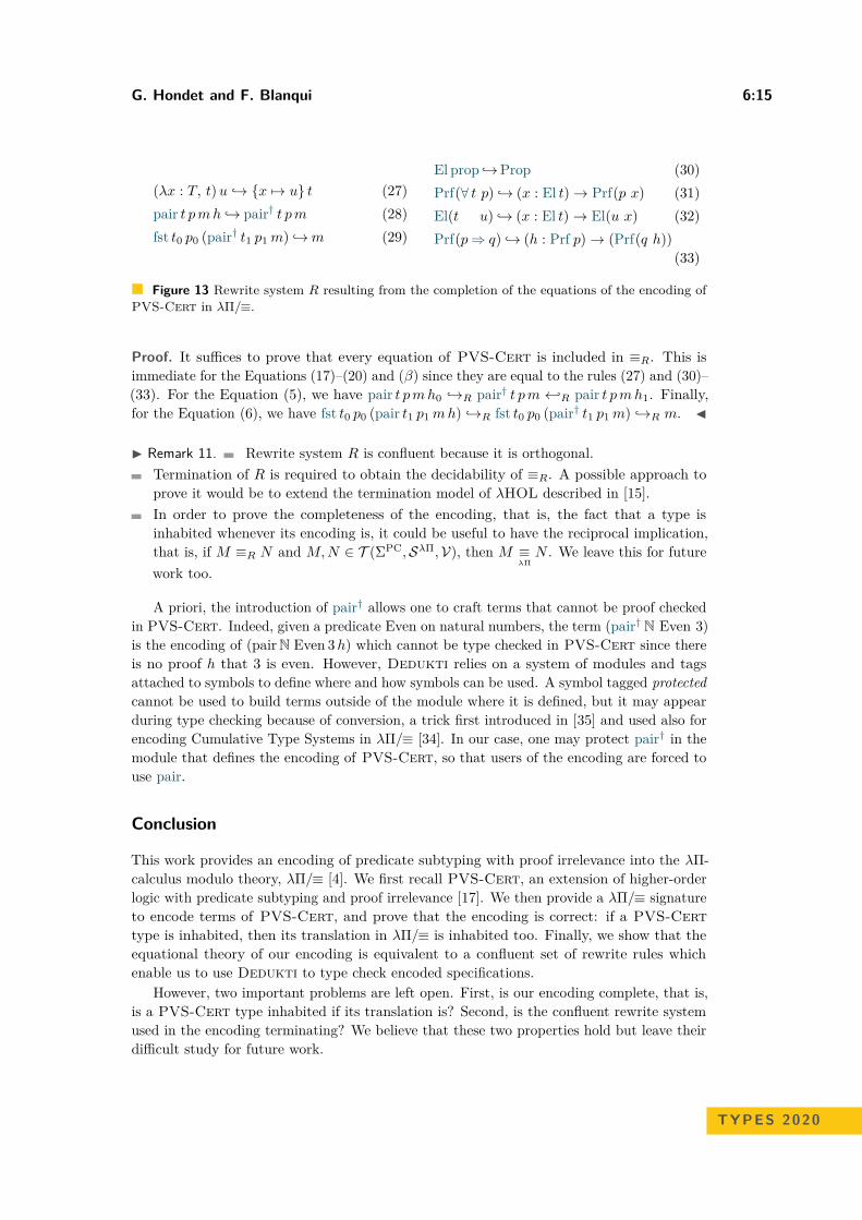
G. Hondet and F. Blanqui 6:15

(λx : T, t) u → x 7→ u t (27)pair t p m h → pair† t p m (28)fst t0 p0 (pair† t1 p1 m) →m (29)

El prop →Prop (30)Prf(∀ t p) → (x : El t)→ Prf(p x) (31)El(t u) → (x : El t)→ El(u x) (32)Prf(p⇒ q) → (h : Prf p)→ (Prf(q h))

(33)

Figure 13 Rewrite system R resulting from the completion of the equations of the encoding ofPVS-Cert in λΠ/≡.

Proof. It suffices to prove that every equation of PVS-Cert is included in ≡R. This isimmediate for the Equations (17)–(20) and (β) since they are equal to the rules (27) and (30)–(33). For the Equation (5), we have pair t p m h0 →R pair† t p m ←R pair t p m h1. Finally,for the Equation (6), we have fst t0 p0 (pair t1 p1 m h) →R fst t0 p0 (pair† t1 p1 m) →R m.

Remark 11. Rewrite system R is confluent because it is orthogonal.Termination of R is required to obtain the decidability of ≡R. A possible approach toprove it would be to extend the termination model of λHOL described in [15].In order to prove the completeness of the encoding, that is, the fact that a type isinhabited whenever its encoding is, it could be useful to have the reciprocal implication,that is, if M ≡R N and M, N ∈ T (ΣPC,SλΠ,V), then M ≡

λΠN . We leave this for future

work too.

A priori, the introduction of pair† allows one to craft terms that cannot be proof checkedin PVS-Cert. Indeed, given a predicate Even on natural numbers, the term (pair† N Even 3)is the encoding of (pairN Even 3 h) which cannot be type checked in PVS-Cert since thereis no proof h that 3 is even. However, Dedukti relies on a system of modules and tagsattached to symbols to define where and how symbols can be used. A symbol tagged protectedcannot be used to build terms outside of the module where it is defined, but it may appearduring type checking because of conversion, a trick first introduced in [35] and used also forencoding Cumulative Type Systems in λΠ/≡ [34]. In our case, one may protect pair† in themodule that defines the encoding of PVS-Cert, so that users of the encoding are forced touse pair.

Conclusion

This work provides an encoding of predicate subtyping with proof irrelevance into the λΠ-calculus modulo theory, λΠ/≡ [4]. We first recall PVS-Cert, an extension of higher-orderlogic with predicate subtyping and proof irrelevance [17]. We then provide a λΠ/≡ signatureto encode terms of PVS-Cert, and prove that the encoding is correct: if a PVS-Certtype is inhabited, then its translation in λΠ/≡ is inhabited too. Finally, we show that theequational theory of our encoding is equivalent to a confluent set of rewrite rules whichenable us to use Dedukti to type check encoded specifications.

However, two important problems are left open. First, is our encoding complete, that is,is a PVS-Cert type inhabited if its translation is? Second, is the confluent rewrite systemused in the encoding terminating? We believe that these two properties hold but leave theirdifficult study for future work.

TYPES 2020

6:16 Predicate Subtyping with Proof Irrelevance in λΠ/≡

Perspectives

The encoding of PVS-Cert in λΠ/R is the stepping stone towards an automatic translatorfrom PVS to Dedukti. Indeed, PVS does not have proof terms in its syntax, and con-sequently type checking is undecidable. The creation of PVS-Cert allows to convert PVSterms to a syntax whose type checking is decidable. This was the work of F. Gilbert in [17].Now we are able to express this decidable syntax in λΠ/R and hence in Dedukti. However,the type system proposed here only allows to coerce from a type to its direct supertype ora subtype, that is, we can go from (psub (psub ι P ) Q) to psub ι P in one coercion, but wecannot coerce from (psub (psub ι P ) Q) to ι, whereas PVS can. Consequently, an algorithmto elaborate the correct sequence of coercions is needed to obtain terms that can be typechecked in Dedukti.

Other features of PVS can be integrated into PVS-Cert and the encoding: dependenttypes like (psub list (λℓ, length ℓ = n)), recursive definitions of functions, and dependentrecords. With those features encoded, almost all the standard library5 of PVS can betranslated to Dedukti.

Finally, while the previous points were concerned with the translation of specificationsfrom PVS, we may also want to translate proofs developed in PVS. These proofs are witnessesof type correctness conditions (TCC), which are required to type check terms. Since PVS isa highly automated prover, proof terms often come from application of complex tactics thatcannot be mimicked into Dedukti. However, proof terms may either be provided by hand,emulating the interaction provided by TCC’s, or we may call external solvers [19].

References1 Andreas Abel, Thierry Coquand, and Miguel Pagano. A modular type-checking algorithm for

type theory with singleton types and proof irrelevance. Log. Methods Comput. Sci., 7(2), 2011.doi:10.2168/LMCS-7(2:4)2011.

2 Andrea Asperti, Wilmer Ricciotti, and Claudio Sacerdoti Coen. Matita tutorial. J. Formaliz.Reason., 7(2):91–199, 2014. doi:10.6092/issn.1972-5787/4651.

3 A. Assaf. A framework for defining computational higher-order logics. PhD thesis, ÉcolePolytechnique, France, 2015. URL: https://tel.archives-ouvertes.fr/tel-01235303/.

4 A. Assaf, G. Burel, R. Cauderlier, D. Delahaye, G. Dowek, C. Dubois, F. Gilbert, P. Hal-magrand, O. Hermant, and R. Saillard. Dedukti: a logical framework based on the λπ-calculusmodulo theory, 2019. Draft. URL: http://lsv.fr/~dowek/Publi/expressing.pdf.

5 Ali Assaf and Guillaume Burel. Translating HOL to dedukti. In Cezary Kaliszyk and AndreiPaskevich, editors, Proceedings Fourth Workshop on Proof eXchange for Theorem Proving,PxTP 2015, Berlin, Germany, August 2-3, 2015, volume 186 of EPTCS, pages 74–88, 2015.doi:10.4204/EPTCS.186.8.

6 Franz Baader and Tobias Nipkow. Term rewriting and all that. Cambridge University Press,1998.

7 Henk Barendregt and Kees Hemerik. Types in Lambda Calculi and Programming Languages.In Neil D. Jones, editor, ESOP’90, 3rd European Symposium on Programming, Copenhagen,Denmark, May 15-18, 1990, Proceedings, volume 432 of Lecture Notes in Computer Science,pages 1–35. Springer, 1990. doi:10.1007/3-540-52592-0_53.

8 F. Blanqui. Théorie des types et récriture. PhD thesis, Université Paris-Sud, France, 2001.URL: http://tel.archives-ouvertes.fr/tel-00105522.

5 http://www.cs.rug.nl/~grl/ar06/prelude.html

G. Hondet and F. Blanqui 6:17

9 Frédéric Blanqui. Definitions by rewriting in the calculus of constructions. MathematicalStructures in Computer Science, 15(1), 2005. doi:10.1017/S0960129504004426.

10 M. Boespflug and G. Burel. CoqInE: translating the calculus of inductive constructionsinto the lambda-Pi-calculus modulo. In Proceedings of the 2nd International Workshopon Proof eXchange for Theorem Proving, CEUR Workshop Proceedings 878, 2012. URL:http://ceur-ws.org/Vol-878/paper3.pdf.

11 Robert L. Constable, Stuart F. Allen, Mark Bromley, Rance Cleaveland, J. F. Cremer, R. W.Harper, Douglas J. Howe, Todd B. Knoblock, N. P. Mendler, Prakash Panangaden, James T.Sasaki, and Scott F. Smith. Implementing mathematics with the Nuprl proof developmentsystem. Prentice Hall, 1986. URL: http://dl.acm.org/citation.cfm?id=10510.

12 D. Cousineau and G. Dowek. Embedding pure type systems in the lambda-Pi-calculus modulo.In Proceedings of the 8th International Conference on Typed Lambda Calculi and Applications,Lecture Notes in Computer Science 4583, 2007. doi:10.1007/978-3-540-73228-0_9.

13 N.G. de Bruijn. Some Extensions of Automath: The AUT-4 Family. In R.P. Nederpelt,J.H. Geuvers, and R.C. de Vrijer, editors, Selected Papers on Automath, volume 133 ofStudies in Logic and the Foundations of Mathematics, pages 283–288. Elsevier, 1994. doi:10.1016/S0049-237X(08)70209-X.

14 Leonardo Mendonça de Moura, Soonho Kong, Jeremy Avigad, Floris van Doorn, and Jakob vonRaumer. The lean theorem prover (system description). In Amy P. Felty and Aart Middeldorp,editors, Automated Deduction - CADE-25 - 25th International Conference on AutomatedDeduction, Berlin, Germany, August 1-7, 2015, Proceedings, volume 9195 of Lecture Notes inComputer Science, pages 378–388. Springer, 2015. doi:10.1007/978-3-319-21401-6_26.

15 Gilles Dowek. Models and termination of proof reduction in the lambda pi-calculus modulotheory. In Ioannis Chatzigiannakis, Piotr Indyk, Fabian Kuhn, and Anca Muscholl, editors,44th International Colloquium on Automata, Languages, and Programming, ICALP 2017, July10-14, 2017, Warsaw, Poland, volume 80 of LIPIcs, pages 109:1–109:14. Schloss Dagstuhl -Leibniz-Zentrum für Informatik, 2017. doi:10.4230/LIPIcs.ICALP.2017.109.

16 G. Genestier. ncoding agda programs using rewriting. In Proceedings of the 5th InternationalConference on Formal Structures for Computation and Deduction, Leibniz InternationalProceedings in Informatics 167, 2020. doi:10.4230/LIPIcs.FSCD.2020.31.

17 Frederic Gilbert. Extending higher-order logic with predicate subtyping : application to PVS.Theses, Université Sorbonne Paris Cité, 2018. URL: https://tel.archives-ouvertes.fr/tel-02058937.

18 Gaëtan Gilbert, Jesper Cockx, Matthieu Sozeau, and Nicolas Tabareau. Definitional proof-irrelevance without k. Proc. ACM Program. Lang., 3(POPL), 2019. doi:10.1145/3290316.

19 Mohamed Yacine El Haddad, Guillaume Burel, and Frédéric Blanqui. EKSTRAKTO Atool to reconstruct dedukti proofs from TSTP files (extended abstract). In Giselle Reisand Haniel Barbosa, editors, Proceedings Sixth Workshop on Proof eXchange for TheoremProving, PxTP 2019, Natal, Brazil, August 26, 2019, volume 301 of EPTCS, pages 27–35,2019. doi:10.4204/EPTCS.301.5.

20 Joe Hurd. Predicate subtyping with predicate sets. In Richard J. Boulton and Paul B. Jackson,editors, Theorem Proving in Higher Order Logics, 14th International Conference, TPHOLs2001, Edinburgh, Scotland, UK, September 3-6, 2001, Proceedings, volume 2152 of LectureNotes in Computer Science, pages 265–280. Springer, 2001. doi:10.1007/3-540-44755-5_19.

21 Matt Kaufmann and J. Strother Moore. An industrial strength theorem prover for a logic basedon common lisp. IEEE Trans. Software Eng., 23(4):203–213, 1997. doi:10.1109/32.588534.

22 Jan Willem Klop, Vincent van Oostrom, and Femke van Raamsdonk. Combinatory reductionsystems: Introduction and survey. Theor. Comput. Sci., 121(1&2):279–308, 1993. doi:10.1016/0304-3975(93)90091-7.

23 D. Knuth and P. Bendix. Simple word problems in universal algebras. In Automation ofReasoning. Symbolic Computation (Artificial Intelligence). Springer, 1983.

TYPES 2020

6:18 Predicate Subtyping with Proof Irrelevance in λΠ/≡

24 William Lovas and Frank Pfenning. Refinement types for logical frameworks and theirinterpretation as proof irrelevance. Log. Methods Comput. Sci., 6(4), 2010. doi:10.2168/LMCS-6(4:5)2010.

25 Zhaohui Luo. An extended calculus of constructions. PhD thesis, University of Edinburgh,UK, 1990. URL: http://hdl.handle.net/1842/12487.

26 S. Owre, N. Shankar, J. M. Rushby, and D. W. J. Stringer-Calvert. PVS Language Reference.Computer Science Laboratory, SRI International, Menlo Park, CA, 1999.

27 Sam Owre, John Rushby, N. Shankar, and David Stringer-Calvert. PVS: an experience report.In Dieter Hutter, Werner Stephan, Paolo Traverso, and Markus Ullman, editors, AppliedFormal Methods—FM-Trends 98, volume 1641 of Lecture Notes in Computer Science, pages338–345, Boppard, Germany, October 1998. Springer-Verlag. URL: http://www.csl.sri.com/papers/fmtrends98/.

28 Sam Owre and Natarajan Shankar. The formal semantics of PVS. Technical Report SRI-CSL-97-2, Computer Science Laboratory, SRI International, Menlo Park, CA, 1997.

29 Frank Pfenning. Intensionality, extensionality, and proof irrelevance in modal type theory.In 16th Annual IEEE Symposium on Logic in Computer Science, Boston, Massachusetts,USA, June 16-19, 2001, Proceedings, pages 221–230. IEEE Computer Society, 2001. doi:10.1109/LICS.2001.932499.

30 John M. Rushby, Sam Owre, and Natarajan Shankar. Subtypes for specifications: Predicatesubtyping in PVS. IEEE Trans. Software Eng., 24(9):709–720, 1998. doi:10.1109/32.713327.

31 Anne Salvesen and Jan M. Smith. The strength of the subset type in martin-löf’s typetheory. In Proceedings of the Third Annual Symposium on Logic in Computer Science (LICS’88), Edinburgh, Scotland, UK, July 5-8, 1988, pages 384–391. IEEE Computer Society, 1988.doi:10.1109/LICS.1988.5135.

32 Matthieu Sozeau. Subset coercions in coq. In Thorsten Altenkirch and Conor McBride, editors,Types for Proofs and Programs, International Workshop, TYPES 2006, Nottingham, UK, April18-21, 2006, Revised Selected Papers, volume 4502 of Lecture Notes in Computer Science,pages 237–252. Springer, 2006. doi:10.1007/978-3-540-74464-1_16.

33 The Agda Team. Agda Manual. URL: https://agda.readthedocs.io/.34 F. Thiré. Interoperability between proof systems using the Dedukti logical framework. PhD

thesis, Université Paris-Saclay, France, 2020.35 F. Thiré and G. Férey. Proof irrelevance and predicate subtyping in dedukti. https://eutypes.

cs.ru.nl/eutypes_pmwiki/uploads/Main/books-of-abstracts-TYPES2019.pdf, p. 106,2019. Abstract of a talk given at the TYPES conference.

36 Benjamin Werner. On the strength of proof-irrelevant type theories. Log. Methods Comput.Sci., 4(3), 2008. doi:10.2168/LMCS-4(3:13)2008.

Λ-Symsym: An Interactive Tool for Playing withInvolutions and TypesFurio Honsell !

University of Udine, Italy

Marina Lenisa !

University of Udine, Italy

Ivan Scagnetto !

University of Udine, Italy

AbstractWe present the web portal Λ-symsym, available at http://158.110.146.197:31780/automata/,for experimenting with game semantics of λ!-calculus, and its normalizing elementary sub-calculus,the λEAL-calculus. The λ!-calculus is a generalization of the λ-calculus obtained by introducing amodal operator !, giving rise to a pattern β-reduction. Its sub-calculus corresponds to an applicativelyclosed class of terms normalizing in an elementary number of steps, in which all elementary functionscan be encoded. The game model which we consider is the Geometry of Interaction model Iintroduced by Abramsky to study reversible computations, consisting of partial involutions over avery simple language of moves.

Given a λ!- or a λEAL-term, M , Λ-symsym provides:an abstraction algorithm A!, for compiling M into a term, A!(M), of the linear combinatorylogic CL!, or the normalizing combinatory logic CLEAL;an interpretation algorithm [[ ]]I yielding a specification of the partial involution [[A!(M)]]I inthe model I;an algorithm, I2T , for synthesizing from [[A!(M)]]I a type, I2T ([[A!(M)]]I), in a multimodal,intersection type assignment discipline, ⊢!.an algorithm, T 2I, for synthesizing a specification of a partial involution from a type in ⊢!,which is an inverse to the former.

We conjecture that ⊢! M : I2T ([[A!(M)]]I). Λ-symsym permits to investigate experimentally thefine structure of I, and hence the game semantics of the λ!- and λEAL-calculi. For instance, we caneasily verify that the model I is a λ!-algebra in the case of strictly linear λ-terms, by checking allthe necessary equations, and find counterexamples in the general case.

We make this tool available for readers interested to play with games (-semantics). The paperbuilds on earlier work by the authors, the type system being an improvement.

2012 ACM Subject Classification Theory of computation → Linear logic

Keywords and phrases game semantics, lambda calculus, involutions, linear logic, implicit computa-tional complexity

Digital Object Identifier 10.4230/LIPIcs.TYPES.2020.7

Supplementary Material Software (Tool): http://158.110.146.197:31780/automata/

Acknowledgements The authors would like to thank the anonymous referees for their helpfulcomments.

1 Introduction

We present the web portal Λ-symsym, available at http://158.110.146.197:31780/automata/, for experimenting, in the spirit of [24], with the game semantics of the λ!-calculus,and its normalizing elementary affine sub-calculus, the λEAL-calculus. The λ!-calculus isa generalization of the λ-calculus obtained by introducing a co-monadic modal operator !,which gives rise to a pattern β-reduction. Its sub-calculus corresponds to an applicativelyclosed class of terms normalizing in an elementary number of steps. All elementary functions

© Furio Honsell, Marina Lenisa, and Ivan Scagnetto;licensed under Creative Commons License CC-BY 4.0

26th International Conference on Types for Proofs and Programs (TYPES 2020).Editors: Ugo de’Liguoro, Stefano Berardi, and Thorsten Altenkirch; Article No. 7; pp. 7:1–7:18

Leibniz International Proceedings in InformaticsSchloss Dagstuhl – Leibniz-Zentrum für Informatik, Dagstuhl Publishing, Germany

7:2 Λ-Symsym

can be encoded in the λEAL-calculus, cf [20, 6]. The game model that we consider consistsof partial involutions, i.e. partial symmetric functions. These were introduced by Abramskyin [3] to provide a Geometry of Interaction model, I, of reversible computation for linearcombinatory logic, see also [4, 5].

In a series of papers by the authors, [12, 10, 11, 18], we have explored and extendedAbramsky’s model I. In particular, we have introduced:

a generalized co-monadic λ-calculus, the λ!-calculus, which subsumes also the elementaryaffine and linear affine calculi [26, 7, 6, 15, 16];abstraction algorithms for compiling the above calculi in corresponding fragments of anextended linear combinatory logic, CL! or the normalizing CLEAL;a semantics of these combinatory logics in terms of partial involutions, and hence asemantics of the λ!-calculus via the abstraction algorithm;a multi-modal intersection type systems ⊢! for the λ!-calculus;an algorithm T 2I for obtaining a specification of a partial involution, given a type in thelanguage of ⊢!, and an algorithm I2T for synthesizing a type given a specification of apartial involution, which are “morally” mutual inverses.

Moreover, we have shown that linear application between involutions, i.e. the gameanalogue of Girard’s “Execution Formula”, amounts to a kind of resolution between types in⊢!. In particular, in the case of strictly linear terms M, N , we have that I2T ([[MN ]]I) =I2T ([[M ]]I · [[N ]]I) = Res(I2T ([[M ]]I), I2T ([[N ]]I)), [12]. In this perspective, types derivingfrom I2T can be viewed as a kind of principal types for terms in the λ!-calculus.

In this paper, we outline the implementation of the algorithms above and present the on-line tool Λ-symsym1 for experimenting with them in a user-friendly interactive setting, thusallowing for the investigation of the fine structure and the peculiarities of the symmetric gamesemantics of λ!-calculus. The sheer combinatorial complexity of applying linear applicationby hand, in effect, makes it essential to use a machine for checking equalities and findingcounterexamples.

Λ-symsym easily provides evidence for the following facts.The model I of partial involutions does not satisfy any form of the ξ-rule, if the termsinvolved are not strictly linear. Namely, we can check all the necessary equations for I tobe a λ!-algebra in the strictly linear case and provide counterexamples otherwise.Partial involutions keep track of the history of the execution, such as the erasures ofarguments or the comonad !.

In particular, given a normalizing λ!-term, or a λEAL-term, M , the web tool provides a webapplication for compiling M into a term of linear combinatory logic, A!(M) or AEAL(M),respectively. Another web application provides the interpretation of A!(M) as a specification,[[A!(M)]]I , of a partial involution over a very simple language of moves, in the model I of [3].Yet another application permits to synthesize from [[A!(M)]]I a type, I2T ([[A!(M)]]I), in amultimodal, intersection type discipline. The type assignment system is given in the formof a general type system ⊢!, for which we conjecture that ⊢! M : I2T ([[A!(M)]]I). In thispaper we do not discuss the other web applications made available by the tool Λ-symsymfor dealing with the other λ!-calculi of [18], and non normalizing terms.

We wrote this paper to encourage interested readers to enjoy utilizing Λ-symsym. Wemade it available for people to play with games (-semantics)!

1 We combine Λ to the magic word of the formula Open Sesame, (iftah ya symsym), in the

Arab collection of novels 1001 Nights, (kitab alf laylah wa-laylah), which reminds thatour semantics are symmetric partial functions.

F. Honsell, M. Lenisa, and I. Scagnetto 7:3

Synopsis. In Section 2, we introduce in a self-contained format the formal systems usedin the web tool, namely the λ!-calculus, and the λEAL-calculus, the linear combinatorylogics CL! and CLEAL, !-intersection-types, and the ⊢! type discipline. In Subsection 2.1 wegive the corresponding abstraction algorithms. In Section 3, we present the game theoreticsemantics of the linear combinatory logic CL!, and hence of its normalizing sublogic CLEAL,in terms of partial involutions. We introduce also the crucial concept of specification of aninvolution. In Subsection 3.1, we present the two algorithms I2T and T 2I, for mappingspecifications of partial involutions into types and back. In Section 4, we illustrate the webtool Λ-symsym and present its web interface. In Subsection 4.2 we discuss remarkableexample sessions. Finally, in Section 5, we draw some conclusions and outline future directions.In the Appendix A, we give the Erlang code corresponding to the implementation of linearapplication of involutions. The complete code of our web tool is available in [13].

2 The λ!-calculus, Linear Combinatory Logic, !-intersection-types

In this section we recall the formal systems used in the web tool. Most of these appearalready in earlier papers by the authors, see [12, 10, 11, 18], but for the definition of the typeassignment system ⊢!.

We start with the λ!-calculus and its sub-calculus.

Definition 1 (λ!-calculus, λEAL-calculus).The language Λ! of the λ!-calculus is inductively defined from variables x, y, z, . . . andconstants c, . . ., and it is closed under the following formation rules:

M ∈ Λ! N ∈ Λ!

MN ∈ Λ! (app) M ∈ Λ!

!M ∈ Λ! (!)

M ∈ Λ! O!≤1(x, M)

λx.M ∈ Λ! (λ) M ∈ Λ! O≥1(x, M)λ!x.M ∈ Λ! (λ!)

where FV (M) denotes the set of free variables of M , and O#? (x, M) (O#

? (M)), for #denoting either ! or blank, and ? denoting ≤ 1 or ≥ 1 or no constraint, means that thevariable x (the free variables of M) appears at most once (≤ 1) or at least once (≥ 1) inM , respectively, and, when # is not blank, that it cannot appear in the scope of !.We denote by ≡ syntactical identity on λ-terms.The language ΛEAL of the λEAL-calculus is the restriction of Λ! obtained by consideringrules (app), (λ), and the following versions of the rules (λ!) and (!):

M ∈ ΛEAL O≥1(x, M) x is in the scope of a single !λ!x.M ∈ ΛEAL

M ∈ ΛEAL O!(M)!M ∈ ΛEAL

The reduction rules of the λ!-calculus include the restrictions of the standard (β)-rule and(ξ)-rule to linear abstractions, the pattern-β-reduction rule, which define the behaviourof the ! pattern abstraction operator, the corresponding (str !) structural rule, and the (ξ!)rule, namely:

(β) (λx.M)N →! M [N/x] (β!) (λ!x.M)!N →! M [N/x]

(ξ) M →! N λx.M ∈ Λ!

λx.M →! λx.N(ξ!) M →! N λ!x.M ∈ Λ!

λ!x.M →! λ!x.N(str !) M →! N

!M →!!N

(applL) M1 →! M ′1

M1M2 →! M ′1M2

(applR) M2 →! M ′2

M1M2 →! M1M ′2

We denote by →∗! the reflexive and transitive closure of →!.

The reduction rules of the λEAL-calculus are the restrictions of the rules of the λ!-calculusto ΛEAL-terms. We denote by →EAL the corresponding reduction relation.

TYPES 2020

7:4 Λ-Symsym

We define strong normal forms as the irreducible terms which do not contain stuck redexes,i.e. subterms of the shape (!M)N or (λ!x.M)P , where P is irreducible and not a !-term.

Definition 2 (Strong Normal Forms). The set SN ! of strong normal forms is inductivelydefined as follows:

Mi ∈ SN ! ∀i ∈ 1, . . . , nxM1 . . . Mn ∈ SN !

M ∈ SN !

!M ∈ SN !

M ∈ SN ! λx.M ∈ Λ!

λx.M ∈ SN !M ∈ SN ! λ!x.M ∈ Λ!

λ!x.M ∈ SN !

Of course many terms containing stuck redexes are typable in the typing system ofDefinition 6 below, and receive the appropriate involution semantics, e.g. λx.(λ!y.y)x behavesas λ!x.x, but these intricacies are not worthwhile considering for the purposes of this paper.

The involution semantics of terms in Λ! and in ΛEAL will be given via a compilation inlinear combinatory logic.

Definition 3 (Linear Combinatory Logics).The language of the extended linear combinatory logic CL! consists of variables x, y, . . .,distinguished constants (combinators) B, C, I, K, W, D, δ, F, and it is closed under ap-plication and !-promotion, i.e.:

M ∈ CL! N ∈ CL!

MN ∈ CL!M ∈ CL!

!M ∈ CL!

In CL!-terms, we associate · to the left and we assume ! to have order of precedencegreater than ·. Combinators reduce according to the following pattern reduction rules:

BMNP →! M(NP ) IM →! M CMNP →! (MP )N KMN →! M

WM !N →! M !N !N δ!M →!!!M D!M →! M F!M !N →!!(MN)M →! M ′

C[M ] →! C[M ′] for any context C[ ],

where one-hole contexts are defined as usual.The language of elementary affine combinatory logic CLEAL includes only the combinatorsB, I, C, K, W, F, and is closed under the rules of application and !-promotion. Thereduction relation restricted to CLEAL is denoted by →EAL.

We use the notation Comb to denote any of the combinators in the above definition.

We recall the following proposition because it is not so immediate:

Proposition 4 (Normalization [18]). The λEAL-calculus and CLEAL linear combinatorylogic are strongly normalizing.

The type discipline introduced in this section is a refinement of the ones introduced in[10, 12, 11] and originated in the process of relating partial involutions and principal types.It amounts essentially to a multimodal intersection type discipline, which generalizes [8].

Definition 5 (Type Language). The language of types, Type!, is a two sorted languagegiven by the following grammars, where ω is a constant, and α, β, . . . and i, j, . . . are typeand index variables respectively:(Type! ∋) σ, τ ::= ω | α | . . . | σ ⊸ τ | σ

(T ype! ∋) σ, τ ::= !uσ | σ ∧ τ

u, v ::= ϵ | i | j | . . . | ⟨u, v⟩.The syntactic category σ-types isolates types whose main constructor is ! or ∧. Moreover, weconsider the equivalence relation on types ∼ induced by ω ∼ σ, for any type σ which containsonly the constant ω and no type variables.

F. Honsell, M. Lenisa, and I. Scagnetto 7:5

Definition 6 (Type System).The type system ⊢! derives judgements Γ ⊢! M : τ , where the environment Γ is a set of pairsof the following shapes: x : σ, !x : σ; each variable occurs at most once in Γ either as a linearvariable or a !-variable. dom(Γ) denotes the set of variables which appear in Γ.

Assumption rule:

x : α ⊢! x : α(Var)

Introduction and elimination rules:

Γ ⊢! M : σ i fresh!i(Γ) ⊢! !M :!iσ

(!Intro) Γ ⊢! !M :!iσ !(Γ) ⊢! M : σ[ϵ/i]

(!-Elim)

Γ1 ⊢! !M : σ Γ2 ⊢! !M : τ !(Γ1) !(Γ2)Γ1 ∧ Γ2 ⊢! !M : σ ∧ τ

(∧- Intro)

Γ ⊢! M : σ ∧ τΓ ⊢! M : σ

(∧-E-left) Γ ⊢! M : σ ∧ τΓ ⊢! M : τ

(∧-E-right)

Γ1 ⊢! M : σ ⊸ τ Γ2 ⊢! N : σ⋂

!(Γ1, Γ2)Γ1 ∧ Γ2 ⊢! MN : τ

(MP)

Γ, x : σ ⊢! M : τΓ ⊢! λx.M : σ ⊸ τ

(λ) Γ, !x : σ ⊢! M : τΓ ⊢! λ!x.M : σ ⊸ τ

(λ!)

Γ ⊢! M : σU(Γ) ⊢! M : U(σ) (Inst)

Structural-rules:

Γ ⊢! M : σ x /∈ dom(Γ)Γ, x : τ ⊢! M : σ

(weak) σ ∼ ωΓ ⊢! M : σ

(ω)

where!(Γ) means that all variables in Γ are banged (Γ is possibly empty);by a slight abuse of notation

!u(Γ, x : τ) = !u(Γ), !x : !u(τ) and

!u(τ) =!uτ if τ /∈ T ype!

!u(!vτ) =!⟨u,v⟩τ

!u(τ ∧ σ) = !u(τ) ∧ !u(σ); = , !x : τ [ϵ/i];⋂

!(Γ1, Γ2) means that each variable in the intersection of dom(Γ1) and dom(Γ2) is!-prefixed both in Γ1 and Γ2;for Γ1, Γ2 such that

⋂!(Γ1, Γ2), the environment Γ1 ∧ Γ2 is defined by:

if x : σ ∈ Γ1 or x : σ ∈ Γ2, then x : σ ∈ Γ1 ∧ Γ2if !x : σ ∈ Γ1 and x ∈ dom(Γ2), or !x : σ ∈ Γ2 and x ∈ dom(Γ1), then !x : σ ∈ Γ1 ∧ Γ2if !x : σ1 ∈ Γ1 and !x : σ2 ∈ Γ2, then !x : σ1 ∧ σ2 ∈ Γ1 ∧ Γ2;

U is a substitution, mapping type/index variables to types/indexes, respectively.

We will denote by Type!− and ⊢−! the set of types without ω and the type system without the

ω-rule, respectively.The type system ⊢EAL is obtained by giving up the rule (!-Elim) and restricting the rules of⊢! to λ-terms in ΛEAL.

Some comments and remarks on the above definitions are in order:

TYPES 2020

7:6 Λ-Symsym

The type connective ∧ is neither commutative nor idempotent nor associative.The notion of type equivalence ∼ defined above for the system of Definition 6 is a sharprestriction of the usual type equivalence on intersection types, cf. [8]. The traditionalrule does not hold in the involution model of Section 3.Not all terms of Λ! can be typed in ⊢−

! , i.e. without the ω-rule, e.g.⊢! (λ!x.x!x)(λ!x.x!x) : ω ⊢! λ!x!y.(λ!z.z)(xy) : (α ⊸ ω) → (α ⊸ ω).The former is not normalizing, while in the latter pattern matching fails and hence itdoes not have a strong normal form. Notice however that the type which can be assignedto it records the fact that the two variables can be applied. The meaningfulness of suchtypes is the reason for weakening the traditional definition of type equivalence ∼ as in thesystem of Definition 6. The issue is rather intricate and will be taken up in Section 4.2.2.Rule (Inst) could be made redundant by allowing arbitrary types in rule (Var) andarbitrary indices in rule (!Intro).One could consider also second or higher order (possibly recursive) type systems. Theirtyping strength is subsumed by the ∧-rules.

A relevant class of types is that of binary types, which, as we will see in Section 3.1, arisenaturally from specifications of partial involutions:

Definition 7.A type τ ∈ Type! is binary if each type variable appears at most twice in τ .A judgement Γ ⊢! M : τ is binary if each type variable occurs at most twice in it.

A slight modification of Theorem 30 [11] allows to prove that:

Proposition 8. If Γ ⊢! M : τ is derivable, then there exist a binary judgement Γ′ ⊢! M : τ ′

and a substitution U such that U(Γ′) = Γ and U(τ ′) = τ .

2.1 Abstraction AlgorithmThe abstraction algorithm for mapping terms of the λ!-calculus into the linear combinatoryalgebra CL! is a refinement of the standard abstraction algorithm, but this needs to becarefully spelled out so as to factor out as an abstraction algorithm also from λEAL toCLEAL.

Definition 9 (Abstraction Algorithms A!, AEAL).Let Λ!

CL denote the set of terms of the λ!-calculus obtained by taking combinators as theconstants of the calculus. We define A! : Λ!

CL → CL! as in Figure 1, where # denotesthe modality ! or no modality.Let ΛEAL

CL be the set of λEAL-terms obtained by taking CLEAL-combinators as constants.We define AEAL : ΛEAL

CL → CLEAL as the restriction of A! to terms in ΛEALCL .

Vice versa, we denote by ( )λ : CL! → Λ! the natural mapping of a CL-term into aλ-term obtained by replacing, in place of each combinator, the corresponding Λ!-term asfollows:

(B)λ = λxyz.x(yz) (C)λ = λxyz.(xz)y (I)λ = λx.x (K)λ = λxy.x

(W)λ = λx!y.x!y!y (D)λ = λ!x.x (δ)λ = λ!x.!!x (F)λ = λ!x!y.!(xy).The following theorem justifies the above definition. For ease of readability we will oftenuse the notation λ∗#x1 . . . #xn.M , for M ∈ CL!, to denote A!(λ#x1 . . . #xn.M), where #stands for either the modality ! or no modality (see [18] for more details).

F. Honsell, M. Lenisa, and I. Scagnetto 7:7

A!(M)

=

x if M ≡ x

Comb if M ≡ CombI if M ≡ λx.x

F(!I) if M ≡ λ!x.!xD if M ≡ λ!x.x

Kc if M ≡ λx.c

Ky if M ≡ λx.y

C(A!(λx.M1))A!(M2) if M ≡ λx.M1M2 and x ∈ F V (M1)BA!(M1)A!(λx.M2) if M ≡ λx.M1M2 and x ∈ F V (M2)K(A!(M1)A!(M2)) if M ≡ λx.M1M2 and x ∈ F V (M1M2)A!(λ#x.A!(λ#y.M1)) if M ≡ λ#x.λ#y.M1

W(B(CA!(λ!x.M1))(A!(λ!x.M2))) if M ≡ λ!x.M1M2 and x ∈ FV (M1), x ∈ FV (M2)BA!(M1)A!(λ!x.M2) if M ≡ λ!x.M1M2 and x ∈ F V (M1), x ∈ F V (M2)CA!(λ!x.M1)A!(M2) if M ≡ λ!x.M1M2 and x ∈ F V (M1), x ∈ F V (M2)F!(λx.A!(M1)) if M ≡ λ!x.!M1 and x occurs once in M1 and O!(M1)WA!(λ!y.λ!x.!M1[y/x1]) if M ≡ λ!x.!M1[x1], x occurs in M1 more than once

and x1 is the leftmost occurrence of x in M1 and O!(M1)B(F(!A!(λ!x.M1)))δ if M ≡ λ!x.!M1 and ¬O!(M1)A!(M1)A!(M2) if M = M1M2

!A!(M1) if M =!M1

F AIL otherwise

Figure 1 The Abstraction Algorithm A! : Λ!CL → CL!.

Theorem 10 (Soundness of the Abstraction Algorithms A! and AEAL).Let M ∈ CL!, let #M1, . . . , #Mn ∈ Λ!, n ≥ 0, then(λ∗#x1 . . . #xn.M)A!(#M1) . . . A!(#Mn) →∗

! M [A!(M1)/x1, . . . , A!(Mn)/xn] .

Let M ∈ CLEAL, let #M1, . . . , #Mn ∈ ΛEAL, n ≥ 0, then AEAL(M) ∈ ΛEAL andmoreover:(λ∗#x1 . . . #xn.M)AEAL(#M1) . . . AEAL(#Mn) →∗

! M [AEAL(M1)/x1, . . . , AEAL(Mn)/xn] .

The abstraction algorithm in Fig. 1 is implemented in Λ-symsym, see Section 4.

3 Game Semantics for Combinatory Logics and λ-calculi

In this section, we present the game theoretic semantics of the linear combinatory logic CL!,and hence of its sublogic CLEAL, in terms of partial involutions. Then, via the abstractionalgorithm, we obtain a game semantics for terms in Λ! and ΛEAL. Finally, we present twoalgorithms, I2T and T 2I, which relate schematic representations of partial involutions andtypes.

We start by introducing the model of partial involutions, I, originally defined by Abramskyin [3] in order to study reversible computations, and studied in [12, 11, 18]. The notion ofapplication on this model amounts to the categorical trace on a subcategory of the categoryof relations, introduced in [23] (see also [2]).

Definition 11 (The Model of Partial Involutions, I).TΣ, the language of moves, is defined by the signature Σ0= ϵ, Σ1 = l, r, Σ2 = ⟨ , ⟩(where Σi is the set of constructors of arity i); terms r(t) are output words, while termsl(t) are input words (often denoted simply by rt and lt);

TYPES 2020

7:8 Λ-Symsym

I is the set of partial involutions over TΣ, i.e. the set of all partial functions f : TΣ TΣsuch that f(t) = t′ ⇔ f(t′) = t;the operation of replication is defined by !f = (⟨t, t1⟩, ⟨t, t2⟩) | t ∈ TΣ ∧ (t1, t2) ∈ f;the notion of linear application is defined by f · g = frr ∪ (frl; g; (fll; g)∗; flr), wherefij = (t1, t2) | (i(t1), j(t2)) ∈ f, for i, j ∈ r, l (see diagram below), where “;” denotespostfix composition of relations.

in // •frr //

frl

• // out

•g // •

fll

oo

flr

OO

Proposition 12 ([3]). I is closed under !-replication and linear application.

Next we give the notion of schematic specification of the graph of a partial involution,which was introduced in [18] and recall some of its main properties. Schematic specificationsinduce a substructure of I which is still closed under application and replication, and it issufficient to interpret all combinators, see [18] for full details.

Definition 13 (Schematic Specification). Let TΣ[Var ] denote the set of terms generated bythe signature Σ \ ϵ starting from a set of variables Var , where we distinguish between termvariables x, y, . . . and index variables i, j, . . ., i.e.:(TΣ[Var ] ∋) t ::= x | y | . . . | lt | rt | ⟨u, t⟩ where u ::= ϵ | i | j | . . . | lu | ru | ⟨u, v⟩ .

A specification P of a partial involution is a (possibly infinite) irreflexive set of pairst1 ↔ t′

1, t2 ↔ t′2, . . ., where:

(i) ti, t′i ∈ TΣ[Var ];

(ii) a single pair ti ↔ t′i represents both (ti, t′

i) and (t′i, ti);

(iii) in any pair ti ↔ t′i exactly one term variable appears, once in ti and once in t′

i;(iv) for any pairs ti ↔ t′

i, tj ↔ t′j, ti is not an instance of tj.

Schematic specifications generate graphs of partial involutions as follows:

Definition 14 (G). Given a schematic specification P , the set G(P ) is the symmetricclosure of the set (U(t1), U(t2)) | (t1 ↔ t2) ∈ P ∧ U : TΣ[Var ] → TΣ.

The following lemma follows immediately from the above definitions:

Lemma 15. If P is a specification, then G(P ) is the graph of a partial involution on TΣ.

Not all partial involutions are generated by specifications, e.g. the relation rϵ ↔ lϵ istrivially not induced by any specification.

A notion of composition on specifications, which corresponds to composition on partialinvolutions can be defined as follows:

Definition 16 (Composition of Specifications). Let P, P ′ be specifications. We define

P ; P ′ = (t, t′) | ∃(t1, t2) ∈ P, (t′1, t′

2) ∈ P ′, U. (U = U(t2, t′1) ∧ t = U(t1) ∧ t′ = U(t′

2)) ,

where U(t2, t′1) is the most general unifier of t2 and t′

1.

This definition essentially amounts to composition in Clause Algebras, as in [19].The above definitions permits to define a notion of application between specifications,

P · P ′, which mimics the one between partial involutions in Definition 11.

F. Honsell, M. Lenisa, and I. Scagnetto 7:9

[[B]]I = r3x ↔ lrx , l2x ↔ rlrx , rl2x ↔ r2lx[[I]]I = lx ↔ rx[[C]]I = l2x ↔ r2lx , lrlx ↔ rlx , lr2x ↔ r3x[[K]]I = lx ↔ r2x[[F]]I = l⟨i, rx⟩ ↔ r2⟨i, x⟩ , l⟨i, lx⟩ ↔ rl⟨i, x⟩[[W]]I = r2x ↔ lr2x , l2⟨i, x⟩ ↔ rl⟨li, x⟩ , lrl⟨i, x⟩ ↔ rl⟨ri, x⟩[[δ]]I = l⟨⟨i, j⟩, x⟩ ↔ r⟨i, ⟨j, x⟩⟩[[D]]I = l⟨ϵ, x⟩ ↔ rx[[MN ]]I = [[M ]]I · [[N ]]I[[!M ]]I = ![[M ]]I

Figure 2 Game Semantics for CL!.

Lemma 17 ([18]). Let P, P ′ be specifications. Then(i) G(P ; P ′) = G(P ); G(P ′);(ii) G(P · P ′) = G(P ) · G(P ′).

One can easily check that:

Lemma 18 ([18]). The substructure of I induced by schematic specifications is closedunder application and replication.

Now we are in the position of giving the interpretation in I of CL!, by defining the schematicspecifications of the graphs of the combinators.

Definition 19 (Game Semantics of CL!). The combinatory logic CL! is interpreted in I asin Figure 2, where we use the abbreviation lnt and rnt for the terms l . . . l︸ ︷︷ ︸

n

t, and r . . . r︸ ︷︷ ︸n

t.

In following proposition for (i) see [3], for (ii) see [11].

Proposition 20.(i) I is a model of CL!, and hence of the combinatory sublogic CLEAL.(ii) I is a model of all the reduction rules of Λ!, but the ξ-rules.

Using the semantics for CL!-combinators defined in Figure 2, and the abstraction al-gorithm described in Section 2.1, one can derive the partial involution corresponding to agiven λ-term, by repeatedly applying our implementation of linear application on involutions(see Appendix A). However, not all interpretations of CL!-combinators are partial involutionswith finite specifications, since graphs of finite specifications are not closed under linearapplication. E.g. the fixed point combinator (λ∗!x!y.y!(x!y!y!x))!(λ∗!x!y.y!(x!y!y!x)) has aninfinite specification. This is taken care of in Λ-symsym by outputting the stream of pairsin the partial specification.

3.1 Correspondence Algorithms, I2T , T 2IHere we present the two algorithms, I2T and T 2I, which relate schematic representations ofpartial involutions and types in Type!. The first algorithm, given a schematic specification ofa partial involution, yields a binary type, the latter, given a binary type, provides a schematicspecification of a partial involution. The two transformations are one inverse of the anotherover suitable domains of schematic specifications and types.

TYPES 2020

7:10 Λ-Symsym

We begin by explaining how the algorithm I2T works. First of all, we need the followingbuild_type_tree( ) function, in order to build a skeleton type tree from a term t ∈ TΣ[V ar].The function definition is syntax driven:

build_type_tree(t)

=

αx if t ≡ x

build_type_tree(t′) → _ if t ≡ lt′

_ → build_type_tree(t′) if t ≡ t′

!ubuild_type_tree(t′) if τ ≡ ⟨u, t′⟩and u does not contain l/r constructors

build_type_tree(⟨u′, t′⟩) ∧ _ if t ≡ ⟨u, t′⟩ and l is the leftmost l/r constructorin u and u′ is obtained from u by erasing it

_ ∧ build_type_tree(⟨u′, t′⟩) if t ≡ ⟨u, t′⟩ and r is the leftmost l/r constructorin u and u′ is obtained from u by erasing it

where the underscore characters (_) above stand for “missing parts” of the resulting typetree. Such holes will be (hopefully) filled in by successive unifications, as explained below.

Hence, for each rule ti ↔ t′i (for i = 1, . . . , n) of a given specification, we compute the

two (partial) types build_type_tree(ti) and build_type_tree(t′i). Finally, we try to unify

all such partial types, over all rules. If we succeed, we infer a type representing the originalpartial specification; otherwise, we fail. Notice that the possible final type may still contain“holes”. E.g. partial specifications of erasing terms do not exhibit any rule for the variablewhich is erased.

Due to the peculiar syntax of types in Type!, unification of types is not a plain unificationà la Robinson. Indeed, we have subcases which may need to spawn ∧-constructors in order toinstantiate new instances of some types. For instance, a !-subtype like !uσ may need to spawnnew instances of !uσ, becoming !u′σ′∧!u′′σ′′ ∧ . . ., in order to unify against another type. Inour implementation, we implement such spawnings in order to ease the unification process asmuch as possible. At the end there can be some leftovers of those spawning activities; thus,we implement a sort of “garbage collector” which takes care of those dummy ∧’s, beforereturning the final type-candidate to the user.

Another subtle issue comes from the fact that the order in which the pairs of thespecification are processed may imply success or failure in the unification process (becausethe spawning of ∧-constructors must trigger at the right moment). Hence, we restart theprocedure until a type is found, permuting in all possible ways the pairs in the specification.

Finally, the type synthesis algorithm may fail, totally or partially. Total failure can beeasily detected, since the algorithm returns Ω, meaning that it was not able to build evena partial skeleton. On the other hand, partial failure occurs when the algorithm does notsucceed in recovering a complete type tree from the partial specification, i.e., there remainsome “holes” to be filled in. Such holes are marked by placeholders of the form Ωi, where i

is some integer index. Such Ωi’s correspond to the underscore characters generated by thebuild_type_tree() function above which have not been instantiated by the type unificationalgorithm. We could safely replace them with a plain Ω, since the type ω is a wild card, butwe do not make this choice in the web tool, see Section 4.2.2.

The other way round is dealt with by the algorithm T 2I. Here the input can be anytype and the output is a specification of a symmetric relation; if the input type is binary,then the result is the specification of a partial involution. The algorithm processes all typevariables occurring in a given type by means of the function var_type2PI, which producesa list L of partial specification terms. If the type is binary the list has at most length 2. The

F. Honsell, M. Lenisa, and I. Scagnetto 7:11

partial specification rules for that type variable are obtianed by combining in all possibleways the terms of L. Repeating this procedure for all type variables of a type, we recoverthe corresponding partial specification. We give only var_type2PI:

var_type2P I(α, τ)

=

[xα] if τ ≡ α

l(var_type2P I(α, τ ′)) + +r(var_type2P I(α, τ ′′)) if τ ≡ τ ′ → τ ′′

and α ∈ fv(τ ′), α ∈ fv(τ ′′)l(var_type2P I(α, τ ′)) if τ ≡ τ ′ → τ ′′

and α ∈ fv(τ ′) \ fv(τ ′′)r(var_type2P I(α, τ ′′)) if τ ≡ τ ′ → τ ′′

and α ∈ fv(τ ′′) \ fv(τ ′)add_index(u, var_type2P I(α,

∧n

i=1!vi τi)) if τ ≡∧n

i=1!<u,vi>τi

compose_index(l, var_type2P I(α, τ ′)) + +compose_index(r, var_type2P I(α, τ ′′)) if τ ≡ τ ′ ∧ τ ′′

and α ∈ fv(τ ′), α ∈ fv(τ ′′)and ! indices in τ have different π1’s

compose_index(l, var_type2P I(α, τ ′)) if τ ≡ τ ′ ∧ τ ′′

and α ∈ fv(τ ′) \ fv(τ ′′)and ! indices in τ have different π1’s

compose_index(r, var_type2P I(α, τ ′′)) if τ ≡ τ ′ ∧ τ ′′

and α ∈ fv(τ ′′) \ fv(τ ′)and ! indices in τ have different π1’s

add_index(u, var_type2P I(α, τ ′)) if τ ≡!uτ ′ and α ∈ fv(τ ′)[] otherwise

where:fv(τ) is the set of free variables of type τ ;in the expression τ ≡

∧ni=1 τi the right-hand side term denotes the atomic components of

τ ;++ is the list concatenation operator;the functions l() and r(), when applied to a list (i.e., the return type of var_type2PI()),distribute, respectively the l and r constructors at the head of all elements of the list, i.e.,each t ∈ L will be substituted by lt (resp. rt);compose_index(c, L) (where c is either l or r) is a function distributing the constructorc to all the pairs of the list L, i.e., each ⟨u, t⟩ ∈ L will be substituted by ⟨cu, t⟩;add_index(u, t) is a function distributing the index u to all elements of the list L, i.e.each tinL will be substituted by ⟨u, t⟩.

Notice that in dealing with types whose outermost constructor is ∧, we distinguish betweenthe cases where all atomic components have a common prefix in their !’s, denoting thatpromotions have been carried after the ∧ operations, and the cases where there is no suchcommon prefix, where the ∧-constructor was indeed the last to be used in producing the type.

It is easy to check that:

Lemma 21.1. For any specification P of a partial involution, I2T (P ) is a binary type.2. For any binary type τ , T 2I(τ) is a specification of a partial involution.

TYPES 2020

7:12 Λ-Symsym

The two transformations, I2T and T 2I, are the inverse of one another in the sense:

Conjecture 22.1. Let M ∈ Λ! be a closed term which reduces to a term in strong normal form, without the

use of the ξ-rules, then: ⊢ M : I2T ([[M ]]I) and T 2I(I2T ([[M ]]I)) = [[M ]]I .

2. Let τ be a binary type, then I2T (T 2I(τ)) = τ .When a closed term M ∈ Λ! needs the ξ-rules to reduce to strong normal form its semanticsas a partial involution does not necessarily yield an immediately meaningful type. We willdiscuss this issue further in Section 5.

Conjecture 22 applies also when we restrict to terms of ΛEAL.

4 The Web Tool Λ-symsym

In the following, we will illustrate how to use the web tool, Λ-symsym, available athttp://158.110.146.197:31780/automata/, in order to experiment with the algorithmsprovided in the previous section. We will provide excerpts from various sessions illustratinghow to convert λ!-terms to combinators, from the latter to partial involutions, and finallyto types. Moreover, we will also show how to infer a partial involution from a type. Theweb tool is implemented in the language Erlang, [17]. We chose this language because ofits rich pattern matching features, its flexible constructors such as the set data type and forthe large number of libraries which allow for a rapid prototyping. The fine details of theimplementation appear in [13]

4.1 Encoding λ-terms, partial involutions and typesFirst we give the syntax representation; the following tables contain the correspondencesbetween the syntax we use with “pencil and paper”, the actual input syntax and the internalrepresentation used by our algorithms.

λ-termsOn the paper Input syntax Internal representationx X var, "X"C C comb, CMN M@N lapp, M, Nλx.M l*X.M abs, var, "X", Mλ!x.M l*!X.M abs_b, var, "X", M!M !M bang, M

Partial InvolutionsOn the paper Input syntax Internal representationϵ e ex X var, "X"lM lM l, MrM rM r, M⟨M, N⟩ <M,N> p, M, NM ↔ N M <-> N [M,N,N,M]

TypesOn the paper Input syntax Internal representationα A var, "A"α −→ β A -> B map, A, Bα ∧ β A /\ B cap, A, B!iα !I M bang, I, M

F. Honsell, M. Lenisa, and I. Scagnetto 7:13

Figure 3 The interface of the web tool.

4.1.1 The web interfaceFigure 3 depicts the web interface we can use to call the algorithms. It has 4 components:1. a green drop-down menu allowing the user to choose the function to execute (e.g.,

lambda2type() in the general setting, as it appears in Figure 3); it provides a number offunctions for the general case, Λ! and for the ΛEAL case, namely:

(i) the function lambda2type() which given a term produces its combinatory logictranslation, its semantics as a specification of a partial involution, and the typecorresponding to the specification;

(ii) the function show_partial_involution which produces a specification of a partialinvolution, given a type;

(iii) the function show_type which yields a type given a partial involution;(iv) more functions which have not been discussed in this paper for dealing with polyno-

mial terms, and Hindley-Milner Types;2. a text area where the user can write the argument to pass to the selected function;3. another text area where the result will appear after clicking the button “Compute”;4. a red button (“Compute”) to start the computation.

4.2 Sessions4.2.1 Strictly Linear Combinators in I are a λ-algebraOne can see that the partial involutions corresponding to the two terms in input are equal.This is one of the many equations which need to be checked to show that the ξ rule holds.

Input:l*X.l*Y.l*Z.X@(Y@Z)Combinators abstraction:((C((BB)((BB)I)))((C((BB)I))I))Partial involution rules:--- begin ---l(r(_X7)) <-> r(r(r(_X7)))l(l(_X7)) <-> r(l(r(_X7)))r(l(l(_X7))) <-> r(r(l(_X7)))--- end ---Principal type:((_X10 -> _X9) -> ((_X8 -> _X10) -> (_X8 -> _X9)))

Input:BPartial involution rules:--- begin ---r(r(r(_X1))) <-> l(r(_X1))l(l(_X1)) <-> r(l(r(_X1)))r(l(l(_X1))) <-> r(r(l(_X1)))--- end ---Principal type:((_X4 -> _X3) -> ((_X2 -> _X4) -> (_X2 -> _X3)))

4.2.2 The ξ-rule fails for erasersThe following example shows that the ξ-rule fails in I when terms erase variables. Thesession on the right hand side shows that erased subterms might still leave an echo in thepartial involution. This is the reason why we have not taken the standard ω-equivalence

TYPES 2020

7:14 Λ-Symsym

as for intersection types. Please bear in mind that, when an inferred type features some_Omegai variables (for i=1,2,3...), these variables stand for placeholders for any type.They are “holes” in the type tree structure which arise since partial involutions do notprovide unnecessary information.

Input:l*X.l*Y.((l*Z.I)@(X@Y))Combinators abstraction:((B(B(KI)))((C((BB)I))I))Partial involution rules:--- begin ---r(r(l(_X4))) <-> r(r(r(_X4)))l(l(_X4)) <-> r(l(_X4))--- end ---Principal type:((_X5 -> _Omega3) -> (_X5 -> (_X6 -> _X6)))

Input:l*X.l*Y.l*Z.ZCombinators abstraction:(K(KI))Partial involution rules:--- begin ---r(r(l(_X2))) <-> r(r(r(_X2)))--- end ---Principal type:(_Omega1 -> (_Omega2 -> (_X3 -> _X3)))

4.2.3 The ξ-rule fails when modalities are erasedAs was the case in the above example, also in this case there remains an echo in the partialinvolution when modalities are erased.

Input:l*!X.D@!XCombinators abstraction:((BD)(F!(I)))Partial involution rules:--- begin ---l(<e, _X1>) <-> r(_X1)--- end ---Principal type:((!e _X2) -> _X2)

Input:l*!X.D@!(D@!X)Combinators abstraction:((BD)((B(F!(((BD)(F!(I))))))d))Partial involution rules:--- begin ---l(<<e, e>, _X1>) <-> r(_X1)--- end ---Principal type:((!<e, e> _X2) -> _X2)

4.2.4 The ξ-rule fails in generalThe following sessions illustrate that the ξ-rule fails in the encoding of standard λ-calculusvia application in the Kleisli category. This issue will be briefly discussed in Section 5.

Input:l*!X.(l*!Y.Y@!Y)@!(X@!X)Combinators abstraction:((B(W((C((BB)D))(F!(I)))))((B(F!((W((C((BB)D))(F!(I)))))))d))Partial involution rules:--- begin ---l(<<l(e), l(e)>, r(r(_X15))>) <-> r(_X15)l(<<_X15, l(e)>, l(<_X16, _X17>)>) <-> l(<<_X15, r(_X16)>, _X17>)l(<<l(e), l(e)>, r(l(<_X15, _X16>))>) <-> l(<<r(_X15), l(e)>, r(_X16)>)--- end ---Principal type:(((!<e, e> (_Omega6 -> ((!_X17 _X18) -> _X21))) /\ (!<_X22, e> ((!_X19 _X20) -> _Omega10))) /\

/\ (((!<_X22, _X19> _X20) /\ (!<_X17, e> (_Omega4 -> _X18))) /\/\(!<_X22, e> ((!_X19 _X20) -> _Omega10))))

-> _X21

but

Input:l*!X.X@!X@!(X@!X)Combinators abstraction:(W((C((BB)(W((C((BB)D))(F!(I))))))((B(F!((W((C((BB)D))(F!(I)))))))d)))Partial involution rules:--- begin ---r(_X14) <-> l(<l(l(e)), r(r(_X14))>)l(<l(l(e)), l(<_X14, _X15>)>) <-> l(<l(r(_X14)), _X15>)l(<l(l(e)), r(l(<_X14, _X15>))>) <-> l(<r(<_X14, l(e)>), r(_X15)>)l(<r(<_X14, l(e)>), l(<_X15, _X16>)>) <-> l(<r(<_X14, r(_X15)>), _X16>)--- end ---Principal type:(((!e ((!_X20 _X21) -> ((!_X17 _X23) -> _X24))) /\ (!_X20 _X21))/\

/\ ((!<_X17, e> ((!_X18 _X19) -> _X23)) /\ (!<_X17, _X18> _X19))) -> _X24

F. Honsell, M. Lenisa, and I. Scagnetto 7:15

4.2.5 Church Binary Words in the λEAL-calculusThis is the encoding of Church binary word < 0, 0, 1 > as would appear in [6].

Input:l*!X.l*!Y.!(l*Z.X@(X@(Y@Z)))Combinators abstraction:((BF)(W((BF)(F!(((C((BB)((BB)((BB)I))))((C((BB)((BB)I)))((C((BB)I))I))))))))Partial involution rules:--- begin ---l(<l(_X9), r(_X10)>) <-> r(r(<_X9, r(_X10)>))l(<l(_X9), l(_X10)>) <-> l(<r(_X9), r(_X10)>)l(<r(_X9), l(_X10)>) <-> r(l(<_X9, r(_X10)>))r(r(<_X9, l(_X10)>)) <-> r(l(<_X9, l(_X10)>))--- end ---Principal type:(((!_X11 (_X15 -> _X14)) /\ (!_X11 (_X16 -> _X15))) -> ((!_X11 (_X12 -> _X16)) -> (!_X11 (_X12 -> _X14))))

5 Final Remarks

In this paper we have introduced the web tool Λ-symsym which implements variousalgorithms for computing the game semantics, in terms of involutions, of λ!- and λEAL-termsand their types. Using Λ-symsym we have uncovered many peculiarities of game semantics.The fact that in Abramsky’s model, I, the ξ-rule fails in the general case, but not in thestrictly linear case is perhaps the most remarkable one. Actually the portal Λ-symsymmakes available algorithms, similar to the ones introduced in this paper, for dealing withthe λLAL-calculus, introduced by the authors in [18], which captures in our frameworkthe polynomial calculi underpinning Light Linear Logic, cf [20, 26]. Furthermore, partialinvolutions easily generalize to symmetric partial relations, see [18]. In this broader settingone can model ML-types. Λ-symsym provides algorithms also for this case.

We list, in a cursory manner, a number of intriguing issues deserving future attention.There is a plausible duality between types in ⊢! and partial involutions, which shouldbuild up to a framework such as the one in [14, 1] for domain theory and intersectiontypes, cf [9].Conjecture 22 appears to be very difficult to prove in full generality. A proof shouldrelate two dual alternative ways of carrying out unification. In analogy to Abramsky’sterminology, we could call the wave-style traditional unification and the particle-styleunification, which goes on when linearly applying two specifications of involutions.The failure of the ξ-rule in the model I uncovers the fact that sometimes, rather thancomputing the most general unifier between the corresponding types, linear applicationof partial involutions stops short of that and just computes some sort of least generalancestor of the type. This has not been fully appreciated yet. In this respect, exploringthe connections of the present work with Girard’s Clause Algebras and the ExecutionFormula as in [19] should prove fruitful.The λ!-calculus is worthwhile investigating per se, but many well established notions needto be generalized, most notably normal forms, because of stuck terms. The paper [21]should provide some suggestions.J.-Y. Girard in [20] introduced a polynomial time set-theory, which bears some relationto the one of Fitch as presented in [25], which we have studied in [22]. The experiencegathered with λLAL-calculus should improve our understanding of its applicability.

In conclusion we think that the fine structure of game semantics of the λ-calculus needsmore investigation. This could be quite rewarding, provided more concrete experiments arecarried out. Λ-symsym is our contribution to making them a little more feasible.

TYPES 2020

7:16 Λ-Symsym

References1 Samson Abramsky. Domain theory in logical form. Annals of Pure and Applied Logic,

51(1):1–77, 1991. doi:10.1016/0168-0072(91)90065-T.2 Samson Abramsky. Retracing some paths in process algebra. In Ugo Montanari and Vladimiro

Sassone, editors, CONCUR ’96: Concurrency Theory, pages 1–17, Berlin, Heidelberg, 1996.Springer Berlin Heidelberg.

3 Samson Abramsky. A structural approach to reversible computation. Theoretical ComputerScience, 347(3):441–464, 2005. doi:10.1016/j.tcs.2005.07.002.

4 Samson Abramsky, Esfandiar Haghverdi, and Philip Scott. Geometry of interaction and linearcombinatory algebras. Mathematical Structures in Computer Science, 12(5):625–665, 2002.

5 Samson Abramsky and Marina Lenisa. Linear realizability and full completeness for typedlambda-calculi. Annals of Pure and Applied Logic, 134(2):122–168, 2005. doi:10.1016/j.apal.2004.08.003.

6 Patrick Baillot, Erika De Benedetti, and Simona Ronchi Della Rocca. Characterizing Polyno-mial and Exponential Complexity Classes in Elementary Lambda-Calculus. In Josep Diaz,Ivan Lanese, and Davide Sangiorgi, editors, Theoretical Computer Science, pages 151–163,Berlin, Heidelberg, 2014. Springer Berlin Heidelberg.

7 Patrick Baillot and Kazushige Terui. A Feasible Algorithm for Typing in Elementary AffineLogic. In Paweł Urzyczyn, editor, Typed Lambda Calculi and Applications, pages 55–70, Berlin,Heidelberg, 2005. Springer Berlin Heidelberg.

8 Henk Barendregt, Mario Coppo, and Mariangiola Dezani-Ciancaglini. A Filter Lambda Modeland the Completeness of Type Assignment. The Journal of Symbolic Logic, 48(4):931–940,1983. URL: http://www.jstor.org/stable/2273659.

9 Henk Barendregt, Wil Dekkers, and Richard Statman. Lambda calculus with types. CambridgeUniversity Press, 2013.

10 A. Ciaffaglione, P. Di Gianantonio, F. Honsell, M. Lenisa, and I. Scagnetto. ReversibleComputation and Principal Types in λ!-calculus. The Bulletin of Symbolic Logic, 25(2):931–940, 2019.

11 Alberto Ciaffaglione, Pietro Di Gianantonio, Furio Honsell, Marina Lenisa, and Ivan Scagnetto.Λ!-calculus, Intersection Types, and Involutions. In Herman Geuvers, editor, 4th InternationalConference on Formal Structures for Computation and Deduction (FSCD 2019), volume 131of Leibniz International Proceedings in Informatics (LIPIcs), pages 15:1–15:16, Dagstuhl,Germany, 2019. Schloss Dagstuhl–Leibniz-Zentrum fuer Informatik. doi:10.4230/LIPIcs.FSCD.2019.15.

12 Alberto Ciaffaglione, Furio Honsell, Marina Lenisa, and Ivan Scagnetto. The involutions-as-principal types/application-as-unification Analogy. In LPAR, volume 57, pages 254–270,2018.

13 Alberto Ciaffaglione, Furio Honsell, Marina Lenisa, and Ivan Scagnetto. Web Appendixwith Erlang code. http://www.dimi.uniud.it/scagnett/pubs/automata-erlang.pdf, 2020.Accessed: 2020-01-19.

14 M. Coppo, M. Dezani-Ciancaglini, F. Honsell, and G. Longo. Extended type structures andfilter lambda models. In G. Lolli, G. Longo, and A. Marcja, editors, Logic Colloquium ’82,volume 112 of Studies in Logic and the Foundations of Mathematics, pages 241–262. Elsevier,1984. doi:10.1016/S0049-237X(08)71819-6.

15 Paolo Coppola, Ugo Dal Lago, and Simona Ronchi Della Rocca. Light Logics and the Call-by-Value Lambda Calculus. Logical Methods in Computer Science, Volume 4, Issue 4, 2008.doi:10.2168/LMCS-4(4:5)2008.

16 Paolo Coppola and Simone Martini. Optimizing Optimal Reduction: A Type InferenceAlgorithm for Elementary Affine Logic. ACM Trans. Comput. Logic, 7(2):219–260, 2006.doi:10.1145/1131313.1131315.

17 Erlang Ecosystem Foundation. Erlang official website. http://www.erlang.org, 2020. Ac-cessed: 2020-01-19.

F. Honsell, M. Lenisa, and I. Scagnetto 7:17

18 I. Scagnetto F. Honsell, M. Lenisa. Types-as-game strategies for Hilbert style ComputationalComplexity. (submitted), 2020.

19 Jean-Yves Girard. Geometry of interaction III: accommodating the additives. LondonMathematical Society Lecture Note Series, pages 329–389, 1995.

20 Jean-Yves Girard. Light linear logic. Information and Computation, 143(2):175–204, 1998.21 Furio Honsell and Marina Lenisa. Semantical analysis of perpetual strategies in λ-calculus.

Theoretical Computer Science, 212(1):183–209, 1999. doi:10.1016/S0304-3975(98)00140-6.22 Furio Honsell, Marina Lenisa, Luigi Liquori, and Ivan Scagnetto. Implementing Cantor’s

Paradise. In Atsushi Igarashi, editor, Programming Languages and Systems, pages 229–250,Cham, 2016. Springer International Publishing.

23 André Joyal, Ross Street, and Dominic Verity. Traced monoidal categories. In MathematicalProceedings of the Cambridge Philosophical Society, volume 119(3), pages 447–468. [Cambridge,Eng.] Cambridge Philosophical Society., 1996.

24 Robin Milner. Is Computing an Experimental Science? Journal of Information Technology,2(2):58–66, 1987. doi:10.1177/026839628700200202.

25 Dag Prawitz. Natural deduction: A proof-theoretical study. Courier Dover Publications, 2006.26 Kazushige Terui. Light logic and polynomial time computation. PhD thesis, PhD thesis, Keio

University, 2002.

A An Erlang implementation of application between specifications ofpartial involutions

The definition of linear application between specifications of partial involutions follows thedefinition in [3], namely the flow diagram in Definition 11 (see Section 3). Given f, g,f · g = frr ∪ frl; g; (fll; g)∗; flr, where fij = (u, v) | (i(u), j(v)) ∈ f for i, j ∈ l, r. Hence,we must begin by implementing a function extract, which infers l- and r- rewriting rulesfrom the partial involution represented by the list L, according to Op1 and Op2:

extract(L,Op1,Op2) ->case L of

[] -> [];[e,_|T] -> extract(T,Op1,Op2);[_,e|T] -> extract(T,Op1,Op2);[p,_,_,_|T] -> extract(T,Op1,Op2);[_,p,_,_|T] -> extract(T,Op1,Op2);[T1,T2|T] -> O1,S1=T1,

O2,S2=T2,if

(O1==Op1) and (O2==Op2) -> [S1,S2 | extract(T,Op1,Op2)];true -> extract(T,Op1,Op2)

endend.

Thus, if F represents a partial involution, then extract(F,r,l) will compute Frl.Then, we define the core function composeRuleList which composes rule R1→R2 with

all the rules in L (exploiting the natural unification and substitution functions):

composeRuleList(R1,R2,L) ->case L of

[] -> [];[S1,S2|T] -> ExitStatus,MGU=unify(R2,S1,[]),

if(ExitStatus==ok) -> [subListTerm(MGU,R1),subListTerm(MGU,S2)

| composeRuleList(R1,R2,T)];true -> composeRuleList(R1,R2,T)

endend.

TYPES 2020

7:18 Λ-Symsym

In order to avoid possible clashes between variable names, the alpha function definedbelow replaces all variables in Ruleset1 which also occur in Ruleset2 with freshly generatedones:

alpha(Ruleset1,Ruleset2) ->Vars1=ruleListVars(Ruleset1),Vars2=ruleListVars(Ruleset2),FreshSubst=separateVars(Vars1,Vars2),subListRuleset(FreshSubst,Ruleset1).

alpha is used fruitfully in the definition of compose which computes all possible chainingsbetween rewriting rules of L1 and L2:

compose(L1,L2) ->L1_Fresh=alpha(L1,L2),compose_fresh(L1_Fresh,L2).

compose_fresh(L1_Fresh,L2) ->case L1_Fresh of

[] -> [];[H1|T1] -> R1,R2=H1,

composeRuleList(R1,R2,L2)++compose_fresh(T1,L2)end.

The function star capitalizes on the definition of compose, in order to implement thecomputation of H; (F; G)∗:

star(H,F,G) ->S=compose(H,F),if

S==[] -> H;true -> T=compose(S,G),

ifT==[] -> H;true -> H++star(T,F,G)

endend.

At this point, the implementation of linear application, according to Definition 11 ofSection 3, is straightforward:

lapp(F,G) ->FRR=extract(F,r,r),FRL=extract(F,r,l),FLL=extract(F,l,l),FLR=extract(F,l,r),FRL_G=compose(FRL,G),FRL_G_STAR=star(FRL_G,FLL,G),FRR++compose(FRL_G_STAR,FLR).

Why Not W?Jasper Hugunin !

Carnegie Mellon University, Pittsburgh, PA, USA

AbstractIn an extensional setting, W types are sufficient to construct a broad class of inductive types, butin intensional type theory the standard construction of even the natural numbers does not satisfythe required induction principle. In this paper, we show how to refine the standard construction ofinductive types such that the induction principle is provable and computes as expected in intensionaltype theory without using function extensionality. We extend this by constructing from W an internaluniverse of codes for inductive types, such that this universe is itself an inductive type described bya code in the next larger universe. We use this universe to mechanize and internalize our refinedconstruction.

2012 ACM Subject Classification Theory of computation → Type theory

Keywords and phrases dependent types, intensional type theory, inductive types, W types

Digital Object Identifier 10.4230/LIPIcs.TYPES.2020.8

Supplementary Material Software (Source Code):https://github.com/jashug/WhyNotW/releases/tag/v0.1

archived at swh:1:rel:75acce4d588f3622361f0adc3f1255ac24147669

Acknowledgements I want to thank Jon Sterling and the anonymous reviewers for their helpfulfeedback.

1 Introduction

In intensional type theory with only type formers 0, 1, 2, Σ, Π, W, Id and U, can the naturalnumbers be constructed?

The W type [12] captures the essence of induction (that we have a collection of possiblecases, and for each case there is a collection of sub-cases to be handled inductively), and inextensional type theory it is straightforward to construct familiar inductive types out of it,including the natural numbers [6]. Taking the elements of the two-element type 2 to be Oand S, we define

N = Wb:2(case b of O 7→ 0, S 7→ 1). (1)

(the tilde distinguishes the standard construction from our refined construction of the naturalnumbers in Section 2)

However, as is well known [6, 10, 13, 14], in intensional type theory we cannot prove theinduction principle for N without some form of function extensionality. The obstacle is inthe O case, where we end up needing to prove P f for an arbitrary f : 0 → N, when we onlyknow P (x 7→ case x of ).

Can this obstacle be avoided? The answer turns out to be yes; in this paper, we showthat refining the standard construction allows the natural numbers and many other inductivetypes to be constructed from W in intensional type theory. 1

1 These results have been formalized in Coq 8.12 [17]: see the link to supplementary material in the topmatter of this article.

© Jasper Hugunin;licensed under Creative Commons License CC-BY 4.0

26th International Conference on Types for Proofs and Programs (TYPES 2020).Editors: Ugo de’Liguoro, Stefano Berardi, and Thorsten Altenkirch; Article No. 8; pp. 8:1–8:9

Leibniz International Proceedings in InformaticsSchloss Dagstuhl – Leibniz-Zentrum für Informatik, Dagstuhl Publishing, Germany

8:2 Why Not W?

Type-theoretic notations and assumptions

We work in a standard intensional type theory with dependent function types Πa:AB[a] (alsowritten ∀a:AB[a], (a : A) → B[a], non-dependent version A → B, constructed as (x 7→ y[x])or (λx. y[x])), dependent pair types Σa:AB[a] (also written (a : A) × B[a], non-dependentversion A × B, constructed as (x, y), destructed as fst p, snd p), finite types 0, 1 (withinhabitant ⋆), 2 (with inhabitants ff and tt, aliased to O and S when we are talking aboutconstructing the natural numbers), W types Wa:A B[a] (constructor sup af for a : A andf : B[a] → Wa B[a]), identity types IdA x y (constructor refl, destruction of e : Id x y keepsx fixed and generalizes over y and e), and a universe U. We define the coproduct A + B as∑

b:2 case b of ff 7→ A, tt 7→ B, and notate the injections as inl and inr.Function extensionality is the principle that ∀x Id (f x) (g x) implies Id f g, and unique-

ness of identity proofs is the principle that IdId x y p q is always inhabited. We do not assumeeither of these principles.

We require strict β-rules for all type formers, and strict η for Σ (that p = (fst p, snd p))and Π (that f = (x 7→ fx)). For convenience we will also assume strict η for 1 (that u = ⋆).

2 Constructing N (for real this time)

We run into problems in the O case because we don’t know that f = (x 7→ case x of ) foran arbitrary f : 0 → N. To solve those problems, we will assume them away. To constructN, we will first define a predicate canonical : N → U such that canonical(sup Of) impliesId (x 7→ case x of ) f . We then let N = Σx:N canonical x be the canonical elements of N(with N defined by Equation (1)). This predicate will be defined by induction on W, so wecan start out with

canonical(sup xf) = ? : U (x : 2, f : · · · → N, may use canonical(f i) : U).

The obvious next thing to do is to split by cases on x : 2:

canonical(sup Of) = ? : U (f : 0 → N, may use canonical(f i)),canonical(sup Sf) = ? : U (f : 1 → N, may use canonical(f i)).

We need canonical terms to be hereditarily canonical, that is, we want to include thecondition that all sub-terms are canonical. For the S case, thanks to the strict η rules for 1and Π, the types canonical(f ⋆) and (i : 1) → canonical(f i) are equivalent; we can useeither one. This will be the only condition we need for the S case, so we can complete thispart of the definition:

canonical(sup Sf) = canonical(f ⋆).

The O case is the interesting one. The blind translation of “every sub-term is canonical”is (i : 0) → canonical(f i), but this leads to the same problem as before: without functionextensionality we can’t work with functions out of 0. Luckily, we have escaped the rigidconstraints of the W type former, and have the freedom to translate the recursive conditionas simply 1. No sub-terms of zero, no conditions necessary!

canonical(sup Of) = ? : U (f : 0 → N)

That is all well and good, but we can’t forget why we are here in the first place: we needId (x 7→ case x of ) f . Luckily, there is a hole just waiting to be filled:

canonical(sup Of) = Id (x 7→ case x of ) f.

J. Hugunin 8:3

N = Wb:2(case b of O 7→ 0, S 7→ 1) : U,

canonical : N → U,

canonical(sup Of) = Id (x 7→ case x of ) f,

canonical(sup Sf) = canonical(f ⋆),(2)

N = Σx:N canonical x : U, (3)O = (sup O(x 7→ case x of ), refl) : N, (4)S = n 7→ (sup S(⋆ 7→ fst n), snd n) : N → N. (5)

Figure 1 The complete definition of N.

Induction

Now we are ready for the finale: induction for N with the right computational behavior.Assume we are given a type P [n] which depends on n : N, along with terms ISO : P [O]

and ISS : ∀n:NP [n] → P [S n]. Our mission is to define a term recN : ∀n:NP [n]. Happily, theproof goes through if we simply follow our nose.

We begin by performing induction on fst n : N, and then case on O vs S, just like thedefinition of canonical.

recN(sup Of, y) = ? : P [(sup Of, y)] (f : 0 → N, y : Id (x 7→ case x of ) f),recN(sup Sf, y) = ? : P [(sup Sf, y)] (f : 1 → N, y : canonical(f ⋆)).(where we may make recursive calls recN(f i, y′) for any i and y′)

In the S case, f = (⋆ 7→ f ⋆) by the η rules for 1 and Π, and thus (sup Sf, y) = S (f ⋆, y).We can thus define

recN(sup Sf, y) = ISS (f ⋆, y) (recN(f ⋆, y)).

The O case is again the interesting one, but it is only a little tricky. We know ISO :P [(sup O (x 7→ case x of ), refl)], and we want P [(sup O f, y)]. But since we have y :Id (x 7→ case x of ) f , this is a direct application of the eliminator for Id. We thuscomplete the definition of recN with

recN(sup Of, y) = case y of refl 7→ ISO.

Examining the definitions, we can see that as long as we have strict η for Σ and strictβ for Id, recNO = ISO and recN(S n) = ISS n (recN n). Thus we have indeed defined thenatural numbers with the expected induction principle and computational behavior in termsof the W type.

Theorem 1. The natural numbers can be constructed in intensional type theory with onlytype formers 0, 1, 2, Σ, Π, W, Id and U, such that the induction principle has the expectedcomputational behavior.

3 The General Case

Above, we have refuted a widely held intuition about the expressiveness of intensional typetheory with W as the only primitive inductive type. Once we know we can construct thenatural numbers, that we can construct lots of other inductive types is much less surprising.

TYPES 2020

8:4 Why Not W?

Given

a type P [n] depending on n : N, (6)ISO : P [O], (7)ISS : ∀n:NP [n] → P [S n], (8)

we have

recN : ∀n:NP [n],recN(sup Of, y) = case y of refl 7→ ISO,

recN(sup Sf, y) = ISS (f ⋆, y) (recN(f ⋆, y)),(9)

recNO = ISO, (10)recN(S n) = ISS n (recN n). (11)

Figure 2 Induction for N.

Nevertheless, for completeness we define below an internal type of codes for inductivetypes along with the construction from W types of the interpretation of those codes. Forconvenience, in this section we assume that we have not just one universe U but an infinitecumulative tower of universes U0 : U1 : · · · : Ui : Ui+1 : . . . all closed under 0, 1, 2, Σ, Π, W,and Id such that A : Ui implies A : Ui+1.

The end result is a universe of inductive types which is self-describing, or “levitating” inthe sense of [4].

3.1 Inductive Codes

We will let Codei : Ui+1 be the type of codes for inductive types in Ui, and implement it fornow as a primitive inductive type. In Section 3.4 we will show how to construct Code itselffrom W.

To define Code, we adapt the axiomatization of induction-recursion from [7]. Thus Codei

is generated by the constructors

nil : Codei, nonind : (A : Ui) → (A → Codei) → Codei, ind : Ui → Codei → Codei.

Looking at Ui as the usual category of types and functions, a code A : Codei defines anendofunctor F A : Ui → Ui defined by recursion on A by

Fnil X = 1, (12)Fnonind(A,B) X = Σa:AF(B a) X, (13)Find(Ix,B) X = (Ix → X) × FB X. (14)

Example 2. We can define a code for the natural numbers as

“N” = nonind(2, b 7→ case b of O 7→ nil, S 7→ ind(1, nil)) : Code0.

Each code also defines a polynomial functor GA X = Σs:SA(PA s → X), which is what is

used in the standard construction:

J. Hugunin 8:5

Snil = 1 Pnil ⋆ = 0 (15)Snonind(A,B) = Σa:AS(B a) Pnonind(A,B) (a, b) = P(B a) b (16)Sind(Ix,B) = SB Pind(Ix,B) b = Ix + PB b. (17)GA X = Σs:SA

(PA s → X) El A = Ws:SAPA. (18)

The idea here is that SA collects up all the non-inductive data, and then PA counts thenumber of inductive sub-cases.

There is an easy-to-define natural transformation ϵ : F ⇒ G, and it even has a leftinverse on objects, but without function extensionality ϵ does not have a right inverse(roughly speaking, ϵ is not surjective); there are usually terms g : G X not in the imageof ϵ. This is exactly the problem we ran into in the case of the natural numbers: the map(⋆ 7→ (x 7→ case x of )) : 1 → (0 → X) is not surjective. (The above S, P , and ϵ roughlycorrespond to Lemma 3 in [6])

The last component we need is AllA s : (Q : PA s → Uj) → Uj (for universe level j ≥ i),the quantifier “holds at every position” (a refinement of ∀p, Q p):

Allnil ⋆ Q = 1, (19)Allnonind(A,B)(a, b) Q = All(B a) b Q, (20)Allind(Ix,B) b Q = (∀i, Q (inl i)) × AllB b (Q inr). (21)

Noting that snd(ϵ t) : P (fst(ϵ t)) → X enumerates the sub-terms of t : F X, we findthat All(Q snd(ϵ t)) lifts a predicate Q : X → Uj to a predicate over t : F X.

Lemma 3. There is an equivalence r (à la Voevodsky, a function with contractible fibers)

r : F (Σx:XC x) ≃ Σ(t:F X) All(C snd(ϵ t)). (22)

Proof. Follows easily by induction on the code A. We use equivalences à la Voevodskyas a concrete definition of coherent equivalences, which are the “right” way to define typeequivalence in the absence of UIP.

3.2 The General ConstructionWe are finally ready to define the true construction of inductive types El : Code → Ui.As with natural numbers, we define a “canonicity” predicate on El A, which says that “allsubterms are canonical, and this node is in the image of ϵ”. This translates as:

canonical(sup sf) = All(canonical f) × (t : F (El A)) × IdG (El A) (ϵ t) (s, f) : Ui, (23)

and thus we finally have

El A = Σx:El A canonical x. (24)

For the constructors, we expect to have intro : F (El A) → El A, which we define by

intro x = (sup (ϵ (fst (r x))), (snd(r x), fst (r x), refl)). (25)

using the equivalence r from Lemma 3 to split x : F (El A) into fst(r x) : F (El A) andsnd(r x) : All(canonical snd(ϵ fst (r x))).

TYPES 2020

8:6 Why Not W?

3.3 General InductionWhen we go to define the induction principle for El A, we are given P : El A → Uj for somej ≥ i and the induction step IS : ∀(x:F (El A)) All(P snd(ϵ x)) → P (intro x), and want todefine rec : ∀(x:El A)P x. The definition proceeds by induction on fst x:

rec(sup sf, (h, t, e)) = ? : P (sup sf, (h, t, e)) h : All(canonical f) e : Id (ϵ t) (s, f),

and we have induction hypothesis H = p 7→ c 7→ rec(f p, c) : ΠpΠcP (f p, c). Next, wedestruct the identity proof e, generalizing over both h and H, leaving us with

rec(sup(ϵ t), (h, t, refl)) = ? : P (sup(ϵ t), (h, t, refl)),

for t : F (El A), h : All(canonical snd(ϵ t)), and H : ΠpΠcP (snd(ϵ t) p, c). The last stepto bring us in line with the definition of intro is to use the equivalence from Lemma 3 toreplace (t, h) with r x for some x : F (El A), leaving us with

rec(sup(ϵ (fst(r x))), (snd(r x), fst(r x), refl)) = ? : P (intro x)

and induction hypothesis H : ΠpΠcP (snd(ϵ (fst(r x))) p, c). We can then apply IS, butthat leaves us with an obligation to prove All(P snd(ϵ x)). Fortunately, it is easy to showby induction on the code A that our hypothesis H is sufficient to dispatch this obligation.

This completes the definition of the induction principle, and it can be observed on concreteexamples like the natural numbers to have the expected computational behavior. We can alsoprove a propositional equality Id (rec(intro x)) (IS x (rec snd(ϵ x))) witnessing the expectedcomputation rule, and observe on concrete examples that this witness computes to reflexivity.The details of this construction have all been formalized in Coq.

3.4 BootstrappingIn Section 3.1 we postulated the type Codei to be a primitive inductive type, which leadsto the question of whether the general construction we have proposed is really constructinginductive types out of W or whether it is making sneaky use of the inductive structure ofCodei to perform the construction.

As a first observation, Codei : Ui+1 while El : Codei → Ui, thus Codei can’t appear asdata in El A: it is too big! However, this argument doesn’t show that we can completelyeliminate Codei from the construction.

Next, we observe that the inductive type Codei itself has a code “Codei” : Codei+1:

“Codei” = nonind((1 + Ui) + Ui, t 7→ case t of inl(inl ⋆) 7→ nil, (case nil)inl(inr A) 7→ ind(A, nil), (case nonind)inr Ix 7→ ind(1, nil), (case ind)

).

Then we can propose to define Codei = El “Codei”, but this is a circular definition: wedefine Codei by using recursion on Codei+1. What we really want, and in some ways shouldbe able to expect, is that El “Codei” computes to a normal form which no longer mentionsCode but is expressed purely in terms of W. We could then tie the knot by defining Codei tobe what El “Codei” will compute to, once we have defined El.

J. Hugunin 8:7

There is just one minor, rather technical problem to resolve, which is that currently El(which is defined by recursion on codes) gets stuck on El(case t of . . .) which is used tobranch on constructor tags; we are missing some sort of commuting conversion [9, section10]. Fortunately, this problem is easy to work around by reifying the operation of branchingon constructor tags as part of Code. We add another constructor

choice : Codei → Codei → Codei, F choice(A,B) X = FA X + FB X (26)

which encodes the simple binary sum of functors, specializing the dependent sum of functorsnonind(2, b 7→ case b of . . .) (but with all proofs essentially the same). With this in hand,we can define

“Codei” = choice(choice( (27)nil, (case nil)choice(

nonind(Ui, A 7→ ind(A, nil)), (case nonind)ind(1, ind(1, nil)))), (case choice)

nonind(Ui, Ix 7→ ind(1, nil))). (case ind)

With this adjustment, the structure of the code is not hidden inside case, and thecomputation of El “Codei” proceeds to completion without becoming stuck, resulting ina term which does not mention Code at all. From there, we can define El such thatEl “Codei” = Codei, as in [4] but with no invisible cables, just the W type.

Theorem 4. In intensional type theory with type formers 0, 1, 2, Σ, Π, W, Id and aninfinite tower of universes Ui, we can construct terms Codei : Ui+1 and El : Codei → Ui

such that El A is an inductive type, and we can also construct terms “Codei” : Codei+1 suchthat El “Codei” = Codei. Furthermore, Codei is not trivial: it contains codes for naturalnumbers, lists, binary trees, and many other inductive types, including inductive types suchas W that have infinitary inductive arguments.

4 Discussion

4.1 CompositionBeing codes for functors, one may ask if Codei is closed under composition of functors? Aswith the codes for inductive-recursive types we have modified, without function extensionalitywe do not appear to have composition (for similar reasons as considered in [8]). Indeed,experiments suggest that the general construction of a class of inductive types closed undercomposition of the underlying functors essentially requires function extensionality. Evenworse, to get definitional computation rules for the resulting inductive types, all our attemptshave required that transporting over funext(x 7→ refl) computes to the identity, a propertywhich not even cubical type theory [5] satisfies (it is satisfied, however, by observational typetheory [2]). Thus, we do not know how to combine a class of inductive types closed undercomposition constructed from the W type as we have in Section 3 with the the principle ofUnivalence [16] while maintaining good computational behavior.

We do however wish to emphasize that the construction in Section 3 (which is not closedunder composition) is completely compatible with Univalence, and could be implemented incubical type theory as long as an identity type with strict β rule is used.

TYPES 2020

8:8 Why Not W?

4.2 CanonicityDespite being constructed from W types, our natural numbers enjoy the canonicity property(that for every closed term n of type N, either n = O or n = S m for some closed m : N), atleast as long as 2 and Id enjoy canonicity (closed b : 2 implies b = O or b = S, and closede : Id x y implies e = refl and x = y). The trick is that when we have some representationof zero, it looks like (sup Of, e), where e is a closed term of type Id (x 7→ case x of ) f ,and thus by canonicity for Id, this must be (sup O(x 7→ case x of ), refl) = O.

However, in a situation like cubical type theory where function extensionality holds, Idno longer enjoys canonicity, and neither does our construction of the natural numbers.

4.3 ProblemsWhat are the problems with using this construction as the foundation for inductive types ina proof assistant? While we have shown bare possibility, this is not an obviously superiorsolution when compared to the inductive schemes present in proof assistants today.

The construction is complex, which has the possibility of confusing unification and otherelaboration algorithms. While the reduction behavior simulates the expected such, thereduction engine has to make many steps to simulate one step of a primitive inductive type,which can lead to a large slowdown. As an example, we observed the general constructionslow down from seconds to check to half an hour when replacing primitive inductive typesthe bootstrapped definition of Code. Understanding exactly why this slowdown happens andhow to alleviate it is an important question to be answered before attempting to apply thisconstruction in practice.

There are also some (fairly esoteric) limitations to the expressivity of this construction.Nested inductive types such as Inductive tree := node : list tree → tree do not appearto be constructible, nor do mutual inductive types landing in a mixture of impredicative andpredicative sorts at different levels, and nor do inductive-inductive types.

4.4 SetoidsIn [15], Palmgren uses W types to construct a setoid model of extensional type theory inintensional type theory, including the natural numbers. In contrast, we have different goals (weare not concerned with extensional type theory), and our construction has different properties:we construct the natural numbers as a set not a setoid, with definitional computation rulesand canonicity rather than working only up to an extensional setoid notion of equality. Otherwork on setoid models includes [11] and [1].

4.5 ConclusionWe have shown that intensional type theory with W and Id types is more expressive than waspreviously believed. It supports not only the natural numbers, but a whole host of inductivetypes, generated by an internal type of codes, which is itself an inductive type coded for byitself (one universe level up). This brings possibilities for writing generic programs acting oninductive types internally (like in [3]), and perhaps simplifies the general study of extensionsof intensional type theory: once you know W works, you know lots of inductive types work.

Thus we return to the titular question: why not use W as the foundation of inductivetypes, for example in a proof assistant like Coq or Agda? Equipped with this result, one canno longer say that it is impossible.

J. Hugunin 8:9

References1 Thorsten Altenkirch. Extensional equality in intensional type theory. In 14th Annual IEEE

Symposium on Logic in Computer Science, Trento, Italy, July 2-5, 1999, pages 412–420. IEEEComputer Society, 1999. doi:10.1109/LICS.1999.782636.

2 Thorsten Altenkirch, Conor McBride, and Wouter Swierstra. Observational equality, now!In Aaron Stump and Hongwei Xi, editors, Proceedings of the ACM Workshop ProgrammingLanguages meets Program Verification, PLPV 2007, Freiburg, Germany, October 5, 2007,pages 57–68. ACM, 2007. doi:10.1145/1292597.1292608.

3 Marcin Benke, Peter Dybjer, and Patrik Jansson. Universes for generic programs and proofsin dependent type theory. Nord. J. Comput., 10(4):265–289, 2003.

4 James Chapman, Pierre-Évariste Dagand, Conor McBride, and Peter Morris. The gentleart of levitation. In Paul Hudak and Stephanie Weirich, editors, Proceeding of the 15thACM SIGPLAN international conference on Functional programming, ICFP 2010, Baltimore,Maryland, USA, September 27-29, 2010, pages 3–14. ACM, 2010. doi:10.1145/1863543.1863547.

5 Cyril Cohen, Thierry Coquand, Simon Huber, and Anders Mörtberg. Cubical Type Theory:A Constructive Interpretation of the Univalence Axiom. In Tarmo Uustalu, editor, 21stInternational Conference on Types for Proofs and Programs (TYPES 2015), volume 69 ofLeibniz International Proceedings in Informatics (LIPIcs), pages 5:1–5:34, Dagstuhl, Germany,2018. Schloss Dagstuhl–Leibniz-Zentrum für Informatik. doi:10.4230/LIPIcs.TYPES.2015.5.

6 Peter Dybjer. Representing inductively defined sets by wellorderings in Martin-Löf’s type theory.Theoretical Computer Science, 176(1):329–335, 1997. doi:10.1016/S0304-3975(96)00145-4.

7 Peter Dybjer and Anton Setzer. A finite axiomatization of inductive-recursive definitions. InJean-Yves Girard, editor, Typed Lambda Calculi and Applications, 4th International Conference,TLCA’99, L’Aquila, Italy, April 7-9, 1999, Proceedings, volume 1581 of Lecture Notes inComputer Science, pages 129–146. Springer, 1999. doi:10.1007/3-540-48959-2_11.

8 Neil Ghani, Conor McBride, Fredrik Nordvall Forsberg, and Stephan Spahn. Variations oninductive-recursive definitions. In Kim G. Larsen, Hans L. Bodlaender, and Jean-FrançoisRaskin, editors, 42nd International Symposium on Mathematical Foundations of ComputerScience, MFCS 2017, August 21-25, 2017 - Aalborg, Denmark, volume 83 of LIPIcs, pages63:1–63:13. Schloss Dagstuhl - Leibniz-Zentrum für Informatik, 2017. doi:10.4230/LIPIcs.MFCS.2017.63.

9 Jean-Yves Girard. Proofs and Types. Cambridge University Press, 1990. Translated and withappendices by Paul Taylor and Yves Lafont. URL: http://www.paultaylor.eu/stable/prot.pdf.

10 Healfdene Goguen and Zhaohui Luo. Inductive data types: Well-ordering types revisited. LogicalEnvironments, 1992. URL: https://www.cs.rhul.ac.uk/home/zhaohui/WTYPES93.pdf.

11 Martin Hoffman. Extensional Constructs in Intensional Type Theory. PhD thesis, Universityof Edinburgh, 1995.

12 Per Martin-Löf. Intuitionistic Type Theory. Bibliopolis, 1984. Notes by G. Sambin of a seriesof lectures given in Padua, 1980.

13 Conor McBride. W-types: good news and bad news, March 2010. URL: https://mazzo.li/epilogue/index.html%3Fp=324.html.

14 Bengt Nordsrtöm, Kent Petersson, and Jan Smith. Programming in Martin-Löf’s Type Theory.Oxford University Press, 1990.

15 Erik Palmgren. From type theory to setoids and back, 2019. arXiv:1909.01414.16 The Univalent Foundations Program. Homotopy Type Theory: Univalent Foundations of

Mathematics. Institute for Advanced Study, 2013. URL: https://homotopytypetheory.org/book/.

17 The Coq Development Team. The Coq proof assistant, version 8.12.0, 2020. doi:10.5281/zenodo.4021912.

TYPES 2020

Subtype UniversesHarry Maclean !

Royal Holloway, University of London, UK

Zhaohui Luo !

Royal Holloway, University of London, UK

AbstractWe introduce a new concept called a subtype universe, which is a collection of subtypes of aparticular type. Amongst other things, subtype universes can model bounded quantification withoutundecidability. Subtype universes have applications in programming, formalisation and naturallanguage semantics. Our construction builds on coercive subtyping, a system of subtyping thatpreserves canonicity. We prove Strong Normalisation, Subject Reduction and Logical Consistencyfor our system via transfer from its parent system UTT[C]. We discuss the interaction betweensubtype universes and other sorts of universe and compare our construction to previous work onPower types.

2012 ACM Subject Classification Theory of computation → Type theory

Keywords and phrases Type theory, coercive subtyping, subtype universe

Digital Object Identifier 10.4230/LIPIcs.TYPES.2020.9

1 Introduction

In this paper we define a new sort of universe, which we call a subtype universe. The keyidea is embodied in the following two pseudo-rules:

UNIVERSE-FORMΓ ⊢ A : Type

Γ ⊢ U(A) : Type

UNIVERSE-INTROΓ ⊢ B ≤ A

Γ ⊢ B : U(A)

The first rule states that for any type A, there is a type U(A) which we call the subtypeuniverse of A. The second rule states that any subtype of A is an object of U(A). U(A)is therefore a type representing a collection of all subtypes of A. It is similar to universessuch as Type0 in that its objects are types (technically, names for types), but whilst Type0contains all types (at the time of formation, at least), the membership of a type in U(A) isbased on the presence of a subtyping judgement between the type in question and A.

Subtype universes provide a simple model for bounded quantification, a concept firstintroduced by Cardelli and Wegner for the language Fun[5]. Bounded quantification extendsthe notion of parametric polymorphism with support for subtypes. In a system with supportfor subtyping, the bounded quantifier ΠA ≤ B.T binds a type A in the body T under theconstraint that A is a subtype of B. In essence, bounded quantification allows a function tobe defined over all subtypes of a particular type.

A typical use of bounded quantification is in writing operations on records. Considera system with record types similar to [13], although for simplicity without dependence ofrecord fields on each other. We write record types as R := ⟨⟩ | ⟨R, l : A⟩ and records asr := ⟨⟩ | ⟨r, l = a : A⟩. Record types each have a corresponding kind RType[L], where L isthe set of labels occurring in the record type. We can define the following function, whichtranslates a one-dimensional point by a given amount to the right.

translateX : Nat → ⟨x : Nat⟩ → ⟨x : Nat⟩translateX(n, r) = set(r, x, r.x + n)

© Harry Maclean and Zhaohui Luo;licensed under Creative Commons License CC-BY 4.0

26th International Conference on Types for Proofs and Programs (TYPES 2020).Editors: Ugo de’Liguoro, Stefano Berardi, and Thorsten Altenkirch; Article No. 9; pp. 9:1–9:16

Leibniz International Proceedings in InformaticsSchloss Dagstuhl – Leibniz-Zentrum für Informatik, Dagstuhl Publishing, Germany

9:2 Subtype Universes

⟨x : Nat⟩ is a record type containing a single field x of type Nat. set(r, l, a) is a primitiveoperation on records which updates the record r, setting the value of the field labelled l to a.r.l selects the value in the record r corresponding to the label l.

We may wish to apply this function to coordinates in higher dimensions, such as objectsof type ⟨x : Nat, y : Nat⟩. This prompts us to consider a subtyping relation for records, andthere is a natural one arising from the record restriction operator [r], which removes theoutermost field of a record: ⟨R, l : A⟩ ≤[_] R. In other words, any extension of a record typeR by additional fields produces a subtype of R. Thus we have ⟨x : Nat, y : Nat⟩ ≤ ⟨x : Nat⟩.We can now apply translateX to objects of ⟨x : Nat, y : Nat⟩, but this will implicitlydowncast them, as the result type is ⟨x : Nat⟩.

Bounded quantification solves this problem by introducing quantification over subtypes.In this way the original subtype is named and can be given in the result type. With boundedquantification we can write the type of translateX as

translateX : ΠR ≤ ⟨x : Nat⟩.Nat → R → R

which describes a function that takes an argument of some arbitrary record type R constrainedto be a subtype of ⟨x : Nat⟩. When a function of this type is applied to an argument of type⟨x : Nat, y : Nat⟩, R is instantiated to ⟨x : Nat, y : Nat⟩ and the result is an object of thesame type.

System F≤[4] is System F[9, 22] extended with subtyping and bounded quantification, andis a foundation for much of the research on subtyping in functional programming languages.However there is one drawback: typechecking in F≤ is undecidable [20]. The crux of theproblem is the rule for subtyping between bounded quantifiers:

Γ ⊢ A1 ≤ B1 Γ, x ≤ A1 ⊢ B2 ≤ A2

Γ ⊢ Π(x ≤ B1). B2 ≤ Π(x ≤ A1). A2

When combined with a Top type, of which every type is a subtype, this rule causes thesubtyping relation to become undecidable, which in turn causes typechecking to becomeundecidable [2]. Various modifications have been proposed to get around this problem[6, 23].For example, disallowing Top in the bounds of quantifiers or requiring A1 = B1 in the ruleabove. Each has its own trade-offs in terms of expressiveness and algorithmic practicality.

Because of this undecidability result and the difficulties in extending System F withbounded quantification, many researchers have thought that extending dependent typetheories with bounded quantification would also be problematic, or at least, it would not bean easy task. This has turned out to be mistaken. We take up this challenge in this paperand show that bounded quantification can be modelled by subtype universes in a way thatmaintains nice meta-theoretic properties. Moreover, our system is a full dependent typetheory, providing richer types than F≤.

With subtype universes, bounded quantification can be modelled using normal Π types:the type ΠX : U(A).B is equivalent to ΠX ≤ A.B. However it is important to note thatΠ types cannot model all uses of subtype universes. A subtype universe U(A) is a type oftypes, whereas Π is a type of functions. Using subtype universes we can construct types suchas A → U(A). The right hand side of this function type is a type whose objects are subtypesof A, and there is no equivalent to this using Π types.

We use coercive subtyping, which is a subtyping system well suited to type theories due toits preservation of canonicity. The system UTT[C] is an extension of UTT [11] with coercivesubtyping. We further extend this system with support for subtype universes, forming thesystem UTT[C]U . The extension consists of a handful of new syntactic forms and six new

H. Maclean and Z. Luo 9:3

typing rules, which are described in Section 2. Working in a dependent type theory ratherthan a weaker language allows us to apply the concept to a wide range of fields. Section 3describes examples applicable to programming, formalisation and natural language semantics.Section 4 proves several important meta-theoretic properties, including logical consistencyand strong normalisation. Section 5 discusses the design decisions we have taken and someinteresting alternatives.

2 Subtype Universes

In Martin-Löf’s intuitionistic type theory [17] the concept of a universe is introduced torepresent a collection of types which is closed under specific type-forming operations. Typicallyone starts by defining a group of base type-forming operations and then one defines a universeType0 which contains the closure of these operations. Type0 is itself a type, and can be usedin combination with other type-forming operations to form new types. For example, we canconstruct the polymorphic identity function ΠT : Type0. Πx : T. T . A function with thistype can be applied to any type in Type0, but not to Type0 itself. We can construct a morepowerful type for the identity function by repeating the process: we define a new universeType1 which contains the closure of all type-forming operations including Type0. We canthen construct the type Π(T : Type1). Π(x : T ). T , objects of which can be applied to Type0.This process can be iterated indefinitely, forming a hierarchy of predicative universes, eachone stronger than the previous one. This hierarchy allows us to quantify over arbitrarily largecollections of types, providing great proof-theoretic strength. At the same time, the absenceof a “type of all types” means that it neatly avoids Girard’s Paradox[8]. Intuitively, thisconstruction of universes is an application of the reflection principle well known to set theory,and there are analogous constructions in other fields (such as the Grothendieck universes ofcategory theory). Universes are typically expressed in either Tarski style or Russell style.Tarski style is more explicit, and to avoid ambiguity it is the style we use here.

2.1 Tarski style universesThe Tarski formulation introduces a new type for each universe, objects of which are namesfor other types. Alongside, we introduce a family of operators to map names to theircorresponding types. We will briefly walk through this construction, as our system builds onsome of the concepts. Firstly, to represent each universe we form a type Typei, where i is apositive integer indicating the level of the universe.

Γ validΓ ⊢ Typei : Type

Objects of the universe Typei are names of other types. For each universe we introduce areflection operator Ti which maps names in Typei to their corresponding types.

Γ ⊢ a : Typei

Γ ⊢ Ti(a) : Type

Now whenever we introduce a new type to the system, we also introduce its name in eachuniverse. For example, if we introduce a type Nat of natural numbers then we would alsoadd the following axiom, which states that each universe contains a name nat for Nat.

TYPES 2020

9:4 Subtype Universes

Γ validΓ ⊢ nati : Typei

We also add rules defining how Ti behaves on these new names:

Γ validΓ ⊢ Ti(nati) = Nat : Type

Finally, for each universe we introduce a lifting operator ti which “lifts” names from auniverse Typei into the successive universe Typei+1.

Γ ⊢ a : Typei

Γ ⊢ ti(a) : Typei+1

Γ ⊢ a : Typei

Γ ⊢ T(ti(a)) = T(a) : Type

Thus (informally) for the type Nat we have a name nat0 in Type0, and T0(nat0) yields Nat.We can apply the lifting operator t1 to this name, giving t1(nat0) = nat1, and of courseT1(nat1) = Nat. We can lift again, giving t2(nat1) = nat2, and so on.

2.2 Coercive subtypingCoercive subtyping [12, 15] is a model of subtyping in type theories which expresses thesubtyping relationship via a specific coercion, which is a function from the subtype to thesupertype. It is a powerful form of subtyping which is particularly well suited to type theorieswith canonical objects, as it preserves canonicity [15]. A type theory T can be extendedwith coercive subtyping by adding two new judgement forms, for subtyping and subkinding.We will focus on the former; for a full description of this extension we refer the reader to[15]. The subtyping judgement is written Γ ⊢ A ≤c B : Type. It declares that A is a propersubtype of B via a coercion c : (A)B.1 There are associated rules that define subtyping tobe congruent and transitive, among other things. A particularly important addition is thecoercive definition rule:

Γ ⊢ f : (x : B)C Γ ⊢ a : A Γ ⊢ A ≤c B

Γ ⊢ f(a) = f(c(a)) : [c(a)/x]C

This rule states that if A ≤c B, then a function f , despite having domain B, may be appliedto an object a of A. When this happens, it is equal to f(c(a)), which is the application off to the coercion of a to an object of B, using the specific coercion c. This is the primarymechanism by which coercive subtyping relations are put to work.

1 The systems described in this paper are defined in the meta-level framework LF, which is a typedversion of Martin-Löf’s Logical Framework. Where appropriate we will use LF syntax. In brief, (x : A)Bis the type of a meta-level function from A to B, where x : A is bound in B. [x : A]b is a meta-levelfunction from an object of A to an expression b, where x : A is bound in b. See [11] for a full descriptionof the language.

H. Maclean and Z. Luo 9:5

Finally, we add a set C of axiomatic subtyping judgements. The only restriction on Cis that it must be coherent. This means that all coercions between any two types A and B

must be the same, i.e. A ≤c B and A ≤c′ B implies c = c′. We can then write T [C] for thesystem formed by extending T with coercive subtyping and a coherent set C of axiomaticsubtyping judgements. A key property of this process is that T [C] is a conservative extensionof T : any T -judgement is derivable in T [C] if and only if it is derivable in T .

Coercive subtyping is a conservative extension of type theory, as stated in the followingresult, where T is either the type theory UTT [11] or Martin-Löf’s type theory [19]. Forexample, a corollary of the following theorem is that T [C] is logically consistent if T is.

Theorem 1 (Conservativity [15]). For any coherent set C of coercion judgements, T [C] isequivalent to a system that is a conservative extension of the type theory T .

Extending the type theory UTT [11] with coercive subtyping yields the system UTT[C](“replacing” T by UTT ), and it is this system that we build on in this paper. Specifically,we extend UTT[C] with additional syntax and rules concerning subtype universes, yielding asystem we call UTT[C]U .

2.3 The system UTT[C]U

Our system is an extension of UTT [11], although any type theory with a predicative universehierarchy is suitable. The extension consists of some new syntactic forms and six new typingrules. The syntactic forms are Ui(A), TA

Ui, n(A) and ui(A). Ui(A) is a subtype universe

parameterised by the type A. TAUi

is an operator parameterised by the subtype universeUi(A). n(A) is a meta-level operation which gives the name for the type A. Similarly, ui(A)is a meta-level operation which gives the name for the subtype universe Ui(A). These formsare given meaning via six new typing rules. The rules are given in Figure 1. They can bedivided into four groups, which we call formation (U-FORM), introduction (U-INTRO),reflection (U-REFL1, U-REFL2) and predicativity (U-PRED1, U-PRED2). Note that theseare convenient labels rather than precise categorisations.

The formation rule (U-FORM) introduces a subtype universe Ui(A) for every type A

which has a name in a traditional universe Typei. We apply a single restriction in the formof the side condition LΓ(A) = i, which requires that the type level of A is equal to i.

Type levels are explained in Definition 2, but informally the level of a type is the indexof the smallest traditional universe in which the type has a name. For example, Bool hastype level 0 whilst Type0 has type level 1. Type levels are important because they allow usto determine “size” of a type. By annotating every subtype universe with a type level, wesyntactically expose a lower bound for the type when placing it in the traditional universehierarchy. For example, we cannot allow the subtype universe U2(Type1) to have a namein Type0, as Type1 is a strictly larger type. We prevent this by ensuring that any subtypeuniverse Ui(A) has a name only in the traditional universe Typei+1 (see rules (U-PRED1)and (U-PRED2)).

Definition 2 (Type Level). For any type A in a context Γ, in UTT[C] or UTT[C]U , itstype level LΓ(A) is defined as follows:

If ∃P. Γ ⊢ Prf(P ) = A : Type, LΓ(A) =df −1Otherwise, LΓ(A) is the least m such that ∃a. Γ ⊢ Tm(a) = A : Type

Since every type in UTT[C] and UTT[C]U has a name in some universe, Definition 2 is welldefined for all types.

TYPES 2020

9:6 Subtype Universes

U-FORMΓ ⊢ Ti(a) = A : Type

Γ ⊢ Ui(A) : Type(LΓ(A) = i)

U-INTROΓ ⊢ Ti(a) = A : Type Γ ⊢ B ≤c A : Type

Γ ⊢ n(B) : Ui(A)(LΓ(B) ≤ LΓ(A))

U-REFL1Γ ⊢ n(B) : Ui(A)

Γ ⊢ TAUi

(n(B)) : Type

U-REFL2Γ ⊢ Ti(a) = A : Type Γ ⊢ B ≤c A : Type

Γ ⊢ TAUi

(n(B)) = B : Type(LΓ(B) ≤ LΓ(A))

U-PRED1Γ ⊢ Ui(A) : Type

Γ ⊢ ui(A) : Typei+1

U-PRED2Γ ⊢ Ui(A) : Type

Γ ⊢ Ti+1(ui(A)) = Ui(A) : Type

Figure 1 The typing rules for subtype universes. The extension of UTT[C] by these rules formsthe system UTT[C]U .

It is important to note that because proof types (types of the form Prf(P ) for someproposition P ) have a defined type level of −1, we cannot form subtype universes of them.This is because the premiss of (U-FORM) is Γ ⊢ Ti(a) = A : Type, where i = LΓ(A). Thereis no operator T−1 in UTT[C], and therefore we cannot derive this judgement for prooftypes. Proof types can have names in other subtype universes, if there exists a correspondingsubtyping relation, but the inverse is not possible. Intuitively, proof types are not data typesand one usually does not consider subtyping relationships between them. We therefore donot consider subtype universes of a proof type. This decision is a point in the design spaceand there are alternative options. We discuss some of these in Section 5.

The introduction rule (U-INTRO) defines the membership of subtype universes. If a typeB is a subtype of A, then its name, given by n(B), is an object of the subtype universe of A.As we shall see, we will be able to convert from n(B) to B. In this way we represent theconcept that B is a “member” of Ui(A). Again, there is an additional restriction on this rule:the type level of B must not be greater than the type level of A. This restriction ensuresthat we can translate derivations in our system into derivations in UTT[C], and is critical inproving some meta-theoretic properties, as we will describe shortly.

We now have a connection between subtypes of A and their corresponding names in Ui(A).The reflection rules (U-REFL1) and (U-REFL2) complete the circle by relating the namesback to their subtypes. (U-REFL1) introduces an operator TA

Ui, which is parameterised

by a type A and its type level i. For any object n(B) in Ui(A), TAUi

(n(B)) is a type.(U-REFL2) then tells us what type: TA

Ui(n(B)) is equal to the type B. This rule has the

H. Maclean and Z. Luo 9:7

same side condition as (U-INTRO), which has no effect on the semantics but simplifies themetatheory. Together, these four rules are effectively a translation of (UNIVERSE-FORM)and (UNIVERSE-INTRO) into the Tarski universe formulation.

Finally, we relate subtype universes to the traditional universe hierarchy. Rules (U-PRED1) and (U-PRED2) state that a subtype universe Ui(A) has a name in the universeTypei+1. Placing subtype universes into the traditional universes is a design choice, ratherthan a necessary construction. We discuss this approach and alternatives in Section 5.

3 Applications

Subtype universes have a clear use as a way to model bounded quantification, and this sectiondescribes some examples in programming, formalisation and natural language semantics. Assubtype universes are first-class types in the system they are inherently more flexible thanbounded quantifiers and we expect there are other applications to be discovered.

3.1 Bounded QuantificationWith subtype universes we can straightforwardly construct an equivalent to the boundedquantifier ΠA ≤ B. Continuing our running example, the function translateX can be giventhe following type:

translateX : Πr : Ui(⟨x : Nat⟩).Nat → T⟨x:Nat⟩Ui

(r) → T⟨x:Nat⟩Ui

(r)

Applying translateX to ⟨x = 1, y = 2⟩ gives a result of type T⟨x:Nat⟩Ui

(n(⟨x : Nat, y : Nat⟩)),which reduces to ⟨x : Nat, y : Nat⟩. Thus we retain the information that the result is antwo-dimensional coordinate.

This kind of extensibility has many applications in programming, where it is useful tobe able to deal with partially specified data. As a software system is evolved, data is oftenembellished with new fields. Functions like translateX will continue to work as new fieldsare added to the records it is applied to, allowing for easy and type-safe system extension.

Being a type itself, a subtype universe provides more flexibility than bounded quantifica-tion. For example, a subtype universe can appear in both the domain and codomain positionof a function type, whereas bounded quantification is only valid in the domain. For example,we can construct types such as A → U0(A), which are functions from objects of type A tosubtypes of A. Another example is the type

U0(A) → U0(B) → U0(Σ(A, [x : A]B))

Given a subtype of A and a subtype of B, a function of this type will return a subtype oftheir sum, Σ(A, [x : A]B).

3.2 Extending predicates to subtypesWith coercive subtyping it is straightforward for a predicate P : (x : A)Prop on some typeA to be extended to all subtypes of A, since we can always convert objects of a subtype toobjects of the supertype. For example, given B ≤c A and b : B then P (b) becomes P (c(b))after coercion insertion, which is well typed.

However this fact is not expressed in the type. We rely on meta-level reasoning to knowthat the domain of P is implicitly extended to all subtypes of A. If we rewrite P to usesubtype universes we can better express this property:

P : (t : Ui(A))(x : TAUi

(t))Prop

TYPES 2020

9:8 Subtype Universes

Here P is now a predicate on subtypes of A. Its first argument is the name of a type in thesubtype universe for A, and its second argument is an object of that type, as before. Wecan apply P both to A and its subtypes: P (n(A), a) and P (n(B), b) are both well typed,assuming a : A and b : B.

3.3 Natural language semanticsAs well as applications in programming, subtype universes have proved to be useful informalising the semantics of natural language. In order to describe this application we willfirst introduce some basic concepts in natural language semantics. Then we will describehow subtype universes can model gradable adjectives.

3.3.1 Montague GrammarThe seminal treatment of natural language semantics is the system developed by Montague inthe 1970s [18]. Known as Montague Grammar, this system uses an embedding of higher-orderlogic in the simply typed lambda calculus to model sentences of natural language. Languageconstructs are divided into categories: sentences, verb phrases, noun phrases, and commonnouns, amongst others. Each category is assigned a type with respect to the two atomictypes e and t, representing objects and propositions respectively. A complete sentence (e.g.“Socrates is a man”) is regarded as a proposition, and thus has type t. Verb phrases such as“is a man” form complete propositions when supplied with an object, and therefore have typee → t. Common nouns are interpreted as predicates. For example, the common noun “man”is represented by the function λx.man(x). Common nouns therefore have the type e → t.We can also make use of logical operators such as implication (⇒), universal quantification(∀) and existential quantification (∃): the sentence “all men are mortal” can be expressed as∀x. man(x) ⇒ mortal(x).

There are two notable downsides to this approach. Firstly, the use of a single type e forall objects means there is no distinction between different classes of objects, and we cantherefore form nonsensical sentences such as “the colour green plays football”. Secondly, theinterpretation of common nouns (and indeed, noun phrases) is not intuitive. One wouldnaturally expect common nouns to be interpreted simply as objects.

3.3.2 MTT SemanticsAn alternative model of natural language based on Modern Type Theories (MTTs) [21][14]provides a solution to these problems. In MTT semantics, common nouns are interpretedas types in a type theory such as UTT. The interpretation of “man” is as the type Man,and the sentence “Socrates is a man” is interpreted as Socrates : Man. We can constructas many types as necessary to precisely describe the context, for example a type Man

representing men and a type Human representing humans. This naturally leads to problemswhen a particular object can be seen to inhabit multiple types. For example, both of thejudgements Socrates : Man and Socrates : Human seem reasonable. To solve this wecan apply coercive subtyping. We might define Man ≤c Human via some coercion c, andthen we have Socrates : Man and c(Socrates) : Human. A full comparison of Montaguegrammar with MTT semantics is not within the scope of this paper; we refer the readerto [7] for details.

In the context of MTT semantics, subtype universes turn out to be useful in modellinggradable adjectives [16]. Gradable adjectives (words such as “tall”) can be interpreted aspredicates which involve comparison of a measurement on the entity with some threshold

H. Maclean and Z. Luo 9:9

δ : UTT[C]U → UTT[C]δ(Ui(A)) = Typei

δ(ui(A)) = typei

δ(TAUi

) = Ti

δ(Type) = Typeδ(El(A)) = El(δ(A))

δ([x : A]B) = [x : δ(A)]δ(B)δ((x : A)B) = (x : δ(A))δ(B)

δ(f(x)) = δ(f)(δ(x))δ(c) = c

Figure 2 The transformation δ converts terms in UTT[C]U to terms in UTT[C].

value. In the case of “tall”, the measurement is the height of the argument. Furthermore,the threshold often varies based on the type of the argument. The threshold height that isconsidered tall for a human is very different from the height considered tall for a building.We will describe how “tall” can be interpreted in UTT[C]U , thereby motivating the use ofsubype universes in formal semantics.

We first collect together into a new universe T all the common nouns for which it makessense to measure a height. T may contain, amongst others, (names for) the types Human

and Building. Each of these may have subtypes such as Man ≤ Human. We will define afunction height which measures the height of an object of some type in the universe T , anda function ξ which calculates the threshold height for a particular type to be considered tall:

height : ΠA : T.ΠB : U0(A).B → Nat

ξ : ΠA : T.U0(A) → Nat

Note that height and ξ are defined over all subtypes of all types in T . For simplicity, weassume that all types in T have names in the universe Type0. We can then define tall asfollows:

tall : ΠA : T. ΠB : U0(A).B → Prop

tall(A, B, x) = height(A, B, x) ≥ ξ(A, B)

Compared to other approaches subtype universes provide a simpler semantic constructionfor gradable adjectives, and may be useful in modelling other linguistic features.

4 Metatheory

The system UTT[C]U retains many of the nice meta-theoretic properties of its base systemUTT[C]: logical consistency, strong normalisation and subject reduction. In particular,logical consistency and strong normalisation results can be transferred from UTT[C] becauseour new rules are admissible in UTT[C] after applying a simple syntactic transformation.This transformation is named δ, and it converts terms of UTT[C]U to terms of UTT[C], asshown in Figure 2.

TYPES 2020

9:10 Subtype Universes

For any type A, δ converts the universe Ui(A) to Typei, which is a valid type in UTT[C].For any object A, δ converts ui(A) to typei. For any object a, δ converts an application ofthe subtype universe lifting operator TA

Ui(a) to an application of the traditional universe

lifting operator Ti(a). For any constant c, δ leaves c unchanged. The translation is extendedto other syntax forms by recursion on their structure, ensuring that the result contains noneof the syntax introduced by our extension. Using δ we can transform the typing rules inFigure 1, producing rules in the syntax of UTT[C]. These are shown in Figure 3.

In this section we will need to refer to derivations in both UTT[C]U and UTT[C]. Toavoid confusion we will use ⊢U for judgements in UTT[C]U and ⊢ for judgements in UTT[C].Contexts in UTT[C]U will be written Γ whereas contexts in UTT[C] will typically be of theform δ(Γ).

We first note that the side condition LΓ(B) ≤ LΓ(A) in (U-INTRO) and (U-REFL2)provides information about the traditional universes in which A and B have names.

Lemma 3. If Γ ⊢ Ti(a) = A : Type, Γ ⊢ B : Type and LΓ(B) ≤ LΓ(A) then there existsa name b : Typej such that Γ ⊢ Tj(b) = B : Type for some j ≤ i.

Proof. There are six cases to consider:1. LΓ(B) = LΓ(A) = −12. LΓ(B) = −1, LΓ(A) ≥ 03. LΓ(B) ≥ 0, LΓ(A) = −14. LΓ(B) = LΓ(A) ≥ 05. LΓ(B) > LΓ(A) ≥ 06. LΓ(B) < LΓ(A) ≥ 0Cases 3 and 5 violate the premiss LΓ(B) ≤ LΓ(A) and can be discounted.

For cases 1 and 2 we follow the same reasoning: via the definition of type level (Definition 2)there exists some PB such that Γ ⊢ Prf(PB) = B : Type. Thus we have Γ ⊢ T0(t0(PB)) =B : Type. We also have i ≥ 0 (otherwise Ti would not be defined) and therefore we canchoose j = 0 and b = t0(PB) to satisfy the conclusion.

Cases 4 and 6 also follow the same reasoning: we use the definition of type level to get∃b′. Γ ⊢ TLΓ(B)(b′) = B : Type. Choosing j = LΓ(B) and b = b′ satisfies the conclusion.

Lemma 4. The rules in Figure 3 are admissible in UTT[C].

Proof. The conclusions of (δ-U-FORM), (δ-U-PRED1) and (δ-U-PRED2) are all axioms inUTT, so these rules are trivially admissible. (δ-U-REFL1) follows from the definition of Ti,which has type (Typei)Type. This leaves (δ-U-INTRO) and (δ-U-REFL2).

For (δ-U-REFL2), we consider the premiss δ(Γ) ⊢ Ti(a) = δ(A) : Type and side conditionLδ(Γ)(δ(B)) ≤ Lδ(Γ)(δ(A)). By Lemma 3 we can deduce ∃j ≤ i. δ(Γ) ⊢ Tj(b) = δ(B) : Type,where b is the name for δ(B) in Typej . Since the traditional universes form a cumulativehierarchy we can conclude δ(Γ) ⊢ Ti(b′) = δ(B) : Type, where b′ is the name for δ(B) inTypei.

For (δ-U-INTRO), we follow the same derivation. From δ(Γ) ⊢ Ti(b) = δ(B) : Type wecan then conclude δ(Γ) ⊢ b : Typei.

Theorem 5 (Logical consistency). There is no proof M such that Γ ⊢U M : ∀X : Prop.X.

Proof. By contradiction. Assume there is an M such that ⊢U M : ∀X : Prop.X. Then itfollows that ⊢ δ(M) : δ(∀X : Prop.X), and therefore ⊢ δ(M) : ∀X : Prop.X. This impliesthat UTT[C] is logically inconsistent, which is false [15].

H. Maclean and Z. Luo 9:11

δ-U-FORMδ(Γ) ⊢ Ti(a) = δ(A) : Type

δ(Γ) ⊢ Typei : Type(Lδ(Γ)(δ(A)) = i)

δ-U-INTROδ(Γ) ⊢ Ti(a) = δ(A) : Type

δ(Γ) ⊢ δ(B) ≤δ(c) δ(A) : Typeδ(Γ) ⊢ n(B) : Typei

(Lδ(Γ)(δ(B)) ≤ Lδ(Γ)(δ(A)))

δ-U-REFL1δ(Γ) ⊢ n(B) : Typei

δ(Γ) ⊢ Ti(n(B)) : Type

δ-U-REFL2δ(Γ) ⊢ Ti(a) = δ(A) : Type

δ(Γ) ⊢ δ(B) ≤δ(c) δ(A) : Typeδ(Γ) ⊢ Ti(n(B)) = δ(B) : Type

(Lδ(Γ)(δ(B)) ≤ Lδ(Γ)(δ(A)))

δ-U-PRED1δ(Γ) ⊢ Typei : Type

δ(Γ) ⊢ typei : Typei+1

δ-U-PRED2δ(Γ) ⊢ Typei : Type

δ(Γ) ⊢ Ti+1(typei) = Typei : Type

Figure 3 The rules in Figure 1 after transformation by δ.

Definition 6 (Reduction). We write M N to mean that applying a single step ofreduction to the expression M yields the expression N . We write M ∗ N to mean thatapplying zero or more steps of reduction to the expression M yields the expression N .

Lemma 7 (δ preserves one-step reduction). For every term M in UTT[C]U , if M N

then in UTT[C] we have δ(M) δ(N).

Proof. See appendix A.

Lemma 8 (δ preserves multi-step reduction). For every term M in UTT[C]U , if M ∗ N

then in UTT[C] we have δ(M)∗ δ(N).

Proof. There are two cases to consider: a reduction sequence of zero steps and a reductionsequence of one or more steps. For the former case we have M = N and therefore it followsthat δ(M) = δ(N) and hence δ(M) ∗ δ(N). The latter case follows from Lemma 7 byinduction.

Theorem 9 (Strong Normalisation). If Γ ⊢U M : A then M is strongly normalisable. Inother words, every sequence of reductions starting from M is finite.

Proof. Assume that Strong Normalisation does not hold for UTT[C]U - i.e. there exists aterm M in UTT[C]U with an infinite reduction sequence. By Lemma 8 it follows that there is acorresponding infinite reduction sequence in UTT[C] for δ(M). This is a contradiction becauseStrong Normalisation holds for UTT[C], as it is a conservative extension of UTT [15].

TYPES 2020

9:12 Subtype Universes

Theorem 10 (Subject Reduction). If Γ ⊢U M : A and M N , then Γ ⊢U N : A.

Proof. UTT[C]U is an extension of UTT[C], for which subject reduction holds. Thereforeit is sufficient to show that the new syntax forms and rules we have introduced preservethis property. We proceed by induction on the structure of terms. Most cases followstraightforwardly by the induction hypothesis, except for the two base cases induced by thereduction rules urefl and upred, derived from the typing rules (U-REFL2) and (U-PRED2).Given the premises of each rule we can derive identical types for either side of the equalityin the conclusion. For urefl we have M ≡ TA

Ui(n(B)), N ≡ B and M urefl N . From the

premises of (U-REFL2) we can then derive Γ ⊢U M : Type and Γ ⊢ _UN : Type:

Γ ⊢U Ti(a) = A : Type Γ ⊢U B ≤c A : Type(U-INTRO)

Γ ⊢U n(B) : Ui(A)(U-REFL1)

Γ ⊢U TAUi

(n(B)) : Type(definition of M)

Γ ⊢U M : Type

Γ ⊢U A ≤c B : TypeΓ ⊢U B : Type

(definition of N)Γ ⊢U N : Type

For upred we have M ≡ Ti+1(ui(A)), N ≡ Ui(A) and M upred N . From the premissof (U-PRED2) we already have Γ ⊢U N : Type. We can then derive Γ ⊢U M : Type asfollows:

Γ ⊢U Ui(A) : Type(U-PRED1)

Γ ⊢U ui(A) : Typei+1 (definition of Ti+1)Γ ⊢U Ti+1(ui(A)) : Type

(definition of M)Γ ⊢U M : Type

The four new syntactic forms, Ui(A), ui(A), n(B) and TAUi

(n(B)), are irreducible underthe existing reduction rules of UTT[C] and so do not affect the subject reduction property ofthe original rules. Therefore subject reduction holds for UTT[C]U .

5 Discussion on design choices

Whilst most aspects of our system follow directly from the pseudo rules given in Section 2 orfrom metatheoretic constraints (for example, the annotation of subtype universes with typelevels), some parts reflect specific design choices that could be modified. These areas concernhow subtype universes interact with other universes, such as the traditional predicativeuniverses Typei, the impredicative universe Prop and even other subtype universes. Wemight ask if a particular subtype universe can have a name in the universe Type1, or viceversa. Or even: can we construct subtype universes containing names for other subtypeuniverses? Whilst these questions are formally interesting, we have not identified any clearapplications of alternative designs.

Firstly, our rules permit universes such as U1(Type0), meaning that judgements likeType0 : U1(Type0) are derivable. In the opposite direction, the rules (U-PRED1) and(U-PRED2) define that Ui(A) : Typei+1. However, these two rules are optional. We includethem so that the traditional universes continue to allow quantification over “all types”, butthe system remains standing if they are removed. There are three main options for this pointin the design.

H. Maclean and Z. Luo 9:13

The first option is that subtype universes have names in the same traditional universe asthe type they are parameterised by - i.e. Ui(A) : Typei. It is straightforward to show thatthis option leads to inconsistency when translated to UTT[C]. Applying δ to the judgementΓ ⊢ Ui(A) : Typei yields δ(Γ) ⊢ δ(Ui(A)) : δ(Typei), which simplifies to δ(Γ) ⊢ Typei : Typei.

The second option is that subtype universes are contained in the traditional universedirectly “above” the universe of the type they are parameterised by: Ui(A) : Typei+1. Sofor some base type T : Type0, U0(T ) : Type1. When translated to UTT this judgementbecomes (in the general case) Γ ⊢ Typei : Typei+1 which is a derivable judgement in UTT.This, therefore, seems the most natural option for the relation between subtype universesand traditional universes, not least because Typei+1 is the smallest universe in which we canplace Ui(A) without encountering paradoxes.

The third option is not to include subtype universes as objects in the traditional universehierarchy. This is equivalent to removing the rules (U-PRED1) and (U-PRED2). Theresulting system is still admissible in UTT, and therefore retains the desired meta-theoreticproperties. However this weakens the traditional universes, because there are now types thatthey cannot capture (the subtype universes).

Subtype universes can be formed from any type in our system, with the except of prooftypes of propositions, i.e. types of the form Prf(P ). We have made this decision to simplifythe typing rules, but there is also an intuitive argument that subtyping between proof typesis not desirable. It is important to note that whilst we cannot construct subtype universesof proof types, these types can still have names in the subtype universes of other types.Subtype universes of proof types can be supported by a small modification to the system:removing the first clause from Definition 2. This has the auxiliary effect of making thesystem independent of Prop entirely. We have not fully explored the relationship betweensubtype universes and the impredicative universe Prop (and its related types); further workis needed in this area.

Subtyping as a relation has the property of transitivity:

Γ ⊢ T ≤c A : Type Γ ⊢ A ≤c′ B : TypeΓ ⊢ T ≤c′c C : Type

By analogy with set theory, we might expect there to be a corresponding subtyping relationbetween the subtype universes of A and B. The (informal) reasoning for this is as follows:every type with a name in Ui(A) is a subtype of A, and therefore by transitivity it is also asubtype of B, and must have a name in Uj(B). To formalise this argument we must finda coercion between names of T in Ui(A) and names of T in Uj(B). This is not generallyderivable in our system as-is, but we can support it by the addition of the following rule:

U-EQUIVΓ ⊢ A ≤c B : Type

Γ ⊢ TAUi

(t) = T : Type Γ ⊢ TBUj

(t′) = T : TypeΓ ⊢ tA,B

i,j (t) = t′ : Uj(B)(LΓ(A) ≤ LΓ(B))

Here we introduce a lifting operator tA,Bi,j which takes a name in the universe Ui(A) to a

name of the same type in Uj(B). This operator can act as a coercion between universes,allowing us to state the following subtype relation:

Γ ⊢ Ui(A) ≤tA,Bi,j

Uj(B)

TYPES 2020

9:14 Subtype Universes

By (U-PRED2) we have LΓ(Uj(B)) = j + 1, and therefore we can derive

Γ ⊢ Uj+1(Uj(B)) : TypeΓ ⊢ TB

Uj(n(Ui(A))) = Ui(A) : Type

6 Conclusion

Subtype universes are a novel and useful construct, providing amongst other things adecidable alternative to bounded quantification. We have seen that a coercive subtypingsystem can be extended to support subtype universes with the addition of six typing rules.Our implementation builds on UTT[C], an existing system supporting coercive subtyping.We prove logical consistency, strong normalisation and subject reduction for our system.

We have extended UTT[C] with subtype universes in a way that preserves its nicemetatheoretic properties. In this process we rely on the existence of the predicative universesTypei in order to syntactically convert subtype universes into predicative universes. Howeverit is important to note that this is done only to make the metatheoretic proofs straightforward.An early abstract of this paper [16] specified a simpler system where subtype universes werenot annotated with a type level. This formulation was entirely independent of UTT’spredicative universes, but proving the admissibility of the typing rules was difficult. As aresult, it is possible that subtype universes can be formulated without predicative universes;this would be an interesting subject for further work.

Although we believe that the system UTT[C]U has the Church-Rosser property, wehave not succeeded in proving it. We also leave unanswered the question of exactly whya system with subtype universes enjoys decidable typechecking whilst traditional boundedquantification does not. Notably absent in our system is the maximal type Top of whichevery other type is a subtype. Indeed it is not clear how one could introduce such a type ina system with a predicative universe hierarchy, for the same reason that we cannot introducea type of all types. This distinction is worthy of further investigation.

Related Work. Subtype universes bear similarities to Cardelli’s power type [3] Power(A),a type containing all subtypes of A. Power types are constructed in the context of a systemof structural subtyping, where subtyping relations are determined by the structure of typesrather than by arbitrary axioms. This is motivated by the desire for types to be “self-describing”, simplifying typechecking and enabling features like the type-safe (de)serialisation.There is no distinct subtyping relation; the judgement ⊢ A : Power(B) reads “A is a subtypeof B” and is abbreviated ⊢ A ≤ B. A notable typing rule is that of Power Subtyping, written:

Γ ⊢ B ≤ A

Γ ⊢ Power(B) ≤ Power(A)

This rule states that if B is a subtype of A then the power type of B is a subtype of thepower type of A. The conclusion can also be written Γ ⊢ Power(B) : Power(Power(A)).Written this way, it is clear that this has the same effect as the rule (U-EQUIV) described inSection 5.

Another important aspect of Cardelli’s system is that it includes the axiom Type : Type,well known to be logically inconsistent. A full discussion of the problems with this propertyis beyond the scope of this paper; we merely note that, as an extension of UTT, our systemdoes not share this property.

Aspinall’s λP ower [1] is a predicative and simplified alternative to Cardelli’s system, butit has been difficult to prove some of its metatheoretic properties (such as subject reduction).

H. Maclean and Z. Luo 9:15

References1 David Aspinall. Subtyping with power types. In Computer Science Logic, 14th Annual

Conference of the EACSL, Fischbachau, Germany, August 21-26, 2000 Proceedings, volume1862 of Lecture Notes in Computer Science, pages 156–171. Springer, 2000. doi:10.1007/3-540-44622-2_10.

2 David Aspinall and Adriana B. Compagnoni. Subtyping dependent types (summary). InProceedings, 11th Annual IEEE Symposium on Logic in Computer Science, New Brunswick,New Jersey, USA, July 27-30, 1996, pages 86–97. IEEE Computer Society, 1996. doi:10.1109/LICS.1996.561307.

3 Luca Cardelli. Structural subtyping and the notion of power type. In Conference Record ofthe Fifteenth Annual ACM Symposium on Principles of Programming Languages, San Diego,California, USA, January 10-13, 1988, pages 70–79. ACM Press, 1988. doi:10.1145/73560.73566.

4 Luca Cardelli, Simone Martini, John C. Mitchell, and Andre Scedrov. An extension of systemF with subtyping. Inf. Comput., 109(1-2):4–56, 1994. doi:10.1006/inco.1994.1013.

5 Luca Cardelli and Peter Wegner. On understanding types, data abstraction, and polymorphism.ACM Comput. Surv., 17(4):471–522, 1985. doi:10.1145/6041.6042.

6 Giuseppe Castagna and Benjamin C. Pierce. Decidable bounded quantification. In ConferenceRecord of POPL’94: 21st ACM SIGPLAN-SIGACT Symposium on Principles of ProgrammingLanguages, Portland, Oregon, USA, January 17-21, 1994, pages 151–162. ACM Press, 1994.doi:10.1145/174675.177844.

7 Stergios Chatzikyriakidis and Zhaohui Luo. On the interpretation of common nouns: Typesversus predicates. In Modern perspectives in type-theoretical semantics, pages 43–70. Springer,2017.

8 Thierry Coquand. An analysis of girard’s paradox. In Proceedings of the Symposium on Logicin Computer Science (LICS ’86), Cambridge, Massachusetts, USA, June 16-18, 1986, pages227–236. IEEE Computer Society, 1986.

9 Jean-Yves Girard. Interprétation functionelle et Élimination des coupures dans l’arithmétiqued’order supérieure. PhD thesis, Université Paris VII, 1972.

10 Healfdene Goguen. The metatheory of UTT. In Types for Proofs and Programs, InternationalWorkshop TYPES’94, Båstad, Sweden, June 6-10, 1994, Selected Papers, volume 996 of LectureNotes in Computer Science, pages 60–82. Springer, 1994. doi:10.1007/3-540-60579-7_4.

11 Zhaohui Luo. Computation and reasoning - a type theory for computer science, volume 11 ofInternational series of monographs on computer science. Oxford University Press, 1994.

12 Zhaohui Luo. Coercive subtyping. J. Log. Comput., 9(1):105–130, 1999. doi:10.1093/logcom/9.1.105.

13 Zhaohui Luo. Dependent record types revisited. In Proceedings of the 1st Workshop onModules and Libraries for Proof Assistants, MLPA ’09, page 30–37, New York, NY, USA, 2009.Association for Computing Machinery. doi:10.1145/1735813.1735819.

14 Zhaohui Luo. Formal semantics in modern type theories with coercive subtyping. Linguisticsand Philosophy, 35(6):491–513, 2012.

15 Zhaohui Luo, Sergei Soloviev, and Tao Xue. Coercive subtyping: Theory and implementation.Inf. Comput., 223:18–42, 2013. doi:10.1016/j.ic.2012.10.020.

16 Harry Maclean and Zhaohui Luo. Subtype universes (extended abstract). 26th InternationalConference on Types for Proofs and Programs (TYPES20), 2020.

17 Per Martin-Löf. Intuitionistic type theory. Bibliopolis, 1984.18 Richard Montague. Formal Philosophy: Selected Papers of Richard Montague. Springer, 1974.19 Bengt Nordström, Kent Petersson, and Jan M Smith. Programming in Martin-Löf’s type

theory. An introduction. Oxford University Press, 1990.20 Benjamin C. Pierce. Bounded quantification is undecidable. Inf. Comput., 112(1):131–165,

1994. doi:10.1006/inco.1994.1055.21 Aarne Ranta. Type-Theoretical Grammar. Oxford University Press, 1994.

TYPES 2020

9:16 Subtype Universes

22 John C. Reynolds. Towards a theory of type structure. In Programming Symposium, ProceedingsColloque sur la Programmation, Paris, France, April 9-11, 1974, volume 19 of Lecture Notesin Computer Science, pages 408–423. Springer, 1974. doi:10.1007/3-540-06859-7_148.

23 Sergei G. Vorobyov. Structural decidable extensions of bounded quantification. In Proceedingsof the 22nd ACM SIGPLAN-SIGACT Symposium on Principles of Programming Languages,POPL ’95, page 164–175, New York, NY, USA, 1995. Association for Computing Machinery.doi:10.1145/199448.199479.

A Proof of Lemma 7

Lemma (δ preserves one-step reduction). For every term M in UTT[C]U , if M N thenin UTT[C] we have δ(M) δ(N).

Proof. By induction on the terms of UTT[C]U . For each reduction step M R N inUTT[C]U via a computation rule R we will show that there is a reduction δ(M)S δ(N) inUTT[C] via a (possibly identical) rule S. In the special case where δ(M) = M , we will showthat δ(N) = N . There are eight reduction (or computation) rules in UTT [10]:1. ([x : K]k′)k β [k/x]k′

2. E∀(A, P, R, f, Λ(A, P, g))E∀ f(g)3. Ti+1(typei)typei Typei

4. T0(prop)prop Prop

5. Ti+1(ti+1(a))ti+1 Ti(a)6. T0(t0(P ))prf Prf(P )7. the computation rule for inductive types E[Θ]8. Ti(µi[Θ])µ M[Θ]Our extension adds two more:1. TA

Ui(n(B))urefl B

2. Ti+1(ui(A))upred Ui(A)We will consider the last two rules in detail. The others follow straightforwardly from thedefinition of δ. By induction we can therefore extend the result to all expressions in UTT[C]U .

Case 1 (M urefl N). This rule eliminates n(B), the name for a type B in the subtypeuniverse Ui(A).

TAUi

(n(B))urefl B

δ(TAUi

(n(B))) = δ(TAUi

)(δ((n(B))))= Ti(n(δ(B)))X δ(B)

where X stands for the relevant reduction rule reflecting a name in a traditional universe toits type. For example, if B is an inductive type then X stands for the rule µ.

Case 2 (M upred N). This rule eliminates ui(A), the name for the subtype universeUi(A).

Ti+1(ui(A))upred Ui(A)δ(Ti+1(ui(A))) = δ(Ti+1)(δ((ui(A))))

= Ti+1(typei)typei Typei

= δ(Ui(A))

Two Applications of Logic Programming to CoqMatteo Manighetti !

Inria, Palaiseau, FranceLIX, Ecole Polytechnique, Palaiseau, France

Dale Miller ! Ï

Inria, Palaiseau, FranceLIX, Ecole Polytechnique, Palaiseau, France

Alberto Momigliano ! Ï

Dipartimento di Informatica, University of Milan, Italy

AbstractThe logic programming paradigm provides a flexible setting for representing, manipulating, checking,and elaborating proof structures. This is particularly true when the logic programming languageallows for bindings in terms and proofs. In this paper, we make use of two recent innovationsat the intersection of logic programming and proof checking. One of these is the foundationalproof certificate (FPC) framework which provides a flexible means of defining the semantics of arange of proof structures for classical and intuitionistic logic. A second innovation is the recentlyreleased Coq-Elpi plugin for Coq in which the Elpi implementation of λProlog can send and retrieveinformation to and from the Coq kernel. We illustrate the use of both this Coq plugin and FPCswith two example applications. First, we implement an FPC-driven sequent calculus for a fragmentof the Calculus of Inductive Constructions and we package it into a tactic to perform property-basedtesting of inductive types corresponding to Horn clauses. Second, we implement in Elpi a proofchecker for first-order intuitionistic logic and demonstrate how proof certificates can be suppliedby external (to Coq) provers and then elaborated into the fully detailed proof terms that can bechecked by the Coq kernel.

2012 ACM Subject Classification Theory of computation → Logic and verification

Keywords and phrases Proof assistants, logic programming, Coq, λProlog, property-based testing

Digital Object Identifier 10.4230/LIPIcs.TYPES.2020.10

Supplementary Material Software (Source Code): https://github.com/proofcert/fpc-elpiarchived at swh:1:dir:2da6ff73379af393bef8a3a3a6419d07906af713

Acknowledgements We thank Enrico Tassi for his help with Coq-Elpi. His comments and those ofthe anonymous reviewers on an early draft of this paper have also been very helpful.

1 Introduction

Recently, Enrico Tassi et al. developed the Elpi implementation [21] of λProlog [47], and morerecently, Tassi has made Elpi available as the Coq-Elpi plugin [62] (https://github.com/LPCIC/coq-elpi) to the Coq proof assistant. This implementation of λProlog extends earlierones in primarily two directions: First, Elpi adds a notion of constraints and constraintshandling rules, which makes it more expressive than the Teyjus implementation [51] ofλProlog. Second, the plugin version of Elpi comes equipped with a quotation and anti-quotation syntax for mixing Coq expressions with λProlog program elements and an API foraccessing the Coq environment, including its type checker.

The logic programming interpreter that underlies Elpi provides several convenient featuresfor the kind of meta-programming tasks that can arise within modern proof assistants. Forexample, λProlog provides a declarative and direct treatment of abstract syntax that containsbindings, including capture-avoiding substitution, unification, and recursive programming.Elpi spares the programmer from dealing with low-level aspects of the representation ofbinders (e.g., De Bruijn indexes) while still having clean and effective ways to manipulatebinding structures.

© Matteo Manighetti, Dale Miller, and Alberto Momigliano;licensed under Creative Commons License CC-BY 4.0

26th International Conference on Types for Proofs and Programs (TYPES 2020).Editors: Ugo de’Liguoro, Stefano Berardi, and Thorsten Altenkirch; Article No. 10; pp. 10:1–10:19

Leibniz International Proceedings in InformaticsSchloss Dagstuhl – Leibniz-Zentrum für Informatik, Dagstuhl Publishing, Germany

10:2 Two Applications of Logic Programming to Coq

Since relations (not functions) are central in λProlog, Elpi is capable of providing directsupport for the many relations that have a role in implementation and usage of proofassistants. Such relations include typing (e.g., Γ ⊢ M : σ), evaluation (e.g., natural semanticsspecifications [37, 33]), and interaction (e.g., structured operational semantics [49, 57]).

Felty has also made the point that LCF-style tactics and tacticals can be given anelegant and natural specification using the higher-order relational specifications providedby λProlog [23]. Some recent implementations built using Elpi support the usefulness ofhigher-order logic programming as a meta-programming language for proof assistants ingeneral [20, 32] and, in particular, for Coq via the Coq-Elpi plugin [18, 63].

In this paper, we present two applications of Elpi within Coq. With these applications,we shall illustrate that Elpi is useful not only because of its meta-programming features butalso because it soundly implements a higher-order intuitionistic logic: such implementationsof higher-order logic have long been known to provide powerful and flexible approaches toimplementing many different logics and their proof systems [24, 53]. Following that tradition,the Elpi system makes it possible to encode the proofs and proof theory of various subsets ofthe logic behind Coq (see also [22]).

While other meta-programming frameworks based on functional programming such asMetaCoq [61] can and have been used for related endeavors, we believe (together with [20])that they would require much more boilerplate code.

Before we can present these examples, we first highlight the rather striking differences innotions of computing and reasoning that arise on each side of the Coq-Elpi API. We willalso present a quick summary of the key proof theory concepts that are used by our exampleapplications.

2 Two cultures

When studying structural proof theory, one learns quickly that many concepts come in pairs:negative/positive, left/right, bottom-up/top-down, premises/conclusion, introduction/elimi-nation, etc. When we examine the larger setting of this project of linking a logic programmingengine with Coq and its kernel, we find a large number of new pairings that are valuable toexplicitly discuss.

2.1 Proof theory vs type theory

In many ways, proof theory is more elementary and low-level than most approaches to typetheory. For example, type theories usually answer the question “What is a proof?” withthe response “a (dependently) typed λ-term”. That is, when describing a type theory, oneusually decides that a proof is a certain kind of λ-term within the system. In contrast, prooftheory treats logical propositions and proofs as separate. For example, proof theory does notassume that there are terms within the logic that describe proofs.

Gentzen’s discovery that the key to treating classical and intuitionistic logics in the sameproof system was identifying the structural rules of the weakening and contraction and placingthem on the right-side of sequents [29]. This discovery led him away from natural deductionto multiple-conclusion sequent calculus. This same innovation of Gentzen’s also opened theway to another key proof-theoretic discovery, that of linear logic and linear negation [30].While sequent calculus provides an elegant presentation of full linear logic, most treatmentsof linear logic in type theory have been limited to single-conclusion sequents [5] or restricted,multiple-conclusion variants [36].

M. Manighetti, D. Miller, and A. Momigliano 10:3

As is often observed, however, sequent calculus is too low-level to be used explicitly ascapturing the “essence of a proof”. Fortunately, the notion of focused proof systems [1, 42],makes it possible to collect and join the micro-level inference rules of the sequent calculus intolarge-scale, synthetic inference rules. As a result, using such proof systems, it is possible toextract from sequent calculus not only natural deduction proofs [56], but also proof nets [13],and Herbrand-style expansion trees [12]. The role of focused proof systems to characterizeclasses of proof structures is described in the next section and used in our two exampleapplications of Elpi with Coq.

2.2 Proof search vs proof normalizationGentzen-style proofs are used to model computation in at least two different ways. Thefunctional programming paradigm, following the Curry-Howard correspondence, modelscomputation abstractly as β-reduction within natural deduction proofs: that is, computationis modeled as proof normalization. On the other hand, the logic programming paradigm,following the notion of goal-directed proof search, models computation abstractly as aregimented search for cut-free sequent calculus proofs: that is, computation is modeled asproof search.

Proof search has features that are hard to capture in the proof normalization setting. Inparticular, Gentzen’s eigenvariables are a kind of proof-level binder. In the proof normalizationsetting, such eigenvariables are instantiated during proof normalization. However, during thesearch for cut-free proofs, eigenvariables do not vary, and they are part of the syntax of termsand formulas. As a result, they can be used in the treatment of bindings in data structuresmore generally. Such eigenvariables can be used by the logic programming paradigm toprovide a natural and powerful approach to computing with bindings within syntax.

It is worth noting that the role of the cut rule and cut-elimination is different in thesetwo approaches to computing. In the proof normalization paradigm, the cut rule can be usedto model β reduction, especially via the explicit substitution approach [40]. In the proofsearch paradigm, since computing involves the search for cut-free proofs, the cut rule playsno part in the performance of computation. However, cut and cut-elimination can be used toreason about computation: for example, cut-elimination can be used to prove “substitutionlemmas for free” that arise in the study of operational semantics [28].

2.3 λProlog vs CoqGiven that λProlog and Coq both result from combining the λ-calculus with logic, it isimportant to understand some of their differences. The confusion around the term higher-orderabstract syntax (HOAS), is a case in point. In the functional programming setting, includingthe Coq system, the HOAS approach leads to encoding binding structures within terms usingfunctions. The earliest such encodings were unsatisfactory since they would allow for exoticterms [19] and for structures on which induction was not immediately possible [59]. Laterapproaches yielded non-canonical and complex encodings [17, 35], as well as sophisticatedtype theories [55]. All of these could support inductive and coinductive reasoning. In thelogic programming setting, particularly λProlog, HOAS is well supported since bindingsare allowed with terms (λ-bindings), formulas (quantifiers), and proofs (eigenvariables). (Infact, the original paper on HOAS [54] was inspired by λProlog.) For this reason, the termλ-tree syntax was introduced to name this particular take on HOAS [46]. The Abella proofassistant [3] was designed, in part, to provide inductive and co-inductive inference involvingspecifications using the λ-tree syntax approach.

TYPES 2020

10:4 Two Applications of Logic Programming to Coq

Another difference between λProlog and functional programming can be illustrated byconsidering how they are used in the specification of tactics. The origin story for the MLfunctional programming language was that it was the meta-language for implementing theLCF suite of tactics and tacticals [31]. To implement tactics, ML adopted not only novelfeatures such as polymorphically typed higher-order functional programming but also thenon-functional mechanisms of failure and exception handling. While λProlog is also based onML-style polymorphically typed higher-order relational programming, it also comes with acompletely declarative version of failure and backtracking search. Combining those featuresalong with its support of unification (even in the presence of term-level bindings), λPrologprovides a rather different approach to the specification of tactics [23].

3 Proof theory and proof certificates

In this section, we introduce the main ideas from focused proof systems, foundational proofcertificates, and the Coq-Elpi plugin that we need for this paper.

3.1 Proofs for the Horn fragmentA Horn clause is a formula of the form ∀x1.A1 ⊃ ∀x2.A2 ⊃ ∀xn.An ⊃ A0 where ∀xi denotea list of universal quantifiers (i ∈ 1, . . . , n) and A0, . . . , An are atomic formulas. It is wellknown that the following set of sequent calculus proof rules are complete for both classicaland intuitionistic logic when one is attempting to prove that a given atomic formula A isprovable from a set P of Horn clauses.

D ∈ P P ⇓ D ⊢ A

P ⊢ Adecide P ⇓ A ⊢ A

init

P ⇓ D[t/x] ⊢ A

P ⇓ ∀x.D ⊢ A∀L

P ⊢ B P ⇓ D ⊢ A

P ⇓ B ⊃ D ⊢ A⊃ L

Here, we use two different styles of sequents. The sequent P ⊢ A is the usual sequent whichwe generally use as the end sequent (the conclusion) of a proof. The sequent P ⇓ D ⊢ A is afocused sequent in which the formula D is the focus of the sequent. The two left introductionrules and the initial rule can only be applied to the focused formula. This latter point is incontrast to Gentzen’s sequent calculus where these rules can involve any formula on the leftof the ⊢. The fact that this proof system is complete for both classical and intuitionisticlogic (when restricted to the Horn clause fragment) follows from rather simple considerationsof Horn clauses [50] and from the completeness of uniform proofs [48] or LJT proofs [34].The use of the term focus comes from Andreoli’s proof system for linear logic [1].

Figure 1 contains an annotated version of these proof rules: the annotations help usconnect to elements of the Coq proof system.1. Instead of having separate connectives for ∀ and ⊃, we have the dependent product

connective (x : A)D.2. We account for computation inside atoms by generalizing the init rule to allow type-level

conversion.3. We have incorporated proof certificates [16] (using the schematic variable Ξ) along with

expert predicates (predicates with the e subscript). We explain these in Section 3.2.4. The inference rules are annotated by terms structures that can be given directly to the

Coq kernel for checking.5. We have added various premises which are responsible for interacting with Coq.

M. Manighetti, D. Miller, and A. Momigliano 10:5

Ind[p] (ΓI := ΓC) ∈ E (head A) : T ∈ ΓI k : D ∈ ΓC Ξ1 ⇓ l : D ⊢ A decidee(Ξ, Ξ1)Ξ ⊢ k l : A

E[] ⊢CIC A : s sorte(Ξ,)Ξ ⊢ A : s

E[] ⊢CIC A =βδιξ A′ initiale(Ξ)Ξ ⇓ [] : A ⊢ A′

Ξ1 ⊢ t : B Ξ2 ⇓ l : D[t/x] ⊢ A prode(Ξ, Ξ1, Ξ2, t)Ξ ⇓ (t :: l) : (x : B)D ⊢ A

Figure 1 Specification of a core calculus.

The proof system described in Figure 1 (and implemented in Figure 2) corresponds to asubset of the Calculus of Inductive Constructions in which inductive definitions are limited toHorn clauses. This system is inspired by the calculus for proof search in Pure Type Systemsintroduced in [41], based in turn on ideas stemming from focusing (in particular, uniformproofs [48] and the LJT calculus [34]). Similar to that calculus, we have a term languagethat includes terms and lists of terms, and two typing judgments for the two categories. Thisstyle of proof terms coincides with the idea behind the spine calculus [11]. The main noveltyof our proof system here is that proof terms and proof certificates are used simultaneously inall inference rules.

The proof system is parameterized by Coq’s global environment E, here a set of constantand inductive definitions; following Coq’s reference manual, inductive definition are denotedby Ind[p](ΓI := ΓC), where ΓI determines the names and types of the (possibly mutually)inductive type and ΓC the names and types of its constructors; finally p denotes the numberof parameters and plays here no role. The local context is empty, since we are only dealingwith types that correspond to Horn clauses, and atomic types are inductively defined. In fact,we do not have a ∀ rule on the right, although the proof theory would gladly allow it. Thismeans that there are no bound variables in our grammar of terms. Terms are always appliedto a (possibly empty) list of arguments. We delegate to Coq’s type checking the enforcementof the well-sortedness of inductive types. The decide rule, as in the previous proof systemfor Horn logic, given an atom, selects a clause on which to backchain on: we lookup theconstructors of an inductive definition from the global environment, one that matches thehead symbol of the atom we aim to backchain on, and then call the latter judgment thatwill find a correct instantiation, if any. The rules for backchaining include the (conflation ofthe) left introduction rules for ∀ and ⊃, as well as the init rule, which incorporates Coq’sconversion.

It may be at first surprising that there are no introduction rules for propositionalconnectives, nor equality for that matter. However, one of the beauties of the Calculus ofInductive Construction is that they are, in fact, defined inductively and therefore the deciderule will handle those. Thus, the syntax of proof-terms is rather simple.

3.2 Proof certificate checking

Figure 2 contains the Elpi implementation of the inference rules in Figure 1: Ξ ⊢ t : A corre-sponds to check Cert (go A T) and Ξ ⇓ l : D ⊢ A corresponds to check Cert (bc D A L),The code in that figure mixes both Coq-specific and FPC-specific items. We describe bothof these separately.

TYPES 2020

10:6 Two Applications of Logic Programming to Coq

kind goal type.type go term → term → goal.type bc term → term → list term → goal.type check cert → goal → o.

check Cert (go (sort S) A):−sortE Cert,coq.typecheck A (sort S) ok.

check Cert (go A Tm) :−coq.safe-dest-app A (global (indt Prog)) _,coq.env.indt Prog _ _ _ _ Kn KTypes,decideE Kn Cert Cert’ K,std.zip Kn KTypes Clauses,std.lookup Clauses K D,check Cert’ (bc D A L),Tm = (app [global (indc K)|L]).

check Cert (bc (prod _ B D) A [Tm|L]) :−prodE Cert Cert1 Cert2 Tm,check Cert1 (bc (D Tm) A L),check Cert2 (go B Tm).

check Cert (bc A A’ []) :−initialE Cert,coq.unify-eq A A’ ok.

Figure 2 Implementation of the core calculus.

3.2.1 Coq-specific codeCoq terms are accessed through the Coq-Elpi API, and their representation in λProlog takesadvantage of native λProlog constructs such as lists and binders. The following is part of theCoq-Elpi API signature of constants that we use.

kind term type. % reification of Coq termskind gref type. % reification of refs to globalstype global gref → term. % coercion to termtype indt inductive → gref. % reification of inductive typestype indc constructor → gref. % reification of their constructorstype app list term → term. % reification of nary applicationtype prod name → term → (term → term) → term. % reification of dependent product

Note that prod encodes dependent products by taking a name for pretty printing, aterm and a λProlog abstraction from terms to terms: i.e., (x : B)D is encoded byprod ‘‘x’’ B (x\ D x); when, in the implementation of the product-left rule, we ap-ply D to the variable Tm, we get a new term that can be used to continue backchaining.This application is obtained via meta-level substitution, in the style of HOAS. In thissense, our calculus uses implicit substitutions, rather than explicit ones as in the LJT andPTSC’s tradition; this is consistent with proof search in our application being cut-free,whereas explicit substitutions are linked to cuts. The decide rule makes use of the Coq-Elpiprimitives coq.safe-dest-app to obtain the head term of a (possibly nested) application,and coq.env.indt to access the global environment of inductive definitions and query forinformation about them. The decideE predicate, has, among others, the role of selectingwhich constructor to focus on from the inductive type. The kernel will successively obtain thetype of the selected constructor, and initiate the backchaining phase. The latter is terminatedwhen the focused atom unifies with the current goal, via Elpi’s primitive coq.unify-eq.

M. Manighetti, D. Miller, and A. Momigliano 10:7

3.2.2 FPC-specific code

The foundational proof certificates (FPC) framework was proposed in [16] as a flexibleapproach to specifying a range of proof structures in first-order classical and intuitionisticlogics. Such specifications are also executable using a simple logic programming interpreter.As a result of using logic programming, proof certificates in this framework are allowed tolack details that can be reconstructed during the checking phase. For example, substitutioninstances of quantifiers do not need to be explicitly described within a certificate sinceunification within the logic programming checker is often capable of reconstructing suchsubstitutions.

In this and the next section, we shall only use a much reduced subset of the FPCframework: in essence, an FPC will be used as a simple mechanism for bounding the searchfor proofs. In our examples, a proof certificate, denoted by the schematic variable Ξ, is aparticular term that is threaded throughout a logic programming interpreter. For example,the inference rules in Figure 1 are augmented with an additional premise that invokes an expertpredicate with is responsible for extracting relevant information from a proof certificate Ξ aswell as constructing continuation certificates, such as, Ξ1 and Ξ2. For example, the premiseprode(Ξ, Ξ1, Ξ2, t) calls the expert for products which should extract from the certificate Ξ asubstitution term t and two continuation certificates Ξ1 and Ξ2 for the two premises of thisrule. If the certificate Ξ does not contain an explicit substitution term, the expert predicatecan simply return a logic variable which would denote any term that satisfies subsequentunification problems arising in completing the check of this certificate.

In our case here, an FPC is a collection of λProlog clauses that provide the remainingdetails not supplied in Figures 1 and 2: that is, the exact set of constructors for the typeof certificates cert as well as the specification of the expert predicates listed ibidem. Thetop of Figure 3 displays two FPCs, both of which can be used to describe proofs wherewe bound the dimension of a proof. For example, the first FPC dictates that the query(check (qheight 5) A) is provable in the kernel using the clauses in Figures 2 and 3 ifand only if the height of that proof is 5 or less. Similarly, the second FPC can be used tobound the total number of instances of the decide rule in a proof. (Obviously, such proofcertificates do not contain, for example, substitution terms.)

As it has been described in [6], it is also possible to pair together two different proofcertificates, defined by two different FPC definitions, and do the proof checking in par-allel. This means that we can build an FPC that restricts proofs satisfying two FPCssimultaneously. In particular, the infix constructor <c> in Figure 3 forms the pair of twoproof certificates and the pairing experts for the certificate Cert1 <c> Cert2 simply requestthat the corresponding experts also succeed for both Cert1 and Cert2. Thus, the querycheck ((qheight 4) <c> (qsize 10)) A will succeed if there is a proof of A that has aheight less than or equal to 4 while also being of size less than or equal to 10.

3.3 A Prolog-like tactic

Thanks to the Coq-Elpi interface, in particular to the “main” procedure solve, we canpackage the λProlog code for the checker as a tactic that can be called as any other tactic ina Coq script.

TYPES 2020

10:8 Two Applications of Logic Programming to Coq

type qheight int → cert.type qsize int → int → cert.type <c> cert → cert → cert. infixr <c> 5.

ttE (qheight _).sortE (qheight _).prodE (qheight H) (qheight H) (qheight H) T.decideE Kn (qheight H) (qheight H’) K :− std.mem Kn K, H > 0, H’ is H - 1.%ttE (qsize In In).sortE (qsize In In).prodE (qsize In Out) (qsize In Mid) (qsize Mid Out) T.decideE Kn (qsize In Out) (qsize In’ Out) K :− std.mem Kn K, In > 0, In’ is In - 1.%ttE (A <c> B) :− ttE A, ttE B.sortE (A <c> B) :− sortE A, sortE B.prodE (C1 <c> C2) (D1 <c> D2) (E1 <c> E2) T :− prodE C1 D1 E1 T, prodE C2 D2 E2 T.decideE Kn (A <c> B) (C <c> D) K :− decideE Kn A C K, decideE Kn B D K.

Figure 3 Sample FPCs.

Elpi Tactic dprolog.Elpi Accumulate lp:

solve [str ’’ height’’, int N] [ goal _ Ev G _] _ :−coq.say "Goal:" coq.term→ string G,check (qheight N) (go G Term),Ev = Term,coq.say "Proof:" coq.term→ string Ev.

... (* Other clauses for different fpc omitted *).

The glue code between Coq-Elpi and the implementation of our calculus is straightforward:the goal consists of a quadruple of a (here inactive) context, an evar, a type (goal) and a listof extra information, also inactive. In addition, we supply the certificate: it consists of aninteger (or two in the case of pairing) and a string to identify the “resource” FPC that wewill use in this case. We just need to call check on the goal G, together with the certificate,in order to obtain a reconstructed proof term. We do not call the reconstruction directly onthe evar because Coq-Elpi ensures that evars manipulated by λProlog are well-typed at alltimes; since we cannot guarantee that, as we work with partially reconstructed term, we getaround this by an explicit unification.

The following example shows how we can use the above tactic to do FPC-driven logicprogramming modulo conversion in Coq and return a Coq proof-term:

Inductive insert (x:nat) : list nat → list nat → Prop :=| i_n : insert x [] [ x]| i_s : ∀ y: nat, ∀ ys, x <= y → insert x (y :: ys) (x :: y :: ys)| i_c : ∀ y: nat, ∀ ys rs, y <= x → insert x ys rs → insert x (y :: ys) (x :: rs).Lemma i1: ∃ R, insert 2 ([0] ++ [1]) R.elpi dprolog height 10.Qed.Print i1.ex_intro (fun R : list nat ⇒ insert 2 ([0] ++ [1]) R) [0; 1; 2]

(i_c 2 0 [1] [1; 2] (le_S 0 1 (le_S 0 0 (le_n 0)))(i_c 2 1 [] [2] (le_S 1 1 (le_n 1)) (i_n 2)))

M. Manighetti, D. Miller, and A. Momigliano 10:9

The dprolog tactic implements some of the features of Coq’s eauto; it is programmableand as such not restricted to depth-first search, since it follows the dictates of the given FPC;for example we could easily add iterative-deepening search. Furthermore, FPCs can providea trace that may be more customizable than the one offered by (e)auto’s hard-wired Debugfacility.

4 Revisiting property-based testing for Coq

We have presented in a previous paper [9] a proof-theoretical reconstruction of property-basedtesting (PBT) [26] of relational specifications, adopting techniques from foundational proofcertificates to account for several features of this testing paradigm: from various generationstrategies, to shrinking and fault localization.

Given the connection that Coq-Elpi offers between logic programming and the internalsof Coq, it is natural to extend the FPC-driven logic programming interpreter of the previoussection to perform PBT over Inductive types.

While nothing prevents us from porting all the PBT features that we have accountedfor in [9], for the sake of this paper we will implement only FPC corresponding to differentflavors of exhaustive generation, as adopted, e.g., in SmallCheck [60] and αCheck [14, 15],and their combination. Note however that it would take no more than two lines of code in thedecideE expert to implement a form of random data generation in the sense of randomizedbacktracking [25].

Of course, Coq already features QuickChick [52] (https://softwarefoundations.cis.upenn.edu/qc-current), which is a sophisticated and well-supported PBT tool, based on adifferent perspective: being a clone of Haskell’s QuickCheck, it emphasizes testing executable(read decidable) specifications with random generators. While current research [39] aims toincrease automation, it is fair to say that testing with QuickChick, in particular relationalspecifications, is still very labor intensive. We do not intend to compete with QuickChickat this stage, but we shall see that we can test immediately Inductive definitions thatcorresponds to pure Horn programs, without having to provide a decidability proof for thosedefinitions. Furthermore, we are not committed to a fixed random generation strategy, which,in general, requires additional work in the configuration of generators and shrinkers.

4.1 PBT as proof reconstructionIf we view a Horn property (in uncurried form) as a many-sorted logical formula

∀x1 : τ1 . . . xn : τm, A1 ∧ · · · ∧ Am ⊃ B (*)

where the Ai and B are predicates defined using Horn clause specifications, a counter-exampleto this conjecture consists of a witness of the negated formula

∃x1 : τ1 . . . xn : τn, A1 ∧ · · · ∧ Am ∧ ¬B (**)

In our Coq setting Ai and B will be propositions, while the τj are honest-to-goodnessdatatypes. We will treat the two quite differently, in so far as elements of those datatypeswill be generated, while predicates will only be checked. This distinction is reminiscent ofbi-directional type-checking and plays also a part in interpreting the negation sign. In aproof system for intuitionistic logic extended with fixed points [2], negation corresponds tothe usual intuitionistic interpretation, which is what Coq supports. However, for the sake ofPBT and as we argued in [9] , we can identify a proof certificate for (∗∗) simply with a proof

TYPES 2020

10:10 Two Applications of Logic Programming to Coq

certificate for ∃x1 : τ1 . . . xn : τn, A1 ∧ · · · ∧ Am and we can resort to negation-as-failure tocheck that the conclusion does not hold without caring for any evidence for the latter. Thisalso means that we do not produce a Coq proof term for the refutation of our property –and neither does QuickChick, which runs at the OCaml level – although we can return thewitness for the existential.

4.2 An Elpi tactic for PBTWe will invoke the tactic in a proof environment where the overall goal is the property thatthe system-under-test (SUT) should meet. This means that, after intro has been used tointroduce the relevant hypotheses, the user specifies which variables of the environmentshould be used for generating data and which for executing the specification. In addition tothis, the user should specify all the certificate information that will guide the data generationphase. Concretely, for the property (∗) and the specification of a FPC, the call to the tacticwill be:

elpi dep_pbt <fpc> (A1 ∧ · · · ∧ Am) (x1) . . . (xn).

The tactic calls check with the given FPC on the dependent variables and delegates to avanilla meta-interpreter (see Section A.1 in the appendix) the test of the hypotheses and ofthe negation of the goal:interp (A1 ∧ · · · ∧ Am), not (interp B)

where not is λProlog’s negation-as-failure operator.To exemplify, let us add to the previous specification of list insertion a definition of

ordered list:Inductive ordered : list nat → Prop :=| o_n : ordered []| o_s : ∀ x : nat, ordered [x]| o_c : ∀ (x y : nat), ∀ xs, ordered xs → x <= y → ordered (x :: y :: xs).

A property we may wish to check before embarking on a formal proof is whether insertionpreserves ordered-ness:Conjecture ins_ord: ∀ (x : nat) xs rs, ordered xs → insert x xs rs → ordered rs.intros x xs rs Ho Hi.elpi dep_pbt (height 5) (Ho ∧ Hi) (x) (xs).Abort.

In this query the tactic tests the hypotheses Ho and Hi against data x,xs generated ex-haustively up to a height at most 5 from the library Inductive definitions of nat andlist. We do not generate values for rs, since by (informal) mode information we know thatit will be computed. Since we did slip in an error, our tactic reports a counter-example,namely Proof Term: [0, [0; 1; 0]], which unpacks to x = 0 and xs = [0; 1; 0]. Asthe latter is definitely not an ordered list, this points to a quite evident bug in the definitionof ordered. We leave the fix to the reader.

In order to generate the PBT query, some pre-processing is needed. In particular, weturn variables inhabiting datatypes into λProlog logic variables when they appear inside aspecification, and generate queries for each of these logic variables in association with thetype of the data variable it corresponds to. In order to realize this pre-processing step, weleverage extensively λProlog’s higher order programming features. The substitutions arehandled with the technique of copy clauses [44].

M. Manighetti, D. Miller, and A. Momigliano 10:11

Note that testing the above conjecture with QuickChick would have required much moresetup: if we wished to proceed relationally as above, we would have had to provide a proofof decidability of the relevant notions. Were we to use functions, then we would have toimplement a generator and shrinker for ordered lists, since automatic derivation of the formerdoes not (yet) work for this kind of specification.

For a more significant case study, let us turn to the semantics of programming languages,where PBT has been used extensively and successfully [38]. Here we will consider a farsimpler example, a typed arithmetic language featuring numerals with predecessor andtest-for-zero, and Booleans with if-then-else, which comes from the Software Foundationsbook series (https://softwarefoundations.cis.upenn.edu/plf-current/Types.html).Whereas this example is admittedly quite simple-minded, it has, among others, been used asa benchmark for evaluating QuickChick’s automation of generators under invariants [39], andto be amenable to the tool, the specification had to be massaged non-insignificantly.Inductive tm : Type :=| ttrue : tm | tfalse : tm | tif : tm → tm → tm → tm | tzero : tm | tsucc : tm → tm| tpred : tm → tm | tiszero : tm → tm.Inductive typ : Type := | TBool : typ | TNat : typ.

The completely standard static and small step dynamic semantics rules are reported inappendix A.2.

While it is obvious that subject expansion fails for this calculus, it is gratifying to have itconfirmed by our tactic, with counterexample e = tif ttrue tzero ttrue:Conjecture subexp: ∀ e e’ t, step e e’ → has_type e’ t → has_type e t.intros e e’ t HS HT.elpi dep_pbt (height 2) (HS ∧ HT) (e).Abort.

Another way to asses the fault detection capability of a PBT setup is via mutationanalysis [10], whereby localized bugs are purposely inserted, with the view that they shouldbe caught (“killed”) by a “good enough” testing suite. Following on an exercise in the afore-mentioned chapter of SF, we modify the typing relation by adding the following (nonsensical)clause:Module M1.Inductive has_type : tm → typ → Prop :=. . .

| T_SuccBool : ∀ t, has_type t TBool → has_type (tsucc t) TBool.end M1.

Some of the desired properties for our SUT now fails: not only type uniqueness, but alsoprogress with counterexample e = tsucc ttrue:Definition progress (e : tm) (Has_type : tm → typ → Prop) (Step : tm → tm → Prop):=

∀ t, Has_type e t → notstuck e Step.Conjecture progress_m1: ∀ e, progress e M1.has_type step.unfold progress.intros e t Ht.elpi dep_pbt (height 2) (Ht) (e).Abort.

To make the example slightly more interesting, we now move to an intrinsically-typedrepresentation [4] of our object language, where by indexing terms with object types, weinternalize the typing judgment into the syntax:

TYPES 2020

10:12 Two Applications of Logic Programming to Coq

Inductive tm : typ → Type :=| ttrue : tm TBool | tfalse : tm TBool | tzero : tm TNat | tsucc : tm TNat → tm TNat| tpred : tm TNat→ tm TNat | tiszero : tm TNat→ tm TBool| tif: ∀ (T : typ), tm TBool→ tm T → tm T → tm T.

Now, the operational semantics is by construction type-preserving, but bugs can stilloccur, see variations 3 in the same chapter that falsifies determinism of evaluation:

Module M3.Inductive step : ∀ T: typ, tm T → tm T → Prop :=. . .

| ST_Funny2 : ∀ T t1 t2 t2’ t3, (*bug*)t2 =⇒ t2’ → (tif T t1 t2 t3) =⇒ (tif T t1 t2’ t3)

End M3.Goal ∀ (T : typ) (x y1 y2 : tm T ), M3.step x y1 → M3.step x y2 → y1 = y2.intros T x y1 y2 H1 H2.elpi dep_pbt pair 3 5 (H1 ∧ H2) (x).Abort.Counterexample:x = (tif TBool ttrue (tiszero tzero) ttrue

While we can deal with this encodings seamlessly, QuickChick’s automatic derivation ofgenerators is not applicable to dependent types, forcing us again either to provide decidabilityproofs for all judgments affected by the mutation or to embark in some non-trivial dependentfunctional programming, possibly based on monad transformers.

5 Elaboration of external proof certificates for the Coq kernel

The trusted base of Coq is its kernel, which is a type-checking program that certifies thata dependently typed λ-term has a given type. If type checking succeeds, the formulacorresponding to that type is, in fact, accepted by Coq users as a theorem of intuitionisticlogic (along with any axioms that have been asserted). The rest of the Coq system, especiallyits tactic language, is designed to help a human user build proofs-as-λ-terms that can bechecked by the kernel.

There are many theorem provers for intuitionistic logic [58] for which a successful proofis not the kind of detailed λ-term required by the Coq kernel. Often, such provers provideno information about the proofs they discover. To the extent that some evidence is outputafter a successful run, such evidence is usually just a trace of some key aspects of a proof,where some details are often not included. For example:1. Substitution instances of quantifiers might not be recorded in a proof since such instances

can, in principle, be reconstructed using unification.2. Detailed typing information might not need to be stored within a proof since types can

often be reconstructed during proof checking [45].3. Some simplifications steps might be applied within a proof without recording which

rewrites were used. A simple non-deterministic proof-search engine might be expected toreconstruct an equivalent simplification.

A majority of the external and automatic theorem provers for intuitionistic logic do notinvolve induction. Instead, they go beyond Horn clause by permitting formulas with norestriction on occurrences of ∀ and ⊃. In that case, we need to modify the focused proofrules that we have seen in Section 3.1 by adding the following rules.

M. Manighetti, D. Miller, and A. Momigliano 10:13

kind deb type.type lambda deb → deb.type apply int → list deb → deb.type idx int → index.type lc int → deb → cert.type args int → list deb → cert.

impC (lc C (lambda D)) (lc C D).impE (args C (A:: As)) (lc C A) (args C As).initialE (args C []) .decideE (lc C (apply H A)) (args C A) (idx V) :− V is C - H - 1.storeC (lc C D) (x\ lc C’ D) (x\ idx C) :− C’ is C + 1.

Figure 4 The FPC definition of De Bruijn notation as proof evidence.

P, B ⊢ D

P ⊢ B ⊃ D⊃ R

P ⊢ D[y/x]P ⊢ ∀x.D

∀R

As usual, the ∀R rule has the restriction that the eigenvariable y is not free in its conclusion.As has been detailed in earlier work on foundational proof certificates, this richer notion

of proof system can provide for richer proof certificates. The main differences with whatwe have seen before is that the left-hand sides of sequents can now grow during the proofchecking process. When reading the right introduction rule for ⊃ from conclusion to premise,we shall say that the antecedent of the implication is stored in the left side of the context.When this store action occurs, an index is used by the store command to name that new,left-hand formula occurrence. In this extended situation, the decide expert uses the index ofan assumption in order to enter a focus phase of inference. A full proof checking kernel forfirst-order intuitionistic logic has been given in [16] so we do not reproduce it here.

To give an example, consider using untyped λ-terms encoded using De Bruijn’s notationas proof certificates for propositional intuitionistic logic over just ⊃. The fact that suchterms can be used as proof certificates for such formulas (denoting simple types) can beformally defined using the FPC description in Figure 4. Using the constants provided in thatfigure, the untyped λ-term λx(x(λy(y(λz(x(λu z)))))) can be encoded as the following Elpiterm of type deb.

(lambda (apply 0 [lambda (apply 0 [lambda (apply 2 [lambda (apply 1 [])])]) ]) )

Using the constructor lc and args, terms in De Bruijn syntax (terms of type deb) areincorporated into proof certificates (terms of type cert) along with other integer argumentsthat are needed to compute offsets to address bound variables.

We describe here briefly how to use the technology behind FPCs and logic programming inorder to provide a flexible approach to connecting external provers of first-order intuitionisticlogic to Coq. Following the general outline that has been described in [6, 7], we assume thatthe following steps are taken.1. Modify an external prover to output some form of proof evidence (proof certificate) for

formulas it claims are theorems.2. Develop a formal definition of the semantics behind such proof certificates using the FPC

framework. The FPC for De Bruijn expressions given in Figure 4 is an example of thisstep.

3. Check proofs by executing the logic programming checker that is parameterized by theparticular FPC definition.

TYPES 2020

10:14 Two Applications of Logic Programming to Coq

As we have mentioned in Section 3.2.2, the logic programming setting allows parallel checkingand synthesizing of a pair of certificates. That is, during the checking of one certificate, itis possible to synthesize, for example, a fully detailed term that is appropriate for handingto the Coq kernel. If one is interested only in building Coq kernel proof structures, wecan bypass the use of an explicit pairing operation and build the synthesis of such proofstructures directly into the FPC proof checker. We took exactly this step in Figure 1 whereproof checking involved both proof certificates as well as Coq terms. If one is interested inchecking only one kind of external proof structure, then the FPC for that structure couldalso be built into the checker (via, say, partial evaluation of logic programs [43]).

Continuing with the previous example, consider an external theorem prover for proposi-tional intuitionistic logic which returns proof structures as untyped λ-terms using De Bruijn’snotation. Using the FPC provided in Figure 4 and the proof certificate checker in the fileljf-dep.mod, of the repository https://github.com/proofcert/fpc-elpi, the De Bruijnterm displayed above can be elaborated into a proper proof for the following Coq theorem.

Theorem dneg_peirce_mid : ∀ P Q: Prop, (((((P → Q) → P) → P) → Q) → Q).

We note that this proof certificate checker and Coq proof synthesizer is rather compact,comprising less than 90 lines of Elpi code.

6 Conclusion and future work

This paper follows a line of research starting in the late 1980s and gaining more steam inthe last five years, which advocates the usefulness of proof theory and higher-order logicprogramming for the many tasks concerning the development, enrichment, and even formalverification of proof assistants. The development of the Coq-Elpi plug-in has made thisconnection tighter.

We have presented two applications of this synergy: one supporting an out-of-the-boxway to do property-based testing for inductive relations; the other geared towards providinga flexible approach to connecting external provers of first-order intuitionistic logic to Coq

The code reported in Fig. 1 is a simplification for exposition purposes of the realimplementation of the kernel. Following ideas from bidirectional type checking, we havefactored out the product left rule in ∀ − L and ⊃ −L, where the former delegates to Coq thecheck that the instantiation term t is well-typed w.r.t. B, while in the latter, proof searchwill generate such a term, given the type B. There are also other minor tweaks, such as arule performing weak-head reduction, allowing us to handle directly existential goals.

There are many avenues of development for this line of research. We would like to exploitone of the distinguishing features of Elpi: the delay mechanism. The use of constraints fordata generation is well developed [27] and we could try to leverage it to improve our PBTtactic to generate partially instantiated terms, without recurring to needed narrowing asin LazySmallCheck [60]. On the more practical side, it would be worthwhile to investigaterandom generation, following the ideas in [25, 9].

Finally, it makes sense to tie together the two threads of this paper and provide a way ofchecking and elaborating proof evidence for intuitionistic logic over (inductively) definedatoms using previously proved lemmata, that is capturing most of the features of eauto.This can be pushed further up to FPC for (co)inductive proofs [8].

The source files mentioned in this paper are available at https://github.com/proofcert/fpc-elpi.

M. Manighetti, D. Miller, and A. Momigliano 10:15

References1 Jean-Marc Andreoli. Logic programming with focusing proofs in linear logic. J. of Logic and

Computation, 2(3):297–347, 1992. doi:10.1093/logcom/2.3.297.2 David Baelde. Least and greatest fixed points in linear logic. ACM Trans. on Computational

Logic, 13(1):2:1–2:44, 2012. doi:10.1145/2071368.2071370.3 David Baelde, Kaustuv Chaudhuri, Andrew Gacek, Dale Miller, Gopalan Nadathur, Alwen

Tiu, and Yuting Wang. Abella: A system for reasoning about relational specifications. Journalof Formalized Reasoning, 7(2):1–89, 2014. doi:10.6092/issn.1972-5787/4650.

4 Nick Benton, Chung-Kil Hur, Andrew Kennedy, and Conor McBride. Strongly typed term repre-sentations in Coq. J. Autom. Reason., 49(2):141–159, 2012. doi:10.1007/s10817-011-9219-0.

5 G. Bierman. On Intuitionistic Linear Logic. PhD thesis, Computing Laboratory, University ofCambridge, 1994.

6 Roberto Blanco, Zakaria Chihani, and Dale Miller. Translating between implicit and explicitversions of proof. In Leonardo de Moura, editor, Automated Deduction - CADE 26 - 26thInternational Conference on Automated Deduction, Gothenburg, Sweden, August 6-11, 2017,Proceedings, volume 10395 of Lecture Notes in Computer Science, pages 255–273. Springer,2017. doi:10.1007/978-3-319-63046-5_16.

7 Roberto Blanco, Matteo Manighetti, and Dale Miller. FPC-Coq: Using Elpi to elaborateexternal proof evidence into Coq proofs. Technical Report hal-02974002, Inria, July 2020.Presented at the Coq Workshop 2020. URL: https://hal.inria.fr/hal-02974002.

8 Roberto Blanco and Dale Miller. Proof outlines as proof certificates: a system description. InIliano Cervesato and Carsten Schürmann, editors, Proceedings First International Workshopon Focusing, volume 197 of Electronic Proceedings in Theoretical Computer Science, pages7–14. Open Publishing Association, 2015. doi:10.4204/EPTCS.197.2.

9 Roberto Blanco, Dale Miller, and Alberto Momigliano. Property-based testing via proofreconstruction. In E. Komendantskaya, editor, Principles and Practice of ProgrammingLanguages 2019 (PPDP ’19), October 2019. doi:10.1145/3354166.3354170.

10 Matteo Cavada, Andrea Colò, and Alberto Momigliano. MutantChick: Type-preservingmutation analysis for Coq. In CILC, volume 2710 of CEUR Workshop Proceedings, pages105–112. CEUR-WS.org, 2020. URL: http://ceur-ws.org/Vol-2710/short2.pdf.

11 Iliano Cervesato and Frank Pfenning. A linear spine calculus. Journal of Logic and Computation,13(5):639–688, 2003. doi:10.1093/logcom/13.5.639.

12 Kaustuv Chaudhuri, Stefan Hetzl, and Dale Miller. A multi-focused proof system isomorphicto expansion proofs. J. of Logic and Computation, 26(2):577–603, 2016. doi:10.1093/logcom/exu030.

13 Kaustuv Chaudhuri, Dale Miller, and Alexis Saurin. Canonical sequent proofs via multi-focusing. In G. Ausiello, J. Karhumäki, G. Mauri, and L. Ong, editors, Fifth InternationalConference on Theoretical Computer Science, volume 273 of IFIP, pages 383–396. Springer,September 2008. doi:10.1007/978-0-387-09680-3_26.

14 James Cheney and Alberto Momigliano. αCheck: A mechanized metatheory modelchecker. Theory and Practice of Logic Programming, 17(3):311–352, 2017. doi:10.1017/S1471068417000035.

15 James Cheney, Alberto Momigliano, and Matteo Pessina. Advances in property-based testingfor \alpha prolog. In TAP@STAF, volume 9762 of Lecture Notes in Computer Science, pages37–56. Springer, 2016. doi:10.1007/978-3-319-41135-4_3.

16 Zakaria Chihani, Dale Miller, and Fabien Renaud. A semantic framework for proof evidence.J. of Automated Reasoning, 59(3):287–330, 2017. doi:10.1007/s10817-016-9380-6.

17 Adam Chlipala. Parametric higher-order abstract syntax for mechanized semantics. In JamesHook and Peter Thiemann, editors, Proceeding of the 13th ACM SIGPLAN internationalconference on Functional programming, ICFP 2008, Victoria, BC, Canada, September 20-28,2008, pages 143–156. ACM, 2008. doi:10.1145/1411204.1411226.

TYPES 2020

10:16 Two Applications of Logic Programming to Coq

18 Cyril Cohen, Kazuhiko Sakaguchi, and Enrico Tassi. Hierarchy builder: Algebraic hierarchiesmade easy in coq with elpi (system description). In FSCD, volume 167 of LIPIcs, pages34:1–34:21. Schloss Dagstuhl, 2020. doi:10.4230/LIPIcs.FSCD.2020.34.

19 Joëlle Despeyroux, Amy Felty, and Andre Hirschowitz. Higher-order abstract syntax in Coq.In Second International Conference on Typed Lambda Calculi and Applications, pages 124–138.Springer, April 1995. doi:10.1007/BFb0014049.

20 Cvetan Dunchev, Claudio Sacerdoti Coen, and Enrico Tassi. Implementing HOL in anhigher order logic programming language. In LFMTP, pages 4:1–4:10. ACM, 2016. doi:10.1145/2966268.2966272.

21 Cvetan Dunchev, Ferruccio Guidi, Claudio Sacerdoti Coen, and Enrico Tassi. ELPI: fast,embeddable, λprolog interpreter. In LPAR, volume 9450 of Lecture Notes in Computer Science,pages 460–468. Springer, 2015. doi:10.1007/978-3-662-48899-7_32.

22 Amy Felty. Encoding the calculus of constructions in a higher-order logic. In M. Vardi,editor, 8th Symp. on Logic in Computer Science, pages 233–244. IEEE, June 1993. doi:10.1109/LICS.1993.287584.

23 Amy Felty. Implementing tactics and tacticals in a higher-order logic programming language.Journal of Automated Reasoning, 11(1):43–81, 1993. doi:10.1007/BF00881900.

24 Amy Felty and Dale Miller. Specifying theorem provers in a higher-order logic pro-gramming language. In Ninth International Conference on Automated Deduction, num-ber 310 in Lecture Notes in Computer Science, pages 61–80, Argonne, IL, 1988. Springer.doi:10.1007/BFb0012823.

25 Burke Fetscher, Koen Claessen, Michal H. Palka, John Hughes, and Robert Bruce Findler.Making random judgments: Automatically generating well-typed terms from the definition ofa type-system. In ESOP, volume 9032 of Lecture Notes in Computer Science, pages 383–405.Springer, 2015. doi:10.1007/978-3-662-46669-8_16.

26 George Fink and Matt Bishop. Property-based testing: a new approach to testing forassurance. ACM SIGSOFT Software Engineering Notes, pages 74–80, July 1997. doi:10.1145/263244.263267.

27 Fabio Fioravanti, Maurizio Proietti, and Valerio Senni. Efficient generation of test datastructures using constraint logic programming and program transformation. J. Log. Comput.,25(6):1263–1283, 2015. doi:10.1093/logcom/ext071.

28 Andrew Gacek, Dale Miller, and Gopalan Nadathur. A two-level logic approach toreasoning about computations. J. of Automated Reasoning, 49(2):241–273, 2012. doi:10.1007/s10817-011-9218-1.

29 Gerhard Gentzen. Investigations into logical deduction. In M. E. Szabo, editor, The CollectedPapers of Gerhard Gentzen, pages 68–131. North-Holland, Amsterdam, 1935. doi:10.1007/BF01201353.

30 Jean-Yves Girard. Linear logic. Theoretical Computer Science, 50(1):1–102, 1987. doi:10.1016/0304-3975(87)90045-4.

31 Michael J. Gordon, Arthur J. Milner, and Christopher P. Wadsworth. Edinburgh LCF: AMechanised Logic of Computation, volume 78 of Lecture Notes in Computer Science. Springer,1979. doi:10.1007/3-540-09724-4.

32 Ferruccio Guidi, Claudio Sacerdoti Coen, and Enrico Tassi. Implementing type theory inhigher order constraint logic programming. Mathematical Structures in Computer Science,29(8):1125–1150, 2019. doi:10.1017/S0960129518000427.

33 John Hannan. Extended natural semantics. J. of Functional Programming, 3(2):123–152,April 1993. doi:10.1017/S0956796800000666.

34 Hugo Herbelin. A lambda-calculus structure isomorphic to Gentzen-style sequent calculusstructure. In CSL, volume 933 of Lecture Notes in Computer Science, pages 61–75. Springer,1994. doi:10.1007/BFb0022247.

35 Furio Honsell, Marino Miculan, and Ivan Scagnetto. π-calculus in (co)inductive type theories.Theoretical Computer Science, 2(253):239–285, 2001. doi:10.1016/S0304-3975(00)00095-5.

M. Manighetti, D. Miller, and A. Momigliano 10:17

36 Martin Hyland and Valeria de Paiva. Full intuitionistic linear logic (extended abstract). Annalsof Pure and Applied Logic, 64(3):273–291, 11 November 1993. doi:10.1016/0168-0072(93)90146-5.

37 Gilles Kahn. Natural semantics. In Franz-Josef Brandenburg, Guy Vidal-Naquet, andMartin Wirsing, editors, Proceedings of the Symposium on Theoretical Aspects of ComputerScience, volume 247 of Lecture Notes in Computer Science, pages 22–39. Springer, 1987.doi:10.1007/BFb0039592.

38 Casey Klein, John Clements, Christos Dimoulas, Carl Eastlund, Matthias Felleisen, MatthewFlatt, Jay A. McCarthy, Jon Rafkind, Sam Tobin-Hochstadt, and Robert Bruce Findler. Runyour research: on the effectiveness of lightweight mechanization. In Proceedings of the 39thannual ACM SIGPLAN-SIGACT symposium on Principles of programming languages, POPL’12, pages 285–296, New York, NY, USA, 2012. ACM. doi:10.1145/2103656.2103691.

39 Leonidas Lampropoulos, Zoe Paraskevopoulou, and Benjamin C. Pierce. Generating goodgenerators for inductive relations. Proc. ACM Program. Lang., 2(POPL):45:1–45:30, 2018.doi:10.1145/3158133.

40 Stéphane Lengrand. Normalisation & Equivalence in Proof Theory & Type Theory. PhDthesis, University of St. Andrews, December 2006. URL: https://tel.archives-ouvertes.fr/tel-00134646.

41 Stéphane Lengrand, Roy Dyckhoff, and James McKinna. A sequent calculus for type theory.In CSL, volume 4207 of Lecture Notes in Computer Science, pages 441–455. Springer, 2006.doi:10.1007/11874683_29.

42 Chuck Liang and Dale Miller. Focusing and polarization in linear, intuitionistic, and classicallogics. Theoretical Computer Science, 410(46):4747–4768, 2009. doi:10.1016/j.tcs.2009.07.041.

43 J.W. Lloyd and J.C. Shepherdson. Partial evaluation in logic programming. The Journal ofLogic Programming, 11(3):217–242, 1991. doi:10.1016/0743-1066(91)90027-M.

44 Dale Miller. A logic programming language with lambda-abstraction, function variables, andsimple unification. J. of Logic and Computation, 1(4):497–536, 1991. doi:10.1093/logcom/1.4.497.

45 Dale Miller. Proof checking and logic programming. Formal Aspects of Computing, 29(3):383–399, 2017. doi:10.1007/s00165-016-0393-z.

46 Dale Miller. Mechanized metatheory revisited. Journal of Automated Reasoning, 63(3):625–665,October 2019. doi:10.1007/s10817-018-9483-3.

47 Dale Miller and Gopalan Nadathur. Programming with Higher-Order Logic. CambridgeUniversity Press, 2012. doi:10.1017/CBO9781139021326.

48 Dale Miller, Gopalan Nadathur, Frank Pfenning, and Andre Scedrov. Uniform proofs asa foundation for logic programming. Annals of Pure and Applied Logic, 51:125–157, 1991.doi:10.1016/0168-0072(91)90068-W.

49 Robin Milner. Communication and Concurrency. Prentice-Hall International, 1989.50 Gopalan Nadathur and Dale Miller. Higher-order Horn clauses. Journal of the ACM, 37(4):777–

814, 1990. doi:10.1145/96559.96570.51 Gopalan Nadathur and Dustin J. Mitchell. System description: Teyjus — A compiler and

abstract machine based implementation of λProlog. In H. Ganzinger, editor, 16th Conf. onAutomated Deduction (CADE), number 1632 in LNAI, pages 287–291, Trento, 1999. Springer.doi:10.1007/3-540-48660-7_25.

52 Zoe Paraskevopoulou, Catalin Hritcu, Maxime Dénès, Leonidas Lampropoulos, and Benjamin C.Pierce. Foundational property-based testing. In Christian Urban and Xingyuan Zhang, editors,ITP 2015, volume 9236 of Lecture Notes in Computer Science, pages 325–343. Springer, 2015.doi:10.1007/978-3-319-22102-1_22.

53 Lawrence C. Paulson. The foundation of a generic theorem prover. J. Autom. Reason.,5(3):363–397, 1989. doi:10.1007/BF00248324.

54 Frank Pfenning and Conal Elliott. Higher-order abstract syntax. In Proceedings of the ACM-SIGPLAN Conference on Programming Language Design and Implementation, pages 199–208.ACM Press, June 1988. doi:10.1145/53990.54010.

TYPES 2020

10:18 Two Applications of Logic Programming to Coq

55 Brigitte Pientka and Joshua Dunfield. Beluga: A framework for programming and reasoningwith deductive systems (system description). In J. Giesl and R. Hähnle, editors, FifthInternational Joint Conference on Automated Reasoning, number 6173 in Lecture Notes inComputer Science, pages 15–21, 2010. doi:10.1007/978-3-642-14203-1_2.

56 Elaine Pimentel, Vivek Nigam, and Jo ao Neto. Multi-focused proofs with different polarityassignments. In Mario Benevides and Rene Thiemann, editors, Proceedings of the TenthWorkshop on Logical and Semantic Frameworks, with Applications (LSFA 2015), volume 323of Electronic Notes in Theoretical Computer Science, pages 163–179, 2016. doi:10.1016/j.entcs.2016.06.011.

57 Gordon D. Plotkin. A structural approach to operational semantics. DAIMI FN-19, AarhusUniversity, Aarhus, Denmark, 1981.

58 Thomas Raths, Jens Otten, and Christoph Kreitz. The ILTP problem library for in-tuitionistic logic. Journal of Automated Reasoning, 38(1):261–271, 2007. doi:10.1007/s10817-006-9060-z.

59 C. Röckl, D. Hirschkoff, and S. Berghofer. Higher-order abstract syntax with inductionin Isabelle/HOL: Formalizing the pi-calculus and mechanizing the theory of contexts. InF. Honsell and M. Miculan, editors, Proc. FOSSACS’01, volume 2030 of Lecture Notes inComputer Science, pages 364–378. Springer, 2001. doi:10.1007/3-540-45315-6_24.

60 Colin Runciman, Matthew Naylor, and Fredrik Lindblad. Smallcheck and Lazy Smallcheck:automatic exhaustive testing for small values. In Andy Gill, editor, Proceedings of the 1stACM SIGPLAN Symposium on Haskell, Haskell 2008, Victoria, BC, Canada, 25 September2008, pages 37–48. ACM, 2008. doi:10.1145/1411286.1411292.

61 Matthieu Sozeau, Abhishek Anand, Simon Boulier, Cyril Cohen, Yannick Forster, FabianKunze, Gregory Malecha, Nicolas Tabareau, and Théo Winterhalter. The metacoq project. J.Autom. Reason., 64(5):947–999, 2020. doi:10.1007/s10817-019-09540-0.

62 Enrico Tassi. Elpi: an extension language for Coq. CoqPL 2018: The Fourth Interna-tional Workshop on Coq for Programming Languages, 2018. URL: https://hal.inria.fr/hal-01637063/.

63 Enrico Tassi. Deriving proved equality tests in Coq-Elpi: Stronger induction principles forcontainers in Coq. In ITP, volume 141 of LIPIcs, pages 29:1–29:18. Schloss Dagstuhl, 2019.doi:10.4230/LIPIcs.ITP.2019.29.

A Appendix

In this appendix we list some definitions and pieces of code that we have mentioned in themain paper.

A.1 The vanilla meta-interpreterWe report below the encoding of the vanilla meta-interpreter used in the testing phase ofthe dep_pbt tactic. Differently from Fig. 2 we appeal, via quotations, to Coq’s definedconnectives. An atomic proposition is one defined Inductively.

type interp term → o.type backchain term → term → o.

interp True.interp (sort _).interp lp:G1 ∧ lp:G2 :− interp G1, interp G2.interp lp:G1 ∨ lp:G2 :− interp G1; interp G2.interp lp:T1 = lp:T2 :− coq.unify-eq T1 T2 ok.interp ex (lp:G) :− interp (G X).

M. Manighetti, D. Miller, and A. Momigliano 10:19

interp Atom :−atomic Atom,coq.safe-dest-app Atom (global (indt Prog)) _,coq.env.indt Prog _ _ _ _ _ KTypes,std.mem KTypes D, backchain D Atom.

backchain A A’ :− atomic A, coq.unify-eq A A’ ok.backchain D A :− is_imp D A D’, !, backchain D’ A, interp Ty.backchain D A :− is_uni D D’, backchain (D’ X) A.

A.2 Semantics of the typed arithmetic languageWe list the rules for static and dynamic semantics of the language mentioned in Section 4.2and related notions:

Inductive has_type : tm → typ → Prop :=| T_Tru : has_type ttrue TBool| T_Fls : has_type tfalse TBool| T_Test : ∀ t1 t2 t3 T,

has_type t1 TBool → has_type t2 T → has_type t3 T → has_type (tif t1 t2 t3) T| T_Zro : has_type tzero TNat| T_Scc : ∀ t1, has_type t1 TNat → has_type (tsucc t1) TNat| T_Prd : ∀ t1, has_type t1 TNat → has_type (tpred t1 ) TNat| T_Iszro : ∀ t1, has_type t1 TNat → has_type (tiszero t1) TBool.

Inductive nvalue : tm → Prop :=| nv_zero : nvalue tzero| nv_succ : ∀ t, nvalue t → nvalue (tsucc t).

Inductive bvalue : tm → Prop :=| bv_t : bvalue ttrue| bv_f : bvalue tfalse.

Reserved Notation "t1 ’=⇒ ’ t2" (at level 40).Inductive step : tm → tm → Prop :=

| ST_IfTrue : ∀ t1 t2, (tif ttrue t1 t2) =⇒ t1| ST_IfFalse : ∀ t1 t2, (tif tfalse t1 t2) =⇒ t2| ST_If : ∀ t1 t1’ t2 t3,

t1 =⇒ t1’ → (tif t1 t2 t3) =⇒ (tif t1’ t2 t3)| ST_Succ : ∀ t1 t1’,

t1 =⇒ t1’ → (tsucc t1) =⇒ (tsucc t1’)| ST_PredZero : (tpred tzero) =⇒ tzero| ST_PredSucc : ∀ t1,

nvalue t1 → (tpred (tsucc t1)) =⇒ t1| ST_Pred : ∀ t1 t1’,

t1 =⇒ t1’ → (tpred t1) =⇒ (tpred t1’)| ST_IszeroZero : (tiszero tzero) =⇒ ttrue| ST_IszeroSucc : ∀ t1,

nvalue t1 → (tiszero (tsucc t1)) =⇒ tfalse| ST_Iszero : ∀ t1 t1’,

t1 =⇒ t1’ → (tiszero t1) =⇒ (tiszero t1’)where "t1 ’=⇒ ’ t2" := (step t1 t2).

Inductive notstuck (e : tm) (Step : tm → tm → Prop) : Prop :=| pn : nvalue e → notstuck e Step| pb : bvalue e → notstuck e Step| ps e’ : Step e e’ → notstuck e Step.

TYPES 2020

Duality in Intuitionistic Propositional LogicPaweł Urzyczyn !

Institute of Informatics, University of Warsaw, Poland

AbstractIt is known that provability in propositional intuitionistic logic is Pspace-complete. As Pspace isclosed under complements, there must exist a Logspace-reduction from refutability to provability.Here we describe a direct translation: given a formula φ, we define φ so that φ is provable if andonly if φ is not.

2012 ACM Subject Classification Theory of computation → Proof theory; Theory of computation→ Constructive mathematics; Theory of computation → Complexity theory and logic

Keywords and phrases Intuitionistic logic, Complexity

Digital Object Identifier 10.4230/LIPIcs.TYPES.2020.11

IntroductionA dual concept to proof theory is refutation theory [9] where one asks how to refute ordisprove a formula. Various refutation systems occur in the literature, e.g. [2, 4, 9] to deriveformal refutations. This paper takes a look from another angle: we ask if one can internalizerefutability as provability. A positive answer to this question may depend on the particularlogic, the intuitionistic propositional calculus (IPC) being a most promising case. Indeed,the Pspace-completeness of IPC means that non-provability is Logspace reducible toprovability and vice versa. Here we show how to construct, for a given formula φ, anotherformula φ which is provable if and only if φ is not. The construction works in logarithmicspace, in particular in polynomial time.

The inspiration for our approach comes from a computational interpretation of logic,which can be seen as yet another side of Curry-Howard isomorphism, namely the equivalence:

Proof construction ⇔ Computation

This paradigm is implicitly exploited by many authors, especially in hardness and undecid-ability proofs, e.g. [5], but it is rarely explicitly formulated. The idea is extremely simple:the task to prove a judgment of the form

Γ ⊢ τ

is nothing else than a configuration of a machine, whereτ is the present internal state, andΓ is the contents of memory.

The use of machine memory has to be cautious: usually assumptions are non-disposable(unless we deal with some substructural logic) and one cannot verify that an assumption is notavailable. On the other hand, proof search algorithms naturally use both nondeterministicchoices and universal splits (recursive calls). Machines adequate for IPC should thereforebe defined as alternating automata operating on write-once binary registers. Every registerrepresents an assumption: the value true means that the assumption is available. Registerscan only be accessed as positive guards: to execute an action the machine may have to checkthat a given register is set to true. A register cannot be checked for the value false norunset to false. A variant of this model is mentioned in [6], an elaborated first-order versionis developed in [7]. The Wajsberg/Ben-Yelles algorithm for IPC, like in [10], can easily

© Paweł Urzyczyn;licensed under Creative Commons License CC-BY 4.0

26th International Conference on Types for Proofs and Programs (TYPES 2020).Editors: Ugo de’Liguoro, Stefano Berardi, and Thorsten Altenkirch; Article No. 11; pp. 11:1–11:10

Leibniz International Proceedings in InformaticsSchloss Dagstuhl – Leibniz-Zentrum für Informatik, Dagstuhl Publishing, Germany

11:2 Duality in Intuitionistic Propositional Logic

be implemented on such monotone automata [8]. On the other hand, for every monotoneautomaton M one can construct a formula φM such that φM is a theorem of IPC if and onlyif M halts. The formula φM can be defined using implication as the only conjective. So it isjust a simple type and only of order 3.

Under this understanding, our construction in this paper can be seen as complementationof monotone automata: given an automaton M define another automaton M so that M

halts if and only if M does not halt. Such interpretation inspired our presentation belowwhich can be easily translated to the language of automata. This could make the wholedevelopment somewhat more concise and technically direct, but we decided to remain withinthe language of propositional logic, to demonstrate its flexibility.

Our goal is to define a formula φ that has a proof when a given φ has none. What φ

actually states is that φ has no normal proof without repeated judgments (and therefore ofbounded size). To handle the first aspect we use lambda-notation for proofs and we appeal tonormalization. To control proof size we found it convenient to define a restricted version ofnatural deduction rules (Figure 1) where additional annotations are used to disallow cycles.

Natural deductionWe consider propositional formulas built from the connectives ∧, ∨, → and ⊥. Variablesand ⊥ are called atoms. Negation ¬α is defined as α → ⊥. We assume that implicationis right-associative, i.e., we write α → β → γ for α → (β → γ). If S = α1, . . . , αk thenS → β abbreviates any formula of the form α1 → · · · → αk → β (disregarding the order ofpremises). Notation for sets of formulas is simplified, e.g. Γ, Σ stands for Γ ∪ Σ and Γ, α forΓ ∪ α.

Our natural deduction calculus (Figure 1) derives judgments of the form Γ ⊢ α [Σ],where Γ and Σ are sets of formulas, and α is a formula. The meaning of Γ ⊢ α [Σ] is that theordinary judgment Γ ⊢ α is provable without (directly) addressing proof goals in Σ. To seethis, one reads the rules upwards, in the order of proof search. Then, at every step, the set Σof forbidden goals is expanded by the current goal unless a new assumption is added; then Σis reset to ∅. This protocol ensures that no judgment can be repeated on any proof branch.Note that the rules are “upward-preserving” in that all assumptions occurring in conclusionmust occur in the premises as well.

A convenient proof notation for propositional intuitionistic logic is an extended lambda-calculus as e.g. in [1]. From this point of view, natural deduction becomes a type-assignment(or, perhaps more adequately, “term-assignment” or “proof-assignment”) system (Figure 2),deriving judgments Γ ⊢ M : α [Σ] with the additional term component M . (N.B. we identifyα-convertible terms.) Strictly speaking, Γ can no longer be just a set of formulas and must beunderstood as a type environment, i.e., a set of variable declarations (x : α). Fortunately, wedo not need to consider environments Γ involving more than one declaration of the same α.To make it precise, we say that an environment is simple when (x : α), (y : α) ∈ Γ impliesx = y. Simple environments can thus be identified with sets of formulas. In Figure 2, weassume Γ simple in all rules,1 so the notation α ∈ Γ (resp. α ∈ Γ) can safely be read as“there is (resp. is not) a variable of type α in Γ”). Note that in rule (W→2) it is assumedthat γ ∈ Γ despite the lambda-introduction.

1 The insightful reader should note that we do not claim subject reduction for the system in Figure 2,cf. e.g. [3]; the existence of normal forms is inherited from the standard system.

P. Urzyczyn 11:3

(Ax) Γ ⊢ α [Σ] [α ∈ Γ] (E⊥)Γ ⊢ ⊥ [Σ, α]

[⊥ ∈ Σ]Γ ⊢ α [Σ]

(E∧1)Γ ⊢ α ∧ β [Σ, α]

[α ∧ β ∈ Σ ]Γ ⊢ α [Σ]

(E∧2)Γ ⊢ β ∧ α [Σ, α]

[β ∧ α ∈ Σ ]Γ ⊢ α [Σ]

(W∧)Γ ⊢ γ [Σ, γ ∧ δ] Γ ⊢ δ [Σ, γ ∧ δ]

[γ, δ ∈ Σ]Γ ⊢ γ ∧ δ [Σ]

(E∨)Γ ⊢ γ ∨ δ [Σ, α] Γ, x : γ ⊢ α[∅] Γ, y : δ ⊢ α[∅]

[γ ∨ δ ∈ Σ, γ, δ ∈ Γ]Γ ⊢ α [Σ]

(W∨1)Γ ⊢ γ [Σ, γ ∨ δ]

[γ ∈ Σ]Γ ⊢ γ ∨ δ [Σ]

(W∨2)Γ ⊢ δ [Σ, γ ∨ δ]

[δ ∈ Σ]Γ ⊢ γ ∨ δ [Σ]

(E→)Γ ⊢ β → α [Σ, α] Γ ⊢ β [Σ, α]

[β, β → α ∈ Σ]Γ ⊢ α [Σ]

(W→1)Γ, γ ⊢ δ[∅]

[γ ∈ Γ]Γ ⊢ γ → δ [Σ]

(W→2)Γ ⊢ δ [Σ, γ → δ]

[δ ∈ Σ, γ ∈ Γ]Γ ⊢ γ → δ [Σ]

Figure 1 Natural deduction.

It is convenient to use term notation to express properties of proofs. But the principaluse of lambda-terms is that they normalize, and thus proof search can be restricted tolambda-terms in normal form [1].

We are very relaxed regarding the notation. For example we write Γ ⊢ M : α [Σ] when itis convenient to mention the proof M , and and Γ ⊢ α [Σ] when M is not relevant. Lambda-terms are, for simplicity, written in Curry-style (without type decoration) but types arealways implicit, and can be marked e.g. as superscripts, whenever it is useful. The notationΓ ⊢ α and Γ ⊢ M : α means ordinary intuitionistic provability and term-assignment as in [1].Substitution of N for free occurrences of x in M is written M [x := N ].

The following definition is needed for the proof of completeness of our system (Lemma 2).Let a term M be typable in a simple environment Γ. The set UΓ(M) of types directly usedin M with respect to Γ is defined by induction below. Informally, members of UΓ(M) are(with one exception) types of proper subterms of M , not in scope of a variable binding in M .The exception is a lambda-abstraction representing an unnecessary (duplicated) assumption.

UΓ(x) = ∅;UΓ(P γ→δMγ) = UΓ(P ) ∪ UΓ(M) ∪ γ → δ, γ;UΓ(λxγ . N δ) = UΓ(N [x := y]) ∪ δ, when (y : γ) ∈ Γ, and UΓ(λxγ . N δ) = ∅, otherwise;UΓ(M [α]) = UΓ(M) ∪ ⊥;UΓ(P γ∧δ1) = UΓ(P γ∧δ2) = UΓ(P ) ∪ γ ∧ δ;UΓ(⟨Mγ , N δ⟩) = UΓ(M) ∪ UΓ(N) ∪ γ, δ;UΓ(⟨Mγ⟩1) = UΓ(M) ∪ γ, and UΓ(⟨M δ⟩2) = UΓ(M) ∪ δ;UΓ(P γ∨δ[x.M, y.N ]) = UΓ(P ) ∪ γ ∨ δ.

TYPES 2020

11:4 Duality in Intuitionistic Propositional Logic

(Ax) Γ, x : α ⊢ x : α [Σ] (E⊥)Γ ⊢ P : ⊥ [Σ, α]

[⊥ ∈ Σ]Γ ⊢ P [α] : α [Σ]

(E∧1)Γ ⊢ P : α ∧ β [Σ, α]

[α ∧ β ∈ Σ ]Γ ⊢ P1 : α [Σ]

(E∧2)Γ ⊢ P : β ∧ α [Σ, α]

[β ∧ α ∈ Σ ]Γ ⊢ P2 : α [Σ]

(W∧)Γ ⊢ M : γ [Σ, γ ∧ δ] Γ ⊢ N : δ [Σ, γ ∧ δ]

[γ, δ ∈ Σ]Γ ⊢ ⟨M, N⟩ : γ ∧ δ [Σ]

(E∨)Γ ⊢ P : γ ∨ δ [Σ, α] Γ, x : γ ⊢ M : α[∅] Γ, y : δ ⊢ N : α[∅]

[γ ∨ δ ∈ Σ, γ, δ ∈ Γ]Γ ⊢ P [x.M, y.N ] : α [Σ]

(W∨1)Γ ⊢ M : γ [Σ, γ ∨ δ]

[γ ∈ Σ]Γ ⊢ ⟨M⟩1 : γ ∨ δ [Σ]

(W∨2)Γ ⊢ M : δ [Σ, γ ∨ δ]

[δ ∈ Σ]Γ ⊢ ⟨M⟩2 : γ ∨ δ [Σ]

(E→)Γ ⊢ P : β → α [Σ, α] Γ ⊢ M : β [Σ, α]

[β, β → α ∈ Σ]Γ : PM : α [Σ]

(W→1)Γ, x : γ ⊢ M : δ[∅]

[γ ∈ Γ]Γ ⊢ λx M : γ → δ [Σ]

(W→2)Γ ⊢ M : δ [Σ, γ → δ]

[δ ∈ Σ, γ ∈ Γ]Γ ⊢ λx M : γ → δ [Σ]

Figure 2 Extended lambda-calculus.

Lemma 1. If Γ ⊢ M : α, and β ∈ UΓ(M), then Γ ⊢ N : β, for some term N , shorterthan M . In particular, if M is the shortest term of type α in Γ, then α ∈ UΓ(M).

Proof. Easy induction with respect to M .

Lemma 2. The system in Figure 2 is sound and complete in the following sense:If Γ ⊢ M : α [Σ], for some Σ, then Γ ⊢ M : α;If Γ ⊢ M : α, and Γ is simple, then Γ ⊢ M : α [Σ], for all Σ with Σ ∩ UΓ(M) = ∅.

In particular, Γ ⊢ M : α is equivalent to Γ ⊢ M : α [∅].

Proof. The first part follows by a simple erasure of the unnecessary annotations. The secondpart we prove by induction with respect to the size of a smallest possible witness M suchthat Γ ⊢ M : α holds. From Lemma 1 we know that α ∈ UΓ(M).

If M is a variable then the claim holds trivially. Assume that M = P [α] with P of type ⊥.Then α ∈ UΓ(M) = UΓ(P ) ∪ ⊥, hence (Σ, α) ∩ UΓ(P ) = ∅. Observe that P is the shortestterm of type ⊥, hence Γ ⊢ P : ⊥ [Σ, α] holds by induction. Also Σ ∩ UΓ(M) = ∅, so ⊥ ∈ Σ,rule (E⊥) applies, and yields Γ ⊢ M : α [Σ].

Consider the case M = P [x.R, y.N ] with P of type γ ∨ δ. Then Γ ⊢ P : γ ∨ δ [Σ, α] holdsby induction, because Σ, α is disjoint with UΓ(P ), as α ∈ UΓ(M) ⊇ UΓ(P ). Now note thatγ, δ ∈ Γ, as otherwise either R or N would make a shorter inhabitant of α than M . It followsthat environments Γ, γ and Γ, δ are simple. Hence the judgments Γ, x : γ ⊢ R : α[∅] andΓ, y : δ ⊢ N : α[∅] also hold by induction, because the empty set is disjoint with everything.To apply rule (E∨) we check that γ ∨ δ ∈ Σ because γ ∨ δ ∈ UΓ(M).

P. Urzyczyn 11:5

As another example consider α = γ → δ, and let M = λx N . Then Γ, x : γ ⊢ N : δ,and we have two cases depending on whether γ ∈ Γ or not. If γ ∈ Γ then Γ, x : γ isa simple environment, and Γ, x : γ ⊢ N : δ [∅] holds by the induction hypothesis. ThusΓ ⊢ λx N : γ → δ [Σ] using rule (W→1).

If γ ∈ Γ, say (y : γ) ∈ Γ, then Γ, x : γ is not simple. But then Γ ⊢ N [x := y] : δ. Theterm N [x := y] is of the same size as N , so it is still a smallest possible term of type δ.Now UΓ(N [x := y]) ∩ (Σ, γ → δ) = ∅ because γ → δ ∈ UΓ(M) ⊇ UΓ(N [x := y]) andUΓ(M) ∩ Σ = ∅. So we can apply the induction hypothesis to Γ ⊢ N [x := y] : δ and inferΓ ⊢ N [x := y] : δ [Σ, γ → δ]. Since δ ∈ UΓ(M), we have δ ∈ Σ, so rule (W→2) yieldsΓ ⊢ λy. N [x := y] : γ → δ [Σ] and it remains to observe that λy. N [x := y] is just the sameterm as λx N . Other cases are similar.

The constructionIn what follows we fix a formula φ and we define a formula φ to satisfy the equivalence:

⊬ φ ⇔ ⊢ φ. (*)

Let φ be of length n and let S be the set of all subformulas of φ. Then S has at most n

elements. For α, β ∈ S, and t = 0, ..., n, the following propositional symbols may occur in φ:Dα,t – “Refute α in n − t phases”;D′

α,t – “Refute α in n − t phases without addressing goal α again”;Pα,t – “Assumption α present in phase t”;Nα,t – “Assumption α not added in phase t”;Xα,t – “Goal α cannot be derived in phase t using the axiom rule”;Wα,t, W1

α,t, W2α,t – “Goal α cannot be derived in phase t by introduction”;

Eα,β,t – “Goal α cannot be derived in phase t by elimination of β”.

Atoms subscripted by t are called t-atoms. The intuitive meaning of those is given above.However, the role of Dα,t is twofold and depends on whether Dα,t occurs as a proof goal or asan assumption. While proving Dα,t amounts to disproving α, an assumption of Dα,t shouldbe read as disqualifying α as a possible proof goal.When β ∈ S, t ≤ n, Γ ⊆ S, we use the abbreviations:

Aβ,t = Pβ,t ∪ Nα,t | α ∈ S ∧ α = β – “The unique assumption added in phase t is β”;Nβ,t↓ = Nβ,u | u ≤ t – “Formula β not assumed until phase t”;NΓ,t↓ = Nβ,u | u ≤ t ∧ β ∈ Γ – “No formula outside of Γ assumed until phase t”;PΓ,t = Pγ,t | γ ∈ Γ – “Formulas in Γ assumed in phase t”;DΣ,t = Dβ,t | β ∈ Σ – “Goals in Σ are forbidden in phase t”.

The formula φ to be defined has the form:

φ = ∆ → Dφ,0,

where ∆ is the set consisting of the following implicational formulas (called axioms):1. Nα,0, for all α ∈ S;2. Pα,t → Pα,t+1, for all α ∈ S, t < n;3. (Dα,t → D′

α,t) → Dα,t, for all α ∈ S, and all t ≤ n;4. Mα,t → D′

α,t, for all α ∈ S, and all t ≤ n, where the set Mα,t consists of the atoms:Xα,t;Eα,⊥,t, and Eα,β∧α,t, Eα,α∧β,t, Eα,β∨γ,t, Eα,β→α,t, for all β, γ ∈ S;Wα,t, in case α is not an atom;

TYPES 2020

11:6 Duality in Intuitionistic Propositional Logic

5. Nα,t↓ → Xα,t;6. Dγ,t → Wα,t, and Dδ,t → Wα,t, for α = γ ∧ δ;7. Dγ,t → Dδ,t → Wα,t, for α = γ ∨ δ;8. W1

α,t → W2α,t → Wα,t, Pγ,t → W1

α,t, (Aγ,t+1 → Dδ,t+1) → W1α,t, Nγ,t↓ → W2

α,t,and Dδ,t → W2

α,t, for α = γ → δ;9. D⊥,t → Eα,⊥,t;

10. Dα∧β,t → Eα,α∧β,t, and Dβ∧α,t → Eα,β∧α,t, for all β ∈ S;11. Dβ,t → Eα,β→α,t, and Dβ→α,t → Eα,β→α,t, for all β ∈ S;12. Dγ∨δ,t → Eα,γ∨δ,t, Pγ,t → Eα,γ∨δ,t, Pδ,t → Eα,γ∨δ,t, (Aδ,t+1 → Dα,t+1) → Eα,γ∨δ,t, and

(Aγ,t+1 → Dα,t+1) → Eα,γ∨δ,t, for all δ, γ ∈ S.The main equivalence (*) follows from Lemma 3 below, for Γ = Σ = ∅, α = φ, and t = 0.(Note that N∅,0↓ ⊆ ∆, P∅,0 = D∅,0 = ∅.)

Lemma 3. For |Γ| = t, and α ∈ Σ:

Γ ⊬ α [Σ] iff ∆, NΓ,t↓, PΓ,t, DΣ,t ⊢ Dα,t.

Proof of Lemma 3We begin with some additional notation and preparatory lemmas. Consider a set of atoms ofshape Ξ = N , P, D, where N , P , and D consist, respectively, of atoms of the form Nα,u, Pα,u,and Dα,u. Write max Ξ for the largest u such that a u-atom occurs in Ξ. For t = max Ξ,define |Ξ|t = |N |t↓, |P|t, |D|t, where:

|N |t↓ =⋃

Nα,t↓ | Nα,t↓ ⊆ N , |P|t = Pα,t | ∃u ≤ t. Pα,u ∈ P, |D|t = Dα,t | Dα,t ∈ D.

The set |Ξ|t consists of atoms (either occurring in Ξ or derivable from Ξ) that are relevanttowards a t-atomic proof goal, as stated in Lemma 5.

Lemma 4. Let Ξ = N , P, D be as above, with t = max Ξ. If ∆, Ξ ⊢ Pα,u, for some u ≤ t,then there is v ≤ u such that Pα,v ∈ P. In particular, Pα,t ∈ |P|t.

Proof. Induction with respect to the size of a normal term M such that ∆, Ξ ⊢ M : Pα,u. If M

is a variable then v = u. Otherwise M = xN , where x is a variable of type Pα,u−1 → Pα,u

and N has type Pα,u−1, as only axioms (2) have targets of the form Pα,u. We apply theinduction hypothesis to N .

We define the weight of a term M as the number of symbols in M , excluding parenthesesand occurrences of variables of type (2).

Lemma 5. Let Ξ = N , P, D be as above, with t = max Ξ, and let Ct be a t-atom, not ofthe form Nα,t. If ∆, Ξ ⊢ M : Ct, and M is normal, then also ∆, |Ξ|t ⊢ M ′ : Ct, where theweight of the proof M ′ does not exceed the weight of M .

Proof. Induction with respect to the weight of a normal term M such that ∆, Ξ ⊢ M : Ct.Clearly, M must be an application of an assumption variable to zero, one or more arguments.If M is a variable (has no arguments), then Ct ∈ Ξ. Then also Ct ∈ |Ξ|t, by definition (recallthat atoms Nα,t are excluded), and we can take M ′ = M .

Otherwise let x be the head variable of M . The type of x is one of the axioms in ∆.Assume first that x : Pα,t−1 → Pα,t. Then M has type Pα,t, whence Pα,t ∈ |P|t, by Lemma 4.We take the appropriate variable as M ′.

Now M = xN , for some vector N of arguments. If types of these arguments are t-atomsin Ξ, other than Nα,u, then we apply the induction hypothesis to each component of N .

P. Urzyczyn 11:7

Atoms Nα,u only occur as arguments in the axioms: Nα,t↓ → Xα,t and Nγ,t↓ → W2γ→δ,t.

If one of them is the type of x then Nα,t↓ (resp. Nγ,t↓) must be a subset of Ξ, more preciselya subset of N . But then it is actually a subset of |N |t↓, so we can take M ′ = M .

There are four cases when an assumption of an axiom is not an atom. The case ofaxiom (3) is simple: then M = x(λy N) with y : Dα,t and N : D′

α,t. In this case we apply theinduction hypothesis to ∆, Ξ, Dα,t ⊢ N : D′

α,t.A less obvious case is when the head variable of M has e.g. type (Aγ,t+1 → Dδ,t+1) → W1

α,t.Then we have ∆, Ξ, Aγ,t+1 ⊢ N : Dδ,t+1, for a subterm N of M , to which we apply theinduction hypothesis. This yields

∆, |N , N ′|(t+1)↓, |P , Pγ,t+1|t+1, |D|t+1 ⊢ N ′ : Dδ,t+1

where N ′ = Nα,t+1 | α ∈ S ∧α = γ. We want to show ∆, |Ξ|t, Aγ,t+1 ⊢ N ′′ : Dδ,t+1, that is,

∆, |N |t↓, |P|t, |D|t, Aγ,t+1 ⊢ N ′′ : Dδ,t+1 . (†)

First observe that |D|t+1 = ∅ ⊆ |D|t. We also have |N , N ′|(t+1)↓ ⊆ |N |t↓ ∪ Aγ,t+1. Indeed,if Nα,u ∈ |N , N ′|(t+1)↓ then the whole set Nα,(t+1)↓ is contained in N ∪ N ′. Thus, for all v,if v ≤ t then Nα,v ∈ N , and if v = t + 1 then Nα,v ∈ N ′, in particular α = γ. It follows thatNα,u ∈ |N |t, for u ≤ t, and Nα,u ∈ Aγ,t+1 when u = t + 1.

However, it is not the case that |P , Pγ,t+1|t+1 ⊆ |P|t, Aγ,t+1, so we cannot take N ′′ = N ′.But the missing atoms Pβ,t+1 are derivable (for free) from Pβ,t ∈ |P|t. That is, we canreplace in N ′ any occurrence of a variable of type Pβ,t+1 by an application of one or moreaxioms of type (2) without adding more weight. We conclude that the judgment (†) holdswith some term N ′′ of the same weight as N ′.

Proof of Lemma 3 (“if” part). Assume ∆, NΓ,t↓, PΓ,t, DΣ,t ⊢ Dα,t, where |Γ| = t, andα ∈ Σ. Suppose towards contradiction that Γ ⊢ α [Σ]. We proceed by induction with respectto the weight of a normal proof of Dα,t. Of course Dα,t ∈ DΣ,t, so the proof is an applicationof the axiom (Dα,t → D′

α,t) → Dα,t. Hence ∆, NΓ,t↓, PΓ,t, DΣ,t, Dα,t ⊢ D′α,t, and this means

that ∆, NΓ,t↓, PΓ,t, DΣ,α,t ⊢ Ct, for every atom Ct ∈ Mt. Indeed, no other axiom targets D′α,t,

and we have DΣ,t, Dα,t = DΣ,α,t.In particular, ∆, NΓ,t↓, PΓ,t, DΣ,α,t ⊢ Xt , and that can only happen when Nα,t↓ ⊆ NΓ,t↓,

i.e., when α ∈ Γ. It follows that the judgment Γ ⊢ α [Σ] is not an axiom.Since ∆, NΓ,t↓, PΓ,t, DΣ,α,t ⊢ Eα,⊥,t, it must be the case that ∆, NΓ,t↓, PΓ,t, DΣ,α,t ⊢ D⊥,t,

whence Γ ⊬ ⊥ [Σ, α] by induction. Thus, Γ ⊢ α [Σ] cannot be obtained from rule (E⊥).Suppose Γ ⊢ α [Σ] is derived using (E∧1) in the last step. Then Γ ⊢ α ∧ β [Σ, α], for

some β such that α ∧ β ∈ Σ. But ∆, NΓ,t↓, PΓ,t, DΣ,α,t ⊢ Eα,α∧β,t implies that Dα∧β,t isderivable, whence Γ ⊬ α ∧ β [Σ, α], by the induction hypothesis.

In a similar fashion we exclude all rules where Γ remains unchanged in the premises. Letus consider rule (E∨). For any γ, δ we have a proof of Eα,γ∨δ using one of the five availableaxioms (12) targetting this atom.

Suppose that Eα,γ∨δ was derived using the axiom Dγ∨δ,t → Eα,γ∨δ,t. This means thatDγ∨δ,t was proved in the same environment. If γ ∨ δ ∈ Σ then Γ ⊬ γ ∨ δ [Σ, α], by induction,and rule (E∨) is not applicable. This rule is also excluded when γ ∨ δ ∈ Σ.

Axiom Pγ,t → Eα,γ∨δ,t can be used only if Pγ,t ∈ PΓ,t, i.e., when γ ∈ Γ. Then rule (E∨)is not applicable too (and similarly for δ). So γ, δ ∈ Γ and we must have used e.g. the axiom(Aδ,t+1 → Dα,t+1) → Eα,γ∨δ,t. It follows that M is of shape y(λx N), where

∆, NΓ,t↓, PΓ,t, DΣ,t, Dα,t, Aδ,t+1 ⊢ N : Dα,t+1 .

TYPES 2020

11:8 Duality in Intuitionistic Propositional Logic

From Lemma 5 we obtain:

∆, |NΓ,t↓, PΓ,t, DΣ,t, Dα,t, Aδ,t+1|t+1 ⊢ N ′ : Dα,t+1 ,

that is:

∆, |NΓ,t↓ ∪ Nβ,t+1 | β = δ|(t+1)↓, |PΓ,t, Pδ,t+1|t+1, |DΣ,t, Dα,t|t+1 ⊢ N ′ : Dα,t+1 .

Now we should observe that:|DΣ,t, Dα,t|t+1 = ∅ = D∅,t+1;|NΓ,t↓ ∪ Nβ,t+1 | β = δ|(t+1)↓ ⊆ NΓ,δ,(t+1)↓;|PΓ,t, Pδ,t+1|t+1 = PΓ,δ,t+1.

Therefore, we can write:

∆, NΓ,δ,(t+1)↓, PΓ,δ,t+1, D∅,t+1 ⊢ N ′ : Dα,t+1 .

Since N ′ is smaller than M in weight, we have Γ, δ ⊬ α [∅] by the induction hypothesis, andrule (E∨) is now excluded too. In other cases we proceed in an analogous way.

Proof of Lemma 3 (“only if” part). Let Γ ⊬ α [Σ]. We prove ∆, NΓ,t↓, PΓ,t, DΣ,t ⊢ Dα,t, byinduction with respect to two parameters:

(1) the cardinality n − t of S − Γ, (2) the cardinality of S − Σ.

We need to show that all atoms in Mα,t can be derived from ∆, NΓ,t↓, PΓ,t, DΣ,t, Dα,t, whichis the same as ∆, NΓ,t↓, PΓ,t, DΣ,α,t. Then we can obtain Dα,t using the axioms Mα,t → D′

α,t

and (Dα,t → D′α,t) → Dα,t.

We begin with Xα,t. From Γ ⊬ α [Σ] it follows that α ∈ Γ, hence all formulas Nα,u, foru ≤ t, are in NΓ,t↓, and the axiom Nα,t↓ → Xα,t can be used to prove Xα,t.

In order to prove Eα,⊥,t, we consider two cases. If ⊥ ∈ Σ then we observe that Γ ⊬ ⊥[Σ, α],as otherwise rule (E⊥) could be used to derive Γ ⊢ α [Σ]. By the induction hypothesis we have∆, NΓ,t↓, PΓ,t, DΣ,α,t ⊢ D⊥,t, because the cardinality of Γ is unchanged and the cardinality ofΣ, α is greater by one than that of Σ. Our goal is accomplished with the axiom D⊥,t → Eα,⊥,t.The case ⊥ ∈ Σ is simpler, because then D⊥,t just belongs to DΣ,t.

Consider a constant Eα,β→α,t. If β ∈ Σ or β → α ∈ Σ then Dβ,t ∈ DΣ,t or Dβ→α,t ∈ DΣ,t,and Eα,β→α,t follows easily. Otherwise, one of the premises of rule (E→) does not hold, andone can apply the induction hypothesis to derive either Dβ,t or Dβ→α,t. The induction couldfail when β = α, in which case β ∈ Σ, α. But then we already have Dβ,t = Dα,t ∈ DΣ,t.

As the next example we consider the atom Wα, where α = γ → δ. We should derive thetwo atoms W1

α,t and W2α,t .

If γ ∈ Γ then Pγ,t ∈ Pα,t and Pγ,t → W1α,t implies W1

α,t. Otherwise Γ, γ ⊬ δ [∅], as γ → δ

should not be derivable using rule (W→1). We can apply the induction hypothesis, becausethe set Γ, γ is larger than Γ. Thus, ∆, NΓ,γ,(t+1)↓, PΓ,γ,t+1, D∅,t+1 ⊢ Dδ,t+1 . Observe thatNΓ,γ,(t+1)↓ ⊆ NΓ,t↓ ∪Aγ,t+1, and that all atoms Pσ,t+1 ∈ PΓ,γ,t+1 can be derived from the setPΓ,t, Aγ,t+1, because Pγ,t+1 ∈ Aγ,t+1. Therefore ∆, NΓ,t↓, PΓ,t, DΣ,t, Dα,t, Aγ,t+1 ⊢ Dδ,t+1.Using the axiom (Aγ,t+1 → Dδ,t+1) → W1

α,t we obtain what we need.The atom W2

γ→δ,t is easily derived from Dδ,t in case δ ∈ Σ. Similarly, if γ ∈ Γ thenwe can use the axiom Nγ,t↓ → W2

α,t. So we assume δ ∈ Σ, γ ∈ Γ and we apply in-duction to Γ ⊬ δ [Σ, γ → δ]. This yields ∆, NΓ,t↓, PΓ,t, DΣ,γ→δ,t ⊢ Dδ,t, and we use theaxiom Dδ,t → W 2

α,t to complete the job. Other cases are similar.

P. Urzyczyn 11:9

A simple exampleFor a formula φ of length n, the “dual” formula φ is of size O(n3) with a decently largeconstant, and may be quite incomprehensible even for short φ. We therefore consider anextremely simple example φ = (p → p) → p. By our definition we have φ = ∆ → Dφ,0,where ∆ abbreviates the sequence of all axioms (1–12). Not all of them are actually needed,and some can be simplified in this case. For example, a normal proof of φ itself cannot be anelimination, because only subformulas of φ are used and neither ⊥ or ∨ occurs in φ. Hencethe set Mφ,t in (4) reduces to two elements (cf. type of X4 below). Here we only list therelevant part of ∆, in the form of variable declarations. We use the abbreviation α = p → p.

1. X1 : Nφ,0, Z1 : Nα,0, Y1 : Np,0;3. X3 : (Dφ,0 → D′

φ,0) → Dφ,0, Y3 : (Dp,1 → D′p,1) → Dp,1, U3 : (Dφ,1 → D′

φ,1) → Dφ,1;4. X4 : Xφ,0 → Wφ,0 → D′

φ,0, Y4 : Xp,1 → Ep,φ,1 → Ep,α,1 → D′p,1, U4 : Xφ,1 → Wφ,1 → D′

φ,1;5. X5 : Nφ,0 → Xφ,0, Y5 : Np,0 → Np,1 → Xp,1, U5 : Nφ,0 → Nφ,1 → Xφ,1;8. X1

8 : W1φ,0 → W2

φ,0 → Wφ,0, X38 : (Pα,1 → Nφ,1 → Np,1 → Dp,1) → W1

φ,0, X48 : Nα,0 → W2

φ,0 ,U1

8 : W1φ,1 → W2

φ,1 → Wφ,1, U28 : Pα,1 → W1

φ,1, U58 : Dp,1 → W2

φ,1.11. Y 1

11 : Dp,1 → Ep,α,1, Y 211 : Dφ,1 → Ep,φ,1 .

A proof of Dφ,0 can now be presented as the lambda-term:

X3(λx:Dφ,0. X4(X5X1)(X18 T (X4

8 Z1))),

where T = X38 (λw:Pα,1λx1:Nφ,1λy1:Np,1. Y3(λy:Dp,1. Y4(Y5Y1y1) S (Y 1

11y))) has type W1φ,0,

and S = Y 211(U3(λu:Dφ,1. U4(U5X1x1)(U1

8 (U28 w)(U5

8 y)))) has type Ep,φ,1.The above term represents the following refutation of φ. First check that φ is not

assumed (this is the meaning of the subterm X5X1). Then check that φ cannot be obtainedby introduction from α ⊢ p. Since α is not yet assumed (X4

8 Z1) we now assume it (variable w)but not the other formulas (variables x1, y1). The goal p is now addressed for the first timeand is marked as forbidden in this phase (variable y). It is easy to check that p is not anassumption (Y5Y1y1) and that it cannot be derived by elimination from α: indeed, the latterrequires re-addressing the goal p in the same environment (Y 1

11y).The subterm S refutes the possibility that p is obtained by elimination from φ, because

an attempt to derive α ⊢ φ will fail. Indeed, φ must be obtained by introduction from α ⊢ p

(the subterms U28 w and U5X1x1 certify that α has already been assumed, but φ has not).

But p is a forbidden goal (U58 y), hence using the introduction rule is illegal.

ConclusionWe have demonstrated a logarithmic space algorithm to construct a “dual” formula φ forany given propositional formula φ, so that φ is provable in IPC if φ is not. The constructionis inspired by an automata-theoretic view of proof-search. This can be seen as alternative tointroducing rules to derive refutability: just apply the old ones towards a different task.

The formula φ uses only implication and (as a simple type) is of order (depth) at most 3.Since φ is provable iff so is φ, we conclude that IPC provability reduces to provability offormulas of particularly simple form.2 The formula φ is not equivalent to φ, but is computablein logarithmic space (note the analogy with Cnf-Sat).

2 Of course that can be done much simpler in a direct way [8].

TYPES 2020

11:10 Duality in Intuitionistic Propositional Logic

Intuitionistic propositional logic can represent combinatorial problems as easily (or better)as classical propositional satisfiability, and it is far more expressive because it reaches beyondthe class NP. Provability in IPC reduces to the case of order three. Those should be relativelyeasy to simplify and manipulate by various heuristics (like joining and deleting some formulacomponents). It is about time for an intuitionistic analogue of Davis-Putnam algorithm.This issue is raised in a subsequent work [8].

References1 Philippe de Groote. On the strong normalisation of intuitionistic natural deduction with

permutation-conversions. Information and Computation, 178(2):441–464, 2002.2 Camillo Fiorentini and Mauro Ferrari. A forward unprovability calculus for intuitionistic

propositional logic. In R. A. Schmidt and C. Nalon, editors, Proc. TABLEAUX 2017, volume10501 of LNAI, pages 114–130. Springer, 2017.

3 D. Leivant. Assumption classes in natural deduction. Zeitschrift für mathematische Logik undGrundlagen der Mathematik, 25:1–4, 1979.

4 Luis Pinto and Roy Dyckhoff. Loop-free construction of counter-models for intuitionisticpropositional logic. In R. Behara, M. Fritsch and R.G. Lintz, editors, Symposia Gaussiana,Conf. A, 1993, pages 225–232. De Gruyter, 1995.

5 Sylvain Schmitz. Implicational relevance logic is 2-exptime-complete. J. Symb. Log., 81:641–661, 2016.

6 Aleksy Schubert, Wil Dekkers, and Hendrik Pieter Barendregt. Automata theoretic accountof proof search. In Stephan Kreutzer, editor, 24th EACSL Annual Conference on ComputerScience Logic, CSL 2015, September 7-10, 2015, Berlin, Germany, volume 41 of LIPIcs, pages128–143. Schloss Dagstuhl – Leibniz-Zentrum für Informatik, 2015.

7 Aleksy Schubert, Paweł Urzyczyn, and Daria Walukiewicz-Chrząszcz. How hard is positivequantification? ACM Trans. Comput. Log., 17(4):30:1–30:29, 2016.

8 Aleksy Schubert, Paweł Urzyczyn, and Konrad Zdanowski. Between proof construction andSAT-solving, 2021. To appear.

9 Tomasz Skura. Refutation systems in propositional logic. In D.M. Gabbay and F. Guenthner,editors, Handbook of Philosophical Logic, volume 16, pages 115–157. Springer, 2011.

10 Paweł Urzyczyn. Intuitionistic games: Determinacy, completeness, and normalization. StudiaLogica, 104(5):957–1001, 2016.