2006 IEEE Symposium on Computational Intelligence and

Games

CIG’06

May 22-24 2006

Reno/Lake Tahoe, USA

Sushil Louis and Graham Kendall (editors)

IEEE Catalog Number: 06EX1415 ISBN: 1-4244-0464-9 Library of Congress: 2006926422 Copyright and Reprint Permission: Abstracting is permitted with credit to the source. Libraries are permitted to photocopy beyond the limit of U.S. copyright law for private use of patrons those articles in this volume that carry a code at the bottom of the first page, provided the per-copy fee indicated in the code is paid through Copyright Clearance Center, 222 Rosewood Drive, Danvers, MA 01923. For other copying, reprint or republication permission, write to IEEE Copyrights Manager, IEEE Operations Center, 445 Hoes Lane, P.O. Box 1331, Piscataway, NJ 08855-1331. All rights reserved. Copyright ©2006 by the Institute of Electrical and Electronics Engineers

1-4244-0464-9/06/$20.00 2006 IEEE. 2 CIG'06 (May 22-24 2006)

Contents Preface … … … … … … … … … … … … … … … … … … … … … … … … … … … 5

Acknowledgements … … … … … … … … … … … … … … … … … … … … … … 6

Program Committee … … … … … … … … … … … … … … … … … … … … …. 7

Plenary Presentations Looking Back at Deep Blue Murray Campbell, Member of the Deep Blue Team, IBM TJ Watson Research Center. … …… 9 Challenges for Game AI Ian Lane Davis, CEO of MAD DOC software ………….…………………………………………… 9 Beyond Entertainment: AI Challenges for Serious Games Michael Van Lent, Institute for Creative Technologies ……………………….…………………. 9

Oral Presentations ChessBrain II – A Hierarchical Infrastructure for Distributed Inhomogeneous Speed-Critical Computation Colin M. Frayn, Carlos Justiniano and Kevin Lew ………………………………………………..13 Grid-Robot Drivers: an Evolutionary Multi-agent Virtual Robotics Task Daniel Ashlock …………………………………………………………………………………………… 19 Optimizations of data structures, heuristics and algorithms for path-finding on maps Tristan Cazenave …………………………………………………………………………………………. 27 Decentralized Decision Making in the Game of Tic-tac-toe Edwin Soedarmadji ………………………………………………………………………………………. 34 Integration and Evaluation of Exploration-Based Learning in Games Igor V. Karpov, Thomas D’Silva, Craig Varrichio, Kenneth O. Stanley, Risto Miikkulainen ….. 39 A Coevolutionary Model for The Virus Game P.I.Cowling, M.H.Naveed and M.A. Hossain ………………………………………………………… 45 Temporal Difference Learning Versus Co-Evolution for Acquiring Othello Position Evaluation Simon M. Lucas and Thomas P. Runarsson …………………………………………………………… 52 The Effect of Using Match History on the Evolution of RoboCup Soccer Team Strategies Tomoharu Nakashima, Masahiro Takatani, Hisao Ishibuchi and Manabu Nii ………………….. 60 Training Bao Game-Playing Agents using Coevolutionary Particle Johan Conradie and Andries P. Engelbrecht …………………………………………………………. 67 Towards the Co-Evolution of Influence Map Tree Based Strategy Game Players Chris Miles and Sushil J. Louis ………………………………………………………………………… 75 A Player for Tactical Air Strike Games Using Evolutionary Computation Aaron J. Rice, John R. McDonnell, Andy Spydell and Stewart Stremler …………………………. 83 Exploiting Sensor Symmetries in Example-based Training for Intelligent Agents Bobby D. Bryant and Risto Miikkulainen ……………………………………………………………… 90 Using Wearable Sensors for Real-Time Recognition Tasks in Games of Martial Arts – An Initial Experiment Ernst A. Heinz, Kai S. Kunze, Matthias Gruber, David Bannach and Paul Lukowicz …………… 98 Self-Adapting Payoff Matrices in Repeated Interactions Siang Y. Chong and Xin Yao …………………………………………………………………………….. 103 Training Function Stacks to play the Iterated Prisoner’s Dilemma Daniel Ashlock …………………………………………………………………………………………….. 111 Optimization Problem Solving using Predator/Prey Games and Cultural Algorithms Robert G. Reynolds, Mostafa Ali and Raja’ S. Alomari ……………………………………………… 119

1-4244-0464-9/06/$20.00 2006 IEEE. 3 CIG'06 (May 22-24 2006)

Capturing The Information Conveyed By Opponents’ Betting Behavior in Poker Eric Saund …………………………………………………………………………………………………. 126 Modeling Children’s Entertainment in the Playware Playground Georgios N. Yannakakis, Henrik Hautop Lund and John Hallam ………………………………….. 134 NPCs and Chatterbots with Personality and Emotional Response Dana Vrajitoru …………………………………………………………………………………………….. 142 A Behavior-Based Architecture for Realistic Autonomous Ship Control Adam Olenderski, Monica Nicolescu and Sushil J. Louis …………………………………………….148 Modelling and Simulation of Combat ID - the INCIDER Model Vincent A., Dean D., Hynd K., Mistry B. and Syms P. ……………………………………………….. 156 Evolving Adaptive Play for the Game of Spoof Using Genetic Programming Mark Wittkamp and Luigi Barone ………………………………………………………………………. 164 A Comparison of Different Adaptive Learning Techniques for Opponent Modelling in the Game of Guess It Anthony Di Pietro, Luigi Barone, and Lyndon While ……………………………………………….. 173 Improving Artificial Intelligence In a Motocross Game Benoit Chaper and Colin Fyfe …………………………………………………………………………… 181 Monte-Carlo Go Reinforcement Learning Experiments Bruno Bouzy and Guillaume Chaslot …………………………………………………………………… 187

Poster Presentations Optimal Strategies of the Iterated Prisoner’s Dilemma Problem for Multiple Conflicting Objectives Shashi Mittal and Kalyanmoy Deb ……………………………………………………………………… 197 Trappy Minimax - using Iterative Deepening to Identify and Set Traps in Two-Player Games V. Scott Gordon and Ahmed Reda ………………………………………………………………………. 205 Evaluating Individual Player Strategies in a Collaborative Incomplete-Information Agent-Based Game Playing Environment Andrés Gómez de Silva Garza …………………………………………………………………………… 211 Highly Volatile Game Tree Search in Chain Reaction Dafyd Jenkins and Colin Frayn …………………………………………………………………………. 217 Towards Generation of Complex Game Worlds Telmo L. T. Menezes, Tiago R. Baptista, and Ernesto J. F. Costa ………………………………….. 224 The Blondie25 Chess Program Competes Against Fritz 8.0 and a Human Chess Master David B. Fogel, Timothy J. Hays, Sarah L. Hahn and James Quon ……………………………….. 230 Anomaly Detection in Magnetic Motion Capture using a 2-Layer SOM network Iain Miller, Stephen McGlinchey and Benoit Chaperot ……………………………………………… 236 Intelligent Battle Gaming Pragmatics with Belief Network Trees Carl G. Looney …………………………………………………………………………………………….. 243 Fun in Slots Kevin Burns ………………………………………………………………………………………………… 249 Style in Poker Kevin Burns ………………………………………………………………………………………………… 257 Voronoi game on graphs and its complexity Sachio Teramoto, Erik D. Demaine and Ryuhei Uehara …………………………………………….. 265 Evolving Warriors for the Nano Core Ernesto Sanchez, Massimiliano Schillaci and Giovanni Squillero …………………………………. 272

Author Index … … … … … … … … … … … … … … … … … … … … … … … … 280

1-4244-0464-9/06/$20.00 2006 IEEE. 4 CIG'06 (May 22-24 2006)

Preface The 2006 IEEE Symposium on Computational Intelligence and Games is the second in a series of annual meetings. This volume contains 34 papers scheduled to be presented at the conference as well as 12 posters. There are several papers focusing on computational intelligence in board games. In addition, there seems to be increased interest signified by a growing number of papers relating to evolutionary computing applications in 3D computer games. Papers are organized approximately in the order in which they will be presented. This year, we have contributions from Africa, Asia, Europe, and the Americas. We would like to welcome you all to Reno/Lake Tahoe and we hope you have a productive and enjoyable symposium. Next year’s symposium is in Hawaii – see you there in April 2007. Sushil Louis and Graham Kendall The University of Nevada, Reno, USA and The University of Nottingham, UK

1-4244-0464-9/06/$20.00 2006 IEEE. 5 CIG'06 (May 22-24 2006)

Acknowledgements This symposium could not have taken place without the help of a great many people and organisations. We would like to thank the IEEE Computational Intelligence Society for supporting this second symposium. Their knowledge and experience was tremendous in helping us manage the symposium. We again used the on-line review system developed by Tomasz Cholewo. The system worked perfectly and Tom was always on hand to answer any queries we had. We would like to thank our plenary speakers (Murray Campbell, Ian Lane Davis and Michael Van Lent). Their participation at this event was an important element of the symposium and we are grateful for their time and expertise. The program committee (see next page) reviewed all the papers in a timely and professional manner. We realise that we have been fortunate to have internationally recognised figures in computational intelligence and games represented at this symposium. Sushil Louis and Graham Kendall The University of Nevada, Reno, USA and The University of Nottingham, UK

1-4244-0464-9/06/$20.00 2006 IEEE. 6 CIG'06 (May 22-24 2006)

Program Committee

• David Aha, Naval Research Laboratory, USA • Peter Angeline, Quantam Leap Innovations, Inc, USA • Daniel Ashlock, University of Guelph, Canada • Ian Badcoe, NavisWorks Ltd, UK • Luigi Barone, The University of Western Australia, Australia • Bir Bhanu, University of California at Riverside, USA • Darse Billings, University of Alberta, Canada • Alan Blair, University of New South Wales, Australia • Misty Blowers, Air Force Research Laboratory, USA • Bruno Bouzy, Universite Paris 5, France • Kevin Burns, MITRE, USA • Murray Campbell, IBM T.J. Watson Research Center, USA • Darryl Charles, University of Ulster, UK • Ke Chen, The University of Manchester, UK • Sung-Bae Cho, Yonsei University, Korea • Abdenour Elrhalibi, Liverpool John Moores University, UK • Andries Engelbrecht, University of Pretoria, South Africa • Thomas English, The Tom English Project, USA • Maria Fasli, University of Essex, UK • David Fogel, Natural Selection, Inc., USA • Colin Frayn, CERCIA, University of Birmingham, UK • Colin Fyfe, University of Paisley, UK • Andres Gomez de Silva Garza, Instituto Tecnologico Autonomo de Mexico

(ITAM), Mexico • Scott Gordon, California State University Sacramento, USA • Tim Hays, Natural Selection, Inc., USA • Ernst A. Heinz, UMIT, Austria • Phil Hingston, Edith Cowan University, Australia • Evan Hughes, Cranfield University, UK • Hisao Ishibuchi, Osaka Prefecture University, Japan • Graham Kendall, The University of Nottingham, UK • Andruid Kerne, Texas A and M Interface Ecology Lab, USA • Howard Landman, Ageia Technologies, USA • Sushil Louis, University of Nevada, Reno, USA • Simon Lucas, University of Essex, UK • Stephen McGlinchey, University of Paisley, UK • Risto Miikkulainen, The University of Texas at Austin, USA • Chris Miles, University of Nevada, Reno, USA • Martin Müller, University of Alberta, Canada • Monica Nicolescu, University of Nevada, Reno, USA • Jeffrey Ridder, Innovating Systems, Inc., USA • Thomas Runarsson, University of Iceland, Iceland • Kristian Spoerer, The University of Nottingham, UK • Giovanni Squillero, Politecnico di Torino, Italy • Du Zhang, California State University, USA

1-4244-0464-9/06/$20.00 2006 IEEE. 7 CIG'06 (May 22-24 2006)

1-4244-0464-9/06/$20.00 2006 IEEE. 8 CIG'06 (May 22-24 2006)

Plenary Speakers Murray Campbell Member of the Deep Blue Team, IBM TJ Watson Research Center Looking Back at Deep Blue It has been nine years since IBM Research's Deep Blue defeated Garry Kasparov, the then-reigning world chess champion, in an epic six-game match that was closely watched by millions. In this talk I will present the background that led up to the decisive match, review the match itself, and discuss some of the broader implications of Deep Blue's victory. Issues I will cover include Deep Blue's connections to high-performance computing, what "intelligence" really means, and the roles that games play in the fields of artificial intelligence, education, and entertainment. Ian Lane Davis CEO of MAD DOC software Challenges for Game AI. The Video Game industry has grown rapidly in the last few years, and the demand for more compelling and convincing characters, opponents, and comrades in games has made AI one of the hottest areas for research in games. Additionally, the AI and simulation techniques found in games have broad application in "serious" simulations of all sorts, and game developers find a lot of common areas of interest with academic and industry researchers. In this talk, I will give an overview of the AI problems found in both First Person and Strategy games, and tie this into areas of AI outside of the video game industry. Video Games turn out to be the ultimate laboratory for developing the most advanced and successful AI techniques, and we'll look at the current state of the art as well as the open problems now and in the near future Michael Van Lent Institute for Creative Technologies Beyond Entertainment: AI Challenges for Serious Games In the commercial video game industry artificial intelligence (AI) is starting to rival graphics as the key technology component that sells games. Most game reviews comment on the quality of the title's artificial intelligence for better or worse. Games with innovative AI, such as The Sims and F.E.A.R., are often top sellers. As a result game studios are actively exploring new AI techniques that fit within the many constraints of the commercial development process. Serious games, which focus on non-entertainment goals such as education, training, and communication, pose different AI challenges and have different constraints. The University of Southern California's Institute for Creative Technologies has developed ten different serious games, largely focused on military training, and has a number of research efforts focused on artificial intelligence for serious games. While these research efforts focus on the AI requirements of serious games, they often suggest innovations that have potential applications in the entertainment game industry as well.

1-4244-0464-9/06/$20.00 2006 IEEE. 9 CIG'06 (May 22-24 2006)

1-4244-0464-9/06/$20.00 2006 IEEE. 10 CIG'06 (May 22-24 2006)

Oral Presentations

1-4244-0464-9/06/$20.00 2006 IEEE. 11 CIG'06 (May 22-24 2006)

1-4244-0464-9/06/$20.00 2006 IEEE. 12 CIG'06 (May 22-24 2006)

ChessBrain II – A Hierarchical Infrastructure for Distributed Inhomogeneous Speed-Critical Computation

Colin M. Frayn, Carlos Justiniano, Kevin Lew

Abstract—The ChessBrain project currently holds an official Guinness World Record for the largest number of computers used to play one single game of chess. In this paper, we cover the latest developments in the ChessBrain project, which now includes the use of a highly scalable, hierarchically distributed communications model.

I. INTRODUCTION & BACKGROUND HE ChessBrain project was initially created to investigate the feasibility of massively distributed,

inhomogeneous, speed-critical computation via the Internet. The game of chess lends itself extremely well to such an experiment by virtue of the innately parallel nature of game tree analysis, allowing many autonomous contributors to concurrently and independently evaluate segments of the game tree. With diminishing returns coming from increased search speed, we believe that distributed computation is a valuable avenue to pursue for all manner of substantial tree-search problems. ChessBrain is among the class of applications which leverage volunteered distributed computing resources to address the need for considerable computing power. Earlier projects include the distributed.net (Prime number search) and the SETI@home project which is focused on the distributed analysis of radio signals.

Unlike similar projects which are content to receive processed results within days and weeks, ChessBrain requires feedback in real-time due to the presence of an actual time bound game. We believe that ChessBrain is the first project of its kind to address many of the challenges posed by stringent time limits in distributed calculations – a nearly ubiquitous feature of game-playing situations.

In the two years since ChessBrain played its first match,

we have been working on a second generation framework into which we can host the same chess-playing AI structure, but which will enable us to make far better use of that same

AI and will permit efficient access to a far wider range of contributors, including locally networked machines and dedicated compute clusters.

Manuscript received December 17, 2005. C. M. Frayn is with the Centre of Excellence for Computational

Intelligence and Applications (CERCIA), School of Computer Science, University of Birmingham, UK. (e-mail: C.M.Frayn@cs.bham.ac.uk.)

C. Justiniano is a senior member of the Artificial Intelligence group at Countrywide Financial Corporation (CFC) by day and an independent researcher and open source contributor by night (e-mail: cjus@chessbrain.net)

Kevin Lew is a software architect at CCH. In his spare time he builds Beowulf Clusters. (e-mail: rawr@inorbit.com)

During the first demonstration match, the ChessBrain

central server received work units from 2,070 machines in 56 different countries. Far more machines attempted to connect, but were unable to do so due to our reliance on a single central server. Our primary goal for ChessBrain II was to address this critical issue in a way that allowed for far greater scalability and removed much of the communication related processing overhead that was present in earlier versions.

As a result, we chose a hierarchical model, which we

explain in detail in the following section. This model recursively distributes the workload thus freeing the central server from much of its prior time-consuming maintenance and communications management tasks.

II. PARALLEL GAME TREE SEARCH

We included the basic algorithms for parallel game tree search in our earlier papers[1,2,3], and they have been covered in detail in the literature. The ChessBrain project’s core distributed search uses the APHID algorithm[4]. It implements an incremental, iterative deepening search, firstly locally on the server and then, after a certain fixed time, within the distribution loop. During this latter phase, the top few ply of the search tree are analysed repeatedly with new leaf nodes being distributed for analysis as soon as they arise. Information received from the distributed network is then incorporated into the search tree, with branches immediately being extended or pruned as necessary.

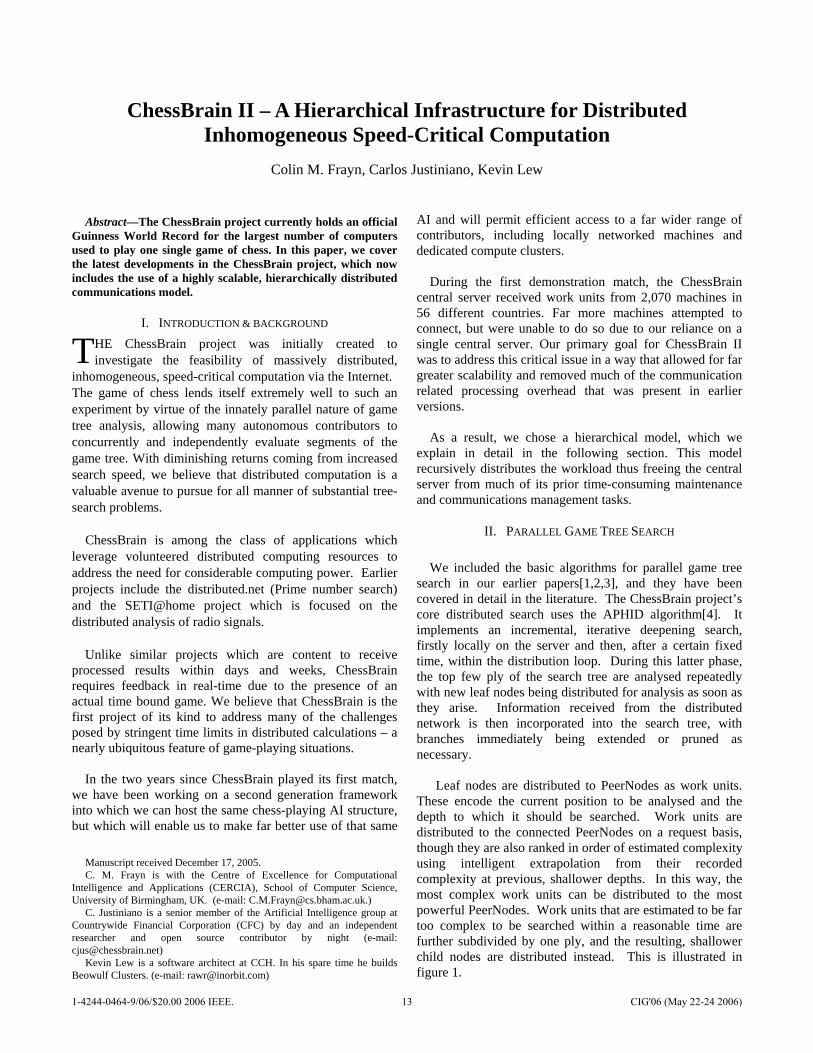
Leaf nodes are distributed to PeerNodes as work units. These encode the current position to be analysed and the depth to which it should be searched. Work units are distributed to the connected PeerNodes on a request basis, though they are also ranked in order of estimated complexity using intelligent extrapolation from their recorded complexity at previous, shallower depths. In this way, the most complex work units can be distributed to the most powerful PeerNodes. Work units that are estimated to be far too complex to be searched within a reasonable time are further subdivided by one ply, and the resulting, shallower child nodes are distributed instead. This is illustrated in figure 1.

T

1-4244-0464-9/06/$20.00 2006 IEEE. 13 CIG'06 (May 22-24 2006)

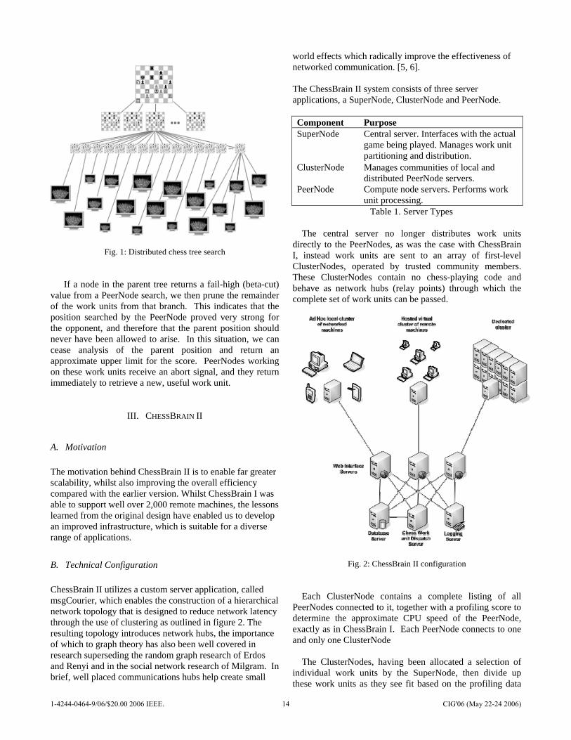
Fig. 1: Distributed chess tree search

If a node in the parent tree returns a fail-high (beta-cut) value from a PeerNode search, we then prune the remainder of the work units from that branch. This indicates that the position searched by the PeerNode proved very strong for the opponent, and therefore that the parent position should never have been allowed to arise. In this situation, we can cease analysis of the parent position and return an approximate upper limit for the score. PeerNodes working on these work units receive an abort signal, and they return immediately to retrieve a new, useful work unit.

III. CHESSBRAIN II

A. Motivation The motivation behind ChessBrain II is to enable far greater scalability, whilst also improving the overall efficiency compared with the earlier version. Whilst ChessBrain I was able to support well over 2,000 remote machines, the lessons learned from the original design have enabled us to develop an improved infrastructure, which is suitable for a diverse range of applications.

B. Technical Configuration ChessBrain II utilizes a custom server application, called msgCourier, which enables the construction of a hierarchical network topology that is designed to reduce network latency through the use of clustering as outlined in figure 2. The resulting topology introduces network hubs, the importance of which to graph theory has also been well covered in research superseding the random graph research of Erdos and Renyi and in the social network research of Milgram. In brief, well placed communications hubs help create small

world effects which radically improve the effectiveness of networked communication. [5, 6]. The ChessBrain II system consists of three server applications, a SuperNode, ClusterNode and PeerNode.

Component Purpose SuperNode

Central server. Interfaces with the actual game being played. Manages work unit partitioning and distribution.

ClusterNode

Manages communities of local and distributed PeerNode servers.

PeerNode

Compute node servers. Performs work unit processing.

Table 1. Server Types The central server no longer distributes work units

directly to the PeerNodes, as was the case with ChessBrain I, instead work units are sent to an array of first-level ClusterNodes, operated by trusted community members. These ClusterNodes contain no chess-playing code and behave as network hubs (relay points) through which the complete set of work units can be passed.

Fig. 2: ChessBrain II configuration

Each ClusterNode contains a complete listing of all

PeerNodes connected to it, together with a profiling score to determine the approximate CPU speed of the PeerNode, exactly as in ChessBrain I. Each PeerNode connects to one and only one ClusterNode

The ClusterNodes, having been allocated a selection of

individual work units by the SuperNode, then divide up these work units as they see fit based on the profiling data

1-4244-0464-9/06/$20.00 2006 IEEE. 14 CIG'06 (May 22-24 2006)

that they obtain from their own network of PeerNodes. The primary considerations are that the work units are distributed to sufficient machines to ensure a reliable reply within the time required, plus to ensure that the work units perceived to require a greater computation effort are allocated to those PeerNodes deemed most fit to analyse them.

In subsequent versions, we intend to move some of the

chess logic from the SuperNode onto the ClusterNodes, further reducing the communications overhead. Our anticipation is that the SuperNode will divide up the initial position into large tree chunks, and then distribute just these positions to the ClusterNodes. The ClusterNodes will then further subdivide the given positions, allocating the leaf nodes to the attached PeerNodes as it sees fit, and accumulating the returned results as and when they arrive. The ClusterNodes will then return a single result to the central SuperNode, instead of many.

C. ChessBrain II Communication Protocols Early versions of ChessBrain relied on industry standard

XML data encoding first using XMLRPC, and later using SOAP. The decision to use SOAP was driven by a desire for interoperability with emerging web services. However, the need to streamline communication has steered us toward minimizing our use of XML in favour of economical string based S-Expressions[7].

To further streamline communication we've implemented

a compact communication protocol similar to the Session Initiation Protocol (SIP)[8] for use in LAN and cluster environments where we favour the use of connectionless UDP rather than stream-based TCP communication.

The ChessBrain I communication protocol consisted of

XML content which was first compressed using ZLib compression and then encrypted using the AES Rijndael cipher. Although each PeerNode was quickly able to decrypt and decompress the payload content, the burden was clearly on the SuperNode server where each message to and from a PeerNode required encryption and compression operations. The situation was compounded by the fact that each PeerNode communication occurred directly with a single central SuperNode server.

With ChessBrain II we’ve eliminated direct PeerNode

communication with the central SuperNode and introduced the concept of batch jobs, which combine multiple jobs into a single communication package. The reduction in messaging reduces the impact to the TCP stack while the grouping of jobs greatly improves the compression ratio.

D. Architecture Advantages The most significant architectural change to ChessBrain involves the introduction of network hubs called ClusterNodes, as outlined in section IIIB.

ChessBrain I used a single SuperNode server to handle

the remote coordination of hundreds of machines. Each dispatched job required a direct session involving the exchange of multiple messages between the SuperNode and its PeerNode clients. With ChessBrain II, jobs are distributed from a central server at distributedchess.net to remote ClusterNodes, which in turn manage local communities of PeerNodes. Each ClusterNode receives a batch of jobs, which it can directly dispatch to local PeerNodes thereby eliminating the need for individual PeerNode to communicate directly with the central server. This is necessary to harness a compute cluster effectively. Each ClusterNode collects completed jobs and batches them for return shipment to the central SuperNode server. The efficient use of ClusterNode hubs and job batching results in a reduced load on the central server, efficient use of clusters, reduced network lag, and improved fault tolerance.

We envision that ClusterNodes will largely be used by individuals desiring to cluster local machines. Indeed during the use of ChessBrain I we detected locally networked machines containing five to eighty machines. Most local networks in existence today support connection speeds between 10 to 1000 MBit per second, with the lower end of the spectrum devoted to wireless networks, and the higher end devoted to corporate networks, research networks and compute clusters. ChessBrain II is designed to utilise cluster machines by taking full advantage of local intranet network speeds and only using slower Internet connections to communicate with the SuperNode when necessary.

If we assume that there are roughly as many PeerNodes connected to each ClusterNode as there are ClusterNodes, then effectively the communications costs for each Cluster node, and indeed the SuperNode itself, is reduced to its square root. So, with total node count N, instead of one single bottleneck of size N, we now have approximately (sqrt(N)+1) bottlenecks, each of size sqrt(N). When addressing scalability issues, this is a definite advantage, allowing us to move from an effective node limit of approximately 2,000 to around one million machines.

E. Architecture Drawbacks

It is only fair to consider the drawbacks of the above architecture and to explain why it may not be suitable for every gaming application.

Firstly, as with any distributed computation environment,

there is a substantial overhead introduced by remote communication. Indeed, communication costs increase as the number of available remote machines increases. ChessBrain I involved a single server solution that was overburdened as an unexpectedly large number of remote machines became available. Communication overhead on

1-4244-0464-9/06/$20.00 2006 IEEE. 15 CIG'06 (May 22-24 2006)

ChessBrain I reached approximately one minute per move under peak conditions. However, with the experience gained since that first exhibition match, and with the subsequent redesign of ChessBrain I, we have reduced the overhead to less than ten seconds per move.

The presence of communication overhead means that

shorter time scale games are not currently suitable for distributed computation. However, games that favour a higher quality of play over speed of play are likely to make good use of distributed computation.

Anyone who has ever attempted to write a fully-functioning alpha-beta pruning chess search algorithm featuring a multitude of unsafe pruning algorithms such as null-move, will immediately appreciate the complexity of debugging a search anomaly produced from a network of several thousand computers, each of which is running a number of local tree searches and returning their results asynchronously. Some of the complexities of such an approach are covered in [9].

Adding hierarchical distribution increases complexity,

and highlights the importance of considering how a distributed application will be tested early in the design phase. With ChessBrain II we’ve had to build specialized testing applications in order to identify and correct serious flaws which might have otherwise proceeded undetected. Such a suite of testing tools is invaluable for a distributed application of this size.

F. Comparison with alternative parallel implementations

Other approaches towards parallelising search problems focus primarily on tightly-coupled compute clusters with shared memory. The aim of this paper is not to offer a thorough analysis of the advantages and drawbacks of remotely distributed search versus supercomputer or cluster-based search. The main advantages of this method over that used by, for example, the Deep Blue project [10] and the more recent Hydra project are as follows:

• Processing power – With many entirely separable applications, parallelising the search is a simple way to get extra processing power for very little extra overhead. For chess, the parallelisation procedure is highly inefficient when compared to serial search, but we chose this application because of its inherent difficulty, our own interest and its public image.

• Distributed memory – With many machines contributing to the search, the total memory of the system is increased massively. Though there is much repetition and redundancy, this still partly overcomes the extra practical barrier imposed by the finite size of a transposition table in conventional search.

• Availability – the framework described in this paper is applicable to a wide range of projects requiring

substantial computing power. Not everyone has access to a supercomputer or a substantial Beowulf cluster.

• Costs – It’s easier to appeal to 10,000 people to freely contribute resources than it is to convince one person to fund a 10,000 node cluster.

Drawbacks include:

• Communication overheads – time is lost in sending/receiving the results from PeerNodes.

• Loss of shared memory – In games such as chess, the use of shared memory for a transposition table is highly beneficial. Losing this (amongst other cases) introduces many overheads into the search time [11]

• Lack of control – the project manager has only a very limited control over whether or not the contributors choose to participate on any one occasion.

• Debugging – This becomes horrendously complicated, as explained above.

• Software support – The project managers must offer support on installing and configuring the software on remote machines.

• Vulnerability – The distributed network is vulnerable to attacks from hackers, and must also ensure that malicious PeerNode operators are unable to sabotage the search results.

At the present time, we are not aware of any other effort to evaluate game trees in a distributed style over the internet.

G. Comparison with other Chess projects

We are often asked to compare ChessBrain with more famous Chess machines such as Deep Blue and the more recent Hydra project. A direct comparison is particularly difficult as ChessBrain relies on considerably slower communication and commodity hardware. In contrast, both Deep Blue and Hydra are based on a hardware-assisted brute force approach. A more reasonable comparison would be between distributed chess applications running on GRIDs and distributed clusters.

H. The need for MsgCourier

While considering architectural requirements for ChessBrain II, we investigated a number of potential frameworks including the Berkeley Open Infrastructure for Network Computing (BOINC) project. BOINC is a software application platform designed to simplify the construction of public computing projects and is presently in use by the SETI@home project, CERN’s Large Hadron Collider project and other high-profile distributed computing projects[12].

After extensive consideration we concluded that

ChessBrain's unique requirements necessitated the

1-4244-0464-9/06/$20.00 2006 IEEE. 16 CIG'06 (May 22-24 2006)

construction of a new underlying server application technology[13]. One of our requirements for ChessBrain II's software is that it must be a completely self-contained application that is free of external application dependencies. In addition, our solution must be available for use on both Microsoft Windows and Linux based servers, while requiring near zero configuration. The rationale behind these requirements is that ChessBrain II allows some of our contributors to host ClusterNode servers. It is critically important that our contributors feel comfortable with installing and operating the project software. We found that BOINC requires a greater level of system knowledge than we're realistically able to impose on our contributors. Lastly, BOINC was designed with a client and server methodology in mind, while our emerging requirements for ChessBrain II include Peer-to-Peer functionality.

Well over a year ago we began work on the Message Courier (msgCourier) application server in support of ChessBrain II. MsgCourier is designed to support speed critical computation using efficient network communication and enables clustering, which significantly improves overall efficiency. Unlike other technologies, msgCourier is designed to enable ad-hoc machine clusters and to leverage existing Beowulf clusters.

MsgCourier is a hybrid server application that combines

message queuing, HTTP server and P2P features. When we embarked on this approach there were few such commercial server applications. Today, Microsoft has release SQL Server 2005 which combines a SQL Engine, HTTP server and messaging server features. The industry demands for performance necessitates the consideration of hybrid servers.

We chose to build msgCourier independently of

ChessBrain (and free of chess related functionality) in the hopes that it would prove useful to other researchers.

The following were a few of our primary design considerations:

• A hybrid application server, combining message queuing and dispatching with support for store and forward functionality.

• Multithreaded concurrent connection server design able to support thousands of concurrent connections.

• High-speed message based communication using TCP and UDP transport.

• Built-in P2P functionality for self-organization and clustering, service adverting and subscribing.

• Ease of deployment with minimal configuration requirements.

• Built-in security features which are comparable to the use of SSL and or SSH.

The msgCourier project is under continued development.

We are keen to emphasize here that the relevance of the

ChessBrain project is not just to the specific field of computer chess, but to any distributed computation project. Hence, we believe that the msgCourier software is a valuable contribution to all areas of computationally intensive research. The direct application here demonstrates that the framework is also flexible enough to operate within gaming scenarios, where results are required on demand at high speed and with high fidelity, often in highly unpredictable search situations.

More information on the msgCourier project is available

at http://www.msgcourier.com

CONCLUSIONS : THE FUTURE OF DISTRIBUTED GAMING

Distributed computation offers the potential for deeper game tree analysis for a variety of potential gaming applications. In particular, it overcomes the restrictions imposed by Moore’s law, producing substantial gains for any game-playing code that is primarily computationally limited. For games such as Go, the effective contribution is reduced as the branching factor is so high that such games are algorithmically limited rather than computationally limited in most cases.

Speed-critical distributed computation also has many clear

applications within the financial sector where rapid decisions must be made, often based on approximate or inadequate data.

During the past decade we’ve seen high profile Man vs.

Machine exhibitions. We feel that the general public will eventually lose interest in exhibitions where a single human player competes against a machine which is virtually indistinguishable from the common personal desktop computer. Not since Deep Blue has any Man vs. Machine event really captured the public’s imagination.

We feel strongly that the future of Man vs. Machine

competitions will migrate toward a format where a human team competes against a distributed network. Such events will take place over the Internet with distributed human members collaborating remotely from their native countries. This exhibition format will likely capture the public’s imagination as it more closely resembles themes played out in popular science fiction.

On the ChessBrain project we’ve learned the importance

of capturing the public’s imagination for without their support massively distributed computation would not be economically feasible[14]. Generally, a project is only as good as the contributors that it is able to attract. This entire field of research – that of attracting distributed computation teams to a project – seems remarkably underdeveloped in the literature, despite the fact that it has an arguably greater effect on the success of any distributed project than any

1-4244-0464-9/06/$20.00 2006 IEEE. 17 CIG'06 (May 22-24 2006)

degree of algorithmic sophistication. More work in this area seems extremely important, though it lies firmly within the realms of psychology and sociology rather than pure computer science.

We’ve completed preliminary testing on small clusters with the support of ChessBrain community members [15]. During the first quarter of 2006 we intend to release a major update of our project software when we will begin large-scale public testing of ChessBrain II. We expect ChessBrain II to be fully operational by the second quarter of 2006.

We are actively preparing for a second demonstration match between ChessBrain II and a leading international chess grandmaster within the next 12 months. Anyone wishing to contribute to this event is welcome to contact the authors at the addresses supplied.

ACKNOWLEDGMENT We would like to acknowledge the hundreds of

international contributors who have supported the ChessBrain project over the past four years. In addition, and by name, we would like to thank Cedric Griss and the Distributed Computing Foundation; Kenneth Geisshirt and the Danish Unix users Group; Peter Wilson; Gavin M. Roy with EHPG Networks; and Y3K Secure Enterprise Software Inc., whose outstanding support enabled us to establish a world record and to further contribute to this emerging field. Colin Frayn is currently supported by a grant from Advantage West Midlands (UK).

REFERENCES [1] Frayn, C.M. & Justiniano, C., “The ChessBrain Project – Massively

Distributed Inhomogeneous Speed-Critical Computation”, Proceedings IC-SEC, Singapore, 2004

[2] Justiniano, C. & Frayn, C.M. “The ChessBrain Project: A Global Effort To Build The World's Largest Chess SuperComputer”, 2003 ICGA Journal, Vol. 26, No. 2, 132-138

[3] Justiniano, C. “ChessBrain: A Linux-Based Distributed Computing Experiment”, 2003 Linux Journal, September 2003

[4] Brockington, M. “Asynchronous Parallel Game-Tree Search”, 1997 PhD Thesis, University of Alberta, Dept. of Computer Science

[5] Barabasi, A-L. “Linked: The new Science of Networks”, 2002. Cambridge, MA: Perseus

[6] Gladwell, M. “The Tipping Point”, 2000. Boston: Little and Company [7] Rivest, R. L., “S-Expressions”., MIT Theory group,

http://theory.lcs.mit.edu/~rivest/sexp.txt [8] Session Initiation Protocol (SIP) http://www.cs.columbia.edu/sip/ [9] Feldmann, R., Mysliwietz, P., Monien, B., “A Fully Distributed Chess

Program”, Advances in Computer Chess 6, 1991 [10] Campbell, M., Joseph Hoane Jr., A., Hsu, F., “Deep Blue”, Artificial

Intelligence 134 (1-2), 2002. [11] Feldmann, R., Mysliwietz, P., Monien, B., “Studying overheads in

massively parallel MIN/MAX-tree evaluation”, Proc. 6th annual ACM symposium on Parallel algorithms and architectures , 1994

[12] Berkeley Open Infrastructure for Network Computing (BOINC) project: http://boinc.berkeley.edu/

[13] Justiniano, C., “Tapping the Matrix: Revisited”, BoF LinuxForum, Copenhagen 2005

[14] Justiniano, C., “Tapping the Matrix”, 2004, O’Reilly Network Technical Articles, 16th, 23rd April 2004. http://www.oreillynet.com/pub/au/1812

[15] Lew, K., Justiniano, C., Frayn, C.M., “Early experiences with clusters and compute farms in ChessBrain II”. BoF LinuxForum, Copenhagen 2005

1-4244-0464-9/06/$20.00 2006 IEEE. 18 CIG'06 (May 22-24 2006)

Grid-Robot Drivers:an Evolutionary Multi-agent Virtual Robotics Task

Daniel AshlockDepartment of Mathematics and Statistics

University of GuelphGuelph, Ontario, Canada, N1G 2W1

dashlock@uoguelph.ca

ABSTRACT

Beginning with artificial ants and including such tasks asTartarus, software agents that are situated on a grid havebeen a staple of evolutionary computation. This manuscriptintroduces a grid-robot problem in which the agents simulatesingle or multiple drivers on a two-lane interstate freeway thatmay have obstructions. The drivers are represented as If-Skip-Action lists, a linear genetic programming structure. With onedriver present, the problem is similar to an artificial ant task,requiring only that the grid robot learn where fixed obstaclesare placed. When multiple drivers are present, the process ofdriving can be cast as a game similar to the prisoner’s dilemma.The relative advantage to be gained from inducing anothervehicle to crash is analogous to defection in the prisoner’sdilemma. The game differs from prisoner’s dilemma in thatdefecting is a complex learned behavior, not simply a movethe grid robot may choose. A skilled opponent may doge anattempt at “defection”. Six sets of experiments with up to fivedrivers and two fixed obstacles are performed in this study.In multi-driver simulations evolution locates a diversity ofbehaviors within the context of the driver task.

I. INTRODUCTION

The problem of evolving a controller for a model race caris one that has been examined before in the evolutionary com-putation literature [10]. Evolved controllers have competed atthe Congress on Evolutionary Computation in a competitionorganized by Simon Lucas for the last several years. This paperintroduces a grid-robot version of the car racing problem, adiscrete version of the problem. A grid robot is a virtual robotthat lives on a grid made of squares. The robot has a positionand heading on the the grid and shares it with other roboticagents and both fixed and movable obstacles. Examples ofother grid-robot problems are the Tartarus task [11], [1], [3],[6], [2] in which a robot living on a 6 × 6 grid is awardedfitness for pushing boxes against the wall, the Herbivore [2]task in which a grid-robot forages for food, and the North Wallbuilder task [4], [2] in which a grid robot tries to retrieve boxesfrom a delivery site and use them to build a wall. Grid robotshave also been used in studying the theoretical biology of apredator-prey system [5].

The motivation for this research is the creation of a simpleframework in which evolutionary algorithms can be used toinvestigate the game theory of driving. In this case “simple”means a simulation with low computational cost in whicha large number of evolutionary runs can be performed in ashort time to survey the strategy space and obtain statisticalperspective. The idea occurred to the author during drivesback and forth between Southern Ontario and Iowa. In theregions of Michigan, Indiana, and Illinois at the southerntip of Lake Michigan the interstate system is in a state ofalmost continuous repair. This situation often leads to twostreams of traffic becoming one. This, in turn, creates anarena in which informal behavioral experiments take placein an often infuriating fashion. The goal of this research isa modeling environment in which this situation can be studiedwith evolved software agents. This study presents the basicframework and examines the impact of varying the numberof obstacles and drivers on the road. The remainder of themanuscript is organized as follows. Section II specifies a two-lane grid-robot driver problem with variable numbers of carsand obstructions. Section III gives the representation usedto encode the evolvable grid-robot drivers. Section IV givesthe design of the experiments performed. Section V givesthe results of the experiments and performs some analysis.Section VI draws conclusions and outlines the next steps inthis research.

II. THE GRID-ROBOT DRIVER PROBLEM

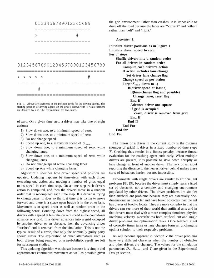
A grid robot is a virtual robot embedded in a grid environ-ment. The grid for the robotic drivers is a 2×N grid with thelong dimension wrapping to form an arbitrarily long periodicroad. The road contains other grid-robot drivers and obstacleswith a fixed position. Examples of driving grids are shown inFigure 1.

Henceforth grid-robot drivers will be called drivers. A driveron the grid has a position along the long dimension of the grid,a lane, and a speed. The driver is given as inputs the distanceto the next other driver and the next barrier both in his ownand in the other lane. In addition the driver is given his ownspeed. Distances to the next obstacle and driver are limited toa sight distance Ds. If no driver or obstacle is visible withinsight distance for a given lane then the input reports a value

1-4244-0464-9/06/$20.00 2006 IEEE. 19 CIG'06 (May 22-24 2006)

0123456789012345689===================> #-------------------

===================

012345678901234567890123456789==============================> > > > > #------------------------------

#==============================

Fig. 1. Above are segments of the periodic grids for the driving agents. Thestarting position of driving agents on the grid is shown with > while barriersare denoted by a #. The environment has two lanes.

of zero. On a given time step, a driver may take one of eightactions:

1) Slow down two, to a minimum speed of zero.2) Slow down one, to a minimum speed of zero.3) Do not change speed.4) Speed up one, to a maximum speed of Smax.5) Slow down two, to a minimum speed of zero, while

changing lanes.6) Slow down one, to a minimum speed of zero, while

changing lanes.7) Do not change speed while changing lanes.8) Speed up one while changing lanes.Algorithm 1 specifies how driver speed and position are

updated. Updating happens by time-steps with each driverexecuting one action and moving a number of grids equalto its speed in each time-step. On a time step each driversaction is computed, and then the drivers move in a randomorder that is recomputed each time step. If a driver is tryingto change lanes, it does so the first time it is trying to moveforward and there is a space open beside it in the other lane.Movement is in speed order as well as random order in thefollowing sense. Counting down from the highest speed, alldrivers with a speed at least the current speed in the countdownadvance one grid. If a driver advances into a grid occupiedby another driver or an obstacle, then the advancing driver“crashes” and is removed from the simulation. This is not thetypical result of a crash, that only the nominally guilty partyshould suffer. The exploration of other alternatives such asboth drivers being removed or a probabilistic result are leftfor subsequent studies.

This updating algorithm was chosen because it is simple andapproximates continuous movement as well as possible given

the grid environment. Other than crashes, it is impossible todrive off the road because the lanes are “‘current” and “other”rather than “left” and “right.”

Algorithm 1:

Initialize driver positions as in Figure 1Initialize driver speed to zeroFor T steps

Shuffle drivers into a random orderFor all drivers in random order

Compute each driver’s actionIf action includes lane-change

Set driver lane change flagChange speed as per actionFor(s=Smax down to 1)

If(driver speed at least s)If(lane-change flag and possible)

Change lanes, reset flagEnd IfAdvance driver one squareIf grid is occupied

crash, driver is removed from gridEnd If

End IfEnd For

End forEnd For

The fitness of a driver in the current study is the distance(number of grids) it drives in a fixed number of time stepsT . Crashing thus results in a fitness penalty, because fitnessevaluation for the crashing agent ends early. When multipledrivers are present, it is possible to slow down abruptly orlane change in front of another driver. The lack of an inputreporting the distance to the nearest driver behind makes thesesorts of behaviors harder, but not impossible.

Experiments with single drivers are similar to artificial antproblems [8], [9], because the driver must simply learn a fixedset of obstacles, not a complex and changing environmentpopulated by other drivers. The driver problems are simplerthan artificial ant problems because they are essentially one-dimensional in character and have fewer obstacles than the anthas pieces of food to locate. They are more complex in that thedrivers can see more of their world than artificial ants and inthat drivers must deal with a more complex simulated physicsinvolving velocity. Nevertheless both artificial ant and singledriver problems are optimization tasks. Once learned, a setof correctly times turns or lane changes form an unchangingoptima solution to their respective problems.

As will become apparent in Section V the driver problemshave very different character when the number of obstaclesand other drivers are changed. The values for the simulationparameters Ds, Smax, and T are given in the ExperimentalDesign section.

1-4244-0464-9/06/$20.00 2006 IEEE. 20 CIG'06 (May 22-24 2006)

III. ISAC LIST DRIVERS

The evolvable structure used to control the driver is an ISAclist. The ISAc list used in this manuscript is a generalizationof the one presented in [1], [5], and [2]. An ISAc list is anarray of ISAc nodes. An ISAC node is a hextuple

(a, b, c, t, act, jmp)

where a and b are indexes into the set of inputs available toto the driver, c is a constant in the range 0 ≤ c ≤ Ds, t

is the type of the Boolean test used by the node, act is anaction that the ISAc list may take, and jmp is a specificationof which position in the list to jump to if the action happensto be a jump action. An ISAc list comes equipped with a setof Boolean tests available to each node. The tests available tothe nodes in this study have types 0-3 and are, respectively,v[a] < v[b], v[a] < c, v[a] ≤ v[b], and v[a] ≤ c. The arrayv[] is the set of inputs available to the driver. Execution in anISAc list is controlled by the instruction pointer.

The instruction pointer starts at the beginning of the ISAclist, indexing the zeroth node. Using the entries a, b, c, t, act,and jmp of that node, inputs v[a] and v[b] are retrieved forthe current driver, and the Boolean test of type t is applied tov[a] and v[b] or a and c, as appropriate. Recall that the vectorv[] holds the distance from the driver to the next driver andobstacle ahead in each lane as well as the driver’s currentspeed, a total of five inputs.. If the test is true, then theaction in the act field of the node is performed; otherwise,nothing is done. If that action is “jump,” the contents of thejmp field are loaded into the instruction pointer. Any otheraction is executed according to its own type, as describedsubsequently. After execution of any action, the instructionpointer is incremented. Pseudocode for the basic ISAc listexecution loop is given in Algorithm 2.

Algorithm 2:IP← 0 //Set Instruction Pointer to 0.Get Inputs; //Put initial values in data vector.Repeat //ISAc evaluation loop

With ISAc[IP] do //with the current ISAc node,If test(v[a],v[b],c) then //Conditionally

PerformAction(act); //perform actionUpdate Inputs; //Revise the data vectorIP ← IP + 1 //Increment instruction pointerifIP > Length IP ← 0 //Wrap at end

Until Done;

There are 3 types of actions used in the act field of anISAc node. The first is the NOP action, which does nothing.The inclusion of the NOP action is inspired by experience inmachine-language programming. An ISAc list that has beenevolving for a while will have its performance tied to thepattern of jumps it has chosen. If new instructions are inserted,then the target addresses of many of the jumps change. An“insert an instruction” mutation operator could be tied to a “re-number all the jumps” routine, but this is clumsy. In particular,it would create problems when the crossover operator wasapplied is one parent had been renumbered and the other had

not. Instead a “do nothing” instruction serves as a placeholder.Instructions can be inserted by mutating a NOP instruction,and they can be deleted by mutating the instruction to bedeleted into a NOP instruction. Both of these mutations arepossible without the annoyance of renumbering everything.The second type of action is the jmp or jump action that movesthe instruction pointer, changing the flow of control. The thirdtype of actions is an exterior action that causes an ISAc list togenerate an action relevant to the simulation. In this study thereare eight external actions corresponding to the eight possibleactions a driver can take. There are thus 10 total actions; donothing, jump, and the eight possible simulation actions.

ISAc lists are initialized at random, filling in uniformlyselected, semantically valid values to the six fields of eachnode. This means that it is not difficult to create an ISAc listthat can run indefinitely without generating an exterior action.To prevent such “infinite loop” behaviors, there is a maximumnumber of ISAc nodes an ISAc list may execute. This limit iscalled the node limit for the ISAc list. If it exceeds this limitthe list has timed out and is removed from the simulation asif the driver it was controlling had crashed.

ISAc lists are a form of genetic programming [7] that usesa fixed-size linear data structure. The data structure has beenspecified: it remains to specify the variation operators. Theevolution used in this study uses two variation operators. Thefirst is two-point crossover operating on the array of ISAcnodes with the nodes treated as atomic objects. The secondis a mutation operator that first selects a node uniformly atrandom and then modifies one of its six fields to a new, validvalue, also selected uniformly at random.

The ISAc lists presented here are a generalization of earlierdesigns in that they permit multiple Boolean tests to beavailable rather than a single test and in that they haveconstants localized to the nodes. The constants also have agreater range of values. Previously, ISAc lists used constantsas additional inputs. This means that when the number ofconstants is large there is a high probability of two constantsbeing compared. The grid-robot driving problem uses moreconstants (0-Ds = 8) than inputs (5) and so has an enhancedprobability of comparing constants in the original design forISAc lists.

IV. EXPERIMENTAL DESIGN

The evolutionary algorithm used in this study operates on apopulation of 120 ISAc lists functioning as drivers. Each ISAclist has 30 nodes. The model of evolution is single tournamentselection [2] with tournament size four. The model of evolutionis generational. The population is shuffled into groups of fourdrivers. The two best in each group of four are copied over thetwo worst. The copies undergo crossover and a single mutationeach. Evolution continues for 1000 generations in each run.

For fitness evaluation the following parameters are used.Drivers execute T = 100 time steps with a maximum speedof Smax = 6, a sight distance of Ds = 8, and a node limitof 2000 ISAc nodes. A collection of six experiments wereperformed using the two grids shown in Figure 1 as well as

1-4244-0464-9/06/$20.00 2006 IEEE. 21 CIG'06 (May 22-24 2006)

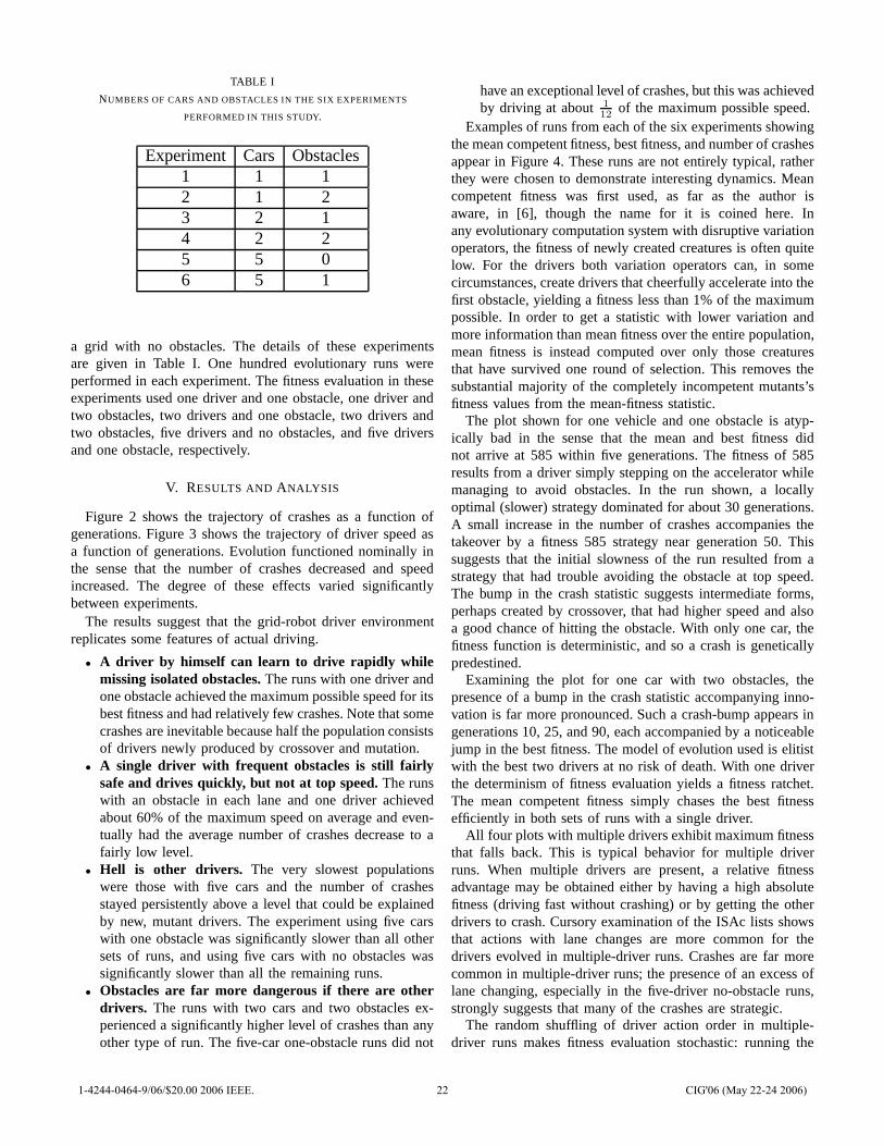
TABLE I

NUMBERS OF CARS AND OBSTACLES IN THE SIX EXPERIMENTS

PERFORMED IN THIS STUDY.

Experiment Cars Obstacles1 1 12 1 23 2 14 2 25 5 06 5 1

a grid with no obstacles. The details of these experimentsare given in Table I. One hundred evolutionary runs wereperformed in each experiment. The fitness evaluation in theseexperiments used one driver and one obstacle, one driver andtwo obstacles, two drivers and one obstacle, two drivers andtwo obstacles, five drivers and no obstacles, and five driversand one obstacle, respectively.

V. RESULTS AND ANALYSIS

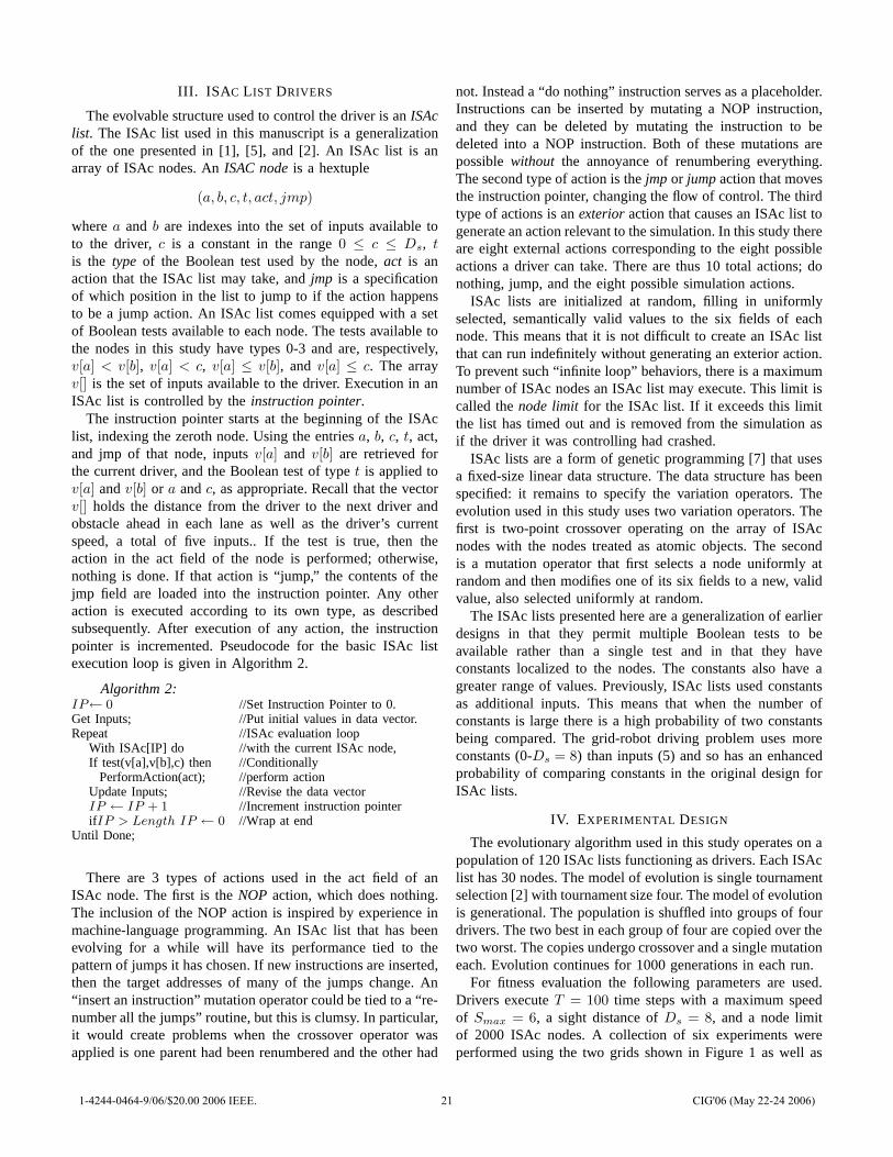
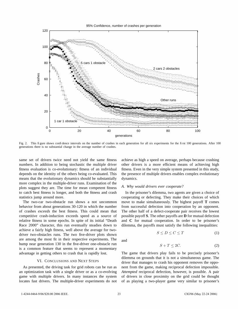
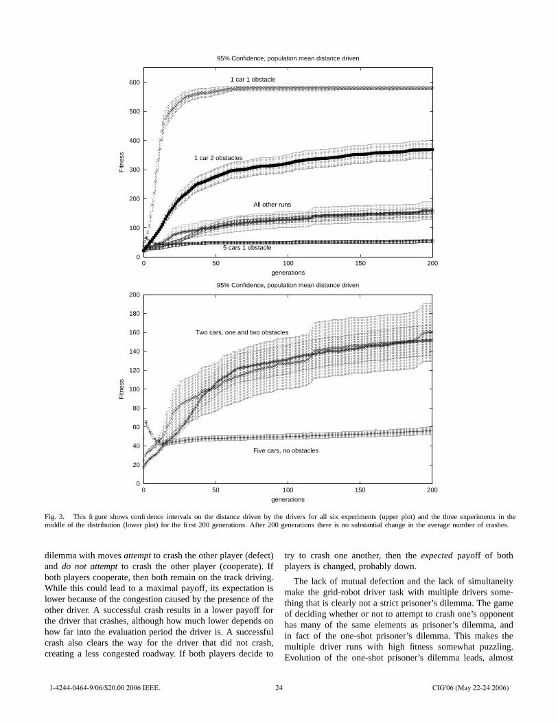
Figure 2 shows the trajectory of crashes as a function ofgenerations. Figure 3 shows the trajectory of driver speed asa function of generations. Evolution functioned nominally inthe sense that the number of crashes decreased and speedincreased. The degree of these effects varied significantlybetween experiments.

The results suggest that the grid-robot driver environmentreplicates some features of actual driving.

• A driver by himself can learn to drive rapidly whilemissing isolated obstacles. The runs with one driver andone obstacle achieved the maximum possible speed for itsbest fitness and had relatively few crashes. Note that somecrashes are inevitable because half the population consistsof drivers newly produced by crossover and mutation.

• A single driver with frequent obstacles is still fairlysafe and drives quickly, but not at top speed. The runswith an obstacle in each lane and one driver achievedabout 60% of the maximum speed on average and even-tually had the average number of crashes decrease to afairly low level.

• Hell is other drivers. The very slowest populationswere those with five cars and the number of crashesstayed persistently above a level that could be explainedby new, mutant drivers. The experiment using five carswith one obstacle was significantly slower than all othersets of runs, and using five cars with no obstacles wassignificantly slower than all the remaining runs.

• Obstacles are far more dangerous if there are otherdrivers. The runs with two cars and two obstacles ex-perienced a significantly higher level of crashes than anyother type of run. The five-car one-obstacle runs did not

have an exceptional level of crashes, but this was achievedby driving at about 1

12of the maximum possible speed.

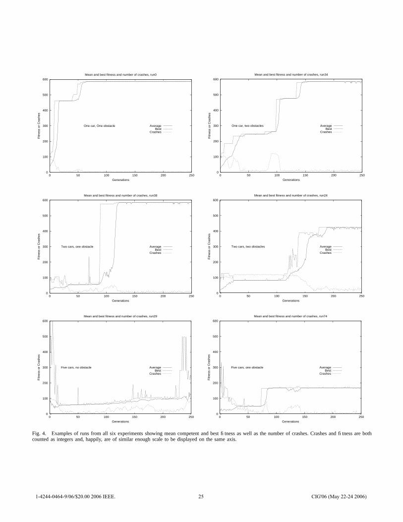
Examples of runs from each of the six experiments showingthe mean competent fitness, best fitness, and number of crashesappear in Figure 4. These runs are not entirely typical, ratherthey were chosen to demonstrate interesting dynamics. Meancompetent fitness was first used, as far as the author isaware, in [6], though the name for it is coined here. Inany evolutionary computation system with disruptive variationoperators, the fitness of newly created creatures is often quitelow. For the drivers both variation operators can, in somecircumstances, create drivers that cheerfully accelerate into thefirst obstacle, yielding a fitness less than 1% of the maximumpossible. In order to get a statistic with lower variation andmore information than mean fitness over the entire population,mean fitness is instead computed over only those creaturesthat have survived one round of selection. This removes thesubstantial majority of the completely incompetent mutants’sfitness values from the mean-fitness statistic.

The plot shown for one vehicle and one obstacle is atyp-ically bad in the sense that the mean and best fitness didnot arrive at 585 within five generations. The fitness of 585results from a driver simply stepping on the accelerator whilemanaging to avoid obstacles. In the run shown, a locallyoptimal (slower) strategy dominated for about 30 generations.A small increase in the number of crashes accompanies thetakeover by a fitness 585 strategy near generation 50. Thissuggests that the initial slowness of the run resulted from astrategy that had trouble avoiding the obstacle at top speed.The bump in the crash statistic suggests intermediate forms,perhaps created by crossover, that had higher speed and alsoa good chance of hitting the obstacle. With only one car, thefitness function is deterministic, and so a crash is geneticallypredestined.

Examining the plot for one car with two obstacles, thepresence of a bump in the crash statistic accompanying inno-vation is far more pronounced. Such a crash-bump appears ingenerations 10, 25, and 90, each accompanied by a noticeablejump in the best fitness. The model of evolution used is elitistwith the best two drivers at no risk of death. With one driverthe determinism of fitness evaluation yields a fitness ratchet.The mean competent fitness simply chases the best fitnessefficiently in both sets of runs with a single driver.

All four plots with multiple drivers exhibit maximum fitnessthat falls back. This is typical behavior for multiple driverruns. When multiple drivers are present, a relative fitnessadvantage may be obtained either by having a high absolutefitness (driving fast without crashing) or by getting the otherdrivers to crash. Cursory examination of the ISAc lists showsthat actions with lane changes are more common for thedrivers evolved in multiple-driver runs. Crashes are far morecommon in multiple-driver runs; the presence of an excess oflane changing, especially in the five-driver no-obstacle runs,strongly suggests that many of the crashes are strategic.

The random shuffling of driver action order in multiple-driver runs makes fitness evaluation stochastic: running the

1-4244-0464-9/06/$20.00 2006 IEEE. 22 CIG'06 (May 22-24 2006)

0

20

40

60

80

100

120

0 20 40 60 80 100

Cra

shes

generations

95% Confidence, number of crashes per generation

2 cars 2 obstacles

1 car 1 obstacle

5 cars 1 obstacle

Other runs

Fig. 2. This figure shows confidence intervals on the number of crashes in each generation for all six experiments for the first 100 generations. After 100generations there is no substantial change in the average number of crashes.

same set of drivers twice need not yield the same fitnessnumbers. In addition to being stochastic the multiple driverfitness evaluation is co-evolutionary: fitness of an individualdepends on the identity of the others being co-evaluated. Thismeans that the evolutionary dynamics should be substantiallymore complex in the multiple-driver runs. Examination of theplots suggest they are. The time for mean competent fitnessto catch best fitness is longer, and both the fitness and crashstatistics jump around more.

The two-car two-obstacle run shows a not uncommonbehavior from about generations 30-120 in which the numberof crashes exceeds the best fitness. This could mean thatcompetitive crash-induction exceeds speed as a source ofrelative fitness in some epochs. In spite of its initial “DeathRace 2000” character, this run eventually steadies down toachieve a fairly high fitness, well above the average for two-driver two-obstacles runs. The two five-driver plots shownare among the most fit in their respective experiments. Thebump near generation 130 in the five-driver one-obstacle runis a common feature that seems to represent a momentaryadvantage in getting others to crash that is rapidly lost.

VI. CONCLUSIONS AND NEXT STEPS

As presented, the driving task for grid robots can be run asan optimization task with a single driver or as a co-evolvinggame with multiple drivers. In many instances the systemlocates fast drivers. The multiple-driver experiments do not

achieve as high a speed on average, perhaps because crashingother drivers is a more efficient means of achieving highfitness. Even in the very simple system presented in this study,the presence of multiple drivers enables complex evolutionarydynamics.

A. Why would drivers ever cooperate?

In the prisoner’s dilemma, two agents are given a choice ofcooperating or defecting. They make their choices of whichmove to make simultaneously. The highest payoff T comesfrom successful defection into cooperation by an opponent.The other half of a defect-cooperate pair receives the lowestpossible payoff S. The other payoffs are D for mutual defectionand C for mutual cooperation. In order to be prisoner’sdilemma, the payoffs must satisfy the following inequalities:

S ≤ D ≤ C ≤ T (1)

andS + T ≤ 2C. (2)

The game that drivers play fails to be precisely prisoner’sdilemma on grounds that it is not a simultaneous game. Thedriver that manages to crash his opponent removes the oppo-nent from the game, making reciprocal defection impossible.Attempted reciprocal defection, however, is possible. A pairof drivers in close proximity on the grid could be thoughtof as playing a two-player game very similar to prisoner’s

1-4244-0464-9/06/$20.00 2006 IEEE. 23 CIG'06 (May 22-24 2006)

0

100

200

300

400

500

600

0 50 100 150 200

Fitn

ess

generations

95% Confidence, population mean distance driven

1 car 1 obstacle

1 car 2 obstacles

5 cars 1 obstacle

All other runs

0

20

40

60

80

100

120

140

160

180

200

0 50 100 150 200

Fitn

ess

generations

95% Confidence, population mean distance driven

Five cars, no obstacles

Two cars, one and two obstacles

Fig. 3. This figure shows confidence intervals on the distance driven by the drivers for all six experiments (upper plot) and the three experiments in themiddle of the distribution (lower plot) for the first 200 generations. After 200 generations there is no substantial change in the average number of crashes.

dilemma with moves attempt to crash the other player (defect)and do not attempt to crash the other player (cooperate). Ifboth players cooperate, then both remain on the track driving.While this could lead to a maximal payoff, its expectation islower because of the congestion caused by the presence of theother driver. A successful crash results in a lower payoff forthe driver that crashes, although how much lower depends onhow far into the evaluation period the driver is. A successfulcrash also clears the way for the driver that did not crash,creating a less congested roadway. If both players decide to

try to crash one another, then the expected payoff of bothplayers is changed, probably down.

The lack of mutual defection and the lack of simultaneitymake the grid-robot driver task with multiple drivers some-thing that is clearly not a strict prisoner’s dilemma. The gameof deciding whether or not to attempt to crash one’s opponenthas many of the same elements as prisoner’s dilemma, andin fact of the one-shot prisoner’s dilemma. This makes themultiple driver runs with high fitness somewhat puzzling.Evolution of the one-shot prisoner’s dilemma leads, almost

1-4244-0464-9/06/$20.00 2006 IEEE. 24 CIG'06 (May 22-24 2006)

0

100

200

300

400

500

600

0 50 100 150 200 250

Fitn

ess

or C

rash

es

Generations

Mean and best fitness and number of crashes, run0

One car, One obstacle AverageBest

Crashes

0

100

200

300

400

500

600

0 50 100 150 200 250

Fitn

ess

or C

rash

es

Generations

Mean and best fitness and number of crashes, run34

One car, two obstacles AverageBest

Crashes

0

100

200

300

400

500

600

0 50 100 150 200 250

Fitn

ess

or C

rash

es

Generations

Mean and best fitness and number of crashes, run38

Two cars, one obstacle AverageBest

Crashes

0

100

200

300

400

500

600

0 50 100 150 200 250

Fitn

ess

or C

rash

es

Generations

Mean and best fitness and number of crashes, run24

Two cars, two obstacles AverageBest

Crashes

0

100

200

300

400

500

600

0 50 100 150 200 250

Fitn

ess

or C

rash

es

Generations

Mean and best fitness and number of crashes, run29

Five cars, no obstacle AverageBest

Crashes

0

100

200

300

400

500

600

0 50 100 150 200 250

Fitn

ess

or C

rash

es

Generations

Mean and best fitness and number of crashes, run74

Five cars, one obstacle AverageBest

Crashes

Fig. 4. Examples of runs from all six experiments showing mean competent and best fitness as well as the number of crashes. Crashes and fitness are bothcounted as integers and, happily, are of similar enough scale to be displayed on the same axis.

1-4244-0464-9/06/$20.00 2006 IEEE. 25 CIG'06 (May 22-24 2006)

inexorably, to a population of mutually defecting agents. Itis conjectured that non-simultaneity is the key differencethat permits cooperation among drivers. An attempt to crashanother driver requires some preparation. With sight distancemore than maximum speed, a driver can see another driverahead of it and avoid it. If a driver just misses another drivera couple times via lane-changing, then it may deduce thatan attempted crash is in progress. This will manifest as ashort distance to the next car in its own lane several times.In this case the driver could choose to slow down, cedingsome fitness to substantially lower the probability of a crash.Behavior consisting in slowing down to avoid a wild driver isconsistent with the very low speeds observed in the runs withfive drivers.

B. A need for visualization.

The speculation in the preceding section points firmly tothe need for a visualization tool to aid in analysis. Such atool, with the ability to load evolved drivers and design boardson which to test them, would permit resolution of some ofthe questions about the behavior of the evolved drivers. Inaddition such a tool would be valuable for fish-out-of-wateranalysis of the drivers. Examining a driver evolved in a five-driver world by itself on a grid would permit a researcherto check and see if the low speed of drivers in the five-driverworld is genetically hard-coded or the result of congestion. Thevisualization tool might also be an entree into making a gamewhere evolved and designed vehicles compete against oneanother, a further application of this piece of computationalintelligence to games.

It seems likely that drivers within a population evolve aparticular “culture,” akin to the rules of the road for drivers inthe United States of Canada. This could be tested in a ham-handed way by juxtaposing drivers from distinct populationsand examining the crash and fitness statistics in the resultinggroups of drivers. An understanding or comparison of the self-organized cultures would require a good visualization tool.

C. Angel drivers: a next step.

The motivating situation for this research is observationof human drivers on sections of a two-lane interstate that isunder repair. Thus far, negative behavior has been emphasized,largely because it was what arose under the selfish imperativeof a fitness function which rewards driving farther than theother drivers on the road with you. A next step is to modelhelpful drivers. What fitness function might permit evolutionto search for those atypical drivers that help traffic movesmoothly and quickly past an obstruction?

The following is proposed. The current study yields adiverse set of 600 best-of-run drivers that exhibit various“typical driver” behaviors. Placing a substantial number ofthese driver on the grid, without permitting them to evolve,yields a training ground for angel drivers. The fitness of anangel driver is the total distance moved by all drivers in thesimulation. This rewards not only the promotion of traffic flowbut the avoidance of crashes by any driver. There is a chance,

if the total number of drivers is small, that an angel driverwould remove itself from the simulation in order to reducecongestion.

Interesting questions for an angel driver simulation include:

• What fraction of angels is required to see improvement?• What behavior would arise if no “typical” drivers were

present?• Are angels among the slowest drivers within their fitness

evaluation cohorts?• Would an angel ever identify and terminate a very trou-

blesome driver?• Are there general-purpose angel drivers or are they spe-

cific to one culture of “typical” drivers?

Many other experiments are possible within the frameworkpresented here: co-evolving difficult patterns of obstacles oroptimizing to produce psychotic drivers whose fitness is thenumber of crashes they cause. It is also possible to generalizethe problem to include more lanes, entrance and exit ramps,and other sources of automotive chaos.

VII. ACKNOWLEDGMENTS

The author would like to thank the University of GuelphDepartment of Mathematics and Statistics for its support ofthis research. The author acknowledges the contribution ofvarious rude and helpful drivers on the interstate system southof Lake Michigan who inspired this work.

REFERENCES

[1] Dan Ashlock and Mark Joenks. ISAc lists, a different representation forprogram induction. In Genetic Programming 98, proceedings of the thirdannual genetic programming conference., pages 3–10, San Francisco,1998. Morgan Kaufmann.

[2] Daniel Ashlock. Evolutionary Computation for Opimization and Mod-eling. Springer, New York, 2006.

[3] Daniel Ashlock and Jennifer Freeman. A pure finite state baselinefor tartarus. In Proceedings of the 2000 Congress on EvolutionaryComputation, pages 1223–1230. IEEE Press, 2000.

[4] Daniel Ashlock and James I. Lathrop. Program induction: Building awall. In Proceedings of the 2004 Congress on Evolutionary Computa-tion, volume 2, pages 1844–1850. IEEE Press, 2004.

[5] Daniel Ashlock and Adam Sherk. Non-local adaptation of artificialpredators and prey. In Proceedings of the 2005 Congress on EvolutionaryComputation, volume 1, pages 98–105. IEEE Press, 2005.

[6] Daniel Ashlock, Stephen Willson, and Nicole Leahy. Coevolutionand tartus. In Proceedings of the 2004 Congress on EvolutionaryComputation, volume 2, pages 1618–1624. IEEE Press, 2004.

[7] Wolfgang Banzhaf, Peter Nordin, Robert E. Keller, and Frank D.Francone. Genetic Programming : An Introduction : On the AutomaticEvolution of Computer Programs and Its Applications. Morgan Kauf-mann, San Francisco, 1998.

[8] John R. Koza. Genetic Programming. The MIT Press, Cambridge, MA,1992.

[9] William B. Langdon and Riccardo Poli. Foundations of GeneticProgramming. Springer, New York.

[10] T. P. Runarsson and S. M. Lucas. Evolving controllers for simulatedcar racing. In Proceedings of the 2005 Congress on EvolutionaryComputation, volume 1, pages 1906–1913, Piscataway NJ, 2005. IEEEPress.

[11] Astro Teller. The evolution of mental models. In Kenneth Kinnear,editor, Advances in Genetic Programming, chapter 9. The MIT Press,1994.

1-4244-0464-9/06/$20.00 2006 IEEE. 26 CIG'06 (May 22-24 2006)

Optimizations of data structures, heuristics and algorithms for

path-finding on maps

Tristan CazenaveLabo IA

Dept. InformatiqueUniversite Paris 8, Saint-Denis, France

cazenave@ai.univ-paris8.fr

Abstract— This paper presents some optimizations of A* andIDA* for pathfinding on maps. The best optimal pathfinder wepresent can be up to seven times faster than the commonlyused pathfinders as shown by experimental results. We alsopresent algorithms based on IDA* that can be even fasterat the cost of optimality. The optimizations concern the datastructures used for the open nodes, the admissible heuristic andthe re-expansion of points. We uncover a problem related tothe non re-expansion of dead-ends for sub-optimal IDA*, andwe provide a way to repair it.

Keywords: path-finding, game maps, mazes, A-star, IDA*

I. INTRODUCTION

Path-finding is an important part of many applications,including commercial games and robot navigation. In gamesit is important to use an optimized path-finding algorithmbecause the CPU resources are also needed by other algo-rithms, and because many games are real-time. The particularproblem addressed in this paper is grid-based path-finding.It is often used in real-time strategy games for example, inorder to find the shortest path for an agent to its ������� locationon the map.

A* [1] is the standard algorithm for finding shortest paths.The usual heuristic associated to A* is the Manhattan heuris-tic. We present data structures and heuristics that enable A*to be up to seven times faster than the usual implementation.

The contributions of this paper are :� It is better to use an array of stacks than a priority queue

for maintaining the open nodes of an A* search.� The ���� �������� heuristic is introduced, and is shown

to perform better than the Manhattan heuristic and thanthe ALT heuristic [2].

� It is useful for IDA* to maintain a two-step lazy cacheof the length of the shortest paths found so far.

� Adding a constant to the next threshold of IDA* enableslarge speed-ups at the cost of optimality. However thelengths of the paths are within 2% of the optimal. Sub-optimal IDA* can be competitive with A*.

� Recording the minimum f for each searched locationis useful to find dead-ends, but it can cut valid pathswhen used with a sufficiently large added constant to thethreshold of IDA*. Our program can detect and repairthe problem.

Section two describes related work. Section three presentsoptimizations related to the choice of the best open node.

Section four deals with the re-expansion of points. Sectionfive presents the different admissible heuristics we havetested. Section six details experimental results. Section sevenconcludes and outlines future work.

II. RELATED WORK

A* [1] is a search algorithm that finds shortest paths. Ituses a fast heuristic function that never over-estimates thelength of the path to the goal state, i.e. an admissible heuristicoften named h. For each node, it knows g the cost of the pathfrom the root of the search to the node, and it computes f =g + h. The f function is used to develop the tree in a bestfirst manner: A* expands the node with the smallest possiblef. IDA* [5] is the iterative deepening version of A*. It canbe enhanced with a transposition table that detects positionsthat have already been searched [6].

Fringe Search [4] is a hybrid of A* and IDA* that reducesslightly the computation time compared to A*. The FringeSearch paper also presents useful optimizations of IDA* forgame maps.

The use of map abstractions can be combined with A* tomake it faster. For example, Path-Refinement A* [7] buildshigh level plans and progressively refines them into low-levelactions.

The admissible heuristic used for path-finding on roadmaps, which are much more constrained than game maps,can be improved (i.e. give greater admissible values) usingthe ALT heuristic [2]. The heuristics used on road maps canbe reused for game maps, especially when the game mapsare complex and are close to mazes.

III. CHOOSING THE BEST OPEN NODE

Each time it expands a node, A* chooses the node withthe smallest f function. Therefore the cost of finding thenode with the smallest f is very important for A*. In thissection we present three methods and the associated datastructures used to find the best open node. The first methodis using a list of open nodes. The second method is widelyused and implements the open list as a priority queue. Thethird method is faster than the two others and uses an arrayof stacks.

1-4244-0464-9/06/$20.00 2006 IEEE. 27 CIG'06 (May 22-24 2006)

A. Maintaining a list

The naive method for finding the open node with thesmallest f is to go through all the open list to find it. Whenthe open list grows up to more than ten thousand nodes asit can be the case for game maps, it becomes quite timeconsuming.

B. Maintaining a priority queue

A commonly used optimization for maintaining the openlist is to use a priority queue [8], [3], [4], [7]. If N is thenumber of elements in the priority queue, the insertion andthe extraction of an element both take O(log N) which isfaster than a constant time for inserting and a linear time forextracting as in the list implementation.

C. Maintaining an array of stacks

Given that the f values are bounded by a relatively smallvalue, it is possible to implement a data structure that insertsnodes in constant time, and that extracts the best node in ashort time. This structure is an array of stacks. The index ofa stack in the array is the common f value of all the nodesin the stack.

The node class has a � ��� � field which is a pointer toanother node, and which can be used to put the node on topof a stack of nodes. The code is as follows:

Node Open [MaxLength + 1];int currentf;

void insert (Node *node) {Node * tmp = & Open [node->f ()];node->next = tmp->next;tmp->next = node;

}

Node * best () {while (Open [currentf].next == NULL &&

currentf < MaxLength)currentf++;

return Open [currentf].next;}

The insert function inserts a node in constant time in thearray of stacks. The best function is used to extract the nodewith the best f, and takes very little time too.

The property used to extract the best node starting atcurrentf in the

� � ��� function is that moves in the map domainnever decrease the f function, given the h heuristics used bythe program. In domains with possibly decreasing f values,it is straightforward to adapt the code by maintaining thecurrentf variable in the insert function, taking the minimumof the f of the inserted node and of currentf.

The space complexity of the array is the maximum lengthof a shortest path, which is low. The space complexity of thestacks is proportional to the number of open nodes.

IV. AVOIDING RE-EXPANSION OF POINTS

Avoiding re-expansion of points is important for path-finding on maps because there are many paths that goesthrough a point. Among these paths, many arrive at the pointwith a path longer than the shortest path to the point and mustnot be expanded. Among the paths that arrive with a lengthequal to the length of the shortest path, it is necessary toexpand only one, and it saves time to cut the others.

A. Checking of the open and closed nodes

A simple method to avoid re-expanding points that havealready been expanded with a shorter path is to go throughthe open and closed lists and verify if the point has alreadybeen seen. However when the number of open and closednodes grows up, this method is quite inefficient.

B. The lazy cache optimization

As game maps fits in memory, it is more efficient to usean array of the size of the map. Each point in the map hasan associated index, and the value stored at this index in thearray is the shortest path found so far to the point. As it istime consuming to reinitialize the whole array before eachsearch, an optimization is to use a lazy initialization [4]. Itconsists in having an integer named the � ����� � � initially setto zero, and another array of the size of the map initially setto zero too. Let � � �� be the name of the array that containsthe length of the shortest path found, and � � � ��� be the nameof the array that is used for the lazy initialization. Beforeeach search, the only thing to do to reinitialize the arraysis to increment the � ����� � � . To verify if the length of theshortest path to a point has been stored, the program verifiesthat the � � � �� array has the value of the � ���� � � at theindex of the point. To update a shortest path, the programstores the length of the shortest path in the � � ��� array at theindex of the point, and put the value of � ����� � � at the indexof the point in the � � � �� array. This optimization can beused both for the A* and the IDA* algorithms.

C. Maintaining the best path for each visited point

For each point the program keeps the length of the shortestpath to this point that has been found yet. Each time thesearch passes through the point, the value of g is comparedto the stored value for the point. If g is strictly smaller,the value is replaced with g and the search continues. Ifg is greater or equal to the value of the point, the search isstopped. When using the lazy cache optimization for A*, asingle lazy initialization is sufficient. When using it for IDA*,two lazy initializations are better. A first lazy initializationis used before the first search of IDA*, as in A*, in orderto reinitialize the values. However, before performing thesecond search of the IDA* algorithm, we are faced witha dilemma: if we reinitialize the values the program losesthe valuable information of the length of the shortest pathsfound so far, and if we do not reinitialize the values, theprogram won’t expand the nodes that have already beensearched coming from a shortest path and then the searchwill fail. The solution is to use two lazy arrays and two

1-4244-0464-9/06/$20.00 2006 IEEE. 28 CIG'06 (May 22-24 2006)

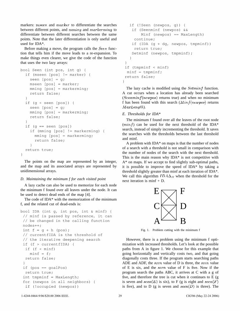
markers: � ��� �� and � ����� � � to differentiate the searchesbetween different points, and � �

�� � and � ����� � � � � � � to

differentiate between different searches between the samepoints. Note that the later differentiation is only useful andused for IDA*.

Before making a move, the program calls the � � �� func-tion that tells him if the move leads to a re-expansion. Tomake things even clearer, we give the code of the functionthat uses the two lazy arrays:

bool Seen (int pos, int g) {if (mseen [pos] != marker) {

seen [pos] = g;mseen [pos] = marker;mming [pos] = markerming;return false;

}if (g < seen [pos]) {

seen [pos] = g;mming [pos] = markerming;return false;

}if (g == seen [pos])

if (mming [pos] != markerming) {mming [pos] = markerming;return false;

}return true;

}

The points on the map are represented by an integer,and the map and its associated arrays are represented byunidimensional arrays.

D. Maintaining the minimum f for each visited point

A lazy cache can also be used to memorize for each nodethe minimum f found over all leaves under the node. It canbe used to detect dead ends of the map [4].

The code of IDA* with the memorization of the minimumf, and the related cut of dead-ends is:

bool IDA (int g, int pos, int & minf) {// minf is passed by reference, it can// be changed in the calling functionnodes++;int f = g + h (pos);// currentfIDA is the threshold of// the iterative deepening searchif (f > currentfIDA) {if (f < minf)

minf = f;return false;

}if (pos == goalPos)return true;

int tmpminf = MaxLength;for (newpos in all neighbors) {if (!occupied (newpos))

if (!Seen (newpos, g)) {if (Seenminf (newpos) &&

Minf (newpos) == MaxLength)continue;

if (IDA (g + dg, newpos, tmpminf))return true;

Setminf (newpos, tmpminf);}

}if (tmpminf < minf)minf = tmpminf;

return false;}

The lazy cache is modified using the ����� � ���� function.

A cut occurs when a location has already been searched( � � �� � � ����� � ��� � ��� returns true) and when no minimumf has been found with this search ( �

����� � ��� � ��� returns � � �� � ��� ).

E. Thresholds for IDA*

The minimum f found over all the leaves of the root node( �

���� ) can be used for the next threshold of the IDA*

search, instead of simply incrementing the threshold. It savesthe searches with the thresholds between the last thresholdand minf.

A problem with IDA* on maps is that the number of nodesof a search with a threshold is not small in comparison withthe number of nodes of the search with the next threshold.This is the main reason why IDA* is not competitive withA* on maps. If we accept to find slightly sub-optimal paths,it is possible to improve the speed of IDA* by taking athreshold slightly greater than minf at each iteration of IDA*.We call this algorithm ��� ����� when the threshold for thenext iteration is minf + D.

A

C D

B

E F

Fig. 1. Problem cutting with the minimum f

However, there is a problem using the minimum f opti-mization with increased thresholds. Let’s look at the possiblepaths from A in figure 1. We choose for this example thatgoing horizontally and vertically costs two, and that goingdiagonally costs three. If the program starts searching pathsADE and ADF, the ��� �� value of D is three, the � � �� valueof E is six, and the � � �� value of F is five. Now if theprogram search the paths ABC, it arrives at C with a g offive, and therefore the tree is cut when it continues to E (gis seven and � � ������� is six), to F (g is eight and � � ��������is five), and to D (g is seven and � � ������� is three). The

1-4244-0464-9/06/$20.00 2006 IEEE. 29 CIG'06 (May 22-24 2006)

consequence is that the minimum f stored at C is MaxLengthand that C is considered a dead-end. So when the programlooks at the path that starts with AC (and which may be theshortest path), the tree is cut.

In our experiments the problem does not appear whenusing the minf threshold with IDA* or when using tiles.However it appears on complex maps using octiles and alarge delta for ��� � � � .

V. IMPROVING THE ADMISSIBLE HEURISTIC

The usual heuristic for path-finding on maps is the Man-hattan heuristic. The ALT heuristic usually finds better valuesthan the Manhattan heuristic, but it takes more memory sincefor each point of the heuristic the pre-computations take amemory proportional to the size of the map, and it also takesmore time to compute. The ALTBest � heuristic gives bettervalues than the Manhattan heuristic but takes more time thanit, and worse values than the ALT heuristic but takes less timethan it. This section presents these three heuristics.

A. The Manhattan heuristic

The Manhattan heuristic is a very popular heuristic. It isused for path-finding on maps, but also for other games suchas the 15-Puzzle or Rubik’s cube. It consists in consideringthat the path to the goal is free of obstacles, which allowsa very fast computation of a lower bound on the lengthof the shortest path. For maps, the heuristic is different ifthe moves are restricted to the four horizontal and verticalneighbors (tiles), or if the eight neighbors including diagonalsare allowed (octiles). The code for the Manhattan heuristicon maps is:

int h (int pos) {int dx = abs (x (goalPos) - x (pos));int dy = abs (y (goalPos) - y (pos));if (nbNeighbors == 8)

return CostDiag * min (dx, dy) +Cost * (max (dx, dy) -

min (dx, dy));else

return dx + dy;}

where� � � � is the cost of moving to a horizontal or vertical

neighbor, and� � ��� � � � � the cost of moving to a diagonal

neighbor.

B. The ALT heuristic

ALT is a heuristic that works well on road maps [2]. Itconsists in pre-computing the distance to all points from agiven point, and then in using these pre-computed distancesto calculate an admissible heuristic. The heuristic is basedon the triangular inequality. For example if � ������� � is thelength of the shortest path between � and � , if the distancesare pre-computed from � � , the current node is at �� � � ,and the goal position is at � � � , we have the followinginequalities:

� � �� � ����� � ������� � �� � ��� � � ������� � � � ����� � ��� (1)

� � �� � ��� � � ������� ���� � ����� � ������� � � � ��� � � ��� (2)

� � � � ����� � ������� � � � ������ � ������� � �� � ���� � ��� (3)

From 1 and 3 we can show, respectively:

� � �� � ��� � � ������� ���� � ����� � ������� � � � ���� � ��� (4)

and

� � � � ������ � ������� � � � ����� � ������� � �� � ���� � ��� (5)

Given that � � � � ������ � ���! "� ���# � �$� � � ��� we have ( � � �is the absolute value):

� � � � ������ � ����� � � � � � � � � ����� � �����%� ���# � �$��� � �����(6)

Therefore, an admissible heuristic, which only uses pre-computed values, is:

�& � � ����� � � � ���� � ������� ���� � ���� � ����� (7)

If distances are pre-computed for multiple points, the heuris-tic chooses for h the maximum value over the ALT valuesgiven by each point.

C. The ALTBest � heuristic

The ALTBest � uses pre-computed distances from P points.Instead of taking the maximum value over the h valuescomputed with the P points at each node of the search, itselects among the P points the one that gives the highest hvalue at the root node. For all nodes of the search, it choosesas h value the maximum of the ALT value computed with theselected point and of the Manhattan heuristic. The h valuesfound with this heuristic are worse than the h values foundwith the ALT heuristic, therefore the search will developmore nodes. The advantage of ALTBest � is that it takes lesstime at each node and that it is not much worse.

D. Other use of pre-computed distances

Pre-computed distances can also be used to find if a goalis impossible. If the starting location has a distance to a pre-computed point, and that the goal location has an infinitedistance to the pre-computed point, the program knows it isuseless to search a path, and it can find it without search.This is also true for the reverse situation where there is aninfinite distance to the starting location, and a finite distanceto the goal location.

The symmetric use of pre-computed points is to find ifa path is possible. This can be useful for the � � � � �algorithm when it has problems due to the minimum f dead-end cuts. If the algorithm finds a path is impossible when apre-computed point finds there is one, the program can revertto a slower but more safe algorithm such as IDA* withoutthe minimum f dead-end cut optimization, or to a simpleIDA* with a D set to zero.

1-4244-0464-9/06/$20.00 2006 IEEE. 30 CIG'06 (May 22-24 2006)

VI. EXPERIMENTAL RESULTS

The maximum number of nodes per search is set to10,000,000. Experiments are performed on a Celeron 1.7GHz with 1GB of RAM. When the program only considersfour neighbors for each point on the map, the cost of amove to one of the four neighbor is set to one. When itconsiders eight neighbors, the cost of going to a vertical ora horizontal neighbor is set to two, and the cost of goingto a diagonal neighbor is set to three. If the horizontal andvertical cost is two, the real diagonal cost is 2.8 which isclose to three. The reason we choose three is that the arrayof stacks optimization works more simply with integer costs.

A. Memory allocation

Memory allocation is one of the instructions that takes themost time with current operating systems. The standard A*algorithm allocates memory for each new node of the search.In order to optimize further A*, we have used pre-allocation.An array of 10,000,000 nodes is allocated once for all thesearches at the beginning of the program, and when a newnode is needed it is taken from the array. When a search isover, to reinitialize memory, the only thing to do is to put theinteger associated to the array back to the top of the array.This optimization is linked to the buffering optimization usedin [3], but we find the use of a pre-allocated array moresimple and more efficient.

B. The tested algorithms

The different algorithms that have been tested are:� ��� � is A* with the Manhattan heuristic, each point

has N neighbors. The structure used to maintain theopen list sorted is an array of stacks, and new nodesare taken from a pre-allocated array of nodes.

� � �� ��� � is M (N) with memory allocation at eachnode.

� ���� ��� � ��� � is M (N) with a STL (Standard TemplateLibrary) priority queue for finding the best open node.

� ���� � ��� � is A* with the ALT heuristic, points onthe map have N neighbors, and P points chosen atrandom are used for computing the distances for theALT heuristic. All the distances are pre-computed, andtheir pre-computation is not taken into account forthe timing of the algorithm. The admissible heuristicconsists in computing, for all the pre-computed P points,the absolute value of the difference of the distancebetween the point and the goal position, and of thedistance between the point and the node’s position. Itthen chooses the maximum value over all the absolutevalues and the Manhattan heuristic.

� ���� � ��� � ��� � is A* with the ALTBest � heuristic,points on the map have N neighbors. P points arerandomly chosen and the distances to each point ofthe map are pre-computed for each of the P points.At the root of the search, the program selects the pre-computed point which has the highest h value. Duringthe remainder of the search, it computes h as the

maximum of the ALT value computed with this pointand of the Manhattan heuristic.

� � � � ��� � is iterative deepening A* with the Manhattanheuristic. Each point has N neighbors.

� � � �� ������ � ��� � is iterative deepening A* with theALTBest � heuristic. Each point on the map has Nneighbors.

� � � �� ��������������� � is iterative deepening A* with theALTBest � heuristic. Each point on the map has Nneighbors. At each iteration of the iterative deepeningsearch, instead of taking minf as the next threshold forthe search, the programs takes the minimum f over theleaves of the previous search (minf) plus D.

� � � ��������� � is iterative deepening A* with the Man-hattan heuristic. At each iteration, the next threshold isminf + D.

� � � � � � ����� � is � � ����� � except that the program doesnot use the recorded minf at each node to cut the search.

C. The experimental testbed

The algorithms have been tested with different values forthe number of neighbors, the number of pre-computed points,and the delta threshold. There are three experiments, all with300x300 maps. The experiments use maps with respectivelytwo hundred walls of size twenty, four hundred walls, and sixhundred walls. A set of one hundred maps has been generatedfor each experiment. The walls of a map are generated bytaking at random an unoccupied point and one of the eightdirections, for vertical and horizontal directions the wall isgenerated as a line with a thickness of one, and for diagonaldirections it is generated as a line with a thickness of twoin order to avoid a path that goes diagonally through adiagonal wall. For each map, two unoccupied points arechosen at random and the algorithm searches for a shortestpath between these two points. For each algorithm, we givethe sum of the number of nodes of all the searches, the timespent, the number of problems where the algorithm found apath, and the sum of the lengths of the found paths.

D. Results on simple maps

Table I gives the nodes, time, number of solved problemsand sum of lengths of paths found for different algorithmson 300x300 maps with 200 random walls of size 20.

The best algorithm for speed is ��� � � ��������� both fortiles and octiles. The length of the paths it finds is close tothe shortest path as can be seen comparing the sums of thelengths.

The best exact algorithm is ���� � ��� � . For tiles it isinteresting and surprising to note that ��� �� ������ � ����� alwaysfinds the shortest path and is faster than � � ������ �� ����� .

Another result is that using an array of stacks ( ����� ) istwice as fast as using priority queues ( ���� ��� � ����� ) for oc-tiles, and three times faster for tiles ( ����� vs ���� ��� � ��� � ).The number of nodes is different in the favor of priorityqueue for the two algorithms because they do not expandnodes in the same order due to their different algorithms forselecting the best node.

1-4244-0464-9/06/$20.00 2006 IEEE. 31 CIG'06 (May 22-24 2006)

TABLE I

300X300 MAPS WITH 200 WALLS OF SIZE 20.

������������ �� ������� ������ ����������� �������� �! "��#�%$'&)(�$'&+*�,�-

1,102,592 0.79s 98 36,387�/.10! "�����%$'&+*�,�-480,407 1.60s 98 35,998��� �! "��#� $'& *�,�-

2,146,234 1.98s 98 35,9982 *�,�-764,262 2.10s 98 35,998�/.10 $'& *�,�-335,418 3.21s 98 35,998��� �3*�,�-

4,340,651 3.42s 98 35,998�/.10�4�*�,�-500,989 3.80s 98 35,998265 �7���7��*�,�-722,344 4.16s 98 35,998��� �! "��#�%$'&)(�$'&+*�8�-479,046 0.26s 98 21,300��� �! "��#�%$'&+*�8�-690,457 0.49s 98 21,072�/.10! "�����%$'&+*98�-399,839 0.77s 98 21,0722 *�8�-611,595 0.91s 98 21,072��� �3*98�-

1,628,550 1.08s 98 21,072�/.10:$'&+*98�-256,310 1.23s 98 21,072265 �7���7��*98�-664,504 2.96s 98 21,072

TABLE II

300X300 MAPS WITH 400 WALLS OF SIZE 20.

�/�;�������� <� ��������� ������ ���������� �#�7��=� �/ "����%$'&)(>$'&+*�,�-

2,601,120 2.05s 95 39,362�=� �/ "����%$'&)(@?%&+*�,�-2,773,262 2.07s 95 39,969�/.:0/ "��#�%$'&A*�,�-

950,862 2.93s 95 38,9112 *�,�-1,455,092 4.24s 95 38,911�/.:0B4=*�,�-

866,041 4.85s 95 38,9112 �C���D*�,�-1,455,092 6.30s 95 38,911�=� �/ "����%$'&+*�,�-7,901,822 7.92s 95 38,911265 �7���7��*�,�-1,358,262 8.36s 95 38,911�/.:01$'&+*�,�-

646,554 11.74s 95 38,911�=� �E*�,�-21,837,340 19.71s 95 38,911�=� �F���)GB*�,�-

133,089,043 98.93s 95 38,911

� � � ����� and ��� ������� are worse than ��� � and ��� � asalready found in other studies [4], but the difference betweenthe two is much smaller than what was found before (20%to 60% more time instead of six to twenty times more time).

The ALT heuristic searches half of the nodes of theManhattan heuristic but is slower.

E. Results on moderately complex maps

Table II gives the results for different algorithms on300x300 maps with 400 random walls of size 20.

The � � � ������ � �� � ��� � is the fastest algorithm, it solvesall the solvable problems, and the sum of the lengths of thefound paths is within 2% of the sum of the shortest paths.

The best exact algorithm is again � � ������ �� ��� � , itdevelops less nodes in less time than the Manhattan heuristic.� �IH ����� and ���� � ����� also develop less nodes than the twoprevious algorithms, but take more time due to the overheadof computing the ALT heuristic at each node.

Comparing ���� ��� � ��� � and ��� � , we can see that main-taining an array of stacks enables a speed-up of two com-pared to maintaining a priority queue. Pre-allocating nodesin an array gives a speed-up of 1.5 as can be seen whencomparing � �� ��� � and ��� � .

Concerning the � � � ����� algorithm, it is almost five timesslower than the ��� � algorithm. Even if the minimum f

TABLE III

300X300 MAPS WITH 600 WALLS OF SIZE 20.

������������ �� ������� ������ ����;�=��� �#�7���� �! "��#�%$'&)(�$'&+*�,�-

1,880,053 1.42s 61 36,513��� �! "��#�%$'&)(J?%&+*�,�-2,262,738 1.71s 60 36,008�/.10! "����� $'& *�,�-

604,461 1.81s 61 36,208��� �! "��#� $'& ( ?%& ���)GB*�,�-3,302,562 2.36s 61 36,785��� �! "��#� $'& ( $'& ���)GB*�,�-3,318,593 2.50s 61 36,469�/.10�4�*�,�-

542,129 2.71s 61 36,208�/.10:$'&+*�,�-347,189 3.00s 61 36,208��� �! "��#�%$'&+*�,�-

6,683,647 6.33s 61 36,2082 *�,�-2,438,460 6.67s 61 36,208��� �/(J?%&=*�,�-

12,111,234 9.45s 56 33,0872 �C���D*�,�-2,438,460 10.05s 61 36,208��� �/(�$'&=*�,�-

12,233,668 10.93s 61 36,637265 �7���7��*�,�-2,296,036 13.67s 61 36,208��� �3*�,�-

67,483,398 70.27s 61 36,247��� �! "��#� $'& ( $'& *�8�-614,865 0.37s 44 15,889��� �! "��#� $'& ( ?%& *�8�-693,650 0.37s 44 16,161�/.10! "����� $'& *98�-401,287 0.61s 44 15,711��� �! "��#�%$'&+*�8�-

2,954,173 1.81s 44 15,7112 *�8�-1,886,487 2.94s 44 15,711��� �/(J?%&=*98�-7,575,321 4.66s 44 16,199��� �/(�$'&=*98�-7,839,990 5.49s 44 15,959��� �3*98�-

233,428,544 131.24s 44 15,711

dead-end cut can be harmful with � � �� ������ � �� � ���� � orwith ��� �� ������ �� �LK ������ , it is not the case here as theysolve all the problems. However we tested the usefulnessof the minimum f dead-end cut by removing it, and wesee that � � � � � ������� is five times slower than ��� ����� � withthe optimization. Using the ���� � ����� heuristic with IDA*improves it since ��� � ��� � � ��� � is more than twice as fastas � � � ����� .

F. Results on complex maps

Table III gives the nodes and time for different algorithmson 300x300 maps with 600 random walls of size 20.

The first observation is that on complex maps that lookmore like mazes or road maps, the ALT H and the ALT ��heuristics are now faster than the Manhattan heuristic. Theoverhead of computing the ALT values at each node iscompensated by a greater number of cut nodes. Howeverthe � � ������ � ����� is still the best exact algorithm and it ismore than three times faster than the Manhattan heuristic,and more than seven times faster than ���� ��� ����� � which isthe standard implementation for path-finding on game maps. ����� with arrays of stacks is still twice as fast as

���� ��� � ����� , and 1.5 faster than � ��� ����� .The fastest algorithm is still ��� � ��� � � � � and it

is within 2% of the optimal sum of lengths. However��� � ��� � � � K ��� � and ��� ��� K ����� do not find all thepaths, due to the problem with the minf dead-end cutwhen employed with a sufficiently large delta. This problemappears on octiles and not on tiles. A possible repair to theproblem is to use the pre-computed distances. If the programknows a path is possible, and � � ���MK ���� � does not find it,it can revert to � � � ������ ����NK � � ����� � or ��� � ��� � ������ �only for this problem.

1-4244-0464-9/06/$20.00 2006 IEEE. 32 CIG'06 (May 22-24 2006)

Unlike � � � � � ������� which was five times slowerthan ��� � ��� � in the previous experiment, here��� � � ��� � � � � � ����� � is less than two times slowerthan � � �� ������ � � �� ����� , and ��� �� ������ � � K � � ������� findsall the paths when ��� � ��� � � � K ��� � misses one.

The ���� ��� � �� heuristic is even more useful on complexmaps than on more simple maps. ��� � ��� �� ���� � is morethan ten times faster than ��� � ��� � , and it is even better withtiles since � � �� ������ � ����� is more than seventy times fasterthan ��� ������� .

VII. CONCLUSIONS AND FUTURE WORK

New data structures, heuristics and algorithms for fastpath-finding have been described and tested.

We showed that maintaining an array of stacks enablesA* to be faster than usual implementations of A* that use apriority queue.

We presented the ���� ������ � heuristic and we experimen-tally proved it is better than the Manhattan heuristic and theALT heuristic for maps of different complexities, both forA* and IDA*. The best exact algorithm we have presented,based on ���� ��� � � and A* with arrays of stacks, is up toseven times faster than the usual algorithm for path-findingon maps.

Another result is that IDA* can be competitive withA* on maps. We presented an algorithm based on IDA*( � � �� ������ �� � �� ) that finds close to optimal paths fasterthan our best implementation of A* ( � � ������ �� ). We alsoobserved that the speed up of traditional A* over traditionalIDA* depends on the complexity of the map.

We have also shown that it is useful to have a two-step lazycache strategy for remembering the length of the shortest pathto visited points of the maps. A potential problem with theuse of a recorded minimum f for each visited point, whenit is used to cut the search, has been uncovered. A repairstrategy has been proposed when this problem happens. Ituses the pre-computed distances from the ALT heuristic todetect the problem, and it falls back on a safe algorithm whenthe problem occurs.

The ���� � ����� heuristic as well as the lazy cache opti-mizations increase the space requirements of the algorithmsby an ammount proportional to the size of the map.

For future work, it is interesting to find a way to deal betterwith the problems encountered while cutting nodes due to thememorized minimum f. In particular, it would be valuable tokeep the current power of memorizing the minimum f-valuefor each node and of cutting dead-end nodes, while enablingto increase the threshold of IDA* by more than the minimumf, without losing some paths.

It is also interesting to have a better selection of the pointsused for the ALT heuristic, like for example selecting thepoints which are the farthest away from already existingpoints [2].

Combining the optimizations presented in this paper withoptimizations due to abstractions of the maps, or optimiza-tions related to way-points can also be of interest.

REFERENCES

[1] P. Hart, N. Nilsson, and B. Raphael, “A formal basis for the heuristicdetermination of minimum cost paths,” IEEE Trans. Syst. Sci. Cybernet.,vol. 4, no. 2, pp. 100–107, 1968.

[2] A. V. Goldberg and C. Harrelson, “Computing the shortest path: A*search meets graph theory,” in SODA’05, 2005.

[3] P. Kumar, L. Bottaci, Q. Mehdi, N. Gough, and S. Natkin, “Efficientpath finding for 2D games,” in CGAIDE 2004, Reading, UK, 2004, pp.263–267.

[4] Y. Bjornsson, M. Enzenberger, R. C. Holte, and J. Schaeffer, “Fringesearch: beating A* at pathfinding on game maps,” in IEEE CIG’05,Colchester, UK, 2005, pp. 125–132.

[5] R. E. Korf, “Depth-first iterative-deepening: an optimal admissible treesearch,” Artificial Intelligence, vol. 27, no. 1, pp. 97–109, 1985.

[6] A. Reinefeld and T. Marsland, “Enhanced iterative-deepening search,”IEEE Transactions on Pattern Analysis and Machine Intelligence,vol. 16, pp. 701–710, 1994.

[7] N. Sturtevant and M. Buro, “Partial pathfinding using map abstractionand refinement,” in AAAI 2005, Pittsburgh, 2005.

[8] B. Stout, “Smart moves: Intelligent path-finding,” Game DevelopperMagazine., pp. 28–35, October 1996.

1-4244-0464-9/06/$20.00 2006 IEEE. 33 CIG'06 (May 22-24 2006)

Abstract — Traditionally, the game of Tic-tac-toe is a pencil and paper game played by two people who take turn to place their pieces on a 3×3 grid with the objective of being the first player to fill a horizontal, vertical, or diagonal row with their pieces. What if instead of having one person playing against another, one person plays against a team of nine players, each of whom is responsible for one cell in the 3×3 grid? In this new way of playing the game, the team has to coordinate its players, who are acting independently based on their limited informa-tion. In this paper, we present a solution that can be extended to the case where two such teams play against each other, and also to other board games. Essentially, the solution uses a de-centralized decision making, which at first seems to complicate the solution. However, surprisingly, we show that in this mode, an equivalent level of decision making ability comes from sim-ple components that reduce system complexity.

I. INTRODUCTION

ERHAPS it is not an exaggeration to claim that the game of Tic-tac-toe is among the most popular childhood

games in the world. The game is played by two players who place their different colored or shaped game pieces on a 3×3 grid. Unlike checker, chess, weiqi (go), and many other board games, the relatively simple grid enables people since antiquity to play Tic-tac-toe on beach sands, napkins, dusty windshields, or wherever the grid can be drawn. The rule is very simple: players take turn, each time placing one of their pieces in an unoccupied position on the grid until the grid is filled, or until someone wins. The objective is also easy to understand: the first player to fill a horizontal, vertical, or diagonal row with his / her pieces wins the game.

The fact that Tic-tac-toe is so simple and widely known makes it the ideal game of choice for classroom introduction to programming, game theory, data structure, and combina-torial enumeration of all possible game outcomes. By one account, there are 765 essentially different configurations of the game pieces, which translate into 26,830 possible games, taking into account different symmetries. If symmetry is not considered, in total, there are 255,168 possible games.

While 255,168 sounds like a large number for a human player to memorize, it is certainly not a large number for most modern computers. One can imagine “training” a com-puter to be a competent player in Tic-tac-toe by memorizing all 255,168 games and use this knowledge to calculate the best move based on the existing board configuration. Manuscript received December 18, 2005. E. Soedarmadji is with the California Institute of Technology, Pasadena, CA 91125 USA. edwins@systems.caltech.edu. This work was sponsored by the Lee Center for Advanced Networking.

This approach is of course a far cry from how people play. No one memorizes all 255,168 games to calculate the best move. Instead, we humans use simple rules that provide several possible moves, from which the best move was cho-sen. Sooner or later, most human players discover that the game of Tic-tac-toe always ends in a draw when both play-ers know and use the optimal rules of the game.

Just as we humans develop our decision making ability through playing games — starting from the simple and con-crete games to the more complex and abstract games — in its evolution, computers spent some of their “childhood” years playing Tic-tac-toe (ironically, after being forced into the horror of calculating ballistic trajectories, code breaking, and simulating atomic explosions in its “infanthood” years!)

One of the first computers in the 1950’s to play Tic-Tac-Toe, EDSAC1 was capable of playing a perfect game with a program less than 4,000 bytes long. A human played against a single player, the machine. This tradition continued well into the modern era of Internet. A casual search on the Internet would return hundreds, if not thousands, of interac-tive web pages capable of playing perfect games against human players. Taking a peek into the source codes behind these games and stripping away the user interface codes — leaving behind only the equations, logic, and database used by the programs — one cannot avoid the impression of rela-tive complexity for such a simple game. Can we do better?

This paper addresses the interesting question: is there a simpler way to program a competent Tic-tac-toe player? Can complexity be further reduced by a different, i.e., decentral-ized mode of decision making? Later, we elaborate the defi-nition of a competent player. For now, we simply mean a player who makes no mistake and can consistently force a draw, regardless of which player starts the game.

What if instead of trying to create one monolithic compe-tent player, we create nine agents and one manager, together acting as a single competent player? At first, it sounds like we have increased the complexity of our solution. After all, the team still has to respect the original rules of the game, meet the same priorities, and on top of that, coordinate its action. However, in this paper we show that surprisingly, the end result is a simpler set of rules for each agent. Conse-quently, the team has a much lower complexity compared to an equivalent centralized implementation, as evidenced by the types and numbers of instructions used by the team.

Further, it is not hard to imagine that in certain computing platforms, decentralized decision making is the only possi-ble avenue of computation. In the next section, we begin the presentation by analyzing a competent Tic-tac-toe player.

Decentralized Decision Making in the Game of Tic-tac-toe Edwin Soedarmadji, Student Member, IEEE

P

1-4244-0464-9/06/$20.00 2006 IEEE. 34 CIG'06 (May 22-24 2006)

II. COMPETENT PLAYER A competent player is defined as a player who has in its

arsenal a complete collection of strategies that are necessary to consistently force a draw when faced with another com-petent player or win when the other player makes a mistake. In contrast, a less-than-competent player only has a subset of these strategies. For convention, the grid is numbered as in Figure 1 below. In this paper, we assume that the opponent plays the O (for “opponent”) while the team plays the X.

1 2 34 5 67 8 9

Figure 1 Grid cell numbering convention

Based on which defensive strategies a player has, we can categorize the players into the following player categories:

A. Defensive Strategic Categories A novice defensive player can block an immediate threat,

i.e., it can prevent an opponent from completing a row. Such a player detects the presence of two opponent pieces on a row and reacts by placing its own piece in the remain-ing space on the targeted row.

An intermediate defensive player can detect and preempt any attempt by the opponent to introduce two possible com-pletions. For example, in Figure 2, suppose the opponent, player O, just moved. An intermediate defensive player would know that the right move is to prevent the opponent from occupying cell 8, thus preventing a two-completion attack on cell 5 and 9 in the next move.

O OX X

O O X Figure 2 Intermediate defensive player

However, note that the opponent can also launch a two-completion attack on cell 3 and 4 by occupying cell 1. To force a draw, the player needs to utilize more than defensive moves. As the famous dictum says, “The best defense is offense.” If we occupy cell 5, the opponent is forced to fol-low a series of defensive moves that lead to a draw.

An advanced defensive player can react appropriately to an opening move. In Tic-tac-toe, this translates to placing a piece in the center cell if the opponent starts anywhere but the center. If the opponent starts from the center cell, such a player reacts by occupying one of the corner cells.

Similarly, we can categorize players based on their offen-sive capabilities, which are listed below.

B. Offensive Strategic Categories A novice offensive player can complete a row when two

of its own pieces are already placed in a row with one re-maining empty position. This is, as the name suggests, the most basic offensive capability a player must have to have a chance of effectively winning against another player.

An intermediate offensive player can threaten the oppo-nent with a one-completion attack, thus forcing the opponent to react and defend the position, possibly disrupting any planned move. For example, in Figure 3, suppose the oppo-nent just placed an O in cell 6. An intermediate offensive player would threaten the opponent by placing his piece in cell 1 (or 2), forcing the opponent to occupy cell 2 (or 1).

X X XO O

O O Figure 3 Intermediate offensive player

An experienced offensive player can threaten the oppo-nent with two possible completions on two rows, thus guar-anteeing a win. For example, in Figure 4, suppose the oppo-nent just placed an O in cell 6. An experienced offensive player would force a win by placing an X in cell 2, threaten-ing a two-completion attack in cell 1 and 5.

X X XO O

O X O X Figure 4 Experienced offensive player

Finally, an advanced offensive player can make the most aggressive opening move. Playing against an opponent exe-cuting random moves, this means occupying any one of the corner cells, giving a 7 out of 8 chance of winning. Playing against a competent opponent, the most strategic move is to occupy the center cell, denying four possible completions.

III. TEAM INFRASTRUCTURE Having described the different player categories, of

course we eventually want to create a team of 9 agents (plus one manager) that can emulate, through their independent actions, the level of competence shown by an advanced de-fensive and offensive player. However, first let us describe the infrastructure available to the team members.

First, let us describe the role of the manager as shown in the algorithm below. It performs a primitive coordinating role for the agents and nothing more. In fact, the same man-ager can be used for Tic-tac-toe or other turn-based (could be multi-player) board games because the manager knows almost nothing about the game its agents are playing.

MANAGER 1: Wait until a new opponent piece is placed. 2: Once placed, ask all active agents to start calculation. 3: Wait for the agents to submit their responses. 4: Choose one of the responses with the highest priority. 5: Notify all agents which agent is selected. 6: If all cells are filled, then end. Otherwise, go back to 1.

Each agent responds back with a priority number, essen-tially saying “let me handle this.” In step 4, the manager selects the agent with the highest priority. If there is a tie, it selects one response (either at random or first arrival, etc.)

1-4244-0464-9/06/$20.00 2006 IEEE. 35 CIG'06 (May 22-24 2006)

These priority numbers convey the subjective and private belief of each agent of how important it thinks the informa-tion it has, and the reaction it plans to do, to the success of the team (in this case, in playing the Tic-tac-toe game, al-though this could be easily extended to other applications!) The manager thus resolves any possibly conflicting subjec-tive views by impartially (or partially, in a consistent way) selecting one of the agents. Let us now describe the role of the agents, as shown in the algorithm below:

AGENT 1: Wait for the instruction to start from the manager. 2: If the opponent already landed in this cell, or reaction

is already made, then end. Otherwise, move to 3. 3: Obtain all accessible information about the board. 4: Consult the function T for a priority number. 5: Once found, submit the priority number as a response. 6: Wait for the selection notification from the manager. 7: If selected, then react. Otherwise, go to 1.

Before explaining the algorithm, let us distinguish the word “response” and “reaction”. An agent responds to the manager by providing a priority number. In contrast, an a-gent reacts to the opponent by placing a friendly piece where the agent is assigned to operate.

Step 1 is trivial. It simply asks the agent to wait for the in-struction from the manager before it begins calculating. This is important because in order for a calculation to be reliable, it has to be done based on the most current and relevant state of information available. The manager has a global knowl-edge of when the opponent introduces a new piece into the board. Therefore, step 1 provides the synchronizing signal for information processing that precedes decision making.

Step 2 is also easy to understand. An agent no longer has to compute a reaction if it has already made one, or if the opponent has eliminated any reason for the agent to make one (by placing its piece where the agent is located.)

Step 3 is very crucial to an agent’s operation. In one ex-treme case, an agent might calculate a response in absence of any factual information of the board configuration, i.e., it is simply a “fortune-teller” – providing suggestion to the manager based on its internal and unsubstantiated private beliefs. In another extreme, an agent has complete informa-tion on the board configuration. It is easy to say that both modes of information access are not desirable (or practical).

What makes our model interesting is the case where the agents have incomplete information (by design) about the board, from which they infer the best move in their own areas of responsibility. The agents then convey this infer-ence to a manager, who then arbitrates conflicting priorities.

In what will become clear in the imminent examples in this paper, the agents do not have to access the same rule, level, scope, and type of information. In many simple board games, the agents can be identically programmed. However, in more complex games, the agents can easily operate within an informational and operational (rule) hierarchy.

Step 4 essentially declares the existence of a “rule book” for each agent. Of course, in some games, the agents can also be permitted to “improvise”, i.e., suggesting certain actions and priorities based on their own internal probabilis-tic process unknown to the manager. Confronted with a board scenario (which is nothing more than the information about the board available to the agent), the agent attempts to judge, “how important is my reaction going to be compared to those of other agents?” The answer is scored by its prior-ity number and then submitted to the manager in step 5.

Finally, in steps 6 and 7, the agent simply waits for the manager’s response. If the manager decides to activate the agent, then the agent reacts and fulfills its mission. If not, it waits for another round of decision making.

IV. TIC-TAC-TOE TEAM The team infrastructure described in the previous section

allows us to start our construction of a competent Tic-tac-toe player by first building a novice defensive team that per-fectly emulates a novice defensive player.

Let us assume that there are three types of agents, each with their own programs and level of information access. Therefore, there are three types of functions T used in step 4.

In case of Tic-tac-toe, the information access rule is such that “an agent has perfect information on the states of all cells located in the same horizontal and vertical (and when-ever appropriate, diagonal) row as the cell it is in”. The state could be empty, occupied by an opponent piece, or by a friendly piece. Each agent knows the cell it occupies. In Figure 5, the agent is marked by an X, and the cells to which it has perfect information is marked by the bullet symbols.

• • • X • • •• X • • • X • •• • • • • •

Figure 5 Information access rule

The agent located in the center cell of the grid must have what amounts to a perfect information on all the cells (see the left box). The agents in the corner cells must have ac-cess to the horizontal, vertical, and diagonal rows (6 cells – see the middle box), and the agents along the edges only have to know the horizontal and vertical rows (4 cells).

if n(oo) ≥ 1 then return 1 return 2

Figure 6 Novice defensive strategy

We claim that for a novice defensive team, the function T can be as simple as the one shown in Figure 6. The notation n(oo) means the number of horizontal, vertical, and diago-nal rows containing two opponent pieces. In this notation, a friendly piece is denoted by an x, and a blank cell is by a b. For example, n(bx) means the number of rows containing a blank and a friendly piece. Evaluated at the center, corner, and edge cells, the function n(•) can return up to four, three, and two rows, respectively.

1-4244-0464-9/06/$20.00 2006 IEEE. 36 CIG'06 (May 22-24 2006)

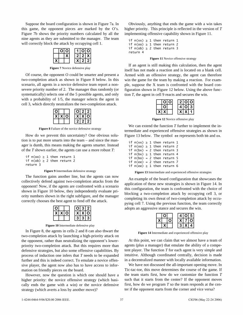
Suppose the board configuration is shown in Figure 7a. In this game, the opponent pieces are marked by the O’s. Figure 7b shows the priority numbers calculated by all the nine agents as they are submitted to the manager. The team will correctly block the attack by occupying cell 1.

O O 1 O OX 2 2 X

X X 2 2 Figure 7 Novice defensive play

Of course, the opponent O could be smarter and present a two-completion attack as shown in Figure 8 below. In this scenario, all agents in a novice defensive team report a non-severe priority number of 2. The manager thus randomly (or systematically) selects one of the 5 possible agents, and only with a probability of 1/5, the manager selects the agent in cell 3, which directly neutralizes the two-completion attack.

O O 2 2X X O X X O

2 2 2 Figure 8 Failure of the novice defensive strategy

How do we prevent this uncertainty? One obvious solu-tion is to put more smarts into the team – and since the man-ager is dumb, this means making the agents smarter. Instead of the T shown earlier, the agents can use a more robust T:

if n(oo) ≥ 1 then return 1 if n(ob) ≥ 2 then return 2 return 3

Figure 9 Intermediate defensive strategy

The function gains another line, but the agents can now collectively defend against two-completion attacks from the opponent! Now, if the agents are confronted with a scenario shown in Figure 10 below, they independently evaluate pri-ority numbers shown in the right subfigure, and the manager correctly chooses the best agent to fend off the attack.

O O 3 2X X O X X O

3 3 3 Figure 10 Intermediate defensive play

In Figure 8, the agents in cells 2 and 8 can also thwart the two-completion attack by launching a high-priority attack on the opponent, rather than neutralizing the opponent’s lower-priority two-completion attack. But this requires more than defensive strategies, but also some offensive capabilities. By process of induction one infers that T needs to be expanded further and this is indeed correct. To emulate a novice offen-sive player, the agent now also has to have access to infor-mation on friendly pieces on the board.

However, now the question is which one should have a higher priority: the novice offensive strategy (which basi-cally ends the game with a win) or the novice defensive strategy (which averts a loss by another move)?

Obviously, anything that ends the game with a win takes higher priority. This principle is reflected in the version of T implementing offensive capability shown in Figure 11.

if n(xx) ≥ 1 then return 1 if n(oo) ≥ 1 then return 2 if n(ob) ≥ 2 then return 3 return 4

Figure 11 Novice offensive strategy

If an agent is still making this calculation, then the agent itself has not made a reaction and is located on a blank cell. Armed with an offensive strategy, the agent can therefore win the game for the team by making a reaction. For exam-ple, suppose the X team is confronted with the board con-figuration shown in Figure 12 below. Using the above func-tion T, the agent in cell 9 reacts and secures the win.

O O 2 O OO 4 O 3

X X X X 1 Figure 12 Novice offensive play

We can extend the function T further to implement the in-termediate and experienced offensive strategies as shown in Figure 13 below. The symbol ee represents both bb and ox.

if n(xx) ≥ 1 then return 1 if n(oo) ≥ 1 then return 2 if n(bx) = 2 then return 3 if n(bx) ≥ 1 then return 4 if n(bo) = 2 then return 5 if n(ee) = 2 then return 7 if n(ee) ≥ 1 then return 6

Figure 13 Intermediate and experienced offensive strategies

An example of the board configuration that showcases the application of these new strategies is shown in Figure 14. In this configuration, the team is confronted with the choice of blocking a two-completion attack by occupying cell 3, or completing its own threat of two-completion attack by occu-pying cell 7. Using the previous function, the team correctly adopts an aggressive stance and secures the win.

O 4 O 5X O X 7 O

X 3 X 4 Figure 14 Intermediate and experienced offensive play

At this point, we can claim that we almost have a team of agents (plus a manager) that emulate the ability of a compe-tent player. The function T for each agent is very simple and intuitive. Although coordinated centrally, decision is made in a decentralized manner with locally available information.

We have not discussed the all-important opening move. In Tic-tac-toe, this move determines the course of the game. If the team starts first, how do we customize the function T such that it starts from the center? If the opponent moves first, how do we program T so the team responds at the cen-ter if the opponent starts from the corner and vice versa?

1-4244-0464-9/06/$20.00 2006 IEEE. 37 CIG'06 (May 22-24 2006)

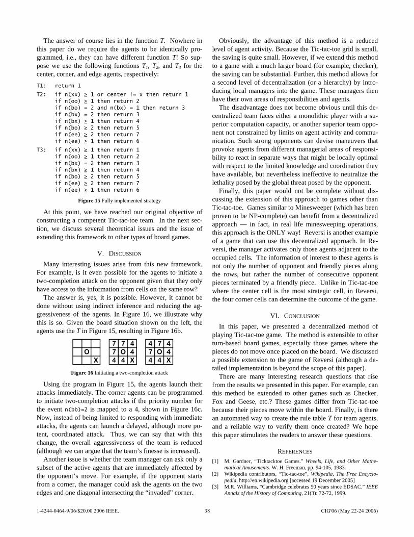
The answer of course lies in the function T. Nowhere in this paper do we require the agents to be identically pro-grammed, i.e., they can have different function T! So sup-pose we use the following functions T1, T2, and T3 for the center, corner, and edge agents, respectively:

T1: return 1

T2: if n(xx) ≥ 1 or center != x then return 1 if n(oo) ≥ 1 then return 2 if n(bo) = 2 and n(bx) = 1 then return 3 if n(bx) = 2 then return 3 if n(bx) ≥ 1 then return 4 if n(bo) ≥ 2 then return 5 if n(ee) ≥ 2 then return 7 if n(ee) ≥ 1 then return 6

T3: if n(xx) ≥ 1 then return 1 if n(oo) ≥ 1 then return 2 if n(bx) = 2 then return 3 if n(bx) ≥ 1 then return 4 if n(bo) ≥ 2 then return 5 if n(ee) ≥ 2 then return 7 if n(ee) ≥ 1 then return 6

Figure 15 Fully implemented strategy

At this point, we have reached our original objective of constructing a competent Tic-tac-toe team. In the next sec-tion, we discuss several theoretical issues and the issue of extending this framework to other types of board games.

V. DISCUSSION Many interesting issues arise from this new framework.

For example, is it even possible for the agents to initiate a two-completion attack on the opponent given that they only have access to the information from cells on the same row?

The answer is, yes, it is possible. However, it cannot be done without using indirect inference and reducing the ag-gressiveness of the agents. In Figure 16, we illustrate why this is so. Given the board situation shown on the left, the agents use the T in Figure 15, resulting in Figure 16b.

7 7 4 4 7 4O 7 O 4 7 O 4

X 4 4 X 4 4 X Figure 16 Initiating a two-completion attack

Using the program in Figure 15, the agents launch their attacks immediately. The corner agents can be programmed to initiate two-completion attacks if the priority number for the event n(bb)=2 is mapped to a 4, shown in Figure 16c. Now, instead of being limited to responding with immediate attacks, the agents can launch a delayed, although more po-tent, coordinated attack. Thus, we can say that with this change, the overall aggressiveness of the team is reduced (although we can argue that the team’s finesse is increased).

Another issue is whether the team manager can ask only a subset of the active agents that are immediately affected by the opponent’s move. For example, if the opponent starts from a corner, the manager could ask the agents on the two edges and one diagonal intersecting the “invaded” corner.

Obviously, the advantage of this method is a reduced level of agent activity. Because the Tic-tac-toe grid is small, the saving is quite small. However, if we extend this method to a game with a much larger board (for example, checker), the saving can be substantial. Further, this method allows for a second level of decentralization (or a hierarchy) by intro-ducing local managers into the game. These managers then have their own areas of responsibilities and agents.

The disadvantage does not become obvious until this de-centralized team faces either a monolithic player with a su-perior computation capacity, or another superior team oppo-nent not constrained by limits on agent activity and commu-nication. Such strong opponents can devise maneuvers that provoke agents from different managerial areas of responsi-bility to react in separate ways that might be locally optimal with respect to the limited knowledge and coordination they have available, but nevertheless ineffective to neutralize the lethality posed by the global threat posed by the opponent.

Finally, this paper would not be complete without dis-cussing the extension of this approach to games other than Tic-tac-toe. Games similar to Minesweeper (which has been proven to be NP-complete) can benefit from a decentralized approach — in fact, in real life minesweeping operations, this approach is the ONLY way! Reversi is another example of a game that can use this decentralized approach. In Re-versi, the manager activates only those agents adjacent to the occupied cells. The information of interest to these agents is not only the number of opponent and friendly pieces along the rows, but rather the number of consecutive opponent pieces terminated by a friendly piece. Unlike in Tic-tac-toe where the center cell is the most strategic cell, in Reversi, the four corner cells can determine the outcome of the game.

VI. CONCLUSION In this paper, we presented a decentralized method of

playing Tic-tac-toe game. The method is extensible to other turn-based board games, especially those games where the pieces do not move once placed on the board. We discussed a possible extension to the game of Reversi (although a de-tailed implementation is beyond the scope of this paper).

There are many interesting research questions that rise from the results we presented in this paper. For example, can this method be extended to other games such as Checker, Fox and Geese, etc.? These games differ from Tic-tac-toe because their pieces move within the board. Finally, is there an automated way to create the rule table T for team agents, and a reliable way to verify them once created? We hope this paper stimulates the readers to answer these questions.

REFERENCES [1] M. Gardner, “Ticktacktoe Games.” Wheels, Life, and Other Mathe-

matical Amusements. W. H. Freeman, pp. 94-105, 1983. [2] Wikipedia contributors, “Tic-tac-toe”, Wikipedia, The Free Encyclo-

pedia, http://en.wikipedia.org [accessed 19 December 2005] [3] M.R. Williams, “Cambridge celebrates 50 years since EDSAC.” IEEE

Annals of the History of Computing, 21(3): 72-72, 1999.

1-4244-0464-9/06/$20.00 2006 IEEE. 38 CIG'06 (May 22-24 2006)

Integration and Evaluation of Exploration-Based Learning in Games

Igor V. Karpov 1, Thomas D’Silva2, Craig Varrichio 3, Kenneth O. Stanley4, Risto Miikkulainen 1

1,2,3 Department of Computer Sciences, The University of Texas at Austin, Austin, TX 78712, USA4 School of Electrical Engineering and Computer Science, University of Central Florida, Orlando, FL 32816, USA

Abstract

Video and computer games provide a rich platform for test-ing adaptive decision systems such as value-based reinforce-ment learning and neuroevolution. However, integrating suchsystems into the game environment and evaluating their per-formance in it is time and labor intensive. In this paper, anapproach is developed for using general integration and eval-uation software to alleviate these problems. In particular, theTestbed for Integrating and Evaluating Learning Techniques(TIELT) is used to integrate a neuroevolution learner with anoff-the-shelf computer game Unreal TournamentTM5 (Aha andMolineaux 2004). The resulting system is successfully used toevolve artificial neural network controllers with basic naviga-tion behavior. Our work leads to formulating a set of require-ments that make a general integration and evaluation systemsuch as TIELT a useful tool for benchmarking adaptive deci-sion systems.

1 IntroductionIt is often necessary to compare new machine learning tech-niques empirically against other similar techniques to gaugehow they improve on previous results. In order to minimizethe influence ofdata biasin the evaluation process, new al-gorithms should be tested in as large a variety of domains aspossible, especially when general claims about their perfor-mance are being made. Existing video and computer gamesprovide a rich platform for testing adaptive decision systemssuch as value-based reinforcement learning and neuroevolu-tion. However, integrating and evaluating multiple algorithmsand implementations against multiple simulation domains isa difficult process. Moreover, any benchmarking results canalso be skewed byimplementation bias, or intentional or un-intentional disparity in quality of implementation of the pro-posed approach vs. the quality of implementation of compet-ing approaches (Keogh and Kassetty 2002).

One potential way to make empirical comparisons of learn-ing techniques easier and more principled is to build a flex-ible software platform that provides a uniform interface forthe learning system across multiple rich simulation domains.

1{ikarpov,risto}@cs.utexas.edu2tdsilva@mail.utexas.edu3cavarrichio@yahoo.com4kstanley@cs.ucf.edu5Unreal Tournament is a trademark of Epic Games, Inc.

Such a system allows researchers to concentrate on imple-menting and optimizing their approach to solving the learn-ing problem and to validate it empirically by comparing withother approaches.

In this paper we present the results of using one such “glue”framework to integrate an existing reinforcement learningtechnique with an existing game environment. The “glue”framework used is the Testbed for Integrating and EvaluatingLearning Techniques (TIELT), developed by David Aha andMatthew Molineaux (Aha and Molineaux 2004). It has beendesigned to “integrate AI systems with (e.g., real-time) gam-ing simulators, and to evaluate how well those systems learnon selected simulation tasks” (Molineaux and Aha 2005).

The project uses NeuroEvolution of Augmenting Topolo-gies (NEAT) method as the learning technique (Stanley andMiikkulainen 2002a). NEAT is a genetic algorithm thatevolves increasingly complex artificial neural network con-trollers by applying mutation and crossover operators to theirpopulations based on a fitness function. A real time variantof NEAT, called rtNEAT, has been used successfully in thegame NERO, produced by the Digital Media Collaboratoryat the University of Texas at Austin (Gold 2005; Stanley et al.2005b).

Using TIELT, NEAT is embedded into UnrealTournamentTM , a popular First Person Shooter (FPS)computer game produced by Epic Games, Inc. in 1999and winning a Game of the Year title for that year. UnrealTournamentTMwas previously integrated with the TIELT sys-tem and other learning methods were tested on it. However,exploration-based learning algorithms such as value-functionand evolution-based reinforcement learning have not beentested with Unreal/TIELT before (Molineaux 2004).

The next section describes the state of AI in gaming, thelearning technique of neuroevolution, and the TIELT ap-proach to integration and evaluation. Section 3 gives anoverview of our system’s architecture, Section 4 summarizesexperiments performed and their results, and Section 5 anal-yses the results and describes future work.

2 Background2.1 AI in gamingVideo game technology can provide a rich platform for val-idating and advancing theoretical AI research (Gold 2005).On the other hand, the video game industry stands to benefitfrom the adapting artificial intelligence and machine learning

1-4244-0464-9/06/$20.00 2006 IEEE. 39 CIG'06 (May 22-24 2006)

techniques into new, more interactive games.

Computer and video games constitute a large and lucrativemarket, 7.3 billion dollars in the US in 2004 (ESA 2005).This allows game studios to develop a variety of what canbe seen as high realism simulations for human-level controltasks, such as navigation, combat, team and individual tacticsand strategy. The emergence of online multi-player and mas-sively multi-player games offers unprecedented opportunitiesfor real-time interaction between human players and artifi-cially intelligent elements. Because of these factors, com-puter and video games may indeed be a ’killer application’for developing and validating machine learning techniques(Laird and van Lent 2000).

However, adaptive algorithms are used in the game indus-try setting surprisingly rarely. Most popular video games onthe market today use scripted non-player characters to addinteractivity to their games (Gold 2005). A large fraction ofAI development in the industry is devoted to path-finding al-gorithms such as A*-search and simple behaviors built us-ing finite state machines. There may be several reasons forwhy this is the case. One is that high-end game applicationshave traditionally pushed hardware systems to their limits andsimply did not have the resources to perform online learning.This is becoming less of a problem with the availability ofcheap processing power and true parallelism. Another, deeperreason may be that it is difficult to adopt results from aca-demic AI to games because they are not built and tested withthese applications directly in mind. Where the goal of an AIresearcher is often to build a system that is able to adapt toan environment to solve difficult tasks, the goal of a game de-veloper is to build a system that is “human-like” and “fun”.Integration systems such as TIELT can allow researchers andengineers to more easily integrate and test new learning algo-rithms with games, benefiting both academic AI research andcommercial game development.

2.2 Neuroevolution

Neuroevolution is a powerful technique for solving non-linear, non-Markovian control tasks (Gomez 2003). In neu-roevolution, a genetic algorithm is used to evolve artificialneural networks. NeuroEvolution of Augmenting Topologies(NEAT) is a particularly efficient method of this kind ableto evolve both network weights and topologies (Stanley andMiikkulainen 2002b). NEAT starts with a population of min-imal network topologies and complexifies them when neces-sary to solve the problem at hand. NEAT is able to protectinnovation through a speciation mechanism, and has an ef-fective encoding scheme that allows it to perform mutationand recombination operations efficiently.

Neuroevolution and NEAT in particular have been shownto outperform other methods on a number of benchmarklearning tasks. For example, neuroevolution has beensuccessfully used in a number of game-playing domains(Agogino et al. 2000; Stanley et al. 2005a). It is thereforeimportant to show that methods such as NEAT can benefitfrom general integration and evaluation tools such as TIELT.

2.3 Testbed for Integration and Evaluation ofLearning Techniques (TIELT)

The Testbed for Integration and Evaluation of Learning Tech-niques, or TIELT, is a Java application intended to connect agame engine to a decision system that learns about the game(Aha and Molineaux 2004). The goal of the system is to pro-vide the researcher with a tool that simplifies the task of test-ing a general learner in several different environments.

The application consists of fiveknowledge basesor mod-ules which correspond to different areas of TIELT’s function-ality. The Game Modelencapsulates the information aboutthe game from a single player’s perspective. TheGame In-terface Modeldescribes how TIELT communicates with thegame. TheDecision System Interface Modeldescribes in-teractions with the decision system. TheAgent Descriptiondescribes tasks performed by the system in order to play thegame, and theExperimental Methodologymodule is used asan evaluation platform for particular games and learning tech-niques.

During integration, TIELT is connected with the game en-vironment and with the learning system using the appropriateknowledge bases. The software allows the user to define thecommunication protocols between TIELT, the game engineand the learning system. TIELT also includes a visual script-ing language that allows scripting of the game behavior andupdate rules.

TIELT provides the ability to connect environments andlearners with arbitrary interfaces and rules into a cohesivelearning system and to automate the evaluation of this sys-tem’s performance. This paper explores how well these fea-tures support neuroevolution.

3 System architectureAt the highest level, the system consists of three parts: theUnreal TournamentTMserver, the TIELT integration platform,and the decision system based on NEAT. The game serversimulates the environment for the learning agent. TIELTcommunicates with the environment and accumulates a state,which is then communicated to the decision system. The de-cision system selects an action in the environment and com-municates it back through TIELT. The decision system con-tinually adopts its behavior by evolving artificial neural net-work controllers to perform the task.

3.1 Game engineUnreal TournamentTM is a real-time first person shooter(FPS) computer game in which a player navigates a three-dimensional space. The player can walk, run, jump, turn,shoot and interact with objects in the game such as armor,doors and health vials. The goal of one variant of the game(the tournament) is to be the first to destroy a certain numberof opponents. Up to 16 players can play the game concur-rently in a single level. A player can be controlled either by ahuman player connected over a network or an automated botcontrolled by a built-in script.

The Gamebots API from the University of Southern Cali-fornia modifies the original game to allow players to be con-trolled via sockets connected to other programs such as an

1-4244-0464-9/06/$20.00 2006 IEEE. 40 CIG'06 (May 22-24 2006)

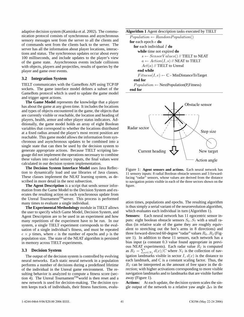
adaptive decision system (Kaminka et al. 2002). The commu-nication protocol consists of synchronous and asynchronoussensory messages sent from the server to all the clients andof commands sent from the clients back to the server. Theserver has all the information about player locations, interac-tions and status. The synchronous updates occur about every100 milliseconds, and include updates to the player’s viewof the game state. Asynchronous events include collisionswith objects, players and projectiles, results of queries by theplayer and game over events.

3.2 Integration SystemTIELT communicates with the GameBots API using TCP/IPsockets. The game interface model defines a subset of theGameBots protocol which is used to update the game modeland trigger agent actions.

The Game Modelrepresents the knowledge that a playerhas about the game at any given time. It includes the locationsand types of objects encountered in the game, the objects thatare currently visible or reachable, the location and heading ofplayers, health, armor and other player status indicators. Ad-ditionally, the game model holds an array of eight Booleanvariables that correspond to whether the locations distributedat a fixed radius around the player’s most recent position arereachable. This game model allows the information from syn-chronous and asynchronous updates to be combined into asingle state that can then be used by the decision system togenerate appropriate actions. Because TIELT scripting lan-guage did not implement the operations necessary to combinethese values into useful sensory inputs, the final values werecalculated in our decision system implementation.

The Decision System Interface Modeluses Java Reflec-tion to dynamically load and use libraries of Java classes.These classes implement the NEAT learning system, as de-scribed in more detail in the next subsection.

The Agent Description is a script that sends sensor infor-mation from the Game Model to the Decision System and ex-ecutes the resulting action on each synchronous update fromthe Unreal TournamentTMserver. This process is performedmany times to evaluate a single individual.

The Experimental Methodologymodule in TIELT allowsthe user to specify which Game Model, Decision System, andAgent Description are to be used in an experiment and howmany repetitions of the experiment have to be run. In oursystem, a single TIELT experiment corresponds to the eval-uation of a single individual’s fitness, and must be repeatede × p times, wheree is the number of epochs andp is thepopulation size. The state of the NEAT algorithm is persistedin memory across TIELT experiments.

3.3 Decision SystemThe output of the decision system is controlled by evolving

neural networks. Each static neural network in a populationperforms a number of decisions during a predefined lifetimeof the individual in the Unreal game environment. The re-sulting behavior is analyzed to compute a fitness score (sec-tion 4). The Unreal TournamentTMworld is then reset and anew network is used for decision-making. The decision sys-tem keeps track of individuals, their fitness functions, evalu-

Algorithm 1 Agent description tasks executed by TIELT

Population← RandomPopulation()for each epoche do

for each individualI dowhile time not expireddo

s← SensorV alues() // TIELT to NEATa← Action(I, s) // NEAT to TIELTAct(a) // TIELT to Unreal

end whileFitness(I, e)← C - MinDistanceToTarget

end forPopulation← NextPopulation(P,Fitness)

end for

Obstacle sensor

Current heading

Radar sectorStep size

Action angle

New target

Figure 1: Agent sensors and actions.Each neural network has11 sensory inputs: 8 radial Boolean obstacle sensors and 3 forward-facing “radar” sensors, whose values are derived from the distanceto navigation points visible in each of the three sectors shown on thefigure.

ation times, populations and epochs. The resulting algorithmis thus simply a serial variant of the neuroevolution algorithm,which evaluates each individual in turn (Algorithm 1).Sensors: Each neural network has 11 egocentric sensor in-puts: eight boolean obstacle sensorsS0..S7 with a small ra-dius (in relative scale of the game they are roughly equiv-alent to stretching out the bot’s arms in 8 directions) andthree forward-directed 60-degree “radar” valuesR0..R2 (Fig-ure 1). In addition to these 11 sensors, each network has abias input (a constant 0.3 value found appropriate in previ-ous NEAT experiments). Each radar valueRI is computedasRI =

∑x∈NI

d(x)/C whereNI is the collection of nav-igation landmarks visible in sectorI, d(x) is the distance toeach landmark, and C is a constant scaling factor. Thus, theRI can be interpreted as the amount of free space in the di-rection; with higher activations corresponding to more visiblenavigation landmarks and to landmarks that are visible furtheraway (Figure 1).Actions: At each update, the decision system scales the sin-gle output of the network to a relative yaw angle∆α in the

1-4244-0464-9/06/$20.00 2006 IEEE. 41 CIG'06 (May 22-24 2006)

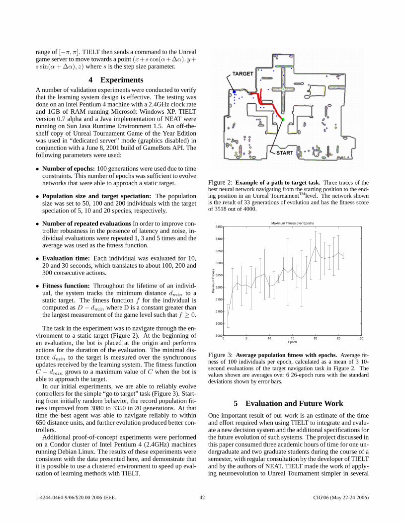
range of[−π, π]. TIELT then sends a command to the Unrealgame server to move towards a point(x+s cos(α+∆α), y+s sin(α + ∆α), z) wheres is the step size parameter.

4 ExperimentsA number of validation experiments were conducted to verifythat the learning system design is effective. The testing wasdone on an Intel Pentium 4 machine with a 2.4GHz clock rateand 1GB of RAM running Microsoft Windows XP. TIELTversion 0.7 alpha and a Java implementation of NEAT wererunning on Sun Java Runtime Environment 1.5. An off-the-shelf copy of Unreal Tournament Game of the Year Editionwas used in “dedicated server” mode (graphics disabled) inconjunction with a June 8, 2001 build of GameBots API. Thefollowing parameters were used:

• Number of epochs:100 generations were used due to timeconstraints. This number of epochs was sufficient to evolvenetworks that were able to approach a static target.

• Population size and target speciation:The populationsize was set to 50, 100 and 200 individuals with the targetspeciation of 5, 10 and 20 species, respectively.

• Number of repeated evaluationsIn order to improve con-troller robustness in the presence of latency and noise, in-dividual evaluations were repeated 1, 3 and 5 times and theaverage was used as the fitness function.

• Evaluation time: Each individual was evaluated for 10,20 and 30 seconds, which translates to about 100, 200 and300 consecutive actions.

• Fitness function: Throughout the lifetime of an individ-ual, the system tracks the minimum distancedmin to astatic target. The fitness functionf for the individual iscomputed asD − dmin where D is a constant greater thanthe largest measurement of the game level such thatf ≥ 0.

The task in the experiment was to navigate through the en-vironment to a static target (Figure 2). At the beginning ofan evaluation, the bot is placed at the origin and performsactions for the duration of the evaluation. The minimal dis-tancedmin to the target is measured over the synchronousupdates received by the learning system. The fitness functionC − dmin grows to a maximum value ofC when the bot isable to approach the target.

In our initial experiments, we are able to reliably evolvecontrollers for the simple “go to target” task (Figure 3). Start-ing from initially random behavior, the record population fit-ness improved from 3080 to 3350 in 20 generations. At thattime the best agent was able to navigate reliably to within650 distance units, and further evolution produced better con-trollers.

Additional proof-of-concept experiments were performedon a Condor cluster of Intel Pentium 4 (2.4GHz) machinesrunning Debian Linux. The results of these experiments wereconsistent with the data presented here, and demonstrate thatit is possible to use a clustered environment to speed up eval-uation of learning methods with TIELT.

Figure 2: Example of a path to target task. Three traces of thebest neural network navigating from the starting position to the end-ing position in an Unreal TournamentTM level. The network shownis the result of 33 generations of evolution and has the fitness scoreof 3518 out of 4000.

0 5 10 15 20 25 303000

3050

3100

3150

3200

3250

3300

3350

3400

3450

Ma

xim

um

Fitn

ess

Epoch

Maximum Fitness over Epochs

Figure 3: Average population fitness with epochs.Average fit-ness of 100 individuals per epoch, calculated as a mean of 3 10-second evaluations of the target navigation task in Figure 2. Thevalues shown are averages over 6 26-epoch runs with the standarddeviations shown by error bars.

5 Evaluation and Future Work

One important result of our work is an estimate of the timeand effort required when using TIELT to integrate and evalu-ate a new decision system and the additional specifications forthe future evolution of such systems. The project discussed inthis paper consumed three academic hours of time for one un-dergraduate and two graduate students during the course of asemester, with regular consultation by the developer of TIELTand by the authors of NEAT. TIELT made the work of apply-ing neuroevolution to Unreal Tournament simpler in several

1-4244-0464-9/06/$20.00 2006 IEEE. 42 CIG'06 (May 22-24 2006)

ways. Above all, the communication layer between Unrealand TIELT was already implemented and required only mi-nor adjustments to integrate with the NEAT decision system.

At the end of the semester, the learner-environment systemhad basic functionality to evolve agents as single actors in theenvironment. However, the system was found to not be well-suited for running and analyzing repeated experiments effi-ciently. TIELT’s design did not provide a convenient way toparallelize evaluations of agents or to evolve multiple agentsacting in the same environment. As a result, a large portion ofthe functionality that can be taken care of in the “glue” frame-work has to be implemented in the decision system. Thismakes the decision system specific to the Unreal Tournamentapplication and reduces the advantages of the middle layer.

There are several ways in which the TIELT system could bemodified or other similar integration platforms be built in thefuture to better support exploration-based learning. In partic-ular, the system can be more efficient, provide better supportfor batch experiments, easier to use, more flexible and moreopen.

Efficiency: Because the integration, evaluation and deci-sion systems are implemented as Java applications, they canincur unexpected garbage collection delays and are oftenslower than native implementations. The Unreal Tournamentserver, which executes separately and as a native binary, doesnot incur such delays. In addition, the extra layers of in-direction between the environment and the decision systemadd computational overhead to the process of making an in-dividual decision. We observed these factors add up to cre-ate highly variable per-action latency, which introduces newchallenges into learning a task in a simulated real-time envi-ronment. A system such as TIELT can minimize these irreg-ularities by providing a more efficient implementation or byusing low-pause garbage collection techniques.

Parallelism: TIELT is currently designed for evaluation ofa single player learning agent, against an external or a hu-man opponent, and there is no directly supported way to com-bine evaluations of several individuals in parallel into a singlelearning system, even though such evaluation is possible inthe environment (Unreal Tournament supports up to 16 simul-taneous players). Adding explicit multi-agent functionality toTIELT would greatly increase the utility of the platform whenevaluating population-based learning systems like NEAT.

Support for Batch Experiments: While TIELT does pro-vide some support for running experiments in batch mode,some settings are only available through the graphical userinterface. This interactive component of TIELT makes it dif-ficult to run long series of repeated experiments, especiallywhen distributing the work to a cluster of machines. For someof our experiments, additional software was used to scriptuser interactions in a virtual environment, which created un-necessary overhead. In designing a testbed such as TIELT,care should be taken to ensure that all use cases can be recre-ated in non-interactive batch mode.

TIELT has the capability to integrate the game engine, theTIELT application itself, and the decision system while theyare running on different physical machines and communi-

cate via network messages. This is a powerful feature, and itshould be expanded with the ability to script experiments andto distribute evaluations over several different computers run-ning TIELT. This would help optimize use of computationalresources and researcher time.

Usability and Flexibility: In order to make TIELT integra-tion less time-consuming, the framework can be simplified bymaking use of existing technology. Instead of using a customscripting language, future integration systems can be mademore powerful and easier to approach by using an existingscripting language such as Python or Ruby, bringing to bearexisting documentation, libraries, and experience.

If the goal of the middleware is to support many differ-ent kinds of learning systems, its architecture should be flex-ible enough to be usable in all those models. The knowledgebases and modules of TIELT, while well-suited for rule-basedlearning, are not as useful with neuroevolution or online rein-forcement learning. For NEAT as well as other reinforcementlearning methods, the concepts of an evaluation episode, anindividual agent, and a population are beneficial. Future ver-sions of TIELT and other integration and evaluation systemscan benefit from a more modular architecture which suppliessome specific features needed by different kinds of learningagents and environments.

Access to Source: Learning agent benchmarking interfacessuch as TIELT must have their source open to the users. Do-ing so will greatly shorten the debugging cycle as well asallow researchers to have complete knowledge of the im-plementation of their experimental system. Unfortunately,TIELT is currently a closed source project.

6 ConclusionThe results in this paper show that a generic framework suchas TIELT can be used to integrate and evaluate adaptive de-cision systems with rich computer game environments. Basictarget-seeking behavior was evolved with NEAT neuroevo-lution method for an agent in the Unreal Tournament videogame. However, in order to make such frameworks practicaland their use more widespread, progress needs to be made inseveral aspects. They must be designed and implemented ashigh-performance and lightweight applications, better utilizestandard interfaces and existing scripting languages, and pro-vide support for distributed and scripted operation for batchcomputational experiments. With these extensions, it may bepossible to use sophisticated game playing domains in devel-oping better exploration-based learning methods, as well asdevelop more interesting adoptive elements for future games.

A AcknowledgmentsThanks to David Aha and Matthew Molineaux for provid-ing the TIELT platform. This work was supported in part byDARPA through an NRL grant #N00173041G025.

ReferencesAgogino, A., Stanley, K., and Miikkulainen, R. (2000). On-

line interactive neuro-evolution.Neural Processing Let-ters, 11:29–38.

1-4244-0464-9/06/$20.00 2006 IEEE. 43 CIG'06 (May 22-24 2006)

Aha, D. W., and Molineaux, M. (2004). Integrating learningin interactive gaming simulators. InChallenges of GameAI: Proceedings of the AAAI’04 Workshop. AAAI Press.

ESA (2005). Essential facts about the computer and videogame industry.

Gold, A. (2005). Academic AI and video games: a casestudy... InProceedings of the IEEE 2005 Symposium onComputational Intelligence and Games (CIG’05). IEEE.

Gomez, F. (2003).Robust Non-Linear Control Through Neu-roevolution. PhD thesis, Department of Computer Sci-ences, The University of Texas at Austin.

Kaminka, G. A., Veloso, M. M., Schaffer, S., Sollitto, C.,Adobbati, R., Marshall, A. N., Scholer, A., and Tejada,S. (2002). Gamebots: a flexible test bed for multiagentteam research.Communications of the ACM, 45(1):43–45.

Keogh, E., and Kassetty, S. (2002). On the need for timeseries data mining benchmarks: a survey and empiri-cal demonstration. In8th ACM SIGKDD InternationalConference on Knowledge Discovery and Data Mining,102–111.

Laird, J. E., and van Lent, M. (2000). Human-level AI’s killerapplication: Interactive computer games. InProceed-ings of the 17th National Conference on Artificial Intel-ligence and the 12th Annual Conference on InnovativeApplications of Artificial Intelligence. Menlo Park, CA:AAAI Press.

Molineaux, M. (2004).TIELT (v0.5 Alpha) User’s Manual.Molineaux, M., and Aha, D. W. (2005). TIELT project

website. Project web site, Naval Research Laboratory,http://nrlsat.ittid.com/ .

Stanley, K. O., Bryant, B. D., and Miikkulainen, R. (2005a).Evolving neural network agents in the NERO videogame. InProceedings of the 2005 IEEE Symposium onComputational Intelligence and Games(CIG’05). IEEE.

Stanley, K. O., Cornelius, R., Miikkulainen, R., D’Silva, T.,and Gold, A. (2005b). Real-time learning in the NEROvideo game. InProceedings of the Artificial Intelligenceand Interactive Digital Entertainment Conference (AI-IDE 2005) Demo Papers.

Stanley, K. O., and Miikkulainen, R. (2002a). Efficient evolu-tion of neural network topologies. InProceedings of the2002 Congress on Evolutionary Computation (CEC’02).Piscataway, NJ: IEEE. In press.

Stanley, K. O., and Miikkulainen, R. (2002b). Evolving neu-ral networks through augmenting topologies.Evolution-ary Computation, 10:99–127.

1-4244-0464-9/06/$20.00 2006 IEEE. 44 CIG'06 (May 22-24 2006)

Abstract— In this paper, coevolution is used to evolve Artificial Neural Networks (ANN) which evaluate board positions of a two player zero-sum game (The Virus Game). The coevolved neural networks play at a level that beats a group of strong hand-crafted AI players. We investigate the per formance of coevolution star ting from random initial weights and star ting with weights that are tuned by gradient based adaptive learning methods (Backpropagation, RPROP and iRPROP). The results of coevolutionary exper iments show that pre training of the population is highly effective in this case.

I. INTRODUCTION

In biology, coevolution is the mutual evolutionary influence between two species that become dependent on each other. Each species in a coevolutionary relationship exerts selective pressures on the other species. Coevolution occurs if the traits of one species A have evolved due to the presence of a second species B and vice versa. This natural phenomenon has motivated AI researchers to apply coevolution in solving different types of problems where two or more entities are interacting with each other. Coevolution is an unsupervised learning method that requires only relative measurement of phenotype performance, well-suited to the game-playing domain.

The gradient-based learning methods: Backpropagation [17], resilient backpropagation (RPROP) [16] and improved resilient backpropagation (iRPROP) [9] are supervised learning methods. They use a delta rule and can be applied to the problem of learning neural network weights to give a network which produces the desired outputs with minimised error.

Games continue to be important domains for investigating problem solving techniques [13]. Games offer tremendous complexity in a computer manageable form and need sophisticated AI methods to play at expert level. Board games like Chess [4], checkers [8], Othello [24] and backgammon [22] have been used to explore new ideas in AI. We will survey this work late in this section. In this paper, we used the “Virus Game” as a testbed to explore coevolutionary ideas.

The “Virus Game” [6] [7] [10] is a two-person perfect information board game of skill. The game is played on a

square board. The start position of the game is shown in Figure 1. The player who always starts the game is the Black Player and the other player is the White Player.

In the Virus Game, there are two kinds of moves available for each turn. The first kind of move is grow move or one step move. In this kind of move, a player moves a piece of his colour to an empty position adjacent to its current position. The positions are adjacent if their borders or corners are adjacent. The result of this move reproduces the moving piece and occupies both positions, the new position (which was empty) and the old position. The grow move is shown in Figure 2. The second kind of move is called jump move or two step-move. In this case, a player moves a piece to an empty position which is two squares away from its current position via an empty square. The piece leaves the old position empty and occupies the new position. Figure 3 shows a jump move. In either case, all opposing pieces adjacent to the new player’s piece change colour. Players alternate, moving only one piece per turn. The game ends when neither player can move. The player with the greatest number of pieces is the winner. The game is declared a draw if both players have the same number of pieces at game end.

The Virus Game has higher branching factor than chess, draughts and Othello and appears to be a difficult game for a human player to play well despite its simple rules [7]. We have a strong pool of hand-crafted AI players for the Virus Game, each written by a different person since these were used in an AI-writing competition [6].Competitive learning was initially explored by Samuel [20] to adjust the parameters of a deterministic evaluation function in a checkers playing computer program. Tesauro [22] used the temporal-difference learning approach to evolve a backgammon-playing neural network. Tesauro’s TD-Gammon yields a computer playing backgammon program of world-champion strength. Coevolutionary competitive learning is explored for the Repeated Prisoner’s Dilemma (RPD) by Axelrod [2] and Miller [11]. Axelrod evolve RPD playing strategies using a fixed environment (i.e. using eight fixed opponents) while Miller coevolved the RPD strategies by playing each strategy against every other strategy and itself in a population. According to the results shown by

A Coevolutionary Model for The Virus Game

P.I.Cowling, M.H.Naveed and M.A. Hossain MOSAIC Research Centre, Department of Computing,

University of Bradford Bradford, BD7 1DP, UK.

E-mail: P.I.Cowling, M.H.Naveed and M.A.Hossain1@bradford.ac.uk

1-4244-0464-9/06/$20.00 2006 IEEE. 45 CIG'06 (May 22-24 2006)

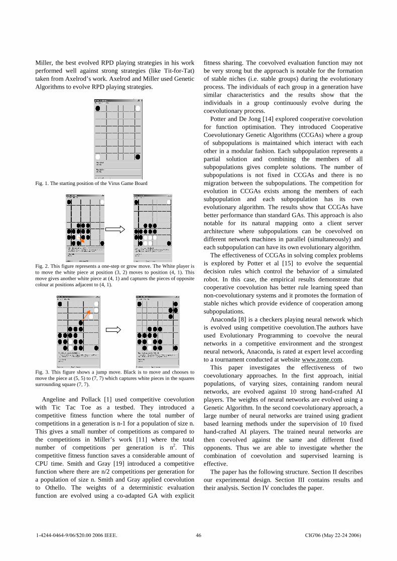
Miller, the best evolved RPD playing strategies in his work performed well against strong strategies (like Tit-for-Tat) taken from Axelrod’s work. Axelrod and Miller used Genetic Algorithms to evolve RPD playing strategies.

Fig. 1. The starting position of the Virus Game Board

Fig. 2. This figure represents a one-step or grow move. The White player is to move the white piece at position (3, 2) moves to position (4, 1). This move gives another white piece at (4, 1) and captures the pieces of opposite colour at positions adjacent to (4, 1).

Fig. 3. This figure shows a jump move. Black is to move and chooses to move the piece at (5, 5) to (7, 7) which captures white pieces in the squares surrounding square (7, 7).

Angeline and Pollack [1] used competitive coevolution

with Tic Tac Toe as a testbed. They introduced a competitive fitness function where the total number of competitions in a generation is n-1 for a population of size n. This gives a small number of competitions as compared to the competitions in Miller’s work [11] where the total number of competitions per generation is n2. This competitive fitness function saves a considerable amount of CPU time. Smith and Gray [19] introduced a competitive function where there are n/2 competitions per generation for a population of size n. Smith and Gray applied coevolution to Othello. The weights of a deterministic evaluation function are evolved using a co-adapted GA with explicit

fitness sharing. The coevolved evaluation function may not be very strong but the approach is notable for the formation of stable niches (i.e. stable groups) during the evolutionary process. The individuals of each group in a generation have similar characteristics and the results show that the individuals in a group continuously evolve during the coevolutionary process.

Potter and De Jong [14] explored cooperative coevolution for function optimisation. They introduced Cooperative Coevolutionary Genetic Algorithms (CCGAs) where a group of subpopulations is maintained which interact with each other in a modular fashion. Each subpopulation represents a partial solution and combining the members of all subpopulations gives complete solutions. The number of subpopulations is not fixed in CCGAs and there is no migration between the subpopulations. The competition for evolution in CCGAs exists among the members of each subpopulation and each subpopulation has its own evolutionary algorithm. The results show that CCGAs have better performance than standard GAs. This approach is also notable for its natural mapping onto a client server architecture where subpopulations can be coevolved on different network machines in parallel (simultaneously) and each subpopulation can have its own evolutionary algorithm.

The effectiveness of CCGAs in solving complex problems is explored by Potter et al [15] to evolve the sequential decision rules which control the behavior of a simulated robot. In this case, the empirical results demonstrate that cooperative coevolution has better rule learning speed than non-coevolutionary systems and it promotes the formation of stable niches which provide evidence of cooperation among subpopulations.

Anaconda [8] is a checkers playing neural network which is evolved using competitive coevolution.The authors have used Evolutionary Programming to coevolve the neural networks in a competitive environment and the strongest neural network, Anaconda, is rated at expert level according to a tournament conducted at website www.zone.com.

This paper investigates the effectiveness of two coevolutionary approaches. In the first approach, initial populations, of varying sizes, containing random neural networks, are evolved against 10 strong hand-crafted AI players. The weights of neural networks are evolved using a Genetic Algorithm. In the second coevolutionary approach, a large number of neural networks are trained using gradient based learning methods under the supervision of 10 fixed hand-crafted AI players. The trained neural networks are then coevolved against the same and different fixed opponents. Thus we are able to investigate whether the combination of coevolution and supervised learning is effective.

The paper has the following structure. Section II describes our experimental design. Section III contains results and their analysis. Section IV concludes the paper.

1-4244-0464-9/06/$20.00 2006 IEEE. 46 CIG'06 (May 22-24 2006)

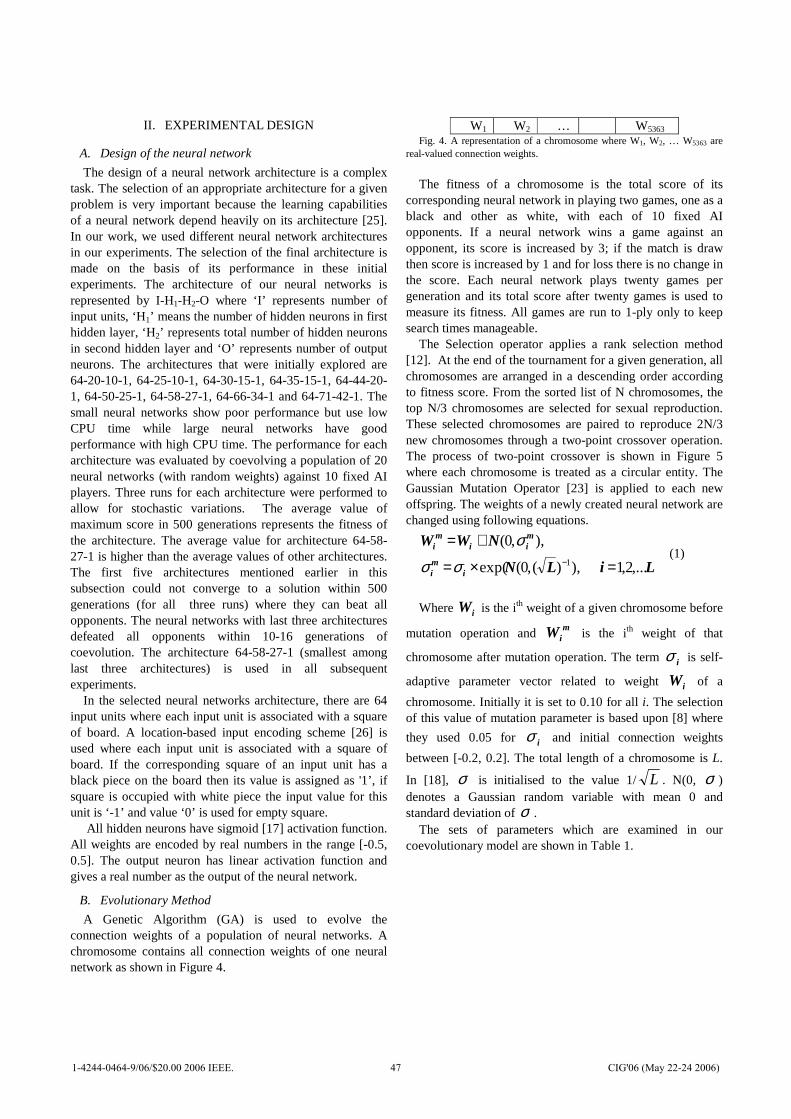
II. EXPERIMENTAL DESIGN

A. Design of the neural network

The design of a neural network architecture is a complex task. The selection of an appropriate architecture for a given problem is very important because the learning capabilities of a neural network depend heavily on its architecture [25]. In our work, we used different neural network architectures in our experiments. The selection of the final architecture is made on the basis of its performance in these initial experiments. The architecture of our neural networks is represented by I-H1-H2-O where ‘I’ represents number of input units, ‘H1’ means the number of hidden neurons in first hidden layer, ‘H2’ represents total number of hidden neurons in second hidden layer and ‘O’ represents number of output neurons. The architectures that were initially explored are 64-20-10-1, 64-25-10-1, 64-30-15-1, 64-35-15-1, 64-44-20-1, 64-50-25-1, 64-58-27-1, 64-66-34-1 and 64-71-42-1. The small neural networks show poor performance but use low CPU time while large neural networks have good performance with high CPU time. The performance for each architecture was evaluated by coevolving a population of 20 neural networks (with random weights) against 10 fixed AI players. Three runs for each architecture were performed to allow for stochastic variations. The average value of maximum score in 500 generations represents the fitness of the architecture. The average value for architecture 64-58-27-1 is higher than the average values of other architectures. The first five architectures mentioned earlier in this subsection could not converge to a solution within 500 generations (for all three runs) where they can beat all opponents. The neural networks with last three architectures defeated all opponents within 10-16 generations of coevolution. The architecture 64-58-27-1 (smallest among last three architectures) is used in all subsequent experiments.

In the selected neural networks architecture, there are 64 input units where each input unit is associated with a square of board. A location-based input encoding scheme [26] is used where each input unit is associated with a square of board. If the corresponding square of an input unit has a black piece on the board then its value is assigned as '1’, if square is occupied with white piece the input value for this unit is ‘-1’ and value ‘0’ is used for empty square.

All hidden neurons have sigmoid [17] activation function. All weights are encoded by real numbers in the range [-0.5, 0.5]. The output neuron has linear activation function and gives a real number as the output of the neural network.

B. Evolutionary Method

A Genetic Algorithm (GA) is used to evolve the connection weights of a population of neural networks. A chromosome contains all connection weights of one neural network as shown in Figure 4.

W1 W2 … W5363 Fig. 4. A representation of a chromosome where W1, W2, … W5363 are

real-valued connection weights.

The fitness of a chromosome is the total score of its

corresponding neural network in playing two games, one as a black and other as white, with each of 10 fixed AI opponents. If a neural network wins a game against an opponent, its score is increased by 3; if the match is draw then score is increased by 1 and for loss there is no change in the score. Each neural network plays twenty games per generation and its total score after twenty games is used to measure its fitness. All games are run to 1-ply only to keep search times manageable.

The Selection operator applies a rank selection method [12]. At the end of the tournament for a given generation, all chromosomes are arranged in a descending order according to fitness score. From the sorted list of N chromosomes, the top N/3 chromosomes are selected for sexual reproduction. These selected chromosomes are paired to reproduce 2N/3 new chromosomes through a two-point crossover operation. The process of two-point crossover is shown in Figure 5 where each chromosome is treated as a circular entity. The Gaussian Mutation Operator [23] is applied to each new offspring. The weights of a newly created neural network are changed using following equations.

LiLN

NWW

imi

mii

mi

,...2,1),)(,0(exp(

),,0(1 =×=

+=−σσ

σ (1)

Where iW is the ith weight of a given chromosome before

mutation operation and miW is the ith weight of that

chromosome after mutation operation. The term iσ is self-

adaptive parameter vector related to weight iW of a

chromosome. Initially it is set to 0.10 for all i. The selection of this value of mutation parameter is based upon [8] where

they used 0.05 for iσ and initial connection weights

between [-0.2, 0.2]. The total length of a chromosome is L.

In [18], σ is initialised to the value 1/L . N(0, σ ) denotes a Gaussian random variable with mean 0 and standard deviation of σ .

The sets of parameters which are examined in our coevolutionary model are shown in Table 1.

1-4244-0464-9/06/$20.00 2006 IEEE. 47 CIG'06 (May 22-24 2006)

Fig. 5. The process of two-point crossover. C1 and C2 are the chromosomes selected for sexual reproduction.

TABLE.1: PARAMETERS FOR GA EXPERIMENTS

POPULATION

SIZE CROSS OVER

RATE MUTATION SELF-

ADAPTIVE PARAMETER 6 0% 0.10 6 20% 0.10

15 0% 0.10 15 20% 0.10 20 0% 0.10 20 20% 0.10 30 0% 0.10 30 20% 0.10 50 0% 0.10 50 20% 0.10

C. Supervised learning Methods

Neural networks are trained under the supervision of 10 hand-crafted AI players using gradient-based techniques: Backpropagation (BP), RPROP and iRPROP. In this case, 10 different training sets are created where each training set contains a large number of board positions and their evaluation values as determined by a hand-crafted AI player. Therefore, each neural network is trained to learn the evaluation function of a given hand-crafted AI player. Each neural network is trained using one training set. Four neural networks are trained using iRPROP, three are trained using RPROP and three are trained using BP, for each hand-crafted AI player. BP uses a learning rate of 0.01. The learning parameters for RPROP and iRPROP are set to � +=1.2, � -=0.50, � o=0.5, � min=0 and � max=50. The selection of the learning parameters of gradient-based learning methods is made according to the recommended values by authors in [21], [16] and [9]. Thus a pool of 100 neural networks is trained under the supervision of 10 different training data sets (each based on a different hand-crafted AI player).

D. Coevolutionary Model

Our coevolutionary model uses two different approaches for generating the starting population. In the first approach, an initial population of neural networks with random weights is coevolved against ten fixed opponents. The coevolution of

neural networks continues until at least one neural network in a given population beats all of the fixed opponents or there is no improvement in the scores of the best neural network for 10 consecutive generations. All games in this coevolutionary approach are played at 1-ply by both neural networks and fixed opponents.

In the second approach an initial population of trained neural networks is used. These neural networks are selected from the pool of 100 pre-trained neural networks. If the population size is less than or equal to 10, all neural networks used are based on different hand-crafted AI players. If population size is greater than 10, these are selected randomly in such a way as to ensure that a neural network trained by each of the 10 hand-crafted AI players is in the starting population. Therefore two populations of size 20 would have 10 identical and 10 different neural networks in the initial population. The trained neural networks are coevolved against 10 fixed opponents. The stopping condition and ply depth is same as used in first approach. So, the difference between two approaches is that the second approach combines two machine learning techniques i.e. gradient-based learning and coevolution.

To assess the generality of approach, we also test against another 10 hand-crafted AI players which are not used in pre-training or coevolution.

III. RESULTS AND ANALYSIS

The results obtained from the randomly initialised neural networks are summarized in table 2 while the performance of the best of these coevolved neural networks against 10 hand-crafted AI players is shown in table 3. All experiments are run on Pentium IV 1.2 GHz using C#.Net running under Windows XP.

TABLE. 2. RESULTS OF COEVOLUTION WITH AN INITIAL POPULATION OF

RANDOMLY CREATED NEURAL NETWORKS. COLUMNS 3, 4 AND 5 SHOW

PERFORMANCE AGAINST TEN HAND-CRAFTED OPPONENTS AVERAGED OVER

10 COEVOLUTIONARY RUNS POP SIZE

CROSS OVER

RATE

MEAN

OF

MAX

MEAN

OF MIN

MEAN

OF MEAN

MEAN

OF GENER

ATION

MEAN CPU TIME (SEC)

6 0% 3 0 2 11 9 6 20% 18 0 9 10 13

15 0% 9 0 1 10 28 15 20% 6 0 1 11 40 20 0% 12 0 5 11 53 20 20% 30 0 3 6 57 30 0% 30 0 16 11 61 30 20% 60 0 34 6 72 50 0% 21 0 22 11 132 50 20% 60 0 35 5 72

Table 2 shows the results of coevolution with populations starting from randomly created neural networks. The column “Mean of Generation” represents average number of generations over 10 runs and “mean CPU time” represents

1-4244-0464-9/06/$20.00 2006 IEEE. 48 CIG'06 (May 22-24 2006)

usage of average CPU time in seconds by a population during coevolutionary process over 10 runs.

We can see that small populations give much worse results than large ones. The difference between the performance of small and large populations is probably due to the number of parallel directions for exploring potential solutions in the search space. The experimental results also demonstrate that small populations use less CPU time than large populations, essentially since less neural network evolution are required..

The average maximum scores with 0% and 20% crossover rates demonstrate that neural networks evolved using crossover generally have higher scores than those which do not. The crossover operation appears to help the evolutionary process to explore a more interesting region of the search space. The crossover operator speeds convergence, and the population converges to better solution than without crossover. The mean of min and mean values show that diverse populations are maintained. TABLE. 3. THE SCORE OF THE STRONGEST NEURAL NETWORK FROM EACH

COEVOLVED POPULATION STARTING FROM AN INITIAL POPULATION OF

RANDOMLY CREATED NEURAL NETWORKS AGAINST 10 HAND-CRAFTED AI OPPONENTS.

POP

SIZE CROSS OVER RATE

PLAYING AS BLACK PLAYING AS WHITE

WIN DRAW WIN DRAW

6 0% 10 0 0 0 6 20% 10 0 10 0

15 0% 10 0 0 0 15 20% 10 0 0 0 20 0% 10 0 0 0 20 20% 10 0 10 0 30 0% 10 0 0 10 30 20% 10 0 10 0 50 0% 10 0 0 0 50 20% 10 0 10 0

Table 3 summarises the results of the best evolved neural

network from each population where coevolution was started from an initial population of randomly generated neural networks. Each evolved neural network plays as black and white against ten hand-crafted AI, as in table 2. All the best neural networks with 0% crossover rate have won games as black against all AI opponents but none is able to win when playing as white. The best-evolved neural networks of all populations (except population of size 15) with 20% crossover rate won all games when playing as black and white. Table 2 and 3 provide clear evidence for the effectiveness of the crossover operator, and support the advantage of Black and White in the Virus game, at least for approaches using 1-ply search.

Table 4 shows the mean of maximum, mean, and minimum scores of coevolved neural networks with a starting population of pre-trained neural networks. The table also shows the mean number of generations and CPU time (in seconds) for each population with different crossover rates. Again we see that small populations perform more poorly than larger populations. If we compare the results of

tables 2 and 4, it can be construed that starting from a population of pre trained neural networks gives better and more consistent performance (in terms of playing strength) than starting from a population of random neural networks. Large sized populations (started with initial population of pre trained neural networks) use a smaller number of generations but still require more CPU time during the coevolution of neural networks than small size populations. The values of mean of minimum and maximum scores show the diversity is maintained in the population. Note that CPU times in this case include the time need for learning of the initial population

Generally, we see from table 4 that coevolution with crossover needs fewer generations and less CPU time than without crossover.

TABLE. 4. RESULTS OF COEVOLUTION WITH AN INITIAL POPULATION OF PRE-TRAINED NEURAL NETWORKS. COLUMNS 3, 4 AND 5 SHOW PERFORMANCE

AGAINST TEN HAND-CRAFTED OPPONENTS AVERAGED OVER 10

COEVOLUTIONARY RUNS. POP SIZE

CROSS

OVER

RATE

MEAN

OF

MAX

MEAN

OF MIN

MEAN

OF MEAN

MEAN OF

GENER

ATIONS

MEAN CPU TIME (SEC)

6 0% 40 0 28 13 12 6 20% 60 0 31 5 7

15 0% 60 0 22 3 18 15 20% 60 0 28 1 18 20 0% 60 0 26 3 31 20 20% 60 0 31 1 25 30 0% 60 0 29 2 66 30 20% 60 0 36 1 55 50 0% 60 0 32 1 84 50 20% 60 0 34 1 84

Table 5 gives the mean results of the maximum, mean and

minimum scores of the initial populations before the start of evolution. The results after the coevolution are shown in table 4. In many cases evolution is not required, in spite of the fact that the performance of the AI players is variable, as table 7 shows.

TABLE 5. RESULTS FOR PRE TRAINED NEURAL NETWORKS PRIOR TO

EVOLUTION. POP SIZE

CROSS OVER

RATE

MEAN OF

MAX

MEAN OF

MIN

MEAN OF MEAN

6 0% 40 0 30 6 20% 40 0 30

15 0% 55 0 40 15 20% 55 0 44 20 0% 55 0 40 20 20% 60 0 45 30 0% 55 0 44 30 20% 60 0 45 50 0% 60 10 35 50 20% 60 0 40

The results of table 5 show that the populations of large

size (starting from the initial population of pre trained neural

1-4244-0464-9/06/$20.00 2006 IEEE. 49 CIG'06 (May 22-24 2006)

networks) generally have at least one pre trained neural network which beats all the opponents before the start of coevolution when playing as black and white. We see from table 4 that the values of mean of mean scores are reduced during coevolutionary process when compared with the values in table 5, and that average mean scores with crossover are larger than average mean scores without crossover.

In order to further investigate the generality of populations starting from an initial population of pre trained neural networks, we introduced 10 more hand-crafted AI opponents which were not used in the training of the initial population. Table 6 gives the average results of coevolution with different populations starting from initial population of trained neural networks where neural networks play as black and white against 20 AI opponents in each generation which include the 10 previously unseen opponents. In this case, pre trained neural networks in larger populations were able to beat not only AI players used for initialisation but also the AI players which were unseen by them during the supervised training of initial population of pre trained neural networks. The results shown in tables 6 and 4 are quite similar. The results of these both tables with populations of small sizes show that coevolution with 20% crossover rate has better performance than coevolution with 0% crossover rate. The coevolution of populations of large size has same performance with both crossover rates (essentially since the initial populations were very strong). TABLE . 6. SUMMARY OF RESULTS FROM 10 RUNS OF COEVOLUTION OF PRE-TRAINED NEURAL NETWORKS USING 20 OPPONENTS.

POP SIZE

CROSS OVER

RATE

MEAN

OF

MAX

MEAN

OF MIN

MEAN

OF MEAN

MEAN

OF GENER

ATION

MEAN CPU TIME (SEC)

6 0% 80 0 66 12 102 6 20% 120 60 73 4 96

15 0% 120 0 45 2 48 15 20% 120 0 52 1 48 20 0% 120 0 45 2 48 20 20% 120 0 55 1 78 30 0% 120 0 59 1 102 30 20% 120 0 70 1 132 50 0% 120 0 87 1 168 50 20% 120 0 95 1 210

Table 7 shows the results of tournament among the 10 AI

players used for population initialisation. The results of the tournament reveal that all these players have similar strength with no obvious champion. According to the table 5, in the populations of large size, there is at least one trained neural network, which beats all 10 opponents when playing as black and white against them. According to Tesauro and Sejnowski [26], a trained neural network can play as well as the teacher that trained it. Our results appear to indicate that a trained network can greatly outperform its teacher in this case.

TABLE. 7. SUMMARY OF RESULTS OF TOURNAMENT AMONG FIXED AI

PLAYERS. COLUMNS 2 AND 3 SHOW THE PERFORMANCE OF EACH HAND-CRAFTED AI PLAYER AGAINST 9 OTHER HAND-CRAFTED AI PLAYERS. FIXED PLAYER

NO PLAYING AS BLACK PLAYING AS WHITE

WIN DRAW WIN DRAW

1 4 1 4 1 2 1 0 7 0 3 7 1 5 0 4 3 0 6 0 5 5 0 4 0 6 6 0 5 0 7 1 0 7 1 8 7 1 5 1 9 3 0 7 0

10 6 1 6 0

TABLE. 8. SUMMARY OF TOURNAMENT RESULTS FOR COEVOLVED NEURAL

NETWORKS FROM INITIAL POPULATIONS OF RANDOMLY CREATED NEURAL

NETWORKS. COLUMNS 2 AND 3 SHOW THE PERFORMANCE OF EACH ANN

AGAINST EACH OTHER ANN. PLAYERS

NO NO OF

GAMES

WON AS

BLACK

PLAYER

NO OF

GAMES

WON AS

WHITE PLAYER

TOTAL

SCORE RANK (1-20)

R6,0 4 4 26 18 R6,20 1 7 32 16 R15,0 4 5 28 17 R15,20 5 2 22 19 R20,0 5 5 32 15 R20,20 9 6 47 12 R30,0 9 9 54 11 R30,20 2 4 20 20 R50,0 7 7 42 13 R50,20 7 6 39 14

TABLE. 9. SUMMARY OF TOURNAMENT RESULTS FOR COEVOLVED NEURAL

NETWORKS FROM POPULATIONS STARTING FROM PRE TRAINED NEURAL

NETWORKS. COLUMNS 2 AND 3 SHOW THE PERFORMANCE OF EACH ANN

AGAINST EACH OTHER ANN PLAYERS

NO NO OF

GAMES

WON AS

BLACK

PLAYER

NO OF

GAMES

WON AS

WHITE PLAYER

TOTAL

SCORE RANK (1-20)

P6,0 10 10 63 10 P6,20 14 13 83 5 P15,0 16 15 93 1 P15,20 16 15 93 2 P20,0 16 15 93 3 P20,20 16 7 70 8 P30,0 16 7 70 9 P30,20 13 13 84 4 P50,0 16 8 73 6 P50,20 16 8 73 7

Tables 8 and 9 present the results for a tournament

between the best player from each set of experiments starting with random initial weights, R6,0, R6,20, ..., R50,20, and the best player from each set of experiments starting with pre-trained networks, P6,0, P6,20, ..., P50,20. Each of these players plays 19 games as black against each other player,

1-4244-0464-9/06/$20.00 2006 IEEE. 50 CIG'06 (May 22-24 2006)

and 19 games as white against each other player. Since every one of P6,0, P6,20, ..., P50,20 is ranked higher than every one of R6,0, R6,20, ..., R50,20 this provides very clear evidence for the superiority of pre-training, particularly since the training times for pre-trained networks were significantly smaller than for the random initial population. Within R6,0, R6,20, ..., R50,20 and within P6,0, P6,20, ..., P50,20 we see significant variations in performance. It is clear that there are still significant variations in the phenotype among these best players.

IV. CONCLUSION

A coevolutionary model is presented where artificial neural networks adapt and learn to play the Virus Game using competitions with fixed strong hand-crafted (deterministic) AI players. The neural networks are provided with only raw board positions.

The results presented in this paper evidence the potential advantages of a combination of coevolution and supervised learning techniques for building knowledge into artificial neural networks. The combination of coevolution and gradient-based learning techniques gives improved playing performance and faster learning when compared to either approach combined in isolation. It would be interesting to explore the combination of gradient-based learning techniques and coevolution for other games and in the case where a deeper search is used.

The Genetic Operators of Crossover and Mutation are also analysed and we show that an evolutionary algorithm with crossover has much better performance than one with mutation alone in most experiments. In future we aim to investigate the dynamics which make crossover an effective operator.

REFERENCES

[1] P.J. Angeline and J.B. Pollack, “Competitive Environments Evolve Better Solutions for Complex Tasks”, in the proceedings of 5th International Conference on Genetic Algorithms (GAs-93), pp. 264-270, 1993.

[2] R. Axelrod, “The Evolution of Strategies in the Iterated Prisoner’s Dilemma”, Genetic Algorithms and Simulated Annealing, in Lawrence Davis (ed.), Morgan Kaufmann, pp. 32-41, 1987.

[3] D. Beasley, D.R. Bull and R.R. Martin, “An Overview of Genetic Algorithms: Part2, Research Topics”, University Computing, Vol. 15, No. 4, pp. 170-181, 1993.

[4] M. Campbell, A.J. Haone Jr., F-h. Hsu, “Deep Blue”, Artificial Intelligence, Vol.134, pp.57-83, 2002.

[5] S.Y. Chong, M.K. Tan and J.D. White, “Observing the Evolution of Neural Networks Learning to Play the Game of Othello”, IEEE Transactions on Evolutionary Computation, Vol.9, No.3, pp. 240-251, 2005.

[6] P.I. Cowling, R. Fennell , R. Hogg , G. King, P. Rhodes, N. Sephton, “Using Bugs and Viruses to Teach Artificial Intelligence”, in the proceedings of 5th Game-on International Conference on Computer Games: Artificial Intelligence, Design and Education, pp. 360-364, 2004.

[7] P.I. Cowling, “Board Evaluation for the Virus Game”, in the proceeding of IEEE 2005 Symposium on computational Intelligence and Games (CIG’05), Graham Kendall and Simon Lucas (editors), pp. 59-65, 2005.

[8] D.B. Fogel and K. Chellapilla, “Verifying Anaconda’s expert rating by competing against Chinook: experiments in co-evolving a neural checkers player”, Neurocomputing, Vol.42, pp.69-86, 2002.

[9] C. Igel and M. Husken, “Empirical Evaluation of the Improved RPROP Learning Algorithms”, Neurocomputing, Vol. 50C, pp.105-123, 2003.

[10] J. Matthews, “Virus Game Project”, http://www.generation5.org/content/2000/virus.asp, 2000.

[11] J.H. Miller, “The Coevolution of automata in the repeated prisoner’s dilemma”, Journal of Economics Behavior and Organization, Vol.29, pp.87-112, 1996.

[12] M. Mitchell, “An Introduction to Genetic Algorithms”, MIT Press, 1998.

[13] D.E. Moriarty and R. Miikkulainen, “Discovering Complex Othello Strategies Through Evolutionary Neural Networks”, Connection Science, Vol.7 No.3, pp. 195-209, 1995.

[14] M.A. Potter and K.A. De Jong, “A Cooperative Coevolutionary Approach to Function Optimization”, in the proceedings of 3rd Parallel Problem Solvign From Nature, pp. 249-257, 1994.

[15] M.A. Potter, K.A. De jong and J.J. Grefenstette, “A Coevolutionary Approach to Learning Sequential Decision Rules”, in the proceedings of the 6th International Conference on Genetic Algorithms, pp.366-372, 1995.

[16] M. Riedmiller and B. Heinrich, “A Direct Adaptive Method for Faster Backpropagation Learning: The RPROP Algorithm”, in the proceedings of IEEE International conference on Neural Networks, pp.586-591, 1993.

[17] D.E. Rumelhart, J.L. McMlelland and the PDP Research Group, “Parallel Distributed Processing”, Exploration in the Microstructure of Cognition, Vol. 1, MIT Press, 1986.

[18] T.P. Runarsson and S. Lucas, “Co-evolution versus Self-play Temporal Difference Learning for Acquiring Position Evaluation in Small-Board Go”, IEEE Transaction on Evolutionary Computation: Special Issue on Evolutionary Computation and Games, Vol.9, pp. 628-640, 2005.

[19] R.E. Smith and B. Gray, “Co-Adaptive Genetic Algorithms: An Example in Othello Strategy”, in the proceeding of The Florida Artificial Intelligence Research Symposium, 1994.

[20] A.L. Samuel, “Some Studies in Machine Learning using the Game of checkers”, IBM Research and Development Journal, pp. 211-229, 1959.

[21] W. Schiffmann, M. Joost and R. Werner, “Optimization of the Backpropagation Algorithm for Training Multilayer Perceptrons”, Technical Report, Second edition, University of Koblenz, Institute of Physics, 1993.

[22] G.J. Tesauro, “Temporal Difference Learning and TD-Gammon”, Communications of the ACM, Vol. 38, No. 3, pp. 56-68, 1995.

[23] X. Yao and Y. Liu, “Fast Evolutionary Programming”, in the proceedings of 5th annaual conference on Evolutionary programming, pp. 451-460, 1996.

[24] M. Buro, “The Othello Match of the Year: Takeshi Murakami vs. Logistello”, ICCA Journal, Vol. 20, No.3, pp.189-193, 1997.

[25] X. Yao, “Evolving Artificial Neural Networks”, in the proceedings of the IEEE, Vol. 87, No.9, pp.1423-1446, 1999.

[26] G.J. Tesauro and T.J. Sejnowski, “A Parallel Network that Learns to Play Backgammon”, Artificial Intelligence, Vol. 39, pp.357-390, 1989.

1-4244-0464-9/06/$20.00 2006 IEEE. 51 CIG'06 (May 22-24 2006)

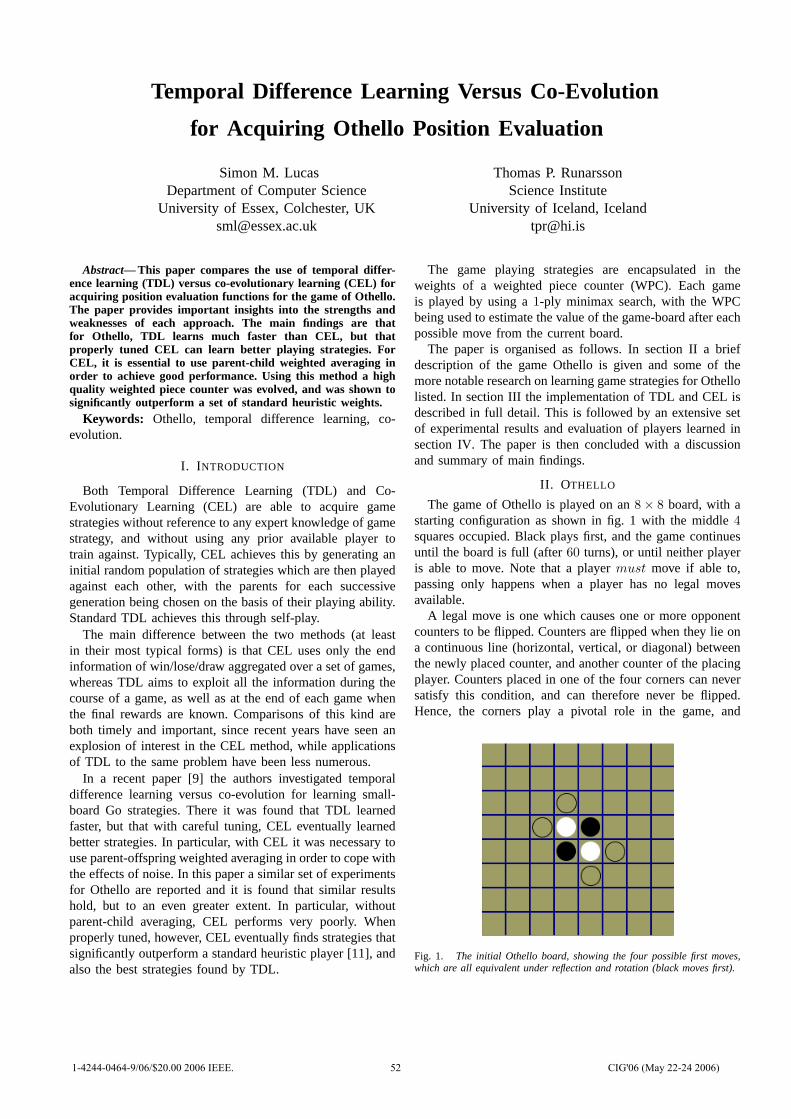
Temporal Difference Learning Versus Co-Evolution

for Acquiring Othello Position Evaluation

Simon M. LucasDepartment of Computer Science

University of Essex, Colchester, UKsml@essex.ac.uk

Thomas P. RunarssonScience Institute

University of Iceland, Icelandtpr@hi.is

Abstract— This paper compares the use of temporal differ-ence learning (TDL) versus co-evolutionary learning (CEL) foracquiring position evaluation functions for the game of Othello.The paper provides important insights into the strengths andweaknesses of each approach. The main findings are thatfor Othello, TDL learns much faster than CEL, but thatproperly tuned CEL can learn better playing strategies. ForCEL, it is essential to use parent-child weighted averaging inorder to achieve good performance. Using this method a highquality weighted piece counter was evolved, and was shown tosignificantly outperform a set of standard heuristic weights.

Keywords: Othello, temporal difference learning, co-evolution.

I. I NTRODUCTION

Both Temporal Difference Learning (TDL) and Co-Evolutionary Learning (CEL) are able to acquire gamestrategies without reference to any expert knowledge of gamestrategy, and without using any prior available player totrain against. Typically, CEL achieves this by generating aninitial random population of strategies which are then playedagainst each other, with the parents for each successivegeneration being chosen on the basis of their playing ability.Standard TDL achieves this through self-play.

The main difference between the two methods (at leastin their most typical forms) is that CEL uses only the endinformation of win/lose/draw aggregated over a set of games,whereas TDL aims to exploit all the information during thecourse of a game, as well as at the end of each game whenthe final rewards are known. Comparisons of this kind areboth timely and important, since recent years have seen anexplosion of interest in the CEL method, while applicationsof TDL to the same problem have been less numerous.

In a recent paper [9] the authors investigated temporaldifference learning versus co-evolution for learning small-board Go strategies. There it was found that TDL learnedfaster, but that with careful tuning, CEL eventually learnedbetter strategies. In particular, with CEL it was necessarytouse parent-offspring weighted averaging in order to cope withthe effects of noise. In this paper a similar set of experimentsfor Othello are reported and it is found that similar resultshold, but to an even greater extent. In particular, withoutparent-child averaging, CEL performs very poorly. Whenproperly tuned, however, CEL eventually finds strategies thatsignificantly outperform a standard heuristic player [11],andalso the best strategies found by TDL.

The game playing strategies are encapsulated in theweights of a weighted piece counter (WPC). Each gameis played by using a1-ply minimax search, with the WPCbeing used to estimate the value of the game-board after eachpossible move from the current board.

The paper is organised as follows. In section II a briefdescription of the game Othello is given and some of themore notable research on learning game strategies for Othellolisted. In section III the implementation of TDL and CEL isdescribed in full detail. This is followed by an extensive setof experimental results and evaluation of players learned insection IV. The paper is then concluded with a discussionand summary of main findings.

II. OTHELLO

The game of Othello is played on an8 × 8 board, with astarting configuration as shown in fig. 1 with the middle4squares occupied. Black plays first, and the game continuesuntil the board is full (after60 turns), or until neither playeris able to move. Note that a playermust move if able to,passing only happens when a player has no legal movesavailable.

A legal move is one which causes one or more opponentcounters to be flipped. Counters are flipped when they lie ona continuous line (horizontal, vertical, or diagonal) betweenthe newly placed counter, and another counter of the placingplayer. Counters placed in one of the four corners can neversatisfy this condition, and can therefore never be flipped.Hence, the corners play a pivotal role in the game, and

Fig. 1. The initial Othello board, showing the four possible first moves,which are all equivalent under reflection and rotation (black moves first).

1-4244-0464-9/06/$20.00 2006 IEEE. 52 CIG'06 (May 22-24 2006)

valuing them highly tends to be the first thing learned, a factthat can be seen easily by inspecting the evolution of weightvalues in a WPC. Indeed the WPC [11] used as a benchmarkin that study also reflects this. There the highest value of1is given to all four corners. To hinder the possibility of anopponent getting a corner, the squares next to them shouldbe avoided. For this reason they are given the lowest value−0.25. As a consequence the WPC encourages the playersto place its counter at advantageous squares. The total setof weights for this heuristic player is given in fig. 2. Notethat the weights of this heuristic player are symmetric underreflection and rotation, and have just10 distinct values out ofa possible64. It would be possible to simplify the learningtask by enforcing this kind of symmetry, and evolving just10 parameters instead of64. This would mean buildingin more expert knowledge however, and could also placeundesirable constraints on the value function. Indeed, thebest weights evolved in this paper are not symmetric (seeTable 10). A direct comparison of learning the reduced setof 10 weights compared with learning the full64 weightswould be interesting future work.

1.00 -0.25 0.10 0.05 0.05 0.10 -0.25 1.00-0.25 -0.25 0.01 0.01 0.01 0.01 -0.25 -0.250.10 0.01 0.05 0.02 0.02 0.05 0.01 0.100.05 0.01 0.02 0.01 0.01 0.02 0.01 0.050.05 0.01 0.02 0.01 0.01 0.02 0.01 0.050.10 0.01 0.05 0.02 0.02 0.05 0.01 0.10

-0.25 -0.25 0.01 0.01 0.01 0.01 -0.25 -0.251.00 -0.25 0.10 0.05 0.05 0.10 -0.25 1.00

Fig. 2. The weights (w) for the heuristic player [11].

The first strong learning Othello program developed wasBill [6], [7]. Later, the first program to beat a humanchampion was Logistello [2], the best Othello program from1993–1997. Logistello also uses a linear weighted evaluationfunction but with more complex features than just the plainboard. Nevertheless, the weights are tuned automaticallyusing self-play. Logistello also uses an opening book basedon over23, 000 tournament games and fast game tree search[1].

More recently, Chonget al [4] co-evolved a spatially awaremulti-layer perceptron (MLP) for playing Othello. TheirMLP was similar to the one used by Fogel and Chellapillafor playing checkers [3], and had a dedicated input unit forevery possible sub-square of the board. Together with thehidden layers this led to a network with5, 900 weights, whichthey evolved with around one hundred thousand games. TheWPC used in the current paper has only64 weights. Theresults below show that optimal tuning of such WPCs cantake hundreds of thousands of games, and relies heavilyon parent-child averaging. These considerations suggest thatfurther improvement in the performance of evolved spatialMLPs should be possible.

III. I MPLEMENTATION

In order to achieve effective learning it may be necessaryto play many games. This is particularly true for CEL, which

may require hundreds of thousands of games in order toachieve good performance. Indeed, the experimental workunderlying this paper involved the running of several billiongames of Othello. Therefore, the efficiency of the gameengine plays an important part in this research.

We developed two implementations of all the software,one written by the first author in Java, the other by thesecond author in C. In this way all results are double-checkedand enabled a speed comparison of each implementation tobe made. The speed of each game naturally depends onthe type of player. A multi-layered perceptron (MLP) withhidden units is necessarily slower than a WPC, for example.Regarding the WPC, there is a trick implemented for the Javaversion, which evaluates only the difference in evaluationscore that a move would make, without actually making themove. This is however, only applicable for a WPC using 1-ply lookahead. This means that for WPCs the Java versionis the fastest implementation we have, and is able to playaround1, 500 games per second. The C version plays around1, 200 games per second using WPCs, but in the case ofgreater ply search and MLPs it is faster than Java. At present,the Java MLP implementation is not particularly efficient,and in this mode is only able to manage around 60 gamesper second, compared with 500 games per second for the Cversion.

Each board is represented as a10×10 array ofint, witha border of ‘off-board’ values surrounding the8 × 8 board.This enables efficient checking of off-board positions forline-search termination, which is much faster than catchingArrayOutOfBounds exceptions, or than explicitly check-ing the range constraints.

It would be interesting to investigate the use of a bit-boardrepresentation for further speeding up the Othello engine,asdescribed by Cowling [5] for the Virus game. This couldconceivably lead to a significant speed increase for weightedpiece counter players, but would make little difference formore complex players (such as MLPs).

A. Co-Evolution

A number of different versions of the evolution strategy(ES) as implemented in [9] were tried. It was decidedthat the more simplified version, described in fig. 3, wassufficient for the game Othello. This is the so called(1, λ) ESusing arithmetical averaging between the parent and the bestoffspring. In this algorithm the parent is deleted at everygeneration (non-elitist). Theλ offspring play a single gameagainst one another both as Black and White. This resultsin a total of λ(λ − 1) games per generation. The parent-child averaging is a standard evolution strategy techniquefor dealing with noisy fitness functions. Pollack and Blair [8]also used averaging when using a random hill-climber (i.e. a(1 + 1) ES) to successfully learn backgammon strategy, butfor the current paper a(1+1) ES with averaging performedpoorly (though without averaging it performed even worse).

Regarding the win/draw/lose payoffs listed in fig. 3 cap-tion, we also experimented with basing fitness solely on thenumber of wins, but found that these different payoffs did

1-4244-0464-9/06/$20.00 2006 IEEE. 53 CIG'06 (May 22-24 2006)

not lead to a significant difference in final playing quality.An alternative that was not investigates would be to base thefitness function on the piece difference at the end of eachgame.

The WPC (w) co-evolved in this manner is described by:

f(x) =

8×8∑

i=1

wixi + x0 (1)

wherexi is the value at squarei on the board, which is0when Empty,1 if Black, and−1 for White. The bias termx0

is set to zero for the CEL runs. The single scalar output offunction f(x) is interpreted as follows. The value indicateswhich position is most favorable for a particular player, withlarger values favouring Black, and smaller values White.

1 Initialize: w′ = 0 andβ = 0.05 (or 1.0)

2 while termination criteria not satisfieddo3 for k := 1 to λ do (replication)4 wk ← w

′ + N(0, 1/n)5 od6 each individualwk, k = 1, . . . , λ plays another

(once each color) for a total ofλ(λ − 1) games,7 find the playeri with the highest score (breaking ties randomly)8 w

′← w

′ + β(wi − w′) (arithmetic average)

9 od

Fig. 3. The(1, λ) evolution strategy. For each win the player receives ascore of1, 0 for a draw, and−2 for loss.

It is also possible to force random moves during gameplay. The experimental studies show that this slows downlearning, but may lead to slightly better strategies in the longrun. The best player found in this paper was evolved withforced random play.

B. Temporal Difference Learning

In TDL the weights of the evaluation function are updatedduring game play using a gradient-descent method. Letx bethe board observed by a player about to move, and similarlyx′ the board after the player has moved. Then the evaluation

function may be updated during play as follows [10, p.199]:

wi ← wi + α[

v(x′) − v(x)]∂v(x)

∂wi

(2)

= wi + α[

v(x′) − v(x)](

1 − v(x)2)

xi

where

v(x) = tanh(f(x)) =2

1 + exp(−2f(x))− 1 (3)

is used to force the value functionv to be in the range−1to 1. This method is known as gradient-descent TD(0) [10].If x

′ is a terminal state then the game has ended and thefollowing update is used:

wi ← wi + α[

r − v(x)](

1 − v(x)2)

xi

wherer corresponds to the final utilities:+1 if the winneris Black,−1 when White, and0 for a draw.

The update rule is perhaps the simplest version of temporaldifference learning and works quite well on this task. If the

1 if u() < ε do2 make purely random legal move3 else4 make best legal move based on the state evaluation function5 od

Fig. 4. The ε-greedy technique for forcing random moves, whereu()returns a random number drawn from a uniform distribution∈ [0 1].

step size parameterα, in (2), is reduced properly over timethis method will also converge [10, p. 13]. During game play,with probability ε = 0.1, a random or exploratory move isforced. This is known as anε-greedy policy and is describe infig 4. Note that, TD(0) is attempting to learn the probabilityof winning from a given state (when following theε-greedypolicy), while the ES is only learning the relative orderingof the set of game states.

To satisfy our curiosity, a TDL run with no noise (i.e.ε =0.0) was tried. In this case, every run is deterministic, with allweight-values initialised to zero, and a deterministic tie-breakpolicy being used (always picking the first encountered moveamong a set of equal moves). Under these conditions, exactlythe same sequence of players is always produced. Whilethis approach did not produce the best TDL players, it didnonetheless produce quite reasonable players. The interestingpoint here is that the dynamics of the game, and of theweight updates are sufficient to produce a large degree ofgame strategy exploration.

IV. EXPERIMENTAL RESULTS

For each learning method, some time was spent experi-mentally tuning the parameters in order to get best perfor-mance. The critical factor for TDL is the update rateα, whilefor CEL it is the population sizeλ and smoothing factorβ. Inour previous study for Go [9] it was found that a populationsize ofλ = 30 was needed for a5×5 Go board and a settingof β = 0.05 was necessary. Similar finding are observed herefor Othello, however, smaller population sizes are adequate,resulting in much faster CEL learning for Othello than forGo. For TDL an initial step size ofα = 0.01 worked best,which was then reduced by a factor of0.95 every 45, 000games played.

A. Evaluation

Each experiment is repeated independently30 times, withthe average and standard deviations reported. During CELand TDL the players are evaluated by playing against astandard heuristic player (see fig. 2) and a random playerat 1-ply. This is repeated10, 000 times for each point on thegraphs (the player under test plays5, 000 games as Whiteand5, 000 games as Black).

Secondly, leagues of learned players are played againsteach other. It is interesting to note that which player isregarded as best depends on the chosen evaluation method.Evaluation against a fixed opponent can give a very quickguide to a player’s ability, but what usually matters more ishow well the player fares against a wide variety of players.

1-4244-0464-9/06/$20.00 2006 IEEE. 54 CIG'06 (May 22-24 2006)

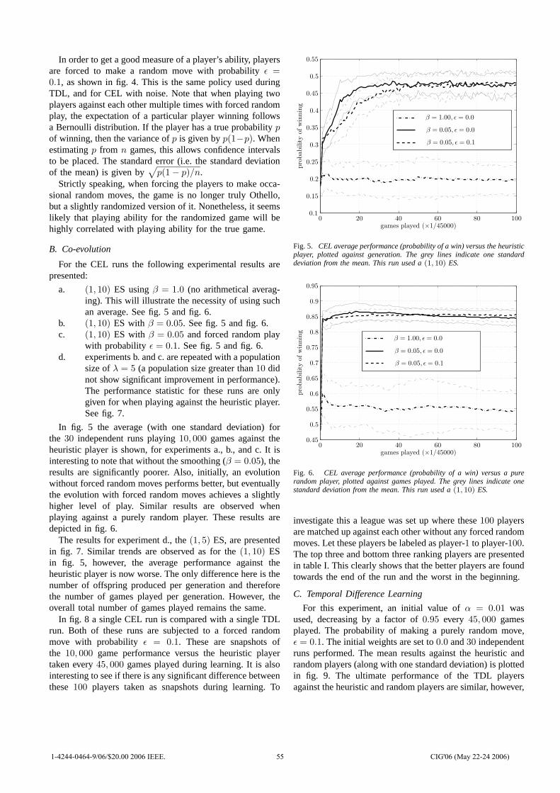
In order to get a good measure of a player’s ability, playersare forced to make a random move with probabilityε =0.1, as shown in fig. 4. This is the same policy used duringTDL, and for CEL with noise. Note that when playing twoplayers against each other multiple times with forced randomplay, the expectation of a particular player winning followsa Bernoulli distribution. If the player has a true probability pof winning, then the variance ofp is given byp(1−p). Whenestimatingp from n games, this allows confidence intervalsto be placed. The standard error (i.e. the standard deviationof the mean) is given by

√

p(1 − p)/n.Strictly speaking, when forcing the players to make occa-

sional random moves, the game is no longer truly Othello,but a slightly randomized version of it. Nonetheless, it seemslikely that playing ability for the randomized game will behighly correlated with playing ability for the true game.

B. Co-evolution

For the CEL runs the following experimental results arepresented:

a. (1, 10) ES usingβ = 1.0 (no arithmetical averag-ing). This will illustrate the necessity of using suchan average. See fig. 5 and fig. 6.

b. (1, 10) ES with β = 0.05. See fig. 5 and fig. 6.c. (1, 10) ES with β = 0.05 and forced random play

with probability ε = 0.1. See fig. 5 and fig. 6.d. experiments b. and c. are repeated with a population

size ofλ = 5 (a population size greater than10 didnot show significant improvement in performance).The performance statistic for these runs are onlygiven for when playing against the heuristic player.See fig. 7.

In fig. 5 the average (with one standard deviation) forthe 30 independent runs playing10, 000 games against theheuristic player is shown, for experiments a., b., and c. It isinteresting to note that without the smoothing (β = 0.05), theresults are significantly poorer. Also, initially, an evolutionwithout forced random moves performs better, but eventuallythe evolution with forced random moves achieves a slightlyhigher level of play. Similar results are observed whenplaying against a purely random player. These results aredepicted in fig. 6.

The results for experiment d., the(1, 5) ES, are presentedin fig. 7. Similar trends are observed as for the(1, 10) ESin fig. 5, however, the average performance against theheuristic player is now worse. The only difference here is thenumber of offspring produced per generation and thereforethe number of games played per generation. However, theoverall total number of games played remains the same.

In fig. 8 a single CEL run is compared with a single TDLrun. Both of these runs are subjected to a forced randommove with probability ε = 0.1. These are snapshots ofthe 10, 000 game performance versus the heuristic playertaken every45, 000 games played during learning. It is alsointeresting to see if there is any significant difference betweenthese100 players taken as snapshots during learning. To

0 20 40 60 80 100

0.55

0.5

0.45

0.4

0.35

0.3

0.25

0.2

0.15

0.1

pro

bability

ofw

innin

g

games played (×1/45000)

β = 1.00, ε = 0.0

β = 0.05, ε = 0.0

β = 0.05, ε = 0.1

Fig. 5. CEL average performance (probability of a win) versus the heuristicplayer, plotted against generation. The grey lines indicate one standarddeviation from the mean. This run used a(1, 10) ES.

0 20 40 60 80 100

0.95

0.9

0.85

0.8

0.75

0.7

0.65

0.6

0.55

0.5

0.45

pro

bability

ofw

innin

g

games played (×1/45000)

β = 1.00, ε = 0.0

β = 0.05, ε = 0.0

β = 0.05, ε = 0.1

Fig. 6. CEL average performance (probability of a win) versus a purerandom player, plotted against games played. The grey linesindicate onestandard deviation from the mean. This run used a(1, 10) ES.

investigate this a league was set up where these100 playersare matched up against each other without any forced randommoves. Let these players be labeled as player-1 to player-100.The top three and bottom three ranking players are presentedin table I. This clearly shows that the better players are foundtowards the end of the run and the worst in the beginning.

C. Temporal Difference Learning

For this experiment, an initial value ofα = 0.01 wasused, decreasing by a factor of0.95 every 45, 000 gamesplayed. The probability of making a purely random move,ε = 0.1. The initial weights are set to0.0 and30 independentruns performed. The mean results against the heuristic andrandom players (along with one standard deviation) is plottedin fig. 9. The ultimate performance of the TDL playersagainst the heuristic and random players are similar, however,

1-4244-0464-9/06/$20.00 2006 IEEE. 55 CIG'06 (May 22-24 2006)

0 20 40 60 80 100

0.55

0.5

0.45

0.4

0.35

0.3

0.25

0.2

0.15

0.1

pro

bability

ofw

innin

g

games played (×1/45000)

β = 0.05, ε = 0.0

β = 0.05, ε = 0.1

Fig. 7. CEL average performance (probability of a win) versus the heuristicplayer, plotted against games played. The grey lines indicate one standarddeviation from the mean. This run used a(1, 5) ES.

TABLE I

A partial league of players sampled at regular intervals during a CEL

run, then played against each other.

Place Played Won Drew Lost Player1 198 123 7 68 Player-822 198 119 6 73 Player-863 198 119 11 68 Player-92

98 198 44 5 149 Player-299 198 43 2 153 Player-6100 198 27 6 165 Player-1

there appears to be a downward trend towards the end ofthe runs. Recall that the step size is being reduced overtime. Furthermore, when observing a single typical TDLrun in fig. 8 one can see that there is greater variationin performance against the heuristic player during learning.This difference can be observed by playing the100 snapshotplayers against each other and labeling them as before, fromPlayer-1 to Player-100. Here the top three and bottom threeplayers may be found at any time as shown in table II.

TABLE II

A partial league of players sampled at each epoch during a TDLrun, then

played against each other.

Place Played Won Drew Lost Player1 198 134 4 60 Player-682 198 130 6 62 Player-603 198 129 5 64 Player-298 198 69 10 119 Player-9299 198 66 5 127 Player-5100 198 62 9 127 Player-64

D. Champions League

As a final evaluation six different WPCs are compared in achampions league. These are the heuristic WPC (see fig. 2),the best TDL and CEL found against the heuristic player(TDL-HB and CEL-HB). Furthermore, the best out of the

0 20 40 60 80 100

0.55

0.5

0.45

0.4

0.35

0.3

0.25

0.2

pro

bability

ofw

innin

g

games played (×1/45000)

CEL, β = 0.05

TD(0)

Fig. 8. An example of a single run of CEL and TDL performance againstthe heuristic player. In both cases a noise level ofε = 0.1 is used duringgame play.

0 20 40 60 80 100

0.8

0.7

0.6

0.5

0.4

0.3

0.2

pro

bability

ofw

innin

g

games played (×1/45000)

playing heuristic

playing random

Fig. 9. TD(0) average performance (probability of a win) versus theheuristic and random player, plotted against games played.The grey linesindicate one standard deviation from the mean.

30 final players found for the different CEL experiments b.and c. and TDL experiments are tested. These are calledCEL, CEL-N, and TDL respectively and were found using aseparate champions league among the final30 players, eachplaying 10, 000 games with forced random moves.

TABLE III

Champions league with the selected WPCs.

Place Played Won Drew Lost Player1 10000 5502 350 4148 CEL-N2 10000 5474 314 4212 CEL3 10000 5229 301 4470 CEL-HB4 10000 4875 308 4817 Heuristic5 10000 4243 315 5442 TDL-HB6 10000 3735 296 5969 TDL

The results are shown in Table III where these6 different

1-4244-0464-9/06/$20.00 2006 IEEE. 56 CIG'06 (May 22-24 2006)

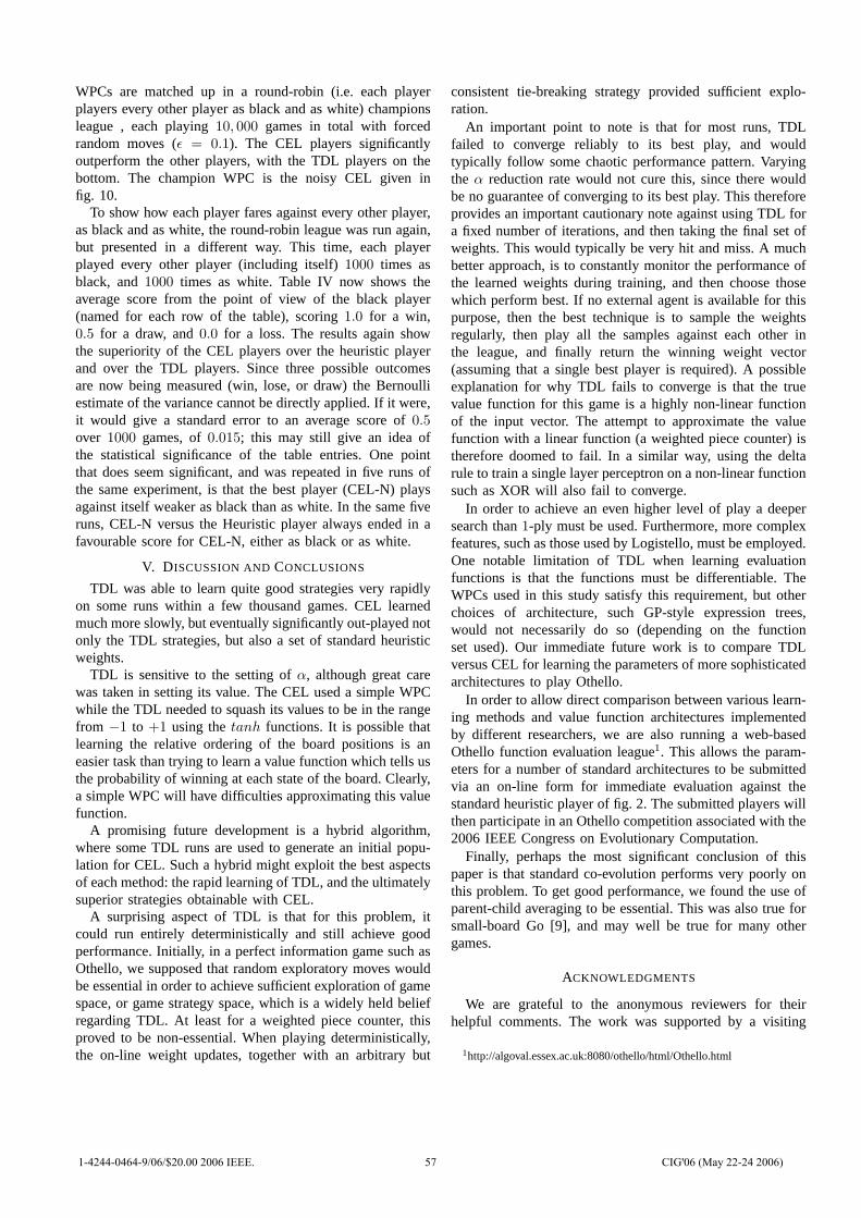
WPCs are matched up in a round-robin (i.e. each playerplayers every other player as black and as white) championsleague , each playing10, 000 games in total with forcedrandom moves (ε = 0.1). The CEL players significantlyoutperform the other players, with the TDL players on thebottom. The champion WPC is the noisy CEL given infig. 10.

To show how each player fares against every other player,as black and as white, the round-robin league was run again,but presented in a different way. This time, each playerplayed every other player (including itself)1000 times asblack, and1000 times as white. Table IV now shows theaverage score from the point of view of the black player(named for each row of the table), scoring1.0 for a win,0.5 for a draw, and0.0 for a loss. The results again showthe superiority of the CEL players over the heuristic playerand over the TDL players. Since three possible outcomesare now being measured (win, lose, or draw) the Bernoulliestimate of the variance cannot be directly applied. If it were,it would give a standard error to an average score of0.5over 1000 games, of0.015; this may still give an idea ofthe statistical significance of the table entries. One pointthat does seem significant, and was repeated in five runs ofthe same experiment, is that the best player (CEL-N) playsagainst itself weaker as black than as white. In the same fiveruns, CEL-N versus the Heuristic player always ended in afavourable score for CEL-N, either as black or as white.

V. D ISCUSSION ANDCONCLUSIONS

TDL was able to learn quite good strategies very rapidlyon some runs within a few thousand games. CEL learnedmuch more slowly, but eventually significantly out-played notonly the TDL strategies, but also a set of standard heuristicweights.

TDL is sensitive to the setting ofα, although great carewas taken in setting its value. The CEL used a simple WPCwhile the TDL needed to squash its values to be in the rangefrom −1 to +1 using thetanh functions. It is possible thatlearning the relative ordering of the board positions is aneasier task than trying to learn a value function which tellsusthe probability of winning at each state of the board. Clearly,a simple WPC will have difficulties approximating this valuefunction.

A promising future development is a hybrid algorithm,where some TDL runs are used to generate an initial popu-lation for CEL. Such a hybrid might exploit the best aspectsof each method: the rapid learning of TDL, and the ultimatelysuperior strategies obtainable with CEL.

A surprising aspect of TDL is that for this problem, itcould run entirely deterministically and still achieve goodperformance. Initially, in a perfect information game suchasOthello, we supposed that random exploratory moves wouldbe essential in order to achieve sufficient exploration of gamespace, or game strategy space, which is a widely held beliefregarding TDL. At least for a weighted piece counter, thisproved to be non-essential. When playing deterministically,the on-line weight updates, together with an arbitrary but

consistent tie-breaking strategy provided sufficient explo-ration.

An important point to note is that for most runs, TDLfailed to converge reliably to its best play, and wouldtypically follow some chaotic performance pattern. Varyingthe α reduction rate would not cure this, since there wouldbe no guarantee of converging to its best play. This thereforeprovides an important cautionary note against using TDL fora fixed number of iterations, and then taking the final set ofweights. This would typically be very hit and miss. A muchbetter approach, is to constantly monitor the performance ofthe learned weights during training, and then choose thosewhich perform best. If no external agent is available for thispurpose, then the best technique is to sample the weightsregularly, then play all the samples against each other inthe league, and finally return the winning weight vector(assuming that a single best player is required). A possibleexplanation for why TDL fails to converge is that the truevalue function for this game is a highly non-linear functionof the input vector. The attempt to approximate the valuefunction with a linear function (a weighted piece counter) istherefore doomed to fail. In a similar way, using the deltarule to train a single layer perceptron on a non-linear functionsuch as XOR will also fail to converge.

In order to achieve an even higher level of play a deepersearch than1-ply must be used. Furthermore, more complexfeatures, such as those used by Logistello, must be employed.One notable limitation of TDL when learning evaluationfunctions is that the functions must be differentiable. TheWPCs used in this study satisfy this requirement, but otherchoices of architecture, such GP-style expression trees,would not necessarily do so (depending on the functionset used). Our immediate future work is to compare TDLversus CEL for learning the parameters of more sophisticatedarchitectures to play Othello.

In order to allow direct comparison between various learn-ing methods and value function architectures implementedby different researchers, we are also running a web-basedOthello function evaluation league1. This allows the param-eters for a number of standard architectures to be submittedvia an on-line form for immediate evaluation against thestandard heuristic player of fig. 2. The submitted players willthen participate in an Othello competition associated withthe2006 IEEE Congress on Evolutionary Computation.

Finally, perhaps the most significant conclusion of thispaper is that standard co-evolution performs very poorly onthis problem. To get good performance, we found the use ofparent-child averaging to be essential. This was also true forsmall-board Go [9], and may well be true for many othergames.

ACKNOWLEDGMENTS

We are grateful to the anonymous reviewers for theirhelpful comments. The work was supported by a visiting

1http://algoval.essex.ac.uk:8080/othello/html/Othello.html

1-4244-0464-9/06/$20.00 2006 IEEE. 57 CIG'06 (May 22-24 2006)

researcher grant for Thomas Runarsson, funded by the Com-puter Science Department, University of Essex.

APPENDIX

To allow others to test our best player directly, we listhere the weights of our overall champion (see fig. 10). Theweights are listed in row order, left to right, top to bottom(i.e. the first eight weights are for the top row).

REFERENCES

[1] M. Buro, “ProbCut: An effective selective extension of the Aalpha-Beta algorithm,”ICGA Journal, vol. 18, pp. 71 – 76, 1995.

[2] ——, “LOGISTELLO – a strong learning othello program,” 1997,http://www.cs.ualberta.ca/ mburo/ps/log-overview.ps.gz.

[3] K. Chellapilla and D. Fogel, “Evolving an expert checkers playingprogram without using human expertise,”IEEE Transactions on Evo-lutionary Computation, vol. 5, pp. 422 – 428, 2001.

[4] S. Y. Chong, M. K. Tan, and J. D. White, “Observing the evolutionof neural networks learning to play the game of othello,”IEEETransactions on Evolutionary Computation, vol. 9, pp. 240 – 251,2005.

[5] P. Cowling, “Board evaluation for the virus game,” inIEEE Symposiumon Computational Intelligence and Games, 2005, pp. 59 – 65.

[6] K.-F. Lee and S. Mahajan, “A pattern classification approach toevaluation function learning,”Artificial Intelligence, vol. 36, pp. 1 –25, 1988.

[7] ——, “The development of a world class othello program,”ArtificialIntelligence, vol. 43, pp. 21 – 36, 1990.

[8] J. Pollack and A. Blair, “Co-evolution in the successfullearning ofbackgammon strategy,”Machine Learning, vol. 32, pp. 225–240, 1998.

[9] T. P. Runarsson and S. M. Lucas, “Co-evolution versus self-playtemporal difference learning for acquiring position evaluation in small-board go,” IEEE Transactions on Evolutionary Computation, vol. 9,pp. 628 – 640, 2005.

[10] R. Sutton and A. Barto,Introduction to Reinforcement Learning. MITPress, 1998.

[11] T. Yoshioka, S. Ishii, and M. Ito, “Strategy acquisition for the game”othello” based on reinforcement learning,” inIEICE Transactions onInformation and Systems E82-D 12, 1999, pp. 1618–1626.

1-4244-0464-9/06/$20.00 2006 IEEE. 58 CIG'06 (May 22-24 2006)

TABLE IV

Champions league showing the round-robin results. Each entry shows the score (see text) obtained by the black player averaged over1000 games. The

player named on each row plays as black, against the player named in each column playing as white.

CEL-N CEL CEL-HB Heuristic TDL-HB TDLCEL-N 0.4555 0.458 0.4955 0.5645 0.582 0.661CEL 0.4865 0.5065 0.4845 0.4435 0.5785 0.6545

CEL-HB 0.4625 0.434 0.534 0.491 0.582 0.684Heuristic 0.4425 0.4505 0.4935 0.4975 0.5705 0.5345TDL-HB 0.387 0.4475 0.412 0.4445 0.4585 0.52

TDL 0.3035 0.3 0.3075 0.4575 0.5305 0.5155

4.622507 -1.477853 1.409644 -0.066975 -0.305214 1.633019 -1.050899 4.365550-1.329145 -2.245663 -1.060633 -0.541089 -0.332716 -0.475830 -2.274535 -0.0325952.681550 -0.906628 0.229372 0.059260 -0.150415 0.321982 -1.145060 2.986767

-0.746066 -0.317389 0.140040 -0.045266 0.236595 0.158543 -0.720833 -0.131124-0.305566 -0.328398 0.073872 -0.131472 -0.172101 0.016603 -0.511448 -0.2641252.777411 -0.769551 0.676483 0.282190 0.007184 0.269876 -1.408169 2.396238

-1.566175 -3.049899 -0.637408 -0.077690 -0.648382 -0.911066 -3.329772 -0.8709625.046583 -1.468806 1.545046 -0.031175 0.263998 2.063148 -0.148002 5.781035

Fig. 10. The weights for the overall champion.

1-4244-0464-9/06/$20.00 2006 IEEE. 59 CIG'06 (May 22-24 2006)

The Effect of Using Match History

on the Evolution of RoboCup Soccer Team Strategies

Tomoharu Nakashima Masahiro TakataniDept. of Computer Science and Intelligent Systems Dept. of Industrial Engineering

Osaka Prefecture University, Japan Osaka Prefecture University, Japannakashi@cs.osakafu-u.ac.jp takatani@ci.cs.osakafu-u.ac.jp

Hisao Ishibuchi Manabu NiiDept. of Computer Science and Intelligent Systems Dept. of Computer Engineering

Osaka Prefecture University, Japan University of Hyogo, Japanhisaoi@cs.osakafu-u.ac.jp nii@eng.u-hyogo.ac.jp

Abstract— In this paper we improve the performance of anevolutionary method for obtaining team strategies in simulatedrobot soccer. In the previous method each team strategy wasevaluated based on the goals and the goals against of a singlegame. It is possible for a good team strategy to be eliminatedfrom the population in the evolutionary method as there isa high degree of uncertainty in the simulated soccer field. Inorder to tackle the problem of uncertainty, we propose a robustevaluation method using match history. The performance ofteam strategies in the proposed method is measured by theaverage goals and average goals against. Through a series ofcomputer simulations, we show the effectiveness of our robustevaluation method.

Keywords: Evolutionary Computation, Match History,Multi-Agent Systems, RoboCup Soccer, Rule-Based Systems

I. I NTRODUCTION

RoboCup soccer [1] is a competition between soccerrobots/agents. Its ultimate aim is to win against the hu-man soccer champion team by the year 2050. DevelopingRoboCup teams typically involves solving the cooperationof multiple agents, the learning of adaptive behavior, andthe problem of noisy data handling. Many approaches havebeen presented that try to tackle these problems, an exampleis the application of soft computing techniques [2].

In general, the behavior of the soccer agents is hierarchi-cally structured. This structure is divided into two groups.One is low-level behavior which performs basic informationprocessing such as visual and sound information. Basicactions such as dribble, pass, and shoot are also includedin the low-level behavior. The other is high-level behaviorthat makes a decision from the viewpoint of global teamstrategy such as cooperative play among the teammates.

For the low-level behavior Nakashima et al. [2] proposed afuzzy Q-learning method for acquiring a ball intercept skill.It was shown that the performance of the agent graduallyimproves in an on-line manner.

Evolutionary computation has been used to evolve strate-gies of various games. For example, Chellapilla and Fo-gel [3], [4] proposed a method based on the frameworkof evolutionary programming to automatically generate a

checker player without incorporating human expertise onthe game. An idea of coevolution is also employed in [3],[4]. For RoboCup soccer agents a genetic programmingapproach has been applied to obtain the soccer team strategyin [5]. In [5] the idea of coevolution is also employed. Theevolution of team strategy from kiddy soccer (i.e., all playersgather around the ball) to formation soccer (i.e., each playermaintains its own position during the game) is reported.

Another evolutionary method for RoboCup soccer hasbeen proposed by Nakashima et al. [6] where a set ofaction rules is used to determine the action of players. Theantecedent part of the action rule concerns the position ofthe nearest opponent and the position of the player. Eachaction rule is examined whether its antecedent part matcheswith the player’s current situation. The action of the player isspecified by the consequent part of the action rule that exactlymatches the current situation. A strategy for a single teamis constructed by concatenating a set of action rules of theagents in the team. Each set of action rules are representedby an integer string and treated as an individual throughthe course of evolutionary process. It was shown that theperformance of the generated soccer team improved againsta fixed opponent team.

The performance of the team strategy in [6] is evaluated byscores (i.e., goals and goals against) in the game. However, aproblem arises because there is a high degree of uncertaintyin the game. For example, different game results can beobtained against the same team if we iterate a number oftimes. We observed that some good teams are eliminatedfrom the evolutionary process because their performance isnot good enough in a single evaluation. On the other hand,poor teams can remain in the evolutionary process as theyhappen to score more than the potentially high-performingteams.

In order to tackle the problem of uncertainty, we propose arobust evaluation method of the soccer team strategy wherethe performance of soccer team strategies is evaluated byusing the match history of the teams. In the evolutionaryprocess, those integer strings with high average goals have a

1-4244-0464-9/06/$20.00 2006 IEEE. 60 CIG'06 (May 22-24 2006)

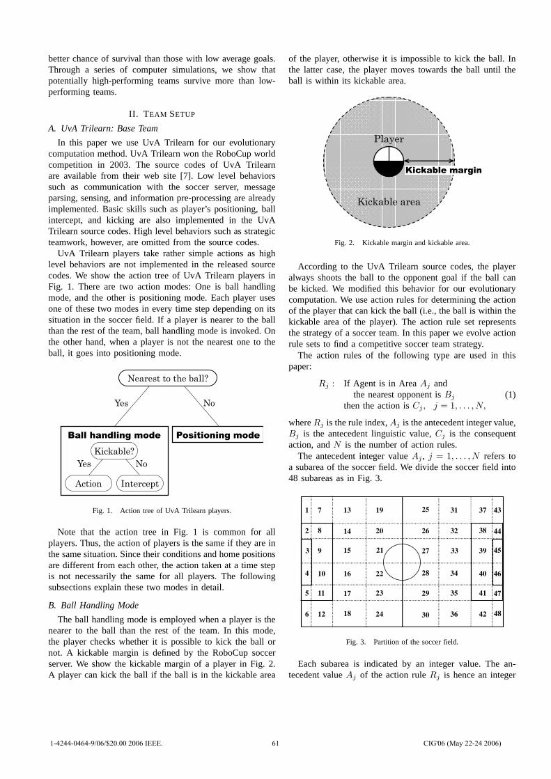
better chance of survival than those with low average goals.Through a series of computer simulations, we show thatpotentially high-performing teams survive more than low-performing teams.

II. T EAM SETUP

A. UvA Trilearn: Base Team

In this paper we use UvA Trilearn for our evolutionarycomputation method. UvA Trilearn won the RoboCup worldcompetition in 2003. The source codes of UvA Trilearnare available from their web site [7]. Low level behaviorssuch as communication with the soccer server, messageparsing, sensing, and information pre-processing are alreadyimplemented. Basic skills such as player’s positioning, ballintercept, and kicking are also implemented in the UvATrilearn source codes. High level behaviors such as strategicteamwork, however, are omitted from the source codes.

UvA Trilearn players take rather simple actions as highlevel behaviors are not implemented in the released sourcecodes. We show the action tree of UvA Trilearn players inFig. 1. There are two action modes: One is ball handlingmode, and the other is positioning mode. Each player usesone of these two modes in every time step depending on itssituation in the soccer field. If a player is nearer to the ballthan the rest of the team, ball handling mode is invoked. Onthe other hand, when a player is not the nearest one to theball, it goes into positioning mode.

Nearest to the ball?

Positioning mode Ball handling mode

Kickable?

Yes No

Yes No

Action Intercept

Fig. 1. Action tree of UvA Trilearn players.

Note that the action tree in Fig. 1 is common for allplayers. Thus, the action of players is the same if they are inthe same situation. Since their conditions and home positionsare different from each other, the action taken at a time stepis not necessarily the same for all players. The followingsubsections explain these two modes in detail.

B. Ball Handling Mode

The ball handling mode is employed when a player is thenearer to the ball than the rest of the team. In this mode,the player checks whether it is possible to kick the ball ornot. A kickable margin is defined by the RoboCup soccerserver. We show the kickable margin of a player in Fig. 2.A player can kick the ball if the ball is in the kickable area

of the player, otherwise it is impossible to kick the ball. Inthe latter case, the player moves towards the ball until theball is within its kickable area.

Player

Kickable margin

Kickable area

Fig. 2. Kickable margin and kickable area.

According to the UvA Trilearn source codes, the playeralways shoots the ball to the opponent goal if the ball canbe kicked. We modified this behavior for our evolutionarycomputation. We use action rules for determining the actionof the player that can kick the ball (i.e., the ball is within thekickable area of the player). The action rule set representsthe strategy of a soccer team. In this paper we evolve actionrule sets to find a competitive soccer team strategy.

The action rules of the following type are used in thispaper:

Rj : If Agent is in AreaAj andthe nearest opponent isBj

then the action isCj , j = 1, . . . , N,(1)

whereRj is the rule index,Aj is the antecedent integer value,Bj is the antecedent linguistic value,Cj is the consequentaction, andN is the number of action rules.

The antecedent integer valueAj , j = 1, . . . , N refers toa subarea of the soccer field. We divide the soccer field into48 subareas as in Fig. 3.

48

47

46

45

44

43 37

38

39

40

41

42

31

32

33

34

35

36 30

29

28

27

26

25

18

17

16

15

14

13 7

8

9

10

11

12

19

20

21

22

23

24

1

2

3

4

5

6

Fig. 3. Partition of the soccer field.

Each subarea is indicated by an integer value. The an-tecedent valueAj of the action ruleRj is hence an integer

1-4244-0464-9/06/$20.00 2006 IEEE. 61 CIG'06 (May 22-24 2006)

value in the interval [1, 48]. In this way, the action of a socceragent depends on the position of the agent. The action of thesoccer agent also depends on the distance between the agentand its nearest opponent. The antecedentBj takes one of twolinguistic values near or not near. The player that is able tokick the ball examines whether the nearest opponent is nearthe agent or not. The nearest opponent is regarded as nearif the distance between the agent and its nearest opponent isless than a prespecified value. If not, the nearest opponentis regarded as not near. The consequent actionCj representsthe action that is taken by the agent when the two conditionsin the antecedent part of the action ruleRj (i.e., Aj andBj ) are satisfied. In this paper we use the following twelveactions for the consequent actionCj .

1. Dribble toward the opponent side. The direction is parallelto the horizontal axis of the soccer field.

2. Dribble toward the opponent side. The direction is thecenter of the opponent goal.

3. Dribble carefully toward the opponent side. The directionis the center of the opponent goal. The dribble speed islow so that the agent can avoid opponent agents.

4. Dribble toward the nearest post of the opponent goal.5. Dribble carefully toward the nearest post of the opponent

goal. The dribble speed is low so that the agent can avoidopponent agents.

6. Dribble toward the nearest side line.7. Pass the ball to the nearest teammate. If the nearest

teammate is not ahead of the agent, the agent does notkick to the nearest teammate. Instead, it clears the balltoward the opponent side.

8. Pass the ball to the second nearest teammate. If the secondnearest teammate is not ahead of the agent, the agent doesnot kick to the second nearest teammate. Instead, it clearsthe ball toward the opponent side.

9. Clear the ball toward the opponent side.10. Clear the ball toward the nearest side line of the soccer

field.11. Kick the ball toward the penalty area of the opponent side

(i.e., centering).12. Perform a leading pass to the nearest teammate.

Note that each player has a set of action rules. Since thereare 48 subareas in the soccer field and near and not nearare available for the second antecedent part in action rules(i.e., Bj), the number of action rules for a single player is48 × 2 = 96. There are96 × 10 = 960 action rules in totalfor a single team with ten field players. Action rules for agoal keeper are not considered in this paper.

There is a special case where players do not follow theaction rules. If a player keeps the ball within the penaltyarea of the opponent side (i.e., if the agent is in Areas 38 -41 or 44 - 47 in Fig. 3), the player checks if it is possibleto shoot the ball to the opponent goal. The player decides toshoot the ball if the line segment from the ball to either goalpost of the opponent side is clear (i.e., there are no playersnear the line segment). If the line is not clear, the playerfollows the action rule whose antecedent part is compatible

to the player’s condition.If the ball cannot be kicked by a player that is in the ball

handling mode, the player’s action is to intercept the ball,that is, the player moves to catch the ball. In the interceptprocess the player determines whether it dashes forward orturns its body angle based on the relative distance of the ballto the player.

C. Positioning Mode

UvA Trilearn players have their own home positions inthe field (see Fig. 4). We use a 4-3-3 formation systemwhere there are four defenders, three mid-fielders, and threeforwards. This formation system is fixed and never changesthroughout a game. The home position of a player and theball position are used to determine the player’s position whenit is in the positioning mode. The position is specified asan externally dividing point of the ball position and thehome position. If the current position of the player in thepositioning mode is different from the determined position,the player moves toward the determined position. If thedifference between the two positions is not large, the playerremains in its current position.

1

2

3 4 5 8

10

9

FW DF DF

DF

DF

MF

MF

MF

FW

FW

Attack direction

GK

6

7

Fig. 4. Home positions of the soccer agents.

III. E VOLUTIONARY COMPUTATION

In this paper we use an evolutionary method to obtainteam strategies for soccer agents that are effective for playingsoccer. Specifically, our aim is to find the best action rulesets for ten soccer players. Each player has its own set ofaction rules that are used when it is in the ball handling mode(see Subsection II-B). We encode an entire team strategyinto an integer string. Note that we do not optimize player’sindividual behavior but a team strategy as a whole. Thus, weevaluate the performance of a team strategy only from itsmatch result, not from players’ individual tactics. We showin our computer simulations that the performance of teamstrategies successfully improves through the evolutionaryprocess. The following subsections explain our evolutionarymethod in detail.

1-4244-0464-9/06/$20.00 2006 IEEE. 62 CIG'06 (May 22-24 2006)

A. Encoding

As described in Subsection II-B, the action of the agents isspecified by the action rules in (1) when they keep the ball.Considering that the soccer field is divided into 48 subareas(see Fig. 3) and the position of the nearest opponent agent(i.e., it is near the agent or not near) is taken into account inthe antecedent part of the action rules, we can see that thereare48 × 2 = 96 action rules for each player. We apply ourevolutionary method to ten soccer agents excluding the goalkeeper. Thus, the total number of action rules for a singleteam is96 × 10 = 960. We use an integer string of length960 to represent a rule set of action rules for ten players.The task of our evolutionary method is then to evolve theinteger strings of length 960 to obtain team strategies withhigh performance. We show in Fig. 5 the first 96 bits of aninteger string in our evolutionary method. This figure showsan integer string for a single agent. Thus, the integer stringof an individual in our evolutionary method has ten suchinteger strings as we optimize the team strategy with tensoccer agents excluding a goal keeper.

8 3 4 5 3 10 9 6

96 integers

1s 2s 3s 4s 93s 94s 95s 96s

Rule 1

1R :

If Player 1 is in Area 1 and the nearest opponent

is near then Action is Dribble toward the nearest side line

Fig. 5. Integer string for a single agent.

In Fig. 5, the first 48 bits represent the action of an agentwhen the nearest opponent agent is near the agent. The orderof the integer bits is based on the division of the soccer field(see Fig. 3). On the other hand, the actions of the agent in thecase where the nearest opponent agent is not near the agentare shown in the other 48 bits. The value of each integer bitranges from an integer interval of [1, 12] as the number ofpossible actions for each rule is twelve. These integer valuescorrespond to the index number of twelve actions describedin Subsection II-B.

B. Evaluation of Integer Strings

In the evaluation process, each of the integer strings in thepopulation plays a soccer game once against a fixed opponentteam. That is, the evaluation of integer strings is based on thegame results with a fixed opponent team. In the experimentsof this paper, UvA Trilearn Base is employed as a fixedopponent team in the evaluation process of our evolutionarymethod.

Generally, the main idea of evolutionary methods is to ex-ploit the information of those individuals whose performanceis highly evaluated. In the previous work [6], we evaluatedthe performance of integer strings from one single gameresult. Since the game has a high degree of uncertainty such

as noise in object movement and the sensing information, thesame game result cannot be obtained from multiple gameswith the same teams. Thus it is possible for potentially high-performing teams to have poor results and conversely it isalso possible for low-performing teams to have better results.This problem is caused because the performance is measuredfrom only a single game. One solution to this problem is toplay multiple games. However, this leads to an extremelytime-consuming process as it takes ten minutes to completea single game.

We therefore propose a new evaluation method that usesa match history of integer strings. Each integer string hasa match history since it is generated by genetic operations.The average goals and the average goals against are used inthe proposed method.

In the proposed method we first check the goals scored bythe soccer teams that are represented by the integer strings.The performance of integer strings is evaluated as high if ithas a large number of average goals. In our evolutionarymethod, the number of average goals is more importantthan that of average goals against. When the number of thegoals is the same among multiple soccer teams, the averagegoals against are used as a second performance measure. Thesoccer teams with lower goals against are evaluated as betterteams. We do not consider the average goals against at allwhen the average goals are different between different soccerteams to be evaluated.

C. Evolutionary Operation

We use one-point crossover, bit-change mutation, and ES-type selection as evolutionary operations in our evolutionarymethod. New integer strings are generated by crossover andmutation, and selection is used for generation update.

In the crossover operation, we first randomly select twointeger strings without considering the fitness value. Thena cut point is randomly selected that is used for both thetwo selected integer strings. The latter part of both stringsis exchanged with each other from the cut point. Note thatwe do not use any evaluation results when two integerstrings for the crossover operation are selected from thecurrent population. All new integer strings generated by thecrossover operation are subject to a mutation operation. In themutation operation, the value of each integer bit is replacedwith a randomly specified integer value in the interval [1, 12]with a prespecified mutation probability. It is possible thatthe replaced value is the same as the one before the mutationoperation.

Generation update is performed by using ES-type selectionin our method. We use a so-called(µ + λ)-ES [8] for ourgeneration update scheme. By iterating the crossover and themutation operations we produce the same number of newinteger strings as that of current strings. Then the best halfinteger strings from the merged set of the current and thenew strings are chosen as the next population. The selectionis based on the match results as described in SubsectionIII-B. Note that the current strings are also evaluated inthis selection process. Thus, it is possible that a current

1-4244-0464-9/06/$20.00 2006 IEEE. 63 CIG'06 (May 22-24 2006)

integer string with the best performance at the previousgeneration update is not selected in the next generationupdate because the average goals of the integer string afterthe next performance evaluation may become lower if theresult of the game at the next evaluation is poor.

To summarize, our evolutionary method is written asfollows:

[Procedure of the evolutionary method]

Step 1. Initialization. A prespecified number of integerstrings of length 960 are generated by randomlyassigning an integer value from the interval [1, 12]for each bit.

Step 2.Generation of new integer strings.First randomlyselect two integer strings from the current popu-lation. Then the one-point crossover and the bit-change mutation operations are performed to gen-erate new integer strings. This process is iterateduntil a prespecified number of new integer stringsare generated.

Step 3.Performance evaluation.The performance of boththe current integer strings and new integer stringsgenerated by Step 2 is evaluated through the re-sults of soccer games. Note that the performanceof current integer strings is also evaluated everygeneration because the game results are not the samebut different game by game.

Step 4.Generation update.From the merged set of the cur-rent integer strings and new ones, select best integerstrings according to the performance evaluation inSubsection III-B. The selected bit strings form thenext generation.

Step 5.Termination of the procedure.If a prespecified ter-mination condition is satisfied, stop the procedure.Otherwise go to Step 2.

IV. COMPUTATIONAL EXPERIMENTS

The following parameter specifications were used for allthe computer simulations in this paper:

The number of integer strings in a population: 5,The probability of crossover: 1.0,The probability of mutation for each bit: 5/96,Termination condition: 500 generations.

The population size is specified as five. This is asmall number compared to commonly used parameterspecifications. The reason for this is that it takes atleast five minutes to complete a single soccer game. Ifthe population size is specified large, it is difficult toperform the evolutionary method for a large number ofgenerations. Currently we use a 16-node cluster system forthe computational experiments in this paper. It still takesseveral days to perform a single run of the evolutionaryprocess. The population size will be increased when the

more powerful computational environments are equipped inthe laboratory.

The number of new integer strings generated from thepopulation at each generation is five. Thus it can be saidthat the values ofµ andλ are specified asµ = 5 andλ = 5.

The initial population was created by randomly assigningan integer value in the interval [1, 12] for each integer bit.We performed the proposed method for 500 generations. Weiterated the above experiment five times to obtain the averagegoals and goals against for each generation over the fivetrials.

Figure 6 shows the average goals and the average goalsagainst at each generation. That is, we examined the per-formance of the five integer strings after they are selectedas the next population. From Fig. 6, we can see that theperformance of integer strings becomes better as the numberof generations increases. For example, the average goalsincrease over generation. On the other hand, the averagegoals against do not change over generation. This is becausewe focus on the evolution of offensive ability of teamstrategies. Nevertheless, it should be noted that the averagegoals against do not increase because we consider not onlyoffensive ability but also defensive ability. It should be notedthat the performance of integer strings does not improvemonotonically over generation because the soccer games inthe evaluation process for the best half integer strings areperformed every generation. That is, Fig. 6 shows the on-line performance of the best half integer strings and theperformance at a generation is discarded at the followingone.

Generation( 10)

Avera

ge g

oals

and

avera

ge g

oals

again

st Goals

Goals against

0 10 20 30 40 500

1

2

3

4

5

6

7

8

9

10

×

Fig. 6. Simulation results with match history.

For the purpose of comparison, we show an experimentalresult in the case where match history was not used in theevolutionary process. That is, the fitness of integer stringsis calculated by using only the game results at the currentgeneration. From Fig. 6 and Fig. 7, we can see that thehigher offensive ability is obtained by using match historythan without match history (i.e., average goals with matchhistory is larger than without it). We can also see that thedefensive ability is slightly higher when match history isused.

Next, we further examined the performance of obtained

1-4244-0464-9/06/$20.00 2006 IEEE. 64 CIG'06 (May 22-24 2006)

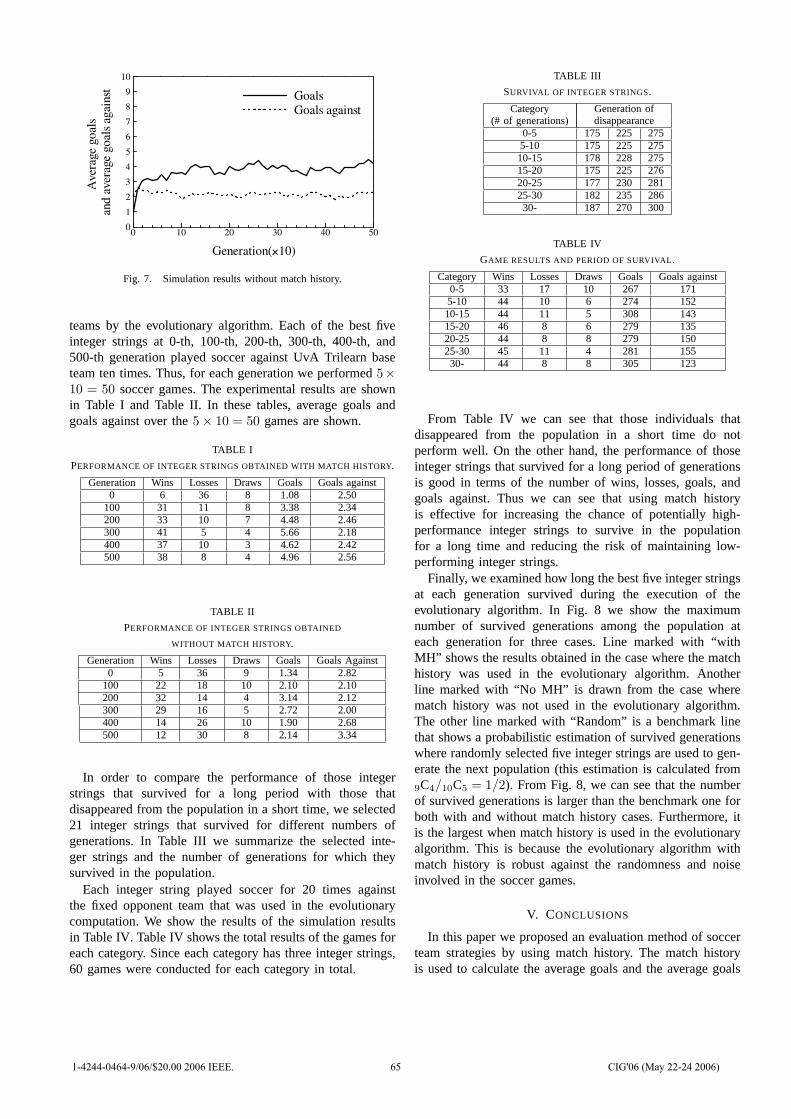
Generation( 10)

Avera

ge g

oals

and

avera

ge g

oals

again

st Goals

Goals against

0 10 20 30 40 500

1

2

3

4

5

6

7

8

9

10

×

Fig. 7. Simulation results without match history.

teams by the evolutionary algorithm. Each of the best fiveinteger strings at 0-th, 100-th, 200-th, 300-th, 400-th, and500-th generation played soccer against UvA Trilearn baseteam ten times. Thus, for each generation we performed5×10 = 50 soccer games. The experimental results are shownin Table I and Table II. In these tables, average goals andgoals against over the5× 10 = 50 games are shown.

TABLE I

PERFORMANCE OF INTEGER STRINGS OBTAINED WITH MATCH HISTORY.

Generation Wins Losses Draws Goals Goals against0 6 36 8 1.08 2.50

100 31 11 8 3.38 2.34200 33 10 7 4.48 2.46300 41 5 4 5.66 2.18400 37 10 3 4.62 2.42500 38 8 4 4.96 2.56

TABLE II

PERFORMANCE OF INTEGER STRINGS OBTAINED

WITHOUT MATCH HISTORY.

Generation Wins Losses Draws Goals Goals Against0 5 36 9 1.34 2.82

100 22 18 10 2.10 2.10200 32 14 4 3.14 2.12300 29 16 5 2.72 2.00400 14 26 10 1.90 2.68500 12 30 8 2.14 3.34

In order to compare the performance of those integerstrings that survived for a long period with those thatdisappeared from the population in a short time, we selected21 integer strings that survived for different numbers ofgenerations. In Table III we summarize the selected inte-ger strings and the number of generations for which theysurvived in the population.

Each integer string played soccer for 20 times againstthe fixed opponent team that was used in the evolutionarycomputation. We show the results of the simulation resultsin Table IV. Table IV shows the total results of the games foreach category. Since each category has three integer strings,60 games were conducted for each category in total.

TABLE III

SURVIVAL OF INTEGER STRINGS.

Category Generation of(# of generations) disappearance

0-5 175 225 2755-10 175 225 27510-15 178 228 27515-20 175 225 27620-25 177 230 28125-30 182 235 28630- 187 270 300

TABLE IV

GAME RESULTS AND PERIOD OF SURVIVAL.

Category Wins Losses Draws Goals Goals against0-5 33 17 10 267 1715-10 44 10 6 274 15210-15 44 11 5 308 14315-20 46 8 6 279 13520-25 44 8 8 279 15025-30 45 11 4 281 15530- 44 8 8 305 123

From Table IV we can see that those individuals thatdisappeared from the population in a short time do notperform well. On the other hand, the performance of thoseinteger strings that survived for a long period of generationsis good in terms of the number of wins, losses, goals, andgoals against. Thus we can see that using match historyis effective for increasing the chance of potentially high-performance integer strings to survive in the populationfor a long time and reducing the risk of maintaining low-performing integer strings.

Finally, we examined how long the best five integer stringsat each generation survived during the execution of theevolutionary algorithm. In Fig. 8 we show the maximumnumber of survived generations among the population ateach generation for three cases. Line marked with “withMH” shows the results obtained in the case where the matchhistory was used in the evolutionary algorithm. Anotherline marked with “No MH” is drawn from the case wherematch history was not used in the evolutionary algorithm.The other line marked with “Random” is a benchmark linethat shows a probabilistic estimation of survived generationswhere randomly selected five integer strings are used to gen-erate the next population (this estimation is calculated from9C4/10C5 = 1/2). From Fig. 8, we can see that the numberof survived generations is larger than the benchmark one forboth with and without match history cases. Furthermore, itis the largest when match history is used in the evolutionaryalgorithm. This is because the evolutionary algorithm withmatch history is robust against the randomness and noiseinvolved in the soccer games.

V. CONCLUSIONS

In this paper we proposed an evaluation method of soccerteam strategies by using match history. The match historyis used to calculate the average goals and the average goals

1-4244-0464-9/06/$20.00 2006 IEEE. 65 CIG'06 (May 22-24 2006)

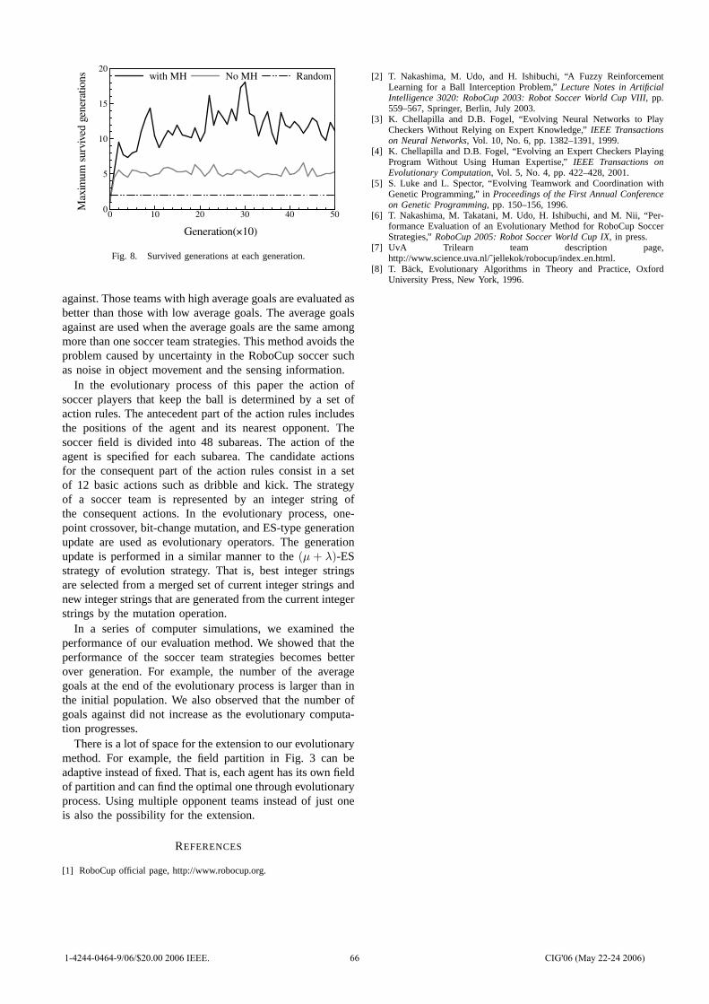
×Generation( 10)

Maxim

um

surv

ived g

enera

tions with MH No MH Random

0 10 20 30 40 500

5

10

15

20

Fig. 8. Survived generations at each generation.

against. Those teams with high average goals are evaluated asbetter than those with low average goals. The average goalsagainst are used when the average goals are the same amongmore than one soccer team strategies. This method avoids theproblem caused by uncertainty in the RoboCup soccer suchas noise in object movement and the sensing information.

In the evolutionary process of this paper the action ofsoccer players that keep the ball is determined by a set ofaction rules. The antecedent part of the action rules includesthe positions of the agent and its nearest opponent. Thesoccer field is divided into 48 subareas. The action of theagent is specified for each subarea. The candidate actionsfor the consequent part of the action rules consist in a setof 12 basic actions such as dribble and kick. The strategyof a soccer team is represented by an integer string ofthe consequent actions. In the evolutionary process, one-point crossover, bit-change mutation, and ES-type generationupdate are used as evolutionary operators. The generationupdate is performed in a similar manner to the(µ + λ)-ESstrategy of evolution strategy. That is, best integer stringsare selected from a merged set of current integer strings andnew integer strings that are generated from the current integerstrings by the mutation operation.

In a series of computer simulations, we examined theperformance of our evaluation method. We showed that theperformance of the soccer team strategies becomes betterover generation. For example, the number of the averagegoals at the end of the evolutionary process is larger than inthe initial population. We also observed that the number ofgoals against did not increase as the evolutionary computa-tion progresses.

There is a lot of space for the extension to our evolutionarymethod. For example, the field partition in Fig. 3 can beadaptive instead of fixed. That is, each agent has its own fieldof partition and can find the optimal one through evolutionaryprocess. Using multiple opponent teams instead of just oneis also the possibility for the extension.

REFERENCES

[1] RoboCup official page, http://www.robocup.org.

[2] T. Nakashima, M. Udo, and H. Ishibuchi, “A Fuzzy ReinforcementLearning for a Ball Interception Problem,”Lecture Notes in ArtificialIntelligence 3020: RoboCup 2003: Robot Soccer World Cup VIII, pp.559–567, Springer, Berlin, July 2003.

[3] K. Chellapilla and D.B. Fogel, “Evolving Neural Networks to PlayCheckers Without Relying on Expert Knowledge,”IEEE Transactionson Neural Networks, Vol. 10, No. 6, pp. 1382–1391, 1999.

[4] K. Chellapilla and D.B. Fogel, “Evolving an Expert Checkers PlayingProgram Without Using Human Expertise,”IEEE Transactions onEvolutionary Computation, Vol. 5, No. 4, pp. 422–428, 2001.

[5] S. Luke and L. Spector, “Evolving Teamwork and Coordination withGenetic Programming,” inProceedings of the First Annual Conferenceon Genetic Programming, pp. 150–156, 1996.

[6] T. Nakashima, M. Takatani, M. Udo, H. Ishibuchi, and M. Nii, “Per-formance Evaluation of an Evolutionary Method for RoboCup SoccerStrategies,”RoboCup 2005: Robot Soccer World Cup IX, in press.

[7] UvA Trilearn team description page,http://www.science.uva.nl/˜jellekok/robocup/indexen.html.

[8] T. Back, Evolutionary Algorithms in Theory and Practice, OxfordUniversity Press, New York, 1996.

1-4244-0464-9/06/$20.00 2006 IEEE. 66 CIG'06 (May 22-24 2006)

Training Bao Game-Playing Agents using Coevolutionary Particle

Swarm Optimization

Johan ConradieDepartment of Computer Science

University of Pretoria, PretoriaSouth Africa

Andries P. EngelbrechtDepartment of Computer Science

University of Pretoria, PretoriaSouth Africa

engel@cs.up.ac.za

Abstract— Bao, an African board game of the Mancalafamily, is a complex two-player game with a very large searchspace and complex rule set. The success of game tree approachesto create game-playing agents rests heavily on the, usuallyhandcrafted, static evaluation function. One of the first stepstowards using a game tree is to design an appropriate, efficientevaluation function. This paper investigates the effectiveness ofa coevolutionary particle swarm optimization (PSO) approachto evolve the evaluation function for the game of Bao. Thisapproach uses a PSO algorithm to evolve a neural network asevaluation function, using an unsupervised, competitive learningapproach. The coevolutionary approach to evolving game-playing agents assumes no prior knowledge of game strategies.The only domain specific information used by the model arethe rules of the game, and the outcomes of games played.

The performance of the evolved game-playing agents iscompared to a game tree-based agent using a handcraftedevaluation function, as well as a player that makes randommoves. Results show that the coevolutionary PSO approachsucceeded in learning playing strategies for Bao.

Keywords: Bao, Particle swarm optimization, coevolution

I. INTRODUCTION

Traditional game agents for two-player board games usegame trees to determine the best next move. A staticallydefined evaluation function is typically used to evaluate thedesirability of board states, represented by the leaf nodesof the game tree. Such static evaluators force the agent tobecome unnecessarily rigid in its decision process, whichleaves it unable to compensate for weaknesses. Furthermore,with handwritten evaluation functions expert knowledge ofthe game in question is required to design an efficientevaluation function. This is not problematic for well-known,popular games such as checkers or chess. However, for less-known and played games, it is difficult to obtain expertknowledge about the game and playing strategies.

The ideal is that the game agent learns for itself howto play the game, without being biased with a predefinedevaluation function. Given only the rules of the game, theagent should be able to discover and exploit different gamestrategies by playing against other game agents.

Co-evolutionary techniques have been used successfullyto evolve game-playing agents for games such as chess [1],[2], go [3], [4], checkers [5], [6], othello [7], the iteratedprisoner’s dilemma [8], Awari [9], and Kalah [10].

The co-evolutionary approach to train agents to playcheckers, developed by Chellapilla and Fogel [5], [6], enables

and algorithm to learn by itself to play the game at thelevel of expert human players using the rules of the game,and the number, type, and location of pieces on the board.Neural networks were used as evaluation function of leaf-nodes. A population of neural networks was trained usingan evolutionary program. Extensive online testing was doneto verify the performance of the algorithm, where playersfrom all over the world could play against the best evolvedneural network (known as Blondie24 [6]) over the Internet atwww.zone.com. It was shown that after playing 165 games,Blondie24 was rated better than 99.61% of over 120000 ratedplayers at the website. Recently, Fogel et al [2] applied thesame model to evolve chess players. In simulated tournamentconditions in 12 games (6 as black and 6 as white), theevolved chess player competed against Pocket Fritz 2.0(having a rating of 2300-2350). The evolved player won thecontest with 9 wins, 2 losses and 1 draw.

Messerschmidt and Engelbrecht [11] adapted this co-evolutionary approach to train the neural network evaluationfunctions using particle swarm optimization (PSO) algo-rithms for the simple game of tic-tac-toe. The PSO approachperformed significantly better than using an evolutionaryprogramming approach. Franken and Engelbrecht extendedthe PSO co-evolutionary approach to the games of Checkersand the iterated prisoner’s dilemma (IPD) [8]. Three novelapproaches to using PSO to evolve IPD strategies weredeveloped. Results in [8] have shown that the PSO co-evolutionary approach is successful on more complex games.

Based on this sucess, the main objective of this paper is toillustrate the performance of PSO on an even more complexgame, namely Bao. In addition to the application to a morecomplex game, the paper investigates

• performance against a handcrafted evaluation function;• methods to address premature stagnation to a point

where no more learning occurs; and• performance under different game tree ply depths.

The rest of the paper is organized as follows: The gameBao is described in Section II, along with the rules usedfor this paper. Section III provides a short overview ofgame tree approaches to Bao, and presents a handcraftedevaluation function for Bao. A brief overview of PSO isgiven in Section IV. The co-evolutionary PSO method issummarised in Section V. Experimental results are presented

1-4244-0464-9/06/$20.00 2006 IEEE. 67 CIG'06 (May 22-24 2006)

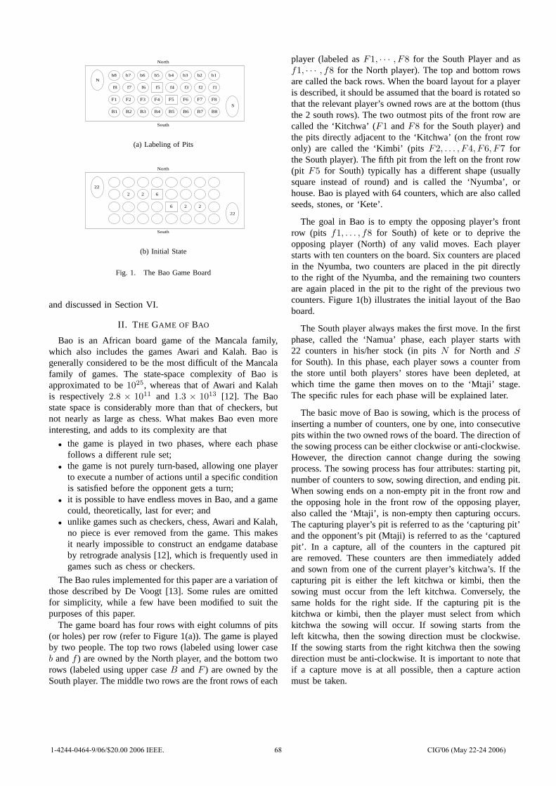
North

South

F1 F2 F3 F4 F5 F6 F7 F8

f1f2f3f4f5f6f7f8

S

N

B4 B5 B6

b3b4

B1 B2 B3 B7 B8

b1b2b5b6b7b8

(a) Labeling of Pits

2

2 2 6

6 2

22

22

North

South

(b) Initial State

Fig. 1. The Bao Game Board

and discussed in Section VI.

II. THE GAME OF BAO

Bao is an African board game of the Mancala family,which also includes the games Awari and Kalah. Bao isgenerally considered to be the most difficult of the Mancalafamily of games. The state-space complexity of Bao isapproximated to be 1025, whereas that of Awari and Kalahis respectively 2.8 × 1011 and 1.3 × 1013 [12]. The Baostate space is considerably more than that of checkers, butnot nearly as large as chess. What makes Bao even moreinteresting, and adds to its complexity are that

• the game is played in two phases, where each phasefollows a different rule set;

• the game is not purely turn-based, allowing one playerto execute a number of actions until a specific conditionis satisfied before the opponent gets a turn;

• it is possible to have endless moves in Bao, and a gamecould, theoretically, last for ever; and

• unlike games such as checkers, chess, Awari and Kalah,no piece is ever removed from the game. This makesit nearly impossible to construct an endgame databaseby retrograde analysis [12], which is frequently used ingames such as chess or checkers.

The Bao rules implemented for this paper are a variation ofthose described by De Voogt [13]. Some rules are omittedfor simplicity, while a few have been modified to suit thepurposes of this paper.

The game board has four rows with eight columns of pits(or holes) per row (refer to Figure 1(a)). The game is playedby two people. The top two rows (labeled using lower caseb and f ) are owned by the North player, and the bottom tworows (labeled using upper case B and F ) are owned by theSouth player. The middle two rows are the front rows of each

player (labeled as F1, · · · , F8 for the South Player and asf1, · · · , f8 for the North player). The top and bottom rowsare called the back rows. When the board layout for a playeris described, it should be assumed that the board is rotated sothat the relevant player’s owned rows are at the bottom (thusthe 2 south rows). The two outmost pits of the front row arecalled the ‘Kitchwa’ (F1 and F8 for the South player) andthe pits directly adjacent to the ‘Kitchwa’ (on the front rowonly) are called the ‘Kimbi’ (pits F2, . . . , F4, F6, F7 forthe South player). The fifth pit from the left on the front row(pit F5 for South) typically has a different shape (usuallysquare instead of round) and is called the ‘Nyumba’, orhouse. Bao is played with 64 counters, which are also calledseeds, stones, or ‘Kete’.

The goal in Bao is to empty the opposing player’s frontrow (pits f1, . . . , f8 for South) of kete or to deprive theopposing player (North) of any valid moves. Each playerstarts with ten counters on the board. Six counters are placedin the Nyumba, two counters are placed in the pit directlyto the right of the Nyumba, and the remaining two countersare again placed in the pit to the right of the previous twocounters. Figure 1(b) illustrates the initial layout of the Baoboard.

The South player always makes the first move. In the firstphase, called the ‘Namua’ phase, each player starts with22 counters in his/her stock (in pits N for North and S

for South). In this phase, each player sows a counter fromthe store until both players’ stores have been depleted, atwhich time the game then moves on to the ‘Mtaji’ stage.The specific rules for each phase will be explained later.

The basic move of Bao is sowing, which is the process ofinserting a number of counters, one by one, into consecutivepits within the two owned rows of the board. The direction ofthe sowing process can be either clockwise or anti-clockwise.However, the direction cannot change during the sowingprocess. The sowing process has four attributes: starting pit,number of counters to sow, sowing direction, and ending pit.When sowing ends on a non-empty pit in the front row andthe opposing hole in the front row of the opposing player,also called the ‘Mtaji’, is non-empty then capturing occurs.The capturing player’s pit is referred to as the ‘capturing pit’and the opponent’s pit (Mtaji) is referred to as the ‘capturedpit’. In a capture, all of the counters in the captured pitare removed. These counters are then immediately addedand sown from one of the current player’s kitchwa’s. If thecapturing pit is either the left kitchwa or kimbi, then thesowing must occur from the left kitchwa. Conversely, thesame holds for the right side. If the capturing pit is thekitchwa or kimbi, then the player must select from whichkitchwa the sowing will occur. If sowing starts from theleft kitcwha, then the sowing direction must be clockwise.If the sowing starts from the right kitchwa then the sowingdirection must be anti-clockwise. It is important to note thatif a capture move is at all possible, then a capture actionmust be taken.

1-4244-0464-9/06/$20.00 2006 IEEE. 68 CIG'06 (May 22-24 2006)

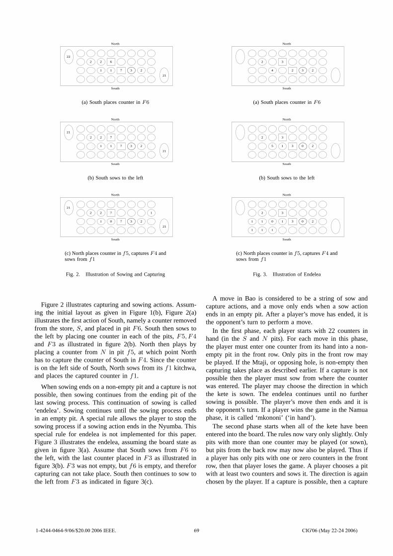
2

2 2 6

7 3

22

21

North

South

11

(a) South places counter in F6

2

2 2 7

7 3

21

21

North

South

11

(b) South sows to the left

2

2 2 7

7 3

21

21

North

South

01

1

(c) North places counter in f5, captures F4 andsows from f1

Fig. 2. Illustration of Sowing and Capturing

Figure 2 illustrates capturing and sowing actions. Assum-ing the initial layout as given in Figure 1(b), Figure 2(a)illustrates the first action of South, namely a counter removedfrom the store, S, and placed in pit F6. South then sows tothe left by placing one counter in each of the pits, F5, F4and F3 as illustrated in figure 2(b). North then plays byplacing a counter from N in pit f5, at which point Northhas to capture the counter of South in F4. Since the counteris on the left side of South, North sows from its f1 kitchwa,and places the captured counter in f1.

When sowing ends on a non-empty pit and a capture is notpossible, then sowing continues from the ending pit of thelast sowing process. This continuation of sowing is called‘endelea’. Sowing continues until the sowing process endsin an empty pit. A special rule allows the player to stop thesowing process if a sowing action ends in the Nyumba. Thisspecial rule for endelea is not implemented for this paper.Figure 3 illustrates the endelea, assuming the board state asgiven in figure 3(a). Assume that South sows from F6 tothe left, with the last counter placed in F3 as illustrated infigure 3(b). F3 was not empty, but f6 is empty, and thereforcapturing can not take place. South then continues to sow tothe left from F3 as indicated in figure 3(c).

2

2

2 3

North

South

4

3

(a) South places counter in F6

2

2

3 0

North

South

5

3

1

(b) South sows to the left

2

2

3 0

North

South

0

3

111

1 1 1

(c) North places counter in f5, captures F4 andsows from f1

Fig. 3. Illustration of Endelea

A move in Bao is considered to be a string of sow andcapture actions, and a move only ends when a sow actionends in an empty pit. After a player’s move has ended, it isthe opponent’s turn to perform a move.

In the first phase, each player starts with 22 counters inhand (in the S and N pits). For each move in this phase,the player must enter one counter from its hand into a non-empty pit in the front row. Only pits in the front row maybe played. If the Mtaji, or opposing hole, is non-empty thencapturing takes place as described earlier. If a capture is notpossible then the player must sow from where the counterwas entered. The player may choose the direction in whichthe kete is sown. The endelea continues until no furthersowing is possible. The player’s move then ends and it isthe opponent’s turn. If a player wins the game in the Namuaphase, it is called ‘mkononi’ (‘in hand’).

The second phase starts when all of the kete have beenentered into the board. The rules now vary only slightly. Onlypits with more than one counter may be played (or sown),but pits from the back row may now also be played. Thus ifa player has only pits with one or zero counters in the frontrow, then that player loses the game. A player chooses a pitwith at least two counters and sows it. The direction is againchosen by the player. If a capture is possible, then a capture

1-4244-0464-9/06/$20.00 2006 IEEE. 69 CIG'06 (May 22-24 2006)

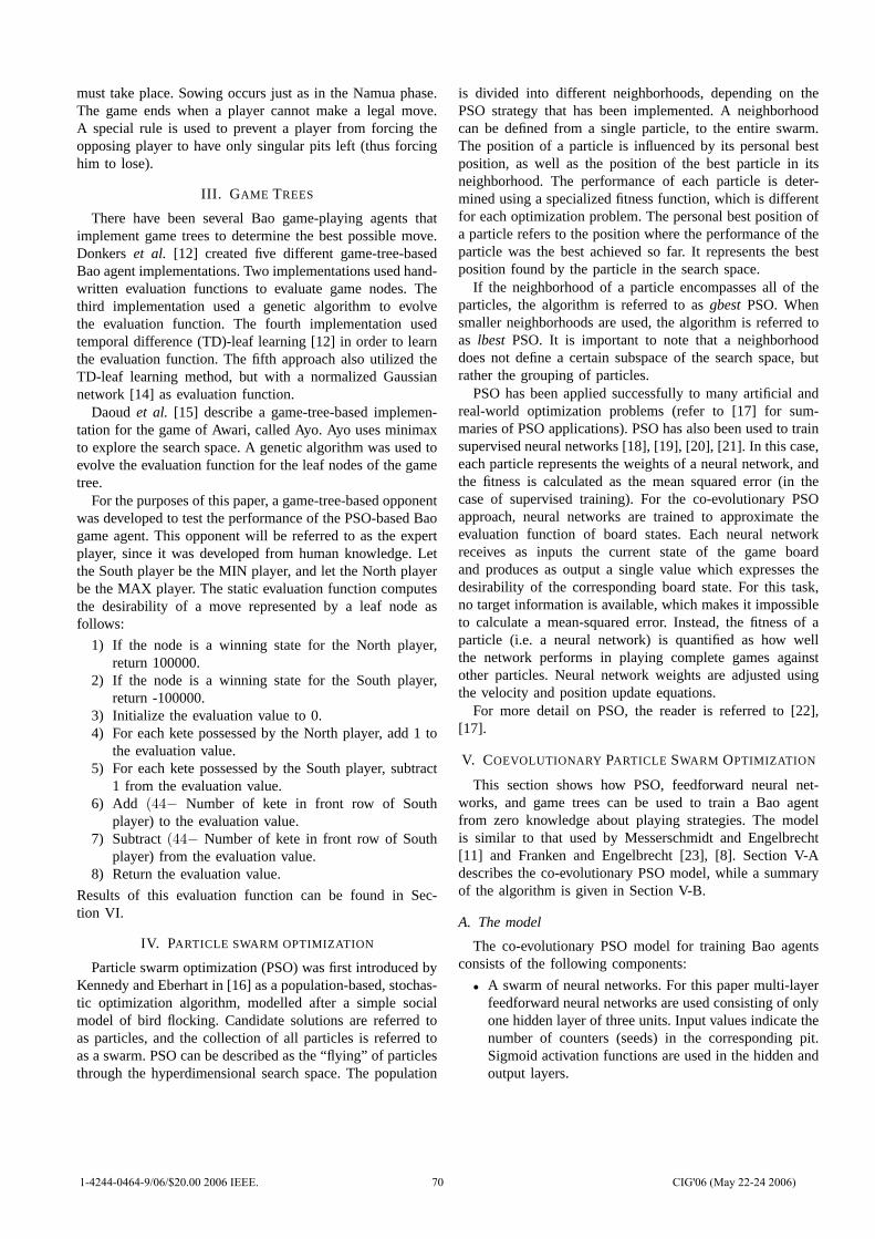
must take place. Sowing occurs just as in the Namua phase.The game ends when a player cannot make a legal move.A special rule is used to prevent a player from forcing theopposing player to have only singular pits left (thus forcinghim to lose).

III. GAME TREES

There have been several Bao game-playing agents thatimplement game trees to determine the best possible move.Donkers et al. [12] created five different game-tree-basedBao agent implementations. Two implementations used hand-written evaluation functions to evaluate game nodes. Thethird implementation used a genetic algorithm to evolvethe evaluation function. The fourth implementation usedtemporal difference (TD)-leaf learning [12] in order to learnthe evaluation function. The fifth approach also utilized theTD-leaf learning method, but with a normalized Gaussiannetwork [14] as evaluation function.

Daoud et al. [15] describe a game-tree-based implemen-tation for the game of Awari, called Ayo. Ayo uses minimaxto explore the search space. A genetic algorithm was used toevolve the evaluation function for the leaf nodes of the gametree.

For the purposes of this paper, a game-tree-based opponentwas developed to test the performance of the PSO-based Baogame agent. This opponent will be referred to as the expertplayer, since it was developed from human knowledge. Letthe South player be the MIN player, and let the North playerbe the MAX player. The static evaluation function computesthe desirability of a move represented by a leaf node asfollows:

1) If the node is a winning state for the North player,return 100000.

2) If the node is a winning state for the South player,return -100000.

3) Initialize the evaluation value to 0.4) For each kete possessed by the North player, add 1 to

the evaluation value.5) For each kete possessed by the South player, subtract

1 from the evaluation value.6) Add (44− Number of kete in front row of South

player) to the evaluation value.7) Subtract (44− Number of kete in front row of South

player) from the evaluation value.8) Return the evaluation value.

Results of this evaluation function can be found in Sec-tion VI.

IV. PARTICLE SWARM OPTIMIZATION

Particle swarm optimization (PSO) was first introduced byKennedy and Eberhart in [16] as a population-based, stochas-tic optimization algorithm, modelled after a simple socialmodel of bird flocking. Candidate solutions are referred toas particles, and the collection of all particles is referred toas a swarm. PSO can be described as the “flying” of particlesthrough the hyperdimensional search space. The population

is divided into different neighborhoods, depending on thePSO strategy that has been implemented. A neighborhoodcan be defined from a single particle, to the entire swarm.The position of a particle is influenced by its personal bestposition, as well as the position of the best particle in itsneighborhood. The performance of each particle is deter-mined using a specialized fitness function, which is differentfor each optimization problem. The personal best position ofa particle refers to the position where the performance of theparticle was the best achieved so far. It represents the bestposition found by the particle in the search space.

If the neighborhood of a particle encompasses all of theparticles, the algorithm is referred to as gbest PSO. Whensmaller neighborhoods are used, the algorithm is referred toas lbest PSO. It is important to note that a neighborhooddoes not define a certain subspace of the search space, butrather the grouping of particles.

PSO has been applied successfully to many artificial andreal-world optimization problems (refer to [17] for sum-maries of PSO applications). PSO has also been used to trainsupervised neural networks [18], [19], [20], [21]. In this case,each particle represents the weights of a neural network, andthe fitness is calculated as the mean squared error (in thecase of supervised training). For the co-evolutionary PSOapproach, neural networks are trained to approximate theevaluation function of board states. Each neural networkreceives as inputs the current state of the game boardand produces as output a single value which expresses thedesirability of the corresponding board state. For this task,no target information is available, which makes it impossibleto calculate a mean-squared error. Instead, the fitness of aparticle (i.e. a neural network) is quantified as how wellthe network performs in playing complete games againstother particles. Neural network weights are adjusted usingthe velocity and position update equations.

For more detail on PSO, the reader is referred to [22],[17].

V. COEVOLUTIONARY PARTICLE SWARM OPTIMIZATION

This section shows how PSO, feedforward neural net-works, and game trees can be used to train a Bao agentfrom zero knowledge about playing strategies. The modelis similar to that used by Messerschmidt and Engelbrecht[11] and Franken and Engelbrecht [23], [8]. Section V-Adescribes the co-evolutionary PSO model, while a summaryof the algorithm is given in Section V-B.

A. The model

The co-evolutionary PSO model for training Bao agentsconsists of the following components:

• A swarm of neural networks. For this paper multi-layerfeedforward neural networks are used consisting of onlyone hidden layer of three units. Input values indicate thenumber of counters (seeds) in the corresponding pit.Sigmoid activation functions are used in the hidden andoutput layers.

1-4244-0464-9/06/$20.00 2006 IEEE. 70 CIG'06 (May 22-24 2006)

• An alpha-beta game tree, which is used in this study toa ply-depth of three. The leaf nodes are evaluated usinga neural network.

• A neural network training algorithm, which is the gbestPSO for this paper.

• A competition pool consisting of all particles in theswarm and all personal best positions. The competitionpool includes the personal best positions since these arethe best positions found by the swarm and therefor pro-vide the best known competitors. Each particle (neuralnetwork) in the swarm plays complete games against arandomly selected group from the competition pool.

The training process consists of first randomly initializingthe swarm of neural networks. The performance of eachneural network against a randomly selected group of com-petitors is calculated and used as the fitness evaluation ofthe particle. Weight adjustments are then done using thefollowing position and velocity update equations:

xi(t) = xi(t − 1) + vi(t) (1)

where

vij(t + 1) = wvij(t) + c1r1j(t)[yij(t) − xij(t)]

+c2r2j(t)[yj(t) − xij(t)] (2)

with xi the position of particle i (i.e. the weights of the i-thneural network), vi is the velocity of particle i, yi and y arerespectively the personal best and global best positions, w

is the inertia weight, c1 and c2 are acceleration coefficients,and r1j , r2j ∼ U(0, 1).

For the purposes of this paper, the training process con-tinued for 500 iterations.

The training of the agents is unsupervised, which meansthat the performance of a candidate solution is gauged byhow well it plays against its peers. There is no humanintervention or insight on how the performance of thatindividual candidate solution is determined.

In [11], [8], [23], each neural network was played againstindividuals of the current population. Theoretical studieshave shown that, for gbest PSO (under convergent parameterchoices), each particle converges to one stable point [18],[24]. At this point, no further learning occurs. Experimentalresults in Section VI illustrate the problem occurs relativelyearly in the training process for Bao. To address this problem,the model is extended such that each particle also competesagainst five ‘dumb’ opponents. A dumb opponent is simplya neural network with randomly generated weight values,representing a player that makes random moves. A dumbagent thus has no intelligent behavior.

In addition to adding competitions against random oppo-nents, two other variations to the model have been imple-mented for this study. Both approaches add an expert playerto the competition pool (using the evaluation function ofSection II. The one approach adds the expert player fromthe first iteration, while the second approach adds the expertplayer after 250 iterations. The ply is one more for the expertplayer than for the agent.

It is important to note that for every match played against acompetitor, two games are played: One as the North playerand one as the South player. This ensures that the agentdoes not receive any advantage simply because it made thefirst move. From playing dumb agents against each otherfor 100000 games, it was determined that the South player(which moves first) has a 48.744% chance of winning, whilethe North player as a 51.25% chance of winning. The Northplayer thus has a slight advantage.

B. The algorithm

The coevolutionary PSO algorithm is summarized below:

• Initialize the swarm of particles (neural networks) torandom weight values.

• Repeat for 500 iterations.

– For every agent in the competition pool (includingpersonal best positions), set the score for the agentto 0, and repeat for 5 opponents:

∗ Pick an opponent at random from the competi-tion pool (excluding itself)

∗ Play a match against the selected opponent. Ifthe agent won, add 5 points to the agent’s score.Otherwise, deduct 10 points from the agent’sscore.

∗ Play a match against a dumb opponent, using thesame scoring as above.

∗ Optionally, play a match against an ‘expert’opponent, using the same scoring as above.

– Find the agent with the highest score, and flag thatagent as the ‘global best’ agent.

– Update the personal best positions using the com-puted scores.

– Update the velocities and positions of all particles(i.e. adjust the weights of the neural networks).

• Return the global best particle as the game-playingagent.

VI. EXPERIMENTAL RESULTS

This section presents results of the application of the co-evolutionary PSO approach to the game of Bao. For allexperiments, 15 particles have been used, trained for 500iterations. The inertia weight was set to w = 0.729844, andthe acceleration coefficients to c1 = c2 = 1.496810. Theseparameter values have been shown to ensure convergentbehavior [18]. The maximum velocity was set to Vmax =0.729844. Each particle represented a neural network with32 input units (one for each pit), 3 hidden units and 1output unit. The swarm consisted of 15 particles. Due to thecomputational effort and time constraints, each experimentwas repeated for only 10 times to report an average behaviourof the model.

For the experimental work, three variations of the co-evolutionary PSO model have been tested, namely

• Model A, where particles competed against agents inthe competition pool and dumb agents.

1-4244-0464-9/06/$20.00 2006 IEEE. 71 CIG'06 (May 22-24 2006)

• Model B, where an expert player is added from the firsttraining iteration.

• Model C, where the expert player is added after iteration250.

A. Computational Complexity

For the given architecture1 it took respectively 1, 5 and 24seconds per iteration to train for agents of ply-depth 1, 2 and3. It is clear that the calculation times increase exponentiallyin relation to the ply-depth of the agent. To get a betteridea of the computational time of the training process, threeexperiments were conducted for each of the models listedabove, where each experiment uses a different ply-depth. Foreach experiment 10 different runs were executed, each withdifferent starting conditions. The average training time persimulation is 0.1387 hours for ply 1, 0.6943 hours for ply 2,and 3.3333 hours for ply 3. For the results presented in thissection, the computational time amounts to 5.2 days.

B. Performance Results

This section summarizes the performance results of thedifferent models. Table I summarizes the performance againsta random player. Performance is measured as the percent-age of games won against the opponent. These results areaverages over the games played as both the South and theNorth player. For each side, 10000 games have been played.Table II gives the performance against the expert player.Results are given separately for the directions South andNorth as averages over 10 runs.

For the remainder of this section, the trained Bao agentis referred to as Agent(Level), where Level refers to theply-depth of the agent. The expert player is referred to asExpert(Level), where Level refers to the ply-depth of theexpert player.

Theoretically, results against the expert player should showa decline in performance if the ply-depth of the expert playeris higher than the agent. Also, results against the dumb playershould show an increase in performance as the ply-depth ofthe Bao agent is increased. Performances above 50% showthat the agent learned some good playing strategies. Resultsobtained against dumb opponents are the average over 20000games (10000 games each for North and South).

Model A

In this case, agents competed (during training) against thecompetition pool and dumb opponents. No other externalinfluences were allowed.

The results against the dumb opponent are very encour-aging. Agent(1) managed to achieve an average win rate of74%. As expected, the performance of the agent increaseswith larger ply-depths.

The performance against the expert player, however, wasnot as encouraging. Agent(1) managed to win 60% of thegames against Expert(1). The performance of the agentdropped sharply to only 5% against Expert(2). While a drop

1AMD Athlon(tm) XP 2600+

in performance was expected, the sudden drop from 60% to5% demonstrates that the agent in this model seems incapableof playing against the expert player at larger ply-depths.

The performance of Agent(2) against Expert(1) curiouslydrops down to 30%, while the performance of Agent(3)against Expert(1) seems to recover. Agent(2) and Agent(3)achieved slightly better results than Agent(1) for higherlevels of the expert player. Overall, the results show thatthe performance did not improve significantly when the ply-depth of the Bao agent was increased.

While the Bao game agent performed well against thedumb opponent, it clearly has a weakness against the expertplayer. The main cause for the bad performance stems fromthe fact that the Bao agent has never before encounteredthe expert player. This means that the Bao agent nevertrained against the expert player, causing the agent to becomemore specialized at winning against the dumb opponents. Itis for this reason that an expert player is included in thecompetitions in later experiments.

Model B

For model B, matches against the expert player wereintroduced from the beginning, allowing the expert playerto have an influence on training as from iteration 0. Usingthe expert player as a competitor during training tests thehypothesis that the trained agents will perform better if theyplay against stronger opponents.

Results against dumb players showed similar performanceto that of model A. Agent(1) achieved an average perfor-mance of 72%. As expected, performance increased with anincrease in ply-depth.

Results against the expert player showed a dramaticincrease in performance over that of model A. Agent(1)managed to achieve a performance of 90% against bothExpert(1) and Expert(2). The performance against Expert(3)dropped down to 10%. This drop in performance is expected,since the ply-depth of the Bao agent was only 1.

Agent(2) still managed a high performance of 85% againstExpert(1), while showing a decline in performance againstExpert(2). The performance of Agent(2) showed the expecteddecline in performance as the ply-depth of the expert playerwas increased.

Model B agents show an overall increase in performanceas the ply-depth of the Bao agent is increased.

Compared to the results of model A, model B clearlyillustrates that introduction of an expert player into the com-petition pool too early in the training process has a negativeinfluence on performance. The reason for this behavior needsto be further investigated.

Model C

For the results presented in this section, the expert playerwas introduced at training iteration 250 (arbitrarily chosen)and onwards.

Results against the dumb player showed similar perfor-mance to that of models A and B. Agent(1) achieved an

1-4244-0464-9/06/$20.00 2006 IEEE. 72 CIG'06 (May 22-24 2006)

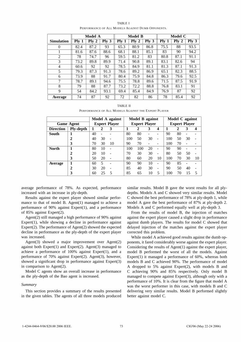
TABLE I

PERFORMANCE OF ALL MODELS AGAINST DUMB OPPONENTS.

Model A Model B Model CSimulation Ply 1 Ply 2 Ply 3 Ply 1 Ply 2 Ply 3 Ply 1 Ply 2 Ply 3

0 82.4 87.2 93 65.3 80.9 86.8 75.5 88 93.51 81.6 87.6 88.6 68.1 88.1 85.1 83 90 94.22 78 74.7 96 59.5 81.2 83 80.8 87.1 91.13 73.2 89.8 89.9 71.4 90.8 89.1 83.1 82.6 944 60.6 92 92 78.5 84.9 81.1 81.3 87.1 91.35 79.3 87.3 91.3 78.6 89.2 86.9 65.1 82.3 88.56 73.9 88 91.7 80.4 75.9 84.8 86.3 79.6 92.57 78.7 89.1 94.6 75.5 78.8 89.6 71.5 87.5 91.98 79 88 87.7 73.2 72.2 88.8 76.8 83.1 919 54 84.2 93.1 69.4 85.4 84.9 76.9 87 92

Average 74 87 92 72 82 86 78 85.4 92

TABLE II

PERFORMANCE OF ALL MODELS AGAINST THE EXPERT PLAYER

Model A against Model B against Model C againstGame Agent Expert Player Expert Player Expert Player

Direction Ply-depth 1 2 3 1 2 3 4 1 2 3 4South 1 40 - - 80 80 - - 90 80 - -

2 40 30 - 100 50 30 - 100 50 30 -3 70 30 10 90 70 - - 100 70 - -

North 1 80 10 - 100 100 20 - 90 90 - -2 20 10 - 70 30 30 - 80 50 50 -3 50 20 - 80 60 20 10 100 70 30 10

Average 1 60 5 - 90 90 10 - 90 85 - -2 30 20 - 85 40 30 - 90 50 40 -3 60 25 5 85 65 10 5 100 70 15 5

average performance of 78%. As expected, performanceincreased with an increase in ply-depth.

Results against the expert player showed similar perfor-mance to that of model B. Agent(1) managed to achieve aperformance of 90% against Expert(1), and a performanceof 85% against Expert(2).

Agent(2) still managed a high performance of 90% againstExpert(1), while showing a decline in performance againstExpert(2). The performance of Agent(2) showed the expecteddecline in performance as the ply-depth of the expert playerwas increased.

Agent(3) showed a major improvement over Agent(2)against both Expert(1) and Expert(2). Agent(3) managed toachieve a performance of 100% against Expert(1), and aperformance of 70% against Expert(2). Agent(3), however,showed a significant drop in performance against Expert(3)in comparison to Agent(2).

Model C agents show an overall increase in performanceas the ply-depth of the Bao agent is increased.

Summary

This section provides a summary of the results presentedin the given tables. The agents of all three models produced

similar results. Model B gave the worst results for all ply-depths. Models A and C showed very similar results. ModelC showed the best performance of 78% at ply-depth 1, whilemodel A gave the best performance of 87% at ply-depth 2.Models A and C performed equally well at ply-depth 3.

From the results of model B, the injection of matchesagainst the expert player caused a slight drop in performanceagainst dumb players. The results for model C showed thatdelayed injection of the matches against the expert playercorrected this problem.

While model A achieved good results against the dumb op-ponents, it fared considerably worse against the expert player.Considering the results of Agent(1) against the expert player,model B performed the worst of all the models. AgainstExpert(1) it managed a performance of 60%, whereas bothmodels B and C achieved 90%. The performance of modelA dropped to 5% against Expert(2), with models B andC achieving 90% and 85% respectively. Only model Bmanaged to compete against Expert(3), although only with aperformance of 10%. It is clear from the figure that model Awas the worst performer in this case, with models B and Cdelivering very similar results. Model B performed slightlybetter against model C.

1-4244-0464-9/06/$20.00 2006 IEEE. 73 CIG'06 (May 22-24 2006)

For Agent(2) against the expert player, model A was againthe worst performer of the group, with models B and C givingsimilar results. Model C performed the best overall, withmodel B just behind. It is curious to note that the overallperformance against Expert(2) dropped with Agent(2). Thereason behind this could be because Agent(2) only trainedagainst Expert(3), causing the visible increase in performanceagainst Expert(3). Models B and C performed much betteragainst Expert(3) than with Agent(1).

For Agent(3) against the expert player, model C againshowed to be the best performer.

In summary: (1) Models A and C achieved the highestoverall performance against the dumb opponents; (2) ModelC achieved the highest overall performance against theexpert player; and (3) Model B gave similar, and sometimessuperior, performance as model C against the expert player.

Overall, model C produced the best Bao game play-ing agent. Model B was designed to improve the overallperformance against the expert player, which was clearlyshown. Unfortunately model B’s performance against thedumb opponent suffered as a result. Model C improved theperformance against the expert player, while maintaining ahigh performance against the dumb opponent.

VII. CONCLUSION AND FUTURE WORK

This paper adapted the co-evolutionary PSO model pre-sented in [11], [8], [23] to train Bao game playing agents.The same trained agent is used for both phases of the Baogame. Three different models have been tested, where eachmodel differs in the competitors used during training. Thefirst model includes competitions against random players inan effort to increase diversity. For the second model, eachagent also competes, during training, against an expert player(a game tree with a static evaluation function) from the firsttraining iteration. The last model introduces the expert playeronly mid-way through the training process. The objective ofthe last two models is to ensure that the agents train againsta good adversary.

The results have shown that the co-evolutionary PSOmodel is successfull both against random players and theexpert players at different ply-depths. Using the expert playerfrom mid-training significantly improved the performance ofthe Bao agent.

Future research will include a more rigorous analysis ofthe influence of PSO and neural network parameters onthe performance. Investigations into the effects of differentPSO neighborhood topologies will also be done. A detailedanalysis of the steps made by the agent will be done todetermine exactly what the agent has learned. The reasons fordecrease in performance due to inclusion of an expert playerin the competition pool, and for certain ply depths will beinvestigated. Finally, the model will be extended such thata different neural network is used for the two phases of thegame.

REFERENCES

[1] G. Kendall and G. Whitwell, “An Evolutionary Approach for theTraining of a Chess Evaluation Function using Population Dynamics,”in Proceedings of the IEEE Congress on Evolutionary Computation,2001, pp. 995–1002.

[2] D. Fogel, T. Hays, S. Hahn, and J. Quan, “An Evolutionary Self-Learning Chess Program,” in Proceedings of the IEEE, 2004, pp.1947–1954.

[3] N. Richards, D. Moriarty, and P. McQueston, “Evolving NeuralNetworks to Play Go,” in Proceedings of the Seventh InternationalConference on Genetic Algorithms, 1998.

[4] A. Lubberts and R. Miikkulainen, “Co-Evolving a Go-Playing NeuralNetwork,” in in: Coevolution: Turnnig Adaptive Algorithms uponThemselves, 2001, pp. 14–19.

[5] K. Chellapilla and D. Fogel, “Evolving Neural Networks to PlayCheckers without Expert Knowledge,” IEEE Transactions on NeuralNetworks, vol. 10, no. 6, pp. 1382–1391, 1999.

[6] D. Fogel, Blondie24: Playing at the Edge of AI. Academic Press,2002.

[7] D. Moriarty and R. Miikkulainen, “Discovering Complex OthelloStrategies through Evolutionary Neural Networks,” Connection Sci-ence, vol. 7, no. 3-4, pp. 195–209.

[8] N. Franken and A. Engelbrecht, “Particle Swarm Optimization Ap-proaches to Coevolve Strategies for the Iterated Prisoner’s Dilemma,”IEEE Transactions on Evolutionary Computation, vol. 9, no. 6, pp.562–579, 2005.

[9] J. Davis and G. Kendall, “An Investigation, using Co-Evolution, toEvolve an Awari Player,” in Proceedings of the IEEE Congress onEvolutionary Computation, 2002, pp. 1408–1413.

[10] W.-C. Oon and Y.-J. Lim, “An Investigation on Piece DifferentialInformation in Co-Evolution on Games using Kalah,” in Proceedingsof the IEEE Congress on Evolutionary Computation, 2003, pp. 1632–1638.

[11] L. Messerschmidt and A. Engelbrecht, “Learning to play games usinga pso-based competitive learning approach,” IEEE Transactions OnEvolutionary Computation, vol. 8, no. 3, pp. 280–288, June 2004.

[12] H. Donkers, H. van den Herik, and J. Uiterwijk, “Opponent-model search in bao: Conditions for a successful application,”http://www.cs.unimaas.nl/ donkers/pdf/acg10.pdf.

[13] A. J. de Voogt, “Limits of the mind. towards a characterization of baomastership,” Ph.D. dissertation, Rijksuniversiteit Leiden, Leiden, TheNetherlands, 1995.

[14] T. Yoshioka, S. Ishii, and M. Ito, “Strategy Acquisition for the GameOthello based on Reinforcement Learnnig,” IEICE Transactions onInformation and Systems, vol. E82-D, no. 12, pp. 1618–1626, 1999.

[15] M. Daoud, N. Kharma, A. Haidar, and J.Popoola, “Ayo, the awariplayer, or how better representation trumps deeper search,” in Pro-ceedings of IEEE Congress on Evolutionary Computation, 2004, pp.1001–1006.

[16] J. Kennedy and R. C. Eberhart, “Particle swarm optimization,” in Pro-ceedings of the IEEE International Conference on Neural Networks,vol. IV, 1995, pp. 1942–1948.

[17] A. Engelbrecht, Fundamentals of Computational Swarm Intelligence.Wiley & Sons, 2005.

[18] F. van den Bergh, “An Analysis of Particle Swarm Optimizers,” Ph.D.dissertation, Department of Computer Science, University of Pretoria,Pretoria, South Africa, 2002.

[19] B. Al-kazemi and C. Mohan, “Training feedforward neural networkswith multi-phase particle swarm optimization,” in Proceedings of the9th International Conference on Neural Information Processing, 2002.

[20] R. Eberhart and Y. Shi, “Evolving artificial neural networks,” inProceedings of the International Conference on Neural Networks andBrain, 1998, pp. PL5–PL13.

[21] A. Engelbrecht and I. Ismail, “Training product unit neural networks,”Stability and Control: Theory and Applications, vol. 2, no. 1-2, pp.59–74, 1999.

[22] J. Kennedy, R. Eberhart, and Y. Shi, Swarm Intelligence. MorganKauffmann, 2001.

[23] C. Franken and A. Engelbrehct, “Evolving intelligent game-playingagents,” South African Computer Journal, vol. 32, pp. 44–49, 2004.

[24] M. Clerc and J. Kennedy, “The particle swarm-explosion, stability, andconvergence in multidimensional complex space,” IEEE Transactionson Evolutionary Computation, vol. 6, no. 1, pp. 58–73, 2002.

1-4244-0464-9/06/$20.00 2006 IEEE. 74 CIG'06 (May 22-24 2006)

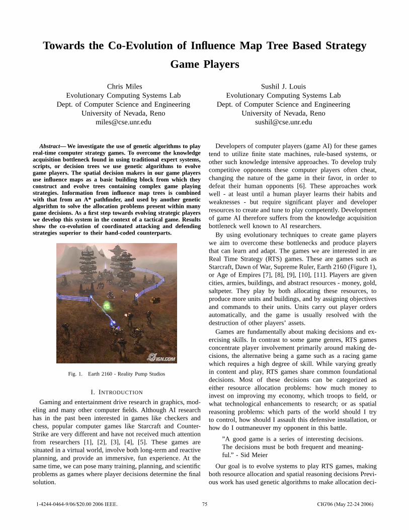
Towards the Co-Evolution of Influence Map Tree Based Strategy

Game Players

Chris MilesEvolutionary Computing Systems Lab

Dept. of Computer Science and EngineeringUniversity of Nevada, Reno

miles@cse.unr.edu

Sushil J. LouisEvolutionary Computing Systems Lab

Dept. of Computer Science and EngineeringUniversity of Nevada, Reno

sushil@cse.unr.edu

Abstract— We investigate the use of genetic algorithms to playreal-time computer strategy games. To overcome the knowledgeacquisition bottleneck found in using traditional expert systems,scripts, or decision trees we use genetic algorithms to evolvegame players. The spatial decision makers in our game playersuse influence maps as a basic building block from which theyconstruct and evolve trees containing complex game playingstrategies. Information from influence map trees is combinedwith that from an A* pathfinder, and used by another geneticalgorithm to solve the allocation problems present within manygame decisions. As a first step towards evolving strategic playerswe develop this system in the context of a tactical game. Resultsshow the co-evolution of coordinated attacking and defendingstrategies superior to their hand-coded counterparts.

Fig. 1. Earth 2160 - Reality Pump Studios

I. INTRODUCTION

Gaming and entertainment drive research in graphics, mod-eling and many other computer fields. Although AI researchhas in the past been interested in games like checkers andchess, popular computer games like Starcraft and Counter-Strike are very different and have not received much attentionfrom researchers [1], [2], [3], [4], [5]. These games aresituated in a virtual world, involve both long-term and reactiveplanning, and provide an immersive, fun experience. At thesame time, we can pose many training, planning, and scientificproblems as games where player decisions determine the finalsolution.

Developers of computer players (game AI) for these gamestend to utilize finite state machines, rule-based systems, orother such knowledge intensive approaches. To develop trulycompetitive opponents these computer players often cheat,changing the nature of the game in their favor, in order todefeat their human opponents [6]. These approaches workwell - at least until a human player learns their habits andweaknesses - but require significant player and developerresources to create and tune to play competently. Developmentof game AI therefore suffers from the knowledge acquisitionbottleneck well known to AI researchers.

By using evolutionary techniques to create game playerswe aim to overcome these bottlenecks and produce playersthat can learn and adapt. The games we are interested in areReal Time Strategy (RTS) games. These are games such asStarcraft, Dawn of War, Supreme Ruler, Earth 2160 (Figure 1),or Age of Empires [7], [8], [9], [10], [11]. Players are givencities, armies, buildings, and abstract resources - money, gold,saltpeter. They play by both allocating these resources, toproduce more units and buildings, and by assigning objectivesand commands to their units. Units carry out player ordersautomatically, and the game is usually resolved with thedestruction of other players’ assets.

Games are fundamentally about making decisions and ex-ercising skills. In contrast to some game genres, RTS gamesconcentrate player involvement primarily around making de-cisions, the alternative being a game such as a racing gamewhich requires a high degree of skill. While varying greatlyin content and play, RTS games share common foundationaldecisions. Most of these decisions can be categorized aseither resource allocation problems: how much money toinvest on improving my economy, which troops to field, orwhat technological enhancements to research; or as spatialreasoning problems: which parts of the world should I tryto control, how should I assault this defensive installation, orhow do I outmaneuver my opponent in this battle.

”A good game is a series of interesting decisions.The decisions must be both frequent and meaning-ful.” - Sid Meier

Our goal is to evolve systems to play RTS games, makingboth resource allocation and spatial reasoning decisions Previ-ous work has used genetic algorithms to make allocation deci-

1-4244-0464-9/06/$20.00 2006 IEEE. 75 CIG'06 (May 22-24 2006)

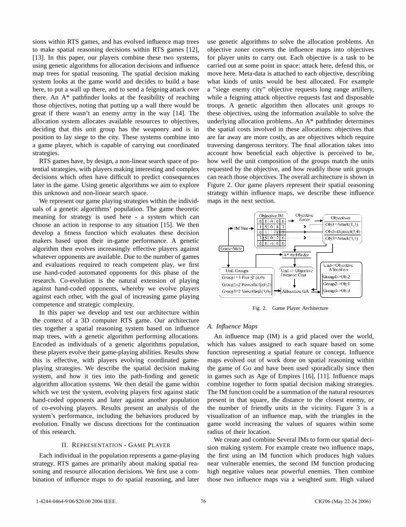
sions within RTS games, and has evolved influence map treesto make spatial reasoning decisions within RTS games [12],[13]. In this paper, our players combine these two systems,using genetic algorithms for allocation decisions and influencemap trees for spatial reasoning. The spatial decision makingsystem looks at the game world and decides to build a basehere, to put a wall up there, and to send a feigning attack overthere. An A* pathfinder looks at the feasibility of reachingthose objectives, noting that putting up a wall there would begreat if there wasn’t an enemy army in the way [14]. Theallocation system allocates available resources to objectives,deciding that this unit group has the weaponry and is inposition to lay siege to the city. These systems combine intoa game player, which is capable of carrying out coordinatedstrategies.

RTS games have, by design, a non-linear search space of po-tential strategies, with players making interesting and complexdecisions which often have difficult to predict consequenceslater in the game. Using genetic algorithms we aim to explorethis unknown and non-linear search space.

We represent our game playing strategies within the individ-uals of a genetic algorithms’ population. The game theoreticmeaning for strategy is used here - a system which canchoose an action in response to any situation [15]. We thendevelop a fitness function which evaluates these decisionmakers based upon their in-game performance. A geneticalgorithm then evolves increasingly effective players againstwhatever opponents are available. Due to the number of gamesand evaluations required to reach competent play, we firstuse hand-coded automated opponents for this phase of theresearch. Co-evolution is the natural extension of playingagainst hand-coded opponents, whereby we evolve playersagainst each other, with the goal of increasing game playingcompetence and strategic complexity.

In this paper we develop and test our architecture withinthe context of a 3D computer RTS game. Our architectureties together a spatial reasoning system based on influencemap trees, with a genetic algorithm performing allocations.Encoded as individuals of a genetic algorithms population,these players evolve their game-playing abilities. Results showthis is effective, with players evolving coordinated game-playing strategies. We describe the spatial decision makingsystem, and how it ties into the path-finding and geneticalgorithm allocation systems. We then detail the game withinwhich we test the system, evolving players first against statichand-coded opponents and later against another populationof co-evolving players. Results present an analysis of thesystem’s performance, including the behaviors produced byevolution. Finally we discuss directions for the continuationof this research.

II. REPRESENTATION - GAME PLAYER

Each individual in the population represents a game-playingstrategy. RTS games are primarily about making spatial rea-soning and resource allocation decisions. We first use a com-bination of influence maps to do spatial reasoning, and later

use genetic algorithms to solve the allocation problems. Anobjective zoner converts the influence maps into objectivesfor player units to carry out. Each objective is a task to becarried out at some point in space: attack here, defend this, ormove here. Meta-data is attached to each objective, describingwhat kinds of units would be best allocated. For examplea ”siege enemy city” objective requests long range artillery,while a feigning attack objective requests fast and disposabletroops. A genetic algorithm then allocates unit groups tothese objectives, using the information available to solve theunderlying allocation problems. An A* pathfinder determinesthe spatial costs involved in these allocations: objectives thatare far away are more costly, as are objectives which requiretraversing dangerous territory. The final allocation takes intoaccount how beneficial each objective is perceived to be,how well the unit composition of the groups match the unitsrequested by the objective, and how readily those unit groupscan reach those objectives. The overall architecture is shown inFigure 2. Our game players represent their spatial reasoningstrategy within influence maps, we describe these influencemaps in the next section.

Fig. 2. Game Player Architecture

A. Influence Maps

An influence map (IM) is a grid placed over the world,which has values assigned to each square based on somefunction representing a spatial feature or concept. Influencemaps evolved out of work done on spatial reasoning withinthe game of Go and have been used sporadically since thenin games such as Age of Empires [16], [11]. Influence mapscombine together to form spatial decision making strategies.The IM function could be a summation of the natural resourcespresent in that square, the distance to the closest enemy, orthe number of friendly units in the vicinity. Figure 3 is avisualization of an influence map, with the triangles in thegame world increasing the values of squares within someradius of their location.

We create and combine Several IMs to form our spatial deci-sion making system. For example create two influence maps,the first using an IM function which produces high valuesnear vulnerable enemies, the second IM function producinghigh negative values near powerful enemies. Then combinethose two influence maps via a weighted sum. High valued

1-4244-0464-9/06/$20.00 2006 IEEE. 76 CIG'06 (May 22-24 2006)

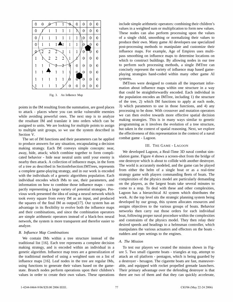
Fig. 3. An Influence Map

points in the IM resulting from the summation, are good placesto attack - places where you can strike vulnerable enemieswhile avoiding powerful ones. The next step is to analyzethe resultant IM and translate it into orders which can beassigned to units. We are looking for multiple points to assignto multiple unit groups, so we use the system described inSection V.

The set of IM functions and their parameters can be appliedto produce answers for any situation, encapsulating a decisionmaking strategy. Each IM conveys simple concepts: near,away, hide, attack; which combine together to form compli-cated behavior - hide near neutral units until your enemy isnearby then attack. A collection of influence maps, in the formof a tree as described in Sectionrefsection:IMTrees, representsa complete game-playing strategy, and in our work is encodedwith the individuals of a genetic algorithms population. Eachindividual encodes which IMs to use, their parameters, andinformation on how to combine those influence maps - com-pactly representing a large variety of potential strategies. Pre-vious work presented the idea of using a neural network whichtook every square from every IM as an input, and producedthe squares of the final IM as output[17]. Our system has anadvantage in its flexibility to evolve both the influence mapsand their combinations, and since the combination operatorsare simple arithmetic operators instead of a black-box neuralnetwork, the system is more transparent and therefor easier toanalyze.

B. Influence Map Combinations

We contain IMs within a tree structure instead of thetraditional list [16]. Each tree represents a complete decisionmaking strategy, and is encoded within an individual in agenetic algorithm. Influence map trees are a generalization ofthe traditional method of using a weighted sum on a list ofinfluence maps [16]. Leaf nodes in the tree are regular IMs,using functions to generate their values based on the game-state. Branch nodes perform operations upon their children’svalues in order to create their own values. These operations

include simple arithmetic operators: combining their children’svalues in a weighted sum or multiplication to form new values.These nodes can also perform processing upon the valuesof a single child, smoothing or normalizing their values toproduce their own. Many game AI developers use specializedpost-processing methods to manipulate and customize theirinfluence maps. For example, Age of Empires uses multi-pass smoothing on influence maps to determine locations onwhich to construct buildings. By allowing nodes in our treeto perform such processing methods, a single IMTree canconcisely represent the variety of influence map based game-playing strategies hand-coded within many other game AIsystems.

IMTrees were designed to contain all the important infor-mation about influence maps within one structure in a waythat could be straightforwardly encoded. Each individual inthe population encodes an IMTree, including 1) the structureof the tree, 2) which IM functions to apply at each node,3) which parameters to use in those functions, and 4) anyprocessing to be done. With crossover and mutation operatorswe can then evolve towards more effective spatial decisionmaking strategies. This is in many ways similar to geneticprogramming as it involves the evolution of a tree structure,but taken in the context of spatial reasoning. Next, we explorethe effectiveness of this representation in the context of a navalcombat game - Lagoon.

III. THE GAME - LAGOON

We developed Lagoon, a Real-Time 3D naval combat sim-ulation game. Figure 4 shows a screen-shot from the bridge ofone destroyer which is about to collide with another destroyer.The world is accurately modeled, and the game can be playedfrom either the helm of a single boat or as a real-timestrategy game with players commanding fleets of boats. Thecomplexities of the physics model are particularly demandingon the players, as the largest boats take several minutes tocome to a stop. To deal with these and other complexities,Lagoon has a hierarchical AI system which distributes thework. At the top level sits the strategic planning system beingdeveloped by our group, this system allocates resources andassigns objectives to the various groups of boats. Behaviornetworks then carry out those orders for each individualboat, following proper naval procedure within the complexitiesand constraints of the physics model. They then relay theirdesired speeds and headings to a helmsman controller, whichmanipulates the various actuators and effectors on the boats -rudders and rpm settings to the engines.

A. The Mission

To test our players we created the mission shown in Fig-ure 5. Two small cigarette boats - triangles at top, attempt toattack an oil platform - pentagon, which is being guarded bya destroyer - hexagon. The cigarette boats are fast, maneuver-able, and equipped with rocket propelled grenade launchers.Their primary advantage over the defending destroyer is thatthere are two of them and that they can quickly accelerate,

1-4244-0464-9/06/$20.00 2006 IEEE. 77 CIG'06 (May 22-24 2006)

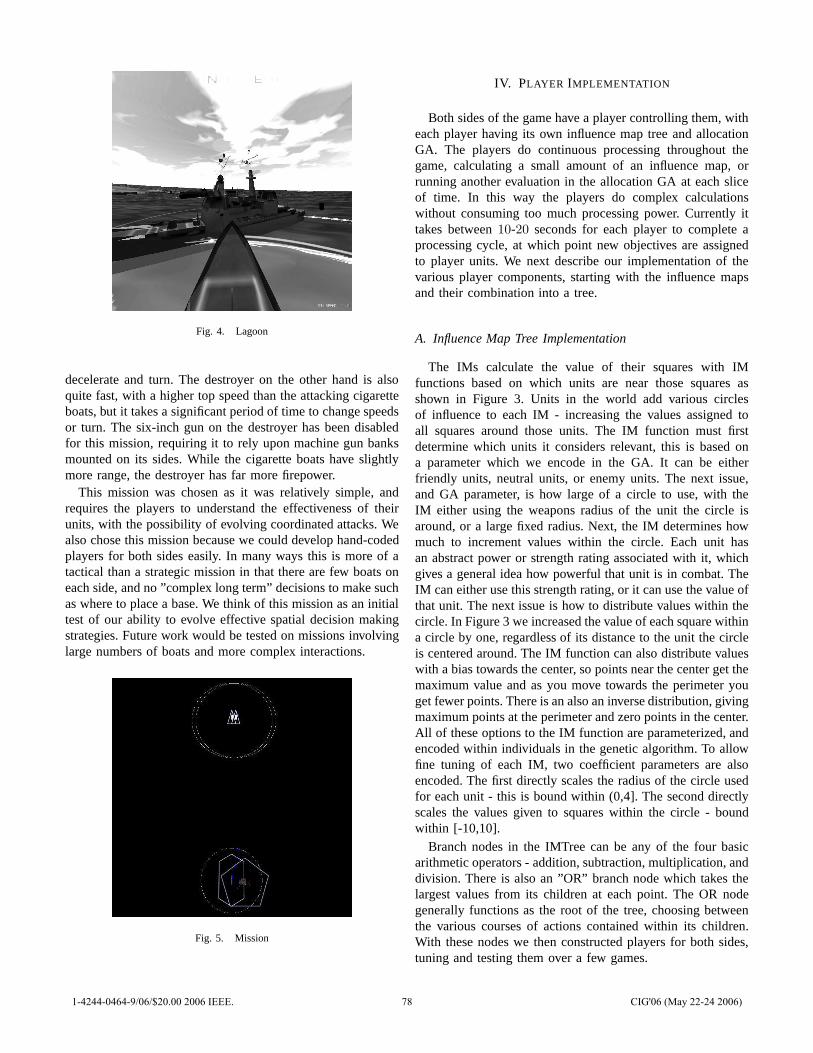
Fig. 4. Lagoon

decelerate and turn. The destroyer on the other hand is alsoquite fast, with a higher top speed than the attacking cigaretteboats, but it takes a significant period of time to change speedsor turn. The six-inch gun on the destroyer has been disabledfor this mission, requiring it to rely upon machine gun banksmounted on its sides. While the cigarette boats have slightlymore range, the destroyer has far more firepower.

This mission was chosen as it was relatively simple, andrequires the players to understand the effectiveness of theirunits, with the possibility of evolving coordinated attacks. Wealso chose this mission because we could develop hand-codedplayers for both sides easily. In many ways this is more of atactical than a strategic mission in that there are few boats oneach side, and no ”complex long term” decisions to make suchas where to place a base. We think of this mission as an initialtest of our ability to evolve effective spatial decision makingstrategies. Future work would be tested on missions involvinglarge numbers of boats and more complex interactions.

Fig. 5. Mission

IV. PLAYER IMPLEMENTATION

Both sides of the game have a player controlling them, witheach player having its own influence map tree and allocationGA. The players do continuous processing throughout thegame, calculating a small amount of an influence map, orrunning another evaluation in the allocation GA at each sliceof time. In this way the players do complex calculationswithout consuming too much processing power. Currently ittakes between 10-20 seconds for each player to complete aprocessing cycle, at which point new objectives are assignedto player units. We next describe our implementation of thevarious player components, starting with the influence mapsand their combination into a tree.

A. Influence Map Tree Implementation

The IMs calculate the value of their squares with IMfunctions based on which units are near those squares asshown in Figure 3. Units in the world add various circlesof influence to each IM - increasing the values assigned toall squares around those units. The IM function must firstdetermine which units it considers relevant, this is based ona parameter which we encode in the GA. It can be eitherfriendly units, neutral units, or enemy units. The next issue,and GA parameter, is how large of a circle to use, with theIM either using the weapons radius of the unit the circle isaround, or a large fixed radius. Next, the IM determines howmuch to increment values within the circle. Each unit hasan abstract power or strength rating associated with it, whichgives a general idea how powerful that unit is in combat. TheIM can either use this strength rating, or it can use the value ofthat unit. The next issue is how to distribute values within thecircle. In Figure 3 we increased the value of each square withina circle by one, regardless of its distance to the unit the circleis centered around. The IM function can also distribute valueswith a bias towards the center, so points near the center get themaximum value and as you move towards the perimeter youget fewer points. There is an also an inverse distribution, givingmaximum points at the perimeter and zero points in the center.All of these options to the IM function are parameterized, andencoded within individuals in the genetic algorithm. To allowfine tuning of each IM, two coefficient parameters are alsoencoded. The first directly scales the radius of the circle usedfor each unit - this is bound within (0,4]. The second directlyscales the values given to squares within the circle - boundwithin [-10,10].

Branch nodes in the IMTree can be any of the four basicarithmetic operators - addition, subtraction, multiplication, anddivision. There is also an ”OR” branch node which takes thelargest values from its children at each point. The OR nodegenerally functions as the root of the tree, choosing betweenthe various courses of actions contained within its children.With these nodes we then constructed players for both sides,tuning and testing them over a few games.

1-4244-0464-9/06/$20.00 2006 IEEE. 78 CIG'06 (May 22-24 2006)

V. OBJECTIVE ZONER

Processing the influence map produced by the influencemap tree into objectives is the job of the objective zoner. Anobjective is a task for a unit group to carry out at some pointin space. The objective zoner should reduce the influence mapto a set of objectives representing its most important points,including all the distinct peaks in the landscape without beingredundant. In Figure 2 the IMTree produces as output theobjective IM, from which the objectives are parsed. The zonerin response picks three key points, the two peaks on the left,and one of the points from the plateau on the right. The zonerdetermines the first two points correspond to attack actions,because the influence map which produced them was linkedto that behavior, while the third point and its correspondingIM was linked to a move behavior. This gives three objectives,attack those two points, or move to this point and distract theenemy.

Our objective zoner uses a simple algorithm to create theobjectives. It finds the highest point in the influence map thatis not to close to an already chosen objective, and takes itas an objective. It then repeats the process, until no eligiblepoints are left. Points are ineligible if their value is less thensome ratio of the highest point, 1/2 in this case. They arealso ineligible if they are too close to a previously assignedobjective. Currently all objectives carry a generic attack-movebehavior, where they move directly to the target point firingat enemies that come within range.

VI. A* PATHFINDER

Once the objectives have been calculated, an A* routerdetermines how accessible they are. A* looks at the unitgroups available to the player, searching for how easily theycan reach each objective. The allocation genetic algorithmuses this information to prioritize more accessible objectivesand keep units from being allocated to objectives they cannotreach.

We used a traditional A* pathfinder to do path-finding,A* is shown to always produce the optimal path through agraph so long as it has a proper underestimate, which wehave. Our pathfinder searches through squares in an influencemap to find the optimal path from one point to another.The A* influence map is separate from the players influencemap tree, with each square representing how preferable it isto route through. It has high negative values near powerfulenemies, and more positive numbers in open water. Becausethe A* router uses an influence map, the search space couldbe arbitrarily complicated, routing units so that they try to stayclose to neutral units, or as far from land as possible.

VII. ALLOCATION GA

AllocGA, a genetic algorithm, allocates units to objectives.AllocGA is a non-generational GA which uses single pointcrossover, bitwise mutation and roulette wheel selection. Itdetermines its resources currently available, and maps themto appropriate objectives taking into account the informationprovided by the other systems. Each individual in AllocGA’s

population encodes an allocation table, listing which objectiveeach unit is assigned too. The fitness for each individual is asummation of the benefit expected from allocating each unitgroup to its objective. The benefit for allocating a group to anobjective is given by: 1) the expected benefit from the objective2) how well that groups units match the units requested forthe objective 3) how easily the unit group can reach thatobjective. The expected benefit for an objective is the valuefrom its location in the influence map. How well units matchthose requested is based upon the composition of the group,and the meta-data assigned to those objectives as discussedin SectionVII-.1. The penalties for risk incurred, and traveldistance is the total cost associated with the route from unitto objective found by the A* pathfinder. Attacking an enemycity might yield tremendous benefit, but not for a group ofunits without the appropriate weaponry, or for units occupiedon the far side of the map.

1) Objective Meta-Data: To determine which units to allo-cate to which objectives we attach meta-data describing whatkind of units would be useful to each objective. We use threecoefficients, representing the power, speed, and value of theunits allocated. To each unit we associate three abstract values,a power rating summarizing how effective it is in combat, aspeed rating summarizing how fast and maneuverable it is, anda value rating representing its cost. Each is an abstract handset value summarizing the complex workings of the entity, thedestroyer’s has a high power rating, the cigarette boats havehigh speed ratings, and the oil-platform has a high value rating.AllocGA calculates benefit based how the units allocatedto an objective match up with the coefficients attached tothe objective. If an objective has a high power coefficient,then allocating powerful units increases the fitness of thatallocation. Conversely if an objective has a negative valuecoefficient, then allocating expensive units reduces the fitness.Each unit’s attributes are multiplied by the correspondingcoefficient, and the summation is applied to the fitness of thatallocation. By changing these values an influence map candeclare itself as suited for fast cheap units, powerful expensiveones, or weak valuable units (maybe a hide in the rear IM).Each objective can also have a unit cap, beyond which nobenefit is received for adding units, so that distracting with 10units is not more beneficial than using 1.

VIII. HAND-CODED PLAYERS

To test this system we first develop hand-coded players forboth sides, tuning their behavior over a few games to test howwell the players work. Our hand-coded attacker work by usingan OR node on two child subtrees. The first subtree representsan attack behavior which takes the weighted sum of two nodes.The first node has high values near vulnerable enemies, thesecond has large negative values near powerful enemies. Thisgives points near vulnerable enemies, but away from powerfulones The second subtree represents a distract behavior wherethe cigarette boat tries to stay just out of range of the destroyer,baiting it into following it and in the process abandoning theoil platform. The distract child node has two children of its

1-4244-0464-9/06/$20.00 2006 IEEE. 79 CIG'06 (May 22-24 2006)

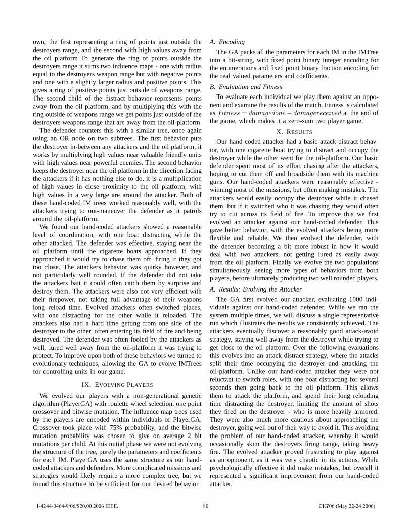
own, the first representing a ring of points just outside thedestroyers range, and the second with high values away fromthe oil platform To generate the ring of points outside thedestroyers range it sums two influence maps - one with radiusequal to the destroyers weapon range but with negative pointsand one with a slightly larger radius and positive points. Thisgives a ring of positive points just outside of weapons range.The second child of the distract behavior represents pointsaway from the oil platform, and by multiplying this with thering outside of weapons range we get points just outside of thedestroyers weapons range that are away from the oil-platform.

The defender counters this with a similar tree, once againusing an OR node on two subtrees. The first behavior putsthe destroyer in-between any attackers and the oil platform, itworks by multiplying high values near valuable friendly unitswith high values near powerful enemies. The second behaviorkeeps the destroyer near the oil platform in the direction facingthe attackers if it has nothing else to do, it is a multiplicationof high values in close proximity to the oil platform, withhigh values in a very large are around the attacker. Both ofthese hand-coded IM trees worked reasonably well, with theattackers trying to out-maneuver the defender as it patrolsaround the oil-platform.

We found our hand-coded attackers showed a reasonablelevel of coordination, with one boat distracting while theother attacked. The defender was effective, staying near theoil platform until the cigarette boats approached. If theyapproached it would try to chase them off, firing if they gottoo close. The attackers behavior was quirky however, andnot particularly well rounded. If the defender did not takethe attackers bait it could often catch them by surprise anddestroy them. The attackers were also not very efficient withtheir firepower, not taking full advantage of their weaponslong reload time. Evolved attackers often switched places,with one distracting for the other while it reloaded. Theattackers also had a hard time getting from one side of thedestroyer to the other, often entering its field of fire and beingdestroyed. The defender was often fooled by the attackers aswell, lured well away from the oil-platform it was trying toprotect. To improve upon both of these behaviors we turned toevolutionary techniques, allowing the GA to evolve IMTreesfor controlling units in our game.

IX. EVOLVING PLAYERS

We evolved our players with a non-generational geneticalgorithm (PlayerGA) with roulette wheel selection, one pointcrossover and bitwise mutation. The influence map trees usedby the players are encoded within individuals of PlayerGA.Crossover took place with 75% probability, and the bitwisemutation probability was chosen to give on average 2 bitmutations per child. At this initial phase we were not evolvingthe structure of the tree, purely the parameters and coefficientsfor each IM. PlayerGA uses the same structure as our hand-coded attackers and defenders. More complicated missions andstrategies would likely require a more complex tree, but wefound this structure to be sufficient for our desired behavior.

A. Encoding

The GA packs all the parameters for each IM in the IMTreeinto a bit-string, with fixed point binary integer encoding forthe enumerations and fixed point binary fraction encoding forthe real valued parameters and coefficients.

B. Evaluation and Fitness

To evaluate each individual we play them against an oppo-nent and examine the results of the match. Fitness is calculatedas fitness = damagedone− damagereceived at the end ofthe game, which makes it a zero-sum two player game.

X. RESULTS

Our hand-coded attacker had a basic attack-distract behav-ior, with one cigarette boat trying to distract and occupy thedestroyer while the other went for the oil-platform. Our basicdefender spent most of its effort chasing after the attackers,hoping to cut them off and broadside them with its machineguns. Our hand-coded attackers were reasonably effective -winning most of the missions, but often making mistakes. Theattackers would easily occupy the destroyer while it chasedthem, but if it switched who it was chasing they would oftentry to cut across its field of fire. To improve this we firstevolved an attacker against our hand-coded defender. Thisgave better behavior, with the evolved attackers being moreflexible and reliable. We then evolved the defender, withthe defender becoming a bit more robust in how it woulddeal with two attackers, not getting lured as easily awayfrom the oil platform. Finally we evolve the two populationssimultaneously, seeing more types of behaviors from bothplayers, before ultimately producing two well rounded players.

A. Results: Evolving the Attacker

The GA first evolved our attacker, evaluating 1000 indi-viduals against our hand-coded defender. While we ran thesystem multiple times, we will discuss a single representativerun which illustrates the results we consistently achieved. Theattackers eventually discover a reasonably good attack-avoidstrategy, staying well away from the destroyer while trying toget close to the oil platform. Over the following evaluationsthis evolves into an attack-distract strategy, where the attackssplit their time occupying the destroyer and attacking theoil-platform. Unlike our hand-coded attacker they were notreluctant to switch roles, with one boat distracting for severalseconds then going back to the oil platform. This allowsthem to attack the platform, and spend their long reloadingtime distracting the destroyer, limiting the amount of shotsthey fired on the destroyer - who is more heavily armored.They were also much more cautious about approaching thedestroyer, going well out of their way to avoid it. This avoidingthe problem of our hand-coded attacker, whereby it wouldoccasionally skim the destroyers firing range, taking heavyfire. The evolved attacker proved frustrating to play againstas an opponent, as it was very chaotic in its actions. Whilepsychologically effective it did make mistakes, but overall itrepresented a significant improvement from our hand-codedattacker.

1-4244-0464-9/06/$20.00 2006 IEEE. 80 CIG'06 (May 22-24 2006)

Fig. 6. Behavior Exhibited by Evolved Attacker

B. Results: Evolving the Defender

The evolved attackers were effective against the hand-codeddefender, coordinating an effective attack-distract strategy. Wenext re-ran the genetic algorithm to evolve the defender tosee if it could find a counter to the attackers strategy. Theattack distract behavior capitalizes well on the advantagegiven to the attackers, making it difficult for the destroyerto effectively defend. The defenders evolved did surpass thequality of our own hand-coded defenders however, learninghow to trick the attackers into making mistakes. Figure 7shows an exceptional defense, where the defender pushesboth attackers back by manipulating their constant switches inroles. While the evolved attacker and evolved defender wereeffective, particularly against each other, they made obviousmistakes against human opponents. To improve our playersfurther we utilized co-evolution, aiming to generate ever morerobust players.

Fig. 7. Behavior Exhibited by Evolved Defender

C. Co-Evolution

Co-evolution occurs when the evaluation of an individ-ual is dependent upon other individuals. We implementedco-evolution with a traditional two population model, withone population containing attacking strategies, and the othercontaining defending strategies. We evaluated individuals byplaying them against un-evaluated individuals in the otherpopulation, with fitness calculated as before. The goal beingan ”arms race” whereby each side is constantly innovating newstrategies in order to better their opponent.

D. Results: Co-evolving Attackers and Defenders

To implement co-evolution we run two genetic algorithms- one evolving attackers, and one evolving defenders. Weplay unevaluated members from each population against eachother, and calculate fitness as before. As before we allowedeach GA to evaluate 1000 candidate strategies. Figure 8shows the minimum, maximum, and average fitness in the twopopulations over time. At first there is chaos, with both playersusing random strategies. Effective attackers and defenders startto emerge however, with the attacker learning to go for the oilplatform and the defender learning to go for the attackers.The attackers suffer for a few hundred generations, trying tolearn an attack-distract or an attack-avoid behavior. Eventuallythose start to emerge, and their fitness rises dramatically. Thisleads to improvements in the defenders AI, learning not tobe lured away from the oil platform, and to keep its speedup. Ultimately they develop the behaviors shown in Figure 9- the attacker develops a well rounded attack-distract-avoidbehavior, and the defender develops a diligent defensive be-havior. The attackers spends less time distracting than before,preferring to stay on the opposite side of the oil-platform andfight. One boat will occasionally lure the defender away, andthen return while the defender turns around. The attackersalso tend to stay far away, generally opposite sides as shownin Figure 9, which makes them much more flexible than ifthey bunch up. The defenders behavior was very protective,generally staying very close to the oil-platform. It was difficultto lure off, and did a good job of overcoming its slow turningrate by staying in good positions.. Both attacker and defenderlearned generalized behaviors, similar to those we had tried todevelop in our hand-coded behaviors. The co-evolved playerswere superior to the hand-coded players, with the attackersclearly out-maneuvering the destroyer, and the defender doingits best to defend the oil-platform. Co-evolution gave them therobustness necessary to play against human opponents.

XI. CONCLUSIONS AND FUTURE WORK

Co-evolved influence map trees were capable of produc-ing competent behavior inside our RTS game. While ourmission was relatively simple, and the IMTrees were usedmore as operational controllers than as strategic planners,the IMTrees functioned adequately. By combining influencemaps with genetic algorithms we produced behavior thatwas much more coordinated than in either of the previoussystems. The attackers learned how to effectively work as a

1-4244-0464-9/06/$20.00 2006 IEEE. 81 CIG'06 (May 22-24 2006)

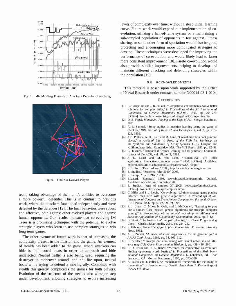
Fig. 8. Min/Max/Avg Fitness’s of Attacker / Defender Co-evolving

Fig. 9. Final Co-Evolved Players

team, taking advantage of their unit’s abilities to overcomea more powerful defender. This is in contrast to previouswork, where the attackers functioned independently and weredefeated by the defender [12]. The final behaviors were robustand effective, both against other evolved players and againsthuman opponents. Our results indicate that co-evolving IMTrees is a promising technique, with the potential to evolvestrategic players who learn to use complex strategies to winlong-term games.

The other avenue of future work is that of increasing thecomplexity present in the mission and the game. An elementof stealth has been added to the game, where attackers canhide behind neutral boats in order to approach and hideundetected. Neutral traffic is also being used, requiring thedestroyer to maneuver around, and not fire upon, neutralboats while trying to defend a moving ally. Combined withstealth this greatly complicates the games for both players.Evolution of the structure of the tree is also a major stepunder development, allowing strategies to evolve increasing

levels of complexity over time, without a steep initial learningcurve. Future work would expand our implementation of co-evolution, utilizing a hall-of-fame system or a maintaining asub-sampled population of opponents to test against. Fitnesssharing, or some other form of speciation would also be good,protecting and encouraging more complicated strategies todevelop. These techniques were developed for improving theperformance of co-evolution, and would likely lead to fastermore consistent improvement [18]. Pareto co-evolution wouldalso provide similar improvements, helping to develop andmaintain different attacking and defending strategies withinthe population [19].

XII. ACKNOWLEDGMENTS

This material is based upon work supported by the Officeof Naval Research under contract number N00014-03-1-0104.

REFERENCES

[1] P. J. Angeline and J. B. Pollack, “Competitive environments evolve bettersolutions for complex tasks,” in Proceedings of the 5th InternationalConference on Genetic Algorithms (GA-93), 1993, pp. 264–270.[Online]. Available: citeseer.ist.psu.edu/angeline93competitive.html

[2] D. B. Fogel, Blondie24: Playing at the Edge of AI. Morgan Kauffman,2001.

[3] A. L. Samuel, “Some studies in machine learning using the game ofcheckers,” IBM Journal of Research and Development, vol. 3, pp. 210–229, 1959.

[4] J. B. Pollack, A. D. Blair, and M. Land, “Coevolution of a backgammonplayer,” in Artificial Life V: Proc. of the Fifth Int. Workshop onthe Synthesis and Simulation of Living Systems, C. G. Langton andK. Shimohara, Eds. Cambridge, MA: The MIT Press, 1997, pp. 92–98.

[5] G. Tesauro, “Temporal difference learning and td-gammon,” Communi-cations of the ACM, vol. 38, no. 3, 1995.

[6] J. E. Laird and M. van Lent, “Human-level ai’s killerapplication: Interactive computer games,” 2000. [Online]. Available:http://ai.eecs.umich.edu/people/laird/papers/AAAI-00.pdf

[7] R. E. Inc., “Dawn of war,” 2005, http://www.dawnofwargame.com.[8] B. Studios., “Supreme ruler 2010,” 2005.[9] R. Pump., “Earth 2160,” 2005.

[10] Blizzard, “Starcraft,” 1998, www.blizzard.com/starcraft. [Online].Available: www.blizzard.com/starcraft

[11] E. Studios, “Age of empires 3,” 2005, www.ageofempires3.com.[Online]. Available: www.ageofempires3.com

[12] C. Miles and S. J. Louis, “Co-evolving real-time strategy game playinginfluence map trees with genetic algorithms,” in Proceedings of theInternational Congress on Evolutionary Computation, Portland, Oregon.IEEE Press, 2006, pp. 0–999 999 999 999.

[13] S. J. Louis, C. Miles, N. Cole, and J. McDonnell, “Learning to playlike a human: Case injected genetic algorithms for strategic computergaming,” in Proceedings of the second Workshop on Military andSecurity Applications of Evolutionary Computation, 2005, pp. 6–12.

[14] B. Stout, “The basics of a* for path planning,” in Game ProgrammingGems. Charles River media, 2000, pp. 254–262.

[15] R. Gibbons, Game Theory for Applied Economists. Princeton UniversityPress, 1992.

[16] A. L. Zobrist, “A model of visual organization for the game of go,” inAFIPS Conf. Proc., 1969, pp. 34, 103–112.

[17] P. Sweetser, “Strategic decision-making with neural networks and influ-ence maps,” AI Game Programming Wisdom 2, pp. 439–446, 2001.

[18] C. D. Rosin and R. K. Belew, “Methods for competitive co-evolution:Finding opponents worth beating,” in Proceedings of the Sixth Inter-national Conference on Genetic Algorithms, L. Eshelman, Ed. SanFrancisco, CA: Morgan Kaufmann, 1995, pp. 373–380.

[19] A. Bucci and J. Pollack, “A mathematical framework for the study ofcoevolution,” in Foundations of Genetic Algorithms 7. Proceedings ofFOGA VII, 2002.

1-4244-0464-9/06/$20.00 2006 IEEE. 82 CIG'06 (May 22-24 2006)

AbstractThis work discusses the use of evolutionary computation for an automated player of a real-time strategic tactics game in which assets are assigned to targets and threats belonging to the opposing team. Strategy games such as this are essentially a series of asset allocation problems to which evolutionary algorithms are particularly adept. This game contains a significant coupling affect between the assets assigned to targets and those assigned to threats. The effort considers targets and threats in a non-spatiotemporal framework to evaluate the proposed approach. In addition, the architecture that supports the implemented evolutionary search algorithm is also discussed.

I. INTRODUCTION HIS work explores the use of an evolutionary search algorithm as the core of an automated player of strategic tactical games in which two players attempt to defend

their own assets while accomplishing objectives of destruction against the other. This class of games can be viewed essentially as a series of generalized asset allocation problems. These allocation problems often contain complicated spatial and temporal constraints affected by such things as target placement, time windows, fuel, and geographic features. Further complexity is introduced by the existence of coupling effects between a player’s assets.

If your paper is intended for a conference, please contact your conference editor concerning acceptable word processor formats for your particular conference.

Our research focuses on an automated player for the blue team in a tactical air strike game similar to the one presented in [1]-[3] and maps to a range of asset allocation problems found throughout the military and industry. The objective of the game for the blue team is to inflict predefined levels of destruction to a dynamically changing set of targets belonging to the red team while preserving the health of its own strike aircraft. For the red team, the objective is to

Manuscript received January 31, 2006. This work was supported as an

Internal Applied Research project for SPAWAR Systems Center – San Diego.

A. J. Rice is with SPAWAR Systems Center – San Diego, San Diego, CA 92152-5001 USA (phone: 619-553-9597; fax: 619-553-9483; e-mail: aaron.rice@navy.mil).

J. R. McDonnell is with SPAWAR Systems Center – San Diego, San Diego, CA 92152-5001 USA (phone: 619-553-5762; fax: 619-553-9483; e-mail: john.mcdonnell@navy.mil).

A. Spydell was with G2 Software Systems, Encinitas, CA 92024 USA (e-mail: aspydell@g2ss.com).

S. Stremler is with G2 Software Systems, Encinitas, CA 92024 USA (e-mail: stremler@g2ss.com).

protect valuable assets (targets) while inflicting as much destruction as possible to the blue force aircraft.

To accomplish their objectives the blue team assigns weapons, with varying effectiveness against different structure types, to enemy targets. Each target has a predefined priority value, and the most important targets should be hit over targets with a lower priority value. Each red target may be protected by one or more air defense sites (hereafter referred to simply as threats), each of which has its own destruction capabilities against the various types of blue force aircraft. To protect its strike aircraft, the blue player allocates Suppression of Enemy Air Defense (SEAD) assets to threats of concern in the area of an attack. These SEAD assets have distinct levels of effectiveness for suppressing different types of threats. This introduces the coupling affect, shown in Fig. 1, where the effectiveness of the SEAD assets has a direct influence on the risk level of the attack aircraft. This risk level is based upon an aircraft’s exposure to the threat systems. This assignment problem represents unique challenges because of the coupling effect. The temporal component increases the problem complexity due to the need for SEAD assets to maintain suppression of enemy threats over time windows to allow the Attack assets to effectively prosecute the desired target set and is not addressed in the context of this effort.

The red team seeks to accomplish its objectives by changing the layout of its targets and threats. Certain targets and threats can be moved whereas others are stationary. The red team may have threats and targets that are hidden or not present when the game starts. Strategic introduction of these entities is key to the red team’s success. Changing the layout of red team assets creates the need for the blue team to retask its assets in order to adapt to the changes and maintain objectives.

Previous efforts on strike force asset allocation have

A Player for Tactical Air Strike Games Using Evolutionary Computation

Aaron J. Rice, John R. McDonnell, Andy Spydell and Stewart Stremler

T

Strike Assets

SEAD Assets

Targets

Threats

Fig. 1. The Coupling effect between strike and SEAD assets caused by threats that protect prosecuted targets.

1-4244-0464-9/06/$20.00 2006 IEEE. 83 CIG'06 (May 22-24 2006)

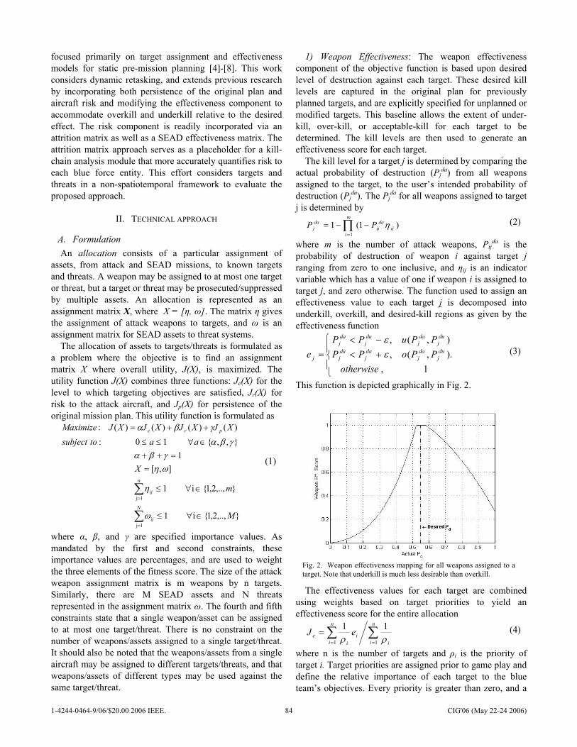
focused primarily on target assignment and effectiveness models for static pre-mission planning [4]-[8]. This work considers dynamic retasking, and extends previous research by incorporating both persistence of the original plan and aircraft risk and modifying the effectiveness component to accommodate overkill and underkill relative to the desired effect. The risk component is readily incorporated via an attrition matrix as well as a SEAD effectiveness matrix. The attrition matrix approach serves as a placeholder for a kill-chain analysis module that more accurately quantifies risk to each blue force entity. This effort considers targets and threats in a non-spatiotemporal framework to evaluate the proposed approach.

II. TECHNICAL APPROACH

A. Formulation An allocation consists of a particular assignment of

assets, from attack and SEAD missions, to known targets and threats. A weapon may be assigned to at most one target or threat, but a target or threat may be prosecuted/suppressed by multiple assets. An allocation is represented as an assignment matrix X, where X = [η, ω]. The matrix η gives the assignment of attack weapons to targets, and ω is an assignment matrix for SEAD assets to threat systems.

The allocation of assets to targets/threats is formulated as a problem where the objective is to find an assignment matrix X where overall utility, J(X), is maximized. The utility function J(X) combines three functions: Je(X) for the level to which targeting objectives are satisfied, Jr(X) for risk to the attack aircraft, and Jp(X) for persistence of the original mission plan. This utility function is formulated as

},..,2,1{i 1

},..,2,1{i 1

],[ 1

},,{ 10 :)()()()( :

1j

1j

M

m

X

aatosubjectXJXJXJXJMaximize

N

ij

n

ij

pre

∈∀≤

∈∀≤

==++

∈∀≤≤

++=

∑

∑

=

=

ω

η

ωηγβα

γβα

γβα

(1)

where α, β, and γ are specified importance values. As mandated by the first and second constraints, these importance values are percentages, and are used to weight the three elements of the fitness score. The size of the attack weapon assignment matrix is m weapons by n targets. Similarly, there are M SEAD assets and N threats represented in the assignment matrix ω. The fourth and fifth constraints state that a single weapon/asset can be assigned to at most one target/threat. There is no constraint on the number of weapons/assets assigned to a single target/threat. It should also be noted that the weapons/assets from a single aircraft may be assigned to different targets/threats, and that weapons/assets of different types may be used against the same target/threat.

1) Weapon Effectiveness: The weapon effectiveness component of the objective function is based upon desired level of destruction against each target. These desired kill levels are captured in the original plan for previously planned targets, and are explicitly specified for unplanned or modified targets. This baseline allows the extent of under-kill, over-kill, or acceptable-kill for each target to be determined. The kill levels are then used to generate an effectiveness score for each target.

The kill level for a target j is determined by comparing the actual probability of destruction (Pj

da) from all weapons assigned to the target, to the user’s intended probability of destruction (Pj

du). The Pjda for all weapons assigned to target

j is determined by

∏=

−−=m

iij

daij

daj PP

1

)1(1 η (2)

where m is the number of attack weapons, Pijda is the

probability of destruction of weapon i against target j ranging from zero to one inclusive, and ηij is an indicator variable which has a value of one if weapon i is assigned to target j, and zero otherwise. The function used to assign an effectiveness value to each target j is decomposed into underkill, overkill, and desired-kill regions as given by the effectiveness function

.1,

),(,),(,

+<−<

=otherwise

PPoPPPPuPP

e duj

daj

daj

duj

duj

daj

duj

daj

j εε

(3)

This function is depicted graphically in Fig. 2.

The effectiveness values for each target are combined using weights based on target priorities to yield an effectiveness score for the entire allocation

∑∑==

=n

i i

n

ii

ie eJ

11

11ρρ

(4)

where n is the number of targets and ρi is the priority of target i. Target priorities are assigned prior to game play and define the relative importance of each target to the blue team’s objectives. Every priority is greater than zero, and a

Fig. 2. Weapon effectiveness mapping for all weapons assigned to a target. Note that underkill is much less desirable than overkill.

1-4244-0464-9/06/$20.00 2006 IEEE. 84 CIG'06 (May 22-24 2006)

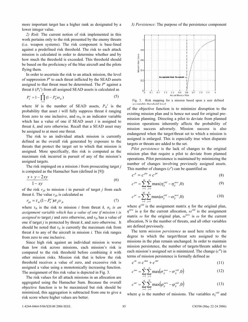
more important target has a higher rank as designated by a lower integer value.

2) Risk: The current notion of risk implemented in this work pertains only to the risk presented by the enemy threats (i.e. weapon systems). The risk component is base-lined against a predefined risk threshold. The risk to each attack mission is calculated in order to determine whether and by how much the threshold is exceeded. This threshold should be based on the proficiency of the blue aircraft and the pilots flying them.

In order to ascertain the risk to an attack mission, the level of suppression Ps to each threat inflicted by the SEAD assets assigned to that threat must be determined. The Ps against a threat k (Pk

s) from all assigned SEAD assets is calculated as

∏=

−−=M

iik

sik

sk PP

1

)1(1 ω (5)

where M is the number of SEAD assets, Piks is the

probability that asset i will fully suppress threat k ranging from zero to one inclusive, and ωik is an indicator variable which has a value of one if SEAD asset i is assigned to threat k, and zero otherwise. Recall that a SEAD asset may be assigned to at most one threat.

The risk to an individual attack mission is currently defined as the overall risk generated by exposure to the threats that protect the target set to which that mission is assigned. More specifically, this risk is computed as the maximum risk incurred in pursuit of any of the mission’s assigned targets.

The risk impinged on a mission i from prosecuting target j is computed as the Hamacher Sum (defined in [9])

xyxyyx

−−+

12

(6)

of the risk rijk to mission i in pursuit of target j from each threat k. The value rijk is calculated as

jkijs

kikijk Pr υστ )1( −= (7)

where τik is the risk to mission i from threat k, σij is an assignment variable which has a value of one if mission i is assigned to target j and zero otherwise, and υjk has a value of one if target j is protected by threat k, and zero otherwise. It should be noted that τik is currently the maximum risk from threat k to any of the aircraft in mission i. This risk ranges from zero to one inclusive.

Since high risk against an individual mission is worse than low risk across missions, each mission’s risk is compared to the risk threshold before combining it with other mission risks. Mission risk that is below the risk threshold receives a value of zero, and excessive risk is assigned a value using a monotonically increasing function. The assignment of this risk value is depicted in Fig. 3.

The risk values for all attack missions in an allocation are aggregated using the Hamacher Sum. Because the overall objective function is to be maximized but risk should be minimized, this aggregation is subtracted from one to give a risk score where higher values are better.

3) Persistence: The purpose of the persistence component

of the objective function is to minimize disruption to the existing mission plan and is hence not used for original pre-mission planning. Directing a pilot to deviate from planned mission operations inherently affects the probability of mission success adversely. Mission success is also endangered when the target/threat set to which a mission is assigned is enlarged. This is especially true when disparate targets or threats are added to the set.

Pilot persistence is the lack of changes to the original mission plan that require a pilot to deviate from planned operations. Pilot persistence is maintained by minimizing the number of changes involving previously assigned assets. This number of changes (cp) can be quantified as

prpap ccc += (8)

∑∑= =

−=m

i

n

j

newij

oldij

pac1 1

)0,max( ηη (9)

∑∑= =

−=M

i

N

j

newij

oldij

prc1 1

)0,max( ωω (10)

where ηold is the assignment matrix η for the original plan, ηnew is η for the current allocation, ωold is the assignment matrix ω for the original plan, ωnew is ω for the current allocation, N is the number of threats, and all other variables are defined previously.

The term mission persistence as used here refers to the degree to which the target/threat sets assigned to the missions in the plan remain unchanged. In order to maintain mission persistence, the number of targets/threats added to each mission’s assigned set is minimized. The change (cm) in terms of mission persistence is formally defined as

mrmam ccc += (11)

( )∑∑= =

−=q

i

n

j

oldij

newij

mac1 1

0,max σσ (12)

( )∑∑= =

−=q

i

N

j

oldij

newij

mrc1 1

0,max ϕϕ (13)

where q is the number of missions. The variables σijold and

Fig. 3. Risk mapping for a mission based upon a user defined acceptable threshold level

1-4244-0464-9/06/$20.00 2006 IEEE. 85 CIG'06 (May 22-24 2006)

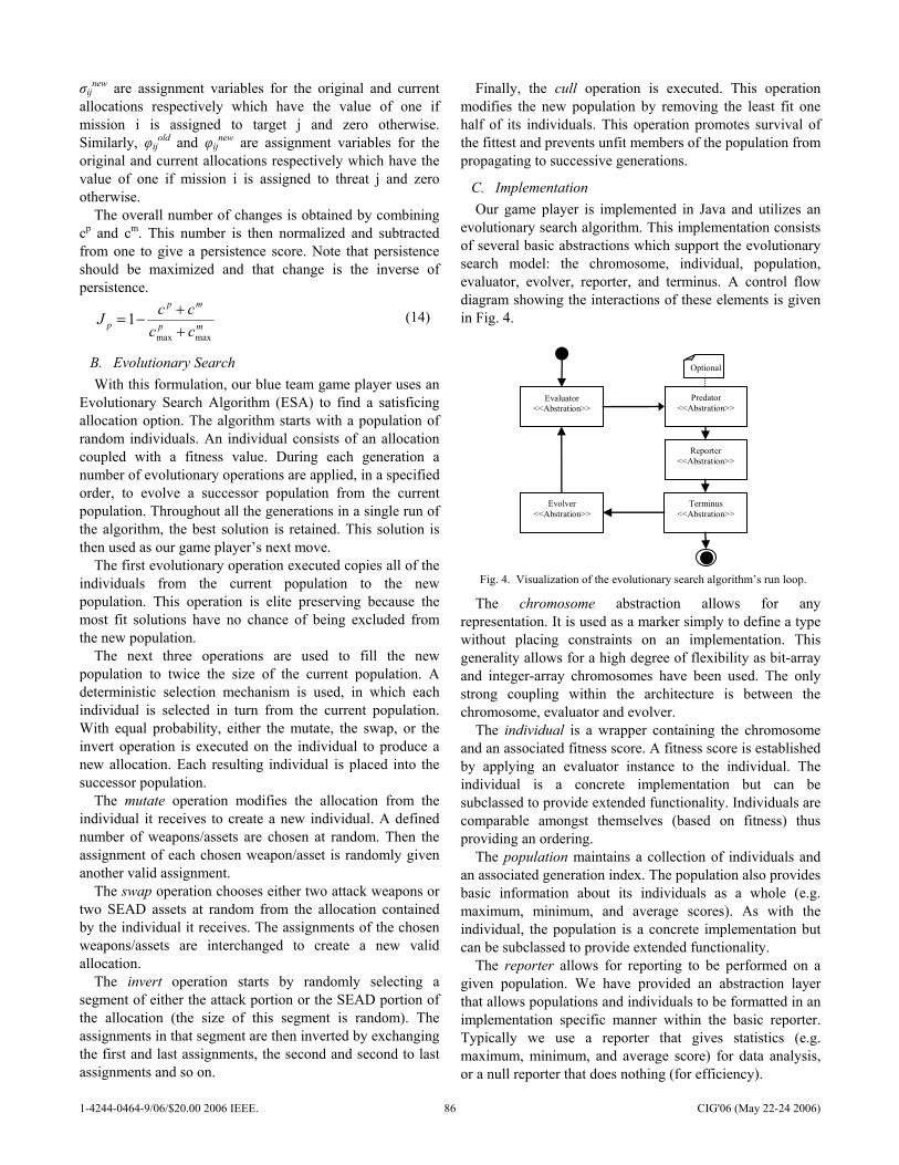
σijnew are assignment variables for the original and current

allocations respectively which have the value of one if mission i is assigned to target j and zero otherwise. Similarly, φij

old and φijnew are assignment variables for the

original and current allocations respectively which have the value of one if mission i is assigned to threat j and zero otherwise.

The overall number of changes is obtained by combining cp and cm. This number is then normalized and subtracted from one to give a persistence score. Note that persistence should be maximized and that change is the inverse of persistence.

mp

mp

p ccccJ

maxmax

1++

−= (14)

B. Evolutionary Search With this formulation, our blue team game player uses an

Evolutionary Search Algorithm (ESA) to find a satisficing allocation option. The algorithm starts with a population of random individuals. An individual consists of an allocation coupled with a fitness value. During each generation a number of evolutionary operations are applied, in a specified order, to evolve a successor population from the current population. Throughout all the generations in a single run of the algorithm, the best solution is retained. This solution is then used as our game player’s next move.

The first evolutionary operation executed copies all of the individuals from the current population to the new population. This operation is elite preserving because the most fit solutions have no chance of being excluded from the new population.

The next three operations are used to fill the new population to twice the size of the current population. A deterministic selection mechanism is used, in which each individual is selected in turn from the current population. With equal probability, either the mutate, the swap, or the invert operation is executed on the individual to produce a new allocation. Each resulting individual is placed into the successor population.

The mutate operation modifies the allocation from the individual it receives to create a new individual. A defined number of weapons/assets are chosen at random. Then the assignment of each chosen weapon/asset is randomly given another valid assignment.

The swap operation chooses either two attack weapons or two SEAD assets at random from the allocation contained by the individual it receives. The assignments of the chosen weapons/assets are interchanged to create a new valid allocation.

The invert operation starts by randomly selecting a segment of either the attack portion or the SEAD portion of the allocation (the size of this segment is random). The assignments in that segment are then inverted by exchanging the first and last assignments, the second and second to last assignments and so on.

Finally, the cull operation is executed. This operation modifies the new population by removing the least fit one half of its individuals. This operation promotes survival of the fittest and prevents unfit members of the population from propagating to successive generations.

C. Implementation Our game player is implemented in Java and utilizes an

evolutionary search algorithm. This implementation consists of several basic abstractions which support the evolutionary search model: the chromosome, individual, population, evaluator, evolver, reporter, and terminus. A control flow diagram showing the interactions of these elements is given in Fig. 4.

The chromosome abstraction allows for any representation. It is used as a marker simply to define a type without placing constraints on an implementation. This generality allows for a high degree of flexibility as bit-array and integer-array chromosomes have been used. The only strong coupling within the architecture is between the chromosome, evaluator and evolver.

The individual is a wrapper containing the chromosome and an associated fitness score. A fitness score is established by applying an evaluator instance to the individual. The individual is a concrete implementation but can be subclassed to provide extended functionality. Individuals are comparable amongst themselves (based on fitness) thus providing an ordering.

The population maintains a collection of individuals and an associated generation index. The population also provides basic information about its individuals as a whole (e.g. maximum, minimum, and average scores). As with the individual, the population is a concrete implementation but can be subclassed to provide extended functionality.

The reporter allows for reporting to be performed on a given population. We have provided an abstraction layer that allows populations and individuals to be formatted in an implementation specific manner within the basic reporter. Typically we use a reporter that gives statistics (e.g. maximum, minimum, and average score) for data analysis, or a null reporter that does nothing (for efficiency).

Evaluator <<Abstration>>

Reporter <<Abstration>>

Evolver <<Abstration>>

Predator <<Abstration>>

Terminus <<Abstration>>

Optional

Fig. 4. Visualization of the evolutionary search algorithm’s run loop.

1-4244-0464-9/06/$20.00 2006 IEEE. 86 CIG'06 (May 22-24 2006)

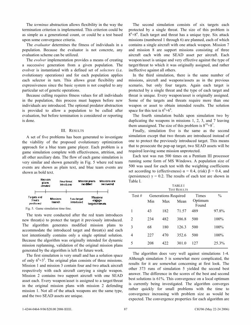
The terminus abstraction allows flexibility in the way the termination criterion is implemented. This criterion could be as simple as a generational count, or could be a test based upon some convergence criteria.

The evaluator determines the fitness of individuals in a population. Because the evaluator is not concrete, any evaluation scheme can be utilized.

The evolver implementation provides a means of creating a successive generation from a given population. The evolver is instantiated with a defined set of selectors (i.e. evolutionary operations) and for each population applies each selector in turn. This allows great flexibility and expressiveness since the basic system is not coupled to any particular set of genetic operations.

Because culling requires fitness values for all individuals in the population, this process must happen before new individuals are introduced. The optional predator abstraction is provided to allow a population to be culled after evaluation, but before termination is considered or reporting is done.

III. RESULTS A set of five problems has been generated to investigate

the viability of the proposed evolutionary optimization approach for a blue team game player. Each problem is a game simulation complete with effectiveness, attrition, and all other auxiliary data. The flow of each game simulation is very similar and shown generally in Fig. 5 where red team events are shown as plain text, and blue team events are shown as bold text.

The tests were conducted after the red team introduces new threat(s) to protect the target it previously introduced. The algorithm generates modified mission plans to accommodate the introduced target and threat(s) and each test intentionally contains only a single optimal solution. Because the algorithm was originally intended for dynamic mission replanning, validation of the original mission plans generated by the algorithm is left for future work.

The first simulation is very small and has a solution space of only 66+32. The original plan consists of three missions. Mission 1 and mission 3 contain four and two attack aircraft respectively with each aircraft carrying a single weapon. Mission 2 contains two support aircraft with one SEAD asset each. Every weapon/asset is assigned to a target/threat in the original mission plans with mission 2 defending mission 1. Not all of the attack weapons are the same type, and the two SEAD assets are unique.

The second simulation consists of six targets each protected by a single threat. The size of this problem is 86+86. Each target and threat has a unique type. Six attack missions (numbered 1 through 6) are planned, each of which contains a single aircraft with one attack weapon. Mission 7 and mission 8 are support missions consisting of three aircraft each with one SEAD asset per aircraft. Each weapon/asset is unique and very effective against the type of target/threat to which it was originally assigned, and rather ineffective against all others.

In the third simulation, there is the same number of missions, aircraft and weapons/assets as in the previous scenario, but only four targets. Again each target is protected by a single threat and the type of each target and threat is unique. Every weapon/asset is originally assigned. Some of the targets and threats require more than one weapon or asset to obtain intended results. The solution space for this test is 66+66.

The fourth simulation builds upon simulation two by duplicating the weapons in missions 1, 2, 3, and 7 leaving them unassigned. The size of this problem is 810+87.

Finally, simulation five is the same as the second simulation except that two threats are introduced instead of one to protect the previously introduced target. This means that to prosecute the pop-up target, two SEAD assets will be required leaving some mission unprotected.

Each test was run 500 times on a Pentium III processor running some form of MS Windows. A population size of 500 was used for each test with the weighting coefficients set according to (effectiveness) α = 0.4, (risk) β = 0.4, and (persistence) γ = 0.2. The results of each test are shown in Table I.

TABLE I TEST RESULTS

Generations Required Test # Min Max Mean

Times Optimum

Found

%

1 43 182 71.57 489 97.8%

2 234 482 386.8 500 100%

3 68 180 126.3 500 100%

4 227 470 352.6 500 100%

5 208 422 301.0 127 25.3%

The algorithm does very well against simulations 1-4. Although simulation 5 is somewhat more complicated, the results for it are somewhat concerning at first look. The other 373 runs of simulation 5 yielded the second best answer. The difference in the scores of the best and second best solutions is 61%. This convergence on a local optimum is currently being investigated. The algorithm converges rather quickly for small problems with the time to convergence increasing with problem size as would be expected. The convergence properties for each algorithm are

Fig. 5. Game simulation time-line.

1-4244-0464-9/06/$20.00 2006 IEEE. 87 CIG'06 (May 22-24 2006)

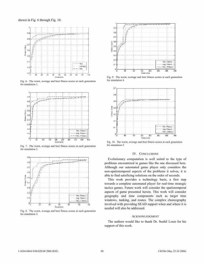
shown in Fig. 6 through Fig. 10.

IV. CONCLUSIONS Evolutionary computation is well suited to the type of

problems encountered in games like the one discussed here. Although our automated game player only considers the non-spatiotemporal aspects of the problems it solves, it is able to find satisficing solutions on the order of seconds.

This work provides a technology basis, a first step towards a complete automated player for real-time strategic tactics games. Future work will consider the spatiotemporal aspects of game presented herein. This work will consider geography and time components such as target time windows, tanking, and routes. The complex choreography involved with providing SEAD support when and where it is needed will also be addressed.

ACKNOWLEDGMENT The authors would like to thank Dr. Sushil Louis for his

support of this work.

Fig. 10. The worst, average and best fitness scores at each generation for simulation 5.

Fig. 9. The worst, average and best fitness scores at each generation for simulation 4.

Fig. 8. The worst, average and best fitness scores at each generation for simulation 3.

Fig. 7. The worst, average and best fitness scores at each generation for simulation 2.

Fig. 6. The worst, average and best fitness scores at each generation for simulation 1.

1-4244-0464-9/06/$20.00 2006 IEEE. 88 CIG'06 (May 22-24 2006)

REFERENCES [1] S. Louis and C. Miles, “Combining case-based memory with genetic

algorithm search for competent game AI,” in Proc. 2005 Workshop on CBR in Games, 2005.

[2] S. Louis, C. Miles, N. Cole, and J. McDonnell, “Learning to play like a human: Case injected genetic algorithms for strategic computer gaming,” in Proc. 2nd Workshop on Military and Security Applications of Evolutionary Computation, Seattle, WA, 2005.

[3] C. Miles and S. Louis, “Case-injection improves response time for a real-time strategy game,” in Proc. 2005 IEEE Symposium on Computational Intelligence in Game, New York, 2005.

[4] B. Griggs, G. Parnell, and L. Lehmkuhl, “An air mission planning algorithm using decision analysis and mixed integer programming,” Operations Research, vol. 45, no. 5, pp. 662-676, 1997.

[5] V. C. Li, G. L. Curry, and E. A. Boyd, “Towards the real time solution of strike force asset allocation problems,” Computers & Operations Research, vol. 31, no. 2, pp. 273-291, 2004.

[6] P. Abrahams, et al., “Maap: the military aircraft allocation planner,” in Proc. IEEE World Congress on Computational Intelligence, pp. 336-341, 1998.

[7] J. McDonnell, N. Gizzi, and S. Louis, “Strike force asset allocation using genetic search,” in Proc. International Conference on Artificial Intelligence, Las Vegas, NV, 2002

[8] S. Louis, J. McDonnell, and N. Gizzi, “Dynamic strike force asset allocation using genetic algorithms and case-based reasoning,” in Proc. 6th Conference on Systemics, Cybernetics, and Informatics, Orlando, FL, pp. 855-861, 2002.

[9] L. F. Sugianto, “Optimal decision making with imprecise data,” International Journal of Fuzzy Systems, vol. 3, no. 4, pp. 569-576, 2001.

1-4244-0464-9/06/$20.00 2006 IEEE. 89 CIG'06 (May 22-24 2006)

Exploiting Sensor Symmetries in Example-based Trainingfor Intelligent Agents

Bobby D. BryantDepartment of Computer SciencesThe University of Texas at Austin

bdbryant@cs.utexas.edu

Risto MiikkulainenDepartment of Computer SciencesThe University of Texas at Austin

risto@cs.utexas.edu

Abstract— Intelligent agents in games and simulators oftenoperate in environments subject to symmetric transformationsthat produce new but equally legitimate environments, such asreflections or rotations of maps. That fact suggests two hypothesesof interest for machine-learning approaches to creating intelligentagents for use in such environments. First, that exploitingsymmetric transformations can broaden the range of experiencemade available to the agents during training, and thus result inimproved performance at the task for which they are trained.Second, that exploiting symmetric transformations during train-ing can make the agents’ response to environments not seenduring training measurably more consistent. In this paper thetwo hypotheses are evaluated experimentally by exploiting sensorsymmetries and potential symmetries of the environment whiletraining intelligent agents for a strategy game. The experimentsreveal that when a corpus of human-generated training examplesis supplemented with artificial examples generated by means ofreflections and rotations, improvement is obtained in both taskperformance and consistency of behavior.

Keywords: Agents, Multi-Agent Systems, Adaptive Teamof Agents, Games, Simulators,Legion II, Sensors, Symmetries,Human-generated Examples

I. I NTRODUCTION

Intelligent agents in games and simulators often operate ingeometric environments subject to reflections and rotations.For example, a two dimensional map can be reflected across anexplorer agent or rotated about it, providing new and differentbut still reasonable maps. Similarly, the visible universe canbe reflected or rotated on any of the three axes of a roboticconstruction worker in deep space. A well trained generalpurpose agent for deployment in such environments shouldbe able to operate equally well in a given environment andits symmetric transformations. In general it is desirable forintelligent agents to exhibit symmetrical behavior as well. Thatis, if the optimal action in a given environment is to move tothe left, then the optimal action in a mirror image of thatenvironment would be to move to the right.

Symmetry of behavior is desirable for two reasons. First, ifa correct or optimal move can be defined for a given context,failing to choose the symmetrical move in the symmetricalcontext will be sub-optimal behavior, and will degrade anagent’s overall performance if it ever encounters such acontext. Second, if the agent operates in an environment ob-servable by humans, such as a game or a simulator, the humanswill expect to see “visibly intelligent” behavior, i.e., they willexpect the agent to always do the right thing because it issmart, rather than intermittently doing the right thing because

it has been programmed or trained to manage only certaincases.

If an agent’s controller operates by mapping sensory inputsonto behavioral responses, the desired symmetries can beidentified by analyzing the structure of the agent and itssensors. For example, if the agent and its sensors are bothbilaterally symmetrical then it will be desirable for the agent’sresponses to be bilaterally symmetrical as well. However, ifthey are not symmetrical – e.g. for a construction robot with agrip on one side and a tool on the other – then its optimalbehavior is asymmetrical. Thus the desirable symmetry ofbehavior depends critically on the symmetry of the agent andits sensors.

When an agent’s controller is directly programmed it is astraightforward task to ensure that its behavior observes thedesired symmetries. However, when a controller is trainedby machine learning there is no guarantee that it will learnsymmetrical behavior. Therefore it will be useful to devisemachine learning methods that encourage behavioral invariantsacross relevant symmetries in agents trained by those methods.

This paper reports initial results on solving the symmetrychallenge with supervised learning. A controller is trained foragents that operate in an environment that supports multiplesymmetries of reflection and rotation. Human-generated ex-amples of appropriate contextual behavior are used for thetraining, and artificial examples are generated from the humanexamples to expose the learner to symmetrical contexts andthe appropriate symmetrical moves. This training mechanismaddresses both of the motivations for symmetrical behavioralinvariants, i.e. it improves the agents’ task performance andalso provides measurable improvements in the symmetry oftheir behavior with respect to their environment, even inenvironments not seen during training.

The learning environment and the structure of the agents’sensors and controller are described in the following section,then the training methodology and experimental results areexplained in section III. The experimental results are discussedin section IV, along with a look at future directions for theresearch.

II. T HE LEARNING ENVIRONMENT

The use of artificial examples generated by exploitingsymmetries was tested in a game/simulator calledLegion II,which is a slight modification of theLegion I game describedin [1]. Legion II is a discrete-state strategy game designed

1-4244-0464-9/06/$20.00 2006 IEEE. 90 CIG'06 (May 22-24 2006)

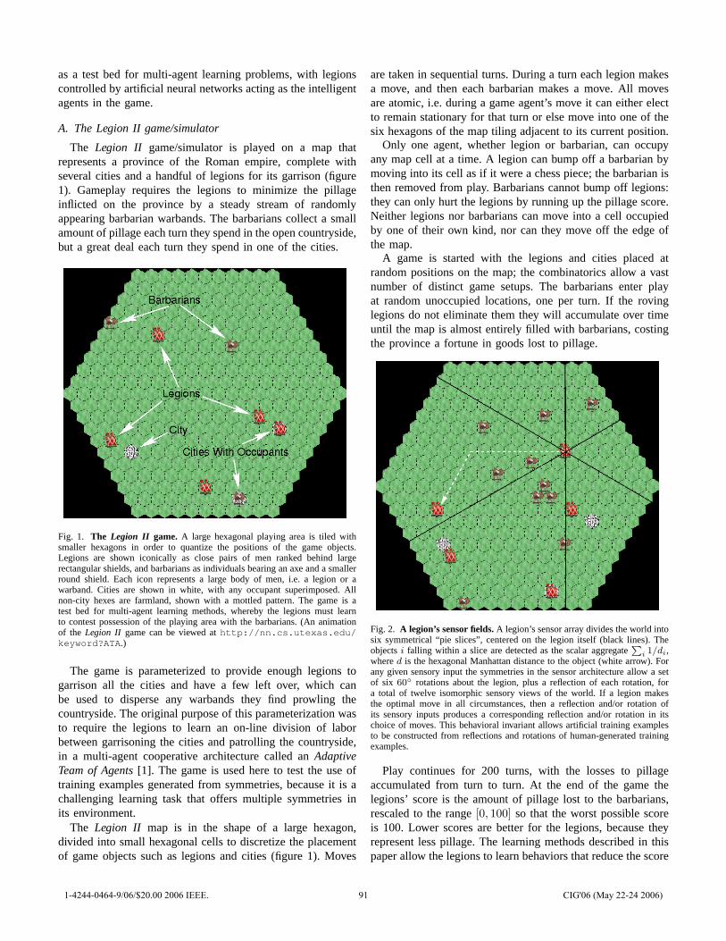
as a test bed for multi-agent learning problems, with legionscontrolled by artificial neural networks acting as the intelligentagents in the game.

A. The Legion II game/simulator

The Legion II game/simulator is played on a map thatrepresents a province of the Roman empire, complete withseveral cities and a handful of legions for its garrison (figure1). Gameplay requires the legions to minimize the pillageinflicted on the province by a steady stream of randomlyappearing barbarian warbands. The barbarians collect a smallamount of pillage each turn they spend in the open countryside,but a great deal each turn they spend in one of the cities.

Fig. 1. The Legion II game. A large hexagonal playing area is tiled withsmaller hexagons in order to quantize the positions of the game objects.Legions are shown iconically as close pairs of men ranked behind largerectangular shields, and barbarians as individuals bearing an axe and a smallerround shield. Each icon represents a large body of men, i.e. a legion or awarband. Cities are shown in white, with any occupant superimposed. Allnon-city hexes are farmland, shown with a mottled pattern. The game is atest bed for multi-agent learning methods, whereby the legions must learnto contest possession of the playing area with the barbarians. (An animationof the Legion II game can be viewed athttp://nn.cs.utexas.edu/keyword?ATA .)

The game is parameterized to provide enough legions togarrison all the cities and have a few left over, which canbe used to disperse any warbands they find prowling thecountryside. The original purpose of this parameterization wasto require the legions to learn an on-line division of laborbetween garrisoning the cities and patrolling the countryside,in a multi-agent cooperative architecture called anAdaptiveTeam of Agents[1]. The game is used here to test the use oftraining examples generated from symmetries, because it is achallenging learning task that offers multiple symmetries inits environment.

The Legion II map is in the shape of a large hexagon,divided into small hexagonal cells to discretize the placementof game objects such as legions and cities (figure 1). Moves

are taken in sequential turns. During a turn each legion makesa move, and then each barbarian makes a move. All movesare atomic, i.e. during a game agent’s move it can either electto remain stationary for that turn or else move into one of thesix hexagons of the map tiling adjacent to its current position.

Only one agent, whether legion or barbarian, can occupyany map cell at a time. A legion can bump off a barbarian bymoving into its cell as if it were a chess piece; the barbarian isthen removed from play. Barbarians cannot bump off legions:they can only hurt the legions by running up the pillage score.Neither legions nor barbarians can move into a cell occupiedby one of their own kind, nor can they move off the edge ofthe map.

A game is started with the legions and cities placed atrandom positions on the map; the combinatorics allow a vastnumber of distinct game setups. The barbarians enter playat random unoccupied locations, one per turn. If the rovinglegions do not eliminate them they will accumulate over timeuntil the map is almost entirely filled with barbarians, costingthe province a fortune in goods lost to pillage.

Fig. 2. A legion’s sensor fields.A legion’s sensor array divides the world intosix symmetrical “pie slices”, centered on the legion itself (black lines). Theobjectsi falling within a slice are detected as the scalar aggregate

Pi 1/di,

whered is the hexagonal Manhattan distance to the object (white arrow). Forany given sensory input the symmetries in the sensor architecture allow a setof six 60◦ rotations about the legion, plus a reflection of each rotation, fora total of twelve isomorphic sensory views of the world. If a legion makesthe optimal move in all circumstances, then a reflection and/or rotation ofits sensory inputs produces a corresponding reflection and/or rotation in itschoice of moves. This behavioral invariant allows artificial training examplesto be constructed from reflections and rotations of human-generated trainingexamples.

Play continues for 200 turns, with the losses to pillageaccumulated from turn to turn. At the end of the game thelegions’ score is the amount of pillage lost to the barbarians,rescaled to the range[0, 100] so that the worst possible scoreis 100. Lower scores are better for the legions, because theyrepresent less pillage. The learning methods described in thispaper allow the legions to learn behaviors that reduce the score

1-4244-0464-9/06/$20.00 2006 IEEE. 91 CIG'06 (May 22-24 2006)

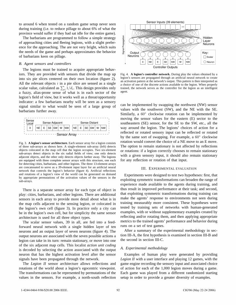
to around 6 when tested on a random game setup never seenduring training (i.e. to reduce pillage to about 6% of what theprovince would suffer if they had sat idle for the entire game).

The barbarians are programmed to follow a simple strategyof approaching cities and fleeing legions, with a slight prefer-ence for the approaching. The are not very bright, which suitsthe needs of the game and perhaps approximates the behaviorof barbarians keen on pillage.

B. Agent sensors and controllers

The legions must be trained to acquire appropriate behav-iors. They are provided with sensors that divide the map upinto six pie slices centered on their own location (figure 2).All the relevant objectsi in a pie slice are sensed as a singlescalar value, calculated as

∑i 1/di. This design provides only

a fuzzy, alias-prone sense of what is in each sector of thelegion’s field of view, but it works well as a threat/opportunityindicator: a few barbarians nearby will be seen as a sensorysignal similar to what would be seen of a large group ofbarbarians further away.

NE E NWSE SW W NE E NWSE SW WX

Sense Adjacent Sense DistantLocalSense

Sensor Array

Fig. 3. A legion’s sensor architecture.Each sensor array for a legion consistsof three sub-arrays as shown here. A single-element sub-array (left) detectsobjects colocated in the map cell that the legion occupies. Two six-elementsub-arrays detect objects in the six radial fields of view; one only detectsadjacent objects, and the other only detects objects farther away. The legionsare equipped with three complete sensor arrays with this structure, one eachfor detecting cities, barbarians, and other legions. The three 13-element arraysare concatenated to serve as a 39-element input layer for an artificial neuralnetwork that controls the legion’s behavior (figure 4). Artificial reflectionsand rotations of a legion’s view of the world can be generated on demandby appropriate permutations of the activation values of the sensors in thesub-arrays.

There is a separate sensor array for each type of object inplay: cities, barbarians, and other legions. There are additionalsensors in each array to provide more detail about what is inthe map cells adjacent to the sensing legion, or colocated inthe legion’s own cell (figure 3). In practice only a city canbe in the legion’s own cell, but for simplicity the same sensorarchitecture is used for all three object types.

The scalar sensor values, 39 in all, are fed into a feed-forward neural network with a single hidden layer of tenneurons and an output layer of seven neurons (figure 4). Theoutput neurons are associated with the seven possible actions alegion can take in its turn: remain stationary, or move into oneof the six adjacent map cells. This localistaction unit codingis decoded by selecting the action associated with the outputneuron that has the highest activation level after the sensorsignals have been propagated through the network.

The Legion II sensor architecture allows reflections androtations of the world about a legion’s egocentric viewpoint.The transformations can be represented by permutations of thevalues in the sensors. For example, a north-south reflection

X NE E SE SW W NW

HiddenLayerNeurons

Key:

Neuron

Scalar

Sig

nal P

ropa

gatio

n

OutputNeurons

Controller Outputs

Sensor Inputs (39 elements)...

Fig. 4. A legion’s controller network. During play the values obtained by alegion’s sensors are propagated through an artificial neural network to createan activation pattern at the network’s output. This pattern is then interpreted asa choice of one of the discrete actions available to the legion. When properlytrained, the network serves as the controller for the legion as an intelligentagent.

can be implemented by swapping the northwest (NW) sensorvalues with the southwest (SW), and the NE with the SE.Similarly, a 60◦ clockwise rotation can be implemented bymoving the sensor values for the eastern (E) sector to thesoutheastern (SE) sensor, for the SE to the SW, etc., all theway around the legion. The legions’ choices of action for areflected or rotated sensory input can be reflected or rotatedby the same sort of swapping. For example, a60◦ clockwiserotation would convert the choice of a NE move to an E move.The option to remain stationary is not affected by reflectionsor rotations: if a legion correctly chooses to remain stationarywith a given sensory input, it should also remain stationaryfor any reflection or rotation of that input.

III. E XPERIMENTAL EVALUATION

Experiments were designed to test two hypotheses: first, thatexploiting symmetric transformations can broaden the range ofexperience made available to the agents during training, andthus result in improved performance at their task; and second,that exploiting symmetric transformations during training canmake the agents’ response to environments not seen duringtraining measurably more consistent. These hypotheses weretested by training sets of networks with human-generatedexamples, with or without supplementary examples created byreflecting and/or rotating them, and then applying appropriatemetrics to the trained agents’ performance and behavior duringruns on a set of test games.

After a summary of the experimental methodology in sec-tion III-A, the first hypothesis is examined in section III-B andthe second in section III-C.

A. Experimental methodology

Examples of human play were generated by providingLegion II with a user interface and playing 12 games, with thegame engine recording the sensory input and associated choiceof action for each of the 1,000 legion moves during a game.Each game was played from a different randomized startingsetup in order to provide a greater diversity of examples.

1-4244-0464-9/06/$20.00 2006 IEEE. 92 CIG'06 (May 22-24 2006)

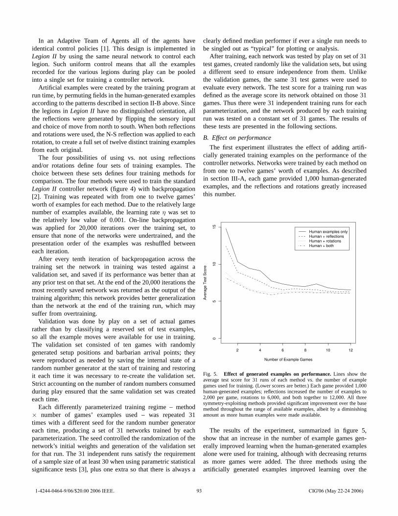
In an Adaptive Team of Agents all of the agents haveidentical control policies [1]. This design is implemented inLegion II by using the same neural network to control eachlegion. Such uniform control means that all the examplesrecorded for the various legions during play can be pooledinto a single set for training a controller network.

Artificial examples were created by the training program atrun time, by permuting fields in the human-generated examplesaccording to the patterns described in section II-B above. Sincethe legions inLegion II have no distinguished orientation, allthe reflections were generated by flipping the sensory inputand choice of move from north to south. When both reflectionsand rotations were used, the N-S reflection was applied to eachrotation, to create a full set of twelve distinct training examplesfrom each original.

The four possibilities of using vs. not using reflectionsand/or rotations define four sets of training examples. Thechoice between these sets defines four training methods forcomparison. The four methods were used to train the standardLegion II controller network (figure 4) with backpropagation[2]. Training was repeated with from one to twelve games’worth of examples for each method. Due to the relatively largenumber of examples available, the learning rateη was set tothe relatively low value of 0.001. On-line backpropagationwas applied for 20,000 iterations over the training set, toensure that none of the networks were undertrained, and thepresentation order of the examples was reshuffled betweeneach iteration.

After every tenth iteration of backpropagation across thetraining set the network in training was tested against avalidation set, and saved if its performance was better than atany prior test on that set. At the end of the 20,000 iterations themost recently saved network was returned as the output of thetraining algorithm; this network provides better generalizationthan the network at the end of the training run, which maysuffer from overtraining.

Validation was done by play on a set of actual gamesrather than by classifying a reserved set of test examples,so all the example moves were available for use in training.The validation set consisted of ten games with randomlygenerated setup positions and barbarian arrival points; theywere reproduced as needed by saving the internal state of arandom number generator at the start of training and restoringit each time it was necessary to re-create the validation set.Strict accounting on the number of random numbers consumedduring play ensured that the same validation set was createdeach time.

Each differently parameterized training regime – method× number of games’ examples used – was repeated 31times with a different seed for the random number generatoreach time, producing a set of 31 networks trained by eachparameterization. The seed controlled the randomization of thenetwork’s initial weights and generation of the validation setfor that run. The 31 independent runs satisfy the requirementof a sample size of at least 30 when using parametric statisticalsignificance tests [3], plus one extra so that there is always a

clearly defined median performer if ever a single run needs tobe singled out as “typical” for plotting or analysis.

After training, each network was tested by play on set of 31test games, created randomly like the validation sets, but usinga different seed to ensure independence from them. Unlikethe validation games, the same 31 test games were used toevaluate every network. The test score for a training run wasdefined as the average score its network obtained on those 31games. Thus there were 31 independent training runs for eachparameterization, and the network produced by each trainingrun was tested on a constant set of 31 games. The results ofthese tests are presented in the following sections.

B. Effect on performance

The first experiment illustrates the effect of adding artifi-cially generated training examples on the performance of thecontroller networks. Networks were trained by each method onfrom one to twelve games’ worth of examples. As describedin section III-A, each game provided 1,000 human-generatedexamples, and the reflections and rotations greatly increasedthis number.

2 4 6 8 10 12

05

1015

Number of Example Games

Ave

rage

Tes

t Sco

re

Human examples onlyHuman + reflectionsHuman + rotationsHuman + both

Fig. 5. Effect of generated examples on performance.Lines show theaverage test score for 31 runs of each method vs. the number of examplegames used for training. (Lower scores are better.) Each game provided 1,000human-generated examples; reflections increased the number of examples to2,000 per game, rotations to 6,000, and both together to 12,000. All threesymmetry-exploiting methods provided significant improvement over the basemethod throughout the range of available examples, albeit by a diminishingamount as more human examples were made available.

The results of the experiment, summarized in figure 5,show that an increase in the number of example games gen-erally improved learning when the human-generated examplesalone were used for training, although with decreasing returnsas more games were added. The three methods using theartificially generated examples improved learning over the

1-4244-0464-9/06/$20.00 2006 IEEE. 93 CIG'06 (May 22-24 2006)

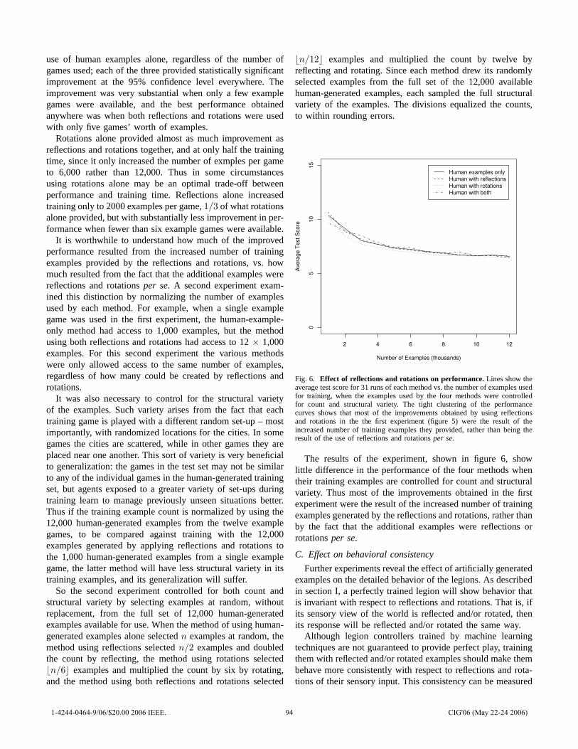
use of human examples alone, regardless of the number ofgames used; each of the three provided statistically significantimprovement at the 95% confidence level everywhere. Theimprovement was very substantial when only a few examplegames were available, and the best performance obtainedanywhere was when both reflections and rotations were usedwith only five games’ worth of examples.

Rotations alone provided almost as much improvement asreflections and rotations together, and at only half the trainingtime, since it only increased the number of exmples per gameto 6,000 rather than 12,000. Thus in some circumstancesusing rotations alone may be an optimal trade-off betweenperformance and training time. Reflections alone increasedtraining only to 2000 examples per game,1/3 of what rotationsalone provided, but with substantially less improvement in per-formance when fewer than six example games were available.

It is worthwhile to understand how much of the improvedperformance resulted from the increased number of trainingexamples provided by the reflections and rotations, vs. howmuch resulted from the fact that the additional examples werereflections and rotationsper se. A second experiment exam-ined this distinction by normalizing the number of examplesused by each method. For example, when a single examplegame was used in the first experiment, the human-example-only method had access to 1,000 examples, but the methodusing both reflections and rotations had access to 12× 1,000examples. For this second experiment the various methodswere only allowed access to the same number of examples,regardless of how many could be created by reflections androtations.

It was also necessary to control for the structural varietyof the examples. Such variety arises from the fact that eachtraining game is played with a different random set-up – mostimportantly, with randomized locations for the cities. In somegames the cities are scattered, while in other games they areplaced near one another. This sort of variety is very beneficialto generalization: the games in the test set may not be similarto any of the individual games in the human-generated trainingset, but agents exposed to a greater variety of set-ups duringtraining learn to manage previously unseen situations better.Thus if the training example count is normalized by using the12,000 human-generated examples from the twelve examplegames, to be compared against training with the 12,000examples generated by applying reflections and rotations tothe 1,000 human-generated examples from a single examplegame, the latter method will have less structural variety in itstraining examples, and its generalization will suffer.

So the second experiment controlled for both count andstructural variety by selecting examples at random, withoutreplacement, from the full set of 12,000 human-generatedexamples available for use. When the method of using human-generated examples alone selectedn examples at random, themethod using reflections selectedn/2 examples and doubledthe count by reflecting, the method using rotations selectedbn/6c examples and multiplied the count by six by rotating,and the method using both reflections and rotations selected

bn/12c examples and multiplied the count by twelve byreflecting and rotating. Since each method drew its randomlyselected examples from the full set of the 12,000 availablehuman-generated examples, each sampled the full structuralvariety of the examples. The divisions equalized the counts,to within rounding errors.

2 4 6 8 10 12

05

1015

Number of Examples (thousands)

Ave

rage

Tes

t Sco

re

Human examples onlyHuman with reflectionsHuman with rotationsHuman with both

Fig. 6. Effect of reflections and rotations on performance.Lines show theaverage test score for 31 runs of each method vs. the number of examples usedfor training, when the examples used by the four methods were controlledfor count and structural variety. The tight clustering of the performancecurves shows that most of the improvements obtained by using reflectionsand rotations in the the first experiment (figure 5) were the result of theincreased number of training examples they provided, rather than being theresult of the use of reflections and rotationsper se.

The results of the experiment, shown in figure 6, showlittle difference in the performance of the four methods whentheir training examples are controlled for count and structuralvariety. Thus most of the improvements obtained in the firstexperiment were the result of the increased number of trainingexamples generated by the reflections and rotations, rather thanby the fact that the additional examples were reflections orrotationsper se.

C. Effect on behavioral consistency

Further experiments reveal the effect of artificially generatedexamples on the detailed behavior of the legions. As describedin section I, a perfectly trained legion will show behavior thatis invariant with respect to reflections and rotations. That is, ifits sensory view of the world is reflected and/or rotated, thenits response will be reflected and/or rotated the same way.

Although legion controllers trained by machine learningtechniques are not guaranteed to provide perfect play, trainingthem with reflected and/or rotated examples should make thembehave more consistently with respect to reflections and rota-tions of their sensory input. This consistency can be measured

1-4244-0464-9/06/$20.00 2006 IEEE. 94 CIG'06 (May 22-24 2006)

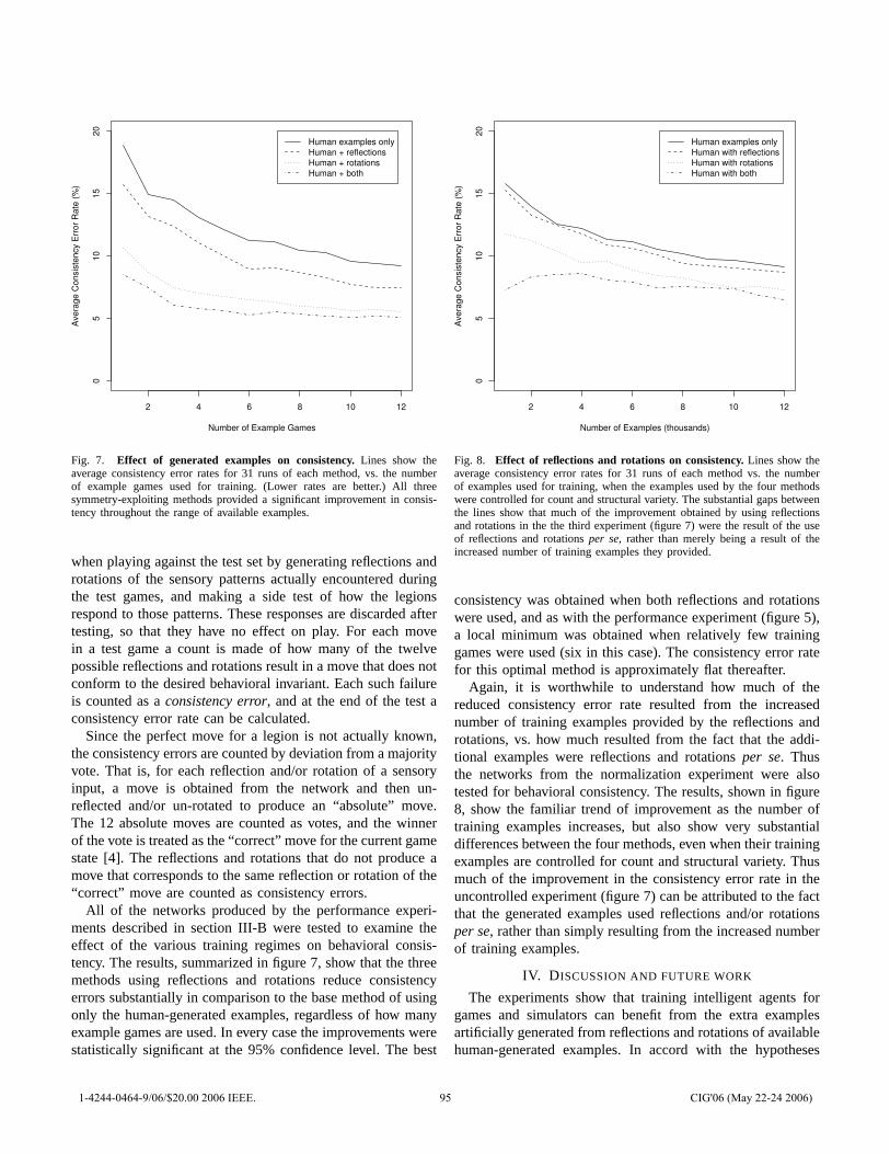
2 4 6 8 10 12

05

1015

20

Number of Example Games

Ave

rage

Con

sist

ency

Err

or R

ate

(%)

Human examples onlyHuman + reflectionsHuman + rotationsHuman + both

Fig. 7. Effect of generated examples on consistency.Lines show theaverage consistency error rates for 31 runs of each method, vs. the numberof example games used for training. (Lower rates are better.) All threesymmetry-exploiting methods provided a significant improvement in consis-tency throughout the range of available examples.

when playing against the test set by generating reflections androtations of the sensory patterns actually encountered duringthe test games, and making a side test of how the legionsrespond to those patterns. These responses are discarded aftertesting, so that they have no effect on play. For each movein a test game a count is made of how many of the twelvepossible reflections and rotations result in a move that does notconform to the desired behavioral invariant. Each such failureis counted as aconsistency error, and at the end of the test aconsistency error rate can be calculated.

Since the perfect move for a legion is not actually known,the consistency errors are counted by deviation from a majorityvote. That is, for each reflection and/or rotation of a sensoryinput, a move is obtained from the network and then un-reflected and/or un-rotated to produce an “absolute” move.The 12 absolute moves are counted as votes, and the winnerof the vote is treated as the “correct” move for the current gamestate [4]. The reflections and rotations that do not produce amove that corresponds to the same reflection or rotation of the“correct” move are counted as consistency errors.

All of the networks produced by the performance experi-ments described in section III-B were tested to examine theeffect of the various training regimes on behavioral consis-tency. The results, summarized in figure 7, show that the threemethods using reflections and rotations reduce consistencyerrors substantially in comparison to the base method of usingonly the human-generated examples, regardless of how manyexample games are used. In every case the improvements werestatistically significant at the 95% confidence level. The best

2 4 6 8 10 12

05

1015

20

Number of Examples (thousands)

Ave

rage

Con

sist

ency

Err

or R

ate

(%)

Human examples onlyHuman with reflectionsHuman with rotationsHuman with both

Fig. 8. Effect of reflections and rotations on consistency.Lines show theaverage consistency error rates for 31 runs of each method vs. the numberof examples used for training, when the examples used by the four methodswere controlled for count and structural variety. The substantial gaps betweenthe lines show that much of the improvement obtained by using reflectionsand rotations in the the third experiment (figure 7) were the result of the useof reflections and rotationsper se, rather than merely being a result of theincreased number of training examples they provided.

consistency was obtained when both reflections and rotationswere used, and as with the performance experiment (figure 5),a local minimum was obtained when relatively few traininggames were used (six in this case). The consistency error ratefor this optimal method is approximately flat thereafter.

Again, it is worthwhile to understand how much of thereduced consistency error rate resulted from the increasednumber of training examples provided by the reflections androtations, vs. how much resulted from the fact that the addi-tional examples were reflections and rotationsper se. Thusthe networks from the normalization experiment were alsotested for behavioral consistency. The results, shown in figure8, show the familiar trend of improvement as the number oftraining examples increases, but also show very substantialdifferences between the four methods, even when their trainingexamples are controlled for count and structural variety. Thusmuch of the improvement in the consistency error rate in theuncontrolled experiment (figure 7) can be attributed to the factthat the generated examples used reflections and/or rotationsper se, rather than simply resulting from the increased numberof training examples.

IV. D ISCUSSION AND FUTURE WORK

The experiments show that training intelligent agents forgames and simulators can benefit from the extra examplesartificially generated from reflections and rotations of availablehuman-generated examples. In accord with the hypotheses

1-4244-0464-9/06/$20.00 2006 IEEE. 95 CIG'06 (May 22-24 2006)

stated in section III, the technique results in agents that scorebetter in the game and behave more consistently.

The improved performance scores were shown to resultprimarily from the increased number of training examplesprovided by the reflections and rotations, but the improvedbehavioral consistency resulted largely from the fact that thoseexamples were reflections and rotationsper se. In principle,reflections and rotationsper se could improve performancescores as well, by providing a more systematic coverage of theinput space. However, inLegion II, the base method alreadyprovided over 80% consistency with respect to reflections androtations when only a single game’s examples were used fortraining (figure 7). The agents quickly learned the symmetriesnecessary for the situations that had the most impact on theirgame scores. Further improvements in behavioral consistencyprovided polish, but had no substantial impact on the scores. Inother domains the base coverage may be more idiosyncratic,so that reflections and rotationsper se would significantlyimprove performance.

The combination of both reflections and rotations providedthe best results throughout. That method provided the best per-formance and consistency when relatively few example gameswere made available for training, five and six games respec-tively. This is a very promising result, because it suggests thatgood training can be obtained without excessive human effortat generating examples. Rapid learning from relatively fewexamples will be important for training agents in a MachineLearning Game [5], where a player trains game agents byexample at run time, and for simulations where agents mustbe re-trained to adapt to changed environments, doctrines, oropponent strategies. Future work will thus investigate whetherrapid learning from relatively few examples is seen in otherapplications, and also whether a greatly increased number ofhuman-generated examples will ever converge to the sameoptimum.

The number of examples that can be generated from sym-metries depends critically on the sensor geometry of the agentbeing trained. The number of radial sensors may vary with theapplication and implementation, providing a greater or lessernumber of rotations. However, if radial sensors do not allencompass equal arcs then rotations may not be possible atall. For example, the agents in the NERO video game [5] alsouse “pie slice” sensors, but with narrower arcs to the frontthan to the rear, in order to improve their frontal resolution.There is therefore no suitable invariant for the rotation of theNERO agents’ sensors.

However, the NERO agents, and probably most mechanicalrobots as well, have a bilateral symmetry that allows applyingthe behavioral invariant for reflections across their longitudinalaxis. The results presented in this paper show that artificiallygenerated examples provide significant training benefits evenwhen only reflections are used, especially when relatively fewhuman-generated examples are available (figures 5 and 7).Thus the methods examined here should prove useful evenin situations with far more restrictive symmetries than inthe Legion II game. On the other hand, agents operating in

three-dimensional environments, such as under water or inouter space, may have a greater number of symmetries to beexploited, offering even greater advantage for these methods.Future work will also investigate the effect of exploitingsymmetries in boardgames with symmetrical boards, suchas Go, where an external player-agent manipulates passiveplaying pieces on the board.

Supervised learning is not always the best way to trainagents for environments such asLegion II. Work in progressshows that training with neuroevolution ([6], [7], [8], [5]),using on-line gameplay for fitness evaluations, can producecontroller networks that perform somewhat better than thoseproduced by backpropagation in the experiments reported here.However, evolutionary results can sometimes be improvedby combining evolution with supervised learning. Thus anobvious avenue of future work is to use examples artificiallygenerated from sensor symmetries with methods such asBaldwinian or Lamarckian evolution ([9], [10]) in order toimprove performance and behavioral consistency, the waythey benefited ordinary backpropagation in the experimentsreported in this paper.

V. CONCLUSIONS

Intelligent agents with sense-response controllers often havesymmetries in their sensor architecture, and it is then possibleto define behavioral invariants that would be observed acrossthose symmetries by perfectly trained agents. This observa-tion suggests that symmetrical invariants of sense-responsebehavior can be exploited for training the agents, makingtheir responses more symmetrical and effective. This papershows that both types of improvement are obtained in a game-like test environment, and suggests that further attempts toexploit sensor symmetries may provide similar benefits inother environments and with other learning methods.

ACKNOWLEDGMENTS

This research was supported in part by the Digital MediaCollaboratory at the IC2 Institute at the University of Texasat Austin. The images used inLegion II’s animated displayare derived from graphics supplied with the gameFreeciv,http://www.freeciv.org/ .

REFERENCES

[1] B. D. Bryant and R. Miikkulainen, “Neuroevolution for adaptive teams,”in Proceeedings of the 2003 Congress on Evolutionary Computation(CEC 2003), vol. 3. Piscataway, NJ: IEEE, 2003, pp. 2194–2201.[Online]. Available: http://nn.cs.utexas.edu/keyword?bryant:cec03

[2] D. E. Rumelhart, G. E. Hinton, and R. J. Williams, “Learning in-ternal representations by error propagation,” inParallel DistributedProcessing: Explorations in the Microstructure of Cognition, Volume 1:Foundations, D. E. Rumelhart and J. L. McClelland, Eds. Cambridge,MA: MIT Press, 1986, pp. 318–362.

[3] R. R. Pagano,Understanding Statistics in the Behavioral Sciences,2nd ed. St. Paul, MN: West Publishing, 1986.

[4] B. D. Bryant, “Virtual bagging for an evolved agent controller,” 2006,manuscript in preparation.

[5] K. O. Stanley, B. D. Bryant, and R. Miikkulainen, “Real-timeneuroevolution in the NERO video game,”IEEE Transactions onEvolutionary Computation Special Issue on Evolutionary Computationand Games, vol. 9, no. 6, pp. 653–668, 2005. [Online]. Available:http://nn.cs.utexas.edu/keyword?stanley:ieeetec05

1-4244-0464-9/06/$20.00 2006 IEEE. 96 CIG'06 (May 22-24 2006)

[6] J. Branke, “Evolutionary algorithms for neural network designand training,” in Proceedings 1st Nordic Workshop on GeneticAlgorithms and Its Applications, J. T. Alander, Ed. Vaasa, Finland:University of Vaasa Press, 1995, pp. 145 – 163. [Online]. Available:http://citeseer.nj.nec.com/branke95evolutionary.html

[7] X. Yao, “Evolving artificial neural networks,”Proceedings of theIEEE, vol. 87, no. 9, pp. 1423–1447, 1999. [Online]. Available:ftp://www.cs.adfa.edu.au/pub/xin/yaoie3proconline.ps.gz

[8] F. Gomez, “Learning robust nonlinear control with neuroevolution,”Ph.D. dissertation, Department of Computer Sciences, The University

of Texas at Austin, 2003. [Online]. Available: http://nn.cs.utexas.edu/keyword?gomez:phd03

[9] R. K. Belew and M. Mitchell, Eds., Adaptive Individuals inEvolving Populations: Models and Algorithms. Reading, MA:Addison-Wesley, 1996. [Online]. Available: http://www.santafe.edu/sfi/publications/Bookinforev/ipep.html

[10] D. Whitley, V. S. Gordon, and K. Mathias, “Lamarckian evolution,the Baldwin effect and function optimization,” inProceedings of theInternational Conference on Evolutionary Computation, Y. Davidor, H.-P. Schwefel, and R. Maenner, Eds., vol. 866, Jerusalem, Israel, October1994.

1-4244-0464-9/06/$20.00 2006 IEEE. 97 CIG'06 (May 22-24 2006)

Using Wearable Sensors for Real-Time Recognition Tasks

in Games of Martial Arts – An Initial Experiment

Ernst A. Heinz, Kai S. Kunze, Matthias Gruber, David Bannach, Paul Lukowicz

Institute for Computer Systems and Networks (CSN)UMIT – University of Health Systems, Medical Informatics and Technology

Hall in Tyrol, =Austria=

{ernst.heinz, kai.kunze, matthias.gruber, david.bannach, paul.lukowicz}@ umit.at, URL = http://csn.umit.at/

Abstract— Beside their stunning graphics, modern entertain-ment systems feature ever-higher levels of immersive user-interaction. Today, this is mostly achieved by virtual (VR) andaugmented reality (AR) setups. On top of these, we envisionto add ambient intelligence and context awareness to gamingapplications in general and games of martial arts in particular.To this end, we conducted an initial experiment with inexpensivebody-worn gyroscopes and acceleration sensors for the ChumKiu motion sequence in Wing Tsun (a popular form of KungFu). The resulting data confirm the feasibility of our vision.Fine-tuned adaptations of various thresholding and pattern-matching techniques known from the fields of computationalintelligence and signal processing should suffice to automate theanalysis and recognition of important Wing Tsun movementsin real time. Moreover, the data also seem to allow for thepossibility of automatically distinguishing between certain levelsof expertise and quality in executing the movements.

Keywords: Body-worn Sensors, Experiment, Games ofMartial Arts, Kung Fu, Motion Analysis, Movement Recog-nition, Wearable Computing, Wing Tsun

I. INTRODUCTION

Video analysis and motion capturing are standard tools inprofessional sports to monitor and improve athletic perfor-mance by recognizing and fine-tuning the quality of move-ment. Cutting-edge systems with high-quality sensors hardlysuffice to fulfill these professionals’ needs. Quite often,trainers and other experts still process the recorded data byhand. The whole setup and procedure are not only expensiveand time-consuming but also error-prone in the sense that theeffectiveness of the analysis depends on the humans doing it.Hence, the large-scale use of similar analyses for the hobbyistand gaming masses requires a completely different approach.In particular, as we like to increase the immersiveness of theuser experience and interaction in video games of martialarts where people’s real-world physical actions directly needto directly affect their playing reality.

We envision to employ inexpensive wearable sensors toachieve this – preferably tiny gyroscopes and accelerometersworn by people on their bodies integrated into their clothesand other personal accessories (e.g., watches or jewelery).Such body-mounted sensors provide an inexpensive alterna-tive for motion analysis while letting users move and roamabout freely, independent of any additional infrastructure.Whether our envisioned applications will actually becomereal depends on the ability of data processing algorithms to

compensate for various inaccuracies inherent in inexpensivewearable sensor system. The inaccuracies result from thelimited resolution and sampling rate of the sensors, variationsin sensor placement, dynamic sensor displacement duringuser motion, and other sources of noise (e.g., environmentalmagnetic fields or temperature-related sensor drift). Thechallenge in algorithmic design is to find features that aresensitive to the relevant motion characteristics and at thesame time insensitive to the inaccuracies mentioned before.

As decribed in Section III, we conducted an initial exper-iment capturing Wing Tsun movements with wearable gyro-scopes and acceleration sensors to test the feasibility of ourvision. Section IV discusses and analyzes the experimentalresults, proving to be very promising indeed. Based thereon,it certainly seems worthwhile to continue in this directionand try to automate at least some parts (if not all) of anexpert analysis for many important Wing Tsun movements.

Beside in sports and game play, martial arts from theFar East gain ever more popularity and importance in manyother areas as well. Tai Chi, for instance, is of specialinterest because clinical studies show that it helps to reducethe probability of falling, especially for the elderly [1] andpatients with chronic conditions [2].

II. RELATED WORK

By now, many independent researchers have demonstratedthe suitability and excellent further potential of body-wornsensors for automatic context and activity recognition, e.g.,[3], [4], [5], [6], [7], [8], [9], [11]. The available scientificliterature reports about successful applications of such sen-sors to various types of activities, ranging from the analysisof simple modes of locomotion [5] to more complex tasksof everyday life [4] and even workshop assembly [10].

There are much fewer publications, however, about usingwearable sensors in martial arts. In [12], wearable pressuresensors integrated into body protectors help to control and de-cide the counting of points for Taekwando. Supposedly help-ing children with their Kung Fu education, [13] introducessome kind of interactive computerized toy ball. Focusing onKung Fu, [14] presents a video capturing system for artificialand augmented reality games of martial arts. The workemphasizes the specific gaming aspects of the application andsuffers from the usual drawbacks of video-based approaches,

1-4244-0464-9/06/$20.00 2006 IEEE. 98 CIG'06 (May 22-24 2006)

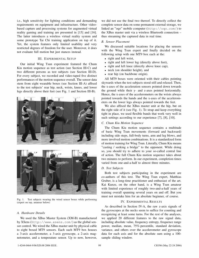
i.e., high sensitivity for lighting conditions and demandingrequirements on equipment and infrastructure. Other video-based capture and processing systems for augmented virtualreality gaming and training are presented in [15] and [16].The latter introduces a wireless virtual reality system andsome prototype Tai Chi training application on top of it.Yet, the system features only limited usability and veryrestricted degrees of freedom for the user. Moreover, it doesnot evaluate full motion but just stances instead.

III. EXPERIMENTAL SETUP

Our initial Wing Tsun experiment featured the ChumKiu motion sequence as test action (see Section III-C) andtwo different persons as test subjects (see Section III-D).For every subject, we recorded and video-taped five distinctperformances of the motion sequence overall. The sensor datastem from eight wearable boxes (see Section III-A) affixedto the test subjects’ rear hip, neck, wrists, knees, and lowerlegs directly above their feet (see Fig. 1 and Section III-B).

Fig. 1. Test subjects wearing the wired sensor boxes while performing(expert on top, amateur below)

A. Hardware Details

We used the XBus Master System (XM-B) manufacturedby XSens (http://www.xsens.com/) as the global sen-sor control. We wired the XBus master unit by physical cableto eight boxed MT9 sensors. Each such MT9 box housesa 3-axis accelerometer, a 3-axis gyroscope, a 2-axis mag-netometer, and a temperature sensor. Up to now, however,

we did not use the final two thereof. To directly collect thecomplete sensor data on some permanent external storage, welinked an ”oqo” mobile computer (http://oqo.com/) tothe XBus master unit via a wireless Bluetooth connection –thus streaming the captured data in real time.

B. Sensor PlacementWe discussed suitable locations for placing the sensors

with the Wing Tsun expert and finally decided on thefollowing setup with one MT9 box each at the:

• right and left wrist,• right and left lower leg (directly above feet),• right and left knee (directly above knee cap),• neck (on shoulder height), and• rear hip (on backbone origin).All MT9 boxes were oriented with their cables pointing

skywards when the test subjects stood still and relaxed. Then,the x-axes of the acceleration sensors pointed down towardsthe ground while their y- and z-axes pointed horizontally.Hence, the x-axes of the accelerometers on the wrists alwayspointed towards the hands and the x-axes of the accelerom-eters on the lower legs always pointed towards the feet.

We also affixed the XBus master unit at the hip, but onthe right side of it (see Fig. 1). To strap and keep everythingtight in place, we used flexible bands that work very well insuch settings according to our experience [7], [8], [10].

C. Chum Kiu Motion SequenceThe Chum Kiu motion sequence contains a multitude

of basic Wing Tsun movements (forward and backward)including side steps, full-body turns, arm and leg blows, andmore involved motion combinations. It is a standardized formof motion training for Wing Tsun. Literally, Chum Kiu means”casting / seeking a bridge” to the opponent. While doingso, you should try to adhere to your so-called central lineof action. The full Chum Kiu motion sequence takes abouttwo minutes to perform. In our experiment, completion timesvaried from one-and-a-half to almost three minutes.

D. Test SubjectsBoth test subjects participating in the experiment are

co-authors of this text. The Wing Tsun expert, MatthiasGruber, is a long-time practitioner and enthusiast of the art.Kai Kunze, on the other hand, is a Wing Tsun amateurwith limited experience of roughly two-and-a-half years oftraining overall spanning several years on and off. But youmust not mistake him for an absolute beginner, of course.

IV. EXPERIMENTAL RESULTS

As described in Section IV-A, the raw z-axis signals ofthe gyroscopes at the necks seem to suffice for counting andrecognizing at least some turns. For the rest of the analyses,we applied 20 different features to the raw signal data,including absolute value, frequency entropy, frequence rangepower, median, mean, 75%-percentile, standard deviation,variance, and others over the accelerometer and gyroscopedata for each axis and for the absolute sum using a 100-sample sliding window.

1-4244-0464-9/06/$20.00 2006 IEEE. 99 CIG'06 (May 22-24 2006)

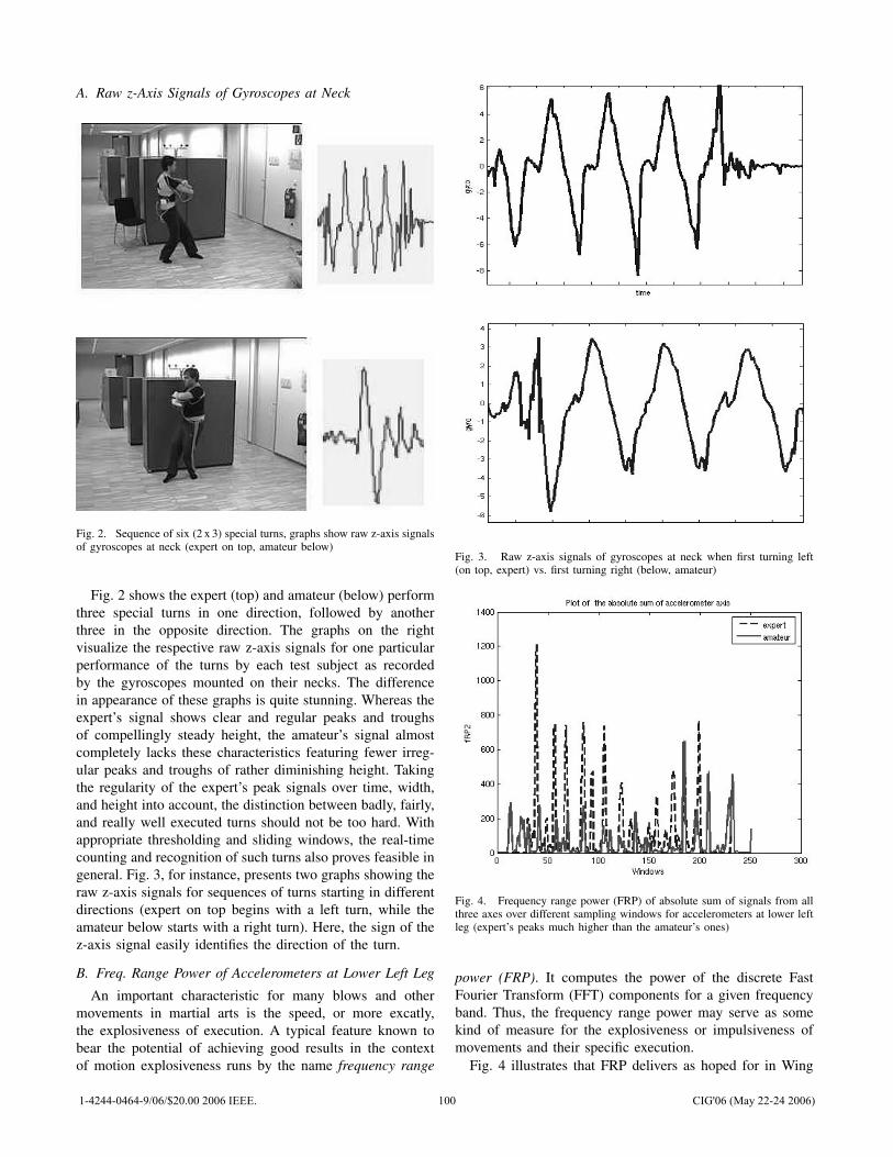
A. Raw z-Axis Signals of Gyroscopes at Neck

Fig. 2. Sequence of six (2 x 3) special turns, graphs show raw z-axis signalsof gyroscopes at neck (expert on top, amateur below)

Fig. 2 shows the expert (top) and amateur (below) performthree special turns in one direction, followed by anotherthree in the opposite direction. The graphs on the rightvisualize the respective raw z-axis signals for one particularperformance of the turns by each test subject as recordedby the gyroscopes mounted on their necks. The differencein appearance of these graphs is quite stunning. Whereas theexpert’s signal shows clear and regular peaks and troughsof compellingly steady height, the amateur’s signal almostcompletely lacks these characteristics featuring fewer irreg-ular peaks and troughs of rather diminishing height. Takingthe regularity of the expert’s peak signals over time, width,and height into account, the distinction between badly, fairly,and really well executed turns should not be too hard. Withappropriate thresholding and sliding windows, the real-timecounting and recognition of such turns also proves feasible ingeneral. Fig. 3, for instance, presents two graphs showing theraw z-axis signals for sequences of turns starting in differentdirections (expert on top begins with a left turn, while theamateur below starts with a right turn). Here, the sign of thez-axis signal easily identifies the direction of the turn.

B. Freq. Range Power of Accelerometers at Lower Left Leg

An important characteristic for many blows and othermovements in martial arts is the speed, or more excatly,the explosiveness of execution. A typical feature known tobear the potential of achieving good results in the contextof motion explosiveness runs by the name frequency range

Fig. 3. Raw z-axis signals of gyroscopes at neck when first turning left(on top, expert) vs. first turning right (below, amateur)

Fig. 4. Frequency range power (FRP) of absolute sum of signals from allthree axes over different sampling windows for accelerometers at lower leftleg (expert’s peaks much higher than the amateur’s ones)

power (FRP). It computes the power of the discrete FastFourier Transform (FFT) components for a given frequencyband. Thus, the frequency range power may serve as somekind of measure for the explosiveness or impulsiveness ofmovements and their specific execution.

Fig. 4 illustrates that FRP delivers as hoped for in Wing

1-4244-0464-9/06/$20.00 2006 IEEE. 100 CIG'06 (May 22-24 2006)

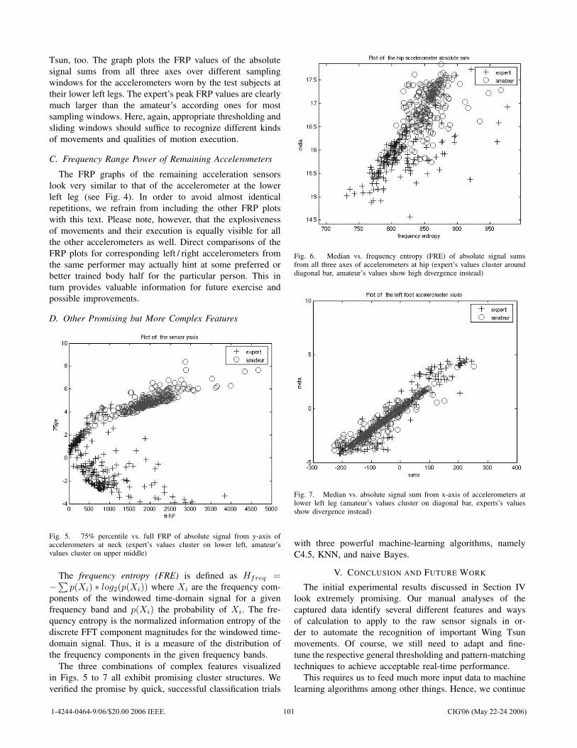
Tsun, too. The graph plots the FRP values of the absolutesignal sums from all three axes over different samplingwindows for the accelerometers worn by the test subjects attheir lower left legs. The expert’s peak FRP values are clearlymuch larger than the amateur’s according ones for mostsampling windows. Here, again, appropriate thresholding andsliding windows should suffice to recognize different kindsof movements and qualities of motion execution.

C. Frequency Range Power of Remaining Accelerometers

The FRP graphs of the remaining acceleration sensorslook very similar to that of the accelerometer at the lowerleft leg (see Fig. 4). In order to avoid almost identicalrepetitions, we refrain from including the other FRP plotswith this text. Please note, however, that the explosivenessof movements and their execution is equally visible for allthe other accelerometers as well. Direct comparisons of theFRP plots for corresponding left / right accelerometers fromthe same performer may actually hint at some preferred orbetter trained body half for the particular person. This inturn provides valuable information for future exercise andpossible improvements.

D. Other Promising but More Complex Features

Fig. 5. 75% percentile vs. full FRP of absolute signal from y-axis ofaccelerometers at neck (expert’s values cluster on lower left, amateur’svalues cluster on upper middle)

The frequency entropy (FRE) is defined as Hfreq =−

∑p(Xi) ∗ log2(p(Xi)) where Xi are the frequency com-

ponents of the windowed time-domain signal for a givenfrequency band and p(Xi) the probability of Xi. The fre-quency entropy is the normalized information entropy of thediscrete FFT component magnitudes for the windowed time-domain signal. Thus, it is a measure of the distribution ofthe frequency components in the given frequency bands.

The three combinations of complex features visualizedin Figs. 5 to 7 all exhibit promising cluster structures. Weverified the promise by quick, successful classification trials

Fig. 6. Median vs. frequency entropy (FRE) of absolute signal sumsfrom all three axes of accelerometers at hip (expert’s values cluster arounddiagonal bar, amateur’s values show high divergence instead)

Fig. 7. Median vs. absolute signal sum from x-axis of accelerometers atlower left leg (amateur’s values cluster on diagonal bar, experts’s valuesshow divergence instead)

with three powerful machine-learning algorithms, namelyC4.5, KNN, and naive Bayes.

V. CONCLUSION AND FUTURE WORK

The initial experimental results discussed in Section IVlook extremely promising. Our manual analyses of thecaptured data identify several different features and waysof calculation to apply to the raw sensor signals in or-der to automate the recognition of important Wing Tsunmovements. Of course, we still need to adapt and fine-tune the respective general thresholding and pattern-matchingtechniques to achieve acceptable real-time performance.

This requires us to feed much more input data to machinelearning algorithms among other things. Hence, we continue

1-4244-0464-9/06/$20.00 2006 IEEE. 101 CIG'06 (May 22-24 2006)

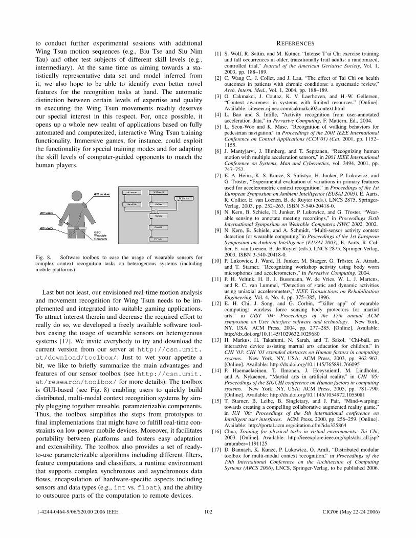
to conduct further experimental sessions with additionalWing Tsun motion sequences (e.g., Biu Tse and Siu NimTau) and other test subjects of different skill levels (e.g.,intermediary). At the same time as aiming towards a sta-tistically representative data set and model inferred fromit, we also hope to be able to identify even better novelfeatures for the recognition tasks at hand. The automaticdistinction between certain levels of expertise and qualityin executing the Wing Tsun movements readily deservesour special interest in this respect. For, once possible, itopens up a whole new realm of applications based on fullyautomated and computerized, interactive Wing Tsun trainingfunctionality. Immersive games, for instance, could exploitthe functionality for special training modes and for adaptingthe skill levels of computer-guided opponents to match thehuman players.

Fig. 8. Software toolbox to ease the usage of wearable sensors forcomplex context recognition tasks on heterogenous systems (includingmobile platforms)

Last but not least, our envisioned real-time motion analysisand movement recognition for Wing Tsun needs to be im-plemented and integrated into suitable gaming applications.To attract interest therein and decrease the required effort toreally do so, we developed a freely available software tool-box easing the usage of wearable sensors on heterogenoussystems [17]. We invite everybody to try and download thecurrent version from our server at http://csn.umit.at/download/toolbox/. Just to wet your appetite abit, we like to briefly summarize the main advantages andfeatures of our sensor toolbox (see http://csn.umit.at/research/toolbox/ for more details). The toolboxis GUI-based (see Fig. 8) enabling users to quickly builddistributed, multi-modal context recognition systems by sim-ply plugging together reusable, parameterizable components.Thus, the toolbox simplifies the steps from prototypes tofinal implementations that might have to fulfill real-time con-straints on low-power mobile devices. Moreover, it facilitatesportability between platforms and fosters easy adaptationand extensibility. The toolbox also provides a set of ready-to-use parameterizable algorithms including different filters,feature computations and classifiers, a runtime environmentthat supports complex synchronous and asynchronous dataflows, encapsulation of hardware-specific aspects includingsensors and data types (e.g., int vs. float), and the abilityto outsource parts of the computation to remote devices.

REFERENCES

[1] S. Wolf, R. Sattin, and M. Kutner, “Intense T’ai Chi exercise trainingand fall occurrences in older, transitionally frail adults: a randomized,controlled trial,” Journal of the American Geriatric Society, Vol. 1,2003, pp. 188–189.

[2] C. Wang C., J. Collet, and J. Lau, “The effect of Tai Chi on healthoutcomes in patients with chronic conditions: a systematic review,”Arch. Intern. Med., Vol. 1, 2004, pp. 188–189.

[3] O. Cakmakci, J. Coutaz, K. V. Laerhoven, and H.-W. Gellersen,“Context awareness in systems with limited resources.” [Online].Available: citeseer.nj.nec.com/cakmakci02context.html

[4] L. Bao and S. Intille, “Activity recognition from user-annotatedacceleration data,” in Pervasive Computing, F. Mattern, Ed., 2004.

[5] L. Seon-Woo and K. Mase, “Recognition of walking behaviors forpedestrian navigation,” in Proceedings of the 2001 IEEE InternationalConference on Control Applications (CCA’01) (Cat, 2001, pp. 1152–1155.

[6] J. Mantyjarvi, J. Himberg, and T. Seppanen, “Recognizing humanmotion with multiple acceleration sensors,” in 2001 IEEE InternationalConference on Systems, Man and Cybernetics, vol. 3494, 2001, pp.747–752.

[7] E. A. Heinz, K. S. Kunze, S. Sulistyo, H. Junker, P. Lukowicz, andG. Troster, “Experimental evaluation of variations in primary featuresused for accelerometric context recognition,” in Proceedings of the 1stEuropean Symposium on Ambient Intelligence (EUSAI 2003), E. Aarts,R. Collier, E. van Loenen, B. de Ruyter (eds.), LNCS 2875, Springer-Verlag, 2003, pp. 252–263, ISBN 3-540-20418-0.

[8] N. Kern, B. Schiele, H. Junker, P. Lukowicz, and G. Troster, “Wear-able sensing to annotate meeting recordings,” in Proceedings SixthInternational Symposium on Wearable Computers ISWC 2002, 2002.

[9] N. Kern, B. Schiele, and A. Schmidt, “Multi-sensor activity contextdetection for wearable computing,”in Proceedings of the 1st EuropeanSymposium on Ambient Intelligence (EUSAI 2003), E. Aarts, R. Col-lier, E. van Loenen, B. de Ruyter (eds.), LNCS 2875, Springer-Verlag,2003, ISBN 3-540-20418-0.

[10] P. Lukowicz, J. Ward, H. Junker, M. Staeger, G. Troster, A. Atrash,and T. Starner, “Recognizing workshop activity using body wornmicrophones and accelerometers,” in Pervasive Computing, 2004.

[11] P. H. Veltink, H. B. J. Bussmann, W. de Vries, W. L. J. Martens,and R. C. van Lummel, “Detection of static and dynamic activitiesusing uniaxial accelerometers,” IEEE Transactions on RehabilitationEngineering. Vol. 4, No. 4, pp. 375–385, 1996.

[12] E. H. Chi, J. Song, and G. Corbin, “”killer app” of wearablecomputing: wireless force sensing body protectors for martialarts,” in UIST ’04: Proceedings of the 17th annual ACMsymposium on User interface software and technology. New York,NY, USA: ACM Press, 2004, pp. 277–285. [Online]. Available:http://dx.doi.org/10.1145/1029632.1029680

[13] H. Markus, H. Takafumi, N. Sarah, and T. Sakol, “Chi-ball, aninteractive device assisting martial arts education for children,” inCHI ’03: CHI ’03 extended abstracts on Human factors in computingsystems. New York, NY, USA: ACM Press, 2003, pp. 962–963.[Online]. Available: http://dx.doi.org/10.1145/765891.766095

[14] P. Haemaelaeinen, T. Ilmonen, J. HoeysniemI, M. Lindholm,and A. Nykaenen, “Martial arts in artificial reality,” in CHI ’05:Proceedings of the SIGCHI conference on Human factors in computingsystems. New York, NY, USA: ACM Press, 2005, pp. 781–790.[Online]. Available: http://dx.doi.org/10.1145/1054972.1055081

[15] T. Starner, B. Leibe, B. Singletary, and J. Pair, “Mind-warping:towards creating a compelling collaborative augmented reality game,”in IUI ’00: Proceedings of the 5th international conference onIntelligent user interfaces. ACM Press, 2000, pp. 256–259. [Online].Available: http://portal.acm.org/citation.cfm?id=325864

[16] Chua, Training for physical tasks in virtual environments: Tai Chi,2003. [Online]. Available: http://ieeexplore.ieee.org/xpls/abs all.jsp?arnumber=1191125

[17] D. Bannach, K. Kunze, P. Lukowicz, O. Amft, “Distributed modulartoolbox for multi-modal context recognition,” in Proceedings of the19th International Conference on the Architecture of ComputingSystems (ARCS 2006), LNCS, Springer-Verlag, to be published 2006.

1-4244-0464-9/06/$20.00 2006 IEEE. 102 CIG'06 (May 22-24 2006)

Self-Adapting Payoff Matrices in Repeated Interactions

Siang Y. Chong and Xin YaoThe Centre of Excellence for Research in

Computational Intelligence and ApplicationsSchool of Computer Science

University of Birmingham, UKS.Y.Chong;X.Yao@cs.bham.ac.uk

Abstract— Traditional iterated prisoner’s dilemma (IPD) as-sumed a fixed payoff matrix for all players, which may not berealistic because not all players are the same in the real-world.This paper introduces a novel co-evolutionary framework whereeach strategy has its own self-adaptive payoff matrix. Thisframework is generic to any simultaneous two-player repeatedencounter game. Here, each strategy has a set of behavioralresponses based on previous moves, and an adaptable payoffmatrix based on reinforcement feedback from game interactionsthat is specified by update rules. We study how different updaterules affect the adaptation of initially random payoff matrices,and how this adaptation in turn affects the learning of strategybehaviors.

Keywords: Evolutionary games, Co-evolution, IteratedPrisoner’s Dilemma, Mutualism, Repeated Encounter Games

I. I NTRODUCTION

The IPD game is well-known as the standard metaphorto explain cooperative behaviors among selfish, unrelatedindividuals [1]. In its classical form, two players engagedinrepeated interactions are given two choices: cooperate anddefect. The two players receive their payoffs that depend onthe choices that they make during the course of behavioralexchange. The game captures thedilemma of cooperatingwith unrelated, and ultimately selfish players (i.e., thosethat seek the highest payoffs) by rewarding the player thatexploited its opponents with the highest payoff even thoughthe payoff for mutual cooperation is higher than that formutual defection.

In the IPD, defection is not always the best choice. Forexample, Axelrod [2], [3] showed through tournaments ofexperts-designed strategies that a particular form of coop-erative strategy, e.g.,tit for tat, which cooperates in thefirst round, and reciprocates thereafter the choice that theopponent made in the previous round, can be viable. Otherstudies, such as in [1], [4], have explained cooperation inthe IPD game using the idea of reciprocal altruism. Inparticular, cooperation can arise through the mechanismof direct reciprocity, which requires repeated encountersbetween individuals, so that cooperation received can bereturned. Further studies that use co-evolutionary models[5],[6], [7], [8], [9], [10] stressed that cooperative behaviorscan be learned through a process of adaptation based onthe mechanism of direct reciprocity that is provided throughinteractions (game play between strategies).

However, all of these studies assumed that the payoffmatrix, which defines the reward for making a certain choice

in light of the opponent’s, is fixed and symmetric. That is,the utility expectation of a strategy on rewards for certainbehaviors does not change (i.e., fixed payoff matrix) andis similar for all strategies (i.e., symmetric payoff matrix).These two basic assumptions might not be realistic if the IPDgame is used as a model to explain outcomes of real-worldinteractions due to variations between individuals on thepayoff matrix [11]. More importantly, these two assumptionshave significant implications to modelling behavioral inter-actions because they restrict strategies from adapting (e.g.,learning) their individual payoff matrices based on feedbackof game interactions that reinforces certain behaviors. Assuch, cooperative outcomes may not be a result of IPD-likepayoffs [11]. Instead, cooperative outcomes may be due to adifferent payoff matrix that favors mutual cooperation (i.e.,mutualism [12]).

Here, we present a preliminary study that is aimed at ad-dressing the problem of restrictive assumptions on the payoffmatrix (fixed and symmetric) to the evolutionary outcome ofrepeated encounter games. For this paper, we consider theevolution of strategy payoff matrices through an adaptationprocess based on reinforcement feedback from behavioralinteractions using a fixed update rule, and how this process inturn affects the learning of strategy behaviors. Although thisupdate-rule-based feedback mechanism may not reflect actualmechanisms found in real-world interactions, its simplicityallows for an in-depth study using a co-evolutionary approachto emphasize how the simultaneous adaptations on behavioralresponses and the expectations of rewards for behavioralresponses affect the learning of behaviors. This approach isdifferent compared to previous studies that consider a fixed,symmetric payoff matrix throughout the evolutionary process[5], [6], [7], [8], [9], [10], or perturbed payoff matrices basedon a noise sources with a fixed probability distribution [11],i.e., no learning process on payoff matrices.

Through an empirical study, we show how different updaterules, which specify how different elements in the strategypayoff matrices can be reinforced based on past interactions,can affect the adaptation of initially random payoff matrices,which in turn, affects the learning of strategy behaviorsfor future interactions. On the one hand, when IPD-likeupdate rules are used (i.e., favors exploitation of opponentpayoff even though the reinforcement for mutual cooperationpayoff is higher than that of mutual defection), defectionoutcomes are more likely to be obtained. On the ther hand,

1-4244-0464-9/06/$20.00 2006 IEEE. 103 CIG'06 (May 22-24 2006)

when update rules favor mutual cooperation, cooperativeoutcomes can be easily obtained. However, update rules onlysignificantly impact the learning of behaviors if the strategypayoff matrix is not overly constrained, e.g., allows for largevariations between elements of the strategy payoff matrixfrom reinforcement feedbacks of game interactions.

The rest of the paper is organized as follows. Section II de-scribes the general setting for iterated, two-player, two-choicegames. Section III describes the co-evolutionary model usedfor the experiments. Section IV presents the results of theexperiments, while section V discusses observations obtainedfrom the experimental results. Finally, section VI concludesthe paper, with some remarks for future studies.

II. I TERATED GAMES WITH TWO CHOICES

Behavioral interactions can be modelled using a game.One simple example is to use a symmetric, two-player, two-choice game as a model for cooperation [13]. Here, thegame consists of two players, each having the choice ofeither to cooperate or defect. Depending of the choices thatboth players have made, each player receives a payoff thatis specified by a predefined payoff matrix (e.g., Fig. 1).Referring to figure 1, both players receiveR units if bothcooperates, orP units if both defects. However, if one playercooperates while the other defects, the cooperator will receiveS units while the defector receivesT units. The valuesR,S, T , and P must satisfy the constraints,R > P andR > (S + T )/2. The game is symmetrical if the payoffmatrix is the same for both players [13].

Cooperate Defect

R T

Cooperate

R S

S P

Defect

T P

Fig. 1. The payoff matrix framework of a two-player, two-choice game.The payoff given in the lower left-hand corner is assigned tothe player (row)choosing the move, while that of the upper right-hand corner is assigned tothe opponent (column).

Depending on the specifications forR, S, T , andP , gameswith different characteristics can be produced. Consideringa single iteration, whenT > R > P > S, one obtainsthe prisoner’s dilemma game, where the best choice is todefect. However, whenR > T andS > P , one obtains themutualism game, where the best choice is to cooperate [12].Both of these games can be extended to have more than oneiteration, i.e., iterated (repeated encounter) games. Figures2 and 3 give examples of payoff matrices for the IPD anditerated mutualism games, respectively [11].

For this paper, we propose a generic framework of repeatedencounter games, whereby the payoff matrix is differentand adaptable for each strategy. That is, the framework is

Cooperate Defect

3 5

Cooperate

3 0

0 1

Defect

5 1

Fig. 2. Typical payoff matrix for an IPD game. The payoff given inthe lower left-hand corner is assigned to the player (row) choosing themove, while that of the upper right-hand corner is assigned tothe opponent(column).

Cooperate Defect

5 3

Cooperate

5 1

1 0

Defect

3 0

Fig. 3. Typical payoff matrix for an iterated mutualism game. The payoffgiven in the lower left-hand corner is assigned to the player(row) choosingthe move, while that of the upper right-hand corner is assigned to theopponent (column).

applicable to any repeated encounter game with differentpayoff matrices, and not just limited to those that satisfyspecific constraints (e.g., IPD or mutualism games).

III. C O-EVOLUTIONARY MODELS FOR LEARNING

PAYOFF MATRIX

A. Strategy Representation

We limit our investigation to only deterministic, memory-one strategy, both for simplicity and a starting point for astudy on the effect of strategies with different, but adaptablepayoff matrices. As such, we require a simple strategyrepresentation that consists of: (a) a behavioral responsepart (e.g., determines the choice to make based on choicesmade in the previous move), and, (b) a payoff matrix part(e.g., determines what payoff the strategy should receive).To achieve this, we use the simple direct look-up tablerepresentation [14], which allows direct behavioral evolutionof strategies, to represent a strategy’s behavioral responsesbased on previous moves. The look-up table is extended tostore values of a two-choice payoff matrix.

Figure 4 illustrates the direct look-up table representa-tion for the strategies with two choices and memory-one.mij , i, j = 1, 2 specifies the choice to be made, given theinputs i (player’s own previous choice) andj (opponent’sprevious choice). Rather than using pre-game inputs (twofor memory-one strategies), the first move is specified in-dependently,mfm. Binary choices of+1 and−1 are used.The payoff matrix part for each strategy specifies payoffs

1-4244-0464-9/06/$20.00 2006 IEEE. 104 CIG'06 (May 22-24 2006)

that the strategy receives given choices made by the strategyand its opponent for that particular iteration. The elements inthe payoff matrix,pij , i, j = 1, 2, are not fixed, but instead,variable and depends on choices made by the strategy duringinteractions. That is, evolutionary variation is not applieddirectly to the payoff matrix (details of the update rule usedto adaptpij is presented in the following section).

Opponent�s Previous Move

+1 1

Player�s +1 m11 m12

Previous Move 1 m21 m22

(a) Behavior

Opponent�s Previous Move

+1 1

Player�s +1 p11 p12

Previous Move 1 p21 p22

(b) Payoff Matrix

Fig. 4. The look-up table representation for the two-playerrepeatedencounter game with two choices and memory length one. (a) BehavioralResponse (also includesmfm for the first move, which is not shown in thefigure). (b) Payoff Matrix (utility expectation).

A simple mutation operator is used to generate offspringfrom parents. When a response, i.e., the element of the directlook-up table for behavioral responses (includesmfm andmij) mutates, it changes to the other possible choice. Eachtable element has a fixed probability,pm, of being replacedby the other choice. The valuepm is not optimized. Ineffect, the variation operator for the strategy representationof the two-choice IPD used here is a uniform mutation withprobability pm.

Crossover is not used in any experiment. With the directlook-up table for strategy representation, any variation opera-tor will introduce variations on behavioral responses directly.As investigated earlier in [14] (even for the more complexIPD game with intermediate choices), a simple mutationoperator is more than sufficient to introduce the requiredvariations of strategy behaviors. The use of crossover is notnecessary.

B. Co-evolutionary Procedure

The co-evolutionary learning approach that is used hereis similar to that used in [14]. The original system in [14]is changed to accommodate the co-evolutionary learningof strategy behavioral responses and payoff matrix. Giventhat the adaptation process occurs for strategy payoff matrixas well, more experiments are conducted to investigate theimpact of initial strategy payoff matrices on the learning ofstrategy behaviors. The initialization schemes are summa-rized in table I.

The following gives the flow of the co-evolutionary pro-cedure:

TABLE I

INITIALIZATION SCHEMES FOR STRATEGY PAYOFF MATRIX OF INITIAL

POPULATION. U(0, 5) REFERS TO A RANDOM VALUE DRAWN FROM A

UNIFORM DISTRIBUTION BETWEEN0 AND 5. ASYM REFERS TO THE

INITIALIZATION SCHEME WHERE STRATEGIES CAN BE INITIALIZED

WITH DIFFERENT PAYOFF MATRICES. SYM REFERS TO THE

INITIALIZATION SCHEME WHERE STRATEGIES ARE INITIALIZED WITH

THE SAME PAYOFF MATRIX.

RanAll Ran IPD1 IPD2 MUT1 MUT2p11 U(0, 5) U(0, 5) 4 3 5 5p12 U(0, 5) U(0, 5) 0 0 1 1p21 U(0, 5) U(0, 5) 5 5 4 3p22 U(0, 5) U(0, 5) 1 1 0 0

ASYM SYM SYM SYM SYM SYM

1) Generation step,t = 0:Initialize N/2 parent strategies,Pi, i = 1, 2, ..., N/2,randomly.

a) Each table element,mfm andmij , i, j = 1, 2, isinitialized to values,+1 or −1, each with equalprobability.

b) Each element for the payoff matrix,pij , i, j =1, 2, is initialized according to values dependingon the investigated initialization scheme (table I).

2) GenerateN/2 offspring, Oi, i = 1, 2, ..., N/2, fromN/2 parents using a mutation operator with probabilitypm.

3) All pairs of strategies compete, including the pairwhere a strategy plays itself (i.e., round-robin tourna-ment). ForN strategies in a population, every strategycompetes a total ofN games. Each strategy’s payoffmatrix is updated after every iteration for each game.The updated payoff matrix is used immediately in thenext iteration. The updates are described as follows:

a) Player cooperates, opponent cooperates:p′11

= p11 + δ11

b) Player defects, opponent cooperates:p′21

= p21 + δ21

c) Player cooperates, opponent defects:p′12

= p12 + δ12

d) Player defects, opponent defects:p′22

= p22 + δ22

whereδij ≥ 0, i, j = 1, 2.4) Select the bestN/2 strategies based on total payoffs of

all games played. Increment generation step,t = t+1.5) Step 2 to 4 are repeated until termination criterion (i.e.,

a fixed number of generation) is met.In particular, we useN = 20, and repeat the co-

evolutionary process for 200 generations, which is suffi-ciently long to observe an evolutionary outcome (e.g., per-sistent cooperation). A fixed game length of 150 iterationsis used for all games. Experiments are repeated for 30independent runs.

The update rule, i.e.,δij , i, j = 1, 2, determines how theelements for each strategy’s payoff matrix part are changedbased on the strategy’s interactions with the opponent. The

1-4244-0464-9/06/$20.00 2006 IEEE. 105 CIG'06 (May 22-24 2006)

update rule follows a reinforcement view whereby only theelement in the payoff matrix that corresponds to the pair ofchoices made by the strategy and its opponent is updated.Note that the adaptation process of the strategy’s payoffmatrix is indirect, i.e., evolutionary variation is not applieddirectly to the payoff matrix. Instead, variation to the payoffmatrix is a result of interactions between strategies, whichdepend on their behavioral responses that are subjected toevolutionary variations. Lastly, for simplicity, we assume thatthe update rule (e.g., given by theδs) is the same for allstrategies.

As such, it is emphasized that not all interactions conformto a specific payoff matrix (e.g., IPD) because each strategy’spayoff matrix is evolving as well. With this in mind, we caninvestigate what payoff matrices that emerged, and also whatbehaviors that are obtained based on those payoff matricesfrom a co-evolutionary process.

IV. RESULTS

A. Learning Behaviors when Exploitation of Opponents isFavored

We first consider IPD-like update rules to investigate howupdate rules can affect the evolution of payoff matrices,and in turn, the learning of strategy behaviors. IPD-likeupdate rules favor exploitation of opponents, even thoughreinforcement for mutual cooperation is higher compared tothat of mutual defection. That is, the values forδs in theupdate rule satisfy the IPD constraints, i.e.,δ21 > δ11 >δ22 > δ12. The following experiments are motivated tofacilitate the investigation on what strategy payoff matricesand behaviors that emerged when the update rule favorsstrategies exploiting their opponents.

Table II summarizes and compares all update rules used forthe experiments in this paper. We first focus on theURIPD1

update rule with the followingδ values, δ11 = 0.4/150,δ21 = 0.5/150, δ12 = 0.0/150, δ22 = 0.1/150. Given thatan update to a strategy’s payoff matrix is made after everyiteration, we scale theδs to the number of iteration of a game(e.g., dividing values by 150).

TABLE II

UPDATE RULES USED FOR THE EMPIRICAL STUDY. BOTH URIPD1 AND

URIPD2 UPDATE RULES FAVOR EXPLOITATION OF OPPONENTS. WITH

URIPD2 , THE REINFORCEMENT OF REWARDS FOR EXPLOITATION OF

OPPONENTS IS FURTHER EMPHASIZED. URMUT UPDATE RULE FAVORS

MUTUAL COOPERATION.

URIPD1 URIPD2 URMUT

δ11 0.4/150 0.4/150 0.5/150δ12 0.0/150 0.0/150 0.1/150δ21 0.5/150 0.7/150 0.3/150δ22 0.1/150 0.1/150 0.0/150

For the first experiment, we considered the RanAll initial-izations of strategy payoff matrices (table I). Results showthe populations of 12 runs out of 30 evolved to mutualcooperation (RanAll row andURIPD1 column in table III).Closer inspection shows that surviving strategies converged

to a similar payoff matrix, and that the the element in thepayoff matrix corresponding to mutual cooperation is muchhigher compared to the other elements in these 12 mutualcooperative runs (e.g.,p11 � p12, p21, p22). This observationsuggests strategies evolving to cooperative behaviors early onafter a random initialization. The persistent cooperationto theend of the run is a result of continued reinforcement feedbackbetween mutual cooperative play and strategies’ expectationson rewards for mutual cooperation.

The populations in the remaining 18 runs evolved to apoint where they engaged in mutual defection. Similar ob-servation of strategies converging to a similar payoff matrix ismade. Closer inspection reveals that the element in the payoffmatrix corresponding to mutual defection is much higherthan other elements except that of the element correspondingto exploitation of opponents (or temptation to defect). That is,p22 � p11, p12 andp22 > p21, suggesting that the defectionoutcomes are the result of initial random strategies evolvingto exploit one another first, before evolving to play mutualdefection.

In general, results from the experiment (RanAll) suggestthat cooperative outcomes are less likely to be obtained whenthe IPD-like update rule, which favors strategies exploitingtheir opponents, is used. This is also observed from resultssummarized in table IV that shows the average cooperationfrequency of 30 runs for each experiment. In particular, in theRanAll row andURIPD1 column of table IV, the averagecooperation frequency of 40.06% (less than 50%) showsthat the co-evolutionary process resulted with more defectionplays.

However, given the convergence to a similar payoff matrixfor the co-evolving population, we conducted additionalexperiments with different initializations of payoff matrices(table I) to determine their impact on the evolutionaryoutcome. Results of these experiments are summarized inURIPD1 column of tables III, IV, and V. In particular, nostatistically significant difference is observed for comparisonbetween results of experiments (URIPD1 column of table V)where all strategies were initialized with the same randompayoff matrix (Ran) and where each strategy was randomlyinitialized with different payoff matrix (RanAll). Similarly,no statistically significant difference is observed for compar-ison between the RanAll experiment and experiments wherestrategy payoff matrices were initialized with the same IPDpayoff matrix (IPD1 and IPD2 in table I). However, whenstrategy payoff matrices were initialized with mutualism-likepayoffs (MUT1 and MUT2 in table I), cooperative outcomeswere obtained easily, e.g., the higher number of cooperativeoutcomes (URIPD1 column of table III) and higher averagecooperation frequencies (URIPD1 column of table IV) arestatistically significantly different compared to that of RanAllexperiment.

Furthermore, as in the original experiment (RanAll), strate-gies are also observed to converge to a similar payoff matrixregardless of how strategy payoff matrices are initialized.In particular, runs with cooperative outcome are always a

1-4244-0464-9/06/$20.00 2006 IEEE. 106 CIG'06 (May 22-24 2006)

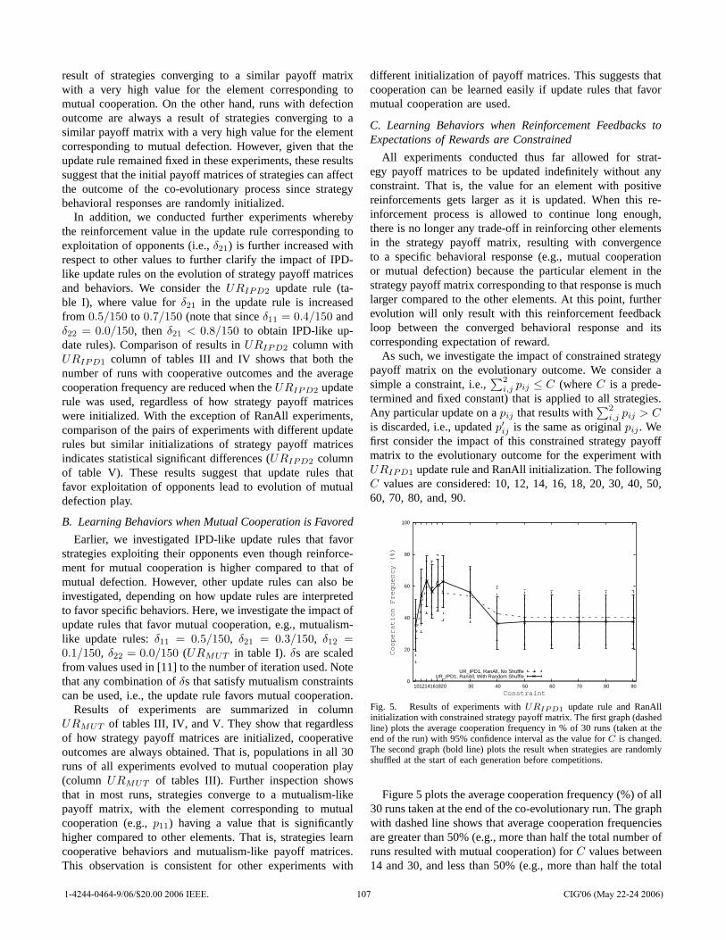
result of strategies converging to a similar payoff matrixwith a very high value for the element corresponding tomutual cooperation. On the other hand, runs with defectionoutcome are always a result of strategies converging to asimilar payoff matrix with a very high value for the elementcorresponding to mutual defection. However, given that theupdate rule remained fixed in these experiments, these resultssuggest that the initial payoff matrices of strategies can affectthe outcome of the co-evolutionary process since strategybehavioral responses are randomly initialized.

In addition, we conducted further experiments wherebythe reinforcement value in the update rule corresponding toexploitation of opponents (i.e.,δ21) is further increased withrespect to other values to further clarify the impact of IPD-like update rules on the evolution of strategy payoff matricesand behaviors. We consider theURIPD2 update rule (ta-ble I), where value forδ21 in the update rule is increasedfrom 0.5/150 to 0.7/150 (note that sinceδ11 = 0.4/150 andδ22 = 0.0/150, then δ21 < 0.8/150 to obtain IPD-like up-date rules). Comparison of results inURIPD2 column withURIPD1 column of tables III and IV shows that both thenumber of runs with cooperative outcomes and the averagecooperation frequency are reduced when theURIPD2 updaterule was used, regardless of how strategy payoff matriceswere initialized. With the exception of RanAll experiments,comparison of the pairs of experiments with different updaterules but similar initializations of strategy payoff matricesindicates statistical significant differences (URIPD2 columnof table V). These results suggest that update rules thatfavor exploitation of opponents lead to evolution of mutualdefection play.

B. Learning Behaviors when Mutual Cooperation is Favored

Earlier, we investigated IPD-like update rules that favorstrategies exploiting their opponents even though reinforce-ment for mutual cooperation is higher compared to that ofmutual defection. However, other update rules can also beinvestigated, depending on how update rules are interpretedto favor specific behaviors. Here, we investigate the impactofupdate rules that favor mutual cooperation, e.g., mutualism-like update rules:δ11 = 0.5/150, δ21 = 0.3/150, δ12 =0.1/150, δ22 = 0.0/150 (URMUT in table I). δs are scaledfrom values used in [11] to the number of iteration used. Notethat any combination ofδs that satisfy mutualism constraintscan be used, i.e., the update rule favors mutual cooperation.

Results of experiments are summarized in columnURMUT of tables III, IV, and V. They show that regardlessof how strategy payoff matrices are initialized, cooperativeoutcomes are always obtained. That is, populations in all 30runs of all experiments evolved to mutual cooperation play(column URMUT of tables III). Further inspection showsthat in most runs, strategies converge to a mutualism-likepayoff matrix, with the element corresponding to mutualcooperation (e.g.,p11) having a value that is significantlyhigher compared to other elements. That is, strategies learncooperative behaviors and mutualism-like payoff matrices.This observation is consistent for other experiments with

different initialization of payoff matrices. This suggests thatcooperation can be learned easily if update rules that favormutual cooperation are used.

C. Learning Behaviors when Reinforcement Feedbacks toExpectations of Rewards are Constrained

All experiments conducted thus far allowed for strat-egy payoff matrices to be updated indefinitely without anyconstraint. That is, the value for an element with positivereinforcements gets larger as it is updated. When this re-inforcement process is allowed to continue long enough,there is no longer any trade-off in reinforcing other elementsin the strategy payoff matrix, resulting with convergenceto a specific behavioral response (e.g., mutual cooperationor mutual defection) because the particular element in thestrategy payoff matrix corresponding to that response is muchlarger compared to the other elements. At this point, furtherevolution will only result with this reinforcement feedbackloop between the converged behavioral response and itscorresponding expectation of reward.

As such, we investigate the impact of constrained strategypayoff matrix on the evolutionary outcome. We consider asimple a constraint, i.e.,

∑2

i,j pij ≤ C (whereC is a prede-termined and fixed constant) that is applied to all strategies.Any particular update on apij that results with

∑2

i,j pij > Cis discarded, i.e., updatedp′ij is the same as originalpij . Wefirst consider the impact of this constrained strategy payoffmatrix to the evolutionary outcome for the experiment withURIPD1 update rule and RanAll initialization. The followingC values are considered: 10, 12, 14, 16, 18, 20, 30, 40, 50,60, 70, 80, and, 90.

0

20

40

60

80

100

90 80 70 60 50 40 30 20 18 16 14 12 10

Cooperation Frequency (%)

Constraint

UR_IPD1, RanAll, No ShuffleUR_IPD1, RanAll, With Random Shuffle

Fig. 5. Results of experiments withURIPD1 update rule and RanAllinitialization with constrained strategy payoff matrix. The first graph (dashedline) plots the average cooperation frequency in % of 30 runs(taken at theend of the run) with 95% confidence interval as the value forC is changed.The second graph (bold line) plots the result when strategies are randomlyshuffled at the start of each generation before competitions.

Figure 5 plots the average cooperation frequency (%) of all30 runs taken at the end of the co-evolutionary run. The graphwith dashed line shows that average cooperation frequenciesare greater than 50% (e.g., more than half the total number ofruns resulted with mutual cooperation) forC values between14 and 30, and less than 50% (e.g., more than half the total

1-4244-0464-9/06/$20.00 2006 IEEE. 107 CIG'06 (May 22-24 2006)

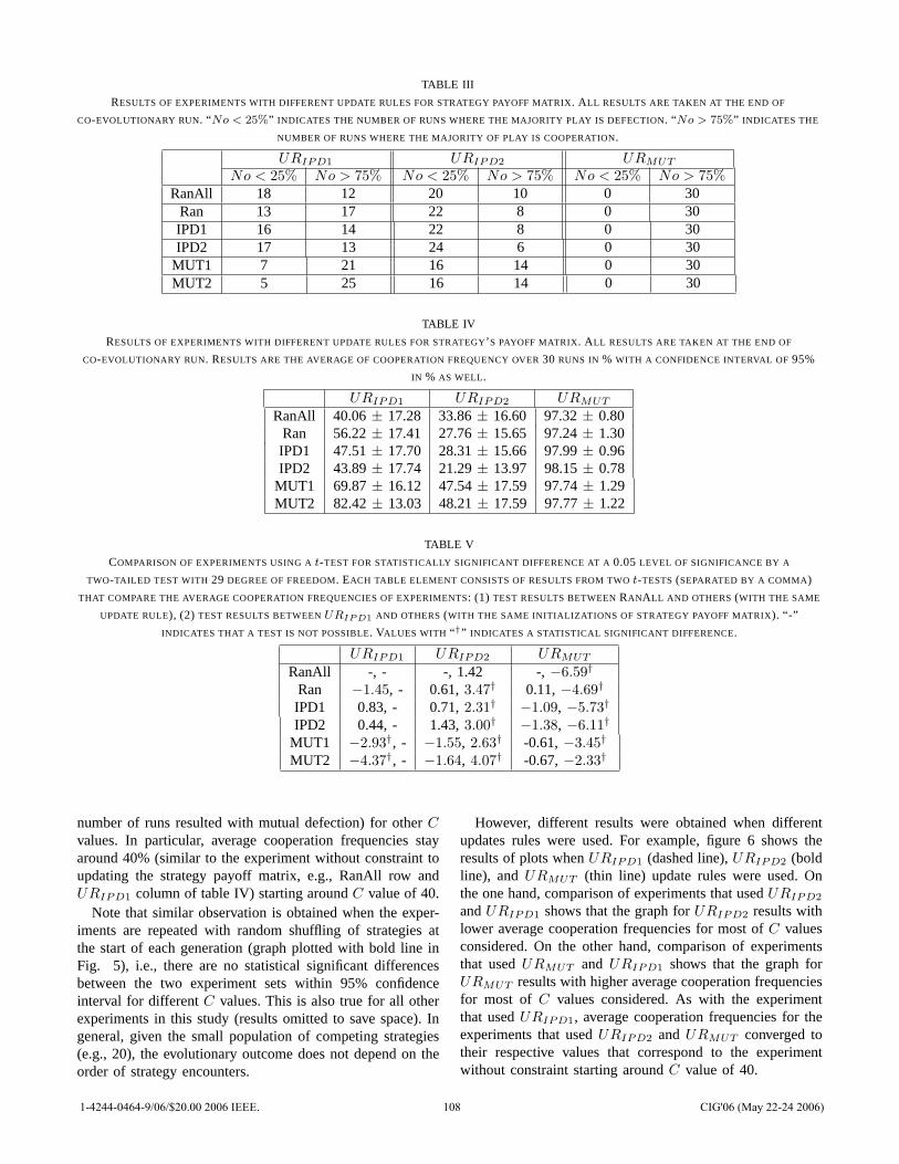
TABLE III

RESULTS OF EXPERIMENTS WITH DIFFERENT UPDATE RULES FOR STRATEGY PAYOFF MATRIX. ALL RESULTS ARE TAKEN AT THE END OF

CO-EVOLUTIONARY RUN. “No < 25%” INDICATES THE NUMBER OF RUNS WHERE THE MAJORITY PLAY IS DEFECTION. “No > 75%” INDICATES THE

NUMBER OF RUNS WHERE THE MAJORITY OF PLAY IS COOPERATION.

URIPD1 URIPD2 URMUT

No < 25% No > 75% No < 25% No > 75% No < 25% No > 75%RanAll 18 12 20 10 0 30

Ran 13 17 22 8 0 30IPD1 16 14 22 8 0 30IPD2 17 13 24 6 0 30

MUT1 7 21 16 14 0 30MUT2 5 25 16 14 0 30

TABLE IV

RESULTS OF EXPERIMENTS WITH DIFFERENT UPDATE RULES FOR STRATEGY’ S PAYOFF MATRIX. ALL RESULTS ARE TAKEN AT THE END OF

CO-EVOLUTIONARY RUN. RESULTS ARE THE AVERAGE OF COOPERATION FREQUENCY OVER30 RUNS IN % WITH A CONFIDENCE INTERVAL OF 95%

IN % AS WELL.

URIPD1 URIPD2 URMUT

RanAll 40.06± 17.28 33.86± 16.60 97.32± 0.80Ran 56.22± 17.41 27.76± 15.65 97.24± 1.30IPD1 47.51± 17.70 28.31± 15.66 97.99± 0.96IPD2 43.89± 17.74 21.29± 13.97 98.15± 0.78

MUT1 69.87± 16.12 47.54± 17.59 97.74± 1.29MUT2 82.42± 13.03 48.21± 17.59 97.77± 1.22

TABLE V

COMPARISON OF EXPERIMENTS USING At-TEST FOR STATISTICALLY SIGNIFICANT DIFFERENCE AT A0.05LEVEL OF SIGNIFICANCE BY A

TWO-TAILED TEST WITH 29 DEGREE OF FREEDOM. EACH TABLE ELEMENT CONSISTS OF RESULTS FROM TWOt-TESTS(SEPARATED BY A COMMA)

THAT COMPARE THE AVERAGE COOPERATION FREQUENCIES OF EXPERIMENTS: (1) TEST RESULTS BETWEENRANALL AND OTHERS (WITH THE SAME

UPDATE RULE), (2) TEST RESULTS BETWEENURIPD1 AND OTHERS (WITH THE SAME INITIALIZATIONS OF STRATEGY PAYOFF MATRIX). “-”

INDICATES THAT A TEST IS NOT POSSIBLE. VALUES WITH “ †” INDICATES A STATISTICAL SIGNIFICANT DIFFERENCE.

URIPD1 URIPD2 URMUT

RanAll -, - -, 1.42 -, −6.59†

Ran −1.45, - 0.61,3.47† 0.11,−4.69†

IPD1 0.83, - 0.71,2.31† −1.09, −5.73†

IPD2 0.44, - 1.43,3.00† −1.38, −6.11†

MUT1 −2.93†, - −1.55, 2.63† -0.61,−3.45†

MUT2 −4.37†, - −1.64, 4.07† -0.67,−2.33†

number of runs resulted with mutual defection) for otherCvalues. In particular, average cooperation frequencies stayaround 40% (similar to the experiment without constraint toupdating the strategy payoff matrix, e.g., RanAll row andURIPD1 column of table IV) starting aroundC value of 40.

Note that similar observation is obtained when the exper-iments are repeated with random shuffling of strategies atthe start of each generation (graph plotted with bold line inFig. 5), i.e., there are no statistical significant differencesbetween the two experiment sets within 95% confidenceinterval for differentC values. This is also true for all otherexperiments in this study (results omitted to save space). Ingeneral, given the small population of competing strategies(e.g., 20), the evolutionary outcome does not depend on theorder of strategy encounters.

However, different results were obtained when differentupdates rules were used. For example, figure 6 shows theresults of plots whenURIPD1 (dashed line),URIPD2 (boldline), andURMUT (thin line) update rules were used. Onthe one hand, comparison of experiments that usedURIPD2

andURIPD1 shows that the graph forURIPD2 results withlower average cooperation frequencies for most ofC valuesconsidered. On the other hand, comparison of experimentsthat usedURMUT and URIPD1 shows that the graph forURMUT results with higher average cooperation frequenciesfor most of C values considered. As with the experimentthat usedURIPD1, average cooperation frequencies for theexperiments that usedURIPD2 and URMUT converged totheir respective values that correspond to the experimentwithout constraint starting aroundC value of 40.

1-4244-0464-9/06/$20.00 2006 IEEE. 108 CIG'06 (May 22-24 2006)

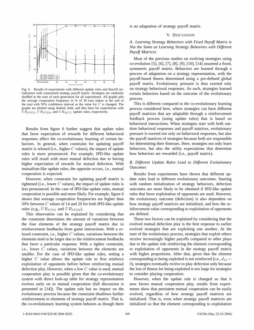
0

20

40

60

80

100

90 80 70 60 50 40 30 20 18 16 14 12 10

Cooperation Frequency (%)

Constraint

UR_IPD1, RanAllUR_IPD2, RanAllUR_MUT, RanAll

Fig. 6. Results of experiments with different update rules and RanAll ini-tialization with constrained strategy payoff matrix. Strategies are randomlyshuffled at the start of each generation for all experiments. All graphs plotthe average cooperation frequency in % of 30 runs (taken at the end ofthe run) with 95% confidence interval as the value forC is changed. Thegraphs are plotted using dashed, bold, and thin lines for experiments withURIPD1, URIPD2, andURMUT update rules, respectively.

Results from figure 6 further suggest that update rulesthat favor expectation of rewards for different behavioralresponses affect the co-evolutionary learning of certain be-haviors. In general, when constraint for updating payoffmatrix is relaxed (i.e., higherC values), the impact of updaterules is more pronounced. For example, IPD-like updaterules will result with more mutual defection due to havinghigher expectation of rewards for mutual defection. Withmutualism-like update rules, the opposite occurs, i.e., mutualcooperation is expected.

However, when constraint for updating payoff matrix istightened (i.e., lowerC values), the impact of update rules isless pronounced. In the case of IPD-like update rules, mutualcooperation is possible and more likely. For example, figure6shows that average cooperation frequencies are higher than50% betweenC values of 14 and 20 for both IPD-like updaterules (e.g.,URIPD1 andURIPD2).

This observation can be explained by considering thatthe constraint determines the amount of variations betweenthe four elements of the strategy payoff matrix due toreinforcement feedbacks from game interactions. With a re-laxed constraint, i.e., higherC values, variations between theelements tend to be larger due to the reinforcement feedbacksthat favor a particular response. With a tighter constraint,i.e., lower C values, variations between the elements aresmaller. For the case of IPD-like update rules, setting ahigher C value allows the update rule to first reinforceexploitation of opponents before before reinforcing mutualdefection play. However, when a lowC value is used, mutualcooperation play is possible given that the co-evolutionarysystem with direct look-up table for strategy representationevolves early on to mutual cooperation (full discussion ispresented in [14]). The update rule has no impact on theevolutionary process because the constraint disallows furtherreinforcement to elements of strategy payoff matrix. That is,the co-evolutionary learning system behaves as though there

is no adaptation of strategy payoff matrix.

V. D ISCUSSION

A. Learning Strategy Behaviors with Fixed Payoff Matrix isNot the Same as Learning Strategy Behaviors with DifferentPayoff Matrices

Most of the previous studies on evolving strategies usingco-evolution [5], [6], [7], [8], [9], [10], [14] assumed a fixed,symmetric payoff matrix. Behaviors are learned through aprocess of adaptation on a strategy representation, with thepayoff-based fitness determined using a pre-defined globalpayoff matrix. Evolutionary pressure is thus exerted onlyon strategy behavioral responses. As such, strategies learnedcertain behaviors based on the outcome of the evolutionaryprocess.

This is different compared to the co-evolutionary learningprocess considered here, where strategies can have differentpayoff matrices that are adaptable through a reinforcementfeedback process (using update rules) that is based onbehavioral interactions. When strategies start with both ran-dom behavioral responses and payoff matrices, evolutionarypressure is exerted not only on behavioral responses, but alsothe payoff matrices of strategies because both are responsiblefor determining their fitnesses. Here, strategies not only learnbehaviors, but also the utility expectations that determinehow behaviors are rewarded (i.e., payoff matrix).

B. Different Update Rules Lead to Different EvolutionaryOutcomes

Results from experiments have shown that different up-date rules lead to different evolutionary outcomes. Startingwith random initialization of strategy behaviors, defectionoutcomes are more likely to be obtained if IPD-like updaterules that favor exploitation of opponents are used. However,the evolutionary outcome (defection) is also dependent onhow strategy payoff matrices are initialized, and how the re-inforcement value corresponding to exploitation of opponentsare defined.

These two factors can be explained by considering that theevolved mutual defection play is the best response to earlierevolved strategies that are exploiting one another. At thestart of the evolutionary process, strategies that exploitothersreceive increasingly higher payoffs compared to other playsdue to the update rule reinforcing the element correspondingto exploitation of opponents in the strategy payoff matrixwith higher proportions. After that, given that the elementcorresponding to being exploited is not reinforced (i.e.,d12 =0), strategies eventually evolve to play defection only becausethe lost of fitness for being exploited is too large for strategiesto consider playing cooperation.

However, when the update rule is changed so that itnow favors mutual cooperation play, results from experi-ments show that persistent mutual cooperation can be easilyevolved, regardless of how strategy payoff matrices areinitialized. That is, even when strategy payoff matrices areinitialized so that the element corresponding to exploitation

1-4244-0464-9/06/$20.00 2006 IEEE. 109 CIG'06 (May 22-24 2006)

of opponents are higher compared to the others (e.g., IPDpayoff matrices), strategies that engaged in mutual coopera-tion receives increasingly higher payoffs due to the updaterule reinforcing the element corresponding to mutual coop-eration in the strategy payoff matrix with higher proportions.

It should be noted that the impact of update rules onthe evolution of behaviors is only significant if there aresufficient reinforcements from game interactions that resultwith large variations between elements in a strategy payoffmatrix. That is, if updates to the strategy payoff matrixare not overly constrained to allow for sufficient variationsbetween the elements that correspond to expectations ofrewards for different responses from reinforcement feedbacksof game interactions, update rules with different emphasison behavioral responses can significantly affect the co-evolutionary learning of strategy behaviors.

VI. CONCLUSION

This paper presents a preliminary study on evolving strat-egy payoff matrices, and how such an adaptation processcan affect the learning of strategy behaviors. The study ismotivated from the observation that the assumption of havingfixed, symmetric payoff matrix for all evolving strategiesmay not be realistic. Furthermore, the assumption of fixed,symmetric payoff matrix is highly restrictive because it doesnot allow strategies adapting their individual payoff matricesbased on feedback of game interactions that reinforces certainbehaviors.

To facilitate our investigation on the impact of relaxingthe restrictive assumption of fixed, symmetric payoff ma-trix for each strategy, thereby allowing strategies to havedifferent payoff matrices that are also adaptable, we focusspecifically on an adaptation process of payoff matrix basedon past behavioral interactions. A simple update rule thatreinforces the elements of the payoff matrix is considered.The update rule provides a reinforcement feedback processbetween strategy behaviors and payoff matrices during theco-evolutionary process.

The result is a co-evolutionary process, whereby the evo-lutionary outcome is dependent on the adaptation process ofboth behaviors (i.e., strategy behavioral responses) and utilityexpectations that determine how behaviors are rewarded(i.e., strategy payoff matrices). In particular, experimentsare conducted to show how different update rules affectthe adaptation process of payoff matrices, which in turn,affect the learning of strategy behaviors. Results show thatdefection outcomes are more likely to be obtained if IPD-likeupdate rules that favor the exploitation of opponents are used.However, cooperative outcomes can be easily obtained whenmutualism-like update rules that favor mutual cooperationareused. Update rules affect the learning of strategy behaviorswhen they lead to large variations between elements inthe strategy payoff matrix (e.g., mutualism-like update ruleresults with a significantly larger element corresponding tomutual cooperation in the payoff matrix compared to theothers).

It is noted that the update-rule-based feedback mechanismmay not reflect actual mechanisms in real-world interactionseven though its simplicity allows for an in-depth studyon how simultaneous adaptations of behavioral responsesand expectations on rewards for behavioral responses af-fect the learning of strategy behaviors. For future work,studies should be carried out to determine how adaptationsof behavioral responses and that of the expectations onrewards are linked with each other, and how this link canbe abstracted and modelled as a mechanism in the co-evolutionary framework introduced here.

ACKNOWLEDGMENTS

The authors are grateful to EPSRC for its support throughGrant GR/S63472/01, to ARC (Australian Research Council)for its support through an ARC International Link grant,and to the School of Computer Science at the Universityof Birmingham for its studentship to the first author.

REFERENCES

[1] R. Axelrod, The Evolution of Cooperation. New York: Basic Books,1984.

[2] ——, “Effective choice in the prisoner’s dilemma,”The Journal ofConflict Resolution, vol. 24, no. 1, pp. 3–25, Mar. 1980.

[3] ——, “More effective choice in the prisoner’s dilemma,”The Journalof Conflict Resolution, vol. 24, no. 3, pp. 379–403, Sept. 1980.

[4] M. A. Nowak and K. Sigmund, “Tit for tat in heterogeneous popula-tions,” Nature, vol. 355, pp. 250–253, 1992.

[5] R. Axelrod, “The evolution of strategies in the iteratedprisoner’sdilemma,” in Genetic Algorithms and Simulated Annealing, L. D.Davis, Ed. New York: Morgan Kaufmann, 1987, ch. 3, pp. 32–41.

[6] D. B. Fogel, “The evolution of intelligent decision making in gaming,”Cybernetics and Systems: An International Journal, vol. 22, pp. 223–236, 1991.

[7] ——, “Evolving behaviors in the iterated prisoner’s dilemma,” Evolu-tionary Computation, vol. 1, no. 1, pp. 77–97, 1993.

[8] ——, “On the relationship between the duration of an encouterand the evolution of cooperation in the iterated prisoner’sdilemma,”Evolutionary Computation, vol. 3, no. 3, pp. 349–363, 1996.

[9] P. Darwen and X. Yao, “On evolving robust strategies for iteratedprisoner’s dilemma,” inProgress in Evolutionary Computation, ser.Lecture Notes in Artificial Intelligence, vol. 956, 1995, pp. 276–292.

[10] B. A. Julstrom, “Effects of contest length and noise on reciprocalaltruism, cooperation, and payoffs in the iterated prisoner’s dilemma,”in Proc. 7th International Conf. on Genetic Algorithms (ICGA’97).San Francisco, CA: Morgan Kauffman, 1997, pp. 386–392.

[11] D. D. P. Johnson, P. Stopka, and J. Bell, “Individual variation evadesthe prisoner’s dilemma,”BMC Evolutionary Biology, vol. 2, no. 15,2002.

[12] K. C. Clements and D. W. Stephens, “Testing models of non-kin co-operation: Mutualism and the prisoner’s dilemma,”Animal Behaviour,vol. 50, pp. 527–535, 1995.

[13] M. Mesterton-Gibbons and L. A. Dugatkin, “Cooperationamongunrelated individuals: Evolutionary factors,”The Quarterly Review ofBiology, vol. 67, no. 3, pp. 267–281, 1992.

[14] S. Y. Chong and X. Yao, “Behavioral diversity, choices,and noise inthe iterated prisoner’s dilemma,”IEEE Transactions on EvolutionaryComputation, vol. 9, no. 6, pp. 540–551, 2005.

1-4244-0464-9/06/$20.00 2006 IEEE. 110 CIG'06 (May 22-24 2006)

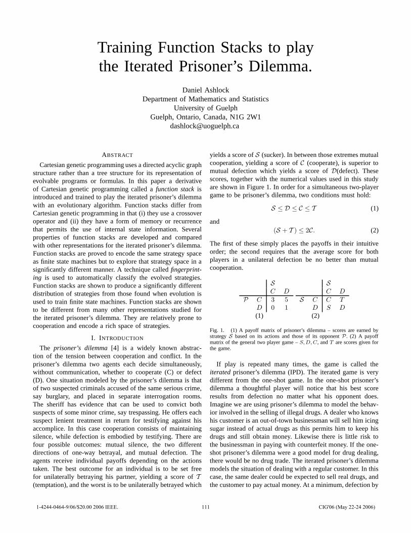
Training Function Stacks to playthe Iterated Prisoner’s Dilemma.

Daniel AshlockDepartment of Mathematics and Statistics

University of GuelphGuelph, Ontario, Canada, N1G 2W1

dashlock@uoguelph.ca

ABSTRACT

Cartesian genetic programming uses a directed acyclic graphstructure rather than a tree structure for its representation ofevolvable programs or formulas. In this paper a derivativeof Cartesian genetic programming called a function stack isintroduced and trained to play the iterated prisoner’s dilemmawith an evolutionary algorithm. Function stacks differ fromCartesian genetic programming in that (i) they use a crossoveroperator and (ii) they have a form of memory or recurrencethat permits the use of internal state information. Severalproperties of function stacks are developed and comparedwith other representations for the iterated prisoner’s dilemma.Function stacks are proved to encode the same strategy spaceas finite state machines but to explore that strategy space in asignificantly different manner. A technique called fingerprint-ing is used to automatically classify the evolved strategies.Function stacks are shown to produce a significantly differentdistribution of strategies from those found when evolution isused to train finite state machines. Function stacks are shownto be different from many other representations studied forthe iterated prisoner’s dilemma. They are relatively prone tocooperation and encode a rich space of strategies.

I. INTRODUCTION

The prisoner’s dilemma [4] is a widely known abstrac-tion of the tension between cooperation and conflict. In theprisoner’s dilemma two agents each decide simultaneously,without communication, whether to cooperate (C) or defect(D). One situation modeled by the prisoner’s dilemma is thatof two suspected criminals accused of the same serious crime,say burglary, and placed in separate interrogation rooms.The sheriff has evidence that can be used to convict bothsuspects of some minor crime, say trespassing. He offers eachsuspect lenient treatment in return for testifying against hisaccomplice. In this case cooperation consists of maintainingsilence, while defection is embodied by testifying. There arefour possible outcomes: mutual silence, the two differentdirections of one-way betrayal, and mutual defection. Theagents receive individual payoffs depending on the actionstaken. The best outcome for an individual is to be set freefor unilaterally betraying his partner, yielding a score of T

(temptation), and the worst is to be unilaterally betrayed which

yields a score of S (sucker). In between those extremes mutualcooperation, yielding a score of C (cooperate), is superior tomutual defection which yields a score of D(defect). Thesescores, together with the numerical values used in this studyare shown in Figure 1. In order for a simultaneous two-playergame to be prisoner’s dilemma, two conditions must hold:

S ≤ D ≤ C ≤ T (1)

and(S + T ) ≤ 2C. (2)

The first of these simply places the payoffs in their intuitiveorder; the second requires that the average score for bothplayers in a unilateral defection be no better than mutualcooperation.

S

C D

P C 3 5D 0 1(1)

S

C D

S C C T

D S D

(2)

Fig. 1. (1) A payoff matrix of prisoner’s dilemma – scores are earned bystrategy S based on its actions and those of its opponent P . (2) A payoffmatrix of the general two player game – S,D,C, and T are scores given forthe game.

If play is repeated many times, the game is called theiterated prisoner’s dilemma (IPD). The iterated game is verydifferent from the one-shot game. In the one-shot prisoner’sdilemma a thoughtful player will notice that his best scoreresults from defection no matter what his opponent does.Imagine we are using prisoner’s dilemma to model the behav-ior involved in the selling of illegal drugs. A dealer who knowshis customer is an out-of-town businessman will sell him icingsugar instead of actual drugs as this permits him to keep hisdrugs and still obtain money. Likewise there is little risk tothe businessman in paying with counterfeit money. If the one-shot prisoner’s dilemma were a good model for drug dealing,there would be no drug trade. The iterated prisoner’s dilemmamodels the situation of dealing with a regular customer. In thiscase, the same dealer could be expected to sell real drugs, andthe customer to pay actual money. At a minimum, defection by

1-4244-0464-9/06/$20.00 2006 IEEE. 111 CIG'06 (May 22-24 2006)

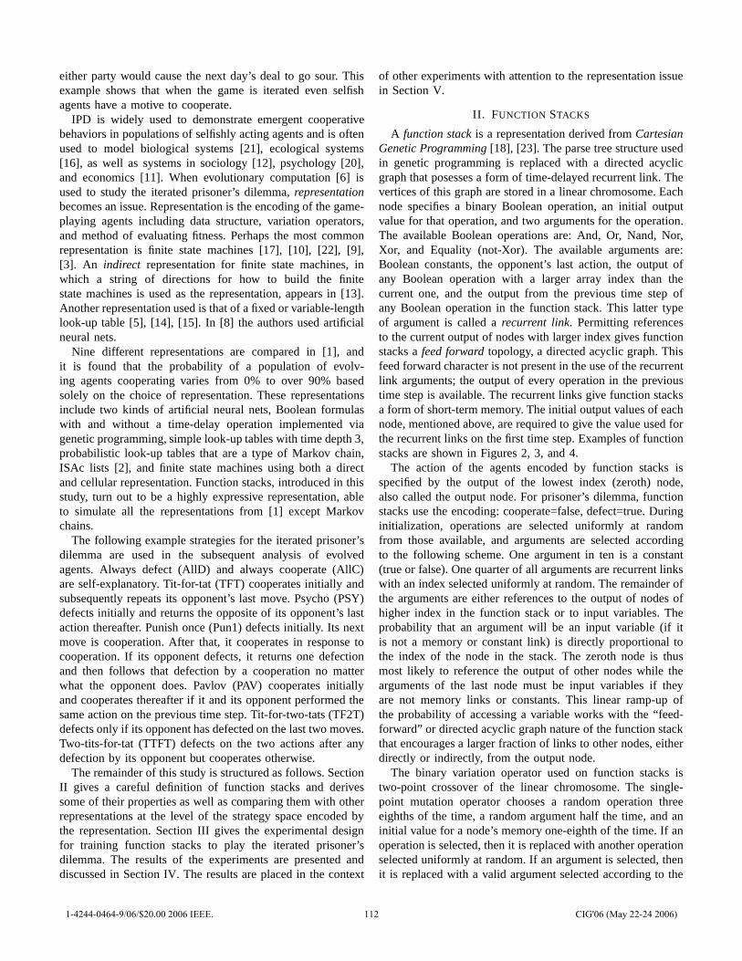
either party would cause the next day’s deal to go sour. Thisexample shows that when the game is iterated even selfishagents have a motive to cooperate.

IPD is widely used to demonstrate emergent cooperativebehaviors in populations of selfishly acting agents and is oftenused to model biological systems [21], ecological systems[16], as well as systems in sociology [12], psychology [20],and economics [11]. When evolutionary computation [6] isused to study the iterated prisoner’s dilemma, representationbecomes an issue. Representation is the encoding of the game-playing agents including data structure, variation operators,and method of evaluating fitness. Perhaps the most commonrepresentation is finite state machines [17], [10], [22], [9],[3]. An indirect representation for finite state machines, inwhich a string of directions for how to build the finitestate machines is used as the representation, appears in [13].Another representation used is that of a fixed or variable-lengthlook-up table [5], [14], [15]. In [8] the authors used artificialneural nets.

Nine different representations are compared in [1], andit is found that the probability of a population of evolv-ing agents cooperating varies from 0% to over 90% basedsolely on the choice of representation. These representationsinclude two kinds of artificial neural nets, Boolean formulaswith and without a time-delay operation implemented viagenetic programming, simple look-up tables with time depth 3,probabilistic look-up tables that are a type of Markov chain,ISAc lists [2], and finite state machines using both a directand cellular representation. Function stacks, introduced in thisstudy, turn out to be a highly expressive representation, ableto simulate all the representations from [1] except Markovchains.

The following example strategies for the iterated prisoner’sdilemma are used in the subsequent analysis of evolvedagents. Always defect (AllD) and always cooperate (AllC)are self-explanatory. Tit-for-tat (TFT) cooperates initially andsubsequently repeats its opponent’s last move. Psycho (PSY)defects initially and returns the opposite of its opponent’s lastaction thereafter. Punish once (Pun1) defects initially. Its nextmove is cooperation. After that, it cooperates in response tocooperation. If its opponent defects, it returns one defectionand then follows that defection by a cooperation no matterwhat the opponent does. Pavlov (PAV) cooperates initiallyand cooperates thereafter if it and its opponent performed thesame action on the previous time step. Tit-for-two-tats (TF2T)defects only if its opponent has defected on the last two moves.Two-tits-for-tat (TTFT) defects on the two actions after anydefection by its opponent but cooperates otherwise.

The remainder of this study is structured as follows. SectionII gives a careful definition of function stacks and derivessome of their properties as well as comparing them with otherrepresentations at the level of the strategy space encoded bythe representation. Section III gives the experimental designfor training function stacks to play the iterated prisoner’sdilemma. The results of the experiments are presented anddiscussed in Section IV. The results are placed in the context

of other experiments with attention to the representation issuein Section V.

II. FUNCTION STACKS

A function stack is a representation derived from CartesianGenetic Programming [18], [23]. The parse tree structure usedin genetic programming is replaced with a directed acyclicgraph that posesses a form of time-delayed recurrent link. Thevertices of this graph are stored in a linear chromosome. Eachnode specifies a binary Boolean operation, an initial outputvalue for that operation, and two arguments for the operation.The available Boolean operations are: And, Or, Nand, Nor,Xor, and Equality (not-Xor). The available arguments are:Boolean constants, the opponent’s last action, the output ofany Boolean operation with a larger array index than thecurrent one, and the output from the previous time step ofany Boolean operation in the function stack. This latter typeof argument is called a recurrent link. Permitting referencesto the current output of nodes with larger index gives functionstacks a feed forward topology, a directed acyclic graph. Thisfeed forward character is not present in the use of the recurrentlink arguments; the output of every operation in the previoustime step is available. The recurrent links give function stacksa form of short-term memory. The initial output values of eachnode, mentioned above, are required to give the value used forthe recurrent links on the first time step. Examples of functionstacks are shown in Figures 2, 3, and 4.

The action of the agents encoded by function stacks isspecified by the output of the lowest index (zeroth) node,also called the output node. For prisoner’s dilemma, functionstacks use the encoding: cooperate=false, defect=true. Duringinitialization, operations are selected uniformly at randomfrom those available, and arguments are selected accordingto the following scheme. One argument in ten is a constant(true or false). One quarter of all arguments are recurrent linkswith an index selected uniformly at random. The remainder ofthe arguments are either references to the output of nodes ofhigher index in the function stack or to input variables. Theprobability that an argument will be an input variable (if itis not a memory or constant link) is directly proportional tothe index of the node in the stack. The zeroth node is thusmost likely to reference the output of other nodes while thearguments of the last node must be input variables if theyare not memory links or constants. This linear ramp-up ofthe probability of accessing a variable works with the “feed-forward” or directed acyclic graph nature of the function stackthat encourages a larger fraction of links to other nodes, eitherdirectly or indirectly, from the output node.

The binary variation operator used on function stacks istwo-point crossover of the linear chromosome. The single-point mutation operator chooses a random operation threeeighths of the time, a random argument half the time, and aninitial value for a node’s memory one-eighth of the time. If anoperation is selected, then it is replaced with another operationselected uniformly at random. If an argument is selected, thenit is replaced with a valid argument selected according to the

1-4244-0464-9/06/$20.00 2006 IEEE. 112 CIG'06 (May 22-24 2006)

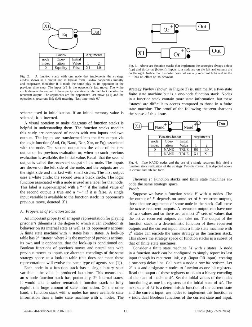
X1OutEq −

Pavlov Argumentsnode Oper- Initialindex ation Value 1 2

0 Equality False X1 L0

Fig. 2. A function stack with one node that implements the strategyPavlov shown as a circuit and in tabular form. Pavlov cooperates initiallyand cooperates thereafter if it made the same play as its opponent in theprevious time step. The input X1 is the opponent’s last move. The whitecircle denotes the output of the equality operation while the black denotes therecurrent output. The arguments are the opponent’s last move (X1) and theoperation’s recurrent link (L0) meaning “last-time node 0.”

scheme used in initialization. If an initial memory value isselected, it is inverted.

A visual notation to make diagrams of function stacks ishelpful in understanding them. The function stacks used inthis study are composed of nodes with two inputs and twooutputs. The inputs are transformed into the first output viathe logic function (And, Or, Nand, Nor, Xor, or Eq) associatedwith the node. The second output has the value of the firstoutput on its previous evaluation or, when no such previousevaluation is available, the initial value. Recall that the secondoutput is called the recurrent output of the node. The inputsare shown on the left side of the node, and the outputs are onthe right side and marked with small circles. The first outputuses a white circle; the second uses a black circle. The logicfunction associated with a node is used as a label for that node.This label is super-scripted with a “+” if the initial value ofthe second output is true and a “−” if it is false. A singleinput variable is available to the function stack: its opponent’sprevious move, denoted X1.

A. Properties of Function Stacks

An important property of an agent representation for playingprisoner’s dilemma is the degree to which it can condition itsbehavior on its internal state as well as its opponent’s actions.A finite state machine with n states has n states. A look-uptable has 2k “states” where k is the number of previous actions,its own and it opponents, that the look-up is conditioned on.Boolean functions of previous moves and neural nets withprevious moves as inputs are alternate encodings of the samestrategy space as a look-up table (this does not mean theserepresentations will evolve the same type of agents, see [1]).

Each node in a function stack has a single binary statevariable - the value it produced last time. This means thatan n-node function stack has, potentially, 2n internal states.It would take a rather remarkable function stack to fullyexploit this huge amount of state information. On the otherhand, a function stack with n nodes has more available stateinformation than a finite state machine with n nodes. The

+ OutOr

+OrX1 Out

Fig. 3. Above are function stacks that implement the strategies always-defect(top) and tit-for-tat (bottom). Inputs to a node are on the left and outputs areon the right. Notice that tit-for-tat does not use any recurrent links and so the“+” has no effect on its behavior.

strategy Pavlov (shown in Figure 2) is, minimally, a two-statefinite state machine but is a one-node function stack. Nodesin a function stack contain more state information, but these“states” are difficult to access compared to those in a finitestate machine. The proof of the following theorem sharpensthe sense of this issue.

X1 Nand+ Nand+ Out

Two-tits-for-tat Argumentsnode Oper- Initialindex ation Value 1 2

0 NAND TRUE R0 L01 NAND TRUE X1 X1

Fig. 4. Two NAND nodes and the use of a single recurrent link yield afunction stack realization of the strategy Two-tits-for-tat. It is depicted abovein circuit and tabular form.

Theorem 1: Function stacks and finite state machines en-code the same strategy space.Proof:

Suppose we have a function stack F with n nodes. Thethe output of F depends on some set of k recurrent outputs,those that are arguments of some node in the stack. Call thesethe active recurrent outputs. A recurrent output can have oneof two values and so there are at most 2k sets of values thatthe active recurrent outputs can take on. The output of thefunction stack is a deterministic function of these recurrentoutputs and the current input. Thus a finite state machine with2k states can encode the same strategy as the function stack.This shows the strategy space of function stacks is a subset ofthat of finite state machines.

Consider a finite state machine M with s states. A nodein a function stack can be configured to simply report its lastinput though its recurrent link, e.g. (input OR input), creatinga one-step delay line. Call such a node a one bit register. Let2r > s and designate r nodes to function as one bit registers.Read the output of these registers to obtain a binary encodingof the state of machine M . Set the initial values of the nodesfunctioning as one bit registers to the initial state of M . Thenext state of M is a deterministic function of the current stateand the current input; use nodes to implement this function asr individual Boolean functions of the current state and input.

1-4244-0464-9/06/$20.00 2006 IEEE. 113 CIG'06 (May 22-24 2006)

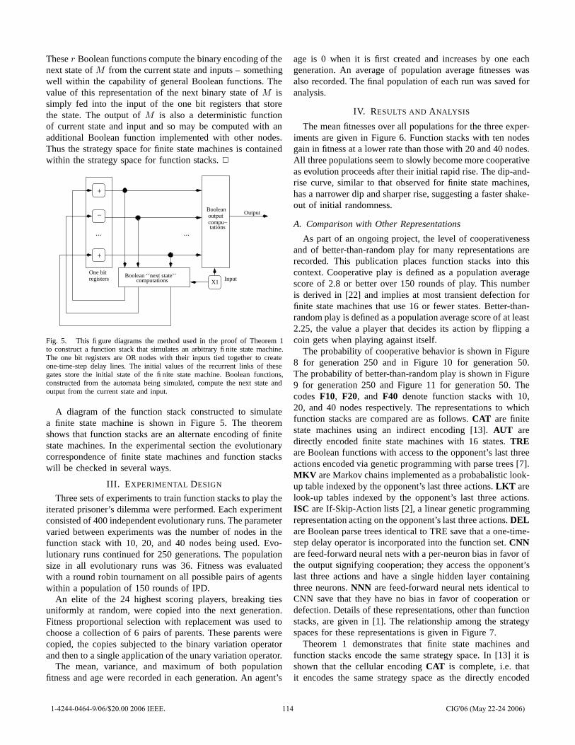
These r Boolean functions compute the binary encoding of thenext state of M from the current state and inputs – somethingwell within the capability of general Boolean functions. Thevalue of this representation of the next binary state of M issimply fed into the input of the one bit registers that storethe state. The output of M is also a deterministic functionof current state and input and so may be computed with anadditional Boolean function implemented with other nodes.Thus the strategy space for finite state machines is containedwithin the strategy space for function stacks. 2

����

����

����

...

Boolean ‘‘next state’’computations

One bitregisters

output

...

X1 Input

Boolean

compu−tations

Output

+

−

+

Fig. 5. This figure diagrams the method used in the proof of Theorem 1to construct a function stack that simulates an arbitrary finite state machine.The one bit registers are OR nodes with their inputs tied together to createone-time-step delay lines. The initial values of the recurrent links of thesegates store the initial state of the finite state machine. Boolean functions,constructed from the automata being simulated, compute the next state andoutput from the current state and input.

A diagram of the function stack constructed to simulatea finite state machine is shown in Figure 5. The theoremshows that function stacks are an alternate encoding of finitestate machines. In the experimental section the evolutionarycorrespondence of finite state machines and function stackswill be checked in several ways.

III. EXPERIMENTAL DESIGN

Three sets of experiments to train function stacks to play theiterated prisoner’s dilemma were performed. Each experimentconsisted of 400 independent evolutionary runs. The parametervaried between experiments was the number of nodes in thefunction stack with 10, 20, and 40 nodes being used. Evo-lutionary runs continued for 250 generations. The populationsize in all evolutionary runs was 36. Fitness was evaluatedwith a round robin tournament on all possible pairs of agentswithin a population of 150 rounds of IPD.

An elite of the 24 highest scoring players, breaking tiesuniformly at random, were copied into the next generation.Fitness proportional selection with replacement was used tochoose a collection of 6 pairs of parents. These parents werecopied, the copies subjected to the binary variation operatorand then to a single application of the unary variation operator.

The mean, variance, and maximum of both populationfitness and age were recorded in each generation. An agent’s

age is 0 when it is first created and increases by one eachgeneration. An average of population average fitnesses wasalso recorded. The final population of each run was saved foranalysis.

IV. RESULTS AND ANALYSIS

The mean fitnesses over all populations for the three exper-iments are given in Figure 6. Function stacks with ten nodesgain in fitness at a lower rate than those with 20 and 40 nodes.All three populations seem to slowly become more cooperativeas evolution proceeds after their initial rapid rise. The dip-and-rise curve, similar to that observed for finite state machines,has a narrower dip and sharper rise, suggesting a faster shake-out of initial randomness.

A. Comparison with Other Representations

As part of an ongoing project, the level of cooperativenessand of better-than-random play for many representations arerecorded. This publication places function stacks into thiscontext. Cooperative play is defined as a population averagescore of 2.8 or better over 150 rounds of play. This numberis derived in [22] and implies at most transient defection forfinite state machines that use 16 or fewer states. Better-than-random play is defined as a population average score of at least2.25, the value a player that decides its action by flipping acoin gets when playing against itself.

The probability of cooperative behavior is shown in Figure8 for generation 250 and in Figure 10 for generation 50.The probability of better-than-random play is shown in Figure9 for generation 250 and Figure 11 for generation 50. Thecodes F10, F20, and F40 denote function stacks with 10,20, and 40 nodes respectively. The representations to whichfunction stacks are compared are as follows. CAT are finitestate machines using an indirect encoding [13]. AUT aredirectly encoded finite state machines with 16 states. TREare Boolean functions with access to the opponent’s last threeactions encoded via genetic programming with parse trees [7].MKV are Markov chains implemented as a probabalistic look-up table indexed by the opponent’s last three actions. LKT arelook-up tables indexed by the opponent’s last three actions.ISC are If-Skip-Action lists [2], a linear genetic programmingrepresentation acting on the opponent’s last three actions. DELare Boolean parse trees identical to TRE save that a one-time-step delay operator is incorporated into the function set. CNNare feed-forward neural nets with a per-neuron bias in favor ofthe output signifying cooperation; they access the opponent’slast three actions and have a single hidden layer containingthree neurons. NNN are feed-forward neural nets identical toCNN save that they have no bias in favor of cooperation ordefection. Details of these representations, other than functionstacks, are given in [1]. The relationship among the strategyspaces for these representations is given in Figure 7.

Theorem 1 demonstrates that finite state machines andfunction stacks encode the same strategy space. In [13] it isshown that the cellular encoding CAT is complete, i.e. thatit encodes the same strategy space as the directly encoded

1-4244-0464-9/06/$20.00 2006 IEEE. 114 CIG'06 (May 22-24 2006)

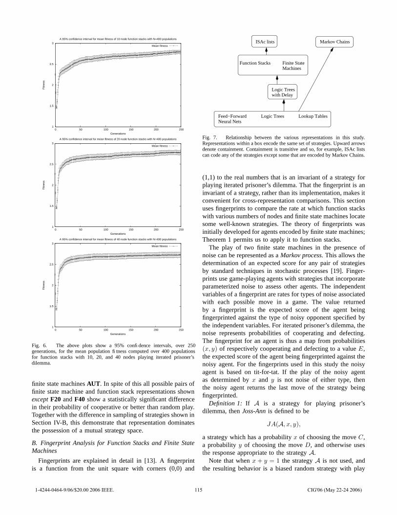
1

1.5

2

2.5

3

0 50 100 150 200 250

Fitn

ess

Generations

A 95% confidence interval for mean fitness of 10 node function stacks with N=400 populations

Mean fitness

1

1.5

2

2.5

3

0 50 100 150 200 250

Fitn

ess

Generations

A 95% confidence interval for mean fitness of 20 node function stacks with N=400 populations

Mean fitness

1

1.5

2

2.5

3

0 50 100 150 200 250

Fitn

ess

Generations

A 95% confidence interval for mean fitness of 40 node function stacks with N=400 populations

Mean fitness

Fig. 6. The above plots show a 95% confidence intervals, over 250generations, for the mean population fitness computed over 400 populationsfor function stacks with 10, 20, and 40 nodes playing iterated prisoner’sdilemma.

finite state machines AUT. In spite of this all possible pairs offinite state machine and function stack representations shownexcept F20 and F40 show a statistically significant differencein their probability of cooperative or better than random play.Together with the difference in sampling of strategies shown inSection IV-B, this demonstrate that representation dominatesthe possession of a mutual strategy space.

B. Fingerprint Analysis for Function Stacks and Finite StateMachines

Fingerprints are explained in detail in [13]. A fingerprintis a function from the unit square with corners (0,0) and

Feed−ForwardNeural Nets

Logic Trees Lookup Tables

Logic Treeswith Delay

Function Stacks Finite StateMachines

Markov ChainsISAc lists

Fig. 7. Relationship between the various representations in this study.Representations within a box encode the same set of strategies. Upward arrowsdenote containment. Containment is transitive and so, for example, ISAc listscan code any of the strategies except some that are encoded by Markov Chains.

(1,1) to the real numbers that is an invariant of a strategy forplaying iterated prisoner’s dilemma. That the fingerprint is aninvariant of a strategy, rather than its implementation, makes itconvenient for cross-representation comparisons. This sectionuses fingerprints to compare the rate at which function stackswith various numbers of nodes and finite state machines locatesome well-known strategies. The theory of fingerprints wasinitially developed for agents encoded by finite state machines;Theorem 1 permits us to apply it to function stacks.

The play of two finite state machines in the presence ofnoise can be represented as a Markov process. This allows thedetermination of an expected score for any pair of strategiesby standard techniques in stochastic processes [19]. Finger-prints use game-playing agents with strategies that incorporateparameterized noise to assess other agents. The independentvariables of a fingerprint are rates for types of noise associatedwith each possible move in a game. The value returnedby a fingerprint is the expected score of the agent beingfingerprinted against the type of noisy opponent specified bythe independent variables. For iterated prisoner’s dilemma, thenoise represents probabilities of cooperating and defecting.The fingerprint for an agent is thus a map from probabilities(x, y) of respectively cooperating and defecting to a value E,the expected score of the agent being fingerprinted against thenoisy agent. For the fingerprints used in this study the noisyagent is based on tit-for-tat. If the play of the noisy agentas determined by x and y is not noise of either type, thenthe noisy agent returns the last move of the strategy beingfingerprinted.

Definition 1: If A is a strategy for playing prisoner’sdilemma, then Joss-Ann is defined to be

JA(A, x, y),

a strategy which has a probability x of choosing the move C,a probability y of choosing the move D, and otherwise usesthe response appropriate to the strategy A.

Note that when x + y = 1 the strategy A is not used, andthe resulting behavior is a biased random strategy with play

1-4244-0464-9/06/$20.00 2006 IEEE. 115 CIG'06 (May 22-24 2006)

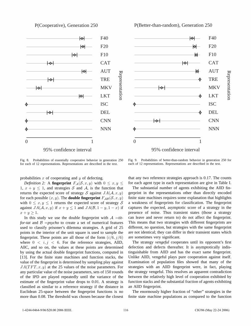
NNN

CNN

DEL

ISC

LKT

MKV

TRE

AUT

CAT

F10

F20

F40

0 1

95% confidence interval

P(Cooperative), Generation 250

Representation

Fig. 8. Probabilities of essentially cooperative behavior in generation 250for each of 12 representations. Representations are described in the text.

probabilities x of cooperating and y of defecting.Definition 2: A fingerprint FA(S, x, y) with 0 ≤ x, y ≤

1, x + y ≤ 1, and strategies S and A, is the function thatreturns the expected score of strategy S against JA(A, x, y)for each possible (x, y). The double fingerprint FAB(S, x, y)with 0 ≤ x, y ≤ 1 returns the expected score of strategy S

against JA(A, x, y) if x + y ≤ 1 and JA(B, 1 − y, 1 − x) ifx + y ≥ 1.

In this study we use the double fingerprint with A =tit-for-tat and B =psycho to create a set of numerical featuresused to classify prisoner’s dilemma strategies. A grid of 25points in the interior of the unit square is used to sample thefingerprint. These points are all those of the form (i/6, j/6)where 0 < i, j < 6. For the reference strategies, AllD,AllC, and so on, the values at these points are determinedby using the actual double fingerprint functions, computed in[13]. For the finite state machines and function stacks, thevalue of the fingerprint is determined by sampling play againstJA(TFT, x, y) at the 25 values of the noise parameters. Forany particular value of the noise parameters, sets of 150 roundsof the IPD are played repeatedly until the variance of theestimate of the fingerprint value drops to 0.01. A strategy isclassified as similar to a reference strategy if the distance inEuclidean 25-space between the fingerprint functions is nomore than 0.08. The threshold was chosen because the closest

NNN

CNN

DEL

ISC

LKT

MKV

TRE

AUT

CAT

F10

F20

F40

0 1

95% confidence interval

P(Better-than-random), Generation 250R

epresentation

Fig. 9. Probabilities of better-than-random behavior in generation 250 foreach of 12 representations. Representations are described in the text.

that any two reference strategies approach is 0.17. The countsfor each agent type in each representation are give in Table I.

The substantial number of agents exhibiting the AllD fin-gerprint in the representations other than directly encodedfinite state machines requires some explanation that highlightsa weakness of fingerprints for classification. The fingerprintcaptures the expected, asymptotic score of a strategy in thepresence of noise. Thus transient states (those a strategycan leave and never return to) do not affect the fingerprint.This means that two strategies with different fingerprints aredifferent, no question, but strategies with the same fingerprintare not identical; they can differ in their transient states whichare sometimes very significant.

The strategy vengeful cooperates until its opponent’s firstdefection and defects thereafter. It is asymptotically indis-tinguishable from AllD and has the exact same fingerprint.Unlike AllD, vengeful plays pure cooperation against itself.Examination of population files showed that many of thestrategies with an AllD fingerprint were, in fact, playingthe strategy vengeful. This resolves an apparent contradictionbetween the relatively high level of cooperation exhibited byfunction stacks and the substantial fraction of agents exhibitingan AllD fingerprint.

The enormously higher fraction of “other” strategies in thefinite state machine populations as compared to the function

1-4244-0464-9/06/$20.00 2006 IEEE. 116 CIG'06 (May 22-24 2006)

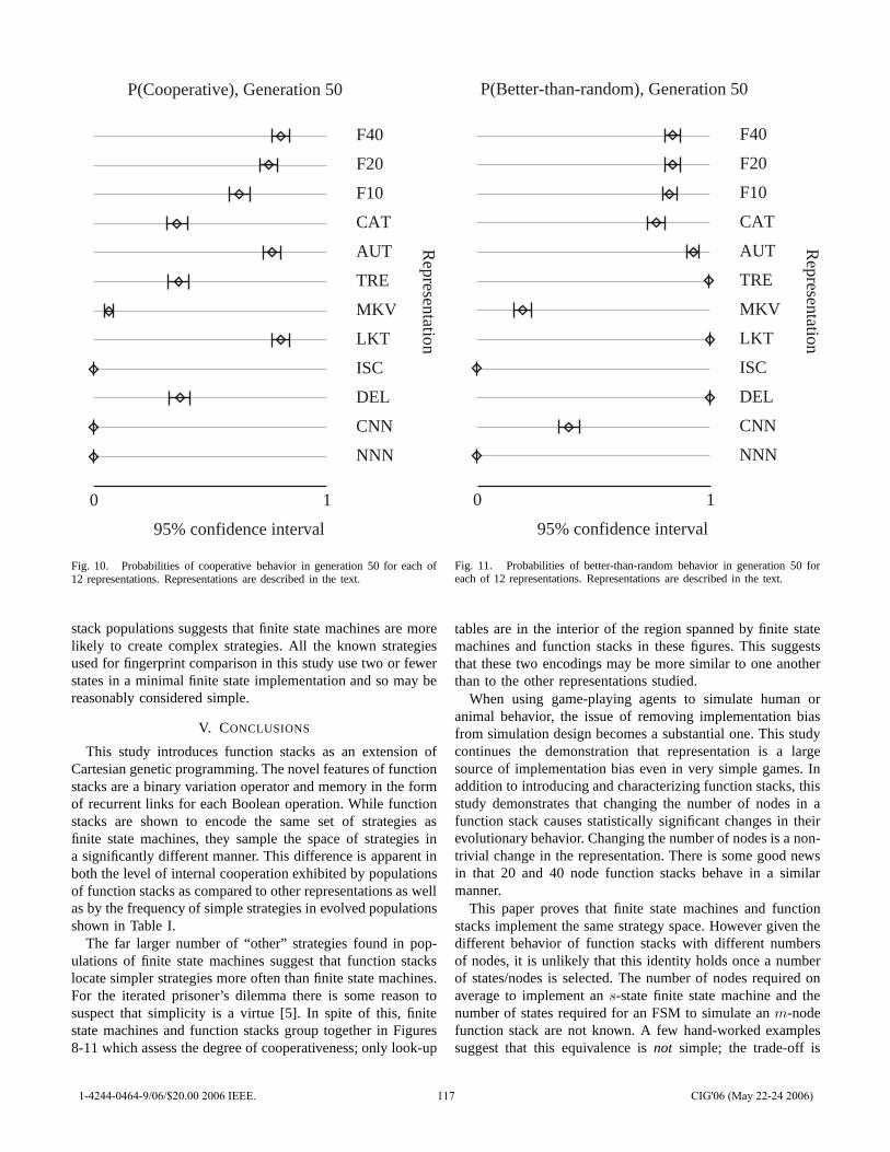
NNN

CNN

DEL

ISC

LKT

MKV

TRE

AUT

CAT

F10

F20

F40

0 1

95% confidence interval

P(Cooperative), Generation 50

Representation

Fig. 10. Probabilities of cooperative behavior in generation 50 for each of12 representations. Representations are described in the text.

stack populations suggests that finite state machines are morelikely to create complex strategies. All the known strategiesused for fingerprint comparison in this study use two or fewerstates in a minimal finite state implementation and so may bereasonably considered simple.

V. CONCLUSIONS

This study introduces function stacks as an extension ofCartesian genetic programming. The novel features of functionstacks are a binary variation operator and memory in the formof recurrent links for each Boolean operation. While functionstacks are shown to encode the same set of strategies asfinite state machines, they sample the space of strategies ina significantly different manner. This difference is apparent inboth the level of internal cooperation exhibited by populationsof function stacks as compared to other representations as wellas by the frequency of simple strategies in evolved populationsshown in Table I.

The far larger number of “other” strategies found in pop-ulations of finite state machines suggest that function stackslocate simpler strategies more often than finite state machines.For the iterated prisoner’s dilemma there is some reason tosuspect that simplicity is a virtue [5]. In spite of this, finitestate machines and function stacks group together in Figures8-11 which assess the degree of cooperativeness; only look-up

NNN

CNN

DEL

ISC

LKT

MKV

TRE

AUT

CAT

F10

F20

F40

0 1

95% confidence interval

P(Better-than-random), Generation 50R

epresentation

Fig. 11. Probabilities of better-than-random behavior in generation 50 foreach of 12 representations. Representations are described in the text.

tables are in the interior of the region spanned by finite statemachines and function stacks in these figures. This suggeststhat these two encodings may be more similar to one anotherthan to the other representations studied.

When using game-playing agents to simulate human oranimal behavior, the issue of removing implementation biasfrom simulation design becomes a substantial one. This studycontinues the demonstration that representation is a largesource of implementation bias even in very simple games. Inaddition to introducing and characterizing function stacks, thisstudy demonstrates that changing the number of nodes in afunction stack causes statistically significant changes in theirevolutionary behavior. Changing the number of nodes is a non-trivial change in the representation. There is some good newsin that 20 and 40 node function stacks behave in a similarmanner.

This paper proves that finite state machines and functionstacks implement the same strategy space. However given thedifferent behavior of function stacks with different numbersof nodes, it is unlikely that this identity holds once a numberof states/nodes is selected. The number of nodes required onaverage to implement an s-state finite state machine and thenumber of states required for an FSM to simulate an m-nodefunction stack are not known. A few hand-worked examplessuggest that this equivalence is not simple; the trade-off is

1-4244-0464-9/06/$20.00 2006 IEEE. 117 CIG'06 (May 22-24 2006)

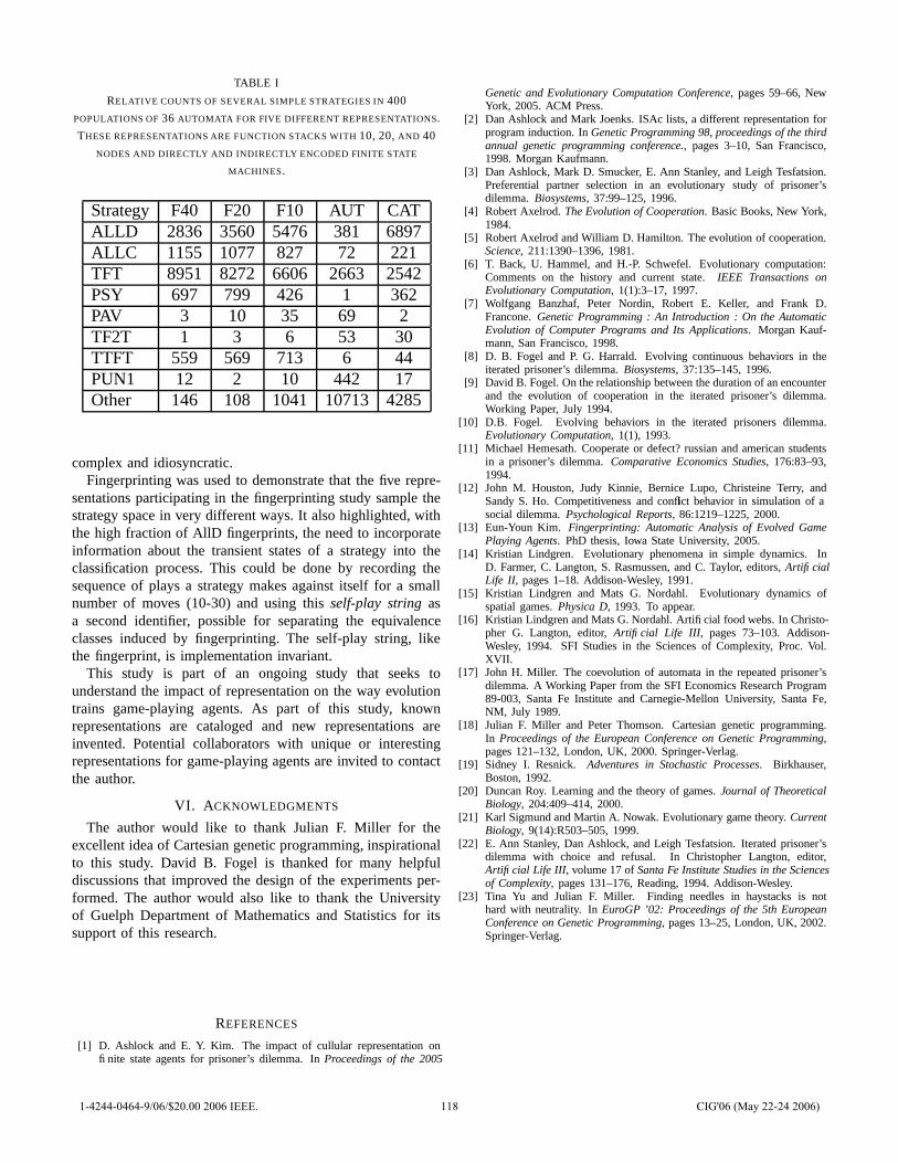
TABLE I

RELATIVE COUNTS OF SEVERAL SIMPLE STRATEGIES IN 400

POPULATIONS OF 36 AUTOMATA FOR FIVE DIFFERENT REPRESENTATIONS.

THESE REPRESENTATIONS ARE FUNCTION STACKS WITH 10, 20, AND 40

NODES AND DIRECTLY AND INDIRECTLY ENCODED FINITE STATE

MACHINES.

Strategy F40 F20 F10 AUT CATALLD 2836 3560 5476 381 6897ALLC 1155 1077 827 72 221TFT 8951 8272 6606 2663 2542PSY 697 799 426 1 362PAV 3 10 35 69 2TF2T 1 3 6 53 30TTFT 559 569 713 6 44PUN1 12 2 10 442 17Other 146 108 1041 10713 4285

complex and idiosyncratic.Fingerprinting was used to demonstrate that the five repre-

sentations participating in the fingerprinting study sample thestrategy space in very different ways. It also highlighted, withthe high fraction of AllD fingerprints, the need to incorporateinformation about the transient states of a strategy into theclassification process. This could be done by recording thesequence of plays a strategy makes against itself for a smallnumber of moves (10-30) and using this self-play string asa second identifier, possible for separating the equivalenceclasses induced by fingerprinting. The self-play string, likethe fingerprint, is implementation invariant.

This study is part of an ongoing study that seeks tounderstand the impact of representation on the way evolutiontrains game-playing agents. As part of this study, knownrepresentations are cataloged and new representations areinvented. Potential collaborators with unique or interestingrepresentations for game-playing agents are invited to contactthe author.

VI. ACKNOWLEDGMENTS

The author would like to thank Julian F. Miller for theexcellent idea of Cartesian genetic programming, inspirationalto this study. David B. Fogel is thanked for many helpfuldiscussions that improved the design of the experiments per-formed. The author would also like to thank the Universityof Guelph Department of Mathematics and Statistics for itssupport of this research.

REFERENCES

[1] D. Ashlock and E. Y. Kim. The impact of cullular representation onfinite state agents for prisoner’s dilemma. In Proceedings of the 2005

Genetic and Evolutionary Computation Conference, pages 59–66, NewYork, 2005. ACM Press.

[2] Dan Ashlock and Mark Joenks. ISAc lists, a different representation forprogram induction. In Genetic Programming 98, proceedings of the thirdannual genetic programming conference., pages 3–10, San Francisco,1998. Morgan Kaufmann.

[3] Dan Ashlock, Mark D. Smucker, E. Ann Stanley, and Leigh Tesfatsion.Preferential partner selection in an evolutionary study of prisoner’sdilemma. Biosystems, 37:99–125, 1996.

[4] Robert Axelrod. The Evolution of Cooperation. Basic Books, New York,1984.

[5] Robert Axelrod and William D. Hamilton. The evolution of cooperation.Science, 211:1390–1396, 1981.

[6] T. Back, U. Hammel, and H.-P. Schwefel. Evolutionary computation:Comments on the history and current state. IEEE Transactions onEvolutionary Computation, 1(1):3–17, 1997.

[7] Wolfgang Banzhaf, Peter Nordin, Robert E. Keller, and Frank D.Francone. Genetic Programming : An Introduction : On the AutomaticEvolution of Computer Programs and Its Applications. Morgan Kauf-mann, San Francisco, 1998.

[8] D. B. Fogel and P. G. Harrald. Evolving continuous behaviors in theiterated prisoner’s dilemma. Biosystems, 37:135–145, 1996.

[9] David B. Fogel. On the relationship between the duration of an encounterand the evolution of cooperation in the iterated prisoner’s dilemma.Working Paper, July 1994.

[10] D.B. Fogel. Evolving behaviors in the iterated prisoners dilemma.Evolutionary Computation, 1(1), 1993.

[11] Michael Hemesath. Cooperate or defect? russian and american studentsin a prisoner’s dilemma. Comparative Economics Studies, 176:83–93,1994.

[12] John M. Houston, Judy Kinnie, Bernice Lupo, Christeine Terry, andSandy S. Ho. Competitiveness and conflict behavior in simulation of asocial dilemma. Psychological Reports, 86:1219–1225, 2000.

[13] Eun-Youn Kim. Fingerprinting: Automatic Analysis of Evolved GamePlaying Agents. PhD thesis, Iowa State University, 2005.

[14] Kristian Lindgren. Evolutionary phenomena in simple dynamics. InD. Farmer, C. Langton, S. Rasmussen, and C. Taylor, editors, ArtificialLife II, pages 1–18. Addison-Wesley, 1991.

[15] Kristian Lindgren and Mats G. Nordahl. Evolutionary dynamics ofspatial games. Physica D, 1993. To appear.

[16] Kristian Lindgren and Mats G. Nordahl. Artificial food webs. In Christo-pher G. Langton, editor, Artificial Life III, pages 73–103. Addison-Wesley, 1994. SFI Studies in the Sciences of Complexity, Proc. Vol.XVII.

[17] John H. Miller. The coevolution of automata in the repeated prisoner’sdilemma. A Working Paper from the SFI Economics Research Program89-003, Santa Fe Institute and Carnegie-Mellon University, Santa Fe,NM, July 1989.

[18] Julian F. Miller and Peter Thomson. Cartesian genetic programming.In Proceedings of the European Conference on Genetic Programming,pages 121–132, London, UK, 2000. Springer-Verlag.

[19] Sidney I. Resnick. Adventures in Stochastic Processes. Birkhauser,Boston, 1992.

[20] Duncan Roy. Learning and the theory of games. Journal of TheoreticalBiology, 204:409–414, 2000.

[21] Karl Sigmund and Martin A. Nowak. Evolutionary game theory. CurrentBiology, 9(14):R503–505, 1999.

[22] E. Ann Stanley, Dan Ashlock, and Leigh Tesfatsion. Iterated prisoner’sdilemma with choice and refusal. In Christopher Langton, editor,Artificial Life III, volume 17 of Santa Fe Institute Studies in the Sciencesof Complexity, pages 131–176, Reading, 1994. Addison-Wesley.

[23] Tina Yu and Julian F. Miller. Finding needles in haystacks is nothard with neutrality. In EuroGP ’02: Proceedings of the 5th EuropeanConference on Genetic Programming, pages 13–25, London, UK, 2002.Springer-Verlag.

1-4244-0464-9/06/$20.00 2006 IEEE. 118 CIG'06 (May 22-24 2006)

Abstract— This paper looks at optimization problem solving from the standpoint of a predator/prey paradigm. In that paradigm, knowledge sources (or decision makers) control the placement of individuals onto a multi-dimensional landscape. Their score is the sum of the resources collected by each of the individuals that they control. While simple, this game has many of the properties present in much more complex real-time strategy games such as Age of Empires. In the next time step individuals are allocated from a fixed population to knowledge sources (empires) in proportion to the relative scores of the knowledge sources. This game is embedded in a Cultural Algorithm framework and we show how it can be used as a paradigm with which to study the optimization of an engineering design problem from a more strategic perspective.

Key Words: Cultural Algorithms, Prey/Predator Games, Optimization, Game AI, Evolutionary Computation.

I. INTRODUCTION

Recently, a number of socially motivated algorithms have been used to solve optimization problems. Some of the example algorithms are Particle Swarm Algorithm [1], Ant Colony Algorithm [2], and Cultural Algorithm [3]-[4]. These three algorithms all use a population-based model as the backbone of the algorithm and solve problems by sharing information via social interaction among agents in the population.

Here we develop a simple strategy game based upon a predator /prey analogy and use it as a framework in which to test different strategies for controlling search in a complex multi-dimensional domain. An individual collects a certain amount of renewable resources when placed at a location by a controlling knowledge source. Knowledge sources that are more successful in guiding individuals to above average collections are more likely to control more individuals from a fixed population in the next generation according to an influence function.

While the current game prototype allows up to five individuals, human or automated, we only use cultural algorithm knowledge sources to control the placement of

Robert G. Reynolds is a professor at Computer Science Department, Wayne State University, MI, 48202, USA, e-mail: reynolds@cs.wayne.edu.

Mostafa Ali, PhD candidate, Computer Science Department, Wayne State University, MI 48202, USA, e-mail: mostafa@wayne.edu.

Raja’ S. Alomari, PhD student, Computer Science Department, Wayne State University, MI, 48202, USA, e-mail: raja80@ wayne.edu.

individuals on a multi-dimensional landscape in this paper. In future work we will use different human players with different strategies in order to compare the relative impact of different strategy combinations for different resource distribution or optimization problems.

Based on Cultural Algorithms in the proposed game, we employ the basic set of knowledge sources that are supported by Cultural Algorithms. These knowledge sources are then combined to direct the decisions of the individuals (provinces following empires in our case) in solving optimization problems. Here we develop an algorithm based upon an analogy to the marginal value theorem in foraging theory to guide the integration of these different knowledge sources to direct the agent population. Various phases of problem solving emerge from the combined use of these knowledge sources and these phases result in the emergence of individual roles within the population in terms of leaders and followers. These roles result in organized swarming in the population and knowledge swarms in the social belief space.

Viewed as a real-time strategy game, our game has up to five players taking the role of empires (predators here) to join the game, each with a different strategy of playing and affecting surrounding preys (individual provinces), for the purpose of searching for a treasure placed randomly on the landscape according to a certain function, and the winner empire is the one having one or more of the individual follower preys reaching that final stage by finding the treasure and optimizing the state.

The rest of this paper is organized as follows: Section �II gives an overview of Cultural Algorithms. Section �III gives the theory behind the proposed game in this paper using a Cultural Algorithm framework. In section �IV the proposed game scenario is sketched. Experimental results are given in section �V. The paper is concluded in section �VI.

II. CULTURAL ALGORITHMS

The Cultural Algorithm (CA) is a class of computational models derived from observing the cultural evolution process in nature [4]. CA has three major components: a population space, a belief space, and a protocol that describes how knowledge is exchanged between the first two components. The population space can support any population-based computational model, such as Genetic Algorithms, and Evolutionary Programming. The basic framework is shown in fig. 1.

The Cultural Algorithm is a dual inheritance system that characterizes evolution in human culture at both the macro-

Robert G. Reynolds, Mostafa Ali, Raja’ S. Alomari

Optimization Problem Solving using Predator/Prey Games and Cultural Algorithms

1-4244-0464-9/06/$20.00 2006 IEEE. 119 CIG'06 (May 22-24 2006)

evolutionary level, which takes place within the belief space, and at the micro-evolutionary level, which occurs in the population space. Knowledge produced in the population space at the micro-evolutionary level is selectively accepted or passed to the belief space and used to adjust the knowledge structures there. This knowledge can then be used to influence the changes made by the population in the next generation. What differentiates Cultural Algorithms is the fact that the CA can use many knowledge types in the problem solving process rather than just one or two locally transmitted values. There are currently five distinct knowledge types used in the basic Cultural Algorithm: Normative, Situational, Domain, History, and Topographic knowledge There is evidence from the field of cognitive science that each of these knowledge types is supported by various animal species [5]-[6] and it is assumed that human social systems minimally support each of these knowledge types as well. The knowledge sources include normative knowledge (ranges of acceptable behaviors), situational knowledge (exemplars or memories of successful and unsuccessful solutions etc.), domain knowledge (knowledge of domain objects, their relationships, and interactions), history knowledge (temporal patterns of behavior), and topographical knowledge (spatial patterns of behavior). This set of categories is viewed as being complete for a given domain in the sense that all available knowledge can be expressed in terms of a combination of one of these classifications [19], and [7].

Cultural Algorithms have been studied with benchmark

optimization problems [8] as well as applied successfully in a number of diverse application areas such as modeling the evolution of agriculture [9], concept learning [3], real-valued function optimization [10], re-engineering of knowledge bases for the manufacturing assembly process, and agent-based modeling of price incentive systems [12] among others.

III. CULTURAL ALGORITHMS AS A PREY/PREDATOR GAME

In this paper we are concerned with using the Cultural Algorithms framework to simulate a Prey/Predator game. The knowledge sources exist in the belief space, and the individuals in the population space are controlled by these

empires (knowledge sources). Knowledge sources compete for control of the limited number of individuals over time.

A. Motivation: Peng [7] found the emergence of certain problem solving

phases in terms of the relative performance of different knowledge sources over time. She labeled these phases as coarse grained, fine grained, and backtracking phases. Each phase is characterized by the dominance of a suite or subset of the knowledge sources that are most successful in generating new solutions in that phase. In fact, the dominant subset of knowledge sources is often applied in a specific sequence within each phase. It appears that one type of knowledge produces new solutions that are consequently exploited by another knowledge source. Transitions between phases occur when the solutions produced by one phase can be better exploited by knowledge sources associated with the next phase.

If we view the knowledge sources as predators, then they can recruit individuals from a population to look for prey. The question is how does each predator shift the area over which they are looking in an automated fashion here? Here we take our clue from foraging theory. In foraging theory, it had been shown that the Marginal Value Theorem (MVT) was able under certain conditions to optimize the long-term average rate of energy intake within a patch-base environment [13]. The principle behind the Marginal Value Theorem is that residence time in a patch by a forager affects the expected energy gain. The marginal value principle states that the forager should reside in the patch "until the intake rate in a patch drops to the average rate for the habitat” [14]. It is the "moving-on threshold" intake rate that is important". The forager when doing so will maximize the average long term energy intake of the individual. One of the key assumptions is that the gain function associated with a patch is initially increasing but eventually negatively accelerated. Other assumptions are shown in fig. 2 taken from [15].

Fig. 3 gives a description of the calculation for a single patch. This figure is also taken from [15]. There are two quantities plotted on the abscissa, travel time or placement effort and patch residence time. Each of the knowledge sources in the influence function is viewed as a predator. Travel time increases from the origin (vertical line) to the left, and patch residence time increases from the origin to the right. The gain function shape exhibits an initial increase and then escalating decrease. The optimal residence time can be found by constructing a line tangent to the gain function that begins at the point (1/λ) on the travel time axis. The slope of this line is the long-term average rate of energy intake, because (1/λ) is the average time required to travel between patches. When the travel time is long (1/λ2), then the rate-maximizing residence time (t2) is long. When the travel time is short (1/λ1), then the rate-maximizing residence time (t1) is shorter. Here travel time is a constant amount that represents a model time step.

Fig. 1: Framework of Cultural Algorithms

1-4244-0464-9/06/$20.00 2006 IEEE. 120 CIG'06 (May 22-24 2006)

B. MVT and CA The choice of influence function has a great impact on the

problem solving process. Some influence functions are more successful than others, as measured by the success of the agents that each has influenced in the past. Early influence functions randomly applied the five knowledge sources to individuals in the population in order to guide their problem solving process. However, it was felt that some systematic application of the knowledge sources would be beneficial to the problem solving process.

Fig. 2: Summary of the Patch Model [15]

Fig. 3: The Marginal-Value Theorem in the One-Patch-Type Case [15].

It was felt that a good approach would optimize the rate at which resources are processed by the foraging agents as they searched for the optimum amount of resources. While the distribution was continuous it was observed that at each time step that the individuals generated by each knowledge source using a normal distribution could be described by a "bounding box" or patch with a given central tendency and standard deviation. For example, fig. 4 and fig. 5 show the shifting of the patch for situational knowledge from one place on the landscape to another. In fact, the original patch orientation is rotated and then translated towards the optimal point "+" over time.

Fig. 4: Situational Means and Standard Deviation at Year 1001.

Fig. 5: Situational Means and Standard Deviation at Year 1003.

Peng [7] developed an influence function based upon the

Marginal Value Theorem, MVI. The Marginal Value Theorem is implemented here in terms of a modification of the basic roulette wheel process so as to emulate the action of the energy intake function. The size of a knowledge sources area under the wheel is a function of its ability to produce above average gains. Each of the five knowledge sources, predators, is initially given 20% of the wheel area with which to generate their patch as shown in fig. 6.

The likelihood of using one of the knowledge sources is based on size of the area under the wheel and the area for a knowledge source (predator) is adjusted based upon its performance of those agents (preys) it influences. At every time step, each of the agents in the population is influenced by one of the knowledge sources based upon a spin of the

1/�2 2 1/�1 t1 t2 t2 Travel time

Patch residence

ASSUMPTIONS Decision The set of residence times for each patch type, ti for patch type i. Feasible choices: For all patch types 0� ti < �. Currency Maximization of long-term average rate of energy intake. Constraint C.1 Searching for and hunting within patches are mutually exclusive activities. C.2 Encounter with patches is sequential and is a Poisson process. C.3 Encounter rates when searching are independent of the residence times chosen. C.4 Net expected energy gain in a patch is related to residence time

by a well-defined gain function [gi(ti)] with the following characteristics:

(i) Change in energy gain is zero when zero time is spent in a patch. (ii) The function is initially increasing and eventually negatively

accelerated. C.5 Complete information is assumed. The forager knows the

model’s parameters and recognizes patch types, and it does not acquire and use information about patches while foraging in them.

IMPORTANT GENERAL POINTS 1. The model solves for an encounter-contingent policy. 2. Significant changes must be made to the model if the forager

assesses patch quality while hunting in patches. 3. The model applies only to patches with negatively accelerated gain

functions – patch depression. This should be confirmed by observation in empirical tests of the model.

4. The marginal-value condition (equation 1), gives only an implicit solution of the rate-maximizing patch residence time. It is incorrect to treat the average rate of energy intake, the right side of equation 1, as if it were independent of patch residence time.

iii

iiiiii

ctktg

tg+

+=λ

λ )()(' (1)

1-4244-0464-9/06/$20.00 2006 IEEE. 121 CIG'06 (May 22-24 2006)

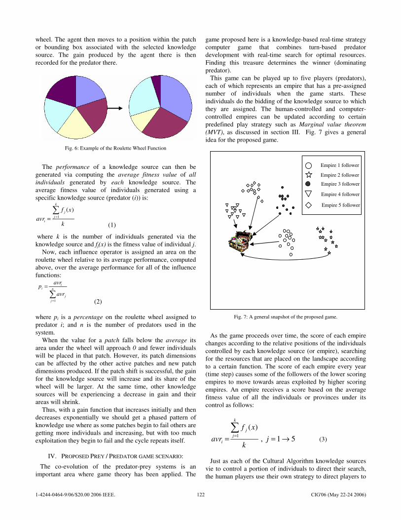
wheel. The agent then moves to a position within the patch or bounding box associated with the selected knowledge source. The gain produced by the agent there is then recorded for the predator there.

Fig. 6: Example of the Roulette Wheel Function

The performance of a knowledge source can then be

generated via computing the average fitness value of all individuals generated by each knowledge source. The average fitness value of individuals generated using a specific knowledge source (predator (i)) is:

k

xfavr

k

jj

i

�== 1

)(

(1)

where k is the number of individuals generated via the knowledge source and fj(x) is the fitness value of individual j. Now, each influence operator is assigned an area on the roulette wheel relative to its average performance, computed above, over the average performance for all of the influence functions:

�

=

= n

jj

ii

avr

avrp

1 (2) where pi is a percentage on the roulette wheel assigned to predator i; and n is the number of predators used in the system. When the value for a patch falls below the average its area under the wheel will approach 0 and fewer individuals will be placed in that patch. However, its patch dimensions can be affected by the other active patches and new patch dimensions produced. If the patch shift is successful, the gain for the knowledge source will increase and its share of the wheel will be larger. At the same time, other knowledge sources will be experiencing a decrease in gain and their areas will shrink. Thus, with a gain function that increases initially and then decreases exponentially we should get a phased pattern of knowledge use where as some patches begin to fail others are getting more individuals and increasing, but with too much exploitation they begin to fail and the cycle repeats itself.

IV. PROPOSED PREY / PREDATOR GAME SCENARIO:

The co-evolution of the predator-prey systems is an important area where game theory has been applied. The

game proposed here is a knowledge-based real-time strategy computer game that combines turn-based predator development with real-time search for optimal resources. Finding this treasure determines the winner (dominating predator).

This game can be played up to five players (predators), each of which represents an empire that has a pre-assigned number of individuals when the game starts. These individuals do the bidding of the knowledge source to which they are assigned. The human-controlled and computer-controlled empires can be updated according to certain predefined play strategy such as Marginal value theorem (MVT), as discussed in section �III. Fig. 7 gives a general idea for the proposed game.

Fig. 7: A general snapshot of the proposed game.

As the game proceeds over time, the score of each empire

changes according to the relative positions of the individuals controlled by each knowledge source (or empire), searching for the resources that are placed on the landscape according to a certain function. The score of each empire every year (time step) causes some of the followers of the lower scoring empires to move towards areas exploited by higher scoring empires. An empire receives a score based on the average fitness value of all the individuals or provinces under its control as follows:

51,)(

1 →==�

= jk

xfavr

k

jj

i (3)

Just as each of the Cultural Algorithm knowledge sources

vie to control a portion of individuals to direct their search, the human players use their own strategy to direct players to

Empire 1 follower

Empire 2 follower

Empire 3 follower

Empire 4 follower

Empire 5 follower

1-4244-0464-9/06/$20.00 2006 IEEE. 122 CIG'06 (May 22-24 2006)

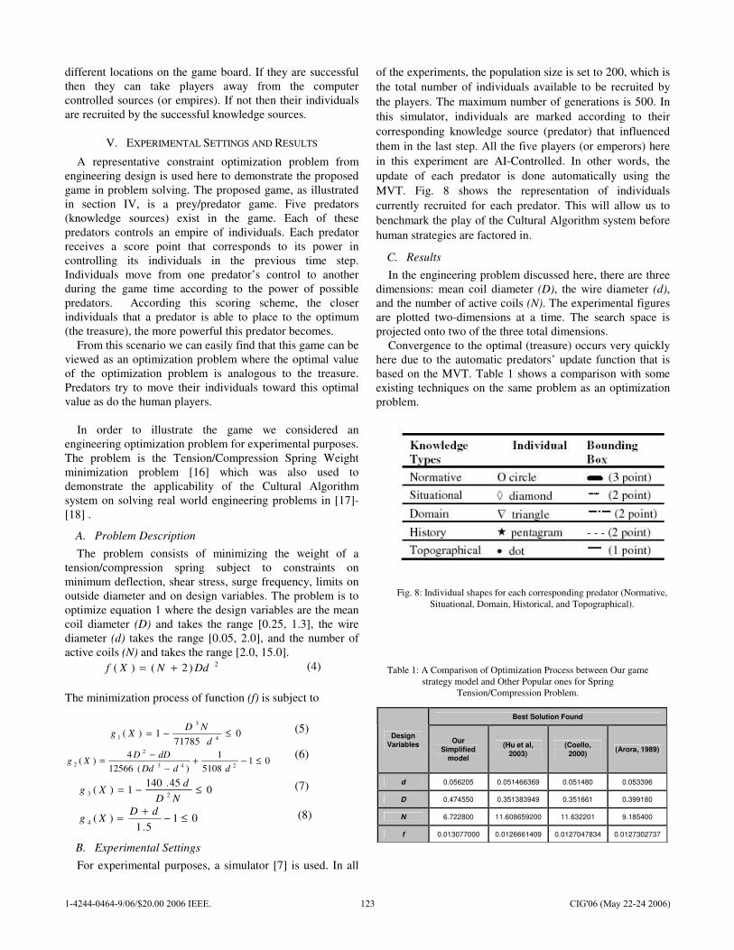
different locations on the game board. If they are successful then they can take players away from the computer controlled sources (or empires). If not then their individuals are recruited by the successful knowledge sources.

V. EXPERIMENTAL SETTINGS AND RESULTS

A representative constraint optimization problem from engineering design is used here to demonstrate the proposed game in problem solving. The proposed game, as illustrated in section �IV, is a prey/predator game. Five predators (knowledge sources) exist in the game. Each of these predators controls an empire of individuals. Each predator receives a score point that corresponds to its power in controlling its individuals in the previous time step. Individuals move from one predator’s control to another during the game time according to the power of possible predators. According this scoring scheme, the closer individuals that a predator is able to place to the optimum (the treasure), the more powerful this predator becomes.

From this scenario we can easily find that this game can be viewed as an optimization problem where the optimal value of the optimization problem is analogous to the treasure. Predators try to move their individuals toward this optimal value as do the human players.

In order to illustrate the game we considered an

engineering optimization problem for experimental purposes. The problem is the Tension/Compression Spring Weight minimization problem [16] which was also used to demonstrate the applicability of the Cultural Algorithm system on solving real world engineering problems in [17]-[18] .

A. Problem Description The problem consists of minimizing the weight of a

tension/compression spring subject to constraints on minimum deflection, shear stress, surge frequency, limits on outside diameter and on design variables. The problem is to optimize equation 1 where the design variables are the mean coil diameter (D) and takes the range [0.25, 1.3], the wire diameter (d) takes the range [0.05, 2.0], and the number of active coils (N) and takes the range [2.0, 15.0].

2)2()( DdNXf += (4)

The minimization process of function (f) is subject to

071785

1)( 4

3

1 ≤−=d

NDXg (5)

015108

1)(12566

4)(

243

2

2 ≤−+−

−=ddDd

dDDXg

(6)

045.140

1)( 23 ≤−=ND

dXg (7)

015.1

)(4 ≤−+= dDXg (8)

B. Experimental Settings For experimental purposes, a simulator [7] is used. In all

of the experiments, the population size is set to 200, which is the total number of individuals available to be recruited by the players. The maximum number of generations is 500. In this simulator, individuals are marked according to their corresponding knowledge source (predator) that influenced them in the last step. All the five players (or emperors) here in this experiment are AI-Controlled. In other words, the update of each predator is done automatically using the MVT. Fig. 8 shows the representation of individuals currently recruited for each predator. This will allow us to benchmark the play of the Cultural Algorithm system before human strategies are factored in.

C. Results In the engineering problem discussed here, there are three

dimensions: mean coil diameter (D), the wire diameter (d), and the number of active coils (N). The experimental figures are plotted two-dimensions at a time. The search space is projected onto two of the three total dimensions.

Convergence to the optimal (treasure) occurs very quickly here due to the automatic predators’ update function that is based on the MVT. Table 1 shows a comparison with some existing techniques on the same problem as an optimization problem.

Fig. 8: Individual shapes for each corresponding predator (Normative, Situational, Domain, Historical, and Topographical).

Table 1: A Comparison of Optimization Process between Our game strategy model and Other Popular ones for Spring

Tension/Compression Problem.

Best Solution Found

Design Variables Our

Simplified model

(Hu et al, 2003)

(Coello, 2000) (Arora, 1989)

d 0.056205 0.051466369 0.051480 0.053396

D 0.474550 0.351383949 0.351661 0.399180

N 6.722800 11.608659200 11.632201 9.185400

f 0.013077000 0.0126661409 0.0127047834 0.0127302737

1-4244-0464-9/06/$20.00 2006 IEEE. 123 CIG'06 (May 22-24 2006)

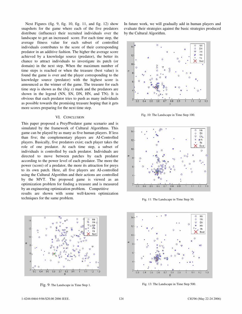
Next Figures (fig. 9, fig. 10, fig. 11, and fig. 12) show snapshots for the game where each of the five predators distribute (influence) their recruited individuals over the landscape to get an increased score. For each time step, the average fitness value for each subset of controlled individuals contributes to the score of their corresponding predator in an additive fashion. The higher the average score achieved by a knowledge source (predator), the better its chance to attract individuals to investigate its patch (or domain) in the next step. When the maximum number of time steps is reached or when the treasure (best value) is found the game is over and the player corresponding to the knowledge source (predator) with the highest score is announced as the winner of the game. The treasure for each time step is shown as the (big x) mark and the predators are shown in the legend (NN, SN, DN, HN, and TN). It is obvious that each predator tries to push as many individuals as possible towards the promising treasure hoping that it gets more scores preparing for the next time step.

VI. CONCLUSION

This paper proposed a Prey/Predator game scenario and is simulated by the framework of Cultural Algorithms. This game can be played by as many as five human players. If less than five; the complementary players are AI-Controlled players. Basically, five predators exist; each player takes the role of one predator. At each time step, a subset of individuals is controlled by each predator. Individuals are directed to move between patches by each predator according to the power level of each predator. The more the power (score) of a predator, the more its attraction for preys to its own patch. Here, all five players are AI-controlled using the Cultural Algorithm and their actions are controlled by the MVT. The proposed game is viewed as an optimization problem for finding a treasure and is measured by an engineering optimization problem. Competitive results are shown with some well-known optimization techniques for the same problem.

In future work, we will gradually add in human players and evaluate their strategies against the basic strategies produced by the Cultural Algorithm.

Fig. 11: The Landscape in Time Step 30.

Fig. 13: The Landscape in Time Step 500.

Fig. 10: The Landscape in Time Step 100.

Fig. 9: The Landscape in Time Step 1.

1-4244-0464-9/06/$20.00 2006 IEEE. 124 CIG'06 (May 22-24 2006)

REFERENCES [1] Eberhart, R. C., and Kennedy, J. (1995). A new optimizer using

particle swarm theory. Proceedings of the Sixth International Symposium on Micro Machine and Human Science, Nagoya, Japan, 39-43. Piscataway, NJ: IEEE Service Center.

[2] Dorigo M., V. Maniezzo & A. Colorni (1996). The Ant System: Optimization by a colony of cooperating agents. IEEE Transactions on Systems, Man, and Cybernetics-Part B, 26, 1, 29-41

[3] Reynolds, R., (1994). An introduction to Cultural Algorithms. Proceedings of the 3rd Annual Conference on Evolutionary Programming, Sebald, A.V., Fogel, L. J. Ed. World Scientific Publishing, River Edge, NJ, pp., 131-139.

[4] Reynolds, R. G. (1978). “On Modeling the Evolution of Hunter-Gatherer Decision-Making Systems”, Geographical Analysis, 10(1), 31-46.

[5] Wynne C. D. (2001). Animal Cognition - The Mental Lives of Animals. Palgrave Macmillan, Great Britain.

[6] Clayton, N. S., Griffiths, D. P., and Dickinson A. (2000). Declarative and Episodic-like Memory in Animals: Personal Musings of a Scrub Jay, in The Evolution of Cognition. Edited by Heyes, C. and Huber, L. the MIT Press, Cambridge, Massachusetts.

[7] Peng, B., (2005). “Knowledge and population swarms in Cultural Algorithms for dynamic environments,” PhD dissertation, Department of Computer Science, Wayne State University, MI, US.

[8] Chung, C., and Reynolds, R., (1998). CAEP.an evolution-based tool for real-valued function optimization using Cultural Algorithms. International Journal on Artificial Intelligence Tools, vol. 7, no. 3, pp. 239-291.

[9] Reynolds, R. G., "An Adaptive Computer Model for the Evolution of Plant Collecting and Early Agriculture in the Eastern Valley of Oaxaca", in Guila Naquitz: Archaic Foraging and Early Agriculture in Oaxaca, Mexico, K. V. Flannery, Editor, Academic Press, 1986. pp.

[10] Jin, X., and Reynolds, R., (1999). Using knowledge-based evolutionary computation to solve nonlinear constraint optimization problems: a Cultural Algorithm approach. In Proceeding of the 1999 Congress on Evolutionary Computation, pp. 1672-1678, Washington DC, US.

[11] Reynolds, R., and Saleem, S., (2005). The impact of environmental dynamics on cultural emergence: Perspectives on Adaptations in Natural and Artificial Systems. Oxford University Press, 253-280.

[12] Reynolds, R. G., and Ostrowski, D.*, “Using Cultural Algorithms to Evolve Strategies for Recessionary Markets”, in Proceedings of IEEE International Congress on Evolutionary Computation, Portland, OR, June 19-24, 2004, pp: 1780-1785.

[13] Charnov, E. L. (1976). Optimal foraging: the marginal value theorem. Theoretical Population Biology, 9, 129-136.

[14] Reynolds, R., Whallon, R., Ali, M., Zadegan, B., (2006). Agent-Based Modeling of early Cultural Evolution. IEEE World Congress on Computational Intelligence

[15] Stephens, D.W. and J.R. Krebs. (1986). Foraging theory Princeton, NJ: Princeton University Press.

[16] Hansen, L., and Salamon P., (1990). Neural network ensembles. IEEE Transactions on Pattern Analysis and Machine Intelligence, vol. 12, no. 10, pp. 993-1001.

[17] Reynolds, R., Peng, B., (2004). Cultural Algorithms: modeling of how cultures learn to solve problems. In 16th IEEE International Conference Tools with Artificial Intelligence (ICTAI’04), pp.166 – 172.

[18] Reynolds R., Peng B., and Alomari, R., (2006). Cultural Evolution of Ensemble Learning for Problem Solving. IEEE World Congress on Computational Intelligence (WCCI’06), July, Canada.

[19] Reynolds R., Peng B., and Alomari, R., (2006). The Role of Culture in the Emergence of Decision-Making Roles: An Example Using Cultural Algorithms. IEEE Swarm Intelligence Symposium 2006 (SIS’06). May, Indiana, USA.

1-4244-0464-9/06/$20.00 2006 IEEE. 125 CIG'06 (May 22-24 2006)

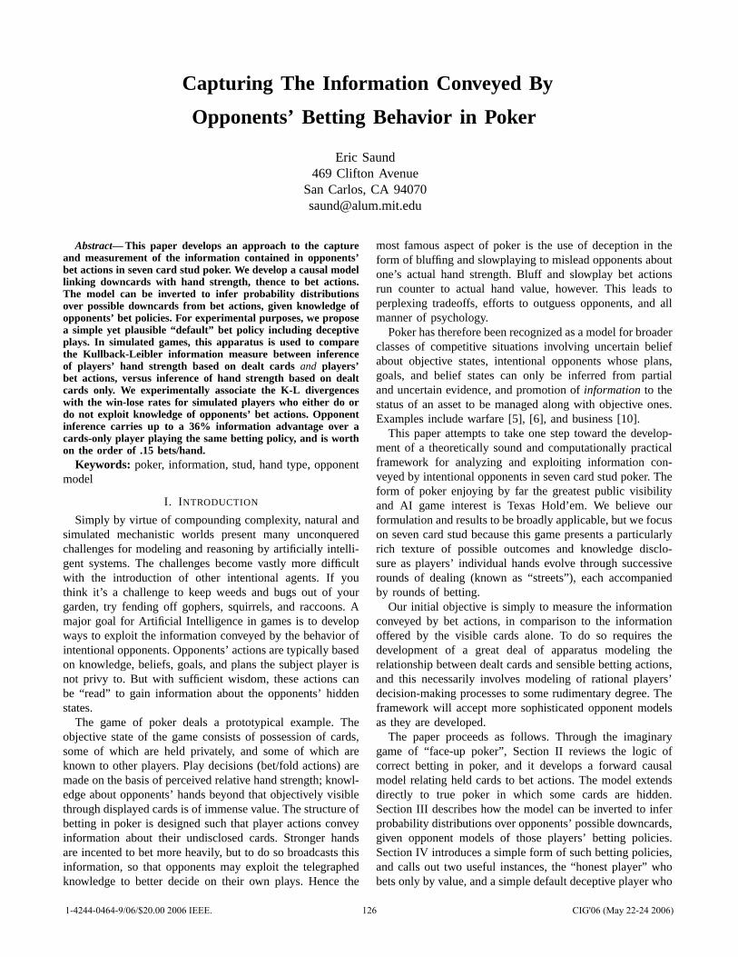
Capturing The Information Conveyed By

Opponents’ Betting Behavior in Poker

Eric Saund469 Clifton Avenue

San Carlos, CA 94070saund@alum.mit.edu

Abstract— This paper develops an approach to the captureand measurement of the information contained in opponents’bet actions in seven card stud poker. We develop a causal modellinking downcards with hand strength, thence to bet actions.The model can be inverted to infer probability distributionsover possible downcards from bet actions, given knowledge ofopponents’ bet policies. For experimental purposes, we proposea simple yet plausible “default” bet policy including deceptiveplays. In simulated games, this apparatus is used to comparethe Kullback-Leibler information measure between inferenceof players’ hand strength based on dealt cardsand players’bet actions, versus inference of hand strength based on dealtcards only. We experimentally associate the K-L divergenceswith the win-lose rates for simulated players who either do ordo not exploit knowledge of opponents’ bet actions. Opponentinference carries up to a 36% information advantage over acards-only player playing the same betting policy, and is worthon the order of .15 bets/hand.

Keywords: poker, information, stud, hand type, opponentmodel

I. I NTRODUCTION

Simply by virtue of compounding complexity, natural andsimulated mechanistic worlds present many unconqueredchallenges for modeling and reasoning by artificially intelli-gent systems. The challenges become vastly more difficultwith the introduction of other intentional agents. If youthink it’s a challenge to keep weeds and bugs out of yourgarden, try fending off gophers, squirrels, and raccoons. Amajor goal for Artificial Intelligence in games is to developways to exploit the information conveyed by the behavior ofintentional opponents. Opponents’ actions are typically basedon knowledge, beliefs, goals, and plans the subject player isnot privy to. But with sufficient wisdom, these actions canbe “read” to gain information about the opponents’ hiddenstates.

The game of poker deals a prototypical example. Theobjective state of the game consists of possession of cards,some of which are held privately, and some of which areknown to other players. Play decisions (bet/fold actions) aremade on the basis of perceived relative hand strength; knowl-edge about opponents’ hands beyond that objectively visiblethrough displayed cards is of immense value. The structure ofbetting in poker is designed such that player actions conveyinformation about their undisclosed cards. Stronger handsare incented to bet more heavily, but to do so broadcasts thisinformation, so that opponents may exploit the telegraphedknowledge to better decide on their own plays. Hence the

most famous aspect of poker is the use of deception in theform of bluffing and slowplaying to mislead opponents aboutone’s actual hand strength. Bluff and slowplay bet actionsrun counter to actual hand value, however. This leads toperplexing tradeoffs, efforts to outguess opponents, and allmanner of psychology.

Poker has therefore been recognized as a model for broaderclasses of competitive situations involving uncertain beliefabout objective states, intentional opponents whose plans,goals, and belief states can only be inferred from partialand uncertain evidence, and promotion ofinformation to thestatus of an asset to be managed along with objective ones.Examples include warfare [5], [6], and business [10].

This paper attempts to take one step toward the develop-ment of a theoretically sound and computationally practicalframework for analyzing and exploiting information con-veyed by intentional opponents in seven card stud poker. Theform of poker enjoying by far the greatest public visibilityand AI game interest is Texas Hold’em. We believe ourformulation and results to be broadly applicable, but we focuson seven card stud because this game presents a particularlyrich texture of possible outcomes and knowledge disclo-sure as players’ individual hands evolve through successiverounds of dealing (known as “streets”), each accompaniedby rounds of betting.

Our initial objective is simply to measure the informationconveyed by bet actions, in comparison to the informationoffered by the visible cards alone. To do so requires thedevelopment of a great deal of apparatus modeling therelationship between dealt cards and sensible betting actions,and this necessarily involves modeling of rational players’decision-making processes to some rudimentary degree. Theframework will accept more sophisticated opponent modelsas they are developed.

The paper proceeds as follows. Through the imaginarygame of “face-up poker”, Section II reviews the logic ofcorrect betting in poker, and it develops a forward causalmodel relating held cards to bet actions. The model extendsdirectly to true poker in which some cards are hidden.Section III describes how the model can be inverted to inferprobability distributions over opponents’ possible downcards,given opponent models of those players’ betting policies.Section IV introduces a simple form of such betting policies,and calls out two useful instances, the “honest player” whobets only by value, and a simple default deceptive player who

1-4244-0464-9/06/$20.00 2006 IEEE. 126 CIG'06 (May 22-24 2006)

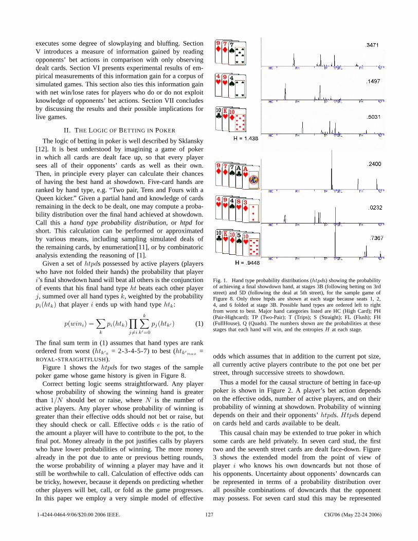
executes some degree of slowplaying and bluffing. SectionV introduces a measure of information gained by readingopponents’ bet actions in comparison with only observingdealt cards. Section VI presents experimental results of em-pirical measurements of this information gain for a corpus ofsimulated games. This section also ties this information gainwith net win/lose rates for players who do or do not exploitknowledge of opponents’ bet actions. Section VII concludesby discussing the results and their possible implications forlive games.

II. T HE LOGIC OFBETTING IN POKER

The logic of betting in poker is well described by Sklansky[12]. It is best understood by imagining a game of pokerin which all cards are dealt face up, so that every playersees all of their opponents’ cards as well as their own.Then, in principle every player can calculate their chancesof having the best hand at showdown. Five-card hands areranked by hand type, e.g. “Two pair, Tens and Fours with aQueen kicker.” Given a partial hand and knowledge of cardsremaining in the deck to be dealt, one may compute a proba-bility distribution over the final hand achieved at showdown.Call this a hand type probability distribution, or htpd forshort. This calculation can be performed or approximatedby various means, including sampling simulated deals ofthe remaining cards, by enumeration[11], or by combinatoricanalysis extending the reasoning of [1].

Given a set ofhtpds possessed by active players (playerswho have not folded their hands) the probability that playeri’s final showdown hand will beat all others is the conjunctionof events that his final hand typeht beats each other playerj, summed over all hand typesk, weighted by the probabilitypi(htk) that playeri ends up with hand typehtk:

p(wini) =∑

k

pi(htk)∏

j 6=i

k∑

k′=0

pj(htk′) (1)

The final sum term in (1) assumes that hand types are rankordered from worst (htk′

0= 2-3-4-5-7) to best (htk′

max=

ROYAL-STRAIGHTFLUSH).Figure 1 shows thehtpds for two stages of the sample

poker game whose game history is given in Figure 8.Correct betting logic seems straightforward. Any player

whose probability of showing the winning hand is greaterthan 1/N should bet or raise, whereN is the number ofactive players. Any player whose probability of winning isgreater than their effective odds should not bet or raise, butthey should check or call. Effective oddse is the ratio ofthe amount a player will have to contribute to the pot, to thefinal pot. Money already in the pot justifies calls by playerswho have lower probabilities of winning. The more moneyalready in the pot due to ante or previous betting rounds,the worse probability of winning a player may have and itstill be worthwhile to call. Calculation of effective odds canbe tricky, however, because it depends on predicting whetherother players will bet, call, or fold as the game progresses.In this paper we employ a very simple model of effective

Fig. 1. Hand type probability distributions (htpds) showing the probabilityof achieving a final showdown hand, at stages 3B (following betting on 3rdstreet) and 5D (following the deal at 5th street), for the sample game ofFigure 8. Only three htpds are shown at each stage because seats 1, 2,4, and 6 folded at stage 3B. Possible hand types are ordered left to rightfrom worst to best. Major hand categories listed are HC (HighCard); PH(Pair-Highcard); TP (Two-Pair); T (Trips); S (Straight); FL (Flush); FH(FullHouse), Q (Quads). The numbers shown are the probabilities at thesestages that each hand will win, and the entropiesH at each stage.

odds which assumes that in addition to the current pot size,all currently active players contribute to the pot one bet perstreet, through successive streets to showdown.

Thus a model for the causal structure of betting in face-uppoker is shown in Figure 2. A player’s bet action dependson the effective odds, number of active players, and on theirprobability of winning at showdown. Probability of winningdepends on their and their opponents’htpds. Htpds dependon cards held and cards available to be dealt.

This causal chain may be extended to true poker in whichsome cards are held privately. In seven card stud, the firsttwo and the seventh street cards are dealt face-down. Figure3 shows the extended model from the point of view ofplayer i who knows his own downcards but not those ofhis opponents. Uncertainty about opponents’ downcards canbe represented in terms of a probability distribution overall possible combinations of downcards that the opponentmay possess. For seven card stud this may be represented

1-4244-0464-9/06/$20.00 2006 IEEE. 127 CIG'06 (May 22-24 2006)

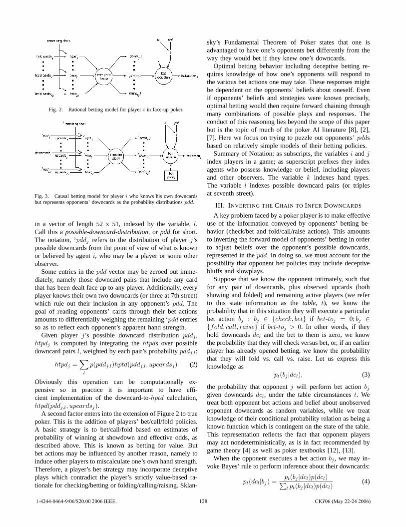
Fig. 2. Rational betting model for playeri in face-up poker.

Fig. 3. Causal betting model for playeri who knows his own downcardsbut represents opponents’ downcards as the probability distributionspdd.

in a vector of length 52 x 51, indexed by the variable,l.Call this apossible-downcard-distribution, or pdd for short.The notation,ipddj refers to the distribution of playerj’spossible downcards from the point of view of what is knownor believed by agenti, who may be a player or some otherobserver.

Some entries in thepdd vector may be zeroed out imme-diately, namely those downcard pairs that include any cardthat has been dealt face up to any player. Additionally, everyplayer knows their own two downcards (or three at 7th street)which rule out their inclusion in any opponent’spdd. Thegoal of reading opponents’ cards through their bet actionsamounts to differentially weighing the remainingipdd entriesso as to reflect each opponent’s apparent hand strength.

Given player j’s possible downcard distributionpddj ,htpdj is computed by integrating thehtpds over possibledowncard pairsl, weighted by each pair’s probabilitypddj,l:

htpdj =∑

l

p(pddj,l)hptd(pddj,l, upcardsj) (2)

Obviously this operation can be computationally ex-pensive so in practice it is important to have effi-cient implementation of the downcard-to-hptd calculation,htpd(pddj,l, upcardsj).

A second factor enters into the extension of Figure 2 to truepoker. This is the addition of players’ bet/call/fold policies.A basic strategy is to bet/call/fold based on estimates ofprobability of winning at showdown and effective odds, asdescribed above. This is known as betting for value. Butbet actions may be influenced by another reason, namely toinduce other players to miscalculate one’s own hand strength.Therefore, a player’s bet strategy may incorporate deceptiveplays which contradict the player’s strictly value-based ra-tionale for checking/betting or folding/calling/raising. Sklan-

sky’s Fundamental Theorem of Poker states that one isadvantaged to have one’s opponents bet differently from theway they would bet if they knew one’s downcards.

Optimal betting behavior including deceptive betting re-quires knowledge of how one’s opponents will respond tothe various bet actions one may take. These responses mightbe dependent on the opponents’ beliefs about oneself. Evenif opponents’ beliefs and strategies were known precisely,optimal betting would then require forward chaining throughmany combinations of possible plays and responses. Theconduct of this reasoning lies beyond the scope of this paperbut is the topic of much of the poker AI literature [8], [2],[7]. Here we focus on trying to puzzle out opponents’pddsbased on relatively simple models of their betting policies.

Summary of Notation: as subscripts, the variablesi andjindex players in a game; as superscript prefixes they indexagents who possess knowledge or belief, including playersand other observers. The variablek indexes hand types.The variablel indexes possible downcard pairs (or triplesat seventh street).

III. I NVERTING THE CHAIN TO INFER DOWNCARDS

A key problem faced by a poker player is to make effectiveuse of the information conveyed by opponents’ betting be-havior (check/bet and fold/call/raise actions). This amountsto inverting the forward model of opponents’ betting in orderto adjust beliefs over the opponent’s possible downcards,represented in thepdd. In doing so, we must account for thepossibility that opponent bet policies may include deceptivebluffs and slowplays.

Suppose that we know the opponent intimately, such thatfor any pair of downcards, plus observed upcards (bothshowing and folded) and remaining active players (we referto this state information as thetable, t), we know theprobability that in this situation they will execute a particularbet action bj : bj ∈ {check, bet} if bet-toj = 0; bj ∈{fold, call, raise} if bet-toj > 0. In other words, if theyhold downcardsdcl and the bet to them is zero, we knowthe probability that they will check versus bet, or, if an earlierplayer has already opened betting, we know the probabilitythat they will fold vs. call vs. raise. Let us express thisknowledge as

pt(bj |dcl), (3)

the probability that opponentj will perform bet actionbj

given downcardsdcl, under the table circumstancest. Wetreat both opponent bet actions and belief about unobservedopponent downcards as random variables, while we treatknowledge of their conditional probability relation as being aknown function which is contingent on the state of the table.This representation reflects the fact that opponent playersmay act nondeterministically, as is in fact recommended bygame theory [4] as well as poker textbooks [12], [13].

When the opponent executes a bet actionbj , we may in-voke Bayes’ rule to perform inference about their downcards:

pt(dcl|bj) =pt(bj |dcl)p(dcl)∑l pt(bj |dcl)p(dcl)

(4)

1-4244-0464-9/06/$20.00 2006 IEEE. 128 CIG'06 (May 22-24 2006)

The prior p(dcl) is the belief held that the opponent hasdowncardsdcl before we observed the bet action. This priorserves the role of carrying information forward from onestreet to the next. This calculation effectively performs are-weighting of the possible-downcard-distribution by thelikelihood of the bet action, followed by normalization.

Through implicit means, this mechanism achieves fairlysubtle and complex reasoning. Opponents’ actions of plac-ing a bet (as opposed to checking or calling) tend toreweigh more heavily the possible downcard pairs that wouldoffer that opponent a greater chance of winning giventheir upcards. Moreover, raises and re-raises weigh strongerdowncards more heavily still, through an additional mecha-nism. Because the model has every player re-estimating thestrength of every other players’ hand after every action, whenPlayer A bets, every other player will necessarily increasetheir belief that Player A has strong cards, which in turndecreases their beliefs in their own chances of winning. Thisnarrows the pool of possible downcards that any player musthold to meet Player A’s strength. So if Player B then goeson to raise or re-raise anyway, then for all of the playerstrying to estimate what Player B must be holding, (modulobluffing) only the much stronger possible downcards for Bwill gain significant probability mass through the applicationof equation 4.

In a simpler game model and different network architec-ture, a Bayesian view of uncertainty and opponent modelingin poker was taken by Korb et. al. [9]. Following the traditionof Bayesian networks where conditional probabilities arestraightforwardly represented by transition matrices, theirwork was designed for the probabilities to be acquired andmodified by learning; a consequence however was a strugglewith the curse of dimensionality due to the combinatoriccomplexity of the game.

For heads-up Hold’em games, Southey et. al. usedBayesian inference to select opponent models from a plau-sible prior distribution of models after relatively few ob-servations [14]. Opponent hand strength was not modeleddirectly, but, for a simplified version of Hold’em it couldbe inferred from opponents’ bet behavior after sufficienttraining. Because of the size of full heads-up Hold’empoker, extension to the full game required simplification ofthe model. Nonetheless, intelligent responses to differentialopponent play of their partially hidden hands could bedemonstrated.

IV. SIMPLE MODEL FORRATIONAL BETTING BEHAVIOR

The opponent knowledge function (3) may be quite com-plex and difficult to discern. We propose to model it byappealing to the forward causal model for betting expressedin Figure 3. While the table situational factort can be quitecomplex, significant elements will always be found in thetwo key parameters, probability of winning and effectiveodds. Generally, any halfway decent player will fold mostof their losing hands (i.e. hands whose chances of winningare below the effective odds) (while perhaps bluffing witha few), raise their winning hands (i.e. hands whose chances

of winning are greater than1/N )(while perhaps slowplayingsome of these) and call their intermediate hands. Under thisreasoning, the opponent model (3) may be factored into twosimpler components:

pt(bj |dcl) ≈ pe,N (bj |winj)p(winj |dcl), (5)

This factored opponent model employs the probability ofopponentj winning at showdown, given the downcards theyhold, as a random variablewinj that isolates their bettingpolicy from their estimate of the overall strength of theirhand. The complex situation embodied in the term, table,t in(3) decomposes now into two simpler terms, one containingeffective odds and number of active players, and the otherrelating to the player’s chances of winning at showdownaccording to the cards remaining to be dealt from the deck,and estimates of other players’ hand strengths.

The termp(win|dcl) was discussed in Section II; this isthe probability of winning under thehtpd computed fromthe downcardsdcl, the upcards, and the remaining deck. Allthat remains to express the factored opponent model is todefine the opponents’ betting policy as a function of theirprobability of completing the winning showdown hand, theeffective oddse, and number of other active playersN . Thisform of representation for player betting policy is shownby example in Figure 4. The different regions of Figure 4arepresent probability of check vs. bet, while the differentregions of Figure 4b represent probability of fold vs. callvs. raise. Different styles of play may be interpreted asdifferent shapes of these bet policy graphs. An interpretationof tight play would be a shift of the fold/call boundary tothe right, corresponding to a requirement for a greater chanceof winning to stay in the hand; aggressive play would shiftthe check/bet and call/raise boundaries to the left. “Honest”players who bet only for value would shrink to zero the bluffand slowplay probability regions, while very deceptive stylesof play would increase these.

Clearly, this is a vast simplification of the betting strategyused by advanced players, and it is dumb in the AI sensethat it relies heavily on calculation while it lacks strategy.Notably, this model fails to maintain a stance throughout ahand (e.g. a sustained bluff), or to decide how to bet basedon anticipated responses of other players, such as planningand execution of check-raise maneuvers.

Nonetheless, we assert that the proposed factored bettingpolicy model approximates a baseline default player modelthat is suitable for the purposes of this study, which is to gaininsight into the quantity and value of information gained byexploiting knowledge of opponents betting behavior. Moresophisticated modeling of betting behavior as representedby(3) may be substituted cleanly into the framework devisedhere, and is left for future work.

As a technical matter, it is useful to apply a simpletransformation in the definition of the policy graphs. Defaultbetting policy is expressed as a function of three variables,probability of winning, effective oddse, and number of activeplayers,N . Instead of defining a separate pair of graphs

1-4244-0464-9/06/$20.00 2006 IEEE. 129 CIG'06 (May 22-24 2006)

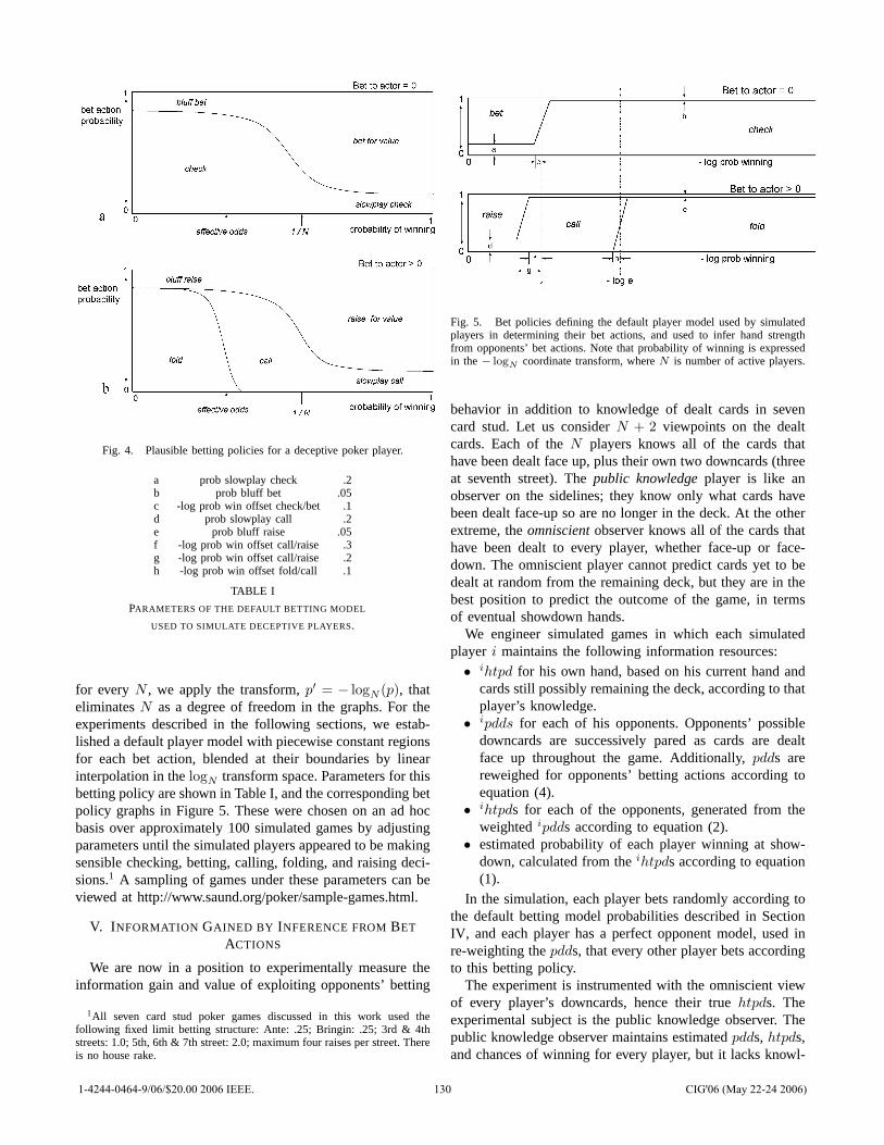
Fig. 4. Plausible betting policies for a deceptive poker player.

a prob slowplay check .2b prob bluff bet .05c -log prob win offset check/bet .1d prob slowplay call .2e prob bluff raise .05f -log prob win offset call/raise .3g -log prob win offset call/raise .2h -log prob win offset fold/call .1

TABLE I

PARAMETERS OF THE DEFAULT BETTING MODEL

USED TO SIMULATE DECEPTIVE PLAYERS.

for every N , we apply the transform,p′ = − logN (p), thateliminatesN as a degree of freedom in the graphs. For theexperiments described in the following sections, we estab-lished a default player model with piecewise constant regionsfor each bet action, blended at their boundaries by linearinterpolation in thelogN transform space. Parameters for thisbetting policy are shown in Table I, and the corresponding betpolicy graphs in Figure 5. These were chosen on an ad hocbasis over approximately 100 simulated games by adjustingparameters until the simulated players appeared to be makingsensible checking, betting, calling, folding, and raisingdeci-sions.1 A sampling of games under these parameters can beviewed at http://www.saund.org/poker/sample-games.html.

V. I NFORMATION GAINED BY INFERENCE FROMBET

ACTIONS

We are now in a position to experimentally measure theinformation gain and value of exploiting opponents’ betting

1All seven card stud poker games discussed in this work used thefollowing fixed limit betting structure: Ante: .25; Bringin:.25; 3rd & 4thstreets: 1.0; 5th, 6th & 7th street: 2.0; maximum four raises per street. Thereis no house rake.

Fig. 5. Bet policies defining the default player model used by simulatedplayers in determining their bet actions, and used to infer hand strengthfrom opponents’ bet actions. Note that probability of winning is expressedin the− log

Ncoordinate transform, whereN is number of active players.

behavior in addition to knowledge of dealt cards in sevencard stud. Let us considerN + 2 viewpoints on the dealtcards. Each of theN players knows all of the cards thathave been dealt face up, plus their own two downcards (threeat seventh street). Thepublic knowledgeplayer is like anobserver on the sidelines; they know only what cards havebeen dealt face-up so are no longer in the deck. At the otherextreme, theomniscientobserver knows all of the cards thathave been dealt to every player, whether face-up or face-down. The omniscient player cannot predict cards yet to bedealt at random from the remaining deck, but they are in thebest position to predict the outcome of the game, in termsof eventual showdown hands.

We engineer simulated games in which each simulatedplayer i maintains the following information resources:• ihtpd for his own hand, based on his current hand and

cards still possibly remaining the deck, according to thatplayer’s knowledge.

• ipdds for each of his opponents. Opponents’ possibledowncards are successively pared as cards are dealtface up throughout the game. Additionally,pdds arereweighed for opponents’ betting actions according toequation (4).

• ihtpds for each of the opponents, generated from theweightedipdds according to equation (2).

• estimated probability of each player winning at show-down, calculated from theihtpds according to equation(1).

In the simulation, each player bets randomly according tothe default betting model probabilities described in SectionIV, and each player has a perfect opponent model, used inre-weighting thepdds, that every other player bets accordingto this betting policy.

The experiment is instrumented with the omniscient viewof every player’s downcards, hence their truehtpds. Theexperimental subject is the public knowledge observer. Thepublic knowledge observer maintains estimatedpdds, htpds,and chances of winning for every player, but it lacks knowl-

1-4244-0464-9/06/$20.00 2006 IEEE. 130 CIG'06 (May 22-24 2006)

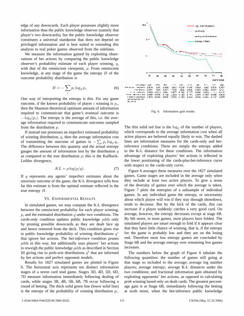
edge of any downcards. Each player possesses slightly moreinformation than the public knowledge observer (namely thatplayer’s two downcards), but the public knowledge observerconstitutes a universal standpoint that does not depend onprivileged information and is best suited to extending thisanalysis to real poker games observed from the sidelines.

We measure the information gained by exploiting obser-vations of bet actions by comparing the public knowledgeobserver’s probability estimate of each player winning,q,with that of the omniscient viewpoint,p. From omniscientknowledge, at any stage of the game the entropyH of theoutcome probability distribution is

H = −∑

i

pi log2pi. (6)

One way of interpreting the entropy is this. For any gameoutcome, if the known probability of playeri winning is pi,then the Shannon theoretical optimum amount of informationrequired to communicate that game’s eventual outcome is− log

2(pi). The entropy is the average of this, i.e. the aver-

age information required to communicate outcomes sampledfrom the distributionp.

If instead one possesses an imperfect estimated probabilityof winning distribution,q, then the average information costof transmitting the outcome of games is−

∑i pi log

2qi.

The difference between this quantity and the actual entropygauges the amount of information lost by the distributionqas compared to the true distributionp; this is the Kullback-Leibler divergence,

KL = p log(p/q). (7)

If q represents any agents’ imperfect estimates about theuncertain outcome of the game, the K-L divergence tells howfar this estimate is from the optimal estimate reflected in thetrue entropyH.

VI. EXPERIMENTAL RESULTS

In simulated games, we may compute the K-L divergencebetween the omniscient probability for each player winning,p, and the estimated distributionq under two conditions. Thecards-only condition updates public knowledgepdds onlyby pruning possible downcards as they are dealt face upand hence removed from the deck. This condition gives riseto public knowledge probability of winning distributionsqc

that ignore bet actions. Thebet-inferencecondition prunespdds in this way, but additionally uses players’ bet actionsto reweigh the public knowledgepdds as described in SectionIII giving rise to prob-win distributionsqb that are informedby bet actions and perfect opponent models.

Results for 1827 simulated games are plotted in Figure6. The horizontal axis represents ten distinct informationstages of a seven card stud game. Stages 3D, 4D, 5D, 6D,7D measure information immediately following dealing ofcards, while stages 3B, 4B, 5B, 6B, 7B occur following around of betting. The thick solid green line (lower solid line)is the entropy of the probability of winning distributionpi.

Fig. 6. Information gain results.

The thin solid red line is thelog2

of the number of players,which corresponds to the average information cost when allactive players are believed equally likely to win. The dashedlines are information measures for the cards-only and bet-inference conditions. These are simply the entropy addedto the K-L distance for these conditions. The informationadvantage of exploiting players’ bet actions is reflected inthe lower positioning of the cards-plus-bet-inference curvewith respect to the cards-only curve.

Figure 6 averages these measures over the 1827 simulatedgames. Game stages are included in the average only whenthey include at least two active players. To give a senseof the diversity of games over which the average is taken,Figure 7 plots the entropies of a subsample of individualgames. In any individual game the entropy, or uncertaintyabout which player will win if they stay through showdown,tends to decrease. But by the luck of the cards, this canincrease if a player suddenly catches a very good card. Onaverage, however, the entropy decreases except at stage 6B.By 6th street, in most games, most players have folded. Thesimulated players are smart enough to fold if it appears clearthat they have little chance of winning, that is, if the entropyfor the game is probably low and they are on the losingend. Therefore most low entropy games are concluded byStage 6B and the average entropy over remaining live gamesincreases.

The numbers below the graph of Figure 6 tabulate thefollowing quantities: the number of games still going atthat stage so included in the average; average log numberplayers; average entropy; average K-L distances under thetwo conditions; and fractional information gain obtained byexploiting opponents’ bet actions, as opposed to calculatingprob winning based only on dealt cards. The greatest percent-age gain is at Stage 6B, immediately following the bettingat sixth street, when the bet-inference public knowledge

1-4244-0464-9/06/$20.00 2006 IEEE. 131 CIG'06 (May 22-24 2006)

Fig. 7. Entropies for a sampling of 80 games played by the defaultsimulated players. Circles identify two stages in the game whose historyis shown in Figure 8. Thehtpds at these stages are shown in Figure 1.

.

Fig. 8. Game history for a sample game whose entropy is plotted inredin Figure 7. Notation: “.” denotes lead actor at each street;“B”: Bring-inbet; “k”: check (no one checked in this particular game); “b”:bet; “f”: fold;“c”: call; “r”: raise.

observer gains a 36% information advantage over the cards-only observer. The percent advantage drops at Stages 7D and7B simply because at this point all the cards have been dealtand the omniscient observer knows the outcome of the game.The optimal baseline entropy is zero here so the percentagegain of the bet-inference condition is smaller even thoughthe magnitude of its information gain over the cards-onlycondition increases. (A nonzero entropy at Stages 7D or 7Dindicate that a tie between two or more players occurred ina few games.)

An interesting feature of Figure 6 is that the cards-onlycondition for predicting game outcome actually performsworse than chance at seventh street. This is an indicationthat if a player remains in the game while their four upcardsshow a weaker hand than opponents’, then this player musthave a strong hand hidden. The cards-only estimation of handstrength has no way of accounting for this, while the bet-inference condition successfully makes this inference in thecourse of thepdd reestimation procedure described in SectionIII.

It would be a mistake to read Figure 6 as suggesting thatestimation of opponents’ possible downcards is of little value

simply because the cards-only and cards-plus-bet-inferencecurves look similar to the naivelog

2N curve in comparison

to the true entropy. These curves were generated fromsimulated games whose players followed tight-aggressivedeceptive bet policies dictated by Figure 5, and therefore theactive players at each street had undergone a severe, informedself-selection procedure of folding perceived disadvantagedhands. Note also that success in poker often hinges onexploitation of relatively few big-pot hands; flat averagesof information gain such as Figure 6 may not reflect thisdifferential value of information.

How does this information advantage translate to win/lossrates? We performed a second experiment in which threeplayers were constrained to be cards-only players by per-mitting them to use only their visible card knowledge inestimating their probability of winning, and hence in decidingtheir bet actions. In other words, thepdd re-estimationprocedure exploiting opponents’ bet actions was omitted forthese players. The remaining four players were providedthis information; their opponent models used to infer handstrength from bet actions accurately reflected that four play-ers were making use of the bet-inference public knowledgehtpds in calculating their own chances of winning prior toevery bet decision. These four players used the cards-onlypublic knowledgehtpds as a best available approximationto the beliefs held by the constrained, cards-only players,who know but obviously do not share their own downcardinformation.

It is well known that poker win/lose outcomes occur withhigh variance. Over 8977 simulated games, the resultingwin/lose rates are shown in Figure 9. The four bet-inferenceplayers won on average .14 bets/game, while the three cards-only players lost on average .19 bets/game. This is clearlyattributable to the cards-only players not folding when theyshould have. The bet-inference players bet an average of1.57/hand and won pots at a average rate of 1.71/hand(netting .14/hand). The cards only players won significantlymore pots, 2.50/hand, but at the cost of betting an averageof 2.69/hand.

VII. D ISCUSSION ANDCONCLUSION

It is by no means surprising that it is advantageous toexploit information transmitted by opponents’ bet actionsinpoker. This paper has introduced a framework for doing so ina way that delineates the roles of exposed cards, calculationand comparison of possible hand outcomes, rational betstrategy, styles of play, opponent models, and knowledgeand belief carried by players and observers. Using thisapparatus, we have obtained experimental results quantifyinginformation gain and its implications for win/lose rate bysimulated deceptive players who possess perfect models oftheir opponents’ betting policies.

To extend these results to live poker games would raiseseveral major challenges.

First, unless studies could be conducted from behind theHouse or game host’s omniscient viewpoint, in real gameswe would lack information about players’ downcards except

1-4244-0464-9/06/$20.00 2006 IEEE. 132 CIG'06 (May 22-24 2006)

.

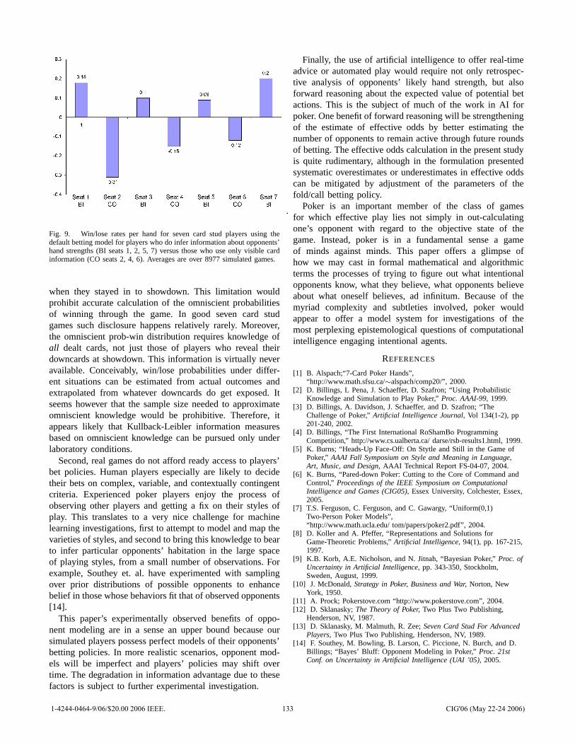
Fig. 9. Win/lose rates per hand for seven card stud players using thedefault betting model for players who do infer information about opponents’hand strengths (BI seats 1, 2, 5, 7) versus those who use only visible cardinformation (CO seats 2, 4, 6). Averages are over 8977 simulated games.

when they stayed in to showdown. This limitation wouldprohibit accurate calculation of the omniscient probabilitiesof winning through the game. In good seven card studgames such disclosure happens relatively rarely. Moreover,the omniscient prob-win distribution requires knowledge ofall dealt cards, not just those of players who reveal theirdowncards at showdown. This information is virtually neveravailable. Conceivably, win/lose probabilities under differ-ent situations can be estimated from actual outcomes andextrapolated from whatever downcards do get exposed. Itseems however that the sample size needed to approximateomniscient knowledge would be prohibitive. Therefore, itappears likely that Kullback-Leibler information measuresbased on omniscient knowledge can be pursued only underlaboratory conditions.

Second, real games do not afford ready access to players’bet policies. Human players especially are likely to decidetheir bets on complex, variable, and contextually contingentcriteria. Experienced poker players enjoy the process ofobserving other players and getting a fix on their styles ofplay. This translates to a very nice challenge for machinelearning investigations, first to attempt to model and map thevarieties of styles, and second to bring this knowledge to bearto infer particular opponents’ habitation in the large spaceof playing styles, from a small number of observations. Forexample, Southey et. al. have experimented with samplingover prior distributions of possible opponents to enhancebelief in those whose behaviors fit that of observed opponents[14].

This paper’s experimentally observed benefits of oppo-nent modeling are in a sense an upper bound because oursimulated players possess perfect models of their opponents’betting policies. In more realistic scenarios, opponent mod-els will be imperfect and players’ policies may shift overtime. The degradation in information advantage due to thesefactors is subject to further experimental investigation.

Finally, the use of artificial intelligence to offer real-timeadvice or automated play would require not only retrospec-tive analysis of opponents’ likely hand strength, but alsoforward reasoning about the expected value of potential betactions. This is the subject of much of the work in AI forpoker. One benefit of forward reasoning will be strengtheningof the estimate of effective odds by better estimating thenumber of opponents to remain active through future roundsof betting. The effective odds calculation in the present studyis quite rudimentary, although in the formulation presentedsystematic overestimates or underestimates in effective oddscan be mitigated by adjustment of the parameters of thefold/call betting policy.

Poker is an important member of the class of gamesfor which effective play lies not simply in out-calculatingone’s opponent with regard to the objective state of thegame. Instead, poker is in a fundamental sense a gameof minds against minds. This paper offers a glimpse ofhow we may cast in formal mathematical and algorithmicterms the processes of trying to figure out what intentionalopponents know, what they believe, what opponents believeabout what oneself believes, ad infinitum. Because of themyriad complexity and subtleties involved, poker wouldappear to offer a model system for investigations of themost perplexing epistemological questions of computationalintelligence engaging intentional agents.

REFERENCES

[1] B. Alspach;“7-Card Poker Hands”,“http://www.math.sfsu.ca/∼alspach/comp20/”, 2000.

[2] D. Billings, L Pena, J. Schaeffer, D. Szafron; “Using ProbabilisticKnowledge and Simulation to Play Poker,”Proc. AAAI-99, 1999.

[3] D. Billings, A. Davidson, J. Schaeffer, and D. Szafron; “TheChallenge of Poker,”Artificial Intelligence Journal, Vol 134(1-2), pp201-240, 2002.

[4] D. Billings, “The First International RoShamBo ProgrammingCompetition,” http://www.cs.ualberta.ca/ darse/rsb-results1.html, 1999.

[5] K. Burns; “Heads-Up Face-Off: On Stytle and Still in the Game ofPoker,” AAAI Fall Symposium on Style and Meaning in Language,Art, Music, and Design, AAAI Technical Report FS-04-07, 2004.

[6] K. Burns, “Pared-down Poker: Cutting to the Core of CommandandControl,” Proceedings of the IEEE Symposium on ComputationalIntelligence and Games (CIG05), Essex University, Colchester, Essex,2005.

[7] T.S. Ferguson, C. Ferguson, and C. Gawargy, “Uniform(0,1)Two-Person Poker Models”,“http://www.math.ucla.edu/ tom/papers/poker2.pdf”, 2004.

[8] D. Koller and A. Pfeffer, “Representations and Solutions forGame-Theoretic Problems,”Artificial Intelligence,94(1), pp. 167-215,1997.

[9] K.B. Korb, A.E. Nicholson, and N. Jitnah, “Bayesian Poker,” Proc. ofUncertainty in Artificial Intelligence, pp. 343-350, Stockholm,Sweden, August, 1999.

[10] J. McDonald,Strategy in Poker, Business and War,Norton, NewYork, 1950.

[11] A. Prock; Pokerstove.com “http://www.pokerstove.com”, 2004.[12] D. Sklanasky;The Theory of Poker,Two Plus Two Publishing,

Henderson, NV, 1987.[13] D. Sklanasky, M. Malmuth, R. Zee;Seven Card Stud For Advanced

Players,Two Plus Two Publishing, Henderson, NV, 1989.[14] F. Southey, M. Bowling, B. Larson, C. Piccione, N. Burch, and D.

Billings; “Bayes’ Bluff: Opponent Modeling in Poker,”Proc. 21stConf. on Uncertainty in Artificial Intelligence (UAI ’05), 2005.

1-4244-0464-9/06/$20.00 2006 IEEE. 133 CIG'06 (May 22-24 2006)

Modeling Children’s Entertainment in the Playware Playground

Georgios N. Yannakakis∗, Henrik Hautop Lund† and John Hallam‡Mærsk Mc-Kinney Møller Institute for Production Technology

University of Southern DenmarkCampusvej 55, DK-5230, Odense{georgios∗;hhl†;john‡}@mip.sdu.dk

Abstract— This paper introduces quantitative measure-ments/metrics of qualitative entertainment features within inter-active playgrounds inspired by computer games and proposesartificial intelligence (AI) techniques for optimizing entertain-ment in such interactive systems. For this purpose the innovativePlayware playground is presented and a quantitative approachto entertainment modeling based on psychological studies in thefield of computer games is introduced. Evolving artificial neuralnetworks (ANNs) are used to model player satisfaction (interest)in real-time and investigate quantitatively how the qualitativefactors of challenge and curiosity contribute to human enter-tainment according to player reaction time with the game.The limitations of the methodology and the extensibility of theproposed approach to other genres of digital entertainment arediscussed.

Keywords: Entertainment modeling, intelligent interactiveplaygrounds, neuro-evolution.

I. INTRODUCTION

Cognitive modeling within human-computer interactivesystems is a prominent area of research. Computer games,as examples of such systems, provide an ideal environmentfor research in AI, because they are based on simulationsof highly complex and dynamic multi-agent worlds [1], [2],[3], and cognitive modeling since they embed rich formsof interactivity between humans and non-player characters(NPCs). Being able to model the level of user (gamer)engagement or satisfaction in real-time can provide insightsto the appropriate AI methodology for enhancing the qualityof playing experience [4] and furthermore be used to adjustdigital entertainment environments according to individualuser preferences.

Features of computer games that keep children (amongothers) engaged more than other digital media include theirhigh degree of interactivity and the freedom for the childto develop and play a role within a fantasy world whichis created during play [5]. On the other hand, traditionalplaygrounds offer the advantage of physical play, whichfurthermore improves the child’s health condition, augmentchildren’s ability to engage in social and fantasy play [6], [7]and provide the freedom for children to generate their ownrules on their own developed games. The ‘Playware’ [8] in-telligent interactive physical playground attempts to combinethe aforementioned features of both worlds: computer gamesand traditional playgrounds. This innovative platform will bedescribed comprehensively and experiments with children ondeveloped Playware games will be introduced in this paper.

Motivated by the lack of quantitative cognitive models of

entertainment, an endeavor on capturing player satisfactionduring gameplay (i.e. entertainment modeling) and providingquantitative measurements of entertainment in real-time isintroduced in the work presented here. This is achievedby following the theoretical principles of Malone’s intrinsicqualitative factors for engaging gameplay [5], namely chal-lenge (i.e. ‘provide a goal whose attainment is uncertain’),curiosity (i.e. ‘what will happen next in the game?’) andfantasy (i.e. ‘show or evoke images of physical objects orsocial situations not actually present’) and driven by thebasic concepts of the theory of flow (‘flow is the mental statein which players are so involved in the game that nothingelse matters’) [9]. Quantitative measures for challenge andcuriosity are inspired by previous work on entertainmentmetrics [10] and extracted from corresponding game featuresthat emerge through the opponent behavior. A mappingbetween the aforementioned factors and humans notion ofentertainment is derived using a game developed on thePlayware playground as a test-bed. Personalization is addedto the model through the player’s reaction (response) timewith the game environment.

A feedforward ANN is trained through artificial evolutionon gameplay experimental data to approximate the functionbetween the examined entertainment factors and player sat-isfaction with and without the presence of individual playercharacteristics. Results demonstrate that the ANN mapsa function whose qualitative features are consistent withMalone’s corresponding entertainment factors in that non-extreme levels of challenge and curiosity generate highly en-tertaining games. Moreover, we show that player’s responsetime has a positive impact on providing a more accuratemodel of player satisfaction where children (classified bytheir response time) project different requirements on thelevels of the examined entertainment factors for the game tobe entertaining. The generality of the proposed methodologyand its extensibility to other genres of digital entertainmentare discussed as well as its applicability as an efficient AItool for enhancing entertainment in real-time is outlined.

II. ENTERTAINMENT MODELING

The current state-of-the-art in machine learning in com-puter games is mainly focused on generating human-like [1]and intelligent characters (see [3], [11], [12] among others).Even though complex opponent behaviors emerge throughvarious learning techniques, there is no further analysis ofwhether these behaviors contribute to the satisfaction of

1-4244-0464-9/06/$20.00 2006 IEEE. 134 CIG'06 (May 22-24 2006)

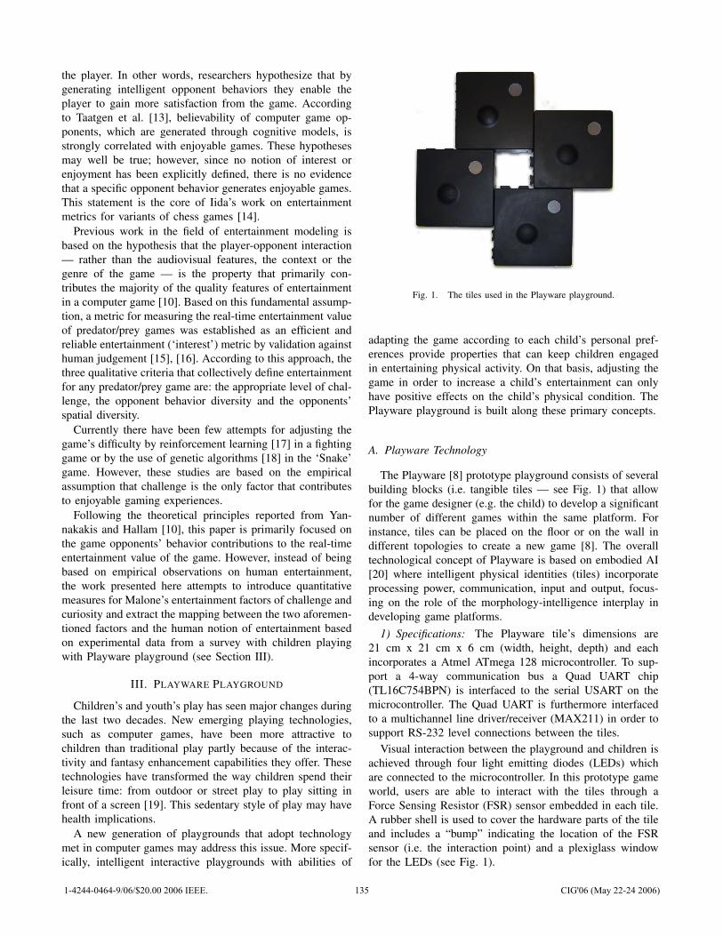
the player. In other words, researchers hypothesize that bygenerating intelligent opponent behaviors they enable theplayer to gain more satisfaction from the game. Accordingto Taatgen et al. [13], believability of computer game op-ponents, which are generated through cognitive models, isstrongly correlated with enjoyable games. These hypothesesmay well be true; however, since no notion of interest orenjoyment has been explicitly defined, there is no evidencethat a specific opponent behavior generates enjoyable games.This statement is the core of Iida’s work on entertainmentmetrics for variants of chess games [14].

Previous work in the field of entertainment modeling isbased on the hypothesis that the player-opponent interaction— rather than the audiovisual features, the context or thegenre of the game — is the property that primarily con-tributes the majority of the quality features of entertainmentin a computer game [10]. Based on this fundamental assump-tion, a metric for measuring the real-time entertainment valueof predator/prey games was established as an efficient andreliable entertainment (‘interest’) metric by validation againsthuman judgement [15], [16]. According to this approach, thethree qualitative criteria that collectively define entertainmentfor any predator/prey game are: the appropriate level of chal-lenge, the opponent behavior diversity and the opponents’spatial diversity.

Currently there have been few attempts for adjusting thegame’s difficulty by reinforcement learning [17] in a fightinggame or by the use of genetic algorithms [18] in the ‘Snake’game. However, these studies are based on the empiricalassumption that challenge is the only factor that contributesto enjoyable gaming experiences.

Following the theoretical principles reported from Yan-nakakis and Hallam [10], this paper is primarily focused onthe game opponents’ behavior contributions to the real-timeentertainment value of the game. However, instead of beingbased on empirical observations on human entertainment,the work presented here attempts to introduce quantitativemeasures for Malone’s entertainment factors of challenge andcuriosity and extract the mapping between the two aforemen-tioned factors and the human notion of entertainment basedon experimental data from a survey with children playingwith Playware playground (see Section III).

III. PLAYWARE PLAYGROUND

Children’s and youth’s play has seen major changes duringthe last two decades. New emerging playing technologies,such as computer games, have been more attractive tochildren than traditional play partly because of the interac-tivity and fantasy enhancement capabilities they offer. Thesetechnologies have transformed the way children spend theirleisure time: from outdoor or street play to play sitting infront of a screen [19]. This sedentary style of play may havehealth implications.

A new generation of playgrounds that adopt technologymet in computer games may address this issue. More specif-ically, intelligent interactive playgrounds with abilities of

Fig. 1. The tiles used in the Playware playground.

adapting the game according to each child’s personal pref-erences provide properties that can keep children engagedin entertaining physical activity. On that basis, adjusting thegame in order to increase a child’s entertainment can onlyhave positive effects on the child’s physical condition. ThePlayware playground is built along these primary concepts.

A. Playware Technology

The Playware [8] prototype playground consists of severalbuilding blocks (i.e. tangible tiles — see Fig. 1) that allowfor the game designer (e.g. the child) to develop a significantnumber of different games within the same platform. Forinstance, tiles can be placed on the floor or on the wall indifferent topologies to create a new game [8]. The overalltechnological concept of Playware is based on embodied AI[20] where intelligent physical identities (tiles) incorporateprocessing power, communication, input and output, focus-ing on the role of the morphology-intelligence interplay indeveloping game platforms.

1) Specifications: The Playware tile’s dimensions are21 cm x 21 cm x 6 cm (width, height, depth) and eachincorporates a Atmel ATmega 128 microcontroller. To sup-port a 4-way communication bus a Quad UART chip(TL16C754BPN) is interfaced to the serial USART on themicrocontroller. The Quad UART is furthermore interfacedto a multichannel line driver/receiver (MAX211) in order tosupport RS-232 level connections between the tiles.

Visual interaction between the playground and children isachieved through four light emitting diodes (LEDs) whichare connected to the microcontroller. In this prototype gameworld, users are able to interact with the tiles through aForce Sensing Resistor (FSR) sensor embedded in each tile.A rubber shell is used to cover the hardware parts of the tileand includes a “bump” indicating the location of the FSRsensor (i.e. the interaction point) and a plexiglass windowfor the LEDs (see Fig. 1).

1-4244-0464-9/06/$20.00 2006 IEEE. 135 CIG'06 (May 22-24 2006)

B. Systems Related to Playware

The Smart Floor [21] and the KidsRoom [22] are amongthe few systems that are related primarily to the conceptuallevel of the Playware tiles. The first is developed for trans-parent user identification and tracking based on a person’sfootstep force features and the latter is a perceptually-based, multi-person, fully automated, interactive, narrativeplay room that adjusts its behavior (story-line) by analyzingthe children’s behavior through computer vision. As far asthe concept of intelligent floors consisting of several buildingblocks is concerned, the Z-tiles [23] are closely related toPlayware. However, the Z-tiles are mainly used as inputdevices only whereas Playware comprises building blocksthat offer interactivity by incorporating both input and outputdevices.

C. Bug-Smasher Game

The test-bed game used for the experiments presentedhere is called ‘Bug-Smasher’. The game is developed on a6 x 6 square tile topology (see Fig. 2). During the game,different ‘bugs’ (colored lights) appear on the game surfaceand disappear sequentially after a short period of time byturning a tile’s light on and off respectively. A bug’s positionis picked within a radius of three tiles from the previous bugand according to the predefined level of the bugs’ spatialdiversity (see Section IV). Spatial diversity is measured bythe entropy of the bug-visited tiles which is calculated andnormalized into [0, 1] via (1)

H =

[− 1

log36

∑

i

vi

Vlog

(vi

V

)](1)

where vi is the number of bug-visits to tile i and V is thetotal number of visits to all visited tiles (i.e. V =

∑i vi). If

the bug visits all tiles equally then vi = V/36 for all 36 tilesand H will be 1; if the bug visits exactly one tile, H is zero.

The child’s goal is to smash as many bugs as possibleby stepping on the lighted tiles. Different sounds and colorsrepresent different bugs when appearing and when smashedin order to increase the fantasy entertainment factor [5].Moreover, feedback to the player, which is essential for asuccessful game design [5], is provided through differentcharacteristic sounds that represent good or bad performance.

IV. EXPERIMENTAL DATA

The Bug-Smasher game has been used to acquire data ofhuman judgement on entertainment. Two states (‘Low’ and‘High’) are used for each of the three entertainment factorsof challenge, curiosity and fantasy summing up to 8 differentgame states. While the fantasy factor is also investigatedthrough this survey, the focus of this paper is on the opponent(bug) contribution on entertainment and, therefore, only therelation between challenge, curiosity and entertainment isreported here.

We consider the speed (S — in sec−1) that the bugs appearand disappear from the game and their spatial diversity (H)on the game’s plane as appropriate measures to represent the

Fig. 2. A child playing the Bug-Smasher game.

level of challenge and the level of curiosity (unpredictability)respectively [5] during gameplay. The former provides anotion for a goal whose attainment is uncertain — the higherthe S value, the higher the goal uncertainty and furthermorethe higher the challenge — and the latter effectively portraysa notion of unpredictability in the subsequent events ofthe game — the higher the H value the higher the bugappearance unpredictability and therefore the higher thecuriosity.

To that end, 28 children — C82 = 28 being the required

number of all combinations of 2 out of 8 game states since,by experimental design, each subject plays against two of theselected game states in all permutations of pairs — whoseage covered a range between 8 and 10 years participated inan experiment. In this experiment, each subject plays twogames (A and B) — differing in the levels of one or moreentertainment factors of challenge, curiosity and fantasy —for 90 seconds each. Each time a pair of games is finished,the child is asked whether the first game was more interestingthan the second game i.e. whether A or B generated a moreinteresting game. The child’s answers are used to guide thetraining of an ANN model of entertainment (see Section V).In order to minimize any potential order effects we let eachsubject play the aforementioned games in the inverse ordertoo. Statistical analysis of the subjects’ answers shows thatthe order effect on children judgement on entertainment is notstatistically significant (rc = −0.0714, p-value= 0.3444).

Since at the current implementation of the Playware theonly input to the system is through the FSR sensor, quan-titative individual playing characteristics can only be basedon three measurable features: the state (position and LEDscolor) of a pressed tile, the time that a tile-press event tookplace and the pressure force on a pressed tile.

Pressed tile events are recorded in real-time and a selectionof personalized playing features are calculated for each child.These include the total numbers of smashed bugs P andinteractions with the game environment NI ; the averageresponse time E{rt}; the average distance between thepressed tile and the bugs appearing on the game E{Db};the average pressure recorded from the FSR sensor E{p};and the entropy of the tiles that the child visited HC .

1-4244-0464-9/06/$20.00 2006 IEEE. 136 CIG'06 (May 22-24 2006)

A. Statistical Analysis

The aim of the statistical analysis presented here is toidentify statistically significant correlations between humannotion of entertainment and any of the aforementioned indi-vidual quantitative playing characteristics. For this purposethe following null hypothesis is formed: The correlationbetween observed human judgement of entertainment andrecorded individual playing characteristics, as far as the dif-ferent game states are concerned, is a result of randomness.The test statistic is obtained through c(−→z ) =

∑Ni=1{zi/N},

where N is the total number of game pairs played and zi = 1,if the subject chooses as the more entertaining game theone with the larger value of the examined characteristic andzi = −1, if the subject chooses the other game in the gamepair i.

Table I presents the c(−→z ) values and their correspondingp-values for all above-mentioned personal characteristics.Average response time appears to be the only characteristicexamined that is significantly — significance equals 10%,high significance equals 5% in this paper — correlated toentertainment. The obtained effect of E{rt} appears to becommonsensical since the Bug-Smasher game belongs to thegenre of action games where reaction time tends to have asignificant effect on the level of engagement of the user [24].

The first attempt to include subjectivity in entertainmentmodeling, presented in this paper, will be through investi-gating the impact of entertainment factors on entertainmentaccording to the average response time E{rt}. The choiceof this specific measure, instead of others examined, ismade due to its demonstrated statistically significant effectto entertainment.

TABLE ICORRELATION COEFFICIENTS BETWEEN ENTERTAINMENT AND

INDIVIDUAL GAMEPLAY QUANTITATIVE CHARACTERISTICS. P IS THE

TOTAL NUMBER OF SMASHED BUGS; NI IS THE TOTAL NUMBER OF

INTERACTIONS; E{rt} IS THE AVERAGE RESPONSE TIME; E{Db} IS

THE AVERAGE DISTANCE BETWEEN THE PRESSED TILE AND THE BUGS

APPEARING ON THE GAME; E{p} IS THE AVERAGE PRESSURE

RECORDED FROM THE FSR SENSOR AND HC IS THE ENTROPY OF THE

TILES THAT THE CHILD VISITED.

Characteristic c(−→z ) p-value

P -0.0384 0.4449

NI 0.1923 0.1058

HC -0.1153 0.2442

E{rt} -0.2307 0.0631

E{p} 0.0769 0.3389

E{Db} -0.0384 0.4449

V. EVOLVING ANN

A fully-connected feedforward ANN for learning the rela-tion between the challenge and curiosity factors, the averageresponse time of children and the entertainment value of agame has been used and is presented here. The assumption is

that the entertainment value y of a given game is an unknownfunction of S and H (and perhaps E{rt}), which the ANNwill learn. The children’s expressed preferences constrain butdo not specify the values of y for individual games. Since, theoutput error function is not differentiable, ANN training al-gorithms such as back-propagation are inapplicable. Learningis achieved through artificial evolution [25] and is describedin Section V-A.

The sigmoid function is employed at each neuron, theconnection weights take values from -5 to 5 and all inputvalues are normalized into [0, 1] before they are enteredinto the ANN. In an attempt to minimize the controller’ssize, it was determined that single hidden-layered ANNarchitectures, containing 10 hidden neurons, are capable ofsuccessfully obtaining solutions of high fitness.

A. Genetic Algorithm

A generational genetic algorithm (GA) [26] is imple-mented, which uses an “exogenous” evaluation function thatpromotes the minimization of the difference in matchingthe human judgement of entertainment. The ANN is itselfevolved. In the algorithm presented here, the ANN topologyis fixed and the GA chromosome is a vector of ANNconnection weights.

The evolutionary procedure used can be described asfollows. A population of N (N is 1000 in this paper) networksis initialized randomly. Initial real values that lie within [-5,5] for their connection weights are picked randomly from auniform distribution. Then, at each generation:

Step 1 Each member (neural network) of the populationgets two triples of (S, H , E{rt}) values one forA and one for B and returns two output values,namely yj,A (output of the game against opponentA) and yj,B (output of the game against opponentB) for each pair j of games played in the survey(Ns = 56). When the yj,A, yj,B values are consis-tent with the judgement of subject j then we statethat: ‘the values agree with the subject’ or thatthere is ‘agreement’ with the subject throughoutthis paper. In the opposite case, we state that:‘the values disagree with the subject’ or there is‘disagreement.’

Step 2 Each member i of the population is evaluated viathe fitness function fi:

fi =Ns∑

j=1

{g(dj , 30), if agreement;g(dj , 5), if disagreement. (2)

where dj = yj,A − yj,B and g(dj , p) = 1/(1 +e−pdj ) is the sigmoid function.

Step 3 A fitness-proportional scheme is used as the selec-tion method.

Step 4 Selected parents clone an equal number of off-spring so that the total population reaches Nmembers or reproduce offspring by crossover. The

1-4244-0464-9/06/$20.00 2006 IEEE. 137 CIG'06 (May 22-24 2006)

00.1

0.20.3

0.40.5

0.60.7

0.80.9

1

00.1

0.20.3

0.40.5

0.60.7

0.80.9

1

0

0.5

1

Curiosity (H)Challenge (S)

Ent

erta

inm

ent (

y)

Fig. 3. Fittest ANN (f = 22.82) trained on absence of individual playingcharacteristics.

Montana and Davis [27] crossover operator isapplied with a probability 0.4.

Step 5 Gaussian mutation occurs in each gene (connec-tion weight) of each offspring’s genome with asmall probability pm = 1/n, where n is thenumber of genes.

The algorithm is terminated when either a good solution(i.e. fi > 54) is found or a large number of generations g iscompleted (g = 10000).

VI. RESULTS

Results obtained from the ANN evolutionary approachesare presented in this section. In order to diminish the non-deterministic effect of the GA initialization phase, we repeatthe learning procedure ten times — we believe that thisnumber is adequate to illustrate a clear picture of the behaviorof the mechanism — with different random initial conditions.

A. Objective Entertainment Value

The experiment presented here tests the hypothesis of theexistence of an objective notion of entertainment given thelevel of challenge and curiosity in a game. Thus, the aimhere is to extract a mapping between challenge, curiosityand entertainment independently of player individual char-acteristics (E{rt} values are not included in the ANN inputvector). Given the 30 pairs of games, where the gameshave different levels of S and/or H , an ANN is evolvedby following the approach presented in Section V-A. Thefittest ANN found was able to correctly match only 20 outof 30 children answers on entertainment. Such a poor fitnessindicates the difficulty of adjusting values of challenge andcuriosity for inferring entertainment values in an objectivemanner (without the presence of individual characteristics).The relation between bug speed (S), bug spatial diversity(H) and the game’s entertainment value (y) is illustrated inFig. 3.

Despite the best solution’s poor fitness, the correlationbetween entertainment, challenge and curiosity generatedthrough the evolved ANN (see Fig. 3) appears to follow

0 0.1 0.2 0.3 0.4 0.5 0.6 0.7 0.8 0.9 10

0.1

0.2

0.3

0.4

0.5

0.6

0.7

0.8

0.9

1

E{rt}

Em

tert

ainm

ent (

y)

S = 0.2 (Low), H= 0.51 (Low)S = 0.2 (Low), H= 0.99 (High)S = 0.7 (High), H= 0.51 (Low)S = 0.7 (High), H= 0.99 (High)

Fig. 4. Fittest ANN (f = 52.68): Entertainment over average responsetime for both states (Low, High) of each entertainment factor S and H .

the qualitative principles of Malone’s work [5]. Accordingto these, a game should maintain an appropriate level ofchallenge and curiosity in order to be entertaining. In otherwords, too difficult and/or too easy and/or too unpredictableand/or too predictable opponents to play against make thegame uninteresting. As seen from Fig. 3, average levels ofchallenge (0.5 < S < 0.8) and curiosity (0.3 < H < 0.9)generate high entertainment values objectively. Moreover, itappears that games of the lowest challenge level (S ≈ 0)combined with the highest curiosity level (H ≈ 1) may yieldhigh entertainment values.

B. Response time

As previously presented in Fig. 3, extreme values ofchallenge and curiosity appear to generally generate lowvalues of player satisfaction. However, what it still needsto be extracted are the appropriate levels of challenge andunpredictability required by individual players for a game tobe entertaining.

This section presents experiments where individual charac-teristics are present in the evaluation of entertainment. Thus,the average response time of the child is included in theinput vector of the ANN which is evolved by following theapproach presented in Section V-A. For space considerations,only the fittest solution is presented in this paper. Note that,the qualitative features of the lines and surfaces plotted inFig. 4 and Fig. 5 appeared in all ten learning attempts.

More specifically, Fig. 4 illustrates that challenge has ahigher impact on children’s notion of entertainment thancuriosity. In fact, low levels of curiosity appear to entertainchildren more. This could be explained through the factthat for the game experiments presented in this paper theHigh value for H is the highest possible value of entropy(H ≈ 1.0). This level of bugs entropy appears to generatetoo unpredictable games for the majority of children and,therefore, confusion during play and furthermore less sat-isfaction. Fig. 4 also shows that highly entertaining gamesare generated when challenge is Low and children are fast

1-4244-0464-9/06/$20.00 2006 IEEE. 138 CIG'06 (May 22-24 2006)

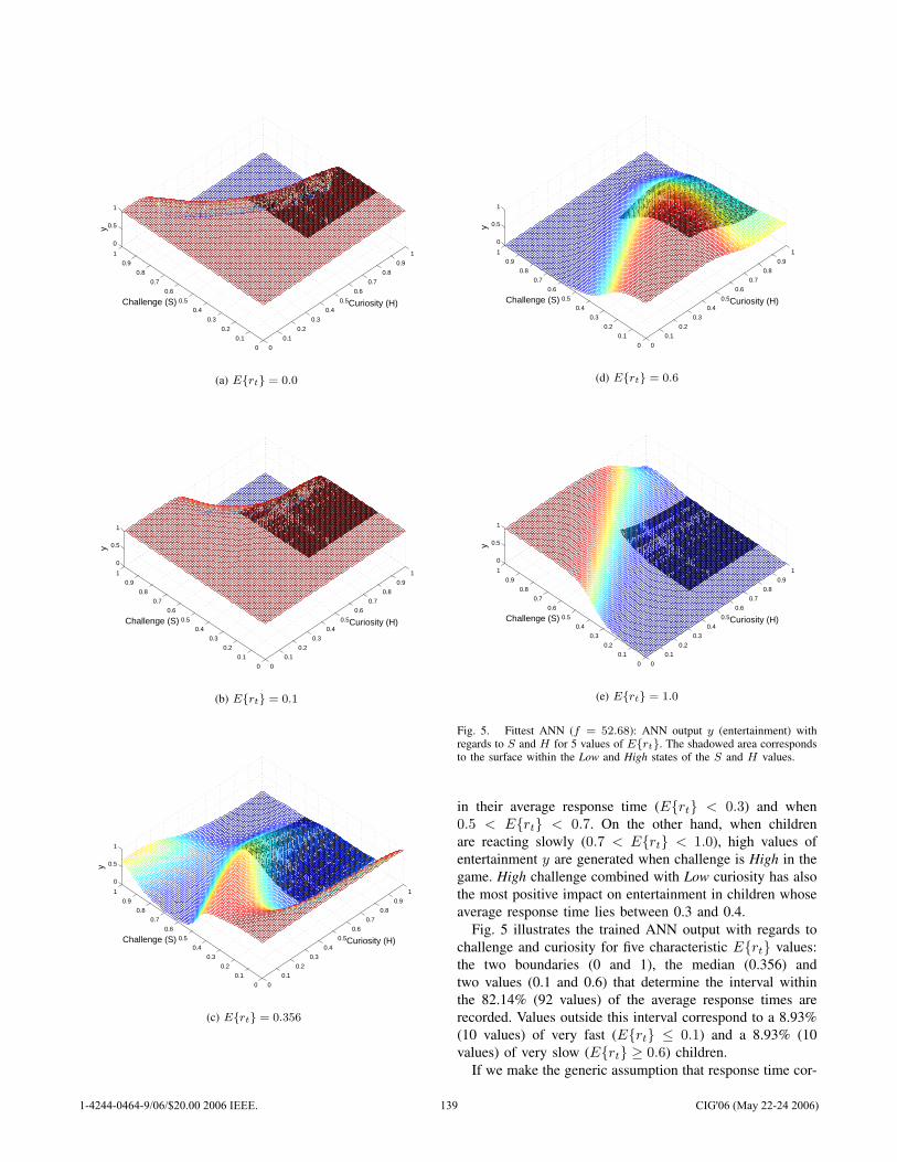
0

0.1

0.2

0.3

0.4

0.5

0.6

0.7

0.8

0.9

1

0

0.1

0.2

0.3

0.4

0.5

0.6

0.7

0.8

0.9

1

0

0.5

1

Curiosity (H)Challenge (S)

y

(a) E{rt} = 0.0

0

0.1

0.2

0.3

0.4

0.5

0.6

0.7

0.8

0.9

1

0

0.1

0.2

0.3

0.4

0.5

0.6

0.7

0.8

0.9

1

0

0.5

1

Curiosity (H)Challenge (S)

y

(b) E{rt} = 0.1

0

0.1

0.2

0.3

0.4

0.5

0.6

0.7

0.8

0.9

1

0

0.1

0.2

0.3

0.4

0.5

0.6

0.7

0.8

0.9

1

0

0.5

1

Curiosity (H)Challenge (S)

y

(c) E{rt} = 0.356

0

0.1

0.2

0.3

0.4

0.5

0.6

0.7

0.8

0.9

1

0

0.1

0.2

0.3

0.4

0.5

0.6

0.7

0.8

0.9

1

0

0.5

1

Curiosity (H)Challenge (S)

y

(d) E{rt} = 0.6

0

0.1

0.2

0.3

0.4

0.5

0.6

0.7

0.8

0.9

1

0

0.1

0.2

0.3

0.4

0.5

0.6

0.7

0.8

0.9

1

0

0.5

1

Curiosity (H)Challenge (S)

y

(e) E{rt} = 1.0

Fig. 5. Fittest ANN (f = 52.68): ANN output y (entertainment) withregards to S and H for 5 values of E{rt}. The shadowed area correspondsto the surface within the Low and High states of the S and H values.

in their average response time (E{rt} < 0.3) and when0.5 < E{rt} < 0.7. On the other hand, when childrenare reacting slowly (0.7 < E{rt} < 1.0), high values ofentertainment y are generated when challenge is High in thegame. High challenge combined with Low curiosity has alsothe most positive impact on entertainment in children whoseaverage response time lies between 0.3 and 0.4.

Fig. 5 illustrates the trained ANN output with regards tochallenge and curiosity for five characteristic E{rt} values:the two boundaries (0 and 1), the median (0.356) andtwo values (0.1 and 0.6) that determine the interval withinthe 82.14% (92 values) of the average response times arerecorded. Values outside this interval correspond to a 8.93%(10 values) of very fast (E{rt} ≤ 0.1) and a 8.93% (10values) of very slow (E{rt} ≥ 0.6) children.

If we make the generic assumption that response time cor-

1-4244-0464-9/06/$20.00 2006 IEEE. 139 CIG'06 (May 22-24 2006)

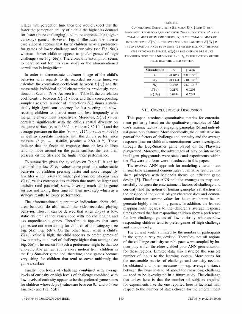
relates with perception time then one would expect that thefaster the perception ability of a child the higher its demandfor faster (more challenging) and more unpredictable (highercuriosity) games. However, Fig. 5 illustrates the inversecase since it appears that faster children have a preferencefor games of lower challenge and curiosity (see Fig. 5(a))whereas slower children appear to prefer games of highchallenge (see Fig. 5(e)). Therefore, this assumption seemsto be ruled out for this case study or the aforementionedcorrelation is insignificant.

In order to demonstrate a clearer image of the child’sbehavior with regards to its recorded response time, wecalculate the correlation coefficients between E{rt} and themeasurable individual child characteristics previously men-tioned in Section IV-A. As seen from Table II, the correlationcoefficient rc between E{rt} values and their correspondingsample size (total number of interactions NI ) shows a statis-tically high significant tendency for fast-reacting and slow-reacting children to interact more and less frequently withthe game environment respectively. Moreover, E{rt} valuescorrelate significantly with the child’s spatial diversity onthe game surface (rc = 0.3305, p-value = 7.82·10−4) and theaverage pressure on the tiles (rc = 0.2175, p-value = 0.0296)as well as correlate inversely with the child’s performancemeasure P (rc = −0.4058, p-value = 2.80·10−5). Theseindicate that the faster the response time the less childrentend to move around on the game surface, the less theirpressure on the tiles and the higher their performance.

To summarize given the rc values on Table II, it can beassumed that low E{rt} values correspond to a rather staticbehavior of children pressing faster and more frequentlyfew tiles which results to higher performance, whereas highE{rt} values correspond to children that move on larger anddecisive (and powerful) steps, covering much of the gamesurface and taking their time for their next step which as astrategy results to lower performance.

The aforementioned quantitative indications about chil-dren behavior do also match the video-recorded playingbehavior. Thus, it can be derived that when E{rt} is low,static children cannot easily cope with too challenging andtoo unpredictable games. Therefore, it appears that suchgames are not entertaining for children of this category (seeFig. 5(a), Fig. 5(b)). On the other hand, when a child’sE{rt} value is high, the child appears to prefer games oflow curiosity at a level of challenge higher than average (seeFig. 5(e)). The reason for such a preference might be that toounpredictable games require more motion from children inthe Bug-Smasher game and, therefore, these games becomevery tiring for children that tend to cover uniformly thegame’s surface.

Finally, low levels of challenge combined with averagelevels of curiosity or high levels of challenge combined withlow levels of curiosity appear to be the preferred game statesfor children whose E{rt} values are between 0.1 and 0.6 (seeFig. 5(c) and Fig. 5(d)).

TABLE IICORRELATION COEFFICIENTS BETWEEN E{rt} AND OTHER

INDIVIDUAL GAMEPLAY QUANTITATIVE CHARACTERISTICS. P IS THE

TOTAL NUMBER OF SMASHED BUGS; NI IS THE TOTAL NUMBER OF

INTERACTIONS; E{rt} IS THE AVERAGE RESPONSE TIME; E{Db} IS

THE AVERAGE DISTANCE BETWEEN THE PRESSED TILE AND THE BUGS

APPEARING ON THE GAME; E{p} IS THE AVERAGE PRESSURE

RECORDED FROM THE FSR SENSOR AND HC IS THE ENTROPY OF THE

TILES THAT THE CHILD VISITED.

Characteristic rc p-value

P -0.4058 2.80·10−5

NI -0.4324 7.01·10−6

HC 0.3305 7.82·10−4

E{p} 0.2175 0.0296

E{Db} 0.0494 0.6249

VII. CONCLUSIONS & DISCUSSION

This paper introduced quantitative metrics for entertain-ment primarily based on the qualitative principles of Mal-one’s intrinsic factors for engaging gameplay [5] and individ-ual game play features. More specifically, the quantitative im-pact of the factors of challenge and curiosity and the averageresponse time on children’s entertainment were investigatedthrough the Bug-Smasher game played on the Playwareplayground. Moreover, the advantages of play on interactiveintelligent playgrounds were stated and experiments withinthe Playware platform were introduced in this paper.

The evolved ANN approach for modeling entertainmentin real-time examined demonstrates qualitative features thatshare principles with Malone’s theory on efficient gamedesign [5]. The fittest ANN solution manages to map suc-cessfully between the entertainment factors of challenge andcuriosity and the notion of human gameplay satisfaction onthe absence of individual player characteristics and demon-strated that non-extreme values for the entertainment factorsgenerate highly entertaining games. In addition, the learnedmapping with regards to the children’s average responsetimes showed that fast responding children show a preferencefor low challenge games of low curiosity whereas slowresponding children tend to prefer games of high challengeand low curiosity.

The current work is limited by the number of participantsin the game survey we devised. Therefore, not all regionsof the challenge-curiosity search space were sampled by hu-man play which therefore yielded poor ANN generalizationfor these regions. Limited data also restricted the sensiblenumber of inputs to the learning system. More states forthe measurable metrics of challenge and curiosity need tobe obtained and other measures — e.g. average distancebetween the bugs instead of speed for measuring challenge— need to be investigated in a future study. The challengethat arises here is that the number of subjects requiredfor experiments like the one reported here is factorial withrespect to the number of states chosen for the entertainment

1-4244-0464-9/06/$20.00 2006 IEEE. 140 CIG'06 (May 22-24 2006)

factors and the total number of entertainment factors underinvestigation. Moreover, Malone’s entertainment factor offantasy is omitted from the results in this paper since thefocus is on the contribution of the opponent behaviors tothe generation of entertainment; however, fantasy’s impacton entertainment is planned to be reported in a forthcominganalysis.

The entertainment modeling approach presented heredemonstrates generality over the majority of action gamescreated with Playware since the quantitative means of chal-lenge and curiosity are estimated through the generic featuresof speed and spatial diversity of the opponent on the game’ssurface. Thus, these or similar measures could be used toadjust player satisfaction in any future game developmenton the Playware tiles. However, each game demonstratesindividual entertainment features that might need to beextracted and added on the proposed measures and therefore,more games of the same and/or other genres need to be testedto cross-validate this hypothesis. The proposed approach canbe used for adaptation of the game opponents (e.g. bugs)according to the player’s individual playing style (reactiontime) and as far as the challenge and curiosity factors ofentertainment are concerned. Given the real-time averageresponse time of a child, the partial derivatives of ϑy/ϑS andϑy/ϑH can be used to appropriately adjust the speed and theentropy of the opponent respectively for the entertainmentvalue y to be augmented.

Such a direction constitutes an example of future workon Playware, computer and educational games. The level ofengagement or motivation of the user/player/gamer of suchinteractive environments can be identified and increased bythe use of the presented approaches. Apart from providingsystems of richer interaction and qualitative entertainment[4], such approaches can generate augmented motivation ofthe user for deep learning in learning environments that usegames (i.e. edutainment).

ACKNOWLEDGMENTS

The authors would like to thank Henrik Jørgensen and allchildren of Henriette Hørlucks School, Odense, Denmark thatparticipated in the experiments. The tiles were designed byC. Isaksen from Isaksen Design and parts of their hardwareand software implementation were collectively done by A.Derakhshan, F. Hammer, T. Klitbo and J. Nielsen. KOMPAN,Mads Clausen Institute, and Danfoss Universe also partici-pated in the development of the tiles.

REFERENCES

[1] J. E. Laird and M. van Lent, “Human-level AI’s killer application:Interactive computer games,” in Proceedings of the Seventh NationalConference on Artificial Intelligence (AAAI), 2000, pp. 1171–1178.

[2] J. D. Funge, Artificial Intelligence for Computer Games. A. K. PetersLtd, 2004.

[3] A. J. Champandard, AI Game Development. New Riders Publishing,2004.

[4] G. N. Yannakakis and J. Hallam, “A scheme for creating digitalentertainment with substance,” in Proceedings of the Workshop onReasoning, Representation, and Learning in Computer Games, 19thInternational Joint Conference on Artificial Intelligence (IJCAI), Au-gust 2005, pp. 119–124.

[5] T. W. Malone, “What makes computer games fun?” Byte, vol. 6, pp.258–277, 1981.

[6] N. Postman, The Disappearance of Childhood. London: Allen, 1983.[7] S. Kline, Out of the Garden: Toys and Children’s Culture in the Age

of Marketing. Verso, 1993.[8] H. H. Lund, T. Klitbo, and C. Jessen, “Playware technology for

physically activating play,” Artifical Life and Robotics Journal, vol. 9,no. 4, pp. 165–174, 2005.

[9] M. Csikszentmihalyi, Flow: The Psychology of Optimal Experience.New York: Harper & Row, 1990.

[10] G. N. Yannakakis and J. Hallam, “Evolving Opponents for InterestingInteractive Computer Games,” in From Animals to Animats 8: Proceed-ings of the 8th International Conference on Simulation of AdaptiveBehavior (SAB-04), S. Schaal, A. Ijspeert, A. Billard, S. Vijayakumar,J. Hallam, and J.-A. Meyer, Eds. Santa Monica, LA, CA: The MITPress, July 2004, pp. 499–508.

[11] T. Graepel, R. Herbrich, and J. Gold, “Learning to fight,” in Proceed-ings of the International Conference on Computer Games: ArtificialIntelligence, Design and Education, Microsoft Campus, Reading, UK,November 2004, pp. 193–200.

[12] A. Nareyek, “Intelligent agents for computer games,” in Computersand Games, Second International Conference, CG 2002, T. Marslandand I. Frank, Eds., 2002, pp. 414–422.

[13] N. A. Taatgen, M. van Oploo, J. Braaksma, and J. Niemantsverdriet,“How to construct a believable opponent using cognitive modeling inthe game of set,” in Proceedings of the fifth international conferenceon cognitive modeling, 2003, pp. 201–206.

[14] H. Iida, N. Takeshita, and J. Yoshimura, “A metric for entertainmentof boardgames: its implication for evolution of chess variants,” inIWEC2002 Proceedings, R. Nakatsu and J. Hoshino, Eds. Kluwer,2003, pp. 65–72.

[15] G. N. Yannakakis, “AI in Computer Games: Generating InterestingInteractive Opponents by the use of Evolutionary Computation,” Ph.D.thesis, University of Edinburgh, November 2005.

[16] G. N. Yannakakis and J. Hallam, “A Generic Approach for ObtainingHigher Entertainment in Predator/Prey Computer Games,” Journal ofGame Development, vol. 1, no. 3, pp. 23–50, December 2005.

[17] G. Andrade, G. Ramalho, H. Santana, and V. Corruble, “Extendingreinforcement learning to provide dynamic game balancing,” in Pro-ceedings of the Workshop on Reasoning, Representation, and Learningin Computer Games, 19th International Joint Conference on ArtificialIntelligence (IJCAI), August 2005, pp. 7–12.

[18] M. A. Verma and P. W. McOwan, “An adaptive methodology for syn-thesising mobile phone games using genetic algorithms,” in Congresson Evolutionary Computation (CEC-05), Edinburgh, UK, September2005, pp. 528–535.

[19] M. Lindstrom and P. Seybold, BRANDchild: Insights into the Minds ofToday’s Global Kids: Understanding Their Relationship with Brands.Kogan Page, 1994.

[20] R. Pfeifer and C. Scheier, Understanding Intelligence. Cambridge,MIT Press, 1999.

[21] R. J. Orr and G. D. Abowd, “The smart floor: a mechanism fornatural user identification and tracking,” in CHI ’00: CHI ’00 extendedabstracts on Human factors in computing systems. NY, USA: ACMPress, 2000, pp. 275–276.

[22] A. Bobick, S. Intille, J. Davis, F. Baird, C. Pinhanez, L. Campbell,Y. Ivanov, A. Schutte, and A. Wilson, “The kidsroom: A perceptually-based interactive and immersive story environment,” MIT MediaLaboratory, Technical Report 398, December 1996.

[23] B. Richardson, K. Leydon, M. Fernstrom, and J. A. Paradiso, “Z-tiles: Building blocks for modular, pressure-sensing floorspaces,” inProceedings of CHI 2004. NY, USA: ACM Press, 2004, pp. 1529–1532.

[24] C. Beal, J. Beck, D. Westbrook, M. Atkin, and P. Cohen, “Intelligentmodelling of the user in interactive entertainment,” in Proceedings ofthe AAAI Spring Symposium on Artificial Intelligence and InteractiveEntertainment, Stanford, 2002, pp. 8–12.

[25] X. Yao, “Evolving artificial neural networks,” in Proceedings of theIEEE, vol. 87, no. 9, 1999, pp. 1423–1447.

[26] J. H. Holland, Adaptation in Natural and Artificial Systems. AnnArbor, MI: University of Michigan Press, 1975.

[27] D. J. Montana and L. D. Davis, “Training feedforward neural networksusing genetic algorithms,” in Proceedings of the Eleventh InternationalJoint Conference on Artificial Intelligence (IJCAI-89). San Mateo,CA: Morgan Kauffman, 1989, pp. 762–767.

1-4244-0464-9/06/$20.00 2006 IEEE. 141 CIG'06 (May 22-24 2006)

NPCs and Chatterbots with Personality and Emotional Response

Dana VrajitoruIntelligent Systems Laboratory, Computer and Information Sciences

Indiana University South Benddanav@cs.iusb.edu

Abstract— Chatterbots are computer programs that simulateintelligent conversation. They are situated between games andtoys, as their aim is mostly to be entertaining, but the userdoesn’t have to follow precise rules when playing with theprogram. Currently business and educational applications havestarted to emerge as a further development of the idea ofintelligent dialog. For the game industry, they come close tothe concept of NPC, or Non-Player Character, and they maybecome part of making such virtual beings more believableand life-like in the future. In this paper we present applicationintroducing an emotional component designed to enhance therealism of the conversation.

Keywords: Intelligent NPCs

I. INTRODUCTION

NPCs or non-player characters are an important aspectof games, especially in the role playing category. Theirfunctionality is to add to the game content by providingaccess to the backstory, assigning and rewarding quests, andgenerally, offering information about the game to the player.Their conversation skills are relatively limited and are ingeneral scripted, and context-based.

There are several foreseeable developments for NPCs, andone of them consists in expanding their dialog capabilities.It is likely that in the future, NPCs will merge with some ofthe functionality currently present in chatterbots.

Chatterbots are computer programs that simulate intelli-gent conversation. The typical execution involves an inputfrom the user in natural language to which the programprovides an answer that should be a reasonable and possiblyintelligent response to the original sentence. The process isrepeated while the human keeps the conversation going.

The very first chatterbot, named Eliza [1], simulated aRogerian psychotherapist. The idea was simple and consistedin a pattern matching algorithm and sentence reconstructionfollowing templates, with no in-depth knowledge or pro-cessing of the natural language. The program proved to beamazingly efficient in sustaining people’s attention duringthe conversation and the success of the original program hasinfluenced the development of many others.

Using similar ideas, Colby from the Stanford AI Labdeveloped Parry, the paranoid, in 1971. Parry is the oppositeof Eliza as it simulates a patient and has been intended as astudy of the nature of paranoia and is capable of expressingbeliefs, fears, and anxieties [2], [3]. Among the famouschatterbots we can mention Racter, a story-teller, [4] byW. Chamberlain and T. Etter, the stated author of the bookThe Policeman’s Beard Was Half Constructed. However, theauthenticity of the book has been questioned since then [5].

Another chatterbot worth mentioning is A.L.I.C.E, Arti-ficial Linguistic Internet Computer Entity (www.alice.org),that has its own development language called AIML (artifi-cial intelligence markup language) and earned the LoebnerPrize, based on the Turing Test [6], in 2000 and 2001.

Among recent developments are the virtual agents that canprovide online help and customer service by incorporatingknowledge about the company (www.egain.com). Some ofthe recent research also focuses on a definition of config-urable personality for virtual characters [7], [8]. Some studieshave also been conducted on the behavior of the humanparticipants in the interaction with the chatterbots [9], [10].

The goal of the chatterbots we implemented is to simulateparticular personalities, either fictional or real, mostly takenfrom literature, film, or television shows. This mostly appliesto NPCs in adventure games inspired from an externalstory source, like the Lord of the Rings. We typically startfrom a database of sentences that can be attributed to thepersonality to be simulated, as for example, the text of thebook or their lines from a script. The first prototypes canbe found online (http://www.cs.iusb.edu/˜danav/chatterbots/).An integrated 3D environment for the chatterbot is currentlyunder development.

The current chatterbot model represents an extension of[11]. In our primary model, we construct an answer to thehuman’s input by a probabilistic choice between patternmatching and templates, sentence keyword retrieval basedon automatic indexing, and database matching based ona personality-specific database. Several of the chatterbotconstruction operations have been automated, but a largehuman contribution is still necessary. The newest aspectof our program is represented by the emotional componentdesigned to enhance the credibility of the character.

The emotional response in an essential component ofany believable character [12], [13], [14]. The importance ofthis aspect has been recognized in the artificial intelligencecommunity and several studies focused on it [15]. Amongthe possible applications of emotional agents and virtualcharacters we can cite teaching and tutoring [16], [17].

The paper is structured the following way. The secondsection presents the outline of the chatterbot program. Thethird section discusses the general chatterbot techniques weimplemented. The fourth section introduces the personal-ity database and emotional component of the program. Afollowing section presents some experimental results andcompares them with out previous work. The paper ends withconclusions.

1-4244-0464-9/06/$20.00 2006 IEEE. 142 CIG'06 (May 22-24 2006)

II. THE VIRTUAL CHARACTER

The chatterbot algorithm consists in a loop reading aninput from the user and generating an answer, until the userends the dialog by either closing the browser or typing in asynonym of “bye”. The program will attempt to generatean answer with a certain probability using the followingmethods in this order:

1) personal features database, 90% probability,2) pattern matching and templates, 90% probability,3) first word question-matching, using a different set of

answers for inputs starting with “where” than for thosestarting with “how” and so on, 80% probability,

4) keyword-matching in the database created by automaticindexing, 90% probability.

5) random answer distinguishing between declarative sen-tences and questions, 100% probability.

The probabilities expressed in the list above are condi-tional. Thus, the pattern matching probability of 90% isconditioned by the 10% probability that the personal featuredatabase will not be used, and by the event that this databasedid not contain a valid answer to the user’s input. As the lastmethod always succeeds, a hopefully valid answer will bereturned in any case.

III. GENERAL PURPOSE CHATTERBOT TECHNIQUES

In this section we briefly introduce some of the techniquesused by chatterbots, which are pattern-matching, indexing,and randomly matched answers. We classify these as generalpurpose techniques because most chatterbots are using acombination of them, but for the purposes of creating apersonality for the chatterbot they are insufficient.

A. Pattern Matching and Templates

The pattern matching technique consists in finding oneor several patterns that match the sentence entered by theuser. A pattern is generally defined as a sentence in naturallanguage in which certain parts have been replaced by wildcards that can be matched by any group of words in amatching sentence.

For each pattern defined in the database, a correspondingtemplate is utilized to generate the answer to the sentence.The parts of the original sentence that are identified with thewild cards are first subjected to a person transformation inwhich words like “I, my, mine” become “you, your, yours”and the other way around.

For example, a pattern in the original Eliza program canbe expressed as

I want *in which the ’*’ character can be replaced by any sequence

of words. The corresponding template to generate the answercan be expressed by

What would it mean to you if you got *in which the ’*’ is replaced by the sequence of words that

was matched to the wild card in the pattern.An application of this pattern could be the following

dialog:

User: I want to know how your program works.Eliza: What would it mean to you if you got to know how

my program works?Beside the list of patterns, the original Eliza program also

contained a list of sentences that can be given in answer tosentences that cannot be matched to any of the patterns, like:

What does that suggest to you ?Please go on.For a virtual character, the patterns are built from the

database of character lines from the book or from the script.They are based on the lines of any other character thatprecedes the character we are developing in the dialog andthe response templates are generated from the character’sanswer in the original dialog.

Here are some examples of answers generated with thepattern-template model. This method is still one of the bestoptions because it uses part of the sentence provided by theuser and thus the answer seems to have a strong connectionto it.

Input: “can you proceed without clearance?”Answer: “we don’t need clearance. we need the 16-digit

code.”We developed an automatic pattern-template generating

algorithm for this application that takes as input two sen-tences, the first one belonging to any character in the originalscript, and the second one belonging to the character thatthe chatterbot emulates and representing an answer to thefirst. Let q and a be the two sentences. The algorithm startsby identifying a sequence of substrings of q such that eachof them is also a substring of a, but not necessarily in thesame order, as shown in Equation 2. The sequence maynot be the longest and its selection process is randomized.The algorithm avoids selecting common substrings that arecomposed of only words that are too common, like “the”.

q = q0 s0 q1 s1 . . . qn−1 sn−1 qn (1)such that ∀i = 0, n − 1, si is a substring of a (2)

The program then generates a pattern by replacing eachsi in q by a “*”, the wild card symbol that can be matchedby any substring, even empty. The corresponding template isgenerated by replacing every occurrence of si in the sentencea with a symbol representing the substring index in thepattern, in our case denoted by ∗#i∗.

The algorithm is not yet sufficient to automatically gener-ate the entire database of the chatterbot with no human inter-vention. After the patterns were automatically generated, itwas necessary for a human indexer to verify their quality andeliminate some of them. Even so, this represents a significantimprovement to the task of generating a chatterbot. Withoutit, the human indexer must define all of the pattern-templatecouples by hand. This process usually involves reading asubstantial amount of text looking for pieces of dialog thatcan be used. The algorithm shortened the development timefor the chatterbot considerably.

1-4244-0464-9/06/$20.00 2006 IEEE. 143 CIG'06 (May 22-24 2006)

B. Automatic Indexing for Chatterbots

In the classical IR approach [18], we are given a collectionof documents (ASCII text in natural language) and a queryexpressed by a human in natural language. The task of thesystem is to find the documents in the collection that are theclosest match to the given query.

We extended this model to the chatterbot application byconsidering that each document consists of one or twosentences associated with the character in the original script,usually one of the character’s lines. The user’s input to theprogram can be seen as the query. In our case we want tofind one particular document (sentence) that can be seen asa good answer to the query.

Thus, in the first step, we process all sentences available inthe database by eliminating the words that are too common,such as “a”, “is”, “for”, and removing the unnecessarysuffixes and prefixes to retain only the root of each word. Forexample, “program”, “programs” and “programming” will allbe indexed under “program”. We used the Porter stemmingalgorithm for this step [18].

In the next step, we build an inverted index database,where we store a reference to all the sentences in thedatabase that contain any given keyword. Sometimes wordsthat appear in the text before the sentence being processedcan also be significant to it, so our indexing also takesinto account the context of a document. Our model followsa Boolean indexing [19] meaning that we record only thepresence or absence of a term in an indexed sentence, withno assumption as to its importance.

In contrast to the IR approaches where the goal is toprovide the user with a reasonable number of documentspresented in an order corresponding to their relevance to thequery, in our case the program must return a single coherentanswer to the user’s input. The retrieval process starts byapplying the same transformation to the input to extract thekeywords. Based on these, we make a probabilistic choiceof one of the stored sentences that are indexed by any ofthe terms present in the user’s input. Our database is smallenough that the program does not require a more refinedretrieval system.

This approach presents certain limitations in its use forchatterbots. The first one is that the sentences it generatescome from a static database so even if the answer is proba-bilistic, the limit of choice may cause repetition and decreasethe life-like impression of the program. Another limitationis that having some keywords in common with the input isoften not sufficient for a good answer. For these reasons, thismethod is given a lower priority than others. It is still usefulsometimes when the user is looking for very specific type ofinformation.

Here is an example of a good answer generated byindexing:

Input: “Where is Michael?”Answer: “nikita and michael just called. they’ve got the

antibiotic and they’re on their way in.”This next example can be described as accidentally good.

It was indexed by the word “proceed”.Input: “can you proceed without clearance?”Answer: “no. insufficient personnel. how do we proceed?”Here is another example that resulted from a match of two

keywords but that doesn’t sound like it had much to do withthe input:

Input: “I need an address for the conference.”Answer: “david zacharoff’s attached to the canadian trade

commission. he was in brussels the night rudy said he sawhim addressing a conference. there’s about 5,000 witnesses.”

Sometimes this gives the impression that the chatterbot iseither trying to change the subject, or that the answers aresomewhat “off the wall”. This method seems to be workingbetter when the discussion focuses on subjects related to thecharacter’s backstory.

In the following example, the answer resulted from anindexing method that took into consideration the precedingsentence that the character was answering to. The result isthat the answer seems to have nothing to do with the input:

Input: “I need advise about changing my major.”Answer: “that’s us.”Of all the methods used by the chatterbot, the automatic

indexing seems to generate the least coherent answers. Thisdoesn’t mean that the method should be completely aban-doned, but rather limited to questions related to the gamebackstory, identifiable for example by keywords specific tocertain quests, like character names and quest items.

C. Randomly Generated Answers

While writing a chatterbot, the programmer must take intoaccount that there are many situations in which the sentenceentered by the user can be matched neither by a pattern,nor by any of the indexed keywords. The database usuallycontains a number of answers that can be provided in suchcases. For the original Eliza, they would be things like “Thisis interesting, please continue” and “Can you elaborate onthis?”.

We refined this technique to distinguish first between inputexpressed as a question or as a declarative sentence. Thequestions are further classified by the word they start with.Thus, a question starting with “where” can result in an an-swer containing a random location, while a question startingwith “who” can result in the identification or description of arandom person. There are also a number of answers that canbe provided to questions that do not start with such specialkeywords, as for example, “I don’t know – yet.”

Here are some examples of answers generated this way:Input: “Where is Michael?”Answer: “20 degrees to the left.”Input: “I’m bored.”Answer: “sad.”Input: “what are the latest news?”Answer: “a vapor trail. whatever it is, it’s getting closer.

could be a nato plane on maneuvers?”

1-4244-0464-9/06/$20.00 2006 IEEE. 144 CIG'06 (May 22-24 2006)

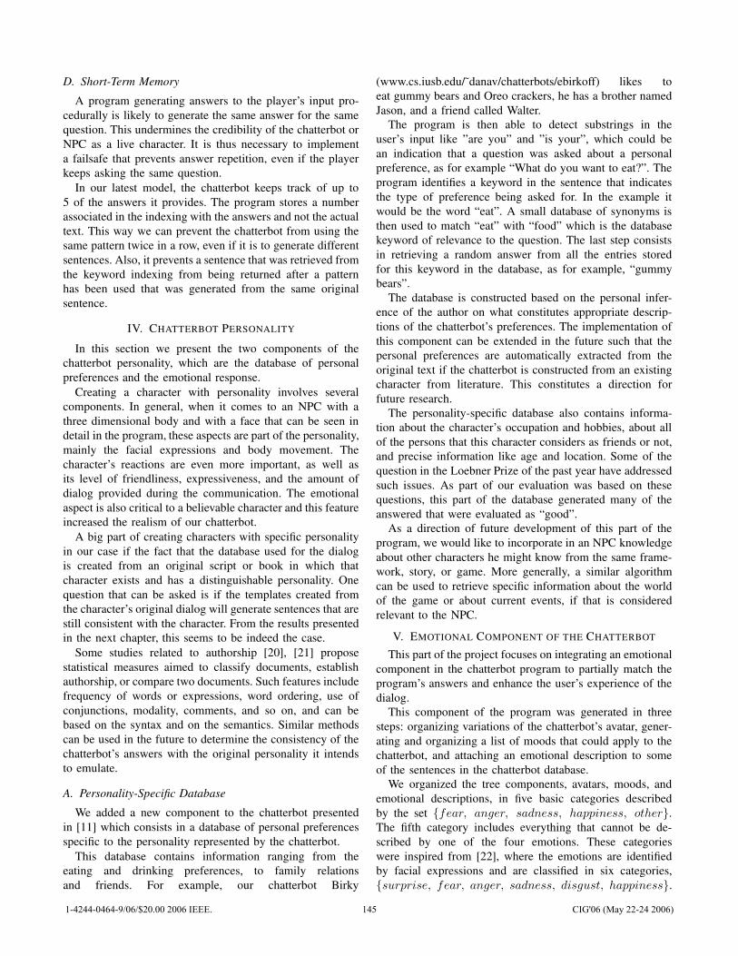
D. Short-Term Memory

A program generating answers to the player’s input pro-cedurally is likely to generate the same answer for the samequestion. This undermines the credibility of the chatterbot orNPC as a live character. It is thus necessary to implementa failsafe that prevents answer repetition, even if the playerkeeps asking the same question.

In our latest model, the chatterbot keeps track of up to5 of the answers it provides. The program stores a numberassociated in the indexing with the answers and not the actualtext. This way we can prevent the chatterbot from using thesame pattern twice in a row, even if it is to generate differentsentences. Also, it prevents a sentence that was retrieved fromthe keyword indexing from being returned after a patternhas been used that was generated from the same originalsentence.

IV. CHATTERBOT PERSONALITY

In this section we present the two components of thechatterbot personality, which are the database of personalpreferences and the emotional response.

Creating a character with personality involves severalcomponents. In general, when it comes to an NPC with athree dimensional body and with a face that can be seen indetail in the program, these aspects are part of the personality,mainly the facial expressions and body movement. Thecharacter’s reactions are even more important, as well asits level of friendliness, expressiveness, and the amount ofdialog provided during the communication. The emotionalaspect is also critical to a believable character and this featureincreased the realism of our chatterbot.

A big part of creating characters with specific personalityin our case if the fact that the database used for the dialogis created from an original script or book in which thatcharacter exists and has a distinguishable personality. Onequestion that can be asked is if the templates created fromthe character’s original dialog will generate sentences that arestill consistent with the character. From the results presentedin the next chapter, this seems to be indeed the case.

Some studies related to authorship [20], [21] proposestatistical measures aimed to classify documents, establishauthorship, or compare two documents. Such features includefrequency of words or expressions, word ordering, use ofconjunctions, modality, comments, and so on, and can bebased on the syntax and on the semantics. Similar methodscan be used in the future to determine the consistency of thechatterbot’s answers with the original personality it intendsto emulate.

A. Personality-Specific Database

We added a new component to the chatterbot presentedin [11] which consists in a database of personal preferencesspecific to the personality represented by the chatterbot.

This database contains information ranging from theeating and drinking preferences, to family relationsand friends. For example, our chatterbot Birky

(www.cs.iusb.edu/˜danav/chatterbots/ebirkoff) likes toeat gummy bears and Oreo crackers, he has a brother namedJason, and a friend called Walter.

The program is then able to detect substrings in theuser’s input like ”are you” and ”is your”, which could bean indication that a question was asked about a personalpreference, as for example “What do you want to eat?”. Theprogram identifies a keyword in the sentence that indicatesthe type of preference being asked for. In the example itwould be the word “eat”. A small database of synonyms isthen used to match “eat” with “food” which is the databasekeyword of relevance to the question. The last step consistsin retrieving a random answer from all the entries storedfor this keyword in the database, as for example, “gummybears”.

The database is constructed based on the personal infer-ence of the author on what constitutes appropriate descrip-tions of the chatterbot’s preferences. The implementation ofthis component can be extended in the future such that thepersonal preferences are automatically extracted from theoriginal text if the chatterbot is constructed from an existingcharacter from literature. This constitutes a direction forfuture research.

The personality-specific database also contains informa-tion about the character’s occupation and hobbies, about allof the persons that this character considers as friends or not,and precise information like age and location. Some of thequestion in the Loebner Prize of the past year have addressedsuch issues. As part of our evaluation was based on thesequestions, this part of the database generated many of theanswered that were evaluated as “good”.

As a direction of future development of this part of theprogram, we would like to incorporate in an NPC knowledgeabout other characters he might know from the same frame-work, story, or game. More generally, a similar algorithmcan be used to retrieve specific information about the worldof the game or about current events, if that is consideredrelevant to the NPC.

V. EMOTIONAL COMPONENT OF THE CHATTERBOT

This part of the project focuses on integrating an emotionalcomponent in the chatterbot program to partially match theprogram’s answers and enhance the user’s experience of thedialog.

This component of the program was generated in threesteps: organizing variations of the chatterbot’s avatar, gener-ating and organizing a list of moods that could apply to thechatterbot, and attaching an emotional description to someof the sentences in the chatterbot database.

We organized the tree components, avatars, moods, andemotional descriptions, in five basic categories describedby the set {fear, anger, sadness, happiness, other}.The fifth category includes everything that cannot be de-scribed by one of the four emotions. These categorieswere inspired from [22], where the emotions are identifiedby facial expressions and are classified in six categories,{surprise, fear, anger, sadness, disgust, happiness}.

1-4244-0464-9/06/$20.00 2006 IEEE. 145 CIG'06 (May 22-24 2006)

While the original classification is more complete, we did notfind any images of the character Birky showing disgust, andthe distinction between the images showing fear and surprisewas not clear enough to create separate categories.

We selected a number of expressive images of the charac-ter emulated by the chatterbot and organized them in the fivecategories described above. The images in each class exceptfor the fifth one were then sorted by intensity.

For the second step we generated a list of about 100different moods collected from mood descriptors commonlyused in online communication like blogs, message boards,emoticons, and synonyms of the four basic categories. Abouta fifth of the moods couldn’t be classified as any of thefour basic emotions and constitute the fifth category. Themoods in each class were then also sorted by intensity.For example, the “fear” class contains moods ranging from“uncomfortable” and “confused” to “shaken” or “terrified”.Many of these moods reflect a combination of fear andsurprise in various degrees.

In the last step we identified the sentences in the chatter-bot’s indexed database for which one of the four emotioncategories could apply. These sentences are identified by anumber and are used by the patterns, by the keyword-basedindexing, and to generate random answers.

The mood-generation process for any answer provided bythe chatterbot consists in three steps. First, we identify oneof the five categories that applies to the answer, either as oneof the four emotions if such an emotion could be identifiedfor the sentence, or the category “other” if not. Second, arandom avatar is selected from the identified category. Andlast, the avatar’s index in the set of pictures is projected ontothe range of moods for the same category, and a mood isselected within a range of 20% around the projected index.This way we approximately match the mood with the avatar’sexpression without providing the same avatar every time forany particular mood.

The selected avatar image is displayed, and acaption above the picture identifies the mood ofthe chatterbot. The program can be seen online atwww.cs.iusb.edu/˜danav/chatterbots/ebirkoff/.

VI. EXPERIMENTAL RESULTS

In this section we present some experimental results of ourchatterbot.

A. Previous Work

We compare the current chatterbot with and without theemotional component with the previous work we presentedin [11]. The chatterbots discussed in that paper can be seenonline at www.cs.iusb.edu/˜danav/chatterbots/.

In the former state, our chatterbots were using patternmatching and templates that were entirely constructed byhand. The random answers used a distinction betweendeclarative inputs and question-type inputs, with no furtherclassification of the questions. From the various discussionsconducted with the chatterbots, the refinement of this random

component seems to represent an improvement to the qualityof the answers.

The first chatterbots were using a very limited versionof keyword indexing. We expanded this component by im-plementing an automatic indexing process. This componentexpanded the diversity of the answers, but also proved toprovide the least quality in the answers. We foresee little useof this technique for the future, and the need for a muchmore selective indexing process.

The previous paper presented an evolutionary algorithmthat allowed us to generate new sentences based on the onesretrieved from the database and enhance the diversity ofresponse of the chatterbot. We did not include this componentin the latest chatterbot, but it is a possible direction for futureresearch. However, the automatic pattern generation andindexing, as well as the personal preference database seemto be better methods for expanding the space of possibleanswers for the chatterbot.

B. Chatterbot Evaluation

To evaluate the new chatterbot program with and withoutthe emotional component, an experiment was conductedconsisting in a dialog with the chatterbot with and withoutthe emotional component. The discussion consisted of 50inputs and answers for each version of the chatterbot. Onesubject participated in the experiments. A different set ofinput sentences was used with each version of the chatterbot,following the thread of the discussion. The answers wereevaluated based on the following categories: reasonable an-swers, good answers, and off topic answers, that seem to havelittle or nothing to do with the input sentence. The judgmentsof the chatterbot answers were made by the subject of theexperiment. Additionally, sentences that were syntacticallyincorrect were also counted, as well as the answers that wereconsistent with the character simulated by the chatterbot.Similar categories were used in [11] to evaluate the answers.

Table I shows the results of this experiment and comparesthe percentages in each categories with those reported in[11]. We computed the average from the previous paperof the percentages in each category, with and without thecontribution of the evolutionary algorithm which is denotedby EA in the last column. From this table we remark asubstantial improvement of the quality of responses providedby the latest chatterbot. The difference between the versionsof the program with and without the emotional component isvery small. This is due to the fact that the mood is added tothe response after the response is generated, and the answergeneration algorithm is identical in the two cases.

The results in last column, denoted by LB, were basedon the Loebner Prize (http://www.loebner.net/Prizef/loebner-prize.html). We selected 150 questions that the referees askedthe chatterbots and the humans in 2005. Birky’s answersto these questions were then judged based on the samecriteria as the other experiments. These results show a lowerpercentage of reasonable and good answers because theywere not asked during a sustained conversation, nor wereany of them specific to this particular chatterbot.

1-4244-0464-9/06/$20.00 2006 IEEE. 146 CIG'06 (May 22-24 2006)

TABLE IEVALUATION OF THE CHATTERBOTS WITH AND WITHOUT THE

EMOTIONAL COMPONENT

plain emotional previous EA LBReasonable 32% 30% 40% 42.5% 31.3%Good 48% 50% 18% 15.5% 32.7%Off topic 20% 20% 42% 42% 32%In character 90% 84% 75% 79% 92%Syntactically 2% 4% 4.5% 6.5% 4%incorrect

These experiments also provided an intuitive idea of whatthe emotional component adds to the program. In general, thechatterbot’s expressed mood enhances the dialog experienceand the impression of realism of the chatterbot. In severalcases the mood also added to the significance of the answer.A few answers that would have been classified as “reason-able” without the mood were classified as “good” based onthis additional information.

For example, when asked “would you like to talk aboutgail?”, who is supposedly a female character in the storythat the character had a romantic connection to in the past,Birky answered “i don’t know.” This answer can make sensewithout being especially to the point in the absence of infor-mation about the mood, which qualifies it as “reasonable”.The mood expressed in this case was “rejected” which addeda new significance to the answer and qualified it as “good”.

The correspondence between the avatars and the mood ex-pressed by the chatterbot was appropriate without being toorepetitive. In most cases, the expressed mood was reasonablefor the answer provided by the program.

VII. CONCLUSION

In this paper we presented a chatterbot application with anemotional component and personality-specific database. Weare currently developing a game integrating this chatterbotin a 3D environment as an intelligent NPC.

In the paper we first introduced the decision makingprocess to generate an answer. We followed with the basictechniques used by the chatterbot, pattern matching, au-tomatic indexing, and random sentence matching, as wellas the short term memory. The next section presented thepersonality database describing personal features like foodpreferences and family links, and the emotional componentthat associates a mood and a corresponding avatar to everyanswer returned by the chatterbot.

The results presented in the previous section are encourag-ing. The quality of response of the chatterbot has improvedas compared to the previous models we implemented, as wellas the space of possible answers for the chatterbot. Moreover,the emotional component adds another dimension of realismto the program and enhances the dialog experience. Thecapacity of emotional response is thus an important aspectin creating believable virtual characters.

REFERENCES

[1] J. Weizenbaum, “Eliza - a computer program for the study of naturallanguage communication between man and machine,” Communica-tions of the ACM, vol. 1, no. 9, 1966.

[2] B. Raphael, The Thinking Computer. New York: Freeman, 1976.[3] G. Guzeldere and S. Franchi, “Dialogues with colorful personalities

of early AI,” Stanford Humanities Review, vol. 4, no. 2, 1995.[4] W. Chamberlain, The Policeman’s Beard is Half Constructed. Warner

Books, 1984.[5] J. Barger, “”The Policeman’s Beard” was largely prefab!” The Journal

of Computer Game Design, vol. 6, 1993.[6] A. Turing, “Computing machinery and intelligence,” Mind, vol. 59,

no. 236, pp. 433–460, 1950.[7] F. Barthelemy, B. Dosquet, S. Gries, and X. Magnant, “Believable

synthetic characters in a virtual emarket,” in IASTED Artificial Intel-ligence and Applications, Innsbruck, Austria, 2004.

[8] A. Galvo, F. Barros, A. Neves, and G. Ramalho, “Persona-AIML: Anarchitecture for developing chatterbots with personality,” in Proceedingof Autonomous Agents and Multi Agent Systems, Columbia University,NY, USA, 2004.

[9] L. Saarine, Chatterbots: Crash Test Dummies of Communication.Master Thesis, University of Arts and Design Helsinki UIAH, 2001.

[10] A. De Angeli, G. I. Johnson, and L. Coventry, “The unfriendlyuser: Exploring social reactions to chatterbots,” in Proc. Int. Conf.Affective Human Factor Design, M. G. Helander, H. M. Kalid, andT. M. Po, Eds. Asean Academic Press, 2001, pp. 467–474. [Online].Available: citeseer.ist.psu.edu/557029.html

[11] D. Vrajitoru and J. Ratkiewicz, “Evolutionary sentence combinationfor chatterbots,” in The IASTED International Conference on ArtificialIntelligence and Applications (AIA 2004). Innsbruck, Austria: ACTAPress, February 16-18 2004, pp. 287–292.

[12] J. Bates, “The role of emotion in believable agents,” Communicationsof the ACM, vol. 37, no. 7, pp. 122–125, 1994.

[13] S. Brave and C. Nass, “Emotion in human-computer interaction,” inThe human-computer interaction handbook: fundamentals, evolvingtechnologies and emerging applications. Lawrence Erlbaum Asso-ciates, Inc, 2002, pp. 81–96.

[14] N. Magnenat-Thalmann, “Creating a smart virtual personality,” LectureNotes in Computer Science, vol. 2773, no. 2, pp. 15 – 16, 1993.

[15] E. Oliveira and L. Sarmento, “Emotional valence-based mechanismsand agent personality,” in Lecture Notes on Artificial Intelligence, ser.2507, G. Bittencourt and G. Ramalho, Eds. Springer, 2002, pp. 152–162.

[16] C. Okonkwo and J. Vassileva, “Affective pedagogical agents and userpersuasion,” in Proceedings of the 9th International Conference onHuman- Computer Interaction, C. Stephanidis, Ed., New Orleans,2001, pp. 397–401.

[17] N. Person, A. Graesser, R. Kreuz, V. Pomeroy, and TRG, “Simulatinghuman tutor dialog moves in AutoTutor,” International Journal ofArtificial Intelligence in Education, vol. 12, pp. 23–39, 2001.

[18] G. Salton, Ed., The SMART Retrieval System - Experiments in Auto-matic Document Processing. Englewood Cliffs (NJ): Prentice-Hall,1971.

[19] G. Salton, E. Fox, and U. Wu, “Extended Boolean informationretrieval,” Communications of the ACM, vol. 26, no. 12, pp. 1022–1036, 1983.

[20] H. v. Halteren, “Linguistic profiling for authorship recognition andverification,” in Proceedings of the 42th Meeting of the Associationfor COmputational Linguistics (ACL’04), Barcelona, Spain, 2004, pp.199–206.

[21] C. Whitelaw and J. Patrick, “Selecting systemic features for text classi-fication,” in Australasian Language Technology Workshop, MacquarieUniversity, NSW Australia, 2004, pp. 93–100.

[22] P. Eckman and V. F. Wallace, Unmasking the Face: A Guide toRecognizing Emotions from Facial Clues. Englewood Cliffs N.J.:Prentice-Hall, 1975.

1-4244-0464-9/06/$20.00 2006 IEEE. 147 CIG'06 (May 22-24 2006)

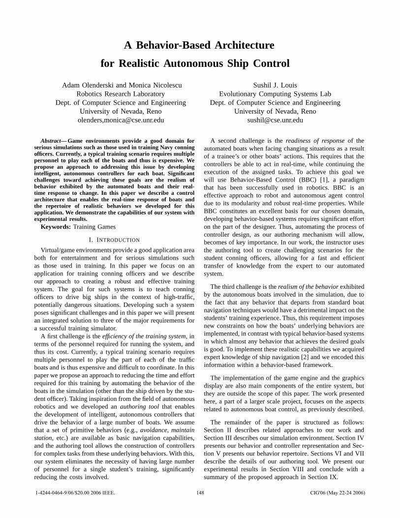
A Behavior-Based Architecture

for Realistic Autonomous Ship Control

Adam Olenderski and Monica NicolescuRobotics Research Laboratory

Dept. of Computer Science and EngineeringUniversity of Nevada, Reno

olenders,monica@cse.unr.edu

Sushil J. LouisEvolutionary Computing Systems Lab

Dept. of Computer Science and EngineeringUniversity of Nevada, Reno

sushil@cse.unr.edu

Abstract— Game environments provide a good domain forserious simulations such as those used in training Navy conningofficers. Currently, a typical training scenario requires multiplepersonnel to play each of the boats and thus is expensive. Wepropose an approach to addressing this issue by developingintelligent, autonomous controllers for each boat. Significantchallenges toward achieving these goals are the realism ofbehavior exhibited by the automated boats and their real-time response to change. In this paper we describe a controlarchitecture that enables the real-time response of boats andthe repertoire of realistic behaviors we developed for thisapplication. We demonstrate the capabilities of our system withexperimental results.

Keywords: Training Games

I. INTRODUCTION

Virtual/game environments provide a good application areaboth for entertainment and for serious simulations suchas those used in training. In this paper we focus on anapplication for training conning officers and we describeour approach to creating a robust and effective trainingsystem. The goal for such systems is to teach conningofficers to drive big ships in the context of high-traffic,potentially dangerous situations. Developing such a systemposes significant challenges and in this paper we will presentan integrated solution to three of the major requirements fora successful training simulator.

A first challenge is the efficiency of the training system, interms of the personnel required for running the system, andthus its cost. Currently, a typical training scenario requiresmultiple personnel to play the part of each of the trafficboats and is thus expensive and difficult to coordinate. In thispaper we propose an approach to reducing the time and effortrequired for this training by automating the behavior of theboats in the simulation (other than the ship driven by the stu-dent officer). Taking inspiration from the field of autonomousrobotics and we developed an authoring tool that enablesthe development of intelligent, autonomous controllers thatdrive the behavior of a large number of boats. We assumethat a set of primitive behaviors (e.g., avoidance, maintainstation, etc.) are available as basic navigation capabilities,and the authoring tool allows the construction of controllersfor complex tasks from these underlying behaviors. With this,our system eliminates the necessity of having large numberof personnel for a single student’s training, significantlyreducing the costs involved.

A second challenge is the readiness of response of theautomated boats when facing changing situations as a resultof a trainee’s or other boats’ actions. This requires that thecontrollers be able to act in real-time, while continuing theexecution of the assigned tasks. To achieve this goal wewill use Behavior-Based Control (BBC) [1], a paradigmthat has been successfully used in robotics. BBC is aneffective approach to robot and autonomous agent controldue to its modularity and robust real-time properties. WhileBBC constitutes an excellent basis for our chosen domain,developing behavior-based systems requires significant efforton the part of the designer. Thus, automating the process ofcontroller design, as our authoring mechanism will allow,becomes of key importance. In our work, the instructor usesthe authoring tool to create challenging scenarios for thestudent conning officers, allowing for a fast and efficienttransfer of knowledge from the expert to our automatedsystem.

The third challenge is the realism of the behavior exhibitedby the autonomous boats involved in the simulation, due tothe fact that any behavior that departs from standard boatnavigation techniques would have a detrimental impact on thestudents’ training experience. Thus, this requirement imposesnew constraints on how the boats’ underlying behaviors areimplemented, in contrast with typical behavior-based systemsin which almost any behavior that achieves the desired goalsis good. To implement these realistic capabilities we acquiredexpert knowledge of ship navigation [2] and we encoded thisinformation within a behavior-based framework.

The implementation of the game engine and the graphicsdisplay are also main components of the entire system, butthey are outside the scope of this paper. The work presentedhere, a part of a larger scale project, focuses on the aspectsrelated to autonomous boat control, as previously described.

The remainder of the paper is structured as follows:Section II describes related approaches to our work andSection III describes our simulation environment. Section IVpresents our behavior and controller representation and Sec-tion V presents our behavior repertoire. Sections VI and VIIdescribe the details of our authoring tool. We present ourexperimental results in Section VIII and conclude with asummary of the proposed approach in Section IX.

1-4244-0464-9/06/$20.00 2006 IEEE. 148 CIG'06 (May 22-24 2006)

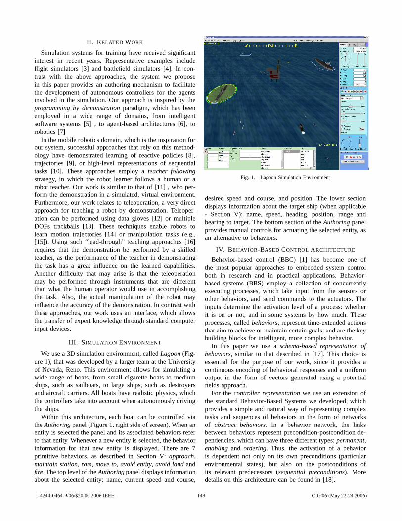
II. RELATED WORK

Simulation systems for training have received significantinterest in recent years. Representative examples includeflight simulators [3] and battlefield simulators [4]. In con-trast with the above approaches, the system we proposein this paper provides an authoring mechanism to facilitatethe development of autonomous controllers for the agentsinvolved in the simulation. Our approach is inspired by theprogramming by demonstration paradigm, which has beenemployed in a wide range of domains, from intelligentsoftware systems [5] , to agent-based architectures [6], torobotics [7]

In the mobile robotics domain, which is the inspiration forour system, successful approaches that rely on this method-ology have demonstrated learning of reactive policies [8],trajectories [9], or high-level representations of sequentialtasks [10]. These approaches employ a teacher followingstrategy, in which the robot learner follows a human or arobot teacher. Our work is similar to that of [11] , who per-form the demonstration in a simulated, virtual environment.Furthermore, our work relates to teleoperation, a very directapproach for teaching a robot by demonstration. Teleoper-ation can be performed using data gloves [12] or multipleDOFs trackballs [13]. These techniques enable robots tolearn motion trajectories [14] or manipulation tasks (e.g.,[15]). Using such “lead-through” teaching approaches [16]requires that the demonstration be performed by a skilledteacher, as the performance of the teacher in demonstratingthe task has a great influence on the learned capabilities.Another difficulty that may arise is that the teleoperationmay be performed through instruments that are differentthan what the human operator would use in accomplishingthe task. Also, the actual manipulation of the robot mayinfluence the accuracy of the demonstration. In contrast withthese approaches, our work uses an interface, which allowsthe transfer of expert knowledge through standard computerinput devices.

III. SIMULATION ENVIRONMENT

We use a 3D simulation environment, called Lagoon (Fig-ure 1), that was developed by a larger team at the Universityof Nevada, Reno. This environment allows for simulating awide range of boats, from small cigarette boats to mediumships, such as sailboats, to large ships, such as destroyersand aircraft carriers. All boats have realistic physics, whichthe controllers take into account when autonomously drivingthe ships.

Within this architecture, each boat can be controlled viathe Authoring panel (Figure 1, right side of screen). When anentity is selected the panel and its associated behaviors referto that entity. Whenever a new entity is selected, the behaviorinformation for that new entity is displayed. There are 7primitive behaviors, as described in Section V: approach,maintain station, ram, move to, avoid entity, avoid land andfire. The top level of the Authoring panel displays informationabout the selected entity: name, current speed and course,

Fig. 1. Lagoon Simulation Environment

desired speed and course, and position. The lower sectiondisplays information about the target ship (when applicable- Section V): name, speed, heading, position, range andbearing to target. The bottom section of the Authoring panelprovides manual controls for actuating the selected entity, asan alternative to behaviors.

IV. BEHAVIOR-BASED CONTROL ARCHITECTURE

Behavior-based control (BBC) [1] has become one ofthe most popular approaches to embedded system controlboth in research and in practical applications. Behavior-based systems (BBS) employ a collection of concurrentlyexecuting processes, which take input from the sensors orother behaviors, and send commands to the actuators. Theinputs determine the activation level of a process: whetherit is on or not, and in some systems by how much. Theseprocesses, called behaviors, represent time-extended actionsthat aim to achieve or maintain certain goals, and are the keybuilding blocks for intelligent, more complex behavior.

In this paper we use a schema-based representation ofbehaviors, similar to that described in [17]. This choice isessential for the purpose of our work, since it provides acontinuous encoding of behavioral responses and a uniformoutput in the form of vectors generated using a potentialfields approach.

For the controller representation we use an extension ofthe standard Behavior-Based Systems we developed, whichprovides a simple and natural way of representing complextasks and sequences of behaviors in the form of networksof abstract behaviors. In a behavior network, the linksbetween behaviors represent precondition-postcondition de-pendencies, which can have three different types: permanent,enabling and ordering. Thus, the activation of a behavioris dependent not only on its own preconditions (particularenvironmental states), but also on the postconditions ofits relevant predecessors (sequential preconditions). Moredetails on this architecture can be found in [18].

1-4244-0464-9/06/$20.00 2006 IEEE. 149 CIG'06 (May 22-24 2006)

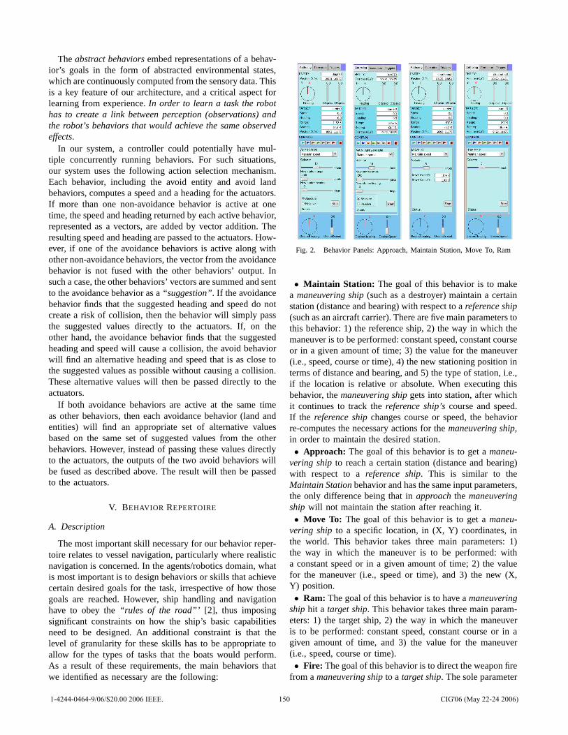
The abstract behaviors embed representations of a behav-ior’s goals in the form of abstracted environmental states,which are continuously computed from the sensory data. Thisis a key feature of our architecture, and a critical aspect forlearning from experience. In order to learn a task the robothas to create a link between perception (observations) andthe robot’s behaviors that would achieve the same observedeffects.

In our system, a controller could potentially have mul-tiple concurrently running behaviors. For such situations,our system uses the following action selection mechanism.Each behavior, including the avoid entity and avoid landbehaviors, computes a speed and a heading for the actuators.If more than one non-avoidance behavior is active at onetime, the speed and heading returned by each active behavior,represented as a vectors, are added by vector addition. Theresulting speed and heading are passed to the actuators. How-ever, if one of the avoidance behaviors is active along withother non-avoidance behaviors, the vector from the avoidancebehavior is not fused with the other behaviors’ output. Insuch a case, the other behaviors’ vectors are summed and sentto the avoidance behavior as a “suggestion”. If the avoidancebehavior finds that the suggested heading and speed do notcreate a risk of collision, then the behavior will simply passthe suggested values directly to the actuators. If, on theother hand, the avoidance behavior finds that the suggestedheading and speed will cause a collision, the avoid behaviorwill find an alternative heading and speed that is as close tothe suggested values as possible without causing a collision.These alternative values will then be passed directly to theactuators.

If both avoidance behaviors are active at the same timeas other behaviors, then each avoidance behavior (land andentities) will find an appropriate set of alternative valuesbased on the same set of suggested values from the otherbehaviors. However, instead of passing these values directlyto the actuators, the outputs of the two avoid behaviors willbe fused as described above. The result will then be passedto the actuators.

V. BEHAVIOR REPERTOIRE

A. Description

The most important skill necessary for our behavior reper-toire relates to vessel navigation, particularly where realisticnavigation is concerned. In the agents/robotics domain, whatis most important is to design behaviors or skills that achievecertain desired goals for the task, irrespective of how thosegoals are reached. However, ship handling and navigationhave to obey the “rules of the road”’ [2], thus imposingsignificant constraints on how the ship’s basic capabilitiesneed to be designed. An additional constraint is that thelevel of granularity for these skills has to be appropriate toallow for the types of tasks that the boats would perform.As a result of these requirements, the main behaviors thatwe identified as necessary are the following:

Fig. 2. Behavior Panels: Approach, Maintain Station, Move To, Ram

• Maintain Station: The goal of this behavior is to makea maneuvering ship (such as a destroyer) maintain a certainstation (distance and bearing) with respect to a reference ship(such as an aircraft carrier). There are five main parameters tothis behavior: 1) the reference ship, 2) the way in which themaneuver is to be performed: constant speed, constant courseor in a given amount of time; 3) the value for the maneuver(i.e., speed, course or time), 4) the new stationing position interms of distance and bearing, and 5) the type of station, i.e.,if the location is relative or absolute. When executing thisbehavior, the maneuvering ship gets into station, after whichit continues to track the reference ship’s course and speed.If the reference ship changes course or speed, the behaviorre-computes the necessary actions for the maneuvering ship,in order to maintain the desired station.• Approach: The goal of this behavior is to get a maneu-

vering ship to reach a certain station (distance and bearing)with respect to a reference ship. This is similar to theMaintain Station behavior and has the same input parameters,the only difference being that in approach the maneuveringship will not maintain the station after reaching it.• Move To: The goal of this behavior is to get a maneu-

vering ship to a specific location, in (X, Y) coordinates, inthe world. This behavior takes three main parameters: 1)the way in which the maneuver is to be performed: witha constant speed or in a given amount of time; 2) the valuefor the maneuver (i.e., speed or time), and 3) the new (X,Y) position.• Ram: The goal of this behavior is to have a maneuvering

ship hit a target ship. This behavior takes three main param-eters: 1) the target ship, 2) the way in which the maneuveris to be performed: constant speed, constant course or in agiven amount of time, and 3) the value for the maneuver(i.e., speed, course or time).• Fire: The goal of this behavior is to direct the weapon fire

from a maneuvering ship to a target ship. The sole parameter

1-4244-0464-9/06/$20.00 2006 IEEE. 150 CIG'06 (May 22-24 2006)

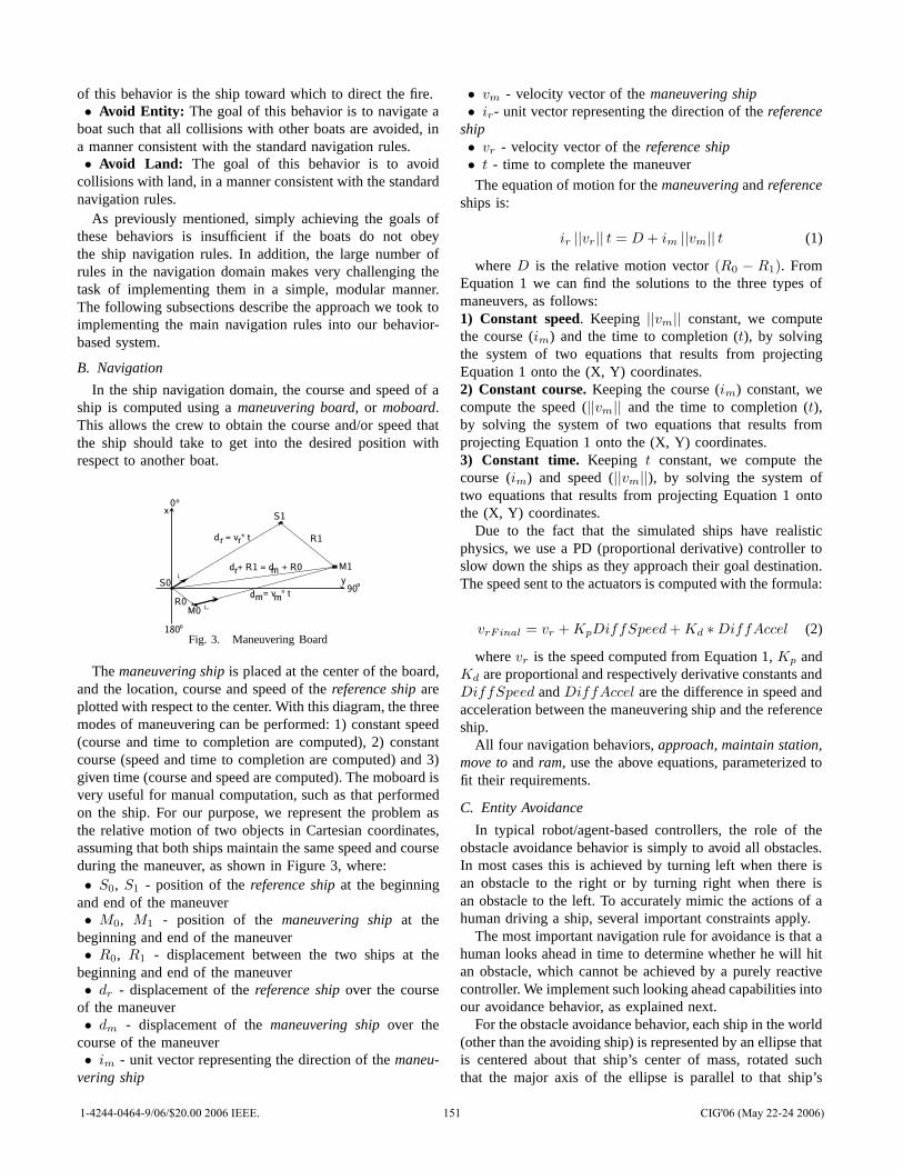
of this behavior is the ship toward which to direct the fire.• Avoid Entity: The goal of this behavior is to navigate a

boat such that all collisions with other boats are avoided, ina manner consistent with the standard navigation rules.• Avoid Land: The goal of this behavior is to avoid

collisions with land, in a manner consistent with the standardnavigation rules.

As previously mentioned, simply achieving the goals ofthese behaviors is insufficient if the boats do not obeythe ship navigation rules. In addition, the large number ofrules in the navigation domain makes very challenging thetask of implementing them in a simple, modular manner.The following subsections describe the approach we took toimplementing the main navigation rules into our behavior-based system.

B. Navigation

In the ship navigation domain, the course and speed of aship is computed using a maneuvering board, or moboard.This allows the crew to obtain the course and/or speed thatthe ship should take to get into the desired position withrespect to another boat.

Fig. 3. Maneuvering Board

The maneuvering ship is placed at the center of the board,and the location, course and speed of the reference ship areplotted with respect to the center. With this diagram, the threemodes of maneuvering can be performed: 1) constant speed(course and time to completion are computed), 2) constantcourse (speed and time to completion are computed) and 3)given time (course and speed are computed). The moboard isvery useful for manual computation, such as that performedon the ship. For our purpose, we represent the problem asthe relative motion of two objects in Cartesian coordinates,assuming that both ships maintain the same speed and courseduring the maneuver, as shown in Figure 3, where:• S0, S1 - position of the reference ship at the beginning

and end of the maneuver• M0, M1 - position of the maneuvering ship at the

beginning and end of the maneuver• R0, R1 - displacement between the two ships at the

beginning and end of the maneuver• dr - displacement of the reference ship over the course

of the maneuver• dm - displacement of the maneuvering ship over the

course of the maneuver• im - unit vector representing the direction of the maneu-

vering ship

• vm - velocity vector of the maneuvering ship• ir- unit vector representing the direction of the reference

ship• vr - velocity vector of the reference ship• t - time to complete the maneuver

The equation of motion for the maneuvering and referenceships is:

ir ||vr|| t = D + im ||vm|| t (1)

where D is the relative motion vector (R0 − R1). FromEquation 1 we can find the solutions to the three types ofmaneuvers, as follows:1) Constant speed. Keeping ||vm|| constant, we computethe course (im) and the time to completion (t), by solvingthe system of two equations that results from projectingEquation 1 onto the (X, Y) coordinates.2) Constant course. Keeping the course (im) constant, wecompute the speed (||vm|| and the time to completion (t),by solving the system of two equations that results fromprojecting Equation 1 onto the (X, Y) coordinates.3) Constant time. Keeping t constant, we compute thecourse (im) and speed (||vm||), by solving the system oftwo equations that results from projecting Equation 1 ontothe (X, Y) coordinates.

Due to the fact that the simulated ships have realisticphysics, we use a PD (proportional derivative) controller toslow down the ships as they approach their goal destination.The speed sent to the actuators is computed with the formula:

vrF inal = vr + KpDiffSpeed + Kd ∗ DiffAccel (2)

where vr is the speed computed from Equation 1, Kp andKd are proportional and respectively derivative constants andDiffSpeed and DiffAccel are the difference in speed andacceleration between the maneuvering ship and the referenceship.

All four navigation behaviors, approach, maintain station,move to and ram, use the above equations, parameterized tofit their requirements.

C. Entity Avoidance

In typical robot/agent-based controllers, the role of theobstacle avoidance behavior is simply to avoid all obstacles.In most cases this is achieved by turning left when there isan obstacle to the right or by turning right when there isan obstacle to the left. To accurately mimic the actions of ahuman driving a ship, several important constraints apply.

The most important navigation rule for avoidance is that ahuman looks ahead in time to determine whether he will hitan obstacle, which cannot be achieved by a purely reactivecontroller. We implement such looking ahead capabilities intoour avoidance behavior, as explained next.

For the obstacle avoidance behavior, each ship in the world(other than the avoiding ship) is represented by an ellipse thatis centered about that ship’s center of mass, rotated suchthat the major axis of the ellipse is parallel to that ship’s

1-4244-0464-9/06/$20.00 2006 IEEE. 151 CIG'06 (May 22-24 2006)

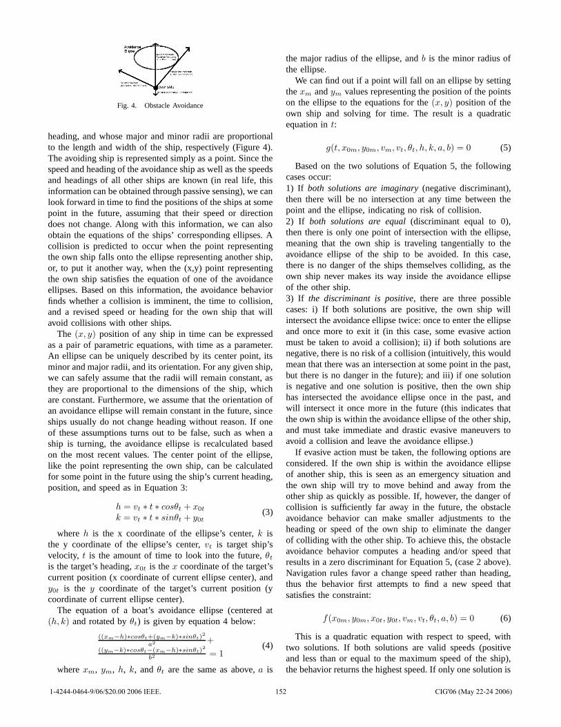
Fig. 4. Obstacle Avoidance

heading, and whose major and minor radii are proportionalto the length and width of the ship, respectively (Figure 4).The avoiding ship is represented simply as a point. Since thespeed and heading of the avoidance ship as well as the speedsand headings of all other ships are known (in real life, thisinformation can be obtained through passive sensing), we canlook forward in time to find the positions of the ships at somepoint in the future, assuming that their speed or directiondoes not change. Along with this information, we can alsoobtain the equations of the ships’ corresponding ellipses. Acollision is predicted to occur when the point representingthe own ship falls onto the ellipse representing another ship,or, to put it another way, when the (x,y) point representingthe own ship satisfies the equation of one of the avoidanceellipses. Based on this information, the avoidance behaviorfinds whether a collision is imminent, the time to collision,and a revised speed or heading for the own ship that willavoid collisions with other ships.

The (x, y) position of any ship in time can be expressedas a pair of parametric equations, with time as a parameter.An ellipse can be uniquely described by its center point, itsminor and major radii, and its orientation. For any given ship,we can safely assume that the radii will remain constant, asthey are proportional to the dimensions of the ship, whichare constant. Furthermore, we assume that the orientation ofan avoidance ellipse will remain constant in the future, sinceships usually do not change heading without reason. If oneof these assumptions turns out to be false, such as when aship is turning, the avoidance ellipse is recalculated basedon the most recent values. The center point of the ellipse,like the point representing the own ship, can be calculatedfor some point in the future using the ship’s current heading,position, and speed as in Equation 3:

h = vt ∗ t ∗ cosθt + x0t

k = vt ∗ t ∗ sinθt + y0t

(3)

where h is the x coordinate of the ellipse’s center, k isthe y coordinate of the ellipse’s center, vt is target ship’svelocity, t is the amount of time to look into the future, θt

is the target’s heading, x0t is the x coordinate of the target’scurrent position (x coordinate of current ellipse center), andy0t is the y coordinate of the target’s current position (ycoordinate of current ellipse center).

The equation of a boat’s avoidance ellipse (centered at(h, k) and rotated by θt) is given by equation 4 below:

((xm−h)∗cosθt+(ym−k)∗sinθt)2

a2 +

((ym−k)∗cosθt−(xm−h)∗sinθt)2

b2 = 1

(4)

where xm, ym, h, k, and θt are the same as above, a is

the major radius of the ellipse, and b is the minor radius ofthe ellipse.

We can find out if a point will fall on an ellipse by settingthe xm and ym values representing the position of the pointson the ellipse to the equations for the (x, y) position of theown ship and solving for time. The result is a quadraticequation in t:

g(t, x0m, y0m, vm, vt, θt, h, k, a, b) = 0 (5)

Based on the two solutions of Equation 5, the followingcases occur:1) If both solutions are imaginary (negative discriminant),then there will be no intersection at any time between thepoint and the ellipse, indicating no risk of collision.2) If both solutions are equal (discriminant equal to 0),then there is only one point of intersection with the ellipse,meaning that the own ship is traveling tangentially to theavoidance ellipse of the ship to be avoided. In this case,there is no danger of the ships themselves colliding, as theown ship never makes its way inside the avoidance ellipseof the other ship.3) If the discriminant is positive, there are three possiblecases: i) If both solutions are positive, the own ship willintersect the avoidance ellipse twice: once to enter the ellipseand once more to exit it (in this case, some evasive actionmust be taken to avoid a collision); ii) if both solutions arenegative, there is no risk of a collision (intuitively, this wouldmean that there was an intersection at some point in the past,but there is no danger in the future); and iii) if one solutionis negative and one solution is positive, then the own shiphas intersected the avoidance ellipse once in the past, andwill intersect it once more in the future (this indicates thatthe own ship is within the avoidance ellipse of the other ship,and must take immediate and drastic evasive maneuvers toavoid a collision and leave the avoidance ellipse.)

If evasive action must be taken, the following options areconsidered. If the own ship is within the avoidance ellipseof another ship, this is seen as an emergency situation andthe own ship will try to move behind and away from theother ship as quickly as possible. If, however, the danger ofcollision is sufficiently far away in the future, the obstacleavoidance behavior can make smaller adjustments to theheading or speed of the own ship to eliminate the dangerof colliding with the other ship. To achieve this, the obstacleavoidance behavior computes a heading and/or speed thatresults in a zero discriminant for Equation 5, (case 2 above).Navigation rules favor a change speed rather than heading,thus the behavior first attempts to find a new speed thatsatisfies the constraint:

f(x0m, y0m, x0t, y0t, vm, vt, θt, a, b) = 0 (6)

This is a quadratic equation with respect to speed, withtwo solutions. If both solutions are valid speeds (positiveand less than or equal to the maximum speed of the ship),the behavior returns the highest speed. If only one solution is

1-4244-0464-9/06/$20.00 2006 IEEE. 152 CIG'06 (May 22-24 2006)

a valid speed, that speed is used. If neither solution is valid,then the heading must be changed to avoid a collision. To finda valid heading, the behavior first finds whether the collisionwould still be imminent if the own ship turned five degreesto the left. If not, then the behavior continues to test potentialheadings, in increments of five degrees, until it finds one thatavoids a collision, at which point it uses the same processto find a corresponding heading to the right of the currentheading. This results in two headings (one to the right, andone to the left) that avoid a collision. The heading closest tothe current heading is the one passed to the actuators.

The solution to avoid one ship could potentially generatecollisions with others. Our approach uses a mechanism todeal with avoiding multiple ships, as follows: for everyship on a collision course with the own ship, the avoidancebehavior puts in a list all the valid speeds and headings thatwill avoid that ship. After all the ships have been analyzedand the list is built, the behavior iterates through the list andeliminates the routes that collide with other ships. The onlyelements remaining in the list will be the speeds or headingsthat avoid collisions with all the other ships in the simulation.Since speed changes take priority over heading changes, ifthere is at least one speed remaining in the list, that speedwill be passed to the actuator with the current heading. Ifthere is more than one potential speed in the list, the highestspeed is passed to the actuators. If no speed changes remainin the list, then the potential heading that is closest to thecurrent heading is passed to the actuators along with thecurrent speed.

D. Land Avoidance

To determine whether or not a ship is in danger ofgrounding itself, the avoid land behavior uses the speed ofthe ship, as indicated in [2]. The behavior uses this speed todetermine the approximate distance that the ship can travel infour minutes. Next, it checks if there is any land within thatdistance, in all directions from the ship. If no land is presentin that area, there is no land to avoid. However, if there is landin front of the own ship, the behavior computes a headingthat will take the ship away from land and a speed that makesthe nearest land be outside of the four minute range. Toachieve this, the behavior uses the distance and bearing tothe nearest land in the front 180-degree field of view. Thenew speed is calculated to be that distance divided by fourminutes, to ensure that the nearest land will lie outside ofthe four minute range. The new heading is calculated to bethat bearing plus or minus 90 degrees, whichever is closer tothe current heading. This ensures that instead of continuingto head toward land, getting slower and slower until theship grounds itself, the ship will turn parallel to the land,following its contour until there is no more land to avoid oruntil the land avoidance behavior is turned off.

VI. TRIGGERS

Triggers are a mechanism that allows the user to indicateimportant situations in the simulation, typically with thepurpose of changing a boat’s behavior when that situation

occurs. A trigger is created through the triggers panel ofour interface (Figure 5). We provide the following types oftriggers: distance between entities, entities within a certainrange, hull strength of a particular ship, or an arbitrary flag.The panel allows the user to specify the parameters for eachtrigger, such as, for example, the entities in the simulationbetween which the distance is to be monitored. The nameand current value (updated every tick) of all created triggersis displayed on the triggers panel main window. Triggers canbe created, monitored, or deleted at any time during eitherauthoring or execution.

Fig. 5. Trigger types and panel

The distance between entities trigger is included for conve-nience, as it does not require user input during authoring andmany maritime maneuvers depend on the distances betweenparticular ships. However, for a more general event thatcannot be described in terms of the distance between twoentities or the damage taken by a particular ship, there arearbitrary flag triggers as well. These work similarly to theother triggers, in that they are user created and indicate whena controller should change behavior. However, these triggersare binary flags, meaning that they can only hold one of twovalues: true or false. Also, these triggers require user inputnot only during authoring, but also during execution. A flagtrigger usually represents an event that the user will have tospecify himself, such as the start of a scenario. For example,to add a flag trigger to start a scenario, the user would createa trigger named ”Start Scenario” before authoring. Whilerecording, when the user is ready to begin the scenario,he would navigate to the triggers panel, click the check-box next to the ”Start Scenario” trigger, click the CriticalJuncture button, and change the behavior of the ship he/sheis controlling. This informs the system that that behaviorshould only be activated after the ”Start Scenario” flag hasbeen set. Then, when the controller is executed, it will waituntil the user explicitly activates that flag before continuing.This is done by navigating to the triggers panel, clicking thecheck-box next to the desired flag trigger, and clicking theCritical Juncture button.

1-4244-0464-9/06/$20.00 2006 IEEE. 153 CIG'06 (May 22-24 2006)

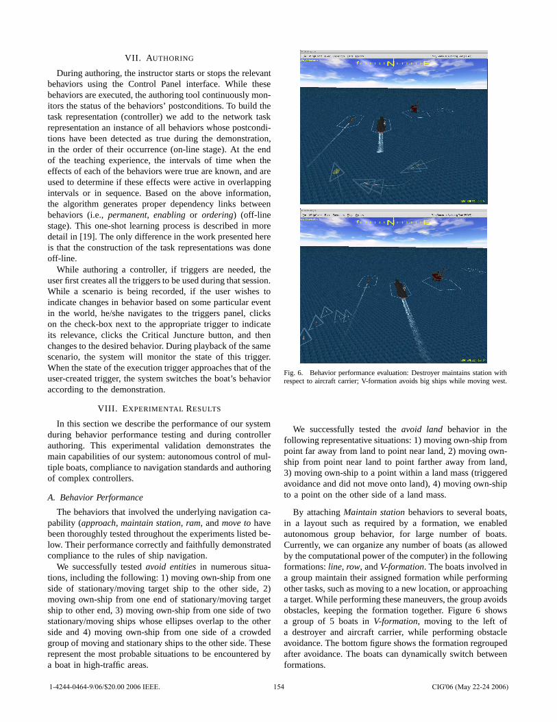
VII. AUTHORING

During authoring, the instructor starts or stops the relevantbehaviors using the Control Panel interface. While thesebehaviors are executed, the authoring tool continuously mon-itors the status of the behaviors’ postconditions. To build thetask representation (controller) we add to the network taskrepresentation an instance of all behaviors whose postcondi-tions have been detected as true during the demonstration,in the order of their occurrence (on-line stage). At the endof the teaching experience, the intervals of time when theeffects of each of the behaviors were true are known, and areused to determine if these effects were active in overlappingintervals or in sequence. Based on the above information,the algorithm generates proper dependency links betweenbehaviors (i.e., permanent, enabling or ordering) (off-linestage). This one-shot learning process is described in moredetail in [19]. The only difference in the work presented hereis that the construction of the task representations was doneoff-line.

While authoring a controller, if triggers are needed, theuser first creates all the triggers to be used during that session.While a scenario is being recorded, if the user wishes toindicate changes in behavior based on some particular eventin the world, he/she navigates to the triggers panel, clickson the check-box next to the appropriate trigger to indicateits relevance, clicks the Critical Juncture button, and thenchanges to the desired behavior. During playback of the samescenario, the system will monitor the state of this trigger.When the state of the execution trigger approaches that of theuser-created trigger, the system switches the boat’s behavioraccording to the demonstration.

VIII. EXPERIMENTAL RESULTS

In this section we describe the performance of our systemduring behavior performance testing and during controllerauthoring. This experimental validation demonstrates themain capabilities of our system: autonomous control of mul-tiple boats, compliance to navigation standards and authoringof complex controllers.

A. Behavior Performance

The behaviors that involved the underlying navigation ca-pability (approach, maintain station, ram, and move to havebeen thoroughly tested throughout the experiments listed be-low. Their performance correctly and faithfully demonstratedcompliance to the rules of ship navigation.

We successfully tested avoid entities in numerous situa-tions, including the following: 1) moving own-ship from oneside of stationary/moving target ship to the other side, 2)moving own-ship from one end of stationary/moving targetship to other end, 3) moving own-ship from one side of twostationary/moving ships whose ellipses overlap to the otherside and 4) moving own-ship from one side of a crowdedgroup of moving and stationary ships to the other side. Theserepresent the most probable situations to be encountered bya boat in high-traffic areas.

Fig. 6. Behavior performance evaluation: Destroyer maintains station withrespect to aircraft carrier; V-formation avoids big ships while moving west.

We successfully tested the avoid land behavior in thefollowing representative situations: 1) moving own-ship frompoint far away from land to point near land, 2) moving own-ship from point near land to point farther away from land,3) moving own-ship to a point within a land mass (triggeredavoidance and did not move onto land), 4) moving own-shipto a point on the other side of a land mass.

By attaching Maintain station behaviors to several boats,in a layout such as required by a formation, we enabledautonomous group behavior, for large number of boats.Currently, we can organize any number of boats (as allowedby the computational power of the computer) in the followingformations: line, row, and V-formation. The boats involved ina group maintain their assigned formation while performingother tasks, such as moving to a new location, or approachinga target. While performing these maneuvers, the group avoidsobstacles, keeping the formation together. Figure 6 showsa group of 5 boats in V-formation, moving to the left ofa destroyer and aircraft carrier, while performing obstacleavoidance. The bottom figure shows the formation regroupedafter avoidance. The boats can dynamically switch betweenformations.

1-4244-0464-9/06/$20.00 2006 IEEE. 154 CIG'06 (May 22-24 2006)

B. Controller Authoring

We have performed a large number of authoring experi-ments (more than 10 different scenarios), with all scenariosbeing learned correctly. Below we list a few examples, whichare most relevant for the training of conning officers.

1. ZigZag Attack: A small boat moves into position withrespect to a big ship, then approaches a group that maintainsdistant station of that ship. The group moves in V-formation.On a flag trigger the small boat approaches the big boat andmaintains station until a second trigger goes off. Next, thesmall boat rejoins the boat group in the distance. When athird flag trigger goes off, the small boat re-approaches thebig boat and maintains close station to it. When getting witha given range (distance trigger), the small boat moves intoposition behind the big ship and rams it.

2. Defend: A destroyer (escort) maintains station with respectto an aircraft carrier to be defended. A small cigarette boatapproaches the destroyer. When the cigarette boat comeswithin a buffer range of the aircraft carrier (e.g., 1000yards) a distance trigger is activated, after which the escort’sbehavior changes from maintain station on carrier to ramcigarette boat.

3. Attack-Distract Two boats take turns distracting so oneor both can ram a target. Boat A maintains a position in frontand slightly to the side of the Target at a long range, as if itwants to be seen but not considered a threat. Boat B starts tothe side of the target and slowly begins to collide with theTarget. Once B is with in a certain range hopefully gainingthe attention of the Target, A starts a full-speed ram. OnceA starts the ram, B stops its approach and backs off.

IX. CONCLUSION

In this paper we presented an approach to efficient andrealistic design of serious game simulators, with applicationto ship navigation. The goal of this system is to providethe infrastructure needed to train conning officers to drivebig ships in the context of high-traffic, potentially dangeroussituations. Developing such a system poses significant chal-lenges and in this paper we presented an integrated solutionto three of the major requirements for a successful trainingsimulator: 1) the efficiency of the training system, 2) thereadiness of response of the boats and 3) the realism ofthe behavior of the automated boat controllers. To addressthese challenges we developed an authoring tool that enablesthe development of intelligent, autonomous controllers thatdrive the behavior of a large number of boats.This eliminatesthe necessity of having large number of personnel for asingle student’s training, significantly reducing the costsinvolved. We developed a Behavior-Based Control architec-ture that provides responsive automated controllers, and weincorporated expert ship navigation knowledge to providerealistic behavior for the automated boats. To demonstrateour approach, we presented experimental results describingthe main capabilities of our system.

X. ACKNOWLEDGMENTS

The authors would like to acknowledge the significantcontribution of Sergiu Dascalu, Chris Miles, Ryan Leigh,and Juan Quiroz, from the University of Nevada, Reno. Thiswork was supported by the Office of Naval Research undergrant number N00014-05-1-0709.

REFERENCES

[1] R. C. Arkin, Behavior-Based Robotics. CA: MIT Press, 1998.[Online]. Available: http://www.usc.edu

[2] J. John V. Noel, Ed., Knight’s Modern Seamanship. John Wiley andSons, 1988.

[3] M. Tambe, L. W. Johnson, R. M. Jones, F. V. Koss, J. E. Laird,P. S. Rosenbloom, and K. Schwamb, “Intelligent agents for interactivesimulation environments,” AI Magazine, vol. 16, no. 1, pp. 15–39,1995.

[4] R. B. Calder, J. E. Smith, A. J. Courtemarche, J. M. F. Mar, andA. Z. Ceranowicz, “Modsaf behavior simulation and control,” inProceedings of the Second Conference on Computer Generated Forcesand Behavioral Representation, July 1993.

[5] H. Lieberman, Human-Computer Interaction for the New Millenium.ACM Press/Addison-Wesley, 2001, ch. Interfaces that Give and TakeAdvice, pp. 475–485.

[6] R. H. Angros, “Learning what to instruct: Acquiring knowledge fromdemonstrations and foccused experimentation,” Ph.D. dissertation,University of Southern California, May 2000.

[7] S. Schaal, “Learning from demonstration,” in Advances in Neural In-formation Processing Systems 9, M. Mozer, M. Jordan, and T. Petsche,Eds. MIT Press, Cambridge, 1997, pp. 1040–1046.

[8] G. Hayes and J. Demiris, “A robot controller using learning byimitation,” in Proc. of the Intl. Symp. on Intelligent Robotic Systems,Grenoble, France, 1994, pp. 198–204.

[9] P. Gaussier, S. Moga, J. Banquet, and M. Quoy, “From perception-action loops to imitation processes: A bottom-up approach of learningby imitation,” Applied Artificial Intelligence Journal, vol. 12(78), pp.701–729, 1998.

[10] M. N. Nicolescu and M. J. Mataric, “Natural methods for robot tasklearning: Instructive demonstration, generalization and practice,” inProc., Second Intl. Joint Conf. on Autonomous Agents and Multi-AgentSystems, Melbourne, Australia, July 2003.

[11] J. Aleotti, S. Caselli, and M. Reggiani, “Leveraging on a virtualenvironment for robot programming by demonstration,” Robotics andAutonomous Systems, vol. 47, pp. 153–161, 2004.

[12] R. Voyles and P. Khosla, “A multi-agent system for programmingrobots by human demonstration,” Integrated Computer-Aided Engi-neering, vol. 8, no. 1, pp. 59–67, 2001.

[13] M. Kaiser and R. Dillmann, “Building elementary robot skills fromhuman demonstration,” in Proc., IEEE Intl. Conf. on Robotics andAutomation, Minneapolis, Minnesota, apr 1996, pp. 2700–2705.

[14] N. Delson and H. West, “Robot programming by human demonstra-tion: Adaptation and inconsistency in constrained motion,” in Proc.,IEEE Intl. Conf. on Robotics and Automation, Minneapolis, MN, apr1996, pp. 30–36.

[15] J. Yang, Y. Xu, and C. S. Chen, “Hidden markov model approach toskill learning and its application in telerobotics,” in Proc., Intl. Conf.on Intelligent Robots and Systems, Yokohama, Japan, 1993, pp. 396–402.

[16] D. J. Todd, Fundamentals of Robot Technology. John Wiley and Sons,1986.

[17] R. C. Arkin, “Motor schema based navigation for a mobile robot:An approach to programming by behavior,” in IEEE Conference onRobotics and Automation, 1987, 1987, pp. 264–271.

[18] M. N. Nicolescu and M. J. Mataric, “A hierarchical architecture forbehavior-based robots,” in Proc., First Intl. Joint Conf. on AutonomousAgents and Multi-Agent Systems, Bologna, Italy, July 2002, pp. 227–233.

[19] ——, “Learning and interacting in human-robot domain,” IEEE Trans-actions on Systems, Man, and Cybernetics, Part A: Systems andHumans, Special Issue on Socially Intelligent Agents - The Humanin the Loop, vol. 31, no. 5, pp. 419–430, 2001.

1-4244-0464-9/06/$20.00 2006 IEEE. 155 CIG'06 (May 22-24 2006)

Modelling and Simulation of Combat ID – the INCIDER Model D. Dean, P. Syms, K. Hynd, B. Mistry, A. Vincent

Abstract—This paper explores a method of incorporating the human decision making process and human factors (such as fatigue, experience and confirmatory bias) into a one-on-one combat model, the INCIDER model. It discusses some of the theory behind the decision making cycle and explains the sensor fusion techniques used to combine information from several distinct sources. It then explains how the INCIDER model incorporates these processes to represent the manner in which an individual decision maker identifies an unknown battlespace object (a process often referred to as “combat ID”). The paper goes on to discuss ongoing work validating the parameters used within the model, involving a series of experiments using a synthetic environment. It also explores possible uses of the model, both as a standalone tool and as an information feed to higher level constructive simulations and wargames.

I. INTRODUCTION

The use of modelling and simulation in the UK Ministry of Defence (MoD) is becoming more and more widespread. As the Defence budget becomes more constrained, expensive mistakes are becoming less and less acceptable to the public. Among other things, modelling and simulation provides:

• A proven method of reducing risk before investing in new equipment;

• Cheap and effective ways of providing training; • A mechanism to investigate the root causes of

battlefield incidents and identify lessons learned. However, although many of the models used by the UK

contain very high-fidelity physical representations (i.e. of aspects like ballistics, fluid flow etc.) the “human” aspects of the battle have been modelled with a great deal less fidelity (and in some cases largely ignored). These “human factors” include areas like fatigue, stress, attitude to risk, individual personality, level of training, level of experience and so on. These parameters can have a massive effect on

Manuscript received January 30th, 2006. This work was funded by the

U.K. Ministry of Defence. D. Dean and A. Vincent are with the Land Battlespace Systems

Department of the Defence Science and Technology Laboratory (Dstl), Portsdown West, PO17 6AD, UK. Email: dfdean@dstl.gov.uk, avincent@dstl.gov.uk

P. Syms is with the Land Battlespace Systems Department of the Defence Science and Technology Laboratory (Dstl), Fort Halstead, TN14 7BP, UK. Email: prsyms@dstl.gov.uk

K. Hynd and B. Mistry are with the Information Management Department of the Defence Science and Technology Laboratory (Dstl), Portsdown West, PO17 6AD, UK. Email: kshynd@dstl.gov.uk, bmistry@dstl.gov.uk

the outcome of a battle; for example, the effects of sleep deprivation have been proven to significantly reduce both the ability to make complex decisions and to perform straightforward tasks (Harrison and Horne, [1]), but still factors like this are often considered too complex to represent within a model.

One area where the effects of human factors cannot be overstated is in the identification of entities in the battlespace (often referred to as combat identification). The physical environment can contribute significantly to the problem (e.g. constrained line of sight to a target, poor weather conditions limiting sensor utility etc.), but analysis of historical incidents has shown that often the factors that will have the most telling contribution are far less cut and dried; psychological factors such as confirmatory bias and the personality of the individual attempting to make the identification, for example, have had a very significant effect in many cases.

Combat identification is also an important example because one of the possible repercussions of a combat identification failure is fratricide. Historically, fratricide (sometimes known as Blue-on-Blue or friendly fire) has been a feature of warfare since the beginning of recorded history. During WW1 and WW2 it is believed to have accounted for between 10% and 20% of all casualties. In the more recent Gulf conflicts the mismatch between forces led to low overall numbers of UK and US casualties, bringing into focus the significance of own-force casualties. The public are becoming more and more reluctant to accept casualties in war, but when casualties arise through identification errors and result in friendly fire incidents the political impact is dramatically increased.

Effective combat identification (CID) of entities encountered in the battlespace is critical in reducing fratricide. CID is defined by the British Army [2] as:

‘The process of combining situational awareness, target identification, specific tactics, techniques and procedures to increase operational effectiveness of weapon systems and reduce the incidence of casualties caused by friendly fire’

Good combat identification can improve the tempo of operations, and increase the effectiveness of manoeuvre and engagement. Conversely, poor CID can:

• lower tempo (wasting time as unknown forces are positively identified);

• introduce Blue fratricide casualties, lowering morale and effectiveness;

1-4244-0464-9/06/$20.00 2006 IEEE. 156 CIG'06 (May 22-24 2006)

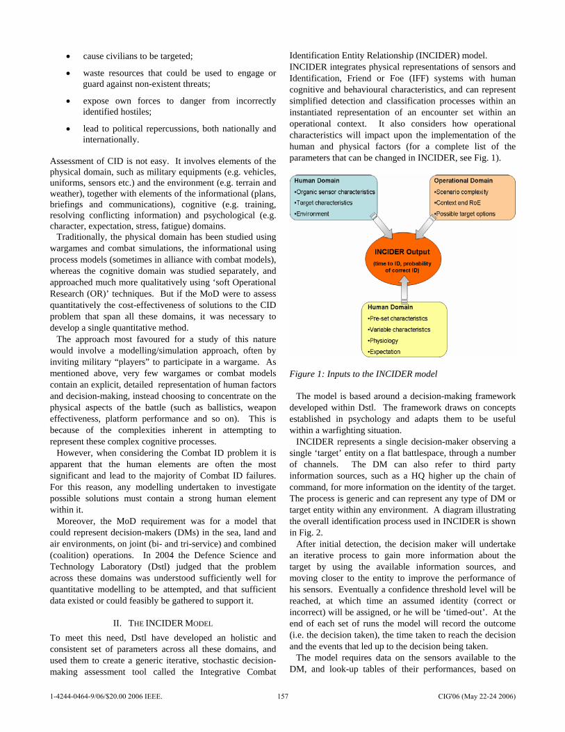
• cause civilians to be targeted;

• waste resources that could be used to engage or guard against non-existent threats;

• expose own forces to danger from incorrectly identified hostiles;

• lead to political repercussions, both nationally and internationally.

Assessment of CID is not easy. It involves elements of the physical domain, such as military equipments (e.g. vehicles, uniforms, sensors etc.) and the environment (e.g. terrain and weather), together with elements of the informational (plans, briefings and communications), cognitive (e.g. training, resolving conflicting information) and psychological (e.g. character, expectation, stress, fatigue) domains.

Traditionally, the physical domain has been studied using wargames and combat simulations, the informational using process models (sometimes in alliance with combat models), whereas the cognitive domain was studied separately, and approached much more qualitatively using ‘soft Operational Research (OR)’ techniques. But if the MoD were to assess quantitatively the cost-effectiveness of solutions to the CID problem that span all these domains, it was necessary to develop a single quantitative method.

The approach most favoured for a study of this nature would involve a modelling/simulation approach, often by inviting military “players” to participate in a wargame. As mentioned above, very few wargames or combat models contain an explicit, detailed representation of human factors and decision-making, instead choosing to concentrate on the physical aspects of the battle (such as ballistics, weapon effectiveness, platform performance and so on). This is because of the complexities inherent in attempting to represent these complex cognitive processes.

However, when considering the Combat ID problem it is apparent that the human elements are often the most significant and lead to the majority of Combat ID failures. For this reason, any modelling undertaken to investigate possible solutions must contain a strong human element within it.

Moreover, the MoD requirement was for a model that could represent decision-makers (DMs) in the sea, land and air environments, on joint (bi- and tri-service) and combined (coalition) operations. In 2004 the Defence Science and Technology Laboratory (Dstl) judged that the problem across these domains was understood sufficiently well for quantitative modelling to be attempted, and that sufficient data existed or could feasibly be gathered to support it.

II. THE INCIDER MODEL To meet this need, Dstl have developed an holistic and consistent set of parameters across all these domains, and used them to create a generic iterative, stochastic decision-making assessment tool called the Integrative Combat

Identification Entity Relationship (INCIDER) model. INCIDER integrates physical representations of sensors and Identification, Friend or Foe (IFF) systems with human cognitive and behavioural characteristics, and can represent simplified detection and classification processes within an instantiated representation of an encounter set within an operational context. It also considers how operational characteristics will impact upon the implementation of the human and physical factors (for a complete list of the parameters that can be changed in INCIDER, see Fig. 1).

Figure 1: Inputs to the INCIDER model

The model is based around a decision-making framework developed within Dstl. The framework draws on concepts established in psychology and adapts them to be useful within a warfighting situation.

INCIDER represents a single decision-maker observing a single ‘target’ entity on a flat battlespace, through a number of channels. The DM can also refer to third party information sources, such as a HQ higher up the chain of command, for more information on the identity of the target. The process is generic and can represent any type of DM or target entity within any environment. A diagram illustrating the overall identification process used in INCIDER is shown in Fig. 2.

After initial detection, the decision maker will undertake an iterative process to gain more information about the target by using the available information sources, and moving closer to the entity to improve the performance of his sensors. Eventually a confidence threshold level will be reached, at which time an assumed identity (correct or incorrect) will be assigned, or he will be ‘timed-out’. At the end of each set of runs the model will record the outcome (i.e. the decision taken), the time taken to reach the decision and the events that led up to the decision being taken.

The model requires data on the sensors available to the DM, and look-up tables of their performances, based on

1-4244-0464-9/06/$20.00 2006 IEEE. 157 CIG'06 (May 22-24 2006)

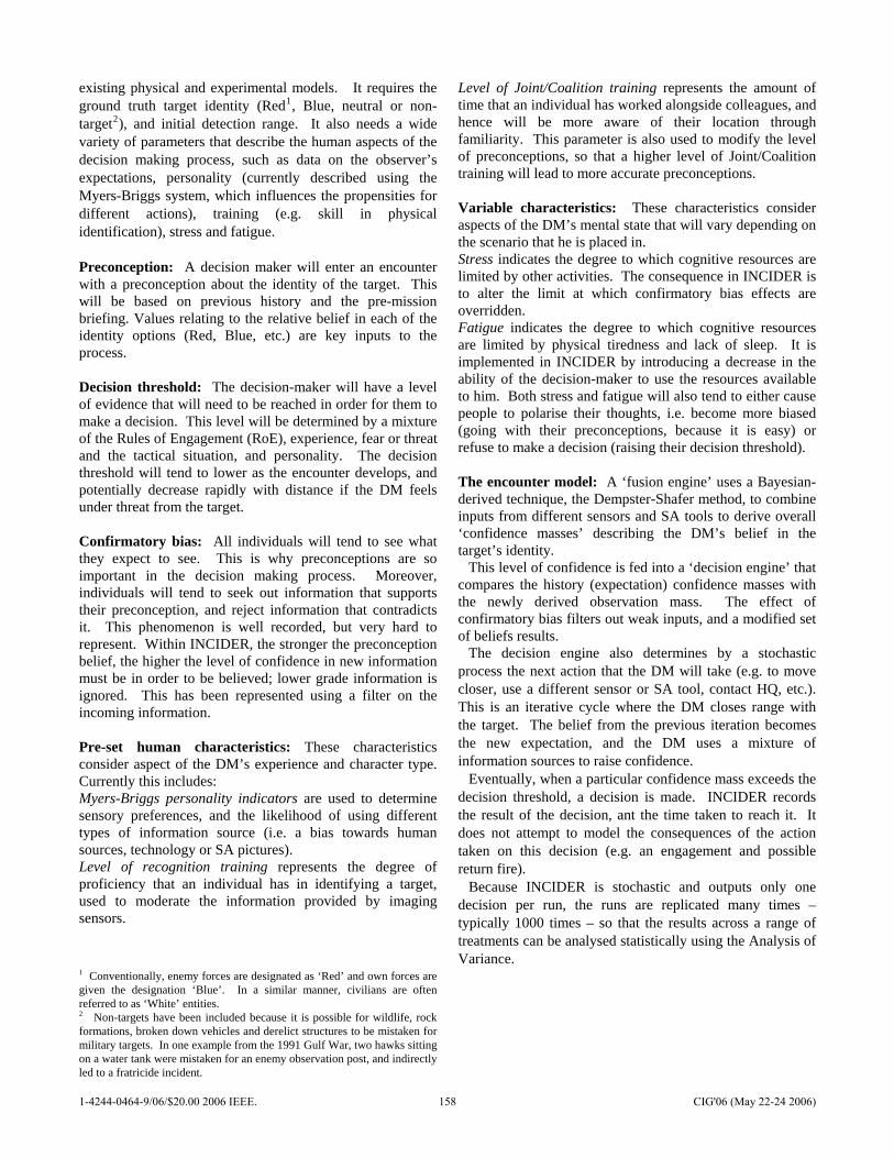
existing physical and experimental models. It requires the ground truth target identity (Red1, Blue, neutral or non-target2), and initial detection range. It also needs a wide variety of parameters that describe the human aspects of the decision making process, such as data on the observer’s expectations, personality (currently described using the Myers-Briggs system, which influences the propensities for different actions), training (e.g. skill in physical identification), stress and fatigue. Preconception: A decision maker will enter an encounter with a preconception about the identity of the target. This will be based on previous history and the pre-mission briefing. Values relating to the relative belief in each of the identity options (Red, Blue, etc.) are key inputs to the process. Decision threshold: The decision-maker will have a level of evidence that will need to be reached in order for them to make a decision. This level will be determined by a mixture of the Rules of Engagement (RoE), experience, fear or threat and the tactical situation, and personality. The decision threshold will tend to lower as the encounter develops, and potentially decrease rapidly with distance if the DM feels under threat from the target. Confirmatory bias: All individuals will tend to see what they expect to see. This is why preconceptions are so important in the decision making process. Moreover, individuals will tend to seek out information that supports their preconception, and reject information that contradicts it. This phenomenon is well recorded, but very hard to represent. Within INCIDER, the stronger the preconception belief, the higher the level of confidence in new information must be in order to be believed; lower grade information is ignored. This has been represented using a filter on the incoming information. Pre-set human characteristics: These characteristics consider aspect of the DM’s experience and character type. Currently this includes: Myers-Briggs personality indicators are used to determine sensory preferences, and the likelihood of using different types of information source (i.e. a bias towards human sources, technology or SA pictures). Level of recognition training represents the degree of proficiency that an individual has in identifying a target, used to moderate the information provided by imaging sensors.

1 Conventionally, enemy forces are designated as ‘Red’ and own forces are given the designation ‘Blue’. In a similar manner, civilians are often referred to as ‘White’ entities. 2 Non-targets have been included because it is possible for wildlife, rock formations, broken down vehicles and derelict structures to be mistaken for military targets. In one example from the 1991 Gulf War, two hawks sitting on a water tank were mistaken for an enemy observation post, and indirectly led to a fratricide incident.

Level of Joint/Coalition training represents the amount of time that an individual has worked alongside colleagues, and hence will be more aware of their location through familiarity. This parameter is also used to modify the level of preconceptions, so that a higher level of Joint/Coalition training will lead to more accurate preconceptions. Variable characteristics: These characteristics consider aspects of the DM’s mental state that will vary depending on the scenario that he is placed in. Stress indicates the degree to which cognitive resources are limited by other activities. The consequence in INCIDER is to alter the limit at which confirmatory bias effects are overridden. Fatigue indicates the degree to which cognitive resources are limited by physical tiredness and lack of sleep. It is implemented in INCIDER by introducing a decrease in the ability of the decision-maker to use the resources available to him. Both stress and fatigue will also tend to either cause people to polarise their thoughts, i.e. become more biased (going with their preconceptions, because it is easy) or refuse to make a decision (raising their decision threshold). The encounter model: A ‘fusion engine’ uses a Bayesian-derived technique, the Dempster-Shafer method, to combine inputs from different sensors and SA tools to derive overall ‘confidence masses’ describing the DM’s belief in the target’s identity.

This level of confidence is fed into a ‘decision engine’ that compares the history (expectation) confidence masses with the newly derived observation mass. The effect of confirmatory bias filters out weak inputs, and a modified set of beliefs results.

The decision engine also determines by a stochastic process the next action that the DM will take (e.g. to move closer, use a different sensor or SA tool, contact HQ, etc.). This is an iterative cycle where the DM closes range with the target. The belief from the previous iteration becomes the new expectation, and the DM uses a mixture of information sources to raise confidence.

Eventually, when a particular confidence mass exceeds the decision threshold, a decision is made. INCIDER records the result of the decision, ant the time taken to reach it. It does not attempt to model the consequences of the action taken on this decision (e.g. an engagement and possible return fire).

Because INCIDER is stochastic and outputs only one decision per run, the runs are replicated many times – typically 1000 times – so that the results across a range of treatments can be analysed statistically using the Analysis of Variance.

1-4244-0464-9/06/$20.00 2006 IEEE. 158 CIG'06 (May 22-24 2006)

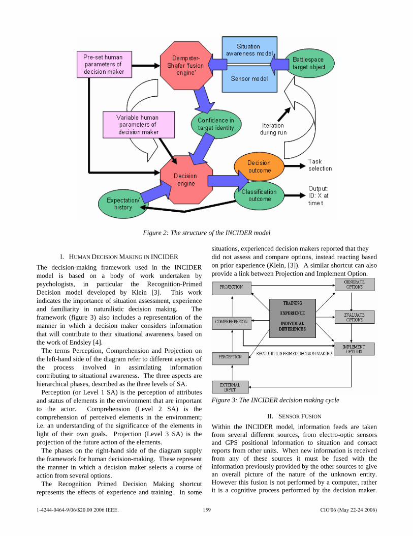
Figure 2: The structure of the INCIDER model

I. HUMAN DECISION MAKING IN INCIDER The decision-making framework used in the INCIDER model is based on a body of work undertaken by psychologists, in particular the Recognition-Primed Decision model developed by Klein [3]. This work indicates the importance of situation assessment, experience and familiarity in naturalistic decision making. The framework (figure 3) also includes a representation of the manner in which a decision maker considers information that will contribute to their situational awareness, based on the work of Endsley [4].

The terms Perception, Comprehension and Projection on the left-hand side of the diagram refer to different aspects of the process involved in assimilating information contributing to situational awareness. The three aspects are hierarchical phases, described as the three levels of SA.

Perception (or Level 1 SA) is the perception of attributes and status of elements in the environment that are important to the actor. Comprehension (Level 2 SA) is the comprehension of perceived elements in the environment; i.e. an understanding of the significance of the elements in light of their own goals. Projection (Level 3 SA) is the projection of the future action of the elements.

The phases on the right-hand side of the diagram supply the framework for human decision-making. These represent the manner in which a decision maker selects a course of action from several options.

The Recognition Primed Decision Making shortcut represents the effects of experience and training. In some

situations, experienced decision makers reported that they did not assess and compare options, instead reacting based on prior experience (Klein, [3]). A similar shortcut can also provide a link between Projection and Implement Option.

Figure 3: The INCIDER decision making cycle

II. SENSOR FUSION Within the INCIDER model, information feeds are taken from several different sources, from electro-optic sensors and GPS positional information to situation and contact reports from other units. When new information is received from any of these sources it must be fused with the information previously provided by the other sources to give an overall picture of the nature of the unknown entity. However this fusion is not performed by a computer, rather it is a cognitive process performed by the decision maker.

1-4244-0464-9/06/$20.00 2006 IEEE. 159 CIG'06 (May 22-24 2006)

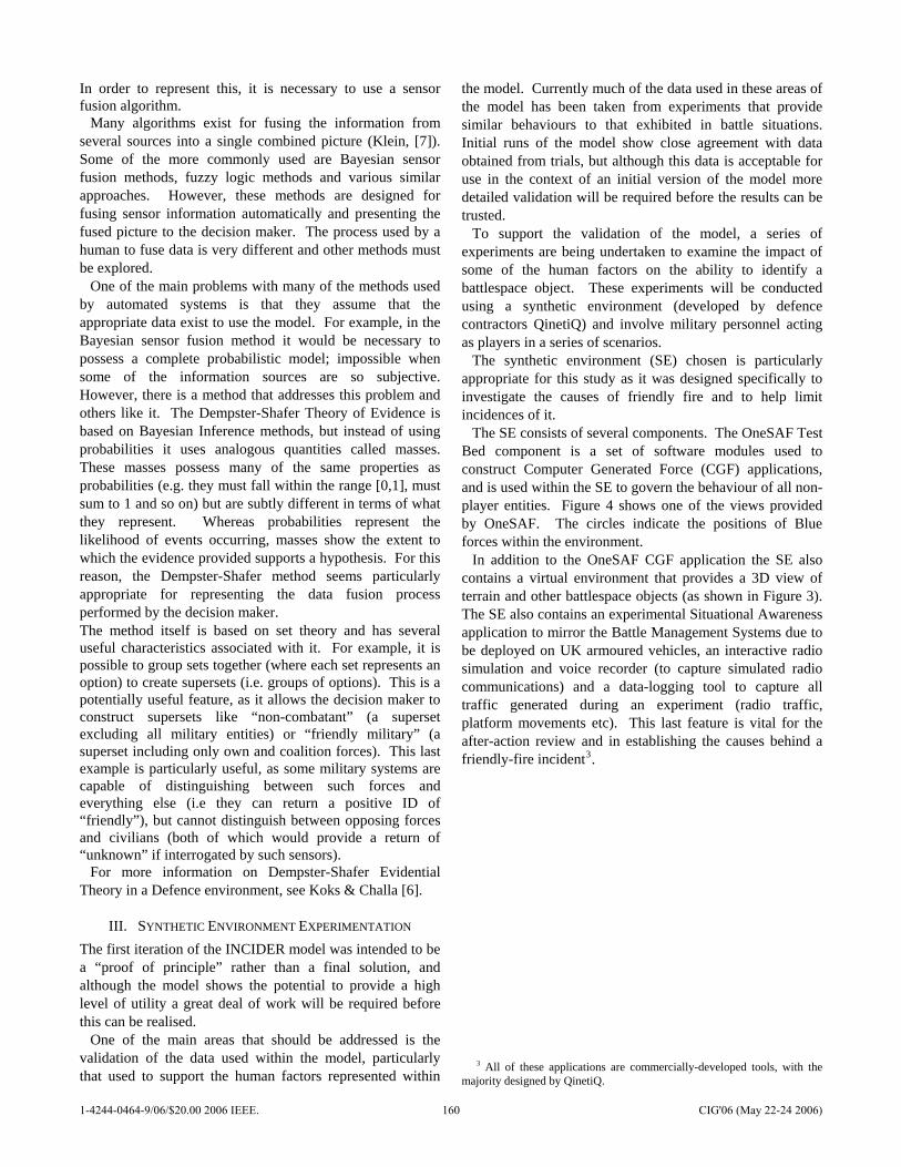
In order to represent this, it is necessary to use a sensor fusion algorithm.

Many algorithms exist for fusing the information from several sources into a single combined picture (Klein, [7]). Some of the more commonly used are Bayesian sensor fusion methods, fuzzy logic methods and various similar approaches. However, these methods are designed for fusing sensor information automatically and presenting the fused picture to the decision maker. The process used by a human to fuse data is very different and other methods must be explored.

One of the main problems with many of the methods used by automated systems is that they assume that the appropriate data exist to use the model. For example, in the Bayesian sensor fusion method it would be necessary to possess a complete probabilistic model; impossible when some of the information sources are so subjective. However, there is a method that addresses this problem and others like it. The Dempster-Shafer Theory of Evidence is based on Bayesian Inference methods, but instead of using probabilities it uses analogous quantities called masses. These masses possess many of the same properties as probabilities (e.g. they must fall within the range [0,1], must sum to 1 and so on) but are subtly different in terms of what they represent. Whereas probabilities represent the likelihood of events occurring, masses show the extent to which the evidence provided supports a hypothesis. For this reason, the Dempster-Shafer method seems particularly appropriate for representing the data fusion process performed by the decision maker. The method itself is based on set theory and has several useful characteristics associated with it. For example, it is possible to group sets together (where each set represents an option) to create supersets (i.e. groups of options). This is a potentially useful feature, as it allows the decision maker to construct supersets like “non-combatant” (a superset excluding all military entities) or “friendly military” (a superset including only own and coalition forces). This last example is particularly useful, as some military systems are capable of distinguishing between such forces and everything else (i.e they can return a positive ID of “friendly”), but cannot distinguish between opposing forces and civilians (both of which would provide a return of “unknown” if interrogated by such sensors).

For more information on Dempster-Shafer Evidential Theory in a Defence environment, see Koks & Challa [6].

III. SYNTHETIC ENVIRONMENT EXPERIMENTATION The first iteration of the INCIDER model was intended to be a “proof of principle” rather than a final solution, and although the model shows the potential to provide a high level of utility a great deal of work will be required before this can be realised.

One of the main areas that should be addressed is the validation of the data used within the model, particularly that used to support the human factors represented within

the model. Currently much of the data used in these areas of the model has been taken from experiments that provide similar behaviours to that exhibited in battle situations. Initial runs of the model show close agreement with data obtained from trials, but although this data is acceptable for use in the context of an initial version of the model more detailed validation will be required before the results can be trusted.

To support the validation of the model, a series of experiments are being undertaken to examine the impact of some of the human factors on the ability to identify a battlespace object. These experiments will be conducted using a synthetic environment (developed by defence contractors QinetiQ) and involve military personnel acting as players in a series of scenarios.

The synthetic environment (SE) chosen is particularly appropriate for this study as it was designed specifically to investigate the causes of friendly fire and to help limit incidences of it.

The SE consists of several components. The OneSAF Test Bed component is a set of software modules used to construct Computer Generated Force (CGF) applications, and is used within the SE to govern the behaviour of all non-player entities. Figure 4 shows one of the views provided by OneSAF. The circles indicate the positions of Blue forces within the environment.

In addition to the OneSAF CGF application the SE also contains a virtual environment that provides a 3D view of terrain and other battlespace objects (as shown in Figure 3). The SE also contains an experimental Situational Awareness application to mirror the Battle Management Systems due to be deployed on UK armoured vehicles, an interactive radio simulation and voice recorder (to capture simulated radio communications) and a data-logging tool to capture all traffic generated during an experiment (radio traffic, platform movements etc). This last feature is vital for the after-action review and in establishing the causes behind a friendly-fire incident3.

3 All of these applications are commercially-developed tools, with the

majority designed by QinetiQ.

1-4244-0464-9/06/$20.00 2006 IEEE. 160 CIG'06 (May 22-24 2006)

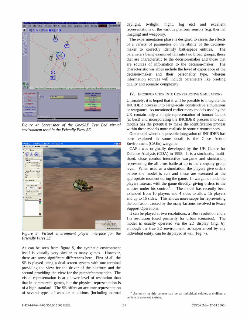
Figure 4: Screenshot of the OneSAF Test Bed virtual environment used in the Friendly Fires SE

Figure 5: Virtual environment player interface for the Friendly Fires SE As can be seen from figure 5, the synthetic environment itself is visually very similar to many games. However, there are some significant differences here. First of all, the SE is played using a dual-screen system with one terminal providing the view for the driver of the platform and the second providing the view for the gunner/commander. The visual representation is at a lower level of resolution than that in commercial games, but the physical representation is of a high standard. The SE offers an accurate representation of several types of weather conditions (including normal

daylight, twilight, night, fog etc) and excellent representations of the various platform sensors (e.g. thermal imaging) and weaponry.

The experimentation phase is designed to assess the effects of a variety of parameters on the ability of the decision-maker to correctly identify battlespace entities. The parameters being examined fall into two broad groups; those that are characteristic to the decision-maker and those that are sources of information to the decision-maker. The characteristic variables include the level of experience of the decision-maker and their personality type, whereas information sources will include parameters like briefing quality and scenario complexity.

IV. INCORPORATION INTO CONSTRUCTIVE SIMULATIONS Ultimately, it is hoped that it will be possible to integrate the INCIDER process into large-scale constructive simulations or wargames. As mentioned earlier many models used by the UK contain only a simple representation of human factors (at best) and incorporating the INCIDER process into such models has the potential to make the identification process within these models more realistic in some circumstances.

One model where the possible integration of INCIDER has been explored in some detail is the Close Action Environment (CAEn) wargame.

CAEn was originally developed by the UK Centre for Defence Analysis (CDA) in 1995. It is a stochastic, multi-sided, close combat interactive wargame and simulation, representing the all-arms battle at up to the company group level. When used as a simulation, the players give orders before the model is run and these are executed at the appropriate moment during the game. In wargame mode the players interact with the game directly, giving orders to the entities under his control4. The model has recently been extended from 10 players and 4 sides to allow 15 players and up to 15 sides. This allows more scope for representing the confusion caused by the many factions involved in Peace Support Operations.

It can be played at two resolutions; a 10m resolution and a 1m resolution (used primarily for urban scenarios). The model is usually operated via the 2D display (Fig. 6), although the true 3D environment, as experienced by any individual entity, can be displayed at will (Fig. 7).

4 An entity in this context can be an individual soldier, a civilian, a

vehicle or a remote system.

1-4244-0464-9/06/$20.00 2006 IEEE. 161 CIG'06 (May 22-24 2006)

Figure 6: CAEn birds-eye view

Figure 7: CAEn sensor view

It is suggested that the INCIDER identification process could be amalgamated into CAEn, potentially allowing more human factors to be integrated into the model. This could be done by incorporating the INCIDER decision-making process into the identification process currently employed by CAEn.

For example, the current CAEn representation already possesses sophisticated line of sight and sensor algorithms. Using the information from the sensor models as an input when line of sight is open would allow INCIDER to be used directly as the identification mechanism for the soldier entities within CAEn, potentially providing a more realistic representation of the human factors involved.

Alternatively it would be possible to perform multiple runs of INCIDER in advance of running a CAEn wargame and using these runs to create a probability distribution giving the likelihood of a correct identification within a particular scenario. This approach would allow an easier implementation into CAEn, but would probably also lose some of the fidelity of the INCIDER representation.

V. CONCLUSIONS AND FUTURE WORK This paper has introduced a method of incorporating the effects of human decision making and human factors into a one-on-one combat model, the INCIDER model. This is intended largely as an aid to understanding the difficulties

involved in identifying entities in battle, currently considered a high-profile problem within the UK MoD.

At this stage the model is intended purely as a proof of principle, but it is envisaged that in future it could be used to help advise procurement in Balance of Investment studies (in its standalone form) and could also act as a feed to higher level combat models and wargames.

The INCIDER model is unusual in that it concentrates less on the physical aspects than most combat models (containing a fairly cursory representation of the various sensor systems available to the platforms), placing these at the same level of importance as the human elements. This helps to quantify the effects of factors such as confirmatory bias, fatigue, training etc. on the ability of the decision maker to identify unknown objects. This in turn will help the MoD to compare the potential gains in investing in new equipment compared with investing in improved training (for example).

The INCIDER model is still at an early stage in its development and although the results from the model so far show close agreement with those obtained from a recently conducted live exercise, more work will be required before it can be fully trusted. Work has begun on validating some of the parameters used via a series of experiments using a synthetic environment and more work will be conducted to investigate other parameters.

In addition work has begun on adapting INCIDER to represent combat ID in the Maritime and Air domains. The current model concentrates largely on Land engagements (with some representation of the Air environment) because this historically this has been the main area where combat ID failures occur. However the model was designed to be generic enough to be able to represent identification between platforms in any domain and the current work is investigating how the identification procedure in these domains differs from that in the Land Domain.

Finally, as mentioned earlier the representation of the sensors and situational information tools is currently constrained to a fairly simplistic one. Although the main strength of INCIDER is its representation of human factors and the decision making process, this should not be improved at the expense of the sensor representation and so a further strand of work will involve improving these system-level models to provide more overall fidelity.

VI. ACKNOWLEDGEMENTS We would like to thank Dr. Nick Stanbridge of Dstl Land Battlespace Systems for his input regarding the Close Action Environment wargame. All pictures of the Friendly Fires Synthetic Environment appear with the kind permission of QinetiQ Ltd.

REFERENCES [1] Y. Harrison and J. A. Horne, “The Impact of Sleep Deprivation on

Decision Making: A Review”, Journal of Experimental Psychology: Applied, Vol. 6, 2000

1-4244-0464-9/06/$20.00 2006 IEEE. 162 CIG'06 (May 22-24 2006)

[2] “UK Policy for Combat Identification”; Annex A to D/DJW/183/21, 2nd July 2001

[3] G.A. Klein, “Recognition Primed Decisions”, Advances in Man-machine System Research, Vol 5, 1989

[4] M. R. Endsley, “SAGAT: A methodology for the Measurement of Situation Awareness”, NOR DOC 87-83 Hawthorne, CA: Northrop Corps, 1987

[5] G. Shafer, A Mathematical Theory of Evidence, Princeton University Press, 1976

[6] D. Koks and S. Challa, An Introduction to Bayesian and Dempster-Shafer Data Fusion, DSTO Systems Sciences Laboratory, July 2003

[7] L.A. Klein, Data and Sensor Fusion; A Tool for Information Assessment and Decision Making, Bellingham SPIE Press, 2004

1-4244-0464-9/06/$20.00 2006 IEEE. 163 CIG'06 (May 22-24 2006)

Evolving Adaptive Play for

the Game of Spoof Using Genetic Programming

Mark Wittkamp and Luigi BaroneSchool of Computer Science & Software Engineering

The University of Western Australia{wittkm01,luigi}@csse.uwa.edu.au

Abstract— Many games require opponent modelling for op-timal performance. The implicit learning and adaptive natureof evolutionary computation techniques offer a natural way todevelop and explore models of an opponent’s strategy withoutsignificant overhead. In this paper, we propose the use of geneticprogramming to play the game of Spoof, a simple guessinggame of imperfect information. We discuss the technical detailsneeded to equip a computer to play the game and report onexperiments using this approach that demonstrate emergentadaptive behaviour. We further show that specialisation viaadaptation is crucial to maximise winnings and that no generalstrategy will suffice against all opponents.

Keywords: Imperfect Information Games, Spoof, GeneticProgramming, Opponent Modelling

I. INTRODUCTION

In certain types of games like Poker, players do nothave complete knowledge about the state of the game andmust make value decisions about their relative strength usingonly the public information available to them. Such gamesare called games of imperfect information because someinformation is unknown or must be inferred by the player(e.g. hidden opponent cards in Poker). Indeed, correctlyhandling this incomplete information is essential for optimalperformance. Due to their non-deterministic nature, the taskof programming satisfactory artificial opponents for thesetypes of games is extremely difficult. The large branchingfactors result in significant combinatoric explosion in theircorresponding game trees, rendering standard search tech-niques (e.g. minimax) less useful.

Spoof is a simple guessing game requiring players todetermine an unknown number using only partial knowledgeabout the number and publicly announced guesses of thenumber by other players. Like the games of Roshambo (rock-paper-scissors) and IPD, opponent modelling (constructionof a model of an opponent’s playing style, typically inorder to exploit inherent weaknesses in their play) in thegame of Spoof is crucial. Given a model of an opponent’sstrategy, the model can be analysed to discover weaknessesand predictabilities in the opponent’s strategy and a counter-strategy determined. But how can an opponent’s strategy beexplored in order to determine weaknesses?

One such technique that has gained recent popularity isthe field of evolutionary computation [1]. Evolutionary com-putation is the term used to describe the different computa-tional techniques that employ the principle of neo-Darwiniannatural selection as an optimisation tool to solve problems

in computers. Using a population of candidate solutions, ameans of assessing the quality of a particular solution (thefitness function), and Darwinian selection pressure to driveindividuals towards better solutions, evolutionary computa-tion techniques search through the space of possible solutionsin an attempt to find “satisfactory” solutions to a problem.However, a careful balance between exploitation of the best“fit” solutions (local optimisation) and global exploration ofthe search space must be constantly maintained to ensureoptimal progress of the algorithm.

Evolutionary computation is more than simple functionoptimisation — by utilising the inherent learning capabilitiesof natural selection, programs capable of learning and adapt-ing in dynamic and noisy environments are possible. Forthese reasons, evolutionary approaches are well-suited to theapplication of developing strong strategies for play againstdiffering, potentially adapting, opponents in games. Indeed,the application of evolutionary computation techniques tothe task of opponent modelling for games of imperfectinformation has led to some notable successes [2], [3], [4],including the game of IPD [5], [6].

Genetic programming is one such form of evolutionarycomputation. Introduced by Koza [7], this paradigm definesgenetic operators (crossover, mutation, and fitness propor-tionate selection) directly over tree-like computer programs,thus offering practitioners the opportunity to evolve complexprograms without having to define the structure or size ofthe genetic material in advance. Nodes in the tree representfunctions in the evolving computer program, and terminals(leaves of the tree) represent either variables, constants,or zero argument functions with side-effects. Operators toreduce the size of the tree, reducing “bloat” and redundantgenetic material (itrons), may also be useful to speed upthe evolutionary process [8]. Genetic programming has beenused for a myriad of problems [9], [10], [11], includingstrategy development in games [12], [13], [14].

In this paper, we use genetic programming techniques tocreate a Spoof player capable of learning and exploitingweaknesses in different opponent playing styles in order todevelop successful strategies for play. Through the implicitlearning process of evolution, we hope to develop strategiesfor the game of Spoof for a variety of playing styles.

The rest of the paper is structured as follows. Section IIintroduces the game of Spoof in more detail, explaining themechanics of how the game is played. In Section III, we

1-4244-0464-9/06/$20.00 2006 IEEE. 164 CIG'06 (May 22-24 2006)

introduce our approach for building an automated computerSpoof player and in Section IV, we describe experimentsthat demonstrate the adaptive behaviour of our approach. Inparticular, we demonstrate that our approach is able to evolvedifferent strategies capable of winning against vastly differentplaying styles — the specialisation crucial for them to winmore than any generalised strategy. Section V concludes thework and discusses future ideas.

II. THE GAME OF SPOOF

Spoof is a game of imperfect information played by twoor more players. The game begins by each player selectinga number of tokens (typically coins) from 0 to 3 (calledthe player’s selection), which remain hidden from all otherplayers. In turn, each player attempts to guess the totalnumber of coins held by all players (called the player’s guess)with the constraint that no player may repeat a previousplayer’s total. The winner of the game is the player whocorrectly guesses the total number of coins. In the event thatno player guesses the correct total, the game is deemed adraw and is typically repeated.

At first thought, the game may seem purely random andlittle can be done other than to guess the maximum ofthe probability distribution of possible totals. However, asplayers announce their guesses, they may well be providinginformation about the number of coins they have selected.For example, consider a two player game where the firstplayer guesses a total of 5. Assuming rational play, thisplayer must have selected either 2 or 3 coins, otherwisea total of 5 would be impossible. The second player cannow use this information in making their guess, and shouldannounce a total of 2 or 3 plus their own selection. Using thisapproach, the player improves their chances of immediatelywinning the game (without replay) from 25% (with noinformation about the first player’s selection) to 50% (withknowledge that the first player’s selection is one of twopossiblities). Similar analysis is possible for other gamestates in Spoof [15], but the analysis becomes exceedinglymore complex as the number of players increases.

Observe that the position in the game a player is forcedto act (announce a guess) induces a trade-off between whatinformation is available and opportunity to guess a total.Being first to act means all possible totals are available to beguessed, but no information about the number of coins eachplayer has selected is available to be used. Being last toact provides maximal information about the selections of theother players (and, assuming rational play, may well meanthe total can be determined with a high degree of certainty),but the correct total may well have already been announcedby another player. A clear trade-off arises — acting first pro-vides minimal information, but maximal opportunity; actinglast provides maximal information, but minimal opportunityto guess the correct total.

Opponent modelling in the game of Spoof is crucial foroptimal performance. For example, consider the problemof acting first in three player Spoof. A general strategyfor acting in this position is to guess the number of coins

one is holding plus 3 (as 3 is probabilistically the mostlikely outcome for the total of the remaining players’ coins).However, this strategy is only sound if both opponents choosetheir hidden coins uniformly randomly. Consider instead, ifboth opponents tend never to hold 2 or 3 coins. The previousstrategy now performs poorly, and a better opponent-specificstrategy should be used instead (a better strategy will be toguess 1 or 2 more than the number of coins being held).Indeed, experience shows that human players often do notselect their coins randomly (preferring certain coin choices orpatterns over others), and more typically, provide informationabout their selection in the way they guess (it is especiallythe case that human players use the same guessing algorithmtime and time again).

In this paper, we examine the question of whether we canuse genetic programming to build models of an opponent’sstrategy in order to create a strong artificial Spoof player.Note that this work will not follow a traditional opponentmodelling approach where a direct model of the opponent’sstrategy is built from experience and then analysed forweaknesses. Instead, we use a more indirect approach whereevolution will implicitly build the model by evolving the bestcountering strategy over time. Our aim remains the samehowever — exploit weaknesses in an individual’s strategy inorder to maximise performance of our automated player.

As we are interested in examining whether we are ableto use genetic programming to learn opponent strategies, wewill focus this work on investigations where our adaptiveSpoof player is last to act (recall, being last to act providesmaximal information). This is not to say acting in an earlyposition is more trivial (indeed, acting in an earlier positionopens up the possibility of bluffing should you know howyour opponents will interpret your guess), just that we areinterested in determining how well an evolutionary approachis able to learn from the public information provided to it.Indeed, we plan to investigate how well an evolutionaryapproach is able to handle the task of playing in earlierpositions in future work. For simplicity in analysis, we willrestrict our experiments to three player Spoof.

III. BUILDING AN ADAPTIVE SPOOF PLAYER

Recall that to play the game of Spoof, a player must dotwo things:

1) select a hidden number of coins between 0 and 3 (theselection), and

2) when asked to do so, announce a guess of the totalnumber of coins held by all players (the guess).

Our automated Spoof player will obviously need to do both.For coin selection, we force our player to always choose

uniformly randomly from the range 0 to 3. This of coursemay be a poor choice (being able to alter the probabilitydistribution of totals may well be advantageous), but sinceour test players will be non-responsive and will assume ratio-nal coin selection by our player, allowing our player to selectnon-randomly would provide it with an unfair advantage. Weinstead force our player to select uniformly randomly, and

1-4244-0464-9/06/$20.00 2006 IEEE. 165 CIG'06 (May 22-24 2006)

require it use its evolutionary intelligence to learn counteringstrategies in order to maximise performance instead of simplyexploiting the non-intelligence of its opponents.

For guess determination, we use the genetic programmingparadigm to evolve an algorithm to determine the guess.We use a population of candidate “genetic programs” andevaluate them to determine how well they play the game.Over time, evolutionary selection pressure will drive thepopulation towards good solutions. We use version 2b ofQureshi’s GPsys [16] as our genetic programming engine.

Each candidate solution in the population consists ofa program tree that determines the guess for the player.Program trees are mixed-type, using float and boolean types,with the root node constrained to evaluate to a float. Whenrequired to announce a guess, the program tree is evaluatedand the resultant float value is cast down to an integer toform the guess for the player. Should the integer value beinvalid (the guess may have already been made by an earlierplayer), the Spoof game engine automatically adjusts theguess to the next closest valid guess by checking aboveand below the desired value by an incrementally increasingamount (one more is tried before one less). So, for example,if our evolving player wanted to make a guess of 3, but 3was already taken, a guess of 4 would be tried before 2. Thisallows for less complex program trees, as they need not beburdened with the additional task of ensuring unique guesses.

As detailed in Table I, we use a number of game specificterminals in our genetic programming system to equip ourevolving player with the ability to make an informed guess.

TABLE IGAME SPECIFIC TERMINALS USED IN THIS STUDY

Terminal Explanationp1Guess The first player’s publicly announced guess.p2Guess The second player’s publicly announced guess.CoinsHeld The number of coins selected by the player.NumPlayers The number of players in the game. For this

study, this terminal is constant (3).

We also allow the genetic programming system use offour numerical constants, 0, 1, 2, and 3 to represent thefour possible coin-held values, standard arithmetic operatornodes (addition, subtraction, multiplication, and division)to combine numerical values together, standard comparisonoperators (greater-than, less-than, and equal-to) to comparenumerical values, standard boolean operator nodes (negation,conjunction, and disjunction), and a conditional selectionmechanism (the if function) to select between sub-programsbased on a boolean condition. The depth of a candidateprogram tree is limited to 10.

A steady-state population of size 50 is used throughoutthe evolution. The initial population is constructed using theramped half and half scheme for all depths 1 through 10.Reproduction is performed sexually — two parents producetwo offspring by swapping compatible subtrees. Parents arechosen using tournament-based selection, using a tournamentsize of 7.

A generational engine is used for reproduction — eachgeneration the existing parent population is discarded andreplaced with an entirely new set of individuals. Note thatthis approach is non-elitist and hence does not ensure the bestindividual of one generation will be present in the next. Weinstead archive the best individual discovered during a runand use this player as the “answer” Spoof player regardlessof whether or not that individual remains in the population.

Mutation occurs after reproduction with a fixed probabilityof 10%. In the event of a mutation occurring, a terminalnode is selected at random from the program tree and ischanged into some other terminal of the same type. GPsysrestricts reproduction and mutation of program trees to onlyallow valid swaps and alterations based on type. This isa workaround solution of Koza’s closure requirement [7]and ensures only valid program trees are created. Unlessotherwise stated, evolution proceeds for 5000 generations.

Naturally, we would like our resulting guessing strategy tobe perfect — that is, always return the correct total number ofcoins. However, such a strategy can still not guarantee a winbecause the correct guess may have already been announcedby a previous player. To reduce the effects of this “noise” inthe game, we use a fitness function based on the accuracyof the player’s desired guess, not the actual number of winsscored by the strategy (note that this not cheating — allplayers must necessarily reveal their secret selections at theend of game in order to determine the winner). This meansfitness is not a direct measure of success in the game, butinstead measures how well the implicit internal model of theopponent (via a countering strategy) fits.

IV. EXPERIMENTAL RESULTS

In this section, we present a series of experiments aimed atexamining how well a genetic programming approach can beused to learn models of opponent strategies for the game ofSpoof. We evolve guessing strategies for a simplified gameof Spoof, considering a restricted form of the three playergame where our evolving player guesses third. Neither newgames nor the occurrence of a draw will alter the guessingorder of the players.

A. Computer Opponents

To test how well our approach is able to learn differentopponent strategies, we designed several fixed (non-adaptive)Spoof players for our evolving player to play against. Theselection and guessing strategies for these players is detailedin Table II. Note the use of the following terminology inthis table: c denotes the selected number of coins held bythe player and n denotes the number of players in the game.The Spoof game engine ensures all guesses are valid, castingdown and adjusting a guess to the closest valid integer shoulda desired value already be taken (checking above and thenbelow by increasing amounts until a unique value is found).

We define the term table to represent a three player Spoofgame consisting of two identical non-adaptive opponentstaken from Table II (in first and second position) and

1-4244-0464-9/06/$20.00 2006 IEEE. 166 CIG'06 (May 22-24 2006)

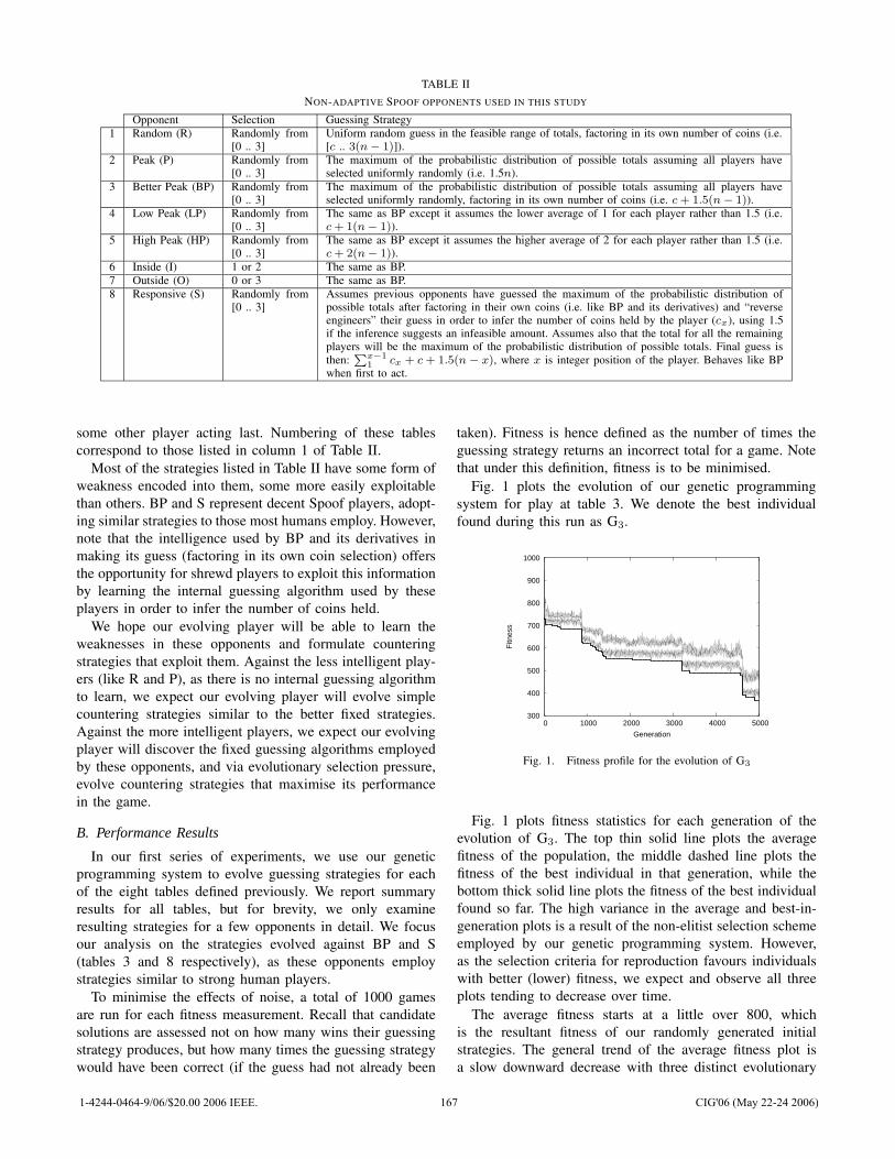
TABLE IINON-ADAPTIVE SPOOF OPPONENTS USED IN THIS STUDY

Opponent Selection Guessing Strategy1 Random (R) Randomly from

[0 .. 3]Uniform random guess in the feasible range of totals, factoring in its own number of coins (i.e.[c .. 3(n − 1)]).

2 Peak (P) Randomly from[0 .. 3]

The maximum of the probabilistic distribution of possible totals assuming all players haveselected uniformly randomly (i.e. 1.5n).

3 Better Peak (BP) Randomly from[0 .. 3]

The maximum of the probabilistic distribution of possible totals assuming all players haveselected uniformly randomly, factoring in its own number of coins (i.e. c + 1.5(n − 1)).

4 Low Peak (LP) Randomly from[0 .. 3]

The same as BP except it assumes the lower average of 1 for each player rather than 1.5 (i.e.c + 1(n − 1)).

5 High Peak (HP) Randomly from[0 .. 3]

The same as BP except it assumes the higher average of 2 for each player rather than 1.5 (i.e.c + 2(n − 1)).

6 Inside (I) 1 or 2 The same as BP.7 Outside (O) 0 or 3 The same as BP.8 Responsive (S) Randomly from

[0 .. 3]Assumes previous opponents have guessed the maximum of the probabilistic distribution ofpossible totals after factoring in their own coins (i.e. like BP and its derivatives) and “reverseengineers” their guess in order to infer the number of coins held by the player (cx), using 1.5if the inference suggests an infeasible amount. Assumes also that the total for all the remainingplayers will be the maximum of the probabilistic distribution of possible totals. Final guess isthen:

P

x−1

1cx + c + 1.5(n − x), where x is integer position of the player. Behaves like BP

when first to act.

some other player acting last. Numbering of these tablescorrespond to those listed in column 1 of Table II.

Most of the strategies listed in Table II have some form ofweakness encoded into them, some more easily exploitablethan others. BP and S represent decent Spoof players, adopt-ing similar strategies to those most humans employ. However,note that the intelligence used by BP and its derivatives inmaking its guess (factoring in its own coin selection) offersthe opportunity for shrewd players to exploit this informationby learning the internal guessing algorithm used by theseplayers in order to infer the number of coins held.

We hope our evolving player will be able to learn theweaknesses in these opponents and formulate counteringstrategies that exploit them. Against the less intelligent play-ers (like R and P), as there is no internal guessing algorithmto learn, we expect our evolving player will evolve simplecountering strategies similar to the better fixed strategies.Against the more intelligent players, we expect our evolvingplayer will discover the fixed guessing algorithms employedby these opponents, and via evolutionary selection pressure,evolve countering strategies that maximise its performancein the game.

B. Performance Results

In our first series of experiments, we use our geneticprogramming system to evolve guessing strategies for eachof the eight tables defined previously. We report summaryresults for all tables, but for brevity, we only examineresulting strategies for a few opponents in detail. We focusour analysis on the strategies evolved against BP and S(tables 3 and 8 respectively), as these opponents employstrategies similar to strong human players.

To minimise the effects of noise, a total of 1000 gamesare run for each fitness measurement. Recall that candidatesolutions are assessed not on how many wins their guessingstrategy produces, but how many times the guessing strategywould have been correct (if the guess had not already been

taken). Fitness is hence defined as the number of times theguessing strategy returns an incorrect total for a game. Notethat under this definition, fitness is to be minimised.

Fig. 1 plots the evolution of our genetic programmingsystem for play at table 3. We denote the best individualfound during this run as G3.

300

400

500

600

700

800

900

1000

0 1000 2000 3000 4000 5000

Fitn

ess

Generation

Fig. 1. Fitness profile for the evolution of G3

Fig. 1 plots fitness statistics for each generation of theevolution of G3. The top thin solid line plots the averagefitness of the population, the middle dashed line plots thefitness of the best individual in that generation, while thebottom thick solid line plots the fitness of the best individualfound so far. The high variance in the average and best-in-generation plots is a result of the non-elitist selection schemeemployed by our genetic programming system. However,as the selection criteria for reproduction favours individualswith better (lower) fitness, we expect and observe all threeplots tending to decrease over time.

The average fitness starts at a little over 800, whichis the resultant fitness of our randomly generated initialstrategies. The general trend of the average fitness plot isa slow downward decrease with three distinct evolutionary

1-4244-0464-9/06/$20.00 2006 IEEE. 167 CIG'06 (May 22-24 2006)

“breakthroughs” evident at approximately generations 900,3200, and 4600. The final average fitness score of 480corresponds to a >30% increase in the number of gamesguessed correctly. The best-of-generation plot is similar,although obviously lower and less erratic. The best-of-runplot has the same general trend, but monotonically decreasesover time (the archived best solution can never get worse).

We performed similar experiments at the other tables,naming the best individual found during each run Gx, wherex is the corresponding table number from Table II. Table IIIsummarises the performance of each of these resulting strate-gies and the eight fixed strategies at each table.

TABLE IIIPERFORMANCE OF DIFFERENT STRATEGIES AT EACH TABLE

R P BP LP HP I O S Gx

1 32 40 45 41 38 45 45 41 452 25 30 37 33 33 30 28 33 373 18 24 31 28 25 30 32 33 414 23 31 39 36 29 30 50 39 585 26 36 36 36 30 32 43 34 586 17 33 43 33 33 13 83 47 477 20 22 27 22 0 80 0 22 568 18 24 31 28 24 30 32 47 47

Avg 22 30 36 32 26 36 39 37 49

Each column of Table III reports the percentage of gameswon by each strategy when played at each of the eight tables(the strategy taking the place of third player). The finalcolumn reports the percentage of games won by the best-of-run strategy discovered during the evolution of our geneticprogramming system at each table. Each percentage is theresult of 1 million games, rounded to the nearest percent.Drawn games were replayed until a winner was determined.

Inspection of Table III confirms our initial beliefs aboutthe fixed players. Of little surprise, R performs the worst onaverage as it guesses uniformly randomly instead of towardsthe maximum of the probabilistic distribution of possibletotals. P performs better than R (it selects the maximumof the probabilistic distribution), but worse than BP as BPuses knowledge of its own selection when making its guess(P does not). BP, I, and O do reasonably well on averagebecause their guessing strategy selects the maximum of theprobability distribution of possible totals after factoring intheir own selection. O in particular is able to do well guessingwith this strategy because its extremum coin selections have atendency to skew the probability distribution, which of courseit then takes into account. Note that even though LP andHP are symmetric in behaviour, LP on average outperformsHP due to the non-symmetric adjustment algorithm used bythe Spoof game engine to correct taken guesses, somewhatcorrecting LP’s under-estimation while further exaggeratedHP’s over-estimation of the total.

Examining the variance in the results, we conclude that BPand S are indeed reasonably good all-round players. Both BPand S obtain good overall average performance, with lowervariance in their percentage of winning games than the otherfixed players. Both factor in their own number of coins when

making a guess. S behaves even a little more intelligently,inferring where possible the coin selections of earlier playersbased on the guesses they made. This offers S an advantagein certain situations, most notably when playing against otherS-like players.

Table III also shows the strength of the resulting strategiesproduced by our genetic programming approach. For alltables except 6 and 7, the evolved strategy produced byour genetic programming system obtained the highest (orequally high) percentage of games won. This confirms thatthe genetic programming system was able to discover strate-gies that exploit the weaknesses of each different opponentstrategy at least as well as (and often better than) any ofthe fixed strategies. The two exceptions on tables 6 and 7occur as a result of players O and I being able to alter theprobability distribution of possible totals by selecting non-uniformly, artificially increasing their percentage of gameswon (recall we deliberately forced our evolving player toselect uniformly randomly to ensure it could not exploit non-intelligent players in this way). We do note however thatour genetic programming approach obtains the best (or equalbest) results of the “non-skewing” players.

Note that G3 obtains a higher percentage of wins thanG2, even though BP is considered a “better” player than P(recall BP factors in its own coins into its guess while Pdoes not). As P’s guess does not depend on its own numberof coins held, no information about its coin selection can beinferred from the public guess it announces. However, whenBP announces its guess, it inevitably reveals informationabout its selection (its selection will be 3 less than its guess).Over time, our genetic programming system is able to learnthe algorithm employed by BP and evolves a counteringstrategy that factors this information into its own guessingalgorithm, thus exploiting the information provided by BP.As there is no equivalent information provided by P, thegenetic programming is unable to exploit it in the same way,thus explaining why it is able to obtain a higher percentageof wins against BP than against P.

Table III also demonstrates the importance of specialisa-tion in order to maximise winnings. As we indicated above,the evolved strategies produced by our genetic programmingsystem obtained the highest (or equally high) percentage ofgames won at each table. Table III further shows that theaverage performance of these evolved strategies far exceedsthe average of any of the fixed strategies (the evolvedstrategies on average won 49% of games compared to 39%for player O or 37% for the best “non-cheating” player). Thatnone of the fixed strategies performed as well on average asour genetic programming system suggests that in order tomaximise winnings against a variety of different opponents,a Spoof player can not simply adopt one of these fixedstrategies and must instead vary their strategy depending onthe particular opponents at hand.

C. Strategy Analysis

In this section, we analyse a few of the resulting strategiesproduced by our genetic programming system in order to un-

1-4244-0464-9/06/$20.00 2006 IEEE. 168 CIG'06 (May 22-24 2006)

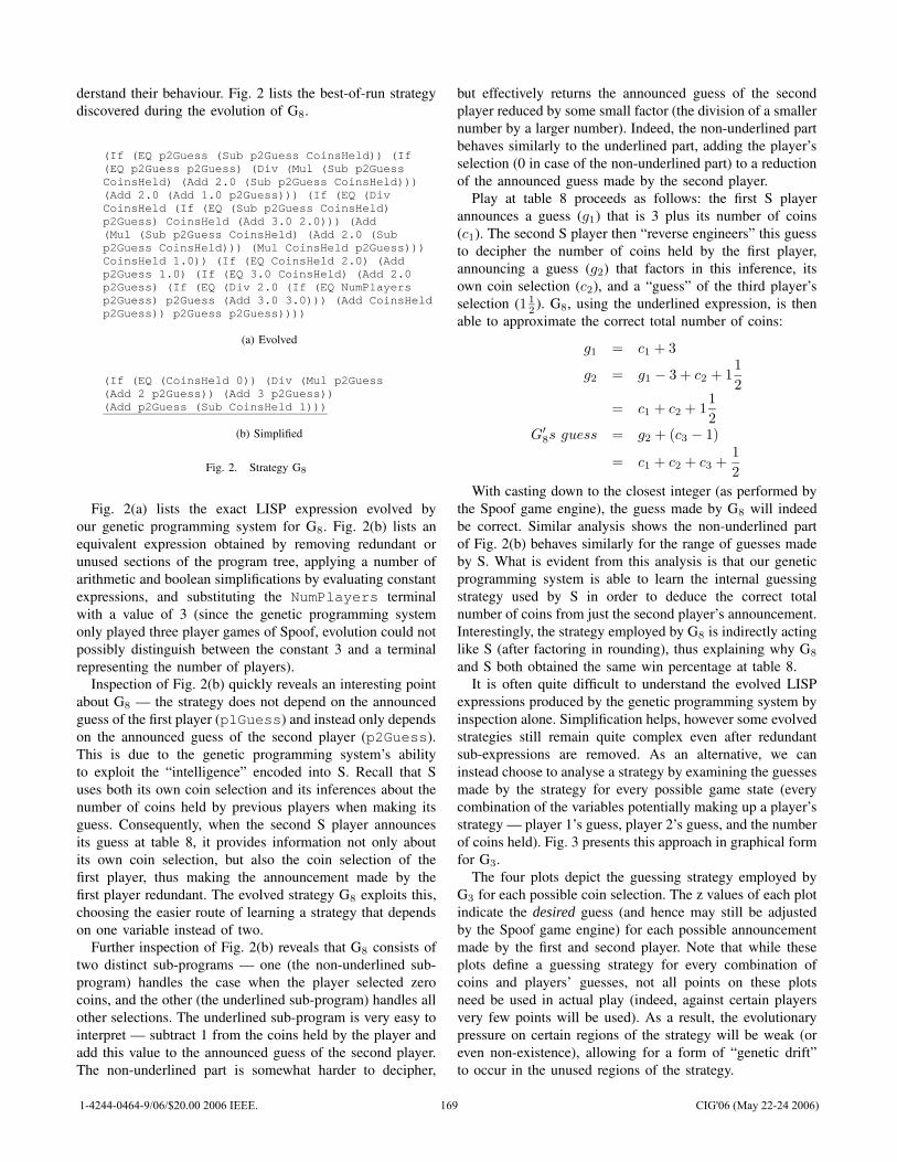
derstand their behaviour. Fig. 2 lists the best-of-run strategydiscovered during the evolution of G8.

(If (EQ p2Guess (Sub p2Guess CoinsHeld)) (If(EQ p2Guess p2Guess) (Div (Mul (Sub p2GuessCoinsHeld) (Add 2.0 (Sub p2Guess CoinsHeld)))(Add 2.0 (Add 1.0 p2Guess))) (If (EQ (DivCoinsHeld (If (EQ (Sub p2Guess CoinsHeld)p2Guess) CoinsHeld (Add 3.0 2.0))) (Add(Mul (Sub p2Guess CoinsHeld) (Add 2.0 (Subp2Guess CoinsHeld))) (Mul CoinsHeld p2Guess)))CoinsHeld 1.0)) (If (EQ CoinsHeld 2.0) (Addp2Guess 1.0) (If (EQ 3.0 CoinsHeld) (Add 2.0p2Guess) (If (EQ (Div 2.0 (If (EQ NumPlayersp2Guess) p2Guess (Add 3.0 3.0))) (Add CoinsHeldp2Guess)) p2Guess p2Guess))))

(a) Evolved

(If (EQ (CoinsHeld 0)) (Div (Mul p2Guess(Add 2 p2Guess)) (Add 3 p2Guess))(Add p2Guess (Sub CoinsHeld 1)))

(b) Simplified

Fig. 2. Strategy G8

Fig. 2(a) lists the exact LISP expression evolved byour genetic programming system for G8. Fig. 2(b) lists anequivalent expression obtained by removing redundant orunused sections of the program tree, applying a number ofarithmetic and boolean simplifications by evaluating constantexpressions, and substituting the NumPlayers terminalwith a value of 3 (since the genetic programming systemonly played three player games of Spoof, evolution could notpossibly distinguish between the constant 3 and a terminalrepresenting the number of players).

Inspection of Fig. 2(b) quickly reveals an interesting pointabout G8 — the strategy does not depend on the announcedguess of the first player (p1Guess) and instead only dependson the announced guess of the second player (p2Guess).This is due to the genetic programming system’s abilityto exploit the “intelligence” encoded into S. Recall that Suses both its own coin selection and its inferences about thenumber of coins held by previous players when making itsguess. Consequently, when the second S player announcesits guess at table 8, it provides information not only aboutits own coin selection, but also the coin selection of thefirst player, thus making the announcement made by thefirst player redundant. The evolved strategy G8 exploits this,choosing the easier route of learning a strategy that dependson one variable instead of two.

Further inspection of Fig. 2(b) reveals that G8 consists oftwo distinct sub-programs — one (the non-underlined sub-program) handles the case when the player selected zerocoins, and the other (the underlined sub-program) handles allother selections. The underlined sub-program is very easy tointerpret — subtract 1 from the coins held by the player andadd this value to the announced guess of the second player.The non-underlined part is somewhat harder to decipher,

but effectively returns the announced guess of the secondplayer reduced by some small factor (the division of a smallernumber by a larger number). Indeed, the non-underlined partbehaves similarly to the underlined part, adding the player’sselection (0 in case of the non-underlined part) to a reductionof the announced guess made by the second player.

Play at table 8 proceeds as follows: the first S playerannounces a guess (g1) that is 3 plus its number of coins(c1). The second S player then “reverse engineers” this guessto decipher the number of coins held by the first player,announcing a guess (g2) that factors in this inference, itsown coin selection (c2), and a “guess” of the third player’sselection (1 1

2). G8, using the underlined expression, is then

able to approximate the correct total number of coins:

g1 = c1 + 3

g2 = g1 − 3 + c2 + 11

2

= c1 + c2 + 11

2G′

8s guess = g2 + (c3 − 1)

= c1 + c2 + c3 +1

2

With casting down to the closest integer (as performed bythe Spoof game engine), the guess made by G8 will indeedbe correct. Similar analysis shows the non-underlined partof Fig. 2(b) behaves similarly for the range of guesses madeby S. What is evident from this analysis is that our geneticprogramming system is able to learn the internal guessingstrategy used by S in order to deduce the correct totalnumber of coins from just the second player’s announcement.Interestingly, the strategy employed by G8 is indirectly actinglike S (after factoring in rounding), thus explaining why G8

and S both obtained the same win percentage at table 8.It is often quite difficult to understand the evolved LISP

expressions produced by the genetic programming system byinspection alone. Simplification helps, however some evolvedstrategies still remain quite complex even after redundantsub-expressions are removed. As an alternative, we caninstead choose to analyse a strategy by examining the guessesmade by the strategy for every possible game state (everycombination of the variables potentially making up a player’sstrategy — player 1’s guess, player 2’s guess, and the numberof coins held). Fig. 3 presents this approach in graphical formfor G3.

The four plots depict the guessing strategy employed byG3 for each possible coin selection. The z values of each plotindicate the desired guess (and hence may still be adjustedby the Spoof game engine) for each possible announcementmade by the first and second player. Note that while theseplots define a guessing strategy for every combination ofcoins and players’ guesses, not all points on these plotsneed be used in actual play (indeed, against certain playersvery few points will be used). As a result, the evolutionarypressure on certain regions of the strategy will be weak (oreven non-existence), allowing for a form of “genetic drift”to occur in the unused regions of the strategy.

1-4244-0464-9/06/$20.00 2006 IEEE. 169 CIG'06 (May 22-24 2006)

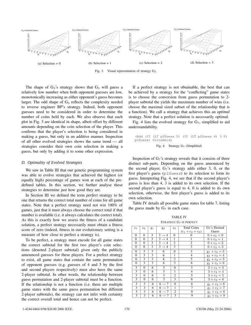
0 1 2 3 4 5 6 7 8 9g1 0 1 2 3 4 5 6 7 8 9

g2 0 1 2 3 4 5 6 7 8 9

G3’s Desired Guess

(a) Selection = 0

0 1 2 3 4 5 6 7 8 9g1 0 1 2 3 4 5 6 7 8 9

g2 0 1 2 3 4 5 6 7 8 9

G3’s Desired Guess

(b) Selection = 1

0 1 2 3 4 5 6 7 8 9g1 0 1 2 3 4 5 6 7 8 9

g2 0 1 2 3 4 5 6 7 8 9

G3’s Desired Guess

(c) Selection = 2

0 1 2 3 4 5 6 7 8 9g1 0 1 2 3 4 5 6 7 8 9

g2 0 1 2 3 4 5 6 7 8 9

G3’s Desired Guess

(d) Selection = 3

Fig. 3. Visual representation of strategy G3

The shape of G3’s strategy shows that G3 will guess arelatively low number when both opponent guesses are low,monotonically increasing as either opponent’s guess becomeslarger. The odd shape of G3 reflects the complexity neededto reverse engineer BP’s strategy. Indeed, both opponentguesses need to be considered in order to determine thenumber of coins held by each. We also observe that eachplot in Fig. 3 are identical in shape, albeit offset by differentamounts depending on the coin selection of the player. Thisconfirms that the player’s selection is being considered inmaking a guess, but only in an additive manner. Inspectionof all other evolved strategies shows the same trend — allstrategies consider their own coin selection in making aguess, but only by adding it to some other expression.

D. Optimality of Evolved Strategies

We saw in Table III that our genetic programming systemwas able to evolve strategies that achieved the highest (orequally high) percentage of games won at each of the pre-defined tables. In this section, we further analyse thesestrategies to determine just how good they are.

In Section III we defined the term perfect strategy to beone that returns the correct total number of coins for all gamestates. Note that a perfect strategy need not win 100% ofgames, just that it must always choose the correct total if thatnumber is available (i.e. it always calculates the correct total).As this is exactly how we assess the fitness of a candidatesolution, a perfect strategy necessarily must obtain a fitnessscore of zero (indeed, fitness in our evolutionary setting is ameasure of how close to perfect a strategy is).

To be perfect, a strategy must encode for all game statesthe correct subtotal for the first two player’s coin selec-tions (denoted 2-player subtotal) given only the publiclyannounced guesses for these players. For a prefect strategyto exist, all game states that contain the same permutationof opponent guesses (e.g. guesses of 4 and 5 by the firstand second players respectively) must also have the same2-player subtotal. In other words, the relationship betweenguess permutation and 2-player subtotal must be a function.If the relationship is not a function (i.e. there are multiplegame states with the same guess permutation but different2-player subtotals), the strategy can not infer with certaintythe correct overall total and hence can not be perfect.

If a perfect strategy is not obtainable, the best that canbe achieved by a strategy for the “conflicting” game statesis to choose the conversion from guess permutation to 2-player subtotal the yields the maximum number of wins (i.e.choose the maximal sized subset of the relationship that isa function). We call a strategy that achieves this an optimalstrategy. Note that a perfect solution is necessarily optimal.

Fig. 4 lists the evolved strategy for G7, simplified to aidunderstandability.

(Add (If (LT p2Guess 5) (If (LT p2Guess 4) 3 0)p1Guess) CoinsHeld)

Fig. 4. Strategy G7 (Simplified)

Inspection of G7’s strategy reveals that it consists of threedistinct sub-parts. Depending on the guess announced bythe second player, G7’s strategy adds either 3, 0, or thefirst player’s guess (p1Guess) to its selection to form itsguess. Interpreting Fig. 4, we see that if the second player’sguess is less than 4, 3 is added to its own selection. If thesecond player’s guess is equal to 4, 0 is added to its ownselection, otherwise, the first player’s guess is added to itsown selection.

Table IV details all possible game states for table 7, listingthe guess made by G7 in each case.

TABLE IVSTRATEGY G7 IS PERFECT

c1 c2 g1 g2 c3 Total Coins G7’s Desired(c1 + c2 + c3) Guess

0 0 3 3 → 4 0 0 0 + c3 = 0

0 0 3 3 → 4 1 1 0 + c3 = 1

0 0 3 3 → 4 2 2 0 + c3 = 2

0 0 3 3 → 4 3 3 0 + c3 = 3

0 3 3 6 0 3 g1 + c3 = 3

0 3 3 6 1 4 g1 + c3 = 4

0 3 3 6 2 5 g1 + c3 = 5

0 3 3 6 3 6 g1 + c3 = 6

3 0 6 3 0 3 3 + c3 = 3

3 0 6 3 1 4 3 + c3 = 4

3 0 6 3 2 5 3 + c3 = 5

3 0 6 3 3 6 3 + c3 = 6

3 3 6 6 → 7 0 6 g1 + c3 = 6

3 3 6 6 → 7 1 7 g1 + c3 = 7

3 3 6 6 → 7 2 8 g1 + c3 = 8

3 3 6 6 → 7 3 9 g1 + c3 = 9

1-4244-0464-9/06/$20.00 2006 IEEE. 170 CIG'06 (May 22-24 2006)

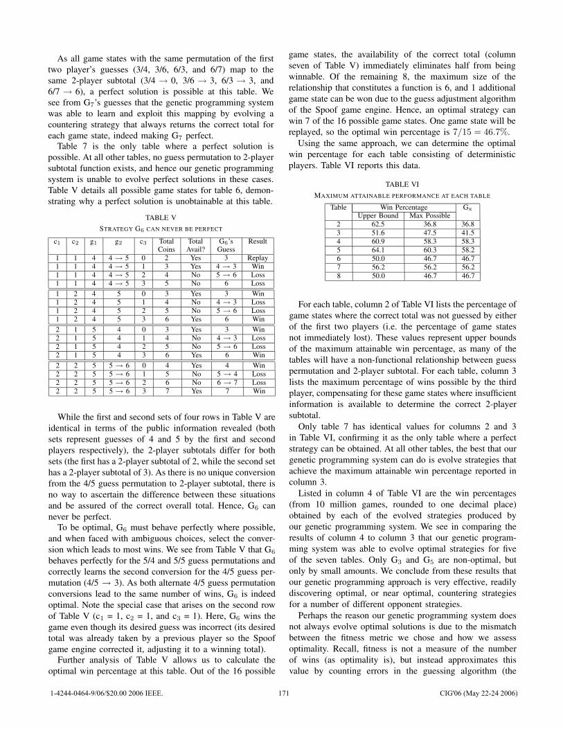
As all game states with the same permutation of the firsttwo player’s guesses (3/4, 3/6, 6/3, and 6/7) map to thesame 2-player subtotal (3/4 → 0, 3/6 → 3, 6/3 → 3, and6/7 → 6), a perfect solution is possible at this table. Wesee from G7’s guesses that the genetic programming systemwas able to learn and exploit this mapping by evolving acountering strategy that always returns the correct total foreach game state, indeed making G7 perfect.

Table 7 is the only table where a perfect solution ispossible. At all other tables, no guess permutation to 2-playersubtotal function exists, and hence our genetic programmingsystem is unable to evolve perfect solutions in these cases.Table V details all possible game states for table 6, demon-strating why a perfect solution is unobtainable at this table.

TABLE VSTRATEGY G6 CAN NEVER BE PERFECT

c1 c2 g1 g2 c3 Total Total G6’s ResultCoins Avail? Guess

1 1 4 4 → 5 0 2 Yes 3 Replay1 1 4 4 → 5 1 3 Yes 4 → 3 Win1 1 4 4 → 5 2 4 No 5 → 6 Loss1 1 4 4 → 5 3 5 No 6 Loss1 2 4 5 0 3 Yes 3 Win1 2 4 5 1 4 No 4 → 3 Loss1 2 4 5 2 5 No 5 → 6 Loss1 2 4 5 3 6 Yes 6 Win2 1 5 4 0 3 Yes 3 Win2 1 5 4 1 4 No 4 → 3 Loss2 1 5 4 2 5 No 5 → 6 Loss2 1 5 4 3 6 Yes 6 Win2 2 5 5 → 6 0 4 Yes 4 Win2 2 5 5 → 6 1 5 No 5 → 4 Loss2 2 5 5 → 6 2 6 No 6 → 7 Loss2 2 5 5 → 6 3 7 Yes 7 Win

While the first and second sets of four rows in Table V areidentical in terms of the public information revealed (bothsets represent guesses of 4 and 5 by the first and secondplayers respectively), the 2-player subtotals differ for bothsets (the first has a 2-player subtotal of 2, while the second sethas a 2-player subtotal of 3). As there is no unique conversionfrom the 4/5 guess permutation to 2-player subtotal, there isno way to ascertain the difference between these situationsand be assured of the correct overall total. Hence, G6 cannever be perfect.

To be optimal, G6 must behave perfectly where possible,and when faced with ambiguous choices, select the conver-sion which leads to most wins. We see from Table V that G6

behaves perfectly for the 5/4 and 5/5 guess permutations andcorrectly learns the second conversion for the 4/5 guess per-mutation (4/5 → 3). As both alternate 4/5 guess permutationconversions lead to the same number of wins, G6 is indeedoptimal. Note the special case that arises on the second rowof Table V (c1 = 1, c2 = 1, and c3 = 1). Here, G6 wins thegame even though its desired guess was incorrect (its desiredtotal was already taken by a previous player so the Spoofgame engine corrected it, adjusting it to a winning total).

Further analysis of Table V allows us to calculate theoptimal win percentage at this table. Out of the 16 possible

game states, the availability of the correct total (columnseven of Table V) immediately eliminates half from beingwinnable. Of the remaining 8, the maximum size of therelationship that constitutes a function is 6, and 1 additionalgame state can be won due to the guess adjustment algorithmof the Spoof game engine. Hence, an optimal strategy canwin 7 of the 16 possible game states. One game state will bereplayed, so the optimal win percentage is 7/15 = 46.7%.

Using the same approach, we can determine the optimalwin percentage for each table consisting of deterministicplayers. Table VI reports this data.

TABLE VIMAXIMUM ATTAINABLE PERFORMANCE AT EACH TABLE

Table Win Percentage Gx

Upper Bound Max Possible2 62.5 36.8 36.83 51.6 47.5 41.54 60.9 58.3 58.35 64.1 60.3 58.26 50.0 46.7 46.77 56.2 56.2 56.28 50.0 46.7 46.7

For each table, column 2 of Table VI lists the percentage ofgame states where the correct total was not guessed by eitherof the first two players (i.e. the percentage of game statesnot immediately lost). These values represent upper boundsof the maximum attainable win percentage, as many of thetables will have a non-functional relationship between guesspermutation and 2-player subtotal. For each table, column 3lists the maximum percentage of wins possible by the thirdplayer, compensating for these game states where insufficientinformation is available to determine the correct 2-playersubtotal.

Only table 7 has identical values for columns 2 and 3in Table VI, confirming it as the only table where a perfectstrategy can be obtained. At all other tables, the best that ourgenetic programming system can do is evolve strategies thatachieve the maximum attainable win percentage reported incolumn 3.

Listed in column 4 of Table VI are the win percentages(from 10 million games, rounded to one decimal place)obtained by each of the evolved strategies produced byour genetic programming system. We see in comparing theresults of column 4 to column 3 that our genetic program-ming system was able to evolve optimal strategies for fiveof the seven tables. Only G3 and G5 are non-optimal, butonly by small amounts. We conclude from these results thatour genetic programming approach is very effective, readilydiscovering optimal, or near optimal, countering strategiesfor a number of different opponent strategies.

Perhaps the reason our genetic programming system doesnot always evolve optimal solutions is due to the mismatchbetween the fitness metric we chose and how we assessoptimality. Recall, fitness is not a measure of the numberof wins (as optimality is), but instead approximates thisvalue by counting errors in the guessing algorithm (the

1-4244-0464-9/06/$20.00 2006 IEEE. 171 CIG'06 (May 22-24 2006)

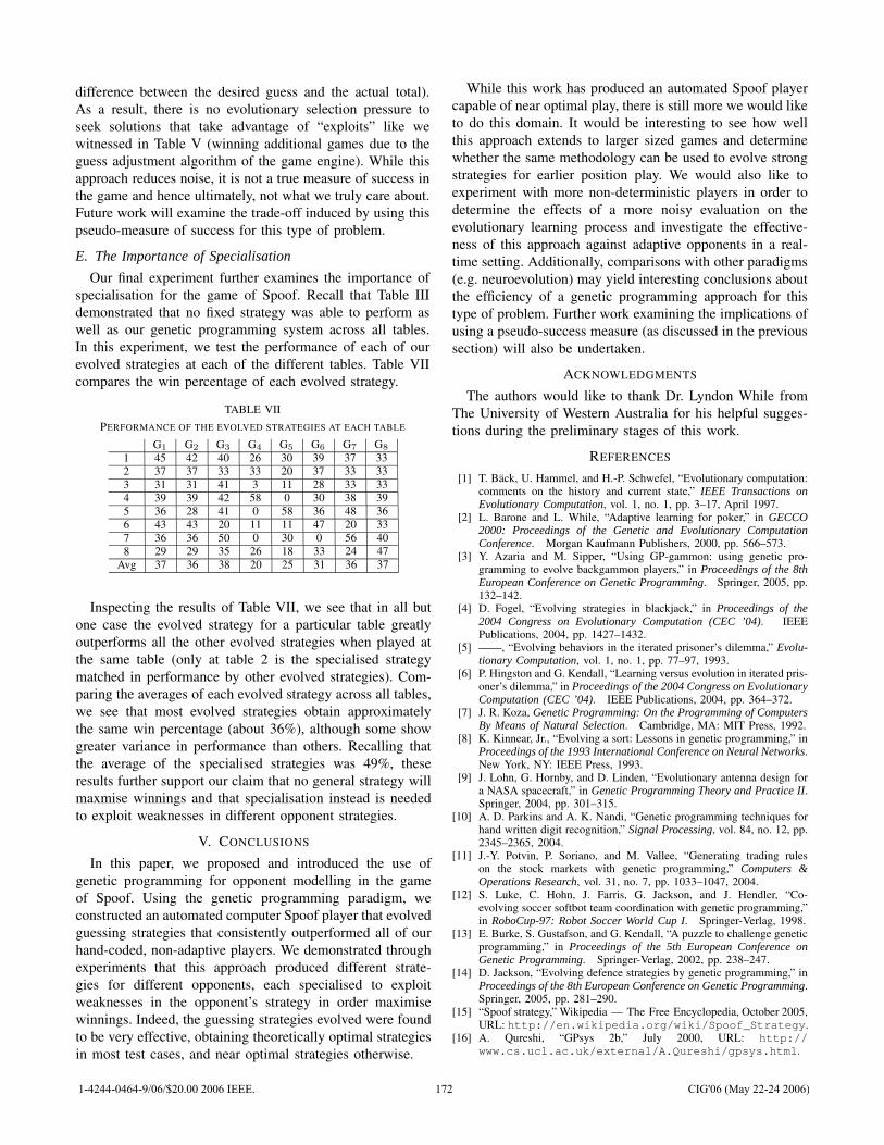
difference between the desired guess and the actual total).As a result, there is no evolutionary selection pressure toseek solutions that take advantage of “exploits” like wewitnessed in Table V (winning additional games due to theguess adjustment algorithm of the game engine). While thisapproach reduces noise, it is not a true measure of success inthe game and hence ultimately, not what we truly care about.Future work will examine the trade-off induced by using thispseudo-measure of success for this type of problem.

E. The Importance of Specialisation

Our final experiment further examines the importance ofspecialisation for the game of Spoof. Recall that Table IIIdemonstrated that no fixed strategy was able to perform aswell as our genetic programming system across all tables.In this experiment, we test the performance of each of ourevolved strategies at each of the different tables. Table VIIcompares the win percentage of each evolved strategy.

TABLE VIIPERFORMANCE OF THE EVOLVED STRATEGIES AT EACH TABLE

G1 G2 G3 G4 G5 G6 G7 G8

1 45 42 40 26 30 39 37 332 37 37 33 33 20 37 33 333 31 31 41 3 11 28 33 334 39 39 42 58 0 30 38 395 36 28 41 0 58 36 48 366 43 43 20 11 11 47 20 337 36 36 50 0 30 0 56 408 29 29 35 26 18 33 24 47

Avg 37 36 38 20 25 31 36 37

Inspecting the results of Table VII, we see that in all butone case the evolved strategy for a particular table greatlyoutperforms all the other evolved strategies when played atthe same table (only at table 2 is the specialised strategymatched in performance by other evolved strategies). Com-paring the averages of each evolved strategy across all tables,we see that most evolved strategies obtain approximatelythe same win percentage (about 36%), although some showgreater variance in performance than others. Recalling thatthe average of the specialised strategies was 49%, theseresults further support our claim that no general strategy willmaxmise winnings and that specialisation instead is neededto exploit weaknesses in different opponent strategies.

V. CONCLUSIONS

In this paper, we proposed and introduced the use ofgenetic programming for opponent modelling in the gameof Spoof. Using the genetic programming paradigm, weconstructed an automated computer Spoof player that evolvedguessing strategies that consistently outperformed all of ourhand-coded, non-adaptive players. We demonstrated throughexperiments that this approach produced different strate-gies for different opponents, each specialised to exploitweaknesses in the opponent’s strategy in order maximisewinnings. Indeed, the guessing strategies evolved were foundto be very effective, obtaining theoretically optimal strategiesin most test cases, and near optimal strategies otherwise.

While this work has produced an automated Spoof playercapable of near optimal play, there is still more we would liketo do this domain. It would be interesting to see how wellthis approach extends to larger sized games and determinewhether the same methodology can be used to evolve strongstrategies for earlier position play. We would also like toexperiment with more non-deterministic players in order todetermine the effects of a more noisy evaluation on theevolutionary learning process and investigate the effective-ness of this approach against adaptive opponents in a real-time setting. Additionally, comparisons with other paradigms(e.g. neuroevolution) may yield interesting conclusions aboutthe efficiency of a genetic programming approach for thistype of problem. Further work examining the implications ofusing a pseudo-success measure (as discussed in the previoussection) will also be undertaken.

ACKNOWLEDGMENTS

The authors would like to thank Dr. Lyndon While fromThe University of Western Australia for his helpful sugges-tions during the preliminary stages of this work.

REFERENCES

[1] T. Back, U. Hammel, and H.-P. Schwefel, “Evolutionary computation:comments on the history and current state,” IEEE Transactions onEvolutionary Computation, vol. 1, no. 1, pp. 3–17, April 1997.

[2] L. Barone and L. While, “Adaptive learning for poker,” in GECCO2000: Proceedings of the Genetic and Evolutionary ComputationConference. Morgan Kaufmann Publishers, 2000, pp. 566–573.

[3] Y. Azaria and M. Sipper, “Using GP-gammon: using genetic pro-gramming to evolve backgammon players,” in Proceedings of the 8thEuropean Conference on Genetic Programming. Springer, 2005, pp.132–142.

[4] D. Fogel, “Evolving strategies in blackjack,” in Proceedings of the2004 Congress on Evolutionary Computation (CEC ’04). IEEEPublications, 2004, pp. 1427–1432.

[5] ——, “Evolving behaviors in the iterated prisoner’s dilemma,” Evolu-tionary Computation, vol. 1, no. 1, pp. 77–97, 1993.

[6] P. Hingston and G. Kendall, “Learning versus evolution in iterated pris-oner’s dilemma,” in Proceedings of the 2004 Congress on EvolutionaryComputation (CEC ’04). IEEE Publications, 2004, pp. 364–372.

[7] J. R. Koza, Genetic Programming: On the Programming of ComputersBy Means of Natural Selection. Cambridge, MA: MIT Press, 1992.

[8] K. Kinnear, Jr., “Evolving a sort: Lessons in genetic programming,” inProceedings of the 1993 International Conference on Neural Networks.New York, NY: IEEE Press, 1993.

[9] J. Lohn, G. Hornby, and D. Linden, “Evolutionary antenna design fora NASA spacecraft,” in Genetic Programming Theory and Practice II.Springer, 2004, pp. 301–315.

[10] A. D. Parkins and A. K. Nandi, “Genetic programming techniques forhand written digit recognition,” Signal Processing, vol. 84, no. 12, pp.2345–2365, 2004.

[11] J.-Y. Potvin, P. Soriano, and M. Vallee, “Generating trading ruleson the stock markets with genetic programming,” Computers &Operations Research, vol. 31, no. 7, pp. 1033–1047, 2004.

[12] S. Luke, C. Hohn, J. Farris, G. Jackson, and J. Hendler, “Co-evolving soccer softbot team coordination with genetic programming,”in RoboCup-97: Robot Soccer World Cup I. Springer-Verlag, 1998.

[13] E. Burke, S. Gustafson, and G. Kendall, “A puzzle to challenge geneticprogramming,” in Proceedings of the 5th European Conference onGenetic Programming. Springer-Verlag, 2002, pp. 238–247.

[14] D. Jackson, “Evolving defence strategies by genetic programming,” inProceedings of the 8th European Conference on Genetic Programming.Springer, 2005, pp. 281–290.

[15] “Spoof strategy,” Wikipedia — The Free Encyclopedia, October 2005,URL: http://en.wikipedia.org/wiki/Spoof_Strategy.

[16] A. Qureshi, “GPsys 2b,” July 2000, URL: http://www.cs.ucl.ac.uk/external/A.Qureshi/gpsys.html.

1-4244-0464-9/06/$20.00 2006 IEEE. 172 CIG'06 (May 22-24 2006)

A Comparison of Different Adaptive Learning Techniques

for Opponent Modelling in the Game of Guess It

Anthony Di Pietro, Luigi Barone, and Lyndon WhileSchool of Computer Science & Software Engineering

The University of Western Australia{anthony,luigi,lyndon}@csse.uwa.edu.au

Abstract— Guess It is a simple card game of bluffing andopponent modelling designed by Rufus Isaacs of the RandCorporation. In this paper, we discuss the technical detailsneeded to equip an adaptive learning algorithm with the abilityto play the game and report a series of experiments thatcompare the performance of different learning techniques.Our results show that in most cases the different techniquesproduce perfect countering strategies against a number offixed opponents, although there are differences in the speedof learning and robustness to change between the differentalgorithms. We further report experiments where the learningtechniques compete against each other in a coadaptive setting.

Keywords: Adaptive Learning, Opponent Modelling,Guess It

I. INTRODUCTION

In certain games, playing well depends primarily on de-termining which actions are objectively the best based onanalysis of the game state. This is especially true for perfectinformation games such as Chess [1] and Draughts [2]. Inmany other games, however, playing well depends primarilyon predicting opponents’ actions. This is especially true forgames that prominently feature bluffing, such as Poker [3].

The ability to play the former category of games wellwas once widely regarded as evidence of intelligence, butnowadays the idea that machines can compete with the besthumans at such games is generally seen as a consequenceof the computational power of machines, and instead game-playing agents are derided for their inability to understandthe psychological aspects of games.

In this paper, we study a bluffing game called Guess It,a game where optimal performance depends primarily onpredicting opponents’ actions. This means that when adaptivelearning techniques learn to play it, they are not only learningdomain knowledge of the game, but moreso forming a modelof the behaviour of specific opponents (opponent modelling).

The primary contribution that this paper makes is a com-parison of some common adaptive learning techniques for thetask of opponent modelling. Specifically, we examine hillclimbing, evolutionary algorithms, genetic algorithms, andparticle swarm optimisation. We also present and examinea variant of particle swarm optimisation that we designedspecifically to adapt to dynamic environments or opponents.

The rest of this paper is structured as follows: section IIintroduces and analyses the game of Guess It; section IIIdefines a generalised structure for a Guess It player fromwhich our adaptive players are built; section IV describes the

learning techniques that we examine in this paper; section VIexplains how we implemented our learning players; sec-tion VII presents and analyses our results; and section VIIIdraws conclusions from the results and analysis.

II. THE GAME OF GUESS IT

In the early 1950s, Rufus Isaacs of the Rand Corporationconducted his pioneer research on differential game theory.During this period, he invented a card game called GuessIt [4]. His original version of the game used 11 cards, butwe study an extended version of the game that uses 13 cards.

A. Rules

Guess It is a card game for two players. One suit is takenfrom a standard deck of cards and six cards are dealt face-down to each player. The remaining card is placed face-downin the centre. Players look at their own cards, but not at theiropponent’s cards or the centre card. The objective of thegame is to identify the centre card, or to fool one’s opponentinto incorrectly identifying the centre card.

Players alternate turns. Let A denote the current player andB the opponent. On its turn, A can do one of three things:

1) attempt to name the centre card — if A is correct, Awins; otherwise, A loses;

2) ask whether B has a card that is not in A’s hand — ifB has the card, B discards it; or

3) bluff by “asking” whether B has a card that is in A’shand in an attempt to fool B into incorrectly identifyingthe centre card. If a player bluffs, they must discard thecard in question on their next turn.

B. Terminology

For convenience, we define the following terms for dis-cussing elements of the game:

Ask: To query whether one’s opponent hasa card that is not in one’s own hand.

Bluff: To query whether one’s opponent hasa card that is in one’s own hand.

Potential Bluff: When a player either bluffs or asks forthe centre card.

Bluff Card: The card referred to in a potential bluff.Name: To attempt to identify the centre card.Call: To name the bluff card as the centre

card.

1-4244-0464-9/06/$20.00 2006 IEEE. 173 CIG'06 (May 22-24 2006)

Guess: To name a card that has never beenreferred to as the centre card.

Revealed Cards: The cards that have been discarded.Hidden Cards: The cards that are neither in one’s hand

nor discarded.

C. Introductory Strategy

Guess It appears to be a trivial game, but it is not. Whileopponent modelling is far more important than strategyagainst a predictable opponent, a game typically lasts severalturns, and therefore has long-term strategy.

On each turn, A must name, ask, or bluff. If A names,the game ends immediately; if A asks for the centre card,the game ends within two turns (either B calls or A namesnext turn); if A asks for a card in B’s hand, B discards it,eliminating a card from B’s hand; and if A bluffs, the bluffcard will be revealed from A’s hand unless B calls (endingthe game). The net effect is that each turn that does notterminate the game reveals one card from one player’s hand.If A bluffed, a card from A’s hand is revealed; otherwise, acard from B’s hand is revealed.

Since much of the game is concerned with deducing thecentre card before one’s opponent, it is advantageous tohave more cards in hand than one’s opponent (there is moreuncertainty for the opponent). Similarly, it is disadvantageousto have fewer cards in hand. For example, if B has nocards, B necessarily loses as A must know the centre card.Alternatively, if A has no cards, A is forced to guess thecentre card, making A’s probability of winning inverselyproportional to the number of cards in B’s hand. This meansthat not only is having more cards than one’s opponent anadvantage, but also that the advantage increases with thenumber of extra cards. Note that A has a slight advantageeven if the numbers of cards in each player’s hand are equal.

The objective of bluffing is to fool one’s opponent intobelieving that the bluff card is the centre card. Thus, A shouldbluff less often when B has more cards in hand (as there aremore hidden cards, from B’s point-of-view, A is less likelyto have asked for the centre card if not bluffing), and moreoften when A has more cards in hand (as having less cardsthan B is less significant if A still has a large number ofcards in hand).

D. Rand Analysis

Isaacs [4] mathematically analyses the game in order tofind the optimal mixed strategy and the value of the game.We summarise the results of his analysis here and refer tohis resultant strategy as the Rand strategy.

Let m be the number of cards in A’s hand and n be thenumber of cards in B’s hand. Denote the probability of Awinning as P (m,n).

If n = 0, then A knows the centre card, and hence,

P (m, 0) = 1 (1)

If n > 0, but m = 0, then A must guess. Hence,

P (0, n) =1

n + 1(2)

Finally, if n > 0 and m > 0, then if both players playaccording to the Rand strategy,

P (m,n) =1 + nP (n,m − 1)[1 − P (n − 1,m)]

1 + (n + 1)P (n,m − 1)(3)

Table I shows the probability of the current player winningfor all possible values of m and n and confirms the intuitivestrategies described in section II-C.

The Rand strategy specifies the probability of bluffing andthe probability of calling for each possible game state. Inthis strategy, the decision-making process begins by decidingwhether to call (if a potential bluff occurred) with probability

c(m,n) =(m + 1)P (m,n − 1) − mP (m − 1, n)

1 + (m + 1)P (m,n − 1)(4)

If not calling, the next decision is whether to bluff. Theprobability of bluffing is given by

b(m,n) =1

1 + (n + 1)P (n,m − 1)(5)

Note that if B bluffed, n is reduced by one in equation 5because we assume that one of B’s cards is the bluff card(otherwise we have already lost by not calling) and thereforeeffectively revealed. When bluffing, the bluff card is chosenrandomly.

Finally, if neither calling nor bluffing, a random hiddencard is asked for. Exceptions are made to this procedure incases where the centre card is known, or a player has nocards left (see section III).

E. The Need for Opponent Modelling

Note that in Guess It, the value of bluffing depends onhow likely the opponent is to call, and similarly, the valueof calling depends on how likely an opponent is to bluff.If a player bluffs too often, it is vulnerable to an opponentthat rarely calls; and if a player does not bluff enough, itis vulnerable to an opponent that would call too much. Forexample, against an opponent who never bluffs, the optimalcountering strategy is to always call a potential bluff (thebluff card will certainly be the centre card), while against anopponent who always bluffs, calling is erroneous (the bluffcard will certainly not be the centre card), and some othernon-calling countering strategy should be used instead.

While the Rand strategy is the optimal mixed strategy forplaying against all opponents, against a particular opponent,it is generally not the best strategy. The Rand strategy bal-ances the probability of bluffing and calling such that it per-forms equally well regardless of how often its opponent callsand bluffs (it maximises the minimum probability of winningagainst any opponent), thus ensuring it is not vulnerable toany particular opponent. This comes at a cost — sacrificingperformance against specific opponents (observe that theRand strategy wins less than each optimal countering strategyin the examples above). Indeed, to maximise performanceagainst a specific opponent, a countering strategy specific tothe opponent is needed; a general strategy (like the Randstrategy) will not generally perform as well.

1-4244-0464-9/06/$20.00 2006 IEEE. 174 CIG'06 (May 22-24 2006)

TABLE ITHE PROBABILITY OF THE CURRENT PLAYER WINNING WITH THE RAND STRATEGY.

Cards in A’s hand (m)0 1 2 3 4 5 6

0 1 1 1 1 1 1 1Cards 1 0.5 0.5 0.666667 0.6875 0.733333 0.75 0.771429in 2 0.333333 0.5 0.555556 0.625 0.64693 0.680851 0.697201B’s 3 0.25 0.4 0.511111 0.547619 0.596642 0.61894 0.648174Hand 4 0.2 0.375 0.45 0.512589 0.54309 0.580968 0.602375(n) 5 0.166667 0.333333 0.422548 0.466683 0.512131 0.538851 0.570444

6 0.142857 0.3125 0.387063 0.441135 0.474902 0.511194 0.535342

III. GENERALISED GUESS IT PLAYER

Following the observations made by Isaacs [4], we notethe following about how a Guess It player should play.

Regarding naming and guessing, we specify that• if A knows the centre card (due to a previous ask), A

should name it because this guarantees A will win;• if there is only one hidden card (i.e., B has no cards),

A should name it because this guarantees A will win;• if A has no cards, A should guess because B will

certainly win on B’s next turn;• if B has one card and potentially bluffed, then B will

certainly name on B’s next turn, therefore A shouldname on A’s turn because this denies B the opportunityto guess if B bluffed; and

• unless one of the above scenarios occurs, A should neverguess.

Regarding calling, we specify that• if B potentially bluffed, and A chooses not to call, then

A can assume that the bluff card is revealed becausethis assumption will only ever be false if A has alreadylost by not calling; and

• if B has one card and potentially bluffed, and A choosesnot to call, then A should name the only hidden card.

Regarding calling and bluffing, we specify that• if A does not call, and A does not bluff, then A should

ask for a hidden card (other than the bluff card, if any);• if A bluffs, the bluff card may be chosen randomly from

A’s hand because from B’s point-of-view, all hiddencards are equally likely to be the centre card; and

• if A asks, the card should be chosen randomly from theset of hidden cards (minus the bluff card, if any), as allsuch cards are equally likely to be the centre card.

These specifications form the basis of a generalised modelfor decision-making in the game. A flowchart of the decision-making process is shown pictorially in Fig. 1.

Using this model, at most two decisions need to be madeon each turn: whether to call, and whether to bluff. Asthese decisions can be made probabilistically, a strategymust encode both a probability of bluffing and a probabilityof calling for each game state. Hence, a complete strategyconsists of n = 2m probabilities for the m possible gamestates in the game.

Centreknown?

Start

NameCentre End

Yes

Handempty?

No

Guess End

Opponentpotentiallybluffed?

Shall Ibluff?

Yes

No

NoEndBluff

Yes

Ask

End

No

Shall Icall?

Yes

from hiddenbluff cardRemove

cards

No

Only onehidden?

No

Namehidden

Yes End

CallYes

End

Fig. 1. The generalised decision-making process for Guess It players.

IV. ADAPTIVE LEARNING TECHNIQUES

Finding the correct countering strategy for a particularopponent is in essence an optimisation problem. The n-dimensional array of numbers that make a strategy constitutesan n-dimensional search space in which the adaptive learningtechniques search for a solution. Better strategies win morefrequently than inferior strategies, so we use the proportion ofgames won as the fitness function for the learning algorithms.

The following subsections describe the adaptive learningtechniques that we examine in this paper.

A. Hill Climbing

We consider a basic hill climber that maintains a single so-lution, generates a single test solution, and keeps whicheveris better. The initial solution is generated using a uniformrandom distribution. The test solutions are generated byadding a Gaussian random variable with mean zero andstandard deviation 0.001 to each dimension of the solution.

1-4244-0464-9/06/$20.00 2006 IEEE. 175 CIG'06 (May 22-24 2006)

We used 0.001 as the standard deviation because we foundthat this produced good solutions in a tolerable time.

B. Evolutionary and Genetic Algorithms

Evolutionary computation [5] is a broad term that encom-passes all methods to solve problems on a computer thatare inspired by biological evolution [6]. A population ofcandidate solutions is maintained with solutions encoded intotheir genotype. The notion of biological fitness serves as amodel for fitness in evolutionary computation, implementedvia the fitness function. Mutation and genetic crossover aremodelled via the mutation and crossover operators.

For our evolutionary and genetic algorithms, we used apopulation size of 10. We set the mutation probability to0.5. Our mutation operator added a Gaussian random variablewith mean zero and standard deviation 0.1 to each dimensionof the solution. We kept parents in the population after theyreproduced (their children replace the weakest candidates),and replaced their fitness each time that they were evaluated.In our evolutionary algorithm, each child had one parent.In our genetic algorithm, each child had two parents. Ourcrossover operator used one dimension of the solution fromeach of the parents.

C. Particle Swarm Optimisation

Particle swarm optimisation is a learning technique mod-elled on the flocking patterns birds use to search for food [7].It maintains a swarm of particles, and regularly updateseach of their velocities by adjusting them towards the bestsolution found by that particle so far (its personal best), whilealso adjusting them towards the best solution found by anyparticle so far (the global best). These velocity adjustmentsare proportional to the particle’s distance from its personalbest and the global best respectively, and also incorporate anelement of randomness:

vi = w ∗ vi + c1 ∗ R1 ∗ (pi − xi) + c2 ∗ R2 ∗ (pg − xi) (6)

where xi is the position vector of particle i, vi is the velocityvector of particle i, pi is the personal best position vectorof particle i, pg is the global best position vector (g is theparticle whose personal best is the global best), R1 and R2

are uniformly random variables from the range [0, 1] sampledanew for each dimension of each vector, and c1, c2, and w

are constants that determine the weights of the personal best,the global best, and inertia respectively [8], [9].

According to Kennedy and Eberhart [7], c1 and c2 shouldboth be set to 2. Our implementation follows this advice,but similar to Clerc’s constriction coefficient scheme [9],we multiply the entire velocity by a manually specifiedscaling factor (VELOCITY SCALE, set to 0.75) to preventthe velocities of the particles from increasing out of control.

Table II lists the constants that we used for our particleswarm optimisation. We used a swarm size of 10 particles.

D. Dynamic Particle Swarm Optimisation

Particle swarm optimisation is not well-suited to dynamicenvironments because the personal bests (and hence the

TABLE IITHE CONSTANTS USED FOR PARTICLE SWARM OPTIMISATION.Constant Meaning Value

w Inertia weight VELOCITY SCALEc1 Personal best weight 2 * VELOCITY SCALEc2 Global best weight 2 * VELOCITY SCALE

global best) are never changed unless a better solution isfound. If the environment suddenly changes, the global andpersonal bests may no longer be good solutions, but theparticles will still be attracted to them. The result is thatthe particles will circle a solution that is no longer good.

We developed a variant of particle swarm optimisation,which we call dynamic particle swarm optimisation, thataddresses this problem to give better performance in dynamicenvironments. The way that this algorithm works is that ineach generation there is a fixed probability (called the forgetprobability) that the algorithm will “forget” the global best.When this happens, the personal best utility of the global bestparticle, g, is set to −∞, and the particle with the second-best personal best becomes g.

The effect of this is that if the global best is no longerapplicable (e.g., due to a change in the environment), thesystem forgets it, allowing it to search for the new optimum.However, if the global best is still applicable, then becausethe second-best personal best takes its place and is probablyvery close to the global best, the overall effect on thealgorithm is small. Furthermore, the position and velocityof the global best particle, g, are not modified, and so g

itself is not significantly affected. For our experiments, weused a forget probability of 0.1.

Carlisle and Dozier [10] use a similar technique to adaptparticle swarm optimisation to dynamic environments, buttheir algorithm differs on when and how forgetting occurs. Intheir algorithm, when forgetting occurs, every particle resetsits personal best to its current position. They consider twoways to manage when forgetting occurs: periodic (based onthe number of iterations) and triggered (based on how muchthe fitness of a particular point has changed).

V. EXPERIMENTAL FRAMEWORK

We implemented an experimental framework within whichthe adaptive learning algorithms learn to play Guess It. Thisframework defines the players, a test suite of basic opponentsthat play predictably, and a way of testing the performanceof one player against another.

A. Basic Players

We implemented four basic players as test subjects:AlwaysAsk: Never calls; always asks.AlwaysBluff: Never calls; always bluffs.CallThenAsk: Always calls if possible; otherwise, al-

ways asks.CallThenBluff: Always calls if possible; otherwise, al-

ways bluffs.

1-4244-0464-9/06/$20.00 2006 IEEE. 176 CIG'06 (May 22-24 2006)

These players are instances of the generalised Guess Itplayer described in section III with each of their bluff andcall probabilities set to either zero or one.

B. Comparison of Basic Players

The basic players are deterministic and easy to beat. Usingthe correct strategy, each of them can be beaten in everygame (except for AlwaysAsk, which can only be beaten98% of the time), regardless of whether playing first orsecond. However, the correct strategy against each of thebasic players is different. Indeed, no fixed strategy exists thatcan consistently win even half the time against every basicplayer when playing second. This means that adaptation isrequired to perform well against even the basic players.

Table III shows the probability of the first player winningfor each possible pairing of the basic players. Matching theRand player against any basic player gives the first playera win probability of 0.535 (regardless of whether the Randplayer plays first or second).

C. Fitness Evaluation

Guess It does not have any concept of scoring, so theperformance of a player against a particular opponent isjudged by how often it wins — i.e., its probability ofwinning. To estimate this by playing games, we wouldneed to play many games, which would be time consuming.Furthermore, the estimate would be noisy, meaning that wewould be dealing with a noisy fitness function [11], requiringsome form of noise compensation technique.

To avoid noisy evaluations, we implemented a frameworkwhereby fully-specified strategies are received from eachof the players and used to calculate each player’s exactprobability of winning by expanding the game tree. Eachplayer then receives its probability as feedback. Using thistechnique, players are provided with faster, more accuratefeedback, allowing them to learn more quickly and accuratelythan would be possible by playing games.

Recall from section III that a fully-specified bluff strategyconsists of a probability of bluffing and a probability ofcalling for each possible game state. Due to parity, only somestates will be possible, so the players are only queried forspecific probabilities as required.

VI. LEARNING GUESS IT PLAYERS

Each learning player extends the generalised Guess Itplayer by using an adaptive learning technique to determinethe best countering strategy for a particular opponent.

Since cards are equal in the sense that their identity servesonly as a means of referring to them (i.e., there is no conceptof rank or value in Guess It as there is in most card games),a Guess It player can represent the state of the game as anobject containing the following information: the number ofcards in each player’s hand, whether a potential bluff justoccurred, and the current player.

As a game of Guess It may last several turns, there aremany possible game states. Fitness evaluation requires that aplayer provides a response (bluff and call probabilities) for

each possible state, and since the correct probabilities maydiffer for each state, the learning algorithm must maintainseparate probabilities for each. One way to do so is to havethe learning algorithm store in each candidate solution aresponse for all states. However, this necessarily makes thedimensionality of the search space very high.

We instead use an alternative approach: we associate aunique instance of the learning algorithm with each gamestate. When a learning player is required to return a response,it consults the instance of the learning algorithm associatedwith the current game state and uses the response suggestedby that instance. That is, for each different state, a learningplayer uses a different instance of the learning algorithmspecific to that game state. In essence, each instance of thelearning algorithm is responsible for learning the correct re-sponse for its particular game state — the learning instancescoming together to form a non-persistent “team” of responsesthat form the overall strategy for a player.

When feedback is provided to a learning player, the playerreturns this feedback to all instances of the learning algorithmthat were used in the evaluation of the performance of theplayer (i.e., the success of individuals in the team directlydepends on the success of the team). Over time, the learningalgorithms are able to cooperatively learn a good strategy.

Note however, that this approach fails to consider whichstates and probabilities had the most effect on the result.Indeed, the success of individual responses in a team maybe inflated or deflated depending on the performance ofits fellow team members. A poor response in one statemay receive inappropriately good feedback because it wasteamed with a good response in another state, and vice-versa. Consequently, while the feedback provided to theplayer is its exact probability of winning with its fully-specified strategy, the feedback provided to each instanceof the learning algorithm is potentially misleading.

This often leads to situations where a suboptimal responseis favoured in a particular state because it previously receivedgood feedback, and no subsequently tested responses havereceived better feedback (even though they may have beensuperior). To recover from such a situation, a learningalgorithm must have some way of replacing old feedbackthat is no longer applicable with new feedback that applies tothe current search domain (e.g. overwriting old results in theevolutionary based approaches, or the forgetting mechanismof dynamic particle swarm optimisation). It can then learnthat the suboptimal response is not as good as it believes,and it can then recognise and learn a better one.

This team-based approach for constructing a strategywould be infeasible if there were a large number of possiblestates, but when the number of possible states is smallenough, experience shows that this technique works well [3].

We allow the learning algorithms to search outside the[0, 1] range allowed for probabilities. If this occurs, the learn-ing player returns the nearest allowed value (either 0 or 1)to the player evaluation system as its probability, but returns−∞ as the feedback to the learning algorithm instance.

1-4244-0464-9/06/$20.00 2006 IEEE. 177 CIG'06 (May 22-24 2006)

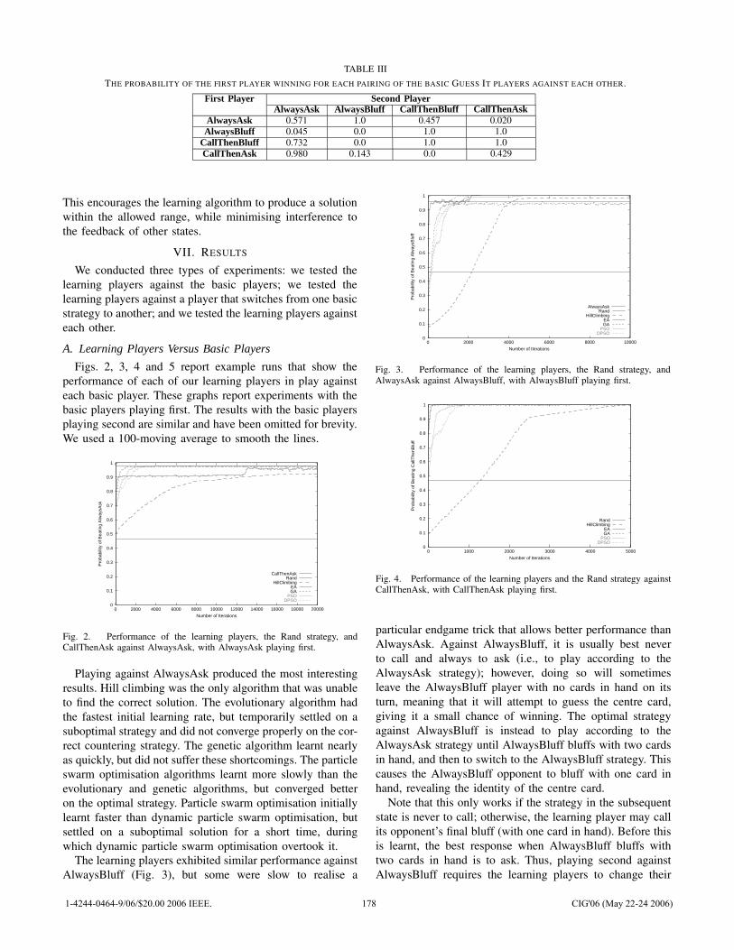
TABLE IIITHE PROBABILITY OF THE FIRST PLAYER WINNING FOR EACH PAIRING OF THE BASIC GUESS IT PLAYERS AGAINST EACH OTHER.

First Player Second PlayerAlwaysAsk AlwaysBluff CallThenBluff CallThenAsk

AlwaysAsk 0.571 1.0 0.457 0.020AlwaysBluff 0.045 0.0 1.0 1.0

CallThenBluff 0.732 0.0 1.0 1.0CallThenAsk 0.980 0.143 0.0 0.429

This encourages the learning algorithm to produce a solutionwithin the allowed range, while minimising interference tothe feedback of other states.

VII. RESULTS

We conducted three types of experiments: we tested thelearning players against the basic players; we tested thelearning players against a player that switches from one basicstrategy to another; and we tested the learning players againsteach other.

A. Learning Players Versus Basic Players

Figs. 2, 3, 4 and 5 report example runs that show theperformance of each of our learning players in play againsteach basic player. These graphs report experiments with thebasic players playing first. The results with the basic playersplaying second are similar and have been omitted for brevity.We used a 100-moving average to smooth the lines.

0

0.1

0.2

0.3

0.4

0.5

0.6

0.7

0.8

0.9

1

0 2000 4000 6000 8000 10000 12000 14000 16000 18000 20000

Pro

babi

lity

of B

eatin

g A

lway

sAsk

Number of Iterations

CallThenAskRand

HillClimbingEAGA

PSODPSO

Fig. 2. Performance of the learning players, the Rand strategy, andCallThenAsk against AlwaysAsk, with AlwaysAsk playing first.

Playing against AlwaysAsk produced the most interestingresults. Hill climbing was the only algorithm that was unableto find the correct solution. The evolutionary algorithm hadthe fastest initial learning rate, but temporarily settled on asuboptimal strategy and did not converge properly on the cor-rect countering strategy. The genetic algorithm learnt nearlyas quickly, but did not suffer these shortcomings. The particleswarm optimisation algorithms learnt more slowly than theevolutionary and genetic algorithms, but converged betteron the optimal strategy. Particle swarm optimisation initiallylearnt faster than dynamic particle swarm optimisation, butsettled on a suboptimal solution for a short time, duringwhich dynamic particle swarm optimisation overtook it.

The learning players exhibited similar performance againstAlwaysBluff (Fig. 3), but some were slow to realise a

0

0.1

0.2

0.3

0.4

0.5

0.6

0.7

0.8

0.9

1

0 2000 4000 6000 8000 10000

Pro

babi

lity

of B

eatin

g A

lway

sBlu

ff

Number of Iterations

AlwaysAskRand

HillClimbingEAGA

PSODPSO

Fig. 3. Performance of the learning players, the Rand strategy, andAlwaysAsk against AlwaysBluff, with AlwaysBluff playing first.

0

0.1

0.2

0.3

0.4

0.5

0.6

0.7

0.8

0.9

1

0 1000 2000 3000 4000 5000

Pro

babi

lity

of B

eatin

g C

allT

henB

luff

Number of Iterations

RandHillClimbing

EAGA

PSODPSO

Fig. 4. Performance of the learning players and the Rand strategy againstCallThenAsk, with CallThenAsk playing first.

particular endgame trick that allows better performance thanAlwaysAsk. Against AlwaysBluff, it is usually best neverto call and always to ask (i.e., to play according to theAlwaysAsk strategy); however, doing so will sometimesleave the AlwaysBluff player with no cards in hand on itsturn, meaning that it will attempt to guess the centre card,giving it a small chance of winning. The optimal strategyagainst AlwaysBluff is instead to play according to theAlwaysAsk strategy until AlwaysBluff bluffs with two cardsin hand, and then to switch to the AlwaysBluff strategy. Thiscauses the AlwaysBluff opponent to bluff with one card inhand, revealing the identity of the centre card.

Note that this only works if the strategy in the subsequentstate is never to call; otherwise, the learning player may callits opponent’s final bluff (with one card in hand). Before thisis learnt, the best response when AlwaysBluff bluffs withtwo cards in hand is to ask. Thus, playing second againstAlwaysBluff requires the learning players to change their

1-4244-0464-9/06/$20.00 2006 IEEE. 178 CIG'06 (May 22-24 2006)

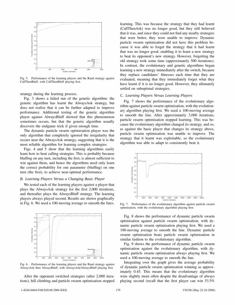
0

0.1

0.2

0.3

0.4

0.5

0.6

0.7

0.8

0.9

1

0 500 1000 1500 2000 2500

Pro

babi

lity

of B

eatin

g C

allT

henB

luff

Number of Iterations

RandHillClimbing

EAGA

PSODPSO

Fig. 5. Performance of the learning players and the Rand strategy againstCallThenBluff, with CallThenBluff playing first.

strategy during the learning process.Fig. 3 shows a failed run of the genetic algorithm: the

genetic algorithm has learnt the AlwaysAsk strategy, butdoes not realise that it can be further adapted to improveperformance. Additional testing of the genetic algorithmplayer against AlwaysBluff showed that this phenomenonsometimes occurs, but that the genetic algorithm usuallydiscovers the endgame trick if given enough time.

The dynamic particle swarm optimisation player was theonly algorithm that completely ignored the irregularity thatoccurs near the AlwaysAsk strategy, suggesting that it is themost reliable algorithm for learning complex strategies.

Figs. 4 and 5 show that the learning algorithms easilylearn how to beat calling strategies. This is probably becausebluffing on any turn, including the first, is almost sufficient towin against them, and hence the algorithms need only learnthe correct probability for one parameter (bluffing) on oneturn (the first), to achieve near-optimal performance.

B. Learning Players Versus a Changing Basic Player

We tested each of the learning players against a player thatplays the AlwaysAsk strategy for the first 2,000 iterations,and thereafter plays the AlwaysBluff strategy. The learningplayers always played second. Results are shown graphicallyin Fig. 6. We used a 100-moving average to smooth the lines.

0

0.1

0.2

0.3

0.4

0.5

0.6

0.7

0.8

0.9

1

0 1000 2000 3000 4000 5000 6000 7000 8000 9000 10000

Pro

babi

lity

of W

inni

ng

Number of Iterations

HillClimbingEAGA

PSODynamicPSO

Fig. 6. Performance of the learning players and the Rand strategy againstAlwaysAsk then AlwaysBluff, with AlwaysAsk/AlwaysBluff playing first.

After the opponent switched strategies (after 2,000 itera-tions), hill climbing and particle swarm optimisation stopped

learning. This was because the strategy that they had learnt(CallThenAsk) was no longer good, but they still believedthat it was, and since they could not find any nearby strategiesthat were better, they were unable to improve. Dynamicparticle swarm optimisation did not have this problem be-cause it was able to forget the strategy that it had learntthat was no longer good, enabling it to learn a new strategyto beat its opponent’s new strategy. However, forgetting theold strategy took some time (approximately 500 iterations).In contrast, the evolutionary and genetic algorithms beganlearning a new strategy immediately after the switch, becausethey replace candidates’ fitnesses each time that they areevaluated, meaning that they immediately forget what theyhave learnt if it is no longer good. However, they ultimatelysettled on suboptimal strategies.

C. Learning Players Versus Learning Players

Fig. 7 shows the performance of the evolutionary algo-rithm against particle swarm optimisation, with the evolution-ary algorithm playing first. We used a 100-moving averageto smooth the line. After approximately 3,000 iterations,particle swarm optimisation stopped learning. This was be-cause the evolutionary algorithm changed its strategy, and so,as against the basic player that changes its strategy above,particle swarm optimisation was unable to improve. Thestrategy that it learnt was exploitable, so the evolutionaryalgorithm was able to adapt to consistently beat it.

0

0.1

0.2

0.3

0.4

0.5

0.6

0.7

0.8

0.9

1

0 2000 4000 6000 8000 10000 12000 14000 16000 18000 20000

Pro

babi

lity

of E

A W

inni

ng

Number of Iterations

Fig. 7. Performance of the evolutionary algorithm against particle swarmoptimisation, with the evolutionary algorithm playing first.

Fig. 8 shows the performance of dynamic particle swarmoptimisation against particle swarm optimisation, with dy-namic particle swarm optimisation playing first. We used a100-moving average to smooth the line. Dynamic particleswarm optimisation beats particle swarm optimisation insimilar fashion to the evolutionary algorithm.

Fig. 9 shows the performance of dynamic particle swarmoptimisation against the evolutionary algorithm, with dy-namic particle swarm optimisation always playing first. Weused a 100-moving average to smooth the line.

Integrating over the graph gives the average probabilityof dynamic particle swarm optimisation winning as approx-imately 0.45. This means that the evolutionary algorithmwins slightly more often despite the disadvantage of alwaysplaying second (recall that the first player can win 53.5%

1-4244-0464-9/06/$20.00 2006 IEEE. 179 CIG'06 (May 22-24 2006)

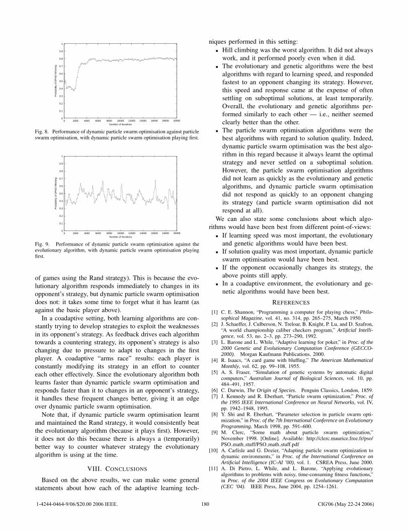
0

0.1

0.2

0.3

0.4

0.5

0.6

0.7

0.8

0.9

1

0 2000 4000 6000 8000 10000 12000 14000 16000 18000 20000

Pro

babi

lity

of D

PS

O W

inni

ng

Number of Iterations

Fig. 8. Performance of dynamic particle swarm optimisation against particleswarm optimisation, with dynamic particle swarm optimisation playing first.

0

0.1

0.2

0.3

0.4

0.5

0.6

0.7

0.8

0.9

1

0 2000 4000 6000 8000 10000 12000 14000 16000 18000 20000

Pro

babi

lity

of D

PS

O W

inni

ng

Number of Iterations

Fig. 9. Performance of dynamic particle swarm optimisation against theevolutionary algorithm, with dynamic particle swarm optimisation playingfirst.

of games using the Rand strategy). This is because the evo-lutionary algorithm responds immediately to changes in itsopponent’s strategy, but dynamic particle swarm optimisationdoes not: it takes some time to forget what it has learnt (asagainst the basic player above).

In a coadaptive setting, both learning algorithms are con-stantly trying to develop strategies to exploit the weaknessesin its opponent’s strategy. As feedback drives each algorithmtowards a countering strategy, its opponent’s strategy is alsochanging due to pressure to adapt to changes in the firstplayer. A coadaptive “arms race” results: each player isconstantly modifying its strategy in an effort to countereach other effectively. Since the evolutionary algorithm bothlearns faster than dynamic particle swarm optimisation andresponds faster than it to changes in an opponent’s strategy,it handles these frequent changes better, giving it an edgeover dynamic particle swarm optimisation.

Note that, if dynamic particle swarm optimisation learntand maintained the Rand strategy, it would consistently beatthe evolutionary algorithm (because it plays first). However,it does not do this because there is always a (temporarily)better way to counter whatever strategy the evolutionaryalgorithm is using at the time.

VIII. CONCLUSIONS

Based on the above results, we can make some generalstatements about how each of the adaptive learning tech-

niques performed in this setting:• Hill climbing was the worst algorithm. It did not always

work, and it performed poorly even when it did.• The evolutionary and genetic algorithms were the best

algorithms with regard to learning speed, and respondedfastest to an opponent changing its strategy. However,this speed and response came at the expense of oftensettling on suboptimal solutions, at least temporarily.Overall, the evolutionary and genetic algorithms per-formed similarly to each other — i.e., neither seemedclearly better than the other.

• The particle swarm optimisation algorithms were thebest algorithms with regard to solution quality. Indeed,dynamic particle swarm optimisation was the best algo-rithm in this regard because it always learnt the optimalstrategy and never settled on a suboptimal solution.However, the particle swarm optimisation algorithmsdid not learn as quickly as the evolutionary and geneticalgorithms, and dynamic particle swarm optimisationdid not respond as quickly to an opponent changingits strategy (and particle swarm optimisation did notrespond at all).

We can also state some conclusions about which algo-rithms would have been best from different point-of-views:

• If learning speed was most important, the evolutionaryand genetic algorithms would have been best.

• If solution quality was most important, dynamic particleswarm optimisation would have been best.

• If the opponent occasionally changes its strategy, theabove points still apply.

• In a coadaptive environment, the evolutionary and ge-netic algorithms would have been best.

REFERENCES

[1] C. E. Shannon, “Programming a computer for playing chess,” Philo-sophical Magazine, vol. 41, no. 314, pp. 265–275, March 1950.

[2] J. Schaeffer, J. Culberson, N. Treloar, B. Knight, P. Lu, and D. Szafron,“A world championship caliber checkers program,” Artificial Intelli-gence, vol. 53, no. 2–3, pp. 273–290, 1992.

[3] L. Barone and L. While, “Adaptive learning for poker,” in Proc. of the2000 Genetic and Evolutionary Computation Conference (GECCO-2000). Morgan Kaufmann Publications, 2000.

[4] R. Isaacs, “A card game with bluffing,” The American MathematicalMonthly, vol. 62, pp. 99–108, 1955.

[5] A. S. Fraser, “Simulation of genetic systems by automatic digitalcomputers,” Australian Journal of Biological Sciences, vol. 10, pp.484–491, 1957.

[6] C. Darwin, The Origin of Species. Penguin Classics, London, 1859.[7] J. Kennedy and R. Eberhart, “Particle swarm optimization,” Proc. of

the 1995 IEEE International Conference on Neural Networks, vol. IV,pp. 1942–1948, 1995.

[8] Y. Shi and R. Eberhart, “Parameter selection in particle swarm opti-mization,” in Proc. of the 7th International Conference on EvolutionaryProgramming, March 1998, pp. 591–600.

[9] M. Clerc, “Some math about particle swarm optimization,”November 1998. [Online]. Available: http://clerc.maurice.free.fr/pso/PSO math stuff/PSO math stuff.pdf

[10] A. Carlisle and G. Dozier, “Adapting particle swarm optimization todynamic environments,” in Proc. of the International Conference onArtificial Intelligence (IC-AI ’00), vol. 1. CSREA Press, June 2000.

[11] A. Di Pietro, L. While, and L. Barone, “Applying evolutionaryalgorithms to problems with noisy, time-consuming fitness functions,”in Proc. of the 2004 IEEE Congress on Evolutionary Computation(CEC ’04). IEEE Press, June 2004, pp. 1254–1261.

1-4244-0464-9/06/$20.00 2006 IEEE. 180 CIG'06 (May 22-24 2006)

Improving Artificial Intelligence

In a Motocross Game

Benoit ChaperotSchool of ComputingUniversity of Paisley

Scotlandbenoit.chaperot@paisley.ac.uk

Colin FyfeSchool of ComputingUniversity of Paisley

Scotlandcolin.fyfe@paisley.ac.uk

Abstract— We have previously investigated the use of artificialneural networks to ride simulated motorbikes in a new com-puter game. These artificial neural networks were trained usingtwo different training techniques, the Evolutionary Algorithmsand the Backpropagation Algorithm. In this paper, we detailsome of the investigations to improve the training, with a viewto having the computer controlled bikes performing as well orbetter than a human player at playing the game. Techniquesinvestigated here to improve backpropagation are bagging andboosting, while alternative crossover techniques have also beeninvestigated to improve Evolution.

Keywords: Motorbikes, Computational Intelligence, Ar-tificial Neural Networks, Back Propagation, EvolutionaryAlgorithm, Genetic Algorithm, Driving Game.

I. INTRODUCTION

We [1] have previously investigated the use of artificialneural networks to ride simulated motorbikes in a newcomputer game. In this paper, we investigate techniques forimproving the training of artificial neural networks to ridesimulated motorbikes in a new computer game. The useof such methods in control is not new (see e.g.[2], [3]),but it is one of the first time these methods are appliedto a video game (see e.g.[4]). Two training techniquesare used, Evolutionary Algorithms and the BackpropagationAlgorithm. To improve the Backpropagation Algorithm inthis paper, two optimisation techniques for augmenting thetraining are used: bagging [5] and boosting [6]. There arevarious interesting aspects in using artificial neural networks(ANN’s) in a motocross game. The main reason is that,although the control of the bike is assisted by the gameengine, turning the bike, accelerating, braking and jumpingon the bumps involve behaviours which are difficult toexpress as a set of procedural rules, and make the use ofANN’s very appropriate. Our main aim is then to have theANN’s to perform as well as possible at riding the motorbike.We suspect that we can train the network to play better thanany living player; however, an ANN can always be penalisedat a later stage if it becomes so good that it decreases theenjoyment of human competitors.

II. THE GAME

There are various interesting aspects in using artificialneural network methods in a motocross game. Because thedesign of an ANN’s is motivated by analogy with the brain,and the rationale for their use in the current context is that

entities controlled by ANN’s are expected to behave in ahuman or animal manner, these behaviours can add somelife and content to the game. The human player has also thepossibility to create new tracks. ANN’s have the capabilityto perform well and extrapolate when presented with newand different sets of inputs from the sets that were used totrain them; hence an ANN trained to ride a motorbike on atrack should be able to ride the same motorbike on anothersimilar track. ANN’s are adaptible in that their parameterscan be trained or evolved. ANN’s may be able to performwith good lap times on any given track while still retainingelements of human behaviour.

Motocross The Force is a motocross game featuring terrainrendering and rigid body simulation applied to bikes andcharacters. An example of it in use can be seen at

http://cis.paisley.ac.uk/chap-ci1

and a screen shot from the game is shown in Figure 1.The game has been developed and is still being developedin conjunction with Eric Breistroffer (2D and 3D artist). Atrack has been created in a virtual environment and the gameinvolves riding a motorbike as quickly as possible round thetrack while competing with other riders who are software-controlled.

There is one position known as a way point which marksthe position and orientation of the centre of the track, everymetre along the track. These way points are used to ensurebikes follow the track and we will discuss positions in waypoint space when giving positions with respect to the waypoints.

For example, for the evolutionary algorithms, the score iscalculated as follows:

• vPassWayPointBonus is a bonus for passingthrough a way point.

• vMissedWayPointBonus is a bonus/penalty (i.e.normally negative) for missing a way point.

• vCrashBonus is a bonus/penalty (i.e. normally neg-ative) for crashing the bike.

• vFinalDistFromWayPointBonusMultiplier is abonus/penalty (i.e. normally negative) for every metreaway from the centre of the next way point.

The inputs to the ANN are:

• Position of the bike in way point space.

1-4244-0464-9/06/$20.00 2006 IEEE. 181 CIG'06 (May 22-24 2006)

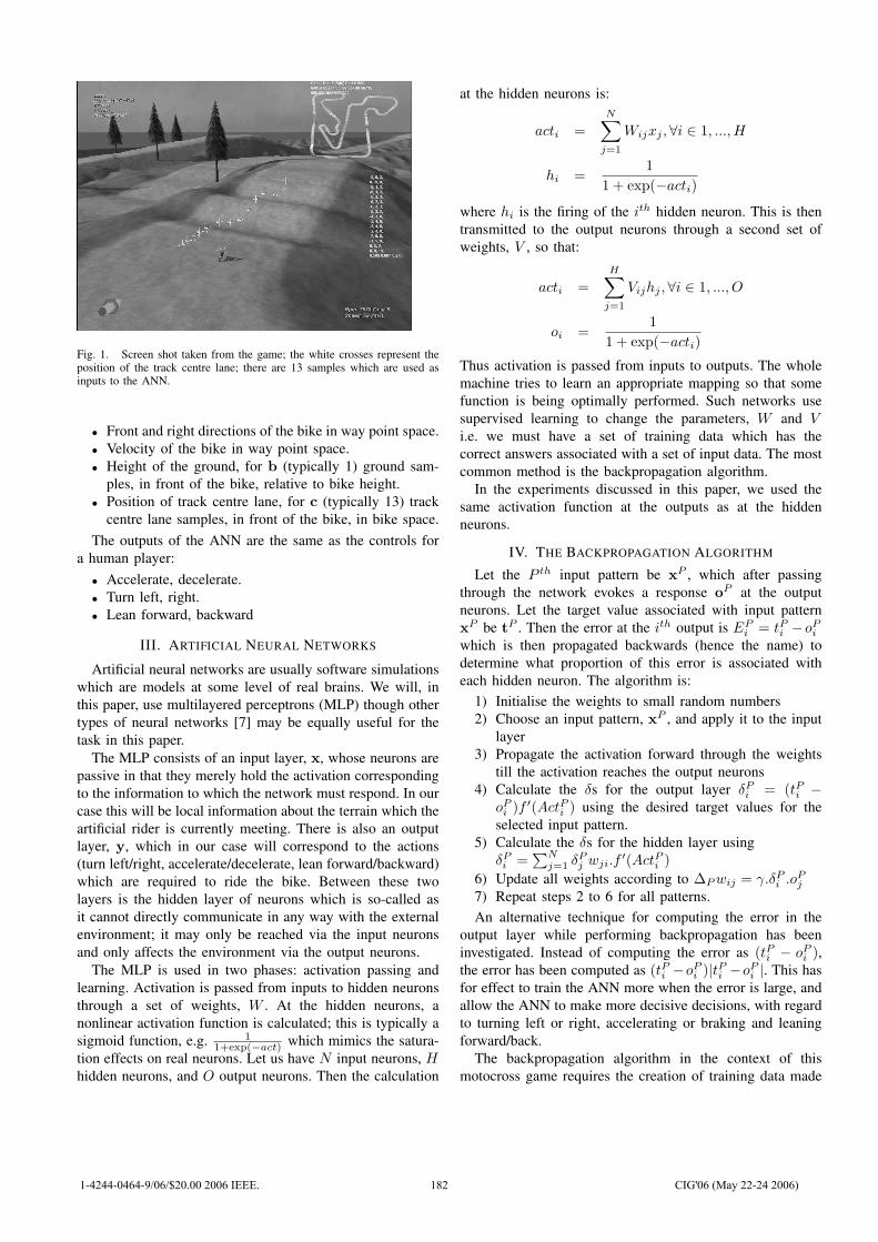
Fig. 1. Screen shot taken from the game; the white crosses represent theposition of the track centre lane; there are 13 samples which are used asinputs to the ANN.

• Front and right directions of the bike in way point space.• Velocity of the bike in way point space.• Height of the ground, for b (typically 1) ground sam-

ples, in front of the bike, relative to bike height.• Position of track centre lane, for c (typically 13) track

centre lane samples, in front of the bike, in bike space.

The outputs of the ANN are the same as the controls fora human player:

• Accelerate, decelerate.• Turn left, right.• Lean forward, backward

III. ARTIFICIAL NEURAL NETWORKS

Artificial neural networks are usually software simulationswhich are models at some level of real brains. We will, inthis paper, use multilayered perceptrons (MLP) though othertypes of neural networks [7] may be equally useful for thetask in this paper.

The MLP consists of an input layer, x, whose neurons arepassive in that they merely hold the activation correspondingto the information to which the network must respond. In ourcase this will be local information about the terrain which theartificial rider is currently meeting. There is also an outputlayer, y, which in our case will correspond to the actions(turn left/right, accelerate/decelerate, lean forward/backward)which are required to ride the bike. Between these twolayers is the hidden layer of neurons which is so-called asit cannot directly communicate in any way with the externalenvironment; it may only be reached via the input neuronsand only affects the environment via the output neurons.

The MLP is used in two phases: activation passing andlearning. Activation is passed from inputs to hidden neuronsthrough a set of weights, W . At the hidden neurons, anonlinear activation function is calculated; this is typically asigmoid function, e.g. 1

1+exp(−act) which mimics the satura-tion effects on real neurons. Let us have N input neurons, Hhidden neurons, and O output neurons. Then the calculation

at the hidden neurons is:

acti =N∑

j=1

Wijxj ,∀i ∈ 1, ..., H

hi =1

1 + exp(−acti)

where hi is the firing of the ith hidden neuron. This is thentransmitted to the output neurons through a second set ofweights, V , so that:

acti =H∑

j=1

Vijhj , ∀i ∈ 1, ..., O

oi =1

1 + exp(−acti)

Thus activation is passed from inputs to outputs. The wholemachine tries to learn an appropriate mapping so that somefunction is being optimally performed. Such networks usesupervised learning to change the parameters, W and Vi.e. we must have a set of training data which has thecorrect answers associated with a set of input data. The mostcommon method is the backpropagation algorithm.

In the experiments discussed in this paper, we used thesame activation function at the outputs as at the hiddenneurons.

IV. THE BACKPROPAGATION ALGORITHM

Let the P th input pattern be xP , which after passingthrough the network evokes a response oP at the outputneurons. Let the target value associated with input patternxP be tP . Then the error at the ith output is EP

i = tPi − oPi

which is then propagated backwards (hence the name) todetermine what proportion of this error is associated witheach hidden neuron. The algorithm is:

1) Initialise the weights to small random numbers2) Choose an input pattern, xP , and apply it to the input

layer3) Propagate the activation forward through the weights

till the activation reaches the output neurons4) Calculate the δs for the output layer δP

i = (tPi −oP

i )f ′(ActPi ) using the desired target values for theselected input pattern.

5) Calculate the δs for the hidden layer usingδPi =

∑Nj=1 δP

j wji.f′(ActPi )

6) Update all weights according to ∆P wij = γ.δPi .oP

j

7) Repeat steps 2 to 6 for all patterns.An alternative technique for computing the error in the

output layer while performing backpropagation has beeninvestigated. Instead of computing the error as (tPi − oP

i ),the error has been computed as (tPi −oP

i )|tPi −oPi |. This has

for effect to train the ANN more when the error is large, andallow the ANN to make more decisive decisions, with regardto turning left or right, accelerating or braking and leaningforward/back.

The backpropagation algorithm in the context of thismotocross game requires the creation of training data made

1-4244-0464-9/06/$20.00 2006 IEEE. 182 CIG'06 (May 22-24 2006)

from a recording of the game played by a good humanplayer. The targets are the data from the human player i.e.how much acceleration/deceleration, left/right turning andfront/back leaning was done by the human player at that pointin the track. The aim is to have the ANN reproduce what agood human player is doing. The human player’s responsesneed not be the optimal solution but a good enough solutionand, of course, the ANN will learn any errors which thehuman makes.

We investigated two techniques to improve the training,bagging and boosting.

V. ENSEMBLE METHODS

Recently a number of ways of combining predictors havebeen developed e.g. [8], [9], [6], [10]. Perhaps the simplestis bagging predictors. The term “bagging” was coined byjoining bootstrapping and aggregating- we are going toaggregate predictors and in doing so we are bootstrappinga system. We note that the term “bootstrapping” was derivedfrom the somewhat magical possibilities of “pulling oneselfup by one’s bootstraps” and the process of aggregatingpredictors in this way does give a rather magical result -the aggregated predictor is much more powerful than anyindividual predictor trained on the same data. It is no wonderthat statisticians have become very convincing advocates ofthese methods.

A. Using Bagging

In ([1]), the ANN was trained using training data madefrom a recording of the game being played by a good humanplayer. The data was made from the recording of the firstauthor playing the game on many different motocross tracks(here 10). Bootstrapping [8] is a simple and effective way ofestimating a statistic of a data set. Let us suppose we havea data set, D = {xi, i = 1, . . . , N}. The method consists ofcreating a number of pseudo data sets, Di, by sampling fromD with uniform probability with replacement of each sample.Thus each data point has a probability of (N−1

N )N ≈ 0.368of not appearing in each bootstrap sample, Di. Each predictoris then trained separately on its respective data set and thebootstrap estimate is some aggregation (almost always asimple averaging) of the estimate of the statistic from theindividual predictors. Because the predictors are trained onslightly different data sets, they will disagree in some placesand this disagreement can be shown to be beneficial insmoothing the combined predictor. Typically, the algorithmcan be explained as follows:

1) Create N bags by randomly sampling from the data setwith replacement.

2) The probability for a piece of data to be in the bag isapproximately 0.63.

3) ANN’s are trained on the bags separately.4) The trained ANN’s are then presented with an input

and the outputs of the ANN’s are combined.

TABLE I

BAGGING RESULTS

NN Trained Training Data Lap TimeOn Track Length (sec) Track m16

0 Expert 234.41 1’58”1 hat 144.42 6’43”2 hillclimb 35.36 4’01”3 jat 339.69 4’24”4 L 261.51 2’22”5 m1 247.32 4’45”6 m10 131.72 NA7 m11 187.47 14’25”8 m12 100.62 4’08”9 m13 112.06 6’21”Average (0,9) ALL ALL 1’38”11 ALL 1794.58 1’31”Good Human ALL NA 1’23”

The combination operator, in spirit similar to [10], usedwas as below:

OANN = OAV E ∗ (1− w) + OWIN ∗ w; (1)

With OAV E , the average of all ANN’s outputs, OWIN , theoutput of the most confident ANN, which is the output withthe largest magnitude, and w a parameter varying from 0to 1. Experiments were done using ten ANN’s. Experimentshave shown that:

1) With w = 0, the combined output was a smooth output,and the computer controlled bikes tended to ride in aslow but safe manner.

2) With w = 1 (similar to “bumping” [10]) , the combinedoutput was a decisive output and the computer con-trolled bikes tended to ride in a fast but risky manner.

This w parameter can allow to change the computercontrolled bike behaviour, and could be used to have theartificial intelligence performance match that of the player.However, experiments proved that whatever the value forw, the performance was still a lot less than that of a goodhuman player, and similar to or less than that of a singleANN trained using the entire training set.

Better results were achieve by, instead of creating bags byrandomly sampling from data set, creating bags by samplingdata according to data origin i.e. from data from a singletrack. The data set was made from the recording of the firstauthor playing the game on ten motocross tracks. Now eachbag contained data for one separate motocross track. Theresults are given in Table I.

(1) was used for combination with w equal to zero (pureaveraging which is exactly bagging) and Table I shows thatthe combination of ten ANN’s is better than every singleANN taken separately, but still not as good as another ANNtrained using the full data set.

B. Using Boosting

There has been recent work identifying the most importantdata samples [11]; and presenting the ANN more with the

1-4244-0464-9/06/$20.00 2006 IEEE. 183 CIG'06 (May 22-24 2006)

most important data samples (boosting [6]). We investigatedthe effect of different types of training data. For example,some parts of the track are relatively easy and the rider canaccelerate quickly over these while other parts are far moredifficult and so more care must be taken. The latter parts arealso those where most accidents happen. Our first conjecturewas that training the neural network on these more difficultparts might enable it to concentrate its efforts on the difficultsections of the track and so a training routine was developedin which each training sample has a probability to be selectedfor training the ANN proportional to the error produced thelast time the sample was presented to the ANN. This allowsus to train the ANN with more difficult situations.

The first algorithm was not efficient; it was storing anaverage error value for each of the training samples, whichis not memory efficient, and made use of a roulette to selectthe samples according to the average error, which is notprocessing efficient. There was a time during which theaverage error was computed, and then the average error wasreset. The algorithm was complicated, was making use ofmany parameters and was hard to tune.

Then, it appeared that because the learning rate is low,the ANN does not change very much with time, and it ispossible to use the instantaneous error, and not the averageerror. Instead of selecting samples according to the error thesample produces, it is possible to select samples randomly,evaluate the error, and modify the instantaneous learning rateaccording to this instantaneous error.

The training routine had a negative effect on the training.Without the routine, the average lap time was 2 minutes and40 seconds. With the routine, the average lap time was 3minutes. On the other hand, when the routine was inverted(so that the backpropagation was performed with a learningrate proportional to the inverse of the error produced by thesample) this had a positive effect. The ANN performed betterwhen being trained more with the easy samples.

Finally, the learning rate multiplier (to compute the ef-fective learning rate from the original learning rate) wasevaluated as:

m = MIN(0.1, 1− Error); (2)

Using this technique, after 24 hours of training, or34560000 iterations, the ANN average lap time can go downfrom 2 minutes 30 seconds on track L, to only 2 minutes 18seconds. Training can take a long time, because the ANNhas to train and select the right set of training samples at thesame time.

Our alternative technique for computing the error in theoutput layer while performing backpropagation as (tPi −oP

i )|tPi − oPi | was originally considered as having a positive

effect on the training because it allowed more decisivedecisions from the ANN, and proved to improve trained ANNperformance. Since the time this alternative technique wasimplemented, the first author worked on the physics side ofthe game and the handling of the motorbike has improved;

this alternative technique does not any more have a positiveeffect on the final performance of the ANN. Worse, it canhave a negative effect.

It finally appeared that with the new physics, reverting tothe classic technique for computing the error in the outputlayer, and removing the anti-boosting as described aboveallowed the ANN to train faster and produced equally goodperformances.

VI. EVOLUTIONARY ALGORITHMS

We can identify the problem of finding appropriate weightsfor the MLP as an optimisation problem and have thisproblem solved using the GA ([12]): we must code theweights as floating point numbers and use the algorithm onthem with a score function.

The algorithm is:

1) Initialise a population of chromosomes randomly.2) Evaluate the fitness of each chromosome (string) in the

population.3) For each new child chromosome:

a) Select two members from the current population.The chance of being selected is proportional tothe chromosomes’ fitness.

b) With probability, Cr, the crossover rate, crossover the numbers from each chosen parent chro-mosome at a randomly chosen point to create thechild chromosomes.

c) With probability, Mr, the mutation rate, modifythe chosen child chromosomes’ numbers by aperturbation amount.

d) Insert the new child chromosome into the newpopulation.

4) Repeat steps 2-3 till convergence of the population.

An alternative technique for crossover has also beeninvestigated: instead of crossing over the numbers (corre-sponding to the ANN’s weights) from each chosen parentchromosome at a randomly chosen point to create the childchromosomes, numbers from parents are averaged to createthe child chromosomes. This seems appropriate because weare working with floating point numbers and not binary digitsand is a method which is sometimes used with the EvolutionStrategies [13] which are designed for use with floating pointnumbers. Initial experimentation revealed that a blend ofthese two techniques worked best. The particular crossovertechnique was chosen randomly, with each technique beinggiven equal chance, for each new child chromosome and thenapplied as usual.

Other techniques have also been tested: if starting the evo-lution from a randomly initialised chromosome population,we showed ([1]) that the ANN’s do not perform as wellas other ANN’s trained using backpropagation. Some testshave been made starting the evolution from a populationof different ANN’s already trained using BP. One majorproblem with doing crossover with ANN’s is that eachneuron has a functionality or part of the behaviour (forexample turning right), and while doing crossover, the child

1-4244-0464-9/06/$20.00 2006 IEEE. 184 CIG'06 (May 22-24 2006)

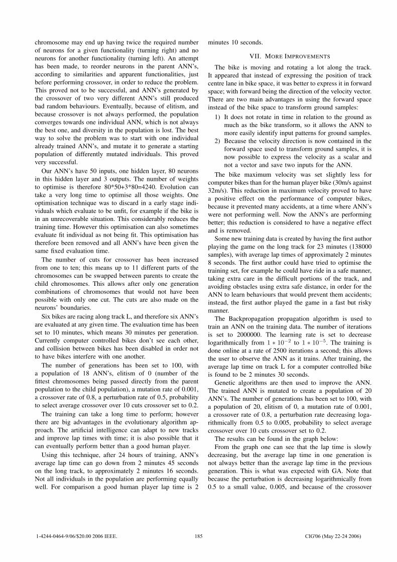
chromosome may end up having twice the required numberof neurons for a given functionality (turning right) and noneurons for another functionality (turning left). An attempthas been made, to reorder neurons in the parent ANN’s,according to similarities and apparent functionalities, justbefore performing crossover, in order to reduce the problem.This proved not to be successful, and ANN’s generated bythe crossover of two very different ANN’s still producedbad random behaviours. Eventually, because of elitism, andbecause crossover is not always performed, the populationconverges towards one individual ANN, which is not alwaysthe best one, and diversity in the population is lost. The bestway to solve the problem was to start with one individualalready trained ANN’s, and mutate it to generate a startingpopulation of differently mutated individuals. This provedvery successful.

Our ANN’s have 50 inputs, one hidden layer, 80 neuronsin this hidden layer and 3 outputs. The number of weightsto optimise is therefore 80*50+3*80=4240. Evolution cantake a very long time to optimise all those weights. Oneoptimisation technique was to discard in a early stage indi-viduals which evaluate to be unfit, for example if the bike isin an unrecoverable situation. This considerably reduces thetraining time. However this optimisation can also sometimesevaluate fit individual as not being fit. This optimisation hastherefore been removed and all ANN’s have been given thesame fixed evaluation time.

The number of cuts for crossover has been increasedfrom one to ten; this means up to 11 different parts of thechromosomes can be swapped between parents to create thechild chromosomes. This allows after only one generationcombinations of chromosomes that would not have beenpossible with only one cut. The cuts are also made on theneurons’ boundaries.

Six bikes are racing along track L, and therefore six ANN’sare evaluated at any given time. The evaluation time has beenset to 10 minutes, which means 30 minutes per generation.Currently computer controlled bikes don’t see each other,and collision between bikes has been disabled in order notto have bikes interfere with one another.

The number of generations has been set to 100, witha population of 18 ANN’s, elitism of 0 (number of thefittest chromosomes being passed directly from the parentpopulation to the child population), a mutation rate of 0.001,a crossover rate of 0.8, a perturbation rate of 0.5, probabilityto select average crossover over 10 cuts crossover set to 0.2.

The training can take a long time to perform; howeverthere are big advantages in the evolutionary algorithm ap-proach. The artificial intelligence can adapt to new tracksand improve lap times with time; it is also possible that itcan eventually perform better than a good human player.

Using this technique, after 24 hours of training, ANN’saverage lap time can go down from 2 minutes 45 secondson the long track, to approximately 2 minutes 16 seconds.Not all individuals in the population are performing equallywell. For comparison a good human player lap time is 2

minutes 10 seconds.

VII. MORE IMPROVEMENTS

The bike is moving and rotating a lot along the track.It appeared that instead of expressing the position of trackcentre lane in bike space, it was better to express it in forwardspace; with forward being the direction of the velocity vector.There are two main advantages in using the forward spaceinstead of the bike space to transform ground samples:

1) It does not rotate in time in relation to the ground asmuch as the bike transform, so it allows the ANN tomore easily identify input patterns for ground samples.

2) Because the velocity direction is now contained in theforward space used to transform ground samples, it isnow possible to express the velocity as a scalar andnot a vector and save two inputs for the ANN.

The bike maximum velocity was set slightly less forcomputer bikes than for the human player bike (30m/s against32m/s). This reduction in maximum velocity proved to havea positive effect on the performance of computer bikes,because it prevented many accidents, at a time where ANN’swere not performing well. Now the ANN’s are performingbetter; this reduction is considered to have a negative effectand is removed.

Some new training data is created by having the first authorplaying the game on the long track for 23 minutes (138000samples), with average lap times of approximately 2 minutes8 seconds. The first author could have tried to optimise thetraining set, for example he could have ride in a safe manner,taking extra care in the difficult portions of the track, andavoiding obstacles using extra safe distance, in order for theANN to learn behaviours that would prevent them accidents;instead, the first author played the game in a fast but riskymanner.

The Backpropagation propagation algorithm is used totrain an ANN on the training data. The number of iterationsis set to 2000000. The learning rate is set to decreaselogarithmically from 1 ∗ 10−2 to 1 ∗ 10−5. The training isdone online at a rate of 2500 iterations a second; this allowsthe user to observe the ANN as it trains. After training, theaverage lap time on track L for a computer controlled bikeis found to be 2 minutes 30 seconds.

Genetic algorithms are then used to improve the ANN.The trained ANN is mutated to create a population of 20ANN’s. The number of generations has been set to 100, witha population of 20, elitism of 0, a mutation rate of 0.001,a crossover rate of 0.8, a perturbation rate decreasing loga-rithmically from 0.5 to 0.005, probability to select averagecrossover over 10 cuts crossover set to 0.2.

The results can be found in the graph below:From the graph one can see that the lap time is slowly

decreasing, but the average lap time in one generation isnot always better than the average lap time in the previousgeneration. This is what was expected with GA. Note thatbecause the perturbation is decreasing logarithmically from0.5 to a small value, 0.005, and because of the crossover

1-4244-0464-9/06/$20.00 2006 IEEE. 185 CIG'06 (May 22-24 2006)

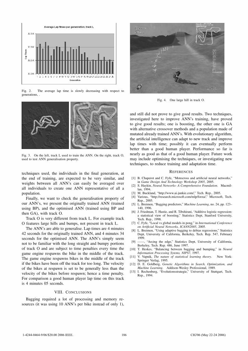
Fig. 2. The average lap time is slowly decreasing with respect togenerations, .

Fig. 3. On the left, track L used to train the ANN. On the right, track O,used to test ANN generalisation property.

techniques used, the individuals in the final generation, atthe end of training, are expected to be very similar, andweights between all ANN’s can easily be averaged overall individuals to create one ANN representative of all apopulation.

Finally, we want to check the generalisation property ofour ANN’s, we present the originally trained ANN (trainedusing BP), and the optimised ANN (trained using BP andthen GA), with track O.

Track O is very different from track L. For example trackO features large hills and bumps, not present in track L.

The ANN’s are able to generalise. Lap times are 4 minutes42 seconds for the originally trained ANN, and 4 minutes 34seconds for the optimised ANN. The ANN’s simply seemnot to be familiar with the long straight and bumpy portionsof track O and are subject to time penalties every time thegame engine respawns the bike in the middle of the track.The game engine respawns bikes in the middle of the trackif the bikes have been off the track for too long. The velocityof the bikes at respawn is set to be generally less than thevelocity of the bikes before respawn; hence a time penalty.For comparison a good human player lap time on this trackis 4 minutes 05 seconds.

VIII. CONCLUSIONS

Bagging required a lot of processing and memory re-sources (it was using 10 ANN’s per bike instead of only 1),

Fig. 4. One large hill in track O.

and still did not prove to give good results. Two techniques,investigated here to improve ANN’s training, have provedto give good results; one is boosting, the other one is GAwith alternative crossover methods and a population made ofmutated already trained ANN’s. With evolutionary algorithm,the artificial intelligence can adapt to new track and improvelap times with time; possibly it can eventually performbetter than a good human player. Performance so far isnearly as good as that of a good human player. Future workmay include optimising the techniques, or investigating newtechniques, to reduce training and adaptation time.

REFERENCES

[1] B. Chaperot and C. Fyfe, “Motocross and artificial neural networks,”in Game Design And Technology Workshop 2005, 2005.

[2] S. Haykin, Neural Networks- A Comprehensive Foundation. Macmil-lan, 1994.

[3] M. Buckland, “http://www.ai-junkie.com/,” Tech. Rep., 2005.[4] Various, “http://research.microsoft.com/mlp/forza/,” Microsoft, Tech.

Rep., 2005.[5] L. Breimen, “Bagging predictors,” Machine Learning, no. 24, pp. 123–

140, 1996.[6] J. Friedman, T. Hastie, and R. Tibshirani, “Additive logistic regression:

a statistical view of boosting,” Statistics Dept, Stanford University,Tech. Rep., 1998.

[7] C. Fyfe, “Local vs global models in pong,” in International Conferenceon Artificial Neural Networks, ICANN2005, 2005.

[8] L. Breimen, “Using adaptive bagging to debias regressions,” StatisticsDept, University of California, Berkeley, Tech. Rep. 547, February1999.

[9] ——, “Arcing the edge,” Statistics Dept, University of California,Berkeley, Tech. Rep. 486, June 1997.

[10] T. Heskes, “Balancing between bagging and bumping,” in NeuralInformation Processing Sytems, NIPS7, 1997.

[11] V. Vapnik, The nature of statistical learning theory. New York:Springer Verlag, 1995.

[12] D. E. Goldberg, Genetic Algorithms in Search, Optimization, andMachine Learning. Addison-Wesley Professional, 1989.

[13] I. Rechenberg, “Evolutionsstrategie,” University of Stuttgart, Tech.Rep., 1994.

1-4244-0464-9/06/$20.00 2006 IEEE. 186 CIG'06 (May 22-24 2006)

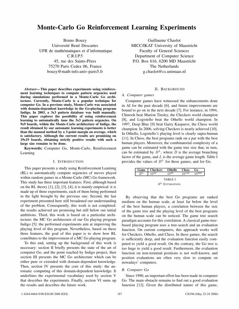
Monte-Carlo Go Reinforcement Learning ExperimentsBruno Bouzy

Universite Rene DescartesUFR de mathematiques et d’informatique

C.R.I.P.545, rue des Saints-Peres

75270 Paris Cedex 06, Francebouzy@math-info.univ-paris5.fr

Guillaume ChaslotMICC/IKAT University of Maastricht

Faculty of General SciencesDepartment of Computer Science

P.O. Box 616, 6200 MD MaastrichtThe Netherlands

g.chaslot@cs.unimaas.nl

Abstract— This paper describes experiments using reinforce-ment learning techniques to compute pattern urgencies usedduring simulations performed in a Monte-Carlo Go archi-tecture. Currently, Monte-Carlo is a popular technique forcomputer Go. In a previous study, Monte-Carlo was associatedwith domain-dependent knowledge in the Go-playing programIndigo. In 2003, a 3x3 pattern database was built manually.This paper explores the possibility of using reinforcementlearning to automatically tune the 3x3 pattern urgencies. On9x9 boards, within the Monte-Carlo architecture of Indigo, theresult obtained by our automatic learning experiments is betterthan the manual method by a 3-point margin on average, whichis satisfactory. Although the current results are promising on19x19 boards, obtaining strictly positive results with such alarge size remains to be done.

Keywords: Computer Go, Monte-Carlo, ReinforcementLearning

I. INTRODUCTION

This paper presents a study using Reinforcement Learning(RL) to automatically compute urgencies of moves playedwithin random games in a Monte-Carlo (MC) Go framework.This study has three important features. First, although basedon the RL theory [1], [2], [3], [4], it is mainly empirical: it ismade up of three experiments, each of them being performedin the light brought by the previous one. Second, the lastexperiment presented here still broadened our understandingof the problem. Consequently, this work is not completed:the results achieved are promising but still below our initialambitions. Third, this work is based on a particular archi-tecture: the MC Go architecture of our Go playing programIndigo [5]: the performed experiments aim at improving theplaying level of this program. Nevertheless, based on thesethree features, the goal of this paper is to show how RLcontributes to the improvement of a MC Go playing program.

To this end, setting up the background of this work isnecessary: section II briefly presents the state of the art ofcomputer Go, and the point reached by Indigo project, thensection III presents the MC Go architecture which can beeither pure or extended with domain-dependent knowledge.Then, section IV presents the core of this study: the au-tomatic computing of this domain-dependent knowledge. Itunderlines the experimental vocabulary used by section Vthat describes the experiments. Finally, section VI sums upthe results and describes the future work.

II. BACKGROUND

A. Computer gamesComputer games have witnessed the enhancements done

in AI for the past decade [6], and future improvements arebound to go on in the next decade [7]. For instance, in 1994,Chinook beat Marion Tinsley, the Checkers world champion[8], and Logistello beat the Othello world champion. In1997, Deep Blue [9] beat Garry Kasparov, the Chess worldchampion. In 2006, solving Checkers is nearly achieved [10].In Othello, Logistello’s playing level is clearly supra-human[11]. In Chess, the best programs rank on a par with the besthuman players. Moreover, the combinatorial complexity of agame can be estimated with the game tree size that, in turn,can be estimated by BL, where B is the average branchingfactor of the game, and L is the average game length. Table Iprovides the values of BL for these games, and for Go.

Game Checkers Othello Chess GoB

L 1032 1058 10123 10360

TABLE IB

L ESTIMATION.

By observing that the best Go programs are rankedmedium on the human scale, at least far below the levelof the best human players, a correlation between the sizeof the game tree and the playing level of the best programson the human scale can be noticed. The game tree searchparadigm accounts for this correlation. A classical game-tree-based playing program uses a tree-search and an evaluationfunction. On current computers, this approach works wellfor Checkers, Othello, and Chess. In these games, the searchis sufficiently deep, and the evaluation function easily com-puted to yield a good result. On the contrary, the Go tree istoo huge to yield a good result. Furthermore, the evaluationfunction on non-terminal positions is not well-known, andposition evaluations are often very slow to compute onnowadays’ computers.

B. Computer GoSince 1990, an important effort has been made in computer

Go. The main obstacle remains to find out a good evaluationfunction [12]. Given the distributed nature of this game,

1-4244-0464-9/06/$20.00 2006 IEEE. 187 CIG'06 (May 22-24 2006)

it was natural to study the breakdown of a position intosub-parts, and to perform local tree searches using intensivepattern-matching and knowledge bases [13], [14]. The bestprograms are sold on the market: Many Faces of Go [15],Goemate, Handtalk, Go++ [16], Haruka, KCC Igo. Conse-quently, the sources of these programs are not available.In 2002, GNU Go [17], an open source program, becamealmost as strong as these programs. Since then, this programhas been used as an example to launch new computer Goprojects. Various academic programs exists : Go Intellect,Indigo, NeuroGo [18], Explorer [19], GoLois [20], Magog.Some aspects of these programs are described in scientificpapers: [21] for Go Intellect, [22] for NeuroGo, [23] forExplorer, [24] for Golois, and [25] for Magog.

C. Indigo projectThe Indigo project was launched in 1991 as a PhD

research. Indigo is a Go playing program which has regularlyattended international competitions since 1998. Its mainresults are listed below.

• 9th KGS, 19x19, Dec 2005 (Formal: 3rd/7, Open: 1st/9)• 8th KGS, 9x9, Formal, Nov 2005 (4th/11)• 7th KGS, 19x19, Open, Oct 2005 (2th/7)• 2005 WCGC, Tainan, Taiwan, Sept 2005 (6th/7)• 10th CO, Taipei, Sept 2005 (19x19: 4th/7, 9x9: 3rd/9)• 9th CO, Ramat-Gan, Jul 2004 (19x19: 3rd/5, 9x9: 4th/9)• 8th CO, Graz, Nov 2003 (19x19: 5th/11, 9x9: 4th/10)• Comp. Go Festival, Guyang, China, Oct 2002 (6th/10)• 21st Century Cup, 2002, Edmonton, Canada (10th/14)• Mind Sport Olymp. 2000, London, England (5th/6)• Ing Cup 1999 Shanghai, China (13th/16)• Ing Cup 1998 London, England (10th/17)Participating in these events has allowed Indigo to be as-

sessed against various opponents, which brings about keepinggood and efficient methods, and eliminating bad or inefficientones. Until 2002, Indigo was a classical Go program: itused the breakdown approach, and local tree searches with alarge knowledge base. The results improved in 2003, whichcorresponds to the integration of MC techniques into Indigo.The historical vision of the Indigo development shows therelevance of the MC approach in computer Go. However, theeffect of the knowledge approach must not be overlooked.Without knowledge, Indigo would be less strong than it is.

III. MONTE-CARLO GO

This section presents the MC technique [26] for computergames, then MC Go as such, without specific knowledge,lastly MC Go associated with specific knowledge.

A. Monte-Carlo gamesMonte-Carlo is appropriate for games containing random-

ness, for example for Backgammon in which the playersthrow dice. In Backgammon, although the best program usedtree search instead simulations during its games, simulationsare used after the games or at learning time [27] to find outnew policies. MC is also adapted to games including hiddeninformation such as Poker or Scrabble. Poki, one of the best

Poker programs [28], and Maven, the best Scrabble program[29], perform simulations during their games in order to rep-resent hidden information. For complete information games,simulations can be appropriate as well. Abramson proposeda Monte-Carlo model for such games [30]. To obtain theevaluation of a given position, the basic idea consists inlaunching a given number N of random games starting onthis position, scoring the terminal positions, and averagingall the scores. To choose a move on a given position, thecorresponding idea is the greedy algorithm at depth one. Foreach move on the given position, launch a given number N ofrandom games starting on this position, score the terminal po-sitions, and average all the scores, and finally play the movewith the best mean. The obvious upside of MC is its lowcomplexity when B and L are high: O(BL) for tree search,and O(NBL) for Monte-Carlo. For complete informationgames, when the tree is too large for a successful tree search,simulations allow the program to sample tree sequencesthat reach terminal positions meaningful for evaluating thegiven position. By averaging the scores, evaluations on non-terminal positions are robust, which is hard to obtain withclassical evalution functions based on knowledge extractedfrom human expertise.

B. Basic Monte-Carlo GoIn the early 1990’s, the general MC model by Abramson

was used on games with low complexity such as 6x6 Othello.However, in 1993, Bernd Brugmann succeeded in devel-opping the first 9x9 MC Go program, Gobble [31]. Moreprecisely, Gobble was based on simulated annealing [32].In addition, to make the program work on the computersavailable at that time, Brugmann used a heuristic latercalled the all-moves-as-first heuristic [33]. Theoretically, thisheuristic enables the process to divide the response time bythe size of the board. In practice on 9x9, it enables theprogram to divide the response time by a few dozens, whichis a huge speed-up, and worth considering. After a randomgame with a score, instead of updating the mean of the firstmove of the random game, the all-moves-as-first heuristicupdates with the score the means of all moves played firston their intersections with the same color as the first move.Symmetrically, the all-moves-as-first heuristic updates withthe opposite score the means of all moves played first on theirintersections with a different color from the first move. All inall, this heuristic updates the mean of almost all the moves asif they were played first in the random game. Unfortunately,this heuristic is not completely correct because it may updatewith the same score two moves that have different effectsdepending on when they are played: before or after a capture(capture being the basic concept in Go). However, this Go-specific heuristic had to be mentioned.

Since 2002, the MC approach has gained popularity inthe computer Go community, which can be explained bythespeed of current computers. The standard deviation of ran-dom games played on 9x9 boards is roughly 35. If we lookfor a one-point precision evaluation, 1,000 games give 68%of statistical confidence, and 4,000 games 95%. Given that

1-4244-0464-9/06/$20.00 2006 IEEE. 188 CIG'06 (May 22-24 2006)

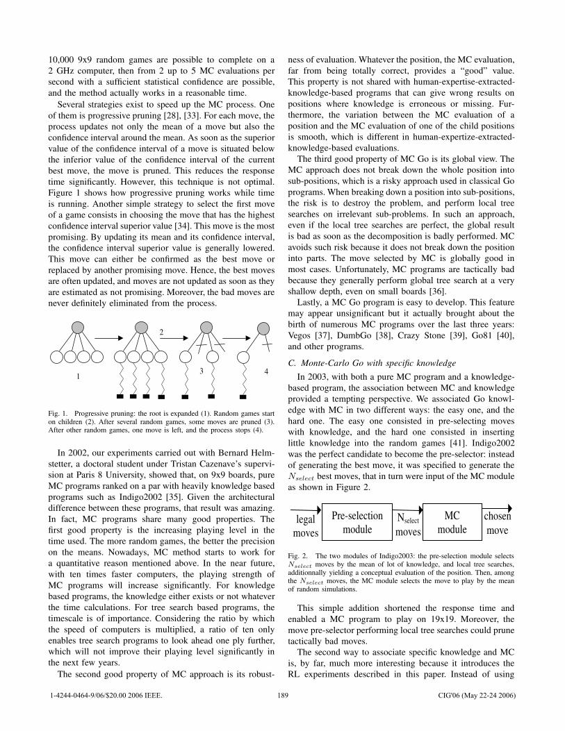
10,000 9x9 random games are possible to complete on a2 GHz computer, then from 2 up to 5 MC evaluations persecond with a sufficient statistical confidence are possible,and the method actually works in a reasonable time.

Several strategies exist to speed up the MC process. Oneof them is progressive pruning [28], [33]. For each move, theprocess updates not only the mean of a move but also theconfidence interval around the mean. As soon as the superiorvalue of the confidence interval of a move is situated belowthe inferior value of the confidence interval of the currentbest move, the move is pruned. This reduces the responsetime significantly. However, this technique is not optimal.Figure 1 shows how progressive pruning works while timeis running. Another simple strategy to select the first moveof a game consists in choosing the move that has the highestconfidence interval superior value [34]. This move is the mostpromising. By updating its mean and its confidence interval,the confidence interval superior value is generally lowered.This move can either be confirmed as the best move orreplaced by another promising move. Hence, the best movesare often updated, and moves are not updated as soon as theyare estimated as not promising. Moreover, the bad moves arenever definitely eliminated from the process.

1

2

3 4

Fig. 1. Progressive pruning: the root is expanded (1). Random games starton children (2). After several random games, some moves are pruned (3).After other random games, one move is left, and the process stops (4).

In 2002, our experiments carried out with Bernard Helm-stetter, a doctoral student under Tristan Cazenave’s supervi-sion at Paris 8 University, showed that, on 9x9 boards, pureMC programs ranked on a par with heavily knowledge basedprograms such as Indigo2002 [35]. Given the architecturaldifference between these programs, that result was amazing.In fact, MC programs share many good properties. Thefirst good property is the increasing playing level in thetime used. The more random games, the better the precisionon the means. Nowadays, MC method starts to work fora quantitative reason mentioned above. In the near future,with ten times faster computers, the playing strength ofMC programs will increase significantly. For knowledgebased programs, the knowledge either exists or not whateverthe time calculations. For tree search based programs, thetimescale is of importance. Considering the ratio by whichthe speed of computers is multiplied, a ratio of ten onlyenables tree search programs to look ahead one ply further,which will not improve their playing level significantly inthe next few years.

The second good property of MC approach is its robust-

ness of evaluation. Whatever the position, the MC evaluation,far from being totally correct, provides a “good” value.This property is not shared with human-expertise-extracted-knowledge-based programs that can give wrong results onpositions where knowledge is erroneous or missing. Fur-thermore, the variation between the MC evaluation of aposition and the MC evaluation of one of the child positionsis smooth, which is different in human-expertize-extracted-knowledge-based evaluations.

The third good property of MC Go is its global view. TheMC approach does not break down the whole position intosub-positions, which is a risky approach used in classical Goprograms. When breaking down a position into sub-positions,the risk is to destroy the problem, and perform local treesearches on irrelevant sub-problems. In such an approach,even if the local tree searches are perfect, the global resultis bad as soon as the decomposition is badly performed. MCavoids such risk because it does not break down the positioninto parts. The move selected by MC is globally good inmost cases. Unfortunately, MC programs are tactically badbecause they generally perform global tree search at a veryshallow depth, even on small boards [36].

Lastly, a MC Go program is easy to develop. This featuremay appear unsignificant but it actually brought about thebirth of numerous MC programs over the last three years:Vegos [37], DumbGo [38], Crazy Stone [39], Go81 [40],and other programs.

C. Monte-Carlo Go with specific knowledgeIn 2003, with both a pure MC program and a knowledge-

based program, the association between MC and knowledgeprovided a tempting perspective. We associated Go knowl-edge with MC in two different ways: the easy one, and thehard one. The easy one consisted in pre-selecting moveswith knowledge, and the hard one consisted in insertinglittle knowledge into the random games [41]. Indigo2002was the perfect candidate to become the pre-selector: insteadof generating the best move, it was specified to generate theNselect best moves, that in turn were input of the MC moduleas shown in Figure 2.

Nselectmoves

legalmoves

chosenmove

Pre-selectionmodule

MCmodule

Fig. 2. The two modules of Indigo2003: the pre-selection module selectsN

selectmoves by the mean of lot of knowledge, and local tree searches,

additionnally yielding a conceptual evaluation of the position. Then, amongthe N

selectmoves, the MC module selects the move to play by the mean

of random simulations.

This simple addition shortened the response time andenabled a MC program to play on 19x19. Moreover, themove pre-selector performing local tree searches could prunetactically bad moves.

The second way to associate specific knowledge and MCis, by far, much more interesting because it introduces theRL experiments described in this paper. Instead of using

1-4244-0464-9/06/$20.00 2006 IEEE. 189 CIG'06 (May 22-24 2006)

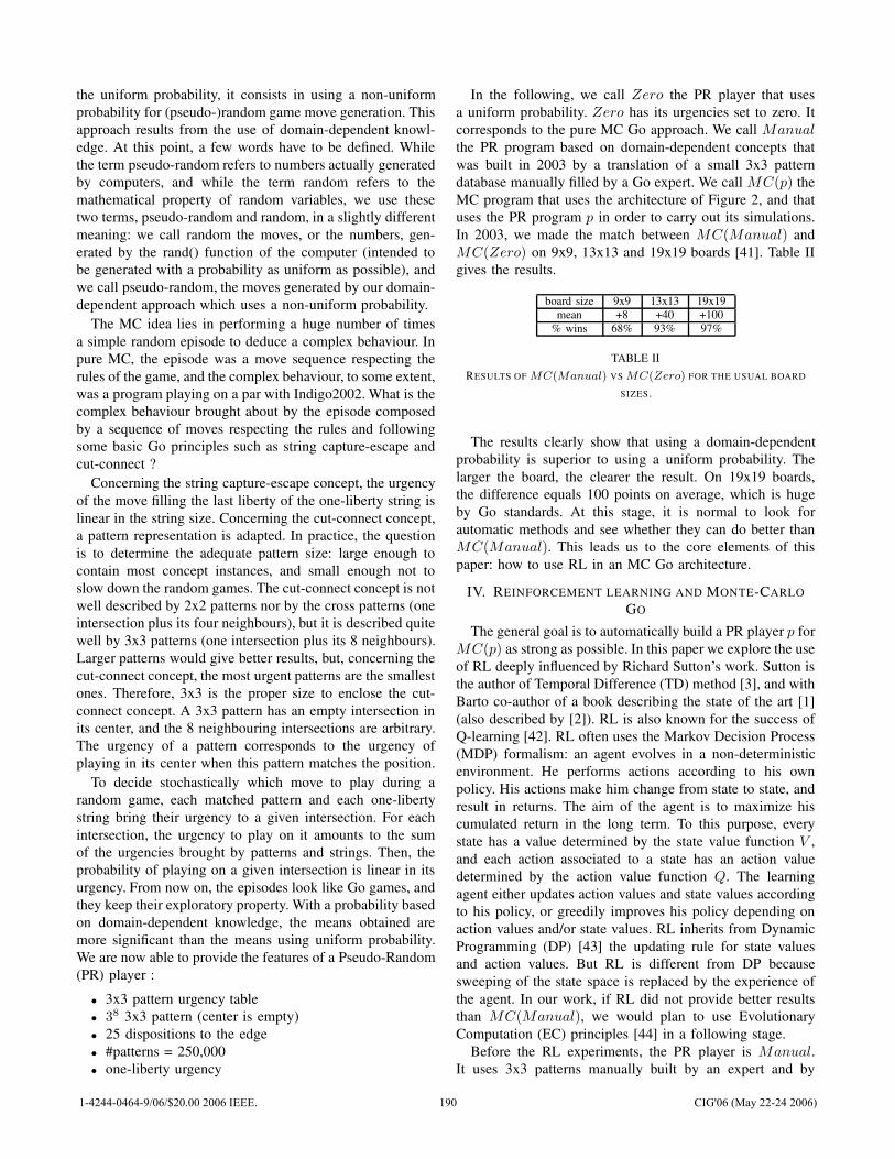
the uniform probability, it consists in using a non-uniformprobability for (pseudo-)random game move generation. Thisapproach results from the use of domain-dependent knowl-edge. At this point, a few words have to be defined. Whilethe term pseudo-random refers to numbers actually generatedby computers, and while the term random refers to themathematical property of random variables, we use thesetwo terms, pseudo-random and random, in a slightly differentmeaning: we call random the moves, or the numbers, gen-erated by the rand() function of the computer (intended tobe generated with a probability as uniform as possible), andwe call pseudo-random, the moves generated by our domain-dependent approach which uses a non-uniform probability.

The MC idea lies in performing a huge number of timesa simple random episode to deduce a complex behaviour. Inpure MC, the episode was a move sequence respecting therules of the game, and the complex behaviour, to some extent,was a program playing on a par with Indigo2002. What is thecomplex behaviour brought about by the episode composedby a sequence of moves respecting the rules and followingsome basic Go principles such as string capture-escape andcut-connect ?

Concerning the string capture-escape concept, the urgencyof the move filling the last liberty of the one-liberty string islinear in the string size. Concerning the cut-connect concept,a pattern representation is adapted. In practice, the questionis to determine the adequate pattern size: large enough tocontain most concept instances, and small enough not toslow down the random games. The cut-connect concept is notwell described by 2x2 patterns nor by the cross patterns (oneintersection plus its four neighbours), but it is described quitewell by 3x3 patterns (one intersection plus its 8 neighbours).Larger patterns would give better results, but, concerning thecut-connect concept, the most urgent patterns are the smallestones. Therefore, 3x3 is the proper size to enclose the cut-connect concept. A 3x3 pattern has an empty intersection inits center, and the 8 neighbouring intersections are arbitrary.The urgency of a pattern corresponds to the urgency ofplaying in its center when this pattern matches the position.

To decide stochastically which move to play during arandom game, each matched pattern and each one-libertystring bring their urgency to a given intersection. For eachintersection, the urgency to play on it amounts to the sumof the urgencies brought by patterns and strings. Then, theprobability of playing on a given intersection is linear in itsurgency. From now on, the episodes look like Go games, andthey keep their exploratory property. With a probability basedon domain-dependent knowledge, the means obtained aremore significant than the means using uniform probability.We are now able to provide the features of a Pseudo-Random(PR) player :

• 3x3 pattern urgency table• 38 3x3 pattern (center is empty)• 25 dispositions to the edge• #patterns = 250,000• one-liberty urgency

In the following, we call Zero the PR player that usesa uniform probability. Zero has its urgencies set to zero. Itcorresponds to the pure MC Go approach. We call Manual

the PR program based on domain-dependent concepts thatwas built in 2003 by a translation of a small 3x3 patterndatabase manually filled by a Go expert. We call MC(p) theMC program that uses the architecture of Figure 2, and thatuses the PR program p in order to carry out its simulations.In 2003, we made the match between MC(Manual) andMC(Zero) on 9x9, 13x13 and 19x19 boards [41]. Table IIgives the results.

board size 9x9 13x13 19x19mean +8 +40 +100

% wins 68% 93% 97%

TABLE IIRESULTS OF MC(Manual) VS MC(Zero) FOR THE USUAL BOARD

SIZES.

The results clearly show that using a domain-dependentprobability is superior to using a uniform probability. Thelarger the board, the clearer the result. On 19x19 boards,the difference equals 100 points on average, which is hugeby Go standards. At this stage, it is normal to look forautomatic methods and see whether they can do better thanMC(Manual). This leads us to the core elements of thispaper: how to use RL in an MC Go architecture.

IV. REINFORCEMENT LEARNING AND MONTE-CARLOGO

The general goal is to automatically build a PR player p forMC(p) as strong as possible. In this paper we explore the useof RL deeply influenced by Richard Sutton’s work. Sutton isthe author of Temporal Difference (TD) method [3], and withBarto co-author of a book describing the state of the art [1](also described by [2]). RL is also known for the success ofQ-learning [42]. RL often uses the Markov Decision Process(MDP) formalism: an agent evolves in a non-deterministicenvironment. He performs actions according to his ownpolicy. His actions make him change from state to state, andresult in returns. The aim of the agent is to maximize hiscumulated return in the long term. To this purpose, everystate has a value determined by the state value function V ,and each action associated to a state has an action valuedetermined by the action value function Q. The learningagent either updates action values and state values accordingto his policy, or greedily improves his policy depending onaction values and/or state values. RL inherits from DynamicProgramming (DP) [43] the updating rule for state valuesand action values. But RL is different from DP becausesweeping of the state space is replaced by the experience ofthe agent. In our work, if RL did not provide better resultsthan MC(Manual), we would plan to use EvolutionaryComputation (EC) principles [44] in a following stage.

Before the RL experiments, the PR player is Manual.It uses 3x3 patterns manually built by an expert and by

1-4244-0464-9/06/$20.00 2006 IEEE. 190 CIG'06 (May 22-24 2006)

means of an automatic translation from a database to atable. The expert was not be able to build a larger databaseeasily containing larger patterns and adequate urgencies. Ifwe wish to enlarge this knowledge, we must use an automaticmethod. The playing level of MC(Manual) is quite good,and it is not easy to find p such as MC(p) be better thanMC(Manual). But if we succeed with 3x3 patterns, we willbe certain that the automatic method produces better resultsthat the manual method on larger patterns, even if the expertmanually tunes the large database.

Subsequently, we can say that p1 is better than p2 atthe low level, or random level, when p1 beats p2 by apositive score on average after a sufficient number of games.We can say that p1 is better than p2 at the high level, orMC level, when MC(p1) beat MC(p2) by a positive scoreon average after a sufficient number of games. We aim atseeing the PR players improving at the MC level, and notnecessarily at the low level. Improving a PR player at thelow level can be a red herring. For instance, a PR playerp that is quite good (because he beats Zero at the lowlevel by a given score) can be improved at the low levelonly by making him less exploratory. This determinisationresults in a better score for the PR player p against Zero

but, his exploratory capacity being low, MC(p) may beweak, and even be beaten by MC(Zero). When consideringthe balance between exploration and exploitation [1], wemay draw Figure 3 showing the programs on a randomnessdimension. On the left, there are deterministic and greedyprograms, then, on their right, ε-greedy programs that playrandomly in an ε proportion, and that play deterministicallyin a 1−ε proportion. On the right of Figure 3, there is Zero,the random program based on the uniform probability, and onits left the PR programs used in our MC architecture. Thoseprograms are constrained to keep their exploratory capacityand to stay on the right of the figure.

Deterministic Greedy Exploitation

�-greedy low temperatures

Pseudo-random RLPR Manual high temperatures

Random

Zero

Exploration

Fig. 3. The randomness dimension: the completely deterministic programsare situated on the left. Zero is situated on the right. On the left of Zero,there are the PR programs and Manual. On the right of deterministicprograms, there are ε-greedy programs [1]. The temperature indicates arandomisation degree: 0 for deterministic programs, and infinite for Zero,the uniform probability player.

In the following, we call RLPR, a PR player whose tableis built with RL techniques. We may perform experiments atthe low level, or at the MC level. The upside of the lowlevel is the high speed of games. Its downside is to favourexploitation against exploration. Despite of its slowness, MClevel remains in keeping with our aim..

V. EXPERIMENTS

This section describes two experiments: one experiment(experiment 1a) performed at the low level, with one pro-gram. This experiment uncovers the obstacle of determini-sation during learning. Experiment 1b attempts to solve thisobstacle by replacing the sole program by a population ofprograms. Experiment 2 is performed at the MC level withone single player, and explicitly manages the obstacle ofdeterminisation.

A. Experiment 1: low level, one program or a population ofprograms

This subsection describes an experiment made at the lowlevel, with one program in self-play or with a populationof programs. The result of a game is either its outcome(+1 for a win and −1 for loss) or a score. This subsectionassumes that the result used is the outcome. A pattern has anassociated action: playing the advised move when the patternis matching. A pattern has an action value Q that is the meanof the games’ results when the pattern has been matched andplayed. Q belongs to ]−1, +1[. In our experiment, a patternhas an urgency U linked to Q by:

U =(

1+Q

1−Q

)

k

During a pseudo-random game, the probability of playinga move advised by a pattern is linear in U . k is a parametercorresponding to the determinisation degree of the program.When k = 0, then U = 1 for every patterns, and theprobability of playing a move is uniform. When k is high,the highest urgency dominates all the other urgencies and theprogram is almost deterministic. The nth update of Q for apattern is given by:

Qn = Qn−1 + α(R − Qn−1)R is the result of the random game, and α = 1/(1 + n).

Thus, Qn converges to the mean value of the results of therandom games.

More precisely, two tables are used: one for playing, onefor learning. This is an off-line learning. After a block ofgames, the values of the learnt table Qlearn update the valuesof the table used for playing Qplay by:

Qplay = Qplay + λbQlearn

λ is a parameter set in ]0, 1[. Its actual value is set by theexperiments. b is the number of the block. In the updatingformula, the addition is used to keep track of good patterns.During the first block of games, all Qplay values equalzero, and the games follow a uniform probability. At theend of the first block of games, a good pattern has a highQlearn value because it generates good moves among a setof games played badly. This value corresponds to the meanvalue of results of games given that the policy follows theuniform probability. Qlearn is copied into Qplay to be usedfor playing in the next block of games. A good patternquickly increases its Qplay value. At the end of a block ofgames, Qlearn corresponds to the mean value of results ofgames given that the policy uses the Qplay table. Because λ

is strictly inferior to 1, Qplay converges to a limit when b

increases.

1-4244-0464-9/06/$20.00 2006 IEEE. 191 CIG'06 (May 22-24 2006)

1) Experiment 1a: one unique learning program: Thisfirst experiment contains results on 9x9 boards only :

• RLPR >> Zero

• RLPR < Manual

• MC(RLPR) << MC(Manual)

RLPR >> Zero shows a learning at the low level.This is the minimal result expected. However, RLPR <

Manual shows that learning is not completely satisfactory.MC(RLPR) << MC(Manual) lets us think that RLPR

is too deterministic. As soon as the learner has learnt Qvalues for relevant patterns, instead of learning new Qvalues for new patterns, the learner prefers to increase theexisting Q values. This results in a player becoming toodeterministic to be used as a basis of the MC player. We callthis phenomenon determinisation. Experiment 2 will show adifferent update rule that avoids determinisation in self-play.However, experiment 1b will use the same update rule asexperiment 1a but it will prevent determinisation by using apopulation of learners.

We may comment upon the off-line learning used in thisexperiment. λ is strictly inferior to 1 to garantee convergenceof Qplay. However, in practice, we set λ = 1 because weobserved that, for good patterns, Qlearn converges to 0.Furthermore, we observed that, even though λ = 1, Qplay

practically stays in ] − 1, +1[. We do not have theoreticalproof of this phenomenon, but we may provide an intuitiveexplanation: when b is sufficiently high, at the end of a blockof games, Qlearn corresponds to the mean value of resultsof games given that the policy is good as well. Thus, whena good pattern is chosen during a game using a good policy,this is not a surprise, and the mean value of results of gamesgiven that this good pattern is chosen, roughly equals zero.Finally, with this comment, we observe that what happens inthe first block of random games is crucial to the actual finalvalue of Qplay . Launching several executions of the processleads to players that roughly share the same playing levelbut may have quite different tables. Using a population oflearners intends to lower the importance of the first block ofgames.

2) Experiment 1b: a population of learning programs: Toavoid determinisation of a program, and inspired by the rule:“when RL does not work, try EC principles”, we performedan experiment similar to experiment 1a by replacing oneRLPR program by a population of RLPR programs. Thesize of the population is N = 64. The underlying ideais that each individual program learns in its own manner(increases Q values of specific patterns only). If a programlearns by determinisation, he cannot survive the next gen-eration against other programs having learnt differently. Ageneration includes three phases: reinforcement learning, testand selection. During the reinforcement learning phase, theRLPR programs play against each other while learning withthe update rule of experiment 1a. Then, for each learner, thelearnt table is added into the playing table. During the testphase, the RLPR programs play against fixed opponents(Zero and Manual) without learning. This phase yields a

ranking. The selection phase follows the code below:

Delete the N/2 worst RLPR playersFor (D=N/4; D>0; D=D/2)copy the best D RLPR players

Add Zero player

(The best RLPR program of the generation is copiedfive times). This experiment does not use other classicalEC concepts: mutation or cross-over. We obtained results on19x19:

• Starting population = Zero

– RLPR = Zero + 180– RLPR = Manual − 50– MC(RLPR) << MC(Manual)

• Starting population = Manual

– RLPR = Zero + 180– RLPR = Manual + 50– MC(RLPR) = MC(Manual)− 20

With a population of programs, learning is possible on19x19, which was not possible with one unique program.In the whole set of programs, some of them learn with-out determinisation, which is right. The convergence de-pends on the starting program. When starting with Zero,the population goes toward a local maximum (RLPR =Manual − 50) inferior to the maximum reached whenstarting from Manual (RLPR = Manual + 50). Besides,MC(RLPR) = MC(Manual)− 20 is a better result thanMC(RLPR) << MC(Manual) obtained in the previousexperiment. In this perspective, this result is good (20 pointscan be considered as a reasonable difference on 19x19).However, the two results MC(RLPR) = MC(Manual)−20 and RLPR = Manual+50 underlines that learning stillcorresponds to determinisation.

Our conclusion on experiment 1 is that, at the low level,the RLPR programs have a tendency to determinisation thathides true learning. Replacing one program by a populationlowers the determinisation problem without removing itcompletely. Therefore, in the following experiment, we leavethe low level to perform games at the MC level, even if thiscosts computing time.

B. Experiment 2: relative difference at MC levelIn this experiment, a MC(RLPR) player plays against

itself again. There is no population. We need a mechanismthat prevents determinisation of experiment 1a. Therefore,the update rule of experiment 2 is different from the updaterule of experiment 1a. Instead of updating pattern urgenciesone by one, our idea is to consider pairs of patterns, and arelative differences between variables associated to the pairsof patterns. Thus, the player uses a relative difference formulato learn. a and b being two patterns with two MC evaluations,Va and Vb, and two urgencies, ua and ub, on average we aimat:

exp(C(Va − Vb)) = ua/ub

This is the basic formula underlying this experiment. Itestablishes a correlation between a difference of evaluations

1-4244-0464-9/06/$20.00 2006 IEEE. 192 CIG'06 (May 22-24 2006)

on average, and a ratio between the two urgencies that weseek. This way, the over-determinisation of pattern urgenciesshould not occur. For pattern i, we define Qi :

Qi = log(ui)Thus, for two patterns a and b, we look for:Qa − Qb = C(Va − Vb)C is assumed to be constant. On a given position with a

and b matching, the observed relative difference is actually:delta = Qa − Qb − C(Va − Vb)The updating rules are:Qa = Qa − αdelta

Qb = Qb + αdelta

When comparing two patterns, a et b, these rules updatethe ratio ua/ub according to delta avoiding exagerateddeterminisation. We performed learning on 9x9. We haveused a small number of random games to compute Va andVb: 20 random games only. C = 0.7, 0.8, 0.9, 1.0 were rathergood values. If Ni is the number of times that pattern i

matches, we set α proportional to the inverse of√

Ni. We

have tested our 9x9 learner on 9x9 and 19x19 boards.• on 9x9:

– MC(RLPR) = MC(Manual) + 3

• on 19x19:– MC(RLPR) = MC(Manual)− 30

An investigation on aspects in which MC(RLPR) playsdifferent, better or worse than MC(Manual) player can beperformed along the way of playing or along the achievedresult. Concerning the achieved result, and assessing on19x19 boards a MC(RLPR) player that learnt on 9x9boards, the achieved result (-30) is similar to the result ofexperiment 1b (-20). In other terms, the results obtainedon 19x19 are promising. On 19x19, the results could havebeen better if we performed learning on 19x19 as well,but we did not have enough time to do it. Additionally,MC(RLPR) = MC(Manual) + 3 shows that the methodworks better on 9x9 at the MC level than the manual method(this result was what we aimed at). The determinisationproblem seems to be solved partially. The way we usedrelative difference looks like advantage updating [45]. Wemay hardly investigate on the way of playing, and on thestyle of MC(RLPR) against MC(Manual), because bothprograms share the same design, and their playing styleis almost identical. However, we may give some remarksconcerning the inside of the urgency tables. Because thepatterns used by Manual were created by a human expert,the patterns always correspond to go concepts such as cut andconnect. Thus, the urgency table of Manual contains non-zero-and-very-high values very sparsely, and the intersectionurgency computing process is optimized to this respect. Adrawback of RLPR players, is that the urgency table isalmost completely filled with non-zero values with a smoothcontinuum of values. The intersection urgency computingprocess during random games cannot be optimized in thisrespect, which slows down RLPR players. Thus, to beefficiently used, the tables of RLPR players should beadequately post-processed after learning.

VI. CONCLUSION

This paper has presented the Monte-Carlo Go architectureusing domain-dependent knowledge, and has described RLexperiments to enhance 3x3 pattern urgencies used duringsimulations. In experiment 1a, we identified the determin-isation obstacle that negated a good learning. Experiment1b, a copy of experiment 1a at the low level and replacingone RL learner by a population of RL learners, avoideddeterminisation. Experiment 2 using relative difference andusing Q values instead of raw urgencies, explicitly managedthe determinisation. Consequently, experiment 2 worked wellat the MC level with one learner only, instead of a populationof learners. Quantitatively, the results obtained by experiment1b and 2 are very promising: after learning on 9x9, theautomatic method is 3 points better than the manual method.On 19x19, the automatic method is (only) 20 points belowthe manual method. But in experiment 2, learning wasperformed on 9x9 and tested on 19x19. Thus, the perspectiveis to perform learning of experiment 2 on 19x19 and teston 19x19. Nevertheless, the results of the automatic methodmust be reinforced to be certain that the automatic methodis really better than the manual one for 3x3 patterns. Withsuch certainty, we may replace 3x3 patterns by larger patternsthat a Go expert would have too difficulties to qualify withadequate urgencies, whereas the automatic method wouldeasily tackle them.

Discussing ideas linked to EC might be enlightening.Experiments has been carried out on Go with EC [46]. Thesize of the board, although small in these experiments playeda key role: a preliminary learning on a small board speeds upthe following learning performed on a larger board. In ourwork, learning urgencies of 3x3 patterns on 9x9 boards yieldsa playing level well-tuned for 9x9 boards, but less adaptedto 19x19 boards. To play well on 19x19 boards, learning on19x19 boards is advisable. However, it is possible to playor learn on 19x19 boards with a player that learnt on 9x9boards.

Besides, in experiment 1b, we observed that the resultdepended on the initial conditions, and the optimum reachedwas only local. This experimental result confirmed the the-oretical result known on partially observable MDP [47].

Within the current debate between RL and EC, RL aloneseems to be able to tackle our problem almost entirely(experiment 2). But, instead of using one unique RL learner,using a population of learners and a selection mechanismwithout mutation or cross-over (experiment 1b) unwoundthe situation (experiment 1a). In this view, experiment 1demonstrates the success of the cooperation of principlesborrowed from both sides, RL and EC. The training methodcan be viewed as a memetic algorithm in which randomnessreplaces the role of genetic variation. Furthermore, thisconclusion enriches previous results concerning the RL-vs-EC debate using Go as a testbed [48].

Lastly, if we have a closer look at the results on 19x19boards, how to account for the slightly worse results obtainedby the automatic method compared to the manual method ?

1-4244-0464-9/06/$20.00 2006 IEEE. 193 CIG'06 (May 22-24 2006)

The MC environment may be too exploratory, and the deter-minisation is actually too tempting and easy a solution forRL learners whose goal is to learn by winning. Giving up theMC environment for a while, performing classical Q-learningexperiments [42], [49] on ε-greedy programs might constitutethe first steps to the solution: the ε-greedy programs beingalmost deterministic (see Figure 3), determinisation might beminimized. Then, randomizing such programs, and testingthem within the MC environment would be the final steps.

VII. AKNOWLEDGEMENTS

This work was started in 2004 by Bruno Bouzy, and wascontinued during spring 2005 by Guillaume Chaslot for hislast year placement at Ecole Centrale de Lille, in cooperationwith Remi Coulom we warmly thank for the discussions andthe clever ideas he suggested.

REFERENCES

[1] R. Sutton and A. Barto, Reinforcement Learning: an introduction,T. Dietterich, Ed. MIT Press, 1998.

[2] L. P. Kaelbling, M. Littman, and A. Moore, “Reinforcementlearning: A survey,” Journal of Artificial IntelligenceResearch, vol. 4, pp. 237–285, 1996. [Online]. Available:citeseer.ist.psu.edu/kaelbling96reinforcement.html

[3] R. Sutton, “Learning to predict by the method of temporal differences,”Machine Learning, vol. 3, pp. 9–44, 1988.

[4] C. Watkins, “Learning from delayed rewards,” Ph.D. dissertation,Cambridge University, 1989.

[5] B. Bouzy, “Indigo home page,” www.math-info.univ-paris5.fr/∼bouzy/INDIGO.html, 2005.

[6] J. Schaeffer and J. van den Herik, “Games, Computers, and ArtificialIntelligence,” Artificial Intelligence, vol. 134, pp. 1–7, 2002.

[7] H. van den Herik, J. Uiterwijk, and J. van Rijswijck, “Games solved:Now and in the future,” Artificial Intelligence, vol. 134, pp. 277–311,2002.

[8] J. Schaeffer, One Jump Ahead: Clallenging Human Supremacy inCheckers. Springer-Verlag, 1997.

[9] M. Campbell, A. Hoane, and F.-H. Hsu, “Deep blue,” ArtificialIntelligence, vol. 134, pp. 57–83, 2002.

[10] J. Schaeffer, Y. Bjornsson, N. Burch, A. Kishimoto, M. Muller,R. Lake, P. Lu, and S. Sutphen, “Solving checkers,” in IJCAI, 2005,pp. 292–297.

[11] M. Buro, “Improving heuristic mini-max search by supervised learn-ing,” Artificial Intelligence Journal, vol. 134, pp. 85–99, 2002.

[12] M. Muller, “Position evaluation in computer go,” ICGA Journal,vol. 25, no. 4, pp. 219–228, December 2002.

[13] ——, “Computer go,” Artificial Intelligence, vol. 134, pp. 145–179,2002.

[14] B. Bouzy and T. Cazenave, “Computer go: an AI oriented survey,”Artificial Intelligence, vol. 132, pp. 39–103, 2001.

[15] D. Fotland, “The many faces of go,” www.smart-games.com/manyfaces.html.

[16] M. Reiss, “Go++,” www.goplusplus.com/.[17] D. Bump, “Gnugo home page,”

www.gnu.org/software/gnugo/devel.html, 2006.[18] M. Enzenberger, “Neurogo,” www.markus-

enzenberger.de/neurogo.html.[19] M. Muller, “Explorer,” web.cs.ualberta.ca/∼mmueller/cgo/explorer.html,

2005.[20] T. Cazenave, “Golois,” www.ai.univ-paris8.fr/∼cazenave/Golois.html.[21] K. Chen, “Some practical techniques for global search in go,” ICGA

Journal, vol. 23, no. 2, pp. 67–74, 2000.[22] M. Enzenberger, “Evaluation in go by a neural network using soft

segmentation,” in 10th Advances in Computer Games, E. A. H. H. Jaapvan den Herik, Hiroyuki Iida, Ed. Graz: Kluwer Academic Publishers,2003, pp. 97–108.

[23] M. Muller, “Decomposition search: A combinatorial games approachto game tree search, with applications to solving go endgame,” inIJCAI, 1999, pp. 578–583.

[24] T. Cazenave, “Abstract proof search,” in Computers and Games, ser.Lecture Notes in Computer Science, I. F. T. Marsland, Ed., no. 2063.Springer, 2000, pp. 39–54.

[25] E. van der Werf, J. Uiterwijk, and J. van den Herik, “Learning to scorefinal positions in the game of go,” in Advances in Computer Games,Many Games, Many Challenges, H. J. van den Herik, H. Iida, andE. A. Heinz, Eds., vol. 10. Kluwer Academic Publishers, 2003, pp.143–158.

[26] Fishman, Monte-Carlo : Concepts, Algorithms, Applications.Springer, 1996.

[27] G. Tesauro and G. Galperin, “On-line policy improvement using MonteCarlo search,” in Advances in Neural Information Processing Systems.Cambridge MA: MIT Press, 1996, pp. 1068–1074.

[28] D. Billings, A. Davidson, J. Schaeffer, and D. Szafron, “The challengeof poker,” Artificial Intelligence, vol. 134, pp. 201–240, 2002.

[29] B. Sheppard, “World-championship-caliber scrabble,” Artificial Intel-ligence, vol. 134, pp. 241–275, 2002.

[30] B. Abramson, “Expected-outcome : a general model of static evalua-tion,” IEEE Transactions on PAMI, vol. 12, pp. 182–193, 1990.

[31] B. Brugmann, “Monte Carlo go,” 1993,www.joy.ne.jp/welcome/igs/Go/computer/mcgo.tex.Z.

[32] S. Kirkpatrick, C. Gelatt, and M. Vecchi, “Optimization by simulatedannealing,” Science, May 1983.

[33] B. Bouzy and B. Helmstetter, “Monte Carlo go developments,” in10th Advances in Computer Games, E. A. H. H. Jaap van den Herik,Hiroyuki Iida, Ed. Graz: Kluwer Academic Publishers, 2003, pp.159–174.

[34] L. P. Kaelbling, “Learning in embedded systems,” Ph.D. dissertation,MIT, 1993.

[35] B. Bouzy, “The move decision process of Indigo,” InternationalComputer Game Association Journal, vol. 26, no. 1, pp. 14–27, March2003.

[36] ——, “Associating shallow and selective global tree search withMonte Carlo for 9x9 go,” in Computers and Games: 4th InternationalConference, CG 2004, ser. Lecture Notes in Computer Science, N. N.J. van den Herik, Y. Bjornsson, Ed., vol. 3846 / 2006. Ramat-Gan,Israel: Springer Verlag, July 2004, pp. 67–80.

[37] P. Kaminski, “Vegos home page,” www.ideanest.com/vegos/, 2003.[38] J. Hamlen, “Seven year itch,” ICGA Journal, vol. 27, no. 4, pp. 255–

258, 2004.[39] R. Coulom, “Efficient selectivity and back-up operators in monte-

carlo tree search,” in Computers and Games, Torino, Italy, 2006, papercurrently submitted.

[40] T. Raiko, “The go-playing program called go81,” in Finnish ArtificialIntelligence Conference, Helsinki, Finland, September 2004, pp. 197–206.

[41] B. Bouzy, “Associating knowledge and Monte Carlo approaches withina go program,” Information Sciences, vol. 175, no. 4, pp. 247–257,November 2005.

[42] C. Watkins and P. Dayan, “Q-learning,” Machine Learning, vol. 8, pp.279–292, 1992.

[43] D. P. Bertsekas, Dynamic Programming and Optimal Control. AthenaScientific, 1995.

[44] D. Goldberg, Genetic Algorithms in Search, Optimization, and Ma-chine Learning. Addison-Wesley Publishing Co, 1989.

[45] L. Baird, “Advantage updating,” 1993. [Online]. Available:citeseer.ist.psu.edu/baird93advantage.html

[46] K. Stanley and R. Miikkulainen, “Evolving a roving eye for go,” inGenetic and Evolutionary Computation Conference, New-York, 2004.

[47] T. Jaakkola, S. P. Singh, and M. I. Jordan, “Reinforcementlearning algorithm for partially observable Markov decisionproblems,” in Advances in Neural Information ProcessingSystems, G. Tesauro, D. Touretzky, and T. Leen, Eds., vol. 7.The MIT Press, 1995, pp. 345–352. [Online]. Available:citeseer.ist.psu.edu/jaakkola95reinforcement.html

[48] T. P. Runarsson and S. Lucas, “Co-evolution versus self-play temporaldifference learning for acquiring position evaluation in small-boardgo,” IEEE Transactions on Evolutionary Computation, vol. 9, no. 6,pp. 628–640, December 2005.

[49] M. L. Littman, “Markov games as a framework for multi-agentreinforcement learning,” in Proceedings of the 11th InternationalConference on Machine Learning (ML-94). New Brunswick,NJ: Morgan Kaufmann, 1994, pp. 157–163. [Online]. Available:citeseer.ist.psu.edu/littman94markov.html

1-4244-0464-9/06/$20.00 2006 IEEE. 194 CIG'06 (May 22-24 2006)

Poster Presentations

1-4244-0464-9/06/$20.00 2006 IEEE. 195 CIG'06 (May 22-24 2006)

1-4244-0464-9/06/$20.00 2006 IEEE. 196 CIG'06 (May 22-24 2006)

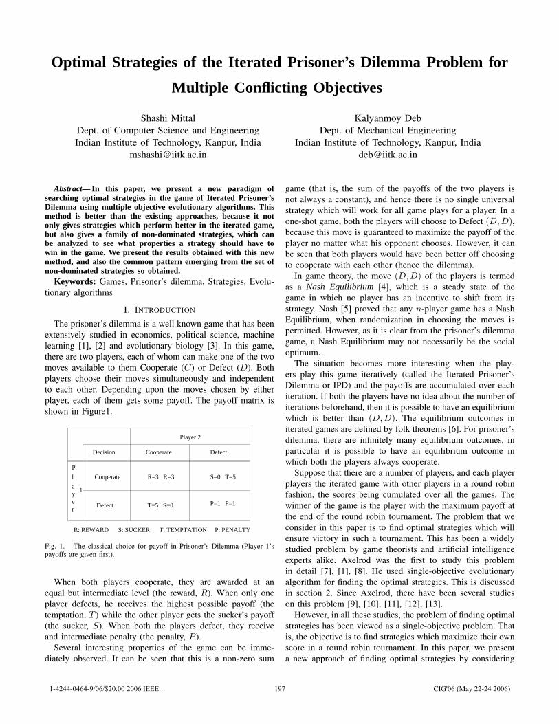
Optimal Strategies of the Iterated Prisoner’s Dilemma Problem for

Multiple Conflicting Objectives

Shashi MittalDept. of Computer Science and EngineeringIndian Institute of Technology, Kanpur, India

mshashi@iitk.ac.in

Kalyanmoy DebDept. of Mechanical Engineering

Indian Institute of Technology, Kanpur, Indiadeb@iitk.ac.in

Abstract— In this paper, we present a new paradigm ofsearching optimal strategies in the game of Iterated Prisoner’sDilemma using multiple objective evolutionary algorithms. Thismethod is better than the existing approaches, because it notonly gives strategies which perform better in the iterated game,but also gives a family of non-dominated strategies, which canbe analyzed to see what properties a strategy should have towin in the game. We present the results obtained with this newmethod, and also the common pattern emerging from the set ofnon-dominated strategies so obtained.

Keywords: Games, Prisoner’s dilemma, Strategies, Evolu-tionary algorithms

I. INTRODUCTION

The prisoner’s dilemma is a well known game that has beenextensively studied in economics, political science, machinelearning [1], [2] and evolutionary biology [3]. In this game,there are two players, each of whom can make one of the twomoves available to them Cooperate (C) or Defect (D). Bothplayers choose their moves simultaneously and independentto each other. Depending upon the moves chosen by eitherplayer, each of them gets some payoff. The payoff matrix isshown in Figure1.

Player 2

Defect

Cooperate R=3 R=3 S=0 T=5

T=5 S=0 P=1 P=1Defect

Decision Cooperate

P

l

ayer

1

R: REWARD S: SUCKER T: TEMPTATION P: PENALTY

Fig. 1. The classical choice for payoff in Prisoner’s Dilemma (Player 1’spayoffs are given first).

When both players cooperate, they are awarded at anequal but intermediate level (the reward, R). When only oneplayer defects, he receives the highest possible payoff (thetemptation, T ) while the other player gets the sucker’s payoff(the sucker, S). When both the players defect, they receiveand intermediate penalty (the penalty, P ).

Several interesting properties of the game can be imme-diately observed. It can be seen that this is a non-zero sum

game (that is, the sum of the payoffs of the two players isnot always a constant), and hence there is no single universalstrategy which will work for all game plays for a player. In aone-shot game, both the players will choose to Defect (D,D),because this move is guaranteed to maximize the payoff of theplayer no matter what his opponent chooses. However, it canbe seen that both players would have been better off choosingto cooperate with each other (hence the dilemma).

In game theory, the move (D,D) of the players is termedas a Nash Equilibrium [4], which is a steady state of thegame in which no player has an incentive to shift from itsstrategy. Nash [5] proved that any n-player game has a NashEquilibrium, when randomization in choosing the moves ispermitted. However, as it is clear from the prisoner’s dilemmagame, a Nash Equilibrium may not necessarily be the socialoptimum.

The situation becomes more interesting when the play-ers play this game iteratively (called the Iterated Prisoner’sDilemma or IPD) and the payoffs are accumulated over eachiteration. If both the players have no idea about the number ofiterations beforehand, then it is possible to have an equilibriumwhich is better than (D,D). The equilibrium outcomes initerated games are defined by folk theorems [6]. For prisoner’sdilemma, there are infinitely many equilibrium outcomes, inparticular it is possible to have an equilibrium outcome inwhich both the players always cooperate.

Suppose that there are a number of players, and each playerplayers the iterated game with other players in a round robinfashion, the scores being cumulated over all the games. Thewinner of the game is the player with the maximum payoff atthe end of the round robin tournament. The problem that weconsider in this paper is to find optimal strategies which willensure victory in such a tournament. This has been a widelystudied problem by game theorists and artificial intelligenceexperts alike. Axelrod was the first to study this problemin detail [7], [1], [8]. He used single-objective evolutionaryalgorithm for finding the optimal strategies. This is discussedin section 2. Since Axelrod, there have been several studieson this problem [9], [10], [11], [12], [13].

However, in all these studies, the problem of finding optimalstrategies has been viewed as a single-objective problem. Thatis, the objective is to find strategies which maximize their ownscore in a round robin tournament. In this paper, we presenta new approach of finding optimal strategies by considering

1-4244-0464-9/06/$20.00 2006 IEEE. 197 CIG'06 (May 22-24 2006)

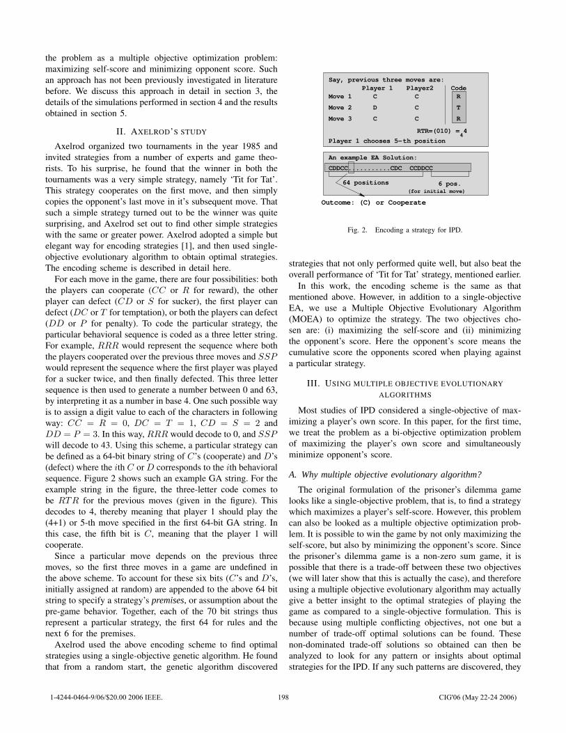
the problem as a multiple objective optimization problem:maximizing self-score and minimizing opponent score. Suchan approach has not been previously investigated in literaturebefore. We discuss this approach in detail in section 3, thedetails of the simulations performed in section 4 and the resultsobtained in section 5.

II. AXELROD’S STUDY

Axelrod organized two tournaments in the year 1985 andinvited strategies from a number of experts and game theo-rists. To his surprise, he found that the winner in both thetournaments was a very simple strategy, namely ‘Tit for Tat’.This strategy cooperates on the first move, and then simplycopies the opponent’s last move in it’s subsequent move. Thatsuch a simple strategy turned out to be the winner was quitesurprising, and Axelrod set out to find other simple strategieswith the same or greater power. Axelrod adopted a simple butelegant way for encoding strategies [1], and then used single-objective evolutionary algorithm to obtain optimal strategies.The encoding scheme is described in detail here.

For each move in the game, there are four possibilities: boththe players can cooperate (CC or R for reward), the otherplayer can defect (CD or S for sucker), the first player candefect (DC or T for temptation), or both the players can defect(DD or P for penalty). To code the particular strategy, theparticular behavioral sequence is coded as a three letter string.For example, RRR would represent the sequence where boththe players cooperated over the previous three moves and SSP

would represent the sequence where the first player was playedfor a sucker twice, and then finally defected. This three lettersequence is then used to generate a number between 0 and 63,by interpreting it as a number in base 4. One such possible wayis to assign a digit value to each of the characters in followingway: CC = R = 0, DC = T = 1, CD = S = 2 andDD = P = 3. In this way, RRR would decode to 0, and SSP

will decode to 43. Using this scheme, a particular strategy canbe defined as a 64-bit binary string of C’s (cooperate) and D’s(defect) where the ith C or D corresponds to the ith behavioralsequence. Figure 2 shows such an example GA string. For theexample string in the figure, the three-letter code comes tobe RTR for the previous moves (given in the figure). Thisdecodes to 4, thereby meaning that player 1 should play the(4+1) or 5-th move specified in the first 64-bit GA string. Inthis case, the fifth bit is C, meaning that the player 1 willcooperate.

Since a particular move depends on the previous threemoves, so the first three moves in a game are undefined inthe above scheme. To account for these six bits (C’s and D’s,initially assigned at random) are appended to the above 64 bitstring to specify a strategy’s premises, or assumption about thepre-game behavior. Together, each of the 70 bit strings thusrepresent a particular strategy, the first 64 for rules and thenext 6 for the premises.

Axelrod used the above encoding scheme to find optimalstrategies using a single-objective genetic algorithm. He foundthat from a random start, the genetic algorithm discovered

(for initial move)

Say, previous three moves are:

Move 3

Move 2

Move 1Player 1 Player2

C

C

CC

D

CCode

R

T

R

CDDCC...........CDC CCDDCC

An example EA Solution:

64 positions 6 pos.

RTR=(010) = 44

Outcome: (C) or Cooperate

Player 1 chooses 5−th position

Fig. 2. Encoding a strategy for IPD.

strategies that not only performed quite well, but also beat theoverall performance of ‘Tit for Tat’ strategy, mentioned earlier.

In this work, the encoding scheme is the same as thatmentioned above. However, in addition to a single-objectiveEA, we use a Multiple Objective Evolutionary Algorithm(MOEA) to optimize the strategy. The two objectives cho-sen are: (i) maximizing the self-score and (ii) minimizingthe opponent’s score. Here the opponent’s score means thecumulative score the opponents scored when playing againsta particular strategy.

III. USING MULTIPLE OBJECTIVE EVOLUTIONARYALGORITHMS

Most studies of IPD considered a single-objective of max-imizing a player’s own score. In this paper, for the first time,we treat the problem as a bi-objective optimization problemof maximizing the player’s own score and simultaneouslyminimize opponent’s score.

A. Why multiple objective evolutionary algorithm?

The original formulation of the prisoner’s dilemma gamelooks like a single-objective problem, that is, to find a strategywhich maximizes a player’s self-score. However, this problemcan also be looked as a multiple objective optimization prob-lem. It is possible to win the game by not only maximizing theself-score, but also by minimizing the opponent’s score. Sincethe prisoner’s dilemma game is a non-zero sum game, it ispossible that there is a trade-off between these two objectives(we will later show that this is actually the case), and thereforeusing a multiple objective evolutionary algorithm may actuallygive a better insight to the optimal strategies of playing thegame as compared to a single-objective formulation. This isbecause using multiple conflicting objectives, not one but anumber of trade-off optimal solutions can be found. Thesenon-dominated trade-off solutions so obtained can then beanalyzed to look for any pattern or insights about optimalstrategies for the IPD. If any such patterns are discovered, they

1-4244-0464-9/06/$20.00 2006 IEEE. 198 CIG'06 (May 22-24 2006)

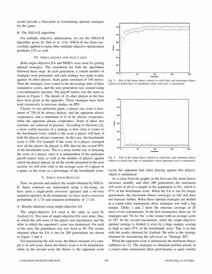
would provide a blue-print in formulating optimal strategiesfor the game.

B. The NSGA-II algorithm

For multiple objective optimization, we use the NSGA-IIalgorithm given by Deb et al. [14]. NSGA-II has been suc-cessfully applied to many other multiple objective optimizationproblems [15] as well.

IV. SIMULATIONS AND TEST CASES

Both single-objective EA and MOEA were used for gettingoptimal strategies. The simulation for both the algorithmsfollowed these steps. In each generation, a certain number ofstrategies were generated, and each strategy was made to playagainst 16 other players. Each game consisted of 150 moves.Then the strategies were sorted in the decreasing order of theircumulative scores, and the next generation was created usinga recombination operator. The payoff matrix was the same asshown in Figure 1. The details of 16 other players in the frayhave been given in the appendix. These strategies have beenused extensively in previous studies on IPD.

Clearly, in one particular game, a player can score a max-imum of 750 (if he always defects, and the opponent alwayscooperates), and a minimum of 0 (if he always cooperates,while the opponent always cooperates). None of these twoextremes are achieved in practice. According to Dawkins [3],a more useful measure of a strategy is how close it comes tothe benchmark score, which is the score a player will have ifboth the players always cooperate. In this case, the benchmarkscore is 450. For example if the score of a player, averagedover all the players he played, is 400, then he has scored 89%of the benchmark score. This is a more useful way of denotingthe score of a player, since it is independent of the particularpayoff matrix used, as well as the number of players againstwhich the player played. In all the results presented in the nextsection, we will refer only to the average score of a player ina game, or the score as a percentage of the benchmark score.

V. SIMULATION RESULTS

Now, we present and analyze the results obtained by NSGA-II. Since solutions are represented using a bit-string, wehave used a single-point crossover operator and a bit-wisemutation operator. In all simulations, we have used a crossoverprobability of 1/70 and mutation probability of 1/140.

A. Results obtained using single-objective EA

The single-objective EA used is the same as used byAxelrod [1]. Two runs of single-objective EA were done. One,in which the self-score of the player was maximized, and theother in which the opponent’s score was minimized. For eachof the runs, the population size was fixed at 40. The resultsobtained when the EA is run for 200 generations are shownin Figure 3 and 4.

For maximizing the self-score, the fitness measure of a sam-ple is its self-score, hence the fitness score is to be maximized,while in the second score the fitness is the opponent score

320

340

360

380

400

420

440

0 50 100 150 200

Fitn

ess

Generation

320

340

360

380

400

420

440

0 50 100 150 200

Fitn

ess

Generation

Fig. 3. Plot of the mean fitness (shown in solid line) and maximum fitness(shown in dotted line) of population when self-score is maximized.

100

150

200

250

300

350

400

0 50 100 150 200

Fitn

ess

Generation

100

150

200

250

300

350

400

0 50 100 150 200

Fitn

ess

Generation

Fig. 4. Plot of the mean fitness (shown in solid line) and minimum fitness(shown in dotted line line) of population when opponent score is minimized.

(score the opponent had when playing against this player),which is minimized.

As is clear from the graphs, in the first case the mean fitnessincreases steadily, and after 200 generations the maximumself-score of all of a sample in the population is 441, which is97% of the benchmark score. When the EA is run for longergenerations, the maximum fitness converges at 442 and doesnot increase further. When these optimal strategies are fieldedin a round robin tournament, these strategies win with a bigmargin. Tables 1 and 2 show the outcome (average of 20runs) of two tournaments. In the first tournament, there are 16strategies and ‘Tit for Tat’ is the winner with an average scoreof 387. In the second tournament, when the single-objectiveoptimal strategy is fielded, it wins by a huge margin, scoringas high as upto 97% of the benchmark score. This is in linewith the results obtained by Axelrod. We refer to the strategyobtained by maximizing the self-score as “Strategy SO”.

When the opponent score is minimized, the minimum fitnessstabilizes at 112. The strategies so obtained perform poorly ina round robin tournament (their performance is quite similar

1-4244-0464-9/06/$20.00 2006 IEEE. 199 CIG'06 (May 22-24 2006)

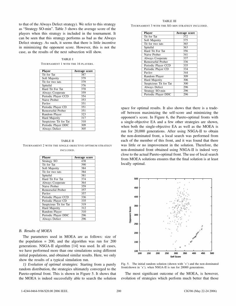
to that of the Always Defect strategy). We refer to this strategyas “Strategy SO-min”. Table 3 shows the average score of theplayers when this strategy is included in the tournament. Itcan be seen that this strategy performs as bad as the AlwaysDefect strategy. As such, it seems that there is little incentivein minimizing the opponent score. However, this is not thecase, as the results of the next subsection will show.

TABLE ITOURNAMENT 1 WITH THE 16 PLAYERS.

Player Average scoreTit for Tat 387Soft Majority 379Tit for two tats 379Spiteful 376Hard Tit For Tat 370Always Cooperate 359Periodic Player CCD 354Naive Prober 353Pavlov 351Periodic Player CD 351Remorseful Prober 351Random Player 323Hard Majority 317Suspicious Tit for Tat 310Periodic Player DDC 309Always Defect 305

TABLE IITOURNAMENT 2 WITH THE SINGLE OBJECTIVE OPTIMUM STRATEGY

INCLUDED.

Player Average scoreStrategy SO 438Tit for Tat 390Soft Majority 384Tit for two tats 384Spiteful 381Hard Tit For Tat 374Always Cooperate 364Naive Prober 359Remorseful Prober 357Pavlov 357Periodic Player CCD 336Periodic Player CD 335Suspicious Tit for Tat 319Hard Majority 312Random Player 310Periodic Player DDC 296Always Defect 296

B. Results of MOEA

The parameters used in MOEA are as follows: size ofthe population = 200, and the algorithm was run for 200generations. NSGA-II algorithm [14] was used. In all cases,we have performed more than one simulations using differentinitial populations, and obtained similar results. Here, we onlyshow the results of a typical simulation run.

1) Evolution of optimal strategies: Starting from a purelyrandom distribution, the strategies ultimately converged to thePareto-optimal front. This is shown in Figure 5. It shows thatthe MOEA is indeed successfully able to search the solution

TABLE IIITOURNAMENT 3 WITH THE SO-MIN STRATEGY INCLUDED.

Player Average scoreTit for Tat 372Soft Majority 375Tit for two tats 365Spiteful 363Hard Tit For Tat 356Naive Prober 341Always Cooperate 337Remorseful Prober 336Periodic Player CCD 335Periodic Player CD 334Pavlov 344Random Player 309Hard Majority 306Suspicious Tit for Tat 300Always Defect 296Strategy SO-min 296Periodic Player DDC 296

space for optimal results. It also shows that there is a trade-off between maximizing the self-score and minimizing theopponent’s score. In Figure 6, the Pareto-optimal fronts witha single-objective EA and a few other strategies are shown,when both the single-objective EA as well as the MOEA isrun for 20,000 generations. After using NSGA-II to obtainthe non-dominated front, a local search was performed fromeach of the member of this front, and it was found that therewas little or no improvement in the solution. Therefore, thenon-dominated front obtained using NSGA-II is indeed veryclose to the actual Pareto-optimal front. The use of local searchfrom MOEA solutions ensures that the final solution is at leastlocally optimal.

100

150

200

250

300

350

400

450

500

100 150 200 250 300 350 400 450 500

Opp

onen

t Sco

re

Self Score

100

150

200

250

300

350

400

450

500

100 150 200 250 300 350 400 450 500

Opp

onen

t Sco

re

Self Score

Fig. 5. The initial random solution (shown with ’+’) and the non-dominatedfront(shown in ’x’), when NSGA-II is run for 20000 generations.

The most significant outcome of the MOEA, is however,evolution of strategies which perform much better that those

1-4244-0464-9/06/$20.00 2006 IEEE. 200 CIG'06 (May 22-24 2006)

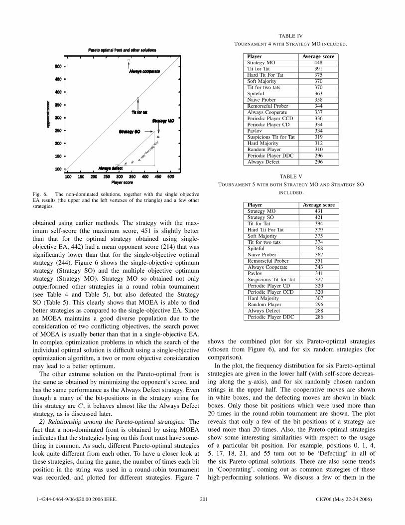
100

150

200

250

300

350

400

450

500

100 150 200 250 300 350 400 450 500

oppo

nent

sco

re

Player score

Pareto optimal front and other solutions

Always defect

Always cooperate

Tit for tat

Strategy SO

Strategy MO

Always defect

Always cooperate

Tit for tat

Strategy SO

Strategy MO

100

150

200

250

300

350

400

450

500

100 150 200 250 300 350 400 450 500

oppo

nent

sco

re

Player score

Pareto optimal front and other solutions

Always defect

Always cooperate

Tit for tat

Strategy SO

Strategy MO

Always defect

Always cooperate

Tit for tat

Strategy SO

Strategy MO

100

150

200

250

300

350

400

450

500

100 150 200 250 300 350 400 450 500

oppo

nent

sco

re

Player score

Pareto optimal front and other solutions

Always defect

Always cooperate

Tit for tat

Strategy SO

Strategy MO

Always defect

Always cooperate

Tit for tat

Strategy SO

Strategy MO

100

150

200

250

300

350

400

450

500

100 150 200 250 300 350 400 450 500

oppo

nent

sco

re

Player score

Pareto optimal front and other solutions

Always defect

Always cooperate

Tit for tat

Strategy SO

Strategy MO

Always defect

Always cooperate

Tit for tat

Strategy SO

Strategy MO

Fig. 6. The non-dominated solutions, together with the single objectiveEA results (the upper and the left vertexes of the triangle) and a few otherstrategies.

obtained using earlier methods. The strategy with the max-imum self-score (the maximum score, 451 is slightly betterthan that for the optimal strategy obtained using single-objective EA, 442) had a mean opponent score (214) that wassignificantly lower than that for the single-objective optimalstrategy (244). Figure 6 shows the single-objective optimumstrategy (Strategy SO) and the multiple objective optimumstrategy (Strategy MO). Strategy MO so obtained not onlyoutperformed other strategies in a round robin tournament(see Table 4 and Table 5), but also defeated the StrategySO (Table 5). This clearly shows that MOEA is able to findbetter strategies as compared to the single-objective EA. Sincean MOEA maintains a good diverse population due to theconsideration of two conflicting objectives, the search powerof MOEA is usually better than that in a single-objective EA.In complex optimization problems in which the search of theindividual optimal solution is difficult using a single-objectiveoptimization algorithm, a two or more objective considerationmay lead to a better optimum.

The other extreme solution on the Pareto-optimal front isthe same as obtained by minimizing the opponent’s score, andhas the same performance as the Always Defect strategy. Eventhough a many of the bit-positions in the strategy string forthis strategy are C, it behaves almost like the Always Defectstrategy, as is discussed later.

2) Relationship among the Pareto-optimal strategies: Thefact that a non-dominated front is obtained by using MOEAindicates that the strategies lying on this front must have some-thing in common. As such, different Pareto-optimal strategieslook quite different from each other. To have a closer look atthese strategies, during the game, the number of times each bitposition in the string was used in a round-robin tournamentwas recorded, and plotted for different strategies. Figure 7

TABLE IVTOURNAMENT 4 WITH STRATEGY MO INCLUDED.

Player Average scoreStrategy MO 448Tit for Tat 391Hard Tit For Tat 375Soft Majority 370Tit for two tats 370Spiteful 363Naive Prober 358Remorseful Prober 344Always Cooperate 337Periodic Player CCD 336Periodic Player CD 334Pavlov 334Suspicious Tit for Tat 319Hard Majority 312Random Player 310Periodic Player DDC 296Always Defect 296

TABLE VTOURNAMENT 5 WITH BOTH STRATEGY MO AND STRATEGY SO

INCLUDED.

Player Average scoreStrategy MO 431Strategy SO 421Tit for Tat 394Hard Tit For Tat 379Soft Majority 375Tit for two tats 374Spiteful 368Naive Prober 362Remorseful Prober 351Always Cooperate 343Pavlov 341Suspicious Tit for Tat 327Periodic Player CD 320Periodic Player CCD 320Hard Majority 307Random Player 296Always Defect 288Periodic Player DDC 286

shows the combined plot for six Pareto-optimal strategies(chosen from Figure 6), and for six random strategies (forcomparison).

In the plot, the frequency distribution for six Pareto-optimalstrategies are given in the lower half (with self-score decreas-ing along the y-axis), and for six randomly chosen randomstrings in the upper half. The cooperative moves are shownin white boxes, and the defecting moves are shown in blackboxes. Only those bit positions which were used more than20 times in the round-robin tournament are shown. The plotreveals that only a few of the bit positions of a strategy areused more than 20 times. Also, the Pareto-optimal strategiesshow some interesting similarities with respect to the usageof a particular bit position. For example, positions 0, 1, 4,5, 17, 18, 21, and 55 turn out to be ‘Defecting’ in all ofthe six Pareto-optimal solutions. There are also some trendsin ‘Cooperating’, coming out as common strategies of thesehigh-performing solutions. We discuss a few of them in the

1-4244-0464-9/06/$20.00 2006 IEEE. 201 CIG'06 (May 22-24 2006)

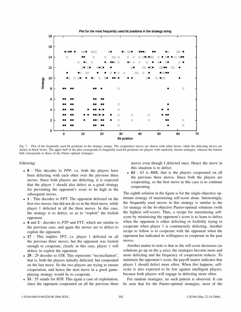
0

2

4

6

8

10

12

14

16

18

0 10 20 30 40 50 60 70

Str

ateg

y

Bit position

Plot for the most frequently used bit positions in the strategy string

0

2

4

6

8

10

12

14

16

18

0 10 20 30 40 50 60 70

Str

ateg

y

Bit position

Plot for the most frequently used bit positions in the strategy string

Fig. 7. Plot of the frequently used bit positions in the strategy strings. The cooperative moves are shown with white boxes, while the defecting moves areshown in black boxes. The upper half of the plot corresponds to frequently used bit positions for players with randomly chosen strategies, whereas the bottomhalf corresponds to those of the Pareto optimal strategies.

following:

• 0 : This decodes to PPP, i.e. both the players havebeen defecting with each other over the previous threemoves. Since both players are defecting, it is expectedthat the player 1 should also defect as a good strategyfor preventing the opponent’s score to be high in thesubsequent moves.

• 1 : This decodes to PPT. The opponent defected on thefirst two moves, but did not do so in the third move, whileplayer 1 defected in all the three moves. In this case,the strategy is to defect, so as to “exploit” the foolishopponent.

• 4 and 5 : decodes to PTP and PTT, which are similar tothe previous case, and again the moves are to defect toexploit the opponent.

• 17 : This implies TPT, i.e. player 1 defected on allthe previous three moves, but the opponent was foolishenough to cooperate, clearly in this case, player 1 willdefect, to exploit the opponent.

• 29 : 29 decodes to STR. This represents “reconciliation”,that is, both the players initially defected, but cooperatedon the last move. So the two players are trying to ensurecooperation, and hence the next move in a good game-playing strategy would be to cooperate.

• 55 : 55 stands for RTR. This again a case of exploitation,since the opponent cooperated on all the previous three

moves even though I defected once. Hence the move inthis situation is to defect.

• 63 : 63 is RRR, that is the players cooperated on allthe previous three moves. Since both the players arecooperating, so the best move in this case is to continuecooperating.

The eighth solution in the figure is for the single-objective op-timum strategy of maximizing self-score alone. Interestingly,the frequently used moves in this strategy is similar to the1st strategy of the bi-objective Pareto-optimal solutions (withthe highest self-score). Thus, a recipe for maximizing self-score by minimizing the opponent’s score is to learn to defectwhen the opponent is either defecting or foolishly trying tocooperate when player 1 is continuously defecting. Anotherrecipe to follow is to cooperate with the opponent when theopponent has indicated its willingness to cooperate in the pastmoves.

Another matter to note is that as the self-score decreases (assolutions go up on the y axis), the strategies become more andmore defecting and the frequency of cooperation reduces. Tominimize the opponent’s score, the payoff matrix indicates thatplayer 1 should defect more often. When this happens, self-score is also expected to be low against intelligent players,because both players will engage in defecting more often.

For random strategies, no such pattern is observed. It canbe seen that for the Pareto-optimal strategies, most of the

1-4244-0464-9/06/$20.00 2006 IEEE. 202 CIG'06 (May 22-24 2006)

bit positions are either sparingly used, or are not used atall. For example, the strategy with the least self-score alwaysmakes defecting moves, even though there are many C’s in itsstrategy string, showing that it behaves almost like the AlwaysDefect strategy.

VI. SIGNIFICANCE OF THE RESULTS

The above results demonstrate the power of MOEAs insearching better strategies for the IPD problem. The optimalstrategies obtained using this method outperforms all otherstrategies. In particular, it performs better than the strategiesobtained using single-objective optimization procedure. Thisshows that MOEAs are a more useful methods for findingoptimal strategies, as compared to single-objective EAs.

The fact that a non-dominated front (which is quite closeto the actual Pareto-optimal front) shows that there is indeeda trade-off between maximizing self-score and minimizingopponent score. Therefore, to be successful in a round robintournament, a player should not only try to maximize its ownscore, but also minimize the opponent score.

We further observe that the strategies lying on the non-dominated front share some common properties. This can giveus valuable insight about the optimal strategies for a roundrobin tournament. It will be interesting to make some prototypestrategies using these common features and observing theirperformance in a tournament; we leave this for a futureresearch work.

We had also carried out another simulation in which weused NSGA-II to minimize two other objectives: Maximizeself-score, and minimize the maximum of the opponent scores(in previous case, we had minimized the average score ofthe opponents). The Pareto-optimal front obtained is shownin Figure 8 by marking the obtained strategies (maximumopponent score) with ‘X’. When the average score (markedwith diamonds) over all opponent players are computed andplotted for these strategies, they are found to be dominated bythe previous Pareto-optimal solutions. The second objectivevalue of Pareto-optimal solutions using this method is worsethan before, as the maximum of the opponents’ scores isgoing to be always more than average of opponents’ scores.A good spread in solutions is still obtained, but since this newobjective is non-differentiable, the obtained front in this caseis not as smooth as before. As discussed above, the solutionsobtained are also inferior from the earlier solutions. Based onthis study, we may conclude that minimizing the average scoreof opponents is a better optimization strategy than minimizingthe maximum score of opponents.

VII. CONCLUSIONS

We have presented a new paradigm for searching optimalstrategies in Iterated Prisoner’s Dilemma (IPD) using a multi-objective optimization procedure. Such a method has not beenused before in the literature for this problem. It has beenrevealed that such a solution strategy has several advantagesover the existing single-objective methods for finding usefuloptimal game-playing strategies. Hopefully, such an approach

min−avg

min−max

100

150

200

250

300

350

400

450

500

100 150 200 250 300 350 400 450 500Self Score

Opponent Score

Fig. 8. Pareto-optimal front obtained when maximum of the opponent score isminimized (maximum opponent score is represented by ’X’ and correspondingaverage score is represented by diamonds) against the Pareto-optimal frontobtained earlier (shown in circles).

will find further application in related game-playing problemsin the near future.

ACKNOWLEDGMENTS

We thank three anonymous reviewers whose comments havebeen very useful in improving the quality of the paper.

REFERENCES

[1] R. Axelrod, “The evolution of strategies in the iterated prisoner’sdilemma,” in Genetic Algorithms and Simulated Annealing, L. Davis,Ed. Los Altos, CA: Morgan Kaufmann, 1987.

[2] D. E. Goldberg, Genetic Algorithms for Search, Optimization andMachine Learning. Reading: Addison-Wesley, 1989.

[3] R. Dawkins, The Selfish Gene. New York: Oxford University Press,1989.

[4] M. Rubenstein and M. Osborne, A Course in Game Theory. MIT Press,1994.

[5] J. F. Nash, “Equilibrium points in n-person games,” in Proceedings ofthe National Academy of Sciences, vol. 36, 1950, pp. 48–49.

[6] D. Fudenberg and E. Maskin, “The folk theorem in repeated games withdiscounting or incomplete information,” Econometrica, vol. 54, no. 3,1986.

[7] R. Axelrod and W. Hamilton, “The evolution of coperation,” Science,vol. 211, pp. 1390–6, 1981.

[8] R. Axelrod, The Evolution of Cooperation. New York: Basic Books,1989.

[9] D. Fogel, “Evolving behaviors in the iterated prisoner’s dilemma,”Evolutionary Computation, vol. 1, pp. 77–97, 1983.

[10] M. Nowak and K. Sigmund, “A strategy of win-stay, lose-shift thatoutperforms tit-for-tat in the prisoner’s dilemma game,” Nature, vol.364, pp. 56–58, 1993.

[11] B. Beaufils, J. P. Delahaye, and P. Mathieu, “Our meeting with gradual,a good strategy for the iterated prisoner’s dilemma,” in Artificial LifeV: Proceedings of the Fifth International Workshop on the Synthesisand Simulation of Living Systems, C. Langton and K. Shimohara, Eds.Cambridge, MA, USA: The MIT Press, 1996, pp. 202–209.

[12] D. Bragt, C. Kemenade, and H. Poutr, “The influence of evolutionaryselection schemes on the iterated prisoner’ s dilemma,” ComputationalEconomics, vol. 17, pp. 253–263, 2001.

1-4244-0464-9/06/$20.00 2006 IEEE. 203 CIG'06 (May 22-24 2006)

[13] D. Jang, P. Whigham, and G. Dick, “On evolving fixed pattern strategiesfor iterated prisoner’s dilemma,” in Proceedings of the 27th conferenceon Australasian computer science, Dunedin, New Zealand, 2004, pp.241–247.

[14] K. Deb, A. Pratap, S. Agarwal, and T. Meyarivan, “A fast and elitistmultiobjective algorithm: NSGA-II,” IEEE Transactions on EvolutionaryComputation, vol. 6, no. 2, pp. 182–197, 2002.

[15] K. Deb, Multiobjective Optimisation Using Evolutionary Algorithms.Chichester, U.K.: Wiley, 2001.

APPENDIX IDetails about the different strategies used in the round-robin

tournament:1) Always Cooperate : Cooperates on every move2) Always Defect : Defects on every move3) Tit for Tat : Cooperates on the first move, then simply

copies the opponent’s last move.4) Suspicious Tit for Tat : Same as Tit for Tat, except that

it defects on the first move5) Pavlov : Cooperates on the first move, and defects only

if both the players did not agree on the previous move.6) Spiteful : Cooperates, until the opponent defects, and

thereafter always defects.7) Random Player : Makes a random move.8) Periodic player CD : Plays C, D periodically.9) Periodic player DDC : Plays D, D, C periodically.

10) Periodic player CCD : Plays C, C, D periodically.11) Tit for Two Tats : Cooperates on the first move, and

defects only when the opponent defects two times.12) Soft Majority : Begins by cooperating, and cooperates

as long as the number of times the opponent hascooperated is greater than or equal to the number oftimes it has defected, else it defects.

13) Hard Majority : Defects on the first move, and defectsif the number of defections of the opponent is greaterthan or equal to the number of times it has cooperated,else cooperates.

14) Hard Tit for Tat : Cooperates on the first move, anddefects if the opponent has defects on any of the previousthree moves, else cooperates.

15) Naive Prober : Like Tit for Tat, but occasionally defectswith a probability of 0.01.

16) Remorseful Prober : Like Naive Prober, but it tries tobreak the series of mutual defections after defecting.

1-4244-0464-9/06/$20.00 2006 IEEE. 204 CIG'06 (May 22-24 2006)

Trappy Minimax - using Iterative Deepening to

Identify and Set Traps in Two-Player Games

V. Scott Gordon Ahmed Reda CSU, Sacramento CSU, Sacramento gordonvs@ecs.csus.edu ahmedcsus@yahoo.com

Abstract

Trappy minimax is a game-independent extension of the minimax adversarial search algorithm that attempts to take advantage of human frailty. Whereas minimax assumes best play by the opponent, trappy minimax tries to predict when an opponent might make a mistake by comparing the various scores returned through iterative-deepening. Sometimes it chooses a slightly inferior move, if there is an indication that the opponent may fall into a trap, and if the potential profit is high. The algorithm was implemented in an Othello program named Desdemona, and tested against both computer and human opponents. Desdemona achieved a higher rating against human opposition on Yahoo! Games when using the trappy algorithm than when it used standard minimax.

1. Introduction Minimax is a well-known algorithm for performing adversarial search in two-player strategy games. Although it is known to work very well in practice, it also has its shortcomings. One of these is that it assumes best play by the opponent. Often, a human (or even a computer) may be fallible, and may be tricked into playing an inferior move. Minimax never takes this into account, and thus it never purposefully tries to set traps. This paper introduces trappy minimax, a variation of minimax that utilizes iterative deepening to identify possible traps, and under the right conditions, set them. Traps are defined in a game-independent manner, based only on the generic search tree and the backed up values from its associated terminal evaluation function. Alpha- beta pruning still works without modification. Thus, trappy minimax can be used wherever standard minimax can be used. At times, trappy minimax chooses different moves than standard minimax. Depending on the type of opponent, the trappy version may be more effective.

Section 2 gives a brief historical background and related work; Section 3 defines the concept of a trap; Section 4 presents the trappy minimax algorithm; Section 5 gives experimental results for two board games, and Section 6 offers a summary and conclusions. 2. Background The minimax algorithm was first proposed by Claude Shannon in 1950 [Shannon50], as suitable for programming a computer to play the game of chess. An improvement called alpha-beta pruning was described in 1962 by Kotok [Kotok62]. Alpha-beta pruning allows the algorithm to eliminate certain branches from consideration, speeding up the search without changing the result. Minimax with alpha-beta pruning has been used in most computer implementations of popular board games such as chess and checkers, and forms the basis of the search algorithms used in successful competitive programs such as Deep Blue (for chess) [HCH02] and Logistello (for Othello) [Buro97]. When minimax considers every possible move at each level, it is performing a full-width search. When it only considers a subset of the allowable moves, it is performing a selective search. A minimax algorithm is shown in Figure 1.

Negamax(board,depth) If (game over) then return(result) If (max depth) then return EVAL(board) best = -∞ For each move { make move on board score = -Negamax(board, depth+1) if score > best then best=score retract move from board } return (best)

Figure 1 — Minimax

1-4244-0464-9/06/$20.00 2006 IEEE. 205 CIG'06 (May 22-24 2006)

Various improvements to minimax have been developed. Most attempt to alter the ordering of generated moves in order to accelerate alpha-beta pruning [Schaeffer89]. Others use game-dependent knowledge to determine whether certain branches of the tree should be ignored, allowing for deeper search.

Iterative Deepening is when a minimax search of depth N is preceded by separate searches at depths 1, 2, etc., up to depth N. That is, N separate searches are performed, and the results of the shallower searches are used to help alpha-beta pruning work more effectively.

Carmel and Markovitch [CM95] examined a variation of minimax called M*, in which an opponent model is incorporated into the search algorithm. M* allows minimax to consider whether an opponent is likely to make an inferior move, and to take better advantage of it. They also examined using M* to take advantage of opponents that search to a shallower depth, and thus linking search depth with setting traps.

In this paper, the notion of a trap specifically as a function of search depth is explored in greater detail. Whereas M* utilizes an opponent model, trappy minimax does not require it. It also does not need to know what algorithm the opponent is using or to what depth he/she/it is searching. Traps are defined as a function of search depth, and can be set at many levels. The only assumption is that certain opponents may be vulnerable to these sorts of traps - particularly humans.

3. Definition and evaluation of Traps

3.1 Definition of a Trap A trap is a move that looks good in the short term

but has bad consequences in the long term. Thus, in the minimax algorithm, it is a move with high evaluations at shallow depths and a low evaluation at the maximum depth. Traps have the significance that a non-optimal opponent might be tricked into thinking that they are good moves when in fact they are not.

Although our definition of a trap does not require opponent modeling, it is useful to consider the sort of opponent that would fall for a trap. An opponent that performs a full-width minimax search to a depth greater than the trappy minimax player, would not fall for a trap. Humans, however, are always susceptible to traps, since they in general do not perform full-width search, and do not consider every variation to a uniform depth.

Setting a trap is only of practical benefit if the result of an opponent not falling for the trap is not much worse than the evaluation of the move recommended by standard minimax. In other words, if the opponent does not fall for the trap, setting the trap which didn’t materialize should not yield a significant negative cost.

3.2 Trap Evaluation

A trap is evaluated using two factors: (1) how likely the opponent will fall into the trap, (2) how profitable the trap is if the opponent falls into it. A trap could be very deceiving to a human opponent yet not profitable, and similarly, a trap could be highly profitable but easy to avoid. A good trap is hard to spot, and profitable.

Since most minimax implementations utilize iterative deepening, it is relatively easy to accumulate evaluations at various search depths. Thus, accumulating the data needed for evaluating traps is very inexpensive, and alpha-beta pruning can still be employed at each search depth.

To assess how deceiving a trap is, evaluations are made using depths other than just at the maximum depth. When the opponent is a human, looking at all the depths other than the maximum depth is useful, while for an opponent using a shallower minimax search, looking at just that depth would be sufficient. We examined three different methods for assessing evaluations at shallow tree depths:

1. The median method: calculates the median of the

evaluations at all but the maximum depth, 2. The best value method: uses the best evaluation for

the opponent among the shallower evaluations, 3. The last level method: uses only the evaluation at

MaxDepth-1 (MaxDepth is the deepest level of search examined by the program).

The first two methods are directed towards human

opponents, while the third method is targetted at opponents who use the minimax algorithm either at a shallower depth (up to MaxDepth-2), or selective search.

4. Trappy Minimax Depending on which assessment method is being

used, the resulting aggregate shallow evaluation is compared to the evaluation at the maximum depth. Two factors are then determined: trappiness, and profitability.

Trappiness is based on the distance between a high positive score and an actual negative score, and is calculated from the point of view of the opponent. That is, it attempts to measure the likelihood that the opponent could miss the trap.

Profitability is the gain to the program if the opponent falls for the trap. It is calculated from the point of view of the algorithm.

Trappiness and profitability are both factored into the evaluation of each possible computer move, along with the standard minimax evaluation. The resulting trappy minimax algorithm is shown in Figure 2.

1-4244-0464-9/06/$20.00 2006 IEEE. 206 CIG'06 (May 22-24 2006)

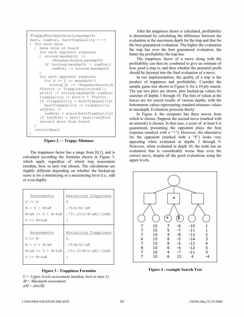
7 7 7 6 7 8 7 7

10 15 10 15 15 10 10 10

7 5 4 8 9 6 4 6

-6 -7 -8 -5 -5 -4 -7 12

-10 -11 -12 -14 -13 -12 -11 4

1 1 2 3 4 5 3 -4

TrappyMinimax(board,maxdepth) best, rawEval, bestTrapQuality = -∞ { For each move { make move on board for each opponent response { scores[maxdepth] := -Negamax(board,maxdepth) if (scores[maxdepth] > rawEval) rawEval := scores[maxdepth] } for each opponent response for d := 2 to maxdepth-1 scores[d] := -Negamax(board,d) Tfactor := Trappiness(scores[]) profit := scores[maxdepth]-rawEval trapQuality := profit * Tfactor if (trapQuality > bestTrapQuality) bestTrapQuality := trapQuality adjEval := rawEval + scale(bestTrapQuality) if (adjEval > best) best:=adjEval retract move from board } return(best) }

Figure 2 — Trappy Minimax

The trappiness factor has a range from [0,1], and is

calculated according the formulas shown in Figure 3, which apply regardless of which trap assessment (median, best, or last) was chosen. The calculations are slightly different depending on whether the backed-up score is for a minimizing or a maximizing level (i.e., odd or even depth).

Assessments Maximizing Trappiness

U <= M 0

M < U < M+aM .75(U-M)/aM

M+aM <= U < M+4aM .75+.25(U-M-aM)/(3aM)

U >= M+4aM 1

Assessments Minimizing Trappiness

U >= M 0

M > U > M-aM .75(M-U)/aM

M-aM >= U > M-4aM .75+.25(M-U-aM)/(3aM)

U >= M-4aM 1

Figure 3 - Trappiness Formulas U = Upper levels assessment (median, best or max-1) M = Maxdepth assessment aM = abs(M)

After the trappiness factor is calculated, profitability is determined by calculating the difference between the evaluation at the maximum depth for the trap and that for the best guaranteed evaluation. The higher the evaluation the trap has over the best guaranteed evaluation, the better the profitability the trap has.

The trappiness factor of a move along with the profitability can then be combined to give an estimate of how good a trap is, and then whether the potential profit should be factored into the final evaluation of a move.

In our implementation, the quality of a trap is the product of trappiness and profitability. Consider the sample game tree shown in Figure 4, for a 10-ply search. The top two plies are shown, plus backed-up values for searches of depths 3 through 10. The lists of values at the leaves are for search results of various depths, with the bottommost values representing standard minimax values at maxdepth. Evaluation proceeds thusly:

In Figure 4, the computer has three moves from which to choose. Suppose the second move (marked with an asterisk) is chosen. In that case, a score of at least 6 is guaranteed, presuming the opponent plays the best response (marked with a “+”). However, the alternative for the opponent (marked with a “$”) looks very appealing when evaluated at depths 3 through 9. However, when evaluated at depth 10, the node has an evaluation that is considerably worse than even the correct move, despite all the good evaluations using the upper levels.

*

+ $

Figure 4 - example Search Tree

1-4244-0464-9/06/$20.00 2006 IEEE. 207 CIG'06 (May 22-24 2006)

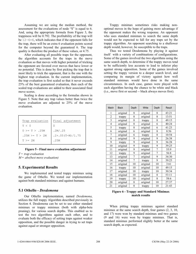
Assuming we are using the median method, the assessment for the evaluations of node “$” is equal to 6. And, using the appropriate formula from Figure 3, the trappiness will be 0.792. The profitability of the trap will be 12-6=6, which indicates that if the opponent falls for the trap, there will be an extra 6 evaluation points scored for the computer beyond the guaranteed 6. The trap quality is therefore the product of these values, or 4.75.

After evaluating all possible traps for the opponent, the algorithm accounts for the traps in the move evaluation so that moves with higher potential of tricking the opponent are favored over moves that have lower or no potential. This is done by first picking the trap that is most likely to trick the opponent, that is the one with the highest trap evaluation. In the current implementation, the trap evaluation is first scaled so that it never exceeds 25% of the best guaranteed evaluation, then each of the scaled trap evaluations are added to their associated final move scores.

Scaling is done according to the formulas shown in Figure 5. Note that any trap values better than twice the move evaluation are adjusted to 25% of the move evaluation.

Trap evaluation Final adjustment

T < 0 0

0 >= T > .25M .2M/.25

.25M >= T > 2M .2+.05(T-M)/1.75

T >= 2M .25M

Figure 5 - Final move evaluation adjustment T = trap evaluation M = abs(best move evaluation)

5. Experimental Results We implemented and tested trappy minimax using

the game of Othello. We tested our implementation against both standard minimax and against humans.

5.1 Othello - Desdemona Our Othello implementation, named Desdemona,

utilizes the full trappy Algorithm described previously in Section 4. Desdemona can be set to use either standard minimax or trappy minimax (both with alpha-beta pruning), for various search depths. This enabled us to test the two algorithms against each other, and to evaluate both the efficacy of setting traps against weaker opposition, and the possible danger in trying to set traps against equal or stronger opposition.

Trappy minimax sometimes risks making non-optimal moves in the hope of gaining more advantage if the opponent makes the wrong response. An opponent who uses standard minimax to search the same depth would not be expected to fall for any traps set by the trappy algorithm. An opponent searching to a shallower depth would, however, be susceptible to the traps.

Thus we tested Desdemona by playing it against itself with a variety of combinations of configurations. Some of the games involved the two algorithms using the same search depth, to determine if the trappy moves tend to be sufficiently less accurate to lead to inferior play against strong opposition. Some of the games involved setting the trappy version to a deeper search level, and comparing its margin of victory against how well standard minimax would have done in the same circumstances. In each case, games were played with each algorithm having the chance to be white and black (i.e., move first or second -- black always moves first).

Match Black Depth White Depth Result

1 original 8 original 8 43:21 2 trappy 8 original 8 13:51 3 original 8 trappy 8 49:15 4 original 8 original 6 40:24 5 trappy 8 original 6 41:23 6 original 6 original 8 8:56 7 original 6 trappy 8 10:54 8 original 9 original 9 26:38 9 trappy 9 original 9 36:28

10 original 9 trappy 9 39:25 11 original 9 original 7 55:9 12 trappy 9 original 7 56:8 13 original 7 original 9 34:30 14 original 7 trappy 9 39:25 15 original 10 original 10 3:61 16 trappy 10 original 10 49:15 17 original 10 trappy 10 30:34 18 original 10 original 8 53:11 19 trappy 10 original 8 58:6 20 original 8 original 10 27:37 21 original 8 trappy 10 21:43

Figure 6 - Trappy and Standard Minimax match results

When pitting trappy minimax against standard minimax at the same search depth, four games (2, 3, 10, and 17) were won by standard minimax and two games (9 and 16) were won by trappy minimax. That is, standard minimax performed slightly better at the same search depth, as expected.

1-4244-0464-9/06/$20.00 2006 IEEE. 208 CIG'06 (May 22-24 2006)

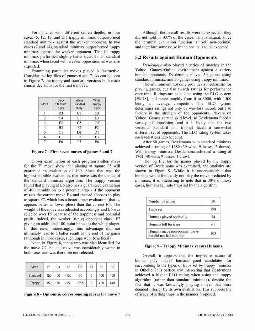
For matches with different search depths, in four cases (5, 12, 19, and 21) trappy minimax outperformed standard minimax against the weaker opponent. In two cases (7 and 14), standard minimax outperformed trappy minimax against the weaker opponent. That is, trappy minimax performed slightly better overall than standard minimax when faced with weaker opposition, as was also expected.

Examining particular moves played is instructive. Consider the log files of games 6 and 7. As can be seen in Figure 7, the trappy and standard versions both made similar decisions for the first 6 moves:

Move Black

Standard 6-ply

White Standard

8-ply

White Trappy 8-ply

1 D3 C3 C3 2 C4 E3 E3 3 F2 C5 C5 4 B3 F2 F2 5 C1 D1 D1 6 E1 F3 F3 7 F6 F5 E6

Figure 7 - First seven moves of games 6 and 7 Closer examination of each program’s alternatives

for the 7th move show that playing at square F5 will guarantee an evaluation of 400. Since that was the highest possible evaluation, that move was the choice of the standard minimax algorithm. The trappy version found that playing at E6 also has a guaranteed evaluation of 400 in addition to a potential trap - if the opponent misses the correct move B4 and instead chooses to play to square F7, which has a better upper evaluation (that is, appears better at lower plies) than the correct B4. The weight of the move was adjusted accordingly and E6 was selected over F5 because of the trappiness and potential profit. Indeed, the weaker (6-ply) opponent chose F7 giving an additional 100-point bonus to the white player. In this case, interestingly, this advantage did not ultimately lead to a better result at the end of the game (although in more cases, such traps were beneficial).

Note, in Figure 8, that a trap was also identified for the move C2, but the move was considerably worse in both cases and was therefore not selected.

Move F1 G1 A2 C2 A3 F5 E6

Standard 150 50 -150 -50 0 400 400

Trappy 150 50 -150 -37.5 0 400 448

Figure 8 - Options & corresponding scores for move 7

Although the overall results were as expected, they did not hold in 100% of the cases. This is natural, since the terminal evaluation function is itself non-optimal, and therefore some noise in the results is to be expected.

5.2 Results against Human Opponents Desdemona also played a series of matches in the

Yahoo! Games Online environment against a variety human opponents. Desdemona played 50 games using standard minimax, and 50 games using trappy minimax.

The environment not only provides a mechanism for playing games, but also awards ratings for performance over time. Ratings are calculated using the ELO system [Elo78], and range roughly from 0 to 3000, with 1500 being an average competitor. The ELO system determines ratings not only by win-loss record, but also factors in the strength of the opponents. Players on Yahoo! Games vary in skill level, so Desdemona faced a variety of opposition, and it is likely that the two versions (standard and trappy) faced a somewhat different set of opponents. The ELO rating system takes such variations into account.

After 50 games, Desdemona with standard minimax achieved a rating of 1680 (39 wins, 9 losses, 2 draws). With trappy minimax, Desdemona achieved a rating of 1702 (40 wins, 9 losses, 1 draw).

The log file for the games played by the trappy version of Desdemona was examined, and statistics are shown in Figure 9. While it is understandable that humans would frequently not play the move predicted by minimax, it is interesting to note that in 30% of those cases, humans fell into traps set by the algorithm.

Number of games 50

Traps set 198

Humans played optimally 34

Humans fell for traps 61

Humans made non-optimal move but did not fall into trap 103

Figure 9 - Trappy Minimax versus Humans

Overall, it appears that the imprecise nature of

human play makes humans good candidates for succombing to the types of traps set by trappy minimax in Othello. It is particularly interesting that Desdemona achieved a higher ELO rating when using the trappy algorithm (rather than standard minimax), despite the fact that it was knowingly playing moves that were deemed inferior by its own evaluation. This supports the efficacy of setting traps in the manner proposed.

1-4244-0464-9/06/$20.00 2006 IEEE. 209 CIG'06 (May 22-24 2006)

6. Conclusions Trappy minimax is a game-independent extension of

the minimax algorithm that further takes advantage of human frailty. Whereas minimax assumes best play by the opponent, trappy minimax tries to predict when an opponent might err. It works by identifying moves that qualify as potential traps, by comparing the various backed-up scores returned through iterative-deepening. Three methods were described for aggregating those scores: median, best, and last level. Traps were evaluated for both trappiness and profitability, and the results factored into the algorithm’s move selection.

Our Othello implementation, named Desdemona, was used to test the algorithm both against computer and human opposition.

The trappy algorithm was better able to capitalize on weaker computer opposition than standard minimax. In 67% of the cases, using the trappy algorithm enabled Desdemona to achieve a better final score than when standard minimax was used. This was because a weak opponent was likely to fall into some of the traps.

Desdemona achieved a higher rating against human opposition when using the trappy algorithm than when it used standard minimax. Humans frequently fell for the traps set by the algorithm. Yahoo! Games was used to facilitate the games, and the rating calculation was done by a neutral (online) system.

Desdemona’s occasional deliberate choice of a slightly inferior move, in the interests of setting a trap, caused it to perform slightly worse against strong computer opposition. This did not come as a surprise.

Trappy minimax requires no more time and space complexity than standard minimax. In fact, when iterative deepening is used (and it usually is), the mechanism for including trappy analysis is already present. Alpha-beta pruning can also still be used without modification. The trappy method is therefore an inexpensive and effective form of minimax, particularly against human opposition.

7. Future Work Given the encouraging results shown by

Desdemona, we intend to test the trappy algorithm on other games such as Chess and Checkers. Checkers is well-known to be a game that lends itself to short-term tactical analysis, so we optimistically are hoping to realize benefits that match or exceed those observed in Desdemona.

8. References

[Buro97] M. Buro, The Othello Match of the Year: Takeshi Murakami vs. Logistello, ICCA Journal 20(3), 1997 pp 189-193

[CM95] D. Carmel and S. Markovitch, “Opponent Modeling in a Multi-Agent System”, Workshop on Adaptation and Learning in Multiagent Systems - IJCAI, Montreal 1995.

[Elo78] The Rating of Chessplayers, Past and Present. Batsford, 1978.

[HCH02] A. Hoane., M. Campbell, and F. Hsu, Deep Blue, Artificial Intelligence 134, 2002, pp 57-83.

[Kotok62] A. Kotok, A Chess Playing Program for the IBM 7090 Computer. B.S. Thesis, MIT, June 1962.

[Schaeffer89] J. Schaeffer, The History Heuristic and Alpha-Beta Search Enhancements in Practice, IEEE Trans. on Pattern Analysis and Machine Intelligence, 1989, pp 1203-1212.

[Shannon50] C. Shannon, Programming a Computer for Playing Chess, Philosophical Magazine 41, 1950, pp 256-275.

1-4244-0464-9/06/$20.00 2006 IEEE. 210 CIG'06 (May 22-24 2006)

Evaluating Individual Player Strategies in a Collaborative Incomplete-Information Agent-Based Game Playing Environment

Andrés Gómez de Silva Garza

Abs ract—In Spanish-speaking countries, the game of dominoes is usually played by four people divided into two teams, with teammates sitting opposite each other. The players cannot communicate with each other or receive information from onlookers while a game is being played. Each player only knows for sure which tiles he/she has available in order to make a play, but must make inferences about the plays that the other participants can make in order to try to ensure that his/her team wins the game. The game is governed by a set of standardized rules, and successful play involves the use of highly-developed mathematical, reasoning and decision-making skills. In this paper we describe a computer system designed to simulate the game of dominoes by using four independent game-playing agents split into teams of two. The agents have been endowed with different strategies, including the traditional strategy followed by experienced human players. An experiment is described in which the success of each implemented strategy is evaluated compared to the traditional one. The results of the experiment are given and discussed, and possible future extensions mentioned.

t

I. INTRODUCTION HE game of dominoes, as played in Spanish-speaking countries, provides an environment in which one can

research the collaborative and decision-making abilities of individual players. The players participate in the game with incomplete information about which moves the other players can and cannot make, as they cannot communicate with anyone during the game or examine the tiles that the other players have been dealt. However, despite this missing information players must try to collaborate with their teammate against the other team in order to win each game. Several strategies can be envisioned which players can follow in order to decide which move to make at each turn during a game depending on the current game state, the possible moves they can make, and the potential effects of these moves on their teammate and opponents. We have implemented an agent-based architecture that allows us to change the strategies followed by the different players in order to perform a computational evaluation of the relative effectiveness of each.

In Section II of this paper we describe the game of

dominoes as played in Spanish-speaking countries in order to set the context for the rest of the discussion. In Section III we describe our computational implementation of the game of dominoes in an agent-based system. In Section IV we describe the experiment we performed in order to evaluate the alternate playing strategies we have implemented and present the results of the experiment. In Section V we discuss our results. Section VI mentions possible future extensions, both to the system and to the experiment.

Manuscript received December 16, 2005. This work was supported in part by the Asociación Mexicana de Cultura, A.C.

Andrés Gómez de Silva Garza is with the Department of Computer Engineering, Instituto Tecnológico Autónomo de México (ITAM), Río Hondo #1, Colonia Tizapán-San Ángel, 01000—México, D.F., México (phone: (+52-55) 5628-4000x3644, fax: (+52-55) 5628-4065; e-mail: agomez@itam.mx).

II. THE GAME OF DOMINOES Most people in most countries, if given a set of dominoes,

would probably not know what to do with them. They would probably be familiar with dominoes from having seen on TV the latest world record being set for the largest number of consecutively-toppled dominoes forming designs and words (as seen from above), but would probably have to research the rules in order to find out how to use the dominoes in order to play a game. The search might end up providing a large and confusing set of potential games that can be played (e.g., see [1]), each with its own variations on the rules (many of them very different from each other). On the other hand, in Spanish-speaking countries there is a highly-standardized set of rules for playing dominoes, with few local variations only in some minor details, which most people learn as they are growing up. The game of dominoes is therefore common and widespread amongst the population in, and therefore can be considered a cultural invariant of, these countries.

There are 28 pieces (normally called tiles) in a set of dominoes. The face of each tile is split into two halves, and each half has a certain number of dots (between 0 and 6) painted on it. There is only one tile in each set of dominoes for each combination of dots a tile might have (e.g., there is only one tile having 4 dots on one half and 5 dots on the other, known as the 4-5 or 5-4 tile). Some tiles have the same number of dots on both halves, such as the 0-0 tile; these are known as doubles or, in Spanish, mules. Fig. 1 shows a few domino tiles and the standardized appearance of each of the possible number of dots on the halves of the tiles.

T

1-4244-0464-9/06/$20.00 2006 IEEE. 211 CIG'06 (May 22-24 2006)

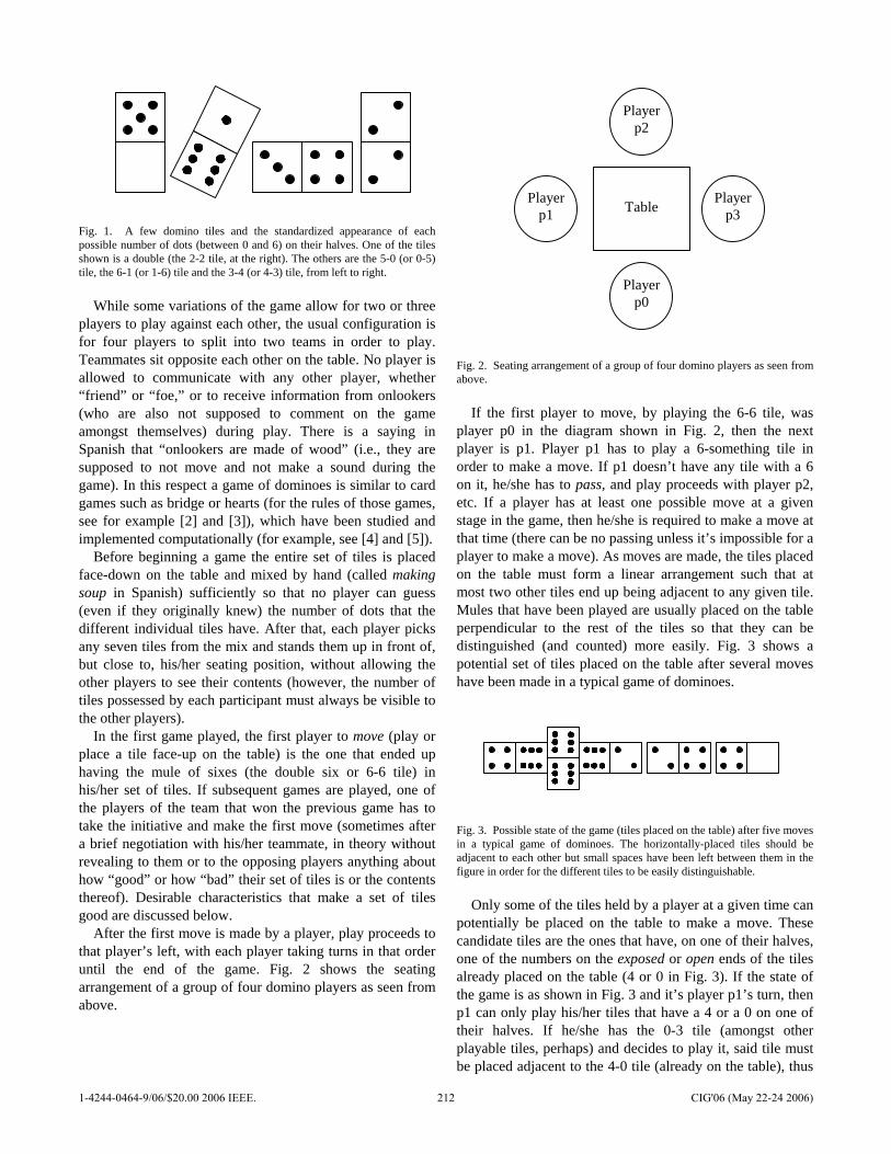
Fig. 1. A few domino tiles and the standardized appearance of each possible number of dots (between 0 and 6) on their halves. One of the tiles shown is a double (the 2-2 tile, at the right). The others are the 5-0 (or 0-5) tile, the 6-1 (or 1-6) tile and the 3-4 (or 4-3) tile, from left to right.

While some variations of the game allow for two or three

players to play against each other, the usual configuration is for four players to split into two teams in order to play. Teammates sit opposite each other on the table. No player is allowed to communicate with any other player, whether “friend” or “foe,” or to receive information from onlookers (who are also not supposed to comment on the game amongst themselves) during play. There is a saying in Spanish that “onlookers are made of wood” (i.e., they are supposed to not move and not make a sound during the game). In this respect a game of dominoes is similar to card games such as bridge or hearts (for the rules of those games, see for example [2] and [3]), which have been studied and implemented computationally (for example, see [4] and [5]).

Before beginning a game the entire set of tiles is placed face-down on the table and mixed by hand (called making soup in Spanish) sufficiently so that no player can guess (even if they originally knew) the number of dots that the different individual tiles have. After that, each player picks any seven tiles from the mix and stands them up in front of, but close to, his/her seating position, without allowing the other players to see their contents (however, the number of tiles possessed by each participant must always be visible to the other players).

In the first game played, the first player to move (play or place a tile face-up on the table) is the one that ended up having the mule of sixes (the double six or 6-6 tile) in his/her set of tiles. If subsequent games are played, one of the players of the team that won the previous game has to take the initiative and make the first move (sometimes after a brief negotiation with his/her teammate, in theory without revealing to them or to the opposing players anything about how “good” or how “bad” their set of tiles is or the contents thereof). Desirable characteristics that make a set of tiles good are discussed below.

After the first move is made by a player, play proceeds to that player’s left, with each player taking turns in that order until the end of the game. Fig. 2 shows the seating arrangement of a group of four domino players as seen from above.

Table

Playerp0

Playerp2

Playerp1

Playerp3

Fig. 2. Seating arrangement of a group of four domino players as seen from above.

If the first player to move, by playing the 6-6 tile, was

player p0 in the diagram shown in Fig. 2, then the next player is p1. Player p1 has to play a 6-something tile in order to make a move. If p1 doesn’t have any tile with a 6 on it, he/she has to pass, and play proceeds with player p2, etc. If a player has at least one possible move at a given stage in the game, then he/she is required to make a move at that time (there can be no passing unless it’s impossible for a player to make a move). As moves are made, the tiles placed on the table must form a linear arrangement such that at most two other tiles end up being adjacent to any given tile. Mules that have been played are usually placed on the table perpendicular to the rest of the tiles so that they can be distinguished (and counted) more easily. Fig. 3 shows a potential set of tiles placed on the table after several moves have been made in a typical game of dominoes.

Fig. 3. Possible state of the game (tiles placed on the table) after five moves in a typical game of dominoes. The horizontally-placed tiles should be adjacent to each other but small spaces have been left between them in the figure in order for the different tiles to be easily distinguishable.

Only some of the tiles held by a player at a given time can

potentially be placed on the table to make a move. These candidate tiles are the ones that have, on one of their halves, one of the numbers on the exposed or open ends of the tiles already placed on the table (4 or 0 in Fig. 3). If the state of the game is as shown in Fig. 3 and it’s player p1’s turn, then p1 can only play his/her tiles that have a 4 or a 0 on one of their halves. If he/she has the 0-3 tile (amongst other playable tiles, perhaps) and decides to play it, said tile must be placed adjacent to the 4-0 tile (already on the table), thus

1-4244-0464-9/06/$20.00 2006 IEEE. 212 CIG'06 (May 22-24 2006)

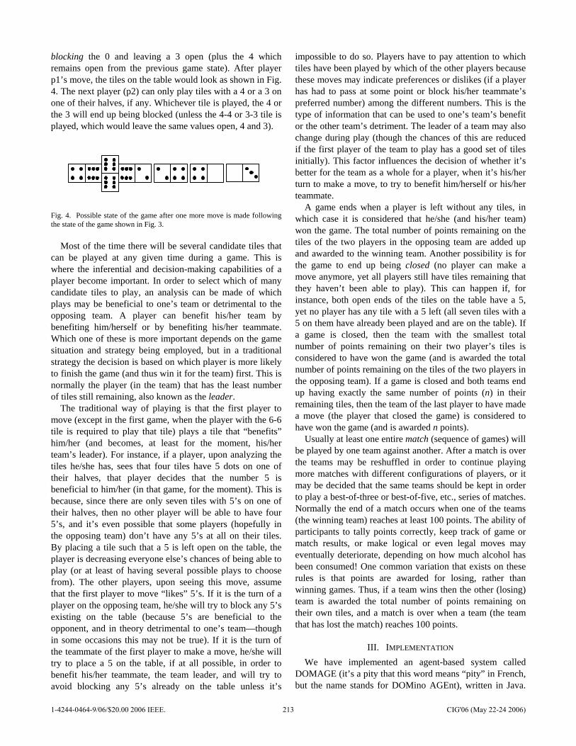
blocking the 0 and leaving a 3 open (plus the 4 which remains open from the previous game state). After player p1’s move, the tiles on the table would look as shown in Fig. 4. The next player (p2) can only play tiles with a 4 or a 3 on one of their halves, if any. Whichever tile is played, the 4 or the 3 will end up being blocked (unless the 4-4 or 3-3 tile is played, which would leave the same values open, 4 and 3).

Fig. 4. Possible state of the game after one more move is made following the state of the game shown in Fig. 3.

Most of the time there will be several candidate tiles that

can be played at any given time during a game. This is where the inferential and decision-making capabilities of a player become important. In order to select which of many candidate tiles to play, an analysis can be made of which plays may be beneficial to one’s team or detrimental to the opposing team. A player can benefit his/her team by benefiting him/herself or by benefiting his/her teammate. Which one of these is more important depends on the game situation and strategy being employed, but in a traditional strategy the decision is based on which player is more likely to finish the game (and thus win it for the team) first. This is normally the player (in the team) that has the least number of tiles still remaining, also known as the leader.

The traditional way of playing is that the first player to move (except in the first game, when the player with the 6-6 tile is required to play that tile) plays a tile that “benefits” him/her (and becomes, at least for the moment, his/her team’s leader). For instance, if a player, upon analyzing the tiles he/she has, sees that four tiles have 5 dots on one of their halves, that player decides that the number 5 is beneficial to him/her (in that game, for the moment). This is because, since there are only seven tiles with 5’s on one of their halves, then no other player will be able to have four 5’s, and it’s even possible that some players (hopefully in the opposing team) don’t have any 5’s at all on their tiles. By placing a tile such that a 5 is left open on the table, the player is decreasing everyone else’s chances of being able to play (or at least of having several possible plays to choose from). The other players, upon seeing this move, assume that the first player to move “likes” 5’s. If it is the turn of a player on the opposing team, he/she will try to block any 5’s existing on the table (because 5’s are beneficial to the opponent, and in theory detrimental to one’s team—though in some occasions this may not be true). If it is the turn of the teammate of the first player to make a move, he/she will try to place a 5 on the table, if at all possible, in order to benefit his/her teammate, the team leader, and will try to avoid blocking any 5’s already on the table unless it’s

impossible to do so. Players have to pay attention to which tiles have been played by which of the other players because these moves may indicate preferences or dislikes (if a player has had to pass at some point or block his/her teammate’s preferred number) among the different numbers. This is the type of information that can be used to one’s team’s benefit or the other team’s detriment. The leader of a team may also change during play (though the chances of this are reduced if the first player of the team to play has a good set of tiles initially). This factor influences the decision of whether it’s better for the team as a whole for a player, when it’s his/her turn to make a move, to try to benefit him/herself or his/her teammate.

A game ends when a player is left without any tiles, in which case it is considered that he/she (and his/her team) won the game. The total number of points remaining on the tiles of the two players in the opposing team are added up and awarded to the winning team. Another possibility is for the game to end up being closed (no player can make a move anymore, yet all players still have tiles remaining that they haven’t been able to play). This can happen if, for instance, both open ends of the tiles on the table have a 5, yet no player has any tile with a 5 left (all seven tiles with a 5 on them have already been played and are on the table). If a game is closed, then the team with the smallest total number of points remaining on their two player’s tiles is considered to have won the game (and is awarded the total number of points remaining on the tiles of the two players in the opposing team). If a game is closed and both teams end up having exactly the same number of points (n) in their remaining tiles, then the team of the last player to have made a move (the player that closed the game) is considered to have won the game (and is awarded n points).

Usually at least one entire match (sequence of games) will be played by one team against another. After a match is over the teams may be reshuffled in order to continue playing more matches with different configurations of players, or it may be decided that the same teams should be kept in order to play a best-of-three or best-of-five, etc., series of matches. Normally the end of a match occurs when one of the teams (the winning team) reaches at least 100 points. The ability of participants to tally points correctly, keep track of game or match results, or make logical or even legal moves may eventually deteriorate, depending on how much alcohol has been consumed! One common variation that exists on these rules is that points are awarded for losing, rather than winning games. Thus, if a team wins then the other (losing) team is awarded the total number of points remaining on their own tiles, and a match is over when a team (the team that has lost the match) reaches 100 points.

III. IMPLEMENTATION We have implemented an agent-based system called

DOMAGE (it’s a pity that this word means “pity” in French, but the name stands for DOMino AGEnt), written in Java.

1-4244-0464-9/06/$20.00 2006 IEEE. 213 CIG'06 (May 22-24 2006)

Each agent reasons independently of the rest. It knows exactly which tiles it has at any given time but can only “see” how many tiles the other players have at any stage of the game, not which tiles they are. Assumptions and inferences must be made about these during the decision-making process based on which moves each of the other players has previously made during the game. No communication takes place between the agents in DOMAGE.

In DOMAGE, in order to perform a “negotiation” to decide which of the two players of the team that won the previous game will begin the next game, each player’s set of tiles is evaluated. In this evaluation, a good starting set of tiles is considered to be one in which the dots are well distributed and at least one tile is held which has each of the possible number of dots on it (i.e., at least one tile has a 0 on one of its halves, at least one tile has a 1, at least one tile has a 2, etc., all the way to 6). In addition, a good starting set of tiles should have at least one dominant number, i.e., number of dots for which at least three different tiles are held (e.g., at least three separate tiles have a 2 on one of their halves). Finally, a good starting set of tiles is one in which no more than two tiles are doubles. In DOMAGE, if both players in the team that won the previous game match all three requirements for having a good starting set of tiles, then one of them is chosen at random to start the game. However, if one of the players in the team that won the previous game has a clear advantage (a better set of tiles) over its teammate, given these three criteria, then the player with the better set of tiles is the one that is assumed to “volunteer” to begin (make the first move of) the next game.

The system creates four instances of the domino-playing agent (p0, p1, p2, and p3) in order to set up a match. Seven different strategies have been implemented. Perhaps more strategies could be thought of, but the idea was to come up with clearly distinct strategies for the purpose of evaluating them, and in fact the last two are really subsets or combinations of the first five. In the current implementation each agent, from the moment it is created, follows only one of the implemented strategies. The differences between the seven strategies stem from the fact that each is based on prioritizing in different ways the basic goals (or some of the basic goals) that an agent may pursue when deciding which move to make. Some examples of these goals are: benefit oneself, benefit one’s teammate, block the opposing team’s leader, etc. The seven strategies that have been implemented are explained in the following paragraphs (assuming it’s player p’s turn to make a move).

In the traditional strategy (T) the first priority for p is to benefit its team. If p is the team leader then p decides on a move that is beneficial to p, if possible (this is the highest-priority goal for p). Otherwise p makes a move that is beneficial to p’s teammate, if possible. If p is not the team leader then the relative priorities of these two possibilities are switched. If none of these two options are possible with

the playable tiles that p has, then p tries to block the leader of the opposing team. If that’s not possible then p tries to block the non-leader of the opposing team. Finally, if it is impossible to satisfy any of the other intentions mentioned given the playable tiles that p has at a given point during the game, then p simply chooses to play the playable tile with the highest number of dots in total (in order to at least minimize the damage in case of an eventual loss).

The second strategy that has been implemented is a completely altruistic strategy (A)—player p only thinks about the other players and about making “positive” (beneficial) rather than “negative” (blocking) moves, while still giving a higher priority to p’s team over the opposing team. The highest priority, given these constraints, is that first p attempts to make a move that is beneficial to p’s teammate. If this isn’t possible, then p tries to make a move that is beneficial to the non-leader of the opposing team. If this isn’t possible then p tries to benefit the opposing team’s leader. Finally, if none of these options are possible then p chooses at random from amongst its playable tiles (rather than try to benefit itself or block any other player, since none of these options would be completely altruistic).

The third strategy that has been implemented is a completely selfish strategy (S)—player p thinks only of itself. In this strategy the highest priority is for p to benefit itself. If this isn’t possible given the playable tiles p currently has, then one of the playable tiles is simply chosen at random (rather than making a decision on which move to make by thinking of the other players and whether the move would be to their benefit or detriment).

The fourth implemented strategy is a completely random strategy (R). Player p decides from amongst its playable tiles at random, without bothering to analyze the possible effects of any move, whether beneficial or detrimental, on any of the other players (or itself).

The fifth strategy that has been implemented is a suicidal strategy (SU)—player p only tries explicitly to benefit the opposing team. First an attempt is made to benefit the opposing team’s leader, and if that’s not possible then an attempt is made to benefit the opposing team’s non-leader. If that’s not possible either then a random move is made, without any attempt at all to explicitly make a move that is beneficial to p or its team.

The sixth implemented strategy is a combination of the traditional and altruistic strategies (TA)—it’s a traditional strategy but with a slight bias towards thinking more of others than of oneself. The first thing player p attempts to do in this strategy is to benefit its teammate (whether that teammate is the team leader or not). If that’s not possible, then p tries to make a move that will benefit p. If that’s not possible then an attempt is made to block the opposing team’s leader. If that’s not possible then an attempt is made to block the non-leader of the opposing team. If none of the previous possibilities pan out then the highest-valued playable tile is chosen.

1-4244-0464-9/06/$20.00 2006 IEEE. 214 CIG'06 (May 22-24 2006)

The seventh strategy that has been implemented is a combination of the traditional and selfish strategies (TS)—it’s a traditional strategy but with a slight bias towards thinking more of oneself than anyone else. The first thing that player p attempts to do in this strategy is to make a move that will benefit itself, and if that’s not possible, then p tries to benefit its teammate (irrespective of whether p or p’s teammate is the team leader). If that’s not possible then p tries to block the opposing team’s leader. If that’s not possible then p tries to block the non-leader of the opposing team. Finally, if none of the previous options are possible then p chooses a tile to play at random.

IV. EXPERIMENT AND RESULTS As our goal was to evaluate the different strategies that

have been implemented as compared to the traditional strategy, we arbitrarily chose player p0 to be our “guinea pig.” Therefore, in the experiments the strategy followed by p0 was varied, whereas the strategy followed by the other three player agents was always the traditional strategy. Each time that p0’s strategy was changed, 100 matches were played. For each set of 100 matches, statistics were gathered on which player agent (and therefore which team) won the match. Thus, a total of 700 matches were played between the four domino-playing agents, 100 for each strategy employed by p0. The teammate of player p0 is p2; their team will be labeled team0 from now on.

In the 100 matches in which p0 used the traditional strategy, all four agents were behaviorally equivalent. Therefore, it is to be expected that each of the four agents should win approximately 25% of the games. We decided that we would tolerate a variation of ±10% due to random or other factors. Therefore, in the experiments it will be considered “normal” if a player agent wins between 22.5% and 27.5% of the games. Any strategy for which p0 wins more than 27.5% of the games will therefore be considered a good strategy for p0 compared to the traditional one (though this does not necessarily mean that it will be good for p2, and therefore for team0 as a whole). Any strategy for which p0 wins less than 22.5% of the games will be considered a bad strategy for p0 compared to the traditional one (though this does not necessarily mean that it will be bad for p2, and therefore for team0 as a whole). Any strategy for which team0 wins more than 55% of the matches will be considered a good strategy for team0 compared to the traditional one. Any strategy for which team0 wins less than 45% of the matches will be considered a bad strategy for team0 compared to the traditional one.

The results of the experiment are shown in Table 1 below. The table lists the strategy used by p0 in each of the sets of 100 matches, the percentage of games won by p0 when playing the corresponding strategy (PGWp0), the percentage of games won by p2 when p0 was playing the corresponding strategy (PGWp2), and the percentage of matches won by team0 when p0 was playing each strategy (PMWteam0).

TABLE I

RESULTS OF THE EXPERIMENT Strategy for p0: PGWp0: PGWp2: PMWteam0:

Traditional (T): 25.6% 24.4% 54% Altruistic (A): 24.4% 20.3% 35%

Selfish (S): 27.5% 25.2% 54% Random (R): 28.8% 21.6% 48% Suicidal (SU): 25% 21.7% 35% Traditional-Altruistic (TA):

26.2% 23.3% 49%

Traditional-Selfish (TS):

26.5% 25.5% 50%

Percentage of games won by player p0 (PCWp0), percentage of games won by p0’s teammate, p2 (PCWp2), and percentage of matches won by p0 and p2’s team, team0 (PMWteam0) after 100 matches were played for each of seven different strategies (T, A, S, R, SU, TA, and TS) followed by p0.

V. DISCUSSION As the results in Table I show, a few strategies stand out

for different reasons. The random (R) strategy produced the highest percentage of games won for player p0 (28.8%). However, p2’s percentage of games won for the same strategy was 21.6%, one of the lowest, thereby producing a total of 51.4% of all games won for team0, but only 48% of the matches won by team0. The high value for the percentage of games won by player p0 can perhaps be explained by the fact that playing randomly instead of trying to make an intelligent move based on analyzing the game state was misleading to the other players (including p0’s teammate, p2), and therefore their decisions (which were made in a more systematic manner) didn’t have the impact they were designed to have. On the other hand, the percentage of matches won by team0 wasn’t as low as it could have been despite this fact. This result might be useful to take into account if a non-collaborative version of DOMAGE is implemented, as in that situation it doesn’t matter (in fact it might be better) if a player’s random moves become misleading to the rest of the players.

The selfish strategy (S) also produced a high percentage of game wins for p0 (just barely on the limit of the ±10% tolerance of variation from the norm), 27.5%. On the other hand, the percentage of matches won by team0 when p0 played with this strategy is 54%, not quite 10% above what would be expected, and the same as the percentage of matches won when p0 used the traditional (T) strategy. This leads us to believe that the result is more due to random factors than to any real benefit of the selfish strategy over the others. Strangely enough, the selfish strategy (S) seems to perform slightly less well than the purely random strategy (R) even though it involves first trying to determine if any potential move is beneficial to the player making the decision and only making a random move if no self-beneficial move can be found. But it might be another worthwhile strategy to consider in a non-collaborative version of DOMAGE.

1-4244-0464-9/06/$20.00 2006 IEEE. 215 CIG'06 (May 22-24 2006)

The altruistic (A) and suicidal (SU) strategies allowed p0 to win 24.4% and 25% of the games, respectively, close to what would be expected from a traditional (T) strategy. However, both resulted in very low percentages of games won for p0’s teammate p2 (20.3% and 21.7%, respectively). The percentage of matches won by team0 when p0 used these strategies was also very low: 35% for both. Thus, neither of these two strategies seems to be recommendable.

None of the other strategies tested stand out when compared to the traditional strategy (T). This experiment has allowed us to arrive at some conclusions on the relative performance of the different strategies that we thought of. These strategies make sense in the context of the game of dominoes and have only been implemented for that domain. In contrast, [5] presents a comparison of different general-purpose search strategies used in the context of several games. However, even though the strategies have only been implemented and tested for dominoes, the results might well be applicable to other, similar games (where team members try to collaborate with each other, and compete against the opposing team, based on incomplete information).

VI. FUTURE WORK The DOMAGE system in its current incarnation can serve

as a test-bed for further experiments, but extensions to the implementation would both enhance the system’s capabilities and provide the means for different types of experiments. A long-term goal is to enable the system to play with humans. In its current state the system is probably too dumb to serve as a teammate to a human player against another pair of human players or even to play against humans in a non-collaborative version of the game of dominoes. This is because its strategies are rigid—once a game begins the same initial strategy is followed blindly throughout. Allowing for adaptive strategies (which can change the priorities of the goals they attempt to achieve as the game progresses) or allowing the player agent making the decisions to change strategies during the game might give DOMAGE some of the flexibility needed to play with people. For instance, as a game progresses it becomes more and more important to get rid of the double tiles that one might have (though how important depends on how many doubles one has) in order to avoid the possibility of a double becoming strangled. A double becomes strangled when all six tiles with a given number (for instance, all tiles with a 5 on one of their halves) have been played except the double. This makes it impossible for the double ever to be played (because the number 5 will never be able to be left open on the table, a necessary precondition in order to be able to play another tile with a 5, in this case the 5-5 tile). Coming up with additional strategies might also be worthwhile.

The current implementation of DOMAGE also focuses on positive aspects of a game’s history. Agents pay attention to which domino tiles have been played by which of the other players while the game has been going on, and therefore can

infer which numbers are “liked” by them. However, there are currently no mechanisms implemented to allow an agent to predict which move another player will make, and therefore to infer which numbers are disliked (not present on any of the halves of the tiles possessed) by other players. For instance, if the values open on the table are 3 and 5, and a player p blocks the 5 even though he/she has previously seemed to like 5’s, it probably means that that player does not have any tiles with 3 on them. By making this inference the opposing team can increase the possibility of making p pass (or at least continue to block him/herself or his/her teammate) by leaving the 3 open on one (or, even better, both) ends of the tiles already on the table. Thus, a more complex reasoning engine that tries to hypothesize about other players’ motivations in making different moves may give the system more intelligence.

In addition, the different possible goals that are attempted (according to a predefined list of priorities) in the strategies are currently mutually exclusive. In the current implementation, once a tile has been identified that, if played, will achieve the goal with the highest priority possible (out of the goals involved in the strategy), that move is made by the player agent. Instead, if all playable tiles were analyzed according to all possible goals, then for instance a move might be identified that not only benefits the agent’s teammate but also blocks the opposing team’s leader at the same time. When the goals are allowed to interact in this way the candidate tile might be assigned a higher weight when deciding which move to make, thus again resulting in more intelligent decision-making capabilities for the game-playing agents.

The experimental results we presented in Section IV and discussed in Section V will help guide us in making these adjustments to the DOMAGE system. Additional experiments might also give us useful information. For instance, it might be interesting to see what happens if both players in a team “agree” on following a specific strategy (out of the ones discussed earlier) before a game begins. In fact, it might also be interesting to see what happens if each player in a team agrees to follow a specific strategy (but a different one for each player) before a game begins. In both of these situations the players in a team would have additional information (that cannot be communicated during play) that might help them lead their team to win a game.

REFERENCES [1] http://www.dominorules.com/dominorules.aspx. [2] http://www.pagat.com/boston/bridge.html. [3] http://nelson.oit.unc.edu/~alanh/hearts-copy-

strategy.html. [4] M. Ginsberg, “GIB: imperfect information in a computationally

challenging game,” Journal of Artificial Intelligence Research, vol. 14, pp. 303-358, 2001.

[5] N. Sturtevant, “A comparison of algorithms for multi-player games,” in Proc. 3rd Int. Conf. Computers and Games, Edmonton, Canada, July 2002, pp. 108-122, Springer-Verlag.

1-4244-0464-9/06/$20.00 2006 IEEE. 216 CIG'06 (May 22-24 2006)

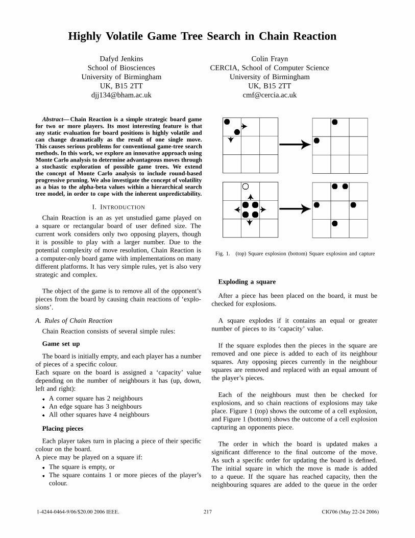
Highly Volatile Game Tree Search in Chain Reaction

Dafyd JenkinsSchool of Biosciences

University of BirminghamUK, B15 2TT

djj134@bham.ac.uk

Colin FraynCERCIA, School of Computer Science

University of BirminghamUK, B15 2TT

cmf@cercia.ac.uk

Abstract— Chain Reaction is a simple strategic board gamefor two or more players. Its most interesting feature is thatany static evaluation for board positions is highly volatile andcan change dramatically as the result of one single move.This causes serious problems for conventional game-tree searchmethods. In this work, we explore an innovative approach usingMonte Carlo analysis to determine advantageous moves througha stochastic exploration of possible game trees. We extendthe concept of Monte Carlo analysis to include round-basedprogressive pruning. We also investigate the concept of volatilityas a bias to the alpha-beta values within a hierarchical searchtree model, in order to cope with the inherent unpredictability.

I. INTRODUCTION

Chain Reaction is an as yet unstudied game played ona square or rectangular board of user defined size. Thecurrent work considers only two opposing players, thoughit is possible to play with a larger number. Due to thepotential complexity of move resolution, Chain Reaction isa computer-only board game with implementations on manydifferent platforms. It has very simple rules, yet is also verystrategic and complex.

The object of the game is to remove all of the opponent’spieces from the board by causing chain reactions of ‘explo-sions’.

A. Rules of Chain Reaction

Chain Reaction consists of several simple rules:

Game set up

The board is initially empty, and each player has a numberof pieces of a specific colour.Each square on the board is assigned a ‘capacity’ valuedepending on the number of neighbours it has (up, down,left and right):

� A corner square has 2 neighbours� An edge square has 3 neighbours� All other squares have 4 neighbours

Placing pieces

Each player takes turn in placing a piece of their specificcolour on the board.A piece may be played on a square if:

� The square is empty, or� The square contains 1 or more pieces of the player’s

colour.

Fig. 1. (top) Square explosion (bottom) Square explosion and capture

Exploding a square

After a piece has been placed on the board, it must bechecked for explosions.

A square explodes if it contains an equal or greaternumber of pieces to its ‘capacity’ value.

If the square explodes then the pieces in the square areremoved and one piece is added to each of its neighboursquares. Any opposing pieces currently in the neighboursquares are removed and replaced with an equal amount ofthe player’s pieces.

Each of the neighbours must then be checked forexplosions, and so chain reactions of explosions may takeplace. Figure 1 (top) shows the outcome of a cell explosion,and Figure 1 (bottom) shows the outcome of a cell explosioncapturing an opponents piece.

The order in which the board is updated makes asignificant difference to the final outcome of the move.As such a specific order for updating the board is defined.The initial square in which the move is made is addedto a queue. If the square has reached capacity, then theneighbouring squares are added to the queue in the order

1-4244-0464-9/06/$20.00 2006 IEEE. 217 CIG'06 (May 22-24 2006)

Left, Right, Up, Down.

B. Motivation for using Chain Reaction

Whilst Chain Reaction has very simple rules and gameplay, the game has an ‘easy to learn; hard to master’complexity to it. It shares many similarities with Go, suchas the importance of structure within a game position, andan extremely large branching factor (the exact branchingfactor is, at this time, currently unknown). This means thatmany standard game playing techniques give poor results.Chain Reaction also does not have a decreasing complexityas the game progresses, unlike chess for example, where thecomplexity begins to decrease as pieces are captured. Thecomplexity only generally decreases during the extremelyshort end-game of Chain Reaction (usually one or twomoves).

II. STANDARD APPROACHES

Perhaps the most commonly used game playing techniqueis the Minimax algorithm, along with its many variants.Minimax has been used on a wide variety of games, mostnotably Chess (such as ‘Deep Blue’[1] and ‘ChessBrain’[2])and Draughts/Checkers (such as ‘Chinook’[3]). However,the Minimax algorithm has several drawbacks:

� High time complexity for large branching factors� Requires large amounts of subjective domain knowledge

incorporated into a heuristic function for board evalua-tion

� The ‘horizon effect’ in which good moves may bemissed if the ply depth is not large enough, or badmoves may be inadvertently selected if a specific branchcurrently looks promising, but leads to an extremelypoor move one or more ply ahead.

Evolutionary methods have also been widely used ingame playing algorithms, in particular in Go. This islargely due to the inherent problems the Minimax approachencounters when applied to such a complex game. Neuralnetworks have been applied to board evaluation to offsetthe problems associated with hand-crafting a sufficientevaluation heuristic function for a Minimax search[4].Spatial reasoning techniques have also been used toinfluence neural network design for Go, in order to attempta ‘divide and conquer’ approach to board evaluation [5], [4]and this also referred to as ‘soft segmentation’ [6].

Our original work consisted of attempting to use severalevolutionary techniques, along with the classical Minimaxalgorithm to develop game players for Chain Reaction. Arange of players were designed and played against eachother, including an evolutionary player using neural networkboard evaluation functions influenced by spatial reasoning,together with genetic algorithms and data mining techniquesfor knowledge discovery. We also implemented a standardMinimax player with � � � pruning and a simple piece

counter heuristic. Finally, we investigate the application ofparticle swarm optimisation to a piece-position table boardevaluation heuristic. The results of these experiments can befound in our earlier work[7].

In our earlier work, we were unable to evolve significantlysuccessful strategies using a spatial neural-network approachunder a number of different training schemes. The motivationfor this new work was to explore new and distinct techniquesfor evolving strategies within this complex game, and toinvestigate whether or not the new methods are capable ofovercoming the difficulties of dealing with a highly volatilegame tree.

III. MONTE CARLO APPROACH

The Monte Carlo method (also known as statisticalsampling) is a stochastic technique designed to sample alarge search space, allowing inferences to be made aboutthe properties of that search space as a whole. This hasbeen used to explore the behaviour of various physical andmathematical systems such as numerical integration andoptimisation problems, and it relies on random (or pseudo-random) number generators to allow the non-determinismrequired to generate statistically valid results. The useof Monte Carlo simulations for a problem assumes thatthe problem can be described using probability densityfunctions. The simulation then proceeds to randomly samplethe probability density function many times. Such repeatedsampling allows an average result to be generated, which isthen used as the solution[8].

The Monte Carlo method was first applied to Go in 1993by Brugmann[9]. In this paper the method was combinedwith a Simulated Annealing process which was used toassign probabilities to each available move. Using theseprobabilities many random games (samples) are playedfrom the current board position until completion. The movewhich returns the highest average score from these statisticalsamplings (that is, the move with the highest win-fraction),will then be the move selected and played.

Whilst this is an incredibly simple algorithm, and isbased purely on random sampling, it performs quite wellwith the authors citing a ranking of around 25 kyu (Kyu isthe ranking system used within Go; a lower Kyu indicatesa stronger player. A new or extremely novice player usuallyhas a kyu of over 30) on a 9x9 board. This result is veryinteresting as the choice of the moves made is based solelyon random numbers, and randomly sampled games, with nodomain knowledge required other than the rules of the game.

Bouzy and Helmstetter also investigated the use of theMonte Carlo method in Go in their 2003 paper[10]. Theauthors used a simpler approach than that used by Brugmanncalled Expected-Outcome proposed by Abramson[11], and

1-4244-0464-9/06/$20.00 2006 IEEE. 218 CIG'06 (May 22-24 2006)

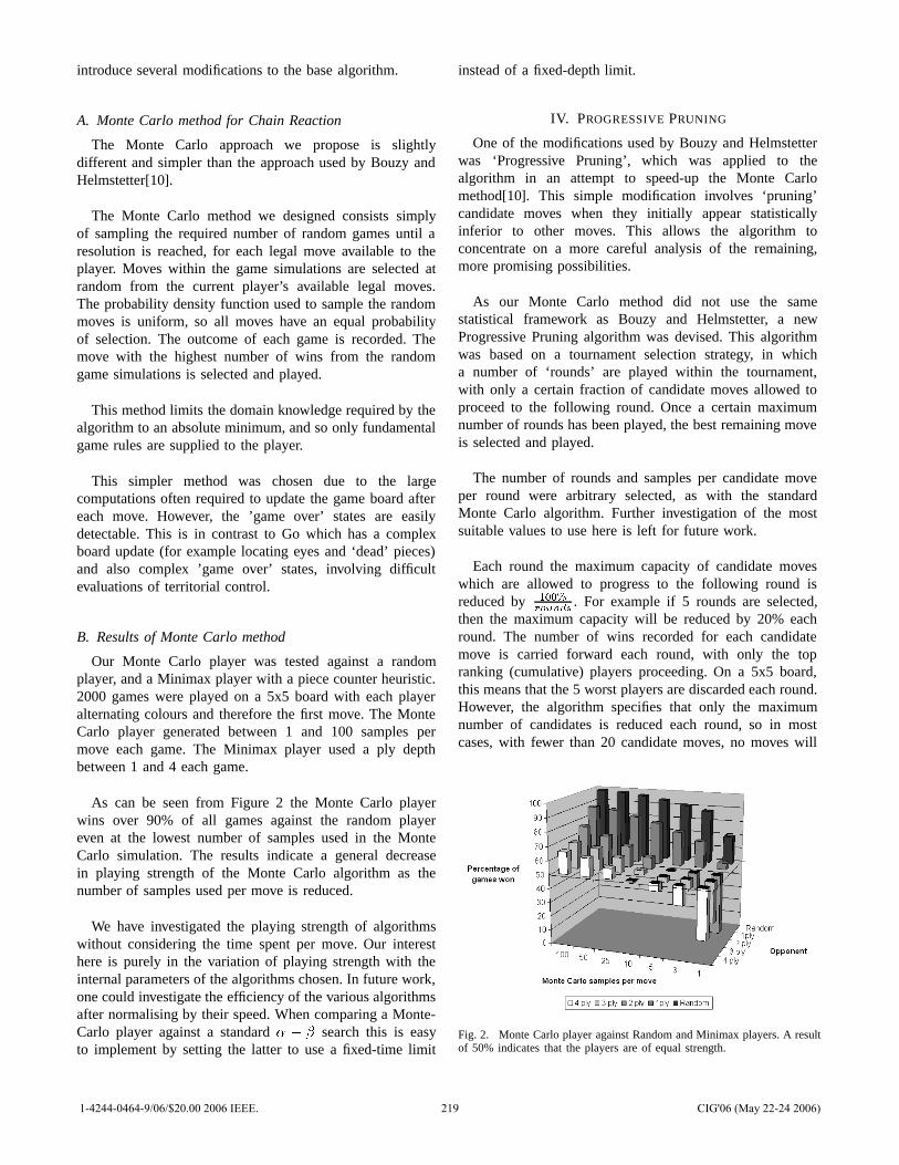
introduce several modifications to the base algorithm.

A. Monte Carlo method for Chain Reaction

The Monte Carlo approach we propose is slightlydifferent and simpler than the approach used by Bouzy andHelmstetter[10].

The Monte Carlo method we designed consists simplyof sampling the required number of random games until aresolution is reached, for each legal move available to theplayer. Moves within the game simulations are selected atrandom from the current player’s available legal moves.The probability density function used to sample the randommoves is uniform, so all moves have an equal probabilityof selection. The outcome of each game is recorded. Themove with the highest number of wins from the randomgame simulations is selected and played.

This method limits the domain knowledge required by thealgorithm to an absolute minimum, and so only fundamentalgame rules are supplied to the player.

This simpler method was chosen due to the largecomputations often required to update the game board aftereach move. However, the ’game over’ states are easilydetectable. This is in contrast to Go which has a complexboard update (for example locating eyes and ‘dead’ pieces)and also complex ’game over’ states, involving difficultevaluations of territorial control.

B. Results of Monte Carlo method

Our Monte Carlo player was tested against a randomplayer, and a Minimax player with a piece counter heuristic.2000 games were played on a 5x5 board with each playeralternating colours and therefore the first move. The MonteCarlo player generated between 1 and 100 samples permove each game. The Minimax player used a ply depthbetween 1 and 4 each game.

As can be seen from Figure 2 the Monte Carlo playerwins over 90% of all games against the random playereven at the lowest number of samples used in the MonteCarlo simulation. The results indicate a general decreasein playing strength of the Monte Carlo algorithm as thenumber of samples used per move is reduced.

We have investigated the playing strength of algorithmswithout considering the time spent per move. Our interesthere is purely in the variation of playing strength with theinternal parameters of the algorithms chosen. In future work,one could investigate the efficiency of the various algorithmsafter normalising by their speed. When comparing a Monte-Carlo player against a standard � � � search this is easyto implement by setting the latter to use a fixed-time limit

instead of a fixed-depth limit.

IV. PROGRESSIVE PRUNING

One of the modifications used by Bouzy and Helmstetterwas ‘Progressive Pruning’, which was applied to thealgorithm in an attempt to speed-up the Monte Carlomethod[10]. This simple modification involves ‘pruning’candidate moves when they initially appear statisticallyinferior to other moves. This allows the algorithm toconcentrate on a more careful analysis of the remaining,more promising possibilities.

As our Monte Carlo method did not use the samestatistical framework as Bouzy and Helmstetter, a newProgressive Pruning algorithm was devised. This algorithmwas based on a tournament selection strategy, in whicha number of ‘rounds’ are played within the tournament,with only a certain fraction of candidate moves allowed toproceed to the following round. Once a certain maximumnumber of rounds has been played, the best remaining moveis selected and played.

The number of rounds and samples per candidate moveper round were arbitrary selected, as with the standardMonte Carlo algorithm. Further investigation of the mostsuitable values to use here is left for future work.

Each round the maximum capacity of candidate moveswhich are allowed to progress to the following round isreduced by ����

������. For example if 5 rounds are selected,

then the maximum capacity will be reduced by 20% eachround. The number of wins recorded for each candidatemove is carried forward each round, with only the topranking (cumulative) players proceeding. On a 5x5 board,this means that the 5 worst players are discarded each round.However, the algorithm specifies that only the maximumnumber of candidates is reduced each round, so in mostcases, with fewer than 20 candidate moves, no moves will

Fig. 2. Monte Carlo player against Random and Minimax players. A resultof 50% indicates that the players are of equal strength.

1-4244-0464-9/06/$20.00 2006 IEEE. 219 CIG'06 (May 22-24 2006)

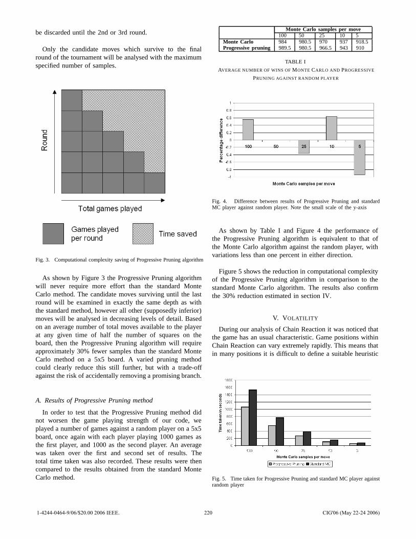
be discarded until the 2nd or 3rd round.

Only the candidate moves which survive to the finalround of the tournament will be analysed with the maximumspecified number of samples.

Fig. 3. Computational complexity saving of Progressive Pruning algorithm

As shown by Figure 3 the Progressive Pruning algorithmwill never require more effort than the standard MonteCarlo method. The candidate moves surviving until the lastround will be examined in exactly the same depth as withthe standard method, however all other (supposedly inferior)moves will be analysed in decreasing levels of detail. Basedon an average number of total moves available to the playerat any given time of half the number of squares on theboard, then the Progressive Pruning algorithm will requireapproximately 30% fewer samples than the standard MonteCarlo method on a 5x5 board. A varied pruning methodcould clearly reduce this still further, but with a trade-offagainst the risk of accidentally removing a promising branch.

A. Results of Progressive Pruning method

In order to test that the Progressive Pruning method didnot worsen the game playing strength of our code, weplayed a number of games against a random player on a 5x5board, once again with each player playing 1000 games asthe first player, and 1000 as the second player. An averagewas taken over the first and second set of results. Thetotal time taken was also recorded. These results were thencompared to the results obtained from the standard MonteCarlo method.

Monte Carlo samples per move100 50 25 10 5

Monte Carlo 984 980.5 970 937 918.5Progressive pruning 989.5 980.5 966.5 943 910

TABLE I

AVERAGE NUMBER OF WINS OF MONTE CARLO AND PROGRESSIVE

PRUNING AGAINST RANDOM PLAYER

Fig. 4. Difference between results of Progressive Pruning and standardMC player against random player. Note the small scale of the y-axis

As shown by Table I and Figure 4 the performance ofthe Progressive Pruning algorithm is equivalent to that ofthe Monte Carlo algorithm against the random player, withvariations less than one percent in either direction.

Figure 5 shows the reduction in computational complexityof the Progressive Pruning algorithm in comparison to thestandard Monte Carlo algorithm. The results also confirmthe 30% reduction estimated in section IV.

V. VOLATILITY

During our analysis of Chain Reaction it was noticed thatthe game has an usual characteristic. Game positions withinChain Reaction can vary extremely rapidly. This means thatin many positions it is difficult to define a suitable heuristic

Fig. 5. Time taken for Progressive Pruning and standard MC player againstrandom player

1-4244-0464-9/06/$20.00 2006 IEEE. 220 CIG'06 (May 22-24 2006)

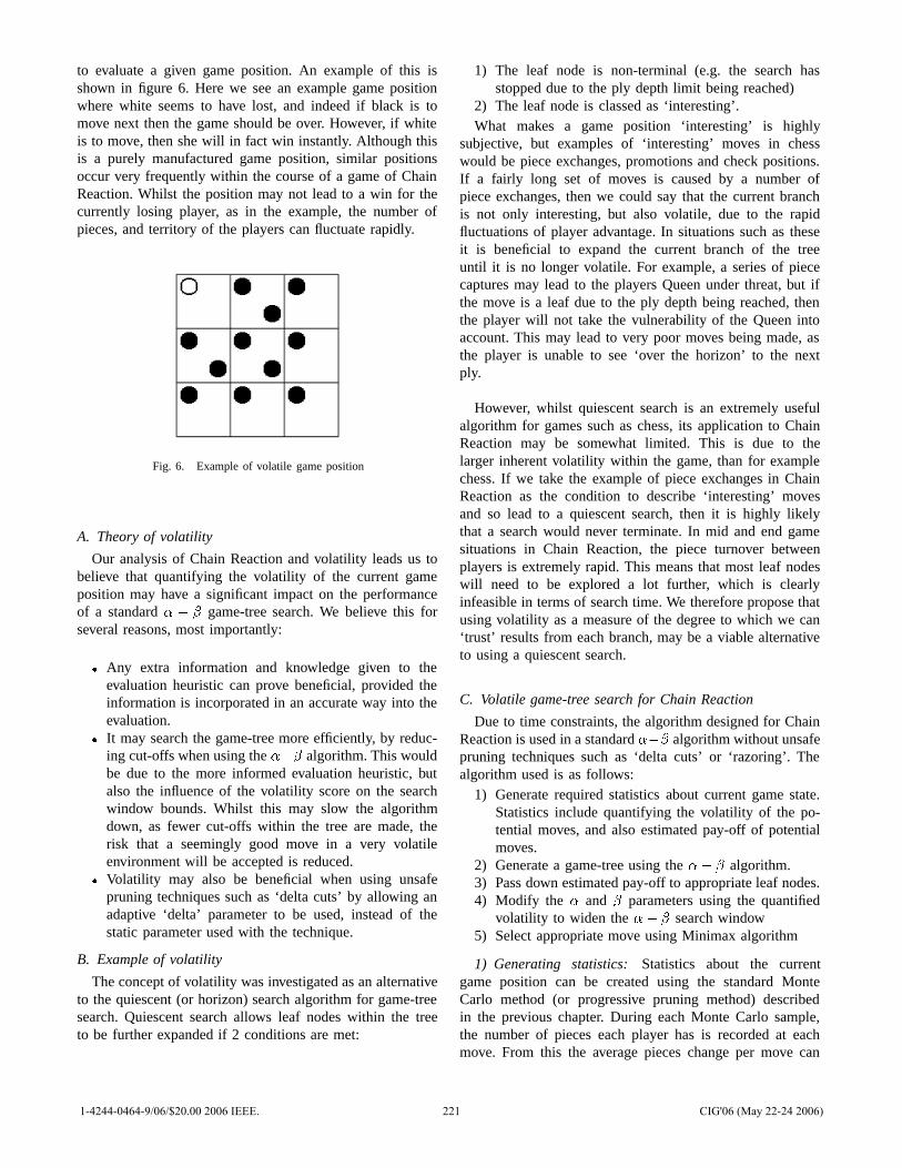
to evaluate a given game position. An example of this isshown in figure 6. Here we see an example game positionwhere white seems to have lost, and indeed if black is tomove next then the game should be over. However, if whiteis to move, then she will in fact win instantly. Although thisis a purely manufactured game position, similar positionsoccur very frequently within the course of a game of ChainReaction. Whilst the position may not lead to a win for thecurrently losing player, as in the example, the number ofpieces, and territory of the players can fluctuate rapidly.

Fig. 6. Example of volatile game position

A. Theory of volatility

Our analysis of Chain Reaction and volatility leads us tobelieve that quantifying the volatility of the current gameposition may have a significant impact on the performanceof a standard � � � game-tree search. We believe this forseveral reasons, most importantly:

� Any extra information and knowledge given to theevaluation heuristic can prove beneficial, provided theinformation is incorporated in an accurate way into theevaluation.

� It may search the game-tree more efficiently, by reduc-ing cut-offs when using the ��� algorithm. This wouldbe due to the more informed evaluation heuristic, butalso the influence of the volatility score on the searchwindow bounds. Whilst this may slow the algorithmdown, as fewer cut-offs within the tree are made, therisk that a seemingly good move in a very volatileenvironment will be accepted is reduced.

� Volatility may also be beneficial when using unsafepruning techniques such as ‘delta cuts’ by allowing anadaptive ‘delta’ parameter to be used, instead of thestatic parameter used with the technique.

B. Example of volatility

The concept of volatility was investigated as an alternativeto the quiescent (or horizon) search algorithm for game-treesearch. Quiescent search allows leaf nodes within the treeto be further expanded if 2 conditions are met:

1) The leaf node is non-terminal (e.g. the search hasstopped due to the ply depth limit being reached)

2) The leaf node is classed as ‘interesting’.What makes a game position ‘interesting’ is highly

subjective, but examples of ‘interesting’ moves in chesswould be piece exchanges, promotions and check positions.If a fairly long set of moves is caused by a number ofpiece exchanges, then we could say that the current branchis not only interesting, but also volatile, due to the rapidfluctuations of player advantage. In situations such as theseit is beneficial to expand the current branch of the treeuntil it is no longer volatile. For example, a series of piececaptures may lead to the players Queen under threat, but ifthe move is a leaf due to the ply depth being reached, thenthe player will not take the vulnerability of the Queen intoaccount. This may lead to very poor moves being made, asthe player is unable to see ‘over the horizon’ to the nextply.

However, whilst quiescent search is an extremely usefulalgorithm for games such as chess, its application to ChainReaction may be somewhat limited. This is due to thelarger inherent volatility within the game, than for examplechess. If we take the example of piece exchanges in ChainReaction as the condition to describe ‘interesting’ movesand so lead to a quiescent search, then it is highly likelythat a search would never terminate. In mid and end gamesituations in Chain Reaction, the piece turnover betweenplayers is extremely rapid. This means that most leaf nodeswill need to be explored a lot further, which is clearlyinfeasible in terms of search time. We therefore propose thatusing volatility as a measure of the degree to which we can‘trust’ results from each branch, may be a viable alternativeto using a quiescent search.

C. Volatile game-tree search for Chain Reaction

Due to time constraints, the algorithm designed for ChainReaction is used in a standard ��� algorithm without unsafepruning techniques such as ‘delta cuts’ or ‘razoring’. Thealgorithm used is as follows:

1) Generate required statistics about current game state.Statistics include quantifying the volatility of the po-tential moves, and also estimated pay-off of potentialmoves.

2) Generate a game-tree using the �� � algorithm.3) Pass down estimated pay-off to appropriate leaf nodes.4) Modify the � and � parameters using the quantified

volatility to widen the �� � search window5) Select appropriate move using Minimax algorithm

1) Generating statistics: Statistics about the currentgame position can be created using the standard MonteCarlo method (or progressive pruning method) describedin the previous chapter. During each Monte Carlo sample,the number of pieces each player has is recorded at eachmove. From this the average pieces change per move can

1-4244-0464-9/06/$20.00 2006 IEEE. 221 CIG'06 (May 22-24 2006)

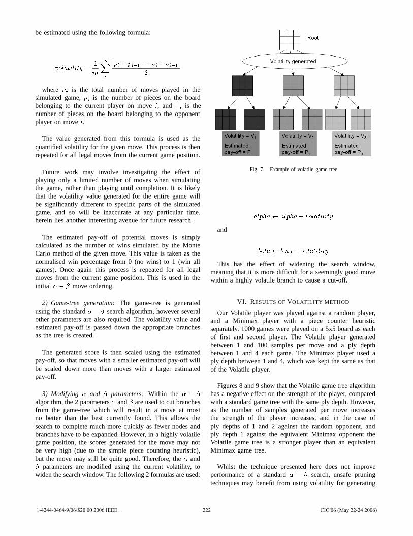
be estimated using the following formula:

��������� ��

��

�

��� � ������ ��� � �����

�

where is the total number of moves played in thesimulated game, �� is the number of pieces on the boardbelonging to the current player on move �, and � � is thenumber of pieces on the board belonging to the opponentplayer on move �.

The value generated from this formula is used as thequantified volatility for the given move. This process is thenrepeated for all legal moves from the current game position.

Future work may involve investigating the effect ofplaying only a limited number of moves when simulatingthe game, rather than playing until completion. It is likelythat the volatility value generated for the entire game willbe significantly different to specific parts of the simulatedgame, and so will be inaccurate at any particular time.herein lies another interesting avenue for future research.

The estimated pay-off of potential moves is simplycalculated as the number of wins simulated by the MonteCarlo method of the given move. This value is taken as thenormalised win percentage from 0 (no wins) to 1 (win allgames). Once again this process is repeated for all legalmoves from the current game position. This is used in theinitial �� � move ordering.

2) Game-tree generation: The game-tree is generatedusing the standard �� � search algorithm, however severalother parameters are also required. The volatility value andestimated pay-off is passed down the appropriate branchesas the tree is created.

The generated score is then scaled using the estimatedpay-off, so that moves with a smaller estimated pay-off willbe scaled down more than moves with a larger estimatedpay-off.

3) Modifying � and � parameters: Within the � � �

algorithm, the 2 parameters � and � are used to cut branchesfrom the game-tree which will result in a move at mostno better than the best currently found. This allows thesearch to complete much more quickly as fewer nodes andbranches have to be expanded. However, in a highly volatilegame position, the scores generated for the move may notbe very high (due to the simple piece counting heuristic),but the move may still be quite good. Therefore, the � and� parameters are modified using the current volatility, towiden the search window. The following 2 formulas are used:

Fig. 7. Example of volatile game tree

������ ������ ���������

and

���� ���� ���������

This has the effect of widening the search window,meaning that it is more difficult for a seemingly good movewithin a highly volatile branch to cause a cut-off.

VI. RESULTS OF VOLATILITY METHOD

Our Volatile player was played against a random player,and a Minimax player with a piece counter heuristicseparately. 1000 games were played on a 5x5 board as eachof first and second player. The Volatile player generatedbetween 1 and 100 samples per move and a ply depthbetween 1 and 4 each game. The Minimax player used aply depth between 1 and 4, which was kept the same as thatof the Volatile player.

Figures 8 and 9 show that the Volatile game tree algorithmhas a negative effect on the strength of the player, comparedwith a standard game tree with the same ply depth. However,as the number of samples generated per move increasesthe strength of the player increases, and in the case ofply depths of 1 and 2 against the random opponent, andply depth 1 against the equivalent Minimax opponent theVolatile game tree is a stronger player than an equivalentMinimax game tree.

Whilst the technique presented here does not improveperformance of a standard � � � search, unsafe pruningtechniques may benefit from using volatility for generating

1-4244-0464-9/06/$20.00 2006 IEEE. 222 CIG'06 (May 22-24 2006)

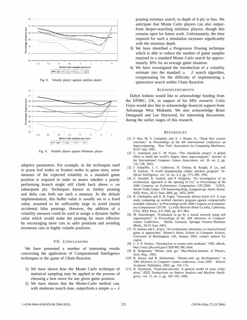
Fig. 8. Volatile player against random player

Fig. 9. Volatile player against Minimax player

adaptive parameters. For example, in the techniques usedto prune leaf nodes or frontier nodes in game trees, somemeasure of the expected volatility in a standard gameposition is required in order to assess whether a poorlyperforming branch might still climb back above � onsubsequent ply. Techniques known as futility pruningand delta cuts both use such a measure. In the defaultimplementation, this buffer value is usually set to a fixedvalue, assumed to be sufficiently large to avoid (most)accidental false prunings. However, the addition of avolatility measure could be used to assign a dynamic buffervalue which would make the pruning far more effectiveby encouraging more cuts in safer positions and avoidingerroneous cuts in highly volatile positions.

VII. CONCLUSIONS

We have presented a number of interesting resultsconcerning the application of Computational Intelligencetechniques to the game of Chain Reaction.

1) We have shown how the Monte Carlo technique ofstatistical sampling may be applied to the process ofchoosing a best move for any given game position.

2) We have shown that the Monte-Carlo method can,with moderate search time, outperform a simple ���

pruning minimax search, to depth of 4 ply or less. Weanticipate that Monte Carlo players can also outper-form deeper-searching minimax players, though thisremains open for future work. Unfortunately, the timerequired for such a simulation increases significantlywith the minimax depth.

3) We have identified a Progressive Pruning techniquewhich is able to reduce the number of game samplesrequired in a standard Monte Carlo search by approx-imately 30% for an average game situation.

4) We have investigated the introduction of a volatilityestimate into the standard � � � search algorithm,compensating for the difficulty of implementing aquiescence search within Chain Reaction.

ACKNOWLEDGMENTS

Dafyd Jenkins would like to acknowledge funding fromthe EPSRC, UK, in support of his MSc research. ColinFrayn would also like to acknowledge financial support fromAdvantage West Midlands. We also acknowledge BrianDamgaard and Lee Haywood, for interesting discussionsduring the earlier stages of this research.

REFERENCES

[1] F. Hsu, M. S. Campbell, and A. J. Hoane, Jr., “Deep blue systemoverview,” in Proceedings of the 9th international conference onSupercomputing. New York: Association for Computing Machinery,03-07 July 1995.

[2] C. Justiniano and C. M. Frayn, “The chessbrain project: A globaleffort to build the world’s largest chess supercomputer,” Journal ofthe International Computer Games Association, vol. 26, no. 2, pp.132–138, 2003.

[3] J. Schaeffer, J. C. Culberson, N. Treloar, B. Knight, P. Lu, andD. Szafron, “A world championship caliber checkers program,” Ar-tificial Intelligence, vol. 53, no. 2-3, pp. 273–289, 1992.

[4] G. Kendall, R. Yaakob, and P. Hingston, “An investigation of anevolutionary approach to the opening of Go,” in Proceedings of the2004 Congress on Evolutionary Computation CEC2004. COEX,World Trade Center, 159 Samseong-dong, Gangnam-gu, Seoul, Korea:IEEE Press, 20-23 June 2004, pp. 2052–2059.

[5] K. Chellapilla and D. B. Fogel, “Anaconda defeats hoyle 6-0: A casestudy competing an evolved checkers program against commerciallyavailable software,” in Proceedings of the 2000 Congress on Evolution-ary Computation CEC00. La Jolla Marriott Hotel La Jolla, California,USA: IEEE Press, 6-9 2000, pp. 857–863.

[6] M. Enzenberger, “Evaluation in go by a neural network using softsegmentation,” in Proceedings of the 10th Advances in ComputerGames Conference. Berlin, Germany: Springer Science+BusinessMedia, 20-23 June 2003.

[7] D. Jenkins and C. Frayn, “An evolutionary alternative to classical boardgame ai approaches,” Master’s thesis, School of Computer Science,University of Birmingham, UK, January 2005, contact authors forcopies.

[8] C. S. E. Project, “Introduction to monte carlo methods,” 1995, eBook,http://csep1.phy.ornl.gov/CSEP/MC/MC.html.

[9] B. Brugmann, “Monte carlo go,” Max-Planck-Institute of Physics,Tech. Rep., 1993.

[10] B. Bouzy and B. Helmstetter, “Monte-carlo go developments,” in10th Advances in Computer Games conference, Graz 2003. KluwerAcademic Publishers, 2003, pp. 159–174.

[11] B. Abramson, “Expected-outcome: A general model of static evalu-ation,” IEEE Transactions on Pattern Analysis and Machine Intelli-gence, vol. 12, no. 2, pp. 182–193, 1990.

1-4244-0464-9/06/$20.00 2006 IEEE. 223 CIG'06 (May 22-24 2006)

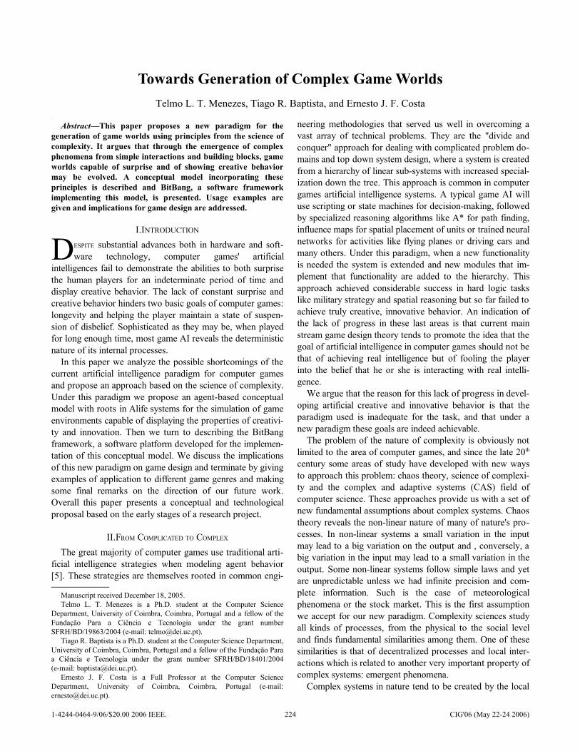
es

Abstract—This paper proposes a new paradigm for the generation of game worlds using principles from the science of complexity. It argues that through the emergence of complex phenomena from simple interactions and building blocks, game worlds capable of surprise and of showing creative behavior may be evolved. A conceptual model incorporating these principles is described and BitBang, a software framework implementing this model, is presented. Usage examples are given and implications for game design are addressed.

I.INTRODUCTION

ESPITE substantial advances both in hardware and soft-ware technology, computer games' artificial

intelligences fail to demonstrate the abilities to both surprise the human players for an indeterminate period of time and display creative behavior. The lack of constant surprise and creative behavior hinders two basic goals of computer games: longevity and helping the player maintain a state of suspen-sion of disbelief. Sophisticated as they may be, when played for long enough time, most game AI reveals the deterministic nature of its internal processes.

D

In this paper we analyze the possible shortcomings of the current artificial intelligence paradigm for computer games and propose an approach based on the science of complexity. Under this paradigm we propose an agent-based conceptual model with roots in Alife systems for the simulation of game environments capable of displaying the properties of creativi-ty and innovation. Then we turn to describing the BitBang framework, a software platform developed for the implemen-tation of this conceptual model. We discuss the implications of this new paradigm on game design and terminate by giving examples of application to different game genres and making some final remarks on the direction of our future work. Overall this paper presents a conceptual and technological proposal based on the early stages of a research project.

II.FROM COMPLICATED TO COMPLEX

The great majority of computer games use traditional arti-ficial intelligence strategies when modeling agent behavior [5]. These strategies are themselves rooted in common engi-

Manuscript received December 18, 2005. Telmo L. T. Menezes is a Ph.D. student at the Computer Science

Department, University of Coimbra, Coimbra, Portugal and a fellow of the Fundação Para a Ciência e Tecnologia under the grant number SFRH/BD/19863/2004 (e-mail: telmo@dei.uc.pt).

Tiago R. Baptista is a Ph.D. student at the Computer Science Department, University of Coimbra, Coimbra, Portugal and a fellow of the Fundação Para a Ciência e Tecnologia under the grant number SFRH/BD/18401/2004 (e-mail: baptista@dei.uc.pt).

Ernesto J. F. Costa is a Full Professor at the Computer Science Department, University of Coimbra, Coimbra, Portugal (e-mail: ernesto@dei.uc.pt).

neering methodologies that served us well in overcoming a vast array of technical problems. They are the "divide and conquer" approach for dealing with complicated problem do-mains and top down system design, where a system is created from a hierarchy of linear sub-systems with increased special-ization down the tree. This approach is common in computer games artificial intelligence systems. A typical game AI will use scripting or state machines for decision-making, followed by specialized reasoning algorithms like A* for path finding, influence maps for spatial placement of units or trained neural networks for activities like flying planes or driving cars and many others. Under this paradigm, when a new functionality is needed the system is extended and new modules that im-plement that functionality are added to the hierarchy. This approach achieved considerable success in hard logic tasks like military strategy and spatial reasoning but so far failed to achieve truly creative, innovative behavior. An indication of the lack of progress in these last areas is that current main stream game design theory tends to promote the idea that the goal of artificial intelligence in computer games should not be that of achieving real intelligence but of fooling the player into the belief that he or she is interacting with real intelli-gence.

We argue that the reason for this lack of progress in devel-oping artificial creative and innovative behavior is that the paradigm used is inadequate for the task, and that under a new paradigm these goals are indeed achievable.

The problem of the nature of complexity is obviously not limited to the area of computer games, and since the late 20th

century some areas of study have developed with new ways to approach this problem: chaos theory, science of complexi-ty and the complex and adaptive systems (CAS) field of computer science. These approaches provide us with a set of new fundamental assumptions about complex systems. Chaos theory reveals the non-linear nature of many of nature's pro-cesses. In non-linear systems a small variation in the input may lead to a big variation on the output and , conversely, a big variation in the input may lead to a small variation in the output. Some non-linear systems follow simple laws and yet are unpredictable unless we had infinite precision and com-plete information. Such is the case of meteorological phenomena or the stock market. This is the first assumption we accept for our new paradigm. Complexity sciences study all kinds of processes, from the physical to the social level and finds fundamental similarities among them. One of these similarities is that of decentralized processes and local inter-actions which is related to another very important property of complex systems: emergent phenomena.

Complex systems in nature tend to be created by the local

Towards Generation of Complex Game WorldsTelmo L. T. Menezes, Tiago R. Baptista, and Ernesto J. F. Costa

1-4244-0464-9/06/$20.00 2006 IEEE. 224 CIG'06 (May 22-24 2006)

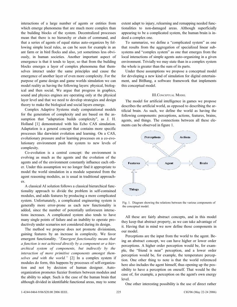
interactions of a large number of agents or entities from which emerge phenomena that are much more complex than the building blocks of the system. Decentralized processes mean that there is no hierarchy or chain of command, and that a series of agents of equal status auto-organizes by fol-lowing simple local rules, as can be seen for example in an ant farm or in bird flocks and also, yet sometimes less obvi-ously, in human societies. Another important aspect of emergence is that it tends to layer, so that from the building blocks emerges a layer of complex phenomena that them-selves interact under the same principles and cause the emergence of another layer of even more complexity. For the purpose of game design and game worlds simulation we can model reality as having the following layers: physical, biolog-ical and then social. We argue that progress in graphics, sound and physics engines are operating only at the physical layer level and that we need to develop strategies and design theory to make the biological and social layers emerge.

Complex Adaptive Systems study computational models for the generation of complexity and are based on the as-sumption that "adaptation builds complexity", as J. H. Holland [1] demonstrated with his Echo CAS simulation. Adaptation is a general concept that contains more specific processes like darwinist evolution and learning. On a CAS, evolutionary pressure and/or learning processes on a co-evo-lutionary environment push the system to new levels of complexity.

Co-evolution is a central concept: the environment is evolving as much as the agents and the evolution of the agents and of the environment constantly influence each oth-er. Under this assumption we no longer find it appropriate to model the world simulation in a module separated from the agent reasoning modules, as is usual in traditional approach-es.

A classical AI solution follows a classical hierarchical func-tionality approach to divide the problem in self-contained modules, and adds features by producing a more complicated system. Unfortunately, a complicated engineering system is generally more error-prone as each new functionality is added, since the number of potentially unforeseen interac-tions increases. A complicated system also tends to have many single points of failure and an inability to operate pro-ductively under scenarios not considered during its design.

The method we propose does not promote divisionism, gaining features by an increase in complexity. We favor emergent functionality. “Emergent functionality means that a function is not achieved directly by a component or a hier-archical system of components, but indirectly by the interaction of more primitive components amongst them-selves and with the world.” [2] In a complex system if modules do form, this happens by processes of self-organiza-tion and not by decision of human designer. Auto-organization promotes fuzzier frontiers between modules and the ability to adapt. Such is the case of the human brain that although divided in identifiable functional areas, may to some

extent adapt to injury, relearning and remapping needed func-tionalities to non-damaged areas. Although superficially appearing to be a complicated system, the human brain is in-deed a complex one.

To summarize, we define a “complicated system” as one that results from the aggregation of specialized linear sub-systems and “complex system” as one that emerges from the local interactions of simple agents auto-organizing in a given environment. Trivially we may state than in a complex system the whole is greater than the sum of its parts.

Under these assumptions we propose a conceptual model for developing a new kind of simulation for digital entertain-ment, and BitBang, a software framework that implements this conceptual model.

III.CONCEPTUAL MODEL

The model for artificial intelligence in games we propose describes the artificial world, as opposed to describing the ar-tificial brain. As such, we define the world as having the following components: perceptions, actions, features, brains, agents, and things. The connections between all these ele-ments can be observed in figure 1.

All these are fairly abstract concepts, and in this model they keep that abstract property, as we can take advantage of it. Having that in mind we now define those components in our model.

Perceptions are the input from the world to the agent. Be-ing an abstract concept, we can have higher or lower order perceptions. A higher order perception would be, for exam-ple, the “friend is near” perception, and a lower order perception would be, for example, the temperature percep-tion. One other thing to note is that the world referenced here also includes the agent himself, thus opening up the pos-sibility to have a perception on oneself. That would be the case of, for example, a perception on the agent's own energy level.

One other interesting possibility is the use of direct rather

Fig. 1. Diagram showing the relations between the various components of the conceptual model.

1-4244-0464-9/06/$20.00 2006 IEEE. 225 CIG'06 (May 22-24 2006)

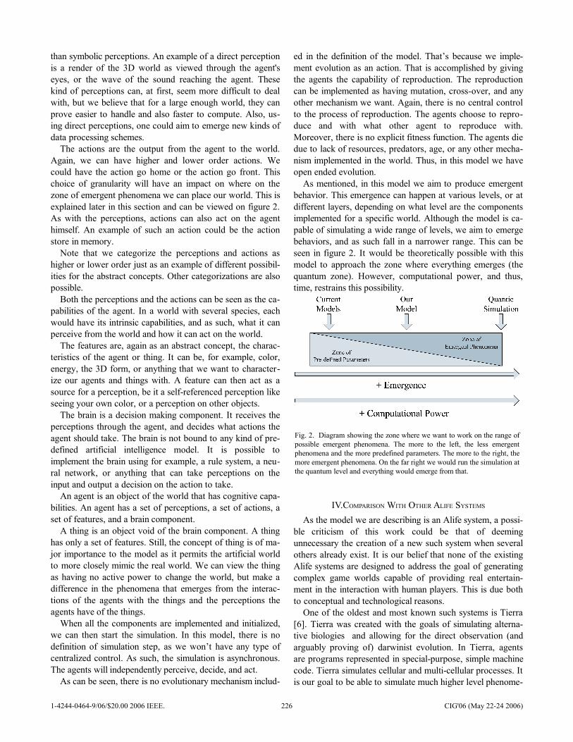
than symbolic perceptions. An example of a direct perception is a render of the 3D world as viewed through the agent's eyes, or the wave of the sound reaching the agent. These kind of perceptions can, at first, seem more difficult to deal with, but we believe that for a large enough world, they can prove easier to handle and also faster to compute. Also, us-ing direct perceptions, one could aim to emerge new kinds of data processing schemes.

The actions are the output from the agent to the world. Again, we can have higher and lower order actions. We could have the action go home or the action go front. This choice of granularity will have an impact on where on the zone of emergent phenomena we can place our world. This is explained later in this section and can be viewed on figure 2. As with the perceptions, actions can also act on the agent himself. An example of such an action could be the action store in memory.

Note that we categorize the perceptions and actions as higher or lower order just as an example of different possibil-ities for the abstract concepts. Other categorizations are also possible.

Both the perceptions and the actions can be seen as the ca-pabilities of the agent. In a world with several species, each would have its intrinsic capabilities, and as such, what it can perceive from the world and how it can act on the world.

The features are, again as an abstract concept, the charac-teristics of the agent or thing. It can be, for example, color, energy, the 3D form, or anything that we want to character-ize our agents and things with. A feature can then act as a source for a perception, be it a self-referenced perception like seeing your own color, or a perception on other objects.

The brain is a decision making component. It receives the perceptions through the agent, and decides what actions the agent should take. The brain is not bound to any kind of pre-defined artificial intelligence model. It is possible to implement the brain using for example, a rule system, a neu-ral network, or anything that can take perceptions on the input and output a decision on the action to take.

An agent is an object of the world that has cognitive capa-bilities. An agent has a set of perceptions, a set of actions, a set of features, and a brain component.

A thing is an object void of the brain component. A thing has only a set of features. Still, the concept of thing is of ma-jor importance to the model as it permits the artificial world to more closely mimic the real world. We can view the thing as having no active power to change the world, but make a difference in the phenomena that emerges from the interac-tions of the agents with the things and the perceptions the agents have of the things.

When all the components are implemented and initialized, we can then start the simulation. In this model, there is no definition of simulation step, as we won’t have any type of centralized control. As such, the simulation is asynchronous. The agents will independently perceive, decide, and act.

As can be seen, there is no evolutionary mechanism includ-

ed in the definition of the model. That’s because we imple-ment evolution as an action. That is accomplished by giving the agents the capability of reproduction. The reproduction can be implemented as having mutation, cross-over, and any other mechanism we want. Again, there is no central control to the process of reproduction. The agents choose to repro-duce and with what other agent to reproduce with. Moreover, there is no explicit fitness function. The agents die due to lack of resources, predators, age, or any other mecha-nism implemented in the world. Thus, in this model we have open ended evolution.

As mentioned, in this model we aim to produce emergent behavior. This emergence can happen at various levels, or at different layers, depending on what level are the components implemented for a specific world. Although the model is ca-pable of simulating a wide range of levels, we aim to emerge behaviors, and as such fall in a narrower range. This can be seen in figure 2. It would be theoretically possible with this model to approach the zone where everything emerges (the quantum zone). However, computational power, and thus, time, restrains this possibility.

IV.COMPARISON WITH OTHER ALIFE SYSTEMS

As the model we are describing is an Alife system, a possi-ble criticism of this work could be that of deeming unnecessary the creation of a new such system when several others already exist. It is our belief that none of the existing Alife systems are designed to address the goal of generating complex game worlds capable of providing real entertain-ment in the interaction with human players. This is due both to conceptual and technological reasons.

One of the oldest and most known such systems is Tierra [6]. Tierra was created with the goals of simulating alterna-tive biologies and allowing for the direct observation (and arguably proving of) darwinist evolution. In Tierra, agents are programs represented in special-purpose, simple machine code. Tierra simulates cellular and multi-cellular processes. It is our goal to be able to simulate much higher level phenome-

Fig. 2. Diagram showing the zone where we want to work on the range of possible emergent phenomena. The more to the left, the less emergent phenomena and the more predefined parameters. The more to the right, the more emergent phenomena. On the far right we would run the simulation at the quantum level and everything would emerge from that.

1-4244-0464-9/06/$20.00 2006 IEEE. 226 CIG'06 (May 22-24 2006)

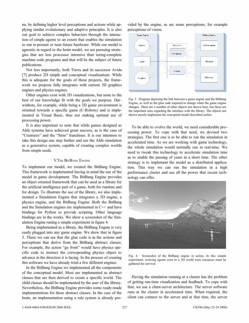
na, by defining higher level perceptions and actions while ap-plying similar evolutionary and adaptive principles. It is also out goal to achieve complex behaviors through the interac-tion of simple agents to an extent that enables the simulation to run in present or near-future hardware. While our model is agnostic in regard to the brain model, we are pursuing strate-gies that are less processor intensive than turing-complete machine code programs and that will be the subject of future publications.

Not less importantly, both Tierra and its successor Avida [7] produce 2D simple and conceptual visualizations. While this is adequate for the goals of these projects, the frame-work we propose fully integrates with current 3D graphics engines and physics engines.

Other engines exist with 3D visualizations, but none to the best of our knowledge fit with the goals we purpose. Dar-winbots, for example, while being a 3D game environment is oriented towards a specific game (C-Robots) and is imple-mented in Visual Basic, thus not making optimal use of processing power.

It is also important to note that while games designed as Alife systems have achieved great success, as is the case of “Creatures” and the “Sims” franchises. It is our intention to take this design one step further and use the Alife simulation as a generative system, capable of creating complex worlds from simple seeds.

V.THE BITBANG ENGINE

To implement our model, we created the BitBang Engine. This framework is implemented having in mind the use of the model in game development. The BitBang Engine provides an object oriented framework that can be used as a library for the artificial intelligence part of a game, both for runtime and for design. To illustrate the use of the library, we also imple-mented a Simulation Engine that integrates a 3D engine, a physics engine, and the BitBang Engine. Both the BitBang and the Simulation engines are implemented in C++ and have bindings for Python to provide scripting. Other language bindings are in the works. We show a screenshot of the Sim-ulation Engine runing a simple experiment in figure 4.

Being implemented as a library, the BitBang Engine is very easily plugged into any game engine. We show that in figure 3. There we can see that the glue code is in the actions and perceptions that derive from the BitBang abstract classes. For example, the action “go front” would have physics spe-cific code to instruct the corresponding physics object to advance in the direction it is facing. In the process of creating this software we have already tried a few different engines.

In the BitBang Engine we implemented all the components of the conceptual model. Most are implemented as abstract classes that are then derived to create a specific world. The child classes should be implemented by the user of the library. Nevertheless, the BitBang Engine provides some ready-made implementations for these abstract classes. In the case of the brain, an implementation using a rule system is already pro-

vided by the engine, as are some perceptions, for example perceptions of vision.

To be able to evolve the world, we need considerable pro-cessing power. To cope with that need, we devised two strategies. The first one is to be able to run the simulation in accelerated time. As we are working with game technology, the whole simulation would normally run in real-time. We need to tweak this technology to accelerate simulation time as to enable the passing of years in a short time. The other strategy is to implement the model as a distributed applica-tion. This way we can run the simulation in a high performance cluster and use all the power that recent tech-nology can offer.

Having the simulation running at a cluster has the problem of getting run-time visualization and feedback. To cope with that, we use a client-server architecture. The server software runs at the cluster in accelerated time. When required, the client can connect to the server and at that time, the server

Fig. 3. Diagram depicting the link between a game engine and the BitBang Engine, as well as the glue code required to change when the game engine changes. There are a number of other objects not shown here, but these are the important ones regarding the interface with the library. The objects not shown merely implement the conceptual model described earlier.

Fig. 4. Screenshot of the BitBang engine in action. In this simple experiment, evolving agents exist in a 3D world were resources must be gathered for survival.

1-4244-0464-9/06/$20.00 2006 IEEE. 227 CIG'06 (May 22-24 2006)

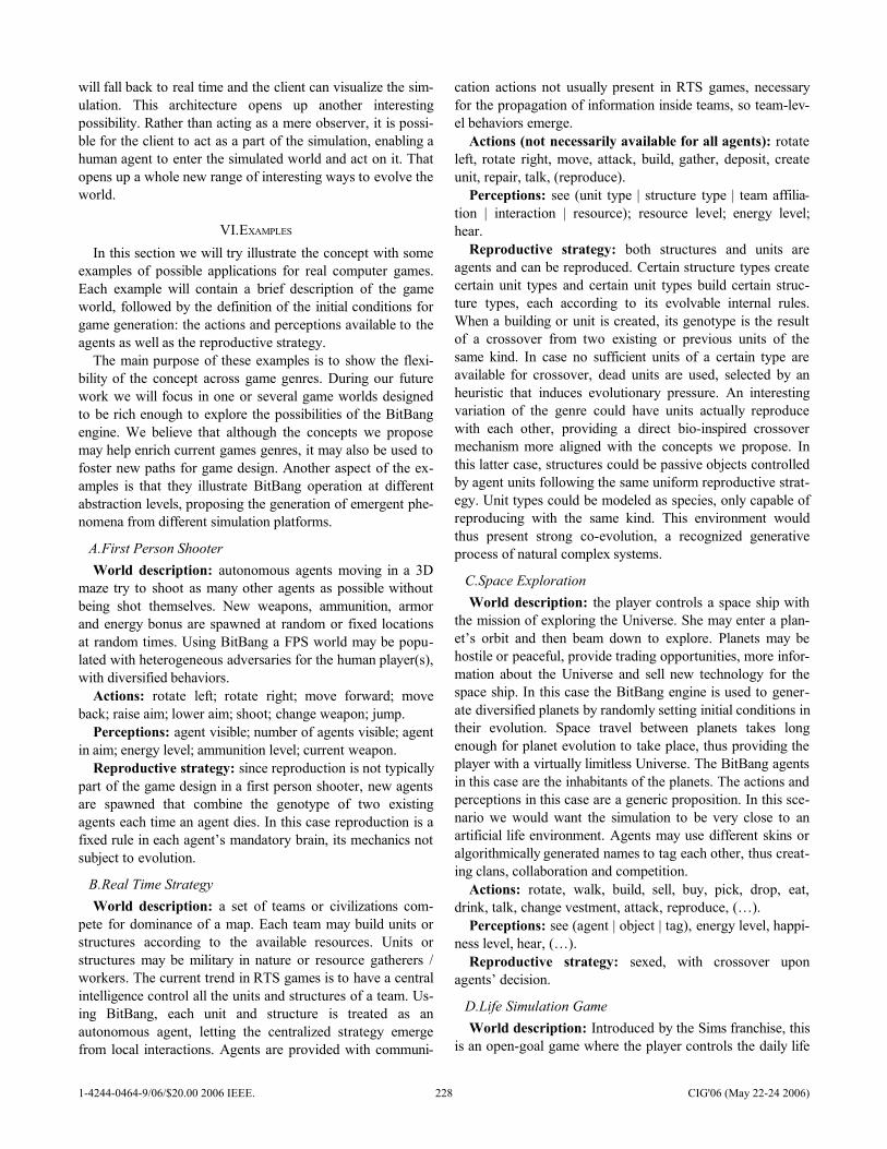
will fall back to real time and the client can visualize the sim-ulation. This architecture opens up another interesting possibility. Rather than acting as a mere observer, it is possi-ble for the client to act as a part of the simulation, enabling a human agent to enter the simulated world and act on it. That opens up a whole new range of interesting ways to evolve the world.

VI.EXAMPLES

In this section we will try illustrate the concept with some examples of possible applications for real computer games. Each example will contain a brief description of the game world, followed by the definition of the initial conditions for game generation: the actions and perceptions available to the agents as well as the reproductive strategy.

The main purpose of these examples is to show the flexi-bility of the concept across game genres. During our future work we will focus in one or several game worlds designed to be rich enough to explore the possibilities of the BitBang engine. We believe that although the concepts we propose may help enrich current games genres, it may also be used to foster new paths for game design. Another aspect of the ex-amples is that they illustrate BitBang operation at different abstraction levels, proposing the generation of emergent phe-nomena from different simulation platforms.

A.First Person ShooterWorld description: autonomous agents moving in a 3D

maze try to shoot as many other agents as possible without being shot themselves. New weapons, ammunition, armor and energy bonus are spawned at random or fixed locations at random times. Using BitBang a FPS world may be popu-lated with heterogeneous adversaries for the human player(s), with diversified behaviors.

Actions: rotate left; rotate right; move forward; move back; raise aim; lower aim; shoot; change weapon; jump.

Perceptions: agent visible; number of agents visible; agent in aim; energy level; ammunition level; current weapon.

Reproductive strategy: since reproduction is not typically part of the game design in a first person shooter, new agents are spawned that combine the genotype of two existing agents each time an agent dies. In this case reproduction is a fixed rule in each agent’s mandatory brain, its mechanics not subject to evolution.

B.Real Time StrategyWorld description: a set of teams or civilizations com-

pete for dominance of a map. Each team may build units or structures according to the available resources. Units or structures may be military in nature or resource gatherers / workers. The current trend in RTS games is to have a central intelligence control all the units and structures of a team. Us-ing BitBang, each unit and structure is treated as an autonomous agent, letting the centralized strategy emerge from local interactions. Agents are provided with communi-

cation actions not usually present in RTS games, necessary for the propagation of information inside teams, so team-lev-el behaviors emerge.

Actions (not necessarily available for all agents): rotate left, rotate right, move, attack, build, gather, deposit, create unit, repair, talk, (reproduce).

Perceptions: see (unit type | structure type | team affilia-tion | interaction | resource); resource level; energy level; hear.

Reproductive strategy: both structures and units are agents and can be reproduced. Certain structure types create certain unit types and certain unit types build certain struc-ture types, each according to its evolvable internal rules. When a building or unit is created, its genotype is the result of a crossover from two existing or previous units of the same kind. In case no sufficient units of a certain type are available for crossover, dead units are used, selected by an heuristic that induces evolutionary pressure. An interesting variation of the genre could have units actually reproduce with each other, providing a direct bio-inspired crossover mechanism more aligned with the concepts we propose. In this latter case, structures could be passive objects controlled by agent units following the same uniform reproductive strat-egy. Unit types could be modeled as species, only capable of reproducing with the same kind. This environment would thus present strong co-evolution, a recognized generative process of natural complex systems.

C.Space ExplorationWorld description: the player controls a space ship with

the mission of exploring the Universe. She may enter a plan-et’s orbit and then beam down to explore. Planets may be hostile or peaceful, provide trading opportunities, more infor-mation about the Universe and sell new technology for the space ship. In this case the BitBang engine is used to gener-ate diversified planets by randomly setting initial conditions in their evolution. Space travel between planets takes long enough for planet evolution to take place, thus providing the player with a virtually limitless Universe. The BitBang agents in this case are the inhabitants of the planets. The actions and perceptions in this case are a generic proposition. In this sce-nario we would want the simulation to be very close to an artificial life environment. Agents may use different skins or algorithmically generated names to tag each other, thus creat-ing clans, collaboration and competition.

Actions: rotate, walk, build, sell, buy, pick, drop, eat, drink, talk, change vestment, attack, reproduce, (…).

Perceptions: see (agent | object | tag), energy level, happi-ness level, hear, (…).

Reproductive strategy: sexed, with crossover upon agents’ decision.

D.Life Simulation GameWorld description: Introduced by the Sims franchise, this

is an open-goal game where the player controls the daily life

1-4244-0464-9/06/$20.00 2006 IEEE. 228 CIG'06 (May 22-24 2006)

of a person or family in its mundane aspects, interacting with other AI controlled persons in the game world. The Sims game is a notable example of a new paradigm game, incorpo-rating already some of the concepts we describe. This genre is perfectly suited for the introduction of co-evolutionary generative strategies.

Actions: rotate, walk, buy, pick, drop, eat, act upon, talk, change clothes, reproduce, sleep, (…).

Perceptions: energy, cleanliness, environment light level, sleepiness, hunger level, time of day, blather level, see (agent | object | tag), (…).

Reproductive strategy: sexed, with crossover upon agen-t's decision.

VII.IMPLICATIONS FOR GAME DESIGN

A change in paradigm like the one we describe in this pa-per has important implications in game design strategies. We claim that to achieve real surprising, creative and innovative behavior in game agents, the level of control that the design-ers have over the game must be lowered. We also claim that such a system will have the ability to surprise the game de-signer herself, and that attempts to exert greater control over the system will limit its capacity to reach the goals we pro-pose. This happens because under a model where simple processes auto-organize to cause the emergence of a layer of more complex behavior, the full understanding of the individ-ual workings of the simple processes will not imply the full understanding of the emergent layer of complexity. Although this may appear to be a shortcoming of our model, it is in-deed the property that makes it succeed. We can not expect to be surprised by a system we fully understand. Note that the degree to which each agent is a black box depends great-ly on the brain algorithm being used. A rule list exposes its internal processes to a human observer so she can easily un-derstand the results of evolution on a given experience, but a neural network may prove much more difficult to decode. Also note that even when we understand the individual work-ings of an agent, we may not be able to fully grasp the emergent phenomena that derive from a large number of in-teractions.

Under our model the game designer will not design the world, but instead design the seed that will generate the world. These seeds consist of the basic laws of the world, and of the set of actions, perceptions and features available to the agents. The design process will consist of a loop of defin-ing the seed, allowing the world to evolve, evaluate the results and then redefine or tweak the seed and iterate until the end result is satisfying. The definition of the seed is a new method in game design that needs to be studied. Studying seed design methodologies is one of the current focuses of our work.

In a complex simulation, quality control through exhaus-tive test cases is not feasible. Two concepts that are central to emergent complex phenomena are positive and negative feedback. Positive feedback tends to exaggerate a phe-

nomenon over time while negative feedback tends to attenu-ate it. Negative feedback is typically used in classical engineering for control systems. Uncontrolled positive feed-back is often dangerous and potentially destructive to a system. During the evaluation design phase, these two con-cepts may be used to analyze the system and access its stability for the purpose of the game. It should be noted that although the possibility of exhaustive testing of the system is lost, auto-organizative systems tend by its very nature to be very resistant to unexpected situations and have the property of graceful degradation. This means that a failure or destruc-tion of a component of the system will not cause it to fail but only to degrade its quality to some extent. Failure is only reached when a critical percentage of the system's building blocks are compromised.

Another interesting consequence of this model is the possi-bility of incorporating evolution in the game itself. This could be done in several ways. In a god-like game we may let the player tweak basic world rules and thus influence global evo-lution. In a first or third-person game we may let the player influence individual agents, altering their learning or survival chances and thus influencing global evolution from the prop-agation of the effects of local interactions.

VIII.FINAL REMARKS

The work presented in this paper is in progress since late 2004 and this is the first paper presenting the ideas, models and software produced by the work. We are now in the state of having a stable version of the BitBang Engine. The Simu-lation Engine is in active development and near ready to produce the first large scale experiments and scenarios.

In the future, the BitBang Engine will include more bind-ings for other languages, for example for .NET, enabling the use of a large range of languages like C#, Boo, Lisp, and many others. We also aim to provide more ready-made final classes for the easier creation of common experiments.

We will also experiment and study specific design strate-gies for games.

REFERENCES

[1] J. H. Holland, Hidden Order – How adaptation builds complexity. Helix Books, 1995.

[2] L. Steels, “Towards a Theory of Emergent Functionality” in J.-A. Meyer and S. W. Wilson (eds) From Animals to Animats: Proceedings of the First International Conference on Simulation of Adaptive Behaviour, Cambridge, MA: The MIT Press, 1990, pp. 451–461.

[3] S. Wolfram, A New Kind of Science. Wolfram Media, Inc., 2002.[4] Per Bak, How Nature Works – The Science of Self-Organized

Criticality. Oxford University Press, 1997.[5] Steve Rabin et al, AI Game Programming Wisdom. Charles River

Media, 2002.[6] Ray, T. S, “Overview of Tierra at ATR” in Technical Information,

No.15, Technologies for Software Evolutionary Systems, Kyoto, Japan, ATR-HIP, 2001.

[7] C. Adami and C.T. Brown, “Evolutionary Learning in the 2D Artificial Life Systems Avida”, in Proceedings of Artificial Life IV, R. Brooks, P. Maes, Eds., MIT Press p. 377-381, 1994.

1-4244-0464-9/06/$20.00 2006 IEEE. 229 CIG'06 (May 22-24 2006)

The Blondie25 Chess Program Competes Against Fritz 8.0 and a Human Chess Master

David B. Fogel Timothy J. Hays Sarah L. Hahn

James Quon Natural Selection, Inc.

3333 N. Torrey Pines Ct., Suite 200 La Jolla, CA 92037 USA

dfogel@natural-selection.com

Abstract- Previous research on the use of coevolution to improve a baseline chess program demonstrated a performance rating of 2650 against Pocket Fritz 2.0 based on 16 games played (13 wins, 0 losses, 3 draws). The resultant program, named Blondie25, did not use any rules for managing the time allocated per move; it simply used three minutes on each move. Heuristics to more effectively manage time were developed by trial and error, play testing against Fritz 8.0. The best heuristics discovered were different for black and white. The results of 12 games played on each side were 1 win, 4 losses, and 7 draws for black, and 2 wins, 6 losses, and 4 draws for white. Fritz 8.0 is rated currently at 2752 (±20) on SSDF (the acronym for the Swedish Chess Computer Association), placing it as the 12th strongest program in the world. At the time of the contest between Blondie25 and Fritz 8.0, Fritz 8.0 was rated #5 in the world. The results are the first case of an evolved chess program defeating a world-class chess program (three times). The performance rating for Blondie25 against Fritz 8.0 was 2635.33, which compares well with the previous performance rating of 2650 against Pocket Fritz 2.0. Blondie25 was then tested against a nationally ranked human chess master, rated 2301. In four games, Blondie25 won three and lost one.

1 Introduction and Background

As noted in [1], chess has served as a testing ground for efforts in artificial intelligence, both in terms of computers playing against other computers, and computers playing against humans for more than 50 years [2-9]. This paper reports on progress in testing the self-learning evolutionary chess program, named Blondie25. (A similar protocol for learning to play checkers was named Blondie24 [10]). Results reported in [11] indicated that the evolved program earned a 16-game performance rating of 2650 against Pocket Fritz 2.0, rated between 2300-2350, with 13 wins, 0 losses, and 3 draws.

Blondie25 is the result of 7462 generations of evolution in self-play in which the static board evaluator was evolved, including material values, positional values, and three object neural networks (front, back, and center of the chessboard). Moves are selected based on minimax with alpha-beta pruning. Readers interested in background on the development of the program should review [11]. One of the limitations of the Blondie25 program is that it has not evolved (because it has not been allowed to evolve) the use of time per move as a facet of play. Instead, it has devoted an equal amount of time for each move, regardless of the current situation or history of moves. For tournament conditions, three minutes per move have been used. An effort was made to incorporate simple heuristics for using time more effectively. Performance was judged on competitions with Fritz 8.0, a highly rated chess program that was in the top five of all chess programs rated on [12] at the time of our testing. Fritz 8.0 is currently ranked as the 11th best program in the world. The approach undertaken was to reflect the time control management in Fritz 8.0, while also taking into account whether or not a move made by Fritz 8.0 was anticipated. Anticipated moves suggest that prior searching was effective in gaining insight into future play; unanticipated moves suggest that more time may be required to search a branch of the game tree that was not appreciated. 2 Heuristics for Time Management

Experimentation in 153 games (some of which crashed mid-play) yielded two different sets of heuristics for time management for Blondie25 playing black or white.1 It may be helpful to recall that 120 minutes are allocated for the first 40 moves (first time period), 60 minutes are allocated for the next 20 moves (second time period), and 30 minutes are allocated for all remaining moves. 1 During this experimentation, it was verified that allowing Blondie25 to use a constant time per move resulted in poor performance against Fritz 8.0.

1-4244-0464-9/06/$20.00 2006 IEEE. 230 CIG'06 (May 22-24 2006)

The heuristics were chosen for black are presented in the following algorithm, where Ft is the amount of time used by Fritz 8.0 on the previous move and x is Blondie25’s time:

1. If Fritz 8.0’s move was anticipated, then x = Ft – 10 seconds, but not less than 20 seconds.

2. If Fritz 8.0’s move was unanticipated, then if: a. Ft < 3 minutes, x = Ft + 1 minute b. 3 < Ft < 5 minutes, x = Ft + 2 minutes c. Ft > 5 minutes, x = Ft + 4 minutes

3. Regardless of whether or not Fritz 8.0’s move was anticipated, if Ft > 8, then x = Ft + 3 minutes.

4. In addition, if Blondie25 is down on pawns but not other pieces then add 1 minute to x. If Blondie25 is down on pieces other than pawns, add 4 minutes to x. If Blondie25 is down both pawns and pieces, set x = 10 minutes.

5. After leaving the opening book, for the first three moves, x = 20 seconds.

6. For the fourth move out of the book, x = 10 minutes.

7. For the 41st move, which begins the second period of time control, x = 8 minutes.

8. If the duration assigned for any move would cause an overtime condition or leave fewer than 20 seconds for each remaining move, then x is set to the ratio of the time remaining to the number of moves remaining in the time period.

Rules 2 and 3 above applied to the first and second time periods. The heuristics for white were similar, but simpler: 1. If Fritz 8.0’s move was anticipated, then x = Ft –

10 seconds, but not less than 20 seconds. 2. If Fritz 8.0’s move was unanticipated, then if:

a. Ft < 3 minutes, x = Ft + 1 minute b. 3 < Ft < 5 minutes, x = Ft + 2 minutes c. Ft > 5 minutes, x = Ft + 4 minutes

3. Regardless of whether or not Fritz 8.0’s move was anticipated, if Ft > 8, then x = Ft + 3.

4. For the first three moves out of the opening book, x = 20 seconds.

5. If the duration assigned for any move would causes an overtime condition or leave fewer than 20 seconds for each remaining move, then x is set to the ratio of the time remaining to the number of moves remaining in the time period.

It is unclear presently why the effects of the additional black rules were helpful for playing black but not white. The rationale for some of the rules can be offered; however, the values assigned for time periods only reflect the results of experimentation and no claim of optimality should be inferred.

The baseline for 20 seconds/move was arbitrary. Using less time than Fritz 8.0 used when Fritz 8.0’s move was anticipated assisted in saving time for situations that were unanticipated. In such situations, the longer that Fritz 8.0 used to find its move suggests a deeper required search. For black, more time is provided when Blondie25 is playing behind; however, testing with this strategy for white did not evidence any tangible benefits. Also for black, extra time is provided at the beginning of play (fourth move out of the book) to provide an initial deeper search, and at the beginning of the second time period, but it is not entirely clear why this may be effective for black. Both Fritz 8.0 and Blondie25 were executed using a Pentium II processor running at 1.5GHz with 512MB of RAM. The SSDF (Swedish Chess Computer Association) rating of 2752±20 of for Fritz 8.0 was based on a Athlon 1200MHz with 256MB of RAM. Thus, the computing equipment used was slightly more powerful than used by SSDF. Fritz 8.0 was run using default parameters on the Fritz 8.0 engine, which includes a hashtable size of 409 MB, contempt value, selectivity, tablebase depth, agressiveness, the “permanent brain,” five-piece perfect endings, and so forth.

3 Results Twenty-four games were played between Blondie25 and Fritz 8.0 with the above-described heuristics for time management. An equal number (12) of games were played with Blondie25 as black and as white. The results were 1 win, 4 losses, and 7 draws for Blondie25 as black, and 2 wins, 6 losses, and 4 draws as white. Thus, the overall performance was 3 wins, 10 losses, and 11 draws. Given Fritz 8.0’s current rating [10] of 2752, this corresponds to a performance rating for Blondie25 of 2635, commensurate with grand masters. We believe this is the first result of chess program that was optimized using evolutionary algorithms that was able to defeat a (then) top-5 chess program (now ranked 11 on [10]). Following this contest, it was desired to compete Blondie25 against a competent human player. It is well known that computer chess programs do not play in the same manner that human masters and grand masters do, and that rating earned solely in comparison to other computer programs may not reflect ratings earned against human competition. Co-author James Quon, a nationally ranked chess master, played a four-game series against Blondie25 (two as black, two as white). The program won three of the four games and lost the other, earning a performance rating of 2501. 4 Discussion Co-author James Quon, a nationally ranked chess master, analyzed each of the 24 games against Fritz 8.0. His

1-4244-0464-9/06/$20.00 2006 IEEE. 231 CIG'06 (May 22-24 2006)

assessment is that the match between the two programs was very competitive, where the programs seemed more closely matched than the score would indicate. The opening phase of the game is still a weak point for Blondie25, not only because it does not have knowledge of the theoretical variations but it would also often maneuver pieces in apparently mysterious ways other than simply developing the pieces. Multiple bad openings were played repeatedly, so this handicap was manifested multiple times. The quality of the openings was varied. Some extremely poor lines were chosen, but there were other games in which the program would go deep into chess theory. Of note was one game in which an early queen check should likely not be found in Fritz 8.0’s normal opening book, since it is judged to be a poor move; however, we verified that the default opening book was indeed in use in all games. In contrast, there were many instances in which Blondie25 was able to achieve a superior endgame. At times, it appeared that Fritz 8.0 was not playing with the use of an endgame database, but Blondie25 was unable to convert the advantage of poor play and would have won more games if it had been able. There were, however, missed opportunities by both sides in the endgames. There were theoretical endings that were not winnable, but the programs (both Blondie25 and Fritz 8.0) readily cashed in their middlegame advantages to enter these endgames because they did not realize that although the endings gave them a mathematical advantage, this advantage could not be converted into a win. James Quon’s analysis of each of the 24 games is posted at www.natural-selection.com/b25vf8.html. James Quon also analyzed the four games that he played against Blondie25. His assessment of these games is offered in the appendix and also appears at www.natural-selection.com/b25vjquon.html.

5 Conclusions

The good use of time in chess can provide a significant advantage over a poor use, or a method that applies an equal amount of time to each situation. Although Blondie25 was able to easily defeat Pocket Fritz 2.0 in an earlier competition without using time management, playing against Fritz 8.0, one of the top programs in the world, required more effective time management. The results of trial-and-error hand tuning of ideas that should assist in time management, which reflect the time management that Fritz 8.0 uses, earned three wins against Fritz 8.0. Although Blondie25 cannot compete evenly versus Fritz 8.0, the performance in 24 games suggests a rating of about 2635. Blondie25’s results against James Quon evidence the first time that an evolved chess program has defeated a human

master. Quon noted, however, that the program’s opening play is often weak and he was able to detect a horizon effect in some games (in which the program can be manipulated because it can only see to a fixed ply depth). Future work will be aimed at offering additional object neural networks to Blondie25 to allow it to learn other features of the chessboard and pieces in coevolutionary self-play, and also incorporating a more meaningful opening book that would ensure a competitive start to matches against strong players. Fritz 8.0 has been optimized in many successive versions of program releases for extremely rapid position evaluation and game tree search. In contrast, very little such optimization has been used in Blondie25. This suggests an opportunity to improve the competitive performance of Blondie25 with software engineering. In addition, performance ratings on small sets of games are inherently variable. It would be of interest to evolve time management rules and determine if more effective rules could be discovered, and to evaluate these rules across a wider array of chess programs and human competitors in a sufficient number of games to provide bounds on the program’s rating that are in line with those offered by the Swedish Chess Computer Association.

Acknowledgments

The authors thank Digenetics, Inc. for use of its chess game engine, and Garry Kasparov for comments on our earlier research. Portions of this paper were reprinted or revised from [1] in accordance with IEEE Copyright procedures. This work was sponsored in part by NSF Grants DMI-0232124 and DMI-0349604. Any opinions, findings and conclusions or recommendations expressed in this material are those of the authors and do not necessarily reflect the views of the National Science Foundation (NSF). The authors thank the reviewers for their important criticisms that improved the paper.

Bibliography

1. Fogel, D.B., Hays, T.J., Hahn, S.L., and Quon, J. (2004) “An Evolutionary Self-Learning Chess Program,” Proceedings of the IEEE, December, pp. 1947-1954. 2. Shannon, C.E. (1950) “Programming a Computer for Playing Chess,” Philosophical Magazine, Vol. 41, pp. 256-275. 3. Turing, A.M. (1953) “Digital Computers Applied to Games,” in Faster than Thought, B.V. Bowden, Ed., London: Pittman, pp. 286-310. 4. Newell, A, Shaw, J.C., and Simon, H.A. (1958) “Chess-Playing Programs and the Problem of Complexity,” IBM J. Res. Dev., Vol. 2, pp. 320-325. 5. Levy, D.N.L. and Newborn, M. (1991) How Computers Play Chess, New York: Computer Science Press, pp. 28-29, 35-39. 6. Cipra, B. (1996) “Will a Computer Checkmate a Chess Champion at Last?” Science, Vol. 271, p. 599.

1-4244-0464-9/06/$20.00 2006 IEEE. 232 CIG'06 (May 22-24 2006)

7. McCarthy, J. (1997) “AI as Sport,” Science, Vol. 276, pp. 1518-1519. 8. Markman, A.B. (2000) “If You Build It, Will It Know?” Science, Vol. 288, pp. 624-625. 9. Holden, C. (2002) “Draw in Bahrain,” Science, Vol. 298, p. 959. 10. Fogel, D.B. (2002) Blondie24: Playing at the Edge of AI, Morgan Kaufmann, San Francisco. 11. Fogel, D.B., Hays, T.J., Hahn, S.L., and Quon, J. (2005) “Further Evolution of a Self-Learning Chess Program,” Proc. 2005 IEEE Symp. Computational Inteligence and Games, G. Kendall and S. Lucas (chairs), IEEE, Piscataway, NJ, pp. 73-77. 12. The Swedish Chess Computer Association publishes ratings of the top 50 computer programs at http://w1.859.telia.com/~u85924109/ssdf/list.htm Appendix This appendix provides annotations by James Quon (a national chess master rated 2301) of a 4-game series between Blondie25 versus Quon, under simulated tournament conditions. Blondie25 plays as black in the first 12 games, and as white in the remaining 12 games.

Standard legend for chess symbols: = equal += slight advantage white =+ slight advantage black +- clear advantage white -+ clear advantage black +-- decisive advantage white --+ decisive advantage black ! good move !! brilliant move ? bad move ?? blunder !? interesting move involving some risk ?! dubious move + check # checkmate 1-0 white wins 0-1 black wins ½-½ draw

Quon, Jim - Blondie [E40] (Game 1) E40: Nimzo-Indian: Rubinstein (4 e3): Unusual Black 4th move. Black plays the opening very slowly, allowing White to gain a space advantage. It does a good job finding defensive maneuvers to hold the position. White misses a chance to push the advantage with 15.g4! allowing Black to play successful break in the center. When the position turns tactical, Blondie is in its element and finds the win. 1.d4 e6 2.c4 Nf6 3.Nc3 Bb4 4.e3 Ne4 This is not considered a serious threat to White. 5.Bd2 Nxd2 6.Qxd2 d5 last book move [6...0–0 7.Nf3 f5 8.Be2 b6 9.a3 Bd6 10.0–0 Bb7 11.b4 Rf6 White gets a space

advantage, while Black has the Bishop pair and chances on the kingside.] 7.a3 [7.Nf3 0–0 8.0–0–0!?] 7...Be7 8.f4 I wanted to create a closed position which in general is a computer's weak point. [8.cxd5 exd5 9.Bd3 c6 10.Nf3 0–0 11.0–0 is about equal.] 8...Nc6 [Blocking the c-pawn. More active is 8...dxc4 9.Nf3 c5 10.Bxc4 cxd4 11.exd4 0–0 12.0–0 Nc6] 9.c5 [9.cxd5? exd5 straddle white with a backward pawn on the now open e-file.] 9...Bh4+? wastes time. Black played very slowly allowing White free development. 10.g3 Bf6 11.Nf3 b6 12.b4 [also playable is 12.cxb6 cxb6 13.Bb5 Bb7 14.Ne5 Rc8 15.Nxc6 Bxc6 16.Bxc6+ Rxc6] 12...bxc5 13.bxc5 g6 14.Rb1 [14.Ne5 Nxe5 (14...Bxe5 15.fxe5 f6 16.Bb5 Bd7 17.exf6 Qxf6 18.Rf1 Qe7 +=) 15.fxe5 Bg7 16.Bb5+ Bd7 17.Bxd7+ Qxd7 18.0–0 0–0 19.Rab1 f6 20.exf6 Rxf6 21.Rxf6 Bxf6=; 14.g4 h6 15.h4 Na5 =+] 14...Ne7 [14...Bd7 15.e4!? dxe4 16.Nxe4 Bg7 17.Bg2 0–0 18.0–0 with complications that should favor White because of his active pieces and space advantage.] 15.Bd3 [15.Be2 Bg7 16.0–0 f6 17.e4 dxe4 18.Nxe4 0–0 19.Bc4 Nd5 20.Rfe1 Rf7=; 15.g4!? Bg7 16.h4 (16.g5 h6 17.Bd3 hxg5 18.fxg5 Nf5 =+) 16...f6 a)16...a6 17.h5 gxh5 18.Rxh5 e5 19.dxe5 Bxg4 20.Rg5 Bxf3 21.Rxg7 Nf5 22.Rg5 d4 23.exd4 (a)23.Rxf5 dxc3 24.Qxd8+ Rxd8 25.Rc1 c2 26.Be2 Be4 27.Rg5) 23...Nxd4 24.Kf2 Bc6 25.Rh5 +/-; b)16...h5 17.g5 +=; 17.h5 gxh5 18.Rxh5 e5 19.dxe5 Bxg4 20.exf6 Bxh5 21.fxg7 Rg8 22.Ng5 Qd7 23.Nb5 +-] 15...c6 16.Ne2 [16.0–0 0–0 17.e4 dxe4 18.Bxe4 Ba6 19.Rfe1=] 16...Bg7 17.0–0 f6 Controls e5+g5 Black does a good job preparing counterplay with the e5 pawn push. 18.Rb3 [White can try 18.e4 dxe4 19.Bxe4 0–0 20.Rb2 Nd5 21.Rfb1] 18...0–0 19.Rfb1 Qe8 [19...Qc7 seems more natural, avoiding placing the Queen on the potentially dangerous e-file and hemming in the f8 Rook as well.] 20.Qa5 e5 Attacks the pawn chain 21.Ba6?! Probably this is a little too ambitious. [Better is 21.dxe5 fxe5 22.Nxe5 Bxe5 23.fxe5 Qf7 24.Qe1 and White can still keep the advantage.] 21...Bg4 22.Kf2 Nf5 23.Qd2 Rf7 Black has created a strong attack. 24.Neg1 Ne7 [Another strange retreat that seems to be one of Blondie's more common problems. More direct is 24...exd4 25.exd4 Re7 26.h3 Bxf3 27.Nxf3] 25.Bb7 Rb8 26.Qa5 [Not 26.fxe5 fxe5 27.dxe5 Qf8] 26...Bf5 27.R1b2 Rf8 28.Qxa7 It seems White should have enough time to grab the pawn and then return to defend the King. 28...exf4 29.exf4 Qd7 30.Qa5 Be4 31.Qd2? [31.Qe1 Rfe8 32.Nd2 Bf5 33.Ngf3 Nc8 34.Qf1 Qe6 And White has retaken the advantage due to the outside passed pawn.] 31...g5!? 32.Ba6 Rxb3 33.Rxb3 Qf5 [Not 33...Ng6 34.Rb7 Qe6 35.Qa5 gxf4 36.Qc7] 34.Bf1 [Better might be 34.Ne2 g4 35.Ne1 Qe6] 34...Ng6 35.Rb6 Qd7 36.Qb2 [36.fxg5? fxg5 37.h3 g4 38.hxg4 Bxf3 39.Nxf3 Qxg4; 36.Ne2 Bh6 37.a4 gxf4 38.gxf4 Qc7 is better for Black.] 36...gxf4 37.Rb8 Qe6 38.Rxf8+ Bxf8 39.Qc3 Be7 40.Bh3 f5 41.Ne2 fxg3+ 42.hxg3 Qf7 43.a4 f4 44.g4? A mistake that prove costly. White succumbs to Black's pressure. [44.gxf4!? is worth looking at 44...Nxf4 45.Nxf4 Qxf4 46.Qe3 Bh4+ 47.Ke2 Bxf3+ 48.Qxf3 Qxd4 49.Be6+ Kg7 50.Qf7+ Kh6 51.Qf8+ Qg7 52.Qxg7+ Kxg7 53.Bxd5=] 44...Bd8

1-4244-0464-9/06/$20.00 2006 IEEE. 233 CIG'06 (May 22-24 2006)

45.Qb3 Bxf3 46.Qxf3 Bh4+ 47.Kf1 Qb7 48.Nxf4? [48.g5 Qb1+ 49.Kg2] 48...Qf7 49.a5 Nxf4 [49...Qxf4? 50.Qxf4 Nxf4 51.g5 Nxh3 52.a6 Nxg5 53.a7] 50.a6 Bg5 [50...Nxh3?? is definitely not advisable 51.Qxf7+ Kxf7 52.a7] 51.Kg1 [51.Bg2 doesn't change the outcome of the game 51...Qa7 52.Qa3 Ne6] 51...Qg7 [51...Qg7 52.Bf1 Qxd4+ 53.Kh1 Qxc5] 0–1 Blondie - Quon, Jim [B01] (Game 2) This loss by Blondie can be almost entirely blamed on the lack of opening theory, and inability to overcome its "horizon effect." White has may chances to gain a clear advantage in the opening, but instead goes into a forced losing line. It sees that at the end of the variation it is head material, but doesn't realize that it will ultimately lose its Knight. It continues to sacrifice pawns to stall the loss of this material, but this simply makes the win much easier for Black. 1.e4 d5 2.exd5 Qxd5 3.Nc3 Qe6+? [3...Qa5 4.d4 Nf6 5.Nf3 c6 6.Bc4 Bf5 7.Bd2 e6 8.Qe2 Bb4 9.0–0–0 Nbd7 would be following normal lines.] 4.Be2 Qg6 5.Bf3? [Better is 5.Nf3 Qxg2 (5...c6 6.0–0 Bh3 7.Ne1 Nf6 8.d4 e6 9.Bd3 Bf5 10.Nf3 Bxd3 11.Ne5 Qh5 12.Qxd3 Nbd7 and White retains a slight advantage.) 6.Rg1 Qh3 7.d4 Qd7 8.Ne5 Qd8 9.Bc4 e6 10.Qf3 Nf6 11.Be3 with compensation.] 5...c6 6.Nge2 Bg4 7.Nf4 [Better is: 7.Bxg4 Qxg4 8.0–0 Nd7 9.d4 White's lead in development gives him the advantage.] 7...Bxf3 8.Nxg6 [8.Qxf3 Qxc2 9.0–0 Qf5 10.g4 Qd7 and it's unclear whether White has compensation for it's pawn.] 8...Bxd1 9.Nxh8 Bxc2 10.d3? Gives away a pawn for no good reason. It seems be trying to push the loss of its Knight beyond the horizon. [10.0–0 g6 11.d4 Bg7 12.Nxf7 Kxf7 13.Be3 loses less material but White is still lost.] 10...Bxd3 11.Be3 g6 12.0–0–0 Bf5 13.g4? This sacrifice is not helpful. 13...Bxg4 14.Rd4 Bf5 [14...Nf6 15.Bg5 Nbd7 16.Re1 Bf5 17.Rb4 Nc5 would also work, but the game forces the exchange of more pieces.; 14...Bh5! 15.Rf4 f5 eliminates any White counterplay.] 15.Rh4 Nf6 16.Bd4 Nbd7 [16...g5 is a little more to the point after 17.Bxf6 gxh4 18.Re1 Nd7 19.Bxh4 Bh6+ 20.Kd1 f6 21.Ne4 Kf8] 17.Re1 g5 18.Bxf6 Nxf6 19.Rb4 b6 20.f4 g4 21.Rc4 Rc8 [21...Bg7 22.Rxc6 Bxh8 23.Rc7 Nd7 24.Nd5 e6 25.Ne3 Kd8 is fine for Black, but I did not want open lines for White's Rooks.] 22.Ra4 Rc7 23.Re5 [23.Rc4 Bh6! 24.Nb5 cxb5 25.Rxc7 Bxf4+ with the double attack.] 23...Be6 24.Ne4 [24.Rg5 Bd5 25.Rd4 h6 doesn't help either.] 24...Nxe4 25.Raxe4 f5! 26.Re2 Bc8 27.h3 Bg7 28.hxg4 Bxh8 the rest is technique. 29.Rxf5 Bxf5 30.gxf5 Bg7 31.Rh2 h6 32.Rc2 Kf7 33.Kd1 c5 34.Rd2 a5 35.Ke2 Rc6 36.Ke3 Bd4+ 37.Ke4 h5 38.Rh2 Rh6 39.b3 h4 40.Kf3 h3 41.Kg4 Kf6 42.a4 [42.Re2 h2 43.Re6+ Kg7 44.Rxe7+ Kf8 45.Re1 Bg1] 42...Bg1 43.Rxh3 Rxh3 44.Kxh3 Kxf5 45.Kg3 Be3 0–1 Quon, Jim - Blondie [E48] (Game 3) E48: Nimzo-Indian: Rubinstein: 5 Bd3 d5 including 6 Ne2, but excluding 6 a3. In this game Blondie

demonstrates its prowess in wide open games. White chooses a line that allows Black to achieve early equality. Black breaks with e5 while White cannot find a way to utilize his Bishop pair advantage. Black finds a tactic to win a pawn in the ending and the rest is history. 1.d4 e6 2.c4 Bb4+ 3.Nc3 Nf6 4.e3 0–0 5.Bd3 c5 6.Nge2 d5 7.a3?! [Better is 7.cxd5 exd5 8.a3 cxd4 9.axb4 dxc3 10.Nxc3] 7...cxd4 8.exd4 dxc4 9.Bxc4 Be7 10.0–0 Nbd7 11.Bg5 e5!? An interesting choice by Blondie. White is straddled with an isolated pawn which Black is more than happy to eliminate for active piece play. In theory this is probably not the correct choice, although White does not find a way to refute it. Blondie's lack of understanding of strategies in this position seems to be the cause of this move. [11...Nb6 12.Ba2 Bd7 13.Qd3 Rc8 is a more common.] 12.Ba2 h6 13.Bh4 exd4 14.Qxd4 Nb6= 15.Rfd1 Qxd4 16.Rxd4= [16.Nxd4 Rd8=] 16...Re8 17.h3 Secures g4 17...Bf5 18.Rad1 Rac8 With the accuracy of a computer, Black has covered all weak points in its position. White still possesses the Bishop-pair which gives him a slight pull. 19.Bb3 Bh7 [19...g5 20.Bg3 Nh5 21.Bd6 Bxd6 22.Rxd6 Be6 23.Bxe6 Rxe6 and White's superior pawn structure may not be enough to win.] 20.Kf1 g5 21.Bg3 Bf8 22.Nb5 Bc5 23.Nd6 Bxd6 24.Bxd6?? A decisive mistake. [24.Rxd6!? is noteworthy 24...Kg7 25.Nc3=] 24...Bc2 25.Bxc2 Rxc2 26.R4d2 Rxd2 27.Rxd2 Nc4 28.Rd4 Nxb2 29.Ng3 [29.Bb4 Na4] 29...Kh7 30.Nf5 b5 31.g4 Nc4 32.a4 [32.Bb4!?] 32...Re4–+ [Worse is 32...Nxd6 33.Rxd6 Kg6 34.axb5] 33.Be7 [33.Rxe4 Nxe4 34.Bf8 bxa4 35.f3–+] 33...Rxd4 34.Nxd4 Nd5 35.Bc5 bxa4 36.Bxa7 a3 37.Nc2 a2 38.Bd4 Nd2+ 39.Ke2 Nb3 40.Kd3 [40.Be5 f6 41.Bb2 Nf4+ 42.Kf3 Nd2+ 43.Kg3–+] 0–1 Blondie - Quon, Jim [B70] (Game 4) B70: Sicilian Dragon: 6 g3 and 6 Be2 (without a later Be3) This game follows along the lines of the Sicilian Dragon Defense. Normally White will try to attack Black's king with a combination of pawns and pieces. Blondie tries to do this attack with just pieces. Black has chances to hold the position but plays a blunder and loses a piece. 1.e4 c5 2.Nf3 d6 3.d4 cxd4 4.Nxd4 Nf6 5.Nc3 g6 6.Bb5+? Why exchange this Bishop? Better is Bc4 putting pressure on Black's kingside. 6...Bd7 7.Bg5 Bg7 8.0–0 last book move 8...a6 9.Bxd7+ This exchange gives Black more room to develop his pieces. 9...Nbxd7 10.Qf3 [10.Nd5 Nxd5 11.exd5 h6=] 10...0–0 11.Rad1 Qc7= Black's position is a bit passive, but there are no apparent weaknesses. 12.Qh3 Rfe8 13.Rfe1 b5 14.a3 e6 Covers d5+f5 [14...Nb6 is also playable. ] 15.Bh6 Bh8 16.Re3 [16.f4 White's Rooks are already well placed. This pawn move threatens to break open Black's fragile position. ] 16...Ne5 17.Rg3 This rather artificial attack should be defensible with proper defense. There is no clear way to break through Black's wall without the help of pawns. 17...Qb7? This plan to attack along the b-file is too slow and goes nowhere. Better is: [17...Rac8 18.Qh4 Nc4 19.Bc1 Nd7 20.Rh3 Nf8= and Black's game is fine.]

1-4244-0464-9/06/$20.00 2006 IEEE. 234 CIG'06 (May 22-24 2006)

18.Qh4 b4 19.axb4 Qxb4 20.b3 Prevents intrusion on c4 20...Rac8 21.Nce2 Nc6 [21...Ned7 22.c3 Qb7 23.f3=] 22.Nxc6 Rxc6 23.c4 Blondie has created a fortress on the Queenside and now the threats on the Kingside become serious. 23...Nd7 [23...d5 24.e5 a)24.exd5 exd5 25.Re3 Rce6; b)24.cxd5 exd5 25.Re3 dxe4µ (b)25...Rxe4?! 26.Rxe4 Qxe4 27.Qxe4 Nxe4 28.Rxd5=) ; 24...Ne4 25.Rh3 Bxe5 26.Bf4] 24.Rh3 Bf6 25.Bg5 Bxg5 26.Qxg5 Qc5 27.Qf4 Rb6?? [Black needed to play 27...Re7 28.Rhd3 Ne5 with only a slight advantage to White.] 28.Rxh7!!+- Demolishes the pawn shield 28...Kxh7 Theme: Deflection from f7 [28...Rf8 29.Qh6 Qe5+-] 29.Qxf7+ A double attack 29...Kh6 30.Qxe8 [30.Qxe8 Qe5 31.Qxd7 Rxb3 32.Ng3+- (32.Qxd6?? that pawn is deadly bait and will cause White grave problems 32...Qxd6 33.Rf1 Qb4–+) ; 30.Qxd7?! is a useless try 30...Rf8 31.Nd4 Rxb3=] 1–0

1-4244-0464-9/06/$20.00 2006 IEEE. 235 CIG'06 (May 22-24 2006)

Anomaly Detection in Magnetic Motion Captureusing a 2-Layer SOM network

Iain MillerSchool of ComputingUniversity of Paisley

United KingdomEmail: iain.miller@paisley.ac.uk

Stephen McGlincheySchool of ComputingUniversity of Paisley

United KingdomEmail: stephen.mcglinchey@paisley.ac.uk

Benoit ChaperotSchool of ComputingUniversity of Paisley

United KingdomEmail: benoit.chaperot@paisley.ac.uk

Abstract— Over recent years, the fall in cost, and increasedavailability of motion capture equipment has led to an increasein non-specialist companies being able to use motion capturedata to guide animation sequences for computer games andother applications.[1] A bottleneck in the animation productionprocess is in the clean-up of capture sessions to remove and/orcorrect anomalous (unusable) frames and noise. In this paper aninvestigation is carried out on the use of a system comprisingof two layers of self-organising maps in identifying anomalousframes in a magnetic motion capture session.

I. INTRODUCTION

Motion capture is the process of recording the motion ofactors and/or objects, and this data is often used in computergames to animate characters and other game objects. Theprocess normally involves tracking sensors or markers thathave been placed in key positions on the actor’s body, anddetecting their locations in three-dimensional space. As thecost of equipment decreases, the realm of Motion Captureis no longer the preserve of specialist companies who takecare of all aspects of data capture and post-processing. Thetask of supplying animation scenes from a motion capturesystem is now seen as a commodity, and so the focus hasstarted to veer towards processing the output from a capturesession as quickly and cheaply as possible. By improving post-processing, motion capture studios can get more useful (andcommercial) application out of the capture equipment.

In previous work ([4]), a statistical method based on thevariance of the distances between nodes, was used to detectanomalous points, whilst Kovar and Gleicher [3] use distancemetrics to automatically detect similar motions in a session.Muller et al. [5] focus on using geometric relations to performcontent-based retrieval and Gibson et al. [2] use principalcomponent analysis and a multi-layered perceptron to extractmotion information from a video or film. However, the lattertwo methods of feature extraction or recognition still requirea considerable amount of input from an animator. Ideally, theanimator interaction would be either non-exisentant or minimaland with this paper the aim is to investigate the usefulnessand accuracy of a two-layered unsupervised neural network tothe problem area of capture data clean-up. Section 2 gives anoverview of the factors that produce noise and anomalies intothe magnetic motion capture sessions, plus notes of the ideas

behind the network design. Section 3 describes the form ofthe network and the parameters for learning, whilst section 4provides a discussion and display of some of the results.

II. BACKGROUND

The noise that can be produced during a capture are splitinto two types: sensor noise and positional anomalies. Sensornoise comes about by small variations in the magnetic fieldsused to induce a signal, the synchronization of the magneticphases and interference from unwanted metal objects in oraround the capture space. Positional anomalies come aboutwhen the sensors move too close to or too far from the fieldgenerators and where the sensors are unable to detect thefield strength accurately and so produce anomalous results.The outcome being sensors reporting their positions that areinverted in the vertical axis or placed at a seemingly randomposition and breaking the skeleton of the captured article(which can be human, animal or an inanimate object).

The fact that the system should work autonomously of allexternal influences proscribes that, in a neural network methodof anomaly detection, Self-Organising Maps, SOMs, provideone possible method for the system. The unsupervised natureof the SOMs allows the system to train each net to a session’sparticular structural make-up. The approach outlined here usesan initial layer of SOMs (one for each sensor in the capturesession) to create inputs for a higher, second-layer SOM,thereby cutting the dimensionality of the final grid down by athird.

III. METHODOLOGY

Data is read in and stored in a separate matrix for eachsensor in the session (called nodes from here on). Equation1 shows one node’s data in one frame in the session, whilstequation 2 (i is the node number and F is the total numberof frames) shows the overall storage matrix for a node.

ni(t) =[

ni1(t) ni2(t) ni3(t)]

(1)

Ni =

ni(1)ni(2)

...ni(F )

(2)

1-4244-0464-9/06/$20.00 2006 IEEE. 236 CIG'06 (May 22-24 2006)

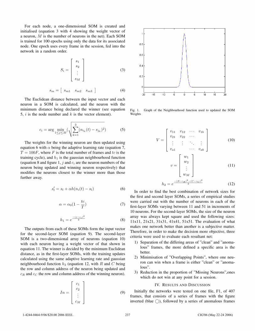
For each node, a one-dimensional SOM is created andinitialised (equation 3 with 4 showing the weight vector ofa neuron, M is the number of neurons in the net). Each SOMis trained for 100 epochs using only the data for its associatednode. One epoch uses every frame in the session, fed into thenetwork in a random order.

Si =

s1

s2

...sM

(3)

sm =[

sm1 sm2 sm3

](4)

The Euclidean distance between the input vector and eachneuron in a SOM is calculated, and the neuron with theminimum distance being declared the winner (see equation5, i is the node number and k is the vector element).

ci = arg min1≤j≤M

(

√√√√ 3∑k=1

(nik(t)− sjk

)2) (5)

The weights for the winning neuron are then updated usingequation 6 with α being the adaptive learning rate (equation 7,T = 100F , where F is the total number of frames and tc is thetraining cycle), and h1 is the gaussian neighbourhood function(equation 8 and figure 1, j and ci are the neuron numbers of theneuron being updated and winning neuron respectively) thatmodifies the neurons closest to the winner more than thosefurther away.

s′l = sl + αh(ni(t)− sl) (6)

α = α0(1−tc

T) (7)

h1 = e−(j−ci)

2

2 (8)

The outputs from each of these SOMs form the input vectorfor the second-layer SOM (equation 9). The second-layerSOM is a two-dimensional array of neurons (equation 10)with each neuron having a weight vector of that shown inequation 11. The winner is decided by the minimum Euclideandistance, as in the first-layer SOMs, with the training updatescalculated using the same adaptive learning rate and gaussianneighbourhood function h2 (equation 12, with R and C beingthe row and column address of the neuron being updated andcR and cC the row and column address of the winning neuron).

In =

c1

c2

...cM

(9)

Fig. 1. Graph of the Neighbourhood function used to updated the SOMWeights

V =

v11 v12 · · · v1b

v21 v22 · · ·...

.... . .

...va1 · · · vab

(10)

v =

w1

w2

...wM

(11)

h2 = e−(R−cR)2−(C−cC )2

2 (12)

In order to find the best combination of network sizes forthe first and second layer SOMs, a series of empirical studieswere carried out with the number of neurons in each of thefirst-layer SOMs varying between 11 and 51 in increments of10 neurons. For the second-layer SOMs, the size of the neuronarray was always kept square and used the following sizes:11x11, 21x21, 31x31, 41x41, 51x51. The evaluation of whatmakes one network better than another is a subjective matter.Therefore, in order to make the decision more objective, threecriteria were used to evaluate each resultant net:

1) Separation of the differing areas of ”clean” and ”anoma-lous” frames, the more defined a specific area is thebetter.

2) Minimisation of ”Overlapping Points”, where one neu-ron can win when a frame is either ”clean” or ”anoma-lous”.

3) Reduction in the proportion of ”Missing Neurons”,oneswhich do not win at any point for a session.

IV. RESULTS AND DISCUSSION

Initially the networks were tested on one file, F1, of 407frames, that consists of a series of frames with the figureinverted (blue ©), followed by a series of anomalous frames

1-4244-0464-9/06/$20.00 2006 IEEE. 237 CIG'06 (May 22-24 2006)

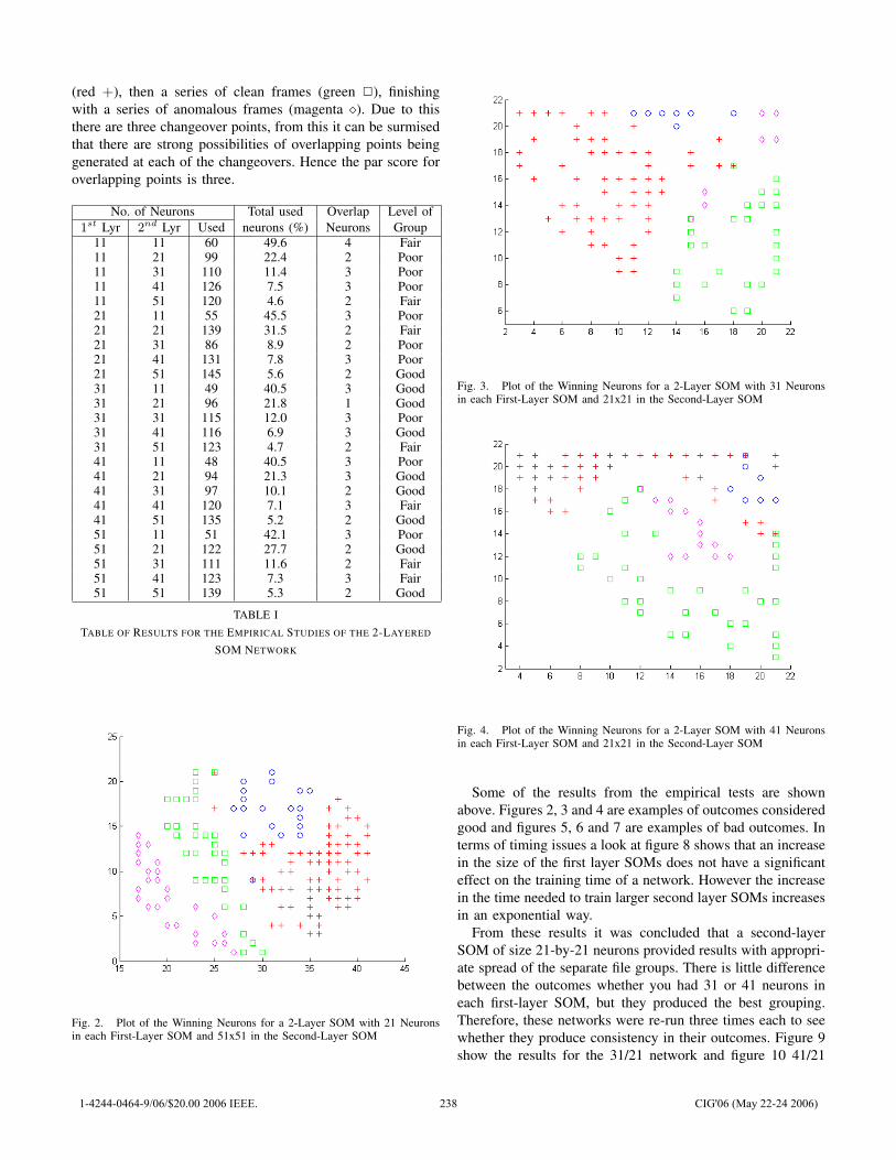
(red +), then a series of clean frames (green 2), finishingwith a series of anomalous frames (magenta �). Due to thisthere are three changeover points, from this it can be surmisedthat there are strong possibilities of overlapping points beinggenerated at each of the changeovers. Hence the par score foroverlapping points is three.

No. of Neurons Total used Overlap Level of1st Lyr 2nd Lyr Used neurons (%) Neurons Group

11 11 60 49.6 4 Fair11 21 99 22.4 2 Poor11 31 110 11.4 3 Poor11 41 126 7.5 3 Poor11 51 120 4.6 2 Fair21 11 55 45.5 3 Poor21 21 139 31.5 2 Fair21 31 86 8.9 2 Poor21 41 131 7.8 3 Poor21 51 145 5.6 2 Good31 11 49 40.5 3 Good31 21 96 21.8 1 Good31 31 115 12.0 3 Poor31 41 116 6.9 3 Good31 51 123 4.7 2 Fair41 11 48 40.5 3 Poor41 21 94 21.3 3 Good41 31 97 10.1 2 Good41 41 120 7.1 3 Fair41 51 135 5.2 2 Good51 11 51 42.1 3 Poor51 21 122 27.7 2 Good51 31 111 11.6 2 Fair51 41 123 7.3 3 Fair51 51 139 5.3 2 Good

TABLE ITABLE OF RESULTS FOR THE EMPIRICAL STUDIES OF THE 2-LAYERED

SOM NETWORK

Fig. 2. Plot of the Winning Neurons for a 2-Layer SOM with 21 Neuronsin each First-Layer SOM and 51x51 in the Second-Layer SOM

Fig. 3. Plot of the Winning Neurons for a 2-Layer SOM with 31 Neuronsin each First-Layer SOM and 21x21 in the Second-Layer SOM

Fig. 4. Plot of the Winning Neurons for a 2-Layer SOM with 41 Neuronsin each First-Layer SOM and 21x21 in the Second-Layer SOM

Some of the results from the empirical tests are shownabove. Figures 2, 3 and 4 are examples of outcomes consideredgood and figures 5, 6 and 7 are examples of bad outcomes. Interms of timing issues a look at figure 8 shows that an increasein the size of the first layer SOMs does not have a significanteffect on the training time of a network. However the increasein the time needed to train larger second layer SOMs increasesin an exponential way.

From these results it was concluded that a second-layerSOM of size 21-by-21 neurons provided results with appropri-ate spread of the separate file groups. There is little differencebetween the outcomes whether you had 31 or 41 neurons ineach first-layer SOM, but they produced the best grouping.Therefore, these networks were re-run three times each to seewhether they produce consistency in their outcomes. Figure 9show the results for the 31/21 network and figure 10 41/21

1-4244-0464-9/06/$20.00 2006 IEEE. 238 CIG'06 (May 22-24 2006)

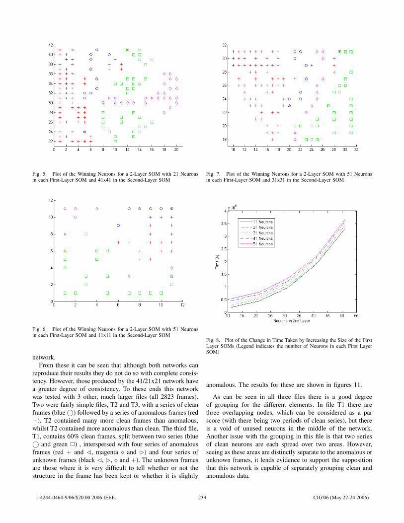
Fig. 5. Plot of the Winning Neurons for a 2-Layer SOM with 21 Neuronsin each First-Layer SOM and 41x41 in the Second-Layer SOM

Fig. 6. Plot of the Winning Neurons for a 2-Layer SOM with 51 Neuronsin each First-Layer SOM and 11x11 in the Second-Layer SOM

network.From these it can be seen that although both networks can

reproduce their results they do not do so with complete consis-tency. However, those produced by the 41/21x21 network havea greater degree of consistency. To these ends this networkwas tested with 3 other, much larger files (all 2823 frames).Two were fairly simple files, T2 and T3, with a series of cleanframes (blue ©) followed by a series of anomalous frames (red+). T2 contained many more clean frames than anomalous,whilst T2 contained more anomalous than clean. The third file,T1, contains 60% clean frames, split between two series (blue© and green 2) , interspersed with four series of anomalousframes (red + and �, magenta � and �) and four series ofunknown frames (black �, �, � and +). The unknown framesare those where it is very difficult to tell whether or not thestructure in the frame has been kept or whether it is slightly

Fig. 7. Plot of the Winning Neurons for a 2-Layer SOM with 51 Neuronsin each First-Layer SOM and 31x31 in the Second-Layer SOM

Fig. 8. Plot of the Change in Time Taken by Increasing the Size of the FirstLayer SOMs (Legend indicates the number of Neurons in each First LayerSOM)

anomalous. The results for these are shown in figures 11.

As can be seen in all three files there is a good degreeof grouping for the different elements. In file T1 there arethree overlapping nodes, which can be considered as a parscore (with there being two periods of clean series), but thereis a void of unused neurons in the middle of the network.Another issue with the grouping in this file is that two seriesof clean neurons are each spread over two areas. However,seeing as these areas are distinctly separate to the anomalous orunknown frames, it lends evidence to support the suppositionthat this network is capable of separately grouping clean andanomalous data.

1-4244-0464-9/06/$20.00 2006 IEEE. 239 CIG'06 (May 22-24 2006)

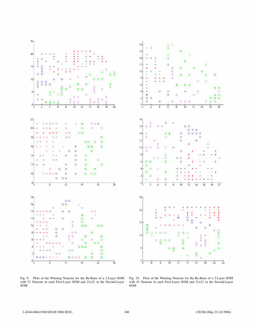
Fig. 9. Plots of the Winning Neurons for the Re-Runs of a 2-Layer SOMwith 31 Neurons in each First-Layer SOM and 21x21 in the Second-LayerSOM

Fig. 10. Plots of the Winning Neurons for the Re-Runs of a 2-Layer SOMwith 41 Neurons in each First-Layer SOM and 21x21 in the Second-LayerSOM

1-4244-0464-9/06/$20.00 2006 IEEE. 240 CIG'06 (May 22-24 2006)

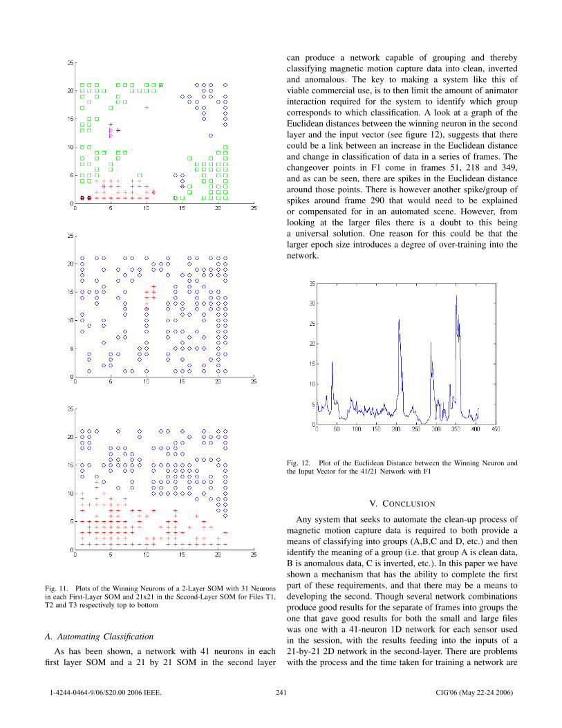
Fig. 11. Plots of the Winning Neurons of a 2-Layer SOM with 31 Neuronsin each First-Layer SOM and 21x21 in the Second-Layer SOM for Files T1,T2 and T3 respectively top to bottom

A. Automating Classification

As has been shown, a network with 41 neurons in eachfirst layer SOM and a 21 by 21 SOM in the second layer

can produce a network capable of grouping and therebyclassifying magnetic motion capture data into clean, invertedand anomalous. The key to making a system like this ofviable commercial use, is to then limit the amount of animatorinteraction required for the system to identify which groupcorresponds to which classification. A look at a graph of theEuclidean distances between the winning neuron in the secondlayer and the input vector (see figure 12), suggests that therecould be a link between an increase in the Euclidean distanceand change in classification of data in a series of frames. Thechangeover points in F1 come in frames 51, 218 and 349,and as can be seen, there are spikes in the Euclidean distancearound those points. There is however another spike/group ofspikes around frame 290 that would need to be explainedor compensated for in an automated scene. However, fromlooking at the larger files there is a doubt to this beinga universal solution. One reason for this could be that thelarger epoch size introduces a degree of over-training into thenetwork.

Fig. 12. Plot of the Euclidean Distance between the Winning Neuron andthe Input Vector for the 41/21 Network with F1

V. CONCLUSION

Any system that seeks to automate the clean-up process ofmagnetic motion capture data is required to both provide ameans of classifying into groups (A,B,C and D, etc.) and thenidentify the meaning of a group (i.e. that group A is clean data,B is anomalous data, C is inverted, etc.). In this paper we haveshown a mechanism that has the ability to complete the firstpart of these requirements, and that there may be a means todeveloping the second. Though several network combinationsproduce good results for the separate of frames into groups theone that gave good results for both the small and large fileswas one with a 41-neuron 1D network for each sensor usedin the session, with the results feeding into the inputs of a21-by-21 2D network in the second-layer. There are problemswith the process and the time taken for training a network are

1-4244-0464-9/06/$20.00 2006 IEEE. 241 CIG'06 (May 22-24 2006)

still an issue. However, some of these could be alleviated bythe generation of a generic test file for a specific sensor set-up, which contained series of clean, anomalous and invertedframes for a given capture space. A network could then betrained for that file and the different groups identified by ahuman operator, this could then be used to identify frames inother capture sessions using the same capture sensor set-upand space.

So far no pre-processing has been applied to the data beforeit is fed into the network, so that the effects of the capturespace can be taken into account. However, it may be thatthe use of pre-processing techniques (such as centring orsphering), improve the grouping of the outputs and/or makethe identification of what groups are easier. Other experimentscould focus on the size of an epoch and whether using arandom sample of all the frames rather than all of the frames ina session can produce quicker training, without compromisingthe usefulness of the technique. Alternatively, the use ofsome form of stopping criteria could be employed to saveunnecessary training cycles and thereby improve the overalltiming of the system.

ACKNOWLEDGMENT

The authors would like to thank Artem Digital for theprovision of the test data, www.artem-digital.co.uk.

REFERENCES

[1] Margaret S. Geroch, Motion Capture for the Rest of us, Journal ofComputing Sciences in Colleges,Vol. 19 No. 3, 2004. pp157-164.

[2] David P. Gibson, Neill W. Campbell, Colin J. Dalton and Barry T.Thomas, Extraction of Motion Data from Image Sequences to AssistAnimators, Proceedings of the British Machine Vision Conference 2000.

[3] Lucas Kovar, Michael Gleicher, Automated Extraction and Parameteri-zation of Motions in Large Data Sets, ACM Transactions on Graphics,Vol. 23, Issue 3, p.559-568. August 2004.

[4] Iain Miller, Stephen McGlinchey Automating the Clean-up Process ofMagnetic Motion Capture Systems Proceedings of the Game Design andTechnology Workshop, November 2005.

[5] Meinard Muller, Tido Roder, Michael Clausen Efficient Content-BasedRetrieval of Motion Capture Data ACM Transactions on Graphics, Vol.24, Issue 3, p677-685. July 2005.

1-4244-0464-9/06/$20.00 2006 IEEE. 242 CIG'06 (May 22-24 2006)

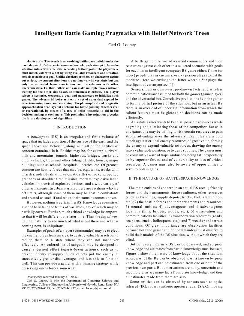
Intelligent Battle Gaming Pragmatics with Belief Network Trees

Carl G. Looney

Abstract – The events in an evolving battlespace unfold under the

partial control of adversarial commanders, who each attempt to force thesituation into a favorable state according to their goals. The player heremust match wits with a bot by using available resources and situationmodels to achieve a goal. Unlike checkers or chess, or characters actingout scripts, the current situations are not known with certainty but canonly be estimated from associations and correlations with otheruncertain data. Further, either side can make multiple moves withoutwaiting for the other side to act, so timeliness is critical. The playerselects a scenario, weapons, a goal and parameters to initialize suchgames. The adversarial bot starts with a set of rules that expand byexperience using case-based reasoning. The philosophical and pragmaticapproach taken here lays out a scheme for battle gamimg, whether realor recreational, by means of a tree of belief networks to aid in thedecision making at each move. This preliminary investigation precedesthe future development of algorithms.

I. INTRODUCTION

A battlespace (BS) is an irregular and finite volume of

space that includes a portion of the surface of the earth and the

space above and below it, along with all of the entities of

concern contained in it. Entities may be, for example, rivers,

hills and mountains, tunnels, highways, bridges, trucks and

other vehicles, trees and other foliage, fields, houses, major

buildings such as schools, hospitals, libraries, etc. Of greatest

concern are hostile forces that may be, e.g., tanks, trucks with

missiles, individuals with automatic rifles or rocket propelled

grenades or shoulder fired missiles, mortars, explosive laden

vehicles, improvised explosive devices, and a wide variety of

other armaments. In urban warfare, there are civilians who are

off limits, although some of them may be hostile combatants

and treated as such if and when their status becomes known.

However, nothing is certain in a BS. Knowledge consists of

a set of beliefs in the truths of variables, any of which may be

partially correct. Further, much critical knowledge is temporal

so that it will be different at a later time. Thus the fog of war,

i.e, the inability to see much of what is out there and what is

coming next, is ubiquitous.

Examples of goals of a player (commander) may be to eject

the enemy forces from an area, to destroy valuable assets, or to

reduce them to a state where they can not maneuver

effectively. An ordered list of subgoals may be designed to

cause a desired effect (effects-based actions), such as to

prevent enemy re-supply. Such effects put the enemy at

successively greater disadvantages and less able to function

well. This can provide a gamer with a winning strategy while

preserving one’s forces somewhat.

Manuscript received January 31, 2006. Carl G. Looney is with the Department of Computer Science and

Engineering, College of Engineering, University of Nevada, Reno, Reno, NV89557; 775-784-4313; fax: 775-784-1877; email: looney@cse.unr.edu.

A battle game pits two adversarial commanders and their

resources against each other in a selected scenario with goals

for each. In an intelligent computer BS game either: i) two (or

more) people play as enemies; or ii) a person plays against the

machine. Here we envisage the latter where a bot plays the

intelligent adversarym(see [1]).

Sensors, human observers, pre-known facts, and wireless

communications are assumed for both the gamer (game player)

and the adversarial bot. Correlative predictions help the gamer

to form a partial picture of the situation, but in an actual BS

there is an overload of uncertain information from which the

salient features must be gleaned so decisions can be made

efficiently.

An astute gamer wants to keep all possible resources while

degrading and eliminating those of the competitor, but as in

any game, one may be willing to risk certain resources to gain

strong advantage over the adversary. Examples are a bold

attack against critical enemy resources of great value, forcing

the enemy to expend valuable resources, drawing the enemy

into a vulnerable position, or to deny supplies. The gamer must

be constantly aware of traps, ambushes, being hit unexpectedly

or by superior forces, and of vulnerability to loss of critical

resources. A gamer must also be aware of opportunities to

seize to obtain gains.

II. THE NATURE OF BATTLESPACE KNOWLEDGE

The main entities of concern in an actual BS are: 1) friendly

forces and their armaments, force readiness, other resources

(such as buildings, supply depots, trucks, fuel, ammunition,

etc.); 2) the hostile forces and their armaments and resources;

3) neutral entities; 4) advantageous and disadvantageous

locations (hills, bridges, woods, etc.); 5) observation and

communications facilities; 6) transportation resources (roads,

sea ports, trucks, helicopters, etc.), and 7) weather and terrain

conditions. Of great importance are observation facilities

because both the gamer and bot commanders must observe to

build their models of the BS situation, without which they are

blind.

But not everything in a BS can be observed, and so prior

knowledge and estimates from partial knowledge must be used.

Figure 1 shows the nature of knowledge about the situation,

where part of the BS can be observed, part is known by prior

knowledge and part can be estimated from one or both of the

previous two parts. But observations are noisy, uncertain and

incomplete, as are many facts from prior knowledge, and thus

all estimates made from them are also.

Some entities can be observed by sensors such as optic,

infrared (IR), radar, synthetic aperture radar (SAR), moving

1-4244-0464-9/06/$20.00 2006 IEEE. 243 CIG'06 (May 22-24 2006)

target indicator (MTI) radar, laser radar (ladar), human

observers and signal intelligence (SIGINT), which detects

frequency bands, repetition intervals, etc., to determine the

type of equipment being used. But there are also hidden

entities, missing data and noise so that it is not possible to

observe all of the entities or even many of the particulars of

those observed (for correct identification of target type). Thus

the BS situation must be modeled with beliefs (0 to 1) of the

existence, type and status of many entities.

Figure 1. The nature of knowledge.

Both the gamer and the adversarial bot operate according

to their respective models of the BS situation, but the bot’s

modus operandi is determined by its rules, some of which it

will learn from game playing experience.

The relationships between entities and between their

attributes provide knowledge of the BS because gamers use

them to organize entities into echelons (unit levels) of the

adversary, the mix of forces, their locations and stances, and

patterns of behavior. The questions they pose are: how do

these entities support, supply, and reinforce each other? What

purposes do the organizational units of the given mixtures

imply? How may they be used separately or together? What

threats do they present? What does their behavior indicate? If

the bot attacks the bridge from the South, e.g., could the

gamer’s forces on the South side of the bridge become

trapped?

III. INTELLIGENT BATTLESPACE GAMING

On start-up of each game, the Game Controller module

calls the Initializer that permits the selection of a scenario,

armaments and parameters. The Initializer then builds an

uncertain BS model situation for the gamer and another one for

the bot. The Game controller then calls the Move Controller

that permits a next move by either the gamer or bot, whichever

one issues the next call to an event handler. Here, either the

Bot Move or the Gamer Move handles the event.

The Bot Move module accesses the bot’s BS model and

feeds key truth values to the bot’s rule base that controls its

moves. The Gamer Move module must display the Gamer’s

BS model on the screen and accept input from the gamer that

commands actions to be taken by the gamer’s forces. In a fully

developed system, the BS model also posts belief values

computed from belief networks (described later) that represent

a case base for learning.

The Game Controller then generates some random values

as noise on new observations and updates the Actual BS and

the two BS models for the gamer and the bot commanders. It

also adds any results to the case bases of each side for

learning. It then checks for the next move event from either the

gamer or the bot.

Scenarios may be an urban environment such that one of a

set of bridges over a river must be taken and secured; or it may

be a rescue operation on an island where guerilla forces hold

hostages in a town school and guard the roads leading into the

town. New scenarios may be added by descriptors of the

terrain, situation, goals, etc., at later times. Figure 2 shows the

Selector Interface that allows the gamer to chose the scenario

and other conditions for the battle game. Figure 3 presents a

high level functional diagram of the battle game system.

Figure 2. Selecting the BS conditions.

Figure 3. A high level functional diagram.

As in a chess game (see [2] for the most complete gaming

strategies for chess), there are myriads of moves and counter

moves possible in a tree of moves, but unlike board games (see

[3] for a discussion of artificial intelligence and computer

games), the current situation here is only partially known and

a move may not be an actual move because there may be feints

and other uncertainties. Also the adversaries are not restricted

to a single move before the other side moves, so if one side has

a plan and can move several times before the other one moves

it can be an advantage (or disadvantage if the moves are not

good ones). A move need not be a single action but may

1-4244-0464-9/06/$20.00 2006 IEEE. 244 CIG'06 (May 22-24 2006)

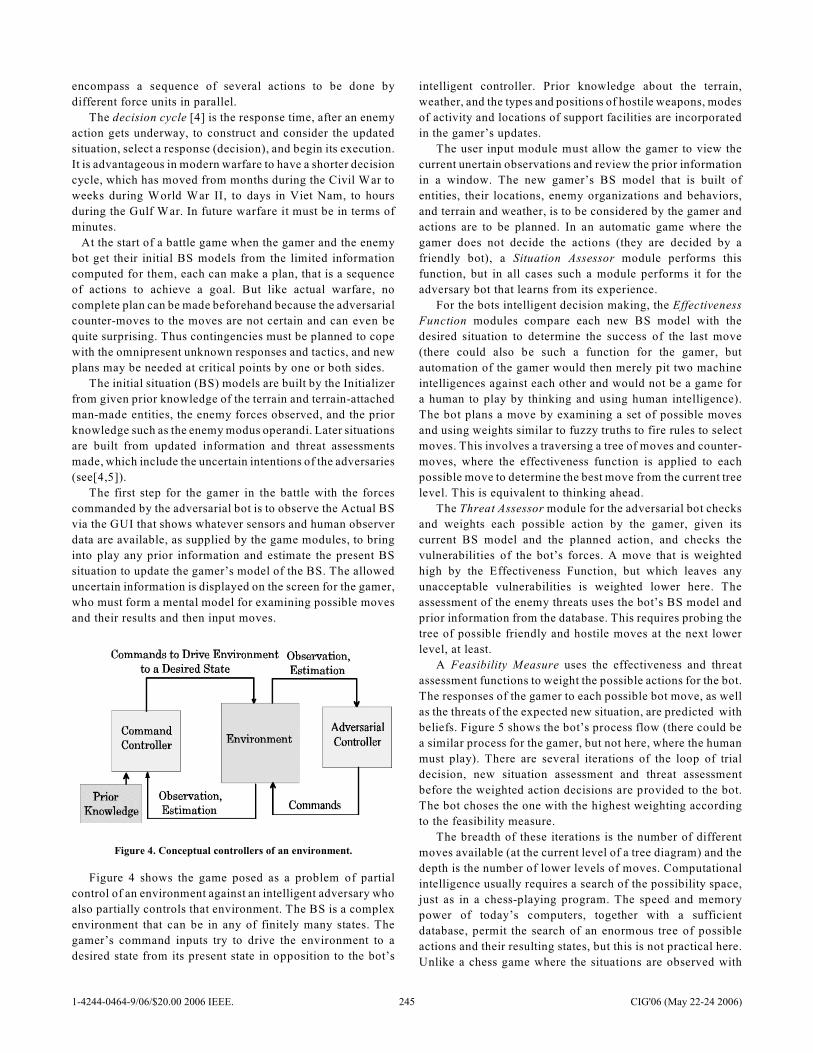
encompass a sequence of several actions to be done by

different force units in parallel.

The decision cycle [4] is the response time, after an enemy

action gets underway, to construct and consider the updated

situation, select a response (decision), and begin its execution.

It is advantageous in modern warfare to have a shorter decision

cycle, which has moved from months during the Civil War to

weeks during World War II, to days in Viet Nam, to hours

during the Gulf War. In future warfare it must be in terms of

minutes.

At the start of a battle game when the gamer and the enemy

bot get their initial BS models from the limited information

computed for them, each can make a plan, that is a sequence

of actions to achieve a goal. But like actual warfare, no

complete plan can be made beforehand because the adversarial

counter-moves to the moves are not certain and can even be

quite surprising. Thus contingencies must be planned to cope

with the omnipresent unknown responses and tactics, and new

plans may be needed at critical points by one or both sides.

The initial situation (BS) models are built by the Initializer

from given prior knowledge of the terrain and terrain-attached

man-made entities, the enemy forces observed, and the prior

knowledge such as the enemy modus operandi. Later situations

are built from updated information and threat assessments

made, which include the uncertain intentions of the adversaries

(see[4,5]).

The first step for the gamer in the battle with the forces

commanded by the adversarial bot is to observe the Actual BS

via the GUI that shows whatever sensors and human observer

data are available, as supplied by the game modules, to bring

into play any prior information and estimate the present BS

situation to update the gamer’s model of the BS. The allowed

uncertain information is displayed on the screen for the gamer,

who must form a mental model for examining possible moves

and their results and then input moves.

Figure 4. Conceptual controllers of an environment.

Figure 4 shows the game posed as a problem of partial

control of an environment against an intelligent adversary who

also partially controls that environment. The BS is a complex

environment that can be in any of finitely many states. The

gamer’s command inputs try to drive the environment to a

desired state from its present state in opposition to the bot’s

intelligent controller. Prior knowledge about the terrain,

weather, and the types and positions of hostile weapons, modes

of activity and locations of support facilities are incorporated

in the gamer’s updates.

The user input module must allow the gamer to view the

current unertain observations and review the prior information

in a window. The new gamer’s BS model that is built of

entities, their locations, enemy organizations and behaviors,

and terrain and weather, is to be considered by the gamer and

actions are to be planned. In an automatic game where the

gamer does not decide the actions (they are decided by a

friendly bot), a Situation Assessor module performs this

function, but in all cases such a module performs it for the

adversary bot that learns from its experience.

For the bots intelligent decision making, the Effectiveness

Function modules compare each new BS model with the

desired situation to determine the success of the last move

(there could also be such a function for the gamer, but

automation of the gamer would then merely pit two machine

intelligences against each other and would not be a game for

a human to play by thinking and using human intelligence).

The bot plans a move by examining a set of possible moves

and using weights similar to fuzzy truths to fire rules to select

moves. This involves a traversing a tree of moves and counter-

moves, where the effectiveness function is applied to each

possible move to determine the best move from the current tree

level. This is equivalent to thinking ahead.

The Threat Assessor module for the adversarial bot checks

and weights each possible action by the gamer, given its

current BS model and the planned action, and checks the

vulnerabilities of the bot’s forces. A move that is weighted

high by the Effectiveness Function, but which leaves any

unacceptable vulnerabilities is weighted lower here. The

assessment of the enemy threats uses the bot’s BS model and

prior information from the database. This requires probing the

tree of possible friendly and hostile moves at the next lower

level, at least.

A Feasibility Measure uses the effectiveness and threat

assessment functions to weight the possible actions for the bot.

The responses of the gamer to each possible bot move, as well

as the threats of the expected new situation, are predicted with

beliefs. Figure 5 shows the bot’s process flow (there could be

a similar process for the gamer, but not here, where the human

must play). There are several iterations of the loop of trial

decision, new situation assessment and threat assessment

before the weighted action decisions are provided to the bot.

The bot choses the one with the highest weighting according

to the feasibility measure.

The breadth of these iterations is the number of different

moves available (at the current level of a tree diagram) and the

depth is the number of lower levels of moves. Computational

intelligence usually requires a search of the possibility space,

just as in a chess-playing program. The speed and memory

power of today’s computers, together with a sufficient

database, permit the search of an enormous tree of possible

actions and their resulting states, but this is not practical here.

Unlike a chess game where the situations are observed with

1-4244-0464-9/06/$20.00 2006 IEEE. 245 CIG'06 (May 22-24 2006)

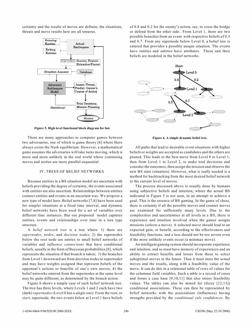
certainty and the results of moves are definite, the situations,

threats and move results here are all tenuous.

Figure 5. High level functional block diagram for bot.

There are many approaches to computer games between

two adversaries, one of which is game theory [6] where there

always exists the Nash equilibrium. However, a mathematical

game assumes the adversaries will take turns moving, which is

more and more unlikely in the real world where continuing

moves and sorties are more parallel-sequential.

IV. TREES OF BELIEF NETWORKS

Because entities in a BS situation model are uncertain with

beliefs providing the degree of certainty, the events associated

with entities are also uncertain. Relationships between entities

connect entities and events in an uncertain way. We propose a

new type of model here. Belief networks [7,8] have been used

for simpler situations at a fixed time interval, and dynamic

belief networks have been used for a set of variables over

different time instances. But our proposed model captures

entities, events and relationships over time in a tree type

structure.

A belief network tree is a tree where: 1) there are

supernodes, nodes, and decision nodes; 2) the supernodes

below the root node are entries to small belief networks of

variables and influence connections that have conditional

beliefs, usually in the form of Bayesian probabilities [8], which

represents the situation if that branch is taken; 3) the branches

from Level 1 downward are from decision nodes to supernodes

and may have weights assigned that represent beliefs of the

opponent’s actions or benefits of one’s own moves; 4) the

belief networks entered from the supernodes at the same level

may be quite different, as determined by the branch action.

Figure 6 shows a simple case of such belief network tree.

The tree has three levels, where Levels 1 and 2 each have two

(dark) supernodes (Level 0 has a single one). From the root, or

start, supernode, the two events below at Level 1 have beliefs

of 0.8 and 0.2 for the enemy’s action, say, to cross the bridge

or defend from the other side.. From Level 1, there are two

possible branches from an event with respective beliefs of 0.3

and 0.7. From any supernode below Level 0, a belief tree is

entered that provides a possibly unique situation. The events

have entities and entities have attributes. These and their

beliefs are modeled in the belief networks.

Figure 6. A simple dynamic belief tree.

All paths that lead to desirable event situations with higher

beliefs or weights are accepted as candidates and the others are

pruned. This leads to the best move from Level 0 to Level 1,

then from Level 1 to Level 2, to make trial decisions and

consider the outcomes, then assign the mission and observe the

new BS state (situation). However, what is really needed is a

method for backtracking from the most desired belief network

to the current level of moves.

The process discussed above is usually done by humans

using subjective beliefs and intuition, where the actual BS

indicated in Figure 5 is not seen, in an attempt to achieve a

goal. This is the essence of BS gaming. In the game of chess,

there is certainty if all the possible moves and counter moves

are examined for sufficiently many levels. Due to the

complexities and uncertainties at all levels in a BS, there is

experience and intuition involved when the gamer assigns

missions (selects a move). A selected move should lead to an

expected gain, or benefit, according to the effectiveness and

feasibility functions, and a loss should not be too severe even

if the more unlikely events occur (a minimax move).

An intelligent gaming system should incorporate experience

and intuition, and so must have memory of experiences and an

ability to extract benefits and losses from these to select

suboptimal moves in the future. Thus it must store the actual

moves and the results, along with a feasibility value of the

move. It can do this in a relational table of rows of values for

the columnar field variables. Such a table is a record of cases

and forms a case base [9,10,11] that also stores feasibility

values. The tables can also be mined for (fuzzy [12,13])

conditional associations. These can then be represented by

belief networks with the associations (influences) having

strengths provided by the conditional rule confidences. By

1-4244-0464-9/06/$20.00 2006 IEEE. 246 CIG'06 (May 22-24 2006)

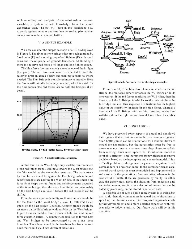
such recording and analysis of the relationships between

variables, a system extracts knowledge from the stored

experience data. The bot will learn in this fashion to play

expertly against humans and can then be used to play against

enemy commanders in actual battles.

V. A SIMPLE EXAMPLE

We now consider the simple scenario of a BS as displayed

in Figure 7. The river has two bridges that are each guarded by

5 red tanks (R) and a small group of red fighters (F) with small

arms and rocket propelled grenade launchers. At Building 2

there is a reserve red force of 6 tanks and one fighter group.

The blue force (bottom center) is to take one of the bridges

(the goal). The red force command is expected to hold the

reserves until an attack occurs and then move them to where

needed. The East Bridge is considered more vulnerable. Here

the forces will initially be evenly matched, which is a risk for

the blue forces (the red forces are to hold the bridges at all

costs).

Figure 7. A simple battlespace example.

A blue feint on the West bridge may start the reinforcement

of the red forces from Building 2 toward the West bridge, but

the feint would require some blue resources. The main attack

by blue forces would be against the East bridge when the red

reinforcements are nearing the West bridge. If the small blue

force feint keeps the red forces and reinforcements occupied

at the West bridge, then the main blue force can presumably

hit the East bridge and take it before the red reserves can be

shifted.

From the root supernode in Figure 8, one branch would be

for the feint on the West bridge (Level 1) followed by an

attack on the East bridge (Level 2). Another branch would be

an attack on the East bridge with no feint on the West bridge.

Figure 8 shows the blue force events in bold font and the red

force events in italics. A symmetrical situation is for the East

and West bridges to be interchanged so we prune those

branches. Thus there would be the two branches from the root

node that would yield two different situations.

Figure 8. A belief network tree for the simple example.

From Level 0, if the blue force feints an attack on the W.

Bridge, the red force either reinforces the W. Bridge or holds

the reserves. If the red forces reinforce the W. Bridge, then the

blues attack the E. Bridge, in which case the reds reinforce the

E. Bridge too late. This sequence of situations has the highest

value of the feasibility function for the blue forces, whereas a

blue attack on E. Bridge with no feint resulting in the blue

withdrawal on the right bottom would have a low feasibility

value.

VI. CONCLUSIONS

We have presented some aspects of actual and simulated

battle games that are not present in the usual computer games.

Such battle games can be simulations with random draws to

model the uncertainty, but the adversaries must be free to

move as many times at whatever times they chose, or refrain

from moving. Each must update its BS situation model at

(probably different) time increments from which to make move

decisions based on the incomplete and uncertain model. It is a

difficult problem to design such a game or a system to aid

commanders in a real war game. In the computer games case,

the real world scenarios must be modeled and implemented in

software with the generation of uncertainties, whereas in the

real world of battle, these are generated by reality. In either

case the gamer must assess the situation from uncertain data

and select moves, and it is the selection of moves that can be

aided by processing on the stored experience data.

A possible use of such a battle game system is to train a bot

that could then aid commanders in actual battle situations to

speed up the decision cycle. Our proposed approach needs

further development and a more detailed expansion with real

scenarios to judge its utility. Our future work will be in this

direction.

1-4244-0464-9/06/$20.00 2006 IEEE. 247 CIG'06 (May 22-24 2006)

REFERENCES

[1] John E. Laird, “Using a computer game to develop

advanced AI,” IEEE Computer, July, 2001, 70 - 71.

[2] E. A. Heinz, “Scalable search in computer chess,” Vieweg,

Braunschweig, Germany, 2000.

[3] Stuart Russell and Peter Norvig, Artificial Intelligence, A

Modern Approach, 2 Edition, Prentice-Hall, Upper Saddle nd

River, 2003.

[4] Carl G. Looney, “Exploring fusion architecture for a

common operational picture,” Information Fusion 2, 2001,

251 - 260.

[5] C. G. Looney and L. R. Liang, “Cognitive situation and

threat assessments of ground battlespaces,” Info. Fusion 4,

2003, 297 - 308.

[6] Don Ross, “Game Theory,” The Stanford Encyclopedia of

Philosophy (W inter 2005 Edition), Edward N. Zalta (ed.),

http://plato.stanford.edu/archives/win2005/entries/game-theory/

[7] Nadkarni, S. and P. Shenoy, A Bayseian network approach

to making inferences in causal maps. European J. Operations

Research, 2001. 128: p. 479-498.

[8] Pearl, J., Probabilistic Reasoning in Intelligent Systems:

Networks of Plausible Inference. 1988, San Mateo, California:

Morgan Kaufmann Publishers.

[9] A. Aamodt, and E. Plaza, Case-based reasoning:

foundational issues, methodological variations and system

approaches. IEEE AI Communications, 1994. 7(i): p. 39-59.

[10] Kolodner, J.L., Maintaining Organization in a Dynamic

Long-Term Memory. Cognitive Science, 1983. 7(4): p. 243-

280.

[11] Schank, R., Dynamic memory: a theory of reminding and

learning in computers and people. 1982, Cambridge, UK:

Cambridge University Press.

[12] Lily Liang and Carl Looney, “Fuzzy belief state-based

data mining,” Proc. IEEE IRI 2004, Las Vegas, Mar. 2004.

[13] Kuok, C.M., Fu A. and Wong, M.H. M ining Fuzzy

Association Rules in Databases. ACM SIGMOD Record ,,

March,1998. 27(1): p. 41-46.

1-4244-0464-9/06/$20.00 2006 IEEE. 248 CIG'06 (May 22-24 2006)

Fun in Slots Kevin Burns

Abstract— People play games for fun. Yet we are lacking a fundamental understanding of what fun is and how fun works in games and other media. For example, why do thousands of people spend millions of dollars playing slot machines, especially when most know they will lose money in the long run? To answer this question, I present an aesthetic analysis of slot play using a Bayesian-information approach. The finding is that fun in slots can be seen as arising from a difference in information gained from good versus bad outcomes. This difference is modeled by marginal entropies and the result is a measure of fun in slot play, showing for what range of payoff probabilities slots are fun and at what probability they are most fun. The approach is extended to games of skill and the same Bayesian-information theory is used to derive computational measures of fun in these games.

I. INTRODUCTION UN is serious business, especially in the entertainment industry. But games are also used in other industries for

testing-out strategies and training of employees, and real fights against competitors and enemies are driven by feelings of tension and pleasure. Yet these feelings and fun are poorly understood, especially from a computational perspective. This may be acceptable and even desirable for game consumers, but it is not acceptable for game designers if they are to advance the state of their art and practice through systematic engineering.

This paper takes a small step towards understanding fun in games, with a focus on gambling in slot machines. The approach is one of computational aesthetics, which is relevant to computational intelligence because human emotions affect human cognition, and vice versa. From a practical perspective, aesthetics are important to efforts aimed at: (i) designing machines that adapt to the feelings of users, i.e., in human-computer interface design, and (ii) designing machines that can simulate human behavior, i.e., in artificially intelligent agents. The bottom line is that human actions are driven by both thinking and feelings, in both occupational work and recreational play; hence a computational understanding of intelligence must include a computational understanding of aesthetics.

The question is: Why do people play gambling games like slot machines, even when they know they will lose in the long run? Clearly they play for fun, but then what is fun?

Manuscript received March 31, 2006. This work was supported by the

MITRE Technology Program. Kevin Burns is with the MITRE Corporation, 202 Burlington Road,

Bedford, MA 01730-1420 USA (phone: 781-271-8762; fax: 781-271-2101; e-mail: kburns@mitre.org).

In one answer, Koster [1] writes, “Fun is just another word for learning” (pg. 46); “Games that are too hard kind of bore me, and games that are too easy also kind of bore me.” (pg. 10). But all learning is not so fun, and “Goldilocks” statements about people liking things “not too hard or too easy” are really just common sense.

Slot machines are a good example because playing them is clearly fun for many people, and yet the game does not seem to be much of a learning challenge. In fact it is rather remarkable that slots, which are so repetitive [2], are such a popular amusement for cognitive intelligence. Therefore, a theory of fun must address the pleasure that comes from repetition as well as the pleasure that comes from a learning challenge; plus slots are not fun for everyone so personal preferences must be part of the equation, too.

Here I develop an equation, f = G * E + G’ * E’, for fun in slots, based on a general theory of aesthetic experience called EVE’ [3]. According to EVE’, fun comprises two types of pleasure, each stemming from subjective success in different but related types of cognitive processing. One type is pleasure that arises from success in forward-looking Expectations (E) of what will happen in a media experience (e.g., game). The other type is pleasure-prime that arises from success in backward-looking Explanations (E’) of what has happened in a media experience (e.g., game). The two are related by Violations (V) of E that create opportunities for E’ in the sequence E-V-E’ .

Here, following EVE’, I argue that fun in slots is a tradeoff between pleasure (p) at E and pleasure-prime (p’) at E’, where p corresponds roughly to the idea of repetition [2] and p’ corresponds roughly to the idea of a learning challenge [1]. In expanding and evaluating the equation, f = G * E + G’ * E’, I show that while fun in slots involves both repetition at E and a learning challenge at E’, logically most of the fun must come from E’. I also discuss how E’ itself is governed by a tradeoff between good/bad outcomes, and how personal preferences and a sense of humor affect the computed measure of fun.

The analysis is generalized beyond slots to games of skill, and the same basic equation is shown to apply. The main finding is that fun in slots and other games can be modeled and measured as a difference in information gained from good outcomes versus bad outcomes, where information is measured by marginal entropy. The net fun in games is made possible by Violations (V) of Expectations (E) for good and bad outcomes, which create tension that is ultimately resolved with pleasurable or displeasurable Explanations (E’).

F

1-4244-0464-9/06/$20.00 2006 IEEE. 249 CIG'06 (May 22-24 2006)

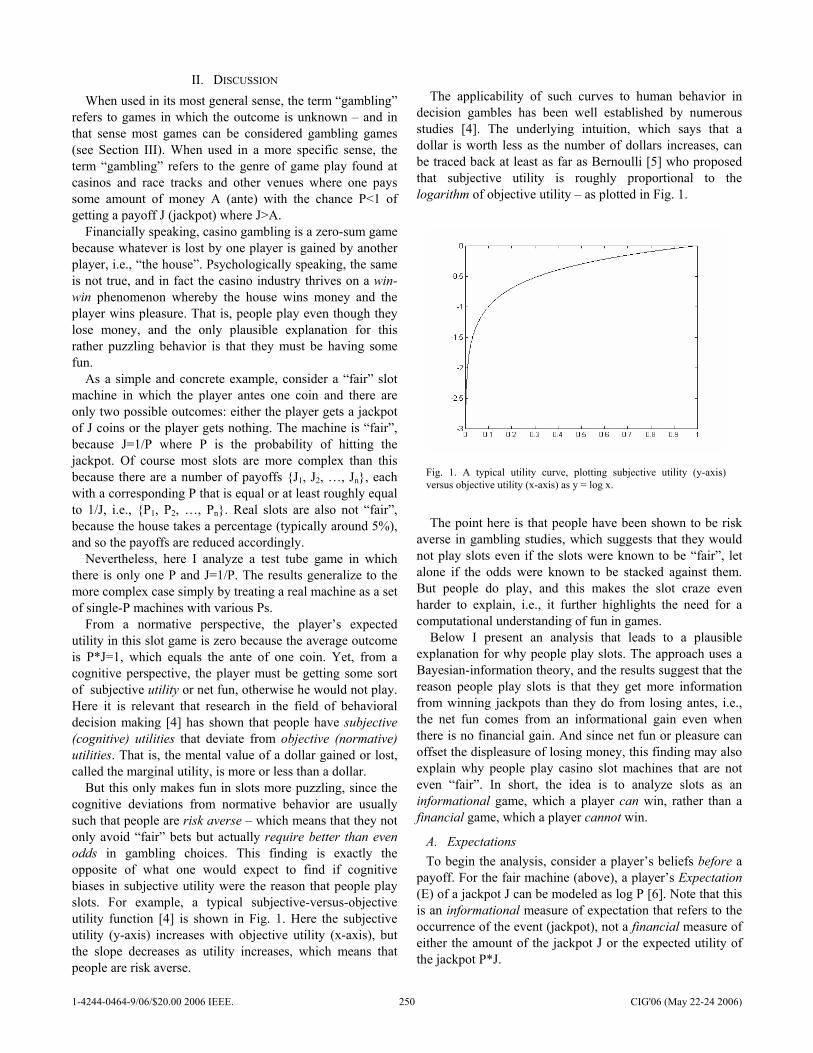
II. DISCUSSION When used in its most general sense, the term “gambling”

refers to games in which the outcome is unknown – and in that sense most games can be considered gambling games (see Section III). When used in a more specific sense, the term “gambling” refers to the genre of game play found at casinos and race tracks and other venues where one pays some amount of money A (ante) with the chance P<1 of getting a payoff J (jackpot) where J>A.

Financially speaking, casino gambling is a zero-sum game because whatever is lost by one player is gained by another player, i.e., “the house”. Psychologically speaking, the same is not true, and in fact the casino industry thrives on a win-win phenomenon whereby the house wins money and the player wins pleasure. That is, people play even though they lose money, and the only plausible explanation for this rather puzzling behavior is that they must be having some fun.

As a simple and concrete example, consider a “fair” slot machine in which the player antes one coin and there are only two possible outcomes: either the player gets a jackpot of J coins or the player gets nothing. The machine is “fair”, because J=1/P where P is the probability of hitting the jackpot. Of course most slots are more complex than this because there are a number of payoffs {J1, J2, …, Jn}, each with a corresponding P that is equal or at least roughly equal to 1/J, i.e., {P1, P2, …, Pn}. Real slots are also not “fair”, because the house takes a percentage (typically around 5%), and so the payoffs are reduced accordingly.

Nevertheless, here I analyze a test tube game in which there is only one P and J=1/P. The results generalize to the more complex case simply by treating a real machine as a set of single-P machines with various Ps.

From a normative perspective, the player’s expected utility in this slot game is zero because the average outcome is P*J=1, which equals the ante of one coin. Yet, from a cognitive perspective, the player must be getting some sort of subjective utility or net fun, otherwise he would not play. Here it is relevant that research in the field of behavioral decision making [4] has shown that people have subjective (cognitive) utilities that deviate from objective (normative) utilities. That is, the mental value of a dollar gained or lost, called the marginal utility, is more or less than a dollar.

But this only makes fun in slots more puzzling, since the cognitive deviations from normative behavior are usually such that people are risk averse – which means that they not only avoid “fair” bets but actually require better than even odds in gambling choices. This finding is exactly the opposite of what one would expect to find if cognitive biases in subjective utility were the reason that people play slots. For example, a typical subjective-versus-objective utility function [4] is shown in Fig. 1. Here the subjective utility (y-axis) increases with objective utility (x-axis), but the slope decreases as utility increases, which means that people are risk averse.

The applicability of such curves to human behavior in

decision gambles has been well established by numerous studies [4]. The underlying intuition, which says that a dollar is worth less as the number of dollars increases, can be traced back at least as far as Bernoulli [5] who proposed that subjective utility is roughly proportional to the logarithm of objective utility – as plotted in Fig. 1.

The point here is that people have been shown to be risk averse in gambling studies, which suggests that they would not play slots even if the slots were known to be “fair”, let alone if the odds were known to be stacked against them. But people do play, and this makes the slot craze even harder to explain, i.e., it further highlights the need for a computational understanding of fun in games.

Fig. 1. A typical utility curve, plotting subjective utility (y-axis) versus objective utility (x-axis) as y = log x.

Below I present an analysis that leads to a plausible explanation for why people play slots. The approach uses a Bayesian-information theory, and the results suggest that the reason people play slots is that they get more information from winning jackpots than they do from losing antes, i.e., the net fun comes from an informational gain even when there is no financial gain. And since net fun or pleasure can offset the displeasure of losing money, this finding may also explain why people play casino slot machines that are not even “fair”. In short, the idea is to analyze slots as an informational game, which a player can win, rather than a financial game, which a player cannot win.

A. Expectations To begin the analysis, consider a player’s beliefs before a

payoff. For the fair machine (above), a player’s Expectation (E) of a jackpot J can be modeled as log P [6]. Note that this is an informational measure of expectation that refers to the occurrence of the event (jackpot), not a financial measure of either the amount of the jackpot J or the expected utility of the jackpot P*J.

1-4244-0464-9/06/$20.00 2006 IEEE. 250 CIG'06 (May 22-24 2006)

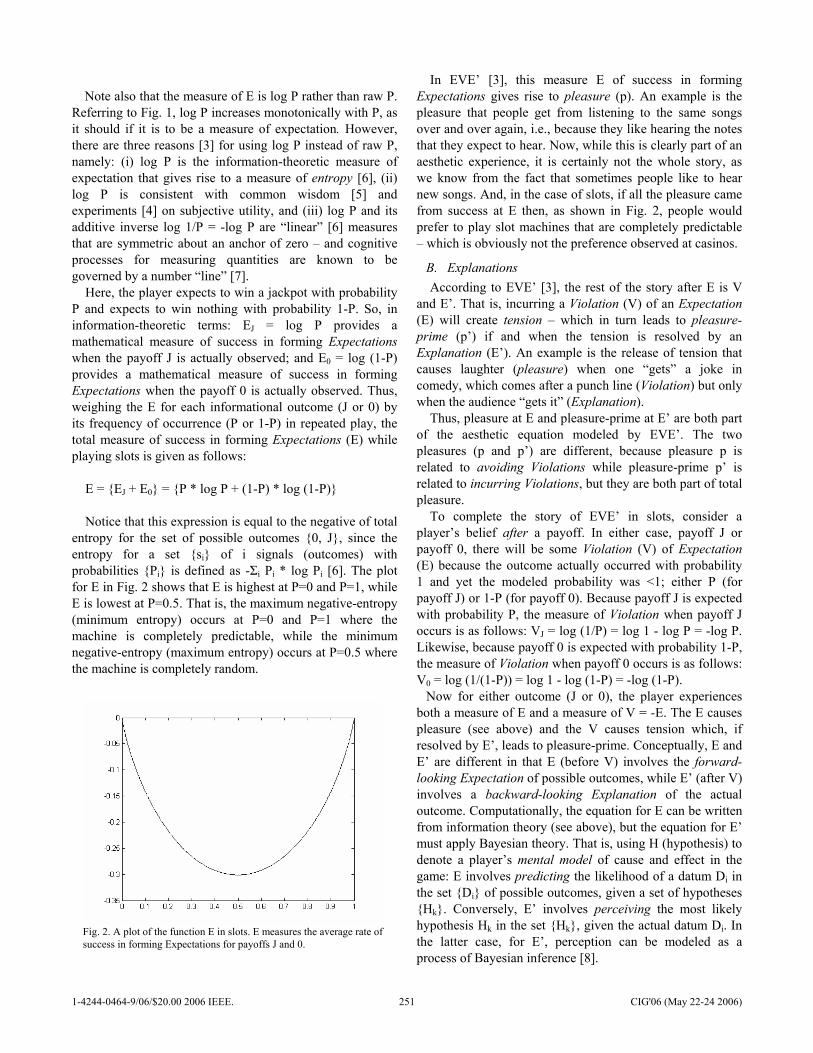
Note also that the measure of E is log P rather than raw P.

Referring to Fig. 1, log P increases monotonically with P, as it should if it is to be a measure of expectation. However, there are three reasons [3] for using log P instead of raw P, namely: (i) log P is the information-theoretic measure of expectation that gives rise to a measure of entropy [6], (ii) log P is consistent with common wisdom [5] and experiments [4] on subjective utility, and (iii) log P and its additive inverse log 1/P = -log P are “linear” [6] measures that are symmetric about an anchor of zero – and cognitive processes for measuring quantities are known to be governed by a number “line” [7].

Here, the player expects to win a jackpot with probability P and expects to win nothing with probability 1-P. So, in information-theoretic terms: EJ = log P provides a mathematical measure of success in forming Expectations when the payoff J is actually observed; and E0 = log (1-P) provides a mathematical measure of success in forming Expectations when the payoff 0 is actually observed. Thus, weighing the E for each informational outcome (J or 0) by its frequency of occurrence (P or 1-P) in repeated play, the total measure of success in forming Expectations (E) while playing slots is given as follows:

E = {EJ + E0} = {P * log P + (1-P) * log (1-P)} Notice that this expression is equal to the negative of total

entropy for the set of possible outcomes {0, J}, since the entropy for a set {si} of i signals (outcomes) with probabilities {Pi} is defined as -Σi Pi * log Pi [6]. The plot for E in Fig. 2 shows that E is highest at P=0 and P=1, while E is lowest at P=0.5. That is, the maximum negative-entropy (minimum entropy) occurs at P=0 and P=1 where the machine is completely predictable, while the minimum negative-entropy (maximum entropy) occurs at P=0.5 where the machine is completely random.

In EVE’ [3], this measure E of success in forming Expectations gives rise to pleasure (p). An example is the pleasure that people get from listening to the same songs over and over again, i.e., because they like hearing the notes that they expect to hear. Now, while this is clearly part of an aesthetic experience, it is certainly not the whole story, as we know from the fact that sometimes people like to hear new songs. And, in the case of slots, if all the pleasure came from success at E then, as shown in Fig. 2, people would prefer to play slot machines that are completely predictable – which is obviously not the preference observed at casinos.

B. Explanations According to EVE’ [3], the rest of the story after E is V

and E’. That is, incurring a Violation (V) of an Expectation (E) will create tension – which in turn leads to pleasure-prime (p’) if and when the tension is resolved by an Explanation (E’). An example is the release of tension that causes laughter (pleasure) when one “gets” a joke in comedy, which comes after a punch line (Violation) but only when the audience “gets it” (Explanation).

Thus, pleasure at E and pleasure-prime at E’ are both part of the aesthetic equation modeled by EVE’. The two pleasures (p and p’) are different, because pleasure p is related to avoiding Violations while pleasure-prime p’ is related to incurring Violations, but they are both part of total pleasure.

To complete the story of EVE’ in slots, consider a player’s belief after a payoff. In either case, payoff J or payoff 0, there will be some Violation (V) of Expectation (E) because the outcome actually occurred with probability 1 and yet the modeled probability was <1; either P (for payoff J) or 1-P (for payoff 0). Because payoff J is expected with probability P, the measure of Violation when payoff J occurs is as follows: VJ = log (1/P) = log 1 - log P = -log P. Likewise, because payoff 0 is expected with probability 1-P, the measure of Violation when payoff 0 occurs is as follows: V0 = log (1/(1-P)) = log 1 - log (1-P) = -log (1-P).

Now for either outcome (J or 0), the player experiences both a measure of E and a measure of V = -E. The E causes pleasure (see above) and the V causes tension which, if resolved by E’, leads to pleasure-prime. Conceptually, E and E’ are different in that E (before V) involves the forward-looking Expectation of possible outcomes, while E’ (after V) involves a backward-looking Explanation of the actual outcome. Computationally, the equation for E can be written from information theory (see above), but the equation for E’ must apply Bayesian theory. That is, using H (hypothesis) to denote a player’s mental model of cause and effect in the game: E involves predicting the likelihood of a datum Di in the set {Di} of possible outcomes, given a set of hypotheses {Hk}. Conversely, E’ involves perceiving the most likely hypothesis Hk in the set {Hk}, given the actual datum Di. In the latter case, for E’, perception can be modeled as a process of Bayesian inference [8].

Fig. 2. A plot of the function E in slots. E measures the average rate of success in forming Expectations for payoffs J and 0.

1-4244-0464-9/06/$20.00 2006 IEEE. 251 CIG'06 (May 22-24 2006)

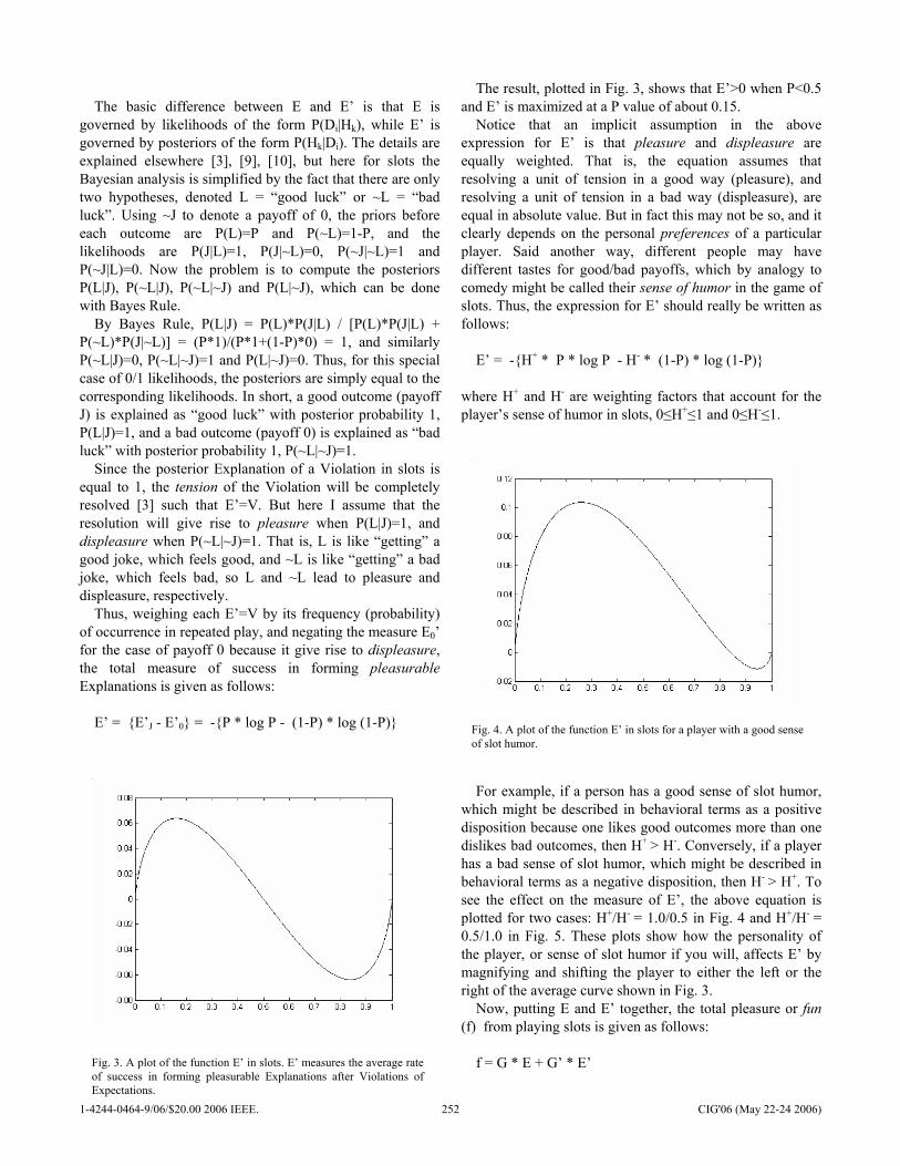
The basic difference between E and E’ is that E is

governed by likelihoods of the form P(Di|Hk), while E’ is governed by posteriors of the form P(Hk|Di). The details are explained elsewhere [3], [9], [10], but here for slots the Bayesian analysis is simplified by the fact that there are only two hypotheses, denoted L = “good luck” or ~L = “bad luck”. Using ~J to denote a payoff of 0, the priors before each outcome are P(L)=P and P(~L)=1-P, and the likelihoods are P(J|L)=1, P(J|~L)=0, P(~J|~L)=1 and P(~J|L)=0. Now the problem is to compute the posteriors P(L|J), P(~L|J), P(~L|~J) and P(L|~J), which can be done with Bayes Rule.

By Bayes Rule, P(L|J) = P(L)*P(J|L) / [P(L)*P(J|L) + P(~L)*P(J|~L)] = (P*1)/(P*1+(1-P)*0) = 1, and similarly P(~L|J)=0, P(~L|~J)=1 and P(L|~J)=0. Thus, for this special case of 0/1 likelihoods, the posteriors are simply equal to the corresponding likelihoods. In short, a good outcome (payoff J) is explained as “good luck” with posterior probability 1, P(L|J)=1, and a bad outcome (payoff 0) is explained as “bad luck” with posterior probability 1, P(~L|~J)=1.

Since the posterior Explanation of a Violation in slots is equal to 1, the tension of the Violation will be completely resolved [3] such that E’=V. But here I assume that the resolution will give rise to pleasure when P(L|J)=1, and displeasure when P(~L|~J)=1. That is, L is like “getting” a good joke, which feels good, and ~L is like “getting” a bad joke, which feels bad, so L and ~L lead to pleasure and displeasure, respectively.

Thus, weighing each E’=V by its frequency (probability) of occurrence in repeated play, and negating the measure E0’ for the case of payoff 0 because it give rise to displeasure, the total measure of success in forming pleasurable Explanations is given as follows:

E’ = {E’J - E’0} = -{P * log P - (1-P) * log (1-P)}

The result, plotted in Fig. 3, shows that E’>0 when P<0.5 and E’ is maximized at a P value of about 0.15.

Notice that an implicit assumption in the above expression for E’ is that pleasure and displeasure are equally weighted. That is, the equation assumes that resolving a unit of tension in a good way (pleasure), and resolving a unit of tension in a bad way (displeasure), are equal in absolute value. But in fact this may not be so, and it clearly depends on the personal preferences of a particular player. Said another way, different people may have different tastes for good/bad payoffs, which by analogy to comedy might be called their sense of humor in the game of slots. Thus, the expression for E’ should really be written as follows:

E’ = -{H+ * P * log P - H- * (1-P) * log (1-P)}

where H+ and H- are weighting factors that account for the player’s sense of humor in slots, 0≤H+≤1 and 0≤H-≤1.

Fig. 4. A plot of the function E’ in slots for a player with a good sense of slot humor.

Fig. 3. A plot of the function E’ in slots. E’ measures the average rate of success in forming pleasurable Explanations after Violations of Expectations.

For example, if a person has a good sense of slot humor, which might be described in behavioral terms as a positive disposition because one likes good outcomes more than one dislikes bad outcomes, then H+ > H-. Conversely, if a player has a bad sense of slot humor, which might be described in behavioral terms as a negative disposition, then H- > H+. To see the effect on the measure of E’, the above equation is plotted for two cases: H+/H- = 1.0/0.5 in Fig. 4 and H+/H- = 0.5/1.0 in Fig. 5. These plots show how the personality of the player, or sense of slot humor if you will, affects E’ by magnifying and shifting the player to either the left or the right of the average curve shown in Fig. 3.

Now, putting E and E’ together, the total pleasure or fun (f) from playing slots is given as follows:

f = G * E + G’ * E’

1-4244-0464-9/06/$20.00 2006 IEEE. 252 CIG'06 (May 22-24 2006)

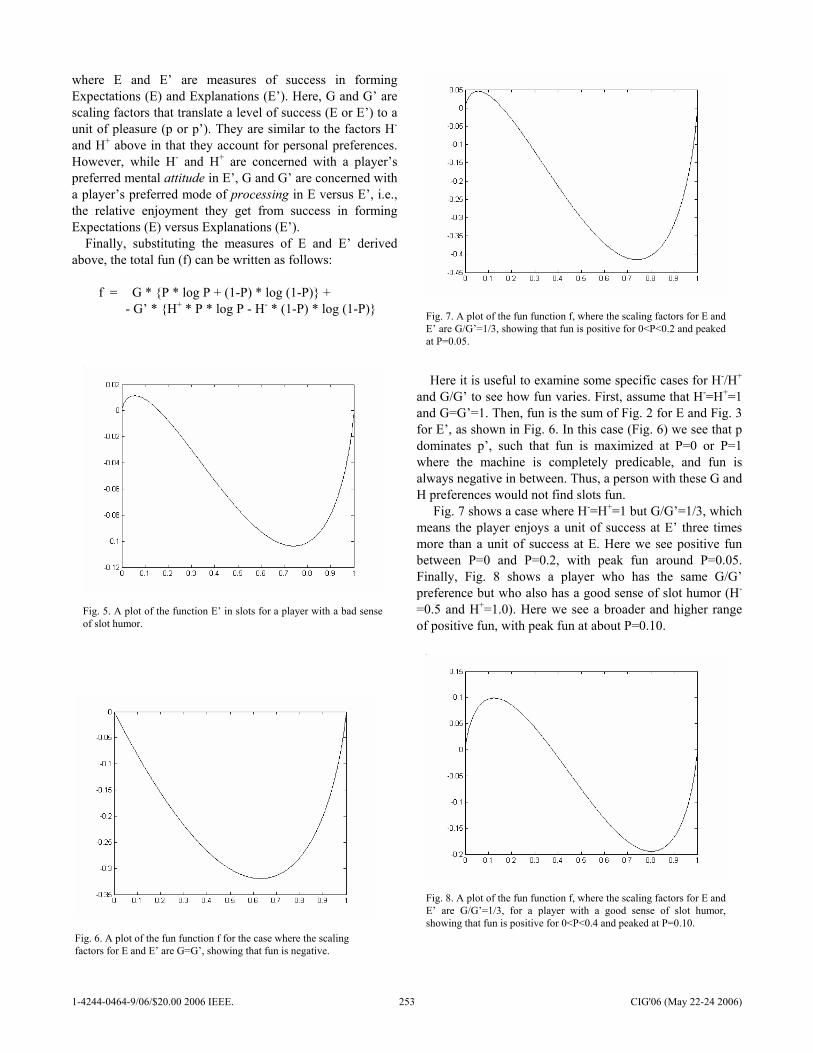
where E and E’ are measures of success in forming Expectations (E) and Explanations (E’). Here, G and G’ are scaling factors that translate a level of success (E or E’) to a unit of pleasure (p or p’). They are similar to the factors H- and H+ above in that they account for personal preferences. However, while H- and H+ are concerned with a player’s preferred mental attitude in E’, G and G’ are concerned with a player’s preferred mode of processing in E versus E’, i.e., the relative enjoyment they get from success in forming Expectations (E) versus Explanations (E’).

Fig. 7. A plot of the fun function f, where the scaling factors for E and E’ are G/G’=1/3, showing that fun is positive for 0<P<0.2 and peaked at P=0.05.

Finally, substituting the measures of E and E’ derived above, the total fun (f) can be written as follows:

f = G * {P * log P + (1-P) * log (1-P)} +

- G’ * {H+ * P * log P - H- * (1-P) * log (1-P)}

Fig. 5. A plot of the function E’ in slots for a player with a bad sense of slot humor.

Here it is useful to examine some specific cases for H-/H+ and G/G’ to see how fun varies. First, assume that H-=H+=1 and G=G’=1. Then, fun is the sum of Fig. 2 for E and Fig. 3 for E’, as shown in Fig. 6. In this case (Fig. 6) we see that p dominates p’, such that fun is maximized at P=0 or P=1 where the machine is completely predicable, and fun is always negative in between. Thus, a person with these G and H preferences would not find slots fun.

Fig. 7 shows a case where H-=H+=1 but G/G’=1/3, which means the player enjoys a unit of success at E’ three times more than a unit of success at E. Here we see positive fun between P=0 and P=0.2, with peak fun around P=0.05. Finally, Fig. 8 shows a player who has the same G/G’ preference but who also has a good sense of slot humor (H-

=0.5 and H+=1.0). Here we see a broader and higher range of positive fun, with peak fun at about P=0.10.

Fig. 8. A plot of the fun function f, where the scaling factors for E and E’ are G/G’=1/3, for a player with a good sense of slot humor, showing that fun is positive for 0<P<0.4 and peaked at P=0.10.

Fig. 6. A plot of the fun function f for the case where the scaling factors for E and E’ are G=G’, showing that fun is negative.

1-4244-0464-9/06/$20.00 2006 IEEE. 253 CIG'06 (May 22-24 2006)

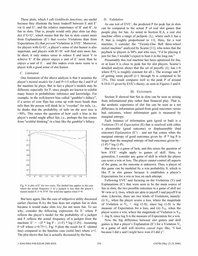
These plots, which I call Goldilocks functions, are useful because they illustrate the basic tradeoff between E and E’ via G and G’, and the relative importance of H- and H+, to fun in slots. That is, people would only play slots (as they do) if G<G’, which means that the fun in slots comes more from Explanations (E’) that resolve Violations than from Expectations (E) that prevent Violations in EVE’. Moreover, for players with G<G’, a player’s sense of slot humor is also important, and players with H-<H+ will find slots more fun. In short, it only makes sense to reduce E and incur V to achieve E’ if the player enjoys a unit of E’ more than he enjoys a unit of E – and this makes even more sense to a player with a good sense of slot humor.

C. Limitation One limitation of the above analysis is that it assumes the

player’s mental models for J and P=1/J reflect the J and P of the machine he plays. But in fact a player’s models may be different, especially for P, since people are known to exhibit many biases in probabilistic inference and knowledge. For example, in the well-known bias called “gambler’s fallacy”, if a series of coin flips has come up with more heads than tails then the person will think he is “overdue” for tails, i.e., he thinks that the probability of tails on the next toss is >50%. This raises the question of how such a bias in the player’s model might affect fun, i.e., perhaps the fun comes from “wishful thinking” in a bias like the gambler’s fallacy.

But here again, like the case of subjective utility discussed earlier (Section II.A), the bias does not explain fun in slots because it would make slots less fun not more fun. To see why, consider the following expression for E’ where P reflects the player’s model for the probability of a jackpot and F reflects the actual frequency of a jackpot from the machine: E’ = -{F * log P - (1-F) * log (1-P)}. Assuming F=cP where c=0.75<1, Fig. 9 plots the result for E’ (dotted line) compared to the baseline case (solid line) where c=1. The plot shows that fun is actually decreased by the bias.

D. Validation As one test of EVE’, the predicted P for peak fun in slots

can be compared to the actual P of real slot games that people play for fun. As noted in Section II.A, a real slot machine offers a range of jackpots {Ji}, where each Ji has a Pi that is roughly proportional to 1/Ji. Here, for a real machine, I consider the “Twenty-One Bell three-wheel nickel machine” analyzed by Scarne [11], who notes that the payback to players is 94% and who says, “I’d be playing it just for fun; I wouldn’t expect to beat it in the long run.”

Presumably this real machine has been optimized for fun, or at least it is close to peak fun for slot players. Scarne’s detailed analysis shows that the set of payoffs {Ji} has i=8 where Pi*Ji is roughly constant for all i. The average rate P of getting some payoff (i=1 through 8) is computed to be 13%. This result compares well to the peak P of around 0.10-0.15 given by EVE’s theory, as seen in Figures 3 and 8.

III. EXTENSION Section II showed that fun in slots can be seen as arising

from informational play rather than financial play. That is, the aesthetic experience of slot fun can be seen as a net difference in information gained from good outcomes versus bad outcomes, where information gain is measured by marginal entropy.

Each instance of information gain (good or bad) is a Violation (V) of Expectation (E) that is resolved with either a pleasurable (good outcome) or displeasurable (bad outcome) Explanation (E’) – and net fun comes when the marginal entropy of good outcomes given by -P * log P is larger than the marginal entropy of bad outcomes given by -(1-P) * log (1-P).

But slots is a game of luck, and this raises the question of how EVE’ might apply to games of skill. Here, to generalize, I consider any game of skill in which the player can score a win or loss. The player cannot control all aspects of the game, so the outcome is unknown. Thus, a player of this game can be modeled by a win probability S, which is like P in slot games because it establishes a player’s Expectations for a win or loss on each attempt.

Following EVE’ and focusing on the Violations (V) and Explanations (E’) that were seen to be the main source of fun in slots, the two possible outcomes in a game of skill are W=win or L=loss, which are akin to payoff J and payoff 0 in slots. Likewise, there are two kinds of Violations, namely: (i) VL, when the player scores a loss, where the magnitude of Violation is VL = -log (1-S), since log (1-S) is the measure of Expectation for a loss, and (ii) VW, when the player scores a win, where the magnitude of Violation is VW = -log S, since log S is the measure of Expectation for a win.

Now the big difference between slot games and skill games is that a player’s Explanation (E’) for a Violation VL in a game of skill will involve causal logic like, “I lost because I did x and I might have won if I did y”.

Fig. 9. A plot of E’ for two cases. The dashed line applies to the case where the actual frequency F of a jackpot is less than the player’s mental model P, F=0.75*P. The solid line applies when F=P.

1-4244-0464-9/06/$20.00 2006 IEEE. 254 CIG'06 (May 22-24 2006)

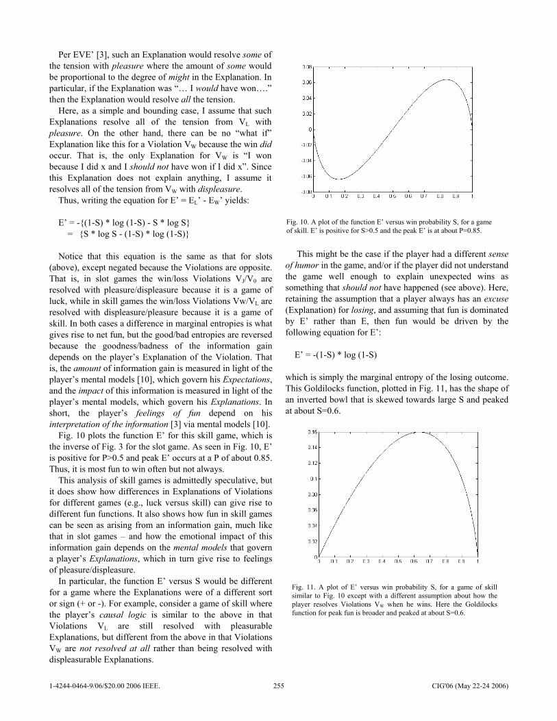
Per EVE’ [3], such an Explanation would resolve some of the tension with pleasure where the amount of some would be proportional to the degree of might in the Explanation. In particular, if the Explanation was “… I would have won….” then the Explanation would resolve all the tension.

Here, as a simple and bounding case, I assume that such Explanations resolve all of the tension from VL with pleasure. On the other hand, there can be no “what if” Explanation like this for a Violation VW because the win did occur. That is, the only Explanation for VW is “I won because I did x and I should not have won if I did x”. Since this Explanation does not explain anything, I assume it resolves all of the tension from VW with displeasure.

Thus, writing the equation for E’ = EL’ - EW’ yields: E’ = -{(1-S) * log (1-S) - S * log S} = {S * log S - (1-S) * log (1-S)} Notice that this equation is the same as that for slots

(above), except negated because the Violations are opposite. That is, in slot games the win/loss Violations VJ/V0 are resolved with pleasure/displeasure because it is a game of luck, while in skill games the win/loss Violations Vw/VL are resolved with displeasure/pleasure because it is a game of skill. In both cases a difference in marginal entropies is what gives rise to net fun, but the good/bad entropies are reversed because the goodness/badness of the information gain depends on the player’s Explanation of the Violation. That is, the amount of information gain is measured in light of the player’s mental models [10], which govern his Expectations, and the impact of this information is measured in light of the player’s mental models, which govern his Explanations. In short, the player’s feelings of fun depend on his interpretation of the information [3] via mental models [10].

Fig. 10 plots the function E’ for this skill game, which is the inverse of Fig. 3 for the slot game. As seen in Fig. 10, E’ is positive for P>0.5 and peak E’ occurs at a P of about 0.85. Thus, it is most fun to win often but not always.

This analysis of skill games is admittedly speculative, but it does show how differences in Explanations of Violations for different games (e.g., luck versus skill) can give rise to different fun functions. It also shows how fun in skill games can be seen as arising from an information gain, much like that in slot games – and how the emotional impact of this information gain depends on the mental models that govern a player’s Explanations, which in turn give rise to feelings of pleasure/displeasure.

In particular, the function E’ versus S would be different for a game where the Explanations were of a different sort or sign (+ or -). For example, consider a game of skill where the player’s causal logic is similar to the above in that Violations VL are still resolved with pleasurable Explanations, but different from the above in that Violations VW are not resolved at all rather than being resolved with displeasurable Explanations.

This might be the case if the player had a different sense of humor in the game, and/or if the player did not understand the game well enough to explain unexpected wins as something that should not have happened (see above). Here, retaining the assumption that a player always has an excuse (Explanation) for losing, and assuming that fun is dominated by E’ rather than E, then fun would be driven by the following equation for E’:

Fig. 10. A plot of the function E’ versus win probability S, for a game of skill. E’ is positive for S>0.5 and the peak E’ is at about P=0.85.

E’ = -(1-S) * log (1-S) which is simply the marginal entropy of the losing outcome. This Goldilocks function, plotted in Fig. 11, has the shape of an inverted bowl that is skewed towards large S and peaked at about S=0.6.

Fig. 11. A plot of E’ versus win probability S, for a game of skill similar to Fig. 10 except with a different assumption about how the player resolves Violations VW when he wins. Here the Goldilocks function for peak fun is broader and peaked at about S=0.6.

1-4244-0464-9/06/$20.00 2006 IEEE. 255 CIG'06 (May 22-24 2006)

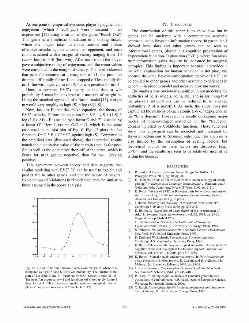
As one point of empirical evidence, player’s judgments of enjoyment (which I call fun) were measured in an experiment [12] using a variant of the game “Punch Out”. This game is a simplistic simulation of a boxing match, where the player takes defensive actions and makes offensive attacks against a computer opponent, and each round is scored with a margin of victory ranging from -10 (worst loss) to +10 (best win). After each round the player gave a subjective rating of enjoyment, and the mean values were correlated to the margin of victory. The results showed that peak fun occurred at a margin m of +1; the peak fun dropped off rapidly for m<1 and dropped off less rapidly for m>1; fun was negative for m<-2; fun was positive for m>-1.

Here, to compare EVE’s theory to this data, a win probability S must be converted to a measure of margin m. Using the standard approach of a Rasch model [13], margin m would vary roughly as logit (S) = log (S/(1-S)).

Now, besides E’ per the above equation, the theory of EVE’ includes E from the equation E = S * log S + (1-S) * log (1-S). Also, E is scaled by a factor G and E’ is scaled by a factor G’. Here I assume G/G’=1/3, which is the same ratio used in the slot plot of Fig. 8. Fig. 12 plots the fun function, f = G * E + G’ * E’, against logit (S). Compared to the empirical data (discussed above), the theoretical results match the quantitative value of the margin (m=+1) for peak fun as well as the qualitative drop-off of the curve, which is faster for m<1 (going negative) than for m>1 (staying positive).

This agreement between theory and data suggests that similar modeling with EVE’ [3] can be used to explain and predict fun in other games, and that the nature of players’ Explanations of Violations in “Punch Out” may be similar to those assumed in the above analysis.

IV. CONCLUSION The contribution of this paper is to show how fun in

games can be analyzed with a computational-aesthetic approach, using Bayesian-information theory. In particular, I showed how slots and other games can be seen as informational games, played in a cognitive progression of Expectation-Violation-Explanation (EVE’), where fun arises from information gains that can be measured by marginal entropies. This finding is important because it provides a plausible explanation for human behavior in slot play, and because the same Bayesian-information theory of EVE’ can be applied to other games and other aesthetic experiences in general – in order to model and measure how fun works.

The analysis was obviously simplified in not modeling the aesthetics of bells, wheels, coins, etc., and in assuming that the player’s anticipations can be reduced to an average probability P of a payoff J. As such, the study does not capture all the nuances of each atomic E-V-E’ experience in the “time domain”. However, the results do capture major modes of time-averaged aesthetics in the “frequency domain”, plotted as Goldilocks functions. These functions show how enjoyment can be modeled and measured by Bayesian extensions to Shannon entropies. The analysis is also limited by the assumption of scaling factors, but theoretical bounds on these factors are discussed (e.g., G<G’), and the results are seen to be relatively insensitive within the bounds.

REFERENCES [1] R. Koster, A Theory of Fun for Game Design. Scottsdale, AZ:

Paraglyph Press, 2005, pg. 10, pg. 46. [2] E. Huhtamo, “Slots of fun, slots of trouble: An archaeology of arcade

gaming,” in Handbook of Computer Game Studies, J. Raessens and J. Goldstein, Eds. Cambridge, MA: MIT Press, 2005, pp. 3-21.

[3] K. Burns, “Atoms of EVE’: A Bayesian basis for aesthetic analysis of style in sketching,” Artificial Intelligence for Engineering, Design, Analysis and Manufacturing, in press.

Fig. 12. A plot of the fun function f versus win margin m, where m is computed as logit (S) and S is the win probability. The function is the sum of fun from E and E’, weighted by G:G’ factors in ratio of 1:3. The peak fun occurs at m=+1 and fun drops off more rapidly for m<1 than for m>1. This theoretical model matches empirical data on players’ enjoyment in a game of “Punch Out” [12].

[4] J. Baron, Thinking and Deciding, Third Edition. New York, NY: Cambridge University Press, 2000, pp. 238-243.

[5] D. Bernoulli, “Exposition of a new theory of the measurement of risk,” L. Sommer, Trans. Econometrica, vol. 22, 1954, pp. 23-26. Original work published 1738.

[6] C. Shannon and W. Weaver, The Mathematical Theory of Communication. Urbana, IL: University of Chicago Press, 1949.

[7] S. Dehaene, The Number Sense: How the Mind Creates Mathematics. New York, NY: Oxford University Press, 1997.

[8] D. Knill and W. Richards, Perception as Bayesian Inference. Cambridge, UK: Cambridge University Press, 1996.

[9] K. Burns, “Bayesian inference in disputed authorship: A case study of cognitive errors and new system for decision support,” Information Sciences, vol. 176, no. 11, 2006, pp. 1570-1589.

[10] K. Burns, “Mental models and normal errors,” in How Professionals Make Decisions, H. Montgomery, R. Lipshitz and B. Brehmer, Eds. Mahwah, NJ: Lawrence Erlbaum, 2005, pp. 15-28.

[11] J. Scarne, Scarne’s New Complete Guide to Gambling. New York, NY: Simon & Schuster, 1961, pp. 445-448.

[12] P. Piselli, “Relating cognitive models of computer games to user evaluations of entertainment,” MS thesis, Dept. of Computer Science, Worcester Polytechnic Institute, 2006.

[13] G. Rasch, Probabilistic Models for Some Intelligence and Attainment Tests. Chicago, IL: University of Chicago Press, 1980.

1-4244-0464-9/06/$20.00 2006 IEEE. 256 CIG'06 (May 22-24 2006)

Style in Poker Kevin Burns

Abstract— Style is the cognitive basis for behavior in game play. This is because mental limits force human beings to act based on reduced rule-sets, which in game parlance are called styles, rather than exhaustive enumeration of options, which in game theory are called strategies. This paper explores the computational underpinnings of style in poker, by analyzing three versions of a two-player game ranging from very simple to rather complex, using theoretical analyses and deterministic calculations. The results show that simple styles derived from commonsense reasoning often closely approximate the Nash equilibrium strategies. Moreover, styles often outperform Nash equilibrium strategies against sub-optimal strategies, and some styles are seen to be nearly maximally super-optimal – i.e., almost equivalent to a player who is perfectly Bayesian. This is an important finding with respect to the practical tradeoff between effort and winnings, because the computational implementation of styles is trivial compared to that of strategies.

I. INTRODUCTION TYLE in poker is a distinctive pattern of decision making. Poker players often refer to styles like Tight versus

Loose or Passive versus Aggressive [1], [2], [3], and poker programs often reflect these same styles in artificial agents [4], [5], [6]. But how do such styles arise in human heads? And how well do simple styles perform against sophisticated strategies in head to head competition? These are the questions explored in this paper.

Here style is analyzed in three versions of poker ranging from very simple to rather complex. The simplest game, discussed in Section II, is a Borel [7] type game, denoted AB because the longest path through the game tree is AB, where player A bets and player B calls. Here the game is simplified even further in that there are only two possible hands that each player may hold, high or low. This game is denoted AB-2. A more complex game, discussed in Section III, adds a raise option for player B, and a fold/call decision for player A, so it is denoted ABA’-2. The most complex game, analyzed in Section IV, is an ABA’-11 game of integer poker played with a deck of 11 cards.

All three games are tractable to mathematical analysis of optimal strategies. This provides a useful benchmark for comparing and contrasting “normative” (game theoretical) strategies to “cognitive” (game psychological) styles. The three-game progression has a threefold objective, as follows:

Manuscript received March 31, 2006. This work was supported by the MITRE Technology Program.

Kevin Burns is with the MITRE Corporation, 202 Burlington Road, Bedford, MA 01730-1420 USA (phone: 781-271-8762; fax: 781-271-2101; e-mail: kburns@mitre.org).

First, the simplest game serves to introduce the psychological notion of style in game playing and relate it to the mathematical definition of strategy in game theory. Second, the more complex games show how styles scale as the game tree and game states grow. Finally, the progression suggests directions for future work aimed at extending research on styles of play beyond poker to real life problems in business and warfare [8], [9].

The present research differs from previous research in combining a cognitive perspective on style in game playing [10] with a normative perspective on strategies in game theory. Other studies have been concerned with finding [11] and learning [12] optimal or near-optimal strategies in scaled-down or full-scale [13], [14] pokers, including recent research on the problem of opponent modeling [15], [16] where Bayesian methods [17], [18] can be used to exploit opponents who play with sub-optimal strategies. The problem of combinatorial explosion and the notion of conceptual abstraction [19] to deal with this problem are ubiquitous in these studies, but there is still a big gap between normative strategies in game theory and cognitive abstractions in game playing.

The reality is that cognitive styles are vastly simpler that normative strategies, computationally, because people cannot exhaustively enumerate and evaluate the huge (order >E10) game trees of full-scale poker. And yet people can play very well against computer opponents [20], which means that cognitive styles can be extremely efficient compared to normative and near-normative strategies.

The question addressed in this paper is: How can people play so well? The approach compares normative strategies to cognitive styles in a progression of poker games, to see how they relate and to see how styles might scale. In so doing, it is shown that commonsense styles are effective in capturing the computational advantages of optimal strategies with reduced rule-sets that are extremely simplified. In particular, it is shown that bet/raise styles characterized by a fixed [x, y] vector of hand strengths can approximate the performance of sophisticated strategies in Bayesian updating of win:loss odds and Bayesian decisions on betting and raising.

These findings suggest that research on style can shed light on how to win in poker, as well as how to win in real life. And that is the purpose of this paper, namely to analyze the basis behind commonsense styles and compare their performance to optimal strategies – in order to assess the advantages and disadvantages of style-based reasoning in the constrained context of poker playing.

S

1-4244-0464-9/06/$20.00 2006 IEEE. 257 CIG'06 (May 22-24 2006)

II. AB-2 GAME

A. Strategies As perhaps the simplest poker, consider a two-player

Borel [7] type game, similar to [21] in that each hand is either high (H) or low (L). This game could be played by dealing each player a coin where heads is H and tails is L, and each player would see only his own coin. Player A must bet or fold, and if he bets then player B must call or fold. Before the deal each player antes “a” chips to the pot, then a bet by A or a call by B adds “b” chips to the pot.

For this game there are only three possible outcomes: (1) A folds so B nets “a” chips; (2) A bets and B folds so A nets “a” chips; (3) A bets and B calls so the player with the higher hand (H>L) nets “a+b” chips. In a showdown where both hands are equal, then the pot is split and each player nets 0 chips.

Since each player is dealt either L or H, a strategy can be expressed as a doublet (L, H), e.g., (fold, fold) means a player will fold with L and fold with H. Using the notation f=fold, b=bet and c=call, each player has four possible strategies. Putting A’s strategies in rows and B’s strategies in columns, the payoff matrix (Table 1) has 16 cells, each computed as an average over all possible game states.

As an example, consider the cell for row A(b, b) and column B(f, c). There are four possible game states to consider, namely: (1) A=L and B=L; (2) A=L and B=H; (3) A=H and B=L; (4) A=H and B=H. Applying the strategies A(b, b) and B(f, c) to each state yields the following payoffs for A: (1) +a; (2) -(a+b); (3) +a; (4) 0; where + is a win for A and - is a win for B. Since each state is equally likely, the average payoff is +(a-b)/4. The remaining cells are computed similarly.

Now, for a specific game with real numbers for “a” and “b”, the payoff matrix can be quantified and solved for the optimal strategies, using standard techniques [21]. For example, when a=1 and b=4, the payoff matrix is as shown in Table 2. Examination shows that, for player A, the strategy A(f, b) dominates A(f, f) and A(b, f). Eliminating the first and third rows, player B’s strategy B(f, c) dominates B(f, f), B(c, f) and B(c, c). Thus, there is a minimax or Nash equilibrium, which is the minimum of columns and the maximum of rows, at B(f, c) and A(f, b). Here the value of the game (to player A) is -1/4.

This type of strategic analysis to find optimal (Nash equilibrium) solutions is standard in the field of game theory. It is presented here not as an original contribution but rather to highlight (below) how psychological styles of game playing differ from mathematical strategies of game theory. In game theory (above), decisions are made by exhaustive enumeration of all possible actions and outcomes, assuming one’s opponent does the same, and then by selecting one’s own strategy to provide maximum benefit to oneself, assuming the opponent does the same for himself. But in game playing, by cognitive humans as opposed to normative systems, there are three major differences.

First, human players cannot in general perform exhaustive enumeration of all possible scenarios due to mental limits. Second, although maximum benefit is a reasonable objective, humans will and should balance the possible winnings with the cognitive effort, i.e., they will not and should not expend large increases in effort for small increases in winnings. Finally, in game play, humans will often assign values to attributes that are not modeled in the payoff matrix.

For example, a player may assign value to the act of betting itself because it is more fun [22] than folding, and after all most players are playing for pleasure as well as money – as there may be much better (less effort) ways of making money. Plus, even if money is the only value considered in the equation, the value of a dollar to a person depends on how many dollars that person has, i.e., it is well known from research studies on human judgment [23] that people have non-linear utility functions.

TABLE 1 PAYOFF MATRIX FOR AB-2 GAME

B(f, f) B(f, c) B(c , f) B(c, c)

A(f, f) -a -a -a -a

A(f, b) 0 -a/4 +b/4 +(b-a)/4

A(b, f) 0 -(2a+b)/4 -a/4 -(3a+b)/4

A(b, b) +a +(a-b)/4 +(3a+b)/4 0

Cells show payoff for A; negative is loss for A and win for B; A’s

strategies are in rows; B’s strategies are in columns; f=fold, b=bet, c=call.

A B bet

fold fold

call

Fig. 1. Game tree for AB poker. Player A must bet or fold; if A bets then B must call or fold. Before the deal, each player antes “a” chips to the pot; a bet by A or a call by B adds “b” chips to the pot.

TABLE 2 PAYOFF MATRIX FOR AB-2 GAME

a=1, b=4

B(f, f) B(f, c) B(c, f) B(c, c)

A(f, f) -1 -1 -1 -1

A(f, b) 0 -1/4 +1 +3/4

A(b, f) 0 -6/4 -1/4 -7/4

A(b, b) +1 -3/4 +7/4 0

1-4244-0464-9/06/$20.00 2006 IEEE. 258 CIG'06 (May 22-24 2006)

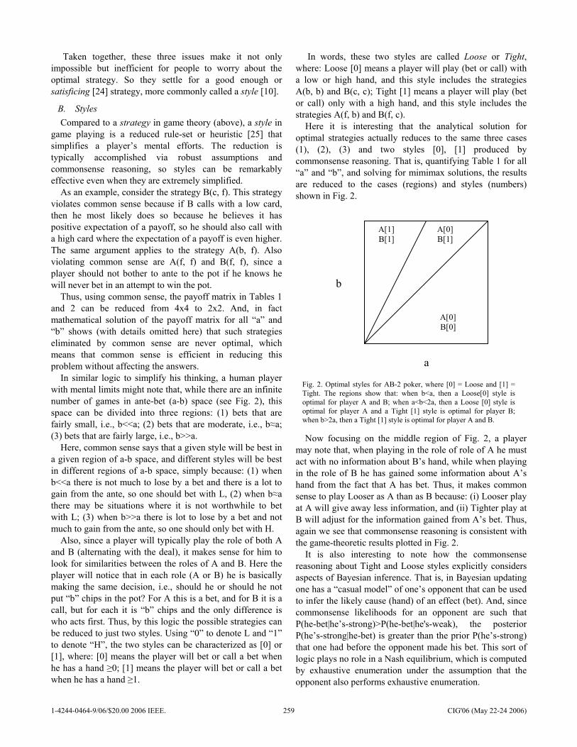
Taken together, these three issues make it not only impossible but inefficient for people to worry about the optimal strategy. So they settle for a good enough or satisficing [24] strategy, more commonly called a style [10].

B. Styles Compared to a strategy in game theory (above), a style in

game playing is a reduced rule-set or heuristic [25] that simplifies a player’s mental efforts. The reduction is typically accomplished via robust assumptions and commonsense reasoning, so styles can be remarkably effective even when they are extremely simplified.

As an example, consider the strategy B(c, f). This strategy violates common sense because if B calls with a low card, then he most likely does so because he believes it has positive expectation of a payoff, so he should also call with a high card where the expectation of a payoff is even higher. The same argument applies to the strategy A(b, f). Also violating common sense are A(f, f) and B(f, f), since a player should not bother to ante to the pot if he knows he will never bet in an attempt to win the pot.

Thus, using common sense, the payoff matrix in Tables 1 and 2 can be reduced from 4x4 to 2x2. And, in fact mathematical solution of the payoff matrix for all “a” and “b” shows (with details omitted here) that such strategies eliminated by common sense are never optimal, which means that common sense is efficient in reducing this problem without affecting the answers.

In similar logic to simplify his thinking, a human player with mental limits might note that, while there are an infinite number of games in ante-bet (a-b) space (see Fig. 2), this space can be divided into three regions: (1) bets that are fairly small, i.e., b<<a; (2) bets that are moderate, i.e., b≈a; (3) bets that are fairly large, i.e., b>>a.

Here, common sense says that a given style will be best in a given region of a-b space, and different styles will be best in different regions of a-b space, simply because: (1) when b<<a there is not much to lose by a bet and there is a lot to gain from the ante, so one should bet with L, (2) when b≈a there may be situations where it is not worthwhile to bet with L; (3) when b>>a there is lot to lose by a bet and not much to gain from the ante, so one should only bet with H.

Also, since a player will typically play the role of both A and B (alternating with the deal), it makes sense for him to look for similarities between the roles of A and B. Here the player will notice that in each role (A or B) he is basically making the same decision, i.e., should he or should he not put “b” chips in the pot? For A this is a bet, and for B it is a call, but for each it is “b” chips and the only difference is who acts first. Thus, by this logic the possible strategies can be reduced to just two styles. Using “0” to denote L and “1” to denote “H”, the two styles can be characterized as [0] or [1], where: [0] means the player will bet or call a bet when he has a hand ≥0; [1] means the player will bet or call a bet when he has a hand ≥1.

In words, these two styles are called Loose or Tight, where: Loose [0] means a player will play (bet or call) with a low or high hand, and this style includes the strategies A(b, b) and B(c, c); Tight [1] means a player will play (bet or call) only with a high hand, and this style includes the strategies A(f, b) and B(f, c).

Here it is interesting that the analytical solution for optimal strategies actually reduces to the same three cases (1), (2), (3) and two styles [0], [1] produced by commonsense reasoning. That is, quantifying Table 1 for all “a” and “b”, and solving for mimimax solutions, the results are reduced to the cases (regions) and styles (numbers) shown in Fig. 2.

Now focusing on the middle region of Fig. 2, a player may note that, when playing in the role of role of A he must act with no information about B’s hand, while when playing in the role of B he has gained some information about A’s hand from the fact that A has bet. Thus, it makes common sense to play Looser as A than as B because: (i) Looser play at A will give away less information, and (ii) Tighter play at B will adjust for the information gained from A’s bet. Thus, again we see that commonsense reasoning is consistent with the game-theoretic results plotted in Fig. 2.

It is also interesting to note how the commonsense reasoning about Tight and Loose styles explicitly considers aspects of Bayesian inference. That is, in Bayesian updating one has a “casual model” of one’s opponent that can be used to infer the likely cause (hand) of an effect (bet). And, since commonsense likelihoods for an opponent are such that P(he-bet|he’s-strong)>P(he-bet|he's-weak), the posterior P(he’s-strong|he-bet) is greater than the prior P(he’s-strong) that one had before the opponent made his bet. This sort of logic plays no role in a Nash equilibrium, which is computed by exhaustive enumeration under the assumption that the opponent also performs exhaustive enumeration.

a

b

A[1] B[1]

A[0] B[1]

A[0] B[0]

Fig. 2. Optimal styles for AB-2 poker, where [0] = Loose and [1] = Tight. The regions show that: when b<a, then a Loose[0] style is optimal for player A and B; when a<b<2a, then a Loose [0] style is optimal for player A and a Tight [1] style is optimal for player B; when b>2a, then a Tight [1] style is optimal for player A and B.

1-4244-0464-9/06/$20.00 2006 IEEE. 259 CIG'06 (May 22-24 2006)

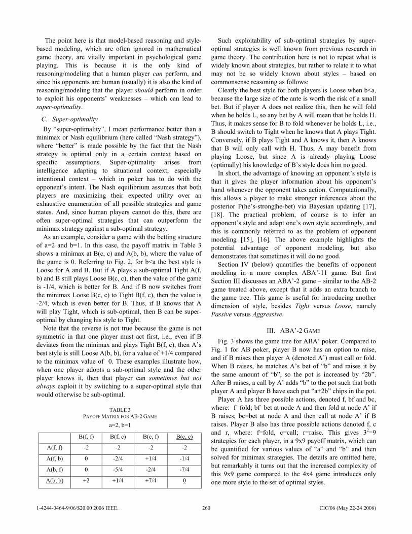
The point here is that model-based reasoning and style-based modeling, which are often ignored in mathematical game theory, are vitally important in psychological game playing. This is because it is the only kind of reasoning/modeling that a human player can perform, and since his opponents are human (usually) it is also the kind of reasoning/modeling that the player should perform in order to exploit his opponents’ weaknesses – which can lead to super-optimality.

C. Super-optimality By “super-optimality”, I mean performance better than a

minimax or Nash equilibrium (here called “Nash strategy”), where “better” is made possible by the fact that the Nash strategy is optimal only in a certain context based on specific assumptions. Super-optimality arises from intelligence adapting to situational context, especially intentional context – which in poker has to do with the opponent’s intent. The Nash equilibrium assumes that both players are maximizing their expected utility over an exhaustive enumeration of all possible strategies and game states. And, since human players cannot do this, there are often super-optimal strategies that can outperform the minimax strategy against a sub-optimal strategy.

As an example, consider a game with the betting structure of a=2 and b=1. In this case, the payoff matrix in Table 3 shows a minimax at B(c, c) and A(b, b), where the value of the game is 0. Referring to Fig. 2, for b<a the best style is Loose for A and B. But if A plays a sub-optimal Tight A(f, b) and B still plays Loose B(c, c), then the value of the game is -1/4, which is better for B. And if B now switches from the minimax Loose B(c, c) to Tight B(f, c), then the value is -2/4, which is even better for B. Thus, if B knows that A will play Tight, which is sub-optimal, then B can be super-optimal by changing his style to Tight.

Note that the reverse is not true because the game is not symmetric in that one player must act first, i.e., even if B deviates from the minimax and plays Tight B(f, c), then A’s best style is still Loose A(b, b), for a value of +1/4 compared to the minimax value of 0. These examples illustrate how, when one player adopts a sub-optimal style and the other player knows it, then that player can sometimes but not always exploit it by switching to a super-optimal style that would otherwise be sub-optimal.

Such exploitability of sub-optimal strategies by super-optimal strategies is well known from previous research in game theory. The contribution here is not to repeat what is widely known about strategies, but rather to relate it to what may not be so widely known about styles – based on commonsense reasoning as follows:

Clearly the best style for both players is Loose when b<a, because the large size of the ante is worth the risk of a small bet. But if player A does not realize this, then he will fold when he holds L, so any bet by A will mean that he holds H. Thus, it makes sense for B to fold whenever he holds L, i.e., B should switch to Tight when he knows that A plays Tight. Conversely, if B plays Tight and A knows it, then A knows that B will only call with H. Thus, A may benefit from playing Loose, but since A is already playing Loose (optimally) his knowledge of B’s style does him no good.

In short, the advantage of knowing an opponent’s style is that it gives the player information about his opponent’s hand whenever the opponent takes action. Computationally, this allows a player to make stronger inferences about the posterior P(he’s-strong|he-bet) via Bayesian updating [17], [18]. The practical problem, of course is to infer an opponent’s style and adapt one’s own style accordingly, and this is commonly referred to as the problem of opponent modeling [15], [16]. The above example highlights the potential advantage of opponent modeling, but also demonstrates that sometimes it will do no good.

Section IV (below) quantifies the benefits of opponent modeling in a more complex ABA’-11 game. But first Section III discusses an ABA’-2 game – similar to the AB-2 game treated above, except that it adds an extra branch to the game tree. This game is useful for introducing another dimension of style, besides Tight versus Loose, namely Passive versus Aggressive.

III. ABA’-2 GAME Fig. 3 shows the game tree for ABA’ poker. Compared to

Fig. 1 for AB poker, player B now has an option to raise, and if B raises then player A (denoted A’) must call or fold. When B raises, he matches A’s bet of “b” and raises it by the same amount of “b”, so the pot is increased by “2b”. After B raises, a call by A’ adds “b” to the pot such that both player A and player B have each put “a+2b” chips in the pot.

Player A has three possible actions, denoted f, bf and bc, where: f=fold; bf=bet at node A and then fold at node A’ if B raises; bc=bet at node A and then call at node A’ if B raises. Player B also has three possible actions denoted f, c and r, where: f=fold, c=call; r=raise. This gives 32=9 strategies for each player, in a 9x9 payoff matrix, which can be quantified for various values of “a” and “b” and then solved for minimax strategies. The details are omitted here, but remarkably it turns out that the increased complexity of this 9x9 game compared to the 4x4 game introduces only one more style to the set of optimal styles.

TABLE 3 PAYOFF MATRIX FOR AB-2 GAME

a=2, b=1

B(f, f) B(f, c) B(c, f) B(c, c)

A(f, f) -2 -2 -2 -2

A(f, b) 0 -2/4 +1/4 -1/4

A(b, f) 0 -5/4 -2/4 -7/4

A(b, b) +2 +1/4 +7/4 0

1-4244-0464-9/06/$20.00 2006 IEEE. 260 CIG'06 (May 22-24 2006)

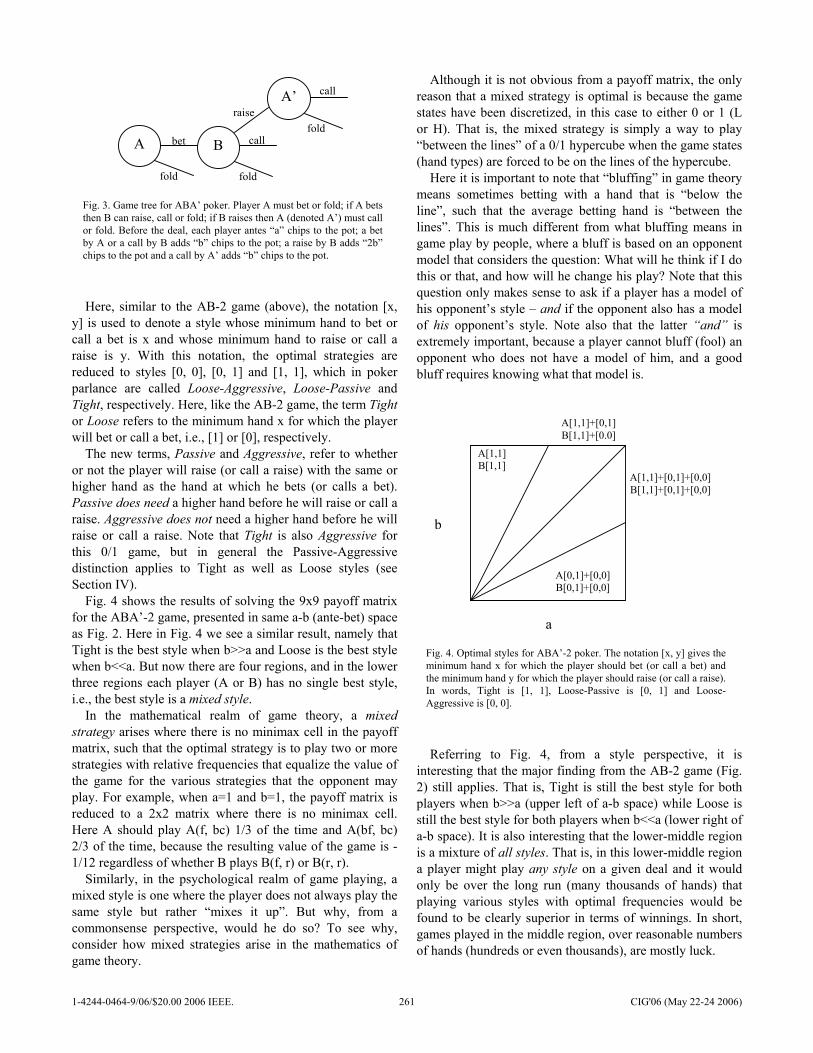
Here, similar to the AB-2 game (above), the notation [x, y] is used to denote a style whose minimum hand to bet or call a bet is x and whose minimum hand to raise or call a raise is y. With this notation, the optimal strategies are reduced to styles [0, 0], [0, 1] and [1, 1], which in poker parlance are called Loose-Aggressive, Loose-Passive and Tight, respectively. Here, like the AB-2 game, the term Tight or Loose refers to the minimum hand x for which the player will bet or call a bet, i.e., [1] or [0], respectively.

The new terms, Passive and Aggressive, refer to whether or not the player will raise (or call a raise) with the same or higher hand as the hand at which he bets (or calls a bet). Passive does need a higher hand before he will raise or call a raise. Aggressive does not need a higher hand before he will raise or call a raise. Note that Tight is also Aggressive for this 0/1 game, but in general the Passive-Aggressive distinction applies to Tight as well as Loose styles (see Section IV).

Fig. 4 shows the results of solving the 9x9 payoff matrix for the ABA’-2 game, presented in same a-b (ante-bet) space as Fig. 2. Here in Fig. 4 we see a similar result, namely that Tight is the best style when b>>a and Loose is the best style when b<<a. But now there are four regions, and in the lower three regions each player (A or B) has no single best style, i.e., the best style is a mixed style.

In the mathematical realm of game theory, a mixed strategy arises where there is no minimax cell in the payoff matrix, such that the optimal strategy is to play two or more strategies with relative frequencies that equalize the value of the game for the various strategies that the opponent may play. For example, when a=1 and b=1, the payoff matrix is reduced to a 2x2 matrix where there is no minimax cell. Here A should play A(f, bc) 1/3 of the time and A(bf, bc) 2/3 of the time, because the resulting value of the game is -1/12 regardless of whether B plays B(f, r) or B(r, r).

Similarly, in the psychological realm of game playing, a mixed style is one where the player does not always play the same style but rather “mixes it up”. But why, from a commonsense perspective, would he do so? To see why, consider how mixed strategies arise in the mathematics of game theory.

Although it is not obvious from a payoff matrix, the only reason that a mixed strategy is optimal is because the game states have been discretized, in this case to either 0 or 1 (L or H). That is, the mixed strategy is simply a way to play “between the lines” of a 0/1 hypercube when the game states (hand types) are forced to be on the lines of the hypercube.

Here it is important to note that “bluffing” in game theory means sometimes betting with a hand that is “below the line”, such that the average betting hand is “between the lines”. This is much different from what bluffing means in game play by people, where a bluff is based on an opponent model that considers the question: What will he think if I do this or that, and how will he change his play? Note that this question only makes sense to ask if a player has a model of his opponent’s style – and if the opponent also has a model of his opponent’s style. Note also that the latter “and” is extremely important, because a player cannot bluff (fool) an opponent who does not have a model of him, and a good bluff requires knowing what that model is.

Referring to Fig. 4, from a style perspective, it is interesting that the major finding from the AB-2 game (Fig. 2) still applies. That is, Tight is still the best style for both players when b>>a (upper left of a-b space) while Loose is still the best style for both players when b<<a (lower right of a-b space). It is also interesting that the lower-middle region is a mixture of all styles. That is, in this lower-middle region a player might play any style on a given deal and it would only be over the long run (many thousands of hands) that playing various styles with optimal frequencies would be found to be clearly superior in terms of winnings. In short, games played in the middle region, over reasonable numbers of hands (hundreds or even thousands), are mostly luck.

A B

A’

bet

fold

fold

fold

call

call

raise

Fig. 3. Game tree for ABA’ poker. Player A must bet or fold; if A bets then B can raise, call or fold; if B raises then A (denoted A’) must call or fold. Before the deal, each player antes “a” chips to the pot; a bet by A or a call by B adds “b” chips to the pot; a raise by B adds “2b” chips to the pot and a call by A’ adds “b” chips to the pot.

a

b

A[1,1] B[1,1]

A[1,1]+[0,1] B[1,1]+[0.0]

A[1,1]+[0,1]+[0,0] B[1,1]+[0,1]+[0,0]

A[0,1]+[0,0] B[0,1]+[0,0]

Fig. 4. Optimal styles for ABA’-2 poker. The notation [x, y] gives the minimum hand x for which the player should bet (or call a bet) and the minimum hand y for which the player should raise (or call a raise). In words, Tight is [1, 1], Loose-Passive is [0, 1] and Loose-Aggressive is [0, 0].

1-4244-0464-9/06/$20.00 2006 IEEE. 261 CIG'06 (May 22-24 2006)

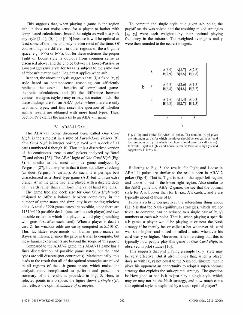
This suggests that, when playing a game in the region a≈b, it does not make sense for a player to bother with complicated calculations. Instead he might as well just pick any style [1, 1], [0, 1] or [0, 0] because it will be optimal at least some of the time and maybe even most of the time. Of course things are different in other regions of the a-b game space, e.g., b>>a or b<<a, but for these extremes the proper Tight or Loose style is obvious from common sense as discussed above, and the choice between a Loose-Passive or Loose-Aggressive style for b<<a is subject to the same sort of “doesn’t matter much” logic that applies when a≈b.

In short, the above analysis suggests that: (i) a fixed [x, y] style based on commonsense reasoning can efficiently replicate the essential benefits of complicated game-theoretic calculations, and (ii) the difference between various strategies (styles) may or may not matter much. But these findings are for an ABA’ poker where there are only two hand types, and this raises the question of whether similar results are obtained with more hand types. Thus, Section IV extends the analysis to an ABA’-11 game.

IV. ABA’-11 GAME The ABA’-11 poker discussed here, called One Card

High, is the simplest in a suite of Pared-down Pokers [9]. One Card High is integer poker, played with a deck of 11 cards numbered 0 though 10. Thus, it is a discretized version of the continuous “zero-to-one” pokers analyzed by Borel [7] and others [26]. The ABA’ logic of One Card High (Fig. 3) is similar to the most complex game analyzed by Ferguson [27], but simpler in that it does not allow checking (as does Ferguson’s variant). As such, it is perhaps best characterized as a Borel type game (AB) but with an extra branch A’ in the game tree, and played with a discrete deck of 11 cards rather than a uniform interval of hand strengths.

The game tree and deck size for One Card High were designed to offer a balance between complexity in the number of game states and simplicity in estimating win:loss odds. A total of 220 game states are possible, since there are 11*10=110 possible deals (one card to each player) and two possible orders in which the players would play (switching who goes first after each hand). When a player is dealt a card Z, his win:loss odds are easily computed as Z:(10-Z). This facilitates experiments on human performance in Bayesian inference, since the prior is trivial to compute, but these human experiments are beyond the scope of this paper.

Compared to the ABA’-2 game, this ABA’-11 game has a finer discretization of possible game states, but the hand types are still discrete (not continuous). Mathematically, this leads to the result that all of the optimal strategies are mixed in all regions of the a-b game space, which makes the analysis more complicated to perform and present. A summary of the results is provided in Fig. 5. Here, at selected points in a-b space, the figure shows a single style that reflects the optimal mixture of strategies.

To compute the single style at a given a-b point, the payoff matrix was solved and the resulting mixed strategies [xi, yi] were each weighted by their optimal playing frequency in the mixture. The weighted average x and y were then rounded to the nearest integers.

Referring to Fig. 5, the results for Tight and Loose in ABA’-11 poker are similar to the results seen in ABA’-2 poker (Fig. 4). That is, Tight is best in the upper left region, and Loose is best in the lower right region. Also similar to the AB-2 game and ABA’-2 game, we see that the optimal style for A is Looser than for B, i.e., A’s cards x and y are typically about -2 those of B.

From a stylistic perspective, the interesting thing about Fig. 5 is that the Nash equilibrium strategies, which are not trivial to compute, can be reduced to a single pair of [x, y] numbers at each a-b point. That is, when playing a specific a-b game, a player would be playing at or near the Nash strategy if he merely bet or called a bet whenever his card was x or higher, and raised or called a raise whenever his card was y or higher. Moreover, it is interesting that this is typically how people play this game of One Card High, as observed in pilot studies [10].

This suggests that just playing a simple [x, y] style may be very effective. But it also implies that, when a player does so with [x, y] not equal to the Nash equilibrium, then it gives his opponent an opportunity to adopt a super-optimal strategy that exploits the sub-optimal strategy. The question is: How good or bad is it to just play a single style, which may or may not be the Nash strategy, and how much can a sub-optimal style be exploited by a super-optimal player?

a

b

A[6,9] B[7,9]

A[3,7] B[5,8]

A[2,6] B[4,8]

A[4,8] B[6,8]

A[2,6] B[4,8]

A[1,5] B[3,7]

A[2,6] B[4,8]

A[1,4] B[2,7]

A[0,3] B[1,5]

2 5 8

2

5

8

Fig. 5. Optimal styles for ABA’-11 poker. The notation [x, y] gives the minimum card x for which the player should bet (or call a bet) and the minimum card y for which the player should raise (or call a raise). In words, Tight is high x and Loose is low x; Passive is high y-x and Aggressive is low y-x.

1-4244-0464-9/06/$20.00 2006 IEEE. 262 CIG'06 (May 22-24 2006)

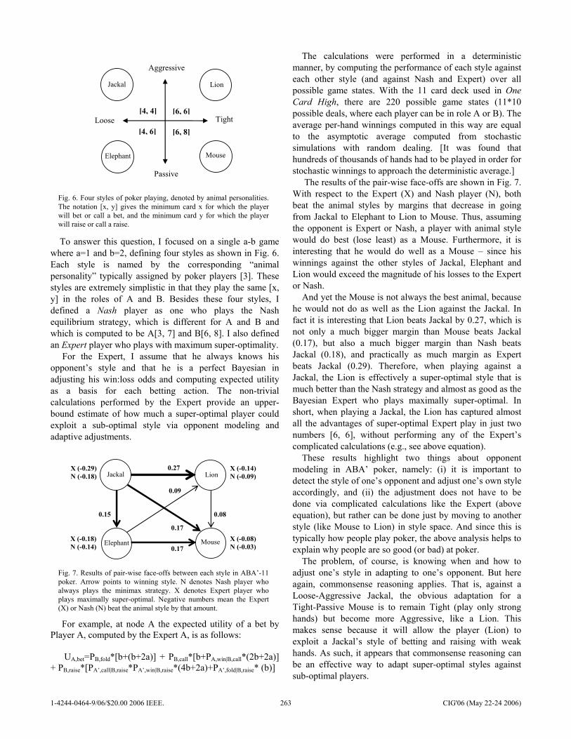
To answer this question, I focused on a single a-b game where a=1 and b=2, defining four styles as shown in Fig. 6. Each style is named by the corresponding “animal personality” typically assigned by poker players [3]. These styles are extremely simplistic in that they play the same [x, y] in the roles of A and B. Besides these four styles, I defined a Nash player as one who plays the Nash equilibrium strategy, which is different for A and B and which is computed to be A[3, 7] and B[6, 8]. I also defined an Expert player who plays with maximum super-optimality.

For the Expert, I assume that he always knows his opponent’s style and that he is a perfect Bayesian in adjusting his win:loss odds and computing expected utility as a basis for each betting action. The non-trivial calculations performed by the Expert provide an upper-bound estimate of how much a super-optimal player could exploit a sub-optimal style via opponent modeling and adaptive adjustments.

For example, at node A the expected utility of a bet by Player A, computed by the Expert A, is as follows:

UA,bet=PB,fold*[b+(b+2a)] + PB,call*[b+PA,win|B,call*(2b+2a)]

+ PB,raise*[PA’,call|B,raise*PA’,win|B,raise*(4b+2a)+PA’,fold|B,raise* (b)]

The calculations were performed in a deterministic manner, by computing the performance of each style against each other style (and against Nash and Expert) over all possible game states. With the 11 card deck used in One Card High, there are 220 possible game states (11*10 possible deals, where each player can be in role A or B). The average per-hand winnings computed in this way are equal to the asymptotic average computed from stochastic simulations with random dealing. [It was found that hundreds of thousands of hands had to be played in order for stochastic winnings to approach the deterministic average.]

The results of the pair-wise face-offs are shown in Fig. 7. With respect to the Expert (X) and Nash player (N), both beat the animal styles by margins that decrease in going from Jackal to Elephant to Lion to Mouse. Thus, assuming the opponent is Expert or Nash, a player with animal style would do best (lose least) as a Mouse. Furthermore, it is interesting that he would do well as a Mouse – since his winnings against the other styles of Jackal, Elephant and Lion would exceed the magnitude of his losses to the Expert or Nash.

And yet the Mouse is not always the best animal, because he would not do as well as the Lion against the Jackal. In fact it is interesting that Lion beats Jackal by 0.27, which is not only a much bigger margin than Mouse beats Jackal (0.17), but also a much bigger margin than Nash beats Jackal (0.18), and practically as much margin as Expert beats Jackal (0.29). Therefore, when playing against a Jackal, the Lion is effectively a super-optimal style that is much better than the Nash strategy and almost as good as the Bayesian Expert who plays maximally super-optimal. In short, when playing a Jackal, the Lion has captured almost all the advantages of super-optimal Expert play in just two numbers [6, 6], without performing any of the Expert’s complicated calculations (e.g., see above equation).

These results highlight two things about opponent modeling in ABA’ poker, namely: (i) it is important to detect the style of one’s opponent and adjust one’s own style accordingly, and (ii) the adjustment does not have to be done via complicated calculations like the Expert (above equation), but rather can be done just by moving to another style (like Mouse to Lion) in style space. And since this is typically how people play poker, the above analysis helps to explain why people are so good (or bad) at poker.

Tight

Aggressive

Passive

Loose [6, 6]

[6, 8] [4, 6]

Jackal

[4, 4]

Elephant

Lion

Mouse

Fig. 6. Four styles of poker playing, denoted by animal personalities. The notation [x, y] gives the minimum card x for which the player will bet or call a bet, and the minimum card y for which the player will raise or call a raise.

Jackal

Elephant

Lion

Mouse

X (-0.14) N (-0.09)

0.15

0.09

0.17

0.17

0.08

0.27

X (-0.08) N (-0.03)

X (-0.29) N (-0.18)

X (-0.18) N (-0.14)

Fig. 7. Results of pair-wise face-offs between each style in ABA’-11 poker. Arrow points to winning style. N denotes Nash player who always plays the minimax strategy. X denotes Expert player who plays maximally super-optimal. Negative numbers mean the Expert (X) or Nash (N) beat the animal style by that amount.

The problem, of course, is knowing when and how to adjust one’s style in adapting to one’s opponent. But here again, commonsense reasoning applies. That is, against a Loose-Aggressive Jackal, the obvious adaptation for a Tight-Passive Mouse is to remain Tight (play only strong hands) but become more Aggressive, like a Lion. This makes sense because it will allow the player (Lion) to exploit a Jackal’s style of betting and raising with weak hands. As such, it appears that commonsense reasoning can be an effective way to adapt super-optimal styles against sub-optimal players.

1-4244-0464-9/06/$20.00 2006 IEEE. 263 CIG'06 (May 22-24 2006)

V. CONCLUSION This paper explored the computational basis for

psychological styles in three poker games, ranging from very simple to rather complex. The finding was that commonsense styles efficiently reduce the computational complexity of strategic reasoning, while approximating Nash optimal and super-optimal (against sub-optimal) strategies.

Some styles were shown to perform better than Nash equilibrium strategies against sub-optimal styles, and one style was seen to be almost maximally super-optimal. This finding is important because it helps explain human success in poker playing, and because it suggests how poker research might be applied to real life problems that are similar to poker. That is, people succeed at poker to the extent that they act in accordance with effective strategies. The analysis here showed how this could be achieved, without strategic calculations, by adopting simple styles based on commonsense reasoning.

Especially in real life, where the game rules and game states are much more complex than even full-scale poker, the basic problem is not to find the optimal solution in a well-defined game space, but rather to find a good enough solution in an ill-defined game space. Since styles are typically based on robust assumptions and commonsense reasoning, they can be applied to such ill-defined problems in cases where game theory cannot. Thus, a better understanding of how styles perform in poker games, which are well-defined and which can be measured, may help to understand how and how well styles work in real life.

For example, this research raises the question of why, if the “good” styles are just common sense, do some players adopt “bad” styles (like the Jackal) that cause them to lose money in poker games? The answer, I believe, is that common sense extends beyond the assumptions of previous research to encompass other values that players have, like the desire for “pleasure” in game play. For most people it is more fun to bet than fold, and people who play poker do so for pleasure as well as money, since there are other ways of making money (and other ways of getting pleasure).

Therefore, with an eye towards future research, I would argue that the study of computational intelligence in games must be augmented by a study of computational aesthetics in games [22], in order to understand why and how people play. Any rational person will act in accordance with his own preferences, e.g., in the case of a Jackal who may like the fun of betting and raising, so these preferences must be considered in efforts to explain and predict human behavior in games or in life. This makes topics like style (here) and fun [22] important to gaming applications – as well as to real-world problems in judgment and decision making.

ACKNOWLEDGEMENT Many thanks to Craig Bonaceto for numerous discussions

and computer programming.

REFERENCES [1] A. Schoonmaker, The Psychology of Poker. Las Vegas, NV: Two Plus

Two Publishing, 2000. [2] D. Sklansky, The Theory of Poker. Las Vegas, NV: Two Plus Two

Publishing, 1987. [3] P. Hellmuth, Play Poker Like the Pros. New York, NY: Harper-

Collins, 2003. [4] L. Barone and L. While, “Evolving computer opponents to play a

game of simplified poker,” Proc. IEEE Int. Conf. on Evolutionary Computation (ICEC), 1998, pp. 108-113.

[5] L. Barone and L. While, “An adaptive learning model for simplified poker using evolutionary algorithms,” Proc. Congress of Evolutionary Computation (CEC), 1999, pp. 153-160.

[6] G. Kendall and M. Willdig, “An investigation of an adaptive poker player,” Proc. 14th Australian Joint Conf. on Artificial Intelligence (LNAI-2256), 2001, pp. 189-200.

[7] É. Borel, “Traité du Calcul des Probabilités et ses Applications Volume 4, Fascicule 2”, Applications aux jeux des hazard. Paris: Gautier-Villars, 1938.

[8] J. McDonald, Strategy in Poker, Business and War. New York, NY: Norton, 1950.

[9] K. Burns, “Pared-down Poker: Cutting to the core of command and control,” Proc. IEEE Conf. Computational Intelligence in Games, 2005. Available: http://csapps.essex.ac.uk/cig/2005/

[10] K. Burns, “Heads-up face-off: On style and skill in the game of poker,” Proc. Am. Ass. Artificial Intelligence Fall Symposium on Style in Language, Art, Music and Design, 2004. Available: http://music.ucsd.edu/~sdubnov/style2004.htm

[11] H. Kuhn, “A simplified two-person poker,” in Contributions to the Theory of Games, Vol. 1. Princeton, NJ: Princeton University Press, 1950, pp. 97-103.

[12] B. Hoehn, F. Southey, R. Holte and V. Bulitko, “Effective short-term opponent exploitation in simplified poker,” Proc. AAAI’05, 2005, pp. 783-788.

[13] D. Billings, N. Burch, A. Davidson, R. Holte, J. Schaeffer, T. Schauenberg and D. Szafron, “Approximating game-theoretic optimal strategies for full-scale poker,” in 18th Int. Joint Conf. on Artificial Intelligence (IJCAI), 2003.

[14] D. Koller and A. Pfeffer, “Representations and solutions for game-theoretic problems,” Artificial Intelligence, Vol. 94, No. 1, 1997, pp. 167-215.

[15] D. Billings, D. Papp, J. Schaeffer and D. Szafron, “Opponent modeling in poker,” Proc. 15th Nat. Conf. on Artificial Intelligence (AAAI), 1998, pp. 493-498.

[16] A. Davidson, D. Billings, J. Schaeffer and D. Szafron, “Improved opponent modeling in poker,” Proc. Int. Conf. on Artificial Intelligence (ICAI), 2000, pp. 1467-1473.

[17] K. Korb, A. Nicholson and N. Jitnah, “Bayesian poker,” Proc. Conf. on Uncertainty in Artificial Intelligence (UAI), 1999, pp. 343-350.

[18] F. Southey, M. Bowling, B. Larson, C. Piccione, N. Burch, D. Billings and C. Rayner, “Bayes bluff: Opponent modeling in poker,” Proc. Conf. on Uncertainty in Artificial Intelligence (UAI), 2005, pp. 550-558.

[19] J. Shi and M. Littman, “Abstraction methods for game-theoretic poker,” in Proc 2nd Int. Conference on Computers in Games, 2000, pp. 333-345.

[20] D. Billings, A. Davidson, J. Schaeffer and D. Szafron, “The challenge of poker,” Artificial Intelligence, Vol. 134, 2002, pp. 201-240.

[21] M. Davis, Game Theory. New York, NY: Dover, 1997. [22] K. Burns, “Fun in slots,” Proc. IEEE Conf. Computational

Intelligence in Games, 2006. [23] J. Baron, Thinking and Deciding, 3rd Edition. New York, NY:

Cambridge University Press, 2000. [24] H. Simon, The Sciences of the Artificial, 3rd Edition. Cambridge, MA:

MIT Press, 1997. [25] G. Gigerenzer and P. Todd, Simple Heuristics that Make Us Smart.

New York, NY: Oxford University Press, 1999. [26] C. Ferguson and T. Ferguson, “On the Borel and von Neumann poker

models,” Game Theory and Applications, Vol. 9, 2003, pp. 17-32. [27] C. Ferguson, T. Ferguson and C. Gawargy, ‘Uniform(0,1) two-person

poker models”, Working Paper, Dept. of Mathematics, UCLA, 2004.

1-4244-0464-9/06/$20.00 2006 IEEE. 264 CIG'06 (May 22-24 2006)

Voronoi game on graphs and its complexity

Sachio Teramoto∗, Erik D. Demaine†, Ryuhei Uehara∗∗ School of Information Science, Japan Advanced Institute of Science and Technology (JAIST),

1-1, Asahidai, Nomi, Ishikawa, 923-1292 Japan† Computer Science and Artificial Intelligence Lab, the Massachusetts Institute of Technology,

32 Vassar Street, Cambridge, Massachusetts 02139, USA

Abstract— The Voronoi game is a two-person game which isa model for competitive facility location. The game is playedon a continuous domain, and only two special cases (the 1-dimensional case and the 1-round case) are well investigated.We introduce the discrete Voronoi game in which the gamearena is given as a graph. We first show the best strategy whenthe game arena is a large complete k-ary tree. Next we showthat the discrete Voronoi game is intractable in general. Evenin the 1-round case, and the place occupied by the first playeris fixed, the game is NP-complete in general. We also show thatthe game is PSPACE-complete in general case.

Keywords: Voronoi Game, graphs, k-trees, NP-completeness, PSPACE-completeness.

I. Introduction

The Voronoi game is an idealized model for competi-tive facility location, which was proposed by Ahn, Cheng,Cheong, Golin, and Oostrum [1]. The Voronoi game isplayed on a bounded continuous arena by two players. TwoplayersW (white) and B (black) put n points alternately, andthe continuous field is subdivided according to the nearestneighbor rule. At the final step, the player who dominatesthe larger area wins.

The Voronoi game is a natural game, but the general caseseems to be very hard to analyze from the theoretical point ofview. Hence, in [1], Ahn et al. investigated the case that thegame field is a bounded 1-dimensional continuous domain.On the other hand, Cheong, Har-Peled, Linial, and Matousek[2], and Fekete and Meijer [3] deal with a 2- or higher-dimensional case, but they restrict themselves to the one-round game; first, W puts all n points, and next B puts alln points.

In this paper, we introduce the discrete Voronoi game.Two players alternately occupy n vertices on a graph, whichis a bounded discrete arena. (Hence the graph contains atleast 2n vertices.) This restriction seems to be appropriatesince real estates are already bounded in general, and wehave to build shops in the bounded area. More precisely, thediscrete Voronoi game is played on a given finite graph G,instead of a bounded continuous arena. Each vertex of Gcan be assigned to the nearest vertices occupied by W orB, according to the nearest neighbor rule. (Hence a vertexcan be a “tie” when it has the same distance from a vertexoccupied by W and another vertex occupied by B.) Finally,the player who dominates larger area (or a larger number ofvertices) wins. We note that the two players can tie in somecases.

We first consider the case that the graph G is a completek-ary tree. A complete k-ary tree is a natural generalizationof a path which is the discrete analogy of 1-dimensionalcontinuous domain. We also mention that complete k-arytrees form a very natural and nontrivial graph class. In [1],Ahn et al. showed that the second player B has an advantageon a 1-dimensional continuous domain. In contrast to thisfact, we first show that the first player W has an advantagefor the discrete Voronoi game on a complete k-ary tree, whenthe tree is sufficiently large (comparing to n and k). Moreprecisely, we show that W has a winning strategy if (1)2n ≤ k, or (2) k is odd and the complete k-ary tree containsat least 4n2 vertices. On the other hand, when k is even and2n > k, two players tie if they do their best.

Next, we show computational hardness results for thediscrete Voronoi game. When we admit a general graph as agame arena, the discrete Voronoi game becomes intractableeven in the following strongly restricted case: the gamearena is an arbitrary graph, the first player W occupiesjust one vertex which is predetermined, the second playerB occupies n vertices in any way. The decision problemfor the strongly restricted discrete Voronoi game is definedas follows: determine whether B has a winning strategyfor given graph G with the occupied vertex by W. Thisrestricted case seems to be advantageous for B. However,the decision problem is NP-complete. This result is alsoquite different from the previously known results in the 2-or higher-dimensional problem (e.g., B can always dominatethe fraction 1

2 + ε of the 2- or higher-dimensional domain)by Cheong et al. [2] and Fekete and Meijer [3]. However,Fekete and Meijer [3] showed that maximizing the area Bcan claim is NP-hard in the one-round game in which thegiven arena is a polygon with holes.

We also show that the discrete Voronoi game is PSPACE-complete in the general case. This can be seen as a positiveanswer to the conjecture by Fekete and Meijer [3].

II. Problem Definitions

In this section, we formulate the discrete Voronoi game ona graph. Let us denote a Voronoi game by VG(G, n), where Gis the game arena, and the players play n rounds. Hereafter,the game arena is an undirected and unweighted simple graphG = (V, E) with N = |V | vertices.

For each round, the two players,W (white) and B (black),alternately occupy an unoccupied vertex on the graph G (Walways starts the game, as in Chess). This implies that W

1-4244-0464-9/06/$20.00 2006 IEEE. 265 CIG'06 (May 22-24 2006)

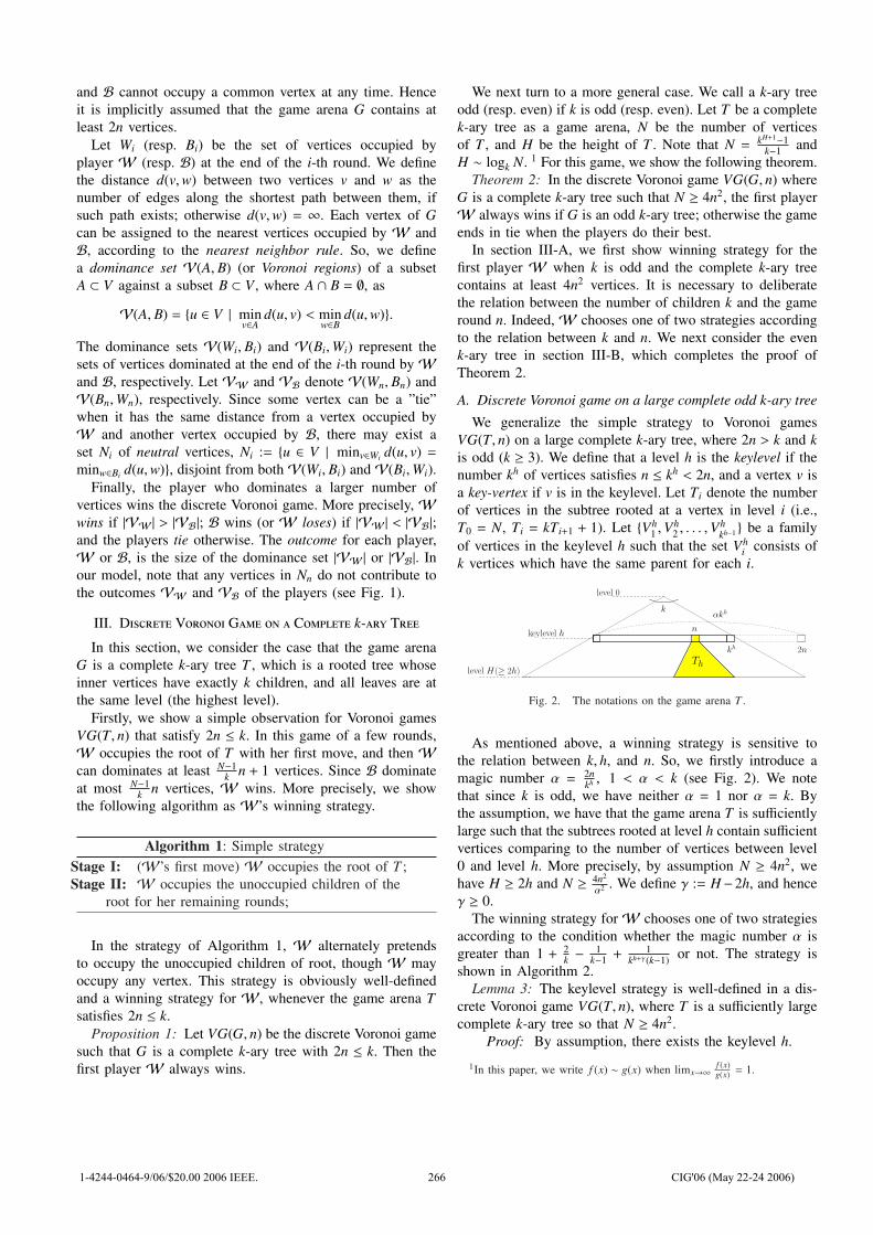
and B cannot occupy a common vertex at any time. Henceit is implicitly assumed that the game arena G contains atleast 2n vertices.

Let Wi (resp. Bi) be the set of vertices occupied byplayer W (resp. B) at the end of the i-th round. We definethe distance d(v,w) between two vertices v and w as thenumber of edges along the shortest path between them, ifsuch path exists; otherwise d(v,w) = ∞. Each vertex of Gcan be assigned to the nearest vertices occupied by W andB, according to the nearest neighbor rule. So, we definea dominance set V(A, B) (or Voronoi regions) of a subsetA ⊂ V against a subset B ⊂ V , where A ∩ B = ∅, as

V(A, B) = {u ∈ V | minv∈A

d(u, v) < minw∈B

d(u,w)}.

The dominance sets V(Wi, Bi) and V(Bi,Wi) represent thesets of vertices dominated at the end of the i-th round byWand B, respectively. Let VW and VB denote V(Wn, Bn) andV(Bn,Wn), respectively. Since some vertex can be a ”tie”when it has the same distance from a vertex occupied byW and another vertex occupied by B, there may exist aset Ni of neutral vertices, Ni := {u ∈ V | minv∈Wi d(u, v) =minw∈Bi d(u,w)}, disjoint from both V(Wi, Bi) and V(Bi,Wi).

Finally, the player who dominates a larger number ofvertices wins the discrete Voronoi game. More precisely, Wwins if |VW | > |VB|; B wins (or W loses) if |VW | < |VB|;and the players tie otherwise. The outcome for each player,W or B, is the size of the dominance set |VW | or |VB|. Inour model, note that any vertices in Nn do not contribute tothe outcomes VW and VB of the players (see Fig. 1).

III. Discrete Voronoi Game on a Complete k-ary Tree

In this section, we consider the case that the game arenaG is a complete k-ary tree T , which is a rooted tree whoseinner vertices have exactly k children, and all leaves are atthe same level (the highest level).

Firstly, we show a simple observation for Voronoi gamesVG(T, n) that satisfy 2n ≤ k. In this game of a few rounds,W occupies the root of T with her first move, and then Wcan dominates at least N−1

k n + 1 vertices. Since B dominateat most N−1

k n vertices, W wins. More precisely, we showthe following algorithm as W’s winning strategy.

Algorithm 1: Simple strategyStage I: (W’s first move) W occupies the root of T ;Stage II: W occupies the unoccupied children of the

root for her remaining rounds;

In the strategy of Algorithm 1, W alternately pretendsto occupy the unoccupied children of root, though W mayoccupy any vertex. This strategy is obviously well-definedand a winning strategy for W, whenever the game arena Tsatisfies 2n ≤ k.

Proposition 1: Let VG(G, n) be the discrete Voronoi gamesuch that G is a complete k-ary tree with 2n ≤ k. Then thefirst player W always wins.

We next turn to a more general case. We call a k-ary treeodd (resp. even) if k is odd (resp. even). Let T be a completek-ary tree as a game arena, N be the number of verticesof T , and H be the height of T . Note that N = kH+1−1

k−1 andH ∼ logk N. 1 For this game, we show the following theorem.

Theorem 2: In the discrete Voronoi game VG(G, n) whereG is a complete k-ary tree such that N ≥ 4n2, the first playerW always wins if G is an odd k-ary tree; otherwise the gameends in tie when the players do their best.

In section III-A, we first show winning strategy for thefirst player W when k is odd and the complete k-ary treecontains at least 4n2 vertices. It is necessary to deliberatethe relation between the number of children k and the gameround n. Indeed,W chooses one of two strategies accordingto the relation between k and n. We next consider the evenk-ary tree in section III-B, which completes the proof ofTheorem 2.

A. Discrete Voronoi game on a large complete odd k-ary tree

We generalize the simple strategy to Voronoi gamesVG(T, n) on a large complete k-ary tree, where 2n > k and kis odd (k ≥ 3). We define that a level h is the keylevel if thenumber kh of vertices satisfies n ≤ kh < 2n, and a vertex v isa key-vertex if v is in the keylevel. Let Ti denote the numberof vertices in the subtree rooted at a vertex in level i (i.e.,T0 = N, Ti = kTi+1 + 1). Let {Vh

1 ,Vh2 , . . . ,V

hkh−1 } be a family

of vertices in the keylevel h such that the set Vhi consists of

k vertices which have the same parent for each i.

kh 2n

n

level 0

keylevel h

Th

αkhk

level H(≥ 2h)

Fig. 2. The notations on the game arena T .

As mentioned above, a winning strategy is sensitive tothe relation between k, h, and n. So, we firstly introduce amagic number α = 2n

kh , 1 < α < k (see Fig. 2). We notethat since k is odd, we have neither α = 1 nor α = k. Bythe assumption, we have that the game arena T is sufficientlylarge such that the subtrees rooted at level h contain sufficientvertices comparing to the number of vertices between level0 and level h. More precisely, by assumption N ≥ 4n2, wehave H ≥ 2h and N ≥ 4n2

α2 . We define γ := H−2h, and henceγ ≥ 0.

The winning strategy forW chooses one of two strategiesaccording to the condition whether the magic number α isgreater than 1 + 2

k −1

k−1 +1

kh+γ(k−1) or not. The strategy isshown in Algorithm 2.

Lemma 3: The keylevel strategy is well-defined in a dis-crete Voronoi game VG(T, n), where T is a sufficiently largecomplete k-ary tree so that N ≥ 4n2.

Proof: By assumption, there exists the keylevel h.

1In this paper, we write f (x) ∼ g(x) when limx→∞f (x)g(x) = 1.

1-4244-0464-9/06/$20.00 2006 IEEE. 266 CIG'06 (May 22-24 2006)

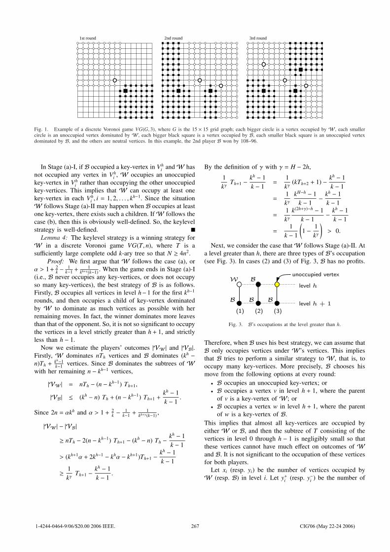
1st round 2nd round 3rd round

Fig. 1. Example of a discrete Voronoi game VG(G, 3), where G is the 15 × 15 grid graph; each bigger circle is a vertex occupied by W, each smallercircle is an unoccupied vertex dominated by W, each bigger black square is a vertex occupied by B, each smaller black square is an unoccupied vertexdominated by B, and the others are neutral vertices. In this example, the 2nd player B won by 108–96.

In Stage (a)-I, if B occupied a key-vertex in Vhi andW has

not occupied any vertex in Vhi , W occupies an unoccupied

key-vertex in Vhi rather than occupying the other unoccupied

key-vertices. This implies that W can occupy at least onekey-vertex in each Vh

i , i = 1, 2, . . . , kh−1. Since the situationW follows Stage (a)-II may happen when B occupies at leastone key-vertex, there exists such a children. IfW follows thecase (b), then this is obviously well-defined. So, the keylevelstrategy is well-defined.

Lemma 4: The keylevel strategy is a winning strategy forW in a discrete Voronoi game VG(T, n), where T is asufficiently large complete odd k-ary tree so that N ≥ 4n2.

Proof: We first argue that W follows the case (a), orα > 1+ 2

k −1

k−1 +1

kh+γ(k−1) . When the game ends in Stage (a)-I(i.e., B never occupies any key-vertices, or does not occupyso many key-vertices), the best strategy of B is as follows.Firstly, B occupies all vertices in level h−1 for the first kh−1

rounds, and then occupies a child of key-vertex dominatedby W to dominate as much vertices as possible with herremaining moves. In fact, the winner dominates more leavesthan that of the opponent. So, it is not so significant to occupythe vertices in a level strictly greater than h + 1, and strictlyless than h − 1.

Now we estimate the players’ outcomes |VW | and |VB|.Firstly, W dominates nTh vertices and B dominates (kh −n)Th +

kh−1k−1 vertices. Since B dominates the subtrees of W

with her remaining n − kh−1 vertices,

|VW | = nTh − (n − kh−1) Th+1,

|VB| ≤ (kh − n) Th + (n − kh−1) Th+1 +kh − 1k − 1

.

Since 2n = αkh and α > 1 + 2k −

1k−1 +

1kh+γ(k−1) ,

|VW | − |VB|

≥ nTh − 2(n − kh−1) Th+1 − (kh − n) Th −kh − 1k − 1

> (kh+1α + 2kh−1 − khα − kh+1)Th+1 −kh − 1k − 1

≥ 1kγ

Th+1 −kh − 1k − 1

.

By the definition of γ with γ = H − 2h,

1kγ

Th+1 −kh − 1k − 1

=1kγ

(kTh+2 + 1) − kh − 1k − 1

=1kγ

kH−h − 1k − 1

− kh − 1k − 1

=1kγ

k(2h+γ)−h − 1k − 1

− kh − 1k − 1

=1

k − 1

(1 − 1

kγ

)> 0.

Next, we consider the case thatW follows Stage (a)-II. Ata level greater than h, there are three types of B’s occupation(see Fig. 3). In cases (2) and (3) of Fig. 3, B has no profits.

level h

level h + 1

W

B BB

unoccupied vertex

(1) (2) (3)

B

Fig. 3. B’s occupations at the level greater than h.

Therefore, when B uses his best strategy, we can assume thatB only occupies vertices under W’s vertices. This impliesthat B tries to perform a similar strategy to W, that is, tooccupy many key-vertices. More precisely, B chooses hismove from the following options at every round:• B occupies an unoccupied key-vertex; or• B occupies a vertex v in level h + 1, where the parent

of v is a key-vertex of W; or• B occupies a vertex w in level h + 1, where the parent

of w is a key-vertex of B.This implies that almost all key-vertices are occupied byeither W or B, and then the subtree of T consisting of thevertices in level 0 through h − 1 is negligibly small so thatthese vertices cannot have much effect on outcomes of Wand B. It is not significant to the occupation of these verticesfor both players.

Let xi (resp. yi) be the number of vertices occupied byW (resp. B) in level i. Let y+i (resp. y−i ) be the number of

1-4244-0464-9/06/$20.00 2006 IEEE. 267 CIG'06 (May 22-24 2006)

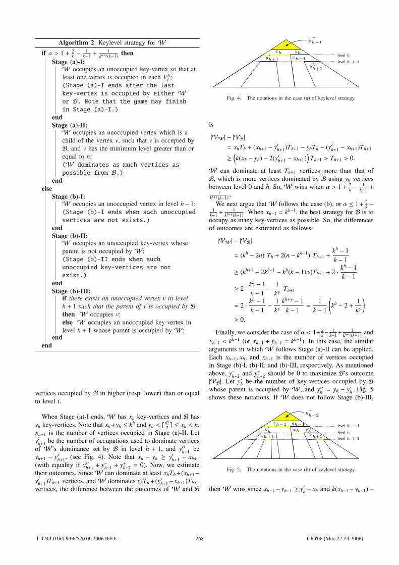
Algorithm 2: Keylevel strategy for Wif α > 1 + 2

k −1

k−1 +1

kh+γ(k−1) thenStage (a)-I:W occupies an unoccupied key-vertex so that atleast one vertex is occupied in each Vh

i ;(Stage (a)-I ends after the last

key-vertex is occupied by either Wor B. Note that the game may finishin Stage (a)-I.)

endStage (a)-II:W occupies an unoccupied vertex which is achild of the vertex v, such that v is occupied byB, and v has the minimum level greater than orequal to h;(W dominates as much vertices as

possible from B.)end

elseStage (b)-I:W occupies an unoccupied vertex in level h− 1;(Stage (b)-I ends when such unoccupied

vertices are not exists.)

endStage (b)-II:W occupies an unoccupied key-vertex whoseparent is not occupied by W;(Stage (b)-II ends when such

unoccupied key-vertices are not

exist.)

endStage (b)-III:

if there exists an unoccupied vertex v in levelh + 1 such that the parent of v is occupied by Bthen W occupies v;else W occupies an unoccupied key-vertex inlevel h + 1 whose parent is occupied by W;

endend

vertices occupied by B in higher (resp. lower) than or equalto level i.

When Stage (a)-I ends, W has xh key-vertices and B hasyh key-vertices. Note that xh+yh ≤ kh and yh < d kh

2 e ≤ xh < n.xh+1 is the number of vertices occupied in Stage (a)-II. Lety′h+1 be the number of occupations used to dominate verticesof W’s dominance set by B in level h + 1, and y′′h+1 beyh+1 − y′h+1. (see Fig. 4). Note that xh − yh ≥ y′h+1 − xh+1(with equality if y′′h+1 + y−h−1 + y+h+2 = 0). Now, we estimatetheir outcomes. SinceW can dominate at least xhTh+(xh+1−y′h+1)Th+1 vertices, andW dominates yhTh+(y′h+1− xh+1)Th+1vertices, the difference between the outcomes of W and B

level h

level h + 1

xh

xh+1

yh

y′′

h+1

y′

h+1

y−

h−1

Fig. 4. The notations in the case (a) of keylevel strategy.

is

|VW | − |VB|= xhTh + (xh+1 − y′h+1)Th+1 − yhTh − (y′h+1 − xh+1)Th+1

≥(k(xh − yh) − 2(y′h+1 − xh+1)

)Th+1 > Th+1 > 0.

W can dominate at least Th+1 vertices more than that ofB, which is more vertices dominated by B using y0 verticesbetween level 0 and h. So, W wins when α > 1 + 2

k −1

k−1 +1

kh+γ(k−1) .We next argue thatW follows the case (b), or α ≤ 1+ 2

k −1

k−1 +1

kh+γ(k−1) . When xh−1 = kh−1, the best strategy for B is tooccupy as many key-vertices as possible. So, the differencesof outcomes are estimated as follows:

|VW | − |VB|

= (kh − 2n) Th + 2(n − kh−1) Th+1 +kh − 1k − 1

≥ (kh+1 − 2kh−1 − kh(k − 1)α)Th+1 + 2 · kh − 1k − 1

≥ 2 · kh − 1k − 1

− 1kγ

Th+1

= 2 · kh − 1k − 1

− 1kγ

kh+γ − 1k − 1

=1

k − 1

(kh − 2 +

1kγ

)> 0.

Finally, we consider the case of α < 1+ 2k−

1k−1+

1kh+γ(k−1) and

xh−1 < kh−1 (or xh−1 + yh−1 = kh−1). In this case, the similararguments in which W follows Stage (a)-II can be applied.Each xh−1, xh, and xh+1 is the number of vertices occupiedin Stage (b)-I, (b)-II, and (b)-III, respectively. As mentionedabove, y−h−2 and y+h+2 should be 0 to maximize B’s outcome|VB|. Let y′h be the number of key-vertices occupied by Bwhose parent is occupied by W, and y′′h = yh − y′h. Fig. 5shows these notations. If W does not follow Stage (b)-III,

level h − 1

level h

level h + 1

xh−1

xhxh+1

yh−1

y′′

hy′

hxh+1

y−

h−2

Fig. 5. The notations in the case (b) of keylevel strategy.

then W wins since xh−1 − yh−1 ≥ y′h − xh and k(xh−1 − yh−1)−

1-4244-0464-9/06/$20.00 2006 IEEE. 268 CIG'06 (May 22-24 2006)

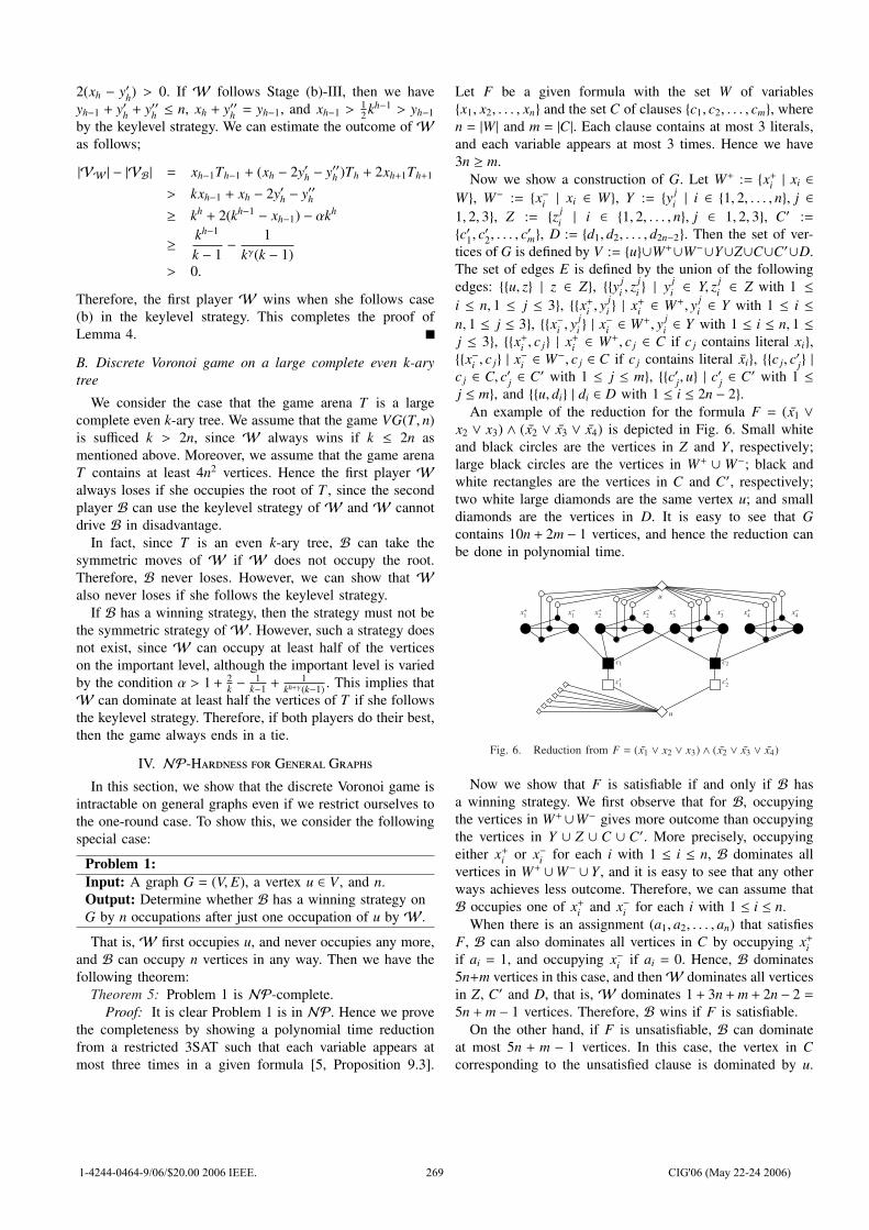
2(xh − y′h) > 0. If W follows Stage (b)-III, then we haveyh−1 + y′h + y′′h ≤ n, xh + y′′h = yh−1, and xh−1 >

12 kh−1 > yh−1

by the keylevel strategy. We can estimate the outcome ofWas follows;

|VW | − |VB| = xh−1Th−1 + (xh − 2y′h − y′′h )Th + 2xh+1Th+1

> kxh−1 + xh − 2y′h − y′′h≥ kh + 2(kh−1 − xh−1) − αkh

≥ kh−1

k − 1− 1

kγ(k − 1)> 0.

Therefore, the first player W wins when she follows case(b) in the keylevel strategy. This completes the proof ofLemma 4.

B. Discrete Voronoi game on a large complete even k-arytree

We consider the case that the game arena T is a largecomplete even k-ary tree. We assume that the game VG(T, n)is sufficed k > 2n, since W always wins if k ≤ 2n asmentioned above. Moreover, we assume that the game arenaT contains at least 4n2 vertices. Hence the first player Walways loses if she occupies the root of T , since the secondplayer B can use the keylevel strategy of W and W cannotdrive B in disadvantage.

In fact, since T is an even k-ary tree, B can take thesymmetric moves of W if W does not occupy the root.Therefore, B never loses. However, we can show that Walso never loses if she follows the keylevel strategy.

If B has a winning strategy, then the strategy must not bethe symmetric strategy ofW. However, such a strategy doesnot exist, since W can occupy at least half of the verticeson the important level, although the important level is variedby the condition α > 1+ 2

k −1

k−1 +1

kh+γ(k−1) . This implies thatW can dominate at least half the vertices of T if she followsthe keylevel strategy. Therefore, if both players do their best,then the game always ends in a tie.

IV. NP-Hardness for General Graphs

In this section, we show that the discrete Voronoi game isintractable on general graphs even if we restrict ourselves tothe one-round case. To show this, we consider the followingspecial case:

Problem 1:Input: A graph G = (V, E), a vertex u ∈ V , and n.Output: Determine whether B has a winning strategy onG by n occupations after just one occupation of u by W.

That is,W first occupies u, and never occupies any more,and B can occupy n vertices in any way. Then we have thefollowing theorem:

Theorem 5: Problem 1 is NP-complete.Proof: It is clear Problem 1 is in NP. Hence we prove

the completeness by showing a polynomial time reductionfrom a restricted 3SAT such that each variable appears atmost three times in a given formula [5, Proposition 9.3].

Let F be a given formula with the set W of variables{x1, x2, . . . , xn} and the set C of clauses {c1, c2, . . . , cm}, wheren = |W | and m = |C|. Each clause contains at most 3 literals,and each variable appears at most 3 times. Hence we have3n ≥ m.

Now we show a construction of G. Let W+ := {x+i | xi ∈W}, W− := {x−i | xi ∈ W}, Y := {y j

i | i ∈ {1, 2, . . . , n}, j ∈1, 2, 3}, Z := {z j

i | i ∈ {1, 2, . . . , n}, j ∈ 1, 2, 3}, C′ :={c′1, c′2, . . . , c′m}, D := {d1, d2, . . . , d2n−2}. Then the set of ver-tices of G is defined by V := {u}∪W+∪W−∪Y∪Z∪C∪C′∪D.The set of edges E is defined by the union of the followingedges: {{u, z} | z ∈ Z}, {{y j

i , zji } | y j

i ∈ Y, z ji ∈ Z with 1 ≤

i ≤ n, 1 ≤ j ≤ 3}, {{x+i , yji } | x+i ∈ W+, y j

i ∈ Y with 1 ≤ i ≤n, 1 ≤ j ≤ 3}, {{x−i , y

ji } | x−i ∈ W+, y j

i ∈ Y with 1 ≤ i ≤ n, 1 ≤j ≤ 3}, {{x+i , c j} | x+i ∈ W+, c j ∈ C if c j contains literal xi},{{x−i , c j} | x−i ∈ W−, c j ∈ C if c j contains literal xi}, {{c j, c′j} |c j ∈ C, c′j ∈ C′ with 1 ≤ j ≤ m}, {{c′j, u} | c′j ∈ C′ with 1 ≤j ≤ m}, and {{u, di} | di ∈ D with 1 ≤ i ≤ 2n − 2}.

An example of the reduction for the formula F = (x1 ∨x2 ∨ x3) ∧ (x2 ∨ x3 ∨ x4) is depicted in Fig. 6. Small whiteand black circles are the vertices in Z and Y , respectively;large black circles are the vertices in W+ ∪ W−; black andwhite rectangles are the vertices in C and C′, respectively;two white large diamonds are the same vertex u; and smalldiamonds are the vertices in D. It is easy to see that Gcontains 10n + 2m − 1 vertices, and hence the reduction canbe done in polynomial time.

x−3x+3x−2x+2x−1x+1 x−4x+4

c1 c2

c′1 c′2

u

u

Fig. 6. Reduction from F = (x1 ∨ x2 ∨ x3) ∧ (x2 ∨ x3 ∨ x4)

Now we show that F is satisfiable if and only if B hasa winning strategy. We first observe that for B, occupyingthe vertices in W+∪W− gives more outcome than occupyingthe vertices in Y ∪ Z ∪ C ∪ C′. More precisely, occupyingeither x+i or x−i for each i with 1 ≤ i ≤ n, B dominates allvertices in W+ ∪W− ∪ Y , and it is easy to see that any otherways achieves less outcome. Therefore, we can assume thatB occupies one of x+i and x−i for each i with 1 ≤ i ≤ n.

When there is an assignment (a1, a2, . . . , an) that satisfiesF, B can also dominates all vertices in C by occupying x+iif ai = 1, and occupying x−i if ai = 0. Hence, B dominates5n+m vertices in this case, and thenW dominates all verticesin Z, C′ and D, that is, W dominates 1 + 3n +m + 2n − 2 =5n + m − 1 vertices. Therefore, B wins if F is satisfiable.

On the other hand, if F is unsatisfiable, B can dominateat most 5n + m − 1 vertices. In this case, the vertex in Ccorresponding to the unsatisfied clause is dominated by u.

1-4244-0464-9/06/$20.00 2006 IEEE. 269 CIG'06 (May 22-24 2006)

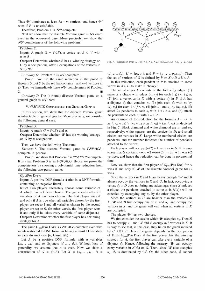
Thus W dominates at least 5n + m vertices, and hence Wwins if F is unsatisfiable.

Therefore, Problem 1 is NP-complete.Next we show that the discrete Voronoi game is NP-hard

even in the one-round case. More precisely, we show theNP-completeness of the following problem:

Problem 2:Input: A graph G = (V, E), a vertex set S ⊆ V withn := |S |.Output: Determine whether B has a winning strategy onG by n occupations, after n occupations of the vertices inS by W.

Corollary 6: Problem 2 is NP-complete.Proof: We use the same reduction in the proof of

theorem 5. Let S be the set that contains u and n−1 vertices inD. Then we immediately have NP-completeness of Problem2.

Corollary 7: The (n-round) discrete Voronoi game on ageneral graph is NP-hard.

V. PSPACE-Completeness for General Graphs

In this section, we show that the discrete Voronoi gameis intractable on general graphs. More precisely, we considerthe following general case:

Problem 3:Input: A graph G = (V, E) and n.Output: Determine whether W has the winning strategyon G by n occupations.

Then we have the following Theorem:Theorem 8: The discrete Voronoi game is PSPACE-

complete in general.Proof: We show that Problem 3 is PSPACE-complete.

It is clear Problem 3 is in PSPACE. Hence we prove thecompleteness by showing a polynomial time reduction fromthe following two-person game:

Gpos(Pos Dnf):Input: A positive DNF formula A (that is, a DNF formulacontaining no negative literal).Rule: Two players alternately choose some variable ofA which has not been chosen. The game ends after allvariables of A has been chosen. The first player wins ifand only if A is true when all variables chosen by the firstplayer are set to 1 and all variables chosen by the secondplayer are set to 0. (In other words, the first player winsif and only if he takes every variable of some disjunct.)Output: Determine whether the first player has a winningstrategy for A.

The game Gpos(Pos Dnf) is PSPACE-complete even withinputs restricted to DNF formulas having at most 11 variablesin each disjunct (see [6, Game 5(b)]).

Let A be a positive DNF formula with n variables{x1, . . . , xn} and m disjuncts {d1, . . . , dm}. Without loss ofgenerality, we assume that n is even. Now we show aconstruction of G = (V, E). Let X = {x1, . . . , xn}, D =

16

d1 d2 d3

u1 u224 24

16 16 16 16 16 16 16

Clique

x1 x2 x3 x4 x5 x6 x7 x8

Fig. 7. Reduction from A = (x1∧ x2∧ x4∧ x5)∨(x3∧ x5∧ x7∧ x8)∨(x6∧ x8)

{d1, . . . , dm}, U = {u1, u2}, and P = {p1, . . . , p2n2+6n}. Thenthe set of vertices of G is defined by V := X ∪ D ∪ U ∪ P.

In this reduction, each pendant in P is attached to somevertex in X ∪ U to make it “heavy.”

The set of edges E consists of the following edges: (1)make X a clique with edges {xi, x j} for each 1 ≤ i < j ≤ n,(2) join a vertex xi in X with a vertex d j in D if A hasa disjunct d j that contains xi, (3) join each d j with u2 by{d j, u2} for each 1 ≤ j ≤ m, (4) join u1 and u2 by {u1, u2}, (5)attach 2n pendants to each xi with 1 ≤ i ≤ n, and (6) attach3n pendants to each ui with i = 1, 2.

An example of the reduction for the formula A = (x1 ∧x2 ∧ x4 ∧ x5) ∨ (x3 ∧ x5 ∧ x7 ∧ x8) ∨ (x6 ∧ x8) is depictedin Fig. 7. Black diamond and white diamond are u1 and u2,respectively; white squares are the vertices in D; and smallcircles are vertices in X. Large white numbered circles arependants, and the number indicates the number of pendantsattached to the vertex.

Each player will occupy (n/2)+ 1 vertices in G. It is easyto see that G contains n+m+2+6n+2n2 = 2n2 +7n+m+2vertices, and hence the reduction can be done in polynomialtime.

Now we show that the first player of Gpos(Pos Dnf) for Awins if and only if W of the discrete Voronoi game for Gwins.

Since the vertices in X and U are heavy enough,W and Balways occupy the vertices in X and U. In fact, occupying avertex d j in D does not bring any advantage; since X inducesa clique, the pendants attached to some xi in N(d j) will becanceled by occupying any xi′ by the other player.

Since the vertices in U are heavier than the vertices inX, W and B first occupy one of u1 and u2, and occupy thevertices in X, and the game will end when all vertices in Xare occupied.

The player W has two choices.We first consider the case in whichW occupies u2. Then B

has to occupy u1, andW and B occupy n/2 vertices in X. Itis easy to see that, in this case, they tie on the graph inducedby U ∪ X ∪ P. Hence the game depends on the occupationof D. In Gpos(Pos Dnf), if the first player has the winningstrategy for A, the first player can take every variable of adisjunct d j. Hence, following the strategy, W can occupyevery variable in N(d j) on G. Then, since W also occupiesu2, d j is dominated by W. On the other hand, B cannot

1-4244-0464-9/06/$20.00 2006 IEEE. 270 CIG'06 (May 22-24 2006)

dominate any vertex in D since W occupies u2. Hence, ifthe first player of Gpos(Pos Dnf) has a winning strategy, sodoes W. (Otherwise, the game ends in a tie.)

Next, we consider the case in whichW occupies u1. ThenB can occupy u2. The game again depends on the occupationof D. However, in this case, W cannot dominate any vertexin D since B has already occupied u2. Hence W will loseor they will tie at best.

Thus W has to occupy u2 at first, and then W has awinning strategy if the first player of Gpos(Pos Dnf) has it.

Therefore, Problem 3 is PSPACE-complete.

VI. Concluding Remarks and Further Research

We give winning strategies for the first player W on thediscrete Voronoi game VG(T, n), where T is a large completek-ary tree with odd k. It seems thatW has an advantage evenif the complete k-ary tree is not large, which is future work.

In our strategy, it is essential that each subtree of the samedepth has the same size. Therefore, considering general treesis the next problem. The basic case is easy: When n = 1, thediscrete Voronoi game on a tree is essentially equivalent tofinding a median vertex of a tree. The deletion of a medianvertex partitions the tree so that no component contains morethan n/2 of the original n vertices. It is well known that atree has either one or two median vertices, which can befound in linear time (see, e.g., [4]). In the former case, Wwins by occupying the median vertex. In the later case, twoplayers tie. This algorithm corresponds to our Algorithm 1.

References[1] H.-K. Ahn, S.-W. Cheng, O. Cheong, M. Golin, R. van Oostrum.

Competitive facility location: the Voronoi game, Theoretical ComputerScience, vol. 310, pp. 457–467, 2004.

[2] O. Cheong, S. Har-Peled, N. Linial, J. Matousek. The one-roundVoronoi game, Discrete and Computational Geometry, vol. 31,pp. 125–138, 2004.

[3] S. P. Fekete, H. Meijer. The one-round Voronoi game replayed:Computational Geometry Theory and Applications, vol. 30, pp. 81–94,2005.

[4] F. Harary. Graph Theory, Addison-Wesley, 1972.[5] C. H. Papadimitriou. Computational Complexity, Addison-Wesley Pub-

lishing Company, 1994.[6] T. J. Schaefer. On the Complexity of Some Two-Person Perfect-

Information Games, Journal of Computer and System Sciences,Vol. 16, pp. 185–225, 1978.

1-4244-0464-9/06/$20.00 2006 IEEE. 271 CIG'06 (May 22-24 2006)

Abstract—The paper describes the attempt to cultivate pro-

grams to climb the nano hill, a contest with exceptionally tight parameters of the game called corewar. An existing tool, called µGP, has been exploited. Two genetic operators were added to tackle the peculiarities of the objective. The generated programs compared favorably with others, either manually written or evolved. µGP autonomously reproduced the same structure of the current champion of the competition, and devised a sharp self-modifying program exploiting a completely new strategy.

I. INTRODUCTION

In August 2004, a program called White Noise challenged SAL Tiny Hill, the hardest corewar contests available on the internet. White Noise defeated all opponents becoming the new King Of The Hill (i.e., the champion). The program re-coiled from the top on summer 2005 when Larger Than In-finity was submitted, but became king again after 10 days when on-a-tiny-amount-of-speed challenged the hill (ranks in a corewar competition are updated continuously, and scores may either increase or decrease). Today, White Noise is still in the upper half of the hill, fighting to get to the top again.

The point of interest in this story is that White Noise was not written by a corewar expert as other programs on the hill, but it was cultivated by an evolutionary algorithm called µGP [1]. The corewar community traditionally pays fairly attention to evolvers (as they call all evolutionary algo-rithms) [8] [9], nevertheless White Noise was the first evolved beast able to top the difficult SAL Tiny Hill. The description of the enhanced techniques exploited to evolve it can be found in [2].

This paper further extends the research targeting a differ-ent type of contest, the so-called nano hills. The rules used in nano hills makes this competition quite interesting from a mere evolutionary point of view, while it would not be ap-propriate if the final goal is to evolve a test program for a microprocessor.

The main movelty in this paper is the description of two new evolutionary operators for µGP, that allow different search schemes to be exploited. In the contest of the nano hill competition these enhance the search efficiency.

This paper is organized as follows: Section II describes

the game called corewar and the different competitions. Sec-tion III focuses on the enhancements required to the evolu-tionary core, while section IV details the fitness functions used. Section V describes the experiments. Section VI con-cludes the paper.

II. COREWAR

Corewar is a very peculiar game where two or more pro-grams fight in a virtual-computer memory. Programs are written in an assembly-like language called redcode and run on a virtual machine named memory array redcode simula-tor (MARS). The memory in MARS, also called core, is organized as a circular array, so that there are no absolute addresses but only relative offsets.

Thread 2

Thread 2

Thread 3

Thread 1

Thread 1

Thread 2

t=1 Thread 1

Thread 1

Program 2

Program 1t=3

t=4

t=5

t=6

t=7

t=8

t=2

Figure 1: a graphical representation of the MARS time-sharing environment

The instructions available in redcode are few, but with a

vast array of addressing modes, including immediate, indi-rect, self-postincrement indirect, and so on. Indeed, it is computationally a rather powerful language. The final goal of a redcode program, however, is not to compute something useful but to win a competiton. Programs are executed in a time-slicing style, one instruction at a time each. Every pro-gram may be composed of different threads; to ensure a fair competition the MARS always gives each program (and not each thread) an equal amount of time, so having multiple threads means being able to perform more operations, but at a slower pace. In figure 1 this is shown graphically in the case of two programs, one with three threads and the other with two.

A program wins if it causes all processes of the opposing programs to terminate, remaining in sole possession of the

Evolving Warriors for the Nano Core

Ernesto Sanchez, Massimiliano Schillaci, Giovanni Squillero Politecnico di Torino, Italy

All authors are with the Politecnico di Torino (DAUIN), Corso Duca degli Abruzzi 24, 10123 Torino (e-mail: giovanni.squillero@ polito.it)

1-4244-0464-9/06/$20.00 2006 IEEE. 272 CIG'06 (May 22-24 2006)

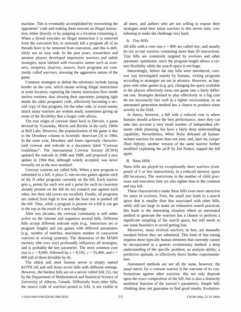
machine. This is eventually accomplished by overwriting the opponents’ code and making them execute an illegal instruc-tion, either directly or by jumping to a location containing it. When a thread executes an illegal instruction it is removed from the execution list; to seriously kill a program all of its threads have to be removed from execution, and this is defi-nitely not an easy task. In the past years, researchers and amateur players developed impressive warriors and subtle strategies, most labeled with evocative names such as scan-ners, vampires, dwarves, stoners. Such programs are com-monly called warriors, stressing the aggressive nature of the game.

Common strategies to defeat the adversary include laying bombs on the core, which means writing illegal instructions at some location; capturing the enemy instruction flow inside useless routines, thus slowing their operation; jumping right inside the other program's code, effectively becoming a sec-ond copy of that program. On the other side, to avoid enemy attack many warriors are written small, sometimes giving up some of the flexibility that a longer code allows.

The true origin of corewar dates back to Darwin, a game devised by Vyssotsky, Morris and Ritchie in the early 1960s at Bell Labs. However, the popularization of the game is due to the Dewdney column in Scientific American [3] in 1984. In the same year, Dewdney and Jones rigorously character-ized corewar and redcode in a document titled “Corewar Guidelines”. The International Corewar Society (ICWS) updated the redcode in 1986 and 1988, and proposed a new update in 1994 that, although widely accepted, was never formally set as the new standard.

Corewar contests are called hills. When a new program is submitted to a hill, it plays G one-on-one games against each of the N other programs currently on the hill. Each warrior gets sw points for each win and st point for each tie (warriors already present on the hill do not rematch one against each other, but their old scores are recalled). Finally, all programs are ranked from high to low and the least one is pushed off the hill. Thus, while a program is present on a hill it can get to the top as the result of a new challenge.

After two decades, the corewar community is still rather active on the internet and organizes several hills. Different hills accept different redcode style (e.g., instruction set or program length) and run games with different parameters (e.g., number of matches, maximum number of concurrent warriors or scoring systems). The dimension of the MARS memory (the core size) profoundly influences all strategies, and is probably the key parameter. The most common core size is c = 8,000, followed by c = 8,192, c = 55,400, and c = 800 (all of them divisible by 4).

The oldest and most famous server is simply named KOTH [4] and still hosts seven hills with different settings. However, the hardest hills are on a server called SAL [5], run by the Department of Mathematical and Statistical Science of University of Alberta, Canada. Differently from other hills, the source code of warriors posted to SAL is not visible to

all users, and authors who are not willing to expose their strategies send their latest warriors to this server only, con-tributing to make the challenge very hard.

A. Tiny Hills

All hills with a core size c = 800 are called tiny, and usually do not accept warriors containing more than 20 instructions. Tiny hills are commonly targeted by evolvers and other automatic optimizers, since the program length allows a cer-tain flexibility while the search space is not huge.

Interestingly, before the tiny hills were introduced, core-war was investigated mainly by humans, writing programs according to strategies set out in advance. However, as hap-pens with other games (e.g. go), changing the space available to the players effectively turns one game into a fairly differ-ent one. Strategies devised to play effectively in a big core do not necessarily fare well in a tighter environment, so an automated generation method has a chance to produce some novelty in the field.

In theory, however, a hill with a reduced core is where humans should achieve the best performance, since they can take into account a very small number of independent ele-ments while planning, but have a fairly deep understanding capability. Nevertheless, White Noise defeated all human-written warriors for more than one year, and, later on, Larger Than Infinity, another version of the same warrior further modified exploiting the µGP by Zul Nadzri, topped the hill again.

B. Nano Hills

Nano hills are played by exceptionally short warriors (com-posed of 5 or less instructions), in a reduced memory space (80 locations). The restrictions in the number of child proc-esses and execution time are also tighter than in the common and tiny hill.

These characteristics make these hills even more attractive for users of evolvers. First, the small size leads to a search space that is smaller than that associated with other hills, while still too large to make an exhaustive search practical; this leads to the interesting situation where an automated method to generate the warriors has a chance to perform a significant sampling of the search space, but still needs to use some heuristics to avoid getting lost.

Moreover, many evolved warriors, in fact, are manually tweaked before they are submitted. This kind of fine tuning requires three typically human elements that currently cannot be incorporated in a generic evolutionary method: a deep understanding of the specific problem; an analysis ability; a predictive aptitude, to effectively direct further experimenta-tion.

Automated methods are not all the same, however; the usual metric for a corewar warrior is the outcome of its con-frontations against other warriors: this not only depends upon the exact composition of the hill, but is also a distinctly nonlinear function of the warrior’s parameters. Simple hill-climbing does not guarantee to find good results. Evolution-

1-4244-0464-9/06/$20.00 2006 IEEE. 273 CIG'06 (May 22-24 2006)

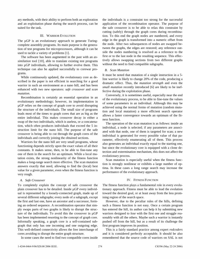
ary methods, with their ability to perform both an exploration and an exploitation phase during the search process, can be suited for the task.

III. WARRIOR EVOLUTION

The µGP is an evolutionary approach to generate Turing-complete assembly programs. Its main purpose is the genera-tion of test programs for microprocessors, although it can be used to tackle a variety of problems [1].

The software has been augmented in the past with an as-similation tool [10], able to translate existing test programs into µGP individuals, allowing to further evolve them. This technique can also be applied successfully to corewar pro-grams.

While continuously updated, the evolutionary core as de-scribed in the paper is not efficient in searching for a good warrior in such an environment as a nano hill, and has been enhanced with two new operators: safe crossover and scan mutation.

Recombination is certainly an essential operation in an evolutionary methodology; however, its implementation in µGP relies on the concept of graph core to avoid disrupting the structure of the individuals. The small size of programs leads most of the times to graph cores that are as big as the entire individual. This makes crossover decay in either a swap of the two individuals, which is useless, or a concatena-tion, which often produces individuals that exceed the 5 in-struction limit for the nano hill. The purpose of the safe crossover is being able to cut through the graph cores of the individuals and correctly joining the obtained sections.

Warriors for the nano hill are very small programs, whose functioning depends strictly upon the exact values of all their constants. It makes sense, then, to be able to fine-tune any one of them in the search for an optimum. While a local mu-tation exists, the strong nonlinearity of the fitness function makes a long-range search more effective. The scan mutation answers exactly that need, allowing to find the (local) best value for a given parameter, even when the fitness function is very rough.

A. Safe Crossover

To completely explain the concept of safe crossover the plain crossover has to be detailed. Inside µGP every individ-ual is represented by a loosely-connected graph, made up of several different subgraphs; every node of a subgraph, except the first and last one, have an ancestor and a successor, form-ing an ordered sequence. A recombination operator that sim-ply swaps parts of two graphs is likely to disrupt the struc-ture of the individuals. To avoid this the crossover in µGP has been implemented resorting to the concept of graph core. Informally speaking, a graph core is a self-contained sub-graph that only has one incoming and one outgoing edge. This well-defined connectivity allows the free interchange of cores avoiding to disrupt the entire graph structure.

In some cases the need to find two compatible cores inside

the individuals is a constraint too strong for the successful application of the recombination operator. The purpose of the safe crossover is to be able to relax this constraint by cutting (safely) through the graph cores during recombina-tion. To this end the graph nodes are numbered, and every edge in the graph is transformed into a numeric offset from the node. After two subsequences of nodes are swapped be-tween the graphs, the edges are restored; any reference out-side the nodes numbering is resolved as a reference to the first or to the last node in the resulting sequence. This effec-tively allows swapping sections from two different graphs without the need to find compatible subgraphs.

B. Scan Mutation

It must be noted that mutation of a single instruction in a 5-line warrior is likely to change 20% of the code, producing a dramatic effect. Thus, the mutation strength and even the small mutation recently introduced [6] are likely to be inef-fective during the exploitation phase.

Conversely, it is sometimes useful, especially near the end of the evolutionary process, to be able to fine-tune the values of some parameters in an individual. Although this may be achieved using the normal forms of mutation (random muta-tion and local mutation) a more efficient search operator allows a faster convergence towards an optimum of the fit-ness function.

The operation of the scan mutation is as follows: inside an individual, a node is selected; if any parameters are associ-ated with that node, one of them is targeted for scan; a new individual is generated for every possible value of that pa-rameter, effectively enumerating all of them. This process also generates an individual exactly equal to the starting one, but since the evolutionary core is equipped with a clone de-tection and extermination mechanism, this does not affect the evolutionary process.

Scan mutation is especially useful when the fitness func-tion is strongly nonlinear or exhibits a large number of op-tima. In these cases a long range search may increase the performance of the evolutionary approach.

IV. FITNESS FUNCTION

The fitness function plays a fundamental role in every evolu-tionary approach. Fitness must be able to lead the evolution toward the desired goal, or at least away from the less prom-ising region of the search space.

However, due to the peculiar rules of the hills, defining such a fitness function is not easy. Once a certain program has entered the hill, its author can help it by submitting new warriors designed to lose with the first one and struggle rea-sonably with all the others. Maybe such a warrior is instantly pushed off from the hill, but as a result of its challenge the first program improves its position.

This is a fairly standard practice among expert redcoders and it is considered perfectly acceptable. It should be also remembered that the source code of warriors on SAL is not

1-4244-0464-9/06/$20.00 2006 IEEE. 274 CIG'06 (May 22-24 2006)

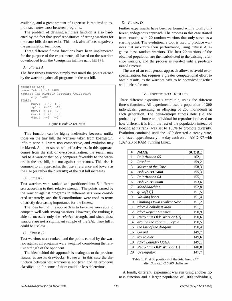
available, and a great amount of expertise is required to ex-ploit such team work between programs.

The problem of devising a fitness function is also hard-ened by the fact that good repositories of strong warriors for the nano hills do not exist. This lack also affects negatively the assimilation technique.

Three different fitness functions have been implemented for the purpose of the experiments, all based on the warriors downloaded from the koenigstuhl infinite nano hill [7].

A. Fitness A

The first fitness function simply measured the points earned by the warrior against all programs in the test hill. ;redcode-nano ;name Bob v2.1r1.7408 ;author The MicroGP Corewars Collective org START START: mov.i <-30, $-9 spl.a #-36, >18 mov.i >-14, {0 mov.i >-29, {-2 djn.f $-2, $-3

Figure 1: Bob v2.1r1.7408

This function can be highly ineffective because, unlike

those on the tiny hill, the warriors taken from koenigstuhl infinite nano hill were non competitive, and evolution may be biased. Another source of ineffectiveness in this approach comes from the risk of overspecialization: the search may lead to a warrior that only compares favorably to the warri-ors in the test hill, but not against other ones. This risk is common to all approaches that use a reference and lowers as the size (or rather the diversity) of the test hill increases.

B. Fitness B

Test warriors were ranked and partitioned into 5 different sets according to their relative strength. The points earned by the warrior against programs in different sets were consid-ered separately, and the 5 contributions were used as terms of strictly decreasing importance for the fitness.

The idea behind this approach is to favor warriors able to compete well with strong warriors. However, the ranking is able to measure only the relative strength, and since these warriors are not a significant sample of the SAL nano hill it could be useless.

C. Fitness C

Test warriors were ranked, and the points earned by the war-rior against all programs were weighted considering the rela-tive strength of the opponent.

The idea behind this approach is analogous to the previous fitness, as are its drawbacks. However, in this case the dis-tinction between test warriors is not fixed and an erroneous classification for some of them could be less deleterious.

D. Fitness D

Further experiments have been performed with a totally dif-ferent, endogenous approach. The process in this case started from scratch, with 20 random warriors that only serve as a starting point. The evolutionary tool is used to produce war-riors that maximize their performance, using Fitness A, a-gainst these random warriors. The best 20 warriors of the obtained population are then substituted to the existing refer-ence warriors, and the process is iterated until a predeter-mined timeout.

The use of an endogenous approach allows to avoid over-specialization, but requires a greater computational effort to obtain results, as the warriors have to be coevolved together with their reference.

V. EXPERIMENTAL RESULTS

Three different experiments were run, using the different fitness functions. All experiments used a population of 300 individuals, generating an offspring of 200 individuals at each generation. The delta-entropy fitness hole (i.e. the probability to choose an individual for reproduction based on how different it is from the rest of the population instead of looking at its rank) was set to 100% to promote diversity. Evolution continued until the µGP detected a steady state, and lasted approximately one day each on an AMD-K7 with 1,024GB of RAM, running Linux.

# NAME SCORE 1 Polarization 05 162,1 2 Resolute 159,2 3 Master of the Core 158,3 4 Bob v2.1r1.7408 155,3 5 Polarization 04 155,1 6 Bob v2.1r2.6680 153,6 7 Man&Machine 152,8 8 qEvo[[3]] 151,5 9 Walking boots 151,4 10 Shutting Down Evolver Now 151,2 11 rdrc: Alcoholism Malt 151,1 12 rdrc: Repent Linemen 150,9 13 Petro "I'm Old" Warrior [II] 150,6 14 around the core in 80 cycle 150,5 15 the last of the dragons 150,4 16 Go on! 149,7 17 toy soldier 149,6 18 rdrc: Laundry OSHA 149,1 19 Petro "I'm Old" Warrior [I] 148,8 20 Ucekupatox 147,7

Table 1: First 30 positions of the SAL Nano Hill after Bob v2.1r2.6680 challenge

A fourth, different, experiment was run using another fit-

ness function and a larger population of 1000 individuals,

1-4244-0464-9/06/$20.00 2006 IEEE. 275 CIG'06 (May 22-24 2006)

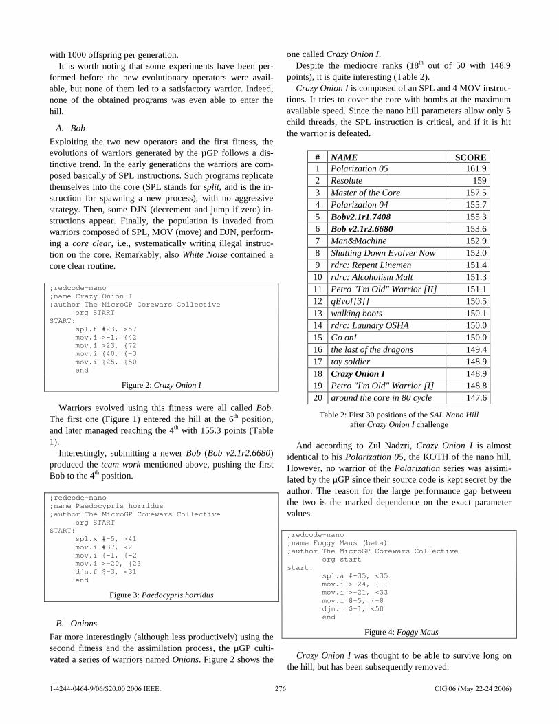
with 1000 offspring per generation. It is worth noting that some experiments have been per-

formed before the new evolutionary operators were avail-able, but none of them led to a satisfactory warrior. Indeed, none of the obtained programs was even able to enter the hill.

A. Bob

Exploiting the two new operators and the first fitness, the evolutions of warriors generated by the µGP follows a dis-tinctive trend. In the early generations the warriors are com-posed basically of SPL instructions. Such programs replicate themselves into the core (SPL stands for split, and is the in-struction for spawning a new process), with no aggressive strategy. Then, some DJN (decrement and jump if zero) in-structions appear. Finally, the population is invaded from warriors composed of SPL, MOV (move) and DJN, perform-ing a core clear, i.e., systematically writing illegal instruc-tion on the core. Remarkably, also White Noise contained a core clear routine. ;redcode-nano ;name Crazy Onion I ;author The MicroGP Corewars Collective org START START: spl.f #23, >57 mov.i >-1, {42 mov.i >23, {72 mov.i {40, {-3 mov.i {25, {50 end

Figure 2: Crazy Onion I

Warriors evolved using this fitness were all called Bob.

The first one (Figure 1) entered the hill at the 6th position, and later managed reaching the 4th with 155.3 points (Table 1).

Interestingly, submitting a newer Bob (Bob v2.1r2.6680) produced the team work mentioned above, pushing the first Bob to the 4th position.

;redcode-nano ;name Paedocypris horridus ;author The MicroGP Corewars Collective org START START: spl.x #-5, >41 mov.i #37, <2 mov.i {-1, {-2 mov.i >-20, {23 djn.f $-3, <31 end

Figure 3: Paedocypris horridus

B. Onions

Far more interestingly (although less productively) using the second fitness and the assimilation process, the µGP culti-vated a series of warriors named Onions. Figure 2 shows the

one called Crazy Onion I. Despite the mediocre ranks (18th out of 50 with 148.9

points), it is quite interesting (Table 2). Crazy Onion I is composed of an SPL and 4 MOV instruc-

tions. It tries to cover the core with bombs at the maximum available speed. Since the nano hill parameters allow only 5 child threads, the SPL instruction is critical, and if it is hit the warrior is defeated.

# NAME SCORE 1 Polarization 05 161.9 2 Resolute 159 3 Master of the Core 157.5 4 Polarization 04 155.7 5 Bobv2.1r1.7408 155.3 6 Bob v2.1r2.6680 153.6 7 Man&Machine 152.9 8 Shutting Down Evolver Now 152.0 9 rdrc: Repent Linemen 151.4 10 rdrc: Alcoholism Malt 151.3 11 Petro "I'm Old" Warrior [II] 151.1 12 qEvo[[3]] 150.5 13 walking boots 150.1 14 rdrc: Laundry OSHA 150.0 15 Go on! 150.0 16 the last of the dragons 149.4 17 toy soldier 148.9 18 Crazy Onion I 148.9 19 Petro "I'm Old" Warrior [I] 148.8 20 around the core in 80 cycle 147.6

Table 2: First 30 positions of the SAL Nano Hill after Crazy Onion I challenge

And according to Zul Nadzri, Crazy Onion I is almost

identical to his Polarization 05, the KOTH of the nano hill. However, no warrior of the Polarization series was assimi-lated by the µGP since their source code is kept secret by the author. The reason for the large performance gap between the two is the marked dependence on the exact parameter values.

;redcode-nano ;name Foggy Maus (beta) ;author The MicroGP Corewars Collective org start start: spl.a #-35, <35 mov.i >-24, {-1 mov.i >-21, <33 mov.i @-5, {-8 djn.i $-1, <50 end

Figure 4: Foggy Maus

Crazy Onion I was thought to be able to survive long on

the hill, but has been subsequently removed.

1-4244-0464-9/06/$20.00 2006 IEEE. 276 CIG'06 (May 22-24 2006)

C. Small Animals

More interesting result was produced by the µGP running with the third fitness and not exploiting assimilation. Warri-ors cultivated in this experiments were named from small animals. The first one (Paedocypris horridus) is shown in Figure 3.

Before submitting it, all other µGP generated warriors were removed to avoid the team work effect. Paedocypris horridus scored 155.9, ranking 2nd on the hill, just after Po-larization 05 (Table 3).

# NAME SCORE 1 Polarization 05 160.1 2 Paedocypris horridus 155.9 3 Resolute 155.0 4 Polarization 04 153.9 5 Master of the Core 152.5 6 Rdrc: Repent Linemen 151.8 7 Shutting Down Evolver Now 151.7 8 Man&Machine 151.6 9 the last of the dragons 151.6 10 Petro "I'm Old" Warrior [II] 151.5 11 rdrc: Laundry OSHA 151.3 12 Petro "I'm Old" Warrior [I] 150.3 13 rdrc: Alcoholism Malt 150.0 14 qEvo[[3]] 148.8 15 Go on! 148.2 16 toy soldier 148.2 17 around the core in 80 cycle 147.9 18 My nano Qscan III 147.6 19 rdrc: Delicate Crowbait 147.0 20 rdrc: Blanch Autoclave 145.9

Table 3: First 30 positions of the SAL Nano Hill after Paedocypris horridus challenge

It’s quite hard to understand why Paedocypris horridus

won (and kept on winning). According to corewar experts, it lays a carpet of MOV instruction from 20 locations away which eventually combines with the main program, overwrit-ing the DJN instruction, and creates a 23 line long warrior (a SPL followed by 22 MOVs). This greatly increases the pro-portion of time available for bombing with respect to the total. Some of the threads execute the newly created code, resulting in a more effective bombing, and making it more difficult to kill.

D. Fancy animals

In about three days of computation, a warrior, named Foggy Maus, has been produced using the Fitness D. Its structure (shown in figure 4) resembles the Paedocypris horridus one: a split followed by three mov’s and a djn. However, all con-stants have different value.

Interestingly, these give the warrior a great versability:

Foggy Maus, first entered the hill at the 5th position and has been subsequently pushed to the top of the hill, where it re-sisted for more than 20 challenges.

VI. CONCLUSIONS

The new evolutionary heuristics detailed above have shown their effectiveness in the field of corewar program cultiva-tion. The generated warriors compare favorably with others, either manually written or evolved, on the nano hill.

However, µGP autonomously reproduced the same struc-ture of the current champion (Happy Onion I), and devised a sharp self-modifying warrior exploiting a completely new strategy (Paedocypris horridus): two results that could be considered as requiring intelligence.

Lastly, an evolved non-specialized warrior (Foggy Maus) eventually became KOTH, showing the efficacy of the method.

New experiments are currently run, working together with corewar experts.

# NAME SCORE 1 Foggy Maus (beta) 156.5 2 Petro "I'm Old" Warrior [03] 155.7 3 Millionaire Landlord 155.6 4 Polarization 05 154.6 5 Resolute 153.6 6 rdrc: Repent Linemen 152.6 7 Master of the Core 151.2 8 rdrc: Alcoholism Malt 151.1 9 Bombus Sylvestris 150.2 10 Paedocypris horridus 150.2 11 iEvo[[1]] 150.1 12 Mellisuga helenae 149.4 13 Polarization 04 149.3 14 Unit 0446 148.4 15 Muddy Mouse 147.9 16 SuperSentryIV 147.9 17 Man&Machine 147.8 18 qEvo[[3]] 147.6 19 Shutting Down Evolver Now.. 147.6 20 Drunken Onion I 147.5

Table 4: First 30 positions of the SAL Nano Hill challenges after uniquely twisted challenge

ACKNOWLEDGMENT

Authors whish to thank Zul Nadzri for his precious support.

1-4244-0464-9/06/$20.00 2006 IEEE. 277 CIG'06 (May 22-24 2006)

REFERENCES

[1] G. Squillero, “MicroGP — An Evolutionary Assembly Program Gen-erator”, Journal of Genetic Programming and Evolvable Machines, Vol. 6, No. 3, 2005, pp. 247-263

[2] F. Corno, G. Squillero, E. Sánchez, “Evolving Assembly Programs: How Games Help Microprocessor Validation”, IEEE Transactions On Evolutionary Computation, Vol. 9, 2005, pp. 695-706

[3] A. K. Dewdney, “Computer recreations: In the game called Core War hostile programs engage in a battle of bits”, Scientific American, 250(5), 1984, pp. 14-22

[4] http://www.koth.org/ [5] http://sal.math.ualberta.ca/ [6] E. Sanchez, M. Schillaci, M. Sonza Reorda, G. Squillero, L. Sterpone,

M. Violante, “New Evolutionary Techniques for Test-Program Gen-eration for Complex Microprocessor Cores”, Genetic and Evolution-ary Computation Conference, 2005, pp. 2193-2194

[7] http://www.ociw.edu/~birk/COREWAR/koenigstuhl.html [8] http://students.fhs-hagenberg.ac.at/se/se00001/yace.html [9] http://users.erols.com/dbhillis/

1-4244-0464-9/06/$20.00 2006 IEEE. 278 CIG'06 (May 22-24 2006)

1-4244-0464-9/06/$20.00 2006 IEEE. 279 CIG'06 (May 22-24 2006)

Author Index

Ali M., 119 Alomari R. S., 119 Ashlock D., 19, 111 Bannach D., 98 Baptista T. R., 224 Barone L, 164, 173 Bouzy B., 187 Bryant B. D., 90 Burns K., 249, 257 Campbell M., 9 Cazenave T., 27 Chaperot B., 181, 236 Chaslot G., 187 Chong S.Y., 103 Conradie J., 67 Costa E. J. F., 224 Cowling P. I., 45 Davis I. L., 9 D’Silva T., 39 de Silva Garza A. G., 211 Dean D., 156 Deb K., 197 Demaine E. D., 265 Di Pietro A., 173 Engelbrecht A. P., 67 Fogel D. B., 230 Frayn C., 13, 217 Fyfe C., 181 Gordon S. V., 205 Gruber M., 98 Hahn S. J., 230 Hallam J., 134 Hays T. J., 230 Heinz E. A., 98 Hossain M. A., 45 Hynd K., 157 Ishibuchi H., 60 Jenkins D., 217 Justiniano C., 13 Karpov I. V., 39 Kunze K. S., 98 Lew K., 13 Looney C. G., 243

Louis S. J., 75, 148 Lucas S. L., 52 Lukowicz P., 98 Lund H. H., 134 McDonnell J. R., 83 McGlinchey S., 236 Menezes T. L. T., 224 Miikkulainen R., 39, 90 Miles C., 75 Miller I., 236 Mistry B., 156 Mittal S., 197 Nakashima T., 60 Naveed M. H., 45 Nicolescu M., 148 Nii M., 60 Olenderski A., 148 Quon J., 230 Reda A., 205 Reynolds R. G., 119 Rice A. J., 83 Runarsson T. P., 52 Sanchez E., 272 Saund E., 126 Schillaci M., 272 Soedarmadji E., 34 Spydell A., 83 Squillero G., 272 Stanley K. O., 39 Stremler S., 83 Syms P., 156 Takatani M., 60 Teramoto S., 265 Uehara R., 265 Van Lent M., 9 Varrichio C., 39 Vincent A., 157 Vrajitoru D., 142 While L., 173 Wittkamp M., 164 Yannakakis G. N., 134 Yao X., 103

1-4244-0464-9/06/$20.00 2006 IEEE. 280 CIG'06 (May 22-24 2006)