1999Topo Index-mediano

TDA - A Method for Topologically Indexing Spatial Attributes

Maurcio Riguette MedianoMarco Antnio Casanova

Marcelo Gattass

Computer Science DepartmentPontifcia Universidade Catlica do Rio de Janeiro,

Rua Marqus de So Vicente, 225, 22453-900, Rio de Janeiro, RJ, Brazilmediano,casanova,[email protected]

Abstract

This work presents a method for topologically indexing a set of spatial attributes, called TDA -Topological Data Access Method. The TDA method maintains a topological data structure for eachset of spatial attributes for which one wishes to optimize the calculation of topological operators. Thetopological data structure, which is internally manipulated by the geographic database manager system,is responsible for generating the faces, vertices, and edges that compose the topological representationof each spatial attribute. In certain circumstances, the topological representation is several times morecompact than the exact geometric representation of the spatial attributes, thus offering a significant gainin the processing of topological operators. This work initially presents the TDA method in an abstractway, including the formalism used to define the geometric representation of spatial attributes. Then itdetails the topological data structures used. Finally, it discusses issues related to the persistent storage ofthe data structures underlying the method.

1 Problem and Contribution

Geographic Information Systems, or GIS, are information systems built especially to store, analyze,and manipulate geographic objects, that is, objects that represent artifacts or phenomena in which thegeographic location is an inherent, and essential characteristic [CCH+96]. GIS typically offer spatialquery languages, which explicitly incorporate spatial operators, describing relationships (or operations)among geographic objects. Among the various spatial operators, there are the topological operators, suchas adjacent to, intercepts, etc., which define strictly topological relationships among geographic objects.Even though such operators are very useful for geographic analysis, they will have a very high cost if thegeometric representation of the objects’ geographic locations is used directly.

Therefore, this work proposes to store a representation of the topological relationship between thegeographic objects, and to use such information to optimize the processing of the topological operators,instead of directly using the geometric representation of the objects’ geographic location. In certaincircumstances, this additional representation, called topological representation, is several times morecompact than the exact geometric representation, thus providing a considerable gain in the query pro-cessing cost. The method that generates and mantains this representation is called TDA - TopologicalData Access Method.

Almost all efforts to optimize the performance of spatial queries center on the development of datastructures adequate to store and retrieve the geometric representation of the objects’ geographic location.The R-tree proposed by Guttman [Gut84] was one of the most outstanding access methods due to itssimplicity and efficiency. Its variant, the R�-tree proposed by Beckmann and others [BKSS90], has beenwidely adopted as a spatial access method for optimizing queries involving spatial attributes. Othervariants were proposed, such as the grouping techniques using R�-trees presented by Brinkhoff and

mgattass

Text Box

MEDIANO, M. R. ; CASANOVA, M. A. ; GATTASS, M. . TDA - UM MÉTODO PARA INDEXAR TOPOLOGICAMENTE ATRIBUTOS ESPACIAIS. In: Simpósio Brasileiro de Bancos de Dados, 1999, Curitiba. Anais do SBBD'99. Rio de Janeiro: Sociedade Brasileira de Computação, 1999.

Kriegel [BK94]. Gaede [GG98] presents a chronology with the history of 54 access methods of thiskind. Nievergelt and Widmayer [NW98] proposes some criteria for classifying multidimensional accessmethods. Saalfeld [Saa98] presents methods to sort spatial entities according to proximity in space,called tree-orderings, which can be constructed from topological data structures. According to Martha[Mar89], “The great contribution of the use of topological data structures is that (adjacency) queries tothe database are executed locally using algorithms whose complexity is, at worse, linear on the numberof topological elements of the result.”

The study of which topological operators must be adopted is a whole new chapter. Egenhofer andFranzosa [EF91] proposed a framework for defining topological representations. From a 4-intersectionmatrix M4IM, 16 possible combinations of intersections between the boundary (@) and the interior (�) oftwo spatial attributes of dimension 2, soi and soj , are generated. Egenhofer and Herring [EH90] haveenlarged the method’s matrix from 4 intersections to 9 intersections. Matrix M9IM of the 9-intersectionmethod generates a total of 512 intersection combinations between the boundary, the interior, and theexterior (�) of two spatial attributes of dimensions 0, 1, or 2. Egenhofer [Ege93] has proven that the9-intersection method is more adequate for treating spatial attributes of dimension 1. Clementini andothers [CFvO93] have proposed a set of 8 operators called Calculus-Based Method, CBM. In the samework, the authors have defined yet another method, called dimension-extended 4-intersection method, orDE+4IM, in which the dimension of the results from the intersections in the matrix M4IM is taken intoaccount. Finally, the authors have proven that the operators from the CBM method are more expressivethan the ones from the DE+4IM method. Clementini and Di Felice [CF95] have defined another method,called dimension-extended 9-intersection method, or DE+9IM, in which the dimension of the results ofthe intersections in the M9IM matrix is taken into account.

MDE+9IM =

0@

dim(@soi \ @soj ) dim(s�oi \ @soj ) dim(s�oi \ @soj )

dim(@soi \ s�

oj) dim(s�

oi\ s�

oj) dim(s�

oi\ s�

oj)

dim(@soi \ s�

oj) dim(s�oi \ s

�

oj) dim(s�oi \ s

�

oj)

1A :

The authors have also shown that the CBM method is equivalent to the DE+9IM method.In the present work, we will present two types of topological representations: the Complete Topolog-

ical Representation (CTR) and the Reduced Topological Representation (RTR). Topological representa-tions are proposed to calculate detailed tological operators of complex attributes (Clementini and others[CF96]) in the refinement step of the storage and access architecture proposed by Brinkhoff and others[BHKS93]. We will also propose algorithms to insert, delete, and calculate topological operators of theMDE+9IM matrix.

The same work includes tests with vegetation data in which topological representations were gener-ated with magnitudes smaller than the respective geometric representations.

This work is organized as follows. Section 2 contains a summary of the concepts used along thiswork, including the formalism used in the definition of complex spatial attributes, an intuitive definitionof planar subdivision, and the geometric representation of the objects’ geographic location. Section3 describes the TDA topological indexing method. Section 4 discusses persistent storage of the datastructure underlying the method. Section 5 presents the insertion and removal algorithms of the TDAmethod. Section 6 presents the algorithms from the MDE+9IM matrix’ operators for the TDA method.Section 7 shows test results with geographic data. Finally, in Section 8, conclusions and future works arepresented.

2

2 Preliminary Concepts

2.1 Basic Concepts

A spatial attribute soi of a geographic object oi is any attribute of oi which contains a definition of thegeographic location of oi. A geographic object may naturally have more than one spatial attribute. Inthe context of this work, we are interested in spatial attributes whose values represent, in a general case,sets of complex points, complex lines, or complex areas, defined according to the point-set topology ofClementini and Di Felice [CF96], resumed in Section 2.2. We call the internal representation of the valueof a spatial attribute soi the geometric representation g(soi) of that spatial attribute.

The remaining of this section summarizes the main definitions concerning point-set topology, brieflydiscusses the concept of planar subdivision, and defines the geometric representations of complex points,complex lines, and complex areas, adopted here.

2.2 Concepts in Point-Set Topology

Following Egenhofer and Franzosa [EF91], given a complex point, line or area T , we use the notationT �, @T , T�, T , and dim(T ) to denote the interior, boundary, exterior, closure, and dimension of T ,respectively.

A simple point is a point-set of dimension zero (non-empty) consisting of only one element. Acomplex point is a point-set of dimension zero (non-empty) consisting of a finite number of distinctelements P1; : : : ; Pn. The boundary @P of a complex point is empty. As a consequence, the interior P�

of a complex point P equals the union of all elements in P .A simple line is a closed point-set L such that dim(L) = 1, defined as the image of a continuous

mapping f : [0; 1] ! <2 so that it does not admit self-intersections. The mappings of 0 and 1 in f arethe end-points which form the boundary of a simple line on the plane. Removing the restriction, we havea notion of a line with self-intersections. Being f1; f2; : : : ; fn continuous mappings of the interval [0; 1]on the plane, a complex line is considered as any closed point-set L so that dim(L) = 1, defined as theunion of the image of the functions f1; f2; : : : ; fn.

The notion of complex area is defined from the notions of connectivity and component. A separationof a point-set A � <2 is a pair of non-empty disjoint open-sets A1 and A2 whose union is A. Thepoint-set A is connected if there are no separations in A; if this is not true then A is disconnected, andA1 and A2 are called components of a separation of A.

Given a point-set A such that dim(A) = 2, A is called regular closed only if A = A�. A simple areais a regular closed (non-empty) point-set of two dimensions with connected interior. Exterior separationsimply the existence of an outer exterior (set with no boundaries), and n > 0 inner exteriors (sets withboundaries). The outer exterior is denoted by A�0 , and the inner exteriors are denoted by A�1 : : : A

�

n .Their union defines the exterior A� of A.

An area with holes A is a regular closed (non-empty) point-set of two dimensions with the interiorconnected, so that the intersection of the closure of any two different exteriors is empty or equal to afinite set of points.

A complex area A is a closed point-set of dimension two with closed components A1 : : : An, wherefor every i 2 [1; n] each component Ai is a simple area or an area with holes, so that the intersection ofany two different components is empty or equal to a finite set of points.

2.3 Planar Subdivision

Intuitively, when we project on a plane the values of a set of spatial attributes referent to a given geo-graphic region, breaking up the lines in the crossings, the regions in the overlapping sub-regions, etc.,

3

we induce a planar subdivision of that region, that is, a set of simple points, simple lines, and areas withholes that completely cover the region and only touch on their boundaries.

2.4 The Geometric Representation of Spatial Attributes

Let us consider soi as a spatial attribute of geographic object oi. Remember that, in the general case, thevalue of soi in a state of the geographic database is a complex point, a complex line, or a complex area.

In this work we shall adopt a particular geometric representation for the value of soi . This represen-tation is denoted by g(soi), and inductively defined as follows:

� a simple point is represented by a sequence of coordinates (x; y);

� a complex point is represented by a number n indicating how many simple point representationsdoes the complex point representation contain, followed by a sequence of n simple point represen-tations;

� a simple line is represented by a number n which indicates how many simple point representationsdoes the simple line representation contain, followed by a sequence of n simple point representa-tions;

� a closed simple line is represented by a simple line in which the coordinates of the first and the lastpoints are equal;

� a complex line is represented by a number n indicating how many lines does the complex linecontain, followed by a sequence of n simple line representations;

� a loop is represented by a closed simple line;

� a simple area is represented by a number n indicating how many loops does the region contain,followed by a sequence of n loop representations; the first loop represents the external one, theothers represents the holes in the area; the orientation of the external loop is always counter-clockwise, and the orientation of the holes is always clockwise;

� a complex area is represented by a number n indicating how many simple areas does the complexarea contain, followed by a sequence of n simple area representations;

� when dim(soi) = 0, g(soi) is a complex point representation;

� when dim(soi) = 1, g(soi) is a complex line representation; and

� when dim(soi) = 2, g(soi) is a complex area representation.

3 The TDA Method

In this section we present the basic concepts of the TDA method. Storage details, a layer architecture tothe method, and an example are left to the following section.

Let O = fo1; o2; : : : ; ong be a set of geographic objects and SO = fso1 ; so2 ; : : : ; song be a set ofspatial attributes of the objects in O (keeping in mind that each object may have more than one spatialattribute), where soi is the selected spatial attribute of oi, and g(soi) is the geometric representation ofsoi .

The purpose of the TDA method is to dynamically maintain a planar subdivision stored in a topo-logical data structure TSO , associated with SO, so that the values of the spatial attributes in SO can be

4

represented by a set of faces, edges, and vertices of TSO , called components of TSO . The TSO structurewill be dynamically updated from the geometric representation of each spatial attribute inserted in orremoved from SO so as to maintain this property.

Let FTSO = ff1; : : : ; fkg, ETSO= fe1; : : : ; emg, and VTSO = fv1; : : : ; vng be the sets (from the set

theory) of faces, edges, and vertices of TSO , respectively.Given a spatial attribute soi , we can define the following sets:

� F �

oi, E�

oi, and V �

oicontain, respectively, the faces, edges, and vertices of TSO that represent the

interior s�oi

of soi :

F �

oi=fc � FTSO jc� � s�

oig (1)

E�

oi=fc � ETSO

jc� � s�oig (2)

V �

oi=fc � VTSO jc� � s�

oig (3)

� @Foi , @Eoi, and @Voi contain, respectively, the faces, edges, and vertices of TSO that represent the

boundary @soi of soi :

@Foi = ; (4)

@Eoi=fc � ETSO

jc� � @soig (5)

@Voi =fc � VTSO jc� � @soig (6)

� F�

oi, E�

oi, and V �

oicontain, respectively, the faces, edges, and vertices of TSO that represent the

boundary @soi of soi :

F�

oi=fc � FTSO jc� � s�

oig (7)

E�

oi=fc � ETSO

jc� � s�oig (8)

V �

oi=fc � VTSO jc� � s�oig (9)

Notice that F�

oi, E�

oi, V �

oi, @Foi , @Eoi

, @Voi , F�

oi, E�

oi, and V �

oiare not point-sets, but sets in the

usual sense. Hence, the operators \ and [, when applied to these sets, mean the intersection and unionoperators from the set theory, respectively. On the other hand, the geometric representation of faces,vertices, and edges, and the geometric representation of spatial attributes represent point-sets. Hence,the operators \ and [ applied to point-sets are the intersection and union operators in point-set topology,respectively. The reader can distinguish between these uses of the operators \, [, and � considering theoperands involved.

The TDA method maintains, for each spatial attribute soi , a representation toi called the topologicalrepresentation of soi . The topological representation toi consists of components of TSO so that:

toi = F �

oi[E�

oi[ V �

oi[ @Foi [ @Eoi

[ @Voi : (10)

The following properties relating components of TSO and spatial attributes soi 2 SO are worthnoting:

FTSO= F �

oi[ @Foi [ F

�

oi(11)

ETSO= E�

oi[ @Eoi

[E�

oi(12)

VTSO= V �

oi[ @Voi [ V

�

oi(13)

5

Given the dimension of the spatial attribute, some of the nine sets defined in (1) through (9) are empty,because s�

oicontains only components of TSO with a dimension smaller than or equal to the dimension

of soi , and @soi contains only the components of TSO with a dimension smaller than soi (s�oi

containscomponents of TSO with any dimension), as summarized in the following table:

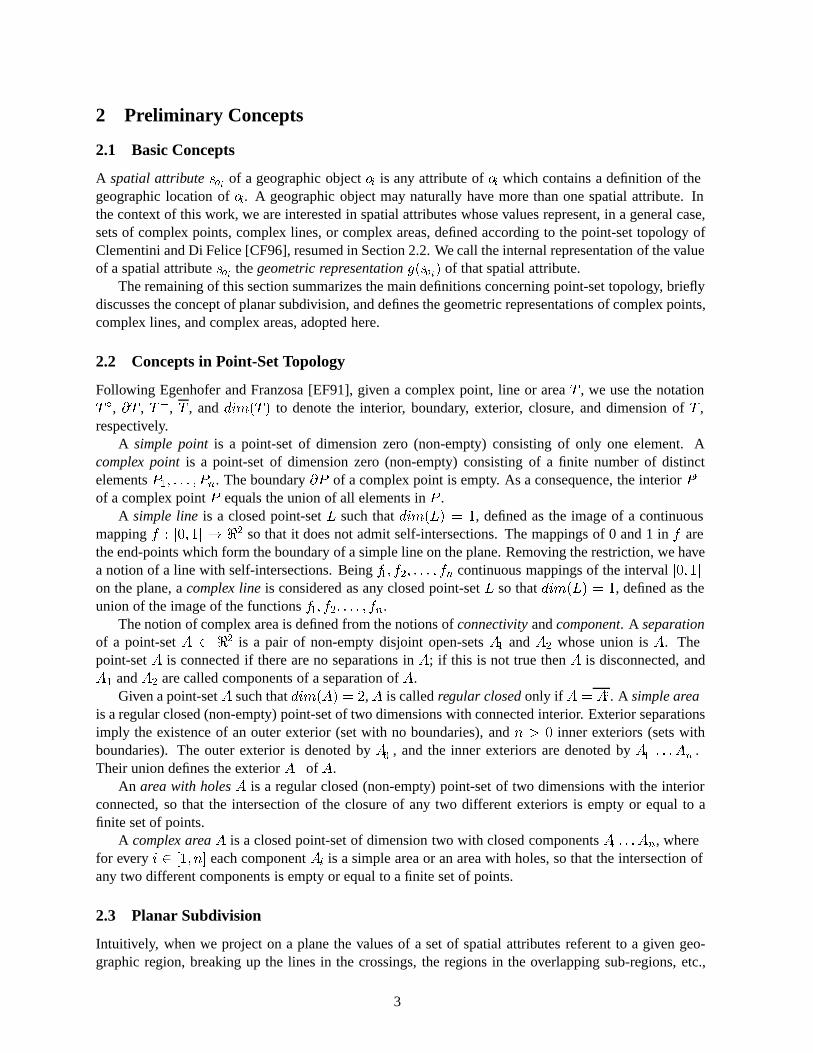
From Table 1 we can simplify (10), (11), (12), and (13) according to the dimension of soi :

� when dim(soi) = 2 we have:

toi = F �

oi[E�

oi[ V �

oi[ @Eoi

[ @Voi (14)


toi = E�

oi[ V �

oi[ @Voi (15)


toi = V �

oi(16)

F �

oiE�

oiV �

oi@Foi @Eoi

@Voi F�

oiE�

oiV �

oi

dim(soi) = 0 ; ; ; ; ;

dim(soi) = 1 ; ; ;

dim(soi) = 2 ;

Table 1: Sets of empty components according to the spatial attribute’s dimension.

In (10), there are the six subsets of components of TSO from which toi can be composed. Restricting(10) to each of the dimensions 2, 1, and 0, we have (14), (15), and (16), respectively.

We then propose two ways of storing the topological representation toi of a spatial attribute soi . Thefirst way is called the Complete Topological Representation, or CTR, defined as follows:

CTR(soi) =

8><>:

�F �

oi; E�

oi; V �

oi; @Eoi

; @Voi�

se dim(soi) = 2�E�

oi; V �

oi; @Voi

�se dim(soi) = 1�

V �

oi

�se dim(soi) = 0

(17)

Notice that, to store toi , we can also omit some of the subsets from the CTR. Basically, the smallerthe number of TSO in toi , the smaller the space occupied in secondary memory by the topological rep-resentations (which is advisable in indexing techniques). Nevertheless, as we will see, storing the CTRhas an efficiency gain when calculating the operators. The basic criterion used for selecting the subsetsof components of TSO which will be stored by toi is the following: the subsets selected must sufficeso that it is not necessary to resort to the geometric representation g(soi) of soi , or to the geometricrepresentation of the TSO edges in order to calculate topological operators.

The second way of storing the topological representation toi of a spatial attribute soi is by means ofthe Reduced Topological Representation, or RTR, defined as follows:

RTR(soi) =

8><>:

�F �

oi; @Eoi

; @Voi�

se dim(soi) = 2�E�

oi; V �

oi; @Voi

�se dim(soi) = 1�

V �

oi

�se dim(soi) = 0

(18)

6

We may conclude that the RTR is more compact than the CTR. However, when using the RTR, it isnecessary to navigate through the topological data structure to calculate some topological operators.

To prove the completeness of the TDA method, we present is Section 6 algorithms for each one ofthe MDE+9IM matrix operators, easily calculated from both topological representations, introduced by theTDA method.

4 Storage

In order to store a set SO of spatial attributes, topologically indexed according to the TDA method, it isnecessary to store the topological representations of the spatial attributes in SO and the topological datastructure TSO associated with SO. In this section we will describe how SO and TSO will be stored. Wecan say in advance that all descriptors of the data structures used to store SO and TSO have a fixed sizeand are persistently allocated.

4.1 The Multi Level Architecture of the TDA Method

Figure 1 illustrates the TDA method’s level architecture. It is worth noting that the descriptor of thespatial attribute in the geographic database management system (GDBMS) references the descriptor ofthe spatial attribute in the topological index, and vice-versa. As a consequence, the GDBMS is capableof optimizing topological operators by means of the access to the spatial attribute’s topological represen-tation, and the TDA method is capable of accessing this geometric representation stored in the GDBMS.Example in Section 4.4 details this architecture.

geometricdescriptions

of spatialattibutes

topological representationsof spatial attributes

geometric representationsof edges

spatial attributes

TDA MethodGDBMS

topological data structure

(a)

(c)

(d)

(e)

(b)

Figure 1: The TDA method’s level architecture.

4.2 Topological Data Structure Storage

To adapt TSO in secondary memory, the first change to be made is to substitute adequate access methodsfor the lists of faces, edges, and vertices. This change is based on the observation that, during the accessto these lists, insertions and removals of spatial objects, and queries are made such as “Retrieve thecomponents in the list of faces (vertices or edges) that intercept a given region or that contain a point.”Thus, even in main memory, it is more adequate to use data structures that group spatial objects close toone another. As these lists are stored in secondary memory, we have chosen to use R�-trees.

The geometric representation of the vertex is stored together with the vertex descriptor. The geomet-ric representation of each edge must be stored by means of an access method to vectorial data capableof optimizing geometric algorithms used by the topological data structure, and of efficiently storing the

7

geometric representation of the edge in secondary memory. The SV-tree (static V-tree) proposed by Me-diano and others [MCD94] is an access method adequate to these requirements. It has an occupancylevel of almost 100% in its nodes, and is capable of retrieving, in time O(N), the N points that describethe stored polygonal line.

4.3 Topological Representation Storage

The topological representation toi is stored by means of B-trees, each B-tree storing one of the subsetsF �

oi; E�

oi; V �

oi; @Eoi

and @Voi . The RTR toi has three B-trees when dim(soi) = 2 or dim(soi) = 1, andjust one B-tree when dim(soi) = 0. The B-trees store references to the components of TSO . To store theCTR toi , five B-trees would be needed when dim(soi) = 2.

We shall store an R�-tree associated to the set SO of spatial attributes, topologically indexed bymeans of the TDA method. Each spatial attribute in set SO will contain an entry in the R�-tree of SO.Each entry in the SO R�-tree, relative to a spatial attribute soi 2 SO, is composed of the bounding box ofg(soi) and a reference to the soi descriptor. The descriptor of the spatial attribute soi contains a numberrepresenting dim(soi), a reference to g(soi) in the GDBMS, and a reference to the toi descriptor. Thedescriptor of the RTR toi contains the B-tree descriptors.

4.4 Examples

Figure 2 details the TDA method’s level architecture using an example with a spatial attribute of dimen-sion 1 whose topological representation is composed of two vertices (@Voi ) and one edge (E�

oi).

1 R-tree

B-trees

SV-trees

face vertex vertex edge

(c2)

(c1)

(a2)

(a1)

(b1)

(b2)

GDBMS

11

TDA Method

(e)

(d)

Figure 2: Example of a spatial attribute of dimension 1 in the TDA method’s level architecture.

We have subdivided the levels (a), (b), and (c) of the TDA method and the GDBMS level that ma-nipulates the geometric representation of the spatial attribute, as follows:

� level (a) of the spatial attributes of the TDA method is composed by levels: (a1) containing theR�-tree that references the descriptors of the topologically indexed spatial attributes, and (a2)containing the descriptors of the TDA method’s spatial attributes;

� level (b) of the geometric representations of spatial attributes stored in the GDBMS is composedby levels: (b1) containing the descriptors of spatial attributes in the GDBMS, and (b2) containingspatial attributes’ geometric representations;

8

� level (c) of the TDA method’s topological representations is composed by levels: (c1) containingtopological representation descriptors, and (c2) containing the B-trees that store the references tothe components of TSO that compose the topological representations;

� level (d) of the TDA method’s topological data structure is composed by (see Section 4.2): thethree face, vertex, and edge R�-trees; the face, vertex, and edge descriptors; and other auxiliarydescriptors, according to with the topological data structure used;

� level (e) of the geometric representations of the edges in the topological data structure is com-posed by the SV-trees that store the geometric representations of the edges in the topological datastructure.

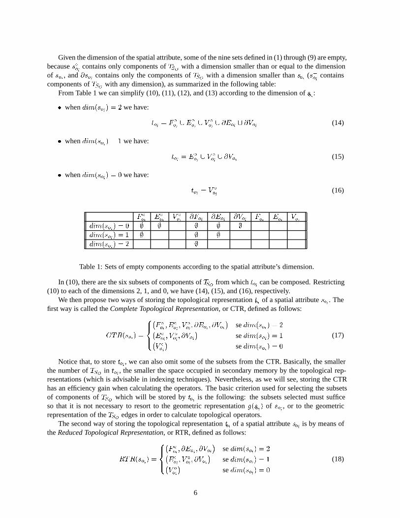
The following example illustrates two spatial attributes soj and sok stored in a set SO topologicallyindexed by the TDA method. Figure 3 shows soj and sok . Each attribute is constituted by one region,and soj has a hole. Figure 4 shows TSO (19) after de insertion of soj and sok . Note that faces f3 and f5

Figure 3: Spatial attributes soj and sok and their relative position.

belong to both toj (20) and tok (21), which means that dim(soj \ sok) = 2 (Section 5 details topologicaloperators’ algorithms). Faces f0, f2, and f4 do not belong to any topological representation.

TSO =

8><>:

FTSO= ff0; f1; f2; f3; f4; f5; f6g

ETSO= fe1; e2; e3; e4; e5; e6; e7; e8; e9g

VTSO= fv1; v2; v3; v4; v5g

(19)

toj =

8><>:

F �

oj= ff1; f3; f5g

@Eoj= fe1; e2; e3; e4; e5g

@Voj = fv1; v2; v3; v4; v5g

(20)

tok =

8><>:

F �

ok= ff3; f5; f6g

@Eok= fe6; e7; e8; e9g

@Vok = fv1; v2; v3; v4g

(21)

9

v1 v2

v3

v4

v5

e1

e2

e3e5

e6

e7

e8

e9

f0

f1

f2

f4

f5f6

e4f3

Figure 4: The TSO topological data structure after the insertion of soj and sok .

5 The Insertion and Removal Algorithms

To insert (or remove) spatial attributes in (or from) a set SO of spatial attributes indexed according tothe TDA method implies in executing three basic tasks: editing the topological structure, creating (ordestroying) the topological representation of the inserted (or removed) spatial attribute, and updating thetopological representations of the SO spatial attributes whose topological representations were affectedby the topological structure’s edition. The Insertion and Removal algorithms of the TDA method arepresented in Figures 5 and 6, respectively. Each step of the Insertion and Removal algorithms will bepresently commented on.

Step 1 Identify S00O� SO

Step 2 For each sok 2 S00O

do T �1(tok)

Step 3 Edit the topological structure TSO inserting g(soi)

Step 4 toi = T (g(soi); TSO)

Step 5 C(toi ; TSO)


do tok = T (g(sok); TSO)

Figure 5: Algorithm for inserting the spatial attribute soi in the set of spatial attributes SO indexed bythe TDA Method.

5.1 Vertex and Edge Reference Counters

For the edition of TSO to work properly, it is necessary to modify the topological structure, addingreference counters to the descriptors of edges and vertices. The reference counters are used for theproper removal of vertices and edges, as they allow the identification of vertices and edges which are notreferenced to in topological representations. The reference counters are initialized with zero during theapplication of Euler operators that create vertices and/or edges. The only exception is the Euler operator

10

Step 1 Identify S00O� SO


do T �1(tok)

Step 3 C�1(toi ; TSO)

Step 4 Edit the topological structure TSO removing from toiunecessary components

Step 5 T �1(toi)


do tok = T (g(sok); TSO)

Figure 6: Algorithm for removing the spatial attribute soi from the set of spatial attributes SO indexedby the TDA Method.

that creates a vertex by dividing an edge in two. In this case, the reference counters of the two edges thatresult from the division will have the same value as the counter of the original edge.

Operator C, in Step 5 of the Insertion algorithm (Figure 5), increments the reference counters ofthe vertices and edges referenced to in the topological representation of the inserted spatial attribute.Operator C�1, in Step 3 of the Removal algorithm (Figure 6), decrements the reference counters of thevertices and edges referenced to in the topological representation of the removed spatial attribute.

5.2 Editing the TSO Topological Structure

Let us consider soi as a new spatial attribute to be inserted in or removed from SO. Editing the TSOtopological structure, in Step 3 of the Insertion algorithm (Figure 5), consists in editing the planar subdi-vision stored in TSO from g(soi) (for further details on the geometric representation of spatial attributes,see Section 2.4) by means of the application of Euler operators.

NO DEVIAMOS REMOVER ESSA DISCUSSO SOBRE COMO EDITAR A ESTRUTURATOPOLOGICA (PRXIMOS 3 PARAGRAFOS), TEMOS QUE DIMINUIR E ISSO NAO ACRES-CENTA NADA.

Given a spatial attribute soi to be inserted in SO, we will consider that the auto-intersections inthe polygonal lines of g(soi) , when dim(soi) = 1, are removed in a pre-processing stage by meansof geometric algorithms (Preparata [PS85]). The first step to be executed during the edition of thetopological structure is to select the edges that touch or intercept g(soi) and to generate intersectionsbetween the edges selected and the polygonal lines of g(soi). Notice that the polygonal lines of g(soi)are also split. For such, one must select the edges in ETSO whose bounding box touches or intercepts thebounding box of g(soi). Then one must split the selected edges (using the respective Euler operator) andthe polygonal lines in g(soi), in the intersection points found, by means of algorithms for intersectingpolygonal lines. If dim(soi) = 0, the points in g(soi) that coincide with vertices in VTSO are removed;if dim(soi) = 1 or dim(soi) = 2, the polygonal line segments in g(soi) that coincide with the selectededges are removed. The remaining of g(soi) after the intersections with vertices and edges of TSO andafter the removal of parts of g(soi) that coincided with the vertices of TSO will be called g0(soi).

The second step is to create new vertices. The candidates to be new vertices are: when dim(soi) = 0,the points of g0(soi); when dim(soi) = 1 or dim(soi) = 2, the first and the last points of each openpolygonal line of g0(oi) and any point of each closed polygonal line of g0(soi). Before applying the Euleroperators that create vertices, one must verify whether there already exists a vertex in VTSO in the samecoordinates as the point which is candidate to be a new vertex. The operator is not applied when there isa vertex in the same position (or close enough to it, according to certain tolerance parameters).

The third step is to create edges from the polygonal lines in g0(oi). For each polygonal line lj suchthat lj 2 g0(oi), a new edge ej is created so that lj is the geometric representation of ej .

11

During removal, considering that the effects of the insertion of g(soi) in TSO must be undone in orderto reduce the size of TSO , the edition of TSO consists in applying destructive Euler operators. Step 4 ofthe Removal algorithm (Figure 6) is responsible for editing the topological structure during the removalof soi from SO.

Given a topological representation toi of a spatial attribute soi removed from TSO , the componentsthat can be removed from TSO are certainly among the components belonging to toi , because only thesecomponents’ reference counters were decremented. Thus, the first step is to traverse toi looking in @Eoiand E�

oifor the edges that can be removed, presently removing them. The edges that can be removed are

those whose reference counters have value 0. The second step is to traverse toi looking in @Voi and V �

oi

for the vertices that can be removed, removing them by means of Euler operators. The vertices that canbe removed are those whose reference counters have value 0 and those adjacent to no more and no lessthan 2 different edges. Is should be noted that when a vertex adjacent to 2 different edges is removed,these 2 edges are collapsed into one.

Note that no geometric computation is made during the removal.

5.3 Creation and Destruction of Topological Representations

Being soi a spatial attribute inserted in or removed from a topological index indexed by the TDA method,operator T is responsible for selecting the TSO components whose interiors are contained in soi , and forgenerating the topological representation toi . Operator T in Step 4 of the Insertion algorithm (Figure 5)creates the topological representation of the inserted atributte soi . Operator T in Step 6 of the Insertionalgorithm (Figure 5) and in Step 6 of the Removal algorithm (Figure 6) creates the topological represen-tations destroyed in Step 2 of the Insertion algorithm in Figure 5 and in Step 2 of the Removal algorithmin Figure 6, respectively. Steps 2 and 6 of the Insertion algorithm and Steps 2 and 6 of the Removalalgorithm are part of the topological representation updating strategy and are commented on in Section5.4.

There is a total of 9 possibilities for selecting subsets of TSO components to create CTRs of spatialattributes:

� F �

oi, @Eoi

and @Voi when dim(soi) = 2;

� @Voi , V�

oiand E�

oiwhen dim(soi) = 1; and

� V �

oiwhen dim(soi) = 0.

Remember that when creating RTRs its not necessary to generate E�oi

and V �


The selection of V �

oiwhen dim(soi) = 0 is done by looking for the vertices in VTSO whose geometric

representation intercepts the bounding box of g(soi). For the set of vertices selected, a geometric test isperformed to find out whether the vertex belongs to s�oi or not. If it does, then the vertex is inserted intoV �

oi; if not, then the vertex is not considered, because it belongs to s�oi .The selection of E�

oiwhen dim(soi) = 1 is done by looking for the edges in ETSO whose bounding

box intercepts the bounding box of g(soi). For the set of edges selected, a geometric test is performedto find out whether the edge belongs to s�oi or not. If it does, then the edge is inserted into E�oi ; if not,then the edge is not considered, because it belongs to s�

oi.

The selection of V �

oiand @Voi when dim(soi) = 1 is done, from E�

oi, by selecting the vertices

adjacent to the edges of E�

oi. Vertices adjacent to more than one edge of E�

oibelong to V �

oi; the others

belong to @Voi .The selection of @Eoi when dim(soi) = 2 is made using the same procedure described for selecting

E�


12

The selection of @Voi when dim(soi) = 2 is done, from @Eoi , by selecting the vertices adjacent tothe edges of @Eoi .

The selection of F�

oiwhen dim(soi) = 2 is done from @Eoi . Let us consider that TSO has the

following property: any edge e 2 ETSObetween two faces f1 and f2, stores in its descriptor the

necessary information for distinguish which of the two faces is at the right of the orientation ofits geometric representation g(e). Firstly, one of the two faces laterally adjacent to each edge in @Eoimust be selected. To find out which one of the two faces, the one to the right or the one to the left ofg(e1), belongs to F�

oi, the orientation of g(e1) must be checked in relation to the orientation of g(soi)’s

loop that matches g(e1). If the orientations match, the face to the left of g(e1) belongs to s�oi ; if not, theface to the right of g(e1) belongs to s�

oi. Then the faces adjacent to the already selected faces in F�

oimust

be recursively selected, only when the edges that separate the faces do not belong to @Eoi . The recursionis executed only once for each selected face.

The selection of E�

oi(and V �

oi) when dim(soi) = 2 is done selecting all the edges (and vertices)

adjacent to faces in F�

oi, removing the edges (and vertices) that belong to @Eoi (and @Voi).

Operator T �1 destroys the topological representation toi generated by T , that is, T�1 liberates thepersistent objects allocated to store toi . Operator T �1 does not need TSO as an argument, because it isnot necessary to access TSO to destroy toi . Operator T �1 in Step 5 of the Removal algorithm (Figure6) destroys the topological representation of the removed atributte soi . Operator T �1 in Step 2 of theInsertion algorithm (Figure 5) and Step 2 of the Removal algorithm (Figure 6) destroys the topologicalrepresentations created in Step 6 of the Insertion algorithm (Figure 5) and in Step 6 of the Removalalgorithm (Figure 6), respectively.

5.4 The Topological Representations Update Strategy

Updating topological representations of spatial attributes in a set SO of spatial attributes indexed accord-ing to the TDA method implies in identifying spatial attributes S0

Owhose topological representations

have become inconsistent after editing TSO , and in updating the topological representations of the at-tributes in S0

O.

During the insertion or removal of a spatial attribute soi in or from SO, the TDA method mustidentify the subset S0

Oof affected spatial attributes of SO whose topological representations have become

inconsistent. Initially, set S00O

such that S0O� S00

O� SO, formed by the spatial attributes whose bounding

boxes of the geometric representations intercept the bounding boxes of soi’s geometric representationg(soi), is selected. The selected attributes in S00

Oare likely to be affected spatial attributes. The option

adopted here consists in treating all spatial attributes in S00O

as if they were affected spatial objects, eventhough not always all of them have been affected by the edition of TSO . The identification of S00

Ois the

first step (Step 1) of the Insertion algorithm (Figure 5) and of the Removal algorithm (Figure 6).The topological representations updating strategy adopted in this paper consists in destroying and

reconstructing the topological representations of the spatial attributes in S00O

by means of operators T�1

and T . This strategy is used in Steps 2 and 6 of the Insertion algorithm and in Steps 2 and 6 of theRemoval algorithm.

6 The Algorithms from theMDE+9IM Matrix’ Operators

Let us consider:

� soi and soj as two complex spatial attributes of SO so that dim(soi) = 0, 1, or 2, and dim(soj ) =

0, 1, or 2;

13

� g(soi) and g(soj ) as the geometric representations of soi and soj ; and

� toi and toj as the topological representations of soi and soj .

The computation of the MDE+9IM(soi ; soj ) matrix’ operators is traditionally done from g(soi) andg(soj ). The TDA method’s proposal is to compute the MDE+9IM(soi ; soj ) matrix’ operators by meansof toi , toj , and TSO . We will show that the topological representations toi and toj , together with thetopological data structure TSO , are enough to compute the 9 operators of the MDE+9IM matrix. Thegeometric representations of spatial attributes, edges, and vertices are not used in this computation.

6.1 Possible Results from the Operators

Given two spatial attributes soi and soj , Egenhofer and Herring [EH90] proposes 6 groups of operators,one for each of the six 9-intersection matrices, to represent the 9IM method among spatial attributes withdimensions 0, 1, and 2. Clementini and Di Felice have extended the 9IM method by dimension, definingthe DE+9IM method.

Initially, each one of the 54 operators can return �1 (when there is no intersection), 0, 1, or 2.However, we can list a series of conditions to restrict the real result possibilities for each of the 9 operatorsof the six MDE+9IM matrices. Some of these conditions are derived from the conditions presented toreduce the result possibilities for the 9IM method in [EH90].

� Condition 1 We can notice that dim(soi \ soj ) is smaller than or equal to the smallest valuebetween dim(soi) and dim(soj ). For instance, if dim(soi) = 1, we can conclude that any inter-section operator involving @soi will have as a result, at most, 0, because dim(@soi) = 0.

� Condition 2 Since the existence of infinite spatial attributes is not admitted, we can establish thatdim(s�oi\s

�

oj) = 2. Due to this property, it is not necessary to compute the operator dim(s�oi\s

�

oj)

for any of the six matrices.

� Condition 3 If dim(soi) > dim(soj ), then dim(soi \ s�

oj) = dim(soi).

� Condition 4 If dim(soi) = 0, then @soi = ;. Thus, any intersection operator with @soi will have�1 as a result.

� Condition 5 In the three matrices whose spatial attributes have the same dimension, the operatorsto the left of the main diagonal are symmetrical to those to the right.

� Condition 6 If dim(soi) = 1 and dim(soj ) = 2 , then dim(soi \ s�

oj) 6= 0. If dim(soi \ s

�

oj) were

equal to 0, then there would be a point belonging to soi isolated in s�oj

, which is impossible.

� Condition 7 If dim(soi) = 1 and dim(soj ) � 1, then dim(soi \ s�

oj) 6= 0. If dim(soi \ s

�

oj) were

equal to 0, then there would be a point belonging to soi isolated in s�oj


� Condition 8 If dim(soi) = 2 and dim(soj ) = 2, then dim(s�oi \ s�

oj) 6= 0 ^ dim(s�oi \ s

�

oj) 6= 1.

If dim(s�oi \ s�

oj) were equal to 0 or 1, then there would be a point or line belonging to s�oi isolated

in s�oj , which is impossible.

� Condition 9 If dim(soi) = 2 and dim(soj ) = 2, then dim(s�oi\ s�

oj) 6= 0 ^ dim(s�

oi\ s�

oj) 6= 1.

If dim(s�oi \ s�

oj) were equal to 0 or 1, then there would be a point or line belonging to s�oi isolated

in s�oj


14

The six following matrices Rdim(soi )dim(soj )illustrate the possible results of each one of the 9 oper-

ators of the MDE+9IM matrix according to the dimension of soi and soj :

R22 =

0@

f1; 0;�1g

f1;�1g f2;�1g

f1;�1g f2;�1g f2g

1AR21 =

0@

f0;�1g f0;�1g f0;�1g

f1; 0;�1g f1;�1g f1;�1g

f1;�1g f2g f2g

1A

R20 =

0@

f�1g f�1g f�1g

f0;�1g f0;�1g f0;�1g

f1g f2g f2g

1AR11 =

0@

f0;�1g

f0;�1g f1; 0;�1g

f0;�1g f1;�1g f2g

1A

R10 =

0@

f�1g f�1g f�1g

f0;�1g f0;�1g f0;�1g

f0;�1g f1g f2g

1AR00 =

0@

f�1g

f�1g f0;�1g

f�1g f0;�1g f2g

1A

6.2 The Operators’ Algorithms

With the purpose of validating the TDA method, in this section we present algorithms for each of theoperators of the DE+9IM method for both topological representations, RTR and CTR.

Figures 7, 8, 9, 10, 11, and 12 show operators’ algorithms of the matrices M22, M21, M20, M11,M10, and M00 using the RTR. Some of the operators’ algorithms of the matrices M22, M21, and M20

access the topological data structure to obtain the adjacency relations between either edges and faces,or vertices and faces. When CTR is used, it is possible to write more efficiently algorithms that avoidthe access to the topological data structure. Figures 13, 14, and 15 show operators’ algorithms of thematrices M22, M21, and M20 rewritten for CTR.

Algorithm dim(@soi \ @soj )

Step 1 If any component of @Eoi belongs to @Eoj , return 1

Step 2 If any component of @Voi belongs to @Voj , return 0, otherwise return �1

Algorithm dim(@soi \ s�

oj)

Single step If any component of @Eoi does not belong to @Eoj and is laterally adjacent to anycomponent of F�

oj, return 1, otherwise return �1


oj)

Single step If any component of @Eoi is not laterally adjacent to any component of F�oj , return 1,otherwise return �1

Algorithm dim(s�oi\ s�

oj)

Single step If any component of F�oi

belongs to F�


Algorithm dim(s�oi \ s�

oj)

Single step If any component of F�oi

does not belong to F�


Figure 7: Algorithms of the operators of the M22 matrix for RTR.

The operators from the MDE+9IM matrix can be divided in three groups: group R with the operatorsfor RTR (and CTR) which do not access the topological data structure, group RT with the operatorsfor RTR that access the topological data structure, and group C with the operators from the RT group

15


Single step If any component of @Voi belongs to @Voj , return 0, otherwise return �1.Algorithm dim(@soi \ s

�

oj)

Step 1 If any component of @Eoi belongs to E�

oj, return 1

Step 2 If any component of @Voi belongs to V �



oj)

Single step If any component of E�oj

neither belongs to @Eoi nor is laterally adjacent to any com-ponent of F�

oi, return 1, otherwise return �1

Algorithm dim(s�oi\ @soj )

Single step If any component of @Voj does not belong to @Voi and is laterally adjacent to anycomponent of F�



oj)

Single step If any component of E�oj does not belong to @Eoi and is laterally adjacent to anycomponent of F�


Algorithm dim(s�oi \ @soj )

Single step If any component of @Voj neither belongs to @Voi nor is adjacent to F�

oi, return 0,

otherwise return �1


oj)

Single step If no component of E�oj

belongs to @Eoi nor is laterally adjacent to F�oi

, return 1,otherwise return �1



oj)

Single step If any component of @Voi belongs to V �



oj)

Single step If any component of V�

ojdoes not belong to @Voi and is adjacent to any component of

F �



oj)

Single step If any component of V�oj neither belongs to @Voi nor is adjacent to any component ofF �



16


Single step If any component of @Voi belongs to @Voj , return 0, otherwise return �1


oj)




oj)

Single step If any component of @Voi does not belong neither to @Voj nor to V �

oj, return 0, other-

wise return �1


oj)

Step 1 If any component of E�

oibelongs to E�

oj, return 1,

Step 2 If any component of V�

oibelongs to V �



oj)

Single step If any component of E�oi does not belong to E�




oj)




oj)

Single step If any component of V�oj

belongs to V �



oj)

Single step If any component of V�oj does not belong neither to @Voi nor to V �

oi, return 0, otherwise

return �1


oj)

Single step If any component of @Voi does not belong to V �




oj)




oj)

Single step If any component of V�oj

belongs to V �




oj)

Single step If any component of @Eoi belongs to E�

oj, return 1, otherwise return �1.


oj)

Single step If any component of @Eoi does not belong neither to E�oj nor to @Eoj , return 1, other-wise return �1.

Figure 13: Algorithms of the operators of the M22 matrix for CTR.

17

Algorithm dim(@s�oi\ s�

oj)


ojbelongs to @E�

oi, return �1,


ojbelongs to E�

oi, return �1, otherwise return 1


Single step If any component of @Voj belongs to V �



oj)

Single step If any component of E�oj

belongs to E�



Single step If any component of @Voj does not belong neither to @Voi nor to V �

oi, return 0, other-

wise return �1


oj)

Single step If no component of E�oj

belongs to @Eoi nor to E�




oj)

Single step If any component of V�oj belongs to V �



oj)

Single step If any component of V�oj does not belong neither to @Voi nor to V �

oi, return 0, otherwise

return �1


18

rewritten for CTR. When CTR is not used (in this option, E�oi

and V �

oiare not stored when dim(soi) =

2), the lack of E�

oiand V �

oi, used in algorithms of group C , is replaced by the navigation through the

topological data structure in algorithms of group RT .The algorithms from groups R and RT are those of all operators of the MDE+9IM matrix for RTR,

and the algorithms from groups R and C are those of all operators of the MDE+9IM matrix for CTR. Asall the presented algorithms from the operators of the MDE+9IM matrix do not make use of the geometricrepresentation neither of spatial attributes nor of edges and vertices of the topological data structure tocompute topological operators, it is thus proven that the CTR and RTR do not use geometric representa-tions to compute topological operators.

6.3 Complexity Analysis

The algorithms from groups R and C have one or two occurrences of the generic step presented in Figure16. Supposing that X and Y have the same number of components and that the number of componentsin X is N . Given that X and Y are ordered, the complexity of the algorithms of groups R and C and,consequently, of all algorithms for CTR, is O(N).

Single step If f any j nog component of X [does not] belong(s) to Y , return f2 j 1 j 0 g, [otherwisereturn �1]

Figure 16: Generic step used in the algorithms of operators in groups R and C .

The algorithms in group RT have a coherence of one of the two steps presented in Figure 17. Theadjacencies used in the algorithms of the RT group are either edges and faces, or vertices and faces. Inthe first option, whenever is necessary, one can check, for every component c of X , if the componentsadjacent to component c belong to Z . The difference between the first and the second option is that inthe second it is necessary to check whether the component belongs (or not) to set Y before checking ifthe adjacencies belong to Z .

Step A If fany j no g component of X is [not] adjacent to f any j no g component of Z , returnf 2 j 1 j 0 g, [otherwise return -1]

Step B If fany j no g component of X [does not] belong(s) to Y and is [not] adjacent to f anyj no g component of Z, return f 2 j 1 j 0 g, [otherwise return -1]

Figure 17: Two generic steps used in the algorithms of operators in group RT .

Once again, let us suppose that the number of components in X , Y and Z is the same, that thenumber of components in X is N , and that the number of faces adjacent to a vertex is never greater thana constant K . Notice that the overlap between two natural maps hardly contains more than two linescrossing in a same point, that is, more than 4 faces adjacent to a vertex. Given that Y and Z are in order,the search for component c of X in Y has complexity O(log(N)), and the complexity of the search forthe components adjacent to c in Z is also O(log(N)). Thus, the complexity of the algorithms in groupRT is equal to O(N � log(N)). The complexity of the algorithms for RTR is equal to the sum of thecomplexities of the algorithms in groups R and RT : O(N � log(N)).

19

7 Tests with Geographic Data

The data used in the tests were generated from 26 vegetation maps from legal Amazon courtesy of theSpatial Research National Institute, INPE. From the polygonal lines of the vegetation maps, 26 sets ofgeometric representations of dimension 2 were generated. For the tests’ sake, we shall consider eachgeometric representation obtained as the geometric representation of a spatial attribute.

Two groups of tests were made. In the first group, each of the 26 maps were inserted side by side,just as they occur in geographic space, in only one set indexed by the TDA method. In the second group,6 maps of rectangular area were overlapped.

The topological data structure used is the Half-Edge [Man88].The graph in Figure 18 shows the average number of identifiers in topological representations for the

first test group (N1) and to the second test group (N2) on axis Y, and the number os attributes in SO,on axis X, after the insertion of each set of spatial attributes. We have noticed that another consequenceof the increased overlap between spatial attributes is a raise in the average number of identifiers intopological representations. In the first test group, in which there was no overlap between the spatialattributes, N1 remained around 17 identifiers, while in the second test group, after the insertion (overlap)of the sixth set of spatial attributes, the value of N2 reached 180 identifiers.

0

45

90

135

180

0 4000 8000 12000 16000 20000

N1

N2

Figure 18: Graph with the average number of identifiers in topological representations N1 and N2, onvertical axis, and the number os attributes in SO, on horizontal axis, after inserting each set of spatialattributes from the first and the second test group, respectively.

To perform the tests with topological operators, we have modified the operators’ algorithms. Beforethe computation of each operator, all of the topological representations to be used by the operators weretransferred to a vector. Therefore, all searches made in B-trees were replaced by binary searches. Eventhough this modification has no impact on the complexity analysis of operators’ algoritms, the operators’computation became 3 or 4 times faster compared to the computation using B-trees. At the end of theinsertion of each set of spatial attributes, up to 10000 operations were performed between pairs of spatialattributes whose bounding boxes intercepted.

These operations were the following:

� Id1 - average time taken to read the geometric representation of both spatial attributes;

� Id2 - average time taken to read the geometric representation of both spatial attributes and to ordertheir points in the X axis;

� MDE+9IM - average time taken to calculate the 8 topological operators of the matrix MDE+9IM

(keeping in mind that dim(s�oi \ s�

oj) = 2); and

20

� the average time taken to compute operators dim(@soi \@soj ), dim(@soi \ s�

oj), dim(@soi \ s

�

oj),

dim(s�oi \ s�

oj), and dim(s�oi \ s

�

oj).

We can say that the greater the number of points per edge the smaller will the size of topologicalrepresentations be when compared to those of geometric representations, that is, the faster will the com-putation of topological operators be using topological representations. It should be noted that the greaterthe overlap between spatial attributes, regardless of the number of points in the geometric representa-tions, the greater will the size of the topological representation be, and the worse will the performance ofTDA method be.

The graph in Figure 19 shows the average time spent to execute the above operations in vertical axisand the number of spatial attributes in horizontal axis for the first group of tests. The most importantresult in this graph is the verification that a all of the operators’ algorithms using RTRs is faster thansimple access to the spatial attributes’ geometric representation.

0.0001

0.001

0.01

0 5000 10000 15000 20000 25000

Id2

MDE+9IM

Id1

��

�@soi

\s�

oj@soi

\@soj

@soi\s

�

ojs�

oi\s

�

ojs�

oi\s

�

oj

Figure 19: Graph of the average time taken to compute topological operators in vertical axis (withlogarithmic scale) and of the number of spatial attributes inserted in horizontal axis after the insertion ofeach set of spatial attributes in the first group of tests.

The graph in Figure 20 shows the average time spent to execute the same operations of the previousgraph for the second group of tests. The main difference between the two graphs is that, increasingthe size of the RTR, due to the overlap of the spatial attributes, we have a decrease in the topologicaloperators’ performance.

8 Conclusions and Future Works

In this work we have presented a method capable of topologically indexing complex spatial attributes.Despite the TDA method being extensive, we were sure to emphasize along the text that it is basedon formalisms such as point-set topology and topological data structures, which are concepts used ingeometric modeling.

21

0.0001

0.001

0.01

0.1

1000 2000 3000 4000 5000 6000

Id2

MDE+9IM

Id1

� � � � ��

�@soi

\s�

oj@soi

\@soj

@soi\s

�

ojs�

oi\s

�

ojs�

oi\s

�

oj

Figure 20: Graph of the average time taken to compute topological operators in vertical axis (withlogarithmic scale) and of the number of spatial attributes inserted in horizontal axis after the insertion ofeach set of spatial attributes in the second group of tests.

We have presented two kinds of topological representations of spatial attributes: RTR and CTR. Wehave concluded, from the definition of both representations, that RTR is more compact than CTR. Wehave shown that the complexity of the topological operators in the MDE+9IM matrix for CTR, O(N), issmaller than the complexity of the same operators for RTR, O(N � log(N)). Tests for RTR show thatthe larger the overlap among the indexed spatial attributes the worse will the performance of the TDAmethod’s algorithms be, because the size of the topological representations is directly proportional to theoverlap among the spatial attributes. That is, the smaller the size of the topological representations whencompared to the geometric representations, the better will the TDA method’s performance be.

Concerning future works, we suggest the investigation, among others, of grouping and cache tech-niques for the TDA method, and of special concurrency control techniques to allow good performanceand concurrency during simultaneous accesses to the index.

References

[BHKS93] T. Brinkhoff, H. Horn, H. Kriegel, and R. Schneider. A Storage and Access Architecture forEfficient Query Processing in Spatial Database Systems. In 3rd Int. Symp. on Large SpatialDatabases, pages 357–376, 1993.

[BK94] T. Brinkhoff and H. Kriegel. The Impact of Global Clustering on Spatial Database Systems.In Proceedings of the 20th VLDB Conference, September 1994.

[BKSS90] N. Beckmann, H. Kriegel, R. Schneider, and B. Seeger. The R�-Tree: An Efficient andRobust Access Method for Points and Retangles. In Proceedings of the ACM SIGMODConference on Management of Data, pages 322–332, May 1990.

22

[CCH+96] G. Cmara, M. Casanova, A. Hemerly, G. Magalhes, and C. Medeiros. Anatomia de Sistemasde Informao Geogrfica. 10

a Escola de Computao, 1996.

[CF95] E. Clementini and P. Di Felice. A Comparison of Methods for Representing TopologicalRelationships. Information Sciences, 3(3):149–178, 1995.

[CF96] E. Clementini and P. Di Felice. A Model for Representing Topologial Relationships BetweenComplex Geometric Features in Spatial Databases. Information Sciences, 90(1-4):121–136,1996.

[CFvO93] E. Clementini, P. Di Felice, and P. van Oosteron. A Small Set of Formal Topological Rela-tionships Suitable for End-User Interaction. In Proc. SSD, pages 277–295, 1993.

[EF91] M. Egenhofer and R. Franzosa. Point-set topological spatial relations. International Journalof Geographical Information Systems, 5(2):161–174, 1991.

[Ege93] M. Egenhofer. Definitions of Line-Line Relations for Geographic Databases. Data Engi-neering, 16(6):40–45, 1993.

[EH90] M. Egenhofer and J. Herring. Categorizing Binary Topological Relations Between Regions,Lines, and Points in Geographic Databases. Technical report, University of Maine - NCGIA,1990.

[GG98] V. Gaede and O. Gnther. Multidimensional Access Methods. ACM Computing Surveys,30(2):170–231, June 1998.

[Gut84] A. Guttman. R-Trees: A Dynamic Index Structure for Spatial Searching. In Proceedings ofthe ACM SIGMOD Conference on Data Engineering, pages 47–56, June 1984.

[Man88] M. Mantyla. Solid Modelling. Computer Science Press, 1988.

[Mar89] L. Martha. Topological and geometrical modelling approach to numerical discretization andarbitrary fracture simulation in three-dimensions. PhD thesis, Cornell University, August1989.

[MCD94] M. Mediano, M. Casanova, and M. Dreux. V-tree - A Storage Method for Long Vector Data.In Proceedings of the 20th VLDB Conference, September 1994.

[NW98] J. Nievergelt and P. Widmayer. Spatial Data Structures: Concepts and Design Choices,pages 153–197. Springer-Verlag, 1998.

[PS85] F. Preparata and M. Shamos. Computational Geometry: An Introduction. Springer-Verlag,1985.

[Saa98] A. Saalfeld. Sorting Spatial Data for Sampling and Other Geographic Applications. GeoIn-formatica, 2(2):37–57, 1998.

23

1999Topo Index-mediano

Documents

Transcript of 1999Topo Index-mediano