1 2 3 4 5 6 7 8 9 10 11 12 13 14 15 16 17 18 19 20 21 22 23 24 25 26 27 28 29 30 31 32 33 34 35 36 37 38 39 40 41 42 43 44 45 46 47 48 49 50 51 52 53 54 55 56 57 58 59 60 61 62 63 64 65

1

Systematic Conservation Assessment for the Mesoamerica, Chocó, and Tropical Andes Biodiversity Hotspots: A Preliminary Analysis

Sahotra Sarkar1, Víctor Sánchez-Cordero2, Maria Cecilia Londoño2, and Trevon Fuller1

1 Biodiversity and Biocultural Conservation Laboratory, Section of Integrative Biology, University of Texas at Austin, Austin, TX 78712 –1180, USA;

2 Departamento de Zoología, Instituto de Biología, Universidad Nacional Autónoma de México, Apartado Postal 70-153, México D. F. 04510, México.

Abstract

Using IUCN Red List species as biodiversity surrogates, supplemented withadditional analyses based on ecoregional diversity, priority areas for conservation in Mesoamerica, Chocó, and the Tropical Andes were identified using the methods of systematic conservation planning. Species’ ecological niches were modeled from occurrence records using a maximum entropy algorithm. Niche models for 78 species were refined to produce geographical distributions. Areas were prioritized for conservation attention using a complementarity-based algorithm implemented in the ResNet software package. Targets of representation for Red List species were explored from 10 - 90 % of the modeled distributions at 10 % increments; for the 53 ecoregions, the target was 10 % for each ecoregion. Selected areas were widely dispersed across the region, reflecting the widespreaddistribution of Red List species in Mesoamerica, Chocó, and the Tropical Andes, which underscores the region’s importance for biodiversity. In general, existing protected areas were no more representative of biodiversity than areas outside them. Among the countries in the region, the protected areas of Belize performed best and those of Colombia and Ecuador worst. A high representation target led to the selection of a very large proportion of each country except Colombia and Ecuador (for a 90 % target, 83 -95 % of each country was selected). Since such large proportions of land cannot realistically be set aside as parks or reserves, biodiversity conservation in Mesoamerica, Chocó, and the Tropical Andeswill require integrative landscape management which combines human use of the land with securing the persistence of biota.

Running Head: Priority areas for Red List species in Mesoamerica, Chocó, and the Tropical Andes.

Key Words: area prioritization; ecological niche models; Mesoamerica; Tropical Andes;Chocó; reserve selection algorithms; ResNet; systematic conservation planning.

Corresponding author; E-mail: sarkar@mail.utexas.edu.

Revised ManuscriptClick here to download Manuscript: Mesoamerica-15102008.doc Click here to view linked References

1 2 3 4 5 6 7 8 9 10 11 12 13 14 15 16 17 18 19 20 21 22 23 24 25 26 27 28 29 30 31 32 33 34 35 36 37 38 39 40 41 42 43 44 45 46 47 48 49 50 51 52 53 54 55 56 57 58 59 60 61 62 63 64 65

2

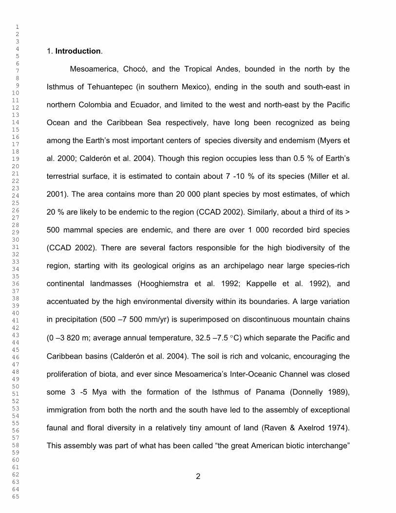
1. Introduction.

Mesoamerica, Chocó, and the Tropical Andes, bounded in the north by the

Isthmus of Tehuantepec (in southern Mexico), ending in the south and south-east in

northern Colombia and Ecuador, and limited to the west and north-east by the Pacific

Ocean and the Caribbean Sea respectively, have long been recognized as being

among the Earth’s most important centers of species diversity and endemism (Myers et

al. 2000; Calderón et al. 2004). Though this region occupies less than 0.5 % of Earth’s

terrestrial surface, it is estimated to contain about 7 -10 % of its species (Miller et al.

2001). The area contains more than 20 000 plant species by most estimates, of which

20 % are likely to be endemic to the region (CCAD 2002). Similarly, about a third of its >

500 mammal species are endemic, and there are over 1 000 recorded bird species

(CCAD 2002). There are several factors responsible for the high biodiversity of the

region, starting with its geological origins as an archipelago near large species-rich

continental landmasses (Hooghiemstra et al. 1992; Kappelle et al. 1992), and

accentuated by the high environmental diversity within its boundaries. A large variation

in precipitation (500 –7 500 mm/yr) is superimposed on discontinuous mountain chains

(0 –3 820 m; average annual temperature, 32.5 –7.5 C) which separate the Pacific and

Caribbean basins (Calderón et al. 2004). The soil is rich and volcanic, encouraging the

proliferation of biota, and ever since Mesoamerica’s Inter-Oceanic Channel was closed

some 3 -5 Mya with the formation of the Isthmus of Panama (Donnelly 1989),

immigration from both the north and the south have led to the assembly of exceptional

faunal and floral diversity in a relatively tiny amount of land (Raven & Axelrod 1974).

This assembly was part of what has been called “the great American biotic interchange”

1 2 3 4 5 6 7 8 9 10 11 12 13 14 15 16 17 18 19 20 21 22 23 24 25 26 27 28 29 30 31 32 33 34 35 36 37 38 39 40 41 42 43 44 45 46 47 48 49 50 51 52 53 54 55 56 57 58 59 60 61 62 63 64 65

3

(Stehli & Webb 1985).

Because of this high species richness and endemism, Mesoamerica, Chocó, and

the Tropical Andes have been a major focus of biodiversity conservation interest for

several decades (Jukofsky 1993; Miller et al. 2001). In spite of many well-publicized

initiatives for conservation both nationally (Sarukhán et al., 1996; Sarukhán & Dirzo,

2001; Evans 1999; Fandiño-Lozano & Wyngaarden 2005) and trans-nationally (CCAD

1993; Illueca 1997; Miller et al. 2001; Calderón et al. 2004), the biodiversity of

Mesoamerica is under continued threat from a variety of factors including a

deforestation rate of about 1 % per year from 2000 to 2005 (FAO 2005), a human

population growth rate of over 2 % per year (Miller et al. 2001), and the reliance of the

majority of the human population on biological resources taken directly from the wild

(Miller et al. 2001). According to some estimates, about 30% of the region’s primary and

secondary vegetation have been completely transformed to agricultural fields and urban

settlements (Bryant et al. 1997). Other habitats, including coral reefs, mangroves,

wetlands, and grasslands have suffered similar losses (Burke et al. 2000; Matthews et

al. 2000; Revenga et al. 2000). Poverty is a major factor in maintaining threats to all

habitats, with almost half the human population living below the poverty line, and much

of it lacking access to basic health care, education, and safe water (Miller et al. 2001).

These threats, the high species richness, and the high level of endemism led to

the designation of Mesoamerica, Chocó, and the Tropical Andes as three of the 25

global biodiversity “hotspots” (Myers et al. 2000). Conservation planning for this region

as an integral whole has been a priority for several organizations for almost two

decades. In 1990, the New York Zoological Society (which became the Wildlife

1 2 3 4 5 6 7 8 9 10 11 12 13 14 15 16 17 18 19 20 21 22 23 24 25 26 27 28 29 30 31 32 33 34 35 36 37 38 39 40 41 42 43 44 45 46 47 48 49 50 51 52 53 54 55 56 57 58 59 60 61 62 63 64 65

4

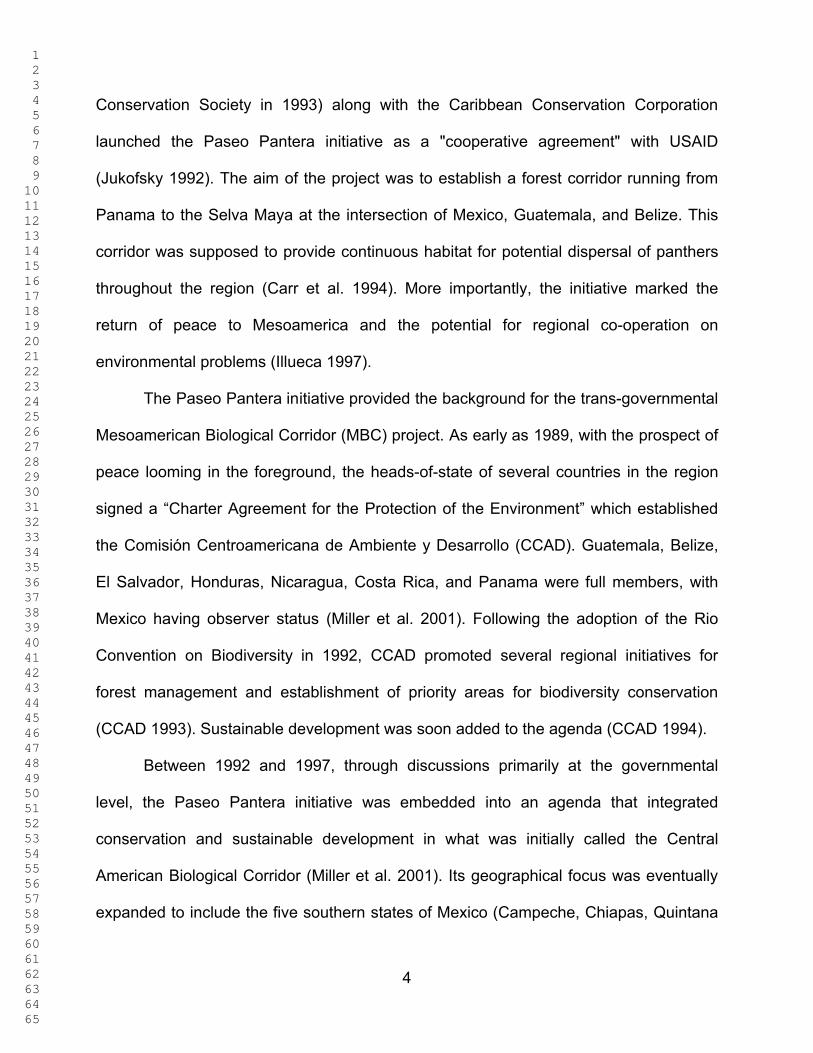
Conservation Society in 1993) along with the Caribbean Conservation Corporation

launched the Paseo Pantera initiative as a "cooperative agreement" with USAID

(Jukofsky 1992). The aim of the project was to establish a forest corridor running from

Panama to the Selva Maya at the intersection of Mexico, Guatemala, and Belize. This

corridor was supposed to provide continuous habitat for potential dispersal of panthers

throughout the region (Carr et al. 1994). More importantly, the initiative marked the

return of peace to Mesoamerica and the potential for regional co-operation on

environmental problems (Illueca 1997).

The Paseo Pantera initiative provided the background for the trans-governmental

Mesoamerican Biological Corridor (MBC) project. As early as 1989, with the prospect of

peace looming in the foreground, the heads-of-state of several countries in the region

signed a “Charter Agreement for the Protection of the Environment” which established

the Comisión Centroamericana de Ambiente y Desarrollo (CCAD). Guatemala, Belize,

El Salvador, Honduras, Nicaragua, Costa Rica, and Panama were full members, with

Mexico having observer status (Miller et al. 2001). Following the adoption of the Rio

Convention on Biodiversity in 1992, CCAD promoted several regional initiatives for

forest management and establishment of priority areas for biodiversity conservation

(CCAD 1993). Sustainable development was soon added to the agenda (CCAD 1994).

Between 1992 and 1997, through discussions primarily at the governmental

level, the Paseo Pantera initiative was embedded into an agenda that integrated

conservation and sustainable development in what was initially called the Central

American Biological Corridor (Miller et al. 2001). Its geographical focus was eventually

expanded to include the five southern states of Mexico (Campeche, Chiapas, Quintana

1 2 3 4 5 6 7 8 9 10 11 12 13 14 15 16 17 18 19 20 21 22 23 24 25 26 27 28 29 30 31 32 33 34 35 36 37 38 39 40 41 42 43 44 45 46 47 48 49 50 51 52 53 54 55 56 57 58 59 60 61 62 63 64 65

5

Roo, Tabasco, and Yucatan) after which it was renamed as the Mesoamerican

Biological Corridor (MBC). The MBC was endorsed by regional heads-of-state in 1997

and responsibility for planning and co-ordinating its implementation was assigned to the

CCAD. By 1998 CCAD had prepared a proposal, “Program for the Consolidation of the

Mesoamerican Biological Corridor,” to submit for funding to the United Nations

Development Program (UNDP)’s Global Environment Facility (GEF) and the German

Gesellschaft für Technische Zusammenarbeit (GTZ) (Miller et al. 2001). Funding was

approved in 1999, and an MBC Regional Office Coordinating Unit was opened in

Managua; since then, additional funds have come from other sources, including the

World Bank (see Global Transboundary Protected Area Network

[http://www.tbpa.net/case_10.htm; last accessed 17 October 2008]).

Transnational non-governmental organizations (NGOs) have also begun

developing regional conservation plans which are intended to complement the planning

initiatives of the official MBC project. Conservation International (CI) has begun the

process of identifying “Key Biodiversity Areas” (Conservation International 2004) on the

basis of habitat requirements of critically endangered species and those with restricted

ranges (Jaime Garcia-Moren, personal communication). In 2004, The Nature

Conservancy (TNC) published a “portfolio” of both terrestrial and marine “action sites”

for 27 terrestrial and five marine ecoregions (as defined by Olson et al. [2001]) as well

as coarser-scale “action areas” (Calderón et al. 2004). As biodiversity surrogates (which

it calls “targets”) TNC used 403 terrestrial, 25 freshwater, and 34 coastal-marine

ecological communities and systems. The viability of the surrogates in each area was

assessed by experts on the basis of size, condition, and landscape context (connectivity

1 2 3 4 5 6 7 8 9 10 11 12 13 14 15 16 17 18 19 20 21 22 23 24 25 26 27 28 29 30 31 32 33 34 35 36 37 38 39 40 41 42 43 44 45 46 47 48 49 50 51 52 53 54 55 56 57 58 59 60 61 62 63 64 65

6

and intactness) following the methodology of Morris et al. (1999). Experts selected a

network of priority sites so that the best occurrence and at least ten viable occurrences

of each surrogate was achieved, resulting in a portfolio of 78 terrestrial, 50 freshwater,

and 15 coastal-marine sites. These sites were then aggregated at a coarser spatial

scale to identify 20 priority areas (Calderón et al. 2004).

The analysis reported here uses systematic conservation planning (SCP)

methods (sensu Margules & Pressey [2000], Cowling & Pressey [2003], Sarkar [2005],

and Margules & Sarkar [2007]) to identify priority areas for conservation planning using

IUCN Red List species and ecoregions as biodiversity surrogates. These priority areas

are then compared to the existing protected areas of the region to assess the

performance of the latter with respect to the inclusion of habitats of Red List species

and the diverse ecoregions of Mesoamerica, Chocó, and the Tropical Andes. The

analysis is limited to the terrestrial context, including freshwater and coastal but not

marine habitats. The study region consists of 53 ecoregions (sensu Olson et al. [2001]).

Species’ distributions were modeled using a maximum entropy algorithm and the area

prioritization used a complementarity-based algorithm. The use of such algorithms to

supplement expert opinion and analysis is the main distinguishing feature of the SCP

approach (Cowling et al. 2003; Margules & Sarkar 2007). This appears to be the first

use of this approach in a trans-national context in Mesoamerica, Chocó, and the

Tropical Andes. However, this analysis carries out a priority area identification only for a

preliminary assessment of conservation goals and the performance of existing protected

areas (PAs); it is not intended to prescribe management policies.

The SCP protocol envisions a set of stages to formulate a conservation plan for a

1 2 3 4 5 6 7 8 9 10 11 12 13 14 15 16 17 18 19 20 21 22 23 24 25 26 27 28 29 30 31 32 33 34 35 36 37 38 39 40 41 42 43 44 45 46 47 48 49 50 51 52 53 54 55 56 57 58 59 60 61 62 63 64 65

7

region, including: stakeholder identification and involvement; data collection and

assessment; modeling and corrective data treatment, when necessary; the choice of

biodiversity surrogates, conservation targets, and goals; a review of existing

conservation areas; prioritization of additional potential conservation areas; assessment

of site viability; feasibility assessment of a conservation proposal weighed against

competing demands for land; and the eventual implementation and periodic

reassessment of a plan (Margules & Sarkar 2007). Since its purpose is assessment

rather than the formulation of an implementation-oriented plan, this analysis does not

include all stages of the SCP protocol. There is no explicit stakeholder involvement;

however, preliminary identification of priority areas is important because it can guide the

identification of potential stakeholders and help instigate their active involvement as

more sophisticated implementation-oriented plans are developed. Feasibility

assessment can only be performed with the full involvement of such stakeholders.

Finally, biological viability analysis is only incorporated in this analysis in a rudimentary

way by excluding anthropogenically transformed areas (see Section 3.1).

This analysis also differs from the past and ongoing transnational analyses of

conservation in the region in including a larger study area than is customary, extending

into Colombia and Ecuador. The delineation of the study area was based on the

ecological definition of Mesoamerica, Chocó, and the Tropical Andes (as explained in

Section 2.1). In contrast, the MBC project uses political boundaries because

implementation must take place in political context. The World Resources Institute

(WRI) also used the political delineation of the study area from the MBC project (Miller

et al. 2001). While it is true that implementation depends on political boundaries, the

1 2 3 4 5 6 7 8 9 10 11 12 13 14 15 16 17 18 19 20 21 22 23 24 25 26 27 28 29 30 31 32 33 34 35 36 37 38 39 40 41 42 43 44 45 46 47 48 49 50 51 52 53 54 55 56 57 58 59 60 61 62 63 64 65

8

presumption here is that ecological analyses should be based on ecological criteria and,

after priority areas are identified in this way, the question of political implementation

should be broached—this is the “feasibility assessment” stage of SCP. If political

implementation of conservation plans is impractical in some areas, then the SCP

process envisions the replacement of these areas with other (biologically) functionally

equivalent areas with such areas also chosen using ecological criteria.

In contrast, TNC used ecoregions to delineate its study region but its analysis is

restricted to a subset of the area analyzed here, ignoring parts of Mexico to the north

and Colombia and Ecuador to the south. There are two additional and more important

differences between TNC’s analysis and this one: (i) TNC chose to ignore species-level

surrogates on the grounds that there were insufficient data on them. However, there is

some good data available for a suite of Red List species (see below) and to ignore

these altogether when identifying priority areas for conservation is unwarranted and

TNC could have profitably supplemented their surrogate set with Red List species. Such

a mixed strategy was followed by the Australian BioRap Project to develop a provisional

conservation portfolio for Papua New Guinea when faced with sparse species-level data

(Faith et al. 2001); and (ii) even though TNC has advocated methods similar to SCP in

other contexts (see Groves et al. [2002]), its Mesoamerican analysis was based on

expert judgment. Cowling et al. (2003) and others (Pressey 1994; Smith et al. 2006;

Margules & Sarkar 2007) have pointed out the pitfalls of not using systematic (often

algorithmic) methods to supplement expert opinion: systematic methods lead to

repeatable analyses, permit detailed exploration of alternative choices of surrogates,

targets, and goals, and enable explicit quantitative evaluation of results in meeting those

1 2 3 4 5 6 7 8 9 10 11 12 13 14 15 16 17 18 19 20 21 22 23 24 25 26 27 28 29 30 31 32 33 34 35 36 37 38 39 40 41 42 43 44 45 46 47 48 49 50 51 52 53 54 55 56 57 58 59 60 61 62 63 64 65

9

targets and goals. Expert-based plans have also been known to produce plans that do

not provide adequate representation of biodiversity surrogates and are often not optimal

with respect to spatial economy (Sarakinos et al. 2001; Cowling et al. 2003). Good

planning involves the use of both systematic methods and expert judgment; this

analysis aims to provide some baseline results that may be evaluated by experts and

then re-analyzed systematically. Expert judgment was used here to refine species’

ecological niche models (see below).

More specifically, the major aims of this analysis were (i) a broad identification of

priority areas for Red List species in the Mesoamerica, Chocó, and Tropical Andes

region, (ii) an identification of priority areas that also represent the ecoregional diversity

of Mesoamerica, Chocó, and the Tropical Andes; and (iii) an analysis of the

performance of existing protected areas (PAs) with respect to both these goals. A

subsidiary goal was to analyze the portfolio produced by TNC. However, these results

should not be interpreted as recommending individual areas for immediate protection.

Rather, the analysis should form the basis for discussion with stakeholders about

opportunities and constraints, and experts about appropriate surrogates, targets, and

goals. Simultaneously, there must be significantly more data collection and assessment

so that more sophisticated analyses geared towards producing implementation-oriented

results can be performed.

2. Landscape Features.

2.1. Study Region. For this study the Mesoamerica, Chocó, and Tropical Andes

region was defined using the ecoregional classification of Olson et al. (2001), which is a

1 2 3 4 5 6 7 8 9 10 11 12 13 14 15 16 17 18 19 20 21 22 23 24 25 26 27 28 29 30 31 32 33 34 35 36 37 38 39 40 41 42 43 44 45 46 47 48 49 50 51 52 53 54 55 56 57 58 59 60 61 62 63 64 65

10

refinement Dinnerstein et al. (1995) and Ricketts et al. (1995). The study region

consisted of 53 ecoregions in 10 countries (see Figure 1): Mexico, Belize, Guatemala,

Honduras, El Salvador, Nicaragua, Costa Rica, Panama, Colombia, and Ecuador.

Marine habitats were excluded from consideration. Major islands were included: Isla

Cozumel and Isla del Carmen in Mexico; Ambergris Caye and the Turneffe Islands in

Belize; Isla de Roatán in Honduras; and Isla de Coiba and Isla de Rey (in the

Archipelago de Las Perlas) in Panama. The Pacific Ocean and the Caribbean Sea

define the western and north-eastern boundaries of the study region.

The northern boundary was delineated within the Isthmus of Tehuantepec in

Mexico, including the Balsas depression and ecoregions associated with it because of

their high biogeographic affinity with Mesoamerican biota (Morrone 2005; Escalante et

al. 2007). This boundary marks the southern range limits of several Nearctic taxa and

northern range limits of several Neotropical taxa. Such Nearctic taxa consist of a wide

range of floristic and faunistic groups including terrestrial vertebrates (Fa & Morales

1991; Escalante et al., 2007), lepidoptera (Peterson et al. 1999), cacti (Bravo &

Scheinvar 1999), and composites and bryophytes (Delgadillo 2000; Delgadillo &

Villaseñor 2002). The Neotropical taxa include mammals such as shrews, armadillo,

muroid rodents (Briones & Sánchez-Cordero 2004), as well as amphibians, reptiles, and

birds (Casas et al. 1996; Peterson et al. 1993, 1999, 2004). From the west to the east,

11 ecoregions comprise the northern boundary: Balsas dry forests, Sierra Madre del

Sur pine-oak forests, Oaxaca montane forests, Sierra Madre de Oaxaca, Veracruz dry

forests, Tehuacán Valley matorral, Mesoamerican Gulf-Caribbean mangroves, Sierra de

los Tuxtlas, Petén-Veracruz moist forests, Pantanos de Centla, and Yucatan dry forests.

1 2 3 4 5 6 7 8 9 10 11 12 13 14 15 16 17 18 19 20 21 22 23 24 25 26 27 28 29 30 31 32 33 34 35 36 37 38 39 40 41 42 43 44 45 46 47 48 49 50 51 52 53 54 55 56 57 58 59 60 61 62 63 64 65

11

Three other ecoregions could have potentially been included but were excluded

because recent work, based on mammal distributions, has determined that these are

part of a separate biogeographical region (Escalante et al. 2007): these are the Trans-

Mexican volcanic belt, the Jalisco dry forests, and the Veracruz moist forest.

The southern and south-eastern boundaries were taken to lie in northern

Ecuador and Colombia because the ranges of several Mesoamerican species, including

endemic species of conservation concern, end there. These include mammal species,

especially rodents such as heteromyids and peromiscines (Anderson et al. 2002a, b;

Anderson 2003), bats (Albuja 1992, 1999), birds (Cracraft 1985; Best and Kessler 1995;

Joseph and Stockwell 2002), and other terrestrial vertebrates (Albuja et al. 1980; Jarrín

2001). More importantly, this is where the Andes split into three separate ranges:

Cordillera Occidental, Cordillera Central, and Cordillera Oriental. This topographical

transition was used to define these boundaries. The ecoregions at the boundary are

those that intersect with the three ranges emerging from the Andes. From west to east,

the southern boundary ends with three ecoregions in Ecuador: the Eastern Cordillera

Real montane forests, Northwestern Andean montane forests, and Western Ecuador

moist forests. The south-eastern boundary continues in Ecuador and Colombia ending

with three more ecoregions: Cordillera Oriental montane forests, Catatumbo moist

forests, and Guajira-Barranquilla xeric scrub.

The study area includes 809 existing protected areas (PAs) as identified by the

World Data Base on Protected Areas (http://www.unep-wcmc.org/wdpa/; last accessed

22 June 2007); 557 of these are classified by the World Conservation Union (IUCN)

under one of their categories, I –VI, while 252 other PAs, although being so designated

1 2 3 4 5 6 7 8 9 10 11 12 13 14 15 16 17 18 19 20 21 22 23 24 25 26 27 28 29 30 31 32 33 34 35 36 37 38 39 40 41 42 43 44 45 46 47 48 49 50 51 52 53 54 55 56 57 58 59 60 61 62 63 64 65

12

in the different countries, are yet to be placed under any of the IUCN categories. These

other PAs and the PAs from all IUCN categories (I –VI) were included in the analysis

with no distinction made between levels of protection since there was no information

available at a regional scale on the relative performance of the different categories.

While it is customary wisdom that strictly protected categories (I and II) perform better

than the others, recent work in Mexico indicates that Biosphere Reserves (category VI)

perform better than National Parks (Sánchez-Cordero & Figueroa 2007; Figueroa &

Sánchez-Cordero 2008).

Table 1 shows the area and percentage area of each ecoregion in the total study

area and the percentage of the ecoregion already in a protected area. Table 2 shows

the area and percentage of each ecoregion present in each country, the percentage of

each ecoregion represented within each country, and the percentage of that ecoregion

protected within each country.

2.2. Biodiversity Surrogates. SCP requires the identification of biodiversity

surrogates, that is, quantifiable features of biodiversity on which data can be realistically

obtained for use in planning protocols. In the terminology of Sarkar and Margules (2002;

see, also, Sarkar [2002] and Margules & Sarkar [2007]), “true” surrogates are those

such features that are themselves the components of biodiversity targeted for

conservation; “estimator” surrogates are environmental or biological features which can

be used to estimate the representation of true surrogates in conservation areas. In this

study, species at risk of extinction, as identified by the IUCN Red List

(http://www.iucnredlist.org; last accessed 21 June 2007), were taken as true surrogates

which is uncontroversial. However, distributional data were available for only 9 % of

1 2 3 4 5 6 7 8 9 10 11 12 13 14 15 16 17 18 19 20 21 22 23 24 25 26 27 28 29 30 31 32 33 34 35 36 37 38 39 40 41 42 43 44 45 46 47 48 49 50 51 52 53 54 55 56 57 58 59 60 61 62 63 64 65

13

these species, and only 2 % could be reliably modeled. Moreover, most of these were

plants To address this deficiency, the 53 ecoregions defined by Olson et al. (2001) were

also added as estimator surrogates in a subsequent analysis. This assumes that

representing the full variety of ecoregions in conservation areas will lead to the

representation of the Red List species for which no modeled distributions were

available. (A more detailed classification into ecoregions—that is, one with more

categories—which would be more desirable was not available at the regional scale.)

For the 10 countries in the study region, the total number of species in the three

categories of the IUCN Red List, Critically Endangered (CR), Endangered (EN), and

Vulnerable (VU) are, for the four orders of vertebrates: Amphibians--CR 222, EN 286,

VU, 184; Mammals--CR 19, EN 53 VU 67; Birds--CR 26, EN 62, VU 112; Reptiles--CR

13, EN 8, VU 22; and for Plants--CR 372, EN 916, VU 1271. In total there are 3 633

such species. Note that these numbers include areas outside the study region in the

cases of Mexico, Colombia, and Ecuador. Table S1 lists the 333 species for which

occurrence data are available in publicly accessible data bases (see

Acknowledgments). It includes the number of geo-referenced data points available and

the number of those points that are post-1980. Only post-1980 data were used to model

species’ distributions because the large-scale deforestation of the previous decades is

known to have significantly altered the land cover of Mesoamerica (Utting 1997).

3. Methods of Analysis.

3.1. Landscape GIS Models. Maps of ecoregions were obtained from the

WorldWide Fund for Nature (http://www.worldwildlife.org/science/data/terreco.cfm; last

1 2 3 4 5 6 7 8 9 10 11 12 13 14 15 16 17 18 19 20 21 22 23 24 25 26 27 28 29 30 31 32 33 34 35 36 37 38 39 40 41 42 43 44 45 46 47 48 49 50 51 52 53 54 55 56 57 58 59 60 61 62 63 64 65

14

accessed 22 June 2007). The study region was divided into 0.02° × 0.02° longitude

latitude cells. This resulted in 343 383 cells with an average area of 4.818 km2 (SD =

0.098; max = 4.946; min = 4.599). All point occurrence data for the Red List species

were resampled to this grid, reducing multiple records of a species in the same cell to

one occurrence point. Land cover data for the study region was obtained from the

Global Land Cover 2000 (Hansen et al. 2000). These data were classified into 60

categories (see Table 6 in the Supplementary Material). Cropland, intensive agriculture,

and urban/ built categories were interpreted as transformed areas while the rest of the

categories were interpreted as being untransformed enough for potential inclusion

within conservation areas as they are or for ecological restoration aimed at the

persistence of biota. The Global Land Cover 2000 data had a resolution of 0.01 × 0.01

which were resampled to a 0.02° × 0.02° resolution. The percentage of transformation

of each ecoregion is given in Table 1, and that for each ecoregion in each country is

given in Table 2.

Data on the protected areas were obtained from the World Database of

Protected Areas (WDPA; http://www.unep-wcmc.org/wdpa/; last accessed 22 June

2007) maintained by the United Nations Environment Programme and the World

Conservation Monitoring Centre. Areas in Tables 1 and 2 were calculated using the

equal area cylindrical projection (by using Projector! extension in ArcView 3.2).

3.2. Ecological Niche Models. Point occurrence data for animals and plants

listed in the categories CR, EN and VU of the IUCN Red List were obtained from

several scientific collections (see Acknowledgments). In order to reflect the current state

of the habitat, only point occurrence data collected since 1980 were retained. Ecological

1 2 3 4 5 6 7 8 9 10 11 12 13 14 15 16 17 18 19 20 21 22 23 24 25 26 27 28 29 30 31 32 33 34 35 36 37 38 39 40 41 42 43 44 45 46 47 48 49 50 51 52 53 54 55 56 57 58 59 60 61 62 63 64 65

15

niche models were then constructed for the 101 listed animal and plant species for

which there were sufficient data (that is, there were at least four occurrence records—

see below).

The Maxent software package (Version 2.2; Phillips et al. 2004; 2006) was used

to construct ecological niche models. Maxent has been shown to be robust for modeling

distributions from presence-only data (Elith et al. 2006). Following published

recommendations, Maxent was run without the threshold feature and without duplicates

so that there was at most one sample per pixel; linear, quadratic and product features

were used (Phillips et al. 2004; 2006; Pawar et al. 2007). The convergence threshold

was set to 1.0 × 10-5, which is a conservative value based upon North American

breeding bird survey data and small mammal data from Latin America (Phillips et al.

2004; 2006).

For climatic variables, 19 layers, each at a resolution of 30 (0.0083° × 0.0083°),

were obtained from the WorldClim database (Hijmans et al. 2005; http://worldclim.org;

last accessed 12-12-06); These layers (Pawar et al. [2007] provide a complete list) were

used along with elevation, slope, and aspect as the environmental variables. Elevation

was obtained from the U.S. Geological Survey’s Hydro-1K DEM data set (USGS 1998)

and slope and aspect were derived from the DEM using the Spatial Analyst extension of

ArcMap 9.0. All climate and spatial layers were clipped to an area bounded by 21º 30

30.27 N by 5º 0 1.12 S and 103º 30 52.49 W by 71º 6 45.72 W, a box containing

the study region, and were resampled to a 0.02° × 0.02° resolution in ArcGIS.

Niche model accuracy was evaluated by constructing the models using 75 % of

the available records, with the other 25 % used for testing. At least four occurrence

1 2 3 4 5 6 7 8 9 10 11 12 13 14 15 16 17 18 19 20 21 22 23 24 25 26 27 28 29 30 31 32 33 34 35 36 37 38 39 40 41 42 43 44 45 46 47 48 49 50 51 52 53 54 55 56 57 58 59 60 61 62 63 64 65

16

records are necessary to construct such a niche model. Model accuracy was

determined using a receiver operating characteristic (ROC) analysis (Phillips et al.

2006). For all thresholds an ROC curve was produced with sensitivity plotted on the y

axis and (1 – specificity) plotted on the x-axis. The area under the curve (AUC) provides

a measure of model performance. An optimal model would have an AUC of 1 while a

model that predicted species occurrences at random would have an AUC of 0.5.

Following Pawar et al. (2007), only those niche models possessing an AUC

greater than 0.75 and a p-value of less than 0.05 (for the sensitivity and specificity tests)

were retained for further use. Finally, the relative probabilities predicted by Maxent were

converted into expected presences for a species by dividing all relative probabilities

across the landscape by the highest relative probability achieved for that species. This

normalization assumes that a species is at least present in the cell with the highest

predicted relative probability of its occurrence.

Geographic projection of species’ ecological niches must be modified to produce

distributions because species may not occupy all regions ecologically suitable for them

for a variety of reasons including barriers to dispersal and competition with other

species (Soberón & Peterson 2005). Refinement removed from each model all cells

with a predicted probability of less than 0.1. Stricter refinement protocols have

sometimes been used; for instance, in many analyses by restricting to cells that are

contiguous with those that have a reported occurrence of species (Soberón & Peterson

2005). However, because of the sparse available data for the study region, which is a

result of inadequate sampling, such strict refinement is likely to exclude many areas in

which a species is likely to be present. For the species used in this analysis, there is no

1 2 3 4 5 6 7 8 9 10 11 12 13 14 15 16 17 18 19 20 21 22 23 24 25 26 27 28 29 30 31 32 33 34 35 36 37 38 39 40 41 42 43 44 45 46 47 48 49 50 51 52 53 54 55 56 57 58 59 60 61 62 63 64 65

17

suggestion of geographical barriers to their dispersal within Mesoamerica, Chocó, and

the Tropical Andes. Expert knowledge was used to drop niche models which showed

systematic over-prediction (see Section 4).

3.3. Area Prioritization and Representation Targets. Area prioritization was

carried out with a heuristic complementarity-based algorithm implemented in the

ResNet software package (Garson et al. 2002; Sarkar et al. 2002) because such

algorithms are computationally fast while finding near-optimal solutions to problems

(Csuti et al. 1997; Sarkar et al. 2004). The optimization problem to be solved is the

minimum-area problem: finding the smallest set of areas in which all biodiversity

surrogates meet their representation targets. ResNet selects areas to solve the

minimum-area problem using a two-pass algorithm. In the version of ResNet that was

used, the first pass uses complementarity to select the area with the largest total

expected value for the presence of surrogates with unmet targets. Ties are broken by

selecting one of the tied cells at random. Area selection terminates when the targeted

representation for each species has been met. The second pass removes cells that may

have become redundant with respect to achieving the representation targets due to later

cell selection. Other versions of ResNet use both rarity and complementarity in the first

pass; however, Sarkar et al. (2004) reported that using complementarity alone produces

better results with probabilistic data.

The aim of this analysis was a broad identification of priority areas for Red List

species and to analyze the performance of existing PAs, and not to recommend

individual areas for immediate protection. Thus, a range of representation targets was

used to identify priority areas without recommending a specific target. Those areas that

1 2 3 4 5 6 7 8 9 10 11 12 13 14 15 16 17 18 19 20 21 22 23 24 25 26 27 28 29 30 31 32 33 34 35 36 37 38 39 40 41 42 43 44 45 46 47 48 49 50 51 52 53 54 55 56 57 58 59 60 61 62 63 64 65

18

are selected at low targets of representation of Red List species have higher priority

values than those only selected at higher targets. Four prioritization scenarios were run

in this analysis. Two different surrogate sets were used. In both, the Red List species

were included, and targets of representation were set from 10 % to 90 % in 10 %

increments for each of the species. In the second, a uniform target of 10 % was

additionally set for the ecoregions. In general, targets of representation used in such

prioritization protocols do not have full biological justification (Soulé & Sanjayan 1997;

Margules & Sarkar 2007). Using a wide range of targets for the most important

biodiversity surrogates in this analysis, the Red List species, avoids this problem. The

10 % target for the ecoregions is also conventional (Margules & Sarkar 2007), though

the Secretariat of the Convention on Biological Diversity (2002) set that target for each

of the world’s ecoregions. Hence the use of the 10 % target here; it was assumed that

higher targets for them would be unrealistic. Area prioritization was carried twice for

each of these alternatives, once for the whole study area and once removing the

transformed areas from the study region.

The effectiveness of each country’s existing protected areas at representing

biodiversity was estimated by calculating: (i) the proportion of the entire country

selected by ResNet (hereafter cp ) and (ii) the proportion of the country’s protected areas

so prioritized (hereafter pap ). At each representation target, the following were

computed: the point estimate of the difference in proportions )pp( pac , the lower limit of

the 95% confidence interval of the difference (hereafterL ), and upper limit of the 95%

confidence interval (hereafterU ). If pac pp , 0L , and 0U , then the prioritized

proportion of the entire country was significantly greater than the prioritized proportion of

1 2 3 4 5 6 7 8 9 10 11 12 13 14 15 16 17 18 19 20 21 22 23 24 25 26 27 28 29 30 31 32 33 34 35 36 37 38 39 40 41 42 43 44 45 46 47 48 49 50 51 52 53 54 55 56 57 58 59 60 61 62 63 64 65

19

the country’s protected areas. Conversely, if pac pp , 0L , and 0U , then the

prioritized proportion of the country’s protected areas was significantly greater than the

prioritized proportion of the entire country.

The point estimate )pp( pac may be too liberal due to the non-independence of

cp and pap (Agresti 2002). To address this issue, separate contingency tables were

constructed for the country and protected area data. In the former, cellj1 represented the

number of selected sites in country j and cellj2 represented the number of unselected

sites. In the latter, cellj1 represented the number of selected sites in the protected areas

of country j and cellj2 represented the number of unselected sites in the protected

areas. Pearson residuals > 3 indicated that more sites were selected in a given category

than expected (Simonoff 2003).

4. Results.

Of the IUCN Red List species in the study region (that is, species that that are

Critically Endangered, Endangered, or Vulnerable), there was at least one occurrence

record for 333 species in the accessible databases (see Table S1 of Supplementary

Materials). However, at least four post-1980 occurrence records were only available for

101 species. Niche models were constructed for all of these; only 94 species had an

AUC greater than 0.75 (Table S1). Seven additional species were dropped because of

large p-values. A further nine species were dropped from the analysis because of

presumed overprediction, as described in Section 3.2. Whereas the modeled

distribution predicted the species to be distributed across the entire study region, these

1 2 3 4 5 6 7 8 9 10 11 12 13 14 15 16 17 18 19 20 21 22 23 24 25 26 27 28 29 30 31 32 33 34 35 36 37 38 39 40 41 42 43 44 45 46 47 48 49 50 51 52 53 54 55 56 57 58 59 60 61 62 63 64 65

20

species have restricted distributions as specified by IUCN Red List

(http://www.iucnredlist.org; last accessed 21 June 2007): Cyanolyca nana is restricted in

Mexico to Oaxaca, Queretaro, north Hidalgo and central Veracruz; Thorius narisovalis is

restricted in Mexico to north-central Oaxaca; Lonchocarpus yoroensis is restricted to

Honduras, Mexico and Nicaragua; Mollinedia ruae and Lonchocarpus retiferus are

restricted to Honduras and Nicaragua; Dendropanax sessiliflorus, Quararibea

gomeziana, and Stenanona panamensis are restricted to Costa Rica and Panama; and

Inga canonegrensis is restricted to Costa Rica. For the other species, the two most

common parameters producing the largest AUC when used independently (Explanatory

Variable 1 in Table S1) were temperature seasonality (16 times) and precipitation of the

wettest month (14 times) and the two most common parameters reducing the AUC most

when excluded (Explanatory Variable 2 in Table S1) were altitude (24 times) and

temperature (19 times). Table S1 shows these critical explanatory variables for all 78

species (5 CR; 21 EN; 52 VU) used in this analysis; there were 10 amphibian (3 CR; 5

EN; 2 VU), 3 bird (2 EN; 1 VU), 3 mammal (3 VU), and 62 plant (2 CR; 14 EN; 46 VU)

species. This means 80 % of the species used for the area prioritization were plants.

We further refined our species list to 51 species that included 10 or more point locality

records. The intersection between the set of sites prioritized to be put under a

conservation plan when sites were selected to represent the 78 species with at least

four records and the set of sites selected to represent the 51 species with at least 10

records was 81% on average (range: 74-92%; Supplementary Material Table S5). In

light of this, the use of species with at least 10 records does not appear to result in a

significantly different conservation area network than the use of species with at least

1 2 3 4 5 6 7 8 9 10 11 12 13 14 15 16 17 18 19 20 21 22 23 24 25 26 27 28 29 30 31 32 33 34 35 36 37 38 39 40 41 42 43 44 45 46 47 48 49 50 51 52 53 54 55 56 57 58 59 60 61 62 63 64 65

21

four records.

Figures 2 - 3 show the ResNet solutions for the different targets; the total

selected area increases as the representation targets increase. In Figure 2, only Red

List species are used as surrogates. The percentage of total area selected varied from

5.1 % for the 10% target to 82.04 % for the 90% target. The percentage of overlap

between the selected area and the PAs ranged between 6.46 % and 87.7% for these

two targets. Figure 3 corresponds to Figure 2 when the ecoregions are also included as

surrogates (with a uniform representation target of 10 %). The percentage of total area

selected was now 9.96 % for the 10% target and 82.03 % for the 90% target. The

percentage of overlap between the selected area and the PAs ranged between 10.97 %

and 87.63 %. In both these figures selected cells are widely dispersed across the region

and, as expected, the amount of land selected increases monotonically with the target.

Figure 4 shows the percentage of untransformed area in each country selected

at different targets, and Figure 5 shows the percentage of the country selected in

untransformed areas, both under two scenarios: Red List species as surrogates, and

both Red List species and ecoregions as surrogates. Figure 6 shows the percentage of

the existing PAs selected as a function of the representation target under the two

scenarios. Throughout the analyses, the results for Mexico, Colombia, and Ecuador

only refer to areas within the study region. What is striking is that similar patterns are

seen for the percentage of the country´s untransformed area and that of the existing

PAs that is selected at different targets. When Red List species alone are used as

biodiversity surrogates, the PA network of Belize performs better than those of all other

countries at all representation targets in the sense that a larger fraction of it was

1 2 3 4 5 6 7 8 9 10 11 12 13 14 15 16 17 18 19 20 21 22 23 24 25 26 27 28 29 30 31 32 33 34 35 36 37 38 39 40 41 42 43 44 45 46 47 48 49 50 51 52 53 54 55 56 57 58 59 60 61 62 63 64 65

22

selected in the ResNet runs. When ecoregions are also included as surrogates, Costa

Rica and El Salvador performs better than Belize (Fig. 6). The existing PA network of

Ecuador performs worst using Red List species as surrogates, followed by Mexico,

Honduras and Colombia. At the higher targets the same conclusion once again holds

when ecoregions are included as surrogates (Fig. 6). However, for all countries except

Colombia, Ecuador, and Mexico, protecting 90 % of the modeled distribution for just

these 78 species takes up 82.3 – 99.7 % of each country’s area. for Ecuador, Colombia,

and Mexico, 65.8 – 79.7% is selected. (Figs. 3 and 4).

The most important priority areas are those selected at the lowest representation

targets for biodiversity surrogates because these areas are needed even to maintain

minimal representation of species at risk. This fact can also be used to assess the

performance of the existing PAs. Areas within 189 of the existing PAs were selected

even at the lowest target used (10 %). However, in most cases very few cells were

selected (see Figures 2a and 3a). For each country in the study area, Table S2 of the

Supplementary Materials lists the PAs which have at least one cell represented in a

solution at the 10 % species representation target. In addition, Table S2 lists the PAs

that have some cells represented at the 10 % species and ecoregion representation

target, the 50 % species representation target, and so on.

For prioritizations using only species, as well as for prioritizations that included

both the species and the ecoregions, the prioritized proportion of Guatemala’s protected

areas was significantly greater than the prioritized proportion of the entire country at all

representation targets (range of )pp( cpa : 4.08-26.29%). Conversely, for Panama, the

prioritized proportion of the entire country selected was significantly greater than the

1 2 3 4 5 6 7 8 9 10 11 12 13 14 15 16 17 18 19 20 21 22 23 24 25 26 27 28 29 30 31 32 33 34 35 36 37 38 39 40 41 42 43 44 45 46 47 48 49 50 51 52 53 54 55 56 57 58 59 60 61 62 63 64 65

23

prioritized proportion of the protected areas (range of )pp( pac : 2.4-14.75%). For the

species only prioritizations at each representation target, the null hypothesis that equal

proportions of each country were selected was rejected ( 8847042 . ), as was the

hypothesis that equal proportions of the protected areas of each country were selected

( 0719412 . ); in each case, 9df and 161022 .p . For all representation targets

greater than 10%, the surplus of selected sites in Guatemala was significantly greater

than that of any other country (range of Pearson residuals: 19.59 - 48.36).

5. Discussion.

The results obtained here are of relevance to other regional planning exercises

for Mesoamerica, Chocó, and the Tropical Andes that are under way, for instance, as

part of the MBC project even though those exercises are limited to a subset of the study

region analyzed here. The larger landscape ecological context—which was adopted

here on biogeographical grounds (see Section 2.1)—helps place more restricted

analyses in their proper regional context. Even at this larger scale, the most salient

result obtained here is that, for all countries except Colombia, Mexico and Ecuador,

protection of a large proportion of the distribution of only 78 Red List species takes up a

very large proportion of the untransformed land: if the distribution representation target

is 90 %, the untransformed land needed amounts to 85 % - 98 % of each country.

Including more species will only increase this area. The size of this area is a result of

species at risk being widely distributed throughout Mesoamerica, Chocó, and the

Tropical Andes which, in turn, underscores the region’s importance for biodiversity. In

the case of Colombia, Mexico and Ecuador, less area is probably being selected only

1 2 3 4 5 6 7 8 9 10 11 12 13 14 15 16 17 18 19 20 21 22 23 24 25 26 27 28 29 30 31 32 33 34 35 36 37 38 39 40 41 42 43 44 45 46 47 48 49 50 51 52 53 54 55 56 57 58 59 60 61 62 63 64 65

24

because there were many fewer species’ records (including those of endemic species)

in the data set.

High representation targets are inevitable to ensure the persistence of species at

risk (Sarakinos et al. 2001; Margules & Sarkar 2007). However, it is unreasonable to

expect such large proportions of the land of any country to be set aside for conservation

if that involves no human activity or use of the land. What this analysis shows is that, for

biodiversity conservation to work in Mesoamerica, Chocó, and the Tropical Andes, an

integrative approach to land use over the entire landscape must be developed.

Exclusionary policies such as setting up National Parks or “absolute” biological reserves

may have far less a role to play than land management through ecologically sound

practices as, for instance, encouraged in Biosphere Reserves (Figueroa & Sánchez-

Cordero, 2008). This means that planning must involve human stakeholders from the

beginning as envisioned in the SCP protocol.

It is encouraging that 189 of the 809 existing PAs (see Table S1) are selected

when Red List species are surrogates, and the target is only 10 %, which is a very

modest target for such species. This seems to suggest that, unlike the ad hoc selection

of existing PAs in many areas of the world (Pressey 1994; Pressey et al. 1996), those in

Mesoamerica, Chocó, and the Tropical Andes were better selected to represent its

biodiversity. However, what Figures 4, 5, and 6 show is that only a slightly higher

fraction of the area within existing PAs is selected at any target compared to the fraction

of the area of each country that is selected at that target. Thus, areas within the existing

PAs are doing little better than areas outside with respect to representing biodiversity. In

Figures 4-6 this conclusion is particularly obvious in the case of Colombia, Mexico, and

1 2 3 4 5 6 7 8 9 10 11 12 13 14 15 16 17 18 19 20 21 22 23 24 25 26 27 28 29 30 31 32 33 34 35 36 37 38 39 40 41 42 43 44 45 46 47 48 49 50 51 52 53 54 55 56 57 58 59 60 61 62 63 64 65

25

Ecuador. The goal of SCP is to avoid this problem of inappropriate land allocation by

prioritizing the most representative areas for conservation action.

Turning to individual countries, it is striking that all analyses show the existing PA

network of Guatemala outperforming those of the other Mesoamerican countries.

However, this is only true because those regions of Guatemala that were considered

consisted of the remaining anthropogenically untransformed areas. Similarly, this

analysis shows that the protected areas of Panama performing poorly compared to the

other countries, once again when we restrict attention to the untransformed areas.

Though there was no uniform statistical trend across all representations targets,

Colombia and Ecuador also perform poorly in terms of the representativeness of their

existing PAs which confirms the results of earlier analyses. Sierra et al. (2002) noted

that, though more than 14 % of Ecuador’s terrestrial area falls within existing PAs, some

habitat types, especially ecosystems on the coast and in the western Andes were

under-represented. In this analysis, these ecosystems, when they fall within the study

area, were selected at even low targets, using either the Red List species or both

species and ecoregions as surrogates (see Figures 2a and 3a). Similarly, Fandiño-

Lozano (1996) noted that though almost 10 % of Colombia’s habitat falls within PAs,

47.2 % of the habitat types were unprotected. In both countries it is likely that excessive

attention to tropical wet forests has led to their over-representation in the existing PA

network at the expense of other habitats.

The results obtained here should be compared to those from other area

prioritization efforts in the region both in order to identify areas that are assigned high

priority by all methods (so that these areas receive special attention) and to see whether

1 2 3 4 5 6 7 8 9 10 11 12 13 14 15 16 17 18 19 20 21 22 23 24 25 26 27 28 29 30 31 32 33 34 35 36 37 38 39 40 41 42 43 44 45 46 47 48 49 50 51 52 53 54 55 56 57 58 59 60 61 62 63 64 65

26

SCP techniques make any unique contribution. The methodology followed by CI in

designating priority areas is very similar to the one used here; indeed in some regions of

the world such as Melanesia, CI is using SCP techniques (Chris Margules, personal

communication, 2007). It is therefore quite likely that CI’s results will be similar to those

obtained here when they are made public. However, it is particularly instructive to

compare these results to the portfolio published by the Nature Conservancy because

the methodology used by Calderón et al. (2004), with its reliance only on environmental

(non-taxonomic) surrogates and expert judgment is very different from the one used

here. TNC distinguished its “portfolio” which consisted of 143 nominal conservation

areas from 20 more coarse-grained “conservation action areas” (Calderón et al. 2004).

At a coarse spatial resolution TNC’s portfolio and this analysis identify similar

priority areas, for instance, the Lacandon-Maya forest in Mexico, the Maya Mountains of

Belize, the Cordillera Central of Costa Rica, and the Bosque San Blas Darién of

Panama. For Costa Rica there is very good concordance between TNC’s portfolio and

the results of this exercise, probably reflecting the high level of expertise readily

available on Costa Rica’s biodiversity (Evans 1999). At finer spatial resolutions, there

are important differences: uniformly, this analysis selects a small fraction of the areas in

TNC’s portfolio even in the same region (especially for the 10 % and 20 % targets), thus

providing a more fine-tuned identification of priority areas. This suggests that SCP

methods can be usefully deployed to refine that portfolio. Moreover, there were some

major differences: (i) in Honduras, TNC’s portfolio prioritizes the Bosawar—Río Plátano

area which does not emerge as important in this analysis for targets less than 70 %; (ii)

in Nicaragua, TNC prioritized the Mahogany area which this analysis does not; and (iii)

1 2 3 4 5 6 7 8 9 10 11 12 13 14 15 16 17 18 19 20 21 22 23 24 25 26 27 28 29 30 31 32 33 34 35 36 37 38 39 40 41 42 43 44 45 46 47 48 49 50 51 52 53 54 55 56 57 58 59 60 61 62 63 64 65

27

this analysis identified some of the tropical deciduous forests of Panama as priority

areas even at 10 % and 20 % targets, whereas TNC’s portfolio ignores them. These

forests should probably be part of any conservation portfolio, but the differences

between TNC’s portfolio and these SCP results merit further detailed analysis.

Turning to TNC’s conservation action areas, these are concentrated to the north-

east of the region (at the Mexico-Guatemala border and in Guatemala and Honduras)

and to the south (Costa Rica and Panama). Each such area is large and an SCP

analysis could be used to specify conservation areas within them more exactly.

However, some important habitat types are not included in any TNC conservation action

area. For instance, tropical dry forests of Costa Rica and Nicaragua (the Central

American Dry Forest ecoregion) are not in an action area, in spite of being one of the

most threatened ecotypes in the region (see that percentages of protection and

transformation in Table 1). Similarly the Sierra Madre de Oaxaca pine-oak forests are

not targeted even though they are not adequately protected (Table 1). These habitats

were selected in this analysis at targets as low as 10 % and 20 % with either surrogate

set. TNC’s conservation action areas should be treated with caution.

Colombia and Ecuador were not part of TNC’s analysis. For Colombia, at the

national level, Fandiño-Lozano and Wyngaarden (2005b) have recently carried out an

SCP exercise using the Focalize (Fandiño-Lozano & Wyngaarden 2005a) and C-Plan

(Pressey 1999; Ferrier et al. 2000) software packages. As surrogates they used 337

topological and 62 chorological types that were established using remote-sensed data

(Landsat images). Representation targets were set individually for each topological type

based on the estimated area needed for minimal viable populations of four mammal

1 2 3 4 5 6 7 8 9 10 11 12 13 14 15 16 17 18 19 20 21 22 23 24 25 26 27 28 29 30 31 32 33 34 35 36 37 38 39 40 41 42 43 44 45 46 47 48 49 50 51 52 53 54 55 56 57 58 59 60 61 62 63 64 65

28

species, Panthera onca, Puma concolor, Tapirus terrestris and Tapirus pinchaque.

When the target here was 10 % or 20 %, areas selected here were similar to those

prioritized by Fandiño-Lozano and Wyngaarden (2005b) in much of the area within the

study region. However, they prioritize areas between the Sanquianga and the

Farallones de Cali PAs as well as an area between the Muchique and Galeras PAs in

the southwest part of the country. These do not emerge as priority areas in this

analysis. Moreover, this analysis does prioritize areas in the extreme west of the

Cordillera de los Picachos PA as well as an area between the Laguna de Cocha, the

Purace, and the Alto Fragua Indi Wasi PAs, an area south of Los Colorados and areas

in the extreme north of the Western Ecuador Moist Forests which Fandiño-Lozano and

Wyngaarden’s (2005b) analysis excludes.

Finally, six limitations of this analysis should also be noted: (i) the most important

limitation is that it was based on modeled distributions of only 78 species which is a

mere 2 % of the Red List species of the Mesoamerica, Chocó, Tropical Andes region.

Moreover, 62 or 80 % of the species used were plants. Efforts are now under way to

collate and systematize data from many regional museums, universities, and other

repositories to create a comprehensive public database for the region. It is hoped that

the publication of this preliminary analysis will encourage local and regional scientists to

share data by showing how useful these data can be in generating an adequate

conservation plan for the region. This analysis will be repeated every year with

additional data so that results become increasingly relevant towards the design of an

implementation-oriented plan; (ii) this analysis only used species deemed to be at risk

by IUCN. These should be supplemented by subregional—for instance, national—

1 2 3 4 5 6 7 8 9 10 11 12 13 14 15 16 17 18 19 20 21 22 23 24 25 26 27 28 29 30 31 32 33 34 35 36 37 38 39 40 41 42 43 44 45 46 47 48 49 50 51 52 53 54 55 56 57 58 59 60 61 62 63 64 65

29

priority lists of species at risk. However, other species are also of strong conservation

concern, for instance, species that are endemic to the region even if they are not at

present at risk. Future analyses will try to include as many of these as possible; (iii) the

land cover data set used was coarse and may not indicate all anthropogenically

transformed areas that should not be regarded as candidate areas for conservation.

Efforts are also under way to use remote-sensed data to generate a finer-resolution and

more accurate land cover map so that all biologically unviable land can be excluded

when developing a conservation plan; (iv) the classification of the study area into only

53 ecoregions was also coarse. Future work will have to use a finer classification which

will have to be created for the region. While such classifications exist for many of the

countries individually, for instance, Mexico (CONABIO 1998), Costa Rica (Holdridge

1967), and Colombia (Fandiño-Lozano & Wyngaarden 2005b), a regional classification

is still lacking; (v) there was no attempt at all to incorporate spatial criteria such as size,

shape, connectivity, dispersion, replication, and alignment into the priority area network

designed here. These are obviously important for the persistence of biota (Sarkar et al.

2006; Margules & Sarkar 2007) and should be included in future analysis; and (vi) the

analysis performed here is still quite far from one that can produce an implementation-

oriented plan. For that purpose stakeholders must be brought in as decision-makers

and the analysis must take into full account sociopolitical opportunities and constraints.

1 2 3 4 5 6 7 8 9 10 11 12 13 14 15 16 17 18 19 20 21 22 23 24 25 26 27 28 29 30 31 32 33 34 35 36 37 38 39 40 41 42 43 44 45 46 47 48 49 50 51 52 53 54 55 56 57 58 59 60 61 62 63 64 65

30

Acknowledgments

Animal species data were obtained from MaNIS (http://manisnet.org; last accessed 4 April 2007), HerpNET (http://www.herpnet.org/; last accessed 4 April 2007), ORNIS (http://olla.berkeley.edu/ornisnet/; last accessed 4 April 2007), and REMIB (Red Mundial de Información sobre Biodiversidad; http://www.conabio.gob.mx/remib/doctos/remib_esp.html; last accessed 4 April 2007). Additional records were obtained from Smithsonian National Museum of Natural History (http://www.mnh.si.edu/rc/; last accessed 4 April 2007). Plant species data were obtained from the University of Missouri Botanical Garden, W3TROPICOS (http://mobot.mobot.org/W3T/Search/vast.html; last accessed 22 January 2007)—thanks are due to Nancy Shackelford for processing these data. MCL thanks the Consejo Nacional de Ciencia y Tecnología (CONACyT) for support and J. Nicolás Urbina-Cardona for assistance with the preparation of the Tables and Figures and for comments on an earlier draft. This work was supported by NSF Grant No. SES-0645884, 2007–2009 (“From Ecological Diversity to Biodiversity,” PI: SS). TFacknowledges support from the Marion Elizabeth Eason Endowed Scholarship for the Study of Biology and the University Continuing Fellowship from the University of Texas.

1 2 3 4 5 6 7 8 9 10 11 12 13 14 15 16 17 18 19 20 21 22 23 24 25 26 27 28 29 30 31 32 33 34 35 36 37 38 39 40 41 42 43 44 45 46 47 48 49 50 51 52 53 54 55 56 57 58 59 60 61 62 63 64 65

31

References

Albuja V L (1992) Mammal list; July trip. In: Parker T.A. III, Carr, J.L. (eds) Status of forest remnants in the Cordillera de la Costa and adjacent areas of southwestern Ecuador. Conservation International Rapid Assessment Program Working Papers Vol. 2

Albuja V L (1999) Murciélagos del Ecuador. Second ed. Cicetrónic Compañía Limitada, Quito, Ecuador

Albuja V L, Ibarra M, Urgilés J et al (1980) Estudio preliminar de los vertebrados ecuatorianos. Escuela Politécnica Nacional, Quito, Ecuador

Agresti A (2002) Categorical data analysis. Second edition. Wiley-Interscience: Hoboken, New Jersey, USA

Anderson R P, Peterson A T, Gómez-Laverde M (2002a) Using GIS-based niche modeling to test geographic predictions of competitive exclusion and competitive release in South America pocket mice. Oikos 98:3-16

Anderson R P, Gómez-Laverde M, Peterson A T (2002b) Geographical distributions of spiny pocket mice in South America: insights form predictive models. Glob Ecol Biog 11:131-141

Bravo H, Scheinvar H, Scheinvar L (1999) El interesante mundo de las cactáceas. 2nd. Ed. Fondo de Cultura Económica. México, D.F.

Briones M, and Sánchez-Cordero V (2004) Diversidad de mamíferos del estado de Oaxaca. In: García-Mendoza A, Ordónez MJ, Briones-Salas M (eds) Diversidad biológica del estado de Oaxaca. Instituto de Biología, UNAM, Fondo Oaxaqueño para la Conservación de la Naturaleza, and World Wildlife Fund

Bryant D, Nielsen D, Tangley L (1997) The last frontier forests. Is Sci Tech 14:85 -87

Burke L, Kura, Y, Kassem K et al (2000) Pilot analysis of global ecosystems: coastal ecosystems. World Resources Institute: Washington, DC, USA

Calderón R, Boucher T, Bryer M et al (2004) Setting biodiversity conservation priorities in Central America. The Nature Conservancy: Arlington, Virginia, USA

Carr M H, Lambert, J D, Zwick P D (1994) Mapeo de la potencialidad de un corredor biológico continuo en América Central/ Mapping of continuous biological corridor potential in Central America. Paseo Pantera, University of Florida: Gainesville, Florida, USA

Casas-Andreu G, Méndez de la Cruz F R, Camarillo-Rangel J L (1996) Anfíbios y reptiles de Oaxaca: lista, distribución y conservación. Acta Zoológica Mexicana69: 1-35

CCAD (Comisión Centroamericana de Ambiente y Desarrollo) (1989) Central American agreement for the protection of the environment. CCAD: San Isidro, Costa Rica.

CCAD (Comisión Centroamericana de Ambiente y Desarrollo) (1993) Plan de acción forestal tropical para Centroamerica. CCAD: Guatemala City, Guatemala

1 2 3 4 5 6 7 8 9 10 11 12 13 14 15 16 17 18 19 20 21 22 23 24 25 26 27 28 29 30 31 32 33 34 35 36 37 38 39 40 41 42 43 44 45 46 47 48 49 50 51 52 53 54 55 56 57 58 59 60 61 62 63 64 65

32

CCAD (Comisión Centroamericana de Ambiente y Desarrollo) (1994) Central American alliance for sustainable development. CCAD: San José, Costa Rica

CCAD (Comisión Centroamericana de Ambiente y Desarrollo) (2002) Nature, people, and well being. World Bank and CCAD: Paris

CONABIO (Comisión Nacional para el Conocimiento y Uso de la Biodiversidad) (1998) La diversidad biológica de México: estudio de país. Comisión Nacional para el Conocimiento y Uso de la Biodiversidad: Mexico City

Conservation International (2004) Conserving earth's living heritage: a proposed framework for designing biodiversity conservation strategies. Conservation International: Washington, DC, USA

Cowling R M and Pressey R L (2003) Introduction to systematic conservation planning in the Cape Floristic Region. Biol Cons 12:1 -13

Cowling R M, Pressey R L, Sims-Castley R et al (2003) The expert or the algorithm?--comparison of priority conservation areas in the Cape Floristic Region identified by park managers and reserve selection software. Biol Con 112:147 -167

Cracraft J (1985) Historical biogeography and patterns of differentiation within the South American avifauna: areas of endemism. In: Buckley P A, Foster M S, Morton, E Set al (eds.). Neotropical ornithology. Ornithological Monographs Vol. 36.

Delgadillo M C (2000) Mosses and the Caribbean connection between North and South America. Bryologist 103:82-86

Delgadillo M C and Villaseñor J L (2002) The status of the South American Grimmia herzogii (Musci). Taxon 51:123-129

Donnelly T W (1989) Geologic history of the Caribbean and Central America. In: Bally A W and Palmer A R (eds.), Geological Society of America decade of North American geology, Vol. A, The geology of North America: an overview. Geological Society of America: Boulder, Colorado, USA

Elith J, Graham, C H, Anderson R P et al (2006) Novel methods improve prediction of species' distributions from occurrence data. Ecography 29(2): 129-151

Escalante T, Sánchez-Cordero V, Morrone J J et al (2007) Parsimony analysis of endemicity, Goloboff fit, and areas of endemism in Mexico: a case study using species’ ecological niche modelling of terrestrial mammals. Interciencia32(3):151-159

Evans S. (1999) The green republic: a conservation history of Costa Rica. University of Texas Press: Austin, Texas, USA

Faith D P, Margules, C R, Walker, P A. (2001) A biodiversity conservation plan for Papua New Guinea based on biodiversity trade-offs analysis. Pac Con Biol 6:304 -324

Fandiño-Lozano M (1996) Framework for ecological evaluation oriented at establishment and management of protected areas. Dissertation, University of Amsterdam

1 2 3 4 5 6 7 8 9 10 11 12 13 14 15 16 17 18 19 20 21 22 23 24 25 26 27 28 29 30 31 32 33 34 35 36 37 38 39 40 41 42 43 44 45 46 47 48 49 50 51 52 53 54 55 56 57 58 59 60 61 62 63 64 65

33

Fandiño-Lozano M, van Wyngaarden W (2005a) Focalize software. Grupo ARCO: Bogotá, Colombia

Fandiño-Lozano M, and van Wyngaarden W (2005b) Prioridades de consevación biológica para Colombia. Grupo ARCO: Bogotá, Colombia

FAO (United Nations Food and Agriculture Association) (2005) State of the world’s forests. United Nations Food and Agriculture Association: Rome

Ferrier S, Pressey R L, Barrett T W (2000) A new predictor of the irreplacability of areas for achieving a conservation goal, its application to real-world planning, and a research agenda for further refinement. Biol Con 93:303 -325

Figueroa, F, and Sánchez-Cordero, V (2008) Effectiveness of natural protected areas to prevent land use and land cover change in Mexico. Biodiversity and Conservation. In press.

Garson J, Aggarwal A, Sarkar S (2002) ResNet Ver 1.2 Manual. University of Texas Biodiversity and Biocultural Conservation Laboratory: Austin, Texas, USA

Graham, D (2007) Mesoamerican Biological Corridor. In: Global Transboundary Protected Areas Network. http://www.tbpa.net/case_10.htm. Cited 26 May 2008

Groves C R, Jensen D B, Valutis L L et al (2002) Planning for biodiversity conservation: putting conservation science into practice. BioScience 52:499 -512

Hansen M, DeFries R, Townshend J R G et al (2000) Global land cover classification at 1km resolution using a decision tree classifier. International Journal of Remote Sensing 21: 1331-1365

Holdridge L R (1967) Life zone ecology. Tropical Science Center: San Jose, Costa Rica.

Hooghiemstra H, Cleef A M, Noldus G et al (1992) Upper quarternary vegetation dynamics and palaeoclimatology of the La Chonta Bog Area (Cordillera de Talamanca, Costa Rica). J Quart Sci 7:205 -225

Illueca J (1997) The paseo pantera agenda for regional conservation. In: Coates A G (ed) Central America: a natural and cultural history. Yale University Press: New Haven, Connecticut, USA

The IUCN Species Survival Commission (2007) IUCN Red List of Threatened Species. http://www.iucnredlist.org/ Cited 26 May 2008

Jarrín-V P (2001) Mamíferos en la niebla: Otonga, un bosque nublado del Ecuador. Publicaciones Especiales, Museo de Zoología, Centro de Biodiversidad y Ambiente, Pontificia Universidad Católica del Ecuador 5:1–244

Joseph L, Stockwell D (2002) Climatic modeling of the distribution of some Pyrrhura parakeets of northwestern South America with notes on their systematics and special reference to Pyrrhura caeruleiceps Todd, 1947. Ornit Neotrop 13:1–8

Jukofsky D (1992) Path of the panther. Wildlife Cons 95 (5):18-24

Justus J, Fuller T, Sarkar S (2008) Influence of representation targets on the total area of conservation area networks. Cons Biol, in press. DOI: 10.1111/j.1523-

1 2 3 4 5 6 7 8 9 10 11 12 13 14 15 16 17 18 19 20 21 22 23 24 25 26 27 28 29 30 31 32 33 34 35 36 37 38 39 40 41 42 43 44 45 46 47 48 49 50 51 52 53 54 55 56 57 58 59 60 61 62 63 64 65

34

1739.2008.00928.x

Kappelle M, Cleef A M, Chaverri A (1992) Phytogeography of Talamanca montane Quercus forests, Costa Rica. J Biog 19:299 -315

Margules C R, Pressey R L (2000) Systematic conservation planning. Nature 405:242 -253

Margules C R, Sarkar S (2007) Systematic conservation planning. Cambridge University Press: Cambridge, UK

Matthews E, Payne R, Rohweder M et al (2000) Pilot analysis of global ecosystems: forest ecosystemsWorld Resources Institute. Washington, DC, USA

Miller K, Chang E, Johnson N (2001) Defining common ground for the Mesoamerican Biological Corridor. World Resources Institute: Washington, DC, USA

Myers N, Mittermeier R A, Mittermeier C G et al (2000) Biodiversity hotspots for conservation priorities. Nature 403:853-858

Morris W, Doak D, Groom M et al (1999) A practical handbook for population viability analysis. The Nature Conservancy: Arlington, Virginia, USA

Pawar S, Koo M S, Kelley C et al (2007) Conservation assessment and prioritization of areas in northeast India: priorities for amphibians and reptiles. Biol Cons 136:346 -361

Peterson A T, Caneco-Márquez L, Contreras Jiménez J L et al (2004) A preliminary biological survey of Cerro Piedra Larga, Oaxaca, Mexico: birds, mammals, reptiles, amphibians, and plants. An Inst Biol, Univ Nac Aut Méx, Serie Zool 75(2):439-466

Peterson A T, Flores-Villela O, León-Paniagua L et al (1993) Conservation priorities innorthern Middle America: moving up in the world. Biod Lett 1:33-38

Peterson A T, Soberón J, Sánchez-Cordero V (1999) Conservatism of ecological niches in evolutionary time. Science 285:1265-1267

Phillips S J, Dudik M, Shapire R E (2004) A maximum entropy approach to species distribution modeling. In: Greiner R, Schuurmans D (eds). Proceedings of the twenty-first international conference on machine learning. ACM: New York pp 655-662

Phillips S J, Anderson R P, Schapire R E (2006) Maximum entropy modeling of species geographic distributions. Ecol Mod 190:231-259

Pressey R L (1994) Ad hoc reservations: forward or backward steps in developing representative reserve systems. Cons Biol 8:662 -668

Pressey R L (1999) Applications of irreplaceability analysis to planning and management problems. Parks 9:42–51

Pressey R L, Ferrier S, Hager T C et al (1996) How well protected are the forests of north-eastern New South Wales? analyses of forest environments in relation to formal protection measures, land tenure, and vulnerability to clearing. For Ecol Manag 85:311 -333

1 2 3 4 5 6 7 8 9 10 11 12 13 14 15 16 17 18 19 20 21 22 23 24 25 26 27 28 29 30 31 32 33 34 35 36 37 38 39 40 41 42 43 44 45 46 47 48 49 50 51 52 53 54 55 56 57 58 59 60 61 62 63 64 65

35

Raven P H, Axelrod D I (1974) Angiosperm biogeography and past continental movement. Ann Miss Bot Gard 61:539 -673

Revenga C, Brunner J, Henninger N et al (2000) Pilot analysis of global ecosystems: freshwater systems. World Resources Institute: Washington, DC, USA

Sánchez-Cordero V, Figueroa F (2007) La efectividad de las Reservas de la Biosfera en México para contener procesos de cambio en el uso del suelo. In: Halffter, Gand Guevara, S (eds.) Hacia una cultura de conservación de la diversidad biológica Sociedad Entomológica Aragonesa, CONABIO, CONANP, CONACyT, Instituto de Ecología, A. C., MAB-UNESCO, Ministerio de Medio Ambiente-Gobierno de España: Zaragoza, España

Sarakinos H, Nicholls A O, Tubert A et al (2001) Area prioritization for biodiversity conservation in Québec on the basis of species distributions: A preliminary analysis. Biod and Cons 10:1419 -1472

Sarkar S (2002) Defining ‘biodiversity’: assessing biodiversity. Monist 85:131 -155

Sarkar S, Aggarwal A, Garson J et al (2002) Place prioritization for biodiversity content. J Bios 27(S2):339 -346

Sarkar S, Margules C R. (2002) Operationalizing biodiversity for conservation planning. J Bios 27(S2):299 -308

Sarkar S, Pappas C, Garson J et al (2004) Place prioritization for biodiversity conservation using probabilistic surrogate distribution data. Diver and Dist 10: 125 -133

Sarkar S, Pressey R L, Faith D P et al (2006) Biodiversity conservation planning tools: Present status and challenges for the future. Ann Rev Environ Res 31:123 -159

Sarukhán J, Dirzo, D (2001) Biodiversity rich countries. In: Levin S A (ed)Encyclopedia of biodiversity. Academic Press, San Diego, pp 419-436

Sarukhán J, Soberón J, Larson, J (1996) Biological conservation in a high beta-diversity country. In: di Castri F, Younes T (eds), Biodiversity, science and development. Towards a new partnership. CAB International - IUBS, Paris, pp246 -263

Secretariat of the Convention on Biological Diversity (2002) Global strategy for plant conservation. Secretariat of the Convention on Biological Diversity, Montreal. http://www.bgci.org/files/7/0/global_strategy.pdf Cited 24 June 2007.

Sierra R, Campos F, Chamberlin J (2002) Conservation priorities in continental Ecuador: a study based on landscape and species level biodiversity patterns. Land Urb Plann 59:95 -110

Simonoff J S (2003) Analyzing categorical data. Springer: Berlin

Smith R J, Goodman P S, Matthews W S (2006) Systematic conservation planning: a review of perceived limitations and an illustration of the benefits, using a case study from Maputaland, South Africa. Oryx 40:400 -410

Soberón J, Peterson A T (2005) Interpretation of models of fundamental ecological

1 2 3 4 5 6 7 8 9 10 11 12 13 14 15 16 17 18 19 20 21 22 23 24 25 26 27 28 29 30 31 32 33 34 35 36 37 38 39 40 41 42 43 44 45 46 47 48 49 50 51 52 53 54 55 56 57 58 59 60 61 62 63 64 65

36

niches and species’ distributional areas. Biod Inf 2:1-10

Stehli F G, Webb S D (eds) (1985) The great american biotic interchance. Plenum Press, New York

USGS (U. S. Geological Survey) (1998). GTOPO30 Global 30 Arc-second Digital Elevation Model. USGS: Reston, Virginia, USA. http://edcdaac.usgs.gov/gtopo30/gtopo30.html Cited 31 May 2007

Utting P (1997) Deforestation in Central America: historical and contemporary dynamics. In: de Groot J P, Ruben R.(eds.) Sustainable agriculture in Central America. St. Martin's Press: New York, pp 9–29

WDPA Consortium (2007) World Database on Protected Areas 2007. Available via World Conservation Union (IUCN) and UNEP-World Conservation Monitoring Centre (UNEP-WCMC). http://sea.unep-wcmc.org/wdbpa/index.htm. Cited 26 May 2008

WWF (2008) Terrestrial Ecoregions GIS Database Request. http://www.worldwildlife.org/science/data/item1875.html Cited 26 May 2008

1 2 3 4 5 6 7 8 9 10 11 12 13 14 15 16 17 18 19 20 21 22 23 24 25 26 27 28 29 30 31 32 33 34 35 36 37 38 39 40 41 42 43 44 45 46 47 48 49 50 51 52 53 54 55 56 57 58 59 60 61 62 63 64 65

37

Figure Captions

Figure 1: Study Region. AOSCM: Amazon-Orinoco-Southern Caribbean mangroves, BDF: Balsas dry forests, BPF: Belizian pine forests, CaMF: Catatumbo moist forests, CVDF: Cauca Valley dry forests, CVMF: Cauca Valley montane forests, CAAMF: Central American Atlantic moist forests, CADF: Central American dry forests, CAMF: Central American montane forests, CAPOF: Central American pine-oak forests, CDDF: Chiapas Depression dry forests, CMF: Chiapas montane forests, ChiMF: Chimalapas montane forests, CDMF: Chocó-Darién moist forests, CCP: Cordillera Central páramo, COMF: Cordillera Oriental montane forests, CRSMF: Costa Rican seasonal moist forests, ECRMF: Eastern Cordillera real montane forests, EPMF: Eastern Panamanian montane forests, GBXS: Guajira-Barranquilla xeric scrub, IAMF: Isthmian-Atlantic moist forests, IPMF: Isthmian-Pacific moist forests, Lake: Lake, MVDF: Magdalena Valley dry forests, MVMF: Magdalena Valley montane forests, MUMF: Magdalena-Urabá moist forests, MGCM: Mesoamerican Gulf-Caribbean mangroves, MPF: Miskito pine forests, MVT: Motagua Valley thornscrub, NAP: Northern Andean páramo, NMPM: Northern Mesoamerican Pacific mangroves, NAMF: Northwestern Andean montane forests, OMF: Oaxacan montane forests, PDF: Panamanian dry forests, PC: Pantanos de Centla, PVDF: Patía Valley dry forests, PVMF: Petén-Veracruz moist forests, SMMF: Santa Marta montane forests, SMP: Santa Marta páramo, ST: Sierra de los Tuxtlas, SMCMF: Sierra Madre de Chiapas moist forests, SMOPOF: Sierra Madre de Oaxaca pine-oak forests, SMSPOF: Sierra Madre del Sur pine-oak forests, SVDF: Sinú Valley dry forests, SAPM: South American Pacific mangroves, SMPM: Southern Mesoamerican Pacific mangroves, SPDF: Southern Pacific dry forests, TMF: Talamancan montane forests, TVM: Tehuacán Valley matorral, VDF: Veracruz dry forests, WEMF: Western Ecuador moist forests, YDF: Yucatán dry forests, YMF: Yucatán moist forests.

Figure 2: Selected Areas, Red List Species as Biodiversity Surrogates: (a) target of representation for Red List species = 10 %; (b) target = 20 %; (c) target = 30 %; (d) target = 40 %; (e) target = 50 %; (f) target = 60 %; (g) target = 70 %; (h) target = 80 %; (i) target = 90 %. Black areas correspond to cells that are common to the exisitng PAs and the ResNet solutions; the dark grey cells are the additional ones in the existing PAs; and the light grey cells are those in the ResNet solutions.

Figure 3: Selected Areas, Red List Species and Ecoregions as Biodiversity Surrogates: The target of representation was uniformly 10 % of each ecoregion. For Red List species’ targets and the interpretation of the cells, see the caption of Figure 2.

Figure 4: Percentage of Untransformed Area Selected in Each Country as a Function of the Representation Target for Red List Species: (a) Only Red List species used as biodiversity surrogates; (b) both Red List species and ecoregions used as biodiversity surrogates.

1 2 3 4 5 6 7 8 9 10 11 12 13 14 15 16 17 18 19 20 21 22 23 24 25 26 27 28 29 30 31 32 33 34 35 36 37 38 39 40 41 42 43 44 45 46 47 48 49 50 51 52 53 54 55 56 57 58 59 60 61 62 63 64 65

38

Figure 5: Percentage of Country´s untransformed area Selected as a Function of the Representation Target for Red List Species: (a) Only Red List species used as biodiversity surrogates; (b) both Red List species and ecoregions used as biodiversity surrogates.

Figure 6: Percentage of Protected Areas Selected as a Function of the Representation Target for Red List Species. The entire area were available for selection. (a) Only Red List species used as biodiversity surrogates; (b) both Red List species and ecoregions used as biodiversity surrogates.

1 2 3 4 5 6 7 8 9 10 11 12 13 14 15 16 17 18 19 20 21 22 23 24 25 26 27 28 29 30 31 32 33 34 35 36 37 38 39 40 41 42 43 44 45 46 47 48 49

39

Table 1

Ecoregions of Mesoamerica, Relative Prevalence, and Representation in Protected Areas

ECOREGION Area km2 % Area of Mesoamerica

% Ecoregion in Protected

Areas

% Transformation

Petén-Veracruz moist forests 148770.721 8.963 16.715 40.921Central American pine-oak forests 111342.561 6.708 4.357 50.422Magdalena Valley montane forests 105053.236 6.329 1.08 13.759Central American Atlantic moist forests 89473.642 5.39 10.754 22.927Northwestern Andean montane forests 81164.133 4.89 5.07 14.429Magdalena-Urabá moist forests 76741.005 4.623 0.448 40.670Eastern Cordillera real montane forests 76445.092 4.606 5.05 5.116Chocó-Darién moist forests 72846.025 4.389 5.818 19.057Yucatán moist forests 69533.519 4.189 4.011 8.916Central American dry forests 67519.839 4.068 1.227 60.957Balsas dry forests 62441.917 3.762 1.114 35.831Sierra Madre del Sur pine-oak forests 61173.904 3.686 0.426 18.461Cordillera Oriental montane forests 58681.511 3.535 4.676 5.753Isthmian-Atlantic moist forests 57820.55 3.483 6.411 31.904Yucatán dry forests 49723.833 2.996 0.366 16.653Southern Pacific dry forests 41790.925 2.518 0.356 49.914Western Ecuador moist forests 33886.716 2.042 0.661 17.801Cauca Valley montane forests 32055.07 1.931 0.558 16.092Northern Andean páramo 29635.932 1.785 3.988 2.729Isthmian-Pacific moist forests 28955.537 1.744 1.556 49.568Guajira-Barranquilla xeric scrub 27462.73 1.655 3.968 21.043Sinú Valley dry forests 24980.499 1.505 0.388 44.107Mesoamerican Gulf-Caribbean mangroves 21545.447 1.298 4.324 11.801Magdalena Valley dry forests 19635.192 1.183 0.003 10.832Miskito pine forests 18053.745 1.088 0.482 8.856

1 2 3 4 5 6 7 8 9 10 11 12 13 14 15 16 17 18 19 20 21 22 23 24 25 26 27 28 29 30 31 32 33 34 35 36 37 38 39 40 41 42 43 44 45 46 47 48 49

40

Pantanos de Centla 17082.886 1.029 1.865 58.292Talamancan montane forests 16341.725 0.985 4.285 11.295Sierra Madre de Oaxaca pine-oak forests 14345.454 0.864 0.323 26.423Chiapas Depression dry forests 14021.603 0.845 0.105 77.723Central American montane forests 13299.105 0.801 1.368 42.736Sierra Madre de Chiapas moist forests 11258.153 0.678 0.66 60.214Costa Rican seasonal moist forests 10628.901 0.64 0.441 32.716Tehuacán Valley matorral 9892.221 0.596 0.687 10.643Lake 8014.42 0.483 0.121 1.183Oaxacan montane forests 7600.825 0.458 0.001 47.172Cauca Valley dry forests 7344.886 0.443 0 17.552Catatumbo moist forests 6764.966 0.408 0.342 18.247South American Pacific mangroves 6628.151 0.399 0.42 15.985Veracruz dry forests 6610.969 0.398 0.001 60.874Southern Mesoamerican Pacific mangroves 6281.579 0.378 0.881 24.155Chiapas montane forests 5778.264 0.348 0.109 64.325Panamanian dry forests 5070.623 0.305 0.065 84.418Santa Marta montane forests 4784.658 0.288 1.467 0.381Sierra de los Tuxtlas 3825.368 0.23 0.639 67.993Eastern Panamanian montane forests 3044.012 0.183 0.914 59.566Belizian pine forests 2830.694 0.171 0.423 16.648Amazon-Orinoco-Southern Caribbean mangroves 2509.693 0.151 0.238 12.307Motagua Valley thornscrub 2336.769 0.141 0.189 87.720Patía Valley dry forests 2270.689 0.137 0 4.821Chimalapas montane forests 2083.674 0.126 0.056 55.642Santa Marta páramo 1243.629 0.075 0.53 0.000Northern Mesoamerican Pacific mangroves 720.046 0.043 0.012 12.550Cordillera Central páramo 500.16 0.03 0.051 0.219Total 1659847.404 100 100 28.252

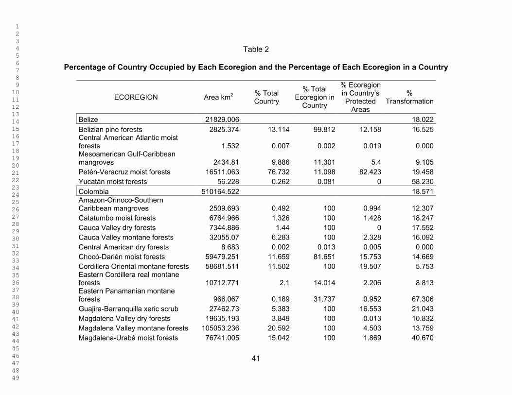
1 2 3 4 5 6 7 8 9 10 11 12 13 14 15 16 17 18 19 20 21 22 23 24 25 26 27 28 29 30 31 32 33 34 35 36 37 38 39 40 41 42 43 44 45 46 47 48 49

41

Table 2

Percentage of Country Occupied by Each Ecoregion and the Percentage of Each Ecoregion in a Country

ECOREGION Area km2 % Total Country

% Total Ecoregion in

Country

% Ecoregion in Country’s Protected

Areas

% Transformation

Belize 21829.006 18.022

Belizian pine forests 2825.374 13.114 99.812 12.158 16.525Central American Atlantic moist forests 1.532 0.007 0.002 0.019 0.000Mesoamerican Gulf-Caribbean mangroves 2434.81 9.886 11.301 5.4 9.105Petén-Veracruz moist forests 16511.063 76.732 11.098 82.423 19.458Yucatán moist forests 56.228 0.262 0.081 0 58.230

Colombia 510164.522 18.571Amazon-Orinoco-Southern Caribbean mangroves 2509.693 0.492 100 0.994 12.307Catatumbo moist forests 6764.966 1.326 100 1.428 18.247Cauca Valley dry forests 7344.886 1.44 100 0 17.552Cauca Valley montane forests 32055.07 6.283 100 2.328 16.092Central American dry forests 8.683 0.002 0.013 0.005 0.000Chocó-Darién moist forests 59479.251 11.659 81.651 15.753 14.669Cordillera Oriental montane forests 58681.511 11.502 100 19.507 5.753Eastern Cordillera real montane forests 10712.771 2.1 14.014 2.206 8.813Eastern Panamanian montane forests 966.067 0.189 31.737 0.952 67.306Guajira-Barranquilla xeric scrub 27462.73 5.383 100 16.553 21.043Magdalena Valley dry forests 19635.193 3.849 100 0.013 10.832Magdalena Valley montane forests 105053.236 20.592 100 4.503 13.759Magdalena-Urabá moist forests 76741.005 15.042 100 1.869 40.670

1 2 3 4 5 6 7 8 9 10 11 12 13 14 15 16 17 18 19 20 21 22 23 24 25 26 27 28 29 30 31 32 33 34 35 36 37 38 39 40 41 42 43 44 45 46 47 48 49

42

Northern Andean páramo 14205.196 2.784 47.932 8.986 2.002Northwestern Andean montane forests 48962.26 9.597 60.325 13.954 15.240Patía Valley dry forests 2270.689 0.445 100 0 4.821Santa Marta montane forests 4784.658 0.938 100 6.119 0.381Santa Marta páramo 1243.629 0.244 100 2.21 0.000Sinú Valley dry forests 24980.499 4.897 100 1.621 44.107South American Pacific mangroves 3917.766 0.768 59.108 0.997 6.230Western Ecuador moist forests 2384.764 0.467 7.037 0.002 14.726

Costa Rica 50531.604 24.963

Central American dry forests 5953.959 11.783 8.818 6.718 56.314Costa Rican seasonal moist forests 8513.287 16.847 80.096 6.111 27.042Isthmian-Atlantic moist forests 16687.546 33.024 28.861 25.566 21.071Isthmian-Pacific moist forests 9166.819 18.141 31.658 16.425 26.206Mesoamerican Gulf-Caribbean mangroves 271.807 0.538 1.262 1.61 3.919Southern Mesoamerican Pacific mangroves 762.778 1.51 12.143 0.825 20.760Talamancan montane forests 9175.409 18.158 56.147 42.745 9.499

Ecuador 146261.303 9.226

Cordillera Central páramo 500.16 0.342 100 0.575 0.219Eastern Cordillera real montane forests 65732.321 44.942 85.986 50.815 4.513Northern Andean páramo 15430.736 10.55 52.068 20.616 3.398Northwestern Andean montane forests 32201.873 22.017 39.675 19.382 13.195South American Pacific mangroves 894.262 0.611 13.492 1.191 8.139Western Ecuador moist forests 31501.952 21.538 92.963 7.421 18.034

El Salvador 20601.449 56.337

Central American dry forests 8289.927 40.24 12.278 36.25 61.962Central American montane forests 950.425 4.613 7.147 23.343 37.344Central American pine-oak forests 10748.755 52.175 9.654 35.476 56.127

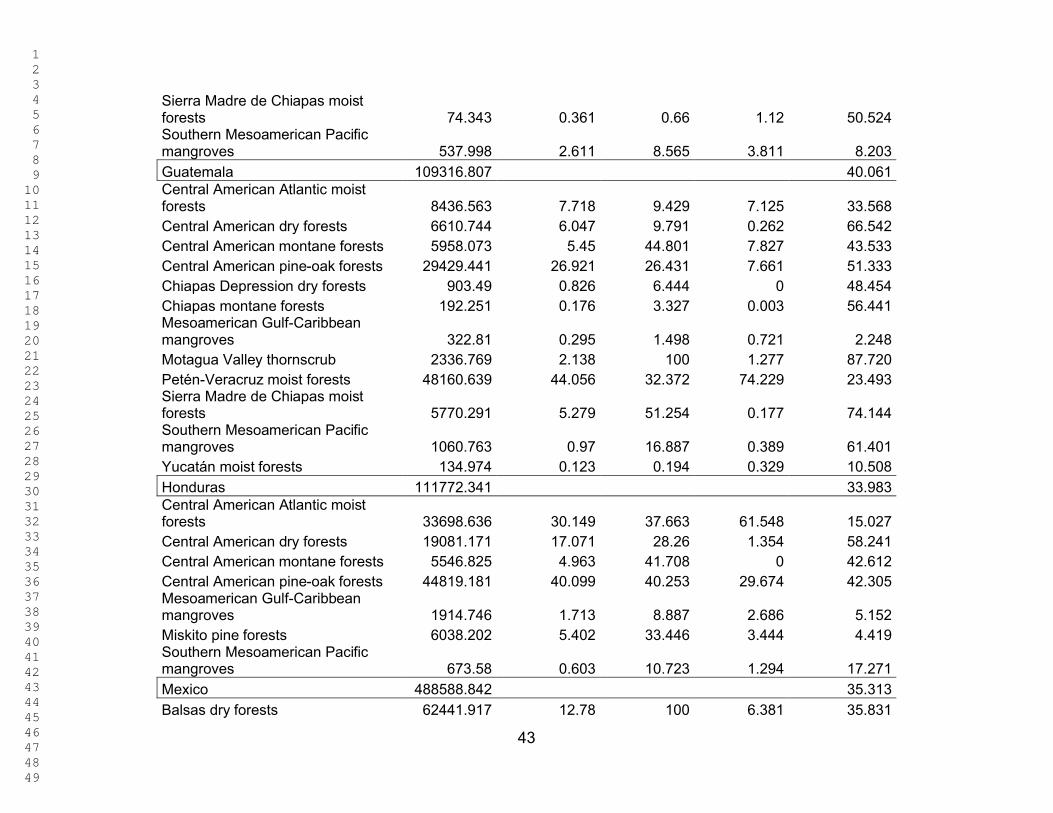
1 2 3 4 5 6 7 8 9 10 11 12 13 14 15 16 17 18 19 20 21 22 23 24 25 26 27 28 29 30 31 32 33 34 35 36 37 38 39 40 41 42 43 44 45 46 47 48 49

43

Sierra Madre de Chiapas moist forests 74.343 0.361 0.66 1.12 50.524Southern Mesoamerican Pacific mangroves 537.998 2.611 8.565 3.811 8.203

Guatemala 109316.807 40.061Central American Atlantic moist forests 8436.563 7.718 9.429 7.125 33.568Central American dry forests 6610.744 6.047 9.791 0.262 66.542Central American montane forests 5958.073 5.45 44.801 7.827 43.533Central American pine-oak forests 29429.441 26.921 26.431 7.661 51.333Chiapas Depression dry forests 903.49 0.826 6.444 0 48.454Chiapas montane forests 192.251 0.176 3.327 0.003 56.441Mesoamerican Gulf-Caribbean mangroves 322.81 0.295 1.498 0.721 2.248Motagua Valley thornscrub 2336.769 2.138 100 1.277 87.720Petén-Veracruz moist forests 48160.639 44.056 32.372 74.229 23.493Sierra Madre de Chiapas moist forests 5770.291 5.279 51.254 0.177 74.144Southern Mesoamerican Pacific mangroves 1060.763 0.97 16.887 0.389 61.401Yucatán moist forests 134.974 0.123 0.194 0.329 10.508

Honduras 111772.341 33.983Central American Atlantic moist forests 33698.636 30.149 37.663 61.548 15.027Central American dry forests 19081.171 17.071 28.26 1.354 58.241Central American montane forests 5546.825 4.963 41.708 0 42.612Central American pine-oak forests 44819.181 40.099 40.253 29.674 42.305Mesoamerican Gulf-Caribbean mangroves 1914.746 1.713 8.887 2.686 5.152Miskito pine forests 6038.202 5.402 33.446 3.444 4.419Southern Mesoamerican Pacific mangroves 673.58 0.603 10.723 1.294 17.271

Mexico 488588.842 35.313

Balsas dry forests 62441.917 12.78 100 6.381 35.831

1 2 3 4 5 6 7 8 9 10 11 12 13 14 15 16 17 18 19 20 21 22 23 24 25 26 27 28 29 30 31 32 33 34 35 36 37 38 39 40 41 42 43 44 45 46 47 48 49

44

Belizian pine forests 5.321 0.001 0.188 0 81.657Central American dry forests 3214.949 0.658 4.761 0.993 74.532Central American pine-oak forests 15982.722 3.271 14.355 2.116 61.081Chiapas Depression dry forests 13118.113 2.685 93.556 0.598 79.739Chiapas montane forests 5586.013 1.143 96.673 0.625 64.597Chimalapas montane forests 2083.674 0.426 100 0.319 55.642Mesoamerican Gulf-Caribbean mangroves 13103.022 2.682 60.816 17.814 15.536Northern Mesoamerican Pacific mangroves 720.046 0.147 100 0.07 12.550Oaxacan montane forests 7600.825 1.556 100 0.001 47.172Pantanos de Centla 17082.886 3.496 100 10.685 58.292Petén-Veracruz moist forests 84099.019 17.213 56.529 16.314 55.115Sierra de los Tuxtlas 3825.368 0.783 100 3.662 67.993Sierra Madre de Chiapas moist forests 5413.519 1.108 48.085 3.62 45.500Sierra Madre de Oaxaca pine-oak forests 14345.454 2.936 100 1.853 26.423Sierra Madre del Sur pine-oak forests 61173.904 12.521 100 2.441 18.461Southern Mesoamerican Pacific mangroves 1431.826 0.293 22.794 1.728 16.317Southern Pacific dry forests 41790.925 8.553 100 2.038 49.914Tehuacán Valley matorral 9892.221 2.025 100 3.937 10.643Veracruz dry forests 6610.969 1.353 100 0.002 60.874Yucatán dry forests 49723.833 10.177 100 2.099 16.653Yucatán moist forests 69342.317 14.192 99.725 22.704 8.873

Nicaragua 127729.399 32.076Central American Atlantic moist forests 47336.911 37.06 52.906 47.455 26.655Central American dry forests 24360.385 19.072 36.079 4.279 60.592Central American montane forests 843.781 0.661 6.345 1.679 44.007Central American pine-oak forests 10362.462 8.113 9.307 2.939 60.588

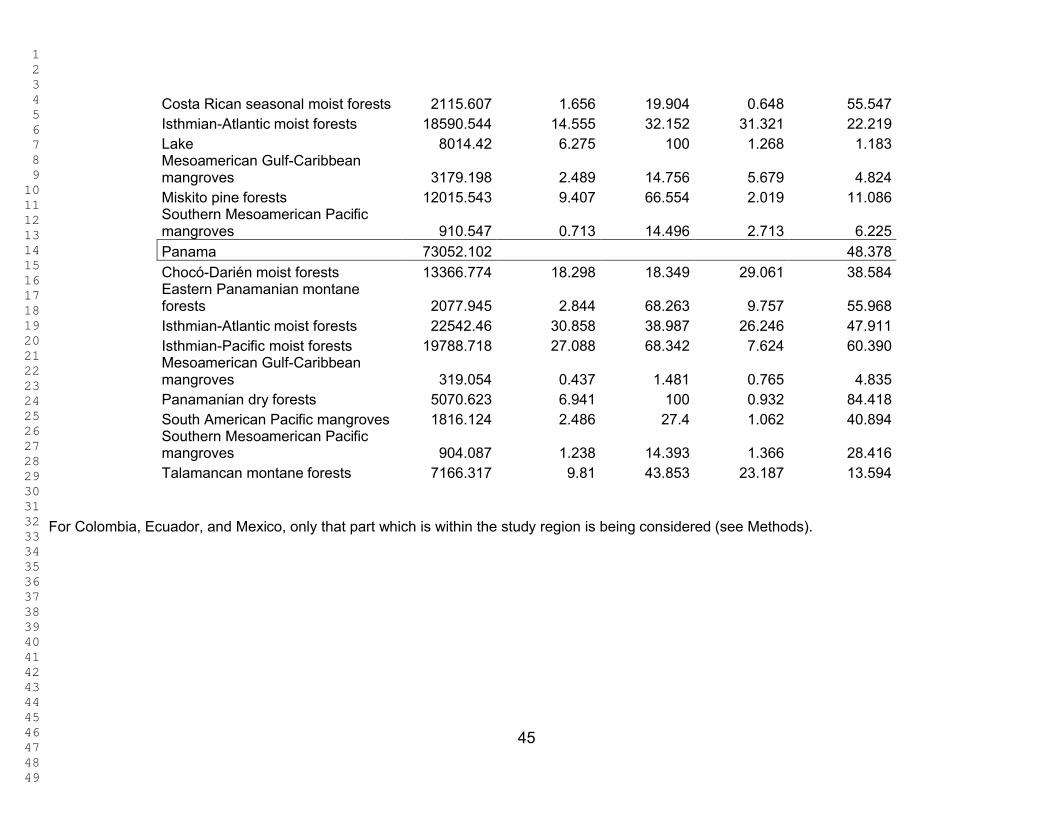
1 2 3 4 5 6 7 8 9 10 11 12 13 14 15 16 17 18 19 20 21 22 23 24 25 26 27 28 29 30 31 32 33 34 35 36 37 38 39 40 41 42 43 44 45 46 47 48 49

45

Costa Rican seasonal moist forests 2115.607 1.656 19.904 0.648 55.547Isthmian-Atlantic moist forests 18590.544 14.555 32.152 31.321 22.219Lake 8014.42 6.275 100 1.268 1.183Mesoamerican Gulf-Caribbeanmangroves 3179.198 2.489 14.756 5.679 4.824Miskito pine forests 12015.543 9.407 66.554 2.019 11.086Southern Mesoamerican Pacific mangroves 910.547 0.713 14.496 2.713 6.225

Panama 73052.102 48.378

Chocó-Darién moist forests 13366.774 18.298 18.349 29.061 38.584Eastern Panamanian montane forests 2077.945 2.844 68.263 9.757 55.968Isthmian-Atlantic moist forests 22542.46 30.858 38.987 26.246 47.911Isthmian-Pacific moist forests 19788.718 27.088 68.342 7.624 60.390Mesoamerican Gulf-Caribbeanmangroves 319.054 0.437 1.481 0.765 4.835Panamanian dry forests 5070.623 6.941 100 0.932 84.418South American Pacific mangroves 1816.124 2.486 27.4 1.062 40.894Southern Mesoamerican Pacific mangroves 904.087 1.238 14.393 1.366 28.416Talamancan montane forests 7166.317 9.81 43.853 23.187 13.594

For Colombia, Ecuador, and Mexico, only that part which is within the study region is being considered (see Methods).

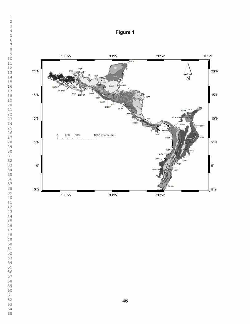
1 2 3 4 5 6 7 8 9 10 11 12 13 14 15 16 17 18 19 20 21 22 23 24 25 26 27 28 29 30 31 32 33 34 35 36 37 38 39 40 41 42 43 44 45 46 47 48 49 50 51 52 53 54 55 56 57 58 59 60 61 62 63 64 65

46

Figure 1

1 2 3 4 5 6 7 8 9 10 11 12 13 14 15 16 17 18 19 20 21 22 23 24 25 26 27 28 29 30 31 32 33 34 35 36 37 38 39 40 41 42 43 44 45 46 47 48 49 50 51 52 53 54 55 56 57 58 59 60 61 62 63 64 65

47

Figure 2

a

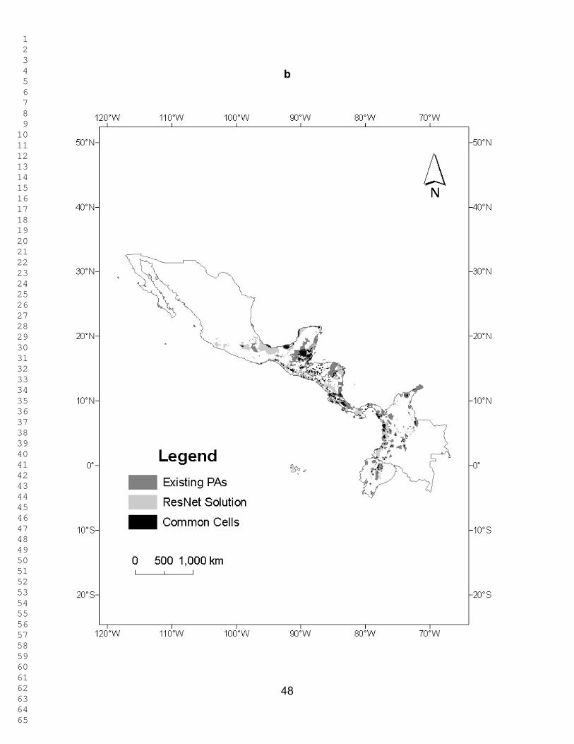
1 2 3 4 5 6 7 8 9 10 11 12 13 14 15 16 17 18 19 20 21 22 23 24 25 26 27 28 29 30 31 32 33 34 35 36 37 38 39 40 41 42 43 44 45 46 47 48 49 50 51 52 53 54 55 56 57 58 59 60 61 62 63 64 65

48

b

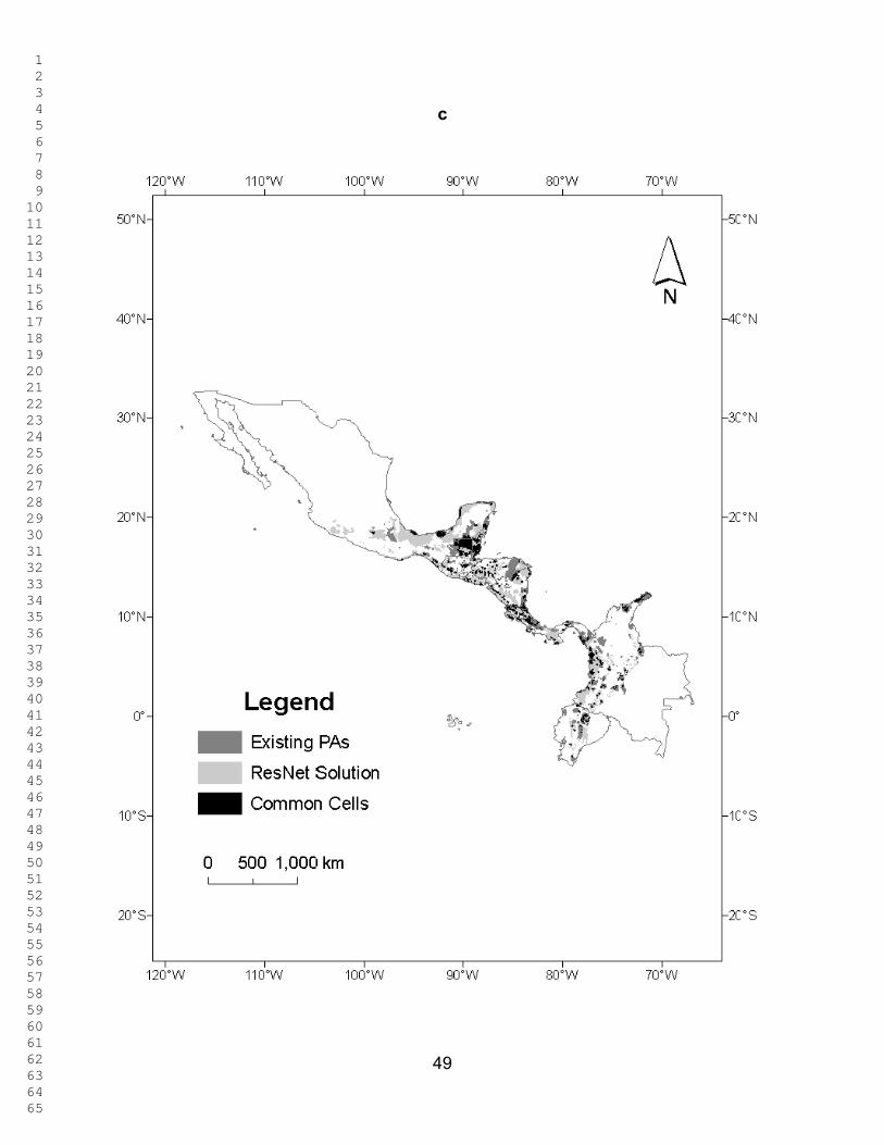
1 2 3 4 5 6 7 8 9 10 11 12 13 14 15 16 17 18 19 20 21 22 23 24 25 26 27 28 29 30 31 32 33 34 35 36 37 38 39 40 41 42 43 44 45 46 47 48 49 50 51 52 53 54 55 56 57 58 59 60 61 62 63 64 65

49

c

1 2 3 4 5 6 7 8 9 10 11 12 13 14 15 16 17 18 19 20 21 22 23 24 25 26 27 28 29 30 31 32 33 34 35 36 37 38 39 40 41 42 43 44 45 46 47 48 49 50 51 52 53 54 55 56 57 58 59 60 61 62 63 64 65

50

d

1 2 3 4 5 6 7 8 9 10 11 12 13 14 15 16 17 18 19 20 21 22 23 24 25 26 27 28 29 30 31 32 33 34 35 36 37 38 39 40 41 42 43 44 45 46 47 48 49 50 51 52 53 54 55 56 57 58 59 60 61 62 63 64 65

51

e

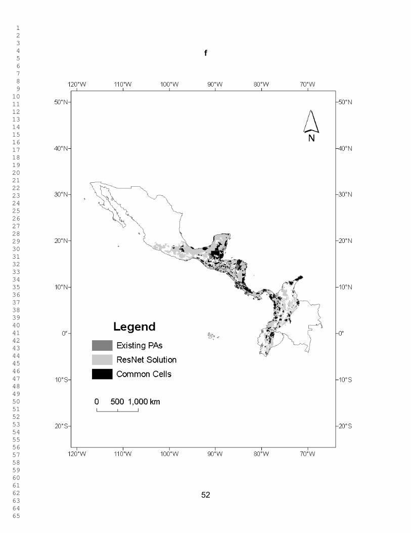
1 2 3 4 5 6 7 8 9 10 11 12 13 14 15 16 17 18 19 20 21 22 23 24 25 26 27 28 29 30 31 32 33 34 35 36 37 38 39 40 41 42 43 44 45 46 47 48 49 50 51 52 53 54 55 56 57 58 59 60 61 62 63 64 65

52

f

1 2 3 4 5 6 7 8 9 10 11 12 13 14 15 16 17 18 19 20 21 22 23 24 25 26 27 28 29 30 31 32 33 34 35 36 37 38 39 40 41 42 43 44 45 46 47 48 49 50 51 52 53 54 55 56 57 58 59 60 61 62 63 64 65

53

g

1 2 3 4 5 6 7 8 9 10 11 12 13 14 15 16 17 18 19 20 21 22 23 24 25 26 27 28 29 30 31 32 33 34 35 36 37 38 39 40 41 42 43 44 45 46 47 48 49 50 51 52 53 54 55 56 57 58 59 60 61 62 63 64 65

54

h

1 2 3 4 5 6 7 8 9 10 11 12 13 14 15 16 17 18 19 20 21 22 23 24 25 26 27 28 29 30 31 32 33 34 35 36 37 38 39 40 41 42 43 44 45 46 47 48 49 50 51 52 53 54 55 56 57 58 59 60 61 62 63 64 65

55

i

1 2 3 4 5 6 7 8 9 10 11 12 13 14 15 16 17 18 19 20 21 22 23 24 25 26 27 28 29 30 31 32 33 34 35 36 37 38 39 40 41 42 43 44 45 46 47 48 49 50 51 52 53 54 55 56 57 58 59 60 61 62 63 64 65

56

j

1 2 3 4 5 6 7 8 9 10 11 12 13 14 15 16 17 18 19 20 21 22 23 24 25 26 27 28 29 30 31 32 33 34 35 36 37 38 39 40 41 42 43 44 45 46 47 48 49 50 51 52 53 54 55 56 57 58 59 60 61 62 63 64 65

57

Figure 3

a

1 2 3 4 5 6 7 8 9 10 11 12 13 14 15 16 17 18 19 20 21 22 23 24 25 26 27 28 29 30 31 32 33 34 35 36 37 38 39 40 41 42 43 44 45 46 47 48 49 50 51 52 53 54 55 56 57 58 59 60 61 62 63 64 65

58

b

1 2 3 4 5 6 7 8 9 10 11 12 13 14 15 16 17 18 19 20 21 22 23 24 25 26 27 28 29 30 31 32 33 34 35 36 37 38 39 40 41 42 43 44 45 46 47 48 49 50 51 52 53 54 55 56 57 58 59 60 61 62 63 64 65

59

c

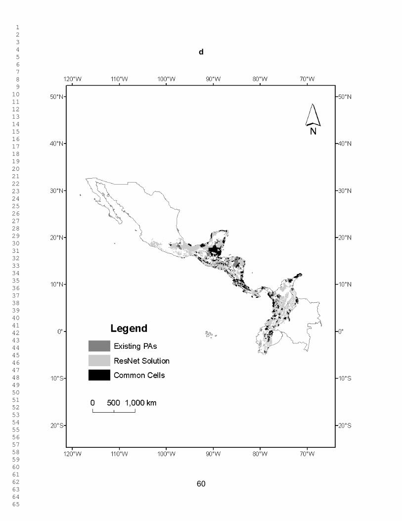
1 2 3 4 5 6 7 8 9 10 11 12 13 14 15 16 17 18 19 20 21 22 23 24 25 26 27 28 29 30 31 32 33 34 35 36 37 38 39 40 41 42 43 44 45 46 47 48 49 50 51 52 53 54 55 56 57 58 59 60 61 62 63 64 65

60

d

1 2 3 4 5 6 7 8 9 10 11 12 13 14 15 16 17 18 19 20 21 22 23 24 25 26 27 28 29 30 31 32 33 34 35 36 37 38 39 40 41 42 43 44 45 46 47 48 49 50 51 52 53 54 55 56 57 58 59 60 61 62 63 64 65

61

e

1 2 3 4 5 6 7 8 9 10 11 12 13 14 15 16 17 18 19 20 21 22 23 24 25 26 27 28 29 30 31 32 33 34 35 36 37 38 39 40 41 42 43 44 45 46 47 48 49 50 51 52 53 54 55 56 57 58 59 60 61 62 63 64 65

62

f

1 2 3 4 5 6 7 8 9 10 11 12 13 14 15 16 17 18 19 20 21 22 23 24 25 26 27 28 29 30 31 32 33 34 35 36 37 38 39 40 41 42 43 44 45 46 47 48 49 50 51 52 53 54 55 56 57 58 59 60 61 62 63 64 65

63

g

1 2 3 4 5 6 7 8 9 10 11 12 13 14 15 16 17 18 19 20 21 22 23 24 25 26 27 28 29 30 31 32 33 34 35 36 37 38 39 40 41 42 43 44 45 46 47 48 49 50 51 52 53 54 55 56 57 58 59 60 61 62 63 64 65

64

h

1 2 3 4 5 6 7 8 9 10 11 12 13 14 15 16 17 18 19 20 21 22 23 24 25 26 27 28 29 30 31 32 33 34 35 36 37 38 39 40 41 42 43 44 45 46 47 48 49 50 51 52 53 54 55 56 57 58 59 60 61 62 63 64 65

65

i

1 2 3 4 5 6 7 8 9 10 11 12 13 14 15 16 17 18 19 20 21 22 23 24 25 26 27 28 29 30 31 32 33 34 35 36 37 38 39 40 41 42 43 44 45 46 47 48 49 50 51 52 53 54 55 56 57 58 59 60 61 62 63 64 65

66

Figure 4

(a)

(b)

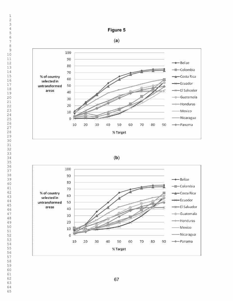
1 2 3 4 5 6 7 8 9 10 11 12 13 14 15 16 17 18 19 20 21 22 23 24 25 26 27 28 29 30 31 32 33 34 35 36 37 38 39 40 41 42 43 44 45 46 47 48 49 50 51 52 53 54 55 56 57 58 59 60 61 62 63 64 65

67

Figure 5

(a)

(b)

1 2 3 4 5 6 7 8 9 10 11 12 13 14 15 16 17 18 19 20 21 22 23 24 25 26 27 28 29 30 31 32 33 34 35 36 37 38 39 40 41 42 43 44 45 46 47 48 49 50 51 52 53 54 55 56 57 58 59 60 61 62 63 64 65

68

Figure 6

(a)

(b)

1

Systematic Conservation Assessment for the Mesoamer ica, Chocó, and Tropical Andes Biodiversity Hotspots : A Preliminary Analysis

Sahotra Sarkar1∗, Víctor Sánchez-Cordero2, Maria Cecilia Londoño2, and Trevon Fuller1

1 Biodiversity and Biocultural Conservation Laboratory, Section of Integrative Biology, University of Texas at Austin, Austin, TX 78712 –1180, USA;

2 Departamento de Zoología, Instituto de Biología, Universidad Nacional Autónoma de

México, Apartado Postal 70-153, México D. F. 04510, México.

Supplementary Materials

∗Corresponding author; E-mail: sarkar@mail.utexas.edu.

Revised Supplementary MaterialsClick here to download attachment to manuscript: Mesoamerica-SM-15102008.doc Click here to view linked References

2

Table S1

Occurrence Data for Critically Endangered , Endangered , and Vulnerable Species and Niche Model Results

“CR”: Critically Endangered; “EN”: Endangered; “VU”: Vulnerable. § : These species were excluded because p-values for the sensititvity-specificity test were not less than 0.05. *: These species were excluded because of known unreliability of predicted fundamental niche (see text) for further explanation. #: There were less than 4 records in different 0.02° × 0.02° longitude × latitude cells. Note that sample points falling within the same grid cell were collapsed for ecological niche modeling. Key for explanatory variables: BIO1 = Annual Mean Temperature; BIO2 = Mean Diurnal Range (Mean of monthly (max temp - min temp)); BIO3 = Isothermality (BIO2/BIO7) (* 100); BIO4 = Temperature Seasonality (standard deviation×100); BIO5 = Max Temperature of Warmest Month; BIO6 = Min Temperature of Coldest Month; BIO7 = Temperature Annual Range; BIO8 = Mean Temperature of Wettest Quarter; BIO9 = Mean Temperature of Driest Quarter; BIO10 = Mean Temperature of Warmest Quarter; BIO11 = Mean Temperature of Coldest Quarter; BIO12 = Annual Precipitation; BIO13 = Precipitation of Wettest Month; BIO14 = Precipitation of Driest Month; BIO15 = Precipitation Seasonality (Coefficient of Variation); BIO16 = Precipitation of Wettest Quarter; BIO17 = Precipitation of Driest Quarter; BIO18 = Precipitation of Warmest Quarter; BIO19 = Precipitation of Coldest Quarter.

Species Name Red List Category

Geographical records

Geographical records after

1980

Records used in MaxEnt

AUC value

Exp. Var. 1

Exp Var. 2

Amphibians

Ambystoma taylori CR 1 Atelopus eusebianus CR 1 1 Atelopus

pachydermus CR 1

Bolitoglossa heiroreias CR 1

Bufo holdridgei CR 1 Colostethus

vertebralis CR 1

Hyla bocourti CR 1 Oedipina maritima CR 1 1 Plectrohyla

acanthodes CR 1

Plectrohyla ixil CR 1

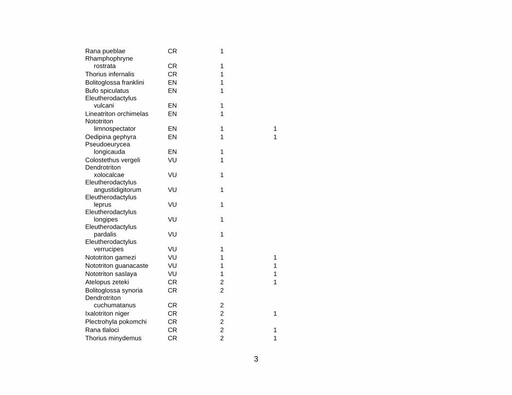
3

Rana pueblae CR 1 Rhamphophryne

rostrata CR 1

Thorius infernalis CR 1 Bolitoglossa franklini EN 1 Bufo spiculatus EN 1 Eleutherodactylus

vulcani EN 1

Lineatriton orchimelas EN 1 Nototriton

limnospectator EN 1 1

Oedipina gephyra EN 1 1 Pseudoeurycea

longicauda EN 1

Colostethus vergeli VU 1 Dendrotriton

xolocalcae VU 1

Eleutherodactylus angustidigitorum VU 1

Eleutherodactylus leprus VU 1

Eleutherodactylus longipes VU 1

Eleutherodactylus pardalis VU 1

Eleutherodactylus verrucipes VU 1

Nototriton gamezi VU 1 1 Nototriton guanacaste VU 1 1 Nototriton saslaya VU 1 1 Atelopus zeteki CR 2 1 Bolitoglossa synoria CR 2 Dendrotriton

cuchumatanus CR 2

Ixalotriton niger CR 2 1 Plectrohyla pokomchi CR 2 Rana tlaloci CR 2 1 Thorius minydemus CR 2 1

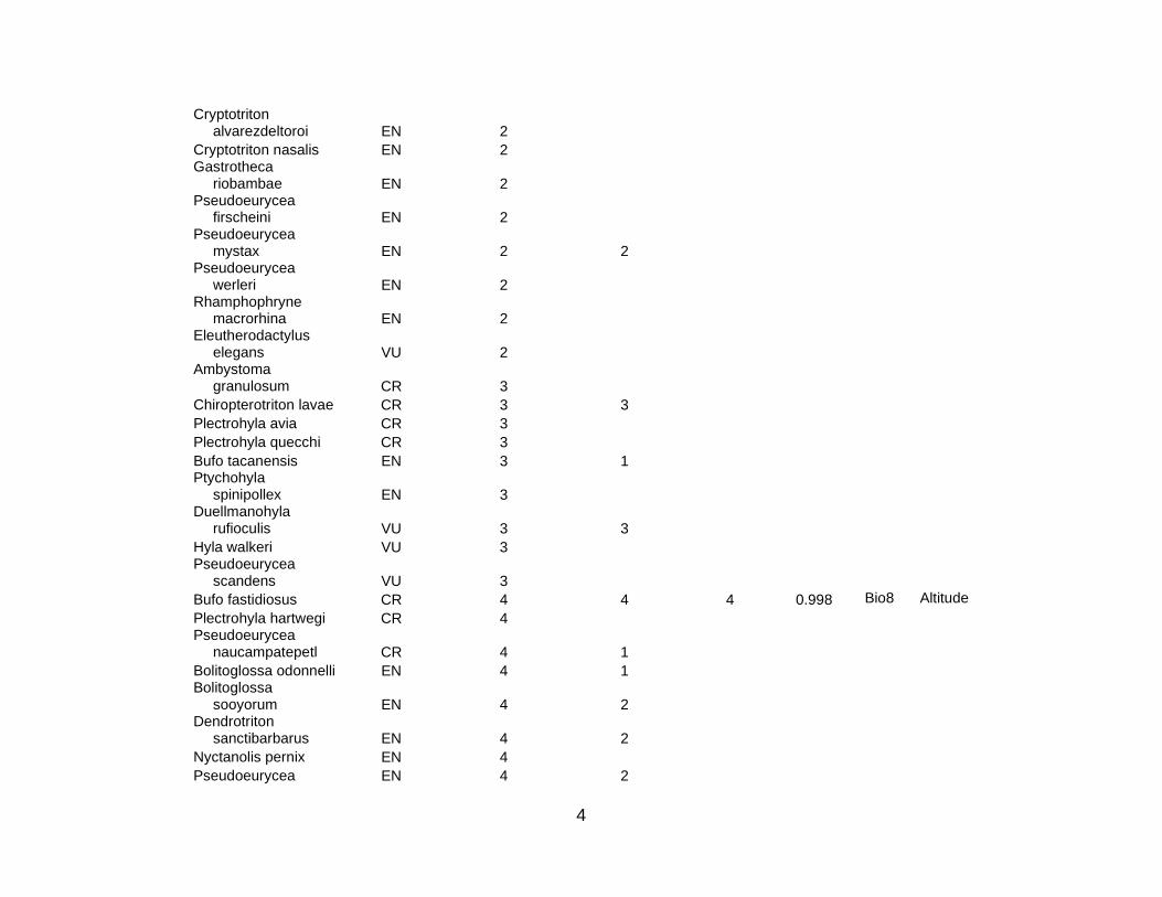
4

Cryptotriton alvarezdeltoroi EN 2

Cryptotriton nasalis EN 2 Gastrotheca

riobambae EN 2

Pseudoeurycea firscheini EN 2

Pseudoeurycea mystax EN 2 2

Pseudoeurycea werleri EN 2

Rhamphophryne macrorhina EN 2

Eleutherodactylus elegans VU 2

Ambystoma granulosum CR 3

Chiropterotriton lavae CR 3 3 Plectrohyla avia CR 3 Plectrohyla quecchi CR 3 Bufo tacanensis EN 3 1 Ptychohyla

spinipollex EN 3

Duellmanohyla rufioculis VU 3 3

Hyla walkeri VU 3 Pseudoeurycea

scandens VU 3

Bufo fastidiosus CR 4 4 4 0.998 Bio8 Altitude Plectrohyla hartwegi CR 4 Pseudoeurycea

naucampatepetl CR 4 1

Bolitoglossa odonnelli EN 4 1 Bolitoglossa

sooyorum EN 4 2

Dendrotriton sanctibarbarus EN 4 2

Nyctanolis pernix EN 4 Pseudoeurycea EN 4 2

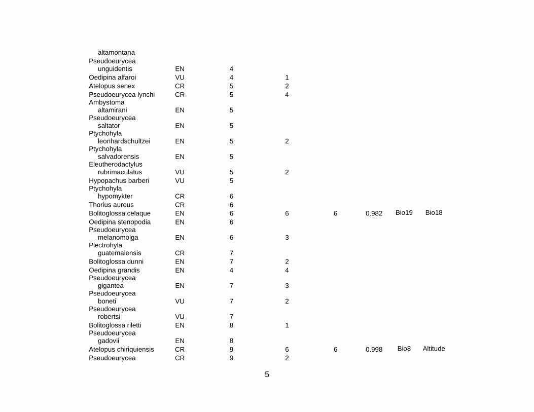
5

altamontana Pseudoeurycea

unguidentis EN 4

Oedipina alfaroi VU 4 1 Atelopus senex CR 5 2 Pseudoeurycea lynchi CR 5 4 Ambystoma

altamirani EN 5

Pseudoeurycea saltator EN 5

Ptychohyla leonhardschultzei EN 5 2

Ptychohyla salvadorensis EN 5

Eleutherodactylus rubrimaculatus VU 5 2

Hypopachus barberi VU 5 Ptychohyla

hypomykter CR 6

Thorius aureus CR 6 Bolitoglossa celaque EN 6 6 6 0.982 Bio19 Bio18 Oedipina stenopodia EN 6 Pseudoeurycea

melanomolga EN 6 3

Plectrohyla guatemalensis CR 7

Bolitoglossa dunni EN 7 2 Oedipina grandis EN 4 4 Pseudoeurycea

gigantea EN 7 3

Pseudoeurycea boneti VU 7 2

Pseudoeurycea robertsi VU 7

Bolitoglossa riletti EN 8 1 Pseudoeurycea

gadovii EN 8

Atelopus chiriquiensis CR 9 6 6 0.998 Bio8 Altitude Pseudoeurycea CR 9 2

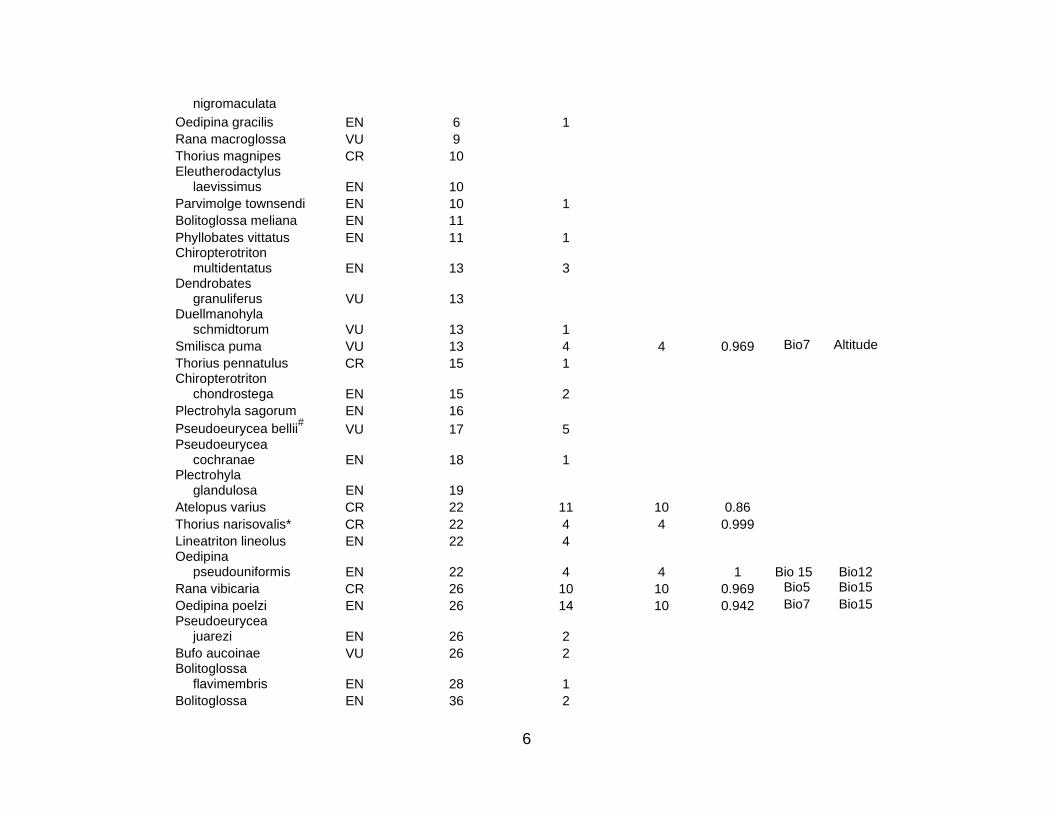
6

nigromaculata Oedipina gracilis EN 6 1 Rana macroglossa VU 9 Thorius magnipes CR 10 Eleutherodactylus

laevissimus EN 10

Parvimolge townsendi EN 10 1 Bolitoglossa meliana EN 11 Phyllobates vittatus EN 11 1 Chiropterotriton

multidentatus EN 13 3

Dendrobates granuliferus VU 13

Duellmanohyla schmidtorum VU 13 1

Smilisca puma VU 13 4 4 0.969 Bio7 Altitude Thorius pennatulus CR 15 1 Chiropterotriton

chondrostega EN 15 2

Plectrohyla sagorum EN 16

Pseudoeurycea bellii# VU 17 5 Pseudoeurycea

cochranae EN 18 1

Plectrohyla glandulosa EN 19

Atelopus varius CR 22 11 10 0.86 Thorius narisovalis* CR 22 4 4 0.999 Lineatriton lineolus EN 22 4 Oedipina

pseudouniformis EN 22 4 4 1 Bio 15

Bio12

Rana vibicaria CR 26 10 10 0.969 Bio5 Bio15 Oedipina poelzi EN 26 14 10 0.942 Bio7 Bio15 Pseudoeurycea

juarezi EN 26 2

Bufo aucoinae VU 26 2 Bolitoglossa

flavimembris EN 28 1

Bolitoglossa EN 36 2

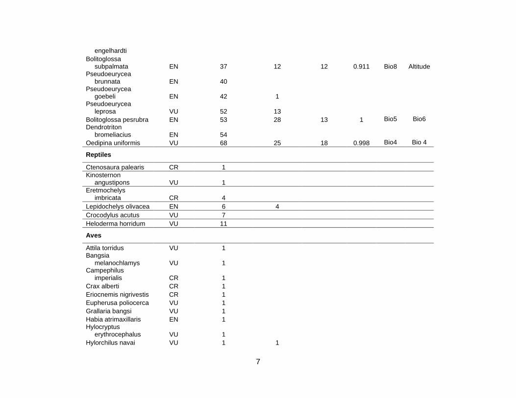
7

engelhardti Bolitoglossa

subpalmata EN 37 12 12 0.911

Bio8

Altitude Pseudoeurycea

brunnata EN 40

Pseudoeurycea goebeli EN 42 1

Pseudoeurycea leprosa VU 52 13

Bolitoglossa pesrubra EN 53 28 13 1 Bio5 Bio6 Dendrotriton

bromeliacius EN 54

Oedipina uniformis VU 68 25 18 0.998 Bio4 Bio 4

Reptiles

Ctenosaura palearis CR 1 Kinosternon

angustipons VU 1

Eretmochelys imbricata CR 4

Lepidochelys olivacea EN 6 4

Crocodylus acutus VU 7 Heloderma horridum VU 11

Aves

Attila torridus VU 1 Bangsia

melanochlamys VU 1

Campephilus imperialis CR 1

Crax alberti CR 1 Eriocnemis nigrivestis CR 1 Eupherusa poliocerca VU 1 Grallaria bangsi VU 1 Habia atrimaxillaris EN 1 Hylocryptus

erythrocephalus VU 1

Hylorchilus navai VU 1 1

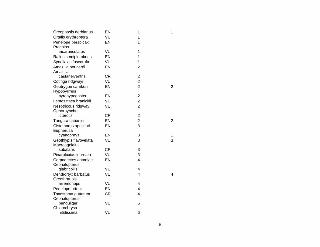
8

Oreophasis derbianus EN 1 1 Ortalis erythroptera VU 1 Penelope perspicax EN 1 Procnias

tricarunculatus VU 1

Rallus semiplumbeus EN 1 Synallaxis fuscorufa VU 1 Amazilia boucardi EN 2 Amazilia

castaneiventris CR 2

Cotinga ridgwayi VU 2 Geotrygon carrikeri EN 2 2 Hypopyrrhus

pyrohypogaster EN 2

Leptosittaca branickii VU 2 Nesotriccus ridgwayi VU 2 Ognorhynchus

icterotis CR 2

Tangara cabanisi EN 2 2 Cistothorus apolinari EN 3 Eupherusa

cyanophrys EN 3 1

Geothlypis flavovelata VU 3 3 Macroagelaius

subalaris CR 3

Pinaroloxias inornata VU 3 Carpodectes antoniae EN 4 Cephalopterus

glabricollis VU 4

Dendrortyx barbatus VU 4 4 Oreothraupis

arremonops VU 4

Penelope ortoni EN 4 Toxostoma guttatum CR 4 Cephalopterus

penduliger VU 6

Chlorochrysa nitidissima VU 6

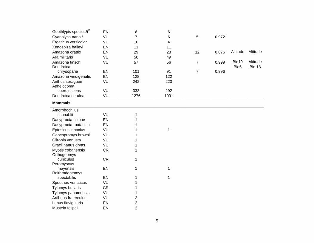
9

Geothlypis speciosa# EN 6 6

Cyanolyca nana * VU 7 6 5 0.972 Ergaticus versicolor VU 10 4 Xenospiza baileyi EN 11 11 Amazona oratrix EN 29 28 12 0.876 Altitude Altitude Ara militaris VU 50 49 Amazona finschi VU 57 56 7 0.999 Bio19 Altitude Dendroica

chrysoparia EN 101 91 7 0.996 Bio6 Bio 18

Amazona viridigenalis EN 128 122 Anthus spragueii VU 242 223 Aphelocoma

coerulescens VU 333 292

Dendroica cerulea VU 1276 1091

Mammals

Amorphochilus schnablii VU 1

Dasyprocta coibae EN 1 Dasyprocta ruatanica EN 1 Eptesicus innoxius VU 1 1 Geocapromys brownii VU 1 Glironia venusta VU 1 Gracilinanus dryas VU 1 Myotis cobanensis CR 1 Orthogeomys

cuniculus CR 1

Peromyscus mayensis EN 1 1

Reithrodontomys spectabilis EN 1 1

Speothos venaticus VU 1 Tylomys bullaris CR 1 Tylomys panamensis VU 1 Artibeus fraterculus VU 2 Lepus flavigularis EN 2 Mustela felipei EN 2

10

Rhogeessa genowaysi VU 2 1

Trichechus manatus VU 2 Dinomys branickii EN 3 Heteromys nelsoni CR 3 1 Platyrrhinus

chocoensis VU 3 1

Romerolagus diazi EN 4 Saguinus leucopus VU 4 Sylvilagus dicei EN 4 Anotomys leander EN 5 2 Bauerus

dubiaquercus * VU 5 5 5 0.353

Reithrodontomys rodriguezi VU 5

Tapirus terrestris VU 5 3 Tremarctos ornatus VU 6 Artibeus inopinatus VU 7 3 Tapirus pinchaque EN 7 Alouatta pigra EN 8 Ateles belzebuth VU 9 Saimiri oerstedii EN 9 Musonycteris

harrisoni VU 10 2

Saguinus oedipus EN 10 Tapirus bairdii EN 10 Peromyscus

zarhynchus VU 12 12 12 0.989

Bio6

Bio18 Aotus lemurinus VU 13 Plecotus townsendii VU 16 Cryptotis gracilis VU 17 1 Myotis vivesi VU 20 Leptonycteris nivalis EN 21 Caluromys derbianus VU 45 3 Leptonycteris

curasoae VU 47 11 11 0.912

Bio19

Bio16 Microtus mexicanus VU 95 7 7 0.999 Bio6 Bio4

11

Plants

Abarema racemiflora VU 4 1 Aegiphila fasciculata VU 13 6 5 0.949 Aegiphila panamensis VU 240 118 99 0.913 Bio4 Bio4 Aiouea obscura EN 10 10 10 0.997 Bio13 Bio13 Amphitecna isthmica VU 32 13 10 0.979 Bio13 Bio19 Amphitecna molinae EN 8 7 7 0.999 Bio4 Altitude Amphitecna

sessilifolius VU 2 2

Anaxagorea phaeocarpa EN 27 21 17 0.891

Bio15

Bio4

Anthodiscus chocoensis VU 6 6 5 0.984

Bio13

Bio14

Ardisia furfuracella VU 1 1 Bactris longiseta VU 5 5 Bombacopsis quinata VU 48 17 14 0.805 Altitude Bio19 Caryocar

costaricense VU 20 17 16 0.99

Bio13

Bio19 Cedrela fissilis EN 19 3 Cedrela odorata VU 198 128 101 0.76 Bio17 Altitude Cordia croatii VU 15 10 9 0.825 Cornus disciflora VU 180 99 57 0.843 Bio8 Altitude Couratari guianensis VU 13 10 9 0.995 Bio13 Bio19 Couratari scottmorii VU 14 13 9 0.999 Bio13 Bio19 Cryosophila cookii CR 2 2 Cryosophila grayumii CR 10 10 9 0.995 Bio16 Bio19 Cymbopetalum

torulosum * VU 34 22 12 0.659

Dalbergia retusa VU 34 18 16 0.751 Bio14 Bio4 Dendropanax alberti-

smithii VU 13 1

Dendropanax sessiliflorus * VU 28 15 13 0.969

Dichapetalum costaricense VU 1 1

Eugenia salamensis EN 44 25 14 0.663 Freziera biserrata VU 1 1

12

Guaiacum sanctum EN 117 90 63 0.936 Bio18 Altitude Guarea pyriformis VU 1 1 Hyperbaena allenii VU 3 Ilex costaricensis VU 34 29 24 0.991 Bio4 Bio18 Ilex pallida VU 46 37 28 0.995 Bio8 Altitude Ilex vulcanicola VU 16 12 12 0.95 Bio4 Altitude Inga allenii VU 10 9 8 0.977 Bio13 Bio2 Inga bracteifera EN 2 2 Inga canonegrensis * VU 6 5 4 1 Inga golfodulcensis EN 2 2 Inga latipes EN 5 3 Inga litoralis EN 17 15 11 0.995 Bio16 Altitude Inga mortoniana EN 29 20 19 0.957 Bio4 Bio4 Inga skutchii VU 10 7 7 0.994 Bio13 Bio13 Inga stenophylla * EN 6 6 6 0.866 Inga tenuiloba EN 1 1 Juglans olanchana EN 43 30 26 0.91 Altitude Altitude Lacunaria

panamensis EN 28 21 17 0.998

Bio2

Bio4 Lennea viridiflora VU 16 12 12 0.886 Altitude Bio18 Lonchocarpus

calcaratus# VU 5 4

Lonchocarpus miniflorus EN 2 2

Lonchocarpus phaseolifolius CR 78 60 47 0.98

Bio17

Altitude

Lonchocarpus phlebophyllus EN 46 40 36 0.977

Bio4 Bio4

Lonchocarpus retiferus * EN 30 17 16 0.992

Lonchocarpus yoroensis * CR 7 5 5 0.988

Meriania grandiflora VU 13 2 Mollinedia ruae * CR 21 11 9 0.976 Nectandra hypoleuca VU 19 14 6 0.993 Bio19 Bio4 Nectandra

longipetiolata EN 3 3

Nectandra mirafloris VU 16 12 6 1 Altitude Altitude

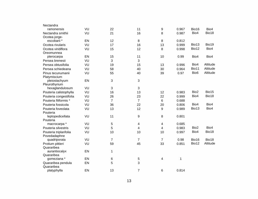
13

Nectandra ramonensis VU 22 11 9 0.967

Bio16

Bio4

Nectandra smithii VU 21 16 8 0.987 Bio4 Bio18 Ocotea jorge-

escobarii * EN 12 8 8 0.812

Ocotea rivularis VU 17 16 13 0.999 Bio13 Bio19 Ocotea viridiflora VU 15 12 8 0.998 Bio12 Bio4 Oreomunnea

pterocarpa EN 15 11 10 0.99

Bio4

Bio4 Persea brenesii VU 3 3 Persea obtusifolia VU 19 15 13 0.996 Bio4 Altitude Persea schiedeana VU 58 40 30 0.964 Bio11 Altitude Pinus tecunumanii VU 55 40 39 0.97 Bio6 Altitude Platymiscium

pleiostachyum EN 3 3

Pleurothyrium hexaglandulosum VU 3 3

Pouteria calistophylla VU 16 13 12 0.983 Bio2 Bio15 Pouteria congestifolia VU 26 23 22 0.999 Bio4 Bio18 Pouteria filiformis * VU 7 7 6 0.688 Pouteria fossicola VU 36 22 20 0.806 Bio4 Bio4 Pouteria foveolata VU 13 12 9 0.989 Bio13 Bio4 Pouteria

leptopedicellata VU 11 9 8 0.801

Pouteria macrocarpa * VU 5 4 4 0.685

Pouteria silvestris VU 5 4 4 0.983 Bio2 Bio4 Pouteria triplarifolia VU 10 10 10 0.997 Bio4 Bio18 Povedadaphne

quadriporata VU 7 7 7 0.98

Bio16

Bio18 Protium pittieri VU 59 45 33 0.851 Bio12 Altitude Quararibea

aurantiocalyx EN 1

Quararibea gomeziana * EN 6 5 4 1

Quararibea pendula EN 5 3 Quararibea

platyphylla EN 13 7 6 0.814

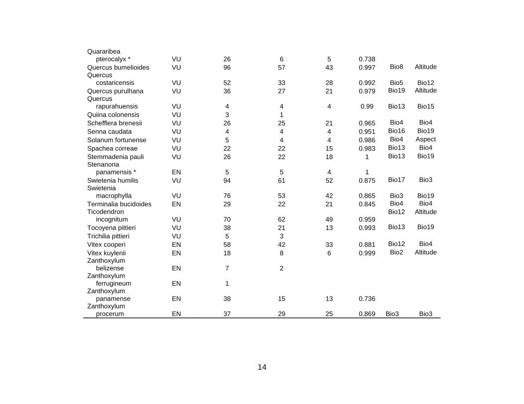
14

Quararibea pterocalyx * VU 26 6 5 0.738

Quercus bumelioides VU 96 57 43 0.997 Bio8 Altitude Quercus

costaricensis VU 52 33 28 0.992

Bio5

Bio12 Quercus purulhana VU 36 27 21 0.979 Bio19 Altitude Quercus

rapurahuensis VU 4 4 4 0.99

Bio13 Bio15 Quiina colonensis VU 3 1 Schefflera brenesii VU 26 25 21 0.965 Bio4 Bio4 Senna caudata VU 4 4 4 0.951 Bio16 Bio19 Solanum fortunense VU 5 4 4 0.986 Bio4 Aspect Spachea correae VU 22 22 15 0.983 Bio13 Bio4 Stemmadenia pauli VU 26 22 18 1 Bio13 Bio19 Stenanona

panamensis * EN 5 5 4 1

Swietenia humilis VU 94 61 52 0.875 Bio17 Bio3 Swietenia

macrophylla VU 76 53 42 0.865

Bio3

Bio19 Terminalia bucidoides EN 29 22 21 0.845 Bio4 Bio4 Ticodendron

incognitum VU 70 62 49 0.959 Bio12 Altitude

Tocoyena pittieri VU 38 21 13 0.993 Bio13 Bio19 Trichilia pittieri VU 5 3 Vitex cooperi EN 58 42 33 0.881 Bio12 Bio4 Vitex kuylenii EN 18 8 6 0.999 Bio2 Altitude Zanthoxylum

belizense EN 7 2

Zanthoxylum ferrugineum EN 1

Zanthoxylum panamense EN 38 15 13 0.736

Zanthoxylum procerum EN 37 29 25 0.869

Bio3

Bio3

15

Table S2

Selected Existing Protected Areas for Different Tar gets of Representation

Names of the existing protected areas that first get cells within them selected at representation targets of 10 % for species and then species and ecoregions, and similarly for 50 %, and 90 %. For Colombia, Ecuador, and Mexico, only that part which is within Mesoamerica is being considered.

Target Country Protected Areas First Selected

Belize

Machaca; Sarstoon-Temash; Boden Creek Ecological Research; Golden Stream Reserve; Deep River; Paynes Creek; Swasey-Bladen; Mango Creek; Chiquibul; Sibun; Mountain Pine Ridge; Vaca; Tapir Mountain; Manatí; Gales Point; Spanish Creek; Community Baboon Sanctuary; Crooked Tree; Fesh Water Creek; Burdon Creek

10 % Species

Colombia

Juradó; Alto Río Bojayá; Ríos Valle y Boroboro; Utría; Alto Río Buey; Bete; Río Negua; Puerto Alegre y La Divisa; Ríos Catre y Dubasa; Río Panguí; Río Nuquí; Agua Clara y Bella Luz del Río Ampora; Kananeruba; Río Icho y Quebrada Baratudo; Tarena; Tatamá; Puadó; Unión Chocó-San Cristóbal; Río Taparaí; Santa Marái de Pangalá; Camí Río Garrapatas; Los Nevados; Sierra Nevada de Santa Marta; Arhuaco de la Sierra Nevada; Las Hermosas; Nevado del Huila; Guanguí; Calle Santa Rosa; Puracé; Cuenca Alta del Río Mocoa; Galeras; Laguna La Cocha; Sierra de la Macarena; Sumapaz; Qubrada Honda y Caños Parrado y Duque; Chingaza; Pisbá; El Cocuy; Tamá

Costa Rica

Santa Rosa; Guanacaste; Rincón de la Vieja; Finca del Estado; Finca Las Delicias; Miravalles; Volcán Tenorio; Arernal-Monteverde; Península de Nicoya; Tivives; Carara; Cerros de Turrubares; Zapatón; Juan Castro Blanco; Volcán Poás; Grecia; Braulio Carrilo; Cordillera Volcánica Central; Barra del Colorado; Tortuguero; Río Pacuare; Bajo Chirripó; Río Macho; Internacional La Amistad; Tayni; Ujarrás; Golfo Dulce; Corcovado; Piedras Blancas

Ecuador Cayambe-Coca; Antisana; Cotopaxi; Llanganates; Los Illinizas; Cajas

El Salvador Volcán de San Vicente; Laguna Verde; Andrés-Paraíso-Ciprés-San José Miramar-San Isidro; Isla Argentina-Colunbia-14 y 15 de Marzo-Abriles-Jabalí

Guatemala Volcán Tacaná (Mexico and Guatemala); Maya Biosphere; Mirador Rio Azul; Dos Lagunas; Tikal; El Pucté Complejos I y II APSP; Petexbatún; Aguateca; Dos Pilas; Sierra de Las Minas; Volcán Santo Tomás; Quetzaltenango Saqbé; Volcán de Pacaya; Volcán Zunil; Volcán Tajumulco; Volcán Lacandón;

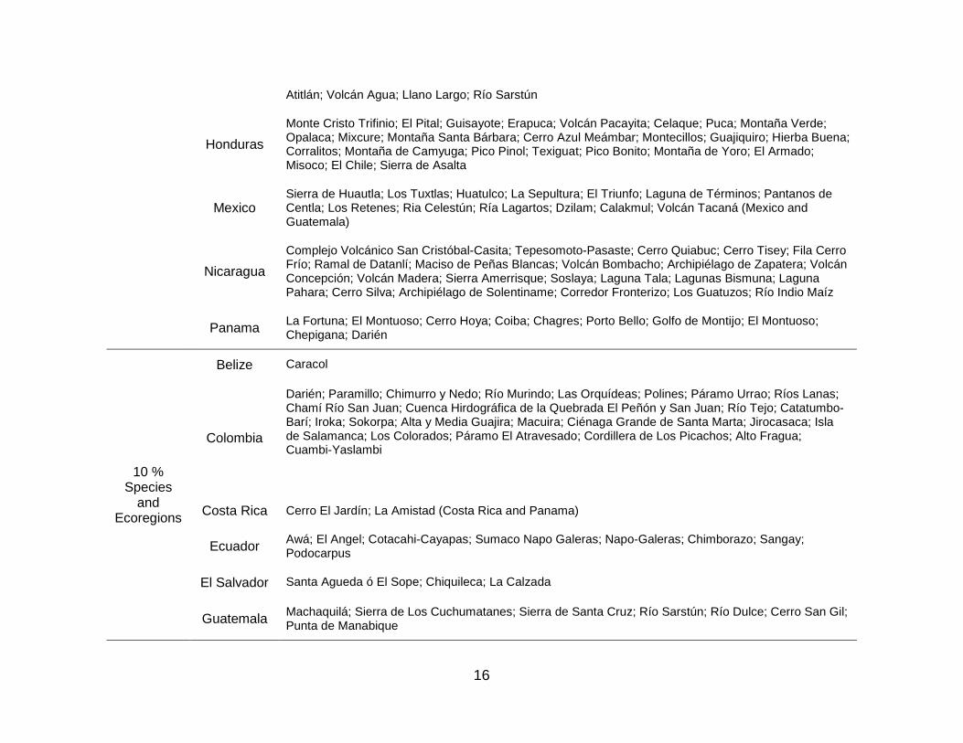
16

Atitlán; Volcán Agua; Llano Largo; Río Sarstún

Honduras

Monte Cristo Trifinio; El Pital; Guisayote; Erapuca; Volcán Pacayita; Celaque; Puca; Montaña Verde; Opalaca; Mixcure; Montaña Santa Bárbara; Cerro Azul Meámbar; Montecillos; Guajiquiro; Hierba Buena; Corralitos; Montaña de Camyuga; Pico Pinol; Texiguat; Pico Bonito; Montaña de Yoro; El Armado; Misoco; El Chile; Sierra de Asalta

Mexico Sierra de Huautla; Los Tuxtlas; Huatulco; La Sepultura; El Triunfo; Laguna de Términos; Pantanos de Centla; Los Retenes; Ria Celestún; Ría Lagartos; Dzilam; Calakmul; Volcán Tacaná (Mexico and Guatemala)

Nicaragua

Complejo Volcánico San Cristóbal-Casita; Tepesomoto-Pasaste; Cerro Quiabuc; Cerro Tisey; Fila Cerro Frío; Ramal de Datanlí; Maciso de Peñas Blancas; Volcán Bombacho; Archipiélago de Zapatera; Volcán Concepción; Volcán Madera; Sierra Amerrisque; Soslaya; Laguna Tala; Lagunas Bismuna; Laguna Pahara; Cerro Silva; Archipiélago de Solentiname; Corredor Fronterizo; Los Guatuzos; Río Indio Maíz

Panama La Fortuna; El Montuoso; Cerro Hoya; Coiba; Chagres; Porto Bello; Golfo de Montijo; El Montuoso; Chepigana; Darién

10 % Species

and Ecoregions

Belize Caracol

Colombia

Darién; Paramillo; Chimurro y Nedo; Río Murindo; Las Orquídeas; Polines; Páramo Urrao; Ríos Lanas; Chamí Río San Juan; Cuenca Hirdográfica de la Quebrada El Peñón y San Juan; Río Tejo; Catatumbo-Barí; Iroka; Sokorpa; Alta y Media Guajira; Macuira; Ciénaga Grande de Santa Marta; Jirocasaca; Isla de Salamanca; Los Colorados; Páramo El Atravesado; Cordillera de Los Picachos; Alto Fragua; Cuambi-Yaslambi

Costa Rica Cerro El Jardín; La Amistad (Costa Rica and Panama)

Ecuador Awá; El Angel; Cotacahi-Cayapas; Sumaco Napo Galeras; Napo-Galeras; Chimborazo; Sangay; Podocarpus

El Salvador Santa Agueda ó El Sope; Chiquileca; La Calzada

Guatemala Machaquilá; Sierra de Los Cuchumatanes; Sierra de Santa Cruz; Río Sarstún; Río Dulce; Cerro San Gil; Punta de Manabique

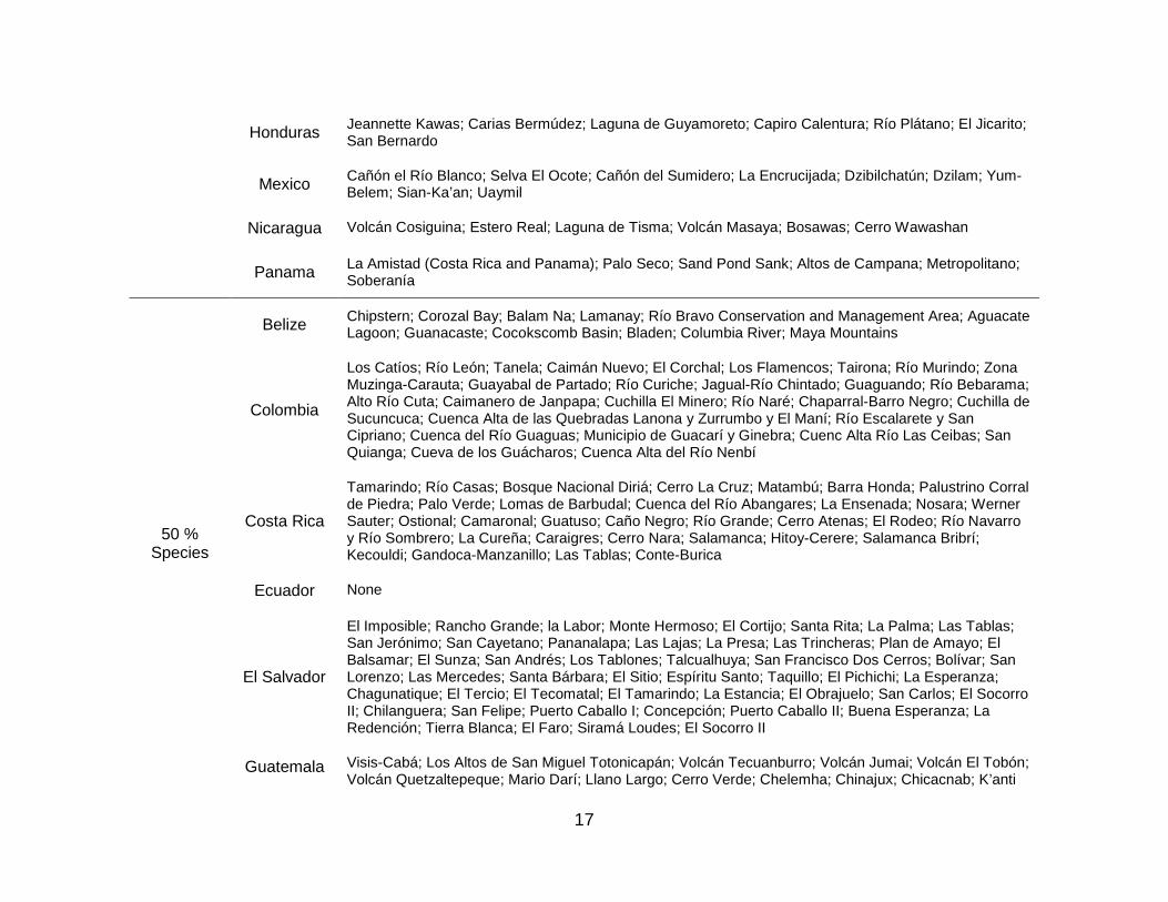
17

Honduras Jeannette Kawas; Carias Bermúdez; Laguna de Guyamoreto; Capiro Calentura; Río Plátano; El Jicarito; San Bernardo

Mexico Cañón el Río Blanco; Selva El Ocote; Cañón del Sumidero; La Encrucijada; Dzibilchatún; Dzilam; Yum-Belem; Sian-Ka’an; Uaymil

Nicaragua Volcán Cosiguina; Estero Real; Laguna de Tisma; Volcán Masaya; Bosawas; Cerro Wawashan

Panama La Amistad (Costa Rica and Panama); Palo Seco; Sand Pond Sank; Altos de Campana; Metropolitano; Soberanía

50 % Species

Belize Chipstern; Corozal Bay; Balam Na; Lamanay; Río Bravo Conservation and Management Area; Aguacate Lagoon; Guanacaste; Cocokscomb Basin; Bladen; Columbia River; Maya Mountains

Colombia

Los Catíos; Río León; Tanela; Caimán Nuevo; El Corchal; Los Flamencos; Tairona; Río Murindo; Zona Muzinga-Carauta; Guayabal de Partado; Río Curiche; Jagual-Río Chintado; Guaguando; Río Bebarama; Alto Río Cuta; Caimanero de Janpapa; Cuchilla El Minero; Río Naré; Chaparral-Barro Negro; Cuchilla de Sucuncuca; Cuenca Alta de las Quebradas Lanona y Zurrumbo y El Maní; Río Escalarete y San Cipriano; Cuenca del Río Guaguas; Municipio de Guacarí y Ginebra; Cuenc Alta Río Las Ceibas; San Quianga; Cueva de los Guácharos; Cuenca Alta del Río Nenbí

Costa Rica

Tamarindo; Río Casas; Bosque Nacional Diriá; Cerro La Cruz; Matambú; Barra Honda; Palustrino Corral de Piedra; Palo Verde; Lomas de Barbudal; Cuenca del Río Abangares; La Ensenada; Nosara; Werner Sauter; Ostional; Camaronal; Guatuso; Caño Negro; Río Grande; Cerro Atenas; El Rodeo; Río Navarro y Río Sombrero; La Cureña; Caraigres; Cerro Nara; Salamanca; Hitoy-Cerere; Salamanca Bribrí; Kecouldi; Gandoca-Manzanillo; Las Tablas; Conte-Burica

Ecuador None

El Salvador

El Imposible; Rancho Grande; la Labor; Monte Hermoso; El Cortijo; Santa Rita; La Palma; Las Tablas; San Jerónimo; San Cayetano; Pananalapa; Las Lajas; La Presa; Las Trincheras; Plan de Amayo; El Balsamar; El Sunza; San Andrés; Los Tablones; Talcualhuya; San Francisco Dos Cerros; Bolívar; San Lorenzo; Las Mercedes; Santa Bárbara; El Sitio; Espíritu Santo; Taquillo; El Pichichi; La Esperanza; Chagunatique; El Tercio; El Tecomatal; El Tamarindo; La Estancia; El Obrajuelo; San Carlos; El Socorro II; Chilanguera; San Felipe; Puerto Caballo I; Concepción; Puerto Caballo II; Buena Esperanza; La Redención; Tierra Blanca; El Faro; Siramá Loudes; El Socorro II

Guatemala Visis-Cabá; Los Altos de San Miguel Totonicapán; Volcán Tecuanburro; Volcán Jumai; Volcán El Tobón; Volcán Quetzaltepeque; Mario Darí; Llano Largo; Cerro Verde; Chelemha; Chinajux; Chicacnab; K’anti

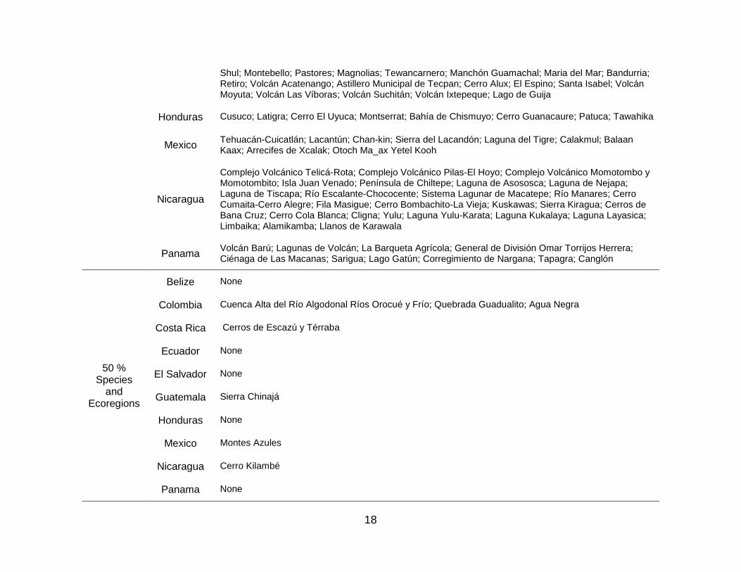
18

Shul; Montebello; Pastores; Magnolias; Tewancarnero; Manchón Guamachal; Maria del Mar; Bandurria; Retiro; Volcán Acatenango; Astillero Municipal de Tecpan; Cerro Alux; El Espino; Santa Isabel; Volcán Moyuta; Volcán Las Víboras; Volcán Suchitán; Volcán Ixtepeque; Lago de Guija

Honduras Cusuco; Latigra; Cerro El Uyuca; Montserrat; Bahía de Chismuyo; Cerro Guanacaure; Patuca; Tawahika

Mexico Tehuacán-Cuicatlán; Lacantún; Chan-kin; Sierra del Lacandón; Laguna del Tigre; Calakmul; Balaan Kaax; Arrecifes de Xcalak; Otoch Ma_ax Yetel Kooh

Nicaragua

Complejo Volcánico Telicá-Rota; Complejo Volcánico Pilas-El Hoyo; Complejo Volcánico Momotombo y Momotombito; Isla Juan Venado; Península de Chiltepe; Laguna de Asososca; Laguna de Nejapa; Laguna de Tiscapa; Río Escalante-Chococente; Sistema Lagunar de Macatepe; Río Manares; Cerro Cumaita-Cerro Alegre; Fila Masigue; Cerro Bombachito-La Vieja; Kuskawas; Sierra Kiragua; Cerros de Bana Cruz; Cerro Cola Blanca; Cligna; Yulu; Laguna Yulu-Karata; Laguna Kukalaya; Laguna Layasica; Limbaika; Alamikamba; Llanos de Karawala

Panama Volcán Barú; Lagunas de Volcán; La Barqueta Agrícola; General de División Omar Torrijos Herrera; Ciénaga de Las Macanas; Sarigua; Lago Gatún; Corregimiento de Nargana; Tapagra; Canglón

50 % Species

and Ecoregions

Belize None

Colombia Cuenca Alta del Río Algodonal Ríos Orocué y Frío; Quebrada Guadualito; Agua Negra

Costa Rica Cerros de Escazú y Térraba

Ecuador None

El Salvador None

Guatemala Sierra Chinajá

Honduras None

Mexico Montes Azules

Nicaragua Cerro Kilambé

Panama None

19

90 % Species

Belize None

Colombia Cerranía de Coraza y Montes de María; Carraipía; Cuenca Alta de Caño Alonso; Los Estoraques; Santa Rosa de Sucumbios y Santa Rosa del Guamuez; Cuenca Alta del Caño Vanguardia; Cuenca Alta del Río Cravo del Sur; Quebrada La Tablona; Guanenta Alto Río Fonce; Parque El Higuerón

Costa Rica Peñas Blancas; Río Titibí; Cerros de la Carpintera; Guayabo; Manuel Antonio; Portalón; Transilvania; Finca Barú del Pacífico; Rancho La Merced; Marino Ballena; Sierpe Térraba; Abrojo-Montezuma

Ecuador None

El Salvador La Magdalena; San Rafael Los Naranjos; El Once y La Paz

Guatemala

Chajumpec; Entre Ríos; Laguna Lachuá; Mixco Viejo-Cerro Potosí; Semuc Champey; Medio Día; Ona; Abaj Takalik; Los Aposentos; Corral Viejo; Volcán Cerro Redondo; Laguna El Pino; Santa Isabel; Volcán Cruz Quemada; Volcán Jumaytepec; Volcán y Laguna de Ipala; Volcán Tahual; Cumbre Alta; Volcán Chingo; Cipacate-Naranjo; Volcán Culma; Laguna Chichój

Honduras Cuero y Salado; Los Delgaditos; Las Iguanas-Punta Condega

Mexico Palenque; Cascada de Agua Azul; Metzabok; Najá; Lagunas de Montebello; Yagul; Lagunas de Chacagua; El Tepozteco; ZNI Calchihuites; Corredor Chichinautzin; El Veladero

Nicaragua Cerro Tomabu; Cerro Apante; Salto de Río Yasica; Yucul; Cerro Guabule; Cerro Pancasan; Cerro Musun; Cerro Bombachito-La Vieja; Llanos de Makantaka; Cabo Viejo

Panama Lagunas de Volcán

90 % Species

and Ecoregions

None

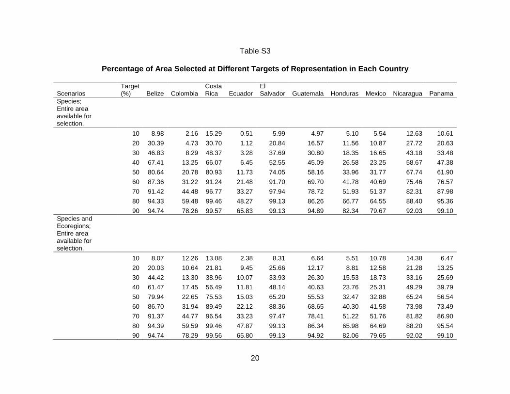
20

Table S3

Percentage of Area Selected at Different Targets of Representation in Each Country

Scenarios Target (%) Belize Colombia

Costa Rica Ecuador

El Salvador Guatemala Honduras Mexico Nicaragua Panama

Species; Entire area available for selection.

10 8.98 2.16 15.29 0.51 5.99 4.97 5.10 5.54 12.63 10.61

20 30.39 4.73 30.70 1.12 20.84 16.57 11.56 10.87 27.72 20.63

30 46.83 8.29 48.37 3.28 37.69 30.80 18.35 16.65 43.18 33.48

40 67.41 13.25 66.07 6.45 52.55 45.09 26.58 23.25 58.67 47.38

50 80.64 20.78 80.93 11.73 74.05 58.16 33.96 31.77 67.74 61.90

60 87.36 31.22 91.24 21.48 91.70 69.70 41.78 40.69 75.46 76.57

70 91.42 44.48 96.77 33.27 97.94 78.72 51.93 51.37 82.31 87.98

80 94.33 59.48 99.46 48.27 99.13 86.26 66.77 64.55 88.40 95.36

90 94.74 78.26 99.57 65.83 99.13 94.89 82.34 79.67 92.03 99.10 Species and Ecoregions; Entire area available for selection.

10 8.07 12.26 13.08 2.38 8.31 6.64 5.51 10.78 14.38 6.47

20 20.03 10.64 21.81 9.45 25.66 12.17 8.81 12.58 21.28 13.25

30 44.42 13.30 38.96 10.07 33.93 26.30 15.53 18.73 33.16 25.69

40 61.47 17.45 56.49 11.81 48.14 40.63 23.76 25.31 49.29 39.79

50 79.94 22.65 75.53 15.03 65.20 55.53 32.47 32.88 65.24 56.54

60 86.70 31.94 89.49 22.12 88.36 68.65 40.30 41.58 73.98 73.49

70 91.37 44.77 96.54 33.23 97.47 78.41 51.22 51.76 81.82 86.90

80 94.39 59.59 99.46 47.87 99.13 86.34 65.98 64.69 88.20 95.54

90 94.74 78.29 99.56 65.80 99.13 94.92 82.06 79.65 92.02 99.10

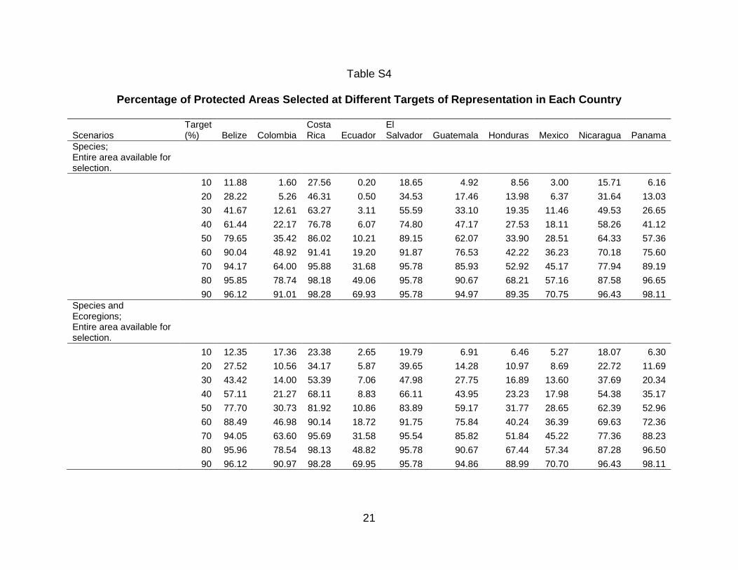
21

Table S4

Percentage of Protected Areas Selected at Different Targets of Representation in Each Country

Scenarios Target (%) Belize Colombia

Costa Rica Ecuador

El Salvador Guatemala Honduras Mexico Nicaragua Panama

Species; Entire area available for selection.

10 11.88 1.60 27.56 0.20 18.65 4.92 8.56 3.00 15.71 6.16

20 28.22 5.26 46.31 0.50 34.53 17.46 13.98 6.37 31.64 13.03

30 41.67 12.61 63.27 3.11 55.59 33.10 19.35 11.46 49.53 26.65

40 61.44 22.17 76.78 6.07 74.80 47.17 27.53 18.11 58.26 41.12

50 79.65 35.42 86.02 10.21 89.15 62.07 33.90 28.51 64.33 57.36

60 90.04 48.92 91.41 19.20 91.87 76.53 42.22 36.23 70.18 75.60

70 94.17 64.00 95.88 31.68 95.78 85.93 52.92 45.17 77.94 89.19

80 95.85 78.74 98.18 49.06 95.78 90.67 68.21 57.16 87.58 96.65

90 96.12 91.01 98.28 69.93 95.78 94.97 89.35 70.75 96.43 98.11 Species and Ecoregions; Entire area available for selection.

10 12.35 17.36 23.38 2.65 19.79 6.91 6.46 5.27 18.07 6.30

20 27.52 10.56 34.17 5.87 39.65 14.28 10.97 8.69 22.72 11.69

30 43.42 14.00 53.39 7.06 47.98 27.75 16.89 13.60 37.69 20.34

40 57.11 21.27 68.11 8.83 66.11 43.95 23.23 17.98 54.38 35.17

50 77.70 30.73 81.92 10.86 83.89 59.17 31.77 28.65 62.39 52.96

60 88.49 46.98 90.14 18.72 91.75 75.84 40.24 36.39 69.63 72.36

70 94.05 63.60 95.69 31.58 95.54 85.82 51.84 45.22 77.36 88.23

80 95.96 78.54 98.13 48.82 95.78 90.67 67.44 57.34 87.28 96.50

90 96.12 90.97 98.28 69.95 95.78 94.86 88.99 70.70 96.43 98.11

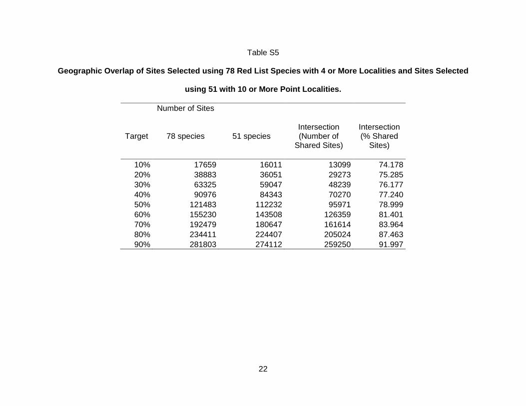
22

Table S5

Geographic Overlap of Sites Selected using 78 Red L ist Species with 4 or More Localities and Sites Sel ected

using 51 with 10 or More Point Localities.

Number of Sites

Target 78 species 51 species Intersection (Number of

Shared Sites)

Intersection (% Shared

Sites)

10% 17659 16011 13099 74.178 20% 38883 36051 29273 75.285 30% 63325 59047 48239 76.177 40% 90976 84343 70270 77.240 50% 121483 112232 95971 78.999 60% 155230 143508 126359 81.401 70% 192479 180647 161614 83.964 80% 234411 224407 205024 87.463 90% 281803 274112 259250 91.997

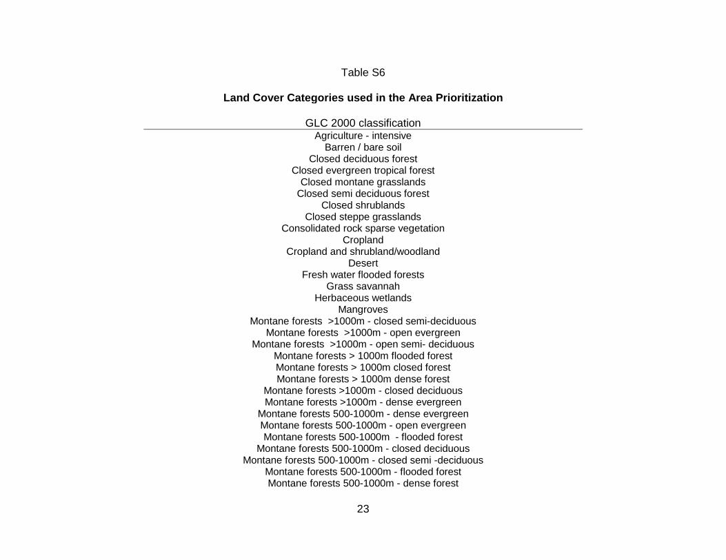
23

Table S6

Land Cover Categories used in the Area Prioritization

GLC 2000 classification Agriculture - intensive

Barren / bare soil Closed deciduous forest

Closed evergreen tropical forest Closed montane grasslands

Closed semi deciduous forest Closed shrublands

Closed steppe grasslands Consolidated rock sparse vegetation

Cropland Cropland and shrubland/woodland

Desert Fresh water flooded forests

Grass savannah Herbaceous wetlands

Mangroves Montane forests >1000m - closed semi-deciduous

Montane forests >1000m - open evergreen Montane forests >1000m - open semi- deciduous

Montane forests > 1000m flooded forest Montane forests > 1000m closed forest Montane forests > 1000m dense forest

Montane forests >1000m - closed deciduous Montane forests >1000m - dense evergreen

Montane forests 500-1000m - dense evergreen Montane forests 500-1000m - open evergreen Montane forests 500-1000m - flooded forest

Montane forests 500-1000m - closed deciduous Montane forests 500-1000m - closed semi -deciduous

Montane forests 500-1000m - flooded forest Montane forests 500-1000m - dense forest

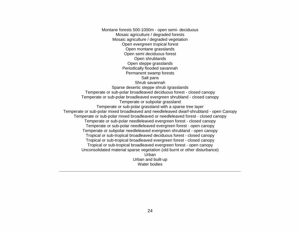
24

Montane forests 500-1000m - open semi- deciduous Mosaic agriculture / degraded forests

Mosaic agriculture / degraded vegetation Open evergreen tropical forest

Open montane grasslands Open semi deciduous forest

Open shrublands Open steppe grasslands

Periodically flooded savannah Permanent swamp forests

Salt pans Shrub savannah

Sparse desertic steppe shrub /grasslands Temperate or sub-polar broadleaved deciduous forest - closed canopy

Temperate or sub-polar broadleaved evergreen shrubland - closed canopy Temperate or subpolar grassland

Temperate or sub-polar grassland with a sparse tree layer Temperate or sub-polar mixed broadleaved and needleleaved dwarf-shrubland - open Canopy

Temperate or sub-polar mixed broadleaved or needleleaved forest - closed canopy Temperate or sub-polar needleleaved evergreen forest - closed canopy Temperate or sub-polar needleleaved evergreen forest - open canopy

Temperate or subpolar needleleaved evergreen shrubland - open canopy Tropical or sub-tropical broadleaved deciduous forest - closed canopy Tropical or sub-tropical broadleaved evergreen forest - closed canopy Tropical or sub-tropical broadleaved evergreen forest - open canopy

Unconsolidated material sparse vegetation (old burnt or other disturbance) Urban

Urban and built-up Water bodies

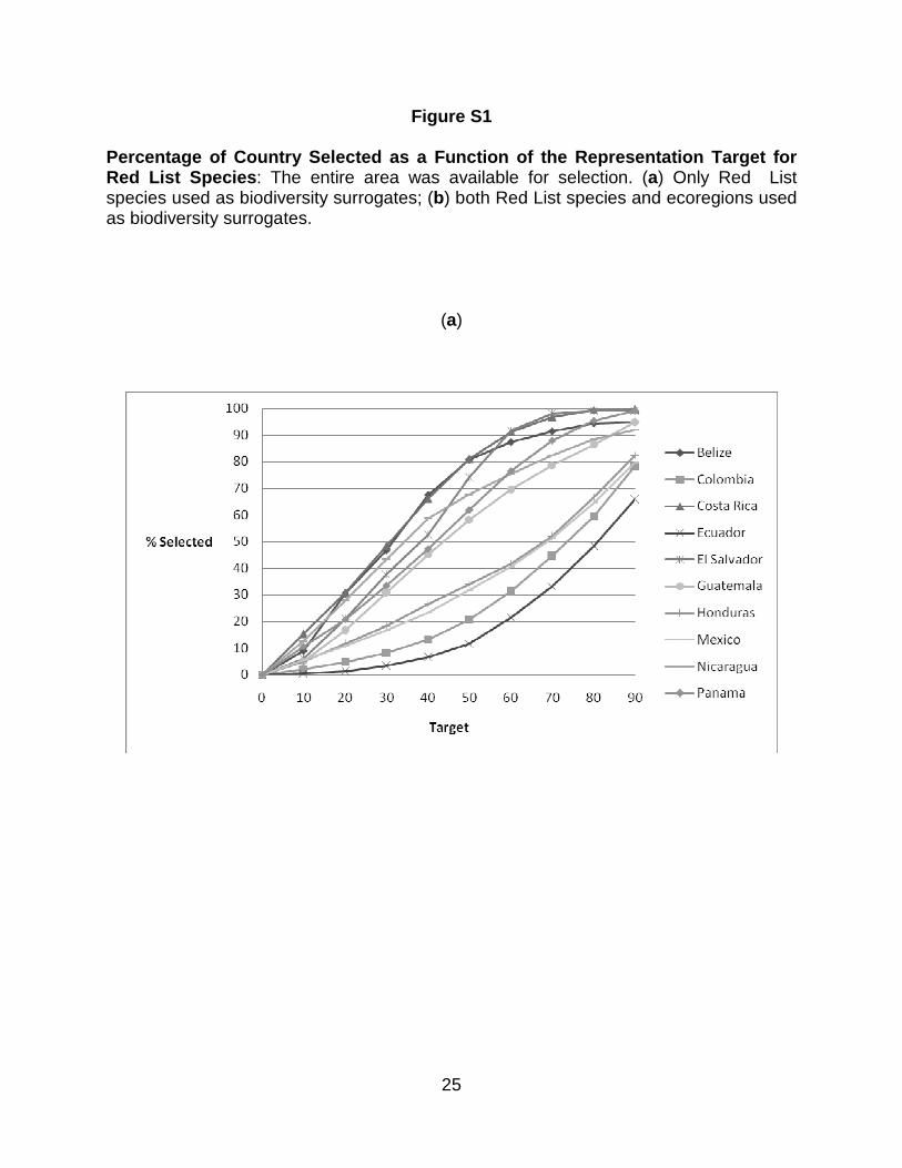
25

Figure S1 Percentage of Country Selected as a Function of the Representation Target for Red List Species : The entire area was available for selection. (a) Only Red List species used as biodiversity surrogates; (b) both Red List species and ecoregions used as biodiversity surrogates.

(a)

26

(b)