© Copyright 2021 Natalie Lowell - Scholarly Publishing Services

© Copyright 2021

Natalie Lowell

A genetic risk assessment of native shellfish aquaculture

Natalie Lowell

A dissertation

submitted in partial fulfillment of the

requirements for the degree of

Doctor of Philosophy

University of Washington

2021

Reading Committee:

Lorenz Hauser, Chair

Eric Ward

Kerry-Ann Naish

Sarah Converse

Phillip Scott Levin

Program Authorized to Offer Degree:

School of Aquatic and Fishery Sciences

University of Washington

Abstract

A genetic risk assessment of native shellfish aquaculture

Natalie Lowell

Chair of the Supervisory Committee:

Dr. Lorenz Hauser

School of Aquatic and Fishery Sciences

Global aquaculture production is expanding, as the demand for marine protein cannot be

met by capture fisheries alone. Within shellfish aquaculture, growers have begun to cultivate

native shellfish to limit introduction of non-native species. However, cultivation of native species

poses genetic risks to wild populations if farmed and wild animals interbreed, such as loss of

genetic diversity within and among populations and loss of fitness due to domestication

selection. These risks threaten long-term viability of wild populations, and are thus a concern for

sustainable resource management. Genetic risks of native shellfish aquaculture have received

little science and policy attention, limiting effective management of aquaculture impacts to wild

populations. In my first two chapters, I quantified and characterized population structure in wild

populations of two native shellfish species considered for aquaculture: the Purple-hinged Rock

Scallop, Crassadoma gigantea (Chapter 1), and the California Sea Cucumber, Apostichopus

californicus (Chapter 2). These results can be used by decision-makers to inform spatial

management of wild shellfish species, including mitigating impacts from aquaculture. To support

potential policy development regarding the genetic risks of native shellfish aquaculture, I

interviewed co-managers of shellfish resources along the Pacific Coast of the United States to

characterize the regulatory context for this emerging policy issue (Chapter 3). Lastly, I

developed a simulation model for quantifying genetic risks of native shellfish aquaculture and

used the model in a management strategy evaluation for Olympia oyster (Chapter 4), a species

grown for commercial and conservation purposes.

i

TABLE OF CONTENTS

List of Figures ................................................................................................................................ vi

List of Tables ................................................................................................................................ vii

List of Supplemental Tables ........................................................................................................ viii

List of Supplemental Figures ........................................................................................................ xii

Chapter 1. Subtle population structure and adaptive differentiation in the purple-hinged rock

scallop, Crassadoma gigantea ........................................................................................................ 2

1.1 Introduction ..................................................................................................................... 2

1.2 Methods........................................................................................................................... 5

1.2.1 Sample collection ........................................................................................................ 5

1.2.2 DNA library preparation ............................................................................................. 6

1.2.3 Genotyping individuals ............................................................................................... 6

1.2.4 Quantifying population structure ................................................................................ 7

1.2.5 Identifying putatively adaptive SNPs ......................................................................... 9

1.2.6 Comparing putatively neutral and adaptive SNPs .................................................... 11

1.2.7 Simulations ............................................................................................................... 11

1.3 Results ........................................................................................................................... 12

1.3.1 Sequencing ................................................................................................................ 12

1.3.2 Population structure .................................................................................................. 13

1.3.3 Putatively adaptive differentiation ............................................................................ 14

1.3.4 Neutral vs. putatively adaptive differentiation .......................................................... 14

ii

1.3.5 Simulations ............................................................................................................... 15

1.4 Discussion ..................................................................................................................... 16

1.4.1 Evidence for subtle population structure and adaptive differentiation ..................... 16

1.4.2 Considerations for inferring population connectivity from subtle population structure

19

1.4.3 Conclusions and future directions ............................................................................. 24

1.5 Tables and figures ......................................................................................................... 26

1.6 Supplementary Materials .............................................................................................. 32

Chapter 2. Population structure and adaptive differentiation in the sea cucumber Apostichopus

californicus and implications for spatial resource management ................................................... 42

2.1 Introduction ................................................................................................................... 42

2.2 Methods......................................................................................................................... 47

2.2.1 Sample collection ...................................................................................................... 47

2.2.2 DNA library preparation ........................................................................................... 47

2.2.3 Genotyping individuals ............................................................................................. 48

2.2.4 Population genetic structure analyses ....................................................................... 49

2.2.5 Identifying putative adaptive differentiation ............................................................ 50

2.2.6 Comparing putatively neutral and adaptive differentiation ...................................... 53

2.2.7 Simulations ............................................................................................................... 54

2.3 Results ........................................................................................................................... 55

2.3.1 Sequencing ................................................................................................................ 55

2.3.2 Population structure .................................................................................................. 56

2.3.3 Adaptive differentiation ............................................................................................ 57

iii

2.3.4 Neutral vs. putatively adaptive differentiation .......................................................... 59

2.3.5 Simulations ............................................................................................................... 60

2.4 Discussion ..................................................................................................................... 61

2.4.1 Broad- and fine-scale population genetic structure and potential drivers ................. 61

2.4.2 Spatial considerations for sustainable management of A. californicus .................... 66

2.5 Tables and figures ......................................................................................................... 69

2.6 Supplementary materials ............................................................................................... 77

Chapter 3. Informal policy and factors affecting policy change for genetic risks of native

shellfish aquaculture ..................................................................................................................... 90

3.1 Introduction ................................................................................................................... 90

3.1.1 What are the genetic risks of native shellfish aquaculture? ...................................... 90

3.1.2 What information would inform potential policy development? .............................. 93

3.1.3 Study aim .................................................................................................................. 94

3.2 Methods......................................................................................................................... 95

3.2.1 Study system ............................................................................................................. 95

3.2.2 Interview methodology ............................................................................................. 96

3.3 Results and discussion .................................................................................................. 98

3.3.1 If and how are genetic risks currently managed? ...................................................... 99

3.3.2 What factors may affect policy change regarding genetic risks of native shellfish

aquaculture? ........................................................................................................................ 100

3.3.3 How much policy attention do genetic risks of native shellfish aquaculture receive

and why? ............................................................................................................................. 106

3.4 Study limitations ......................................................................................................... 109

iv

3.5 Conclusions ................................................................................................................. 110

3.6 Tables and figures ....................................................................................................... 111

Chapter 4. Genetic risk assessment model for native shellfish aquaculture ............................... 119

4.1 Introduction ................................................................................................................. 119

4.2 Methods....................................................................................................................... 123

4.2.1 Model description ................................................................................................... 123

4.2.2 State variables and scales ........................................................................................ 126

4.2.3 Process overview and scheduling ........................................................................... 128

4.2.4 Initialization ............................................................................................................ 130

4.2.5 Input ........................................................................................................................ 130

4.2.6 Submodels ............................................................................................................... 131

4.2.7 Simulation experiment: Olympia Oyster management strategy evaluation ........... 134

4.3 Results ......................................................................................................................... 136

4.3.1 Within-population genetic diversity ....................................................................... 138

4.3.2 Among-population genetic diversity....................................................................... 139

4.3.3 Fitness ..................................................................................................................... 140

4.4 Discussion ................................................................................................................... 141

4.4.1 Within-population genetic diversity ....................................................................... 142

4.4.2 Among-population genetic diversity....................................................................... 146

4.4.3 Fitness ..................................................................................................................... 149

4.4.4 Evaluating model approach & future directions ..................................................... 151

4.4.5 Management implications and conclusions ............................................................ 153

4.5 Tables and figures ....................................................................................................... 155

v

4.6 Supplementary materials ............................................................................................. 160

Bibliography ............................................................................................................................... 184

vi

LIST OF FIGURES

Figure 1-1: A map of collection sites and DAPC results for C. gigantea. ....................... 29

Figure 1-2: Summary of putatively adaptive loci for C. gigantea. ................................... 30

Figure 1-3: Simulation results to contextualize empirical population differentiation and estimate

connectivity for C. gigantea...................................................................................... 31

Figure 2-1: A map of collection sites and DAPC results for A. californicus. ................... 73

Figure 2-2: Evidence for isolation-by-distance in A. californicus. ................................... 74

Figure 2-3: Results of FST outlier detection methods for A. californicus. ........................ 74

Figure 2-4: Summary of the results of univariate (Bayenv2) and multivariate (RDA) gene-

environment associations for A. californicus. ........................................................... 75

Figure 2-5: Simulation results to contextualize empirical population differentiation and estimate

connectivity for A. californicus. ................................................................................ 76

Figure 3-1: Conceptual diagram of the types of genetic risks and their relevance to conservation

and sustainable resource management. ................................................................... 115

Figure 3-2: Manager responses to whether the manager’s agency (A) manages for genetic risks

of native shellfish aquaculture in any way and (B) regulates or advises aquaculture in any

way. ......................................................................................................................... 116

Figure 3-3: Graphical representation of the frequency and relationship of reported concerns for

the future of wild shellfish resources using direct and indirect questioning. .......... 117

Figure 3-4: Histograms representing level of concern regarding genetic risks of native shellfish

aquaculture, reported directly by managers. ........................................................... 118

Figure 4-1: Model structure and order of processes in monthly time steps. ................... 156

Figure 4-2: Comparing response variables by scenario theme, under High Selection and High

Escape conditions. ................................................................................................... 157

Figure 4-3: Box plots comparing percent change per response variable by scenario. .... 158

Figure 4-4: Box plots comparing percent change per response variable by scenario theme.159

Figure 4-5: Box plots comparing percent change per response variable by scenario conditions.

................................................................................................................................. 159

vii

LIST OF TABLES

Table 1-1: General information by collection site for C. gigantea. .................................. 26

Table 1-2: Pairwise FST between collection sites using all SNPs for C. gigantea. ........... 26

Table 1-3: Hierarchical population structure results (AMOVA) for C. gigantea. ............ 27

Table 1-4: Summary of gene-environment association results for C. gigantea, for five

environmental variables with the highest number of correlated SNPs. .................... 27

Table 1-5: LD Ne estimates with 95% confidence intervals per collection site for C. gigantea.

................................................................................................................................... 28

Table 2-1: General information by collection site for A. californicus. ............................. 69

Table 2-2: Hierarchical population structure results (AMOVA) for A. californicus. ....... 69

Table 2-3: Pairwise FST and genic differentiation test results for A. californicus. ........... 70

Table 2-4: LD effective population size (Ne) estimates with 95% confidence intervals per

collection site for A. californicus. ............................................................................. 70

Table 2-5: Summary of results from Bayenv2 for A. californicus, for five environmental

predictors with the most correlated SNPs. ................................................................ 71

Table 2-6: Results of the redundancy analyses (RDA). .................................................... 72

Table 3-1: Summary of manager responsibilities. .......................................................... 111

Table 3-2: Examples of Hatchery and Genetic Management Plan requirements pertaining to all

three types of genetic risks. ..................................................................................... 112

Table 3-3: Manager recommendations for future policy development regarding genetic risks of

native shellfish aquaculture. .................................................................................... 113

Table 3-4: The reported factors driving concern and lack of concern for genetic risks of native

shellfish aquaculture. .............................................................................................. 113

Table 3-5: Reported methods of regulating or advising aquaculture. ............................. 114

Table 4-1: Allele fitness effects. ..................................................................................... 155

Table 4-2: Scenario theme descriptions. ......................................................................... 155

Table 4-3: Percent of significant Tukey tests per response variable. ............................. 155

viii

LIST OF SUPPLEMENTAL TABLES

Supplemental Table 1-1: Environmental predictor codes and descriptions from Bio-Oracle (BO)

and Bio-Oracle2 (BO2) databases, used in Bayenv2. ............................................... 32

Supplemental Table 1-2: Sites remaining after each filtering step for C. gigantea. ......... 33

Supplemental Table 1-3: Summary of Bayenv2 results for C. gigantea........................... 34

Supplemental Table 1-4: Correlation among environmental predictors measured at collection

sites for C. gigantea. ................................................................................................. 35

Supplemental Table 1-5: Spatial autocorrelation of environmental predictors used in Bayenv2 for

C. gigantea. ............................................................................................................... 36

Supplemental Table 1-6: Global, mean pairwise, minimum pairwise, and maximum pairwise FST

using all (n = 5,932), putatively neutral (n = 5,823), and putatively adaptive SNPs (n = 109).

................................................................................................................................... 37

Supplemental Table 1-7: Pairwise FST using putatively neutral SNPs. ............................ 37

Supplemental Table 1-8: Pairwise FST using putatively adaptive SNPs. .......................... 37

Supplemental Table 2-1: Pairwise FST and genic differentiation test results, to compare de novo

and reference-guided locus assemblies. .................................................................... 77

Supplemental Table 2-2: Expected heterozygosity, observed heterozygosity, and proportion of

polymorphic SNPs by collection site, comparing de novo and reference-guided assemblies.

................................................................................................................................... 78

Supplemental Table 2-3: Pearson’s correlation coefficients among 29 environmental predictors.

................................................................................................................................... 78

Supplemental Table 2-4: All environmental predictor loadings on retained PCs. ........... 79

Supplemental Table 2-5: Sea surface predictor loadings for retained PCs. ...................... 80

Supplemental Table 2-6: Bottom depth predictor loadings for retained PCs. .................. 81

Supplemental Table 2-7: Current velocity and temperature predictor loadings for retained PCs.

................................................................................................................................... 82

Supplemental Table 2-8: Sites retained at each filtering step in A. californicus. ............. 82

ix

Supplemental Table 2-9: Pairwise FST with confidence intervals and pairwise genic

differentiation test results. ......................................................................................... 83

Supplemental Table 2-10: Bayenv2 results for A. californicus. ........................................ 84

Supplemental Table 2-11: Loadings for RDA using sea surface predictors. .................... 86

Supplemental Table 2-12: Loadings for RDA using current and temperature predictors. 86

Supplemental Table 2-13: Counts of gene ontology slim terms in the database. ............. 87

Supplemental Table 4-1: Parameter symbols, descriptions, and default values. ............ 160

Supplemental Table 4-2: Mean, minimum, and pairwise FST from simulations and the empirical

values for comparison. ............................................................................................ 161

Supplemental Table 4-3: Transition matrix for wild migration. ..................................... 161

Supplemental Table 4-4: Stable subpopulation sizes, by model phase. ......................... 161

Supplemental Table 4-5: Stable Farm sizes, by theme. .................................................. 161

Supplemental Table 4-6: Survival and survivorship estimates by age class for the population.

................................................................................................................................. 162

Supplemental Table 4-7: Analysis of variance (ANOVA) results, using all wild subpopulations.

................................................................................................................................. 162

Supplemental Table 4-8: Tukey test results using all wild subpopulations for percent change in

heterozygosity, for pairwise comparisons of the 12 scenarios................................ 163


mean fitness, for pairwise comparisons of the 12 scenarios. .................................. 164


adaptive FST, for pairwise comparisons of the 12 scenarios. .................................. 164


neutral FST, for pairwise comparisons of the 12 scenarios. ..................................... 165


allelic richness, for pairwise comparisons of the 12 scenarios. .............................. 165


heterozygosity, for pairwise comparisons of the three scenario themes. ................ 166


allelic richness, for pairwise comparisons of the three scenario themes. ............... 166

x


neutral FST, for pairwise comparisons of the three scenario themes. ...................... 166


adaptive FST, for pairwise comparisons of the three scenario themes. ................... 167


mean fitness, for pairwise comparisons of the three scenario themes. ................... 167


heterozygosity, for pairwise comparisons of the four scenario conditions. ............ 167


adaptive FST, for pairwise comparisons of the four scenario conditions. ............... 168


mean fitness, for pairwise comparisons of the four scenario conditions. ............... 168


allelic richness, for pairwise comparisons of the four scenario conditions. ........... 168


neutral FST, for pairwise comparisons of the four scenario conditions. .................. 168

Supplemental Table 4-23: Analysis of variance (ANOVA) results, using only Wild 1. 169

Supplemental Table 4-24: Tukey test results using only Wild 1 for percent change in

heterozygosity, for pairwise comparisons of the 12 scenarios................................ 169

Supplemental Table 4-25: Tukey test results using only Wild 1 for percent change in mean

fitness, for pairwise comparisons of the 12 scenarios. ............................................ 170

Supplemental Table 4-26: Tukey test results using only Wild 1 for percent change in adaptive

FST, for pairwise comparisons of the 12 scenarios. ................................................. 170

Supplemental Table 4-27: Tukey test results using only Wild 1 for percent change in neutral FST,

for pairwise comparisons of the 12 scenarios. ........................................................ 171

Supplemental Table 4-28: Tukey test results using only Wild 1 for percent change in allelic

richness, for pairwise comparisons of the 12 scenarios. ......................................... 171


heterozygosity, for pairwise comparisons of the three scenario themes. ................ 172

xi


richness, for pairwise comparisons of the three scenario themes. .......................... 172

Supplemental Table 4-31: Tukey test results using only subpopulation pairs containing Wild 1

for percent change in neutral FST, for pairwise comparisons of the three scenario themes.

................................................................................................................................. 172


for percent change in adaptive FST, for pairwise comparisons of the three scenario themes.

................................................................................................................................. 173


fitness, for pairwise comparisons of the three scenario themes. ............................. 173


heterozygosity, for pairwise comparisons of the four scenario conditions. ............ 173

Supplemental Table 4-35: Tukey test results using only subpopulations containing Wild 1 for

percent change in adaptive FST, for pairwise comparisons of the four scenario conditions.

................................................................................................................................. 174


fitness, for pairwise comparisons of the four scenario conditions. ......................... 174


richness, for pairwise comparisons of the four scenario conditions. ...................... 174

Supplemental Table 4-38: Tukey test results using only Wild 1 for percent change in neutral FST,

for pairwise comparisons of the four scenario conditions. ..................................... 174

xii

LIST OF SUPPLEMENTAL FIGURES

Supplemental Figure 1-1: Histograms of locus FIS. .......................................................... 38

Supplemental Figure 1-2: Discriminant analysis of principal components, presented separately

by discriminant function. .......................................................................................... 39

Supplemental Figure 1-3: Results from ADMIXTURE for C. gigantea. .......................... 39

Supplemental Figure 1-4: Tests for isolation-by-distance for C. gigantea. ...................... 40

Supplemental Figure 1-5: Venn diagram demonstrating overlap of putatively adaptive SNPs by

method for C. gigantea. ............................................................................................ 41

Supplemental Figure 2-1: Principal component analysis to compare reference-guided and de

novo locus assemblies. .............................................................................................. 88

Supplemental Figure 2-2: Overfitting of RDA models occurred quickly with the addition of

predictor variables. .................................................................................................... 88

Supplemental Figure 2-3: Cross validation error by number of assumed underlying populations

in ADMIXTURE clustering analysis. ........................................................................ 89

Supplemental Figure 2-4: Venn diagram showing overlap among putatively adaptive SNPs by

method for A. californicus. ....................................................................................... 89

Supplemental Figure 4-1: Grower survey results, reporting distance between farm and closest

wild population. ...................................................................................................... 175

Supplemental Figure 4-2: Grower survey results for seasonality of planting and harvesting.

................................................................................................................................. 175

Supplemental Figure 4-3: Mean population size (and 95% confidence interval) over time, per

subpopulation, faceted by scenario theme and conditions. ..................................... 176

Supplemental Figure 4-4: Mean heterozygosity (and 95% confidence interval) over time, per


Supplemental Figure 4-5: Mean log10 allelic richness (and 95% confidence interval) over time,

per subpopulation, faceted by scenario theme and conditions. ............................... 178

Supplemental Figure 4-6: Mean neutral FST (and 95% confidence interval) over time, per


xiii

Supplemental Figure 4-7: Mean neutral FST (and 95% confidence interval) over time between

Wild 1 and Wild 2, faceted by scenario theme and conditions. .............................. 180

Supplemental Figure 4-8: Mean adaptive FST (and 95% confidence interval) over time by


Supplemental Figure 4-9: Mean fitness (and 95% confidence interval) over time, by


Supplemental Figure 4-10: Mean fitness (and 95% confidence interval) over time, by wild


xiv

ACKNOWLEDGEMENTS

I am grateful to so many people for supporting my education and professional

development during my PhD. I thank my adviser, Lorenz Hauser, for his guidance on population

genetic theory and his support for my choice to pursue a multi-disciplinary PhD. I am also

grateful to my committee members, which included Kerry Naish, Sarah Converse, Eric Ward,

and Phil Levin, for their mentorship and for helping me see the path to graduation when I

couldn’t see it myself. I am grateful to Steven Roberts and Sam White for providing access to

computing resources and supporting the development of my computing skills. My research

would not have been possible (or nearly as fun) without the mentorship of my lab mates and

peers, especially Eleni Petrou, Carolyn Tarpey, Isadora Jimenez-Hidalgo, Katherine Silliman,

Molly Jackson, Charlie Waters, Dan Drinan, Maya Garber-Yonts, and Mary Fisher.

My research would not have been possible without the support of funding agencies and

collaborators. This work was supported by the NOAA Saltonstall-Kennedy program

(#NA15NMF4270322), by a grant from Washington Sea Grant, University of Washington,

pursuant to National Oceanic and Atmospheric Administration (Award No. NA17OAR4170223,

R/SFA/N-5), and a National Marine Fisheries Service – Sea Grant Joint Fellowship (Award No

NA17OAR4170241). The views or opinions expressed herein are those of the author(s) and do not

necessarily reflect the views of NOAA or any of its sub-agencies. I am grateful for all of my helpful

co-authors and other collaborators that made this work possible. Scallop samplers included Brian

Allen and Josh Bouma (Puget Sound Restoration Fund), Gordon King (Taylor Shellfish Farms),

Hans Daubenberger (Port Gamble S’Klallam Tribe), Kelly Toy, Ralph Riccio and Christopher

Burns (Jamestown S’Klallam Tribe), Luke Kelly and Viviane Berry (Suquamish Tribe), Bob

xv

Sizemore, Michael Ulrich, Ocean Working, Bethany Stevick and Henry Carson (Washington

Department of Fish and Wildlife). Sea cucumber samplers included Vassili Kalashnikov, Michael

Ulrich, and Larry LeClair, (Washington Department of Fish and Wildlife), Viviane Barry and

Elizabeth Unsell (Suquamish Tribe), and Mike McCorkle (California Department of Fish and

Wildlife). We thank W. Stewart Grant and Wei Cheng (Alaska Department of Fish and Game) for

providing DNA samples. I extend my gratitude to the 23 shellfish growers that responded to our

survey and the 18 co-managers that participated in our interviews, making this research possible.

I rarely felt like I belonged in my PhD, and am particularly grateful for everyone who

took risks to make academia more fair, safe, and inclusive, especially Isadora Jimenez-Hidalgo,

Ann Corboy, Staci Amburgey, Lisa Cantore, Eleni Petrou, Ashley Townes, Yaamini

Venkataraman, Kristin Privatera-Johnson, Jenny Stern, Hannah Bassett, Natalie Mastick, Sara

Faiad, and Mark Sorel. Thanks to Amy Fox and Sam Scherer for supporting students and

amplifying their voices.

I am grateful for Seven Star Women’s Kung Fu. Through my training at Seven Star, I

developed fighting skills that were transferable to and necessary for my success in graduate

school, including staying grounded through adversity, setting and affirming boundaries, and

accessing my fighting spirit.

My family and friends are the best. I am grateful for the unending love and support from

my parents, Bob and Diana. My brother, Alex, was my personal tech support, dropping anything

to help me with a computing problem. I am grateful for my family in Orinda, who have always

been among my greatest supporters. Through my friendship with Emily Jacobs-Palmer, I am

always growing, laughing, and feeling good in my skin. I am grateful for Analucia Arredondo for

having supported my pursuit of science since we were children. I am grateful for Jenny Stern,

xvi

who knew exactly how graduate school made me feel and what to say to keep me grounded,

especially as I approached the finish line. I extend my gratitude to Molly Korab and Mathis

Messager, who taught me that I don’t have to feel alone in hardship. I thank Mike Chang for

teaching me to stay heart-centered in my professional life. I am grateful for Caroline Daws, who

inspires me with her ambition and centers me with her kindness. I thank Erica Newman for

teaching me how I deserve to be treated professionally. I am grateful for my supportive

neighbors at Capitol Hill Apartments who make my home so special, especially Joe and Shana

Tinsley, Scot Augustson, Tonia Arehart, Anders Chen, Mike Klein, and Kate and Michael

Decramer.

The pandemic made finishing a PhD even harder. I would not have made it through the

pandemic without M Auden, Chris Landingin, Narisa Spaulding, Max Glass, and Elia Grenier,

who helped make sure that we stayed socially connected despite physical distancing. Regular

alley walks, owl visits, and porch hangs are tender memories for me, despite the backdrop of

hardship. I learned a lot about being part of a community with these friends, especially that it’s

good (for everyone) to ask for help when we need it.

xvii

DEDICATION

This dissertation is dedicated to the Pacific Ocean. Hey there, Ocean, you’re so big.

2

Chapter 1. Subtle population structure and adaptive differentiation in the

purple-hinged rock scallop, Crassadoma gigantea

1.1 INTRODUCTION

Over the last several decades, many studies have uncovered population structure in marine

species and thus overturned the traditional paradigm of ubiquitous panmixia in marine populations

(Hauser & Carvalho, 2008; Palumbi, 2004; Sanford & Kelly, 2011). Increasing evidence suggests

that marine dispersal is more restricted than previously thought, due to larval behavior that results

in non-random dispersal (D’Aloia et al., 2015; Gerlach et al., 2007) and oceanographic barriers

such as narrow straits and gyres (Shields et al., 2010) Additionally, the increased statistical power

associated with advances in sequencing technologies, including higher marker density and

inclusion of markers under selection (Stapley et al., 2010), has allowed for improved detection of

subtle population differentiation. Nonetheless, population differentiation in marine species

remains generally smaller than in terrestrial systems (Waples, 1998), due in part to greater

dispersal potential (Kinlan & Gaines, 2003), lack of physical barriers, and larger population sizes

common to many marine species. These factors lead to high gene flow and minimal genetic drift,

both of which act to minimize the development of population differentiation. However, in some

species, adaptive differentiation can be maintained despite high gene flow (G. Anderson et al.,

2019). Thus, selection may play a larger role than drift in driving subtle patterns of population

differentiation in some marine species.

If populations are differentiated in an exploited species, then effective resource

management will benefit from characterization of population structure. Although populations lack

a singular definition, a common definition is a group of individuals that can reproduce with each

other (R. S. Waples & Gaggiotti, 2006). In the context of fisheries, populations can be considered

3

as an important criterion for designating appropriate units for management. When management

units do not match with true biological populations, fishing may lead to overexploitation (Ying et

al., 2011). In the context of aquaculture, data on population structure can be used to restrict transfer

of broodstock and seed to within distinct populations, such as shellfish transfer zones used in

British Columbia (DFO Aquaculture Management Division, 2016), in order to minimize loss of

genetic diversity among populations (Waples et al., 2012).

One species that supports recreational fisheries and aquaculture is the Purple-hinged Rock

Scallop, Crassadoma gigantea, a marine bivalve of the Pacific Coast of North America. Due to its

patchy distribution and potentially limited abundance, commercial fisheries are prohibited across

the range (Leet, 2001). The lack of commercial fisheries for C. gigantea has led many to pursue

aquaculture production as a promising method of increasing supply. However, C. gigantea

aquaculture has been slow to develop (Leighton & Phleger, 1977; Menzel, 2018) due to challenges

in identifying necessary settlement conditions (RaLonde et al., 2012). Nevertheless, there are

renewed efforts in developing large-scale production methods (Catalina Sea Ranch, 2019; Culver

et al., 2006). Because of their patchy distribution and potentially limited abundance, there is

potential for local depletions through broodstock collection and potential for population

differentiation that could be disrupted through broodstock collection and farm escape. The likely

expansion of C. gigantea aquaculture warrants careful consideration of population structure for

effective management, yet no estimates of population structure exist for the species.

Population differentiation can be shaped by life history, such as high dispersal in species

with pelagic larvae leading to lower population differentiation (Selkoe & Toonen, 2011). C.

gigantea is a broadcast spawning species with a pelagic larval duration of about four weeks

(Shumway & Parsons, 2016). After settlement, young juveniles can swim in short bursts and attach

4

to substrates with byssal threads. Unlike most species of scallop, C. gigantea cement to a substrate

permanently at around six months of age (Menzel, 2018; Shumway & Parsons, 2016), suggesting

lower dispersal potential than other scallop species and comparable dispersal potential to other

sessile, broadcast-spawning bivalves. Although life span has not been rigorously estimated, C.

gigantea are considered relatively long-lived, with a life span of at least 20 years (MacDonald et

al., 1991). Fecundity has not been quantified, although C. gigantea is generally considered to have

high fecundity (Laurén, 1982; Llodra, 2002); for comparison, other scallop species produce

hundreds of thousands to millions of eggs per spawn event (Cochard & Devauchelle, 1993). C.

gigantea are iteroparous, and may be able to spawn multiple times per year (Laurén, 1982). Spawn

timing varies by region, with spawning occurring in summer to fall in Washington (Laurén, 1982)

and British Columbia (MacDonald & Bourne, 1989) and in fall to winter in California (Jacobsen,

1977), a potential signal of adaptive differentiation.

Population differentiation can also be shaped by marine biogeography (Costello &

Chaudhary, 2017; Selkoe et al., 2016). C. gigantea is patchily distributed from Baja California,

Mexico to Alaska, from subtidal habitats to depths of 80 m (Dijkstra, 2010). Within this region,

several known oceanographic barriers to dispersal have shaped population structure in other

marine species. For example, the North Pacific Current, which bifurcates as it approaches the coast

of British Columbia, has been identified as an oceanographic barrier to dispersal in the California

Sea Cucumber (Chapter 2; Xuereb et al., 2018) and the Bat Star (Keever et al., 2009). Point

Conception in central California has also been identified as an oceanographic barrier to dispersal

in several marine species with planktonic dispersal (Pelc et al., 2009). Lastly, the Salish Sea, an

estuary divided into sub-basins by shallow sills, contains genetically distinct populations of Pacific

5

Cod (Cunningham et al., 2009) and Brown Rockfish (Buonaccorsi et al., 2005). It is unknown

whether these oceanographic features shape population structure in C. gigantea.

The goals of this study were to quantify and describe patterns of population differentiation

for C. gigantea to facilitate the development of guidelines for aquaculture and fisheries

management. We sampled populations at a small geographic scale within the Salish Sea and at a

large geographic scale across the species range along the northeastern Pacific coast to test for both

fine- and broad-scale population structure. The Salish Sea was chosen as a region of focus because

it is known to harbor genetically distinct populations of some marine species (Andrews et al., 2018;

Buonaccorsi et al., 2005; Cunningham et al., 2009) and because it contains the majority of

aquaculture production in Washington state, the largest shellfish aquaculture producer in the

United States (Northern Economics, 2013). Our results were used to generate hypotheses about

potential drivers of population structure, including environmental factors that may drive observed

putative adaptive differentiation. Lastly, we considered the management implications of a weak

signal in population structure and made recommendations for decision makers regarding

designation of management units for C. gigantea.

1.2 METHODS

1.2.1 Sample collection

Approximately 50 adult C. gigantea were collected by scuba divers from seven sites along

the Pacific Coast of North America, ranging from Alaska to California (Table 1-1). For each

animal, a tissue sample was excised from the mantle and stored in 100% ethanol.

6

1.2.2 DNA library preparation

DNA was extracted from tissue samples using the EZNA Mollusc DNA Kit (OMEGA Bio-

tek, Norcross, GA, USA) and quantified using the Quant-iT PicoGreen dsDNA Assay Kit (Thermo

Fisher Scientific, Waltham, MA, USA). DNA quality was checked by gel electrophoresis. DNA

concentration was normalized to 500 ng in 20 µL of PCR-grade water. We selected samples with

high DNA quality for RAD sequencing, and RAD libraries were prepared following an established

protocol (Etter et al., 2011) with restriction enzyme SbfI. Briefly, DNA samples were restricted

and barcodes with a unique six-base identifier sequence and the Illumina P1 adapter were attached

to the restricted DNA. Samples were then pooled into sublibraries, containing approximately 12

individuals. Sublibraries were sheared using a Bioruptor sonicator and size selected to 200-400 bp

using a MinElute Gel Extraction Kit (Qiagen, Germantown, MD, USA). Illumina P2 adapters were

ligated to DNA in sublibraries and amplified with PCR using 12-18 cycles. Finally, amplified

sublibraries were combined into pools of approximately 72 individuals for sequencing. Paired-end

2 x 150-base pair sequencing was performed on an Illumina HiSeq4000 (San Diego, California,

USA) at the Beijing Genomics Institute and the University of Oregon Genomics and Cell

Characterization Core Facility. Only forward reads were used for analysis. To estimate genotyping

error, five individuals were sequenced twice.

1.2.3 Genotyping individuals

Prior to locus assembly, raw sequence data were demultiplexed using the process_radtags

module in the STACKS v.1.44 pipeline (Catchen et al., 2013). Individuals with a threshold of

1.25M reads were retained, thus excluding poorly sequenced individuals. The dDocent v.2.7.8

pipeline (Puritz et al., 2014) was then used to assemble loci. As a genome was not available for C.

gigantea or any close relative, we conducted a de novo assembly of loci using an 80% clustering

7

similarity threshold. To be retained in the reference assembly, a read had to have a minimum depth

of four within an individual and appear in a minimum of 20 individuals; these parameters were

chosen following the dDocent user guide (Puritz, 2019). Default dDocent parameters were used

for read mapping (matching score = 1; mismatch penalty = 4; gap open penalty = 6).

To filter variant sites for data quality, the program vcftools v.0.1.16 (Danecek et al., 2011)

was used to remove indels and to retain only SNPs with a minimum quality score of 20. We only

retained SNPs with a minimum minor allele count of 5 reads and minimum genotype depth of 10

reads, per individual. Only SNPs with a minimum minor allele frequency of 5% across all

collection sites and less than 30% missing data across individuals were retained. Individuals with

more than 30% missing data across SNPs were removed. In cases of multiple SNPs per RAD tag,

we retained the SNP with the highest minor allele frequency (Larson et al., 2014). SNPs

significantly deviating from Hardy Weinberg Equilibrium (HWE) were removed to filter out

sequencing errors and poorly assembled loci from our data set, as selection and inbreeding are

unlikely to cause significant deviations from HWE equilibrium at biallelic loci (R. S. Waples,

2015). We tested deviations from HWE at each SNP using the program genepop v.1.1.4 (Rousset,

2008). SNPs were identified as deviating from HWE if they had a q-value below 0.05 in at least

two of the collection sites, after correcting for multiple tests using a false discovery rate approach

(R. S. Waples, 2015).

1.2.4 Quantifying population structure

We quantified genetic diversity and population structure using a suite of packages in R

v.3.5.0 (R Core Team, 2020) and stand-alone software. We used Weir-Cockerham FST (Weir &

Cockerham, 1984) to quantify population differentiation and exact G-tests to test for significant

genic and genotypic differentiation, using the R package genepop (Rousset, 2008). To investigate

8

patterns of population differentiation, we conducted discriminant analysis of principal

components (DAPC) using the R package adegenet v.2.1.1 (Jombart, 2008). A DAPC is a

multivariate method that summarizes the between-group variation (i.e., population structure),

while minimizing within-group variation (Jombart et al., 2010). The built-in optimization

algorithm was used to determine the number of principal components to be retained without over-

fitting the model. To estimate the number of underlying ancestral populations, we used the

program ADMIXTURE v.1.3.0 (Alexander & Lange, 2011). This program uses a maximum

likelihood-based clustering analysis to estimate individual ancestries across different assumed

numbers of populations, with the best fit selected by minimizing cross-validation error. We used

the R package poppr v.2.8.1 (Kamvar et al., 2015) to conduct analyses of molecular variance

(AMOVA), which summarize the partitioning of genetic variance among different hierarchical

groupings. In addition to among-group and within-group variance, AMOVAs partitioned variance

within individuals to allow for deviations from HWE. As a consequence, ΦST was not calculated.

Specifically, we used AMOVAs to test whether patterns in population differentiation supported

hypotheses of particular oceanographic barriers to dispersal: 1) whether the North Pacific Current

is an oceanographic barrier to dispersal (NPC grouping) and 2) whether the Salish Sea contains a

distinct genetic population (Salish Sea grouping). Collection sites were assigned to groups within

each grouping in Table 1-1. Sekiu, WA was considered outside of the Salish Sea because it is west

of the Victoria Sill, the outermost oceanographic barrier between the Strait of Juan de Fuca and

the Salish Sea. An additional AMOVA was conducted by state (State grouping). Although not

biologically meaningful, this grouping was included to evaluate how well state boundaries capture

observed genetic variation. Shellfish fisheries and aquaculture generally occur within state waters,

and thus are co-managed by states and tribes. To look for evidence of limited dispersal driving

9

continuous population differentiation (isolation-by-distance), we tested for correlation between

linearized FST using all SNPs and shortest Euclidean distance through water (hereafter in-water

distance) approximated in Google Maps (Google, 2019), using Mantel tests (Mantel & Valand,

1970) in R.

1.2.5 Identifying putatively adaptive SNPs

We used two approaches to investigate putatively adaptive SNPs: FST outlier detection and

gene-environment association. FST outlier detection is used to identify loci potentially under spatial

selection (Foll & Gaggiotti, 2008; Whitlock & Lotterhos, 2015), although the potential cause of

selection is not investigated using this method. Gene-environment association is used to identify

locus-environment associations as evidence for potential local adaptation (Günther & Coop, 2013),

but does not explicitly test whether such associations are adaptive. For the purposes of this study,

SNPs were classified as putatively adaptive if they were detected as FST outliers or if they were

significantly correlated to environmental predictors using gene-environment association.

For FST outlier detection, we used Bayescan v.2.1 (Foll & Gaggiotti, 2008) and the R

package OutFLANK v.0.2 (Whitlock & Lotterhos, 2015). Bayescan first applies linear regression

to decompose locus-population specific coefficients into a population- and a locus-specific

component. Using these as Bayesian priors, the program estimates the posterior probability of a

SNP being under selection (Foll & Gaggiotti, 2008). OutFLANK detects FST outliers using a

maximum likelihood approach. The program first infers a distribution of neutral FST from a

trimmed distribution of empirically collected FST values. Then it uses this neutral model to detect

outliers. This approach builds upon earlier methods (Lewontin & Krakauer, 1973) by accounting

for sampling error and non-independent sampling of populations, and has lower false positive rates

10

compared to other FST outlier methods (Whitlock & Lotterhos, 2015). SNPs were classified as FST

outliers if they were detected with either program.

For gene-environment association, we used Bayenv2 (Günther & Coop, 2013). The

program uses a Bayesian framework to test for significant correlation between allele frequencies

and environmental variables, accounting for population structure using previously estimated

covariance among loci. We selected a broad suite of 29 ecologically relevant variables (such as

temperature, salinity, and pH; Supplemental Table 1-1) for investigation with gene-environment

association. Estimates for oceanographic variables at each collection site were collected using the

Bio-Oracle and Bio-Oracle 2 databases (Assis et al., 2018), through the package sdmpredictors

v.0.2.8 in R (Bosch et al., 2017). Where possible, oceanographic variables for both sea surface and

mean bottom depth were used to account for the conditions experienced by both pelagic larvae and

benthic adults. Correlations with a minimum Bayes Factor of 10, or minimum “strong” support

(Kass & Raftery, 1995), were retained in the analysis. Interpretation of gene-environment results

can be complicated by correlation among environmental predictors and/or spatial auto-correlation

of environmental predictors. Thus, we quantified correlation among environmental predictors

using Pearson’s correlation coefficients and spatial auto-correlation for each environmental

predictor using Moran’s autocorrelation I coefficient. Because Bayenv2 is a univariate approach,

we reported gene-association results for all environmental predictors despite correlation among

some predictors, as opposed to removing correlated predictors based on variance inflation in

multivariate approaches. We nonetheless report potentially confounding correlations so that results

can be interpreted in light of them.

11

1.2.6 Comparing putatively neutral and adaptive SNPs

SNPs were classified as putatively adaptive if they were detected as FST outliers (with either

Bayescan or OutFLANK) or if they were significantly correlated to at least one environmental

predictor (Bayenv2). Once we identified putatively adaptive SNPs, they were used to distinguish

putatively neutral SNPs. To evaluate whether selection causes different patterns of population

differentiation than demographic processes alone, we used putatively adaptive (affected by

demographic processes and selection) and putatively neutral SNPs (affected by demographic

processes) separately in AMOVA, DAPC, and Mantel tests for isolation-by-distance, using the

same methods as used for all SNPs. Putatively neutral SNPs were used in the program NeEstimator

(Do et al., 2014) to estimate effective population size (Ne) per collection site using the linkage

disequilibrium method.

We used blastx v.2.5.0 (Altschul et al., 1990) and the UniProt Knowledge Base (Swiss-

Prot, manually annotated) (The UniProt Consortium, 2019) to identify potentially associated

biological processes for putatively adaptive SNPs. Specifically, we queried the entire RAD tag

containing each SNP and retained matches with a maximum e-value score of 10-10.

1.2.7 Simulations

To contextualize our genetic results and their implications for population connectivity, we

developed a simulation model using the Python module simuPOP v.1.1.10.9 (Peng & Kimmel,

2005) to evaluate population sizes, migration rates, and number of generations of drift that

reproduced empirically derived pairwise FST results. Two populations of equivalent size were

simulated with discrete generations, random mating, and no selection. Two parents were selected

at random with replacement to produce one offspring, allowing for a random distribution of

reproductive success and for census size to approximate Ne. The model was parameterized using

12

empirical global allele frequencies for all putatively neutral SNPs from this study. Five simulations

were run for each combination of Ne (500, 2,500, 10,000) and migration rate (0.01%, 0.03%, 0.1%,

0.3%, 1%, 3%, 10%, 30%). Additionally, simulations were run for 10 (short-term), 100 (medium-

term), and 1,000 (long-term) generations of drift. Pairwise FST was calculated at the end of each

simulation and compared to the range of empirical pairwise FST calculated in this study.

1.3 RESULTS

1.3.1 Sequencing

After removing 20 (6.6% of 301 sequenced individuals) poorly sequenced individuals, the

average number of reads per individual was 2.86M (standard deviation (SD) = 1.07M). The

dDocent assembly produced 585,186 variant sites and 5,932 SNPs were retained after filtering

(Supplemental Table 1-2). One individual was removed for missing data, resulting in 280 retained

individuals with an average of 40 individuals per population (SD = 16.7) (Table 1-1). Genotyping

error was estimated to be 0.991%. among the five replicated individuals. Of those errors, the

majority were a mismatch of a single allele. Only one error (0.3% of all errors) included

mismatches of two alleles. Errors were distributed fairly evenly across 261 SNPs, with one error

at 93% of SNPs, two errors at 6% of SNPs, and three errors at 1% of SNPs, across replicated

individuals.

We did not observe notable patterns in expected heterozygosity, observed heterozygosity,

FIS, or proportion of polymorphic SNPs (Table 1-1). Expected and observed heterozygosity by

collection site ranged from 0.248-0.253 and 0.214-0.222, respectively. FIS ranged by collection

site ranged from 0.107-0.125 (Supplemental Figure 1-1). The proportion of polymorphic SNPs by

collection site ranged from 0.930-0.999.

13

1.3.2 Population structure

Global population differentiation using all SNPs was small (global FST = 0.0009) but

significant (genic differentiation test, p < 0.001, genotypic differentiation test: p < 0.001).

Estimated pairwise FST ranged from -0.0002 to 0.0021, with the greatest values for comparisons

among the Port Gamble, WA and the two California collections (Table 1-2). None of the pairwise

genic or genotypic differentiation tests were significant (p > 0.05). The DAPC using all SNPs

revealed differentiation between collections from inside and outside of the Salish Sea along the

first discriminant function (Figure 1-1 and Supplemental Figure 1-2A), and less clear geographic

patterns along the second discriminant function (Supplemental Figure 1-2B). Permutation test

results from AMOVAs using all SNPs demonstrated significant population structure for Salish Sea

and State groupings, with comparable among-group variation explained by these groupings (Table

1-3). Permutation tests for AMOVA demonstrated that the NPC grouping was not significant (ΦCT

= -0.0003, p > 0.05; Table 1-3), and that variation among collection sites within NPC groups was

significant (NPC ΦSC = 0.0007, p < 0.05; Table 1-3). Permutation tests for AMOVA did not detect

significant variation among collection sites within groups for the State or Salish Sea groupings (p

> 0.05). The ratio of ΦCT / ΦSC, which increases when among-group variance is high and within

group-variance is low (i.e., a proxy for strength of the grouping), was highest for the Salish Sea

and State groupings. Clustering analyses with ADMIXTURE provided the strongest support for the

model with one population (Supplemental Figure 1-3). A Mantel test for correlation between

pairwise linearized FST using all SNPs and in-water distance was not significant (Mantel R = -

0.517, p > 0.05; Supplemental Figure 1-4).

14

1.3.3 Putatively adaptive differentiation

We identified 109 (1.8% of 5,932 total SNPs) putatively adaptive SNPs: 11 using Bayescan,

21 using OutFLANK, and 90 using Bayenv2 (Figure 1-2 and Supplemental Figure 1-5; sequences

containing putatively adaptive SNPs will be available upon publication). At least one SNP was

correlated to each of the 29 environmental variables (Supplemental Table 1-3). None of the

putatively adaptive SNPs matched homologous genes in the UniProt Knowledge Base, and

therefore it was not possible to annotate putatively adaptive loci.

SNPs identified as putatively adaptive using the gene-environment association method were

correlated to an average of 2.08 environmental variables per SNP (SD = 1.68, range = 1 - 9). The

five environmental variables with the most associated SNPs included minimum temperature,

maximum current velocity, range in temperature, and minimum current velocity, all at mean

bottom depth, and range in temperature at sea surface (Table 1-4). Roughly 48% more SNPs were

correlated to environmental variables measured at mean bottom depth than at the surface, for the

set of variables with both measurements: 98 SNP matches to mean bottom depth variables and 66

SNP matches to sea surface variables. We detected significant correlation among 16 environmental

predictor pairs (3.9% of total pairs; Supplemental Table 1-4) and spatial autocorrelation for 5

environmental predictors: pH, mean and minimum current velocity and mean salinity at sea

surface, and mean temperature at mean bottom depth (Supplemental Table 1-5).

1.3.4 Neutral vs. putatively adaptive differentiation

Global FST, pairwise FST, DAPC, and AMOVA revealed higher differentiation and different

spatial patterns for putatively adaptive SNPs compared to putatively neutral SNPs (Table 1-3,

Supplemental Tables 1-6 through 1-8, and Figure 1-1). Specifically, global FST, mean pairwise FST,

15

and ΦCT (for Salish Sea and State groupings) were over 27, 33, and 9 times greater, respectively,

using putatively adaptive SNPs than putatively neutral SNPs (Supplemental Tables 1-6 through

1-8). The highest pairwise FST using putatively neutral SNPs and putatively adaptive SNPs were

between the Salish Sea sites and the California sites (Supplemental Tables 1-7 and 1-8). The ratio

of ΦCT / ΦSC was higher for neutral SNPs than putatively adaptive SNPs for the Salish Sea and

State groupings, suggesting that demographic processes (e.g., limited migration) may drive

differentiation among these groups to a greater extent than selection. The NPC grouping yielded

significant variation among collection sites within groups using putatively neutral SNPs,

suggesting that demographic processes (e.g., limited migration) cause detectable differences not

captured by this grouping. We did not find significant correlation (p > 0.05) between in-water

distance and linearized FST using putatively neutral or putatively adaptive SNPs (Supplemental

Figure 1-4).

1.3.5 Simulations

Across all scenarios of genetic drift (10, 100, and 1,000 generations), simulated pairwise

FST values were never within the range of observed pairwise FST values, due to our parameter value

choices, which were few and captured a broad parameter space. However, simulated pairwise FST

values within the range of observed pairwise FST values would have occurred in the parameter

space between our parameter values: when the migration rate was between 10% and 30%, when

Ne was small (Ne = 500), or when the migration rate was between 0.3% and 3% with moderate to

large Ne (Ne = 2,500-10,000). Under assumptions of large populations and populations that have

been stabilizing for many generations (Ne = 10,000 and 1,000 generations of drift), which may be

realistic for large marine populations, results suggested that simulated pairwise FST values that fell

16

within the range observed in this study occurred with migration rates between 0.3% and 1% (Figure

1-3).

1.4 DISCUSSION

In this study, we quantified and characterized patterns of population differentiation in C.

gigantea, providing the first investigation of its kind in the species. We found evidence for low

but significant population structure, with results consistent with a distinct Salish Sea group.

Additionally, we found subtle signatures of adaptive differentiation correlated to variation in

temperature and current velocity. Putatively adaptive differentiation was greater than neutral

differentiation but neutral differentiation aligned more closely with geographic patterns.

1.4.1 Evidence for subtle population structure and adaptive differentiation

We found limited evidence for population differentiation in C. gigantea. Only the global

genic and genotypic differentiation tests and the AMOVA permutation tests provided evidence for

population structure, and the proportions of variation explained by the site groupings with

AMOVA were small and consistent with the small FST values. Overall, population structure was

subtle enough that the ADMIXTURE clustering analysis results suggested our data are best

explained by one underlying population. This result was consistent with a lack of distinct clustering

by site using DAPC and no significant pairwise genic or genotypic differentiation tests between

collection sites. Although these results are fairly consistent with the traditional paradigm of marine

populations as large and connected populations (Hauser & Carvalho, 2008), the subtle

differentiation may be surprising given the broad geographic range sampled, the lack of adult

dispersal (Shumway & Parsons, 2016), and the great statistical power associated with thousands

of SNPs. Many other marine bivalves demonstrated greater degrees of population differentiation

17

over similar or smaller geographic scales (Lal et al., 2016; K. Silliman, 2019; Van Wyngaarden et

al., 2017). Although our sample sizes warrant caution in interpretation of Ne estimates (Marandel

et al., 2019), it is likely that Ne estimates per collection site are not small given the infinite upper

confidence limits in estimates across collection sites. Furthermore, Ne estimates using small sample

sizes (~50 individuals, compared to the recommended 1% of total individuals) are generally

downward biased (Marandel et al., 2019). Thus, simulation results for realistic conditions (Ne >

500) suggested that differentiation as low as observed here occurred when migration rates were

between 0.3-3%, which is less than the 10% threshold used as a benchmark for demographic

independence (R. S. Waples & Gaggiotti, 2006).

As for the factors potentially driving the observed population differentiation, we did not

find evidence for isolation-by-distance shaping population structure, which is consistent with

results in the Sea Scallop (Van Wyngaarden et al., 2017) but not in the Weathervane Scallop

(Gaffney et al., 2010) or Great Scallop (Vendrami et al., 2017). Instead, our results were consistent

with differentiation between collection sites inside and outside of the Salish Sea, suggesting that

the Victoria Sill may limit dispersal between coastal waters and the Salish Sea. Differentiation

among sites within and outside of the Salish Sea likely drove much of the differentiation in the

State grouping, as most Washington State collection sites are situated within the Salish Sea.

The small percentage of putatively adaptive SNPs (1.8%) and the small overlap (3 SNPs)

among putatively adaptive SNPs using FST outlier and gene environment association approaches

suggests that our results provide only inconclusive evidence for adaptive differentiation. Subtle

adaptive differentiation observed here may be due to selection related to temperature and current

velocity, as these environmental predictors had the most correlated SNPs in the gene-environment

association analysis. Evidence for temperature-related selection driving population differentiation

18

has also been observed in the Sea Scallop (Lehnert et al., 2019; Wyngaarden et al., 2018), including

at small scales and with uneven breaks between environments. Additionally, sea surface

temperature and dissolved oxygen were correlated to genetic divergence in the Great Scallop and

its sister species the Mediterranean Scallop, (Vendrami et al., 2017). The greater proportion of

SNPs significantly correlated to environmental variables at mean bottom depth than at the surface

may point to a signal of selection on larval settlement site choice in C. gigantea. For example, Bay

Barnacle larvae actively select sites with a particular flow rate that allows for optimized feeding

in adult stages (Larsson & Jonsson, 2006). Additional research is needed to determine the potential

of these factors as drivers of adaptive differentiation in C. gigantea.

Inferences on selection may be affected by spatial auto-correlation of environmental

predictors and correlation among environmental predictors. Spatial auto-correlation can bias

results in Bayenv2 (Günther & Coop, 2013) when spatial population structure is present. Here,

spatial population structure was subtle and pH was the only predictor with significant spatial

autocorrelation included in the top ten predictors with the most correlated SNPs. Three of the top

ten environmental predictors with the most correlated SNPs using gene-environment association

were significantly correlated to other environmental predictors investigated here. Correlation

among environmental predictors and spatial auto-correlation of predictors increase the uncertainty

over which predictors are most important as selection factors in gene-environment association

analyses. Nonetheless, our results can be used alongside future results to contribute to future

studies on the mechanisms underlying adaptive differentiation in C. gigantea.

Lastly, inferences about putative adaptive differentiation should be considered within the

context of the biology of the species and study design. For example, adaptive differentiation

detected in adults may represent local adaptation or balanced polymorphism (Sanford & Kelly,

19

2011). Local adaptation occurs when resident genotypes have higher fitness in native habitats

compared to distant ones, and develops when the scale of dispersal is smaller than that of the

selection gradient. A similar signal of genetic differentiation can be created by balanced

polymorphism, but develops when the scale of dispersal is greater than that of the selection

gradient, and when purifying selection increases the frequency of adaptive genotypes. The two are

distinguished by whether genetic differentiation is present at settlement or occurs via post-

settlement mortality (Sanford & Kelly, 2011). Without sampling early life history stages (here, we

only sampled adults) and obtaining robust estimates of dispersal, local adaptation and balanced

polymorphism cannot be distinguished.

1.4.2 Considerations for inferring population connectivity from subtle population structure

The use of thousands of molecular markers allows for detection of quite subtle differences,

which creates a multi-tiered dilemma for decision makers: Is observed subtle population

differentiation signal or noise (R. S. Waples, 1998)? If it is a true signal, what can we infer from

subtle spatial differentiation about population connectivity (Marko & Hart, 2011)? And when is

differentiation too subtle to warrant management action (R. S. Waples, 1998)? Although there are

no straightforward answers, we outline guiding principles below.

Subtle population structure can represent a false detection of population structure when

there is none if assumptions of random sampling are violated. Populations may exist in broad

geographic regions, yet scientists often sample in discrete locations due to limited resources. If

non-random sampling leads to sampling of related individuals, results may reflect measurable

differences in allele frequencies among collections that do not reflect true population

differentiation (Schwartz & McKelvey, 2009; R. S. Waples, 1998). Such a false positive result

could also be due to chaotic genetic patchiness, ascribed to temporally unstable genetic

20

heterogeneity that occurs at micro-scales in some marine species (Eldon et al., 2016). However,

our collection sites within the Salish Sea served as spatial replicates given the low levels of

divergence among them, and strengthened our conclusions. Because truly random sampling is hard

to achieve, an alternative is to include temporal replicates in the study design. Assuming

populations are in equilibrium, biologically significant population structure should be temporally

stable over short time scales. Although temporal samples that reproduce results can be used to

separate signal from noise (Waples, 1998), obtaining temporal samples across multiple generations

is challenging for long-lived species such as C. gigantea, and was outside the scope of this study.

Assumptions of random sampling can also be violated in sampling the genome. RAD loci

are generally assumed to be independent but in many studies thousands of RAD loci are distributed

across tens of chromosomes, suggesting some RAD loci may be physically linked (Willis et al.,

2017). However, linkage disequilibrium decays more rapidly with physical genomic distance in

species with large Ne (Hemmer-Hansen et al., 2014) such as many marine species, increasing the

likelihood that RAD loci are independent in such study systems. Although some RAD loci may be

linked, they are likely few, and their bias on estimating parameters such as Ne is likely small (R.

K. Waples et al., 2016). Without a reference genome, our ability to estimate linkage disequilibrium

due to physical linkage and interpret results was limited. Furthermore, artifacts and biases may be

introduced in library preparation, bioinformatic assembly, and filtering of loci, resulting in non-

random sampling. For example, using too low a clustering threshold in de novo assembly can result

in multiple loci being grouped as one locus, creating both an artifactual SNP and artificially

increasing heterozygosity (O’Leary et al., 2018). Many of these errors can be mitigated by

following best practices outlined elsewhere (O’Leary et al., 2018), many of which were followed

herein.

21

Population genetic analyses may fail to detect true population structure if there is limited

statistical power, adding uncertainty as to whether results reflect a true biological signal or

sampling “noise” when only few tests yield significant results. Generally, power increases with

the number and size of collections, number of loci and alleles, and magnitude of true divergence

(Morin et al., 2009). Our use of nearly 6,000 SNPs suggests we had substantial statistical power

for detecting divergence. Power also depends on statistical method (Ryman et al., 2006). For

example, pairwise tests compare fewer individuals than global tests, resulting in reduced power.

Here, only the global genic and genotypic differentiation tests and some AMOVA permutation

tests yielded significant results. We suspect some of our negative test results (e.g., pairwise genic

differentiation) were due to limited statistical power a small true signal. For example, the statistical

power of the Mantel tests may have been limited by the relatively few pairs of sites (21) in this

study. Similarly, clustering analyses such as those conducted in ADMIXTURE have particularly

reduced power when the magnitude of true divergence is small (R. S. Waples & Gaggiotti, 2006),

as was the case in this study. However, the geographic pattern in neutral differentiation is unlikely

to occur by chance, suggesting it is a true, weak signal of limited dispersal shaping population

structure.

Assuming a signal in subtle population structure is a true positive result, there remain limits

on inferences of population connectivity from spatial differentiation alone. Differentiation can be

a result of a suite of factors including mutation, gene flow, and genetic drift. To make population

connectivity inferences from spatial differentiation, empiricists make assumptions that studied

populations are in migration-drift equilibrium, such that the rate of differentiation decline by gene

flow is equal to the rate of its increase due to drift (Marko & Hart, 2011). However, wild

populations are often not in migration-drift equilibrium (Hellberg, 2009) and without estimating

22

the effects of these other factors, it is impossible to attribute subtle spatial differentiation to limited

gene flow with confidence. For example, subtle differentiation may reflect populations with small

Ne connected by high gene flow or populations with large effective populations connected by

limited gene flow (Marko & Hart, 2011), each warranting different management

recommendations. For example, populations with large effective populations connected by limited

gene flow may be more susceptible to local over-exploitation. Here, we estimated Ne to be large

and unbounded, suggesting at the least that Ne is not small, although we acknowledge that our

sample size and the likely large population size of C. gigantea greatly limit power and likely bias

our estimates of Ne downward (Marandel et al., 2019). Thus, one possible explanation for subtle

population differentiation in C. gigantea is populations with large Ne and low levels of gene flow.

Due to a lack of information on the population history this species, we cannot exclude other

scenarios including recent vicariance, in which subtle population differentiation represents

recently diverged populations with limited or no gene flow.

Even with certainty that population differentiation is due to limited dispersal, it remains

challenging to determine when subtle differentiation is biologically meaningful (R. S. Waples,

1998). Complicating the question of the appropriate level of differentiation sufficient to

differentiate populations is the ambiguity regarding what constitutes a population in the first place

(Waples and Gagiotti, 2006). There are many definitions for “population” that can be categorized

into ecological and genetic paradigms (Waples and Gagiotti, 2006). Specifically, the genetic

framework for populations describes a group of individuals that reproduce with each other, defined

by a limited number of effective migrants (Nem) among populations, whereas the ecological

framework describes a group that co-occurs in space, defined by a limited migration rate (m).

Approximations for operationalization suggest that within a genetic paradigm, Nem < 25 represents

23

a boundary for the lower end of population differentiation observed in natural populations (Waples

& Gaggiotti, 2006). Using the approximation by Wright, FST = 1

1+4𝑁𝑒𝑚 (Wright, 1984), 25 effective

migrants per generation corresponds to an FST of ~0.01. Even the greatest pairwise FST estimated

between populations herein (0.0021) corresponds to a number of effective migrants almost five

times greater. However, this generalization for a genetic population provided by Waples &

Gaggiotti (2006) is strongly affected by marker type (e.g., high mutation rate such as

microsatellites versus low mutation rate such as SNPs) and assumes conditions that may not be

appropriate for marine populations, such as an island model with distinct population boundaries

under selective neutrality. Although, in some cases, inferences of population connectivity that

assume an island model may be good approximations (Spies et al., 2018). Differentiation in marine

species smaller in scale than the generalization (FST < 0.01 or Nem > 25) provided by Waples &

Gaggiotti (2006) has been considered biologically meaningful, especially when correlated to

variation in life history traits such as spawn-timing (Kovach et al., 2010) or aggregation site

(Jackson et al., 2014).

A central null hypothesis in population genetic analyses is panmixia, in which statistical

tests are used to determine whether allele frequencies from collections are drawn from a single

distribution (Rousset, 2008). This null hypothesis mirrors the traditional paradigm of marine

populations as demographically “open” (Hauser & Carvalho, 2008). However, detecting subtle

population structure and thus rejecting the null hypothesis of panmixia has become commonplace

in studies of marine populations due to greater statistical power associated with advances in

sequencing technology, including species once characterized as panmictic (Vendrami et al., 2017).

The European eel is a rare example of a marine species with negligible levels of spatial

differentiation assessed using whole genome sequencing, although it has a unique life history

24

consistent with random mating in which all adults migrate to and reproduce in the Sargasso Sea

(Enbody et al., 2021). Thus, rejecting the null hypothesis of panmixia alone is not as informative

for decision-makers as characterizing the spatial and/or temporal population differentiation

alongside guidance for determining biological significance, particularly when signals are subtle.

Overall, the level of differentiation observed in C. gigantea is less than the accepted definitions

for genetically isolated populations (R. S. Waples & Gaggiotti, 2006). Our findings are comparable

with levels of subtle differentiation considered panmictic in some species (e.g., significant pairwise

FST = 0.004 – 0.008 in Skipjack Tuna (G. Anderson et al., 2020)) but representative of population

genetic structure in others (Jackson et al., 2014; Kovach et al., 2010). Using our empirical and

simulation results, we propose that the subtle signal of genetic differentiation in C. gigantea

reflects genetically connected but demographically independent populations. Further fine-scale

sampling, temporal replicates, and comparisons of genetic data with morphological or life history

traits would facilitate estimates of population connectivity and designation of meaningful

biological populations in C. gigantea. Inevitably, any threshold for defining minimum

differentiation to warrant management action will be context specific and not always driven by

genetic data alone (Waples, 1995).

1.4.3 Conclusions and future directions

There is risk in wrongly assuming a lack of meaningful differentiation and then losing true

differentiation due to mismanagement; there is also risk in wasting limited resources by managing

smaller units than are biologically meaningful (Waples, 1998). We found differentiation consistent

with a distinct Salish Sea group, although finer scale sampling is needed to evaluate how distinct

this genetic breaks is. Thus, we recommend that the Victoria Sill (separating the Salish Sea from

the Strait of Juan de Fuca) be used as a boundary for designating management units. Using state

25

boundaries as well may serve as a precautionary approach, as the exact genetic breaks were not

identified due to the coarse sampling scheme in our study and the State grouping captured the most

among-group genetic variation. Because demographic independence may occur at a scale smaller

than that suggested by genetic differentiation, managers should take precautions to prevent local

exploitation from broodstock mining, as demographically independent populations take longer to

be replenished by migrants than more connected populations. Because management horizons (e.g.,

a few years) may be much shorter than the life span of C. gigantea (> 20 years), local depletions

may be slow to be replenished for this species.

Additionally, we recommend that future research on population connectivity in C. gigantea

collect complementary genetic data, particularly from sites along the Pacific coast between Sekiu,

WA and Monterey Bay, CA to identify potential oceanographic barriers causing genetic

divergence between our northern and southern coastal sites. With evidence for the Victoria Sill as

an oceanographic barrier to dispersal, we also recommend sampling within the Haro Strait and

Strait of Georgia, which are also separated by sills within the Salish Sea (Davenne & Masson,

2001). If future sampling includes early life history stages, results could be used to evaluate

whether putative adaptive differentiation is a signal of local adaptation or balanced polymorphism.

Using whole genome sequencing in future studies would allow for detection of potential rare

adaptive peaks. Lastly, complementing genetic data with other data types, including direct

estimates of larval dispersal and morphological data, could facilitate separation of signal and noise

in inferring population connectivity from differentiation.

26

1.5 TABLES AND FIGURES

Table 1-1: General information by collection site for C. gigantea. Columns State, NPC and SS

assign collection sites to groups for AMOVA. Specifically, column State refers to state using two

letter codes, column NPC refers to whether north (N) or south (S) of the North Pacific Current,

column SS refers to whether inside (I) or outside (O) the Salish Sea, columns Lat and Long refer

to latitude and longitude of collection sites, respectively, column IS refers to the number of

individuals sequenced, column IR refers to the number of individuals retained in analyses, column

HE refers to mean expected heterozygosity, column HO refers to mean observed heterozygosity,

and column SP refers to the proportion of SNPs that are polymorphic.

Site State NPC SS Lat Long IS IR HE HO FIS SP

Seward AK N O 60.100 -149.400 22 20 0.248 0.215 0.107 0.994

Sekiu WA S O 48.160 -124.175 59 59 0.249 0.217 0.130 0.998

Port Gamble WA S I 47.857 -122.580 19 15 0.248 0.216 0.122 0.997

Cypress Island WA S I 48.559 -122.727 50 50 0.248 0.216 0.125 0.996

Dabob Bay WA S I 47.441 -124.175 55 53 0.250 0.214 0.125 0.930

Monterey CA S O 36.821 -121.969 48 44 0.249 0.217 0.124 0.999

Catalina Isl. CA S O 48.332 -122.410 48 39 0.253 0.222 0.125 0.962

Table 1-2: Pairwise FST between collection sites using all SNPs for C. gigantea. Cells are

shaded darker green for higher values. SW_AK = Seward, Alaska; SK_WA = Sekiu, Washington;

PG_WA = Port Gamble, Washington, CI_WA = Cypress Island, Washington; DB_WA = Dabob

Bay Washington; MB_CA = Monterey Bay, California; CI_CA = Catalina Island, California.

SW_AK SK_WA PG_WA CI_WA DB_WA MB_CA CI_CA

SW_AK -

SK_WA -0.0002 -

PG_WA -0.0001 0.0010 -

CI_WA 0.0010 0.0007 0.0005 -

DB_WA 0.0010 0.0010 0.0005 0.0000 -

MB_CA 0.0010 0.0009 0.0021 0.0014 0.0018 -

CI_CA 0.0005 0.0013 0.0021 0.0013 0.0014 0.0001 -

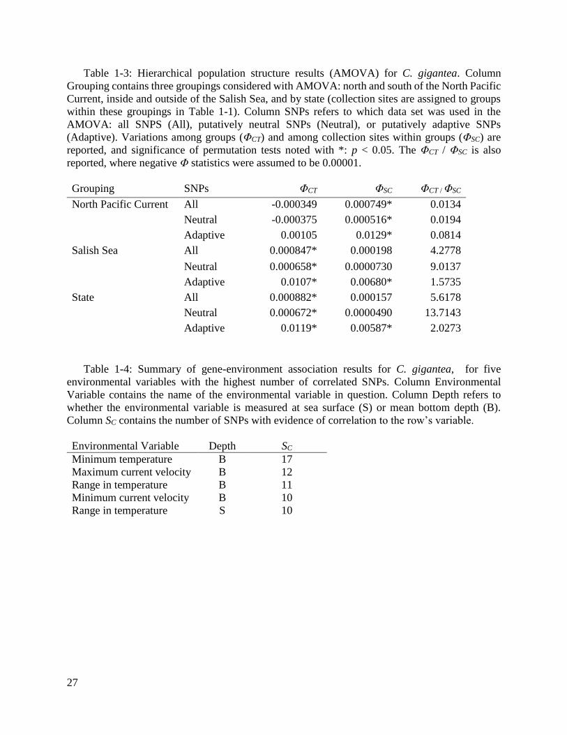
27

Table 1-3: Hierarchical population structure results (AMOVA) for C. gigantea. Column

Grouping contains three groupings considered with AMOVA: north and south of the North Pacific

Current, inside and outside of the Salish Sea, and by state (collection sites are assigned to groups

within these groupings in Table 1-1). Column SNPs refers to which data set was used in the

AMOVA: all SNPS (All), putatively neutral SNPs (Neutral), or putatively adaptive SNPs

(Adaptive). Variations among groups (ΦCT) and among collection sites within groups (ΦSC) are

reported, and significance of permutation tests noted with *: p < 0.05. The ΦCT / ΦSC is also

reported, where negative Φ statistics were assumed to be 0.00001.

Grouping SNPs ΦCT ΦSC ΦCT / ΦSC

North Pacific Current All -0.000349 0.000749* 0.0134

Neutral -0.000375 0.000516* 0.0194

Adaptive 0.00105 0.0129* 0.0814

Salish Sea All 0.000847* 0.000198 4.2778

Neutral 0.000658* 0.0000730 9.0137

Adaptive 0.0107* 0.00680* 1.5735

State All 0.000882* 0.000157 5.6178

Neutral 0.000672* 0.0000490 13.7143

Adaptive 0.0119* 0.00587* 2.0273

Table 1-4: Summary of gene-environment association results for C. gigantea, for five

environmental variables with the highest number of correlated SNPs. Column Environmental

Variable contains the name of the environmental variable in question. Column Depth refers to

whether the environmental variable is measured at sea surface (S) or mean bottom depth (B).

Column SC contains the number of SNPs with evidence of correlation to the row’s variable.

Environmental Variable Depth SC

Minimum temperature B 17

Maximum current velocity B 12

Range in temperature B 11

Minimum current velocity B 10

Range in temperature S 10

28

Table 1-5: LD Ne estimates with 95% confidence intervals per collection site for C. gigantea.

Confidence intervals estimated by jackknifing across samples. Pcrit is the minimal allele

frequency to retain a SNP in the analysis. Both Pcrit0.05 (0.05%) and Pcrit0.0 (0%) because rare

alleles can affect Ne estimates.

Pcrit0.05 Pcrit0.0

Site Estimate 95% CI Estimate 95% CI

Seward, AK 2259.4 790.1 - Infinity 5394.2 951.1 - Infinity

Sekiu, WA Infinity 6114.4 - Infinity Infinity 7964.0 - Infinity

Port Gamble, WA Infinity 1105.1 - Infinity Infinity 107933.2 - Infinity

Cypress Island, WA Infinity 7267.0 - Infinity Infinity 9502.8 - Infinity

Dabob Bay, WA 23408.6 11050.1 - Infinity 24327.9 11922.0 - Infinity

Monterey, CA Infinity 6741.6 - Infinity Infinity 6033.6 - Infinity

Catalina Island, CA 41053.6 2898.4 - Infinity 60635.3 3135.2 - Infinity

29

Figure 1-1: A map of collection sites and DAPC results for C. gigantea. The map (upper left)

is color-coordinated with the DAPCs. DAPCs represent the first two discriminant functions, using

all SNPs (A), putatively neutral SNPs (B), and putatively adaptive SNPs (C). For each plot, axes

are labeled with the proportion of among-population variance explained by that discriminant

function. Point shapes differ by state to highlight regional effects.

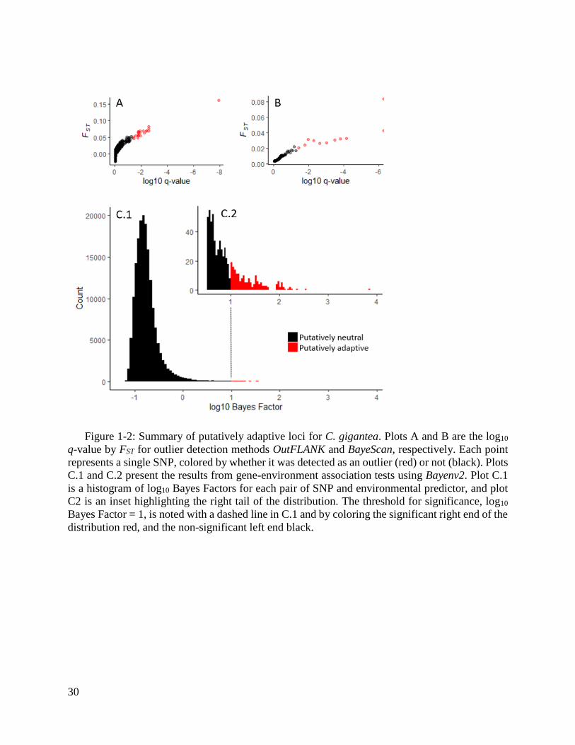
30

Figure 1-2: Summary of putatively adaptive loci for C. gigantea. Plots A and B are the log10

q-value by FST for outlier detection methods OutFLANK and BayeScan, respectively. Each point

represents a single SNP, colored by whether it was detected as an outlier (red) or not (black). Plots

C.1 and C.2 present the results from gene-environment association tests using Bayenv2. Plot C.1

is a histogram of log10 Bayes Factors for each pair of SNP and environmental predictor, and plot

C2 is an inset highlighting the right tail of the distribution. The threshold for significance, log10

Bayes Factor = 1, is noted with a dashed line in C.1 and by coloring the significant right end of the

distribution red, and the non-significant left end black.

31

Figure 1-3: Simulation results to contextualize empirical population differentiation and

estimate connectivity for C. gigantea. Tile maps representing mean pairwise FST across replicate

simulations for each combination of effective population size, migration rate, and number of

generations of drift elapsed. Short-term (left) represents results from 10 generations of drift,

Medium-term (middle) from 100 generations of drift, and Long-term (right) from 1,000

generations of drift. Tile color is divided into two groups based on the scale of FST: smaller than

the observed pairwise FST values between collection sites and greater than the observed pairwise

FST between collection sites in this study. No simulations yielded an FST value within the range of

observed FST values.

32

1.6 SUPPLEMENTARY MATERIALS

Supplemental Table 1-1: Environmental predictor codes and descriptions from Bio-Oracle

(BO) and Bio-Oracle2 (BO2) databases, used in Bayenv2.

Number Code Description

1 BO_bathymean Average depth of the seafloor

2 BO_calcite

Calcite concentration indicates the mean

concentration of calcite (CaCO3) in oceans.

3 BO_ph Measure of acidity in the ocean.

4 BO2_curvelmax_bdmean

Maximum sea water velocity at mean bottom

depth

5 BO2_curvelmax_ss Maximum surface current velocity

6 BO2_curvelmean_bdmean Mean sea water velocity at mean bottom depth

7 BO2_curvelmean_ss Mean surface current velocity

8 BO2_curvelmin_bdmean

Minimum sea water velocity at mean bottom

depth

9 BO2_curvelmin_ss Minimum surface current velocity

10 BO2_curvelrange_bdmean

Range of the sea water velocity at mean bottom

depth

11 BO2_curvelrange_ss Range of surface current velocity

12 BO2_dissoxmean_bdmean

Mean mole concentration of dissolved molecular

oxygen in sea water at mean bottom depth

13 BO2_dissoxmean_ss Mean dissolved oxygen concentration

14 BO2_nitratemean_bdmean

Mean mole concentration of nitrate in sea water

at mean bottom depth

15 BO2_nitratemean_ss

Mean mole concentration of nitrate at the sea

surface

16 BO2_phosphatemean_bdmean

Mean mole concentration of phosphate in sea

water at mean bottom depth

17 BO2_phosphatemean_ss

Mean mole concentration of phosphate at the sea

surface

18 BO2_ppmean_bdmean

Mean net primary productivity of carbon at

mean bottom depth

19 BO2_ppmean_ss

Mean sea surface net primary productivity of

carbon

20 BO2_salinitymean_bdmean

Mean sea water salinity at the bottom at mean

bottom depth

21 BO2_salinitymean_ss Mean sea surface salinity

22 BO2_tempmax_bdmean

Maximum sea water temperature at the bottom at

mean bottom depth

23 BO2_tempmax_ss Maximum sea surface temperature

24 BO2_tempmean_bdmean

Mean sea water temperature at the bottom at

mean bottom depth

25 BO2_tempmean_ss Mean sea surface temperature

33

26 BO2_tempmin_bdmean

Minimum sea water temperature at the bottom at

mean bottom depth

27 BO2_tempmin_ss Minimum sea surface temperature

28 BO2_temprange_bdmean

Range of the sea water temperature at the bottom

at mean bottom depth

29 BO2_temprange_ss Range of sea surface temperature

Supplemental Table 1-2: Sites remaining after each filtering step for C. gigantea.

Filtering step Sites

After dDocent 585,186

After removing indels 480,812

After requiring a minimum minor allele count = 5 103,373

After requiring minimum quality score = 20 102,826

After requiring minimum genotype depth = 10 102,826

After requiring minimum minor allele frequency = 0.05 35,555

After requiring maximum missing data = 30% 15,035

After removing SNPs out of Hardy Weinberg Equilibrium 11,280

After retaining SNP with highest minor allele frequency per RAD locus 5,932

34

Supplemental Table 1-3: Summary of Bayenv2 results for C. gigantea. Number of SNPs

(column Correlated SNPs) with at least strong evidence for correlation with environmental

predictors (column Environmental Predictor). Column S or B refers to whether the environmental

predictor was measured at sea surface (S) or mean bottom depth (B).

Environmental Predictor S or B Correlated SNPs

Minimum temperature B 17

Maximum current velocity B 12

Range in temperature B 11

Minimum current velocity B 10

Range in temperature S 10

Mean current velocity B 9

Mean bathymetry B 8

pH S 8

Mean nitrate S 8

Mean calcite S 7

Range in current velocity B 7

Mean dissolved oxygen S 7

Mean phosphate S 7

Maximum current velocity S 6

Mean primary production B 6

Maximum temperature B 6

Mean temperature B 6

Minimum temperature S 6

Maximum temperature S 5

Mean nitrate B 4

Mean phosphate B 4

Mean primary production S 4

Mean temperature S 4

Mean dissolved oxygen B 3

Mean salinity B 3

Mean salinity S 3

Mean current velocity S 2

Minimum current velocity S 2

Range in current velocity S 2

35

Supplemental Table 1-4: Correlation among environmental predictors measured at collection

sites for C. gigantea. Pearson’s correlation coefficients (lower left) for each pair of 29

environmental predictors, shaded blue-white-red for negative-zero-positive. And asterisk in the

upper right denotes a significant test (p < 0.05) result after Holm correction. Column and row

numbers refer to a specific environmental predictor, which match those in Supplemental Table

1-1.

36

Supplemental Table 1-5: Spatial autocorrelation of environmental predictors used in Bayenv2

for C. gigantea. For each environmental predictor (column Environmental Predictor), we report

Moran’s I autocorrelation index (column I) and p-value (column p-value) from a two-sided test for

each environmental predictor. Environmental predictors that are significantly (p < 0.05) spatially

auto-correlated are shaded in red.

Environmental Predictor I p-value

BO_bathymean -0.039 0.223

BO_calcite -0.190 0.816

BO_ph 0.066 0.049

BO2_curvelmax_bdmean -0.118 0.664

BO2_curvelmax_ss -0.115 0.659

BO2_curvelmean_bdmean -0.043 0.216

BO2_curvelmean_ss 0.082 0.038

BO2_curvelmin_bdmean -0.083 0.433

BO2_curvelmin_ss 0.079 0.042

BO2_curvelrange_bdmean -0.055 0.265

BO2_curvelrange_ss 0.069 0.052

BO2_dissoxmean_bdmean -0.045 0.309

BO2_dissoxmean_ss -0.038 0.215

BO2_nitratemean_bdmean -0.019 0.210

BO2_nitratemean_ss -0.012 0.163

BO2_phosphatemean_bdmean -0.055 0.340

BO2_phosphatemean_ss -0.140 0.826

BO2_ppmean_bdmean 0.029 0.115

BO2_ppmean_ss -0.118 0.698

BO2_salinitymean_bdmean -0.040 0.283

BO2_salinitymean_ss 0.090 0.033

BO2_tempmax_bdmean -0.059 0.357

BO2_tempmax_ss -0.067 0.376

BO2_tempmean_bdmean 0.088 0.039

BO2_tempmean_ss -0.092 0.501

BO2_tempmin_bdmean -0.058 0.285

BO2_tempmin_ss -0.097 0.528

BO2_temprange_bdmean -0.100 0.573

BO2_temprange_ss -0.067 0.371

37

Supplemental Table 1-6: Global, mean pairwise, minimum pairwise, and maximum pairwise

FST using all (n = 5,932), putatively neutral (n = 5,823), and putatively adaptive SNPs (n = 109).

Global

FST

Mean pairwise

FST

Min. pairwise

FST

Max. pairwise

FST

All SNPs 0.0009 0.000919 -0.0002 0.0021

Putatively neutral SNPs 0.0006 0.000567 -0.0006 0.0014

Putatively adaptive SNPs 0.0163 0.0188 0.0058 0.0409

Supplemental Table 1-7: Pairwise FST using putatively neutral SNPs. Cells are shaded darker

green for greater values of FST. Site code key in Table 1-2.

Neutral SW_AK -

SK_WA -0.0004 -

PG_WA -0.0006 0.0005 -

CI_WA 0.0006 0.0005 0 -

DB_WA 0.0007 0.0009 0.0002 -0.0001 -

MB_CA 0.0006 0.0007 0.0013 0.0009 0.0014 - CI_CA 0.0004 0.0011 0.0013 0.0009 0.001 0 -

Supplemental Table 1-8: Pairwise FST using putatively adaptive SNPs. Cells are shaded darker

green for greater values of FST. Site code key in Table 1-2.

Adaptive

SW_AK -

SK_WA 0.0141 -

PG_WA 0.0255 0.0261 -

CI_WA 0.0177 0.0127 0.0236 -

DB_WA 0.0135 0.0075 0.0158 0.0058 -

MB_CA 0.0192 0.0107 0.0409 0.0259 0.0227 - CI_CA 0.0063 0.0134 0.0399 0.0251 0.0214 0.0077 -

38

Supplemental Figure 1-1: Histograms of locus FIS. Subplots A and B contain locus FIS for all

sites and by collection site, respectively.

39

Supplemental Figure 1-2: Discriminant analysis of principal components, presented separately

by discriminant function.

Supplemental Figure 1-3: Results from ADMIXTURE for C. gigantea. Cross-validation error

for models with different numbers of assumed populations (K). The model with 1 underlying

population had the lowest cross-validation error, and thus most support.

40

Supplemental Figure 1-4: Tests for isolation-by-distance for C. gigantea. No significant (p >

0.05) correlation between linearized FST and in-water distance using all SNPs (y = (-5.52*10-5)*x

+ 1.53*10-03; Mantel R = -0.517), putatively neutral SNPs (y = (-4.99*10-5)*x + 1.12*10-3;

Mantel R = -0.557), or putatively adaptive SNPs (y = (3.51-*10-4)*x + 0.0232; Mantel R = -

0.2114).

41

Supplemental Figure 1-5: Venn diagram demonstrating overlap of putatively adaptive SNPs

by method for C. gigantea.

42

Chapter 2. Population structure and adaptive differentiation in the sea

cucumber Apostichopus californicus and implications for

spatial resource management

2.1 INTRODUCTION

Over the last two decades, genetic studies have provided evidence that some marine species

can develop spatial population structure despite very large population sizes and planktonic larval

dispersal (Hauser & Carvalho, 2008; Palumbi, 2004; Sanford & Kelly, 2011). The traditional view

of marine populations as demographically panmictic followed from the hypothesis that an apparent

lack of barriers to dispersal in the marine environment and long-distance planktonic larval

dispersal common to many marine species would result in high gene flow across large geographic

regions (Hauser & Carvalho, 2008). However, it is likely that dispersal in marine populations is

more restricted than previously thought, likely due to larval behavior (D’Aloia et al., 2015; Gerlach

et al., 2007) and the presence of oceanographic barriers (Costello & Chaudhary, 2017). Moreover,

selection can drive population differentiation in marine populations characterized by negligible

genetic drift and/or high gene flow (Lamichhaney et al., 2012; Pettersson et al., 2019). Lastly,

intrinsic reproductive barriers such as chromosome inversions or genetic incompatibilities may

further restrict gene flow (Barth et al., 2019).

Characterization of genetic population structure is particularly important to effective

management of exploited species. Genetic population structure can be used to define the scale of

management actions to best meet management objectives (Carvalho & Hauser, 1994; Reiss et al.,

2009). Ignoring spatial structure in fishery management may result in overexploitation of less

productive or more accessible populations (Spies & Punt, 2015). In turn, overexploitation may

43

reduce population diversity supporting adaptability, and thus sustainability, for current and future

uses (Kenchington et al., 2003; Schindler et al., 2010). Additionally, demographic parameters such

as the scale and direction of migration can be inferred from population structure (Rousset, 2004),

and this information can be used to inform sustainable management practices aimed at maintaining

and rebuilding wild populations, such as those in marine protected areas (Palumbi, 2003).

Estimates of genetic population structure are also useful in informing best practices for

aquaculture. Sourcing wild broodstock is a common practice in aquaculture production of species

that are outplanted within their native range (Davis et al., 1985; Tringali et al., 2007). If spatial

population structure exists, then collecting wild broodstock from one distinct population and

outplanting their seed into another can erode spatial population genetic structure and may lead to

negative fitness consequences such as loss of local adaptations (R. S. Waples et al., 2012).

Conversely, sourcing broodstock and outplanting their seed within a single population could help

maintain both the differentiation among wild populations and fitness of released offspring in the

local environment if populations are locally adapted (Ward, 2006). In recognition of such

processes, the Department of Fisheries and Oceans Canada restricts translocation to within

“shellfish transfer zones,” in part to minimize loss of population differentiation associated with

aquaculture (Miller et al., 2006; Xuereb, Benestan, et al., 2018).

The California sea cucumber, Apostichopus californicus, supports wild fisheries and is a

novel aquaculture species, and thus would benefit from the characterization of spatial population

structure. Demand for A. californicus has increased over the last several decades (Carson et al.,

2016) as part of a global trend of growing demand for sea cucumbers (S. C. Anderson et al., 2011).

Within Washington State, intense fishing pressure on this species peaked between 1988 and 1994,

which reduced wild population sizes (S. C. Anderson et al., 2011; Mueller, 2016; Purcell et al.,

44

2013) and resulted in the closure of the Central Puget Sound fishery in 2014 (Carson et al., 2016).

Despite some management intervention, including reduced quotas and a closure during peak

spawning season, stocks have been slow to recover (Carson et al., 2016). Fishing pressure within

Washington State is distributed differentially among six management areas (WDFW, 2020a),

largely based on historic administrative boundaries and tribal fishing rights, but it is not known

whether these areas represent biologically meaningful populations. Moreover, shellfish growers

and scientists are developing methods for commercial aquaculture production of A. californicus

(DeWeerdt, 2020) to supplement wild harvest, because demand remains high in overseas markets

(Carson et al., 2016). Defining management units relevant to fisheries would benefit the

development of aquaculture as well, as it could help to develop guidelines for broodstock sourcing

and stocking practices.

Population differentiation depends in part on life history. A. californicus reproduce through

broadcast spawning, with females producing approximately 100,000-600,000 eggs per spawning

event (Whitefield & Hardy, 2019). Larvae may remain in the planktonic stage for weeks to months

until they settle, while adults are motile (Cameron & Fankboner, 1989; Strathmann, 2017). Recent

evidence suggests that adult sea cucumber dispersal can be facilitated through tumbling and

floating behaviors, allowing them to take advantage of currents (Sheehan, 2019). Formal estimates

of life span are unavailable for A. californicus, but have been postulated to be about 12 years

(Phillips & Boutillier, 1995). Other species of sea cucumbers live to be 5 to 10 years old (Keegan

& O’Connor, 1985). Thus, dispersal potential is high in A. californicus because all life history

stages are motile and A. californicus are potentially long-lived, which could lead to high population

connectivity. The life history strategy of A. californicus is that of a periodic strategist with long

generation time, moderate reproductive effort, high batch fecundity and low investment per

45

offspring (Winemiller, 2005). This strategy is an adaptation to situations where environmental

variation affecting juvenile survival is unpredictable but occurs on a large geographic scale

(Winemiller & Rose, 1992), which in turn may result in high interannual variation in recruitment

(Winemiller, 2005), high variance in reproductive success and low Ne/N ratios (Hedgecock, 1994).

The life history of A. californicus may therefore suggest higher population differentiation than

expected from census population sizes and high susceptibility to overfishing (Winemiller, 2005).

A. californicus is distributed from Baja California, Mexico, to Alaska, from the lower

intertidal to depths of 250m (Abbott & Haderlie, 1980; Cameron & Fankboner, 1989), a region

containing oceanographic barriers to dispersal that could shape population connectivity in A.

californicus. For example, the Salish Sea, a large estuary divided into sub-basins by sills, is known

to harbor genetically distinct populations in Pacific Cod (Cunningham et al., 2009) and Brown

Rockfish (Buonaccorsi et al., 2005). The Victoria Sill and Admiralty Inlet are two potentially

important oceanographic barriers to dispersal within the Salish Sea. The Victoria Sill is the

outermost oceanographic barrier dividing the Salish Sea from the Strait of Juan de Fuca, which

connects the Salish Sea to the outer coast (Davenne & Masson, 2001). The two sills at Admiralty

Inlet separate the main Puget Sound basin from the San Juan Islands region and the Georgia Strait

(Cannon et al., 1990). Another potential oceanographic barrier is the North Pacific Current (NPC),

which bifurcates as it approaches the Pacific coast of North America into the northward Alaska

and southward California currents. The NPC was already identified as an oceanographic barrier to

dispersal in A. californicus (Xuereb, Benestan, et al., 2018) and the bat star (Keever et al., 2009).

Spatial population structure correlated with oceanographic processes was recently

characterized in A. californicus in the region near British Columbia, Canada (Xuereb, Benestan,

et al., 2018; Xuereb, Kimber, et al., 2018). These authors found evidence for local adaptation

46

associated with mean bottom temperature, and to a lesser extent, surface salinity and bottom

current velocity (Xuereb, Kimber, et al., 2018). However, this study was restricted to British

Columbia, and did not include the southern extent of the range, in particular the southern Salish

Sea, where the majority of sea cucumbers are harvested in the contiguous United States

(Washington Sea Grant, 2015) and where the fishery has experienced closures due to overfishing

(Carson et al., 2016). Thus, estimates of spatial population structure are particularly needed in this

region. Sampling the northern and southern extents of the region, beyond British Columbia, is also

needed, as fisheries for A. californicus extend from Alaska to California.

In this study, we quantified and described patterns of population differentiation for A.

californicus to inform effective management of wild populations and facilitate the development of

management guidelines for aquaculture. We sampled populations at small and large geographic

scales to test for both fine- and broad-scale population structure, particularly in regions that allow

us to test hypotheses of potential oceanographic barriers to dispersal. Using restriction site-

associated DNA (RAD) sequencing, we quantified genetic structure and investigated its potential

drivers. Specifically, we tested whether limited dispersal and local adaptation shape population

structure. We compared our results with existing estimates of spatial population structure to

identify common patterns and build hypotheses about drivers of differentiation in the species. To

contextualize our results for managers, we developed a two-population model to evaluate which

conditions of effective population size (Ne), migration rate, number of generations of drift resulted

in pairwise population differentiation within the range observed in this study.

47

2.2 METHODS

2.2.1 Sample collection

Approximately 50 adult A. californicus were collected by scuba divers from nine collection

sites along the Pacific Coast of North America, ranging from Alaska to Oregon, including three

collection sites within the southern Salish Sea (Table 2-1, Figure 2-1). For each animal, a tissue

sample was excised from a radial muscle band and stored in 100% ethanol.

2.2.2 DNA library preparation

DNA was extracted from tissue samples using the EZNA Mollusc DNA Kit (OMEGA Bio-

tek, Norcross, GA, USA) and the Qiagen DNeasy Kit (Qiagen, Germantown, MD, USA). DNA

was quantified using the Quant-iT PicoGreen dsDNA Assay Kit (Thermo Fisher Scientific,

Waltham, MA, USA) and DNA quality was checked by gel electrophoresis. DNA concentration

was normalized to 500 ng in 20 μL of PCR-grade water. We selected samples with high DNA

quality for restriction site-associated DNA (RAD) sequencing and RAD libraries were prepared

following standard protocols (Etter et al., 2011). Briefly, DNA samples were barcoded with an

individual six-base identifier sequence attached to an Illumina P1 adapter. Samples were then

pooled into sub-libraries, containing approximately 12 individuals. Sub-libraries were sheared

using a Bioruptor sonicator and size selected to 200-400 bp using a MinElute Gel Extraction Kit

(Qiagen, Germantown, MD, USA). P2 adapters were ligated to DNA in sub-libraries and amplified

with PCR using 12-18 cycles as in Etter et al. (2011). Finally, amplified sub-libraries were

combined into pools of approximately 72 individuals. Paired-end 2 x 150-base pair sequencing

was performed on an Illumina HiSeq4000 (San Diego, California, USA) at the Beijing Genomics

Institute and the University of Oregon Genomics and Cell Characterization Core Facility. Only

48

forward reads were used for analysis. To estimate genotyping error, 14 individuals were sequenced

twice.

2.2.3 Genotyping individuals

Raw RAD sequencing data were demultiplexed using the process_radtags module in the

pipeline STACKS v.1.44 (Catchen et al., 2013). A threshold of 800,000 reads was used to exclude

poorly sequenced individuals. Because a genome was not available for A. californicus, we aligned

individual sequences to the genome of a closely related species, A. parvimensis (GenBank

accession number = GCA_000934455.1). The A. parvimensis genome was 760,654,621 bp, with

21,559 scaffolds and an N50 size of 9,587. We retained reads with a minimum mapping quality

score of 20. Then, we used dDocent v.2.7.8 to perform a reference-guided locus assembly using

the filtered reads and default parameters (J. B. Puritz et al., 2014). Additionally, a parallel de novo

assembly was performed, which produced nearly identical results for population structure

(Supplemental Tables 2-1 and 2-2, and Supplemental Figure 2-1) and 1.8-2.8% lower mean

expected heterozygosity, 0.9-1.8% higher mean observed heterozygosity, and 1.2-3.3% higher

proportions of polymorphic SNPs than in the with-reference assembly, although with similar

patterns across collection sites. The reference-guided assembly was retained for further analyses

due to decreased confidence in identifying genotyping errors in the de novo assembly (Shafer et

al., 2017).

We used vcftools v.0.1.16 (Danecek et al., 2011) to remove indels and to retain only single

nucleotide polymorphisms (SNPs) with a minimum quality score of 20, minimum minor allele

frequency of 0.05 and maximum missing data per locus of 30% across collection sites. Individuals

with more than 30% missing data across SNPs were removed. In cases of multiple SNPs per RAD

tag, we retained the SNP with the highest minor allele frequency (Larson et al., 2014). SNPs that

49

were not in Hardy Weinberg Equilibrium (HWE) were considered sequencing errors or poorly

assembled loci and were removed from our data set, as selection and inbreeding are unlikely to

cause significant deviations from HWE equilibrium at biallelic loci (R. S. Waples, 2015). We

tested SNPs for deviations from HWE using the R package genepop v.1.1.4 (Rousset, 2008). SNPs

were identified as being out of HWE if they had a q-value below 0.05 in at least 2 of the collection

sites after correcting for false discovery rate, following R. S. Waples (2015).

2.2.4 Population genetic structure analyses

We used a suite of R packages, stand-alone software, and custom scripts in the

programming language R v.3.5.0 (R Core Team, 2020) to quantify genetic diversity and population

structure. Mean expected heterozygosity, observed heterozygosity, and the inbreeding coefficient

(FIS) per SNP were calculated using the R package genepop. The proportion of polymorphic SNPs

per collection site was calculated using a custom R script.

To investigate population structure, we first calculated Weir-Cockerham fixation index

(FST) (Weir & Cockerham, 1984) to quantify population differentiation using the R packages

genepop and hierfstat v.0.5.7. Exact G-tests (Goudet et al., 1996) were used to test for significant

genic differentiation using the R package genepop. To investigate patterns of spatial differentiation

among collection sites, the R package adegenet v.2.1.1 (Jombart, 2008) was used to conduct

discriminant analysis of principal components (DAPC), a multivariate method that summarizes

the between-group variation (i.e., population structure), while minimizing within-group variation

(Jombart et al., 2010). The built-in optimization algorithm was used to retain the number of

principal components that minimized over-fitting and under-fitting of the model. To determine the

potential number of underlying populations, the program ADMIXTURE v.1.3.0 was used to

conduct a clustering analysis (Alexander & Lange, 2011). Specifically, ADMIXTURE uses a

50

maximum likelihood-based approach to estimate individual ancestries across different assumed

numbers of populations, with the best fit selected using cross-validation. To examine the presence

of hierarchical population structure, we conducted analyses of molecular variance (AMOVA)

using the ade4 method of the R package poppr v.2.8.1 (Kamvar et al., 2015). Significance of

AMOVAs was determined using permutation tests with 1,000 iterations. Using AMOVA, we

investigated whether the following oceanographic barriers limit dispersal: 1) the Victoria Sill

(Salish Sea grouping), 2) Admiralty Inlet (Puget Sound grouping), and 3) the North Pacific Current

(NPC grouping). Additionally, we conducted an AMOVA by state or province (State grouping).

Although not biologically meaningful, we included the State grouping to determine how much

genetic variation is captured by regional management boundaries.

2.2.5 Identifying putative adaptive differentiation

Adaptive differentiation was investigated using two approaches: FST outlier detection and

gene-environment association. FST outlier detection methods identify statistical outliers in

distributions of FST per SNP, as evidence for potential spatially-divergent selection. For FST outlier

detection, two methods were used: the program Bayescan v.2.1 (Foll & Gaggiotti, 2008) and the

R package OutFLANK v.0.2 (Whitlock & Lotterhos, 2015). Bayescan first applies linear regression

to decompose FST into a population- and a locus-specific component. Using these components as

Bayesian priors, the program estimates the posterior probability that a locus is under selection (Foll

& Gaggiotti, 2008). OutFLANK detects FST outliers using a maximum likelihood approach. The

program first infers a distribution of neutral FST from a trimmed distribution of empirically

collected FST values and uses this neutral distribution to identify outliers. OutFLANK advances

earlier FST outlier methods (Lewontin & Krakauer, 1973) by accounting for sampling error and

51

non-independent sampling of populations, and has lower false positive rates compared to other FST

outlier methods (Whitlock & Lotterhos, 2015). We used default parameters in both programs,

including a false discovery rate of 0.05. SNPs were classified as FST outliers if they were detected

with either program, to include SNPs under weak selection, which are likely the majority of SNPs

under selection (Lotterhos & Whitlock, 2015).

Prior to investigating gene-environment association, we gathered estimates for

oceanographic variables at each collection site using the Bio-Oracle and Bio-Oracle 2 databases

(Assis et al., 2018), which contain geophysical, biotic, and environmental data layers for marine

realms, through the R package sdmpredictors v.0.2.8 (Bosch et al., 2017). We selected a broad

suite of 29 oceanographic variables (including temperature, current velocity, salinity, and pH;

complete list in Supplemental Table 1-1), including those used by Xuereb, Kimber, et al. (2018)

for comparison. Where possible, oceanographic variables for both sea surface and mean bottom

depth (near-bottom) were used to account for the conditions experienced by pelagic larvae and

benthic adults respectively. The Eld Inlet, Washington collection site was removed from these

analyses because environmental predictor data were not available. We also calculated correlation

among predictor variables (Supplemental Table 2-3) and interpreted results in light of these

correlations.

To investigate genomic evidence for local adaptation, gene-environment associations were

explored using a univariate association method, Bayenv2 (Günther & Coop, 2013) and a

multivariate method, redundancy analysis (RDA). We used both methods as each has an

advantage: the interpretation of results for univariate methods like Bayenv2 can be clearer than

multivariate methods for gene-environment association, and multivariate methods such as RDA

52

have lower false positive rates and greater sensitivity for detecting weak and multi-locus selection

(Forester et al., 2018).

The program Bayenv2 (Günther & Coop, 2013) uses a univariate Bayesian framework to

test for significant correlation between allele frequencies and environmental predictor variables,

accounting for population structure by first estimating covariance among loci. Correlations with a

minimum Bayes Factor of 10, or minimum “strong” support (Kass & Raftery, 1995), were retained

in the analysis.

Redundancy analyses were performed in the R package vegan v.2.5-6 (Oksanen et al., 2007).

Redundancy analysis summarizes the variation in a set of response variables (here, the allele

frequencies) due to a set of explanatory variables (here, the oceanographic variables), using an

extension of multiple linear regression that allows regression of multiple response variables on

multiple explanatory variables. Here, only biallelic SNPs were retained, and allele frequencies

were Hellinger-transformed prior to RDA (Legendre & Gallagher, 2001). To avoid

overdetermination of RDA models with many environmental predictors (Supplemental Figure

2-2), we conducted multiple RDAs on subsets of environmental predictors and reduced the

dimensionality of our environmental predictors within sets by first combining them into orthogonal

principal components (Supplemental Tables 2-4 through 2-7). Specifically, environmental

predictors were grouped into four a priori sets: (1) all, (2) sea surface, (3) near-bottom and (4)

current velocity and temperature predictors (measured at either sea surface or near-bottom). Sets

2 and 3 were chosen to investigate differences in putative adaptation at pelagic and benthic life

history stages. Environmental predictor set 4 was chosen for comparison with the existing study

on A. californicus in a different part of the species range, as these variables were strongly correlated

with genetic population structure (Xuereb, Kimber, et al., 2018). Predictors were standardized to

53

a mean of 0 and standard deviation of 1 prior to PCA. PCA was performed on each set of predictors,

and principal components were retained if their corresponding eigenvalue was above the mean

eigenvalue across principal components.

To account for the potential confounding factor of neutral population structure in our RDA,

we conducted a complementary partial RDA for each set of predictor variables, in which the effects

of spatial variation were partialled out. We used Euclidean distances among collection sites to

compute distance-based Morgan’s eigenvector maps (MEMs) using the R package codep v.0.9-1

(Guénard et al., 2010), to be used as conditioning variables in partial RDAs (Dray et al., 2006).

We report the variance inflation factors (VIF) to identify collinearity among spatial variables and

environmental predictors, although we note that the effects of such collinearity are addressed in

the removal of genetic variation explained by spatial variables in partial RDAs. ANOVA

permutation tests for full models and per axis were used to assess the significance of RDA results.

For significant models, we identified SNPs putatively involved in local adaption based on the

loadings of SNPs in ordination space for significant axes. Specifically, SNPs were classified as

putatively adaptive if their loading score was outside of 3 standard deviations of the mean (Forester

et al., 2018).

2.2.6 Comparing putatively neutral and adaptive differentiation

SNPs were classified as putatively adaptive if they were detected as FST outliers using either

BayeScan or OutFLANK, or if they were significantly correlated to environmental predictors using

Bayenv2 or RDA. Once putatively adaptive SNPs were identified, they were used to distinguish a

putatively neutral SNP set and a putatively adaptive SNP set.

We used the putatively neutral and putatively adaptive data sets to address questions related

to demographic and selective processes, respectively. We estimated effective population size (Ne)

54

per collection site from putatively neutral SNPs using NeEstimator v.2.1 with default settings (Do

et al., 2014). Using Mantel tests (Mantel & Valand, 1970) in R, we tested for correlation between

linearized FST (Rousset, 1997), using all, putatively neutral, and putatively adaptive SNPs, and

shortest Euclidean distance through water (in-water distance hereafter), approximated in Google

Maps (Google, 2019).

To build hypotheses for the mechanisms underlying adaptive differentiation, potential

biological processes associated with putatively adaptive SNPs were identified using blastx v.2.5.0

(Altschul et al., 1990) and the UniProt Knowledge Base (Swiss-Prot, manually annotated) (The

UniProt Consortium, 2019). We queried the 2,000 bp region flanking the SNP, following

alignment against the reference genome of A. parvimensis. Matches with a maximum e-value score

of 10-10 were retained. Gene ontology slim terms for biological processes were retrieved using an

adaptation of the Mouse Genome Informatics database, as developed in Gavery & Roberts (2012).

Gene ontology slim terms “other biological processes” and “other metabolic processes” were

excluded. A particular locus could be associated with multiple gene ontologies, and a particular

gene ontology could be associated with multiple gene ontology slim terms for biological processes.

All matches were retained.

2.2.7 Simulations

To contextualize genetic connectivity in terms of migration rate for management, we

developed a simulation model using simuPOP v.1.1.10.9 (Peng & Kimmel, 2005) in Python

v.3.7.3 to determine which population sizes, migration rates, and number of generations of drift

reproduced our empirically derived pairwise FST results. The model simulated two populations of

equivalent size, with discrete generations, random mating, and no selection. Within each

population, two parents were selected at random with replacement to produce one offspring,

55

leading to a random distribution of reproductive success, and allowing for census size to

approximate Ne. The model was parameterized using empirical global allele frequencies for

putatively neutral SNPs and simulations were run for each combination of Ne (500, 2500, 10,000)

and migration rate (0.01%, 0.03%, 0.1%, 0.3%, 1%, 3%, 10%, 30%). Additionally, simulations

were run for 10 (short-term), 100 (medium-term), and 1,000 (long-term) generations of drift. The

long-term option was chosen to approximate equilibrium conditions, although true equilibrium

depends on population history and may not be reached in some wild populations within 1,000

generations. Pairwise FST was calculated after the pre-determined number of generations of drift

had elapsed and averaged across 5 replicates for each parameter combination.

2.3 RESULTS

2.3.1 Sequencing

After removing 33 (9% of 358 sequenced individuals) poorly sequenced individuals, the

average number of reads per individual was 1.76M (standard deviation (SD) = 0.787M). The

dDocent assembly produced 6,738,423 variant sites, and 2,075 SNPs were ultimately retained after

filtering (Supplemental Table 2-8). All individuals included in the dDocent assembly were retained

after filtering for missing data across SNPs, resulting in an average of 36 individuals per population

(SD = 13.7) (Table 2-1). Genotyping error was estimated to be 1.4% among the 14 replicated

individuals. All errors were mismatches of a single allele. Errors were distributed fairly evenly

across SNPs, with one error at 246 SNPs, two errors at 19 SNPs, three errors at 7 SNPs, and four

errors at one SNP, across replicated individuals.

56

2.3.2 Population structure

Global population differentiation was significant (global FST = 0.0068, 95% CI [0.005,

0.0105]; global genic differentiation test, p < 0.001). For the DAPC using all SNPs, we retained

53 PCs based on the optimization algorithm and observed clustering by collection site (Figure 2-1).

The first PC explained 52.1% of the variance and separated sites longitudinally. The second PC

explained 22.2% of the variance and separated sites latitudinally. The DAPC showed evidence for

separation of Alaska, British Columbia, Washington, and Oregon sites, with some evidence for

separation between sites inside and outside of the Salish Sea and between sites north and south of

Admiralty Inlet within the Salish Sea. Permutation test results from AMOVAs demonstrated

significant population structure for the NPC grouping using all SNPs (Table 2-2), suggesting that

the North Pacific Current is an oceanographic barrier to dispersal in A. californicus. Significant

population structure for the State grouping was also detected using permutation test results from

AMOVAs using all SNPs. The State grouping also had the highest ΦCT / ΦSC, a ratio that is higher

when the among-group variation is greater than the within-group variation. Clustering analyses

with ADMIXTURE provided the strongest support for the model with one underlying population

(Supplemental Figure 2-3). A Mantel test revealed significant positive correlations between

pairwise linearized FST using all SNPs and in-water distance (Mantel R = 0.758, p < 0.001; Figure

2-2).

Of all 36 pairwise site comparisons (Table 2-3), 24 revealed significant genic

differentiation (p < 0.05), with 8 of the 12 insignificant tests corresponding to collection site

pairings with the small collection from Auke Bay, AK (Table 2-1). Only one pairwise site

comparison (Keyport and Eld Inlet, WA) yielded a pairwise FST value that contained 0 in the 95%

confidence interval (Supplemental Table 2-9). The largest pairwise FST values were found among

57

collection sites from the northern (Alaska and British Columbia) and southern (Washington and

Oregon) parts of the species range (FST = 0.005 – 0.015). There was greater differentiation among

pairs of Washington collection sites (pairwise FST = 0.001-0.006) compared to Alaska collection

sites (pairwise FST = 0.004).

Mean expected heterozygosity and proportion of polymorphic SNPs did not vary

substantially across collection sites, apart from a reduced proportion of polymorphic SNPs in Auke

Bay and Chiniak Bay, AK (Table 2-1). Observed heterozygosity decreased and FIS increased from

North to South (Table 2-1). All collection site Ne estimates were large or infinite, with infinite

upper confidence limits, using both all putatively neutral SNPs and only those with a minor allele

frequency of at least 5% (Table 2-4).

2.3.3 Adaptive differentiation

The FST outlier SNP detection methods identified 60 (2.9% of 2,075) SNPs as putatively

adaptive (Figure 2-3), with 50 identified by BayeScan, 46 identified by OutFLANK, and 36 SNPs

overlapping across both methods.

Using Bayenv2, 181 SNPs (8.7% of 2,075) were identified as putatively adaptive. Each of

these SNPs was correlated with an average of 2.5 environmental predictors per SNP and at least

one SNP was correlated with each of the 29 environmental predictors (Supplemental Table 2-10).

The five environmental variables with the most associated SNPs included mean salinity, mean

nitrate, temperature range, and pH, all at the sea surface, and mean temperature at near-bottom

(Table 2-5). Over 60% more SNP-predictor correlations represented environmental variables

measured at the surface than at near-bottom, for variables with both measurements: 397 and 615

SNP-predictor correlations with near-bottom and sea surface variables, respectively.

58

After removing 10 multiallelic SNPs, we retained 2,065 biallelic SNPs for use in

redundancy analyses (RDA). We retained two RDA models (out of 8) for statistical significance:

the model using sea surface predictors was marginally significant at the full model level (ANOVA,

p = 0.063) and for the first axis (ANOVA, p = 0.052), and the model using temperature and current

velocity predictors (at sea surface or near-bottom) was significant at the full model level (ANOVA,

p = 0.034) and for the first axis (ANOVA, p = 0.035). For the RDA using sea surface predictors,

the first RDA axis explained 24.8% of the variance, and PC 2 had the greatest loading on the first

RDA axis (Supplemental Table 2-11). The three predictors with the greatest loadings on PC 2

included pH, mean salinity, and temperature range (Supplemental Table 2-5). For the RDA using

temperature and current velocity predictors, the first RDA axis explained 26.8% of the variance,

and PC 2 had the greatest loading on the first RDA axis (Supplemental Table 2-12). The three

predictors with the greatest loadings on PC 2 included temperature range at the sea surface and

near-bottom, and minimum temperature at the near-bottom (Supplemental Table 2-7). Collection

site clustering patterns were similar among RDA biplots (Figure 2-4), including the Salish Sea

collection sites clustering tightly together and North-South separation driven by the first RDA axis

in each model. Charleston, Oregon clustered more closely with the Salish Sea collection sites in

the model using temperature and current velocity predictors (Figure 2-4). We identified 32

putatively adaptive SNPs based on loadings of significant (and marginally significant) RDA axes,

with 24 SNPs identified from the RDA using sea surface predictors and 29 from the RDA using

temperature and current velocity predictors. No partial RDAs were significant. Spatial variables

used in partial RDAs covaried with predictor variables in most models, measured with variance

inflation factors (Table 2-6). The environmental predictor loadings for retained PCs in all models

59

and a correlation matrix of environmental predictors can be found in the Supplementary

Information (Supplemental Tables 2-3 through 2-7).

In total, we identified 211 (10.2% of 2,075 total SNPs) putatively adaptive SNPs, of which

41 (19.4% of 211 putatively adaptive SNPs) were detected with either FST outlier approaches and

at least one gene-environment association approach and 134 (63.5% of 211) were only identified

by Bayenv2 (Supplemental Figure 2-4). Sequences of RAD loci containing putatively adaptive

SNPs will be available upon publication.

Only 19 (9% of 211) putatively adaptive SNPs matched to gene ontologies, and 15 (79%

of 19) matched to more than one gene ontology. Of the SNPs identified as putatively adaptive

using Bayenv2, 15 SNPs matched to gene ontologies (Table 2-5, Supplemental Table 2-10). Of

these 15 SNPs, three were also identified using Bayescan and OutFLANK and one was also

identified using Bayescan, OutFLANK, and RDA. An additional four SNPs were also identified

as putatively adaptive using only FST outlier methods, with the most represented biological

processes including DNA metabolism, cell organization and biogenesis, and developmental

processes. For comparison, the top five most frequent biological processes in the database in

descending order are 1) developmental processes, 2) cell organization and biogenesis, 3)

transport, 4) protein metabolism, and 5) stress response (Supplemental Table 2-13).

2.3.4 Neutral vs. putatively adaptive differentiation

DAPC and AMOVA revealed higher differentiation but similar spatial patterns for

putatively adaptive SNPs compared to putatively neutral SNPs (Table 2-2, Figure 2-1). We

retained 53 and 26 PCs for the DAPC using putatively neutral SNPs and putatively adaptive SNPs,

respectively, based on the optimization algorithm. Clustering patterns using putatively neutral and

putatively adaptive SNPs reflected those using all SNPs, with more distinct clustering using

60

putatively adaptive SNPs (Figure 2-1). Permutation test results from AMOVAs demonstrate

significant population structure for NPC and State groupings, using putatively neutral and adaptive

SNPs (Table 2-2). The ratio of among-group variation to within-group variation (ΦCT / ΦSC) was

higher using putatively adaptive SNPs for the State and NPC groupings, and higher using

putatively neutral SNPs for the Salish Sea and Puget Sound groupings. Mantel tests for correlation

among linearized FST and in-water distance were significant using putatively neutral SNPs (Mantel

R = 0.4891, p < 0.01) and putatively adaptive SNPs (Mantel R = 0.7855, p < 0.0001) (Figure 2-2).

Correlation among linearized FST and in-water distance was strongest and the slope of the linear

regression was greatest using putatively adaptive SNPs: the slope of the linear regression using

putatively adaptive SNPs was nearly 7 and 20 times greater than the slopes using all SNPs and

putatively neutral SNPs, respectively.

2.3.5 Simulations

Simulations revealed that in an idealized two-population system, simulated pairwise FST

within the range observed in this study occurred in the long-term (1,000 generations since

divergence) with small Ne (Ne = 500) and high migration (m ≥ 3%), with moderate Ne (Ne = 2,500)

and moderate migration (1% ≥ m ≥ 3%), and with large Ne (Ne = 10,000) and small to moderate

migration (0.1% ≥ m ≥ 1%). Most simulations that produced pairwise FST estimates within the

range observed in this study were cases with moderate to large Ne (Ne ≥ 2,500) and migration rates

below 10%. Simulated pairwise FST remained below the lowest empirically observed pairwise FST

in this study in the long-term (1,000 generations) so long as Ne was at least moderate (Ne ≥ 2,500)

and migration rate was high (m ≥ 10%). Under realistic conditions (e.g., Ne = 10,000 and 1,000

generations since divergence; our Ne estimates were large and unbounded), simulated pairwise FST

was within the range of empirical pairwise FST when migration rates were 0.1-1.0% (Figure 2-5).

61

2.4 DISCUSSION

In this study, we quantified patterns of population differentiation in A. californicus and

investigated potential drivers of differentiation from Alaska to Oregon, representing a significant

portion of the species range. We observed population genetic structure at both fine- and broad-

scales, likely driven by limited dispersal and local adaptation. Notably, we found detectable

differentiation at small scales within the Salish Sea, co-varying signals of adaptive and neutral

differentiation, and a latitudinal pattern in genetic diversity. Estimates of Ne were large. Using

simulations, we found that migration rates may be as low as 0.1% if populations of A. californicus

are large (Ne = 10,000) and have undergone many (1,000) generations of drift.

2.4.1 Broad- and fine-scale population genetic structure and potential drivers

Broad-scale population structure that we observed can be described by two patterns:

isolation-by-distance and differentiation across the bifurcation zone of the North Pacific Current

(NPC). Isolation-by-distance was also detected in A. californicus along the coast of British

Columbia (Xuereb, Benestan, et al., 2018), as well as in other species of sea cucumbers including

Holothuria edulis (Soliman et al., 2016), H. scabra (Uthicke & Purcell, 2004), and H. nobilis

(Uthicke & Benzie, 2003). Many species of marine invertebrate exhibit population differentiation

along a latitudinal gradient, with the region between Alaska and Oregon as a known region of

divergence (Kelly & Palumbi, 2010; Kyle & Boulding, 2000). Xuereb, Benestan, et al. (2018)

posit that the genetic break observed in A. californicus in British Colombia is due to limited

dispersal across the bifurcation zone of the NPC. The NPC has also been identified as an

oceanographic barrier to gene flow in the Bat Star, Patiria miniata (Keever et al., 2009; Sunday et

al., 2014), and the Rosethorn Rockfish, Sebastes helvomaculatus (Rocha-Olivares & Vetter, 1999).

62

Our results did not provide evidence for limited dispersal across the Victoria Sill or the sills at

Admiralty Inlet, despite their potential roles in shaping population structure in other marine species

(Andrews et al., 2018; Buonaccorsi et al., 2005; Cunningham et al., 2009; Iwamoto et al., 2004).

Although not biologically meaningful, the State grouping yielded the greatest among-group

variation, likely because it captured the effects of isolation-by-distance and the divergence across

the NPC bifurcation zone.

Additionally, we found a subtle pattern of decreasing observed heterozygosity from north

to south (this pattern can also be observed in the data of Xuereb, Benestan, et al. (2018) following

re-estimation; North, mean HO = 0.113; South, mean HO = 0.108). In the Northern Hemisphere,

latitudinal patterns of genetic diversity are typically opposite (higher diversity in the south, lower

diversity in the north), as these northerly regions were more recently colonized after the

Pleistocene ice ages (Hampe & Petit, 2005). However, patterns of glaciation in the northeast

Pacific are complex (Darvill et al., 2018). Since there were multiple glacial refugia along the

Pacific Northwest Coast (Darvill et al., 2018), it is possible that A. californicus populations

remained established in the northern extent of the range throughout the Last Glacial Maximum.

Alternatively, this latitudinal pattern in genetic diversity may also be explained by differences in

Ne. Here, our estimates of Ne all had infinite upper confidence limits, limiting possible inferences

about relative population size across collection sites. Alaska supports larger sea cucumber fisheries

compared to southern regions (Bruckner, 2005), which could be evidence for larger Ne, reduced

genetic drift, and greater heterozygosity in the northern part of the species range.

Notably, we found that geographic distance was more strongly correlated to genetic

distance among collection sites using putatively adaptive SNPs than using putatively neutral SNPs.

This suggests that selection gradients may reduce effective dispersal distances, leading to stronger

63

signals in isolation-by-distance from neutral processes alone (Orsini et al., 2013). One exception

may be the Charleston, Oregon collection site, which clusters more distinctly from other collection

sites using putatively adaptive SNPs and is positioned more closely to the Salish Sea collection

sites in the RDA biplot for temperature and current velocity predictors than the biplot for sea

surface predictors. The difference in RDA biplots suggests different patterns in adaptive

differentiation, dependent on environmental predictors. Lastly, co-variation between neutral and

adaptive differentiation could also represent a false positive result for gene-environment

association. Isolation-by-distance, as we found in this study, can increase the chance of a false

negative result for gene-environment association if the environmental predictor is spatially auto-

correlated (Nadeau et al., 2016).

At finer scales, we found detectable differences among most collection site pairs and

between collection sites as close together as 110 km (in-water distance) apart, consistent with

earlier findings on differentiation as close as 60 km in A. californicus (Xuereb, Benestan, et al.,

2018) and 100 km apart in the Tar-spot Sea Cucumber, Cucumaria pseudocurata (Arndt & Smith,

1998). The sample from Auke Bay, Alaska behaved as an outlier across multiple analyses, likely

due to stochasticity associated with smaller sample size, and leading to most insignificant pairwise

genic differentiation tests and a lower proportion of polymorphic SNPs. Notably, genetic

differentiation among collection sites within Washington was broader in range and at times greater

than that within Alaska, despite substantially smaller in-water distances (mean = 162 km, SD = 62

km in WA and mean = 731km, SD = 339 km in AK). Lower differentiation between populations

in Alaska compared to the Salish Sea may be due to colder temperatures in Alaska slowing larval

growth, as colder temperatures led to slow larval growth in laboratory experiments in the sister

species, the Japanese sea cucumber, A. japonicus (Yang et al., 2015). Slower larval growth may

64

result in longer pelagic larval phases and increased potential dispersal distances. Alternatively,

greater genetic differentiation among populations within Washington compared to Alaska may

point to underlying oceanographic barriers that can shape dispersal in complex and asymmetrical

ways. In future work, a denser sampling scheme paired with an oceanographic model could be

used to illuminate the potential for seascape features to influence dispersal, particularly within the

Salish Sea.

We found evidence for putatively adaptive differentiation, corroborated by multiple lines

of investigation. The majority of SNPs identified as putatively adaptive using FST outlier detection

were identified using both methods and were also identified as putatively adaptive using at least

one gene-environment association method. Using Bayenv2, we detected many SNPs that were not

identified as putatively adaptive compared to redundancy analysis, consistent with expectations

that Bayenv2 may produce more false positives compared to redundancy analysis (Forester et al.,

2018). The five environmental predictors with the most significantly correlated SNPs were

salinity, nitrate, temperature range, and pH at sea surface and mean temperature at near-bottom.

Of these, salinity at the sea surface and temperature at the sea bottom were also identified as

potential drivers of local adaptation in the same species in British Columbia (Xuereb, Kimber, et

al., 2018). Temperature and salinity are significant factors shaping growth and survival in many

marine organisms (Kinne, 1964) and have been shown to affect growth and survival in A. japonicus

juveniles (Dong et al., 2008) and growth, survival, locomotory speed, and metamorphosis in A.

japonicus larvae (Yang et al., 2015). The greater number of SNPs significantly correlated to sea

surface predictor variables using Bayenv2 and the occurrence of temperature variables as top

predictor variables is consistent with RDA results: the significant RDA models were those with

environmental predictors at the sea surface and environmental predictors related to temperature

65

and current velocity. Thus, we hypothesize that selection at early life history stages, when larvae

are at the sea surface, drives adaptive differentiation in A. californicus, with salinity, nitrate, pH,

and temperature as possible selection factors.

We note that we cannot exclude balanced polymorphism as an alternative explanation to

observed putative adaptive differentiation: it is possible that selective mortality at early life stages

leads to observed patterns of putative adaptive differentiation in adults (as were sampled here), but

that genetic variation is maintained across time through high gene flow (Sanford & Kelly, 2011).

However, increasing evidence suggests that selection for locally adapted alleles can occur despite

high gene flow (Fitzpatrick et al., 2020; Lamichhaney et al., 2012), particularly in species with

large Ne.

In generating hypotheses about which environmental predictors are potential drivers of

selection, it is prudent to be cautious and highlight 1) spatial auto-correlation of predictors,

particularly in light of correlation between geographic distance and genetic distance using

putatively adaptive SNPs as observed here, and 2) correlation among environmental predictors.

Almost all environmental predictor sets contained spatially auto-correlated variables, evidenced

by high variance inflation factors for spatial variables and environmental predictor variables in

partial RDAs (Table 2-6). Additionally, the correlation among environmental variables adds

uncertainty about which predictors are driving patterns in adaptive differentiation. These

correlations highlight the limits of these analyses. However, our results are fairly consistent with

those of Xuereb, Kimber, et al. (2018), even though they sampled genetic and environmental data

from different collection sites. Confidence in gene-environment association results may increase

if results are further corroborated in future studies, particularly if using alternative methods.

66

For the environmental variables with the most correlated SNPs, and for such SNPs with

associated biological processes, signal transduction appeared among the most common biological

processes. Future research investigating the connections between genotype, phenotype, and

observed patterns in adaptive differentiation may start with the potential connection between signal

transduction pathways and salinity, nitrate, temperature, and pH. Others have identified signal

transduction genes as part of an adaptive response to salinity adaptation and stress in sea

cucumbers (Zhang et al., 2018). In A. japonicus, high salinity conditions were correlated with

downregulation of acetylcholinesterase, the enzyme that terminates signal transduction. Inhibition

of this enzyme can lead to excessive stimulation of nerve and muscle tissue, ultimately leading to

paralysis and even death in some species (Kirby et al., 2000). Transcriptomic approaches can be

used in future studies of wild populations of A. californicus across environmental gradients or in

common garden experiments with varying environmental treatments to build cases for which

environmental factors shape adaptive differentiation and through which physiological pathways.

2.4.2 Spatial considerations for sustainable management of A. californicus

Simulation results suggest limited dispersal among collection sites: if Ne per collection site

was at least 10,000 and separated at least 1,000 generations ago, genetic differentiation suggested

migration rates of 0.1-1% (Figure 2-5). Here, our estimates of Ne were large with infinite upper

confidence limits, demonstrating that populations are likely not small (Hare et al., 2011). This level

of migration (0.1-1%) may be large enough to prevent genetic isolation, but small enough to lead

to demographic independence (R. S. Waples & Gaggiotti, 2006). This has implications for spatial

management of wild A. californicus, though those implications may differ depending on the

management aim. For example, marine protected areas for A. californicus may need to operate at

smaller scales than expected from signals of genetic differentiation at broad scales, to maintain

67

demographic connectivity and prevent overexploitation of local populations. Designation of

management units for fisheries may need to occur at similar scales, because fishery management

units are used to prevent overexploitation of local populations (Spies & Punt, 2015), largely a

demographic concern. On the other hand, management units designed to protect wild populations

as a genetic resource for aquaculture aim to prevent the loss of genetic diversity and fitness of wild

populations due to broodstock collection and farm escapees, and may thus be better defined at a

larger geographic scale than demographic units for fisheries management.

Gradual differentiation associated with the isolation-by-distance (IBD) pattern of

population structure poses a unique challenge in determining the spatial scale of management units

for fisheries and aquaculture. Without distinct boundaries between populations, it is difficult to

delineate management units. However, in species with IBD, genetic variation can be preserved

even if arbitrary boundaries are chosen (Spies et al., 2015). In A. californicus, it is likely that IBD

and oceanographic barriers such as the NPC shape population structure, such that variation may

be gradual in many parts of the range at fine and broad scales, but that oceanographic barriers may

create distinct boundaries at fine scales (Xuereb, Benestan, et al., 2018). Assessing population

structure at finer scales in areas of interest may illuminate oceanographic barriers to dispersal not

yet detected and facilitate delineation of management units. In the absence of further sampling, it

may be assumed from a precautionary standpoint that distances over which detectable variation

can occur (~100 km) may be a useful starting point for defining boundaries in delineation of

management units, particularly for fishery management units. As populations are further

subdivided for management based on genetic data, decision-makers must also consider the risk of

reduced precision associated with the need to complete stock assessments for more stocks with

less data (R. S. Waples et al., 2008). From a less precautionary standpoint, state and provincial

68

boundaries may also be used in the absence of further data, as clustering patterns and partitioning

of variance using AMOVAs suggested that this hierarchical grouping explained the most genetic

variation of considered groupings. Due to observed isolation-by-distance, it is likely that additional

samples will uncover differentiation at smaller scales than states and provinces.

69


Table 2-1: General information by collection site for A. californicus. Column Site, State refers

to the collection site name, followed by the state or province using two letter codes, column SS

refers to whether inside (I) or outside (O) the Salish Sea, column NPC refers to whether north (N)

or south (S) of the North Pacific Current (NPC), column Code contains the collection site code

used in tables and figures, columns Lat and Long refer to latitude and longitude of collection sites,

respectively, column IS refers to number of individuals sequenced (excluding replicates), IR refers

to number of individuals retained in analyses (excluding replicates), column HE refers to mean

expected heterozygosity, column HO refers to mean observed heterozygosity, column FIS refers to

mean locus FIS, and column SP refers to the proportion of SNPs that are polymorphic.

Site, State SS PS NPC Code Lat Long IS IR HE HO FIS SP

Chiniak Bay, AK O O N CB_AK 57.712 -152.357 27 19 0.28 0.25 0.07 0.93

Yakutat Bay, AK O O N YB_AK 59.716 -139.846 41 39 0.28 0.25 0.09 0.97

Auke Bay, AK O O N AB_AK 58.367 -134.668 12 10 0.28 0.24 0.09 0.84

Bella Bella, BC O O N BB_BC 52.152 -128.139 41 32 0.29 0.23 0.12 0.95

Sekiu, WA O O S SK_WA 48.160 -124.175 47 47 0.28 0.24 0.15 0.98

James Island, WA I O S JI_WA 48.513 -122.774 53 50 0.28 0.23 0.15 0.97

Keyport, WA I I S KP_WA 47.701 -122.634 44 42 0.28 0.23 0.16 0.96

Eld Inlet, WA I I S EI_WA 47.147 -122.935 53 48 0.28 0.23 0.15 0.97

Charleston, OR O O S CH_OR 43.340 -124.378 39 38 0.28 0.23 0.16 0.97

Table 2-2: Hierarchical population structure results (AMOVA) for A. californicus. Column

Grouping contains four groupings (column Grouping) considered with AMOVA: North Pacific

Current (NPC), Salish Sea, Puget Sound, and State. Column SNPs refers to which data set was

used in the AMOVA: all SNPS (All), putatively neutral SNPs (Neutral), or putatively adaptive

SNPs (Adaptive). Variations among groups (column ΦCT) and among collection sites within

groups (column ΦSC) are reported, and significance of permutation tests noted with *: p < 0.05.

The ratio of among-group variation to within-group variation is also reported (column ΦCT / ΦSC).

Grouping SNPs ΦCT ΦSC ΦCT / ΦSC

NPC All 0.0040* 0.0043* 0.944

Neutral 0.0016* 0.0020* 0.804

Adaptive 0.0253* 0.0247* 1.024

Salish Sea All 0.0012 0.0056* 0.207

Neutral 0.0006 0.0025* 0.234

Adaptive 0.0063 0.0334* 0.187

Puget Sound All 0.0007 0.0059 0.123

Neutral 0.0005 0.0026 0.197

Adaptive 0.0026 0.0357 0.074

State All 0.0045* 0.0032* 1.424

Neutral 0.0015* 0.0018* 0.833

Adaptive 0.0313* 0.0154* 2.032

70

Table 2-3: Pairwise FST and genic differentiation test results for A. californicus. Pairwise FST

in the lower left and pairwise genic differentiation test results in the upper right of the table (*: p

< 0.05). Cells with higher FST values are shaded darker green. Site abbreviations provided in Table

2-1.

CB_AK

YB_AK

AB_AK

BB_BC

SK_WA

JI_WA

KP_WA

EI_WA

CH_OR

CB_AK - * * * * *

YB_AK 0.004 - * * * * * *

AB_AK 0.004 0.004 -

BB_BC 0.008 0.005 0.005 - * * * * *

SK_WA 0.011 0.009 0.008 0.006 - * * *

JI_WA 0.015 0.012 0.012 0.007 0.002 - * * *

KP_WA 0.010 0.009 0.008 0.007 0.004 0.006 - *

EI_WA 0.011 0.008 0.011 0.006 0.005 0.005 0.001 - *

CH_OR 0.009 0.008 0.007 0.009 0.008 0.010 0.004 0.005 -

Table 2-4: LD effective population size (Ne) estimates with 95% confidence intervals per

collection site for A. californicus. Confidence intervals estimated by jackknifing across samples.

Pcrit is the minimal allele frequency to retain a locus in the analysis. Both Pcrit0.05 (0.05%) and

Pcrit0.0 (0%) were included because rare alleles can affect Ne estimates.

Pcrit0.05 Pcrit0.0

Site Estimate 95% CI Estimate 95% CI

Chiniak Bay, AK 1170.4 319.6 - Infinity 40375.1 389.6 - Infinity

Yakutat Bay, AK 6368.8 1088.9 - Infinity 21798.0 1223.1 - Infinity

Auke Bay, AK Infinity 312.6 - Infinity Infinity 312.6 - Infinity

Bella Bella, BC 1063.5 238.1 - Infinity 1453.5 248.2 - Infinity

Sekiu, WA 16057.9 2365.8 - Infinity 21545.6 2550.8 - Infinity

James Island, WA 181563.8 2407.7 - Infinity 25852.1 2949.4 - Infinity

Keyport, WA Infinity 4596.7 - Infinity Infinity 5719.8 - Infinity

Eld Inlet, WA 5117.3 1605.0 - Infinity 5683.6 2055.4 - Infinity

Charleston, OR Infinity 2645.8 - Infinity Infinity 3272.6 - Infinity

71

Table 2-5: Summary of results from Bayenv2 for A. californicus, for five environmental

predictors with the most correlated SNPs. Column Environmental Predictor contains the

environmental predictor variable with correlated SNPs. Column Depth refers to whether the

environmental variable is measured at sea surface (S) or mean bottom depth (B). Column SC

contains the number of SNPs with evidence of correlation to the row’s variable. Column SP

contains the number of correlated SNPs that also had matching gene ontology slim terms for

biological processes. Column Biological Processes contains the associated biological processes

from matching GO slim terms in order of decreasing frequency, with the proportion of matches

per process noted in parentheses.

Environmental Predictor Depth SC SP Biological Processes

Mean salinity S 38 4 signal transduction (0.259),

cell organization and biogenesis (0.207),

protein metabolism (0.207),

cell cycle and proliferation (0.138),

RNA metabolism (0.086),

transport (0.069),

DNA metabolism (0.034)

Mean nitrate S 34 4 signal transduction (0.294),


developmental processes (0.216),


transport (0.078),



Temperature range S 31 2 cell organization and biogenesis (0.387),

signal transduction (0.29),



DNA metabolism (0.065),


stress response (0.032)

pH S 30 3 cell organization and biogenesis (0.353),




Mean temperature B 27 1 signal transduction (0.5),

transport (0.5)

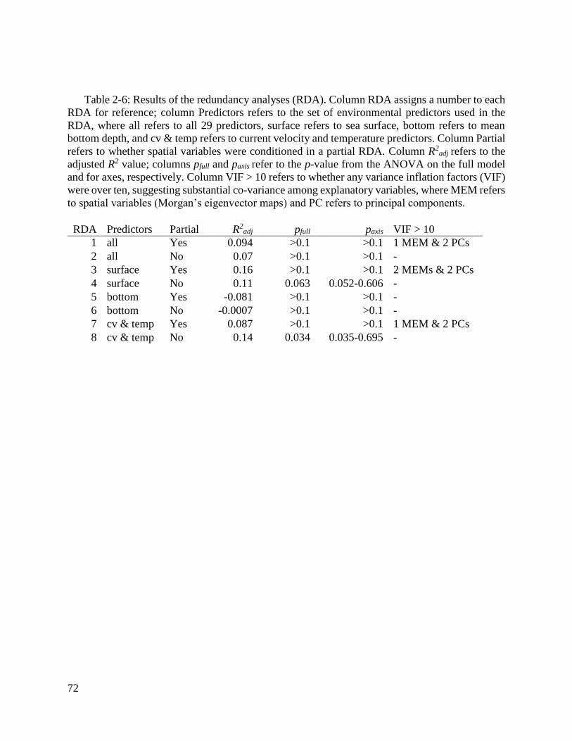
72

Table 2-6: Results of the redundancy analyses (RDA). Column RDA assigns a number to each

RDA for reference; column Predictors refers to the set of environmental predictors used in the

RDA, where all refers to all 29 predictors, surface refers to sea surface, bottom refers to mean

bottom depth, and cv & temp refers to current velocity and temperature predictors. Column Partial

refers to whether spatial variables were conditioned in a partial RDA. Column R2adj refers to the

adjusted R2 value; columns pfull and paxis refer to the p-value from the ANOVA on the full model

and for axes, respectively. Column VIF > 10 refers to whether any variance inflation factors (VIF)

were over ten, suggesting substantial co-variance among explanatory variables, where MEM refers

to spatial variables (Morgan’s eigenvector maps) and PC refers to principal components.

RDA Predictors Partial R2adj pfull paxis VIF > 10

1 all Yes 0.094 >0.1 >0.1 1 MEM & 2 PCs

2 all No 0.07 >0.1 >0.1 -

3 surface Yes 0.16 >0.1 >0.1 2 MEMs & 2 PCs

4 surface No 0.11 0.063 0.052-0.606 -

5 bottom Yes -0.081 >0.1 >0.1 -

6 bottom No -0.0007 >0.1 >0.1 -

7 cv & temp Yes 0.087 >0.1 >0.1 1 MEM & 2 PCs

8 cv & temp No 0.14 0.034 0.035-0.695 -

73

Figure 2-1: A map of collection sites and DAPC results for A. californicus. A map of collection

sites, including an inset of the southern Salish Sea (upper left). Individuals colored by collection

site plotted across the first two discriminant functions of DAPCs using all SNPs (upper right, n =

2,075), putatively adaptive SNPs (lower left, n = 211), and putatively neutral SNPs (lower right

n=1,864). For each plot, axes are labeled with the proportion of among-population variance

explained by that principal component. Point shapes differ by state or province to highlight

regional effects.

74

Figure 2-2: Evidence for isolation-by-distance in A. californicus. Correlation between in-water

distance and linearized FST using all SNPs (y = (3.2*10-6)*x + 3.5*10-3, adjusted R2 = 0.5622, p <

0.001), putatively neutral SNPs (y = (1.1*10-6)*x + 1.7*10-3, adjusted R2 = 0.2217, p < 0.01), and

putatively adaptive SNPs (y = 2.2*10-5)*x, adjusted R2 = 0.5786, p < 0.001).

Figure 2-3: Results of FST outlier detection methods for A. californicus. Log10 q-value by FST

for outlier detection methods, using results generated by OutFLANK (n = 46) in panel A and

BayeScan (n = 50) in panel B. Each point represents a single SNP, colored by whether it was

detected as an outlier (red) or not (black).

75

Figure 2-4: Summary of the results of univariate (Bayenv2) and multivariate (RDA) gene-

environment associations for A. californicus. Panel A is a histogram of log10 Bayes Factors for

each combination of SNP and environmental predictor. Panels B and C are RDA biplots of the

first two RDA axes, with predictors as vectors and sites as points in ordination space, using Type

1 scaling, a scaling method appropriate for questions related to distance among objects. Panel B is

of the retained model using sea surface predictors, and panel C is of the retained model using

temperature and current velocity predictors. For each RDA biplot, the proportion of variance

explained by each RDA axis is labeled on the axis.

76

Figure 2-5: Simulation results to contextualize empirical population differentiation and

estimate connectivity for A. californicus. Tile maps represent pairwise FST for each combination

of effective population size, migration rate, and number of generations of drift elapsed. Short-term

(left) represents results from 10 generations of drift, Medium-term (middle) from 100 generations

of drift, and Long-term (right) from 1,000 generations of drift. Tile color is divided into three

groups based on the scale of FST: smaller than the observed FST values in this study, within the

range of observed pairwise FST, and greater than the observed pairwise FST.

77


Supplemental Table 2-1: Pairwise FST and genic differentiation test results, to compare de novo

and reference-guided locus assemblies. Global FST = 0.0068 in both the de novo and reference-

guided assembly.

De novo CB_AK YB_AK AB_AK BB_BC SK_WA JI_WA KP_WA EI_WA CH_OR

CB_AK - * * * * * *

YB_AK 0.0036 - * * * * * *

AB_AK 0.0043 0.0037 -

BB_BC 0.0076 0.006 0.0038 - * * * * *

SK_WA 0.0122 0.0094 0.0075 0.0049 - * * *

JI_WA 0.0139 0.0114 0.0099 0.0061 0.0014 - * * *

KP_WA 0.0101 0.0088 0.0074 0.006 0.0033 0.0056 - *

EI_WA 0.0108 0.0098 0.0088 0.0062 0.004 0.0048 0.0006 - *

CH_OR 0.011 0.011 0.0089 0.0093 0.0081 0.0109 0.0036 0.0045 -

Reference CB_AK YB_AK AB_AK BB_BC SK_WA JI_WA KP_WA EI_WA CH_OR

CB_AK - * * * * *

YB_AK 0.004 - * * * * * *

AB_AK 0.004 0.004 -

BB_BC 0.008 0.005 0.005 - * * * * *

SK_WA 0.011 0.009 0.008 0.006 - * * *

JI_WA 0.015 0.012 0.012 0.007 0.002 - * * *

KP_WA 0.010 0.009 0.008 0.007 0.004 0.006 - *

EI_WA 0.011 0.008 0.011 0.006 0.005 0.005 0.001 - *

CH_OR 0.009 0.008 0.007 0.009 0.008 0.010 0.004 0.005 -

78

Supplemental Table 2-2: Expected heterozygosity, observed heterozygosity, and proportion of

polymorphic SNPs by collection site, comparing de novo and reference-guided assemblies.

Column HE refers to mean expected heterozygosity, column HO refers to mean observed

heterozygosity, and column SP refers to the proportion of SNPs that were polymorphic.

De novo Reference

Collection site HE HO SP HE HO SP

Chiniak Bay, AK 0.273 0.256 0.946 0.278 0.251 0.932

Yakutat Bay, AK 0.274 0.253 0.985 0.279 0.250 0.973

Auke Bay, AK 0.271 0.242 0.865 0.275 0.240 0.837

Bella Bella, BC 0.278 0.235 0.969 0.286 0.232 0.951

Sekiu, WA 0.273 0.241 0.989 0.279 0.238 0.977

James Island, WA 0.271 0.235 0.987 0.277 0.233 0.968

Keyport, WA 0.271 0.237 0.987 0.278 0.233 0.964

Eld Inlet, WA 0.273 0.236 0.987 0.280 0.234 0.970

Charleston, OR 0.271 0.237 0.982 0.277 0.233 0.968

Supplemental Table 2-3: Pearson’s correlation coefficients among 29 environmental

predictors. Coefficients are shaded blue-white-red for negative-zero-positive. Column and row

numbers refer to a specific environmental variable, noted in Supplemental Table 1-1.

79

Supplemental Table 2-4: All environmental predictor loadings on retained PCs.

Environmental Predictor PC1 PC2 PC3

BO_bathymean 0.077 -0.321 0.041

BO_calcite -0.081 -0.014 -0.035

BO_ph 0.047 -0.047 -0.398

BO2_curvelmax_bdmean 0.286 0.055 -0.100

BO2_curvelmax_ss 0.212 0.030 -0.234

BO2_curvelmean_bdmean 0.168 -0.076 -0.010

BO2_curvelmean_ss 0.186 0.099 -0.239

BO2_curvelmin_bdmean 0.238 -0.070 -0.155

BO2_curvelmin_ss 0.280 0.109 -0.141

BO2_curvelrange_bdmean -0.203 0.027 0.056

BO2_curvelrange_ss 0.251 0.026 -0.177

BO2_dissoxmean_bdmean -0.067 -0.313 -0.073

BO2_dissoxmean_ss -0.287 -0.141 0.063

BO2_nitratemean_bdmean -0.054 0.345 -0.044

BO2_nitratemean_ss -0.021 0.018 -0.281

BO2_phosphatemean_bdmean -0.042 0.338 0.122

BO2_phosphatemean_ss -0.004 0.096 0.307

BO2_ppmean_bdmean 0.057 -0.285 0.233

BO2_ppmean_ss 0.180 -0.088 0.144

BO2_salinitymean_bdmean -0.048 0.334 -0.092

BO2_salinitymean_ss -0.006 0.014 -0.390

BO2_tempmax_bdmean 0.198 -0.244 0.114

BO2_tempmax_ss 0.251 -0.190 -0.064

BO2_tempmean_bdmean 0.283 -0.058 0.182

BO2_tempmean_ss 0.285 0.054 0.157

BO2_tempmin_bdmean 0.265 0.139 0.167

BO2_tempmin_ss 0.268 0.099 0.193

BO2_temprange_bdmean -0.016 -0.338 -0.020

BO2_temprange_ss -0.141 -0.224 -0.251

80

Supplemental Table 2-5: Sea surface predictor loadings for retained PCs.

Environmental Predictor PC1 PC2

BO_calcite -0.086 0.059

BO_ph 0.186 0.405

BO2_curvelmax_ss 0.328 0.156

BO2_curvelmean_ss 0.326 0.144

BO2_curvelmin_ss 0.395 -0.006

BO2_curvelrange_ss 0.375 0.062

BO2_dissoxmean_ss -0.385 0.098

BO2_nitratemean_ss 0.096 0.283

BO2_phosphatemean_ss -0.078 -0.351

BO2_ppmean_ss 0.154 -0.216

BO2_salinitymean_ss 0.131 0.401

BO2_tempmax_ss 0.276 0.004

BO2_tempmean_ss 0.285 -0.307

BO2_tempmin_ss 0.265 -0.348

BO2_temprange_ss -0.122 0.384

81

Supplemental Table 2-6: Bottom depth predictor loadings for retained PCs.

Environmental Predictor PC1 PC2

BO2_curvelmax_bdmean 0.058 -0.458

BO2_curvelmean_bdmean 0.147 -0.140

BO2_curvelmin_bdmean 0.169 -0.279

BO2_curvelrange_bdmean -0.115 0.321

BO2_dissoxmean_bdmean 0.301 0.289

BO2_nitratemean_bdmean -0.395 -0.097

BO2_phosphatemean_bdmean -0.364 -0.127

BO2_ppmean_bdmean 0.343 0.029

BO2_salinitymean_bdmean -0.387 -0.088

BO2_tempmax_bdmean 0.354 -0.197

BO2_tempmean_bdmean 0.205 -0.413

BO2_tempmin_bdmean -0.014 -0.480

BO2_temprange_bdmean 0.345 0.182

82

Supplemental Table 2-7: Current velocity and temperature predictor loadings for retained PCs.

Environmental Predictor PC1 PC2 PC3

BO2_curvelmax_bdmean 0.317 -0.066 0.098

BO2_curvelmax_ss 0.236 -0.257 0.268

BO2_curvelmean_bdmean 0.170 -0.044 0.054

BO2_curvelmean_ss 0.213 -0.118 0.454

BO2_curvelmin_bdmean 0.259 -0.167 0.116

BO2_curvelmin_ss 0.312 0.003 0.243

BO2_curvelrange_bdmean -0.216 0.189 0.105

BO2_curvelrange_ss 0.272 -0.103 0.268

BO2_tempmax_bdmean 0.194 -0.251 -0.460

BO2_tempmax_ss 0.259 -0.299 -0.152

BO2_tempmean_bdmean 0.297 0.064 -0.338

BO2_tempmean_ss 0.308 0.202 -0.174

BO2_tempmin_bdmean 0.291 0.304 -0.091

BO2_tempmin_ss 0.291 0.286 -0.164

BO2_temprange_bdmean -0.040 -0.471 -0.365

BO2_temprange_ss -0.161 -0.496 0.088

Supplemental Table 2-8: Sites retained at each filtering step in A. californicus. All loci were

SNPs after removing indels. MAF = minor allele frequency.

Filtering step Loci

Total from dDocent 6738423

After removing indels 3987180

After maximum missing data per locus = 30% 94543

After minimum MAF = 0.05 9178

After minimum quality score = 20 9133

After removing SNPs out of Hardy Weinberg Equilibrium 5042

After retaining one SNP per RAD locus, with highest MAF 2075

83

Supplemental Table 2-9: Pairwise FST with confidence intervals and pairwise genic

differentiation test results. Pairwise FST (and 95% confidence intervals) in the lower left and

pairwise genic differentiation test results in the upper right of the table (*: p < 0.05). Confidence

intervals were generated by bootstrapping across SNPs with 100 repetitions. Cells with higher FST

values were shaded darker green. Site abbreviations provided in Table 2-1.

CB_AK YB_AK AB_AK BB_BC SK_WA JI_WA KP_WA EI_WA CH_OR

CB_AK - * * * * *

YB_AK 0.004

(0.001-0.005) - * * * * * *

AB_AK 0.004

(0.001-0.007) 0.004

(0.001-0.007) -

BB_BC 0.008

(0.005-0.011) 0.005

(0.003-0.007) 0.005

(0.001-0.008) - * * * * *

SK_WA 0.011

(0.009-0.013) 0.009

(0007-0.011) 0.008

(0.004-0.011) 0.006

(0.004-0.009) - * * *

JI_WA 0.015

(0.012-0.018) 0.012

(0.010-0.014) 0.012

(0.008-0.017) 0.007

(0.006-0.010) 0.002

(0.001-0.004) - * * *

KP_WA 0.010

(0.009-0.014) 0.009

(0.007-0.012) 0.008

(0.003-0.012) 0.007

(0.005-0.010) 0.004

(0.002-0.006) 0.006

(0.005-0.010) - *

EI_WA 0.011

(0.009-0.014) 0.008

(0.007-0.012) 0.011

(0.007-0.016) 0.006

(0.005-0.010) 0.005

(0.003-0.006) 0.005

(0.004-0.006) 0.001

(0.000-0.003) - *

CH_OR 0.009

(0.006-0.011) 0.008

(0.006-0.011) 0.007

(0.003-0.010) 0.009

(0.007-0.013) 0.008

(0.007-0.010) 0.010

(0.008-0.013) 0.004

(0.001-0.005) 0.005

(0.004-0.008) -

84

Supplemental Table 2-10: Bayenv2 results for A. californicus. Column Environmental

Predictor refers to the environmental predictor with correlated SNPs. Column Depth refers to

whether the variable was measured at sea surface (S) or mean bottom depth (B). Column SC refers

to the number of correlated SNPs. Column SP refers to the number of correlated SNPs with

associated gene ontology slim terms for biological processes. Column Biological Processes

contains the associated biological processes from matching gene ontology slim terms in order of

decreasing frequency, with the proportion of matches per process noted in parentheses.

Environmental Predictor Depth SC SP Biological Processes

Mean salinity S 38 4 signal transduction (0.259),





transport (0.069),


Mean nitrate S 34 4 signal transduction (0.294),




transport (0.078),



Temperature range S 31 2 cell organization and biogenesis (0.387),




DNA metabolism (0.065),


stress response (0.032)

pH S 30 3 cell organization and biogenesis (0.353),




Mean temperature B 27 1 signal transduction (0.5),

transport (0.5)

Mean phosphate S 26 2 cell organization and biogenesis (0.522),



Minimum temperature S 24 1 signal transduction (0.5),

transport (0.5)

Minimum temperature B 22 1 signal transduction (0.5),

transport (0.5)

Mean primary

productivity

S 19 2 cell organization and biogenesis (0.308),


85



cell cycle and proliferation (0.103)

Mean temperature S 18 1 signal transduction (0.5),

transport (0.5)

Mean current velocity B 14 2 cell organization and biogenesis (0.367),

transport (0.245),


signal transduction (0.184)

Mean dissolved oxygen S 14 1 developmental processes (0.522),

transport (0.217),


RNA metabolism (0.087)

Maximum temperature S 14 2 stress response (1)

Maximum current

velocity

B 13 1 transport (0.333),


stress response (0.148),




death (0.037),



Minimum current

velocity

B 12 NA NA

Minimum current

velocity

S 12 1 developmental processes (0.522),

transport (0.217),



Range in current velocity S 12 1 DNA metabolism (1)

Maximum temperature B 12 NA NA

Mean primary

productivity

B 11 1 DNA metabolism (1)

Mean dissolved oxygen B 10 1 transport (0.42),





cell adhesion (0.043),



Range in current velocity B 9 1 cell organization and biogenesis (0.571),

signal transduction (0.429)

Mean phosphate B 9 1 signal transduction (0.326),

stress response (0.256),


86


transport (0.093),

death (0.07),

cell-cell signaling (0.023),


Maximum current

velocity

S 8 1 protein metabolism (1)

Mean current velocity S 8 1 protein metabolism (1)

Mean nitrate B 6 NA NA

Calcite S 5 NA NA

Mean salinity B 5 NA NA

Range in temperature B 5 NA NA

Mean bathymetry B 3 NA NA

Supplemental Table 2-11: Loadings for RDA using sea surface predictors. The loadings for

each PC are presented in Supplemental Table 2-5.

RDA1 RDA2

PC1 0.266 -0.964

PC2 -0.964 -0.266

Supplemental Table 2-12: Loadings for RDA using current and temperature predictors. The

loadings for each PC are presented in Supplemental Table 2-7.

RDA1 RDA2 RDA3

PC1 0.456 -0.742 0.492

PC2 0.810 0.574 0.116

PC3 -0.368 0.346 0.863

87

Supplemental Table 2-13: Counts of gene ontology slim terms in the database.

Gene ontology slim term n

other metabolic processes 4102

other biological processes 3320

developmental processes 3092

cell organization and biogenesis 1712

transport 1398

protein metabolism 1261

stress response 1000

signal transduction 917

cell cycle and proliferation 675

RNA metabolism 574

cell-cell signaling 302

DNA metabolism 299

death 267

cell adhesion 107

88

Supplemental Figure 2-1: Principal component analysis to compare reference-guided and de

novo locus assemblies. Individuals are plotted across the first two principal components.

Supplemental Figure 2-2: Overfitting of RDA models occurred quickly with the addition of

predictor variables. Using randomly generated data based on the mean and standard deviations of

environmental predictor data used in this study, we demonstrated that R2 reaches 1 with the

addition of 8 predictor variables.

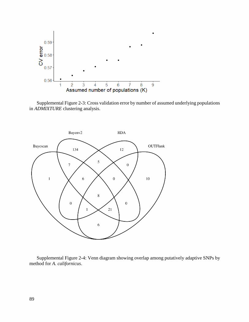
89

Supplemental Figure 2-3: Cross validation error by number of assumed underlying populations

in ADMIXTURE clustering analysis.

Supplemental Figure 2-4: Venn diagram showing overlap among putatively adaptive SNPs by

method for A. californicus.

90

Chapter 3. Informal policy and factors affecting policy change for

genetic risks of native shellfish aquaculture

3.1 INTRODUCTION

Shellfish constitute the majority of marine aquaculture production in the United States

(NOAA Fisheries, 2021b). Many of the cultivated shellfish species are non-native, including the

most widely grown species on the West Coast, the Pacific Oyster (Pacific Shellfish Institute,

2021b). The shellfish aquaculture industry is growing (Sea Grant Association, 2016) and one facet

of industry expansion is the development of new species for cultivation. Because importing non-

native species poses ecological risks to native species and the broader ecosystem, many have

turned to native shellfish species for commercial development. For example, on the Pacific Coast

of North America, multiple native shellfish species including the Olympia Oyster, Pacific

Geoduck, and Purple-hinged Rock Scallop have been identified as species to target for

development or expansion of current commercial production (Sea Grant Association, 2016).

However, aquaculture of native species poses genetic risks to wild populations if hatchery-

produced and wild animals interbreed (Laikre et al., 2010). These risks threaten long-term

population viability of both wild populations and aquaculture (R. S. Waples et al., 2012) and are

thus a concern for decision makers at natural resource management agencies.

3.1.1 What are the genetic risks of native shellfish aquaculture?

Although hatchery production methods differ based on the goal of the program (e.g.,

commercial or conservation goals), they generally differ from wild reproduction, resulting in

genetic impacts for offspring. These genetic impacts can affect wild populations if hatchery-

produced and wild individuals interbreed, such as through escape or intentional release (Laikre et

91

al., 2010). Although not mutually exclusive, these genetic impacts of aquaculture can be organized

into a simple framework with three genetic risks: loss of genetic diversity within populations, loss

of population differentiation, and loss of fitness (R. S. Waples et al., 2012).

The first genetic risk of hatchery production is loss of genetic diversity within a population.

For production facilities, collecting and maintaining large populations of parents may be cost

prohibitive and logistically challenging. Thus, hatchery production often involves relatively few

parents producing many offspring, compared to wild populations (Straus et al., 2015). However,

small parental populations may produce offspring with less genetic diversity than a wild cohort.

Upon interbreeding between hatchery-produced and wild animals, the genetic diversity of the wild

population may decline (Ryman & Laikre, 1991). Moreover, interbreeding between highly related

individuals can lead to inbreeding depression, in which fitness declines (Plough & Hedgecock,

2011; Taris et al., 2007; S. Wang et al., 2002).

Second, hatchery production can also reduce population differentiation among wild

populations if movement of broodstock and seed occurs across distinct populations or if

broodstock from distinct populations are crossed in the hatchery and seed are released into either

population (R. S. Waples et al., 2012). Population differentiation may also be reduced when the

proportion of hatchery-produced escapees in several wild populations is high enough that their

genetic contribution overrides genetic differences among wild populations, a process known as

swamping (Waples & Do, 1994) (Figure 2-1).

Third, loss of fitness can occur due to domestication selection, through relaxation of natural

selection, selection for traits that provide advantages in the captive environment, or both

(Reisenbichler & Rubin, 1999). The purpose of shellfish hatcheries is to increase survival of

offspring, and in commercial aquaculture specifically, to maximize optimal growing conditions.

92

Thus, natural selection is usually relaxed (Lynch & O’Hely, 2001). Optimal growing conditions

(density, ambient temperature, etc.) may differ slightly from the natural environment.

Additionally, animals with traits better suited to the captive environment have higher reproductive

success in the captive environment than their wild counterparts (Doyle, 1983), leading to

domestication selection. Domestication selection can be intentional, such as selection for

production traits in hatchery lines (Dale-Kuys et al., 2017; de Melo et al., 2016), or unintentional,

through favoring specific traits, such as culling slowly developing larvae, leading to selection for

faster development (Taris et al., 2007). As a result, hatchery-produced offspring that survive in the

captive environment can be less fit in the wild one (Fritts et al., 2007; Pearsons et al., 2007). If

hatchery-related traits are passed on to the wild population through interbreeding of hatchery-

produced and wild animals, fitness of wild populations can decline (Besnier et al., 2015).

Domestication selection can also result in loss of genetic diversity, as fit individuals have greater

reproductive success, leading to fewer effective breeders (Currens & Busack, 1995).

A central concern to natural resource managers is the sustainability of wild resources for

present and future uses (ADFG, 2019; LNRD, 2019; NNRD, 2019; WDFW, 2019). Maintaining

fitness and genetic diversity, both within and among populations, can support the sustainability of

wild resources because these factors contribute to adaptability and productivity (Hughes et al.,

2008; Schindler et al., 2010). For these reasons, the genetic risks associated with hatchery-

produced finfish, in particular salmon, have resulted in decades of research and policy

development to mitigate risks to wild populations (Mobrand et al., 2005; Naish et al., 2007; Paquet

et al., 2011). There is substantially less research on shellfish (Nascimento-Schulze et al., 2021;

Valenzuela-Quiñonez, 2016) and formal regulation of these risks in shellfish species.

93

3.1.2 What information would inform potential policy development?

Informal policy is becoming increasingly more common (Mendelson, 2006), particularly

for emerging risks (Blais & Wagner, 2007), because of the associated time and resource costs

associated with formal policies. Formal policies require a public comment period and are legally

binding (e.g., 85 FR 81822, a federal rule updating designation of Pacific salmon hatchery

programs under the Endangered Species Act). Informal policies, often in the form of guidance

documents, provide specificity and practical guidance for implementation of formal policy

(Mendelson, 2006). Although designed to not be legally binding, informal policies can be deemed

legally binding through litigation (Franklin, 2010). Informal policies can therefore change

behavior of regulated entities, albeit not to the extent of formal policy. Given the lack of formal

policy for genetic risks of native shellfish aquaculture, it remains unclear to what extent agencies

use informal policy to mitigate these risks. Because informal policies do not require a public

comment period, they may be less visible to agency outsiders unless they specifically request it.

Illuminating to what extent agencies use informal policy for mitigating the genetic risks of

native shellfish aquaculture may be useful for many reasons. Because the genetic risks of native

shellfish aquaculture is often a trans-boundary issue (involving coordination among states and

provinces), characterizing patterns and variation in informal policy will benefit interagency

coordination. Such activities might include identification of shared management goals and targets

(Kark et al., 2015) and the definition of management units in shared waters, used for restricting

movement of broodstock and seed (Fisheries and Oceans Canada, 2011). Furthermore, the

multiplicity of state and tribal agencies along the Pacific Coast of the United States likely provides

variation in policy approaches (Galle & Leahy, 2008), and raising awareness of such variation in

94

policies may serve as a starting point for comparing policy alternatives, a critical step of many

policy development processes (Greco et al., 2016; Punt et al., 2016).

Potential policy development for genetic risks of native shellfish aquaculture will likely be

influenced by more than top-down directives, regardless of whether policies are formal or informal

(Miner, 2006). According to the punctuated equilibrium theory of policy change (PET), most

policy changes are incremental except for rare, substantial changes (True et al., 1999) due to

bounded rationality. Bounded rationality refers to the rational, cognitive, and institutional factors

that constrain an individual’s decision making within an organization, and that lead to behavior

better described by satisficing rather than by strictly rational optimization (Miner, 2006). These

factors may include an individual’s values relating to organizational goals and knowledge of

potential policy outcomes (Bell, 1985; Miner, 2006), as well as the cognitive difficulties associated

with accounting for uncertainty, conceptualizing the problem, and risk perception (Jones, 2003).

Institutional factors such as budgets, organizational culture, and existing relationships with interest

groups also shape individual decision making (Lester, 1995; Sapat, 2004). PET posits that rare,

substantial changes are due to changes in agenda setting due to limited attention spans in

organizations (True et al., 1999) and that these shifts in attention are due to external perturbations

that disrupt policy ideas, beliefs, and institutions (Sabatier & Jenkins-Smith, 1993; Smith, 2000;

Thelen, 2003). Shedding light on these factors and how they shape the level of attention given to

this issue may inform potential policy change regarding genetic risks of native shellfish

aquaculture.

3.1.3 Study aim

The aim of this study is to describe the regulatory context regarding the genetic risks of

native shellfish aquaculture (hereafter referred to as genetic risks), within the Pacific Coast region

95

of the United States. Specifically, we used a mixed-methods approach, which combines

quantitative and qualitative methods (Johnson & Onwuegbuzie, 2004), to interview state and tribal

government shellfish resource managers, in order to illuminate 1) current management practices,

2) factors that may influence decision-making, and 3) the level of policy attention given to this

issue. Where possible, we provided comparisons to the same issues in the management of hatchery

production of Pacific salmon. Although Pacific salmon and their hatchery production differ from

their counterparts in shellfish, the management of hatchery production of Pacific salmon provides

the closest example of what policies could be in place for native shellfish aquaculture. Our results

will benefit decision makers considering potential policy development for the genetic risks of

native shellfish aquaculture, at a time when this issue is receiving increased attention in academic

(Hornick & Plough, 2019; Nascimento-Schulze et al., 2021) and policy arenas (WDFW, 2016).

3.2 METHODS

3.2.1 Study system

We focused our study on the Pacific Coast region of the United States, which supports the

largest shellfish aquaculture industry in the country (Washington Sea Grant, 2015), with

demonstrated interest in expanding native shellfish aquaculture (Culver et al., 2006; Pacific

Shellfish Institute, 2021a). Shellfish aquaculture largely takes place in coastal waters where states

(Alaska, Washington, Oregon, California) and tribes have jurisdiction. Though a number of tribes

have land rights in this region, we only included Western Washington treaty tribes (n = 20) in our

study because of their reaffirmed rights for shellfish harvest (J. W. Anderson, 1999) and status as

co-managers for shellfish resources. Although there is variation in governance and policy-making

among tribes and states, in general, formal policy making is directed by rule-making bodies (e.g.,

legislature, fish and wildlife commissions, tribal councils) and implemented by administrative

96

bodies (e.g., Department of Natural Resources, Department of Fish and Wildlife) with often broad

agency discretion (SOSU, 2016; WDFW, 2021). We targeted shellfish resource managers at state

and tribal agencies for interviews because we were interested primarily in informal policy making.

3.2.2 Interview methodology

For each of the four U.S. Pacific Coast states and twenty Western Washington treaty tribes,

we identified potential interviewees as individuals whose work pertained to management or

regulation relating to shellfish aquaculture and/or wild shellfish resources. Depending on the

administration, managers with such positions worked in a variety of agencies (e.g., natural

resources, fish and wildlife, and agriculture). Herein, we refer to these agencies collectively as

“natural resource agencies.” Individuals were identified through online research and by contacting

natural resource agency offices. We incentivized participation using a raffle for an Amazon gift

card. The University of Washington Human Subjects Division deemed this study “exempt” from

federal human subjects regulations, including the requirement for Institutional Review Board

approval and continuing review.

In the spring of 2018, we interviewed 18 shellfish resource managers from 14 state and

tribal natural resource agencies, representing all four US states along the Pacific west coast (n=4)

and half (n=10) of the Western Washington treaty tribes. We used semi-structured interviews

(Charnley et al., 2017; Dillman, 2014; Saldaña & Omasta, 2016) to gather information regarding

the regulatory context surrounding this emerging management issue. Throughout, we apply the

PET framework not for the purposes of testing the theory or predicting policy change, but for

illuminating relevant factors for informing potential decision making. Specifically, our objectives

were 1) to characterize current management practices, 2) to illuminate factors that may influence

decision-making, and 3) to assess the relative attention given to genetic risks of native shellfish

97

aquaculture as it relates to agenda setting. To provide context on manager and agency priorities

and values, we asked managers about their responsibilities, their three highest priority tasks, and

rationales for why such tasks were high priority. Below we provide an overview of the interview

themes, and the full interview protocol is provided in the Supplementary Materials.

For the first objective, we asked managers about the degree to which their agency currently

manages for genetic risks of native shellfish aquaculture, regardless of the program goal

(commercial aquaculture, restoration aquaculture, etc.). For the second objective, we identified a

priori factors for investigation: how managers conceptualize of genetic risks of native shellfish

aquaculture, how they perceive these risks, the degree of resource limitation (i.e., available

funding) at the agency, and the nature of the relationship with a primary interest group, the

aquaculture industry. To shed light on how managers conceptualized the problem, we asked

managers to rationalize responses to questions related to genetic risks, which encouraged them to

define the problem. To gauge the level of risk perceived by managers for this issue, we used both

indirect and direct lines of questioning and contextualized these results with the greatest concerns

managers held for the future of wild shellfish resources. To characterize the degree of resource

limitation, we asked managers what tasks they would delegate to a hypothetical new staff member

and searched for responses related to resource limitation in rationales for other responses. Lastly,

we asked managers to what degree the relationship between the agencies and the aquaculture

industry is regulatory or advisory in nature. Throughout, we asked for the rationale behind stated

priorities, concerns, and other responses to illuminate manager values and beliefs. For the third

objective, we synthesized our results to characterize the level of policy attention and

contextualized the level of policy attention with rationales provided by managers and paradigm

shifts in the scientific literature.

98

We included multiple considerations in our methodology to circumvent social desirability

bias, in which participants answer questions in a way that is expected to be viewed favorably,

while gathering information about relative concern over genetic risks of native shellfish

aquaculture. To accomplish this task we 1) maximized neutral language in the interview tool

(Nederhof, 1985), 2) used triangulation by asking questions in multiple ways (Krefting, 1991), and

3) ordered questions from broad to specific, such that the direct, closed-ended question that was

more likely to lead to bias in subsequent responses (Fisher, 1993) was asked last.

Closed questions were analyzed by tallying frequencies of possible answers. For open

questions, we transcribed interviews and developed a coding methodology based on values coding

(Miles et al., 2014) and thematic analysis (Ayres, 2008) for data condensation in ATLAS.ti v8.4.4

(Hwang, 2008). We then aggregated codes into themes and described the frequency and

relationships among codes and themes within the context of our research objectives (Huberman &

Miles, 2002; Miles et al., 2014). We reported the occurrence of codes and themes by number of

managers and number of agencies represented by interviewed managers where appropriate. A

single coder (the first author) coded all interviews.

3.3 RESULTS AND DISCUSSION

Although all 18 interviewed managers held positions with responsibilities in shellfish

resource and/or shellfish aquaculture management, the professional responsibilities for

interviewed managers varied (Table 3-1). Managers from most surveyed agencies (number of

responding agencies (a) = 11 of 14) reported native shellfish aquaculture within their jurisdictions.

99

3.3.1 If and how are genetic risks currently managed?

Half of the agencies represented in interviews (a = 7) responded that they managed

shellfish resources for genetic risks in some capacity (Figure 3-2A). As one interviewee noted:

We do manage genetic risks in the fact that that’s one of our primary concerns when we

get proposals for [growing] native species. Genetics is always a big question.

The most reported methods for managing genetic risks included 1) encouraging use of local

broodstock in hatcheries (a = 4), 2) preventing aquaculture of native shellfish species (a = 3) either

completely or for species that are not yet cultivated within their jurisdiction, and 3) encouraging

use of many broodstock individuals (a = 2). Reported methods centered on broodstock choice (i.e.,

number and source of broodstock) and did not include considerations related to breeding design,

captive environment conditions, or growing practices on farms.

By comparison, the genetic risks of hatchery-reared finfish, especially salmon, have

resulted in more complex and formal policy at multiple levels. At a national level, the United States

Congress tasked a team of scientists to comprehensively review Pacific salmon hatcheries in the

Columbia River Basin and Puget Sound region (Mobrand et al., 2005), initiating an era of broad

hatchery reform (California Hatchery Scientific Review Group, 2012; USFWS, 2013). This review

resulted in recommended operational procedures, of which many aimed to reduce genetic risks

(Mobrand et al., 2005). Moreover, hatcheries enhancing populations protected under the

Endangered Species Act of 1973 (ESA) that use wild broodstock or producing animals that are

likely to interact with species protected under the ESA are required to comply with the ESA. This

entails development of a Hatchery and Genetic Management Plan (NOAA Fisheries, 2019), in

which NOAA Fisheries works with program operators to identify growing practices that mitigate

all three types of genetic risks (Table 3-2). Once permitted, hatcheries are required to submit

100

annual reports so that agencies can ensure compliance (NOAA Fisheries, 2012, 2021a). Many state

and tribal natural resource agencies have implemented statutes, regulations, and best management

practices to address genetic risks of aquaculture to wild populations in finfish (Davis et al., 1989;

NWIFC: Genetics, 2008; WDFW, 2020b). More complex and formal policy in the management of

native shellfish aquaculture should be considered, particularly without empirical data suggesting

genetic risks will be less severe in shellfish than in Pacific salmon.

3.3.2 What factors may affect policy change regarding genetic risks of native shellfish

aquaculture?

We identified potential a priori factors that may bound rational decision making, leading

to incremental policy change (Miner, 2006). Specifically, we analyzed manager responses

regarding problem conceptualization, level of risk perception, degree of resource limitation, and

the relationship with a primary interest group, the aquaculture industry.

How do managers conceptualize genetic risks?

Policy change can be slow when policy problems are hard to conceptualize (Jones, 2003).

Genetic concepts, when compared to other biological concepts, pose greater cognitive challenges

to both students and teachers, likely due to genetic processes occurring on scales not accessible to

the senses, the complex and extensive vocabulary, and central use of mathematics in defining

concepts (Bahar et al., 1999). To understand to what degree genetic risks as a policy problem poses

cognitive challenges, we investigated 1) whether descriptions of genetic risks were consistent with

best available science and 2) the completeness of managers’ perceptions of the policy problem.

Most managers demonstrated understanding consistent with best available science

regarding genetic concepts, although a couple of commonly shared ideas were at odds with our

scientific understanding. Firstly, some managers did not fully appreciate that many shellfish

101

production practices beyond broodstock choice have genetic consequences. Secondly, some

managers suggested that escape can be beneficial to wild populations. It is unsurprising that the

conditions under which hatchery production can provide demographic and genetic risks or benefits

is unclear, as there is a history of controversy and disagreement among experts (Brannon et al.,

2004; R. S. Waples, 1999). Although supplementation can provide a demographic boost (Janowitz-

Koch et al., 2019), it can still be accompanied by a loss of genetic diversity (Christie et al., 2012).

Hatchery production is expected to reduce genetic diversity in large wild marine populations under

most circumstances (Hedgecock & Coykendall, 2007; R. S. Waples et al., 2016). However, the

application of these guiding principles is made challenging by the lack of empirical data on central

genetic parameters (e.g., the effective population size to census size ratio) in wild shellfish

populations and generally few studies tracking genetic effects of aquaculture releases on wild

shellfish populations (Hornick & Plough, 2019; Morvezen et al., 2016).

Biodiversity conservation and specifically genetic biodiversity are complex topics, and this

can lead to reduced policy attention (Haig et al., 2016; R. Taylor et al., 2017; Sandström et al.,

2019). This was noted by one manager:

It's more at an academic level, something we talk about at the beer pub, but it's not

something that I'm getting calls from mayors or chambers of commerce about.

Biodiversity can be measured using many units of measurement and at multiple scales, from the

visible (ecosystems and species) to the invisible (genetic diversity), complicating its

operationalization and policy development to mitigate its loss (Lidskog, 2014). Furthermore, the

effects of biodiversity loss are rarely observed by individuals, especially for genetic processes that

are subcellular and cannot be observed without advanced technologies (Zaccai and Adams 2012).

Perhaps as a result, efforts to conserve biodiversity rarely go as far as conserving genetic diversity

102

(with the exception of key agricultural and forest interest species, gene banks for imperiled species,

and some hatchery programs) despite the role of genetic diversity in species persistence that can

then contribute species richness and ecosystem diversity (Laikre, 2010).

Notably, of the three categories of genetic risks identified in Table 3-2, loss of genetic

diversity among populations (number of managers (m) = 11) and within populations (m = 9)

were discussed more frequently than loss of fitness associated with domestication selection (m =

2). We observed the same pattern in asking for manager recommendations for future policy

development (Table 3-3). This pattern may suggest that domestication selection is not perceived

as a significant component of genetic risks of aquaculture to wild shellfish populations, and is

surprising given the prominence of concerns over domestication selection in the literature on

genetic risks of hatchery production in salmon (Baskett & Waples, 2013; Castellani et al., 2018;

Ford, 2002). The reduced attention to domestication selection in shellfish aquaculture may be

due in part to the fact that broodstock movement is already regulated in many jurisdictions using

permits for the mitigation of another risk, disease (m = 6, a = 4). The availability of a relevant

policy instrument focused on limited mixing of distinct groups may have led to greater focus on

this risk, as policy instruments may influence problem conceptualization (Simons & Voß, 2018).

How do managers perceive genetic risks?

Risk perception can affect administrator decision making (Jones, 2003). To contextualize

how genetic risks are perceived among other risks, we first asked managers to report their greatest

concerns for the future of wild shellfish resources and noted whether genetic risks were listed

among these concerns. Managers then were asked directly to discuss their level of concern over

genetic risks compared to previously named concerns.

103

Few managers (m = 4, a = 2) reported genetic risks as one of their greatest concerns for the

future of wild shellfish resources, suggesting relatively low risk perception among managers. For

comparison, most managers reported being most concerned about long-term sustainability of

managed resources (m = 15, a =12), with the remaining named concerns being environmental

threats to such sustainability, such as ocean change and pollution (Figure 3-3). Notably, named

concerns were not mutually exclusive, and mitigating genetic risks is a means towards resilience

to environmental threats named by managers.

Mirroring results from indirect questioning, most managers reported feeling “a little

concerned” over genetic risks in response to direct questioning (Figure 3-4). The direct question

gauging level of concern over genetic risks was the question managers declined to answer most.

Because social desirability bias can lead to nonresponse (Kreuter et al., 2008), fewer responses to

this question suggest that social desirability most affected this question. A greater level of concern

about genetic risks was associated with managers who reported aquaculture activities within their

high priority tasks (Figures 3-4B.1 and 3-4B.2) and those who reported managing for genetic risks

(Figures 4C.1 and 4C.2). These patterns point to correlation between degree of agency proximity

to the aquaculture industry (e.g., advising, regulation, or participation) and managers’ perception

of genetic risks of native shellfish aquaculture. Although causal relationships cannot be inferred

from these data, this correlation may provide evidence for either manager risk perception driving

informal policy development for genetic risks or risk perception driven by organizational practices

and norms. The most reported factors driving high concern were fear of local population

displacement and expectation that the problem will worsen. The most reported factor driving low

concern was lack of information on genetic risks (Table 3-4).

What is the nature of resource limitation?

104

Resource limitation can drive path dependency, in which decisions are dependent on

previous decisions, bounding rational decision making and slowing policy change (Kirk et al.,

2007). Resource limitation was a common theme among manager responses. Managers reported

that their budgets did not increase alongside their mandated responsibilities or that new issues

could not be addressed due to limited budgets (m = 7, a = 7), for example:

The scale of our capacity is not scaled appropriately to the size of ... the seriousness of the

issue and what it takes to manage it.

When asked what tasks would be given to a hypothetical new staff member, more than half of

managers (m = 11, a = 8) named current tasks as opposed to novel tasks, suggesting that resources

were not sufficient for current goals.

Resource limitation comes as no surprise, as the last couple of decades have brought

financial hardships. For example, the Great Recession of 2008 created budget deficits for many

agencies with long lasting impacts (O’Sullivan, 2020), including for state wildlife agencies

(Frankovich, 2019). Moreover, state wildlife management is in a period of heightened reform and

budget crisis, defined in part by increasing threats to wild resources and reduced hunting- and

fishing-dependent revenue (e.g., license sales) (Jacobson & Decker, 2006). The economic crisis

associated with the Covid-19 pandemic will likely deepen lingering budget deficits, which may

further slow policy change for low priority issues.

What is the nature of the relationship between surveyed agencies and the aquaculture

industry, beyond genetic risks?

Periods of incremental policy change are expected particularly in cases with resource

limitation and limited information for decision making (Kirk et al., 2007; Simon, 2013), as were

reported by managers in this study (resource limitation, m = 7, a = 7; limited information on genetic

105

risks, m = 6, a = 6). In particular, policy instrument choice is often constrained by institutional

factors such as implementation style and organizational setting (Jones, 2003; Linder & Peters,

2016; Miner, 2006). Thus, we asked managers if and how their agency advises or regulates the

aquaculture industry (a primary interest group) beyond genetic risks, in order to illuminate possible

policy instruments for genetic risks.

Almost all managers reported that their agency regulates or advises aquaculture in some

capacity (m = 17, a = 13, Figure 3-2B), including through indirect input, such as commenting on

federal permits and advising shellfish growers on growing practices (Table 3-5). A commonality

among regulatory or advisory actions at most agencies was that compliance was voluntary except

for a select few actions, such as registration of facilities and regulating broodstock import and

transfer. In the absence of sudden policy attention to this issue, it is likely that policy

development will resemble these policy actions: few formal regulations, such as regulating

broodstock collection, and non-binding recommendations for production.

One factor that may slow policy development for mitigation of genetic risks is a lack of

clarity around agency authority, given involvement of multiple agencies. When asked whether

their agency has regulatory or advisory influence over industry growing practices, one manager

responded:

Our agency … doesn't do a lot of managing [aquaculture companies] at all... I don't know

if anyone in our staff is running around inspecting anything, so, it just sort of could be, lack of

clarity on which agency would do that.

Multiple agencies share regulatory authority over aspects of the aquaculture industry. For example,

depending on the exact state, their departments of health, natural resources, wildlife, ecology, and

agriculture all may hold some regulatory authority over aquaculture companies. This may lead to

106

a lack of role clarity around which agency has authority for a specific issue, slowing policy change

in a manner parallel to a by-stander effect (Fischer et al., 2011).

Furthermore, natural resource agencies often have complicated relationships with powerful

interest groups, including regulated industries, due to paradoxical and competing goals of

preservation and use of natural resources (Cheever, 1996). This complexity may be further

exacerbated by conflicts of interest, such as an agency deriving revenue from the profits of a

regulated industry, as in the case with revenue from the wild geoduck fishery funding of

Washington Department of Natural Resources and Washington Department of Fish and Wildlife

activities (WDNR, 2008). A potential complexity for the relationship between natural resource

agencies and shellfish aquaculture companies as it relates to genetic risks is the participation of

agencies in hatchery production: almost half of the managers reported that their agency funds

and/or operates a shellfish hatchery and/or farm (m = 8, a = 7), with purposes ranging from growing

native species for restoration or commercial production to growing non-native species for beach

enhancement or commercial production. Balancing mitigation of genetic risks among other goals

may be complicated by the agency’s institutional history of involvement in shellfish production.

3.3.3 How much policy attention do genetic risks of native shellfish aquaculture receive and

why?

After synthesizing results across managers and agencies, genetic risks receive relatively

little policy attention. Few managers (m = 6, a = 3) reported mitigating genetic risks as part of their

responsibilities or highest priority tasks in their current position. Although managers from half of

agencies reported managing for genetic risks in some capacity (a = 7), this task included small-

scale and non-binding actions. This finding is mirrored by a relatively low level of concern across

managers (Figure 3-4A) and low occurrence of genetic risks among the greatest concerns for the

107

future of wild shellfish resources (m = 4, a = 2). Only two managers included tasks related to

managing genetic risks for the hypothetical new staff member. A third of managers specifically

named managing genetic risks as low priority considering limited resources and higher priorities

(m = 6, a = 6).

Low risk perception and little policy attention to this issue are unsurprising given some of

the factors reported by managers and explored here: perceived lack of information, perceived lack

of clarity on agency authority, and cognitive challenges posed by genetic concepts, to name a few.

However, a match between risk perception and policy attention should not always be expected.

Risk perception can be affected by the degree of power to control outcomes (Slovic, 1987), such

as greater concern for risks that decision-makers have limited power to mitigate. Possible

mismatch between risk perception and degree of power may explain why ocean change was among

the most widely reported concerns for the future of wild shellfish resources and yet only one

manager reported developing climate change policy among highest priority tasks. Furthermore,

although agencies hold much discretion over policy implementation, legal mandates still constrain

aspects of decision-making and agenda setting.

Multiple factors identified here as potentially driving low risk perception and little policy

attention also apply to finfish systems. Why, then, has this issue received more policy attention in

finfish than in shellfish? Low policy attention and limited regulation around genetic risks of

aquaculture to wild shellfish populations may be associated with fewer conservation protections

and resources directed towards invertebrate taxa generally. In 2012, roughly 94% of government

funding for species protected under the ESA went to vertebrate species, despite the majority of

listed species being invertebrates, plants, and lichens (Evans et al., 2016). Similarly, although

invertebrates can be protected at the subspecies level, only vertebrate populations can be

108

designated as distinct population segments under the ESA (16 U.S.C. 1532(16)). Listing

limitations for invertebrates suggest that vertebrates are prioritized over invertebrates for limited

conservation funding.

Reduced attention to genetic risks of aquaculture to wild shellfish populations may also be

due to traditional paradigms in the scientific literature, that have since shifted. Historically, many

believed marine invertebrate populations could not develop population differentiation, let alone

local adaptation, because of their immense population sizes, broadcast spawning behavior, and

large larval dispersal distances (Sanford & Kelly, 2011). However, upon investigation and boosted

by more sensitive technologies, population differentiation has been observed in marine

invertebrate populations (Bible & Sanford, 2016; Sanford & Kelly, 2011; K. Silliman et al., 2018;

Wendling & Wegner, 2015). Historically, many believed that the large census sizes must harbor

immense levels of genetic diversity, and that reductions due to interbreeding with hatchery-

produced animals would have a negligible effect. However, many species of shellfish have smaller

effective population sizes (Ne) relative to the census size compared to finfish, with some more than

an order of magnitude smaller (Hauser & Carvalho, 2008). This may be due in part to the high

fecundity of shellfish, often on the scale of up to tens of millions of gametes per individual (Gjerde,

1986), and the vulnerability of generally smaller gametes to environmental conditions. Together,

this could result in fewer parents than expected contributing to following generations, and result

in less genetic diversity than expected given the census size (Hedgecock & Pudovkin, 2011).

Perhaps in part due to this paradigm shift, genetic risks have received increased attention

and consideration for policy development. The impetus for this current study arose from an ad-hoc

stakeholder meeting convened by Washington Department of Fish and Wildlife in 2016, in which

multiple agencies, shellfish companies, and scientists called for genetic risks assessments to inform

109

whether policy development is necessary (Childers et al., 2016). The Puget Sound Federal Task

Force Action Plan, FY2017-2021, identified the need for genetic risk assessment of shellfish

aquaculture as a priority federal action (Puget Sound Federal Task Force, 2017). Genetic risks

have even been cited as a reason for downgrading the sustainability label for Pacific Geoduck from

“Green” to “Yellow” by the Monterey Bay Aquarium Seafood Watch program (Monterey Bay

Aquarium, 2016).

3.4 STUDY LIMITATIONS

Our study provides novel insights into the regulatory context of this emerging management

issue. Nonetheless, our study has some limitations. First, we only surveyed natural resource

managers at administrative agencies, and thus did not survey other potentially important policy

actors including legislators. Second, we expect particular biases to have influenced our results

despite our best attempts to eliminate them. We expect sampling bias because we surveyed

managers from a subset of possible governments. Although we achieved a relatively high

participation rate (nearly 60% of agencies), our results are likely more representative of

participating managers and agencies than non-participating managers and agencies. We suspect

participating agencies reported higher levels of concern than those that did not participate, which

might be related to social desirability and willingness to participate. We expect social desirability

bias skewed our results towards greater levels of concern for genetic risks. Our characterization of

risk perception was performed with broad strokes; risk perception is a highly complex process

(Slovic, 1987), for which there are many models for analysis (Jasanoff, 1998). Within the context

of risk perception and political decision making, our framing of the study and interview questions

may have introduced other biases, including status quo bias and loss aversion bias (Moshinsky &

110

Bar-Hillel, 2010). Lastly, although theories of PET and agenda setting have been widely applied

to different governments including different scales of government (Liu et al., 2010; True et al.,

1999), they were developed in the context of national public policy in the United States. Factors

driving policy change and agenda setting may differ between nations, states, and tribes.

3.5 CONCLUSIONS

In this study, we provided the first characterization of the regulatory context surrounding

genetic risks of native shellfish aquaculture on the Pacific Coast of the United States, including

documenting the use of informal policy and making it visible to agency-outsiders. Notably,

reported measures for managing genetic risks of native shellfish aquaculture did not include

measures for mitigating domestication selection, such as requiring particular hatchery conditions

or preventing use of selected hatchery stocks. This pattern was also reflected in the greater attention

to loss of genetic diversity than to loss of fitness due to domestication selection in problem

conceptualization and manager recommendations for mitigating genetic risks. Domestication

selection may be a great risk in shellfish hatcheries due to the vulnerability of calcifying larvae to

ocean acidification and the practice at some shellfish hatcheries of buffering sea water pH (J. C.

Clements & Chopin, 2017). This practice may result in reduced resilience to ocean acidification at

a critical life history stage. We hope that the identification of informal policy for genetic risks

provided here can be used to inform potential policy development and can serve as an impetus to

further investigate the potential for domestication selection in shellfish hatcheries.

111


Table 3-1: Summary of manager responsibilities. Most reported priority tasks (A) and rationale

for priority tasks (B) in descending order of the number of managers (m), as well as species focus

(C) in manager positions. Priority tasks and rationales for priority tasks were only included if they

were reported by a minimum of five managers. The number of agencies represented by manager

responses was also reported where applicable (a).

m a

A. Priority tasks

1. Managing wild harvest 15 13

2. Aquaculture activities 8 6

B. Rationale for priority tasks

1. Sustainability of wild resources 15 11

2. Producing economic value 15 11

3. Providing subsistence, cultural, and recreational uses 10 8

4. Exercising sovereignty 7 6

C. Species focus

1. Shellfish only 11 7

2. Shellfish and finfish 7 7

112

Table 3-2: Examples of Hatchery and Genetic Management Plan requirements pertaining to all

three types of genetic risks. The three genetic risks include loss of genetic diversity within

populations, loss of population differentiation, and loss of fitness (Figure 3-1). The column Genetic

Risk contains a specific genetic impact and the column HGMP Requirement contains requirements

from the Hatchery and Genetic Management Template (NOAA Fisheries, 2019) that pertain to the

genetic risk.

Genetic Risk HGMP Requirement

Loss of genetic diversity within a population Describe breeding design (Section 8.3)

Describe measures used to minimize loss of

genetic diversity within a population (Section

8.5)

Loss of population differentiation Describe the origin of broodstock and their

relationship to wild fish of the same species or

population (Section 6.1)

Describe measures used to minimize loss of

genetic diversity among populations (Section

6.3)

Loss of fitness Describe water source, including differences

between 1) hatchery water and source water

and 2) hatchery water and water used by a

naturally spawning population (Section 4.1)

For hatchery broodstock, describe any

intentional or unintentional selection that

changed characteristics of broodstock (Section

6.2)

113

Table 3-3: Manager recommendations for future policy development regarding genetic risks

of native shellfish aquaculture. Recommendations (column Recommendation) listed in descending

order of the number of managers (column m), and the number of agencies is also reported (column

a). The associated genetic risk (column Risk) accompanies each recommendation.

Recommendations included using local broodstock relative to outplant location (Local

broodstock), requiring a minimum number of broodstock on spawns (Number of broodstock),

monitoring population genetic parameters to inform broodstock collection (Monitoring population

differentiation), shifting from informal to formal policy (Formal regulation), and reducing escape

(Reducing escape).

Recommendation m a Risk

1. Local broodstock 6 4 Loss of genetic diversity among

populations 2. Number of broodstock 3 3 Loss of genetic diversity within

populations 3. Monitoring population differentiation 3 2 Loss of genetic diversity among

populations 4. Formal regulation 2 2 All genetic risks

5. Reducing escape 1 1 All genetic risks

Table 3-4: The reported factors driving concern and lack of concern for genetic risks of native

shellfish aquaculture. Factors listed in descending order of the number of agencies represented by

manager responses (column a). The number of manager responses per method is also reported

(column m).

Factor m a

Driving concern Local population displacement 3 3

Problem expected to worsen 3 3

Uncertainty driving precaution 1 1

Driving lack of

concern

Lack of information 6 6

Low priority 3 3

Hatcheries already following best practices 3 3

Genetic risks secondary to demographic boost 3 3

114

Table 3-5: Reported methods of regulating or advising aquaculture. Methods (column Method)

listed in descending order of the number of agencies represented by manager responses (column

a). The number of manager responses per method is also reported (column m).

Method m a

1. Providing indirect input such as commenting on federal permits 8 8

2. Advising shellfish growers on growing practices 5 5

3. Tracking and controlling import and transport of broodstock 6 4

4. Limiting which species can be cultivated 4 4

5. Managing for disease and pest control 5 3

6. Requiring registration of facilities 4 3

7. Outreach and education, including forming stakeholder committees to develop best practices 3 3

115

Figure 3-1: Conceptual diagram of the types of genetic risks and their relevance to conservation

and sustainable resource management.

116

Figure 3-2: Manager responses to whether the manager’s agency (A) manages for genetic risks

of native shellfish aquaculture in any way and (B) regulates or advises aquaculture in any way.

117

Figure 3-3: Graphical representation of the frequency and relationship of reported concerns for

the future of wild shellfish resources using direct and indirect questioning. Relative frequencies of

concerns were similar when looking at responses to direct questioning versus both direct and

indirect questioning. Font size represents the relative frequency with which each concern was

named: sustainability of wild resources, ocean change (m=14, a=12), pollution (m=11, a=10),

urban development (m=9, a=7), illegal harvest (m=6, a=5), pests and disease (m=2, a=2), and slow

bureaucracy (m=4, a=4). The boxes with arrows were chosen to represent different types of

concerns that ultimately relate to sustainability of wild resources. The box with a thick outline and

containing multiple concerns represents external impacts that threaten the sustainability of wild

resources. The box containing a single concern, slow bureaucracy, represents the internal factors

slowing policy change for sustainability. Concerns included in the figure were named by at least

two managers and by managers representing at least two agencies.

118

Figure 3-4: Histograms representing level of concern regarding genetic risks of native shellfish

aquaculture, reported directly by managers. The first row (A) includes all responses for all

managers. The second row divides responses from all managers into two groups: those that

reported aquaculture activities in their priority work (B.1) and those that did not (B.2). The third

row divides responses for all managers into two groups: those that reported their agency did

manage genetic risks of native shellfish aquaculture (C.1) and those that did not. Greater levels of

concern are associated with managers that reported aquaculture activities in high priority tasks and

from agencies that manage genetic risks of native shellfish aquaculture.

119

Chapter 4. Genetic risk assessment model for native shellfish

aquaculture

4.1 INTRODUCTION

Aquaculture is rapidly developing worldwide because the global demand for marine

protein can no longer be satisfied by capture fisheries alone (Merino et al., 2012). The U.S. marine

aquaculture industry is growing at an average of 8% per year (NOAA Fisheries Office of

Aquaculture, 2016), with shellfish aquaculture valued at over $300 million annually (FAO, 2017;

NOAA Fisheries Office of Aquaculture, 2016). Although farmed shellfish is among the more

sustainable animal proteins (Hilborn et al., 2018), shellfish aquaculture is not without

environmental costs, including spreading disease (Elston, 1990) and producing marine debris

(Lusher et al., 2017). Additionally, aquaculture of native species poses genetic risks to wild

populations when farmed and wild individuals interbreed. Understanding the genetic risks of

native shellfish aquaculture has become increasingly salient as shellfish growers have begun to

cultivate native species, in part to avoid introduction of non-native species.

Genetic risks of aquaculture are well studied in finfish systems, primarily salmonids, in

which a robust body of literature shows that hatchery production of fish can reduce genetic

diversity and fitness in wild populations (reviewed in Naish et al., 2007). Comparatively, only

sparse research exists on the genetic risks of native shellfish aquaculture to wild populations

(Camara & Vadopalas, 2009; Morvezen et al., 2016; Nascimento-Schulze et al., 2021).

Traditionally, it was assumed that marine populations generally had immense population sizes

with little to no population structure (Hauser & Carvalho, 2008), characteristics that would make

marine species nearly immune to the genetic impacts of relatively small-scale shellfish farming.

However, more recent studies suggest that shellfish populations can exhibit population structure

120

(Sanford & Kelly, 2011) and Ne can be smaller than expected based on census size (Hauser &

Carvalho, 2008), likely due to high fecundity and high family-specific mortality at early life history

stages (Hedgecock, 1994).

Existing models that investigate genetic risks to wild finfish populations have provided

valuable insights for mitigating genetic risks of aquaculture. For example, Ford (2002) developed

a model and demonstrated that reductions in fitness can occur in wild salmon population receiving

escapees over short time-scales (within 20 generations) and using wild broodstock does not prevent

domestication selection altogether. (Baskett & Waples, 2013) developed a model that

demonstrated how highly domesticated broodstock can lead to fewer reductions in fitness in the

wild salmon populations than wild broodstock, if strong purifying selection acts between release

and reproduction. Volk et al. (2015) applied the Offshore Mariculture Escapees Genetic

Assessment model to show that fitness reductions can lead to demographic impacts in Sablefish.

However, existing models that investigate genetic risks to wild populations make

assumptions about life history and aquaculture production that are more applicable to finfish than

shellfish species. For example, models quantifying genetic risks in salmonids often assume

semelparity and short generation times (Baskett & Waples, 2013; Ford, 2002). Yet, many shellfish

species are long-lived and iteroparous, such as the cultivated Pacific geoduck with a life span of

over 100 years (Shaul & Goodwin, 1982). These characteristics of shellfish allow for potentially

greater opportunity for interbreeding of farmed and wild animals and greater variation in

reproductive success (R. S. Waples et al., 2011), both of which shape outcomes for genetic risks

of aquaculture to wild populations.

Available models are also limited in their suitability for genetic risk assessment of native

shellfish aquaculture in that they focus on a single risk, such as loss of fitness (Baskett & Waples,

121

2013; Castellani et al., 2015; Ford, 2002; Volk et al., 2015) or loss of genetic diversity within

populations (Darden et al., 2017). Yet, hatchery production results in many genetic impacts to

offspring, and through escape or release, can causes genetic impacts in wild populations if farmed

and wild animals interbreed. These genetic impacts can be broadly categorized into three genetic

risks (R. S. Waples et al., 2012). The first genetic risk is the loss of genetic diversity within wild

populations, resulting from high reproductive success of hatchery individuals compared to their

wild counterparts. Given that many marine shellfish species have high fecundity, few broodstock

individuals can produce many offspring in a hatchery setting, and thus, escapees from relatively

few families can make up a large proportion of wild recruitment (Ryman & Laikre, 1991). The

second genetic risk is the loss of genetic diversity among populations, caused by artificially

increasing gene flow between isolated populations, for example, through movement of breeding

individuals (broodstock) and hatchery-produced offspring (seed) across biological populations.

Population diversity contributes to population viability because it diversifies the response to

environmental variability; this is known as the portfolio effect (Schindler et al., 2010). The third

genetic risk is loss of fitness, which can occur due to multiple factors. One process that can lead

to loss of fitness is the relaxation of wild selection pressures (e.g., food scarcity) and introduction

of new selection pressures (e.g., selection for growth rate), resulting in domestication selection and

production of individuals with traits that may not be well suited to the natural environment. When

hatchery individuals escape and interbreed with wild individuals, these maladapted traits may

reduce the fitness of wild populations (Skaala et al., 2019). Although some level of domestication

selection is inevitable in hatchery production (Currens & Busack, 1995), it can be mitigated

through equalizing family sizes (Allendorf, 1993) and avoiding use of domesticated broodstock

lines (Ford, 2002). Another process leading to loss of fitness is inbreeding depression, when

122

recessive deleterious alleles are exposed to selection (Plough & Hedgecock, 2011). Inbreeding

depression becomes a greater risk in small populations, such as hatchery broodstock, and can be

mitigated through breeding designs that maintain genetic diversity (Fiumera et al., 2004). Finally,

fitness can also be lost if the scale of movement of broodstock and seed across locally adapted

populations is sufficient to erode local adaptations (Allendorf et al., 2001). Managers may be more

focused on preserving fitness than neutral genetic diversity, as fitness may affect demographic

changes in the short-term more than neutral genetic diversity (Ryman, 1991). However, genetic

diversity is correlated to fitness outcomes (Reed & Frankham, 2003), and even neutral

differentiation may become adaptive under changing environmental conditions (Barrett &

Schluter, 2008). Thus, in addition to maintaining fitness of wild populations, preserving both

neutral and adaptive genetic diversity is central to conservation practitioners (Kardos et al., 2021).

A simulation model quantifying all genetic risks is better suited to capturing the overall

effect of aquaculture than models focused on fewer risks because genetic risks interact. For

example, using few broodstock may increase the risk of loss of genetic diversity within a

population, but decrease the risk of loss of fitness due to domestication selection, as drift can

overpower selection in small populations (Li, 1978). Movement of broodstock and seed across

isolated populations may cause loss of genetic diversity among populations as well as loss of

fitness if genetic differentiation is adaptive (R. S. Waples et al., 2012) but may increase diversity

within populations (Lind et al., 2007). Lastly, growing practices can lead to a reduction in fitness

through multiple processes, such as inbreeding, domestication selection, and loss of local

adaptations (R. S. Waples et al., 2012).

Rapid shellfish aquaculture development has produced a pressing need to quantify genetic

risks so that best management practices can create a balance between a thriving coastal economy

123

and the protection of wild marine natural resources. To quantify these risks, we built an open-

source, individual-based model using the simuPOP module (Peng & Kimmel, 2005) in Python

(Van & Drake, 2009) that captured all three genetic risks to wild populations and reflects shellfish

life history and aquaculture production. Individual-based models are particularly well suited for

investigating genetic questions because they allow for individual variability and transmission of

attributes across generations (Castellani et al., 2013). Our model simulated shellfish production

and escape, and quantified changes in genetic diversity within populations, genetic diversity

among populations, and population-level fitness. We defined a simple fitness landscape that allows

for simulation of both local adaptation and domestication selection, and included dominance

effects among alleles to simulate inbreeding depression. We demonstrated the model’s utility by

using it in a management strategy evaluation for Olympia Oyster, Ostrea lurida, in which we

quantified each of the three genetic risks, trade-offs, and emergent effects. We selected Olympia

Oyster because it is a threatened species cultivated along the Northwest Pacific Coast for both

species restoration and commercial production. The model was designed for application to species

cultivated in the Northeast Pacific, where the largest shellfish aquaculture sector in the United

States resides (Washington Sea Grant, 2015), but can be applied to other contexts. Our results

provide an important contribution to the limited literature on genetic risks of native shellfish

aquaculture (Hornick & Plough, 2019; Morvezen et al., 2016) and practical management

recommendations for a species of conservation concern.

4.2 METHODS

4.2.1 Model description

We built a novel individual-based model, with spatial structure, to explore the potential

effects of aquaculture production practices and escape on neighboring wild populations. In

124

addition to using values from previously published studies, we gathered some parameter values

from a survey of 23 native shellfish growers in 2017-2018. A complete list of default parameter

values is provided in Supplemental Table 4-1. We adapted the Grimm et al. (2006) protocol to

describe the model here, including sections for model description, state variables and scales,

process overview and scheduling, initialization, input, and submodels. Simulation was done in

Python v.3.7.3 using the module simuPOP v.1.1.10.9 (Peng & Kimmel, 2005).

The purpose of the model was to quantify genetic impacts to wild populations due to

interbreeding with escapees from native shellfish aquaculture, for different shellfish production

scenarios. The genetic impacts measured by the model included 1) loss of genetic diversity within

populations, 2) loss of genetic diversity among populations, and 3) loss of fitness. We assumed

three wild subpopulations (Wild 1, Wild 2, and Wild 3) and one farm subpopulation (Farm),

individuals with 35 loci, and a fitness landscape capturing the effects of local adaptation and

domestication selection in order to measure all genetic risks.

We measured genetic diversity within populations using two metrics: heterozygosity and

allelic richness. For these metrics, we simulated a set of 10 multiallelic neutral loci initialized with

entirely unique alleles per locus as in an identity-by-descent framework (J. Wang et al., 2016).

Using this framework, heterozygosity (the observed proportion of heterozygous genotypes) began

at 1 and allelic richness (the number of unique alleles per locus) began at 2N (where 2 represents

the two alleles of each diploid individual and N = census size), and both decreased over time due

to genetic drift and no mutation. After some reductions in allelic richness occurred within

subpopulations, heterozygosity and allelic richness could increase in a subpopulation due to

introduction of foreign alleles through migration. The identity-by-descent framework was chosen

to increase sensitivity to genetic drift and to estimate Ne in future applications of the model.

125

Among-population genetic diversity was measured using Weir-Cockerham FST (Weir &

Cockerham, 1984) at a separate set of ten biallelic neutral loci. We added this set of loci because

the identity-by-descent loci inherently started at FST = 0, far from migration-drift equilibrium FST,

making it more challenging to measure changes in FST.

Fitness was measured using mean fitness, defined here as the average individual fitness

value per subpopulation. An individual’s fitness value (fi) was defined by the mean fitness across

five adaptive loci:

(4.1)

in which An represented the fitness value of the genotype at the nth (of 5) adaptive locus, which

was affected by the individual’s environment (e.g., Farm, Wild 1, Wild 2, or Wild 3; Table 4-1).

Different sets of five adaptive loci contributed to fitness for each life history stage (larva, juvenile,

adult) to reflect expected differences in particular loci affecting distinct traits across life history

stages (Castellani et al., 2015). Thus, 15 adaptive loci were simulated in total and the 10 adaptive

loci that did not affect fitness in a particular life history stage behaved as neutral loci during that

stage. Allele fitness effects were defined using two selection coefficients, s (default s = 0.05) and

z (default z = 0.5), where s << z, to produce both local adaptation and domestication selection

dynamics (Table 4-1). Specifically, domestication selection dynamics were created by assigning

opposite advantageous alleles in the wild and farm environments and by using z to define the

fitness effects of disadvantageous alleles in the farm environment. Local adaptation dynamics were

created by varying fitness effects for the disadvantageous allele in the wild subpopulations by a

factor of s. Because inbreeding depression often occurs in development (Ehiobu et al., 1989;

Hemmings et al., 2012; Taris et al., 2007; Tiira et al., 2006), simulated alleles incurred dominance

126

effects (the advantageous allele had complete dominance) in the larval stage and additive effects

in the juvenile and adult stages. Thus, mean fitness captured the effects of local adaptation,

domestication selection, and inbreeding depression. Pairwise FST at adaptive loci were also

estimated, although this response variable reflected a combination of demographic and selective

forces on genetic diversity among subpopulations.

4.2.2 State variables and scales

Our model comprised four hierarchical levels (Figure 4-1A), with unique state variables at

each level. Ordered from lowest to highest, levels included individual, subpopulation, population,

and the abiotic environment. State variables that we included for individuals were identity, age,

sex, genotypes, fitness, mother identifier, father identifier, and a broodstock indicator denoting

whether an individual was broodstock. Some of these variables were static (identity, sex,

genotypes, mother identifier, father identifier), while others changed over the course of an

individual’s life (age, fitness, broodstock indicator). Hatchery-produced individuals and their

descendants had an additional state variable, filial generation number, denoting the generation

number since wild broodstock were used to produce seed.

We developed our model to address the complicated and diverse life histories of marine

invertebrates, including bivalves, crustaceans, and echinoderms (McHugh & Rouse, 1998). To

simplify, we divided simulated shellfish life histories into three phases: 1) fertilized eggs and

larvae, which have not reached age at settlement, 2) juveniles, between settlement and first

maturity, and 3) adults past the age at first maturity. These phases broadly reflect the life history

of many shellfish species cultivated or considered for cultivation, including 1) Olympia Oyster,

Ostrea lurida, 2) Pacific Geoduck, Panopea generosa, 3) Purple-hinged Rock Scallop,

Crassadoma gigantea, 4) Blue Mussel, Mytilus trossolus, and 5) California Sea Cucumber,

127

Apostichopus californicus. In general, most marine invertebrate eggs and larvae are planktonic and

disperse for several weeks, then settle out of the water column and metamorphose into sessile

juveniles, then mature into sessile reproducing adults. There are some exceptions, for example, the

motile juvenile and adult stages of California Sea Cucumber (Cameron & Fankboner, 1989) and

the brooded larvae of Olympia Oyster (Baker, 1995). Our model is sufficiently flexible to

accommodate stage-specific migration and escape rates for a particular species’ life history.

Subpopulations in our modeling framework constituted groups of individuals that

reproduced with each other and were characterized by two state variables, 1) the number and 2)

list of individuals present. Subpopulations included a farm (Farm) with individuals produced in a

hatchery, and three wild subpopulations (Wild 1, Wild 2, and Wild 3). The population comprised

all subpopulations (including the Farm when present), which were connected through migration,

broodstock collection, and escape.

The highest hierarchical level was the abiotic environment. The abiotic environment was

characterized by the state variable climate effect (cx), which affected the scale of recruitment across

the entire population and represented bottom-up forcing on population dynamics, which have been

observed in multiple marine invertebrate species (Menge et al., 2009, 2011; Ortega et al., 2012).

The climate effect was an auto-correlated random walk

, (4.2)

in which the climate effect in year x (Cx) was a function of an AR(1) autoregressive parameter

(0.9), the climate effect in the previous year (Cx-1), and a normally distributed random variable

with zero mean and unit variance (Y). The autoregressive parameter controlled the degree of mean-

reversion, such that simulated values fluctuated around a common mean with a high degree of

autocorrelation. Without the autoregressive parameter, the time series of 𝐶𝑥 behaved as a random

128

walk. Heterogeneity in the abiotic environment was characterized by state variables for the relative

fitness effects of alleles at adaptive loci by subpopulation (Table 4-1), such that subpopulations

were distributed across unique local environments arranged in a gradient, and local environments

were homogenous.

We divided the temporal structure of the model into three consecutive phases: pre-farm,

during-farm, and post-farm, to be able to evaluate the effect of farmed escapees on wild

subpopulations (Underwood, 1992). Each phase of the model was constructed to last fifty years;

fifty years was chosen as a duration that represented a realistic duration of a shellfish farm, with

sufficient time for genetic impacts to accrue and for wild subpopulations to begin to return to pre-

disturbance conditions after farm removal. In addition to the changes across years, we built in

seasonal variation with monthly time steps, allowing processes such as reproduction, seed

production, migration, and escape to be parameterized to a particular species’ seasonal timing. The

spatial structure of the model was taken into account by the migration rates that connected

subpopulations in a stepping-stone model (Figure 4-1A), in which migration was limited to

neighboring subpopulations.

4.2.3 Process overview and scheduling

The model proceeded in monthly time steps, in which some processes occurred every

month and others occurred in only some months with specified seasonality. We modeled the pre-

and post-farm phases (Figure 4-1B) as identical regarding the processes and order of processes:

migration, aging, natural mortality, and wild recruitment. We included three additional processes

in the during-farm phase (Figure 4-1C): migration, aging, natural mortality, harvest, wild

recruitment, seed production, and escape (in order).

129

During all phases of the model, migration, aging, and natural mortality occurred in each

month (in order). During the pre- and post-farm phases, an opportunity for wild recruitment

occurred after mortality, as defined by input parameters for monthly probabilities of wild

recruitment (oi for probability of wild recruitment in month i, default values in Supplemental Table

4-1). The Farm was created through collection of wild broodstock and production of seed at the

beginning of the first year of the during-farm phase of the model, prior to migration, aging, and

natural mortality. In each year of the during-farm phase, harvest occurred (Supplemental Figure

4-1) after natural mortality, according to a harvest control rule. After potential for harvest, wild

recruitment, seed production, and escape were allowed to occur, as defined by input parameters

for monthly probabilities for these processes (oi, yi, vi, wi for probabilities of wild recruitment, seed

production, larval and gamete escape, and juvenile and adult escape in month i, respectively;

default values in in Supplemental Table 4-1). The Farm was removed at the end of the during-farm

phase.

For simplicity, response variables were reported once a year despite monthly time steps.

Response variables were retrieved in December of each simulated year for simulation output.

Response variables measured internally within simuPOP (allelic richness, heterozygosity, and

pairwise FST) were measured immediately after reproduction and were not retrieved for output

until December. Mean fitness was measured using a custom function and retrieved for simulation

output in December of each year. Additionally, the model output subpopulation size and,

optionally, 1) allele frequencies at biallelic loci per subpopulation, per year and 2) individual

information (age, sex, identification number, parent identification numbers) per subpopulation, per

month.

130

4.2.4 Initialization

Each wild subpopulation was initialized with 3,000 individuals (equal sex probabilities for

each animal). Because stable age distributions were skewed, we initialized the subpopulations with

a right-skewed age distribution. Specifically, the probability of initializing a particular age for an

individual (Pa) was defined by

, (4.3)

in which e represented Euler’s number, a represented the age in years, and um represented the

maximum age in years (default um = 10). Advantageous alleles at adaptive loci (depending on

subpopulation) were initialized at a frequency of 0.9. Neutral alleles at multiallelic loci (for

measuring heterozygosity and allelic richness) were initialized in an identity-by-descent

framework, with two unique alleles in each individual of the entire population for a given locus.

Neutral alleles at biallelic loci (for measuring pairwise FST) were initialized using an input file

(described in the next section) with allele frequencies that yielded an equilibrium pairwise FST near

empirical values for Olympia Oyster (Silliman, 2019; Supplemental Table 4-2).

4.2.5 Input

Our model optionally allowed initial allele frequencies to be specified for each

subpopulation, to yield desired pairwise FST among wild subpopulations. We constructed sets of

these initial frequencies by initializing the model from random starting values, running the model

for a large number of time steps (analogous to a ‘burn in phase’), and sampling allele frequencies

from years after which neutral FST stabilized at desired values. By exploring the parameter space

and running simulations until allele frequencies reached migration-drift equilibrium, we generated

131

allele frequencies yielding equilibrium and desired pairwise FST. We initialized allele frequencies

from a random year in the data file.

4.2.6 Submodels

Migration: We modeled individual migration rates as stage-based (ml, mj, and ma for larvae,

juveniles, and adults, respectively; default values in Supplemental Table 4-1). Migration (and

escape) rates were treated as stage-based because dispersal is often limited to gametes and larvae

in shellfish species considered for aquaculture. Migration was also asymmetric: individuals from

Wild 1 and Wild 3 were only allowed to migrate to Wild 2, but individuals from Wild 2 could

migrate to either Wild 1 or Wild 3, leading to approximately two times as many immigrants in

Wild 2 as in Wild 1 and Wild 3 (Supplemental Table 4-3).

Natural mortality: For wild subpopulations, we modeled the mortality rate for an individual as the

product of the specified stage-based mortality rate (tl, tj, and ta for larvae, juveniles, and adults,

respectively; default values in Supplemental Table 4-1) and an individual’s fitness factor (Fi). An

individual’s fitness factor was defined by

, (4.4)

in which parameter vf defined the magnitude of variation in mortality rate that was attributed to

differences in fitness, such that an individual’s fitness value, with possible values between 1-z to

1, mapped linearly to a fitness factor value, with possible values between 1- vf to 1+ vf. In other

words, the fitness factor increased the individual mortality rate when individual fitness was low

and decreased it when individual fitness was high. In the Farm, the mortality rate was the product

of the stage-based mortality rate, fitness factor, and an additional parameter (b; default b = 0.1)

governing the relative mortality in the Farm as a proportion of wild mortality, as the very purpose

132

of hatchery production is to increase survival. Additionally, all individuals died upon reaching the

maximum age.

Wild recruitment: In each recruitment event in wild subpopulations, the size of the offspring

generation (Rw) was modeled as a log-normal random variable

, (4.5)

in which r was a constant recruitment size parameter (default r = 750), 𝜎𝑟 was a parameter for the

standard deviation in recruitment (default 𝜎𝑟 = 0.01), and Cx was the current year’s climate effect.

The product of 𝜎𝑟𝐶𝑥 generated a normally distributed random variable with standard deviation 𝜎𝑟,

and the remaining term was a bias correction to ensure the mean deviation was 0. We assumed

density independent recruitment because stock-recruitment relationships are unknown in many

shellfish species (Bradbury et al., 2000). We also allowed recruitment outside the hatchery in the

Farm due to reproduction of hatchery-produced adults. According to grower survey data, the

majority of growers reported wild populations of the native species they grew living either on their

farm or within one mile (Supplemental Figure 4-1). Because younger shellfish are often less fecund

and many shellfish species are sequential hermaphrodites with unequal sex ratios when young

(Charnov & Bull, 1989), recruitment from hatchery-produced adults in the Farm (Rf) was reduced

by a factor q (default q = 0.25) compared to recruitment in wild subpopulations, and otherwise

mirrored recruitment in wild subpopulations:

. (4.6)

Adults with greater individual fitness values had higher probabilities of being selected as parents,

such that the probability of selecting a parent was defined as the parent’s fitness value divided by

the sum of all potential parent fitness values. Each offspring was produced by selecting two parents

133

with replacement (weighting probabilities by individual fitness values) to produce a specified

number of offspring (dw, default dw = 10) for wild families and families produced by hatchery-

produced adults in the Farm. Fecundity did not vary by age.

Harvest: The harvest component of the Farm was only implemented if at least 20 non-broodstock

individuals of minimum harvest age (ca, default ca = 2) or older were present in the Farm. We

allowed harvest to occur based on a defined monthly (based on grower data, Supplemental Figure

4-2) harvest rate (h, default h = 1/12), such that animals over the maximum harvest age (cb, default

cb = 3) were harvested first. Then, any animals older than this cutoff were harvested as well. This

cutoff prevented the rare occurrence of very old animals continuing to persist on the Farm.

Seed production: In each seed production event, wild broodstock were used to produce a number

of seed (𝐾𝑓). We assumed broodstock were collected every f (default f = 1) years and were also

collected if there were not enough remaining broodstock to spawn (at least one male and one

female were needed to spawn). A number of broodstock, n (default n = 100), were collected from

a source subpopulation, p (default p = Wild 1). Broodstock were either 1) selected randomly from

all adults in a subpopulation, regardless of sex, with at least one male and one female or 2) an

equal number of males and females were selected randomly from all adults in the source

subpopulation, depending on the parameter l (default l = equal sex ratio), an option for species that

can be sexed using external characteristics. Broodstock parent selection and production of seed

was modeled as a log-normal variable, as in wild reproduction, except that the number of seed (k,

default k = 250), standard deviation of seed production (𝜎𝑠, default 𝜎𝑠 = 0.01), and family sizes in

the Farm (df, default df = 20) were specified separately from wild equivalents and no climate effect

was included:

134

. (4.7)

Escape: Larval, juvenile, and adult escape mirrored migration, except movement occurred only

from hatchery-produced individuals and their descendants in the Farm to Wild 1 based on stage-

based escape rates (jl, jj, and ja for larvae, juveniles, and adults, respectively; default values in

Supplemental Table 4-1). We considered gamete escape to be potentially significant in shellfish

aquaculture compared to finfish aquaculture, as farms are often near wild subpopulations of

conspecifics (Supplemental Figure 4-1). Because gametes were not explicitly simulated within the

modeling framework, we simulated gamete escape through the production of farm-wild hybrids

recruiting to Wild 1. Potential parents for gamete escape include all non-broodstock adults in the

Farm and all adults in Wild 1. The scale of recruitment in Wild 1 due to gamete escape was defined

by parameter g (default g = 20), and family size for families produced due to gamete escape (dg,

default dg = 10) was specified separately from wild family size.

4.2.7 Simulation experiment: Olympia Oyster management strategy evaluation

To evaluate effects of escape rates, strength of selection, and broodstock collection

practices on wild subpopulation genetics, we developed 12 scenarios. These 12 scenarios

represented all combinations of three scenario themes and four scenario conditions (parameter

combinations of selection strength and escape rate). We chose the themes broadly to represent

theoretical practices in Restoration Aquaculture (RA), Commercial Aquaculture (CA), and a

Worst-case Scenario (WCS) (Table 4-2), in which the Farm represented a novel wild

subpopulation in the RA theme. CA and RA growing practices (e.g., number of broodstock per

spawn, source location relative to outplant site, breeding design) for Olympia Oyster do not vary

substantially beyond the release of broodstock and lack of harvest in RA (B. Vadopalas, R. Crim,

135

M. Jackson, personal communication); our scenario design reflected the similarity in practices.

However, restoration of extirpated or nearly extirpated subpopulations would result in a wild

subpopulation that resembles the Farm subpopulation more than Wild 1 in the model. The WCS

theme was chosen as an extreme case of CA, using fewer broodstock and foreign (as opposed to

local) broodstock. Scenario conditions were each combination of low (s = 0.05, z = 0.5) and high

(s = 0.09, z = 0.9) selection strength and low (0.07, twice the larval migration rate) or high (0.5)

escape rate. We simulated 12 replicates per scenario. A complete list of default parameter values

is included in the Supplementary Materials (Supplemental Table 4-1).

We compared scenarios using the percent change in response variables due to escapees

from the Farm. The percent change (M) was defined by

, (4.8)

in which Xy represented the response variable value in year y, and years 90 – 100 and years 40 –

50 represented the final 10 years of the during-farm and pre-farm phases, respectively. We tested

for significant (p < 0.05) differences among percent change in response variables by scenario,

scenario theme, and scenario conditions using analysis of variance (ANOVA) and Tukey tests in

R 3.5.0 (R Core Team, 2020). Specifically, one-way ANOVAs were performed to compare the

effect of scenario, scenario theme, and scenario conditions on percent change in each response

variable. Tukey tests were then used to evaluate differences among each pair of scenarios, scenario

themes, and scenario conditions. We performed separate ANOVAs and Tukey tests for 1) all wild

subpopulations and subpopulation pairs and 2) only Wild 1 (for heterozygosity, allelic richness,

136

and mean fitness) and subpopulation pairs containing Wild 1 (for neutral and adaptive FST), the

subpopulation receiving escapees, as greatest effects were expected in the subpopulation receiving

escapees (Wild 1). We also noted whether response variables restored to pre-disturbance values

after removal of the Farm. Because some response variables were not expected to return to pre-

disturbance levels at the population level (heterozygosity and allelic richness), we compared

subpopulation-level response variable values in Wild 1 to those in Wild 3, because Wild 3 was the

most sheltered from the genetic impacts of escapees due to stepping-stone migration.

4.3 RESULTS

Based on the recruitment, seed production, escape, and mortality parameters used in our

model (Supplemental Table 4-1), wild subpopulation sizes stabilized near N = 3,300 during the

pre-farm and post-farm phase of simulations. During the farm phase of simulations, the wild

subpopulation sizes stabilized slightly higher near N = 3,300-3,600 and the Farm size stabilized

near N = 1,200 (Supplemental Table 4-4, Supplemental Figure 4-3). Stable Wild 1 subpopulation

sizes varied by theme due to differences in broodstock origin and broodstock fate after use.

Specifically, the Wild 1 subpopulation size was smaller in the CA theme than in the RA theme

because broodstock were killed after use in the CA theme but returned to Wild 1 in the RA theme.

The Wild 1 subpopulation size was smaller in the CA theme than the WCS theme because

broodstock were not collected from Wild 1 in the WCS theme. The Farm size was comparable

across themes, highest in RA, and lowest in WCS (Supplemental Table 4-5), as expected due to

absence and presence of harvest in these themes, respectively.

Generation length and mean survival and survivorship per age class were estimated from

a random selection of 12 simulations that covered all themes and conditions. Generation length,

approximated by the average age of parents, was 3.53 years (95% confidence interval = 3.48 –

137

3.58 years). Mean survival and mean survivorship by year class were consistent across scenarios

(Supplemental Table 4-6). Escape from the Farm produced different patterns in response

variables, with variation by scenario, scenario theme, and scenario conditions (Supplemental

Figures 4-4 through 4-9), with the greatest effects under High Selection and High Escape

conditions (Figure 4-2). Using all wild subpopulations, one-way ANOVAs revealed statistically

significant differences between at least two scenarios in percent change of all response variables,

between at least two scenario themes in all response variables except mean fitness, and between

at least two scenario conditions in all response variables except allelic richness (Supplemental

Table 4-7). Tukey tests following one-way ANOVA revealed that the mean value of percent

change per response variable was significantly different for 29.1% of scenario pairs, 53.3% of

scenario theme pairs, and 33.3% of scenario conditions pairs, across response variables

(Supplemental Tables 4-8 through 4-22).

Compared to the one-way ANOVA and Tukey test results using all wild subpopulations,

one-way ANOVAs and Tukey tests in Wild 1 revealed nearly identical patterns in results but

greater effect sizes (Supplemental Tables 4-23 through 4-38, and Figures 4-3 through 4-5), as were

expected because only Wild 1 received escapees. Tukey tests using only Wild 1 revealed that the

mean value of percent change per response variable was significantly different for 34.2% of

scenario pairs, 53.3% of scenario theme pairs, and 33.3% of scenario conditions pairs, across

response variables. The response variables that yielded the least and most significant Tukey tests

across scenarios, scenario themes, and scenario conditions were neutral FST (12%) and allelic

richness (52%), respectively (Supplemental Tables 4-24 through 4-38).

138

4.3.1 Within-population genetic diversity

As expected, heterozygosity and allelic richness decreased in all subpopulations over time

due to genetic drift (Supplemental Figures 4-4 and 4-5), with greater reductions in allelic richness

than heterozygosity (mean percent change across scenarios and subpopulations: allelic richness =

-43.2%, heterozygosity = -1.51%). At the end of the post-farm phase, heterozygosity and allelic

richness in Wild 1 generally restored to values near those in the relatively unaffected Wild 3

subpopulation in the CA and RA themes (Figure 4-2, Supplemental Figures 4-4 and 4-5).

Under High Selection and High Escape conditions, heterozygosity was lost faster in the

CA and RA themes than in the WCS theme, suggesting that domestication selection was a greater

force in reducing diversity than broodstock size, which was much smaller in the WCS theme

(Figure 4-2). This interpretation was supported by smaller heterozygosity declines in the WCS

theme under Low Selection and High Escape conditions (Supplemental Figure 4-4).

Heterozygosity in Wild 1 followed the Farm dynamics in RA and CA themes under High Escape

conditions, but not under Low Escape conditions (Supplemental Figure 4-4). In contrast, the WCS

theme led to an increase in heterozygosity in Wild 1 compared to Wild 2 and Wild 3 because

offspring of broodstock from Wild 3 escaped, introducing new genetic diversity. Admixture of

Wild 1 and Wild 3 in the WCS theme resulted in significantly smaller reductions in heterozygosity

compared to in other themes (Figure 4-4A). Even when heterozygosity was reduced considerably

in Wild 1, it recovered relatively quickly to levels of the relatively unaffected Wild 3 subpopulation

after the Farm was removed (Figure 4-2).

Allelic richness showed similar patterns to heterozygosity but was more sensitive to

broodstock size than to selection (Figures 4-2 and 4-4B, Supplemental Figure 4-5). The highest

reduction in allelic richness was observed in the Farm in the WCS theme under High Escape and

139

High Selection conditions, while Farm allelic richness reduction was lower in the CA and RA

theme under the same conditions (Figure 4-2). Somewhat surprisingly, allelic richness in Wild 1

was relatively unaffected compared to Wild 3 in all scenarios of the CA and RA themes

(Supplemental Figure 4-5). Under the WCS theme, allelic richness in Wild 1 always increased

relative to Wild 2 and Wild 3 because of introduction of foreign alleles from Wild 3 via escapees.

The allelic richness of Wild 2 was higher than that of Wild 1 and 3 in all scenarios, because it

received more immigrants than the peripheral subpopulations Wild 1 and Wild 3 (Supplemental

Figure 1-1).

4.3.2 Among-population genetic diversity

As expected, neutral FST was fairly stable in the pre- and post-farm phases (Supplemental

Figure 4-6). The lower FST between Wild 1 and Wild 2 compared to the other pairwise comparisons

was a serendipitous result of the burn-in to achieve equilibrium FST. At the end of the post-farm

phase, neutral FST between wild subpopulation pairs including Wild 1 did not generally return to

pre-disturbance values (Supplemental Figure 4-6).

Under High Selection and High Escape conditions, the Farm and Wild 1 diverged more

quickly from other subpopulations in the RA and CA themes than in the WCS theme, due to

domestication selection driving losses of genetic diversity in the Farm and in Wild 1 through

escape (Supplemental Figure 4-6). This interpretation aligned with the greatest reductions in

heterozygosity under the same conditions in the RA and CA themes.

Reduction in neutral differentiation among subpopulations was particularly striking in the

WCS theme compared to the CA and RA themes (Supplemental Figure 4-6). Under High Escape

conditions, neutral FST between Wild 1 and Wild 3 declined to almost zero, and under Low Escape

conditions, neutral FST between Wild 1 and Wild 3 approximately halved (Supplemental Figure

140

4-6), because broodstock were collected from Wild 3 and offspring escaped into Wild 1.

Importantly, this collapse of subpopulation differentiation showed little sign of recovery even 50

years after removal of the Farm.

We also observed low neutral FST between the Farm and the broodstock source

subpopulation, across scenarios, as the Farm was derived from the broodstock source

subpopulation (Wild 1 for the CA and RA themes, Wild 3 for the WCS theme). Lastly, we observed

a decrease and then increase in neutral FST between Wild 1 and Wild 2 in the WCS theme, only

under High Escape conditions (Supplemental Figures 4-6 and 4-7).

Adaptive FST generally increased in the pre- and post-farm phases, as adaptive alleles rose

in frequency due to selection (Supplemental Figure 4-8). For subpopulation pairs with substantial

changes in adaptive FST (e.g., Wild 1 and Wild 3 in the CA theme, under High Selection and High

Escape conditions), adaptive FST did not generally restore to pre-farm values within 50 years of

the Farm’s removal (Supplemental Figure 4-8). Patterns in adaptive FST generally mirrored those

in neutral FST, except for a greater magnitude of effects in CA and RA themes and smaller

magnitudes of effect in the WCS theme (Supplemental Figure 4-8).

4.3.3 Fitness

As expected, mean fitness generally increased in wild subpopulations during the pre- and

post-farm phases (and in wild subpopulations except Wild 1 in the during-farm phase) due to

selection (Supplemental Figures 4-9 and 4-10). Mean fitness in the Farm was lower under High

Selection conditions because, by definition, z was greater in these conditions, leading to greater

reductions in fitness values of alleles (Table 4-1). Mean fitness generally did not return to values

near those in the relatively unaffected Wild 3 subpopulation after removal of the Farm, but began

to return to these values in most scenarios (Supplemental Figure 4-10).

141

Under High Selection and High Escape conditions, domestication selection drove the

greatest increases in mean fitness in the Farm and domesticated escapees drove the greatest

reductions in mean fitness in Wild 1 (Figure 4-2). Mean fitness also approached values near those

in the relatively unaffected Wild 3 subpopulation more quickly under these conditions after Farm

removal. The CA and RA themes caused greater reductions in mean fitness, particularly under

High Selection conditions (Figure 4-3, Supplemental Figures 4-9 and 4-10), because fewer

broodstock used in the WCS resulted in greater genetic drift, limiting effects of domestication

selection. However, reductions in mean fitness in Wild 1 in the WCS theme were smaller but not

significantly smaller than in other themes, across conditions (Figure 4-4).

4.4 DISCUSSION

We produced an open-source, individual-based simulation model for conducting genetic

risk assessments of native shellfish aquaculture and demonstrated its utility in assessing a variety

of genetic impacts, trade-offs among genetic impacts, and potential remedies for Olympia Oyster

aquaculture. We found significant differences in percent change per response variable in

combinations of scenarios, scenario themes, and scenario conditions, driven primarily by High

Selection and High Escape conditions, with notable differences between the Worst-case Scenario

(WCS) theme and the other themes. In general, we found results consistent with population genetic

theory, including localized effects in Olympia Oyster and a rapid reduction in neutral population

differentiation when using foreign broodstock. Validating the use of a complex model to

investigate genetic risks, we also identified emergent and unexpected results including 1) a greater

reduction in neutral heterozygosity in the Farm in Commercial (CA) and Restoration Aquaculture

(RA) themes, despite their use of more broodstock, under High Selection and High Escape

conditions, and 2) the same WCS theme yielding the greatest reduction in allelic richness in the

142

Farm and the smallest reduction in allelic richness in the wild subpopulation receiving escapees

(Wild 1).

4.4.1 Within-population genetic diversity

Within-population genetic diversity, measured with heterozygosity and allelic richness,

decreased most in the Farm across scenario conditions, as expected (Allendorf, 1987; Ryman &

Laikre, 1991). Farm escapees caused localized declines in genetic diversity in wild subpopulations,

specifically reducing heterozygosity in Wild 1 in the CA and RA themes under High Selection and

High Escape conditions only, but not under less extreme conditions or in connected populations

Wild 2 or Wild 3 (Supplemental Figures 4-4 and 4-5). The lack of reductions in genetic diversity

in Wild 2 and Wild 3 suggested that limited wild migration, at rates that reproduced empirical

pairwise FST in Olympia Oyster, protected Wild 2 and Wild 3 from loss of genetic diversity. Of

course, the brooding life history of Olympia Oyster is unusual for most shellfish species, which

are usually broadcast spawners with extended pelagic larval periods. Effects on adjacent

populations may therefore be more pronounced in species with more connected populations such

as rock scallops (Crassadoma gigantea, Chapter 1) and California Giant Sea Cucumber

(Apostichopus californicus, Chapter 2). In scenarios with reductions in heterozygosity,

heterozygosity restored or nearly restored to levels in relatively unaffected Wild 3, suggesting that

even limited gene flow from neighboring subpopulations can alleviate losses in genetic diversity

over short temporal scales (R. S. Waples et al., 2012). In fully isolated populations, only mutation

can restore lost genetic diversity, although very slowly (R. S. Waples et al., 2012). However,

mutation was not simulated in our model.

Although loss of genetic diversity in hatchery-produced populations has been observed in

many shellfish species, including in the Silver-lipped Pearl Oyster (Lind et al., 2009), the New

143

Zealand Greenshell Mussel (Apte et al., 2003), and the Pearl Oyster (Chu, 2006), the effect of such

loss on wild populations is less understood and of greater conservation interest. Genetic diversity

was not significantly lower in wild populations receiving hatchery-produced animals than in only

wild populations in Eastern Oyster restoration (Hornick & Plough, 2019) or Great Scallop stock

enhancement (Morvezen et al., 2016). Different outcomes in our study compared to the Eastern

Oyster and Great Scallop may be due to higher gene flow among populations in these species than

in Olympia Oyster populations. Alternatively, although a hatchery-produced population may

represent few cohorts, a wild population receiving escapees receives many diverse cohorts over

time, potentially ameliorating losses in genetic diversity associated with genetic drift in hatchery

production (Hornick & Plough, 2019). The mean generation length in our study was 3.5 years,

suggesting that multiple cohorts from the Farm may have contributed per generation, further

ameliorating losses of genetic diversity in Wild 1. Furthermore, simulation studies may have

higher power in detecting small changes in genetic diversity, as all simulated individuals (~3,000

per subpopulation) were sampled here compared to a small subsample in empirical studies (e.g.,

48 wild individuals in Hornick & Plough (2019)).

As expected (Nei et al., 1975), the loss in allelic diversity was always greater than in

heterozygosity (Supplemental Figures 4-4 and 4-5). However, allelic diversity and heterozygosity

showed different dynamics in different themes. For example, the Farm in the WCS theme under

High Selection and High Escape conditions had a greater loss in allelic richness compared to the

other themes, but a smaller loss in heterozygosity (Figure 4-2), despite much smaller broodstock

sizes. Because this pattern was less prominent under High Selection and Low Escape conditions,

and absent under the remaining conditions, we hypothesized that this pattern was due to an

interaction between selection and escape. Themes CA and RA under High Escape and High

144

Selection conditions were the only scenarios where fitness in the Farm increased markedly over

time (Supplemental Figure 4-9). It thus seems likely that under these conditions, relatively large

broodstock size allowed strong selection in the Farm, while high escape also increased the

probability of escapees being recaptured and used as broodstock, thus further increasing selective

effects. Furthermore, broodstock collected from Wild 1 had progressively lower heterozygosity

(Figure 4-2), further reducing heterozygosity in the Farm. In the WCS theme, domestication

selection in the small broodstock was weaker, therefore allowing no increase in fitness in the Farm

(Supplemental Figure 4-9). Additionally, broodstock could not be recaptured because they were

collected from a different subpopulation, and thus had heterozygosity that was unaffected by

escapees. The difference between the themes in the dynamics of allelic diversity and

heterozygosity is therefore likely a combination between the use of differently sized broodstock

from different origins, the strength of domestication selection, and the likelihood of using

recaptured farm escapees as new broodstock.

However, if strong domestication selection and collection of hatchery-origin broodstock

explained the greater reduction in heterozygosity in CA and RA themes than in the WCS theme

under High Selection and High Escape conditions, we would have expected the same pattern in

allelic richness. We hypothesize that the different patterns in allelic richness and heterozygosity

were due to the distribution of allele frequencies. Although allelic richness and heterozygosity are

both expected to decrease with genetic drift, heterozygosity is affected by the distribution of allele

frequencies and relatively unaffected by rare alleles. Furthermore, allelic richness and

heterozygosity are not always positively correlated. For example, allelic richness and

heterozygosity were negatively correlated in European Beech trees due to genetic bottlenecks

associated with founder events, selection during population establishment, and increased gene flow

145

at low population densities during post-glacial colonization (Comps et al., 2001). When alleles are

lost due to a population bottleneck, allelic richness is expected to decrease, but heterozygosity may

be buffered if remaining allele frequencies are fairly even (Watterson, 1984). If allele frequencies

are particularly skewed, as could have happened in our simulations due to complex population

dynamics and a large number of alleles, heterozygosity may have been reduced to a greater degree

in the CA and RA themes than the WCS theme compared to allelic richness. Unfortunately, these

hypotheses cannot be directly tested, because tracking allele frequencies at multiallelic loci (with

hundreds to thousands of alleles) was computationally too intensive and thus not included in

simulation output.

Another emergent result was greater levels of genetic diversity, measured by both allelic

richness and heterozygosity, in Wild 1 compared to the other wild subpopulations in the WCS

theme, across conditions (Figure 4-4, Supplemental Figures 4-4 and 4-5). Greater levels of within-

population genetic diversity in the WCS theme suggested that the use of foreign broodstock (Wild

3) introduced novel alleles to Wild 1 through escape, and that this effect counteracted loss of

genetic diversity due to the genetic bottleneck of hatchery production with few broodstock. Darden

et al. (2017) also found greater levels of within-population genetic diversity and greater influxes

of novel alleles in wild populations receiving escapees, associated with using broodstock from

divergent wild populations. In other words, admixture through foreign broodstock collection (Wild

3) and local escape (Wild 1) buffered Wild 1 from large reductions in genetic diversity. Within

our simulation framework, admixture of neutral alleles had no fitness outcomes. However, in real-

world contexts, admixture of distinct populations can result in outbreeding depression if

populations are locally adapted (Gilk et al., 2004). In some cases, local adaptations can persist

even in small, isolated populations receiving high levels of gene flow from foreign populations

146

and such gene flow may provide beneficial genetic diversity to inbred populations (Fitzpatrick et

al., 2020). Because artificial gene flow can create irreversible and unintended consequences

(Laikre et al., 2010), it is crucial to consider potential genetic impacts of mixing potentially distinct

populations through aquaculture production.

Because the Farm in the RA theme represented a newly restored wild subpopulation, the

conservation implications of the CA and RA themes were strikingly different despite similar

outcomes. The largest reductions in genetic diversity occurred in the Farm across scenarios, with

the next largest effects in Wild 1 in few scenarios, suggesting relatively limited impacts to wild

subpopulations in the short-term. However, in the RA theme, the Farm represented a novel wild

subpopulation (Wild 0), suggesting that restoration aquaculture provided a demographic boost to

the wild metapopulation through the addition of Wild 0, but also reduced within-population genetic

diversity. Maintaining genetic diversity in a restored population is vital, particularly if the causes

of initial population decline leading to restoration have not been resolved (Camara & Vadopalas,

2009).

4.4.2 Among-population genetic diversity

Consistent with theoretical expectations, genetic differentiation between subpopulations

increased when one subpopulation diverged due to receiving Farm escapees, and decreased when

gene flow increased between subpopulations due to foreign broodstock collection and local escape

(R. S. Waples et al., 2012). Notably, the reduction in neutral FST between Wild 1 and Wild 3 was

large in the WCS theme, particularly under High Escape conditions, due to foreign broodstock

(Wild 3) and local escape (Wild 1), and did not return to pre-disturbance values after removal of

the Farm (Supplemental Figure 4-6). The same effect has been measured empirically: the use of

foreign broodstock contributed to loss of neutral differentiation in wild populations of Coho

147

Salmon (Eldridge & Naish, 2007) and potentially in Atlantic Salmon (Glover et al., 2012). Because

neutral differentiation can serve as future adaptive differentiation (Kardos et al., 2021), this loss

of neutral among-population genetic diversity represents a threat to population viability associated

with use of foreign broodstock. Neutral FST did not even begin to restore in the WCS under most

scenario conditions, consistent with expectations that neutral divergence accrues over very long

time scales (Whitlock & Mccauley, 1999), highlighting the importance of using local broodstock.

If Ne is large (e.g., 105), it could take thousands of generations for neutral divergence to restore (R.

S. Waples et al., 2012).

Similar to patterns in heterozygosity, neutral FST among Wild 1 and Wild 3 in CA and RA

themes was shaped by an interaction of selection and escape, as it increased fastest under High

Selection and High Escape conditions, but much less under the other conditions. Domestication

selection may therefore contribute to changes in neutral FST among wild subpopulations, a process

that has to our knowledge not been described yet.

We observed two other unexpected patterns in neutral FST. First, neutral FST between the

Farm and broodstock source subpopulation was low, despite a genetic bottleneck in hatchery

production, such as reductions in allelic richness in the Farm across scenarios (Supplemental

Figure 4-5). Genetic drift due to fewer broodstock resulted in a greater neutral FST between the

Farm and Wild 3 in the WCS theme, compared to the Farm and Wild 1 in the CA and RA themes.

Nonetheless, the level of neutral FST between the Farm and broodstock source subpopulation across

themes remained surprisingly low. Broodstock sizes of 25 and 100 may therefore have been

sufficient to minimize genetic divergence from the source subpopulation.

A second unexpected pattern in neutral FST was a decrease, and then increase, between

Wild1 and Wild 2, in the WCS theme under High Escape conditions (Supplemental Figure 4-7).

148

We hypothesize that the change in dynamics in neutral FST was due to an interaction between

foreign broodstock and high escape. Specifically, the initial decrease in neutral FST between Wild1

and Wild 2 may have tracked the decline among Wild 1, Wild 3, and the Farm, suggesting that

Wild 1 and Wild 2 received alleles from Wild 3 through escape and migration, respectively. In

Darden et al. (2017), the influx of novel alleles in the wild population also occurred quickly due

to simulated net pen escapees from foreign broodstock, with additional net pen escapees providing

proportionally smaller numbers of novel alleles. The following increase in neutral FST between

Wild1 and Wild 2 may have been due to the accruing loss of genetic diversity in Wild 1 due to

genetic drift in hatchery production (Supplemental Figures 4-4 and 4-5). This explanation would

also explain why neutral FST between Wild 2 and Wild 3 did not increase, as neither subpopulation

received escapees.

Because allele frequencies at adaptive loci were shaped by both demographic and selective

forces, it is unsurprising that adaptive FST captured a clearer signal of domestication selection in

CA and RA themes and weaker signals of genetic drift in the WCS theme, and otherwise mirrored

neutral FST (Supplemental Figures 4-6 through 4-8). The conservation implications are greater in

the RA theme, where the Farm represented a locally restored wild subpopulation. For example,

rapidly accruing adaptive divergence between the newly restored wild subpopulation (Farm in the

RA theme) and other wild subpopulations (Supplemental Figure 4-8) suggests that the restored

subpopulation contained disadvantageous alleles due to domestication selection, potentially

limiting the demographic benefits of restoration. Although difficult to prove empirically, selection

in the hatchery was one posited explanation for minimal demographic benefits of a restored

population of the Eastern Oyster (Carlsson et al., 2008).

149

4.4.3 Fitness

As expected (Li, 1978), selection drove changes in mean fitness more quickly in scenario

themes with greater numbers of broodstock (CA and RA) and under High Selection and High

Escape conditions (Supplemental Figures 4-9 and 4-10). Consistent with Ford (2002), using wild

broodstock (all themes) was not sufficient to curtail domestication selection completely

(Supplemental Figure 4-9), with fitness reductions in the wild possible over few generations. We

observed the greatest reductions in the Farm, and second greatest reductions in Wild 1, as expected

due to escapees. Most studies investigating fitness reductions due to domestication selection

measured effects in hatchery-produced offspring (like our Farm) compared to wild counterparts

(Araki et al., 2008; Christie et al., 2014; McFarland et al., 2020). Designing experiments to

measure fitness reductions in wild descendants of hatchery-produced offspring is more logistically

challenging but of greater conservation interest. Potential fitness reductions in wild populations

could be mitigated by processes such as purifying selection, which could remove maladapted

animals prior to reproduction (Baskett & Waples, 2013), or domestication selection affecting trait

distributions such as spawn timing (Waters et al., 2015), which could reduce introgression.

Consistent with Castellani et al. (2018), we found only weak signals of reduced fitness in

wild subpopulations receiving escapees over 50 years when escape rate was low (here, 7%;

Castellani et al. (2018), intrusion rate = 5-10%), compared to large reductions in mean fitness when

escape rate was high (here, 50%; Castellani et al. (2018), intrusion rate = 30-50%), suggesting that

escape rates have to be high to create reductions in fitness in wild populations over small temporal

scales. However, genetic impacts such as reductions in fitness due to domestication selection

accrue over time (Castellani et al., 2018), thus managers should consider the generation length of

species relative to the duration of an aquaculture program (Willoughby & Christie, 2019). For

150

example, increasing generation length, such as through using old broodstock in long-lived species,

can mitigate domestication selection and loss of genetic diversity (Wildt, 2000). Extending

generation length to mitigate genetic impacts of captive breeding is a technique used in genome

resource banking, such as for endangered species, but has not been applied in aquaculture contexts,

to the best of our knowledge. Given that some shellfish species are particularly long-lived (Shaul

& Goodwin, 1982), it may be worth the effort to collect old broodstock. Lastly, 50 years of

domestication selection may represent different numbers of generations depending on species life

history, and may represent more generations than expected if aquaculture production results in a

reduction of the generation interval (Hershberger et al., 1990), further increasing effects of genetic

drift and domestication selection.

When domestication selection caused reductions in mean fitness in Wild 1, mean fitness

generally did not return to levels in Wild 2 and Wild 3 (Supplemental Figure 4-10), suggesting

that mean fitness did not recover at similar temporal scales in which it was lost. Similarly, fisheries-

induced selection can cause rapid evolutionary change, such as selection for early maturation due

to removal of large and old fish, and rates of recovery can be quite slow (Law, 2000). The rate of

recovery in fitness depends on the strength of natural selection, which may be weaker than the

strength of anthropogenic selection. Moreover, although fitness can be restored over time,

evolution is irreversible, and the genetic integrity of the original population cannot be restored

exactly (R. S. Waples et al., 2012). Delays in restoration of fitness may be of greater concern in

the RA theme. In the RA theme, the Farm represented a newly restored wild subpopulation, and

low fitness combined with generally low population sizes (for imperiled species targeted for

aquaculture) could increase extinction risk (Lynch & O’Hely, 2001).

151

A central finding of our study was the potential for strong domestication selection to reduce

both fitness and neutral genetic diversity, highlighting both the interactions among genetic risks

and the complexity of the trade-off in mitigating loss of fitness due to domestication selection and

loss of within-population genetic diversity (Fraser, 2008). Equalizing family sizes can limit

domestication selection (Allendorf, 1993), a potentially important practice in shellfish hatcheries

that buffer sea water pH to reduce mortality for calcifying larvae (J. Clements & Chopin, 2016).

Although use of polyploid animals may prevent interbreeding of farmed and wild animals

altogether (Piferrer et al., 2009), the development of polyploid strains inevitably involves severe

domestication and, if polyploidy is incomplete, even limited interbreeding may cause severe

reductions in fitness (R. S. Waples et al., 2012). Intermediate levels of domestication selection can

result in the greatest reductions in fitness after escape (Baskett & Waples, 2013), warranting

caution particularly for intentional selection, including the production of polyploid animals.

However, if strong purifying selection removes maladaptive genes from a population between

escape and reproduction, then polyploid animals may be a reasonable strategy for mitigating

genetic risks of native shellfish aquaculture. Unfortunately, domestication selection, in particular

in connection with triploidization, in shellfish aquaculture is understudied compared to in finfish

aquaculture (Nascimento-Schulze et al., 2021) and future research on this topic is crucial to

mitigating genetic risks of native shellfish aquaculture

4.4.4 Evaluating model approach & future directions

We identified several advantages and disadvantages in using a complex, spatially explicit

individual-based simulation model to quantify genetic impacts of native shellfish aquaculture.

Advantages included explicit consideration of trade-offs among genetic impacts, such as a reduced

loss of mean fitness and greater loss of allelic richness in the WCS theme, and discovery of

152

emergent effects, such as unexpected patterns in heterozygosity and allelic richness. Disadvantages

included computational inefficiency (e.g., each simulation took ~48 hours to complete), which

prevented broad or complete coverage of parameter space, and difficulty in interpreting causes of

observed patterns when multiple factors interacted. For example, the relative contributions of

multiple factors (local adaptation, domestication selection, and inbreeding depression) to

reductions in fitness are of conservation interest, and could not be disentangled using our results.

We also included some oversimplifications that may have limited the application of our results.

For example, we started some parameters at non-equilibrium levels (e.g., adaptive allele

frequencies) and excluded factors such as mutation, which prevented genetic diversity from

reaching mutation-drift equilibrium.

The model is sufficiently flexible to allow exploration of much larger parameter spaces

than was possible in this study. For example, future simulations could be used to further inform

the trade-off between mitigating loss of fitness and loss of within-population genetic diversity.

Because fitness was affected by local adaptation, domestication selection, and inbreeding

depression, evaluating simulations across this parameter space could help resolve the relative

contributions of each.

Future developments of the model will improve assessment of the genetic risks of native

shellfish aquaculture. For example, the inclusion of density dependent processes could increase

sensitivity to population dynamics and potentially increase realism, particularly for dynamics in

small populations like genetic drift in hatchery production and reproduction on the Farm. Density

independent recruitment and mortality were two reasons why the presence and absence of harvest

did not greatly affect the Farm size. Lastly, Ne, a key parameter for conservation concerns, could

also be measured from loss in heterozygosity, after deciding on how to account for complex model

153

structure. The Ryman-Laikre effect, a reduction in the Ne in the total wild-captive system due to a

substantial hatchery contributions (Ryman & Laikre, 1991), is a widely studied and important

genetic impact to assess (R. S. Waples et al., 2012).

4.4.5 Management implications and conclusions

Multiple insights gathered from simulation results can be used to inform Olympia Oyster

aquaculture management. First, most genetic impacts were limited to the local wild subpopulation,

suggesting that realistic migration rates result in localized effects in Olympia Oyster, particularly

for within-population genetic diversity and mean fitness. In species with less structured

populations, effects may be smaller but wider reaching. Second, for scenarios with large genetic

impacts (High Selection and High Escape conditions), most response variables did not return to

pre-disturbance values (or comparable values in relatively unaffected Wild 3) within fifty years

(Figure 4-2), suggesting long-lasting impacts of escapees and the importance of populations

connectivity for recovery of genetic diversity and fitness. Third, our results suggest that restoration

aquaculture can result in significant losses of fitness and genetic diversity in newly restored

populations (the Farm in the RA theme), resulting in potentially negative impacts to the broader

metapopulation. Comparatively, across our scenarios in the CA and WCS themes, few produced

substantial genetic impacts in wild subpopulations (Wild 1, Wild 2, and Wild 3), suggesting

selection strength and escape rates must be high or the number of broodstock quite few for

significant genetic impacts in the short-term (50 years, ~14 generations). However, measured

effects, even if small, were slow to return to pre-disturbance values. Furthermore, we explored a

small portion of the total parameter space and, as with all models, made simplifying assumptions

that may limit the application of our results to real-world contexts. Ultimately, empirical examples

of significant genetic impacts to hatchery-produced animals (Christie et al., 2014; Laikre et al.,

154

2010; Lind et al., 2009) and wild populations receiving escapees (Glover et al., 2012) exist,

demonstrating that greater effects than measured here are possible.

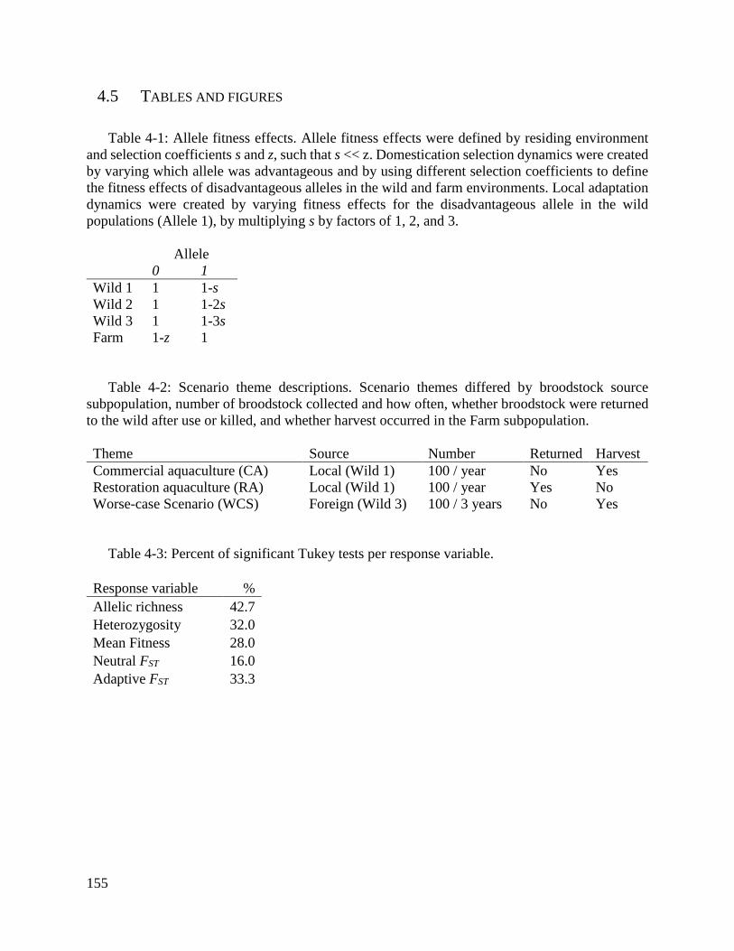
155


Table 4-1: Allele fitness effects. Allele fitness effects were defined by residing environment

and selection coefficients s and z, such that s << z. Domestication selection dynamics were created

by varying which allele was advantageous and by using different selection coefficients to define

the fitness effects of disadvantageous alleles in the wild and farm environments. Local adaptation

dynamics were created by varying fitness effects for the disadvantageous allele in the wild

populations (Allele 1), by multiplying s by factors of 1, 2, and 3.

Allele

0 1

Wild 1 1 1-s

Wild 2 1 1-2s

Wild 3 1 1-3s

Farm 1-z 1

Table 4-2: Scenario theme descriptions. Scenario themes differed by broodstock source

subpopulation, number of broodstock collected and how often, whether broodstock were returned

to the wild after use or killed, and whether harvest occurred in the Farm subpopulation.

Theme Source Number Returned Harvest

Commercial aquaculture (CA) Local (Wild 1) 100 / year No Yes

Restoration aquaculture (RA) Local (Wild 1) 100 / year Yes No

Worse-case Scenario (WCS) Foreign (Wild 3) 100 / 3 years No Yes

Table 4-3: Percent of significant Tukey tests per response variable.

Response variable %

Allelic richness 42.7

Heterozygosity 32.0

Mean Fitness 28.0

Neutral FST 16.0

Adaptive FST 33.3

156

Figure 4-1: Model structure and order of processes in monthly time steps. In Panel A, black

arrows represent movement of animals through escape (farm to wild) and migration (among wild).

The dashed line between the farm and Wild 1 represents the distinction across the three phases of

the model: the spatial structure across phases of the model is identical except for the farm is

introduced in the beginning and removed at the end of the second phase. The four hierarchical

levels are labeled in purple. Panels B and C represent the order of processes in each phase of the

model, with B representing those in the first and last phases (wild subpopulations only) and C

representing those in the middle phase (farm and wild subpopulations).

157

Figure 4-2: Comparing response variables by scenario theme, under High Selection and High

Escape conditions. Mean (and 95% confidence intervals) for heterozygosity, log10 allelic richness,

mean fitness in all subpopulations, mean fitness in only wild subpopulations, neutral FST, and

adaptive FST by scenario theme are displayed. Dashed gray lines represent the introduction of the

farm (year 50) and removal of the farm (year 100).

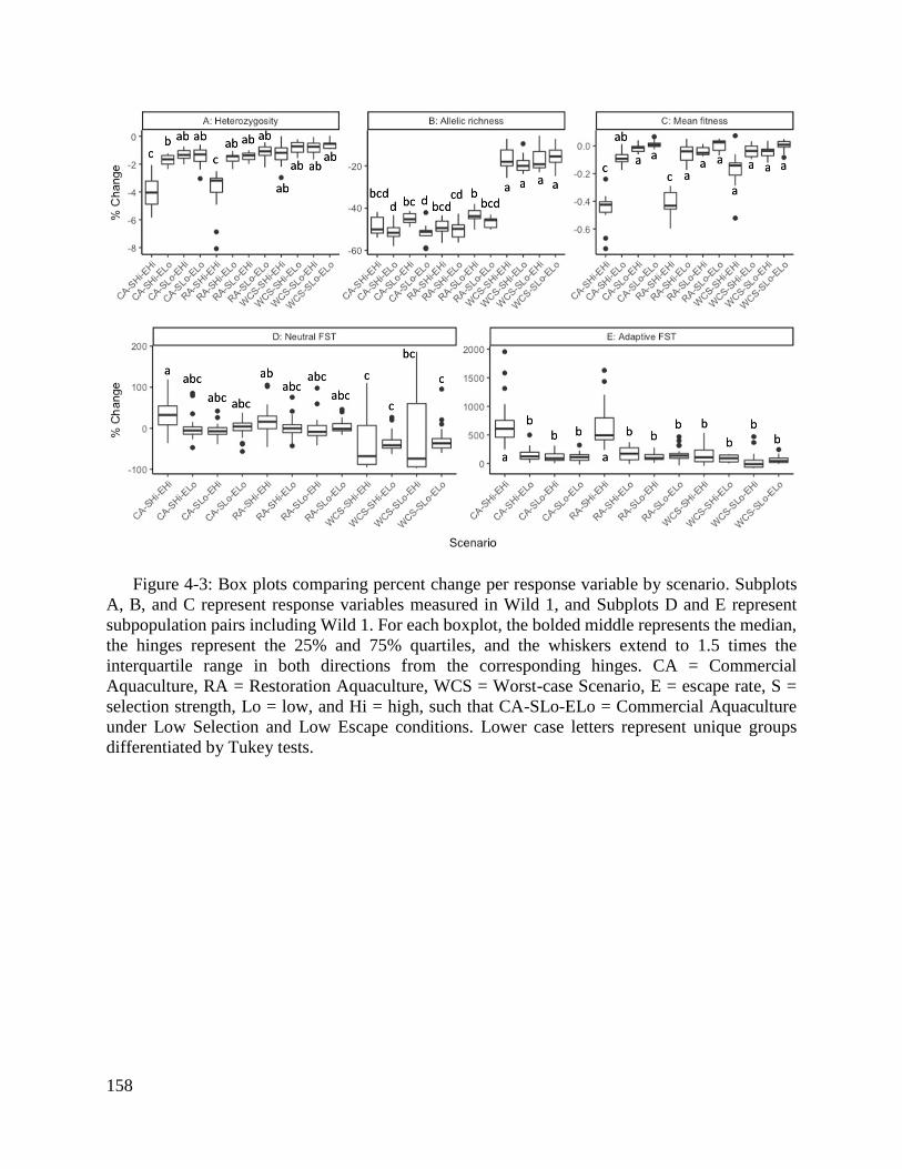
158

Figure 4-3: Box plots comparing percent change per response variable by scenario. Subplots

A, B, and C represent response variables measured in Wild 1, and Subplots D and E represent

subpopulation pairs including Wild 1. For each boxplot, the bolded middle represents the median,

the hinges represent the 25% and 75% quartiles, and the whiskers extend to 1.5 times the

interquartile range in both directions from the corresponding hinges. CA = Commercial

Aquaculture, RA = Restoration Aquaculture, WCS = Worst-case Scenario, E = escape rate, S =

selection strength, Lo = low, and Hi = high, such that CA-SLo-ELo = Commercial Aquaculture

under Low Selection and Low Escape conditions. Lower case letters represent unique groups

differentiated by Tukey tests.

159

Figure 4-4: Box plots comparing percent change per response variable by scenario theme. CA

= Commercial Aquaculture, RA = Restoration Aquaculture, WCS = Worst-Case Scenario. Lower

case letters represent unique groups differentiated by Tukey tests.

Figure 4-5: Box plots comparing percent change per response variable by scenario conditions.

E = escape rate, S = selection strength, Lo = low, and Hi = high, such that SLo-ELo = Low

Selection and Low Escape conditions. Lower case letters represent unique groups differentiated

by Tukey tests.

160


Supplemental Table 4-1: Parameter symbols, descriptions, and default values.

Symbol Description Default value

s Wild-wild selection coefficient 0.05

z Farm-wild selection coefficient 0.5

us Age at settlement 1/12

ua Age at maturity 1

um Maximum age 10

tl Larval mortality rate 0.99

tj Juvenile mortality rate 0.3

ta Adult mortality rate 0.3

ml Monthly larval migration rate 0.035

mj Monthly juvenile migration rate 0

ma Monthly adult migration rate 0

oi Probability of wild reproduction event in month i (of 12 months) O4 = 1, rest = 0

r Scale of wild recruitment 750

dw Family size per breeding event for wild subpopulations 10

𝜎𝑟 Standard deviation in scale of wild recruitment 0.01

yi Probability of seed production event in month i O1 = 1, rest = 0

k Scale of seed production 250

𝜎𝑠 Standard deviation in scale of seed production 0.01

df Family size per breeding event for the farm subpopulation 20

p Broodstock source subpopulation Wild 1

n Number of broodstock collected at once 100

f Interval in years for collecting fresh broodstock 1

l Whether to collect equal sex ratio in broodstock False

q Reduced recruitment in farm subpopulation due to lower

fecundity and uneven sex ratios common to young shellfish

0.25

b Reduced farm mortality factor 0.1

vi Probability of larval or gamete escape event in month i O4 = 1, rest = 0

wi Monthly probability of juvenile or adult escape event All = 0

jl Larval escape rate 0.07

jj Juvenile escape rate 0

ia Adult escape rate 0

g Scale of wild1 recruitment due to gamete escape 20

dg Family size for farm-wild1 hybrid families, to simulate gamete

escape

10

h Monthly harvest rate 0.0833

ca Minimum harvest age 1

cb Maximum harvest age 2

161

Supplemental Table 4-2: Mean, minimum, and pairwise FST from simulations and the empirical

values for comparison. We ran simulations with different migration rates for 750 years to find

which migration rates resulted in equilibrium FST near empirical FST. Migration rates 2%, 3.5%,

and 5% yielded the closest values, and 3.5% was chosen for Management Strategy Evaluation

simulations. Values in the table were measured over years 400-750 in the simulations, when FST

was at equilibrium. Empirical FST was estimated in Silliman (2019).

Simulated migration rate

Empirical 2% 3.5% 5%

Mean pairwise FST 0.118 0.0948 0.109 0.095

Minimum pairwise FST 0.0349 0.0288 0.0289 0.00138

Maximum pairwise FST 0.183 0.175 0.202 0.177

Supplemental Table 4-3: Transition matrix for wild migration. The matrix represents migration

rates from each subpopulation (rows) to each subpopulation (columns).

Wild 1 Wild 2 Wild 3

Wild 1 1–m m 0

Wild 2 0.5m 1-m 0.5m

Wild 3 0 m 1-m

Supplemental Table 4-4: Stable subpopulation sizes, by model phase. Mean (and 95%

confidence interval) subpopulation size in the last 25 years of each phase.

Pre-farm During-farm Post-farm

Wild 1 3,282 (3,280-3,284) 3,589 (3,577-3,601) 3,286 (3,283-3,288)

Wild 2 3,294 (3,291-3,296) 3,301 (3,298-3,303) 3,303 (3,301-3,305)

Wild 3 3,284 (3,282-3,288) 3,280 (3,278-3,283) 3,291 (3,289-3,294)

Farm - 1,209 (1,206-1,212) -

Supplemental Table 4-5: Stable Farm sizes, by theme. Mean, lower 95% confidence interval

limit, and upper 95% confidence interval limit for Farm subpopulation size in the last 25 years of

the during-farm phase, by scenario theme.

Mean Lower 95% CI Upper 95% CI

Commercial Aquaculture 1,223 1,222 1,223

Restoration Aquaculture 1,257 1,257 1,258

Worst Case Scenario 1,148 1,148 1,148

162

Supplemental Table 4-6: Survival and survivorship estimates by age class for the population.

The population includes all subpopulations combined, including the Farm. Estimates were

calculated across 12 random simulations that included all scenario themes and conditions. Ages

were grouped into 10 age classes, in which age 1 represents individuals age 1-11 months, age 2

represents individuals aged 12-23 months, and so forth. Columns sx and lx contain the mean

survival and survivorship respectively, with 95% confidence intervals in parentheses.

Age sx lx

1 0.802 (0.801-0.803) 1.000 (1-1)

2 0.799 (0.796-0.801) 0.802 (0.801-0.803)

3 0.752 (0.748-0.756) 0.641 (0.639-0.643)

4 0.795 (0.793-0.796) 0.481 (0.480-0.484)

5 0.795 (0.793-0.796) 0.383 (0.380-0.385)

6 0.795 (0.793-0.796) 0.304 (0.302-0.306)

7 0.795 (0.794-0.796) 0.242 (0.240-0.244)

8 0.795 (0.794-0.796) 0.192 (0.190-0.194)

9 0.795 (0.793-0.796) 0.153 (0.151-0.154)

10 0.000 (0-0) 0.121 (0.120-0.123)

Supplemental Table 4-7: Analysis of variance (ANOVA) results, using all wild

subpopulations. One-way ANOVAs were performed to compare the effect of scenario, scenario

theme, and scenario conditions on percent change for each of five response variables. F-values are

reported for each ANOVA. p < 0.05 = *.

Scenario Theme Conditions

Allelic richness 9.975* 51.94* 1.072

Heterozygosity 8.161* 11.18* 14.11*

Mean fitness 6.503* 1.552 17.47*

Neutral FST 5.282* 17.52* 3.432*

Adaptive FST 19.44* 15.88* 36.91*

163

Supplemental Table 4-8: Tukey test results using all wild subpopulations for percent change

in heterozygosity, for pairwise comparisons of the 12 scenarios. RA = Restoration Aquaculture,

CA = Commercial Aquaculture, and WCS = Worst-case Scenario. The number represents the set

of conditions, where 1 = High Selection and High Escape conditions, 2 = High Selection and Low

Escape conditions, 3 Low Selection and High Escape conditions, and 4 = Low Selection and Low

Escape conditions. Cells contain the mean difference in percent change between percent

comparisons and are highlighted gray if p < 0.05.

CA-1 CA-2 CA-3 CA-4 RA-1 RA-2 RA-3 RA-4 WCS-

1

WCS-

2

WCS-

3

WCS-

4

CA-1 -

CA-2 0.59 -

CA-3 0.73 0.14 -

CA-4 0.90 0.31 0.17 -

RA-1 0.90 0.31 0.17 -1.07 -

RA-2 0.78 0.20 0.06 -0.12 0.95 -

RA-3 0.84 0.25 0.11 -0.06 1.01 0.06 -

RA-4 0.81 0.22 0.08 -0.09 0.97 0.02 -0.03 -

WCS-

1 0.91 0.32 0.18 0.01 1.07 0.13 0.07 0.10 -

WCS-

2 0.91 0.33 0.19 0.01 1.08 0.13 0.07 0.11 0.00 -

WCS-

3 1.10 0.52 0.38 0.20 1.27 0.32 0.26 0.30 0.20 0.19 -

WCS-

4 0.99 0.40 0.26 0.09 1.16 0.21 0.15 0.18 0.08 0.08 -0.11 -

164


in mean fitness, for pairwise comparisons of the 12 scenarios. Scenario name key in the caption of

Supplemental Table 4-8. Cells contain the mean difference in percent change between percent



1

WCS-

2

WCS-

3

WCS-

4

CA-1 -

CA-2 0.13 -

CA-3 0.13 0.00 -

CA-4 0.14 0.01 0.01 -

RA-1 0.02 -0.11 -0.11 -0.12 -

RA-2 0.14 0.01 0.01 0.00 0.12 -

RA-3 0.13 -0.01 -0.01 -0.02 0.11 -0.02 -

RA-4 0.14 0.01 0.00 -0.01 0.12 0.00 0.01 -

WCS-

1 0.11 -0.03 -0.03 -0.04 0.09 -0.04 -0.02 -0.03 -

WCS-

2 0.15 0.02 0.02 0.01 0.13 0.01 0.03 0.01 0.05 -

WCS-

3 0.11 -0.03 -0.03 -0.04 0.09 -0.03 -0.02 -0.03 0.00 -0.04 -

WCS-

4 0.14 0.01 0.01 0.00 0.12 0.00 0.02 0.00 0.04 -0.01 0.03 -


in adaptive FST, for pairwise comparisons of the 12 scenarios. Scenario name key in the caption of




1

WCS-

2

WCS-

3

WCS-

4

CA-1 -

CA-2 -348.6 -

CA-3 -367.7 -19.1 -

CA-4 -370.5 -21.9 -2.8 -

RA-1 -17.3 331.3 350.4 353.2 -

RA-2 -332.8 15.8 34.8 37.7 -315.5 -

RA-3 -388.7 -40.1 -21.1 -18.2 -371.4 -55.9 -

RA-4 -347.4 1.2 20.3 23.1 -330.1 -14.6 41.4 -

WCS-

1 -365.7 -17.1 2.0 4.8 -348.4 -32.9 23.0 -18.3 -

WCS-

2 -397.8 -49.2 -30.1 -27.3 -380.5 -65.0 -9.1 -50.4 -32.1 -

WCS-

3 -443.1 -94.5 -75.5 -72.6 -425.8 -110.3 -54.4 -95.7 -77.4 -45.3 -

WCS-

4 -420.7 -72.1 -53.0 -50.2 -403.4 -87.9 -32.0 -73.3 -55.0 -22.9 22.4 -

165


in neutral FST, for pairwise comparisons of the 12 scenarios. Scenario name in the caption of




1

WCS-

2

WCS-

3

WCS-

4

CA-1 -

CA-2 -28.8 -

CA-3 -31.6 -2.9 -

CA-4 -26.8 2.0 4.9 -

RA-1 -12.8 16.0 18.8 14.0 -

RA-2 -27.8 1.0 3.8 -1.0 -15.0 -

RA-3 -29.2 -0.4 2.4 -2.5 -16.4 -1.4 -

RA-4 -21.8 7.0 9.8 5.0 -9.0 6.0 7.4 -

WCS-

1 -46.9 -18.1 -15.3 -20.1 -34.1 -19.1 -17.7 -25.1 -

WCS-

2 -52.2 -23.4 -20.5 -25.4 -39.4 -24.4 -23.0 -30.4 -5.3 -

WCS-

3 -38.9 -10.1 -7.2 -12.1 -26.1 -11.1 -9.7 -17.1 8.0 13.3 -

WCS-

4 -45.6 -16.8 -14.0 -18.9 -32.8 -17.8 -16.4 -23.8 1.3 6.6 -6.7 -


in allelic richness, for pairwise comparisons of the 12 scenarios. Scenario name key in the caption

of Supplemental Table 4-8. Cells contain the mean difference in percent change between percent



1

WCS-

2

WCS-

3

WCS-

4

CA-1 -

CA-2 -1.74 -

CA-3 1.61 3.35 -

CA-4 -1.92 -0.18 -3.53 -

RA-1 -1.14 0.59 -2.75 0.78 -

RA-2 -1.31 0.43 -2.92 0.61 -0.17 -

RA-3 2.03 3.77 0.42 3.95 3.18 3.34 -

RA-4 -0.15 1.59 -1.76 1.77 1.00 1.16 -2.18 -

WCS-

1 10.02 11.76 8.41 11.94 11.16 11.33 7.99 10.17 -

WCS-

2 8.73 10.46 7.12 10.65 9.87 10.04 6.70 8.87 -1.29 -

WCS-

3 9.78 11.51 8.17 11.70 10.92 11.08 7.74 9.92 -0.25 1.05 -

WCS-

4 10.39 12.13 8.78 12.31 11.53 11.70 8.36 10.54 0.37 1.66 0.62 -

166


in heterozygosity, for pairwise comparisons of the three scenario themes. RA = Restoration

Aquaculture, CA = Commercial Aquaculture, and WCS = Worst Case Scenario. Cells contain the

mean difference in percent change between percent comparisons and are highlighted gray if p <

0.05.

CA RA WCS

CA -

RA 0.013 -

WCS 0.43 0.41 -


in allelic richness, for pairwise comparisons of the three scenario themes. Scenario theme key in

the caption of Supplemental Table 4-13. Cells contain the mean difference in percent change

between percent comparisons and are highlighted gray if p < 0.05

CA RA WCS

CA -

RA 0.37 -

WCS 10.24 9.87 -


in neutral FST, for pairwise comparisons of the three scenario themes. Scenario themes key in the

caption of Supplemental Table 4-13. Cells contain the mean difference in percent change between

percent comparisons and are highlighted gray if p < 0.05.

CA RA WCS

CA -

RA -1.11 -

WCS -24.10 -22.99 -

167


in adaptive FST, for pairwise comparisons of the three scenario themes. Scenario themes key in the



CA RA WCS

CA -

RA 0.12 -

WCS -135.15 -135.27 -


in mean fitness, for pairwise comparisons of the three scenario themes. Scenario themes key in the



CA RA WCS

CA -

RA 0.004 -

WCS 0.02 0.02 -


in heterozygosity, for pairwise comparisons of the four scenario conditions. S = selection strength,

E = escape rate, Hi = high, and Lo = low, such that SLo-ELo = Low Selection and Low Escape

conditions. Cells contain the mean difference in percent change between percent comparisons and

are highlighted gray if p < 0.05.

SHi_EHi SHi_ELo SLo_EHi SLo_ELo

SHi_EHi -

SHi_ELo -0.51 -

SLo_EHi -0.64 -0.13 -

SLo_ELo -0.65 -0.14 -0.008 -

168


in adaptive FST, for pairwise comparisons of the four scenario conditions. Scenario conditions key

in the caption of Supplemental Table 4-18. Cells contain the mean difference in percent change

between percent comparisons and are highlighted gray if p < 0.05.


SHi_EHi -

SHi_ELo 232.10 -

SLo_EHi 272.18 40.10 -

SLo_ELo 251.86 19.79 -20.31 -


in mean fitness, for pairwise comparisons of the four scenario conditions. Scenario conditions key




SHi_EHi -

SHi_ELo -0.10 -

SLo_EHi -0.082 0.020 -

SLo_ELo -0.0100 0.0010 -0.019 -


in allelic richness, for pairwise comparisons of the four scenario conditions. Scenario conditions

key in the caption of Supplemental Table 4-18. Cells contain the mean difference in percent change



SHi_EHi -

SHi_ELo 1.07 -

SLo_EHi -1.51 -2.58 -

SLo_ELo 0.18 -0.88 1.70 -


in neutral FST, for pairwise comparisons of the four scenario conditions. Scenario conditions key




SHi_EHi -

SHi_ELo 16.36 -

SLo_EHi 13.34 -3.01 -

SLo_ELo 11.50 -4.86 -1.85 -

169

Supplemental Table 4-23: Analysis of variance (ANOVA) results, using only Wild 1. One-

way ANOVAs were performed to compare the effect of scenario, scenario theme, and scenario

conditions on percent change for each of five response variables. F-values are reported for each

ANOVA. p < 0.05 = *.

Scenario Theme Conditions

Allelic richness 154.4* 683.7* 0.678

Heterozygosity 25.07* 16.15* 29.97*

Mean fitness 58.55* 2.741 102.0*

Neutral FST 5.719* 20.83* 2.289

Adaptive FST 32.95* 15.92* 52.48*


heterozygosity, for pairwise comparisons of the 12 scenarios. Scenario key in the caption of



CA-1 CA-2 CA-3 CA-4 RA-1 RA-2 RA-3 RA-4

WCS-

1

WCS-

2

WCS-

3

WCS-

4

CA-1 -

CA-2 2.27 -

CA-3 2.65 0.38 -

CA-4 2.49 0.22 -0.16 -

RA-1 0.00 -2.27 -2.65 -2.49 -

RA-2 2.43 0.16 -0.22 -0.07 2.43 -

RA-3 2.54 0.28 -0.10 0.05 2.55 0.12 -

RA-4 2.84 0.58 0.20 0.35 2.85 0.42 0.30 -

WCS-

1 2.68 0.41 0.03 0.19 2.68 0.25 0.14 -0.16 -

WCS-

2 3.16 0.90 0.52 0.67 3.17 0.74 0.62 0.32 0.48 -

WCS-

3 3.18 0.91 0.54 0.69 3.18 0.76 0.64 0.34 0.50 0.02 -

WCS-

4 3.37 1.10 0.72 0.88 3.37 0.94 0.82 0.52 0.69 0.20 0.19 -

170


fitness, for pairwise comparisons of the 12 scenarios. Scenario key in the caption of Supplemental

Table 4-8. Cells contain the mean difference in percent change between percent comparisons and

are highlighted gray if p < 0.05.


WCS-

1

WCS-

2

WCS-

3

WCS-

4

CA-1 -

CA-2 0.37 -

CA-3 0.44 0.07 -

CA-4 0.47 0.10 0.03 -

RA-1 0.04 -0.33 -0.40 -0.43 -

RA-2 0.41 0.04 -0.03 -0.06 0.36 -

RA-3 0.42 0.05 -0.02 -0.05 0.38 0.01 -

RA-4 0.46 0.09 0.02 -0.01 0.42 0.06 0.04 -

WCS-

1 0.29 -0.08 -0.15 -0.18 0.25 -0.12 -0.13 -0.18 -

WCS-

2 0.42 0.05 -0.02 -0.05 0.38 0.01 0.00 -0.04 0.13 -

WCS-

3 0.41 0.04 -0.03 -0.06 0.37 0.01 -0.01 -0.05 0.13 -0.01 -

WCS-

4 0.46 0.09 0.02 -0.01 0.42 0.05 0.04 0.00 0.17 0.04 0.05 -

Supplemental Table 4-26: Tukey test results using only Wild 1 for percent change in adaptive

FST, for pairwise comparisons of the 12 scenarios. Scenario name key in the caption of




WCS-

1

WCS-

2

WCS-

3

WCS-

4

CA-1 -

CA-2 -34.84 -

CA-3 -40.99 -6.15 -

CA-4 -34.28 0.56 6.71 -

RA-1 -14.89 19.96 26.10 19.39 -

RA-2 -34.85 -0.01 6.14 -0.57 -19.96 -

RA-3 -37.41 -2.57 3.57 -3.14 -22.53 -2.57 -

RA-4 -30.84 4.00 10.15 3.44 -15.96 4.01 6.57 -

WCS-

1 -69.41 -34.57 -28.42 -35.13 -54.52 -34.56 -31.99 -38.57 -

WCS-

2 -70.52 -35.68 -29.54 -36.25 -55.64 -35.68 -33.11 -39.68 -1.12 -

WCS-

3 -52.73 -17.89 -11.74 -18.45 -37.84 -17.88 -15.31 -21.88 16.68 17.80 -

WCS-

4 -63.80 -28.95 -22.81 -29.52 -48.91 -28.95 -26.38 -32.95 5.61 6.73 -11.07 -

171

Supplemental Table 4-27: Tukey test results using only Wild 1 for percent change in neutral

FST, for pairwise comparisons of the 12 scenarios. Scenario name key in the caption of




WCS-

1

WCS-

2

WCS-

3

WCS-

4

CA-1 -

CA-2 -544.2 -

CA-3 -581.0 -36.8 -

CA-4 -584.0 -39.8 -3.0 -

RA-1 -43.9 500.3 537.1 540.1 -

RA-2 -525.2 19.0 55.8 58.8 -481.3 -

RA-3 -579.9 -35.6 1.1 4.1 -535.9 -54.6 -

RA-4 -541.1 3.2 40.0 43.0 -497.1 -15.8 38.8 -

WCS-

1 -551.5 -7.3 29.5 32.5 -507.6 -26.3 28.4 -10.4 -

WCS-

2 -608.9 -64.6 -27.9 -24.9 -565.0 -83.7 -29.0 -67.8 -57.4 -

WCS-

3 -665.7 -121.5 -84.7 -81.7 -621.8 -140.5 -85.9 -124.7 -114.2 -56.9 -

WCS-

4 -630.3 -86.1 -49.3 -46.3 -586.4 -105.1 -50.4 -89.2 -78.8 -21.4 35.4 -


richness, for pairwise comparisons of the 12 scenarios. Scenario name key in the caption of



CA-1 CA-2 CA-3 CA-4 RA-1 RA-2 RA-3 RA-4 WCS-1 WCS-2 WCS-3 WCS-4

CA-1 -

CA-2 -2.72 -

CA-3 3.78 6.51 -

CA-4 -3.02 -0.29 -6.80 -

RA-1 -0.38 2.35 -4.16 2.64 -

RA-2 -1.32 1.40 -5.10 1.70 -0.94 -

RA-3 5.18 7.91 1.40 8.20 5.56 6.50 -

RA-4 1.94 4.67 -1.84 4.96 2.32 3.26 -3.24 -

WCS-

1 31.89 34.62 28.11 34.91 32.27 33.21 26.71 29.95 -

WCS-

2 29.55 32.28 25.77 32.57 29.93 30.87 24.37 27.61 -2.34 -

WCS-

3 32.07 34.79 28.29 35.09 32.45 33.39 26.88 30.13 0.17 2.51 -

WCS-

4 32.92 35.64 29.13 35.93 33.29 34.24 27.73 30.97 1.02 3.36 0.85 -

172


heterozygosity, for pairwise comparisons of the three scenario themes. Scenario themes key in the


percent comparisons and are highlighted gray if p < 0.05

CA RA WCS

CA -

RA 0.1 -

WCS 1.25 1.15 -


richness, for pairwise comparisons of the three scenario themes. Scenario theme key in the caption



CA RA WCS

CA -

RA 1.85 -

WCS 32.10 30.25 -


for percent change in neutral FST, for pairwise comparisons of the three scenario themes. Scenario

themes key in the caption of Supplemental Table 4-13. Cells contain the mean difference in percent

change between percent comparisons and are highlighted gray if p < 0.05.

CA RA WCS

CA -

RA -1.97 -

WCS -36.59 -34.62 -

173


for percent change in adaptive FST, for pairwise comparisons of the three scenario themes. Scenario

themes key in the caption of Supplemental Table 4-13. Cells contain the mean difference in percent

change between percent comparisons and are highlighted gray if p < 0.05.

CA RA WCS

CA -

RA 4.79 -

WCS -186.78 -191.58 -


fitness, for pairwise comparisons of the three scenario themes. Scenario themes key in the caption



CA RA WCS

CA -

RA 0.01 -

WCS 0.07 0.06 -


heterozygosity, for pairwise comparisons of the four scenario conditions. Scenario conditions key




SHi_EHi -

SHi_ELo -1.73 -

SLo_EHi -1.90 -0.17 -

SLo_ELo -2.01 -0.28 -0.11 -

174

Supplemental Table 4-35: Tukey test results using only subpopulations containing Wild 1 for

percent change in adaptive FST, for pairwise comparisons of the four scenario conditions. Scenario

conditions key in the caption of Supplemental Table 4-18. Cells contain the mean difference in

percent change between percent comparisons and are highlighted gray if p < 0.05.


SHi_EHi -

SHi_ELo 360.97 -

SLo_EHi 410.40 49.42 -

SLo_ELo 386.65 25.67 -23.75 -


fitness, for pairwise comparisons of the four scenario conditions. Scenario conditions key in the




SHi_EHi -

SHi_ELo -0.29 -

SLo_EHi -0.32 -0.03 -

SLo_ELo -0.36 -0.07 -0.04 -


richness, for pairwise comparisons of the four scenario conditions. Scenario conditions key in the




SHi_EHi -

SHi_ELo 2.00 -

SLo_EHi -3.17 -5.17 -

SLo_ELo -0.11 -2.11 3.06 -

Supplemental Table 4-38: Tukey test results using only Wild 1 for percent change in neutral

FST, for pairwise comparisons of the four scenario conditions. Scenario conditions key in the




SHi_EHi -

SHi_ELo 18.64 -

SLo_EHi 15.61 -3.03 -

SLo_ELo 14.87 -3.77 -0.74 -

175

Supplemental Figure 4-1: Grower survey results, reporting distance between farm and closest

wild population. We asked “How close is the closest wild population, of the same native shellfish

species you grow, to your farm?” Out of 15 respondents, most reported seeing the population on

their farm.

Supplemental Figure 4-2: Grower survey results for seasonality of planting and harvesting.

Results reported for all species (N = 14), Pacific Geoduck (N = 5), and Olympia Oyster (N = 5).

176

Supplemental Figure 4-3: Mean population size (and 95% confidence interval) over time, per

subpopulation, faceted by scenario theme and conditions. CA = Commercial Aquaculture, RA =

Restoration Aquaculture, and WCS = Worst Case Scenario. S = selection strength, E = escape rate,

Hi = high, and Lo = low, such that SLo-ELo = Low Selection and Low Escape conditions. Dashed

gray lines represent the introduction of the farm (year 50) and removal of the farm (year 100).

177

Supplemental Figure 4-4: Mean heterozygosity (and 95% confidence interval) over time, per

subpopulation, faceted by scenario theme and conditions. Scenario theme and conditions key in

the Supplemental Figure 4-3 caption. Dashed gray lines represent the introduction of the farm (year

50) and removal of the farm (year 100).

178

Supplemental Figure 4-5: Mean log10 allelic richness (and 95% confidence interval) over time,

per subpopulation, faceted by scenario theme and conditions. Scenario theme and conditions key

in the Supplemental Figure 4-3 caption. Dashed gray lines represent the introduction of the farm

(year 50) and removal of the farm (year 100).

179

Supplemental Figure 4-6: Mean neutral FST (and 95% confidence interval) over time, per




180

Supplemental Figure 4-7: Mean neutral FST (and 95% confidence interval) over time between

Wild 1 and Wild 2, faceted by scenario theme and conditions. Scenario theme and conditions key

in the Supplemental Figure 4-3 caption. Dashed gray lines represent the introduction of the farm

(year 50) and removal of the farm (year 100).

181

Supplemental Figure 4-8: Mean adaptive FST (and 95% confidence interval) over time by




182

Supplemental Figure 4-9: Mean fitness (and 95% confidence interval) over time, by




183

Supplemental Figure 4-10: Mean fitness (and 95% confidence interval) over time, by wild




184

BIBLIOGRAPHY

Abbott, D. P., & Haderlie, E. C. (1980). Intertidal Invertebrates of California. Stanford

University Press.

ADFG. (2019). Our Agency Mission, Alaska Department of Fish and Game.

https://www.adfg.alaska.gov/index.cfm?adfg=about.mission

Alexander, D. H., & Lange, K. (2011). Enhancements to the ADMIXTURE algorithm for

individual ancestry estimation. BMC Bioinformatics, 12(1), 246.

https://doi.org/10.1186/1471-2105-12-246

Allendorf, F. W. (1987). Genetic management of hatchery stocks. Population Genetics and

Fishery Management, 141–159.

Allendorf, F. W. (1993). Delay of Adaptation to Captive Breeding by Equalizing Family Size.

Conservation Biology, 7(2), 416–419.

Allendorf, F. W., Leary, R. F., Spruell, P., & Wenburg, J. K. (2001). The problems with hybrids:

Setting conservation guidelines. Trends in Ecology & Evolution, 16(11), 613–622.

https://doi.org/10.1016/S0169-5347(01)02290-X

Altschul, S. F., Gish, W., Miller, W., Myers, E. W., & Lipman, D. J. (1990). Basic local

alignment search tool. Journal of Molecular Biology, 215(3), 403–410.

https://doi.org/10.1016/S0022-2836(05)80360-2

Anderson, G., Hampton, J., Smith, N., & Rico, C. (2019). Indications of strong adaptive

population genetic structure in albacore tuna (Thunnus alalunga) in the southwest and

central Pacific Ocean. Ecology and Evolution, 9(18), 10354–10364.

https://doi.org/10.1002/ece3.5554

Anderson, G., Lal, M., Stockwell, B. L., Hampton, J., Smith, N., & Rico, C. (2020). No

Population Genetic Structure of Skipjack Tuna (Katsuwonus pelamis) in the Tropical

Western and Central Pacific Assessed Using Single Nucleotide Polymorphisms.

https://doi.org/10.3389/fmars.2020.570760

Anderson, J. W. (1999). World Is Their Oyster-Interpreting the Scope of Native American Off-

Reservation Shellfish Rights in Washington State, The. Seattle UL Rev., 23, 145.

Anderson, S. C., Flemming, J. M., Watson, R., & Lotze, H. K. (2011). Serial exploitation of

global sea cucumber fisheries. Fish and Fisheries, 12(3), 317–339.

Andrews, K. S., Nichols, K. M., Elz, A., Tolimieri, N., Harvey, C. J., Pacunski, R., Lowry, D.,

Yamanaka, K. L., & Tonnes, D. M. (2018). Cooperative research sheds light on

population structure and listing status of threatened and endangered rockfish species.

Conservation Genetics, 19(4), 865–878. https://doi.org/10.1007/s10592-018-1060-0

Apte, S., Star, B., & Gardner, J. P. (2003). A comparison of genetic diversity between cultured

and wild populations, and a test for genetic introgression in the New Zealand greenshell

mussel Perna canaliculus (Gmelin 1791). Aquaculture, 219(1–4), 193–220.

Araki, H., Berejikian, B. A., Ford, M. J., & Blouin, M. S. (2008). Fitness of hatchery-reared

salmonids in the wild. Evolutionary Applications, 1(2), 342–355.

Arndt, A., & Smith, M. J. (1998). Genetic diversity and population structure in two species of

sea cucumber: Differing patterns according to mode of development. Molecular Ecology,

7(8), 1053–1064. https://doi.org/10.1046/j.1365-294x.1998.00429.x

Assis, J., Tyberghein, L., Bosch, S., Verbruggen, H., Serrão, E. A., & De Clerck, O. (2018). Bio-

ORACLE v2. 0: Extending marine data layers for bioclimatic modelling. Global Ecology

and Biogeography, 27(3), 277–284.

185

Ayres, L. (2008). Thematic coding and analysis. The SAGE Encyclopedia of Qualitative

Research Methods, 1, 876–868.

Bahar, M., Johnstone, A. H., & Hansell, M. H. (1999). Revisiting learning difficulties in biology.

Journal of Biological Education, 33(2), 84–86.

https://doi.org/10.1080/00219266.1999.9655648

Baker, P. (1995). Review of ecology and fishery of the Olympia oyster, Ostrea lurida with

annotated bibliography. Journal of Shellfish Research, 14(2), 501–518.

Barrett, R. D. H., & Schluter, D. (2008). Adaptation from standing genetic variation. Trends in

Ecology & Evolution, 23(1), 38–44. https://doi.org/10.1016/j.tree.2007.09.008

Barth, J. M. I., Villegas‐Ríos, D., Freitas, C., Moland, E., Star, B., André, C., Knutsen, H.,

Bradbury, I., Dierking, J., Petereit, C., Righton, D., Metcalfe, J., Jakobsen, K. S., Olsen,

E. M., & Jentoft, S. (2019). Disentangling structural genomic and behavioural barriers in

a sea of connectivity. Molecular Ecology, 28(6), 1394–1411.

https://doi.org/10.1111/mec.15010

Baskett, M. L., & Waples, R. S. (2013). Evaluating Alternative Strategies for Minimizing

Unintended Fitness Consequences of Cultured Individuals on Wild Populations:

Minimizing Captive-Wild Fitness Effects. Conservation Biology, 27(1), 83–94.

https://doi.org/10.1111/j.1523-1739.2012.01949.x

Bell, R. (1985). Professional values and organizational decision making. Administration &

Society, 17(1), 21–60.

Besnier, F., Glover, K. A., Lien, S., Kent, M., Hansen, M. M., Shen, X., & Skaala, Ø. (2015).

Identification of quantitative genetic components of fitness variation in farmed, hybrid

and native salmon in the wild. Heredity, 115(1), 47–55.

https://doi.org/10.1038/hdy.2015.15

Bible, J. M., & Sanford, E. (2016). Local adaptation in an estuarine foundation species:

Implications for restoration. Biological Conservation, 193, 95–102.

https://doi.org/10.1016/j.biocon.2015.11.015

Blais, L. E., & Wagner, W. E. (2007). Emerging science, adaptive regulation, and the problem of

rulemaking ruts. Tex. L. Rev., 86, 1701.

Bosch, S., Tyberghein, L., & De Clerck, O. (2017). sdmpredictors: An R package for species

distribution modelling predictor datasets. Marine Species Distributions: From Data to

Predictive Models, 49.

Bradbury, A., Sizemore, B., Rothaus, D., & Ulrich, M. (2000). Stock Assessment of Subtidal

Geoduck Clams (Panopea abrupta) in Washington.

https://wdfw.wa.gov/sites/default/files/publications/00224/wdfw00224.pdf

Brannon, E. L., Amend, D. F., Cronin, M. A., Lannan, J. E., LaPatra, S., McNeil, W. J., Noble,

R. E., Smith, C. E., Talbot, A. J., Wedemeyer, G. A., & Westers, H. (2004). The

Controversy about Salmon Hatcheries. Fisheries, 29(9), 12–31.

https://doi.org/10.1577/1548-8446(2004)29[12:TCASH]2.0.CO;2

Bruckner, A. (2005). The recent status of sea cucumber fisheries in the continental United States

of America. SPC Bêche-de-Mer Information Bulletin, 22.

Buonaccorsi, V. P., Kimbrell, C. A., Lynn, E. A., & Vetter, R. D. (2005). Limited realized

dispersal and introgressive hybridization influence genetic structure and conservation

strategies for brown rockfish, Sebastes auriculatus. Conservation Genetics, 6(5), 697–

713. https://doi.org/10.1007/s10592-005-9029-1

186

California Hatchery Scientific Review Group. (2012). California Hatchery Review Report.

http://cahatcheryreview.com/wp-

content/uploads/2012/08/CA%20Hatchery%20Review%20Report%20Final%207-31-

12.pdf

Camara, M. D., & Vadopalas, B. (2009). Genetic Aspects of Restoring Olympia Oysters and

Other Native Bivalves: Balancing the Need for Action, Good Intentions, and the Risks of

Making Things Worse. Journal of Shellfish Research, 28(1), 121–145.

https://doi.org/10.2983/035.028.0104

Cameron, J. L., & Fankboner, P. V. (1989). Reproductive biology of the commercial sea

cucumber Parastichopus californicus (Stimpson)(Echinodermata: Holothuroidea). II.

Observations on the ecology of development, recruitment, and the juvenile life stage.

Journal of Experimental Marine Biology and Ecology, 127(1), 43–67.

Cannon, G. A., Holbrook, J. R., & Pashinski, D. J. (1990). Variations in the Onset of Bottom-

Water Intrusions over the Entrance Sill of a Fjord. Estuaries, 13(1), 31–42.

https://doi.org/10.2307/1351430

Carlsson, J., Carnegie, R. B., Cordes, J. F., Hare, M. P., Leggett, A. T., & Reece, K. S. (2008).

Evaluating recruitment contribution of a selectively bred aquaculture line of the oyster,

Crassostrea virginica used in restoration efforts. Journal of Shellfish Research, 27(5),

1117–1124.

Carson, H. S., Ulrich, M., Lowry, D., Pacunski, R. E., & Sizemore, R. (2016). Status of the

California sea cucumber (Parastichopus californicus) and red sea urchin (Mesocentrotus

franciscanus) commercial dive fisheries in the San Juan Islands, Washington State, USA.

Fisheries Research, 179, 179–190.

Carvalho, G. R., & Hauser, L. (1994). Molecular genetics and the stock concept in fisheries.

Reviews in Fish Biology and Fisheries, 4(3), 326–350.

https://doi.org/10.1007/BF00042908

Castellani, M., Heino, M., Gilbey, J., Araki, H., Sv\aasand, T., & Glover, K. A. (2015). IBSEM:

An individual-based Atlantic salmon population model. PloS One, 10(9).

Castellani, M., Heino, M., Gilbey, J., Araki, H., Svasand, T., & Glover, K. A. (2018). Modeling

fitness changes in wild Atlantic salmon populations faced by spawning intrusion of

domesticated escapees. Evolutionary Applications, 11(6), 1010–1025.

Castellani, M., Vage, S., Strand, E., Thingstad, T. F., & Giske, J. (2013). The Scaled Subspaces

Method: A new trait-based approach to model communities of populations with largely

inhomogeneous density. Ecological Modelling, 251, 173–186.

Catalina Sea Ranch. (2019). Catalina Sea Ranch | Crops. Catalina Sea Ranch.

https://catalinasearanch.com/crops/

Catchen, J., Hohenlohe, P. A., Bassham, S., Amores, A., & Cresko, W. A. (2013). Stacks: An

analysis tool set for population genomics. Molecular Ecology, 22(11), 3124–3140.

Charnley, S., Carothers, C., Satterfield, T., Levine, A., Poe, M. R., Norman, K., Donatuto, J.,

Breslow, S. J., Mascia, M. B., Levin, P. S., Basurto, X., Hicks, C. C., García-Quijano, C.,

& St. Martin, K. (2017). Evaluating the best available social science for natural resource

management decision-making. Environmental Science & Policy, 73, 80–88.

https://doi.org/10.1016/j.envsci.2017.04.002

Charnov, E. L., & Bull, J. J. (1989). Non-fisherian sex ratios with sex change and environmental

sex determination. Nature, 338(6211), 148–150. https://doi.org/10.1038/338148a0

187

Cheever, F. (1996). The United States Forest Service and National Park Service: Paradoxical

Mandates, Powerful Founders, and the Rise and Fall of Agency Discretion Symposium:

The National Park System. Denver University Law Review, 74(3), 625–648.

Childers, R., Vadopalas, B., Morvezen, R., & Eudeline, B. (2016, August 10). Shellfish

Conservation Genetics Workshop.

Christie, M. R., Ford, M. J., & Blouin, M. S. (2014). On the reproductive success of early-

generation hatchery fish in the wild. Evolutionary Applications, 7(8), 883–896.

https://doi.org/10.1111/eva.12183

Christie, M. R., Marine, M. L., French, R. A., Waples, R. S., & Blouin, M. S. (2012). Effective

size of a wild salmonid population is greatly reduced by hatchery supplementation.

Heredity, 109(4), 254–260. https://doi.org/10.1038/hdy.2012.39

Chu, K. H. (2006). Genetic variation in wild and cultured populations of the pearl oyster

Pinctada fucata from southern China. Aquaculture, 258(1–4), 220–227.

Clements, J. C., & Chopin, T. (2017). Ocean acidification and marine aquaculture in North

America: Potential impacts and mitigation strategies. Reviews in Aquaculture, 9(4), 326–

341.

Clements, J., & Chopin, T. (2016). Ocean acidification and marine aquaculture in North

America: Potential impacts and mitigation strategies. Reviews in Aquaculture.

https://doi.org/10.1111/raq.12140

Cochard, J. C., & Devauchelle, N. (1993). Spawning, fecundity and larval survival and growth in

relation to controlled conditioning in native and transplanted populations of Pecten

maximus (L.): Evidence for the existence of separate stocks. Journal of Experimental

Marine Biology and Ecology, 169(1), 41–56. https://doi.org/10.1016/0022-

0981(93)90042-M

Comps, B., Gömöry, D., Letouzey, J., Thiébaut, B., & Petit, R. J. (2001). Diverging trends

between heterozygosity and allelic richness during postglacial colonization in the

European beech. Genetics, 157(1), 389–397.

Costello, M. J., & Chaudhary, C. (2017). Marine biodiversity, biogeography, deep-sea gradients,

and conservation. Current Biology, 27(11), R511–R527.

Culver, C. S., Richards, J. B., & Page, H. M. (2006). Plasticity of attachment in the purple-hinge

rock scallop, Crassadoma gigantea: Implications for commercial culture. Aquaculture,

254(1–4), 361–369.

Cunningham, K. M., Canino, M. F., Spies, I. B., & Hauser, L. (2009). Genetic isolation by

distance and localized fjord population structure in Pacific cod (Gadus macrocephalus):

Limited effective dispersal in the northeastern Pacific Ocean. Canadian Journal of

Fisheries and Aquatic Sciences, 66(1), 153–166. https://doi.org/10.1139/F08-199

Currens, K. P., & Busack, C. A. (1995). A framework for assessing genetic vulnerability.

Fisheries, 20(12), 24–31.

Dale-Kuys, R., Vervalle, J., Roodt-Wilding, R., & Rhode, C. (2017). Genetic association

analysis of candidate loci under selection with size in the South African abalone.

Aquaculture International, 25(3), 1197–1214. https://doi.org/10.1007/s10499-016-0107-9

D’Aloia, C. C., Bogdanowicz, S. M., Francis, R. K., Majoris, J. E., Harrison, R. G., & Buston, P.

M. (2015). Patterns, causes, and consequences of marine larval dispersal. Proceedings of

the National Academy of Sciences, 112(45), 13940–13945.

Danecek, P., Auton, A., Abecasis, G., Albers, C. A., Banks, E., DePristo, M. A., Handsaker, R.

E., Lunter, G., Marth, G. T., Sherry, S. T., McVean, G., & Durbin, R. (2011). The variant

188

call format and VCFtools. Bioinformatics, 27(15), 2156–2158.

https://doi.org/10.1093/bioinformatics/btr330

Darden, T. L., Robinson, J. D., Strand, A. E., & Denson, M. R. (2017). Forecasting the Genetic

Impacts of Net Pen Failures on Gulf of Mexico Cobia Populations Using Individual-

based Model Simulations. Journal of the World Aquaculture Society, 48(1), 20–34.

Darvill, C. M., Menounos, B., Goehring, B. M., Lian, O. B., & Caffee, M. W. (2018). Retreat of

the western Cordilleran ice sheet margin during the last deglaciation. Geophysical

Research Letters, 45(18), 9710–9720.

Davenne, E., & Masson, D. (2001). Water Properties in the Straits of Georgia and Juan de

Fuca. https://waves-vagues.dfo-mpo.gc.ca/Library/40587976.pdf

Davis, B., Allee, B., Amend, D., Bachen, B., Davidson, B., Gharrett, T., Marshall, S., &

Wertheimer, A. (1985). Alaska Department of Fish and Game Genetic Policy.

http://www.adfg.alaska.gov/static/fishing/PDFs/research/genetics_finfish_policy.pdf

Davis, B., Burkett, R. D., Commissioner, D. W. C., & Allee, B. J. (1989). Background of the

genetic policy of the Alaska Department of Fish and Game. Alaska Department of Fish

and Game, Division of Fisheries Rehabilitation.

de Melo, C. M. R., Durland, E., & Langdon, C. (2016). Improvements in desirable traits of the

Pacific oyster, Crassostrea gigas, as a result of five generations of selection on the West

Coast, USA. Aquaculture, 460, 105–115.

https://doi.org/10.1016/j.aquaculture.2016.04.017

DeWeerdt, S. (2020). Can aquaculture overcome its sustainability challenges? Nature,

588(7837), S60–S62. https://doi.org/10.1038/d41586-020-03446-3

DFO Aquaculture Management Division. (2016). Shellfish Transfer Zones in British Columbia

[Map]. https://www.dfo-mpo.gc.ca/aquaculture/bc-cb/docs/maps-cartes/shellfish-transfer-

zones-transfert-mollusques-crustaces-eng.pdf

Dijkstra, H. (2010). Crassadoma Bernard, 1986. World Register of Marine Species.

http://www.marinespecies.org/aphia.php?p=taxdetails&id=138316

Dillman, D. A. (2014). Internet, phone, mail, and mixed-mode surveys: The tailored design

method (Fourth edition.). Wiley.

http://public.eblib.com/choice/publicfullrecord.aspx?p=1762797

Do, C., Waples, R. S., Peel, D., Macbeth, G. M., Tillett, B. J., & Ovenden, J. R. (2014).

NeEstimator v2: Re-implementation of software for the estimation of contemporary

effective population size (Ne) from genetic data. Molecular Ecology Resources, 14(1),

209–214.

Dong, Y., Dong, S., & Meng, X. (2008). Effects of thermal and osmotic stress on growth,

osmoregulation and Hsp70 in sea cucumber (Apostichopus japonicus Selenka).

Aquaculture, 276(1), 179–186. https://doi.org/10.1016/j.aquaculture.2008.01.028

Doyle, R. W. (1983). An approach to the quantitative analysis of domestication selection in

aquaculture. Aquaculture, 33(1), 167–185. https://doi.org/10.1016/0044-8486(83)90398-

8

Dray, S., Legendre, P., & Peres-Neto, P. R. (2006). Spatial modelling: A comprehensive

framework for principal coordinate analysis of neighbour matrices (PCNM). Ecological

Modelling, 196(3–4), 483–493.

Ehiobu, N. G., Goddard, M. E., & Taylor, J. F. (1989). Effect of rate of inbreeding on inbreeding

depression in Drosophila melanogaster. Theoretical and Applied Genetics, 77(1), 123–

127. https://doi.org/10.1007/BF00292326

189

Eldon, B., Riquet, F., Yearsley, J., Jollivet, D., & Broquet, T. (2016). Current hypotheses to

explain genetic chaos under the sea. Current Zoology, 62(6), 551–566.

Eldridge, W. H., & Naish, K. A. (2007). Long-term effects of translocation and release numbers

on fine-scale population structure among coho salmon (Oncorhynchus kisutch).

Molecular Ecology, 16(12), 2407–2421. https://doi.org/10.1111/j.1365-

294X.2007.03271.x

Elston, R. A. (1990). Mollusc Diseases: Guide for the Shellfish Farmer. Washington Sea Grant

Program.

Enbody, E. D., Pettersson, M. E., Sprehn, C. G., Palm, S., Wickström, H., & Andersson, L.

(2021). Ecological adaptation in European eels is based on phenotypic plasticity.

Proceedings of the National Academy of Sciences, 118(4).

Etter, P. D., Preston, J. L., Bassham, S., Cresko, W. A., & Johnson, E. A. (2011). Local de novo

assembly of RAD paired-end contigs using short sequencing reads. PloS One, 6(4),

e18561.

Evans, D. M., Che-Castaldo, J. P., Crouse, D., Davis, F. W., Epanchin-Niell, R., Flather, C. H.,

Frohlich, R. K., Goble, D. D., Li, Y.-W., Male, T. D., Master, L. L., Moskwik, M. P.,

Neel, M. C., Noon, B. R., Parmesan, C., Schwartz, M. W., Scott, J. M., & Williams, B.

K. (2016). Species recovery in the United States: Increasing the effectiveness of the

Endangered Species Act. 29.

FAO. (2017). FAO Fisheries and Aquaculture Department. National Aquaculture Sector

Overview: United States of America.

http://www.fao.org/fishery/countrysector/naso_usa/en

Fischer, P., Krueger, J. I., Greitemeyer, T., Vogrincic, C., Kastenmüller, A., Frey, D., Heene, M.,

Wicher, M., & Kainbacher, M. (2011). The bystander-effect: A meta-analytic review on

bystander intervention in dangerous and non-dangerous emergencies. Psychological

Bulletin, 137(4), 517–537. https://doi.org/10.1037/a0023304

Fisher, R. J. (1993). Social desirability bias and the validity of indirect questioning. Journal of

Consumer Research, 20(2), 303–315.

Fisheries and Oceans Canada. (2011, June 30). Aquaculture Maps | Pacific Region.

https://www.dfo-mpo.gc.ca/aquaculture/bc-cb/maps-cartes-eng.html

Fitzpatrick, S. W., Bradburd, G. S., Kremer, C. T., Salerno, P. E., Angeloni, L. M., & Funk, W.

C. (2020). Genomic and Fitness Consequences of Genetic Rescue in Wild Populations.

Current Biology, 30(3), 517-522.e5. https://doi.org/10.1016/j.cub.2019.11.062

Fiumera, A. C., Porter, B. A., Looney, G., Asmussen, M. A., & Avise, J. C. (2004). Maximizing

offspring production while maintaining genetic diversity in supplemental breeding

programs of highly fecund managed species. Conservation Biology, 18(1), 94–101.

Foll, M., & Gaggiotti, O. E. (2008). A genome scan method to identify selected loci appropriate

for both dominant and codominant markers: A Bayesian perspective. Genetics.

Ford, M. J. (2002). Selection in captivity during supportive breeding may reduce fitness in the

wild. Conservation Biology, 16(3), 815–825.

Forester, B. R., Lasky, J. R., Wagner, H. H., & Urban, D. L. (2018). Comparing methods for

detecting multilocus adaptation with multivariate genotype–environment associations.

Molecular Ecology, 27(9), 2215–2233.

Franklin, D. (2010). Legislative Rules, Nonlegislative Rules, and the Perils of the Short Cut. The

Yale Law Journal, 120(2), 276–326.

190

Frankovich, E. (2019, May 2). Washington hunting, angling fee increase fails; WDFW faces $7

million deficit. https://apnews.com/article/6a3c70748f884b30a5d92297d943b0f8

Fraser, D. J. (2008). How well can captive breeding programs conserve biodiversity? A review

of salmonids. Evolutionary Applications, 0(0), 080602014503553-???

https://doi.org/10.1111/j.1752-4571.2008.00036.x

Fritts, A. L., Scott, J. L., & Pearsons, T. N. (2007). The effects of domestication on the relative

vulnerability of hatchery and wild origin spring Chinook salmon (Oncorhynchus

tshawytscha) to predation. Canadian Journal of Fisheries and Aquatic Sciences, 64(5),

813–818. https://doi.org/10.1139/f07-057

Gaffney, P. M., Pascal, C. M., Barnhart, J., Grant, W. S., & Seeb, J. E. (2010). Genetic

homogeneity of weathervane scallops (Patinopecten caurinus) in the northeastern Pacific.

Canadian Journal of Fisheries and Aquatic Sciences, 67(11), 1827–1839.

https://doi.org/10.1139/F10-096

Galle, B., & Leahy, J. (2008). Laboratories of Democracy—Policy Innovation in Decentralized

Governments. Emory Law Journal, 58(6), 1333–1400.

Gavery, M. R., & Roberts, S. B. (2012). Characterizing short read sequencing for gene discovery

and RNA-Seq analysis in Crassostrea gigas. Comparative Biochemistry and Physiology

Part D: Genomics and Proteomics, 7(2), 94–99.

https://doi.org/10.1016/j.cbd.2011.12.003

Gerlach, G., Atema, J., Kingsford, M. J., Black, K. P., & Miller-Sims, V. (2007). Smelling home

can prevent dispersal of reef fish larvae. Proceedings of the National Academy of

Sciences, 104(3), 858–863.

Gilk, S. E., Wang, I. A., Hoover, C. L., Smoker, W. W., Taylor, S. G., Gray, A. K., & Gharrett,

A. J. (2004). Outbreeding Depression in Hybrids Between Spatially Separated Pink

Salmon, Oncorhynchus gorbuscha, Populations: Marine Survival, Homing ability, and

Variability in Family Size. Environmental Biology of Fishes, 69(1), 287–297.

https://doi.org/10.1023/B:EBFI.0000022888.28218.c1

Gjerde, B. (1986). Growth and reproduction in fish and shellfish. Aquaculture, 57(1), 37–55.

https://doi.org/10.1016/0044-8486(86)90179-1

Glover, K. A., Quintela, M., Wennevik, V., Besnier, F., Sørvik, A. G., & Skaala, Ø. (2012).

Three decades of farmed escapees in the wild: A spatio-temporal analysis of Atlantic

salmon population genetic structure throughout Norway.

Google. (2019). 'Measure distance" feature. Google Maps. maps.google.com

Goudet, J., Raymond, M., de Meeüs, T., & Rousset, F. (1996). Testing differentiation in diploid

populations. Genetics, 144(4), 1933–1940.

Greco, S., Figueira, J., & Ehrgott, M. (2016). Multiple criteria decision analysis. Springer.

Grimm, V., Berger, U., Bastiansen, F., Eliassen, S., Ginot, V., Giske, J., Goss-Custard, J., Grand,

T., Heinz, S. K., & Huse, G. (2006). A standard protocol for describing individual-based

and agent-based models. Ecological Modelling, 198(1–2), 115–126.

Guénard, G., Legendre, P., Boisclair, D., & Bilodeau, M. (2010). Multiscale codependence

analysis: An integrated approach to analyze relationships across scales. Ecology, 91(10),

2952–2964.

Günther, T., & Coop, G. (2013). Robust identification of local adaptation from allele

frequencies. Genetics, 195(1), 205–220. https://doi.org/10.1534/genetics.113.152462

191

Haig, S. M., Miller, M. P., Bellinger, R., Draheim, H. M., Mercer, D. M., & Mullins, T. D.

(2016). The conservation genetics juggling act: Integrating genetics and ecology, science

and policy. Evolutionary Applications, 9(1), 181–195. https://doi.org/10.1111/eva.12337

Hampe, A., & Petit, R. J. (2005). Conserving biodiversity under climate change: The rear edge

matters. Ecology Letters, 8(5), 461–467. https://doi.org/10.1111/j.1461-

0248.2005.00739.x

Hare, M. P., Nunney, L., Schwartz, M. K., Ruzzante, D. E., Burford, M., Waples, R. S., Ruegg,

K., & Palstra, F. (2011). Understanding and estimating effective population size for

practical application in marine species management. Conservation Biology, 25(3), 438–

449.

Hauser, L., & Carvalho, G. R. (2008). Paradigm shifts in marine fisheries genetics: Ugly

hypotheses slain by beautiful facts. Fish and Fisheries, 9(4), 333–362.

Hedgecock, D. (1994). 2.5: Does variance in reproductive success limit effective population

sizes of marine organisms. In Genetics and evolution of aquatic organisms (p. 122).

https://www.researchgate.net/profile/Dennis_Hedgecock/publication/245970620_Does_v

ariance_in_reproductive_success_limit_effective_population_sizes_of_marine_organism

s_In_A/links/5618340108ae044edbad2220.pdf

Hedgecock, D., & Coykendall, K. (2007). Genetic risks of marine hatchery enhancement: The

good, the bad, and the unknown. In Ecological and genetic implications of aquaculture

activities (pp. 85–101). Springer.

Hedgecock, D., & Pudovkin, A. I. (2011, October). Sweepstakes Reproductive Success in Highly

Fecund Marine Fish and Shellfish: A Review and Commentary [Text].

https://doi.org/info:doi/10.5343/bms.2010.1051

Hellberg, M. E. (2009). Gene Flow and Isolation among Populations of Marine Animals. Annual

Review of Ecology, Evolution, and Systematics, 40(1), 291–310.

https://doi.org/10.1146/annurev.ecolsys.110308.120223

Hemmer-Hansen, J., Therkildsen, N. O., & Pujolar, J. M. (2014). Population Genomics of

Marine Fishes: Next-Generation Prospects and Challenges. The Biological Bulletin,

227(2), 117–132. https://doi.org/10.1086/BBLv227n2p117

Hemmings, N. L., Slate, J., & Birkhead, T. R. (2012). Inbreeding causes early death in a

passerine bird. Nature Communications, 3(1), 1–4.

Hershberger, W. K., Myers, J. M., Iwamoto, R. N., Mcauley, W. C., & Saxton, A. M. (1990).

Genetic changes in the growth of coho salmon (Oncorhynchus kisutch) in marine net-

pens, produced by ten years of selection. Aquaculture, 85(1), 187–197.

https://doi.org/10.1016/0044-8486(90)90018-I

Hilborn, R., Banobi, J., Hall, S. J., Pucylowski, T., & Walsworth, T. E. (2018). The

environmental cost of animal source foods. Frontiers in Ecology and the Environment,

16(6), 329–335.

Hornick, K. M., & Plough, L. V. (2019). Tracking genetic diversity in a large-scale oyster

restoration program: Effects of hatchery propagation and initial characterization of

diversity on restored vs. wild reefs. Heredity, 123(2), 92–105.

Huberman, A., & Miles, M. (2002). The Qualitative Researcher’s Companion. SAGE

Publications, Inc. https://doi.org/10.4135/9781412986274

Hughes, A. R., Inouye, B. D., Johnson, M. T., Underwood, N., & Vellend, M. (2008). Ecological

consequences of genetic diversity. Ecology Letters, 11(6), 609–623.

192

Hwang, S. (2008). Utilizing Qualitative Data Analysis Software: A Review of Atlas.ti. Social

Science Computer Review, 26(4), 519–527. https://doi.org/10.1177/0894439307312485

Iwamoto, E., Ford, M. J., & Gustafson, R. G. (2004). Genetic Population Structure of Pacific

Hake, Merluccius productus, in the Pacific Northwest. Environmental Biology of Fishes,

69(1), 187–199. https://doi.org/10.1023/B:EBFI.0000022895.10683.c5

Jackson, A. M., Semmens, B. X., Mitcheson, Y. S. de, Nemeth, R. S., Heppell, S. A., Bush, P.

G., Aguilar-Perera, A., Claydon, J. A. B., Calosso, M. C., Sealey, K. S., Schärer, M. T.,

& Bernardi, G. (2014). Population Structure and Phylogeography in Nassau Grouper

(Epinephelus striatus), a Mass-Aggregating Marine Fish. PLOS ONE, 9(5), e97508.

https://doi.org/10.1371/journal.pone.0097508

Jacobsen, F. R. (1977). The Reproductive Cycle of the Purple Hinged Rock Scallop, Hinnites

Multirugosus Gale 1928 (Mollusca: Bivalvia). San Diego State University.

Jacobson, C. A., & Decker, D. J. (2006). In My Opinion: Ensuring the Future of State Wildlife

Management: Understanding Challenges for Institutional Change. Wildlife Society

Bulletin, 34(2), 531–536.

Janowitz-Koch, I., Rabe, C., Kinzer, R., Nelson, D., Hess, M. A., & Narum, S. R. (2019). Long-

term evaluation of fitness and demographic effects of a Chinook Salmon supplementation

program. Evolutionary Applications, 12(3), 456–469. https://doi.org/10.1111/eva.12725

Jasanoff, S. (1998). The political science of risk perception. Reliability Engineering & System

Safety, 59(1), 91–99. https://doi.org/10.1016/S0951-8320(97)00129-4

Johnson, R. B., & Onwuegbuzie, A. J. (2004). Mixed methods research: A research paradigm

whose time has come. Educational Researcher, 33(7), 14–26.

Jombart, T. (2008). adegenet: A R package for the multivariate analysis of genetic markers.

Bioinformatics (Oxford, England), 24(11), 1403–1405.

https://doi.org/10.1093/bioinformatics/btn129

Jombart, T., Devillard, S., & Balloux, F. (2010). Discriminant analysis of principal components:

A new method for the analysis of genetically structured populations. BMC Genetics, 11,

94. https://doi.org/10.1186/1471-2156-11-94

Jones, B. D. (2003). Bounded rationality and political science: Lessons from public

administration and public policy. Journal of Public Administration Research and Theory,

13(4), 395–412.

Kamvar, Z. N., Brooks, J. C., & Grünwald, N. J. (2015). Novel R tools for analysis of genome-

wide population genetic data with emphasis on clonality. Frontiers in Genetics, 6, 208.

Kardos, M., Armstrong, E., Fitzpatrick, S., Hauser, S., Hedrick, P., Miller, J., Tallmon, D. A., &

Funk, W. C. (2021). The crucial role of genome-wide genetic variation in conservation.

BioRxiv, 2021.07.05.451163. https://doi.org/10.1101/2021.07.05.451163

Kark, S., Tulloch, A., Gordon, A., Mazor, T., Bunnefeld, N., & Levin, N. (2015). Cross-

boundary collaboration: Key to the conservation puzzle. Current Opinion in

Environmental Sustainability, 12, 12–24. https://doi.org/10.1016/j.cosust.2014.08.005

Kass, R. E., & Raftery, A. E. (1995). Bayes factors. Journal of the American Statistical

Association, 90(430), 773–795.

Keegan, B. F., & O’Connor, B. D. S. (1985). Echinodermata. CRC Press.

Keever, C. C., Sunday, J., Puritz, J. B., Addison, J. A., Toonen, R. J., Grosberg, R. K., & Hart,

M. W. (2009). Discordant Distribution of Populations and Genetic Variation in a Sea Star

with High Dispersal Potential. Evolution, 63(12), 3214–3227.

https://doi.org/10.1111/j.1558-5646.2009.00801.x

193

Kelly, R. P., & Palumbi, S. R. (2010). Genetic Structure Among 50 Species of the Northeastern

Pacific Rocky Intertidal Community. PLOS ONE, 5(1), e8594.


Kenchington, E., Heino, M., & Nielsen, E. E. (2003). Managing marine genetic diversity: Time

for action? ICES Journal of Marine Science, 60(6), 1172–1176.

Kinlan, B. P., & Gaines, S. D. (2003). Propagule Dispersal in Marine and Terrestrial

Environments: A Community Perspective. Ecology, 84(8), 2007–2020.

https://doi.org/10.1890/01-0622

Kinne, O. (1964). The effects of temperature and salinity on marine and brackish water animals:

2. Salinity and temperature-salinity combinations. Oceanography and Marine Biology :

An Annual Review, 2, 281–339.

Kirby, M. F., Morris, S., Hurst, M., Kirby, S. J., Neall, P., Tylor, T., & Fagg, A. (2000). The Use

of Cholinesterase Activity in Flounder (Platichthys flesus) Muscle Tissue as a Biomarker

of Neurotoxic Contamination in UK Estuaries. Marine Pollution Bulletin, 40(9), 780–

791. https://doi.org/10.1016/S0025-326X(00)00069-2

Kirk, E. A., Reeves, A. D., & Blackstock, K. L. (2007). Path Dependency and the

Implementation of Environmental Regulation. Environment and Planning C:

Government and Policy, 25(2), 250–268. https://doi.org/10.1068/c0512j

Kovach, A. I., Breton, T. S., Berlinsky, D. L., Maceda, L., & Wirgin, I. (2010). Fine-scale spatial

and temporal genetic structure of Atlantic cod off the Atlantic coast of the USA. Marine

Ecology Progress Series, 410, 177–195.

Krefting, L. (1991). Rigor in Qualitative Research: The Assessment of Trustworthiness.

American Journal of Occupational Therapy, 45(3), 214–222.

https://doi.org/10.5014/ajot.45.3.214

Kreuter, F., Presser, S., & Tourangeau, R. (2008). Social Desirability Bias in CATI, IVR, and

Web SurveysThe Effects of Mode and Question Sensitivity. Public Opinion Quarterly,

72(5), 847–865. https://doi.org/10.1093/poq/nfn063

Kyle, C. J., & Boulding, E. G. (2000). Comparative population genetic structure of marine

gastropods (Littorina spp.) with and without pelagic larval dispersal. Marine Biology,

137(5), 835–845. https://doi.org/10.1007/s002270000412

Laikre, L. (2010). Genetic diversity is overlooked in international conservation policy

implementation. Conservation Genetics, 11(2), 349–354.

Laikre, L., Schwartz, M. K., Waples, R. S., & Ryman, N. (2010). Compromising Genetic

Diversity in the Wild: Unmonitored Large-Scale Release of Plants and Animals. Trends

in Ecology & Evolution, 25(9), 520–529. https://doi.org/10.1016/j.tree.2010.06.013

Lal, M. M., Southgate, P. C., Jerry, D. R., & Zenger, K. R. (2016). Fishing for divergence in a

sea of connectivity: The utility of ddRADseq genotyping in a marine invertebrate, the

black-lip pearl oyster Pinctada margaritifera. Marine Genomics, 25, 57–68.

https://doi.org/10.1016/j.margen.2015.10.010

Lamichhaney, S., Barrio, A. M., Rafati, N., Sundström, G., Rubin, C.-J., Gilbert, E. R.,

Berglund, J., Wetterbom, A., Laikre, L., Webster, M. T., Grabherr, M., Ryman, N., &

Andersson, L. (2012). Population-scale sequencing reveals genetic differentiation due to

local adaptation in Atlantic herring. Proceedings of the National Academy of Sciences,

109(47), 19345–19350. https://doi.org/10.1073/pnas.1216128109

Larson, W. A., Seeb, L. W., Everett, M. V., Waples, R. K., Templin, W. D., & Seeb, J. E.

(2014). Genotyping by sequencing resolves shallow population structure to inform

194

conservation of Chinook salmon (Oncorhynchus tshawytscha). Evolutionary

Applications, 7(3), 355–369.

Larsson, A. I., & Jonsson, P. R. (2006). Barnacle Larvae Actively Select Flow Environments

Supporting Post-Settlement Growth and Survival. Ecology, 87(8), 1960–1966.

https://doi.org/10.1890/0012-9658(2006)87[1960:BLASFE]2.0.CO;2

Laurén, D. J. (1982). Oogenesis and protandry in the purple-hinge rock scallop, Hinnites

giganteus, in upper Puget Sound, Washington, U.S.A. Canadian Journal of Zoology,

60(10), 2333–2336. https://doi.org/10.1139/z82-300

Law, R. (2000). Fishing, selection, and phenotypic evolution. ICES Journal of Marine Science,

57(3), 659–668.

Leet, W. S. (2001). California’s living marine resources: A status report. University Of

California, Division of Agriculture and Natural Resources ….

Legendre, P., & Gallagher, E. D. (2001). Ecologically meaningful transformations for ordination

of species data. Oecologia, 129(2), 271–280.

Lehnert, S. J., DiBacco, C., Van Wyngaarden, M., Jeffery, N. W., Ben Lowen, J., Sylvester, E.

V. A., Wringe, B. F., Stanley, R. R. E., Hamilton, L. C., & Bradbury, I. R. (2019). Fine-

scale temperature-associated genetic structure between inshore and offshore populations

of sea scallop ( Placopecten magellanicus ). Heredity, 122(1), 69–80.

https://doi.org/10.1038/s41437-018-0087-9

Leighton, D. L., & Phleger, C. F. (1977). The Purple-Hinge Rock Scallop: A New Candidate for

Marine Aquaculture1. Proceedings of the Annual Meeting - World Mariculture Society,

8(1–4), 457–469. https://doi.org/10.1111/j.1749-7345.1977.tb00136.x

Lester, J. P. (1995). Environmental politics and policy: Theories and evidence. Duke University

Press.

Lewontin, R. C., & Krakauer, J. (1973). Distribution of gene frequency as a test of the theory of

the selective neutrality of polymorphisms. Genetics, 74(1), 175–195.

Li, W.-H. (1978). Maintenance of genetic variability under the joint effect of mutation, selection

and random drift. Genetics, 90(2), 349–382.

Lidskog, R. (2014). Representing and regulating nature: Boundary organisations, portable

representations, and the science–policy interface. Environmental Politics, 23(4), 670–

687. https://doi.org/10.1080/09644016.2013.898820

Lind, C. E., Evans, B. S., Knauer, J., Taylor, J. J. U., & Jerry, D. R. (2009). Decreased genetic

diversity and a reduced effective population size in cultured silver-lipped pearl oysters

(Pinctada maxima). Aquaculture, 286(1), 12–19.

https://doi.org/10.1016/j.aquaculture.2008.09.009

Lind, C. E., Evans, B. S., Taylor, J. J. U., & Jerry, D. R. (2007). Population genetics of a marine

bivalve, Pinctada maxima, throughout the Indo-Australian Archipelago shows

differentiation and decreased diversity at range limits. Molecular Ecology, 16(24), 5193–

5203. https://doi.org/10.1111/j.1365-294X.2007.03598.x

Linder, S. H., & Peters, B. G. (2016). Instruments of Government: Perceptions and Contexts.

Annual Review of Policy Design, 4(1), 1–10.

Liu, X., Lindquist, E., Vedlitz, A., & Vincent, K. (2010). Understanding Local Policymaking:

Policy Elites’ Perceptions of Local Agenda Setting and Alternative Policy Selection.

Policy Studies Journal, 38(1), 69–91. https://doi.org/10.1111/j.1541-0072.2009.00345.x

Llodra, E. R. (2002). Fecundity and life-history strategies in marine invertebrates.

LNRD. (2019). Lummi Natural Resources. https://www.lummi-nsn.gov/Website.php?PageID=1

195

Lotterhos, K. E., & Whitlock, M. C. (2015). The relative power of genome scans to detect local

adaptation depends on sampling design and statistical method. Molecular Ecology, 24(5),

1031–1046. https://doi.org/10.1111/mec.13100

Lusher, A., Hollman, P., & Mendoza-Hill, J. (2017). Microplastics in fisheries and aquaculture:

Status of knowledge on their occurrence and implications for aquatic organisms and food

safety. FAO.

Lynch, M., & O’Hely, M. (2001). Captive breeding and the genetic fitness of natural

populations. Conservation Genetics, 2(4), 363–378.

https://doi.org/10.1023/A:1012550620717

MacDonald, B. A., & Bourne, N. F. (1989). Growth of the purple-hinge rock scallop,

Crassadoma gigantea Gray, 1825 under natural conditions and those associated with

suspended culture. J. Shellfish Res, 8(1), 179–186.

MacDonald, B. A., Thompson, R. J., & Bourne, N. F. (1991). Growth and reproductive

energetics of three scallop species from British Columbia (Chlamys hastata, Chlamys

rubida, and Crassadoma gigantea). Canadian Journal of Fisheries and Aquatic Sciences,

48(2), 215–221.

Mantel, N., & Valand, R. S. (1970). A technique of nonparametric multivariate analysis.

Biometrics, 547–558.

Marandel, F., Lorance, P., Berthelé, O., Trenkel, V. M., Waples, R. S., & Lamy, J.-B. (2019).

Estimating effective population size of large marine populations, is it feasible? Fish and

Fisheries, 20(1), 189–198. https://doi.org/10.1111/faf.12338

Marko, P. B., & Hart, M. W. (2011). The complex analytical landscape of gene flow inference.

Trends in Ecology & Evolution, 26(9), 448–456.

McFarland, K., Plough, L. V., Nguyen, M., & Hare, M. P. (2020). Are bivalves susceptible to

domestication selection? Using starvation tolerance to test for potential trait changes in

eastern oyster larvae. PLOS ONE, 15(6), e0230222.


McHugh, D., & Rouse, G. W. (1998). Life history evolution of marine invertebrates: New views

from phylogenetic systematics. Trends in Ecology & Evolution, 13(5), 182–186.

Mendelson, N. A. (2006). Regulatory Beneficiaries and Informal Agency Policymaking. Cornell

Law Review, 92, 397–452.

Menge, B. A., Chan, F., Nielsen, K. J., Lorenzo, E. D., & Lubchenco, J. (2009). Climatic

variation alters supply-side ecology: Impact of climate patterns on phytoplankton and

mussel recruitment. Ecological Monographs, 79(3), 379–395. https://doi.org/10.1890/08-

2086.1

Menge, B. A., Gouhier, T. C., Freidenburg, T., & Lubchenco, J. (2011). Linking long-term,

large-scale climatic and environmental variability to patterns of marine invertebrate

recruitment: Toward explaining “unexplained” variation. Journal of Experimental

Marine Biology and Ecology, 400(1), 236–249.

https://doi.org/10.1016/j.jembe.2011.02.003

Menzel, W. (2018). Estuarine and Marine Bivalve Mollusk Culture. CRC Press.

Merino, G., Barange, M., Blanchard, J. L., Harle, J., Holmes, R., Allen, I., Allison, E. H.,

Badjeck, M. C., Dulvy, N. K., Holt, J., & others. (2012). Can marine fisheries and

aquaculture meet fish demand from a growing human population in a changing climate?

Global Environmental Change, 22(4), 795–806.

Miles, M. B., Huberman, A. M., & Saldana, J. (2014). Qualitative Data Analysis. SAGE.

196

Miller, K. M., Supernault, K. J., Li, S., & Withler, R. E. (2006). Population structure in two

marine invertebrate species (panopea abrupta and strongylocentrotus franciscanus)

targeted for aquaculture and enhancement in british columbia. Journal of Shellfish

Research, 25(1), 33–42. https://doi.org/10.2983/0730-

8000(2006)25[33:PSITMI]2.0.CO;2

Miner, J. B. (2006). Organizational Behavior 2: Essential theories of process and structure,

Chapter 4. Cyert, R., March, J. 1963. Behavioral theory of the firm. Sharp. Inc., New

York.

Mobrand, L. E., Barr, J., Blankenship, L., Campton, D. E., Evelyn, T. T., Flagg, T. A., Mahnken,

C. V., Seeb, L. W., Seidel, P. R., & Smoker, W. W. (2005). Hatchery reform in

Washington State: Principles and emerging issues. Fisheries, 30(6), 11–23.

Monterey Bay Aquarium. (2016, December 5). Monterey Bay Aquarium Seafood Watch: Farmed

Pacific Geoduck. https://seafood.ocean.org/wp-content/uploads/2016/12/Clams-Farmed-

Pacific-Geoduck-Washington-State-USA-and-British-Columbia-Canada-2016.pdf

Morin, P. A., Martien, K. K., & Taylor, B. L. (2009). Assessing statistical power of SNPs for

population structure and conservation studies. Molecular Ecology Resources, 9(1), 66–

73. https://doi.org/10.1111/j.1755-0998.2008.02392.x

Morvezen, R., Boudry, P., Laroche, J., & Charrier, G. (2016). Stock enhancement or sea

ranching? Insights from monitoring the genetic diversity, relatedness and effective

population size in a seeded great scallop population (Pecten maximus). Heredity, 117(3),

142–148. https://doi.org/10.1038/hdy.2016.42

Moshinsky, A., & Bar-Hillel, M. (2010). Loss aversion and status quo label bias. Social

Cognition, 28(2), 191–204.

Mueller, K. (2016). Fishery biology of the sea cucumber Parastichopus californicus (Stimpson

1857) from the San Juan Islands, Washington. Lummi Natural Resources Division.

Nadeau, S., Meirmans, P. G., Aitken, S. N., Ritland, K., & Isabel, N. (2016). The challenge of

separating signatures of local adaptation from those of isolation by distance and

colonization history: The case of two white pines. Ecology and Evolution, 6(24), 8649–

8664. https://doi.org/10.1002/ece3.2550

Naish, K. A., Taylor, J. E., Levin, P. S., Quinn, T. P., Winton, J. R., Huppert, D., & Hilborn, R.

(2007). An Evaluation of the Effects of Conservation and Fishery Enhancement

Hatcheries on Wild Populations of Salmon. In Advances in Marine Biology (Vol. 53, pp.

61–194). Elsevier. https://doi.org/10.1016/S0065-2881(07)53002-6

Nascimento-Schulze, J. C., Bean, T. P., Houston, R. D., Santos, E. M., Sanders, M. B., Lewis,

C., & Ellis, R. P. (2021). Optimizing hatchery practices for genetic improvement of

marine bivalves. Reviews in Aquaculture.

Nederhof, A. J. (1985). Methods of coping with social desirability bias: A review. European

Journal of Social Psychology, 15(3), 263–280. https://doi.org/10.1002/ejsp.2420150303

Nei, M., Maruyama, T., & Chakraborty, R. (1975). The Bottleneck Effect and Genetic

Variability in Populations. Evolution, 29(1), 1–10. https://doi.org/10.2307/2407137

NNRD. (2019). Nisqually Natural Resources. http://www.nisqually-

nsn.gov/index.php/administration/tribal-services/natural-resources/

NOAA Fisheries. (2012). Salmon and Steelhead & Endangered Species Act.

http://orafs.org/meeting2012/ESA%20Wkshp2012%203-

Turner_NOAA%20HGMP%20process.pdf

197

NOAA Fisheries. (2019). Hatchery and Genetic Management Plan Template.

https://media.fisheries.noaa.gov/2020-04/hgmptemplate_508.docx?null

NOAA Fisheries. (2021a, May 19). Endangered Species Act Permits and Authorizations on the

West Coast | NOAA Fisheries (West Coast). NOAA.

https://www.fisheries.noaa.gov/west-coast/endangered-species-conservation/endangered-

species-act-permits-and-authorizations-west

NOAA Fisheries. (2021b, June 8). U.S. Aquaculture | NOAA Fisheries (National). NOAA.

https://www.fisheries.noaa.gov/national/aquaculture/us-aquaculture

NOAA Fisheries Office of Aquaculture. (2016). NOAA Marine Aquaculture Strategic Plan: FY

2016-2020.

http://www.nmfs.noaa.gov/aquaculture/docs/draft_noaa_marine_aquaculture_strategic_pl

an.pdf

Northern Economics. (2013). The economic impact of shellfish aquaculture in Washington,

Oregon, and California. https://protectwillapabay.org/wp-content/uploads/2017/09/25-

percent-102-million.pdf

NWIFC: Genetics. (2008, June 6). Northwest Indian Fisheries Commission.

https://nwifc.org/about-us/enhancement/genetics/

Oksanen, J., Kindt, R., Legendre, P., O’Hara, B., Stevens, M. H. H., Oksanen, M. J., & Suggests,

M. (2007). The vegan package. Community Ecology Package, 10(631–637), 719.

O’Leary, S. J., Puritz, J. B., Willis, S. C., Hollenbeck, C. M., & Portnoy, D. S. (2018). These

aren’t the loci you’e looking for: Principles of effective SNP filtering for molecular

ecologists. Molecular Ecology, 27(16), 3193–3206. https://doi.org/10.1111/mec.14792

Orsini, L., Vanoverbeke, J., Swillen, I., Mergeay, J., & Meester, L. D. (2013). Drivers of

population genetic differentiation in the wild: Isolation by dispersal limitation, isolation

by adaptation and isolation by colonization. Molecular Ecology, 22(24), 5983–5999.

https://doi.org/10.1111/mec.12561

Ortega, L., Castilla, J. C., Espino, M., Yamashiro, C., & Defeo, O. (2012). Effects of fishing,

market price, and climate on two South American clam species. Marine Ecology

Progress Series, 469, 71–85. https://doi.org/10.3354/meps10016

O’Sullivan, J. (2020, June 29). Washington reckons with a budget shortfall that evokes painful

memories of the Great Recession. The Seattle Times.

https://www.seattletimes.com/seattle-news/politics/washington-is-reckoning-with-a-

budget-shortfall-that-evokes-painful-memories-of-the-great-recession/

Pacific Shellfish Institute. (2021a). Sea Cucumbers. http://pacshell.org/seacucumber.asp

Pacific Shellfish Institute. (2021b). Washington. http://www.pacshell.org/washington.asp

Palumbi, S. R. (2003). Population Genetics, Demographic Connectivity, and the Design of

Marine Reserves. Ecological Applications, 13(sp1), 146–158.

https://doi.org/10.1890/1051-0761(2003)013[0146:PGDCAT]2.0.CO;2

Palumbi, S. R. (2004). Marine reserves and ocean neighborhoods: The spatial scale of marine

populations and their management. Annu. Rev. Environ. Resour., 29, 31–68.

Paquet, P. J., Flagg, T., Appleby, A., Barr, J., Blankenship, L., Campton, D., Delarm, M.,

Evelyn, T., Fast, D., & Gislason, J. (2011). Hatcheries, conservation, and sustainable

fisheries—achieving multiple goals: Results of the Hatchery Scientific Review Group’s

Columbia River basin review. Fisheries, 36(11), 547–561.

Pearsons, T. N., Fritts, A. L., & Scott, J. L. (2007). The effects of hatchery domestication on

competitive dominance of juvenile spring Chinook salmon (Oncorhynchus tshawytscha).

198

Canadian Journal of Fisheries and Aquatic Sciences, 64(5), 803–812.

https://doi.org/10.1139/f07-058

Pelc, R. A., Warner, R. R., & Gaines, S. D. (2009). Geographical patterns of genetic structure in

marine species with contrasting life histories. Journal of Biogeography, 36(10), 1881–

1890. https://doi.org/10.1111/j.1365-2699.2009.02138.x

Peng, B., & Kimmel, M. (2005). simuPOP: A forward-time population genetics simulation

environment. Bioinformatics, 21(18), 3686–3687.

https://doi.org/10.1093/bioinformatics/bti584

Pettersson, M. E., Rochus, C. M., Han, F., Chen, J., Hill, J., Wallerman, O., Fan, G., Hong, X.,

Xu, Q., Zhang, H., Liu, S., Liu, X., Haggerty, L., Hunt, T., Martin, F. J., Flicek, P.,

Bunikis, I., Folkvord, A., & Andersson, L. (2019). A chromosome-level assembly of the

Atlantic herring genome—Detection of a supergene and other signals of selection.

Genome Research. https://doi.org/10.1101/gr.253435.119

Phillips, A. C., & Boutillier, J. A. (1995). Stock assessment and quota options for the sea

cucumber fishery. Invertebrate Working Papers Reviewed by the Pacific Stock

Assessment Review Committee (PSARC) In, 147–167.

Piferrer, F., Beaumont, A., Falguière, J.-C., Flajšhans, M., Haffray, P., & Colombo, L. (2009).

Polyploid fish and shellfish: Production, biology and applications to aquaculture for

performance improvement and genetic containment. Aquaculture, 293(3–4), 125–156.

Plough, L. V., & Hedgecock, D. (2011). Quantitative Trait Locus Analysis of Stage-Specific

Inbreeding Depression in the Pacific Oyster Crassostrea gigas. Genetics, 189(4), 1473–

1486. https://doi.org/10.1534/genetics.111.131854

Puget Sound Federal Task Force. (2017). Puget Sound Federal Task Force Action Plan FY 2017-

2021—Interim Draft. 88.

Punt, A. E., Butterworth, D. S., Moor, C. L., De Oliveira, J. A., & Haddon, M. (2016).

Management strategy evaluation: Best practices. Fish and Fisheries, 17(2), 303–334.

Purcell, S. W., Mercier, A., Conand, C., Hamel, J.-F., Toral-Granda, M. V., Lovatelli, A., &

Uthicke, S. (2013). Sea cucumber fisheries: Global analysis of stocks, management

measures and drivers of overfishing. Fish and Fisheries, 14(1), 34–59.

Puritz, J. (2019). User Guide. https://jpuritz.github.io/dDocent//UserGuide/

Puritz, J. B., Hollenbeck, C. M., & Gold, J. R. (2014). dDocent: A RADseq, variant-calling

pipeline designed for population genomics of non-model organisms. PeerJ, 2, e431.

R Core Team. (2020). R: A Language and Environment for Statistical Computing. R Foundation

for Statistical Computing.

RaLonde, R., Brenner, K., & Oliveira, A. (2012, May 2). Alaska’s purple-hinge rock scallops

considered for aquaculture development « Global Aquaculture Advocate. Global

Aquaculture Alliance. https://www.aquaculturealliance.org/advocate/alaskas-purple-

hinge-rock-scallops-considered-for-aquaculture-development/

Reed, D. H., & Frankham, R. (2003). Correlation between Fitness and Genetic Diversity.

Conservation Biology, 17(1), 230–237. https://doi.org/10.1046/j.1523-1739.2003.01236.x

Reisenbichler, R. R., & Rubin, S. P. (1999). Genetic changes from artificial propagation of

Pacific salmon affect the productivity and viability of supplemented populations. ICES

Journal of Marine Science, 56(4), 459–466. https://doi.org/10.1006/jmsc.1999.0455

Reiss, H., Hoarau, G., Dickey‐Collas, M., & Wolff, W. J. (2009). Genetic population structure of

marine fish: Mismatch between biological and fisheries management units. Fish and

Fisheries, 10(4), 361–395. https://doi.org/10.1111/j.1467-2979.2008.00324.x

199

Rocha-Olivares, A., & Vetter, R. D. (1999). Effects of oceanographic circulation on the gene

flow, genetic structure, and phylogeography of the rosethorn rockfish. 56, 11.

Rousset, F. (1997). Genetic differentiation and estimation of gene flow from F-statistics under

isolation by distance. Genetics, 145(4), 1219–1228.

Rousset, F. (2004). Inferences from Spatial Population Genetics. In Handbook of Statistical

Genetics. American Cancer Society. https://doi.org/10.1002/0470022620.bbc24

Rousset, F. (2008). genepop’007: A complete re-implementation of the genepop software for

Windows and Linux. Molecular Ecology Resources, 8(1), 103–106.

R. Taylor, H., Dussex, N., & van Heezik, Y. (2017). Bridging the conservation genetics gap by

identifying barriers to implementation for conservation practitioners. Global Ecology and

Conservation, 10, 231–242. https://doi.org/10.1016/j.gecco.2017.04.001

Ryman, N. (1991). Conservation genetics considerations in fishery management. Journal of Fish

Biology, 39(sA), 211–224. https://doi.org/10.1111/j.1095-8649.1991.tb05085.x

Ryman, N., & Laikre, L. (1991). Effects of supportive breeding on the genetically effective

population size. Conservation Biology, 5(3), 325–329.

Ryman, N., Palm, S., André, C., Carvalho, G. R., Dahlgren, T. G., Jorde, P. E., Laikre, L.,

Larsson, L. C., Palmé, A., & Ruzzante, D. E. (2006). Power for detecting genetic

divergence: Differences between statistical methods and marker loci. Molecular Ecology,

15(8), 2031–2045. https://doi.org/10.1111/j.1365-294X.2006.02839.x

Sabatier, P. A., & Jenkins-Smith, H. C. (1993). Policy change and learning: An advocacy

coalition approach. Westview Pr.

Saldaña, J., & Omasta, M. (2016). Qualitative research: Analyzing life. Sage Publications.

Sandström, A., Lundmark, C., Andersson, K., Johannesson, K., & Laikre, L. (2019).

Understanding and bridging the conservation‐genetics gap in marine conservation.

Conservation Biology, 33(3), 725–728. https://doi.org/10.1111/cobi.13272

Sanford, E., & Kelly, M. W. (2011). Local adaptation in marine invertebrates. Annual Review of

Marine Science, 3, 509–535.

Sapat, A. (2004). Devolution and Innovation: The Adoption of State Environmental Policy

Innovations by Administrative Agencies. Public Administration Review, 64(2), 141–151.

https://doi.org/10.1111/j.1540-6210.2004.00356.x

Schindler, D. E., Hilborn, R., Chasco, B., Boatright, C. P., Quinn, T. P., Rogers, L. A., &

Webster, M. S. (2010). Population diversity and the portfolio effect in an exploited

species. Nature, 465(7298), 609–612.

Schwartz, M. K., & McKelvey, K. S. (2009). Why sampling scheme matters: The effect of

sampling scheme on landscape genetic results. Conservation Genetics, 10(2), 441.

Sea Grant Association. (2016). 10-Year NOAA Sea Grant Aquaculture Vision (p. 16).

https://seagrant.noaa.gov/Portals/0/Documents/Handouts/AquacultureVisionNOAA_Mar

ch2016.pdf

Selkoe, K. A., Aloia, C. C., Crandall, E. D., Iacchei, M., Liggins, L., Puritz, J. B., von der

Heyden, S., & Toonen, R. J. (2016). A decade of seascape genetics: Contributions to

basic and applied marine connectivity. Marine Ecology Progress Series, 554, 1–19.

Selkoe, K. A., & Toonen, R. J. (2011). Marine connectivity: A new look at pelagic larval

duration and genetic metrics of dispersal. Marine Ecology Progress Series, 436, 291–

305. https://doi.org/10.3354/meps09238

Shafer, A. B. A., Peart, C. R., Tusso, S., Maayan, I., Brelsford, A., Wheat, C. W., & Wolf, J. B.

W. (2017). Bioinformatic processing of RAD-seq data dramatically impacts downstream

200

population genetic inference. Methods in Ecology and Evolution, 8(8), 907–917.

https://doi.org/10.1111/2041-210X.12700

Shaul, W., & Goodwin, L. (1982). Geoduck (Panope generosa: Bivalvia) Age as Determined by

Internal Growth Lines in the Shell. Canadian Journal of Fisheries and Aquatic Sciences.

https://doi.org/10.1139/f82-089

Sheehan, E. V. (2019). Motion in the ocean—Paradigm shift in movement ecology requires

“sedentary” organisms to be redefined. Journal of Animal Ecology, 88(6), 816–819.

Shields, J. L., Heath, J. W., & Heath, D. D. (2010). Marine landscape shapes hybrid zone in a

broadcast spawning bivalve: Introgression and genetic structure in Canadian west coast

Mytilus. Marine Ecology Progress Series, 399, 211–223.

https://doi.org/10.3354/meps08338

Shumway, S. E., & Parsons, G. J. (2016). Scallops: Biology, Ecology, Aquaculture, and

Fisheries (Vol. 40). Elsevier.

Silliman, K. (2019). Population structure, genetic connectivity, and adaptation in the Olympia

oyster (Ostrea lurida) along the west coast of North America. Evolutionary Applications,

12(5), 923–939.

Silliman, K., Bowyer, T. K., & Roberts, S. B. (2018). Consistent differences in fitness traits

across multiple generations of Olympia oysters. Scientific Reports, 8(1), 1–8.

https://doi.org/10.1038/s41598-018-24455-3

Simon, H. A. (2013). Administrative behavior. Simon and Schuster.

Simons, A., & Voß, J.-P. (2018). The concept of instrument constituencies: Accounting for

dynamics and practices of knowing governance. Policy and Society, 37(1), 14–35.

https://doi.org/10.1080/14494035.2017.1375248

Skaala, Ø., Besnier, F., Borgstrøm, R., Barlaup, B., Sørvik, A. G., Normann, E., Østebø, B. I.,

Hansen, M. M., & Glover, K. A. (2019). An extensive common-garden study with

domesticated and wild Atlantic salmon in the wild reveals impact on smolt production

and shifts in fitness traits. Evolutionary Applications, 12(5), 1001–1016.

https://doi.org/10.1111/eva.12777

Slovic, P. (1987). Perception of risk. Science, 236(4799), 280–285.

https://doi.org/10.1126/science.3563507

Smith, A. (2000). Policy networks and advocacy coalitions: Explaining policy change and

stability in UK industrial pollution policy? Environment and Planning C: Government

and Policy, 18(1), 95–114.

Soliman, T., Fernandez-Silva, I., & Reimer, J. D. (2016). Genetic population structure and low

genetic diversity in the over-exploited sea cucumber Holothuria edulis Lesson, 1830

(Echinodermata: Holothuroidea) in Okinawa Island. Conservation Genetics, 17(4), 811–

821. https://doi.org/10.1007/s10592-016-0823-8

SOSU. (2016, August 30). How Do Tribal Governments Work? Southeastern Oklahoma State

University. https://online.se.edu/articles/mba/how-do-tribal-governments-work.aspx

Spies, I., Hauser, L., Jorde, P. E., Knutsen, H., Punt, A. E., Rogers, L. A., & Stenseth, N. C.

(2018). Inferring genetic connectivity in real populations, exemplified by coastal and

oceanic Atlantic cod. Proceedings of the National Academy of Sciences, 115(19), 4945–

4950.

Spies, I., & Punt, A. E. (2015). The utility of genetics in marine fisheries management: A

simulation study based on Pacific cod off Alaska. Canadian Journal of Fisheries and

Aquatic Sciences. https://doi.org/10.1139/cjfas-2014-0050

201

Spies, I., Spencer, P. D., & Punt, A. E. (2015). Where do we draw the line? A simulation

approach for evaluating management of marine fish stocks with isolation-by-distance

stock structure. Canadian Journal of Fisheries and Aquatic Sciences, 72(7), 968–982.

https://doi.org/10.1139/cjfas-2014-0366

Stapley, J., Reger, J., Feulner, P. G. D., Smadja, C., Galindo, J., Ekblom, R., Bennison, C., Ball,

A. D., Beckerman, A. P., & Slate, J. (2010). Adaptation genomics: The next generation.

Trends in Ecology & Evolution, 25(12), 705–712.

https://doi.org/10.1016/j.tree.2010.09.002

Strathmann, M. F. (2017). Reproduction and Development of Marine Invertebrates of the

Northern Pacific Coast: Data and Methods for the Study of Eggs, Embryos, and Larvae.

University of Washington Press.

Straus, K. M., Vadopalas, B., Davis, J. P., & Friedman, C. S. (2015). Reduced Genetic Variation

and Decreased Effective Number of Breeders in Five Year-Classes of Cultured Geoducks

(Panopea generosa). Journal of Shellfish Research, 34(1), 163–169.

https://doi.org/10.2983/035.034.0120

Sunday, J. M., Popovic, I., Palen, W. J., Foreman, M. G. G., & Hart, M. W. (2014). Ocean

circulation model predicts high genetic structure observed in a long-lived pelagic

developer. Molecular Ecology, 23(20), 5036–5047. https://doi.org/10.1111/mec.12924

Taris, N., Batista, F. M., & Boudry, P. (2007). Evidence of response to unintentional selection

for faster development and inbreeding depression in Crassostrea gigas larvae.

Aquaculture, 272, S69–S79. https://doi.org/10.1016/j.aquaculture.2007.08.010

The UniProt Consortium. (2019). UniProt: A worldwide hub of protein knowledge. Nucleic

Acids Research, 47(D1), D506–D515. https://doi.org/10.1093/nar/gky1049

Thelen, K. (2003). How institutions evolve: Insights from comparative historical analysis. In

Comparative Historical Analysis in the Social Sciences (pp. 208–240). Cambridge

University Press.

Tiira, K., Piironen, J., & Primmer, C. R. (2006). Evidence for reduced genetic variation in

severely deformed juvenile salmonids. Canadian Journal of Fisheries and Aquatic

Sciences, 63(12), 2700–2707.

Tringali, M. D., Bert, T. M., Cross, F., Dodrill, J. W., Gregg, L. M., Halstead, W. G., Krause, R.

A., Leber, K. M., Mesner, K., Porak, W., Roberts, D., Stout, R., & Yeager, D. (2007).

Genetic policy for the release of finfishes in Florida. Florida Fish and Wildlife Research

Institute Publications, 33.

True, J. L., Jones, B. D., & Baumgartner, F. R. (1999). Punctuated equilibrium theory. Theories

of the Policy Process, 175–202.

Underwood, A. J. (1992). Beyond BACI: The detection of environmental impacts on populations

in the real, but variable, world. Journal of Experimental Marine Biology and Ecology,

161(2), 145–178.

USFWS. (2013). Review of U.S. Fish and Wildlife Service Hatcheries in Washington, Oregon,

and Idaho. Region-Wide Issues, Guidelines and Recommendations, March, 2013

(Hatchery Review Team, Pacific Region).

http://www.fws.gov/Pacific/fisheries/Hatcheryreview/reports.html.

Uthicke, S., & Benzie, J. a. H. (2003). Gene flow and population history in high dispersal marine

invertebrates: Mitochondrial DNA analysis of Holothuria nobilis (Echinodermata:

Holothuroidea) populations from the Indo-Pacific. Molecular Ecology, 12(10), 2635–

2648. https://doi.org/10.1046/j.1365-294X.2003.01954.x

202

Uthicke, S., & Purcell, S. (2004). Preservation of genetic diversity in restocking of the sea

cucumber Holothuria scabra investigated by allozyme electrophoresis. Canadian Journal

of Fisheries and Aquatic Sciences, 61(4), 519–528. https://doi.org/10.1139/f04-013

Valenzuela-Quiñonez, F. (2016). How fisheries management can benefit from genomics?

Briefings in Functional Genomics, 15(5), 352–357.

Van, R. G., & Drake, F. (2009). Python 3 reference manual. Scotts Valley, CA: CreateSpace.

Van Wyngaarden, M., Snelgrove, P. V., DiBacco, C., Hamilton, L. C., Rodríguez-Ezpeleta, N.,

Jeffery, N. W., Stanley, R. R., & Bradbury, I. R. (2017). Identifying patterns of dispersal,

connectivity and selection in the sea scallop, Placopecten magellanicus, using RAD seq-

derived SNP s. Evolutionary Applications, 10(1), 102–117.

Vendrami, D. L. J., Telesca, L., Weigand, H., Weiss, M., Fawcett, K., Lehman, K., Clark, M. S.,

Leese, F., McMinn, C., Moore, H., & Hoffman, J. I. (2017). RAD sequencing resolves

fine-scale population structure in a benthic invertebrate: Implications for understanding

phenotypic plasticity. Royal Society Open Science, 4(2), 160548.

https://doi.org/10.1098/rsos.160548

Volk, J. D., Rust, M. B., Blair, G. R., Mobrand, L. E., Mahnken, C. V. W., & Dickhoff, W. W.

(2015). Modeling intraspecific genetic effects for management of aquaculture programs.

40, 89–96.

Wang, J., Santiago, E., & Caballero, A. (2016). Prediction and estimation of effective population

size. Heredity, 117(4), 193–206. https://doi.org/10.1038/hdy.2016.43

Wang, S., Hard, J. J., & Utter, F. (2002). Salmonid inbreeding: A review. Reviews in Fish

Biology and Fisheries, 11(4), 301–319. https://doi.org/10.1023/A:1021330500365

Waples, R. K., Larson, W. A., & Waples, R. S. (2016). Estimating contemporary effective

population size in non-model species using linkage disequilibrium across thousands of

loci. Heredity, 117(4), 233–240. https://doi.org/10.1038/hdy.2016.60

Waples, R. S. (1995). Evolutionary significant units and the conservation of biodiversity under

the Endangered Species Act. American Fisheries Society Symposium.

https://wdfw.wa.gov/sites/default/files/about/commission/meetings/2016/08/aug0516_13

_summary.pdf

Waples, R. S. (1998). Separating the wheat from the chaff: Patterns of genetic differentiation in

high gene flow species. Journal of Heredity, 89(5), 438–450.

Waples, R. S. (1999). Dispelling some myths about hatcheries. Fisheries, 24(2), 12–21.

Waples, R. S. (2015). Testing for Hardy–Weinberg proportions: Have we lost the plot? Journal

of Heredity, 106(1), 1–19.

Waples, R. S., & Do, C. (1994). Genetic Risk Associated with Supplementation of Pacific

Salmonids: Captive Broodstock Programs. Canadian Journal of Fisheries and Aquatic

Sciences, 51(S1), 310–329. https://doi.org/10.1139/f94-318

Waples, R. S., Do, C., & Chopelet, J. (2011). Calculating Ne and Ne/N in age-structured

populations: A hybrid Felsenstein-Hill approach. Ecology, 92(7), 1513–1522.

Waples, R. S., & Gaggiotti, O. (2006). INVITED REVIEW: What is a population? An empirical

evaluation of some genetic methods for identifying the number of gene pools and their

degree of connectivity. Molecular Ecology, 15(6), 1419–1439.

Waples, R. S., Hindar, K., & Hard, J. J. (2012). Genetic Risks Associated with Marine

Aquaculture (NMFS_NWFSC-119).

http://www.westcoast.fisheries.noaa.gov/publications/aquaculture/geneticrisksaquacultur

etm119.pdf

203

Waples, R. S., Hindar, K., Karlsson, S., & Hard, J. J. (2016). Evaluating the Ryman–Laikre

effect for marine stock enhancement and aquaculture. Current Zoology, 62(6), 617–627.

Waples, R. S., Punt, A. E., & Cope, J. M. (2008). Integrating genetic data into management of

marine resources: How can we do it better? Fish and Fisheries, 9(4), 423–449.

Ward, R. D. (2006). The importance of identifying spatial population structure in restocking and

stock enhancement programmes. Fisheries Research, 80(1), 9–18.

Washington Sea Grant. (2015). Shellfish Aquaculture in Washington State: Final Report to

Washington State Legislature (p. 92). https://wsg.washington.edu/wordpress/wp-

content/uploads/Shellfish-Aquaculture-Washington-State.pdf

Waters, C. D., Hard, J. J., Brieuc, M. S. O., Fast, D. E., Warheit, K. I., Waples, R. S., Knudsen,

C. M., Bosch, W. J., & Naish, K. A. (2015). Effectiveness of managed gene flow in

reducing genetic divergence associated with captive breeding. Evolutionary Applications,

8(10), 956–971. https://doi.org/10.1111/eva.12331

Watterson, G. A. (1984). Allele frequencies after a bottleneck. Theoretical Population Biology,

26(3), 387–407. https://doi.org/10.1016/0040-5809(84)90042-X

WDFW. (2016, August 10). Shellfish Conservation Genetics Workshop.

WDFW. (2019). Mission Statement and Department Goals | Washington Department of Fish and

Wildlife. https://wdfw.wa.gov/about/mission_goals.html

WDFW. (2020a). Commercial sea cucumber fishery.

https://wdfw.wa.gov/fishing/commercial/sea-cucumber

WDFW. (2020b). Hatchery and Fishery Reform.

https://wdfw.wa.gov/about/commission/policies/hatchery-and-fishery-reform

WDFW. (2021). Fish and Wildlife Commission. https://wdfw.wa.gov/about/commission

WDNR, W. (2008). Commercial Wild Stock Geoduck Fishery Management Plan for State-owned

Aquatic Lands. https://file.dnr.wa.gov/publications/aqr_geo_mgmt_plan2008.pdf

Weir, B. S., & Cockerham, C. C. (1984). Estimating F-statistics for the analysis of population

structure. Evolution, 38(6), 1358–1370.

Wendling, C. C., & Wegner, K. M. (2015). Adaptation to enemy shifts: Rapid resistance

evolution to local Vibrio spp. in invasive Pacific oysters. Proceedings of the Royal

Society B: Biological Sciences, 282(1804), 20142244.

https://doi.org/10.1098/rspb.2014.2244

Whitefield, C. R., & Hardy, S. M. (2019). Estimates of Reproductive Potential and Timing in

California Sea Cucumbers Parastichopus californicus (Stimpson, 1857) from Southeast

Alaska Based on Natural Spawning. Journal of Shellfish Research, 38(1), 191–199.

https://doi.org/10.2983/035.038.0118

Whitlock, M. C., & Lotterhos, K. E. (2015). Reliable detection of loci responsible for local

adaptation: Inference of a null model through trimming the distribution of F ST. The

American Naturalist, 186(S1), S24–S36.

Whitlock, M. C., & Mccauley, D. E. (1999). Indirect measures of gene flow and migration:

FST≠1/(4Nm+1). Heredity, 82(2), 117–125. https://doi.org/10.1046/j.1365-

2540.1999.00496.x

Wildt, D. E. (2000). Genome Resource Banking for Wildlife Research, Management, and

Conservation. ILAR Journal, 41(4), 228–234. https://doi.org/10.1093/ilar.41.4.228

Willis, S. C., Hollenbeck, C. M., Puritz, J. B., Gold, J. R., & Portnoy, D. S. (2017). Haplotyping

RAD loci: An efficient method to filter paralogs and account for physical linkage.

Molecular Ecology Resources, 17(5), 955–965. https://doi.org/10.1111/1755-0998.12647

204

Willoughby, J. R., & Christie, M. R. (2019). Long-term demographic and genetic effects of

releasing captive-born individuals into the wild. Conservation Biology, 33(2), 377–388.

Winemiller, K. O. (2005). Life history strategies, population regulation, and implications for

fisheries management. Canadian Journal of Fisheries and Aquatic Sciences, 62(4), 872–

885.

Winemiller, K. O., & Rose, K. A. (1992). Patterns of life-history diversification in North

American fishes: Implications for population regulation. Canadian Journal of Fisheries

and Aquatic Sciences, 49(10), 2196–2218.

Wright, S. (1984). Evolution and the genetics of populations, volume 4: Variability within and

among natural populations (Vol. 4). University of Chicago press.

Wyngaarden, M. V., Snelgrove, P. V. R., DiBacco, C., Hamilton, L. C., Rodríguez‐Ezpeleta, N.,

Zhan, L., Beiko, R. G., & Bradbury, I. R. (2018). Oceanographic variation influences

spatial genomic structure in the sea scallop, Placopecten magellanicus. Ecology and

Evolution, 8(5), 2824–2841. https://doi.org/10.1002/ece3.3846

Xuereb, A., Benestan, L., Normandeau, E., Daigle, R. M., Curtis, J. M., Bernatchez, L., & Fortin,

M.-J. (2018). Asymmetric oceanographic processes mediate connectivity and population

genetic structure, as revealed by RAD seq, in a highly dispersive marine invertebrate

(Parastichopus californicus). Molecular Ecology, 27(10), 2347–2364.

Xuereb, A., Kimber, C. M., Curtis, J. M., Bernatchez, L., & Fortin, M.-J. (2018). Putatively

adaptive genetic variation in the giant California sea cucumber (Parastichopus

californicus) as revealed by environmental association analysis of restriction-site

associated DNA sequencing data. Molecular Ecology, 27(24), 5035–5048.

Yang, H., Hamel, J.-F., & Mercier, A. (2015). The sea cucumber Apostichopus japonicus:

History, biology and aquaculture. Academic Press.

Ying, Y., Chen, Y., Lin, L., & Gao, T. (2011). Risks of ignoring fish population spatial structure

in fisheries management. Canadian Journal of Fisheries and Aquatic Sciences, 68(12),

2101–2120. https://doi.org/10.1139/f2011-116

Zhang, L., Feng, Q., Sun, L., Ding, K., Huo, D., Fang, Y., Zhang, T., & Yang, H. (2018).

Differential gene expression in the intestine of sea cucumber (Apostichopus japonicus)

under low and high salinity conditions. Comparative Biochemistry and Physiology Part

D: Genomics and Proteomics, 25, 34–41. https://doi.org/10.1016/j.cbd.2017.11.001

© Copyright 2021 Natalie Lowell - Scholarly Publishing Services

Documents

Transcript of © Copyright 2021 Natalie Lowell - Scholarly Publishing Services