ﺔﻌﻣﺎﺟﻟا ةوﻔﺻﻟا ﺔﯾﻟﮐ بوﺳﺎﺣﻟا تﺎﯾﻧﻘﺗ ﺔﺳدﻧھ...

“Computing is not about computers any more. It is about living”

https://www.facebook.com/CET.AlSafwa

كلية الصفوة الجامعة

قسم هندسة تقنيات الحاسوب

الرابعة المرحلة: نظرية المعلومات و الترميز أسم المادة:

1 :المحاضرةتسلسل نور يحيى أسم التدريسي:

المالحظات:

Information Theory and Coding Assist.Lec. Noor yahya

1 Lecture 1

Information Theory & Coding Information theory provides a quantitative measure of the information

contained in message signals and allows us to determine the capacity of a

communication system to transfer this information from source to

destination. Through the use of coding, a major topic of information theory,

redundancy can be reduced from message signals so that channels can be

used with improved efficiency. In addition, systematic redundancy can be

introduced to the transmitted signal so that channels can be used with

improved reliability.

Information theory attempts to analyses communication between a

transmitter and a receiver through an unreliable channel, and in this approach

performs, on the one hand, an analysis of information sources, especially the

amount of information produced by a given source, and, on the other hand,

states the conditions for performing reliable transmission through an

unreliable channel. There are three main concepts in this theory:

1. The first one is the definition of a quantity that can be a valid

measurement of information, which should be consistent with a

physical understanding of its properties.

2. The second concept deals with the relationship between the

information and the source that generates it. This concept will be

referred to as source information. Well-known information theory

techniques like compression and encryption are related to this

concept.

3. The third concept deals with the relationship between the information

and the unreliable channel through which it is going to be transmitted.

This concept leads to the definition of a very important parameter

called the channel capacity. A well-known information theory

technique called error-correction coding is closely related to this

concept.


2 Lecture 1

Figure 1.1 illustrates the relationship of information theory to other fields.

As the figure suggests, information theory intersects physics (statistical

mechanics), mathematics (probability theory), electrical engineering

(communication theory) and computer science (algorithmic complexity).

Figure 1.1. The relationship of information theory with other fields.

Digital Communications Model

In the transfer of digital information, the following framework is often used:

The source is an object that produces an event, the outcome of which

is selected at random according to a probability distribution. A


3 Lecture 1

practical source in a communication system is a device that produces

messages, and it can be either analog or discrete. A discrete

information source is a source that has only a finite set of symbols as

possible outputs. The set of source symbols is called the source

alphabet, and the elements of the set are called symbols or letters.

Information sources can be classified as having memory or being

memoryless. A source with memory is one for which a current symbol

depends on the previous symbols. A memoryless source is one for

which each symbol produces is independent of the previous symbols.

A discrete memoryless source (DMS) can be characterized by the list

of the symbols, the probability assignment to these symbols, and the

specification of the rate of generating these symbols by the source.

The source encoder serves the purpose of removing as much

redundancy as possible from the data. This is the data compression

portion.

The channel coder puts a modest amount of redundancy back in order

to do error detection or correction.

The channel is what the data passes through, possibly becoming

corrupted along the way. There are a variety of channels of interest,

including:

o The magnetic recording channel

o The telephone channel

o Other band limited channels

o The multi-user channel

o Deep-space channels

o Fading and/or jamming and/or interference channels

The channel decoder performs error correction or detection

The source decoder undoes what is necessary to get the data back.

There are also other possible blocks that could be inserted into this


4 Lecture 1

model like encryption/decryption and modulation/demodulation

block.

Character





الرابعة المرحلة: نظرية المعلومات و الترميز أسم المادة:

2 :المحاضرةتسلسل نور يحيى سم التدريسي:أ

المالحظات:

Information Theory and Coding Assist.Lec. Noor Yahya

1 Lecture 2

Probability

Probability: How likely something is to happen.

Many events can't be predicted with total certainty. The best we can say is

how likely they are to happen, using the idea of probability.

Tossing a Coin

When a coin is tossed, there are two possible outcomes:

heads (H) or

tails (T)

Throwing Dice

When a single die is thrown, there are six possible outcomes: 1, 2, 3, 4, 5, 6.

>>>>>>>>>>>>>>>>>>>>>>>>>>>>>>>>>>>>>>>>>>>>>>>>>>>>>>>>>>>>>

Probability

In general:

Probability of an event happening =𝑁𝑢𝑚𝑏𝑒𝑟 𝑜𝑓 𝑤𝑎𝑦𝑠 𝑖𝑡 𝑐𝑎𝑛 ℎ𝑎𝑝𝑝𝑒𝑛

𝑻𝒐𝒕𝒂𝒍 𝒏𝒖𝒎𝒃𝒆𝒓 𝒐𝒇 𝒐𝒖𝒕𝒄𝒐𝒎𝒆𝒔

We say that the probability of the coin

landing H is ½.

And the probability of the coin

landing T is ½

The probability of any one of them is 1/6

http://www.mathsisfun.com/geometry/fair-dice.html


2 Lecture 2

Probability Line

Probability is the chance that something will happen. It can be shown on a

line.

The probability of an event occurring is somewhere between impossible and

certain.

http://www.mathsisfun.com/data/probability.html


3 Lecture 2

As well as words we can use numbers (such as fractions or decimals) to

show the probability of something happening:

Impossible is zero

Certain is one.

Here are some fractions on the probability line:

We can also show the chance that something will happen:

a) The sun will rise tomorrow.

b) I will not have to learn mathematics at school.

c) If I flip a coin it will land heads up.

d) Choosing a red ball from a sack with 1 red ball and 3 green balls

Between 0 and 1

The probability of an event will not be less than 0.

This is because 0 is impossible (sure that something will not

happen).

The probability of an event will not be more than 1.

This is because 1 is certain that something will happen.


4 Lecture 2

Questions???????

Which of the arrows A, B, C or D shows the best position on the probability line for the event

'Tomorrow it will snow in Karbala'?

A name is chosen at random from the telephone book. Which of the arrows A, B, C or D

shows the best position on the probability line for the event 'The name begins with Z'?


5 Lecture 2

Complement of an Event: All outcomes that are NOT the event.

When the event is Heads, the complement is Tails

When the event is Monday, Wednesday the

complement is Tuesday, Thursday, Friday, Saturday,

Sunday

When the event is Hearts the complement is Spades,

Clubs, Diamonds, Jokers

So the Complement of an event is all the other outcomes (not the ones we

want).And together the Event and its Complement make all possible

outcomes.

The probability of an event is shown using "P":

P(A) means "Probability of Event A"

The complement is shown by a little mark after the letter such as A' (or

sometimes Ac or A):

P(A') means "Probability of the complement of Event A"

The two probabilities always add to 1

P(A) + P(A') = 1


6 Lecture 2

Why is the Complement Useful?

It is sometimes easier to work out the complement first.


7 Lecture 2

>>>>>>>>>>>>>>>>>>>>>>>>>>>>>>>>>>>>>>>>>>>>>>>>>>>>>>>>>>>>>

Probability: Types of Events

Life is full of random events!

You need to get a "feel" for them to be a smart and successful person.

The toss of a coin, throw of a dice and lottery draws are all examples of

random events

Events : When we say "Event" we mean one (or more) outcomes.


8 Lecture 2

Events can be:

Independent (each event is not affected by other events),

Dependent (also called "Conditional", where an event is affected by other

events)

Mutually Exclusive (events can't happen at the same time)

Let's look at each of those types.

Probability: Independent Events

Life is full of random events!

You need to get a "feel" for them to be a smart and successful person.

The toss of a coin, throwing dice and lottery draws are all examples of random

events. Sometimes an event can affect the next event.

Independent Events are not affected by previous events.

This is an important idea!

A coin does not "know" it came up heads before.

And each toss of a coin is a perfect isolated thing.


9 Lecture 2

Some people think "it is overdue for a Tail", but really truly the next toss

of the coin is totally independent of any previous tosses.

Saying "a Tail is due", or "just one more go, my luck is due" is

called The Gambler's Fallacy

Of course your luck may change, because each toss of the coin has an

equal chance.

Probability of Independent Events

"Probability" (or "Chance") is how likely something is to

happen. So how do we calculate probability?


11 Lecture 2

Ways of Showing Probability

Probability goes from 0 (impossible) to 1 (certain):

It is often shown as a decimal or fraction.

http://www.mathsisfun.com/probability_line.html


11 Lecture 2

Two or More Events

We can calculate the chances of two or more independent events

by multiplying the chances

So each toss of a coin has a ½ chance of being Heads, but lots of Heads in a

row is unlikely.


12 Lecture 2

Notation

We use "P" to mean "Probability Of",

So, for Independent Events:

P(A and B) = P(A) × P(B)

Probability of A and B equals the probability of A times the probability of B


13 Lecture 2

Another Example

Imagine there are two groups:

A member of each group gets randomly chosen for the winners circle,

then one of those gets randomly chosen to get the big money prize:

What is your chance of winning the big prize?

there is a 1/5 chance of going to the winners circle

and a 1/2 chance of winning the big prize

So you have a 1/5 chance followed by a 1/2 chance ... which makes a

1/10 chance overall:

1/5 × 1/2 = 1/10

Or we can calculate using decimals (1/5 is 0.2, and 1/2 is 0.5):

0.2 x 0.5 = 0.1

So your chance of winning the big money is 0.1 (which is the same as

1/10).



رابعةالالمرحلة: نظرية المعلومات و الترميز سم المادة:أ

3تسلسل المحاضرة: نور يحيى م.م. سم التدريسي:أ

المالحظات:

Information Theory and Coding Fourth Stage

2

Chapter One

1. Introduction:

Most scientists agree that information theory began in 1948 with Shannon’s

famous article. In that paper, he provided answers to the following questions:

What is “information” and how to measure it?

What are the fundamental limits on the storage and the transmission of

information?

Shannon Paradigm:

Transmitting a message from a transmitter to a receiver can be sketched as

follows:

The components of information system as described by Shannon are:

1. An information source is a device which randomly delivers symbols

from an alphabet. As an example, a PC (Personal Computer) connected

to internet is an information source which produces binary digits from

the binary alphabet 0, 1.

2. A channel is a system which links a transmitter to a receiver. It includes

signaling equipment and pair of copper wires or coaxial cable or optical

fiber, among other possibilities.

3. A source encoder allows one to represent the data source more

compactly by eliminating redundancy: it aims to reduce the data rate.

A channel encoder adds redundancy to protect the transmitted signal against

transmission errors


3

2- Self- information:

In information theory, self-information is a measure of the information

content associated with the outcome of a random variable. It is expressed in

a unit of information, for example bits, nats, or hartleys, depending on the

base of the logarithm used in its calculation.

A bit is the basic unit of information in computing and

digital communications. A bit can have only one of two values, and may

therefore be physically implemented with a two-state device. These values are

most commonly represented as 0 and 1.

A nat is the natural unit of information, sometimes also nit or nepit, is a

unit of information or entropy, based on natural logarithms and powers of e,

rather than the powers of 2 and base 2 logarithms which define the bit. This

unit is also known by its unit symbol, the nat.

The hartley (symbol Hart) is a unit of information defined by International

Standard IEC 80000-13 of the International Electrotechnical Commission.

One hartley is the information content of an event if the probability of that

event occurring is 1/10. It is therefore equal to the information contained in

one decimal digit (or dit).

1 Hart ≈ 3.322 Sh ≈ 2.303 nat.

The amount of self-information contained in a probabilistic event depends

only on the probability of that event: the smaller its probability, the larger the

self-information associated with receiving the information that the event

indeed occurred.

Suppose that the source of information produces finite set of message

𝑥1, 𝑥2, … … . 𝑥𝑛with prob. 𝑝(𝑥1), 𝑝(𝑥2), … … … . 𝑃(𝑥𝑛) and such that

http://en.wikipedia.org/wiki/Information_theory

http://en.wikipedia.org/wiki/Random_variable

http://en.wikipedia.org/wiki/Units_of_measurement

http://en.wikipedia.org/wiki/Information

http://en.wikipedia.org/wiki/Bit

http://en.wikipedia.org/wiki/Nat_(unit)

http://en.wikipedia.org/wiki/Hartley_(unit)

http://en.wikipedia.org/wiki/Units_of_information


http://en.wikipedia.org/wiki/Computing

http://en.wikipedia.org/wiki/Communication

http://en.wikipedia.org/wiki/Value_(computer_science)


http://en.wikipedia.org/wiki/Information_entropy

http://en.wikipedia.org/wiki/Natural_logarithms

http://en.wikipedia.org/wiki/E_(mathematical_constant)

http://en.wikipedia.org/wiki/Binary_logarithm


http://en.wikipedia.org/wiki/IEC_80000-13

http://en.wikipedia.org/wiki/International_Electrotechnical_Commission

http://en.wikipedia.org/wiki/Probability

http://en.wikipedia.org/wiki/Decimal_digit

http://en.wikipedia.org/wiki/Ban_(unit)

http://en.wikipedia.org/wiki/Shannon_(unit)

http://en.wikipedia.org/wiki/Nat_(unit)

http://en.wikipedia.org/wiki/Event_(probability_theory)



4

∑ 𝑃(𝑥𝑖) = 1

𝑛

𝑖=1

1- Information is zero if 𝑃(𝑥𝑖) = 1 (certain event)

2- Information increase as 𝑃(𝑥𝑖) decrease to zero

3- Information is a +ve quantity

The log function satisfies all previous three points hence:

𝐼(𝑥𝑖) = − log𝑎 𝑃(𝑥𝑖)

Where 𝐼(𝑥𝑖) is self information of (𝑥𝑖) and if:

i- If “a” =2 , then 𝐼(𝑥𝑖) has the unit of bits

ii- If “a”= e = 2.71828, then 𝐼(𝑥𝑖) has the unit of nats

iii- If “a”= 10, then 𝐼(𝑥𝑖) has the unit of hartly

Recall that log𝑎𝑥 =𝑙𝑛𝑥

𝑙𝑛𝑎


5

Example 1:

A fair die is thrown, find the amount of information gained if you are told that

4 will appear.

Solution:

𝑃(1) = 𝑃(2) = ⋯ … … . = 𝑃(6) =1

6

𝐼(4) = −log2 (1

6) =

ln (16

)

𝑙𝑛2= 2.5849 𝑏𝑖𝑡𝑠

Example 2:

A biased coin has P(Head)=0.3. Find the amount of information gained if you

are told that a tail will appear.

Solution:

𝑃(𝑡𝑎𝑖𝑙) = 1 − 𝑃(𝐻𝑒𝑎𝑑) = 1 − 0.3 = 0.7

𝐼(𝑡𝑎𝑖𝑙) = −log2(0.7) = −𝑙𝑛0.7

𝑙𝑛2= 0.5145 𝑏𝑖𝑡𝑠

3.Probability: A probabilistic model is a mathematical description of an

uncertain situation. A probability of an event A: If an experiment has 𝐴1,

𝐴2,……. 𝐴𝑛, outcomes, then:

𝑃𝑟𝑜𝑏(𝐴𝑖) = 𝑃(𝐴𝑖) = lim𝑁→∞

𝑛(𝐴𝑖)

𝑁

Where 𝑛(𝐴𝑖)= no. of times event (outcomes) (𝐴𝑖) occurs

N= total number of trails.

Not that


6

1 ≥ 𝑃(𝐴𝑖) ≥ 0, and

∑ 𝑃(𝐴𝑖)

𝑛

𝑖=1

= 1

If 𝑃(𝐴𝑖) = 1 then 𝐴𝑖 is certain event

When the sample space Ω has a finite number of equally likely outcomes, so

that the discrete uniform probability law applies. Then, the probability of any

event A is given by

𝑃(𝐴) =𝑁𝑢𝑚𝑏𝑒𝑟 𝑜𝑓 𝑒𝑙𝑒𝑚𝑒𝑛𝑡𝑠 𝑜𝑓 𝐴

𝑁𝑢𝑚𝑏𝑒𝑟 𝑜𝑓 𝑒𝑙𝑒𝑚𝑒𝑛𝑡𝑠 𝑜𝑓 Ω

4- Independent and dependent Events

Events can be " Independent ", meaning each event is not affected by any

other events. For example tossing a coin each toss of a coin is a perfect

isolated. But events can also be "dependent" ... which means they can be

affected by previous events. For example: Marbles in a Bag 2 blue and 3 red

marbles are in a bag. What are the chances of getting a blue marble? The

chance is 2 in 5. But after taking one out the chances change. So the next

time, if we got a red marble before, then the chance of a blue marble next is 2

in 4, if we got a blue marble before, then the chance of a blue marble next is 1

in 4.

Example: What are the chances of drawing 2 blue marbles from a group of

2 blue and 3 red marbles?

Solution:

It is a 2/5 chance followed by a 1/4 chance:

2

5×

1

4=

2

20=

1

10

http://www.mathsisfun.com/data/probability-events-independent.html


7

5- Conditional Probability

It is happened when there are dependent events. We have to use the symbol

"|" to mean "given":

- P(B|A) means "Event B given Event A has occurred".

- P(B|A) is also called the "Conditional Probability" of B given A has

occurred .

- And we write it as

𝑃(𝐴 | 𝐵) =𝑛𝑢𝑚𝑏𝑒𝑟 𝑜𝑓 𝑒𝑙𝑒𝑚𝑒𝑛𝑡𝑠 𝑜𝑓 𝐴 𝑎𝑛𝑑 𝐵

𝑛𝑢𝑚𝑏𝑒𝑟 𝑜𝑓 𝑒𝑙𝑒𝑚𝑒𝑛𝑡𝑠 𝑜𝑓 𝐵

Or

𝑃(𝐴 | 𝐵) =𝑃(𝐴 ∩ 𝐵)

𝑃(𝐵)

Where 𝑃(𝐵) > 0


8

Example: A box contains 5 green pencils and 7 yellow pencils. Two pencils

are chosen at random from the box without replacement. What is the

probability they are different colors?

Solution: Using a tree diagram:

Example: We toss a fair coin three successive times. We wish to find the

conditional probability P(A | B) when A and B are the events

A = more heads than tails come up, B = 1st toss is a head.

The sample space consists of eight sequences,

Ω = HHH, HHT, HTH, HTT, THH, THT, TTH, TTT,

𝑃(𝐵) =4

8

𝑃(𝐴 ∩ 𝐵) =3

8

𝑃(𝐴 | 𝐵) =𝑃(𝐴∩𝐵)

𝑃(𝐵)=

3

84

8

= 3/4


9

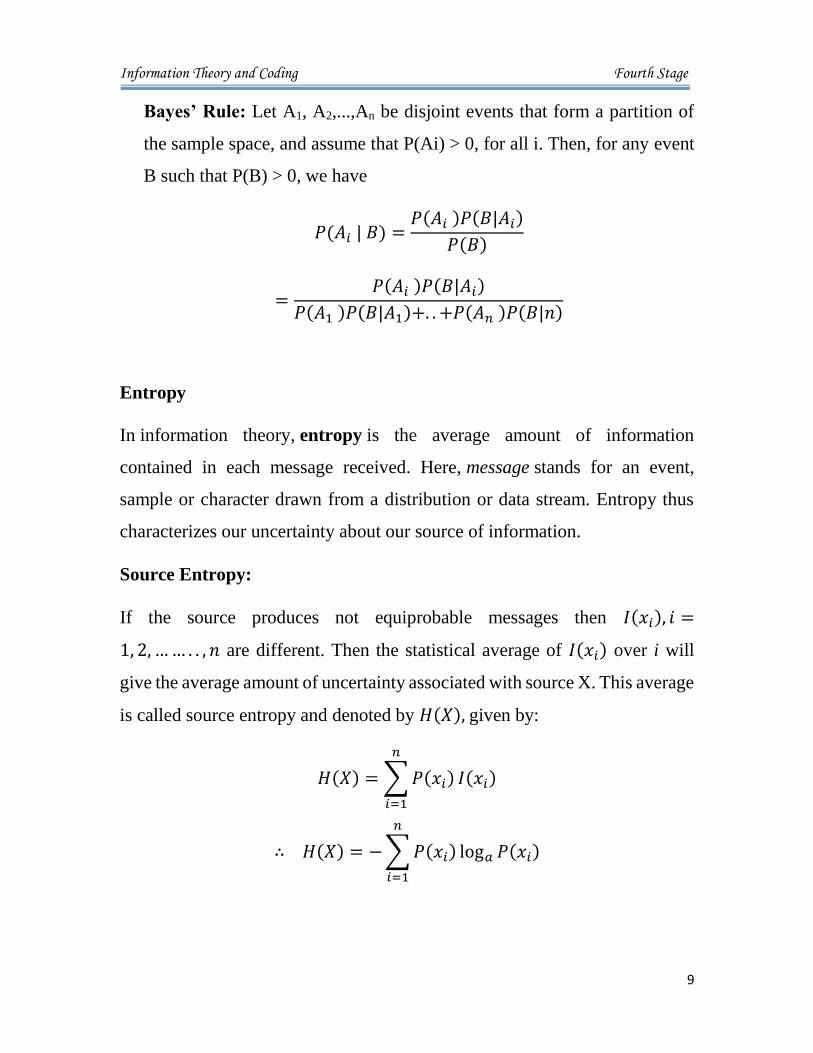
Bayes’ Rule: Let A1, A2,...,An be disjoint events that form a partition of

the sample space, and assume that P(Ai) > 0, for all i. Then, for any event

B such that P(B) > 0, we have

𝑃(𝐴𝑖 | 𝐵) =𝑃(𝐴𝑖 )𝑃(𝐵|𝐴𝑖)

𝑃(𝐵)

=𝑃(𝐴𝑖 )𝑃(𝐵|𝐴𝑖)

𝑃(𝐴1 )𝑃(𝐵|𝐴1)+. . +𝑃(𝐴𝑛 )𝑃(𝐵|𝑛)

Entropy

In information theory, entropy is the average amount of information

contained in each message received. Here, message stands for an event,

sample or character drawn from a distribution or data stream. Entropy thus

characterizes our uncertainty about our source of information.

Source Entropy:

If the source produces not equiprobable messages then 𝐼(𝑥𝑖), 𝑖 =

1, 2, … … . . , 𝑛 are different. Then the statistical average of 𝐼(𝑥𝑖) over i will

give the average amount of uncertainty associated with source X. This average

is called source entropy and denoted by 𝐻(𝑋), given by:

𝐻(𝑋) = ∑ 𝑃(𝑥𝑖)

𝑛

𝑖=1

𝐼(𝑥𝑖)

∴ 𝐻(𝑋) = − ∑ 𝑃(𝑥𝑖)

𝑛

𝑖=1

log𝑎 𝑃(𝑥𝑖)



10

Example:

Find the entropy of the source producing the following messages:

𝑃𝑥1 = 0.25, 𝑃𝑥2 = 0.1, 𝑃𝑥3 = 0.15, 𝑎𝑛𝑑 𝑃𝑥4 = 0.5

Solution:

𝐻(𝑋) = − ∑ 𝑃(𝑥𝑖)

𝑛

𝑖=1

log𝑎 𝑃(𝑥𝑖)

= −[0.25𝑙𝑛0.25 + 0.1𝑙𝑛0.1 + 0.15𝑙𝑛0.15 + 0.5𝑙𝑛0.5]

𝑙𝑛2

𝐻(𝑋) = 1.7427 𝑏𝑖𝑡𝑠

𝑠𝑦𝑚𝑏𝑜𝑙

Example:

Find and plot the entropy of binary source.

𝑃(0𝑇) + 𝑃(1𝑇) = 1

𝐻(𝑋) = −[𝑃(0𝑇) log2 𝑃(0𝑇) + (1

− 𝑃(0𝑇)) log2(1 − 𝑃(0𝑇))] 𝑏𝑖𝑡𝑠/𝑠𝑦𝑚𝑏𝑜𝑙

If 𝑃(0𝑇) = 0.2, 𝑡ℎ𝑒𝑛 𝑃(1𝑇) = 1 − 0.2 = 0.8, 𝑎𝑛𝑑 𝑝𝑢𝑡 𝑖𝑛 𝑎𝑏𝑜𝑣𝑒 𝑒𝑞𝑢𝑎𝑡𝑖𝑜𝑛,

𝐻(𝑋) = −[0.2 log2(0.2) + 0.8 log2(0.8)] = 0.7

Not that H(X) is maximum equal to 1(bit) if: 𝑃(0𝑇) = 𝑃(1𝑇) = 0.5 as shown

in figure.


11

If all messages are equiprobable, then 𝑃(𝑥𝑖) = 1/𝑛 so hat:

𝐻(𝑋) = 𝐻(𝑋)𝑚𝑎𝑥

= −[1

𝑛log𝑎 (

1

𝑛)] × 𝑛 = −log𝑎 (

1

𝑛) = log𝑎𝑛 𝑏𝑖𝑡𝑠/𝑠𝑦𝑚𝑏𝑜𝑙

And 𝐻(𝑋) = 0 if one of the message has the prob of a certain event.

Source Entropy Rate:

It is the average rate of amount of information produced per second.

𝑅(𝑋) = 𝐻(𝑋) × 𝑟𝑎𝑡𝑒 𝑜𝑓 𝑝𝑟𝑜𝑑𝑢𝑐𝑖𝑛𝑔 𝑡ℎ𝑒 𝑠𝑦𝑚𝑏𝑜𝑙𝑠 = 𝑏𝑖𝑡𝑠

𝑠𝑒𝑐= 𝑏𝑝𝑠

The unit of H(X) is bits/symbol and the rate of producing the symbols is

symbol/sec, so that the unit of R(X) is bits/sec.

Sometimes 𝑅(𝑋) =𝐻(𝑋)

,

𝜏 = ∑ 𝜏𝑖𝑃(𝑥𝑖)

𝑛

𝑖=1

𝜏 is the average time duration of symbols, 𝜏𝑖 is the time duration of the

symbol 𝑥𝑖.


12

Example :

A source produces dots ‘.’ And dashes ‘-‘ with P(dot)=0.65. If the time

duration of dot is 200ms and that for a dash is 800ms. Find the average

source entropy rate.

Solution:

𝑃(𝑑𝑎𝑠ℎ) = 1 − 𝑃(𝑑𝑜𝑡) = 1 − 0.65 = 0.35

𝐻(𝑋) = −[0.65log2(0.65) + 0.35log2(0.35)] = 0.934 𝑏𝑖𝑡𝑠/𝑠𝑦𝑚𝑏𝑜𝑙

𝜏 = 0.2 × 0.65 + 0.8 × 0.35 = 0.41 𝑠𝑒𝑐

𝑅(𝑋) =𝐻(𝑋)

𝜏=

0.34

0.41= 2.278 𝑏𝑝𝑠

Mutual Information:

Consider the set of symbols 𝑥1, 𝑥2, … . , 𝑥𝑛, the

transmitter 𝑇𝑥 my produce. The receiver 𝑅𝑥 may receive

𝑦1, 𝑦2 … … … . 𝑦𝑚. Theoretically, if the noise and

jamming is neglected, then the set X=set Y. However and

due to noise and jamming, there will be a conditional

probability 𝑃(𝑦𝑗 ∣ 𝑥𝑖):

1- 𝑃(𝑥𝑖) to be what is so called the apriori prob of the

symbol 𝑥𝑖, which is the prob of selecting 𝑥𝑖 for transmission.

2- 𝑃(𝑦𝑗 ∣ 𝑥𝑖) to be what is called the aposteriori prob of the symbol 𝑥𝑖 after

the reception of 𝑦𝑗.

The amount of information that 𝑦𝑗 provides about 𝑥𝑖 is called the

mutual information between 𝑥𝑖 and 𝑦𝑖 . This is given by:

𝐼(𝑥𝑖 , 𝑦𝑗) = log2 (𝑎𝑝𝑜𝑠𝑡𝑒𝑟𝑜𝑟𝑖 𝑝𝑟𝑜𝑏

𝑎𝑝𝑟𝑖𝑜𝑟𝑖 𝑝𝑟𝑜𝑏) = log2 (

𝑃( 𝑦𝑗 ∣∣ 𝑥𝑖 )

𝑃(𝑦𝑗))


13

Properties of 𝑰(𝒙𝒊, 𝒚𝒋):

1- It is symmetric, 𝐼(𝑥𝑖 , 𝑦𝑗) = 𝐼(𝑦𝑗 , 𝑥𝑖).

2- 𝐼(𝑥𝑖 , 𝑦𝑗) > 0 if aposteriori prob> apriori prob, 𝑦𝑗 provides +ve

information about 𝑥𝑖.

3- 𝐼(𝑥𝑖 , 𝑦𝑗) = 0 if aposteriori prob= apriori prob, which is the case of

statistical independence when 𝑦𝑗 provides no information about 𝑥𝑖.

4- 𝐼(𝑥𝑖 , 𝑦𝑗) < 0 if aposteriori prob< apriori prob, 𝑦𝑗 provides -ve

information about 𝑥𝑖, or 𝑦𝑗 adds ambiguity.

Also 𝐼(𝑥𝑖 , 𝑦𝑗) = log2 (𝑃( 𝑥𝑖∣∣𝑦𝑗 )

𝑃(𝑥𝑖))

Example:

Show that I(X, Y) is zero for extremely noisy channel.

Solution:

For extremely noisy channel, then 𝑦𝑗gives no information about 𝑥𝑖 the

receiver can’t decide anything about 𝑥𝑖 as if we transmit a deterministic signal

𝑥𝑖 but the receiver receives noise like signal 𝑦𝑗 that is completely has no

correlation with 𝑥𝑖. Then 𝑥𝑖 and 𝑦𝑗 are statistically independent so that

𝑃( 𝑥𝑖 ∣∣ 𝑦𝑗 ) = 𝑃(𝑥𝑖)𝑎𝑛𝑑 𝑃( 𝑦𝑗 ∣∣ 𝑥𝑖 ) = 𝑃(𝑥𝑖) 𝑓𝑜𝑟 𝑎𝑙𝑙 𝑖 𝑎𝑛𝑑 𝑗, 𝑡ℎ𝑒𝑛:

𝐼(𝑥𝑖 , 𝑦𝑗) = log21 = 0 𝑓𝑜𝑟 𝑎𝑙𝑙 𝑖 & 𝑗, 𝑡ℎ𝑒𝑛 𝐼(𝑋, 𝑌) = 0

Transinformation (average mutual information):

It is the statistical average of all pair 𝐼(𝑥𝑖 , 𝑦𝑗) , 𝑖 = 1, 2, … . . , 𝑛, 𝑗 =

1, 2, … . . , 𝑚.

This is denoted by 𝐼(𝑋, 𝑌) and is given by:


14

𝐼(𝑋, 𝑌) = ∑ ∑ 𝐼(𝑥𝑖 , 𝑦𝑗)𝑃(𝑥𝑖 , 𝑦𝑗)

𝑚

𝑗=1

𝑛

𝑖=1

𝐼(𝑋, 𝑌) = ∑ ∑ 𝑃(𝑥𝑖 , 𝑦𝑗)

𝑚

𝑗=1

𝑛

𝑖=1

log2 (𝑃( 𝑦𝑗 ∣∣ 𝑥𝑖 )

𝑃(𝑦𝑗))

𝑏𝑖𝑡𝑠


or

𝐼(𝑋, 𝑌) = ∑ ∑ 𝑃(𝑥𝑖 , 𝑦𝑗)

𝑚

𝑗=1

𝑛

𝑖=1

log2 (𝑃( 𝑥𝑖 ∣∣ 𝑦𝑗 )

𝑃(𝑥𝑖)) 𝑏𝑖𝑡𝑠/𝑠𝑦𝑚𝑏𝑜𝑙

Expand above equation:

𝐼(𝑋, 𝑌) = ∑ ∑ 𝑃(𝑥𝑖, 𝑦𝑗)

𝑚

𝑗=1

𝑛

𝑖=1

log2 (𝑃( 𝑥𝑖 ∣∣ 𝑦𝑗 )) − ∑ ∑ 𝑃(𝑥𝑖, 𝑦𝑗)

𝑚

𝑗=1

𝑛

𝑖=1

log2(𝑃(𝑥𝑖))

And we have

∑ 𝑃(𝑥𝑖 , 𝑦𝑗)

𝑚

𝑗=1

= 𝑝(𝑥𝑖)

And by substituting:

𝐼(𝑋, 𝑌) = ∑ ∑ 𝑃(𝑥𝑖, 𝑦𝑗)

𝑚

𝑗=1

𝑛

𝑖=1

log2 (𝑃( 𝑥𝑖 ∣∣ 𝑦𝑗 )) − ∑ 𝑃(𝑥𝑖)

𝑛

𝑖=1

log2(𝑃(𝑥𝑖))

Or 𝐼(𝑋, 𝑌) = 𝐻(𝑋) − 𝐻(𝑋 ∣ 𝑌)

Similarly 𝐼(𝑋, 𝑌) = 𝐻(𝑌) − 𝐻(𝑌 ∣ 𝑋)

Marginal Entropies:

Marginal entropies is a term usually used to denote both source entropy

H(X) defined as before and the receiver entropy H(Y) given by:

𝐻(𝑌) = − ∑ 𝑃(𝑦𝑗)

𝑚

𝑗=1

log2𝑃(𝑦𝑗) 𝑏𝑖𝑡𝑠



15

Joint entropy and conditional entropy:

The average information associated with the pair (𝑥𝑖 , 𝑦𝑗) is called joint or

system entropy H(X,Y):

𝐻(𝑋, 𝑌) = 𝐻(𝑋𝑌)

= − ∑ ∑ 𝑃(𝑥𝑖 , 𝑦𝑗)

𝑛

𝑖=1

𝑚

𝑗=1

log2𝑃(𝑥𝑖 , 𝑦𝑗) 𝑏𝑖𝑡𝑠/𝑠𝑦𝑚𝑏𝑜𝑙

The average amount of information associated with the pairs 𝑃(𝑥𝑖 ∣ 𝑦𝑗)

and 𝑃(𝑦𝑗 ∣ 𝑥𝑖) are called conditional entropies 𝐻( 𝑌 ∣ 𝑋 )𝑎𝑛𝑑 𝐻(𝑋 ∣ 𝑌),

and given by:

𝐻(𝑌 ∣ 𝑋) = − ∑ ∑ 𝑃(𝑥𝑖 , 𝑦𝑗)

𝑛

𝑖=1

𝑚

𝑗=1

log2𝑃(𝑦𝑗 ∣ 𝑥𝑖) 𝑏𝑖𝑡𝑠/𝑠𝑦𝑚𝑏𝑜𝑙

Return to first equation, we have: 𝑃(𝑥𝑖 , 𝑦𝑗) = 𝑃(𝑥𝑖)𝑃(𝑦𝑗 ∣ 𝑥𝑖), put inside

log term

𝐻(𝑋, 𝑌) = − ∑ ∑ 𝑃(𝑥𝑖 , 𝑦𝑗)

𝑛

𝑖=1

𝑚

𝑗=1

log2𝑃(𝑥𝑖)

− ∑ ∑ 𝑃(𝑥𝑖 , 𝑦𝑗)

𝑛

𝑖=1

𝑚

𝑗=1

log2𝑃(𝑦𝑗 ∣ 𝑥𝑖)

But

∑ 𝑃(𝑥𝑖 , 𝑦𝑗)

𝑚

𝑗=1

= 𝑃(𝑥𝑖)

Put it in above equation yields:

𝐻(𝑋, 𝑌) = − ∑ 𝑃(𝑥𝑖)

𝑛

𝑖=1

log2𝑃(𝑥𝑖) − ∑ ∑ 𝑃(𝑥𝑖 , 𝑦𝑗)

𝑛

𝑖=1

𝑚

𝑗=1


So that 𝐻(𝑋, 𝑌) = 𝐻(𝑋) + 𝐻(𝑌 ∣ 𝑋)


16

Example :

The joint probability of a system is given by:

𝑃(𝑋, 𝑌) =

𝑥1

𝑥2

𝑥3

[0.5 0.250 0.125

0.0625 0.0625]

Find:

1- Marginal entropies. 2- Joint entropy

3- Conditional entropies. 4- The mutual information between x1 and y2.

5- The transinformation. 6- Draw the channel model.

1- 𝑃(𝑋) = [𝑥1 𝑥2 𝑥3

0.75 0.125 0.125] 𝑃(𝑌) = [

𝑦1 𝑦2

0.5625 0.4375]

𝐻(𝑋) = −[0.75 ln(0.75) + 2 × 0.125 ln(0.125)]/𝑙𝑛2

= 1.06127 𝑏𝑖𝑡𝑠/𝑠𝑦𝑚𝑏𝑜𝑙

𝐻(𝑌) = −[0.5625 ln(0.5625) + 0.4375 ln(0.4375)]/𝑙𝑛2


2-

𝐻(𝑋, 𝑌) = − ∑ ∑ 𝑃(𝑥𝑖 , 𝑦𝑗)

𝑛

𝑖=1

𝑚

𝑗=1

log2𝑃(𝑥𝑖 , 𝑦𝑗)

𝐻(𝑋, 𝑌)

= −[0.5ln(0.5) + 0.25 ln(0.25) + 0.125 ln(0.125) + 2 × 0.0625 ln(0.0625)]

𝑙𝑛2


3- 𝐻( 𝑌 ∣ 𝑋 ) = 𝐻(𝑋, 𝑌) − 𝐻(𝑋) = 1.875 − 1.06127 =

0.813 𝑏𝑖𝑡𝑠


𝐻( 𝑋 ∣ 𝑌 ) = 𝐻(𝑋, 𝑌) − 𝐻(𝑌) = 1.875 − 0.9887



17

4- 𝐼(𝑥1, 𝑦2) = log2 (𝑃( 𝑥1∣∣𝑦2 )

𝑃(𝑥1)) , 𝑏𝑢𝑡 𝑃( 𝑥1 ∣∣ 𝑦2 ) = 𝑃(𝑥1, 𝑦2)/𝑃(𝑦2)

𝐼(𝑥1, 𝑦2) = log2 (𝑃(𝑥1,𝑦2)

𝑃(𝑥1)𝑃( 𝑦2))=log2

0.25

0.75×0.4375= −0.3923 𝑏𝑖𝑡𝑠

That means y2 gives ambiguity about x1

5- 𝐼(𝑋, 𝑌) = 𝐻(𝑋) − 𝐻( 𝑋 ∣ 𝑌 ) = 1.06127 − 0.8863 =

0.17497 𝑏𝑖𝑡𝑠/𝑠𝑦𝑚𝑏𝑜𝑙.

6- To draw the channel model, must find P(Y∣X) matrix from P(X, Y)

matrix by dividing its rows by the corresponding P(xi):

𝑃(𝑋 ∣ 𝑌) =

𝑥1

𝑥2

𝑥3

[

0.5/0.75 0.25/0.750/0.125 0.125/0.125

0.0625/0.125 0.0625/0.125]

=

𝑥1

𝑥2

𝑥3

[2/3 1/30 1

0.5 0.5]

Venn diagrams:

The Venn diagrams is a helpful mean to understand the relations between

mutual information and conditional entropies as shown below:


18


AlSafwa University College

Dep. Of Computer Techniques Engineering

Subject: Information Theory and Coding

Stage: Fourth

Academic Year: 2020-2021

Lecturer: Assist. Lec. Noor Yahya

Lecture: Chapter Two

Notes:

1

Chapter Two

2.1- Channel:

In telecommunications and computer networking, a communication channel

or channel, refers either to a physical transmission medium such as a wire, or to

a logical connection over a multiplexed medium such as a radio channel. A channel is

used to convey an information signal, for example a digital bit stream, from one or

several senders (or transmitters) to one or several receivers. A channel has a certain

capacity for transmitting information, often measured by its bandwidth in Hz or its data

rate in bits per second.

2.2- Binary symmetric channel (BSC)

It is a common communications channel model used in coding theory and information

theory. In this model, a transmitter wishes to send a bit (a zero or a one), and the receiver

receives a bit. It is assumed that the bit is usually transmitted correctly, but that it will

be "flipped" with a small probability (the "crossover probability").

A binary symmetric channel with crossover probability p denoted by BSCp, is a

channel with binary input and binary output and probability of error p; that is, if X is the

transmitted random variable and Y the received variable, then the channel is

characterized by the conditional probabilities:

Pr( 𝑌 = 0 ∣ 𝑋 = 0 ) = 1 − 𝑃

Pr(𝑌 = 0 ∣ 𝑋 = 1 ) = 𝑃

Pr(𝑌 = 1 ∣ 𝑋 = 0 ) = 𝑃

Pr( 𝑌 = 1 ∣ 𝑋 = 1 ) = 1 − 𝑃

1 1

0 1-P

P

P

1-P

0

http://en.wikipedia.org/wiki/Telecommunications

http://en.wikipedia.org/wiki/Computer_networking

http://en.wikipedia.org/wiki/Transmission_medium

http://en.wikipedia.org/wiki/Connection-oriented_communication

http://en.wikipedia.org/wiki/Multiplexing

http://en.wikipedia.org/wiki/Information_transfer


http://en.wikipedia.org/wiki/Bit_stream

http://en.wikipedia.org/wiki/Sender

http://en.wikipedia.org/wiki/Receiver_(information_theory)

http://en.wikipedia.org/wiki/Bandwidth_(signal_processing)

http://en.wikipedia.org/wiki/Hz

http://en.wikipedia.org/wiki/Data_signaling_rate

http://en.wikipedia.org/wiki/Data_signaling_rate

http://en.wikipedia.org/wiki/Bit_rate

http://en.wikipedia.org/wiki/Communications_channel

http://en.wikipedia.org/wiki/Coding_theory




http://en.wikipedia.org/wiki/Data_transmission


http://en.wikipedia.org/wiki/Random_variable

http://en.wikipedia.org/wiki/Conditional_probability

2

1-2Pe

2.3- Ternary symmetric channel (TSC):

The transitional probability of TSC is:

𝑃( 𝑌 ∣ 𝑋 ) =

𝑥1

𝑥2

𝑥3

[

𝑦1 𝑦2 𝑦3

1 − 2𝑃𝑒 𝑃𝑒 𝑃𝑒 𝑃𝑒 1 − 2𝑃𝑒 𝑃𝑒

𝑃𝑒 𝑃𝑒 1 − 2𝑃𝑒

]

The TSC is symmetric but not very practical since practically 𝑥1 and 𝑥3 are not affected

so much as 𝑥2. In fact the interference between 𝑥1 and 𝑥3 is much less than the

interference between 𝑥1 and 𝑥2 or 𝑥2 and 𝑥3.

Hence the more practice but nonsymmetric channel has the trans. prob.

𝑃(𝑌 ∣ 𝑋 ) =

𝑥1

𝑥2

𝑥3

[

𝑦1 𝑦2 𝑦3

1 − 𝑃𝑒 𝑃𝑒 0 𝑃𝑒 1 − 2𝑃𝑒 𝑃𝑒

0 𝑃𝑒 1 − 𝑃𝑒

]

Where 𝑥1 interfere with 𝑥2 exactly the same as interference between 𝑥2 and 𝑥3, but 𝑥1

and 𝑥3 are not interfere.

1-2Pe

1-2Pe

Pe

Pe

Y1

Y2

Y3 X3

X2

X1

1-2Pe

Pe

Pe

1-Pe

X2

1-Pe

X3

Y2

Y3

Y1 X1

3

2.4- Special Channels:

1- Lossless channel: It has only one nonzero element in each column of the

transitional matrix P(Y∣X).

𝑃(𝑌 ∣ 𝑋 ) =

𝑥1

𝑥2

𝑥3

[

𝑦1 𝑦2 𝑦3 𝑦4 𝑦5

3/4 1/4 0 0 0 0 0 1/3 2/3 0

0 0 0 0 1

]

This channel has H(X∣Y)=0 and I(X, Y)=H(X) with zero losses entropy.

2- Deterministic channel: It has only one nonzero element in each row, the

transitional matrix P(Y∣X), as an example:

𝑃(𝑌 ∣ 𝑋 ) =

𝑥1

𝑥2

𝑥3

[ 𝑦1 𝑦2 𝑦3 1 0 0 1 0 0 0 0 1 0 1 00 1 0 ]

This channel has H(Y∣X)=0 and I(Y, X)=H(Y) with zero noisy entropy.

3- Noiseless channel: It has only one nonzero element in each row and column, the

transitional matrix P(Y∣X), i.e. it is an identity matrix, as an example:

𝑃(𝑌 ∣ 𝑋 ) =

𝑥1

𝑥2

𝑥3

[

𝑦1 𝑦2 𝑦3 1 0 00 1 00 0 1

]

This channel has H(Y∣X)= H(X∣Y)=0 and I(Y, X)=H(Y)=H(X).

2.5- Shannon’s theorem:

1- A given communication system has a maximum rate of information C known as

the channel capacity.

2- If the information rate R is less than C, then one can approach arbitrarily small

error probabilities by using intelligent coding techniques.

3- To get lower error probabilities, the encoder has to work on longer blocks of

signal data. This entails longer delays and higher computational requirements.

4

Thus, if R ≤ C then transmission may be accomplished without error in the presence

of noise. The negation of this theorem is also true: if R > C, then errors cannot be

avoided regardless of the coding technique used.

Consider a bandlimited Gaussian channel operating in the presence of additive

Gaussian noise:

The Shannon-Hartley theorem states that the channel capacity is given by:

𝐶 = 𝐵𝑙𝑜𝑔2 (1 +𝑆

𝑁)

Where C is the capacity in bits per second, B is the bandwidth of the channel in Hertz,

and S/N is the signal-to-noise ratio.

2.6- Discrete Memoryless Channel:

The Discrete Memoryless Channel (DMC) has an input X and an output Y. At any given

time (t), the channel output Y= y only depends on the input X = x at that time (t) and it

does not depend on the past history of the input. DMC is represented by the conditional

probability of the output Y = y given the input X = x, or P(YX).

2.7 Binary Erasure Channel (BEC):

The Binary Erasure Channel (BEC) model are widely used to represent channels or links

that “losses” data. Prime examples of such channels are Internet links and routes. A

BEC channel has a binary input X and a ternary output Y.

X Channel

P(YX)

Y

5

Note that for the BEC, the probability of “bit error” is zero. In other words, the

following conditional probabilities hold for any BEC model:

Pr( 𝑌 = "𝑒𝑟𝑎𝑠𝑢𝑟𝑒" ∣ 𝑋 = 0 ) = 𝑃

Pr( 𝑌 = "𝑒𝑟𝑎𝑠𝑢𝑟𝑒" ∣ 𝑋 = 1 ) = 𝑃

Pr( 𝑌 = 0 ∣ 𝑋 = 0 ) = 1 − 𝑃

Pr( 𝑌 = 1 ∣ 𝑋 = 1 ) = 1 − 𝑃

Pr( 𝑌 = 0 ∣ 𝑋 = 1 ) = 0

Pr( 𝑌 = 1 ∣ 𝑋 = 0 ) = 0

Pe

1-Pe

1-Pe

X2

Erasure

Y2

Y1 X1

6

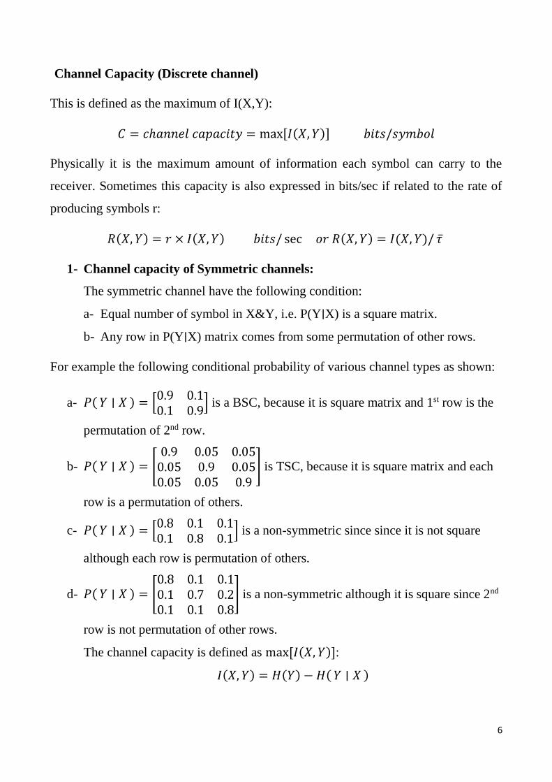
Channel Capacity (Discrete channel)

This is defined as the maximum of I(X,Y):

𝐶 = 𝑐ℎ𝑎𝑛𝑛𝑒𝑙 𝑐𝑎𝑝𝑎𝑐𝑖𝑡𝑦 = max[𝐼(𝑋, 𝑌)] 𝑏𝑖𝑡𝑠/𝑠𝑦𝑚𝑏𝑜𝑙

Physically it is the maximum amount of information each symbol can carry to the

receiver. Sometimes this capacity is also expressed in bits/sec if related to the rate of

producing symbols r:

𝑅(𝑋, 𝑌) = 𝑟 × 𝐼(𝑋, 𝑌) 𝑏𝑖𝑡𝑠/ sec 𝑜𝑟 𝑅(𝑋, 𝑌) = 𝐼(𝑋, 𝑌)/ 𝜏

1- Channel capacity of Symmetric channels:

The symmetric channel have the following condition:

a- Equal number of symbol in X&Y, i.e. P(Y∣X) is a square matrix.

b- Any row in P(Y∣X) matrix comes from some permutation of other rows.

For example the following conditional probability of various channel types as shown:

a- 𝑃(𝑌 ∣ 𝑋 ) = [0.9 0.10.1 0.9

] is a BSC, because it is square matrix and 1st row is the

permutation of 2nd row.

b- 𝑃(𝑌 ∣ 𝑋 ) = [0.9 0.05 0.050.05 0.9 0.050.05 0.05 0.9

] is TSC, because it is square matrix and each

row is a permutation of others.

c- 𝑃(𝑌 ∣ 𝑋 ) = [0.8 0.1 0.10.1 0.8 0.1

] is a non-symmetric since since it is not square

although each row is permutation of others.

d- 𝑃(𝑌 ∣ 𝑋 ) = [0.8 0.1 0.10.1 0.7 0.20.1 0.1 0.8

] is a non-symmetric although it is square since 2nd

row is not permutation of other rows.

The channel capacity is defined as max [𝐼(𝑋, 𝑌)]:

𝐼(𝑋, 𝑌) = 𝐻(𝑌) − 𝐻(𝑌 ∣ 𝑋 )

7

𝐼(𝑋, 𝑌) = 𝐻(𝑌) + ∑∑𝑃(𝑥𝑖 , 𝑦𝑗)

𝑛

𝑖=1

𝑚

𝑗=1


But we have

𝑃(𝑥𝑖 , 𝑦𝑗) = 𝑃(𝑥𝑖)𝑃(𝑦𝑗 ∣ 𝑥𝑖) 𝑝𝑢𝑡 𝑖𝑛 𝑎𝑏𝑜𝑣𝑒 𝑒𝑞𝑢𝑎𝑡𝑖𝑜𝑛 𝑦𝑖𝑒𝑙𝑑𝑒𝑠:

𝐼(𝑋, 𝑌) = 𝐻(𝑌) + ∑∑𝑃(𝑥𝑖)𝑃(𝑦𝑗 ∣ 𝑥𝑖)

𝑛

𝑖=1

𝑚

𝑗=1


If the channel is symmetric the quantity:

∑𝑃(𝑦𝑗 ∣ 𝑥𝑖)log2𝑃(𝑦𝑗 ∣ 𝑥𝑖) = 𝐾

𝑚

𝑗=1

Where K is constant and independent of the row number i so that the equation

becomes:

𝐼(𝑋, 𝑌) = 𝐻(𝑌) + 𝐾 ∑𝑃(𝑥𝑖)

𝑛

𝑖=1

Hence 𝐼(𝑋, 𝑌) = 𝐻(𝑌) + 𝐾 for symmetric channels

Max of 𝐼(𝑋, 𝑌) = max[𝐻(𝑌) + 𝐾] = max[𝐻(𝑌)] + 𝐾

When Y has equiprobable symbols then max[𝐻(𝑌)] = 𝑙𝑜𝑔2𝑚

Then

𝐼(𝑋, 𝑌) = 𝑙𝑜𝑔2𝑚 + 𝐾

Or

𝐶 = 𝑙𝑜𝑔2𝑚 + 𝐾

8

Example 9:

For the BSC shown:

Find the channel capacity and efficiency if 𝐼(𝑥1) = 2𝑏𝑖𝑡𝑠

Solution:

𝑃(𝑌 ∣ 𝑋 ) = [0.7 0.30.3 0.7

]

Since the channel is symmetric then

𝐶 = 𝑙𝑜𝑔2𝑚 + 𝐾 and 𝑛 = 𝑚

𝑤ℎ𝑒𝑟𝑒 𝑛 𝑎𝑛𝑑 𝑚 𝑎𝑟𝑒 𝑛𝑢𝑚𝑏𝑒𝑟 𝑟𝑜𝑤 𝑎𝑛𝑑 𝑐𝑜𝑙𝑢𝑚𝑛 𝑟𝑒𝑝𝑒𝑠𝑡𝑖𝑣𝑒𝑙𝑦

𝐾 = 0.7𝑙𝑜𝑔20.7 + 0.3𝑙𝑜𝑔20.3 = −0.88129

𝐶 = 1 − 0.88129 = 0.1187 𝑏𝑖𝑡𝑠/𝑠𝑦𝑚𝑏𝑜𝑙

The channel efficiency 𝜂 =𝐼(𝑋,𝑌)

𝐶

𝐼(𝑥1) = −𝑙𝑜𝑔2𝑃(𝑥1) = 2

𝑃(𝑥1) = 2−2 = 0.25 𝑡ℎ𝑒𝑛 𝑃(𝑋) = [0.25 0.75]𝑇

And we have 𝑃(𝑥𝑖 , 𝑦𝑗) = 𝑃(𝑥𝑖)𝑃(𝑦𝑗 ∣ 𝑥𝑖) so that

𝑃(𝑋, 𝑌) = [0.7 × 0.25 0.3 × 0.250.3 × 0.75 0.7 × 0.75

]=[0.175 0.0750.225 0.525

]

𝑃(𝑌) = [0.4 0.6] → 𝐻(𝑌) = 0.97095 𝑏𝑖𝑡𝑠/𝑠𝑦𝑚𝑏𝑜𝑙

𝐼(𝑋, 𝑌) = 𝐻(𝑌) + 𝐾 = 0.97095 − 0.88129 = 0.0896 𝑏𝑖𝑡𝑠/𝑠𝑦𝑚𝑏𝑜𝑙

Then 𝜂 =0.0896

0.1187= 75.6%

0.7

0.7 Y1

Y2 X2

X1

9

Review questions:

A binary source sending 𝑥1 with a probability of 0.4 and 𝑥2 with 0.6 probability

through a channel with a probabilities of errors of 0.1 for 𝑥1 and 0.2 for 𝑥2.Determine:

1- Source entropy.

2- Marginal entropy.

3- Joint entropy.

4- Conditional entropy 𝐻(𝑌𝑋).

5- Losses entropy 𝐻(𝑋𝑌).

6- Transinformation.

Solution:

1- The channel diagram:

Or 𝑃(𝑌X) = [0.9 0.10.2 0.8

]

𝐻(𝑋) = −∑𝑝(𝑥𝑖)

𝑛

𝑖=1

𝑙𝑜𝑔2𝑝(𝑥𝑖)

𝐻(𝑋) = −[0.4 ln(0.4) + 0.6 ln(0.6)]

𝑙𝑛2= 0.971

𝑏𝑖𝑡𝑠


2- 𝑃(𝑋, 𝑌) = 𝑃(𝑌X) × 𝑃(𝑋)

∴ 𝑃(𝑋, 𝑌) = [0.9 × 0.4 0.1 × 0.40.2 × 0.6 0.8 × 0.6

] = [0.36 0.040.12 0.48

]

∴ 𝑃(𝑌) = [0.48 0.52]

𝐻(𝑌) = −∑𝑝(𝑦𝑗)

𝑚

𝑗=1

𝑙𝑜𝑔2𝑝(𝑦𝑗)

𝐻(𝑌) = −[0.48 ln(0.48) + 0.52 ln(0.52)]

ln(2)= 0.999 𝑏𝑖𝑡𝑠/𝑠𝑦𝑚𝑏𝑜𝑙

0.9

0.8

0.1

0.2

0.6

0.4 𝑥1

𝑥2

𝑦1

𝑦2

10

3- 𝐻(𝑋, 𝑌)

𝐻(𝑋, 𝑌) = −∑∑𝑃(𝑥𝑖 , 𝑦𝑗)

𝑛

𝑖=1

𝑚

𝑗=1

log2𝑃(𝑥𝑖 , 𝑦𝑗)

𝐻(𝑋, 𝑌) = −[0.36 ln(0.36) + 0.04 ln(0.04) + 0.12 ln(0.12) + 0.48 ln(0.48)]

ln(2)


4- 𝐻(𝑌X)

𝐻(𝑌X) == −∑∑𝑃(𝑥𝑖 , 𝑦𝑗)

𝑛

𝑖=1

𝑚

𝑗=1

log2𝑃(𝑦𝑗𝑥𝑖)

𝐻(𝑌X) = −[0.36 ln(0.9) + 0.12 ln(0.2) + 0.04 ln(0.1) + 0.48 ln(0.8)]

ln(2)

= 0.621𝑏𝑖𝑡𝑠


Or 𝐻(𝑌X) = 𝐻(𝑋, 𝑌) − 𝐻(𝑋) = 1.592 − 0.971 = 0.621𝑏𝑖𝑡𝑠


5- 𝐻(𝑋Y) = 𝐻(𝑋, 𝑌) − 𝐻(𝑌) = 1.592 − 0.999 = 0.593 𝑏𝑖𝑡𝑠/𝑠𝑦𝑚𝑏𝑜𝑙

6- 𝐼(𝑋, 𝑌) = 𝐻(𝑋) − 𝐻(𝑋Y) = 0.971 − 0.593 = 0.378 bits/symbol

2- Cascading of Channels

If two channels are cascaded, then the overall transition matrix is the product of the two

transition matrices.

)/()./()/( yzpxypxzp

matrix

kn )( matrix

mn )( matrix

km )(

For the series information channel, the overall channel capacity is not exceed any of

each channel individually.

𝐼(𝑋, 𝑍) ≤ 𝐼(𝑋, 𝑌) & 𝐼(𝑋, 𝑍) ≤ 𝐼(𝑌, 𝑍)

Channel 1

Channel 1

.

.

1

m

.

.

1

n

.

.

1

k

11

Example:

Find the transition matrix )/( xzp for the cascaded channel shown.

7.003.0

02.08.0)/( xyp ,

01

01

3.07.0

)/( yzp

09.091.0

24.076.0

01

01

3.07.0

7.003.0

02.08.0)/( xzp

0.7

0.8

0.3

0.2

0.7

0.3

1

1





الرابعة المرحلة: زنظرية المعلومات و الترميأسم المادة:

81/2/1208 المالحظات:

CHAPTER THREE

DR. MAHMOOD 30 2017-12-08

Chapter Three

Source Coding

1- Sampling theorem:

Sampling of the signals is the fundamental operation in digital communication. A

continuous time signal is first converted to discrete time signal by sampling process.

Also it should be possible to recover or reconstruct the signal completely from its

samples.

The sampling theorem state that:

i- A band limited signal of finite energy, which has no frequency components higher

than W Hz, is completely described by specifying the values of the signal at instant

of time separated by 1/2W second and

ii- A band limited signal of finite energy, which has no frequency components higher

than W Hz, may be completely recovered from the knowledge of its samples taken

at the rate of 2W samples per second.

When the sampling rate is chosen 𝑓𝑠 = 2𝑓𝑚 each spectral replicate is separated from

each of its neighbors by a frequency band exactly equal to 𝑓𝑠 hertz, and the analog

waveform ca theoretically be completely recovered from the samples, by the use of

filtering. It should be clear that if 𝑓𝑠 > 2𝑓𝑚, the replications will be move farther apart

in frequency making it easier to perform the filtering operation.

When the sampling rate is reduced, such that 𝑓𝑠 < 2𝑓𝑚, the replications will overlap, as

shown in figure below, and some information will be lost. This phenomenon is called

aliasing.

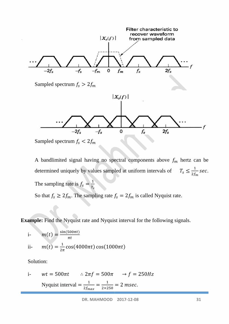
DR. MAHMOOD 31 2017-12-08

Sampled spectrum 𝑓𝑠 > 2𝑓𝑚

Sampled spectrum 𝑓𝑠 < 2𝑓𝑚

A bandlimited signal having no spectral components above 𝑓𝑚 hertz can be

determined uniquely by values sampled at uniform intervals of 𝑇𝑠 ≤1

2𝑓𝑚𝑠𝑒𝑐.

The sampling rate is 𝑓𝑠 =1

𝑇𝑠

So that 𝑓𝑠 ≥ 2𝑓𝑚. The sampling rate 𝑓𝑠 = 2𝑓𝑚 is called Nyquist rate.

Example: Find the Nyquist rate and Nyquist interval for the following signals.

i- 𝑚(𝑡) =sin(500𝜋𝑡)

𝜋𝑡

ii- 𝑚(𝑡) =1

2𝜋cos(4000𝜋𝑡) cos(1000𝜋𝑡)

Solution:

i- 𝑤𝑡 = 500𝜋𝑡 ∴ 2𝜋𝑓 = 500𝜋 → 𝑓 = 250𝐻𝑧

Nyquist interval =1

2𝑓𝑚𝑎𝑥=

1

2×250= 2𝑚𝑠𝑒𝑐.

DR. MAHMOOD 32 2017-12-08

Nyquist rate =2𝑓𝑚𝑎𝑥 = 2 × 250 = 500𝐻𝑧

ii- 𝑚(𝑡) =1

2𝜋[1

2cos(4000𝜋𝑡 − 1000𝜋𝑡) + cos(4000𝜋𝑡 + 1000𝜋𝑡)]

=1

4𝜋cos(3000𝜋𝑡) + cos(5000𝜋𝑡)

Then the highest frequency is 2500Hz

Nyquist interval =1

2𝑓𝑚𝑎𝑥=

1

2×2500= 0.2𝑚𝑠𝑒𝑐.

Nyquist rate =2𝑓𝑚𝑎𝑥 = 2 × 2500 = 5000𝐻𝑧

H. W:

Find the Nyquist interval and Nyquist rate for the following:

i- 1

2𝜋cos(400𝜋𝑡) . cos(200𝜋𝑡)

ii- 1

𝜋𝑠𝑖𝑛𝜋𝑡

Example:

A waveform [20+20sin(500t+30o] is to be sampled periodically and reproduced

from these sample values. Find maximum allowable time interval between

sample values, how many sample values are needed to be stored in order to

reproduce 1 sec of this waveform?.

Solution:

𝑥(𝑡) = 20 + 20 sin(500𝑡 + 300)

𝑤 = 500 → 2𝜋𝑓 = 500 → 𝑓 = 79.58𝐻𝑧

Minimum sampling rate will be twice of the signal frequency:

𝑓𝑠(min) = 2 × 79.58 = 159.15𝐻𝑧

𝑇𝑠(𝑚𝑎𝑥) =1

𝑓𝑠(min)=

1

159.15= 6.283𝑚𝑠𝑒𝑐.

DR. MAHMOOD 33 2017-12-08

Number of sample in 1𝑠𝑒𝑐 =1

6.283𝑚𝑠𝑒𝑐= 159.16 ≈ 160𝑠𝑎𝑚𝑝𝑙𝑒

2- Source coding:

An important problem in communications is the efficient representation of data

generated by a discrete source. The process by which this representation is

accomplished is called source encoding. An efficient source encoder must satisfies two

functional requirements:

i- The code words produced by the encoder are in binary form.

ii- The source code is uniquely decodable, so that the original source sequence can

be reconstructed perfectly from the encoded binary sequence.

The entropy for a source with statistically independent symbols:

𝐻(𝑌) = −∑𝑃(𝑦𝑗)

𝑚

𝑗=1

log2𝑃(𝑦𝑗)

We have:

max[𝐻(𝑌)] = 𝑙𝑜𝑔2𝑚

A code efficiency can therefore be defined as:

𝜂 =𝐻(𝑌)

max[𝐻(𝑌)]× 100

The overall code length, L, can be defined as the average code word length:

𝐿 =∑𝑃(𝑥𝑗)𝑙𝑗

𝑚

𝑗=1

𝑏𝑖𝑡𝑠/𝑠𝑦𝑚𝑏𝑜𝑙

DR. MAHMOOD 34 2017-12-08

The code efficiency can be found by:

𝜂 =𝐻(𝑌)

L× 100

Not that max[𝐻(𝑌)] 𝑏𝑖𝑡𝑠/𝑠𝑦𝑚𝑏𝑜𝑙 = 𝐿𝑏𝑖𝑡𝑠/𝑐𝑜𝑑𝑒𝑤𝑜𝑟𝑑

i- Fixed- Length Code Words:

If the alphabet X consists of the 7 symbols a, b, c, d, e, f, g, then the following

fixed-length code of block length L = 3 could be used.

C(a) = 000

C(b) = 001

C(c) = 010

C(d) = 011

C(e) = 100

C(f) = 101

C(g) = 110.

The encoded output contains L bits per source symbol. For the above example

the source sequence bad... would be encoded into 001000011... . Note that the

output bits are simply run together (or, more technically, concatenated). This

method is nonprobabilistic; it takes no account of whether some symbols occur

more frequently than others, and it works robustly regardless of the symbol

frequencies.

This is used when the source produces almost equiprobable messages

)(...)()()( 321 nxpxpxpxp , then Cn Lllll ...321 and for binary coding

then:

1- nLC 2log bit/message if rn 2 ( ,....16,8,4,2n and r is an

integer) which gives %100

2- 1][log2 nIntLC bits/message if

rn 2 which gives less efficiency

Example

For ten equiprobable messages coded in a fixed length code then

DR. MAHMOOD 35 2017-12-08

10

1)( ixp and 41]10[log2 IntLC

bits

and %048.83%1004

10log%100

)( 2 CL

XH

Example: For eight equiprobable messages coded in a fixed length code then

8

1)( ixp and 38log2 CL bits and %100%100

3

3

Example: Find the efficiency of a fixed length code used to encode messages obtained

from throwing a fair die (a) once, (b) twice, (c) 3 times.

Solution

a- For a fair die, the messages obtained from it are equiprobable with a probability

of 6

1)( ixp with 6n .

31]6[log2 IntLC bits/message

%165.86%1003

6log%100

)( 2 CL

XH

b- For two throws then the possible messages are 3666 n messages with

equal probabilities

61]36[log2 IntLC bits/message 6 bits/2-symbols

while 6log)( 2XH bits/symbol %165.86%100)(2

CL

XH

c- For three throws then the possible messages are 216666 n with equal

probabilities

81]216[log2 IntLC bits/message 8 bits/3-symbols

while 6log)( 2XH bits/symbol %936.96%100)(3

CL

XH

DR. MAHMOOD 36 2017-12-08

ii- Variable-Length Code Words

When the source symbols are not equally probable, a more efficient encoding method

is to use variable-length code words. For example, a variable-length code for the

alphabet X = a, b, c and its lengths might be given by

C(a)= 0 l(a)=1

C(b)= 10 l(b)=2

C(c)= 11 l(c)=2

The major property that is usually required from any variable-length code is that of

unique decodability. For example, the above code C for the alphabet X = a, b, c is

soon shown to be uniquely decodable. However such code is not uniquely decodable,

even though the codewords are all different. If the source decoder observes 01, it

cannot determine whether the source emitted (a b) or (c).

Prefix-free codes: A prefix code is a type of code system (typically a variable-

length code) distinguished by its possession of the "prefix property", which requires

that there is no code word in the system that is a prefix (initial segment) of any other

code word in the system. For example:

𝑎 = 0, 𝑏 = 110, 𝑐 = 10, 𝑑 = 111𝑖𝑠𝑎𝑝𝑟𝑒𝑓𝑖𝑥𝑐𝑜𝑑𝑒.

When message probabilities are not equal, then we use variable length codes. The

following properties need to be considered when attempting to use variable length

codes:

1) Unique decoding:

Example

Consider a 4 alphabet symbols with symbols represented by binary digits as

follows:

0A

01B

11C

DR. MAHMOOD 37 2017-12-08

00D

If we receive the code word 0011 it is not known whether the transmission was DC

or AAC . This example is not, therefore, uniquely decodable.

2) Instantaneous decoding:

Example

Consider a 4 alphabet symbols with symbols represented by binary digits as

follows:

0A

10B

110C

111D

This code can be instantaneously decoded since no complete codeword is a prefix of a

larger codeword. This is in contrast to the previous example where A is a prefix of both

B and D . This example is also a ‘comma code’ as the symbol zero indicates the end

of a codeword except for the all ones word whose length is known.

Example

Consider a 4 alphabet symbols with symbols represented by binary digits as follows:

0A

01B

011C

111D

The code is identical to the previous example but the bits are time reversed. It is still

uniquely decodable but no longer instantaneous, since early codewords are now prefixes

of later ones.

Shannon Code

For messages 1x , 2x , 3x ,…

nx with probabilities )( 1xp , )( 2xp , )( 3xp ,… )( nxp then:

DR. MAHMOOD 38 2017-12-08

1) )(log2 ii xpl if r

ixp

2

1)( ,...

8

1,

4

1,

2

1

2) 1)](log[ 2 ii xpIntl if r

ixp

2

1)(

Also define

1

1

)(i

kki xpF 01 i

then the codeword of ix is the binary equivalent of

iF consisting of il bits.

il

ii FC2

where iC is the binary equivalent of

iF up to il bits. In encoding, messages must be

arranged in a decreasing order of probabilities.

Example

Develop the Shannon code for the following set of messages,

]05.008.01.012.015.02.03.0[)( xp

then find:

(a) Code efficiency,

(b) )0(p at the encoder output.

Solution

ix )( ixp il

iF iC

i0

1x 0.3 2 0 00 2

2x 0.2 3 0.3 010 2

3x 0.15 3 0.5 100 2

4x 0.12 4 0.65 1010 2

5x 0.10 4 0.77 1100 2

6x 0.08 4 0.87 1101 1

7x 0.05 5 0.95 11110 1

DR. MAHMOOD 39 2017-12-08

(a) To find the code efficiency, we have

1.3)(7

1

i

iiC xplL bits/message.

6029.2)(log)()(7

12

i

ii xpxpXH bits/message.

%965.83%100)(

CL

XH

(b) )0(p at the encoder output is

1.3

05.008.02.024.03.04.06.0)(0

)0(

7

1

C

iii

L

xp

p

603.0)0( p

Example

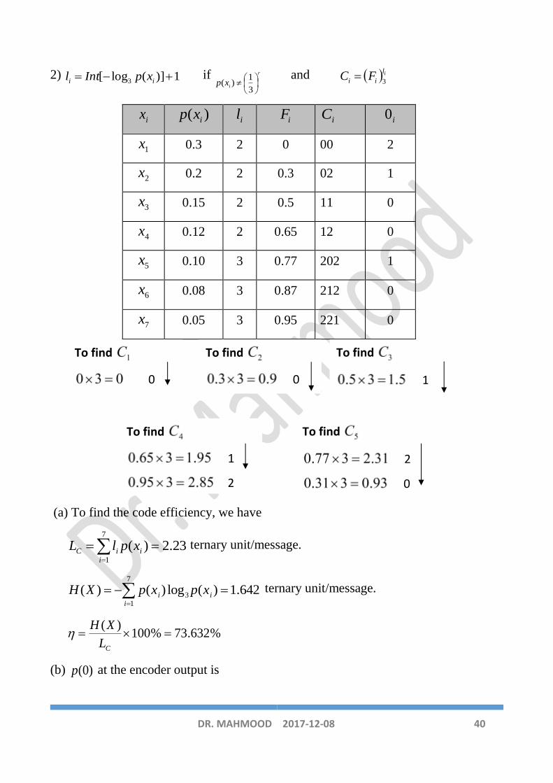
Repeat the previous example using ternary coding.

Solution

1) )(log3 ii xpl if r

ixp

3

1)( ,...

27

1,

9

1,

3

1

To find

1

0

1

0

To find

1

1

0

0

To find

0

0

To find

0

1

To find

1

0 0*2=0 0

0.2 * 2 = 0.4 0

DR. MAHMOOD 40 2017-12-08

2) 1)](log[ 3 ii xpIntl if r

ixp

3

1)(

and il

ii FC3

ix )( ixp il

iF iC

i0

1x 0.3 2 0 00 2

2x 0.2 2 0.3 02 1

3x 0.15 2 0.5 11 0

4x 0.12 2 0.65 12 0

5x 0.10 3 0.77 202 1

6x 0.08 3 0.87 212 0

7x 0.05 3 0.95 221 0

(a) To find the code efficiency, we have

23.2)(7

1

i

iiC xplL ternary unit/message.

642.1)(log)()(7

13

i

ii xpxpXH ternary unit/message.

%632.73%100)(

CL

XH

(b) )0(p at the encoder output is

To find

0

To find

0

To find

1

1

To find

1

2

To find

2

0

DR. MAHMOOD 41 2017-12-08

23.2

1.02.06.0)(0

)0(

7

1

C

iii

L

xp

p

404.0)0( p

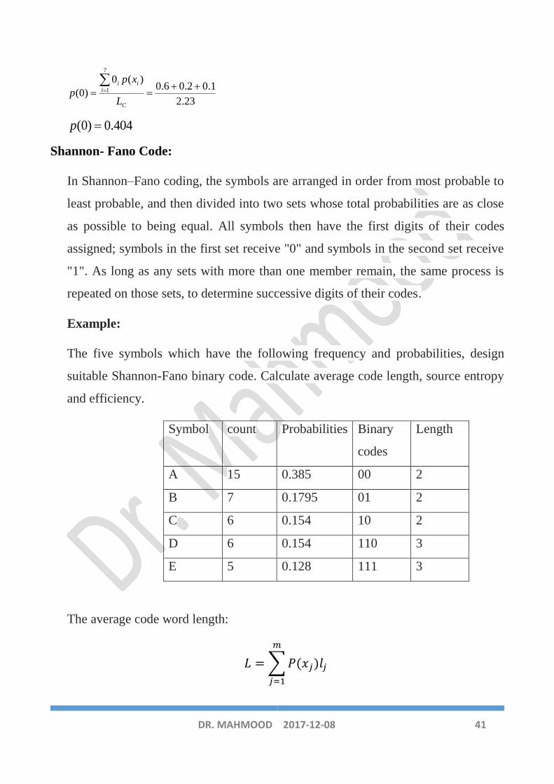
Shannon- Fano Code:

In Shannon–Fano coding, the symbols are arranged in order from most probable to

least probable, and then divided into two sets whose total probabilities are as close

as possible to being equal. All symbols then have the first digits of their codes

assigned; symbols in the first set receive "0" and symbols in the second set receive

"1". As long as any sets with more than one member remain, the same process is

repeated on those sets, to determine successive digits of their codes.

Example:

The five symbols which have the following frequency and probabilities, design

suitable Shannon-Fano binary code. Calculate average code length, source entropy

and efficiency.

Symbol count Probabilities Binary

codes

Length

A 15 0.385 00 2

B 7 0.1795 01 2

C 6 0.154 10 2

D 6 0.154 110 3

E 5 0.128 111 3

The average code word length:

𝐿 =∑𝑃(𝑥𝑗)𝑙𝑗

𝑚

𝑗=1

DR. MAHMOOD 42 2017-12-08

𝐿 = 2 × 0.385 + 2 × 0.1793 + 2 × 0.154 + 3 × 0.154 + 3 × 0.128

= 2.28𝑏𝑖𝑡𝑠/𝑠𝑦𝑚𝑏𝑜𝑙

The source entropy is:

𝐻(𝑌) = −∑𝑃(𝑦𝑗)

𝑚

𝑗=1

log2𝑃(𝑦𝑗)

𝐻(𝑌) = −[0.385𝑙𝑛0.385 + 0.1793𝑙𝑛0.1793 + 2 × 0.154𝑙𝑛0.154

+ 0.128𝑙0.128]/𝑙𝑛2

𝐻(𝑌) = 2.18567𝑏𝑖𝑡𝑠/𝑠𝑦𝑚𝑏𝑜𝑙

The code efficiency:

𝜂 =𝐻(𝑌)

L× 100 =

2.18567

2.28× 100 = 95.86%

Example

Develop the Shannon - Fano code for the following set of messages,

]08.01.012.015.02.035.0[)( xp then find the code efficiency.

Solution

ix )( ixp Code il

1x 0.35 0 0 2

2x 0.2 0 1 2

3x 0.15 1 0 0 3

4x 0.12 1 0 1 3

5x 0.10 1 1 0 3

6x 0.08 1 1 1 3

DR. MAHMOOD 43 2017-12-08

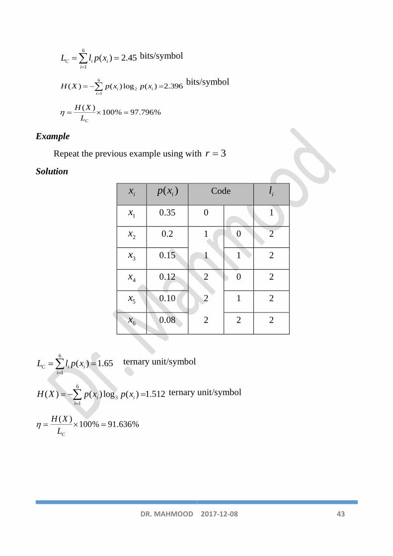
45.2)(6

1

i

iiC xplL bits/symbol

396.2)(log)()(6

12

i

ii xpxpXH bits/symbol

%796.97%100)(

CL

XH

Example

Repeat the previous example using with 3r

Solution

ix )( ixp Code il

1x 0.35 0 1

2x 0.2 1 0 2

3x 0.15 1 1 2

4x 0.12 2 0 2

5x 0.10 2 1 2

6x 0.08 2 2 2

65.1)(6

1

i

iiC xplL ternary unit/symbol

512.1)(log)()(6

13

i

ii xpxpXH ternary unit/symbol

%636.91%100)(

CL

XH

DR. MAHMOOD 44 2017-12-08

Huffman Code

The Huffman coding algorithm comprises two steps, reduction and splitting. These

steps can be summarized as follows:

1) Reduction

a) List the symbols in descending order of probability.

b) Reduce the r least probable symbols to one symbol with a probability

equal to their combined probability.

c) Reorder in descending order of probability at each stage.

d) Repeat the reduction step until only two symbols remain.

2) Splitting

a) Assign r,...1,0 to the r final symbols and work backwards.

b) Expand or lengthen the code to cope with each successive split.

Example: Design Huffman codes for 𝐴 = 𝑎1, 𝑎2, …… . 𝑎5,having the probabilities

0.2, 0.4, 0.2, 0.1, 0.1.

DR. MAHMOOD 45 2017-12-08

The average code word length:

𝐿 = 0.4 × 1 + 0.2 × 2 + 0.2 × 3 + 0.1 × 4 + 0.1 × 4 = 2.2𝑏𝑖𝑡𝑠/𝑠𝑦𝑚𝑏𝑜𝑙

The source entropy:

𝐻(𝑌) = −[0.4𝑙𝑛0.4 + 2 × 0.2𝑙𝑛0.2 + 2 × 0.1𝑙𝑛0.1]/𝑙𝑛2 = 2.12193 bits/symbol

The code efficiency:

𝜂 =2.12193

2.2× 100 = 96.45%

It can be design Huffman codes with minimum variance:

The average code word length is still 2.2 bits/symbol. But variances are different!

Example

Develop the Huffman code for the following set of symbols

Symbol A B C D E F G H

Probability 0.1 0.18 0.4 0.05 0.06 0.1 0.07 0.04

DR. MAHMOOD 46 2017-12-08

Solution

C 0.40 0.40 0.40 0.40 0.40 0.40 0.60 1.0

B 0.18 0.18 0.18 0.19 0.23 0.37 0.40

A 0.10 0.10 0.13 0.18 0.19 0.23

F 0.10 0.10 0.10 0.13 0.18

G 0.07 0.09 0.10 0.10

E 0.06 0.07 0.09

D 0.05 0.06

H 0.04

So we obtain the following codes

Symbol A B C D E F G H

Probability 0.1 0.18 0.4 0.05 0.06 0.1 0.07 0.04

Codeword 011 001 1 00010 0101 0000 0100 00011

il 3 3 1 5 4 4 4 5

552.2)(log)()(8

12

iii xpxpXH bits/symbol

61.2)(8

1

i

iiC xplL bits/symbol

0

1

0

0

0

0

0

0

1

1

1

1

1

1

DR. MAHMOOD 47 2017-12-08

%778.97%100)(

CL

XH

Data Compression:

In computer science and information theory, data compression, source coding, or bit-

rate reduction involves encoding information using fewer bits than the original

representation. Compression can be either lossy or lossless.

Lossless data compression algorithms usually exploit statistical redundancy to

represent data more concisely without losing information, so that the process is

reversible. Lossless compression is possible because most real-world data has statistical

redundancy. For example, an image may have areas of color that do not change over

several pixels.

Lossy data compression is the converse of lossless data compression. In these

schemes, some loss of information is acceptable. Dropping nonessential detail from the

data source can save storage space. There is a corresponding trade-off between

preserving information and reducing size.

Run-Length Encoding (RLE):

Run-Length Encoding is a very simple lossless data compression technique that

replaces runs of two or more of the same character with a number which represents the

length of the run, followed by the original character; single characters are coded as

runs of 1. RLE is useful for highly-redundant data, indexed images with many pixels

of the same color in a row.

Example:

Input: AAABBCCCCDEEEEEEAAAAAAAAAAAAAAAAAAAAAAAAAAAA

AAAAAAAAAA

Output: 3A2B4C1D6E38A

The input message to RLE encoder is a variable while the output code word is fixed,

unlike Huffman code where the input is fixed while the output is varied.

http://en.wikipedia.org/wiki/Lossy_compression

DR. MAHMOOD 48 2017-12-08

Example : Consider these repeated pixels values in an image … 0 0 0 0 0 0 0 0 0 0 0 0

5 5 5 5 0 0 0 0 0 0 0 0 We could represent them more efficiently as (12, 0)(4, 5)(8, 0)

24 bytes reduced to 6 which gives a compression ratio of 24/6 = 4:1.

Example :Original Sequence (1 Row): 111122233333311112222 can be encoded as:

(4,1),(3,2),(6,3),(4,1),(4,2). 21 bytes reduced to 10 gives a compression ratio of 21/10 =

21:10.

Example : Original Sequence (1 Row): – HHHHHHHUFFFFFFFFFFFFFF can be

encoded as: (7,H),(1,U),(14,F) . 22 bytes reduced to 6 gives a compression ratio of 22/6

= 11:3 .

Savings Ratio : the savings ratio is related to the compression ratio and is a measure of

the amount of redundancy between two representations (compressed and

uncompressed). Let:

N1 = the total number of bytes required to store an uncompressed (raw) source image.

N2 = the total number of bytes required to store the compressed data.

The compression ratio Cr is then defined as:

𝐶𝑟 =𝑁1𝑁2

Larger compression ratios indicate more effective compression

Smaller compression ratios indicate less effective compression

Compression ratios less than one indicate that the uncompressed representation

has high degree of irregularity.

The saving ratio Sr is then defined as :

𝑆𝑟 =(𝑁1 −𝑁2)

𝑁1

Higher saving ratio indicate more effective compression while negative ratios are

possible and indicate that the compressed image has larger memory size than the

original.

Example: a 5 Megabyte image is compressed into a 1 Megabyte image, the savings

ratio is defined as (5-1)/5 or 4/5 or 80%.

This ratio indicates that 80% of the uncompressed data has been eliminated in the

compressed encoding.

51

Chapter Four

Channel coding

1- Error detection and correction codes:

The idea of error detection and/or correction is to add extra bits to the digital

message that enable the receiver to detect or correct errors with limited

capabilities. These extra bits are called parity bits. If we have k bits, r parity bits

are added, then the transmitted digits are:

𝑛 = 𝑟 + 𝑘

Here n called code word denoted as (n, k). The efficiency or code rate is equal to

𝑘/𝑛.

Two basic approaches to error correction are available, which are:

a- Automatic-repeat-request (ARQ): Discard those frames in which errors are

detected.

- For frames in which no error was detected, the receiver returns a positive

acknowledgment to the sender.

- For the frame in which errors have been detected, the receiver returns

negative acknowledgement to the sender.

b- Forward error correction (FEC):

Ideally, FEC codes can be used to generate encoding symbols that are transmitted

in packets in such a way that each received packet is fully useful to a receiver to

reassemble the object regardless of previous packet reception patterns. The most

applications of FEC are:

Compact Disc (CD) applications, digital audio and video, Global System Mobile

(GSM) and Mobile communications.

52

2- Basic definitions:

- Systematic and nonsystematic codes: If (a’s) information bits are unchanged

in their values and positions at the transmitted code word, then this code is

said to be systematic (also called block code) where:

Input data 𝐷 = [𝑎1, 𝑎2, 𝑎3, …………𝑎𝑘], The output systematic code word (n,

k) is:

𝐶 = [𝑎1, 𝑎2, 𝑎3, …………𝑎𝑘 , 𝑐1, 𝑐2, 𝑐3, …………𝑐𝑟]

However if the data bits are spread or changed at the output code word then,

the code is said to be nonsystematic. The output of nonsystematic code word of

(n, k):

𝐶 = [𝑐2, 𝑎1, 𝑐1, 𝑎3, 𝑎2, 𝑐3, …………… ]

- Hamming Distance (HD): It is important parameter to measure the ability of

error detection. It the number of bits that differ between any two codewords

𝐶𝑖 and 𝐶𝑗 denoted by 𝑑𝑖𝑗. For a binary (n, k) code with 2𝑘 possible codewords,

then minimum HD (dmin) is min(𝑑𝑖𝑗), where:

𝑛 ≥ 𝑑𝑖𝑗 ≥ 0

For any code word, the possible error detection is:

2𝑡 = 𝑑𝑚𝑖𝑛 − 1

For example, if 𝑑𝑚𝑖𝑛 = 4, then it is possible to detect 3 errors or less. The

possible error correcting is:

𝑡 =𝑑𝑚𝑖𝑛 − 1

2

So that for 𝑑𝑚𝑖𝑛 = 4, it is possible to correct only one bit.

Example (2): Find the minimum HD between the following codwords. Also

determine the possible error detection and the number of error correction bits.

53

𝐶1 = [100110011], 𝐶2 = [111101100]𝑎𝑛𝑑𝐶3 = [101100101]

Solution: Here 𝑑12 = 6, 𝑑13 = 4𝑎𝑛𝑑𝑑23 = 3, hence 𝑑𝑚𝑖𝑛 = 3.

The possible error detection 2𝑡 = 𝑑𝑚𝑖𝑛 − 1 = 2.

The possible error correction 𝑡 =𝑑𝑚𝑖𝑛−1

2= 1.

- Hamming Weight: It is the number of 1’s in the non-zero codeword 𝐶𝑖 ,

denoted by 𝑤𝑖. For example the codewords of 𝐶1 = [1011100], 𝐶2 =

[1011001], 𝑤1 = 4, 𝑎𝑛𝑑𝑤2 = 3 respectively. If we have two valid

codewords- all ones and all zeros, in this case 𝐻𝐷 = 𝑤𝑖

3- Parity check codes (Error detection):

It is a linear block codes (systematic codes). In this code, an extra bit is added

for each k information and hence the code rate (efficiency) is 𝑘 (𝑘 + 1)⁄ . At the

receiver if the number of 1’s is odd then the error is detected. The minimum

Hamming distance for this category is dmin =2, which means that the simple

parity code is a single-bit error-detecting code; it cannot correct any error. There

are two categories in this type: even parity (ensures that a code word has an even

number of 1's) and odd parity (ensures that a code word has an odd number of

1's) in the code word.

Example: an even parity-check code of (5, 4) which mean that, k =4 and n =5.

Data word Code word Data word Code word

0010 00101 0110 01100

54

1010 10100 1000 10001

The above table can be repeated with odd parity-check code of (5, 4) as follow:

Data word Code word Data word Code word

0010 00100 0110 01101

1010 10101 1000 10000

Note:

Error detection was used in early ARQ (Automatic Repeat on Request) systems.

If the receiver detects an error, it asks the transmitter (through another backward

channel) to retransmit.

The sender is calculate the parity bit to be added to the data word to form a code

word. At the receiver, a syndrome is calculated. The syndrome is passed to the

decision logic analyzer. If the syndrome is 0, there is no error in the received

codeword; the data portion of the received codeword is accepted as the data

word; if the syndrome is 1, the data portion of the received codeword is

discarded. The data word is not created as shown in figure below.

55

4- Repetition codes:

The repetition code is one of the most basic error-correcting codes. The idea of

the repetition code is to just repeat the message several times. The encoder is a

simple device that repeats, r times.

For example, if we have a (3, 1) repetition code, then encoding the signal

m=101001 yields a code c=111000111000000111.

Suppose we received a (3, 1) repetition code and we are decoding the signal

c=110001111. The decoded message is m=101. For (r, 1) repetition code an error

correcting capacity of 𝑟/2 (i.e. it will correct up to 𝑟/2 errors in any code word).

In other word the 𝑑𝑚𝑖𝑛 = 𝑟, or increasing the correction capability depending on

r value. Although this code is very simple, it also inefficient and wasteful because

using only (2, 1) repetition code, that would mean we have to double the size of

the bandwidth which means doubling the cost.

http://en.wikipedia.org/wiki/Error-correcting_code

56

5- Linear Block Codes:

Linear block codes extend of parity check code by using a larger number of parity

bits to either detect more than one error or correct for one or more errors. A block

codes of an (n, k) binary block code can be selected a 2k codewords from 2n

possibilities to form the code, such that each k bit information block is uniquely

mapped to one of these 2k codewords. In linear codes the sum of any two

codewords is a codeword. The code is said to be linear if, and only if the sum of

𝑉𝑖(+)𝑉𝑗 is also a code vector, where 𝑉𝑖 &𝑉𝑗 are codeword vectors and (+)

represents modulo-2 addition.

5-1 Hamming Codes

Hamming codes are a family of linear error-correcting codes that generalize the

Hamming (n,k) -code, and were invented by Richard Hamming in 1950.

Hamming codes can detect up to two-bit errors or correct one-bit errors without

detection of uncorrected errors. Hamming codes are perfect codes, that is, they

achieve the highest possible rate for codes with their block length and minimum

distance of three.

In the codeword, there are k data bits and 𝑟 = 𝑛 − 𝑘 redundant (check) bits,

giving a total of n codeword bits. 𝑛 = 𝑘 + 𝑟

Hamming Code Algorithm:

General algorithm for hamming code is as follows:

1. r parity bits are added to an k - bit data word, forming a code word of n

bits .

2. The bit positions are numbered in sequence from 1 to n.

57

3. Those positions are numbered with powers of two, reserved for the parity

bits and the remaining bits are the data bits.

4. Parity bits are calculated by XOR operation of some combination of data

bits. Combination of data bits are shown below following the rule.

5. It Characterized by (𝑛, 𝑘) = (2𝑚 − 1, 2𝑚 − 1 −𝑚), 𝑤ℎ𝑒𝑟𝑒 𝑚 =

2, 3, 4…….

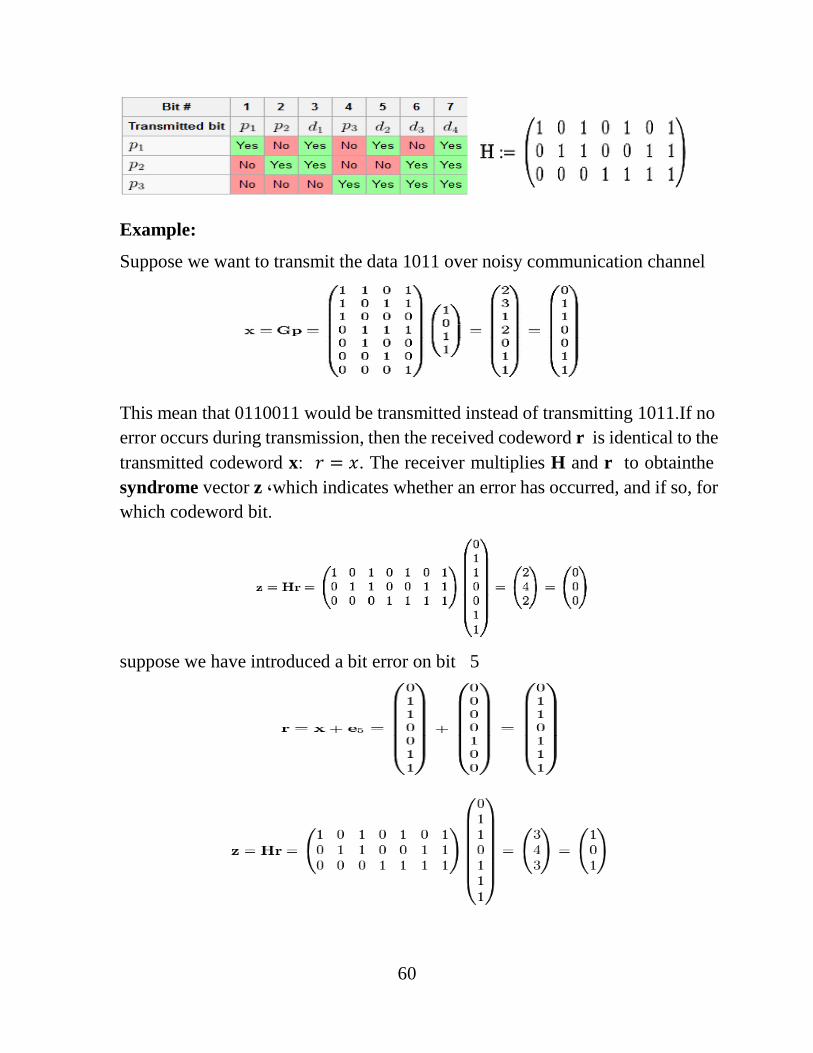
5-2 Exampl: Hamming(7,4)

This table describes which parity bits cover which transmitted bits in the

encoded word. For example, p2 provides an even parity for bits 2, 3, 6, and 7.

It also details which transmitted by which parity bit by reading the column. For

example, d1 is covered by p1 and p2 but not p3. This table will have a striking

resemblance to the parity-check matrix (H).

Or it can be calculate the parity bits from the following equations:

p1 = d1d2d4

p2 = d1d3d4

p3 = d2d3d4

The parity bits generating circuit is as following:

58

At the receiver, the first step in error correction, is to calculate the syndrome bits

which indicate there is an error or no. Also, the value of syndrome determine the

position detecting using syndrome bits = CBA. The equations for generating

syndrome that will be used in the detecting the position of the error are given by:

A = p1d1d2d4

B = p2d1d3d4

C = p3d2d3d4

Example:

Suppose we want to transmit the data 1011 over noisy communication channel.

Determine the Hamming code word.

Solution:

The first step is to calculate the parity bit value as follow and put it in the

corresponding position as follow:

𝑝1 = d1d2d4 = 101 = 0

p2 = d1d3d4 = 111 = 1

p3 = d2d3d4 = 011 = 0

Bit position 1 2 3 4 5 6 7

59

Bit name 𝑝1 𝑝2 𝑑1 𝑝3 𝑑2 𝑑3 𝑑4

Received value 0 1 1 0 0 1 1

The the codeword is c=0110011

Suppose the following noise is added to the code word, then the received code

becomes as:

The noise: 𝑛 = 0000100

The received code word: 𝑐𝑟 = 00001000110011 = 0110111

Now calculate the syndrome:

A = p1d1d2d4 = 0111 = 1

B = p2d1d3d4 = 1111 = 0

C = p3d2d3d4 = 0111 = 1

So that CBA = 101 which indicate that an error in the fifth bit.

Hamming matrices:

Hamming codes can be computed in linear algebra terms through matrices

because Hamming codes are linear codes. For the purposes of Hamming codes,

two Hamming matrices can be defined: the code generator matrix G and the

parity-check matrix H

60

Example:

Suppose we want to transmit the data 1011 over noisy communication channel

This mean that 0110011 would be transmitted instead of transmitting 1011.If no

error occurs during transmission, then the received codeword r is identical to the

transmitted codeword x: 𝑟 = 𝑥. The receiver multiplies H and r to obtainthe

syndrome vector z ,which indicates whether an error has occurred, and if so, for

which codeword bit.

suppose we have introduced a bit error on bit 5

ﺔﻌﻣﺎﺟﻟا ةوﻔﺻﻟا ﺔﯾﻟﮐ بوﺳﺎﺣﻟا تﺎﯾﻧﻘﺗ ﺔﺳدﻧھ...

Documents

Transcript of ﺔﻌﻣﺎﺟﻟا ةوﻔﺻﻟا ﺔﯾﻟﮐ بوﺳﺎﺣﻟا تﺎﯾﻧﻘﺗ ﺔﺳدﻧھ...