Material Properties SMA
39
Modeling and Control of an Integrated Sensing Shape Memory Alloy Actuator J.J.M. Lunenburg, BSc DCT 2009.037 Traineeship report Coa ch(es) : prof. M. T omizuk a, E. Chang -Siu , MSc. Supervisor: prof. dr . ir. M. Stein buch T echnische Universiteit Eindhoven Department Mechanical Engineering Dynamics and Control T echnology Group Eindhoven, April, 2009
-
Upload
letterashish4444 -
Category
Documents
-
view
240 -
download
0
Transcript of Material Properties SMA

7/27/2019 Material Properties SMA
http://slidepdf.com/reader/full/material-properties-sma 1/39
Modeling and Control of an
Integrated Sensing Shape
Memory Alloy Actuator J.J.M. Lunenburg, BSc
DCT 2009.037
Traineeship report
Coach(es): prof. M. Tomizuka, E. Chang-Siu, MSc.
Supervisor: prof. dr. ir. M. Steinbuch
Technische Universiteit EindhovenDepartment Mechanical EngineeringDynamics and Control Technology Group
Eindhoven, April, 2009

7/27/2019 Material Properties SMA
http://slidepdf.com/reader/full/material-properties-sma 2/39
Foreword
This report is the result of three months of research at the Mechanical Systems Control Laboratory of the University of California at Berkeley. This wonderful period has been a great experience on both apersonal and a professional level. I would like to use this opportunity to thank the people who have inany way contributed to this work.
I would like to thank professor Tomizuka for giving me the opportunity to work in such a mo-tivating research lab and for his feedback on the various research issues. Many thanks also to EvanChang-Siu who I have been working with on a daily basis. Your enormous commitment, valuableinput and solid advice has been of great importance in the course of this project.
Furthermore I would like to thank Brendan Till for both his theoretical and practical input, andSumio Sugita for his assistance and advice every time difficulties were encountered. Also many thanksfor dr. Gummin of the Miga Motor company, who was kind enough to provide SMA wires, actuatorsand sensors.
Finally I would like to thank the technical staff, who have given their support in electronics and thedevelopment of the test setup, and all other students of the MSC Lab: it was a pleasure working withyou.
2
7/27/2019 Material Properties SMA
http://slidepdf.com/reader/full/material-properties-sma 3/39
Contents
1 Introduction 5
2 Modular actuators and Shape Memory Alloys 62.1 Modular actuators . . . . . . . . . . . . . . . . . . . . . . . . . . . . . . . . . . . . . . 62.2 Shape Memory Alloys . . . . . . . . . . . . . . . . . . . . . . . . . . . . . . . . . . . . 7
3 The experimental setup 93.1 MigaOne Shape Memory Alloy Actuator . . . . . . . . . . . . . . . . . . . . . . . . . . 93.2 Friction and Abbe’s Principle . . . . . . . . . . . . . . . . . . . . . . . . . . . . . . . . 103.3 Real-time controller . . . . . . . . . . . . . . . . . . . . . . . . . . . . . . . . . . . . . 113.4 Software . . . . . . . . . . . . . . . . . . . . . . . . . . . . . . . . . . . . . . . . . . . . 11
4 Integrated sensing characteristics of the SMA actuator 134.1 Practical issues . . . . . . . . . . . . . . . . . . . . . . . . . . . . . . . . . . . . . . . . 134.2 Experimental results . . . . . . . . . . . . . . . . . . . . . . . . . . . . . . . . . . . . . 14
5 Development of a nonlinear model of the SMA actuator 165.1 Kinematic-dynamic model . . . . . . . . . . . . . . . . . . . . . . . . . . . . . . . . . . 165.2 Wire constitutive model . . . . . . . . . . . . . . . . . . . . . . . . . . . . . . . . . . . 165.3 SMA wire phase transformation model . . . . . . . . . . . . . . . . . . . . . . . . . . . 175.4 Heat transfer model . . . . . . . . . . . . . . . . . . . . . . . . . . . . . . . . . . . . . 175.5 Improvement of numerical performance . . . . . . . . . . . . . . . . . . . . . . . . . . 175.6 Model parameters . . . . . . . . . . . . . . . . . . . . . . . . . . . . . . . . . . . . . . 185.7 Model validation . . . . . . . . . . . . . . . . . . . . . . . . . . . . . . . . . . . . . . . 185.8 Recommendations for improvement of the model . . . . . . . . . . . . . . . . . . . . . 19
6 Controller design 216.1 PID Control . . . . . . . . . . . . . . . . . . . . . . . . . . . . . . . . . . . . . . . . . . 216.2 Simple Switch . . . . . . . . . . . . . . . . . . . . . . . . . . . . . . . . . . . . . . . . 22
6.3 Adding a Boundary Layer . . . . . . . . . . . . . . . . . . . . . . . . . . . . . . . . . . 236.4 Reducing Overshoot . . . . . . . . . . . . . . . . . . . . . . . . . . . . . . . . . . . . . 236.5 Elimination of the Steady State Error . . . . . . . . . . . . . . . . . . . . . . . . . . . . 236.6 Feedforward . . . . . . . . . . . . . . . . . . . . . . . . . . . . . . . . . . . . . . . . . 24
7 Robustness 267.1 Forced convection . . . . . . . . . . . . . . . . . . . . . . . . . . . . . . . . . . . . . . 267.2 Supply voltage . . . . . . . . . . . . . . . . . . . . . . . . . . . . . . . . . . . . . . . . 267.3 Wire diameter . . . . . . . . . . . . . . . . . . . . . . . . . . . . . . . . . . . . . . . . 277.4 General remarks . . . . . . . . . . . . . . . . . . . . . . . . . . . . . . . . . . . . . . . 28
8 Efficiency 31
3

7/27/2019 Material Properties SMA
http://slidepdf.com/reader/full/material-properties-sma 4/39
9 Modularity and further issues 339.1 Multiplexing . . . . . . . . . . . . . . . . . . . . . . . . . . . . . . . . . . . . . . . . . 339.2 Experimental results . . . . . . . . . . . . . . . . . . . . . . . . . . . . . . . . . . . . . 33
9.3 Actuator Matrix Driver . . . . . . . . . . . . . . . . . . . . . . . . . . . . . . . . . . . . 359.4 Further issues . . . . . . . . . . . . . . . . . . . . . . . . . . . . . . . . . . . . . . . . 36
10 Conclusion 37
4

7/27/2019 Material Properties SMA
http://slidepdf.com/reader/full/material-properties-sma 5/39
Chapter 1
Introduction
The human body can be regarded as a highly sophisticated mechanical system with many degrees of freedom. The actuators of this system, skeletal muscle, are unsurpassed by other actuation methods inmany areas such as flexibility, compactness and integrated sensing. Utilizing these properties could beuseful for a wide variety of purposes but is particularly beneficial when synthetic actuators collaboratewith human muscles such as in rehabilitation. Muscles achieve these beneficial properties becausethey consist of many flexible fibers, and one possible way to mimic this behavior is by using wires of aShape Memory Alloy (SMA). A SMA has the ability to go through a deformation while rememberingits initial shape, to which it will return upon heating.
In this report the preliminary research on SMA’s in the Mechanical System Control laboratory atthe University of California at Berkeley is discussed. The ultimate goal is the development of a bio-inspired modular SMA actuator that can be used within a highly versatile platform for rehabilitationdevices. First SMA and other modular actuators are compared with the properties of human muscleand specific properties of SMA materials are reviewed. In order to be able to emphasize research
purely on SMA behavior a custom actuator has been built to discard phenomena such as frictionpresent in the available standard actuators. Next to hardware also the used software will be discussed.Thereafter the supposed integrated sensing capabilities of the material will be investigated followed bythe development of a mathematic model of a SMA actuator. Various controllers have been tuned andthese have been tested on several robustness issues. The final chapters will discuss the measurementson efficiency that have been conducted as well as further issues and research possibilities.
5

7/27/2019 Material Properties SMA
http://slidepdf.com/reader/full/material-properties-sma 6/39
Chapter 2
Modular actuators and Shape
Memory Alloys
2.1 Modular actuators
Compared to known artificial actuation technologies, skeletal muscles have distinct advantages be-cause of their high power-to weight ratio, integrated sensing and high flexibility and durability. Mus-cles have a modular design of energy dense compliant fibers that allows muscle size, shape, mechani-cal properties and energetics to be varied by varying the number and combinations of their componentmodules according to need [12]. The fundamental mechanical unit of a muscle is the sarcomere, a tinycylindrical array of motor proteins and their racks.
Figure 2.1: Structure of a skeletalmuscle
Sarcomeres in series make a myofibril, and many myofib-rils in parallel make a muscle fiber [7]. Muscle fibers are long,flexible cylinders, ranging from about 10 to 100 microns in di-ameter and from millimeters to many centimeters in length.These fibers can in turn be used in different architectures, e.g.short fibers in parallel for strength and force, and long fibersfor speed and range.
Mimicking this modularity would provide significant im-provements over conventional actuator design. The current re-search investigates recreating this modularity with smart mate-rial component actuators and seeks a transformative, flexible,self sensing and reconfigurable synthetic muscle package. Thetarget application of this new package is rehabilitation therapyand restoration of movement, although the technology could
be used in a wider variety of areas.The platform as described would ideally meet or exceed hu-
man muscle characteristics, such as maximum stress, maxi-mum velocity, maximum power per unit mass and the rangeof active force production. In Table 2.1 several component levelactuators have been compared in order to come to a properchoice of technology. The compared methods are pneumaticcomponents, electroactive polymer (EAP) components and shapememory alloy (SMA) components.
Pneumatic actuators function as a contractile element toproduce force. The most popular pneumatic actuator is the de-sign McKibben first developed in the 1950’s. It is an elastomersurrounded by a flexible but inextensible mesh that can be in-flated by a pressure source to induce contraction. Although a pneumatic actuator has a high power-
6
7/27/2019 Material Properties SMA
http://slidepdf.com/reader/full/material-properties-sma 7/39
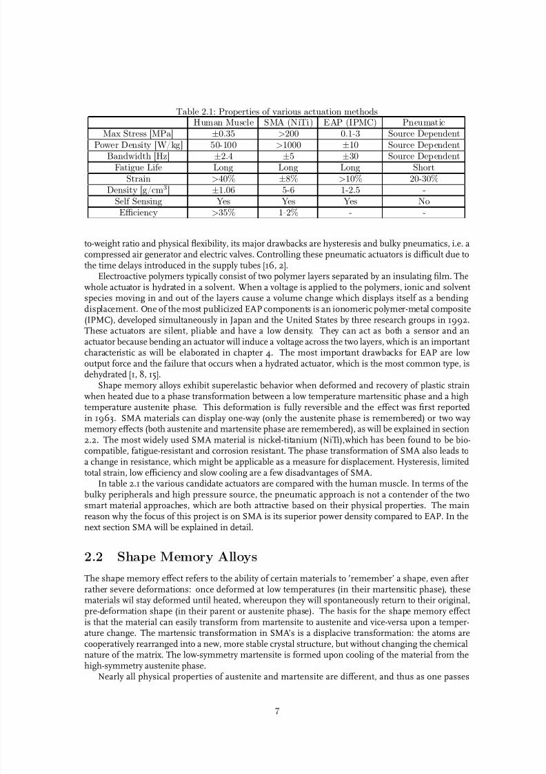
Table 2.1: Properties of various actuation methodsHuman Muscle SMA (NiTi) EAP (IPMC) Pneumatic
Max Stress [MPa] ±0.35 >200 0.1-3 Source DependentPower Density [W/kg] 50-100 >1000 ±10 Source Dependent
Bandwidth [Hz] ±2.4 ±5 ±30 Source DependentFatigue Life Long Long Long Short
Strain >40% ±8% >10% 20-30%Density [g/cm3] ±1.06 5-6 1-2.5 -
Self Sensing Yes Yes Yes NoEfficiency >35% 1-2% - -
to-weight ratio and physical flexibility, its major drawbacks are hysteresis and bulky pneumatics, i.e. acompressed air generator and electric valves. Controlling these pneumatic actuators is difficult due tothe time delays introduced in the supply tubes [16, 2].
Electroactive polymers typically consist of two polymer layers separated by an insulating film. Thewhole actuator is hydrated in a solvent. When a voltage is applied to the polymers, ionic and solventspecies moving in and out of the layers cause a volume change which displays itself as a bendingdisplacement. One of the most publicized EAP components is an ionomeric polymer-metal composite(IPMC), developed simultaneously in Japan and the United States by three research groups in 1992.These actuators are silent, pliable and have a low density. They can act as both a sensor and anactuator because bending an actuator will induce a voltage across the two layers, which is an importantcharacteristic as will be elaborated in chapter 4. The most important drawbacks for EAP are lowoutput force and the failure that occurs when a hydrated actuator, which is the most common type, isdehydrated [1, 8, 15].
Shape memory alloys exhibit superelastic behavior when deformed and recovery of plastic strainwhen heated due to a phase transformation between a low temperature martensitic phase and a high
temperature austenite phase. This deformation is fully reversible and the effect was first reportedin 1963. SMA materials can display one-way (only the austenite phase is remembered) or two waymemory effects (both austenite and martensite phase are remembered), as will be explained in section2.2. The most widely used SMA material is nickel-titanium (NiTi),which has been found to be bio-compatible, fatigue-resistant and corrosion resistant. The phase transformation of SMA also leads toa change in resistance, which might be applicable as a measure for displacement. Hysteresis, limitedtotal strain, low efficiency and slow cooling are a few disadvantages of SMA.
In table 2.1 the various candidate actuators are compared with the human muscle. In terms of thebulky peripherals and high pressure source, the pneumatic approach is not a contender of the twosmart material approaches, which are both attractive based on their physical properties. The mainreason why the focus of this project is on SMA is its superior power density compared to EAP. In thenext section SMA will be explained in detail.
2.2 Shape Memory Alloys
The shape memory effect refers to the ability of certain materials to ’remember’ a shape, even afterrather severe deformations: once deformed at low temperatures (in their martensitic phase), thesematerials wil stay deformed until heated, whereupon they will spontaneously return to their original,pre-deformation shape (in their parent or austenite phase). The basis for the shape memory effectis that the material can easily transform from martensite to austenite and vice-versa upon a temper-ature change. The martensic transformation in SMA’s is a displacive transformation: the atoms arecooperatively rearranged into a new, more stable crystal structure, but without changing the chemicalnature of the matrix. The low-symmetry martensite is formed upon cooling of the material from thehigh-symmetry austenite phase.
Nearly all physical properties of austenite and martensite are different, and thus as one passes
7

7/27/2019 Material Properties SMA
http://slidepdf.com/reader/full/material-properties-sma 8/39
Figure 2.2: Three dimensional stress-strain-temperature diagram for one-way shape memorymaterials [3]
Figure 2.3: Hypothetical plot of propertychange vs. temperature for a martensitictransformation occuring in a SMA
through the transformation point, a variety of significant property changes occur. One property thatchanges in a most significant way is the yield strength. Unlike austenite, the martensitic structurecan deform by moving twin boundaries, i.e. boundaries between martensite plates. A key property of twin boundaries is that they are quite mobile because all of the bonds remain intact in the twinnedstructure. This leads to a low yield strength and completely reversible twinning process.
The one-way shape memory effect (OWSM) can be described with reference to the cooling and heat-ing curves in figure 2.2. Starting at a temperature below the martensite finish temperature (M f ) thespecimen is in the martensitic phase. When it is deformed when the temperature is still below M f itremains deformed until it is heated. The shape recovery begins at the austenite start temperature As
and is completed at the austenite finish temperature Af . Once the shape has recovered at Af thereis no change in shape when the specimen is cooled to below M f again, and the SMA can only be re-
activated by deforming the martensitic specimen once again. Because the specimen does not changeshape upon cooling the effect is referred to as one-way shape memory effect. In contrast to OWSMthe two-way shape memory effect (TWSM) will cause the specimen to change back to its low temperatureshape upon cooling from above Af to below M f (figure 2.3). This changing of shape upon heatingand cooling can be repeated indefinitely. In order to produce this two-way behavior, special thermo-chemical treatment is required, which is called training treatment. In this project only two-way SMA’sare utilized.
8

7/27/2019 Material Properties SMA
http://slidepdf.com/reader/full/material-properties-sma 9/39
Chapter 3
The experimental setup
The first step in the design of the platform is identifying the characteristics of SMA actuators. Fur-thermore a model must be developed as well as a suitable control algorithm. The experimental setupthat is used for identifying these characteristics is discussed in this chapter, starting with the actuatoritself.
3.1 MigaOne Shape Memory Alloy Actuator
Figure 3.1: The MigaOne SMA ac-tuator
The actuator initially used in this research is the MigaOne, thestandard actuator from the Miga Motor Company. This containsfive two-way Flexinol SMA wires which form a series-resistiveelectrical circuit. If a current is induced through these wires theresulting increase in temperature will cause the wires to contract.The contraction starts at around 75C and is fully completed at110C. During contraction a force up to 22 N can be obtained.In order to fully return to its initial position the actuator shouldcool below 60C. Since the MigaOne provides force only in onedirection, a bias spring is attached to the actuator to prevent thewires from ’bulging’ outward during cooling. The specificationsof the actuator are given in Table 3.1. While a contraction timewithin 50 ms is feasible if sufficient current is provided, (passive)cooling and thus returning to its original position takes muchlonger. This process could however be accelerated by applyingactive cooling e.g. thermoelectrically (by a Peltier element), by a fan or by a fluid.
An analog driver is used to power the actuator using a MOSFET switch (metal-oxide-semiconductor
field-effect transistor). When the actuator reaches its end-of-travel, the driver immediately cuts power,
Table 3.1: Specifications of the MigaOne actuatorStroke 9.5 mmOutput force Constant 11 N, peak 22 NActuation time 50 ms to position holdMax actuation speed 200 mm/sWeight 12.8 gDimensions 71×33×2.5 mmWire diameter 0.3 mmWire length 273 mm in 5 segments
Nominal resistance 3.8 Ω
9

7/27/2019 Material Properties SMA
http://slidepdf.com/reader/full/material-properties-sma 10/39
preventing the device from overheating.An Alps resistive sensor is used to measure the displacement of the actuator. To reduce measure-
ment noise caused by the switching of the MOSFET, the signal is low pass filtered before it is fed
into the analog input (AI). In order to measure the current running through the actuator a 6 A closedloop current transducer is installed. The supply voltage of the actuator is too high to measure directly.Therefore two resistors of 10 kΩ in series (the resistance of the actuator is approximately 4 Ω) areplaced parallel to actuator. The voltage measured in between these two resistors is exactly half of thevoltage across the actuator.
3.2 Friction and Abbe’s Principle
During preliminary measurements the system did not perform as expected: an offset seemed to oc-cur in the measurements for the self-sensing characteristics (chapter 4), and tuning a PID controller(chapter 6.1) also posed problems because a step in position was measured when switching direction.This was not due to the feedback controller as was concluded after investigating the controller output.After reviewing the mechanical systems it was concluded that the position sensor was not placed cor-rectly: because it was not placed in the line of movement according to Abbe’s principle (figure 3.2),a rotation of the actuator caused a significant measurement error. Because of the wear of the pinssupporting the intermediate sections this effect would increase with time.
Figure 3.2: Abbe’s Principle Figure 3.3: The newly designed SMAactuator
Furthermore the intermediate sections, or ’bones’, are produced by etching because of low pro-duction volumes. This produces much sharper edges than other production methods like punching,which on their turn cause a significant amount of severely nonlinear friction. Although this frictioncould be modeled, it is beyond the scope of this research: when new modular actuators are designedthe friction of the MigaOne is not relevant anymore. In order to overcome these issues a new design is
made to characterize the SMA wire. This new actuator contains the same SMA wire, MOSFET switchand position sensor as the MigaOne, all set up in one line.
During the course of this research further modifications to this actuator have been made eventuallyleading to the actuator as shown in figure 3.3. A tuner has been added to assure the same amount of initial force is applied when changing wires. Also a force transducer has been added to allow theexperiments regarding efficiency as discussed in chapter 8.
10

7/27/2019 Material Properties SMA
http://slidepdf.com/reader/full/material-properties-sma 11/39
3.3 Real-time controller
Two different real-time controllers and Field Programmable Gate Arrays (FPGA) have been used.
The initial controller was a NI cRIO-9004 embedded real-time controller. This is coupled to a NI9401 8-channel, 100 ns bidirectional digital input module. This module can provide the Pulse WidthModulation (PWM) signal to control the MOSFET and thus the actuator. The displacement, currentand force sensor and voltage across the SMA actuator are coupled to a NI 9215 4-channel analog inputmodule. The FPGA of the cRIO runs at a frequency of 40 MHz. This is sufficient to provide the PWMsignal and to measure at the exact right moments. The real-time controller is via ethernet connectedto a host computer, which acts as the graphical user interface.
However, after a number of measurements and different configurations of FPGA, real-time con-troller and host computer, this hardware does not live up to the needs of the experiment. In thereal-time program a loop frequency of 1 kHz is desired; in reality this number is far from reachedand gaps up to 0.3 seconds appear in the measurement data, making it far too inaccurate for controlpurposes. The cRIO is usually used as a low-level real-time controller where most calculations are
executed on the FPGA. The real-time loop thus runs at a relatively low frequency discarding the needfor a fast CPU. In our case however it is also used for graphical purposes and more calculations sincethis is easier and faster to implement in the real-time program than on the FPGA, which only usesintegers and needs to recompile after every change.
Therefore it is decided to switch to a FPGA PCI 7833R. This is built in a regular desktop pc dedi-cated to this purpose, which has a much faster processor than the cRIO. This real-time controller doesreach the desired loop frequency of 1 kHz. Sensors and actuators are connected directly to the FPGAvia a breakout box.
3.4 Software
Figure 3.4: Softwarearchitecture
The software used for control is NI LabVIEW. A ’project’ with three
programs has been developed to control the actuator and acquire thedesired measurements. The program at the lowest level runs at theFPGA. It acquires the data from the breakout box as well as construct-ingand sending a PWM signal. The voltage at an analog input channelis acquired as an integer value between 0 and 216 = 65536 and sentdirectly to the realtime program. Not all sensors are sampled at thesame moment: the position sensor picks up severe noise in the begin-ning of the duty cycle so this one is sampled near the end of a PWMperiod. Voltage and current on the other hand can only be measuredduring ’on-time’ and should thus be sampled as quickly as possible toreduce the required minimum duty cycle as much as possible, takinginto account the settling time (see section 4.1).
Furthermore two PWM signals are constructed: the first one sim-ply divides the FPGA frequency by the PWM frequency to get a num-ber of ’total ticks’ that one PWM period takes. The product of thisnumber with the desired duty cycle is the number of ’ticks’ that thePWM signal should be on and for the remainder of the period it shouldbe off. The second PWM signal does the same for multiple actuators(chapter 9), i.e. it divides the total number of ticks by the numberof connected actuators. The latest feature of the FPGA program is atimed stacked sequence of Interrupt Requests which provide a hand-shake with the realtime program to ensure that the desired loop fre-quency of that program is met. The FPGA has enough room to ac-commodate the control loop entirely but this would require recompiling after every structural change.This would slow down the process of doing experiments significantly and therefore the control loop isprogrammed in the real-time program.
11

7/27/2019 Material Properties SMA
http://slidepdf.com/reader/full/material-properties-sma 12/39
The real-time controller runs the primary control loop at a loop frequency of 1 kHz. The data re-ceived from the FPGA is first converted to the voltage. Since the FPGA has a range of -10 V to 10 Vthe conversion factor is: 20/216. Since the voltage range is not exact a fine tuning is required. Subse-
quently the voltage is converted to position, current or force depending on their respective calibrationdata. The control loop is a standard SISO control loop with feedforward. It is possible to switch be-tween controllers during operation. Initially the real-time program was also used to display resultsand to save data. In order to address the fact that the loop frequency at the cRIO did not reach 1 kHzthese two tasks are transferred to a host program.
The communication between the host and the real-time program leads through a data library. Thesize of the variables in this library and the buffer size can be chosen according to need. In order tosave data an empty array is initiated with a predetermined size since increasing the array when newdata is received will slow the program down. If the record mode is enabled a loop with a shift registerchecks if new data is received and will put this on the allocated position in the array. As soon as theprogram is stopped the array will be saved regardless of the extent to which it is filled.
12
7/27/2019 Material Properties SMA
http://slidepdf.com/reader/full/material-properties-sma 13/39
Chapter 4
Integrated sensing characteristics of
the SMA actuator
One of the interesting features of SMA actuators is their high power to volume ratio. This couldbe maintained if the need for an additional displacement sensor is discarded and the actuator coulddetermine its own displacement. During the change of crystallographic structure and shape of theSMA wire, the electrical resistance changes too. According to [11], the change in electrical resistanceof the SMA wire could be used to measure the displacement. Especially at high SMA temperaturesthe correlation between displacement and resistance becomes almost linear.
4.1 Practical issues
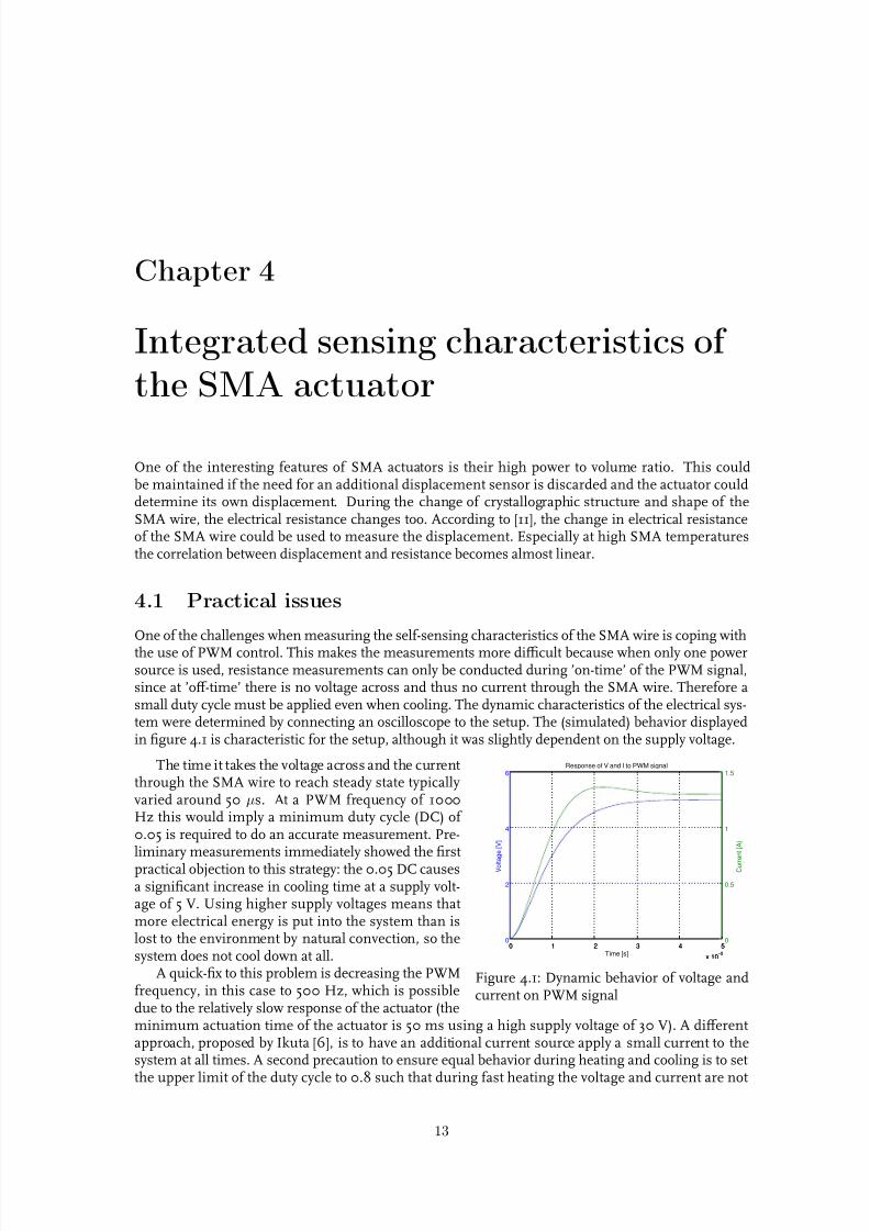
One of the challenges when measuring the self-sensing characteristics of the SMA wire is coping withthe use of PWM control. This makes the measurements more difficult because when only one powersource is used, resistance measurements can only be conducted during ’on-time’ of the PWM signal,since at ’off-time’ there is no voltage across and thus no current through the SMA wire. Therefore asmall duty cycle must be applied even when cooling. The dynamic characteristics of the electrical sys-tem were determined by connecting an oscilloscope to the setup. The (simulated) behavior displayedin figure 4.1 is characteristic for the setup, although it was slightly dependent on the supply voltage.
0 1 2 3 4 5
x 10−5
0
2
4
6
Time [s]
Response of V and I to PWM signal
V o l t a g e [ V ]
0 1 2 3 4 5
x 10−5
0
0.5
1
1.5
C u r r e n t [ A
Figure 4.1: Dynamic behavior of voltage andcurrent on PWM signal
The time it takes the voltage across and the currentthrough the SMA wire to reach steady state typicallyvaried around 50 µs. At a PWM frequency of 1000Hz this would imply a minimum duty cycle (DC) of 0.05 is required to do an accurate measurement. Pre-liminary measurements immediately showed the firstpractical objection to this strategy: the 0.05 DC causesa significant increase in cooling time at a supply volt-age of 5 V. Using higher supply voltages means thatmore electrical energy is put into the system than islost to the environment by natural convection, so thesystem does not cool down at all.
A quick-fix to this problem is decreasing the PWMfrequency, in this case to 500 Hz, which is possibledue to the relatively slow response of the actuator (theminimum actuation time of the actuator is 50 ms using a high supply voltage of 30 V). A differentapproach, proposed by Ikuta [6], is to have an additional current source apply a small current to thesystem at all times. A second precaution to ensure equal behavior during heating and cooling is to set
the upper limit of the duty cycle to 0.8 such that during fast heating the voltage and current are not
13
7/27/2019 Material Properties SMA
http://slidepdf.com/reader/full/material-properties-sma 14/39
constant and therefore do display dynamics. If the duty cycle is maintained at 1, the electronics willremain in steady state and will therefore lead to different results.
4.2 Experimental results
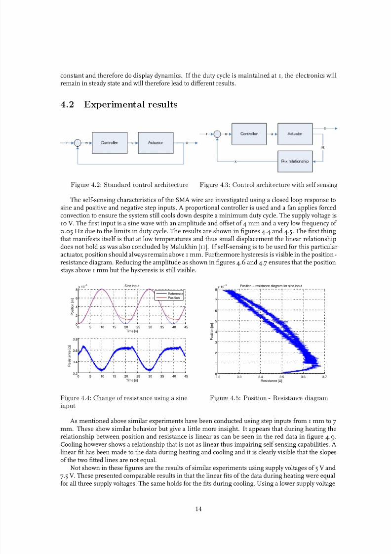
Figure 4.2: Standard control architecture Figure 4.3: Control architecture with self sensing
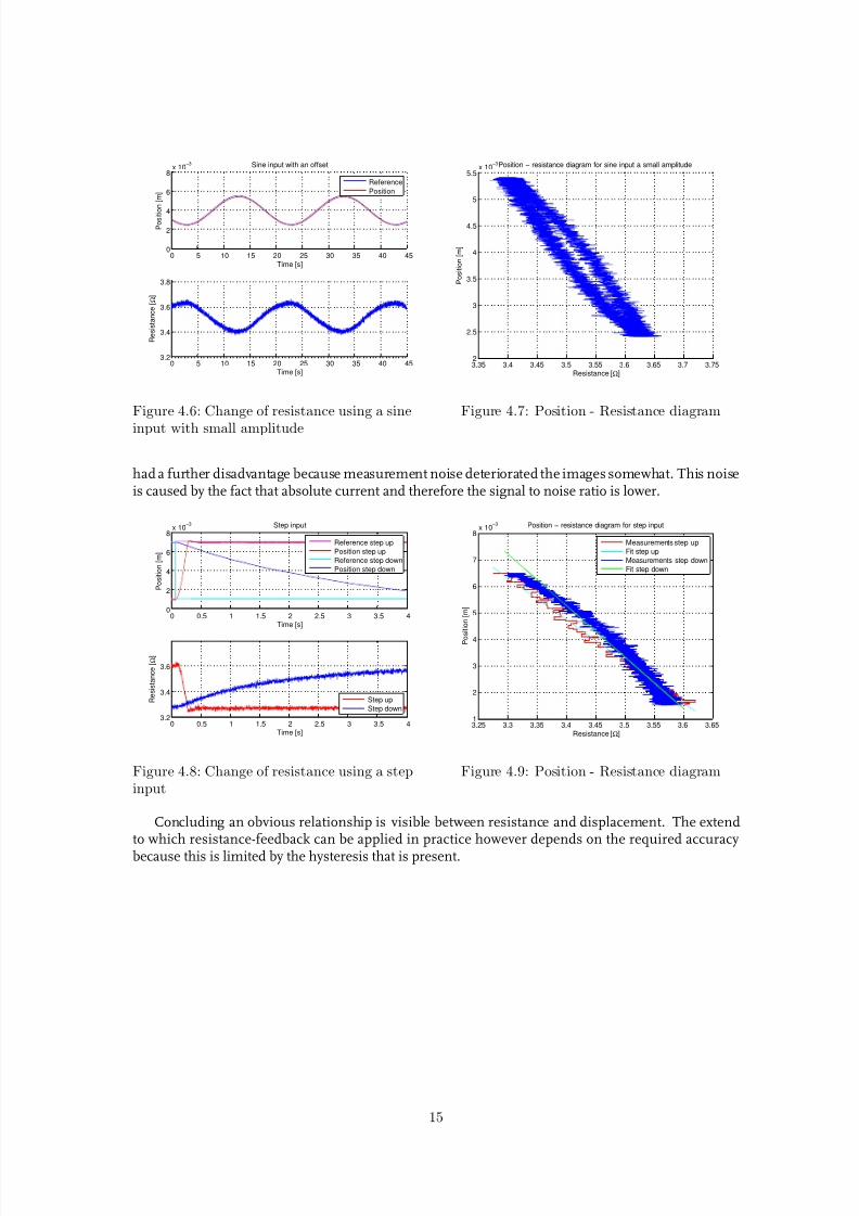
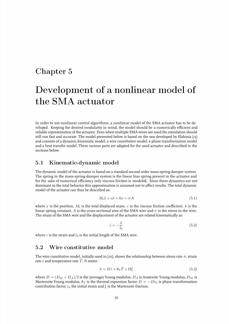
The self-sensing characteristics of the SMA wire are investigated using a closed loop response tosine and positive and negative step inputs. A proportional controller is used and a fan applies forcedconvection to ensure the system still cools down despite a minimum duty cycle. The supply voltage is10 V. The first input is a sine wave with an amplitude and offset of 4 mm and a very low frequency of 0.05 Hz due to the limits in duty cycle. The results are shown in figures 4.4 and 4.5. The first thingthat manifests itself is that at low temperatures and thus small displacement the linear relationshipdoes not hold as was also concluded by Malukhin [11]. If self-sensing is to be used for this particularactuator, position should always remain above 1 mm. Furthermore hysteresis is visible in the position -resistance diagram. Reducing the amplitude as shown in figures 4.6 and 4.7 ensures that the positionstays above 1 mm but the hysteresis is still visible.
0 5 10 15 20 25 30 35 40 450
2
4
6
8
x 10−3
Time [s]
P o s i t i o n [ m ]
Sine input
Reference
Position
0 5 10 15 20 25 30 35 40 453.2
3.4
3.6
3.8
Time [s]
R e s i s t a n c e [ Ω ]
Figure 4.4: Change of resistance using a sineinput
3.2 3.3 3.4 3.5 3.6 3.70
1
2
3
4
5
6
7
8
x 10−3
P o s i t i o n [ m ]
Resistance [Ω]
Position − resistance diagram for sine input
Figure 4.5: Position - Resistance diagram
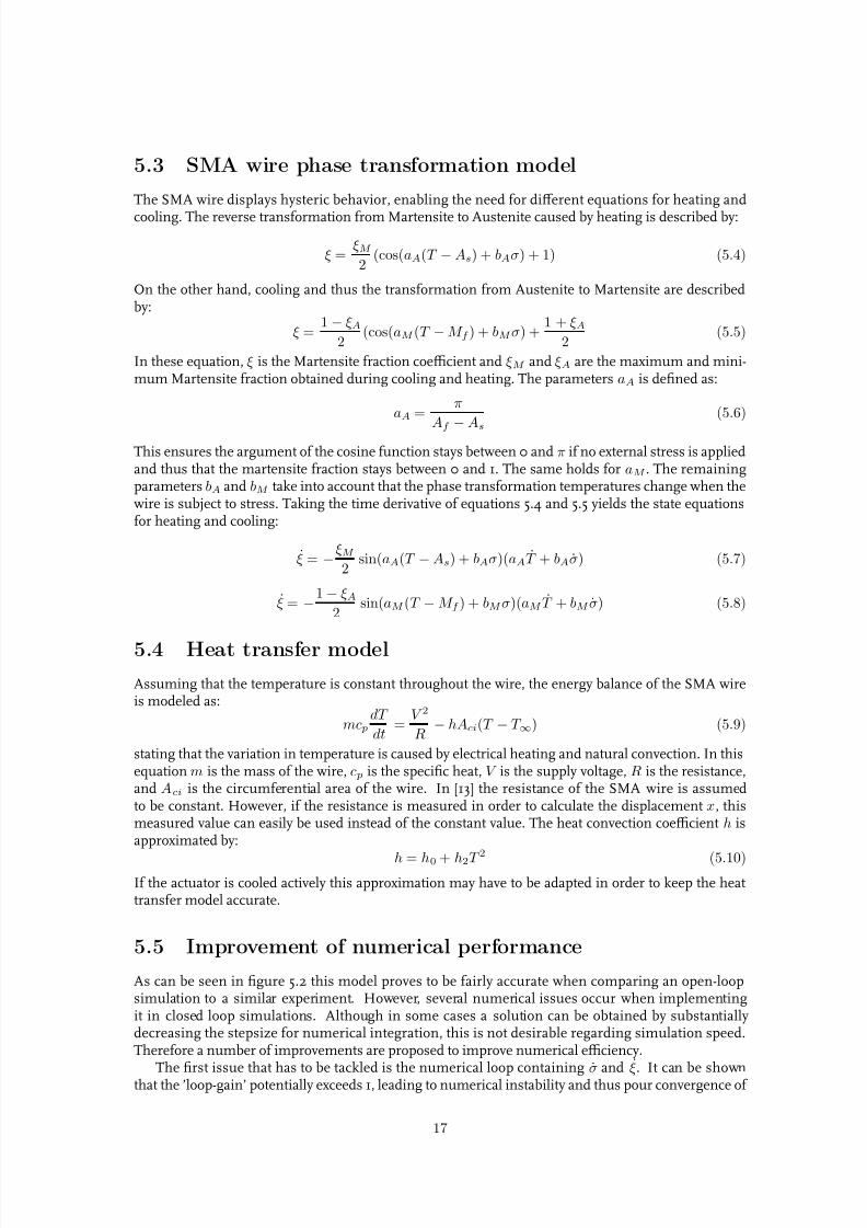
As mentioned above similar experiments have been conducted using step inputs from 1 mm to 7mm. These show similar behavior but give a little more insight. It appears that during heating therelationship between position and resistance is linear as can be seen in the red data in figure 4.9.Cooling however shows a relationship that is not as linear thus impairing self-sensing capabilities. Alinear fit has been made to the data during heating and cooling and it is clearly visible that the slopesof the two fitted lines are not equal.
Not shown in these figures are the results of similar experiments using supply voltages of 5 V and7.5 V. These presented comparable results in that the linear fits of the data during heating were equal
for all three supply voltages. The same holds for the fits during cooling. Using a lower supply voltage
14
7/27/2019 Material Properties SMA
http://slidepdf.com/reader/full/material-properties-sma 15/39
0 5 10 15 20 25 30 35 40 450
2
4
6
8x 10
−3
Time [s]
P o s i t i o n [ m ]
Sine input with an offset
Reference
Position
0 5 10 15 20 25 30 35 40 453.2
3.4
3.6
3.8
Time [s]
R e s i s t a n c e [ Ω ]
Figure 4.6: Change of resistance using a sine
input with small amplitude
3.35 3.4 3.45 3.5 3.55 3.6 3.65 3.7 3.752
2.5
3
3.5
4
4.5
5
5.5x 10
−3
P o s i t i o n [ m ]
Resistance [Ω]
Position − resistance diagram for sine input a small amplitude
Figure 4.7: Position - Resistance diagram
had a further disadvantage because measurement noise deteriorated the images somewhat. This noiseis caused by the fact that absolute current and therefore the signal to noise ratio is lower.
0 0.5 1 1.5 2 2.5 3 3.5 40
2
4
6
8x 10
−3
Time [s]
P o s i t i o n [ m ]
Step input
0 0.5 1 1.5 2 2.5 3 3.5 43.2
3.4
3.6
Time [s]
R e s i s t a n c e [ Ω ]
Reference step up
Position step up
Reference step down
Position step down
Step up
Step down
Figure 4.8: Change of resistance using a stepinput
3.25 3.3 3.35 3.4 3.45 3.5 3.55 3.6 3.651
2
3
4
5
6
7
8x 10
−3
P o
s i t i o n [ m ]
Resistance [Ω]
Position − resistance diagram for step input
Measurements step up
Fit step up
Measurements step down
Fit step down
Figure 4.9: Position - Resistance diagram
Concluding an obvious relationship is visible between resistance and displacement. The extendto which resistance-feedback can be applied in practice however depends on the required accuracy
because this is limited by the hysteresis that is present.
15
7/27/2019 Material Properties SMA
http://slidepdf.com/reader/full/material-properties-sma 16/39
Chapter 5
Development of a nonlinear model of
the SMA actuator
In order to use nonlinear control algorithms, a nonlinear model of the SMA actuator has to be de-veloped. Keeping the desired modularity in mind, the model should be a numerically efficient andreliable representation of the actuator. Even when multiple SMA-wires are used the simulation shouldstill run fast and accurate. The model presented below is based on the one developed by Elahinia [13]and consists of a dynamic/kinematic model, a wire constitutive model, a phase transformation modeland a heat transfer model. These various parts are adapted for the used actuator and described in thesections below.
5.1 Kinematic-dynamic model
The dynamic model of the actuator is based on a standard second order mass-spring-damper system.The spring in the mass-spring-damper system is the linear bias spring present in the actuator andfor the sake of numerical efficiency only viscous friction is modeled. Since these dynamics are notdominant in the total behavior this approximation is assumed not to affect results. The total dynamicmodel of the actuator can thus be described as:
M tx + cx + kx = σA (5.1)
where x is the position, M t is the total displaced mass, c is the viscous friction coefficient, k is thelinear spring constant, A is the cross-sectional area of the SMA wire and σ is the stress in the wire.The strain of the SMA wire and the displacement of the actuator are related kinematically as:
ε =−
x
l0 (5.2)
where ε is the strain and l0 is the initial length of the SMA wire.
5.2 Wire constitutive model
The wire constitutive model, initially used in [10], shows the relationship between stress rate σ, strainrate and temperature rate T . It states:
σ = Dε + θT T + Ω ξ (5.3)
where D = (DM + DA)/2 is the (average) Young modulus, DA is Austenite Young modulus, DM isMartensite Young modulus, θ
T is the thermal expansion factor, Ω = −Dε0 is phase transformation
contribution factor, ε0 the initial strain and ξ is the Martensite fraction.
16
7/27/2019 Material Properties SMA
http://slidepdf.com/reader/full/material-properties-sma 17/39
5.3 SMA wire phase transformation model
The SMA wire displays hysteric behavior, enabling the need for different equations for heating and
cooling. The reverse transformation from Martensite to Austenite caused by heating is described by:
ξ = ξ M
2 (cos(aA(T − As) + bAσ) + 1) (5.4)
On the other hand, cooling and thus the transformation from Austenite to Martensite are describedby:
ξ = 1 − ξ A
2 (cos(aM (T −M f ) + bM σ) +
1 + ξ A2
(5.5)
In these equation, ξ is the Martensite fraction coefficient and ξ M and ξ A are the maximum and mini-mum Martensite fraction obtained during cooling and heating. The parameters aA is defined as:
aA = π
Af −
As
(5.6)
This ensures the argument of the cosine function stays between 0 and π if no external stress is appliedand thus that the martensite fraction stays between 0 and 1. The same holds for aM . The remainingparameters bA and bM take into account that the phase transformation temperatures change when thewire is subject to stress. Taking the time derivative of equations 5.4 and 5.5 yields the state equationsfor heating and cooling:
ξ = −ξ M
2 sin(aA(T −As) + bAσ)(aA T + bA σ) (5.7)
ξ = −1− ξ A
2 sin(aM (T − M f ) + bM σ)(aM
T + bM σ) (5.8)
5.4 Heat transfer model
Assuming that the temperature is constant throughout the wire, the energy balance of the SMA wireis modeled as:
mc pdT
dt =
V 2
R − hAci(T − T ∞) (5.9)
stating that the variation in temperature is caused by electrical heating and natural convection. In thisequation m is the mass of the wire, c p is the specific heat, V is the supply voltage, R is the resistance,and Aci is the circumferential area of the wire. In [13] the resistance of the SMA wire is assumedto be constant. However, if the resistance is measured in order to calculate the displacement x, thismeasured value can easily be used instead of the constant value. The heat convection coefficient h isapproximated by:
h = h0 + h2T 2
(5.10)If the actuator is cooled actively this approximation may have to be adapted in order to keep the heattransfer model accurate.
5.5 Improvement of numerical performance
As can be seen in figure 5.2 this model proves to be fairly accurate when comparing an open-loopsimulation to a similar experiment. However, several numerical issues occur when implementingit in closed loop simulations. Although in some cases a solution can be obtained by substantiallydecreasing the stepsize for numerical integration, this is not desirable regarding simulation speed.Therefore a number of improvements are proposed to improve numerical efficiency.
The first issue that has to be tackled is the numerical loop containing σ and ξ . It can be shownthat the ’loop-gain’ potentially exceeds 1, leading to numerical instability and thus pour convergence of
17

7/27/2019 Material Properties SMA
http://slidepdf.com/reader/full/material-properties-sma 18/39
the solution. The solution is to substitute the phase transformation model into the wire constitutionmodel, thus eliminating ξ . The resulting equations for heating and cooling respectively are:
σ = (1 +Ω ξ M
2 bA sin(aA(T −As) + bAσ))−1(Dε + (θT −Ω ξ M
2 aA sin(aA(T −As) + bAσ)) T ) (5.11)
σ = (1+Ω1− ξ a
2 bM sin(aM (T −M f )+ bM σ))−1(Dε+(θT −Ω
1 − ξ A2
aM sin(aM (T −M f )+ bM σ)) T )
(5.12)
0 0.5 1 1.5 2 2.5 30
0.1
0.2
0.3
0.4
0.5
0.6
0.7
0.8
0.9
1
α
0 . 5
* ( c o s ( α ) + 1 )
cos
tanh
Figure 5.1: Cosine and approximation
The second improvement regards the sine func-tion. The model is designed in such a way that theargument of the sine should always be between 0 andπ. The slope of the sine function however is 1 and -1 re-spectively at these boundaries, such that a saturationin argument will result in a sudden cut-off. This isnumerically undesirable, so an approximation for thesine function is used in simulation in equations 5.11and 5.12:
sin(α) = 1.1− 1.1 tanh(1.1α − 0.55π)2 (5.13)
where α is the argument of the sine function. Theoriginal cosine function (equations 5.4 and 5.5) and itsapproximation are plotted in figure 5.5.
5.6 Model parameters
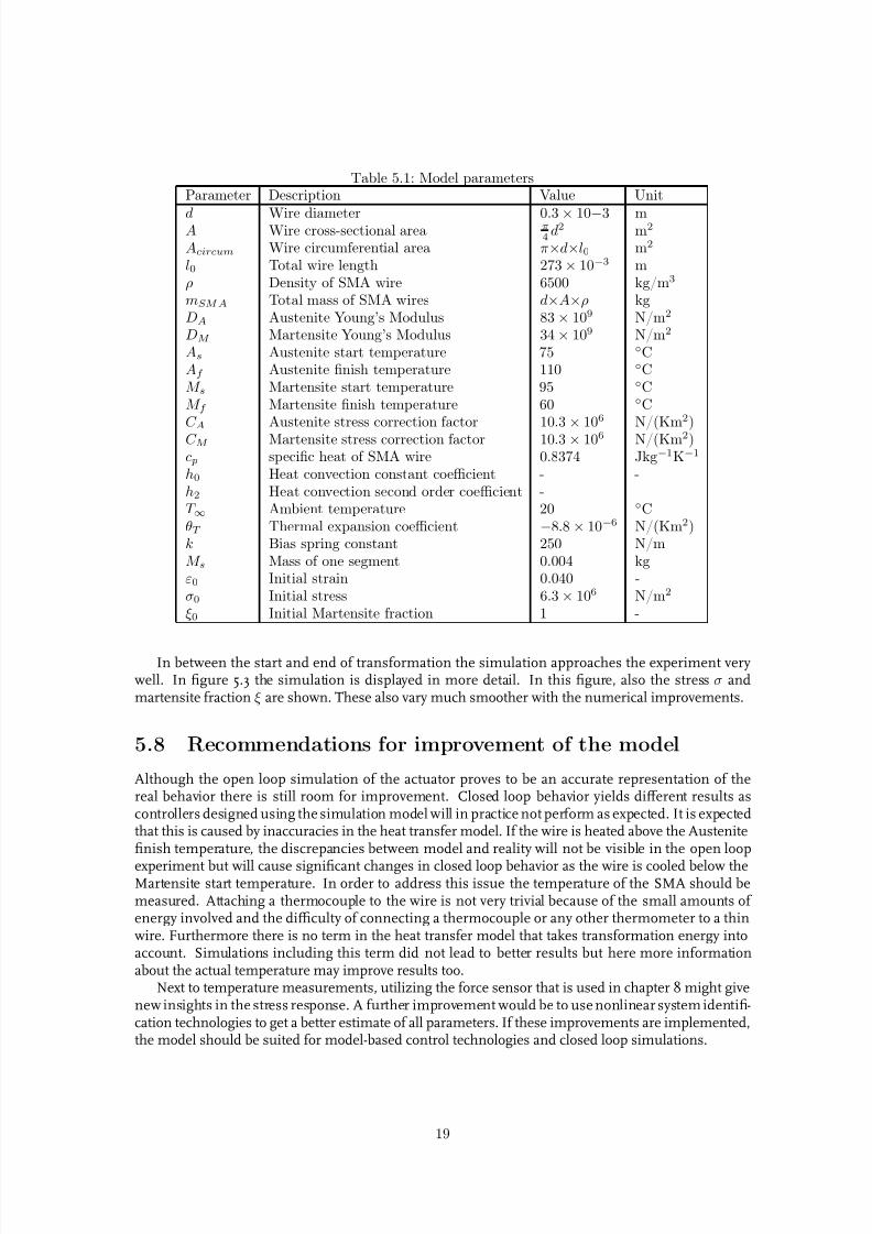
The model parameters in table 5.1 are derived from the application sheets of the MigaOne and theFlexinol wire. The constants C A and C M , which indirectly compensate for the change of the austeniteand martensite start and finish temperatures under stress, are taken from Elahinia. The austenitestart temperature and wire initial (maximum) strain are tuned for a better congruence of model andexperimental results.
5.7 Model validation
The model as discussed in the previous sections is compared to the actual actuator by applying astep in the supply voltage to the open loop system and measuring the resulting displacement, usingsupply voltages of 5V, 7.5V and 10V. The experimental results are shown in figure 5.2, along withsimulation results. In this figure the modified simulation represents the model where the numerical
improvements as discussed in section 5.5 have been implemented.It appears that the model represents the actuator very well. The biggest deviations occur at thebeginning and the end of the transformation: in reality the transformation from martensite to austen-ite starts a little earlier and ends somewhat later than in the model. This is noteworthy since the theoriginal model does not account for any transformation or displacement are present before the tem-perature reaches the austenite start temperature. In reality there is displacement immediately afterapplying a voltage and although it is not confirmed by measurements the assumption seems valid thatthis is below As since the temperature cannot change instantly from T ∞ to As. After consulting amaterial scientist it is concluded that the reason for this behavior is presumably that the transitiontemperature which is mentioned in most literature is in fact a range, and the used resistive heatingis far from uniform and thus introduces localized responses. More research is necessary however totake this into account in the mathematical model. The model which is numerically improved actu-ally performs better than the original in this region since it already starts transforming before As is
reached.
18
7/27/2019 Material Properties SMA
http://slidepdf.com/reader/full/material-properties-sma 19/39
Table 5.1: Model parametersParameter Description Value Unit
d Wire diameter 0.3× 10⁻³ mA Wire cross-sectional area π
4d2 m2
Acircum Wire circumferential area π×d×l0 m2
l0 Total wire length 273× 10−3 mρ Density of SMA wire 6500 kg/m3
mSMA Total mass of SMA wires d×A×ρ kgDA Austenite Young’s Modulus 83× 109 N/m2
DM Martensite Young’s Modulus 34× 109 N/m2
As Austenite start temperature 75 CAf Austenite finish temperature 110 CM s Martensite start temperature 95 CM f Martensite finish temperature 60 CC A Austenite stress correction factor 10.3 × 10⁶ N/(Km2)C M Martensite stress correction factor 10.3 × 10⁶ N/(Km2)c p specific heat of SMA wire 0.8374 Jkg−1K−1
h0 Heat convection constant coefficient - -h2 Heat convection second order coefficient -T ∞ Ambient temperature 20 CθT Thermal expansion coefficient −8.8 × 10⁻⁶ N/(Km2)k Bias spring constant 250 N/mM s Mass of one segment 0.004 kgε0 Initial strain 0.040 -σ0 Initial stress 6.3× 10⁶ N/m2
ξ 0 Initial Martensite fraction 1 -
In between the start and end of transformation the simulation approaches the experiment verywell. In figure 5.3 the simulation is displayed in more detail. In this figure, also the stress σ andmartensite fraction ξ are shown. These also vary much smoother with the numerical improvements.
5.8 Recommendations for improvement of the model
Although the open loop simulation of the actuator proves to be an accurate representation of thereal behavior there is still room for improvement. Closed loop behavior yields different results ascontrollers designed using the simulation model will in practice not perform as expected. It is expectedthat this is caused by inaccuracies in the heat transfer model. If the wire is heated above the Austenitefinish temperature, the discrepancies between model and reality will not be visible in the open loop
experiment but will cause significant changes in closed loop behavior as the wire is cooled below theMartensite start temperature. In order to address this issue the temperature of the SMA should bemeasured. Attaching a thermocouple to the wire is not very trivial because of the small amounts of energy involved and the difficulty of connecting a thermocouple or any other thermometer to a thinwire. Furthermore there is no term in the heat transfer model that takes transformation energy intoaccount. Simulations including this term did not lead to better results but here more informationabout the actual temperature may improve results too.
Next to temperature measurements, utilizing the force sensor that is used in chapter 8 might givenew insights in the stress response. A further improvement would be to use nonlinear system identifi-cation technologies to get a better estimate of all parameters. If these improvements are implemented,the model should be suited for model-based control technologies and closed loop simulations.
19

7/27/2019 Material Properties SMA
http://slidepdf.com/reader/full/material-properties-sma 20/39
1 1.5 2 2.5 3 3.5 40
0.002
0.004
0.006
0.008
0.01
0.012
Time [s]
P o s i t i o n [ m ]
Simulation 5V
Modified simulation 5V
Experiment 5V
Simulation 7.5V
Modified simulation 7.5V
Experiment 7.5V
Simulation 10V
Modified simulation 10V
Experiment 10V
Figure 5.2: Simulation and experimental results of step in supply voltage
1 1.5 2 2.5 3 3.5 40
0.002
0.004
0.006
0.008
0.01
0.012
Time [s]
P o s i t i o n [ m ]
Simulation
Modified simulation
Experiment
1 1.5 2 2.5 3 3.5 420
40
60
80
100
120
140
160
Time [s]
T e m p e r a t u r e [ ° C ]
1 1.5 2 2.5 3 3.5 40
0.2
0.4
0.6
0.8
1
Time [s]
M a r t e n s i t e f r a c t i o n [ − ]
1 1.5 2 2.5 3 3.5 46
7
8
9
10
11
12x 10
6
Time [s]
S t r e s s [ N / m 2 ]
Figure 5.3: Simulation and experimental results of 5V step in supply voltage
20
7/27/2019 Material Properties SMA
http://slidepdf.com/reader/full/material-properties-sma 21/39
Chapter 6
Controller design
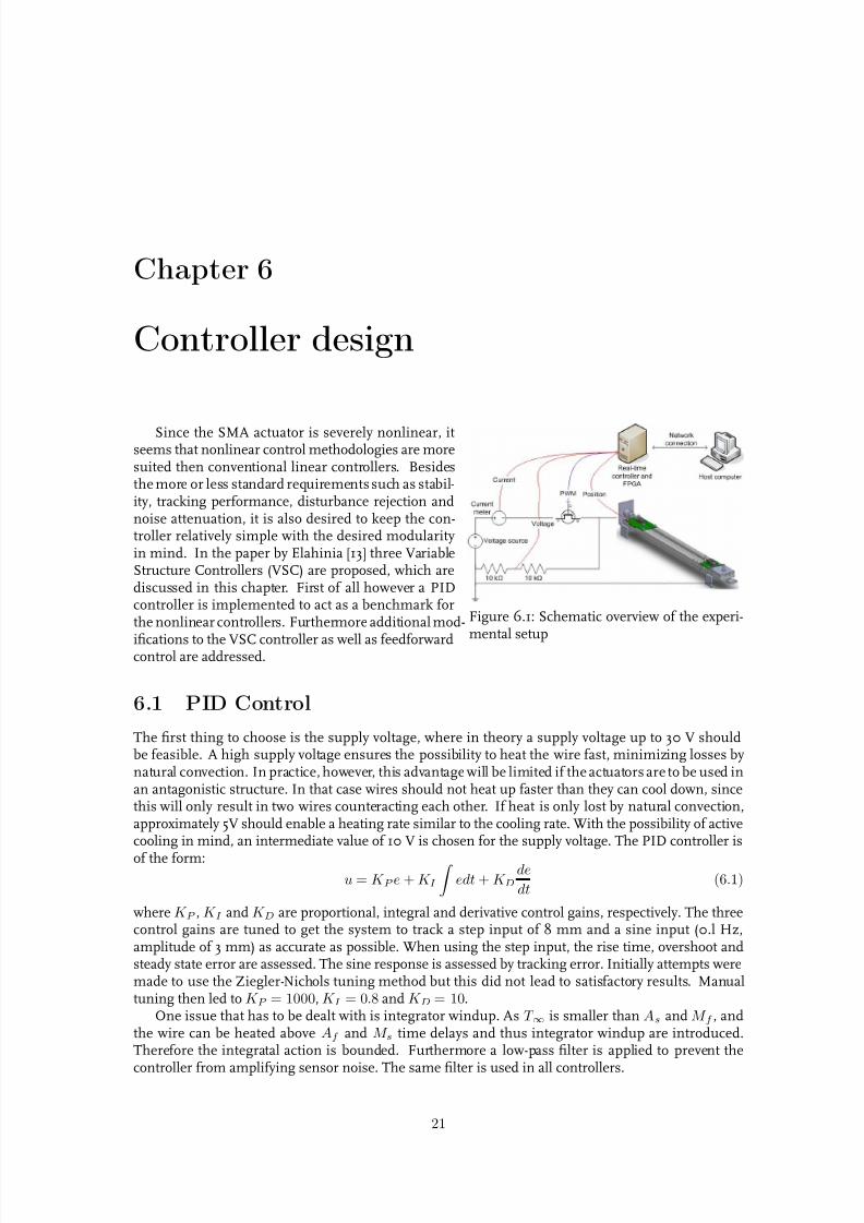
Figure 6.1: Schematic overview of the experi-mental setup
Since the SMA actuator is severely nonlinear, itseems that nonlinear control methodologies are moresuited then conventional linear controllers. Besidesthe more or less standard requirements such as stabil-ity, tracking performance, disturbance rejection andnoise attenuation, it is also desired to keep the con-troller relatively simple with the desired modularityin mind. In the paper by Elahinia [13] three VariableStructure Controllers (VSC) are proposed, which arediscussed in this chapter. First of all however a PIDcontroller is implemented to act as a benchmark forthe nonlinear controllers. Furthermore additional mod-
ifications to the VSC controller as well as feedforwardcontrol are addressed.
6.1 PID Control
The first thing to choose is the supply voltage, where in theory a supply voltage up to 30 V shouldbe feasible. A high supply voltage ensures the possibility to heat the wire fast, minimizing losses bynatural convection. In practice, however, this advantage will be limited if the actuators are to be used inan antagonistic structure. In that case wires should not heat up faster than they can cool down, sincethis will only result in two wires counteracting each other. If heat is only lost by natural convection,approximately 5V should enable a heating rate similar to the cooling rate. With the possibility of activecooling in mind, an intermediate value of 10 V is chosen for the supply voltage. The PID controller is
of the form:u = K P e + K I
edt + K D
de
dt (6.1)
where K P , K I and K D are proportional, integral and derivative control gains, respectively. The threecontrol gains are tuned to get the system to track a step input of 8 mm and a sine input (0.l Hz,amplitude of 3 mm) as accurate as possible. When using the step input, the rise time, overshoot andsteady state error are assessed. The sine response is assessed by tracking error. Initially attempts weremade to use the Ziegler-Nichols tuning method but this did not lead to satisfactory results. Manualtuning then led to K P = 1000, K I = 0.8 and K D = 10.
One issue that has to be dealt with is integrator windup. As T ∞ is smaller than As and M f , andthe wire can be heated above Af and M s time delays and thus integrator windup are introduced.Therefore the integratal action is bounded. Furthermore a low-pass filter is applied to prevent the
controller from amplifying sensor noise. The same filter is used in all controllers.
21
7/27/2019 Material Properties SMA
http://slidepdf.com/reader/full/material-properties-sma 22/39
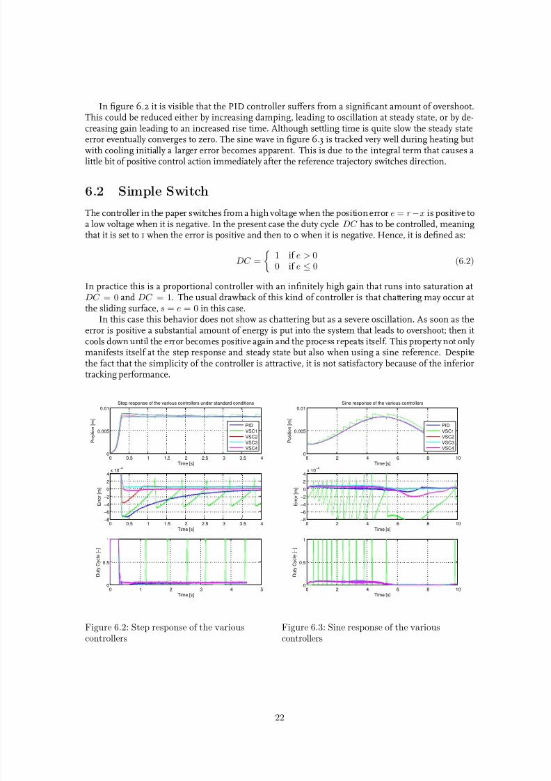
In figure 6.2 it is visible that the PID controller suffers from a significant amount of overshoot.This could be reduced either by increasing damping, leading to oscillation at steady state, or by de-creasing gain leading to an increased rise time. Although settling time is quite slow the steady state
error eventually converges to zero. The sine wave in figure 6.3 is tracked very well during heating butwith cooling initially a larger error becomes apparent. This is due to the integral term that causes alittle bit of positive control action immediately after the reference trajectory switches direction.
6.2 Simple Switch
The controller in the paper switches from a high voltage when the position error e = r−x is positive toa low voltage when it is negative. In the present case the duty cycle DC has to be controlled, meaningthat it is set to 1 when the error is positive and then to 0 when it is negative. Hence, it is defined as:
DC =
1 if e > 00 if e ≤ 0
(6.2)
In practice this is a proportional controller with an infinitely high gain that runs into saturation atDC = 0 and DC = 1. The usual drawback of this kind of controller is that chattering may occur atthe sliding surface, s = e = 0 in this case.
In this case this behavior does not show as chattering but as a severe oscillation. As soon as theerror is positive a substantial amount of energy is put into the system that leads to overshoot; then itcools down until the error becomes positive again and the process repeats itself. This property not onlymanifests itself at the step response and steady state but also when using a sine reference. Despitethe fact that the simplicity of the controller is attractive, it is not satisfactory because of the inferiortracking performance.
0 0.5 1 1.5 2 2.5 3 3.5 40
0.005
0.01
Time [s]
P o s i t i o n [ m ]
Step response of the various controllers under standard conditions
PID
VSC1
VSC2
VSC3VSC4
0 0.5 1 1.5 2 2.5 3 3.5 4−8
−6
−4
−2
0
2
4x 10
−4
Time [s]
E r r o r [ m ]
0 1 2 3 4 50
0.5
1
Time [s]
D u t y C y c l e [ − ]
Figure 6.2: Step response of the variouscontrollers
0 2 4 6 8 100
0.005
0.01
Time [s]
P o s i t i o n [ m ]
Sine response of the various controllers
PID
VSC1
VSC2
VSC3VSC4
0 2 4 6 8 10−8
−6
−4
−2
0
2
4x 10
−4
Time [s]
E r r o r [ m ]
0 2 4 6 8 100
0.5
1
Time [s]
D u t y C y c l e [ − ]
Figure 6.3: Sine response of the variouscontrollers
22

7/27/2019 Material Properties SMA
http://slidepdf.com/reader/full/material-properties-sma 23/39
6.3 Adding a Boundary Layer
The most common way to eliminate chattering when using VSC control is to introduce a boundary
layer. This solution is also applied to eliminate the oscillation that occurs when using the controlleras discussed in section 6.2. The switching law ensures that the system gets into the boundary layerquickly where a proportional controller takes over. It is defined as:
DC =
1 if e > φKe if −φ ≤ e ≤ φ0 if e < −φ
(6.3)
The parameter φ, which is half the boundary layer thickness, should be chosen such that it just pre-vents the system from oscillating and keeps the steady state error introduced by the boundary layer ata minimum.
A thickness of φ = 0.001 is tuned, eliminating the oscillatory behavior, but a significant amountof overshoot is still present as well as a small steady state error. The settling time has decreasedconsiderably compared to the PID controller. Tracking of the sine input shows a small error duringheating but during cooling better results are obtained than when using the PID controller.
6.4 Reducing Overshoot
Linear controllers address overshoot by adding damping. In the case of the VSC controller describedabove, results can be improved by modifying the sliding surface. In this case the sliding surface is:
s = e + λe (6.4)
While maintaining the same controller shown in equation 6.3, a suitable value of λ has to be chosento determine the amount of damping required.
Using φ = 0.011 and λ = 0.0125 the overshoot is eliminated and the settling time is decreasedsignificantly. The sine tracking error is approximately equal to that of the previous controller with amaximum of 0.103 mm. The steady state error is still present however and is addressed in section 6.5.
6.5 Elimination of the Steady State Error
Although the controller in section 6.4 performs well in terms of rise time, settling time and overshoot,there does exist a steady state error. Although this error is small an attempt is made to eliminate itcompletely. This is done by introducing an integral term to the sliding surface, thus resulting in:
s = e + λe + λI
e (6.5)
Again anti integrator windup as described in section 6.1 must be implemented.The parameters used for this controller are φ = 0.011, λ = 0.0125 and λ = 0.00025. As expected,
the steady state error has disappeared completely but this comes at the cost of a small amount of overshoot. Tracking of the sine input during heating has improved but during cooling performancehas deteriorated. This has the same cause as in section 6.1, namely the remaining integral action.
23
7/27/2019 Material Properties SMA
http://slidepdf.com/reader/full/material-properties-sma 24/39
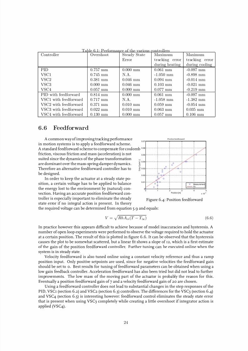
Table 6.1: Performance of the various controllersController Overshoot Steady State
Error
Maximum
tracking errorduring heating
Maximum
tracking errorduring coolingPID 0.757 mm 0.000 mm 0.061 mm -0.097 mmVSC1 0.745 mm N.A. -1.050 mm -0.898 mmVSC2 0.381 mm 0.046 mm 0.094 mm -0.014 mmVSC3 0.000 mm 0.046 mm 0.103 mm -0.021 mmVSC4 0.057 mm 0.000 mm 0.077 mm -0.219 mmPID with feedforward 0.814 mm 0.000 mm 0.061 mm -0.097 mmVSC1 with feedforward 0.717 mm N.A. -1.058 mm -1.382 mmVSC2 with feedforward 0.371 mm 0.010 mm 0.059 mm -0.054 mmVSC3 with feedforward 0.022 mm 0.010 mm 0.063 mm 0.035 mmVSC4 with feedforward 0.130 mm 0.000 mm 0.057 mm 0.106 mm
6.6 Feedforward
0 1 2 3 4 5
x 10−3
0
0.01
0.02
0.03
0.04
0.05
0.06
0.07
Position [m]
D u t y C y c l e [ − ]
Position feedforward
MeasurementFit
Figure 6.4: Position feedforward
A common way of improving tracking performancein motion systems is to apply a feedforward scheme.A standard feedforward scheme to compensate for coulombfriction, viscous friction and mass (acceleration) is notsuited since the dynamics of the phase transformationare dominant over the mass-spring-damper dynamics.Therefore an alternative feedforward controller has tobe designed.
In order to keep the actuator at a steady state po-
sition, a certain voltage has to be applied to balancethe energy lost to the environment by (natural) con-vection. Having an accurate position feedforward con-troller is especially important to eliminate the steadystate error if no integral action is present. In theorythe required voltage can be determined from equation 5.9 and equals:
V =
RhAci(T − T ∞) (6.6)
In practice however this appears difficult to achieve because of model inaccuracies and hysteresis. Anumber of open loop experiments were performed to observe the voltage required to hold the actuatorat a certain position. The result of this is plotted in figure 6.6. It can be observed that the hysteresiscauses the plot to be somewhat scattered, but a linear fit shows a slope of 12, which is a first estimate
of the gain of the position feedforward controller. Further tuning can be executed online when thesystem is in steady state.
Velocity feedforward is also tuned online using a constant velocity reference and thus a rampposition input. Only positive setpoints are used, since for negative velocities the feedforward gainshould be set to 0. Best results for tuning of feedforward parameters can be obtained when using alow gain feedback controller. Acceleration feedforward has also been tried but did not lead to furtherimprovements. The low mass of the moving part of the actuator is probably the reason for this.Eventually a position feedforward gain of 7 and a velocity feedforward gain of 20 are chosen.
Using a feedforward controller does not lead to substantial changes in the step responses of thePID, VSC1 (section 6.2) and VSC2 (section 6.3) controllers. The differences for the VSC3 (section 6.4)and VSC4 (section 6.5) is interesting however: feedforward control eliminates the steady state errorthat is present when using VSC3 completely while creating a little overshoot if integrator action is
applied (VSC4).
24
7/27/2019 Material Properties SMA
http://slidepdf.com/reader/full/material-properties-sma 25/39
0 0.5 1 1.5 2 2.5 3 3.5 40
0.005
0.01
Time [s]
P o s i t i o n
[ m ]
Step response of the various controllers under standard conditions using feedforward
PIDVSC1
VSC2
VSC3VSC4
0 0.5 1 1.5 2 2.5 3 3.5 4−8
−6
−4
−2
0
2
4x 10
−4
Time [s]
E r r o r [ m ]
0 1 2 3 4 50
0.5
1
Time [s]
D u t y C
y c l e [ − ]
Figure 6.5: Step response of the variouscontrollers using feedforward
0 2 4 6 8 100
0.005
0.01
Time [s]
P o s i t i o n
[ m ]
Sine response of the various controllers using feedforward
PIDVSC1
VSC2
VSC3VSC4
0 2 4 6 8 10−8
−6
−4
−2
0
2
4x 10
−4
Time [s]
E r r o r [ m ]
0 2 4 6 8 100
0.5
1
Time [s]
D u t y C
y c l e [ − ]
Figure 6.6: Sine response of the variouscontrollers using feedforward
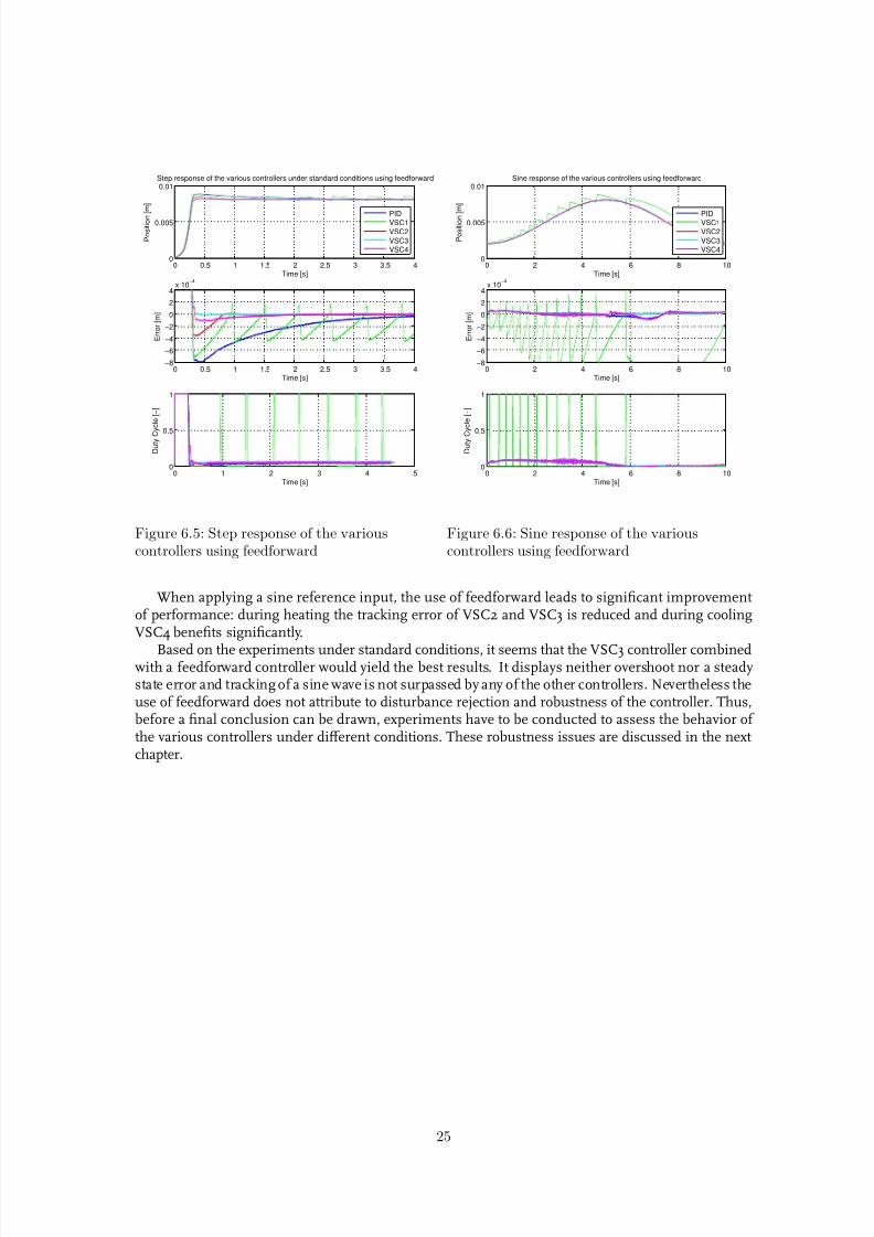
When applying a sine reference input, the use of feedforward leads to significant improvementof performance: during heating the tracking error of VSC2 and VSC3 is reduced and during coolingVSC4 benefits significantly.
Based on the experiments under standard conditions, it seems that the VSC3 controller combinedwith a feedforward controller would yield the best results. It displays neither overshoot nor a steadystate error and tracking of a sine wave is not surpassed by any of the other controllers. Nevertheless theuse of feedforward does not attribute to disturbance rejection and robustness of the controller. Thus,before a final conclusion can be drawn, experiments have to be conducted to assess the behavior of the various controllers under different conditions. These robustness issues are discussed in the nextchapter.
25
7/27/2019 Material Properties SMA
http://slidepdf.com/reader/full/material-properties-sma 26/39
Chapter 7
Robustness
The controllers designed in chapter 6 are tuned for standard conditions, i.e. a 0.3 mm wire, cooling bynatural convection, 10 V supply voltage and a PWM frequency of 500 Hz. A number of the standardconditions have been varied in order to assess the robustness of the various controllers, which havenot been tuned for the specific circumstances. The resulting differences in performance are discussedin the subsequent sections. Emphasis will lie on the PID, VSC3 and VSC4 controllers, both with andwithout feedforward control. These two VSC controllers showed by far the best performance understandard conditions while the PID again represents the benchmark. The results for VSC1 and VSC2have been omitted in order to reduce the number of graphs per plot and thus enhancing clarity. Againboth step and sine signals are used as reference inputs. At the end of this chapter some generalremarks on these robustness issues will be discussed.
7.1 Forced convection
By applying active cooling, the austenite to martensite transformation could be accelerated signifi-cantly. Nevertheless, variations in cooling should not upset the system. In this case a fan is usedfor forced convection to extract more heat from the SMA wire, possibly causing slower heating and asteady state error if integral action is absent or not sufficient.
In figures 7.1 and 7.2 it can be seen that the PID controller is least affected by applying forcedcooling since results are quite similar to those shown in chapter 6. The system with VSC3 shows asteady state error with and without feedforward control implying that if the feedforward gain is nottuned for forced cooling it cannot eliminate the steady state error. The same holds for the integralaction in VSC4 as can be seen in the steady state error that is present without feedforward control. If feedforward control is used in combination with the VSC4 controller, perfect steady state behavior canstill be obtained.
Applying forced cooling improves tracking of a sine wave during cooling since the error of the PIDand in particular the VSC4 controllers have decreased significantly. During heating however the VSC3and VSC4 controllers show substantially increased tracking errors.
The PID controller is least affected by applying forced cooling but still shows a step response thatbehaves significantly worse than that of the VSC3 and VSC4 controllers. Tracking of a sine input onthe other hand shows the best results when using the PID controller.
7.2 Supply voltage
Applying a higher supply voltage will result in faster heating but can cause instability and oscillations.On the other hand a lower supply voltage will lead to slower heating and possibly a steady state error.In that case the energy put into the system is insufficient to balance the heat loss to the environment.
Therefore experiments have been conducted using supply voltages ranging from 5 V to 15 V.
26

7/27/2019 Material Properties SMA
http://slidepdf.com/reader/full/material-properties-sma 27/39
0 0.5 1 1.5 2 2.5 3 3.5 40
0.005
0.01
Time [s]
P o s i t i o n
[ m ]
Step response with forced convection, no feedforward
PID
VSC3
VSC4
0 0.5 1 1.5 2 2.5 3 3.5 4
−5
0
5
x 10−4
Time [s]
E r r o r [ m ]
Error without feedforward
0 0.5 1 1.5 2 2.5 3 3.5 4
−5
0
5
x 10−4
Time [s]
E r r o
r [ m ]
Error with feedforward
Figure 7.1: Step response with forced cooling
0 2 4 6 8 100
0.005
0.01
Time [s]
P o s i t i o n
[ m ]
Sine response with forced convection, no feedforward
PID
VSC3
VSC4
0 2 4 6 8 10
−2
−1
0
1
2
x 10−4
Time [s]
E r r o r [ m ]
Error without feedforward
0 2 4 6 8 10
−2
−10
1
2
x 10−4
Time [s]
E r r o
r [ m ]
Error with feedforward
Figure 7.2: Sine response with forced cooling
The increase of rise time due to reducing the supply voltage is equal for all three controllers. Fur-thermore it leads to a decrease in overshoot using the PID controller, while using the VSC3 and VSC4controllers introduces a steady state error comparable to the one in section 7.1. The VSC controllersalso yield very bad sine responses, while tracking performance using the PID controller only slightly
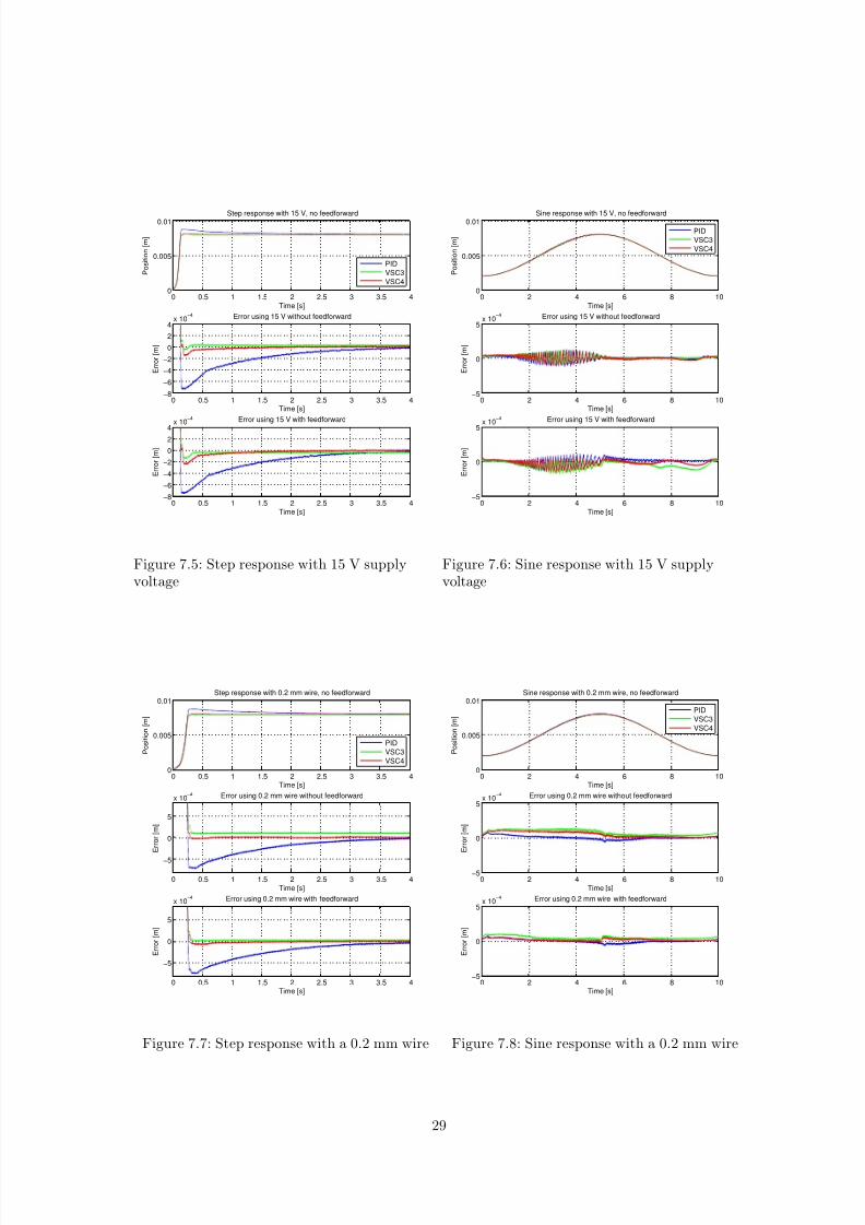
deteriorates due to more integral action.Increasing the supply voltage to 15 V shows a totally different behavior. Minor overshoot is intro-
duced when using the VSC controllers but this is still approximately a factor four less than using thePID controller. All three controllers show oscillation during heating and good tracking during cool-ing. When the supply voltage is increased, the necessity for the feedforward controller is decreasedand may even degrade tracking performance due to improper tuning for these conditions. This canbe seen in figure 7.6 during cooling.
7.3 Wire diameter
In this section the effect of various wire diameters is investigated. Besides the ’standard’ 0.3 mmwire, 0.2 mm and 0.5 mm wires have also been used. The smaller wire diameter should lead to faster
cooling because a higher surface to volume ratio [9]. The thicker wire can be expected to show theopposite behavior.
Using a 0.2 mm wire instead of a 0.3 mm one does not lead to significant changes in trackingperformance and differences between the PID, VSC3 and VSC4 controllers with and without feedbackare similar to those using a 0.3 mm wire.
Increasing the wire diameter to 0.5 mm does corrupt tracking performance. The variable structurecontrollers still perform an acceptable step response but the damping of the PID controller is clearlynot sufficient. This manifests itself in a further increase of overshoot and oscillations. Moreover,the wire dynamics are too slow to cope with the 0.1 Hz sine wave, and an error is introduced duringcooling. Also during heating the controllers do not perform very well and show heavy vibrations.
27

7/27/2019 Material Properties SMA
http://slidepdf.com/reader/full/material-properties-sma 28/39
0 0.5 1 1.5 2 2.5 3 3.5 40
0.005
0.01
Time [s]
P o s i t i o n
[ m ]
Step response with 5 V, no feedforward
PID
VSC3
VSC4
0 0.5 1 1.5 2 2.5 3 3.5 4
−5
0
5
x 10−4
Time [s]
E r r o r [ m ]
Error using 5 V without feedforward
0 0.5 1 1.5 2 2.5 3 3.5 4
−5
0
5
x 10−4
Time [s]
E r r o
r [ m ]
Error using 5 V with feedforward
Figure 7.3: Step response with 5 Vsupply voltage
0 2 4 6 8 100
0.005
0.01
Time [s]
P o s i t i o n
[ m ]
Sine response with 5 V, no feedforward
PID
VSC3
VSC4
0 2 4 6 8 10−5
0
5x 10
−4
Time [s]
E r r o r [ m ]
Error using 5 V without feedforward
0 2 4 6 8 10−5
0
5x 10
−4
Time [s]
E r r o
r [ m ]
Error using 5 V with feedforward
Figure 7.4: Sine response with 5 Vsupply voltage
7.4 General remarks
As discussed in chapter 6 under standard conditions the step responses of the variable structure con-
trollers perform better than that of the PID controller. Even when cooling, supply voltage or wirediameter are varied this remains the same. The VSC controllers always maximize gain outside theboundary layer and therefore high gain within the boundary layer is not required to get a fast re-sponse. This low gain within the boundary layer limits overshoot but comes at the cost of reducedtracking robustness. This poor tracking robustness manifests itself in tracking of a sine wave whichdeteriorates more severely when using a VSC controller under varying circumstances.
In case the controller is to be used with different supply voltages and wire diameters it is recom-mended to tune the gains for the lowest possible supply voltage and largest wire diameter. In section7.2 it becomes apparent that tracking errors are significantly increased when decreasing supply volt-age whereas an increase in voltage does lead to occasional oscillation but not to instability. Choosinga smaller wire diameter does not lead to substantial change in tracking performance while both badtracking and heavy vibrations may be caused by choosing a larger wire diameter.
The effect of using multiple wires in parallel and thus increasing the force of the actuator hasnot been investigated thoroughly. Ideally this would not require a change in controller because thesame voltage is supplied to all wires thereby leading to a similar response. In practice it appeared thatattaching the wires to the actuator under the exact same pre-stress was difficult and led to differentcontractions. Other possible factors such as usage history and manufacturing variability could con-tribute to the difference as well. Therefore no relevant measurement data could be acquired. Furtherdevelopment of the actuator should resolve this issue and the hypothesis stated above can then betested.
Some of the parameters varied above led to significant changes in response. In order to increasehandling of these varying circumstances more advanced control algorithms could be used, examplesof which are robust control, adaptive control and model based feedforward. The downside of thiswould be increased complexity of the controller.
28
7/27/2019 Material Properties SMA
http://slidepdf.com/reader/full/material-properties-sma 29/39
0 0.5 1 1.5 2 2.5 3 3.5 40
0.005
0.01
Time [s]
P o s i t i o n [ m ]
Step response with 15 V, no feedforward
PID
VSC3
VSC4
0 0.5 1 1.5 2 2.5 3 3.5 4−8
−6
−4
−2
0
2
4x 10
−4
Time [s]
E r r o r [ m ]
Error using 15 V without feedforward
0 0.5 1 1.5 2 2.5 3 3.5 4−8
−6
−4
−2
0
24
x 10−4
Time [s]
E r r o r [ m ]
Error using 15 V with feedforward
Figure 7.5: Step response with 15 V supplyvoltage
0 2 4 6 8 100
0.005
0.01
Time [s]
P o s i t i o n [ m ]
Sine response with 15 V, no feedforward
PID
VSC3
VSC4
0 2 4 6 8 10−5
0
5x 10
−4
Time [s]
E r r o r [ m ]
Error using 15 V without feedforward
0 2 4 6 8 10−5
0
5
x 10−4
Time [s]
E r r o r [ m ]
Error using 15 V with feedforward
Figure 7.6: Sine response with 15 V supplyvoltage
0 0.5 1 1.5 2 2.5 3 3.5 40
0.005
0.01
Time [s]
P o s i t i o n [ m ]
Step response with 0.2 mm wire, no feedforward
PID
VSC3
VSC4
0 0.5 1 1.5 2 2.5 3 3.5 4
−5
0
5
x 10−4
Time [s]
E r r o r [ m ]
Error using 0.2 mm wire without feedforward
0 0.5 1 1.5 2 2.5 3 3.5 4
−5
0
5
x 10−4
Time [s]
E r r o r [ m ]
Error using 0.2 mm wire with feedforward
Figure 7.7: Step response with a 0.2 mm wire
0 2 4 6 8 100
0.005
0.01
Time [s]
P o s i t i o n [ m ]
Sine response with 0.2 mm wire, no feedforward
PID
VSC3
VSC4
0 2 4 6 8 10−5
0
5x 10
−4
Time [s]
E r r o r [ m ]
Error using 0.2 mm wire without feedforward
0 2 4 6 8 10−5
0
5x 10
−4
Time [s]
E r r o r [ m ]
Error using 0.2 mm wire with feedforward
Figure 7.8: Sine response with a 0.2 mm wire
29

7/27/2019 Material Properties SMA
http://slidepdf.com/reader/full/material-properties-sma 30/39
0 0.5 1 1.5 2 2.5 3 3.5 40
0.005
0.01
Time [s]
P o s i t i o n [ m ]
Step response with 0.5 mm wire, no feedforward
PID
VSC3
VSC4
0 0.5 1 1.5 2 2.5 3 3.5 4
−10
−5
0
5
x 10−4
Time [s]
E r r o r [ m ]
Error using 0.5 mm wire without feedforward
0 0.5 1 1.5 2 2.5 3 3.5 4
−10
−5
0
5
x 10−4
Time [s]
E r r o r [ m ]
Error using 0.5 mm wire with feedforward
Figure 7.9: Step response with a 0.5 mm wire
0 2 4 6 8 100
0.005
0.01
Time [s]
P o s i t i o n [ m ]
Sine response with 0.5 mm wire, no feedforward
PID
VSC3
VSC4
0 2 4 6 8 10−5
0
5x 10
−3
Time [s]
E r r o r [ m ]
Error using 0.5 mm wire without feedforward
0 2 4 6 8 10−5
0
5x 10
−3
Time [s]
E r r o r [ m ]
Error using 0.5 mm wire with feedforward
Figure 7.10: Sine response with a 0.5 mm wire
30

7/27/2019 Material Properties SMA
http://slidepdf.com/reader/full/material-properties-sma 31/39
Chapter 8
Efficiency
As observed in table 2.1 one of the drawbacks of SMA actuators is the low efficiency which also postsa limiting factor in the use of these actuators for rehabilitation. The actuator used in the experimentsin previous chapters has an electrical resistance of approximately 4 Ω. The nominal supply voltage of 10 V leads to an instantaneous power consumption of P = V 2/R = 25 W which is quite substantialfor a small actuator with a stroke of approximately 1 cm. The maximum Carnot efficiency can bedetermined to be:
ηCarnot = 1−T coldT hot
= 1−As
Af
= 1 −348
383 = 9% (8.1)
In practice an efficiency of about 4 % is expected but this must be verified experimentally.The efficiency of the SMA actuator can be defined as:
η = E out
E in=
mechanical workoutelectrical energy
in
=
F ds
P eldt (8.2)
In this equation F denotes force, s is displacement, P el is electric power and t denotes time. In orderto measure force a force transducer is installed on the actuator in series with the bias spring. Themeasured force is integrated directly over displacement instead of calculating mechanical power andintegrating this over time. This eliminates the necessity for numerical differentiation which usuallygives noisy results.
The methods of measuring voltage and current needs some further explanation since the mea-surements in chapter 4 are measuring instantaneous values during ’on-time’. They do not representthe respective continuous or effective values. In order to calculate the electrical power and energy thedynamics, as displayed earlier in figure 4.1, are ignored in order to assume perfect square waves forboth voltage and current. The total energy of one pulse can then be calculated using:
E pulse = V I [pulsewidth] = V I DC
f PWM (8.3)
This leads to the following expression for P el:
P el = V I DC (8.4)
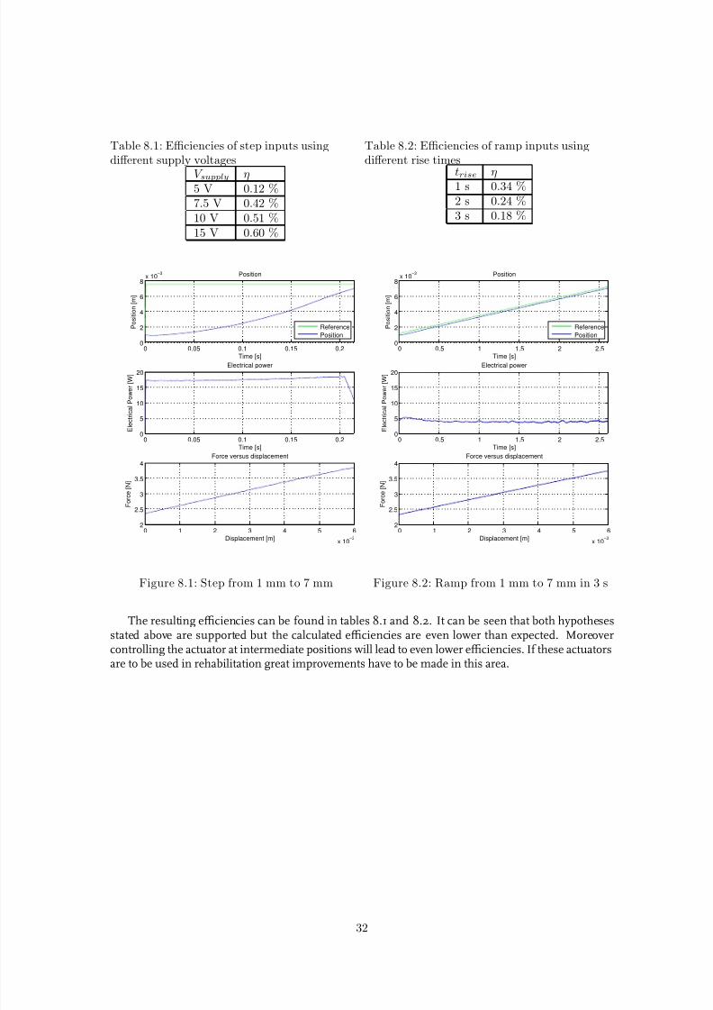
It can be expected that faster excitation leads to a better efficiency because less heat will be lost tothe environment. Therefore a step response should have a better efficiency than a ramp response andthe step response should be more efficient with higher supply voltages. Also keeping the actuator atsteady state should lead to zero efficiency because of the lack of displacement. The effect of varyingthe supply voltage is investigated by applying a step from 1 mm to 7 mm. Furthermore ramps overthe same displacement with different time intervals are tested, using a constant 10 V supply voltage.Results from one step and one ramp experiment are plotted in figures 8.1 and 8.2.
31
7/27/2019 Material Properties SMA
http://slidepdf.com/reader/full/material-properties-sma 32/39
Table 8.1: Efficiencies of step inputs usingdifferent supply voltages
V supply η5 V 0.12 %7.5 V 0.42 %10 V 0.51 %15 V 0.60 %
Table 8.2: Efficiencies of ramp inputs usingdifferent rise times
trise η1 s 0.34 %2 s 0.24 %3 s 0.18 %
0 0.05 0.1 0.15 0.20
2
4
6
8x 10
−3
Time [s]
P o s i t i o n [ m ]
Position
Reference
Position
0 0.05 0.1 0.15 0.20
5
10
15
20
Time [s]
E l e c t r i c a l P o w e r [ W ]
Electrical power
0 1 2 3 4 5 6
x 10−3
2
2.5
3
3.5
4
Displacement [m]
F o r c e [ N ]
Force versus displacement
Figure 8.1: Step from 1 mm to 7 mm
0 0.5 1 1.5 2 2.50
2
4
6
8x 10
−3
Time [s]
P o s i t i o n [ m ]
Position
Reference
Position
0 0.5 1 1.5 2 2.50
5
10
15
20
Time [s]
E l e c t r i c a l P o w e r [ W ]
Electrical power
0 1 2 3 4 5 6
x 10−3
2
2.5
3
3.5
4
Displacement [m]
F o r c e [ N ]
Force versus displacement
Figure 8.2: Ramp from 1 mm to 7 mm in 3 s
The resulting efficiencies can be found in tables 8.1 and 8.2. It can be seen that both hypothesesstated above are supported but the calculated efficiencies are even lower than expected. Moreovercontrolling the actuator at intermediate positions will lead to even lower efficiencies. If these actuatorsare to be used in rehabilitation great improvements have to be made in this area.
32
7/27/2019 Material Properties SMA
http://slidepdf.com/reader/full/material-properties-sma 33/39
Chapter 9
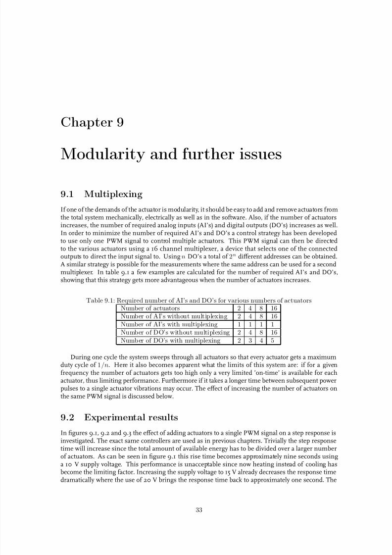
Modularity and further issues
9.1 MultiplexingIf one of the demands of the actuator is modularity, it should be easy to add and remove actuators fromthe total system mechanically, electrically as well as in the software. Also, if the number of actuatorsincreases, the number of required analog inputs (AI’s) and digital outputs (DO’s) increases as well.In order to minimize the number of required AI’s and DO’s a control strategy has been developedto use only one PWM signal to control multiple actuators. This PWM signal can then be directedto the various actuators using a 16 channel multiplexer, a device that selects one of the connectedoutputs to direct the input signal to. Using n DO’s a total of 2n different addresses can be obtained.A similar strategy is possible for the measurements where the same address can be used for a secondmultiplexer. In table 9.1 a few examples are calculated for the number of required AI’s and DO’s,showing that this strategy gets more advantageous when the number of actuators increases.
Table 9.1: Required number of AI’s and DO’s for various numbers of actuatorsNumber of actuators 2 4 8 16Number of AI’s without multiplexing 2 4 8 16Number of AI’s with multiplexing 1 1 1 1Number of DO’s without multiplexing 2 4 8 16Number of DO’s with multiplexing 2 3 4 5
During one cycle the system sweeps through all actuators so that every actuator gets a maximumduty cycle of 1/n. Here it also becomes apparent what the limits of this system are: if for a givenfrequency the number of actuators gets too high only a very limited ’on-time’ is available for eachactuator, thus limiting performance. Furthermore if it takes a longer time between subsequent power
pulses to a single actuator vibrations may occur. The effect of increasing the number of actuators onthe same PWM signal is discussed below.
9.2 Experimental results
In figures 9.1, 9.2 and 9.3 the effect of adding actuators to a single PWM signal on a step response isinvestigated. The exact same controllers are used as in previous chapters. Trivially the step responsetime will increase since the total amount of available energy has to be divided over a larger numberof actuators. As can be seen in figure 9.1 this rise time becomes approximately nine seconds usinga 10 V supply voltage. This performance is unacceptable since now heating instead of cooling hasbecome the limiting factor. Increasing the supply voltage to 15 V already decreases the response timedramatically where the use of 20 V brings the response time back to approximately one second. The
33
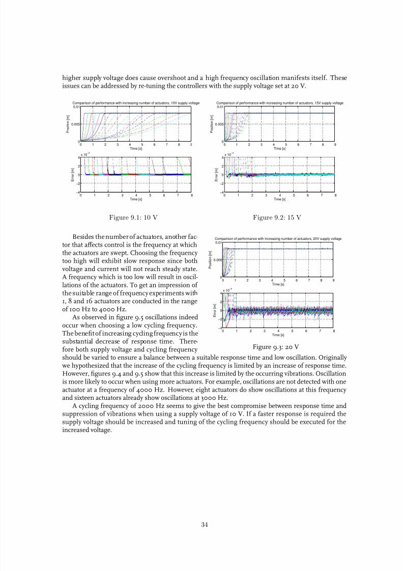
7/27/2019 Material Properties SMA
http://slidepdf.com/reader/full/material-properties-sma 34/39
higher supply voltage does cause overshoot and a high frequency oscillation manifests itself. Theseissues can be addressed by re-tuning the controllers with the supply voltage set at 20 V.
0 1 2 3 4 5 6 7 8 90
0.005
0.01
Time [s]
P o s i t i o n [ m ]
Comparison of performance with increasing number of actuators, 10V supply voltage
0 1 2 3 4 5 6 7 8−4
−2
0
2
4x 10
−4
Time [s]
E r r o r [ m ]
Figure 9.1: 10 V
0 1 2 3 4 5 6 7 8 90
0.005
0.01
Time [s]
P o s i t i o n [ m ]
Comparison of performance with increasing number of actuators, 15V supply voltage
0 1 2 3 4 5 6 7 8−4
−2
0
2
4x 10
−4
Time [s]
E r r o r [ m ]
Figure 9.2: 15 V
0 1 2 3 4 5 6 7 8 90
0.005
0.01
Time [s]
P o s i t i o n [ m ]
Comparison of performance with increasing number of actuators, 20V supply voltage
0 1 2 3 4 5 6 7 8−4
−2
0
2
4x 10
−4
Time [s]
E r r o r [ m ]
Figure 9.3: 20 V
Besides the number of actuators, another fac-tor that affects control is the frequency at whichthe actuators are swept. Choosing the frequencytoo high will exhibit slow response since bothvoltage and current will not reach steady state.A frequency which is too low will result in oscil-lations of the actuators. To get an impression of the suitable range of frequency experiments with
1, 8 and 16 actuators are conducted in the rangeof 100 Hz to 4000 Hz.
As observed in figure 9.5 oscillations indeedoccur when choosing a low cycling frequency.The benefit of increasing cycling frequency is thesubstantial decrease of response time. There-fore both supply voltage and cycling frequencyshould be varied to ensure a balance between a suitable response time and low oscillation. Originallywe hypothesized that the increase of the cycling frequency is limited by an increase of response time.However, figures 9.4 and 9.5 show that this increase is limited by the occurring vibrations. Oscillationis more likely to occur when using more actuators. For example, oscillations are not detected with oneactuator at a frequency of 4000 Hz. However, eight actuators do show oscillations at this frequency
and sixteen actuators already show oscillations at 3000 Hz.A cycling frequency of 2000 Hz seems to give the best compromise between response time andsuppression of vibrations when using a supply voltage of 10 V. If a faster response is required thesupply voltage should be increased and tuning of the cycling frequency should be executed for theincreased voltage.
34

7/27/2019 Material Properties SMA
http://slidepdf.com/reader/full/material-properties-sma 35/39
0 1 2 3 4 5 6 7 8 9 1 00
1
2
3
4
5
6
7
8
x 10−3
Time [s]
P o s i t i o n [ m ]
Comparison of varing cycling frequency
1,100 Hz1,500 Hz1,1000 Hz1,2000 Hz1,3000 Hz1,4000 Hz8,100 Hz8,500 Hz8,1000 Hz8,2000 Hz8,3000 Hz8,4000 Hz16,100 Hz16,500 Hz16,1000 Hz16,2000 Hz16,3000 Hz16,4000 Hz
Figure 9.4: Step responses when using varying cycling frequencies and number of actuators
9.3 Actuator Matrix Driver
0 0.05 0.1 0.15 0.2 0.25 0.3 0.35 0.40
2
4
6
8
x 10−3
Time [s]
P
o s i t i o n [ m ]
1 Actuator
100 Hz
500 Hz
1000 Hz
2000 Hz
3000 Hz
4000 Hz
0 0.5 1 1.5 2 2.5 3 3.50
2
4
6
8
x 10−3
Time [s]
P o s i t i o n [ m ]
8 Actuators
100 Hz
500 Hz
1000 Hz
2000 Hz
3000 Hz
4000 Hz
0 2 4 6 8 100
2
4
6
8
x 10−3
Time [s]
P o s i t i o n [ m ]
16 Actuators
100 Hz
500 Hz
1000 Hz
2000 Hz
3000 Hz
4000 Hz
Figure 9.5: Detail per number of actuators
The multiplexer as described above dramat-ically reduces the number of required AI’s andDIO’s for large numbers of actuators but it doesnot reduce the number of lead wires which is
equal to the number of actuators and a groundwire. In a miniature device the space availablefor even these lead wires may be limited. Mukher-jee [14] proposes the Actuator Matrix Driver con-cept in which the SMA elements are connectedin the form of a matrix. Any of the SMA wirescan be selected by choosing one of the columnsand one of the rows of the matrix, and the to-tal number of lead wires equals the sum of thenumber of rows and the number of columns.In the example by Mukherjee five segments withthree SMA elements are used and the total num-ber of lead wires is thus reduced from 16, in a
conventional setup, to 8, in a matrix setup.A combination of multiplexing and the actu-
ator matrix driver would minimize the requiredresources for actuation of multiple actuators. Theway this technology can be brought into practicehowever depends on the intended application and therefore further research on this topic has not beenperformed yet.
35

7/27/2019 Material Properties SMA
http://slidepdf.com/reader/full/material-properties-sma 36/39
9.4 Further issues
As is examined in the previous chapter the low efficiency poses a limit on the use of SMA actuators
in rehabilitation in spite of their attractive features as discussed in section 2.2. However this doesnot mean that the technology cannot be used in other areas. In the medical field much research hasbeen done in using SMA as micro active catheters [4] and active endoscopes [6]. Here the extremelysmall required volume is the main reason for the choice of SMA actuators. According to Langelaar [9],using SMA actuators on a micro scale has another advantage. The cooling time of SMA wires limitsthe dynamic response when no active cooling is applied, but on micro scale the surface to volume ratioincreases and natural cooling is much faster.
Research has also been done on modular actuators. Grant [5] has developed an actuator that canachieve higher strains to overcome one of the drawbacks of SMA’s. Vivek [17] has designed a binarymanipulator which has the advantage of not using energy when hold stationary. This technologyshould prevent efficiency from decreasing further than the results shown in chapter 8. Furthermoredisplacement sensing is not necessary since the actuators can only achieve two states.
During this research a number of different actuator configurations have been discussed with 2 and3 degrees of freedom per actuator. Either antagonistic structures or bias springs can be used to activelycontrol movement in two directions. Also, combining SMA with other actuators or passive elementsmake for interesting possibilities such as variable stiffness devices. These ideas can be incorporatedinto many bio-inspired robots or artificial grippers.
36

7/27/2019 Material Properties SMA
http://slidepdf.com/reader/full/material-properties-sma 37/39
Chapter 10
Conclusion
This project started off with the ultimate goal of developing a bio-inspired modular actuator suitedfor rehabilitation properties. In the course of the preliminary research however the apparently lowefficiency and high power requirements seemed to pose a limit on the use of SMA in this field of application. This hypothesis was confirmed by the efficiency measurements.
Nevertheless valuable knowledge about shape memory alloys has been acquired. A relationshipbetween electrical resistance and displacement was established and could be used for integrated sens-ing depending on the required accuracy. A mathematical model of a SMA actuator has been developedwhich showed surprisingly accurate results despite the fact that no temperature measurements havebeen done yet. Doing so will lead to further improvements of the model enabling to use it for closedloop simulations and model based control algorithms.
Furthermore variable structure controllers have been implemented and their performance wascompared to that of a PID controller. A VSC control showed much better step response performancethan PID control and if tuned properly showed comparable performance when tracking a smooth
reference signals.As rehabilitation is found not to be the prime application area of SMA’s, other possible applica-
tions for SMA actuators have been discussed. Compliant and semi-active applications appear to beinteresting for the use of SMA and further research should be done in this area. On the short termhowever emphasis will lie on further developments of the mathematical model.
37

7/27/2019 Material Properties SMA
http://slidepdf.com/reader/full/material-properties-sma 38/39
Bibliography
[1] G. Alici, G. M. Spinks, J. D. Madden, Wu Yanzhe, and G. G. Wallace. Response characteriza-tion of electroactive polymers as mechanical sensors. Mechatronics, IEEE/ASME Transactions on,13(2):187–196, 2008.
[2] Chou Ching-Ping and B. Hannaford. Measurement and modeling of mckibben pneumatic artifi-cial muscles. Robotics and Automation, IEEE Transactions on, 12(1):90–102, 1996.
[3] T W Duerig, K N Melton, D Stockel, and C M Wayman. Engineering Aspects of Shape MemoryAlloys. Butterworth-Heinemann, London, 1990.
[4] T. Fukuda, Guo Shuxiang, K. Kosuge, F. Arai, M. Negoro, and K. Nakabayashi. Micro activecatheter system with multi degrees of freedom. In Robotics and Automation, 1994. Proceedings.,1994 IEEE International Conference on, pages 2290–2295 vol.3, 1994.
[5] D. Grant and V. Hayward. Design of shape memory alloy actuator with high strain and variablestructure control. In Robotics and Automation, 1995. Proceedings., 1995 IEEE International Confer-ence on, volume 3, pages 2305–2312 vol.3, 1995.
[6] K. Ikuta, M. Tsukamoto, and S. Hirose. Shape memory alloy servo actuator system with elec-tric resistance feedback and application for active endoscope. In Robotics and Automation, 1988.Proceedings., 1988 IEEE International Conference on, pages 427–430 vol.1, 1988.
[7] Eric R. Kandel, James H. Schwartz, and Thomas M. Jessell. Principles of Neural Science. McGraw-Hill, fourth edition, 2000.
[8] Y. Kaneda, N. Kamamichi, M. Yamakita, K. Asaka, and Z. W. Luo. Control of linear artificialmuscle actuator using ipmc. In SICE 2003 Annual Conference, volume 2, pages 1650–1655 Vol.2,2003.
[9] M. Langelaar, G. H. Yoon, S. Gurav, Y. Y. Kim, and F. van Keulen. Modeling and design of shapememory alloy actuators. In Thermal, Mechanical and Multi-Physics Simulation and Experimentsin Micro-Electronics and Micro-Systems, 2005. EuroSimE 2005. Proceedings of the 6th International Conference on, pages 626–633, 2005.
[10] C. Liang and C. A. Rogers. One-dimensional thermomechanical constitutive relations for shapememory materials. Journal of Intelligent Material Systems and Structures, 1(2):207–234, 1990.
[11] K. Malukhin and K. F. Ehmann. An experimental investigation of the feasibility of “self-sensing” shape memory alloy based actuators. Journal of Manufacturing Science and Engineering ,130(3):031109–10, 2008.
[12] modularity. http://dictionary.reference.com/browse/modularity, November 20th 2008 Novem-ber 20th 2008.
[13] H. Elahinia Mohammad and Ashrafiuon Hashem. Nonlinear control of a shape memory alloy
actuated manipulator. Journal of Vibration and Acoustics, 124(4):566–575, 2002.
38

7/27/2019 Material Properties SMA
http://slidepdf.com/reader/full/material-properties-sma 39/39
[14] Ranjan Mukherjee, Thomas F. Christian, and Richard A. Thiel. An actuation system for thecontrol of multiple shape memory alloy actuators. Sensors and Actuators A: Physical , 55(2-3):185–192, 1996.
[15] R. C. Richardson, M. C. Levesley, M. D. Brown, J. A. Hawkes, K. Watterson, and P. G. Walker.Control of ionic polymer metal composites. Mechatronics, IEEE/ASME Transactions on, 8(2):245–253, 2003.
[16] M. van Damme, F. Daerden, and D. Lefeber. A pneumatic manipulator used in direct contactwith an operator. In Robotics and Automation, 2005. ICRA 2005. Proceedings of the 2005 IEEE International Conference on, pages 4494–4499, 2005.
[17] A. Sujan Vivek and Dubowsky Steven. Design of a lightweight hyper-redundant deployable binarymanipulator. Journal of Mechanical Design, 126(1):29–39, 2004.