HLM SSWR 2004
27
Four Innovative Applications of Hierarchical Linear Modeling (HLM) Shenyang Guo, Ph.D. University of North Carolina at Chapel Hill [email protected]
-
Upload
manishnarang13 -
Category
Documents
-
view
225 -
download
0
Transcript of HLM SSWR 2004
8/8/2019 HLM SSWR 2004
http://slidepdf.com/reader/full/hlm-sswr-2004 1/27
Four Innovative Applicationsof Hierarchical Linear
Modeling (HLM)
Shenyang Guo, Ph.D.
University of North Carolina at Chapel [email protected]

8/8/2019 HLM SSWR 2004
http://slidepdf.com/reader/full/hlm-sswr-2004 2/27
Acknowledgment
Support for this research is provided by theDiscretionary Grants Program of Children¶sBureau to Shenyang Guo (PI). The projectaims to develop innovative quantitativemethods for child welfare research.
8/8/2019 HLM SSWR 2004
http://slidepdf.com/reader/full/hlm-sswr-2004 3/27
O verview of HLMj Why HLM? The need to study multilevel influences
on an outcome variable, and to run growth curveanalysis.
j Central problem: intraclass correlation.j Conceptually one may view HLM as running
regression model several times, or at 2 or 3 levels.j O ther names:multi-level analysis, mixed-effects
model, random-effects model, growth curve analysis,random-coefficient regression model, covariance
components model.j The key idea is to estimate random effects. Inaddition to traditional regression coefficients, HLMestimates a set of random effects associated with eachhigh-level unit, which can be used to control for autocorrelation.
8/8/2019 HLM SSWR 2004
http://slidepdf.com/reader/full/hlm-sswr-2004 4/27
Four innovative models
1. Latent-variable analysis of HLM2. O mnibus score of CBCL & TRF using
latent-variable HLM3. Meta analysis using HLM4. Modeling multivariate change

8/8/2019 HLM SSWR 2004
http://slidepdf.com/reader/full/hlm-sswr-2004 5/27
Latent-variable analysis (1)
j Latent variables: variables that are not directlyobserved. Under this framework, any observedvariable is an indicator, and can be viewed as alatent true-score plus measurement error.
j Statistical models for analyzing latent variables:structural equation modeling: (1) measurementmodel ± relations between indicator and latent
variable; (2) structural model ± relations amonglatent variables.
j In HLM, a latent-variable analysis consists of two parts: measurement model, and structural
model involving explanatory variables.

8/8/2019 HLM SSWR 2004
http://slidepdf.com/reader/full/hlm-sswr-2004 6/27
Latent-variable analysis (2)
Examplej Sampson, Raudenbush, & Earls (1997, Science277 (15): 918-924) applied this approach to analyzingmultilevel influences of collective efficacy, in which
they view collective efficacy as a latent variable. Their three-level HLM treats ten items collected from allsurvey respondents as level 1, and conceptualizesthat these items are commonly determined by a latenttrue score ³collective efficacy´ plus measurement
errors. Their model then explores how informantswithin neighborhoods (i.e., level 2) vary randomlyaround the neighborhood mean of ³collectiveefficacy´, and how neighborhoods across whole studyarea (i.e., level 3) vary randomly about the grandmean of ³collective efficacy´.

8/8/2019 HLM SSWR 2004
http://slidepdf.com/reader/full/hlm-sswr-2004 7/27
O mnibus score of CBCL & TRF (1)j Disentangle multiple raters¶ measurement error
from clients true change (Guo & Hussey, 1999,Social Work Research 23(4): 258-269).
j Ratings are likely to be collected by multiple
raters (e.g., Achenbach instruments: CBCL, TRF,& YSR).
j Attritions can also occur in raters.j None of the prior studies (before 1999) ever
controlled for raters¶ impact on ratings, thoughmany used multiple raters to collect ratings.
j A theoretical framework to investigate multiplesources of measurement error: Cronbach¶s
Generalizability Theory.

8/8/2019 HLM SSWR 2004
http://slidepdf.com/reader/full/hlm-sswr-2004 8/27
The Need: Hypothetical DataTwo raters¶ ratings on a single subject
1a 1b 1c
0
10
20
30
40
50
60
70
0 2 4 6 8 10
Time
Y
Rater A
Rater B
0
10
20
30
40
50
60
70
0 2 4 6 8 10
Time
Y
0
10
20
30
40
50
60
70
0 2 4 6 8 10
Time
Y
0
10
20
30
40
50
60
70
0 2 4 6 8 10
Time
Y1d
O mnibus score of CBCL & TRF (2)

8/8/2019 HLM SSWR 2004
http://slidepdf.com/reader/full/hlm-sswr-2004 9/27
Problem Type of
Data
Causes of the Problem Solution Major Results
Divergent ratingsmade by caregiver,teacher, and youthself
Both cross-sectional &longitudinal
Three versions of ratingforms: CBCL, TRF, &YSR
A three-levelHLM with latent-variable analysis;or Guo & Hussey¶sthree-level HLM
y Both models estimate a ³truescore´ (an omnibus score basedon multiple ratings) for eachstudy child.
y Both facilitate a multivariateanalysis identifying significantpredictors of true-scoredifferences in the study sample.
Attrition of raters or missing ratings
Longitudinal A teacher may change jobin a longitudinal study andmake herself no longer amember of the TRFcollection team. A caregiver may miss oneor more CBCL collections. A youth may miss one or more YSR collections.
Guo & Hussey¶sthree-level HLM
y The model estimates a ³truechange trajectory´ (an omnibustrajectory based on all availableratings) for each study child;
y The model facilitates an inter -individual analysis that identifiessignificant predictors of the overalltrajectory of the study sample.
O mnibus score of CBCL & TRF (3)
Problems & solutions
8/8/2019 HLM SSWR 2004
http://slidepdf.com/reader/full/hlm-sswr-2004 10/27
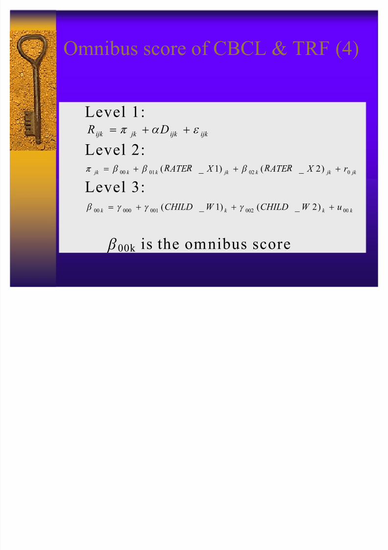
O mnibus score of CBCL & TRF (4)
Level 1:
ijk ijk jk ijk D R I ET !
Level 2: jk jk k jk k k jk r X ATE X ATE 00 20 100 )2 _ ()1 _ (! F F FT
Level 3:k k k k uW CHILDW CHILD 0000 200 100000 )2 _ ()1 _ (! K K K F
F00 k is the omnibus score

8/8/2019 HLM SSWR 2004
http://slidepdf.com/reader/full/hlm-sswr-2004 11/27
O mnibus score of CBCL & TRF (5)
Model 1
Level 1: ijk ijk jk ijk I T !
evel 2: jk k jk r 000! FT
evel 3: k k u 0000000 ! K F
F00 k is the omnibus score
8/8/2019 HLM SSWR 2004
http://slidepdf.com/reader/full/hlm-sswr-2004 12/27
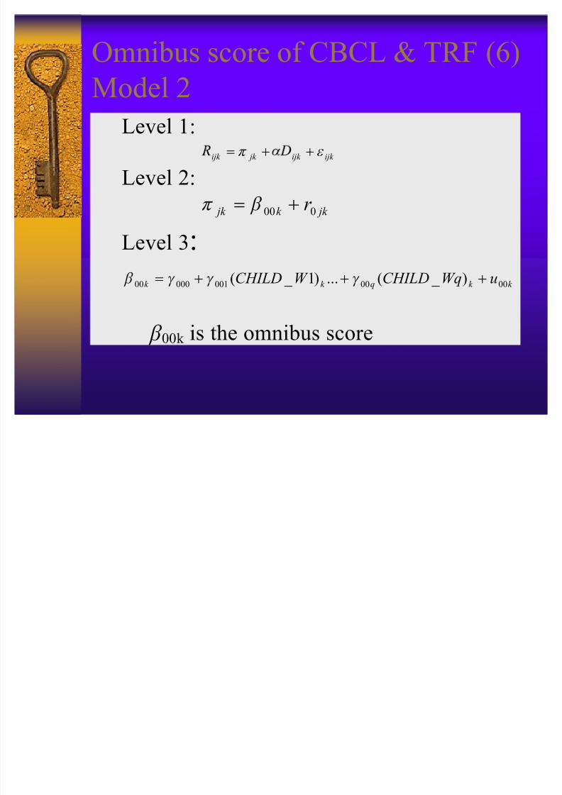
O mnibus score of CBCL & TRF (6)
Model 2Level 1:
ijk ijk jk ijk I T ! Level 2:
jk k jk r 000! FT
Level 3 :k k qk k uWqCHILDW CHILD 000000 100000 ) _ (...)1 _ (! K K K F
F00 k is the omnibus score

8/8/2019 HLM SSWR 2004
http://slidepdf.com/reader/full/hlm-sswr-2004 13/27
O mnibus score of CBCL & TRF (6)
Illustrating examplej Acknowledgment to Dr. Richard Barth and Ms.
Ariana Wall at UNC for their help.j Data: National Survey of Child and Adolescent Well-
being (NSC AW).j We focus on externalizing and internalizing scores.
Each child has four such scores: two from caregiver (CBCL), and two from teacher (TRF). The task: howto create one score?
j Variables employed in level 3 of Model 2: agegender, race, social behavior, MB A reading score,MB A math score, count of risky behaviors of delinquency, count of risky behaviors of substanceabuse, and count of risky behavior of suicidalattempt.

8/8/2019 HLM SSWR 2004
http://slidepdf.com/reader/full/hlm-sswr-2004 14/27
O mnibus score of CBCL & TRF (7)
__________________________________________________________________________ Ec Et Ic It
_______ _______ _______ _______ Externalizing rated by caregiver (E c) 1.000Externalizing rated by teacher (E t) .405** 1.000Internalizing rated by caregiver (I c) .639** .142** 1.000Internalizing rated by teacher (I t) .174** .476** .196** 1.000
Mean (S.D.) 60.8 (11.52) 58.7 (9.60) 57.3 (11.91) 56.0 (9.69)
__________________________________________________________________________ ** p < .01
Correlation coefficients and descriptivestatistics on disagreement betweencaregiver and teacher¶s scores (N=448)

8/8/2019 HLM SSWR 2004
http://slidepdf.com/reader/full/hlm-sswr-2004 15/27
O mnibus score of CBCL & TRF (8)
Evaluation Schemes:C1 Caregiver's scores only.5Ec + .5Ic
C2 Teacher's scores only.5Et + .5It
C3 All 4 scores from both versions with equal weights.25Ec + .25Ic + .25Et + .25It
C4 Similar to C3 but heavier weights giving to caregiver's sc.35Ec + .35Ic + .15Et + .15It
C5 Similar to C3 but heavier weights giving to teacher's score.15Ec + .15Ic + .35Et + .35It
C6 Similar to C3, a 5 0/ 50 split between caregiver and teacher scores but heavier weights giving to externalizing scores
.35Ec + .15Ic + .35Et + .15It

8/8/2019 HLM SSWR 2004
http://slidepdf.com/reader/full/hlm-sswr-2004 16/27

8/8/2019 HLM SSWR 2004
http://slidepdf.com/reader/full/hlm-sswr-2004 17/27
O mnibus score of CBCL & TRF (1 0 )
Evaluations ___________________________________________________________________________
Scheme Mean S.D. Minimum Maximum Correlation Coefficient ____________________________with Omnibus 1 with Omnibus 2
__________ ________ ________ ________ ________ ______________ ______________
Omnibus 1 60.56 3.29 52.30 69.21Omnibus 2 60.56 4.78 49.34 72.81 .707C1 59.03 10.61 32.00 82.50 .855 .700C2 57.32 8.29 39.50 80.00 .747 .406C3 58.18 7.63 39.00 78.25 1.000 .707C4 58.52 8.49 37.00 79.35 .966 .731C5 57.84 7.39 39.40 77.15 .955 .620
C6 58.79 7.90 39.30 77.60 .979 .702C7 57.57 7.69 37.20 79.35 .978 .681C8 53.00 8.22 32.00 74.00 .929 .656C9 63.36 8.21 41.50 82.50 .929 .657C10 57.74 8.09 37.50 76.50 .961 .698C11 58.62 7.81 39.00 81.00 .958 .658
___________________________________________________________________________
All correlation coefficients are statistically significant (p<.01)

8/8/2019 HLM SSWR 2004
http://slidepdf.com/reader/full/hlm-sswr-2004 18/27
O mnibus score of CBCL & TRF (11)Use the score as a dependent variable
______________________________________
Scheme Employed the score crea tedby the scheme
as an ou tcome variable
R2
______________________________________
Omnibus 1 .388
Omnibus 2 .987
C1 .431
C2 .147
C3 .388
C4 .434
C5 .293
C6 .388
C7 .361
C8 .337
C9 .337
C10 .383
C11 .332
______________________________________

8/8/2019 HLM SSWR 2004
http://slidepdf.com/reader/full/hlm-sswr-2004 19/27

8/8/2019 HLM SSWR 2004
http://slidepdf.com/reader/full/hlm-sswr-2004 20/27

8/8/2019 HLM SSWR 2004
http://slidepdf.com/reader/full/hlm-sswr-2004 21/27
Meta analysis using HLM (2)
Based on these data, calculate effect size:
And variance of the effect size:
Square root of V j is called ³standard error of d j´
jCj E j j S Y Y d /)(!
)](2/[)/()( 2C j Ej jC j EjC j Ej j nnd nnnnV !

8/8/2019 HLM SSWR 2004
http://slidepdf.com/reader/full/hlm-sswr-2004 22/27
Meta analysis using HLM (3)j General model
Level 1: d j = H j + e j
Level 2: H j = K0 + u j
or combined model: d j = K0 + u j + e j
where d j ~N( K0, ( j) with ( j = X+ V jj In this model, we only have one subscript j to
indicate study. This is a special case of two-
level model, in which subscript i is omitted,because we don¶t have original data at the studysubject level.
j V-known model: unlike previous HLM, this
model has known variance V j,or S.E.(d j)= V j.

8/8/2019 HLM SSWR 2004
http://slidepdf.com/reader/full/hlm-sswr-2004 23/27
Meta analysis using HLM (4)j Use HLM DOS version to run the v-
known model.j Data look like this:
1 .0 30 .0 16 2. 000
2 .12 0 .0 22 3. 000
3 -.14 0 .0 28 3. 000
««
19 -. 0 70 .0 30 3.000
Format of the raw data file: (a11,3f11.3)See HLM 5 manual pp. 221-226.

8/8/2019 HLM SSWR 2004
http://slidepdf.com/reader/full/hlm-sswr-2004 24/27
Meta analysis using HLM (5)
Ex peri m ental Studies of Teacher Ex pectancy E ffects on Pupil IQ
Study
E ffectSize
E sti m ated ¡
StandardE rror of
d ¡
Wee ks of Prior
Contact
1. Rosenthal et al. (1974) 0.030 0.126 2.0002. Conn et al. (1968) 0.120 0.148 3.0003. Jose & Cody (1971) -0.140 0.167 3.0004. Pellegrini & Hicks (1972) 1.180 0.373 0.0005. Pellegrini & Hicks (1972) 0.260 0.369 0.0006. Evans & Rosenthal (1969) -0.060 0.105 3.0007. Fielder et al. (1971) -0.020 0.105 3.0008. Claiborn (1969) -0.320 0.219 3.0009. Kester & Letchworth (1972) 0.270 0.164 0.000
10. Maxwell (1970) 0.800 0.251 1.00011. Carter (1970) 0.540 0.302 0.00012. Flowers (1966) 0.180 0.224 0.00013. Keshock (1970) -0.020 0.290 1.00014. Henrickson (1970) 0.230 0.290 2.00015. Fine (1972) -0.180 0.158 3.00016 reiger (1970) -0.060 0.167 3.00017. Rosenthal & Jacobson (1968) 0.300 0.138 1.00018. Fleming & Anttonen (1971) 0.070 0.095 2.000
19. insburg (1970) -0.070 0.173 3.000

8/8/2019 HLM SSWR 2004
http://slidepdf.com/reader/full/hlm-sswr-2004 25/27
Meta analysis using HLM (6)
Running HLM, we obtain the following findings:The estimated grand-mean effect size is0.084, implying that, on average, experimentalstudents scored about .084 standard deviation
units above the controls.However, the estimated variance of theeffect parameter is =.019. This correspondsto a standard deviation of .138 (i.e., .019 =
.138), which implies that important variabilityexists in the true-effect sizes. For example, aneffect one standard deviation above theaverage would be .084+.138=.222, which is of
nontrivial magnitude.

8/8/2019 HLM SSWR 2004
http://slidepdf.com/reader/full/hlm-sswr-2004 26/27
I n a cross-sectional study, we usecorrelation coefficients to see the level of association of an outcome variable with othervariables.
I n a longitudinal study, we have a similartask, that is, we need to model multivariatechange: whether two change trajectories(outcome measures) correlate over time?For details of this method, see MacCallum,
R.C., & Kim, C. (2000). Modelingmultivariate change , in Little, Schnabel, &Baumert edited, Modeling Longitudinal andMultilevel Data. Lawrence Erlbaum
Associates, pp.51-68.
Multivariate change (1)

8/8/2019 HLM SSWR 2004
http://slidepdf.com/reader/full/hlm-sswr-2004 27/27
W hat kind of questions can beanswered?
W hether benefits clients gained from anintervention over time negatively correlatewith the intervention s side effects?
W hether clients change in physical healthcorrelates with their change in mental health?
W hether a program s designed change inoutcome (e.g., abstinence from alcohol orsubstance abuse) correlates with clients levelof depression?
Use software MLn/MLwiN to estimatethe model. I t s possible to use SAS ProcMixed.
Multivariate change (2)