Evaluasi pada Iterative Learning Control
175
Iterative Learning Control —a critical review—
-
Upload
jadur-rahman -
Category
Documents
-
view
222 -
download
0
Transcript of Evaluasi pada Iterative Learning Control

8/8/2019 Evaluasi pada Iterative Learning Control
http://slidepdf.com/reader/full/evaluasi-pada-iterative-learning-control 1/175
Iterative Learning Control
—a critical review—

8/8/2019 Evaluasi pada Iterative Learning Control
http://slidepdf.com/reader/full/evaluasi-pada-iterative-learning-control 2/175
This thesis has been completed in partial fulfillment of the
requirements of the Dutch Institute of Systems and Control(DISC) for graduate study.
DISCThe research described in this thesis was undertaken at thedepartments of Electrical Engineering and Applied Mathe-matics, University of Twente, Enschede, with financial sup-port from the ‘Duits-Nederlands Mechatronica Innovatie Cen-
trum’.
Mechatronica
Innovatie
Centrum
No part of this work may be reproduced by print, photocopyor any other means without the permission in writing fromthe author.
Printed by Wohrmann Print Service, The Netherlands.
ISBN: 90-365-2133-5
c 2005 by M.H.A. Verwoerd

8/8/2019 Evaluasi pada Iterative Learning Control
http://slidepdf.com/reader/full/evaluasi-pada-iterative-learning-control 3/175
ITERATIVE LEARNING CONTROL
—A CRITICAL REVIEW—
PROEFSCHRIFT
ter verkrijging van
de graad van doctor aan de Universiteit Twente,op gezag van de rector magnificus,prof. dr. W. H. M. Zijm,
volgens besluit van het College voor Promoties,in het openbaar te verdedigen
op donderdag 13 januari 2005 om 15.00 uur
door
Markus Hendrik Adriaan Verwoerdgeboren op 16 November 1977
te Woerden, Nederland
8/8/2019 Evaluasi pada Iterative Learning Control
http://slidepdf.com/reader/full/evaluasi-pada-iterative-learning-control 4/175
Dit proefschrift is goedgekeurd door:
prof. dr. ir. J. van Amerongen, promotor
dr. ir. T.J.A. de Vries, assistent-promotor
dr. ir. G. Meinsma, assistent-promotor
8/8/2019 Evaluasi pada Iterative Learning Control
http://slidepdf.com/reader/full/evaluasi-pada-iterative-learning-control 5/175
Voorwoord
“Ik had zo graag dat het tussen u en mij niet werd tot een tran-sigeren wat er in kan blijven en wat er uit moet, maar dat u juist degrondgedachten, dus veel meer het algemene, dan het speciale, datwat tussen de regels staat, zoudt aanvoelen en erkennen.”
—L. Brouwers, in een brief aan zijn promotor.
“Spijt in verband met onze slechte kunst is even ongewenst als spijt in ver-band met ons slecht gedrag. De slechtheid moet worden opgespoord, erkenden zo mogelijk in de toekomst worden vermeden. Tobben over de literairetekortkomingen van twintig jaar geleden [...] is ongetwijfeld ijdel en zin-loos.”—Aan deze woorden van Aldous Huxley, geschreven bij de heruitgavevan zijn beroemde Heerlijke Nieuwe Wereld (Brave New World ) moest ikde laatste dagen herhaaldelijk denken. De aanleiding laat zich raden.
Nu maak ik mij wat dit proefschrift betreft overigens geen illusies: vaneen heruitgave zal het waarschijnlijk nooit komen. Toch was daar ook bijmij die angst, dat gevoel van potentiele schaamte. Wat nu als het allemaal‘onzin’ blijkt; als blijkt dat ik, gedreven door naıef idealisme en wat al nietmeer, de plank volledig misgeslagen heb?
Ik besef nu dat dit verkapte ijdelheid is. We moeten, om nogmaals Huxleyaan te halen, “niet de kracht van ons leven gebruiken om de artistieke zondente herstellen die begaan en nagelaten zijn door de ander die we in onze jeugdwaren”. Het is aldus met vrijmoedigheid dat ik dit proefschrift, hetwelkniettegenstaande de zorg eraan besteed vele onvolkomenheden bevat, in uw,de lezers, handen leg.
Het past mij een aantal mensen te bedanken. In de eerste plaats mijnbegeleiders: prof. Job van Amerongen, voor de ruimte die hij mij liet, ook
toen gaandeweg bleek dat mijn onderzoek geen antwoord ging bieden opde vraag waar ik mee van start was gegaan; dr. Theo de Vries, die als eenAaron optrad als niet spreken kon, voor de aanvankelijk dagelijkse en laterwekelijkse begeleiding, alsmede voor de fijne gesprekken, de mentale onder-steuning en de soms niet malse maar altijd eerlijke behandeling; dr. Gjerrit
v

8/8/2019 Evaluasi pada Iterative Learning Control
http://slidepdf.com/reader/full/evaluasi-pada-iterative-learning-control 6/175
Meinsma, voor de wiskundige begeleiding en de voor zijn persoon zo ty-pische positief-cynische levenshouding en zijn aan zelfverachting grenzendebescheidenheid (“ik ben een sukkel”, “ik heb geen geheugen”); prof. Arjanvan der Schaft, inspirator, voor zijn algemene betrokkenheid bij het project,
de fascilitaire ondersteuning (totdat een brand een einde maakte aan mijnzwerftocht bij TW ben ik in twee jaar tijd vier keer verhuisd, heeft eenvoormalig SSB-er mijn papers bij het oud papier gezet en heb ik vele wekennoodgedwongen in de bibliotheek doorgebracht) en zijn kritische suggesties,waarmee hij mij bij het schrijven voor al te veel wolligheid heeft behoed.
Thanks also to professors Kevin Moore and Yang Quan Chen for theirinterest in my work, and for their kind hospitality, which made my stay atUtah State a pleasant one.
Een woord van dank aan mijn collega’s bij EL, voor de uitstekende sfeerbinnen de vakgroep. Als ik om inspiratie verlegen zat of zomaar even eenpraatje wilde maken, kon ik altijd wel ergens terecht. Dat heeft mij goedgedaan, met name toen het schrijven maar niet lukken wilde. In dit ver-band wil ik in het bijzonder bedanken mijn beide paranimfen, PhilippusFeenstra en Vincent Duindam. In Philippus vond ik een collega met wieik meer kon delen dan een kamer alleen. Zijn open, eerlijke houding enbescheiden, nuchtere manier van doen bewaarden mij voor hemelbestor-mend gedrag en deden mij, als dat nodig was, de betrekkelijkheid van onsgezwoeg waarderen. Met Vincent deel ik, naast een wat ongebruikelijkewiskundige orientatie en een niet nader te noemen tic, de herinnering aaneen drietal vakanties en een tachtigtal tennislessen. Het ontwerp voor deomslag is van zijn hand. Van mijn collega’s bij TW wil ik in het bijzon-
der noemen Viswanath Talasila en Stefan Strubbe. Van alle mensen heefteerstgenoemde het meest bijgedragen aan mijn ontwikkeling als wetenschap-per. Buiten ons onderzoek om spraken we over uiteenlopende onderwer-pen als wiskunde, fysica, filosofie en religie, maar toch nog het meest overwetenschap in het algemeen. Stefan wil ik bedanken voor zijn invloed opmijn ontwikkeling als mens. Als scholieren vonden we elkaar in onze passievoor computers. Die liefde hebben we inmiddels ten grave gedragen, maardaarmee gelukkig niet onze vriendschap. We hebben door de jaren heenveel kunnen delen en ik hoop dat we dat ook in de toekomst kunnen blijvendoen.
Vele vrienden, huisgenoten en ex-huisgenoten hebben er direct of indirect,middels telefoontjes, SMSjes, emailtjes of anderszins, toe bijgedragen dat ikdit project tot een goed einde brengen kon. Ik ben hen zeer erkentelijk.
I would like to thank my international friends, for granting me, a foreigner,the privilege to play a part in their lifes. Thanks to all members and former
vi
8/8/2019 Evaluasi pada Iterative Learning Control
http://slidepdf.com/reader/full/evaluasi-pada-iterative-learning-control 7/175
members of BS-Twente, for their spiritual support, prayers, friendship andencouragement in times of need. Special thanks to Mr. P, Arun, Helena,Imelda, Mirjam, Sheela, and Velma.
In dit alles dank ik God, mijn familie niet vergetend. Moeder en broer,
bedankt voor alle steun; dit proefschrift zij aan jullie opgedragen.
vii

8/8/2019 Evaluasi pada Iterative Learning Control
http://slidepdf.com/reader/full/evaluasi-pada-iterative-learning-control 8/175
viii

8/8/2019 Evaluasi pada Iterative Learning Control
http://slidepdf.com/reader/full/evaluasi-pada-iterative-learning-control 9/175
Samenvatting
Iterative Learning Control (ILC) is een regelmethode, ontworpen om inuiteenlopende regelsituaties repetiviteit uit te buiten. Haar doel is prestatiete verbeteren middels een mechanisme van trial and error . De veronder-stelling is dat ILC in staat zou zijn dit doel te realiseren. In dit proefschriftwordt onderzocht of dit potentieel aanwezig is en ook daadwerkelijk wordtbenut. Daartoe wordt een vergelijk gemaakt tussen ILC en niet-iteratieve,
conventionele methoden, in het bijzonder methoden gebaseerd op feedback .De discussie concentreert zich op een klasse van lineaire, eerste-orde recur-rentievergelijkingen met constante coefficienten, geparameteriseerd door eentweetal begrensde lineaire operatoren. Het probleem van ILC wordt opgevatals een optimalisatieprobleem over de ruimte van begrensde lineaire opera-torparen. Twee gevallen worden behandeld: causale ILC en niet-causaleILC.
Bij causale ILC worden beide operatoren begrensd verondersteld. Ditblijkt de maximaal haalbare prestatie te schaden. Onder deze aannametransformeert het ILC syntheseprobleem in een compensator ontwerppro-bleem en blijken de respectievelijke methoden van causale ILC en conven-
tionele feedback equivalent. Het voornaamste resultaat, dat teruggaat ophet principe van Equivalent Feedback stelt dat er met ieder element in deverzameling van causale iteraties een causale terugkoppelafbeelding corres-pondeert, welke dezelfde prestatie geeft als het ILC algoritme, echter zondergebruik te maken van iteraties.
Bij niet-causale ILC vervalt de causaliteits-eis: operatoren mogen ookniet-causaal zijn. Deze extra ontwerpvrijheid blijkt met name nuttig insituaties waarin systemen voorkomen met een hoge relatieve graad of niet-minimumfase gedrag. In zulke situaties blijkt niet-causale ILC de prestatieten opzichte van conventionele methoden aanzienlijk te kunnen verbeteren.
Wat betreft het algemene probleem van iteratief- en lerend regelen: ditproefschrift betoogt dat de klasse van recurrentievergelijkingen met con-stante coefficienten niet geschikt is om adaptatie te implementeren and dat,wanneer modelonzekerheid een probleem wordt, een overschakeling op recur-rentievergelijkingen met variabele coefficienten dient te worden overwogen.
ix

8/8/2019 Evaluasi pada Iterative Learning Control
http://slidepdf.com/reader/full/evaluasi-pada-iterative-learning-control 10/175
x

8/8/2019 Evaluasi pada Iterative Learning Control
http://slidepdf.com/reader/full/evaluasi-pada-iterative-learning-control 11/175
Summary
Iterative Learning Control (ILC) is a control method designed to exploitrepetitiveness in various control situations. Its purpose is to enhance perfor-mance, using a mechanism of trial and error. Supposedly, the method wouldhave considerable potential to effect this purpose. The aim of this thesis isto investigate whether this potential is really there, and if so, whether it isindeed being capitalized on. To that end, a comparison is drawn between
ILC and conventional, noniterative methods, such as feedback control.The discussion focuses on a class of constant-coefficient linear first-orderrecurrences, parameterized by a pair of bounded linear operators. Accord-ingly, the problem of ILC is cast as an optimization problem on the space of bounded linear operator pairs. Two cases are considered: Causal ILC andNoncausal ILC.
In Causal ILC both operators are assumed causal. This assumptionproves restrictive as it impairs the achievable performance. It turns theILC synthesis problem into a compensator design problem, and rendersthe respective methods of Causal ILC and conventional feedback controlequivalent. The main result, which pertains to the principle of Equivalent
Feedback states that to each element in the set of causal iterations, therecorresponds a particular causal feedback map, the Equivalent Controller,which delivers the exact same performance as the ILC scheme, yet withouta need to iterate. The converse result is shown to hold true provided certainconditions on the current cycle operator are met.
In Noncausal ILC, causality constraints do not apply, and noncausal op-erators are allowed. This extra design freedom proves particularly useful inthe context of systems with high relative degree and non-minimum phase be-havior, where noncausal ILC is shown to significantly enhance performance,as compared to e.g. conventional feedback control.
As regards the general problem of learning control and the use of itera-tion, this thesis argues that the class of constant-coefficient recurrences isincapable of implementing adaptive behavior and that variable-coefficientrecurrences, i.e. trial-dependent update laws ought be considered wouldmodel uncertainty become an issue.
xi

8/8/2019 Evaluasi pada Iterative Learning Control
http://slidepdf.com/reader/full/evaluasi-pada-iterative-learning-control 12/175
xii
8/8/2019 Evaluasi pada Iterative Learning Control
http://slidepdf.com/reader/full/evaluasi-pada-iterative-learning-control 13/175
Contents
1. Learning Control: an introduction 1
1.1. Introduction . . . . . . . . . . . . . . . . . . . . . . . . . . . 1
1.2. From Ktesibios to Turing: on the evolution of the autonomousmachine . . . . . . . . . . . . . . . . . . . . . . . . . . . . . 2
1.2.1. Feedback Control: the first generation of autonomousmachines . . . . . . . . . . . . . . . . . . . . . . . . . 2
1.2.2. AI and the second generation of autonomous machines 5
1.3. Iterative Learning Control: a first acquaintance . . . . . . . 7
1.3.1. Iterative Learning Control . . . . . . . . . . . . . . . 7
1.3.2. The problem of ILC . . . . . . . . . . . . . . . . . . 8
1.4. Problem Statement: Iterative Learning vs. Conventional Feed-back Control . . . . . . . . . . . . . . . . . . . . . . . . . . . 10
1.4.1. Problem Statement . . . . . . . . . . . . . . . . . . . 11
1.5. Outline . . . . . . . . . . . . . . . . . . . . . . . . . . . . . . 12
2. Iterative Learning Control: an overview 15
2.1. Basic framework: preliminaries, notation and terminology . . 15
2.1.1. Signals and systems: H2 and H∞ . . . . . . . . . . . 15
2.1.2. Convergence . . . . . . . . . . . . . . . . . . . . . . . 18
2.1.3. Recurrence relations and iterations . . . . . . . . . . 24
2.1.4. Fixed points and contraction operators . . . . . . . . 26
2.2. Literature overview . . . . . . . . . . . . . . . . . . . . . . . 27
2.2.1. Brief history . . . . . . . . . . . . . . . . . . . . . . . 27
2.2.2. Conceptual frameworks—paradigms for learning control 30
2.3. ILC: a two-parameter synthesis problem . . . . . . . . . . . 37
2.3.1. The problem statement . . . . . . . . . . . . . . . . . 38
2.3.2. The Standard ILC Problem . . . . . . . . . . . . . . 40
2.3.3. ILC with current-cycle feedback . . . . . . . . . . . . 41
2.4. Summary and preview . . . . . . . . . . . . . . . . . . . . . 42
xiii

8/8/2019 Evaluasi pada Iterative Learning Control
http://slidepdf.com/reader/full/evaluasi-pada-iterative-learning-control 14/175
Contents
3. Causal ILC and Equivalent Feedback 433.1. Introduction . . . . . . . . . . . . . . . . . . . . . . . . . . . 433.2. Fixed Point Analysis . . . . . . . . . . . . . . . . . . . . . . 44
3.2.1. Fixed point stability . . . . . . . . . . . . . . . . . . 44
3.2.2. Fixed points and the problem of ILC . . . . . . . . . 453.3. The set of admissible pairs . . . . . . . . . . . . . . . . . . . 463.4. Standard ILC and Equivalent Feedback . . . . . . . . . . . . 48
3.4.1. Necessary and sufficient conditions for admissibility . 483.4.2. Equivalent admissible pairs . . . . . . . . . . . . . . 523.4.3. Equivalent Feedback . . . . . . . . . . . . . . . . . . 553.4.4. The synthesis problem revisited . . . . . . . . . . . . 573.4.5. Causal ILC, Equivalent Feedback and Noise . . . . . 61
3.5. Extensions to CCF-ILC . . . . . . . . . . . . . . . . . . . . 643.5.1. Equivalent feedback . . . . . . . . . . . . . . . . . . . 65
3.6. Experimental verification . . . . . . . . . . . . . . . . . . . . 693.6.1. The Experimental setup: the Linear Motor Motion
System . . . . . . . . . . . . . . . . . . . . . . . . . . 693.6.2. Experiment Design . . . . . . . . . . . . . . . . . . . 713.6.3. Implementation details . . . . . . . . . . . . . . . . . 723.6.4. Results . . . . . . . . . . . . . . . . . . . . . . . . . . 73
3.7. Discussion . . . . . . . . . . . . . . . . . . . . . . . . . . . . 773.7.1. Causal ILC and equivalent feedback . . . . . . . . . . 783.7.2. Noncausal ILC . . . . . . . . . . . . . . . . . . . . . 78
4. Noncausal ILC 79
4.1. Introduction . . . . . . . . . . . . . . . . . . . . . . . . . . . 794.2. Noncausal ILC . . . . . . . . . . . . . . . . . . . . . . . . . 80
4.2.1. Literature on Noncausal ILC . . . . . . . . . . . . . . 804.2.2. Introduction: a motivation . . . . . . . . . . . . . . . 814.2.3. Perfect Tracking and the Sensitivity Integral . . . . . 844.2.4. Non-minimum phase plants and Poisson’s Integral . . 88
4.3. Equivalent Feedback . . . . . . . . . . . . . . . . . . . . . . 914.3.1. Admissible pairs . . . . . . . . . . . . . . . . . . . . 914.3.2. Equivalent Feedback . . . . . . . . . . . . . . . . . . 924.3.3. A 2D ‘Equivalent Control’ Configuration . . . . . . . 93
4.4. Discussion . . . . . . . . . . . . . . . . . . . . . . . . . . . . 944.A. Preliminaries: Noncausal operators . . . . . . . . . . . . . . 954.A.1. Notation and Terminology . . . . . . . . . . . . . . . 954.A.2. Noncausal operators on [0, T ] . . . . . . . . . . . . . 984.A.3. A contraction on L2[0, T ] . . . . . . . . . . . . . . . . 99
xiv
8/8/2019 Evaluasi pada Iterative Learning Control
http://slidepdf.com/reader/full/evaluasi-pada-iterative-learning-control 15/175
Contents
4.A.4. Implementation issues . . . . . . . . . . . . . . . . . 101
5. Learning and adaptation: trial-dependent update rules 1055.1. Introduction . . . . . . . . . . . . . . . . . . . . . . . . . . . 1065.2. The problem of Learning Control . . . . . . . . . . . . . . . 107
5.2.1. Performance, performance robustness and learning . . 1075.2.2. Adaptation, Iteration, and Learning . . . . . . . . . . 109
5.3. On trial-dependent update laws . . . . . . . . . . . . . . . . 1125.3.1. Motivation . . . . . . . . . . . . . . . . . . . . . . . . 1125.3.2. A class of trial-dependent update laws . . . . . . . . 1125.3.3. Non-contractive, trial-dependent update laws . . . . . 1155.3.4. Adaptive update schemes . . . . . . . . . . . . . . . 118
5.4. Discussion . . . . . . . . . . . . . . . . . . . . . . . . . . . . 1245.4.1. Brief review . . . . . . . . . . . . . . . . . . . . . . . 1245.4.2. Conclusion . . . . . . . . . . . . . . . . . . . . . . . . 125
5.A. Proofs . . . . . . . . . . . . . . . . . . . . . . . . . . . . . . 126
6. Discussion and Conclusion 1316.1. Some general remarks . . . . . . . . . . . . . . . . . . . . . . 131
6.1.1. A critique? . . . . . . . . . . . . . . . . . . . . . . . 1316.1.2. First-order recurrences and the problem of Learning
Control . . . . . . . . . . . . . . . . . . . . . . . . . 1326.2. Conclusion . . . . . . . . . . . . . . . . . . . . . . . . . . . . 132
6.2.1. Main Results . . . . . . . . . . . . . . . . . . . . . . 1326.2.2. Conclusions . . . . . . . . . . . . . . . . . . . . . . . 139
A. Bibliography 143
Index 151
xv

8/8/2019 Evaluasi pada Iterative Learning Control
http://slidepdf.com/reader/full/evaluasi-pada-iterative-learning-control 16/175
Contents
xvi

8/8/2019 Evaluasi pada Iterative Learning Control
http://slidepdf.com/reader/full/evaluasi-pada-iterative-learning-control 17/175
1
Learning Control: an introduction
Overview – We provide a historical perspective on the evolutionof (Intelligent) Control. Starting from the very first self-regulating mechanism, we track the developments leading to the birth of cy-bernetics, into the era of intelligent machines. Within this context
we introduce and motivate the concept of Learning Control. We outline the central problem, scope and aim of the thesis.
1.1. Introduction
“The extent to which we regard something as behaving in an intel-ligent manner is determined as much by our own state of mind and
training as by the properties of the object under consideration.”
—Alan Turing
Expressed in the most humble of terms, Intelligent Control (IC) stands fora variety of biologically motivated techniques for solving (complex) controlproblems. Situated within the IC paradigm, Learning Control draws itsparticular inspiration from man’s ability to learn . More precisely, it is basedon the idea that machines can, to some extent, emulate this behavior.
Over the years, the question whether machines really can learn has at-tracted quite some debate. Basically, one can take either of three views:
that of the believer, who attests to the possibility; that of the agnost, whoholds it not impossible; and that of the skeptic, who endeavors to prove theopposite.
This issue, however important, falls outside the scope of this thesis. Forwhat it is worth, we do believe that at least some aspects of learning can
1
8/8/2019 Evaluasi pada Iterative Learning Control
http://slidepdf.com/reader/full/evaluasi-pada-iterative-learning-control 18/175
1. Learning Control: an introduction
be mimicked by engineering artifacts. But the important question, as far asthis thesis is concerned, is not whether machines can learn , but whether theycan exploit repetitiveness in a useful way. In this respect, our perception of learning is relevant only in as far as it helps us in deciding what is useful
and what is not.There is no doubt the use of iteration holds considerable potential, if onlyas a means to improve control performance. It is the aim of this thesis tofind out how, in the context of Learning Control, iteration is being deployedas well as how it could be deployed; in other words, to determine whetherthe aforementioned potential is being capitalized on. To that end, we draw acomparison between Iterative Learning Control (ILC), and its non-iterativecounterpart, Conventional Feedback Control (CFC).
1.2. From Ktesibios to Turing: on the evolution
of the autonomous machine
It needs no argument that Learning Control and Conventional FeedbackControl differ in many respects. Yet, one thing links them together, andthat is their role in the development of autonomous mechanisms. Before wezoom in on their distinctive features, let us presently consider their collectivepast.
1.2.1. Feedback Control: the first generation of
autonomous machines“The ‘trick’ of using negative feedback to increase the precision of
an inherently imprecise device was subtle and brilliant.”
—Dennis S. Bernstein
Ktesibios and the water clock
Ever since antiquity, and possibly long before, man has been intrigued bythe idea of autonomous machines. A good example, and one of the first
at that, is the self-regulating water clock—Uber (2004). The water clock(Clepsydra ) is an ancient Egyptian invention dating back to around 1500B.C. It consists of two vessels. The first vessel, having a small apertureat the bottom, drops water into a second, lower vessel, at a supposedlyconstant rate. The indication of time is effected by marks that correspond
2

8/8/2019 Evaluasi pada Iterative Learning Control
http://slidepdf.com/reader/full/evaluasi-pada-iterative-learning-control 19/175
1.2. From Ktesibios to Turing: on the evolution of the autonomous machine
to either the diminuition of water in the supplying vessel, or the increase of water in the receiving vessel.
First-generation water clocks were not very effective—not as a means fortimekeeping, that is. For as it turns out, the water flow is much more rapid
when the supplying vessel is full, than when it is nearly empty (owing tothe difference in water pressure).
It was Ktesibios from Alexandria, who perfected the design by adding acrucial ingredient. Ktesibios, a barber by profession who eventually becamean engineer under Ptolomy II, lived in the third century B.C. A contem-porary of Euclid and Archimedes, he is credited with the invention of thepump, the water organ and several kinds of catapults. Confronted withthe water clock problem, Ktesibios developed a self-regulating valve. Thevalve is comprised of a “cone-shaped float” and a “mating inverted fun-nel”—Kelly (1994). In a normal situation, water flows through the valve,down from the funnel, over the cone, into a bowl. As water comes in and
fills the bowl, the cone floats up into the funnel, blocking the passage. Asthe water diminishes, the float sinks, allowing more water to enter.
The self-regulating valve served its purpose well. And with that, thewater clock became a milestone in the history of Control Theory, even “thefirst nonliving object to self-regulate, self-govern, and self-control”, “thefirst self to be born outside of biology”—Kelly (1994).
Cornelis J. Drebbel and the thermostat
Cornelis Drebbel was a Dutch alchemist and self-made engineer. He is
known for his work on submarines (first prototype in 1620), optics, anddyeing, not to mention his perpetual mobile. His more modest (but no lessuseful) inventions include the thermostat, which, it is said, he thought outwhile trying to forge gold from lead, identifying temperature fluctuationsas the main cause for failure. To counteract these fluctuations, he came upwith the idea to manipulate the combustion process by regulating the air(oxygen) supply; onto one side of the furnace, he mounted “a glass tube [. . . ]filled with alcohol. When heated, the liquid would expand, pushing mercuryinto a connecting, second tube, which in turn would push a rod that wouldclose an air draft on the stove. The hotter the furnace, the further the draft
would close, decreasing the fire. The cooling tube retracted the rod, thusopening the draft and increasing the fire”—Kelly (1994).
Like Ktesibios’ valve, Drebbel’s thermostat is completely autonomous.Strikingly simple and yet very effective, it provides an excellent example of what feedback control can do.
3

8/8/2019 Evaluasi pada Iterative Learning Control
http://slidepdf.com/reader/full/evaluasi-pada-iterative-learning-control 20/175
1. Learning Control: an introduction
James Watt and the self-regulating governor
James Watt (1736-1819), scottish inventor and mechanical engineer, is of-ten credited with the invention of the steam engine. In actual fact, the
steam engine was invented by Thomas Savery and Thomas Newcomen.But like Ktesibios before him, Watt greatly improved on an existing de-sign. Most notably, he came up with the idea of using a separate con-densing chamber, which greatly enhanced both the engine’s power and itsefficiency—Bernstein (2002). But that was not his only contribution: therotary motion of existing steam engines suffered from variations in speed,which limited their applicability. Adapting a design by Mead, Watt develo-ped a mechanism we now know as the Watt governor . The Watt governeris basically a double conical pendulum which, through various levers andlinkages, connects to a throttle valve. The shaft of the governor is spun bythe steam engine. As it spins, centrifugal force pushes the weights outward,
moving linkages that slow the machine down. As the shaft slows down,the weights fall, engaging the throttle that speeds the engine up. Thus thegovernor forces the engine to operate at a constant and consistent speed.
Feedback as a universal principle
The central notion embodied in the work of Ktesibios, Drebbel and Wattis that of feedback . Roughly speaking, the purpose of feedback, as far as
regulators are concerned, is to counteract change, whether this be changein rate of flow, change in temperature, or change in rotational velocity.
An invisible thread through history, feedback has had a tremendous im-pact on the advancement of technology, a fact to which also the 20th centurytestifies. In the late 1920s Harold Black, an engineer at Bell Labs, intro-duced (negative) feedback to suppress the effect of gain variations and non-linear distortions in amplifiers—Bennett (1979); Bernstein (2002). A fewyears later, when World War II necessitated a rapid technological advance,feedback was at the heart of it.
By that time, feedback had become a universal concept and was recog-
nized as one of the most powerful ideas in the general science of systems.Researchers in psychology, (neuro)physiology, mathematics, and computerscience combined forces to conclude that there must be some commonmechanism of communication and control in man and machine. It wastime for cybernetics.
4

8/8/2019 Evaluasi pada Iterative Learning Control
http://slidepdf.com/reader/full/evaluasi-pada-iterative-learning-control 21/175
1.2. From Ktesibios to Turing: on the evolution of the autonomous machine
1.2.2. AI and the second generation of autonomousmachines
“Let us then boldly conclude that man is a machine, and that inthe whole universe there is but a single substance differently modi-fied.”
—Julien Offray de La Mettrie
Cybernetics
The period after the war saw the birth of cybernetics. One of the pioneers inthis area was Norbert Wiener, who, apart from his contributions to mathe-matics proper, is best known for his book entitled ‘Cybernetics, or Controland Communication in the Animal and the Machine’. On the website of
Principia Cybernetica (2004), it is related how Wiener developed some of his ideas. While working on a design of an automatic range finder (a ser-vomechanism for predicting the trajectory of an airplane on the basis of past measurements) Wiener was struck by two facts: (a) the seemingly in-telligent behavior of such machines, i.e. their ability to deal with experienceand to anticipate the future; (b) the ‘diseases’ (certain defects in perfor-mance) that could affect them. Conferring with his friend Rosenbluth, whowas a neurophysiologist, he learned that similar behavior was to be found inman. From this he concluded that in order to allow for purposeful behavior,the path of information inside the human body must form “a closed loopallowing the evaluation of the effects of one’s actions and the adaptation of
future conduct based on past performances”.In other words, Wiener saw a clear parallel between the self-regulating
action in machines and that in man. Purposeful behavior was to be ex-plained in terms of (negative) feedback. The same idea took shape in thework of Warren McCullogh a psychologist perhaps best known for his workon neural networks. In a paper entitled ‘machines that want and think’,McCullogh uses the governor (see Section 1.2.1) as a metaphor for self-regulation in the human body. He writes: “Purposive acts cease when theyreach their ends. Only negative feedback so behaves and only it can set thelink of a governor to any purpose.”
This unifying view on man and machine is not unique to Cybernetics.Throughout history, mankind has attempted to explain itself in terms of metaphors derived from once current technology. Examples include clocks,steam engines, and switchboards—Maessen (1990). But it was not until theadvent of analog and digital computing (the age of cybernetics) that these
5
8/8/2019 Evaluasi pada Iterative Learning Control
http://slidepdf.com/reader/full/evaluasi-pada-iterative-learning-control 22/175
1. Learning Control: an introduction
metaphors became sophisticated enough to threaten man’s superiority andhis exclusive rights to intelligence.
Intelligent machinery—Alan TuringLong before Darwin stepped up to challenge man’s position among otherliving beings, Julien de La Mettrie boldly concluded that “man is a machine,and that in the whole universe there is but a single substance differentlymodified”. During the 19th century, the prevailing thought that man heldspecial position in the whole of creation, slowly began to lose ground. Ina 1948 article entitled ‘intelligent machinery’ (Turing (1968)), Alan Turingtakes up the question whether it is possible for machinery to show intelligentbehavior. In those days, the common opinion was that it is not (“It isusually assumed without argument that it is not possible”). Turing explains
that this negative attitude is due to a number of reasons, varying from theunwillingness of man to give up their intellectual superiority, to Godel’sTheorem, to religious belief, and from the limitations of the then currentmachinery to the viewpoint that every intelligence is to be regarded as areflection of that of its creator. He goes on to refute each one of them.Most notably, he likens the view that intelligence in machinery is merely areflection of that of its creator to the view that the credits for a discovery of a pupil should be given to his teacher. “In such a case the teacher would bepleased with the success of his methods of education, but would not claimthe results themselves, unless he had actually communicated them to hispupil.”
Constrasting the common opinion, Turing argues that there is good reasonto believe in the possibility of making thinking machinery. Among otherthings, he points to the fact that it is possible to make machinery to imitate“any small part of man”. He mentions examples of machine vision (camera),machine hearing (microphone), and machine motion (remotely controlledrobots that perform certain balancing tasks). Rejecting the most sure wayof building a thinking machine (taking a man as a whole and replacing allparts of him by machinery) on grounds of impractability, Turing proposesa research program, slightly less ambitious, and arguably more feasible,namely to build a “brain, which is more or less without a body, providing
at most organs of sight, speech, and hearing”.This very program formed the basis for a new branch of science, whichtoday is called by the name Artificial Intelligence (AI). Turing himself didnot live to witness the full impact of his ideas. He died in 1954, leaving hiswork as a legacy for future generations of researchers.
6

8/8/2019 Evaluasi pada Iterative Learning Control
http://slidepdf.com/reader/full/evaluasi-pada-iterative-learning-control 23/175
1.3. Iterative Learning Control: a first acquaintance
1.3. Iterative Learning Control: a first
acquaintance
As we picture a team of robots lined up alongside some conveyor belt in
a manufacturing plant, performing the exact same operation over and overagain, it occurs to us that if we could find a way to enhance each robot’sperformance, the plant could operate at higher speed, which would effecta higher throughput. One way or another, we ought to be able to exploitrepetitiveness.
1.3.1. Iterative Learning Control
Learning Control comes in many flavors; flavors, which differ mainly in theway they represent knowledge (e.g. using neural networks or other data
structures) as well as in how they update the stored information. In thisthesis we focus on the particular methodology that goes by the name of Iter-ative Learning Control (ILC). For a detailed overview of the ILC literature,we refer to the next chapter. Here, a brief sketch will suffice.
Where Learning Control would merely assume successive control tasksto be related , ILC assumes them to be identical . In addition, ILC assumesa perfect reset after each trial (iteration, execution, run), so as to ensurethat the system can repeatedly operate on the same task under the sameconditions. This latter assumption can be relaxed, for several studies (seefor instance Arimoto et al. (1986); Lee and Bien (1996)) have shown that,although resetting errors generally deteriorate performance, they do not rule
out the possibility of ‘learning’ altogether.ILC is concerned with a single control task. Consequently, all informa-
tion is typically encoded as a function of a single parameter: time. Thedesired behavior (output) is defined accordingly. Extensions based on moreelaborate data structures have been considered. Most notably, Learning Feed-Forward Control (LFFC, Velthuis (2000); de Kruif (2004)) encodes allinformation as a function of a virtual state vector (which may have position,velocity, and acceleration among its components). The obvious advantage of LFFC (over ILC) is that it renders the condition on strict trial-to-trial repe-tition obsolete. A disadvantage is that the method requires less transparent
data structures, and significantly more complex techniques for storage andretrieval. Another, related, approach is that of Direct Learning Control (DLC)—Xu (1996); Xu and Zhu (1999). Given two output trajectories,identical up to an arbitrary scaling in time and/or magnitude, the problemof DLC is to construct the input corresponding to the one using the input
7
8/8/2019 Evaluasi pada Iterative Learning Control
http://slidepdf.com/reader/full/evaluasi-pada-iterative-learning-control 24/175
1. Learning Control: an introduction
corresponding to the other, without resorting to repetition (hence, direct ).
Iterative Learning Control has been applied in various industrial set-tings, usually as an add-on to existing control algorithms. Examples in-clude, among others, wafer stages—de Roover and Bosgra (2000), wel-
ding processes—Schrijver (2002); Naidu et al. (2003), and robot manipula-tors—Kavli (1992). For more information on ILC applications, we refer toBien and Xu (1998) and references therein.
1.3.2. The problem of ILC
“The real problem is not whether machines think, but whetherman do”
—B.F. Skinner
We learned that ILC is about enhancing a system’s performance by meansof repetition , but we did not learn how it is done. This bring us to the coreactivity in ILC research, which is the construction and subsequent analysisof algorithms.
ILC starts from a qualitative description of a learning behavior . Theproblem is to find an algorithm which implements it. As this is not aneasy problem, let us outline what features such an algorithm should have.Indeed, let us take a step back, and ask: “What is the need for (Iterative)Learning Control? ” Admitted, certain applications simply seem to ask forLearning Control, particularly those with a pronouncedly cyclic operational
component. But as a motivation, this does not suffice, since it does not ex-plicate a need. Part of this need becomes apparent when we concentrate onsituations in which conventional control (e.g. feedback control) is not likelyto yield adequate performance, for instance because the a priori knowledgedoes not allow for a competitive design. Whatever ILC is believed to do,this much at least is true: the use of iterations opens a possibility to improveperformance. Needless to say, the real difficulty is to convert this possibilityinto an actuality.
With the early work of Arimoto as a possible exception, the vast body of literature contains few contributions which put serious effort in delineating
ILC’s distinctive features against the spectrum of other control methods.Also, there is no single, widely accepted, formal problem definition, nor anyformat we know of that stands out from the rest. In contrast, there is aclear intuitive agreement on what ILC (as opposed to other, conventionalmethods) should effect:
8

8/8/2019 Evaluasi pada Iterative Learning Control
http://slidepdf.com/reader/full/evaluasi-pada-iterative-learning-control 25/175
1.3. Iterative Learning Control: a first acquaintance
“The Learning Control concept stands for the repeatability of op-erating a given objective system and the possibility of improving thecontrol input on the basis of previous actual operation data.”
—Arimoto et al. (1986)
“Learning Control is a name attributed to a class of self-tuningprocesses whereby the systems performance of a specified task im-proves, based on the previous performance of identical tasks.”
—Heinzinger et al. (1992)
“Learning Control is a technique in which the input signal requiredto achieve a given behavior as output of a dynamical system is builtiteratively from successive experiments.”
—Luca et al. (1992)
“Learning Control is an iterative approach to the problem of im-proving transient behavior for processes that are repetitive in na-ture.”
—Moore (1993)
“The main strategy of the Iterative Learning Control is to improvethe quality of control iteratively by using information obtained fromprevious trials, and finally to obtain the control input that causesthe desired output.”
—Jang et al. (1995)
“The goal of Iterative Learning Control is to improve the accuracyof a system that repeatedly follows a reference trajectory.”
—Goldsmith (2002)
Note that in their original context, these fragments did not necessarilyserve as (formal) problem definitions. Also, they may not be representativeof the authors’ current view. Yet they do reflect how various people, in pastand present, have come to view the problem of ILC. The common theme isthat ILC is an iterative method as opposed to, for instance, conventionalfeedback control, or feedforward control (FFC) (to which we distinctivelyrefer as noniterative , or a priori methods). Iteration is thought of as a means
for contructing the control input corresponding to some fixed desired output.In view of this, various authors have referred to ILC as an iterative inversionprocess. This view however does not account, at least not explicitly, for therole of uncertainty ,; others have suggested (and we tend to agree with them)that uncertainty is where learning comes, or should come, into play.
9

8/8/2019 Evaluasi pada Iterative Learning Control
http://slidepdf.com/reader/full/evaluasi-pada-iterative-learning-control 26/175
1. Learning Control: an introduction
“One way to describe the learning is as a process where the ob- jective of achieving a desired result is obtained by experience when
only partial knowledge about the plant is available.” (emphasis added,MV)
—Chen and Wen (1999)
In another place, the same authors as above cited proclaim: “Learning is abridge between knowledge and experience”. The way we see it, the problemof ILC is to make such notions precise.
1.4. Problem Statement: Iterative Learningvs. Conventional Feedback Control
According to Passino (1993), much of the controversy about Intelligent Con-trol stems from the name itself—no two people would agree on any definitionof intelligence and “even if at one point in time a group of experts wouldagree that a system exhibits intelligence, over the years, as the system isbetter understood, the experts often begin to classify the exhibited behavioras ‘algorithmic’ and ‘unintelligent’ ”—as well as from the hype that it gen-erates (the conception that since it is ‘intelligent’ it must automatically bebetter than other, conventional approaches). Most conventional control en-gineers, Passino argues, are not at all concerned with the question whethertheir controller is intelligent; They simply seek to develop a controller thatwill enhance their system’s performance. “...They prefer to leave the ‘in-
telligence’ issue to persons such as psychologists, philosophers, persons inmedical professions, and the computer scientists in AI that try to emulateit.”
Passino argues that the general negative attitude towards methods of In-telligent Control is due to an unfortunate emphasis on attempts to defineintelligence; much of the controversy could be overcome by focusing on themethodology instead. In effect, he proposes to first define the methodologyand to base the definition of an intelligent controller on that. His definitionof an intelligent control methodology would read: “A control methodologyis an intelligent control methodology if it uses human/animal/biologically
motivated techniques and procedures (e.g., forms of representation and/ordecision making) to develop and/or implement a controller for a dynamicalsystem”. Based on this definition “a controller is an intelligent controllerif it is developed/implemented with (a) an intelligent control methodology,or (b) conventional systems/control techniques to emulate/perform control
10

8/8/2019 Evaluasi pada Iterative Learning Control
http://slidepdf.com/reader/full/evaluasi-pada-iterative-learning-control 27/175
1.4. Problem Statement: Iterative Learning vs. Conventional Feedback Control
functions that are normally performed by humans/animals/biological sys-tems”.
1.4.1. Problem Statement
“The greatest challenge to any thinker is stating the problem in away that will allow a solution.”
—Bertrand Russell
Paraphrasing Passino, we could say that much of the negative attitudetowards Learning Control is due to an unfortunate emphasis on attemptsto define ‘learning’. Rather than asking: what is Learning Control, whynot take a pragmatic approach and ask: “What can we do with it?”.
We see no reason to differ; that is, not as long as there is some room for
critical questions to be asked. One such question concerns the following.We have seen that Learning Control ought to capitalize on repetitiveness;that much is clear. But what does that really mean? To us, it means thatLearning Control ought to outperform any conventional, i.e. noniterativemethod of control. In addition we expect it to have an enhanced abilityto deal with uncertainty (alternatively: an ability to adapt). Both aspectsare covered by different connotations of the word ‘learning’ and it is only inthat sense that we care to ask whether our system implements a learningbehavior.
Our intent with this thesis is not to question, but to underline ILC’sdistinctiveness. And for that reason we thought it good to compare itagainst as well established a method as Conventional Feedback Control.In doing so we try to keep the discussion as general as possible. Yet, forthe most part, our analysis does not extend beyond the realm of linear,time-invariant systems, does not incorporate sampling effects, is confinedto systems defined over infinite time, assumes all operators to be bounded,and restricts attention to the specific class of first-order recurrences (andthough we do believe this class to be generic in a sense to be made precise,it certainly does not encompass each and every algorithm).
Having said that, let us expound on what this thesis is about. Recall thatthe purpose of the thesis is to bring to light the fundamental dinstinction
between Iterarive Learning Control and Conventional Feedback Control.Our investigation hinges on two central issues. These issues are:
1. How does ILC overcome the performance limitations in ConventionalFeedback Control?
11

8/8/2019 Evaluasi pada Iterative Learning Control
http://slidepdf.com/reader/full/evaluasi-pada-iterative-learning-control 28/175
1. Learning Control: an introduction
2. How does it handle uncertainty in the plant model?
Dealing with the first issue, we ask such questions as: What are the maindeterminants for performance, what are the limitations? How does the infor-
mation feedback in ILC differ from that in Conventional Feedback Control?Dealing with the second, we focus on design uncertainty. The issueswe address are: How does ILC counteract a lack of a priori knowledge, if at all? How do the convergence conditions in ILC relate to the stabilityconditions in Feedback Control? Does ILC, like Conventional FeedbackControl, exhibit a tradeoff between robust stability and performance? Whatis the use of iteration with regard to model uncertainty, what with respectto noise? How many iterations are necessary, and how does this numberrelate to the structural complexity of the plant?
In answering these questions we will learn that, notwithstanding the ap-parent differences in evolution and appearance, ILC and Conventional Feed-
back Control have more in common then expected, but are by no meansinterchangeable.
1.5. Outline
The outline of the thesis is as follows. Chapter 2 provides an overview of Iterative Learning Control. This includes a brief historical outline, as wellas a review of commonly deployed design methods. Opening with a recapof relevant background material, the chapter ends with a formal problemstatement.
Chapter 3 deals with a class of causal update equations and its relationwith conventional feedback. It is shown that the basic synthesis problem(that of finding the minimizing argument of some cost functional definedover the space of all causal bounded linear operator pairs) is essentially acompensator design problem .
Basically an extension of Chapter 3, Chapter 4 considers the same familyof update laws, with the exception that the operators involved are no longerconstrained to be causal. The idea of using noncausal update laws insteadof causal update laws is shown to have a solid foundation in the solution tocertain optimization problems. It is shown that noncausal update laws do
not subject to the same limitations as causal update laws.Integrating results from previous chapters, Chapter 5 provides a detaileddiscussion on the subject of Learning Control proper. The word ‘learning’carrying a variety of meanings, the question is posed in what sense, and towhat extent the algorithms discussed in this thesis implement a ‘learning
12

8/8/2019 Evaluasi pada Iterative Learning Control
http://slidepdf.com/reader/full/evaluasi-pada-iterative-learning-control 29/175
1.5. Outline
behavior’. Higher-level update laws are introduced as mathematical objectspotentially capable of modelling rudimentary forms of learning (in a senseto be made precise). Particular instances of such update laws are shown tohave interesting ‘adaptive’ abilities.
The final chapter, Chapter 6, contains a discussion of the main results inrelation to the specific assumptions on the basis of which they were derived.In addition, it presents the thesis’ main conclusions regarding the distinctivenature of ILC vis-a-vis conventional methods of control.
13

8/8/2019 Evaluasi pada Iterative Learning Control
http://slidepdf.com/reader/full/evaluasi-pada-iterative-learning-control 30/175
1. Learning Control: an introduction
14

8/8/2019 Evaluasi pada Iterative Learning Control
http://slidepdf.com/reader/full/evaluasi-pada-iterative-learning-control 31/175
2
Iterative Learning Control: anoverview
Overview – Starting off with a review of preliminary results, this
chapter provides an introduction to the field of Iterative Learning Control. It contains: (a) a brief historical sketch (covering bothbirth and evolution, but with a focus on the former); (b) a digestof frequently encountered algorithms, and (c) an overview of well-established design procedures. Awaiting detailed treatment (due inthe next chapter), the final section introduces the class of algorithms to be looked at, and poses the problem of ILC as a synthesis problemon the space of causal bounded linear operator pairs.
2.1. Basic framework: preliminaries, notation
and terminology
We review some preliminaries, and introduce a notation.
2.1.1. Signals and systems: H2 and H∞Viewed as an abstract mathematical object, a signal is a vector function
u : C → C
u
. The set of signals thus defined forms a vector space underpointwise addition and complex scalar multiplication (over the complex fieldC). Of all signals, those that are in some sense bounded are of particularinterest. This brings us to the concept of a normed vector space. A normedvector space is a vector space whose elements are bounded with respect to
15

8/8/2019 Evaluasi pada Iterative Learning Control
http://slidepdf.com/reader/full/evaluasi-pada-iterative-learning-control 32/175
2. Iterative Learning Control: an overview
some associated norm . In the present text we will be concerned with L2-spaces only, and with L2(R+) in particular. The latter space is the space of all vector functions u : R+ → Ru, such that
u2L2(R+) := ∞0
u(t)22 dt, (2.1)
is finite. Here,. p
denotes the euclidean p-norm, defined asu(t)
p p
:=u
i=1 |ui(t)| p. More generally, for any interval I ⊂ R+, and for 1 ≤ p < ∞,we say that u is in L p(I ) if
I
u(t) p p
dt < ∞. (2.2)
In addition, we define L∞(I ) := {u : I ⊂ R+ → Ru | ess supt∈I maxi
ui(t)
<∞}. The time-domain space L2(R+) is isometric (with respect to the norm
defined by (2.1)) to the frequency-domain space H2. The latter space, H2,is the space of all matrix functions F (s), analytic in Re(s) > 0, such thatF
2H2
:= supσ>0
1
2π
∞−∞
Trace [F ∗(σ + jω)F (σ + jω)] dω (2.3)
is finite. Here, (·)∗ denotes the complex conjugate transpose. It can beshown, see for instance Zhou et al. (1996); Francis (1987), that
F 2
H2=
1
2π
∞−∞
Trace [F ∗( jω)F ( jω)] dω. (2.4)
The isomorphism between L2(R
+) and H2 is given by the Laplace transform.The Laplace Transform allows us to identify every u(t) ∈ L2(R+) with anelement u(s) ∈ H2 and vice versa.
Linear Systems
Having defined the notion of a signal and the associated concept of a(normed) signal space, we are now in position to define what we meanby a system . The following material is largely based on Kwakernaak andSivan (1991). A system (more precisely, an input-output, or IO system ) isdefined by a signal set U , called the input set , a signal set Y , called the
output set , and a subset R on the product set U × Y , called the rule, orrelation of the system. In this thesis we will be solely concerned with socalled input-output mapping (IOM) systems. An element of the larger classof IO systems, an IOM system is characterized by a (single-valued) input-output map P that assigns a unique output y ∈ Y to each input u ∈ U . An
16

8/8/2019 Evaluasi pada Iterative Learning Control
http://slidepdf.com/reader/full/evaluasi-pada-iterative-learning-control 33/175
2.1. Basic framework: preliminaries, notation and terminology
IOM system can have many additional properties. For instance, it may belinear or nonlinear, time-varying or time-invariant, anticipating (noncausal)or non-anticipating (causal), etc.
Let U, Y be vector spaces and let P : U → Y define an IOM system
with input set U and output set Y . A pair (u, y) ∈ U × Y with y = P u issaid to be an input-output pair (IO pair) of the system P . Let (u1, y1) and(u2, y2) be any two IO pairs of the system P . Then P is linear if, for anyα, β ∈ R, (αu1 + βu2, αy1 + βy2) is also an IO pair. A system that is notlinear is said to be nonlinear . Of all nonlinear systems, the affine systemsform a particular subset. An IOM system P : U → Y is said to be affineif the associated operator P ø : U → Y, P ø(u) := P u − P ø is linear (here, ødenotes the zero element of U ). The system P is said to be time-invariant if for every IO pair (u, y) also the time-shifted pair (u(t − τ ), y(t − τ )) is anIO-pair for any admissible time shift τ (with T denoting the time axis, τ isadmissible if T + τ = T). A system that is not time-invariant is said to be
time-varying .Now let U, Y be normed vector spaces and suppose P : U → Y is linear.
Then P is said to be bounded (with respect to vector norms·
U and·
Y ) if there exists a real number c such that
P uY
≤ cuU
for all
u ∈ U . Let P be any linear system, we define its induced norm asP :=
supP u
Y
: u ∈ U,uU
= 1
. Provided U and Y are (normed) vectorspaces, the set of all bounded linear IOM systems with input set U andoutput set Y , is again a vector space. This space is generally denoted asL(U, Y ), with the convention that L(U ) := L(U, U ). Its associated norm isthat induced by U and Y .
Finite-Dimensional LTI systems
Most of our analysis pertains to finite-dimensional , linear, time-invariant(LTI) IOM systems. Recall that an LTI system is finite dimensional if ithas a realization on a finite-dimensional state space. It is well known (seefor instance Kwakernaak and Sivan (1991)) that essentially every LTI IOMsystem can be cast into the form
(P u)(t) = (hP ∗ u)(t)
:= ∞
−∞hP (t
−τ )u(τ )dτ. (2.5)
Systems as defined in (2.5) are known as convolution systems. The functionhP : R → R is called the kernel or impulse response of P . For causalor non-anticipating systems, the impulse response is identically zero for
17

8/8/2019 Evaluasi pada Iterative Learning Control
http://slidepdf.com/reader/full/evaluasi-pada-iterative-learning-control 34/175
2. Iterative Learning Control: an overview
negative time. An LTI operator is BIBO-stable (or simply bounded ) if everybounded input yields a bounded output. A sufficient condition for theconvolution system (2.5) to be BIBO-stable in the sense of L2(R) → L2(R)is hP ∈ L1(R).
Recall that under the (one-sided) Laplace Transform the space of L2-stable causal finite-dimensional LTI operators transforms into the space of real-rational proper transfer functions with no poles in the closed right half plane, i.e. into the frequency domain space RH∞. As a consequence, theL2(R+)-induced norm for stable causal finite dimensional LTI operatorscoincides with the H2-induced norm for operators in RH∞,P
∞ := sup
ω∈Rσ (P ( jω)) . (2.6)
Here σ(·) denotes the largest singular value.
2.1.2. Convergence
Iterative schemes generate sequences of inputs, and convergence analysis isto tell whether, and under what conditions these sequences converge. Themathematical literature contains a number of different notions of conver-gence. As far as sequences of functions are concerned, we may distinguishbetween (a) pointwise convergence: for each t ∈ [0, T ] and every ε > 0 thereexists K ∈ N (possibly depending on t), such that |uk(t) − u(t)| < ε for allk > K ; (b) uniform convergence: for each ε ∈ R there exists K ∈ N (not depending on t) such that |uk(t) − u(t)| < ε for all k > K and all t ∈ [0, T ].
In this thesis, we adopt the following definition.
Definition 2.1.1 (Convergence). Let U be a normed vector space. Asequence {uk} is said to converge to a limit u ∈ U if for every ε > 0 thereexists K such that
uk − uU
< ε for all k > K . Sequences that do not converge are said to diverge.
Convergence of input, and output sequences
In the context of Iterative Learning Control, it is convenient to distinguishbetween input sequences and output sequences. Let P : U → Y be an IOM
system. An input sequence is any sequence {u0, u1, . . .} such that ui ∈ U for all i. Correspondingly, a sequence {y0, y1, . . .} is an output sequence if there exists an input sequence {ui} such that yi := P ui for all i. Input, andoutput sequences are related (by the IO map P ) and so are, to some extent,their convergence properties. Indeed, the following lemma shows that if P
18

8/8/2019 Evaluasi pada Iterative Learning Control
http://slidepdf.com/reader/full/evaluasi-pada-iterative-learning-control 35/175
2.1. Basic framework: preliminaries, notation and terminology
is a bounded linear (IOM) system then convergence of the input sequenceimplies that of the output sequence.
Lemma 2.1.2. Let P : U → Y be a bounded linear IOM system and let
{u0, u1, . . .
}be an input sequence. If the input sequence converges to a limit
u ∈ U , then likewise, the output sequence {P u0, P u1, . . .} converges to a limit y ∈ Y . Moreover we have that y = P u.
Proof. To prove: P uk → P u as k → ∞. By linearity, P uk − P uY =P (uk − u)Y . And by definition of the induced norm,
P (uk − u)Y ≤ P uk − uU . (2.7)
Thus the right hand side of (2.7) converges to zero and ergo the left handside. This completes the proof.
The converse of Lemma 2.1.2 is generally not true, as the following ex-
ample illustrates.
Example 2.1.3 (Diverging input). Let P ∈ RH∞ be such that |1 −P ( jω)| < 1 for all finite frequencies. Consider the update law
uk+1 = uk + (yd − P uk), k = 0, 1, . . . (2.8)
Assume u0, yd ∈ H2. We show that the sequence {P u0, P u1, . . .} convergesto a limit y = yd and does so for all yd and all u0. Define ek := yd − P uk
and rewrite (2.8) to obtain
ek+1 = (1
−P ) ek. (2.9)
To prove: for every ε > 0 there exist K ∈ N such that ek < ε for all k > K . We proceed as follows. Take any ε > 0 and pick a > 0 such that ∞a
|e0|2d ω < ε/4 (one may verify that such a number always exists by virtueof the fact that e0 is in H2). Define γ a := maxω∈[0,a] |1 − P ( jω)|. Note that γ a < 1. We select K such that γ 2K
a
a0
|e0( jω)|2 < ε/4. Suppose k > K . It follows that
ek2/2 =
a0
|1 − P ( jω)|2k |e0( jω)|2d ω +
∞a
|1 − P ( jω)| |e0( jω)|2d ω
≤maxω∈[0,a] |
1−
P ( jω)|2k
a
0 |e0( jω)
|2d ω +
∞
a |e0( jω)
|2d ω
≤ γ 2K a
a0
|e0( jω)|2d ω + ε/2 < ε/4 + ε/4 = ε/2. (2.10)
Which shows that ek < ε. This concludes the proof.
19

8/8/2019 Evaluasi pada Iterative Learning Control
http://slidepdf.com/reader/full/evaluasi-pada-iterative-learning-control 36/175
2. Iterative Learning Control: an overview
Next consider the input sequence {u0, u1, . . .}. Suppose this sequence con-verges to some limit u(yd ) ∈ H2, and does so for every yd ∈ H2. Then it
follows from (2.8) that (I − P )−1 ∈ RH∞. Clearly, with P as in
P (s) :=
1
s + 1 , (2.11)
this condition is not satisfied, which implies that the input sequence diverges for at least one yd ∈ H2. We conclude that convergence of the output sequence does not imply convergence of the input sequence.
We close with a numerical example. Let P (s) be as above and define yd
to be
yd (t) :=
0 t ∈ [0, 2)
1 t ∈ [2, 4](2.12)
We apply update law (2.8) with initial input u0 = 0. Figure 2.1 shows theresults. We observe that the mean squared error ek slowly tends to zero,whereas the mean-squared input uk grows without bound.
100
10−1
10−2100 101 102 103
104
103
102
101
100
100 101 102 103
(a) ek/e0 (b) uk/u0Figure 2.1.: Simulation results corresponding to Exam-
ple 2.1.3. The figure on the left and theright respectively show the normalized mean-squared error ek/e0, and the normalizedmean squared input uk/u0. On the hori-zontal axis is the trial number k.
Example 2.1.3 may appear rather contrived. For it does not require agreat deal of insight to see that the desired output (2.12) is not feasible forthe given system to track, in the sense that no bounded input exists thatwill produce the output asked for. In general (e.g. when dealing with MIMO
20

8/8/2019 Evaluasi pada Iterative Learning Control
http://slidepdf.com/reader/full/evaluasi-pada-iterative-learning-control 37/175
2.1. Basic framework: preliminaries, notation and terminology
systems) this may not be so easy to see. In this respect, information aboutthe system’s relative degree is essential. Without such information, askingfor perfect tracking may well be asking too much.
Convergence over finite timeIn the literature, the problem of ILC is often cast as a tracking problem over
finite time. This is done for a good reason, since most signals of interest(in particular the reference signal itself) are typically not defined outsidesome finite window [0, T ]. In many analyses, signals of finite duration areextended over the entire semi-infinite axis [0, ∞), to allow, for instance, forcertain forms of transform analysis.
In view of this practice, it is important to note that conclusions derivedfrom an infinite time analysis, need not (equally) apply in a finite-timecontext. To give but one example: the system gain (the L2[0, T ]-induced
norm) is known to be a nondecreasing function of T . If we were to estimatethis particular system property using infinite-time data, the estimate wouldbe conservative.
0 T t →
u(t)
u(t)
Figure 2.2.: With any u ∈ L2[0, ∞) we associate u ∈L2[0, T ].
The next observation is particularly relevant in relation to ILC. Let{uk(t)} be a sequence of functions defined on the entire right semi-infinite in-terval, [0, ∞). If uk ∈ L2[0, ∞) for all k ≥ 0 and, in addition, limk→∞ uk =:u ∈ L2[0, ∞) then for any T < ∞ we have that {uk(t)}, with uk(t) :=uk(t), 0 ≤ t ≤ T (see Figure 2.2), has a limit point u ∈ L2[0, T ]. In
other words, for any sequence of functions, and any T < ∞, convergence on[0, ∞) (in the sense of L2[0, ∞)) implies convergence on [0, T ] (in the senseof L2[0, T ]). Obviously, the converse is not true.
The next example may be thought of as a typical ILC analysis problem.Let G : L2[0, ∞) → L2[0, ∞) be some LTI system, and let {u0, u1, . . .} be
21

8/8/2019 Evaluasi pada Iterative Learning Control
http://slidepdf.com/reader/full/evaluasi-pada-iterative-learning-control 38/175
2. Iterative Learning Control: an overview
a sequence of functions (which we may assume to be defined on R+), suchthat uk+1 = Guk for all k ≥ 1, and u0 ∈ L2[0, ∞). Simultaneously, considera sequence {u0, u1, . . .}, with uk(t) := uk(t) for all k ≥ 0, and 0 ≤ t ≤ T (assuming T < ∞).
It is well-known that the first sequence (the one defined over infinite time)converges for all initial inputs u0 if and only if G
∞ < 1. With regard to
the second sequence (the one defined over finite time), this same conditionis also sufficient, but not necessary. Indeed, this latter sequence convergesunder much weaker conditions. To see this, let us introduce the notion of an extended L2-space. For any interval I ⊂ R and any λ > 0 we define thespace Lλ
2(I ),
Lλ2(I ) :=
u : I ⊂ R → R | u(t)e−λt ∈ L2(I )
, (2.13)
and its associated norm
u2L2(I ) := t∈I [u(t)e−λt]2dt. (2.14)
We have the following result. If, for any λ > 0, the sequence {u0, u1, . . .} hasa limit point u ∈ Lλ
2 [0, ∞), then the associated sequence {u0, u1, . . .}, withuk(t) := uk(t), for all k ≥ 0 and all t ∈ [0, T ], has a limit point u ∈ Lλ
2 [0, T ].Moreover, u(t) = u(t) for all t ∈ [0, T ]. Given that, for any T < ∞ and allλ > 0, the spaces Lλ
2 [0, T ] and L2[0, T ] coincide, we conclude that, in orderto prove convergence of the sequence {uk}, it suffices to show that thereexist λ > 0 and u ∈ Lλ
2 [0, ∞) such that limk→∞ uk = u. We next deriveconditions on G under which, for any given λ, the existence of a limit pointis guaranteed.
For all k ≥ 0 and all t ∈ R, define uk(t; λ) := uk(t)e−λt
. Application of the Laplace Transform yields the next identity
uk(s; λ) :=
∞0
uk(t)e−λte−stdt
=
∞0
uk(t)e−(λ+s)tdt =: uk(s + λ), (2.15)
which holds for all s > −λ, since uk ∈ L2[0, ∞) for all k ≥ 0. Using thisidentity it is easy to show that uk(s; λ) satisfies the next recurrence relation:
uk+1(s; λ) = G(s + λ)uk(s; λ). (2.16)
We conclude that a sufficient condition for the sequence {u0, u1, . . .} toconverge to a limit point in Lλ2 [0, ∞), and as such a sufficient condition for
the sequence {u0, u1, . . .} to converge to a limit point in L2[0, T ] is given by
supRe(s)>0
σ (G(s + λ)) < 1. (2.17)
22

8/8/2019 Evaluasi pada Iterative Learning Control
http://slidepdf.com/reader/full/evaluasi-pada-iterative-learning-control 39/175
2.1. Basic framework: preliminaries, notation and terminology
Since this same condition applies for all λ > 0, convergence is ensuredif σ (G(∞)) < 1, a condition much less restrictive than its ‘infinite-time’counterpart
G
< 1.Having found a less restrictive condition is gain, but we would be negli-
gent, not to mention the following. Our result states that under certainweak conditions on G, there exists some λ > 0 such that the sequence of functions defined on R+ converges monotonically in the sense of Lλ
2 [0, ∞).The problem is that this kind of convergence is not the kind that is oftenasked for in practical applications. For we may note that, because of theweighting term involved, the functions {uk}, though bounded on any finitetime interval in both L2, and Lλ
2 -sense, may yet take unacceptably largevalues, even on [0, T ]. Which is why we may prefer to work with the morerestrictive ‘infinite time’ condition after all, since that condition at leastguarantees monotone convergence in the usual, L2[0, ∞)-sense.
Finally, let us remark that in a discrete-time setting with G(z) mapping
uk(z) onto uk+1(z), the finite-time condition translates to σ (G(0)) < 1.
Series
A series is a sum of terms. Let the terms in the series be denoted ai. Thek-th partial sum associated with the series is given by
S k =k
i=0
ai. (2.18)
We say that a series is convergent if the sequence of partial sums S 0, S 1, . . .converges. Of special interest to us (to ILC that is) is the geometric series.A geometric series i ai is a series in which the ratio between consecutiveterms ai+1/ai is constant (alternatively: in which ai+1 = rai for some r).Let r denote this ratio, then the partial sum S k is given by
S k =
1 + r + r2 + . . . + rk
a0. (2.19)
It is not hard to show that in case |r| < 1, the sequence S k converges to alimit
limk→∞
S k =
1
1 − r
a0. (2.20)
Series pop up in solutions to recurrence relations. Consider the general
update law uk+1 := uk + ∆uk. The solution to this first-order recurrencerelation may be expressed in terms of a series involving the increment ∆uk:
uk+1 = u0 +k
i=0
∆ui. (2.21)
23

8/8/2019 Evaluasi pada Iterative Learning Control
http://slidepdf.com/reader/full/evaluasi-pada-iterative-learning-control 40/175
2. Iterative Learning Control: an overview
We can often prove convergence of a sequence {u0, u1, . . .}, by investigatingthe series
i ∆ui. Suppose for instance that the increment ∆uk satisfies a
relation of the type ∆ui+1 = F (∆ui), then it suffices to show that
F
< 1,where · is the induced operator norm.
2.1.3. Recurrence relations and iterations
Reccurence Relations
A recurrence relation (or simply recurrence) is a mathematical contruction,commonly deployed to express the dynamics of an algorithm. It relatescurrent and past instances of certain (sets of) variables; it is the generalterm for what, in the context of ILC, is sometimes refered to as an updatelaw or learning rule.
There are many types of such relations. Sedgewick and Fjajolet (1996) list
a few: first, and higher-order; linear and nonlinear; constant, and variablecoefficient; full-history, etc. Of particular interest to us is the class of linear recurrences.
Definition 2.1.4 (Linear recurrence). Let U be a normed vector space.Given a set of initial conditions {ui ∈ U : i = 0, 1, . . . , N − 1} and someconstant term w ∈ U . For all k ≥ 0, we define the class of linear recurrenceson U as
uk+N = F 1uk+N −1 + F 2uk+N −2 + · · · + F N uk + w, (2.22)
where the F i’s range over all bounded linear operators on U , i.e. F i∈ L
(U ),
i = 1, 2, . . . , N .
Linear recurrences have made frequent appearance in, and are character-istic of, the literature on ‘classical ILC’—Norrlof (2000).
Example 2.1.5 (A first-order, linear recurrence relation). Let U, Y be normed vector spaces, and let Q : U → U , P : U → Y , and L : Y → U be linear operators. Let yd ∈ Y , and consider the following update law:
uk+1 = Quk + Lek
= (Q
−LP ) uk + Lyd . (2.23)
Though immaterial at this point, let us remark that, in an ILC setting, yd
would denote the desired output; yk = P uk the current output (as opposed to yk+1 being the future output); uk the current input; and ek := yd − ykthe current error.
24

8/8/2019 Evaluasi pada Iterative Learning Control
http://slidepdf.com/reader/full/evaluasi-pada-iterative-learning-control 41/175
2.1. Basic framework: preliminaries, notation and terminology
Recurrence (2.23) is first-order, as u does not depend on any but theprevious instance of itself; has constant coefficients, because (Q − LP ) doesnot depend on k; is linear since its first (and only) coefficient, (Q − LP ),is a linear operator—see Definition 2.1.4.
Higher-order (N > 1, Definition 2.1.4), as well as nonlinear relations withvariable coefficients have been studied, but are not considered in this thesis.We focus on a class of first-order linear recurrences, like the one in (2.23).The general class of first-order linear recurrences (see Definition 2.1.4) isgiven as
uk+1 = F uk + d, (2.24)
with F ∈ L(U ) and d ∈ U . For relations of type (2.24), an explicit solutionis easily obtained. Indeed, repeated substitution reveals that
uk = F ku0+F k−1 + F k−2 +· · ·
+ F + I d = F ku0+S k−1, (2.25)
where the partial sum S k is defined as S k :=k
i=0 F id. After some mani-pulation, we arrive at
(I − F ) S k =
I − F k+1
d. (2.26)
Assuming (I − F )−1 exists (as a bounded linear operator on U ), we solvefor S k
S k = (I − F )−1
I − F k+1
d, (2.27)
and substitute (2.27) into (2.25), to obtain
uk = F ku0 + (I − F )−1 I − F k d. (2.28)
Iteration
The mathematical notion of an iteration is very close to that of a recurrencerelation. Note that the word ‘iteration’ is used both as a verb (“the processof iteration”), and as a noun (“an iteration”). We adopt the followingdefinition.
Definition 2.1.6 (Iteration). Let U be some vector space and let F besome operator that maps U into U . Iteration is the repeated application
of F to itself. More precisely, given any u0, iteration is the process of generating a sequence {u[0], u[1], u[2] . . .} such that
u[k] =
u0 if k = 0,
F u[k − 1] if k = 1, 2, . . .(2.29)
25

8/8/2019 Evaluasi pada Iterative Learning Control
http://slidepdf.com/reader/full/evaluasi-pada-iterative-learning-control 42/175
2. Iterative Learning Control: an overview
We say that Equation (2.29) defines an iteration (noun). The operator F is sometimes refered to as the transition map.
Definition 2.1.7 (Fixed point). Let F : U → U be any map. A point u
∈U is a fixed point of F if it satisfies F (u) = u.
We say that an iteration converges if, for every initial condition u0 ∈ U ,there exists a fixed point u(u0) ∈ U such that limk→∞ uk = u(u0). Usuallywe would want the iteration to converge to a unique fixed point u for all u0.For specific spaces and certain classes of iterations, results on the existenceand uniqueness of fixed points are available. One of the more commonlyknown results is Banach’s Fixed Point Theorem , which we will review inSection 2.1.4.
Definition 2.1.6 suggests that an iteration is really a first-order recurrencerelation, and one with constant coefficients at that. However, since U canbe any (normed) space, this does not impose severe restriction on its appli-cability. The next example for instance, shows that within this framework‘trial-dependent’ behavior is easily accommodated.
Example 2.1.8 (Accommodating trial-dependent behavior). Let U be a normed vector space. Given u0 ∈ U and F 0 ∈ L(U ). We consider the
following update law:
uk+1 = F k+1(uk) ; F k+1 = G(F k, uk) k = 0, 1, . . . . (2.30)
The map G : L(U ) × U → L(U ) assigns to each pair (F, u) ∈ L(U ) × U an element G(F, u) ∈ L(U ). Define zk := (uk, F k), and denote its respective
components as z1k, z
2k. We rewrite (2.30) to obtain
zk+1 = (z2k(z1
k), G(z2k, z1
k)) =: F (zk). (2.31)
Note that F is a constant map (does not depend on k). Eqn. (2.31) definesan iteration on the space U × L(U ).
2.1.4. Fixed points and contraction operators
The next material is largely based on Agarwal et al. (2001). Let (U, d) bea metric space. A map F : U → U is said to be Lipschitzian if there exists
a constant α ≥ 0 such thatd(F (u), F (u)) ≤ α d(u, u) for all u, u ∈ U . (2.32)
The smallest α for which (2.32) holds is said to be the Lipschitz constant for F . We denote it by ρ. If ρ < 1 we say that F is a contraction , and if
26
8/8/2019 Evaluasi pada Iterative Learning Control
http://slidepdf.com/reader/full/evaluasi-pada-iterative-learning-control 43/175
2.2. Literature overview
ρ ≤ 1, we say that F is nonexpansive. In the context of a Banach Space(such as L2), the metric may be replaced by a norm. In that case we saythat a map F is a contraction if there exists α < 1 such that
F (u) − F (u) ≤ α u − u for all u, u ∈ U . (2.33)
For (bounded) linear operators, this is equivalent with saying that F < 1.A map F : U → U may have one fixed point, more than one, or none
at all. The following theorem gives a sufficient condition for F to have aunique fixed point in U , along with an iterative procedure to compute it.
Theorem 2.1.9 (Banach’s Fixed Point Theorem). Let (U, d) be a com-plete metric space and let F : U → U be a contraction. Then F has a unique fixed point u ∈ U . Moreover, for any u ∈ U we have
limk→∞F k
(u) = u. (2.34)
2.2. Literature overview
We review some results from the ILC literature most relevant to us. Firstwe present a brief history and timeline. Then we discuss some conceptualframeworks. Additional references can be found in e.g. Moore (1993, 1999);Bien and Xu (1998); Chen and Wen (1999); Xu and Tan (2003).
2.2.1. Brief historyOrigins
Looking at ILC from an evolutionary perspective, the original work of Ari-moto et al. (1984) can certainly be identified as a , if not the Big Bang. Asit appears, the key ingredients of what we now know as ILC were alreadypresent in the ‘primal soup’ of their first paper.
In that 1984 paper, entitled “Bettering Operation of robots by learning”,the authors set out to propose “a practical approach to the problem of bettering the present operation of mechanical robots”. The introductiondraws a lively picture of human beings, engaged in a process of learning.Upon reflection, the authors are led to ask:
“Is it possible to think of a way to implement such a learningability in the automatic operation of dynamic systems?”
27

8/8/2019 Evaluasi pada Iterative Learning Control
http://slidepdf.com/reader/full/evaluasi-pada-iterative-learning-control 44/175
2. Iterative Learning Control: an overview
Although the paper does not provide an answer, the results suggest a ‘yes’.Arimoto and co-workers were by no means the first to write on the sub-
ject of Learning Control. We mention the early work of the Russian authorTsypkin (1971, 1973), who two books, respectively entitled “Foundations of
the Theory of Learning Systems” and “Adaptation and Learning in Auto-matic Systems”, both date back to the early 1970’s. We can even go back asfar as the late 1940’s through the mid 1960’s, when related ideas appear inthe Cybernetics literature (see Chapter 1). Of more recent nature, but stillpredating the work of Arimoto et al., is the theory of multipass processes ,which was developed by Edwards and Owens (1982) in the late 70’s andearly 80’s.
Given all these contributions, one wonders: what is so special about theaforementioned paper? We believe Arimoto’s approach to Learning Con-trol stands out because of its transparancy and simplicity . Stripped to theessential, it evades the common pitfalls of useless generality and needless
complexity. As such, it is found to be very effective and has inspired a greatmany researchers.
Intermezzo: The original algorithm of Arimoto et al.
Let us interrupt our current pursuit for a while, and have a closer lookat Arimoto’s original algorithm. Our aim is to highlight main ideas, andwe will discuss but few results in detail. The interested reader is referedto Arimoto et al. (1984). Picking up the paper where we left it earlier,we are presented with an introductory example in which a simple voltage-controlled dc motor is to track a given angular velocity profile ωd(t) (‘d’
from ‘desired’) during some interval of time [0, T ]. The objective is to findthe corresponding input voltage V d(t). This would not be a hard problem,if not for the following assumption:
“...we implicitly assume that the description of the systemdynamics is unknown...”
The use of the word ‘implicit’ may be a bit confusing at first. Presumably,what the authors meant to say is that, though the paper uses an exact description of the system dynamics, it does not actually assume to knowthe values of the various parameters. Whatever it is, the problem is clear:
how does one determine the required supply to an unknown system?The authors propose an iterative scheme (“betterment process”) in whichthe current (as in ‘present’) supply V k(t) —note the index k, indicating theiteration number—is computed from the previous supply V k−1(t) and theassociated error in the resulting angular velocity ωd(t)−ωk−1(t). It is shown
28

8/8/2019 Evaluasi pada Iterative Learning Control
http://slidepdf.com/reader/full/evaluasi-pada-iterative-learning-control 45/175
2.2. Literature overview
that under certain conditions, the actual supply converges to the desiredsupply.
Later on, a more general class of linear, time-varying systems is consid-ered,
y(t) = g(t) + t0
H (t, τ )u(τ )dτ (2.35)
along with the following iterative scheme:
uk+1(t) := uk(t) + Γ(t)ek(t). (2.36)
Here, ek(t) := yd(t) − yk(t) denotes the current tracking error and Γ(t) issome time-varying ‘learning parameter’. This scheme is sometimes referedto as a D -type learning rule, because of its derivative action.
Under what conditions does the given update scheme (2.36) converge?
The answer is as follows (omitting details). Suppose yd(0) = g(0). If sup
t∈[0,T ]
I − Γ(t)H (t, t) < 1, (2.37)
where· = maxi
j
(·)ij is the ‘maximum absolute row sum’-norm, thenlimk→∞ yk = yd, the convergence being uniform in t on [0, T ]. Condi-tion (2.37) ensures monotone convergence in the λ-norm,
wλ := supt∈[0,T ]
|w(t)e−λt| (2.38)
and, in general, does not ensure monotone convergence in
L∞, or
L2-sense.
The remainder of the paper is about the application of the “bettermentprocess” to the control of a manipulator. In conclusion, the authors write:
“With the goal of applying ‘learning’ control to robot manipu-lators, we proposed an iterative betterment process for mechan-ical sytems that improves their present performance of motionby use of updated data of the previous operation.”
Progress—a brief history continued
Since its early appearence in Arimoto et al. (1984), the original algorithm
for Learning Control has been modified and extended in, we dare say, allpossible ways. By now, there are so many different algorithms that it hasbecome extremely hard to come up with an adequate classification key. Fora detailed overview, the interested reader is referred to Moore (1999); We
just take the bird eye’s view.
29

8/8/2019 Evaluasi pada Iterative Learning Control
http://slidepdf.com/reader/full/evaluasi-pada-iterative-learning-control 46/175
2. Iterative Learning Control: an overview
Inspection of the literature shows that in the early years (mid to late1980’s), research was primarily devoted to such questions as: “Under whatconditions does this algorithm converge?”, “To what class of systems is itapplicable?”, “Is it robust with respect to resetting errors”, etc. Moore
(1993) lists some early contributions.Though bold to say, it appears that, at the time, performance was notreally an issue, for either an algorithm would converge to zero error, or itwould not converge at all. There was the issue of monotone convergence(rather, the lack thereof), as well as issues related to imperfect resetting, butthese do not compare with the synthesis problems that came up in the 90’s.In terms of ILC research, the 90’s are characterized by a growing awarenessof a tradeoff between performance and robustness. This itself may havebeen a result of the paradigm shift that was taking place in the generalfield of control. Following the mainstream control community, researchersin ILC adopted what Zhou et al. (1996) have described as a ‘postmodern
control’ point of view, along with its terminology, and associated analysistechniques. We refer to Padieu and Su (1990); Kavli (1992); Moore et al.(1992); de Roover (1996); Amann et al. (1996c). In these (and other) pa-pers, the problem of ILC is recast as an H∞ synthesis problem in one ortwo parameters (typically causal operators). Owens et al. (1995) detail thestatus quo in the early 90’s, covering, among others, a 2D Systems Theoryapproach to ILC, as well as Norm-optimal ILC (both of which will be dis-cussed in the next section). All in all, we concur with the suggestion madeby Norrlof (2000) that in the past decade, the focus in ILC research hasshifted from typical analysis questions to questions of synthesis and design.
2.2.2. Conceptual frameworks—paradigms for learningcontrol
By now, we have a rough idea of the sorts of algorithms (linear, nonlinear;first-order, higher-order) that are out there. Next, we want to look at someof the conceptual frameworks behind these algorithms. The basic questionwe ask is: why do we look at certain algorithms of a particular kind?
It will become clear that different authors have different ideas of what ILCreally is about. No less our choice of presentation reflects a bias towardscertain paradigms.
Arimoto et al—a betterment process revisited
As mentioned in Section 2.2.1, Arimoto’s original idea was to propose abetterment process for robotic manipulators. And that is what he did: he
30

8/8/2019 Evaluasi pada Iterative Learning Control
http://slidepdf.com/reader/full/evaluasi-pada-iterative-learning-control 47/175
2.2. Literature overview
proposed a learning rule, a D -type learning rule, to be precise. At first sight,there is a certain arbitrariness to this learning rule. Why is the incrementchosen proportional to the derivative of the error? Arimoto et al. (1984)provide ample motivation for looking at betterment processes, but do not
explain why a betterment process should take the particular form that itdoes. Let the following serve as a partial answer. For any SISO real-rationalsystem G(s) with relative degree one (lims→∞ sG(s) exists and is unequalto zero), there exists γ ∈ R such that
lims→∞
1 − γsG(s) < 1. (2.39)
Now consider the update law
uk+1 = uk + γ ek. (2.40)
After applying the Laplace Transform on both sides we arrive at
uk+1(s) = uk(s) + γsek(s), (2.41)
which we rewrite to obtain
ek+1(s) = (1 − γsG(s)) ek(s). (2.42)
Using a result from Section 2.1.2 we conclude that the sequence {ek(t)}converges to zero over any finite time interval, provided γ is such thatCondition (2.39) is satisfied. We conclude that the rationale behind thisalgorithm is based on two assumptions:
1. that the system’s relative degree is unity;
2. that at least the sign (and preferably the magnitude) of lims→∞ sG(s)is known (with (A,b,c, 0) being a realization of G, this amounts toknowing the sign of the first Markov parameter cb).
Vector space optimization—gradient type algorithms
Given that the larger part of the ILC literature is dedicated to the study of first-order linear recurrences, we wonder: what is it about these algorithms
that makes them so special? One particularly appealing answer is that wecan view them as gradient-type algorithms associated with the minimizationof some cost functional. Or at least as their offspring, we can.
Let U and Y be Hilbert spaces and let P (the plant) be a bounded linearmap from U to Y . Given yd ∈ Y (the desired output), the objective of ILC
31

8/8/2019 Evaluasi pada Iterative Learning Control
http://slidepdf.com/reader/full/evaluasi-pada-iterative-learning-control 48/175
2. Iterative Learning Control: an overview
(as viewed within this framework) is to find the input uopt that minimizesthe associated cost functional
J (u) = yd − P u2Y . (2.43)
If, for whatever reason, we are unable to determine the minimum analyti-cally, we may consider iterative methods of optimization. We could thenask: for a given u, what is the optimal increment ∆u? With the latteroptimization problem we associate the functional
J (∆u) = yd − P (u + ∆u)2. (2.44)
What is the minimizing argument? Define e := yd − P u. From Luenberger(1969) we know that if a solution ∆uopt exists, it satisfies
P ∗P ∆uopt = P ∗e, (2.45)
where P ∗ denotes the adjoint of P . If P has a bounded inverse, then so
does P ∗P (and vice versa). Let us suppose it does, and solve for ∆uopt
∆uopt = (P ∗P )−1 P ∗e
= P −1e. (2.46)
In explicit form, the update law reads as
uk+1 = uk + P −1ek. (2.47)
It is not hard to see that it takes just one step for this algorithm to reachits fixed point
u = P −1yd. (2.48)
This fixed point is in fact the solution to the original optimization problemminu∈U J (u).
The idea to associate the problem of ILC with the minimization of somecost functional was particularly advocated in a series of publications byAmann et al . on norm-optimal ILC . Their approach aims at reducing theerror yd − P u whilst bounding the change in control input. To that end,they consider the problem of minimizing the functional
J (∆u; γ ) =
yd − P (u + ∆u)γ ∆u
2
, (2.49)
where γ is some positive weight. A solution can be obtained as follows.First we rewrite (2.49) in the form “y − Ax”
J (∆u; γ ) =
e0
−
P γI
∆u
2 . (2.50)
32
8/8/2019 Evaluasi pada Iterative Learning Control
http://slidepdf.com/reader/full/evaluasi-pada-iterative-learning-control 49/175
2.2. Literature overview
Then we apply the same arguments as before. So again, if a minimizingsolution ∆uopt exists, it satisfies
P ∗ γI P γI ∆uopt = P ∗ γI
e0⇔
P ∗P + γ 2I
∆uopt = P ∗e. (2.51)
Let us suppose that the operator (P ∗P + γ 2I ) is boundedly invertible onU . We obtain the update law
uk+1 = uk +
P ∗P + γ 2I −1
P ∗ek. (2.52)
In case P itself is boundedly invertible, Equation (2.52) takes the interestingform
uk+1 = uk + γ −1 γ −1P + γ (P ∗)−1−1ek. (2.53)
If we substitute γ = 0 into (2.52), we obtain (2.46) as a special case. Inter-estingly enough, Amann et al. (1996a) arrive at a different expression:
uk+1 = uk + γ −2P ∗ek+1. (2.54)
In some references, such as Owens et al. (1995) and Amann et al. (1996b),the γ -parameter is missing. Presumably, these references implicitly assumethat γ = 1. Now, how do we account for the fact that in minimizing theexact same functional we arrive at different expressions? The answer is thatthese expressions are not so different as they appear to be. To see this, note
that
ek+1 = ek − P ∆uk. (2.55)
Hence
P ∗ek = P ∗P ∆uk + P ∗ek+1. (2.56)
Substituting (2.56) into (2.52) and solving for ∆uk gives us update law(2.54). Note that, in (2.54), the adjoint operator is feeding back futureerrors. Thus it seems that, to run this scheme, we would need to knowthe error ahead of time (which we do not). In Owens et al. (1995) how-
ever, it is shown that, with considerable effort, the algorithm may be recastin causal form. Even so, in practice we would prefer to use the alterna-tive scheme (2.52) as it is already in causal form (the noncausal opera-tor, (P ∗P + γ 2I )
−1P ∗ acts on the past error, ek only) and has a relatively
straightforward implementation.
33

8/8/2019 Evaluasi pada Iterative Learning Control
http://slidepdf.com/reader/full/evaluasi-pada-iterative-learning-control 50/175
2. Iterative Learning Control: an overview
Algorithms such as the ones above are examples of so called gradient-descent methods. Gradient methods are commonly used to compute theminimum of a function or functional J : U → R. The general idea is asfollows. Starting from some point u0, we compute the gradient ∇J (u0).
Then we take a step ∆u in the direction of the negative gradient
∆u ∝ − ∇J (u0)
(2.57)
in the hope to descent along the cost surface. The negative gradient of thefunctional J (u) defined in (2.43) is given as
−∇J (u0) = 2P ∗e. (2.58)
We could use (2.58) to build a whole class of update laws:
uk+1 = uk + γP ∗ek, (2.59)
with γ some fixed (positive) scalar. More general update laws can be ob-tained by replacing γ with some arbitrary (positive) linear operator. Aparticular instance of such a learning rule is given by (2.52).
One may note that each of the update laws considered requires preciseknowledge of the plant dynamics. Of course, in engineering practice, suchextensive knowledge is rare. For that reason people frequently considergeneralized update laws, similar in structure, yet not confined to any plantin particular, i.e. update laws of the form:
uk+1 = uk + Lek. (2.60)
By introducing this free parameter L, the problem of Iterative LearningControl is reduced to a one-parameter synthesis problem, where the ob-
jective is to pick L in such a way as to make (2.60) converge. In thisrespect it matters whether we allow L to anticipate or not. Would we insiston causality, convergence conditions would become restrictive. Indeed, forconvergence in the sense of L2[0, ∞) we would need L to satisfy
I − LP ∞ < 1; (2.61)
This condition can be relaxed to
I − L(∞)P (∞) < 1 (2.62)
in case we settle for convergence in some extended space Lλ2 . In order for
(2.61) to be satisfied for some L ∈ RH∞, we need P −1 ∈ RH∞. Condition(2.62), though less restrictive, still requires P (∞) to be full column rank
34
8/8/2019 Evaluasi pada Iterative Learning Control
http://slidepdf.com/reader/full/evaluasi-pada-iterative-learning-control 51/175
2.2. Literature overview
and is thus never satisfied for strictly proper plants. This does not appeara good starting point for a synthesis procedure.
Basically, there are two ways out. One is to allow for noncausal opera-tors (as we will do in Chapter 4). The other is to introduce yet another
parameter:
uk+1 = Quk + Lek. (2.63)
The problem of Learning Control now becomes a two-parameter synthesisproblem. Again, we would need to decide on a suitable range, for both Land Q. But this time, even if we contrain both parameters to be causalbounded linear operators, the problem remains well-posed. That is to say,if P is a bounded linear operator, there is always a parameter pair (Q, L),such that (2.63) converges to a bounded solution u.
Note however that by introducing this extra parameter Q, we somehow
give up perfect tracking; In the one-parameter problem, the error convergesto zero by construction (if it converges at all). Not so in the two-parameterproblem.
In Section 2.3 we return to this family of update laws and the associatedsynthesis problem.
2D system theory
An nD system is a system in which the information propagates in n seperatedirections. In ILC we can recognize two such directions: time t and iteration k. The following example is based on Kurek and Zaremba (1993).
Example 2.2.1. Consider a discrete-time system x(t + 1, k) = Ax(t, k) + Bu(t, k)y(t, k) = Cx(t, k)
(2.64)
The boundary conditions for this system are given as x(0, k) = x0 for k =0, 1, . . . and u(t, 0) = 0 for t = 0, 1, . . . , N . The objective is to track a certain output yd . More precisely, we want to design a 2D controller (an update law) such that y(t, k) → yd (t) for all t ∈ [1, N ]. With ∆u(t, k) yet to be defined, we consider a general update equation of the form
u(t, k + 1) = u(t, k) + ∆u(t, k) (2.65)
Define e(t, k) := yd (t) − y(t, k). Combining (2.65) with (2.64), we arrive at
e(t, k + 1) − e(t, k) = −CAη(t, k) − CB∆u, (2.66)
35

8/8/2019 Evaluasi pada Iterative Learning Control
http://slidepdf.com/reader/full/evaluasi-pada-iterative-learning-control 52/175
2. Iterative Learning Control: an overview
where
η(t, k) := x(t − 1, k + 1) − x(t − 1, k). (2.67)
Combining (2.67) and (2.64), we obtain
η(t + 1, k) = Aη(t, k) + B∆u(t − 1, k). (2.68)
Equations (2.66) and (2.68) may be rewritten in compact form η(t + 1, k)e(t, k + 1)
=
A 0
−CA I
η(t, k)e(t, k)
+
B
−CB
∆u(t − 1, k) (2.69)
The objective is to drive this system to zero. We deploy the following 2D compensator.
∆u(t, k) = Ke(t + 1, k) (2.70)
The closed-loop system dynamics are given as:η(t + 1, k)e(t, k + 1)
=
A BK
−CA I − CBK
η(t, k)e(t, k)
. (2.71)
In the theory of 2D systems, the above model is known as a Roesser model.Using specific tools developed for this class of models, it can be shown that theoverall system is stable (convergent) if and only if I −CBK is asymptotically stable (has all its eigenvalue in the open unit circle).
The above example shows that the problem of ILC can be cast as aparticular 2D stabilization problem. In general, 2D systems theory providesa solid framework for Iterative Learning Control. But then again, to solvea typical ILC problem, we may not need the complete 2D system toolbox.
“It is not necessary to bring the full power of 2D systems to theproblem, because ILC is really a special case in which one of thedimensions (time) is a finite, fixed interval. As a result, stabilityin that direction is [...] always assured. Thus the direction inwhich stability needs to be studied is in repetition.”
—Moore (2000)
For more details on the 2D system theory approach to ILC we refer toe.g. Amann et al. (1994); Rogers et al. (2002).
36
8/8/2019 Evaluasi pada Iterative Learning Control
http://slidepdf.com/reader/full/evaluasi-pada-iterative-learning-control 53/175
2.3. ILC: a two-parameter synthesis problem
Internal Model Control
The Internal Model Principle (IMP), see Francis and Wonham (1975), refersto an important result in the theory of controller synthesis. Informally, theIMP states that, for asymptotic tracking of a signal, the controller mustcontain a model of that signal. In particular, if the tracking signal so hap-pens to be periodic, the controller must contain a model of that periodicity.If we then agree that ILC—and even more so repetitive control—is abouttracking periodic signals, we got ourselves a new paradigm for LearningControl. This point of view is most clearly expressed in (and probably dueto) de Roover et al. (2000). In that paper, it is shown how the design of anILC scheme can be incorporated into a general compensator design prob-lem. The main idea is to append the closed loop with the appropriate filters,and a delay block z−N which implements a storage element (memory block).The paper offers a synthesis procedure for solving the robust periodic control
problem , which is: to asymptotically reject all periodic disturbances. Theresulting compensator is a high-order controller that includes a model of the disturbance.
In a slightly different context, Moore (2000) deployed the IMP to reasonabout first- and higher-order update laws. He showed that, by introducinga shift variable w, acting on the iteration variable k,
(w−1uk)(t) = uk−1(t) (2.72)
the problem of ILC boils down to that of designing a compensator C (w).
Expressed as a rational transfer function in w, it relates past and currentinstances of the input and the error.
uk(t) = C (w)ek(t) (2.73)
Note that the plant P is static in terms of w. In this case, the IMP informsus that if ILC is to reject a constant (again, in terms of w) disturbance, thecompensator C (w) must contain a pure integrator.
2.3. ILC: a two-parameter synthesis problemAs announced in Subsection 2.2.2, this final section poses the problem of ILC as a synthesis problem on the space of causal bounded linear operatorpairs.
37

8/8/2019 Evaluasi pada Iterative Learning Control
http://slidepdf.com/reader/full/evaluasi-pada-iterative-learning-control 54/175
2. Iterative Learning Control: an overview
2.3.1. The problem statement
Let U , Y be vector spaces. Assume U is normed , and let Y n ⊂ Y be a normed subset of Y . The problem of ILC may be cast as follows (see Figure 2.3).Given a plant P : U
→Y , along with some desired output yd
∈Y n: the
objective of ILC is to construct a sequence of inputs {u0, u1, . . .}, such that,with yk := P uk,
1. uk ∈ U for all k ≥ 0, and there exists u ∈ U such that limk→∞ uk = u.
2. yk ∈ Y n for all k ≥ 0 and there exists y ∈ Y n such that limk→∞ yk = y.In addition,
yd − yY n
is ‘small’.
uk
yk
yd
P Y
U
Figure 2.3.: Given P : U → Y and yd ∈ Y . The problem of ILC is to construct a sequence of inputs {uk}such that the corresponding sequence of out-puts {yk} converges to some immediate neigh-borhood of yd.
More specifically, the problem of ILC is to construct an iteration , orsimply a map F : U → U such that: (a) There exist one, and just oneu ∈ U such that F (u) = u; (b) for all u0 ∈ U , limk→∞ uk = u; (c) thereexist y ∈ Y n such that limk→∞ P uk = y; (d) The ‘error’
yd − yY n
is small.
In this thesis, we consider one particular family of iterations F (Q, L; C ) :L2(R+) → L2(R+),
uk+1 = F (Q, L; C )uk
= Quk + Lek + Cek+1. (2.74)
As before, ek denotes the current tracking error. With U = Y n = L2(R+),the free parameters Q : U → Y n and L : Y n → U range over all causal,bounded finite-dimensional LTI operators. That is, we assume Q(s), L(s) ∈RH∞. The parameter C is fixed. It represents a feedback compensator andis assumed to internally stabilize the closed loop. Which is to say that we
38
8/8/2019 Evaluasi pada Iterative Learning Control
http://slidepdf.com/reader/full/evaluasi-pada-iterative-learning-control 55/175
2.3. ILC: a two-parameter synthesis problem
assume the next condition to hold:I C
−P I
−1
=
(I + CP )−1 −C (I + P C )−1
P (I + CP )−1 (I + P C )−1
(2.75)
= I −
C (I + P C )−1 P −
C (I + P C )−1
(I + P C )−1 P (I + P C )−1 ∈ RH∞.
The plant P need not be stable. Neither do we require C to be stable. InChapter 4, we extend the range of Q and L to all bounded LTI operators,not necessarily causal. If asked for, we could even drop the assumptionof boundedness. That is to say, well-posedness does not require Q and Lto be bounded on [0, ∞) (at least not in the sense of L2[0, ∞)). We willnonetheless demand that both operators be bounded on [0, ∞). The reasonis twofold: (a) Depending on the window size T , an operator bounded on[0, T ], but unbounded on [0, ∞), may have unacceptably large gain (unac-ceptable for practical applications that is); (b) There may be no need to
resort to unbounded (causal) operators, since the same control action can beeffected by bounded non causal operators. For instance, for all s ∈ C withRe(s) < 0, let G(s) be given as G(s) = 1/(s − 1). The map G correspondsto a system
z(t) = (Gw) (t) :=
∞−∞
g(t − τ )w(τ )dτ,
where g(t) is defined as
g(t) :=
−et t < 00 t ≥ 0
(2.76)
Note that g ∈ L1, which implies that G is BIBO stable—in the sense of L2(R) → L2(R). In a similar fashion, every real-rational transfer functionwith no poles on the imaginary axis (that is, every G ∈ RL∞) can beimplemented as a bounded operator, not necessarily causal.
The next lemma shows that the class of recurrences defined by (2.74)is well-defined in the sense that each member maps bounded input-outputpairs onto bounded input-output pairs.
Lemma 2.3.1. Consider the class of recurrences (2.74). Let yd ∈ H2.Suppose (P, C ) satisfies (2.75). Then for all Q, L ∈ RH∞, (uk, yk) ∈H2 × H2 ⇒ (uk+1, yk+1) ∈ H2 × H2.
Proof. Suppose (uk, yk) ∈ H2. Define zk := Quk + Lek. With Q, L ∈ RH∞,it follows that zk ∈ H2. To compute (uk+1, yk+1), we solve
uk+1 = zk + C (yd − yk+1)
yk+1 = P uk+1, (2.77)
39
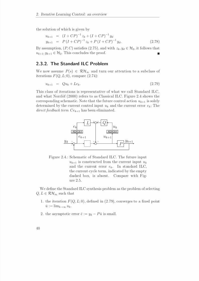
8/8/2019 Evaluasi pada Iterative Learning Control
http://slidepdf.com/reader/full/evaluasi-pada-iterative-learning-control 56/175
2. Iterative Learning Control: an overview
the solution of which is given by
uk+1 = (I + CP )−1 zk + (I + CP )−1 yd
yk+1 = P (I + CP )−1 zk + P (I + CP )−1 yd. (2.78)
By assumption, (P, C ) satisfies (2.75), and with zk, yd ∈ H2, it follows thatuk+1, yk+1 ∈ H2. This concludes the proof.
2.3.2. The Standard ILC Problem
We now assume P (s) ∈ RH∞ and turn our attention to a subclass of iterations F (Q, L; 0), compare (2.74):
uk+1 = Quk + Lek. (2.79)
This class of iterations is representative of what we call Standard ILC,and what Norrlof (2000) refers to as Classical ILC. Figure 2.4 shows thecorresponding schematic. Note that the future control action uk+1 is solelydetermined by the current control input uk and the current error ek; Thedirect feedback term Cek+1 has been eliminated.
uk+1ek+1yk+1
ukek
ydP
L Q++
+++
−
MEMORYMEMORY
Figure 2.4.: Schematic of Standard ILC. The future inputuk+1 is constructed from the current input uk
and the current error ek. In standard ILC,the current cycle term, indicated by the emptydashed box, is absent. Compare with Fig-ure 2.5.
We define the Standard ILC synthesis problem as the problem of selectingQ, L
∈ RH∞such that
1. the iteration F (Q, L; 0), defined in (2.79), converges to a fixed pointu := limk→∞ uk.
2. the asymptotic error e := yd − P u is small.
40
8/8/2019 Evaluasi pada Iterative Learning Control
http://slidepdf.com/reader/full/evaluasi-pada-iterative-learning-control 57/175
2.3. ILC: a two-parameter synthesis problem
Literature on the Standard ILC Problem
The family of iterations (2.79) and the associated synthesis problem have re-ceived considerable attention. Early contributions are due to, among others,Padieu and Su (1990); Liang and Looze (1993); Amann et al. (1996c). Moore
et al. (1992) studied its convergence properties and derived a lower boundon the maximally achievable performance by relating it to the problem of determining a best approximate inverse. Kavli (1992) discussed robust-ness and derived a quasi-heuristic synthesis procedure, on which de Roover(1996) and de Roover and Bosgra (2000) improved, using H∞ optimizationtechniques.
All in all, there is a good degree of consensus on how to choose therespective design parameters: The parameter L should somehow resemblethe approximate inverse of P , whereas Q is typically taken to be a lowpassfilter, understood to improve robustness by suppressing the effect of model
uncertainty at high frequencies.Yet, the interplay between the two parameters is not fully understood.One can argue that Q should be ‘close to unity’ in some sense. By choosingQ to have lowpass characteristics, good tracking can be ensured in the lowfrequency range (where Q is close to unity). Then, for a given Q, theparameter L can be ‘matched’ to the inverse of the given plant by solvingwhat is essentially a model matching problem—de Roover (1996). Thiskind of two-step approach is common to all existing procedures. Thoughvery effective, it lacks rigorous justification. By fixing one of the parameters,the design problem becomes easier, but generality is lost.
In the next chapter we show that the problem of ILC (taken to be the
above) is overparameterized and can be reduced to a 1-parameter problemwithout loss of generality. Finally, we remark that some references workwith the slightly modified update law
uk+1 = Q (uk + Lek) . (2.80)
It is not hard to see that, under the conditions stated (Q, L ∈ RH∞), theoriginal family (2.79) includes the latter (2.80), but not vice versa.
2.3.3. ILC with current-cycle feedback
We now return to the full class, as defined in (2.74). This class is representa-tive of current-cycle feedback ILC (CCF-ILC) or current-iteration tracking error ILC (CITE-ILC). The basic schematic is shown in Figure 2.5. The ideaof including a direct feedback term (Cek+1) has a long history. Instancescan be found in the work of Chen, e.g. Chen et al. (1996a,b, 1997a,b). We
41

8/8/2019 Evaluasi pada Iterative Learning Control
http://slidepdf.com/reader/full/evaluasi-pada-iterative-learning-control 58/175
2. Iterative Learning Control: an overview
also mention the work of Owens (1992) who considered ILC in conjuctionwith high-gain feedback.
uk+1ek+1yk+1
ukek
ydP
L Q
C
++
+++
−
MEMORYMEMORY
Figure 2.5.: Schematic of CCF-ILC. Compare with Fig-ure 2.4. Note the current-cycle term Cek+1.
In the CCF-ILC problem, the parameter C is assumed to be fixed. This
assumption is motivated by the fact that in many applications, an existingcontroller can be appended, but not altogether replaced.
We define the problem of CCF-ILC as the problem of finding Q, L ∈ RH∞such that:
1. The sequence of IO pairs {(uk, yk)} converges to some limit point(u, y) ∈ H2 × H2;
2. The asymptotic error e := yd − y is small.
2.4. Summary and previewWe provided relevant background material and reviewed some of the lite-rature on Iterative Learning Control (ILC). In addition, we formally posedthe problem of ILC as a two-parameter synthesis problem on the spaceof (causal) bounded linear operator pairs. In the next two chapters, thesynthesis problem is studied in greater detail, under various assumptions.Then, in Chapter 5, we ask in what possible sense the algorithms we studyshow a ‘learning behavior’.
42
8/8/2019 Evaluasi pada Iterative Learning Control
http://slidepdf.com/reader/full/evaluasi-pada-iterative-learning-control 59/175
3
Causal ILC and EquivalentFeedback
Overview – We present a detailed analysis of the two-parameter synthesis problem (within the scope of this chapter simply ‘the
problem of ILC’). We require that both parameters (operators) be causal, and discuss how this particular constraint affects the synthe-sis problem. One of our findings states that, under the conditions indicated, the problem of ILC, and that of conventional feedback control are very much akin, not to say essentially equivalent.
3.1. IntroductionIn the preceding chapter we outlined various approaches to the problemof Learning Control, expressing particular interest in a family of first-orderrecurrences (Section 2.3). This same class of recurrences forms the backboneof the present chapter. We address the problem of parameterizing its stablemembers and consider how, from among these members, we may select theones that give best performance.
The question of optimality (“What parameter combination yields thebest performance?”) depends on possible constraints on the parametersinvolved. Apart from boundedness, the one constraint we impose on each
of the parameters (which are really linear operators) is that they be causal .We will see that this assumption has far-reaching consequences. For it turnsout that under this very constraint, the problem of ILC becomes equivalentwith that of conventional feedback control. How we may understand thisequivalence, and what the implications are, will become clear as we proceed.
43
8/8/2019 Evaluasi pada Iterative Learning Control
http://slidepdf.com/reader/full/evaluasi-pada-iterative-learning-control 60/175
3. Causal ILC and Equivalent Feedback
The outline of this chapter is as follows. In Section 3.2 we review someaspects of fixed point analysis so as to motivate the main ideas. Then, inSection 3.3, we define the notion of an admissible pair, which we deploy inSections 3.4 and 3.5 to address the respective problems of Standard ILC and
CCF-ILC. Section 3.6 reports on the results obtained in an experimentalstudy. Section 3.7 closes with a discussion of the main results. The chapteris based on Verwoerd et al. (2003, 2004a,c).
3.2. Fixed Point Analysis
Fixed point analysis, or equilibrium analysis, applied to a ‘system of change’(e.g. a set of difference or differential equations, a recurrence relation oriteration) provides insight into certain aspects of that system’s behavior.For instance, it may tell whether the system is stable, where its solutions
will tend to, etc.ILC deals with systems that are typically expressed as recurrence rela-tions on some (infinite-dimensional) input space. In the previous chapterwe emphasized the algorithmic aspects of such relations. That is to say,we viewed them as computational procedures. But when formulated as anequation to be solved for, a recurrence relation turns into a model . Thismodel implicitly defines a behavior. For an explicit description of the sys-tem’s behavior, we would need to solve the reccurence equation with respectto the particular variable of interest (in our case, the control input).
But that may not be necessary. For perhaps all we want to know iswhether this solution, whatever it be, is ‘acceptable’. This, at least, seems to
be the general philosophy in ILC: people rarely compute complete solutions,even though, for first, and even higher order linear recurrences, it would notbe all that hard. This suggests that the focus of the synthesis problem ison the asymptotic behavior , rather than the temporal behavior. In a laterstage, this will explain why we insist on saying that two solutions convergingto the same fixed point are equivalent, even as their temporal behavior isradically different.
3.2.1. Fixed point stability
Let F map U into U . Recall that any u∈
U satisfying
F (u) = u, (3.1)
is a fixed point of F . The adjective ‘fixed’ indicates a situation of ‘nochange’. The rationale behind this terminology becomes clear upon consid-
44
8/8/2019 Evaluasi pada Iterative Learning Control
http://slidepdf.com/reader/full/evaluasi-pada-iterative-learning-control 61/175
3.2. Fixed Point Analysis
ering the iteration
uk+1 = F (uk) . (3.2)
The dynamics of this algorithm express that if, at some point in time, the
sequence {u0, u1, . . .} reaches a fixed point (which it may never actually do),it is bound to remain there. Fixed points are important as they determine,in part or in full, how an algorithm behaves, asymptotically.
Fixed points may be classified as follows. Let u = F (u) be a fixed pointof F ; u is said to be stable if, for all ε > 0, there exists δ > 0 such thatu0 − u
U
< δ impliesuk − u
U
< ε for all k ≥ 0. That is, if all trajecto-ries starting in a small enough neighborhood of u remain in some specifiedneighborhood of u. Moreover, u is said to be asymptotically stable if it isstable and, in addition, there exists δ > 0 such that
u0 − uU
< δ impliesuk → u as k → ∞. Finally, u is said to be globally asymptotically stableif asymptotic stability is independent of the initial condition u0, i.e. if u
is stable and, in addition, limk→∞ uk = u for all u0 ∈ U . In the contextof linear systems, global asymptotic stability and asymptotic stability areequivalent.
3.2.2. Fixed points and the problem of ILC
Let us recursively define F k(u) as F k(u) := F (F k−1(u)), F 0(u) := u. InSection 2.3 we posed the problem of ILC as that of finding an iteration F :U → U, uk+1 = F (uk) such that certain properties hold. Let us review theseproperties. First of all, we would like the iteration to converge, which impliesthat F must have at least one asymptotically stable fixed point. Secondly,we want the asymptotic behavior to be independent of the choice of initialinput, which implies that F can have only one fixed point, which musttherefore be globally asymptotically stable. Combining the two properties,we may state our first requirement on F as follows:
(R1) There must exist u ∈ U such that for all u0 ∈ U we have
limk→∞
F k(u0) = u. (3.3)
But this is not all. We also require that the sequence {P uk} converge to a
neighborhood of some desired output yd. Let us define P (yd) ⊂ U as theset of all u ∈ U that satisfy this performance criterion, e.g.
P (yd; ε) = {u ∈ U : yd − P u ≤ ε} . (3.4)
The second requirement on F is thus given as:
45
8/8/2019 Evaluasi pada Iterative Learning Control
http://slidepdf.com/reader/full/evaluasi-pada-iterative-learning-control 62/175
3. Causal ILC and Equivalent Feedback
(R2) u must be contained in P (yd).
In the two-parameter synthesis problem, we parameterize F as F (Q, L) andask: how to choose Q, L such that (in accordance with R1 and R2) theequation
u = F (Q, L)u (3.5)
has a unique solution u ∈ P (yd)? In Standard ILC , we define F (Q, L) as
F (Q, L)u := (Q − LP ) u + Lyd. (3.6)
To determine the fixed points of the map F (Q, L), we solve the fixed pointequation
u = (Q − LP ) u + Lyd
⇔(I − Q + LP ) u = Lyd. (3.7)
Depending on Q and L, the above equation may have one or more boundedsolutions, or none whatsoever. We must make sure that it has one andonly one for every yd. This is surely the case if (I − Q + LP ) is boundedlyinvertible on U (its inverse exists and is bounded), in which case we have
u = (I − Q + LP )−1 Lyd. (3.8)
Our synthesis objective is to tune Q and L so as to position the fixed pointat an optimal location, e.g. to minimize the asymptotic error. To that end,
we take the set of all pairs (Q, L) ∈ L(U ) × L(Y, U ), and divide it into aset of pairs that do satisfy R1 (plus some additional constraint, yet to bediscussed) and a set of pairs that do not. The pairs that do satisfy R1, wecall admissible. Naturally, we restrict attention to these admissible pairs.As a next step we recognize that different admissible pairs may define thesame fixed point. This redundancy is removed by introducing an equivalencerelation on the set of admissible pairs. Among equivalent pairs, we appointrepresentatives, and we redefine the synthesis problem in terms of theserepresentatives. In short, that is what the rest of this chapter is about.
3.3. The set of admissible pairsThe controller synthesis literature distinguishes between controllers thatinternally stabilize, and those that do not. Likewise, in ILC, we can distin-guish between certain parameter combinations that are ‘good’, and others
46
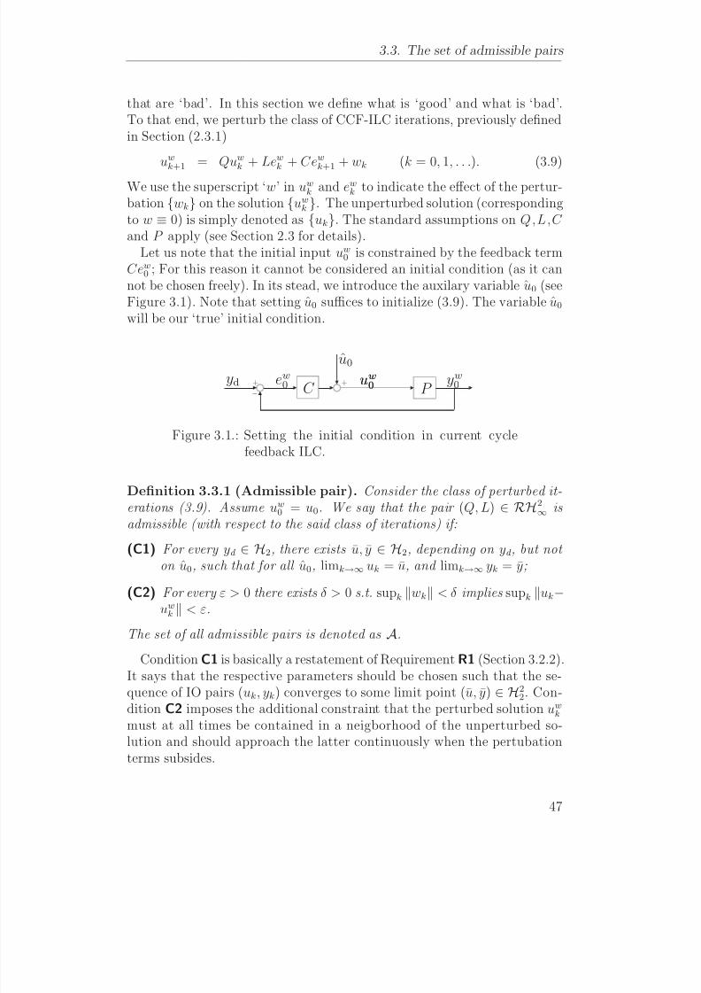
8/8/2019 Evaluasi pada Iterative Learning Control
http://slidepdf.com/reader/full/evaluasi-pada-iterative-learning-control 63/175
3.3. The set of admissible pairs
that are ‘bad’. In this section we define what is ‘good’ and what is ‘bad’.To that end, we perturb the class of CCF-ILC iterations, previously definedin Section (2.3.1)
uwk+1 = Quw
k + Lewk + Cewk+1 + wk (k = 0, 1, . . .). (3.9)
We use the superscript ‘w’ in uwk and ewk to indicate the effect of the pertur-
bation {wk} on the solution {uwk }. The unperturbed solution (corresponding
to w ≡ 0) is simply denoted as {uk}. The standard assumptions on Q,L,C and P apply (see Section 2.3 for details).
Let us note that the initial input uw0 is constrained by the feedback term
Cew0 ; For this reason it cannot be considered an initial condition (as it cannot be chosen freely). In its stead, we introduce the auxilary variable u0 (seeFigure 3.1). Note that setting u0 suffices to initialize (3.9). The variable u0
will be our ‘true’ initial condition.
u0
C P yd
−++ yw
0ew0 uw0uw0
Figure 3.1.: Setting the initial condition in current cyclefeedback ILC.
Definition 3.3.1 (Admissible pair). Consider the class of perturbed it-erations (3.9). Assume uw
0 = u0. We say that the pair (Q, L)
∈ RH2
∞is
admissible (with respect to the said class of iterations) if:
(C1) For every yd ∈ H2, there exists u, y ∈ H2, depending on yd , but not on u0, such that for all u0, limk→∞ uk = u, and limk→∞ yk = y;
(C2) For every ε > 0 there exists δ > 0 s.t. supk wk < δ implies supk uk−uwk < ε.
The set of all admissible pairs is denoted as A.
Condition C1 is basically a restatement of Requirement R1 (Section 3.2.2).It says that the respective parameters should be chosen such that the se-
quence of IO pairs (uk, yk) converges to some limit point (u, y) ∈ H22. Con-dition C2 imposes the additional constraint that the perturbed solution uw
k
must at all times be contained in a neigborhood of the unperturbed so-lution and should approach the latter continuously when the pertubationterms subsides.
47

8/8/2019 Evaluasi pada Iterative Learning Control
http://slidepdf.com/reader/full/evaluasi-pada-iterative-learning-control 64/175
3. Causal ILC and Equivalent Feedback
The notion of admissibility is not to be confused with that of ‘internalstability for ILC’, see (Goldsmith, 2002, Definition 1). In the spirit of thatdefinition (which does not entirely match our terminology), the iteration(3.9) is said to be internally stable if both yk and uk are bounded on each
trial k < ∞ in the presence of bounded disturbances and noise. In our setup,internal stability for ILC is an immediate consequence of the assumptionthat C is internally stabilizing and Q, L stable. Internal stability for ILCguarantees well-posedness (see Lemma 2.3.1), but the notion of admissi-bility is stronger: starting from a family of well-posed (internally stable)iterations, operators (and the corresponding family members) are classifiedinto one of two subsets, depending on whether they have or lack certainproperties.
3.4. Standard ILC and Equivalent Feedback
In this section we apply the ideas outlined in Section 3.2 to the problemof Standard ILC. We derive a necessary and sufficient condition for thepair (Q, L) to be admissible. Then we show that the synthesis problem isoverparameterized, and we define an equivalence relation so as to reducethe 2-parameter problem to a 1-parameter problem. Along the way weintroduce the concept of equivalent feedback, which, as it turns out, putsall things in a whole new perspective.
3.4.1. Necessary and sufficient conditions for admissibility
Consider the family of iterations (3.9). In accordance with the problemdefinition of Standard ILC in Section 2.3.2, we assume P ∈ RH∞ andC = 0,
uwk+1 = Quw
k + Lewk + wk. (3.10)
As there is no direct feedback term (C = 0), it follows that u0 = u0 (seeFigure 3.1).
Lemma 3.4.1. Given the triple (P,Q,L) ∈ RH3∞ and suppose C = 0.
The pair (Q, L) is admissible in the sense of Definition 3.3.1 if and only if Q − LP ∞ < 1.
Proof. The proof of sufficiency follows standard contraction arguments andcan also be found in e.g. Moore et al. (1992); Padieu and Su (1990); Norrlof
48

8/8/2019 Evaluasi pada Iterative Learning Control
http://slidepdf.com/reader/full/evaluasi-pada-iterative-learning-control 65/175
3.4. Standard ILC and Equivalent Feedback
(2000). We rewrite (3.10) to obtain
uwk+1 = (Q − LP )
F
uwk + Lyd
d
+wk. (3.11)
By introducing the shorthand notation F := (Q − LP ), d = Lyd we com-pact Equation (3.11) to the familiar form (compare (2.24))
uwk+1 = F uw
k + d + wk. (3.12)
Repeated substitution gives
uwk = F kuw
0 +k−1 j=0
F j (d + wk−1− j)
= F kuw0 +
k−1
j=0
F jwk−1− j + (I − F )−1
I − F k+1
d. (3.13)
To prove convergence of the unperturbed solution (C1), we set w j equal tozero. The result follows from Theorem 2.1.9, noting that F : H2 → H2,z = F w + d, is a contraction. To verify continuity of the perturbed solution(C2), assume supk wkH2
< δ , and observe that
uwk − ukH2
=k−1
j=0 F jwk−1− jH2
≤k−1 j=0
F j∞δ
≤ (1 − F ∞)−1 δ. (3.14)
This shows that for any ε > 0, we can find δ > 0 s.t. supk uw
k − ukH2 < ε.This proves sufficiency.Next we prove necessity. Suppose F = 1 (the case F > 1 is easy).
We consider the SISO case. What we need to show is that for every δ > 0and every ε > 0 there exists K > 0 such that for at least some u0 and someyd, we can construct a sequence {w j} with w j < δ, j ≤ K − 1, such thatuw
K − uK > ε. Let yd = u0 = 0, so that uk = 0 for all k. Given K , weconstruct w such that
F K w ≥ 1
2w (3.15)
The fact that, for SISO systems, F K
= F K
= 1 implies that suchw exists; this follows by continuity of the norm. Now define wk := F kw,k = 0, 1, . . . , K −1. It follows that uw
k = kF kw and by construction uwK ≥
12K w. Choose w such that w = δ/2 and take K = 4 (ε/δ) + 1. Thenuw
K − uK = uwK > ε. This concludes the proof.
49

8/8/2019 Evaluasi pada Iterative Learning Control
http://slidepdf.com/reader/full/evaluasi-pada-iterative-learning-control 66/175
3. Causal ILC and Equivalent Feedback
Though the definition of admissibility appears rather involved, checkingwhether a given pair is admissible or not turns out to be relatively easy.This is of course no coincidence. We defined admissibility the way we didso as to arrive at a single condition that is both necessary and sufficient.
That is not to say this definition is completely arbitrary either. Condi-tion C1 is common. Were this the only condition, satisfying the inequalityQ − LP ∞ < 1 would still be sufficient, but no longer necessary (we illus-
trate this in the next example). This means that we would need to developmore elaborate tests to be able to determine whether a given pair of oper-ators is admissible or not. Indeed, it appears that without C2, there is nosingle condition for admissibility that is both sufficient and necessary. Inaddition, we may point out that C2 ensures a primitive, but not altogetherartificial form of robustness.
Example 3.4.2. This example intends to show that, in case we leave out C2,the condition
Q
−LP
< 1 (see Lemma 3.4.1) is no longer necessary for
admissibility.Consider the iteration
uk+1 = F uk + d. (3.16)
Suppose F ∈ RH∞ and d ∈ H2. By Theorem 2.1.9 we know that if F ∞ <1, then {uk} tends to a limit point u(d) ∈ H2, independent of u0. We alsoknow that if F ∞ > 1, then there exists u0 such that {uk} does not have a limit. But what if F ∞ = 1? Let F be given as
F (s; γ ) =γs
(s + 1)3. (3.17)
We select γ = 32√3 so that F ∞ = 1. The real-valued function |F ( jω)|
attains its maximum value ( = 1) at ω = ±12
√2. For all other ω (including
the point at infinity), |F ( jω)| is less than unity.For {uk} to converge for all d ∈ H2, the map (I − F ) must be boundedly
invertible on RH∞ (see also Example 2.1.3). We will show that this isindeed the case. First, let us establish that 1 − F (s) does not have any zeros in the open right half plane (RHP). Suppose on the contrary that 1 − F (s0) = 0 for some s0 with Re(s0) > 0. This implies |F (s0)| = 1.As supRe(s)>0 |F (s)| = 1 it follows, by analyticity of F and the maximum modulus principle, that F (·) is a constant map. But this is clearly not true;
hence we conclude that F (s) does not have any zeros in the open RHP. But how about zeros on the imaginary axis? There are none, since |F ( jω)| < 1
for all ω ∈ R except at ω = ±12
√2, and inspection shows that
F (±1
2
√2 j) =
5
9
√3 ∓ 1
9
√2√
3 j (= 1). (3.18)
50
8/8/2019 Evaluasi pada Iterative Learning Control
http://slidepdf.com/reader/full/evaluasi-pada-iterative-learning-control 67/175
3.4. Standard ILC and Equivalent Feedback
Note furthermore that F (∞) = 0, which implies that 1 − F (s) is biproper.We conclude that (1 − F (s))−1 is a proper real-rational transfer function with no poles in the closed RHP, i.e. (1 − F )−1 ∈ RH∞.
This condition is obviously not sufficient. Yet, in our example, the se-
quence {uk} does converge. To prove this, we show that the increment (uk+1 − uk) tends to zero and that {uk} is bounded. Define ∆uk := uk+1−uk.By linearity, we have that
∆uk = F ∆uk−1. (3.19)
Observe that {∆uk} is a nonincreasing sequence, bounded from below, and hence must have a limit point. This implies that there exists w ∈ H2 such that w = F w. Note that, for any ε > 0, there exists δ > 0 such that
F w2/2 ≤
12
√2−δ
0
|F ( jω)|2 |w( jω)|2d ω · · ·
+ ∞12
√2+δ
|F ( jω)|2 |w( jω)|2d ω + ε (3.20)
Assume w = 0. This assumption, combined with the fact that |F ( jω)| < 1 for all ω = 1
2
√2 implies that there exists δ > 0 and γ > 0, such that
whenever δ < δ, 12
√2−δ
0
|F ( jω)|2 |w( jω)|2d ω +
∞12
√2+δ
|F ( jω)|2 |w( jω)|2d ω · · ·
≤ 12
√2−δ
0 |w( jω)
|2d ω +
∞
1
2√2+δ |w( jω)
|2d ω
−γ.(3.21)
This in turn implies that
F w2/2 ≤ 1
2
√2−δ
0
|w( jω)|2d ω +
∞12
√2+δ
|w( jω)|2d ω − γ + ε
≤ w2/2 − γ + ε. (3.22)
Note that γ is fixed and does not depend on δ; The parameter ε on the other hand, can be made arbitrarily small. Indeed for any ε with 0 < ε < γ , thereexists δ with 0 < δ < δ such that (3.20) holds. It follows that F w < w.But this contradicts our starting assumption. We conclude that
w
=:
limk→∞ ∆uk = 0 (and this in turn implies that uk+1 − uk → 0).Next we show that the sequence {uk} is bounded. To that end, we
consider the solution in explicit form
uk = F ku0 + (I − F )−1 I + F k
d. (3.23)
51

8/8/2019 Evaluasi pada Iterative Learning Control
http://slidepdf.com/reader/full/evaluasi-pada-iterative-learning-control 68/175
3. Causal ILC and Equivalent Feedback
The right hand side may be bounded as followsF ku0 + (I − F )−1
I + F k
d ≤ F
k∞ u0 · · ·
+
(I − F )−1
∞ 1 + F k
d
= u0 + 2 (I − F )−1∞ d,
and this proves that supk uk < ∞. We conclude that there exists l ∈ R
such that limk→∞ uk = l. Given that limk→∞ ∆uk = 0, this implies that there exists u ∈ H2 such that limk→∞ uk = u. This concludes the example.
3.4.2. Equivalent admissible pairs
We introduce some additional notation and terminology. Let S denote a setand let R be a relation on S , i.e. a collection of ordered pairs of elementsof S . Suppose R satisfies the following properties
1. (a, a) ∈ R ∀ a ∈ S .2. (a, b) ∈ R ⇒ (b, a) ∈ R ∀ a, b ∈ S .3. (a, b), (b, c) ∈ R ⇒ (a, c) ∈ R ∀ a,b,c ∈ S .
then R is an equivalence relation . In that case two elements a, b ∈ S ,(a, b) ∈ R are said to be equivalent and we write a b. For each a ∈ S , wedefine the equivalence class [a] containing a to be the set of all elements inS equivalent to a, i.e.
[a] = {b ∈ S | b a}
It is easy to see that equivalence classes constitute a partition of S that is,a collection of nonempty disjoint subsets of S whose union is S . In orderto refer to a particular equivalence class, one element can be selected torepresent the entire class. Such an element is called a class representative.
Let us see how we can apply this apparatus to our synthesis problem. Re-call that our current objective is to select from among a family of iterations,a particular member, or set of members, that satisfy certain performanceconstraints (see our discussion in Section 3.2.2). As indicated before, wemay restrict attention to those members corresponding to admissible pairs.It is obvious that different admissible pairs induce different input sequences.Even so, different sequences can converge to the same fixed point. Recall
that if (I − Q + LP ) is boundedly invertible on H2, then the fixed point uis given as
u = (I − Q + LP )−1 Lyd =
I + (I − Q)−1 L K
P )−1 (I − Q)−1 L K
yd.
52
8/8/2019 Evaluasi pada Iterative Learning Control
http://slidepdf.com/reader/full/evaluasi-pada-iterative-learning-control 69/175
3.4. Standard ILC and Equivalent Feedback
(3.24)
For the second equality to hold we assume that the inverse (I − Q)−1 iswell-defined. Shortly, we will see that this assumption is justified. WhatEquation (3.24) shows is that the fixed point u is completely determinedby the matrix fraction K := (I − Q)−1 L. Admissible pairs for which thisfraction is equal are considered equivalent.
Definition 3.4.3 (Equivalence on A). Suppose P ∈ RH∞ is strictly proper. Let A be the set of pairs admissible to the family of iterations(3.10). Two pairs (Q1, L1), (Q2, L2) ∈ A are said to be equivalent if they satisfy the equivalence relation
(I − Q1)−1 L1 = (I − Q2)−1 L2.
Let us verify that the matrix fraction appearing in Definition 3.4.3 iswell-defined. By well-defined we mean that (I − Q)−1 exists (as a properreal-rational, but not necessarily stable transfer function) and that (I − Q)and L are coprime (so that no unstable pole-zero cancellations can occur).The reason for insisting on coprimeness will become clear in Section 3.4.We have the following lemma.
Lemma 3.4.4. Given P ∈ RH∞. For any (Q, L) ∈ A, the pair (I − Q, L)is left-coprime. If P is strictly proper then (I − Q)−1 exists and is proper.
Proof. Recall that two transfer matrices (I − Q) and L in RH∞ are left-
coprime over RH∞ iff there exist matrices X and Y in RH∞ such that(I − Q) X + LY = I (3.25)
Define X = (I − Q + LP )−1, Y = P X . Note that X ∈ RH∞ by assump-tion of admissibility (Q − LP ∞ < 1, see Lemma 3.4.1) and hence alsoY ∈ RH∞. Clearly (I − Q) X + LY = I , which proves left-coprimeness.To prove that (I − Q)−1 defines a (proper) real-rational transfer function,it suffices to show that (I − Q(∞))−1 exists. We consider the boundedreal-rational transfer function (I − Q + LP )−1. Strict properness of P andboundedness of L implies that L(∞)P (∞) = 0. Thus, at infinity, the map(I
−Q + LP )−1 reduces to (I
−Q)−1. Since (I
−Q + LP )−1 is bounded at
infinity, so is (I − Q)−1. This completes the proof.
Lemma 3.4.4 states that, provided the pair (Q, L) is admissible andP strictly proper, the matrix fraction (I − Q)−1 L defines a proper, real-rational, but not necessarily stable transfer function. The condition on
53

8/8/2019 Evaluasi pada Iterative Learning Control
http://slidepdf.com/reader/full/evaluasi-pada-iterative-learning-control 70/175
3. Causal ILC and Equivalent Feedback
strict properness of P is not essential. We could define an equivalence rela-tion independent of this condition. For instance, in view of Equation (3.24),we could define two admissible pairs to be equivalent if
(I −
Q1 + L1P )−1 L1 = (I −
Q2 + L2P )−1 L2. (3.26)
Yet we choose to adopt the given definition. For one, because of its com-pactness; but mainly because of its interpretation in terms of EquivalentFeedback, to be discussed after the next example.
Example 3.4.5. The purpose of this example is to illustrate what it means for two pairs to be equivalent, as well as to motivative the condition of strict properness (Definition 3.4.3). Consider a plant P , given as
P (s) =1
2
s − 2
s + 1. (3.27)
We pick Q and L such that Q − LP ∞ < 1, i.e. we make sure that (Q, L)is admissible (see Lemma 3.4.1). Take L1 = 1 ; Q1 = (s − 1)/(s + 1) and verify that (Q1 − L1P ) = s/(2(s + 1)) is a contraction. We have that
(I − Q1)−1 L1 =1
2(s + 1) . (3.28)
Next we choose L2 = 2(s + 1)/(s + 2) and Q2 = (s − 2)/(s + 2). In this caseQ2 − L2P = 0, and
(I
−Q2)−1 L2 =
1
2
(s + 1) . (3.29)
We observe that the pairs (Q1, L1), (Q2, L2) are equivalent. Figure 3.2 showshow the respective iterations {uk+1 = Qiuk + Liek : i = 1, 2} converge to thesame fixed point. In both cases (I − Q)−1 is well-defined, be it not proper.For SISO systems, it is easy to see that the only case in which (I − Q)−1 isnot defined (as a rational transfer function) is when Q = 1. As regards thisexample, We may verify that there is no L ∈ RH∞ such that (1, L) ∈ A.In other words, for the given plant, the matrix fraction (I − Q)−1 L would be well-defined for all admissible pairs. But in general, this need not be so.Consider for instance, the class of bistable plants, i.e. the set of plants P
such that P, P −1
∈ RH∞. We pick Q = I and L = P −1
so that Q−LP = 0and thus (Q, L) ∈ A. In that case (I − Q)−1 is clearly not defined. The fastest way around this problem is to insist on strict properness. The pricewe pay is that we exclude certain cases of interest, such as the one wediscussed in this example.
54
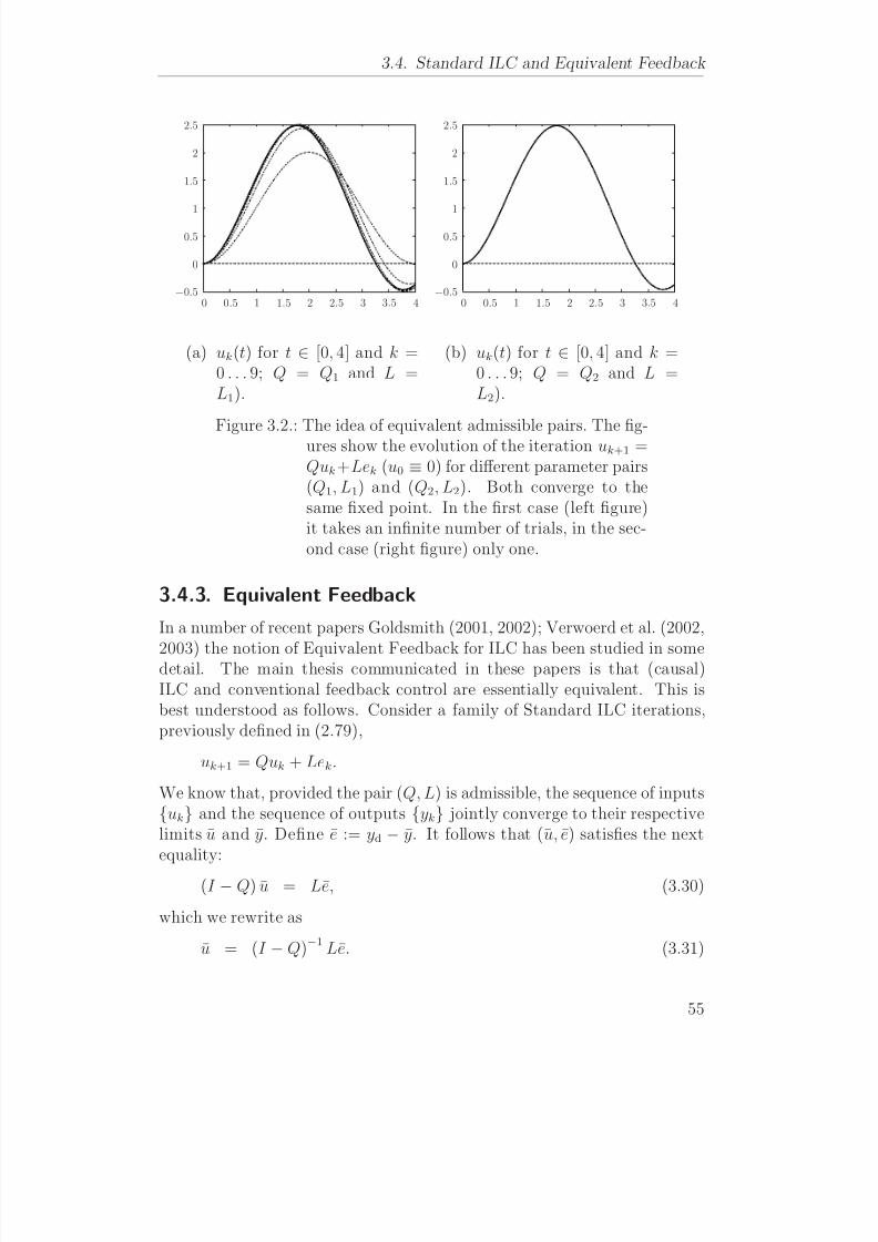
8/8/2019 Evaluasi pada Iterative Learning Control
http://slidepdf.com/reader/full/evaluasi-pada-iterative-learning-control 71/175
3.4. Standard ILC and Equivalent Feedback
2.5
2
1.5
1
0.5
0
−0.50 0.5 1 1.5 2 2.5 3 3.5 4
2.5
2
1.5
1
0.5
0
−0.50 0.5 1 1.5 2 2.5 3 3.5 4
(a) uk(t) for t ∈ [0, 4] and k =0 . . . 9; Q = Q1 and L =L1).
(b) uk(t) for t ∈ [0, 4] and k =0 . . . 9; Q = Q2 and L =L2).
Figure 3.2.: The idea of equivalent admissible pairs. The fig-ures show the evolution of the iteration uk+1 =Quk+Lek (u0 ≡ 0) for different parameter pairs(Q1, L1) and (Q2, L2). Both converge to thesame fixed point. In the first case (left figure)it takes an infinite number of trials, in the sec-ond case (right figure) only one.
3.4.3. Equivalent Feedback
In a number of recent papers Goldsmith (2001, 2002); Verwoerd et al. (2002,
2003) the notion of Equivalent Feedback for ILC has been studied in somedetail. The main thesis communicated in these papers is that (causal)ILC and conventional feedback control are essentially equivalent. This isbest understood as follows. Consider a family of Standard ILC iterations,previously defined in (2.79),
uk+1 = Quk + Lek.
We know that, provided the pair (Q, L) is admissible, the sequence of inputs{uk} and the sequence of outputs {yk} jointly converge to their respectivelimits u and y. Define e := yd − y. It follows that (u, e) satisfies the nextequality:
(I − Q) u = Le, (3.30)
which we rewrite as
u = (I − Q)−1 Le. (3.31)
55
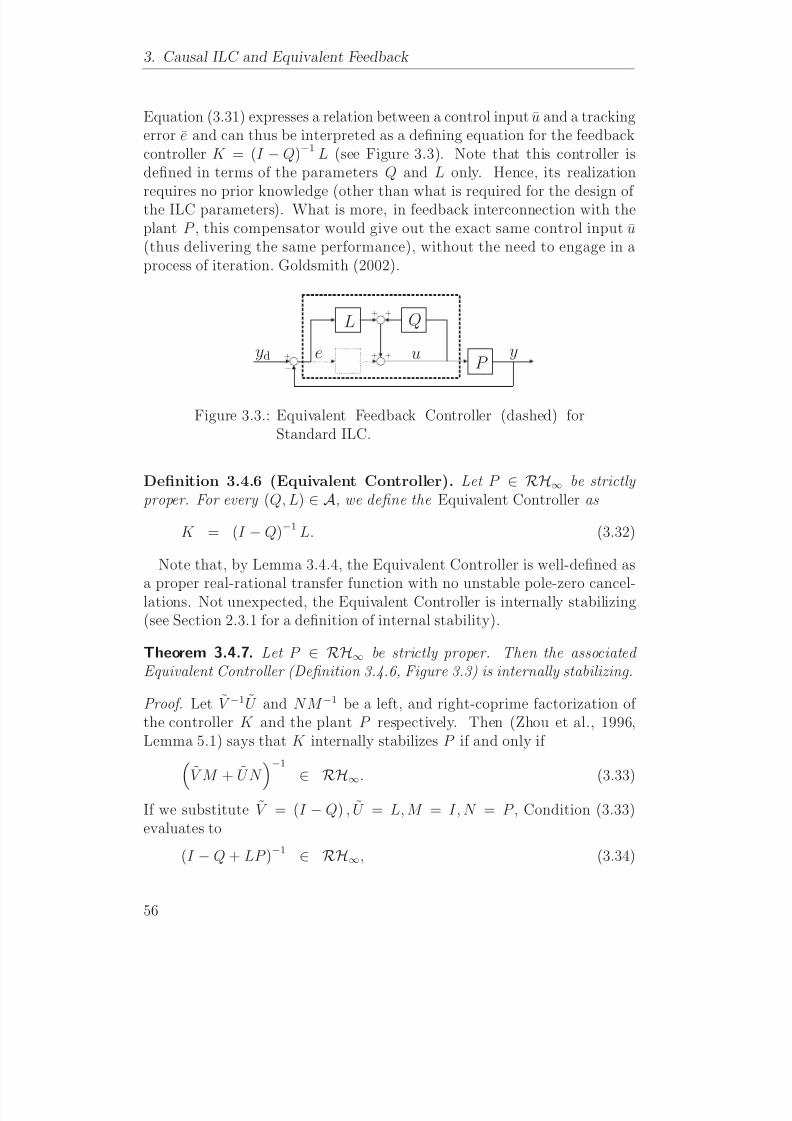
8/8/2019 Evaluasi pada Iterative Learning Control
http://slidepdf.com/reader/full/evaluasi-pada-iterative-learning-control 72/175
3. Causal ILC and Equivalent Feedback
Equation (3.31) expresses a relation between a control input u and a trackingerror e and can thus be interpreted as a defining equation for the feedbackcontroller K = (I − Q)−1 L (see Figure 3.3). Note that this controller isdefined in terms of the parameters Q and L only. Hence, its realization
requires no prior knowledge (other than what is required for the design of the ILC parameters). What is more, in feedback interconnection with theplant P , this compensator would give out the exact same control input u(thus delivering the same performance), without the need to engage in aprocess of iteration. Goldsmith (2002).
L Q
P yd
−+ +
+ +
+ ye u
Figure 3.3.: Equivalent Feedback Controller (dashed) forStandard ILC.
Definition 3.4.6 (Equivalent Controller). Let P ∈ RH∞ be strictly proper. For every (Q, L) ∈ A, we define the Equivalent Controller as
K = (I − Q)−1 L. (3.32)
Note that, by Lemma 3.4.4, the Equivalent Controller is well-defined as
a proper real-rational transfer function with no unstable pole-zero cancel-lations. Not unexpected, the Equivalent Controller is internally stabilizing(see Section 2.3.1 for a definition of internal stability).
Theorem 3.4.7. Let P ∈ RH∞ be strictly proper. Then the associated Equivalent Controller (Definition 3.4.6, Figure 3.3) is internally stabilizing.
Proof. Let V −1U and NM −1 be a left, and right-coprime factorization of the controller K and the plant P respectively. Then (Zhou et al., 1996,Lemma 5.1) says that K internally stabilizes P if and only if
V M + UN −1
∈ RH∞. (3.33)
If we substitute V = (I − Q) , U = L, M = I, N = P , Condition (3.33)evaluates to
(I − Q + LP )−1 ∈ RH∞, (3.34)
56
8/8/2019 Evaluasi pada Iterative Learning Control
http://slidepdf.com/reader/full/evaluasi-pada-iterative-learning-control 73/175
3.4. Standard ILC and Equivalent Feedback
which is satisfied by assumption of admissibility (see Lemma 3.4.1). Notethe we used the fact that for every (Q, L) ∈ A, (I −Q) and L are left-coprime(Lemma 3.4.4).
As a kind of converse result, the following theorem says that every stabi-
lizing controller admits a factorization in terms of admissible pairs.
Theorem 3.4.8. Suppose P ∈ RH∞ is strictly proper and let K be any stabilizing controller. Then there exists (Q, L) ∈ A such that (I − Q)−1 L =K .
Proof. For any F ∈ RH∞, the unique solution (QF , LF ) to the set of equa-tions
QF − LF P = F LF = (I − QF ) K
(3.35)
is given by
QF = I − (I − F ) (I + KP )−1
LF = (I − F ) K (I + P K )−1
(3.36)
By assumtion of internal stability, the closed-loop functions (I + KP )−1
and K (I + P K )−1 are both stable. From this we deduce that QF , LF ∈RH∞. Now let F be a contraction, i.e. F ∞ < 1. Then, by construction,(QF , LF ) ∈ A (Lemma 3.4.1).
The proof of Theorem 3.4.8 shows that there are infinitely many admis-sible pairs that define one and the same equivalent controller. By Defi-nition 3.4.3, these are equivalent pairs. Thus we can interpret equivalentpairs as corresponding to different left-coprime factorizations of the same(equivalent) controller.
3.4.4. The synthesis problem revisited
Let us introduce the set K of all stabilizing controllers corresponding to agiven plant P , along with the map φ : A → K,
φ(Q, L) := (I − Q)−1 L (3.37)
By Theorems 3.4.7 and 3.4.8 we know that φ is many-to-one and onto,i.e. surjective but not injective (see Figure 3.4). By considering equivalenceclasses instead, we can uniquely identify every element K ∈ K with a class
[(Q, L)] =
(Q, L) ∈ A : (Q, L) (Q, L)
. (3.38)
57

8/8/2019 Evaluasi pada Iterative Learning Control
http://slidepdf.com/reader/full/evaluasi-pada-iterative-learning-control 74/175
3. Causal ILC and Equivalent Feedback
A K
Q
L
φ
φ
Figure 3.4.: The map φ : A → K is surjective but not injec-tive.
A Kφ
φQ
L
Figure 3.5.: Every equivalence class in A can be uniquelyidentified with a particular stabilizing con-troller.
This idea is illustrated in Figure 3.5.We are associating elements in K with sets in A. In order to create a map
that is truly one-to-one, we restrict attention to class representatives. Twothings are important to note here. First of all that by restricting attention
to just one element (pair) in the class we do not loose generality. After all,all pairs within a class are equivalent, and by focusing on one element weeffectively remove redundancy. Second that the choice of representativesis, in principle, arbitrary. We choose to select as a representative for agiven class [(Q, L)] the element (Q0, L0) ∈ [(Q, L)] that satisfies the extraconstraint Q0 − L0P = 0. The following lemma says that every class hasprecisely one such member.
Lemma 3.4.9. Let (Q, L) ∈ A be any admissible pair and let [(Q, L)] ⊂ Adenote the corresponding equivalence class. There exists a unique admissiblepair (Q0, L0) ∈ [(Q, L)] such that Q0 − L0P = 0.
Proof. Immediate from the proof of Theorem 3.4.8 (take F = 0).
In the Standard ILC problem, the quantity Q − LP determines the con-vergence speed of the algorithm; the ‘smaller’ Q − LP is, the faster con-vergence is achieved. Setting Q0 − L0P = 0 implies that the recursion
58
8/8/2019 Evaluasi pada Iterative Learning Control
http://slidepdf.com/reader/full/evaluasi-pada-iterative-learning-control 75/175
3.4. Standard ILC and Equivalent Feedback
defined in (2.79) converges to its fixed point after precisely one iteration.It is important to note that, although the location of the fixed point andthe speed of convergence are both determined by the parameter pair (Q, L)they are nevertheless independent. That is to say, we can reach any fixed
point—within the reachable set induced by the admissible pairs—at any rateof convergence. This is essentially what the proof of Theorem 3.4.8 tells us.We define A0 to be the set of all class representatives or, equivalently, the
set of all pairs (Q, L) ∈ A satisfying Q − LP = 0. Note that by definitionevery member of this set has the special form (LP,L). Note furthermorethat A0 cannot contain any equivalent pairs since the representatives weretaken from disjoint sets. As a consequence, the map φ0 := φ|A0
, i.e. therestriction of φ to A0, is injective. Clearly φ0 is also surjective and hencewe conclude that φ0 : A0 → K is a bijection . In other words, the sets A0
and K are identical up to an isomorphism. This fact allows us to prove awell-known result.
Corollary 3.4.10 (Youla). The set K of all (proper real-rational) controllersK stabilizing a (strictly proper) plant P ∈ RH∞ can be parameterized as
follows:
K =
K : K = (I − LP )−1 L ; L ∈ RH∞
Proof. Note that the set of class representatives A0 has a trivial parame-terization
A0 = {(LP,L) : L ∈ RH∞} , (3.39)
and recall that A0 and K are bijective under φ0. Hence any given parame-terization of A0 induces a parameterization of K. In particular:
K = {φ0(LP,L) : L ∈ RH∞} =
(I − LP )−1 L : L ∈ RH∞
This completes the proof.
Corollary 3.4.10 gives a parameterization of the set of all stabilizing con-trollers K. It is easy to see that this parameterization is minimal. Thatis to say, there is no parameterization that uses fewer parameters. The
corresponding block diagram is given in Figure 3.6.The results in this section imply that the Standard ILC problem is equiv-alent to a compensator design problem for a stable plant. The compensatordesign problem has received a great deal of attention over the years andmany of the results obtained (e.g. on robustness) can also be exploited
59
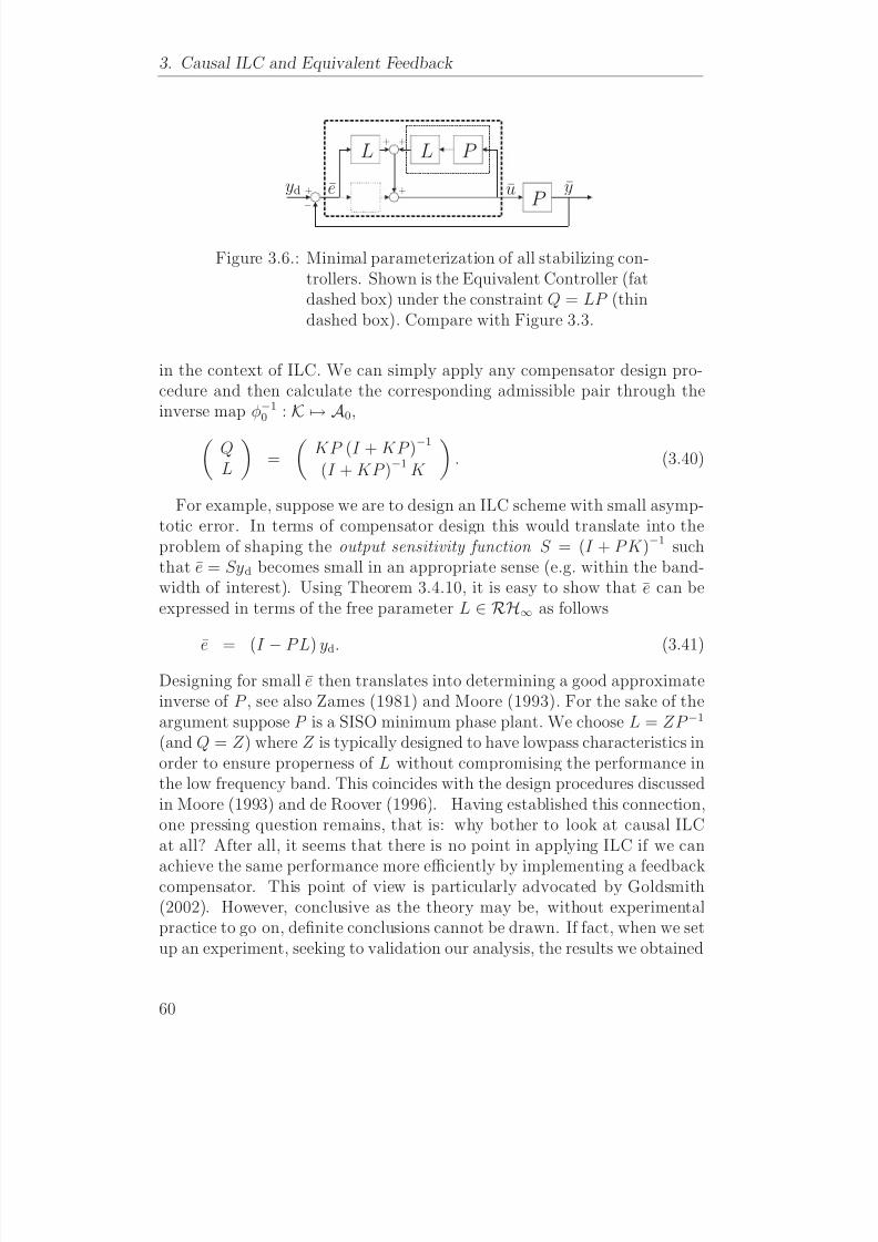
8/8/2019 Evaluasi pada Iterative Learning Control
http://slidepdf.com/reader/full/evaluasi-pada-iterative-learning-control 76/175
3. Causal ILC and Equivalent Feedback
LL P
P yd
−
+
+ +
+ ye u
Figure 3.6.: Minimal parameterization of all stabilizing con-trollers. Shown is the Equivalent Controller (fatdashed box) under the constraint Q = LP (thindashed box). Compare with Figure 3.3.
in the context of ILC. We can simply apply any compensator design pro-cedure and then calculate the corresponding admissible pair through theinverse map φ−1
0 : K → A0,QL
=
KP (I + KP )−1
(I + KP )−1 K
. (3.40)
For example, suppose we are to design an ILC scheme with small asymp-totic error. In terms of compensator design this would translate into theproblem of shaping the output sensitivity function S = (I + P K )−1 suchthat e = Syd becomes small in an appropriate sense (e.g. within the band-width of interest). Using Theorem 3.4.10, it is easy to show that e can beexpressed in terms of the free parameter L ∈ RH∞ as follows
e = (I − P L) yd. (3.41)Designing for small e then translates into determining a good approximateinverse of P , see also Zames (1981) and Moore (1993). For the sake of theargument suppose P is a SISO minimum phase plant. We choose L = ZP −1
(and Q = Z ) where Z is typically designed to have lowpass characteristics inorder to ensure properness of L without compromising the performance inthe low frequency band. This coincides with the design procedures discussedin Moore (1993) and de Roover (1996). Having established this connection,one pressing question remains, that is: why bother to look at causal ILCat all? After all, it seems that there is no point in applying ILC if we can
achieve the same performance more efficiently by implementing a feedbackcompensator. This point of view is particularly advocated by Goldsmith(2002). However, conclusive as the theory may be, without experimentalpractice to go on, definite conclusions cannot be drawn. If fact, when we setup an experiment, seeking to validation our analysis, the results we obtained
60

8/8/2019 Evaluasi pada Iterative Learning Control
http://slidepdf.com/reader/full/evaluasi-pada-iterative-learning-control 77/175
3.4. Standard ILC and Equivalent Feedback
were not fully supportive. Though we found that the Equivalent Controlleris indeed stabilizing (Theorem 3.4.7), we also found slight, but neverthelesssignificant, deviations in performance. More on these results in Section 3.6.
3.4.5. Causal ILC, Equivalent Feedback and NoiseAs a footnote to the discussion on the implications of Equivalent Feedback,let us remark that our analyses did not account for the effect of possible(external) disturbances. This is important, for some of the conclusionsobtained may not generalize to settings less ideal than ours. In particular,the very notion of Equivalent Feedback is based on the explicit assumptionthat all signals in the loop converge to a limit, which is not likely to happenin a setting with noise.
Our next discussion addresses the question as to what extent the Equiv-alent Controller is still ‘equivalent’ under various disturbances. We look at
two cases: that of input disturbances (e.g. unmodelled dynamics and loaddisturbances), and that of measurement noise (e.g. quantization effects andsensor noise).
Adding measurement noise
Given some control input uk, let yk = P uk denote the plant’s actual outputand let yk denote the measured output. We assume that yk = yk + wk wherewk represents the measurement noise. We consider the same update law asbefore, except that we now feed back the measured, instead of the actualoutput:
uk+1 := Quk + L (yd − y) = Quk + Lek − Lwk. (3.42)
Here, ek is defined in the usual way: ek := yd − yk. Assume that supi wiis finite and let (Q, L) be admissible. Then {uk} is bounded. Note thatthe effect of the noise term wk extends into the infinite future. That is tosay, not only does it affect uk, but also uk+1, uk+2, et cetera . As the updatelaw is linear, we can easily isolate its (i.e. the noise term’s) contribution.We set yd = 0 and solve (3.42) for uk.
uk = (Q − LP )k u0 +k−1
i=0
(Q − LP )iLwi
uwk
. (3.43)
The term on the right-hand side of (3.43), denoted by uwk , represents the
total noise contribution to the system’s input at trial k. Evidently, if wi
would be zero for all i, uwk would also be zero.
61

8/8/2019 Evaluasi pada Iterative Learning Control
http://slidepdf.com/reader/full/evaluasi-pada-iterative-learning-control 78/175
3. Causal ILC and Equivalent Feedback
Now the question we ask is the following: Given a stabilizing controllerK , how to choose Q and L so as to minimize the effect of noise under the constraint that (I − Q)−1 L = K ? Based on Theorem 3.4.8 the samequestion may alternatively be put as: Given K , how to choose F := Q−LP
so as to make uw
k as small as possible?It is obvious that for all constant (as in ‘trial-independent’) disturbanceswi := w, i ≥ 0, the choice of F is immaterial. That is to say, as far as suchdisturbances are concerned, there is no advantage in applying Causal ILCinstead of Equivalent Feedback Control. This is a direct consequence of theproof of Theorem 3.4.8 which says that for each F ∈ RH∞ there is a uniquepair (QF , LF ) ∈ A such that QF − LF P = F and (I − QF )
−1 LF = K , theoperators QF and LF being given as
QF = I − (I − F ) (I + KP )−1 , (3.44)
LF = (I
−F ) K (I + P K )−1 . (3.45)
Indeed, for any fixed disturbance w, the noise term uwk converges to a con-
stant value uw, which is given as
uw = (I − Q + LP )−1 Lw = (I + KP )−1 Kw. (3.46)
But what about non-constant, non-deterministic (stochastic) disturbances.Do the same conclusions apply? The answer is ‘no’. Let us run a simulationon a standard second-order plant
P (s) =ω20
s
2
+ 2ζω0s + ω
2
0
, (3.47)
with parameter values ζ = 0.5 and ω0 = 10. We select the (equivalent)controller K as
K (s) =4.00e2 s4 + 1.41e4 s3 + 2.50e5 s2 + 1.41e6 s + 4.00e6
2.50e1 s4 + 1.41e3 s3 + 3.00e4 s2 + 2.82e5 s.
(3.48)
For each k, let wk be given as a zero-mean white noise signal with varianceσ2w = 0.01. We select yd = 0, u0 = 0. For a number of values of F ,
we compute the variance of ywN = P uw
N , where N is a number depending
on F . To be precise, we compute N as the smallest integer greater thanlog(F )/ log(eps), where eps is the floating point relative accuracy (eps ≈1e-16). Striving for a fair comparison, this formula compensates for thedifference in convergence speed. For F = 0.25 and F = 0.50, it respectivelyreturns N = 26 and N = 52. Each experiment is repeated ten times, after
62

8/8/2019 Evaluasi pada Iterative Learning Control
http://slidepdf.com/reader/full/evaluasi-pada-iterative-learning-control 79/175
3.4. Standard ILC and Equivalent Feedback
which we compute the average over all trials. Table 3.1 contains the results.For comparison, we computed the variance of the output in the equivalentfeedback representation (also with yd ≡ 0) to var(yw) = 6.9e − 5. Thedata in Table 3.1 suggests that as F tends to unity, var(yw
N ) tends to zero,
while as F tends to zero, var(yw
N ) tends to a value which compares withthat obtained with equivalent feedback. Our preliminary conclusion is thata slow rate of convergence is advantageous for suppression of measurementnoise. It must be said however that we could also opt for fast convergenceand conventional averaging over trials, in which case var(yw
k ) would decreasewith 1/
√k.
F 0.25 0.50 0.63 0.71N 26 52 78 104
var(ywN ) (average) 4.3e-5 2.4e-5 2.0 e-5 1.3e-5
Table 3.1.: Simulation results for the case of measurementnoise.
Input disturbance
Let uk denote the control input and let dk denote the input disturbance.We define the actual input ud
k as the sum of uk and dk, i.e. udk := uk + dk.
We consider the same update law as before.
uk+1 = Quk + L (yd − P uk)
= Quk + Lek−
LP dk. (3.49)
In first instance, let us assume that di is constant, i.e. di = d for all i. Setyd = 0 and define u := limk→∞ uk, ud := limk→∞ ud
k. It is easy to verify thatud = u + d. From (3.49) we obtain the equality
ud = d − (I − Q + LP )−1 LP d = (I + KP )−1 d, (3.50)
which again shows that the parameter F is immaterial when it comes toattenuating constant (trial-independent) disturbances.
To determine the effect of trial-dependent disturbances, we run the samesimulation as before, but now with an input, instead of an output distur-
bance. We set yd = 0, u0 = 0 and then we compute yd
N = P ud
N for differentvalues of F , using the same formula. Table 3.2 shows the results. Let usremark that var(yd
N ) showed strong fluctuations. In other words, the aver-ages listed give but a poor impression of the actual system behavior. Butbe it poor, it is an impression nevertheless. In the Equivalent Feedback
63
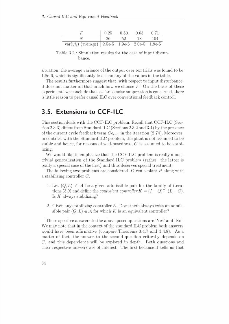
8/8/2019 Evaluasi pada Iterative Learning Control
http://slidepdf.com/reader/full/evaluasi-pada-iterative-learning-control 80/175
3. Causal ILC and Equivalent Feedback
F 0.25 0.50 0.63 0.71N 26 52 78 104
var(ydN ) (average) 2.5e-5 1.9e-5 2.0e-5 1.9e-5
Table 3.2.: Simulation results for the case of input distur-
bance.
situation, the average variance of the output over ten trials was found to be1.8e-6, which is significantly less than any of the values in the table.
The results furthermore suggest that, with respect to input disturbance,it does not matter all that much how we choose F . On the basis of theseexperiments we conclude that, as far as noise suppression is concerned, thereis little reason to prefer causal ILC over conventional feedback control.
3.5. Extensions to CCF-ILCThis section deals with the CCF-ILC problem. Recall that CCF-ILC (Sec-tion 2.3.3) differs from Standard ILC (Sections 2.3.2 and 3.4) by the presenceof the current cycle feedback term Cek+1 in the iteration (2.74). Moreover,in contrast with the Standard ILC problem, the plant is not assumed to bestable and hence, for reasons of well-posedness, C is assumed to be stabi-lizing.
We would like to emphasize that the CCF-ILC problem is really a non-trivial generalization of the Standard ILC problem (rather: the latter isreally a special case of the first) and thus deserves special treatment.
The following two problems are considered. Given a plant P along witha stabilizing controller C .
1. Let (Q, L) ∈ A be a given admissible pair for the family of itera-tions (3.9) and define the equivalent controller K = (I − Q)−1 (L + C ).Is K always stabilizing?
2. Given any stabilizing controller K . Does there always exist an admis-sible pair (Q, L) ∈ A for which K is an equivalent controller?
The respective answers to the above posed questions are ‘Yes’ and ‘No’.
We may note that in the context of the standard ILC problem both answerswould have been affirmative (compare Theorems 3.4.7 and 3.4.8). As amatter of fact, the answer to the second question critically depends onC , and this dependence will be explored in depth. Both questions andtheir respective answers are of interest. The first because it tells us that
64

8/8/2019 Evaluasi pada Iterative Learning Control
http://slidepdf.com/reader/full/evaluasi-pada-iterative-learning-control 81/175
3.5. Extensions to CCF-ILC
there always exists an equivalent stabilizing feedback controller. The secondbecause it says that in case we do decide to apply ILC, the controller C should be considered a design parameter.
3.5.1. Equivalent feedback
The next lemma gives a necessary and sufficient condition for a pair (Q, L)to be admissible with respect to the class of iterations (3.9).
Lemma 3.5.1. Consider the family of iterations (2.74). Let P be a real-rational transfer function and let C be a stabilizing controller for P . Thepair (Q, L) is admissible if and only if
(Q − LP ) (I + CP )−1
∞ < 1 (3.51)
Proof. The proof runs along the same lines as that of Lemma 3.4.1. Theidea is to consider the term zk := Qu pk + Le pk, which can be viewed as‘the ILC contribution’ to the feedback loop. If we can show boundednessof {zk} then, by internal stability, boundedness of {uk} and {yk} follows.Conversely, if we can construct {wk} and pick K , such that zK can bemade arbitrarily large, it follows that either u pK or y pK can grow withoutbound, which would violate the condition for admissibility.
Define F := (Q − LP ) (I + CP )−1 and verify that zk satisfies
zk+1 = F zk + F wk + (F C + L) yd. (3.52)
Note that (F C + L)∈ RH∞
. If we define d := (F C + L) yd and wk := F wk,Equation (3.52) simplifies to
zk+1 = F zk + wk + d, (3.53)
an expression resembling Eqn. (3.11). Let us observe that switching fromwk to wk does not affect the construction used in the proof for the StandardILC case (Lemma 3.4.1). The rest of the proof would be a mere duplicationand is thus omitted.
The next theorem shows that the equivalent controller for CCF-ILC isinternally stabilizing.
Theorem 3.5.2. Given P strictly proper and let (Q, L) be an admissiblepair. Then the equivalent controller K = (I − Q)−1 (L + C ) defines a proper real-rational matrix transfer function. Moreover, the corresponding feedback system (Figure 3.7) is well-posed and internally stable.
65
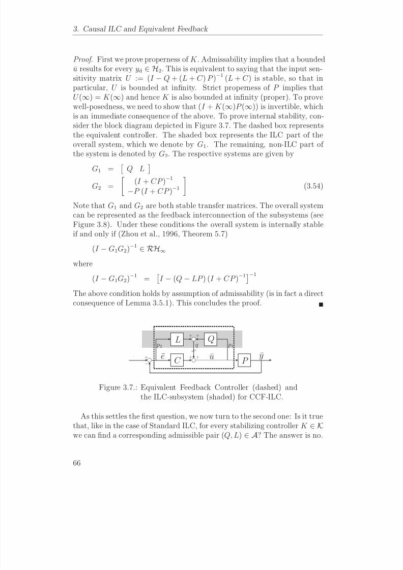
8/8/2019 Evaluasi pada Iterative Learning Control
http://slidepdf.com/reader/full/evaluasi-pada-iterative-learning-control 82/175
3. Causal ILC and Equivalent Feedback
Proof. First we prove properness of K . Admissability implies that a boundedu results for every yd ∈ H2. This is equivalent to saying that the input sen-sitivity matrix U := (I − Q + (L + C ) P )−1 (L + C ) is stable, so that inparticular, U is bounded at infinity. Strict properness of P implies that
U (∞) = K (∞) and hence K is also bounded at infinity (proper). To provewell-posedness, we need to show that (I + K (∞)P (∞)) is invertible, whichis an immediate consequence of the above. To prove internal stability, con-sider the block diagram depicted in Figure 3.7. The dashed box representsthe equivalent controller. The shaded box represents the ILC part of theoverall system, which we denote by G1. The remaining, non-ILC part of the system is denoted by G2. The respective systems are given by
G1 =
Q L
G2 =
(I + CP )−1
−P (I + CP )−1
(3.54)
Note that G1 and G2 are both stable transfer matrices. The overall systemcan be represented as the feedback interconnection of the subsystems (seeFigure 3.8). Under these conditions the overall system is internally stableif and only if (Zhou et al., 1996, Theorem 5.7)
(I − G1G2)−1 ∈ RH∞
where
(I − G1G2)−1 =
I − (Q − LP ) (I + CP )−1−1
The above condition holds by assumption of admissability (is in fact a directconsequence of Lemma 3.5.1). This concludes the proof.
p1 p2 q
C
L Q
P yd
−+ +
+ +
+ ye u
Figure 3.7.: Equivalent Feedback Controller (dashed) and
the ILC-subsystem (shaded) for CCF-ILC.
As this settles the first question, we now turn to the second one: Is it truethat, like in the case of Standard ILC, for every stabilizing controller K ∈ Kwe can find a corresponding admissible pair (Q, L) ∈ A? The answer is no.
66
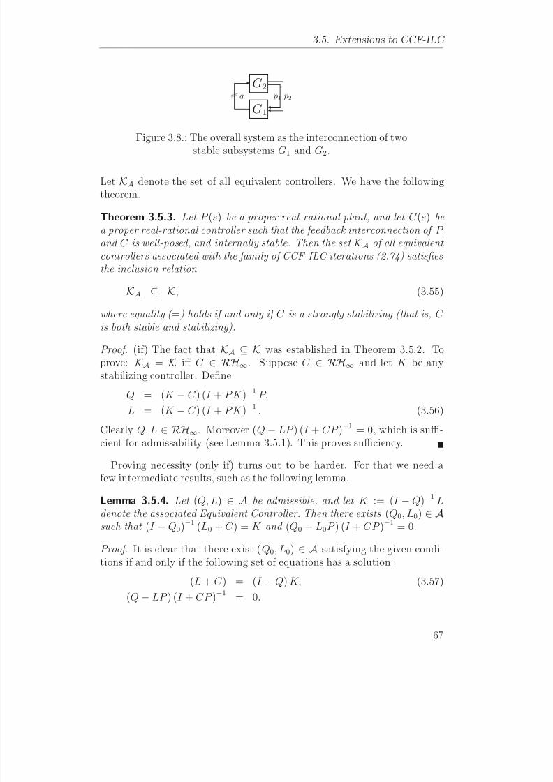
8/8/2019 Evaluasi pada Iterative Learning Control
http://slidepdf.com/reader/full/evaluasi-pada-iterative-learning-control 83/175
3.5. Extensions to CCF-ILC
p1 p2q
G2
G1
Figure 3.8.: The overall system as the interconnection of twostable subsystems G1 and G2.
Let KA denote the set of all equivalent controllers. We have the followingtheorem.
Theorem 3.5.3. Let P (s) be a proper real-rational plant, and let C (s) bea proper real-rational controller such that the feedback interconnection of P and C is well-posed, and internally stable. Then the set KA of all equivalent controllers associated with the family of CCF-ILC iterations (2.74) satisfies
the inclusion relation KA ⊆ K, (3.55)
where equality ( =) holds if and only if C is a strongly stabilizing (that is, C is both stable and stabilizing).
Proof. (if) The fact that KA ⊆ K was established in Theorem 3.5.2. Toprove: KA = K iff C ∈ RH∞. Suppose C ∈ RH∞ and let K be anystabilizing controller. Define
Q = (K − C ) (I + P K )−1 P,
L = (K − C ) (I + P K )−1
. (3.56)
Clearly Q, L ∈ RH∞. Moreover (Q − LP ) (I + CP )−1 = 0, which is suffi-cient for admissability (see Lemma 3.5.1). This proves sufficiency.
Proving necessity (only if) turns out to be harder. For that we need afew intermediate results, such as the following lemma.
Lemma 3.5.4. Let (Q, L) ∈ A be admissible, and let K := (I − Q)−1 Ldenote the associated Equivalent Controller. Then there exists (Q0, L0) ∈ Asuch that (I − Q0)−1 (L0 + C ) = K and (Q0 − L0P ) (I + CP )−1 = 0.
Proof. It is clear that there exist (Q0, L0) ∈ A satisfying the given condi-tions if and only if the following set of equations has a solution:
(L + C ) = (I − Q) K, (3.57)
(Q − LP ) (I + CP )−1 = 0.
67

8/8/2019 Evaluasi pada Iterative Learning Control
http://slidepdf.com/reader/full/evaluasi-pada-iterative-learning-control 84/175
3. Causal ILC and Equivalent Feedback
The unique solution to the above set of equations is given by
Q0 = (K − C ) P (I + KP )−1 ,
L0 = (K − C ) (I + P K )−1 . (3.58)
From (3.57) we obtain
K − C = L + QK. (3.59)
We substitute (3.59) into (3.58) and upon we inspection we conclude thatQ0, L0 ∈ RH∞. By construction, (Q0, L0) is admissible. This concludes theproof.
What Lemma 3.5.4 says is that again, like in the case of Standard ILC,we can restrict attention to a smaller set of representative pairs withoutloosing generality. We exploit this fact to characterize the set
KA. Note
that the set A0 of all (Q, L) ∈ A such that (Q − LP ) (I + CP )−1 = 0 canbe parameterized as follows
A0 = {(Q, L) = (ZN,ZM ); Z ∈ RH∞} (3.60)
where P = M −1N is a left-coprime factorization over RH∞. For stableP we can take M = I and N = P . The corresponding parameterizationcoincides with the one we found in Section 3.4 for the case of StandardILC (Equation 3.39). Through (3.60) we arrive at the following efficientparameterization of the set KA.
Lemma 3.5.5. Let C = V −1U and P = M −1N be any left-coprime fac-torization of the plant and the controller respectively. Then the set of al l equivalent controllers KA is parameterized as
KA =
K = (V − V ZM )−1 (U + V ZN ) ; Z ∈ RH∞
(3.61)
Proof. The equivalent controller is defined as
K = (I − Q)−1 (L + C )
With (Q, L)
∈ A0, this expression evaluates to
K = (I − ZM )−1
V −1U + ZN
= (V − V ZM )−1 (U + V ZN ) (3.62)
This concludes the proof.
68

8/8/2019 Evaluasi pada Iterative Learning Control
http://slidepdf.com/reader/full/evaluasi-pada-iterative-learning-control 85/175
3.6. Experimental verification
Although the above parameterization seems to depend on specific factor-izations, in actual fact the choice of coprime factors is immaterial. This isimmediate from the fact that left-coprime factors are unique up to a leftmultiplication with a bistable transfer function (unit of RH∞).
The following lemma restates an important result in control theory, namelythe parameterization of all stabilizing controllers for a given plant P . Thisresult is due (independently) to Youla and Kucera.
Lemma 3.5.6 (Youla-Kucera). Given C = V −1U and P = M −1N with (U, V ) and (M, N ) left-coprime (over RH∞. Assume C is stabilizing. Then the set K of all stabilizing controllers is given by (Zhou et al., 1996, Theorem 12.7)
K =
K =
V − ZM
−1 U + ZN
; Z ∈ RH∞
(3.63)
If we compare the respective parameterizations of KA (Lemma 3.5.5) andK (Lemma 3.5.6) we see that they are equivalent if and only if for everyZ ∈ RH∞ there exists Z ∈ RH∞ such that Z = V Z . The condition forequality is clearly satisfied in case C is strongly stabilizing (C ∈ RH∞)since then V is bistable and Z can be taken to be Z = V −1Z . This agreeswith Theorem 3.5.3. We conclude this section with the remaining part of the proof of Theorem 3.5.3.
Proof. (of Theorem 3.5.3, only if) We need to show that KA = K only if C ∈ RH∞. Suppose C ∈ RH∞. Take Z = I and let K be the corresponding
stabilizing controller (Lemma 3.5.6). By uniqueness of the Youla parameterit is clear that the corresponding controller K belongs to KA if and only if there exist Z ∈ RH∞ such that V Z = I . This however implies that V isbistable and C = V −1U stable, which contradicts our starting assumption.This concludes the proof.
3.6. Experimental verification
3.6.1. The Experimental setup: the Linear Motor MotionSystem
We conducted some experiments on a linear motor system, the LiMMS (LIn-ear Motor Motion System). A picture of the LiMMS is shown in Figure 3.9.The motor configuration consists of a base plate, covered with permanentmagnets, and a sliding part (the translator ), which holds the electric coils
69

8/8/2019 Evaluasi pada Iterative Learning Control
http://slidepdf.com/reader/full/evaluasi-pada-iterative-learning-control 86/175
3. Causal ILC and Equivalent Feedback
Figure 3.9.: The experimental setup: a magnetically actu-ated linear motor
and their iron cores. The principle of operation is a follows—see Velthuis(2000). A three-phase current generates a sequence of attracting and re-pelling forces between the magnetic poles of the coils in the translator andthat of the permanent magnets in the base plate. The configuration is suchthat for all i, the phase of the current applied to coil i differs by 2π/3(modulo 2π) from that applied to coil i + 1; this effects a net motion.
During operation, the LiMMS suffers from stiction, sliding friction, andcogging . Cogging is an effect that is common to the class of systems theLiMMS represents. It results from a strong magnetic interaction betweenthe permanent magnets in the base plate and the iron cores of the coils of the translator. The cogging force effectively tries to align the magnets and
the iron cores to stable positions of the translator.The LiMMS has an effective range of about 0.6m. An optical (incre-
mental) sensor with a resolution of about 1 µm measures the translator’srelative displacement. ‘Absolute’ displacement is defined with respect to afixed home position. As the LIMMS becomes operational, it goes throughan initialization phase, in which the translator is first aligned with the mag-nets in the base plate, and then steered to its home position, where theencoder is reset.
In each experiment, the LiMMS was to track a second-order polynomialreference signal, as depicted in Figure 3.10. In standard operation mode,the system was controlled by a PD-type feedback controller,
C (s) = 177700
0.0084s + 1
0.00084s + 1
. (3.64)
For the design of the ILC scheme, we used the following, rudimentary, model
70

8/8/2019 Evaluasi pada Iterative Learning Control
http://slidepdf.com/reader/full/evaluasi-pada-iterative-learning-control 87/175
3.6. Experimental verification
of the plant dynamics:
P (s) =1
ms2. (3.65)
We estimated the mass parameter to m = 5kg. Note that this model cap-tures just the basic dynamic behavior (that of a moving mass).
3.6.2. Experiment Design
Let us detail the experiment objective. We consider a family of CCF-ILCiterations,
uk+1 = Quk + Lek + Cek+1. (3.66)
Our hypothesis is that to every causal iteration of the form (3.66), there
corresponds an equivalent feedback controllerK := (I − Q)−1 (L + C ) , (3.67)
which gives the same performance (tracking error), without a single iter-ation. To test this hypothesis, we conduct a series of experiments. Eachexperiment consists of a sequence of steps, detailed below.
1. Pick some admissible pair (Q, L).
2. Run the iteration (3.66) until it has converged.
3. Record and store relevant data over a period of ten consecutive trials.
4. Compute the average over ten trials.
5. Switch to equivalent feedback (3.67).
6. Wait for transients to die out.
7. Record and store relevant data over a period of ten consecutive trials.
8. Compute the averages.
9. Compare the results of steps 4 and 8.A few remarks are in order: (a) We select Q and L so that L := QP −1, and
Q(s) :=1
(sτ + 1)2. (3.68)
71

8/8/2019 Evaluasi pada Iterative Learning Control
http://slidepdf.com/reader/full/evaluasi-pada-iterative-learning-control 88/175
3. Causal ILC and Equivalent Feedback
0.5
0.45
0.4
0.35
0.3
0.25
0.2
0.15
0.1
0.05
00 1 2 3 4 5
p o s i t i o n [ m ]
time [s]
0.4
0.35
0.3
0.25
0.2
0.150.1
0.05
00 1 2 3 4 5
v e l
o c i t y [ m / s ]
time [s]
(a) Position profile (b) Velocity profile
Figure 3.10.: The reference trajectory (left) that the systemhas to track. It has a period of 5s and a am-plitude of 0.5m. The figure on the left showsposition; The one on the right, velocity.
By construction Q−LP = 0, so that by Lemma 3.5.1, the pair (Q, L) is ad-missible. This guarantees that the design is at least nominally convergent.We are aware of other synthesis procedures wherein L is matched to theinverse of the closed-loop map (I + P C )−1 P , instead of to the inverse of P .These procedures would probably yield better performance. But given ourobjective, which is not to select the optimal parameters, but rather to vali-date our hypothesis, we want to keep things as simple as possible; (b) withrespect to step 2, we remark that—by construction, see above—convergenceis practically achieved within a few (even one or two) trials. Convergence isestablished by means of visual inspection; (c) the system is not actually re-set after each trial. Instead, it is periodically excited by the same referenceinput. In the literature, this is known as repetitive control ; (d) The reasonfor averaging over ten trials is to eliminate, or at least reduce the effect of random disturbances.
The results of the experiments are presented in Section 3.6.4. Coming upnext is an overview of implementation details.
3.6.3. Implementation details
The control system was designed and implemented in Matlab Simulink.Using the real-time workshop we created targeted C-code which we down-loaded on a DSP board inside a PC. The DSpace software that we usedfor interfacing, allowed us to change parameters and monitor the system’sperformance, both in real time.
72

8/8/2019 Evaluasi pada Iterative Learning Control
http://slidepdf.com/reader/full/evaluasi-pada-iterative-learning-control 89/175
3.6. Experimental verification
Dynamic filters were implemented using continuous-time ‘blocks’ . Thiswas done to match the ‘analog’ output of the DA convertors. The samplefrequency was set to 1kHz. With a trial length of 5s, this amounts to 5000samples per signal per trial. The buffer length of the memory block was
chosen accordingly.In order to allow for a fair comparison, and to enhance the transparancyof the design, we chose to match the structure of the Equivalent Controllerto that of the ILC scheme. A transition from ILC to Equivalent Feedbackwas effected by shortcutting the memory block. The basic schematic isshown in Figure 3.11.
MEMORY
C
L Q
P yd −
+
++
+
+ ye u
MEMORY
C
L Q
P yd −
+
++
+
+ ye u
(a) ILC (b) Equivalent Feedback
Figure 3.11.: A schematic, showing the respective imple-mentations of CCF-ILC (left) and the corres-ponding equivalent feedback controller (right).
In Figure 3.12 we show how switching from nominal feedback to ILCaffects the system’s performance. We observe that the tracking error is sig-
nificantly reduced, from about 120µm (peak value) to about 40µm. Mostapparent is the successful suppression of the inertial effect in the accelera-tion and deceleration phase. We also observe that the iteration practicallyconverges within one trial, as expected.
3.6.4. Results
We now present the results of our experiments. We compared the aver-age tracking error in ILC with the average tracking error obtained usingEquivalent Feedback. The same experiment was repeated for several dif-
ferent values of τ (see 3.68). Figures 3.13 and 3.14 show the results forτ = 1/150, and τ = 1/325. Let us first establish the fact that, rela-tive to the nominal feedback situation (without ILC or equivalent feedback)both methods greatly improve upon the tracking accuracy. This is impor-tant, since it is conceivable that for certain parameter combinations the
73

8/8/2019 Evaluasi pada Iterative Learning Control
http://slidepdf.com/reader/full/evaluasi-pada-iterative-learning-control 90/175
3. Causal ILC and Equivalent Feedback
1
0
−1
0 5 10 15 20
×10−4
e r r o r [ m ]
time [s]
servo errorreference
Figure 3.12.: The system under standard feedback withoutILC (left of the vertical dashed line), and with
ILC (right of the vertical dashed line). Shownalso (not in scale) is the cycloidal referenceinput. Note that the system practically con-verges after one trial.
5432
10
−1−2−3−4−5
0 1 2 3 4 5
×10−4
e r r o r [ m
/ s ]
time [s]
5432
10
−1−2−3−4−5
0 1 2 3 4 5
×10−4
e r r o r [ m
/ s ]
time [s]
(a) ILC (b) Equivalent Feedback
Figure 3.13.: The average tracking error in ILC comparedwith that of the Equivalent Feedback config-
uration. The average was computed over tenconsecutive trials (cycles). These results wereobtained for τ = 1/150.
74

8/8/2019 Evaluasi pada Iterative Learning Control
http://slidepdf.com/reader/full/evaluasi-pada-iterative-learning-control 91/175
3.6. Experimental verification
543210
−1−2−3−4−5
0 1 2 3 4 5
×10−4
e r r o
r [ m / s ]
time [s]
543210
−1−2−3−4−5
0 1 2 3 4 5
×10−4
e r r o
r [ m / s ]
time [s]
(a) ILC (b) Equivalent Feedback
Figure 3.14.: The average tracking error in ILC comparedwith that of the equivalent feedback configu-ration. The average was computed over ten
consecutive trials (cycles). The scale is thesame as in Figure 3.13. These results wereobtained for τ = 1/325.
impact of learning is negligable, especially so when the nominal PD con-troller is very well tuned. In that case there would be nothing to compare.Secondly, we observe that in both cases the Equivalent Controller is stabi-lizing—as expected, since the corresponding ILC scheme is convergent (seeTheorem 3.5.2). At the same time, it is clear (especially from Figure 3.14)that the respective performances are not identical . The difference is small,
but not negligible. Besides, it is persistent: we observed the same situa-tion in all experiments. The general trend is that the difference increaseswith 1/τ . Closer inspection of the data shows that the cogging effect isreponsible for the larger part of the error. FFT analysis reveals peak ac-tivity at 24Hz (see Figure 3.15). When we compute the first derivative of the reference position with respect to time (see Figure 3.10b), we find thatthe maximum (reference) velocity is 0.40m/s. At the maximum the secondderivative is obviously zero. During this time, the LiMMS operates at rela-tively constant speed. Given that the magnets in the base plate are situated1.6 − 1.7cm apart, we may indeed expect significant activity at and around
0.4/0.0165 ≈ 24Hz.These results pose some serious questions. Do these findings invalidateour conclusions? That is hard to say. On the basis of Figure 3.11a, we wouldexpect that if the iteration converges, then by definition, the signal goinginto the memory block would be identical to that going out. This suggests
75
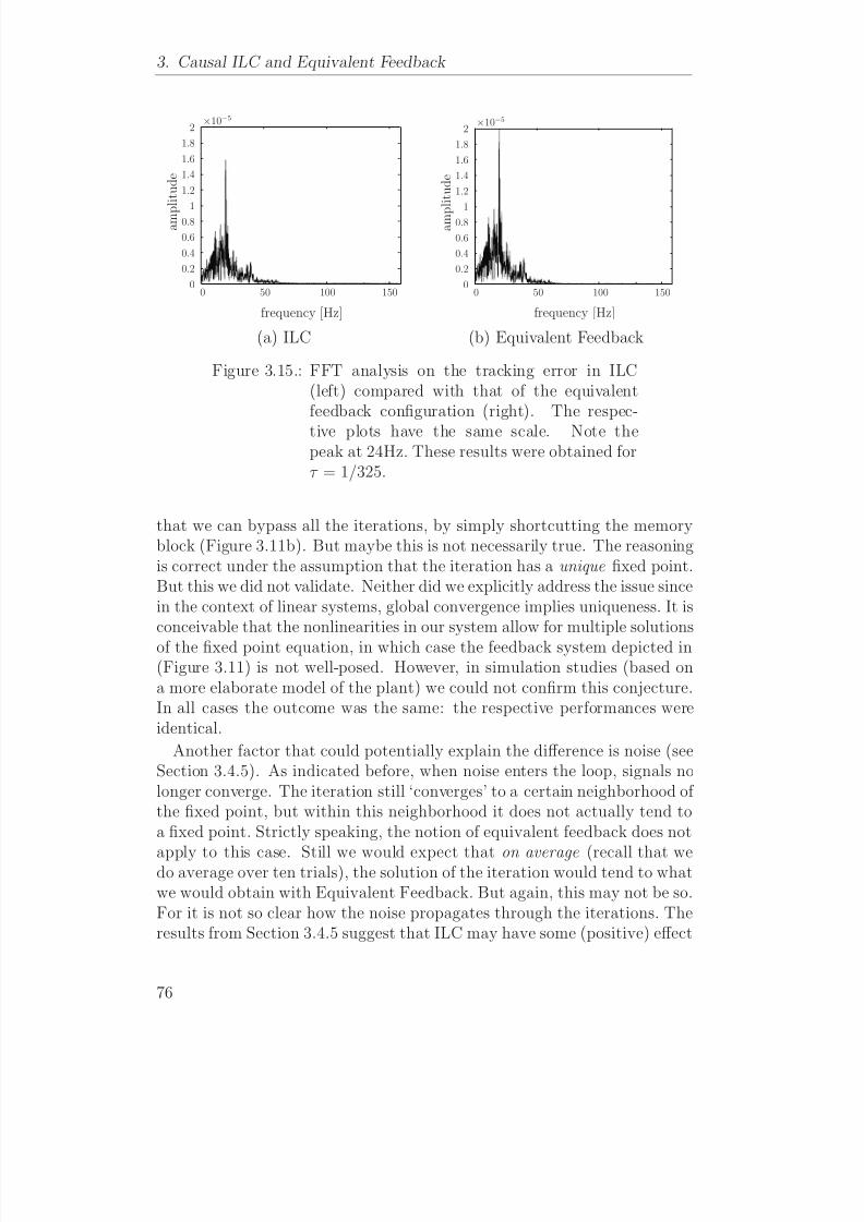
8/8/2019 Evaluasi pada Iterative Learning Control
http://slidepdf.com/reader/full/evaluasi-pada-iterative-learning-control 92/175
3. Causal ILC and Equivalent Feedback
2
1.8
1.6
1.4
1.2
1
0.8
0.6
0.4
0.2
00 50 100 150
×10−5
a m p l i t u d e
frequency [Hz]
2
1.8
1.6
1.4
1.2
1
0.8
0.6
0.4
0.2
00 50 100 150
×10−5
a m p l i t u d e
frequency [Hz]
(a) ILC (b) Equivalent Feedback
Figure 3.15.: FFT analysis on the tracking error in ILC(left) compared with that of the equivalentfeedback configuration (right). The respec-
tive plots have the same scale. Note thepeak at 24Hz. These results were obtained forτ = 1/325.
that we can bypass all the iterations, by simply shortcutting the memoryblock (Figure 3.11b). But maybe this is not necessarily true. The reasoningis correct under the assumption that the iteration has a unique fixed point.But this we did not validate. Neither did we explicitly address the issue sincein the context of linear systems, global convergence implies uniqueness. It isconceivable that the nonlinearities in our system allow for multiple solutions
of the fixed point equation, in which case the feedback system depicted in(Figure 3.11) is not well-posed. However, in simulation studies (based ona more elaborate model of the plant) we could not confirm this conjecture.In all cases the outcome was the same: the respective performances wereidentical.
Another factor that could potentially explain the difference is noise (seeSection 3.4.5). As indicated before, when noise enters the loop, signals nolonger converge. The iteration still ‘converges’ to a certain neighborhood of the fixed point, but within this neighborhood it does not actually tend toa fixed point. Strictly speaking, the notion of equivalent feedback does not
apply to this case. Still we would expect that on average (recall that wedo average over ten trials), the solution of the iteration would tend to whatwe would obtain with Equivalent Feedback. But again, this may not be so.For it is not so clear how the noise propagates through the iterations. Theresults from Section 3.4.5 suggest that ILC may have some (positive) effect
76

8/8/2019 Evaluasi pada Iterative Learning Control
http://slidepdf.com/reader/full/evaluasi-pada-iterative-learning-control 93/175
3.7. Discussion
on noise surpression, but the question is whether this effect can accountfor the difference observed. We ran some simulations to find out. We diddetect differences in the respective performances. But unlike in the realsetup, these differences were not significant.
A third factor, which is more of a guess again, is the software. We useda high-level language to specify our control scheme. The resulting modelhad to be compiled so as to create portable C-code that could be targetedto our DSP board. We do not know what code is actually exported to, andexecuted by the DSP board. Even if we assume that the software does whatit is supposed to do, we still do not know if our code is what we want it tobe. To put it differently: we can only hope that the high-level structuralequivalence is reflected at the code level.
3.7. Discussion
We studied the synthesis problem associated with a class of causal iterations,and ‘solved’ it, to the extent that we showed that the problem can be recastas a compensator design problem. More accurately: we found that bothmethods are essentially equivalent.
Of all questions that remain, the most pressing, no doubt, is the following:why would would we design and implement an iterative scheme, knowingthat, at no extra cost, the same performance can be obtained using a simplefeedback controller? And in view of this, what good is our contribution?
As for the first question, we concur that there appears to be little reason tocontinue research on the type of causal iterations we considered, and indeedall the more reason to consider alternatives, which is what we will do in thenext chapter. Yet, the final word has not been spoken. Our experimentalresults were not fully supportive and more work in this direction is to beconducted.
As for the second question, we believe our contribution to be valuable, if only because of the following:
• Our theory on admissible pairs and equivalent feedback casts new lighton the compensator design problem, providing a new interpretationof classical results on the parameterization of stabilizing controllers,
as contained in e.g. Zames (1981) and Youla et al. (1976)).
• By showing that the location of the fixed point and the speed of con-vergence to the fixed point are independent, we justified an assumptionimplicit in many existing synthesis procedures.
77

8/8/2019 Evaluasi pada Iterative Learning Control
http://slidepdf.com/reader/full/evaluasi-pada-iterative-learning-control 94/175
3. Causal ILC and Equivalent Feedback
• Our approach using equivalent admissible pairs generalizes to familiesof iterations involving noncausal operators, in which case an interpre-tation in terms of Equivalent Feedback cannot be given.
3.7.1. Causal ILC and equivalent feedbackIt is fair to say that the result on Equivalent Feedback, first appearingin Goldsmith (2001), took the community by surprise. On the one hand,this is not much of a surprise itself, as ILC was never meant to have astong bearing on mainstream control methods. On the other hand, certainpapers had been hinting at the same result, see e.g. Moore et al. (1992) andde Roover (1996).
In this respect, ILC research took an important turn when it adoptedH∞-techniques. For only then it became apparent what (causal) ILC wascapable of, and, more importantly, what it was not. The explicit idea of
Equivalent Feedback made it absolutely clear that the problem of (causal)ILC and that of conventional feedback are very much akin and confirmedwhat was already believed for long, namely that both methods subject tothe same performance limitations.
3.7.2. Noncausal ILC
In a conventional feedback situation, the system’s output is directly fed backinto its input. By construction, this kind of ‘closed-loop feedback’ imposesa causality constraint on the feedback map. For if the current value of theinput were to depend on future values of the output, we would have toassume the latter to be known ahead of time. Which, for a typical physicalsystem, is not a realistic assumption. In ILC, the process of informationfeedback takes place offline, and may involve noncausal operations. In thenext chapter we discuss how we can deploy such operations to overcomecertain performance limitations.
78

8/8/2019 Evaluasi pada Iterative Learning Control
http://slidepdf.com/reader/full/evaluasi-pada-iterative-learning-control 95/175
4
Noncausal ILC
Overview – We extend the two-parameter synthesis problem by allowing both operators to be noncausal. We discuss how the ad-ditional freedom may be deployed with particular emphasis on set-tings involving non-minimum phase behavior. We investigate the
possibilities of Equivalent Feedback and show that the candidate equivalent controller is generally destabilizing.
4.1. Introduction
Conventional feedback control studies feedback systems comprising a plant P : U → Y , y(t) := (P u)(t), and a compensator C : Y → U ,
u(t) := (Ce)(t), (4.1)where e(t) := yd(t) − y(t). Typically, the plant is assumed causal, which isto say that for all t0, the value of the output y at time t = t0 is assumed notto depend on values of the input u at times t > t0. In closed-loop feedback,the compensator is always causal, even in the unlikely case the plant is not.In ILC, this is not necessarily the case.
For we may recall that ILC is an offline method; an offline method thatis perhaps best described as open-loop feedback . After all, notwithstandingits open-loop nature, ILC is a feedback method; It feeds back information inmuch the same way as conventional methods do (see Chapter 3 for details).
In any case, being an offline method, ILC allows for ‘noncausal’ oper-ations, by means of which the ‘future’ of past trials can take part in theconstruction of the current control action.
In the present chapter we explain why this could be useful. We also re-turn to our synthesis problem, this time without imposing any causality
79

8/8/2019 Evaluasi pada Iterative Learning Control
http://slidepdf.com/reader/full/evaluasi-pada-iterative-learning-control 96/175
4. Noncausal ILC
constraints. The chapter’s first objective is to justify the additional designfreedom. As we look into plants with non-minimum phase behavior we willsee that these systems alone provide ample motivation. More generally, weshow that noncausal iterations can overcome various closed-loop related per-
formance constraints, such as Bode’s Sensitivity Integral, Poisson’s IntegralFormula, etc.The chapter’s second objective is to establish a result on Equivalent Feed-
back. We show that like in the case of causal ILC, an ‘equivalent’ (virtual)closed-loop feedback stucture may be defined. But it turns out that thecandidate Equivalent Controller is generally destabilizing (when interpretedand implemented as a causal map). More precisely, we find that the Equi-valent Controller is non causal which means that it cannot be implementedin closed loop.
The outline of the chapter is as follows. In Section 4.A we review somepreliminaries on noncausal operators. This involves in particular a discus-
sion on the effects of truncation, and some implementation issues. In Sec-tion 4.2 we show how noncausal operators may be employed in the contextof the ILC synthesis problem. Section 4.3 covers the topic of EquivalentFeedback, and Section 4.4 concludes with a discussion of the main results.
4.2. Noncausal ILC
Let us turn to noncausal ILC. After introducing the basic concepts, we showwhy, in various situations, it may be advantageous to consider noncausaloperators. For details concerning notation and terminology, we refer to
Appendix 4.A.
4.2.1. Literature on Noncausal ILC
The idea of noncausal processing has been widely discussed in the ILCliterature, under various different headings. It is there in Arimoto’s originalalgorithm—Arimoto et al. (1984), see Section 2.2.1, whose derivative actionassumes some preview (be it infinitesimally small) of the future. It is therein its many discrete-time extensions, where its derivative action is replacedby forward shifts. And it is there is many other papers, which we cannot
even begin to list here.In this thesis, we adopt a continuous-time perspective. Ignoring dis-cretization effects, our framework provides us with the conceptual advan-tage of being able to distinguish between noncausal and nonproper oper-ators. Arimoto’s algorithm and most of its offspring is based on the use
80

8/8/2019 Evaluasi pada Iterative Learning Control
http://slidepdf.com/reader/full/evaluasi-pada-iterative-learning-control 97/175
4.2. Noncausal ILC
of nonproper, rather than noncausal operators. Indeed, the main idea inthese approaches is to introduce sufficient derivative action (enough forwardshifts) to compensate for the system’s relative degree, reducing the overallphase shift, thus making the system amenable to a form of high-gain feed-
back (infinite gain in fact, spread out over multiple trials) which forces theerror down to machine precision.
Though powerful, the approach has a number of shortcomings, some of which cannot be resolved, some of which can be. As indicated in Sec-tion 2.2.2, for this approach to be succesful, we need to know the system’srelative degree, and the sign of the first nonzero Markov parameter. Restric-tive as this condition may be, in this context, there is little we can do aboutit. But there is another problem that we can do something about. Andthat has to do with the derivative action. It is well known that computingderivatives is a hazardous undertaking, especially when the source signal iscontaminated with noise. This was also recognized some twenty years ago,shortly after the original algorithm was introduced. At the time, this ledto an increase of interest in P -type learning rules and the like. Recall thatD -type rules were known to converge under relatively mild conditions. Asthese P -type learning rule would not converge under equally mild condi-tions, many of them were equiped with a forgetting factor. This forgettingfactor generally improved convergence, but at the same time compromisedperformance. In this chapter we will show that by using noncausal opera-tors, even bounded noncausal operators, the aggressive D -action, character-istic of most Arimoto-type update laws, may be smoothed out over multipletrials, leading to a well-behaved algorithm, at no extra cost.
In our approach we focus on bounded noncausal, rather than (unbounded)nonproper operators (which we do not consider to be noncausal, or a limitcase at best). We address several performance limitations inherent to causalupdate laws and show that most of these do not apply to noncausal updatelaws. Additionally, we show how to use noncausal operators in connectionwith non-minimum phase plants. In this respect, our approach bears onthe work of Tomizuka (1987), whose Zero Phase Error Tracking Algorithm(ZPETK) is well-known in the general tracking literature.
4.2.2. Introduction: a motivation
To motivate the idea of using noncausal operators, let us go back to Sec-tion 2.2.2. In that section we discussed several perspectives on the problemof ILC. As we may recall, one of these perspectives was connected with the
81

8/8/2019 Evaluasi pada Iterative Learning Control
http://slidepdf.com/reader/full/evaluasi-pada-iterative-learning-control 98/175
4. Noncausal ILC
problem of finding the minimizing argument of the functional
J (∆u; γ ) =
yd − P (u + ∆u)γ ∆u,
2
, (4.2)
the solution of which led us to the update law (compare with (2.53))
uk+1 = uk + γ −1
γ −1P + γ (P ∗)−1−1ek. (4.3)
To arrive at this expression, we had to assume that P is invertible (but notnecessarily boundedly invertible, e.g. P −1(s) must exist, but need not definea bouded operator on H2). Update law (4.3) is of the form
uk+1 = uk + Lek, (4.4)
with L defined as
L := γ −1 γ −1P + γ (P ∗)−1−1 . (4.5)
If P is stable—which indeed we assume—then the adjoint operator P ∗(s) :=P T (−s) is antistable (i.e. has all its poles in the open RHP). The poles of Lare the zeros of (γP (s)) + (γP (−s))−1. It is immediate that if s0 is a poleof L then so is −s0. Hence, in general, L will have poles in both the left,and the right-half plane. This also shows in the next example.
Example 4.2.1. Let P (s) be given as
P (s) =1
s + 1
. (4.6)
We select γ = 1 and apply the update law (4.3) :
uk+1 = uk +
P (s) + (P (−s))−1−1
ek
= uk +
1
s + 1− s + 1
−1ek
= uk +−(s + 1)
(s +√
2)(s − √2)
ek
= uk +−1
2 + 14
√2
s + √2
ek +−1
2− 1
4
√2
s − √2
ek (4.7)
Here, we decomposed the noncausal operator
L(s) :=−(s + 1)
(s +√
2)(s − √2)
(4.8)
82
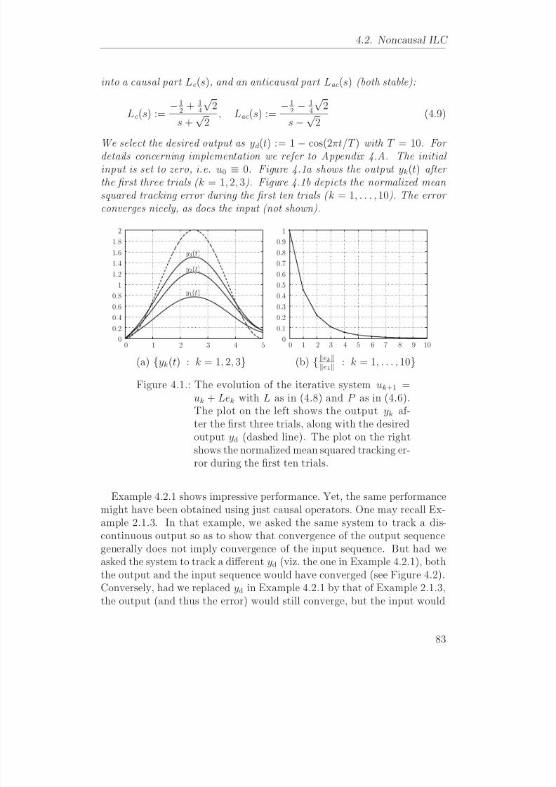
8/8/2019 Evaluasi pada Iterative Learning Control
http://slidepdf.com/reader/full/evaluasi-pada-iterative-learning-control 99/175
4.2. Noncausal ILC
into a causal part Lc(s), and an anticausal part Lac(s) (both stable):
Lc(s) :=−1
2+ 1
4
√2
s +√
2, Lac(s) :=
−12− 1
4
√2
s − √2
(4.9)
We select the desired output as yd (t) := 1 − cos(2πt/T ) with T = 10. For details concerning implementation we refer to Appendix 4.A. The initial input is set to zero, i.e. u0 ≡ 0. Figure 4.1a shows the output yk(t) after the first three trials ( k = 1, 2, 3). Figure 4.1b depicts the normalized mean squared tracking error during the first ten trials ( k = 1, . . . , 10). The error converges nicely, as does the input (not shown).
2
1.8
1.6
1.4
1.21
0.8
0.6
0.4
0.2
00 1 2 3 4 5
y3(t)
y2(t)
y1(t)
1
0.9
0.8
0.7
0.60.5
0.4
0.3
0.2
0.1
00 1 2 3 4 5 6 7 8 9 10
(a) {yk(t) : k = 1, 2, 3} (b) {eke1 : k = 1, . . . , 10}Figure 4.1.: The evolution of the iterative system uk+1 =
uk + Lek with L as in (4.8) and P as in (4.6).
The plot on the left shows the output yk af-ter the first three trials, along with the desiredoutput yd (dashed line). The plot on the rightshows the normalized mean squared tracking er-ror during the first ten trials.
Example 4.2.1 shows impressive performance. Yet, the same performancemight have been obtained using just causal operators. One may recall Ex-ample 2.1.3. In that example, we asked the same system to track a dis-continuous output so as to show that convergence of the output sequence
generally does not imply convergence of the input sequence. But had weasked the system to track a different yd (viz. the one in Example 4.2.1), boththe output and the input sequence would have converged (see Figure 4.2).Conversely, had we replaced yd in Example 4.2.1 by that of Example 2.1.3,the output (and thus the error) would still converge, but the input would
83
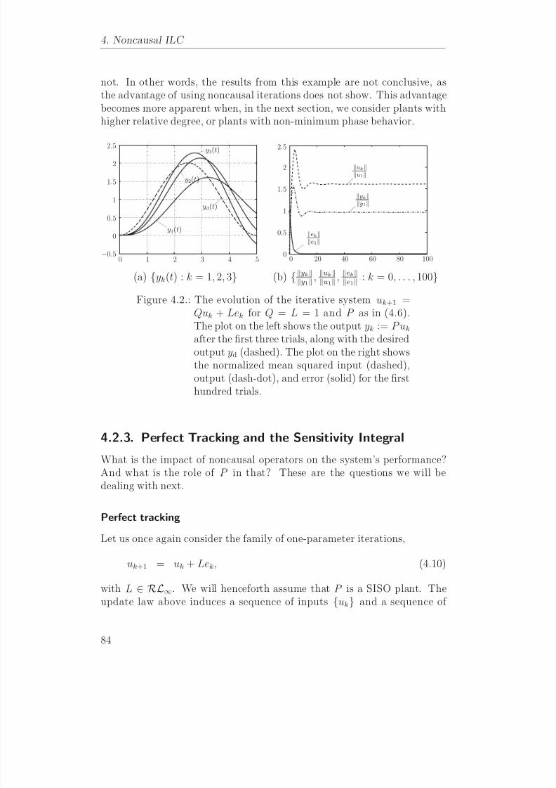
8/8/2019 Evaluasi pada Iterative Learning Control
http://slidepdf.com/reader/full/evaluasi-pada-iterative-learning-control 100/175
4. Noncausal ILC
not. In other words, the results from this example are not conclusive, asthe advantage of using noncausal iterations does not show. This advantagebecomes more apparent when, in the next section, we consider plants withhigher relative degree, or plants with non-minimum phase behavior.
2.5
2
1.5
1
0.5
0
−0.50 1 2 3 4 5
y1(t)
y2(t)
y3(t)
yd(t)
2.5
2
1.5
1
0.5
00 20 40 60 80 100
uku1
yky1
eke1
(a) {yk(t) : k = 1, 2, 3} (b) {yky1 , uku1 , eke1 : k = 0, . . . , 100}Figure 4.2.: The evolution of the iterative system uk+1 =
Quk + Lek for Q = L = 1 and P as in (4.6).The plot on the left shows the output yk := P uk
after the first three trials, along with the desiredoutput yd (dashed). The plot on the right showsthe normalized mean squared input (dashed),output (dash-dot), and error (solid) for the firsthundred trials.
4.2.3. Perfect Tracking and the Sensitivity Integral
What is the impact of noncausal operators on the system’s performance?And what is the role of P in that? These are the questions we will bedealing with next.
Perfect tracking
Let us once again consider the family of one-parameter iterations,
uk+1 = uk + Lek, (4.10)
with L ∈ RL∞. We will henceforth assume that P is a SISO plant. Theupdate law above induces a sequence of inputs {uk} and a sequence of
84

8/8/2019 Evaluasi pada Iterative Learning Control
http://slidepdf.com/reader/full/evaluasi-pada-iterative-learning-control 101/175
4.2. Noncausal ILC
outputs {P uk}. We may verify that yk → yd for all yd ∈ L2( jR) as k → ∞if and only if
|1 − L( jω)P ( jω)| < 1 (4.11)
for almost all ω ∈ R (that is: for all ω ∈ R except on a set of measurezero). In the situation that yk actually converges to yd , we speak of perfect tracking . Whether in that case the input sequence also converges dependson yd, as well as on the plant characteristics. More precisely, it depends onhow well the desired output matches the plant characteristics. If we assumethat the desired output is feasible, that is, if we assume that there existsud ∈ L2( jR) such that yd = P ud, then the sequence of inputs necessarilyconverges to ud. This follows from the fact that under the said conditionthe iteration
(ud − uk+1) = ( 1 − LP ) (ud − uk) (4.12)
converges to zero.
Causality constraints and pole-zero excess
In the light of our current discussion on the use of noncausal operators, aninteresting question to ask is: does there always exist L ∈ RH∞ (the spaceof causal operators) such that the |1 − L( jω)P ( jω)| is less than unity foralmost all ω? And if not, how about if we extend the range of L to RL∞?The following lemma provides a partial answer.
Lemma 4.2.2. Let P ∈ RH∞ be a plant having a pole-zero excess of at least two. Then for all L ∈ RH∞ we have that |1 − L( jω)P ( jω)| ≥ 1 on a set with nonzero measure.
Proof. Let us note that if |1 − L( jω)P ( jω)| < 1 for almost all ω, then ∞−∞
log |1 − L( jω)P ( jω)|dω < 0. (4.13)
To prove the statement, we show that under the conditions stated, (4.13)does not hold. The proof hinges upon a result by Poisson, which may bestated as follows. Let F : C → C be a function, analytic in the closedright-half plane (RHP), such that
limR→∞
|F (Re jθ)|R
= 0, (4.14)
85

8/8/2019 Evaluasi pada Iterative Learning Control
http://slidepdf.com/reader/full/evaluasi-pada-iterative-learning-control 102/175
4. Noncausal ILC
for all θ ∈ [−π2 , π
2 ]. Then the value of F (s) at any point s = x + jy in theopen RHP may be recovered from F ( jω) by the integral relation
F (s) =1
π ∞
−∞
F ( jω)x
x2 + (y
−ω)2
dω. (4.15)
We apply this result to evaluate log |1 − LP |. Let us adopt the shorthandnotation V := 1 − LP . We cancel the RHP zeros of V by introducing
V := B−1zerosV, (4.16)
where Bzeros(s) is the Blaschke product
Bzeros(s) :=i
zi − s
zi + s, (4.17)
formed from the open RHP zeros of V . Note that V is analytic in the openRHP. For any open RHP point s = x + jy we have
log V (s) =1
π
∞−∞
log V ( jω)x
x2 + (y − ω)2dω. (4.18)
Taking real parts on both sides (recall that Re(log(z)) = log(|z|)) gives
log |V (s)| =1
π
∞−∞
log |V ( jω)| x
x2 + (y − ω)2dω. (4.19)
Note that in the integrand on the right-hand side, we may replace |V ( jω)|by |V ( jω)|. We set y = 0 and multiply both sides by πx to get
πx log |V (x)| + πx log |B−1
zeros(x)| = ∞−∞ log |V ( jω)|x2
x2 + ω2 dω.(4.20)
Letting x → ∞, the right-hand side approaches ∞−∞ |V ( jω)|dω, and under
the assumption that P has pole-zero excess greater than one, the first termon the left, x log |V (x)|, approaches 0. For the remaining term on the left-hand side we have:
limx→∞
log |B−1zeros(x)| = lim
x→∞log
i
zi+xzi−x
= lim
x→∞Re
ix log
1 + zix
1 − zix
= i
Re zi
≥ 0. (4.21)
This concludes the proof.
86
8/8/2019 Evaluasi pada Iterative Learning Control
http://slidepdf.com/reader/full/evaluasi-pada-iterative-learning-control 103/175
4.2. Noncausal ILC
The result of Lemma 4.2.2 states that if we restrict attention to causaloperators, the condition for perfect tracking cannot be satisfied for plantswith relative degree greater than one. For plants having relative degreezero or one, we may distinguish between those that are minimum phase
and those that are not. A minimum-phase system is a system having allits zeroes in the in the open left-half plane. For such systems, we have thefollowing lemma.
Lemma 4.2.3. Let P ∈ RH∞ be a stable minimum-phase plant whose rel-ative degree does not exceed one. Then we can always find L ∈ RH∞ such that |1 − L( jω)P ( jω)| < 1 for almost all ω ∈ R.
Proof. Case (a): relative degree zero. Being minimum phase, it follow thatP must be bistable. We select L := P −1 so that 1 − LP = 0. Case (b):relative degree one. In this case we select L := ZP −1 with Z := 1/(s + 1).
It follows that|1 − L( jω)P ( jω)|2 =
ω2
ω2 + 1(4.22)
is less than unity for almost all ω ∈ R (and hence so is |1 − L( jω)P ( jω)|).This concludes the proof.
For non-minimum phase systems of arbitrary relative degree, it is easyto verify that the condition for perfect tracking (|1 − L( jω)P ( jω)| < 1 foralmost all ω) is never satisfied. For suppose s0 is an RHP zero of P . Then1 − L(s0)P (s0) = 1 and by the Maximum Modulus Principle we have thatsupω
|1
−L( jω)P ( jω)
| ≥1 with equality (=) if and only if 1
−L(s)P (s) is
a constant, that is, if and only L = 0. In any case 1 − L( jω)P ( jω) equalsor exceeds unity on a set of nonzero measure. In the next paragraph weshow that regardless whether P is minimum phase and has relative degreeless than two or not, we can always find L ∈ RL∞ (the space of non causaloperators) such that |1 − L( jω)P ( jω)| < 1 for almost all ω ∈ R.
Implications for the two-parameter problem
To conclude this subsection, let us point out that our discussion is notlimited to situations in which we seek to achieve perfect tracking. Indeed,let us consider a family of two-parameter iterations,
uk+1 = Quk + Lek. (4.23)
Let Q, L ∈ RH∞ be an admissible pair (Q − LP ∞ < 1). Without loss of generality (see Section 3.4) we may assume that Q − LP = 0, in which case
87
8/8/2019 Evaluasi pada Iterative Learning Control
http://slidepdf.com/reader/full/evaluasi-pada-iterative-learning-control 104/175
4. Noncausal ILC
we have
e = yd − P u
= yd − P (I − Q + LP )−1 Lyd
= (I − P L) yd. (4.24)
For e to be small, we require |I − P L| to be small (in an appropriate fre-quency range). In an (equivalent) feedback setting, I − P L would be the(output) sensitivity function S = (I + P K )−1 associated with the controllerK = (I − LP )−1 L. Bode’s Sensitivity Integral states that, provided P hasrelative degree two or more, the sensitivity function can only be made small(smaller than unity) over a certain frequency range and necessarily peaks(exceeds unity) in another. More precisely,
∞
0
log|S ( jω)
|dω
≥0, (4.25)
which is exactly the result of Lemma 4.2.2, be it in a different disguise. Inother words, not only does Lemma 4.2.2 inform us about the (im)possibilityof perfect tracking, it also shows that the performance achievable withCausal ILC is constrained in the indicated sense. As we will prove shortly,these design limitations are due to bandwidth constraints which may beovercome by resorting to noncausal operators.
4.2.4. Non-minimum phase plants and Poisson’s Integral
A (SISO) real rational plant P (s) is said to be non-minimum phase if it hasone or more unstable zeros, i.e. zeros in the open RHP. For instance, theplant
P (s) :=s − 1
s + 1(4.26)
has one unstable zero at s = 1. It is well-known that unstable zeros imposeconstraints on the achievable bandwidth in feedback systems—see Freuden-berg and Looze (1985); Engell (1988). And we may expect the same to betrue for causal ILC. Indeed, let z0 = x0 + jy0 with x0 > 0 be an open-RHP
zero of P . Then for all L ∈ RH∞ we have that ∞−∞
log(|1 − P ( jω)L( jω)|) x0
x20 + (y0 − ω)2
dω = π log |B−1zero(z0)|,
(4.27)
88
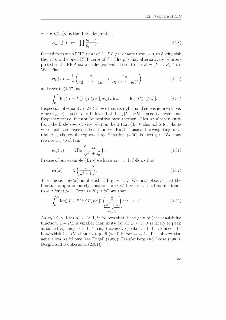
8/8/2019 Evaluasi pada Iterative Learning Control
http://slidepdf.com/reader/full/evaluasi-pada-iterative-learning-control 105/175
4.2. Noncausal ILC
where B−1zero(s) is the Blaschke product
B−1zeros(s) :=
i
pi − s
¯ pi + s, (4.28)
formed from open RHP zeros of I −P L (we denote them as pi to distinguishthem from the open RHP zeros of P . The pi’s may alternatively be inter-preted as the RHP poles of the (equivalent) controller K = (I − LP )−1 L).We define
wz0(ω) :=1
π
x0
x20 + (ω − y0)2
+x0
x20 + (ω + y0)2
, (4.29)
and rewrite (4.27) as ∞0
log(|I − P ( jω)L( jω)|)wz0(ω)dω = log |B−1zeros(z0)|. (4.30)
Inspection of equality (4.30) shows that its right-hand side is nonnegative.
Since wz0(ω) is positive it follows that if log |I − P L| is negative over somefrequency range, it must be positive over another. This we already knowfrom the Bode’s sensitivity relation, be it that (4.30) also holds for plantswhose pole-zero excess is less than two. But because of the weighting func-tion wz0, the result expressed by Equation (4.30) is stronger. We mayrewrite wz0 to obtain
wz0(ω) = 2Re
z0
ω2 + z20
. (4.31)
In case of our example (4.26) we have z0 = 1. It follows that
w1(ω) = 2 1ω2 + 1
. (4.32)
The function w1(ω) is plotted in Figure 4.3. We may observe that thefunction is approximately constant for ω 1, whereas the function tendsto ω−2 for ω 1. From (4.30) it follows that ∞
0
log(|I − P ( jω)L( jω)|)
2
ω2 + 1
w1(ω)
dω ≥ 0 (4.33)
As w1(ω) ≤ 1 for all ω ≥ 1, it follows that if the gain of (the sensitivity
function) 1 − P L is smaller than unity for all ω ≤ 1, it is likely to peakat some frequency ω > 1. Thus, if excessive peaks are to be avoided, thebandwidth 1 − P L should drop off (well) before ω = 1. This observationgeneralizes as follows (see Engell (1988); Freudenberg and Looze (1985);Bosgra and Kwakernaak (2001))
89

8/8/2019 Evaluasi pada Iterative Learning Control
http://slidepdf.com/reader/full/evaluasi-pada-iterative-learning-control 106/175
4. Noncausal ILC
101
100
10−1
10−2
10−3
10−410−2 10−1 100 101 102
Figure 4.3.: The function wz0(ω) (4.31) for z0 = 1.
1. The upper limit of the band over which effective disturbance attentu-ation is possible (i.e. in which |1 − P L| is small) is constrained from
above by the magnitude of the smallest RHP zero.
2. If the plant has unstable poles, the achievable performance is furtherimpaired. This effect is especially pronounced when one or severalRHP pole-zero pairs are close.
3. If the plant has no RHP zeros, the maximally achievable bandwidthis solely constrained by the plant capacity.
Observation (2) is listed only for sake of completeness; it does not concernus, since we have assumed that the plant is stable (as we are working inopen loop). Observation (1) certainly applies, as we demonstrated abovefor the simple plant (4.26) having just one RHP zero. Observation (3) wealready discussed in the previous paragraph with the constraints given byLemma 4.2.2.
Let us now move on to show that with noncausal operators none of theaforementioned constraints applies. We have the following lemma.
Lemma 4.2.4. Let P ∈ RH∞ be a stable transfer matrix, having full nor-malrank. Then we can always find L ∈ RL∞ such that
σ(I − P ( jω)L( jω)) ≤ 1, (4.34)
for almost all ω ∈ R.
Proof. Define L = (I + P ∗P )−1 P ∗ = P ∗ (I + P P ∗)−1. Here P ∗ := P T (−s)denotes the adjoint of P . Note that I + P ( jω)P T (− jω) is positive definitefor all ω, which implies that L does not have any poles on the imaginary
90
8/8/2019 Evaluasi pada Iterative Learning Control
http://slidepdf.com/reader/full/evaluasi-pada-iterative-learning-control 107/175

8/8/2019 Evaluasi pada Iterative Learning Control
http://slidepdf.com/reader/full/evaluasi-pada-iterative-learning-control 108/175
4. Noncausal ILC
The above definition is motivated by the result of Lemma 3.4.1. Wemay note that if (Q, L) is admissible, then we have that the unperturbediteration (Eq. (4.37) with wk ≡ 0) converges to a unique fixed point u ∈ L2.In Section 4.A.2 we prove that if F := Q − LP is a contraction then so is
the finite-time operator F [0,T ]. This implies that the corresponding iterationover finite time (for notation, see Appendix 4.A)
uk+1 = Q[0,T ]uk + L[0,T ]e
k (4.39)
converges to a unique fixed point in L2[0, T ].In line with the notation introduced in the previous chapter, we denote
the set of all admissible pairs (in the sense of Definition 4.3.1) by A. Addi-tionally, we introduce the subset of all causal admissible pairs Ac
Ac = {(Q, L) ∈ A : Q, L ∈ RH∞} . (4.40)
We may now define an equivalence relation on
Aby saying that two pairs
(Q1, L1), and (Q2, L2) (both in A) are equivalent if
(I − Q1)−1 L1 = (I − Q2)−1 L2. (4.41)
Again we can show that to each (Q, L) ∈ A there corresponds (Q0, L0) ∈ Asuch that (Q0, L0) (Q, L) and Q0 − L0P = 0. Thus we may restrictattention to a set of respresentatives A0 := {(Q, L) ∈ A : Q − LP = 0}. InSection 3.4 we found that A0 ∩ Ac and the set of all stabilizing controllersK are bijective. Let us see how this result generalizes.
4.3.2. Equivalent Feedback
For each (Q, L) ∈ A let us define the candidate equivalent controller
K := (I − Q)−1 L (4.42)
We ask: is K always stabilizing? In view of our conclusions on the use of noncausal operators, the answer should be ‘no’. For suppose K would bestabilizing for each (Qnc, Lnc) ∈ A, then by Theorem 3.4.8 we know thatthere must exist (Qc, Lc) ∈ Ac such that (Qc, Lc) (Qnc, Lnc). But thiswould imply that there is no point in considering noncausal operators, whichis in conflict with our earlier findings. Thus we conclude that K is generallydestabilizing.
To make this argument precise, let us restrict attention to the smaller setof representatives A0 := {(LP,L) : L ∈ RL∞}. For each (LP,L) ∈ A0 wehave (compare (4.42))
K 0 = (I − LP )−1 L. (4.43)
92

8/8/2019 Evaluasi pada Iterative Learning Control
http://slidepdf.com/reader/full/evaluasi-pada-iterative-learning-control 109/175
4.3. Equivalent Feedback
(Zhou et al., 1996, Corollary 5.5) states that K 0 is stabilizing if and only if
K 0 (I + P K 0)−1 ∈ RH∞. (4.44)
By substitution of (4.43) we find that this condition is equivalent with
L ∈ RH∞. (4.45)
Since we have assumed that L ∈ RL∞, we conclude that the candidate equi-valent controller (4.43) is generally destabilizing. In fact, Condition (4.45)suggests that the set of representatives A0 may be divided into a set A0∩Ac,isomorphic to the set of stabilizing controllers, and a set A0 − (A0 ∩ Ac),isomorphic to the set of destabilizing controllers.
4.3.3. A 2D ‘Equivalent Control’ Configuration
Let L ∈ RL∞−RH∞ and P ∈ RH∞. From the discussion in Section 4.3.2it is clear that no causal LTI map C : L2 → L2 exist for which the feedbacksystem
u = C (yd − y) (4.46)
y = P u (4.47)
has a unique bounded solution (u, y) ∈ L22 such that in addition y = P Lyd.
The fact that no such map exists does not imply that no other ‘equivalentcontrol’ configurations exist. Indeed, suppose there exist Lc(s), Lac(s), suchthat
1. L(s) = Lc(s)Lac(s),
2. Lc(s), Lac(−s) ∈ RH∞,
and consider the 2D control configuration depicted in Figure 4.4. It is easyto verify that this system implements the map y = P Lyd by means of ananticausal prefilter Las(s) and a stabilizing compensator
K := (I − LcP )−1 Lc. (4.48)
From a synthesis point of view, this control configuration is equivalent with
the class of noncausal iterations. This is evident from the fact that with(Q, L) ∈ A0 (which we may assume without loss of generality), the sequenceof outputs {P uk}, induced by the iteration
uk+1 = Quk + Lek (4.49)
93

8/8/2019 Evaluasi pada Iterative Learning Control
http://slidepdf.com/reader/full/evaluasi-pada-iterative-learning-control 110/175
4. Noncausal ILC
converges to some y ∈ L2(R),
y = P Lyd. (4.50)
From an implementation point of view however, the two are clearly notequivalent. For as soon as the model P disagrees with the true plant, the2D control configuration no longer matches the virtual feedback solution in-duced by the family of noncausal iterations. This is an important distinctionwith equivalent feedback for causal ILC.
Lc
LcLac
P
P yd −
+++
yu
Figure 4.4.: A 2D ‘Equivalent Control’ configuration. WithLc(s), Lac(−s) ∈ RH∞ and L := LcLac, thissystem implements the map y = P Lyd.
4.4. DiscussionWe considered the problem of noncausal ILC and argued that there is goodreason to consider the use of noncausal operators. This is most evident innon-mimimum phase systems, for in such systems, the design limitationsimposed by the causility constraints are particularly restrictive. But alsoin minimum phase systems with high relative degree, noncausal operatorsmay significantly improve the achievable performance.
Our discussion focused on fundamental issues. Much less attention wasgiven to the actual synthesis problem. The one ‘procedure’ that we did
consider (see Section 4.2, particularly Eq. (4.3)) aims at perfect trackingand assumes full plant knowledge. It may not be robust against plantuncertainty. Possibly, we could robustify this algorithm, by re-introducingthe Q-parameter (which was now set to I ). In its generality however, thesynthesis problem is still open.
94
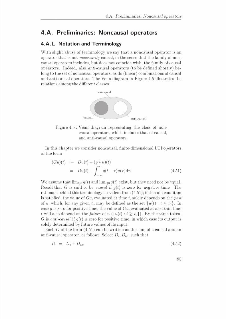
8/8/2019 Evaluasi pada Iterative Learning Control
http://slidepdf.com/reader/full/evaluasi-pada-iterative-learning-control 111/175
4.A. Preliminaries: Noncausal operators
4.A. Preliminaries: Noncausal operators
4.A.1. Notation and Terminology
With slight abuse of terminology we say that a noncausal operator is an
operator that is not necessarily causal, in the sense that the family of non-causal operators includes, but does not coincide with, the family of causaloperators. Indeed, also anti -causal operators (to be defined shortly) be-long to the set of noncausal operators, as do (linear) combinations of causaland anti-causal operators. The Venn diagram in Figure 4.5 illustrates therelations among the different classes.
causal anti-causal
noncausal
Figure 4.5.: Venn diagram representing the class of non-causal operators, which includes that of causal,and anti-causal operators.
In this chapter we consider noncausal, finite-dimensional LTI operatorsof the form
(Gu)(t) := Du(t) + (g ∗ u)(t)
= Du(t) + ∞−∞
g(t − τ )u(τ )dτ. (4.51)
We assume that limt↓0 g(t) and limt↑0 g(t) exist, but they need not be equal.Recall that G is said to be causal if g(t) is zero for negative time. Therationale behind this terminology is evident from (4.51); if the said conditionis satisfied, the value of Gu, evaluated at time t, solely depends on the past of u, which, for any given to may be defined as the set {u(t) : t ≤ t0}. Incase g is zero for positive time, the value of Gu, evaluated at a certain timet will also depend on the future of u ({u(t) : t ≥ t0}). By the same token,G is anti-causal if g(t) is zero for positive time, in which case its output is
solely determined by future values of its input.Each G of the form (4.51) can be written as the sum of a causal and an
anti-causal operator, as follows. Select Dc, Dac, such that
D = Dc + Dac, (4.52)
95

8/8/2019 Evaluasi pada Iterative Learning Control
http://slidepdf.com/reader/full/evaluasi-pada-iterative-learning-control 112/175
8/8/2019 Evaluasi pada Iterative Learning Control
http://slidepdf.com/reader/full/evaluasi-pada-iterative-learning-control 113/175
4.A. Preliminaries: Noncausal operators
to the anti-causal part of the impulse response (typically consisting of a sumof exponentials that decrease with negative time). Every element G(s) inRL∞ may be decomposed into a causal part Gc(s) and an anticausal partGac(s) such that G(s) = Gc(s) + Gac(s) with Gc(s), Gac(−s) ∈ RH∞.
In Section 4.A.2 we show that the action of the antistable operator Gac(−s)may be implemented as a causal operation on a time-reversed signal. Hence,the location of the poles (relative to the imaginary axis) merely determinesthe causality of the operation.
For every G(s) ∈ RL∞, the L2(−∞, ∞)-induced operator norm is definedas
G∞ = supω∈R
σ (G( jω)) , (4.56)
where σ denotes the largest singular value.
Example 4.A.1. We consider the noncausal operator G :L2
(−∞
,∞
)→L2(−∞, ∞), Gu(t) := (g ∗ u)(t), where g is given as
g(t) =
et if t < 0
e−t elsewhere.
Note that G is of the form (4.51) (the feedthrough term, D, is absent). Let us decompose G into a causal part (Gcu)(t) :=
∞−∞ gc(t − τ )u(τ )d τ ,
gc(t) :=
e−t if t ≥ 0
0 elsewhere(4.57)
and a noncausal part (Gacu)(t) := ∞−∞ gac(t − τ )u(τ )d τ
gac(t) :=
et if t < 0
0 elsewhere(4.58)
We compute the two-sided Laplace transform G(s)
G(s) =
0−∞
ete−std t +
0−∞
e−te−std t
=1
1 − s+
1
1 + s(4.59)
Equation (4.59) suggests that we decompose G(s) into a part
Gc(s) :=1
(1 + s)(4.60)
97

8/8/2019 Evaluasi pada Iterative Learning Control
http://slidepdf.com/reader/full/evaluasi-pada-iterative-learning-control 114/175
4. Noncausal ILC
and a part
Gac(s) :=1
(1 − s)(4.61)
such that G(s) = Gc(s) + G
ac(s) and G
c(s), G
ac(−
s)∈ RH∞
.We apply the input
u(t) =
1 if 0 ≤ t ≤ T
0 elsewhere(4.62)
and compute the output y(t) as
y(t) =
⎧⎪⎨
⎪⎩
2 − e−t − e(t−T ) if 0 ≤ t ≤ T
et − e(t−T ) if t < 0
e−(t−T ) − e−t elsewhere
(4.63)
The response of the system is shown in Figure 4.6 for two different valuesof T . Observe that although the respective inputs are equal for all t ≤ 2,the outputs are not. This is a general feature of noncausal systems, and something to keep in mind: we cannot just ignore the future as we sometimesdo with causal systems.
2
1.5
1
0.5
0
−6 −4 −2 0 2 4 6
u(t)
y(t)
2
1.5
1
0.5
0
−6 −4 −2 0 2 4 6
u(t)
y(t)
(a) T = ∞ (b) T = 2
Figure 4.6.: The response of the system y(t) := (g ∗ u)(t) tothe input (4.62) for different values of T .
4.A.2. Noncausal operators on [0, T ]
In the framework introduced, we assumed that all signals are defined overinfinite time. For causal systems we could easily justify this assumption bypointing to the following facts:
98

8/8/2019 Evaluasi pada Iterative Learning Control
http://slidepdf.com/reader/full/evaluasi-pada-iterative-learning-control 115/175
4.A. Preliminaries: Noncausal operators
1. If u(t) = 0 for all t < t0, then for any causal system G, we have that(Gu)(t) = 0 for all t < t0. Without loss of generality t0 can be set tozero. In effect, we can ignore negative time.
2. If u1(t) = u
2(t) for all t < t
0then (Gu
1)(t) = (Gu
2)(t) for all t <
t0. Thus, the truncated response of the original system (defined overinfinite time) coincides with the response of the truncated system(defined over finite time).
When we give up causality, we allow a system’s response to be partlydetermined by future values of its input. As we are generally dealing withsystems having an infinite impulse response (IIR), this means that in orderto compute the output at any given time, we need to know the input’s com-plete future. Needless to say, we generally lack such complete information.In ILC, signals are defined on [0, T ]. That means that, as t approaches T ,
the window on the future gets smaller and smaller. To account for this fact,we do the following. With each G defined over infinite time, we associatean operator G[0,T ], defined over finite time. Let G be a stable (in the senseof L2(R) → L2(R)) convolution operator of the form
(Gu)(t) = Du(t) +
∞−∞
g(t − τ )u(τ )dτ (−∞ < t < ∞). (4.64)
We define the trunctated operator G[0,T ] : L2[0, T ] → L2[0, T ] as
(G[0,T ]u)(t) := Du(t) + T
0
g(t
−τ )u(τ )dτ (0
≤t
≤T ). (4.65)
The former is used for analysis and synthesis; the latter for actual imple-mentation. Naturally, the analysis would not make sense, if we would notfirst verify that certain statements about G translate in a useful way tostatements about G[0,T ]. In the next subsection we prove a particularlyuseful proposition, which relates contractivity of G[0,T ] to that of G.
4.A.3. A contraction on L2[0, T ]
In Example 4.A.1 we saw that (Gu)(t) and (G[0,T ]u)(t) do not (necessarily)
coincide on [0, T ]. To see how G and G[0,T ] are related, let us define theprojection operator Λ[0,T ] : L2(−∞, ∞) → L2(−∞, ∞),
(Λ[0,T ]u)(t) :=
u(t) if 0 ≤ t ≤ T
0 elsewhere(4.66)
99

8/8/2019 Evaluasi pada Iterative Learning Control
http://slidepdf.com/reader/full/evaluasi-pada-iterative-learning-control 116/175
4. Noncausal ILC
The linear operator Λ—we drop the index—is idempotent, i.e. Λ(Λu) = ufor all u. Moreover, Λ is nonexpansive, i.e. Λ = 1. We have the followinglemma.
Lemma 4.A.2. Let G be a stable LTI operator of the form (4.64) and let G[0,T ] denote the corresponding truncated operator (4.65). For all u ∈L2(−∞, ∞), define u ∈ L2[0, T ] as u(t) := u(t), 0 ≤ t ≤ T . We havethat
1. (G[0,T ]u)(t) = (GΛu)(t) for all t ∈ [0, T ].
2.G[0,T ]u
L2[0,T ] =
ΛGΛuL2(−∞,∞)
.
3. If G is a contraction on L2(−∞, ∞), then G[0,T ] is a contraction on L2[0, T ].
Proof. Part (1): For all t ∈R
, the response (GΛu)(t) is given as(GΛu)(t) = Du(t) +
∞−∞
g(t − τ )Λu(τ )dτ
= Du(t) +
T 0
g(t − τ )u(τ )dτ
On [0, T ] we have that u(t) = u(t). Thus for all t ∈ [0, T ]
(GΛu)(t) = (G[0,T ]u)(t) (4.67)
Note that (Gu)(t) is also defined for t < 0. Part (2): The statement followsfrom ΛGΛu
2L2(−∞,∞)
:= ∞−∞
[(ΛGΛu)(t)]T [(ΛGΛu)(t)] dt
=
T 0
[(Gu)(t)]T [(Gu)(t)] dt
=
T 0
[(Gu)(t)]T
[(Gu)(t)] dt
=G[0,T ]u
2L2[0,T ] (4.68)
Part (3): For G[0,T ] to be a contraction, there must exist λ < 1 such that
G[0,T ]u
≤λ
u
for all u
∈ L2[0, T ]. From part (2) we deduce that
G[0,T ]u ≤ λu for all u ∈ L2[0, T ] if and only if ΛGΛu ≤ λΛufor all u ∈ L2(−∞, ∞). Suppose G is a contraction, i.e. G < 1, then wehave
ΛGΛu ≤ GΛu ≤ GΛu (4.69)
100

8/8/2019 Evaluasi pada Iterative Learning Control
http://slidepdf.com/reader/full/evaluasi-pada-iterative-learning-control 117/175
4.A. Preliminaries: Noncausal operators
Here we used the fact that Λ is nonexpansive. Equation (4.69) shows thatthere exists λ (λ = G) such that ΛGΛu ≤ λΛu for all u. This inturn implies that G[0,T ] is a contraction. This concludes the proof.
4.A.4. Implementation issues
Next we show that the action of G can be evaluated in terms of causaloperations on u and Πu. Let us define the permutation operator ΠT :L2(−∞, ∞) → L2(−∞, ∞),
(ΠT u)(t) := u(T − t) (4.70)
It is easy to verify that ΠT is linear, and norm-preserving (
ΠT u
=
u
for
all u). Moreover, ΠT (ΠT u) = u. Figure 4.7 shows the effect of ΠT , actingon a particular u. In the sequel we drop the index T and simply denote ΠT
as Π. We select gc, gac, Dc, Dac in accordance with (4.52)-(4.53), and define
0.12
0.1
0.08
0.06
0.04
0.02
00 1 2 3 4 5
u(t) (Πu)(t)
Figure 4.7.: The action of the permutation operator ΠT .The solid curve is u(t); the dashed (ΠT u)(t).The plot corresponds to the parameter valueT = 5.
yc(t) := Dcu(t) +
∞−∞
gc(t − τ )u(τ )dτ ;
yac(t) := Dacu(t) +
∞−∞
gac(t − τ )u(τ )dτ. (4.71)
101

8/8/2019 Evaluasi pada Iterative Learning Control
http://slidepdf.com/reader/full/evaluasi-pada-iterative-learning-control 118/175
4. Noncausal ILC
Verify that y(t) = yc(t)+yac(t) for all t ∈ [0, T ]. The noncausal contributionyac(t) is computed as follows
(Πyac)(η) = yac(T − η)
= Dac(Πu)(η) + ∞T −η
gac(T − τ − η)u(τ )dτ
= Dac(Πu)(η) +
∞T −η
gac(T − τ − η)(Πu)(T − τ )dτ
= Dac(Πu)(η) +
η−∞
gac(−(η − ξ))(Πu)(ξ)dξ
:= G∗ac(Πu) (4.72)
Note that since gac(−t) = 0 for all t < 0, the above defines a causal operationon Πu, which we denote as G∗
ac(Πu). When we solve for yac(η), we get
yac = Π(Πyac)
= ΠG∗acΠu (4.73)
The causal part evaluates to yc = Gcu, so that
y = (Gc + ΠG∗acΠ) u (4.74)
Let us once again emphasize that y(t) is the response of the system G to theinput u which, in general, does not coincide with the response of the systemG[0,T ] to the truncated input u. The latter response may be computed from(see Lemma 4.A.2)
(G[0,T ]u)(t) = (Gc + ΠG∗
acΠ) Λu(t) (4.75)
Example 4.A.3. To illustrate the ideas presented in this section, let usonce again consider the operator G previously defined in Example 4.A.1.For this system we have
(Gcv)(t) := Dcv(t) +
∞−∞
gc(t − τ )v(τ )d τ
= t
−∞
e−(t−τ )v(τ )d τ (4.76)
(G∗acw)(t) := Dacw(t) +
∞−∞
gac(−(t − τ ))w(τ )d τ
=
t−∞
e−(t−τ )w(τ )d τ (4.77)
102

8/8/2019 Evaluasi pada Iterative Learning Control
http://slidepdf.com/reader/full/evaluasi-pada-iterative-learning-control 119/175
4.A. Preliminaries: Noncausal operators
The output of the truncated system may be evaluated as
(G[0,T ]u)(t) = (GcΛu)(t) + (ΠG∗
acΠΛu)(t)
= t
0
e−(t−τ )u(τ )d τ + Π t
0
e−(t−τ )(Πu)(τ )d τ (4.78)
This corresponds to the schematic shown in Figure 4.8. The general schematic(for arbitrary G) may be obtained by substuting Gc(s) for 1
s+1in the box la-
beled Gc, and Gac(−s) for 1s+1 in the box labeled Gac. On the interval [0, 10],
we apply the input u(t),
u(t) =
1 if 0 ≤ t ≤ 3
0 elsewhere(4.79)
The system’s reponse (G[0,10]u)(t) is given in Figure 4.9.
ΠΠ
u(t) (G[0,T ]u)(t)
Gc
Gac
+
+
1s+1
1s+1
Figure 4.8.: Causal implementation of the noncausal opera-tor G[0,T ].
103
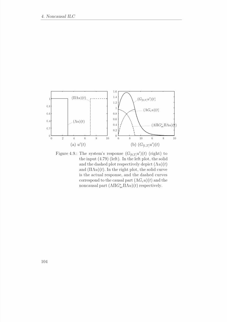
8/8/2019 Evaluasi pada Iterative Learning Control
http://slidepdf.com/reader/full/evaluasi-pada-iterative-learning-control 120/175
4. Noncausal ILC
1
0.8
0.6
0.4
0.2
00 2 4 6 8 10
(Λu)(t)
(ΠΛu)(t)
1.6
1.4
1.2
1
0.8
0.6
0.4
0.2
06 8 10 6 8 10
(G[0,T ]u)(t)
(ΛGcu)(t)
(ΛΠG∗acΠΛu)(t)
(a) u(t) (b) (G[0,T ]u)(t)
Figure 4.9.: The system’s response (G[0,T ]u)(t) (right) to
the input (4.79) (left). In the left plot, the solidand the dashed plot respectively depict (Λu)(t)
and (ΠΛu)(t). In the right plot, the solid curveis the actual response, and the dashed curvescorrespond to the causal part (ΛGcu)(t) and thenoncausal part (ΛΠG∗
acΠΛu)(t) respectively.
104

8/8/2019 Evaluasi pada Iterative Learning Control
http://slidepdf.com/reader/full/evaluasi-pada-iterative-learning-control 121/175
5
Learning and adaptation:trial-dependent update rules
Overview – In this final chapter we return to the general problem of Learning Control. Considering the algorithms discussed in previous chapters, we ask: “In what sense, and to what extent, do these algorithms implement a ‘learning’ behavior?”. Key issue is their alleged ability to adapt; focal point, the use of iteration in relationto plant uncertainty.
We argue that even as these algorithms succesfully enhance per-formance, they do not necessarily ‘learn’, in the sense that this ‘suc-ces’ is typically due to, and thus dependent on, detailed plant know-ledge. We identify this to be a typical feature of ‘trial-independent’
update laws (constant-coefficient recurrences), and by that we are led to consider ‘higher-level’ update laws, that is: update laws thatupdate update laws, etc. We provide two elementary examples of ‘level-one’ update laws, and show that both have certain adaptive abilities (in a sense to be made precise).
As we turn to discuss the use of iteration, we argue that this use includes, but is not limited to, performance refinement. We propose an alternative, not necessarily conflicting view, in which the use of iteration is explained in terms of a need for information—a needarising from a lack of a priori knowledge. We argue that rather than having all algorithms conform to a particular structure, we ought to have them conform to the data.
105

8/8/2019 Evaluasi pada Iterative Learning Control
http://slidepdf.com/reader/full/evaluasi-pada-iterative-learning-control 122/175
5. Learning and adaptation: trial-dependent update rules
5.1. Introduction
In the preceding chapters we concerned ourselves with questions of analysisand synthesis, relating to a family of first-order linear recurrences, param-
eterized by a pair of bounded linear operators. As we initially assumedboth operators to be causal (Chapter 3), we soon dropped this constraint(Chapter 4) so as to maximally exploit ILC’s open-loop nature. The mainfindings pertaining to the distinction between causal and noncausal updatelaws are summarized below.
• Under the assumption of causality the said family of recurrences allowsfor an Equivalent Feedback implementation. The associated (causal)feedback map is a function of the synthesis parameters only and is al-ways stabilizing (provided the underlying update law is convergent).Ergo, the feedback system can be implemented without problems. In
case of Standard ILC (open loop, stable plant) the achievable perfor-mance (bandwidth) is constrained by the plant capacity (the pole-zeroexcess) and the presence of right-half plane zeroes. In case of CCF-ILC (current-cycle feedback, possibly unstable plant) the achievableperformance is further impaired by the RHP poles of the open-loopgain, and by the fact that the set of Equivalent Controllers is gener-ally just a subset of all stabilizing controllers (unless the current-cycleoperator is stable).
• In a noncausal setting, performance is constrained neither by the pres-ence of RHP zeroes, nor by the plant capacity. A candidate Equiva-
lent Controller can be defined, but its ‘application’ is limited to vir-tual feedback systems since the controller is noncausal and the actual(closed-loop) feedback system ill-posed.
Now we ask ourselves the following question: In view of the basic ideasthat make up Learning Control, what can we say about this problem wesolved? And more in particular, what is it these algorithms can do andwhat is it they cannot do?
To start with, let us outline the problem we solved; A somewhat simplifiedversion reads as follows: Given a (SISO) plant P : U → Y , along with somedesired output yd
∈Y , find a map F : U
×Y
→U ,
uk+1 := F (uk, ek), (5.1)
such that limk→∞ P uk = yd. We obtained the following solution:
F (uk, ek) = uk +
γ 2I + P ∗P −1
P ∗ek. (5.2)
106

8/8/2019 Evaluasi pada Iterative Learning Control
http://slidepdf.com/reader/full/evaluasi-pada-iterative-learning-control 123/175
5.2. The problem of Learning Control
Here, P ∗ := P T (−s) denotes the adjoint of the plant and γ > 0 is a pa-rameter that controls the speed of convergence (recall that γ penalizes thesize of the increment ∆uk relative to that of the error ek+1—for detailsrefer to Section 2.2.2).
Implementation of the update law (5.1) with F as in (5.2) involves non-causal operations. That, however, is not a problem, as the update is com-puted offline, after completion of the current cycle.
By construction, the output sequence {P u0, P u1, . . .} converges for allu0 ∈ U and all yd ∈ Y . The input sequence {u0, u1, . . .} converges if andonly if yd is a feasible output.
This, in a nutshell, is the problem we solved. Now what about the problemwe started out with? What about “achieving a desired result when onlypartial knowledge of the plant is available” (Section 1.3.2)? Indeed, whatabout ‘learning’?
5.2. The problem of Learning Control
5.2.1. Performance, performance robustness and learning
As we take up the question of learning , we need to consider at least twoaspects. First we must look at performance proper; Is it true that, relativeto conventional means, these algorithms enhance performance? The answeris, unmistakably, ‘yes’. Then there is the issue of uncertainty; Is it truethat, again relative to conventional means, these algorithms enhance per-formance robustness (against uncertainty in the plant model)? In this case,
the answer, as we will expound on presently, is ‘no’.For one may note that, in the problem statement above, P was assumed
to be given . This is evidently a strong, not to say restrictive, assumption,and it remains to be seen whether this assumption can be relaxed withoutcompromising performance. And so we wonder:
• If we are to assume full plant knowledge, then why engage in a processof physical iteration? Why not compute the optimal input offline,through numerical iteration ?
• If we are to relax the assumption of full plant knowledge, how much do we need to assume to make this algorithm converge? Can we make
it more robust without compromising performance?
• Lastly, if the latter question is to be answered in the negative, thenwhat makes this an algorithm for Learning Control, if not its abilityto deal with uncertainty?
107

8/8/2019 Evaluasi pada Iterative Learning Control
http://slidepdf.com/reader/full/evaluasi-pada-iterative-learning-control 124/175
5. Learning and adaptation: trial-dependent update rules
Why iterate in case of full plant knowledge?
Let us explore these issues in some more detail. First the issue of fullplant knowledge and the possibility of doing numerical, rather than physicaliteration. Our perspective is that physical interaction with the plant is one
of the defining features of Learning Control; The data itself is to steer theplant towards a desired behavior. In case of full plant knowledge, there isnothing we can learn that we do not already know. In other words, therewould be simply no need for Learning Control.
On performance robustness
What if we relax this assumption of full plant knowledge? Indeed, whatif there is a mismatch between the actual plant and the plant model, willthe algorithm still converge? It is hard to say anything in general, but thefollowing example may give us some insight.
Suppose the actual plant P is given as P := P 0 (1 + δM ) where P 0 rep-resents the nominal plant, and δM is a bounded multiplicative pertubation.For the given update law to converge the next condition must be satisfied:
|1 − (P ∗0 P 0)
(γ 2 + P ∗0 P 0)(1 + δM ) | < 1 for almost all ω. (5.3)
This implies that 1+δM must be positive real. We may observe that cannotbe met in case P has two or more parasatic poles. Whether this makes thealgorithm sufficiently robust or not will depend on the specific application.The important thing for us to note, is that for those plants that do satisfy
Condition (5.3) the error converges to zero, whereas for those that do not,the error diverges to infinity. By construction, stability (convergence) im-plies performance. At first sight, this appears to be at variance with thesituation in feedback control, where performance and stability robustnessare typically traded off . However, the discrepancy dissapears when we con-sider generalized update laws such as (5.4), this being a ‘robustified’ versionof update law (5.2):
uk+1 = Q
uk +
γ 2I + P ∗P −1
P ∗ek
. (5.4)
We may assume that Q is nonexpansive so that indeed the condition for
convergence is relaxed. If the nominal design is competitive, we get goodperformance whenever the actual plant is close to the nominal plant, rea-sonable performance when it is not so close and no performance whatsoeverwhen the actual plant deviates from the nominal plant to the extent thatthe algorithm no longer converges. Stability robustness may be increased
108
8/8/2019 Evaluasi pada Iterative Learning Control
http://slidepdf.com/reader/full/evaluasi-pada-iterative-learning-control 125/175
5.2. The problem of Learning Control
by lowering the gain of Q, and, in a typical situation, by reducing its band-width (generically, we cannot assume Q to be of a particular form, butif we confine ourselves to e.g. servomechanisms, it makes sense to assumethat Q has lowpass characteristics). In view of the original algorithm, we
argue that, for good performance, Q should be close to unity (Q = 1). Inother words, we cannot get good performance and stability robustness atthe same time. So, in general, the synthesis problem in ILC does exhibit atradeoff between performance and stability robustness.
Learning Control?
We cannot but conclude that, like in conventional feedback control, heretoo uncertainty poses a threat, as good performance cannot be obtainedwithout compromising the stability robustness. Back in Chapter 1, whenwe motivatived the concept of Learning Control, we pointed to a potential
for dealing with uncertain systems. We trusted that our algorithm hadinherited some of this potential.
But the truth of the matter is that there is no such potential. Our al-gorithm turns out to be just as sensitive to a lack of a priori knowledgeas conventional control is. This in stark constrast with the fact that, inaddition to prior knowledge (on which the feedback design is based), ouralgorithm commands a wealth of data adding on to whatever informationavailable at initialization. So indeed, if not its ability to deal with uncer-tainty then what is it that makes this an algorithm for Learning Control?
5.2.2. Adaptation, Iteration, and LearningNext we argue that the problem of Learning Control, the way we see it, isreally about uncertainty, and not so much about performance.
Uncertainty: the problem of Learning Control
In Learning Control we seek to enhance a system’s performance through aseries of (automated) trials. This seems to work out fine as long as we as-sume to know the system we are working with. But what if this assumptionfails: What if we do not know the system, or perhaps only approximately?
At first, we would think that, in that case, iteration would make up for thelack of a priori knowledge. But upon reflection, this thought, which struckus as self-evident, proves to make no sense. For how are we to update thecurrent input if we cannot (or can only approximately) predict the effect achange in input will have on the system’s output?
109

8/8/2019 Evaluasi pada Iterative Learning Control
http://slidepdf.com/reader/full/evaluasi-pada-iterative-learning-control 126/175
5. Learning and adaptation: trial-dependent update rules
Assuming (extreme) uncertainty, the following scenario may help illus-trate the issue at hand. We are given control over a certain plant P that weknow little or nothing about. As we desire to get to know the system, wedecide to set up a number of experiments (trials). In each experiment we
apply a certain input uk and the system returns the corresponding outputyk = P uk. The data is stored so that, if we so desire, we can use it to steerthe next experiment. During the course of these experiments we gather acertain, possibly large, amount of data D := {(ui, yi), i = 1, 2, . . .}. Butwhat, exactly, does this data tell us about our system?
That depends on the system itself. In an LTI setting, for instance, ittakes just one obversation to characterize the system’s complete IO behav-ior. In this case, the problem of Learning Control degenerates as there isno need for repeated iteration. In general, the data forms a mere subsetof the system’s (input-output) behavior, the subset being not necessarilyrespresentative of the total behavior. So when it comes to predicting the
system’s response to an input that is not in the data set, or, to constructingthe input corresponding to a given output, the data might not be of muchuse. What is lacking is a proper embedding: a model . A model may be fitted to the data, but that will not resolve the problem. For however well such amodel may capture the observed behavior, there are is absolute guaranteethat it will do equally well on the total behavior.
In contrast with e.g. the literature on System Identication and StatisticalLearning Theory, the ILC literature contains but little reference to thisproblem. Its focus seems to lie elsewhere. In fact, the way it is generallyconceived, Learning Control is not at all about “turning experience into
knowledge” (data into performance). And if not many papers would suggestotherwise, we would not be discussing the issue here. In any case, based onour earlier discussion, we cannot but conclude that in the sense alluded toabove, ILC does not ‘learn’.
Iteration and Learning
To make this claim more substantial, let us have another look at the updatelaw we have been considering throughout this thesis:
uk+1 = Quk + Lek. (5.5)
What does this equation represent? Basically, it respresents the law thatgoverns the evolution of the iterative system. It is a rule that tells howto automatically generate a new input from the data collected during pasttrials. Now suppose this algorithm exhibits some intelligent behavior, thenwhere does it reside? Is it in the (structure of the) rule itself? Or perhaps
110

8/8/2019 Evaluasi pada Iterative Learning Control
http://slidepdf.com/reader/full/evaluasi-pada-iterative-learning-control 127/175
5.2. The problem of Learning Control
in the choice of its parameters, Q and L? A simple analysis reveals thatit must be in the latter. For suppose this learning process (the algorithm)converges. Then whatever it is that was learned must show up in the ‘fixedpoint’ equation
(I − Q + LP ) u = Lyd. (5.6)
The quantity u is something we do not know and generally cannot solve for(as we cannot assume to know P ) so if anything was learned then it mustbe u. But note that the value of u is solely determined by Q, L and P , andnot by the evolution of the input {uk}. In that sense, it is not surprisingthat in a causal context we can retrieve the same quantity without a singleiteration (without learning?). And to some extent the same conclusionshold in a noncausal context. Learning and iteration are not the same thing,neither does iteration imply learning. For if the family of causal iterations issaid to implement a learning behavior, then why not conventional feedbackcontrol?
Adaptation
The distinction between iteration and learning bears on the question how
the data is used. Algorithms such as the one above are evidently data-driven ; the data is used, but not necessarily in an instrumental way. Indeedwhat our update law lacks is the ability to interpret the data. Even as thedata invalidates the model on which the design is based, the update law
just keeps on updating the input, ‘ignorant’ of what is actually going on.In that sense, our algorithm does not adapt .
Now suppose we would allow the parameters Q and L to depend on thedata. Would we then consider our algorithm to be adaptive? That depends.We obviously need a rule to make the dependence explicit. And once wedefine a rule, we are back at the same problem but now at the level of the
update rule that updates the update rule. The recursiveness is evident andin that sense the existence of a truly adaptive, (‘self-adaptive’) algorithm isdoubtful. But if we confine ourselves to the level at which the control inputis updated, then yes, we could consider such algorithms to be adaptive. Anexample will follow.
111
8/8/2019 Evaluasi pada Iterative Learning Control
http://slidepdf.com/reader/full/evaluasi-pada-iterative-learning-control 128/175
8/8/2019 Evaluasi pada Iterative Learning Control
http://slidepdf.com/reader/full/evaluasi-pada-iterative-learning-control 129/175
5.3. On trial-dependent update laws
any given sequence of operator pairs {(Qk, Lk)}∞k=1. We assume that {Qk}and {Lk} are strongly converging .
Definition 5.3.1 (Strong convergence). Adapted from Curtain and Zwart (1995). Let
{F k
, k≥
1}
be a sequence of bounded affine operators (on X ).If
F kx − F x → 0, (5.8)
as k → ∞ for all x ∈ X then we say that F k converges strongly to F .
Define F k(u) := (Qk − LkP ) u + Lkyd and rewrite (5.7) as
uk+1 = F k+1(uk). (5.9)
Our next objective is to find conditions on {F k} under which the sequence
{uk}, induced by (5.9), converges to a unique ‘fixed point’ u, independentof u0. It is evident that classical fixed point theory will not help us here.Fortunately, the classical theory is readily extended to accommodate state-ments about strongly converging sequences of operators. For notationalconvenience we adopt the shorthand notation
ki=1
F i
(x) := F k
F k−1
· · · F 1(x) · · · .
We need the following definitions:
Definition 5.3.2 (Fixed point). Let {F k, k ≥ 1} be a sequence of bounded affine operators that strongly converges to a limit F := limk→∞ F k (seeDefinition 5.3.1). We say that a point x ∈ X is a fixed point of the sequenceof operators {F k} if it is a fixed point of F , i.e. if limk→∞ F k(x) − x = 0.
Definition 5.3.3 (Contraction). Let {F k, k ≥ 1} be a strongly con-verging sequence of bounded affine operators, and let λk denote the Lip-schitz constant corresponding to F k. We say that {F k} is contractive if limsupk λk < 1.
Note that in case F k is constant (as a function of the trial number k),
Definition 5.3.3 coincides with that given in Section 2.1.4. We have thefollowing result.
Theorem 5.3.4. Let X be a Banach space and let {F k, k ≥ 1} be a strongly converging sequence of bounded affine operators on X . Let F := limk→∞ F k.
113

8/8/2019 Evaluasi pada Iterative Learning Control
http://slidepdf.com/reader/full/evaluasi-pada-iterative-learning-control 130/175
5. Learning and adaptation: trial-dependent update rules
Suppose {F k} is contractive. Then there exists a unique fixed point x ∈ X such that F (x) = x. Furthermore, for all x ∈ X , we have that
x = limk→∞k
i=1 F i (x). (5.10)
A proof of Theorem 5.3.4 can be found in Section 5.A. Later we show howto apply this theorem to prove convergence for a class of adaptive updatelaws in which Qk and Lk are not given , but depend on the data instead.For now let us just assume that {Qk} and {Lk} are strongly convergingsequences of operators. Define Q := limk→∞ Qk and L := limk→∞ Lk andassume that the conditions of Theorem 5.3.4 are satisfied. Then the iterationuk+1 := F k+1(uk), with F k : U → U defined as
F k(u) := (Qk − LkP ) u + Lkyd, (5.11)
converges to a unique fixed point u ∈ U which, independent of u0 is givenas
u = limk→∞
k
i=1
F i
(u0)
= limk→∞
(Qk − LkP )
k−1i=1
F i
(u0) + Lkyd
= (Q − LP ) u + Lyd. (5.12)
It is worth noting that, had we started from the update rule
uk+1 = Quk + Lek, (5.13)
we would obtain the exact same fixed point equation. This proves that,in an asymptotic sense, update laws (5.7) and (5.13) are equivalent. Theimportance of this observation is tied up with the fact that {Qk} and {Lk},and in particular their respective limits Q and L, are known , or at least
computable on the basis of a priori knowledge. Would we consider updatelaws in which, for instance, the operator Lk+1 depends on the current errorek, an equivalent (feedback) scheme could still exist, but in that case, wewould not be able to determine the value of L := limk→∞ Lk (and thus thatof the equivalent controller), without actually running the scheme.
114
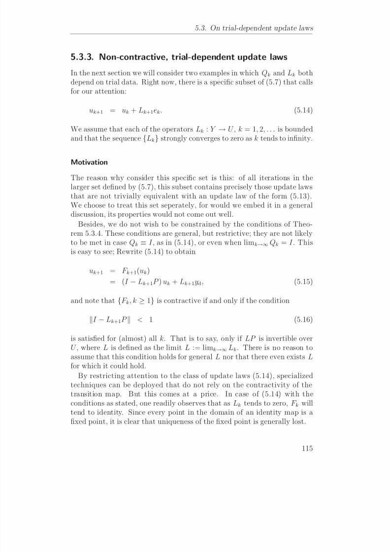
8/8/2019 Evaluasi pada Iterative Learning Control
http://slidepdf.com/reader/full/evaluasi-pada-iterative-learning-control 131/175
5.3. On trial-dependent update laws
5.3.3. Non-contractive, trial-dependent update laws
In the next section we will consider two examples in which Qk and Lk bothdepend on trial data. Right now, there is a specific subset of (5.7) that callsfor our attention:
uk+1 = uk + Lk+1ek. (5.14)
We assume that each of the operators Lk : Y → U , k = 1, 2, . . . is boundedand that the sequence {Lk} strongly converges to zero as k tends to infinity.
Motivation
The reason why consider this specific set is this: of all iterations in thelarger set defined by (5.7), this subset contains precisely those update laws
that are not trivially equivalent with an update law of the form (5.13).We choose to treat this set seperately, for would we embed it in a generaldiscussion, its properties would not come out well.
Besides, we do not wish to be constrained by the conditions of Theo-rem 5.3.4. These conditions are general, but restrictive; they are not likelyto be met in case Qk ≡ I , as in (5.14), or even when limk→∞ Qk = I . Thisis easy to see; Rewrite (5.14) to obtain
uk+1 = F k+1(uk)
= (I
−Lk+1P ) uk + Lk+1yd, (5.15)
and note that {F k, k ≥ 1} is contractive if and only if the condition
I − Lk+1P < 1 (5.16)
is satisfied for (almost) all k. That is to say, only if LP is invertible overU , where L is defined as the limit L := limk→∞ Lk. There is no reason toassume that this condition holds for general L nor that there even exists Lfor which it could hold.
By restricting attention to the class of update laws (5.14), specialized
techniques can be deployed that do not rely on the contractivity of thetransition map. But this comes at a price. In case of (5.14) with theconditions as stated, one readily observes that as Lk tends to zero, F k willtend to identity. Since every point in the domain of an identity map is afixed point, it is clear that uniqueness of the fixed point is generally lost.
115

8/8/2019 Evaluasi pada Iterative Learning Control
http://slidepdf.com/reader/full/evaluasi-pada-iterative-learning-control 132/175
5. Learning and adaptation: trial-dependent update rules
Convergence analysis
Next a theorem is presented, which states conditions under which the classof update rules (5.14) converges to a bounded solution. It requires thenotion of summable sequences.
Definition 5.3.5 (Summable sequence). Let {a1, a2, . . .} be a sequenceof positive real numbers. The sequence is said to be summable if
limN →∞
N k=1
ak < ∞ (5.17)
We have the following theorem.
Theorem 5.3.6 (Convergence on U ). Let {Lk} be a sequence of bounded linear operators from Y to U . Suppose {Lk} is summable. Then thesequence of control inputs {uk} converges to some bounded input u ∈ U .
A proof of Theorem 5.3.6 can be found in Section 4.A. Note that theassumption that Lk strongly converges to zero is implicit in the conditionthat {Lk} is summable.
Application
The next example shows how the result of Theorem 5.3.6 may be applied.
Example 5.3.7. Let U = Y = H2 and suppose P ∈ RH∞. For k ≥ 1 wedefine Lk := L/k2. Assume L ∈ RH∞. It is easy to see that {Lk} issummable:
∞k=1
Lk =
∞k=1
L/k2 = (π2/6)L < ∞. (5.18)
Theorem 5.3.6 says that, provided L and P are both bounded, the se-quence of inputs {uk} converges to a bounded solution in H2. This very
fact implies that convergence does not depend on detailed knowledge of theplant. The error ek satisfies ek = Z ke0, where Z k : Y → Y is defined asZ k :=
k−1i=0 (I − Li+1P ). We define the map Z : Y → Y ,
Z := limk→∞
Z k. (5.19)
This map relates the final error, e∞, to the initial error, e0. In some cases,a closed-form expression for Z can be found. As it turns out, in our example
Z (s) =sin
π
L(s)P (s)
π
L(s)P (s). (5.20)
A plot of Z ( jω) for P (s) = 1/(sτ + 1) and L = 1 is given in Figure 5.1a.
116
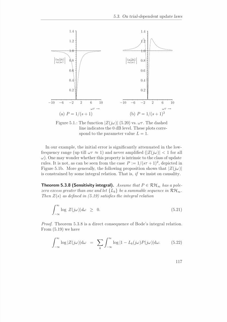
8/8/2019 Evaluasi pada Iterative Learning Control
http://slidepdf.com/reader/full/evaluasi-pada-iterative-learning-control 133/175
5.3. On trial-dependent update laws
1.0 e∞( jω)e0( jω)
0.8
0.6
0.4
0.2
−2
1.2
−6
1.4
−10 2 6 10
ωτ
→
1.0 e∞( jω)e0( jω)
0.8
0.6
0.4
0.2
−2
1.2
−6
1.4
−10 2 6 10
ωτ
→(a) P = 1/(s + 1) (b) P = 1/(s + 1)2
Figure 5.1.: The function |Z ( jω)| (5.20) vs. ωτ . The dashedline indicates the 0 dB level. These plots corre-spond to the parameter value L = 1.
In our example, the initial error is significantly attenuated in the low-frequency range (up till ωτ ≈ 1) and never amplified (|Z ( jω)| < 1 for allω). One may wonder whether this property is intrinsic to the class of updaterules. It is not, as can be seen from the case P := 1/(sτ + 1)2, depicted in
Figure 5.1b. More generally, the following proposition shows that |Z ( jω)|is constrained by some integral relation. That is, if we insist on causality.
Theorem 5.3.8 (Sensitivity integral). Assume that P ∈ RH∞ has a pole-zero excess greater than one and let {Lk} be a summable sequence in RH∞.Then Z (s) as defined in (5.19) satisfies the integral relation
∞−∞
log |Z ( jω)|d ω ≥ 0. (5.21)
Proof. Theorem 5.3.8 is a direct consequence of Bode’s integral relation.From (5.19) we have ∞−∞
log |Z ( jω)|dω =k
∞−∞
log |1 − Lk( jω)P ( jω)|dω. (5.22)
117

8/8/2019 Evaluasi pada Iterative Learning Control
http://slidepdf.com/reader/full/evaluasi-pada-iterative-learning-control 134/175
5. Learning and adaptation: trial-dependent update rules
The result now follows from Lemma 4.2.2 which says that under the condi-tions stated (and for all k),
∞
−∞
log |1 − Lk( jω)P ( jω)|dω ≥ 0. (5.23)
This concludes the proof.
The result expressed by Theorem 5.3.8 is sometimes referred to as thewaterbed effect . What it says is that if the (initial) error is attenuated inone frequency region, it is amplified in another. It particular, the error cannever be zero over some interval with nonzero measure.
Again, these limitations may be overcome by dropping the causality con-straint. To see this, let us consider the update law
uk+1 = uk + γ kP ∗ek. (5.24)
We assume that 0 < γ k < 2/P 2 for all k and limk→∞ γ k = 0. If k γ k isfinite then it follows from Theorem 5.3.6 that the sequence {uk} convergesto a bounded solution u. In this case, the map Z ( jω) satisfies
Z ( jω) =sin(π
P ( jω))
πP ( jω)
. (5.25)
Note that sin(|x|)/|x| is less than unity for all x = 0; Hence |Z ( jω)| < 1 for(almost) all ω. And this is true for all P ∈ RH∞ (except P = 0, in whichcase Z = 1).
5.3.4. Adaptive update schemes
In closing we present two algorithms that bring about a certain adaptivebehavior. The first is based on the class of causal iterations we studied inChapter 3. The second relates to a class of noncausal iterations.
Gain adaptation in causal learning rules
Consider the next class of update laws:
uk+1 = γ (Quk + Lek) . (5.26)
We assume that the parameter γ is nominally set to 1 and that Q, L ∈ RH∞are given. Now as we run this algorithm it may turn out that it does notconverge. If we fix γ , there is nothing we can do about this. But if weallow γ to ‘adapt’ we may enforce convergence in a fairly simple way. The
118
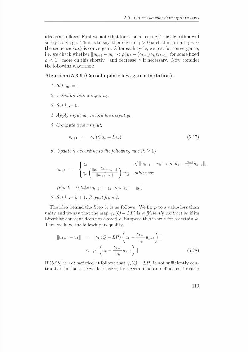
8/8/2019 Evaluasi pada Iterative Learning Control
http://slidepdf.com/reader/full/evaluasi-pada-iterative-learning-control 135/175
5.3. On trial-dependent update laws
idea is as follows. First we note that for γ ‘small enough’ the algorithm willsurely converge. That is to say, there exists γ > 0 such that for all γ < γ the sequence {uk} is convergent. After each cycle, we test for convergence,i.e. we check whether uk+1 − uk < ρuk − (γ k−1/γ k)uk−1 for some fixed
ρ < 1—more on this shortly—and decrease γ if necessary. Now considerthe following algorithm:
Algorithm 5.3.9 (Causal update law, gain adaptation).
1. Set γ 0 := 1.
2. Select an initial input u0.
3. Set k := 0.
4. Apply input uk, record the output yk.
5. Compute a new input.
uk+1 := γ k (Quk + Lek) (5.27)
6. Update γ according to the following rule ( k ≥ 1).
γ k+1 :=
⎧⎨
⎩
γ k if uk+1 − uk < ρuk − γ k−1γ k
uk−1,
γ k
uk−
γk−1γk
uk−1uk+1−uk
ρ
1+δotherwise.
(For k = 0 take γ k+1 := γ k, i.e. γ 1 := γ 0.)
7. Set k := k + 1. Repeat from 4.
The idea behind the Step 6. is as follows. We fix ρ to a value less thanunity and we say that the map γ k (Q − LP ) is sufficiently contractive if itsLipschitz constant does not exceed ρ. Suppose this is true for a certain k.Then we have the following inequality.
uk+1 − uk = γ k (Q − LP )
uk − γ k−1
γ kuk−1
≤ ρuk − γ k−1
γ kuk−1
. (5.28)
If (5.28) is not satisfied, it follows that γ k(Q − LP ) is not sufficiently con-tractive. In that case we decrease γ k by a certain factor, defined as the ratio
119
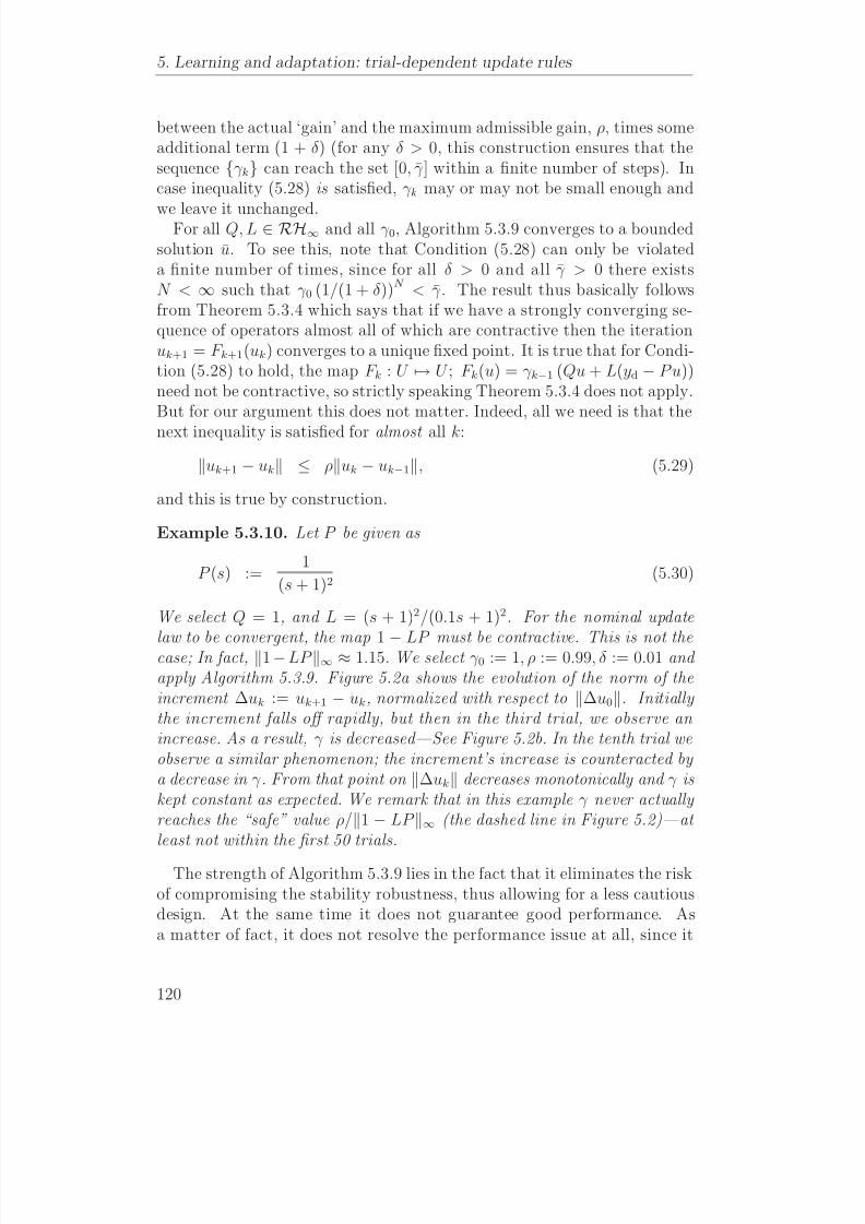
8/8/2019 Evaluasi pada Iterative Learning Control
http://slidepdf.com/reader/full/evaluasi-pada-iterative-learning-control 136/175

8/8/2019 Evaluasi pada Iterative Learning Control
http://slidepdf.com/reader/full/evaluasi-pada-iterative-learning-control 137/175
5.3. On trial-dependent update laws
1
0.9
0.8
0.7
0.6
0.5
0.4
0.3
0.2
0.1
00 10 20 30 40 50
1.1
1.05
1
0.95
0.9
0.85
0.8
0.75
0.70 10 20 30 40 50
(a) ∆u/∆u0 (b) γ k
Figure 5.2.: Simulation results—see Example 5.3.10 for de-tails. The figures on the left and the right re-spectively show (a) the evolution of the incre-ment
∆uk
and (b) the gain γ k, both as a func-
tion of the trial number k.
assumes Q and L—the main determinants— to be given. In addition, thepresent algorithm is not equipped to cope with noise.
Surely we could improve on its design; based on Algorithm 5.3.9 we couldcome up with a dozen other update schemes, each exploiting the particularfeatures we would assume the plant to have. But we believe that strategywould not take us very far. What we would find is that the complexity of the resulting algorithm is inversely proportional to what we assume to knowabout the plant. But the question is where this complexity originates: in
the problem, or in the solution? If it is, like we think, in the solution, thenit may pay off to look for other ways of exploiting the same information.
Learning Control based on single parameter adaptation—a noncausalexample
Let us consider the next algorithm. Starting point is the update law givenin Equation (5.31).
uk+1 = uk + λP ∗ek. (5.31)
It seems evident that, in order to implement this scheme, we need to know
P . But that is not entirely true. For what we need to know is P ∗ek, notP . The difference is important, as we may evaluate P ∗ek even if we do notknow P . This is by virtue of a result from Chapter 4 which says that
P ∗ek = ΠP Πek. (5.32)
121
8/8/2019 Evaluasi pada Iterative Learning Control
http://slidepdf.com/reader/full/evaluasi-pada-iterative-learning-control 138/175
5. Learning and adaptation: trial-dependent update rules
Recall that the operator Π is defined as (Πe)(t) := e(T − t). The conclusionis that even if we do not know P , we can compute P ∗ek from the system’sresponse to the auxiliary input Πek. The drawback of this approach is thatwe need to double the number of iteration steps. From (5.31) it follows that
the error ek satisfies the update equation
ek+1 = (1 − λP ∗P ) ek (5.33)
For convergence we require1 − γP ( jω)∗P ( jω) < 1 for almost all ω (5.34)
We may observe that for λ small enough this condition is always satisfied.
In particular, λ should be smaller than 2/P 2∞. Hence, if we have a lower
bound on P ∞ we can easily pick λ accordingly. But even if we do not,we can make the algorithm converge by setting up an adaptive scheme as
follows.
Algorithm 5.3.11 (Noncausal update law, single parameter adap-tation).
1. Pick some γ 0 > 0.
2. Choose an initial input u0.
3. Set k := 0.
4. Apply the input uk to the system, record the output yk := P uk.
5. Compute the error ek as ek := yd − yk.
6. Compute Πek as (Πek)(t) := ek(T − t).
7. Apply the auxilary input Πek to the system, record the output P Πek.
8. Compute P ∗ek := ΠP Πek.
9. Compute a new input uk+1 = uk + λkP ∗ek.
10. Update λk according to the following rule.
λk+1 :=
λk if ek < ek−1,
λk
ek−1
ek−1+ek
1
1+δotherwise.
(5.35)
122

8/8/2019 Evaluasi pada Iterative Learning Control
http://slidepdf.com/reader/full/evaluasi-pada-iterative-learning-control 139/175
5.3. On trial-dependent update laws
11. Set k := k + 1. Repeat from 4.
The idea behind this update scheme is as follows. If the norm of the errorin the current trial is greater than or equal to that in the previous trial, thenapparently λ is not small enough; In that case we decrease λ as indicated.
If not, we leave λ unchanged. This way we ensure that λk is a nonincreasingfunction of k. By construction the error grows a finite number of times atmost. Consequently, the sequence {ek} is bounded and converges to alimit. However, convergence may be arbirarily slow.
Example 5.3.12. We apply the algorithm in closed loop. That is, we con-sider the feedback interconnection of a plant P open with a compensator C and define P : U → Y, P (u) := (1 + CP open )
−1 CP open u. Let P open and C be given as
P open (s) :=1
37s2 + 10; C (s) := 275280
0.02s + 1
0.002s + 1. (5.36)
We select the reference trajectory yd to equal the unit step response of thesystem
P ref (s) :=1
(0.02s + 1)2(5.37)
We choose λ0 := 1, δ := 0.01 and u0 := yd . Figure 5.3a shows the error in trials 0 (just feedback) and 9. Figure 5.3b shows the normalized mean squared error ek/e0 as a function of the trial number k. We observethat the error decreases exponentially as a function of the trial number.The monotonicity is due to the fact that we chose λ0 small enough (smaller
than 2/P 2∞ ≈ 1.22). Figure 5.4a shows what happens if we start from
λ0 = 2. We observe that during the first few trials, the norm of the error grows. Meanwhile—see Figure 5.4b—λ is decreased and at k = 3, it reachesa value of 0.7, which is well below the critical value 1.22. From that moment on the error decreases monotonically.
Algorithm 5.3.11 provides us with a means to get good tracking perfor-mance in the face of extreme (parametric) uncertainty. Its major weak-ness, as said, is that no upper bound on the speed of convergence canbe given. The problem is caused by the zeroes of P . Assuming we havesome nominal model P 0, we could replace λ by a frequency weighted gain
λ (γ 2
+ P ∗0 P 0)−1
—see Equation (5.38).uk+1 = uk + λk
γ 2 + P ∗0 P 0
−1P ∗ek (5.38)
For γ small enough this could speed up convergence, provided P is closeenough to P 0.
123

8/8/2019 Evaluasi pada Iterative Learning Control
http://slidepdf.com/reader/full/evaluasi-pada-iterative-learning-control 140/175
5. Learning and adaptation: trial-dependent update rules
0.15
0.1
0.05
0
−0.05
−0.10 0.5 1 1.5 2
e0(t)
e9(t)
1
0.9
0.8
0.7
0.6
0.5
0.4
0.3
0.2
0.1
00 1 2 3 4 5 6 7 8 9
(a) {ek(t) : k = 0, 9} (b) The error ek (normalized RMS)
Figure 5.3.: Simulation results corresponding to Algo-rithm 5.3.11 (see Example 5.3.12 for details).The plot on the left shows the error during tri-als 0 (dashed) and 9 (solid); The plot on theright depicts the normalized mean-squared er-ror for trials 0 through 9. The parameter λ0
was set to 1.
5.4. Discussion
5.4.1. Brief review
In this chapter, we looked at a class of trial-dependent update rules of theform
uk+1 := Qk+1uk + Lk+1ek. (5.39)
Initially, we assumed {(Qk, Lk)} to be given and strongly converging. Whenwe additionally assumed the sequence of operators to be contractive, wecould prove this class to be equivalent with a class of trial-independentupdate laws,
uk+1 := Quk + Lek. (5.40)
We also looked at a particular subset of non-contractive update rules,
uk+1 := uk + Lk+1ek (5.41)
where we assumed {Lk} to strongly converge to zero. We found this class toconverge under the relatively mild condition that {Lk} be summable. Westudied the achievable performance and found it to be constrained, muchlike it is in the general class. Besides, we found that performance would
124

8/8/2019 Evaluasi pada Iterative Learning Control
http://slidepdf.com/reader/full/evaluasi-pada-iterative-learning-control 141/175
8/8/2019 Evaluasi pada Iterative Learning Control
http://slidepdf.com/reader/full/evaluasi-pada-iterative-learning-control 142/175
5. Learning and adaptation: trial-dependent update rules
adaptation. Example 5.3.10 lacked many desirable properties, and probablywould not work very well in a noisy situation; it sufficed to show that byadapting a single gain parameter, it is possible to have a competitive designwithout compromising stability robustness.
Perhaps the second example was more interesting, particularly from aperformance point of view. For whereas the first example did not showparticularly good behavior, this one did. To say, the algorithm we developedwould converge to zero error on the basis of but a single assumption: thatthe plant be LTI.
Of course, we used the insight we had obtained in studying trial-independentupdate laws; the basic structure was given. The trick was to make use whatof what did know (the fact that the system is LTI) and to iterate on whatwe did not know (the system gain). This combination turned out to be veryeffective.
Somehow, this seems exemplary to what Learning Control is about, namely:
to combine what is known (prior knowledge) with what is learned duringiteration (trial data). The algorithms we discussed are not likely to workwell in practice for reasons we have not considered. Even so the underlyingphilosophy may have some potential.
5.A. Proofs
Proof of Theorem 5.3.4
Proof. First we prove uniqueness. Let {F i} be contractive and suppose F
has two fixed points x, x ∈ X with x = x. Let λi denote the Lipschitzconstant of the linear operator (F i)ø and define λ := limsupi λi. For all iwe have
F i(x) − F i(x) ≤ λix − x. (5.42)
In particular,
limi→∞
F i(x) − F i(x) ≤ λ x − x < x − x. (5.43)
Here we used the fact λ < 1 (which follows from the assumption of contrac-tivity). On the other hand we have
F i(x) − F i(x) − (x − x) ≤ F i(x) − x + F i(x) − x, (5.44)
which implies that
limi→∞
F i(x) − F i(x) = x − x. (5.45)
126
8/8/2019 Evaluasi pada Iterative Learning Control
http://slidepdf.com/reader/full/evaluasi-pada-iterative-learning-control 143/175
5.A. Proofs
Equations (5.43) and (5.45) cannot both hold true, unless x = x. But thiscontradicts our starting assumption. Hence we conclude that F has onlyone fixed point.
Next we prove that if x := limn→∞ (ni=1 F i) is well defined (in the sense
that the limit exists), x must be a fixed point of F . Indeed, supposelimn→∞ (n
i=1 F i) exists. Then, by definition
limn→∞
n
i=1
F i
= lim
n→∞F n
n−1i=1
F i
. (5.46)
By assumption, the left hand side of (5.46) converges to x. The claim isthat the right hand side converges to F (x). This can be shown as follows.Take any x0 ∈ X , define xn := (
ni=1 F i) (x0), and observe that
F n(xn−1) − F (x) = F n(xn−1) − F n(x) + F n(x) − F (x)
≤ F n(xn
−1)
−F n(x)
+
F n(x)
−F (x)
= F n(xn−1 − x) + F n(x) − F (x)≤ λn xn−1 − x + F n(x) − F (x). (5.47)
Here we used the fact that for each n, F n is a bounded affine operator (withLipschitz constant λn). As n tends to infinity both terms on the right handside of (5.47) vanish. The first because, by assumption, xn−1 converges tox and {λn} is uniformly bounded; The second because {F n} is stronglyconverging. This shows that F n(xn−1) tends to F (x). We conclude that xis a fixed point of F .
Next we show that the sequence {(
ni=1 F i) (x)}∞n=1 does indeed converge
for all x∈
X . To that end, take any x0
∈X and define xn as before. Let N
denote the smallest integer for which supi>N λi < 1. For all n > N we haveni=1
F i
(x0) =
n
i=N +1
F i
(xN ) (5.48)
For i ≥ 1 we define F i := F i+N . To prove the statement, we show that for
all x ∈ X , the term xn :=n
i=1 F i
(x) tends to a limit.
Decompose the operator F n into an affine part (F n)a, and a linear part(F n)ø:
F n
(x) := (F n
)ø(x) + (F
n)a
(x) (5.49)
For all n ≥ 1 we have
xn =
n
i=1
(F i)ø
(x) +
n−1 j=1
n−1i= j
(F i+1)ø
(F j)a(x) + (F n)a(x)
127

8/8/2019 Evaluasi pada Iterative Learning Control
http://slidepdf.com/reader/full/evaluasi-pada-iterative-learning-control 144/175
5. Learning and adaptation: trial-dependent update rules
Define A := supn (F n)a and recall that (F n)ø = λn+N is uniformlybounded by some constant λ < 1. Thus
xn ≤ λnx0 +n−1
j=0
λ jA
= λnx0 +
1 − λn
1 − λ
A (5.50)
Clearly the right hand side of (5.50) is bounded and hence {xn} is bounded.What remains to be shown is that xn − xn−1 tends to zero as n → ∞.We have that
xn − xn−1 = F n(xn−1) − F n(xn−2) + F n(xn−2) − F n−1(xn−2)≤ F n(xn−1) − F n(xn−2) + F n(xn−2) − F n−1(xn−2)≤ λ xn−1 − xn−2 + F n(xn−2) − F n−1(xn−2)
The second term on the right hand side vanishes as n tends to infinity. Thisis because {F n(x), n ≥ 1} is Cauchy for all x ∈ X . Consequently, sinceλ < 1, xn − xn−1 converges to zero. This concludes the proof.
Proof of Theorem 5.3.6
We need the following lemma.
Lemma 5.A.1 (Convergence of an infinite product). If ai ≥ 0 for all values of i, the product
ki=1 (1 + ai) and the series
ki=1 ai converge or
diverge together.
Proof. See Titchmarsh (1939)
We prove the main theorem.
Proof. (of Theorem 5.3.6) Using induction it can be shown that for k ≥ 0
uk =k−1i=0
(I − Li+1P ) u0 +k−1 j=0
k−1i= j+1
(I − Li+1P ) L j+1yd.
Boundedness is proved term by term, starting from the first:
k
i=0
(I − Li+1P ) u0 ≤k
i=0
I − Li+1P u0
≤k
i=0
(1 + Li+1P ) u0.
128

8/8/2019 Evaluasi pada Iterative Learning Control
http://slidepdf.com/reader/full/evaluasi-pada-iterative-learning-control 145/175

8/8/2019 Evaluasi pada Iterative Learning Control
http://slidepdf.com/reader/full/evaluasi-pada-iterative-learning-control 146/175
5. Learning and adaptation: trial-dependent update rules
130
8/8/2019 Evaluasi pada Iterative Learning Control
http://slidepdf.com/reader/full/evaluasi-pada-iterative-learning-control 147/175
6
Discussion and Conclusion
Overview – After some general remarks, we briefly review anddiscuss the main results. Then we draw some conclusions.
6.1. Some general remarks
6.1.1. A critique?
“Don’t mind criticism. If it is untrue, disregard it; if unfair, keepfrom irritation; if it is ignorant, smile; if it is justified it is not criti-cism, learn from it. ”
—Author unknown
This thesis is neither complete nor wholly impartial. From the very start,it was our intention to communicate a particular view. A view that wouldfind itself at odds, not only with popular accounts, but with the larger partof the scientific literature as well. To maximize the effect this view wouldhave, we thought it good to present the discrepancies as sharp as we possiblycould, in the hope our contribution would spur more discussion.
No doubt, some will consider our contribution a critique. And, in a way,
it is. But even so, it is no mere criticism. As we mentioned in the openingchapter, our intention was to lay bare ILC’s distinctiveness. We think ILChas considerable potential, be it that it does not always show. If we wishto further this potential, me must know how to exploit it. Herein ourcontribution lies.
131
8/8/2019 Evaluasi pada Iterative Learning Control
http://slidepdf.com/reader/full/evaluasi-pada-iterative-learning-control 148/175
6. Discussion and Conclusion
6.1.2. First-order recurrences and the problem of LearningControl
We set out to compare two, apparently distinct, methods of control. Wechose to focus on a well-established class of first-order linear recurrences.This class originates one of the strongest currents in ILC research, andis representative of a large majority of algorithms. Indeed, to date mostalgorithms still conform to the same basic structure as was at the basis of Arimoto’s 1984 D -type learning rule—a structure which looks like this:
uk+1 = F (uk, ek). (6.1)
Here, uk+1, uk and ek respectively denote the future input, the current input,and the current error. The operator F : U × Y → U is typically linear (thisis true even if the plant is not) in which case it may be decomposed into anoperator Q : U
→Y , acting on the first argument (the control input), and
an operator L, acting on the second (the tracking error):
F (u, e) = Qu + Le. (6.2)
In this thesis we assumed Q and L to be bounded (on [0, ∞)). This assump-tion may seem restrictive, excluding many algorithms of interest, but it re-ally is not. For we do not need unbounded operators, at least not in the con-text of linear, time-invariant systems. After all, any finite-dimensional LTIoperator G(s) ∈ RL∞ can be decomposed into a causal and an anti-causalpart, both bounded. As for derivative-type (nonproper) operators: thesecan be looked upon as improper limits of particular sequences of (bounded)
noncausal operators. By using (bounded) noncausal, instead of nonproperoperators, the derivative action may be spread out (as it were) over multi-ple trials. The additional advantages: a well-behaved algorithm and smooth(monotone) convergence.
6.2. Conclusion
6.2.1. Main Results
Let us now review the main results of the thesis.
A two-parameter synthesis problem
We chose to define the problem of Iterative Learning Control as an optimiza-tion problem over the space of bounded linear operator pairs (Section 2.3),
132

8/8/2019 Evaluasi pada Iterative Learning Control
http://slidepdf.com/reader/full/evaluasi-pada-iterative-learning-control 149/175
6.2. Conclusion
and distinguished two cases: That of (a) Standard ILC (Section 2.3.2), and(b) Current-Cycle Feedback ILC (CCF-ILC), also known as Current Iter-ation Tracking Error ILC, or CITE-ILC (Section 2.3.3). A special case of CCF-ILC, Standard ILC assumes a stable plant and does not allow any in-
formation to be fed back within the same trial (that is to say, no closed-loopfeedback). CCF-ILC does not impose stability conditions on the plant, butinstead assumes the overall system to be stabilized by some feedback com-pensator. This compensator obviously does feed back information withinthe same trial. Hence the term ‘current-cycle feedback’.
Standard ILC, and CCF-ILC both relate to the same class of first-order(linear) recurrences:
uk+1 = Quk + Lek + Cek+1, (6.3)
a class that is characterized by a threesome parameters: (a) an operator
acting on the previous input, Q; (b) an operator acting on the previouserror, L, and (c) an operator acting on the current error, C . The first twoare considered design parameters; The third is not. In both Standard ILCand CCF-ILC, the objective is to find the parameter combination (Q, L)that maximizes asymptotic performance. As said, in Standard ILC, weassume C = 0.
The notion of admissible pairs
In Chapter 3 we took our first shot at the problem, starting with Stan-dard ILC. For historical reasons, we decided to focus on a class of causal
algorithms, contraining both design parameters to be causal.We started by introducing a notion of admissibility , see Definition 3.3.1.
One would like to think of this notion as the ILC analog of internal stability.Roughly speaking, a pair of operators (Q, L) is said to be admissible if: (a)both the input, and output sequence converge to some bounded fixed point,independent of the initial condition; (b) the convergence refered to in (a) isrobust against all bounded additive disturbances. That is to say, the solutionto the iterative system thus perturbed should remain close to that of theunperturbed system, and the both should converge in case the disturbancesshould subside.
Regarding admissibility, we found a single condition to be both necessaryand sufficient (Section 3.4.1, Lemma 3.4.1). This condition was alreadyknown to be sufficient. We proved it to be necessary. We discussed the factthat there are different ways to define a notion like admissibility. Typical of our definition is: (a) that we require both operators to be bounded on the
133
8/8/2019 Evaluasi pada Iterative Learning Control
http://slidepdf.com/reader/full/evaluasi-pada-iterative-learning-control 150/175
6. Discussion and Conclusion
entire right semi-infinite time interval and (b) that we want our solutionsto be robust in the sense explained above.
Redundancy and equivalent pairs
With this condition of admissibility at our disposal, we were able to tellwhat parameter combinations would warrant an acceptable solution andwhat combinations would not. Next we had to select, from among the‘good’ combinations, the ones that would give best performance.
It turned out that this very set of ‘good combinations‘ (the set of ad-missible pairs) was redundant. That is to say, we found that two pairs of operators could induce different sequences that would eventually converge tothe same fixed point (see in particular Equation (3.24) and Example 3.4.5).In view of the focus of ILC research, which is on asymptotic performance,it appeared sensible to equate these pairs, and so we introduced an equiv-
alence relation (Section 3.4.2, Definition 3.4.3). For two pairs of operatorsto be considered equivalent, they would have to meet a certain equivalencecondition and for this condition to make sense, we had to assume the plantto be strictly proper.
Using this relation we were able to identify equivalent pairs. Now wecould remove redundancy (see Section 3.4.4). What we did was to assign,within each equivalence class, one particular member to represent the class.But then a problem presented itself. For what member would we choose?The choice, of course, was immaterial, as all iterations would converge tothe same fixed point anyway. Yet we had to choose one.
We discovered that, to distinguish equivalent pairs we had to involveanother variable: convergence speed. Indeed, we found that ‘equivalent’iterations would differ, not only in terms of how they would reach the fixedpoint, but also how fast they would reach it. This one parameter, conver-gence speed, thus represented all possible ways in which we could select a setof representatives; All we had to do was fix this parameter and we wouldget our representatives for free. We chose to set it to zero, which meantthat from that point on, we would restrict attention to those iterations thatconverge within a single trial.
Equivalent Feedback
This notion of equivalence turned out to have an unexpected interpretationin terms of Equivalent Feedback. Concisely put, the principle of EquivalentFeedback states that to every iteration of the form (6.3), with (Q, L) ad-missible and causal, there corresponds a particular (causal) feedback map,
134

8/8/2019 Evaluasi pada Iterative Learning Control
http://slidepdf.com/reader/full/evaluasi-pada-iterative-learning-control 151/175
6.2. Conclusion
the Equivalent Controller, which, in closed loop, would reproduce the ex-act same control effort, without iterations. We found that admissible pairs,equivalent in the sense of Definition 3.4.3, corresponded to different left-coprime factorization of the same Equivalent Controller.
We proved this Equivalent Controller to be stabilizing (Theorem 3.4.7)and showed the converse result to hold as well (Theorem 3.4.8). That is tosay, we showed: (a) that each admissible pair defines a particular, stabilizingcontroller, and (b) that every stabilizing controller admits a factorizationin terms of admissible pairs (and more than one factorization at that). Byrestricting attention to a class of representatives, we could establish a bijec-tion between this smaller set of admissible pairs and the set of stabilizingcontrollers.
This showed that the respective methods of Causal ILC and conventionalfeedback control are essentially equivalent; indeed, that Causal ILC is feed-back control in disguise. However, we were unable to justify this claim by
any other than purely theoretical means. Our experimental results (Sec-tion 3.6.1) showed a small, but persistent discrepency in performance, infavor of ILC. There is nothing conclusive at this point, but our best guess isthat this phenomenon is caused by noise (measurement noise, quantizationnoise), see also our discussion in Sections 3.4.5 and 3.6.4. We did confirmthe Equivalent Controller to be stabilizing in all cases considered.
Extensions to CCF-ILC
These results were readily extended to the case of CCF-ILC (Section 3.5, theresult on Equivalent Feedback is in Theorem 3.5.2). But with one exception:it turned out that in CCF-ILC, the set of Equivalent Controllers is just asubset of all stabilizing controllers. These sets do not coincide, unless thecurrent-cycle term (the nominal feedback controller) is strongly stabilizing(i.e. both stable and stabilizing), see Theorem 3.5.3.
Noncausal ILC
Then we turned to Noncausal ILC. Conscious of the historical emphasis oncausal algorithms, our first concern was to make clear that Noncausal ILCis no mere extension of causal ILC; that it is in fact more natural to consider
noncausal algorithms, than it is to consider causal algorithms.To support our argument, we brought in some optimization problem. Theobjective of this problem was to find the minimizing argument of some costfunctional J (∆u), with ∆u the control increment. We showed that the solu-tion would involve the use of noncausal operators (refer to Equation (4.3)).
135
8/8/2019 Evaluasi pada Iterative Learning Control
http://slidepdf.com/reader/full/evaluasi-pada-iterative-learning-control 152/175
6. Discussion and Conclusion
In the course of the chapter (which dealt exclusively with the StandardILC case) we put forth a number of additional arguments as to why wewould want to consider noncausal update laws. Most of these argumentsrelated to performance, or rather the lack therof in case we would insist
on causality. We showed that by imposing causality constraints, we wouldseriously impair the achievable performance, particularly so when the plant:(a) has relative degree greater than one (Lemma 4.2.2) and (b) exhibits non-minimum phase behavior (Section 4.2.4).
In this respect, zero and first-order minimum-phase systems were shownto form an exception. With these systems we can attain perfect trackingeven with causal algorithms (Lemma 4.2.3). The corresponding, causal,operators would not be admissible in the sense of Definition 3.3.1, as theydo not guarantee boundedness of the input. But that, in fact, has more todo with perfect tracking than with causality. For had we used noncausaloperators they would still not be admissible.
In constrast, we showed that, regardless whether the system is minimumphase or non-minimum phase, there is always a bounded noncausal opera-tor pair (I, L) such that I − LP is less than unity for almost all frequencies(Lemma 4.2.4). And this condition implies that, in Noncausal ILC: (a) noneof the aforementioned constraints (Bode’s Sensitivity Integral, Poisson’s In-tegral Relation) applies and (b) perfect tracking can always be achieved(though, again, the input need not converge if we do not constrain theoutput to be feasible).
If we insist on boundedness of the input (which we would do in most prac-tical applications) we ought to consider deploying the somewhat stronger
condition of admissibility. Under the condition of admissibility, perfecttracking will be hard to attain (if P is strictly proper, there is no L suchthat I − LP is a strict contraction). But even then, there is much to begained, performancewise.
As for Equivalent Feedback, we showed that, in general, no causal feed-back map exists that would give the same performance without iterations.A noncausal map would do the trick, but if we would try to implement itcausally, it would be destabilizing. And to implement it noncausally wouldbe impossible in closed loop.
Finally, a remark. In our analyses, we adopted an infinite-time perspec-
tive. We showed that such analysis is conservative in the sense that if Q−LP is a contraction on L2[0, ∞) then it follows that its restriction onto [0, T ] isa contraction on L2[0, T ] (Lemma 4.A.2). This suggests that our approachis ‘safe’. Yet, there are problems. The effects of truncation, for instance,are not well understood. Unwanted behavior may occur, especially during
136

8/8/2019 Evaluasi pada Iterative Learning Control
http://slidepdf.com/reader/full/evaluasi-pada-iterative-learning-control 153/175
6.2. Conclusion
the transient phase. This problem, which originates in the initialization of the noncausal filters, needs further study.
Trial-dependent update laws
In Chapter 5 we looked into a class of trial-dependent update laws. This wasafter we had concluded that, by construction, trial-independent update ruleswould not be able to accommodate even the simplest forms of adaptation. Itwas not performance we were after. In that respect, the class of noncausalalgorithms would do perfectly well. What we did expect to find was apotential for adaptation , an ability to enhance performance robustness.
We would start from the same basic algorithm, augment it so as to ac-commodate different types of trial-dependent behavior, and then study theresults. As a first step we replaced the fixed operator pair (Q, L) with asequence of operator pairs {(Qk, Lk)}, to obtain algorithms of the form
uk+1 = Qk+1uk + Lk+1ek. (6.4)
At first, we did not allow any of the operators to depend on trial data: wesimply assumed (Qk, Lk) to be given for all k.
We derived a condition on {(Qk, Lk)} under which the sequence of inputsinduced by (6.4) would converge to a unique fixed point, independent of the initial condition. This involved extending some known results in fixedpoint theory (Theorem 5.3.4). Basically, Qk − LkP had to be contractivefor almost all k, with a finite number of exceptions at most.
Next we proved the above class of trial-dependent update laws, (6.4), and
the next class of trial-independent update laws,uk+1 = Quk + Lek (6.5)
to be equivalent. More precisely, assuming {Qk, Lk} to be contractive andstrongly converging (Definition 5.3.1), we showed that there exist Q and L,with (Q, L) admissible such that (6.4) and (6.5) both converge to the samefixed point.
Led by this result, we decided to look into a class of non-contractiveupdate laws:
uk+1 = uk + Lk+1ek. (6.6)
The adjective ‘non-contractive’ refers to the fact that I −LkP is not assumedto be contractive for (almost) all k; that condition would be impossible tosatisfy anyway. Instead, we assumed Lk to strongly converge to zero. Weproved that, provided Lk is summable (Definition 5.3.5), the sequence of
137
8/8/2019 Evaluasi pada Iterative Learning Control
http://slidepdf.com/reader/full/evaluasi-pada-iterative-learning-control 154/175
6. Discussion and Conclusion
inputs induced by (6.6) would always converge to some bounded solution(Theorem 5.3.6).
We had argued that since this class does not allow for Equivalent Feed-
back, it might be of interest. We were wrong. The one interesting thingabout algorithms of the form (6.6) is that it is impossible to tell where itwill converge to without actually running the scheme. The iteration can-not be reduced to a competitive scheme of lower complexity. To put itdifferently: each and every parameter Lk matters; we cannot, as we couldbefore, replace the whole sequence of operators with a single operator andget the same outcome. All the same, this class was not going to give uswhat we were looking for. It could do little to enhance performance (Theo-rem 5.3.8), and for sure, it would not make it more robust. Besides, itseffectiveness would depend on the initial condition, which, from a genericstand, is unacceptable.
So what we learned is that: (a) there is little point in considering trial-dependent update laws if we do not allow the operators to ‘adapt’; (b) thereis no point whatsoever in considering trial-dependent update laws for rea-sons of performance. For in general trial-dependent, and trial-independentclasses are subject to the same constraints.
Led by these observations we decided to do a case study on two potentiallyadaptive algorithms. The first algorithm (Algorithm 5.3.9, Example 5.3.10)was based on a simple scheme that would tune a particular gain param-eter to a ‘safe’ value. The purpose of this example was to show that byvery elementary means, we can break the tradeoff between performanceand stability robustness. The use of adaptation allowed for a competitive(i.e. non-cautious) design that would have surely compromised some stabil-ity margins in the nominal setup.
The next case (Algorithm 5.3.11, Example 5.3.12) was still more interest-ing, at least from a performance point of view. For despite its other virtues,the previous algorithm did little to enhance performance robustness. Thistime, our starting point was a noncausal update law. As in the previousexample, a simple scheme was to adapt a single scalar parameter. The effec-
tiveness of the algorithm was remarkable. Performance was not only good(perfect tracking), but also robust. This succes (which is purely theoreticalat this point) was due to a combination of using what we know (exploitingthe fact that the system is LTI) and knowing what we do not know (thesystem gain).
138
8/8/2019 Evaluasi pada Iterative Learning Control
http://slidepdf.com/reader/full/evaluasi-pada-iterative-learning-control 155/175
6.2. Conclusion
6.2.2. Conclusions
How does Iterative Learning Control compare with conventional control?And more in particular, what is the use of iteration, both in relation toperformance enhancement and in dealing with uncertainty? These are thequestions we started out with. Now, finally, the time has come to providesome answers.
The need for iteration
First, let us try to explicate the need for iteration. Basically there aretwo scenarios in which such need arises. In the first scenario, we havea competent model of our system and presumably, an equally competentcontroller. Yet, because of some limitations inherent to any feedback design,performance is not quite what we want it to be. In this scenario, iteration
is to deliver that little bit of extra performance. In the second scenario, themodel we have is not at all that good. In fact, due to a lack of informationwe are forced to opt for a conservative design. As a result, our controller isfar from optimal. In this scenario, iteration is to compensate for the lack of a priori knowledge, by generating data from which additional informationmay be extracted.
In the first scenario, the objective is to get the absolute best achievableperformance. In the second, we would settle for less (say, just ‘good’ perfor-mance), provided this same performance could be guaranteed for all systemswithin a specific range—a range determined by the extent of uncertainty.
We concluded that, as it is, Iterative Learning Control answers to the first
scenario and to the first scenario only. The uncertainty issue (as illustratedby the second scenario) is often ignored. The great majority of algorithms isdesigned with the single purpose of delivering perfect tracking. And manydo a good job at that. So good in fact, that we tend to forget how they pullthe trick. Let us be mindful of the fact that this success critically dependson the availability of prior knowledge.
Causal ILC and Equivalent Feedback
This became poignantly clear when we studied a class of causal algorithms
and found the use of iterations artificial and superfluous. And at this point,we can safely say that Causal ILC is, in essence, noniterative. Not becausethere happens to exist some feedback map that delivers the exact sameperformance. For by itself, this does not prove anything. But rather becauseof the fact that this very controller does not depend on anything but the
139
8/8/2019 Evaluasi pada Iterative Learning Control
http://slidepdf.com/reader/full/evaluasi-pada-iterative-learning-control 156/175
6. Discussion and Conclusion
ILC parameters. For this conclusively shows that, despite their apparentdifferences, Causal ILC and conventional feedback control are nothing butdifferent manifestations of the same idea.
If Causal ILC is taken to be representative of all learning algorithms, then
one of two conclusions must apply: (a) either ILC does not learn, or (b)conventional feedback control is more intelligent than we believed it to be.Fortunately, there is no reason to confine ourselves to causal algorithms.
Noncausal ILC
And indeed, it turns out that much can be gained by considering noncausalalgorithms. At least performancewise, that is. This of course makes sense,as most of the limitations inherent in Causal ILC and conventional feed-back control ultimately pertain to causality related constraints. Not boundby any such constraints, noncausal update laws can effect a significant in-
crease in performance, particularly when applied to systems exhibiting non-minimum phase behavior and high relative degree. What is more, on everySISO LTI system there is at least one noncausal update law that will havethe system’s output converge to a desired output, no matter what thatoutput be. This property makes a good starting point as we take on theuncertainty issue.
The uncertainty issue
Whether they be causal or noncausal, as long as these update laws aretrial-independentg, their effectiveness is constrained by how much we know.
And the general rule is: the more we ask, the more we need to know. Soobviously, to effect perfect tracking, we need to know a lot, though we do nothave a conclusive answer as to say how much that is. In case of Arimoto’sD -type algorithm: at least the sign of the first (nonzero) Markov parameter.And we will not be far from the truth by supposing the same is true for thegeneral class of (non)causal update laws.
By construction, trial-independent update laws will never be able toadapt. These schemes are so rigid that even if the model is falsified bythe data, it will not affect execution. Of course, in practice, iteration willbe terminated long before things get out of hand. Yet, this simple argument
does reveal a serious shortcoming.There are only two possible ways in which ILC can distinguish itself fromconventional control. One has to do with performance proper, the otherwith performance robustness. Though there is more to be said, at thispoint, it appears the performance issue is settled in favor of ILC. With
140

8/8/2019 Evaluasi pada Iterative Learning Control
http://slidepdf.com/reader/full/evaluasi-pada-iterative-learning-control 157/175
6.2. Conclusion
ILC, we can attain good performance for a large variety of plants (and thatincludes the kind of plants we did not discuss in this thesis, such as thosewith nonlinear, time-varying dynamics, etc.). Yet little is known about howto shield performance from uncertainty.
We believe that the Learning Control community would do good if itwould make this issue its focus. We suggested that trial-dependent updatelaws would make a good starting point and provided two examples. Thereare other ways. In fact there is no reason to confine oneself to algorithms of any particular kind. As far as uncertainty is concerned, iteration is just ameans of acquiring data. The problem of Learning Control is to combine thisdata with whatever prior knowledge one has, so as to enhance a system’sperformance. In this sense, Learning Control for LTI systems may be anon-issue, but for less trivial systems, the problem is largely unsolved.
141

8/8/2019 Evaluasi pada Iterative Learning Control
http://slidepdf.com/reader/full/evaluasi-pada-iterative-learning-control 158/175
6. Discussion and Conclusion
142
8/8/2019 Evaluasi pada Iterative Learning Control
http://slidepdf.com/reader/full/evaluasi-pada-iterative-learning-control 159/175
A
Bibliography
Ravi P. Agarwal, Maria Meehan, and Donal O’Regan. Fixed Point Theory and Applications. Number 141 in Cambridge Tracts in Mathematics.Cambridge University Press, 2001.
N. Amann, D. H. Owens, and E. Rogers. 2D systems theory applied to
learning control systems. In Proc. of the 33rd Conf. on Decision and Control , pages 985–986, Lake Bruena, FL, USA, Dec. 1994.
N. Amann, D. H. Owens, and E. Rogers. Iterative learning control using op-timal feedback and feedforward actions. International Journal of Control ,65(2):277–293, September 1996a.
N. Amann, D. H. Owens, and E. Rogers. Robustness of norm-optimaliterative learning control. In Proceedings of International Conference on Control , volume 2, pages 1119–1124, Exeter, UK, September 1996b.
N. Amann, D. H. Owens, E. Rogers, and A. Wahl. An H ∞ approach tolinear iterative learning control design. International Journal of Adap-tive Control and Signal Processing , 10(6):767–781, November-December1996c.
S. Arimoto, S. Kawamura, and F. Miyazaki. Bettering operation of robotsby learning. J. of Robotic Systems, 1(2):123–140, 1984.
S. Arimoto, S. Kawamura, and F. Miyazaki. Convergence, stability and ro-bustness of learning control schemes for robot manipulators. In M. J.Jamishidi, L. Y. Luh, and M. Shahinpoor, editors, Recent Trends in
Robotics: Modelling, Control, and Education , pages 307–316. Elsevier,NY, USA, 1986.
S. Bennett. A History of Control Engineering 1800-1930 . The Institutionof Electrical Engineers (IEE), 1979.
143

8/8/2019 Evaluasi pada Iterative Learning Control
http://slidepdf.com/reader/full/evaluasi-pada-iterative-learning-control 160/175
Bibliography
Dennis S. Bernstein. Feedback control: an invisible thread in the history of technology. Control Systems Magazine, 22(2):53–68, April 2002.
Zeungnam Bien and Jian-Xin Xu. Iterative Learning Control: analysis,design, integration and applications. Kluwer Academic Publishers, 1998.
Okko H. Bosgra and Huibert Kwakernaak. Design methods for control sys-tems. Lecture Notes, Dutch Institute of Systems and Control, 2001.
Y. Chen, C. Wen, and M. Sun. A robust high-order P-type iterative learningcontroller using current-iteration tracking error. Int. J. of Control , 68(2):331–342, Sept. 1997a.
Y. Chen, J.-X. Xu, and T. H. Lee. Current-iteration tracking error assistediterative learning control of uncertain nonlinear discrete-time systems.In Proc. of the 35th IEEE Conference on Decision and Control , pages
3040–5, Kobe, Japan, Dec. 1996a.Y. Chen, J.-X. Xu, and T. H. Lee. An iterative learning controller using
current-iteration tracking error information and initial state learning. InProc. of the 35-th IEEE CDC , pages 3064–9, Kobe, Japan, Dec. 1996b.
Y. Chen, J.-X. Xu, and T.H. Lee. Current-iteration tracking error assistedhigh-order iterative learning control of discrete-time uncertain nonlinearsystems. In Proc. of the 2nd Asian Control Conference (ASCC’97), Vol.I , pages 573–6, Seoul, Korea, Jul. 1997b.
Yangquan Chen and Changyun Wen. Iterative Learning Control: conver-
gence, robustness and applications. Lecture Notes in Control and Infor-mation Sciences. Springer-Verlag, 1999.
R.F. Curtain and H.J. Zwart. An Introduction to Infinite-Dimensional Lin-ear Systems Theory . Springer-Verlag, 1995.
B.J. de Kruif. Function Approximation for Learning Control—a Key SampleBased Approach . PhD thesis, University of Twente, 2004.
Dick de Roover. Synthesis of a robust iterative learning controller usingan H ∞ approach. Proceedings of the 35th Conference on Decision and Control , pages 3044–3049, December 1996.
Dick de Roover, Okko H. Bogra, and Maarten Steinbuch. Internal-model-based design of repetitive and iterative learning controllers for linearmultivariable systems. International Journal of Control , 73(10):914–929,2000.
144

8/8/2019 Evaluasi pada Iterative Learning Control
http://slidepdf.com/reader/full/evaluasi-pada-iterative-learning-control 161/175
Bibliography
Dick de Roover and Okko H. Bosgra. Synthesis of robust multivariableiterative learning controllers with application to a wafer stage motionsystem. International Journal of Control , 73(10):968–979, 2000.
J. B. Edwards and D. H. Owens. Analysis and Control of Multipass Pro-cesses. Research Studies Press, Taunton, Chichester, 1982.
Engell. Optimale lineare regelung: Grenzen der erreichbaren regelgute in lin-earen zeitinvarianten regelkreisen. Fachberichte Messen-Steuern-Regeln ,18, 1988.
B.A. Francis. A Course in H∞ Control Theory , volume 88 of Lecture Notesin Control and Informations Sciences. 1987.
B.A. Francis and W.M. Wonham. The internal model principle for linearmultivariable regulators. Applied mathematics and optimization , 2:175–
194, 1975.J.S. Freudenberg and D.P. Looze. Right half plane poles and zeros and
design tradeoffs in feedback systems. IEEE Transactions on AutomaticControl , 30:555–565, 1985.
Peter B. Goldsmith. The fallacy of causal iterative learning control. InProc. Of the 40th Conference on Decision and Control , pages 4475–4480,Orlando, Florida, USA, 2001.
Peter B. Goldsmith. On the equivalence of causal LTI iterative learningcontrol and feedback control. Automatica , 38(4):703–708, 2002.
G. Heinzinger, D. Fenwick, B. Paden, and F. Miyazaki. Stability of learningcontrol with disturbances and uncertain initial conditions. IEEE Trans.of Automatic Control , 37(1):110–114, 1992.
T.-J. Jang, C.-H. Choi, and H.-S. Ahn. Iterative learning control in feedbacksystems. Automatica , 31(2):243–245, 1995.
T. Kavli. Frequency domain synthesis of trajectory learning controllers forrobot manipulators. Journal of Robotic Systems, 9(5):663–680, 1992.
Kevin Kelly. Out of Control: the rise of neo-biological civilization . Perseus
Publishing, 1994.
J. E. Kurek and M. B. Zaremba. Iterative learning control systhesis basedon 2-D system theory. IEEE Trans. of Automatic Control , 38(1):121–125,1993.
145

8/8/2019 Evaluasi pada Iterative Learning Control
http://slidepdf.com/reader/full/evaluasi-pada-iterative-learning-control 162/175
Bibliography
H. Kwakernaak and R. Sivan. Modern Signals and Systems. Informationand System Sciences. Prentice-Hall, 1991.
Hak-Sung Lee and Zeungnam Bien. Study on robustness of iterative learning
control with non-zero initial error. International Journal of Control , 64:345–359, June 1996.
Y.-J. Liang and D. P. Looze. Performance and robustness issues in iterativelearning control. In Proc. of the 32nd Conf. on Decision and Control ,pages 1990–1995, San Antonio, Texas, USA, Dec. 1993.
A. De Luca, G. Paesano, and G. Ulivi. A frequency-domain approach tolearning control: implementation for a robot manipulator. IEEE Trans.on Industrial Electronics, 39(1):1–10, 1992.
David G. Luenberger. Optimization by Vector Space Methods. John Wiley& Sons, 1969.
Pater Hagoort & Rob Maessen. Geest, Computer, Kunst . Stichting Grafiet,Utrecht, 1990.
Principia Cybernetica . http://pespmc1.vub.ac.be/DEFAULT.html, 2004.
K. L. Moore. Iterative learning control for deterministic systems. Advancesin Industrial Control. Springer-Verlag, 1993.
K. L. Moore. Iterative learning control: an expository overview. Applied & Computational Controls, Signal Processing, and Circuits, 1(1):151–214,1999.
K. L. Moore, M. Dahleh, and S. P. Bhattacharyya. Iterative learning control:a survey and new results. J. of Robotic Systems, 9(5):563–594, 1992.
Kevin L. Moore. A matrix fraction approach to higher-order iterative learn-ing control: 2d dynamics through repetition-domain filtering. In Proceed-ings of the 2nd International Workshop on Multidimensional (nD) Sys-tems, 27-30 June, Czocha Castle, Lower Silesia, Poland , pages 99–104,
2000.
Desineni Subbaram Naidu, Selahattin Ozcelik, and Kevin L. Moore. Mod-eling, Sensing and Control of Gas Metal Arc Welding . Elsevier ScienceLtd., Oxford, UK, 2003.
146

8/8/2019 Evaluasi pada Iterative Learning Control
http://slidepdf.com/reader/full/evaluasi-pada-iterative-learning-control 163/175
Bibliography
Mikael Norrlof. Iterative Learning Control: analysis, design, and exper-iments. PhD thesis, Department of Electrical Engineering, LinkopingsUniversitet, Sweden, 2000.
D. H. Owens. Iterative learning control: convergence using high gain feed-back. In Proceedings of the 1992 Conference on Decision and Control ,volume 4, page 3822, Tucson, AZ, December 1992.
D. H. Owens, N. Amann, and E. Rogers. Iterative learning control:an overview of recent algorithms. Applied Mathematics and Computer Science, 5(3):425–438, 1995.
F. Padieu and R. Su. An H ∞ approach to learning control systems. Int. J.Adap. Contr. and Sig. Proc., 4, 1990.
Kevin M. Passino. Bridging the gap between conventional and intelligentcontrol. IEEE Control Systems Magazine, 13(3):12–18, 1993.
E. Rogers, K. Galkowski, D.H. Owens, T. Al-Towaim, J.D. Ratcliffe, andP.L. Lewin. 2d linear control systems: from theory to experiment totheory. In Proceedings of Int. Symp. On Mathematical Theory of Network and Systems, 2002.
Erwin Schrijver. Improved Robot Tracking Control for Laser Welding . PhDthesis, Drebbel Institute for Mechatronics, University of Twente, 2002.
Robert Sedgewick and Philippe Fjajolet. Analysis of Algorithms. A, 1996.
Alan Titchmarsh. The Theory of Functions, 1939.
Masayoshi Tomizuka. Zero phase error tracking algorithm for digital con-trol. Journal of Dynamic Systems, Measurement, and Control , 109:65–68,1987.
Y.A. Tsypkin. Adaptation and Learning in Automatic Systems. AcademicPress, New York, New York, 1971.
Y.A. Tsypkin. Foundations of the Theory of Learning Systems. Academic
Press, New York, New York, 1973.
A. M. Turing. Intelligent machinery. In C. R. Evans and A. D. J. Robert-son, editors, Cybernetics: Key Papers, number 7. University Park Press,Baltimore, 1968.
147
8/8/2019 Evaluasi pada Iterative Learning Control
http://slidepdf.com/reader/full/evaluasi-pada-iterative-learning-control 164/175
Bibliography
Gordon T. Uber. Clocks and Time—History of time-keeping.http://www.ubr.com/clocks/hist/hist.html, 2004.
W.J.R. Velthuis. Learning Feed-Forward Control . PhD thesis, University of Twente, Enschede, The Netherlands, 2000.
M.H.A. Verwoerd, G. Meinsma, and T.J.A. de Vries. On the use of non-causal LTI operators in iterative learning control. Proceedings of the 41st Conference on Decision and Control , pages 3362–3366, 2002.
M.H.A. Verwoerd, G. Meinsma, and T.J.A. de Vries. On equivalence classesin iterative learning control. Proceedings of the American Control Con-
ference, Denver, Colorado, USA, pages 3632–3637, 2003.
M.H.A. Verwoerd, G. Meinsma, and T.J.A. de Vries. On the parameteriza-tion of all admissable pairs in a class of CCF-ILC algorithms. Proceedings
of the American Control Conference, Boston, Massachusetts, USA, pages5156–5157, 2004.
M.H.A. Verwoerd, G. Meinsma, and T.J.A. de Vries. A class of non-contractive, trial-dependent update rules for Iterative Learning Control.Proceedings of the American Control Conference, Boston, Massachusetts,USA, pages 5132–5137, 2004.
M.H.A. Verwoerd, G. Meinsma, and T.J.A. de Vries. On admissible pairsand Equivalent Feedback: Youla parameterization in Iterative LearningControl. Submitted for publication.
J.-X. Xu. Direct learning of control input profiles with different time scales.In Proceedings of the 35th IEEE Conference on Decision and Control ,Kobe, Japan, December 1996.
Jian-Xin Xu and Ying Tan. Linear and Nonlinear Iterative Learning Con-trol . Number 291 in Lecture Notes in Control and Information Sciences.Springer-Verlag, 2003.
Jian-Xin Xu and Tao Zhu. Dual-scale direct learning control of trajectorytracking for a class of nonlinear uncertain systems. IEEE Transactions
on automatic control , 44(10):1884 – 1888, 1999.
D.C. Youla, H.A Jabr, and J.J. Bongiorno. Modern wiener-hopf design of optimal controllers: Part I. IEEE Transactions on Automatic Control ,21:3–13, 1976.
148

8/8/2019 Evaluasi pada Iterative Learning Control
http://slidepdf.com/reader/full/evaluasi-pada-iterative-learning-control 165/175
Bibliography
G. Zames. Feedback and optimal sensitivity: model reference transforma-tions, multiplicative seminorms and approximate inverses. IEEE Trans-actions on Automatic Control , 26:301–320, 1981.
Kemin Zhou, John C. Doyle, and Keith Glover. Robust and Optimal Control .Prentice Hall, 1996.
149

8/8/2019 Evaluasi pada Iterative Learning Control
http://slidepdf.com/reader/full/evaluasi-pada-iterative-learning-control 166/175
Bibliography
150

8/8/2019 Evaluasi pada Iterative Learning Control
http://slidepdf.com/reader/full/evaluasi-pada-iterative-learning-control 167/175
Index
1-parameter problem, 412-parameter synthesis problem, 35λ-norm, 29A, 47
A0, 59, 68
H2, 16K, 57L2, 16L∞, 16RH∞, 18, 96RL∞, 39, 96
achievablebandwidth, 88performance, 90, 136
adaptation, 5, 111, 137
adaptiveability, 112algorithm, 111, 138behavior, 118update law, 118, 122
adjoint, 32, 82admissibility, 133
necessary and sufficient condi-tions, 48, 133
CCF-ILC, 65
admissible pair, 47notion of equivalence, 53AI, 6algorithm, 8
adaptation, 111
classication, 29well-behaved, 81data-driven, 111
aligning, 70almost all, 85
anti-causal operator, 95applications involving ILC
robot manipulators, 8wafer stages, 8welding processes, 8
approximate inverse, 41, 60Arimoto’s approach
main idea, 81shortcomings, 81
artificial intelligence, 6, 10
assumptionboundedness, 38, 132, 133causality, 38full plant knowledge, 107
asymptoticbehavior, 112performance, 133, 134tracking, 37
autonomous machines, 2first generation, 2
water clock, 2auxilary input, 122auxilary variable, 47average tracking error, 73averaging over trials, 63
151

8/8/2019 Evaluasi pada Iterative Learning Control
http://slidepdf.com/reader/full/evaluasi-pada-iterative-learning-control 168/175
Index
a priori knowledge, 12, 109, 114,139
a priori method, 9
Banach space, 27bandwidth, 106, 109bandwidth constraints, 88base plate, 69Bernstein, Dennis S., 2betterment process, 28, 30BIBO-stable, 18bijection, 135bijective, 59bistable, 69Black, Harold, 4
Blaschke product, 86, 89Bode’s sensitivity integral, 80, 88,
136boundedness
reasons for assuming bounded-ness, 39
bounded map, 17
C-code, 72, 77catapult, 3causality constraint, 78, 85, 118,
140causal
algorithm, 139iteration, 118operator, 95
cautious design, 120CCF-ILC problem, 42, 64, 106, 133
and equivalent feedback, 65assumptions, 42
CFC, 2, 9
Classical ILC, 24, 40class representative, 52, 58clepsydra , 2clock, 5closed-loop feedback, 78, 79, 133
cogging, 70, 75compensator design problem, 37,
77and Standard ILC, 59
competitive design, 8, 108comprime, 53conceptual framework, 30
2D-system theory, 35Arimoto et al., 30gradient-type algorithms, 31internal-model control, 37
constant map, 50constraint
boundedness, 43causality, 43
continuityof the unperturbed solution, 49
contraction, 26, 136on L2[0, T ], 99, 136
contractivityof a sequence of operators, 113
control input, 63controversy, 10conventional feedback control, 2,
9, 79, 140
convergenceanalysis, 18condition, 12, 22, 108conditions for, 22infinite-time condition, 23monotone, 23, 29, 30of an iteration, 26of the input sequence, 83of the output sequence, 83of the unperturbed solution, 49
over finite time, 21pointwise, 18speed, 58, 107, 134strong, 113uniform, 18, 29
152

8/8/2019 Evaluasi pada Iterative Learning Control
http://slidepdf.com/reader/full/evaluasi-pada-iterative-learning-control 169/175
Index
convolution systems, 17coprime factorization, 68cost functional, 31Current-Cycle Feedback ILC, 41
Current-Iteration Tracking Error ILC,41
currenterror, 24input, 24output, 24
cybernetics, 4, 5
D-type learning rule, 29, 31, 140convergence condition, 81rationale, 31
Darwin, Charles, 6data-driven algorithm, 111data structures, 7dc motor, 28derivative action, 29, 81, 132design
parameters, 133procedure, 60
desired behavior, 7desired output, 24
determinants for performance, 112de La Mettrie, Julien, 6Dirac δ-function, 96direct feedback term, 40, 41direct learning control, 7discretization effects, 80disturbance
non-deterministic, 62attenuation, 90
divergence
input sequence, 20DLC, 7Drebbel, Cornelis, 3DSpace software, 72DSP board, 72, 77
emulate intelligence, 10eps, 62equilibrium analysis, 44equivalence
class, 52, 57condition, 134relation, 52, 134
equivalent admissible pairs, 53and left-coprime factorization,
57meaning, 54
equivalent controller, 56CCF-ILC, 65internally stability, 56, 67well-posedness, 56
equivalent feedback, 55, 134, 136and noise, 61the set of stabilizing controllers,
67euclidean p-norm, 16execution, 7experiment, 71extended L2-space, 22
feasible output, 85, 107feedback, 4
impact, 4negative, 2, 5purpose, 4universal concept, 4
feedback map, 78, 106, 136feedback system
achievable bandwidth, 88feedforward control, 9feedthrough term, 97FFC, 9
FFT analysis, 75final error, 116finite-time convergence
conditions, 22finite-time operator, 99
153
8/8/2019 Evaluasi pada Iterative Learning Control
http://slidepdf.com/reader/full/evaluasi-pada-iterative-learning-control 170/175
Index
first-order recurrences, 11, 133linear, 31, 132
fixed point, 26analysis, 44
asymptotic stability, 45globally asymptotic stability, 45sequences of operators, 113reachable set, 59stability, 44, 45theorem, 26, 27, 113uniqueness, 27, 115
forgetting factor, 81forward shift, 80free parameter, 34frequency-domain space, 96
full plant knowledge, 107future, 95future output, 24
gain adaptation, 119gain parameter, 138geometric series, 23Godel’s Theorem, 6governor
self-regulation, 5
Watt governor, 4gradient-descent method, 34
high-gain feedback, 42, 81history of ILC, 27homing, 70hype, 10
IC, 1, 10paradigm, 1
idempotent operator, 100
identity map, 115IIR, 99ILC, 2, 7
problem, 21literature, 7
parameters, 140research, 132core activity, 8early years, 30
focus, 134the 90’s, 30synthesis problem, 37
IMP, 37implementation details, 72impulse response, 17inclusion relation, 67increment, 120, 135index, 28induced norm, 17inertial effect, 73infinite impulse response, 99information
feedback, 12, 78preview, 80
initialcondition, 47error, 116
injective, 57input-output behavior, 110input-output mapping system, 16
causal, 17linear, 17noncausal, 17nonlinear, 17time-invariant, 17time-varying, 17
input-output pair, 17input disturbance, 61, 63input sequence, 18input set, 16
integral relation, 117intelligence, 6, 10, 140intelligent
behavior, 5, 6, 110control, 1, 10
154

8/8/2019 Evaluasi pada Iterative Learning Control
http://slidepdf.com/reader/full/evaluasi-pada-iterative-learning-control 171/175
Index
controller, 10machinery, 6methodology, 10paradigm, 1
internal model principle, 37internal stability, 38, 133
for ILC, 48necessary and sufficient condi-
tion, 39equivalent controller (CCF-ILC),
65isomorphism, 59issues
imperfect resetting, 30iteration, 7, 25
and learning, 111and noise, 61one-parameter family, 84need, 139number, 28numerical vs. physical, 107perturbed, 47steps, 122use, 2, 8, 12, 139
iterative inversion process, 9
iterative learning control, 2, 7applications, 8as add-on, 8distinctive features, 8, 11goal, 9history, 27motivation, 8need, 8objective, 31, 38optimization problem, 132
origins, 27potential, 131problem, 10problem definition, 8problem format, 8
problem of, 38strategy, 9well-posedness, 48
iterative
method, 9scheme, 28
kernel, 17knowledge representation, 7
neural networks, 7Ktesibios, 3Ktesibios’ inventions
catapult, 3pump, 3water organ, 3
L-parameter, 34, 41, 133Laplace transform, 16, 96learning, 2, 107, 112
and iteration, 111and performance, 107and uncertainty, 9, 107behavior, 8, 11, 112control, 1, 5, 20connotations, 11definition, 11
impact, 75knowledge and experience, 10
learning control, 1, 7, 28brief history, 2defining features, 108iterative learning control, 7learning feed-forward control,
7pitfalls, 28pragmatic approach, 11
problem, 109learning feed-forward control, 7learning parameter, 29learning rule, 24left-coprime factorization, 135
155

8/8/2019 Evaluasi pada Iterative Learning Control
http://slidepdf.com/reader/full/evaluasi-pada-iterative-learning-control 172/175
Index
LFFC, 7LiMMS, 69linear motor system, 69lipschitzian map, 26
Lipschitz constant, 26, 113literaturecontroller synthesis, 46noncausal ILC, 80
lowpass characteristics, 109LTI systems, 17
machinebrain, 6hearing, 6learning, 1
motion, 6vision, 6
Markov parameter, 31, 81, 140Matlab Simulink, 72maximally achievable performance,
41maximum-absolute-row-sum norm,
29maximum modulus principle, 50McCullogh, Warren, 5Mead, Thomas, 4measured output, 61measurement noise, 61, 135
suppression, 63measure zero, 85memory block, 73minimum-phase system, 87model, 110
invalidation, 111model matching problem, 41monotone convergence, 29, 30
multipass process, 28
Newcomen, Thomas, 4noise, 12, 76, 81, 121, 135nominally convergent, 72
nominal plant, 108nominal update law, 120non-contractive update laws, 115,
137
limitations, 118non-minimum phase, 80, 81, 88non-minimum phase behavior, 84,
136, 140noncausal
algorithm, 137, 140controller, 106ILC, 135iteration, 80operator, 95, 135update law, 140
nonexpansive map, 27noniterative method, 9nonlinearities, 76nonproper operator, 80, 81, 132nonzero measure, 85norm, 16norm-optimal ILC, 32norm-preserving, 101normalized mean-squared error, 123normalrank, 90
notation, 15
offline, 78, 107offline method, 79one-parameter iteration, 84open-loop feedback, 79, 91optimal increment, 32optimal input, 107ordered pair, 52output sensitivity function, 60, 88output sequence, 18, 107
output set, 16overparameterized, 41
P -type learning rule, 81paradigm shift, 30
156
8/8/2019 Evaluasi pada Iterative Learning Control
http://slidepdf.com/reader/full/evaluasi-pada-iterative-learning-control 173/175
Index
parameterizationof all representative pairs, 68
parasitic pole, 108partial knowledge, 10
partial sum, 23partition, 52Passino, Kevin, 10past, 95perfect reset, 7perfect tracking, 35, 85, 136performance
achievable, 90, 106asymptotic, 133, 134constraints, 80, 88determinants, 112enhancement, 107, 138, 139in low-frequency band, 60limitations, 11, 12, 78, 81, 140main determinants, 12robustness, 107, 137, 138
permutation operator, 101perpetual mobile, 3perturbation, 47
multiplicative, 108perturbed iteration, 47
phase shift, 81physical iteration, 107plant capacity, 106plant characteristics, 85pointwise convergence, 18Poisson’s integral formula, 80, 136pole-zero cancellations, 53pole-zero excess, 85, 86positive real, 108postmodern control, 30
preliminaries, 15prior knowledgeand equivalent feedback, 56
problem of ILC, 10, 382D stabilization problem, 36
overparameterized, 41perspectives, see conceptual frame-
workproblem of learning control, 109
projection operator, 99pump, 3purposeful behavior, 5
Q-parameter, 41, 133quantization effect, 61quantization noise, 135
random disturbances, 72range finder, 5rate of convergence, 59
recurrencehigher-order, 25first-order, 11, 132, 133
recurrence relation, 24computational procedure, 44constant-coefficient, 24first-order, 23, 24full-history, 24higher-order, 24linear, 24model, 44
nonlinear, 24variable-coefficient, 24
redundancy, 58, 134regulator, 4relation, 16, 52relative degree, 31, 81, 136, 140religious belief, 6repeatability, 9repetitiveness, 7repetitive control, 72
repetitive nature, 9representatives, 134resetting errors, 7, 30robustness, 41robust
157

8/8/2019 Evaluasi pada Iterative Learning Control
http://slidepdf.com/reader/full/evaluasi-pada-iterative-learning-control 174/175
Index
convergence, 50performance, 138periodic control problem, 37stability, 12
Roesser model, 36Rosenbluth, Arturo, 5Russel, Bertrand, 11
sampling effect, 11Savery, Thomas, 4second-order plant, 62self-adaptive, 111self-regulating device
thermostat, 3valve, 3
Watt governor, 4self-regulation
in man and machine, 5self-tuning processes, 9sensitivity function, 89sensor noise, 61sequence
convergence, 18of inputs, 18of functions, 18, 21of outputs, 18summable, 116
series, 23convergence, 23geometric, 23partial sum, 23
servomechanism, 5, 109set of admissible pairs, 47
equivalence relation, 52set
of equivalent controllers, 135
of representatives, 59, 68of stabilizing controllers, 57shift variable, 37signal, 15Skinner, B.F., 8
slding friction, 70speed of convergence, 58, 107stability condition, 12stability robustness, 108
stabilizing controllerfactorization in terms of admis-
sible pairs, 57Standard ILC, 133
assumptions, 40literature, 41problem, 40, 58synthesis problem, 40
statistical learning theory, 110steam engine, 4, 5stiction, 70strict properness, 53, 54, 134, 136
motivation, 54strongly stabilizing controller, 67strong convergence, 113sufficiently contractive, 119summable sequence, 116surjective, 57switchboard, 5synthesis parameters, 106synthesis problem, 30
focus, 44Standard ILC, 40two-parameter, 35
synthesis procedure, 35, 41system, 16
affine, 17bounded, 17finite dimensional, 17induced norm, 17input-output, 16
linear, 17linear, time-invariant, 11LTI, 17of change, 44time-invariant, 17
158

8/8/2019 Evaluasi pada Iterative Learning Control
http://slidepdf.com/reader/full/evaluasi-pada-iterative-learning-control 175/175
Index
time-varying, 17, 29system gain, 21system identification, 110
thermostat, 3operating principle, 3
thesisaim, 2central issues, 11intent, 11, 131outline, 12purpose, 11scope, 1, 11
three-phase current, 70time-domain space, 96
tracking error, 29tradeoff, 30, 108, 138transient, 137transient behavior, 9transition map 26 115
parametric, 123uncertain systems, 109uniform convergence, 18update law, 24
higher-order, 37nominal, 120non-contractive, 115trial-dependent, 112
vector space, 15normed, 15
Venn diagram, 95virtual closed-loop feedback, 80, 106virtual state vector, 7
waterbed effect, 118water clock, 2water organ, 3Watt governor, 4Watt, James, 4