


Bahasa
Halaman
Hukum

Decision Support Systems 13 (1995) 3-34 3 North-Holland
Views of mathematical programming models and their instances *
Harvey J. Greenberg Uni+,ersity of Colorado at Dem'er, Denver, CO, USA
Frederic H. Murphy Temple University, Philadelphia, PA, USA
Large-scale mathematical models are built, managed and applied by people with different cognitive skills. This poses a challenge for the design of a multi-view architecture of a system that accommodates these differences. A primary objec- tive of mathematical modeling is providing insights into prob- lem behavior, and there are many constituencies who require different views for different questions. One constituency is composed of modellers who have different views of basic model components. Another constituency is composed of problem owners for whom models are built. These two con- stituencies, which are not exhaustive, have significantly differ- ent needs and skills. This paper addresses this issue of multi- view architecture by presenting a formal framework for the design of a view creation and management system. Specific views we consider include algebraic, block schematic, graphic, and textual. Both form and content are relevant to view creation, and the merits of views are determined by their value in aiding comprehension and insight. The need for a central, formal structure to create and manage views is demonstrated by the inadequacy of direct mappings from any of the popular systems that are typically designed to support only one view of linear programming models and their in- stances.
Keywords: Linear programming; Mathematical programming; Large-scale systems; Structured modeling; Com- puter-assisted analysis; Graphics; Natural language discourse; Modeling languages
Correspondence to: H.J. Greenberg, Mathematics Depart- ment, University of Colorado at Denver, P.O. Box 173364, Denver, CO 80217-3364, USA. BITNET: hgreenberg@cuden ver * This research was supported by a consortium of companies:
Amoco Oil Company, IBM, Shell Development Company, Chesapeake Decision Sciences Inc., GAMS Development Corp., Ketron Management Science, and MathPro, Inc.
Introduction
Different people need different views of a model and of what it represents, each view having its own cognitive value for acquiring insight and understanding. The purpose of this paper is to clarify the meaning of views, formalize their defi- nitions, and present an information structure to support a multi-view architecture. As part of defining the architecture, we identify some of the functions of a multi-view management system for mathematical programming, with a focus on lin- ear forms.
Harvey J. Greenberg received his B.S. in Industrial Engineering from Uni- versity of Miami (1962), and his Ph.D. in Operations Research from The Johns Hopkins University (1968). He is presently Professor of Mathematics at The University of Colorado at Denver, and was formerly with the U.S. Department of Energy (1976-
~ 83). Dr. Greenberg directs a project to develop an Intelligent Mathemati- cal Programming System, sponsored by a consortium of companies. As part
of that research, Dr. Greenberg developed the ANALYZE system, which gives intelligent support for analysis of linear programs, and for which he received the first ORSA/CSTS Prize for Excellence in research in the interfaces of operations research and computer science (1986). He has also received two research awards from CU-Denver (1988 and 1992). Dr. Greenberg has numerous publications, and he was the found- ing editor of the ORSA Journal on Computing.
Frederic H. Murphy is a professor in the Management Science/Operations Management Department in the School of Business and Management at Temple University. Prior to joining Temple, he was with the U.S. Depart- ment of Energy. He received his B.A. in Mathematics and his Ph.D. in Ad- ministrative Sciences from Yale Uni- versity. He has published in the areas of mathematical programming, dy- namic programming, energy policy, energy modeling and game theory. His
current research interests are in decision support for model- ing and managing modeling systems. He is currently the editor of Interfaces and contributing editor to International Abstracts on Operations Research.
0167-9236/95/$09.50 ©1995 - Elsevier Science B.V. All rights reserved SSDI 0167-9236(93)E0029-D
4 H.J. Greenberg, F.H. Murphy / Mathematical programming models and their instances
First, we illustrate some of what we mean by views of models and instances by showing some for the familiar capacitated transportation prob- lem. Then, we define some basic terms and con- cepts, starting with a working definition of a model and of views. We define certain kinds of views in terms of both form and content.
Second, we formally define and illustrate spe- cific views, associated with linear programming models and their instances. This is done in suc- cessive sections, beginning with views of the fun- damental elements of any model: objects and relations among the objects. This also serves to reinforce some basic terms and concepts. Then, familiar views of model structures are formalized in order to define precisely what is needed to create them.
After we have described specific views and indicated some formalism in their definitions, we define mappings to illustrate how one might go directly from one view to another, and the diffi- culties that arise with current systems that repre- sent only one view. In particular, we consider how to map information that supports an alge- braic view to that which supports a block schematic view, and conversely. We demonstrate that, for some linear programming models, the information contained in one view lacks informa- tion needed to construct the other. This sets the stage for the more general formal development that follows, and it raises issues concerning oper- ations on views.
Following through with operations on views, we describe zooming, condensing and switching operations. The notion of zooming and condens- ing is a standard one; however, we introduce the specification of zooming and condensing models that accompany a view. Their purpose is to give an adaptive quality to view management. Switch- ing views is shown to be a 2-step process, even though an observer might see it as one operation.
Special attention is then given to structured modeling for two reasons. First, it is a fundamen- tal approach to model description; and, second, it contains another view, called an outline. We aug- ment SM in several ways after describing why its current form is not designed to support all views of interest.
Building on the concepts that grow from spe- cific view analyses and from the formalism intro- duced, we move towards a more general formal-
ism. First, we present a formal description of a multi-view architecture. Second, we present a central information structure that is, itself, a for- mal description of models and their instances that supports all of the views we consider. Third, we move to a higher level of formalism by defin- ing views in terms of information they must ac- cess. The completeness of this higher level for- malism is an open issue, but it reinforces the proposed scope information structure that goes beyond the specific views we shall describe.
While a multi-view architecture has been dis- cussed by some, only Baldwin's thesis [3] (see also [4, 7, 5, 6 and 8]) has gone deeply into this, including a prototype system, called DOVE (De- veloping and Organizing Views for Examination). Baldwin's formalism is similar to that of Garlan [24], although Garlan's stems from different con- siderations.
Much can be said about developments in rela- tional database theory, but the issues in defining views in a relational database are very different (some interesting connections are given in [19]). Garlan [24] elaborates upon this. Also, Farn's thesis [22] shows how structured modeling con- tains the expressiveness of relational database theory, and we shall give special attention to structured modeling.
It is perhaps interesting to note that recent comparative analyses of a modeling language's expressiveness, such as the studies in [56] and [45], have not considered view creation in their evaluations. This is because there is not yet a fully implemented system to support a multi-view architecture, and the difficulties with presenting one view from information stored to support an- other have not been surfaced. That is one of the primary objectives of this paper: to understand more precisely the issues with view creation and management. In addition, we initiate a formalism based on a foundation of information access.
I. Terms and concepts
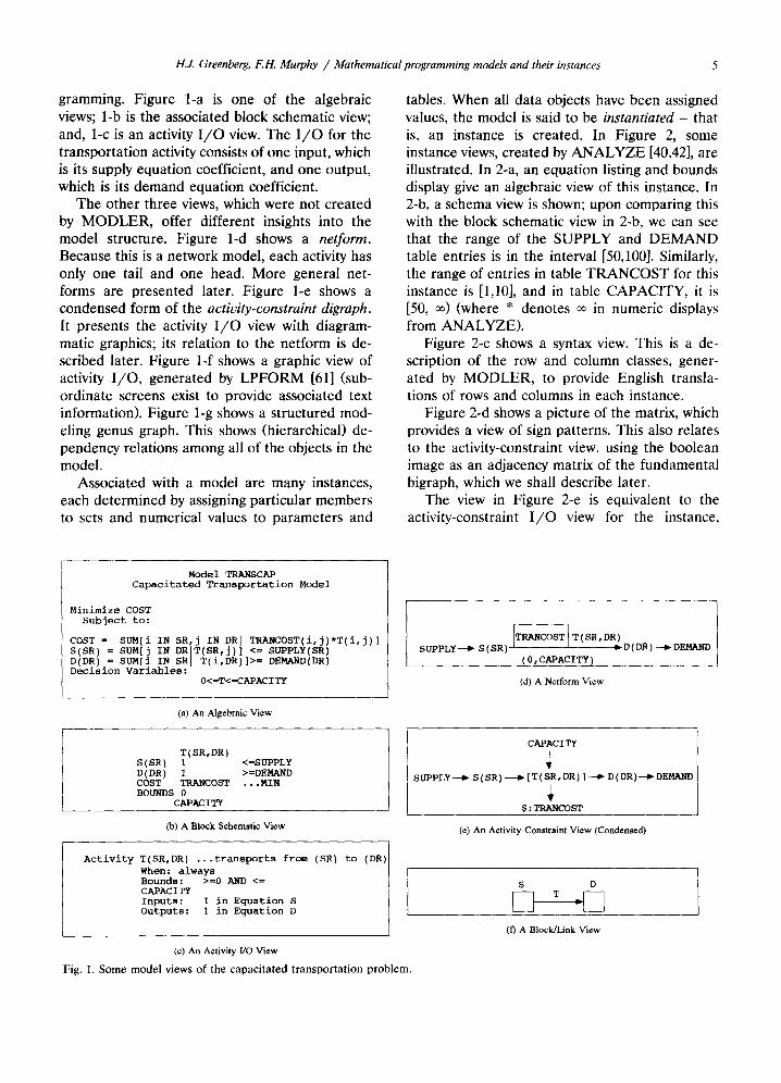
Before formalizing model elements and views, consider some representative views of the famil- iar capacitated transportation problem. Figure 1 gives some model views, the first three of which were generated by M O D L E R [39], which is a modeling language for linear (and integer) pro-
H.J. Greenberg, F.H. Murphy / Mathematical programming models and their instances 5
gramming. Figure 1-a is one of the algebraic views; 1-b is the associated block schematic view; and, 1-c is an activity I / O view. The I / O for the transportation activity consists of one input, which is its supply equation coefficient, and one output, which is its demand equation coefficient.
The other three views, which were not created by MODLER, offer different insights into the model structure. Figure 1-d shows a netform. Because this is a network model, each activity has only one tail and one head. More general net- forms are presented later. Figure 1-e shows a condensed form of the activity-constraint digraph. It presents the activity I / O view with diagram- matic graphics; its relation to the netform is de- scribed later. Figure 1-f shows a graphic view of activity I /O , generated by LPFORM [61] (sub- ordinate screens exist to provide associated text information). Figure 1-g shows a structured mod- eling genus graph. This shows (hierarchical) de- pendency relations among all of the objects in the model.
Associated with a model are many instances, each determined by assigning particular members to sets and numerical values to parameters and
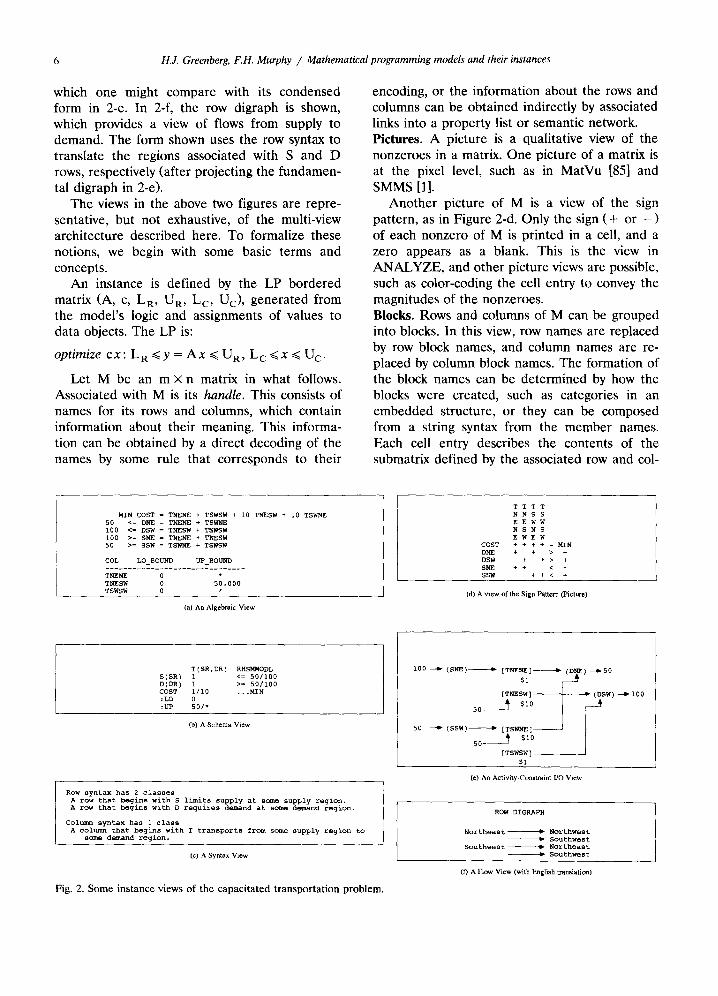
tables. When all data objects have been assigned values, the model is said to be instantiated - that is, an instance is created. In Figure 2, some instance views, created by ANALYZE [40,42], are illustrated. In 2-a, an equation listing and bounds display give an algebraic view of this instance. In 2-b, a schema view is shown; upon comparing this with the block schematic view in 2-b, we can see that the range of the SUPPLY and DEMAND table entries is in the interval [50,100]. Similarly, the range of entries in table TRANCOST for this instance is [1,10], and in table CAPACITY, it is [50, ~) (where * denotes oo in numeric displays from ANALYZE).
Figure 2-c shows a syntax view. This is a de- scription of the row and column classes, gener- ated by MODLER, to provide English transla- tions of rows and columns in each instance.
Figure 2-d shows a picture of the matrix, which provides a view of sign patterns. This also relates to the activity-constraint view, using the boolean image as an adjacency matrix of the fundamental bigraph, which we shall describe later.
The view in Figure 2-e is equivalent to the activity-constraint I / O view for the instance,
Model TRANSCAP Capacitated Transportation Model
Minimize COST Subject to:
COST = SUM[i IN SR, j IN DR I TRANCOST(i,j)*T(i,9)] S(SR) = SUM[j IN DRIT(SR, j) ] <= SUPPLY(SR) D(DR) = SUM[i IN SR I T(i,DR)]>= DEMAND(DR) Decision Variables:
0<=T<=CAPACITY
(a) An Algebraic View
T(SR,DR) S ( SR ) I <=SUPPLY D(DR) 1 >=DEMAND COST TRANCOST ... MIB BOUNDS 0
CAPACITY
~ ) A Block Schematic View
Activity T(SR,DR) ...transports from (SR) to (DR)[ When: always Bounds: >=0 AND <= CAPACITY Inputs: 1 in Equation S Outputs: I in Equation D
(c) An Activity UO View
Fig. 1. Some model views of the capacitated transportation problem.
~ T(SR,DR) SUPPLY--~S(SR) m D(DR)--~DEMAND
(0,CAPACITY)
(d) A Netform View
CAPACITY
SUPPLY--4b S(SR) ~ [T(SR,DR) ] ~ D(DR)--4~ DEMAND
$ : TRANCOST
(e) An Activity-Constraint View (Condensed)
S D
(fi A Block/Link View
6 H.J. Greenberg, F.H. Murphy / Mathematical programming models and their instances
which one might compare with its condensed form in 2-e. In 2-f, the row digraph is shown, which provides a view of flows from supply to demand. The form shown uses the row syntax to translate the regions associated with S and D rows, respectively (after projecting the fundamen- tal digraph in 2-e).
The views in the above two figures are repre- sentative, but not exhaustive, of the multi-view architecture described here. To formalize these notions, we begin with some basic terms and concepts.
An instance is defined by the LP bordered matrix (A, c, L R, U u, L o Uc) , generated from the model's logic and assignments of values to data objects. The LP is:
optimize cx: L R ~<y = A x ~ UR, L c ~<x ~< U c .
Let M be an m × n matrix in what follows. Associated with M is its handle. This consists of names for its rows and columns, which contain information about their meaning. This informa- tion can be obtained by a direct decoding of the names by some rule that corresponds to their
encoding, or the information about the rows and columns can be obtained indirectly by associated links into a property list or semantic network. Pictures. A picture is a qualitative view of the nonzeroes in a matrix. One picture of a matrix is at the pixel level, such as in MatVu [85] and SMMS [1].
Another picture of M is a view of the sign pattern, as in Figure 2-d. Only the sign ( + or - ) of each nonzero of M is printed in a cell, and a zero appears as a blank. This is the view in A N A L Y Z E , and other picture views are possible, such as color-coding the cell entry to convey the magnitudes of the nonzeroes. Blocks. Rows and columns of M can be grouped into blocks. In this view, row names are replaced by row block names, and column names are re- placed by column block names. The formation of the block names can be determined by how the blocks were created, such as categories in an embedded structure, or they can be composed from a string syntax from the member names. Each cell entry describes the contents of the submatrix defined by the associated row and col-
MIN COST = TNENE + TSWSW + i0 TNESW + i0 TSWNE 50 <= DNE = TNENE + TSWNE I00 <= DSW = TNESW + TSWSW i00 >= SNE = TNENE + TNESW 50 >= SSW = TS~n~E + TSWSW
COL LO_BOUND UP_BOUND ...............................
TNENE 0 * TNESW 0 50.000 TSWSW 0 *
(a) An Algebraic View
T T T T N N S S E E W W N S N S E WEW
COST + + + + - MIN DNE + + > + DSW + + > + SEE + + < + SSW + + < +
(d) A view of the Sign Pattern (Picture)
T(SR,DR) RHS~MODL S(SR) 1 <= 50/100 D(DR) 1 >= 50/100 COST 1/10 ...MIN :LO 0 ~UP 50/*
(b) A Schema View
Row syntax has 2 classes A row that begins with S limits supply at some supply region. A row that begins with D requires dew,and at sor, e demand region.
Column syntax has i class A colunm that begins with T transports from some supply region to
scene demand region.
(c) A Syntax View
Fig. 2. Some instance views of the capacitated transportation problem.
100--4~(SNE) ~ [TN~N~]--
$i
[TNESW]
50 # $i0
50 --~(SSW) ~ [TSWNE]
5 0 - ~ $10
[TSWSW]
$1
(DNE) -4~50
(e) An Activity-Cot~traint FO View
ROW DIGRAPH
Northeast P Northwest -- ~ Southwest
Southwest. ~ Northeast Southwest
0) A How View (with English translation)
H.J. Greenberg, F.H. Murphy / Mathematical programming models and their instances 7
umn blocks. A blank means the submatrix is null - that is, all of its coefficients are zero.
Block views arise in a variety of ways. In ANA- LYZE, the most common way is from proce- dures, such as looking for components of the matrix, for redundancies, and for other partitions that support analysis. Matrix schema. A matrix schema has the same form as the block schematic, except the cell en- tries give information about the model instance contained in the nonzeroes in the matrix. As illustrated in figure 2-b, the ANALYZE schema view of an instance has the following meaning. Each row class, including the objective, forms a row strip, presented with the class name and domain. In addition, special row strips are added to represent lower and upper bounds of activity classes. Each column class forms a column strip, presented with the class name and domain. In addition, there is a column strip to represent the limits associated with each row class.
A cell entry in the ANALYZE matrix schema shows the range of the nonzeroes in the associ- ated submatrix. If the submatrix is null, a blank is shown; otherwise, a numerical range is given.
Graphic views of instances derive in natural fashion from the fundamental graphs. Figure 2-e illustrates a row digraph, combined with syntactic translation, to give a view of flows from supply locations to demand locations.
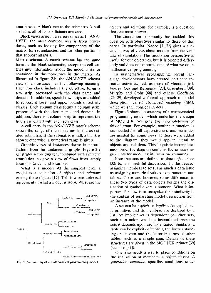
What is a model? At the simplest level, a model is a collection of objects and relations among these objects [17]. This is where universal agreement of what a model is stops. What are the
Model--
[--Explicit [~-Symbolic~sets~
~--Data ~_ U--Implicit [--Constants
Numeric~arameters ables~ -Explicit ~bjects~ ~Implicit
[_Decision~ Activities ~Binaries
f
--Relations
co straiots_ Arith °tic-E:° C °ns Logical Implications
Fig. 3. An anatomy of a mathematical programming model.
objects and relations, for example, is a question that one must answer.
The simulation community has tackled this question with objectives similar to those of this paper. In particular, Nance [71,72] gives a suc- cinct survey of views about models from the van- tage of simulation. The simulation perspective is useful for our objectives, but it is oriented differ- ently and does not capture some of what we do in mathematical programming.
In mathematical programming, recent lan- guage developments have created pertinent re- search activities, such as those of Meeraus [64], Fourer, Gay and Kernighan [23], Greenberg [39], Murphy and Stohr [68] and others. Geoffrion [26-29] developed a formal approach to model description, called structured modeling (SM), which we shall consider in detail.
Figure 3 shows an anatomy of a mathematical programming model, which underlies the design of MODLER. We note the incompleteness of this diagram. For example, nonlinear functionals are needed for full expressiveness, and semantics are needed for some views. If these were added to the diagram, they would appear lateral to objects and relations. This linguistic incomplete- ness aside, the diagram contains the primary in- gredients for modeling in linear programming.
Note that sets are defined as data objects (see [32] for an insightful discussion). In this regard, assigning members to sets is as much a data issue as assigning numerical values to parameters and tables. There are, however, some differences in these two types of data objects besides the dis- tinction of symbolic versus numeric. What is im- portant for now is to recognize their similarity in the context of separating model description from an instance of the model.
A set can be explicit or implicit. An explicit set is primitive, and its members are declared by a list. An implicit set is dependent on other sets, such as a union, and it is instantiated once the sets it depends upon are instantiated. Similarly, a table can be explicit or implicit, the former stand- ing on its own and the latter in terms of other tables, such as a simple sum. Details of these structures are given in the M O D L E R primer [39] (see also [41]).
One also needs a way to place conditions on the realization of members in object classes. A generation condition specifies conditions under
8 H.J. Greenberg, F.H. Murphy / Mathematical programming models and their instances
which a member of a decision object class or a constraint class is generated for a particular in- stance. For example, one may specify that a transportation activity from a supply to a demand region exists only if the associated supply and demand values are positive. An admissibility con-
dition specifies conditions under which a data object class admits realizations, such as simple numeric ranges for parameters and tables.
Following Nance [71], we say a model is a collection of objects and relations among them; and, we say an instance of a model is the assign- ment of values to all data objects. There is, how- ever, another specification, pertaining to the roles
of objects and relations. For example, suppose COST and P R O F I T are
two equations in the model. Let us consider two different roles for these objects. First, suppose the model describes goals or constraints of the form COST ~< c and PROFIT >~ p. If we vary c and p from one instance to another, we do not regard this as a change in the model; they are simply different instances of the same model. Second, suppose these inequalities are not pre- sent, and in one instance we want to MINIMIZE COST and in another we want to MAXIMIZE PROFIT. Are these two instances of the same model, or are they different models, owing to the different roles of COST and PROFIT?
In answer to this last question, role assign- ments could be regarded as part of the model or as an instance. Modeling languages, including the very generic SML [30] and SQLMP [17], do not distinguish the role of objects and relations as part of the model, and it becomes unclear whether they should. Although some advocate specific modeling practices, this is actually a matter of style. View management must respect differences in styles.
In SML, where the term attribute means a specific type of object, a particular attribute could be a variable in one application, and the same attribute could be a parameter in another appli- cation. The SML design requires a change to the model even though one might consider this to be an instance of the same model. In SM (not the particular language, SML), one could steer away from variable attributes altogether and relegate the role specification to a problem description language that takes SM input. SQLMP has added an operation, called CONSTRAINT, to SQL, but
an equation could be a constraint in one applica- tion and not in another. Such roles could be treated as instances of the same model by use of the equivalent of an SQL SELECT function.
In algebraic languages, like AMPL, GAMS, LPL and MODLER, each object must be defined as part of the model description. Role assign- ments cannot be postponed. In analyzing the pooling problem, for example, Lodwick [59] changed the GAMS code simply by changing a variable to be a parameter. Although this was easy to do, it raises a question about extending modeling languages for mathematical program- ming to allow an object to be declared while postponing its role.
This added level of specification to declare roles is important for view creation. Ideally, we want a high-level model description, like SM, but with the same host system supporting problem specification. This is between a model description and an instance, where only roles are defined, not the data. A view, therefore, can be created for a particular role assignment, or without role assign- ments at all. (In general, views do not depend upon complete specification of anything. The model, itself, can be only partially defined; some data can be in place, while others are not. Simi- larly, roles can be completely assigned, partially assigned, or not assigned at all.)
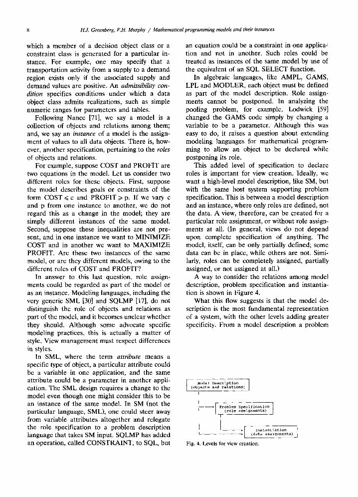
A way to consider the relations among model description, problem specification and instantia- tion is shown in Figure 4.
What this flow suggests is that the model de- scription is the most fundamental representation of a system, with the other levels adding greater specificity. From a model description a problem
Model Description ] (objects and relations)
--~[ Problem Specification 1 (role assignments)
--i[ Instantiation ) (data assignments)~
Fig. 4. Levels for view creation.
H.J. Greenberg, F.H. Murphy / Mathematical programming models and their instances 9
can be specified and data values can be assigned. Instantiation can begin with either a model de- scription or a problem specification (which re- ceives a model description). It then assigns all data values to prepare an instance for optimiza- tion.
This hierarchy is not a procedural recipe. In many situations, modeling is not top-down (or bottom-up); it is more like middle-out. The host system, which supports view creation, must allow partial specifications at all levels.
What is a view? Roughly, a view is a represen- tation that enables a presentat ion of information that is designed to adapt to the cognitive needs of the modeler and the model 's constituency. The actual presentat ion is called a display, which de- pends upon hardware devices. Thus, a view is more abstract in principle than a display; for example, a diagrammatic graphic view can be represented by a node-arc incidence matrix with associated mappings, like labels. The display manager takes this as the view and proceeds to present the graph in some form. The form of display can require algorithms to enhance the display [84,65,62]. A system needs to provide all of the different views that can aid a modeler or a constituent on demand.
Further, although we examine views as an out- put, clearly every modeling system assumes a view for its input specifications. Some are algebraic, some are block schematic, and some are graphic. Technically, there is no need to distinguish whether a view is presented as an input or an output specification. As we shall demonstrate, however, a particular view of a model used as a model specification can run into problems when it a t tempts to create a view that is different from its input.
Further, the views supported during modeling must be consistent with those supported during subsequent analysis, for which the model is built in the first place. Bearing in mind that views are independent of hardware devices, we can, and shall, define those views that should be intrinsic in the system. Murphy, Stohr and Asthana [69] have already contrasted some of the views we consider: algebraic, matrix, block schematic, ac- tivity-constraint digraph, netform, structured modeling SM graphs, and iconic.
A view can be distinguished by what is to be viewed (i.e., content) and how it is to be viewed
(i.e., form). Here is one outline to illustrate the distinction.
Form: Content: Primitive Prim#ice
Algebraic Objects Tabular Relations Schematic Processes Graphic Problem Text Attributes
Dynamics Dependencies Static Explicit Recursive Implicit Animated Aggregates
The primitive forms divide into types, which can be mixed in a view. For example, a graphic can be iconic or diagrammatic. Text could be natural language or computer language. A view can have a mixture of algebraic equations, graph- ics and text. It is possible to assume some primi- tives, but even if a view, or its basic ingredients, are primitive, some familiar specifics need to be described to distinguish a view from other objects in the universe, like a zebra. This is, in part, the purpose of the next few sections: use familiar views to convey what we think a view is. As we build up the formalism, we shall see that form and content are not the only ingredients needed to define a view.
One subtle note in the formal development is the distinction between a model and its instances. The discussion about roles arises because some consider certain roles as instances of the same model while others consider them as changes in the model (c.f., the example of COST and P R O F I T equations). More generally, a uiew man- ager must be able to perform view creation for a model, for problems specified from a model, and for one or more instances of the model.
In addition, there must be some way to distin- guish whether a particular relation is part of the model or whether it is particular to the instance. For example, suppose A and B are two sets, and A = B. There is a difference as to whether this equality is part of the model description, or whether the two sets are equal only in this in- stance.
Another dimension to view management is the purpose of the view. In many cases the purpose is to give insight into a model 's structure. For some people, an algebraic view offers the best insight,
10 H.J. Greenberg, F.H. Murphy / Mathematical programming models and their instances
for others a process network is a bet ter view, and still others see an (SM) outline view as the most informative way to see the structure of a model.
There are, however, other purposes of views, such as insight into the behavior of a model. In some cases, such insight needs views of many instances. In other cases some behavioral proper- ties can be inferred qualitatively, even from a high-level model description. One example is the model 's connectedness.
Another purpose is to support model manage- ment, which needs certain views beyond just structure and behavioral properties. An example is dependency information about objects and re- lations.
2. Views of objects and relations
Let us begin with fundamental objects and relations that (partially) describe a linear pro- gramming model. First, we consider views of sets. Then, we illustrate basic relations in a model description: constraints and conditions.
A fundamental object is a set. A domain is a restricted cross product of sets that is bound to another object. This is a primary difference be- tween a domain and a set: a domain is bound to other objects, such as an activity class, while a set can stand on its own. We can ask for a view of all activities with a given domain, but we cannot ask for all activities with a given set. In the latter case, "with a given set" is ambiguous. For exam- ple, the set could appear in the activity's domain, or it could appear in a condition for generation. This ambiguity does not arise with a domain specification because its binding to the activity is precise. More generally, a domain is the domain of something, which forms an unambiguous bind- ing, while a set is an entity that need not be bound to anything.
Of course, we expect a set to be bound to something, but during model debugging this need not be the case, and a view about the set can be a debugging aid when no dependency is noted. In general, it is useful to think of some objects that depend on domains as having an indirect depen- dency on the sets upon which the domain de- pends.
A domain restriction could be specified in a number of ways, some reflecting model logic and
some data-dependence. For example, suppose T is a set of time periods, S is a set of supply regions, and D is a set of demand regions. The following domains illustrate restrictions that re- flect the model logic: d = {(t,t') in T x T: t ' < t} and d={(s ,d ) in S X D : s ~ d } . The following domains illustrate restrictions that are data-de- pendent: d = { ( t , t ' ) in T X T : t ' = t + L A G } , where LAG is a parameter , and d---{(s,d) in S x D: LINK(s,d) = 1}, where L INK is a control table (more on those later).
Sets are typed in a variety of ways. First, a set can be ordered, partially ordered, or unordered. An ordered set is called a sequence. There are two types of sequences: terminal and cyclic. A terminal sequence is isomorphic to integers, such as time periods in a time-staged model. A cyclic sequence is where every member has exactly one predecessor and exactly one successor; this is isomorphic to N integers with predecessor( i )= j if, and only if, successor(j)= i. We call N the length of the cycle. A terminal sequence is totally ordered - that is, every pair of members is re- lated by the order relation. A partially ordered set arises in project scheduling, where there are precedence relations between some pairs of jobs.
Second, a set can be attributed or not. If a set is attributed, we refer to its attribute. Examples of attributes are form, time and place. A set of form, which can be physical (eg, cars) or concep- tual (eg, information), must have units of mea- surement (eg, mass, volume, number); a set of time must be ordered; and, a set of place must have spatial properties, like distances between members. (These are properties of form, time and place, as illustrated here, but other proper- ties could be assigned in other cases.) The signifi- cance of attributed sets is that certain views can be created from properties, which can be from inheritance, that reflect restrictions on set rela- tions and operations. In M O D L E R , for example, two attributed sets are conformal if they possess the same attributes. A set relation, such as the subset, and a set operation, such as the union, are restricted to be conformal. A modeling system can assume the convention that two non-attri- buted sets are always conformal.
An attributed set and one that is not at- tributed may, or may not, require a conformality resolution rule. For example, suppose A = T x S, where T is ordered and S is not. If it is irrelevant
H.J. Greenberg, F.H. Murphy / Mathematical programming models and their instances 11
whether A is ordered - that is, ordered relations are never used with A - no conformality between T and S is necessary, and A is not attributed. If, however, A needs to be ordered, a conformality resolution rule is needed to order A. A default rule would be to use the order of T and assign an ordering to S, relatiue to its relation to A. The order of a cross product of two ordered sets is defined to be their lexical ordering (so the order- ing of T × S is not the same as the ordering of S x T). Following Nance [71], this relative order- ing of S is defined by a relational attribute of S with respect to A; whereas the attribute of time assigned to T is an indicatiee attribute because it is a property of the object, T, itself.
The particular attributes of form, place and time apply directly to product distribution prob- lems, but their abstractions apply to other situa- tions. Moreover, there can be other types of sets
- that is, attributed with other properties. For example, a set of jobs is none of these three basic types, but some other attribution enables views associated with activities that transform one job into another. This notion of activity transforma- tion offers valuable insights, so we elaborate.
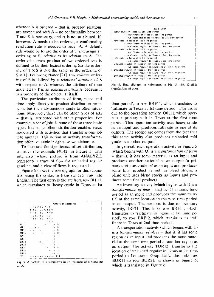
To illustrate the significance of set attribution, consider the example [40,42] in Figure 5. This submatrix, whose picture is from ANALYZE, represents a trace of flow for unleaded regular gasoline, and a view of flows is requested.
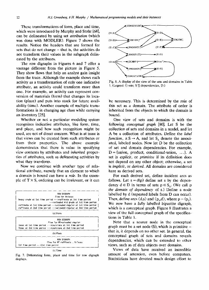
Figure 6 shows the row digraph for this subma- trix, using the syntax to translate each row into English. The first entry is the arc from row BH.11, which translates to 'heavy crude in Texas at 1st
Picture of submatrix I I O 0 0 0 P T T T R R O I I I H U U U F F I I I I . R R R 1 1 1 1 1 1 1 1 1 1
1 2 1 1 2 3 1 2 2 2 1 2 3
BH.1I + > 0
BRFll + - > 0 BRFI2 + - > 0 BRFI3 + > 0 BUMII + > + BURI] + > + BUR12 + > + BURI3 + - > + BUR2] + > + BUR22 + > + 8UR23 + > + COST + + + + + + + + + + = MIN
Fig. 5. A picture of a submatrix in an instance of a blending model.
ROW DIGRAPH
heavy crude in Texas at Is t time period - - ->raf f inate in Texas at is t time period --->unleaded mid grade in Texas at is t time period
raf f inate in Texas at is t time period - - ->ra f f inate in Texas at 2nd time period --->unleaded regular in Texas at Is t time period
raf f inate in Texas at 2nd time period - - ->raf f inate in lexas at 3rd time period --->unleaded regular in Texas at 2nd time period
raf f inate in Texas at 3rd time period -- >unleaded regular in Texas at 3rd time period
unleaded regular in Texas at 1st time period --->unleaded regular in Louisiana at Ist time period
unleaded regular in Texas at 2nd time period --->unleaded regular in Louisiana at 2nd time period
unleaded regular in Texas at 3rd time period --->unleaded regular in Louisiana at 3rd time period
Fig. 6. Row digraph of submatrix in Fig. 5 with English translations of rows.
time period' , to row B R F l l , which translates to ' raffinate in Texas at 1st time period'. This arc is due to the operat ion activity, O0111, which oper- ates a primary unit in Texas at the first time period. This operation activity uses heavy crude as an input and produces raffinate as one of its outputs. The second arc comes from the fact that this same activity also produces unleaded mid grade as another output.
In general, each operation activity in Figure 5 (which begins with O) is a transformation of form - that is, it has some material as an input and produces another material as an output (a pri- mary unit uses crude oil as an input and produces some final product as well as blend stocks; a blend unit uses blend stocks as inputs and pro- duces some final product).
An inventory activity (which begins with I) is a transformation of time - that is, it has some time period as an input and produces the same mate- rial at the same location in the next time period as an output. The next arc is due to inventory activity, I R F l l . This links row B R F l l , which translates to ' raff inate in Texas at 1st time pe- riod', to row BRF12, which translates to ' raf- finate in Texas at 2nd time period'.
A transportation activity (which begins with T) is a transformation of place - that is, it has some region as an input and produces the same mate- rial at the same time period at another region as an output. The activity TUR121 transforms the location of unleaded regular in Texas at 1st time period to Louisiana. Graphically, this links row B U R l l to row BUR21, as shown in Figure 5, which is translated in Figure 6.
12 H.J. Greenberg, F.H. Murphy / Mathematical programming models and their instances
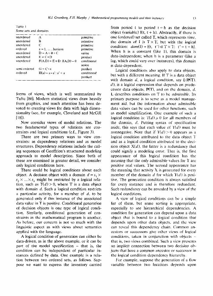
These transformations of form, place and time, which were introduced by Murphy and Stohr [68], can be delineated by using set attribution (which was done with MODLER). Figure 7 shows the results. Notice the headers that are formed for sets that do not change - that is, the activities do not transform their values in the subgraph delin- eated by the attributes.
The row digraphs in Figures 6 and 7 offer a vantage different from the picture in Figure 5. They show flows that help an analyst gain insight from the trace. Although the example shows each activity as a transformation of only one indicative attribute, an activity could transform more than one. For example, an activity can represent con- version of materials (form) that changes its loca- tion (place) and puts into stock for future avail- ability (time). Another example of multiple trans- formations is in changing age class while carrying an inventory [25].
Whether or not a particular modeling system recognizes indicative attributes, like form, time, and place, and how such recognition might be used, are not of direct concern. What is at issue is that views can be created from such attributes or from their properties. The above example demonstrates that there is value in specifying view contents by attributes and inherited proper- ties of attributes, such as delineating activities by what they transform.
Now we continue with another type of rela- tional attribute, namely that an element to which a domain is bound can have a role. In the exam- ple of T X S, ordering can be irrelevant, or it can
ROW DIGRAPH Flow for R-Texas
heavy crude at Ist time period --->raffinate at Ist time period --->unleaded mid grade at ]st time period
raffinate at Ist time period --->unleaded regular at Ist time period raffinate at 2nd time period --->unleaded regular at 2nd time period
(a) Form
ROW DIGRAPH Flow for MT=unleaded regular
Texas at ]st time period --->Louisiana at tst time period Texas at 2nd time period --->Louisiana at 2nd time period
(b) Place
ROW DIGRAPH Flow for MT=raffinate , R=Texas
]st time period --->2rid time period
(c) Time
Fig. 7. Delineating form, place and time for row digraph displays.
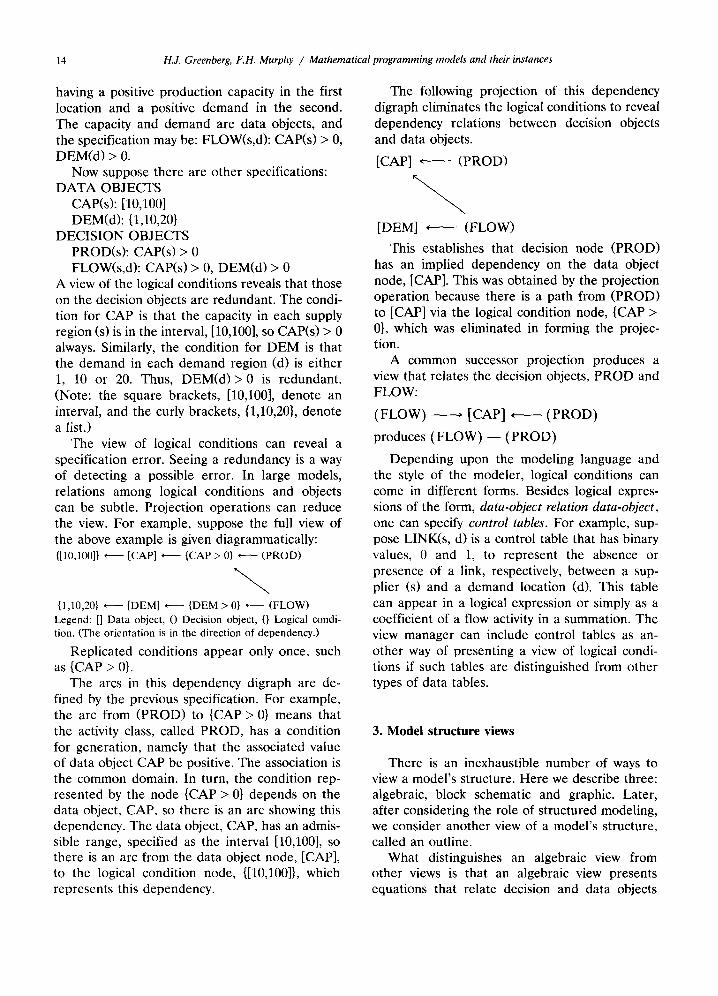
Fig. 8. A display of the view of the sets and domains in Table 1. (Legend: 0 sets; S [] dependencies, D.)
be necessary. This is determined by the role of this set as a domain. The attribute of order is inherited from the objects to which the domain is bound.
One view of sets and domains is with the following conceptual graph [80]. Let S be the collection of sets and domains in a model, and let A be a collection of attributes. Define the label function, A:S ~ A, and let Sx denote the associ- ated, labeled nodes. Now let D be the collection of set and domain dependencies. For example, D = {union, product, conditional-union . . . . }. A set is explicit, or primitive if its definition does not depend on any other object; otherwise, a set is implicit, or derived. All domains are considered here as derived sets.
For each derived set, define incident arcs as follows. Let s = d(p) define set s by the depen- dency d ~ D in terms of sets p ~ S a. (We call p the domain of dependency of s.) Define a node labelled by d (repeated labels from D can occur). Then, define arcs (d,s) and (pi,d), where p = (Pi). We now have a fully labelled bipartite digraph, which is a conceptual graph. Figure 8 illustrates a view of the full conceptual graph of the specifica- tions in Table 1.
Note that a source node in the conceptual graph must be a set node (S), which is primitive - that is, it depends on no other set. In general, the conceptual graph of sets and domains reveals dependencies, which can be extended to other views, such as of data objects over domains.
Views of data have received an incredible amount of attention, even before computers. Statisticians have devoted much design effort to
H.J. Greenberg, F.H. Murphy / Mathematical programming models and their instances 13
T a b l e 1
S o m e sets a n d d o m a i n s
u n o r d e r e d A pr imi t ive
u n o r d e r e d B p r imi t ive
u n o r d e r e d C pr imi t ive
o r d e r e d a = 1, . . . , h o r i z o n pr imi t ive
u n o r d e r e d D = A + B + C u n i o n
u n o r d e r e d E = C * D p r o d u c t
u n o r d e r e d F ( A , D ) = E + D: f (A ,D) = 0 c o n d i t i o n a l
u n i o n
s e m i - o r d e r e d G = C * a p r o d u c t
o r d e r e d H ( a ) = a * a ' : a ' < a c o n d i t i o n a l
p r o d u c t
forms of views, which is well summarized by Tufte [86]. Modern statistical views draw heavily from graphics, and much attention has been de- voted to creating views for data with high dimen- sionality (see, for example, Cleveland and McGill [18]).
Now consider views of model relations. The two fundamental types of relations are con- straints and logical conditions (c.f., Figure 3).
There are two primary ways to view con- straints: as dependency relations and as model structures. Dependency relations include the call- ing sequences of Geoffr ion 's structured modeling approach to model description. Since both of these are examined in greater detail, we consider only logical conditions here.
There could be logical conditions about each object. A decision object with a domain d = s~ x s 2 x ... x & might be restricted by a logical rela- tion, such as T ( d ) > 0, where T is a data object with domain d. Such a logical condition restricts a particular activity, for a member of d, to be generated only if this instance of the associated data value in T is positive. Conditional generation of decision objects is one type of logical condi- tion. Similarly, conditional generation of con- straints in the mathematical program is another. As before, our concern is not so much with the linguistic aspect as with views about semantics applied with the language.
A logical condition of generation can either be data-driven, as in the above example, or it can be part of the model specification - that is, the condition can be independent of particular in- stances defined by data. One example is a rela- tion between two ordered sets, as follows. Sup- pose we want to express the inventory carried
from period t to period t + h as the decision object (variable) I(t, t + h). Abstractly, if there is one (ordered) set called T, which represents time, the domain of I is T x T, but with the logical condition: dom(I) = {(t, t ' ) ~ Y x T: t ' = t + h}. When h is a constant (like 1), this domain is data-independent; when h is a parameter (like a lag, which could vary over instances), this domain is data-dependent .
Logical conditions also apply to data objects, but with a different meaning. If T is a data object with domain d, a logical condition, say L(P(T), d), is a logical expression that depends on prede- cessor data objects, P(T), and on the domain, d. L describes conditions on T to be admissible. Its primary purpose is to serve as a model manage- ment aid, but the information about admissible data values can be used for other functions, such as mode[ simplification. One example of such a logical condition is: T ( d ) > / 0 for all members of the domain, d. Putting syntax of specification aside, this says that each value of T(d) must be nonnegative. Note that if T(d) > 0 appears as a logical condition attributed to the data object T and as a logical condition attributed to the deci- sion object X(d), the latter is a redundancy that could signify a modeling error. That is, the first appearance of this logical condition has the meaning that the only admissible values for T are positive real values. The second appearance has the meaning that activity X is generated for every member of the domain d for which T(d) is posi- tive. The generation condition is always satisfied for every instance and is therefore redundant. Such redundancy can be revealed by a view of the logical conditions.
A view of logical conditions can be a simple list of them, but some sorting is appropriate, especially to see hierarchical dependencies. A condition for generation can depend upon a data object that is bound to a logical condition that depends upon other data objects, and the view can reveal this dependency chain. Common an- cestors or successors give other views of logical conditions, taken in conjunction with objects - that is, two views combined. Such a view presents an implicit connection between two decision ob- jects that have a common ancestor or successor in the logical condition dependency hierarchy.
For example, suppose the generation of a flow variable between two locations depends upon
14 H.J. Greenberg, F.H. Murphy / Mathematical programming models and their instances
having a positive production capacity in the first location and a positive demand in the second. The capacity and demand are data objects, and the specification may be: FLOW(s,d): CAP(s) > 0, DEM(d) > 0.
Now suppose there are other specifications: DATA OBJECTS
CAP(s): [10,100] DEM(d): {1,10,20}
DECISION OBJECTS PROD(s): CAP(s) > 0 FLOW(s,d): CAP(s) > 0, DEM(d) > 0
A view of the logical conditions reveals that those on the decision objects are redundant. The condi- tion for CAP is that the capacity in each supply region (s) is in the interval, [10,100], so CAP(s) > 0 always. Similarly, the condition for DEM is that the demand in each demand region (d) is either 1, 10 or 20. Thus, D E M ( d ) > 0 is redundant. (Note: the square brackets, [10,100], denote an interval, and the curly brackets, {1,10,20}, denote a list.)
The view of logical conditions can reveal a specification error. Seeing a redundancy is a way of detecting a possible error. In large models, relations among logical conditions and objects can be subtle. Projection operations can reduce the view. For example, suppose the full view of the above example is given diagrammatically: {[10,100]} , [CAP] *---- {CAP > 0} ~ (PROD)
-.... {1,10,20} ~ [DEM] ~ {DEM > 0} ~ - - (FLOW)
Legend: [] Data object, 0 Decision object, {/ Logical condi- tion. (The orientation is in the direction of dependency.)
Replicated conditions appear only once, such as {CAP > 0}.
The arcs in this dependency digraph are de- fined by the previous specification. For example, the arc from (PROD) to {CAP > 0} means that the activity class, called PROD, has a condition for generation, namely that the associated value of data object CAP be positive. The association is the common domain. In turn, the condition rep- resented by the node {CAP > 0} depends on the data object, CAP, so there is an arc showing this dependency. The data object, CAP, has an admis- sible range, specified as the interval [10,100], so there is an arc from the data object node, [CAP], to the logical condition node, {[10,100]}, which represents this dependency.
The following projection of this dependency digraph eliminates the logical conditions to reveal dependency relations between decision objects and data objects.
[CAP] , (PROD)
[DEM] , (FLOW)
This establishes that decision node (PROD) has an implied dependency on the data object node, [CAP]. This was obtained by the projection operation because there is a path from (PROD) to [CAP] via the logical condition node, {CAP > 0}, which was eliminated in forming the projec- tion.
A common successor projection produces a view that relates the decision objects, PROD and FLOW:
(FLOW) , [ C A P ] , (PROD)
produces (FLOW) - - (PROD)
Depending upon the modeling language and the style of the modeler, logical conditions can come in different forms. Besides logical expres- sions of the form, data-object relation data-object, one can specify control tables. For example, sup- pose LINK(s, d) is a control table that has binary values, 0 and 1, to represent the absence or presence of a link, respectively, between a sup- plier (s) and a demand location (d). This table can appear in a logical expression or simply as a coefficient of a flow activity in a summation. The view manager can include control tables as an- other way of presenting a view of logical condi- tions if such tables are distinguished from other types of data tables.
3. Model structure views
There is an inexhaustible number of ways to view a model's structure. Here we describe three: algebraic, block schematic and graphic. Later, after considering the role of structured modeling, we consider another view of a model's structure, called an outline.
What distinguishes an algebraic view from other views is that an algebraic view presents equations that relate decision and data objects
H.J. Greenberg, F.H. Murphy / Mathematical programming models and their instances 15
Object definitions: Let ! = set of supply locations.
Let J = set of demand locations.
Let Cij = unit cost of flow from i~l to jeJ.
Let Uij = capacity of flow from i~l to j~J.
Let S i = quantity of supply at i~l.
Let Dj = quantity of demand at j ~ .
Let Tii = flow from icl to j~. Model:
minimize ~j CijTij subject to:
2j Tij _< S i Vi~l
2~Tij ->D~ Vj~J
0 -< Tij -< Uij V(i,j)dxJ
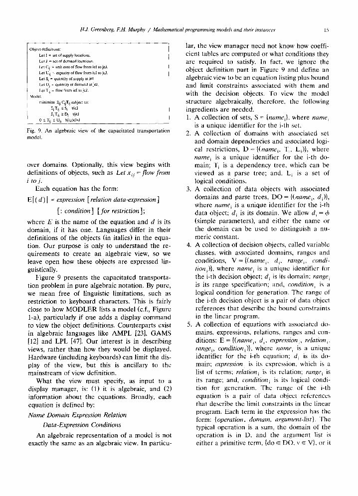
Fig. 9. An a lgebra ic view of the capac i t a t ed t r an spo r t a t i on
model .
over domains. Optionally, this view begins with definitions of objects, such as Let xig = f low f rom i t o j .
Each equation has the form:
E[( d)] = expression [relation data-expression ]
[: condition ] [ for restriction ];
where E is the name of the equation and d is its domain, if it has one. Languages differ in their definitions of the objects (in italics) in the equa- tion. Our purpose is only to understand the re- quirements to create an algebraic view, so we leave open how these objects are expressed lin- guistically.
Figure 9 presents the capacitated transporta- tion problem in pure algebraic notation. By pure, we mean free of linguistic limitations, such as restriction to keyboard characters. This is fairly close to how M O D L E R lists a model (c.f., Figure l-a), particularly if one adds a display command to view the object definitions. Counterparts exist in algebraic languages like AMPL [23], GAMS [12] and LPL [47]. Our interest is in describing views, rather than how they would be displayed. Hardware (including keyboards) can limit the dis- play of the view, but this is ancillary to the mainstream of view definition.
What the view must specify, as input to a display manager, is: (1) it is algebraic, and (2) information about the equations. Broadly, each equation is defined by:
Name Domain Expression Relation
Data-Expression Conditions
An algebraic representation of a model is not exactly the same as an algebraic view. In particu-
lar, the view manager need not know how coeffi- cient tables are computed or what conditions they are required to satisfy. In fact, we ignore the object definition part in Figure 9 and define an algebraic view to be an equation listing plus bound and limit constraints associated with them and with the decision objects. To view the model structure algebraically, therefore, the following ingredients are needed. 1. A collection of sets, S = {namei}, where namei
is a unique identifier for the i-th set. 2. A collection of domains with associated set
and domain dependencies and associated logi- cal restrictions, D = {(name i, Ti, Li)}, where name~ is a unique identifier for the i-th do- main; T~ is a dependency tree, which can be viewed as a parse tree; and, L~ is a set of logical conditions.
3. A collection of data objects with associated domains and parse trees, DO = {(name i, di)}, where name~ is a unique identifier for the i-th data object; d i is its domain. We allow d, = O (simple parameters), and either the name or the domain can be used to distinguish a nu- meric constant.
4. A collection of decision objects, called variable classes, with associated domains, ranges and conditions, V = { ( n a m e i, d i, range i, condi- tioni)} , where name i is a unique identifier for the i-th decision object; d~ is its domain; range~ is its range specification; and, condition~ is a logical condition for generation. The range of the i-th decision object is a pair of data object references that describe the bound constraints in the linear program.
5. A collection of equations with associated do- mains, expressions, relations, ranges and con- ditions: E = {(namei, d i, expression i, relation i, rangei, conditioni)} , where name i is a unique identifier for the i-th equation; di is its do- main; expression i is its expression, which is a list of terms; relation i is its relation; range i is its range; and, condition~ is its logical condi- tion for generation. The range of the i-th equation is a pair of data object references that describe the limit constraints in the linear program. Each term in the expression has the form: {operation, domain, argument-list}. The typical operation is a sum, the domain of the operation is in D, and the argument list is either a primitive term, {do ~ DO, v ~ V}, or it
16 H.J. Greenberg, F.H. Murphy / Mathematical programming models and their instances
is another expression (as, for example, sums within sums). If we apply this specification to obtain the
algebraic view in Figure l-a, the information is as follows. 1. {SR, DR}. 2. {(DOMI,(SR),(b), (DOM2,(DR),6) ,
(DOM3,(SR × DR),(b), (1,(b, = 1)}. 3. { (S UP P LY, DOM1) , ( D E M A N D , D O M 2 ) ,
(CAPACITY,DOM3), (TRANCOST,DOM3), (1,1)}.
4. {(T,DOM3,(0,CAPACITY),@)}. 5. {(COST,@,(SUM,DOM3,(TRANCOST,T)),
MIN,@,@), (S,DOMI,(SUM,DOM2,1,T), < = ,SUPPLY,~b), (D,DOM2,(SUM,DOM1,1,T), > = ,DEMAND,~b)}.
We used the symbol ~b when the field is empty. For example, all condition fields are ~b to indicate no condition is present, and the cost equation has another ~b to indicate there is no data object reference for the MIN relation. The numeric constant 1 is defined in the domain list in order to define it in the list of data objects. This de- scription, (1,~b, = 1), distinguishes the symbolic reference, 1, from its numerical value, = 1. Then, equations S and D enter 1 as the symbolic data object reference, and its value is the coefficient of T in each sum.
The purpose of this example is not to impose a data structure, but to illustrate one. Short-cuts could be taken, such as distinguishing the nu- meric constant, 1. Our concern is with a precise specification of the information needed for a view manager to create an algebraic view.
Not only is each expression a variable-length record, but also the domain can have an arbitrary dimension (viz., number of set dependencies) and an arbitrary number of restrictions, each of which could be a variable length record. All of this pertains to implementation issues, but recogni- tion of this variability is important to understand the breadth of issues in the design of a multi-view architecture.
A block schematic is another view with a dif- ferent cognitive structure. The version given in Figure 1-b is only one of several variants. This view was developed by Baker [2] and by Welch [87] as an interface for model formulation. Their current systems, MIMI [15] and MathPro [63], respectively, have different variations of block
P(t) S(t) I ( t ) B(t) I - i - i / i = 0
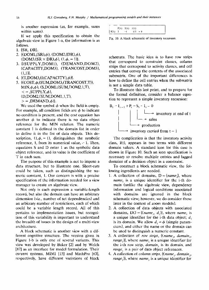
Fig. I0. A block schematic of inventory recursion.
schemata. The basic idea is to have row strips that correspond to constraint classes, column strips that correspond to activity classes, and cell entries that convey the contents of the associated submatrix. One of the important differences is how to define the cell entries when the submatrix is not a simple data table.
To illustrate this last point, and to prepare for the formal definition, consider a balance equa- tion to represent a simple inventory recursion:
Bt = I t - i +Pt - S t - I t = 0
I ' inventory at end of t
sales
, production
, inventory carried from t - 1
The complication is that the inventory activity class, I(t), appears in two terms with different domain values. A standard icon for this case is shown in Figure 10. Such an icon specification is necessary to resolve multiple entries and lagged domains of a decision object in a constraint.
To construct a block schematic view, the fol- lowing ingredients are needed. 1. A collection of domains, D = {namei}, where
name~ is a unique identifier for the i-th do- main (unlike the algebraic view, dependency information and logical conditions associated with domains are ignored in the block schematic view; however, we do consider these later in the context of zoom models).
2. A collection of data objects with associated domains, DO = {(namei , di)}, where nam e i is a unique identifier for the i-th data object; d i is its domain. We allow d i = ~b (simple param- eters), and either the name or the domain can be used to distinguish a numeric constant.
3. A collection of row strips, { (namei , domain i , rangei)}, where nam e i is a unique identifier for the i-th row strip, domain i is its domain, and range i is a pair of data object references. A collection of co lumn strips, { (namei , domain j, rangej)}, where nam e i is a unique identifier for
.
H.J. Greenberg, F.H. Murphy / Mathematical programming models and their instances 17
the j-th column strip, domainj is its domain, and rangej is a pair of data object references.
5. A collection of cells, {(rOWk, columnk, typek, infok)}, where (rOWk, column k) is the row and column strip, respectively; type k is the type of cell entry; and, info k is information, which depends upon the type. The types of cell en- tries are: (1) direct data reference, (2) indirect data reference, and (3) icon. For a direct data reference, the information (info k) is its name. For an indirect data reference, the informa- tion is a key (or pointer) into a data collection. An icon describes a structure for the subma- trix associated with the rows and columns in the cell (see below). Notice that a schema view does not, itself,
present information about logical conditions, such as those for generation of activities in a class. We postpone this consideration until we define zoom operations. We also postpone how to obtain the cell type and associated information until we de- fine schema cell maps, which we do when consid- ering mapping from an algebraic view.
If we apply this specification to obtain the block schematic view in figure l-b, the informa- tion is as follows. 1. {SR, DR}. 2. {(SUPPLY,SR), (DEMAND,DR) , (CAPAC-
ITY,(SR,DR)), (TRANCOST,(SR,DR)) , (1,1)}. 3. { (COST, th , (MIN,&)) , (S ,S R , -w ,S UP P LY) ,
(D,DR,DEMAND,m)}. 4. {(T,(SR,DR),(0,CAPACITY))}. 5. {(COST,T, di rect ,TRANCOST), (S,T,direct,1),
(D,T,direct,1)}. To begin our formalization of views, we con-
sider a mappings between algebraic and block schematic views. We demonstrate difficulties with completeness - that is, the information that is associated with each view is insufficient to com- plete a mapping to the other view. Since each view can be used to construct the same model instances, they share certain core information. There are, however, information structures asso- ciated with each view that are missing in other views. To create mappings between algebraic and block schematic views, we add necessary informa- tion beyond what appears in each view.
An essential difference between algebraic and block schematic views is the way summations are represented. They are explicit in algebraic views by including a sum symbol (or keyword) and
conditions directly. They are implicit in block schematic views by showing icons in a cell that indicate summations or conditions (or both).
Let us begin with an elementary algebraic view, where there are no conditions on summations and the sets defining the domain of the data object are present in those of the row or column strips (or both). We presume that the appearance of a decision object, say v, in an equation, say e, can be expressed with a couple ( f , D), where f is a recognized function and D is a data object.
Here is the mapping for constructing an ele- mentary block schematic from this algebraic view. 1. Define a column strip for each decision object
and a row strip for each equation. 2. Initialize all cells to be null. 3. If the i-th decision object appears in the j-th
equation, let ( f , D) denote the dependence. Define f as the first level of detail in this cell, and enter D into the cell. The inverse mapping is equally straightforward
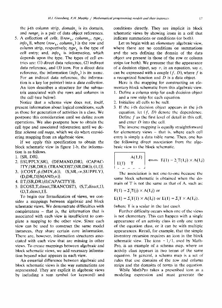
for elementary views - that is, where each cell entry is simply a data table name. Then, one has the following direct association from the alge- braic view to the block schematic.
A( I , J )
E( I ) T E( I ) = ~jT(I , j ) x A(I , j )
The association is not one-to-one because the same block schematic is obtained when the do- main of T is not the same as that of A, such as:
E ( I ) = VjT(j) × A(I~j) or
E ( I ) = VjT(I) × A(I,j) or E ( I ) = ~iT × A(I , j ) .
(where T is a scalar in the last case). Further difficulty occurs when one of the views
is not elementary. This can happen with a single appearance of an activity class in only one term of the equation class, or it can be with multiple appearances. Recall, for example, that the simple inventory recursion requires an icon in the block schematic view. The icon - 1 / 1 , used by Math- Pro, is an example of a schema map, where an activity class appears in two terms of the same equation. In general, a schema map is a set of rules that use domains of the row and column strips and the domains of terms in the equation.
While MathPro takes a prescribed icon as a modeling expression and must generate the
18 1f..1. Greenberg, F.H. Murphy / Mathematical programming models and their instances
equivalent of an algebraic form for each instance, M O D L E R begins with an algebraic representa- tion and applies rules for schema mapping (see Greenberg [39] for details). The particular rules used by both systems influence the general devel- opment here, but our goal is a general frame- work, apart from particular implementations.
Let us generalize this with a schema cell map that maps an algebraic view into a block schematic view, the issue being how to form a cell entry. When activity A appears in equation E only once, and the coefficient is simply a data table, say T, the cell entry is (E, A, T). Now suppose A ap- pears in equation E only once, but there is an operation or condition associated with the rela- tive domains. Algebraically, suppose we have:
E e = ~ s T d A a ,
where e = dom(E) , d = dora(T) and a = dora(A) (dom is the domain). The domain of the sum (s) will be considered shortly.
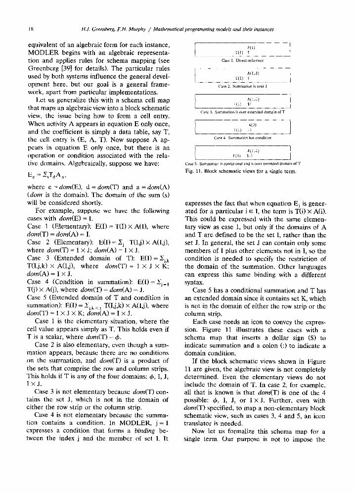
For example, suppose we have the following cases with dom(E) = I.
Case 1 (Elementary): E(I) = T(I) × A(I), where dora(T) = d o m ( A ) = I.
Case 2 (Elementary): E(I) = X i T ( I j ) x A(I,j), where dora(T) = I × J; dora(A) = I x J. Case 3 (Extended domain of T): E( I )=Nj ,k T(I,j,k) × A(I,j), where d o m ( T ) = I × J × K; d o m ( A ) = I × J.
Case 4 (Condition in summation): E ( I ) = X j = I T(j) x A(j), where dora(T) = d o m ( A ) = J. Case 5 (Extended domain of T and condition in summation): E(I) = Xj,k < j T(I,j,k) × A(I,j), where dom(T) = I × J × K; dora(A) = I × J.
Case 1 is the elementary situation, where the cell value appears simply as T. This holds even if T is a scalar, where dora(T) = 49.
Case 2 is also elementary, even though a sum- mation appears, because there are no conditions on the summation, and dora(T) is a product of the sets that comprise the row and column strips. This holds if T is any of the four domains: 49, I, J, I x J .
Case 3 is not elementary because dora(T) con- tains the set J, which is not in the domain of either the row strip or the column strip.
Case 4 is not elementary because the summa- tion contains a condition. In M O D L E R , j = I expresses a condition that forms a binding be- tween the index j and the member of set I. It
A(1) E(U 7
Case 1. Direct reference
A(I,J) E(1) T
Case 2. Summation is over J
A(I,J) E(1) ST
Case 3. Summation is over extended domain ofT
A(J) E{I) :l
Case 4. Summation has condition
AO,a) E(I) $:T
Case 5. Summation is conditional and is over extended domain o f t
F ig . 11. B l o c k s c h e m a t i c v i e w s fo r a s i n g l e t e r m .
expresses the fact that when equation E i is gener- ated for a particular i E I, the term is T(i) × A(i). This could be expressed with the same elemen- tary view as case 1, but only if the domains of A and T are defined to be the set I, rather than the set J. In general, the set J can contain only some members of I plus other elements not in I, so the condition is needed to specify the restriction of the domain of the summation. Other languages can express this same binding with a different syntax.
Case 5 has a conditional summation and T has an extended domain since it contains set K, which is not in the domain of either the row strip or the column strip.
Each case needs an icon to convey the expres- sion. Figure 11 illustrates these cases with a schema map that inserts a dollar sign ($) to indicate summation and a colon (:) to indicate a domain condition.
If the block schematic views shown in Figure 1 1 are given, the algebraic view is not completely determined. Even the elementary views do not include the domain of T. In case 2, for example, all that is known is that dorn(T) is one of the 4 possible: 49, I, J, or I × J. Further, even with dora(T) specified, to map a non-elementary block schematic view, such as cases 3, 4 and 5, an icon translator is needed.
Now let us formalize this schema map for a single term. Our purpose is not to impose the
H.J. Greenberg, F.H. Murphy / Mathematical programming models and their instances 19
par t i cu l a r icons used in the view crea t ion , but to show only tha t we can d is t inguish the cases when m a p p i n g f rom an a lgebra ic view to a b lock schemat ic .
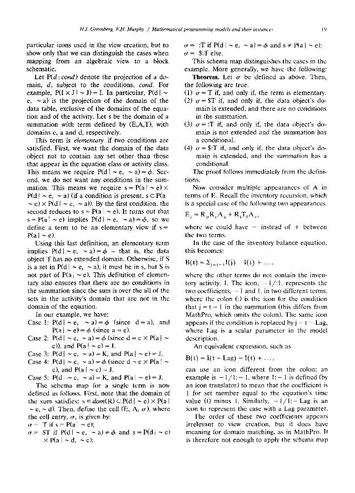
Le t P(d]cond) d e n o t e the p ro j ec t ion of a do- main, d, subject to the condi t ions , cond. F o r example , P(I × J I ~ J) = I. In pa r t i cu la r , P (d l e, ~ a) is the p ro jec t ion of the doma in of the da ta table , exclusive of the doma ins of the equa- t ion and of the activity. Let s be the doma in of a summat ion with t e rm de f ined by (E,A,T) , with doma ins e, a and d, respect ively.
This t e rm is elementary if two condi t ions are sat isf ied. Firs t , we want the d o m a i n of the da t a objec t not to conta in any set o t h e r than those tha t a p p e a r in the equa t ion class or act ivi ty class. This means we requ i re P(d[ ~ e, ~ a) = 4~. Sec- ond, we do not want any condi t ions in the sum- mat ion . This means we requ i re s = P ( a [ ~ e ) × P(d f ~ e, ~ a) (if a cond i t ion is p resen t , s < P(a [ ~ e) × P (d l ~ e, ~ a)). By the first condi t ion , the second r educes to s = P(a] ~ e). It tu rns out that s = P ( a l ~ e ) impl ies P (d l ~ e , ~ a ) = ~ b , so we def ine a t e rm to be an e l e m e n t a r y view if s =
P (a l ~ e). Us ing this last def ini t ion, an e l e m e n t a r y t e rm
impl ies P (d l ~ e, ~ a ) = ~ b - tha t is, the da t a objec t T has no e x t e n d e d domain . Otherwise , if S is a set in P (d l ~ e, ~ a), it must be in s, but S is not pa r t of P(aJ ~ e). This def in i t ion of e l emen- tary also ensures tha t the re a re no condi t ions in the s u m m a t i o n since the sum is over the all of the sets in the activi ty 's doma in that a re not in the doma in of the equa t ion .
In our example , we have: Case 1: P(d] ~ e , ~ a ) = 4 ~ (since d = a ) , and
P (a l ~ e) = ~b (since a = e). Case 2: P(d[ ~ e , ~ a ) = 4 ~ ( s i n c e d = e x P ( a l ~
e)), and P(af ~ e) = J. Case 3: P (d l ~ e, ~ a) = K, and P (a l ~ e) = J. Case 4: P(dJ ~ e , ~ a ) = & ( s i n c e d = e x P ( a [ ~
e), and P (a l ~ e) = J. Case 5: P (d l ~ e, ~ a) = K, and P (a l ~ e) = J.
T h e schema m a p for a single t e rm is now de f ined as follows. Firs t , no te tha t the d o m a i n of the sum satisfies: s - dom(R) c P(d I ~ e) × P (a l ~ e, ~ d). Then , def ine the cell (E, A, o-), whe re the cell entry, ~r, is given by: o -= T i f s = P ( a l ~ e ) ; o r= ST if P (d l ~ e , ~ a ) v=& and s = P ( d l ~ e )
× P(a l ~ d, ~ e);
= :T if P (d l ~ e, - a) = 4~ and s :~ P(a l ~ e); ~r = $:T else.
This schema m a p d is t inguishes the cases in the example . M o r e genera l ly , we have the following:
Theorem. Let o- be de f ined as above. Then , the fol lowing are t rue. (1) o, = T if, and only if, the t e rm is e lementa ry . (2) o -= ST if, and only if, the da ta ob jec t ' s do-
ma in is ex tended , and the re are no condi t ions in the summat ion .
(3) ~r = :T if, and only if, the da t a ob jec t ' s do- main is not ex t ended and the summat ion has a condi t iona l .
(4) o -= $:T if, and only if, the da t a ob jec t ' s do- main is ex tended , and the summat ion has a condi t ional .
The p r o o f follows immed ia t e ly from the defini- t ions.
Now cons ide r mul t ip le a p p e a r a n c e s of A in t e rms of E. Reca l l the inventory recurs ion, which is a special case of the fol lowing two a ppe a ra nc e s .
E e = R p R r A q + RsTjA~,,
where we could have - ins tead of + be tween the two terms.
In the case of the inventory ba lance equat ion , this becomes :
B ( t ) = X j _ t _ , l ( j ) - I ( t ) + . . . .
where the o t h e r te rms do not conta in the inven- tory activity, I. The icon, - 1 / : 1 , r ep re sen t s the two coeff icients , - 1 and 1, in two d i f fe ren t terms, where the colon (:) is the icon for the condi t ion that j = t - 1 in the s u m m a t i o n (this differs f rom M a t h P r o , which omits the colon). The same icon a p p e a r s if the cond i t ion is r ep l aced by j = t - Lag, whe re Lag is a scalar p a r a m e t e r in the mode l descr ip t ion .
A n equiva len t express ion, such as
B ( t ) = I ( t - Lag) - I ( t ) + . . . .
can use an icon d i f fe ren t from the colon; an example is - 1 / 1 : - 1, whe re 1 : - 1 is de f ined (by an icon t rans la to r ) to mean that the coeff ic ient is 1 for set m e m b e r equal to the equa t ion ' s t ime value (t) minus 1. Similarly, - 1 / 1 : - L a g is an icon to r e p r e s e n t the case with a Lag p a r a m e t e r .
The o r d e r of these two coeff ic ients a ppe a r s i r re levan t to view crea t ion , but it does have me a n ing for d o m a i n matching , as in Ma thPro . It is t he re fo re not enough to apply the schema map
20 H.J. Greenberg, F.H. Murphy / Mathematical programming models and their instances
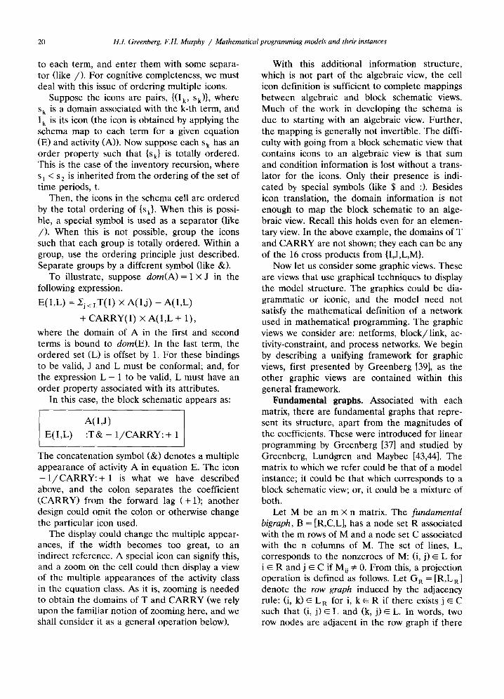
to each term, and enter them with some separa- tor (like / ) . For cognitive completeness, we must deal with this issue of ordering multiple icons.
Suppose the icons are pairs, {(Ik, Sk)}, where s k is a domain associated with the k-th term, and I k is its icon (the icon is obtained by applying the schema map to each term for a given equation (E) and activity (A)). Now suppose each s k has an order property such that {s k} is totally ordered. This is the case of the inventory recursion, where s~ < s2 is inherited from the ordering of the set of time periods, t.
Then, the icons in the schema cell are ordered by the total ordering of {Sk}. When this is possi- ble, a special symbol is used as a separator (like / ) . When this is not possible, group the icons such that each group is totally ordered. Within a group, use the ordering principle just described. Separate groups by a different symbol (like &).
To illustrate, suppose dora(A) = I × J in the following expression.
E( I ,L) = ~j < LT(I) × A(I, j) - A(I ,L)
+ CARRY(I ) X A( I ,L + 1),
where the domain of A in the first and second terms is bound to dom(E). In the last term, the ordered set (L) is offset by 1. For these bindings to be valid, J and L must be conformal; and, for the expression L + 1 to be valid, L must have an order property associated with its attributes.
In this case, the block schematic appears as:
A(I ,J )
E( I ,L) : T & - 1 / C A R R Y : + 1
The concatenation symbol (&) denotes a multiple appearance of activity A in equation E. The icon - 1 / C A R R Y : + 1 is what we have described above, and the colon separates the coefficient (CARRY) from the forward lag (+1) ; another design could omit the colon or otherwise change the particular icon used.
The display could change the multiple appear- ances, if the width becomes too great, to an indirect reference. A special icon can signify this, and a zoom on the cell could then display a view of the multiple appearances of the activity class in the equation class. As it is, zooming is needed to obtain the domains of T and CARRY (we rely upon the familiar notion of zooming here, and we shall consider it as a general operation below).
With this additional information structure, which is not part of the algebraic view, the cell icon definition is sufficient to complete mappings between algebraic and block schematic views. Much of the work in developing the schema is due to starting with an algebraic view. Further, the mapping is generally not invertible. The diffi- culty with going from a block schematic view that contains icons to an algebraic view is that sum and condition information is lost without a trans- lator for the icons. Only their presence is indi- cated by special symbols (like $ and :). Besides icon translation, the domain information is not enough to map the block schematic to an alge- braic view. Recall this holds even for an elemen- tary view. In the above example, the domains of T and CARRY are not shown; they each can be any of the 16 cross products from {I,J,L,M}.
Now let us consider some graphic views. These are views that use graphical techniques to display the model structure. The graphics could be dia- grammatic or iconic, and the model need not satisfy the mathematical definition of a network used in mathematical programming. The graphic views we consider are: netforms, block/ l ink, ac- tivity-constraint, and process networks. We begin by describing a unifying framework for graphic views, first presented by Greenberg [39], as the other graphic views are contained within this general framework.
Fundamental graphs. Associated with each matrix, there are fundamental graphs that repre- sent its structure, apart from the magnitudes of the coefficients. These were introduced for linear programming by Greenberg [37] and studied by Greenberg, Lundgren and Maybee [43,44]. The matrix to which we refer could be that of a model instance; it could be that which corresponds to a block schematic view; or, it could be a mixture of both.
Let M be an m × n matrix. The fundamental bigraph, B = [R,C,L], has a node set R associated with the m rows of M and a node set C associated with the n columns of M. The set of lines, L, corresponds to the nonzeroes of M: (i, j) ~ L for i ~ R and j ~ C if Mij 4: 0. From this, a projection operation is defined as follows. Let G R = [R,LR] denote the row graph induced by the adjacency rule: (i, k) ~ L R for i, k ~ R if there exists j ~ C such that (i, j ) ~ L and (k, j ) ~ L. In words, two row nodes are adjacent in the row graph if there
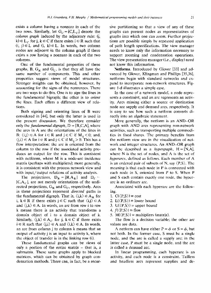
H.J. Greenberg, F.H. Murphy / Mathematical programming models and their instances 2l
exists a column having a nonzero in each of the two rows. Similarly, let G c = [C,L c] denote the column graph induced by the adjacency rule: (j, k) ~ L c for j, k ~ C if there exists i ~ R such that (i, j ) ~ L and (i, k ) ~ L. In words, two column nodes are adjacent in the column graph if there exists a row having a nonzero in each of the two columns.
One of the fundamental propert ies of these graphs, B, G R and G c, is that they all have the same number of components. This and other propert ies suggest views of model structures. Stronger insights can be obtained, however, by accounting for the signs of the nonzeroes. There are two ways to do this. One is to sign the lines in the fundamental bigraph; the other is to orient the lines. Each offers a different view of rela- tions.
Both signing and orienting lines of B were considered in [44], but only the latter is used in the present discussion. We therefore consider only the fundamental digraph, D = [R,C,A], where the arcs in A are the orientations of the lines in B: ( i , j ) ~ A for i ~ R a n d j ~ C if M i j < 0 ; and, (j,i) ~ A for i ~ R and j ~ C if Mij > 0. This has a flow interpretation: the arc is oriented from the column to the row if the associated activity pro- duces an output for the row. This is consistent with netforms, where M is a node-arc incidence matrix (perhaps with multipliers); more generally, it is consistent with the process network view and with i n p u t / o u t p u t relations of activity analysis.
The projections, D R = [R,A R] and D c = [C,Ac], are not merely orientations of the undi- rected projections, G R and Gc, respectively. Arcs in these projections represent directed paths in the fundamental digraph. That is, (i ,k) ~ A R for i, k ~ R if there exists j ~ C such that (i,j) E A and (j,k) ~ A. In words, an arc from row i to row k means there is an activity that transforms a domain object of i to a domain object of k. Similarly, (j,k) ~ A c for j, k ~ C if there exists i ~ R such that (j,i) ~ A and (i,k) ~ A. In words, an arc from column j to column k means that an output of activity j is an input to activity k, where the object of transfer is in the linking row (i).
These fundamental graphs can be views of only a portion of the entire matrix - that is, a submatrix. These same graphs apply to blocked matrices, which can be obtained by graph con- densation methods. There can, in fact, be a recur-
sive partitioning so that a view of any of these graphs can present nodes as representatives of graphs into which one can zoom. Further projec- tions are possible simply by repeated application of path length specifications. The view manager needs to know only the information necessary to support zooming and condensation operations. The view presentation manager (i.e., display) need not know this information.
Netforms. Introduced by Glover [33] and ad- vanced by Glover, Klingman and Phillips [35,36], netforms begin with standard networks and ex- pand to incorporate non-network structures. Fig- ure 1-d illustrates a simple case.
In the case of a network model, a node repre- sents a constraint, and an arc represents an activ- ity. Arcs missing either a source or destination node are supply and demand arcs, respectively. It is easy to see how such a netform converts di- rectly into an algebraic statement.
More generally, the netform is an A N D - O R graph with A N D arcs representing non-network activities, such as transporting multiple commodi- ties in fixed shares. The primary benefits from the netform view are in the visualization of net- work and integer structures. An A N D - O R graph can be described as a hypergraph, H = [N,A], where N is the set of nodes, and A is the set of hyperarcs, defined as follows. Each member of A is an ordered pair of subsets of N, say (P,S). The meaning is that each node in P is connected with each node in S, oriented from P to S. When P and S each contain exactly one node, the hyper- arc is an ordinary arc.
Associated with each hyperarc are the follow- ing. 1. C((P,S)) --- cost 2. L((P,S)) = lower bound 3. U((P,S)) - upper bound 4. f ( (P ,S ) ) = flow 5. M((P,S)) - multipliers (matrix).
The flow is a decision variable; the other arc values are data.
A netform can have either P = ~b or S = 4~, but not both. In the former case, S must be a single node, and the arc is called a supply arc; in the latter case, P must be a single node, and the arc is called a demand arc.
In linear programming, each hyperarc is an activity, and each node is a constraint. Tailless and headless arcs represent supplies and de-
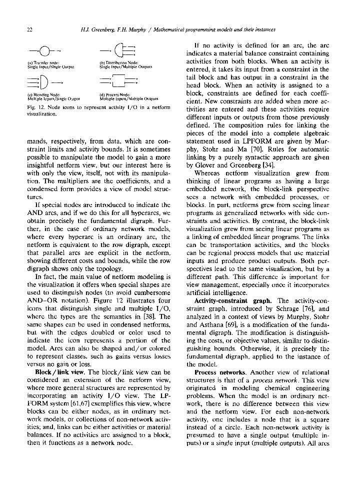
22 H.J. Greenberg, F.H. Murphy / Mathematical programming models and their instances
- 0 - ( ] (a) Transfer node: (b) Distribution Nude: Single Input/Single Output Single Input/Multiple Outputs
- i [ ) - - : (c) Blending Node: (d) Process Node: Multiple Inputs/Single Output Multiple Inputs/Multiple Outputs
Fig. 12. Node icons to represent activity I / O in a ne t form visualization.
mands, respectively, from data, which are con- straint limits and activity bounds. It is sometimes possible to manipulate the model to gain a more insightful netform view, but our interest here is with only the view, itself, not with its manipula- tion. The multipliers are the coefficients, and a condensed form provides a view of model struc- tures.
If special nodes are introduced to indicate the AND arcs, and if we do this for all hyperarcs, we obtain precisely the fundamental digraph. Fur- ther, in the case of ordinary network models, where every hyperarc is an ordinary arc, the netform is equivalent to the row digraph, except that parallel arcs are explicit in the netform, showing different costs and bounds, while the row digraph shows only the topology.
In fact, the main value of netform modeling is the visualization it offers when special shapes are used to distinguish nodes (to avoid cumbersome A N D - O R notation). Figure 12 illustrates four icons that distinguish single and multiple I / O , where the types are the semantics in [38]. The same shapes can be used in condensed netforms, but with the edges doubled or color used to indicate the icon represents a portion of the model. Arcs can also be shaped a n d / o r colored to represent classes, such as gains versus losses versus no gain or loss.
B l o c k / l i n k view. The b lock/ l ink view can be considered an extension of the netform view, where more general structures are represented by incorporating an activity I / O view. The LP- FO RM system [61,67] exemplifies this view, where blocks can be either nodes, as in ordinary net- work models, or collections of non-network activ- ities; and, links can be either activities or material balances. If no activities are assigned to a block, then it functions as a network node.
If no activity is defined for an arc, the arc indicates a material balance constraint containing activities from both blocks. When an activity is entered, it takes its input from a constraint in the tail block and has output in a constraint in the head block. When an activity is assigned to a block, constraints are defined for each coeffi- cient. New constraints are added when more ac- tivities are entered and these activities require different inputs or outputs from those previously defined. The composition rules for linking the pieces of the model into a complete algebraic statement used in LPFORM are given by Mur- phy, Stohr and Ma [70]. Rules for automatic linking by a purely syntactic approach are given by Glover and Greenberg [34].
Whereas netform visualization grew from thinking of linear programs as having a large embedded network, the block-link perspective sees a network with embedded processes, or blocks. In part, netforms grew from seeing linear programs as generalized networks with side con- straints and activities. By contrast, the block-link visualization grew from seeing linear programs as a linking of embedded linear programs. The links can be transportation activities, and the blocks can be regional process models that use material inputs and produce product outputs. Both per- spectives lead to the same visualization, but by a different path. This difference is important for view management, especially once it incorporates artificial intelligence.
Activity-constraint graph. The activity-con- straint graph, introduced by Schrage [76], and analyzed in a context of views by Murphy, Stohr and Asthana [69], is a modification of the funda- mental digraph. The modification is distinguish- ing the costs, or objective values, similar to distin- guishing bounds. Otherwise, it is precisely the fundamental digraph, applied to the instance of the model.
Process networks. Another view of relational structures is that of a process network. This view originated in modeling chemical engineering problems. When the model is an ordinary net- work, there is no difference between this view and the netform view. For each non-network activity, one includes a node that is a square instead of a circle. Each non-network activity is presumed to have a single output (multiple in- puts) or a single input (multiple outputs). All arcs
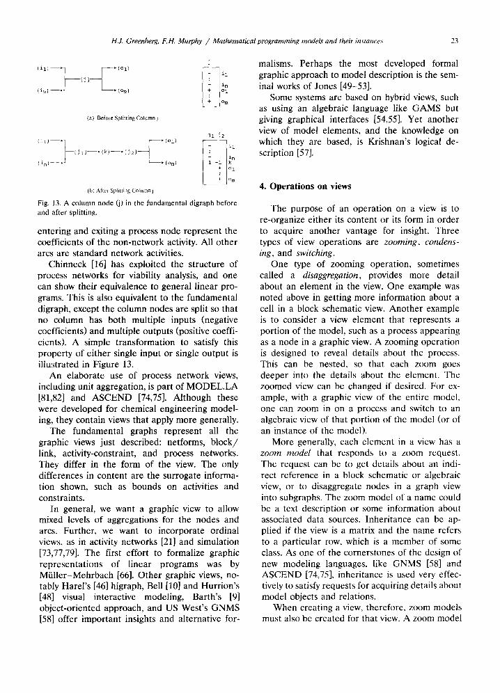
HJ. Greenberg, F.H. Murphy / Mathematical programming models and their instances 23
(il)--'] ~" C°l)
(in) --.~ ~ (om)
(a) Before Splitting Column j
J
i n
Jl J2 -~(°I) ~ il (il)--'~[jl]--~(k)--.[j2]
(in)--P~ --b(Om) ~n o l
o m
(b) After Splitting Column j
Fig. 13. A column node (j) in the fundamental digraph before and after splitting.
entering and exiting a process node represent the coefficients of the non-network activity. All other arcs are standard network activities.
Chinneck [16] has exploited the structure of process networks for viability analysis, and one can show their equivalence to general linear pro- grams. This is also equivalent to the fundamental digraph, except the column nodes are split so that no column has both multiple inputs (negative coefficients) and multiple outputs (positive coeffi- cients). A simple transformation to satisfy this property of either single input or single output is illustrated in Figure 13.
An elaborate use of process network views, including unit aggregation, is part of M O D E L . L A [81,82] and ASCEND [74,75]. Although these were developed for chemical engineering model- ing, they contain views that apply more generally.
The fundamental graphs represent all the graphic views just described: netforms, b lock / link, activity-constraint, and process networks. They differ in the form of the view. The only differences in content are the surrogate informa- tion shown, such as bounds on activities and constraints.
In general, we want a graphic view to allow mixed levels of aggregations for the nodes and arcs. Further, we want to incorporate ordinal views, as in activity networks [21] and simulation [73,77,79]. The first effort to formalize graphic representat ions of linear programs was by Mii l le r -Mehrbach [66]. Other graphic views, no- tably Harel ' s [46] higraph, Bell [10] and Hurr ion 's [48] visual interactive modeling, Barth 's [9] object-oriented approach, and US West 's GNMS [58] offer important insights and alternative for-
malisms. Perhaps the most developed formal graphic approach to model description is the sem- inal works of Jones [49-53].
Some systems are based on hybrid views, such as using an algebraic language like GAMS but giving graphical interfaces [54,55]. Yet another view of model elements, and the knowledge on which they are based, is Krishnan's logical de- scription [57].
4. Operations on views
The purpose of an operat ion on a view is to re-organize either its content or its form in order to acquire another vantage for insight. Three types of view operations are zooming, condens- ing, and switching.
One type of zooming operation, sometimes called a disaggregation, provides more detail about an element in the view. One example was noted above in getting more information about a cell in a block schematic view. Another example is to consider a view element that represents a portion of the model, such as a process appearing as a node in a graphic view. A zooming operation is designed to reveal details about the process. This can be nested, so that each zoom goes deeper into the details about the element. The zoomed view can be changed if desired. For ex- ample, with a graphic view of the entire model, one can zoom in on a process and switch to an algebraic view of that portion of the model (or of an instance of the model).
More generally, each element in a view has a zoom model that responds to a zoom request. The request can be to get details about an indi- rect reference in a block schematic or algebraic view, or to disaggregate nodes in a graph view into subgraphs. The zoom model of a name could be a text description or some information about associated data sources. Inheritance can be ap- plied if the view is a matrix and the name refers to a particular row, which is a member of some class. As one of the cornerstones of the design of new modeling languages, like GNMS [58] and ASCEND [74,75], inheritance is used very effec- tively to satisfy requests for acquiring details about model objects and relations.
When creating a view, therefore, zoom models must also be created for that view. A zoom model
24 H.J. Greenberg, F.H. Murphy / Mathematical programming models and their instances
for an icon in an iconic graph view can be differ- ent f rom a zoom model for the associated portion of the model in an algebraic view. This is because the view manager can have default reasoning mechanisms, where the view requested is gener- ally from a particular constituency whose request for detail is different from that of another con- stituency. For example, suppose the view is alge- braic, and a zoom request is issued for an equa- tion. In this case, the zoom model might provide justification for the equation, such as some physi- cal law about heat transfer meaningful to an engineer. Now suppose the view is an outline, as in structured modeling, and a zoom request is issued for the test object that corresponds to the same equation. The zoom model here might pro- vide a trace of the calling sequence.
Of course, it is not necessary to have different zoom models for different views, but the view manager must allow this flexibility. In other words, the burden of creating zoom models need not be placed entirely on the model builder. Instead, default zoom models are part of the system de- sign, and the model builder can use these or over-ride them.
The inverse of zooming is condensing. This collapses a view according to some criteria, and a view condensation model is needed analogous to a zoom model. In graphic views, each node has propert ies that form a natural binding among nodes. For example, in a transportation problem, all supply nodes could be condensed to form a single node that represents supply, and all de- mand nodes could be condensed to form a single node that represents demand. These bindings can be applied to form a natural condensation model without requiring the model builder to specify it a priori. It is not necessary, however, that a con- densation be a true inverse of a zoom, in a mathematical sense. This is because after con- densing nodes, say, by region, the zoom might be on other details within the condensed node, such as disaggregating by material.
Another operat ion is to switch views. For ex- ample, the active view might be an iconic graphic view superimposed on a map. The user might ask for an algebraic view of that portion of the model represented by one of the icons.
In considering view creation, switching must be regarded as a separate operat ion from zoom- ing, even though a user might think of these as
only one operation. If the active view is iconic and one seeks a view of the equations in one of the icons, the process is two-step: zoom in on the icon and switch to algebraic.
All operations, notably zooming, condensing and switching, can be applied to any part of the active view. Other operations include some found in C A D / C A M systems, particularly a view in the problem domain, where icons and their relative locations correspond to physical objects related spatially or temporally.
5. Connections with structured modeling
Structured modeling (SM) is a formal ap- proach to model description, based on calling sequences of the following five types of objects. 1. primitive entity, such as a set of materials or
regions. 2. compound entity, is defined in terms of other
entities, like a product of sets. 3. attribute, which can be dependent upon enti-
ties (primitive and compound), is an object that can assume a value, like a data table or a variable.
4. function, any computable function of at- tributes, which can depend also on entities.
5. test, any logical function of attributes, which can depend also on entities. From these five fundamental objects, SM views
a model as dependency relations, namely calling sequences, which are hierarchically ordered. One SM view is an elemental graph, which contains a node for each object and arcs for their calling sequences. Another view is a genus graph, which contains nodes for collections of objects and arcs for their common calling sequences. SM has rules to construct a genus graph from an elemental graph, and it is possible to vary levels of detail. One could, for example, zoom in on a portion of the genus graph by constructing its elemental subgraph. In this way, one can view portions of a model relevant to particular questions.
Details of SM are well covered by Geoffrion [26-29]. Our concern here is with the views treated by SM, and with how SM fits into a formal foundation for a multi-view architecture.
A view of model block structures, which is intrinsic to SM, is an outline. SM is a top-down approach to model description, and the SM out-
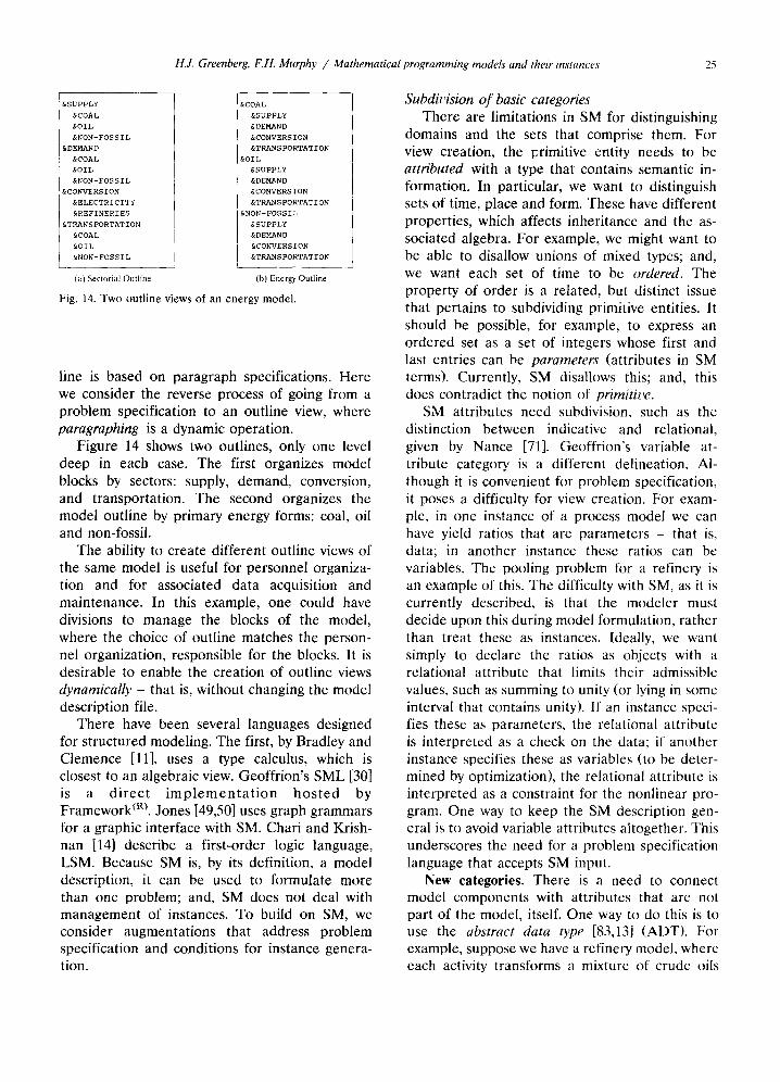
H.J. Greenberg, F.H. Murphy / Mathematical programming models and their instances 25
&SUPPLY
&COAL
&OIL
&NON-FOSSIL
&DEMAND
&COAL
&OIL
&NON-FOSSIL
&CONVERSION
&ELECTRICITY
&REFINERIES
&TRANSPORTATION
&COAL
&OIL
&NON-FOSSIL
&COAL
&SUPPLY
&DEMAND
&CONVERSION
&TRANSPORTATION
&OIL
&SUPPLY
&DEMAND
&CONVERSION
&TRANSPORTATION
&NON-FOSSIL
&SUPPLY
&DEMAND
&CONVERSION
&TRANSPORTATION
(a) Sectorial Outline (b) Energy Outline
Fig. 14. Two outline views of an energy model.
line is based on paragraph specifications. Here we consider the reverse process of going from a problem specification to an outline view, where paragraphing is a dynamic operation.
Figure 14 shows two outlines, only one level deep in each case. The first organizes model blocks by sectors: supply, demand, conversion, and transportation. The second organizes the model outline by primary energy forms: coal, oil and non-fossil.
The ability to create different outline views of the same model is useful for personnel organiza- tion and for associated data acquisition and maintenance. In this example, one could have divisions to manage the blocks of the model, where the choice of outline matches the person- nel organization, responsible for the blocks. It is desirable to enable the creation of outline views dynamically - that is, without changing the model description file.
There have been several languages designed for structured modeling. The first, by Bradley and Clemence [11], uses a type calculus, which is closest to an algebraic view. Geoffrion's SML [30] is a d i r ec t i m p l e m e n t a t i o n h o s t e d by Framework ~m. Jones [49,50] uses graph grammars for a graphic interface with SM. Chari and Krish- nan [14] describe a first-order logic language, LSM. Because SM is, by its definition, a model description, it can be used to formulate more than one problem; and, SM does not deal with management of instances. To build on SM, we consider augmentations that address problem specification and conditions for instance genera- tion.
Subdit~ision of basic categories There are limitations in SM for distinguishing
domains and the sets that comprise them. For view creation, the lzrimitive entity needs to be attributed with a type that contains semantic in- formation. In particular, we want to distinguish sets of time, place and form. These have different properties, which affects inheritance and the as- sociated algebra. For example, we might want to be able to disallow unions of mixed types; and, we want each set of time to be ordered. The property of order is a related, but distinct issue that pertains to subdividing primitive entities. It should be possible, for example, to express an ordered set as a set of integers whose first and last entries can be parameters (attributes in SM terms). Currently, SM disallows this; and, this does contradict the notion of primitit,e.
SM attributes need subdivision, such as the distinction between indicative and relational, given by Nance [71]. Geoffrion's variable at- tribute category is a different delineation. Al- though it is convenient for problem specification, it poses a difficulty for view creation. For exam- ple, in one instance of a process model we can have yield ratios that are parameters - that is, data; in another instance these ratios can be variables. The pooling problem for a refinery is an example of this. The difficulty with SM, as it is currently described, is that the modeler must decide upon this during model formulation, rather than treat these as instances. Ideally, we want simply to declare the ratios as objects with a relational attribute that limits their admissible values, such as summing to unity (or lying in some interval that contains unity). If an instance speci- fies these as parameters, the relational attribute is interpreted as a check on the data; if another instance specifies these as variables (to be deter- mined by optimization), the relational attribute is interpreted as a constraint for the nonlinear pro- gram. One way to keep the SM description gen- eral is to avoid variable attributes altogether. This underscores the need for a problem specification language that accepts SM input.
New categories. There is a need to connect model components with attributes that are not part of the model, itself. One way to do this is to use the abstract data type [83,13] (ADT). For example, suppose we have a refinery model, where each activity transforms a mixture of crude oils
26 H.J. Greenberg, 1:.1t. Murphy / Mathematical programming models and their instances
into yields of intermediate and final refined petroleum products. In matrix terms, it might be difficult to distinguish one processing unit f rom another, but associated activities have different attributes that can contribute insight when viewed by a process engineer. Suppose we declare a variable attribute to be linked to an A D T associ- ated with its process unit type. Then, views that ask for relations of these variable attributes and associated data tables (attributes) can use this link to create a view in terms of its attributes.
Another A D T is a unit of measurement and associated relations. Structured modeling does not require units to be specified (as do some languages [60,11]). Thus, if a flow is measured in gallons and production is measured in barrels, the A D T must account for the conversion in a balance equation that includes production and flow. This affects not only problem specification, but also query, reporting and model manage- ment. By not requiring the units to be specified in the model description, the A D T can allow flexi- ble data instances. One may specify capacities in gallons in one instance and in barrels in another instance. This should not affect the model 's in- tegrity or the views that can be created.
Another A D T fulfills a need to distinguish control tables from other types of data tables. In SM, a control table LINK, say with domain S × D (supply x demand), is the same attribute type as a table COST over the same domain, which con- tains cost data for each link. For problem specifi- cation and for instance generation, this poses no difficulty, but view management is compromised by not have them distinguished. This can be done by appending A D T C O N T R O L to the L INK table properties (alternatively, the attribute could be subdivided to make this distinction explicit).
Goals, constraints and objectives. Currently, all constraints in SM are expressed as test types (t), which is an algebraic representation. This suffices for internal representations, but work is needed to derive the SM representat ion from other views, such as from a process network. Objectives, namely functions (f) to minimize or maximize, are not explicitly expressed; they must be inferred from the text in the function declara- tion. We prefer to subdivide functions into ex- plicit expressions of objectives. We also prefer to have the category of function that describes goals, as in goal-programming. An alternative, of course,
is to use abstract data types. Keeping function as a single category, we could, for example, AP- P E N D M I N I M I Z E , or A P P E N D G O A L < = attribute.
What is important is that these could change from one instance to another, thus changing the views. In multi-objective programming, one may arrive at a pareto optimum. Then, one may want to view the effects on the other criteria if one is required to improve. In practice, this can be done by treating the other criteria as goals or con- straints, shifted from current values, and optimize the one distinguished criterion. In SM terms these other functions change type.
Conditionals. A domain, such as that of an activity, can have conditionals for membership, such as for generation of specific activities in the class. Links between suppliers and markets can be described by a (data-dependent) relationship, such as distance. SM does not distinguish do- mains and sets. To have a sparse set of links, an explicit compound entity must be defined inde- pendent of attributes. In many cases this is not a natural representation, and views about the con- ditions for such links to exist would be lost - that is, they are not part of the SM representation. As in the other cases, this could be accommodated by an A D T or by a new category of sets, called domains, which are like compound entities, ex- cept for the relational attributes that comprise conditionals.
6. Generalized formal development
We have illustrated how an information struc- ture for a specific view cannot, by itself, provide an appropriate internal representation. This is due to ambiguities that arise - that is, a one to many mapping, which precludes a property of independence. This independence can be seen as a distinction between an internal view definition and an external one. An internal view definition relies on information not shown in the view. For example, MathPro and MIMI use block schematic views for model description, but since they can generate instances, they have enough information to give other views, like algebraic. It is necessary to use information beyond what appears in the block schematic view, such as how they create cell icons from the more general information. This is
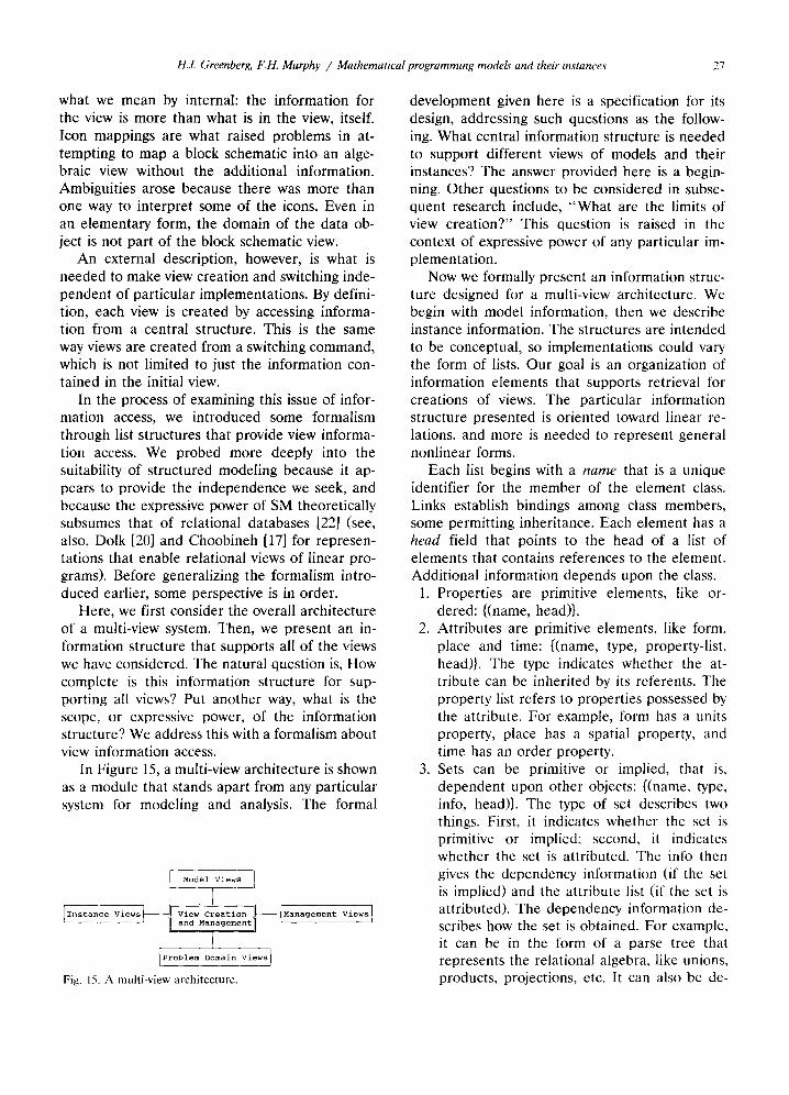
H.J. Greenberg, F.H. Murphy / Mathematical programming models and their instances 27
what we mean by internal: the information for the view is more than what is in the view, itself. Icon mappings are what raised problems in at- tempting to map a block schematic into an alge- braic view without the additional information. Ambiguities arose because there was more than one way to interpret some of the icons. Even in an elementary form, the domain of the data ob- ject is not part of the block schematic view.
An external description, however, is what is needed to make view creation and switching inde- pendent of particular implementations. By defini- tion, each view is created by accessing informa- tion from a central structure. This is the same way views are created from a switching command, which is not limited to just the information con- tained in the initial view.
In the process of examining this issue of infor- mation access, we introduced some formalism through list structures that provide view informa- tion access. We probed more deeply into the suitability of structured modeling because it ap- pears to provide the independence we seek, and because the expressive power of SM theoretically subsumes that of relational databases [22] (see, also, Dolk [20] and Choobineh [17] for represen- tations that enable relational views of linear pro- grams). Before generalizing the formalism intro- duced earlier, some perspective is in order.
Here, we first consider the overall architecture of a multi-view system. Then, we present an in- formation structure that supports all of the views we have considered. The natural question is, How complete is this information structure for sup- porting all views? Put another way, what is the scope, or expressive power, of the information structure? We address this with a formalism about view information access.
In Figure 15, a multi-view architecture is shown as a module that stands apart from any particular system for modeling and analysis. The formal
Model Views ]
I__ IInst .... Views I {~WM~t~Manag .... tViews]
) I Problem Domain Views)
Fig. 15. A multi-view architecture.
development given here is a specification for its design, addressing such questions as the follow- ing. What central information structure is needed to support different views of models and their instances? The answer provided here is a begin- ning. Other questions to be considered in subse- quent research include, "What are the limits of view creation?" This question is raised in the context of expressive power of any particular im- plementation.
Now we formally present an information struc- ture designed for a multi-view architecture. We begin with model information, then we describe instance information. The structures are intended to be conceptual, so implementations could vary the form of lists. Our goal is an organization of information elements that supports retrieval for creations of views. The particular information structure presented is oriented toward linear re- lations, and more is needed to represent general nonlinear forms.
Each list begins with a n a m e that is a unique identifier for the member of the element class. Links establish bindings among class members, some permitting inheritance. Each element has a head field that points to the head of a list of elements that contains references to the element. Additional information depends upon the class.
1. Properties are primitive elements, like or- dered: {(name, head)}.
2. Attributes are primitive elements, like form, place and time: {(name, type, property-list, head)}. The type indicates whether the at- tribute can be inherited by its referents. The property list refers to properties possessed by the attribute. For example, form has a units property, place has a spatial property, and time has an order property.
3. Sets can be primitive or implied, that is, dependent upon other objects: {(name, type, info, head)}. The type of set describes two things. First, it indicates whether the set is primitive or implied; second, it indicates whether the set is attributed. The info then gives the dependency information (if the set is implied) and the attribute list (if the set is attributed). The dependency information de- scribes how the set is obtained. For example, it can be in the form of a parse tree that represents the relational algebra, like unions, products, projections, etc. It can also be de-
28 H.J. Greenberg, F.H. Murphy / Mathematical programming models and their instances
pendent upon certain data objects, like a set of consecutive integers defined by two data objects that give the first and last values.
4. Domains are restricted products of sets: {(name, sets, restrictions, head)}. The sets define a product, and the restrictions can be logical - that is, depend only on relations of set members, or they can be data-dependent.
5. Data objects are numeric constants, parame- ters or tables: {(name, domain, range, seman- tics, head)}. The domain of a numeric con- stant is a keyword, like NUMERIC, and its range is its value, fixed for all instances. The domain of a parameter is the empty set. The range is the admissible range of values for instances. A parameter can be a universal constant, like PI, or it can vary over in- stances. In the former case, the range is a single numeric constant. More generally, the range of a parameter or a table is a specifica- tion of a list of intervals, not dependent on other parameters or tables. The semantics are bindings to properties and attributes.
6. Decision objects are classes of variables: {(name, domain, range, conditions, semantics, head)}. The domain can be the empty set. The range specification is either a pair of data objects that define lower and upper bounds, or a list of data objects that define discrete values that comprise the variable's range. The conditions are logical expressions, which can be data-dependent, that pertain to generation of a member of the decision ob- ject class. The semantics are bindings to properties and attributes.
7. DD objects are classes of objects that will either be data objects or decision objects, according to a role assignment for an in- stance: {(name, domain, range, role, seman- tics, conditions, head)}. The role is a place holder that becomes instantiated as one of: {qS, OMIT, DATA, DECISION}. A role value of ~b means no role is assigned. When the role is OMIT, the object is absent from the instance. When the role is DATA, the rest of the information is treated as a data object. When the role is DECISION, the rest of the information is treated as a decision object.
8. Equations are expressions that form con- straints, goals or objectives in the mathemati- cal program: {(name, domain, role, range,
conditions, terms, semantics, head)}. The role of an equation is one of: {~b, OMIT, MINI- MA N D , M A X I M A N D , G O A L , CON- STRAINT}. The range specification is a pair of data object references, either of which could be absent. For the CONSTRAINT role, this defines lower and upper limits for the level of the equation. The conditions are logi- cal expressions, which can be data-depen- dent, that pertain to generation of a member of the equation class. The semantics are bind- ings to properties and attributes.
9. Logical expressions form constraints in the mathematical program: {(name, domain, role, type, info, conditions, semantics, head)}. The role of a logical expression is one of: {4), OMIT, CONSTRAINT}. The type is a key- word, such as I F - T H E N , COVER, SELECT, etc. The info depends upon the type. For example, I F - T H E N requires antecedent and consequent expressions; and, COVER and SELECT require a set of binary-valued (0, 1) decision objects. The conditions are logical expressions, which can be data-dependent, that pertain to generation of a member of the logical expression class. The semantics are bindings to properties and attributes.
10. Functions are computable expressions that map numeric-valued objects into a real value: {(name, object list, expression, semantics, head)}. The object list is any collection of data objects, decision objects and DD ob- jects. The expression is a computable form, like a parse tree. The semantics are bindings to properties and attributes.
11. Operations are delimiters for terms in an equation: {(name, domain, semantics, head)}. The domain can be empty, as in the case of the implied summation in MODLER. The list of operations must include SUM (or an equivalent keyword). The semantics are bind- ings to properties and attributes.
12. Terms are contained in equations: {(name, equation, sign, operation, function, condi- tions, semantics, head)}. The sign is either + or - . The operation is applied to the func- tion. The conditions are logical expressions, which can be data-dependent, that pertain to inclusion of the term in a member of the equation class. The semantics are bindings to properties and attributes.
H.J. Greenberg, F.H. Murphy / Mathematical programming models and their instances 29
The main difference between this structure and the ones we presented specifically for the algebraic and block-schematic views is that we are independent of what was internal information structures - that is, information not contained in the view. In this external information structure everything has an identity that allows us, for example, to trace back to the most primitive elements of a model 's objects and relations. In lists 1 and 2 above, we define propert ies and attributes that can be associated with the differ- ent objects in the model. These lists are not part of the other data structures, since the other struc- tures do not try to deal with meaning. The set list, 3, is the same, except for added semantic information, as in the algebraic information structure, but this is not in the block schematic information structure because sets a r e always bound to objects and in domains, defined in 4, in this view.
Data objects, given in list 5, and decision ob- jects, given in list 6, are as before, except for the addition of bindings information. Note that col- umn strips are the decision objects in the block schematic information structure. D D objects in list 7 are new; they are added to handle problem definition separately from model definition. The equation object, list 8, has a different meaning here versus algebra. It consists of a list of terms as well as the information for constructing an audit trail. Logical expressions, given in list 9, are restrictions that need not be expressed alge- braically; typically, they are stated as logical im- plications (i.e., IF antecedent T H E N consequent), but any logical expression, such as clause form, can be used to define conditions.
Functions, given in list 10, extend representa- tions of linear programming views to nonlinear forms. Even if the mathematical program is lin- ear, however, the functions may still be used to express data relations. For example, demand data for a linear program can be a sequence over time defined by initial demands and a growth rate. The formula to determine the LP demand for t > 0 is a standard nonlinear expression.
Operations, given in list 11, contain informa- tion to create not only the terms of an equation, but also the associated icons in a block-schematic view. The conditionals on summations are explicit in the equations with the algebraic view, and list 12 contains what is needed with references to
operations and other elements defined previ- ously. The information in lists 11 and 12 deter- mine cell icons in the block schematic. Notice that this separation of the definition of the terms from the definition of the equations is central to defining parts of the model separately that allows us to add semantic information about the model components to explain the model 's parts and how the relate to one another. A key is primitive subdivision with bindings explicit in the informa- tion structure.
The above information structure pertains to the model, itself, apart from instances. It is not difficult to verify that all of the views we have described can be generated from this central in- formation structure. In particular, the difficulties we encountered mapping algebraic and block schematic views are overcome by this information structure. It is also not difficult to note omission of details that distinguish implementations, such as representations of expressions, for example as parse trees, and additional links, such as from decision objects to terms. We now consider addi- tional information to support view creation of instances.
An instance is defined as the assignment of values to all data objects, including sets, and to roles. For each list, we could add another field, called the source, which is a list of unique identi- fiers to cross reference instances. This principle is one of the features of MathPro, as part of its model management facility.
The following information structure is de- signed to support views of instances. This is in addition to the model information structure, in order to support operations, like zooming, con- densing and switching. 1. Header of instance: {(name, parent, help, solu-
tion, head)}. The parent of the instance is some other instance or it is & to indicate it is from the model, itself. In the former case, the remaining lists are deviations from the parent (this is the technique used in MathPro). The help reference is to a file that documents the instance. This could be in addition to the help file of a parent. The solution information de- fines the overall status of the solution of the instance (which might be unsolved) and the optimizer used. The head binds the instance to a list of scenarios.
2. Sources of instance: {(object, source)}. The ob-
30 H.J. Greenberg, F.H. Murphy / Mathematical programming models and their instances
ject is any that was instantiated, such as set members, data object values, and role assign- ments.
3. Objectives of instance: {(equation, value)}. In the case of a single objective, the list has only one equation (the Source list contains the roles). The value is its value for the instance.
4. Constraints of instance: {(row name, type, class, lo, up, status, level, price)}. The type is one of the constraint types in the model information: equation or logical. Then, the class is the name of the equation or logical, respectively. The semantics in the model information can con- tain information about its row form, especially in the case of a logical constraint that has been converted to a linear inequality. The lo and up numeric values are the limits of the constraint, which are bound to the range specification in the model information. The status, level and price comprise the solution values of the con- straint.
5. Activities of instance: {(column name, class, lo, up, status, level, price)}. The class is the name of the decision or DD object. The lo and up numeric values are the bounds of the activity, which are bound to the range specification in the model information. The status, level and price comprise the solution values of the con- straint. It is not difficult to verify that this instance
information structure is sufficient to support all of the instance views we have described. Cur- rently, A N A L Y Z E receives much of this to sup- port the views it creates. Some views require a significant amount of computation, which could be circumvented by additional information not included here. For example, to obtain rates of substitution between basic and nonbasic vari- ables, one must apply an equation-solving algo- rithm. We leave open, for now, whether such information as rearrangement of the basis should accompany the instance structure.
Now we address the question of scope. Are there views about the model or its instances not supported by this information structure? The an- swer is yes if the structure is taken too literally. In particular, the information structure says very little about views for scenario management . Sup- pose someone wants a view to get insight from comparing two or more instances? Suppose one wishes a complete audit trail about an instance,
tracing back not only to model description com- ponents (like equations), but also to primary data sources that can be many steps removed from the information at hand? For example, what is viewed as data input to the instance can be output from a surrogate model, such as one that forecasts demands used as right-hand sides in the con- straints.
On the other hand, the information structure can be regarded as conceptual, and we return to a question raised early in this paper: What is a view? Superficially, one could define a view as a model: a collection of objects and relations. This is, however, incomplete, as the following develop- ment reveals.
At the very highest level, a view is composed of three categories of specifications: (1) its con- tent, (2) its form, and (3) its world. We have illustrated content and form; next, we describe what the world means in this context before we proceed to elaborate on all three.
A view's world gives a contextual meaning to its form and contents [3], which we use to provide some of the semantics behind the view. For one thing, the world provides overview information, including: how the view was requested, how the view relates to entities and relations not in the view, what zoom models to use, and what li- braries, databases and other sources that are bound to the view's content.
A key to understand the formalism based on view information access is to understand the dis- tinction between direct and indirect information. Indirect information access involves such opera- tions as projection, which we illustrated, to obtain relations that are implied by the direct relations and by rules of inference based on the meanings of the relations. One example is the relation between two activity classes that is implied by their common dependence on the same data ob- ject.
This leads to one of the conditions for com- pleteness. That is, if V = [W,C,F] is any view (with W = world, C = content and F = form), and if F ' is some other form, the information struc- ture should support the view V ' = [W,C,F']. This presumes, however, that either F and F ' are content-insensitive, or that form F ' is defined for content C. For example, suppose V is a view of set dependencies, with C = sets and their depen- dency relations, and F = conceptual graph (c.f.,
H.J. Greenberg, F.H. Murphy / Mathematical programming models and their instances 31
Figure 8). Then (absent any equations), an alge- braic view is not defined, so F ' cannot be this form.
Another condition for completeness is based on operations, like zooming. If C ' is obtained from C from a zooming operat ion with appropri- ate changes to F ' effected by the operation, the view V ' = [W, C ' , F ' ] should be supported by the information structure. A similar statement ap- plies to condensations and projections.
We begin to see that the information structure must be defined at an a t o m i c l e v e l - that is, where objects and relations are the most elemen- tary. Considering the information structure de- fined for model information, one needs only to consider the elements more abstractly to see it as a conceptual information structure. To some ex- tent this abstraction can be achieved with the elemental graph in structured modeling, but not quite. What must be added are primitives like indicative attributes, which can also be regarded as property lists from an information structure vantage. Other additions include role assignment information and a g rammar that describes how operations perform. This syntactic approach is fulfilled by the formalism of Baldwin and Garlan.
It is not really necessary to have a separate specification for the information structure of in- stances. This was done above to be specific about the nature of the information and bring attention to links between instance and model description elements.
7. Summary and conclusions
There are many views of mathematical models and their instances. The very definition of a model is not universally accepted beyond agreement that it contains objects and relations among them. The formal approach of structured modeling provides a foundation for model description, but it leaves open issues about problem specification that af- fect view creation.
It is easy to accept the idea that different people gain insights from different views. Be- cause of this, we need a multi-view architecture to support mathematical modeling and analysis. With the exception of Baldwin's D O V E system, this presents the first formal framework for ad- dressing this need in O R / M S decision support
systems that are based on mathematical program- ming.
We have used views that people have found useful in large-scale linear programming over the past 35 years to provide a concrete, applied base upon which to establish a foundation for a multi- view architecture. Close analysis of popular views, notably variants of algebraic, schematic and graphic views, reveals that they are all useful, depending upon the individual and the situation. No single view implementat ion is rich enough to support a multi-view architecture, so a new, cen- tral information structure forms the foundation for such support. The view creation and manage- ment module is designed to switch from any view to any other, not by direct mapping, but by creat- ing each view independently.
Although we have oriented views as an output, clearly every modeling system assumes a view for its input specifications. Some are algebraic, some are block schematic, and some are graphic. We see no need to distinguish whether a view is presented as an input or an output specification. We do, however, see a need to map view inputs into a central information structure, especially since we have demonstrated difficulties with map- ping directly from information about one view to another view. Once views are bet ter understood as a formal construct, their use for input specifi- cation will become a matter of implementation, rather than conception.
Among the open issues, understanding the ex- pressive power of any proposed information structure has both theoretical and practical impli- cations. Future studies of a modeling system's expressiveness must take view creation into con- sideration. Most systems present only those views that conform to its input specification. Abstract formalisms, notably structured modeling, contain the foundations needed for this extension.
Acknowledgements
The authors gratefully acknowledge comments and advice from Dirk Baldwin, H.I. (Gus) Gassman, Arthur M. Geoffrion, Fred Glover, Al- ice M. Ireland, Richard E. Nance, and Laurel Neustadter. Comments from two anonymous ref- erees and from the Editor, Christopher V. Jones, helped create this revision as an improvement
32 H.J. Greenberg, F.H. Murphy / Mathematical programming models and their instances
over the original version. Financial and technical support was provided by a consortium of compa- nies: Amoco Oil Company, IBM, Shell Develop- ment Company, Chesapeake Decision Sciences Inc., GAMS Development Corp., Ketron Man- agement Science, and MathPro, Inc.
References
[1] F.L. Alvarado, 1990. Manipulation and Visualization of Sparse Matrices, ORSA Journal on Computing 2:2, 186- 206.
[2] T.E. Baker, 1983. RESULT: An Interactive Modeling System for Planning and Scheduling, Presented at the ORSA/TIMS meeting, Chicago, IL.
[3] D. Baldwin, 1989. Principles of Design for a Multiple Viewpoint Problem Formulation Support System, Ph.D. Thesis, School of Business Administration, Texas Tech University, Lubbock, TX.
[4] D. Baldwin, 1990. The Development and Architecture of DOVE: A Multiview Viewpoint, Proceedings of ISDSS Conference, Austin, TX.
[5] D. Baldwin, 1992. The Design and Evaluation of a Multi- ple View Decision Support System, Technical Report, College of Business, Virginia Polytechnic Institute and State University, Blacksburg, VA.
[6] D. Baldwin, 1992. Exploring Multiple Views: Examples from Accounting, Mathematical Modeling and Systems Analysis, Technical Report, College of Business, Virginia Polytechnic Institute and State University, Blacksburg, VA.
[7] A.A. Baldwin, D. Baldwin and T.K. Sen, 1991. The Evolution and Problems of Model Management Re- search, OMEGA 19:6, pp. 511-528.
[8] D. Baldwin and S.B. Yadav, 1991. Principles of Design for a Multiple Viewpoint Problem Decision Support Sys- tem, Technical Report, Department of Accounting, Col- lege of Business, Virginia Polytechnic Institute and State University, Blacksburg, VA.
[9] P.S. Barth, 1987. An Object-Oriented Approach to Graphical Interfaces, ACM Transactions on Graphics 5:2, 142-172.
[10] P.C. Bell, 1985. Visual Interactive Modeling as an Opera- tions Research Technique, Interfaces 15, 26-33.
[11] G.H. Bradley and R.D. Clemence, Jr., 1986. A Type Calculus for Executable Modelling Languages, IMA Journal of Mathematics in Management 1,277-292.
[12] A. Brooke, D. Kendrick and A. Meeraus, 1988. GAMS: A User's Guide, Scientific Press, Redwood City, CA.
[13] L. Cardelli and P. Wegner, 1985. On Understanding Types, Data Abstraction, and Polymorphism, Computing Surveys 17:4, 471-522.
[14] S. Chari and R. Krishnan, 1990. Towards a Logical Reconstruction of Structured Modeling, Technical Re- port, School of Urban and Public Affairs, Carnegie-Mel- lon University, Pittsburgh, PA.
[15] Chesapeake Decision Sciences, 1988. MIMI/LP User Manual, New Providence, NJ.
[16] J.W. Chinneck, 1990. Formulating Processing Network
Models: Viability Theory, Naval Research Logistics 37, pp. 245-261.
[17] J. Choobineh, 1990. SQLMP: A Data Sublanguage for Representation and Formulation of Linear Mathematical Models, Technical Report, Department of Business Analysis and Research, Texas A and M University, Col- lege Station, TX.
[18] W.S. Cleveland and M.E. McGill (eds.), 1988. Dynamic Graphics for Statistics, Wadsworth and Brooks/Cole, Pacific Grove, CA.
[19] U. Dayal and H. Hwang, 1984. View Definition and Generalization for Database Integration in Multi- database System, IEEE Transactions on Software Engi- neering SE-10:6, 628-644.
[20] D.R. Dolk, 1988. Model Management and Structured Modeling: The Role of an Information Resource Dictio- nary System, Communications of ACM 31,704-718.
[21] S.E. Elmaghraby, 1977. Activity Networks: Project Plan- ning and Control by Network Models, Wiley, New York, NY.
[22] C.K. Farn, 1985. An Integrated Information System Ar- chitecture Based on Structured Modeling, Ph.D. Thesis, Western Management Science Institute, University of California, Los Angeles, CA.
[23] R. Fourer, D.M. Gay and B.W. Kernighan, 1990. A Mathematical Programming Language, Management Sci- ence 36:5, 519-554.
[24] D. Garlan, 1987. Views for Tools in Integrated Environ- ments, Ph.D. Thesis, Computer Science Department, Carnegie-Mellon University, Pittsburgh, PA.
[25] H.I. Gassmann and A.M. Ireland, 1992. Scenario Formu- lation in an Algebraic Modeling Language, Technical Report WP-92-7, School of Business Administration, Dalhousie University, Halifax, Nova Scotia.
[26] A.M. Geoffrion, 1987. An Introduction to Structured Modeling, Management Science 33, 547-588.
[27] A.M. Geoffrion, 1989. The Formal Aspects of Structured Modeling, Operations Research 37:1, 30-51.
[28] A.M. Geoffrion, 1989. Integrated Modeling Systems, Computer Science in Economics and Management 2:1, pp. 3-15.
[29] A.M. Geoffrion, 1989. Computer-Based Modeling Envi- ronments, European Journal of Operational Research 41:1, pp. 33-43.
[30] A.M. Geoffrion, 1990. SML: A Model Definition Lan- guage for Structured Modeling, Working Paper No. 360, Western Management Science Institute, University of California, Los Angeles, CA (Originally May, 1988).
[31] A.M. Geoffrion, 1990. A Library of Structured Models, Informal Note (revised), Western Management Science Institute, University of California, Los Angeles, CA.
[32] A.M. Geoffrion, 1990. Indexing in Modeling Languages for Mathematical Programming, Working Paper No. 371 (revised), Western Management Science Institute, Uni- versity of California, Los Angeles, CA.
[33] F. Glover, 1983. Netform Modeling, Draft monograph, University of Colorado, Boulder, CO.
[34] F. Glover and H.J. Greenberg, 1987. Netforms Provide Powerful Tools for Enhancing the Operations of Expert Systems, Proceedings of the Rocky Mountain Conference on Artificial Intelligence, Boulder, CO, pp. 259-265.
H.J. Greenberg, F.H. Murphy / Mathematical programming models and their instances 33
[35] F. Glover, D. Klingman and N. Phillips, 1990. Netform Modeling and Applications, Interfaces 20:4, 7-27.
[36] F. Glover, D. Klingman and N.V. Phillips, 1992. Network Models in Optimization and Their Applications in Prac- tice, Wiley-Interscience, New York, NY.
[37] H.J. Greenberg, 1978. A New Approach to Analyze Information Contained in a Model, in Energy Models Validation and Assessment, S.I. Gass (ed.), 517-524, NBS Pub. 569, National Bureau of Standards, Gaithers- burg, MD.
[38] H.J. Greenberg, 1987. A Natural Language Discourse Model to Explain Linear Programs, Decision Support Systems 33, 333-342.
[39] H.J. Greenberg, 1990. A Primer for MODLER: Model- ing by Object-Driven Linear Elemental Relations, Uni- versity of Colorado at Denver, Mathematics Department, Denver, CO.
[40] H.J. Greenberg, 1990. A Primer for ANALYZE: A Com- puter-Assisted Analysis System for Mathematical Pro- gramming Models and Solutions, University of Colorado at Denver, Mathematics Department, Denver, CO.
[41] H.J. Greenberg, 1992. MODLER: Modeling by Object- Driven Linear Elemental Relations, Annals of Opera- tions Research (to appear).
[42] H.J. Greenberg, 1992. Enhancements of ANALYZE: A Computer-Assisted Analysis System for Mathematical Programming Models and Solutions, ACM Transactions On Mathematical Software (to appear).
[43] H.J. Greenberg, J.R. Lundgren and J.S. Maybee, 1981. Graph Theoretic Methods for the Qualitative Analysis of Rectangular Matrices, SIAM Journal of Algebraic and Discrete Methods 2, 221-239.
[44] H.J. Greenberg, J.R. Lundgren and J.S. Maybee, 1989. Extensions of Graph Inversion to Support an Artificially Intelligent Modeling Environment, Annals of Operations Research 21, 127-142.
[45] H.J. Greenberg and F.M. Murphy, 1992. An In-Depth Survey of Modeling Languages for Mathematical Pro- gramming, Annals of Operations Research (to appear).
[46] D. Harel, 1988. On Visual Formalisms, Communications of the ACM 31:5, 514-530.
[47] T. Hiirlimann, 1989. Reference Manual for the LPL Modeling Language (Version 3.1), Institute for Automa- tion and Operations Research, Univesity of Fribourg, CH-1700 Fribourg, Switzerland.
[48] R.D. Hurrion, 1986. Visual Interactive Modeling, Euro- pean Journal of Operations Research 23, 281-287.
[49] C.V. Jones, 1989. Graph Grammars and Structured Mod- eling, Working Paper, The Wharton School, University of Pennsylvania, Philadelphia, PA.
[50] C.V. Jones, 1990. An Introduction to Graph-Based Mod- eling Systems, Part 1: Overview, ORSA Journal on Com- puting 2:2, 136-151.
[51] C.V. Jones, 1990. An Integrated Modeling Environment Based on Attributed Graphs and Graph-Grammars, Technical Report, The Wharton School, University of Pennsylvania, Philadelphia, PA.
[52] C.V. Jones, 1991. An Introduction to Graph-Based Mod- eling Systems, Part 2: Graph-Grammars and the Imple- mentation, ORSA Journal on Computing 2:2, 136-151.
[53] C.V. Jones, 1991. Attributed Graphs, Graph-Grammars
and Structured Modeling, Technical Report, Simon Fraser University, Burnaby BC.
[54] D.A. Kendrick, 1989. Model Representations, CER Working Paper 89-1, Center for Economic Research, Department of Economics, University of Texas, Austin, TX.
[55] D.A. Kendrick, 1990. A Graphical Interface for Produc- tion and Transportation System Modelling: PTS, CER Working Paper 90-08, Center for Economic Research, Department of Economies, University of Texas, Austin, TX.
[56] D.A. Kendrick and R. Krishnan, 1989. A Comparison of Structured Modeling and GAMS, Computer Science in Economics and Management 2:1, 17-36.
[57] R. Krishnan, 1988. A Logic Based Approach to Model Construction, SUPA Technical Report, Carnegie-Mellon University, Pittsburgh, PA.
[58] S. Laufmann, R. Blumenthal, L. Sylvan, E. Freeman and D. Eitelbach, 1988. GNMS: A System for Modeling Net- work Structures, Technical Report. US West Advanced Technologies.
[59] W.A. Lodwick, 1991. Preprocessing Nonlinear Functional Constraints with Application to the Pooling Problem, ORSA Journal on Computing 4:2, 119-131.
[60] C. Lucas and G. Mitra, 1985. CAMPS: Preliminary, User Manual, Department of Mathematics and Statistics, Brunel University, Middlesex, UK.
[61] P-C. Ma, F.H. Murphy and E.A. Stohr, 1989. A Graphics Interface for Linear Programming, Communications of the ACM 32:8, 996-1012.
[62] J. Mackinlay, 1987. Automating the Design of Graphical Presentations of Relational Information, ACM Transac- tions on Graphics 5:2, 110-141.
[63] MathPro, Inc., 1989. MathPro Usage Guide: Introduc- tion and Reference, Washington, D.C.
[64] A. Meeraus, 1983. An Algebraic Approach to Modeling, Journal of Economic Dynamics and Control 5, 81-108.
[65] S. Miyamoto, K. Oi, O. Abe, A. Katsuya and K. Nakayama, 1986. Directed Graph Representations of As- sociation Structures: A Systematic Approach, IEEE Transactions on Systems, Man, and Cybernetics 16:1. 53-61.
[66] H. Miiller-Mehrbach, 1976. Graphically Illustrating LP Models, Presented at the 8-th Mathematical Program- ruing Symposium, Budapest, Hungary.
[67] F.H. Murphy, 1988. A Knowledgebase for Formulating Linear Programs, in G. Mitra, H.J. Greenberg, F.A. Lootsma, M.J. Rijckaert, and H-J. Zimmermann (eds.), Proceedings of NATO ASI: Mathematical Models for Decision Support, Springer-Verlag, 451-470.
[68] F.H. Murphy and E.A. Stohr, 1986. An Intelligent Sys- tem for Formulating Linear Programs, Decision Support Systems 2, 39-47.
[69] F.H. Murphy, E.A. Stohr and A. Asthana, 1992. Repre- sentation Schemes for Mathematical Programming Mod- els, Management Science 38:7, 964-991.
[70] F.H. Murphy, E.A. Stohr and P. Ma, 1991. Composition Rules for Building Linear Programming Models from Component Models, Technical Report, School of Busi- ness, Temple University, Philadelphia, PA.
[71] R.E. Nance, 1981. Model Representation in Discrete
34 H.J. Greenberg, F.H. Murphy / Mathematical programming models and their instances
Event Simulation: The Conical Methodology, Technical Report CS81003-R, Department of Computer Science, Virginia Polytechnic Institute and State University, Blacksburg, VA.
[72] R.E. Nance, 1984. Model Development Revisited, Pro- ceedings of the 1984 Winter Simulation Conference (S. Sheppard, U. Pooch and D. Pegden, eds.), 75-80.
[73] R.E. Nance and C.M. Overstreet, 1988. Diagnostic Assis- tance Using Digraph Representations of Discrete Event Simulation Model Specifications, Transactions of The Society for Computer Simulation 4:1, 33-57.
[74] P.C. Piela, 1989. ASCEND: An Object-Oriented Com- puter Environment For Modeling and Analysis, Ph.D. Dissertation, Department of Chemical Engineering, Technical Report EDRC 02-09-89, Carnegie-Mellon Uni- versity, Pittsburgh, PA.
[75] P.C. Piela, T. Epperly, K. Westerberg and A. Wester- berg, 1990. ASCEND: An Object-Oriented Computer Environment For Modeling and Analysis, Part 1-The Modeling Language, Technical Report EDRC 06-88-90, Carnegie-Mellon University, Pittsburgh, PA.
[76] L. Schrage, 1981. User's Manual for LINDO, Scientific Press, Palo Alto, Calif.
[77] L.W. Schruben, 1983. Simulation Modelling with Event Graphs, Communications of ACM 26:11,957-963.
[78] N.C. Shu, 1988. Visual Programming, van Nostrand Reinhold.
[79] R.K. Som and R.G. Sargent, 1989. A Formal Develop-
ment of Event Graphs as an Aid to Structured and Efficient Simulation Programs, ORSA Journal on Com- puting 1:2, 107-125.
[80] J.F. Sowa, 1984. Conceptual Information Processing, North-Holland.
[81] G. Stephanopoulos, G. Henning and H. Leone, 1990. MODEL.LA. A Modeling Language for Process Engi- neering-I. The Formal Framework, Computers and Chemical Engineering 14:8, 813-846.
[82] G. Stephanopoulos, G. Henning and H. Leone, 1990. MODEL.LA. A Modeling Language for Process Engi- neering-II. Multifaceted Modeling of Processing Systems, Computers and Chemical Engineering 14:8, 847-869.
[83] M. Stonebraker, 1984. Adding Semantic Knowledge to a Relational Database System, in M.L. Brodie, J. Mylopou- los and J.W. Schmidt (eds.), On Conceptual Modelling, Springer-Verlag, 334-353.
[84] K. Sugiyama, S. Tagawa and M. Toda, 1981. Methods for Visual Understanding of Hierarchical System Structures, IEEE Transactions on Systems, Man, and Cybernetics 11:2, 109-125.
[85] A. Tuchman and M. Berry, 1990. Matrix Visualization in the Design of Numerical Algorithms, ORSA Journal on Computing 2:1, 84-92.
[86] E.R. Tufte, 1983. The Visual Display of Quantitative Information, Graphics Press, Cheshire, CT.
[87] J.S. Welch, Jr., 1987. PAM - A Practitioners' Approach to Modeling, Management Science 33, 610-625.
Top Related
Copyright © 2022 FDOKUMEN

