


Bahasa
Halaman
Hukum


University of Windsor University of Windsor
Scholarship at UWindsor Scholarship at UWindsor
Electronic Theses and Dissertations Theses, Dissertations, and Major Papers
1-1-1967
Transient stress concentration. Transient stress concentration.
Sharad Kumar University of Windsor
Follow this and additional works at: https://scholar.uwindsor.ca/etd
Recommended Citation Recommended Citation Kumar, Sharad, "Transient stress concentration." (1967). Electronic Theses and Dissertations. 6486. https://scholar.uwindsor.ca/etd/6486
This online database contains the full-text of PhD dissertations and Masters’ theses of University of Windsor students from 1954 forward. These documents are made available for personal study and research purposes only, in accordance with the Canadian Copyright Act and the Creative Commons license—CC BY-NC-ND (Attribution, Non-Commercial, No Derivative Works). Under this license, works must always be attributed to the copyright holder (original author), cannot be used for any commercial purposes, and may not be altered. Any other use would require the permission of the copyright holder. Students may inquire about withdrawing their dissertation and/or thesis from this database. For additional inquiries, please contact the repository administrator via email ([email protected]) or by telephone at 519-253-3000ext. 3208.

TRANSIENT STRESS CONCENTRATION
A ThesisSubmitted to the Faculty of Graduate Studies through the
Department of Mechanical Engineering in Partial Fulfilment of the Requirements for the Degree of
Master of Applied Science at the University of Windsor
by
Sharad Kumar
Windsor, Ontario 1967
Reproduced with permission of the copyright owner. Further reproduction prohibited without permission.

UMI Number: EC52667
INFORMATION TO USERS
The quality of this reproduction is dependent upon the quality of the copy
submitted. Broken or indistinct print, colored or poor quality illustrations and
photographs, print bleed-through, substandard margins, and improper
alignment can adversely affect reproduction.
In the unlikely event that the author did not send a complete manuscript
and there are missing pages, these will be noted. Also, if unauthorized
copyright material had to be removed, a note will indicate the deletion.
UMIUMI Microform EC52667
Copyright 2008 by ProQuest LLC.
All rights reserved. This microform edition is protected against
unauthorized copying under Title 17, United States Code.
ProQuest LLC 789 E. Eisenhower Parkway
PC Box 1346 Ann Arbor, Ml 48106-1346
Reproduced with permission of the copyright owner. Further reproduction prohibited without permission.
/ )APPROVED BY : /
16808
Reproduced with permission of the copyright owner. Further reproduction prohibited without permission.

ABSTRACT
This study reports an experimental investigation of
stress concentration at a discontinuity in a structural
member loaded dynamically*
The geometry considered was a thin rectangular bar of
finite width containing a semicircular discontinuity located
symmetrically on opposite sides* The experimental procedure
involved dynamic photoelasticity with a high intensity micro
flash and the low modulus urethane model material* The
dynamic loading resulted from a falling mass*
The size of the discontinuity and the time after impact
were the two parameters considered and the investigation was
restricted mainly to the comparison of;
(1) Dynamic and static stress concentration factor
(2) Response of the discontinuity to tensile and
compressive impact*
It was found in this case, that the dynamic stress con
centration factor was always lower than the corresponding
(iii)
Reproduced with permission of the copyright owner. Further reproduction prohibited without permission.

static value; however, it increases as the discontinuity
becomes smaller. The stress concentration factor also
increases with time after impact in the range of time
considered with a trend indicating an optimum.
It was concluded that in the dynamic case, some of the
energy associated with the propagating stress wave was
captured by regions of low stress, hence reducing the
stress concentration at the critical points.
Little variation was apparent in dynamic stress concen
tration when the propagating stress wave was tensile or
compressive in nature.
(iv)
Reproduced with permission of the copyright owner. Further reproduction prohibited without permission.

ACKNOWLEDGMENT
The guidance, help, and constructive criticism
given to me by Dr, W,P,T, North during various
stages of this work is sincerely appreciated.
The financial support of the Defence Research
Board, Grant Number 1330-02, which made this work
possible, is highly valued*
Special thanks is given to Mrs, Jean Deslippe
who produced this typescript*
Reproduced with permission of the copyright owner. Further reproduction prohibited without permission.

CONTENTS
PageABSTRACT iii
ACKNOWLEDGMENT V
TABLE OF CONTENTS vi
LIST OF FIGURES
NOMENCLATURE xi
CHAPTER
1 INTRODUCTION 1
1.1 Importance of Dynamic Stress Concentration 11.2 Scope of this Investigation 1
2 LITERATURE REVIEW 2
2.1 Stress Concentration 22.2 Dynamic Stress Concentration 2
3 THEORETICAL AND EXPERIMENTAL CONSIDERATIONS 7
3.1 Stress Wave Propagation 73.2 The Effect of Impact Pulse Duration 83.3 Use of Low Modulus Model Materials 93.4 Dynamic Stress Concentration Factors 10
4 OUTLINE OF EXPERIMENTAL PROCEDURE 12
4.1 Particular Problem Studied 124.2 Description of the Models 124.3 Technique of Recording the Phenomenon 12
(vi)
Reproduced with permission of the copyright owner. Further reproduction prohibited without permission.

PageCHAPTER
5 RESULTS AND DISCUSSION 15
5.1 Birefringence Photographs 15
5*1.1 Fringe Propagation in a Model 15Without Discontinuity
5*1*2 Wave Propagation Through the 17Discontinuity
5.2 Graphical Interpretation of Photoelastic 19 Data Obtained from the Biréfringent Information5.2.1 Stress Distribution Around the 19
Discontinuity5.2.2 Maximum Fringe Order as a Function 20
of Time5.2.3 Effect of Time After Impact on 20
Stress Concentration Factor5.2.4 Dynamic Stress Concentration as a 22
Function of r/w Ratio5.2.5 Comparison of Dynamic Stress 23
Concentration5.3 Optimum Design Criteria 255.4 Experimental Error — Estimation 26
6 RECOMMENDATION FOR FUTURE WORK AND IMPROVEMENTS 27
6.1 Suggestions for Future Work 276.2 Suggestions for Improvements 27
7 CONCLUSIONS 29
BIBLIOGRAPHY 31
APPENDIX
A CALIBRATION OF HYSOL 4485 54A,1 Static Calibration 54A,2 Dynamic Calibration 55Ao3 Stress Pulse Duration 57
(vii)
Reproduced with permission of the copyright owner. Further reproduction prohibited without permission.

PageAPPENDIX
B THEORETICAL AND EXPERIMENTAL DETERMINATION 60OF MAXIMUM STRESS DURING IMPACT
B,1 Stress in a Model Without Discontinuity 61B*2 Stress in a Model With Discontinuity 62
C STRESS WAVE PROPAGATION IN A RECTANGULAR BAR 64
C.1 Fixed Bar Subjected to Impact 66C,2 Effect of Variable Cross-Section 68
D DESCRIPTION OF EQUIPMENT 70
D,1 Main Equipment 70D,2 Circuit Diagrams 71
E PHOTOELASTICITY - BASIS OF ITS THEORY AND 79RELATED INFORMATION
VITA
E.l Optical Interference and Simple Polariscope 79E.2 Photoelasticity 81E.3 Stress Optic Law 82E.4 Isoclinics 83E.5 Stress Trajectory 84E.6 White Light Illumination 85
87
(viii)
Reproduced with permission of the copyright owner. Further reproduction prohibited without permission.

FIGURES
Figure Page1 Block diagram of the experimental 35
arrangement
2 Photograph of laboratory equipment 36
3 Dimensions of the models used 37
4 Repeatability test 38
5 Birefringence photographs showing the wave 39propagation in a model without any discontinuity
6 Development of dynamic birefringence for 42r/w = 0,156
7 Displacement of half-order fringe vs. 45time after impact
8 Dynamic and static stress distribution 46around the discontinuity
9 Maximum fringe order at the discontinuity 47vs. time after impact
10 Stress concentration factor vs, time 48after impact
11 Strain curve from the oscilloscope records 49
12 Stress concentration factor vs. relative 50size of discontinuity
13 Difference in dynamic and static concentration 51 factor vs, time after impact
14 Fringe order at the position of the dis— 52continuity vs. time after impact in tensionand compression in a model without discontinuity
(ix)
Reproduced with permission of the copyright owner. Further reproduction prohibited without permission.
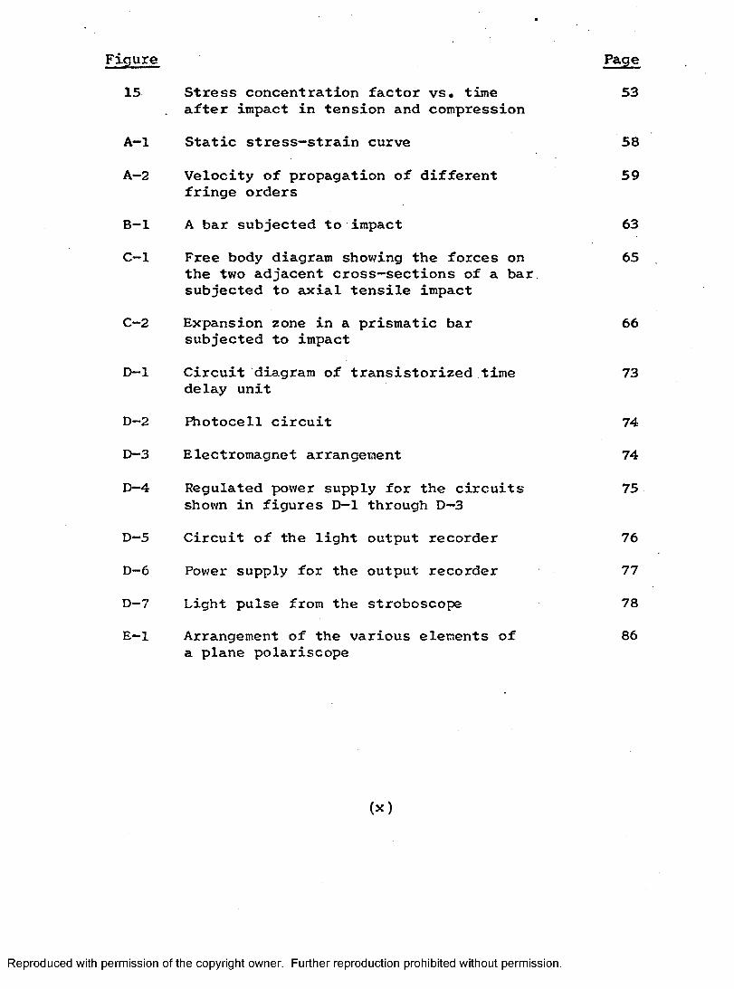
Figure Page15 Stress concentration factor vs. time 53
after impact in tension and compression
A—1 Static stress—strain curve 58
A—2 Velocity of propagation of different 59fringe orders
B-1 A bar subjected to impact 63
C—1 Free body diagram showing the forces on 65the two adjacent cross-sections of a bar. subjected to axial tensile impact
C—2 Expansion zone in a prismatic bar 66subjected to impact
D— 1 Circuit diagram of transistorized time 73delay unit
D—2 Photocell circuit 74
D-3 Electromagnet arrangement 74
D—4 Regulated power supply for the circuits 75shown in figures D— 1 through D—3
D-5 Circuit of the light output recorder 76
D-6 Power supply for the output recorder 77
D-7 Light pulse from the stroboscope 78
E—1 Arrangement of the various elements of 86a plane polariscope
(x)
Reproduced with permission of the copyright owner. Further reproduction prohibited without permission.
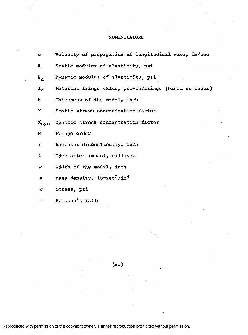
NOMENCLATURE
C Velocity of propagation of longitudinal wave, in/sec
E Static modulus of elasticity, psi
Ej Dynamic modulus of elasticity, psi
f<r Material fringe value, psi-in/fringe (based on shear)
h Thickness of the model, inch
K Static stress concentration factor
Kjjyn Dynamic stress concentration factor
N Fringe order
r Radius cf discontinuity, inch
1: Time after impact, millisec
w Width of the model, inch
P Mass density, Ib-sec^/in^
a Stress, psi
Poisson's ratio
(xi)
Reproduced with permission of the copyright owner. Further reproduction prohibited without permission.

1, INTRODUCTION
1.1 Importance of Dynamic Stress Concentration
Analysis of the behaviour of discontinuities like holes,
notches, etc., present in a structure is of fundamental
importance. Such discontinuity alters the stress distribu
tion in its neighbourhood so that elementary stress equations
no longer describe the state of stress in the structure.
The increasing trend towards higher performances in
projectiles and other dynamically loaded structures has made
it imperative to know the stress concentration factors and
stress distribution at discontinuities. In dynamic loading,
the response of these discontinuities is different than in
the case of static loading. This is mainly because in impact
the action of an external force is not transmitted immediately
or invariably to all parts of the member. Deformations and
corresponding stresses thus produced are propagated in the
form of waves, which react differently than the corresponding
statically applied load,
1.2 Scope of this Investigation
The object of the present project was to carry out pre-
Reproduced with permission of the copyright owner. Further reproduction prohibited without permission.

2litninary investigations on stress concentration factors and
stress distribution in a member under dynamic load conditions.
The effect of the size of the discontinuity, the time after
impact and whether the impulse was tensile or compressive in
nature were the main factors considered.
The particular geometry considered here was a thin, finite
width plate containing a semicircular discontinuity on both
sides, A photoelastic technique of stress analysis was used
with the low modulus model material, Hysol 4485,
Reproduced with permission of the copyright owner. Further reproduction prohibited without permission.

2, LITERATURE REVIEW
2.1 Stress Concentration
The study of stress concentration has been a field of wide
interest, since it gives basic information to the designer
about the probable response of irregularities which are
inevitable in any design. Many papers have been published
which give the value of stress concentration factors under
static load conditions found from experimental and theoretical
investigations. Research conducted by Coker and Filon (2),
Maunsell (19), Neuber (22), Ling (17), Howland (13), Ibrahim
and McCallion (14), etc, theoretically and by Wahl and
Eeeuwkes (28), Frocht (11), etc, experimentally has provided
a great deal of useful information on the behaviour of the
most common discontinuities under static load conditions.
The Engineering Sciences Data Unit of the Royal Aeronautical
Society and the Institute of Mechanical Engineers has recently
published extensive design data sheets on stress concentration
factors (9),
2.2 Dynamic Stress Concentration
With the establishment of the fact that the discontinuities
react differently in dynamic loading, it would be of interest3
Reproduced with permission of the copyright owner. Further reproduction prohibited without permission.

to know their exact reaction in actual practice.
Relatively few investigations have been made in this area
because of the complex nature of the problem. So far as the
author is aware, the particular geometry of a semicircular
groove on either side of a thin rectangular plate has not
been analyzed by any worker. However, plates with a circular
discontinuity at the centre have been of interest to a few,
Pao (24) has theoretically studied the effect of a plane,
compressional wave around a circular cavity in an infinitely
extended, thin elastic plate. He tackled this problem
basically as one of the scattering of stress waves, which, in
fact, more closely approximates the phenomenon of vibratory
loading. He established that the dynamic stress concentration
factors are dependent on the hole size, the incident wave
length and Poisson*s ratio for the plate material and at
certain wavelengths, the stress concentration factors are
larger than those encountered under static loading.
Dally and Halblieb (3) studied a similar problem photo—
elastically and noted that the dynamic stress concentrations
differ significantly from the static stress concentrations
and that this difference is dependent on the geometry of the
model.
Reproduced with permission of the copyright owner. Further reproduction prohibited without permission.

5North and Taylor (20) in a similar approach observed that
the dynamic stress concentration factors do not experience
the very large values characteristic of the static loading
conditions. They also noted that the dynamic stress concen
tration factors varied almost linearly with the ratio of hole
diameter to width of the plate. The same effect was observed
by Dally and Halblieb (3) as well. It should be noted that
Dally and Halblieb (3) and North and Taylor (20) did not
consider the effect of incident wavelength or Poisson's ratio.
Shea (26) approached the same problem using strain gauges
on thin plexiglass. He concentrated on the effect of pulse
wavelength and observed that dynamic concentration factor
varies significantly with pulse wavelength. He, however, '
concluded that the value of dynamic stress concentration factor
is significantly lower than the static value,
Flynn (10) and Durelli and Dally (6) also investigated the
same problem, but their investigations were of preliminary
nature and nothing very significant was observed.
It should be noted that all workers have confined their
studies to the effect of compressive loading, hence it was
considered of interest to determine the effect of tensile
waves in the present study. In one of his recent papers,
Davison (5) has suspected a difference in the response of
Reproduced with permission of the copyright owner. Further reproduction prohibited without permission.

the material to tensile and compressive loadings respectively.
He has attributed this difference toward the possibility of a
material changing its properties under the two types of
loading. In his paper, he also establishes the criterion for
the existence of shock waves.
Reproduced with permission of the copyright owner. Further reproduction prohibited without permission.

3. THEORETICAL AND EXPERIMENTAL CONSIDERATIONS
3,1 Stress Wave Propagation
It has been recognized that a dynamic load can create
stress waves in a medium. In the event of loading such as
that occurring in the present case (a weight falling on a
thin, long, rectangular bar), the waves generated are longi
tudinal (see Appendix C), The velocity of propagation of
these stress waves along the bar can be expressed as
^ ” y d/pwhere E^ = dynamic modulus of elasticity of the
material of the bar,
p = mass density of the material,
and C = propagation velocity of a longitudinal wave.
Dally, Riley and Durelli (4) in their paper established
that in dynamic photoelasticity, the fringes follow the same
law of propagation and reflection as the law for stress waves.
They used a rectangular strut subjected to an axial impact to
illustrate the potentiality of the method of photoelasticity
in visualizing the stress waves in the form of fringes. So
the study of stress waves is essentially the study of these
photoelastic fringes.
Reproduced with permission of the copyright owner. Further reproduction prohibited without permission.

83*2 The Effect of Impact Pulse Duration
The phenomenon of dynamic loading can be divided into
three main groups, viz, (a) processes with a quasistatic
state of stress, (b) vibrations, and (c) the stress waves
(Ref, 26), The titi of contact of the falling weight with
the body is an important factor in categorizing the process
of loading into one of the above groups. Briefly, a quasi-
static state of stress would occur if the time of contact
during impact is much longer than the time of one free—
vibration cycle or the time that a stress wave would take
in passing through the body. This state of stress can more
closely be approximated by static loading conditions and no
real dynamic effect is observed, A state of vibration would
occur if the time of contact is the same as the time of one
cycle of resonance frequency. Finally, the stress waves are
produced only if the time of contact is shorter than the
time of one cycle of a free vibration at resonant frequency,
which for this material and geometry is about three milli
seconds.
Hence, it is apparent that in order to produce any
effective dynamic loading, the time of contact in the process
of impact should be much shorter than the time that a stress
pulse would take to pass through the body.
Reproduced with permission of the copyright owner. Further reproduction prohibited without permission.

3,3 Use of Low Modulus Model Materials
Urethane rubber, commercially known as Hysol 4485 was used
as the model material in obtaining biréfringent information,
Hysol 4485 has an exceptionally low modulus of elasticity of
about 500 psi.
Since the velocity of propagation of the stress waves is
proportional to the square root of the modulus (c^ = E^/p ),
such a low value of modulus reduces the velocity in the model
to a great extent compared to the conventional, more rigid
photoelastic model materials. The low velocity of propagation
helps the investigation in two ways:
1, Slow moving fringes can be photographed relatively
easily,
2, It takes longer for a stress wave to pass through
the body. This makes it possible to satisfy the
dynamic loading condition when a falling mass
generates the impact load.
Besides this, Hysol 4485 has a very high sensitivity. It
exhibits low strain sensitivity so that the time edge effects
are negligible,
Hysol 4485, however, suffers from certain undesirable
characteristics. It exhibits pronounced deviation from
linearity in stress-strain relation at higher stress level.
Reproduced with permission of the copyright owner. Further reproduction prohibited without permission.

10Like many other photoelastic material* its viscoelastic
behaviour is prominent. Finally, Hysol 4485 has relatively
poor machinability,
3.4 Dynamic Stress Concentration Factors
In this report, the dynamic stress concentration factor
has been defined as
Kd(t) = (1)(%om(t)
where “ the maximum dynamic stress at the
boundary of discontinuity as a
function of time, and
Onom(t) “ the stress that would occur at
the same instant and position if
no discontinuity existed.
By making the assumption that the stress waves are only
longitudinal in the present investigation (see Appendix C),
and applying the stress optic law (Appendix E), equation (1)
can be reduced to
( t ) = max (t ) X ^0" nora(f) X Nnom(t) (2)
where f g max(t) = the maximum stress opticalcoefficient.
Reproduced with permission of the copyright owner. Further reproduction prohibited without permission.

11±(f nom(t) “ the nominal stress optical
coefficient, ’
^max(t) “ the maximum fringe order obtained
at the boundary of discontinuity,
aoid
Nnom(t) = the fringe order at the same
position and time if no discon
tinuity existed.
Dally, Durelli and Riley (4) observed that for Hysol 4485
for a large range of strain rate (8 in/in-sec to 65 in/in-sec)
f<r max(t) equal to nom(t) all values of t. In the present investigation, the strain rate had been estimated as
about 17 in/in—sec. This reduces equation (2) to
■ S sIt should be noted that the conventional definition of
stress concentration factor is different than the one given
above. It is generally defined as
K = Ohom
where O^iom Is calculated by using the net area of
cross-section at the position of the discontinuity.
Reproduced with permission of the copyright owner. Further reproduction prohibited without permission.

4, OUTLINE OF EXPERIMENTAL PROCEDURE
4.1 Particular Problem Studied
The problem involved studying the effect of tensile
dynamic loading on stress concentration factors at a dis
continuity, The discontinuities were in the form of semi
circular notches on both the sides of the model, Hysol 4485,
Urethane rubber was used as the model material.
Loading was accomplished by dropping a guided steel
weight of 1-1/2 ounces a distance of 40 inches onto the top
of the load—cell which, in turn, loaded the model in tension,
(See figures 1 and 2,)
4.2 Description of the modelsThe models were machined from a 1/4 inch thick Urethane
rubber sheet. The geometric details of the models tested are
shown in figure 3,
4.3 Technique of Recording the Phenomenon
The repeatability technique was used to record the biré
fringent information. The main requisites for this technique,
besides a conventional polariscope, are a still camera, a
light source which must give a single flash of high intensity
12
Reproduced with permission of the copyright owner. Further reproduction prohibited without permission.

13and short duration, a triggering device synchronized with
the event and a delay circuit. This works as follows;
a. The event begins when a steel weight is released
from its elevated position.
b. The falling weight trips a photoelectric trigger
that monitors the time delay,
c. The weight impacts the load cell on the model and
the fringes begin propagating the length of the
model. This impact also triggers the time delay
circuit,
d. The output from the time delay circuit triggers the
light source and thus a photograph is recorded at a
predetermined time as given by the time delay
circuit,
e. The repetition of the same procedure for different
delay times gives a series of photographs, describing
the entire event.
It should be noted that the camera is left wide open
throughout each cycle and the light source acts as its own
shutter. (See figure 1.)
In this investigation, the falling weight initiates the
triggering pulse by shorting an electrical contact while
striking the load cell. Although a fine delay unit was
Reproduced with permission of the copyright owner. Further reproduction prohibited without permission.

14assembled in the University Research shop, the incorporated
delay circuit of a Tektronix 555 oscilloscope was found
more reliable and easier to handle, and it was used to delay
the pulse throughout the study*
This delayed output from the oscilloscope externally
triggered the light source* The light source used was a
high intensity stroboscope, which provides a light pulse of
about 10 microseconds duration (Appendix D), In this time
interval, the longitudinal wave moves approximately *033
inches and the action is effectively stopped.
Type 47 Polaroid film, which has a very high speed
rating of 3000 ASA was used* The description of the complete
equipment used is given in Appendix D,
The repeatability technique of recording the birefringence
information is probably the best, since it gives large,
accurate, full—field photographs* The high degree of repeat
ability demonstrated in figure 4 shows the potential of the
method.
Reproduced with permission of the copyright owner. Further reproduction prohibited without permission.

5* RESULTS AND DISCUSSION
5.1 Birefringence Photographs
5*1.1 Birefringence Photographs Showing Fringe Propa
gation in a Model Without Discontinuity — Figure 5 is a
series of biréfringent photographs showing the propagation
of fringes in a model without discontinuity. The models
were loaded in tensile impact initiated at the bottom of
the photograph. Photograph 1 shows the no-load condition.
The following should be noted:
a, A-A is the position of the centreline of all dis
continuities of different sizes*
b, B and C are the fringes due to clamping stresses and
should not be mistaken as loading stress,
c. All irregular dark and light spots, such as D, are
due to uneven distribution of light around the
filament of the light source*
d. Dark edges on both the sides of the model show the
poor machinability of Urethane rubber; also, since
the light field is not parallel, boundary definition
is not good*
15
Reproduced with permission of the copyright owner. Further reproduction prohibited without permission.

16The half-order fringe can be seen in photograph 2 of
figure 5, Warping of the plane section of the bar is
suggested by the prominent curvature shown by this half-
order fringe. The 1,5 order fringe is almost straight and
the 2,5 order fringe, which appears in photograph 7, is
straight or slightly curved in the opposite direction. This
phenomenon was expected and has been justified theoretically
by Jones and Ellis (15) as a result of the development of a
two dimensional state of stress. An inspection of photographs
from 2 to 7, however, shows that the fringes have a tendency
to reduce their curvature as they propagate. This effect,
however, has not been considered when describing the stress
concentration factor which was defined for uniaxial stress,
(Sec, 3,1,1*)
It can be confirmed from these photographs that fringes
of different order move at different but almost constant
velocities* Velocity of the half—order fringe was determined
as 3250 inches per second. It is worth mentioning here that
Dally, Riley, and Durelli (4) found the half-order fringe
velocity to be as high as 3420 inch/sec in the same material —
Urethane rubber. Since the velocity of propagation is a
function of the material properties like modulus of elasticity
and density, it suggests that the material properties vary
from lot to lot to an appreciable extent. Figure A-2 of
Reproduced with permission of the copyright owner. Further reproduction prohibited without permission.
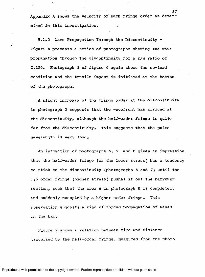
17Appendix A shows the velocity of each fringe order as deter
mined in this investigation.
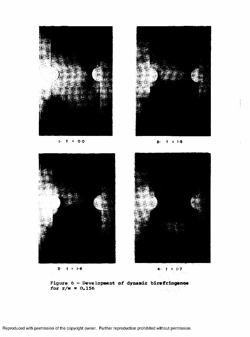
5,1,2 Wave Propagation Through the Discontinuity —
Figure 6 presents a series of photographs showing the wave
propagation through the discontinuity for a r/w ratio of
0,156, Photograph 1 of figure 6 again shows the no-load
condition and the tensile impact is initiated at the bottom
of the photograph©
A slight increase of the fringe order at the discontinuity
in photograph 2 suggests that the wavefront has arrived at
the discontinuity, although the half-order fringe is quite
far from the discontinuity. This suggests that the pulse
wavelength is very long.
An inspection of photographs 6 , 7 and 8 gives an impression
that the half-order fringe (or the lower stress) has a tendency
to stick to the discontinuity (photographs 6 and 7) until the
1,5 order fringe (higher stress) pushes it out the narrower
section, such that the area A in photograph 8 is completely
and suddenly occupied by a higher order fringe. This
observation suggests a kind of forced propagation of waves
in the bar.
Figure 7 shows a relation between time and distance
traversed by the half-order fringe, measured from the photo-
Reproduced with permission of the copyright owner. Further reproduction prohibited without permission.

18graphs of figure 6 * The datum of the measurements was a
point about 0,9 inch below the centreline of the discontin
uity, The half—order fringe arrives at this point 1,5
milliseconds after the impact.
The slope of this curve at any point, therefore, gives
the velocity of half—order fringe at that moment.
Three different zones A, B, and C of the curve are
apparent. Lines ab and cd represent the lower and the upper
boundaries of the discontinuity respectively.
The linear portion Πof the curve in zone A shows the
smooth upbound motion of the wave with almost constant
velocity. Beginning at point E, the slope of the line
decreases rapidly, suggesting a very low wave velocity in
zone B, In zone C, this trend reverses and the slope reaches
a terminal value that is approximately 35 per cent greater
than that in zone A,
It should be noted that zone B starts at a point a little
lower than the beginning of the discontinuity and extends to
about 2 0 per cent of the span of the hole.
It appears that an analogy can be established between the
fringe propagation through the discontinuity and the fluid
flow through a constriction.
Reproduced with permission of the copyright owner. Further reproduction prohibited without permission.

19Velocity of flow goes down at a point just before the
entrance to the nozzle and keeps falling down to a point a
little after the entrance, forming a similar zone B, After
that, the velocity shoots up according to the change in area
of cross—section, forming something similar to zone C of our
case*
5*2 Graphic Interpretation of Photoelastic Data Obtained
from the Biréfringent Information
5.2*1 Stress Distribution Around the Discontinuity -
Figure 8 shows the distribution of stress around one inch
diameter discontinuity 3,5 milliseconds after impact. The
highest fringe order of 9,6 fringes was found at the centre
of the hole ( 0 = O”), To compare this stress distribution
under dynamic loading to that under static loading, the same
model was loaded to 9.6 fringes under static tensile loading,
and this stress distribution is also shown in figure 8 ,
An inspection of figure 8 shows that at 0 close to 90°,
the associated stresses in the dynamic case are higher than
in the static case. This observation probably reveals the
significant difference between dynamic and static loadings.
It is entirely possible, indeed probable, that in the dynamic
case, some of the energy associated with the wavefront is captured by the corners, which is impossible under normal
Reproduced with permission of the copyright owner. Further reproduction prohibited without permission.

20static conditions.
5.2.2 Maximum Fringe Order as a Function of Time —
Figure 9 shows the effect of the time after impact on maximum
fringe order at the discontinuity,
5.2.3 Effect of Time after Impact on Stress Concentration
Factor — Figure 10 shows the variation of stress concentration
factor with time lapse after impact. It should be noted that
dynamic stress concentration factor is always lower than the
static stress concentration factor in the entire range
studied. This difference between the stress concentration
factors varies from 15 per cent to 50 per cent — depending
upon the time after impact. This effect has been observed
by many workers (Ref, 3, 12, 21, 26) but could not be explained
very satisfactorily© The interesting result mentioned in
section 5,2,1 may probably explain this behaviour. It was
expected that some of the energy associated with wavefront
gets captured by the corners and because a part of the
energy is so removed to an area of low stress, it is reason
able to expect lower stress concentration.
It should also be noted that dynamic stress concentration
factor is time dependent. The same effect was observed by
Dally and Halblieb (3) and North and Taylor (21); although
theoretically Pao (24) showed that dynamic stress concentra-
Reproduced with permission of the copyright owner. Further reproduction prohibited without permission.

21tion depends only on size of the discontinuity, impulse
wavelength and Poisson's ratio. Both of these latter para
meters are constant here.
The trend towards increasing stress concentration as the
time after impact increases, however, seems to be reasonable
and can be explained. Although no actual measurements were
made to record the pulse shape, figure 1 1 , which has been
taken from an investigation by Clark (1) would suffice to
give the explanation. The wavefront has relatively low energy
associated with it. As the wavefront reaches the discontinuity,
the part of the energy associated with it which is captured .
by the low stress area, forms an appreciable fraction of the
total energy. Now, as the latter part of the stress pulse
approaches the discontinuity, little or no energy is
captured by the corners since they are already stressed,
thus increasing the concentration at the critical area pro
gressively, This would obviously give rise to progressively
higher stress concentration factors till the peak of the
pulse reaches the position of the discontinuity. If the
study were extended to a longer period after impact, it
should be expected that the stress concentration factor would
tend to decrease as the trailing part of the pulse passes
through the discontinuity. From the curves in figure 10, this
maximum trend is evident, although not completely established.
Reproduced with permission of the copyright owner. Further reproduction prohibited without permission.

225*2.4 Dynamic Stress Concentration Factor as a Function
of r/w Ratio — Figure 12 shows the effect of the size of
discontinuity on stress concentration factor. Values of static
stress concentration factor have been obtained from Peterson
(25).
Figure 13 shows the curves giving per cent decrease of
dynamic stress concentration factor over the corresponding
static value for various hole ratios. A well defined minima
can be noticed in every curve. The difference in the two
values decreases for low values of r/w ratios and then
increases rapidly.
It appears that the net effect of the following two factors
is responsible for this behaviour. Firstly, the deflection
of the energy in the low stress area. This effect would tend
to decrease the stress level. Secondly, the reduction of the
area at the discontinuity, which tends to increase the stress
level.
The initial portion of the curve suggests that the former
factor is gradually losing its effect with the increase in
r/w ratio until its value reaches about 0,2, At this point,
the size of the discontinuity starts getting so large that
the wavefront tends to see it as more of an infinite surface
and reflects from it, thus reducing the boundary stress.
Reproduced with permission of the copyright owner. Further reproduction prohibited without permission.

23An attempt was made to correlate the dynamic stress concentra
tion factor to the hole ratio by a mathematical expression.
The following empirical equation for the dynamic stress
concentration at 2 , 2 milliseconds after impact gives values
agreeing approximately with the test results (see figure 1 2 ),
K^yn = 1.615 + 3.301 (r/w) + 17.767 (r/w)^ - 64.097 (r/w)3
(0.08 < r/w < 0.26)
Wahl and Beeuwkes (28) found a similar equation^ for the
static stress concentration factor as
K = 2.75 + 1.28 (r/w)2 + 8,00 (r/w)^
5,2,5 Comparison of Dynamic Stress Concentration Factors
under Tensile and Compressive Impact — A model with r/w ratio
of 0,156 was tested for compression impact also. Dynamic
stress concentration factor as determined in this case is
given in figures 14 and 15 as a function of time and compared
with the results of tension impact.
It is apparent that dynamic stress concentration factor
under tensile and compressive loading is equivalent until
about 2 milliseconds after impact, after which the concentra
tion factor obtained under compression impact is lower than
1 This equation has been modified according to the changed definition of stress concentration factor used here. The actual equation given by Wahl and Beeuwkes (28) is
K = 2,75 - 2.75 d/w + 0,32 (d/w)^ + 0.68 (d/w)^
Reproduced with permission of the copyright owner. Further reproduction prohibited without permission.

24that obtained under tension impact#
It is quite probable that the tensile properties of the
material may be different from the compressive properties
which may give rise to the difference in wave propagation*
It should be noted, however, that a difference of only two
per cent was found between the values of concentration
factors under tension and compression, which may be attri
buted to experimental error* Although every effort was made
to have the same physical arrangement of loading in both
cases, it was found hard to load the model in compression
because of its flexibility#
Davison (5) established, by purely theoretical considerations,
that a condition of shock prevails when the wave speed increases
upon the passage of the disturbance and centred simple waves
prevail when the wave speed decreases upon the passage of the
disturbance* It was observed that the velocity of fringe
propagation increases when it passes through the major portion
of the discontinuity (see section 5*1*2 — chapter 5), Figure
7 shows an increase of approximately 35 per cent in the fringe
velocity while passing through zone C* Thus, it can rightly
be suspected that it is a condition of shock that is being
observed in zone C of the model# However, Davison showed
that the necessary condition for such a situation is that the
material be "hardening" in tension* It is possible that the
Reproduced with permission of the copyright owner. Further reproduction prohibited without permission.

25material used behaves as a hardening material in dynamic
loading at high strain rate, although no experiment was or
could be executed with the existing apparatus to test this.
The static ttsts for the material indicate that it is not a
hardening material; however, the viscoelastic nature of this
material precludes the assumption that this is still true at
higher strain rates,
5,3 Optimum Design Criteria
If one calculates the maximum stress at this type of
discontinuity theoretically, assuming that all of the
potential energy of the falling weight is absorbed in the
model elastically, and that the static stress concentration
factors are representative, then the design in this material
would certainly be conservative, i.e. this theory gives a
stress that is at least 80 per cent higher than actually
exists (see Appendix B ) . In many situations, this is accep
table since an experimental program is not possible or
economical however, when cost and particularly weight
considerations are important, then this approximate answer
is unacceptable, particularly if 45 per cent of the area can
be removed, thus reducing the weight. Similarly, employing
a simplified stress wave propagation theory (see Appendix C)
and corresponding static stress concentration factor, the
result is some 280 per cent conservative.
168087 UNIVERSITY OF WINDSOR LIBRARY
Reproduced with permission of the copyright owner. Further reproduction prohibited without permission.

265*4 Experimental Error - Estimation
Although no actual calculations can be made to determine
the experimental errors, the following has been estimated
after various trials :
a. Repeatability of the Experiment
It is estimated that the whole experiment can be
repeated within a range of - 5 per cent. This high
repeatability can be attributed towards the use of
precision controls and a reliable technique of
recording the phenomenon*
b* Interpretation of the Information
It is estimated that the interpretation of the
biréfringent information can involve an error as
high as - 15 per cent. This is because of poor
photographs resulting from the use of the low
intensity, nonmonochromatic, relatively long duration
light pulse.
Reproduced with permission of the copyright owner. Further reproduction prohibited without permission.

6 . RECOMMENDATION FOR FUTURE WORK AND IMPROVEMENTS
6,1 Suggestions for Future Work
(1) Since it has been recognized that dynamic stress
concentration factor is dependent on pulse wavelength.
Poisson‘s ratio and the time after impact, an extensive
study should be conducted involving all the above parameters,
(2) The semicircular discontinuity provides sharp corners
that form the region of low stress. It was found that a part
of the energy of the propagating disturbance gets captured
by this low stress area. Different behaviour should be
expected from a discontinuity which does not provide a
similar low stress region. It would, therefore, be of interest
to study the behaviour of discontinuities of other than a
semicircular nature.
(3) Models of different width should be used to make the
study more general.
(4) Use of more than one model material is recommended
since it is suspected that the material properties in tension
may be different from its properties in compression.
(5) Model material should be completely calibrated
dynamically for stress and strain optical coefficients and
modulus of elasticity.27
Reproduced with permission of the copyright owner. Further reproduction prohibited without permission.

286,2 Suggestions for Improvements
(1) Improvements must be made in the present setup for
producing tension impact such as :
(i) Some stiffer material should replace bakelite
for the load cell. Magnesium can make a good
substitute,
(ii) The motion of the load cell should be guided
to prevent it from side swaying,
(2) Since a stress pulse of shorter wavelength is desirable,
it is suggested that loading by an exploding charge or by a
propagating missile be considered,
(3) Efforts should be made to have accurate measurements\of
(i) duration of impact, and
(ii) variation of applied load with time.
This would assist in having a comparatively clear view of the
whole phenomenon,
(4) The low intensity of the light obtained from the
stroboscope made it impossible to use monochromatic light.
This has resulted in the poor biréfringent photographs, A
ruby laser can be an ideal substitute for light source here,
since its output has almost all the desirable qualities for
use in dynamic work; namely, highly intense, monochromatic,
polarized, parallel and a very short duration of light pulse.
Reproduced with permission of the copyright owner. Further reproduction prohibited without permission.

7 CONCLUSIONS
(1) Dynamic stress concentration factor, as determined
in this study and in the region of r/w ratio tested, is always
lower than the corresponding static value, in some cases from
15 per cent to 50 per cent less than the static value
depending on the time after impact,
(2) The difference between dynamic and static concentra
tion factors diverges rapidly for large r/w ratios. It
appears that the wavefront tends to see the increasing size
of discontinuity as more of an infinite surface, thus
reflecting from it and reducing the boundary stress,
(3) Dynamic stress concentration factor depends signi
ficantly on the time after impact. It was found to vary
almost linearly from 1,7 milliseconds to 2.1 milliseconds.
After 2,1 milliseconds of impact, it was almost constant for
higher values of r/w ratio. For the r/w ratio of 0,093,
however, it had a tendency to increase throughout the time
span considered (1,7 milliseconds to 2,3 milliseconds),
(4) Little difference is apparent in stress concentration
for a tensile and compressive dynamic load,
(5) It was found that in case of impact, a part of the
29
Reproduced with permission of the copyright owner. Further reproduction prohibited without permission.

30energy gets captured by the region of low stress, thus
lowering the stress concentration at the critical points and
therefore it would appear that streamlining the discontinuity
would not improve the stress concentration in the dynamic
case as much as it does in the static case,
(6 ) The theoretical estimation of the maximum stress
induced during the impact yields a value which is at least
80 per cent higher than actually exists (see Appendix B).
(7) In general design problems,- it would appear that
the use of the recorded values for static stress concentra
tion factor will give conservative results when dynamic loads
are encountered.
Reproduced with permission of the copyright owner. Further reproduction prohibited without permission.

BIBLIOGRAPHY
1, Clark, A.B.J. "Static and Dynamic Calibration of aFhotoelastic Model Material, CR—39," S.E*S«A. Proceedings, XIV (NO.l), 195-204,
2, Coker, E,G,, and L,N,G, Filon. Photoelasticity,Cambridge: Cambridge University Press, 1931,
3, Dally, J,W, and W.F. Halbleib, "Dynamic Stress Concentrations at Circular Holes in Struts," The Journal of Mechanical Engineering Science, March, 1965
4, Dally, J,W*, W.F, Riley, and A,J, Durelli, "A Photo-elastic Approach to Transient Stress Problems Employing Low—Modulus Materials," Journal of Applied Mechanics, Trans, A.S.M.E., December, 1959, 613-620,
c::>, Davison, L. "Propagation of Plane Waves of FiniteAmplitude in Elastic Solids," 2* Mech, Fhys, Solids,XIV (1966) 249-270,
6 , Durelli, A.J, and J,W. Dally, "Stress ConcentrationFactors under Dynamic Loading Conditions," Journal of Mechanical Engineering Science, I (NO.l, June 1959), 1.
7, Durelli, A.J, and W.F, Riley Introduction to Photomechanics, Englenwood Cliffs, N.J., Prentice—Hall,Inc., 1965,
8 o Durelli, A.J, and W,F, Riley, "Stress Distribution on theBoundary of a Circular Hole in a Large Plate During Passage of a Stress Pulse of Long Duration," Journal of Applied Mechanics, Tyans, A ,S,M,E . , (June , 1961), 245-251.
Reproduced with permission of the copyright owner. Further reproduction prohibited without permission.

329, Engineering Sciences Data Unit, Stress Concentration
Data, NOo 65004, London: Engineering Sciences Data Unit, Inst* Mech, Engrs,, 1965,
10, Flynn, I.D, "Studies in Dynamic Fhotoelasticity,"Ph,D, thesis, Illinois Institute of Technology,1954,
11, Frocht, M,M, "Factors of Stress Concentration Determinedby Fhotoelasticity," Journal of Applied Mechanics, Trans, A.S.M.E,
12, Halbleib, W.F. "The Experimental Determination of theStress Concentration Factors at the Boundary of a Central Circular Hole with Both Soft and Rigid Struts Having Various Hole Diameters to Width Ratios when Subjected to Longitudinal Dynamic Impact Loads," Ph,D, thesis, Cornell University, 1961,
13, Howland, R.C.J. "On the Stresses in the Neighbourhood ofa Circular Hole in a Strip Under Tension," Proc,Royal Society, 1930, (A229), 49,
14, Ibrahim, S.M, and H, McCallion, "Elastic Stress Concentration Factors in Finite Plates Under TensileLoads," Journal of Strain Analysis, I (No, 4, 1966),306-311,
15, Jones, 0,E, and A.T, Ellis, "Longitudinal Strain PulsePropagation in Wide Rectangular Bar—Part I,II," Journal of Applied Mechanics, Trans, A.S.M.E., I (No, 4, March 1963), 51—69,
16, Kuske, Albrech, "Photoelastic Research on DynamicStresses," Experimental Mechanics, VI (NO, 2, Feb. 1966) 105-112.
Reproduced with permission of the copyright owner. Further reproduction prohibited without permission.

3317. Ling, C.B. "Stress in a Notched Strip Under Tension,"
Journal o f Applied Mechanics, Trans. A.S.M.E., XIV (No. 4, Dec. 1947) 275.
18. Lubahn, J.D, "Comparison of Methods of Determining StressConcentration Factors," S.E.S.A. Proceedings, XVI (No, 2), 139-144,
19, Maunsell, F.G, "Stress in a Notched Plate Under Tension,"Philosophical Magazine, XXI (1936), 765,
20, North, W.P.T., and C.E, Taylor, "Dynamic Stress Concentration Using Photoelasticity and Laser Light Source," Experimental Mechanics, XVI (No, 7, July 1966) 337,
21, North, W.P.T. "A Laser Light Source in Dynamic Photo-elasticity," Ph.D. thesis, TAM department.University of Illinois, Urbana, 1965.
22. Neuber, H, "Theory of Notch Stresses: Principles forExact Stress Calculation," Julius Springer, Berlin,1937. Translated by F.A. Raven, David Taylor,Model Basin, Washington, D.C., Nov. 1945.
23. Ozane, J. "Strain Calibration in Dynamic Photoelasticity,"Master's thesis, TAM department. University of Illinois, Urbana, 1965.
24, Pao, Y.H, "Dynamical Stress Concentration in an ElasticPlate," Journal of Applied Mechanics, Trans, A.S.M.E. XXIX (No, 2, June, 1962), 299-305.
25» PPterson, R.E. Stress Concentration Design Factors, NewYork: John Wiley and Sons, Inc,
26. Shea, Richard. "Dynamic Stress Concentration Factors,"Experimental Mechanics, (January, 1964), 20—24,
Reproduced with permission of the copyright owner. Further reproduction prohibited without permission.

3427, Stein, K,0, "Dynamic Photoelasticity-A critical Review
and Experimental Study," Master’s thesis, TAM department, University of Illinois, Urbana, 1963,
28, Wahl, A,M, and Beeuwkes, R., Jr, "Stress ConcentrationProduced by Holes and Notches," Trans, A.S.M.E.LVI (1934), 617-625.
Reproduced with permission of the copyright owner. Further reproduction prohibited without permission.

35
PHOTO CELL
MECHANICAL:C O N T A C T
l o a d c e l l .
CAMERA
TORCL)P O L A R I S C O P E
EXTTRIGGER
DELAYEEOUTPUT TRIGGER S T R O B E
POWER
SUP PL YT E K T R O N I X 5 5 5 O S C I L L O S C O P E
TEKTRONIX 5 6 4 O S C I L L O S C O P E
VERTI N P U TB A S EB A S E A
Figure 1 - Block diagram, of the experimental arrangement
Reproduced with permission of the copyright owner. Further reproduction prohibited without permission.

UJ
>-q:
g<(TOCD<
Xa.<XooI -0X01
CdUJX3o
Reproduced with permission of the copyright owner. Further reproduction prohibited without permission.

373- 3/16 HOLES ON
^ -— -- —_|CVJ
CM
W = 21
♦ = i4
r = 2.5 ,116 16 8 2
ALL DIMENSIONS IN INCHES
Figure 3 - Dimensions of the models used
Reproduced with permission of the copyright owner. Further reproduction prohibited without permission.

Figure 4 - Repeatability testTime after impact - 1.7 milliseconds r/w - 0.25
Reproduced with permission of the copyright owner. Further reproduction prohibited without permission.

t = 0 0 t « I 30
3. t * 1-50 1*75
Figure 5 - Birefringence photographe showing the wave propagation in a model wlthoat any discontinuity
Reproduced with permission of the copyright owner. Further reproduction prohibited without permission.

5. t = 1.90
7. t = 2.10 8. t = 2.25Figure 5 (continued)
Reproduced with permission of the copyright owner. Further reproduction prohibited without permission.

9. t = 2.50 10. t = 2.60
11. t = 2.75 12.Figure 5 (continued)
t = 2.85
Reproduced with permission of the copyright owner. Further reproduction prohibited without permission.
|. t = 0 0 2* t = 15
3- t = 1-6 4- t ® 1-7
Figure 6 - Development of dynamic birefringence for r/w * 0*156
Reproduced with permission of the copyright owner. Further reproduction prohibited without permission.

5- t = 18 6- f = 19
7- t * 2-0 8- t = 2 1
Figure 6 (continued)
Reproduced with permission of the copyright owner. Further reproduction prohibited without permission.

9" t = 2 2 I0« t » 2 3
Figure 6 (continued)
Reproduced with permission of the copyright owner. Further reproduction prohibited without permission.

45
18
r/w = 0 25
o
oXICLcoÜch-zLÜ5 0-8 o <_JÛ.if)Q 06UJozoru_ 0 4
0 2
0 015 1-6 1-7 2018 19 21
TIME AFTER IMPACT , millisec
Figure 7 — Displacement of half-order fringe vSo time after impact
Reproduced with permission of the copyright owner. Further reproduction prohibited without permission.

46O0)
oCO
oN
ou>
olO
o■t
orO
OCM
o>0)i_O'O)TJCD
+»•H3
COu(A•H•OO+>•0c9Ow<c
g•H•H9•HU(A•H•0(A(A0*4■H(AU•H+»(C■*-»(A
•g<cü•HE<0CQ100
2 9•S'
00 CD CM
AdVQNnOQ 310H IV WSaWO 39Niaj
Reproduced with permission of the copyright owner. Further reproduction prohibited without permission.

47
HOLE RATIO r/w6 0 0 250
0 1880-1560:098
5 0
ccÜJoccoLÜCDzcnU- 3 0
2 0
0 015 175 2 0 225 2 5 275
TIME AFTER IMPACT, millisec
Figure 9 - Maximum fringe order at thediscontinuity vs. time after impact
Reproduced with permission of the copyright owner. Further reproduction prohibited without permission.

48
Q:Oh-O<ü_ZOH<ir
LUozoü(fi(fiLUCEt-(fi
3 5
3 0
2 5
2 0
15
1 0
STATICDYNAMIC
r/w* HOLE RATIO
____________r/w 025
•098,0188 015 6
r/ w= 0 25•188
•156
.098
15 I 75 2 0 2 25TIME AFTER IM P A C T, millisec
2-5
Figure 10 - Stress concentration factor vs. time after impact
Reproduced with permission of the copyright owner. Further reproduction prohibited without permission.

49
oôto
omCM
ooCM
OlO
o0)c/>o
ÜJ2
oo
olO
(D st <M o
ujo *iMVd90"inioso N ivd is jo aanindkMV
SW0)+»usou
(0•0M0 ü « M
1Ocmo
•HO(AOClXi+»EOk
Esu•SItsk+»W
Clk3k
Reproduced with permission of the copyright owner. Further reproduction prohibited without permission.

50
a:oh-o<ü_
Zot-<(Th-zLUüZoo
coenLUCHh-co
4 0
T IM E A F T E R IMPACT,millisec
3 0S T A T IC
020
00 05 010 015 0 20 0 25 0 30
HOLE RATIO, r/w
Figure 12 - Stress concentration factor vs, relative size of discontinuity
Reproduced with permission of the copyright owner. Further reproduction prohibited without permission.

51600
500t = T IM E A FTE R IM P A C T, mlllsec
400cO)Ük .<Da.
300
20-02
10 0
0 00 05 0 15010 0 20 0 25 0-30
HOLE RATIO , r / w
Figure 13 — Difference in dynamic and static concentration factor vs, time after impact
Reproduced with permission of the copyright owner. Further reproduction prohibited without permission.

52
TENSION
6*0 COMPRESSION
5 0
irLÜQtro
4 0
UJCDztr
^ 3 03X<2 2 0
0 015 1-75 2 0 2 25 2 5 2 75
TIME AFTER IMPACT, millisec
Figure 14 - Fringe order at the position of the discontinuity vs, time after impact in tension and compression in a model without discontinuity
UNIVERSITY Of WINDSOR UBRARY
Reproduced with permission of the copyright owner. Further reproduction prohibited without permission.

53
a: oI -o<
oh-<ceh-zLUOZo o
cotoLUcrH(O
3*0
25
2 0
15
HO LE RADIUS r/w=O I56
o T E N S IO N
X COMPRESSION
STATIC ( TE N S IO N )
DYNAMIC
15 I 75 2 0 2 25 2 5TIME AFTER IMPACT, millisec
2 75
Figure 15 - Stress concentration factor vs time after impact in tension and compression
Reproduced with permission of the copyright owner. Further reproduction prohibited without permission.

APPENDIX A
CALIBRATION OF HYSOL 4485
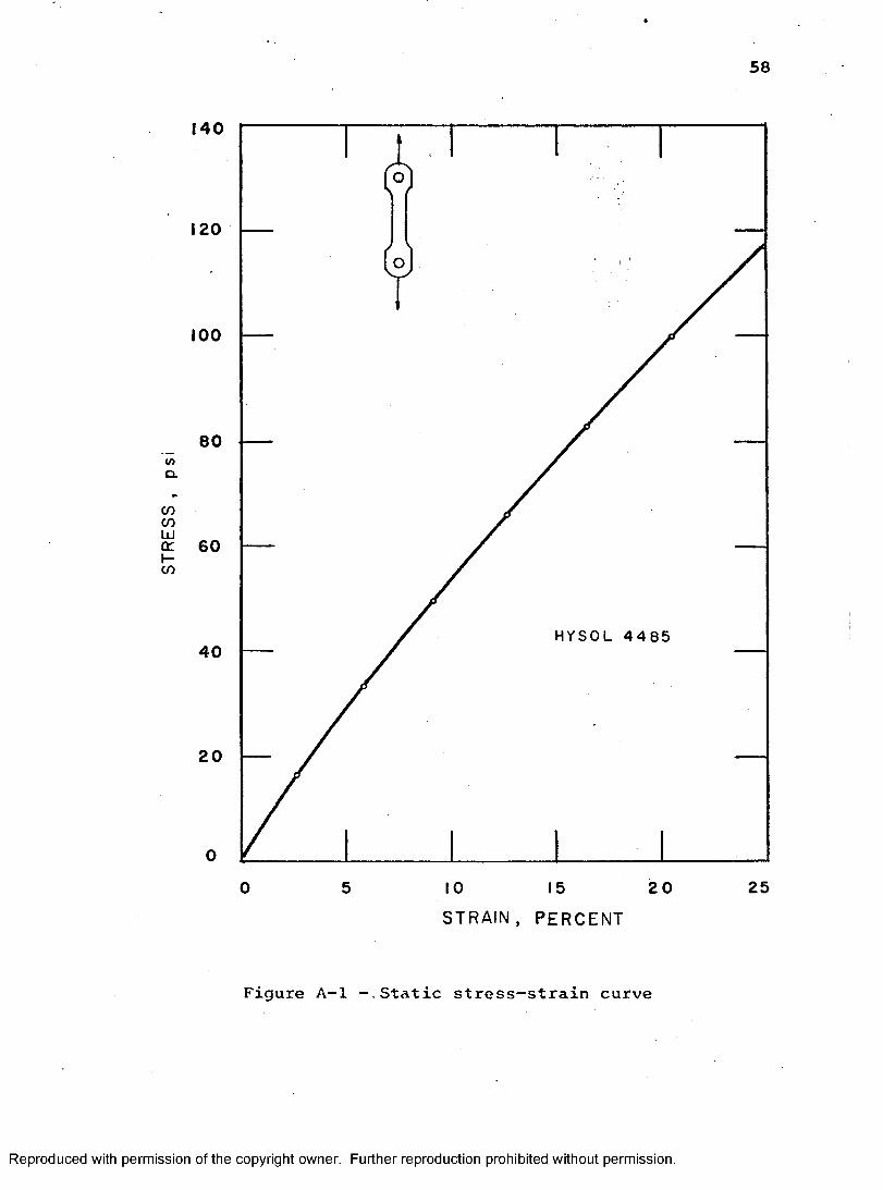
A,1 Static Calibration
(1) Modulus of Elasticity - E
A specimen, fabricated from Hysol 4485 was loaded in
tension. Figure A-1 shows the stress—strain curve obtained
by measuring load and elongation.
The stress level attained during the experiment can be
approximated to be in the range of 30 to 40 psi. The static
stress-strain curve of figure 14 has an almost constant slope
of 500 psi in this range. This gives E = 500 psi,
(2) Material Fringe Constant -
A circular disk of Hysol 4485 under diametral loading was
tested for determining the material fringe constant. It was
found that f = 0,51 psi-in/fringe (based on shear stress),
(3) Density — P
Density of the material was found to be2= Go0 0 0 1 0 0 lb-sec
in4(4) Poisson*s ratio is approximately 0,47,
54
Reproduced with permission of the copyright owner. Further reproduction prohibited without permission.

55A.2 Dynamic Calibration
A specimen of Hysol 4485 having the same dimensions as
given in figure 3 but without a discontinuity was tested.
Loading was in the same manner as in the case of models with
discontinuities. Velocities of fringe propagation were obtained
from the biréfringent photographs of the test mentioned above.
Figure A—2 shows the relation between velocity of propagation
and the fringe order. Each fringe itself propagates with
constant velocity, however.
Although no specific measurements were made for the dynamic
calibration of Hysol 4485, the following can be estimated,
(1) Dynamic Modulus of Elasticity - E^
The curve of figure A-2 was extrapolated to give the
velocity of propagation of the zero order fringe as 3300
inch/sec. An approximation to the dynamic modulus of elasticity
can be made by the relation Ej = p where
p is the mass density of material (0 , 0 0 0 1 0 0 lb-sec^/in^)and
c is the velocity of the zero order fringe (3300 in/sec)
which gives
E^ = 1089 psi
It should be noted that the accuracy of the above estima
tion would depend upon :
(i) The validity of assumptions that Poisson's ratio
is zero, the material is elastic, no inertial
Reproduced with permission of the copyright owner. Further reproduction prohibited without permission.

56dispersion occurs, and that the waves are longitudinal;
and
(ii) The accuracy in the determination of the velocity c*
(2) Dynamic Material Fringe Value
Previous authors have estimated the dynamic fringe value of
Hysol 4485 to be about 9 per cent higher than the corresponding
static value. Expecting similar behaviour of this material,
the dynamic fringe value can be approximated to be 0,556
psi-in/fringe.
An attempt was made to determine the value of f experi
mentally by the grid method [see Durelli and Riley (7)] * The
analysis, however, could not be completed because of the lack
of precise measurements of grid deformations. The procedure
planned for its evaluation is outlined below for reference,
a, A model of the dimensions shown in figure 3, but
without any discontinuity, is machined from a sheet
of Hysol 4485, and a 1/8 in, square grid is scribed
on its surface,
b, A no load photograph of the model is taken to record
the undeformed grid pattern,
c, It is then loaded dynamically emd the photographs of
the fringe propagation are obtained in the manner
outlined in section 4,3 of chapter four.
Reproduced with permission of the copyright owner. Further reproduction prohibited without permission.

57d. The displacement fields are obtained by measuring the
deformation of the grid under loaded conditions from
the photograph,
e. The strain fields are computed by differentiating the
displacement fields,
f* Then the material strain fringe value is given by
f. h (A.l)
where Cy = axial and transverse strains
respectively, at a point in the
model computed from the displacement
field, in/in*
N = Fringe order at the point
h = Model thickness, in
Then the stress fringe value
f, = - % r k
where = dynamic modulus of elasticity,psi
c = dynamic Poisson’s ratio
Dynamic Poisson's ratio can also be computed accurately
from the information obtained in this experiment.
Dynamic Poisson's ratio = - (A,3)Cx
A,3 Stress Pulse Duration
It is estimated that the duration of stress pulse was not
more than 1,25 milliseconds.
Reproduced with permission of the copyright owner. Further reproduction prohibited without permission.
58
V)CL
COCOÜJDC.Hco
140
1 2 0
100
80
60
HY S OL 4 4 8 540
20
0250 5 1 0 15 20
STRAIN, PERCENT
Figure A-1 -.Static stress-strain curve
Reproduced with permission of the copyright owner. Further reproduction prohibited without permission.

59
o0)w
JO I _
Xüzo1-<CD<ÛLOÙ1Û_ü_o
üO_JLU>
4 0
HYSOL 4485
3 0
2 0
00 0 5 1 0 15 2 0 2 5
FRINGE ORDER, N
Figure A-2 — Velocity of propagation of different fringe orders
Reproduced with permission of the copyright owner. Further reproduction prohibited without permission.

APPENDIX B
THEORETICAL AND EXPERIMENTAL DETERMINATION
OF MAXIMUM STRESS DURING IMPACT
Theoretical estimation of the maximum stress in a bar in
impact is based on the assumption that all of the potential
energy of the falling mass is absorbed elastically in the bar
in the form of the strain energy.
Let us consider a bar fixed at its upper end, A weight
falls from the height h on to the flange ab, stretching the
bar by an amount a • (See figure B-1,)
Then, the potential energy of the falling mass
= W(h + A )
wh ( A « h) (B.l)
Elastic energy stored in the bar = 1/2 P A
If P = static load to produce a deflection
A in the bar
A = area of X—section of the bar
E = modulus of elasticity of the bar material
then A = p//AE
60
Reproduced with permission of the copyright owner. Further reproduction prohibited without permission.

61and the elastic energy = P^^/2AE (B*2)
From the basic assumption
Potential energy = elastic energy stored
or Wh = p2//2 AE
or Wh = (j- a //2E
i.e (T = (B.3)
where or* = induced stress
B.l Stress in a Model Without Discontinuity
(1) Theoretical - The experimental values of different
elements in equation (B.3) are as follows
W = 1,5 oz,
h = 4 0 inch
E = 500 psi
A = 2 X 0,25 sq,in,I = 1 0 inch
Then the theoretical stress in the bar from equation (B,3)
^ h e o = 27,4 psi (B.4)
(2) Experimental —
Maximum fringe order N — 4 (figure 14)
Material fringe constant = 0,556 psi-in/fringe
(Appendix A)
Then the experimental stress in the bar
Reproduced with permission of the copyright owner. Further reproduction prohibited without permission.
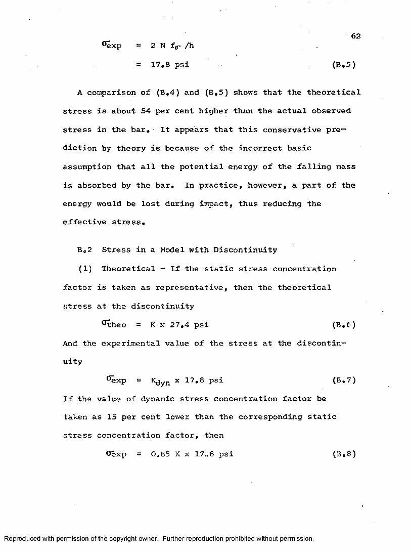
62Oexp = 2 N fjr /h
= 17.8 psi (B.5)
A comparison of (B.4) and (B.5) shows that the theoretical
stress is about 54 per cent higher than the actual observed
stress in the bar. It appears that this conservative pre
diction by theory is because of the incorrect basic
assumption that all the potential energy of the falling mass
is absorbed by the bar. In practice, however, a part of the
energy would be lost during impact, thus reducing the
effective stress.
B.2 Stress in a Model with Discontinuity
(1) Theoretical - If the static stress concentration
factor is taken as representative, then the theoretical
stress at the discontinuity
^theo = K X 27.4 psi (B.6 )
And the experimental value of the stress at the discontin
uity
®exp = X 17.8 psi (B.7)
If the value of dynamic stress concentration factor be
taken as 15 per cent lower than the corresponding static
stress concentration factor, then
Oexp = 0.85 K x 17.8 psi (B.8 )
Reproduced with permission of the copyright owner. Further reproduction prohibited without permission.

63A comparison of equations (B.6 ) and (B.8 ) indicates that the
theoretical estimation of the stress at the discontinuity
would be at least 80 per cent higher than the actual maximum
stress developed in impact.
In this theoretical treatment, it must be assumed that
a quasi—static state of stress is developed since the
propagation of a stress wave is not conceded.
//////////////
W
I_____ ! —»..îfîlK..
Figure B-1 - A bar subjected to impact
Reproduced with permission of the copyright owner. Further reproduction prohibited without permission.

APPENDIX C
STRESS WAVE PROPAGATim IN A RECTANGULAR BAR
It has been mentioned that the effect of impact is
propagated through the body in the form of elastic waves.
In this study, the problem has been considered as that of the
propagation of a longitudinal wave in an elastic bar.
Following are the assumptions made:
(1) Cross-sections of the bar remain plane during
deformation,
(2) Lateral motion of particles is unrestricted,
(3 ) Length of the wave is large compared to the cross-
sectional dimensions of the bar.
Let us consider a bar subjected to an axial tensile
impact. Strain in any section in x direction can be given
by
' I s (c-i)and the corresponding tensile force would be AE È 2 ,axwhere u = displacement in x direction
A = cross-sectional area
E = modulus of elasticity of the bar,
64
Reproduced with permission of the copyright owner. Further reproduction prohibited without permission.

65
AE 3uÔX
• dx r
Figure C— 1 — Free body diagram showing the forces on the two adjacent cross-sections of a bar subjected to axial tensile impact
Considering the free body diagram, the difference of
forces acting on two adjacent cross-sections,dx apart is
AE (— + dx ) - AEÔX 3x2= AE dx
d x ^
auax
(C.2)
Deformation in x direction is a function of time as well*
Hence, from Newton’s Law
where P is the density of the bar. So thatà£u Ôt2
or
= _LP ^2 = c 2 d^u
= éwhere c
The general solution of equation (C,3) is
u = f(x+ct) +G(x-ct)
(C.3)
(C.4)
(C.5)
From the simple physical considerations, it can be shown
that the second part of equation (C,5) represents a wave
travelling in the direction of x—axis with a constant speed c;
Reproduced with permission of the copyright owner. Further reproduction prohibited without permission.

66and the first part represents a wave travelling in opposite
direction with the same velocity* It should be noted that
the velocity of propagation depends only on the material
properties E and p *
The arbitrariness of solution (C*5) can be removed with
the help of initial conditions of the problem concerned,
C*1 Fixed Bar Subjected to Impact
Let us consider the case of a bar of uniform cross—section
loaded at one end by a suddenly applied uniform tensile
stress CT'(see figure C-2), It will develop a tensile zone
of very thin layers, particles of which would move with a
velocity V *
crc f
Figure C-2 - Expansion zone in a prismatic bar subjected to impact
If we take the direction of the wave propagation as
positive direction, the change in the length ct of the
expanded zone = ct ; and therefore, the velocity of
the particles in this region is
Reproduced with permission of the copyright owner. Further reproduction prohibited without permission.

67
a- ^ c (C,6 )Substituting the value of c from equation (C.4),
V = - (C.7)v E P
Minus sign indicates that the velocity of the particles
in the expansion zone is in a direction opposite to the
direction of wave propagation.
Let a rigid body with an impact velocity Vq hit the free
end of the bar, producing a uniform initial tensile stress (JZ «
From equation (C,7), this initial stress would be
(To = - Vjj^EP (C,8)By Newton’s Law, the impact force in the expansion zone is
balanced as given by the following relation
' " 5 7 = ■ (-«"A)or M ÉÜ - (T = 0 (C,9)dtwhere M = HA
= mass of the moving bodyArea of cross-section of the bar
Substituting the value of in equation (C.9) from
equation (C,7), we have
. a o : = 0 ( c . i o )
Solution of this differential equation is
0“ = 07 exp ( (C.ll)M
Reproduced with permission of the copyright owner. Further reproduction prohibited without permission.

68Equation (C,H), therefore, gives the stress at the end of
the bar at any time t after impact#'
C#2 Effect of Variable Cross—Section
If the area of cross-section of the bar is not uniform,
i#e, A = A(x), then the equation (C,10) becomes
^ ^ - Ë2 " + 0 “ = 0. J Ë P A(x) dt
The above equation involves two independent variables and
therefore is not easily solved as such. This indicates that
a case involving a bar with a discontinuity cannot be solved
by the theoretical considerations based on the elastic wave
propagation.
An estimate of the maximum stress in a model without dis
continuity can be made based on the assumption that the
stress propagates without dispersion down the bar.
From equation (C.8 ), the maximum stress that occurs at
the end of the bar
CTo = - Vo^Efwhere
Then,
V q = velocity of impact
= 176,0 in/sec (a weight falling through 40 in)
= - 176,0 yj » 0 0 0 1 x 1089
= 58,0 psi (C,12)
Reproduced with permission of the copyright owner. Further reproduction prohibited without permission.

69If the static stress concentration factor is taken as
representative, then the maximum stress in a model with
discontinuity is
CTq = 58.0 X K psi (C.13)
Again, if the value of dynamic stress concentration factor
is taken as 15 per cent lower than the corresponding static
stress concentration factor, then from equation (B.8 )
^ x p = 0,85 K X 17,8 psi (B,8 )
Hence, per cent difference in the theoretical and experi
mental estimation of maximum stress
= 280 per cent (C,14)
Reproduced with permission of the copyright owner. Further reproduction prohibited without permission.

APPENDIX D
DESCRIP T i m OF EQUIPMENT
D,1 Main Equipment
Figure 1 is a block diagram showing the different components
of the experimental setup used* The actual arrangement of the
laboratory equipment is shown in the photograph of figure 2 ,
Table 1 lists the essential components with their specifications.
Table 1 — Main components of the experimental equipment used
No. COMPONENT DETAILS1 Light Source Philips Stroboscope PR 9104
Flash duration lO^sec.
2 Polariscope 8 — 1 / 2 inch field circular polariscope
3 Camera Graflex Camera with polaroid back and long extension bellows
4 Loading frame With the provision of the adjustments in all the three planes to centre the falling mass on to the model
5 Loading cell Used to produce tension. Fabricated from Bakelite
70
Reproduced with permission of the copyright owner. Further reproduction prohibited without permission.

71D,2 Circuit Diagrams
The following circuits were designed and assembled by
Central Research Shop of the University of Windsor,
(1) Delay Circuit: A delay circuit having the provision
of giving two identical outputs was designed for the electronic
switching of a laser power supply. The circuit shown in
figure D-1 provided the delay ranging from 1 millisecond to
9 milliseconds. It had shown a high repeatability to the
extent of almost 1 0 0 per cent,
(2) Photo Trigger: One major problem involved in the
experiment is to accomplish highly repetitive fast switching
of the light source. Initially, the falling mass itself was
used to provide the triggering pulse by activating the photo
cell circuit, shown in figure D-2, At a later stage, however,
the photocell was used only to permit monitoring of the time
delay after impact and the primary triggering was initiated
by the falling mass which shorted an electrical contact.
Figure D-3 shows an electromagnet arrangement made to drop
the weight,
(3) Regulated Power Supply: A transistorized, regulated
power supply was also assembled (figure D-4), This had the
provision of supplying 21, 10, 5, and 2 volts needed for the
various circuits shown in figures D— 1 through D —3, This
Reproduced with permission of the copyright owner. Further reproduction prohibited without permission.

72circuit was an integrated part of the delay assembly of
figure D-1.
(4) Light Output Recorder and its Power Supply:
Figures D—5 and D - 6 show the circuits of the light output
recorder and its power supply respectively. The circuit was
initially designed for recording the output of a ruby laser
and had a very fast rise time of about 10 nanoseconds, A
trace of the light pulse from the stroboscope, as obtained
with the help of the recorder is shown in figure D-7,
Reproduced with permission of the copyright owner. Further reproduction prohibited without permission.

HR
o<m
% inMo,
O fO in
CJ\ /
z oN _
fOCSJ z O CJ
73
■f»♦rlC3>0)•oi•H
•00)N
•rlMO+>(A•rl(AC<|JM■M0:u0»«tf•rl•o+»•H3t>H•rlu1
Reproduced with permission of the copyright owner. Further reproduction prohibited without permission.

74
R 7+ IOV10 K
PCI
PUCE 2 2 2
TO J6
Figure D—2 — Photocell circuit
SW2
5V
T 0 + 5 V
ELECTRO - MAGNET
J7
Figure D-3 — Electromagnet arrangement
Reproduced with permission of the copyright owner. Further reproduction prohibited without permission.

75
<EOCJCJ
aCJ , — •-fC-N-c CJ h
in
in
lO ^ CJ
CJ
in
CJ,-----O CJr - o CJ
CJ
JtSM JU LIU U U L
O OSin00 ÜJ (O z o
oww4->•HSüw•HüO+»wom
3 en w 3oV4 Ho Æ1 * d r4
A•oOJ•H w«ts oD» en0 -HK k1
î25301•rik
Reproduced with permission of the copyright owner. Further reproduction prohibited without permission.

76
225
2 0 M F
P H O T O T U B E
12 a t 7
6 8 K
O U T P U T
9 3
Figure D-5 - Circuit of the light output recorder
Reproduced with permission of the copyright owner. Further reproduction prohibited without permission.

77
5 Y 3 G T
CHOKE(10x100)80.
I6Mf + 16 Mfg 2 4 t f
I 24 0*NEON
PILOT<k25"'
SLIDERLINE
SWITCH2 7 0 X
T R A N S F O R M E R (HAMMOND)
115
63 '
2 4 0
Figure D - 6 - Power supply for the output recorder
Reproduced with permission of the copyright owner. Further reproduction prohibited without permission.

78
Figure D-7 - Light pulse from the stroboscopeHorizontal scale - 5Vertical scale - 0.1Pulse duration - iq
Msec/division volt/division Msec (as measured at 5 0 % o f the pulse height)
Reproduced with permission of the copyright owner. Further reproduction prohibited without permission.

APPENDIX E
PHOTŒLASTICITY - BASIS OF ITS THEORY AND RELATED INFORMATION
E,1 Optical Interference and Simple Polariscope
The necessary condition for the light waves to combine to
yield optical interference is that they must be coherent and
should be polarized in the same plane* A polariscope is a
system that serves this purpose by transmitting only those
components of the two interfering rays that lie in a common
plane, so that the optical interference can ensue*
A plane polariscope consists of a light source, a
polarizer and an analyzer, arranged in the order shown in
figure E-1* A doubly refracting plate has also been inserted
in between the polarizer and analyzer, with one of its axes
making an angle 0 with the axis of polarization*
Let the plane polarized light vector emerging from the
polarizer be represented by the equation
All ” & sin (wt) (E.l)
where a = amplitude of the light vector
^ = angular frequency
t = time,79
Reproduced with permission of the copyright owner. Further reproduction prohibited without permission.

80The vector upon entering the doubly refracting plate
is resolved into two components given by
A2 1 = a cos 0 . sin (wt) (E,2)
Agg = a sin 0 • sin (wt)
Let A be the relative retardation of the emerging vectors,
which can be represented by
Ao, = a cos 0 . sin (wt)(E.3)
Agg = a sin 0 • sin (wt +A )
Then from figure E— 1, the vector emerging from the analyzer
is given by
A^l = A3 2 cos 0 - A3 1 sin 0
= a sin 0 cos 0 sin (wt + A ) - a cos0 sin 0 sin wt
= [a sin 2 0 sin ( A / 2 )]
[cos (wt ) cos ( A / 2 ) - sin (wt) • sin ( A / 2 )]
= b cos (wt + A/ 2 ) (E*4)
where b = a sin ( 2 0 ) sin ( A /2 )
= the amplitude of the emerging light vectors
The intensity of the light as recorded is proportional to
the square of the amplitude of the light vector emerging
from the analyzer. Therefore, intensity
I = K sinf (2 0 ) sin^ ( A/2) cos^ (wt + A/2) (E.5)
Light extinction is obtained when 1 = 0 , which can be
achieved in the following three ways:
Reproduced with permission of the copyright owner. Further reproduction prohibited without permission.

81(a) When (wt +A/2) = [(2m + 1 ) vr ] /2, (ro = 0,1,2,etc.) (E*6 )
In this case, however, the circular frequency w is so high
that this periodic extinction cannot be recorded and, therefore,
this factor can be ignored*
(b) When © = m vr /2, (m = 0, 1, 2, etc*) (E*7)
i*e* when one principal axis of the doubly refracting plate
is parallel to the polarization plane*
(c) When A / 2 = ihtt , (m = 0, 1, 2, etc*)
or, A/ 2 7T = m (E*8 )
i*e, when relative retardation is an integral number of cycles of retardation,
E,2 Fhotoelasticity
Photoelastic materials have a remarkable property of
becoming double refracting when stressed* A ray of polarized
light incident on such material is split into two components,
each vibrating along a principal axis of the stressed body*
The indices of refraction of these two light paths are
proportional to the magnitude of the principal stresses*
These two emerging light waves, having suffered relative
retardation because of the difference in the refraction
indices of two paths, produce interference when brought
together in a polariscope. The constructive and the destruc-
Reproduced with permission of the copyright owner. Further reproduction prohibited without permission.

82tive interference thus obtained develops a photoelastic
pattern of dark and light bands, depending upon the degree
of relative retardation of the two emerging waves. These
light and dark bands are called isochromatic fringes.
Obviously, therefore, this relative retardation or eventually
the isochromatic fringe pattern is a function of the state
of stress at each point in the body,
E.3 Stress Optic Law
The principal stresses induced in the model, and the
resulting change in the refractive indices described above
are related by the following relation
n = c ( 0^ - 0^) (E,9)
where n = relative change in the refractive indices
of two paths
c = relative stress optic coefficient
, O2 = principal stresses
This difference n in the refraction indices can be related
to the relative retardation of the emerging waves by
^ ^ ’ 2Trh (E.IO)where A = relative phase shift produced by the
model because of its double refractive
behaviour
X = wavelength of the light
h = model thickness
Equations(E.9) and (EolO) give the stress optic law as
Reproduced with permission of the copyright owner. Further reproduction prohibited without permission.

832 7T h . C ( o; - CÇ) (E.ll)
This can be rearranged as
or ^ - ^ 2 = N . f?_ fE.12)hwhere N = , the relative retardation of the
emerging waves (dimensionless )
= isochromatic fringe order
f a - the material fringe value, psi-in/fringe
(based on shear)
h = the model thickness, in
The material fringe value f<y is determined experimentally.
Relation (E.12) indicates that the difference of the two
principal stresses at any point in the body can be determined
by counting the corresponding isochromatic fringe order, and
that every band is the locus of the points of constant
maximum shear stress,
E,4 Isoclinics
It has been shown that extinction is also obtained at
points where one principal stress axis of the stressed model
is parallel to the plane of polarization [equation (E,7)] *
The locus of all such points is a dark band and is called an
isoclinic.
Reproduced with permission of the copyright owner. Further reproduction prohibited without permission.

84An isoclinic is always superimposed on the isochromatic
fringe pattern* If white light is being used, it can be
distinguished from the zero order isochromatic fringe by
rotating the system of polarizer and analyzer simultaneously
in a plane polariscope. The isoclinic would move with the
rotation of the system, whereas a fringe would not.
This new pattern of isoclinics thus obtained after
rotating the system gives the loci of points where a
principal direction makes a constant angle with a fixed
reference axis equal to the angle of rotation of the polarizer
and analyzer. This angle is referred to as an isoclinic
parameter. In practice, isoclinic patterns are obtained for
a number of parameters to give a composite picture and thus
the direction of principal stresses at any point in the
entire model can be found,
E,5 Stress Trajectory
Isoclinics, however, do not give direct information
regarding the stress directions. This is better represented
by a graphical construction derived from isoclinics and is
known as the stress trajectory. The stress trajectories are
the lines parallel or normal to the two principal stress
directions at all points through which they pass. It is
obvious then that free boundaries of the model are stress
trajectories.
Reproduced with permission of the copyright owner. Further reproduction prohibited without permission.
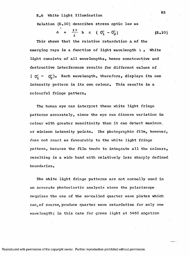
85E . 6 White Light Illumination
Relation (E*10) describes stress optic law as
A = — h c ( O J - O J ) (E.IO)
This shows that the relative retardation A of the
emerging rays is a function of light wavelength X . White
light consists of all wavelengths, hence constructive and
destructive interference results for different values of
( 0 ^ - (^). Each wavelength, therefore, displays its own
intensity pattern in its own colour. This results in a
colourful fringe pattern.
The human eye can interpret these white light fringe
patterns accurately, since the eye can discern variation in
colour with greater sensitivity than it can detect maximum,
or minimum intensity points. The photographic film, however,
does not react as favourably to the white light fringe
pattern, because the film tends to integrate all the colours,
resulting in a wide band with relatively less sharply defined
boundaries.
The white light fringe patterns arc not normally used in
an accurate photoelastic analysis since the polariscope
requires the use of the so-called quarter wave plates which
can,of course, produce quarter wave retardation for only one
wavelength; in this case for green light at 5460 angstrom
Reproduced with permission of the copyright owner. Further reproduction prohibited without permission.

86wavelength. Any retardation for other wavelengths, partic
ularly the extremes of blue and red, are not precise, causing
a non linear effect. As the fringe order increases, the non
linear effect is sufficient to "wash out" the resulting
fringes making it impossible to interpret the results.
Because the light source in this investigation (which is
typical of others used in such analyses) was marginal in
intensity, it was impossible to filter out the other wave
lengths, hence results were not obtained at fringe orders
higher than four.
SOURCE
‘22
LIGHT doubly refrocting p la te
*41
P O L A R I Z E R X ,y - principal axes ANALYZER
Figure E-1 - Arrangement of the various elements of a plane polariscope
Reproduced with permission of the copyright owner. Further reproduction prohibited without permission.

VITA
1944 Born in Lalitpur, U.P., India
1965 Received the degree of Bachelor of Science
in Mechanical Engineering from Banaras
Hindu University, Varanasi, U,P, India
1967 Presently a candidate for the degree of
Master of Applied Science in Mechanical
Engineering at the University of Windsor,
Windsor, Ontario, Canada
87
Reproduced with permission of the copyright owner. Further reproduction prohibited without permission.
Top Related
Copyright © 2022 FDOKUMEN

