


Bahasa
Halaman
Hukum

The Loss of Ef®ciency Estimating LinearFunctions under Restrictions
MIGUEL A. FERNAÂ NDEZ, CRISTINA RUEDA and BONIFACIO SALVADOR
Universidad de Valladolid
ABSTRACT. This article is motivated by the problem of estimating contrast in a one-way
ANOVA model with restrictions in the parameter vector. We prove that when the restrictions
are given by a tree order or a simple order the MLE of some contrast has greater MSE than
the unrestricted estimator. A similar behaviour of the MLE is exhibited in a general
restricted setting given by a multivariate normal distribution with mean vector constrained
to belong to a circular cone. The approach we use focuses on the central direction of the
cones. These directions appear to have the greater MSE when the dimension of the restricted
cone is big enough.
Key words: circular cones, mean square error, order restrictions, restricted maximum
likelihood estimation
1. Introduction
Consider the general model where X (0) � (X(0)1 , . . ., X
(0)k ) is normally distributed with mean
vector è(0) � (è(0)1 , . . ., è(0)
k ) and variance-covariance matrix ó 2Ó where Ó is a known
positive de®nite matrix. Here we assume that è(0) is constrained to belong to a closed
convex cone C(0) in Rk . This general model includes the one-way ANOVA model where
Ó � diag(1=ni). In this setting the order cones describing the simple ordering Cs �fè1 < . . . < èkg and the simple tree ordering Cst � fè1 < èi: i � 2, . . ., kg appear fre-
quently in practice and therefore are extensively treated in the literature and in this paper.
They can be found, for example, when performing a comparison of experimental treatments
with a placebo control assuming that each of the new treatments has a non-negative effect
(tree order) and when an increasing effect of treatments is assumed (simple order).
The statistical problem of making inferences on è(0) can be reduced to a canonical form
making the transformation from X (0) to X � Óÿ1=2 X (0), so that, X?N (è, ó 2 I) where
è � Óÿ1=2è(0) 2 C � Óÿ1=2C(0). The maximum likelihood estimator (MLE) of è is the vector
X� which minimizes (X ÿ è)9(X ÿ è) for è 2 C. See Robertson et al. (1988) for this and other
aspects on restricted inference.
In this paper we focus on the problem of choosing between X or X� to estimate a linear
function of the parameter components, in particular a contrast in ANOVA models. It is known,
Brunk (1965) that the total mean squared error of the MLE is strictly smaller than that of X , i.e.
for any è:
EXk
i�1
(X�i ÿ èi)2
" #< E
Xk
i�1
(X i ÿ èi)2
" #unfortunately this result does not imply that for any ®xed h9 � (h1, . . ., hk):
E(h9X� ÿ h9è)2 < E(h9X ÿ h9è)2
therefore one must be cautious when h9X� is used to estimate h9è.
Several authors have studied the estimation problem when h is the ith coordinate unit vector
# Board of the Foundation of the Scandinavian Journal of Statistics 1999. Published by Blackwell Publishers Ltd, 108 Cowley Road,
Oxford OX4 1JF, UK and 350 Main Street, Malden, MA 02148, USA Vol 26: 579±592, 1999
e9i � (0, . . ., 1, . . ., 0), such as Cohen & Sackrowitz (1970), Lee (1981), and Kelly (1989) who
proves the domination of X�i when the simple order is considered. However, Lee (1988) shows
that the MLE may have a greater MSE than the unrestricted one when one is interested in
estimating the root coordinate, e1 of a simple tree ordering and recently Hwang & Peddada
(1993) consider the problem when the restrictions are given by a sphere and provide results on
the performance of X� in the estimation of èi which reveals also that X�i does not dominate X i
in several situations. See also Hwang & Peddada (1994) for further results.
However, there are no results regarding the performance of X� in the estimation of a general
contrast h9è under any given partial order or cone restriction, neither a fair explanation of the
different behaviour exhibited by X� to estimate èi when è is subject to a simple order or tree
order. It is not even known if in the tree order case there are vectors other than e1 for which the
restricted MLE may have a greater MSE than the unrestricted one or if there is such a vector in
the simple order case. The current study is motivated by these questions and provides reasonable
answer to them. Furthermore the discussion through the paper gives important elements for the
task of searching for estimators which use more ef®ciently the available information on the
parameter.
In the approach presented in this article the concept of `̀ central direction'' of a cone plays an
important role. A direction represents a set of vectors which are all positive multiples of one
another and we use the term `̀ central direction'', following Abelson & Tukey (1963), for the
direction which minimizes the maximum angle with the directions in the cone. In the following
a direction will be represented by the corresponding vector with euclidean norm equal to 1.
Abelson & Tukey (1963) characterize the central direction of a polyhedral cone and propose a
procedure to obtain it which is applied to calculate numerically the central direction of the
simple order cone. In the context of restricted inference central directions are also used to
construct the so-called contrast test (cf. Robertson et al., 1988).
Here we focus on the estimation of c9è where c is the vector de®ning the central direction of
C. This direction is a contrast vector for any order cone C. With respect to the cone C, we deal
at ®rst with Cs and Cst because of the special implications of this order cone in applications. We
obtain in both cases that c9X is not dominated by the restricted estimator c9X� for suf®ciently
large k.
Moreover we consider circular cones. A circular cone C(c, ù) is just de®ned as the set of
vectors whose angle with the axis c is less than or equal to a given angle ù. Although it is hard
to ®nd problems from statistical practice where the parameter space is a circular cone, the study
of the estimation problem in this case is also interesting for other reasons. First, some of the
properties proved for the restricted estimator in the circular setting could also, in our opinion, be
accomplished by the restricted estimator in any polyhedral setting. Moreover, the study of
circular cones is also of interest since a proposed approach in restricted inference is to replace
linear inequalities (the polyhedral cone) by one angular inequality (a circular cone). Akkerboom
(1990) develops this idea in testing problems and derives some distributional properties which
we use in this paper. In concern with circular cones we obtain a formula to calculate E0(h9X�)2
and we conclude that the central direction appears, depending on the axial angle of the cone, as
the least favourable direction to estimate using X� or as the most favourable and that in the
latter case E0(h9X�)2 < E0(h9X )2 for any direction h. Moreover, we prove, for any circular
cone, that c9X is not dominated by the restricted estimator c9X� for suf®ciently large k. The
discussion is completed with results of a simulation study of the MSE for other parameter values
from which we conjecture that for any h 2 C the MSE of h9X�, as a function of è, has a local
maximum in zero and then that E0(c9X�)2 is the key value to evaluate X�.The layout of the article is the following. Section 2 is devoted to prove the results regarding
the simple tree and simple order cones. The study of circular cones is addressed in section 3 and
580 M. A. FernaÂndez et al. Scand J Statist 26
# Board of the Foundation of the Scandinavian Journal of Statistics 1999.
conclusions are given in section 4. In the following we will use the euclidean norm and without
loss of generality we assume that ó 2 � 1 as we can work with Y � X=ó .
2. One-way ANOVA: tree order and simple order
In this section we consider a one-way balanced ANOVA model, so that Ó can be chosen to
be the identity, X � X (0) and C � C(0). We also assume that è 2 Cs or è 2 Cst. In both
cases we prove (theorem 1 and theorem 2 respectively) that for large enough k the MSE of
the restricted MLE is larger than that of the unrestricted one for some values of the
parameter when we want to estimate the central direction for the tree order and the simple
order respectively.
We consider this simple model with equal variances because it is easier to handle but we
conjecture that the result can be generalized to the case of unequal sample sizes and also to any
restrictions on è. This last assertion is con®rmed further by the discussion of circular cones in
section 3. The proposition below provides necessary properties to prove the theorems.
In the following we denote, for any C, by ls(C) the linear space of highest dimension
contained in C, with dim ls(C) � p , k.
Proposition 1
Let C �Rk be a closed convex cone. For any f 2 ls(C) and e 2 ls(C)?, f 9X � f 9X�and f 9X� and e9X� are independent.
Proof. Consider the orthogonal transformation Y � AX such that Y1, . . ., Y p 2 ls(C) and
Y p�1, . . ., Yk 2 ls(C)?. Then X � g1(Y1, . . ., Y p)� g2(Y p�1, . . ., Yk) and from lem. 2.2 in
Raubertas et al. (1986), which is true not only for polyhedral cones but also for any closed
convex cone, and from lem. 2.2 and 2.3 in MeneÂndez et al. (1992)
X� � P(X=C) � P(X=ls(C))� P(X=C \ ls(C)?)
� P(X=ls(C))� P(P(X=ls(C)?)=C)
� g1(Y1, . . ., Y p)� P(g2(Y p�1, . . ., Yk)=C): (1)
Now for f 2 ls(C), f 9X � f 9g1(Y1, . . ., Y p) � f 9X� which is a function of Y1, . . ., Y p and
e9X� � e9P(g2(Y p�1, . . ., Yk)=C) which only depends on Y p�1, . . ., Yk . This implies that
e9X� and f 9X� are independent.
2.1. Tree order
Assume that è 2 Cst and consider c � (k ÿ 1, ÿ1, . . ., ÿ1)=i(k ÿ 1, ÿ1, . . ., ÿ1)i, the
vector de®ning the central direction of Cst, which has been calculated in Robertson et al.
(1988).
Theorem 1
If è1, è2, . . ., èk and n � n1 � � � � � nk are bounded, then for suf®ciently large k,
E(c9X� ÿ c9è)2 . E(c9X ÿ c9è)2:
Proof. It is straightforward to prove that if h � (1, 0, . . ., 0) then
P(h=ls(Cst)?) � ëc, where ë � kÿ1 i(k ÿ 1, ÿ1, . . ., ÿ1)i
Scand J Statist 26 Ef®ciency loss under restrictions 581
# Board of the Foundation of the Scandinavian Journal of Statistics 1999.
which belongs to the central direction of the cone Cst.
From proposition 1 we have that if f � P(h=ls(Cst)),
E((ëc9X� ÿ ëc9è)( f 9X� ÿ f 9è)) � E(ëc9X� ÿ ëc9è)E( f 9X ÿ f 9è) � 0
E( f 9X� ÿ f 9è)2 � E( f 9X ÿ f 9è)2
then
E(h9X� ÿ h9è)2 � E(ëc9X� ÿ ëc9è)2 � E( f 9X� ÿ f 9è)2
� 2E((ëc9X� ÿ ëc9è)( f 9X� ÿ f 9è)) � ë2 E(c9X� ÿ c9è)2 � E( f 9X ÿ f 9è)2: (2)
Now, as h9X� � X�1 , h9è � è1 and E( f 9X ÿ f 9è)2 � (1ÿ ë2)E(X1 ÿ è1)2 we have from
(2) that
E(c9X� ÿ c9è)2 . E(c9X ÿ c9è)2 , E(X�1 ÿ è1)2 . E(X 1 ÿ è1)2: (3)
And the result follows from th. 2.1 in Lee (1988).
Remark 1. Also from (3) and the simulations given in Lee (1988) we know that the smallest
integer k for which c9X� has a larger MSE than c9X for some values of the parameter can be as
small as 5.
2.2. Simple order
Now assume that è 2 Cs. The vector c de®ning the central direction of the simple order
cone has been calculated in Abelson & Tukey (1963), but, as the formula of c is not easy
to handle, in the following we use the r2min values which are de®ned in the same paper as
r2min � minfcos2 (c, g)g, for g 2 fgenerators of Cs \ ls(Cs)
?g: (4)
Lemmas 1 and 2 below are needed to prove theorem 2. Lemma 1, which is stated here for
completeness, is a well-known result (see Robertson et al., 1988, p. 121). The proof of
lemma 2 and that of lemma 3 are given in the appendix. For convenience we will denote
as X�? the projection of X on Cs \ ls(Cs)?.
Lemma 1
For è � 0
E(iX�? i2
k) �Xk
a�2
1
a:
Lemma 2
For r2min de®ned in (4)
r2min .
2
3� ln(k ÿ 1):
Theorem 2
For è � 0 and suf®ciently large k E(c9X�)2 . E(c9X )2.
Proof. As c 2 ls(C)? from (1) we have that c9X� � c9X�? and from the de®nition of
r2min, c9x > r2
min:ixi2, 8x 2 Cs \ ls(Cs)
?. Then
582 M. A. FernaÂndez et al. Scand J Statist 26
# Board of the Foundation of the Scandinavian Journal of Statistics 1999.
E(c9X�)2 � E(c9X�?)2 � E(c9X�?)2
iX�? i2
k
:iX�? i2
k
!
> r2min:E(iX�? i2
k) .2
3� ln(k ÿ 1)
Xk
a�2
1
a
!where the last inequality is obtained applying lemmas 1 and 2. Finally as ln k ,
Pka�11=a
we have
E(c9X�)2 .
Xk
a�1
1
a
!� 3�
Xk
a�2
1
a
!ÿ 4
3�Xk
a�1
1
a
!which is greater than 1 � E(c9X )2 whenever
Pka�21=a . 4.
Remark 2. In Table 1 below we show the result of a simulation study where we ®nd that the
MSE of the restricted MLE is larger than that of the unrestricted one when è � 0 for values of k
as small as 7.
3. Circular cones
In this section C is a circular cone. Let C be written as:
C � C(c, ù) � fx 2 Rk : c9x > ixicosùg:Lemma 3 provides formulas to obtain E0(h9X�)2 for any h. From these formulas we derive
interesting properties in theorems 3, 4 and remarks below.
Let us denote by hci the linear subspace generated by c. The statistics U � c9X and
V � fiX i2 ÿ (c9X )2g1=2 which represent, respectively, the length of the projection of X onto
the axis hci and the distance from X to hci, play an important role in making inferences about èas iX� i and c9X� depend on X through U (X ) and V (X ) (cf. Akkerboom, 1990). We use these
statistics in the proof of lemma 3 and they are also used to obtain some simulation results at the
end of this section.
Table 1. Simulated MSE for the central direction under 100,000 iterations when è � 0
Values of c j
j k � 4 k � 5 k � 6 k � 7 k � 8 k � 9 k � 10
1 ÿ0.698 ÿ0.690 ÿ0.682 ÿ0.674 ÿ0.668 ÿ0.662 ÿ0.656
2 ÿ0.108 ÿ0.155 ÿ0.181 ÿ0.196 ÿ0.206 ÿ0.214 ÿ0.218
3 0.108 0.000 ÿ0.052 ÿ0.083 ÿ0.103 ÿ0.117 ÿ0.127
4 0.698 0.155 0.052 0.000 ÿ0.032 ÿ0.053 ÿ0.069
5 0.690 0.181 0.083 0.032 0.000 ÿ0.022
6 0.682 0.196 0.103 0.053 0.022
7 0.674 0.206 0.117 0.069
8 0.668 0.214 0.127
9 0.662 0.218
10 0.656
MSE 0.813 0.921 0.999 1.074 1.140 1.200 1.253
Scand J Statist 26 Ef®ciency loss under restrictions 583
# Board of the Foundation of the Scandinavian Journal of Statistics 1999.
In the following h and d are vectors in Rk with id i � ihi � 1 so that
E(d9X ÿ d9è)2 � E(h9X ÿ h9è)2 � 1.
Lemma 3
(i) For è � 0, E(c9X�)2 is given by
ÿ cos3ùXrÿ1
p�1
sinkÿ2 pÿ1 ù
B1
2,
k ÿ 2 p� 1
2
� �� 1ÿ cos3 ù
2� cos2 ù
Xkÿ1
j�1
ä j j
0@ 1Awhen k is odd
ÿ cos3 ùXrÿ1
p�1
sinkÿ2 pÿ1 ù
B1
2,
k ÿ 2 p� 1
2
� �� ù� sinù cosù
ð� cos2 ù
Xkÿ1
j�1
ä j j
0@ 1Awhen k is even
where r is the integer part of k=2,
ä j � 1
2
k ÿ 2
jÿ 1
� �B(1
2j, 1
2(k ÿ j))
B(12, 1
2(k ÿ 1))
sin jÿ1 ù coskÿ jÿ1 ù for 1 < j < k ÿ 1 (5)
and B( p, q) is the beta function.
(ii) Let è � 0 and d be such that d?c. Then E(d9X�)2 is a non-decreasing function on ùand is given by
ÿ cosùXrÿ1
p�0
B1
2,
k ÿ 2 p
2
� �sinkÿ2 pÿ1 ù
2ð� 1ÿ cosù
2� sin2 ù
k ÿ 1
Xkÿ1
j�1
ä j j
0@ 1Awhen k is odd
ÿ cosùXrÿ1
p�0
B1
2,
k ÿ 2 p
2
� �sinkÿ2 pÿ1 ù
2ð� ù
ð� sin2 ù
k ÿ 1
Xkÿ1
j�1
ä j j
0@ 1Awhen k is even:
(iii) Let è � 0, hci be the linear subspace generated by c, and d be the vector de®ning the
direction of P(h=hci?). Then
E(h9X�)2 � iP(h=hci)i2 E(c9X�)2 � iP(h=hci?)i2 E(d9X�)2:
(iv) For any è, let hè, ci be the linear subspace generated by è and c and let h1 be the
normed vector de®ning the direction of P(h=hè, ci). Then
E(h9X� ÿ h9è)2 < iP(h=hè, ci)i2 E(h91 X� ÿ h91è)2 � iP(h=hè, ci?)i2:
Remark 3. From (iii) in lemma 3, for a ®xed dimension k and a ®xed angle ù the direction
which has the greatest MSE E(h9X�)2 under è � 0 is either the central one c or the ones
orthogonal to it, d. Notice further that if we consider è � 0 in part (iv) of lemma 3 we obtain
that E(d9X�)2 < E(d9X )2, so that, if there is any direction h for which E(h9X�)2 . E(h9X )2
then necessarily the central direction is the one with the greatest MSE in è � 0 and in this sense
is the most unfavourable.
584 M. A. FernaÂndez et al. Scand J Statist 26
# Board of the Foundation of the Scandinavian Journal of Statistics 1999.
Theorem 3
For è � 0 and any ù 2 (0, ð=2), there is k 2 N such that E(c9X�)2 . E(c9X )2.
Proof. The sum of the ®rst two terms of E0(c9X�)2 in lemma 3 (i) is positive because it is the
integral of a positive function (see the proof of lemma 3 in the appendix). So from this fact and
ä j . 0 we have that
E(c9X�)2 > cos2 ù:Xkÿ1
j�1j odd
ä j: j
0B@1CA: (6)
Now consider k � 2r, an even dimension, and denote j � 2 p� 1. Using the equality
Ã((2 p� 1)=2)=Ã(2 p� 1) � Ã(1=2)=(22 pÃ( p� 1)) we obtain that
2ä j � Ã(2r ÿ 1)
Ã(2 p� 1)Ã(2(r ÿ p)ÿ 1)
Ã2 p� 1
2
� �Ã
2r ÿ 2 pÿ 1
2
� �Ã
1
2
� �Ã
2r ÿ 1
2
� � sin2 p ù cos2(rÿ pÿ1) ù
� Ã(r)
Ã( p� 1)Ã(r ÿ p)sin2 p ù cos2(rÿ pÿ1) ù
�r ÿ 1
p
!(sin2 ù) p(cos2 ù)rÿ pÿ1
and the right hand side of (6) equals
cos2 ùXrÿ1
p�0
( p� 12)
r ÿ 1
p
� �(sin2 ù) p(cos2 ù)rÿ pÿ1
0@ 1A � cos2 ù((r ÿ 1)sin2 ù� 12) (7)
as the sum above can be calculated as E(Z � 12) where Z is a binomial variate with
parameters r ÿ 1 and sin2 ù.
Now (7) grows to1 when r !1 for any ù 2 (0, ð=2) and the proof is complete.
Remark 4. From lemma 3 (iii) and (7) it follows immediately that for any ®xed angle ù and
for any direction h such that its angle ù1 with the central direction of the cone veri®es
ù1 ,ð=2, E0(h9X )2 , E0(h9X�)2 if the dimension of the space k is large enough. So the only
directions where there is never a loss in the mean squared error, under è � 0, are the ones
orthogonal to the central direction c.
Theorem 4
For è � 0
(i) if k , 4, 8ù 2 (0, ð=2), 8h 2 Rk E(h9X�)2 , E(h9X )2
(ii) if k � 4, 9I � (ù I , ùS) such that 8ù 2 I , E(c9X�)2 . E(c9X )2.
Proof. (i) For k � 2, 3 it is quite simple to check from lemma 3 (i) that the maximum value
for E(c9X�)2 is smaller than 1. From (ii) in lemma 3 we also know that E(d9X�)2 < 1 and
®nally the result follows from these properties and (iii) in lemma 3.
(ii) On the other hand when k � 4 we have from lemma 3 (i)
E(c9X�)2 � 1
ð(ù� sinù cosù)� 2
ðcos3 ù sinù� cos2 ù
1
2� sin2 ù
� �
Scand J Statist 26 Ef®ciency loss under restrictions 585
# Board of the Foundation of the Scandinavian Journal of Statistics 1999.
and using numerical methods we obtain that the function is concave and that for
ù I4 � 0:413701 and ùS
4 � 0:889535 we have E(c9X�)2 � 1. Moreover the maximum of this
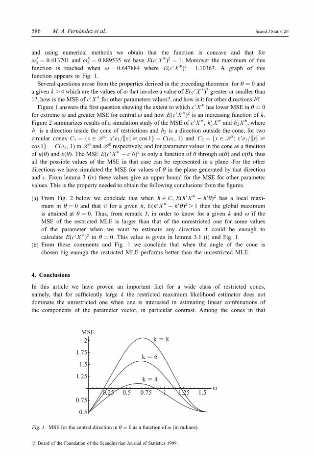
function is reached when ù � 0:647884 where E(c9X�)2 � 1:10363. A graph of this
function appears in Fig. 1.
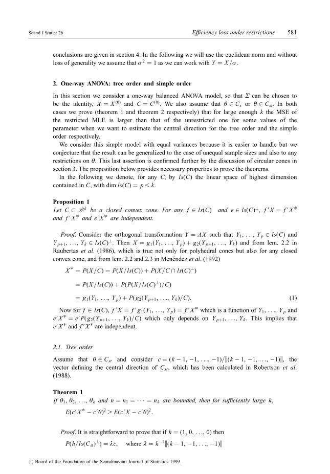
Several questions arose from the properties derived in the preceding theorems: for è � 0 and
a given k . 4 which are the values of ù that involve a value of E(c9X�)2 greater or smaller than
1?, how is the MSE of c9X� for other parameters values?, and how is it for other directions h?
Figure 1 answers the ®rst question showing the extent to which c9X� has lower MSE in è � 0
for extreme ù and greater MSE for central ù and how E(c9X�)2 is an increasing function of k.
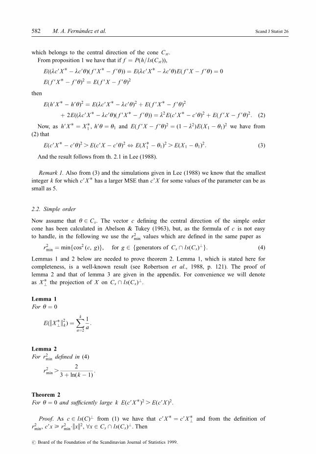
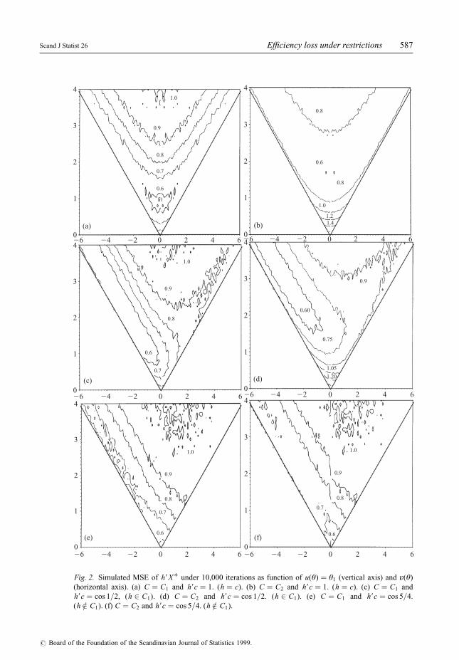
Figure 2 summarizes results of a simulation study of the MSE of c9X�, h91 X� and h92 X�, where
h1 is a direction inside the cone of restrictions and h2 is a direction outside the cone, for two
circular cones C1 � fx 2R4: x9e1=ixi > cos 1g � C(e1, 1) and C2 � fx 2R8: x9e1=ixi >
cos 1g � C(e1, 1) in R4 and R8 respectively, and for parameter values in the cone as a function
of u(è) and v(è). The MSE E(c9X� ÿ c9è)2 is only a function of è through u(è) and v(è), thus
all the possible values of the MSE in that case can be represented in a plane. For the other
directions we have simulated the MSE for values of è in the plane generated by that direction
and c. From lemma 3 (iv) these values give an upper bound for the MSE for other parameter
values. This is the property needed to obtain the following conclusions from the ®gures.
(a) From Fig. 2 below we conclude that when h 2 C, E(h9X� ÿ h9è)2 has a local maxi-
mum in è � 0 and that if for a given h, E(h9X� ÿ h9è)2 . 1 then the global maximum
is attained at è � 0. Thus, from remark 3, in order to know for a given k and ù if the
MSE of the restricted MLE is larger than that of the unrestricted one for some values
of the parameter when we want to estimate any direction it could be enough to
calculate E(c9X�)2 in è � 0. This value is given in lemma 3.1 (i) and Fig. 1.
(b) From these comments and Fig. 1 we conclude that when the angle of the cone is
chosen big enough the restricted MLE performs better than the unrestricted MLE.
4. Conclusions
In this article we have proven an important fact for a wide class of restricted cones,
namely, that for suf®ciently large k the restricted maximum likelihood estimator does not
dominate the unrestricted one when one is interested in estimating linear combinations of
the components of the parameter vector, in particular contrast. Among the cones in that
0.5
0.75
1.25
1.5
1.75
2MSE
0.25 0.75 1.250.5 1 1.5ω
k 5 4
k 5 6
k 5 8
Fig. 1. MSE for the central direction in è � 0 as a function of ù (in radians).
586 M. A. FernaÂndez et al. Scand J Statist 26
# Board of the Foundation of the Scandinavian Journal of Statistics 1999.
0
1
2
3
4
0
1
2
3
4
0
1
2
3
4
0
1
2
3
4
0
1
2
3
4
0
1
2
3
4
(a) (b)
(c) (d)
(e) (f)
26 24 22 0 2 4 6 26 24 22 0 2 4 6
26 24 22 0 2 4 626 24 22 0 2 4 6
26 24 22 0 2 4 626 24 22 0 2 4 6
0.9
1.0
0.8
0.7
0.6
1.0
1.21.4
0.8
0.6
0.8
1.0
0.9
0.8
0.7
0.6
0.9
0.60
0.75
1.05
1.20
1.0
0.9
0.8
0.7
0.6
1.0
0.9
0.8
0.7
0.6
Fig. 2. Simulated MSE of h9X� under 10,000 iterations as function of u(è) � è1 (vertical axis) and v(è)
(horizontal axis). (a) C � C1 and h9c � 1. (h � c). (b) C � C2 and h9c � 1. (h � c). (c) C � C1 and
h9c � cos 1=2, (h 2 C1). (d) C � C2 and h9c � cos 1=2. (h 2 C1). (e) C � C1 and h9c � cos 5=4.
(h =2 C1). (f) C � C2 and h9c � cos 5=4. (h =2 C1).
Scand J Statist 26 Ef®ciency loss under restrictions 587
# Board of the Foundation of the Scandinavian Journal of Statistics 1999.
class are the simple order and the simple tree order cones, and we conjecture that the
result is also true for any polyhedral cone as we have proven it for any circular cone.
On the other hand we have pointed out the different behaviour exhibited by the restricted
estimator of directions located in the middle of the cone or elsewhere. Thus, for the simple order
cone the coordinate directions are well estimated by the MLE (cf. Lee, 1981; Kelly, 1989) but
notice that these directions are in two dimensional faces of the cone. We have proven that the
MLE of the central direction, which is a contrast, does not dominate the unrestricted one. A
similar fact is also true for the tree order cone.
Finally for a circular cone a stronger result is obtained, namely that, depending on the axial
angle and on the dimension k, either, the central direction estimator has the greatest mean
square error in è � 0, or the mean square error in è � 0 is not greater than 1 for any direction
h. Moreover from simulation results we conjecture that the only two possibilities are that
E0(c9X�)2 . 1 or that the restricted MLE is better than the unrestricted MLE to estimate any
given direction h, that is: Eè(h9X� ÿ h9è)2 < 1 for any è 2 C, h 2 Rk , ihi � 1.
The main conclusion in our point of view is that in a restricted setting the maximum
likelihood estimator may have a greater MSE than the unrestricted one independently of the type
of restriction and that in future research devoted to ®nd better estimators the features of the
restricted estimator mentioned above should be taken into account.
Acknowledgements
Research partially supported by Spanish DGICYT grant PB 97-0475 and by PAPIJCL
VA26/99. The authors thank the referees for their detailed reading of the paper and for
comments which resulted in an improved version of the paper.
References
Abelson, R. P. & Tukey, J. W. (1963). Ef®cient utilization of non-numerical information in quantitative
analysis: general theory and the case of the simple order. Ann. Math. Statist. 34, 1347±1369.
Akkerboom, J. C. (1990). Testing problems with linear or angular inequality constraints. Springer, New
York.
Brunk, H. D. (1965). Conditional expectations given a ó-lattice and applications. Ann. Math. Statist. 36,
1339±1350.
Cohen, A. & Sackrowitz, H. (1970). Estimation of the last mean of a monotone sequence. Ann. Math. Statist.
41, 2021±2034.
Hwang, J. T. & Peddada, S. D. (1993). Con®dence interval estimation under some restrictions on the
parameters with non-linear boundaries. Statist. Probab. Lett. 18, 397±403.
Hwang, J. T. & Peddada, S. D. (1994). Con®dence interval estimation subject to order restrictions. Ann.
Statist. 22, 67±93.
Kelly, R. E. (1989). Stochastic reduction of loss in estimating normal means by isotonic regression. Ann.
Statist. 17, 937±940.
Lee, C. C. (1981). The quadratic loss of isotonic regression under normality. Ann. Statist. 9, 686±688.
Lee, C. C. (1988). The quadratic loss of order restricted estimators for treatment means with a control. Ann.
Statist. 16, 751±758.
MeneÂndez, J. A., Rueda, C. & Salvador, B. (1992). Dominance of likelihood ratio tests under cone
constraints. Ann. Statist. 20, 2087±2099.
Raubertas, R. F., Lee, C. C. & Nordheim, E. V. (1986). Hypothesis test for normal means constrained by
linear inequalities. Commun. Statist. Theory Meth. 15, 2809±2833.
Robertson, T., Wright, F. T. & Dykstra, R. L. (1988). Order restricted statistical inference. Wiley, New York.
Received June 1997, in ®nal form September 1998
Miguel A. FernaÂndez, Departamento de EstadõÂstica e I. O., Universidad de Valladolid, 47071-Valladolid, Spain.
588 M. A. FernaÂndez et al. Scand J Statist 26
# Board of the Foundation of the Scandinavian Journal of Statistics 1999.
Appendix: Proofs
Proof of lemma 2. From Abelson & Tukey (1963) we know that
r2min �
1Xk
j�1
d2j
where d j � f( jÿ 1)[1ÿ (( jÿ 1)=k)]g1=2 ÿ f j(1ÿ j=k)]1=2 which can be written as d j �z( jÿ 1)ÿ z( j) with
z(t) � ft(1ÿ t=k)g1=2 for 0 < t < k
also notice that
ÿd j�1 � d kÿ j for j � 0, . . ., k ÿ 1 and d[k=2]�1 � 0 for k odd: (8)
Moreover,
z9(t) � 1ÿ 2t=k
2ft(1ÿ t=k)g1=2
> 0 when 1 < t < k=2
, 0 when k=2 , t < k
and
z 0(t) , 0:
Thus, when 1 < j < k=2, d2j � [z( jÿ 1)ÿ z( j)]2 ,[z9( jÿ 1)]2:
Now, from the last inequality and taking into account (8) we have that
Xk
j�1
d2j , 2d2
1 � 2X[k=2]
j�2
[z9( jÿ 1)]2 � 2d21 � 2[z9(1)]2 � 2
X[k=2]ÿ1
j�2
[z9( j)]2
, 2d21 � 2
(2=k ÿ 1)2
4(1ÿ 1=k)� 2
�[k=2]
1
(1ÿ 2t=k)2
4ft(1ÿ t=k)g d t
< 2d21 �
(2ÿ k)2
2k(k ÿ 1)�� kÿ1
1
(1ÿ 2t=k)2
4ft(1ÿ t=k)g d t
,(2ÿ k)2
2k(k ÿ 1)� 1� 1
2ln(k ÿ 1) ,
3
2� 1
2ln(k ÿ 1)
and the proof is complete.
Proof of lemma 3. Following Akkerboom (1990) we assume without loss of generality that
c � (1, 0, . . ., 0), d � (0, 1, 0, . . ., 0) and consider the change of variable (x1, . . ., xk)!(u, v, ö3, . . ., ök) keeping x1 � u and making the polar change of coordinates with the rest,
that is xk � v sinö3 � � � sinök , xkÿ1 � v sinö3 � � � cosök , . . ., x2 � v cosö3 where v �(x2
2 � � � � � x2k)1=2 and v > 0, ö3 � � � ökÿ1 2 [0, ð), ök 2 [0, 2ð). The Jacobian determinant of
this change of variate is jJ j � vkÿ2 sinkÿ3 ö3 � � � sinökÿ1 so that the joint distribution of
(U , V , Ö3, . . ., Ök) is
f k(u, v, ö3, . . ., ök) � 1������2ðp� �k
exp ÿ 1
2(u2 � v2)
� �vkÿ2 sinkÿ3 ö3 � � � sinökÿ1: (9)
This change of variable will be useful in the following as for a given x, the projection x�keeps the same angular coordinates, and ix� i and c9x� do not depend on ö3, . . ., ök .
Integrating out the angular coordinates the joint distribution of U and V is
Scand J Statist 26 Ef®ciency loss under restrictions 589
# Board of the Foundation of the Scandinavian Journal of Statistics 1999.
f k(u, v) � Ck exp ÿ 1
2(u2 � v2)
� �vkÿ2 for u 2R and 0 < v <1 (10)
where
Ck � 2(kÿ2)=2Ã1
2
� �Ã
k ÿ 1
2
� �� �ÿ1
(i) Consider the partition of Rk in C, C P polar cone of C and Rk ÿ (C [ C P) � R0, where
C P � fy: x9y < 0 for all x 2 Cg, and let f (x) be the density function of a Nk(0, I). Then we
have
E(c9X�)2 ��
C(c9X�)2 f (x) dx��
R0
(c9X�)2 f (x) dx��
C P(c9X�)2 f (x) dx
� I C(c)� I R0(c)� I C p (c) (11)
where I C p (c) � 0 as x� � 0, 8x 2 C p. (In fact, as proved in Akkerboom, 1990, p. 82, C P
can be characterized as the set of points whose projection onto C is 0).
If we denote as Ø f the distribution function of a ÷2f , Ø0 � 1[0,1) and B p,q the distribution
function of a beta variate with parameters p and q, the distribution of iX� i2 is
Pr0(iX� i2 < t) �Xk
j�0
ä jØ j(t)
where ä j can be found in (5) when 1 < j < k ÿ 1 and
ä0 � Pr0(X 2 C P) � 1
2B(kÿ1)=2,1=2(cos2 ù)
äk � Pr0(X 2 C) � 1
2B(kÿ1)=2,1=2(sin2 ù)
(cf. Akkerboom, 1990, p. 118).
Then,
Pr0(iX� i2 . t; X 2 R0) � Pr0(X 2 R0)ÿ Pr0(X 2 R0; iX� i2 < t)
�Xkÿ1
j�1
ä j ÿXkÿ1
j�1
ä jØ j(t) �Xkÿ1
j�1
ä j(1ÿØ j(t)): (12)
Now we are going to evaluate I R0(c) in (11). From the properties of the projection it is easy to
check that
(c9x�)1R0(x) � cosùix� i1R0
(x) (13)
so that from (12)
590 M. A. FernaÂndez et al. Scand J Statist 26
# Board of the Foundation of the Scandinavian Journal of Statistics 1999.
I R0(c) � cos2 ùE(1R0
(X )iX� i2)
� cos2 ù
�10
Pr0(X 2 R0; iX� i2 . t) dt
� cos2 ù
�10
Xkÿ1
j�1
ä j(1ÿØ j(t))
0@ 1A dt
� cos2 ùXkÿ1
j�1
ä j: j
0@ 1A:On the other hand to evaluate the integral I C(c) in (11) we use
(c9x�)1C(x) � (c9x)1C(x) � x11C(x) � u1C(x) (14)
and then from (10)
I C(c) ��
C
(c9x)2 f (x) dx ��1
0
�u tan ù
0
Ck u2 expfÿ12(u2 � v2)g:vkÿ2 dv du
��1
0
u2 expfÿ12u2g Ck
�u tan ù
0
vkÿ2 expfÿ12v2g dv
!du
and integrating by parts we have
Ck
�u tan ù
0
vkÿ2 expfÿ12v2g dv �
ÿXrÿ1
p�1
(u tanù)kÿ2 pÿ1 expfÿ12(u tanù)2g
2(kÿ2 p)=2Ã 12
ÿ �Ã((k ÿ 2 p� 1)=2)
�
�u tan ù
0
expfÿ12v2gvkÿ2r dv
2(kÿ2 r)=2Ã 12
ÿ �Ã((k ÿ 2 r � 1)=2)
:
Then, to calculate I C(c) it is enough to use the change of variable t � u=cosù and the
integrals �10
exp ÿ 1
2t2
� �t p d t � Ã
p� 1
2
� �2( pÿ1)=2
�10
Ö(u tanù)u2 exp ÿ 1
2u2
� �du � 1������
2ðp ð
2� ù� cosù sinù
� �from which we obtain that
I C(c) � ÿcos3 ùXrÿ1
p�1
sinkÿ2 pÿ1 ù
B 12
,k ÿ 2 p� 1
2
� �� 1
2(1ÿ cos3 ù) when k odd
1
ð(ù� sinù cosù) when k even:
8><>:(ii) We reach the formula following (i) and using the following statements
d9x� � x�2 � v� cosö3
E(d9X�)2 � E(V�)2 E(cosÖ3)2
� E(iX� i2 ÿ (c9X�)2)1
k ÿ 1(15)
Scand J Statist 26 Ef®ciency loss under restrictions 591
# Board of the Foundation of the Scandinavian Journal of Statistics 1999.
then,
I R0(d) � sin2 ù
Xkÿ1
j�1
ä j j
0@ 1A 1
k ÿ 1
I C(d) ��1
0
�u tan ù
0
Ck
k ÿ 1exp ÿ 1
2(u2 � v2)
� �vk dv du:
The monotonicity of E(d9X�)2 is obtained from the fact that for each x, (d9x�)2 is non-
decreasing with ù.
(iii) Without loss of generality we can assume that h � (cosù1, sinù1, 0, . . ., 0). Then it is
enough to prove that E(h9X�)2 � cos2 ù1 E(c9X�)2 � sin2 ù1 E(d9X�)2. Obviously (h9x�)2 �cos2 ù1(c9x�)2 � 2 cosù1 sinù1(c9x� � d9x�)� sin2 ù1(d9x�)2 but from (10), (15) we have that
E(c9X�:d9X�) � E(U�:V�)E(cosÖ3) � 0
because E(cosÖ3) � 0.
(iv) Without loss of generality we assume that è � (è1, è2, 0, 0, . . . 0), h � h(1) � h(2) where
h(1) � p(h=hè, ci) and h(2) � p(h=hè, ci?). Using the change of variable (x1, . . ., xk)!(u, v, ö3, . . ., ök) we can write,
h9(1)x � j(u, v, ö3), h9(2)x � v sinö3ø(ö4, . . ., ök) (16)
and the joint distribution of (U , V , Ö3, . . ., Ök) can be factorized as
f k(u, v, ö3, . . ., ök ; è1, è2) � g(u, v, ö3; è1, è2)sinkÿ4 ö4 � � � sinökÿ1 (17)
then from h9(2)è � 0
0 � E(h9(2) X ) � E(V sinÖ3)E(ø(Ö4, . . ., Ök))
and E(V sinÖ3) . 0 implies that:
E(ø(Ö4, . . ., Ök)) � 0 (18)
thus, from (16), (17) and (18)
E((h9(1) X� ÿ h9(1)è):h9(2) X�) � E((j(U�, V�, Ö3)ÿ h9(1)è)V� sinÖ3)E(ø(Ö4, . . ., Ök))
� 0: (19)
Moreover, it is straightforward to prove that for any x, v� is non-decreasing with ù because
v� � 0I C p � vI C � sinùix� i I Ro . It is also easy to prove that for ù � ð=2, v� � v. Then
(v�)2 < v2 and
E(h9(2) X�)2 � E(V�)2 E(sinÖ3ø(Ö4, . . ., Ök))2
< E(V )2 E(sinÖ3ø(Ö4, . . ., Ök))2 � E(h9(2) X )2 � ih(2) i2: (20)
Finally from (19), (20) and the de®nition of h(1) and h(2) we have that
E(h9X� ÿ h9è)2 � E(h9(1) X� ÿ h9(1)è)2 � E(h9(2) X�)2 < E(h9(1) X� ÿ h9(1)è)2 � ih(2) i2
� iP(h=hè, ci)i2 E(h91 X� ÿ h91è)2 � iP(h=hè, ci?)i2:
592 M. A. FernaÂndez et al. Scand J Statist 26
# Board of the Foundation of the Scandinavian Journal of Statistics 1999.
Top Related
Copyright © 2022 FDOKUMEN

