


Bahasa
Halaman
Hukum

The Emergence of Economic Organization
by
Peter Howitt
The Ohio State University
and
Robert Clower
The University of South Carolina
July 2, 1999
This is an updated version of a paper first presented to the meetings of the Canadian Economics
Association at the University of Ottawa, May 1998. We acknowledge helpful comments and
suggestions from Dan Friedman, Miles Kimball, David Laidler, Axel Leijonhufvud, Dick
Lipsey, Scott Page, Michael Salemi and Leigh Tesfatsion. Howitt’s research was conducted
partly at the IDEI, University of Toulouse and partly at the Santa Fe Institute, and was supported
by the Computable and Experimental Economics Laboratory of the University of Trento. The
source code for the program on which the paper is based is available online at
http://www.econ.ohio-state.edu/howitt/ .
1The view of trading firms as the coordinating agents of an economy has also been put forthby Howitt [1974], Clower [1975], Chuchman [1982], Day [1984], Clower [1995], and Heymann,Perazzo and Schuschny [1999]. Clower and Howitt [1996, 1997], and Spulber [1998] haveargued that market-making is the most important role that business firms, even manufacturingfirms, play in a market economy.
1
The Emergence of Economic Organization
by Peter Howitt and Robert Clower
1. Introduction. This paper studies the mechanism by which exchange activities are
coordinated in a decentralized market economy. Our topic is not amenable to conventional
equilibrium theory, which assumes that exchanges plans are coordinated perfectly by an external
agent (usually unspecified but sometimes referred to as "the auctioneer") with no identifiable
real-world counterpart. In contrast, we depict transactors as acting on the basis of trial and error
rather than pre-reconciled calculation, and we start by noting that in reality most transactions are
coordinated by an easily identified set of agents; namely, specialist trading enterprises. Thus we
buy groceries and clothes from grocery and clothing stores; buy or rent lodging from realtors;
buy cars from dealers; acquire medical, legal, accounting, gardening and other services through
specialist sellers; borrow, invest, and insure through financial intermediaries. Likewise, we earn
income by selling labor services to specialist employers (the self-employed are specialist dealers
in their own services).
Specialist traders reduce the costs of search, bargaining and exchange, by using their
expertise and by setting up trading facilities that enable non-specialists to trade on a regular
basis. Collectively they coordinate the exchange process, for better or worse, by setting prices,
holding buffer-stock inventories, announcing times of business, entering into implicit or explicit
contracts with customers and suppliers, and taking care of logistical problems that arise in
delivery, inspection, payment, and other aspects of the transaction process.1 When there are
imbalances between demand and supply, specialist traders typically are responsible for making
whatever adjustments are needed to ensure that non-specialists can continue their activities with
minimal interruption. Those that do the job poorly do not survive competition.
A decentralized economy is one in which the coordinating network of trade specialists
emerges spontaneously. Our immediate objective in the present paper is to show constructively

2See Clower [1967].
3We put "money" in quotation marks to indicate that our use of the term does not correspondto common parlance, in which it refers typically to a pure token money created by a centralauthority.
2
how this might happen. We present a stylized account of an economy in which people pursue
self interest by obeying simple behavioral rules rather than by trying to carry out "optimal" plans.
The analysis focuses on the five activities that we see as most central to the functioning of a
decentralized market economy: exchange, shopping, entrepreneurship, exit and price-setting.
Computer simulation of this model economy shows that, starting from an initially autarkic
situation in which none of the institutions that support economic exchange as we know it exist, a
fully developed market economy will ultimately emerge, at least under some circumstances, with
no central guidance.
By "growing" a market economy, we are following the same strategy as biologists who
have used computer models of evolution to grow such things as eyes (Dawkins [1995], p.78 ff).
Success in following this strategy shows that no divine intervention, state planning, or other
external force is needed to account for the phenomenon in question. Success also supports the
notion that the forces embodied in the computer simulation are related to important forces at
work in reality. All the more so if the object that emerges from the simulation exhibits the same
characteristics as in real life.
Perhaps the most obvious characteristic of real-world market economies, besides the fact
that they are coordinated by specialist traders, is that they are organized along "monetary" lines;
that is, one tradeable object has the property that it (or a direct claim to it) is involved in virtually
every act of exchange2. As it turns out, this characteristic is shared by the market economies that
emerge from our computer simulations. In almost all cases, if a fully developed market economy
emerges, one of the commodities will have become the sole exchange intermediary (commodity
"money"3) in the system. The only significant exceptions to this general rule occur when we
make the extreme assumption that there is no cost to operating a trade facility.

4Iwai [1996] argues, on the contrary, that money is a creature of the state, requiring centralcoordination for its establishment. In our view this "statist" theory of money is refuted byarchaeological evidence to the effect that money was used as early as 2,000 BC, whereas theearliest evidence of government coinage dates to some time around 625 BC. For an introductionto the archaeological evidence, see Snell [1997], esp. pp.58, 73, 106. See also Einzig [1949],esp. pp.353-4, 417.
3
Thus a secondary purpose of the paper is to shed light on the nature and origin of
monetary exchange4. According to the model presented below, money, markets, and the
specialist traders that organize markets, are interdependent trading institutions whose origins all
lie in the elementary forces described by our stylized account of competitive evolution.
Our procedure is adumbrated in Don Walker’s Advances in General Equilibrium Theory
[1997]. As indicated in his preface:
... for a model to be a functioning system, it must be explicitly endowed with the
structural and behavioural features that are necessary to generate economic
behaviour. If the model is a functioning system, its workings can be investigated
and the consequences of different variations of parameters can be compared. It
can be converted into an empirical model and tested, precisely in order to discover
whether it has identified the important features and interconnections of the
economy and how their influence is exerted in the determination of economic
magnitudes....
The program suggested by Walker leads us to view an economy as an algorithm
generating observed outcomes. A functioning system is one whose algorithmic representation is
self contained, leaving no need for "skyhooks" (Dennett [1996], ch.3). Since the algorithm must
work from any initial position, we cannot impose any "equilibrium" concept that would restrict
attention to initial positions in which transactor plans are mutually consistent. Equilibrium is a
possibly emergent property of a functioning system: nothing more. Likewise, institutions such
as organized markets that facilitate commodity trading should "emerge" from transactor
interactions, not be assumed to exist a priori.

5Jackson and Watts [1998], use this approach to study the evolution of "links" between agents,following the analysis of Jackson and Wolinsky [1996]. The random process of search by whichnew links are created in their analysis is similar in many ways to the processes of "shopping" and"entry" described below. Their analysis takes as given the payoffs accruing to various agents as afunction of the links they have formed, whereas in our analysis those agents who are linked bybeing customers or owners of a particular shop will realize a payoff (weekly consumption) thatvaries over time, as prices are adjusted, in ways that the agents are assumed unable to predict,even if the set of links were to remain unchanged.
6Young studies "stochastically stable" states, which he defines ([1998], p.54) as situationswhose probability of being observed remains positive as the per-period probability of a randomaction by any player approaches zero. As Young points out, these states may not correspond tostates that are frequently observed when the latter probability is far from zero.
7Day [1984] has argued that equilibria are inherently unstable because "wise" adaptivebehavior allows random actions, in order to avoid low-level local optima. Our analysis of marketresearch avoids that instability, by shutting down the randomness when an equilibrium is reachedin which all potential gains from trade are fully exploited.
4
2. Relation to recent literature. Our analysis is related to the theoretical literature on evolutionary
game theory, synthesized by Young [1998], that studies how institutions and conventions can
emerge from the interaction of people’s independent attempts at trial and error. This literature
has not focused as we do here on the coordinating role of specialist traders5. Analytically, the
main difference between our approach and the approach followed in this literature concerns the
way random experimentation is modeled. There, it is modeled as an infrequent disturbing force,
taking the form of occasional random actions by some player or players, being likened to rare
mutations in evolutionary biology.6 In our view, the random disturbing force most central to an
economy’s coordination mechanism is the entrepreneurship that creates new trade facilities.
Following Schumpeter, we see entrepreneurship not as a rarely observed phenomenon, but as a
relentless aspect of everyday life in a competitive market economy.
Furthermore, in the theoretical literature on evolutionary game theory, the probability
distribution of random actions is almost always taken to be exogenous, whereas in our view it
varies endogenously with the state of the economy. We model explicitly the process of market
research whereby a prospective entrepreneur decides whether or not to act on a random idea for
creating a new trade facility. This process allows entrepreneurship to play an "annealing" role,
constantly disturbing a system when there are plenty of gains from trade left unexploited but
otherwise leaving the system relatively undisturbed.7
8Vriend also limits his analysis to fixed prices, whereas the specialist traders in our analysisare constantly adjusting prices in response to new information.
9Likewise for the theoretical analyses of evolution in the Kiyotaki-Wright model conductedby Luo [1995] and Johnson [1997], and for the analysis of "replicator dynamics" in the multi-currency extension of search theory by Matsuyama, Kiyotaki and Matsui [1993].
5
Even more closely related to our analysis is the extensive literature (for example Arthur,
Durlauf and Lane [1997]) on "complexity." Within this literature, the papers by Vriend [1995]
and Tesfatsion [1996] are motivated by same idea as ours, namely that of understanding by
means of computer simulation the emergence of a network of trade facilities. Dawid [1999]
pursues a similar idea. Pingle [1999] studies the emergence of market organization
experimentally. Ioannides [1990] studies the formation of trading networks as an equilibrium
phenomenon, using random graph theory. We attempt to go beyond these analyses in studying
the evolution of a closed multi-market system and in portraying the forces giving rise to a
monetary pattern of exchange.8
Our analysis is also related to the literature on the origins of monetary exchange. Much
of that literature has focused recently on the search-theoretic approach to money, developed first
by Jones [1976] and subsequently by Kiyotaki and Wright [1989]. This literature portrays
monetary exchange as solving the familiar "double coincidence" problem, with no reference to
specialist traders. In our view what characterizes a monetary economy is not so much that
different transactors all choose to accept the same exchange intermediary for their production
commodities, as in search theory, but that the shops they deal with don’t give them any choice.
What we seek to explain is why the competitive forces of evolution favor shops that conform to
such a pattern. While search is an important part of the adjustment process in our analysis, the
final equilibrium attained when a fully developed market economy emerges is one in which
search plays no role.
The analysis by Marimon, McGrattan and Sargent [1990] deals with the evolution of
trading strategies in a search economy of the sort portrayed by Kiyotaki and Wright. From our
point of view, this analysis does not deal with the central issue of monetary exchange, since it
abstracts from the role of specialist traders9. Moreover, the assumption underlying this analysis,
to the effect that there does not exist a double coincidence of wants between any two potential
partners, directly precludes direct barter. In the analysis below we do not rule out double

10Thus if there were more than one commodity with the same operating cost, the bandwagoneffect analyzed below would still tend to produce monetary exchange in our model, whereasnothing would rule out a regime with twin "moneys" in Alchian’s model.
11Starr [1998] has independently developed a dynamic adjustment model in which theeconomy moves from barter (one trading post for each pair of commodities) to monetaryexchange, for reasons much the same as in our analysis. In his analysis, the adjustment processis conducted by an "auctioneer," whereas the main objective of the present paper is to portray adecentralized economy making no use of such external processes.
6
coincidences. Direct barter is a possibility, but one that never materializes under the forces we
have portrayed.
Alchian’s [1977] account of money, like ours, emphasizes the cost of trading many
commodities in the same trade facility, but does not take into account the fixed costs of operating
the facility.10 Starr and Stinchcombe [1993, 1998] tell a trading-post story of money in which
fixed costs play an important role. The reason why monetary exchange can occur in equilibrium
in our model is almost identical to the reason portrayed in these papers. The difference is that we
have provided an analysis of how the shops and trading relationships underlying such a monetary
equilibrium might emerge from a decentralized process of evolution, whereas they characterize
organizational structures under full information.11
Thus, in some of the computer runs reported on below, there exist multiple equilibria in
the Starr-Stinchcombe sense, including a barter equilibrium in which a full set of trading posts
exists, one for each pair of tradeable objects. Yet these equilibria never emerge from the
computer simulations, whereas monetary equilibria do. This cannot be explained by the fact that
the most efficient organizational structure is monetary in nature, since often an inefficient
monetary equilibrium emerges in which the commodity that serves as universal medium of
exchange is not the least costly commodity to trade.
3. Narrative Prelude. We start by recognizing that "do-it-yourself" exchange (Hicks
[1968], Ostroy [1973]) is inherently so costly that hardly anyone would trade regularly except
through the intermediation of firms that establish trading times, affirm the quality of
commodities traded, develop procedures to enforce contracts, transfer control of commodities,
and so forth. This fact is embodied in the stark assumption:
7
Individuals trade with each other only through the intermediation
of specialist traders called shops.
Second, we note that real-world firms typically deal with only a small fraction of
potentially tradeable objects. We embody this fact by supposing:
Every shop trades two and only two commodities.
Third, we observe that the typical firm relies for its survival on repeat business from
regular customers (Blinder et al. [1998]), which we simulate by supposing:
Individuals can trade at a particular shop only by forming a
"trading relationship" with it.
In real life most people continue week after week and month after month purchasing from the
same small subset of retail outlets, and selling labor services to the same small subset (usually a
singleton) of employers; so to the preceding assumption we add:
An individual can have a continuing trading relationship with no
more than two shops.
Fourth, real-world firms can be established only by incurring substantial organizational
"setup" costs, and a substantial fraction of "going-firm" operating costs are "overhead" expenses
which depend on the type but not the quantity of commodities traded (Blinder et al. [1998]). We
recognize both these fact by assuming:
The operating cost of each shop (per unit time) is independent of
quantities of commodities traded by the shop.
4. The Mechanism of Exchange. Given the substantive assumptions just introduced,
imagine an economy with n commodities and m transactors--all clustered at a single "location".
The time unit is the week, indexed by t = 1,..,T, fifty consecutive weeks being designated a year.

8
Because we wish to deal with trading actions rather than consumer or producer choice, we
assume initially that each transactor "likes" only commodities that other transactors are endowed
with; specifically, we suppose that each transactor receives as endowment ("makes") just one
unit per week of one kind of commodity, say that labeled i, which we call the transactor’s
"production commodity"; and each transactor is a potential consumer of just one other
commodity, say that labeled j, which we call the transactor’s "consumption commodity". For
each of the n(n-1) ordered pairs (i,j) of commodities, there is the same number b of transactors
for whom i and j are respectively the transactor’s production and consumption commodity; that
is, there are b transactors of each "type" (i,j). The population of the economy is thus m = bn(n-
1). No commodity is storable from one week to the next; thus the economy’s total supply each
week of each commodity is the current endowment flow b(n-1).
Because no transactor "likes" the commodity it "makes", a transactor can acquire a
commodity it "likes" only by trading with another transactor; and according to the assumptions
of the preceding section the transactor must form trading relationships with shops in order to
trade. We discuss below the origin of shops and trading relationships. For now we just take as
given that during a particular week there will exist some number N of shops, each labeled by the
location k at which it is established, each offering to trade two of the n commodities, labeled g0k
and g1k. Thus if the shop at location 2 is offering to trade commodities 3 and 7, we have g02 = 3
and g12 = 7. In addition, each transactor r may have ongoing "trading relationships" with one or
two of these shops.
Consider a "representative" shop, k. The transactors who have trading relationships with
it (the shop’s "customers") will be of two sorts; those that sell commodity g0k to the shop and
those that sell commodity g1k. The shop posts a price p0k that it offers to pay to the first type for
each unit of g0k they sell to the shop, and a price p1k that it offers to pay the second sort for each
unit of g1k they sell. These offers are binding. Thus if the first group of customers sells the total
amount y0k of commodity g0k, they at the same time buy the amount p0ky0k of commodity g1k; and
if the second group sells y1k of commodity g1k they simultaneously buy p1ky1k of commodity g0k.
The "circular" flow of commodities into and out of the shop (shown in Figure 1) then
illustrates the "Janus" aspect of all quid pro quo commodity trades (supply is demand, and
9
demand is supply). We have seller/buyers on both sides, and two "selling/buying" prices (cf,
Walras [1954], p.88; J. N. Keynes [1894], p.539).
Figure 1 here
Figure 1 also illustrates the trilateral nature of organized exchange. Although individual trades
take place between non-specialist transactors and a shop that acts as a specialist trader, the shop is
an intermediary between non-specialist transactors on each side.
The shop’s "trading surplus" in commodity g0k is the difference between the inflow and
outflow in the upper part of Figure 1: y0k - p1ky1k, and its trading surplus in commodity g1k is
y1k - p0ky0k. If both trading surpluses are positive, the shop will be left with some of each
commodity at the end of the week’s trading. These surpluses can be used to defer the shop’s
overhead cost. Anything remaining after covering overhead cost can be consumed by the shop’s
owner. In order for each trading surplus to be positive, the product of the two prices, p0kp1k must
be less than unity. (This product is also an inverse measure of the spread between the firm’s offer
price for each commodity and its bid price for the same commodity, the latter being the reciprocal
of its offer price for the other commodity.)
Next, consider a representative transactor, r, of type (i,j), that enters the week having
ongoing trading relationship with up to two shops. The exact nature of r’s trading relationships is
represented by the two variables sh0r and sh1r. If r has a trading relationship with a shop that
trades the production commodity i, then sh0r denotes the location of that shop, which is called r’s
"outlet". If the transactor has no outlet, then sh0r = 0. If the transactor has a trading relationship
with a "source"; that is, a shop that trades r’s consumption commodity j (but not i), then the
location of the source is sh1r. (If r has no source then sh1r = 0.)
If r has an outlet that also trades the consumption commodity j, then r can trade directly
with this single shop. Each week r will visit the outlet to sell the unit endowment of i; that is, r
will buy (and then consume) the amount p of commodity j, where p is the outlet’s offer price for i.
Alternatively, if r has an outlet and a source, and both trade the same third commodity c, then r
12during the same week, since all commodities perish at the end of the week.
10
can trade indirectly, first visiting the outlet to buy the amount p of commodity c, and then12
visiting the source to buy (and consume) the amount ppN of commodity j, where pN is the source’s
offer price for c. In the latter case, commodity c is the transactor’s "exchange intermediary." If
neither of these cases applies, the transactor does not trade.
5. Shopping, Entry, Exit and Prices. In keeping with conventional wisdom from the time
of Thales and Aristotle, we suppose that transactor behavior is aimed at raising the level of
commodity consumption, which is possible here only through exchange.
Shopping. In general we may presume that transactor information is limited and local; so
we proceed by supposing that in every week some transactors search for information about
possible trading relationships that will increase their weekly commodity consumption.
Specifically, a searcher will gather a sample of shops, some through direct observation of
potential shop locations, and some through contact with other transactors.
Consider the set of shops in this search sample together with the transactor’s existing
source and outlet (if either exists). For each shop in the set, the transactor knows the labels of the
two commodities traded and their currently posted prices. This information is enough to infer the
weekly consumption level attainable from having trading relationships with any one or two shops
in the set, according to the mechanism described in the preceding section. If any such set of
trading relationships would yield the transactor a higher level of consumption than that attainable
under existing relationships, the transactor establishes the new relationships and severs the old
ones. Otherwise the transactor’s trading relationships remain as they were.
Entry. Shops can be opened only by transactors that "innovate" by formulating workable
plans. From historical experience we know that
Entrepreneurship is rare and occurs randomly.
Accordingly, we suppose that in any given week each transactor has a (small) probability of
formulating an idea for opening a new shop at a currently vacant location k (a shop that will offer
to trade the entrepreneur’s production commodity and consumption commodity). One aspect of

11
any such idea is the setting of target incomes tr0k and tr1k, for the two commodities that the
entrepreneur proposes to trade. In our story, the value of each target is drawn randomly from the
set {1, 2, . . . , xMax}. The outcome of these draws represents, so to speak, the entrepreneur’s
"Animal Spirits"%a tangled melange of hope (for customers), fear (of known and potential
competitors), and luck.
Putting the idea for a new shop into effect entails a setup cost to the entrepreneur (here
treated as purely psychic in nature). So before incurring that cost the entrepreneur consults a
small number of transactors that might adopt the newly-created shop as a consumption source and
a few others that might use it as a production outlet. If this "market research" indicates sufficient
strength on either side of the market the entrepreneur will open the shop, terminate existing
trading relationships, and become the shop’s first customer; otherwise the opportunity lapses.
Exit. We begin our discussion of shop exit by specifying that a shop dealing in
commodities i and j will need to expend the amount f(i) of commodity i and the amount f(j) of
commodity j to defer its operating costs. As indicated earlier, f(i) and f(j) are overhead costs. For
convenience we number the commodities in order of ascending cost:
0 1 2≤ < < <f( ) f( ) f(n)L
The "operating surpluses" B0k and B1k of a shop k are the amounts of the two commodities traded
available for the owner’s consumption after all customer demands are satisfied and all operating
costs paid:
( )( )
π
π0 0 1 1 0
1 1 0 0 1
k k k k k
k k k k k
y p y f g
y p y f g
= − −
= − −
A shop will remain in operation as long as these surpluses are positive.
When one of the operating surpluses becomes negative the shop confronts what is, in
effect, a stockout problem: whether and how to honor immediate customer demands (quantities
traded are determined by customers--the raison d’être of the shop is, after all, to facilitate trades
for other transactors). In actual economies, firms deal with impending stockouts by depleting

13We assume that the owner of a shop dealing in i and j seeks compensation in the form ofboth i and j, simply to ensure that the shop’s behavior will not depend on whether the owner is atype (i, j) transactor or type (j, i).
12
inventories, producing overtime, lengthening delivery lags and making emergency purchases from
competitors. Since none of these remedies fits easily into our story we evade the stockout issue at
this point by supposing that shop owners always honor their customers’ demands, engaging when
necessary in negative consumption.
A shopkeeper will not remain in business indefinitely when faced with negative
consumption. Accordingly, we assume that each week in which a shop’s operating surplus is
negative, there is a fixed probability 2 the shop will close. When a shop closes, all trading
relationships with it are severed, and its location is vacated.
Pricing. The most common pricing procedure in actual economies is one or another
version of full cost pricing (Hall and Hitch [1939]; Blinder et al. [1998]). Motivated by pursuit of
gain, but lacking reliable information about the relation of price to profit, the shop posts prices
that promise to yield what the owner regards as a normal return on investment provided it
succeeds in achieving its target income levels. Suppose that the owner regards a fixed
consumption level of C units of each13 commodity it trades (over and above the consumption the
owner achieves as customer of the shop) as constituting a normal return. Then it will want to post
prices such that B0k = C and B1k = C. We refer to C as the "setup cost" of the shop.
Whether or not such prices will be posted will depend, however, on the two income
targets. If, for example, the income target tr0k for commodity g0k is less than the sum of the
overhead cost f(g0k) and the setup cost C, the shop cannot expect to cover its setup cost no matter
how little it pays for the other commodity g1k; in such cases it will set p1k = 0. Likewise, when
tr1k < f(g1k) + C, it will set p0k = 0. It follows that the shop’s prices will be given by the formulas:
( )
( )
ptr f g C
tr
ptr f g C
tr
kk k
k
kk k
k
01 1
0
10 0
1
=− −
=− −
+
+
13
where the notation x+ denotes the maximum of x and 0.
The income targets that enter these pricing formulae, as indicated earlier, are initially
determined by the shop owner’s animal spirits. Over time, however, the owner will observe the
actual incomes y0k and y1k during the course of each week, so we assume that the owner will adapt
gradually to realized trading results by adjusting its targets according to the formula
( )∆tr y tr hhk hk hk = , α − = 0 1, ;
where the parameter " representing the speed of adaptation lies between 0 and 1.
6. System Performance. From an initial state in which few customers have a trading
relationship, if operating and setup costs are not too high entrepreneurs will repeatedly disturb the
system by creating new shops. Many of these new shops will eventually exit. To survive, a shop
must attract enough customers, because of the fixed nature of its costs. Specifically, it must
eventually realize a gross income of at least f(i) + C in each commodity i it trades, and each
customer contributes at most one unit. Failure to achieve this critical income level in each
commodity will tend to be self-reinforcing, because it will eventually induce the shop to cut one
of its offer prices to zero, thus inducing suppliers of that commodity to switch to an alternative
shop. For the same reason, success in attracting customers will breed further success by inducing
the shop to offer higher prices than otherwise.
The smaller are setup and overhead costs, the more likely that any given shop will survive,
and the more likely that every transactor will end up with a "profitable" set of trading
relationships; that is, a set that affords the transactor a positive consumption level. If such a state
of affairs arises the economy is said to have attained "full development." For our story to
constitute a plausible account of economies as we know them, something approximating full
development must be a likely outcome, at least for some set of parameter values.

14These conditions determine what Kauffman [1993] (borrowing from Wright [1931]) callsthe "fitness landscape," which he defines (p.33) as "the distribution of fitness values over thespace of genotypes." In our case a genotype is a shop trading a particular pair of commodities.Although Kauffman typically treats this "fitness" as an inherent property of a genotype, weinterpret it as a likelihood of survival that varies endogenously with the frequency distribution ofgenotypes. Thus, following Friedman and Yellin [1997], we model an evolving fitness landscaperather than a fixed one.
14
A shop’s survival prospects also depend on initial conditions - the number and types of
other shops and the full set of trading relationships14. Consider a shop trading say commodities i
and j, and suppose that there are relatively few other shops trading i. That shop is more likely to
survive the more transactors have trading relationships with other shops that deal in j. Thus a
shop trading apples and gold when all other shops trade gold can potentially attract all
"producers" of apples regardless of their consumption commodities, because they can use gold
acquired at this shop as an exchange intermediary; and the shop can also potentially attract all
potential consumers of apples regardless of their endowments because they can acquire the needed
gold at other shops regardless of their production commodities. This advantage would not be
available to someone setting up shop trading apples for oranges unless numerous other shops were
also trading oranges. When one commodity comes by chance to be more commonly traded than
another, the survival prospects of shops that trade that commodity will be enhanced, and the
prospects of shops that don’t will be dimmed. This bandwagon effect can lead to a situation in
which one commodity is traded by all shops that have customers and is used as exchange
intermediary by all customers that trade indirectly.
Whether or not such a situation emerges will depend, among other things, on the fixed
costs of shops. If these costs are very large, no shop will long survive, and at any date what little
trade occurs will be undertaken with the random collection of shops that have recently opened and
are destined soon to exit. On the other hand if costs are very small, then the bandwagon effect
that favors those trading the most commonly traded commodity might not be large enough to
eliminate other exchange intermediaries. In simulations below we show that for a wide range of
intermediate costs, something approximating "monetary" exchange will eventually be established,
as it is in all advanced economies of record.
Which commodity, if any, emerges as "money" will depend to some extent on the
overhead cost of a shop trading it. A commodity that is more costly to trade will have lower
15
survival probability, other things equal, because the critical income level needed for a shop
trading that commodity to survive is higher. Thus the commodity with smallest overhead cost
(commodity 1) is most likely to emerge as "money". However, luck will also play a role in this
path-dependent process; if by chance a large number of shops trading commodity 2 open at an
early stage of development, the bandwagon effect may offset the otherwise poor survival
prospects of these shops and lead to commodity 2 emerging as "money".
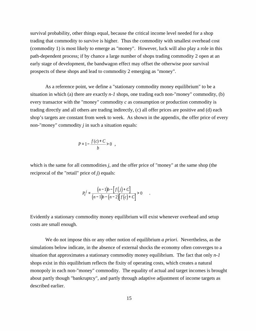
As a reference point, we define a "stationary commodity money equilibrium" to be a
situation in which (a) there are exactly n-1 shops, one trading each non-"money" commodity, (b)
every transactor with the "money" commodity c as consumption or production commodity is
trading directly and all others are trading indirectly, (c) all offer prices are positive and (d) each
shop’s targets are constant from week to week. As shown in the appendix, the offer price of every
non-"money" commodity j in such a situation equals:
,Pf c C
b= −
+>1 0
( )
which is the same for all commodities j, and the offer price of "money" at the same shop (the
reciprocal of the "retail" price of j) equals:
.( ) ( )[ ]
( ) ( ) ( )[ ]P
n b f j C
n b n f c Ccj =
− − +
− − − +>
1
1 20
Evidently a stationary commodity money equilibrium will exist whenever overhead and setup
costs are small enough.
We do not impose this or any other notion of equilibrium a priori. Nevertheless, as the
simulations below indicate, in the absence of external shocks the economy often converges to a
situation that approximates a stationary commodity money equilibrium. The fact that only n-1
shops exist in this equilibrium reflects the fixity of operating costs, which creates a natural
monopoly in each non-"money" commodity. The equality of actual and target incomes is brought
about partly though "bankruptcy", and partly through adaptive adjustment of income targets as
described earlier.
15Compare these pricing formulas to those in Starr and Stinchcombe’s [1998] example IV.2,p.17.
16A shop’s economic profit in any commodity it trades is the operating surplus Bhk minus the"normal profit" C. In a stationary monetary equilibrium, since each actual income yhk equals thecorresponding target trhk, the pricing formulas of section 5 together with the definition of Bhk
imply that economic profit is zero.
17One might think that in a pure exchange economy, the flow of endowments corresponds toGDP. But according to the story we have told, endowments are more like factors of production.Once traded to a shop, they can be used by other transactors to create consumption. But untradedendowments, like unused factors of production, create neither current investment norconsumption.
16
Although our account eschews conventional notions of rational choice, a stationary
commodity money equilibrium is almost identical to the concept of general Bertrand equilibrium
defined in a similar setup by Starr and Stinchcombe15 [1998]. Intuitively, shops in equilibrium
satisfy the same zero-profit condition16 that would characterize a "rational" firm that was limit-
pricing under conditions of free entry and zero search time by customers. Thus although firms are
following simple rules, they may be led (by the visible hand of the functioning system) to act as if
they were maximizing profits.
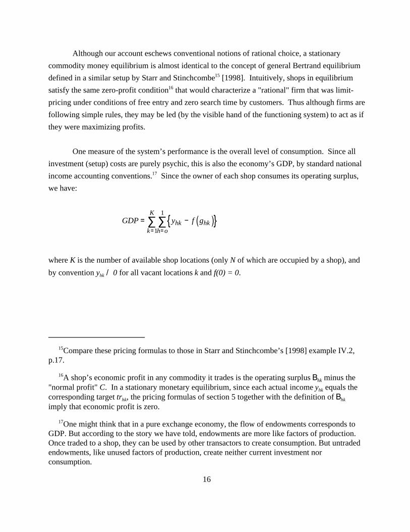
One measure of the system’s performance is the overall level of consumption. Since all
investment (setup) costs are purely psychic, this is also the economy’s GDP, by standard national
income accounting conventions.17 Since the owner of each shop consumes its operating surplus,
we have:
( ){ }GDP y f ghk hkh ok
K= −
==∑∑1
1
where K is the number of available shop locations (only N of which are occupied by a shop), and
by convention yhk / 0 for all vacant locations k and f(0) = 0.
18That is, potential GDP equals .( ) ( ) ( )m f i n fin
− − −=∑ 1
2 1
17
In all specifications simulated here, the stationary commodity money equilibrium with
commodity 1 as "money" (whenever it exists) yields the maximum possible GDP18. Intuitively,
this is because such an equilibrium yields the maximal sum of shop-incomes = m withyhk∑∑the minimal number of shops n-1, operated at the least possible overhead cost (since commodity 1
has the smallest operating cost).
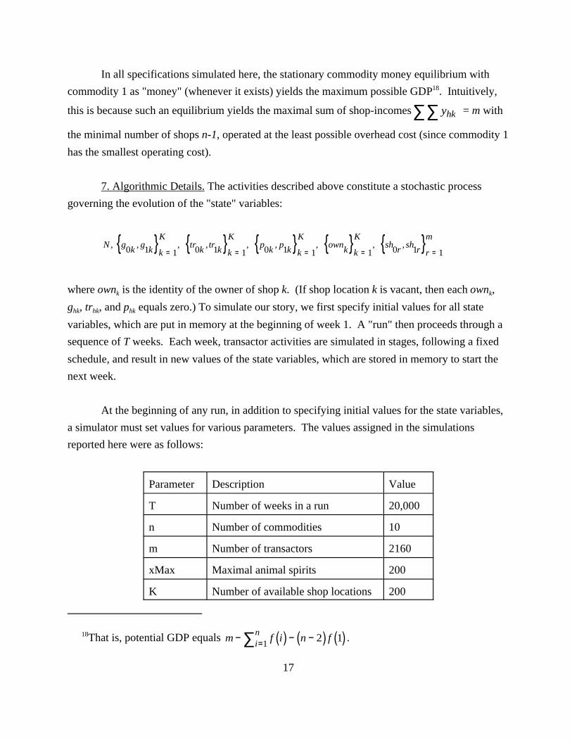
7. Algorithmic Details. The activities described above constitute a stochastic process
governing the evolution of the "state" variables:
{ } { } { } { } { }N gk
gk k
Ktr
ktr
k k
Kp
kp
k k
Kown
k k
Ksh
rsh
r r
m, , , , , , , , ,
0 1 1 0 1 1 0 1 1 1 0 1 1= = = = =
where ownk is the identity of the owner of shop k. (If shop location k is vacant, then each ownk,
ghk, trhk, and phk equals zero.) To simulate our story, we first specify initial values for all state
variables, which are put in memory at the beginning of week 1. A "run" then proceeds through a
sequence of T weeks. Each week, transactor activities are simulated in stages, following a fixed
schedule, and result in new values of the state variables, which are stored in memory to start the
next week.
At the beginning of any run, in addition to specifying initial values for the state variables,
a simulator must set values for various parameters. The values assigned in the simulations
reported here were as follows:
Parameter Description Value
T Number of weeks in a run 20,000
n Number of commodities 10
m Number of transactors 2160
xMax Maximal animal spirits 200
K Number of available shop locations 200
19The numerator of is which turns negative whenpc10 ( ) ( ) ,n b s C s− − + = −1 9 211 9
s > 2349.
18
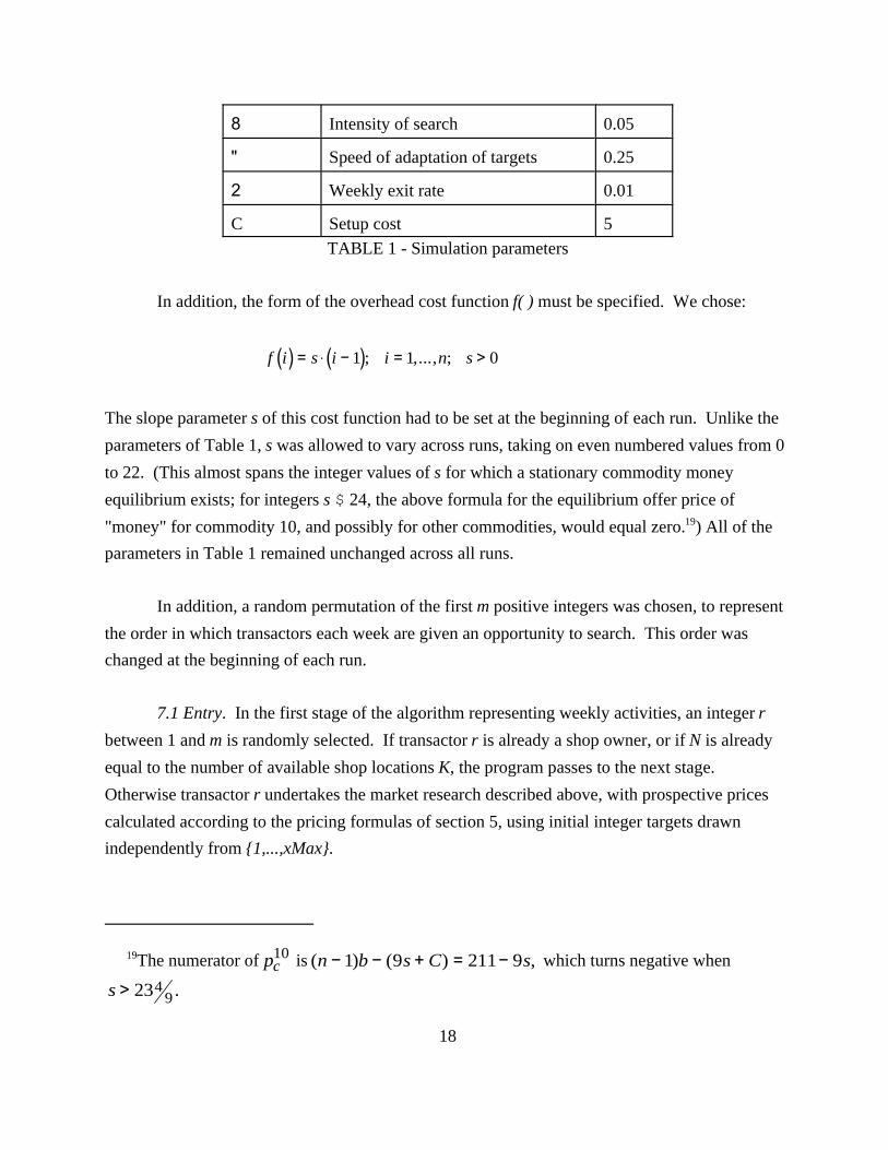
8 Intensity of search 0.05
" Speed of adaptation of targets 0.25
2 Weekly exit rate 0.01
C Setup cost 5
TABLE 1 - Simulation parameters
In addition, the form of the overhead cost function f( ) must be specified. We chose:
( ) ( )f i s i i n s= ⋅ − = >1 1 0; ,..., ;
The slope parameter s of this cost function had to be set at the beginning of each run. Unlike the
parameters of Table 1, s was allowed to vary across runs, taking on even numbered values from 0
to 22. (This almost spans the integer values of s for which a stationary commodity money
equilibrium exists; for integers s $ 24, the above formula for the equilibrium offer price of
"money" for commodity 10, and possibly for other commodities, would equal zero.19) All of the
parameters in Table 1 remained unchanged across all runs.
In addition, a random permutation of the first m positive integers was chosen, to represent
the order in which transactors each week are given an opportunity to search. This order was
changed at the beginning of each run.
7.1 Entry. In the first stage of the algorithm representing weekly activities, an integer r
between 1 and m is randomly selected. If transactor r is already a shop owner, or if N is already
equal to the number of available shop locations K, the program passes to the next stage.
Otherwise transactor r undertakes the market research described above, with prospective prices
calculated according to the pricing formulas of section 5, using initial integer targets drawn
independently from {1,...,xMax}.

19
To simulate market research, the program checks r’s type (i,j) (recall that if r opens a new
shop it will trade commodities i and j) and then selects four other transactors; one whose
production commodity is i, one whose consumption commodity is j, one whose production
commodity is j and one whose consumption commodity is i. The first two are prospective
customers on one side, the other two are prospective customers on the other side. For each of
these prospective customers, the search algorithm outlined in section 5 calculates whether, from
the set including this prospective shop and the prospective customer’s existing outlet and source
(if either exists), a set of trading relationships would be chosen that includes the prospective shop.
If the answer is positive for at least one prospective customer on each side, the shop opens at a
location k chosen randomly from the currently vacant locations among {1,...,K}, and the state
variables in memory are modified accordingly.
7.2 Shopping Next, the program gives each transactor r, in turn, an opportunity to search,
in the order chosen at the beginning of the run. If r is a shop owner, the opportunity is not taken.
Otherwise, if r already has a profitable set of trading relationships, the opportunity is taken with
probability 8, and if not it is taken with certainty. The program generates each searcher’s sample
as follows. First, a shop location k is chosen at random from the integers {1,...,K}; if there is a
shop at location k it is included in the sample. Next, a random transactor ("comrade") with the
same production commodity is chosen. If the comrade has an outlet, it is also included in the
sample. Then a random transactor ("soulmate") with the same consumption commodity is chosen.
If the soulmate has a source, it is also included. The variables sh0r and sh1r are updated according
to the search algorithm of section 5.
A transactor r may have trading relationships that are not profitable. This will happen, for
example, when r is trading indirectly and its source or outlet exits, leaving r with a "widowed"
outlet or source, or when r’s outlet sets to zero its offer price for r’s production commodity. In
such cases if a profitable set of trading relationships is not found the searcher is made to switch to
any prospective outlet found offering a positive price for r’s production commodity.
7.3 Exchange Next, the program calculates the income yhk realized by each shop k in each
commodity ghk traded and stores it in memory.
20Experimentation shows that allowing the runs to continue once "monetary exchange" hasbeen attained for 10 years makes almost no difference to the results. This is because a stationarycommodity equilibrium when it exists is almost always an absorbing state of the algorithm, andas we report below the system is usually very close to such an equilibrium when we terminate therun. Thus there is no repeated switching between quasi-equilibria as in many models ofevolutionary game theory. Allowing a run to continue for more than 400 years when "monetaryexchange" is not achieved increases the likelihood of achieving it, but does not appear to alterany of our qualitative conclusions.
20
7.4 Exit The program then calculates each firm’s operating surplus, on the basis of the
incomes and prices stored in memory. Each shop k whose operating surplus is not positive in
both commodities traded exits with probability 2. When a shop exits, its location is vacated and
all its trading relationships are severed.
7.5 Pricing Finally, the program updates income targets, calculates corresponding offer
prices, and stores the results in memory.
8. Simulation Results. We simulated the economy in 6,000 runs, 500 runs for each of the
12 different values of the slope coefficient s of the overhead-cost schedule, starting each time in a
situation of autarky, with no shops and no trading relationships. Each run proceeded for up to 400
years (20,000 weeks). Different results emerged for each run, even when parameter values
remained unchanged, because of the various random events that take place each week within a run
(who innovates, who is picked as whose comrade or soulmate, etc.).
The state of the system was checked at the end of each year (50 weeks). If the number of
transactors having a profitable trading relationship, or owning a shop, at the end of the year was
within 1% of the total population m for 10 years in a row, we deemed the economy to have
reached full development. If the number trading indirectly using the same exchange intermediary
ever came within 1% of the maximal number m(n-2)/n for 10 years in a row, we deemed that
"monetary exchange" had emerged, and the run was terminated. Otherwise the run was allowed
to continue for 400 years20. The main results are tabulated in Table 2.
A fully developed market economy emerged in just over 90 percent of all runs. In over 99
percent of those cases "monetary exchange" also emerged, except in the limiting case where there
were no overhead costs (s = 0), when it emerged slightly less than 3 percent of the time. Even in

21In absolute terms, the gap is where TR( ) ( )( )m f i TR f gi
n
hkhk
K− − −
= ==∑ ∑∑( ) ,2 0
1
1
denotes the number of transactors with a profitable set of trading relationships, ghk = 0 for shoplocations that are vacant, and f(0) / 0. This can be decomposed into: ,( ) ( )m TR n f c− + − +( )2 ε
where c is the most prevalent exchange intermediary and is defined as a residual. These threeεterms correspond respectively to the three components of the gap reported in Table 2. In astationary commodity money equilibrium with commodity c>1 as "money", only the secondcomponent would be positive. If there were only one shop trading each non-"money"commodity the third component would be zero.
22This component of the gap can almost always be eliminated by allowing the run to proceedanother ten years, since redundant shops are doomed to disappear.
21
this limiting case, the number of transactors trading indirectly (using two shops rather than one) at
the end of a run that achieved full development without "monetary exchange" was on average 77
percent of the maximal number m( n-2) /n = 1728 that would be found in a stationary commodity
money equilibrium, and the number of transactors that were using the most prevalent exchange
intermediary was almost 39 percent of this maximal number.
Generally speaking the market organization that emerged by the end of a run allowed
transactors to achieve a high level of total consumption (GDP). As Table 2 shows, the gap
between actual and potential GDP (the level that would be achieved in a stationary commodity
money equilibrium with commodity 1 as "money") at the end of each run averaged about 3
percent if we exclude the runs with the largest overhead costs (s = 22). Most (over 2 percentage
points on average) of this gap was attributable to the existence of more than the minimum
necessary number of shops, each incurring overhead costs.21
In those runs where "monetary exchange" did emerge, the state of the system at the end of
the run closely approximated a stationary commodity money equilibrium. As Table 3 indicates,
the average GDP gap over such runs was only 2 percent, almost three quarters of which was
attributable to there being too many shops22. Moreover, in those runs where "monetary exchange"
emerged, the distance (measured by root mean square deviation) of actual prices from their
stationary commodity money equilibrium values averaged only one tenth of one percent.
The typical approach to equilibrium is not smooth or gradual, as can be seen from the four
sample runs depicted in Figure 2 (a)~(d). The number of transactors trading directly usually goes
23Although not the level of GDP, which falls steadily as s is increased from 0 to 22. However,this indicator is driven by the assumed deterioration in the underlying transaction technology,which causes potential GDP to fall. What improves is the success of the system in realizing itspotential.
22
fairly quickly to close to its stationary value. But the number trading indirectly often fluctuates;
the system may go for several decades without any noticeable change in trading patterns, and then
jump to a new configuration with the entry or exit of few key shops. The final approach to
equilibrium is almost always sudden, at least in terms of the number of traders using a single
commodity as exchange intermediary, which typically jumps to its ultimate value in the space of
just a few years, often after a number of decades in which it shows no tendency to gravitate
towards any resting place.
The early stage of the process, before a commodity money standard emerges, shows
characteristics typical of the "shakeout" phase of a development cycle in a situation with "network
economies." The number of firms is larger than the eventual equilibrium number of 9, indicating
that there are potential gains from trade to be exploited. However, once the system locks into an
equilibrium, unexploited gains quickly vanish, new entry ceases, and redundant shops soon
vanish. Thus entrepreneurship with research provides a form of "annealing" for market
organization. When the existing organization leaves unexploited profit opportunities,
entrepreneurs repeatedly disturb it by creating new trade facilities, and as the profit opportunities
disappear the disturbing force cools off. Even though it is no part of any transactor’s plan to do
so, a coherent market structure is created and, once created, "solidifies".
The role of transaction costs. According to Table 2, overhead costs make a significant
difference to the system’s performance. When the slope parameter s reaches 22 performance
deteriorates sharply; the probability of full development falls, the average number of years to
reach full development rises, and the gap between actual and potential GDP rises, all dramatically.
When s = 22 a stationary commodity money equilibrium still exists, but the economy usually
remains far away from it even after 400 years; on average, GDP is substantially negative, meaning
that many shops have so few customers that the owners experience negative consumption.
If we exclude the extreme points s = 0 and s = 22, most performance measures improve as
transaction costs rise23. For example, the gap between actual and potential GDP tends to fall as
24In each of these figures, the commodity whose use as exchange intermediary is traced out bythe dark line is the one used by the largest number of transactors at the end of the run.
23
transaction costs rise, partly because the number of active participants tends to rise (as indicated
by Gap1) and partly because the probability of achieving "monetary exchange" with other than
commodity 1 tends to fall (as indicated by Gap2 - - see also Table 4). However, the average gap
rises when s rises from 0 to 2, and again from 20 to 22.
A similar pattern can be seen in the probability of reaching full development, which falls
when s first rises from 0 to 2 but then increases as s continues to rise above 2. Likewise the
average number of years taken to reach full development falls until s reaches 14.
In the dimensions just discussed the system seems generally to perform better when
transaction costs are larger. Some insight into why this happens can be gleaned from observing
runs that fail to reach full development. As Figures 3(a) and 3(b) show, the system often "sticks"
somewhere near a "multiple currency" regime in which two or more commodities are used as
exchange intermediaries but none is close to being a general purpose commodity money24.
Almost always there are more than twice the minimal number (9) of shops, but holes remain in
the market structure, in the sense that for a significant number of transactor types no pair of shops
exists that would afford a positive consumption level. In such a situation most firms have a small
clientele, but they linger for a long time because their operating costs are also small. A potential
entrant that might fill one of the gaps has poor survival prospects because many transactors have
already found a profitable set of trading relationships, hence search only with probability .05 each
week, meaning that a new shop is likely to fail before being located by a critical mass of
customers.
Likewise, the long stretches of incomplete development that characterize even those runs
that end in full development with commodity money tend to be longer when transaction costs are
smaller. Thus large transaction costs, although they lead to a lower potential GDP, can help the
economy realize its full potential by eliminating small-scale shops that don’t conform to a
coherent ("monetary") form of market organization.

25Again as in standard accounts of product development with increasing returns. See, forexample, Arthur [1989].
26The critical condition over this range of values for s is that P > 0. Thisrequires that is, .( )s c b C⋅ − < −1 ; c s< +1 19 /
27A more explicit analysis of how technological progress can lead to the emergence oforganized monetary exchange is being developed by Albert Jodhimani following the lines of his[1999] Ohio State PhD dissertation.
24
9. The selection of a "money" commodity. It seems on the basis of this evidence that the
story we have told contains within it the forces giving rise to market organization of the sort we
know, including the institution of monetary exchange. There are many aspects of real economic
systems that can potentially be studied using this story and the computer program that simulates
it. Here we illustrate that potential by analyzing the question why the medium of exchange in
most economies of record has tended to have classical properties of divisibility, portability,
recognizability, etc.- - properties summarized in our story by low operating cost for a shop dealing
in that commodity.
Which commodity becomes "money" is not "determined" by the story in any absolute
sense; it depends instead25 on random events during the development process, although, as
indicated above, commodities that are less expensive to trade (those labeled with smaller
numbers) are more likely to emerge as "money". Thus Table 4 indicates that in about 17 percent
of the runs in which "monetary exchange" emerged the "money" commodity was not the
commodity least expensive to trade (commodity 1). The probability of any other commodity
becoming "money" falls as the overhead cost of trading it rises, because the larger the slope
coefficient s of operating costs, the fewer commodities can satisfy the equilibrium conditions
described in section 6 above for a stationary commodity money equilibrium.26
One way to reduce the indeterminacy at issue is to cast our story in a historical context of
technological progress, which over the centuries has reduced the cost of operating trade
facilities27. If the fall has been gradual, and if the force of entrepreneurship has always been
present, then the appropriate initial conditions for our purposes should be those in which costs
have not fallen far below the threshold above which a fully developed market structure cannot be
sustained. As indicated by Table 4, these are the conditions under which the only commodity that
28We restricted attention to these cases, because with a population size of only 1080,commodity 1 is the only one likely to emerge as "money" in the original economies whentransaction costs are any higher.
25
stands a chance of emerging as "money" is the least expensive one to trade. Only if the process
begins when s has fallen to 16 or below does the second most expensive commodity have a
significant chance of emerging as "money," and only when it has fallen to 8 or below does the
third have a chance.
A related historical factor that ought to play a role in the determination of which
commodity emerges as medium of exchange is the reduction in transportation and communication
costs that tends to bring previously isolated societies into contact with each other. This contact
can awaken the force of entrepreneurship by opening up new profit opportunities, and the
resulting introduction of new shops will change the fitness landscape, possibly leading to a new
"money" commodity. Consider, for example, two economies that had previously reached full
development in isolation, but each with a different "money" commodity. If they now come
together to form a unified economy, the same forces leading to a single monetary standard will
operate in the new economy. Thus the commodity that was initially the common exchange
intermediary for members of one society may eventually be replaced.
To investigate this possibility, we ran 1000 additional simulations, 500 each with slope
parameters28 2 and 4. In each case the simulation proceeded as before, except that it started not
from autarky but from an initial situation in which there were 18 shops, 9 of them forming a
stationary commodity money equilibrium with commodity 1 as "money" in one of the original
economies, comprising m/2 of the transactors, and the other 9 shops forming a stationary
equilibrium with commodity 2 as "money" in the other original economy, comprising the other
m/2 transactors. Each of the original economies was characterized by the same parameter values
as shown in Table 1 above, with the exception of m (here set at m = 1080 rather than m = 2160).
Table 5 shows the results of these additional simulations. It indicates that the probability
of reaching a stationary commodity money equilibrium in the newly formed economy is much
higher than when we began from autarky in the unified economy. Moreover, the probability that
the commodity which is least expensive to trade (commodity 1) will become "money" is much
larger than when we began from autarky. In this sense a shop trading commodity 2, for example,

29The concept of "evolutionary stability" developed by Maynard Smith [1982] and usedwidely in evolutionary game theory deals only with small scale mutations. The idea of exploringthe consequences of this variant of large scale coordinated mutations was suggested to us by DanFriedman, who has shown (Friedman [1991]) that, from a dynamical systems perspective,evolutionary stability is not coincidental with true dynamic stability.
26
has greater evolutionary fitness in an economy where commodity 2 has emerged as "money", if
the economy is subject only to the small-scale random mutation of the occasional entrepreneur
thinking of opening up shop trading in commodity 1 than if this population of 2-traders is
"invaded" by a large number of 1-traders29. This result, combined with the results summarized in
Table 3, shed light on why, despite the path dependence of the evolutionary process giving rise to
monetary exchange, there has been a tendency nevertheless for less costly to drive out more costly
"money" commodities.
Another factor that helps explain for why a commodity can become "money" is its relative
availability or consumability. Until now we have considered only symmetrical situations in
which all commodities are equally available and consumable. But suppose we make one of the
commodities, say commodity 2, more abundant, and consumable by more transactors, than all the
others. Starting from an initial position of autarky it is clear that this change will tend to confer
some additional evolutionary fitness on shops trading commodity 2, by making them more likely
to acquire enough customers to cover overhead costs. This should increase chances that
commodity 2 becomes "money".
To verify this intuitive result we ran some additional simulations, starting again from
autarky but this time modifying the configuration of tastes and endowments. Specifically, in this
case we assumed there were 20 transactors of each type (i,j), except when either i or j was 2, in
which case there were 40 such transactors. This specification leaves the total number of
transactors (2160) the same as in the baseline simulations of Tables 2~4. To save time we ignored
extreme cases of very low and very high overhead costs, and ran 50 simulations for each of 10
values of the slope parameter s running from 2 through 20. As shown in Table 6, this resulted in a
much higher probability of commodity 2 becoming "money". The overall probability of
commodity 1 becoming the "money" commodity fell from 0.83 to 0.40, while the overall
probability of commodity 2 becoming "money" rose from 0.14 to 0.60.
30Again, this specification leaves the total number of transactors unchanged, at m = 2160.
27
Recently Cuadras-Morato and Wright [1997] have argued that increased consumability
should raise the chances of a commodity becoming "money" but that increased availability should
have the opposite effect. Their reasoning was that by accepting in exchange a commodity that is
widely available one runs the risk of encountering a potential trading partner who already has an
abundant supply of that commodity and is therefore unwilling to accept it in exchange for the
commodity one wants to acquire. This leads to few people choosing the commodity as an
exchange intermediary.
To test this idea we ran another 500 simulations, identical to those reported in Table 5, but
with a slightly different configuration of tastes and endowments. In this case there are 20
transactors of each type (i,j), except when i = 2, in which case there are 60 such transactors30. The
results are shown in Table 7. Commodity 2 was still much more likely to become the "money"
commodity than in the symmetric baseline case reported in Tables 2~4, although not quite by as
much as in the case where commodity 2 was both more available and more consumable than other
commodities. Compared with the baseline case, the overall probability of commodity 1 becoming
"money" fell from 0.83 to 0.49, while the overall probability of commodity 2 becoming "money"
rose from 0.14 to 0.50.
The results of this experiment illustrate a significant advantage of functioning systems for
studying phenomena that are subject to multiple equilibria. The argument of Cuadras-Morato and
Wright is one that identifies the relative "likelihood" of a commodity emerging as "money" with
the relative amount of parameter space over which there exists a monetary equilibrium with that
particular commodity as "money". But such an argument, while perhaps suggestive, does not
address the relevant issue, which is the likelihood that dynamic forces will generate an outcome in
which the commodity is used as "money", since it makes no reference to such forces. It is easy to
construct dynamic models with multiple equilibria in which the equilibria that exist under the
smallest set of parameter values are the only stable ones. Only by spelling out an algorithm
representing dynamic forces at work in any situation can one begin to address the issue.
10. Conclusion. Our analysis of a "functioning system" shows, in the language of Epstein
and Axtell [1996], that it is possible to "grow" economic organization, starting from stark
assumptions based on simple observations concerning transactor behavior in actual economies,
28
rather than relying on a priori principles of equilibrium and rationality. In a world characterized
by these observations, market organization, with commodity "money", is a possible emergent
property of interactions between gain-seeking transactors that are unaware of any system-wide
consequences of their own actions.
Our story of the emergence of market organization bears a strong resemblance to the
emergence of standards in new industries described by such writers as Arthur [1989]. In both
cases there is a ’’network’’ economy conferred on those whose behavioral characteristics conform
with the standard adopted by others. In both cases the establishment of a standard involves an
initial shake-out period in which a number of different contenders may be present, one of which
may at some stage become locked in when a critical mass is reached.
The analysis illustrates some of the promise of computer simulation as an alternative to
formal theoretical analysis. The network economy that confers a "fitness" advantage on shops
conforming to an emerging commodity money standard is easy enough to understand informally.
But just what that standard is likely to be cannot easily be determined with theoretical analysis,
given the multiplicity of equilibria and the complexity of the dynamical systems involved. Yet
distinct patterns can be revealed by controlled simulations, which in this case help shed light on
the forces leading to the selection of a low-cost commodity as medium of exchange and on the
role of transaction costs in allowing a society to realize its potential GDP.
One implication of our analysis is that market forces are in some ways less and in other
ways more powerful than one would infer from general equilibrium theory. They are less
powerful in the sense that the process of creating and maintaining markets consumes resources
that usually are invisible to equilibrium theory, and also in the sense that they do not always bring
the economy near an equilibrium with actual GDP close to potential. But they are more powerful
in that they often allow such a situation to be approximated even though no one in the economy is
capable of performing the elaborate maximization problems postulated by equilibrium theory.
29
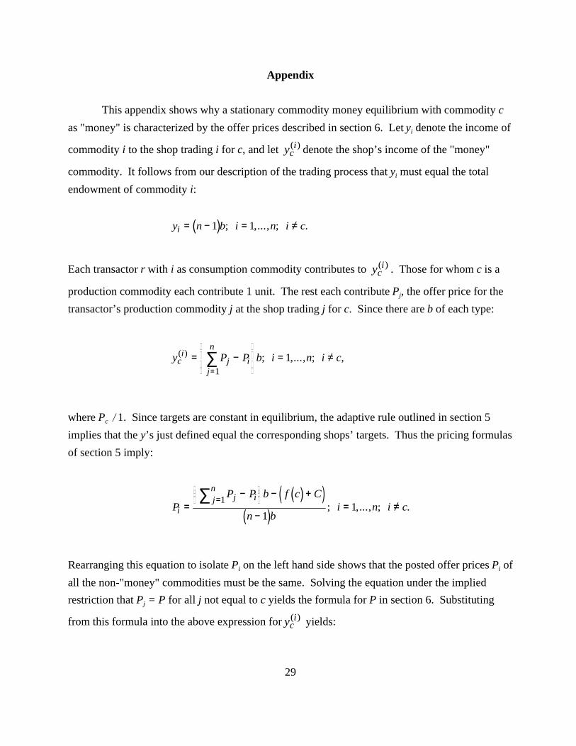
Appendix
This appendix shows why a stationary commodity money equilibrium with commodity c
as "money" is characterized by the offer prices described in section 6. Let yi denote the income of
commodity i to the shop trading i for c, and let denote the shop’s income of the "money"yci( )
commodity. It follows from our description of the trading process that yi must equal the total
endowment of commodity i:
( )y n b i n i ci = − = ≠1 1; ,..., ; .
Each transactor r with i as consumption commodity contributes to . Those for whom c is ayci( )
production commodity each contribute 1 unit. The rest each contribute Pj, the offer price for the
transactor’s production commodity j at the shop trading j for c. Since there are b of each type:
y P P b i n i cci
jj
n
i( ) ; ,..., ; ,= − = ≠
=∑
1
1
where Pc /1. Since targets are constant in equilibrium, the adaptive rule outlined in section 5
implies that the y’s just defined equal the corresponding shops’ targets. Thus the pricing formulas
of section 5 imply:
( )( )( )
PP P b f c C
n bi n i ci
jjn
i=
− − +
−= ≠
=∑ 1
11; ,..., ; .
Rearranging this equation to isolate Pi on the left hand side shows that the posted offer prices Pi of
all the non-"money" commodities must be the same. Solving the equation under the implied
restriction that Pj = P for all j not equal to c yields the formula for P in section 6. Substituting
from this formula into the above expression for yields:yci( )
30
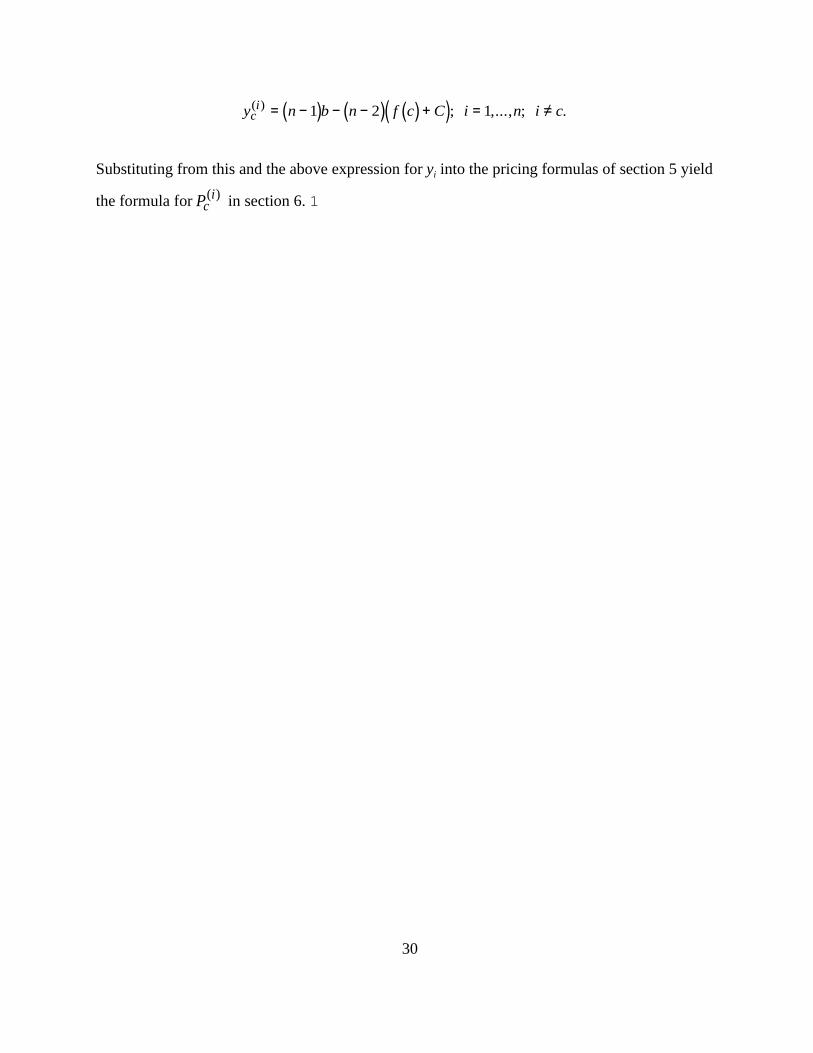
( ) ( ) ( )( )y n b n f c C i n i cci( ) ; ,..., ; .= − − − + = ≠1 2 1
Substituting from this and the above expression for yi into the pricing formulas of section 5 yield
the formula for in section 6. 1Pci( )

31
References
Alchian, Armen. "Why Money." Journal of Money, Credit and Banking 9 (February 1977, Part
2): 133-40.
Arthur, W. Brian. "Competing Technologies, Increasing Returns, and Lock-In by Historical
Events." Economic Journal 99 (March 1989): 116-31.
Arthur, W. Brian, Steven N. Durlauf, and David A. Lane, eds. The Economy as an Evolving
Complex System II. Santa Fe Institute Studies in the Sciences of Complexity. Proceedings
Volume XXVII. Reading, MA: Addison Wesley, 1997.
Blinder, Alan S., Elie R. D. Canetti, David E. Lebow, and Jeremy B. Rudd. Asking About Prices:
A New Approach to Understanding Price Stickiness. New York: Russell Sage Foundation,
1998.
Chuchman, George. "A Model of the Evolution of Exchange Processes." Ph.D. Dissertation,
Department of Economics, University of Western Ontario, 1982.
Clower, Robert W. "A Reconsideration of the Microfoundations of Monetary Theory." Western
Economic Journal 6 (December 1967): 1-9. (now Economic Inquiry).
Clower, Robert W. "Reflections on the Keynesian Perplex." Zeitschrift für Nationalökonomie 35
(July 1975): 1-24.
Clower, Robert W. "On the Origin of Monetary Exchange." Economic Inquiry 33 (October 1995):
525-36.
Clower, Robert, and Peter Howitt. "Taking Markets Seriously: Groundwork for a Post Walrasian
Macroeconomics." In Beyond Microfoundations: Post Walrasian Macroeconomics, edited
by David Colander, 21-37. New York: Cambridge University Press, 1996.
Clower, Robert, and Peter Howitt. "Money, Markets and Coase." In Is Economics Becoming a
Hard Science?, edited by Antoine d’Autume and Jean Cartelier, 189-203. Cheltenham,
UK: Edward Elgar, 1997.
Cuadras-Morató, Xavier, and Randall Wright. "Money as a Medium of Exchange When Goods
Vary by Supply and Demand." Macroeconomic Dynamics 1 (1997): 680-700.
Dawid, Herbert. "On the Emergence of Exchange and Mediation in a Production Economy."
Journal of Economic Behavior and Organization (Forthcoming 1999).
Dawkins, Richard. River Out of Eden: A Darwinian View of Life. New York: BasicBooks, 1995.
Day, Richard H. "Disequilibrium Economic Dynamics: A Post-Schumpeterian Contribution."
Journal of Economic Behavior and Organization 5 (March 1984): 57-76.

32
Dennett, Daniel Clement. Darwin’s Dangerous Idea: Evolution and the Meanings of Life. New
York: Simon and Shuster, 1996.
Einzig, Paul. Primitive Money: In its Ethnological, Historical and Economic Aspects. London:
Eyre and Spottiswoode, 1949.
Epstein, Joshua M., and Robert Axtell. Growing Artificial Societies. Cambridge, MA: MIT Press,
1996.
Friedman, Daniel. "Evolutionary Games in Economics." Econometrica 59 (May 1991): 637-66.
Friedman, Daniel, and Joel Yellin. "Evolving Landscapes for Population Games." Unpublished,
UC Santa Cruz, February 17 1997.
Hall, R. L., and C. J. Hitch. "Price Theory and Business Behaviour." Oxford Economic Papers
(May 1939): 12-45.
Heymann, Daniel, Roberto P. J. Perazzo, and Andrés R. Schuschny. "Price Setting in a Schematic
Model of Inductive Learning." In Money, Markets and Method: Essays in Honor of Robert
W. Clower, edited by Peter Howitt, Elisabetta de Antoni, and Axel Leijonhufvud, 247-66.
Cheltenham: Edward Elgar, 1999.
Hicks, J. R. Critical Essays in Monetary Theory. Oxford: Clarendon Press, 1968.
Howitt, Peter. "Stability and the Quantity Theory." Journal of Political Economy 82
(January/February 1974): 133-51.
Ioannides, Yannis M. "Trading Uncertainty and Market Form." International Economic Review
31 (August 1990): 619-38.
Iwai, Katsuhito. "The Bootstrap Theory of Money: A Search-Theoretic Foundation of Monetary
Economics." Structural Change and Economic Dynamics 7 (December 1996): 451-77.
Jackson, Matthew O., and Alison Watts. "The Evolution of Social and Economic Networks."
Unpublished, August 26 1998.
Jackson, Matthew O., and Asher Wolinsky. "A Strategic Model of Social and Economic
Networks." Journal of Economic Theory 71 (October 1996): 44-74.
Jodhimani, Albert G. "Transactions Costs and the Evolution of Market Completeness." Ph.D.
Dissertation, The Ohio State University, 1999.
Johnson, Phillip Martin. "Essays on Capital Markets: Frictions and Social Forces." Ph.D.
Dissertation, U.C.L.A., 1997.
Jones, Robert A. "The Origin and Development of Media of Exchange." Journal of Political
Economy 84 (August 1976, Part 1): 757-75.
33
Kauffman, Stuart A. The Origins of Order: Self-Organization and Selection in Evolution. New
York: Oxford, 1993.
Keynes, J. N. "Demand." In Dictionary of Political Economy, Vol I, edited by R. H. Inglis
Palgrave, 539-42. London: Macmillan, 1894.
Kiyotaki, Nobuhiro, and Randall Wright. "On Money as a Medium of Exchange." Journal of
Political Economy 97 (August 1989): 927-54.
Luo, Guo Ying. "Evolutionary Models of Market Behavior." Ph.D. Dissertation, University of
Western Ontario, 1995.
Marimon, Ramon, Ellen R. McGrattan, and Thomas J. Sargent. "Money as a Medium of
Exchange in an Economy with Artificially Intelligent Agents." Journal of Economic
Dynamics and Control 14 (May 1990): 329-73.
Matsuyama, Kiminori, Nobuhiro Kiyotaki, and Akihiko Matsui. "Toward a Theory of
International Currency." Review of Economic Studies 60 (April 1993): 283-307.
Maynard Smith, John. Evolution and the Theory of Games. Cambridge, UK: Cambridge
University Press, 1982.
Ostroy, Joseph M. "The Informational Efficiency of Monetary Exchange." American Economic
Review 63 (September 1973): 597-610.
Pingle, Mark. "The Effect of Decision Costs on the Formation of Market-Making Intermediaries:
A Pilot Experiment." Journal of Economic Behavior and Organization (Forthcoming
1999).
Snell, Daniel C. Life in the Ancient Near East: 3100-332 B.C.E. New Haven: Yale University
Press, 1997.
Spulber, Daniel F. The Market Makers: How Leading Companies Create and Win Markets. New
York: BusinessWeek Books, 1998.
Starr, Ross M. "Monetizing Trade: A Tatonnement Example." Unpublished manuscript, UC San
Diego, October 22 1998.
Starr, Ross M., and Maxwell B. Stinchcombe. "Exchange in a Network of Trading Posts."
Discussion Paper 93-13, Department of Economics, University of California San Diego,
April 1993.
Starr, Ross M., and Maxwell B. Stinchcombe. "Monetary Equilibrium with Pairwise Trade and
Transaction Costs." Unpublished, University of California San Diego, September 3, 1998.
Tesfatsion, Leigh. "A Trade Network Game With Endogenous Partner Selection." Unpublished,
Iowa State University, June 1996.

34
Vriend, Nicolaas J. "Self-Organization of Markets: An Example of a Computational Approach."
Computational Economics 8 (August 1995): 205-31.
Walker, Donald A. Advances in General Equilibrium Theory. Cheltenham, UK: Elgar, 1997.
Walras, Léon. Elements of Pure Economics. New York: Augustus M. Kelley, 1926. (Translated
by William Jaffé, 1954).
Wright, Sewall. "Evolution in Mendelian Populations." Genetics 16 (March 1931): 97-159.
Young, H. Peyton. Individual Strategy and Social Structure: An Evolutionary Theory of
Institutions. Princeton: Princeton University Press, 1998.

UsmaxMonfrDist1Dist0Gap3Gap2Gap1GapGDPPrmonAvyrsPrdevSlope
0.3870.7690.5730.5720.0000.0000.0070.00721450.028131.100.86000.5830.8260.1040.1040.0290.0050.0210.05419580.99892.920.81021.0001.0000.0170.0210.0200.0060.0070.03319140.99877.880.9664
0.0170.0260.0410.0080.0090.05817811.00066.050.97260.0090.0130.0290.0090.0050.04317221.00042.030.98680.0010.0010.0090.0100.0000.02016771.00027.600.998100.0020.0020.0210.0120.0010.03515641.00019.040.998120.0010.0010.0190.0100.0000.02914861.00012.191.000140.0010.0010.0170.0050.0000.02314071.00012.871.000160.0010.0010.0260.0000.0000.02613151.00016.781.000180.0010.0010.0280.0000.0000.02812251.00028.131.000200.5550.58611.0020.0311.04312.075-129581.000202.590.25822
0.3890.7700.1070.1110.9370.0080.0911.0364360.92349.570.904overall0.3890.7700.0660.0670.0220.0060.0050.03216540.92145.840.963all but 22
TABLE 2
Each data point is an average over all 500 runs using that value of the slope parameter.Prdev is the fraction of runs in which the economy achieved full development.Avyrs is the average number of years it took to reach full development when that occurred.Prmon is the observed probability that "monetary exchange" emerges when the economy
achieves full development.GDP is total supply of participants minus total overhead costsGap is the proportional gap between actual and maximal GDP. It is decomposed into:
Gap1: Attributable to not enough participantsGap2: Attributable to an inefficent money commodityGap3: Attributable to too many shops
Dist0 is the distance of wholesale prices from stationary commodity money equilibrium values.Dist1 is the distance of retail prices from their monetary equilibrium values.Monfr is the number of transactors that are trading indirectly on the final week of
a run that achieved full development without "monetary exchange" emerging,expressed as a fraction of the maximal number m(n-2)/n = 1728.
Usmax is the number of transactors using the most common exchange intermediary, on thefinal week of such a run, also expressed as a fraction of the maximal number.

0.836112.750559.5921111.4140.024
0.00275.2642.0162.8540.808
0.00275.2343.4563.4560.964
64.2000.972
41.4420.986
27.5460.998
19.0060.998
12.1921.000
12.8741.000
16.7761.000
28.1301.000
52.2680.258

Bdist1Bdist0Bgap3Bgap2Bgap1BgapMdist1Mdist0Mgap3Mgap2Mgap1MgapSlope0.5870.5860.0000.0000.0070.0070.0010.0010.0000.0000.0000.00000.5400.5390.1420.0080.1070.2570.0010.0010.0020.0040.0000.00620.4720.5830.4810.0140.1980.6940.0000.0000.0030.0050.0000.00940.6040.9191.2390.0270.3391.6060.0010.0010.0060.0070.0000.01360.6110.8371.4750.0250.3691.8690.0010.0010.0090.0090.0000.01780.0020.0020.0640.0000.0000.0640.0010.0010.0090.0100.0000.020100.7400.7883.8300.0590.4324.3210.0010.0010.0140.0120.0000.02612
0.0010.0010.0190.0100.0000.029140.0010.0010.0170.0050.0000.023160.0010.0010.0260.0000.0000.026180.0010.0010.0280.0000.0000.02820
0.9471.00014.6340.0411.38916.0640.0020.0010.0420.0000.0000.042220.6950.7205.5050.0170.5426.0650.0010.0010.0140.0060.0000.020overall0.5770.5880.0860.0030.0400.1290.0010.0010.0130.0060.0000.020 all but 22
TABLE 3
Mgap is the proportional GDP gap in those runs where "monetary exchange" emerged.Bgap is the proportional gap in all other runs.Mdist and Bdist are the analogous breakdowns of the Dist statistics between "monetary" and other runsThe shaded cells are those for which the statistic is based on fewer than five runs.

Prmn10Prmn9Prmn8Prmn7Prmn6Prmn5Prmn4Prmn3Prmn2Prmn1Slope0.0000.0000.1670.0830.0830.1670.1670.0000.0000.33300.0000.0000.0000.0000.0020.0050.0220.0920.2620.61620.0000.0000.0000.0000.0000.0000.0060.0440.2300.72040.0000.0000.0000.0000.0000.0000.0000.0370.2040.75960.0000.0000.0000.0000.0000.0000.0000.0280.1950.77780.0000.0000.0000.0000.0000.0000.0000.0000.2220.778100.0000.0000.0000.0000.0000.0000.0000.0000.2060.794120.0000.0000.0000.0000.0000.0000.0000.0000.1320.868140.0000.0000.0000.0000.0000.0000.0000.0000.0580.942160.0000.0000.0000.0000.0000.0000.0000.0000.0001.000180.0000.0000.0000.0000.0000.0000.0000.0000.0001.000200.0000.0000.0000.0000.0000.0000.0000.0000.0001.000220.0000.0000.00040.00020.00040.00080.00280.0180.14410.833overall
TABLE 4
Prmni, for i=1,...,10, is the observed probability that good i is the "money" commodity when"monetary exchange" emerges.
In the shaded cells, a stationary commodity money equilibrium does not exist.

UsmaxMonfrDist1Dist0Gap3Gap2Gap1GapSurplusPrmonAvyrsPrdevSlope
0.7770.8290.0060.0050.0020.0000.0010.00320640.99611.310.99020.0000.0000.0020.0000.0000.00219761.0007.771.0004
Prmn10Prmn9Prmn8Prmn7Prmn6Prmn5Prmn4Prmn3Prmn2Prmn1Slope0.0000.0000.0000.0000.0000.0000.0000.0000.0370.96320.0000.0000.0000.0000.0000.0000.0000.0000.0040.9964
TABLE 5
These data are generated from an initial position of the merger of two fully monetized economies, one with commodity 1 as "money" and the other with commodity 2.

Prm10Prmn9Prmn8Prmn7Prmn6Prmn5Prmn4Prmn3Prmn2Prmn1Prmon PrdevSlope0.9380.0631.0000.96020.8700.1301.0000.92040.7440.2561.0000.86060.7390.2611.0000.92080.6460.3541.0000.960100.6330.3671.0000.980120.5400.4601.0001.000140.4900.5101.0000.980160.3600.6401.0001.000180.0610.9390.9801.000200.5960.4040.9980.958overall
TABLE 6Simulation results when commodity 2 is the most abundant and most widely consumed commodity
Each data point is an average over 50 runs.For every distinct pair (i,j) there were 20 transactors having i as production
commodity and j as consumption commodity, except for i=2 or j=2, in which case there were 40.
Prm10Prmn9Prmn8Prmn7Prmn6Prmn5Prmn4Prmn3Prmn2Prmn1Prmon PrdevSlope0.0400.0800.6200.2601.0001.0002
0.0200.5600.4201.0001.00040.0400.6800.2801.0001.0006
0.5600.4401.0001.00080.5800.4201.0001.000100.5200.4801.0001.000120.5400.4601.0001.000140.2400.7601.0001.00016
1.0001.0000.700180.0050.0160.4940.4851.0000.967overall
TABLE 7Simulation results when commodity 2 is the most abundant commodity
Each data point is an average over 50 runs.For every distinct pair (i,j) there were 20 people having i as production
commodity and j as consumption commodity, except for i=2, in which case there were 60.
0
300
600
900
1200
1500
1800
0
20
40
60
80
100
0 50 100 150 200 250 300
Year
Using 3 as intermediary Trading Indirectly
Trading Directly Number of shops
FIGURE 2 (a)
Run 35 Slope 4
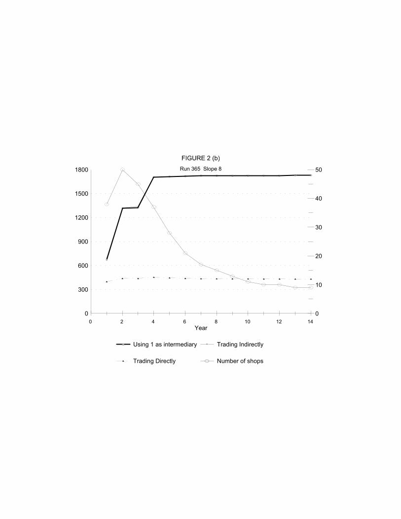
0
300
600
900
1200
1500
1800
0
10
20
30
40
50
0 2 4 6 8 10 12 14 Year
Using 1 as intermediary Trading Indirectly
Trading Directly Number of shops
FIGURE 2 (b)
Run 365 Slope 8
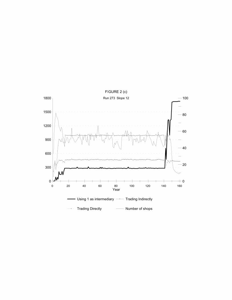
0
300
600
900
1200
1500
1800
0
20
40
60
80
100
0 20 40 60 80 100 120 140 160 Year
Using 1 as intermediary Trading Indirectly
Trading Directly Number of shops
FIGURE 2 (c)
Run 273 Slope 12

0
300
600
900
1200
1500
1800
0
20
40
60
80
100
0 10 20 30 40 50 60 Year
Using 1 as intermediary Trading Indirectly
Trading Directly Number of shops
FIGURE 2 (d)
Run 319 Slope 18
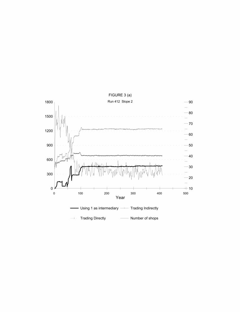
0
300
600
900
1200
1500
1800
10
20
30
40
50
60
70
80
90
0 100 200 300 400 500
Year
Using 1 as intermediary Trading Indirectly
Trading Directly Number of shops
FIGURE 3 (a)
Run 412 Slope 2
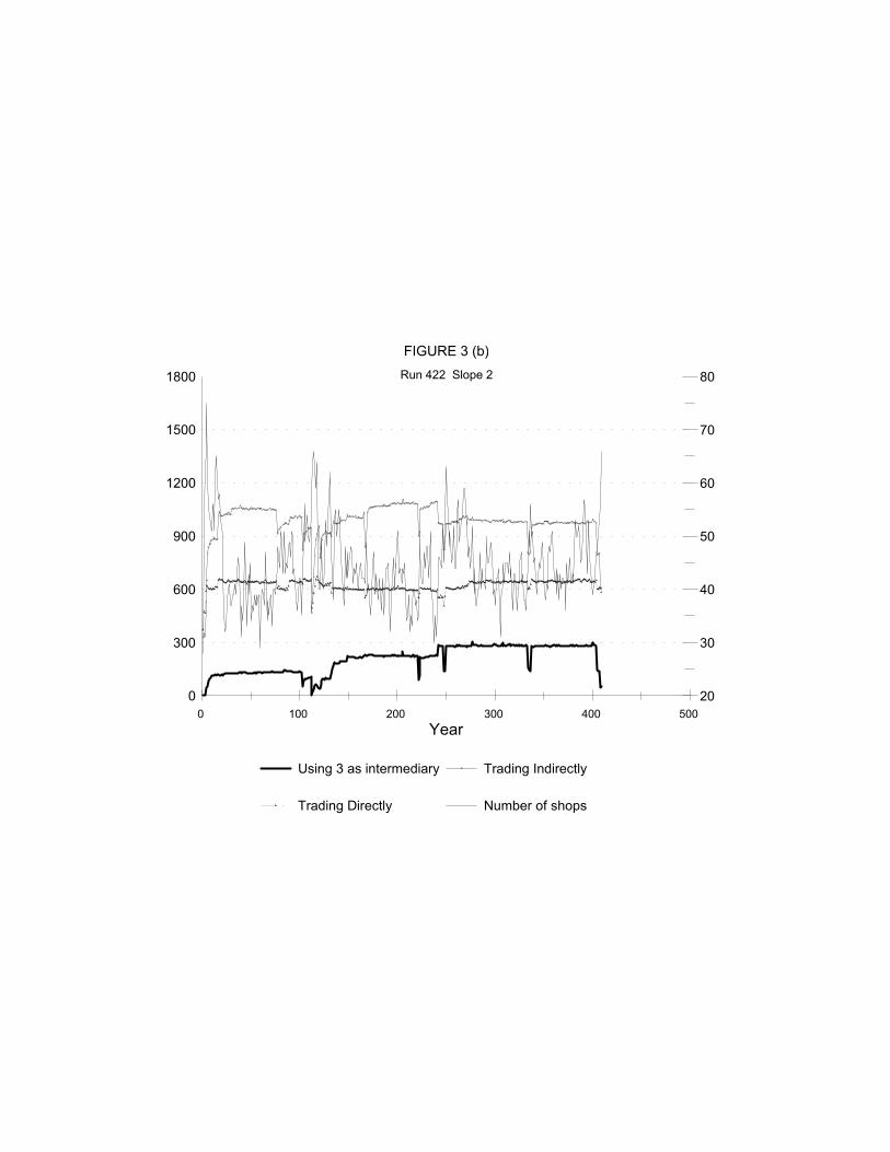
0
300
600
900
1200
1500
1800
20
30
40
50
60
70
80
0 100 200 300 400 500
Year
Using 3 as intermediary Trading Indirectly
Trading Directly Number of shops
FIGURE 3 (b)
Run 422 Slope 2
Copyright © 2022 FDOKUMEN

