The e¤ect of location on �nding a job in the Paris region�

L. Gobillony, T. Magnacz, H. Selodx

March 5, 2009

�We are grateful to a co-editor and two anonymous referees for their comments and we thank as well the partic-

ipants at seminars at INRA, CREST, University of Tokyo, Louvain-la-Neuve and the North American Meetings of

the Regional Science Association International 2006. We thank the French National Employment Agency (ANPE)

and the Ministry of Transport�s Regional Directorate (DREIF) for providing us with the data. All remaining errors

are ours. The �ndings, interpretations, and conclusions expressed in this paper are ours and do not represent the

view of our employers, including the World Bank, its executive directors, or the countries they represent.yInstitut National d�Etudes Démographiques (INED), PSE-INRA and CREST. Address: INED, 133 boulevard

Davout, 75980 Paris Cedex 20, France. E-mail: laurent.gobillon@ined.fr.z Toulouse School of Economics (GREMAQ & IDEI) Address: Manufacture des Tabacs, 21 allée de Brienne,

31000 Toulouse, France. E-mail: magnac@cict.fr.xThe World Bank and CREST. Address: 1818 H Street NW, Washington DC 20433, United States of America:

hselod@worldbank.org.

1

Abstract

An important but empirically debated issue in spatial economics is whether spatial dif-

ferences in unemployment re�ect residential sorting on invidividual characteristics or a true

e¤ect of location. We investigate this issue in the 1,300 French muncipalities that constitute

the Paris region and across which there is overwhelming evidence of spatial disparities in un-

employment durations. We resort to a methodology that enables us to disentangle individual

and unspeci�ed local e¤ects. In order to control for individual determinants, we estimate a

proportional hazard model strati�ed by municipality using an exhaustive dataset of all un-

employment spells starting in the �rst semester of 1996. This model allows us to recover a

survival function for each municipality that is purged of individual observed heterogeneity.

We show that only around 30% of the disparities in the observed determinants of the survival

rates relate to individual variables. Nearly 70% of the remaining disparities are captured by

local indicators which we show to be mainly correlated with local measures of residential

segregation. We are also able to show that local and individual characteristics reinforce one

another in their contribution to spatial disparities in unemployment duration.

Keywords: Unemployment, Duration models, Economic geography, Urban economics.

JEL Codes: C41, J64, R23

2

1 Introduction

The determinants of urban unemployment have raised the interest of economists for decades. In

the US, two major trends of literature have tried to explain how location could have an adverse

impact on employment, involving a variety of mechanisms. The �rst set of works is the so-called

spatial mismatch literature which investigates how the physical disconnection from jobs can ex-

acerbate unemployment among low-skilled minority workers (see Ihlanfeldt and Sjoquist, 1998,

for an empirical survey, and Gobillon, Selod and Zenou, 2007, for a theoretical one). The second

set of works investigates the impact of residential segregation on the poor labor-market outcomes

of ghetto residents (see e.g. Wilson, 1996, Cutler and Glaeser, 1997). In both literatures, papers

usually resort to cross-section methods and try to explain individual unemployment probabilities

or local unemployment rates (see e.g. Ihlanfeldt, 1993, Conley and Topa, 2002, Weinberg, 2000

and 2004).

In this paper, we focus on the local determinants of unemployment duration. Only a few

papers, mainly on the US, have studied unemployment dynamics at the individual level with

a spatial perspective (Holzer, Ihlanfeldt and Sjoquist, 1994, Rogers, 1997, Dawkins, Shen and

Sanchez, 2005, Johnson, 2006). In these works, authors usually investigate the impact of local

indicators proxying for spatial mismatch or residential segregation in an unemployment duration

model. They typically estimate a proportional hazard model with a single baseline hazard common

to all locations, a set of individual variables and local indicators. We adopt a much broader

approach that consists in estimating a baseline hazard function for each location while controlling

for individual characteristics in a proportional hazard model. This key methodological innovation,

known as the Strati�ed Partial Likelihood Estimator (SPLE), was �rst proposed by Ridder and

Tunali (1999) in another context. We apply it in this paper to a large administrative dataset

containing records of unemployment spells and adapt it to include some new econometric features.

Compared to the previous literature, the advantages of our empirical strategy are threefold.

First, we do not need to choose a speci�c function for the local hazard functions. We can thus

measure the overall e¤ects of location without only focusing on a few arbitrarily selected mech-

anisms, proxied by criticizable local indicators. Second, we allow the e¤ect of location to vary

depending on the time spent unemployed. We can thus assess the e¤ect of location on the short

3

run (say, after 6 months) and on the long run (say, after two years). Third, the model is su¢ ciently

versatile to allow us to further restrict local hazard rates while controling for the generality of

these restrictions.

The estimation procedure has three steps. The �rst step consists in estimating a proportional

hazard model with an unspeci�ed municipality-speci�c hazard baseline hazard. In the second

step of the estimation procedure, we impose that the municipality e¤ects are multiplicative in the

hazard rate. This multiplicative component model summarizes the local e¤ects through a single

indicator. In the third stage, we assess how this local indicator may capture local determinants

re�ecting the di¤erent mechanisms put forward by the literature. This is done by regressing mu-

nicipality e¤ects on these variables and computing their explanatory power. We do not interpret

this last stage as a causal regression because omitted variable or reverse causality concerns can-

not be dismissed. Our procedure however ensures that the previous stages are immune to these

endogeneity issues so that we can separate the robust estimation of local e¤ects from less robust

results obtained in the third stage.

Yet, we cannot easily deal with individual unobserved heterogeneity in our proportional haz-

ard speci�cation. This is in line with Baker and Melino (2000)�s �nding that identi�cation of both

�exible hazard rates and the distribution of unobserved heterogeneity is fragile in empirical stud-

ies. Moreover, individual unobserved heterogeneity like, for instance, omitted variables related to

preferences, is partially captured since we model the hazard rate function at the level of the mu-

nicipality. Furthermore, we apply goodness of �t test procedures under the form of a Kolmogorov

statistic as developed in Andrews (1997) and show that the model �ts the data very well at the

level of each municipality.

Our approach requires a very large dataset comprising enough unemployment spells in each

location. We use a unique exhaustive administrative dataset available for the Paris region from

which we extract unemployment spells that started in the �rst semester of 1996. Unemployment

spells can end in three di¤erent ways: �nding a job, dropping out of the labor force, and right-

censorship (including exits for unknown reasons). We model the �rst two exits in an independent

competing risk framework.

Our main empirical results are as follows. We �nd that controling for individual characteristics

explains around 30% of the spatial disparities across municipalities in unemployment durations

4

until �nding a job. Among the main individual determinants of unemployment duration as educa-

tion, it should be stressed that some nationalities, Africans in particular, experience signi�cantly

much larger durations until �nding a job. Furthermore, the association between average individ-

ual characteristics at the municipality level and baseline hazards is positive. Presumably because

of sorting e¤ects, individual and local e¤ects reinforce each other in their contribution to spatial

disparities of unemployment duration. In other words, durations are not only larger because of

an adverse individual characteristic but also because the average of this adverse characteristic is

larger at the local level. Finally, nearly 70% of the remaining local disparities are captured by

local indicators, mainly segregation indices.

The rest of the paper is structured as follows. In section 2, we provide a short survey of the

litterature on how segregation and bad physical accessibility to jobs can increase unemployment

duration. Section 3 presents the data and a selection of descriptive statistics to measure spatial

disparities. Section 4 details the SPLE method. Section 5 discusses the results. Finally, section 6

concludes.

2 Why should location in�uence unemployment duration?

The duration of unemployment depends on many factors. To discuss this issue in an orderly

manner, it is useful to adopt a job-search perspective considering that exit from unemployment

can occur at the end of a three-stage process. In the �rst stage, workers must wait some time

before coming into contact with a job opportunity. In the second stage, an o¤er from an employer

may materialize. Finally, workers may accept or reject the o¤er depending on whether the o¤ered

wage is greater or smaller than their reservation wage. With this framework in mind, job seekers

who, on average, wait long before experiencing contacts with employers and who have few chances

to transform their contacts into o¤ers and matches should experience long unemployment spells.

For instance, educated workers could be advantaged in the �rst stage if they are more e¢ cient in

obtaining information about jobs and in contacting �rms, or if labor demand is biased in their

favor. They may also have an advantage in the second stage if they write better application letters

and resumes, and fare better during interviews. However, educated workers may be more likely

to reject an o¤er when they face or anticipate many well-paid outside o¤ers. Other individual

5

and family characteristics such as gender, race/ethnicity, age, experience, marital status or the

number and age of children and dependants should also be expected to a¤ect unemployment

duration through one or several stages of the job-acquisition process.

This section describes how location, i.e. the disconnection from job opportunities (in cases

where job opportunities are unevenly distributed within a metropolitan area) and/or residential

segregation (in terms of education, race/ethnicity/nationality or employment status), can also

in�uence the duration of unemployment. We decompose the e¤ects on each stage of the job-

acquisition process.

Disconnection from job opportunities may directly a¤ect the time spent searching for a job in

the �rst stage of the process. Indeed, job-seekers residing in areas with few local job vacancies or

in areas located far away from employment centers are exposed only to a small pool of vacancies.

Residing in loose local labor markets, they should spend more time searching before getting into

contact with a potential employer. Of course, job-seekers also have the possibility to search for

jobs in other areas. But having to search away from one�s area of residence penalizes job seekers.

At least three reasons may come into view. Firstly, because of informational frictions, job-seekers

may not search e¢ ciently far away from their residences. For instance, workers residing far away

from job opportunities may not hear about job o¤ers when �rms resort to recruiting methods that

favor the local labor force (i.e. by posting �wanted�signs in retail shops, or by choosing not to

publicize job o¤ers beyond a certain distance). Alternatively, job-seekers may obtain only partial

information on the location of distant jobs or may have only a vague idea about the types of jobs

o¤ered in parts of the metropolitan area they are not familiar with. They may end up searching

in the wrong places (Ihlanfeldt, 1997, Stoll and Raphael, 2000). Secondly, because search is costly,

workers may restrict their search horizon at the vicinity of their neighborhood. They may search

less often in order to reduce the number of job-search trips or may not search at all for jobs

located in distant places. In this context, access to public transport or car ownership can reduce

job-search costs and expand the job-search horizon (Stoll, 1999). Thirdly, the individual search

e¤ort may depend on the local cost of living so that workers residing in areas disconnected from

job opportunities may not search intensively. It has been argued that workers residing in such

areas usually incur low housing costs and thus may feel relatively little less pressure to actively

6

search for a job in order to pay their rent (Smith and Zenou, 2003, Pattachini and Zenou, 2006).

Disconnection from job opportunities may also reduce the frequency of job proposals in the

second stage. Employers may then be reluctant to propose jobs to distant workers because com-

muting long distances would make these workers less productive (they would show up late or be

tired due to excessive commuting, see Zenou, 2002).

Distance to job opportunities may also reduce the probability of a job acceptance in the third

stage. Indeed, workers may reject a job o¤er that would involve commutes that are too long if

commuting to that job would be too costly in view of the proposed wage (Zax and Kain, 1996).

In other words, distance is likely to make the o¤ered wage net of commuting costs drop below a

worker�s given reservation wage.

The e¤ect of residential segregation on the �rst stage of the job-acquisition process is also

likely to be harmful to the extent that job contacts often occur through friends and relatives

(Mortensen and Vishwanath, 1994). Because social networks are at least partly localized, when the

unemployment rate is high in a given area, workers are less likely to know employed neighbors that

can let them know about existing vacancies (Calvó and Jackson, 2004, Selod and Zenou, 2006).

Residential segregation is also likely to reduce the probability for a worker residing in a segre-

gated area to receive a job o¤er. This is because employers may discriminate against residentially

segregated workers, a practice known as redlining (see Wilson, 1996, for stories of �rms not hiring

workers located in �bad�neighborhoods). For employers, the motivation can hinge upon the stigma

or prejudice associated with the residential location of candidates (sheer discrimination), or be-

cause they consider that, on average, workers from stigmatized areas have bad work habits or are

more likely to be criminal (statistical discrimination). In industries and jobs in which workers are

in contact with customers, employers may discriminate against residentially-segregated workers

in order to satisfy the perceived prejudices of their clients, a practice known as customer discrim-

ination (Holzer and Ihlanfeldt, 1998). In France, the issue of redlining is increasingly being put

forward in the public debate to account for the unemployment of the young adults that reside in

distressed areas. To our knowledge, however, the issue has not yet been studied empirically.

All these economic mechanisms suggest that the rate at which workers leave unemployment,

and thus the duration of unemployment, depends on both individual characteristics and local

7

features. In the present paper, we propose a methodology to disentangle individual and unspeci�ed

local e¤ects. We explore the nature of local e¤ects by regressing them on indices of segregation

and distance to job opportunities. We assess the overall impact of these indices on �nding a job,

but we do not try to identify through which speci�c mechanisms they percolate.

3 Description of the Data

3.1 The area of study

The paper focuses on the Ile-de-France region (the Paris region hereafter), an administrative unit

of 10.9 million inhabitants distributed over 1,280 municipalities centered around the city of Paris

and the 20 administrative subdistricts of Paris (which will be treated as municipalities in the

analysis). These 1,300 spatial units may have very di¤erent population sizes which range from

225,000 in the most populous Parisian subdistrict to small villages located some 80 km away from

the center of Paris. They correspond more or less to the Paris Metropolitan Area as can be seen

from Graph 1 which represents the population density in each municipality.

[Insert Graph 1]

Graph 2 provides evidence that the studied area exhibits large spatial disparities in the local

unemployment rates across municipalities. In particular, the unemployment rates in municipalities

located to the North-East of Paris are more than four times higher than in most municipalities

located to the West.

[Insert Graph 2]

3.2 The ANPE historical �le

We use the historical �le of job applicants to the National Agency for Employment (Agence

Nationale pour l�Emploi or ANPE hereafter) for the Paris region to study spatial disparities in

unemployment durations. This database provides a quasi-exhaustive list of unemployment spells

in the region as it has been estimated that 90% of job seekers in France are indeed registered

with the ANPE (Chardon and Goux, 2003). The reason is that registering with the ANPE is

8

a prerequisite for unemployment workers to be able to claim their unemployment bene�ts. A

signi�cant share of those not eligible for unemployment bene�ts� as for instance �rst time job

seekers� also register with the ANPE to assist them in their job search.

The ANPE is organized in hundreds of local agencies and unemployed workers register in the

agency closest to their residence.1 The exhaustive dataset that we have for the Paris region contains

information on the exact date of an application (the very day), the unemployment duration (in

days), and the reason for which the application came to an end. Along with the municipality

where the individual lives and registers, a set of socio-economic characteristics were reported

upon registration with the employment agency: age, gender, nationality, diploma, marital status,

number of children and disabilities. To build our working sample, we select individuals who applied

to the employment agency between January 1 and June 30, 1996 and who lived in the Paris region

at that time. As we have information on unemployment spells until 2003, starting as early as 1996

enables us to follow unemployed workers over a long period of time and to minimize the number of

incomplete spells due to the end of the observation period (which only concerns 0:6% of the exits

in our sample. After deleting the very few observations for which socio-economic characteristics

are missing, we end up with 430; 695 observations on individual unemployment durations. More

details on the construction and the contents of the dataset are given in Appendix A.

We group the reasons given for the termination of the application with the agency into three

types: (1) �nding a job, (2) exiting to non-employment, and (3) right censoring, which groups

together unknown destinations and incomplete spells.2 In the following, we assume that right-

censoring is independent of the durations until exiting to a job or non-employment and that these

two exits are independent, conditional on all observed characteristics including the municipality of

residence. A large proportion of exits are right-censored (55:3%), of which 29:5% correspond to an

1Except in very speci�c occupations (artists, ...).2An exit to non-employment covers the following situations: a training period, an illness, a pregnancy, a job

accident (as some unemployed workers can in fact work for a very small number of hours), an exemption from the

rule imposing to actively search for a job, retirement, or military service. Unknown destinations can result from

mobility between four subregions (see text below), an absence at a control, an expulsion for some misbehavior, an

absence after a noti�cation, a training or job refusal, a fake statement, the lack of a positive action to search for a

job, and other unspeci�ed cases.

9

absence at a control.3 The remaining unemployment spells mostly end up with a job (28%) even

if exit to non-employment is far from negligible (16:7%). The average unemployment duration for

individuals �nding a job is 269 days whereas it stands at a higher level of 368 days for individuals

who exit to non-employment. The higher unemployment duration for exits to non-employment

could possibly re�ect the discouragement of workers that could not �nd a job after a long time.

A crucial issue in this data arises because residential mobility across municipalities could blur

our estimation of spatial disparities. In particular, because mobility can change the way unem-

ployment spells are recorded, it could give rise to (i) right and left censoring, to (ii) measurement

errors of local e¤ects, and (iii) to departures from the independence assumption because of right

censoring. To see how these issues may emerge and why we believe, however, that they may be

relatively minor, consider the following lines of reasoning:

First, the French Employment Agency is organized geographically in large subregions called

ASSEDIC and when residential mobility brings about a change in ASSEDIC, the unemployment

spell is right-censored and a (mistakenly fresh) spell is started in the new ASSEDIC. The unem-

ployment spell is thus cut into two halves, the �rst spell being right censored, and the second spell

being left-censored. Fortunately, there are only 4 ASSEDIC located in the Paris region (West,

East, South-East and Paris) and in our date only 4.83% of unemployed workers change ASSEDIC

as stated in the reasons for exits. Moreover, double counting is also mitigated by the fact that we

consider a �ow-sampling window of only six months starting at the beginning of 1996.

Second, even if mobility takes place within the same ASSEDIC, it might bring a change in

municipality and local agency. Although the spell is registered as uninterrupted, the stated place

of residence may either correspond to that recorded at the origin or at the destination agency.4

Yet, measurement errors of local e¤ects, if anything, would likely attenuate our measures of spatial

disparities.

3There is no evidence that these absences would mainly concern unemployed workers that neglected to report

they found a job. Indeed, a 2005 follow-up survey on a small random sample of unemployed workers having left the

ANPE showed that only approximately half of absentees at controls did �nd a job, which is not in contradiction

with the assumption of independence between right censoring and �nding a job.4The administrative treatment by ANPE of spells which ended in a local agency di¤erent from the one where

it started is very obscure. The two spells are registered and one of them is deleted apparently without following

any precise written rule.

10

Finally, in many aspects, the mobility decision could be partly independent of exiting to a job

or to non-employment. For instance, the prospect of saving money by living with one�s parents

might be an exogenous factor conditional on the individual and local e¤ects. On the other hand,

mobility is clearly endogenous if a job seeker moves with the prospect of waiting until �nding a

job near the new location. Given that mobility is low in France with respect to the US (Baccaini,

Courgeau and Desplanques, 1993), we believe that these issues have second order e¤ects compared

to the main substantive e¤ects of infrastructure, redlining or discrimination to which we now turn.

3.3 Spatial disparities

The Paris region exhibits stark socio-economic disparities which can broadly be depicted as follows.

In the North-East, the population is usually little educated, poor, and composed of blue collar

workers. Recent migrant minorities are over-represented. In the West, the population is very

educated, rich, and comprises mostly white collars. Minorities of recent immigration waves are

under-represented.

To further characterize disparities across municipalities and di¤erences in municipality environ-

ments, we compute municipality-speci�c segregation and job-accessibility variables using several

sources.

3.3.1 Census measures of segregation and job accessibility

Segregation is accounted for by the municipality proportion of education and nationality groups

computed from the 1999 Population Census. Job accessibility is measured by the job density

around each municipality. More precisely, for each municipality we are able to identify all the

other municipalities than can be reached within 45 minutes for a given transport mode (private

vehicles or public transport). The 45-minute cut-o¤ has been chosen just above the average

commuting time of 34 minutes in the Paris region (DREIF-INSEE, 1997). This de�nes a group of

accessible municipalities for which we can calculate the overall job density (the ratio of the number

of jobs located in the area to the number of occupied and unoccupied workers residing in the same

area).5 Data on the location of jobs and workers are from the 1999 census. Travel times between

5For a discussion of alternative indicators see Gobillon and Selod (2007).

11

municipalities are estimated at morning peak hours by the French Department of Transportation

for 2000 using a transport survey on the Paris region (Enquête Générale des Transports).

We compute indices of spatial disparities on these local segregation and job-accessibility vari-

ables. The indices we compute are the inter-decile ratio, the inter-decile range, the Gini index and

the coe¢ cient of variation, and results are reported in Table 1.6 We �nd that spatial disparities

across muncipalities are very pronounced for the percentage of African nationalities as the inter-

decile ratio is over 9 for the percentages of citizens from North Africa and sub-Saharan Africa.

This means that the frequency of African citizens is 9 times larger in municipalities at the 9th

decile than at the �rst. Spatial disparities are also large for segregation in terms of education

and stands near 4 for the percentage of individuals with a university degree and around 2:5 for

the percentage of individuals with a technical degree. Measures of job accessibility also exhibit

signi�cant spatial disparities. The inter-decile ratio for job densities by public transport is 3.

[Insert Table 1]

3.3.2 Spatial Disparities for the Unemployed

Spatial disparities in the characteristics of unemployed workers also exhibit a similar pattern over

the Paris region. Table 2 reports similar indices of spatial disparities across municipalities for

several variables of the ANPE historical �le. We measure the spatial disparities in the occurrence

of exit types, the unemployment duration conditionally on the type of exit, and the individual

variables that we use in our empirical analysis below. As with the census data, the indices we

compute are the inter-decile ratio, the inter-decile range, the Gini index and the coe¢ cient of

variation.

We �rst comment the spatial disparities in the proportions of individuals who respectively

experience an exit to a job, an exit to non-employment, and right-censoring. For simplicity, we

restrict our comments to the inter-decile ratio but other indicators give qualitatively similar results.

The inter-decile ratio is fairly large for the probability that unemployment �nishes with an exit to

6To compute the spatial inter-decile index of a variable, we construct the empirical distribution function of the

local average of the variable. Observations are weighted by the population in each municipality. We smooth the

empirical distribution by a Gaussian kernel with a Silverman�s rule of thumb bandwidth and deciles are retrieved

using a very �ne grid (1; 000; 000 points).

12

a job as it reaches 1:73. This means that, if we order municipalities with respect to the proportion

of unemployment spells ending with an exit to a job, an unemployment spell has 73 percent more

chances to end with an exit to a job in the municipality at the ninth decile than in the municipality

at the �rst decile. The inter-decile ratio is smaller for the probability of an exit to non-employment

(1:37) and for right-censoring (1:32). These variations in spatial disparities across exit types calls

for a careful conditioning on local e¤ects.

If we now look at unemployment durations conditionally on the type of exit, the inter-decile

ratio for unemployment spells ending with an exit to a job reaches 1:37. This means that an

unemployment spell ending with an exit to a job lasts 37 percent longer in the municipality at the

ninth decile than in the municipality at the �rst decile. For unemployment spells ending with an

exit to non-employment, the inter-decile ratio is even greater and stands at 1:43.

[Insert Table 2]

As the above data is right-censored because of exits to other states, these statistics are di¢ cult to

interpret. This is why we also assess disparities between municipalities with the help of duration

models. For each type of exit and for each municipality, we compute the Kaplan-Meier estimator

of the survival function (which takes into account right-censorship). Disparities by exit type can

then be assessed by comparing the survival function across municipalities for any chosen duration.

As survival functions are well estimated only when the number of unemployed workers is large

enough, we restrict our attention to municipalities with a population greater than 5,000 inhabitants

in 1999. Graph 3 represents the probability of �nding a job before 24 months for each municipality

of the Paris region. Disparities are large: the probability of �nding a job before 24 months is below

40% in many municipalities of the North-East, whereas it is above 55% in many municipalities

of the West. Graph 4 represents the probability of exiting to non-employment before 24 months

for each municipality. Contrary to the graph for exit to a job, no speci�c pattern emerges. This

contrast suggests that while job search outcomes strongly depend on location, this is less the case

for labor-market participation decisions.

[Insert Graph 3 and 4]

There are also noticeable spatial disparities in some of the socio-demographic characteristics of

unemployed workers. Whereas the spatial disparities in age, sex or marital status are small (see

13

Table 2), there are much larger disparities for some categories of nationality, education, and

family size, as well as for disability. The inter-decile ratio for instance is greater than 5 for the

proportion of Africans. In other words, the proportion of Africans among unemployed workers in

municipalities at the ninth decile is 5 times greater than in municipalities at the �rst decile. The

inter-decile ratio is above 5 for unemployed workers having three children or more, around 4 for

unemployed workers with no diploma, and above 2:5 for disabled unemployed workers.

In conclusion, spatial disparities of individual characteristics are large. Results in Tables 1

and 2 are hard to compare, data sources being so di¤erent. Likely origins of di¤erences between

them could be reporting errors and composition e¤ects although we did not investigate the point

further. It very much depends on the spatial disparities in entries into unemployment which we

are not in a position to assess using the data that are available to us.

4 The econometric model

We analyze the empirical associations between unemployment durations and the local context

(segregation and job accessibility) using a three-stage procedure. First, we specify a proportional

hazard model (PH model hereafter) with individual covariates and a municipality-speci�c baseline

hazard. Parameters related to individual variables are estimated using the strati�ed partial likeli-

hood estimator (SPLE hereafter) as proposed by Ridder and Tunali (1999). Municipality-speci�c

integrated baseline hazards are then recovered using the Breslow estimator. Second, municipal

baseline hazards are restricted to be a multiplicative function of an aggregate baseline hazard

function and of municipality e¤ects which are both estimated using the �rst-stage outputs. A

third and �nal descriptive stage consists in regressing the municipality e¤ects on local indicators

of segregation (municipality composition) and job accessibility.

Our approach can be justi�ed as follows. The �rst two stages allow to estimate municipality e¤ects.

For computational reasons, this would be unfeasible by maximum likelihood estimation in one stage

only since the number of municipalities (1; 300) is too large. The �nal stage consists in regressing

those municipality e¤ects on aggregate variables. It enables us to analyse the correlation between

spatial e¤ects and segregation or job accessibility indices, although we do not claim to estimate

causal e¤ects in the last stage. Our procedure in three steps guards us against speci�cation errors

14

at each stage. First stage estimates are robust to misspeci�cation of the multiplicative model and

of the descriptive regression of municipality e¤ects. Second stage estimates are robust to errors

at the descriptive regression stage. Furthermore, all steps contribute to the empirical analysis of

spatial disparities in unemployment durations.

4.1 Model Speci�cation

Consider an individual i who enters unemployment (i.e. who enters the ANPE �le). His unem-

ployment spell lasts until he �nds a job (exit labeled e) or drops out of the labor force (exit labeled

ne). The unemployment spell is right-censored if the individual disappears from the records dur-

ing the observation period or has not experienced an exit before the last day of observation in the

panel. A latent duration Tk is associated with each exit k 2 fe; neg. For an individual i, we denote�k (� jXi; j(i)) the conditional hazard rate for exit k where Xi is a set of individual explanatory

variables � that are �xed over time in our application � and j (i) ; where j(i) 2 f1; :::; Jg ; isthe municipality where the individual is located. We adopt the proportional hazard assumption

separating the e¤ect of individual characteristics and the e¤ect of local clusters by writing:

�k (t jXi; j(i)) = �j(i)k (t) exp (Xi�k) for k 2 fe; neg ; (1)

where �jk (t) is the baseline hazard rate function for municipality j and exit k. Observe that the

e¤ect of local variables is not of the proportional hazard type at this stage since the municipality-

speci�c baseline hazard rate is fully �exible. Additionally, the two latent durations and right-

censorship are assumed to be independent so that our framework is an independent competing

risk model where observations are clustered.

Observe also that the above speci�cation features come at the expense of overlooking unob-

served individual heterogeneity whose presence can bias the estimation of the hazard rates and

parameters. Latent durations associated with di¤erent types of exit might also be dependent if

the e¤ect of individual unobserved heterogeneity in�uencing the di¤erent types of exit are cor-

related. Lancaster (1990) proposes to introduce individual unobserved heterogeneity in a partial

likelihood model by modeling it as a gamma distribution and to estimate parameters using an

EM algorithm. Yet, the procedure is burdensome and unfeasible in samples where the number of

observations is as large as in ours. An alternative way to proceed would be to di¤erence out indi-

15

vidual unobserved terms using multiple spells. In theory, this could be done by rede�ning clusters

as couples (municipality, individual) but the number of applicants appearing twice or more is very

small (about 8%) and the issue about biases caused by residential mobility could then become

serious. Also note that Baker and Melino (2000) argue that it is di¢ cult to empirically identify

the unobserved heterogeneity distribution and �exible hazard rates, and that in the current appli-

cation, the hazards are fully �exible at the municipality levels. For all these reasons, we decided

not to incorporate individual unobserved heterogeneity in our econometric speci�cation (1). We

nevertheless discuss below the consequences of its presence on our empirical results. Speci�cally,

we will pay attention to the e¤ects of the sorting of individuals across municipalities according to

their unobserved characteristics.

4.2 Strati�ed Partial Likelihood Estimation (SPLE)

Our estimation follows Ridder and Tunali (1999). Start with the estimation of the e¤ects of

individual explanatory variables using the SPLE. Denote j (t) the set of individuals at risk of

exiting unemployment in municipality j at time t. The probability of individual i experiencing

a type-k exit at time t conditionally on someone in the same municipality experiencing a type-k

exit is:7

Pi (t; k) =exp (Xi�k)X

n2j(i)(t)

exp (Xn�k)(2)

Observe that conditioning on the municipality population at risk (instead of the whole population

at risk) makes all municipality-speci�c baseline hazards cancel out so that we do not need to

specify its functional form. The strati�ed partial likelihood function (calculated on all unemployed

workers who experience an exit to a job or to non-employment) is:

L =Yi

Pi (ti; ki) =Yk

Lk (�k) (3)

7This formula is exact only when time is continuous. In our data where time is expressed in days, several

individuals may exit the same day and it is impossible to order them depending on their time of exit. Nevertheless,

following Breslow (1974), we consider (2) as an approximation of the conditional probability of exit. In practice,

when an individual exits a given day, the risk set includes all the other individuals who exit the same day.

16

where ti is the time of exit of individual i, ki is the type of exit of individual i, and Lk (�k) =

�ijki=k

Pi (ti; ki) is constructed from all unemployment spells that end with a type-k exit. Lk (�k) is

the partial likelihood obtained in the hypothetical context where there is only one possible exit k

and where unemployment spells are censored if they end up with the other exit. Notice that each

set of parameters �k can be separately estimated by maximizing the corresponding term Lk under

the independent competing risks assumption. Denote b�k the estimator.We can now turn to the estimation of the municipality baseline hazard function. For exit k,

the Breslow estimator of the integrated baseline hazard of municipality j, �jk (t), is de�ned as:

b�jk (t) = tZ0

I (Cj (s) > 0)Pi2j(s)

exp(Xib�k)dN j

k (s) ; (4)

where I (�) is the indicator function, Cj (s) = card j (s), and dN jk (s) is a dummy that equals

one if someone in municipality j experiences a type k-exit in an arbitrarily short period of time

before date s (and zero otherwise). For each t, the variance of b�jk (t) can be recovered from Ridderand Tunali�s formulas.8

4.3 Estimation of Spatial E¤ects

In the second stage, for each type of exit, we estimate municipality e¤ects that summarize the

municipality-speci�c baseline hazard rates by a single quantity. This is a restriction of the general

model. Since the estimation procedure can be applied to each type of exit separately, we restrict

our attention to a given exit k and drop subscript k for readability. It should be kept in mind that

all parameters analyzed below are exit-speci�c.

We assume that the municipality-speci�c baseline hazard rates take a multiplicative form:

�j (t) = �j� (t) (5)

where �j is a municipality �xed e¤ect and � (t) is a general baseline hazard function. Here, we

depart from Ridder and Tunali who adopt an additive form. Indeed, we �nd it more natural to use

8This can be done using their equations A25, A27 and A29 and setting K = 1, t0 = 0 and t1 = T in their

equation (22).

17

a multiplicative speci�cation since, when combining (1) and (5), we obtain a proportional hazard

model where spatial e¤ects enter multiplicatively. This is presumably quite restrictive though

worth investigating.

Instead of directly implementing the functional estimation of (5), we divide the period [0;1)into M intervals whose lower (resp. upper) bound is tm�1 (resp. tm), for m = 1; :::;M (where

t0 = 0 and tM = 1). If we denote �m =tmRtm�1

� (s) ds the increment of the integrated aggregate

baseline hazard over the interval m, the increment of the integrated baseline hazard rate over a

time interval m in a municipality j is given by

yjm = �j (tm)��j (tm�1) = �j�m:

An estimate of the average hazard rate yjm can be constructed from equation (4) and is:9

yjm =b�j (tm)� b�j (tm�1) :

Using equation (5), we can now set up the estimated model as a minimum distance problem (or

asymptotic least squares, see Gouriéroux et al., 1985) by writing that:

ln�yjm�= ln

��j�+ ln (�m) + "

jm (6)

where "jm = ln (yjm) � ln (yjm) is the residual due to the sampling variability of estimated hazard

rates (see Appendix B.2.2 for the computation of the covariance matrix).

There are two statistical issues of importance. First, note that (6) is ill-de�ned when byjm takesthe value zero. This happens when there is no exit of type k in municipality j in the time interval

[tm�1; tm]. Corresponding observations are ignored in the estimation. It is a small sample issue that

can be safely ignored if the number of observations is large as in most municipalities. In practice,

there is a trade-o¤between small sample biases and precision when choosing the intervals. Trading

o¤ optimally bias and precision by constructing optimal data-driven intervals is out of the scope

of this paper.

Second, equation (6) is a two-component model that can be estimated using weighted least squares

where the weights are given by the square root of the inverse of the covariance matrix of residuals

"jm. However, this minimum distance estimator is known to perform badly in small samples as

9Dealing with the last interval is speci�c and detailed in the Appendix B.2.1.

18

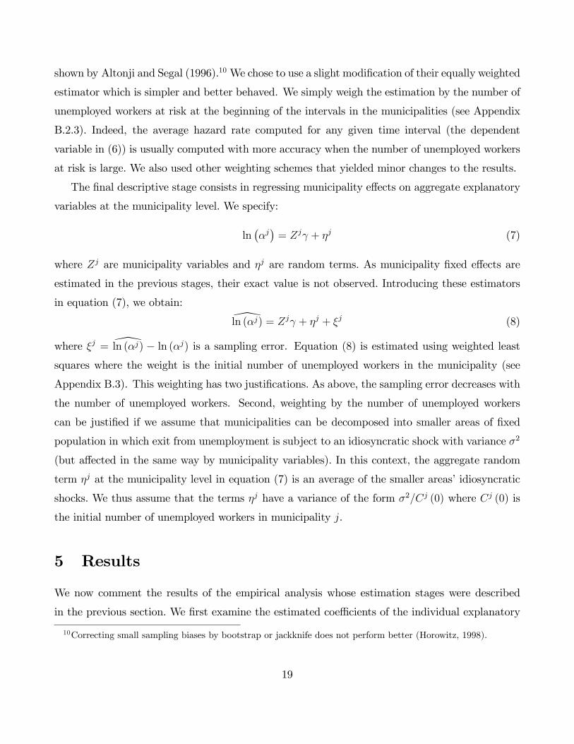
shown by Altonji and Segal (1996).10We chose to use a slight modi�cation of their equally weighted

estimator which is simpler and better behaved. We simply weigh the estimation by the number of

unemployed workers at risk at the beginning of the intervals in the municipalities (see Appendix

B.2.3). Indeed, the average hazard rate computed for any given time interval (the dependent

variable in (6)) is usually computed with more accuracy when the number of unemployed workers

at risk is large. We also used other weighting schemes that yielded minor changes to the results.

The �nal descriptive stage consists in regressing municipality e¤ects on aggregate explanatory

variables at the municipality level. We specify:

ln��j�= Zj + �j (7)

where Zj are municipality variables and �j are random terms. As municipality �xed e¤ects are

estimated in the previous stages, their exact value is not observed. Introducing these estimators

in equation (7), we obtain:\ln (�j) = Zj + �j + �j (8)

where �j = \ln (�j) � ln (�j) is a sampling error. Equation (8) is estimated using weighted leastsquares where the weight is the initial number of unemployed workers in the municipality (see

Appendix B.3). This weighting has two justi�cations. As above, the sampling error decreases with

the number of unemployed workers. Second, weighting by the number of unemployed workers

can be justi�ed if we assume that municipalities can be decomposed into smaller areas of �xed

population in which exit from unemployment is subject to an idiosyncratic shock with variance �2

(but a¤ected in the same way by municipality variables). In this context, the aggregate random

term �j at the municipality level in equation (7) is an average of the smaller areas�idiosyncratic

shocks. We thus assume that the terms �j have a variance of the form �2=Cj (0) where Cj (0) is

the initial number of unemployed workers in municipality j.

5 Results

We now comment the results of the empirical analysis whose estimation stages were described

in the previous section. We �rst examine the estimated coe¢ cients of the individual explanatory

10Correcting small sampling biases by bootstrap or jackknife does not perform better (Horowitz, 1998).

19

variables obtained using the strati�ed partial likelihood estimator (stage 1). We then describe the

spatial disparities in municipality survival functions obtained from the model. We �nally turn to

the results concerning the municipality �xed e¤ects (stage 2) and regress them on local variables

measuring residential segregation and job accessibility (stage 3).

5.1 Individual Determinants of Unemployment Durations

Table 3 reports the coe¢ cients estimated using SPLE for each type of exit (job and non-employment).

Remember that the e¤ects of individual variables should be interpreted as a¤ecting multiplicatively

the hazard rates (through the term exp(Xi�) in (1)).

[Insert Table 3]

Results are as expected although the magnitude of the e¤ects of some variables is surprisingly

large. First, for both exits, younger people have shorter unemployment spells. Although negative

and signi�cant, the e¤ect of age is marginally decreasing (in absolute value) as evidenced by

the square term. Note that it is never positive in any reasonable age range. Second, women

exit signi�cantly more slowly to a job than men (around �18%) while their exit rate to non-employment is much larger (around +35%). Similarly, having children (whatever their number)

decreases the exit rate to a job and increases the exit rate to non-employment. Being in a couple

signi�cantly increases exit rates both to a job and to non-employment.

The strongest e¤ects are for nationality. Africans and other non-European citizens have an

exit rate to a job that is between 45% and 66% lower than the French. In contrast, the e¤ect of

nationality variables on the hazard rate to non-employment is signi�cant only for North Africans

and the magnitude of the coe¢ cient is much lower than for exit to work.

Education variables also have a strong e¤ect. Overall, education a¤ects the exit rate to a job

more than the exit rate to non-employment. For instance, compared to a university degree, a basic

degree lowers the exit rate to a job by 59% while it decreases the exit rate to non-employment

by �only�42%. The shadow wage (i.e. the opportunity cost of time in non participation) is less

a¤ected by education than market wages.

We perform two speci�cation checks. First, it is interesting to compare our results with the

results of the estimation of a standard Cox model where the baseline hazard function is restricted to

20

be constant across municipalities. We use the same individual variables Xi as covariates to which

we add the third-stage municipality variables such as segregation indices and job accessibility

measures Zi. Under these assumptions, our three-stage procedure collapses into one stage only

and results are not robust to misspeci�cation in the second and third stage of our procedure.

The estimated coe¢ cients of individual variables (and their standard errors) are very close to

those obtained using our estimation method (SPLE) in stage 1.11 The estimated coe¢ cients of

geographic variables are also quite close to what we will obtain in stage 3 (see below). Nevertheless,

the standard errors of the estimated coe¢ cients of aggregate variables obtained with a standard

Cox model are at least one-third smaller than those obtained in our third-stage estimation. There

are two explanations for this di¤erence. First, the standard Cox model does not account for

aggregate unobserved e¤ects whereas our estimation method does. It is widely known that this

can lead to very biased standard errors (see Moulton, 1990). Second, there can be an e¢ ciency

loss when using our three stage approach since we are not estimating all equations at the same

time.

As a second speci�cation check, we compare the Kaplan Meyer estimates of the survival func-

tion until an exit to a job with the estimates derived in our model for each municipality.12 We

use a Kolmogorov statistic as developed in Andrews (1997). The di¢ culty in the procedure �

as detailed in Appendix B.1 �is the estimation of the variance of the test statistic evaluated by

bootstrap. The results show that our model provides a very good �t at the municipality level. In

Graph 5 we report the empirical frequency across municipalities of the p-values associated with the

null hypothesis of a good �t. The empirical frequency of municipalities in which we reject a good

�t is indeed lower than the level of the test. It shows that we are able to describe unemployment

durations at the municipality level in a very satisfactory way. This justi�es our speci�cation and,

in particular, our choice of not modeling unobserved heterogeneity.

[Insert Graph 5]

11Complete results are available upon request.12We are thankful to a referee for this suggestion.

21

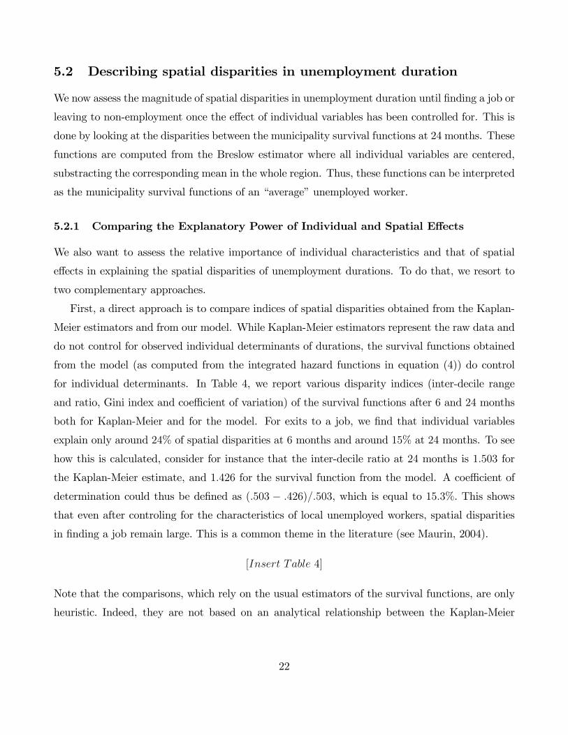
5.2 Describing spatial disparities in unemployment duration

We now assess the magnitude of spatial disparities in unemployment duration until �nding a job or

leaving to non-employment once the e¤ect of individual variables has been controlled for. This is

done by looking at the disparities between the municipality survival functions at 24 months. These

functions are computed from the Breslow estimator where all individual variables are centered,

substracting the corresponding mean in the whole region. Thus, these functions can be interpreted

as the municipality survival functions of an �average�unemployed worker.

5.2.1 Comparing the Explanatory Power of Individual and Spatial E¤ects

We also want to assess the relative importance of individual characteristics and that of spatial

e¤ects in explaining the spatial disparities of unemployment durations. To do that, we resort to

two complementary approaches.

First, a direct approach is to compare indices of spatial disparities obtained from the Kaplan-

Meier estimators and from our model. While Kaplan-Meier estimators represent the raw data and

do not control for observed individual determinants of durations, the survival functions obtained

from the model (as computed from the integrated hazard functions in equation (4)) do control

for individual determinants. In Table 4, we report various disparity indices (inter-decile range

and ratio, Gini index and coe¢ cient of variation) of the survival functions after 6 and 24 months

both for Kaplan-Meier and for the model. For exits to a job, we �nd that individual variables

explain only around 24% of spatial disparities at 6 months and around 15% at 24 months. To see

how this is calculated, consider for instance that the inter-decile ratio at 24 months is 1:503 for

the Kaplan-Meier estimate, and 1:426 for the survival function from the model. A coe¢ cient of

determination could thus be de�ned as (:503 � :426)=:503, which is equal to 15:3%. This showsthat even after controling for the characteristics of local unemployed workers, spatial disparities

in �nding a job remain large. This is a common theme in the literature (see Maurin, 2004).

[Insert Table 4]

Note that the comparisons, which rely on the usual estimators of the survival functions, are only

heuristic. Indeed, they are not based on an analytical relationship between the Kaplan-Meier

22

estimators and the e¤ect of individual variables and the municipality survival functions of the

model.

Our second approach to estimate the relative importance of the contributions of individual

and local characteristics to spatial disparities in unemployment durations does not make use of

the Kaplan-Meier estimator and has �rmer analytical grounds. It is a variance analysis of the

average integrated hazard at the municipality level. To see why such an analysis is feasible, write

the log-integrated hazard of a given individual i as the sum of the e¤ect of individual observed

characteristics Xi� and the logarithm of the municipality integrated hazard �j(i) (t) and a random

term � i:

ln � (t jXi; j (i)) = Xi� + ln�j(i) (t) + � i: (9)

Here, � i is the intrinsic randomness in durations and exp(� i) is exponential(1) distributed (Lan-

caster, 1990). When we take the expectation of this equation in the population of unemployed

workers in a given municipality j, we obtain the following decomposition of the log-integrated

hazard of that municipality:

E(ln� (t jXi; j ) j i 2 j (0)) = Xj� + ln�j (t) + c0 (10)

where j (0) is the population of unemployed workers in the municipality, where Xj is the expec-

tation of individual characteristics in that population and where the constant c0 is the expectation

of � i.13 In practice, the two right-hand side terms can be consistently estimated via the �rst stage

estimations and their sum yields an estimate of the left-hand side term up to the constant term,

c0.

In Table 5, we report the results of a variance analysis across municipalities using equation (10)

for durations of various lengths: short (6 months), intermediate (12 months) and long (24 months).

Averages of individual observable characteristics explain around 30% of spatial e¤ects in job exits.

This confers to individual variables slightly more explanatory power than what we obtained in

Table 4, although it remains quite low. For instance at 12 months, the spatial variance of the

log-integrated hazard is equal to :0508 while the spatial variance of the average log-integrated

hazard in the municipality (LHS of (10)) is :0755. A pseudo-coe¢ cient of determination is thus

13As exp(�i) is exponential(1) distributed, c0 = 1:

23

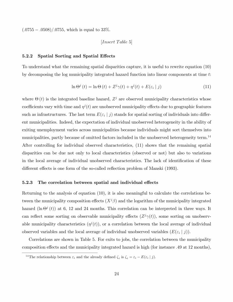
(:0755� :0508)=:0755, which is equal to 33%.

[Insert Table 5]

5.2.2 Spatial Sorting and Spatial E¤ects

To understand what the remaining spatial disparities capture, it is useful to rewrite equation (10)

by decomposing the log municipality integrated hazard function into linear components at time t:

ln�j (t) = ln� (t) + Zj (t) + �j(t) + E("i j j) (11)

where �(t) is the integrated baseline hazard, Zj are observed municipality characteristics whose

coe¢ cients vary with time and �j(t) are unobserved municipality e¤ects due to geographic features

such as infrastructures. The last term E("i j j) stands for spatial sorting of individuals into di¤er-ent municipalities. Indeed, the expectation of individual unobserved heterogeneity in the ability of

exiting unemployment varies across municipalities because individuals might sort themselves into

municipalities, partly because of omitted factors included in the unobserved heterogeneity term.14

After controlling for individual observed characteristics, (11) shows that the remaining spatial

disparities can be due not only to local characteristics (observed or not) but also to variations

in the local average of individual unobserved characteristics. The lack of identi�cation of these

di¤erent e¤ects is one form of the so-called re�ection problem of Manski (1993).

5.2.3 The correlation between spatial and individual e¤ects

Returning to the analysis of equation (10), it is also meaningful to calculate the correlations be-

tween the municipality composition e¤ects (Xj�) and the logarithm of the municipality integrated

hazard (ln�j (t)) at 6, 12 and 24 months. This correlation can be interpreted in three ways. It

can re�ect some sorting on observable municipality e¤ects (Zj (t)), some sorting on unobserv-

able municipality characteristics (�j(t)), or a correlation between the local average of individual

observed variables and the local average of individual unobserved variables (E("i j j)).Correlations are shown in Table 5. For exits to jobs, the correlation between the municipality

composition e¤ects and the municipality integrated hazard is high (for instance :49 at 12 months),

14The relationship between "i and the already de�ned �i is �i = "i � E("i j j).

24

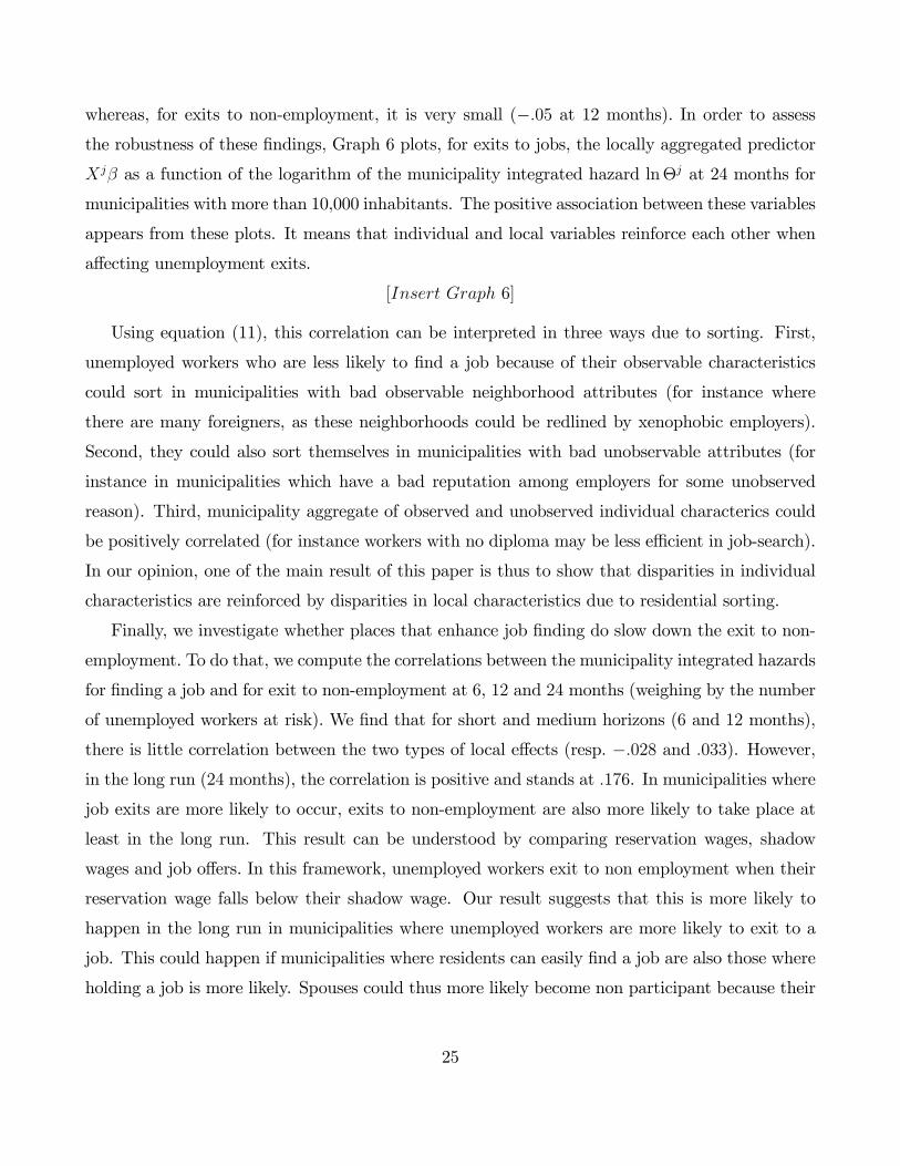
whereas, for exits to non-employment, it is very small (�:05 at 12 months). In order to assessthe robustness of these �ndings, Graph 6 plots, for exits to jobs, the locally aggregated predictor

Xj� as a function of the logarithm of the municipality integrated hazard ln�j at 24 months for

municipalities with more than 10,000 inhabitants. The positive association between these variables

appears from these plots. It means that individual and local variables reinforce each other when

a¤ecting unemployment exits.

[Insert Graph 6]

Using equation (11), this correlation can be interpreted in three ways due to sorting. First,

unemployed workers who are less likely to �nd a job because of their observable characteristics

could sort in municipalities with bad observable neighborhood attributes (for instance where

there are many foreigners, as these neighborhoods could be redlined by xenophobic employers).

Second, they could also sort themselves in municipalities with bad unobservable attributes (for

instance in municipalities which have a bad reputation among employers for some unobserved

reason). Third, municipality aggregate of observed and unobserved individual characterics could

be positively correlated (for instance workers with no diploma may be less e¢ cient in job-search).

In our opinion, one of the main result of this paper is thus to show that disparities in individual

characteristics are reinforced by disparities in local characteristics due to residential sorting.

Finally, we investigate whether places that enhance job �nding do slow down the exit to non-

employment. To do that, we compute the correlations between the municipality integrated hazards

for �nding a job and for exit to non-employment at 6, 12 and 24 months (weighing by the number

of unemployed workers at risk). We �nd that for short and medium horizons (6 and 12 months),

there is little correlation between the two types of local e¤ects (resp. �:028 and :033). However,in the long run (24 months), the correlation is positive and stands at :176. In municipalities where

job exits are more likely to occur, exits to non-employment are also more likely to take place at

least in the long run. This result can be understood by comparing reservation wages, shadow

wages and job o¤ers. In this framework, unemployed workers exit to non employment when their

reservation wage falls below their shadow wage. Our result suggests that this is more likely to

happen in the long run in municipalities where unemployed workers are more likely to exit to a

job. This could happen if municipalities where residents can easily �nd a job are also those where

holding a job is more likely. Spouses could thus more likely become non participant because their

25

opportunity cost of time increases with their spouse�s income.

5.3 Municipality E¤ects and Spatial Characteristics

5.3.1 Multiplicative Component Model

As explained above, we further restrict the hazard function and consider a multiplicative munic-

ipality hazard speci�ed as the product of a municipality e¤ect and an aggregate baseline hazard

(see Equation (5)). To implement this approach, we divide the time line into M = 9 intervals,

with the �rst eight intervals lasting 90 days and the remaining one lasting the rest of the pe-

riod. To assess whether the multiplicative speci�cation is too restrictive, we compare the value of

disparity indices obtained with the unspeci�ed municipality hazard with those obtained with the

multiplicative hazard (see Table 4 and Table 5). We �nd that the multiplicative hazard reproduces

well spatial disparities for �nding a job although it performs poorly for exit to non-employment

at 6 months (though not for the Gini). This good �t justi�es the use of municipality e¤ects as an

adequate summary to study the determinants of spatial disparities for �nding a job.

In line with the theories presented in Section 2, we investigate howmunicipality �xed e¤ects can

be explained by segregation and job accessibility. Segregation is measured here by the composition

of the municipality population by education and by nationality. Job accessibility is measured by

local job density (as de�ned in Section 3.2).

5.3.2 Partial Correlations with Spatial Caracteristics

Table 6 reports various regressions of municipality e¤ects on those spatial characteristics. We com-

puted a pseudo-R2 to assess the explanatory power of the model taking into account the sampling

error (see Appendix B.3). When using only segregation indices as explanatory variables (column

1), we are able to explain 72:4% of the variance of municipality �xed e¤ects. Job accessibility

indices (column 2) have a much lower explanatory power since the pseudo R2 is only 25:9%. This

suggests that spatial disparities in �nding a job are more strongly associated with di¤erences in

the local level of segregation than with variations in job accessibility. When using both segregation

and job accessibility indices (column 3), the pseudo R2 reaches 73:0%.

We now comment on the coe¢ cient of the latter regression (column 3). Large municipality

26

e¤ects in �nding a job are associated with a large proportion of unskilled workers and of non-

French citizens (especially citizens from sub-Saharan Africa). This is consistent with the existence

of redlining (according to nationality and skill) as well as with a social network e¤ect. Munici-

pality e¤ects in �nding a job are also correlated with local job accessibility, especially by private

transport, but the coe¢ cients of both private and public job accessibility measures are negative

in contradiction with the spatial mismatch theory.

[Insert Table 6]

Of course, there are some other interpretations of the results which are based on possible

omitted local variables, reverse causality or sorting on individual unobservables. There can be

omitted local variables correlated with segregation or job-accessibility measures. Our surprising

result for job accessibility could be explained if the job density indices captured the low quality

and high congestion of transports for instance.

Reverse causality can occur if local unemployment acts as an attraction or a repulsion force on

population and jobs. This could a¤ect the job accessibility measure and the segregation indices

(provided that the population categories are di¤erentially attracted or repulsed). To take the

example of segregation for instance, French people may �ee municipalities where unemployment

exits to a job are more di¢ cult. This would increase the local proportion of foreigners, especially

Africans and could explain the negati coe¢ cient of the municipality proportion of Africans on

�nding a job.

Municipality explanatory variables can capture the local average of individual unobserved vari-

ables if there is a correlation between Zj and the omitted term E("i j j) as de�ned in equation(11) above. This is the case for instance when individuals with a given unobserved attribute (such

as motivation to search for a job) choose their location depending on observable municipality

variables (attractive residential neighborhoods where jobs are not easily accessible). This may

explain the negative e¤ect of the job accessibility index by private transport.

27

6 Conclusion

In this paper, we study the spatial disparities in exits from unemployment across municipalities

in the Paris region. We use a unique and exhaustive administrative dataset which contains all

registered unemployment spells over the 1996-2003 period. This dataset contains some individual

characteristics of unemployed workers as well as their residential location. It is merged with spatial

indices of segregation and job accessibility computed from the census and a transport survey.

Our methodology is based on the estimation of independent competing risk duration models with

two exits (�nding a job and dropping out of the labor force). We constructed measures of raw

spatial disparities across municipalities from the local survival functions after 24 months. We

�nd that there are very large disparities. The local composition of workers�characteristics can

explain around 30% of the disparities in �nding a job. Our local indices (especially residential

segregation measures) capture nearly 70% of the remaining di¤erences. Furthermore, we showed

that disparities in individual characteristics are reinforced by disparities in local characteristics

due to residential sorting. The latter �nding lends credit to the idea that spatial factors exacerbate

non spatial factors in the determination of unemployment, or that the most fragile unemployed

workers tend to cumulate local and invididual disadvantages.

Our work nevertheless considered broad local e¤ects related to segregation and job accessibility

without trying to investigate and disentangle the speci�c mechanisms at work, which could be

the basis for furture research. Another extension of this work could be to compute municipality

survival functions by nationality group or class of diploma. This would enable us to assess the

extent to which the e¤ect of local factors may di¤er for these groups. It would also be interesting

to study spatial disparities at a much �ner scale were the data available. Indeed, our accessibility

measures are only at the municipality level whereas accessibility can di¤er even between two small

neighborhoods (e.g. when they are separated by a railroad). Working at a �ner geographic scale

may also allow for an investigation of other important issues such as the role of spatialized social

networks, which are likely to occur within a limited geographic area (see Bayer, Ross and Topa,

2008; Gobillon and Selod, 2007).

28

A Data Appendix

Over the 1993-2003 period, the panel contains 10,290,225 unemployment spells. We selected

unemployment spells beginning between January 1 and June 30, 1996 which form a subsample

of 451,191 unemployment spells. By keeping observations corresponding to unemployed workers

between 16 and 54 years old only, we ended up with a dataset comprising 433,802 unemployment

spells. After deleting observations with missing values and coding problems, the �nal sample is

composed of 430,695 observations. Descriptive statistics about variables in our �nal dataset are

given in Table A1.

B Computational details

B.1 First-stage estimation

We want to test for each municipality that the empirical survival function as estimated by Kaplan

Meier estimation is equal to the survival function predicted by the model.

B.1.1 Construction of the Kolmogorov test statistic

Let S(t; k) be the survival function of the data for exit k and let S(t; k j x; �) be the conditionalsurvival function of the model. Here, � denotes parameters �k and the municipality baseline

hazard. The null hypothesis writes:

H0 : S(t; k) =

ZS(t; k j x; �)dF (x)

where dF (x) is the probability measure of covariates. This is an adaptation of Andrews (1997)

with some di¤erences since the latter paper considers null hypotheses of the form:

H0 : S(t; k jx)F (x) = S(t; k jx; � )F (x) a.s. F (x):

where S(t; k jx) is the conditional survival function of the data. The adaptation of the proofs ofAndrews (1997) are out of the scope of this paper.

Our sample consists in individuals, i = 1; :::; N , of characteristics Xi for whom we observe

unemploment duration ti and type of exit. We restrict our attention to exits to job and we drop

29

index k from the survival functions. Computing the test statistic for exits to non-employment

follows the same principles.

Let HjN(t) be the Kaplan Meier estimator of the survival function of duration t in municipality

j: Let SjN(t; �) be the survival function until an exit to a job in municipality j, as predicted by

the model i.e.

SjN(t) =1

Nj

NXi=1;i2j

Si(t j Xi; �);

where Nj denotes the number of individuals in municipality j, and where � denotes the SPLE

estimator and the functional Breslow estimator of the baseline hazard rate. The conditional

Kolmogorov statistic for municipality j is:

CKjN =

pNj max

i2j

���HjN(ti)� S

jN(ti)

���In practice, we trim out durations in the last percentile when computing our test statistic. This

is because the survival functions are not estimated with accuracy at that percentile and the test

statistic takes arti�cially large values at �nite distance.

Alternatively, we could also consider another statistic which is the mean square di¤erence of

these two survival functions, in analogy with a Cramer-von Mises statistic:

QM jN =

1pNj

Xi2j

�HjN(ti)� S

jN(ti)

�2where Nj is the number of unemployed workers in municipality j.

For these two test statistics, we need to compute the distribution under the null hypothesis.

We proceed by bootstrap as proposed by Andrews (1997).

B.1.2 Computation of the distribution of the test statistic.

We now explain how to compute the distribution of the test statistic for a given municipality. We

drop index j for simplicity. For an individual i having a censored unemployment spell, the duration

before censorship, tic = ti, is an exogenous characteristic of the individual. If the unemployment

spell is not censored, censorship is not relevant and its duration is not taken into account. We

denote eXi the exogenous information i.e. eXi = (Xi; tic) for censored individuals and eXi = (Xi; �)for uncensored ones.

30

The asymptotic distribution of Andrews�test statistic is computed by (semi)-parametric boot-

strap for B replications, b = 1; :::; B. For each replication, we generate a duration for each

individual using the proportional hazard model. The data are generated conditionally on the ex-

ogenous characteristics eXi, the estimated parameters for exit to job b�e and the Breslow estimator.The procedure to simulate durations is the following.

For an individual i, the integrated hazard for exit to job at duration t writes:

� (t jXi ) = � (t) exp (Xi�e)

where � (t) is the integrated baseline hazard. As the survival function is S (t jXi ) = exp [�� (t jXi )] ;

we have:

� (t) =�1

exp (Xi�e)lnS (t jXi )

To obtain simulated durations, we draw the value of the survival function in a uniform distribution

[0; 1], eSbi , and replace unknown parameters by their estimates:b�bi = �1

exp�Xib�e� ln eSbi

There remains to invert function b� at point b�bi to recover duration etbi for individual i. In practice,b�bi increases piecewise and there is a duration at which the function b� makes a jump from �bi to

�b

i such that �bi 6 b�bi < �bi . We de�ne etbi as the duration at which function b� makes this jump.

A practical issue is that b� cannot be computed above the upper bound b� (tmax), where tmaxj

is the largest duration in the sample. If a simulated value is such that b�bi > b� (tmax), we setduration to etbi = tmax. This small sample bias should disappear asymptotically when the numberof individuals in each municipality tends to in�nity.

For individuals who were not censored, the generated duration is tbi = etbi . For individuals whowere right-censored, the generated duration is tbi = min

�etbi ; tic�. The generated exit is �nding ajob if etbi < tic, and it is censorship if etbi > tic. We then construct the Kaplan-Meier�s estimator

denoted Hj;bN (t). For individual i, we compute the value of the Kaplan-Meier�s estimator of his

municipality at the generated duration as: Hbi = H

j;bN

�tbi�. In the same way, we use the Breslow�s

estimator of any municipality j to construct a survival function which is denoted Sj;bN (t). For

individual i, we compute the value of the survival function of his municipality at the generated

duration as: Sbi = Sj;bN

�tbi�.

31

The test statistic of municipality j computed for the bth replication can be written as:

CKj;bN =

pNjsup

i2j

���Hbi � Sbi

���As previously, we trim out durations in the last percentile when computing our test statistic. B

bootstrap samples of size Nj are simulated. The p-value of the test statistic is de�ned as:

pBjN =1

B

BXb=1

1fCKjN > CK

j;bN g:

B.2 Second-stage estimation

B.2.1 Finite-sample issues

We �rst explain how we take into account �nite sample issues when establishing equation (6). For

that purpose, we re�ned appropriatly the quantities involved in (6). We divide the period into

M intervals [tm�1; tm], m = 1; :::;M . We denote �m = 1tm�tm�1

tmRtm�1

� (s) ds the average baseline

hazard over the interval m and djm =tmRtm�1

I (Cj (s) > 0) ds the length of time within interval m

when some individuals in municipality j are at risk. In particular, djm < tm� tm�1 in the last timeinterval in which there are some unemployed workers at risk in municipality j. The average hazard

rate over a time interval m in municipality j where some people are at risk (djm > 0) is given by

yjm =1

djm[�j (tm)��j (tm�1)]. An estimator of this average hazard rate can be constructed from

equation (4) and writes: yjm =1

djm[b�j (tm)� b�j (tm�1)]. We can then re-establish formula (6) where

the quantities have been rede�ned.

B.2.2 Covariance matrix of the sampling errors

We now give the formulas to compute the covariance matrix of ("jm)j;m ;which are the sampling

errors in equation (6), using Ridder and Tunali�s appendix (RT hereafter). We �rst introduce the

following notations that will be used below:

S0j (�; s) =Xi2j(s)

exp(Xi�)

S1j (�; s) =Xi2j(s)

Xi exp(Xi�)

32

where j (s) is the set of unemployed workers still at risk in municipality j at time s. Note

that whereas S0j (�; s) is a 1 � 1 matrix, S1j (�; s) is a 1 � K matrix, where K is the number

of explanatory variables in the �rst stage. We also denote Cj (s) = card j (s) the number of

unemployed workers still at risk in municipality j at time s. According to RT (A28), we have:

exp "jm = �jm +

1pNc0jm� (12)

where N =Xj

Cj (0) is the number of unemployed workers in the Paris region and:

�jm =1

djm

tmZtm�1

I (Cj (s) > 0)h

1S0j (�;s)

dN j (s)� �j (s) dsi(RT A22)

cjm = � 1

djm

tmZtm�1

I (Cj (s) > 0)S1j (�

�;s)

[S0j (��;s)]2dN j (s) (RT A27)

� =pN�b� � ��

where �� is a value between � and b� (coming from a Taylor expansion not detailed here), dN j (s)

is a dummy that equals one if someone in municipality j experiences an exit in an arbitrarily

short period of time before date s (and zero otherwise), and djm =tmRtm�1

I (Cj (s) > 0) ds. Here, �

is uncorrelated with �jm. From equation (12), it is possible to get:

V (exp "jm) = V (�jm) + c

0jmV cjm (RT A29)

cov�exp "jm; exp "

kn

�= c0jmV ckn for j 6= k or m 6= n (RT A30)

where V = V�b��. These covariance-matrix terms of (exp "jm)j;m can be estimated computing

estimators of all terms on the right-hand sides. An estimator of V is obtained from the Fisher

information matrix of SPLE. In practice, there is no need to have the theoretical formula to get

this estimator as it is directly recovered from the estimation software. Some estimators of V (�jm)

and cjm are:

bV (�jm) = 1

(djm)2

tmZtm�1

I (Cj (s) > 0) 1

[S0j (b�;s)]2dN j (s) (from RT A25)

bcjm = � 1

djm

tmZtm�1

I (Cj (s) > 0)S1j (b�;s)[S0j (b�;s)]2dN j (s) (from RT A27)

33

These estimators have to be programmed to be computed. From the covariance matrix of

(exp "jm)j;m, we get the covariance matrix of ("jm)j;m using the delta method.

B.2.3 Estimation

Formulas

We �rst give some notations we use in this section. Denote J the number of municipalities andM

the number of time intervals. For any JM �1 matrix X, Xj refers to theM �1 matrix de�ned byX(j�1)M+[1:M ];1. For any given JM � JM matrix X, Xj;k refers to the M �M submatrix de�ned

by X(j�1)M+[1:M ];(k�1)M+[1:M ] where [1 :M ] is the vector of integers from 1 to M .

The equation to estimate is (6) where we �x �1 = 1 to secure identi�cation. We stack the obser-

vations of (6) and obtain:

Y = A�+G� + " (13)

where A is a JM � J matrix such that A(j�1)M+m;k = 1 if j = k and A(j�1)M+m;k = 0 otherwise,

G is a JM � (M � 1) matrix such that G(j�1)M+m;l = 1 if m = l and A(j�1)M+m;l = 0 otherwise,

Y =�ln y11; :::; ln y

JM

�0and " =

�"11; :::; "

JM

�0are some JM � 1 vectors, � = (ln�1; :::; ln�J)

0 is a

J � 1 vector and � = (ln �2; :::; ln �M)0 is a (M � 1)� 1 vector.

Denote � = diag (N11; :::; NJM) the JM � JM diagonal matrix where Njm is the number of

unemployed workers in municipality j still at risk at the beginning of interval m. After weighting

equation (13) with �1=2, it becomes:

�1=2Y = �1=2A�+�1=2G� +�1=2"

Denote W the projector in the dimension orthogonal to �1=2A. Using the �rst stage of Frisch-

Waugh theorem, we obtain the WLS estimator of �:

b� = (G0�1=2W�1=2G)�1G0�1=2W�1=2Y

= � + (G0�1=2W�1=2G)�1G0�1=2W�1=2" (14)

34

The second stage of the Frisch-Waugh theorem gives the WLS estimator of �:

b� = (A0�A)�1A0�hY �Gb�i

= (A0�A)�1A0�hY �G� �G

�G0�1=2W�1=2G

��1G0�1=2W�1=2"

i= �+ (A0�A)�1A0�

h"�G

�G0�1=2W�1=2G

��1G0�1=2W�1=2"

iDenote � = A0�A, � = G0�1=2W�1=2G and = G0�1=2W�1=2V�1=2W�1=2G, where V = V (").

We have:

V�b�� = ��1��1 (15)

Also, we get:

V (b�) = ��1A0�V�A��1

+��1A0�GV�b��G0�A��1 (16)

���1A0��V�1=2W�1=2G��1G0 +G��1G0�1=2W�1=2V

��A��1

Computation

We have:

� =JXj=1

�W�1=2G

�0j

�W�1=2G

�j=

JXj=1

G0j�j;jGj

=JX

j;k=1

�W�1=2G

�0j�1=2j;j Vj;k�

1=2k;k (W�G)k =

JXj;k=1

G0

j�j;jVj;k�k;kGk

� = diag [tr (�1;1) ; :::; tr (�J;J)]

where for any given variable Zj of dimensionM�1, Zj is its counterpart centered with its weightedaverage: Zj = Zj � 1

tr(�j;j)tr (�j;jZj).

We also have:

(A0�V�A)j;k = N 0jVj;kNk�

A0�GV�b��G0�A�

j;k= N 0

j�V�b��Nk�

where Nj = (Nj;1; :::; Nj;M)0 and Nj� = (Nj;2; :::; Nj;M)

0.

35

Moreover, V�1=2W�1=2 = V� where V is de�ned such that any of its given submatrix V j;k writes:

V j;k = Vj;k � 1tr(�j;j)

�1M N 0

j

�Vj;k with the Kronecker product and 1M a M � 1 matrix �lled

with the value 1. Hence, we have:

�A0�V�1=2W�1=2G��1G0�A

�j;k= N 0

j

�V0�G��1G0

�j;kNk

Moreover, G��1G0 = J:JJ

0@ 0 0

0 ��1

1A with JJ the J � J matrix �lled with the value 1=J .

Hence,�V�G��1G0

�j;k=Pl

�V�

�j;l

0@ 0 0

0 ��1

1A =

�Pl

V j;l�l;l

�0@ 0 0

0 ��1

1A.B.3 Third-stage estimation

The third-stage equation to estimate is given by (8). When we stack the observations, we obtain:

b� = Z + � + � (17)

where b� = �[ln�1; :::;[ln�J

�0, � = (�1; :::; �J)

0 and � = (�1; :::; �J)0 are some J � 1 vectors, and

Z = (Z 01; :::; Z0J)0 is a J � K matrix. We suppose that

��j�1;:::;J

have a covariance matrix �2Q�1

where Q = diag(N11; :::; NJ1). Equation (17) is estimated with weighted least squares where the

weights are the square-roots of the numbers of unemployed workers at the initial date (Q1=2). The

estimated coe¢ cients write: b = (Z 0QZ)�1 Z 0Qb�and their covariance matrix is:

V (b ) = (Z 0QZ)�1Z 0Q

�V (�) + �2Q�1

�QZ (Z 0QZ)

�1

= (Z 0QZ)�1Z 0QV (�)QZ (Z 0QZ)

�1+ �2 (Z 0QZ)

�1

It is possible to construct a consistent estimator of �2 using the residuals [� + � = Q1=2b��Q1=2Zb .This estimator is found from the following calculation sequence:

[� + �0[� + � = (� + �)0

hI �Q1=2Z (Z 0QZ)�1 Z 0

i0QhI � Z (Z 0QZ)�1 Z 0Q1=2

i(� + �)

36

where we made the approximation (for N large enough) that:

[� + �0[� + � � (� + �)0Q (� + �)

We thus have:

Eh[� + �

0[� + �i� �2J + tr [QV (�)]

when V (�) has been computed from the �rst-stage estimation. An estimator of �2 can then be

de�ned as: b�2 = h[� + �0[� + � � tr [QV (�)]i =JWe introduce an error rate coming from sampling error as:

err =tr [QV (�)]

[� + �0[� + �

We also construct a pseudo-R2 de�ned as:

R2p =V eQ (Zb )

V eQ (Zb ) + b�2Jwhere V eQ (�) =

�Zb � Zb �0Q �Zb � Zb � =tr (Q) is the empirical variance obtained when weighting

observations with weights Q (where Z = tr (QZ) =trQ). Note that when there is no sampling error,

this pseudo-R2 is equal to the usual R2.

37

REFERENCES

References

[1] Altonji J.G. and L.M. Segal (1996), �Small Sample Bias in GMM estimation of Covariance

Structures�, Journal of Business & Economic Statistics, 14(3), 353-65.

[2] Andrews D. (1997), �A Conditional Kolmogorov test�, Econometrica, 65(5), 1097-1128

[3] Baccaini B., Courgeau D. and G. Desplanques (1993), �Les migrations internes en France de

1982 à 1990. Comparaison avec les périodes antérieures�, 48(6), 1771-89.

[4] Baker M. and A. Melino (2000), �Duration Dependence and Non-Parametric Heterogeneity:

A Monte-Carlo Study�, Journal of Econometrics, 96, 357-93.

[5] Bayer P., Ross S. and G. Topa (2008), �Place of Work and Place of Residence: Informal Hiring

Networks and Labor Market Outcomes�, Journal of Political Economy, 116(6), 1150-96.

[6] Breslow N.E. (1974), �Covariance Analysis of Censored Survival Data�, Biometrics, 30, pp.

89-99.

[7] Calvo-Armengol A. and M. Jackson (2004), �Social networks in determining unemployment:

Patterns, dynamics and inequality�, American Economic Review, 94, 191-206.

[8] Chardon O. and D. Goux (2003), �The new european de�nition of BIT unemployment�(in

French), Economie et Statistiques, 362, 67-83.

[9] Conley T. and G. Topa (2002), �Socio-economic distance and spatial patterns in unemploy-

ment�, Journal of Applied Econometrics, 17(4), 303-327.

[10] Cutler D. and E. Glaeser (1997), �Are Ghettos Good or Bad?�, Quarterly Journal of Eco-

nomics, 112, 827-872.

[11] Dawkins C., Shen Q. and T. Sanchez (2005), �Race, Space and Unemployment Duration�,

Journal of Urban Economics, 58, 91-113.

38

[12] DREIF (Direction Régionale de l�Equipement Ile-de-France) / INSEE Ile-de-France (1997),

�Daily moves: Ile-de-France population more mobile�(in French), 2 pages.

[13] Gobillon L. and H. Selod (2007), �The e¤ect of segregation and spatial mismatch: evidence

from France�, CEPR Working Paper 6198.

[14] Gobillon L., Selod H. and Y. Zenou (2007), �The mechanisms of spatial mismatch�, Urban

Studies, 44 (12), 2401-27 .

[15] Gouriéroux C., A. Monfort, E. Renault and A. Trognon (1985), �Asymptotic Least Squares�

(in French), Annales de l�INSEE, 58, 91-122.

[16] Holzer H. and K. Ihlanfeldt (1998) �Customer discrimination and employment outcomes for

minority workers�, Quarterly Journal of Economics, 113, 835-867.

[17] Holzer H., Ihlanfeldt K. and D. Sjoquist (1994), �Work, search and travel among white and

black youth�, Journal of Urban Economics, 35, 320-345.

[18] Horowitz J., (1998), �Bootstrap Methods for Covariance Structures�, Journal of Human

Resources, 33, 39-61.

[19] Ihlanfeldt K. (1993), �Intra-urban job accessibility and Hispanic youth employment rate�,

Journal of Urban Economics, 33, 254-271.

[20] Ihlanfeldt K. (1997), �Information on the spatial distribution of job opportunities within

Metropolitan Areas�, Journal of Urban Economics, 41, 218-242.

[21] Ihlanfeldt K. and D. Sjoquist (1998), �The spatial mismatch hypothesis: a review of recent

studies and their implications for welfare reform�, Housing Policy Debate, 9, 849-892.

[22] Johnson R. (2006) �Landing a job in urban space: the extent and e¤ects of spatial mismatch�,

Regional Science and Urban Economics, 36, 331-72.

[23] Lancaster T. (1990), The Econometric Analysis of Transition Data, Cambridge University

Press: Cambridge.

39

[24] Manski C. F. (1993), �Identi�cation of Endogenous Social E¤ects: The Re�ection Problem�,

Review of Economic Studies, 60(3), 531-42.

[25] Maurin E. (2004), The French Ghetto (in French), ed. Seuil, 95p.

[26] Moulton B.R. (1990), �An Illustration of Pitfalls in estimating the E¤ects of Aggregate vari-

ables on Micro Units�, Review of Economics and Statistics, 72, 334-8.

[27] Mortensen D. et T. Vishwanath (1994), �Personal contacts and earnings. It is who you know!�,

Labour Economics, 1, 187-201.

[28] Patacchini E. Y. Zenou (2006), �Search activities, cost of living, and local labor markets�,

Regional Science and Urban Economics, 36(2), 227-48.

[29] Ridder G. and I. Tunali (1999), �Strati�ed partial likelihood estimation�, Journal of Econo-

metrics, 92(2), 193-232.

[30] Rogers C. (1997), �Job Search and Unemployment Duration: Implications for the Spatial

Mismatch Hypothesis�, Journal of Urban Economics, 42, 109-32.

[31] Selod H. and Y. Zenou (2006), �City structure, job search, and labor discrimination. Theory

and policy implications�, Economic Journal, 116, 1057-87.

[32] Smith T. and Y. Zenou (2003), �Spatial mismatch, search e¤ort and urban spatial structure�,

Journal of Urban Economics, 54, 129-156.

[33] Stoll M. (1999), �Spatial job search, spatial mismatch, and the employment and wages of

racial and ethnic groups in Los Angeles�, Journal of Urban Economics, 46, 129-55.

[34] Stoll M. and S. Raphael (2000), �Racial di¤erences in spatial job search patterns: Exploring

the causes and consequences�, Economic Geography, 201-223.

[35] Weinberg B. (2000), �Black residential centralization and the spatial mismatch hypothesis�,

Journal of Urban Economics, 48, 110-134.

[36] Weinberg B. (2004), �Testing the spatial mismatch hypothesis using inter-city variations in

industrial composition�, Regional Science and Urban Economics, 34, 505-32.

40

[37] Wilson,J. (1996), When Work Disappears: The World of the New Urban Poor, New York:

Alfred A. Knopf.

[38] Zax J. and J. Kain (1996), �Moving to the suburbs: Do relocating companies leave their

Black employees behind?�, Journal of Labor Economics, 14, 472-504.

[39] Zenou Y. (2002), �How do �rms redline workers?�, Journal of Public Economics, 52(3), pages

391-408.

41

Graph 1: Population density (per sq km) in the Paris region in 1999

less than 100 100 to 1,500 1,500 to 5,000 5,000 to 10,000 over 10,000

Source: constructed from the 1999 Population Census, INSEE. The geographical unit is the subdistrict for the city of Paris or the municipality for the rest of the region. Bold lines represent the boundaries of the city of Paris (the turtle-shaped area in the middle of the map) and of the seven surrounding subregional administrative districts (départements).

Graph 2: Unemployment rates in the Paris region in 1999

less than 5% 5 – 10% 10 – 15% 15 – 20% above 20%

Source: constructed from the 1999 Population Census, INSEE.

42

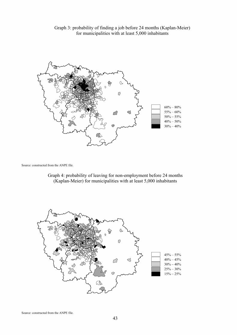
Graph 3: probability of finding a job before 24 months (Kaplan-Meier)

for municipalities with at least 5,000 inhabitants

60% – 80% 55% – 60% 50% – 55% 40% – 50% 30% – 40%

Source: constructed from the ANPE file.

Graph 4: probability of leaving for non-employment before 24 months (Kaplan-Meier) for municipalities with at least 5,000 inhabitants

45% – 55% 40% – 45% 30% – 40% 25% – 30% 15% – 25%

Source: constructed from the ANPE file.

43

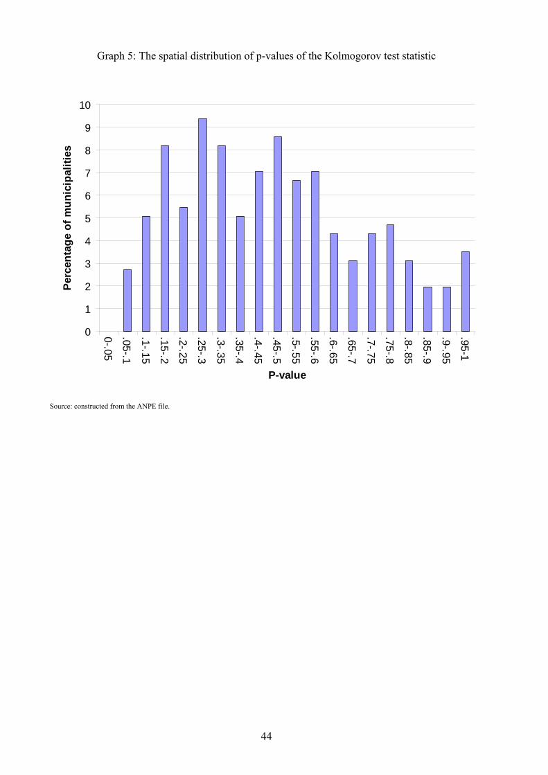
Graph 5: The spatial distribution of p-values of the Kolmogorov test statistic

0

1

2

3

4

5

6

7

8

9

10

0-.05

.05-.1

.1-.15

.15-.2

.2-.25

.25-.3

.3-.35

.35-.4

.4-.45

.45-.5

.5-.55

.55-.6

.6-.65

.65-.7

.7-.75

.75-.8

.8-.85

.85-.9

.9-.95

.95-1

P-value

Perc

enta

ge o

f mun

icip

aliti

es

Source: constructed from the ANPE file.

44

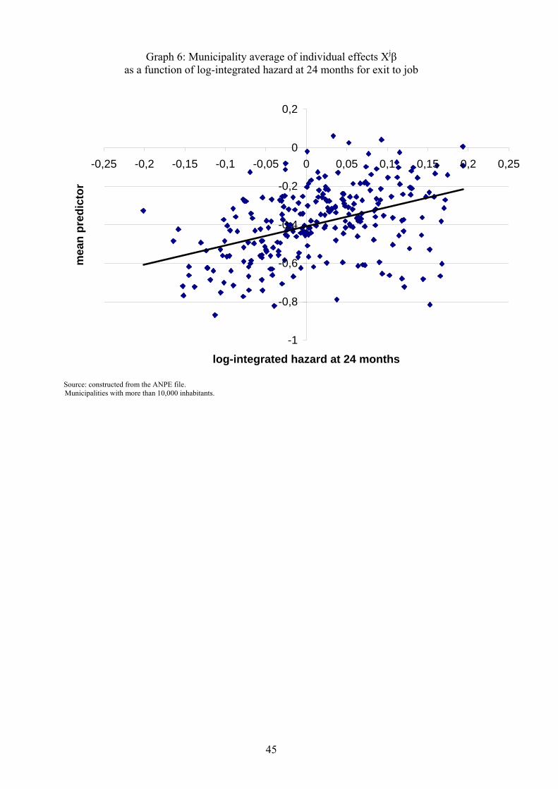
Graph 6: Municipality average of individual effects Xjβ as a function of log-integrated hazard at 24 months for exit to job

-1

-0,8

-0,6

-0,4

-0,2

0

0,2

-0,25 -0,2 -0,15 -0,1 -0,05 0 0,05 0,1 0,15 0,2 0,25

log-integrated hazard at 24 months

mea

n pr

edic

tor

Source: constructed from the ANPE file. Municipalities with more than 10,000 inhabitants.

45

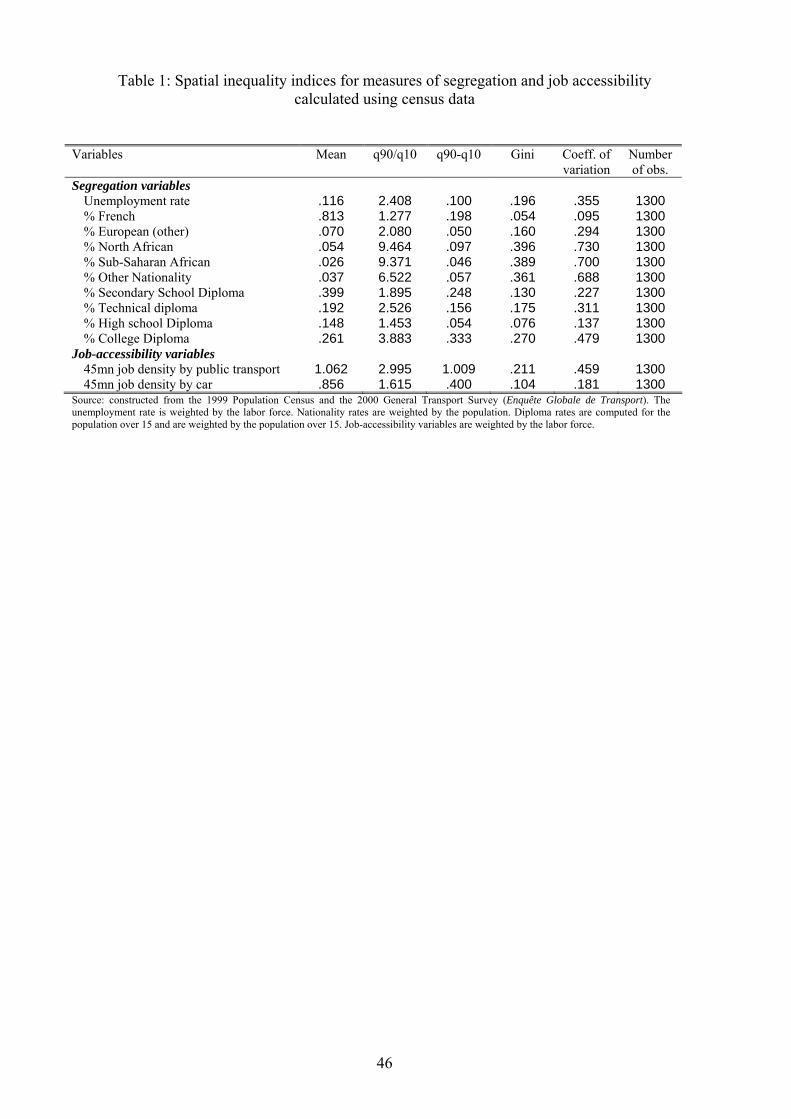
46

Table 1: Spatial inequality indices for measures of segregation and job accessibility calculated using census data

Variables Mean

q90/q10

q90-q10

Gini

Coeff. of variation

Number of obs.

Segregation variables Unemployment rate .116 2.408 .100 .196 .355 1300 % French .813 1.277 .198 .054 .095 1300 % European (other) .070 2.080 .050 .160 .294 1300 % North African .054 9.464 .097 .396 .730 1300 % Sub-Saharan African .026 9.371 .046 .389 .700 1300 % Other Nationality .037 6.522 .057 .361 .688 1300 % Secondary School Diploma .399 1.895 .248 .130 .227 1300 % Technical diploma .192 2.526 .156 .175 .311 1300 % High school Diploma .148 1.453 .054 .076 .137 1300 % College Diploma .261 3.883 .333 .270 .479 1300

Job-accessibility variables 45mn job density by public transport 1.062 2.995 1.009 .211 .459 1300 45mn job density by car .856 1.615 .400 .104 .181 1300

Source: constructed from the 1999 Population Census and the 2000 General Transport Survey (Enquête Globale de Transport). The unemployment rate is weighted by the labor force. Nationality rates are weighted by the population. Diploma rates are computed for the population over 15 and are weighted by the population over 15. Job-accessibility variables are weighted by the labor force.

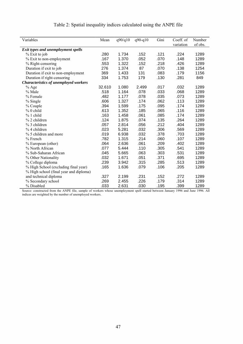
47

Table 2: Spatial inequality indices calculated using the ANPE file Variables

Mean

q90/q10

q90-q10

Gini

Coeff. of variation

Number of obs.

Exit types and unemployment spells % Exit to job .280 1.734 .152 .121 .224 1289 % Exit to non-employment .167 1.370 .052 .070 .148 1289 % Right-censoring .553 1.322 .152 .218 .426 1289 Duration if exit to job 276 1.374 87 .070 .138 1254 Duration if exit to non-employment 369 1.433 131 .083 .179 1156 Duration if right-censoring 334 1.753 179 .130 .281 849

Characteristics of unemployed workers % Age 32.610 1.080 2.499 .017 .032 1289 % Male .518 1.164 .078 .033 .068 1289 % Female .482 1.177 .078 .035 .073 1289 % Single .606 1.327 .174 .062 .113 1289 % Couple .394 1.599 .175 .095 .174 1289 % 0 child .613 1.352 .185 .065 .116 1289 % 1 child .163 1.458 .061 .085 .174 1289 % 2 children .124 1.875 .074 .135 .264 1289 % 3 children .057 2.814 .056 .212 .404 1289 % 4 children .023 5.281 .032 .306 .569 1289 % 5 children and more .019 6.938 .032 .378 .703 1289 % French .782 1.315 .214 .060 .107 1289 % European (other) .064 2.636 .061 .209 .402 1289 % North African .077 5.444 .110 .305 .541 1289 % Sub-Saharan African .045 5.665 .063 .303 .531 1289 % Other Nationality .032 1.671 .051 .371 .695 1289 % College diploma .239 3.942 .315 .285 .513 1289 % High School (excluding final year) .165 1.636 .079 .106 .205 1289 % High school (final year and diploma) and technical diploma .327 2.199 .231 .152 .272 1289 % Secondary school .269 2.455 .226 .179 .314 1289 % Disabled .033 2.631 .030 .195 .399 1289

Source: constructed from the ANPE file, sample of workers whose unemployment spell started between January 1996 and June 1996. All indices are weighted by the number of unemployed workers.

48

Table 3: Estimation results of the first-stage equation (SPLE) Variables Job Non-employment Age /100 -2.9289***

(.2801) -9.0729***

(.3253) (Age/100) squared 1.210***

(.387) 11.330***

(.442) Male <ref> <ref> Female -.1819***

(.0060) .3486*** (.0079)

Single <ref> <ref> Couple .1089***

(.0077) .0710*** (.0094)

No child <ref> <ref> 1 child -.0815***

(.0093) .0834*** (.0110)

2 children -.0266** (.0106)

.0375*** (.0130)

3 children -.1312*** (.0149)

.0352** (.0174)

4 children -.1823*** (.0245)

.0428* (.0260)

5 children and more -.2425*** (.0299)

.0852*** (.0281)

French <ref> <ref> European (other) -.0510***

(.0124) -.1732*** (.0168)

North African -.4455*** (.0143)

-.0810*** (.0154)

Sub-Saharan African -.6638*** (.0209)

-.0244 (.0198)

Other Nationality -.5629*** (.0231)

.0248 (.0224)

College diploma <ref> <ref> High School (first grade) -.2296***

(.0089) -.0970*** (.0118)

High school (other grade) and technical diploma -.3349*** (.0078)

-.2176*** (.0107)

Secondary school -.5872*** (.0095)

-.4252*** (.0119)

Not disabled <ref> <ref> Disabled -03837***

(.0197) .4653*** (.0168)

Number of observations 430,695 Source: constructed from the ANPE file. ***: significant at 1% level; **: significant at 5% level; *: significant at 10% level. Monthly dummy variables were also included to control for seasonality but are not reported in the table.

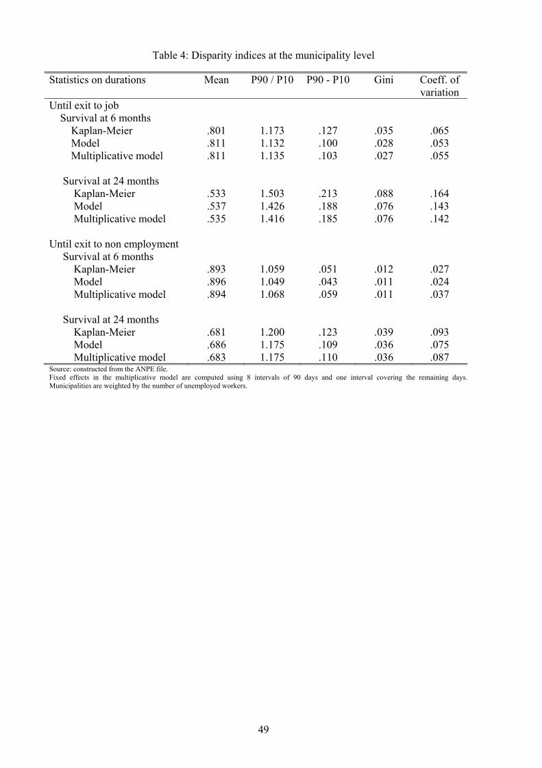
49

Table 4: Disparity indices at the municipality level Statistics on durations

Mean

P90 / P10 P90 - P10 Gini

Coeff. of variation

Until exit to job Survival at 6 months Kaplan-Meier .801 1.173 .127 .035 .065 Model .811 1.132 .100 .028 .053 Multiplicative model .811 1.135 .103 .027 .055 Survival at 24 months Kaplan-Meier .533 1.503 .213 .088 .164 Model .537 1.426 .188 .076 .143 Multiplicative model .535 1.416 .185 .076 .142 Until exit to non employment Survival at 6 months Kaplan-Meier .893 1.059 .051 .012 .027 Model .896 1.049 .043 .011 .024 Multiplicative model .894 1.068 .059 .011 .037 Survival at 24 months Kaplan-Meier .681 1.200 .123 .039 .093 Model .686 1.175 .109 .036 .075 Multiplicative model .683 1.175 .110 .036 .087 Source: constructed from the ANPE file. Fixed effects in the multiplicative model are computed using 8 intervals of 90 days and one interval covering the remaining days. Municipalities are weighted by the number of unemployed workers.

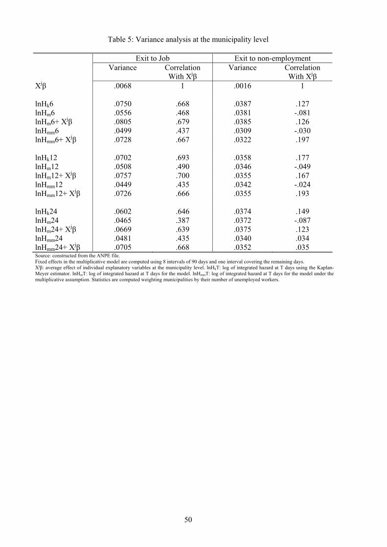
50

Table 5: Variance analysis at the municipality level

Exit to Job Exit to non-employment Variance Correlation

With Xjβ Variance Correlation

With Xjβ Xjβ .0068 1 .0016 1 lnHk6 .0750 .668 .0387 .127 lnHm6 .0556 .468 .0381 -.081 lnHm6+ Xjβ .0805 .679 .0385 .126 lnHmm6 .0499 .437 .0309 -.030 lnHmm6+ Xjβ .0728 .667 .0322 .197 lnHk12 .0702 .693 .0358 .177 lnHm12 .0508 .490 .0346 -.049 lnHm12+ Xjβ .0757 .700 .0355 .167 lnHmm12 .0449 .435 .0342 -.024 lnHmm12+ Xjβ .0726 .666 .0355 .193 lnHk24 .0602 .646 .0374 .149 lnHm24 .0465 .387 .0372 -.087 lnHm24+ Xjβ .0669 .639 .0375 .123 lnHmm24 .0481 .435 .0340 .034 lnHmm24+ Xjβ .0705 .668 .0352 .035 Source: constructed from the ANPE file. Fixed effects in the multiplicative model are computed using 8 intervals of 90 days and one interval covering the remaining days. Xjβ: average effect of individual explanatory variables at the municipality level. lnHkT: log of integrated hazard at T days using the Kaplan-Meyer estimator. lnHmT: log of integrated hazard at T days for the model. lnHmmT: log of integrated hazard at T days for the model under the multiplicative assumption. Statistics are computed weighting municipalities by their number of unemployed workers.

51

Table 6: Regressions of town fixed effects (for exit to job) on municipality variables

(1) (2) (3) Constant -6.717***

(.120) -6.147***

(.035) -6.644***

(.121) Proportion of technical diplomas 1.861***

(.337) 1.966***

(.338) Proportion of high school diplomas -.078

(.384) -.260 (.386)

Proportion of college diplomas .099 (.178)

.354* (.192)

Proportion of European (other) -1.394*** (.246)

-1.402*** (.245)

Proportion of North Africans -1.756*** (.220)

-1.344*** (.250)

Proportion of Sub-Saharan Africans -3.775*** (.513)

-3.872*** (.512)

Proportion of other nationalities -.458* (.246)

-.491** (.245)

Job density within 45mins by public transport

-.092*** (.016)

.000 (.012)

Job density within 45mins by private transport

-.517*** (.047)

-.176*** (.051)

Number of observation 1254 1254 1254 Weighted number of observations 430602 430602 430602 Error rate .468 .246 .473 Pseudo-R² .724 .259 .730 Source: constructed from the ANPE file. ***: significant at 1% level; **: significant at 5% level; *: significant at 10% level. Estimates are computed using 8 intervals of 90 days and one interval covering the remaining days. Municipalities are weighted by the number of unemployed workers.

52

Table A1: Descriptive statistics on variables used in the study Variable Number

of obs. Mean Standard

deviation Minimum Maximum

Exit types and unemployment spells Exit to job 430,695 .280 .449 .000 1.000 Exit to non-employment 430,695 .167 .373 .000 1.000 Right-censoring 430,695 .672 .470 .000 1.000 Duration if exit to job 120,502 273 337 1 2818 Duration if exit to non-employment 71,807 368 452 1 2813 Duration if right-censoring 238,386 287 378 1 2829

Characteristics of unemployed workers Age 430,695 32.610 9.222 16.000 54.000 Male 430,695 .518 .500 .000 1.000 Female 430,695 .482 .500 .000 1.000 Single 430,695 .606 .489 .000 1.000 Couple 430,695 .394 .489 .000 1.000 0 child 430,695 .613 .487 .000 1.000 1 child 430,695 .163 .369 .000 1.000 2 children 430,695 .124 .330 .000 1.000 3 children 430,695 .057 .233 .000 1.000 4 children 430,695 .023 .150 .000 1.000 5 children and more 430,695 .019 .137 .000 1.000 French 430,695 .782 .413 .000 1.000 European (other) 430,695 .064 .245 .000 1.000 North African 430,695 .077 .267 .000 1.000 Sub-Saharan African 430,695 .045 .207 .000 1.000 Other Nationality 430,695 .032 .175 .000 1.000 College diploma 430,695 .239 .427 .000 1.000 High School (excluding final year) 430,695 .165 .371 .000 1.000 High school (final year and diploma) and technical diploma 430,695 .327 .469 .000 1.000 Secondary school 430,695 .269 .443 .000 1.000 Disabled 430,695 .033 .178 .000 1.000

Segregation variables Unemployment rate 430,695 .127 .043 .000 .246 % French 430,695 .794 .078 .569 1.000 % European (other) 430,695 .071 .020 .000 .265 % North African 430,695 .064 .041 .000 .218 % Sub-Saharan African 430,695 .030 .019 .000 .086 % Other Nationality 430,695 .041 .027 .000 .230 % No diploma 430,695 .412 .091 .202 .663 % Technical diploma 430,695 .191 .057 .040 .402 % High school 430,695 .145 .020 .000 .266 % University 430,695 .252 .123 .030 .571

Job-accessibility variables 45mn job density by public transport 430,695 1.085 .436 .076 19.920 45mn job density by car 430,695 .860 .152 .152 1.200

Source: constructed from the ANPE file.