SETP No. 14SETP No. 14

Barry Standish

Employment-Intensive Investment Branch

International Labour Office, Geneva

The Economic Value of Incremental Employment in the South African Construction Sector

A Report commissioned by the International Labour Organisation for the support of the Efficient Application of Labour Based Methods in the Construction Sector

The Economic Value of Incremental Employment in the South African Construction Sector

A Report commissioned by the International Labour Organisation for the support of the Efficient Application of Labour Based

Methods in the Construction Sector

______________________

Barry Standish

Employment-Intensive Investment Branch

INTERNATIONAL LABOUR OFFICE

GENEVA

Copyright © International Labour Organization 2003 First published (2003)

Publications of the International Labour Office enjoy copyright under Protocol 2 of the Universal Copyright Convention. Nevertheless, short excerpts from them may be reproduced without authorization, on condition that the source is indicated. For rights of reproduction or translation, application should be made to the Publications Bureau (Rights and Permissions), International Labour Office, CH-1211 Geneva 22, Switzerland. The International Labour Office welcomes such applications.

Libraries, institutions and other users registered in the United Kingdom with the Copyright Licensing Agency, 90 Tottenham Court Road, London W1T 4LP [Fax: (+44) (0)20 7631 5500; email: cla@cla.co.uk], in the United States with the Copyright Clearance Center, 222 Rosewood Drive, Danvers, MA 01923 [Fax: (+1) (978) 750 4470; email: info@copyright.com] or in other countries with associated Reproduction Rights Organizations, may make photocopies in accordance with the licences issued to them for this purpose.

Employment-Intensive Infrastructure Programmes: Socio-Economic Technical Paper (SETPno. 14) (The Economic Value of Incremental Employment in the South African Construction Sector, Barry Standish)

Geneva, International Labour Office, 2003

ISBN 92-2-114836-X (hardcover) ISBN 92-2-114837-8 (softcover) ISBN 92-2-114838-6 (pdf)

ILO Cataloguing in Publication Data

The designations employed in ILO publications, which are in conformity with United Nations practice, and the presentation of material therein do not imply the expression of any opinion whatsoever on the part of the International Labour Office concerning the legal status of any country, area or territory or of its authorities, or concerning the delimitation of its frontiers.

The responsibility for opinions expressed in signed articles, studies and other contributions rests solely with their authors, and publication does not constitute an endorsement by the International Labour Office of the opinions expressed in them.

Reference to names of firms and commercial products and processes does not imply their endorsement by the International Labour Office, and any failure to mention a particular firm, commercial product or process is not a sign of disapproval.

ILO publications can be obtained through major booksellers or ILO local offices in many countries, or direct from ILO Publications, International Labour Office, CH-1211 Geneva 22, Switzerland. Catalogues or lists of new publications are available free of charge from the above address, or by email: pubvente@ilo.org

Visit our website: www.ilo.org/publns

Printed by International Labour Office, Geneva, Switzerland.

FOREWORD

The macro-economic case for using labour-based, as opposed to equipment-intensive technology in the infrastructure and construction sectors, has been made in many developing countries on the ground of lower unit costs, increased employment generation, higher contribution to GDP, higher multiplier effects, higher levels of household income and consumption, reduced foreign exchange requirements and hence, reduced import dependency. These conclusions apply to countries characterised by surplus labour, low wages, weak local industrial capacity (in tools and equipment production).

South Africa, obviously, is in a different situation, with higher wages and a domestic industry producing equipment of various sizes. Hence, the challenge of this study, which was to investigate whether the macro-economic outcomes of labour-based vs. equipment-based construction would still be in favour of the labour-based option, and if so, to what extent. We are grateful to the author, Barry Standish, resident economist at the Graduate School of Business at the University of Cape Town, to have taken up this challenge and to have made an important contribution to the debate on the macro-economic potential of labour-based investment technology not only in South Africa, but also more generally in the context of world-wide efforts to foster employment-intensive growth wherever technically feasible and economically cost-effective, with a view to combating poverty and reducing inequalities.

We also thank the National Department of Public Works, South Africa, for taking the initiative in establishing the macro-economic benefit of labour-based methods in the South African context. We believe the study will contribute towards the Department's objective to mainstreaming the technology in the construction sector where it will be appropriate and efficient. We are also grateful to the United Nations Development Programme for providing the necessary financial assistance to carrying out this study.

The ILO=s regional support team of the Employment-Intensive Investment Programme for English-speaking African countries, the ASIST Africa programme (Advisory Support, Information Services and Training) in Harare, who were backstopping this work, and the Branch in Geneva would appreciate any comments readers my have on this work.

Jean Majeres Chief

Employment-Intensive Investment Branch

Geneva, October 2003

v

Table of Contents

PREFACE ............................................................................................................................................ IX

STRUCTURE OF THE REPORT..................................................................................................... XI

SUMMARY OF CONCLUSIONS ....................................................................................................XII

1 INTRODUCTION .........................................................................................................................1

2 THEORETICAL FOUNDATIONS .............................................................................................3

3 A LABOUR FOCUSSED PROFILE OF THE CONSTRUCTION INDUSTRY ....................4 CONTRIBUTION TO GROSS DOMESTIC PRODUCT...................................................................................4 CONSTRUCTION EMPLOYMENT .............................................................................................................5 CONSTRUCTION WAGES ........................................................................................................................7

Wage trends .....................................................................................................................................7 Provincial differences ......................................................................................................................9 Size of firm differences...................................................................................................................11 Skill differences..............................................................................................................................11

SUMMARY...........................................................................................................................................24 4 EXPENDITURE PATTERNS AND STANDARDS OF LIVING ...........................................25

INTRODUCTION ...................................................................................................................................25 DESCRIPTION OF METHODOLOGY .......................................................................................................25 A PROFILE OF INCOME AND EXPENDITURE ..........................................................................................26 CHANGES IN EXPENDITURE PATTERNS ...............................................................................................29 SUMMARY AND CONCLUSION..............................................................................................................33

5 THE MACRO ECONOMIC IMPACT OF CHANGING EXPENDITURE PATTERNS....35 INTRODUCTION ...................................................................................................................................35 DESCRIPTION OF METHODOLOGY ........................................................................................................35 NATIONAL MACRO ECONOMIC IMPACT OF CHANGING EXPENDITURE PATTERNS................................39

Aggregate impact...........................................................................................................................39 Male and female head of household differences ............................................................................39 Provincial differences ....................................................................................................................40

SUMMARY AND CONCLUSIONS ............................................................................................................43 6 THE MACRO ECONOMIC IMPACT OF THE LOCAL MANUFACTURE OF CONSTRUCTION EQUIPMENT......................................................................................................44

DESCRIPTION OF METHODOLOGY .......................................................................................................44 DATA ..................................................................................................................................................44 THE MACRO ECONOMIC IMPACT OF A LOCALLY MANUFACTURED WHEELED LOADER.......................47 SUMMARY AND CONCLUSIONS ............................................................................................................48

7 LABOUR-BASED AND EQUIPMENT-BASED CONSTRUCTION: THE NET MACROECONOMIC EFFECT .........................................................................................................49

COSTS AND PRODUCTIVITY.................................................................................................................50 REPAYMENT OF CAPITAL COSTS..........................................................................................................53 THE MACRO ECONOMIC IMPACT OF EQUIPMENT-BASED CONSTRUCTION ..........................................54 COST PREMIUMS .................................................................................................................................59 CONCLUSION ......................................................................................................................................60

8 CONCLUSION ............................................................................................................................61

REFERENCES .....................................................................................................................................64

vi

APPENDIX. TERMS OF REFERENCE ...........................................................................................65 INTRODUCTION AND BACKGROUND....................................................................................................65

The Concept of Efficiency in Value for Money ..............................................................................65 Financial Limits for Labour Substitution.......................................................................................66

ECONOMIC LIMITS FOR LABOUR SUBSTITUTION .................................................................................66 The Economic Value of Employment .............................................................................................66

SCOPE OF WORK .................................................................................................................................67 Labour Economics .........................................................................................................................67 Equipment Economics....................................................................................................................67

METHODOLOGY ..................................................................................................................................68

vii

List of Abbreviations

CBPWP Community Based Public Works Programme

GDP Gross Domestic Product

ILO International Labour Organisation

NDPW The National Department of Public Works

NPWP National Public Works Programme

SALDRU Southern African Labour and Development Research Unit, School of Economics, University of Cape Town.

SIC Standard Industrial Classification of all Economic Activities.

SUT Supply and Use Tables

US$ United States Dollar

ix

Preface

The National Department of Public Works (NDPW) is working on a number of different fronts to reorient the construction sector. The most important underlying aim is to enhance and optimise employment in the construction process itself. In parallel with this, a supplementary aim is to provide targeted opportunities for emerging and previously disadvantaged contractors. The most prominent examples of initiatives completed or under way include:

• the National Public Works Programme (NPWP) launched in 1994/95 and comprising the Community-Based Public Works Programme (CBPWP) and a set of 12 pilot projects (testing the extent to which employment could be optimised whilst relying on mainstream technical consultants and contractors);

• the preparation and promotion of a set of Guidelines on Enhancing Employment Opportunities in the Delivery of Infrastructure Projects based on the experience gained and lessons learned through the pilot projects component of the NPWP;

• the Strategic Projects Initiative (SPI) under which targeted procurement (TP) is aiming for the use of black prime contractors in the implementation of medium and large-scale projects on behalf of the NDPW;

• the Construction Industry Development Programme (CIDP), under which progress is being made towards the creation of a statutory Construction Industry Development Board (CIDB), and which also includes an Emerging Contractors Development Programme (ECDP).

In mid-1996, as these initiatives were at earlier stages of conception or implementation, the NPWP Branch of NDPW requested continuing advisory and research resources from the International Labour Office (ILO). The rationale was twofold. First, the NPWP Branch was eager to draw on international experience with respect to the use of labour-based methods in construction. Secondly (and complementary to this), the NDPW as a whole emphasised that employment creation through construction should not take precedence over (a) value for money to the public sector client, or (b) quality standards in construction outputs. It was these two concerns that led to the title of the current ILO project - Support to the Efficient Application of Labour-Based Methods in the Construction Sector. This investigation is part of that initiative.

xi

Structure of the Report

This report is organised into eight main chapters.

Chapter 1 introduces the study.

Chapter 2 briefly outlines the theoretical foundations of the study and the degree to which there are definitive answers to the questions being asked and the degree to which policy decisions must be made.

Chapter 3 provides a time series and cross sectional profile of the construction industry with a focus on labour and wages. The objective of this section is to answer the first question set by the terms of reference: what are current wage rates in the construction industry? How do they vary by occupation? How do they vary by location?

Chapter 4 analyses the spending patterns of people in lower income groups and answers the second question set by the terms of reference by highlighting the key expenditure changes as incomes change.

Chapter 5 brings together sections 3 and 4 and determines the macro economic impact of income increases that lead to increased and changing expenditure patterns.

Chapter 6 focuses on equipment-based construction with a view to determining the macro economic impact of the local production of earth moving equipment.

Chapter 7 analyses the relative costs of labour and equipment-based construction with the intention of setting the parameters on which policy decisions can be made.

The overall conclusions are drawn in Chapter 8 along with suggestions for future research and the kind of information that should be systematically collected from labour intensive projects.

There is one appendix which contains the terms of reference for this study.

xii

Summary of Conclusions

1. This summary draws together the key conclusions from each of the chapters and presents them in chronological order.

2. The first area of investigation is the construction industry with a view to determining, in particular, wage differences by skill and location. The construction industry is a small and, currently, declining industry. Contribution to GDP has fallen, there are fewer jobs today than twenty years ago and real wages have fallen. About 300,000 people were employed in the construction industry in 1997 and about 70% of these were black.

3. On average the civil engineering industry pays wages that are greater than in house construction with skill differences being the most likely cause of this. There are significant differences in wages between provinces. In 1994, (the latest data of this type) we find the lowest average civil engineering salaries are paid In the Northern Province and the highest in the Eastern Cape. Average house construction salaries were the highest in Gauteng in 1994 and lowest in the Eastern Cape.

4. Determining average salaries by skill level proved a difficult exercise. Both the October Household Surveys and the Population Census were analysed. Unskilled labourers in the Western Cape construction industry have the highest salaries in the country of between R1,460 and R1,215 monthly (R66 and R56 a day). (Although, in contrast, the most common daily wages paid on labour intensive public works projects in the Western Cape ranged between R20 and R30). The lowest paid unskilled construction workers are to be found in the Northern Province. Here the estimated wage was a daily rate of R36. (All wages in year 2000 values).

5. The second area of investigation was to analyse the expenditure patterns of poor and very poor people with a view to determining the macroeconomic effects of income increases. The expenditure patterns that emerge are intuitively appealing. Grain mill products are important for the very poor and fall off rapidly as a percentage of household expenditure as incomes increase. The same holds true for sugar products, petroleum, wood, coal and mining products although the initial importance is not that great. In contrast, as incomes increase so too does the proportion of expenditure on clothing, footwear and meat.

6. Changing expenditure patterns were linked to national input output relationships and the multiplied impact calculated. It is found that if, for example, income increased by R5,000 for households with income currently less than R5,0000, then there would be an increase in GDP equal 1.40 times this increase, indirect household incomes would increase by 0.65 times, 0.26 indirect jobs would be created and there would be increases in income tax, company tax and imports to the value of R605, R307 and R1,280 respectively.

7. The objective of the third area of investigation was to determine the macroeconomic impact of the local manufacturing of machinery used in the construction industry. While this part of study was challenged by inadequate information some estimates were made. A locally produced wheeled loader with a retail price of R600,000 and a 43% import content will contribute R473,000 to GDP and generate 4.52 indirect jobs. A similar machine with a 68% import content will contribute R256,000 to GDP and generate 2.48 indirect jobs.

xiii

8. It is shown in the forth area of investigation that the macro economic effects of labour-based earthwork excavation are greater than those of equipment-based construction. A case can therefore be made for a financial premium for the substitution of labour for equipment. In addition, if we view the import component of locally manufactured earth moving equipment as ‘lost’ expenditure (lost to the country) then labour can compete financially with equipment under a much greater range of physical conditions and wages.

9. These results are sensitive to the import component of locally manufactured construction equipment. From this it follows that the factor that most effects the financial premium is the degree of capital amortisation. Comparing the macro economic effect of labour against new earth moving equipment with a 71% import component indicates that a labour premium of over 50% is justified. However this premium falls to 4% once the capital cost is fully amortised. Similarly comparing labour to a machine with 48% import component calls for a 32% labour premium when the machine is new but again only 4% when fully amortised.

10. A comparison of the direct cost of earthwork excavation indicates that labour-based methods may be financially viable even without macroeconomic premiums. In the Cape Town area this happens only at low wages and easy ground conditions. The competitiveness of labour-based earthworks excavation declines rapidly as wages increase and/or ground conditions deteriorate. It is suspected that higher equipment costs outside of urban areas will result in greater financial viability for labour-based earthwork in rural and remote rural areas. In addition, a programme approach will improve labour productivity and make it more competitive.

11. In general the report draws mixed conclusions about the financial viability of labour-based methods of road rehabilitation. The macroeconomic advantages of labour-based methods are compelling when we use fully imported equipment and remains so even for locally produced equipment with an import component. When the capital cost of the equipment is fully amortised then the macroeconomic advantage of labour-based methods becomes marginal.

12. The overwhelming case that must be made for using labour-based methods is the contribution it will make to economic empowerment. Roads, dams and other infrastructure are good for the regional economy and will allow it to grow. Using labour-based methods will generate jobs and provide incomes further promoting the regional economy. Involving local communities will help in capacity building. Using small and emergent contractors will generate sustainable incomes and opportunities.

13. It is beyond the scope of this report to attempt to quantify the effects of labour-based methods on economic empowerment. In a similar vein we cannot quantify the cost of economically marginalising poor rural people by using equipment-based methods. Yet, even without being able to quantify these effects, we believe that there is an overwhelming case for labour-based methods. Not only will it help the poor but it will also contribute to the generation of sustained economic growth and empowerment.

1

1 Introduction

1.1 South Africa is a land of stark contrasts. Majestic mountains and fertile lands. Barren plains and bleak poverty. It has great economic promise and worrying constraints. On the bright side there has been sustained economic growth over the last seven years. This last happened in the late 1960s. But the economic growth has been too little. At times it has been barely greater than population growth. And the economic growth has been jobless. For the unskilled, in particular, there are less formal jobs, not more.

1.2 This country’s economic problems, as evidenced by desperate poverty and endemic lack of opportunities, have been a hundred years in the making. For problems like this there is no quick fix. The long term and sustainable solution lies in growing productivity - making firms more productive and helping people be more productive. It is only though improved productivity that we can make more of the things that people need and generate sustained increases in living standards.

1.3 One of the greatest constraints to poverty reduction is the challenge of effective economic empowerment. Many South Africans have been consigned to the stagnant backwaters of a powerful economy through decades of bad or non-existent education, discrimination in jobs and opportunities, meagre health services and misguided infrastructural spending. Such poverty does not need welfare payments as much as it needs economic empowerment.

1.4 The National Public Works Programme (NPWP) is part of the initiative that attempts to reduce poverty through a multi-pronged initiative. The NPWP aims at sustainable job creation and economic empowerment through the provision or rehabilitation of necessary and useful infrastructure using labour-based methods. The NPWP does not rely on job creation alone to generate economic empowerment. It provides training and, along with other initiatives, uses targeted procurement and promotes small or emerging business.

1.5 The NPWP should however also provide value for money and use labour-based methods that can compete financially with equipment-based methods. Some experiences in Africa, for example in Lesotho, Botswana, Uganda and Namibia, all demonstrate that labour-based methods are financially viable for activities like road building and road rehabilitation. In South Africa the known higher labour cost and the suspected lower capital cost are likely to challenge the financial viability of labour-based methods.

1.6 Financial viability is one aspect of project assessment. Socio economic effects and multiplier effects are equally important. What are the socio economic effects in the immediate vicinity of a project using labour-based methods? How does this compare to the effect of equipment-based methods? What are the relative macroeconomic effects of the choices in method? This latter question is particularly important in South Africa because there is a successful domestic industry that manufactures heavy machinery for construction.

1.7 The key objective for this investigation was set by the terms of reference as:

what - if any - financial premium per unit of expenditure on construction is economically justified for the substitution of labour for equipment?

2

1.8 In order to achieve this objective, and as part of sub objectives of the terms of reference, a statistical mosaic of the construction industry was created with a view to determining job trends, skill patterns and real wages. This feeds into measures of financial viability and compares the relative cost of labour and equipment-based methods.

1.9 A second strand of the investigation focuses on macroeconomic multiplier effects. Multipliers are calculated for labour-based methods. Similarly, multipliers are calculated for the local manufacturing of construction machinery and the operation of the machinery. Finally the labour-based and equipment-based multipliers are compared and financial premiums measured.

3

2 Theoretical Foundations

2.1 Every choice involves a cost. The choice of labour-based methods over equipment-based methods are not just choices of technique and location but also of who bears the socio economic benefits, who bears the costs and the relative magnitude of these differences.

2.2 The poor and unemployed will benefit from a move to labour-based methods in construction. The households who bear the initial burden of a switch from equipment-based methods are the owners of equipment, drivers, mechanics and so on. Compounding these costs in South Africa is the fact that that there is domestic producer of construction equipment and vehicles. A fall in local production will have the usual multiplier effects on, for example, Atlantic Diesel Engines. Even were a machine is fully imported the actual operation generates local incomes and this portion increases as the capital cost of imported equipment is amortised.

2.3 The economic issues focused on in the terms of reference address three main areas in economics – multiplier analysis, gains from trade and cost reduction through improved productivity.

2.4 It can be shown in the discipline of economics that there are efficiency and welfare gains to be had by people trading with each other and by nations trading with each other. People and nations should seek out and maximise their comparative advantage.

2.5 Hence, if it can be shown that equipment-based construction is simply cheaper than labour-based construction then national welfare gains and comparative advantage are reduced by forcing labour-based construction. The people working on the project receive the benefits. The additional costs are (in this case) borne by the taxpayer.

2.6 Economics also recognises that comparative advantages are not static but change and evolve over time. Many economists would suggest that this process is best left to the market. Policy makers, on the other hand, faced with unemployment and poverty will wish to be proactive. At the heart of the policy decision is the need to search for a change in comparative advantage such that improved future welfare will outweigh the immediate loss of welfare by reducing the gains from trade.

2.7 Such issues are further complicated by the fact that an important economic objective in South Africa is a more equal distribution of income. Hence it may be argued that a financial premium on labour-based projects is a corrective mechanism for unbalanced standards of living. Capital intensive projects deny poor people the opportunity to participate meaningfully in the economy. Labour-based methods generate such opportunities.

2.8 In contrast to gains from trade and long term economic policy, multiplier analysis is more short term in nature. It is well known that multipliers only operate when there is excess industrial capacity. Any increase in demand when industries are at full capacity simply results in an immediate increase in imports. In the longer term this increased demand, if it is sustained, may result in increased production capacity but this depends on comparative advantage.

4

3 A Labour Focussed Profile of the Construction Industry

3.1 This section of the report focuses on the construction industry with the objective of determining a profile of actual salaries and wages. This is clearly the starting point of the study as wages determine the cost differential between labour-based and equipment-based construction and the magnitude of the associated macro economic impact.

3.2 Depth is given to this profile by identifying wage differentials across the country, by occupation and by size of firm and by comparing construction wages to those in manufacturing.

3.3 It will be shown that the construction industry is a small and (currently) declining industry. Not only has output fallen but so too have real wages. Some types of wage measures were easy to determine. Other proved to be less so. Determining wages by occupation by location proved particularly difficult.

Contribution to Gross Domestic Product

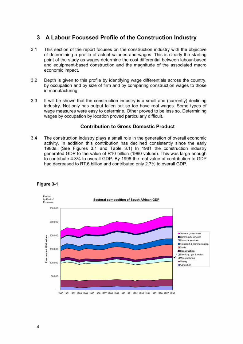
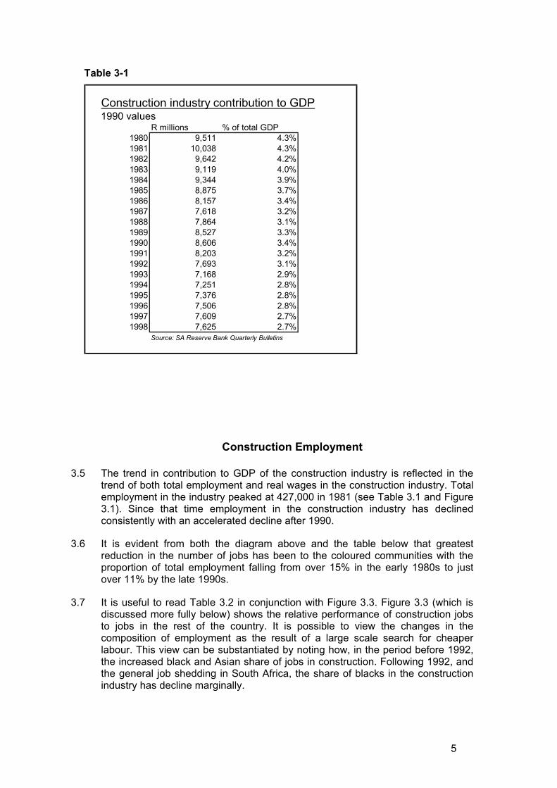
3.4 The construction industry plays a small role in the generation of overall economic activity. In addition this contribution has declined consistently since the early 1980s. (See Figures 3.1 and Table 3.1) In 1981 the construction industry generated GDP to the value of R10 billion (1990 values). This was large enough to contribute 4.3% to overall GDP. By 1998 the real value of contribution to GDP had decreased to R7.6 billion and contributed only 2.7% to overall GDP.

Figure 3-1

Sectoral composition of South African GDP

-

50,000

100,000

150,000

200,000

250,000

300,000

1980 1981 1982 1983 1984 1985 1986 1987 1988 1989 1990 1991 1992 1993 1994 1995 1996 1997 1998

Rm

con

stan

t 199

0 va

lues

General governmentCommunity servicesFinancial servicesTransport & communicationTradeConstructionElecticity, gas & waterManufacturingMiningAgriculture

Product by Kind of Economic

5

Table 3-1

Construction Employment

3.5 The trend in contribution to GDP of the construction industry is reflected in the trend of both total employment and real wages in the construction industry. Total employment in the industry peaked at 427,000 in 1981 (see Table 3.1 and Figure 3.1). Since that time employment in the construction industry has declined consistently with an accelerated decline after 1990.

3.6 It is evident from both the diagram above and the table below that greatest reduction in the number of jobs has been to the coloured communities with the proportion of total employment falling from over 15% in the early 1980s to just over 11% by the late 1990s.

3.7 It is useful to read Table 3.2 in conjunction with Figure 3.3. Figure 3.3 (which is discussed more fully below) shows the relative performance of construction jobs to jobs in the rest of the country. It is possible to view the changes in the composition of employment as the result of a large scale search for cheaper labour. This view can be substantiated by noting how, in the period before 1992, the increased black and Asian share of jobs in construction. Following 1992, and the general job shedding in South Africa, the share of blacks in the construction industry has decline marginally.

Construction industry contribution to GDP1990 values

R millions % of total GDP1980 9,511 4.3%1981 10,038 4.3%1982 9,642 4.2%1983 9,119 4.0%1984 9,344 3.9%1985 8,875 3.7%1986 8,157 3.4%1987 7,618 3.2%1988 7,864 3.1%1989 8,527 3.3%1990 8,606 3.4%1991 8,203 3.2%1992 7,693 3.1%1993 7,168 2.9%1994 7,251 2.8%1995 7,376 2.8%1996 7,506 2.8%1997 7,609 2.7%1998 7,625 2.7%

Source: SA Reserve Bank Quarterly Bulletins

6

Figure 3-2

Table 3-2

Employment in the Construction Industry

-

50,000

100,000

150,000

200,000

250,000

300,000

350,000

400,000

450,000

500,000

Jan-80

Jan-81

Jan-82

Jan-83

Jan-84

Jan-85

Jan-86

Jan-87

Jan-88

Jan-89

Jan-90

Jan-91

Jan-92

Jan-93

Jan-94

Jan-95

Jan-96

Jan-97

Num

ber o

f job

s

BlackAsianColouredWhite

Employment in the Construction Industry

End of year Total jobs White Coloured Asian Black1980 387,400 12.2% 15.5% 1.9% 70.4%1981 427,700 11.8% 15.2% 1.7% 71.3%1982 427,600 11.9% 15.5% 1.8% 70.8%1983 420,700 12.1% 15.5% 1.7% 70.7%1984 416,500 12.0% 15.3% 1.8% 70.9%1985 407,800 11.9% 15.3% 1.7% 71.1%1986 404,900 11.2% 14.9% 1.6% 72.2%1987 407,500 10.9% 14.6% 1.7% 72.8%1988 414,400 10.7% 14.3% 1.8% 73.2%1989 412,700 10.5% 14.1% 1.9% 73.5%1990 403,800 10.5% 14.3% 1.9% 73.3%1991 378,900 10.9% 14.6% 2.0% 72.5%1992 357,100 10.8% 15.0% 2.0% 72.1%1993 364,605 10.1% 13.0% 1.8% 70.5%1994 355,114 10.6% 11.9% 1.8% 71.3%1995 336,939 10.7% 12.0% 2.2% 71.7%1996 312,051 11.4% 11.1% 2.3% 71.3%1997 303,392 11.1% 11.4% 2.2% 71.2%

Source: Stats SA statistical releases (TSE database)

7

Figure 3-3

3.8 The loss of jobs in the construction industry stands in contrast to the rest of the economy. Figure 3.3 illustrates an index of employment of total non-agricultural employment and employment in construction for the years 1980 to 1997. The index base year is 1990. In the economy as a whole there have been net job losses since 1990. The trend in the economy over the past twenty years indicates a general growth in jobs over the 1980s with a sustained loss in jobs between 1990 and 1997. While this is a bleak picture in itself, the construction industry has experienced jobs losses far greater than the rest of the economy, on the one hand, and the job losses have been happening since the early 1980s, on the other.

Construction wages

Wage trends

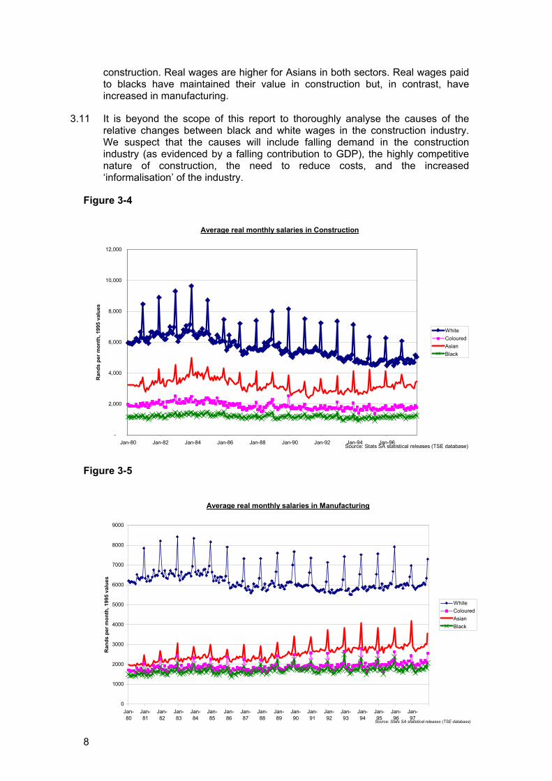
3.9 We see above that construction has a falling contribution to GDP and a falling contribution to total job creation. The changes in real wages reflect this trend although the differences are not as stark. Figures 3.4 and 3.5 illustrate the racial differences in wages and the changes in these real wages since 1980 for the construction and manufacturing industries respectively. (Real wages are estimated by adjusting nominal wages by the South Africa consumer price index).

3.10 For whites real wages have been falling in both construction and manufacturing since the mid-1980s although the fall has been greater in the construction industry. Real wages for coloureds are higher in manufacturing but lower in

Index of employment: Construction and total non-agricultural employment

70

75

80

85

90

95

100

105

110

1980 1981 1982 1983 1984 1985 1986 1987 1988 1989 1990 1991 1992 1993 1994 1995 1996 1997

Inde

x 19

90=1

00

ConstructionTotal non agricultural

Source: SA Reserve Bank Quarterly Bulletin

8

construction. Real wages are higher for Asians in both sectors. Real wages paid to blacks have maintained their value in construction but, in contrast, have increased in manufacturing.

3.11 It is beyond the scope of this report to thoroughly analyse the causes of the relative changes between black and white wages in the construction industry. We suspect that the causes will include falling demand in the construction industry (as evidenced by a falling contribution to GDP), the highly competitive nature of construction, the need to reduce costs, and the increased ‘informalisation’ of the industry.

Figure 3-4

Figure 3-5

Average real monthly salaries in Construction

-

2,000

4,000

6,000

8,000

10,000

12,000

Jan-80 Jan-82 Jan-84 Jan-86 Jan-88 Jan-90 Jan-92 Jan-94 Jan-96

Ran

ds p

er m

onth

, 199

5 va

lues

WhiteColouredAsianBlack

Source: Stats SA statistical releases (TSE database)

Average real monthly salaries in Manufacturing

0

1000

2000

3000

4000

5000

6000

7000

8000

9000

Jan-80

Jan-81

Jan-82

Jan-83

Jan-84

Jan-85

Jan-86

Jan-87

Jan-88

Jan-89

Jan-90

Jan-91

Jan-92

Jan-93

Jan-94

Jan-95

Jan-96

Jan-97

Ran

ds p

er m

onth

, 199

5 va

lues

WhiteColouredAsianBlack

Source: Stats SA statistical releases (TSE database)

9

Provincial differences

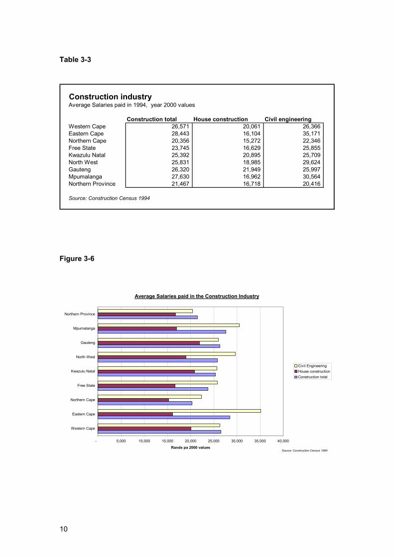
3.12 In the process of determining wage paid in the construction industry, wages are reported for the construction industry generally and the two subsectors of housing construction and civil engineering. Other subsectors are not reported, as they are less likely to have potential for public work projects. The wages that are reported are based on the 1994 construction census inflated to 2000 values

3.13 Average salaries paid in the industry generally and the two subsectors are reported in Table 3.3 and represented graphically in Figure 3.6. These are average salaries across all skill levels and includes unskilled, skilled and professionals.

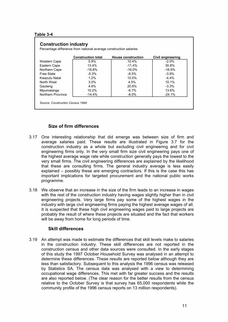
3.14 There is substantial variation in average industry salaries between provinces. In 2000 values, average wages in the construction industry varied between a high of over R28,000 pa in the Eastern Cape and a low of a little over R20,000 in the Northern Cape. The value of these differences are shown in Table 3.4 below

3.15 There are substantial provincial variations in salaries paid in the different subsectors . The Western Cape, for example, has construction salaries that are, on average, nearly 6% higher than the national average. In house construction salaries are more than 10% higher than the national average. Yet in civil engineering these are 2% less than the national average. The Northern Cape, in contrast, has salaries that are nearly 19% lower than the national average, with house construction 16% lower than the national average. Civil engineering, in contrast, has salaries 30% above the national average Working on house construction in Gauteng is financially the most attractive proposition in the construction industry with salaries over 20% greater than the national average.

3.16 On the whole, and as is evident in Figure 3.6, average salaries in civil engineering are generally higher than the industry average in each particular province – as an average of all occupations. In contrast salaries paid to those in house construction are well below provincial industry averages. For construction workers the least financially attractive place to built houses is in the Northern Cape and Northern Province where salaries are R15,000 and nearly R17,000 respectively (per annum 2000 values). This equates to monthly salaries (plus bonus) of than R1,200 and R1,300 a month respectively

10

Table 3-3

Figure 3-6

Construction industryAverage Salaries paid in 1994, year 2000 values

Construction total House construction Civil engineeringWestern Cape 26,571 20,061 26,366 Eastern Cape 28,443 16,104 35,171 Northern Cape 20,356 15,272 22,346 Free State 23,745 16,629 25,855 Kwazulu Natal 25,392 20,895 25,709 North West 25,831 18,985 29,624 Gauteng 26,320 21,949 25,997 Mpumalanga 27,630 16,962 30,564 Northern Province 21,467 16,718 20,416

Source: Construction Census 1994

Average Salaries paid in the Construction Industry

- 5,000 10,000 15,000 20,000 25,000 30,000 35,000 40,000

Western Cape

Eastern Cape

Northern Cape

Free State

Kwazulu Natal

North West

Gauteng

Mpumalanga

Northern Province

Rands pa 2000 values

Civil EngineeringHouse constructionConstruction total

Source: Construction Census 1994

11

Table 3-4

Size of firm differences

3.17 One interesting relationship that did emerge was between size of firm and average salaries paid. These results are illustrated in Figure 3.7 for the construction industry as a whole but excluding civil engineering and for civil engineering firms only. In the very small firm size civil engineering pays one of the highest average wage rate while construction generally pays the lowest to the very small firms. The civil engineering differences are explained by the likelihood that these are consulting firms. The general industry average is less easily explained – possibly these are emerging contractors. If this is the case this has important implications for targeted procurement and the national public works programme.

3.18 We observe that an increase in the size of the firm leads to an increase in wages with the rest of the construction industry having wages slightly higher than in civil engineering projects. Very large firms pay some of the highest wages in the industry with large civil engineering firms paying the highest average wages of all. It is suspected that these high civil engineering wages paid to large projects are probably the result of where these projects are situated and the fact that workers will be away from home for long periods of time.

Skill differences

3.19 An attempt was made to estimate the differences that skill levels make to salaries in the construction industry. These skill differences are not reported in the construction census and other data sources were consulted. In the early stages of this study the 1997 October Household Survey was analysed in an attempt to determine these differences. These results are reported below although they are less than satisfactory. Subsequent to this analysis the 1996 census was released by Statistics SA. The census data was analysed with a view to determining occupational wage differences. This met with far greater success and the results are also reported below. (The clear reason for the better results from the census relative to the October Survey is that survey has 65,000 respondents while the community profile of the 1996 census reports on 13 million respondents).

Construction industryPercentage difference from national average construction salaries

Construction total House construction Civil engineeringWestern Cape 5.9% 10.4% -2.0%Eastern Cape 13.4% -11.4% 30.8%Northern Cape -18.8% -16.0% -16.9%Free State -5.3% -8.5% -3.9%Kwazulu Natal 1.2% 15.0% -4.4%North West 3.0% 4.5% 10.1%Gauteng 4.9% 20.8% -3.3%Mpumalanga 10.2% -6.7% 13.6%Northern Province -14.4% -8.0% -24.1%

Source: Construction Census 1994

12

Figure 3-7

1997 October Household Survey

3.20 The October Household Surveys are very detailed surveys that are capable of providing a wealth of information. The Surveys allow people to very clearly identify the kind of work that they do and the kind of industry where the work is undertaken. Of relevance to this study, Table 3.5 illustrates the level of detail to which work in the construction industry can be categorised.

3.21 The different work categories in Table 3.5 have been aggregated into five general definitions: bricklayers, concrete workers, carpenters, construction labour, semi-skilled construction labour, as shown by the groupings in the table.. Average wages paid to each of the skill categories were calculated. Much to our consternation the results were counterintuitive. The results showed improbably low wages and an inverse relationship between skill levels and wages. In order to address this problem the final calculations are based on the hourly rate worked for the past seven days and are reported in Table 3.6 below. The table reports on the mean and standard deviation for the nine provinces and for the nation as a whole.

3.22 It will be immediately apparent that a similar (although less pronounced) inverse relationship exists between skills and remuneration. In the ‘Total’ column, for example, bricklayers earned an average R3.7 an hour (in 1997) while concrete workers earned R3.2, carpenters R6.1, construction labour R5.2 and semi-skilled labour R3.7. Intuitively one would expect bricklayers and semi-skilled labour to earn more than labour.

- 5,000 10,000 15,000 20,000 25,000 30,000 35,000 40,000

Average annual salary

5 -9

10 -19

20 -49

50 -99

100 -199

200 -299

300 -399

400 -499

500 -999

1000 +

Num

ber o

f em

ploy

ees

in F

irm

Average Annual Salaries paid by Size of Firm2000 values

Civil EngineeringConstruction ex. Civil

13

Table 3-5

Table 3-6

Average hourly pay - rands per hour worked, 1997 values

Job code Description West Cape East Cape Northern Cape Free State KwaZulu NatNorth West Gauteng Mpumalanga Northern ProSouth Africa Daily wage 3

7122 Bricklayer Average 1 3.4 3.3 3.2 3.2 6.4 2.6 3.6 3.5 3.3 3.7 34.6St. dev.2 4.2 4.7 3.0 2.1 13.4 2.2 4.6 2.7 3.0 6.1

7123 Concrete worker Average 1 1.5 2.3 1.4 1.6 9.4 3.6 5.6 2.2 3.2 29.7St. dev.2 0.4 3.1 2.7 4.2 3.0

7124 Carpenter Average 1 6.7 5.1 4.0 7.3 6.0 6.0 8.1 8.3 3.7 6.1 56.7St. dev.2 8.8 3.3 3.7 7.3 6.0 5.5 10.9 8.2 2.9 7.0

9312 Construction labour Average 1 4.6 4.6 3.5 6.3 6.0 5.8 6.2 5.7 4.1 5.2 48.4St. dev.2 4.6 4.2 3.8 5.8 6.1 8.4 5.4 6.8 3.7 5.6

9313 Construction semi-skilled Average 1 2.7 2.8 1.9 3.7 4.0 8.7 10.3 4.9 5.0 3.7 34.3St. dev.2 3.7 2.5 1.7 1.4 3.0 11.8 8.1 2.8 3.5 4.5

Notes: 1. Average hourly wage rate during the past seven days2.. Standard deviation3. Daily wage based on 9.25 hour day for average wage paid across South Africa, 1997 values

Source: Stats SA: October Household Survery 1997

CODE OCCUPATION CODE OCCUPATION

7122 Bricklayer, chimney 7124 Carpenter, wharf7122 Bricklayer, construction 7124 Carpenter-joiner7122 Bricklayer, firebrick 7124 Carpenters and joiners7122 Bricklayer, furnace lining 7124 Fitter, shop7122 Bricklayer, ingot mould lining 7124 Joiner7122 Bricklayer, kiln 7124 Joiner, aircraft7122 Bricklayer, oven 7124 Joiner, bench7122 Bricklayers and stonemasons 7124 Joiner, construction7122 Builder, chimney 7124 Joiner, ship7122 Firebrick layer 7124 Maker, mast and spar/wood7122 Paviour 7124 Shipwright, wood7122 Stonemason, construction 7124 Shopfitter7122 Stonemason, facings7122 Stonemason, paving 9312 Construction and maintenance labourers:

roads, dams and similar construction7122 Tuckpointer 9312 Labourer, construction7123 Caster, concrete products 9312 Labourer, construction/ roads7123 Concrete mixer 9312 Labourer, construction/dams7123 Concrete placers,etc 9312 Labourer, digging/ditch7123 Finisher, cement 9312 Labourer, digging/grave7123 Finisher, concrete 9312 Labourer, digging/trench7123 Iron worker, concrete reinforcement 9312 Labourer, maintenance7123 Mixer, concrete 9312 Labourer, maintenance/ dams7123 Placer, concrete 9312 Labourer, maintenance/ roads7123 Shutterer, concrete moulding 9312 Labourer, tube well7123 Terrazzo worker 9312 Labourer, water well

9312 Land clearer7124 Boatbuilder, wood 9312 Navvy7124 Builder, barge/wooden 9312 Shoveller7124 Carpenter 9312 Trackman, railway7124 Carpenter, bench 9312 Trackwoman, railway7124 Carpenter, bridge7124 Carpenter, construction 9313 Building construction labourers7124 Carpenter, first fixing 9313 Handyman7124 Carpenter, maintenance 9313 Handyman, building maintenance7124 Carpenter, mine 9313 Handywoman7124 Carpenter, second fixing 9313 Handywoman, building maintenance7124 Carpenter, ship's 9313 Hod carrier7124 Carpenter, stage 9313 Labourer, construction, buildings7124 Carpenter, theatre 9313 Labourer, demolition

9313 Stacker, building construction

14

3.23 There are four possible reasons for these results:

• A small sample. The number of respondents for each category were: bricklayers – 214, concrete workers – 17, carpenters – 91, labour – 241, and semi-skilled labour – 86.

• A wide scatter in the data. This is evidenced by the very high standard deviations that are probably caused by the small sample of skilled workers.

• Wages in the civil engineering industry being higher than house construction such that civil engineering labour does earn more house construction bricklayers.

• The falling real wage for whites and coloureds is presumed to have a disproportional impact on skilled labour, contributing to extra deviations in the sample

The 1996 Census

3.24 The recent general availability of the 1996 census allowed for a more reliable estimate of average wages by occupation type. Because of the very large sample – 40 million in theory but 13 million in the ‘labour’ portion of the community profile – we expect to capture a more accurate measure of salaries by occupation.

3.25 For the purposes of this investigation, the occupation categories of relevance are the five shown in Table 3.9 below – professionals, technicians and associated professionals, craft and related workers, plant and machine operators and assemblers, and elementary occupations. Of these categories ‘craft and related workers’ is made up of categories 7122 (bricklayers), 7123 (concrete workers) and 7124 (carpenters) while ‘elementary occupations’ consists of 9312 (construction labour) and 9312 (semi-skilled labour). The term ‘elementary occupations’ is used in the population census and is not a creation of this writer.

National Estimates

3.26 In Table 3.9 we show the full country results of an examination of the occupational structure of the construction industry and average salaries. The first column of the table indicates the number of workers by occupation in the census sample. In theory this sample should represent the occupation profile of the industry. Some concern is expressed at the large number of ‘craft and related workers’ relative to ‘elementary occupations’. The first impression is that this is counter intuitive – construction labourers may have responded to the census questionnaire that they are, for example, bricklayers. This kind of response is a common problem with questionnaires. On the other hand Statistics SA has worked hard to avoid these kind of problems and it may be that the civil engineering part of the construction industry causes these results but that the results are correct in themselves.

3.27 Therefore treating the results with due caution, we are able to report that in 1996 the construction industry was made up of 486,000 workers. Of this 3% are professionals, 4% are technicians, 73% are craft workers, 4% are machine operators and 17% are in elementary occupations.

15

Table 3-7

3.28 In turn these worker earned, on average and in year 2000 values, annual salaries of R108,000 for professionals, R58,000 for technicians, R24,000 for craft workers, R26,000 for machine operators and R17,000 for labourers in elementary occupations. Labourers earned about R65 a day.

3.29 The industry total of 486,000 stands in contrast to the 312,000 total reported in Table 3.2. There are two possible reasons for this difference. First, the population census is directed at people while the construction census is directed at firms. We are therefore capturing more informal firms. Second, the population census is probably capturing an element of underemployment.

3.30 Because of the nature of the way the census data is reported it is not possible to calculate accurate standard deviations. Rather, the data dispersion is illustrated in Figure 3.8 below. Figure 3.8 indicates the number of workers of workers in the construction industry by occupation by monthly income category (1996 census values). Three factors are of note:

• The data dispersion is far smaller than those for the October Household Survey. This is probably due to a far higher sample.

• Both ‘craft workers’ and ‘elementary occupations’ have a maximum number of respondents at the same income category – R500 to R1,000 a month (1996 values). This lends further credence to the ‘blurring’ of craft worker and elementary occupation categories in the construction industry as measured by the population census.

• The above observation is reinforced by the long tail on the right hand side of distribution of salaries for craft workers. What this indicates is that there is a wide distribution of salaries for a (small number) of skilled craft workers.

Average Salaries paid in the Construction Industry

Number of 1996 values 2000 valuesworkers in sample Monthly Monthly Annual

Professionals 13,491 6,659 9,007 108,078 Technicians and associate professionals 17,598 3,604 4,875 58,505 Craft and related trades workers 355,214 1,479 2,000 24,001 Plant and machine operators and assemblers 17,989 1,637 2,215 26,576 Elementary occupations 82,446 1,067 1,443 17,313

Source: SA Community Profile - Census 1996. Extracted with Super Table

16

Figure 3-8

3.31 An attempt was made to adjust the census results to correct for the concerns about inaccurate occupational descriptions. In this exercise we attempt to establish two extreme positions. The first extreme position is given by the unadjusted census results. In establishing the second extreme position an assumption was made that any person recorded as a craft worker but earning a salary less than or equal to an average (unadjusted) labourer salary is in fact a labourer and not a craft worker. Hence the census data was adjusted so that no craft worker earned an income equal to or less than the 1996 R501 to R1,000 monthly income category. All of these workers were reclassified as elementary occupations. Numbers, averages and distributions were recalculated and are given in Table 3.8 and Figure 3.9

3.32 After adjustment we discover that there are about 170,000 craft workers in the construction industry earning an average annual salary of R41,000 (2000 prices). In contrast there were an estimated 270,000 labourers in the industry earning an average annual salary of R11,000 a year. For labourers this is about R43 a day.

Number of persons by income category by occupation in the Construction Industry

0

20000

40000

60000

80000

100000

120000

R1 - R

200

R201 -

R50

0

R501 -

R10

00

R1001

- R15

00

R1501

- R25

00

R2501

- R35

00

R3501

- R45

00

R4501

- R60

00

R6001

- R80

00

R8001

- R11

000

R1100

1 - R

1600

0

R1600

1 - R

3000

0

R3000

1 or m

ore

Monthly income

Num

ber o

f wor

kers

Professionals Technicians and associate professionals Craft and related trades workers Plant and machine operators and assemblers Elementary occupations

17

Table 3-8

Figure 3-9

3.33 In the absence of further evidence, the conclusion we draw from the above analysis is that average salaries for craft workers in the construction industry will lie in the range of R24,000 to R41,000 with the more regular salaried worker being at the top end of the income range. Elementary occupations earn an average of between R11,000 and R17,000 with the more regular salary probably being at the lower end of the income range.

Provincial Estimates

3.34 Where the census is limited by the way in which it aggregates occupations, it is extremely versatile in its geographic coverage. Hence we are able to report on average salaries by province and by location. As one will appreciate that because the more the census is disaggregated the smaller the sample becomes. This makes the interpretation of the mean increasingly more difficult.

Adjusted Average Salaries paid in the Construction IndustryAdjusted made by moving craft workers earning less than R1000 1996 rand a month to elementary occupationsThe 1996 salaries are scaled to 2000 nominal values using changes in the South Africa consumer price indexNo scaling has been used to adjust for the fall in real salaries in construction since 1996

Number of 1996 values 2000 valuesworkers in sample Monthly Monthly Annual

Professionals 13,491 6,659 9,007 108,078 Technicians and associate professionals 17,598 3,604 4,875 58,505 Craft and related trades workers 168,378 2,528 3,419 41,032 Plant and machine operators and assemblers 17,989 1,637 2,215 26,576 Elementary occupations 269,282 696 942 11,303

Source: SA Community Profile - Census 1996. Extracted using Super Table

Adjusted average annual salaries paid in the Construction Industry

0

20000

40000

60000

80000

100000

120000

140000

R1 - R

200

R201 -

R50

0

R501 -

R10

00

R1001

- R15

00

R1501

- R25

00

R2501

- R35

00

R3501

- R45

00

R4501

- R60

00

R6001

- R80

00

R8001

- R11

000

R1100

1 - R

1600

0

R1600

1 - R

3000

0

R3000

1 or m

ore

Annual income category, 1996 values

Num

ber o

f wor

kers

Professionals Technicians and associate professionals Craft and related trades workers Plant and machine operators and assemblers Elementary occupations

18

3.35 Estimates of average provincial wages paid in the construction industry are presented in Figures 3.10 and 3.11 and Tables 3.9 to 3.12. Wages paid to professionals are presented and discussed but the focus is on wages paid to craft workers and construction labourers.

3.36 Table 3.9 reports the number of professionals active in the construction industry and their average 1996 and 2000 salaries. As can be expected a significant number of professional in the construction industry are resident in Gauteng – 5,700 – with 2,500 in KwaZulu Natal and 2,400 in the Western Cape. The other provinces have only a small portion of professionals resident in the province.

3.37 In claiming the lion’s share of professionals, Gauteng pays the highest average wages to professionals in the construction industry – R125,000 pa (2000 values). KwaZulu Natal pays average salaries of just under R110,000 pa while in the Western Cape average professional salaries were just over R103,000 pa. All other provinces pay an average of less R100,000 a year with professionals in the North West and the Northern Province earning little more than R55,000 a year.

Table 3-9

3.38 Table 3.10 indicates the provincial distribution of craft workers in the construction industry and the average salaries that were paid in 1996 (and their 2000 equivalent values). The distribution of numbers employed follows a similar pattern to professional employment. At 106,000 Gauteng has twice as many craft workers in construction as any other province. The Western Cape and KwaZulu Natal each have 50,000 craft workers in construction.

3.39 In contrast to average professional wages, there is not the extreme variation in average craft wages between the nine provinces. On average craft workers in Gauteng and the Western Cape earn R28,000 a year (2000 values). The lowest average wages for craft workers are paid in the Northern Province and the Northern Cape – just under R18,000 a year.

Average Salaries paid to Professionals in the Construction Industry

Number 1996 values 2000 values in sample Monthly Monthly Annual

Western Cape 2,440 6,351 8,590 103,081 Eastern Cape 670 5,899 7,978 95,741 Northern Cape 116 5,712 7,726 92,715 Free State 563 4,867 6,584 79,003 KwaZulu-Natal 2,525 6,761 9,145 109,743 North West 581 3,404 4,604 55,247 Gauteng 5,731 7,717 10,438 125,250 Mpumalanga 382 5,268 7,125 85,501 Northern Province 483 3,510 4,748 56,973

Source: SA Community Profile - Census 1996. Extracted with Super Table

19

Table 3-10

3.40 Figure 3.10 records the number of craft workers by income category for the nine provinces. With the exception of the Western Cape and the Northern Province, the other seven province show a similar wage distribution and one that coincides with the national distribution shown above. In the Western Cape, and to a more limited extent Gauteng, we find that the most common (unadjusted) wages paid to craft workers is R1000 to R1500 a month. This compares to the most common wage at a national level of R500 to R1000 a month. In the Northern Province, in contrast, there are as many craft workers earning R200 to R500 a month as there are earning R500 to R1000.

Figure 3-10

Number of Craft workers per income category in the Construction Industry

0

5000

10000

15000

20000

25000

30000

35000

R1 - R200 R201 - R500 R501 - R1000 R1001 -R1500

R1501 -R2500

R2501 -R3500

R3501 -R4500

R4501 -R6000

Rands per month, 1996 values

Num

ber o

f cra

ft w

orke

rs Western Cape Eastern Cape Northern Cape Free State KwaZulu-Natal North West Gauteng Mpumalanga Northern Province

Source: 1996 census - unadjusted data

Average Salaries paid to Craft workers in the Construction Industry

Number 1996 values 2000 values in sample Monthly Monthly Annual

Western Cape 51,497 1,752 2,370 28,438 Eastern Cape 25,579 1,261 1,705 20,463 Northern Cape 6,359 1,076 1,456 17,470 Free State 22,334 1,148 1,553 18,635 KwaZulu-Natal 51,749 1,521 2,058 24,690 North West 28,736 1,192 1,612 19,341 Gauteng 106,193 1,749 2,366 28,386 Mpumalanga 30,254 1,193 1,614 19,365 Northern Province 32,513 1,092 1,477 17,729

Source: SA Community Profile - Census 1996. Extracted with Super Table

20

3.41 Table 3.11 reports on the provincial distribution of labourers and average salaries paid. In contrast to all other occupations reported in this section, the Western Cape boasts the greatest number of construction labourers – nearly 30,000 in 1996. Gauteng is less than half this number – a little under 14,000. Average wages varied between R20,000 a year in Gauteng (2000 values), R17,500 in the Western Cape and a lowest average in the Northern Cape of R14,000.

Table 3-11

3.42 Figure 3.11 illustrates the distribution of wages in the elementary occupations in the construction industry. With the possible exception of the Northern Province, we find little difference in the distribution of wages paid to construction labourers with the most common wage paid ranging from R500 to R1000 a month. In the Northern Province there are more or less as many labourers earning between R200 and R500 a month as there are earning between R500 and R1000 and between R1000 and R1500. We suspect there is a problem with the underlying data.

3.43 It will be clear that the data problems that were encountered in determining average national salaries – labourers and craft workers reporting to have been paid similar wages – are also being found in the provincial results. The only exception to this is the Western Cape were salaries differences between craft workers and labourers are those than were intuitively expected. Hence the same correction procedure was applied to the provincial data to determine a range of potential salaries between two extreme positions. These adjustments are reported in Table 3.12 below.

Average Salaries paid to 'elementary occupations' 1 in Construction Unadjusted Averages

Number 1996 values 2000 values in sample Monthly Monthly Annual

Western Cape 29,237 1,080 1,460 17,524 Eastern Cape 8,159 925 1,251 15,009 Northern Cape 2,246 878 1,188 14,252 Free State 4,497 1,071 1,449 17,391 KwaZulu-Natal 9,604 952 1,288 15,456 North West 4,687 1,026 1,388 16,654 Gauteng 13,971 1,257 1,701 20,409 Mpumalanga 4,854 1,044 1,412 16,949 Northern Province 5,191 1,050 1,420 17,036

Source: SA Community Profile - Census 1996. Extracted with Super TableNote: 'Elemenetary occupations' is a census definition . It is made up of semi and unskilled labour.

21

Figure 3-11

Table 3-12

3.44 After adjusting the data we establish two extreme boundaries for the average salary of craft workers and labourers in the construction industry. The table is therefore interpreted as, for example, in the Western Cape the average salary paid to a craft worker will fall in the region of R2,400 and R3,200 a month. In the same province the average salary paid to a construction labourer will lie somewhere between R1,200 and R1,460. This amounts to an adjusted daily wage of R55. In the Northern Province the daily wage of a construction labourer will vary between an (unadjusted and unbelievable) R64 a day and (adjusted and believable) R36 a day.

Number of labourers per income category in the Construction Industry

0

2000

4000

6000

8000

10000

12000

14000

R1 - R200 R201 - R500 R501 - R1000 R1001 -R1500

R1501 -R2500

R2501 -R3500

R3501 -R4500

R4501 -R6000

Rands per month, 1996 values

Num

ber i

n el

emen

tary

occ

upat

ions

Western Cape Eastern Cape Northern Cape Free State KwaZulu-Natal North West Gauteng Mpumalanga Northern Province

Adjusted and Unadjusted Average Salaries paid in the Construction IndustryAll year 2000 values, monthly salaries

Craft workers LabourersUnadjusted Adjusted Unadjusted Adjusted

W estern Cape 2,370 3,230 1,460 1,215 Eastern Cape 1,705 3,246 1,251 874 Northern Cape 1,456 3,124 1,188 853 Free State 1,553 3,478 1,449 836 KwaZulu-Natal 2,058 3,539 1,288 863 North W est 1,612 3,009 1,388 856 Gauteng 2,366 3,668 1,701 989 Mpumalanga 1,614 3,275 1,412 834 Northern Province 1,477 3,145 1,420 784

Source: Own calculations

22

3.45 An attempt was made to verify the results in Table 3.13 and a straw poll was conducted among builders in the Western Cape. (The poll included two architects, one quantity surveyor, a consulting engineer and eight building contractors). The general opinion was that for craft workers the adjusted average salary is close to the norm while full time construction labourers will earn closer to the unadjusted monthly salary than to the adjusted salary. (The adjustment methodology can bias labourer wages downward by including underemployed labourers and underemployed craft workers with fully employed labourers). As, of all the provinces, the difference between adjusted and unadjusted labourer salaries is smallest in the Western Cape (R55 a day compared to R65 a day), a challenge remains for a micro verification of the accuracy of these estimates in other provinces.

Town and City estimates

3.46 Estimates of average salaries paid to craft workers and construction labourers for a selection of towns and cities is presented in Table 3.13. The table also provides adjusted average salaries using the same correction procedure used for the national and provincial estimates. As with the provincial estimates, we focus more on the adjusted salaries for craft workers and the unadjusted salary for construction labourers.

3.47 In some of the smaller provinces, the Western Cape and Gauteng in particular, we note that there are few differences with craft worker salaries within the individual province. This is probably due to the mega-city effect and good transport systems leading to an equalisation of wages. The two notable exceptions are for Soweto in Gauteng and Thaba ‘Nchu in the Free State. Here wages for craft workers are considerably lower than those in the nearby cities of Johannesburg and Bloemfontein respectively. Because the census measures people’s place of residence and not their place of work we do not believe that there can be such substantial wage differences for the same kind of labour within what is largely the same market. We take it that the lower reported wage rates ae not distortions in the labour market but the result of underemployment and oversupply of labourers in particular areas, which forces the wage rate down.

3.48 In the provinces that are geographically larger we do note more variation in the average salaries of craft workers. We make a general observation (with exceptions) that there is some correlation between the salaries that craft workers earn in construction and the size of the town or city in which they work.

3.49 For construction labourers it is not possible to make such generalisations. We note substantial variation in the average salaries earned by construction workers in the various towns and cities of South Africa.

23

Table 3-13

Average salaries paid in the Construction Industryfor a selection of towns and cities.All values year 2000, monthly salaries

Craft Workers Elementary OccupationsProvince Town/city Unadjusted Adjusted Unadjusted AdjustedWestern Cape Bellville 2,536 2,967 1,538 1,212

Wynberg 2,268 2,678 1,195 959 Caledon 1,531 2,000 1,024 888 Hermanus 1,325 2,073 855 729 Mossel bay 1,418 2,309 974 747 Riversdal 1,444 2,082 950 849 Ceres 1,588 2,105 1,156 959 Vredenburg 1,655 2,063 1,085 965

Eastern Cape Aliwal North 762 1,824 1,686 659 Barkley-East 546 1,531 713 533 Queenstown 1,104 2,183 797 581 East-London 1,565 2,654 965 719 Graaff-Reinet 921 2,352 804 589 Port Elizabeth 1,706 2,581 1,165 794 Butterworth 1,417 2,827 782 584 Umtata 1,102 2,356 818 582

Northern Cape Calvinia 908 2,297 791 586 Prieska 777 1,902 876 662 De Aar 917 2,333 836 547 Kimberley 1,376 2,592 876 630 Victoria-West 579 2,458 536 415

Free State Welkom 1,529 2,716 1,328 751 Kroonstad 979 2,023 1,111 617 Parys 967 2,289 1,151 579 Bethlehem 1,218 2,693 1,583 631 Harrismith 1,083 2,695 838 572 Bloemfontein 1,498 3,101 1,460 692 Thaba 'Nchu 886 1,868 811 535

KwaZulu-Natal Durban 2,534 3,531 1,253 784 Chatswoth 1,998 2,720 1,287 792 Pietermaritzburg 1,501 2,810 910 585 Port Shepstone 1,246 2,453 733 592 Mooi river 1,112 2,129 890 519 Estcourt 1,375 2,403 999 662 Newcastle 1,298 2,725 824 554 Lower Tugela 1,333 2,421 698 576

North West Lichtenburg 1,183 2,487 950 616 Klerksdorp 1,310 2,641 1,074 630 Potchefstroom 1,320 2,519 1,346 736 Brits 1,575 2,674 1,180 690 Temba 1,111 1,815 1,255 687

Gauteng Pretoria 2,282 3,371 1,294 825 Johannesburg 2,301 3,197 1,411 765 Germiston 2,650 3,610 1,489 914 Springs 2,012 3,190 1,892 818 Westonaria 1,555 2,691 1,035 688 Vanderbijlpark 1,453 2,434 1,088 698 Soweto 1,286 1,917 1,173 664 Ermelo 1,263 3,210 882 591

Mpumalanga Standerton 1,598 2,896 1,146 784 Belfast 875 2,328 735 577 Witbank 1,553 2,755 980 658 Nelspruit 2,042 4,379 1,123 624

Northern Province Messina 853 2,317 588 449 Phalaborwa 2,380 3,388 1,563 975 Pietersburg 3,545 5,284 1,918 916 Potgietersrus 1,313 2,781 2,519 1,404 Mutali 1,157 1,961 1,360 728

Source: SA Community Profile - Census 1996. Extracted with Super Table

24

Summary

3.50 The construction industry is a small and, currently, declining industry. Contribution to GDP has fallen, there are fewer jobs today than twenty years ago and real wages have fallen.

3.51 About 300,000 people were employed in the construction industry in 1997 and about 70% of these were black.

3.52 On average the civil engineering industry pays wages that are greater than in house construction. This is likely to reflect skill differences, particularly, and work conditions.

3.53 There are significant differences in wages paid in the various provinces. In 1994, (the latest construction census) we find the lowest average civil engineering salaries are paid In the Northern Province and the highest in the Eastern Cape. Average house construction salaries were the highest in Gauteng in 1994 and lowest in the Eastern Cape.

3.54 We observe that an increase in the size of the firm leads to an increase in wages with the rest of the construction industry having wages slightly higher than in civil engineering projects. Very large firms pay some of the highest wages in the industry with large civil engineering firms paying the highest average wages of all. It is suspected that these high civil engineering wages paid to large projects are probably the result of where these projects are situated and the fact that workers will be away from home for long periods of time.

3.55 Determining average salaries by skill level proved a difficult exercise. Both the October Household Surveys and the Population Census were analysed. We conclude that average annual salaries paid to craft workers in the construction industry vary between R24,000 and R41,000 and for unskilled workers between R11,000 and R17,000 (all 1996 values).

3.56 Unskilled labourers in the Western Cape construction industry have the highest salaries in the country of between R1,460 and R1,215 monthly (R66 and R56 a day). The lowest paid unskilled construction workers are to be found in the Northern Province. Here the adjusted wage was a daily rate of R36. (All wages in year 2000 values).

25

4 Expenditure patterns and standards of living

Introduction

4.1 As peoples’ income changes so too does the composition of what they spend their income on. This section explores expenditure patterns in South Africa with a view to determining the levels of, and differences in, the expenditure patterns of the various income groups that are targeted by the national public works programme.

4.2 In this section we describe the methodology employed to determine expenditure patterns and the impact of income changes on expenditure patterns. Existing expenditure patterns are reported and the impact of changing income measured.

Description of Methodology

4.3 This section of the investigation makes us of the national Income and Expenditure survey conducted by Statistics SA in 1995. This is a extensive survey that asked very detailed questions of over 65,000 households across the country. In order to make the detailed expenditure questions manageable each of the expenditure items of the survey was classified originally as part of the Final Supply and Use Tables (SUT) of 1993 (Statistics SA). This allowed 600 different expenditure items to be aggregated into the 95 SUT categories. In addition to this the survey was also classified according to the Standard Industrial Classification of all Economic Activities (4th and 5th edition) (the so-called SIC codes). This latter exercise was necessary in order to estimate the economic impact of changes in final demand.

4.4 From this reclassified income and expenditure survey we extracted the expenditure patterns of households. These expenditure patterns were determined individually for male and female headed households respectively, by different household income categories and separately for each of the provinces. For obvious reasons the focus was on the lower income levels. The established income categories that are reported on here are: annual household income from R1 to R5,000; R5,001 to R10,000; R10,001 to R15,000; and R15,001 to R20,000. Income categories of up to R50,000 were calculated and are used later in estimating expenditure changes.

4.5 In order to determine the changes in expenditure following a change in income we determine the differences in expenditure between each of the separate income categories. The assumption is therefore made that as the income of people increases these people will take on the same expenditure profile as other people in their new income category.

4.6 The reported changes in income categories are from changes in income categories from R1 – R5,000 to R5,001 - R10,000; from R5,001 – R10,000 to R10,001 - R20,000; from R10,001 - R20,000 to R20,001 – R 30,000 R20,001 – R 30,000 to R30,001 – R40,000; and from R30,001 – R40,000 to R40,001 - R50,000.

26

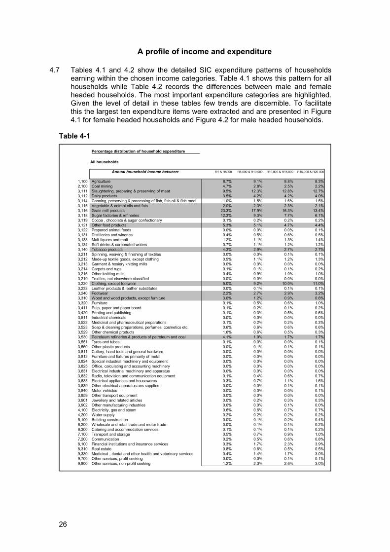
A profile of income and expenditure

4.7 Tables 4.1 and 4.2 show the detailed SIC expenditure patterns of households earning within the chosen income categories. Table 4.1 shows this pattern for all households while Table 4.2 records the differences between male and female headed households. The most important expenditure categories are highlighted. Given the level of detail in these tables few trends are discernible. To facilitate this the largest ten expenditure items were extracted and are presented in Figure 4.1 for female headed households and Figure 4.2 for male headed households.

Table 4-1

Percentage distribution of household expenditure

All households

Annual household income between: R1 & R5000 R5,000 & R10,000 R10,000 & R15,000 R15,000 & R20,000

1,100 Agriculture 8.7% 9.1% 8.8% 8.3%2,100 Coal mining 4.7% 2.8% 2.5% 2.2%3,111 Slaughtering, preparing & preserving of meat 9.5% 12.3% 12.8% 12.7%3,112 Dairy products 3.5% 4.2% 4.2% 4.0%3,114 Canning, preserving & processing of fish, fish oil & fish meal 1.0% 1.5% 1.6% 1.5%3,115 Vegetable & animal oils and fats 2.0% 2.3% 2.3% 2.1%3,116 Grain mill products 23.3% 17.9% 16.3% 13.4%3,118 Sugar factories & refineries 12.3% 9.3% 7.7% 6.1%3,119 Cocoa , chocolate & sugar confectionary 0.1% 0.2% 0.2% 0.2%3,121 Other food products 5.3% 5.1% 4.7% 4.4%3,122 Prepared animal feeds 0.0% 0.0% 0.0% 0.1%3,131 Distilleries and wineries 0.4% 0.5% 0.6% 0.5%3,133 Malt liquors and malt 1.2% 1.1% 1.3% 1.4%3,134 Soft drinks & carbonated waters 0.7% 1.1% 1.2% 1.2%3,140 Tobacco products 4.3% 2.9% 2.7% 2.7%3,211 Spinning, weaving & finishing of textiles 0.0% 0.0% 0.1% 0.1%3,212 Made-up textile goods, except clothing 0.5% 1.1% 1.2% 1.3%3,213 Garment & hosiery knitting mills 0.0% 0.0% 0.0% 0.0%3,214 Carpets and rugs 0.1% 0.1% 0.1% 0.2%3,216 Other knitting mills 0.4% 0.9% 1.0% 1.0%3,219 Textiles, not elsewhere classified 0.0% 0.0% 0.0% 0.0%3,220 Clothing, except footwear 5.0% 9.2% 10.0% 11.0%3,233 Leather products & leather substitutes 0.0% 0.1% 0.1% 0.1%3,240 Footwear 2.2% 2.7% 2.9% 3.2%3,310 Wood and wood products, except furniture 3.0% 1.2% 0.9% 0.6%3,320 Furniture 0.1% 0.5% 0.6% 1.0%3,411 Pulp, paper and paper board 0.1% 0.2% 0.1% 0.2%3,420 Printing and publishing 0.1% 0.3% 0.5% 0.6%3,511 Industrial chemicals 0.0% 0.0% 0.0% 0.0%3,522 Medicinal and pharmaceutical preparations 0.1% 0.2% 0.2% 0.3%3,523 Soap & cleaning preparations, perfumes, cosmetics etc. 0.6% 0.6% 0.6% 0.6%3,529 Other chemical products 1.6% 0.6% 0.5% 0.3%3,530 Petroleum refineries & products of petroleum and coal 4.1% 1.9% 1.7% 1.7%3,551 Tyres and tubes 0.1% 0.0% 0.0% 0.1%3,560 Other plastic products 0.0% 0.1% 0.1% 0.1%3,811 Cutlery, hand tools and general hardware 0.0% 0.0% 0.0% 0.0%3,812 Furniture and fixtures primarily of metal 0.0% 0.0% 0.0% 0.0%3,824 Special industrial machinery and equipment 0.0% 0.0% 0.0% 0.0%3,825 Office, calculating and accounting machinery 0.0% 0.0% 0.0% 0.0%3,831 Electrical industrial machinery and apparatus 0.0% 0.0% 0.0% 0.0%3,832 Radio, television and communication equipment 0.1% 0.4% 0.6% 0.7%3,833 Electrical appliances and housewares 0.3% 0.7% 1.1% 1.6%3,839 Other electrical apparatus ans supplies 0.0% 0.0% 0.1% 0.1%3,840 Motor vehicles 0.0% 0.0% 0.0% 0.1%3,859 Other transport equipment 0.0% 0.0% 0.0% 0.0%3,901 Jewellery and related articles 0.0% 0.2% 0.3% 0.3%3,902 Other manufacturing industries 0.0% 0.0% 0.1% 0.0%4,100 Electricity, gas and steam 0.6% 0.6% 0.7% 0.7%4,200 Water supply 0.2% 0.2% 0.2% 0.2%5,100 Building construction 0.0% 0.1% 0.2% 0.4%6,200 Wholesale and retail trade and motor trade 0.0% 0.1% 0.1% 0.2%6,300 Catering and accommodation services 0.1% 0.1% 0.1% 0.2%7,100 Transport and storage 0.5% 0.7% 0.9% 1.0%7,200 Communication 0.2% 0.5% 0.6% 0.8%8,100 Financial institutions and insurance services 0.3% 1.7% 2.3% 3.9%8,310 Real estate 0.8% 0.6% 0.5% 0.5%9,330 Medicinal , dental and other health and veterinary services 0.4% 1.4% 1.7% 3.0%9,700 Other services, profit seeking 0.0% 0.0% 0.1% 0.1%9,800 Other services, non-profit seeking 1.2% 2.3% 2.6% 3.0%

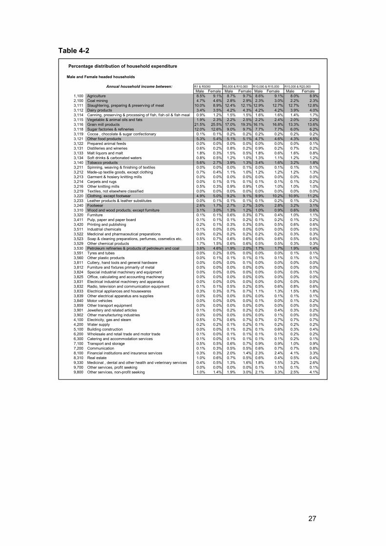
27

Table 4-2

Percentage distribution of household expenditure

Male and Female headed households

Annual household income between: R1 & R5000 R5,000 & R10,000 R10,000 & R15,000 R15,000 & R20,000Male Female Male Female Male Female Male Female

1,100 Agriculture 8.5% 9.1% 8.7% 9.7% 8.6% 9.1% 8.0% 8.9%2,100 Coal mining 4.7% 4.6% 2.8% 2.9% 2.3% 3.0% 2.2% 2.3%3,111 Slaughtering, preparing & preserving of meat 10.0% 8.9% 12.4% 12.1% 12.9% 12.7% 12.7% 12.8%3,112 Dairy products 3.4% 3.5% 4.2% 4.3% 4.2% 4.2% 3.9% 4.0%3,114 Canning, preserving & processing of fish, fish oil & fish meal 0.9% 1.2% 1.5% 1.5% 1.6% 1.6% 1.4% 1.7%3,115 Vegetable & animal oils and fats 1.9% 2.3% 2.2% 2.5% 2.2% 2.4% 2.0% 2.2%3,116 Grain mill products 21.5% 25.5% 17.0% 19.3% 16.1% 16.8% 13.3% 13.6%3,118 Sugar factories & refineries 12.0% 12.6% 9.0% 9.7% 7.7% 7.7% 6.0% 6.2%3,119 Cocoa , chocolate & sugar confectionary 0.1% 0.1% 0.2% 0.2% 0.2% 0.2% 0.2% 0.2%3,121 Other food products 5.3% 5.4% 5.1% 5.1% 4.7% 4.6% 4.3% 4.5%3,122 Prepared animal feeds 0.0% 0.0% 0.0% 0.0% 0.0% 0.0% 0.0% 0.1%3,131 Distilleries and wineries 0.6% 0.2% 0.8% 0.2% 0.9% 0.2% 0.7% 0.2%3,133 Malt liquors and malt 1.8% 0.3% 1.5% 0.5% 1.8% 0.6% 1.6% 0.8%3,134 Soft drinks & carbonated waters 0.8% 0.5% 1.2% 1.0% 1.3% 1.1% 1.2% 1.2%3,140 Tobacco products 5.6% 2.7% 3.9% 1.3% 3.4% 1.6% 3.2% 1.8%3,211 Spinning, weaving & finishing of textiles 0.0% 0.0% 0.0% 0.1% 0.0% 0.1% 0.1% 0.1%3,212 Made-up textile goods, except clothing 0.7% 0.4% 1.1% 1.0% 1.2% 1.2% 1.2% 1.3%3,213 Garment & hosiery knitting mills 0.0% 0.0% 0.0% 0.0% 0.0% 0.0% 0.0% 0.0%3,214 Carpets and rugs 0.0% 0.1% 0.1% 0.1% 0.1% 0.1% 0.1% 0.2%3,216 Other knitting mills 0.5% 0.3% 0.9% 0.9% 1.0% 1.0% 1.0% 1.0%3,219 Textiles, not elsewhere classified 0.0% 0.0% 0.0% 0.0% 0.0% 0.0% 0.0% 0.0%3,220 Clothing, except footwear 4.9% 5.0% 9.2% 9.1% 9.9% 10.2% 10.9% 11.2%3,233 Leather products & leather substitutes 0.0% 0.1% 0.1% 0.1% 0.1% 0.2% 0.1% 0.2%3,240 Footwear 2.6% 1.7% 2.7% 2.7% 3.0% 2.8% 3.2% 3.1%3,310 Wood and wood products, except furniture 3.1% 3.0% 1.3% 1.2% 1.0% 0.9% 0.6% 0.6%3,320 Furniture 0.1% 0.1% 0.6% 0.3% 0.7% 0.4% 1.0% 1.1%3,411 Pulp, paper and paper board 0.1% 0.1% 0.1% 0.2% 0.1% 0.2% 0.1% 0.2%3,420 Printing and publishing 0.2% 0.1% 0.3% 0.3% 0.5% 0.5% 0.6% 0.6%3,511 Industrial chemicals 0.1% 0.0% 0.0% 0.0% 0.0% 0.0% 0.0% 0.0%3,522 Medicinal and pharmaceutical preparations 0.0% 0.2% 0.2% 0.2% 0.2% 0.2% 0.3% 0.3%3,523 Soap & cleaning preparations, perfumes, cosmetics etc. 0.5% 0.7% 0.6% 0.6% 0.6% 0.6% 0.5% 0.6%3,529 Other chemical products 1.7% 1.5% 0.6% 0.6% 0.5% 0.5% 0.3% 0.3%3,530 Petroleum refineries & products of petroleum and coal 3.6% 4.6% 1.9% 2.0% 1.7% 1.7% 1.9% 1.4%3,551 Tyres and tubes 0.0% 0.2% 0.0% 0.0% 0.0% 0.0% 0.1% 0.1%3,560 Other plastic products 0.0% 0.1% 0.1% 0.1% 0.1% 0.1% 0.1% 0.1%3,811 Cutlery, hand tools and general hardware 0.0% 0.0% 0.0% 0.1% 0.0% 0.0% 0.0% 0.0%3,812 Furniture and fixtures primarily of metal 0.0% 0.0% 0.0% 0.0% 0.0% 0.0% 0.0% 0.0%3,824 Special industrial machinery and equipment 0.0% 0.0% 0.0% 0.0% 0.0% 0.0% 0.0% 0.1%3,825 Office, calculating and accounting machinery 0.0% 0.0% 0.0% 0.0% 0.0% 0.0% 0.0% 0.0%3,831 Electrical industrial machinery and apparatus 0.0% 0.0% 0.0% 0.0% 0.0% 0.0% 0.0% 0.0%3,832 Radio, television and communication equipment 0.1% 0.1% 0.5% 0.2% 0.5% 0.6% 0.8% 0.6%3,833 Electrical appliances and housewares 0.3% 0.3% 0.7% 0.7% 1.1% 1.3% 1.5% 1.8%3,839 Other electrical apparatus ans supplies 0.0% 0.0% 0.0% 0.0% 0.0% 0.1% 0.1% 0.1%3,840 Motor vehicles 0.0% 0.0% 0.0% 0.0% 0.1% 0.0% 0.1% 0.2%3,859 Other transport equipment 0.0% 0.0% 0.0% 0.0% 0.0% 0.0% 0.0% 0.0%3,901 Jewellery and related articles 0.1% 0.0% 0.2% 0.2% 0.2% 0.4% 0.3% 0.2%3,902 Other manufacturing industries 0.0% 0.0% 0.0% 0.0% 0.0% 0.1% 0.0% 0.0%4,100 Electricity, gas and steam 0.5% 0.7% 0.6% 0.7% 0.7% 0.7% 0.7% 0.7%4,200 Water supply 0.2% 0.2% 0.1% 0.2% 0.1% 0.2% 0.2% 0.2%5,100 Building construction 0.0% 0.0% 0.1% 0.2% 0.1% 0.6% 0.3% 0.4%6,200 Wholesale and retail trade and motor trade 0.1% 0.0% 0.1% 0.1% 0.1% 0.1% 0.2% 0.2%6,300 Catering and accommodation services 0.1% 0.0% 0.1% 0.1% 0.1% 0.1% 0.2% 0.1%7,100 Transport and storage 0.5% 0.5% 0.6% 0.7% 0.9% 0.9% 1.0% 0.9%7,200 Communication 0.1% 0.3% 0.5% 0.5% 0.6% 0.7% 0.7% 0.8%8,100 Financial institutions and insurance services 0.3% 0.3% 2.0% 1.4% 2.3% 2.4% 4.1% 3.3%8,310 Real estate 1.0% 0.6% 0.7% 0.5% 0.6% 0.4% 0.5% 0.4%9,330 Medicinal , dental and other health and veterinary services 0.4% 0.5% 1.3% 1.6% 1.8% 1.5% 3.2% 2.6%9,700 Other services, profit seeking 0.0% 0.0% 0.0% 0.0% 0.1% 0.1% 0.1% 0.1%9,800 Other services, non-profit seeking 1.0% 1.4% 1.9% 3.0% 2.1% 3.3% 2.5% 4.1%

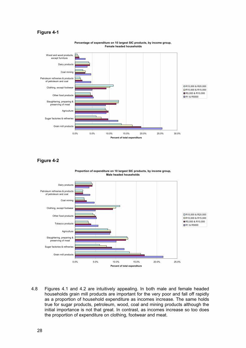
28

Figure 4-1

Figure 4-2

4.8 Figures 4.1 and 4.2 are intuitively appealing. In both male and female headed households grain mill products are important for the very poor and fall off rapidly as a proportion of household expenditure as incomes increase. The same holds true for sugar products, petroleum, wood, coal and mining products although the initial importance is not that great. In contrast, as incomes increase so too does the proportion of expenditure on clothing, footwear and meat.

Percentage of expenditure on 10 largest SIC products, by income group, Female headed households

0.0% 5.0% 10.0% 15.0% 20.0% 25.0% 30.0%

Grain mill products

Sugar factories & refineries

Agriculture

Slaughtering, preparing &preserving of meat

Other food products

Clothing, except footwear

Petroleum refineries & productsof petroleum and coal

Coal mining

Dairy products

Wood and wood products,except furniture

Percent of total expenditure

R15,000 & R20,000R10,000 & R15,000R5,000 & R10,000R1 & R5000

Proportion of expenditure on 10 largest SIC products, by income group, Male headed households

0.0% 5.0% 10.0% 15.0% 20.0% 25.0%

Grain mill products

Sugar factories & refineries

Slaughtering, preparing &preserving of meat

Agriculture

Tobacco products

Other food products

Clothing, except footwear

Coal mining

Petroleum refineries & productsof petroleum and coal

Dairy products

Percent of total expenditure

R15,000 & R20,000R10,000 & R15,000R5,000 & R10,000R1 & R5000

29

4.9 The most interesting difference between male and female headed households is how tobacco products are the fifth most important expenditure item for very poor male headed households while they do not feature in the ten most important expenditure items for female headed households.

Changes in Expenditure Patterns

4.10 Tables 4.3, 4.4 and 4.5 record the rand value of differences in expenditure on the relevant SIC products for individual households between the various income categories. For example there is an annual R465 difference in spending on agricultural products between households with incomes of R1 – R5,000 and those earning R5,001 – R10,000.

4.11 Table 4.3 is for all households while Table 4.4 reports for female headed households and Table 4.5 for male headed households.

4.12 As with the section above, the level of detail is so great as to make casual interpretation very difficult. Figure 4.3 illustrates the ten greatest expenditure changes for the poorest households.

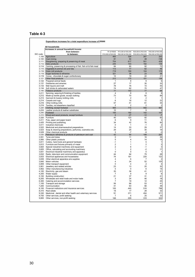
30

Table 4-3

Expenditure increases for a total expenditure increase of R5000

All householdsIncreases in annual household income

from between: R1 & R5000 R10,000 & R20,000 R20,000 & R30,000 R30,000 & R40,000SIC code to between: R10,000 & R20,000 R20,000 & R30,000 R30,000 & R40,000 R40,000 & R50,000

1,100 Agriculture 465 326 267 2432,100 Coal mining 81 64 48 -1383,111 Slaughtering, preparing & preserving of meat 704 617 501 4293,112 Dairy products 235 153 182 1393,114 Canning, preserving & processing of fish, fish oil & fish meal 84 65 92 723,115 Vegetable & animal oils and fats 113 77 62 463,116 Grain mill products 719 190 104 1753,118 Sugar factories & refineries 321 38 23 583,119 Cocoa , chocolate & sugar confectionary 12 19 22 213,121 Other food products 212 175 151 1363,122 Prepared animal feeds 1 8 9 63,131 Distilleries and wineries 27 17 30 333,133 Malt liquors and malt 78 76 15 453,134 Soft drinks & carbonated waters 74 62 70 473,140 Tobacco products 77 142 77 683,211 Spinning, weaving & finishing of textiles 4 8 8 83,212 Made-up textile goods, except clothing 73 70 92 893,213 Garment & hosiery knitting mills 1 2 2 13,214 Carpets and rugs 6 16 12 223,216 Other knitting mills 57 51 61 443,219 Textiles, not elsewhere classified 2 2 2 23,220 Clothing, except footwear 564 715 592 5673,233 Leather products & leather substitutes 10 7 9 63,240 Footwear 155 192 142 1473,310 Wood and wood products, except furniture 6 -27 -12 -73,320 Furniture 40 123 92 823,411 Pulp, paper and paper board 6 9 11 43,420 Printing and publishing 34 42 76 903,511 Industrial chemicals 0 1 -1 23,522 Medicinal and pharmaceutical preparations 14 33 29 373,523 Soap & cleaning preparations, perfumes, cosmetics etc. 29 25 30 193,529 Other chemical products 3 -7 -9 -33,530 Petroleum refineries & products of petroleum and coal 42 90 199 2573,551 Tyres and tubes 0 11 16 263,560 Other plastic products 5 4 14 163,811 Cutlery, hand tools and general hardware -1 1 5 13,812 Furniture and fixtures primarily of metal 2 1 2 33,824 Special industrial machinery and equipment 2 6 -1 33,825 Office, calculating and accounting machinery 1 2 -2 173,831 Electrical industrial machinery and apparatus 0 0 0 13,832 Radio, television and communication equipment 44 64 79 283,833 Electrical appliances and housewares 76 161 220 1223,839 Other electrical apparatus ans supplies 4 6 7 23,840 Motor vehicles 4 24 52 1253,859 Other transport equipment 0 4 2 43,901 Jewellery and related articles 23 13 20 323,902 Other manufacturing industries 5 0 6 144,100 Electricity, gas and steam 35 36 41 214,200 Water supply 7 9 9 65,100 Building construction 21 37 31 416,200 Wholesale and retail trade and motor trade 3 24 46 186,300 Catering and accommodation services 7 19 12 257,100 Transport and storage 56 66 53 417,200 Communication 41 63 66 488,100 Financial institutions and insurance services 155 445 516 7988,310 Real estate 18 17 28 329,330 Medicinal , dental and other health and veterinary services 91 371 454 5719,700 Other services, profit seeking 7 6 25 339,800 Other services, non-profit seeking 146 229 310 222

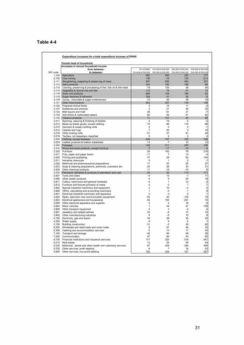
31

Table 4-4

Expenditure increases for a total expenditure increase of R5000

Female head of householdIncreases in annual household income

from between: R1 & R5000 R10,000 & R20,000 R20,000 & R30,000 R30,000 & R40,000SIC code to between: R10,000 & R20,000 R20,000 & R30,000 R30,000 & R40,000 R40,000 & R50,000

1,100 Agriculture 462 393 222 1772,100 Coal mining 138 -10 135 -2133,111 Slaughtering, preparing & preserving of meat 697 656 460 3373,112 Dairy products 243 160 180 883,114 Canning, preserving & processing of fish, fish oil & fish meal 79 105 39 543,115 Vegetable & animal oils and fats 112 74 51 133,116 Grain mill products 686 126 166 833,118 Sugar factories & refineries 326 41 26 -53,119 Cocoa , chocolate & sugar confectionary 10 20 28 183,121 Other food products 203 207 134 1363,122 Prepared animal feeds 2 15 11 -23,131 Distilleries and wineries 5 21 45 243,133 Malt liquors and malt 36 81 21 -73,134 Soft drinks & carbonated waters 60 93 41 823,140 Tobacco products 71 131 67 583,211 Spinning, weaving & finishing of textiles 4 19 5 -23,212 Made-up textile goods, except clothing 75 88 118 883,213 Garment & hosiery knitting mills 2 0 2 -13,214 Carpets and rugs 7 20 3 183,216 Other knitting mills 61 37 91 493,219 Textiles, not elsewhere classified 2 2 2 43,220 Clothing, except footwear 545 747 752 7483,233 Leather products & leather substitutes 13 7 12 123,240 Footwear 149 211 205 1063,310 Wood and wood products, except furniture 5 -17 -14 -43,320 Furniture 26 162 79 2183,411 Pulp, paper and paper board 11 7 13 -43,420 Printing and publishing 37 39 82 1043,511 Industrial chemicals 0 1 0 -13,522 Medicinal and pharmaceutical preparations 17 33 20 273,523 Soap & cleaning preparations, perfumes, cosmetics etc. 28 26 33 213,529 Other chemical products 11 -15 -10 -53,530 Petroleum refineries & products of petroleum and coal 35 30 113 1713,551 Tyres and tubes -4 13 -1 113,560 Other plastic products 6 0 25 183,811 Cutlery, hand tools and general hardware -4 1 12 -23,812 Furniture and fixtures primarily of metal 4 0 1 73,824 Special industrial machinery and equipment 3 10 -4 33,825 Office, calculating and accounting machinery 1 -3 1 83,831 Electrical industrial machinery and apparatus 0 0 0 13,832 Radio, television and communication equipment 55 30 130 153,833 Electrical appliances and housewares 92 184 291 743,839 Other electrical apparatus ans supplies 5 4 16 -63,840 Motor vehicles 1 34 47 1393,859 Other transport equipment 0 3 -2 43,901 Jewellery and related articles 33 -8 13 723,902 Other manufacturing industries 8 -5 10 84,100 Electricity, gas and steam 34 38 30 344,200 Water supply 8 9 6 75,100 Building construction 51 -2 26 826,200 Wholesale and retail trade and motor trade 6 27 46 326,300 Catering and accommodation services 6 13 17 447,100 Transport and storage 48 56 99 297,200 Communication 47 66 43 658,100 Financial institutions and insurance services 177 325 518 9418,310 Real estate 12 25 26 549,330 Medicinal , dental and other health and veterinary services 67 328 394 4099,700 Other services, profit seeking 9 7 16 239,800 Other services, non-profit seeking 180 334 107 537

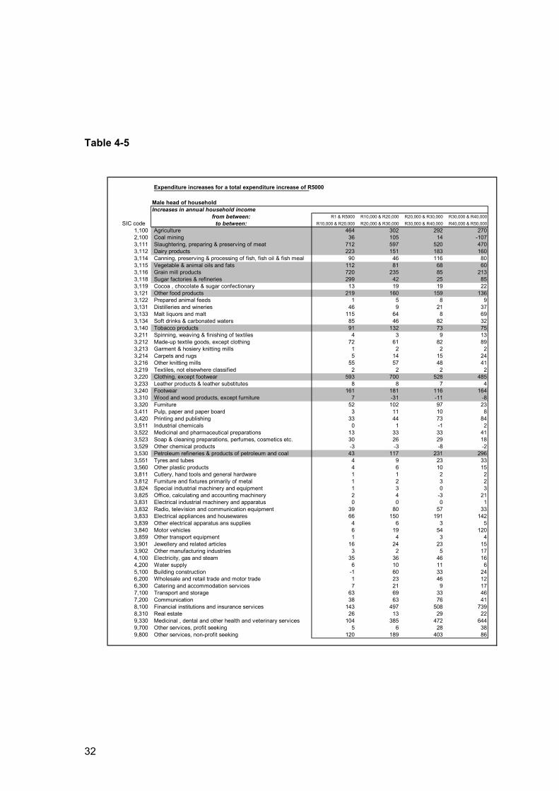
32

Table 4-5

Expenditure increases for a total expenditure increase of R5000

Male head of householdIncreases in annual household income

from between: R1 & R5000 R10,000 & R20,000 R20,000 & R30,000 R30,000 & R40,000SIC code to between: R10,000 & R20,000 R20,000 & R30,000 R30,000 & R40,000 R40,000 & R50,000

1,100 Agriculture 464 302 292 2702,100 Coal mining 36 105 14 -1073,111 Slaughtering, preparing & preserving of meat 712 597 520 4703,112 Dairy products 223 151 183 1603,114 Canning, preserving & processing of fish, fish oil & fish meal 90 46 116 803,115 Vegetable & animal oils and fats 112 81 68 603,116 Grain mill products 720 235 85 2133,118 Sugar factories & refineries 299 42 25 853,119 Cocoa , chocolate & sugar confectionary 13 19 19 223,121 Other food products 219 160 159 1363,122 Prepared animal feeds 1 5 8 93,131 Distilleries and wineries 46 9 21 373,133 Malt liquors and malt 115 64 8 693,134 Soft drinks & carbonated waters 85 46 82 323,140 Tobacco products 91 132 73 753,211 Spinning, weaving & finishing of textiles 4 3 9 133,212 Made-up textile goods, except clothing 72 61 82 893,213 Garment & hosiery knitting mills 1 2 2 23,214 Carpets and rugs 5 14 15 243,216 Other knitting mills 55 57 48 413,219 Textiles, not elsewhere classified 2 2 2 23,220 Clothing, except footwear 593 700 528 4853,233 Leather products & leather substitutes 8 8 7 43,240 Footwear 161 181 116 1643,310 Wood and wood products, except furniture 7 -31 -11 -83,320 Furniture 52 102 97 233,411 Pulp, paper and paper board 3 11 10 83,420 Printing and publishing 33 44 73 843,511 Industrial chemicals 0 1 -1 23,522 Medicinal and pharmaceutical preparations 13 33 33 413,523 Soap & cleaning preparations, perfumes, cosmetics etc. 30 26 29 183,529 Other chemical products -3 -3 -8 -23,530 Petroleum refineries & products of petroleum and coal 43 117 231 2963,551 Tyres and tubes 4 9 23 333,560 Other plastic products 4 6 10 153,811 Cutlery, hand tools and general hardware 1 1 2 23,812 Furniture and fixtures primarily of metal 1 2 3 23,824 Special industrial machinery and equipment 1 3 0 33,825 Office, calculating and accounting machinery 2 4 -3 213,831 Electrical industrial machinery and apparatus 0 0 0 13,832 Radio, television and communication equipment 39 80 57 333,833 Electrical appliances and housewares 66 150 191 1423,839 Other electrical apparatus ans supplies 4 6 3 53,840 Motor vehicles 6 19 54 1203,859 Other transport equipment 1 4 3 43,901 Jewellery and related articles 16 24 23 153,902 Other manufacturing industries 3 2 5 174,100 Electricity, gas and steam 35 36 46 164,200 Water supply 6 10 11 65,100 Building construction -1 60 33 246,200 Wholesale and retail trade and motor trade 1 23 46 126,300 Catering and accommodation services 7 21 9 177,100 Transport and storage 63 69 33 467,200 Communication 38 63 76 418,100 Financial institutions and insurance services 143 497 508 7398,310 Real estate 26 13 29 229,330 Medicinal , dental and other health and veterinary services 104 385 472 6449,700 Other services, profit seeking 5 6 28 389,800 Other services, non-profit seeking 120 189 403 86

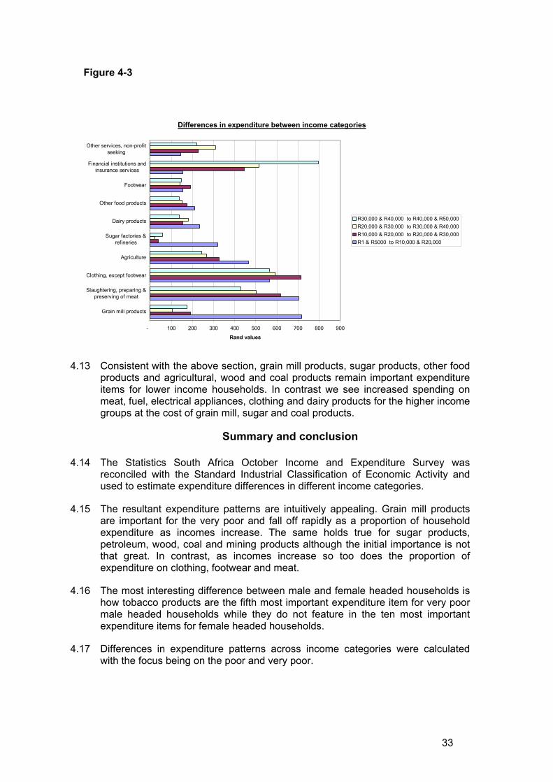
33

Figure 4-3

4.13 Consistent with the above section, grain mill products, sugar products, other food products and agricultural, wood and coal products remain important expenditure items for lower income households. In contrast we see increased spending on meat, fuel, electrical appliances, clothing and dairy products for the higher income groups at the cost of grain mill, sugar and coal products.

Summary and conclusion

4.14 The Statistics South Africa October Income and Expenditure Survey was reconciled with the Standard Industrial Classification of Economic Activity and used to estimate expenditure differences in different income categories.

4.15 The resultant expenditure patterns are intuitively appealing. Grain mill products are important for the very poor and fall off rapidly as a proportion of household expenditure as incomes increase. The same holds true for sugar products, petroleum, wood, coal and mining products although the initial importance is not that great. In contrast, as incomes increase so too does the proportion of expenditure on clothing, footwear and meat.

4.16 The most interesting difference between male and female headed households is how tobacco products are the fifth most important expenditure item for very poor male headed households while they do not feature in the ten most important expenditure items for female headed households.

4.17 Differences in expenditure patterns across income categories were calculated with the focus being on the poor and very poor.

Differences in expenditure between income categories

- 100 200 300 400 500 600 700 800 900

Grain mill products

Slaughtering, preparing &preserving of meat

Clothing, except footwear

Agriculture

Sugar factories &refineries

Dairy products

Other food products

Footwear

Financial institutions andinsurance services

Other services, non-profitseeking

Rand values

R30,000 & R40,000 to R40,000 & R50,000R20,000 & R30,000 to R30,000 & R40,000R10,000 & R20,000 to R20,000 & R30,000R1 & R5000 to R10,000 & R20,000

34

4.18 Here we find that grain mill products, sugar products, other food products and agricultural, wood and coal products remain important expenditure items for lower income households even with increases in income. In contrast we see increased expenditure on meat, fuel, electrical appliances, clothing and dairy products for the higher income groups at the cost of grain mill, sugar and coal products.

4.19 In conclusion we note the relative importance of wood and coal products for the lower income groups must indicate how important access is to natural sources and sellings points.

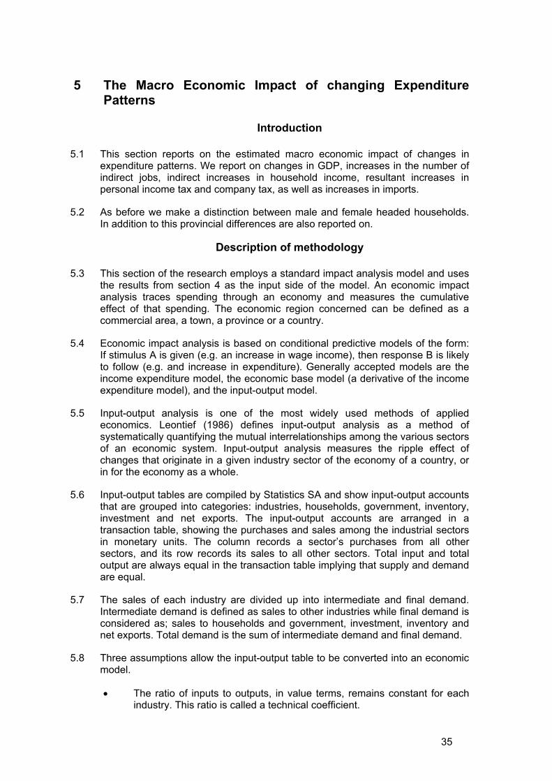
35

5 The Macro Economic Impact of changing Expenditure Patterns

Introduction

5.1 This section reports on the estimated macro economic impact of changes in expenditure patterns. We report on changes in GDP, increases in the number of indirect jobs, indirect increases in household income, resultant increases in personal income tax and company tax, as well as increases in imports.

5.2 As before we make a distinction between male and female headed households. In addition to this provincial differences are also reported on.

Description of methodology

5.3 This section of the research employs a standard impact analysis model and uses the results from section 4 as the input side of the model. An economic impact analysis traces spending through an economy and measures the cumulative effect of that spending. The economic region concerned can be defined as a commercial area, a town, a province or a country.

5.4 Economic impact analysis is based on conditional predictive models of the form: If stimulus A is given (e.g. an increase in wage income), then response B is likely to follow (e.g. and increase in expenditure). Generally accepted models are the income expenditure model, the economic base model (a derivative of the income expenditure model), and the input-output model.

5.5 Input-output analysis is one of the most widely used methods of applied economics. Leontief (1986) defines input-output analysis as a method of systematically quantifying the mutual interrelationships among the various sectors of an economic system. Input-output analysis measures the ripple effect of changes that originate in a given industry sector of the economy of a country, or in for the economy as a whole.

5.6 Input-output tables are compiled by Statistics SA and show input-output accounts that are grouped into categories: industries, households, government, inventory, investment and net exports. The input-output accounts are arranged in a transaction table, showing the purchases and sales among the industrial sectors in monetary units. The column records a sector’s purchases from all other sectors, and its row records its sales to all other sectors. Total input and total output are always equal in the transaction table implying that supply and demand are equal.

5.7 The sales of each industry are divided up into intermediate and final demand. Intermediate demand is defined as sales to other industries while final demand is considered as; sales to households and government, investment, inventory and net exports. Total demand is the sum of intermediate demand and final demand.

5.8 Three assumptions allow the input-output table to be converted into an economic model.

• The ratio of inputs to outputs, in value terms, remains constant for each industry. This ratio is called a technical coefficient.

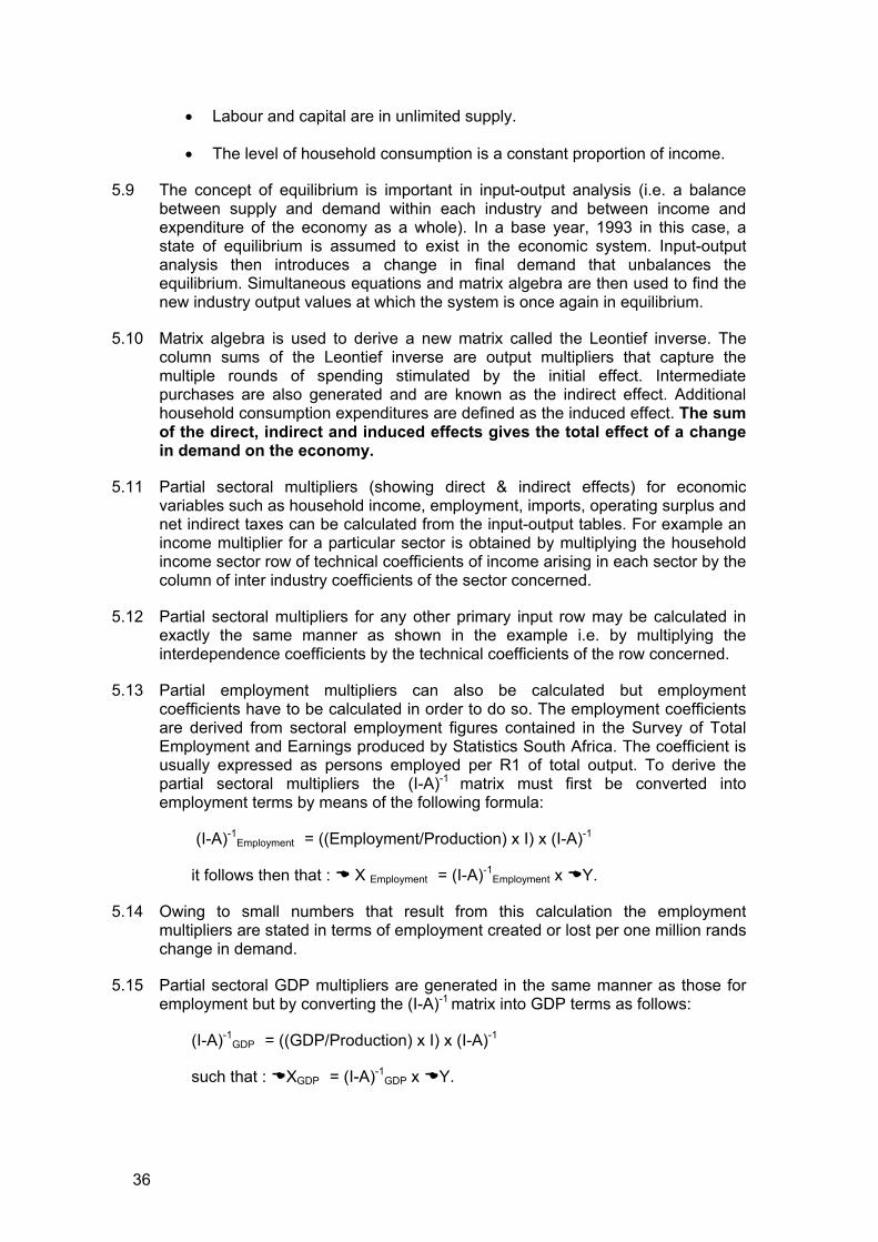
36

• Labour and capital are in unlimited supply.

• The level of household consumption is a constant proportion of income.

5.9 The concept of equilibrium is important in input-output analysis (i.e. a balance between supply and demand within each industry and between income and expenditure of the economy as a whole). In a base year, 1993 in this case, a state of equilibrium is assumed to exist in the economic system. Input-output analysis then introduces a change in final demand that unbalances the equilibrium. Simultaneous equations and matrix algebra are then used to find the new industry output values at which the system is once again in equilibrium.

5.10 Matrix algebra is used to derive a new matrix called the Leontief inverse. The column sums of the Leontief inverse are output multipliers that capture the multiple rounds of spending stimulated by the initial effect. Intermediate purchases are also generated and are known as the indirect effect. Additional household consumption expenditures are defined as the induced effect. The sum of the direct, indirect and induced effects gives the total effect of a change in demand on the economy.

5.11 Partial sectoral multipliers (showing direct & indirect effects) for economic variables such as household income, employment, imports, operating surplus and net indirect taxes can be calculated from the input-output tables. For example an income multiplier for a particular sector is obtained by multiplying the household income sector row of technical coefficients of income arising in each sector by the column of inter industry coefficients of the sector concerned.

5.12 Partial sectoral multipliers for any other primary input row may be calculated in exactly the same manner as shown in the example i.e. by multiplying the interdependence coefficients by the technical coefficients of the row concerned.

5.13 Partial employment multipliers can also be calculated but employment coefficients have to be calculated in order to do so. The employment coefficients are derived from sectoral employment figures contained in the Survey of Total Employment and Earnings produced by Statistics South Africa. The coefficient is usually expressed as persons employed per R1 of total output. To derive the partial sectoral multipliers the (I-A)-1 matrix must first be converted into employment terms by means of the following formula:

(I-A)-1Employment = ((Employment/Production) x I) x (I-A)-1

it follows then that : X Employment = (I-A)-1Employment x Y.

5.14 Owing to small numbers that result from this calculation the employment multipliers are stated in terms of employment created or lost per one million rands change in demand.

5.15 Partial sectoral GDP multipliers are generated in the same manner as those for employment but by converting the (I-A)-1 matrix into GDP terms as follows:

(I-A)-1GDP = ((GDP/Production) x I) x (I-A)-1

such that : XGDP = (I-A)-1GDP x Y.

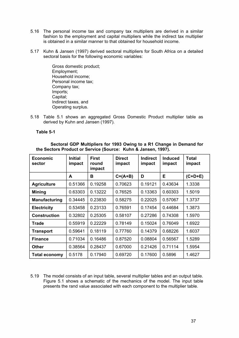
37

5.16 The personal income tax and company tax multipliers are derived in a similar fashion to the employment and capital multipliers while the indirect tax multiplier is obtained in a similar manner to that obtained for household income.

5.17 Kuhn & Jansen (1997) derived sectoral multipliers for South Africa on a detailed sectoral basis for the following economic variables:

Gross domestic product; Employment; Household income; Personal income tax; Company tax; Imports; Capital; Indirect taxes, and Operating surplus.

5.18 Table 5.1 shows an aggregated Gross Domestic Product multiplier table as derived by Kuhn and Jansen (1997).

Table 5-1

Sectoral GDP Multipliers for 1993 Owing to a R1 Change in Demand for the Sectors Product or Service (Source: Kuhn & Jansen, 1997).

Economic sector

Initial impact

First round impact

Direct impact

Indirect impact

Induced impact

Total impact

A B C=(A+B) D E (C+D+E)

Agriculture 0.51366 0.19258 0.70623 0.19121 0.43634 1.3338

Mining 0.63303 0.13222 0.76525 0.13363 0.60303 1.5019

Manufacturing 0.34445 0.23830 0.58275 0.22025 0.57067 1.3737

Electricity 0.53458 0.23133 0.76591 0.17454 0.44684 1.3873

Construction 0.32802 0.25305 0.58107 0.27286 0.74308 1.5970

Trade 0.55919 0.22229 0.78149 0.15024 0.76049 1.6922

Transport 0.59641 0.18119 0.77760 0.14379 0.68226 1.6037

Finance 0.71034 0.16486 0.87520 0.08804 0.56567 1.5289

Other 0.38564 0.28437 0.67000 0.21426 0.71114 1.5954

Total economy 0.5178 0.17940 0.69720 0.17600 0.5896 1.4627

5.19 The model consists of an input table, several multiplier tables and an output table. Figure 5.1 shows a schematic of the mechanics of the model. The input table presents the rand value associated with each component to the multiplier table.

38

Figure 5-1

Schematics of the Mechanics of the Impact Analysis Model

5.20

5.21

Ta

S

With the exception of the sectoral employment multipliers the sectoral multiplier tables show the direct, indirect and induced effects of a R1 change in final demand. The employment multiplier shows the direct, indirect and induced effects of a one million rands change in demand at 1993 prices.

The rand value of each component is then multiplied by the relevant (i.e. GDP, employment) sectoral multiplier to derive the direct, indirect, induced and total effects of a change in demand for that component. The individual sectoral changes are then summed to give the direct, indirect, induced and total economic effects of a change in demand for a particular size wheeled loader. The model presents the effects on GDP, household income and employment together with personal income tax, company tax, imports, indirect taxes and operating surplus effects in rand terms.

ble 5-2

Example of the Sectoral GDP multipliers

X =InputTable

RelevantMultiplier

Table

MultipliedEffect

in Rands

CHANGE IN GDP WITH R1 CHANGE IN FINAL DEMANDIC_CODE SECTOR

Direct Indirect Induced Total3551 Tyres and tubes 0.56716 0.20397 0.54194 1.31313710 Iron and steel basic industries 0.67683 0.16665 0.58753 1.43103710 Iron and steel basic industries 0.67683 0.16665 0.58753 1.43103821 Engines and turbines 0.51712 0.16564 0.50540 1.18823829 Other non-electrical machinery and equipment 0.60982 0.18409 0.65451 1.44843829 Other non-electrical machinery and equipment 0.60982 0.18409 0.65451 1.44843829 Other non-electrical machinery and equipment 0.60982 0.18409 0.65451 1.44843831 Electrical industrial machinery and apparatus 0.69202 0.14851 0.76918 1.6097

39

5.22 Determining the employment effects requires an additional step whereby the prices are deflated to 1993 prices using total inflation figures for 1993 an estimated year 2000 CPI.

National Macro Economic Impact of changing Expenditure patterns

5.23 This section presents the results to the economic impact model that analysis the change in the macro economy following a change in final demand.

Aggregate impact

5.24 The national impact on various macroeconomic variables following a R5,000 change in expenditure as households move from one income category to the next is presented in Table 5.3.

Table 5-3

5.25 The most comprehensive measure of economic impact is contribution to GDP. A R5,000 increase in expenditure will result in GDP increasing from between R7,000 and R7,500 depending on the income category in which the income change is occurring. Generally as the income level increases so to is there a slightly greater impact on the contribution to GDP (up to R50,000 per annum).

5.26 A similar pattern holds true for indirect contribution to household income following a change in expenditure. Here indirect incomes increase from between R3,200 and R3,900.

5.27 In contrast to income increase effects changes in expenditure in the lower income levels has a greater impact on the number of indirect jobs created. For every R5,000 of spending an estimated number of indirect jobs of 0.26 in the lowest income categories and 0.24 in the highest are being created.

5.28 In a similar vein there will be increases in total direct taxes (income and company tax) of between R900 and R1,100. Imports will increase by about R1,300.

Male and female head of household differences

5.29 Tables 5.4 and 5.5 present the same macro economic results as the section above, except in this case separated into female and male headed households.

5.30 Here there is nothing startling or dramatic to report. Changes in expenditure in both female and male headed households have generally similar results. In certain income categories contribution to GDP is slightly higher while in others it is slightly lower. At higher income levels female headed households generate

National macro economic impact following a R5000 increase in expenditure

All householdsIncreases in annual household income

from between: R1 & R5000 R5,000 & R10,000 R10,000 & R20,000 R20,000 & R30,000 R30,000 & R40,000to between: R5,000 & R10,000 R10,000 & R20,000 R20,000 & R30,000 R30,000 & R40,000 R40,000 & R50,000

Contribution to GDP 6,984 7,108 7,318 7,365 7,481 Indirect contribution to household income 3,264 3,444 3,670 3,736 3,850 Indirect jobs created 0.26 0.25 0.25 0.24 0.24 Increases in income tax 605 637 686 706 739 Increases in company taxes 307 317 342 348 369 Increased in imports 1,280 1,337 1,352 1,371 1,369

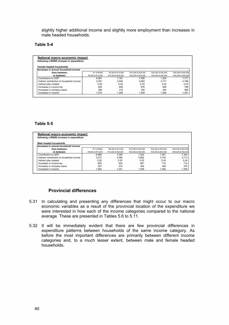
40

slightly higher additional income and slightly more employment than increases in male headed households.

Table 5-4

Table 5-5

Provincial differences

5.31 In calculating and presenting any differences that might occur to our macro economic variables as a result of the provincial location of the expenditure we were interested in how each of the income categories compared to the national average. These are presented in Tables 5.6 to 5.11.

5.32 It will be immediately evident that there are few provincial differences in expenditure patterns between households of the same income category. As before the most important differences are primarily between different income categories and, to a much lesser extent, between male and female headed households.

National macro economic impact following a R5000 increase in expenditure

Female headed householdsIncreases in annual household income

from between: R1 & R5000 R5,000 & R10,000 R10,000 & R20,000 R20,000 & R30,000 R30,000 & R40,000to between: R5,000 & R10,000 R10,000 & R20,000 R20,000 & R30,000 R30,000 & R40,000 R40,000 & R50,000

Contribution to GDP 6,981 7,181 7,306 7,324 7,777 Indirect contribution to household income 3,257 3,540 3,645 3,717 4,168 Indirect jobs created 0.26 0.25 0.25 0.24 0.25 Increases in income tax 605 656 676 695 799 Increases in company taxes 306 315 335 344 366 Increased in imports 1,276 1,359 1,339 1,393 1,391

National macro economic impact following a R5000 increase in expenditure

Male headed householdsIncreases in annual household income

from between: R1 & R5000 R5,000 & R10,000 R10,000 & R20,000 R20,000 & R30,000 R30,000 & R40,000to between: R5,000 & R10,000 R10,000 & R20,000 R20,000 & R30,000 R30,000 & R40,000 R40,000 & R50,000

Contribution to GDP 6,989 7,059 7,324 7,381 7,354 Indirect contribution to household income 3,273 3,380 3,682 3,743 3,713 Indirect jobs created 0.26 0.25 0.25 0.24 0.24 Increases in income tax 605 624 691 710 714 Increases in company taxes 307 319 344 349 370 Increased in imports 1,284 1,321 1,359 1,362 1,359

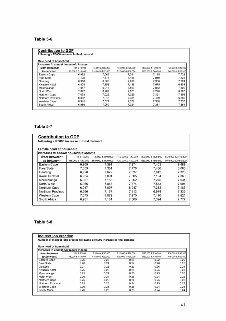
41

Table 5-6

Table 5-7

Table 5-8

Contribution to GDPfollowing a R5000 increase in final demand

Male head of householdIncreases in annual household income

from between: R1 & R5000 R5,000 & R10,000 R10,000 & R20,000 R20,000 & R30,000 R30,000 & R40,000to between: R5,000 & R10,000 R10,000 & R20,000 R20,000 & R30,000 R30,000 & R40,000 R40,000 & R50,000

Eastern Cape 6,992 7,062 7,391 7,115 7,722 Free State 7,125 7,476 7,158 7,910 7,538 Gauteng 6,918 6,866 7,289 7,306 7,281 Kwazulu Natal 6,828 7,158 7,136 7,675 6,803 Mpumalanga 7,057 6,918 7,563 7,072 7,190 North West 7,022 6,987 7,671 7,278 8,287 Northern Cape 7,074 7,022 7,329 7,321 7,456 Northern Province 6,862 7,048 7,384 7,479 6,880 Western Cape 6,945 7,074 7,372 7,388 7,735 South Africa 6,989 7,059 7,324 7,381 7,354

Contribution to GDPfollowing a R5000 increase in final demand

Female head of householdIncreases in annual household income

from between: R1 & R5000 R5,000 & R10,000 R10,000 & R20,000 R20,000 & R30,000 R30,000 & R40,000to between: R5,000 & R10,000 R10,000 & R20,000 R20,000 & R30,000 R30,000 & R40,000 R40,000 & R50,000

Eastern Cape 6,969 7,391 7,274 7,463 9,489 Free State 7,059 7,361 7,778 7,450 8,085 Gauteng 6,920 7,672 7,037 7,642 7,320 Kwazulu Natal 6,954 7,091 7,305 7,194 7,360 Mpumalanga 6,967 7,158 7,062 7,275 7,534 North West 6,956 7,063 7,874 7,543 7,994 Northern Cape 6,947 7,097 6,947 7,283 7,187 Northern Province 6,996 7,157 7,613 6,974 7,339 Western Cape 7,075 7,072 7,275 7,170 7,821 South Africa 6,981 7,181 7,306 7,324 7,777

Indirect job creationNumber of indirect jobs created following a R5000 increase in final demand

Male head of householdIncreases in annual household income

from between: R1 & R5000 R5,000 & R10,000 R10,000 & R20,000 R20,000 & R30,000 R30,000 & R40,000to between: R5,000 & R10,000 R10,000 & R20,000 R20,000 & R30,000 R30,000 & R40,000 R40,000 & R50,000

Eastern Cape 0.26 0.25 0.26 0.22 0.26 Free State 0.26 0.24 0.24 0.26 0.25 Gauteng 0.27 0.28 0.23 0.26 0.24 Kwazulu Natal 0.25 0.26 0.25 0.25 0.23 Mpumalanga 0.25 0.24 0.25 0.23 0.20 North West 0.26 0.24 0.25 0.24 0.22 Northern Cape 0.25 0.26 0.24 0.25 0.22 Northern Province 0.25 0.26 0.24 0.25 0.22 Western Cape 0.26 0.25 0.25 0.24 0.25 South Africa 0.26 0.25 0.25 0.24 0.24

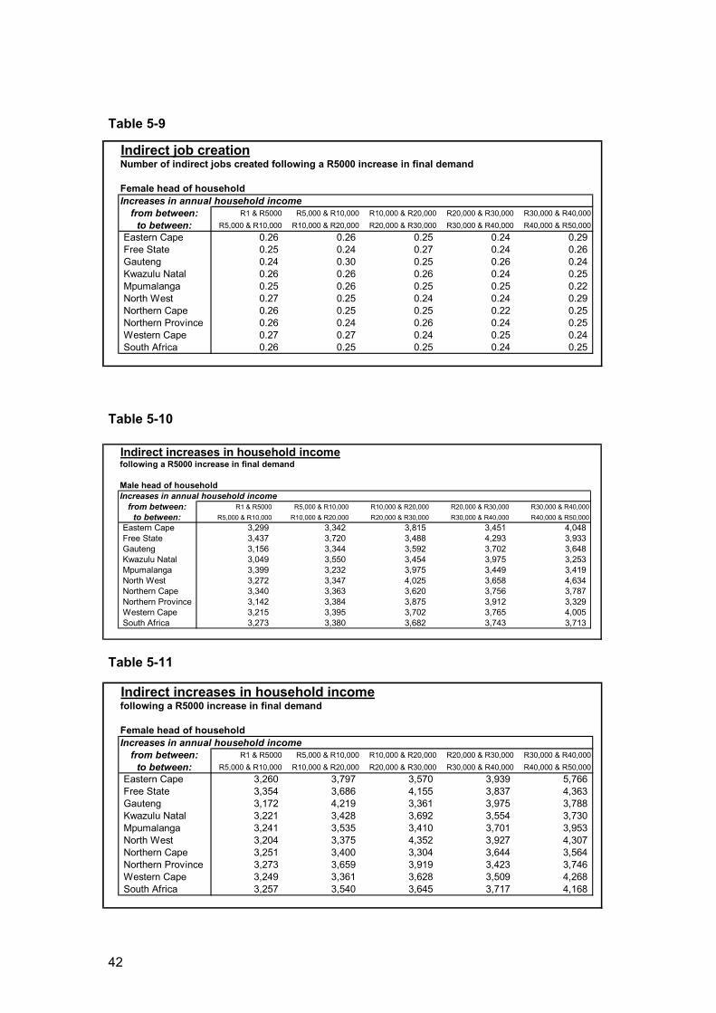
42

Table 5-9

Table 5-10

Table 5-11

Indirect job creationNumber of indirect jobs created following a R5000 increase in final demand

Female head of householdIncreases in annual household income

from between: R1 & R5000 R5,000 & R10,000 R10,000 & R20,000 R20,000 & R30,000 R30,000 & R40,000to between: R5,000 & R10,000 R10,000 & R20,000 R20,000 & R30,000 R30,000 & R40,000 R40,000 & R50,000

Eastern Cape 0.26 0.26 0.25 0.24 0.29 Free State 0.25 0.24 0.27 0.24 0.26 Gauteng 0.24 0.30 0.25 0.26 0.24 Kwazulu Natal 0.26 0.26 0.26 0.24 0.25 Mpumalanga 0.25 0.26 0.25 0.25 0.22 North West 0.27 0.25 0.24 0.24 0.29 Northern Cape 0.26 0.25 0.25 0.22 0.25 Northern Province 0.26 0.24 0.26 0.24 0.25 Western Cape 0.27 0.27 0.24 0.25 0.24 South Africa 0.26 0.25 0.25 0.24 0.25

Indirect increases in household incomefollowing a R5000 increase in final demand

Male head of householdIncreases in annual household income

from between: R1 & R5000 R5,000 & R10,000 R10,000 & R20,000 R20,000 & R30,000 R30,000 & R40,000to between: R5,000 & R10,000 R10,000 & R20,000 R20,000 & R30,000 R30,000 & R40,000 R40,000 & R50,000

Eastern Cape 3,299 3,342 3,815 3,451 4,048 Free State 3,437 3,720 3,488 4,293 3,933 Gauteng 3,156 3,344 3,592 3,702 3,648 Kwazulu Natal 3,049 3,550 3,454 3,975 3,253 Mpumalanga 3,399 3,232 3,975 3,449 3,419 North West 3,272 3,347 4,025 3,658 4,634 Northern Cape 3,340 3,363 3,620 3,756 3,787 Northern Province 3,142 3,384 3,875 3,912 3,329 Western Cape 3,215 3,395 3,702 3,765 4,005 South Africa 3,273 3,380 3,682 3,743 3,713

Indirect increases in household incomefollowing a R5000 increase in final demand

Female head of householdIncreases in annual household income

from between: R1 & R5000 R5,000 & R10,000 R10,000 & R20,000 R20,000 & R30,000 R30,000 & R40,000to between: R5,000 & R10,000 R10,000 & R20,000 R20,000 & R30,000 R30,000 & R40,000 R40,000 & R50,000

Eastern Cape 3,260 3,797 3,570 3,939 5,766 Free State 3,354 3,686 4,155 3,837 4,363 Gauteng 3,172 4,219 3,361 3,975 3,788 Kwazulu Natal 3,221 3,428 3,692 3,554 3,730 Mpumalanga 3,241 3,535 3,410 3,701 3,953 North West 3,204 3,375 4,352 3,927 4,307 Northern Cape 3,251 3,400 3,304 3,644 3,564 Northern Province 3,273 3,659 3,919 3,423 3,746 Western Cape 3,249 3,361 3,628 3,509 4,268 South Africa 3,257 3,540 3,645 3,717 4,168

43

Summary and conclusions

5.33 This chapter takes the results from Chapter 4 and applies them to the national input output relationships. From this we determine the multiplied impact of changing expenditure patterns. This is done for nationally, provincially and for male and female headed households respectively.

5.34 The focus is on poor and very poor households. For example, if household income increased for those people with between R1 to R5,000 a year such that their income increased to between R5,000 and R10,000 a year (and there was a spending increase of R5,000) then, there would be an increase in GDP equal 1.40 times this increase, indirect household incomes would increase by 0.65 times this, 0.26 indirect jobs would be created, there would be increases in income tax, company tax and imports to the value of R605, R307 and R1,280 respectively.

5.35 At low income levels the recorded multipliers increase as income increase. Technically the cause is because of the different composition of expenditure at different income levels. The multiplier effects cannot measure any informal sector activity and regard all expenditure as formal. In reality much of the expenditure changes will be, initially at least, through the informal sector. In consequence we would expect higher indirect income and job multipliers than are being reported.

5.36 There are no startling differences between male and female headed households or between the various provinces.

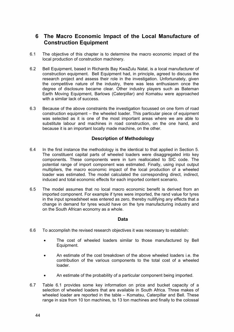
44

6 The Macro Economic Impact of the Local Manufacture of Construction Equipment

6.1 The objective of this chapter is to determine the macro economic impact of the local production of construction machinery.

6.2 Bell Equipment, based in Richards Bay KwaZulu Natal, is a local manufacturer of construction equipment. Bell Equipment had, in principle, agreed to discuss the research project and assess their role in the investigation. Unfortunately, given the competitive nature of the industry, there was less enthusiasm once the degree of disclosure became clear. Other industry players such as Bateman Earth Moving Equipment, Barlows (Caterpillar) and Komatsu were approached with a similar lack of success.

6.3 Because of the above constraints the investigation focussed on one form of road construction equipment – the wheeled loader. This particular piece of equipment was selected as it is one of the most important areas where we are able to substitute labour and machines in road construction, on the one hand, and because it is an important locally made machine, on the other.

Description of Methodology

6.4 In the first instance the methodology is the identical to that applied in Section 5. The constituent capital parts of wheeled loaders were disaggregated into key components. These components were in turn reallocated to SIC code. The potential range of import component was estimated. Finally, using input output multipliers, the macro economic impact of the local production of a wheeled loader was estimated. The model calculated the corresponding direct, indirect, induced and total economic effects for each imported content scenario.

6.5 The model assumes that no local macro economic benefit is derived from an imported component. For example if tyres were imported, the rand value for tyres in the input spreadsheet was entered as zero, thereby nullifying any effects that a change in demand for tyres would have on the tyre manufacturing industry and on the South African economy as a whole.

Data

6.6 To accomplish the revised research objectives it was necessary to establish:

• The cost of wheeled loaders similar to those manufactured by Bell Equipment.

• An estimate of the cost breakdown of the above wheeled loaders i.e. the contribution of the various components to the total cost of a wheeled loader.

• An estimate of the probability of a particular component being imported.

6.7 Table 6.1 provides some key information on price and bucket capacity of a selection of wheeled loaders that are available in South Africa. Three makes of wheeled loader are reported in the table – Komatsu, Caterpillar and Bell. These range in size from 10 ton machines, to 13 ton machines and finally to the colossal

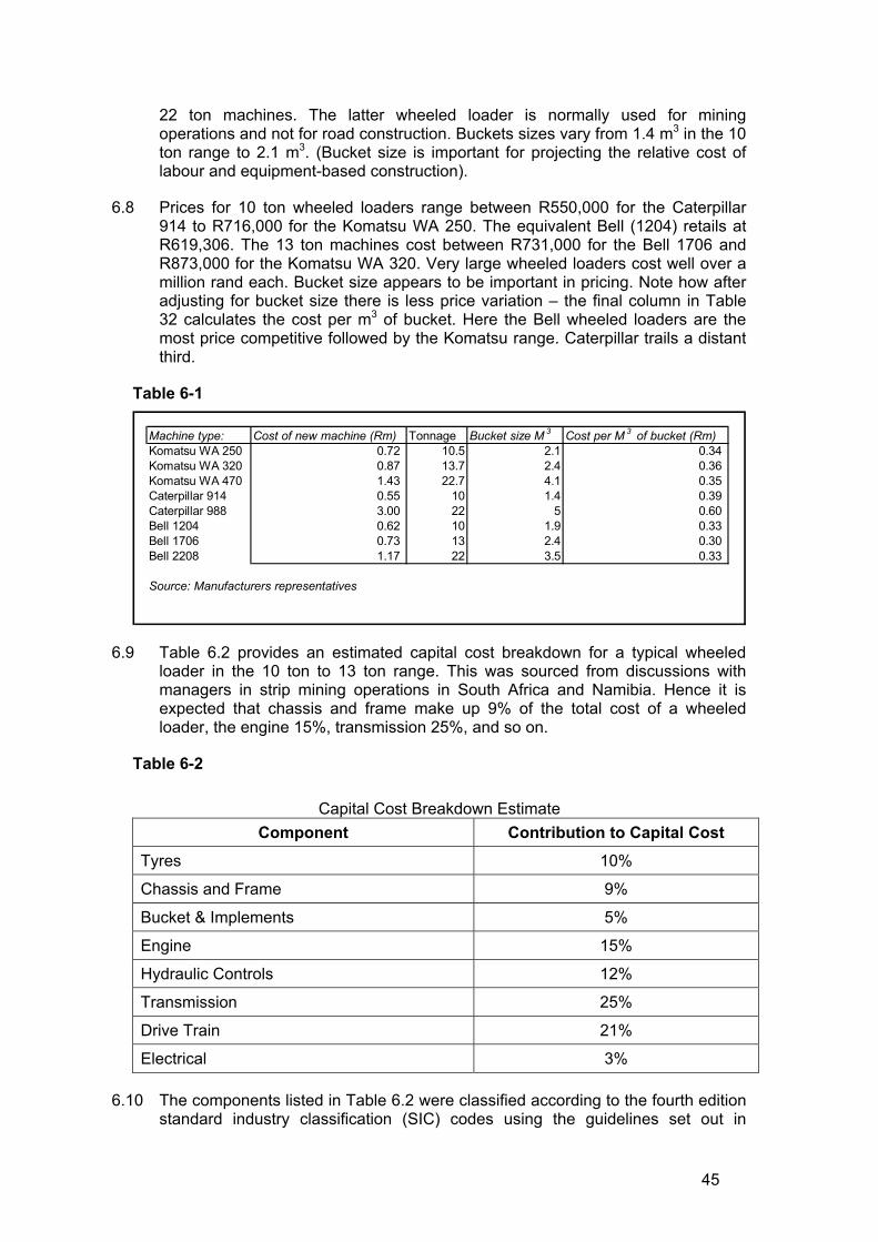
45

22 ton machines. The latter wheeled loader is normally used for mining operations and not for road construction. Buckets sizes vary from 1.4 m3 in the 10 ton range to 2.1 m3. (Bucket size is important for projecting the relative cost of labour and equipment-based construction).

6.8 Prices for 10 ton wheeled loaders range between R550,000 for the Caterpillar 914 to R716,000 for the Komatsu WA 250. The equivalent Bell (1204) retails at R619,306. The 13 ton machines cost between R731,000 for the Bell 1706 and R873,000 for the Komatsu WA 320. Very large wheeled loaders cost well over a million rand each. Bucket size appears to be important in pricing. Note how after adjusting for bucket size there is less price variation – the final column in Table 32 calculates the cost per m3 of bucket. Here the Bell wheeled loaders are the most price competitive followed by the Komatsu range. Caterpillar trails a distant third.

Table 6-1

6.9 Table 6.2 provides an estimated capital cost breakdown for a typical wheeled loader in the 10 ton to 13 ton range. This was sourced from discussions with managers in strip mining operations in South Africa and Namibia. Hence it is expected that chassis and frame make up 9% of the total cost of a wheeled loader, the engine 15%, transmission 25%, and so on.

Table 6-2

Capital Cost Breakdown Estimate Component Contribution to Capital Cost

Tyres 10%

Chassis and Frame 9%

Bucket & Implements 5%

Engine 15%

Hydraulic Controls 12%

Transmission 25%

Drive Train 21%

Electrical 3%

6.10 The components listed in Table 6.2 were classified according to the fourth edition standard industry classification (SIC) codes using the guidelines set out in

Machine type: Cost of new machine (Rm) Tonnage Bucket size M 3 Cost per M 3 of bucket (Rm)Komatsu WA 250 0.72 10.5 2.1 0.34 Komatsu WA 320 0.87 13.7 2.4 0.36 Komatsu WA 470 1.43 22.7 4.1 0.35 Caterpillar 914 0.55 10 1.4 0.39 Caterpillar 988 3.00 22 5 0.60 Bell 1204 0.62 10 1.9 0.33 Bell 1706 0.73 13 2.4 0.30 Bell 2208 1.17 22 3.5 0.33

Source: Manufacturers representatives

46

Standard Industrial Classification of all Economic Activities (Central Statistical Services, 1993). Table 6.3 shows the classification of the components according to the fourth edition SIC codes.

Table 6-3

SIC Code Classification of the Components Component SIC Code Activity

Tyres 3551 Manufacture of tyres and tubes

Chassis and Frame 3710 Iron and steel basic industries

Bucket & Implements 3710 Iron and steel basic industries

Engine 3821 Manufacture of engines and turbines

Hydraulic Controls 3829 All other machinery not elsewhere classified.

Transmission 3829 All other machinery not elsewhere classified.

Drive Train 3829 All other machinery not elsewhere classified.

Electrical 3831 Manufacture of electrical industrial machinery and apparatus.

6.11 The hydraulic controls, transmission and drive train components where allocated to activity 3829 as its sub classifications contain activities associated with driving elements and specialised parts for handling and lifting equipment.

6.12 Based on the above information we estimate the likely imported component of locally produced wheeled loaders. These are presented in Table 6.4. The table is divided into three parts.

• The second gives the contribution to capital cost.

• The third lists the estimated imported percentage of capital component. These are given as ‘Low’, ‘Expected’ and ‘High’. Discussions with manufactures’ representatives yielded information on the likely imported content of locally manufactured wheeled loaders. Tyres, transmission and drive train were in all likelihood imported. While several of the components making up the hydraulic controls could also be imported.

• The forth calculates the weighted import component of a wheeled loader and sums the total import component.

6.13 Table 6.4 reports that the possible range of the imported component of a locally produced wheeled loader will range from a minimum – and unlikely – 47.9% and a maximum – probably also unlikely – of 77%.

47

Table 6-4

The Macro Economic Impact of a locally manufactured Wheeled Loader

6.14 Tables 6.5 to 6.7 report on the macro economic impact of the domestic production of a wheeled loader. This exercise is reported for 10 ton, 13 ton and 22 ton wheeled loaders.

6.15 A ten ton wheeled loader that is fully manufactured in South Africa, and cost R600,000 to produce will have the effect of increasing GDP by nearly R840,000, increase total jobs by nearly 8 positions, generate indirect income to the value of R438,000. It will also generate total taxes to the value of R121,000. While the value of the contribution to GDP is important so too is the value of total imports. It will boost imports by nearly R200,000 even thought the wheeled loader is fully (and totally) locally produced.

6.16 Clearly as the imported component increases so the macro economic impact decreases. A wheeled loader that is 56% imported makes only a R361,000 contribution to GDP, creates 4.5 jobs and generates total imports to the value of R424,000.

Table 6-5

6.17 A machine that has a high 68% imported component and costing R600,000 makes only a R256,000 contribution to GDP, creates 2.48 jobs and generates imports to the value of R473,000.

6.18 Tables 6.6 and 6.7 tell similar tales for 13 ton and 22 ton wheeled loaders.

Estimates of imported component of locally produced wheeled loaders

Imported componentPercentage imported Weighted contribution to capital cost

Component Contribution to Capital Cost Low Expected High Low Expected HighTyres 10% 80% 100% 100% 8.0% 10.0% 10.0%Chassis and Frame 9% 0% 0% 20% 0.0% 0.0% 1.8%Bucket & Implements 5% 0% 0% 25% 0.0% 0.0% 1.3%Engine 15% 0% 0% 20% 0.0% 0.0% 3.0%Hydraulic Controls 12% 80% 100% 100% 9.6% 12.0% 12.0%Transmission 25% 70% 100% 100% 17.5% 25.0% 25.0%Drive Train 21% 50% 100% 100% 10.5% 21.0% 21.0%Electrical 3% 75% 100% 100% 2.3% 3.0% 3.0%Imported component of capital cost 47.9% 71.0% 77.1%

Macro economic impact of local productionof 10 ton Wheeled LoaderInitial cost of R600,000 Contribution Indirect Income Company Induced Total

to GDP No. of jobs income tax tax imports importsFull Local Manufacture 838,946 7.98 438,566 85,819 35,537 199,620 199,620 22% imported 655,876 6.24 343,902 67,096 27,877 156,027 288,027 43% imported 473,375 4.52 245,879 47,637 19,871 114,503 372,503 56% imported 360,399 3.46 185,197 35,591 14,914 88,798 424,798 68% imported 256,113 2.48 129,184 24,472 10,339 65,071 473,071 83% imported 149,179 1.38 75,118 13,754 5,569 27,939 525,939 Fully Imported - - - - - - 600,000

48

Table 6-6

Table 6-7

Summary and conclusions

6.19 The objective of this chapter was to determine the macroeconomic impact of the local manufacturing of machinery used in the construction industry. This chapter was challenged by less than adequate information on the local content of South African manufactured construction equipment.

6.20 Prices for 10 ton wheeled loaders range between R550,000 for the Caterpillar 914 to R716,000 for the Komatsu WA 250. The equivalent Bell (1204) retails at R619,306. The 13 ton machines cost between R731,000 for the Bell 1706 and R873,000 for the Komatsu WA 320. Very large wheeled loaders cost well over a million rand each.

6.21 Bucket size appears to be important in pricing. If bucket capacity is taken into account the Bell wheeled loaders are the most price competitive followed by the Komatsu range. Caterpillar trails a distant third.

6.22 The imported component of locally manufactured wheeled loaders is estimated to be between an extreme minimum of 48% and maximum of 77%.

6.23 A locally produced wheeled loader with no import content and costing R600,000 will generate GDP of R838,000 and 7.98 jobs. A similar machine with a 43% import content will contribute R473,000 to GDP and generate 4.52 jobs. Finally a machine with a 68% import content will generate R256,000 in GDP and 2.48 jobs.

Macro economic impact of local productionof 13 ton Wheeled LoaderInitial cost of R750,000 Contribution Indirect Income Company Induced Total

to GDP No. of jobs income tax tax imports importsFull Local Manufacture 1,048,683 9.98 548,207 107,274 44,421 199,620 199,620 22% imported 819,845 7.80 429,878 83,870 34,846 156,027 321,027 43% imported 591,719 5.65 307,348 59,546 24,838 114,503 437,003 56% imported 450,499 4.32 231,497 44,489 18,643 88,798 508,798 68% imported 320,141 3.09 161,480 30,589 12,924 65,071 575,071 83% imported 186,474 1.73 93,898 17,193 6,961 27,939 650,439 Fully Imported - - - - - - 750,000

Macro economic impact of local productionof 22 ton Wheeled LoaderInitial cost of R1.2 million Contribution Indirect Income Company Induced Total

to GDP No. of jobs income tax tax imports importsFull Local Manufacture 1,677,892 15.97 877,132 171,639 71,073 199,620 199,620 22% imported 1,311,752 12.47 687,805 134,192 55,754 156,027 420,027 43% imported 946,751 9.04 491,757 95,274 39,741 114,503 630,503 56% imported 720,798 6.91 370,395 71,182 29,829 88,798 760,798 68% imported 512,226 4.95 258,368 48,943 20,678 65,071 881,071 83% imported 298,358 2.77 150,236 27,508 11,137 27,939 1,023,939 Fully Imported - - - - - - 1,200,000

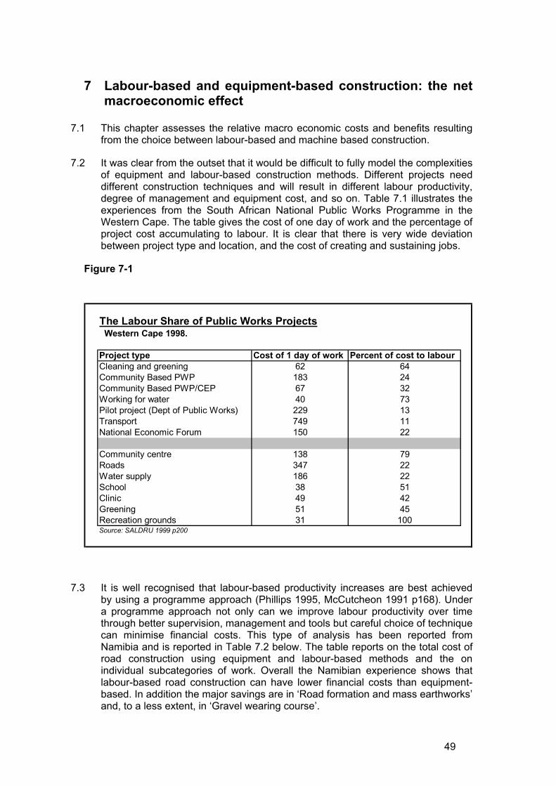
49

7 Labour-based and equipment-based construction: the net macroeconomic effect

7.1 This chapter assesses the relative macro economic costs and benefits resulting from the choice between labour-based and machine based construction.

7.2 It was clear from the outset that it would be difficult to fully model the complexities of equipment and labour-based construction methods. Different projects need different construction techniques and will result in different labour productivity, degree of management and equipment cost, and so on. Table 7.1 illustrates the experiences from the South African National Public Works Programme in the Western Cape. The table gives the cost of one day of work and the percentage of project cost accumulating to labour. It is clear that there is very wide deviation between project type and location, and the cost of creating and sustaining jobs.

Figure 7-1

7.3 It is well recognised that labour-based productivity increases are best achieved by using a programme approach (Phillips 1995, McCutcheon 1991 p168). Under a programme approach not only can we improve labour productivity over time through better supervision, management and tools but careful choice of technique can minimise financial costs. This type of analysis has been reported from Namibia and is reported in Table 7.2 below. The table reports on the total cost of road construction using equipment and labour-based methods and the on individual subcategories of work. Overall the Namibian experience shows that labour-based road construction can have lower financial costs than equipment-based. In addition the major savings are in ‘Road formation and mass earthworks’ and, to a less extent, in ‘Gravel wearing course’.

The Labour Share of Public Works Projects Western Cape 1998.

Project type Cost of 1 day of work Percent of cost to labourCleaning and greening 62 64Community Based PWP 183 24Community Based PWP/CEP 67 32Working for water 40 73Pilot project (Dept of Public Works) 229 13Transport 749 11National Economic Forum 150 22

Community centre 138 79Roads 347 22Water supply 186 22School 38 51Clinic 49 42Greening 51 45Recreation grounds 31 100Source: SALDRU 1999 p200

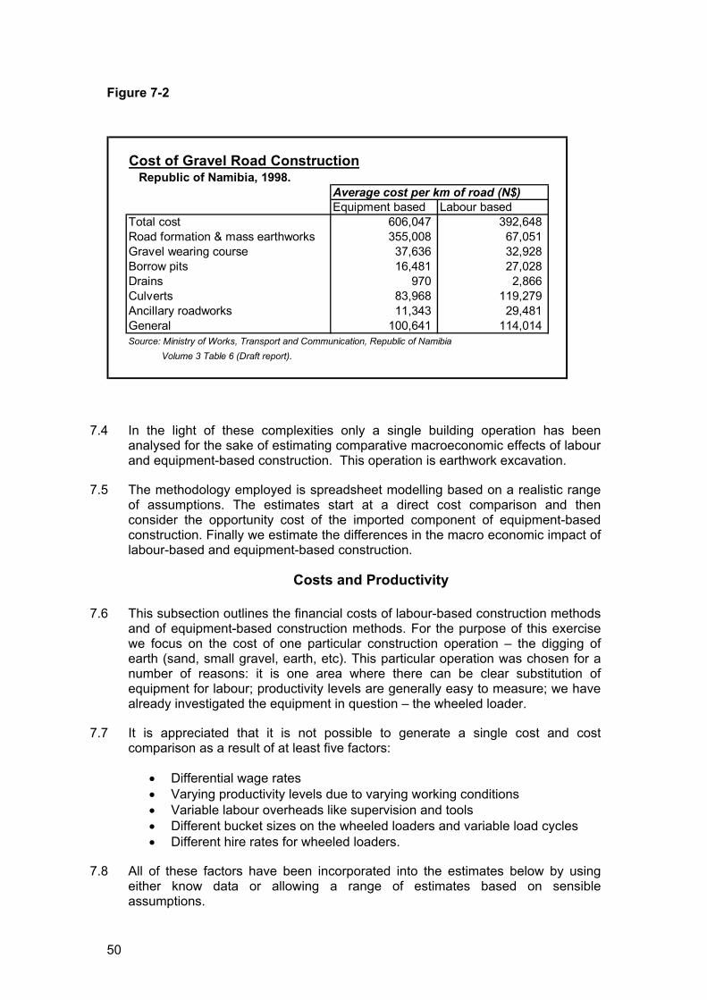
50

Figure 7-2

7.4 In the light of these complexities only a single building operation has been analysed for the sake of estimating comparative macroeconomic effects of labour and equipment-based construction. This operation is earthwork excavation.

7.5 The methodology employed is spreadsheet modelling based on a realistic range of assumptions. The estimates start at a direct cost comparison and then consider the opportunity cost of the imported component of equipment-based construction. Finally we estimate the differences in the macro economic impact of labour-based and equipment-based construction.

Costs and Productivity

7.6 This subsection outlines the financial costs of labour-based construction methods and of equipment-based construction methods. For the purpose of this exercise we focus on the cost of one particular construction operation – the digging of earth (sand, small gravel, earth, etc). This particular operation was chosen for a number of reasons: it is one area where there can be clear substitution of equipment for labour; productivity levels are generally easy to measure; we have already investigated the equipment in question – the wheeled loader.

7.7 It is appreciated that it is not possible to generate a single cost and cost comparison as a result of at least five factors:

• Differential wage rates • Varying productivity levels due to varying working conditions • Variable labour overheads like supervision and tools • Different bucket sizes on the wheeled loaders and variable load cycles • Different hire rates for wheeled loaders.

7.8 All of these factors have been incorporated into the estimates below by using either know data or allowing a range of estimates based on sensible assumptions.

Cost of Gravel Road Construction Republic of Namibia, 1998.

Average cost per km of road (N$)Equipment based Labour based

Total cost 606,047 392,648 Road formation & mass earthworks 355,008 67,051 Gravel wearing course 37,636 32,928 Borrow pits 16,481 27,028 Drains 970 2,866 Culverts 83,968 119,279 Ancillary roadworks 11,343 29,481 General 100,641 114,014 Source: Ministry of Works, Transport and Communication, Republic of Namibia Volume 3 Table 6 (Draft report).

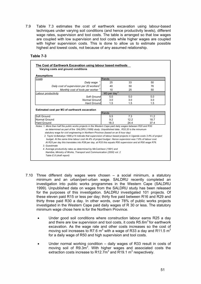
51

7.9 Table 7.3 estimates the cost of earthwork excavation using labour-based techniques under varying soil conditions (and hence productivity levels), different wage rates, supervision and tool costs. The table is arranged so that low wages are coupled with low supervision and tool costs while higher wages are coupled with higher supervision costs. This is done to allow us to estimate possible highest and lowest costs, not because of any assumed relationship.

Table 7-3

7.10 Three different daily wages were chosen – a social minimum, a statutory minimum and an urban/peri-urban wage. SALDRU recently completed an investigation into public works programmes in the Western Cape (SALDRU 1999). Unpublished data on wages from the SALDRU study has been released for the purposes of this investigation. SALDRU investigated 101 projects. Of these eleven paid R15 or less per day; thirty five paid between R16 and R29 and thirty three paid R30 a day. In other words, over 78% of public works projects investigated in the Western Cape paid daily wages of R 30 or less. The statutory minimum wage chose here is for the Northern Province.

• Under good soil conditions where construction labour earns R25 a day and there are low supervision and tool costs, it costs R5.6m3 for earthwork excavation. As the wage rate and other costs increases so the cost of moving soil increases to R7.6 m3 with a wage of R33 a day and R11.5 m3 for a daily wage of R50 and high supervision and tool costs.

• Under normal working condition – daily wages of R33 result in costs of moving soil of R9.3m3. With higher wages and associated costs the extraction costs increase to R12.7m3 and R19.1 m3 respectively.

The Cost of Earthwork Excavation using labour based methods Varying costs and ground conditions

AssumptionsCosts Rands

Daily wage 1 25 33 50Daily cost of supervision per 20 workers2 40 50 76

Monthly cost of tools per worker 3 10 25 50Labour productivity M3 per day 4

Soft Ground 5.0 5.0 5.0Normal Ground 3.0 3.0 3.0

Hard Ground 1.5 1.5 1.5

Estimated cost per M3 of earthwork excavationRands

Soft Ground 5.5 7.3 11.2Normal Ground 9.2 12.2 18.7Hard Ground 18.3 24.4 37.4Notes: 1. More than half the public works projects in the Western Cape paid daily wages between R20 and R30 as determined as part of the SALDRU (1999) study. Unpublished data.. R33.20 is the minumum statutory wage for civil engineering in Northern Province (based on an 8 hour day) 2. Taylor & Bekabye 1999 p14 indicate that supervision of labour based projects in Uganda costs 3.4% of project budget. At the same time labour cost 44.4% of project budger. Hence supevision was 7.6% of labour cost. At R25 per day this translates into R38 per day, at R33 this equals R50 supervision and at R50 wage R76. 3. Guestimate 4. Average productivity rates as determined by McCutcheon (1991) and Namibia, Ministry of Works, Transport and Communication (2000) vol. 2 Table E.8 (draft report)

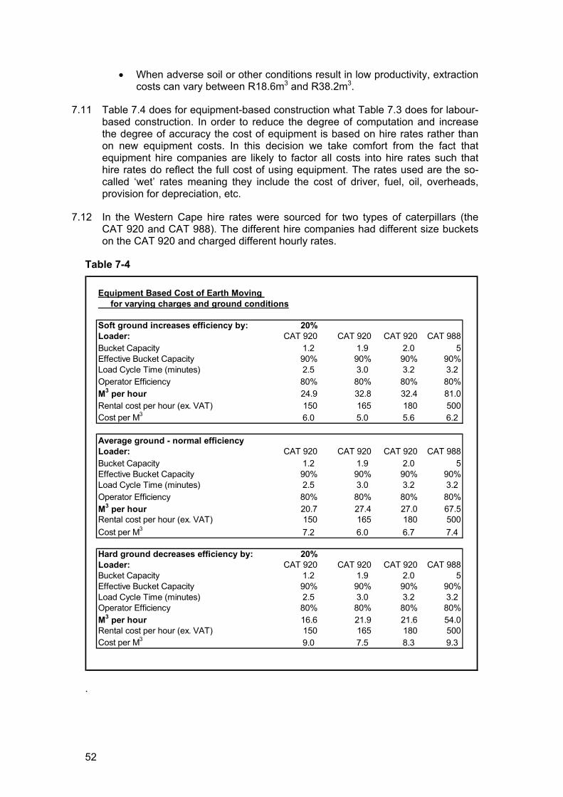
52

• When adverse soil or other conditions result in low productivity, extraction costs can vary between R18.6m3 and R38.2m3.

7.11 Table 7.4 does for equipment-based construction what Table 7.3 does for labour-based construction. In order to reduce the degree of computation and increase the degree of accuracy the cost of equipment is based on hire rates rather than on new equipment costs. In this decision we take comfort from the fact that equipment hire companies are likely to factor all costs into hire rates such that hire rates do reflect the full cost of using equipment. The rates used are the so-called ‘wet’ rates meaning they include the cost of driver, fuel, oil, overheads, provision for depreciation, etc.

7.12 In the Western Cape hire rates were sourced for two types of caterpillars (the CAT 920 and CAT 988). The different hire companies had different size buckets on the CAT 920 and charged different hourly rates.

Table 7-4

.

Equipment Based Cost of Earth Moving for varying charges and ground conditions

Soft ground increases efficiency by: 20%Loader: CAT 920 CAT 920 CAT 920 CAT 988Bucket Capacity 1.2 1.9 2.0 5Effective Bucket Capacity 90% 90% 90% 90%Load Cycle Time (minutes) 2.5 3.0 3.2 3.2 Operator Efficiency 80% 80% 80% 80%M3 per hour 24.9 32.8 32.4 81.0Rental cost per hour (ex. VAT) 150 165 180 500Cost per M3 6.0 5.0 5.6 6.2

Average ground - normal efficiencyLoader: CAT 920 CAT 920 CAT 920 CAT 988Bucket Capacity 1.2 1.9 2.0 5Effective Bucket Capacity 90% 90% 90% 90%Load Cycle Time (minutes) 2.5 3.0 3.2 3.2 Operator Efficiency 80% 80% 80% 80%M3 per hour 20.7 27.4 27.0 67.5Rental cost per hour (ex. VAT) 150 165 180 500Cost per M3 7.2 6.0 6.7 7.4

Hard ground decreases efficiency by: 20%Loader: CAT 920 CAT 920 CAT 920 CAT 988Bucket Capacity 1.2 1.9 2.0 5Effective Bucket Capacity 90% 90% 90% 90%Load Cycle Time (minutes) 2.5 3.0 3.2 3.2 Operator Efficiency 80% 80% 80% 80%M3 per hour 16.6 21.9 21.6 54.0Rental cost per hour (ex. VAT) 150 165 180 500Cost per M3 9.0 7.5 8.3 9.3

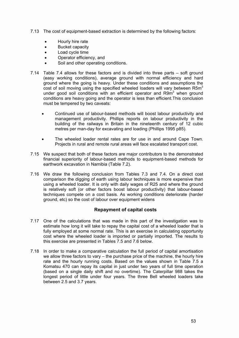
53

7.13 The cost of equipment-based extraction is determined by the following factors:

• Hourly hire rate • Bucket capacity • Load cycle time • Operator efficiency, and • Soil and other operating conditions.

7.14 Table 7.4 allows for these factors and is divided into three parts – soft ground (easy working conditions), average ground with normal efficiency and hard ground where the going is heavy. Under these conditions and assumptions the cost of soil moving using the specified wheeled loaders will vary between R5m3

under good soil conditions with an efficient operator and R9m3 when ground conditions are heavy going and the operator is less than efficient.This conclusion must be tempered by two caveats:

• Continued use of labour-based methods will boost labour productivity and management productivity. Phillips reports on labour productivity in the building of the railways in Britain in the nineteenth century of 12 cubic metres per man-day for excavating and loading (Phillips 1995 p85).

• The wheeled loader rental rates are for use in and around Cape Town. Projects in rural and remote rural areas will face escalated transport cost.

7.15 We suspect that both of these factors are major contributors to the demonstrated financial superiority of labour-based methods to equipment-based methods for earthwork excavation in Namibia (Table 7.2).

7.16 We draw the following conclusion from Tables 7.3 and 7.4. On a direct cost comparison the digging of earth using labour techniques is more expensive than using a wheeled loader. It is only with daily wages of R25 and where the ground is relatively soft (or other factors boost labour productivity) that labour-based techniques compete on a cost basis. As working conditions deteriorate (harder ground, etc) so the cost of labour over equipment widens

Repayment of capital costs

7.17 One of the calculations that was made in this part of the investigation was to estimate how long it will take to repay the capital cost of a wheeled loader that is fully employed at some normal rate. This is an exercise in calculating opportunity cost where the wheeled loader is imported or partially imported. The results to this exercise are presented in Tables 7.5 and 7.6 below.

7.18 In order to make a comparative calculation the full period of capital amortisation we allow three factors to vary – the purchase price of the machine, the hourly hire rate and the hourly running costs. Based on the values shown in Table 7.5 a Komatsu 470 can repay its capital in just under two years of full time operation (based on a single daily shift and no overtime). The Caterpillar 988 takes the longest period of little under four years. The three Bell wheeled loaders take between 2.5 and 3.7 years.

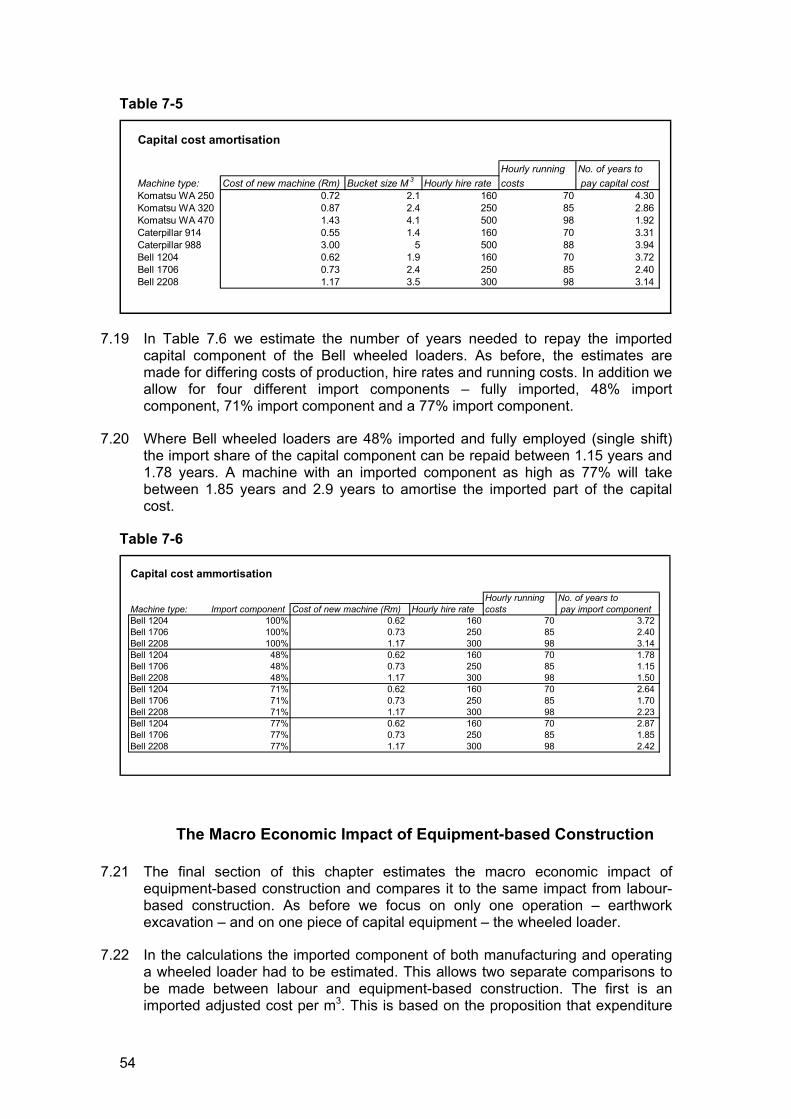
54

Table 7-5

7.19 In Table 7.6 we estimate the number of years needed to repay the imported capital component of the Bell wheeled loaders. As before, the estimates are made for differing costs of production, hire rates and running costs. In addition we allow for four different import components – fully imported, 48% import component, 71% import component and a 77% import component.

7.20 Where Bell wheeled loaders are 48% imported and fully employed (single shift) the import share of the capital component can be repaid between 1.15 years and 1.78 years. A machine with an imported component as high as 77% will take between 1.85 years and 2.9 years to amortise the imported part of the capital cost.

Table 7-6

The Macro Economic Impact of Equipment-based Construction

7.21 The final section of this chapter estimates the macro economic impact of equipment-based construction and compares it to the same impact from labour-based construction. As before we focus on only one operation – earthwork excavation – and on one piece of capital equipment – the wheeled loader.

7.22 In the calculations the imported component of both manufacturing and operating a wheeled loader had to be estimated. This allows two separate comparisons to be made between labour and equipment-based construction. The first is an imported adjusted cost per m3. This is based on the proposition that expenditure

Capital cost amortisation

Hourly running No. of years toMachine type: Cost of new machine (Rm) Bucket size M 3 Hourly hire rate costs pay capital costKomatsu WA 250 0.72 2.1 160 70 4.30 Komatsu WA 320 0.87 2.4 250 85 2.86 Komatsu WA 470 1.43 4.1 500 98 1.92 Caterpillar 914 0.55 1.4 160 70 3.31 Caterpillar 988 3.00 5 500 88 3.94 Bell 1204 0.62 1.9 160 70 3.72 Bell 1706 0.73 2.4 250 85 2.40 Bell 2208 1.17 3.5 300 98 3.14

Capital cost ammortisation

Hourly running No. of years toMachine type: Import component Cost of new machine (Rm) Hourly hire rate costs pay import componentBell 1204 100% 0.62 160 70 3.72 Bell 1706 100% 0.73 250 85 2.40 Bell 2208 100% 1.17 300 98 3.14 Bell 1204 48% 0.62 160 70 1.78 Bell 1706 48% 0.73 250 85 1.15 Bell 2208 48% 1.17 300 98 1.50 Bell 1204 71% 0.62 160 70 2.64 Bell 1706 71% 0.73 250 85 1.70 Bell 2208 71% 1.17 300 98 2.23 Bell 1204 77% 0.62 160 70 2.87 Bell 1706 77% 0.73 250 85 1.85 Bell 2208 77% 1.17 300 98 2.42

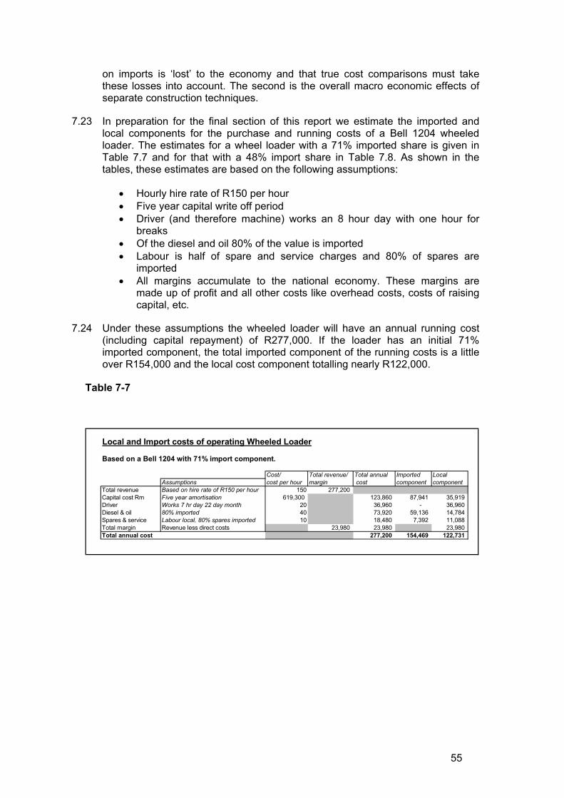
55

on imports is ‘lost’ to the economy and that true cost comparisons must take these losses into account. The second is the overall macro economic effects of separate construction techniques.

7.23 In preparation for the final section of this report we estimate the imported and local components for the purchase and running costs of a Bell 1204 wheeled loader. The estimates for a wheel loader with a 71% imported share is given in Table 7.7 and for that with a 48% import share in Table 7.8. As shown in the tables, these estimates are based on the following assumptions:

• Hourly hire rate of R150 per hour • Five year capital write off period • Driver (and therefore machine) works an 8 hour day with one hour for

breaks • Of the diesel and oil 80% of the value is imported • Labour is half of spare and service charges and 80% of spares are

imported • All margins accumulate to the national economy. These margins are

made up of profit and all other costs like overhead costs, costs of raising capital, etc.

7.24 Under these assumptions the wheeled loader will have an annual running cost (including capital repayment) of R277,000. If the loader has an initial 71% imported component, the total imported component of the running costs is a little over R154,000 and the local cost component totalling nearly R122,000.

Table 7-7

Local and Import costs of operating Wheeled Loader

Based on a Bell 1204 with 71% import component.

Cost/ Total revenue/ Total annual Imported LocalAssumptions cost per hour margin cost component component

Total revenue Based on hire rate of R150 per hour 150 277,200 Capital cost Rm Five year amortisation 619,300 123,860 87,941 35,919 Driver Works 7 hr day 22 day month 20 36,960 - 36,960 Diesel & oil 80% imported 40 73,920 59,136 14,784 Spares & service Labour local, 80% spares imported 10 18,480 7,392 11,088 Total margin Revenue less direct costs 23,980 23,980 23,980 Total annual cost 277,200 154,469 122,731

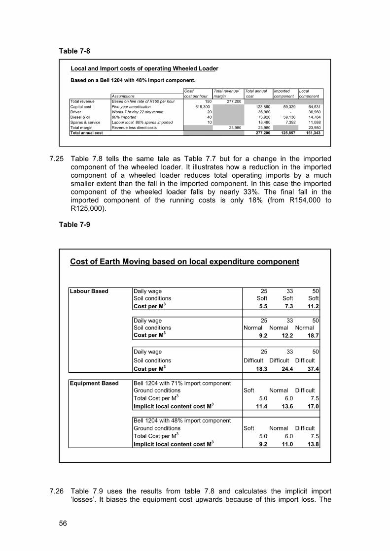
56

Table 7-8

7.25 Table 7.8 tells the same tale as Table 7.7 but for a change in the imported component of the wheeled loader. It illustrates how a reduction in the imported component of a wheeled loader reduces total operating imports by a much smaller extent than the fall in the imported component. In this case the imported component of the wheeled loader falls by nearly 33%. The final fall in the imported component of the running costs is only 18% (from R154,000 to R125,000).

Table 7-9

7.26 Table 7.9 uses the results from table 7.8 and calculates the implicit import ‘losses’. It biases the equipment cost upwards because of this import loss. The

Local and Import costs of operating Wheeled Loader

Based on a Bell 1204 with 48% import component.

Cost/ Total revenue/ Total annual Imported LocalAssumptions cost per hour margin cost component component

Total revenue Based on hire rate of R150 per hour 150 277,200Capital cost Five year amortisation 619,300 123,860 59,329 64,531Driver Works 7 hr day 22 day month 20 36,960 - 36,960Diesel & oil 80% imported 40 73,920 59,136 14,784Spares & service Labour local, 80% spares imported 10 18,480 7,392 11,088Total margin Revenue less direct costs 23,980 23,980 23,980Total annual cost 277,200 125,857 151,343

Cost of Earth Moving based on local expenditure component

Labour Based Daily wage 25 33 50Soil conditions Soft Soft SoftCost per M3 5.5 7.3 11.2

Daily wage 25 33 50Soil conditions Normal Normal NormalCost per M3 9.2 12.2 18.7

Daily wage 25 33 50Soil conditions Difficult Difficult DifficultCost per M3 18.3 24.4 37.4

Equipment Based Bell 1204 with 71% import componentGround conditions Soft Normal DifficultTotal Cost per M3 5.0 6.0 7.5Implicit local content cost M3 11.4 13.6 17.0

Bell 1204 with 48% import componentGround conditions Soft Normal DifficultTotal Cost per M3 5.0 6.0 7.5Implicit local content cost M3 9.2 11.0 13.8

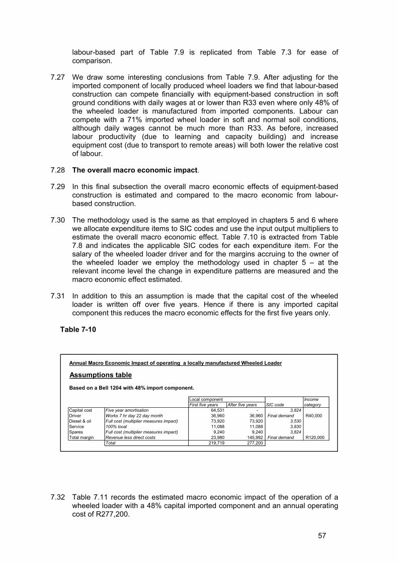
57

labour-based part of Table 7.9 is replicated from Table 7.3 for ease of comparison.

7.27 We draw some interesting conclusions from Table 7.9. After adjusting for the imported component of locally produced wheel loaders we find that labour-based construction can compete financially with equipment-based construction in soft ground conditions with daily wages at or lower than R33 even where only 48% of the wheeled loader is manufactured from imported components. Labour can compete with a 71% imported wheel loader in soft and normal soil conditions, although daily wages cannot be much more than R33. As before, increased labour productivity (due to learning and capacity building) and increase equipment cost (due to transport to remote areas) will both lower the relative cost of labour.

7.28 The overall macro economic impact.

7.29 In this final subsection the overall macro economic effects of equipment-based construction is estimated and compared to the macro economic from labour-based construction.

7.30 The methodology used is the same as that employed in chapters 5 and 6 where we allocate expenditure items to SIC codes and use the input output multipliers to estimate the overall macro economic effect. Table 7.10 is extracted from Table 7.8 and indicates the applicable SIC codes for each expenditure item. For the salary of the wheeled loader driver and for the margins accruing to the owner of the wheeled loader we employ the methodology used in chapter 5 – at the relevant income level the change in expenditure patterns are measured and the macro economic effect estimated.

7.31 In addition to this an assumption is made that the capital cost of the wheeled loader is written off over five years. Hence if there is any imported capital component this reduces the macro economic effects for the first five years only.

Table 7-10

7.32 Table 7.11 records the estimated macro economic impact of the operation of a wheeled loader with a 48% capital imported component and an annual operating cost of R277,200.

Annual Macro Economic Impact of operating a locally manufactured Wheeled Loader

Assumptions table

Based on a Bell 1204 with 48% import component.

Local component IncomeFirst five years After five years SIC code category

Capital cost Five year amortisation 64,531 - 3,824 Driver Works 7 hr day 22 day month 36,960 36,960 Final demand R40,000Diesel & oil Full cost (multiplier measures impact) 73,920 73,920 3,530 Service 100% local 11,088 11,088 3,830 Spares Full cost (multiplier measures impact) 9,240 9,240 3,824 Total margin Revenue less direct costs 23,980 145,992 Final demand R120,000

Total 219,719 277,200

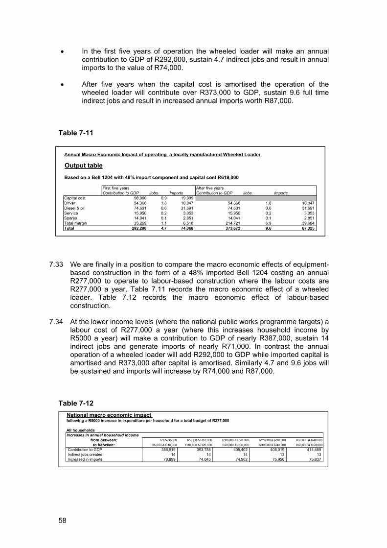
58

• In the first five years of operation the wheeled loader will make an annual contribution to GDP of R292,000, sustain 4.7 indirect jobs and result in annual imports to the value of R74,000.

• After five years when the capital cost is amortised the operation of the wheeled loader will contribute over R373,000 to GDP, sustain 9.6 full time indirect jobs and result in increased annual imports worth R87,000.

Table 7-11

7.33 We are finally in a position to compare the macro economic effects of equipment-based construction in the form of a 48% imported Bell 1204 costing an annual R277,000 to operate to labour-based construction where the labour costs are R277,000 a year. Table 7.11 records the macro economic effect of a wheeled loader. Table 7.12 records the macro economic effect of labour-based construction.

7.34 At the lower income levels (where the national public works programme targets) a labour cost of R277,000 a year (where this increases household income by R5000 a year) will make a contribution to GDP of nearly R387,000, sustain 14 indirect jobs and generate imports of nearly R71,000. In contrast the annual operation of a wheeled loader will add R292,000 to GDP while imported capital is amortised and R373,000 after capital is amortised. Similarly 4.7 and 9.6 jobs will be sustained and imports will increase by R74,000 and R87,000.

Table 7-12

Annual Macro Economic Impact of operating a locally manufactured Wheeled Loader

Output table

Based on a Bell 1204 with 48% import component and capital cost R619,000

First five years After five yearsContribution to GDP Jobs Imports Contribution to GDP Jobs Imports

Capital cost 98,060 0.9 19,909 Driver 54,360 1.8 10,047 54,360 1.8 10,047 Diesel & oil 74,601 0.6 31,691 74,601 0.6 31,691 Service 15,950 0.2 3,053 15,950 0.2 3,053 Spares 14,041 0.1 2,851 14,041 0.1 2,851 Total margin 35,269 1.1 6,518 214,721 6.9 39,684 Total 292,280 4.7 74,068 373,672 9.6 87,325

National macro economic impact following a R5000 increase in expenditure per household for a total budget of R277,000

All householdsIncreases in annual household income

from between: R1 & R5000 R5,000 & R10,000 R10,000 & R20,000 R20,000 & R30,000 R30,000 & R40,000to between: R5,000 & R10,000 R10,000 & R20,000 R20,000 & R30,000 R30,000 & R40,000 R40,000 & R50,000

Contribution to GDP 386,919 393,758 405,402 408,019 414,459 Indirect jobs created 14 14 14 13 13 Increased in imports 70,899 74,043 74,902 75,950 75,837

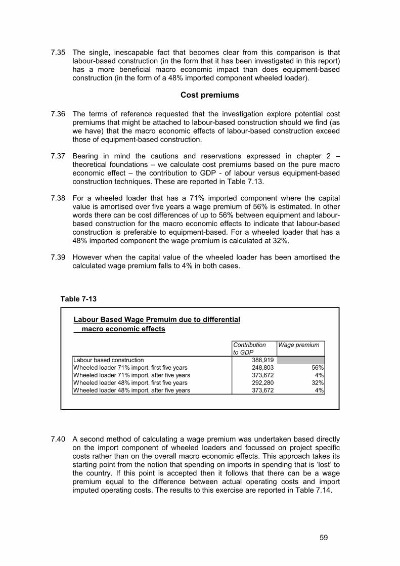
59

7.35 The single, inescapable fact that becomes clear from this comparison is that labour-based construction (in the form that it has been investigated in this report) has a more beneficial macro economic impact than does equipment-based construction (in the form of a 48% imported component wheeled loader).

Cost premiums

7.36 The terms of reference requested that the investigation explore potential cost premiums that might be attached to labour-based construction should we find (as we have) that the macro economic effects of labour-based construction exceed those of equipment-based construction.

7.37 Bearing in mind the cautions and reservations expressed in chapter 2 – theoretical foundations – we calculate cost premiums based on the pure macro economic effect – the contribution to GDP - of labour versus equipment-based construction techniques. These are reported in Table 7.13.

7.38 For a wheeled loader that has a 71% imported component where the capital value is amortised over five years a wage premium of 56% is estimated. In other words there can be cost differences of up to 56% between equipment and labour-based construction for the macro economic effects to indicate that labour-based construction is preferable to equipment-based. For a wheeled loader that has a 48% imported component the wage premium is calculated at 32%.

7.39 However when the capital value of the wheeled loader has been amortised the calculated wage premium falls to 4% in both cases.

Table 7-13

7.40 A second method of calculating a wage premium was undertaken based directly on the import component of wheeled loaders and focussed on project specific costs rather than on the overall macro economic effects. This approach takes its starting point from the notion that spending on imports in spending that is ‘lost’ to the country. If this point is accepted then it follows that there can be a wage premium equal to the difference between actual operating costs and import imputed operating costs. The results to this exercise are reported in Table 7.14.

Labour Based Wage Premuim due to differential macro economic effects

Contribution Wage premiumto GDP

Labour based construction 386,919 Wheeled loader 71% import, first five years 248,803 56%Wheeled loader 71% import, after five years 373,672 4%Wheeled loader 48% import, first five years 292,280 32%Wheeled loader 48% import, after five years 373,672 4%

60

7.41 Table 7.4 is sourced from Tables 7.4 and 7.9 and indicates the cost differential that might be applied to labour for differing ground conditions. Hence on soft ground this cost premium can be as high as 36%, in average conditions 30% and in difficult terrain 24%.

Table 7-14

Conclusion

7.42 It has been shown that the macro economic effects of a certain labour-based construction operation are greater than those of equipment-based construction. A case can therefore be made for a financial premium for the substitution of labour for equipment.

7.43 These results are sensitive to the imported component of locally manufactured construction equipment. The factor that most effects size of the financial premium is the degree to which the capital cost of the equipment has been amortised. Comparing the macro economic effect of labour against new earth moving equipment with a 71% imported component indicates that a labour premium of over 50% is justified. However once the capital cost is fully amortised then this premium falls to 4%. Similarly comparing labour to a machine with 48% import component calls for a 32% labour premium when the machine is new but again only 4% when fully amortised.

7.44 An alternative approach that looks at the direct cost of labour and equipment – rather than the macro economic effects – concludes that under certain conditions labour can compete directly with equipment and result in no cost premium. However as ground conditions deteriorate the cost premium between labour and equipment opens rapidly. These calculations are based on fixed estimates for labour productivity. The reality of labour-based projects is that labour productivity rates can be improved after training over the duration of the programme.

7.45 Alternatively, it can be shown that if we view the import component of locally manufactured earth moving equipment as ‘lost’ expenditure (lost to the country) then labour can compete financially with equipment under a much greater range of physical conditions and wages. This methodology yields a cost premium of 36% in soft conditions falling to 24% in difficult conditions.

Cost differentials between operating cost and implicit local content cost

Costs per m3 for a 10 ton wheeled loader with 1.9 m3 bucket with 48% import component

Actual cost Implicit local content cost Cost differentialSoft conditions 5.0 9.2 36%Average conditions 6.0 11.0 30%Difficult conditions 7.5 13.8 24%

61

8 Conclusion

8.1 What is the cost of building roads and dams and other useful assets? How many jobs can be created and what is the economic impact. Why not, in a country with desperate poverty and unemployment, use people rather than machines to build roads and dams? The roads and dams are needed, as is other infrastructure. The people are able and willing to work.

8.2 One of the answers is cost. Under extreme ground and climatic conditions machines can perform better than people. But not always. Whether people or machines perform better depends on costs, wages and productivity.

8.3 Experiences in Lesotho, Botswana (McCutcheon, 1991), Uganda (Taylor and Bekabye 1999) and Namibia (Ministry of Works, 2000) all demonstrate that labour-based methods are financially viable for road building and rehabilitation.

8.4 In South Africa the known higher labour cost and the suspected lower capital cost conspire against the financial viability of labour-based methods. On the Ugandan road rehabilitation programme average daily wages were the rand equivalent of R7.80 a day (at R6.50 per US$) or R8.90 a day (at R7.40 per US$) (calculated from Taylor and Bekabye 1999 p vi). In Uganda a daily wage of R26.00 or R29.60 (respectively at the two exchange rates) was the upper limit for the financial viability of labour intensive road rehabilitation.

8.5 In South Africa, in the Northern Province, for example, statutory minimum wages in civil engineering are currently R4.15 for rural areas and R5.25 for urban areas (Government Gazette 12 November 1999). This is the daily equivalent of R33.20 and R42.00 respectively.

8.6 In contrast to these minimum wages, R20 to R30 a day was the most common wage paid on the labour intensive public works projects investigated by SALDRU (1999). It was found that there is a direct relationship between proximity to Cape Town and project wages. Some projects, one in Hout Bay for example, paid R50 a day, while at the other extreme projects in Prince Albert paid R15 a day and in Barrydale R12 a day.

8.7 In this investigation one construction task was analysed to determine the financial viability of labour-based methods under various working conditions and wages. The selected task was earthwork excavation and the chosen machine a wheeled loader. It is shown that labour-based earthwork excavation is financially viable at wages of less than R25 a day with easy ground conditions. The wheeled loader is financially superior as wages rise and/or ground conditions deteriorate.

8.8 Two factors are likely to mitigate this conclusion.

8.9 First, this analysis was conducted on the basis of equipment hire rates in the Cape Town metropolitan area. It is likely that equipment costs will be higher in rural and remote rural areas, if only because of transport costs. Under these conditions labour-based earthwork excavation will be viable financially under a greater range of ground types and at higher wages.

62

8.10 Second, the analysis did not take into account the potential for learning on the job and other labour productivity gains that can be achieved using a programme approach to project planning. Many commentators advocate the virtues of using a programme approach for labour-based methods and increasing labour usage in an incremental and financially viable manner.

8.11 A second strand of the investigation focussed on the macroeconomic consequences of the choice between labour and equipment-based methods with the objective of determining whether labour-based methods have macroeconomic advantages over using machines. In most developing countries there is little debate and labour-based methods have far greater macroeconomic benefits than equipment-based techniques. South Africa is different. South Africa makes its own earthmoving equipment, produces a substantial amount of its own oil, produces spare parts locally, and has specialised mechanics and technicians who are residents not contracted expatriates. Hence macroeconomic estimates were made for labour and equipment-based methods.

8.12 This part of the analysis was challenged by limited information on locally produced equipment and local content had to be estimated within bounded assumptions.

8.13 It is shown under these assumptions that labour-based methods have considerable macroeconomic advantages over equipment-based methods for both fully imported and locally made wheeled loaders. However this advantage becomes marginal when the capital cost of the wheeled loader has been amortised.

8.14 Better information on the cost of equipment might prove that there is no macroeconomic advantage to labour-based methods.

8.15 One of the most debated issues is the saving of foreign exchange. There is no doubt that a reduction in imported capital equipment will save on foreign exchange. This foreign exchange is then available to fund other kinds of imports or to be kept in the country and fund local production. It should be recognised that, if there are cost premiums involved, these savings on foreign exchange are at the expense of standards of living.

8.16 A policy conflict exists if it occurs that labour and equipment-based methods have similar macroeconomic effects and labour-based methods cost more. This conflict is between the promotion of a demonstrated comparative advantage in the production of construction equipment and the generation of economic empowerment and a less skewed distribution of income. In this case the choice of labour-based methods is based on the argument that equipment-based methods prevent the very poor from participating in the formal economy. They are therefore marginalised and disempowered. Hence labour-based methods have positive externalities that go beyond anything that can be measured using conventional macroeconomic techniques.

8.17 The overwhelming case that must be made for using labour-based methods is the contribution it will make to economic empowerment. Roads, dams and other infrastructure are good for the regional economy and will allow it to grow. Using labour-based methods will generate jobs and provide incomes further promoting the regional economy. Involving local communities will help in capacity building. Using small and emergent contractors will generate sustainable incomes and opportunities.

63

8.18 It is beyond the scope of this report to attempt to quantify the effects of labour-based methods on economic empowerment. In a similar vein we cannot quantify the cost of economically marginalising poor rural people by using equipment-based methods. Yet, even without being able to quantify these effects, we believe that there is an overwhelming case for labour-based methods. Not only will it help the poor but also it will contribute to the generation of sustained economic growth and empowerment.

8.19 This investigation has raised as many questions as it has answered and suggests several strands for future research. Some of this research can be facilitated by a systematic collection of data on labour intensive projects.

8.20 A more careful and detailed investigation is warranted into the local content of South African manufactured earth moving equipment. Also needed is a more detailed profile of the operating costs of different types of construction equipment and the local content component. What is the productivity rate of different types of equipment? How does, for example, bucket size and operator efficiency impact on productivity? How does the age of a machine impact on productivity. What is the relationship between equipment age and breakdowns? Do machines breakdown more often once capital costs are amortised and therefore have lower macroeconomic effects than estimated here?

8.21 A more focussed view is needed on wages paid in the construction industry. This study found many problems trying to capture a fine resolution on wages and how these vary by skill level and location. This could be done by a small survey, a straw poll or, possibly, through tender documentation. These should be compared to wages paid on the National Public Works Programme.

8.22 Labour productivity on projects must be carefully monitored and recorded. This is best achieved using choice of technique analysis. This will allow for an incremental approach to labour-based methods and give a full profile of labour productivity under a variety of working conditions. It will also allow for an analysis of labour productivity over time and better identification of the factors that promote labour productivity.

8.23 More attention must be paid to the secondary effects from the application of labour-based methods. This study made use of national surveys and input output relationships. A more fine-grained focus is needed and simply describing these effects is not enough. It is recommended that such a study establish a methodology that will carefully measure these secondary effects. The intention should be to have a better understanding of the impact of the National Public Works Programme on poverty alleviation and economic empowerment.

ENDS

64

References

Bulmer-Thomas, V. (1982). Input Output Analysis in Developing Countries. New York: John Wiley and Sons Ltd.

Leontief, W. (1986). Input-Output Economics. Second edition. New York: Oxford University Press, Inc.

Ministry of Works, Transport and Communication, Republic of Namibia, 2000: Draft report on the Impact Assessment of Labour-Based Technology Application in the Provision of Infrastructural Services, Windhoek.

Miller, R.E. & Blair, P.D. (1985). Input-Output Analysis: Foundations and Extensions. Englewood Cliffs, New Jersey: Prentice-Hall inc.

McCutcheon, R (1991): “The main findings of the district pilot project of labour intensive road construction and maintenance in Botswana and the implications for similar projects in South Africa”, Development Southern Africa, vol. 8 No. 2

Muller, A.P.(1992) The importance of promoting tourism and its multiplier for local authorities. The South African Treasurer; Vol. 64, Iss 4, p.68-69, Apr, 1992.

North, D.C. (1955) “Location Theory and Regional Economic Growth.” Journal of Political Economy, pp 243-258.

O’Connor, R. & Henry, E. W. (1975). Input-output analysis and its applications. London and High Wycombe: Charles Griffin & Company Limited.

SALDRU (1999): From Works to Public Works. The performance of labour intensive public works in Western Cape Province, South Africa, SALDRU, University of Cape Town.

Sohn, I. (1986). Readings in Input-Output Analysis: Theory and Applications. New York: Oxford University Press, Inc.

South Africa (Republic of), Central Statistical Services. Input-Output Tables, 1993. Government Printers – Pretoria.

Statistics SA: Final supply and use tables, 1993, Report No. 04 – 04 – 01

Taylor, G. and Bekabye, M. 1999: An Opportunity for Employment Creation, Labour-based Technology in Roadworks: The Macro-Economic Dimension. Uganda.. International Labour Organisation.

United Nations Publication (1966). Problems of Input-Output Tables and Analysis. United Nations, New York.

Van Seventer, D.E.N. Decomposition of interdependencies in the South African economy. Journal for studies in economics and econometrics; Vol. 14, Iss 3, p.53-72, Nov, 1990.

65

Appendix. Terms of Reference

Introduction and Background

1.1 The National Department of Public Works (NDPW) is working on a number of different fronts to reorient the construction sector. The most important underlying aim is to enhance and optimise employment in the construction process itself. In parallel with this, a supplementary aim is to provide targeted opportunities for emerging and previously disadvantaged contractors. The most prominent examples of initiatives completed or under way include:

• the National Public Works Programme (NPWP) launched in 1994/95 and comprising the Community-Based Public Works Programme (CBPWP) and a set of 12 pilot projects (testing the extent to which employment could be optimised whilst relying on mainstream technical consultants and contractors) ;

• the preparation and promotion of a set of Guidelines on Enhancing Employment Opportunities in the Delivery of Infrastructure Projects based on the experience gained and lessons learned through the pilot projects component of the NPWP,

• .the Strategic Projects Initiative (SPI) under which targeted procurement (TP) is aiming for the use of black prime contractors in the implementation of medium and large-scale projects on behalf of the NDPW.

• the Construction Industry Development Programme (CIDP), under which progress is being made towards the creation of a statutory Construction Industry Development Board (CIDB), and which also includes an Emerging Contractors Development Programme (ECDP).

1.2 In mid-1996, as these initiatives were at earlier stages of conception or implementation, the NPWP Branch of NDPW requested continuing advisory and research resources from the International Labour Office (ILO). The rationale was twofold. First, the NPWP Branch was eager to draw on international experience with respect to the use of labour-based methods in construction. Secondly (and complementary to this), the NDPW as a whole emphasised that employment creation through construction should not take precedence over (a) value for money to the public sector client, or (b) quality standards in construction outputs. It was these two concerns that led to the title of the current ILO project - Support to the Efficient Application of Labour-Based Methods in the Construction Sector.

The Concept of Efficiency in Value for Money

1.3 In exactly the same way as the calculation of an internal rate of return on investment, the concept of efficiency in value for money can also be analysed in both financial and economic terms.

1.4 In the production of physical outputs, construction is already relatively labour intensive. Certainly, in comparison with international trends towards mechanisation and robotisation in the manufacturing and appliance assembly industries, even the most equipment-intensive approaches to construction still rely on labour for some operations and activities. Nevertheless, in terms of

66

practical feasibility alone, labour can be fully substituted for equipment in the great majority of civil works projects. The original diamond mine at Kimberley is one of many domestic examples in the mining industry of the extent to which this was - hence (in practical terms) still is - possible.

1.5 The key issue, therefore, is not what the technical boundaries may be for the substitution of labour for equipment. It is rather a matter of (a) when it makes financial sense to do so, and (b) when the overall economic benefit of increased employment, may outweigh any financial premium paid for a given output.

Financial Limits for Labour Substitution

1.6 The financial boundary to the substitution of labour for equipment in construction can be set quite simply and clearly. It is that the enhancement of employment should not lead to a higher cost for a given construction output than for any other balance of labour and equipment inputs. The main issues at stake are the cost of labour per unit output and associated management and supervision costs.

1.7 As noted, it is practically feasible for the complete substitution of labour for mechanised equipment in most civil engineering projects. It is even possible to achieve adequate compaction of earth in roadwork’s using labour-intensive methods. The problem is, however, that the amount of effort required - the work-day inputs, hence the costs - are usually so high that compaction by hand is rarely even considered.

1.8 In sum, the financial limit for substituting labour for equipment in construction is set by the lowest price for which the very same output could be produced by means of any other balance of factor inputs.

1.9 The 'Big Hole' at Kimberley involved the manual excavation of in the order of 60 million tonnes of solid rock. This was then carefully crushed and washed - again by hand - yielding about 45 grams of diamonds per thousand tonnes excavated.

Economic Limits for Labour Substitution

1.10 The economic limits for substituting labour for equipment are more complex. Not only are the economics themselves complicated, but labour substitution as a whole raises complex political issues, particularly in South Africa. There are two broad fronts on which economic valuation is required:

i) the economic benefit of incremental employment:

ii) the economic cost (or benefit) of using equipment.

The Economic Value of Employment

1.11 Keynesian theory emphasises that in conditions of high unemployment, hence broadly depressed demand for goods and services, employment-intensive construction programmes not only support the subsistence of those engaged. They have wider beneficial effects in two main directions:

i) the wages earned give increased purchasing power among the direct beneficiaries (and in turn, there are beneficial multiplier effects among the industries satisfying that demand);

67

ii) there are benefits to those sectors on which the construction industry itself relies - most notably the building materials industry.

1.12 In other words, there are both backward and forward economic linkages which may justify increased spending on labour in construction. The key question is what such linkages offer in terms of aggregate economic benefits? If the benefits of using more labour are strong, the government can take a policy decision. As a key client of the construction industry, it may decide to reap the economic advantage of employment by means of paying a financial premium for a construction process which substitutes more labour for equipment than the industry itself would otherwise choose.

Scope of Work

1.13 The scope of work is determined by the Terms of Reference: The research to be undertaken will aim to provide an answer to the following question:

• what - if any - financial premium per unit of expenditure on construction is economically justified for the substitution of labour for equipment?

1.14 The research will focus on the fronts of both labour and equipment, as indicated below.

Labour Economics

1.15 The starting point for work on this front will be to analyse regional differences in wage levels in relation to prevailing costs of living (in terms of a standard consumption 'basket'). What, if any, are the real differences in wage levels (or earning levels among those paid on a piece-work or task-work basis) in construction -say, for (a) a skilled bricklayer, and (b) an unskilled labourer - in Western Cape, Eastern Cape and Northern Provinces?

1.16 At the next level of detail, the research will explore the likely primary directions of expenditure among those employed under a labour-intensive policy framework set by the government. What shares of incremental income are likely to be spent on food, clothing, house improvements and the like?

1.17 The outcome of the analysis of labour economics will be to establish a multiplier effect for wages in construction.

Equipment Economics

1.18 Most developing countries are obliged to import any equipment to be used in the construction industry. As such, the economics of equipment utilisation are set by the opportunity cost of scarce foreign exchange. In South Africa, however, there is already a domestic construction equipment manufacturing industry. This is dominated by Bell Equipment, though other brands of equipment are imported. The research will establish the proportion of the value of demand for equipment that is satisfied by domestic manufacture versus imported items.

1.19 Of course, the domestic manufacture of construction also has employment benefits, albeit only a limited number of relatively high wage-earning opportunities. The research will calculate a multiplier effect for earnings in this

68

domestic industry to set against that of incremental employment in construction itself.

1.20 For imported equipment, the research will establish an opportunity cost for foreign exchange which could be used for other developmental purposes.

1.21 The choice of labour-based methods in construction is likely not only to depress overall demand for equipment but to shift the pattern of that reduced demand towards lighter and intermediate items. The research will gather data from Bell Equipment and any other major domestic equipment manufacturers on the share of labour in the cost of manufacturing different types and sizes of equipment. These data will be used to calculate the wage (and wage multiplier) effects of possible changes in the pattern of demand for construction equipment.

Methodology

1.22 The research is expected to involve three main stages:

i) conceptualisation, including the development of an economic modelling approach;

ii) the collection of data and information - both on the labour economics and equipment economics fronts:

iii) computer modelling of changes in the balance of labour and equipment factor inputs for construction and associated costs and benefits

1.23 The first stage will be of critical importance as it may affect the scope and nature of data collection and the time required for computer modelling. Accordingly, an Inception Report should be prepared on completion of the first stage of work, including detailed proposals of work required in the second and third stages.

69

RECENT SOCIO-ECONOMIC TECHNICAL PAPERS

No.1 Willem Keddeman, Of Nets and Assets. Effects and Impacts of Employment-Intensive Programmes - A Review of the ILO Experience, 1998.

No.2 Laura Murphy, Rapid Assessment of Poverty Impacts (RAPI) - Elaboration of a Rapid Survey Method of Assessing the Poverty Reduction Impacts of Pilot Employment-Intensive Projects, 1998.

No.3 Franco Olivier et Eddy Bynens, L’Approche HIMO et les Investissements routiers - Perspectives pour la Création d’Emplois et l’Economie de Devises à Madagascar, 1998.

No. 4 Peter Oakley and Ian Clegg, Participation and Poverty Alleviation in Sub-Saharan Africa - Review of the Literature and Practice, 1998.

No.5 Michael Hopkins, An Independent Thematic Evaluation: ILO’s Employment Intensive Programme, 1998.

No. 6 Gary Taylor et Moses Bekakkye, An Opportunity for Employment Creation: Labour-based Technology in Roadworks - The Macro-Economic Dimension, Uganda, 1999.

No. 7 Gabriel Siri, Employment and Social Investment Funds in Latin America, 2000.

No. 8 Kaj Thorndahl, The DANIDA Support to the Employment-Intensive Investment Programme (EIIP) - An External Evaluation, 2001.

No. 9 A. Van der Goes and S. Mastwijk, Socio-economic Development Initiative (SDI) - A discussion paper on planning and implementing socio-economic investments, 2001.

No. 10 Piet Goovaerts, Employment and social Investment Funds in Central/Eastern Europe and The Commonwealth of Independant States (CEE/CIS),2001

No. 11 Khem Raj Sharma, Organisation, Negotiation and Contracting: Case Study of West Gandak and Marchawar Lift Irrigation Systems (Nepal), 2002.

No. 12 Sandra O. Yu , Infrastructure Development and the Informal Sector in the Philippines, 2002.

No. 13 Jane Tournée et Wilma van Esch, Approches et pratiques en contrats communautaires. Leçons tirées d’expériences de terrain, 2002.

Socio-EconomicTechnical Papers (SETPs) are produced by the Employment-Intensive Investment Programme (EIIP) of the Employment-Intensive Investment Branch (EMP/INVEST) of the ILO. They are intended to make information on social and economic aspects of labour-based growth strategies and investment programmes easily accessible to interested organisations, institutions and individuals.