


Bahasa
Halaman
Hukum

CEP Discussion Paper No 827
October 2007
Testing the "Waterbed" Effect in Mobile Telephony
Christos Genakos and Tommaso Valletti

Abstract This paper examines the impact of regulatory intervention to cut termination rates of calls from fixed lines to mobile phones. Under quite general conditions of competition, theory suggests that lower termination charges will result in higher prices for mobile subscribers, a phenomenon known as the “waterbed” effect. The waterbed effect has long been hypothesized as a feature of many two-sided markets and especially the mobile network industry. Using a uniquely constructed panel of mobile operators’ prices and profit margins across more than twenty countries over six years, we document empirically the existence and magnitude of this effect. Our results suggest that the waterbed effect is strong, but not full. We also provide evidence that both competition and market saturation, but most importantly their interaction, affect the overall impact of the waterbed effect on prices. Keywords: telecommunications, regulation, "Waterbed" effect, two-sided markets JEL Classifications: D21, L51, L96 This paper was produced as part of the Centre’s Productivity and Innovation Programme. The Centre for Economic Performance is financed by the Economic and Social Research Council. Acknowledgements We would like to thank Steffen Hoernig, Tobias Kretschmer, Marco Manacorda, Elias Papaioannou, Jonathan Sandbach, Jean Tirole, Julian Wright, John Van Reenen and seminar audiences in Barcelona, Paris and 8th CEPR Empirical IO meeting for helpful comments and discussions. We are also grateful to Bruno Basalisco for research assistance. We acknowledge research funding from Vodafone. The opinions expressed in this paper and all remaining errors are those of the authors alone. Christos Genakos is a Research Associate with the Productivity and Innovation Programme at the Centre for Economic Performance, London School of Economics. He is also a Lecturer in Economics at Selwyn College, University of Cambridge. Tommaso Valletti is Professor of Economics at Imperial College London. Published by Centre for Economic Performance London School of Economics and Political Science Houghton Street London WC2A 2AE All rights reserved. No part of this publication may be reproduced, stored in a retrieval system or transmitted in any form or by any means without the prior permission in writing of the publisher nor be issued to the public or circulated in any form other than that in which it is published. Requests for permission to reproduce any article or part of the Working Paper should be sent to the editor at the above address. © C. Genakos and T. Valletti, submitted 2007 ISBN 978 0 85328 090 3
1
1. Introduction
Mobile termination charges4 have become the regulators’ focus of concern
worldwide in recent years. Especially regarding the fixed-to-mobile termination rates,
a large theoretical literature has demonstrated that independently of the intensity of
competition for mobile customers, mobile operators have an incentive to set charges
that will extract the largest possible surplus from fixed users.5 This competitive
bottleneck problem provided justification for regulatory intervention to cut these
rates. However, reducing the level of termination charges can potentially increase the
level of prices for mobile subscribers, causing what is known as the “waterbed”
effect. The main purpose of this paper is to examine the existence and magnitude of
the waterbed effect in the mobile telephony industry.
Both regulators and academics have recognized the possibility that this effect
might be at work and be strong in practice. The first such debate started in 1997 in the
UK with the original investigation by the Monopolies and Mergers Commission (now
Competition Commission).6 Another example is the New Zealand Commerce
Commission which, in its 2005 investigation, initially took the position that mobile
subscription prices would rise in response to a cut in termination rates only if mobile
firms operated in a perfectly competitive environment. The Commission was
subsequently convinced that the waterbed effect is a more general phenomenon, but
there remained doubts about the importance of such an effect. The most recent
termination rate proposals by the UK regulator Ofcom considered the issue of the
waterbed in order to analyse the impact of regulation of call termination. Ofcom
acknowledged the importance of the waterbed effect, but questioned whether the
effect was “complete”, arguing that this can only be the case if the retail market is
sufficiently competitive.7
Yet, despite the importance of the waterbed effect for welfare calculations, no
systematic evidence exists on its existence or magnitude. Casual empiricism suggests
that mobile subscription prices have been decreasing quite steadily over time in
4 These are the charges mobile operators levy on either fixed network operators or other mobile operators for terminating calls on their networks. 5 See, for example, Armstrong (2002), Wright (2002), Valletti and Houpis (2005) and Hausman and Wright (2006). Armstrong and Wright (2007) also provide an excellent overview of the mobile call termination theoretical literature and policy in the UK. 6 The term “waterbed” was first coined by the late Prof. Paul Geroski, chairman of the Competition Commission in the UK, at the time of the first investigation on interconnection charges in the mobile industry. 7 See “Mobile call termination, Proposals for consultation”, Ofcom, September 2006.
2
virtually every country, despite the regulation of mobile termination rates. At the
same time, though, the industry has become more competitive, with additional entry,
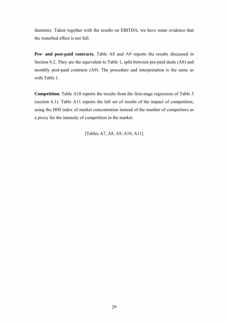
tougher competition, etc., exerting a countervailing force. As an example, Figure 1
plots the evolution of subscription prices and termination rates in France. While
termination rates have been cut steadily over the years, prices to medium user
customers have remained more or less constant. Does this imply there is no waterbed
effect? Not necessarily as competition in the industry might also have intensified and
other trends, such as economies of scale due to growth in traffic volumes, may also
mask the impact of the waterbed on subscription prices.
[Figure 1]
In this paper we analyze the impact of fixed-to-mobile termination rate regulation
on prices and profit margins on a newly constructed dataset of mobile operators
across more than twenty countries during the last decade. The timing of the
introduction of regulated termination rates, but also the severity with which they were
imposed across mobile firms, varied widely and has been driven by legal and
institutional aspects of each country. Using quarterly frequency data and employing
panel data techniques that control for unobserved time-invariant country-operator
characteristics and general time trends, we are able to identify and quantify for the
first time this waterbed effect. Our estimates suggest that although regulation reduced
termination rates by about ten percent, this also led to a ten percent increase in mobile
outgoing prices on average. This waterbed effect is shown to be robust to different
variable definitions and datasets.
However, although the waterbed is shown to be high, our analysis also provides
evidence that it is not full: accounting measures of profits are positively related to
MTR, thus mobile firms suffer from cuts in termination rates. Finally, our empirical
analysis also reveals that both competition and market saturation, but most
importantly their interaction, affect the overall impact of the waterbed effect on
prices: the waterbed effect is stronger the more intense competition is in markets with
high levels of market penetration and high termination rates.
Our paper is related to an emerging literature on “two-sided” markets that studies
how platforms set the structure of prices across the two sides of the business (see
Armstrong, 2006, and Rochet and Tirole, 2006). Telecommunications networks are

3
examples of two-sided markets: providing communication services to their own
customers over the same platform and providing connectivity to their customer base
to other networks. The two markets are linked: more subscribers on the network
means more opportunities for users of other networks to make calls. Whenever we
look at two-sided markets, the structure of prices (i.e., who pays for what) is
fundamentally important for the development of the market. In mobile telephony,
typically it is only senders that pay (under the Calling Party Pays – CPP – system),
while receivers do not. This is why termination rates are not the locus of competition
and, if left unregulated, they will be set at the monopoly level.8 This is also a case
where the mobile firms sell two goods with interdependent demand: at any given
termination rate, the volume of fixed-to-mobile calls that an operator receives depend
on the number of mobile subscribers on its network. In a sense, mobile subscribers
and fixed-to-mobile calls are complements, as an increase in the number of
subscribers will cause an increase in the volume of fixed-to-mobile calls.9 Our work
therefore also contributes to the more general understanding of two-sided markets.
Recent empirical works on two-sided markets include Rysman (2004, on yellow
pages; 2007 on credit cards), Argentesi and Filistrucchi (2006, on newspapers), and
Kaiser and Wright (2006, on magazines).
The rest of the paper is organized as follows. In section 2 we present two simple
models, one under pure competition and one under pure monopoly, with the purpose
of demonstrating that the waterbed effect is expected to arise under quite general
conditions. Section 3 describes our empirical strategy and discusses the data used.
Section 4 presents the main results on the waterbed effect. Section 5 discusses some
dynamic aspects of the regulatory impact on prices. Section 6 analyzes how the level
of competition and market penetration interact with the magnitude of the waterbed
effect, together with some other extensions. Section 7 concludes.
8 The U.S. is a noticeable exception in that there is both a RPP (receiving party pays) system in place and, in addition, termination rates on cellular networks are regulated at the same level as termination rates on fixed networks. The U.S. also has a system of geographic numbers that does not allow to distinguish between calls terminated on fixed or mobile networks. For these reasons, the U.S. is not included in our sample. Most of the mobile world is under a CPP system. 9 It is important to be very careful with the use of standard definitions taken from normal “one-sided” markets. In this example, the notion of complementarity between mobile subscribers and fixed-to-mobile calls is more controversial if one starts instead with a price increase of mobile termination.
4
2. Two simple models of the waterbed effect
In this section we discuss two simple but related models that give rise to the
waterbed effect. The first one is a perfect competition model, where the waterbed
effect arises from the zero-profit condition. The second model analyzes a monopoly
situation, where the waterbed effect arises via an increase in the ‘perceived’ marginal
cost of each customer. The aim of this section is to show how the waterbed effect can
emerge under a rather wide range of circumstances.
First, let us make the simplified assumption that the mobile telephony market is
characterized by perfect competition Also imagine each mobile network operator
derives revenues from two possible sources:
• Services to own customers: these would include subscription services and
outgoing calls to customers in the same network, i.e., calls made by own
subscribers. All these services are bundled together and cost P to the customer,
i.e., P is the total customer’s bill. Let N be the total number of customers that
an operator gets at a price P.
• Incoming calls: these are calls received by own customers but made by
customers of other networks. The total quantity of these calls is denoted by QI
and the corresponding price received by the mobile operator (the MTR) is
denoted by T and is regulated.
For ease of exposition, we assume that all calls received are from fixed users.10
Thus the demand for incoming calls to mobile subscribers coincides with the demand
for (outgoing) fixed-to-mobile calls. The profit of the operator is:
{ {
rentsnterminatiobill
)( ITQNcP +−=π
where c denotes the total cost per customer (this cost includes the handset, and the
cost of the bundle of calls and services offered to the customer), while there are no
other costs from receiving and terminating calls.
Since the industry is assumed to be perfectly competitive, each firm does not
make any extra rent on any customer. The bill therefore is:
10 Calls from other mobile users could be easily accommodated in this framework.

5
τ−=−= cNTQcP I / ,
where NTQI /=τ is the termination rent per customer. In other words, under perfect
competition any available termination rent is entirely passed on to the customer via a
reduction in its bill. Since the overall profit does not change with the level of MTR (it
is always zero), we can differentiate the zero-profit condition for the operator, leading
to T
TQT
NcP I
∂∂−=
∂−∂ )( which can be re-written as
)1()1( IIN QTPN ελε +−=
∂∂+
where NP
PN
N ∂∂=ε and
I
IQT
TQ
I ∂∂=ε are respectively the elasticity of mobile subscription
and the elasticity of fixed-to-mobile calls, and )/(/)( ττλ −−=−= cPcP . We can
now obtain an expression for the waterbed effect, expressed in elasticity terms as:
(1) N
I
N
I
N
IIW cPN
TQPT
TP
ετε
ελε
λεεε
++−+=
++=
++−=
∂∂=
1/1
/11
11 .
The elasticity of incoming calls εI is negative and likely to be less than 1 in
absolute value.11 Also, εN < 0 and the termination rent is typically small compared to
the overall cost per customer, so 1/λ = –c/τ + 1 < 0 too, and the overall sign of the
RHS of equation (1) is negative, i.e., we should indeed expect a waterbed effect
11 In a previous version of this work, using detailed cross country information on fixed-to-mobile quantities data for Vodafone only, we estimated εI around -0.22. Recall once more that MTRs are regulated, otherwise a monopolist will set its price to the point where demand becomes elastic. Therefore, if left alone, the mobile operator would push up the MTR price and obtain higher termination rents. This elasticity refers to the demand for incoming calls from the point of view of the operator, when T is changed. The elasticity of fixed-to-mobile calls with respect to the end user price,
PF, can be written as F
FI
F
F
I
I
I
F
F
IF dP
dTTP
dPdT
TP
QT
dTdQ
QP
dPdQ εε === . Therefore, the elasticity with
respect to the retail price is equal to the elasticity with respect to the MTR (εI), times a “dilution factor” PF/T and a “pass-through rate” dT/dPF. In the case of the UK, Ofcom have assessed a dilution factor of approximately 1.5 (see “Mobile call termination, Proposals for consultation”, Ofcom, September 2006). Ofcom also believe that pass-through of the termination may be less than complete (i.e., dPF/dT < 1, or dT/dPF > 1), since BT’s price regulation applies to a whole basket of services. However, in other European countries the fixed network retention (PF – T) is itself directly regulated (e.g., the case in Belgium, Greece, Italy and the Netherlands).
6
involving a negative relationship between outgoing prices to mobile users and
incoming termination prices.
Equation (1) was derived under the assumption of a “full waterbed” since any
termination rent is simply passed on to the customer. Hence, if there is a full
waterbed, profits should not be affected by the level of T. Still, a full waterbed effect
does not imply a straightforward magnitude of the elasticity εW. By inspection of (1),
the elasticity of the waterbed effect could be above or below 1, in absolute value,
depending on the relative sizes of (a) termination revenues relative to costs (τ vs. c,
which determines the level of λ); and (b) price elasticities for subscriptions and
incoming calls ( Nε vs. Iε ).
A similar argument can be made in the case of pure monopoly. Let N(P) denote
the subscription demand for mobile services, driven as before by the total price P of
the bundled mobile services. QI(N, NF, T) denotes the total amount of fixed-to-mobile
calls, which is assumed to depend on the number of fixed users, number of mobile
users, and the call price paid – directly affected by the termination charge.
The monopolist maximises with respect to P:
),),(()()( TNPNTQPNcP FI+−=π .
The first-order condition gives:
0=+∂∂
⎥⎦⎤
⎢⎣⎡
∂∂+− N
PN
NQTcP I ,
or in elasticity terms:
(2) N
I
PCP
PNQTcP
ε1=−=
⎟⎠⎞
⎜⎝⎛
∂∂−−
,
where εΝ is the elasticity of subscription demand. In other words, the equation above
is the classic inverse elasticity rule modified such that the “perceived” marginal cost
C per customer also includes the termination rents (with a minus sign). Each time a

7
customer is attracted, it comes with a termination rent: the higher the rent, the lower
the perceived marginal cost. If regulation cuts termination rents below the profit
maximising level, this is ‘as if’ marginal costs increase, and as a consequence retail
prices will increase as well. Hence, the waterbed phenomenon is also expected under
monopoly. This increase in the perceived marginal cost exists with perfect
competition as well. The only difference is that the elasticity of the waterbed effect
under competition was obtained by differentiating the zero-budget constraint, while
now it is derived by totally differentiating the monopolist’s first-order condition.
To make some further inroads into the monopoly case, we assume that each fixed
user calls each mobile user with the same per-customer demand function q(T), that is
)(TqNNQ IFI = . Then (2) simplifies into
(3) ( )NP
cPε
τ 1=−− ,
where IF qTN=τ is again the termination rent per mobile customer, with c > τ.
Assuming a constant-elasticity demand for subscription, from (3) the elasticity of the
waterbed effect is negative and given by:
(4) 1/
1+−
+=∂∂=
τεε
cPT
TP I
W ,
which is very similar to the effect derived in (1) under perfect competition (although
(1) is obtained from a binding zero-profit condition and not from the first-order
condition). Similarly, to see the impact on total profits in equilibrium we can write:
N
PNε
π = , or NNP επ loglogloglog −+= .
We can decompose the elasticity of profits with respect to T (assuming a constant
elasticity of subscription demand) into a “waterbed” effect and a “subscription” effect.
Since the last effect is WNPT
TP
NP
TN
NT
TN εε−=
∂∂
∂∂=
∂∂ , we obtain overall:

8
)1( NWT
Tεε
ππεπ −=
∂∂= ,
which is positive as the monopolist will always set the price in the elastic portion of
demand. Higher termination rates should be associated with higher profits to the
extent that the firm enjoys substantial market power.
Notice that our analysis so far focused on an “uncovered” market, in the sense that
there is always some customer who does not buy any mobile service. This assumption
may be called into question as in many countries penetration rates now exceed 100%.
While this does not alter our analysis in the case of perfect competition, the monopoly
example requires a further qualification. Instead of relying on the first order condition,
a monopolist that wants to cover entirely a “saturated” market would choose a price P
to satisfy the participation constraint of the customer with the lowest willingness to
pay. In this limiting situation, a waterbed effect will not exist.
In summary, we discussed how the waterbed effect would arise under the two
extreme cases of perfect competition and monopoly. These simplified models, are
admittedly unrealistic to describe the complex world of mobile telephony, but
appealing as they generate the waterbed effect under very different assumptions.
Mobile markets worldwide are dominated by a small number of firms. Competition
among them is expected to be somewhere between the two extreme scenarios of
perfect competition and monopoly. Under these more general (oligopolistic) market
conditions, the same economic logic applies. We therefore expect the waterbed effect
to be a robust phenomenon even after introducing complexities into the theoretical
model that would make it a better and more realistic description of the industry.
Hence, our main predictions that we bring to an empirical test are:
1. A waterbed effect exists under quite general market conditions. Lower
termination rates induced by regulation should be associated with higher retail
prices to mobile customers. We also warned against a too simplistic
interpretation of the waterbed price elasticities, since in general one should not
expect a 1:1 effect even in a model with perfect competition, since demand
elasticities and cost shares will have an impact too.
2. For low levels of market penetration, the impact on retail prices, via the
waterbed effect, exists independently from the level of competition. As far as
9
profits are concerned, when the industry is perfectly competitive, exogenous
changes in termination rates have no impact on profits. On the other hand,
when the industry is not competitive, profits are negatively affected by
regulatory cuts in termination rates.
3. For high levels of market penetration, we expect an increase in competition to
make the waterbed effect stronger. The waterbed effect is always expected to
be in operation under competition for any level of market penetration.
However, in the limiting case when the market is fully covered, a monopolist
sets its prices just to ensure that the last customer subscribes to the services, in
which case termination rates have no impact on mobile retail prices.
Therefore, when relating the magnitude of the waterbed effect to the intensity
of competition, we will want to control for the market penetration in a given
market, since this is a good proxy for subscription demand elasticity at
different stages of the product life cycle of mobile telephony.
3. Econometric Specification and Data
3.1 Estimation Strategy
Our empirical strategy is in two steps. In the first step, the analysis is based on the
following regression equations:
(5) lnPujct = αujc + αt + β1Regulationjct + εujct
(5a) lnEBITDAjct = αjc + αt + β1Regulationjct + εjct
The dependent variable in (5) is the logarithm of outgoing prices (lnPujct) for the
usage profile u = {low, medium, high} of operator j in country c in quarter t. The
dependent variable in (5a) is the logarithm of earnings before interest, taxes,
depreciation and amortization (lnEBITDAjct) of operator j in country c in quarter t.
EBITDA is defined as the sum of operating income and depreciation and we use it as
a proxy for profits. The main variable of interest, Regulationjct, is for the moment a
binary indicator variable that takes the value one in the quarters when mobile
termination rates are regulated.
Both regressions constitute a difference-in-difference model, where countries that
introduced the regulation are the “treated” group, while non-reforming countries
(always regulated or always unregulated) are the “control” group. Due to the inclusion

10
of (usage-)country-operator and time fixed effects, the impact of regulation on prices
(or profits) is identified from countries that introduced this regulation and measures
the effect of regulation in reforming countries compared to the general evolution of
prices or profits in non-reforming countries. The “waterbed” prediction is that, ceteris
paribus, the coefficient on regulation should have a positive sign in (5), and a
negative or zero effect in (5a) depending on whether the market is competitive or not.
This difference-in-difference specification allows us to control for time-invariant
country-operator characteristics that may influence both regulation and prices or
profits. Furthermore, the specification also accounts for common global trends.
One important concern regarding this difference-in-difference specification is that
the unbiasedness of the estimator requires strict exogeneity of the regulation variable.
For example, our results would be biased if countries and operators, which have
witnessed slower decrease in prices (including fixed-to-mobile prices) than
comparable countries, were more likely candidates for regulation. The direction of
causation here would be reversed: because of high retail prices, then fixed-to-mobile
termination rates are regulated.
There are two ways we can address this concern. Firstly, according to theory, the
intensity of competition should not matter as to whether or not to regulate MTRs.
Unregulated MTRs are always “too high”, independently from the level of
competition (though the level of competition might affect the optimal level of
regulated MTR). In principle, therefore, we should expect every country to regulate
MTRs sooner or later, which is indeed what we observe in the data. Secondly, what
we observe empirically is the exact opposite of the above prediction. Figure 2 plots
the average (time and usage-country-operator demeaned) prices in countries that have
experienced a change in regulation, six quarters before and after the introduction of
regulation. As we can see, compared to prices in the rest of the world, average prices
in countries that experienced a change in regulation were actually lower before the
introduction of regulation. Moreover, in line with our predictions, the introduction of
regulation has a clear positive impact on prices (the waterbed effect) that becomes
stronger as regulation becomes progressively more binding over time. Hence,
classical reverse causality seems to be less of a concern in our context.12
12 In a related vein, we also checked growth rates of prices (again, time and usage-country-operator demeaned) in various groups of countries. Countries which experienced the introduction of regulation, did not show any significant variation in growth rates compared to countries which have been
11
[Figure 2]
Most importantly for establishing causality, the regulation variable should be
“random”. This (non-selectivity) assumption is quite restrictive because regulatory
intervention does not occur randomly, but is the outcome of a long regulatory and
political process. However, this process regarding mobile termination rates has been
driven in practice by legal and institutional aspects. The UK has been at the forefront
of this debate and started regulating MTRs already back in 1997. Other countries
followed suit. Importantly, the European Commission introduced a New Regulatory
Framework for electronic communications in 2002. The Commission defined mobile
termination as a relevant market. Procedurally, every Member State (EU 15 at the
time) was obliged to conduct a market analysis of that market and, to the extent that
market failures were found, remedies would have to be introduced. Indeed, all the
countries that completed the analysis did find problems with no single exception, and
imposed (differential) cuts to MTRs (typically, substantial cuts to incumbents and
either no cut or only mild cuts on entrants). Hence, the timing of the introduction of
regulated termination rates, but also the severity with which they were imposed across
mobile operators has been driven by this regulatory process and varied widely across
countries with no systematic pattern. Finally, we also estimate a variant of (5) and
(5a) allowing for flexible time-varying effects of regulation on prices (Laporte and
Windmeijer, 2005) with the aim of distinguishing among any anticipation, short-run
and long-run effects.
Moreover, conditional on (usage-)country-operator and time fixed effects, the
regulation variable should be uncorrelated with other time-varying factors. In other
words, the main criticism of our framework is that we do not allow for joint country-
time fixed effects. A spurious correlation pointing towards a high waterbed would
arise if, for example, a country is not regulated but is competitive and has low prices,
while another country is regulated with low MTR but is also quite concentrated, so it
has high prices: we attribute econometrically higher prices to the waterbed (via
regulation), even if - in principle - the waterbed effect did not exist at all. While this
unregulated throughout the period, before regulation was introduced. In contrast, growth rates of prices in countries which experienced the introduction of regulation were significantly different from growth rates of prices in countries unregulated throughout the period, after regulation was introduced.
12
may not be very plausible (typically, countries with low MTRs are also competitive,
at least anecdotally, which should give rise to the opposite bias), it is important to
bear in mind this caveat when interpreting our results. In addition, we tried to alleviate
this data limitation problem as much as possible by splitting our sample of countries
into three macro regions (Western Europe, Eastern Europe, and Rest of the World)
and introducing regional-time control variables. Despite this not being the ideal
solution, our results become stronger, as we will demonstrate in the next section.
A final consideration with the difference-in-difference estimators is that they
exacerbate the downward bias in the standard errors arising from positive residual
autocorrelation. Thus, following the solution proposed by Bertrand et al. (2004), all
reported standard errors are based on a generalized White-like formula, allowing for
(usage-)operator-country level clustered heteroskedasticity and autocorrelation.
Before we discuss the various datasources, it should be stressed that using only a
binary indicator for regulation is quite restrictive. It does not allow us to distinguish
between countries that have introduced substantial price cuts in MTRs and countries
that have regulated MTRs too but only mildly. For this reason, we also experiment
with two other measures of the impact of regulation.
In the spirit of Card and Kruger (1994), we construct two additional indexes. The
first one is:
⎪⎩
⎪⎨
⎧
−=regulated is if
dunregulate is if 0
index jct
jct
jctct
jct
jct MTRMTR
MTRMaxMTR
MTR
MaxMTR
In other words, when the country is unregulated, the index takes a value of zero. If
instead the country is regulated, we construct an index that takes larger values the
more regulated a mobile operator is, compared to the operator that is regulated the
least in the same country and period.
This index takes advantage not only of the different timing of the introduction of
regulation across countries, but also of the widespread variation on the rates imposed
across operators within countries. This variation in regulated MTRs was particularly
evident in countries where there was a large asymmetry between the “large”
incumbents and the “small” entrants. While from a theoretical point of view the
13
“monopoly bottleneck” problem exists independently from the size of an operator, in
practice, regulators have been more reluctant in cutting the MTRs of the new entrants.
They did this most likely with the idea of helping entrants secure a stronger position
in the market. Thus new entrants have been either unregulated for many periods
(while the incumbents were regulated at the same time), or they have been regulated
nominally but only very mildly, while much more substantial price cuts were imposed
on the incumbents. Hence, in this index, the highest MTR within a country at every
period becomes the benchmark for comparing how tough regulation has been on the
rest of the firms.
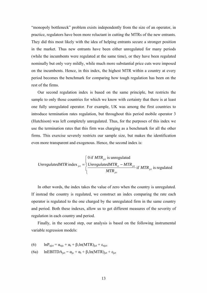
Our second regulation index is based on the same principle, but restricts the
sample to only those countries for which we know with certainty that there is at least
one fully unregulated operator. For example, UK was among the first countries to
introduce termination rates regulation, but throughout this period mobile operator 3
(Hutchison) was left completely unregulated. Thus, for the purposes of this index we
use the termination rates that this firm was charging as a benchmark for all the other
firms. This exercise severely restricts our sample size, but makes the identification
even more transparent and exogenous. Hence, the second index is:
⎪⎩
⎪⎨
⎧
−=regulated is if
dunregulate is if 0
index jct
jct
jctct
jct
jct MTRMTR
MTRdMTRUnregulate
MTR
dMTRUnregulate
In other words, the index takes the value of zero when the country is unregulated.
If instead the country is regulated, we construct an index comparing the rate each
operator is regulated to the one charged by the unregulated firm in the same country
and period. Both these indexes, allow us to get different measures of the severity of
regulation in each country and period.
Finally, in the second step, our analysis is based on the following instrumental
variable regression models:
(6) lnPujct = αujc + αt + β1ln(MTR)jct + εujct
(6a) lnEBITDAjct = αjc + αt + β1ln(MTR)jct + εjct

14
The idea here is to estimate the waterbed effect on prices directly through the
MTRs using regulation as an instrumental variable. Regulation is a valid instrument
as it is not expected to influence prices other than the impact it induces via MTRs.
This is because regulation acts on prices only indirectly via reducing MTRs, while
regulators do not intervene in any other direct manner on customer prices.
3.2 Data
For the purpose of our analysis we matched three different data sources. Firstly, we
use Cullen International to get information on mobile termination rates. Cullen
International is considered the most reliable source for MTRs and collects all
termination rates for official use of the European Commission. Using this source and
various other industry and regulatory publications, we were also in a position to
identify the dates in which regulation was introduced across countries and operators.
Secondly, quarterly information on the total bills paid by consumers across
operators and countries is obtained from Teligen. Teligen collects and compares all
available tariffs of the two largest mobile operators for thirty OECD countries. It
constructs three different consumer usage profiles (large, medium and low) based on
the number of calls and messages, the average call length and the time and type of
call. A distinction between pre-paid (pay-as-you-go) and post-paid (contract) is also
accounted for. These consumer profiles are then held fixed when looking across
countries and time.
Thirdly, we use quarterly information taken from the Global Wireless Matrix of
the investment bank Merrill Lynch (henceforth, ML). ML compiles basic operating
metrics for mobile operators in forty-six countries. For our purposes, we use the
reported average monthly revenue per user (ARPU) and the earnings margin before
interest, taxes, depreciation and amortization (EBITDA). Through this source we also
obtain information on market penetration and number of mobile operators in each
country, together with the number of subscribers and their market shares for each
operator.
All consumer prices, termination rates and revenue data were converted to euros
using the Purchasing Power Parities (PPP) currency conversions published by the
Organization for Economic Cooperation and Development (OECD) to ease
comparability. None of our results depends on this transformation. More detailed data
15
description, together with the dates of the introduction of regulation and summary
statistics, can be found in the Appendix.
The various datasources have different strengths and weaknesses regarding our
empirical question. The Teligen dataset has two main advantages. First, by fixing a
priori the calling profiles of customers, it provides us with information on the best
choices of these customers across countries and time. Second, the prices reported in
this dataset include much of the relevant information for this industry, such as
inclusive minutes, quantity discounts etc. (although it does not include handset
subsidies). However, this richness of information comes at the cost of having data for
only the two biggest operators of every country at each point in time. For instance, if a
country, such as the UK, had five mobile operators, possibly regulated differentially
over time, only two observations per customer profile would be available. This
reduces the variability and makes identification of our variables of interest harder,
especially given that the biggest mobile operators are often regulated at the same rate.
On the contrary, the ML dataset provides us with information on actual revenues
rather than prices. The dependent variables that we use are primarily EBITDA (a
measure of profit and cash flow) and ARPU (which consists of all revenues, including
revenues from MTR). These are aggregate measures encompassing all revenues
associated with mobile voice services. Therefore, they have to be interpreted as
measures of an operator’s revenues and profitability rather than the total customer
bill. Both these measures suffer from endogeneity problems which could introduce
bias and inconsistency in our results. However, this dataset contains information on
almost all mobile operators in each country and hence it allows us to exploit more
within-country variation.
4. Benchmark Results
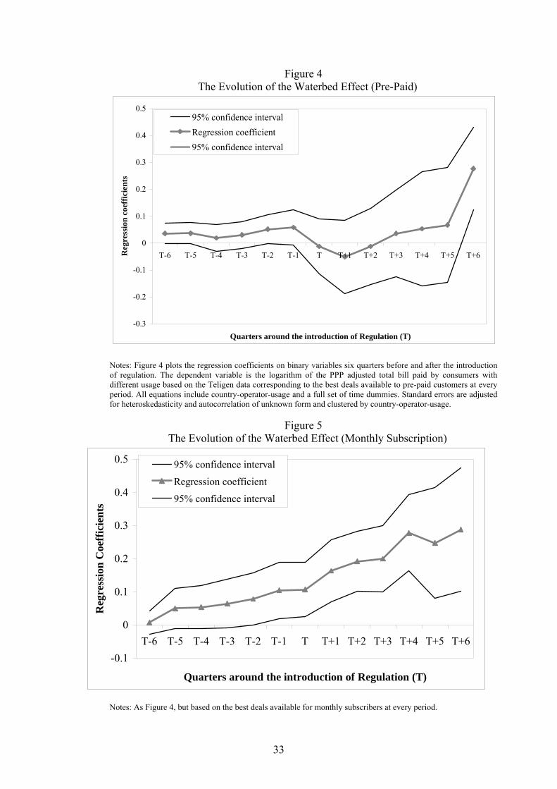
Table 1 reports our benchmark results from specification (5) using the price
information from Teligen as the dependent variable. The data for this table consists of
the best possible deals for each user profile among all possible contracts available,
both pre-paid and post-paid.13 For that reason, we also add a binary variable (Pre-
13 We will later check the robustness of our results if one constraints customers’ choices either to pre-paid or monthly contracts.

16
paidjct) indicating whether the best deal was on a pre-paid contract or not.14 The
estimated waterbed is 0.133 and strongly significant in column 1, where we utilize the
simplest specification with a binary indicator for regulation. That means that the
introduction of regulation of MTRs increased bills to customers by 13% on average.
Notice that the coefficient on pre-paid is negative but insignificant, indicating that
prices on the best pre-paid deals were no different than those on monthly contracts.
In column 2, using the MaxMTR index we obtain again strong evidence of the
waterbed effect. Similarly, in column 3 when we severely restrict our sample to only
those countries we know with certainty they had at least one unregulated mobile
operator, we still get a positive and significant effect.15 Notice also that the coefficient
on pre-paid becomes now negative and significant, indicating that pre-paid customers
were getting significantly better deals from the two main mobile operators when they
were faced with an unregulated competitor. It seems likely that incumbents were
offering significantly better deals to (the more elastic) pre-paid customers as a way of
attracting consumers and putting pressure on the prices charged by their unregulated
competitors.
In the last two columns, for reasons already discussed in the previous section, we
estimate an even more restrictive version of our model by allowing for regional-time
fixed effects. Essentially, our sample of countries can be naturally divided into three
macro regions: Western Europe, Eastern Europe and Rest of the World (Australia,
New Zealand and Japan). Western European countries have been all subject to the
New Regulatory Framework adopted by the European Commission, while other
Eastern European countries have only recently been subject to regulation with the
accession of new member States. Controlling for these regional effects in columns 4
and 5, results in an even stronger waterbed effect, without reducing its statistical
significance.16
Next, we look at the impact of regulation on profitability measures using
specification (5a). Table 2 reports the effect on EBITDA, while we relegate similar
results on the impact on ARPU to the Appendix. Column 1 shows that regulation had
14 It is important to mention that the MTR is applied uniformly and does not distinguish, say, between calls to heavy users on contracts and calls to low users on prepaid. However, the waterbed price reaction of the mobile firm to changes in MTR can in principle differ by type of user or call, since their profile of received calls can differ, or the intensity of competition can differ by type of user too. 15 The elasticities are not directly comparable as the regulatory variables have different mean values. 16 We do not report the results of column 3 with the regional-country fixed effects because the Western Europe region binary indicator includes all the countries that had one operator being not regulated.

17
a negative effect on profit margins, although the data is considerably noisier. Using
our two indexes, instead of the binary regulation variable (columns 2 and 3), reveal
again a negative relationship, though the effect is not statistically significant. In
columns 4 and 5, the inclusion of the regional-time fixed effects increases the
magnitude of the coefficients without affecting much their statistical significance. If
markets were fully competitive there should be no impact on profits. Thus, these
results suggest that competitors seem to have some degree of market power.
In our second step, using specifications (6) and (6a) we report the results from the
IV regressions in Table 3. The first three columns use the same Teligen data as
before, whereas the last three columns examine the effect on EBITDA. First stage
results across all columns confirm that regulation has a significantly negative effect
on MTR as expected. In addition, regulation does not seem to suffer from any weak-
instruments problems as indicated by the first stage F-tests. Column 1 shows that that
regulation through MTR has indeed a negative and significant effect on prices. The
magnitude of the elasticity of the waterbed effect is above 1.17 Over the period
considered, regulation has cut MTR rates by 11% and, at the same time, has increased
bills to mobile customers by 0.11 × 1.207 = 13.3%.
The elasticity of the waterbed effect is lower at 0.938 and 0.334, in columns 2 and
3 respectively, using the more sophisticated indexes of regulation, but still negative
and highly significant. The effect on accounting profits is positive and significant in
column 4, and positive but not significant with the more nuanced measures of
regulation. Table 4 also provides evidence that the results remain unchanged and if
anything become stronger, when we estimate the more restrictive version of our
model that includes region-time fixed effects.
We must remark that the ML dataset is probably less reliable than the Teligen
dataset, so we take our conclusion on accounting profits more cautiously. In addition,
all these results have to be qualified as termination rents could be also exhausted with
non-price strategies, i.e., increasing advertising, or giving handset subsidies that we
cannot control for. However, we do not expect handset subsidies effects to be too
relevant, for instance, for pre-paid customers, and the test on EBITDA should take
17 Note that all the results in Tables 1 and 2 can be directly obtained from Table 3. The impact of
regulation on prices, for instance, can be decomposed asRegulation/
/Regulation/∂∂
∂∂=∂∂MTR
MTRPP ,
where the denominator and the numerator and are obtained from the 1st and 2nd stage respectively in the IV regression.
18
these additional factors into account. If handset subsidies were linked to inter-
temporal subsidies (short-run losses are incurred to get long-run profits from captive
customers), our results on profitability are, if anything, biased downwards. This is
because a cut in MTR would look more profitable as fewer losses are made in the
short run. Therefore our result on profitability would probably look stronger if we
could account for handset subsidies.18
Taken together these benchmark estimates confirm our theoretical intuition that
there exists a strong and significant waterbed effect in mobile telephony. However,
this effect is not full as competing firms seem to enjoy some degree of market power.
[Tables 1, 2, 3, 4]
5. Dynamic Regulation Effects
The effect of regulation on prices might not be just instantaneous. On the one hand,
termination rates are typically regulated over some periods using “glide paths”, in
which charges are allowed to fall gradually towards a target over that period. The
temporal adjustment path is known and anticipated by operators, at least before a new
revision is conducted. On the other hand, there could also be some inertia. For
instance, customers may be locked in with an operator for a certain period, therefore
there would be no immediate need for mobile operators to adjust their prices as these
customers would not be lost right away. Alternatively, when termination rates change,
it may take some time for operators to adjust retail prices because of various “menu”
costs. Hence, we would like to investigate whether firms anticipated regulation
(possibly by trying to affect the outcomes of the regulatory process) and indeed
whether the effect of regulation was short-lived or had any persistent long term
effects. To quantify these dynamic effects of the waterbed phenomenon, we define
binary indicators for twelve, non-overlapping, quarters around the introduction of
18 All our analysis is related to the regulation fixed-to-mobile termination rates and not to mobile-to-mobile termination rates. This should not raise particular concerns in our analysis for two reasons. First, in many jurisdictions mobile-to-mobile rates are not regulated, a part from imposing reciprocity, and therefore cuts in fixed-to-mobile rates do not apply to other types of calls. Second, if for some reasons termination of both types of calls are regulated at the same level, theory says that a change in reciprocal mobile-to-mobile rates should have no obvious impact on profits and tariffs (just a re-balancing in the various components of the customer’s bill). If firms compete in two-part tariffs, the impact of reciprocal access charges on profits and bills is neutral (see Armstrong, 1998, and Laffont et al., 1998). Thus we really interpret our empirical results as the impact of the regulation of fixed-to-mobile termination rates on prices and profits.

19
regulation and a final binary variable isolating the long-run effect of regulation. Our
specification is as follows:
(7) lnPujct = αujc + αt + β1DT-6jct + β2DT-5
jct + …+ β12DT+5jct + β13DT+6
jct + εujct
where DT-6jct = 1 in the sixth quarter before regulation, DT-5
jct = 1 in the fifth quarter
before regulation, and similarly for all other quarters until DT+6jct = 1 in the sixth
quarter after regulation and in all subsequent quarters. Each binary indicator equals
zero in all other quarters than those specified. Hence, the base period is the time
before the introduction of regulation, excluding the anticipation period (i.e., seven
quarters before regulation backwards). This approach accounts for probable
anticipation effects (as captured by DT-6 to DT-1 binary indicators) as well as short
(captured by DT to DT+5) and long run effects (captured by DT+6).19
Figure 3 plots the regression coefficients on these binary indicators together with
their 95% confidence interval. As expected, regulation has no effect on prices six to
four quarters before the actual implementation. However, there is some small but
statistically significant anticipation of the regulatory intervention three to one quarters
before. As discussed before, for the large majority of countries regulation was
preceded by a long consultation period between the regulator and the various mobile
operators. Our results reveal that operators started adjusting their price schedules
slightly upwards even before the actual implementation of the new termination rates.
However, it is the actual implementation of the regulation that has the biggest
impact on prices as revealed by the immediate increase on the coefficients after
regulation. In other words, regulation is binding from the beginning and as it tightens
up over time, the waterbed effect increases. As we can see in figure 3, regulation also
seems to have a large and very significant long-run waterbed effect. The coefficient
estimate on DT+6, which quantifies the effect of regulation on prices post the sixth
quarter after its introduction, is strongly significant and implies a long run elasticity of
the waterbed effect of 33%. Note that this coefficient is not directly comparable to the
previous estimates of the waterbed effect, as it incorporates the effect not only of the
introduction of regulation, but also of the progressive tightening of termination rates.
19 See Laporte and Windmeijer (2005) for a discussion of this approach.

20
What is crucial is that prices seem to respond continuously with every tightening of
the rules giving rise to a waterbed phenomenon that is not a one-off event.
[Figure 3]
6. Interaction with Competition and Further Evidence
6.1 Competition and Market Penetration
Having established that the waterbed effect exists and has a strong long run effect,
we now want to investigate in greater detail how competition affects this
phenomenon. Competition is obviously expected to have a direct impact on prices: the
more competitive the market, the lower the prices to customers. Besides this effect,
however, if termination rates are “high” (e.g., unregulated) or a substantial mark-up is
allowed, competition is expected to have an additional impact via the waterbed effect:
the more competitive the industry, the lower the prices will be, on top of the direct
effect, as any termination rent will be passed on to the customers. As discussed in
Section 2, a waterbed effect is expected to exist also under monopoly, though the
effect is milder as some rents will be kept by the monopolist. However, the waterbed
effect is not expected to be very relevant under monopoly when the market is very
saturated and the monopolist still has an interest in covering it. Hence, in our
empirical specification it is crucial to control for subscription penetration levels. Our
specification reads:
(8) lnPujct = αujc + αt + β1ln(MTR)jct + β2ln(Competitors)ct + β3ln(Penetration)ct +
γ1[ln(ΜTR)jct×ln(Competitors)ct] + γ2[ln(ΜTR)jct×ln(Penetration)ct] +
γ3[ln(Penetration)ct×ln(Competitors)ct] +
δ[ln(ΜTR)jct×ln(Competitors)ct×ln(Penetration)ct] + εujct
Equation (8) is an extension of our previous specification (6) with the aim to
specify a particular channel that might affect the intensity of the waterbed effect. Our
proxy for the intensity of competition is simply the number of rival firms
(Competitorsct) in each country and period. The number of mobile operators in a
country can be taken as exogenous as the number of licences is determined by
spectrum availability. Over the period considered, several countries have witnessed
the release of additional licences. The degree of market saturation/maturity is
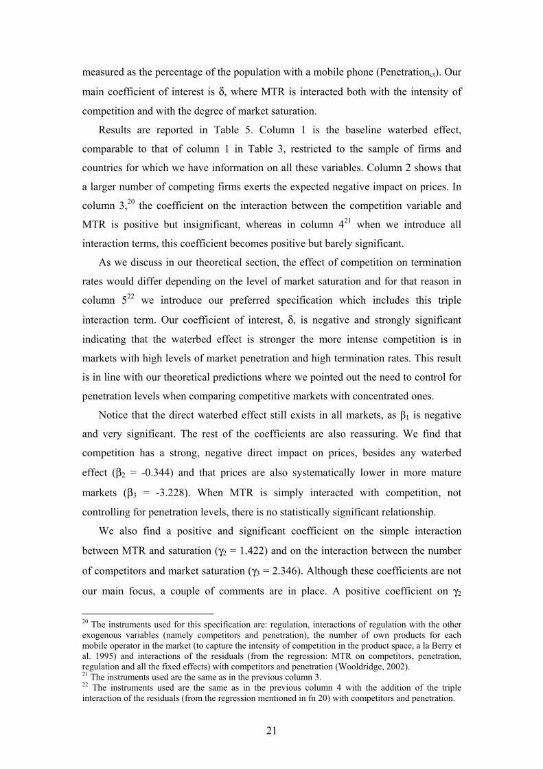
21
measured as the percentage of the population with a mobile phone (Penetrationct). Our
main coefficient of interest is δ, where MTR is interacted both with the intensity of
competition and with the degree of market saturation.
Results are reported in Table 5. Column 1 is the baseline waterbed effect,
comparable to that of column 1 in Table 3, restricted to the sample of firms and
countries for which we have information on all these variables. Column 2 shows that
a larger number of competing firms exerts the expected negative impact on prices. In
column 3,20 the coefficient on the interaction between the competition variable and
MTR is positive but insignificant, whereas in column 421 when we introduce all
interaction terms, this coefficient becomes positive but barely significant.
As we discuss in our theoretical section, the effect of competition on termination
rates would differ depending on the level of market saturation and for that reason in
column 522 we introduce our preferred specification which includes this triple
interaction term. Our coefficient of interest, δ, is negative and strongly significant
indicating that the waterbed effect is stronger the more intense competition is in
markets with high levels of market penetration and high termination rates. This result
is in line with our theoretical predictions where we pointed out the need to control for
penetration levels when comparing competitive markets with concentrated ones.
Notice that the direct waterbed effect still exists in all markets, as β1 is negative
and very significant. The rest of the coefficients are also reassuring. We find that
competition has a strong, negative direct impact on prices, besides any waterbed
effect (β2 = -0.344) and that prices are also systematically lower in more mature
markets (β3 = -3.228). When MTR is simply interacted with competition, not
controlling for penetration levels, there is no statistically significant relationship.
We also find a positive and significant coefficient on the simple interaction
between MTR and saturation (γ2 = 1.422) and on the interaction between the number
of competitors and market saturation (γ3 = 2.346). Although these coefficients are not
our main focus, a couple of comments are in place. A positive coefficient on γ2
20 The instruments used for this specification are: regulation, interactions of regulation with the other exogenous variables (namely competitors and penetration), the number of own products for each mobile operator in the market (to capture the intensity of competition in the product space, a la Berry et al. 1995) and interactions of the residuals (from the regression: MTR on competitors, penetration, regulation and all the fixed effects) with competitors and penetration (Wooldridge, 2002). 21 The instruments used are the same as in the previous column 3. 22 The instruments used are the same as in the previous column 4 with the addition of the triple interaction of the residuals (from the regression mentioned in fn 20) with competitors and penetration.

22
indicates that the waterbed effect is lower in higher penetration markets. Intuitively,
low penetration markets usually consist of heavy users for whom the waterbed effect
is expected to be strong. But as the market becomes more saturated, this typically
involves attracting marginal users who make and receive very few calls. Hence, we
expect the waterbed effect to decrease as the market becomes more saturated because
of the different types of consumers that are drawn into the mobile customer pool. On
the contrary, we have no prior expectations on the coefficient γ3 as there is no strong
reason to believe that, controlling for the number of competitors, the impact of
competition should be more or less intense as the market saturates. On the one hand, a
negative coefficient would arise if operators become less capacity constrained and
compete more fiercely. On the other hand, if operators in mature markets tend to
collude more easily over time, the result would be a positive coefficient.
Finally, in column 6, where we use as an instrument the MaxMTR index instead of
the binary variable Regulation,23 we confirm the conclusions previously drawn.
Results are virtually unaffected for the majority of the coefficients, with the direct
waterbed effect (β1) and the coefficient on the triple interaction (δ) becoming even
stronger.
Therefore, in line with our theoretical predictions, our empirical analysis reveals
that both competition and market saturation, but most importantly their interaction,
affects the overall impact of the waterbed effect on prices. We also experimented
using the HHI index instead of the simple number of competing operators, as a
different measure of competition. While the δ coefficient is still significant and has
the expected sign (now the coefficient is positive, as an increase in HHI means a
lessening of competition), some other results are less stable (see Table A10 in the
Appendix). In our opinion, this reveals the limitations of our dataset (although HHI is
potentially an alternative measure of competition, it clearly suffers from a more
serious endogeneity problem than the number of competitors as discussed above) and
of our reduced-form methodology regarding the effect of market structure on the
waterbed phenomenon. Future research using a structural approach and more detailed
country-level data is required to further understand these mechanisms.
[Table 5]
23 The rest of the instruments used are the same as in column 5.

23
6.2 Waterbed Effect on Different Customer Types
In all our previous specifications using the Teligen data, we assumed that a
customer could ideally choose the best available contracts at any given point in time,
given her/his usage profile. The results are therefore valid if indeed customers behave
in this frictionless way. The introduction of mobile number portability24 certainly
makes this possibility all the more realistic. However, as many market analysts
advocate, there are good reasons to believe that distinguishing between pre-paid (pay-
as-you-go) and post-paid (long-term contract) customers is still important. Customers
on long-term contracts may be looking only at similar long-term deals, and may not
be interested in a temporary pre-paid subscription, even if this turned out to be
cheaper for a while. Switching among operators takes time and for a business user this
might not be a very realistic option, even in the presence of number portability.
Conversely, customers on pre-paid cards, may have budget constraints and do not
want to commit to long-term contracts where they would have to pay a fixed monthly
fee for one or more years. Again, these customers may want to look only at offers
among pre-paid contracts.
Using our benchmark specification (5), we investigate whether there is a
difference in the waterbed effect between pre-paid and post-paid users, when each
type of user is limited in her/his choices within the same type of contracts. Tables A8
and A9 (in the Appendix) report the results. Rather intriguingly, we find that pre-paid
customers essentially are unaffected by regulation, whereas monthly subscribers bear
the bulk of the price increases. This may arise because firms have a more secure
relationship with monthly contract subscribers (who tend to stay with the same
operator for several years), and so have a greater expectation of receiving future
incoming revenues as a result of competing on price for these customers. Post-pay
customers also tend to receive more incoming calls, and so become more (less)
profitable as termination rates rise (fall). On the contrary, pre-pay subscribers, who
are typically very price sensitive, tend to change their number often, therefore it is less
likely that their numbers are known by potential callers.25 Thus pre-pay users receive
24 Mobile number portability is the ability of consumers to switch among mobile operators while keeping the same phone number. 25 Vodafone, for example, reports the following churn rates across its major European markets for the quarter to 30 September 2006 (Source: Vodafone):

24
relatively few calls and a change in MTR has a much lower expected impact
compared to post-pay customers. A further factor may be that network operators have
a preference to change fixed fees in non-linear contracts rather than pre-pay call price
structures which are closer to linear prices.
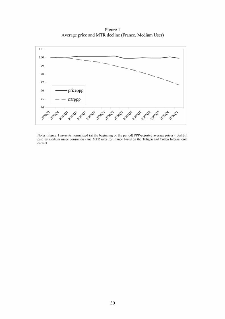
The relationship between regulation and prices might not be monotonic and for
that reason we examine as before the dynamic waterbed effects using our
specification in (7) separately for pre- and post-paid deals. Figures 4 and 5 plot the
regression coefficients on the thirteen binary indicators around the introduction of
regulation together with their 95% confidence interval for pre-paid and post-paid
contracts respectively. In line with our previous analysis, the anticipation of
regulation has very little impact on either pre- or post-paid contracts up to two periods
before regulation. Monthly customers (figure 5) then experience a change similar to
that analysed with the general unconstrained results. On the contrary, the pattern for
pre-paid contracts is more intriguing. As can be seen in figure 4, the inaction before
the introduction of regulation is followed by a short-lived (for periods T and T+1)
non-significant decrease in prices and then a continuous non-significant increase in
prices for the next four quarters (periods T+2, T+3, T+4 and T+5). There is, however,
an overall positive and strongly significant long-run waterbed effect (coefficient on
T+6, around 27%) on these prices too.
Notice also the massive increase in the variance associated with these coefficients
after the introduction of regulation. Mobile operators seem to have reacted
differentially regarding the pricing of these contracts shortly after the introduction of
regulation. At the beginning, they seem on average to reduce the prices charged to
these customers, possibly trying to lure customers into their networks (with the hope
of them upgrading later to monthly subscribers) or potentially as a loss making, short
term strategy against smaller firms that either remained unregulated or were not
regulated at the same rates. In either case, the strong and positive long-run coefficient
illustrates that mobile operators eventually were forced to abandon any such strategies
Markets Prepaid Contract Total Germany 29.5% 13.5% 22.1% Italy 22.4% 13.6% 21.7% Spain 62.5% 13.4% 37.0% UK 49.9% 18.8% 37.6%

25
and raise the prices even for the pre-paid customers, which is another manifestation of
the power of the waterbed effect.
[Figures 4, 5]
7. Conclusions
Regulation of fixed-to-mobile termination charges has become increasingly
prevalent around the world during the last decade. A large theoretical literature has
demonstrated that independently of the intensity of competition for mobile customers,
mobile operators have an incentive to set charges that will extract the largest possible
surplus from fixed users. This competitive bottleneck problem provided scope for the
(possibly) welfare-improving regulatory intervention. However, reducing the level of
termination charges can potentially increase the level of prices for mobile subscribers,
the so called “waterbed” effect.
In this paper we provide the first econometric evidence that the introduction of
regulation resulted to a ten percent waterbed effect on average. However, although the
waterbed effect is high, our analysis also provides evidence that it is not full:
accounting measures of profits are positively related to MTR, thus mobile firms suffer
from cuts in termination rates. Finally, our empirical analysis also reveals that the
waterbed effect is stronger the more intense competition is in markets with high levels
of market penetration and high termination rates.
Our findings have three important implications. First, mobile telephony exhibits
features typical of two-sided markets. The market for subscription and outgoing
services is closely interlinked to the market for termination of incoming calls.
Therefore, any antitrust or regulatory analysis must take these linkages into account
either at the stage of market definition or market analysis.
Second, any welfare analysis of regulation of termination rates cannot ignore the
presence of the waterbed effect. Clearly, if the demand for mobile subscription was
very inelastic, the socially optimal MTR would be the cost of termination (though the
regulation of MTR would impact on the distribution of consumer surplus among fixed
and mobile subscribers). If, instead, the mobile market was not saturated and still
growing there would be a great need to calibrate carefully the optimal MTR. We
acknowledge that this calibration exercise is very difficult and must be done with
great caution. It is therefore all the more important that further analysis and effort are

26
put to understand the behaviour of marginal users that might give up their handsets
when the waterbed effect is fully at work.
Third, our analysis on the existence and magnitude of the waterbed effect is also
relevant in the current debate of regulation of international roaming charges. The
European Commission has voted in 2007 to cap “roaming charges”26 of making and
receiving phone calls within the EU. The aim is to reduce the cost of making a mobile
phone calls while abroad and hence encourage more overseas (but within EU) phone
use. Hence, a reduction in roaming charges may cause a similar waterbed
phenomenon, whereby prices of domestic calls may increase as operators seek to
compensate for their lost revenue elsewhere. While the magnitude of the waterbed
effect caused by this new legislation is debatable, our results demonstrate that
regulators have to acknowledge its existence and carefully account for it in their
welfare calculations.
Future research should concentrate on two aspects that we consider to be the
limitations of this paper. On the one hand, more detailed information would allow
researchers to overcome our data limitations. Having price data on a larger number of
mobile operators within countries, would allow for joint country-time fixed effects to
be properly controlled for in the empirical specification. Furthermore, to investigate
the marginal consumer’s behaviour before and after the introduction of regulation and
their elasticity regarding the waterbed effect, more detailed consumer-level
information is required. On the other hand, given the non-linear retail price schedules
and the complex incentives schemes (handsets, personal vs. business buyers’
contracts, etc.) provided by mobile operators, more detailed customer information at a
country level would allow us to model more satisfactorily the effect of competition
and market penetration on the waterbed effect. Such a structural model would also
enable us to quantify the effects of various regulatory interventions and their welfare
implications. We intend to pursue both avenues in our future research.
26 These are the charges made to customers when using their phones outside their home country, i.e., an Italian customer making/receiving a phone call in Greece.

27
References
Argentesi, E. and L. Filistrucchi, 2006, “Estimating Market Power in a Two-Sided Market: The Case of Newspapers,” Journal of Applied Econometrics, forthcoming.
Armstrong, M., 1998, “Network Interconnection in Telecommunications,” Economic Journal, 108: 545-564.
Armstrong, M., 2002, “The Theory of Access Pricing and Interconnection,” in M. Cave, S. Majumdar and I. Vogelsang (eds.) Handbook of Telecommunications Economics, North-Holland, Amsterdam.
Armstrong, M., 2006, “Competition in Two-Sided Markets,” RAND Journal of Economics, forthcoming.
Berry, S., J. Levinsohn and A. Pakes, 1995, “Automobile Prices in Market Equilibrium,” Econometrica, 63: 841-90.
Bertrand, M., E. Duflo and S. Mullainathan, 2004, “How Much Should We Trust Differences-in-Differences Estimates?” Quarterly Journal of Economics, 119: 249-75.
Card, D. and A.D. Krueger, 1994, “Minimum Wages and Employment: A Case Study of the Fast-Food Industry in New Jersey and Pennsylvania,” American Economic Review, 84: 772-793.
Hausman, J. and J. Wright, 2006, “Two-sided markets with substitution: mobile termination revisited,” mimeo, MIT.
Kaiser, U. and J. Wright, 2006, “Price Structure in Two-Sided Markets: Evidence from the Magazine Industry,” International Journal of Industrial Organization, 24: 1-28.
Laffont, J.-J., Rey, P. and Tirole, J., 1998, “Network competition I: Overview and non-discriminatory pricing,” RAND Journal of Economics, 29: 1-37.
Laporte, A. and F. Windmeijer, 2005, “Estimation of panel data models with binary indicators when treatment effects are not constant over time,” Economics Letters, 88: 389-396.
Rochet, J.-C. and J. Tirole, 2006, “Two-Sided Markets: A Progress Report,” RAND Journal of Economics, forthcoming.
Rysman, M., 2004, “Competition Between Networks: A Study of the Market for Yellow Pages,” Review of Economic Studies, 71: 483-512.
Rysman, M., 2007, “An Empirical Analysis of Payment Card Usage,” Journal of Industrial Economics, 55: 1-36.
Valletti, T. and G. Houpis, 2005, “Mobile termination: What is the “right” charge?” Journal of Regulatory Economics, 28: 235-258.
Wooldridge, J., 2002, Econometric Analysis of Cross Section and Panel Data, MIT Press. Wright, J., 2002, “Access Pricing under Competition: an Application to Cellular
Networks,” Journal of Industrial Economics, 50: 289-316.

28
5. Appendix
5. 1 Data description
To test the waterbed effect we use a variety of different sources. Regarding the mobile
termination rates, we use the biannual data provided by Vodafone using Cullen
International and its own internal sources. The variable identifies those periods in
which the MTRs of network operators were constrained by a formal decision taken by
a national regulatory authority. Because all the other datasets used are in quarterly
format, we extrapolate the mobile termination rates where necessary to get the same
frequency.
For firms’ prices we use two data sources. Teligen (2002Q3-2006Q1) reports
quarterly information on the total bills paid by consumers across countries. The
second dataset is the Global Wireless Matrix of Merrill Lynch. This data is available
also on a quarterly basis (2000Q1-2005Q3). For our purposes, we use the reported
average revenue per user (ARPU) and the earnings before interest, taxes, depreciation
and amortization (EBITDA). ARPU is calculated by dividing total revenues by
subscribers. EBITDA is defined as the sum of operating income and depreciation and
is used to proxy for profit and cash flow.
Variables are described in Table A1. Table A2 gives summary statistics for the
Teligen dataset (and the matched MTRs), while Table A4 gives summary statistics for
Merill Lynch (and the matched MTRs). Tables A3 and A5 correspond to Tables A2
and A4 respectively, but limited to the sample we use when we analyze the effect of
competition, and also include the additional variables used in that exercise. Table A6
reports all the starting dates of regulation in countries which adopted MTR regulation.
[Tables A1, A2, A3, A4, A5, A6]
5.2 Additional results
Impact on ARPU. In the main text (Section 3.1) we considered the impact of MTR
on EBITDA, taken as a measure of profitability. Alternatively, one can also use
ARPU (we recall that this measure also includes termination revenues, and therefore
cannot be taken as a measure of customers’ prices). Results are shown in Table A7. In
line with the results on EBITDA, we find that higher MTRs have a somehow positive
effect on ARPU, though the results are not significant when we include regional-time
29
dummies. Taken together with the results on EBITDA, we have some evidence that
the waterbed effect is not full.
Pre- and post-paid contracts. Table A8 and A9 reports the results discussed in
Section 6.2. They are the equivalent to Table 1, split between pre-paid deals (A8) and
monthly post-paid contracts (A9). The procedure and interpretation is the same as
with Table 1.
Competition. Table A10 reports the results from the first-stage regression of Table 5
(section 6.1). Table A11 reports the full set of results of the impact of competition,
using the HHI index of market concentration instead of the number of competitors as
a proxy for the intensity of competition in the market.
[Tables A7, A8, A9, A10, A11]
30
Figure 1 Average price and MTR decline (France, Medium User)
94
95
96
97
98
99
100
101
2002
Q3
2002
Q4
2003
Q1
2003
Q2
2003
Q3
2003
Q4
2004
Q1
2004
Q2
2004
Q3
2004
Q4
2005
Q1
2005
Q2
2005
Q3
2005
Q4
2006
Q1
priceppp
mtrppp
Notes: Figure 1 presents normalized (at the beginning of the period) PPP-adjusted average prices (total bill paid by medium usage consumers) and MTR rates for France based on the Teligen and Cullen International dataset.

31
Figure 2 Average Price around the introduction of Regulation
-0.100
-0.050
0.000
0.050
0.100
0.150
T-6 T-5 T-4 T-3 T-2 T-1 T T+1 T+2 T+3 T+4 T+5 T+6
Quarters around the introduction of Regulation (T)
Ave
rage
pric
e pa
id (P
PP a
djus
ted
euro
s/ye
ar) p
er
usag
e pr
ofile
(tim
e an
d co
untry
-ope
rato
r-us
age
dem
eane
d)
Notes: Figure 2 plots the evolution of time and country-operator-usage demeaned average logarithm of the PPP adjusted price paid per usage profile six quarters before and after the introduction of regulation of fixed-to-mobile termination charges based on the Teligen data corresponding to the best deals available at every period.

32
Figure 3
The Evolution of the Waterbed Effect
-0.1
0
0.1
0.2
0.3
0.4
0.5
T-6 T-5 T-4 T-3 T-2 T-1 T T+1 T+2 T+3 T+4 T+5 T+6
Quarters around the introduction of Regulation (T)
Reg
ress
ion
coef
ficie
nts
95% confidence intervalRegression Coefficient95% confidence interval
Notes: Figure 3 plots the regression coefficients on binary variables six quarters before and after the introduction of regulation. The dependent variable is the logarithm of the PPP adjusted total bill paid by consumers with different usage based on the Teligen data corresponding to the best deals available at every period. All equations include country-operator-usage and a full set of time dummies. Standard errors are adjusted for heteroskedasticity and autocorrelation of unknown form and clustered by country-operator-usage.
33
Figure 4 The Evolution of the Waterbed Effect (Pre-Paid)
-0.3
-0.2
-0.1
0
0.1
0.2
0.3
0.4
0.5
T-6 T-5 T-4 T-3 T-2 T-1 T T+1 T+2 T+3 T+4 T+5 T+6
Quarters around the introduction of Regulation (T)
Reg
ress
ion
coef
ficie
nts
95% confidence intervalRegression coefficient95% confidence interval
Notes: Figure 4 plots the regression coefficients on binary variables six quarters before and after the introduction of regulation. The dependent variable is the logarithm of the PPP adjusted total bill paid by consumers with different usage based on the Teligen data corresponding to the best deals available to pre-paid customers at every period. All equations include country-operator-usage and a full set of time dummies. Standard errors are adjusted for heteroskedasticity and autocorrelation of unknown form and clustered by country-operator-usage.
Figure 5
The Evolution of the Waterbed Effect (Monthly Subscription)
-0.1
0
0.1
0.2
0.3
0.4
0.5
T-6 T-5 T-4 T-3 T-2 T-1 T T+1 T+2 T+3 T+4 T+5 T+6
Quarters around the introduction of Regulation (T)
Reg
ress
ion
Coe
ffic
ient
s
95% confidence interval
Regression coefficient
95% confidence interval
Notes: As Figure 4, but based on the best deals available for monthly subscribers at every period.
TABLE 1 – ESTIMATING THE “WATERBED” EFFECT (TELIGEN)
(1) (2) (3) (4) (5) Estimation method OLS OLS OLS OLS OLS Dependent variable lnPujct lnPujct lnPujct lnPujct lnPujct
Regulationjct 0.133***
(0.033)
0.152***
(0.033)
MaxMTR indexjct 0.290*** (0.068)
0.316***
(0.066)
UnregulatedMTR indexjct 0.127** (0.051)
Pre-paidjct -0.045 (0.040)
-0.051 (0.041)
-0.127*** (0.044)
-0.052 (0.039)
-0.056 (0.040)
Observations 1734 1734 450 1734 1734 Country-Operator-Usage 150 150 36 150 150 Within-R2 0.220 0.234 0.367 0.252 0.267 Notes: The dependent variable is the logarithm of the PPP adjusted total bill paid by consumers with different usage based on the Teligen data corresponding to the best deals available at every period. All equations include country-operator-usage and a full set of time dummies (first three columns) or a full set of region-time dummies (last two columns). All countries in the sample were divided into three macro regions: Western Europe, Eastern Europe and Rest of the World (RoW); see text for more details. Standard errors adjusted for heteroskedasticity and autocorrelation of unknown form and clustered by country-operator-usage are reported in parenthesis below coefficients: *significant at 10%; **significant at 5%; ***significant at 1%.
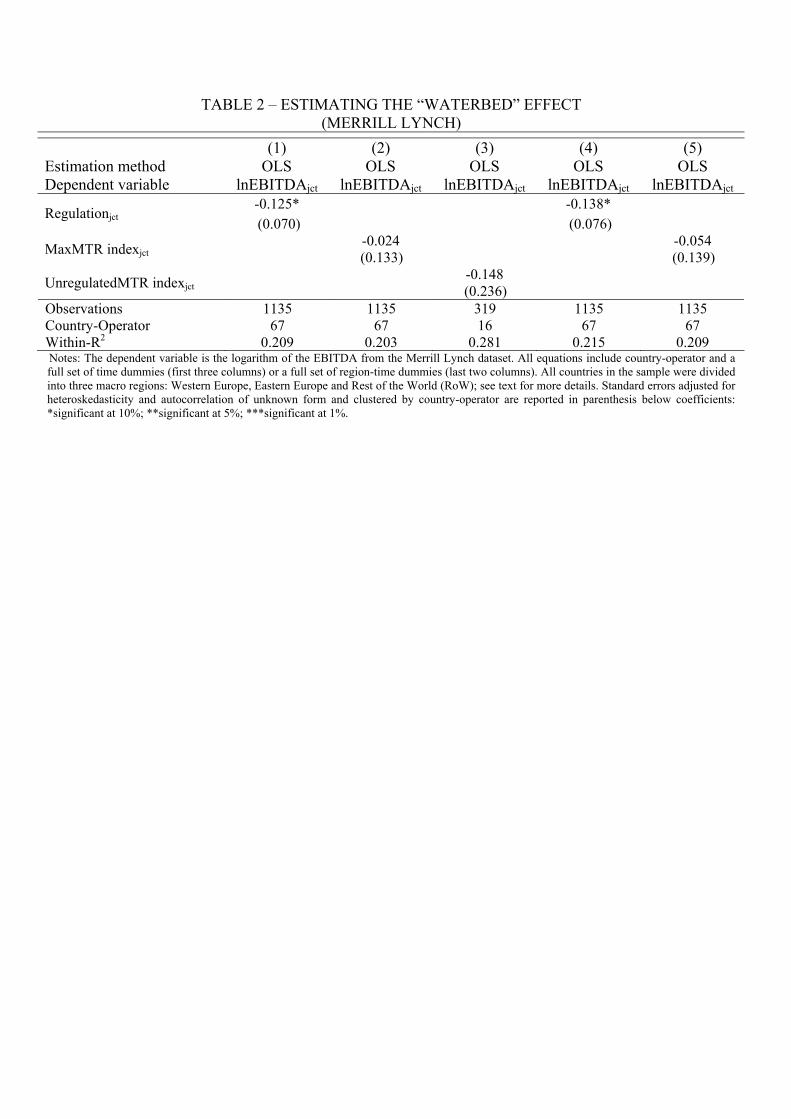
TABLE 2 – ESTIMATING THE “WATERBED” EFFECT (MERRILL LYNCH)
(1) (2) (3) (4) (5) Estimation method OLS OLS OLS OLS OLS Dependent variable lnEBITDAjct lnEBITDAjct lnEBITDAjct lnEBITDAjct lnEBITDAjct
Regulationjct -0.125* (0.070)
-0.138* (0.076)
MaxMTR indexjct -0.024 (0.133) -0.054
(0.139)
UnregulatedMTR indexjct -0.148 (0.236)
Observations 1135 1135 319 1135 1135 Country-Operator 67 67 16 67 67 Within-R2 0.209 0.203 0.281 0.215 0.209 Notes: The dependent variable is the logarithm of the EBITDA from the Merrill Lynch dataset. All equations include country-operator and a full set of time dummies (first three columns) or a full set of region-time dummies (last two columns). All countries in the sample were divided into three macro regions: Western Europe, Eastern Europe and Rest of the World (RoW); see text for more details. Standard errors adjusted for heteroskedasticity and autocorrelation of unknown form and clustered by country-operator are reported in parenthesis below coefficients: *significant at 10%; **significant at 5%; ***significant at 1%.

TABLE 3 – WATERBED EFFECT THROUGH MTR
(1) (2) (3) (4) (5) (6) Estimation method IV IV IV IV IV IV Dependent variable lnPujct lnPujct lnPujct lnEBITDAjct lnEBITDAjct lnEBITDAjct
ln(MTR)jct -1.207***
(0.411) 1.127* (0.603)
MaxMTR indexjct -0.938*** (0.278) 0.070
(0.392)
UnregulatedMTR indexjct
-0.334** (0.133) 0.620
(0.862)
1st Stage Coef. -0.110*** (0.024)
-0.310*** (0.035)
-0.382*** (0.028)
-0.111*** (0.037)
-0.335*** (0.051)
-0.239** (0.098)
1st Stage R2 0.044 0.127 0.523 0.045 0.112 0.137
1st Stage F-test 21.83*** [0.000]
78.85*** [0.000]
188.24*** [0.000]
8.90*** [0.004]
43.88*** [0.000]
5.90** [0.028]
Observations 1734 1734 450 1135 1135 319 Clusters 150 150 36 67 67 16 Notes: Columns 1, 2 and 3 utilize the Teligen data as in Table 1. The dependent variable for these columns is the logarithm of the PPP adjusted total bill paid by consumers with different usage for the best deals available. Columns 4, 5 and 6 utilize the Merrill Lynch dataset as in Table 2. The dependent variable for these columns is the logarithm of the EBITDA. All regressions use the “Regulation” dummy as the instrumental variable. All equations include either country-operator-usage (Teligen) or country-operator (Merrill Lynch) and a full set of time dummies. P-values for diagnostic tests are in brackets and italics. Standard errors adjusted for heteroskedasticity and autocorrelation of unknown form and clustered by either country-operator-usage (Teligen) or country-operator (Merrill Lynch) are reported in parenthesis below coefficients: *significant at 10%; **significant at 5%; ***significant at 1%.
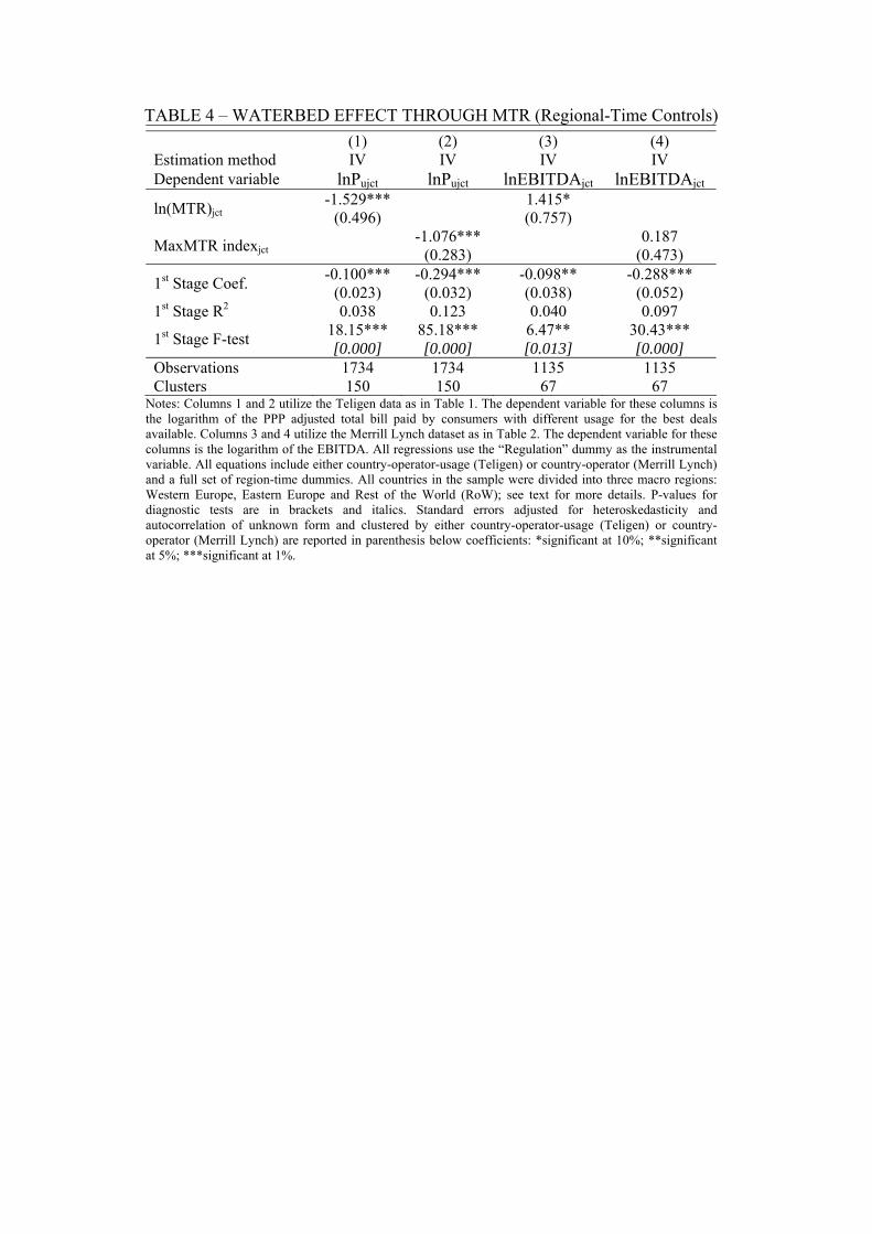
TABLE 4 – WATERBED EFFECT THROUGH MTR (Regional-Time Controls)
(1) (2) (3) (4) Estimation method IV IV IV IV Dependent variable lnPujct lnPujct lnEBITDAjct lnEBITDAjct
ln(MTR)jct -1.529***
(0.496) 1.415* (0.757)
MaxMTR indexjct -1.076*** (0.283) 0.187
(0.473)
1st Stage Coef. -0.100*** (0.023)
-0.294*** (0.032)
-0.098** (0.038)
-0.288*** (0.052)
1st Stage R2 0.038 0.123 0.040 0.097
1st Stage F-test 18.15*** [0.000]
85.18*** [0.000]
6.47** [0.013]
30.43*** [0.000]
Observations 1734 1734 1135 1135 Clusters 150 150 67 67
Notes: Columns 1 and 2 utilize the Teligen data as in Table 1. The dependent variable for these columns is the logarithm of the PPP adjusted total bill paid by consumers with different usage for the best deals available. Columns 3 and 4 utilize the Merrill Lynch dataset as in Table 2. The dependent variable for these columns is the logarithm of the EBITDA. All regressions use the “Regulation” dummy as the instrumental variable. All equations include either country-operator-usage (Teligen) or country-operator (Merrill Lynch) and a full set of region-time dummies. All countries in the sample were divided into three macro regions: Western Europe, Eastern Europe and Rest of the World (RoW); see text for more details. P-values for diagnostic tests are in brackets and italics. Standard errors adjusted for heteroskedasticity and autocorrelation of unknown form and clustered by either country-operator-usage (Teligen) or country-operator (Merrill Lynch) are reported in parenthesis below coefficients: *significant at 10%; **significant at 5%; ***significant at 1%.
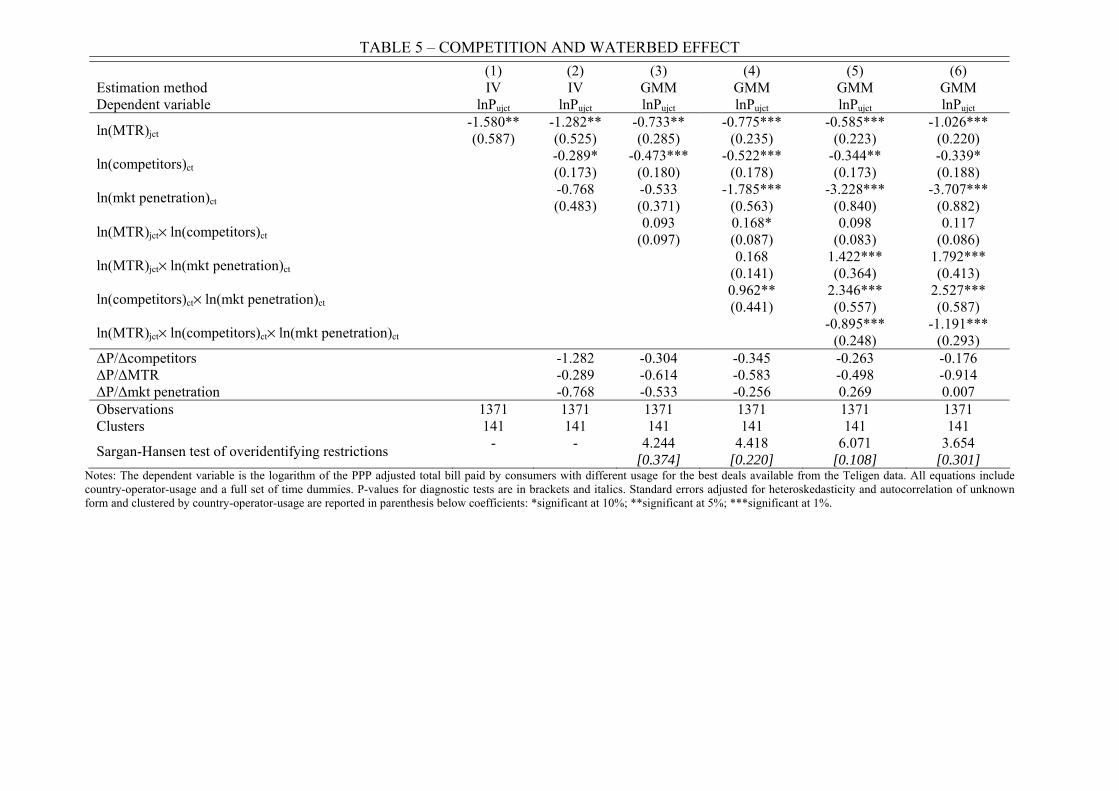
TABLE 5 – COMPETITION AND WATERBED EFFECT
(1) (2) (3) (4) (5) (6) Estimation method IV IV GMM GMM GMM GMM Dependent variable lnPujct lnPujct lnPujct lnPujct lnPujct lnPujct
ln(MTR)jct -1.580** (0.587)
-1.282** (0.525)
-0.733** (0.285)
-0.775*** (0.235)
-0.585*** (0.223)
-1.026*** (0.220)
ln(competitors)ct -0.289* (0.173)
-0.473*** (0.180)
-0.522*** (0.178)
-0.344** (0.173)
-0.339* (0.188)
ln(mkt penetration)ct -0.768 (0.483)
-0.533 (0.371)
-1.785*** (0.563)
-3.228*** (0.840)
-3.707*** (0.882)
ln(MTR)jct× ln(competitors)ct 0.093 (0.097)
0.168* (0.087)
0.098 (0.083)
0.117 (0.086)
ln(MTR)jct× ln(mkt penetration)ct 0.168 (0.141)
1.422*** (0.364)
1.792*** (0.413)
ln(competitors)ct× ln(mkt penetration)ct 0.962** (0.441)
2.346*** (0.557)
2.527*** (0.587)
ln(MTR)jct× ln(competitors)ct× ln(mkt penetration)ct -0.895*** (0.248)
-1.191*** (0.293)
∆P/∆competitors -1.282 -0.304 -0.345 -0.263 -0.176 ∆P/∆MTR -0.289 -0.614 -0.583 -0.498 -0.914 ∆P/∆mkt penetration -0.768 -0.533 -0.256 0.269 0.007 Observations 1371 1371 1371 1371 1371 1371 Clusters 141 141 141 141 141 141
Sargan-Hansen test of overidentifying restrictions -
-
4.244 [0.374]
4.418 [0.220]
6.071 [0.108]
3.654 [0.301]
Notes: The dependent variable is the logarithm of the PPP adjusted total bill paid by consumers with different usage for the best deals available from the Teligen data. All equations include country-operator-usage and a full set of time dummies. P-values for diagnostic tests are in brackets and italics. Standard errors adjusted for heteroskedasticity and autocorrelation of unknown form and clustered by country-operator-usage are reported in parenthesis below coefficients: *significant at 10%; **significant at 5%; ***significant at 1%.

APPENDIX
TABLE A1 – VARIABLE DESCRIPTIONS
Pujct total price paid (PPP adjusted euros/year) per usage
profile (usage profiles: high, medium and low)
MTRjct mobile termination rate (PPP adjusted eurocents/minute)
ARPUjct monthly average revenue per user (PPP adjusted
euros/month)
EBITDAjct earnings before interest, taxes, depreciation and
amortization margin (%)
Notes: The first variable is constructed using the Teligen dataset, the second variable is taken from the Cullen International dataset and the last two variables are from the Merrill Lynch dataset.
TABLE A2 – SUMMARY STATISTICS Variable Observations Mean Standard Deviation Min Max
Teligen Table 1 (Best Overall Deals) lnPujct 1734 5.203 1.708 0.107 7.492 ln(MTR)jct 1734 1.800 1.656 -3.246 3.573 Regulationjct 1734 0.614 0.487 0 1 MaxMTR indexjct 1734 0.163 0.237 0 1.127 UnregulatedMTR indexjct 450 0.150 0.291 -0.137 1.127 Pre-paidjct 1734 0.324 0.468 0 1
Teligen Table 2 (Pre-Paid Best Deals) lnPujct 1686 5.556 1.680 0.114 7.989 ln(MTR)jct 1686 1.883 1.574 -3.246 3.573 Regulationjct 1686 0.603 0.489 0 1 MaxMTR indexjct 1686 0.167 0.239 0 1.127 UnregulatedMTR indexjct 450 0.150 0.291 -0.137 1.127
Teligen Table 3 (Monthly Subscription Best Deals) lnPujct 1734 5.292 1.695 0.107 7.728 ln(MTR)jct 1734 1.800 1.656 -3.246 3.573 Regulationjct 1734 0.614 0.487 0 1 MaxMTR indexjct 1734 0.163 0.237 0 1.127 UnregulatedMTR indexjct 450 0.150 0.291 -0.137 1.127
TABLE A3 – SUMMARY STATISTICS Variable Observations Mean Standard Deviation Min Max
Teligen Table 1 (Best Overall Deals) lnPujct 1371 5.239 1.727 0.107 7.492 ln(MTR)jct 1371 1.809 1.694 -3.246 3.573 Regulationjct 1371 0.626 0.484 0 1 ln(competitors)ct 1371 1.273 0.299 0.693 1.946 ln(mkt penetration)ct 1371 -0.132 0.153 -0.601 0.167

TABLE A4 – SUMMARY STATISTICS
Variable Observations Mean Standard Deviation Min Max lnEBITDAjct 1135 -1.213 0.530 -4.605 -0.545
ln(MTR)jct 1135 1.980 1.830 -3.246 3.934 Regulationjct 1135 0.560 0.497 0 1 MaxMTR indexjct 1135 0.115 0.203 0 1.127 UnregulatedMTR indexjct 319 0.090 0.236 -0.137 1.127 lnARPUjct 1247 3.481 0.242 2.592 4.431 ln(MTR)jct 1247 2.046 1.785 -3.246 3.934 Regulationjct 1247 0.541 0.498 0 1 MaxMTR indexjct 1247 0.105 0.197 0 1.127 UnregulatedMTR indexjct 357 0.080 0.225 -0.137 1.127
TABLE A5 – SUMMARY STATISTICS Variable Observations Mean Standard Deviation Min Max lnEBITDAjct 1135 -1.213 0.530 -4.605 -0.545
ln(MTR)jct 1135 1.980 1.830 -3.246 3.934 Regulationjct 1135 0.560 0.497 0 1 ln(competitors)ct 1135 1.305 0.298 0.693 1.946 ln(mkt penetration)ct 1135 -0.243 0.229 -1.053 0.167
TABLE A6 – REGULATION CHRONOLOGY
Country Year Australia 2005 Austria 2000 Belgium 1999
Czech Republic 2005 Denmark 2001
France 2004 Germany 2005 Greece 2006
Hungary 2002 Ireland 2006 Italy 2000 Japan 2000
Luxembourg 2006 Netherlands 2006
New Zealand 2006 Norway 2001 Poland 1997
Portugal 2003 Slovak Republic 2005
Spain 2000 Sweden 2001
Switzerland 2005 Turkey 2006
UK 1998
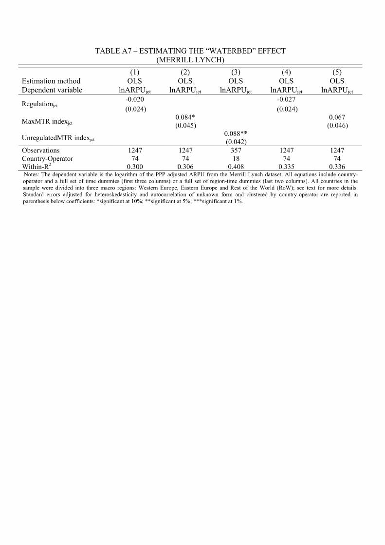
TABLE A7 – ESTIMATING THE “WATERBED” EFFECT (MERRILL LYNCH)
(1) (2) (3) (4) (5) Estimation method OLS OLS OLS OLS OLS Dependent variable lnARPUjct lnARPUjct lnARPUjct lnARPUjct lnARPUjct
Regulationjct -0.020 (0.024)
-0.027 (0.024)
MaxMTR indexjct 0.084* (0.045) 0.067
(0.046)
UnregulatedMTR indexjct 0.088** (0.042)
Observations 1247 1247 357 1247 1247 Country-Operator 74 74 18 74 74 Within-R2 0.300 0.306 0.408 0.335 0.336 Notes: The dependent variable is the logarithm of the PPP adjusted ARPU from the Merrill Lynch dataset. All equations include country-operator and a full set of time dummies (first three columns) or a full set of region-time dummies (last two columns). All countries in the sample were divided into three macro regions: Western Europe, Eastern Europe and Rest of the World (RoW); see text for more details. Standard errors adjusted for heteroskedasticity and autocorrelation of unknown form and clustered by country-operator are reported in parenthesis below coefficients: *significant at 10%; **significant at 5%; ***significant at 1%.
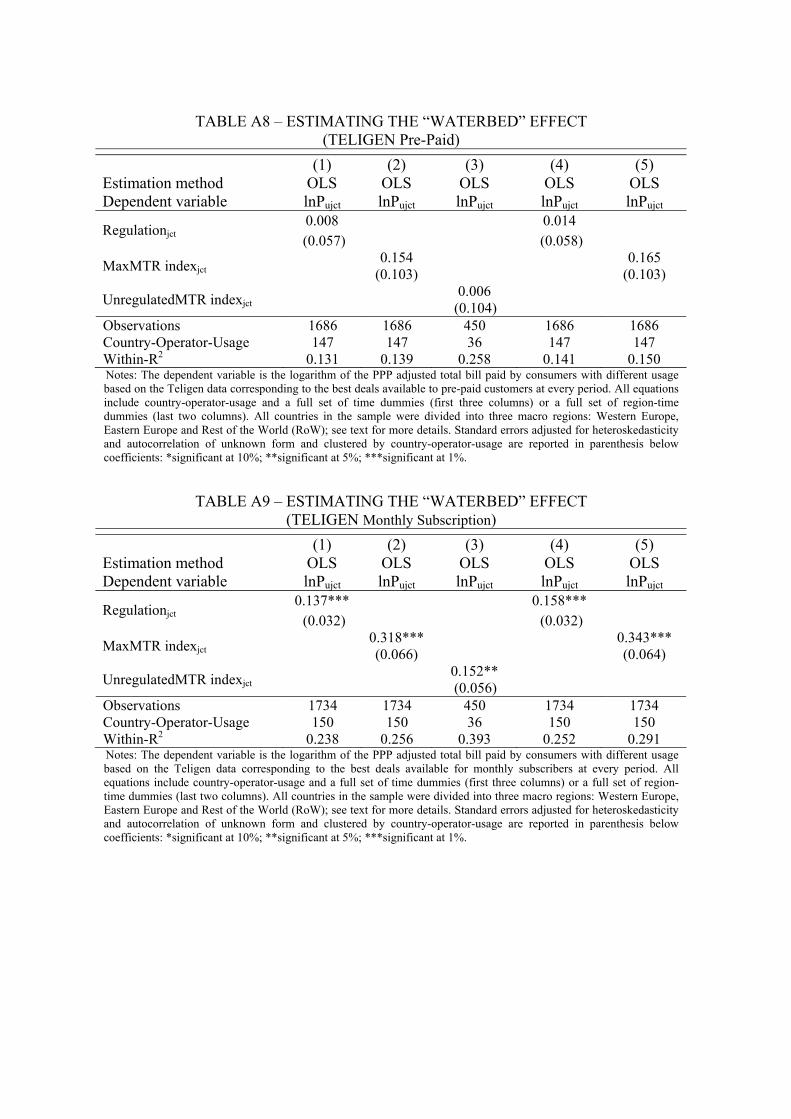
TABLE A8 – ESTIMATING THE “WATERBED” EFFECT
(TELIGEN Pre-Paid)
(1) (2) (3) (4) (5) Estimation method OLS OLS OLS OLS OLS Dependent variable lnPujct lnPujct lnPujct lnPujct lnPujct
Regulationjct 0.008 (0.057)
0.014 (0.058)
MaxMTR indexjct 0.154 (0.103)
0.165
(0.103)
UnregulatedMTR indexjct 0.006 (0.104)
Observations 1686 1686 450 1686 1686 Country-Operator-Usage 147 147 36 147 147 Within-R2 0.131 0.139 0.258 0.141 0.150 Notes: The dependent variable is the logarithm of the PPP adjusted total bill paid by consumers with different usage based on the Teligen data corresponding to the best deals available to pre-paid customers at every period. All equations include country-operator-usage and a full set of time dummies (first three columns) or a full set of region-time dummies (last two columns). All countries in the sample were divided into three macro regions: Western Europe, Eastern Europe and Rest of the World (RoW); see text for more details. Standard errors adjusted for heteroskedasticity and autocorrelation of unknown form and clustered by country-operator-usage are reported in parenthesis below coefficients: *significant at 10%; **significant at 5%; ***significant at 1%.
TABLE A9 – ESTIMATING THE “WATERBED” EFFECT
(TELIGEN Monthly Subscription)
(1) (2) (3) (4) (5) Estimation method OLS OLS OLS OLS OLS Dependent variable lnPujct lnPujct lnPujct lnPujct lnPujct
Regulationjct 0.137***
(0.032)
0.158***
(0.032)
MaxMTR indexjct 0.318*** (0.066)
0.343***
(0.064)
UnregulatedMTR indexjct 0.152** (0.056)
Observations 1734 1734 450 1734 1734 Country-Operator-Usage 150 150 36 150 150 Within-R2 0.238 0.256 0.393 0.252 0.291 Notes: The dependent variable is the logarithm of the PPP adjusted total bill paid by consumers with different usage based on the Teligen data corresponding to the best deals available for monthly subscribers at every period. All equations include country-operator-usage and a full set of time dummies (first three columns) or a full set of region-time dummies (last two columns). All countries in the sample were divided into three macro regions: Western Europe, Eastern Europe and Rest of the World (RoW); see text for more details. Standard errors adjusted for heteroskedasticity and autocorrelation of unknown form and clustered by country-operator-usage are reported in parenthesis below coefficients: *significant at 10%; **significant at 5%; ***significant at 1%.
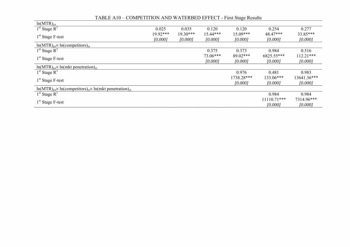
TABLE A10 – COMPETITION AND WATERBED EFFECT - First Stage Results ln(MTR)jct 1st Stage R2 0.025 0.035 0.120 0.120 0.254 0.277
1st Stage F-test 19.92*** [0.000]
19.30*** [0.000]
15.44*** [0.000]
15.09*** [0.000]
48.47*** [0.000]
33.85*** [0.000]
ln(MTR)jct× ln(competitors)ct 1st Stage R2 0.375 0.373 0.984 0.516
1st Stage F-test 73.06*** [0.000]
89.02*** [0.000]
6825.55*** [0.000]
112.21*** [0.000]
ln(MTR)jct× ln(mkt penetration)ct 1st Stage R2 0.976 0.481 0.983
1st Stage F-test 1738.28*** [0.000]
133.06*** [0.000]
13641.36*** [0.000]
ln(MTR)jct× ln(competitors)ct× ln(mkt penetration)ct 1st Stage R2 0.984 0.984
1st Stage F-test 11110.71*** [0.000]
7314.96*** [0.000]
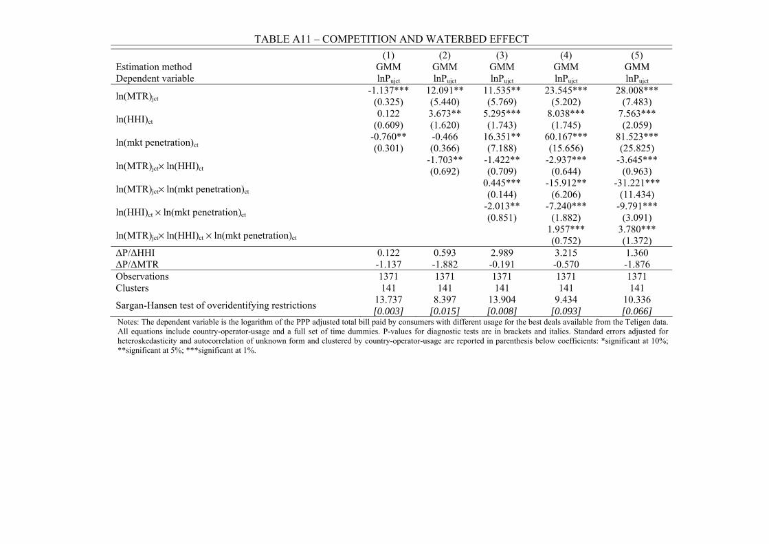
TABLE A11 – COMPETITION AND WATERBED EFFECT
(1) (2) (3) (4) (5) Estimation method GMM GMM GMM GMM GMM Dependent variable lnPujct lnPujct lnPujct lnPujct lnPujct
ln(MTR)jct -1.137***
(0.325) 12.091** (5.440)
11.535** (5.769)
23.545*** (5.202)
28.008*** (7.483)
ln(HHI)ct 0.122
(0.609) 3.673** (1.620)
5.295*** (1.743)
8.038*** (1.745)
7.563*** (2.059)
ln(mkt penetration)ct -0.760** (0.301)
-0.466 (0.366)
16.351** (7.188)
60.167*** (15.656)
81.523*** (25.825)
ln(MTR)jct× ln(HHI)ct -1.703** (0.692)
-1.422** (0.709)
-2.937*** (0.644)
-3.645*** (0.963)
ln(MTR)jct× ln(mkt penetration)ct 0.445*** (0.144)
-15.912** (6.206)
-31.221*** (11.434)
ln(HHI)ct × ln(mkt penetration)ct -2.013** (0.851)
-7.240*** (1.882)
-9.791*** (3.091)
ln(MTR)jct× ln(HHI)ct × ln(mkt penetration)ct 1.957*** (0.752)
3.780*** (1.372)
∆P/∆HHI 0.122 0.593 2.989 3.215 1.360 ∆P/∆MTR -1.137 -1.882 -0.191 -0.570 -1.876 Observations 1371 1371 1371 1371 1371 Clusters 141 141 141 141 141
Sargan-Hansen test of overidentifying restrictions 13.737 [0.003]
8.397 [0.015]
13.904 [0.008]
9.434 [0.093]
10.336 [0.066]
Notes: The dependent variable is the logarithm of the PPP adjusted total bill paid by consumers with different usage for the best deals available from the Teligen data. All equations include country-operator-usage and a full set of time dummies. P-values for diagnostic tests are in brackets and italics. Standard errors adjusted for heteroskedasticity and autocorrelation of unknown form and clustered by country-operator-usage are reported in parenthesis below coefficients: *significant at 10%; **significant at 5%; ***significant at 1%.
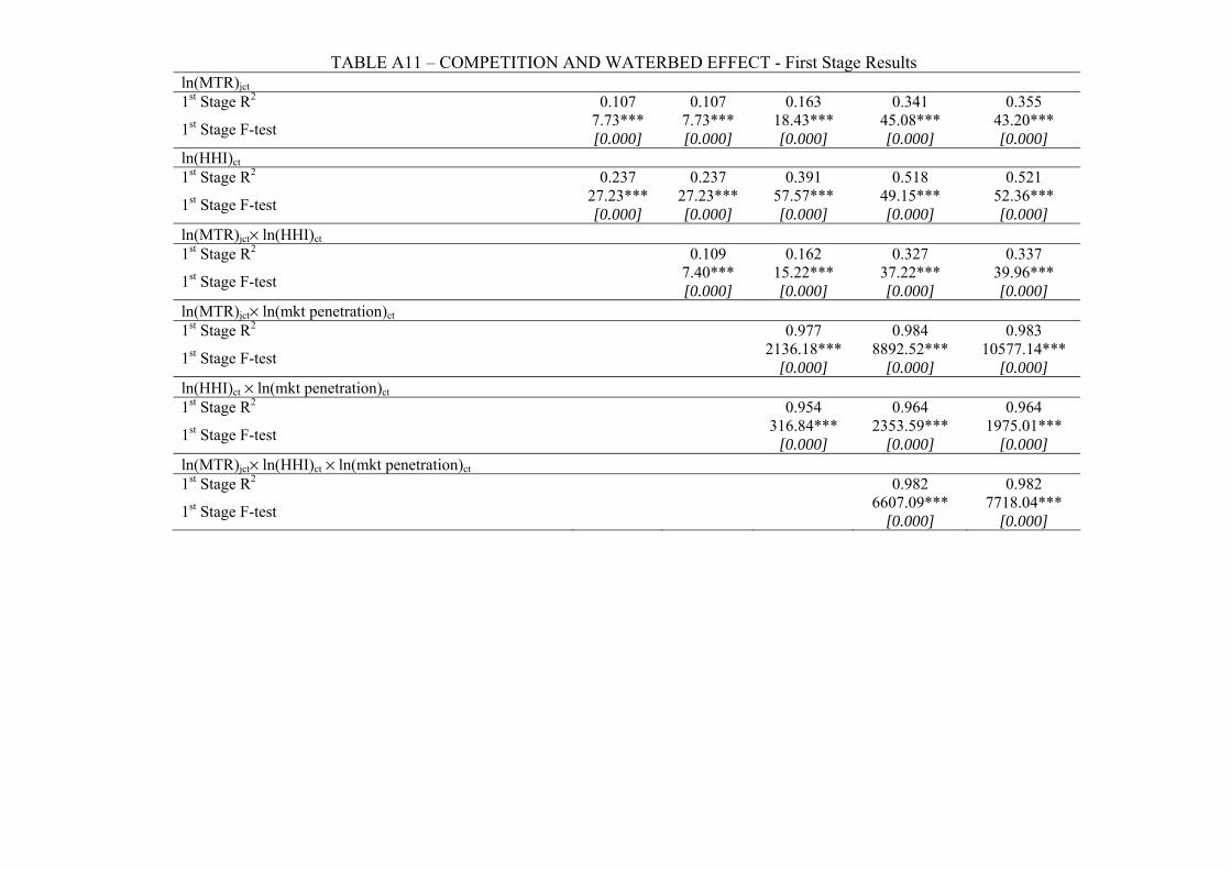
TABLE A11 – COMPETITION AND WATERBED EFFECT - First Stage Results ln(MTR)jct 1st Stage R2 0.107 0.107 0.163 0.341 0.355
1st Stage F-test 7.73*** [0.000]
7.73*** [0.000]
18.43*** [0.000]
45.08*** [0.000]
43.20*** [0.000]
ln(HHI)ct 1st Stage R2 0.237 0.237 0.391 0.518 0.521
1st Stage F-test 27.23*** [0.000]
27.23*** [0.000]
57.57*** [0.000]
49.15*** [0.000]
52.36*** [0.000]
ln(MTR)jct× ln(HHI)ct 1st Stage R2 0.109 0.162 0.327 0.337
1st Stage F-test 7.40*** [0.000]
15.22*** [0.000]
37.22*** [0.000]
39.96*** [0.000]
ln(MTR)jct× ln(mkt penetration)ct 1st Stage R2 0.977 0.984 0.983
1st Stage F-test 2136.18*** [0.000]
8892.52*** [0.000]
10577.14*** [0.000]
ln(HHI)ct × ln(mkt penetration)ct 1st Stage R2 0.954 0.964 0.964
1st Stage F-test 316.84*** [0.000]
2353.59*** [0.000]
1975.01*** [0.000]
ln(MTR)jct× ln(HHI)ct × ln(mkt penetration)ct 1st Stage R2 0.982 0.982
1st Stage F-test 6607.09*** [0.000]
7718.04*** [0.000]

CENTRE FOR ECONOMIC PERFORMANCE Recent Discussion Papers
826 Luis Garicano Paul Heaton
Information Technology, Organization, and Productivity in the Public Sector: Evidence from Police Departments
825 Laura Alfaro Andrew Charlton
Intra-Industry Foreign Direct Investment
824 Miklós Koren Silvana Tenreyro
Technological Diversification
823 Régis Barnichon The Shimer Puzzle and the Correct Identification of Productivity Shocks
822 Carlos Thomas Search Frictions, Real Rigidities and Inflation Dynamics
821 Giulia Faggio Kjell G. Salvanes John Van Reenen
The Evolution of Inequality in Productivity and Wages: Panel Data Evidence
820 Luis Araujo Emanuel Ornelas
Trust-Based Trade
819 Régis Barnichon Productivity, Aggregate Demand and Unemployment Fluctuations
818 Rachel Griffith Sokbae Lee John Van Reenen
Is Distance Dying at Last? Falling Home Bias in Fixed Effects Models of Patent Citations
817 Tsutomu Miyagawa YoungGak Kim
Measuring Organization Capital in Japan: An Empirical Assessment Using Firm-Level Data
816 Andreas Georgiadis Alan Manning
Spend It Like Beckham? Inequality and Redistribution in the UK, 1983-2004
815 Guy Michaels Xiaojia Zhi
Freedom Fries
814 Ralph Ossa Trade Liberalization, Outsourcing, and Firm Productivity
813 Karsten Kohn Alexander C. Lembcke
Wage Distributions by Bargaining Regime: Linked Employer-Employee Data Evidence from Germany
812 Yannis M. Ioannides Henry G. Overman Esteban Rossi-Hansberg Kurt Schmidheiny
The Effect of Information and Communication Technologies on Urban Structure
811 Guy Michaels The Division of Labor, Coordination, and the Demand for Information Processing

810 Maia Güell Jose V. Rodriguez Mora Chris Telmer
Intergenerational Mobility and the Informative Content of Surnames
809 Stephen J. Redding Daniel M. Sturm Nikolaus Wolf
History and Industry Location: Evidence from German Airports
808 Anna Lipinska The Maastricht Convergence Criteria and Optimal Monetary Policy for the EMU Accession Countries
807 Eran Yashiv The Beveridge Curve
806 Ghazala Azmat Alan Manning John Van Reenen
Privatization, Entry Regulation and the Decline of Labor’s Share of GDP: A Cross-Country Analysis of the Network Industries
805 Henry G. Overman Patricia Rice Anthony J. Venables
Economic Linkages Across Space
804 Benjamin Aleman-Castilla The Returns to Temporary Migration to the United States: Evidence from the Mexican Urban Employment Survey
803 Eran Yashiv Labor Search and Matching in Macroeconomics
802 Nicholas Oulton Jeremy Greenwood and Per Krusell, “Growth Accounting with Investment-Specific Technological Progress: A Discussion of Two Approaches” A Rejoinder
801 Mirabelle Muûls Mauro Pisu
Imports and Exports at the Level of the Firm: Evidence from Belgium
800 Richard E. Baldwin Frédéric Robert-Nicoud
Protection for Sale Made Easy
799 Alejandro Cuñat Marc J. Melitz
Volatility, Labor Market Flexibility, and the Pattern of Comparative Advantage
798 Giulia Faggio Job Destruction, Job Creation and Unemployment in Transition Countries: What Can We Learn?
797 Nicholas Oulton Chain Indices of the Cost of Living and the Path-Dependence Problem: an Empirical Solution
796 David Marsden Richard Belfield Salima Benhamou
Inventive Pay Systems and the Management of Human Resources in France and Great Britain
The Centre for Economic Performance Publications Unit
Tel 020 7955 7673 Fax 020 7955 7595 Email [email protected] Web site http://cep.lse.ac.uk
Top Related
Copyright © 2022 FDOKUMEN

