


Bahasa
Halaman
Hukum

Strategic investment decisionsin Zambia’s mining sector
under a constrained energysystem
Bernard TemboUCL Energy Institute
University College London
A thesis submitted in fulfilment of the requirements for thedegree of
Doctor of Philosophy
January 2018


To my loving parents (both deceased) and their grandchildren.


Declaration
I, Bernard Tembo, confirm that the work presented in this thesis is my
own. Where information has been derived from other sources, I confirm
that this has been indicated in the thesis.
Bernard Tembo
January 2018


Acknowledgements
To start, I would like to thank my wife, Fridah Siyanga-Tembo, for her
support and for the many sacrifices she has had to make during the time
I was reading for the PhD. Without her support and sacrifices, this jour-
ney would have been extremely difficult if not impossible. To our children,
Chisomo (Chichi) and Chigomezgo (Chigo), this is for you.
I am grateful to my supervisors Prof. Neil Strachan and Dr Ilkka Keppo
for their guidance and patience. To Neil, your character building words
will forever be cherished. You may never know what you mean to me and
my family.
To my sponsor, UCL Institute for Sustainable Resources, without you this
journey would not have even started. You gave me an opportunity to
study at UCL under great supervisors. I am also indebted to Whole Sys-
tems Energy Modelling Consortium (WholeSEM) who covered my tuition
fees under their grant (EP/K039326/1).
A big thank you to my colleagues at the UCL Energy Institute for their
encouragement, advice and support; particularly, Pablo Carvajal Sarzosa,
Jennifer Love, Maragatham Kumar (Maggie), Joel Guilbaud, Tashweka
Anderson, Dayang Abu Bakar, Melissa Lott, Gabrial Anandarajah, Ivan
Garcia Kerdan, Francis Li, Vig Seewoogoolam, Will Usher, Thuy Duong
Khuu, Baltazar Solano-Rodriguez, Jennifer Cronin, Ukadike Nwaobi (Uka),
Rob Liddiard, Kiran Dhillon, Mae Oroszlany, Andrew Smith to name but a
few. Of course, not forgetting my Basketball team-mates: Sung-Min, Nick,
Marius B., Marius P., Aman, Pip, Yair, Nawfal, Simon and other guys.
To my family, Talingana Tembo, your support and confidence in my abili-
ties is incomparable. My number #1 cheerleader, you are. To my mother-
in-law, Agnes Kambikambi, my gratitude for all you have done for us is im-

6 |
measurable. Let me just say, naonga chomene amama. To Samuel & Anali-
cia Muzata, Kateula & Mulemba Sichalwe, Kangwa & Bukata Lubumbashi,
Michael & Thelma Kapembwa, Fred & Lumba Ng’andu, Nzali Chella, Felix
& Cindy Mwenge, Siloka Siyanga, Siwa Mwene, Claude Mwale, Benjamin
& Ann Chilenga and Adrian & Mwango Ngoma, you guys are indeed a
brother’s keeper.
Finally and more importantly, in You, Oh Lord, I live, move and have my
being. – Acts 17:28
Abstract
This thesis studies the challenge of balancing between economic growth and
social development that many developing countries are facing. The study
sought to understand the impacts that these goals have on each other and
how these impacts could be minimised. It looked at how clean energy
access is modelled in developing countries and also how growth in Zam-
bia’s mining sector would be impacted by meeting the government’s clean
energy access targets in the residential sector. On one hand, increasing ac-
cess to clean energy would lead to increase in energy demand, which would,
in turn, imply increased capital investment in the energy supply system.
This augmented investment means increase in energy prices which in turn
would limit the growth of the mining sector (the backbone of the econ-
omy). Limited growth implicitly means reduced funding for clean energy
projects. Thus, in order to adequately capture these complex interactions,
three bottom-up models were developed: energy demand, energy supply
and mining models. The energy models sought to understand how energy
demand would evolve by 2050 and how much capital investment would be
required to meet this demand. The mining model focused on understanding
how developments in the energy sector would impact strategic investment
decisions in the mining sector. It was found that approaches used to study
how households transition from one energy fuel to another in developing
countries had significant conceptual errors. However, these errors could be
minimised by using a bottom-up approach. Furthermore, it was found that
while profit margins would reduce as a result of increase in energy prices,
the impact of these prices on the firm’s production output was negligible -
except if a firm is a marginal mine operation. The output was not impacted
because mining firms make decisions based on thresholds and not marginal

8 |
decrease in profits. Thus, even though reliable energy supply is critical
in mining operations, the influence of energy price in investment decision
making in Zambia’s mining sector is limited. The key decision variables in
the sector were found to be copper price, grade and type of ore.
Publications
1. Spalding-Fecher et al. 2017. Electricity supply and demand
scenarios for the Southern African power pool, Energy Policy, DOI
http://dx.doi.org/10.1016/j.enpol.2016.10.033.
2. Tembo, B., 2016. Modelling of capital investment decisions. System
Dynamics Conference, Delft, The Netherlands.
https://www.systemdynamics.org/assets/conferences/2016/index.html
3. Tembo, B., 2016. Modelling of energy efficiency in Copper mining
industry. IAEE Conference, Bergen, Norway.
http://www.iaee.org/proceedings/article/13683
4. Spalding-Fecher et al. 2016. The vulnerability of hydropower
production in the Zambezi River Basin to the impacts of climate
change and irrigation developments, Mitig. Adapt. Strateg. Glob.
Change, DOI 10.1007/s11027-014-9619-7.
5. Tembo, B., 2015. Trade-offs in Zambia’s Energy System: Identifying
key drivers. WholeSEM Conference, Cambridge, UK.
http://www.wholesem.ac.uk/wholesem-events-repository/annual-
conf-15
6. Milligan, BM et. al., 2014. (as an academic contributor). 2nd
GLOBE Natural Capital Accounting Study: Legal and policy
developments in twenty-one countries. GLOBE International, UCL
Institute for Sustainable Resources.
http://discovery.ucl.ac.uk/1432359/

10 |
7. Spalding-Fecher, R., et al., 2014. Climate Change and Upstream
Development Impacts on New Hydropower Projects in the Zambezi
Project: Report for Climate and Development Knowledge Network,
January 2014.
http://www.erc.uct.ac.za/groups/esap/current/esap-zambezi1
8. Tembo, B. and Merven, B., 2013. Policy options for the sustainable
development of Zambia’s electricity sector. Journal of Energy in
Southern Africa, 24(2), pp.16–27.
http://www.scielo.org.za/pdf/jesa/v24n2/02.pdf
Contents
Contents 11
List of Figures 17
List of Tables 21
Glossary 25
1 Introduction 29
1.1 Research context . . . . . . . . . . . . . . . . . . . . . . . . 31
1.1.1 Research questions . . . . . . . . . . . . . . . . . . . 33
1.1.2 Contribution to knowledge . . . . . . . . . . . . . . . 34
1.2 Thesis outline . . . . . . . . . . . . . . . . . . . . . . . . . . 35
2 Industry context 37
2.1 Resources and reserves . . . . . . . . . . . . . . . . . . . . . 38
2.2 State of global copper industry . . . . . . . . . . . . . . . . 43
2.2.1 State of the Zambian copper industry . . . . . . . . . 47
2.3 Chapter summary . . . . . . . . . . . . . . . . . . . . . . . . 51
3 Literature review: Review of energy and mining models 53
3.1 What is a model? . . . . . . . . . . . . . . . . . . . . . . . . 54
3.1.1 Modelling paradigms . . . . . . . . . . . . . . . . . . 55
3.1.2 Bottom-up model frameworks . . . . . . . . . . . . . 56
3.1.3 Uncertainty and risks in models . . . . . . . . . . . . 57
3.1.4 Sensitivity analysis . . . . . . . . . . . . . . . . . . . 59
3.2 Studies on energy use and modelling . . . . . . . . . . . . . 60
12 | Contents
3.2.1 Uncertainty in the energy model . . . . . . . . . . . . 61
3.2.2 Industrial energy use and modelling . . . . . . . . . . 61
3.2.3 Energy demand in the copper industry . . . . . . . . 68
3.2.4 Energy efficiency investments . . . . . . . . . . . . . 71
3.2.5 Energy systems in developing countries . . . . . . . . 76
3.3 Studies on copper industry . . . . . . . . . . . . . . . . . . 83
3.3.1 Uncertainty in the copper industry . . . . . . . . . . 84
3.3.2 Material production modelling . . . . . . . . . . . . . 87
3.3.3 Production costs modelling . . . . . . . . . . . . . . . 90
3.3.4 Valuation of copper reserves . . . . . . . . . . . . . . 93
3.3.5 Copper price modelling . . . . . . . . . . . . . . . . . 94
3.3.6 Feedback relationships within a firm . . . . . . . . . 97
3.4 Linkage of energy and mining systems . . . . . . . . . . . . 98
3.5 Chapter summary . . . . . . . . . . . . . . . . . . . . . . . . 99
4 Literature review: Investment decision making 101
4.1 Investment decision making in firms . . . . . . . . . . . . . . 102
4.1.1 Strategic decision making process . . . . . . . . . . . 103
4.1.2 Identification of strategic issues . . . . . . . . . . . . 106
4.1.3 Decision effectiveness . . . . . . . . . . . . . . . . . . 107
4.2 Choice paradigms . . . . . . . . . . . . . . . . . . . . . . . . 109
4.2.1 Decision environment . . . . . . . . . . . . . . . . . . 111
4.2.2 Rationality and bounded rationality . . . . . . . . . . 111
4.2.3 Analytic techniques and their criticism . . . . . . . . 116
4.3 Modelling decision making process . . . . . . . . . . . . . . 119
4.3.1 Characteristics of a system dynamics model . . . . . 120
4.3.2 Decision making in SD models . . . . . . . . . . . . . 121
4.3.3 Model validation process . . . . . . . . . . . . . . . . 124
4.4 Decision making research context . . . . . . . . . . . . . . . 126
4.5 Chapter summary . . . . . . . . . . . . . . . . . . . . . . . . 128
5 Modelling of Zambia’s energy system 129
5.1 Demand model . . . . . . . . . . . . . . . . . . . . . . . . . 130
Contents | 13
5.1.1 Energy consumption in Zambia . . . . . . . . . . . . 133
5.2 Supply model . . . . . . . . . . . . . . . . . . . . . . . . . . 145
5.2.1 Average generation cost of electricity . . . . . . . . . 149
5.3 Scenarios . . . . . . . . . . . . . . . . . . . . . . . . . . . . . 150
5.4 Chapter summary . . . . . . . . . . . . . . . . . . . . . . . . 155
6 Modelling of strategic investment decisions 157
6.1 Introduction . . . . . . . . . . . . . . . . . . . . . . . . . . . 157
6.2 Identification of decision processes . . . . . . . . . . . . . . . 158
6.2.1 Key interview findings . . . . . . . . . . . . . . . . . 160
6.3 Mining model . . . . . . . . . . . . . . . . . . . . . . . . . . 162
6.3.1 Data . . . . . . . . . . . . . . . . . . . . . . . . . . . 163
6.3.2 General Assumptions . . . . . . . . . . . . . . . . . . 164
6.3.3 Framework of a mining firm . . . . . . . . . . . . . . 165
6.3.4 Material module . . . . . . . . . . . . . . . . . . . . 168
6.3.5 Financial module . . . . . . . . . . . . . . . . . . . . 173
6.4 Method for SD model analysis . . . . . . . . . . . . . . . . . 181
6.5 Chapter summary . . . . . . . . . . . . . . . . . . . . . . . . 183
7 Results and discussion 185
7.1 Energy system results . . . . . . . . . . . . . . . . . . . . . . 185
7.1.1 Energy demand . . . . . . . . . . . . . . . . . . . . . 186
7.1.2 Energy supply . . . . . . . . . . . . . . . . . . . . . . 198
7.1.3 Sensitivity analysis on the supply model . . . . . . . 210
7.2 Mining model results . . . . . . . . . . . . . . . . . . . . . . 218
7.2.1 Indicative production scenarios . . . . . . . . . . . . 218
7.2.2 Identification and impacts of key drivers . . . . . . . 224
7.2.3 Impact of increasing access to clean energy . . . . . . 239
7.2.4 Impact of energy efficiency investments . . . . . . . . 243
7.2.5 The impact of expansion strategies on the outlook of
the industry . . . . . . . . . . . . . . . . . . . . . . . 248
7.2.6 Insights from the mining model analysis . . . . . . . 250
7.3 Discussion summary . . . . . . . . . . . . . . . . . . . . . . 252
14 | Contents
7.4 Chapter summary . . . . . . . . . . . . . . . . . . . . . . . . 257
8 Conclusions 259
8.1 Restatement of the research problem . . . . . . . . . . . . . 259
8.2 Main research findings . . . . . . . . . . . . . . . . . . . . . 260
8.2.1 Evolution of Zambia’s energy sector . . . . . . . . . . 260
8.2.2 Decision making in mining firms . . . . . . . . . . . . 263
8.2.3 Impact of access to clean energy . . . . . . . . . . . . 264
8.3 Limitations and future work . . . . . . . . . . . . . . . . . . 265
8.3.1 Modelling of mineral royalty tax . . . . . . . . . . . . 265
8.3.2 Macroeconomic linkage . . . . . . . . . . . . . . . . . 266
8.3.3 Modelling of ore grade . . . . . . . . . . . . . . . . . 266
8.3.4 Impacts of climate change . . . . . . . . . . . . . . . 267
8.3.5 A comprehensive energy resource mapping . . . . . . 267
8.4 Thesis conclusion . . . . . . . . . . . . . . . . . . . . . . . . 268
References 269
A Appendix to Chapter 1 289
A.1 State of the electricity sector in Zambia . . . . . . . . . . . . 290
A.1.1 Energy markets . . . . . . . . . . . . . . . . . . . . . 290
A.1.2 Electricity generation stock . . . . . . . . . . . . . . 292
B Appendix to Chapter 2 293
B.1 Global consumption of copper . . . . . . . . . . . . . . . . . 293
B.2 List of mine operators . . . . . . . . . . . . . . . . . . . . . 294
B.3 Mineral resources in Zambia . . . . . . . . . . . . . . . . . . 297
C Appendix to Chapter 5 299
C.1 CSO summary statistics . . . . . . . . . . . . . . . . . . . . 299
C.2 Input data for demand model . . . . . . . . . . . . . . . . . 300
C.3 Regression results details . . . . . . . . . . . . . . . . . . . . 302
C.4 Projections of energy demand drivers . . . . . . . . . . . . . 303
C.5 Input data for supply model . . . . . . . . . . . . . . . . . . 310
Contents | 15
C.6 Sensitivity analysis data . . . . . . . . . . . . . . . . . . . . 319
D Appendix to Chapter 6 323
D.1 Interview questions . . . . . . . . . . . . . . . . . . . . . . . 323
D.1.1 Interviews with industry consultants . . . . . . . . . 323
D.1.2 Interviews with government agencies . . . . . . . . . 325
D.1.3 Interviews with mining firms . . . . . . . . . . . . . . 327
D.2 Information and consent form . . . . . . . . . . . . . . . . . 329
D.3 Description of the respondents . . . . . . . . . . . . . . . . . 331
D.4 Summary findings of the interviews . . . . . . . . . . . . . . 332
D.4.1 Investment process . . . . . . . . . . . . . . . . . . . 333
D.4.2 Project evaluation and financing . . . . . . . . . . . . 335
D.4.3 Production costs . . . . . . . . . . . . . . . . . . . . 336
D.4.4 Investment policy environment . . . . . . . . . . . . 340
D.4.5 Industry drivers . . . . . . . . . . . . . . . . . . . . 341
D.5 Input data for mining model . . . . . . . . . . . . . . . . . . 344
D.6 Model Tests . . . . . . . . . . . . . . . . . . . . . . . . . . . 351
D.6.1 Applied extreme test . . . . . . . . . . . . . . . . . . 353
E Appendix to Chapter 7 357
E.1 Trade-off analysis . . . . . . . . . . . . . . . . . . . . . . . . 364
E.2 Coal vs Solar comparison analysis . . . . . . . . . . . . . . . 364
E.3 KCM costs structure . . . . . . . . . . . . . . . . . . . . . . 372
E.4 Copper price model estimations . . . . . . . . . . . . . . . . 374
E.5 Impacts of price, ore share and grade . . . . . . . . . . . . . 378

List of Figures
1.1 Zambia’s historical total final energy consumption . . . . . . 32
2.1 Generic process flow in primary copper . . . . . . . . . . . . 42
2.2 Nominal copper price and unit cost . . . . . . . . . . . . . . 46
2.3 Global copper cathode production and consumption . . . . . 47
2.4 Zambian industry’s total final energy demand . . . . . . . . 49
2.5 KCM total final energy demand . . . . . . . . . . . . . . . . 50
2.6 KCM’s final electricity use . . . . . . . . . . . . . . . . . . . 50
2.7 KCM’s electricity demand at end-use level . . . . . . . . . . 51
3.1 Copper industry financial model framework . . . . . . . . . . 75
3.2 Energy consumptions in Africa by sectors . . . . . . . . . . . 77
3.3 Reference Energy System . . . . . . . . . . . . . . . . . . . . 83
3.4 Process flow of primary copper production and energy inputs 88
3.5 Shares of pyro-metallurgy and hydro-metallurgy production 90
3.6 Unit production cost by region . . . . . . . . . . . . . . . . . 92
3.7 The linkage between energy and mining systems . . . . . . . 99
4.1 Generic system dynamic model . . . . . . . . . . . . . . . . 121
4.2 Decision rules govern the rates of flow in systems . . . . . . 124
4.3 Stylised causal loop diagram . . . . . . . . . . . . . . . . . . 125
4.4 Decisions Casual Loop Diagram . . . . . . . . . . . . . . . . 128
5.1 Zambia’s total final energy consumption . . . . . . . . . . . 134
5.2 Zambia’s total final electricity consumption . . . . . . . . . . 135
5.3 Residential sector’s energy end-use services demand . . . . . 137
5.4 Lighting usage patterns . . . . . . . . . . . . . . . . . . . . . 138
18 | List of Figures
5.5 Cooking and heating usage patterns . . . . . . . . . . . . . . 138
5.6 Relationship between energy drivers and end-use services . . 140
6.1 Linkage between the material and financial modules . . . . . 163
7.1 Projected total final energy demand at scenario level . . . . 187
7.2 Projected total final energy demand by sector and fuels . . . 190
7.3 Residential energy demand projection for scenario 1 . . . . . 191
7.4 Fuel-switching and deforestation for Scenario 1 . . . . . . . . 192
7.5 Residential final energy services demand for scenario 1 . . . 193
7.6 Mining energy demand projections (after iterations) . . . . . 196
7.7 Electricity demand uncertainty in the residential and mining
sectors . . . . . . . . . . . . . . . . . . . . . . . . . . . . . . 197
7.8 Levelised cost of electricity (LCoE) for all potential supply
technologies using 2010 cost estimates . . . . . . . . . . . . . 199
7.9 Least cost capacity mix for scenario 1 . . . . . . . . . . . . . 200
7.10 Total electricity generation by technology in scenario 1 . . . 201
7.11 Technology utilisation in scenario 1 . . . . . . . . . . . . . . 202
7.12 System costs and average generating cost in scenario 1 . . . 203
7.13 Relative additional capacity for least cost capacity mix in
scenarios 2 to 5 . . . . . . . . . . . . . . . . . . . . . . . . . 205
7.14 System costs and average generating cost in scenarios 2 to 5 207
7.15 Technology utilisation in scenarios 2 to 5 . . . . . . . . . . . 209
7.16 Effects on total capital investment relative to the REF case . 212
7.17 Effects on average generation cost relative to the REF case . 214
7.18 Effects on solar capacity deployment relative to the REF case215
7.19 Effects on total carbon emissions relative to the REF case . 217
7.20 Range of possible copper cathode production scenarios . . . 219
7.21 Selected copper cathode production regimes . . . . . . . . . 220
7.22 Initial energy demand for selected production regimes . . . . 221
7.23 Average generation cost and electricity demand for selected
iterations . . . . . . . . . . . . . . . . . . . . . . . . . . . . 223
7.24 Monthly cathode production at mining site level . . . . . . . 226
List of Figures | 19
7.25 Unit production cost at mining site level . . . . . . . . . . . 227
7.26 Ore grade at mining site level . . . . . . . . . . . . . . . . . 228
7.27 Average monthly ore production and profit margin at mining
site level . . . . . . . . . . . . . . . . . . . . . . . . . . . . . 229
7.28 Correlation of ore production and production capacities . . . 232
7.29 The impact loss tolerance time on ore production . . . . . . 234
7.30 Components of unit production cost per tonne of cathode
produced . . . . . . . . . . . . . . . . . . . . . . . . . . . . . 236
7.31 Components of Other Production Costs per tonne of cathode
produced . . . . . . . . . . . . . . . . . . . . . . . . . . . . . 238
7.32 Impact of electricity price on cathode production . . . . . . 241
7.33 Impact of electricity price on total profits . . . . . . . . . . . 243
7.34 Impact of energy efficiency investment on total cathode pro-
duction . . . . . . . . . . . . . . . . . . . . . . . . . . . . . . 245
7.35 Impact of energy efficiency investment on total profits . . . . 246
7.36 Impact of energy efficiency investment on total electricity
demand . . . . . . . . . . . . . . . . . . . . . . . . . . . . . 247
7.37 Production based on expansion strategies prices at mining
site level . . . . . . . . . . . . . . . . . . . . . . . . . . . . . 249
A.1 Zambia’s historical total final electricity consumption . . . . 289
D.1 Model extreme conditions testing: Ore production . . . . . . 355
D.2 Model extreme conditions testing: Ore capacity . . . . . . . 356
E.1 Projected mining energy demand at industry level . . . . . . 358
E.2 Projected mining production outputs at industry level . . . . 359
E.3 Projected energy demand for electricity, charcoal and wood
at scenario level . . . . . . . . . . . . . . . . . . . . . . . . . 360
E.4 Residential energy demand projection for scenarios 2-5 . . . 361
E.5 Share of the total river inflows and power output of hydro-
plants . . . . . . . . . . . . . . . . . . . . . . . . . . . . . . 362
E.6 Total electricity generation by technology in scenarios 2-5 . . 363
E.7 LCoE analysis for coal, solar PV and pump storage . . . . . 366
20 | List of Figures
E.8 Replacing coal capacity under constant Fixed O&M costs
for solar PV conditions. . . . . . . . . . . . . . . . . . . . . 367
E.9 Replacing coal capacity under reducing Fixed O&M costs
for solar PV conditions. . . . . . . . . . . . . . . . . . . . . 368
E.10 Replacing coal production under constant Fixed O&M costs
for solar PV conditions. . . . . . . . . . . . . . . . . . . . . 369
E.11 Replacing coal production under reducing Fixed O&M costs
for solar PV conditions. . . . . . . . . . . . . . . . . . . . . 370
E.12 Average ore grade, ore and cathode production . . . . . . . . 376
E.13 Available ore versus produced ore and production capacities 377
E.14 Impact of varying ore grade, ore type share and copper price
on cathode productions . . . . . . . . . . . . . . . . . . . . . 379
E.15 Correlation of ore production and total production cost . . . 380
List of Tables
2.1 Main types of copper ore minerals . . . . . . . . . . . . . . . 40
2.2 Copper Resource and Production by country . . . . . . . . . 44
2.3 Copper Production by company . . . . . . . . . . . . . . . . 45
2.4 Zambia’s mineral resources at mining site level . . . . . . . . 48
3.1 Portfolio of energy policy instruments . . . . . . . . . . . . . 64
3.2 Classification of energy efficiency barriers . . . . . . . . . . . 72
3.3 Sources of uncertainty in mining projects . . . . . . . . . . . 85
3.4 Valuation approaches for mineral properties . . . . . . . . . 93
5.1 Economic assumptions . . . . . . . . . . . . . . . . . . . . . 152
5.2 Scenario description summary . . . . . . . . . . . . . . . . . 154
7.1 Cumulative residential energy demand and deforestation rel-
ative to Scenario 1 . . . . . . . . . . . . . . . . . . . . . . . 194
A.1 Electricity tariffs in Zambia . . . . . . . . . . . . . . . . . . 291
A.2 Electricity generation capacity . . . . . . . . . . . . . . . . . 292
B.1 Copper consumption by country . . . . . . . . . . . . . . . . 293
B.2 Operating firms in Zambia . . . . . . . . . . . . . . . . . . . 294
B.3 Companies’ full name . . . . . . . . . . . . . . . . . . . . . . 296
B.4 Mineral Resources in Zambia . . . . . . . . . . . . . . . . . . 297
C.1 Classification by lighting fuels . . . . . . . . . . . . . . . . . 299
C.2 Classification by cooking fuels . . . . . . . . . . . . . . . . . 299
C.3 Residential energy intensities . . . . . . . . . . . . . . . . . . 300
C.4 Economic sectors’ energy intensities . . . . . . . . . . . . . . 301

22 | List of Tables
C.5 Regression Results . . . . . . . . . . . . . . . . . . . . . . . 302
C.6 Population projections . . . . . . . . . . . . . . . . . . . . . 303
C.7 Sectorial GDP projections . . . . . . . . . . . . . . . . . . . 304
C.8 Rural cooking & heating fuel shares . . . . . . . . . . . . . . 305
C.9 Urban cooking & heating fuel shares . . . . . . . . . . . . . 306
C.10 Lighting fuel shares . . . . . . . . . . . . . . . . . . . . . . . 307
C.11 Other Uses fuel shares . . . . . . . . . . . . . . . . . . . . . 309
C.12 LCoE input data . . . . . . . . . . . . . . . . . . . . . . . . 311
C.13 Minimum new generating capacity . . . . . . . . . . . . . . . 312
C.14 Techno-economic data technologies . . . . . . . . . . . . . . 313
C.15 Variable costs for other technologies . . . . . . . . . . . . . . 316
C.16 Technology production limits . . . . . . . . . . . . . . . . . 317
C.17 Electricity load profiles data . . . . . . . . . . . . . . . . . . 318
C.18 Supply sensitivity scenarios inputs . . . . . . . . . . . . . . . 319
D.1 Unit costs and general inputs . . . . . . . . . . . . . . . . . 344
D.2 Ore characteristics inputs . . . . . . . . . . . . . . . . . . . 349
D.3 Energy intensities inputs . . . . . . . . . . . . . . . . . . . . 350
D.4 Extreme test key inputs . . . . . . . . . . . . . . . . . . . . 354
E.1 Deforestation-electrification trade-off analysis factor . . . . . 364
E.2 Coal-Solar PV-Pump Storage LCoE input data . . . . . . . 365
E.3 Production cost components . . . . . . . . . . . . . . . . . . 373
E.4 Model estimates for Copper prices . . . . . . . . . . . . . . . 375

“Ambition never comes to an end.”KENNETH KAUNDA
Zambia’s First Republican President

Glossary
CEC Copperbelt Energy Corporation Plc 163, 290, 292
clean energy Energy that causes minimal pollution to the atmosphere
and environment when used. Examples of clean energy on the supply
side are solar, wind and hydro technologies. On the demand side,
electricity and gas (bio-gas included) are examples of clean energy.
In this thesis, the discussion on clean energy focuses on the demand
side. As such, a clean energy form is that which leads to minimal
indoor air pollution (in the residential sector). Electricity and gas are
considered clean while charcoal, wood, coal and other crop residuals
are dirty and unsafe fuels. 29, 30, 32, 33, 76, 79–82, 130, 139, 147,
149–151, 153, 155, 186, 187, 194, 197, 203, 218, 239, 240, 244, 252–
255, 259–262, 264–268
COMEX New York Commodity Exchange 46
CSO Central Statistics Office 30, 33, 136, 137, 142, 143, 155, 299
DoE Department of Energy 331
DoM Department of Mines 332
energy efficiency gap The energy use difference that exists between the
current or expected future use and the optimal current or future use.
This helps in quantifying the energy saving opportunity available the
stakeholder. 53, 99, 127, 174, 178, 180
energy intensity A measure of energy consumed per unit of activity or
output. This measure includes, but is not limited to, kWh/tonne,
26 | Glossary
GJ/HH, Btu/US$ or MJ/Kwacha. 58, 61, 70, 78, 130, 131, 133,
140, 143, 145, 188, 242
ERB Energy Regulation Board of Zambia 32, 163, 164, 224, 290
HFO Heavy Fuel Oil 49, 301
IEA International Energy Agency 62, 63, 142, 163, 186
KCM Konkola Copper Mines Plc 49–51, 91, 164, 336
LEAP Long-Range Energy Alternative Planning System 33, 56, 77, 129,
146, 155, 185, 188
LHPL Lunsemfwa Hydro Power Limited 290, 292
LME London Metal Exchange 46
LPG Liquefied Petroleum Gas 30, 149, 187, 194, 252, 255
MARKAL MARket ALlocation 56, 62, 145
MoE Ministry of Energy 32
OAT one-at-a-time 59, 151
ore grade The share of the metal in the ore reserve. This is expressed as
total content of the metal (in tonnes) divided by the total ore size (in
tonnes). 39, 40, 43, 47, 51, 68, 70, 84, 86, 90, 91, 97, 127, 134, 160,
162, 164, 166, 171, 172, 178, 183, 189, 218, 220, 225, 230, 233, 235,
237, 239, 240, 250, 251, 257, 263, 265, 266, 333, 334, 341, 342, 354,
373
OSeMOSYS Open Source Energy Modeling System 33, 129, 145, 147,
185, 188, 198, 219, 222
REDD+ Reducing emissions from deforestation and degradation and en-
hancement of carbon stocks 148, 210, 254
Glossary | 27
SAPP Southern Africa Power Pool 146, 198, 216
SNL SNL Metals and Mining 164
suppressed energy demand The energy demand that is not met. It is a
situation where required energy is not adequately supply to the end-
user: this could be due to limited supply infrastructure or poverty.
131
TAZAMA Tanzania Zambia Mafuta Pipeline Limited 149
tonCath tonnes of copper cathodes 171, 173, 174
tonConc tonnes of copper concentrate 171, 173
tonContCu tonnes of contained copper 171–173, 177, 178
tonOre tonnes of ore 168, 169, 171–173, 177, 181
World Bank The World Bank Group 164, 369
ZESCO ZESCO Limited 146, 148, 163, 224, 291, 292


Chapter 1
Introduction
Policy makers in developing countries are confronted with the challenge
of balancing between social development, economic growth and investing
in infrastructure to support this growth. This is a similar dilemma that
Zambia’s government faces; it hopes to increase access to clean energy1,2
and at the same time hopes that the economy continues growth at a fast
rate (GRZ, 2006). On one hand, increase in access to clean energy leads
to increase in energy demand. This, in turn, implies more capital invest-
ment in the energy supply infrastructure.3 On the other hand, increased
investments in the energy sector mean increase in energy prices which in
turn could limit the growth of energy-intensive economic sectors, such as
the mining sector.
However, these complex interactions between the social goals (such as
increasing access to clean energy), economic growth (such as growth of the
mining sector) and development of the energy system are under-researched
for many African countries. Further, there is limited understanding of how
investment decisions that lead to growth in key economic sectors (such as1See the Glossary for the definition of clean energy.2While a complete discussion of clean energy should include both the demand and the
supply of energy, the discussion of clean energy in this thesis is limited to the demandside only.
3This thesis takes into account that there is a supply shortage. Thus, to meet anyadditional energy demand, there would be need to invest in new supply infrastructurewhich have a higher levelised cost (LCoE) than the current stock.
30 | Introduction
mining sector) are made. Thus, there is need to research and understand
how changes in the economic and energy sectors impact each other and
how this would affect the governments’ development targets.
Zambia is one of the fast-growing economies in Africa, with an annual
average growth rate of 6% between 2005 and 20104. This growth was largely
driven by the mining sector5 which grew by almost 100% between 2002 and
2011 (to 700, 000 tonnes of copper cathodes). This growth coincided with
a copper price increase (in real terms) of almost 300% (from US$1, 850
per tonne in 2002). The mining sector is and has been the backbone of
the Zambia’s economy (GRZ, 2006; IMF, 2008). For instance, in 2010, the
sector accounted for over 80% of the foreign exchange earnings (BoZ, 2011).
Thus, the sector is projected to continue playing a critical role in Zambia’s
social and economic development through to 2030 and beyond (GRZ, 2006;
MOF, 2016).
Furthermore, between 2002 and 2010, while electricity demand in the
mining sector only increased by 4%, demand in the residential sector grew
by over 110%. Despite the growth in residential sector’s demand, access to
clean energy6 only increased by 20% (from 18.4% in 2002 to 22% in 2010)
(CSO, 2005; 2012). It is for this reason that the Zambian government has
increasing access to clean energy as one of its top development priorities
(GRZ, 2006; 2011).
The government plans to use income realised from the mining sector
(through copper exports) to re-invest into different developmental projects
and sectors of the country (GRZ, 2006; MOF, 2016). It is expected that as
the mining sector grows, more financial resources could be generated which
would enable more investments into clean energy supply infrastructure.
This, Zambian government’s logic, therefore makes a good case study to4Complete statistics from Central Statistics Office (CSO) and ZRA only go up to
2010.5The phrases “mining sector” and “copper industry” (in Zambia’s context) will be
used interchangeably throughout this thesis because mining sector is almost only madeup of the copper industry.
6The phrases “access to electricity” and “access to clean energy” will be used inter-changeably through out this thesis. This is because of the three available energy options(wood, charcoal and electricity), only electricity is clean. Gasses (Liquefied PetroleumGas (LPG), biogas and natural gas) are other possible future options.
1.1 Research context | 31
analyse whether such interactions would lead to intended outcomes and
what their impacts would be. This is because the interactions between the
mining sector and these developmental plans are not straightforward as the
above might imply; as there are several feedback loops that would act as
barriers to realising these development aspirations.
This chapter gives the rationale for the study and highlights the main
challenges that Zambia’s energy and mining sectors face. Section 1.1 gives
the context of the research. This section also presents research questions
and gives the contributions that this study makes. Finally, section 1.2 gives
the overview and outline of the thesis.
1.1 Research context
In 2010, Zambia had a population of 13 million with per capita annual
income of $7487 (CSO, 2012; World Bank, 2013). Of the total population,
60% were based in rural areas, of which only 3.1% had access to electricity
while 49.8% of the urban population had access to electricity. Further, all
households that did not have access to electricity used kerosene, candles or
went without lighting service. These households also used traditional fuels
(wood and charcoal) for their cooking and heating needs. Traditional fuels,
however, are neither safe nor clean and do not provide high quality energy
services (Ekholm et al., 2010; Javadi et al., 2013).
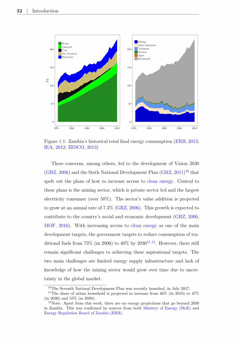
As shown in Figure 1.1 below, final energy consumption in Zambia8
is dominated by traditional fuels and the residential sector. In 2010, the
total final energy consumption was 230 PJ and traditional fuels accounted
for 71%. This 71% was largely consumed in the residential sector by 82%
of the households, for their cooking and heating service (CSO, 2012; IEA,
2012). This means that a large portion (82%) of Zambia’s population9 is
using unsafe and unclean fuel for their energy needs, which also has wider
environmental impacts such as deforestation.7In 2005 US$ constant price.8See Figure A.1 for Zambia’s historical total final electricity consumption.9The population in 2010 was 13 million and it is projected to increase to 25 million
and 45 million by 2030 and 2050 respectively.
32 | Introduction
0
50
100
150
200
1970 1980 1990 2000 2010
PJ
WoodCharcoalCoalPet. ProductsElectricity
0
50
100
150
200
1970 1980 1990 2000 2010
MiningOther IndustriesTransportServicesAgricResidential
Figure 1.1: Zambia’s historical total final energy consumption (ERB, 2013;IEA, 2012; ZESCO, 2013)
These concerns, among others, led to the development of Vision 2030
(GRZ, 2006) and the Sixth National Development Plan (GRZ, 2011)10 that
spelt out the plans of how to increase access to clean energy. Central to
these plans is the mining sector, which is private sector led and the largest
electricity consumer (over 50%). The sector’s value addition is projected
to grow at an annual rate of 7.3% (GRZ, 2006). This growth is expected to
contribute to the country’s social and economic development (GRZ, 2006;
MOF, 2016). With increasing access to clean energy as one of the main
development targets, the government targets to reduce consumption of tra-
ditional fuels from 73% (in 2006) to 40% by 203011,12. However, there still
remain significant challenges to achieving these aspirational targets. The
two main challenges are limited energy supply infrastructure and lack of
knowledge of how the mining sector would grow over time due to uncer-
tainty in the global market.10The Seventh National Development Plan was recently launched, in July 2017.11The share of urban household is projected to increase from 40% (in 2010) to 47%
(in 2030) and 55% (in 2050).12Note: Apart from this work, there are no energy projections that go beyond 2030
in Zambia. This was confirmed by sources from both Ministry of Energy (MoE) andEnergy Regulation Board of Zambia (ERB).
1.1 Research context | 33
1.1.1 Research questions
This research, therefore, answers three questions:
1. How would Zambia’s energy sector evolve by 2050?
2. How do mining organisations make strategic investment decisions and
what are the key decision variables in the mining sector?
3. What impact does increasing access to clean energy in Zambia have
on mining sector’s profitability?
The research is thus divided into two themes: development of the energy
system and decision making in the mining sector. The first theme sought
to understand how energy demand would evolve in Zambia and also how
much capital investment would be required to develop the supply system.13
This theme paid particular attention to how changes in energy use pat-
terns (such as increasing access to clean energy) in the residential sector14
would impact the energy price. To achieve this, a review of journal articles
(given in Chapter 3) and analyses of statistics from Zambia’s CSO and
other government agencies and departments were done and the findings
were integrated into an energy system model (using Long-Range Energy
Alternative Planning System (LEAP) for energy demand and Open Source
Energy Modeling System (OSeMOSYS) for energy supply)15.
The second theme focused on understanding how mining firms make
strategic investment decisions16 and applying this knowledge to Zambia’s
mining sector using a system dynamics (SD) model (built on Vensim plat-
form). Development of the SD model is critical in analysing how the mining
sector would evolve in Zambia. This is necessary because there is limited
knowledge (in Zambia) of how local mining firms make strategic invest-
ment decisions yet the sector is vital and is projected to continue playing a
critical role in the country’s economy (GRZ, 2006; MOF, 2016). Therefore,13See section A.1 of Appendix A for a brief description of the electricity sub-sector
market in Zambia.14The residential sector is the largest final energy consumer in Zambia.15A detailed description of these two models is given in Chapter 5.16Strategic investments are investments that require firms to commit significant re-
sources in order to achieve their desired outcome. See Chapter 4 for more details.

34 | Introduction
understanding the decision processes would help Zambia’s policy makers to
develop policies and regulations that would create a conducive investment
environment.
To achieve the objectives of the second theme, interviews (see Chapter
6 for more details) with local mining firms and industry experts were con-
ducted. The interviews focused on understanding the decision processes
of local mining firms, what their main production costs components were
and the policy environment that would enhance local firms to invest more
were done. Also, a review of industry reports and journal articles (given in
Chapters 3 and 4) which helped in identifying the key exogenous factors in
the sector’s decision making processes as well as the production cost struc-
tures and production processes for different mining operations was carried
out.
1.1.2 Contribution to knowledge
From the reviewed literature, opportunities to contribute to knowledge have
been identified. This research contributes to:
1. Energy system modelling of a small developing country, as most en-
ergy systems studies of developing countries focus on big economies
such as China, India and Brazil.
2. Literature of firms’ strategic investment behaviour under uncertainty,
by considering a key economic sector that is energy intensive in a
country that has limited energy supply infrastructure.
3. Literature that focuses on the interdependence and trade-offs between
developments in the energy sector and growth of key economic sec-
tors. This study captures the feedbacks between these sectors and
the impact they have on each other.

1.2 Thesis outline | 35
1.2 Thesis outline
The thesis consists of 8 chapters and accompanying appendices.
After this introductory chapter, Chapter 2 gives a brief industry context
and introduces some technical terms used in the industry.
Chapters 3 and 4 are literature review chapters. Chapter 3 reviews lit-
erature on energy systems modelling in developing countries and industrial
energy uses. It also looks at the structure and key components of the copper
industry. It then concludes by explaining the linkage between the copper
industry and the energy sector. Chapter 4 reviews literature on strategic
decision making in firms. It highlights the influence that environments in
which firms operate have on their decision making behaviour and how best
this behaviour could be modelled.
Chapters 5 and 6 explain and describe the methods used in modelling
and analysing Zambia’s energy and mining sectors. Chapter 5 describes
the methods used to model energy demand and also identifies key energy
drivers. The chapter also describes how energy supply options were evalu-
ated in the supply model. The methods used in modelling decision making
in the copper industry are described and explained in Chapter 6. This
chapter also identifies key production cost drivers and linkages.
Chapter 7 presents and discusses the results of the research, from the
reviews, interviews and models.
Chapter 8 gives the main conclusions and recommendations, and also
discusses the limitations of the study and possible future work.

Chapter 2
Industry context
This chapter gives a brief industry context of copper. It is divided into
two sections: Section 2.1 defines and introduces some technical concepts
and terminologies of the industry; while section 2.2 highlights the state of
the global copper industry: production and consumption patterns. It also
gives the role that the industry plays in Zambia’s energy sector.
Copper is an important mineral resource; by weight, it is the third most
used metal after iron and aluminium (Radetzki, 2009). It is an important
input in our modern day technology and infrastructure development. Thus,
copper plays a critical role in today’s economies and life-style. In 2010, the
industry’s gross income was US$ 146 billion with a net income of US$ 80
billion1: considering total consumption of 19.332 million tonnes, average
copper price of US$ 7, 535 per tonne and average production cost of US$
3, 391 per tonne (Cochilco, 2012; World Bank, 2015).
Copper is a mineral found in the earth’s crust. It is mainly present
in form of sulphide and oxide minerals (see Table 2.1 below). About 80%
of the world’s primary copper comes from sulphide minerals, with oxide
minerals accounting for the balance. Of the total copper global production,
10-15% is produced from recycled material (Davenport et al., 2002; Norgate
and Jahanshahi, 2010).
1In nominal price value.
38 | Industry context
2.1 Resources and reserves
Resource: A copper resource “is a concentration or occurrence of solid
material of economic interest in or on the Earth’s crust in such form, grade
(or quality), and quantity that there are reasonable prospects for even-
tual economic extraction.” (JORC, 2012; pg. 11). Depending on the level
of confidence, a mineral resource can be categorised into three: Inferred,
Indicated and Measured.
The Inferred resource category includes all the resource that has suffi-
cient geological evidence of the mineral presence but require further explo-
ration and evaluation to upgrade it into the Indicated resource category.
When there is sufficient confidence and details to support feasibility evalu-
ation and mine planning, the resource is referred to as Indicated resource.
To use the word reserve, part of this resource that can be economically
mined could be referred to as probable ore reserve. The final category is
Measured resource, which has detailed and reliable information in order to
support detailed economic analysis and mine planning. When the confi-
dence is high, economically minable Measured resource can be referred to
as proved or proven ore reserve.
Reserve: As described above, part of the mineral resource that can be
economically feasible to extract is referred to as a reserve. A copper ore
reserve is made up of copper, by-products and waste minerals. The size of
the reserve varies depending on the price of copper and the unit production
cost. Low price and high unit production cost reduce the size of the reserve
via raising the ore cut-off grade and vice versa is true. Further, similar to
a resource, a reserve could be sterilised by economic, political, social and
environmental factors (see Crowson (2011) for a further discussion).
Cut-off grade: This is the lowest grade at which mineral extraction
or mining is economically feasible. In other words, it is a threshold below
which a firm chooses not to produce from the ore. Grade is the share of
ore that contains the metal (in this case, copper). On average, the cut-off
grade for copper from open pit mines is 0.5% while from the underground
mines it is 1% (Davenport et al., 2002). Generally, if the ore only con-

2.1 Resources and reserves | 39
tains one mineral say copper, its cut-off grade will be higher than the ore
that contains by-product minerals such as cobalt, gold and silver. This is
because these by-products help reduce the unit production cost (at firm
level). Further, because there is variance in the manner in which ore grade
is distributed in its ore resource, mining firms usually mine different grades
of ore throughout its operational life. For instance, a firm could currently
be producing copper from low grade ore because it is the more accessible
and also because of the ore distribution (ore production does not move
from high ore grade to low ore grade).
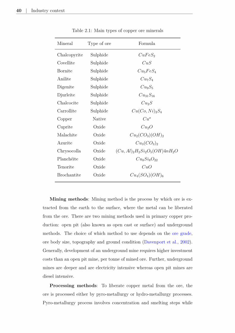
There are two main types of ore: sulphide and oxide. Majority of the
global reserves are sulphide and in particular the chalcopyrite ore (Dav-
enport et al., 2002; Riekkola-Vanhanen, 1999). Table 2.1 below gives a
list of the main types of ore. In addition, the type of ore determines the
processing facility that a mining firm should develop, see below.
40 | Industry context
Table 2.1: Main types of copper ore minerals
Mineral Type of ore Formula
Chalcopyrite Sulphide CuFeS2
Covellite Sulphide CuS
Bornite Sulphide Cu5FeS4
Anilite Sulphide Cu7S4
Digenite Sulphide Cu9S5
Djurleite Sulphide Cu31S16
Chalcocite Sulphide Cu2S
Carrollite Sulphide Cu(Co,Ni)2S4
Copper Native Cuo
Cuprite Oxide Cu2O
Malachite Oxide Cu2(CO3)(OH)2
Azurite Oxide Cu3(CO3)2
Chrysocolla Oxide (Cu,Al)2H2Si2O5(OH)4nH2O
Planchéite Oxide Cu8Si8O22
Tenorite Oxide CuO
Brochantite Oxide Cu4(SO4)(OH)6
Mining methods: Mining method is the process by which ore is ex-
tracted from the earth to the surface, where the metal can be liberated
from the ore. There are two mining methods used in primary copper pro-
duction: open pit (also known as open cast or surface) and underground
methods. The choice of which method to use depends on the ore grade,
ore body size, topography and ground condition (Davenport et al., 2002).
Generally, development of an underground mine requires higher investment
costs than an open pit mine, per tonne of mined ore. Further, underground
mines are deeper and are electricity intensive whereas open pit mines are
diesel intensive.
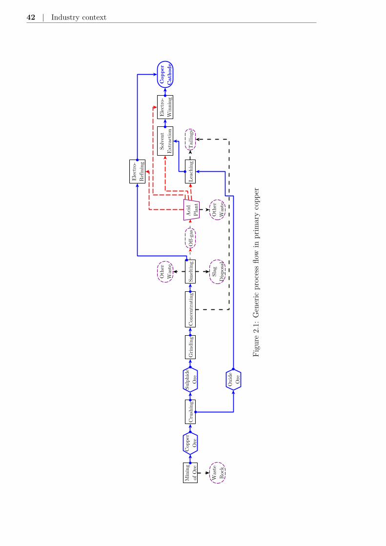
Processing methods: To liberate copper metal from the ore, the
ore is processed either by pyro-metallurgy or hydro-metallurgy processes.
Pyro-metallurgy process involves concentration and smelting steps while

2.1 Resources and reserves | 41
hydro-metallurgy process involves leaching and solvent extraction stages,
as shown in Figure 2.1 below. All sulphide ore is processed using pyro-
metallurgy while hydro-metallurgy is used for oxide ore, with the exception
of Chalcocite ore which can be processed using both processes. Electro-
refining and electro-winning processes are the last steps in the production
process of copper cathodes in pyro-metallurgy and hydro-metallurgy routes
respectively. These two processes are electrolytic processes.
While all the ore that is processed using hydro-metallurgy is processed
on-site or at a facility near the mining site, ore that takes the pyro-metallurgy
route (after the concentration stage) can be processed in facilities far away
from the mining site. After adding value to the ore (at concentration stage),
a mining firm can decide to process the resulting concentrates (30% copper
content) at its facility, sell it to another firm or export it. If the firm decides
to process the concentrates at one of its facility, the resulting blister copper
(99.5% copper content) can be sent to its electro-refinery, sell it to another
firm or export it. Countries like Zambia incentivise firms to process their
sulphide ore at least up to blister copper before exporting it.2
2In order to incentivise firms to add significant value before exporting copper prod-ucts, firms in Zambia have to pay a relatively high export duty for all their ore andconcentrate exports.
42 | Industry context
Figu
re2.
1:G
ener
icpr
oces
sflo
win
prim
ary
copp
er
2.2 State of global copper industry | 43
2.2 State of global copper industry
Historically (from 1800 to 2010), primary copper production has been dom-
inated by 5 countries: Chile, USA, Russia, Canada, and Zambia (Mudd
et al., 2013)3. These countries account for over 63% of the total cumulative
production (a total of 567 million tonnes of contained copper). Until the
early 1980s, the USA was the largest copper producer but now it is Chile;
which accounted for at least 33% of global production in 2010 (Cochilco,
2012; Mudd et al., 2013; Radetzki, 2009). Using a distinction of develop-
ing and developed countries, between 1997 and 2011, developing countries
accounted for at least 62%4 of primary copper production (Cochilco, 2012).
Similarly, as of 2014, developing countries accounted for at least 65%
of the total mineral resource (SNL, 2015). However, the consumption of
copper is and has always been dominated by developed countries. Be-
tween 1997 and 2011, developed countries have consumed at least 83%5
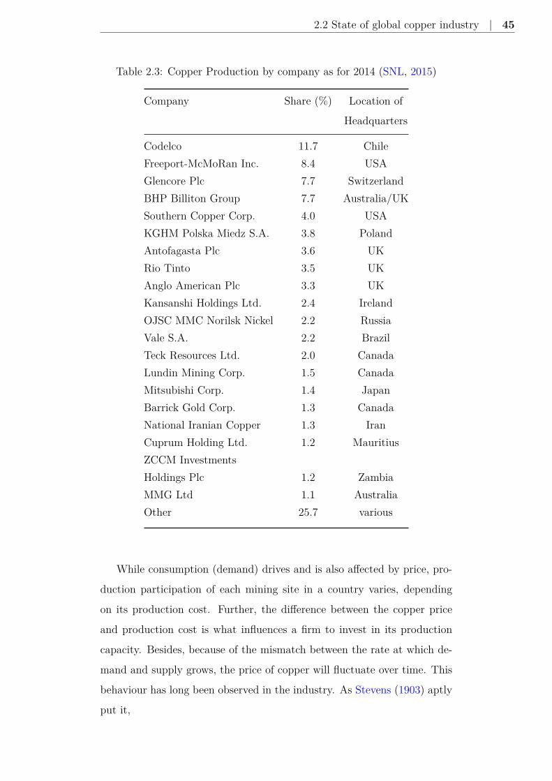
of the total annual production (Cochilco, 2012). The top producing com-
panies (that account for at least 75% of total production) in the industry
are based in developed countries, using headquarters location (SNL, 2015).
This means that even though copper resources are located in developing
countries, the resources are controlled by companies in developed countries.
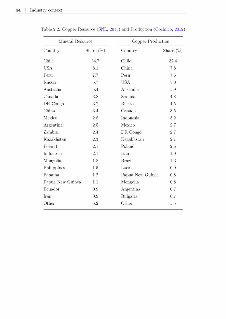
Tables 2.2 and 2.3 below show the list of top 20 locations of mineral re-
sources and primary copper production (by country)6 and top 20 copper
producing companies respectively.7
3See Table 3 in Mudd et al. (2013).4If China is classified as a developed country, otherwise, the share would increase to
67%.5If China is classified as a developed country, otherwise, the share would reduce to
60%.6Profitability of the resource is not dependent on the size but on many other resource
characteristics such as ore grade and by-products.7See Table B.1 of Appendix B for top 20 copper consuming countries.
44 | Industry context
Table 2.2: Copper Resource (SNL, 2015) and Production (Cochilco, 2012)
Mineral Resource Copper Production
Country Share (%) Country Share (%)
Chile 34.7 Chile 32.4USA 8.1 China 7.8Peru 7.7 Peru 7.6Russia 5.7 USA 7.0Australia 5.4 Australia 5.9Canada 3.8 Zambia 4.8DR Congo 3.7 Russia 4.5China 3.4 Canada 3.5Mexico 2.8 Indonesia 3.2Argentina 2.5 Mexico 2.7Zambia 2.4 DR Congo 2.7Kazakhstan 2.3 Kazakhstan 2.7Poland 2.1 Poland 2.6Indonesia 2.1 Iran 1.9Mongolia 1.8 Brazil 1.3Philippines 1.5 Laos 0.9Panama 1.2 Papua New Guinea 0.8Papua New Guinea 1.1 Mongolia 0.8Ecuador 0.9 Argentina 0.7Iran 0.9 Bulgaria 0.7Other 6.2 Other 5.5
2.2 State of global copper industry | 45
Table 2.3: Copper Production by company as for 2014 (SNL, 2015)
Company Share (%) Location of
Headquarters
Codelco 11.7 ChileFreeport-McMoRan Inc. 8.4 USAGlencore Plc 7.7 SwitzerlandBHP Billiton Group 7.7 Australia/UKSouthern Copper Corp. 4.0 USAKGHM Polska Miedz S.A. 3.8 PolandAntofagasta Plc 3.6 UKRio Tinto 3.5 UKAnglo American Plc 3.3 UKKansanshi Holdings Ltd. 2.4 IrelandOJSC MMC Norilsk Nickel 2.2 RussiaVale S.A. 2.2 BrazilTeck Resources Ltd. 2.0 CanadaLundin Mining Corp. 1.5 CanadaMitsubishi Corp. 1.4 JapanBarrick Gold Corp. 1.3 CanadaNational Iranian Copper 1.3 IranCuprum Holding Ltd. 1.2 MauritiusZCCM InvestmentsHoldings Plc 1.2 ZambiaMMG Ltd 1.1 AustraliaOther 25.7 various
While consumption (demand) drives and is also affected by price, pro-
duction participation of each mining site in a country varies, depending
on its production cost. Further, the difference between the copper price
and production cost is what influences a firm to invest in its production
capacity. Besides, because of the mismatch between the rate at which de-
mand and supply grows, the price of copper will fluctuate over time. This
behaviour has long been observed in the industry. As Stevens (1903) aptly
put it,
46 | Industry context
“There will be seasons when demand will follow so closely on the heels of
supply that prices will go skyward, and the fool will say in his heart that the
markets must forever advance. There will also be periods when the supply
will exceed demand, and the faint of heart will say that copper mining
is overdone, and never more can be profitable, but in the aggregate the
great law of averages, immutable as the law of gravitation, will give to the
world the copper for its imperative requirement, at prices not prohibitory
to the consumer, yet sufficiently high to provide for the well-managed mines
profits beyond the dreams of avarice.” (as cited in Prain, 1975; pg. 50)
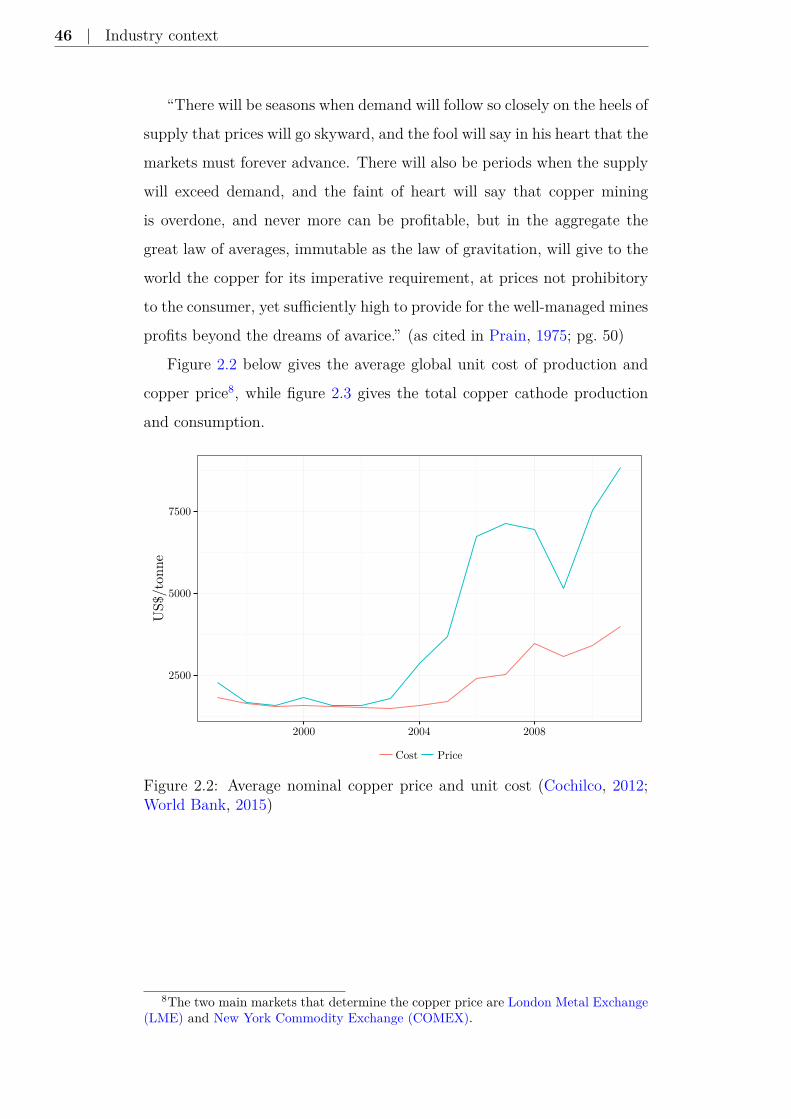
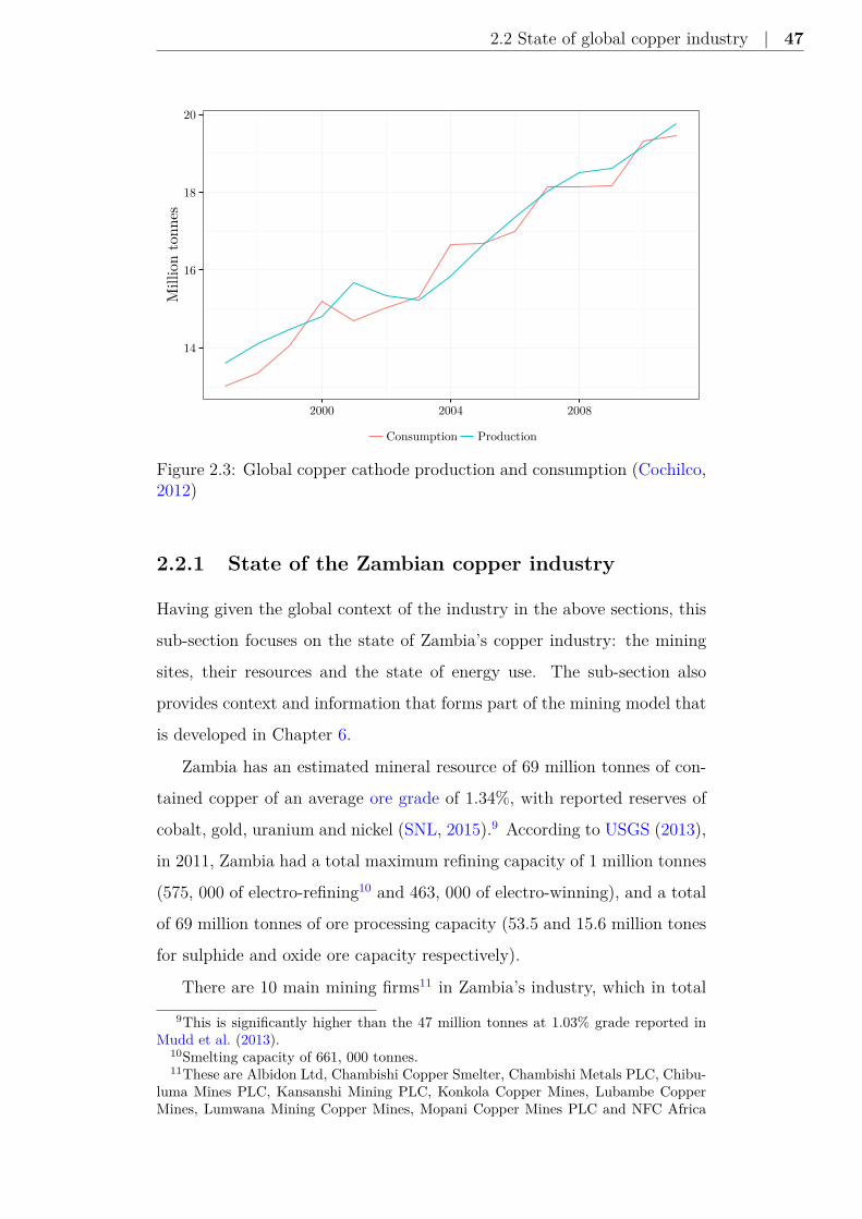
Figure 2.2 below gives the average global unit cost of production and
copper price8, while figure 2.3 gives the total copper cathode production
and consumption.
2500
5000
7500
2000 2004 2008
US$
/ton
ne
Cost Price
Figure 2.2: Average nominal copper price and unit cost (Cochilco, 2012;World Bank, 2015)
8The two main markets that determine the copper price are London Metal Exchange(LME) and New York Commodity Exchange (COMEX).
2.2 State of global copper industry | 47
14
16
18
20
2000 2004 2008
Mill
ion
tonn
es
Consumption Production
Figure 2.3: Global copper cathode production and consumption (Cochilco,2012)
2.2.1 State of the Zambian copper industry
Having given the global context of the industry in the above sections, this
sub-section focuses on the state of Zambia’s copper industry: the mining
sites, their resources and the state of energy use. The sub-section also
provides context and information that forms part of the mining model that
is developed in Chapter 6.
Zambia has an estimated mineral resource of 69 million tonnes of con-
tained copper of an average ore grade of 1.34%, with reported reserves of
cobalt, gold, uranium and nickel (SNL, 2015).9 According to USGS (2013),
in 2011, Zambia had a total maximum refining capacity of 1 million tonnes
(575, 000 of electro-refining10 and 463, 000 of electro-winning), and a total
of 69 million tonnes of ore processing capacity (53.5 and 15.6 million tones
for sulphide and oxide ore capacity respectively).
There are 10 main mining firms11 in Zambia’s industry, which in total9This is significantly higher than the 47 million tonnes at 1.03% grade reported in
Mudd et al. (2013).10Smelting capacity of 661, 000 tonnes.11These are Albidon Ltd, Chambishi Copper Smelter, Chambishi Metals PLC, Chibu-
luma Mines PLC, Kansanshi Mining PLC, Konkola Copper Mines, Lubambe CopperMines, Lumwana Mining Copper Mines, Mopani Copper Mines PLC and NFC Africa
48 | Industry context
employed 63, 300 people and produced 720, 000 tonnes of copper cathodes
in 2012 (CoM, 2014; CSO, 2013). Based on the production statistics and
industry reports, it was estimated that Copperbelt Open Pit, Copperbelt
Underground and North-Western Open Pit accounted for 10.0%, 40.2% and
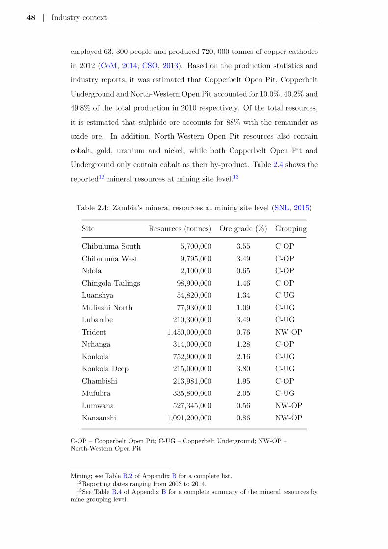
49.8% of the total production in 2010 respectively. Of the total resources,
it is estimated that sulphide ore accounts for 88% with the remainder as
oxide ore. In addition, North-Western Open Pit resources also contain
cobalt, gold, uranium and nickel, while both Copperbelt Open Pit and
Underground only contain cobalt as their by-product. Table 2.4 shows the
reported12 mineral resources at mining site level.13
Table 2.4: Zambia’s mineral resources at mining site level (SNL, 2015)
Site Resources (tonnes) Ore grade (%) Grouping
Chibuluma South 5,700,000 3.55 C-OPChibuluma West 9,795,000 3.49 C-OPNdola 2,100,000 0.65 C-OPChingola Tailings 98,900,000 1.46 C-OPLuanshya 54,820,000 1.34 C-UGMuliashi North 77,930,000 1.09 C-UGLubambe 210,300,000 3.49 C-UGTrident 1,450,000,000 0.76 NW-OPNchanga 314,000,000 1.28 C-OPKonkola 752,900,000 2.16 C-UGKonkola Deep 215,000,000 3.80 C-UGChambishi 213,981,000 1.95 C-OPMufulira 335,800,000 2.05 C-UGLumwana 527,345,000 0.56 NW-OPKansanshi 1,091,200,000 0.86 NW-OP
C-OP – Copperbelt Open Pit; C-UG – Copperbelt Underground; NW-OP –North-Western Open Pit
Mining; see Table B.2 of Appendix B for a complete list.12Reporting dates ranging from 2003 to 2014.13See Table B.4 of Appendix B for a complete summary of the mineral resources by
mine grouping level.
2.2 State of global copper industry | 49
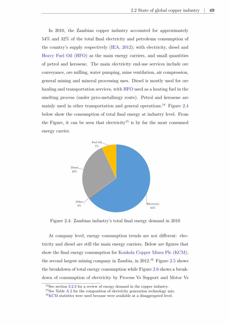
In 2010, the Zambian copper industry accounted for approximately
54% and 32% of the total final electricity and petroleum consumption of
the country’s supply respectively (IEA, 2012); with electricity, diesel and
Heavy Fuel Oil (HFO) as the main energy carriers, and small quantities
of petrol and kerosene. The main electricity end-use services include ore
conveyance, ore milling, water pumping, mine ventilation, air compression,
general mining and mineral processing uses. Diesel is mostly used for ore
hauling and transportation services, with HFO used as a heating fuel in the
smelting process (under pyro-metallurgy route). Petrol and kerosene are
mainly used in other transportation and general operations.14 Figure 2.4
below show the consumption of total final energy at industry level. From
the Figure, it can be seen that electricity15 is by far the most consumed
energy carrier.
Electricity
65%
Other
0%
Diesel
28%
Fuel Oil
7%
Figure 2.4: Zambian industry’s total final energy demand in 2010
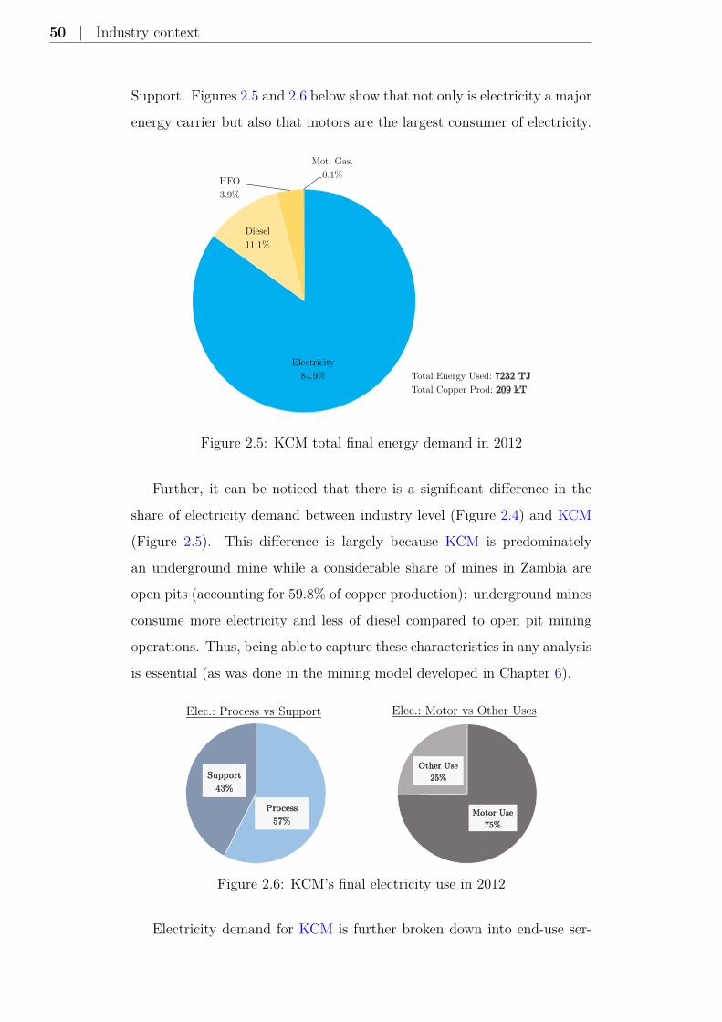
At company level, energy consumption trends are not different: elec-
tricity and diesel are still the main energy carriers. Below are figures that
show the final energy consumption for Konkola Copper Mines Plc (KCM),
the second largest mining company in Zambia, in 2012.16 Figure 2.5 shows
the breakdown of total energy consumption while Figure 2.6 shows a break-
down of consumption of electricity by Process Vs Support and Motor Vs14See section 3.2.3 for a review of energy demand in the copper industry.15See Table A.2 for the composition of electricity generation technology mix.16KCM statistics were used because were available at a disaggregated level.
50 | Industry context
Support. Figures 2.5 and 2.6 below show that not only is electricity a major
energy carrier but also that motors are the largest consumer of electricity.
Electricity
84.9%
Diesel
11.1%
HFO
3.9%
Mot. Gas.
0.1%
Total Energy Used: 7232 TJ
Total Copper Prod: 209 kT
Figure 2.5: KCM total final energy demand in 2012
Further, it can be noticed that there is a significant difference in the
share of electricity demand between industry level (Figure 2.4) and KCM
(Figure 2.5). This difference is largely because KCM is predominately
an underground mine while a considerable share of mines in Zambia are
open pits (accounting for 59.8% of copper production): underground mines
consume more electricity and less of diesel compared to open pit mining
operations. Thus, being able to capture these characteristics in any analysis
is essential (as was done in the mining model developed in Chapter 6).
ProcessProcessProcessProcess
57%57%57%57%
SupportSupportSupportSupport
43%43%43%43%
Elec.: Process vs Support
Motor UseMotor UseMotor UseMotor Use
75%75%75%75%
Other UseOther UseOther UseOther Use
25%25%25%25%
Elec.: Motor vs Other Uses
Figure 2.6: KCM’s final electricity use in 2012
Electricity demand for KCM is further broken down into end-use ser-
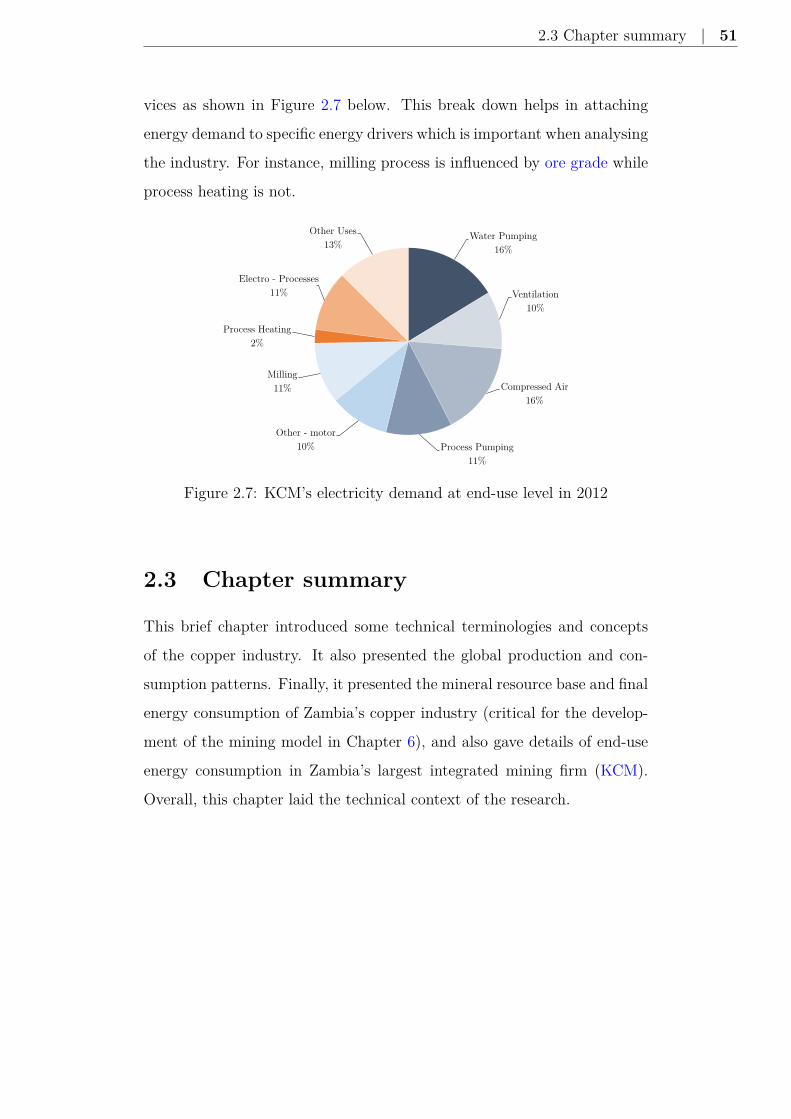
2.3 Chapter summary | 51
vices as shown in Figure 2.7 below. This break down helps in attaching
energy demand to specific energy drivers which is important when analysing
the industry. For instance, milling process is influenced by ore grade while
process heating is not.
Water Pumping
16%
Ventilation
10%
Compressed Air
16%
Process Pumping
11%
Other - motor
10%
Milling
11%
Process Heating
2%
Electro - Processes
11%
Other Uses
13%
Figure 2.7: KCM’s electricity demand at end-use level in 2012
2.3 Chapter summary
This brief chapter introduced some technical terminologies and concepts
of the copper industry. It also presented the global production and con-
sumption patterns. Finally, it presented the mineral resource base and final
energy consumption of Zambia’s copper industry (critical for the develop-
ment of the mining model in Chapter 6), and also gave details of end-use
energy consumption in Zambia’s largest integrated mining firm (KCM).
Overall, this chapter laid the technical context of the research.

Chapter 3
Literature review: Review of
energy and mining models
This chapter is divided into four sections. The first section describes mod-
elling frameworks used when studying energy and mining systems, the
strengths and weakness of these frameworks, and the limitations and uncer-
tainty of using models. The second section reviews and discusses literature
on energy modelling (demand and supply) in developing countries, with a
focus on sub-Saharan energy systems. It discusses how future energy de-
mand has been modelled (a key driver of energy price) and also how the
industrial energy efficiency gap and uptake of efficient technologies have
been characterised. In the third section, a review of copper mining studies
is done. This section focuses on studies that look at aspects that influence
capital investment decision behaviour in mining firms. The fourth section
looks at how the energy (the second section) and mining (the third section)
systems are linked and impact each other. Finally, a chapter summary is
given.
54 | Literature review: Review of energy and mining models
3.1 What is a model?
Models are stylised representations of real-world phenomena (Godfrey-
Smith, 2006; Weisberg, 2007). This representation, among others, can take
a form of graphs, computer programs and mathematical equations. Models
help in studying system interactions and behaviours in a relatively risk free
and inexpensive environment. By analysing the model outcomes, we can
get a deeper understanding of how real-world phenomena work and there-
fore enable us to design a policy environment that could lead to a desired
system outcome.1 Such an outcome could be increase in an organisation’s
productivity or increase in the adoption of energy efficient technologies. In
other words, models are key decision aid tools.
On the whole, a model has three parts (Weisberg, 2007): assignment,
scope and fidelity criteria. The assignment part focuses on the aspects of
the real-world phenomena that need to be studied while the scope looks
at the components of that system that needs to be included to effectively
study the assignment. Finally, the fidelity criteria look at the capability
of the model in representing the real phenomena that need to be studied.
These fidelity criteria focus on the structure of the model that replicates
the structure of the real system and also on how the behaviour (outputs)
of the model compare to those of the system being studied.
Li (2013; pg. 39-40) summarises the series of steps that are taken in
building a model and how to get useful insights from it:
• Choosing a model
• Finding a way of implementing that model
• Studying the output of the resulting model
• Using this entire process to make inferences
• Trying to justify those inferences
1See Wang et al. (2017) for how a model was used to provide a better understandingof future socio-economic dynamics and Koppelaar et al. (2016) for how a model can aidpolicy and decision making.
3.1 What is a model? | 55
3.1.1 Modelling paradigms
There are two energy main modelling paradigms: top-down and bottom-
up. The top-down approach “breaks down a system to gain insight into
its compositional sub-systems, while a bottom-up approach puts together
elements of a system to give rise to grander systems, thus making the orig-
inal systems sub-systems of the emergent system.” (Kesicki, 2012; pg. 73).
An example of a top-down approach is a CGE model (computable general
equilibrium), which focuses on the aggregate behaviour of a system (such
as an economic system) due to change in policy direction or other external
factors that would be acting on that system. This approach relies heavily
on the historical trends and assumes that key underlying relationships of
the model remain constant. On the other hand, energy system models are
a typical example of a bottom-up modelling approach.
The bottom-up approach is built on an engineering thinking. It en-
ables detailed modelling of components of a system. Thus, it is generally a
suitable approach when the purpose of the model is to study the impacts
that each component (disaggregated) has on a system. For instance, when
modelling industrial energy use, a bottom-up approach is more appropriate
because of its ability to capture many energy-related aspects of the system
in disaggregated form (Bhattacharyya and Timilsina, 2010; Fleiter et al.,
2011). This approach, for instance, makes it possible to analyse how invest-
ing in energy efficient technology would impact the total energy demand of
the industry.
The use of either of these approaches (top-down or bottom-up) is deter-
mined by the modelling goal and scope (Fleiter et al., 2011). However, be-
cause this research hopes to understand how different aspects (components)
of the model impact investment behaviour of a mining firm, a bottom-up
approach is used.
56 | Literature review: Review of energy and mining models
3.1.2 Bottom-up model frameworks
Bottom-up models can be categorised into three groups; namely, account-
ing, optimisation and simulation models (Fleiter et al., 2011; Giatrakos
et al., 2009). Accounting models are characterised by less dynamism and
exogenous definition of variables. The model outcome is heavily influenced
by the input assumptions and data. Thus, it is difficult to explicitly model
firm’s investment behaviour. However, because they are simple and trans-
plant, these models are powerful tools for analysing energy demand. An
example of an accounting modelling framework is LEAP2. Wang et al.
(2007) use LEAP to assess the options for emissions abatement in China’s
steel industry.
Optimisation models are prescriptive models. The modeller defines re-
lationship between variables and boundaries from which a solution can be
picked, the model finds the optimal solution. These models are driven by
an objective function, which would be made up of different variables such
as costs and emission limits. This framework assumes that the decision
maker has perfect foresight and knowledge. Thus, it implies that the deci-
sion maker can systematically plan their investment stock profile and also
avoid technology lock-in. This weakness (assumption of perfect foresight
and knowledge) notwithstanding, optimisation models are useful in esti-
mating the efforts that would be required to achieve a desired goal based
on what is currently known to the decision maker (and also based on what
the decision maker thinks the future will be like). An example of an opti-
misation model is a MARket ALlocation (MARKAL) framework. Gielen
and Taylor (2007) analysed the role that different technologies could play
improving energy efficiency and reducing CO2 emissions in the industrial
sector using a MARKAL framework.
Simulation models are varied and follow different modelling philosophies
(Fleiter et al., 2011). These models are used as descriptive tools. They help
in understanding how a system would behave under different environments.
These models help the decision maker (or modeller) to get a deeper under-
2Long-Range Energy Alternative Planning System.
3.1 What is a model? | 57
standing of how the system would behave under different scenarios such
as varying policy instruments or relationship between two variables in a
system. Put in another way, these models are used to answer ‘what if’ type
of questions. This model has three main aspects: the representation of the
problem being studied, the relationships and feedbacks between variables,
and the decision rules. A combination of these three aspects makes the
framework complex, abstract and sometimes less transparent (Giatrakos
et al., 2009).
Two examples of simulation models are Naill (1992) and Worrell and
Price (2001). Naill (1992) is a System Dynamics model3 that studied the
dynamics of energy supply and demand (of oil, gas, electricity and coal)
in the USA economy. On the other hand, the NEMS (national energy
modelling system) model (Worrell and Price, 2001) takes a form of an
accounting model except with detailed modelling of technology stock and
explicitly modelled technology adoption and firm behaviour. This model
was used to study energy efficiency improvements in the USA’s industrial
sector.
3.1.3 Uncertainty and risks in models
Regardless of the modelling paradigm, type of model or care taken to build
models, uncertainty still remains. Uncertainty reflects the inability to esti-
mate the exact value of a variable (Ross, 2004) or comprehensively capture
a relationship. There are broadly two sources of uncertainty in models:
parametric and structural (Kesicki, 2012; Usher, 2016). Methods used to
analyse the impact of uncertainty are briefly discussed in sub-section 3.1.4
below. Apart from uncertainty, systems (being modelled) could also experi-
ence shocks. Shocks such as extreme prices, that would lead to unexpected
model behaviour.
3See section 4.3 for a discussion of System Dynamics model.
58 | Literature review: Review of energy and mining models
Parametric uncertainty
Parametric uncertainty focuses on uncertainty that is introduced in a model
due to the way input values are defined or calibrated. Apart from inputs
into the model, this type of uncertainty also includes missing data, ab-
sence of information and errors in the available data. An example of such
uncertainty is the estimation of energy intensity in an energy model.
Structural uncertainty
This type of uncertainty focuses on the structural description of the model.
Definition of system boundary, mathematical formulation and process flows
fall under this type of uncertainty.
System boundary describes how parts of the model interact with each
other and also whether these parts are modelled as exogenous or endoge-
nous factors. An example of system boundary definition problem is how
the reduction of renewable technologies investment capital cost is modelled.
In most models, this is modelled as an exogenous factor yet the reduction
of investment cost is a function of installed capacity, this (installation) is
usually determined endogenously.
Mathematical model formulations are dependent on historical data and
information, which only captures some variables.4 Another source of un-
certainty is the mental model description of a process flow. An example of
this are models that assume that all the coal consumed in the industrial
sector is for energy purposes, when some of the coal is used as a reducing
agent (as a chemical in some industrial processes).
While some of the (parametric and structural) uncertainty can be min-
imised, simple representation is at the core of modelling philosophy. There-
fore, it is more important that the modeller is aware of these uncertainty
than to actually eliminate them. By being aware, the modeller can take
them into account when interpreting the model results.
4These formulae and relationships may change due to social, economic, political andtechnical reasons.
3.1 What is a model? | 59
System risks
System risks are shocks that can be experienced in a model. Shocks such
as a spike in the crude oil or copper price. These could lead to other
impacts depending on how model relationships are captured. For instance,
the copper price is modelled as an exogenous factor using a mean reverting
model5, this means that the price can suddenly increase or be depressed
consistently at a level that has never been observed before. This could
trigger uncharacteristic model behaviour (something possible but that has
not yet been observed in the industry).
3.1.4 Sensitivity analysis
Whereas the aim of uncertainty analysis is to quantify the extent of uncer-
tainty in an input variable through statistical analyses and other methods,
sensitivity analysis focuses on determining the impact that the input vari-
ables have on model outputs (Usher, 2016). For instance, the standard
deviation of a specified input variable can be 0.2 (uncertainty analysis) but
that variable may have zero (0) influence on the model output (sensitivity
analysis). Thus, by using sensitivity analysis techniques, the modeller can
take mitigating actions to improve the quality of the model and its output
(Ford and Flynn, 2005; Ford, 1999; Taylor et al., 2010).
Two approaches are used in parametric sensitivity analyses: local and
global approaches. The local approach (the one-at-a-time (OAT) method)
considers the impact of one variable at a time, before moving to the next.
This method assumes that there are negligible interactions between model
inputs. The method, nonetheless, is useful when the modeller wants to
have an idea of the impact that each variable has on the model output.
Also, because it is simple and transparent, most modellers will be able to
at least interpret the results more accurately. However, the method can
be inefficient when there are many model input variables that have to be
analysed.5See section 3.3.5 for a discussion of models that are used for modelling commodity
prices.
60 | Literature review: Review of energy and mining models
The second method, global approach, gives a better and more robust
measure of influence that a variable has on the model output. This ap-
proach explores a range of possible input values and also consider all vari-
ables simultaneously. This approach thus accounts for possible interaction
impacts that input variables would have on each other. In addition, because
model sensitivity output files can be significantly huge, further statistical
analyses of the results need to be done (R Core Team (2017) was used
to further analyse the data for this research). For instance, for SD model
sensitivity outputs, a statistical method called screening is usually used to
analysis these outputs. Chapter 6 section 6.4 gives a detailed description
of this method (screening method).
Analysing structural uncertainty is challenging, partly because model
contexts are variant. For instance, in the copper industry, it makes logi-
cal sense to model copper price as an exogenous factor when analysing a
price taker industry but the price has to be modelled endogenously when
analysing a price setter industry. Thus, an effective way to reduce struc-
tural uncertainty is for the modeller to have sufficient knowledge (through
journal articles or industry reports) of the system being analysed. Alter-
natively, a modeller can set up different model structures and then analyse
the model output, as was done by Auping (2011).
3.2 Studies on energy use and modelling
This section looks at common uncertainty in energy models, gives a review
of how energy systems are modelled (in developing countries), how energy
efficiency opportunities are evaluated and then proposes an approach for
modelling energy efficiency decision making in the industrial sector. It also
identifies knowledge gaps that exist in industrial energy efficiency studies.
In 2007, global total final energy consumption was 349 EJ; with the
industrial sector consuming 28% (IEA, 2015). Energy demand in the in-
dustrial sector is projected to increase by at least 50% by 2050 compared
to 2006 consumption (Saygin et al., 2011). Given that most sub-sectors
3.2 Studies on energy use and modelling | 61
in the industrial sector are energy intensive and large contributors to CO2
emissions, efforts around the world have focused on how energy consump-
tion can be reduced in the sector without impacting its production output.
This reduction (energy consumption) is seen as a way of mitigating the
impacts of energy use on global climate and local environment.
Further mining and non-ferrous metals sub-sectors are some of the ma-
jor energy consumers in the sector (Gielen and Taylor, 2007); under which
the copper industry falls. Apart from being an energy intensive industry
and emitter of CO2, the copper industry is a significant emitter of SO2 gas
(Alvarado et al., 1999).
3.2.1 Uncertainty in the energy model
Energy models, particularly those focused on developing countries, suffer
from energy intensity error (parametric uncertainty) and conceptualisation
error (structural uncertainty) (Bhattacharyya and Timilsina, 2010; Pandey,
2002). Parametric uncertainty is largely due to lack or limited energy
statistics in developing countries (Bhattacharyya and Timilsina, 2009).
The second and perhaps more problematic is the conceptualisation er-
ror. Most models tend to model developing countries’ systems using frame-
works of developed countries. They usually emphasise the impact of income
and overlook the critical role that governments (in developing countries)
play in the energy sector. An example of such a study is Zeyringer et al.
(2015).6 Pandey (2002) and Bhattacharyya and Timilsina (2010) proposes
ways of modelling developing countries that could help reduce conceptual-
isation errors.
3.2.2 Industrial energy use and modelling
Globally, the industrial sector is the largest consumer of both primary and
final energy. In 2013, this sector consumed 113 EJ of energy (IEA, 2015), an
increase of 17 EJ between 2007 and 2013. Because of this continued upward6Details on the challenges of modelling energy systems in developing country contexts
are discussed later in section 3.2.5 below
62 | Literature review: Review of energy and mining models
trend, there have been many studies (Fleiter et al., 2012; Giacone and
Mancò, 2012; Gielen and Taylor, 2007; Phylipsen et al., 2002; Saidur et al.,
2009; Saygin et al., 2011) that have focused on how energy consumption in
the sector can be reduced.
Gielen and Taylor (2007) looked at the energy and CO2 emission re-
duction potentials that exist in the global industrial sector. The ETP
MARKAL model7 used in this study, explicitly considered different tech-
nologies, their technology learning and other related costs. A least cost
framework was used to estimate the existing potentials in the industry.
This study assumed that the decision makers were rational and had per-
fect foresight. The study found that not only will energy consumption
increase, but also the sector’s CO2 emissions. They recommended that in
order to realise the reduction potentials in the industry, it would be essen-
tial to combine different regulatory and support measures, such as energy
efficiency regulations.
The role that energy efficiency can play in reducing both energy con-
sumption and CO2 emissions is studied in Saygin et al. (2011). The study
divided the industrial sector into two: industrialised countries and develop-
ing countries sectors. The study found that while industrial energy demand
in industrialised countries has remained fairly flat, energy demand in de-
veloping countries has been growing at an annual rate of 3.2% since 1971.8
Further, when the current energy consumption is compared to the global
best practice, it was found that about a third of the total final consumption
can be saved in the industry, mostly (about 70% of the savings) from devel-
oping countries’ industrial sector. This notwithstanding, they found that
the estimations of energy saving potentials were highly uncertain because
of limited data availability from developing countries.
The role that policy and regulation play in promoting energy efficiency
in the industrial sector is studied in Tanaka (2011). The study focuses
7International Energy Agency (IEA)’s Energy Technology Perspectives (ETP)MARKAL model.
8This increase could be in part because of increasing local demand in those group ofcountries and also because some rich countries have exported manufacturing of energyintensive goods and products to these countries.
3.2 Studies on energy use and modelling | 63
on policies that have been implemented in IEA countries, Brazil, China,
India, Mexico, Russia and South Africa. The study found that industrial
energy use was influenced by many factors, among them, technologies used,
processes involved, energy prices, operating environments, organisation’s
priorities and organisation’s decision making paradigm. It was found that
most energy efficiency improvements could only be achieved through tech-
nical actions. The paper focused three categories of policies that could be
used to incentivise technical improvements within an organisation. These
were prescriptive, economic and supportive policies.
Prescriptive policies focus on regulations and agreement that industries
are subjected to in their operating environment. These policies generally
take a form of equipment or plant efficiency regulation. Economic policies
focus on market instruments that can be used to modify the energy use
behaviour in organisations. An example of such policies are taxes and loan
support schemes. The last category (supportive polices) looks at mecha-
nisms that could be put in place to help organisations identify their energy
saving opportunities, build capacity, get advisory services and similar sup-
port structures. The study argues that for any energy efficiency policy,
a package of policies, to be effective, local context of an industry has to
be considered. This is because of the variant barriers of energy efficiency
that exist. Worrell et al. (2004) give summary of policies (see Table 3.1
below) that can be implemented in order achieve the efficiency targets in
the industrial sector.
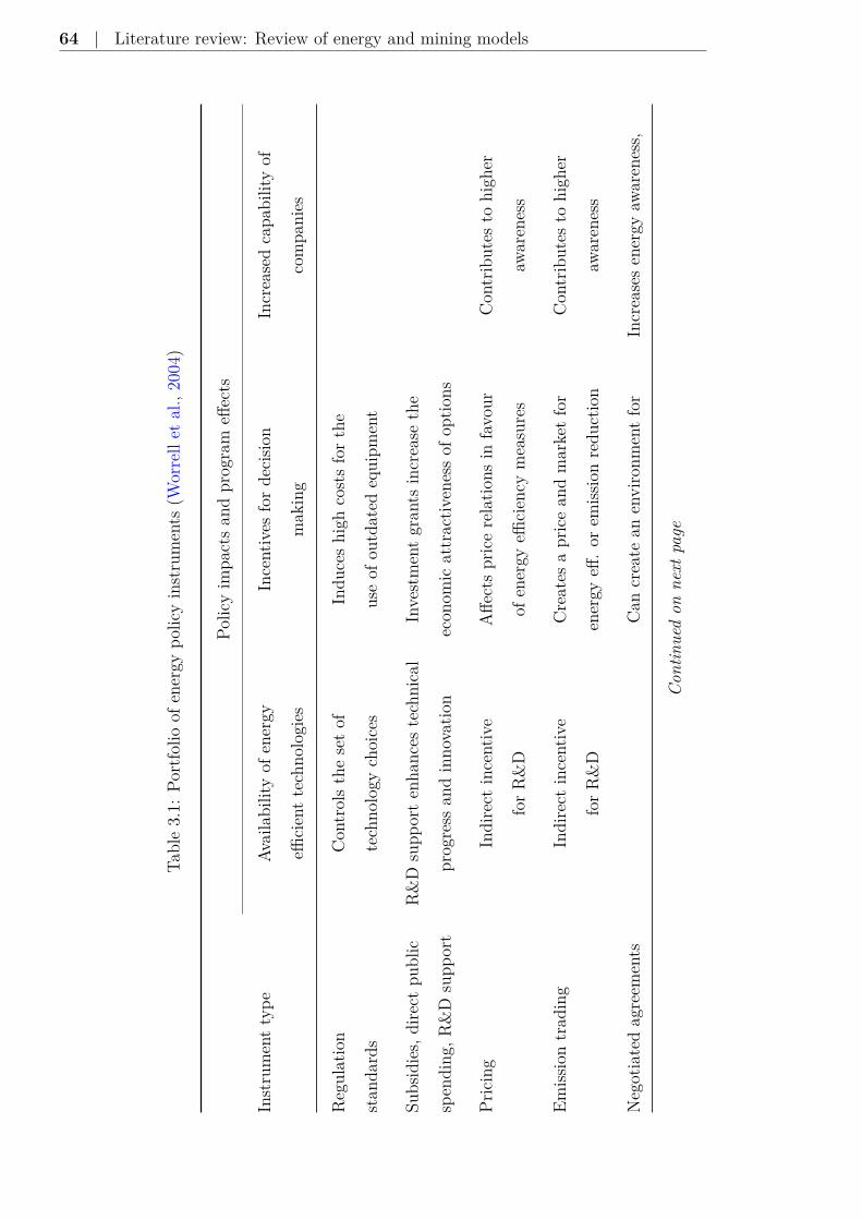
64 | Literature review: Review of energy and mining models
Tabl
e3.
1:Po
rtfo
lioof
ener
gypo
licy
inst
rum
ents
(Wor
rell
etal
.,20
04)
Polic
yim
pact
san
dpr
ogra
meff
ects
Inst
rum
ent
type
Avai
labi
lity
ofen
ergy
Ince
ntiv
esfo
rde
cisio
nIn
crea
sed
capa
bilit
yof
effici
ent
tech
nolo
gies
mak
ing
com
pani
es
Reg
ulat
ion
Con
trol
sth
ese
tof
Indu
ces
high
cost
sfo
rth
e
stan
dard
ste
chno
logy
choi
ces
use
ofou
tdat
edeq
uipm
ent
Subs
idie
s,di
rect
publ
icR
&D
supp
ort
enha
nces
tech
nica
lIn
vest
men
tgr
ants
incr
ease
the
spen
ding
,R&
Dsu
ppor
tpr
ogre
ssan
din
nova
tion
econ
omic
attr
activ
enes
sof
optio
ns
Pric
ing
Indi
rect
ince
ntiv
eA
ffect
spr
ice
rela
tions
infa
vour
Con
trib
utes
tohi
gher
for
R&
Dof
ener
gyeffi
cien
cym
easu
res
awar
enes
s
Emiss
ion
trad
ing
Indi
rect
ince
ntiv
eC
reat
esa
pric
ean
dm
arke
tfo
rC
ontr
ibut
esto
high
er
for
R&
Den
ergy
eff.
orem
issio
nre
duct
ion
awar
enes
s
Neg
otia
ted
agre
emen
tsC
ancr
eate
anen
viro
nmen
tfo
rIn
crea
ses
ener
gyaw
aren
ess,
Con
tinue
don
next
page

3.2 Studies on energy use and modelling | 65
Tabl
e3.
1:Po
rtfo
lioof
ener
gypo
licy
inst
rum
ents
Con
tinue
d
Polic
yim
pact
san
dpr
ogra
meff
ects
Inst
rum
ent
type
Avai
labi
lity
ofen
ergy
Ince
ntiv
esfo
rde
cisio
nIn
crea
sed
capa
bilit
yof
effici
ent
tech
nolo
gies
mak
ing
com
pani
es
ener
gyeffi
cien
cyan
din
nova
tion
com
mun
icat
ion
&di
ssem
inat
ion
Publ
icvo
lunt
ary
Stim
ulat
esR
&D
Prov
ides
info
rmat
ion,
know
-how
,
prog
ram
san
dm
anag
emen
tsu
ppor
t
Man
agem
ent
tool
sLo
wers
(inlo
ngte
rm)
tran
sact
ion
Incr
ease
din
form
atio
n.
cost
sfo
reffi
cien
cyac
tion
Stre
ngth
ened
staff
capa
citie
s.
Indu
ced
lear
ning
effec
ts.
Labe
lling
Bett
erco
mm
unic
atio
nof
Incr
ease
sin
form
atio
n.
cost
para
met
ers
Hig
her
mar
ket
tran
spar
ency
.
Tech
nolo
gypr
ocur
emen
tSt
imul
ates
R&
DD
issem
inat
ion
ofin
form
atio
n
and
inno
vatio
nan
dkn
ow-h
ow.
Con
tinue
don
next
page

66 | Literature review: Review of energy and mining models
Tabl
e3.
1:Po
rtfo
lioof
ener
gypo
licy
inst
rum
ents
Con
tinue
d
Polic
yim
pact
san
dpr
ogra
meff
ects
Inst
rum
ent
type
Avai
labi
lity
ofen
ergy
Ince
ntiv
esfo
rde
cisio
nIn
crea
sed
capa
bilit
yof
effici
ent
tech
nolo
gies
mak
ing
com
pani
es
Qua
lifica
tion
and
trai
ning
.
Best
prac
tice
Incr
ease
saw
aren
ess
and
diss
emin
atio
nin
form
atio
n
Educ
atio
n,qu
alifi
catio
n,Pr
ovisi
onof
info
rmat
ion
trai
ning
and
know
-how
Age
ncy
netw
orks
Net
work
ing
ofac
tors
3.2 Studies on energy use and modelling | 67
Peck and Chipman (2007) discuss industrial energy efficiency, the rea-
sons there has been a strong drive for uptake of efficiency measures and
the different policies that have been adopted to promote uptake of en-
ergy efficient measures. They argue that because the industrial sector is
energy-intensive, many organisations have been forced to consider energy
efficiency options to reduce their costs. They implicitly argue that energy
cost is a significant component of production cost in the sector and as such
any increase in the energy price impacts on the profitability of the sector.
In additional, apart from the impact that energy efficiency would have on
the sector’s profitability, they argue that “in many developing countries en-
ergy efficiency is also a way to alleviate the investment costs for expanding
energy supply infrastructure in the face of tight fiscal constraints.” (Peck
and Chipman, 2007; pg. 334) The latter argument is particularly valuable
to Zambia.
A methodological framework that could be used to measure plant spe-
cific energy efficiency potential is described in Giacone and Mancò (2012).
The paper argues that without taking into consideration the specifics of a
plant being analysed, it would be difficult to measure, monitor and achieve
the desired energy efficiency goal.
Fleiter et al. (2012) use a bottom-up technology-rich model to assess
the energy efficiency opportunities that still exist in German’s pulp and
paper industry. The paper observes like many other studies (Rohdin et al.,
2007; Saidur et al., 2009; Sola et al., 2011; Trianni and Cagno, 2012; Tri-
anni et al., 2013) that implementation of energy efficiency measures has
been low. They attribute this low implementation to lack of appropriate
policies to overcome investment barriers. The study, however, is focused
on the economics of the technologies being analysed. They assume that
if a technology’s economics makes economic sense, then that technology
should be invested into, all things being equal. This is a similar rationale
used in many other energy efficiency studies (Akbaba, 1999; de Almeida
et al., 2003; Saidur et al., 2009; Thirugnanasambandam et al., 2011).
Saidur et al. (2009) focus on identifying equipment that are major con-
68 | Literature review: Review of energy and mining models
sumers of electricity in the Malaysian industry. The study found that
electric motor, pump and compressor systems are the largest consumers.
They argue that even though energy saving potentials exist, lack of govern-
ment regulation and enforcement has led to low implementation. Similarly,
Akbaba (1999) found that electric motors consume about 75% of the total
electric energy in Bahrain. The paper focuses on the impact that replacing
standard electric motors with energy-efficient motors would have on the
total energy demand. As above, the rationale of the analysis was tech-
nology economics. de Almeida et al. (2003) look at electricity used by
motors in European Union’s industrial and services sectors, while Thirug-
nanasambandam et al. (2011) look at potential savings from electric motors
in Indian’s cement industry.
Technology-rich bottom-up method is the dominant approach used in
quantifying the energy saving potential in the industrial sector. This ap-
proach takes one of the following forms: optimisation models (Gielen and
Taylor, 2007), accounting models (Fleiter et al., 2012; Giacone and Mancò,
2012), benchmarking (Phylipsen et al., 2002; Saygin et al., 2011) or simple
NPV and related methods (Akbaba, 1999; de Almeida et al., 2003; Saidur
et al., 2009; Thirugnanasambandam et al., 2011). These approaches are
useful but not sufficient when analysing energy use and possible technol-
ogy diffusion options, as decision makers also consider the economic value
of each of their other investments.
3.2.3 Energy demand in the copper industry
Energy use in the copper industry can be accounted for by using final pro-
duction output (Saygin et al., 2011) or using equipment and process level
approach (Giacone and Mancò, 2012; Norgate and Haque, 2010; Norgate
and Jahanshahi, 2010). The main difference between the two approaches
is that the latter approach is able to capture specific drivers of energy
consumption such as mining methods used, type of ore processed and the
impact that ore grade has on energy consumption. At process level (disag-
gregated level), it is possible to include all the required energy services of
3.2 Studies on energy use and modelling | 69
a process.
The energy end-use services within the copper industry are numerous;
among others, process heating, steam generation, lighting, conveyance,
HVAC, water pumping, ore hauling, mobility and milling purposes. These
services are met by mainly five energy carriers: coal, natural gas, heavy fuel
oil, diesel and electricity. Coal, natural gas and heavy fuel oil are usually
used for process heating and steam generation, while diesel is mainly used
in open pits for ore hauling. Electricity has versatile uses, from hauling
of ore to electrolytic processes. Of these energy carriers, the most energy
saving potentials can be realised in the electricity system; both by replac-
ing inefficient equipment and changing people’s attitude towards electricity
usage (UNIDO, 2012).
Production process stages in the copper industry can be divided into
three parts: mining and mineral processing, smelting and refining compo-
nents. The energy use in each of the stages can then be split into process
and support related energy demand. Further, energy demand for electric-
ity can also be split into electric motor and non-electric motor demand, as
was done in Figure 2.6 above. The distinction between motor and non-
motor energy demand is important because electric motor system is the
largest consumer of electricity and also because most energy saving po-
tentials can be realised from the electric motor system (Akbaba, 1999;
de Almeida et al., 2003; Saidur et al., 2009; Thirugnanasambandam et al.,
2011; UNIDO, 2012).
Industrial electric motor system includes pumps, fans, compressed air,
conveyors, crushers, grinders and mixers (Sola and Mota, 2012). The prime
mover in the system is the electric motor; making electric motors the most
important electric load point (de Almeida et al., 2003). Electricity re-
duction in the motor system can be achieved by implementing several
mechanisms such as replacing inefficient motors, adjusting motor loads,
installing variable speed drive, correct motor sizing, power optimizing de-
vices, maintenance management, information and education and capacitor
banks (Bortoni, 2009; Sola and Mota, 2012). Of these mechanisms, re-
70 | Literature review: Review of energy and mining models
placement of inefficient technologies with efficient motors and installation
of variable speed drive (VSD) would lead to significant reduction in energy
demand (de Almeida et al., 2003; UNIDO, 2012).
The theoretical minimum energy intensity for primary copper produc-
tion (for sulphide ore) is between 1.4 to 2.2 GJ per tonne of metal. How-
ever, the actual specific energy consumption (SEC) for ore from open pit
mine at an ore grade of 1.32% is between 25 - 30 GJ per tonne of metal
(Alvarado et al., 2002; 1999; Norgate and Jahanshahi, 2010). The actual
SEC is largely influenced by the type of mining method, grade of ore and
type of ore being processed (oxide or sulphide ore). For instance, the en-
ergy requirements for processing oxide and sulphide ores (ore grade of 0.5%
from an open pit mine) is 30 and 65 GJ per tonne of metal respectively
(Marsden, 2008).
The difference in energy requirements between Alvarado et al. (2002;
1999), and Marsden (2008) can largely be explained using Equation 3.1
(Gupta, 2003) below, type of ore being processed and energy efficiency of
the processing system. From the equation, it can be seen that as ore grade
reduces (relative to the reference ore grade (OGr)) the quotient increases(OGr−T GOG−T G
), this has a multiplier effect on the total energy demand (for a
particular energy service demand). This relationship (from Equation 3.1)
is however only valid for the mining and mineral processing stage. Energy
demand for smelting and refining stages are not affected by ore grade, thus
only production output (blister or cathode) is important (keeping all other
variables constant) at these two stages.
Ea = Er × (OGr − TG)(OG− TG) (3.1)
where,
Ea is the actual final energy demand,
Er is the reference energy demand (this relates to the ore grade at which
the reference energy demand was calculated),
OGr is the reference ore grade at which Er was calculated,
OG is the ore grade, and
3.2 Studies on energy use and modelling | 71
TG is the tailings grade.
3.2.4 Energy efficiency investments
Despite the existence of energy saving opportunities in the industrial sec-
tor, energy efficiency investments have been low. This low investment has
been attributed to barriers (Fleiter et al., 2011; Sarkar and Singh, 2010;
Sola et al., 2011; Weber, 1997). Barriers can be defined as all factors that
hinder the implementation of energy efficient measures or adoption of en-
ergy efficient technologies. Empirical studies (Rohdin et al., 2007; Schleich,
2009; Trianni and Cagno, 2012) have shown the existence of these barriers
in organisations. For instance, Rohdin et al. (2007) investigated the bar-
riers and drivers of energy efficiency and the significance of each barrier
and driver in the Swedish foundries. An econometric study on German’s
commercial and services sector (Schleich, 2009), considers the impact that
these barriers have on heterogeneous organisations. The study found that
although the barriers were significant at aggregate level, the significance of
different barriers varied across sub-sectors. This study showed that differ-
ent sectors require sector-specific (and organisation-specific) interventions
in overcoming the barriers.
Weber (1997) categorises these barriers into four categories: institu-
tional, organisational, behavioural and market. While Fleiter et al. (2011;
pg. 3102) further classify the barriers into six groups namely; “imperfect
information, hidden costs, risk and uncertainty, split incentives, access to
capital and bounded rationality”. Table 3.2 below shows what constituents
each of the barriers as classified by Fleiter et al.
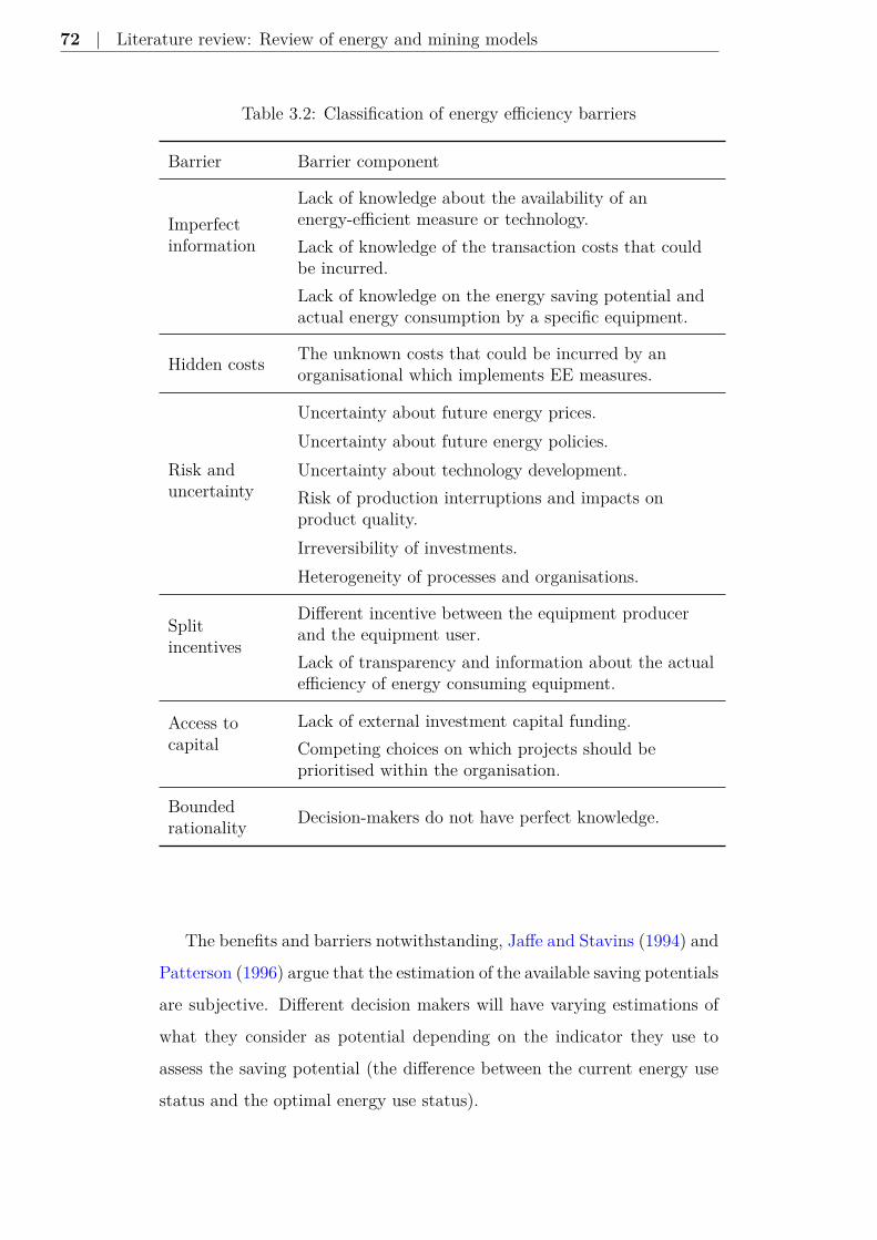
72 | Literature review: Review of energy and mining models
Table 3.2: Classification of energy efficiency barriers
Barrier Barrier component
Imperfectinformation
Lack of knowledge about the availability of anenergy-efficient measure or technology.Lack of knowledge of the transaction costs that couldbe incurred.Lack of knowledge on the energy saving potential andactual energy consumption by a specific equipment.
Hidden costs The unknown costs that could be incurred by anorganisational which implements EE measures.
Risk anduncertainty
Uncertainty about future energy prices.Uncertainty about future energy policies.Uncertainty about technology development.Risk of production interruptions and impacts onproduct quality.Irreversibility of investments.Heterogeneity of processes and organisations.
Splitincentives
Different incentive between the equipment producerand the equipment user.Lack of transparency and information about the actualefficiency of energy consuming equipment.
Access tocapital
Lack of external investment capital funding.Competing choices on which projects should beprioritised within the organisation.
Boundedrationality Decision-makers do not have perfect knowledge.
The benefits and barriers notwithstanding, Jaffe and Stavins (1994) and
Patterson (1996) argue that the estimation of the available saving potentials
are subjective. Different decision makers will have varying estimations of
what they consider as potential depending on the indicator they use to
assess the saving potential (the difference between the current energy use
status and the optimal energy use status).
3.2 Studies on energy use and modelling | 73
Patterson (1996) introduces four main indicators used to measure en-
ergy efficiency: thermodynamic, physical-thermodynamic, economic-thermodynamic,
and economic. He also looks at the challenges that come with usage of any
of these indicators and the steps that must be followed to overcome these
pit-falls. Patterson further argues that developing a proper systems bound-
ary is critical in quantifying the realistic amount of energy that can be saved
by implementing a particular EE measure.
Jaffe and Stavins (1994) discuss the concept of energy gap. This con-
cept looks at the differences that exist between the actual energy being used
and what the optimal energy use should be. They argue that the magni-
tude of the gap is influenced greatly by the view an analyst or a decision
maker take, which would either be: the economists’ economic potential;
the technologists’ economic potential; hypothetical potential; the narrow
social optimum; or the true social optimum. Similar to the selection of
which EE indicator one uses, the energy-gap view that one takes would
result in different estimations. In addition, as opposed to focusing on the
barriers (Weber, 1997), Jaffe and Stavins argue that a holistic approach is
what would be required to achieve optimal levels of energy use.
However, both Jaffe and Stavins (1994) and Patterson (1996), also like
other studies presented in sub-section 3.2.2 above, implicitly argue that if
the saving potentials can be properly estimated and that they make an eco-
nomic sense then energy efficient technology investments should be made.
This argument assumes that energy cost is a significant cost component and
also that the decision maker’s perspective of industry (organisation) related
energy efficiency investments are mainly driven by the energy system.
This view, I argue, is narrow, because it overlooks the impacts that
other costs such as labour cost or profitability would have on decision mak-
ing. As Haglund (2010) observed that with mining organisations focusing
on cost minimisation, it is important that energy costs savings opportuni-
ties are put in context of other costs saving opportunities available to the
organisation. Most organisations make capital investment decisions rela-
tive to other factors (not just energy) and policies. Therefore, previous

74 | Literature review: Review of energy and mining models
studies have lacked a comprehensive view of the system and only focused
on the energy system (shown in Figure 3.1 in the green boundary).

3.2 Studies on energy use and modelling | 75
Figu
re3.
1:C
oppe
rin
dust
ryfin
anci
alm
odel
fram
ewor
k
76 | Literature review: Review of energy and mining models
For instance, to investigate how adoption of efficient technologies could
be enhanced, past studies (Fleiter et al., 2011; Worrell et al., 2004) have
used a high discount or hurdle rate. In this case, a high discount rate or
hurdle rate just helps the decision maker to know if a particular option
is viable or not. It does not, however, establish the state of that option
relative to other options available to the decision maker. Thus, this thesis
captures energy efficiency options9 in the context of other key decision
making drivers such as labour cost and commodity prices, as shown in
Figure 3.1.
3.2.5 Energy systems in developing countries
Having discussed literature surrounding energy use and modelling in the
industrial sector, this section discusses past studies on energy use and mod-
elling in a developing country context. Particular attention is given to the
residential sector (other sectors are transport, services industrial and oth-
ers). The attention on residential sector is mainly because of the challenges
of access to clean energy that the sector faces, it is the largest energy con-
sumer in most sub-Saharan countries (due to usage of primary biofuels)
and finally because many sub-Saharan governments have ambitious plans
for this sector that would have significantly impact the development of the
energy system.
Figure 3.2 below shows the total final energy consumption in Africa be-
tween 1971 and 2013 (IEA, 2015). The residential sector is by far the largest
consumer of final energy in Africa, followed by the transport and industrial
sectors respectively. Almost all the energy consumed in the transport sec-
tor is a product of crude oil (98%) while the industrial sector energy profile
is a mix of coal, natural gas, biofuels, electricity and oil products.
9See section 7.2.4 for an analysis that energy efficiency investments have on totalcopper production and firms’ profits.
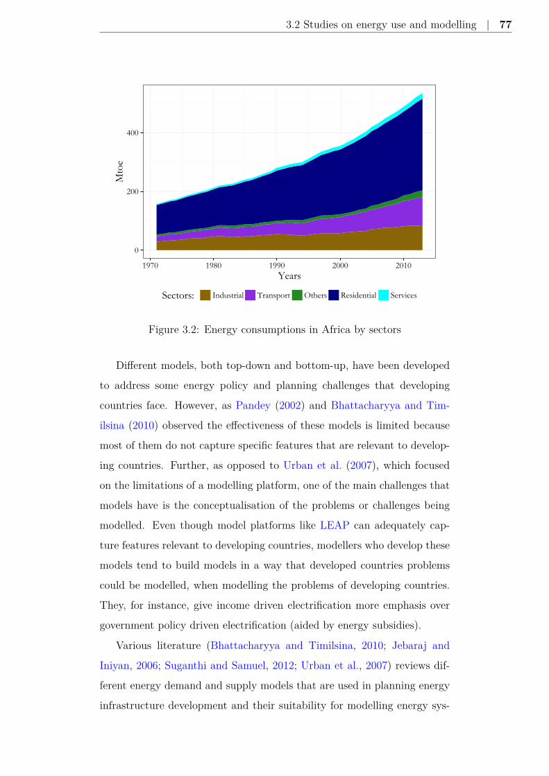
3.2 Studies on energy use and modelling | 77
0
200
400
1970 1980 1990 2000 2010Years
Mto
e
Sectors: Industrial Transport Others Residential Services
Figure 3.2: Energy consumptions in Africa by sectors
Different models, both top-down and bottom-up, have been developed
to address some energy policy and planning challenges that developing
countries face. However, as Pandey (2002) and Bhattacharyya and Tim-
ilsina (2010) observed the effectiveness of these models is limited because
most of them do not capture specific features that are relevant to develop-
ing countries. Further, as opposed to Urban et al. (2007), which focused
on the limitations of a modelling platform, one of the main challenges that
models have is the conceptualisation of the problems or challenges being
modelled. Even though model platforms like LEAP can adequately cap-
ture features relevant to developing countries, modellers who develop these
models tend to build models in a way that developed countries problems
could be modelled, when modelling the problems of developing countries.
They, for instance, give income driven electrification more emphasis over
government policy driven electrification (aided by energy subsidies).
Various literature (Bhattacharyya and Timilsina, 2010; Jebaraj and
Iniyan, 2006; Suganthi and Samuel, 2012; Urban et al., 2007) reviews dif-
ferent energy demand and supply models that are used in planning energy
infrastructure development and their suitability for modelling energy sys-
78 | Literature review: Review of energy and mining models
tems in developing countries. Most of the modelling gaps are in the demand
models: methodological conceptual gaps. To be specific, how specific fea-
tures for developing countries are captured. Bhattacharyya and Timilsina
(2010) discusses the three demand modelling approaches: simple technique,
econometric technique (top-down) and end-use technique (bottom-up).
The simple technique method uses indicators such as growth rate, elas-
ticities and rate of change in energy intensity to forecast energy demand.
This method mostly used as an ad-hoc approach in cases such as where
the modeller does not have data or a solid rationale to base the projections
on. This method is quite common in industry (not common in academic
literature though). The econometric technique focuses on the aggregate
level of energy demand and links the energy demand to economic theory.
It assumes that changes in energy demand are correlated to changes in
the economy. An example of such an approach is Zeyringer et al. (2015).
The end-use technique builds energy demand from a micro-level of energy
services to a macro-level of total energy demand. This technique is able to
capture different energy services and their drivers. This technique is more
suitable because it adequately captures features that are important in de-
veloping countries energy systems (Bhattacharyya and Timilsina, 2010).
An example of an end-use model is Daioglou et al. (2012), a model built to
analyse how a climate policy can be used to reduce emissions from the res-
idential sector. They concluded that end-use models (bottom-up models)
are more suitable for capturing features that are important for developing
countries. However, in practice, these methods or techniques are not used
in isolation but are sometimes combined.
Features that are peculiar to developing countries, include but not lim-
ited to, reliance on traditional energy, the existence of large informal sec-
tors, electrification, urban-rural divide, prevalence of inequity and poverty,
structural changes of the economy, energy transition behaviour from tra-
ditional to modern fuels, inefficient energy supply systems, existence of
social and economic barriers to capital flow and slow technology diffusion
(Bhattacharyya and Timilsina, 2010; Pandey, 2002; Urban et al., 2007).

3.2 Studies on energy use and modelling | 79
For instance in 2013, according to IEA (2015) primary biofuels (traditional
fuels) accounted for more than 50% of the total final energy consumption
in Africa’s energy system. But most models do not explicitly capture the
key drivers of how energy consumption patterns change from traditional
fuels to commercial fuels (electricity and gas).
Of these features listed above, studies that addressed electrification,
urban-rural split, fuel switching and energy transition behaviour from tra-
ditional to commercial fuels are reviewed. This is because they are directly
linked to energy use in the residential sector, which is one of the two main
themes of this research (the other is decision making in the industrial sec-
tor, which also takes into account the change in energy use in the residential
sector). Electricity and gas (clean energy fuels) account for less than 10%
of the total final energy consumed in the residential sector. It is, therefore,
important to study how increased access to clean energy can be achieved,
understand how fuel transition happens in this sector and how this would
impact the whole energy system.
Studies that focus on access to clean energy (in the residential sector
that is) have dominated energy research in sub-Sahara African. This is
because only 31% of the population has access to electricity, with 45%
and 82% of the urban and rural population not having access to electricity
respectively in 2011. Further, more than 80% of this population use tra-
ditional fuels and coal for their cooking and heating service (OECD/IEA,
2010; Zeyringer et al., 2015).
Zeyringer et al. (2015) analyses cost effective options for meeting elec-
tricity demand in Kenya. The study has both energy demand and supply
models. The demand model uses an econometric technique (an exponential
regression model) to estimate electricity demand. Household characteris-
tics such as income, household size, education level and age of the head of
the household and urban-rural split were used as drivers of energy demand.
On the supply, the analysis focused on the economics of grid extension and
off-grid stand alone options (such as solar PV). The off-grid option was
found to be more cost effective way of supplying electricity to rural house-
80 | Literature review: Review of energy and mining models
holds. Komatsu et al. (2011) examines the key determinants that would
help predict if a household in rural Bangladesh would purchase a stand
alone solar PV system or not. This study also uses an econometric model.
Javadi et al. (2013) looked at the role of global policy in increasing electri-
fication in rural areas. Barnes and Floor (1996) looks at how electrification
and access to clean energy can be done in a sustainable way.
While these (Javadi et al., 2013; Komatsu et al., 2011; Zeyringer et al.,
2015) and similar studies explore and contribute to how the energy access
challenge can be solved, they fall short because they either take a nar-
row view of what electrification is or fail to distinguish the type of energy
services that demand energy. For instance, in Komatsu et al. (2011) and
Javadi et al. (2013) electrification was loosely defined to mean lighting.
Therefore, a solution that met lighting service was presented as a solution
for electrification or access to clean energy. This narrow definition of ac-
cess to electricity overlooks the big challenge of energy access: cooking and
heating service. Cooking and heating service account for the largest share
of a household’s total final energy demand (Daioglou et al., 2012). Fur-
ther, whereas lighting is optional, cooking and heating service is a primary
demand.
The econometric methods, such as Zeyringer et al. (2015), aggregate
household energy demand. It is then assumed that electricity supplied
from a solar PV system can be used for cooking or heating the same way
it can be used for lighting. However, this is not the case, because the solar
PV system cannot support heavy loads such as cooking and heating (in
the current form of stand alone solar PV technology). In addition, this
method assumes that increase in electricity and other commercial fuels
demand (non traditional fuels) is only driven by household dynamics such
as increase in income and not, for example, by government policy.
Therefore, for governments that are seeking for solutions that do not
only increase access to electric lighting but also that address other pressing
issues such as reduction in deforestation (through changes in cooking and
heating fuels), these studies would be of limited use. In addition, apart

3.2 Studies on energy use and modelling | 81
from the need to reduce deforestation by increasing access to clean energy,
access to clean energy is central to addressing global challenges such as
poverty, inequality, health and education, and it also comes with different
health implications (Cabraal et al., 2005; Daioglou et al., 2012; OECD/IEA,
2010).
These limitations of econometric methods can be addressed by using an
alternative method: end-use method. This is what Daioglou et al. (2012)
did when analysing how climate policy can be used to reduce emissions from
the residential sector. Individual drivers and services for energy demand in
residential sector were explicitly modelled. This enables a detailed analysis
that changing types of energy fuels of an energy service would have on the
whole system. In this way, access to clean energy can be more appropriately
analysed by using drivers such as income or government policy.
In order to understand how a household transitions from one fuel type
to another, different theories that have been proposed (Barnes and Floor,
1996). At the core of these theories is the energy ladder concept. Masera
et al. (2000) review the concept of energy ladder. The energy ladder concept
studies the transitions that households go through when switching fuels.
The underlying assumption of this concept is that a household decision
maker has access to an array of energy supply (energy fuels) from which
to choose. The concept hypothesises that as households’ income increase,
household abandon traditional fuels (such as primary biomass and coal)
and adopt cleaner energy fuels (electricity and gas).
Barnes and Floor (1996) gives general trends of how household use en-
ergy relative to their levels of income. This paper uses the energy ladder to
explain the linear transition from an inferior fuel to a superior fuel. This
was the approach that Masera et al. (2000) used when studying the en-
ergy use transition in rural Mexico. The study, however, found that energy
transition does not follow a linear path as defined in the classic energy lad-
der concept but that households use multiple fuel energy strategies (a mix
of traditional and clean energy fuels) that are influenced, by among other
factors, income and cultural preferences. Hosier and Dowd (1987) studied
82 | Literature review: Review of energy and mining models
the dynamics of energy use in households of varying incomes. The research
applied energy ladder concept, using a multinomial logit formulation, when
studying fuel transition in rural Zimbabwe. The paper focuses on how deci-
sion making changes among rural households as biomass fuels (traditional
fuels) become scarce and as household income varies. The paper found
that although increase in income is critical for households to transition,
governments need to have policies that encourage such transitions.
These studies (focusing on fuel transition using energy ladder), how-
ever, assume that all the fuels under consideration are at the disposal of
the household decision maker. They do not consider situations where tradi-
tional fuels are the only alternatives available to the decision maker. Thus,
in order for energy transition to happen, a new energy system has to be
created.
This research, therefore, studies the impact that increasing access to
clean energy (either by government policy or household income) would have
on the development of the energy system. This is important because: 1.
many African countries have developmental targets of increasing access to
clean energy, 2. energy systems in Africa are experiencing supply challenges
so even if household income increase, there would be limited fuel switching,
3. increasing energy access would mean increase in energy prices which
would impact the growth of economic sectors, particularly the industrial
sector.
The first aim links the impact that access to clean energy would have on
deforestation, the second focuses on the understanding how much capital
investment could be required to develop the energy system. The third
aim links the impact that increasing access to clean energy would have on
the industrial sector, through energy price. In later sections, these three
aspects are analysed and discussed in the light of this thesis.
The details of both the energy demand and supply models are described
in Chapter 5. The supply model captures the current state of the energy
system, which includes the available energy resources and technical char-
acteristics of the current and future supply technology stock. The model
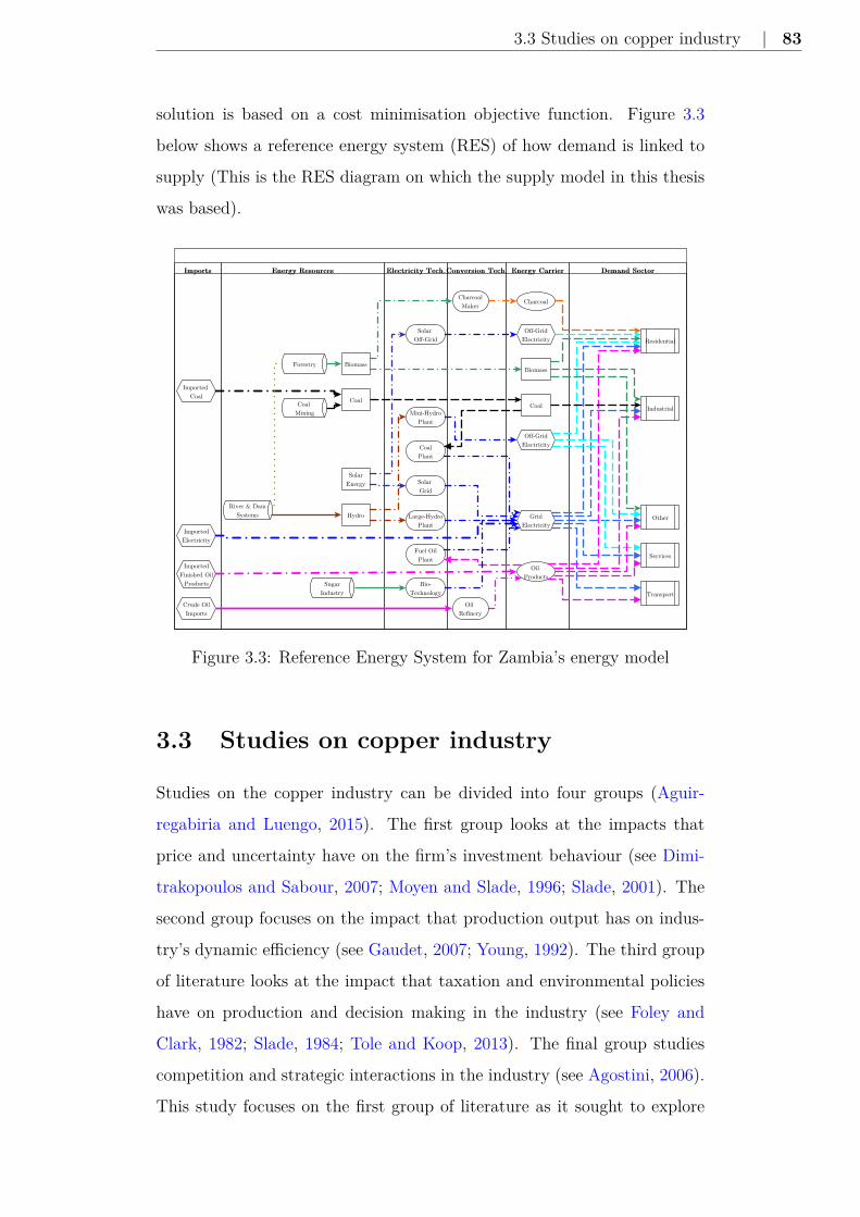
3.3 Studies on copper industry | 83
solution is based on a cost minimisation objective function. Figure 3.3
below shows a reference energy system (RES) of how demand is linked to
supply (This is the RES diagram on which the supply model in this thesis
was based).
Figure 3.3: Reference Energy System for Zambia’s energy model
3.3 Studies on copper industry
Studies on the copper industry can be divided into four groups (Aguir-
regabiria and Luengo, 2015). The first group looks at the impacts that
price and uncertainty have on the firm’s investment behaviour (see Dimi-
trakopoulos and Sabour, 2007; Moyen and Slade, 1996; Slade, 2001). The
second group focuses on the impact that production output has on indus-
try’s dynamic efficiency (see Gaudet, 2007; Young, 1992). The third group
of literature looks at the impact that taxation and environmental policies
have on production and decision making in the industry (see Foley and
Clark, 1982; Slade, 1984; Tole and Koop, 2013). The final group studies
competition and strategic interactions in the industry (see Agostini, 2006).
This study focuses on the first group of literature as it sought to explore
84 | Literature review: Review of energy and mining models
the investment behaviour of a mining firm. The impact of taxation (min-
eral royalty taxation to be specific) on industrial profitability will also be
discussed and analysed in later chapters (Chapters 6 and 7).
Industry investment behaviour can be modelled and studied using top-
down or bottom-up models and analysed using either an optimisation or
simulation framework (Aguirregabiria and Luengo, 2015; Montaldo, 1977;
Sverdrup et al., 2014). To comprehensively explore the behaviour, the
model should capture both the physical (material) and financial compo-
nents of the industry.
The physical component (material module) consists of mining and min-
eral processing, smelting and refining. It focuses on the material produc-
tion process particularly on variables such as the quantity of ore resources
available, type of ore resources, ore grade, methods of mining and capacity
of mining equipment (Mudd et al., 2013; Norgate and Jahanshahi, 2010;
Northey et al., 2014). The financial component (module) focuses on the
investments and profitability of the production capacity and operations
(Auger and Ignacio Guzmán, 2010; Boulamanti and Moya, 2016). In order
to have a better understanding of factors that influence investment be-
haviour, these modules have to be analysed together (Aguirregabiria and
Luengo, 2015; Montaldo, 1977; Sverdrup et al., 2014).
3.3.1 Uncertainty in the copper industry
The value of all mining projects is evaluated based on the characteristics of
their mineral resources10 and the commodity price. It is this valuation that
drives investment decisions such as the mining method to use and the size of
production capacity to invest in. These investments are huge upfront capi-
tal costs yet their economic operational viability are subject to uncertainty.
The value of these resources is significantly influenced by economic (such
as commodity prices) and physical (such as quantity of ore resources and
ore grade) uncertainty (Savolainen, 2016; William et al., 2012). Mayer and
10Characteristics of the mineral resource (ore reserve in particular) directly influencesthe unit production cost.
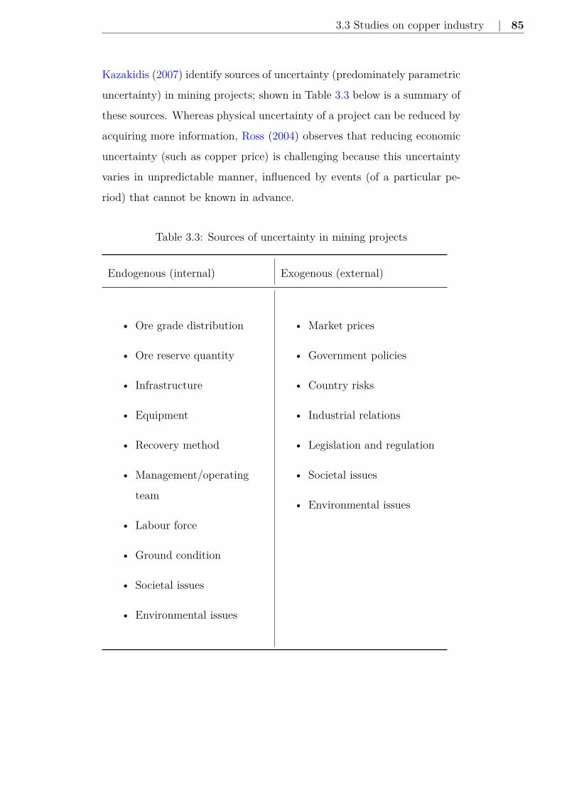
3.3 Studies on copper industry | 85
Kazakidis (2007) identify sources of uncertainty (predominately parametric
uncertainty) in mining projects; shown in Table 3.3 below is a summary of
these sources. Whereas physical uncertainty of a project can be reduced by
acquiring more information, Ross (2004) observes that reducing economic
uncertainty (such as copper price) is challenging because this uncertainty
varies in unpredictable manner, influenced by events (of a particular pe-
riod) that cannot be known in advance.
Table 3.3: Sources of uncertainty in mining projects
Endogenous (internal) Exogenous (external)
• Ore grade distribution
• Ore reserve quantity
• Infrastructure
• Equipment
• Recovery method
• Management/operating
team
• Labour force
• Ground condition
• Societal issues
• Environmental issues
• Market prices
• Government policies
• Country risks
• Industrial relations
• Legislation and regulation
• Societal issues
• Environmental issues
86 | Literature review: Review of energy and mining models
Economic uncertainty
For a copper mining project, economic uncertainty includes, but is not
limited to, copper price, raw material input prices (such as energy price
and chemical costs), taxation, industrial relations and government policies.
This category of uncertainty is the most important driver for decision mak-
ing in the metal mining industry (Savolainen, 2016; William et al., 2012).
This research focuses on the impact that copper price, input prices and
taxation have on a firm’s profitability.
Uncertainty impacts the firm’s profitability in two ways: operational
profitability and recovery of capital investment. Operational profitability
affects the firm’s performance in the short-term. However, uncertainty can
also lead to long-term losses should the firm fail to realise the expected
revenue for its capital investment project. This long-term loss can be due
to a sudden collapse of the commodity markets as was observed between
the early 1970s and 2000s (for the copper markets). To minimise the risks
of long-term loss, it is common practice for firms to use an average com-
modity price of three (3) to five (5) years when evaluating a capital project
(DiNuzzo et al., 2005; Hearne et al., 2006; Lambert and Stone, 2008; Peters
et al., 2013). This is approximately the half life of copper price oscillation11.
Physical uncertainty
Physical uncertainty includes ore grade, quantity of ore resources, equip-
ment and ground condition to mention but a few. However, the main
physical uncertainty in a mining project is ore grade and quantity of ore
resources (Dimitrakopoulos et al., 2002). This could not only lead to over
designing of a mine (which in turn leads to under utilisation of the capacity)
but it also impacts the unit production cost and the expected net present
value of a project (Dimitrakopoulos and Sabour, 2007). This uncertainty
can be reduced by investing more in information acquisition processes such
as exploration (Botín et al., 2012; Ross, 2004).
11See section 3.3.5 for a description of copper price modelling.
3.3 Studies on copper industry | 87
3.3.2 Material production modelling
The production process of primary copper can be divided into three stages:
mining and mineral processing, smelting and refining (see Davenport et al.
(2002) for a thorough description of the copper production processes). The
mining and mineral processing stage focuses on how copper ore is extracted
from the ground using open pit or underground methods and processed
to produce concentrates (under pyro-metallurgy route) or leach solution
(under hydro-metallurgy route). This mineral processing is usually done
within the perimeters of the mining operations as it would not make eco-
nomic sense to transport the ore to another facility for processing, consid-
ering that only about 0.5-3% of the material that would be transported has
economic value.
If the ore being processed follows the pyro-metallurgy route, then the
next stage of processing is smelting. At this stage, copper concentrates
(20%-50% copper content) is transformed into blister copper (99.5% copper
content). The final stage is electro-refining in the pyro-metallurgy route,
this produces copper cathode (99.9% copper content). The smelting and
electro-refining processes can be done at a facility away from the mining site
or even at a facility owned by another mining firm. If the process takes the
hydro-metallurgy route, the next stage from mining and mineral processing
is solvent extraction-electro-winning (SX-EW). The end product of SX-EW
stage is copper cathode at 99.9% copper content. Further, because of the
configuration of the SX-EW process, this stage is done near to the mining
site in order to avoid transport and other logistical costs. This, therefore,
implies that a company that uses hydro-metallurgy to produce copper will
have their capital investment locked in a particular country of operation
as opposed to a firm which uses a pyro-metallurgy route. This is an added
risk dimension for a firm using hydro-metallurgy. Figure 3.4 below shows
the main energy inputs in the production process flow.
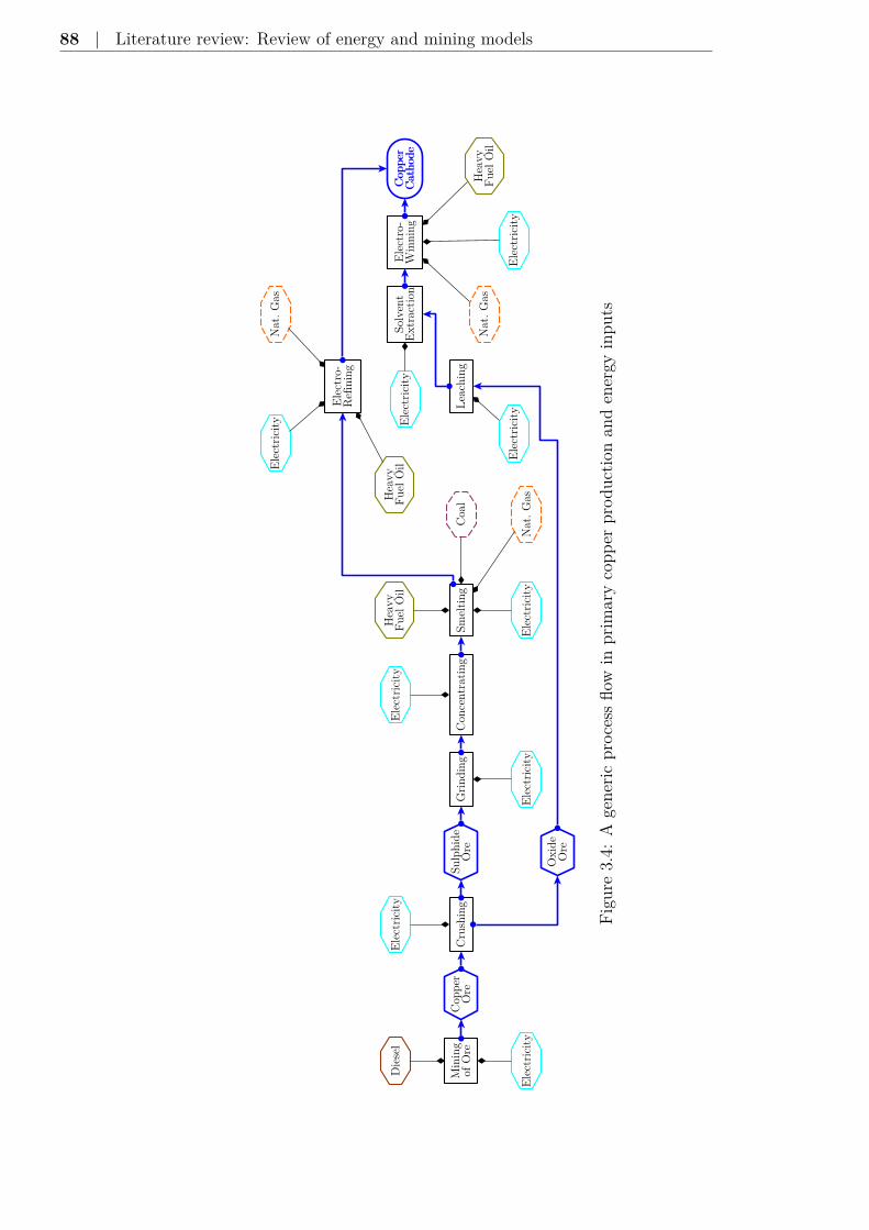
88 | Literature review: Review of energy and mining models
Figu
re3.
4:A
gene
ricpr
oces
sflo
win
prim
ary
copp
erpr
oduc
tion
and
ener
gyin
puts
3.3 Studies on copper industry | 89
Total copper production (global) has increased from 10, 000 tonnes in
1750 to 20 million tonnes in 201112. There have also been changes in the
industry’s key production players, from China (70%) and Europe (30%) in
1750 to Chile (32%), China (7.8%), Peru (7.6%) and USA (7%) in 2011
(Cochilco, 2012; Radetzki, 2009). Apart from changes of key industry play-
ers, other changes have been in mining methods (mass open-pit production
was introduced in 1905), processing of sulphide ore (flotation process was
introduced in 1911) and processing of leachable ore (largely oxide ore, was
introduced in 1968). Changes in mining methods and the introduction of
flotation process made it economically possible to mine and process low
grade sulphide ore. Further, despite the decreasing ore grades, these two
changes (open-pit and flotation process methods) led to a 20% decline in
costs between 1918 and 1923 (Aguirregabiria and Luengo, 2015). The in-
troduction of leaching process (a primary process for oxide ore) lowered
the investment capital cost, shortened the project lead time and provided
an environmentally friendly method of processing copper. It also made it
possible to set-up small scale processing operations (Radetzki, 2009).
Copper output from the leaching process (SX-EW) has continued to
rise (accounting for 18.4% of global output in 2011 from 14% in 1997), this
is partly because of the lower investment capital cost (less than two-thirds
of the traditional pyro-metallurgy process). The process, however, is op-
erational cost intensive and it also relies on acid from the pyro-metallurgy
process (Davenport et al., 2002; Rothschild, 2008), particularly for land-
locked copper producing countries. Figure 3.5 below shows the shares of
pyro-metallurgy and hydro-metallurgy processes.
12See Tables 2.2 and B.1 in Chapter 2 and Appendix B for production and consump-tion statistics respectively.
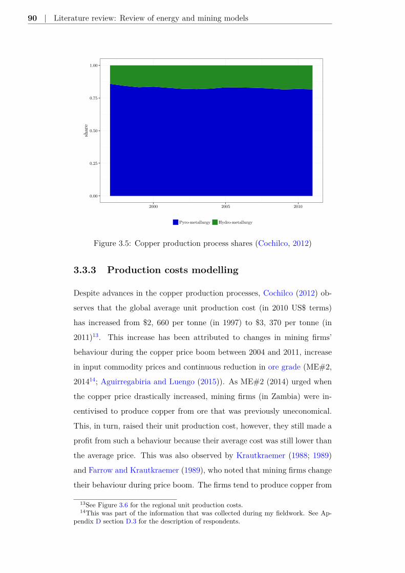
90 | Literature review: Review of energy and mining models
0.00
0.25
0.50
0.75
1.00
2000 2005 2010
sha
re
Pyro-metallurgy Hydro-metallurgy
Figure 3.5: Copper production process shares (Cochilco, 2012)
3.3.3 Production costs modelling
Despite advances in the copper production processes, Cochilco (2012) ob-
serves that the global average unit production cost (in 2010 US$ terms)
has increased from $2, 660 per tonne (in 1997) to $3, 370 per tonne (in
2011)13. This increase has been attributed to changes in mining firms’
behaviour during the copper price boom between 2004 and 2011, increase
in input commodity prices and continuous reduction in ore grade (ME#2,
201414; Aguirregabiria and Luengo (2015)). As ME#2 (2014) urged when
the copper price drastically increased, mining firms (in Zambia) were in-
centivised to produce copper from ore that was previously uneconomical.
This, in turn, raised their unit production cost, however, they still made a
profit from such a behaviour because their average cost was still lower than
the average price. This was also observed by Krautkraemer (1988; 1989)
and Farrow and Krautkraemer (1989), who noted that mining firms change
their behaviour during price boom. The firms tend to produce copper from
13See Figure 3.6 for the regional unit production costs.14This was part of the information that was collected during my fieldwork. See Ap-
pendix D section D.3 for the description of respondents.
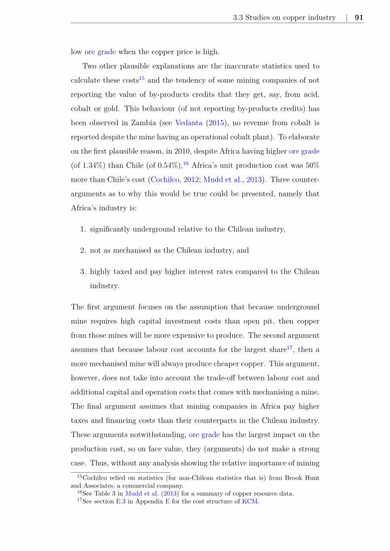
3.3 Studies on copper industry | 91
low ore grade when the copper price is high.
Two other plausible explanations are the inaccurate statistics used to
calculate these costs15 and the tendency of some mining companies of not
reporting the value of by-products credits that they get, say, from acid,
cobalt or gold. This behaviour (of not reporting by-products credits) has
been observed in Zambia (see Vedanta (2015), no revenue from cobalt is
reported despite the mine having an operational cobalt plant). To elaborate
on the first plausible reason, in 2010, despite Africa having higher ore grade
(of 1.34%) than Chile (of 0.54%),16 Africa’s unit production cost was 50%
more than Chile’s cost (Cochilco, 2012; Mudd et al., 2013). Three counter-
arguments as to why this would be true could be presented, namely that
Africa’s industry is:
1. significantly underground relative to the Chilean industry,
2. not as mechanised as the Chilean industry, and
3. highly taxed and pay higher interest rates compared to the Chilean
industry.
The first argument focuses on the assumption that because underground
mine requires high capital investment costs than open pit, then copper
from those mines will be more expensive to produce. The second argument
assumes that because labour cost accounts for the largest share17, then a
more mechanised mine will always produce cheaper copper. This argument,
however, does not take into account the trade-off between labour cost and
additional capital and operation costs that comes with mechanising a mine.
The final argument assumes that mining companies in Africa pay higher
taxes and financing costs than their counterparts in the Chilean industry.
These arguments notwithstanding, ore grade has the largest impact on the
production cost, so on face value, they (arguments) do not make a strong
case. Thus, without any analysis showing the relative importance of mining15Cochilco relied on statistics (for non-Chilean statistics that is) from Brook Hunt
and Associates, a commercial company.16See Table 3 in Mudd et al. (2013) for a summary of copper resource data.17See section E.3 in Appendix E for the cost structure of KCM.
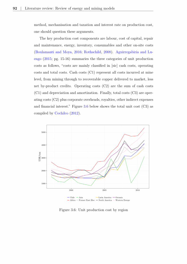
92 | Literature review: Review of energy and mining models
method, mechanisation and taxation and interest rate on production cost,
one should question these arguments.
The key production cost components are labour, cost of capital, repair
and maintenance, energy, inventory, consumables and other on-site costs
(Boulamanti and Moya, 2016; Rothschild, 2008). Aguirregabiria and Lu-
engo (2015; pg. 15-16) summaries the three categories of unit production
costs as follows, “costs are mainly classified in [sic] cash costs, operating
costs and total costs. Cash costs (C1) represent all costs incurred at mine
level, from mining through to recoverable copper delivered to market, less
net by-product credits. Operating costs (C2) are the sum of cash costs
(C1) and depreciation and amortization. Finally, total costs (C3) are oper-
ating costs (C2) plus corporate overheads, royalties, other indirect expenses
and financial interest.” Figure 3.6 below shows the total unit cost (C3) as
compiled by Cochilco (2012).
1000
2000
3000
4000
5000
2000 2005 2010
US$
/ton
ChileAfrica
AsiaFormer East Bloc
Latin AmericaNorth America
OceaniaWestern Europe
Figure 3.6: Unit production cost by region
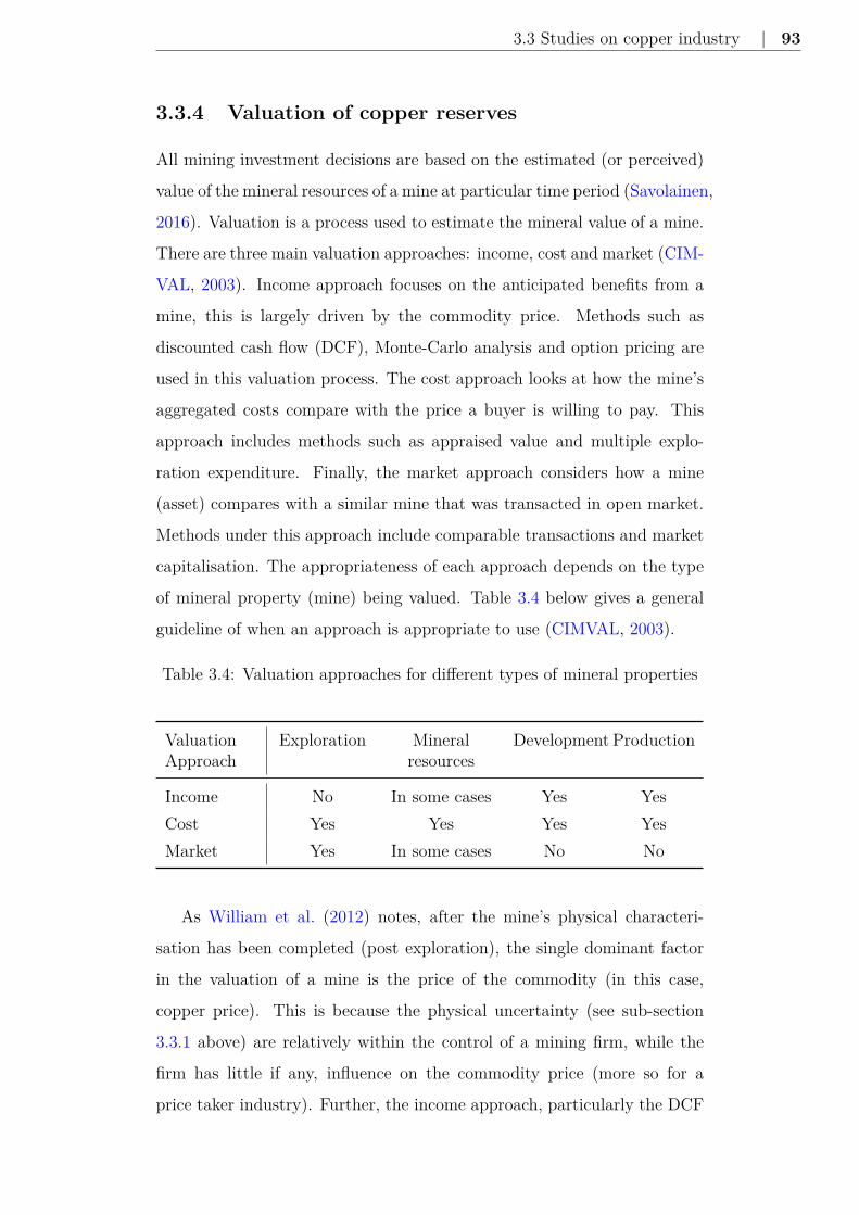
3.3 Studies on copper industry | 93
3.3.4 Valuation of copper reserves
All mining investment decisions are based on the estimated (or perceived)
value of the mineral resources of a mine at particular time period (Savolainen,
2016). Valuation is a process used to estimate the mineral value of a mine.
There are three main valuation approaches: income, cost and market (CIM-
VAL, 2003). Income approach focuses on the anticipated benefits from a
mine, this is largely driven by the commodity price. Methods such as
discounted cash flow (DCF), Monte-Carlo analysis and option pricing are
used in this valuation process. The cost approach looks at how the mine’s
aggregated costs compare with the price a buyer is willing to pay. This
approach includes methods such as appraised value and multiple explo-
ration expenditure. Finally, the market approach considers how a mine
(asset) compares with a similar mine that was transacted in open market.
Methods under this approach include comparable transactions and market
capitalisation. The appropriateness of each approach depends on the type
of mineral property (mine) being valued. Table 3.4 below gives a general
guideline of when an approach is appropriate to use (CIMVAL, 2003).
Table 3.4: Valuation approaches for different types of mineral properties
ValuationApproach
Exploration Mineralresources
Development Production
Income No In some cases Yes YesCost Yes Yes Yes YesMarket Yes In some cases No No
As William et al. (2012) notes, after the mine’s physical characteri-
sation has been completed (post exploration), the single dominant factor
in the valuation of a mine is the price of the commodity (in this case,
copper price). This is because the physical uncertainty (see sub-section
3.3.1 above) are relatively within the control of a mining firm, while the
firm has little if any, influence on the commodity price (more so for a
price taker industry). Further, the income approach, particularly the DCF
94 | Literature review: Review of energy and mining models
method, dominates valuation of mining projects (Bartrop and White, 1995;
Bhappu and Guzman, 1995; CIMVAL, 2003). The popularly notwithstand-
ing, DCF method tends to underestimate the mine value (Dimitrakopoulos
and Sabour, 2007; Moyen and Slade, 1996), however, its ease of use and
robustness are its strength (Phelan, 1997).
3.3.5 Copper price modelling
One of the main limitations of the DCF method is its reliance on a con-
stant future commodity price, overlooking the observed price fluctuations.
However, modelling of commodity prices is challenging, because of the un-
certainty in the behaviour of markets. Dixit and Pindyck (1994) proposes
two stochastic models for modelling commodity or asset prices: Geometric
Brownian Motions (GBM) and Mean-Reverting Process (MRP).
The GBM model (Equation 3.3) is used to model commodities or assets
that are non-stationary such as gold price, stock prices and interest rates.
However, for commodities such as base metals (copper, aluminium etc) an
MRP model is used (Equation 3.4). This is because in the long-run their
prices tend to move towards the marginal production cost (Dimitrakopoulos
and Sabour, 2007; Dixit and Pindyck, 1994; Suarez and Fernandez, 2009).
The model equations are described below:
Let S be
S = ln (P ) (3.2)
with P being the commodity price (in US$ per unit).
Then GBM model will be described as
dS = αSdt+ σSdz (3.3)
where α is the expected trend (drift parameter), σ is the standard de-
viation (variance parameter), dt is the time interval and dz is the standard
Weiner process.

3.3 Studies on copper industry | 95
While MRP model will be described as
dS = µ(S − S)dt+ σdz (3.4)
where, µ is the speed of reversion and S is the long-run marginal cost
of production of the commodity.
Given that S is the uncertain variable and following Equation 3.4, it
follows that when S < S then dS will more likely to be negative, to push
the price down in the following time interval; and the converse is true (when
S > S).
The speed of reversion, µ, is the time it takes for the price shock dissi-
pate(S − S
), this is closely related to the half life of the shock. Half life,
H, is defined as
H = ln (2)µ
(3.5)
Further, the expected future price, E[St], and the price variance, V[St−
S], of a commodity (that follows an MRP model) at any given time, t are
defined below in Equations 3.6 and 3.7 respectively
E [St] = S +(S0 − S
)e−µt (3.6)
V[St − S
]= σ2
2µ(1 − e−2µt
)(3.7)
where,
S is the long-run marginal cost of production of the commodity,
S0 is the initial commodity price at time t0,
St is the commodity price at time t,
µ is the speed of reversion, and
σ is the standard deviation.
In order to estimate the model, the Equation 3.4 can be expressed as
an AR (1) model18 as was done by Dixit and Pindyck (1994) and Suarez18Auto-regressive model of order 1.

96 | Literature review: Review of energy and mining models
and Fernandez (2009). This implies that Equation 3.4 is transformed from
a continuous time process to discrete time process. The resulting equation
is described below
St − St−1 = S(1 − e−µ
)+(e−µ − 1
)St−1 + ϵt (3.8)
with ϵt (the error) following a normal distribution with a standard de-
viation of σϵ.
σϵ = σ2
2µ(1 − e−2µ
)(3.9)
If a = S (1 − e−µ) and b = (e−µ − 1) , it follows that
S = −ab
(3.10)
µ = − ln (1 + b) (3.11)
σ = σϵ
√√√√ ln (1 + b)(1 + b)2 − 1
(3.12)
Having estimated the MRP model19, the half life of the shock can be
calculated. This half life is important for estimating the long-run price,
S, on which an investment decision is based. It has been observed that
decision makers base their capital investment decisions on an average his-
torical price (DiNuzzo et al., 2005; Hearne et al., 2006; Lambert and Stone,
2008; Peters et al., 2013) covering a time interval similar to the half life.
Further, because of the nature of the commodity price behaviour, the range
of time series data used in estimating the model will significantly impact
how the projected price will look (Sick and Cassano, 2012). The model is
sensitive to both µ and σ. Model estimation results are given in section
E.4 of Appendix E.
19See Table E.4 of Appendix E for estimates.
3.3 Studies on copper industry | 97
3.3.6 Feedback relationships within a firm
The link between the physical (material) and financial components (mod-
ules), which are discussed on page 84 above, is what determines the in-
vestment behaviour of the mining firms (Aguirregabiria and Luengo, 2015;
Montaldo, 1977; Sverdrup et al., 2014). This linkage can be captured by
using four main feedback loops20, which would also have a time delay in
them. These are the production-ore grade loop, ore grade-production cost
loop, profitability-investment loop and investment-production loop.
• The production-ore grade loop: considers how production of copper
leads to reduction in the ore grade.
• The ore grade-production cost loop: focuses on how reducing ore
grade impacts production cost.
• The profitability-investment loop: looks at how reduction in prof-
itability (as a result of increasing production cost and fluctuating
copper prices) impact capital investment behaviour of a mining firm.
• The investment-production loop: focuses on how investments (in pro-
duction capacity and other strategic stock) impacts production.
Apart from these four main loops, there is a minor loop, energy efficiency-
production cost loop, that looks at how investment in energy efficient tech-
nologies could help reduce energy cost (which is a component of production
cost). This loop captures the general arguments (Jaffe and Stavins, 1994;
Patterson, 1996; Peck and Chipman, 2007; Sola et al., 2011) of how energy
efficiency would help reduce production cost (assuming that the energy cost
is a major contributor)21. Apart from these feedback loops within a firm,
there is also another exogenous feedback loop between the mining and en-
ergy systems: the production-energy price-production cost loop. This loop
is described in the section below.20See section 4.3 for a discussion on loops in models.21See section 7.2.4 for an analysis of the impact of energy efficiency investments.
98 | Literature review: Review of energy and mining models
3.4 Linkage of energy and mining systems
Having discussed past studies in the energy and mining sectors, the key
energy demand drivers and the main aspects that influence decision making
in the mining sector, this section describes how the models representing the
energy and mining sectors are linked in this study (Chapters 5 and 6 gives
a full description of the Zambian energy and mining models respectively).
There are two important aspects that this link captures: the impact
of copper production on national energy demand and the impact of other
sectors on national energy demand. The impact of copper production on
energy demand focuses on how mining activities would impact on the en-
ergy price. And how the energy price would, in turn, impact the copper
production cost, via the production-energy price-production cost loop. All
things held constant, it follows that increase in energy demand from the
mining sector leads to more investments in the energy infrastructure which
leads to increase in the energy price (and vice-versa is true).
Apart from the increase in energy price as a result of increase in mining
energy demand, the price is also influenced by the developments in other
sectors such as increased electrification in the residential sector and the
growth of the agricultural sector. Therefore, the increase in energy price
due to growth in other sectors would still impact the copper production
cost. This linkage is important because there is uncertainty of how the
energy demand (particularly electricity demand) would evolve22.
Therefore, the energy price is driven by two components, demand from
the mining industry and from other sectors. Figure 3.7 below shows the
interaction between the models (energy and mining). The mining model
requires energy in order to produce copper and the energy model meets
this demand at a cost (the energy price).
22See section 7.1.1 of Chapter 7 for projected energy demands.
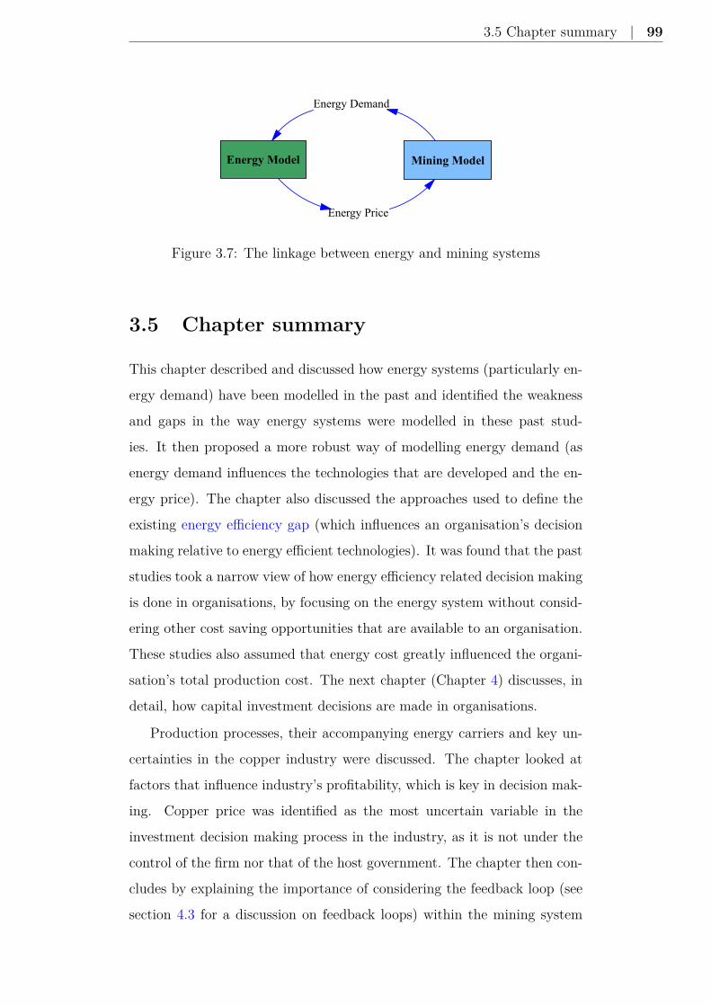
3.5 Chapter summary | 99
Energy Model Mining Model
Energy Demand
Energy Price
Figure 3.7: The linkage between energy and mining systems
3.5 Chapter summary
This chapter described and discussed how energy systems (particularly en-
ergy demand) have been modelled in the past and identified the weakness
and gaps in the way energy systems were modelled in these past stud-
ies. It then proposed a more robust way of modelling energy demand (as
energy demand influences the technologies that are developed and the en-
ergy price). The chapter also discussed the approaches used to define the
existing energy efficiency gap (which influences an organisation’s decision
making relative to energy efficient technologies). It was found that the past
studies took a narrow view of how energy efficiency related decision making
is done in organisations, by focusing on the energy system without consid-
ering other cost saving opportunities that are available to an organisation.
These studies also assumed that energy cost greatly influenced the organi-
sation’s total production cost. The next chapter (Chapter 4) discusses, in
detail, how capital investment decisions are made in organisations.
Production processes, their accompanying energy carriers and key un-
certainties in the copper industry were discussed. The chapter looked at
factors that influence industry’s profitability, which is key in decision mak-
ing. Copper price was identified as the most uncertain variable in the
investment decision making process in the industry, as it is not under the
control of the firm nor that of the host government. The chapter then con-
cludes by explaining the importance of considering the feedback loop (see
section 4.3 for a discussion on feedback loops) within the mining system

100 | Literature review: Review of energy and mining models
and also of linking the energy and mining systems when studying capi-
tal investment decision making behaviour in the mining industry. This is
because both feedbacks within and outside the mining system could poten-
tially influence how energy is used in the industry, the copper production
levels and the total production cost of the industry.
Chapter 4
Literature review: Investment
decision making
This chapter has two main goals: to discuss how investment decisions are
made in organisations (in sections 4.1 and 4.2) and also to discuss and
describe the main models used to study decision making in organisations.
This is important because investment decision making is affected by a vari-
ety of factors. Thus, by understanding how organisations make investment
decisions, different policies and measures that can enhance strategic invest-
ments could be analysed.
The chapter begins by discussing decision making theories and pro-
cesses in organisations. It defines what investment decisions are and the
processes that organisations follow when making such decisions. The next
section then discusses different paradigms used in studying decision making.
The appropriateness and limitations of these paradigms are also discussed.
Then sections 4.3 and 4.4 discuss and describe the approach and scope that
was considered in this research. Overall, this chapter lays the foundation
on which the mining model (in Chapter 6) is developed.
102 | Literature review: Investment decision making
4.1 Investment decision making in firms
The primary motivation for organisations to invest is to create value (Cor-
tazar and Casassus, 1998). These investment decisions are influenced by
many factors, among them but not limited to these; compliance to the
local regulations, replacement of obsolete equipment, desire to increase
production capacity of the organisation, enhancement of company image
and enhancement of company’s competitive edge. An investment, from an
economic perspective, would be defined as “the act of incurring an imme-
diate cost in the expectation of future rewards” (Dixit and Pindyck, 1994;
pg. 3). A decision can also be defined as a commitment of resources to
achieve the desired result (Mintzberg et al., 1976). Thus, an investment
decision can be defined as an act committing organisational resources with
the hope of having better returns.
Generally, investment decisions have three broad characteristics: irre-
versibility, uncertainty and timing. Firstly, investments require an upfront
cost, this cost can be either partially or completely irreversible. A partial
irreversibility is a situation where the decision maker can recover part of
the upfront cost should they decide to halt the investment project devel-
opment. In a situation where the decision maker cannot recover any of the
upfront cost, such an investment is referred to as a completely irreversible.
An investment decision can be reversed or abandoned because the decision
maker realises that the investment will not deliver the expected results, this
could be because of changes in market drivers on which the decision was
based. Secondly, due to limited knowledge and information about future
events, such as commodity prices or regulatory controls, there is uncer-
tainty over the outcome of any investment. The ability of a decision maker
to put off making a decision as more information about an investment op-
tion is collected is the third characteristics of the investment decision (Dixit
and Pindyck, 1994). The interaction of these three characteristics is what
makes decision making a complex process.
Further, investment decisions can be divided into two: strategic and
non-strategic. Strategic investment decisions are those investments that
4.1 Investment decision making in firms | 103
require organisations to commit significant resources to achieving a de-
sired outcome, and are usually made by top management. These types of
decisions contribute to the creation, maintenance and development of an
organisation’s long term performance and sustainable competitive advan-
tage (Butler et al., 1991; Cooremans, 2012; Mintzberg et al., 1976). On the
other hand, non-strategic investment decisions do not significantly impact
organisation’s resources pool, and could be made at lower levels of com-
pany management. This research and chapter focus on strategic investment
decisions.
Empirical research in decision making can be broadly classified into
three categories: research done by cognitive psychologists; social psycholo-
gists; and management theorists and political scientists (Mintzberg et al.,
1976). Cognitive research focuses on how individuals make decisions by
exposing them to different situations through the usage of games. This re-
search (cognitive research) has found that when decision makers are faced
with complex and unusual decisions, they seek for ways to break down
the decision situation into smaller and simplified chunks. By solving these
smaller and simplified chunks, a decision maker can then come up with a
final decision. This final decision is usually a sub-optimal decision. So-
cial psychologists’ research, on the other hand, focuses on group decision
making by studying group dynamics and interactions among participants
in controlled environments such as laboratories. The last category of deci-
sion making research focuses on processes involved in making decisions at
organisational level.
4.1.1 Strategic decision making process
“Strategic investment decision making involves the process of identifying,
evaluating, and selecting among projects that are likely to have a big impact
on a company’s competitive advantage” (Adler, 2000; pg. 15). Mintzberg
et al. (1976) studied 25 strategic decisions by collecting empirical evidence
in organisations of a span of five years. In all the 25 processes studied, they
found that the decision situations were characterised by novelty, complex-
104 | Literature review: Investment decision making
ity, and open-endedness; and organisations generally had limited informa-
tion of the problem at hand. Of the processes studied, there was a wide
variation in the length of time it took to get to the final decision, ranging
from less than one year to above four years.
Decision making process is made up of three parts: stimuli, solution,
and process (Mintzberg et al., 1976). The stimuli component focuses on
understanding what triggers the decision situation; these could be things
such as perceived opportunity or crisis moments like losing market share.
On the continuum scale of stimuli, opportunity moments see organisations
take a proactive step to initiate the idea of seeking to improve or grow the
organisation while on the other extreme of crisis moment, organisations
are more reactive. The decision on how the organisation responds to the
stimuli is found in the solution component. Solutions would be already
made, newly created or modified. The process component studies the steps
taken to move from stimuli to a solution.
In 1910, a framework of decision making was proposed by John Dewey.
This framework consisted of five phases: “(1) suggestion, wherein the mind
leaps to a possible solution; (2) intellectualization [sic] of the felt difficulty
into a problem or question; (3) development of hypotheses; (4) reasoning or
mental elaboration of these; and (5) testing of the hypotheses.” (Mintzberg
et al., 1976; pg. 251-252) Based on this framework, other variations of this
framework have been developed to study decision making. Mintzberg et al.
(1976) use a three-phase framework and defines them as identification, de-
velopment, and selection. In the identification phase, organisations, deci-
sion makers to be precise, identify the real stimuli (from the ‘noise’) of the
situation, determine cause-effect relationships that the stimuli could affect
and look for appropriate possible activities that could be taken to address
the stimuli. The development phase is characterised by activities, tech-
niques and processes that will be used to arrive at a solution or solutions.
Under this phase, the organisations, search for information that would lead
to finding desired solutions and also seeks to find better ways of how these
solutions can be modified to fit into the organisation’s operations. The
4.1 Investment decision making in firms | 105
final phase, selection, is where the organisation makes the final decision on
which solution it will adopt and commits its resources in implementing the
solution. However, even though these phases seem to be sequential, many
studies have found that decision making process is iterative (Butler et al.,
1991; Cauwenbergh et al., 1996; Mintzberg et al., 1976).
There are three modes of choice selection that could be used by a de-
cision maker: judgement, bargaining and analytic modes. The judgement
mode relies heavily on the decision maker’s experiences. This also requires
the decision maker to consider aspects of decision options that cannot be
quantified (Butler et al., 1991). The judgement mode has also been found
to be the fastest method of decision making (Mintzberg et al., 1976). When
decisions are contentious and involve many other stakeholders, the bargain-
ing mode is adopted and used. The final decision is generally a compromise
of interests among involved stakeholders. The most reported selection mode
in literature is the analytic mode. This mode emphasises on the quantita-
tive aspects of the solution alternatives that can be evaluated, and assumes
that the alternative that has the maximum utility is the best and should
be chosen. However, the actual selection mode in organisations is usually
a combined of all the three modes.
In their study, Butler et al. (1991) studied how complexity and politics
can influence strategic decision making processes. The decision process was
conceived to involve two fundamental problems: technical and political.
The technical problem looks at which decision would be the best from the
given alternatives and available information, while the political problem
looks at how conflicting targets and interests within the organisation can
be resolved.
The technical model employs varies forms of techniques to solve the
problem, such as optimisation techniques, pay-back period, net present
value (NPV) and return on investment (RoI) calculations. This model as-
sumes that decision makers are rational and will choose the best solution
all the time in order to achieve the organisation’s goal. However, research
(Alkaraan and Northcott, 2006; Butler et al., 1991; Cauwenbergh et al.,
106 | Literature review: Investment decision making
1996) has suggested that this is not the case. This was also the finding of
my fieldwork (see Appendix D section D.4). The political model considers
decision makers as individuals who come together to realise the organisa-
tional goals but they also have personal goals, which may be in conflict
with organisational goals. When personal goal and politics take centre
stage of the decision process, the final decisions can have negative impli-
cations for the organisation. These two problems (technical and political)
make decision making process complex.
Technical or political models notwithstanding, organisations have gen-
eral procedural guidelines on investments. These guidelines outline how re-
sources of an organisation should be committed for all investment decisions
(Alkaraan and Northcott, 2007; Butler et al., 1991). The guidelines also
provide decision makers with indicators of what they should and should not
consider when making investment decisions, these decision guidelines are
essential for the organisation’s growth and survival. Further, these man-
agement control systems also provide both pre-decision and post-decision
guidelines. Among other benefits, the former, helps the organisation to: 1.
avoid implementation of unplanned investments; and 2. reduce the risks of
personal liability when making organisational decisions, as most strategic
investments involve enormous financial commitments, which are risky and
uncertain. While the latter helps the organisation to monitor and evaluate
the effectiveness of the past decisions taken. This also helps organisations
to learn from its past decisions.
4.1.2 Identification of strategic issues
Recognition of stimuli that would lead to a strategic decision is not easy,
as decision makers are constantly faced with many different organisational
issues (both strategic and non-strategic) that require their attention (Cohen
et al., 1972; Dutton et al., 1989). Thus, organisations have mechanisms
that help their decision makers to be able to easily separate strategic issues
from non-strategic issues. A strategic issue could be defined as “events,
developments or trends that are perceived by decision-makers as having
4.1 Investment decision making in firms | 107
the potential to affect their organization’s [sic] performance.” (Dutton et al.,
1989; pg. 380)
There are three groups of literature that discuss the aspects that deci-
sion makers use to define strategic issues; these are environmental scanning,
issues management, and issue formulation and diagnosis (Dutton et al.,
1989). Environment scanning literature focuses on how decision makers
use their external environment to identify issues. This is done by monitor-
ing the trends that are emerging from the environment. Issues management
literature is concerned with how organisations, top management in partic-
ular, respond to social issues and corporate responsibilities rather than the
identification and evaluation. The final group of literature is issue formu-
lation and diagnosis, it focuses on early stage of decision making where
stimuli are identified and evaluated.
Four dimensions are used to define strategic issues. The first is the an-
alytic dimension, which focuses on specifics of the issues, such as visibility,
complexity and potential impact of an issue. The second is the content di-
mension, which pertains to the nature of the issue such as type (economic,
social, political or technical) and geographical boundaries. Action dimen-
sion is the third class, it looks at the effort and action that is required to
handle the issue, such as controllability and feasibility. The fourth and final
dimension is the source of an issue. This dimension looks at who initiates
the issue and how influential this initiator is. This class has a strong con-
notation of how organisation politics play a major role in strategic decision
making (Dutton et al., 1989).
4.1.3 Decision effectiveness
Having looked at decision making processes in the preceding sub-sections,
this sub-section focuses on how decision processes influence decision ef-
fectiveness. Decision effectiveness can be loosely defined as the extent to
which the process achieves the outcome as intended by the decision maker
at the time the decision was made. This relationship, between process
and outcome, has been studied by Dean and Sharfman (1996). The re-

108 | Literature review: Investment decision making
lationship rests on two assumptions: (1) that different processes lead to
different choices and (2) that different choices lead to different outcomes.
Furthermore, for a relationship to exist, both assumptions have to be true.
In addition to the arguments presented by Dutton et al. (1989) and
Eisenhardt and Zbaracki (1992), that bounded rationality (see section 4.2
for further description) and organisation politics are best suited to model
strategic decision making processes, Dean and Sharfman (1996) suggests
that it is also essential for decision effectiveness to be studied within defined
constraints. In this regard, Dean and Sharfman (1996; pg. 373) suggests
that for decision processes to result into effective decisions, process have
to be “(1) oriented toward achieving appropriate organizational goals, (2)
based on accurate information linking various alternatives to these goals,
and (3) based on an appreciation and understanding of environmental con-
straints.”
To ensure that the process is oriented towards organisational goal, it is
important that a deliberate process of collecting information and analysing
the collected information (which are part of the organisation’s guideline)
is followed. Thus, if such a deliberate process is followed, this process can
be considered rational within constraints – as not all available information
is collected nor analysed. Collection of information and analysing it will:
firstly, create a clearer picture that links proposed solution options to their
outcome. This will give a decision maker an opportunity to clearly see the
relationship between a possible alternative solution and its outcome. Sec-
ondly, this will help decision makers to identify trends that are emerging
from the environment in which the organisation operates. Finally, this will
reduce personal influences (the political model) in coming up with the final
decision. As there will be a clearer picture of what each solution option
holds, and also the decision makers will be more aware of the environment
in which their organisation is operating and also easily recognise emerging
trends. Further, in dynamic environments, the more an organisation col-
lects information about its environment and carries out analyses, the more
it is likely to perform better (Dean and Sharfman, 1996).
4.2 Choice paradigms | 109
Nevertheless, even when chosen options are in line with organisational
goals, this does not automatically translate into desired decision outcomes.
There are other factors that can affect decisions’ effectiveness such as,
among others, the financial position of the organisation, growth prospects,
competitors’ decisions, political environment of the country in which the
organisation is operating and quality of implementation.
4.2 Choice paradigms
Decision making theory at organisational level is dominated by three choice
paradigms: rationality and bounded rationality; politics and power; and
garbage can (Eisenhardt and Zbaracki, 1992). Under the rationality and
bounded rationality paradigm, the rational model assumes that the decision
maker has a set of known decision objectives when they get into a decision
situation. The decision maker then collects the right information to aid the
decision situation and analysis for all possible alternatives, then chooses the
optimal option. The alternative model to the rational model is bounded
rationality. The bounded rational model argues that decision makers have
limited cognitive capacity, are pressed for time and that their decisions
are influenced by experience (Todd and Gigerenzer, 2000). Further, this
model contends that decision goals are not always known at the start of
the process and keep changing over the decision process. Rather than
seeing the rationality and bounded rationality paradigms to mean that the
decision makers are either rational or bounded rational, all decision makers
exhibit both trends. They are rational in other aspects while being bounded
rational in others. See sub-section 4.2.2 for a detailed discussion.
Politics and power paradigm has its roots in political science. This
paradigm assumes that even though organisations can have clear organi-
sational goals, the decision makers (in organisations) have different goals;
as a result of functional, hierarchical and personal factors, personal goals
that could potentially be in conflict with organisational goals. Further,
this paradigm argues that although decision makers can be individually
110 | Literature review: Investment decision making
rational, a collection of them may not lead to rational decisions because
they could have competing preferences. Therefore, because of competing
preferences among decision makers, final decisions can be thought to follow
the choices of the most powerful person in the organisation (Dutton et al.,
1989; Eisenhardt and Zbaracki, 1992).
The final paradigm is the garbage can. This paradigm was first de-
scribed by Cohen et al. (1972) who studied decision processes with a view
that various kinds of problems (stimuli for decisions) and solutions come to
a decision maker at the same time but in an ill-defined and ever changing
way. When compared to the first two paradigms, the garbage can focuses
on the role of chances in decision making process. It contends that final
decisions are not a product of deliberate analysis or political power, but
a matter of random outcome of events (Eisenhardt and Zbaracki, 1992).
However, empirical studies of decision making found that “strategic deci-
sion making is best described as a combination of boundedly rational and
political insights.” (Eisenhardt and Zbaracki, 1992; pg. 31) Thus, garbage
can paradigm is found to be of less relevance in describing how actual
strategic decisions are made; because it is not robust as the other two
paradigms.
Covin et al. (2001) studied how the environment and organisation struc-
ture impacts the relationship between choice paradigm and firm perfor-
mance. Depending on the choice paradigm, organisation’s decisions can be
analysed for different insights. For instance, if the organisation’s decision
making paradigm is predominantly ‘political and power’, then understand-
ing the individual decision making style of the most powerful person would
give more insights on how that organisation makes decisions. This research
focuses on understanding how various input costs, taxation policy and cop-
per price impacts on the organisation’s profitability, a key component in
investment decision making. Thus, the rationality and bounded rationality
paradigm is the main focus.

4.2 Choice paradigms | 111
4.2.1 Decision environment
There are two categories of environments in which organisations operate:
stable and uncertain environments. In stable environments, organisation’s
future is fairly predictable as opposed to uncertain environments such as
the mining industry where key decision drivers like commodity price change
constantly. Because of this, organisations that operate in uncertain envi-
ronments make decisions based on limited and ever changing information.
Thus, their decision rules are usually simplified, more “like rules of thumb
than on extensive analysis of all available data” (Artinger et al., 2014;
pg. 3). However, these organisations have concrete operational procedures
(decision guidelines) and also fairly rigid organisation structures.
Literature (Dutton et al., 1989; Eisenhardt and Zbaracki, 1992; Fredrick-
son and Mitchell, 1984) that studies decision making under uncertainty in
organisations suggests that decision makers rely considerably on rational
procedures (such as decision guidelines). It also found that some aspects
of decision making rely on decision maker’s experience (judgement and in-
tuition). It is, therefore, essential to understand how the two aspects of
decision making interact and how they can be effectively modelled.
4.2.2 Rationality and bounded rationality
Research focusing on how individuals and organisations make decisions
is well documented in literature (Alkaraan and Northcott, 2007; Coore-
mans, 2012; Covin et al., 2001; de Groot et al., 2001; Decanio and Watkins,
1998; Dutton et al., 1989; Eisenhardt and Zbaracki, 1992; Fredrickson and
Mitchell, 1984; Wilson and Dowlatabadi, 2007). Most of this literature
focuses on the rational model of decision making. As mentioned earlier,
this model assumes that the decision makers know exactly what they want
to achieve and are certain (or have known margins of error) about the all
possible decision outcomes and their effects. It further assumes that the
decision maker makes the best decision out of a given decision situation,
within specified constraints; such as alternatives from which a decision
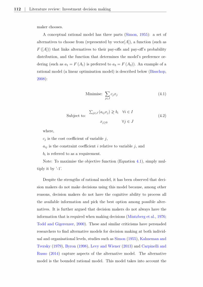
112 | Literature review: Investment decision making
maker chooses.
A conceptual rational model has three parts (Simon, 1955): a set of
alternatives to choose from (represented by vector[A]), a function (such as
F ([A])) that links alternatives to their pay-offs and pay-off’s probability
distribution, and the function that determines the model’s preference or-
dering (such as a1 = F (A1) is preferred to a3 = F (A3)). An example of a
rational model (a linear optimisation model) is described below (Bisschop,
2008):
Minimise:∑j∈J
cjxj (4.1)
Subject to:∑
j∈J (aijxj) ≷ bi ∀i ∈ I
xj≥0 ∀j ∈ J
(4.2)
where,
cj is the cost coefficient of variable j,
aij is the constraint coefficient i relative to variable j, and
bi is referred to as a requirement.
Note: To maximise the objective function (Equation 4.1), simply mul-
tiply it by ’-1’.
Despite the strengths of rational model, it has been observed that deci-
sion makers do not make decisions using this model because, among other
reasons, decision makers do not have the cognitive ability to process all
the available information and pick the best option among possible alter-
natives. It is further argued that decision makers do not always have the
information that is required when making decisions (Mintzberg et al., 1976;
Todd and Gigerenzer, 2000). These and similar criticisms have persuaded
researchers to find alternative models for decision making at both individ-
ual and organisational levels, studies such as Simon (1955), Kahneman and
Tversky (1979), Byron (1998), Levy and Wiener (2013) and Carpinelli and
Russo (2014) capture aspects of the alternative model. The alternative
model is the bounded rational model. This model takes into account the
4.2 Choice paradigms | 113
behavioural aspects of decision making.
Whereas a rational model could have infinite choice alternatives, a
bounded rational model always has finite alternatives. This is a critical
characteristic of the model because it simplifies the decision process, mak-
ing it similar to how decision situations are like in organisations. This
implies that instead of a decision maker seeking a solution from a range
of possible alternative, a decision option is always picked from known and
available alternatives. To illustrate this using an analogy of The Secretary’s
Problem (Bearden et al., 2005; Ferguson, 1989; Freeman, 1983). A rational
model would be described as The Secretary’s Problem in a dynamic envi-
ronment with a known probability distribution while a bounded rational
model would be a Problem with a known desired applicant threshold.
Thus, to get a bounded rational model, three key modifications have
to be made to the rational model (Simon, 1955): simplification of a pay-
off function, simplified information searching rule and partial ordering of
pay-offs.
Simplification of a pay-off function narrows down choice alternatives to
two or three values. A two-value functions could be interpreted as a satis-
factory or unsatisfactory function, whereas a three-value function could be
a win, draw or lose function. The point at which each value is picked (from
the simplified pay-off functions) is defined by thresholds. This simplified
function implies is that the decision maker is satisfied by any alternative
that is equal to or better than the set threshold. Further, the magnitude
by which the alternative exceeds a set threshold is irrelevant.
Simplified information searching rule focuses on only a section of infor-
mation that is critical for making decisions. This rule takes into consid-
eration that decision makers have limited time that they can dedicate to
each decision process. This rule is in line with what researchers (Kerstholt,
1994; Payne et al., 1988) found, that decision makers only focus on specific
information indicators in their decision making.
The third modification is to their pay-off rule. This focuses on how a
decision maker gets to a decision point (choosing between alternatives).

114 | Literature review: Investment decision making
A summary of these modifications is given below (Artinger et al., 2014;
Byron, 1998; Simon, 1955):
1. Set the target thresholds or criteria for each decision category.
2. Search for information that can be used to assess whether an alter-
native satisfies the target thresholds or criteria.
3. Pick any alternative that satisfies all target thresholds or criteria.
Todd and Gigerenzer (2000) studied the concept of how decision makers
make decisions within the bounded rationality model. They focused on how
decision makers make decisions under time pressure, limited information
and cognitive capacity. They introduce a concept of heuristics; heuristics
are strategies used to solve problems that cannot be easily solved by logic
and probability theory (Artinger et al., 2014). Heuristics help reduce the
requirement of cognitive demands of the decision makers; because heuristics
simplify how a decision maker decides. This is done by, among others, any
of the following heuristics; satisficing, recognition, elimination and avail-
ability. Under satisficing heuristics, the decision maker sets a threshold
of what a good enough decision would be. Recognition heuristics is when
the decision maker bases a decision on what he/she had previously chosen.
When the decision maker, however, chooses to eliminate some alternative
simply because they have a low score, for example, such a heuristic is called
elimination heuristics. The final heuristic is called availability heuristic.
This is when a decision maker makes a choice based the alternative that is
readily available to them (Wilson and Dowlatabadi, 2007). For a compre-
hensive description of various types of heuristics, kindly see Payne et al.
(1988) and Todd and Gigerenzer (2000).
Byron (1998) study looks how decision makers pick their preferred alter-
native in a decision situation where there are multiple decision thresholds
or criteria. The paper presents global and local goals concept. A global
goal describes the general direction that a decision maker would want to go
while a local goal focuses on the specifics of what the decision maker would
have to do to achieve the overall goals. For instance, a decision maker could
4.2 Choice paradigms | 115
want to have a healthy cash-flow, as a global goal, and cutting down on
energy bills by investing in energy efficient technologies and retaining the
best employees would be defined as local goals. In this case, a global goal
could indicate the relative importance of each of the local goal to achieving
its desired cash-flow.
This concept of global and local goals is critical when analysing deci-
sion making in organisations because organisations have many different and
unrelated options to achieving their desired goal. For instance, many stud-
ies (Fleiter et al., 2011; Sarkar and Singh, 2010; Sola et al., 2011; Weber,
1997) found that even though the benefits of energy efficiency measures
are obvious, barriers hinder their implementation. However, another plau-
sible argument, which I presented in section 3.2.4, would be that energy
efficiency studies have a narrow perspective of how organisations make de-
cisions (they mostly focus on an organisation’s energy system, as shown
in Figure 3.1 in Chapter 3). If these energy efficiency opportunities are
analysed in the context of a global goal, one could find that they do not
offer the best return.
Simon and Newell (1958) discuss two categories of decision problems
that decision makers face: well-structured and ill-structured problems.
They argue that rational models are suited to handle well-structured prob-
lem while ill-structured problems are better studied using bounded rational
models. A well-structured problem is a problem that can be formulated
explicitly and quantitatively (Simon and Newell, 1958). An ill-structured
problem, therefore, is any problem that is not a well-structured problem.
Its objective is vague and usually not easy to quantify. All well-structured
problems satisfy these criteria (Simon and Newell, 1958):
1. It can be described in terms of numerical variables, scalar and vector
quantities.
2. The goals to be attained can be specified in terms of a well-defined
objective function, such as profit maximisation.
3. There exist computational routines (method) that permit the solution

116 | Literature review: Investment decision making
to be found and stated in actual numerical terms, such as linear
programming algorithms.
Simon and Newell (1958) further argue that organisation’s top manage-
ment decision environments are made up of ill-structured problems. They
observe that decisions in these environments are almost always made based
on judgement and intuition. These judgement and intuition decisions are
rational choices (Byron, 1998). For instance, if a decision maker is faced
with two decision alternatives (one that satisfies the target threshold and
the other that does not), the decision maker will always pick an alterna-
tive that satisfies the target threshold. As choosing the one which does
not, would make them irrational. This was what Butler et al. (1991) and
Alkaraan and Northcott (2007) also found, that organisations have guide-
lines that decision makers follow when making decisions. As part of the
decision process, analytic techniques are used to evaluate all the decision
alternatives (Alkaraan and Northcott, 2006; Cauwenbergh et al., 1996).
4.2.3 Analytic techniques and their criticism
Strategic investments present a dual problem to an organisation, on one
hand, if an organisation gets the decision right that organisation will reap
enormous dividends from that decision. On the contrary, the opposite is
also true. Thus, organisations approach these decision situations with great
caution. In order to reduce uncertainty in decision making, many organ-
isations employ usage of analytic techniques to evaluate decision options,
techniques such as discounted cash flow (DCF), internal rate of return
(IRR) and pay back period (Ashford; et al., 1988; Cauwenbergh et al.,
1996).
For instance, between 1992 and 1994, a study that looked at how formal
(analytic) analysis plays in strategic decision making processes was done in
50 organisations in Belgium (Cauwenbergh et al., 1996). The organisations
that were interviewed during the research indicated that use of formal anal-
ysis varies. Some organisations use it as an aid to decision making while
others use it as a communication tool, and of course a mix of these within
4.2 Choice paradigms | 117
organisations. They also found that even though formal analysis was com-
mon, the results from these analyses were not the sole factor in decision
making. However, perhaps one of the most important findings from this
study was that all the final decisions considered the analytic evaluation of
the decision options (alternatives).
Pay back period
Pay back period of an investment is the length of time it takes for an
organisation to recover its capital investment cost of a project. It is defined
as the total capital cost of a project divided by the total savings realised
from the project per year. This is a simple technique as it ignores to
measure the profitability of the project, by only focusing on the time it takes
to recover the money. Despite its limitations, pay back method is widely
used in organisations (Alkaraan and Northcott, 2006; Sola et al., 2011).
Some of the strengths of pay back period technique are its simplicity of use
and easiness to quantify business risks that could otherwise be difficult to
quantify.
Discounted cash-flow
Discounted cash flow (DCF) uses the concept of time value of money, by
considering the in and out flows of cash from the organisation as a result of a
particular investment (being analysed). Central to DCF, is the net present
value (NPV) concept. The NPV measures the expected financial return on
an investment throughout its entire life. The simple NPV rule is that if
the expected value is greater than zero, then the project should go ahead
otherwise, it should be shelved. This technique is popular in analysing
investments in copper industry (Auger and Ignacio Guzmán, 2010). The
definition of NPV is a shown in the equation below:
NPV = A× (1 + r)n − 1r × (1 + r)n − I (4.3)
where,
A is savings (or avoided costs) as a result of the investment,
118 | Literature review: Investment decision making
r is the discount rate (r > 0),
n is the life span of the investment, and
I is the total capital investment cost of the project.
Like many other techniques, the output of this technique (NPV), is
susceptible to input assumptions and discount rate. High discount rates
tend not to incentivise long term investments that are profitable, but incen-
tivise short term investments that could be less strategic (Moyen and Slade,
1996) but whose benefits can be easily quantified. On the other hand, this
technique is theoretical rigorous and can treat risk and uncertainty more
explicitly than other traditional techniques (Phelan, 1997).
Internal Rate of Return
Internal rate of return (IRR) can be defined as the discount rate (r) of an
investment at which the NPV becomes zero (NPV = 0). This technique is
used to test if an investment will ever break even, and if there is a break-
even point, when would it be.
Apart from the evaluation of whether an investment option can be vi-
able, these tools are also used to compare the profitability of investment
options against each other. However, even though these tools and tech-
niques have stood a test of time and have played a critical role in strategic
decision making, they have been heavily criticised for their limitations.
Overall, the major weaknesses are their inability to capture qualitative and
non-financial aspects of an investment and results output as hugely influ-
enced by the input assumptions such as discount rate. The weaknesses
notwithstanding, these techniques are essential to appraising of investment
options. Therefore, to get the most out of them, these techniques should
not be used as sole informants to decision processes (Adler, 2000; Alkaraan
and Northcott, 2006; Ashford; et al., 1988; Phelan, 1997).
There have been calls for improvement of these techniques and for devel-
opment of completely new techniques for analysing investment options in
organisations. Among the techniques proposed are strategic cost manage-
4.3 Modelling decision making process | 119
ment (SCM), multi-criteria decision making (MCDM), value chain analysis
and real options analysis (Adler, 2000; Alkaraan and Northcott, 2006; Phe-
lan, 1997). All these proposals nonetheless, assume that decision makers
are rational and will choose the options that have the maximum benefit.
However, empirical studies of decision making in organisations have shown
that decision makers also use experience when making decisions.
4.3 Modelling decision making process
In Chapter 3, different modelling approaches and frameworks used to model
energy, organisation and other general systems are discussed. Under the
simulation framework, one of the methods is System Dynamics (SD): a
method used to study the dynamic behaviour of systems. SD modelling
approach provides a good platform for modelling decision making in an
organisation because heuristics decision rules can be adequately captured.
Moreover, because of the myopic and sequential nature of decision mak-
ing in organisations (mining firms in particular), this approach provides a
framework in which effects of decision feedbacks can be represented.
Furthermore, the use of an SD model enables easy capture of opera-
tional behaviours that have been observed in the mining sector. After a
capital investment decision has been made, the way the capital stock is used
(i.e. operational behaviour) varies from one time step to the other (Cor-
tazar and Casassus, 1998; Sabour, 2001). This is because, among other
factors, the commodity prices may decline to unfavourable levels such that
the mining firm has to decide whether to reduce production, suspend op-
erations (temporal closure) or completely abandon the project. The three
behaviours1 are:
• Loss tolerance: This focuses on the length of time that a mine oper-
ator can continue producing despite being in a loss position. Mining
operations do not stop production at the first sight of operational
losses.1See Chapter 6 section 6.3.3 for the description of the governing decision rules.
120 | Literature review: Investment decision making
• Closure or suspension of operations: This is the operational state that
an operator uses to minimise the losses the operation would incur due
to the reduction in commodity price or profits.
• Re-opening of the mine: The behaviour describes the price conditions
under which an operator would re-open the mine after suspending
operations. This explains why mine operations do not re-start at
first sight of higher commodity price than their unit production cost.
4.3.1 Characteristics of a system dynamics model
A system dynamics model is characterised by three types of variables:
stocks (levels), flows (rates) and auxiliaries. A stock describes the state
of the system such as accumulation of profits or losses, the derivative of
the stock is called flow which is also called system policy. Any other vari-
able intermediate to stocks and flows is called an auxiliary. An SD model
can be thought of as a set of differential equations, where the state of the
system (x) at time t is dependent on the history of the system (x), the
system flows (p) and the exogenous factors (ε) that might be acting on
the system. Below is an equation that gives a general description of the
system:
x = F (x, p, ε) (4.4)
where,
x is the current position or state of the system,
x is the history of the state of the system,
p are the policies of the system,
ε are the exogenous factors acting on the system, and
F is a function defining the relationship between variables of the system.
An SD model is a series of nested equations (as described in the equa-
tion 4.4 above), with an established relationship between them. Change
in a sub-system a (xa) impacts how another dependent sub-system n (xn)
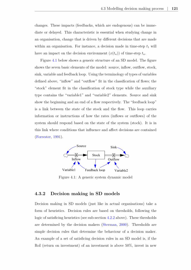
4.3 Modelling decision making process | 121
changes. These impacts (feedbacks, which are endogenous) can be imme-
diate or delayed. This characteristic is essential when studying change in
an organisation, change that is driven by different decisions that are made
within an organisation. For instance, a decision made in time-step t1 will
have an impact on the decision environment (x(tn)) of time-step tn.
Figure 4.1 below shows a generic structure of an SD model. The figure
shows the seven basic elements of the model: source, inflow, outflow, stock,
sink, variable and feedback loop. Using the terminology of types of variables
defined above, “inflow” and “outflow” fit in the classification of flows; the
“stock” element fit in the classification of stock type while the auxiliary
type contains the “variable1” and “variable2” elements. Source and sink
show the beginning and an end of a flow respectively. The “feedback loop”
is a link between the state of the stock and the flow. This loop carries
information or instructions of how the rates (inflows or outflows) of the
system should respond based on the state of the system (stock). It is in
this link where conditions that influence and affect decisions are contained
(Forrester, 1991).
Stock
Feedback loop
Source
Variable2
Sink
Inflow Outflow
Variable1
Figure 4.1: A generic system dynamic model
4.3.2 Decision making in SD models
Decision making in SD models (just like in actual organisations) take a
form of heuristics. Decision rules are based on thresholds, following the
logic of satisficing heuristics (see sub-section 4.2.2 above). These thresholds
are determined by the decision makers (Sterman, 2000). Thresholds are
simple decision rules that determine the behaviour of a decision maker.
An example of a set of satisficing decision rules in an SD model is, if the
RoI (return on investment) of an investment is above 50%, invest in new
122 | Literature review: Investment decision making
capacity of that technology, if it is below 50% but above 15%, only replace
the capacity that is being retired otherwise do not invest in any capacity.
For decision rules to be useful, they have to at least mimic the behaviour
of real decision makers. These rules have to be realistic and also robust
enough for different decision point scenarios. Decisions are a product of
decision rules. Sterman (2000; pg. 514) defines decision rules as “the poli-
cies and protocols specifying how the decision maker processes available
information.” These decision rules assume a degree of rationality both of
the decision maker and decision process.
There are five basic principles that every modeller has to follow in order
to effectively model decision making in SD models. Below is a list of these
principles as described by Sterman (2000; pg. 517).
1. The inputs to all decision rules in models must be restricted to infor-
mation actually available to the real decision makers.
• The future is not known to anyone. All expectations and beliefs
about the future are based on historical information. Expecta-
tions and beliefs may, therefore, be incorrect.
• Actual conditions and perceived conditions differ due to mea-
surement and reporting delays, and beliefs are not updated im-
mediately on receipt of new information. Perceptions often differ
from the actual situation.
• The outcomes of untried contingencies are not known. Expec-
tations about “what if” situations that have never been experi-
enced are based on situations that are known and may be wrong.
2. The decision rules of a model should conform to managerial practice.
• All variables and relationships should have real world counter-
parts and meaning.
• The units of measure in all equations must balance without the
use of arbitrary scaling factors.
4.3 Modelling decision making process | 123
• Decision making should not be assumed to conform to any prior
theory but should be investigated first-hand.
3. Desired and actual conditions should be distinguished. Physical con-
straints to the realization [sic] of desired outcomes must be repre-
sented.
• Desired and actual states should be distinguished.
• Desired and actual rates of change should be distinguished.
4. Decision rules should be robust under extreme conditions.
5. Equilibrium should not be assumed. Equilibrium and stability may
(or may not) emerge from the interaction of the elements of the sys-
tem.
The interactions between the stock (State of the System) and flows
(Inflow and Outflow) are controlled by the decision rules that are contained
in the Input and Output functions, as can be seen in Figure 4.2 below. The
decision maker has an idea of the current state of the system (based on the
Cues) and what the stock (State of the System) should be, then makes
decisions that take the “State of the System” closer to the desired stock
(Desired State of the System). Suppose that the stock (State of the System)
at t0 is 10 units, but the desired stock (Desired State of the System) is 12
units. In the next time-step t1, the decision maker decides on how many
units to invest in based on the Input function and also how many units to
retire based on the Output function. These functions are governed by the
decision rules of the system.

124 | Literature review: Investment decision making
State of the
System
Desired State of
the System
Cue 1,
Cue 2,
. . .,
Cue N
Input = F(Cue 1, Cue 2, . . ., Cue N)
Inflow of System Change Outflow of System Change
Output = F(Cue 1, Cue 2, . . ., Cue N)
Figure 4.2: Decision rules govern the rates of flow in systems
4.3.3 Model validation process
As discussed above, the mining decision model (described in Chapter 6)
is developed using system dynamics (SD) modelling framework. This is
because SD framework is suitable for analysing how a decision made in one
time step affects those that are made in subsequent time steps (Forrester,
1991; Wolstenholme, 1982). This characteristic (feedback loop effect) is
important to capture because it has been observed that mining firms’ op-
erational behaviour vary between time steps (Cortazar and Casassus, 1998;
Sabour, 2001).
An example of a feedback loop effect is shown in Figure 4.3 below. The
diagram shows the impact that copper price has on demand and also on
supply. A high price stimulates investment in copper production (supply
technologies) but at the same time leads to reduction in demand. Depend-
ing on the length of the cycles, copper supply and demand can potentially
be mismatched. This implies that at every time step, conditions driving
decision making could be different and would, therefore, require different
actions to be undertaken.
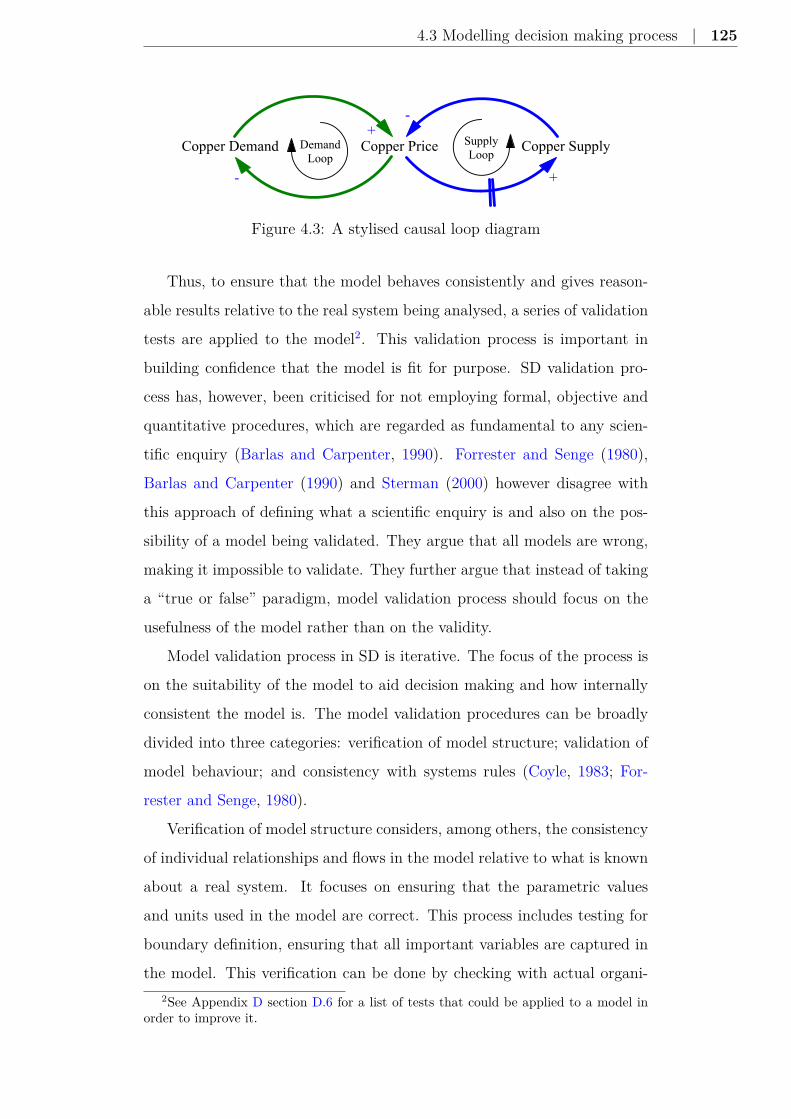
4.3 Modelling decision making process | 125
Copper PriceCopper Demand Copper Supply
-
+
+
-
Demand
Loop
Supply
Loop
Figure 4.3: A stylised causal loop diagram
Thus, to ensure that the model behaves consistently and gives reason-
able results relative to the real system being analysed, a series of validation
tests are applied to the model2. This validation process is important in
building confidence that the model is fit for purpose. SD validation pro-
cess has, however, been criticised for not employing formal, objective and
quantitative procedures, which are regarded as fundamental to any scien-
tific enquiry (Barlas and Carpenter, 1990). Forrester and Senge (1980),
Barlas and Carpenter (1990) and Sterman (2000) however disagree with
this approach of defining what a scientific enquiry is and also on the pos-
sibility of a model being validated. They argue that all models are wrong,
making it impossible to validate. They further argue that instead of taking
a “true or false” paradigm, model validation process should focus on the
usefulness of the model rather than on the validity.
Model validation process in SD is iterative. The focus of the process is
on the suitability of the model to aid decision making and how internally
consistent the model is. The model validation procedures can be broadly
divided into three categories: verification of model structure; validation of
model behaviour; and consistency with systems rules (Coyle, 1983; For-
rester and Senge, 1980).
Verification of model structure considers, among others, the consistency
of individual relationships and flows in the model relative to what is known
about a real system. It focuses on ensuring that the parametric values
and units used in the model are correct. This process includes testing for
boundary definition, ensuring that all important variables are captured in
the model. This verification can be done by checking with actual organi-2See Appendix D section D.6 for a list of tests that could be applied to a model in
order to improve it.
126 | Literature review: Investment decision making
sations or by using literature.
Under this category, tests for extreme conditions are also done.3 An
example of an extreme condition is when the energy consumption is zero,
system production is zero. Extreme condition tests are important because
they help discover model structure flaws and they also test the robustness
of the model for conditions that have not yet happened but could happen
in future.
The second category, model behaviour, looks at how the model responds
to different endogenous stimuli relative to the established real system’s be-
haviour. Behaviours such as, ‘does the model invest in capital equipment of
20 years life span when only one year worth of resource value is available?’
or ‘does the energy consumption increase as the copper ore grade reduce?’
Depending on how the model behaves, inconsistencies in the model can be
identified and rectified. And finally, system rules focus on how a model
responds to different system rules or policies relative to corresponding re-
ality. An example of such a system policy is how the model responds to
influence of commodity price. Say if price is a key driving factor, variance
in price would be expected to produce variance in the model response.
4.4 Decision making research context
This section focuses on describing the decision situation (environment) that
will be considered in this research. The study covers copper production
from mining stage through to refining stage (from cradle to gate). It con-
siders the cost of production and the energy types consumed by different
ore types, as shown in Figure 2.1 of Chapter 2 above. The research looks
at Zambia’s copper industry, a price taker. As a price taker (the industry’s
production patterns does not significantly influence the price of copper on
the global market), Zambia’s industry is exposed to have greater uncer-
tainty when compared to Chile’s industry (the leading producer of copper)
for example. Apart from the uncertainty of price, the uncertainty for other3See section D.6.1 for five extreme tests that were applied to the mining model
developed in Chapter 6.
4.4 Decision making research context | 127
commodity prices such as energy prices, raw material prices and labour
costs are considered.
Capital investment and operational decisions are analysed, with cap-
ital decisions being long-term while operational decisions are short-term.
Capital investment decisions are divided into two categories: production
capacity and electric motor capacity investments. Production capacity in-
vestments are driven by the price of copper, available copper resources and
an organisation’s profitability while investments of electric motor stock are
driven by electricity price, production capacity, the organisation’s prof-
itability and energy efficiency gap. As for operational decisions, they are
driven by the organisation’s profitability. Decision rules and functions that
govern each of these decisions are described and defined in Chapter 6 below.
These three decisions can be thought of as being made by three dif-
ferent actors, whose aims are also different – with all the decisions driven
by both exogenous and endogenous factors. The actor (say actor 1) who
makes decisions of production capacity is driven by the desire to increase
or maintain production of copper (related to organisation’s market share).
By investing in efficient electric motors, the actor (actor 2) hopes to in-
crease the organisation’s productivity for every tonne of copper produced
in the long-term. Finally, the actor (actor 3) who makes operational de-
cisions focuses on minimising operational losses which would result from
fluctuations in commodity prices or reduction in ore grade quality. A com-
bination of these three decisions could further help in understanding how
the organisation’s energy efficiency would change over time, the energy ef-
ficiency indicator used here is the average efficiency of the electric motor
system.
Figure 4.4 below shows an interaction of these three decisions (outputs).
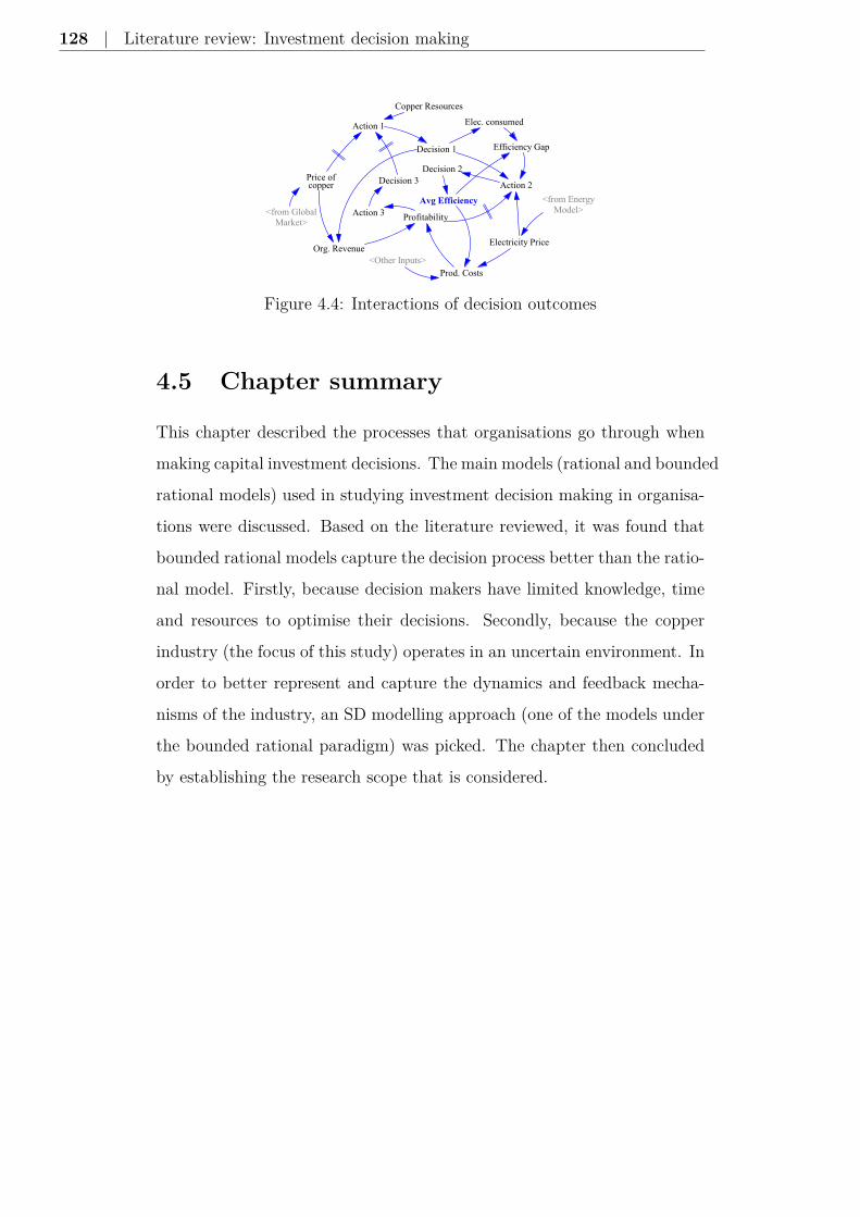
128 | Literature review: Investment decision making
Price ofcopper
Copper Resources
Action 1
Decision 1
Decision 3
Profitability
Prod. Costs
Org. Revenue
Decision 2
Efficiency Gap
Electricity Price
Action 3
Action 2
Avg Efficiency
Elec. consumed
<Other Inputs>
<from Energy
Model><from Global
Market>
Figure 4.4: Interactions of decision outcomes
4.5 Chapter summary
This chapter described the processes that organisations go through when
making capital investment decisions. The main models (rational and bounded
rational models) used in studying investment decision making in organisa-
tions were discussed. Based on the literature reviewed, it was found that
bounded rational models capture the decision process better than the ratio-
nal model. Firstly, because decision makers have limited knowledge, time
and resources to optimise their decisions. Secondly, because the copper
industry (the focus of this study) operates in an uncertain environment. In
order to better represent and capture the dynamics and feedback mecha-
nisms of the industry, an SD modelling approach (one of the models under
the bounded rational paradigm) was picked. The chapter then concluded
by establishing the research scope that is considered.
Chapter 5
Modelling of Zambia’s energy
system
This chapter addresses the first theme of this research, which focused on
the development of Zambia’s energy system model (described in sub-section
1.1.1). This model was used to study how the energy system would evolve
under a range of demand scenarios. It also looked at the technology stock
and how much capital investment cost that would be required in each of
these demand scenarios. The model helped to answer four sub-questions:
• How would residential energy demand change?
• Which supply-side technologies would be required to meet Zambia’s
energy demand?
• How much capital investment would be required to develop Zambia’s
energy system?
• How would the average generation cost change over time?
Two energy models were developed for this study: demand and supply
models. The demand model was developed using a LEAP platform (see
Heaps, 2016) and OSeMOSYS platform (see Howells, 2009; Howells et al.,
2011; Osemosys, 2013; Welsch et al., 2012) was used to build the supply
130 | Modelling of Zambia’s energy system
model. All the data used in the development of these models can be found
in Appendix C.
The chapter is organised as follows: Section 5.1 identifies and describes
the key drivers of energy demand and how future demand was modelled.
The second section (section 5.2), describes the resources available in and
around Zambia to meet this energy demand. An optimisation model was
developed that linked energy resources to demand. Finally, section 5.3
describes the scenarios that were used in this study. These scenarios were
particularly useful when studying the impact of increasing access to clean
energy on the mining industry. The chapter then concludes with a chapter
summary (section 5.4).
5.1 Demand model
Energy demand arises from satisfying an energy service through usage of
an appliance or technology. Total energy demand is, therefore, dependant
on the energy intensity of a service, the choice of a technology and its
(technology) efficiency (Bhattacharyya and Timilsina, 2009). An example
of energy service is a cooking or lighting activity. The choice of technology
to use in order to satisfy an energy service depends on, among others,
the availability of the technology, affordability (i.e. investment cost) of
the technology, the cost of using that technology and preference of the
technology user. Technology efficiency is an embedded characteristic of a
technology.
The transition from one technology use to another (observed using
changes in fuel energy shares and intensities) has exhibited inertia. Apart
from the common reason of affordability (for example in the case of residen-
tial sector), two main aspects are usually overlooked. These are technology
lock-in and unavailability of preferred energy carriers. The first aspect
looks at the cost of disposing off a technology stock that still has opera-
tional life and investing in a new technology that uses a preferred energy
carrier (if available). It argues that sometimes, it is cost effective to con-
5.1 Demand model | 131
tinue using a technology which is inefficient than to invest in an efficient
technology. The second aspect focuses on the choice options available to
the user. It argues that no matter how desirable an energy carrier could
be, if it is not available then it will not be used. This study using these
three aspects (affordability, technology lock-in and availability) to show
how energy demand would evolve.
Drivers of energy use and energy transition in different sectors have
been generally understood (Barnes and Floor, 1996; Bhattacharyya and
Timilsina, 2009). However, the major challenge has been how we think
about energy demand going forward. This is because the future is full of
uncertainty, due to the complex interactions between many different drivers
(Ruijven et al., 2010).
Furthermore, when studying a developing country’s energy system, un-
availability of data and statistics make projecting energy demand challeng-
ing (Ruijven et al., 2008). However, projection of demand would even be
more challenging in some countries with suppressed energy demand. As
Bhattacharyya and Timilsina (2009) observe, availability of statistics in
itself does not imply that all possible demand has been captured because
there would be considerable unmet demand due to the supply shortages
that those countries are experiencing. This, therefore, means that the esti-
mated energy intensity (from such statistics) would have significant errors
(parametric uncertainty). Despite these limitations and uncertainty, mod-
els (in developing or developed countries) are important tools for aiding
decision making and they also help in assessing what would happen if no
action is taken to change the way energy is used.
Two main methodologies are used to model demand: econometric and
end-use approaches. As discussed in sub-section 3.2.5 of Chapter 3, end-use
approach is used in this research because of its ability to adequately capture
features that are important in developing countries’ energy systems (Bhat-
tacharyya and Timilsina, 2010) and also because energy services and their
associated energy carriers can be explicitly represented (Craig et al., 2002).
Further, as Bhattacharyya and Timilsina (2009) observes, the econometric

132 | Modelling of Zambia’s energy system
approach tends to ignore the non-priced transactions of traditional fuels;
the most significant energy carrier in Zambia’s energy sector. Moreover, for
priced transactions but in regulated energy markets (like Zambia), the re-
lationship between energy price and demand may not be meaningful. This
challenge (energy price and demand relationship which is central to the
econometric approach) would be worsened when one factors in the supply
shortages that are experienced in many developing countries.
On the contrary, the end-use approach accounts for energy from end-
use service level; end-use services such as cooking, heating, motive power,
cooling, hauling, conveyance and lighting. The approach accounts for where
energy is used and also which type of energy carriers are used. Further,
depending on the sector or industry being modelled, energy demand could
be modelled as driven by income, climate, population, floor space, physical
output, value added or GDP; activities that lead to energy demand.
In this research, this approach was, however, only used to model energy
demand in residential and mining sectors. For two reasons, these sectors
(the largest end-use sectors) are the focus of the research and secondly
because of availability of better statistics and data for these sectors. In ad-
dition, because of limited statistics and data, simple technique (discussed
in sub-section 3.2.5) was used to model agricultural, services, transport
and other industries sectors. The simplicity and usefulness of the simple
technique notwithstanding, this method (technique) lacks theoretical foun-
dation and hence relies heavily on the judgement of the modeller (Bhat-
tacharyya and Timilsina, 2009).
Examples of end-use and simple technique models are given below in
Equations 5.1 and 5.2 respectively.
Ea = A× U
η(5.1)
where,
Ea is the total final energy demand of activity A,
A is the activity that demands energy, such as lighting or industrial
output,
5.1 Demand model | 133
U is the useful energy intensity of the activity, and
η is a set containing technologies, their accompanying energy carriers
(fuels) and efficiencies that could be used to satisfy energy demand.
Ea(t) = Ea(t0) × (1 + gr)dt (5.2)
where,
Ea(t) is the total final energy demand of an activity or sector at time t,
Ea(t0) is the actual energy demand at time t0,
gr is the growth rate of the demand, and
dt is the time interval for the projection.
Bhattacharyya and Timilsina (2009) summaries the general steps in-
volved in the end-use approach:
• Disaggregation of total energy demand into relevant homogeneous
end-use categories or modules
• A systematic analysis of social, economic and technological determi-
nants
• Organisation of determinants into a hierarchical structure
• Formalisation of the structure in mathematical relationships
• Snap-shot view of Reference year
• Scenario design for the future
• Quantitative forecasting using mathematical relations and scenarios
5.1.1 Energy consumption in Zambia
Final energy demand in Zambia is dominated by the residential and min-
ing sectors. Energy carriers currently used in Zambia’s energy system are
wood, charcoal, electricity, coal, diesel, motor gasoline, fuel oil and other
petroleum products. Traditional fuels (wood and charcoal) are the most
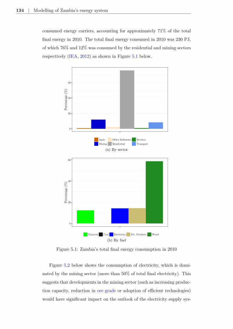
134 | Modelling of Zambia’s energy system
consumed energy carriers, accounting for approximately 71% of the total
final energy in 2010. The total final energy consumed in 2010 was 230 PJ,
of which 76% and 12% was consumed by the residential and mining sectors
respectively (IEA, 2012) as shown in Figure 5.1 below.
0
20
40
60
Per
cent
age
(%)
Agric
Mining
Other Industries
Residential
Services
Transport
(a) By sector
0
20
40
60
Per
cent
age
(%)
Charcoal Coal Electricity Pet. Products Wood
(b) By fuel
Figure 5.1: Zambia’s total final energy consumption in 2010
Figure 5.2 below shows the consumption of electricity, which is domi-
nated by the mining sector (more than 50% of total final electricity). This
suggests that developments in the mining sector (such as increasing produc-
tion capacity, reduction in ore grade or adoption of efficient technologies)
would have significant impact on the outlook of the electricity supply sys-
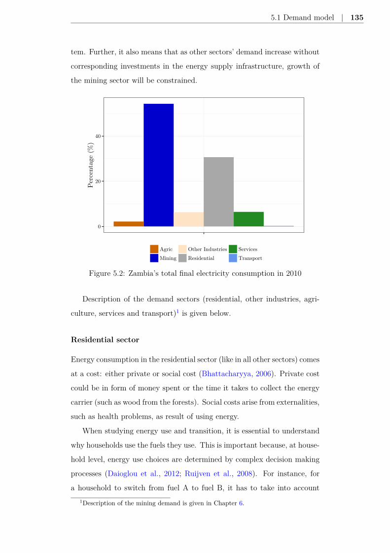
5.1 Demand model | 135
tem. Further, it also means that as other sectors’ demand increase without
corresponding investments in the energy supply infrastructure, growth of
the mining sector will be constrained.
0
20
40
Per
cent
age
(%)
Agric
Mining
Other Industries
Residential
Services
Transport
Figure 5.2: Zambia’s total final electricity consumption in 2010
Description of the demand sectors (residential, other industries, agri-
culture, services and transport)1 is given below.
Residential sector
Energy consumption in the residential sector (like in all other sectors) comes
at a cost: either private or social cost (Bhattacharyya, 2006). Private cost
could be in form of money spent or the time it takes to collect the energy
carrier (such as wood from the forests). Social costs arise from externalities,
such as health problems, as result of using energy.
When studying energy use and transition, it is essential to understand
why households use the fuels they use. This is important because, at house-
hold level, energy use choices are determined by complex decision making
processes (Daioglou et al., 2012; Ruijven et al., 2008). For instance, for
a household to switch from fuel A to fuel B, it has to take into account1Description of the mining demand is given in Chapter 6.
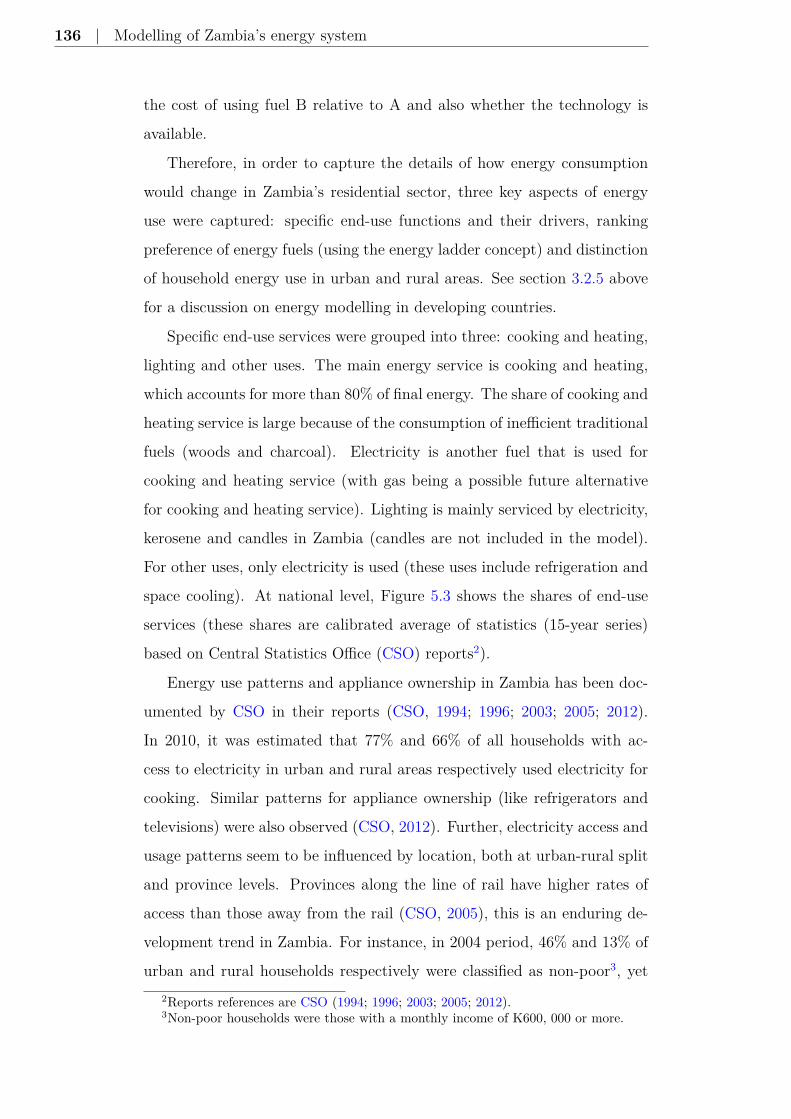
136 | Modelling of Zambia’s energy system
the cost of using fuel B relative to A and also whether the technology is
available.
Therefore, in order to capture the details of how energy consumption
would change in Zambia’s residential sector, three key aspects of energy
use were captured: specific end-use functions and their drivers, ranking
preference of energy fuels (using the energy ladder concept) and distinction
of household energy use in urban and rural areas. See section 3.2.5 above
for a discussion on energy modelling in developing countries.
Specific end-use services were grouped into three: cooking and heating,
lighting and other uses. The main energy service is cooking and heating,
which accounts for more than 80% of final energy. The share of cooking and
heating service is large because of the consumption of inefficient traditional
fuels (woods and charcoal). Electricity is another fuel that is used for
cooking and heating service (with gas being a possible future alternative
for cooking and heating service). Lighting is mainly serviced by electricity,
kerosene and candles in Zambia (candles are not included in the model).
For other uses, only electricity is used (these uses include refrigeration and
space cooling). At national level, Figure 5.3 shows the shares of end-use
services (these shares are calibrated average of statistics (15-year series)
based on Central Statistics Office (CSO) reports2).
Energy use patterns and appliance ownership in Zambia has been doc-
umented by CSO in their reports (CSO, 1994; 1996; 2003; 2005; 2012).
In 2010, it was estimated that 77% and 66% of all households with ac-
cess to electricity in urban and rural areas respectively used electricity for
cooking. Similar patterns for appliance ownership (like refrigerators and
televisions) were also observed (CSO, 2012). Further, electricity access and
usage patterns seem to be influenced by location, both at urban-rural split
and province levels. Provinces along the line of rail have higher rates of
access than those away from the rail (CSO, 2005), this is an enduring de-
velopment trend in Zambia. For instance, in 2004 period, 46% and 13% of
urban and rural households respectively were classified as non-poor3, yet2Reports references are CSO (1994; 1996; 2003; 2005; 2012).3Non-poor households were those with a monthly income of K600, 000 or more.
5.1 Demand model | 137
0
20
40
60
80
All Fuels Electricity
Per
cent
age
(%)
Services: Cooking & Heating Lighting Other Uses
Figure 5.3: Residential sector’s energy end-use services demand
47.6% of urban and only 3.1% of rural households had access to electricity
for lighting4. This discrepancy between the level of household income and
access to and usage of electricity among rural households was also observed
in a CSO survey in 2015 (CSO, 2016). This confirms that income is not the
sole and perhaps the most important determinant of access to electricity
in Zambia. Figures 5.4 and 5.5 below show shares of fuel usage by end-use
service for lighting and cooking respectively, in urban and rural areas in
2010.
4Tables C.1 and C.2 in Appendix C gives percentage classification by lighting andcooking fuels respectively (CSO, 2005).

138 | Modelling of Zambia’s energy system
0
10
20
30
40
50
Rural Urban
Per
cent
age
(%)
Candles Electricity Kerosene None Other
Figure 5.4: Lighting usage patterns
0
20
40
60
80
Rural Urban
Per
cent
age
(%)
Charcoal Electricity Other Wood
Figure 5.5: Cooking and heating usage patterns
Furthermore, it can be inferred from CSO (2005) that location is a
stronger determinant than income of whether households in Zambia would
have access to electricity or not. This is important because it implies
that some households in Zambia do not use electricity because it is not
available rather than that they cannot afford it. To put the argument of
5.1 Demand model | 139
affordability into context, in 2010, an average Zambian household consumed
about 5, 000 kWh per year (415 kWh per month) of electricity, this would
translate to approximately 7% of total household income of a rural non-
poor household5, a share significantly lower than that of a poorer household
in urban area which uses electricity for both lighting and cooking services.
Therefore, if availability is the main challenge to access to clean energy for
households in rural areas, it then implies that more investment in the clean
energy supply infrastructure is required.
The other aspect which was considered in the demand model was the
energy carrier preference ranking; it was assumed that after electricity,
charcoal (which is almost always purchased (CSO, 2005)) is thought to be
a better and cleaner fuel than wood. However, energy use in rural areas is
dominated by wood, partly because wood can be collected from the forests
for free and also because there are more poor households in rural areas
(who cannot afford to purchase charcoal).
Apart from availability (access to a particular fuel) and affordability
(household income); household size, floor-space, climate and population
growth are some of the key energy drivers in the residential sector (Daioglou
et al., 2012). However, because of limitations of available data, the model
developed for Zambia’s residential sector only considered access to clean
energy (electrification), household income, household size and population
growth as key energy drivers. A schematic representation of the relation-
ship between energy drivers (considered in the model) and energy end-use
services is given in Figure 5.6 below.
5In 2004, electricity price was K90 per kWh with a fixed monthly charge of K5, 266for residential customers (ERB, 2013).
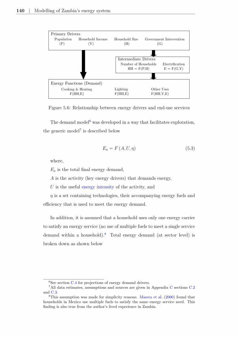
140 | Modelling of Zambia’s energy system
Primary Drivers
Intermediate Drivers
Energy Functions (Demand)
Population (P)
Household Size (H)
Household Income (Y)
Government Intervention (G)
Number of Households HH = F(P,H)
Cooking & Heating F(HH,E)
LightingF(HH,E)
Other UsesF(HH,Y,E)
Electrification E = F(G,Y)
Figure 5.6: Relationship between energy drivers and end-use services
The demand model6 was developed in a way that facilitates exploration,
the generic model7 is described below
Ea = F (A,U, η) (5.3)
where,
Ea is the total final energy demand,
A is the activity (key energy drivers) that demands energy,
U is the useful energy intensity of the activity, and
η is a set containing technologies, their accompanying energy fuels and
efficiency that is used to meet the energy demand.
In addition, it is assumed that a household uses only one energy carrier
to satisfy an energy service (no use of multiple fuels to meet a single service
demand within a household).8 Total energy demand (at sector level) is
broken down as shown below
6See section C.4 for projections of energy demand drivers.7All data estimates, assumptions and sources are given in Appendix C sections C.2
and C.3.8This assumption was made for simplicity reasons. Masera et al. (2000) found that
households in Mexico use multiple fuels to satisfy the same energy service need. Thisfinding is also true from the author’s lived experience in Zambia.
5.1 Demand model | 141
Ea = Ech + Elig + Eoth (5.4)
where,
Ea is the total final energy demand,
Ech is the total final demand for cooking and heating,
Elig is the total final demand for lighting, and
Eoth is the total final demand for other uses.
Cooking and heating service demand is a primary demand (all house-
holds have cooking and heating activity (CSO, 2012)). This service is
assumed to be driven by household size (and total households at sector
level). The fuels used to meet this demand are electricity, charcoal, wood
and gas (future fuel option). It is also assumed that identical households
(same household size) in urban or rural area, use the same quantity of
useful energy (U) for their cooking and heating service. The final energy,
however, could be different depending on the type of fuel and the efficiency
of the technology that is used.
Further, it is assumed that increase in electrification (ϕelec) leads to in-
crease in the share of households using electricity for cooking and heating
(φelec), all things held constant. The share of these fuels (electricity, char-
coal, wood and gas) are modelled as exogenous factors, as described in the
scenarios section (section 5.3) below. This is important because it enables
flexibility to explore what would happen if certain set targets are achieved
(such as increasing electrification). Total demand for cooking and heating
service (Ech) is defined below
Ech = HH × Uch ×t∑
i=0
j=4∑j=1
[φij][ηj]
(5.5)
where,
Ech is the total final demand for cooking and heating,
HH is the total number of households,
Uch is the useful energy for cooking and heating per household,
[φij] is the share of an energy carrier (electricity, charcoal, wood and
142 | Modelling of Zambia’s energy system
gas) in a particular time period (where ∑φi = 1), and
[ηj] is the efficiency of the technology that consumes an energy carrier
used to satisfy the demand (where ηj ≤ 1). The efficiencies for electrical,
charcoal and wood technologies as modelled are 65%, 24% and 14% respec-
tively. These efficiencies are calculated based on the calibration of energy
use from 1993 to 2010 as recorded by CSO and IEA statistics.
Lighting service is considered as secondary energy service (the level of
lighting service penetration is currently less than 100%). It can be seen
in Figure 5.4 that some households go without lighting service. The total
lighting demand (Elig) is defined below
Elig = HH × (Felec × ϕelec + Fkero × ϕelec) (5.6)
ϕelec ≥ φelec (5.7)
where,
Elig is the total final demand for lighting,
HH is the total number of households,
Felec and Fkero are the final energy intensities for electricity and kerosene
respectively,
ϕelec and ϕkero are the shares of households that use electricity and
kerosene for their lighting service respectively (where ϕelec + ϕkero ≤ 1),
φelec is the share of households using electricity for cooking and heating,
and
Equation 5.7 implies that the number of households using electricity for
lighting will always be greater than or equal to those using electricity for
cooking and heating.
Other uses service demands (such as air-conditioning, dish washing and
refrigeration) are satisfied only by electricity. These uses are driven by
assets ownership and income of a household. Not only does increasing in-
come enable households to acquire assets (technologies) that they use for
5.1 Demand model | 143
these uses, it also enables households to use more of those technologies. For
instance, if two households own an air-conditioner, it is assumed that the
richer household will use the air-conditioner more than the poorer house-
hold. Further, it is assumed that the richer household will have more of
electrical appliances than the poorer household. This, therefore, increases
the richer household’s average energy intensity for other uses. Similar to
cooking, the share of households with other uses demand (ψ) is always less
than or equal to those with access to electricity (ϕelec). Total other uses
demand (Eoth) is defined below
Eoth = HH × ψ ×X (5.8)
X = ln (I) × 6.504 − 45.045 (5.9)
where,
Eoth is the total final demand for other uses,
HH is the total number of households,
ψ is the share of households with other uses demand (currently, ψ < 1
for both urban (73%) and rural (70%) areas),
I is the income (in US$ per household in real terms), and
X is a regression function used for estimating the energy intensity of
Other Uses (GJ per HH) in the residential sector. This function was esti-
mated using statistics from CSO9.
Economic sectors
In economic sectors (services, agriculture, transport, other industries and
mining), energy is used as an input to their production processes. Below is
a brief description of what constituents each of these sectors and their key
energy drivers (for mining sector see Chapter 6).
The services sector includes trade, hotel and restaurant, real estate
and business services, financial institutions and insurance, community and9See Appendix C section C.3 for the regression details.
144 | Modelling of Zambia’s energy system
personal services, education and health, and public administration sub-
sectors. Energy services required in this sector are heating, lighting, HVAC
and other utilities (Haw, 2007). Demand is mainly influenced by floor space
and occupancy of the building.
Agriculture sector comprises of agriculture and hunting, forestry, live-
stock and fishing sub-sectors. This sector is the largest employer in Zambia,
employing about 63% of the total workforce in 2010 (CSO, 2012). Most of
the economic activities are done at subsistence level, the largest economic
activity in rural areas (by size of workforce population). Agriculture sec-
tor requires energy for irrigation, harvesting and packing, transportation,
processing, thermal purposes, lighting and other energy uses. However, as
noted above, much of the output in the sector is at subsistence level (which
uses more animal-driven equipment than energy). Thus, energy services
described here are mainly for commercial farmers.
Transport and communication sub-sectors make up the transport sec-
tor. Energy demand in the sector is driven by private, public and freight
transportation. Income and location determine if a person will use private,
public or non-energy based transportation. For instance, the transport sys-
tem in rural and some urban areas is largely non-motorised based. Further,
private car ownership at national level in 2010 stood at 4.9% (24% in urban
and 1.25% in rural areas).
On the other hand, freight transportation is driven by goods produced
by the agriculture, mining and other industries sectors. Thus, an increase
in any one of the sectors leads to an increase in energy demand for freight
transportation, all things held constant. The sector is dominated by road-
based transportation; local aviation and railway modes are not well devel-
oped while the communication sub-sector is not energy intensive. Thus,
petroleum products dominate the transport sector as energy carriers.
Food, beverage and cigarettes; textiles and leather; petroleum; chemi-
cals; other manufacturing; electricity, water and gas; construction and civil
work; and any other sub-sector not covered in sectors above are under other
industries sector. This sector (other industries sector) offers, as noted in
5.2 Supply model | 145
GRZ (2006), the most industrialisation opportunities for Zambia. It is also
identified as a sector with the largest economic growth potential in Vision
2030 (GRZ, 2006). The sector’s energy demand services are for lighting,
HVAC, process heating, conveyance and transportation. Energy demand is
driven by physical production output, value addition and energy efficiency
practices.
Nevertheless, because of the lack of data, these sectors’ energy projec-
tions were modelled as driven by GDP growth of each sector.10 GDP growth
rates were exogenous factors described in the scenarios section (section 5.3
below). These projections used a simple technique model11,12 defined below
Ea(t) = [Fi] × [GDPj (t)] (5.10)
where,
Ea(t) is the total final energy demand of a sector at time t,
[Fi] is a set containing final energy intensity (GJ per US$ GDP) for a
sector,
i is the type of fuel (i.e. electricity, diesel, petrol etc), and
[GDPj(t)] is the GDP of a sector at time t.
5.2 Supply model
An energy supply model13 was developed using OSeMOSYS (Howells, 2009;
Howells et al., 2011; Osemosys, 2013; Welsch et al., 2012). OSeMOSYS
(an open source platform) is a full-fledged systems optimisation model for
long-term energy planning. This platform uses an optimisation framework,
which is often used for energy system analysis (other similar tools to OSe-
MOSYS are MARKAL, TIMES, MESSAGE and TEMOA )14.
10This is a similar approach that was taken in Fais et al. (2016).11All data estimates, assumptions and sources are given in Appendix C sections C.2
and C.3.12Section C.4 gives the projections of GDP.13The Reference Energy System (RES) diagram is given in Figure 3.3 above.14Models built using this framework are also referred to as Energy System Optimisa-
tion Models (see Daly et al., 2015; DeCarolis et al., 2017; Strachan et al., 2016)
146 | Modelling of Zambia’s energy system
This model captured, in detail, the available energy resources and sup-
ply technologies but has stylised demand and transmission technologies.
Exogenous variable costs were included in the model to represent the cost
of operating the transmission network (for grid technologies only) while
no operation or investment costs were considered for demand technologies.
This is because energy demand was exogenously determined using a LEAP
model described in section 5.1 above and the mining model described in
Chapter 6 below.
The supply model was solved by minimising the discounted total energy
system costs. The objective function (an expanded version of Equation 4.1)
is defined below
minT∑
t=0
(It,g +OM fix
t,g +OM vart,g + Cfuel
t,g + Ccarbont,g
)(5.11)
where,
t is a one-year time step from 2010 to 2050,
g is a set of energy technologies,
It,g is the capital inv. costs at time t for a particular technology in g,
OM fixt,g is the fixed ops and maintenance costs for a technology in g,
OM vart,g is the variable ops and maintenance costs for a technology in g,
Cfuelt,g is the fuel cost for a technology in g, and
Ccarbont,g is the carbon tax for a technology in g.
Most of the techno-economic data for energy technologies used in the
model are based on the Southern Africa Power Pool (SAPP) study (Nexant,
2007)15 while technology learning (for renewable technologies) assumptions
are based on RMI (2015). The SAPP study was a regional study of South-
ern Africa power utilities, thus, the main source of the information was
from the utilities themselves and Zambia’s power utility (ZESCO Limited
(ZESCO)) being one of them. However, in instances where the SAPP study
information is dated, it was replaced by latest available information such
as ERB (2008), ZESCO (2008; 2009), JICA/MEWD (2009) and DHEC
15Note that all costs were adjusted to 2010 US$ price.
5.2 Supply model | 147
(2011). Information for other energy supply technologies16 was based on
published sources such as IPA (2007), CSO (2007) and ERC (2013)17.
It should be noted though that because costs of using traditional fuels
and benefits of avoided health complications as a result of increased access
to clean energy are difficult to quantify, they were not included in the
model. However, a trade-off analysis that focused on increasing access to
clean energy in order to avoid deforestation was done (using OSeMOSYS
output but away from OSeMOSYS). The energy resources of the model
were grouped into three sectors: forestry, electricity, and fossil fuels sectors.
The forestry sector is the main source of energy in Zambia, it is the
source of traditional fuels (charcoal and wood). Traditional fuels are par-
ticularly important in rural areas and other urban areas with limited access
to the national grid18 since cooking and heating service (the largest end-
use service in residential sector) is currently satisfied only by electricity
and traditional fuels. Apart from it being a major energy supplier, the
forestry sector is a critical link between the energy sector in general and
bio-diversity and it is also a carbon sink. Therefore, increased consumption
of traditional fuels in Zambia could lead to deforestation. This, in turn,
would lead to extinction of certain plant and animal species and also reduce
the ability of the forests to absorb CO2 emissions.
Thus, explicitly modelling this interaction between energy demand and
available forestry energy resources is important in three main ways. Firstly,
it enables analysis of the impacts that energy use would have on deforesta-
tion or how increasing access to clean energy would help reduce defor-
estation. As van Ruijven et al. (2012) observed there is little evidence in
literature that show that increasing access to clean energy helps in reducing
deforestation.
Secondly, a cost-benefit trade-off analysis between increasing access to
clean energy and deforestation could be done. In this research, an analysis
that compared the total system costs required to increase access to clean
16See Appendix C for the list of other supply technologies.17See Appendix C section C.5 for all the model assumptions.18See sub-section 5.1.1.
148 | Modelling of Zambia’s energy system
energy and the funds that countries like Zambia receive through the Re-
ducing emissions from deforestation and degradation and enhancement of
carbon stocks (REDD+) initiative19 to enhance forest management (for re-
ducing deforestation) was done. From a cost perspective (externalities not
included), I argue (see Chapter 7) that it is cheaper for countries reliant
on traditional fuels to continue deforesting then afforesting than to avoid
deforestation by increasing access clean energy (i.e. if the only purpose of
increasing access is to reduce the rate of deforestation).
Finally, the available forestry resources could be included as one of
the key constraints in the model. For instance, about 70, 000 hectares of
forests20 are cleared every year in order to provide an equivalent of 120 PJ
(CSO, 2007). Energy demand currently accounts for 10% of forest cover
losses with the remainder coming from the agriculture sector (through land
use changes). However, as more households shift from wood (currently at
59%) to charcoal (currently at 12%) a better fuel21, the rate of deforestation
would increase; due to the conversion efficiency of the charcoal making
process.
The electricity sector is dominated by hydro technologies.22 For in-
stance, in 2010, the installed capacity of electricity was 1, 900 MW, of
which hydro technologies accounted for 97% and 99% of total capacity and
electricity generation respectively. Further, hydro and coal technologies
dominate the planned (ZESCO plans that is) capacity expansion portfolio.
However, Zambia has a range of other supply technologies such as solar and
geothermal technologies, though no major comprehensive expansion plan
has been developed for these technologies.23
The model assumes that all fossil fuels are imported. This is because
Zambia does not have crude oil resources and also because the coal mining
19Details for REDD+ mechanism can be found in Jindal et al. (2008), Parker et al.(2009) and Cacho et al. (2014).
20Total forest cover in 2004 was about 440,000 sq. km (CSO, 2007).21See Hibajene and Kalumiana (2003) for a discussion of why charcoal is a better fuel
than wood.22See section A.1.2 of Appendix A for the list of electricity generation stock.23See section C.5 of Appendix C for the energy supply technologies information in
Zambia.
5.2 Supply model | 149
activities are erratic. All crude oil is imported through Tanzania Zam-
bia Mafuta Pipeline Limited (TAZAMA) pipeline to the refinery in Ndola.
The refinery products are diesel, motor gasoline, fuel oil, LPG, domestic
kerosene, aviation kerosene, refinery gas and other products in minor quan-
tities. Apart from petroleum products, Zambia also consumes coal. The
country has considerable coal resources, however, the output of coal from
the mines (under Maamba collieries) is erratic. Thus, it is assumed, in this
model, that all the coal requirements are imported from Zimbabwe.
5.2.1 Average generation cost of electricity
In order to estimate the average electricity generation cost of the energy
model24 (electricity was the main fuel that was analysed as an option of
increasing access to clean energy), the levelised cost approach was used
(IEA/NEA, 2010; Ouedraogo et al., 2015; Ramana and Kumar, 2009). This
approach assumes a constant discount rate (r)25 and energy price through-
out the economic life, n years, of a technology. Further, because Zambia’s
energy markets are largely monopolised and regulated, and market and
technology risks exist, this method (LCoE) is appropriate for estimating
the real cost of electricity generation investments (IEA/NEA, 2010; Tembo,
2012).
The levelised cost of electricity (LCoE) for a generating technology dur-
ing its operating life is defined below,
LCoE = Operational life cycle costTotal electricity generation (5.12)
Operational life cycle cost =n∑
n=0
Costsn
(1 + r)n (5.13)
Total electricity generation =n∑
n=0
Elecn
(1 + r)n (5.14)
24The estimation of costs is based on the least cost system that is developed above.25“. . . the discount rate used in LCOE calculations reflects the return on capital
for an investor in the absence of specific market or technology risks.” (IEA/NEA, 2010;pg. 33).
150 | Modelling of Zambia’s energy system
where,
Costsn is the total sum of investment capital, fixed, variable, fuel and
carbon costs in a particular year,
n is the operational life of a technology,
r is the discount rate (r > 0), and
Elecn is the annual generated electricity.
The average LCoE of the electricity generation system is defined as
follows
LCoEsystem =∑
(ξk × LCoEk) (5.15)
∑ξ = 1 (5.16)
where,
ξk is the share of a particular technology (k) in the system, and
LCoEk is the generation cost of technology k.
5.3 Scenarios
Five scenarios26 were developed to explore plausible energy demand futures
for Zambia from 2010 (base year) to 2050 (end year), with a strong empha-
sis on the residential sector as it is the main consumer of final energy (see
Figure 1.1 above). These scenarios are important because they contain
exogenous factors that influence both the demand and supply sides. As
Rosnes and Vennemo (2012) observed demand projections and supply side
investment costs estimations are influenced by the approach and frame-
work (bottom-up or top-down and optimisation or simulation), the data
and exogenous variables such as technology capital cost, economic growth
and rates of access to clean energy. The scenarios, therefore, focused on
describing the exogenous variables used in this study. Apart from that,26Put correctly, many scenarios were developed and explored but only five scenarios
were reported.
5.3 Scenarios | 151
these scenarios form a neat framework from which the impact of access to
clean energy on mining production output is analysed.27
It is worth mentioning that carbon tax was not modelled in any of
the scenarios because Tembo (2012) found that the tax did not change
the capacity mix in Zambia’s electricity system but just increased the cost
of generating electricity. However, the impact of restricting (reducing)
electricity generation from carbon emitting technologies on total system
capital investment cost, deployment of renewable technologies and energy
price was analysed. Further, OAT28 sensitivity analyses29 were done on the
model by varying key inputs30. Key drivers of these scenarios were energy
use in the residential sector and economic growth.31 Two economic growth
assumptions (base path at 4.5% and high path at 6% annual growth rates)
considered are based on Zambia’s Vision 2030 (GRZ, 2006).
Table 5.1 below gives the components of these economic assumptions.
The two key assumptions of energy use in the residential sector are that
access to clean energy is driven exogenously (that is through government
policy) and that energy fuels preference ranking order is electricity, gas
(when available), charcoal and wood. The first assumption (of energy use)
enables analysis of what (in terms of capacity stock and investment costs)
would be required of government in order to meet its development aspi-
rations of access to clean energy. The second assumption focuses on how
households transition from one fuel to the next. For instance, even if wood
could be freely collected from the forest (by the energy user), a user would
rather use charcoal when it is available at their income level. Hence, as
cleaner energy carriers become available (and/or with increasing income),
residential users abandon traditional fuel (first wood then charcoal) for gas
or electricity.
27See sections 7.1.1 (on page 188) and 7.2.1 (on page 219) for how the energy andmining models were linked and synchronised.
28OAT is an acronym of one-at-a-time.29See section 3.1.4 of Chapter 3 for a discussion on sensitivity analysis.30See Appendix C section C.6 for the full list of variables on which OAT sensitivity
analysis was applied.31See section C.4 for projections of energy demand drivers such as number of house-
holds and GDP.
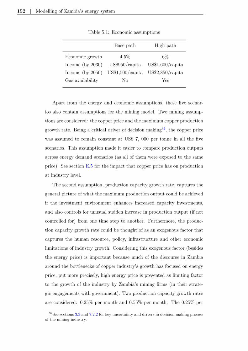
152 | Modelling of Zambia’s energy system
Table 5.1: Economic assumptions
Base path High path
Economic growth 4.5% 6%Income (by 2030) US$950/capita US$1,600/capitaIncome (by 2050) US$1,500/capita US$2,850/capitaGas availability No Yes
Apart from the energy and economic assumptions, these five scenar-
ios also contain assumptions for the mining model. Two mining assump-
tions are considered: the copper price and the maximum copper production
growth rate. Being a critical driver of decision making32, the copper price
was assumed to remain constant at US$ 7, 000 per tonne in all the five
scenarios. This assumption made it easier to compare production outputs
across energy demand scenarios (as all of them were exposed to the same
price). See section E.5 for the impact that copper price has on production
at industry level.
The second assumption, production capacity growth rate, captures the
general picture of what the maximum production output could be achieved
if the investment environment enhances increased capacity investments,
and also controls for unusual sudden increase in production output (if not
controlled for) from one time step to another. Furthermore, the produc-
tion capacity growth rate could be thought of as an exogenous factor that
captures the human resource, policy, infrastructure and other economic
limitations of industry growth. Considering this exogenous factor (besides
the energy price) is important because much of the discourse in Zambia
around the bottlenecks of copper industry’s growth has focused on energy
price, put more precisely, high energy price is presented as limiting factor
to the growth of the industry by Zambia’s mining firms (in their strate-
gic engagements with government). Two production capacity growth rates
are considered: 0.25% per month and 0.55% per month. The 0.25% per
32See sections 3.3 and 7.2.2 for key uncertainty and drivers in decision making processof the mining industry.

5.3 Scenarios | 153
month rate captures a situation where the industry targets to maintain its
production output at the current level while the 0.55% per month captures
a situation where industry targets to double its production output by or
before 2050. The 0.55% per month situation could be thought of as having
fewer growth bottlenecks in the industry than the 0.25% per month (the
0.55% per month rate also captures the government’s optimistic view of
the industry).
Thus, by considering these assumptions together (the energy demand,
economic and mining model assumptions) analyses of the impact of access
to clean energy on mining production output could then be carried out.
This was done and presented in section 7.2.3 below. Further, while pro-
duction capacity growth rates for scenarios 2 to 5 (see the paragraph below)
were the same, the energy prices were different. This is because of differ-
ent energy demand and economic assumptions and final copper production
output of each scenario. The five scenarios are described below:
Scenario 1: considers a slow economic and electrification growth, with
a maximum copper production capacity growth rate of 0.25% per
month (i.e. at best, maintaining production at 900 kton per year).
The national average share of households (of those connected to elec-
tricity) using electricity for cooking and heating is 75%.
Scenario 2: considers slow economic and electrification growth, with a
maximum copper production capacity growth rate of 0.55% per month
(i.e. at best, increasing production to a maximum of 1, 900 kton per
year). The national average share of households (of those connected
to electricity) using electricity for cooking and heating is 75%.
Scenario 3: considers slow economic growth but with fast electrification
growth and a maximum copper production capacity growth rate of
0.55% per month (i.e. at best, increasing production to a maximum
of 1, 900 kton per year). The national average share of households
(of those connected to electricity) using electricity for cooking and
heating is 100%.
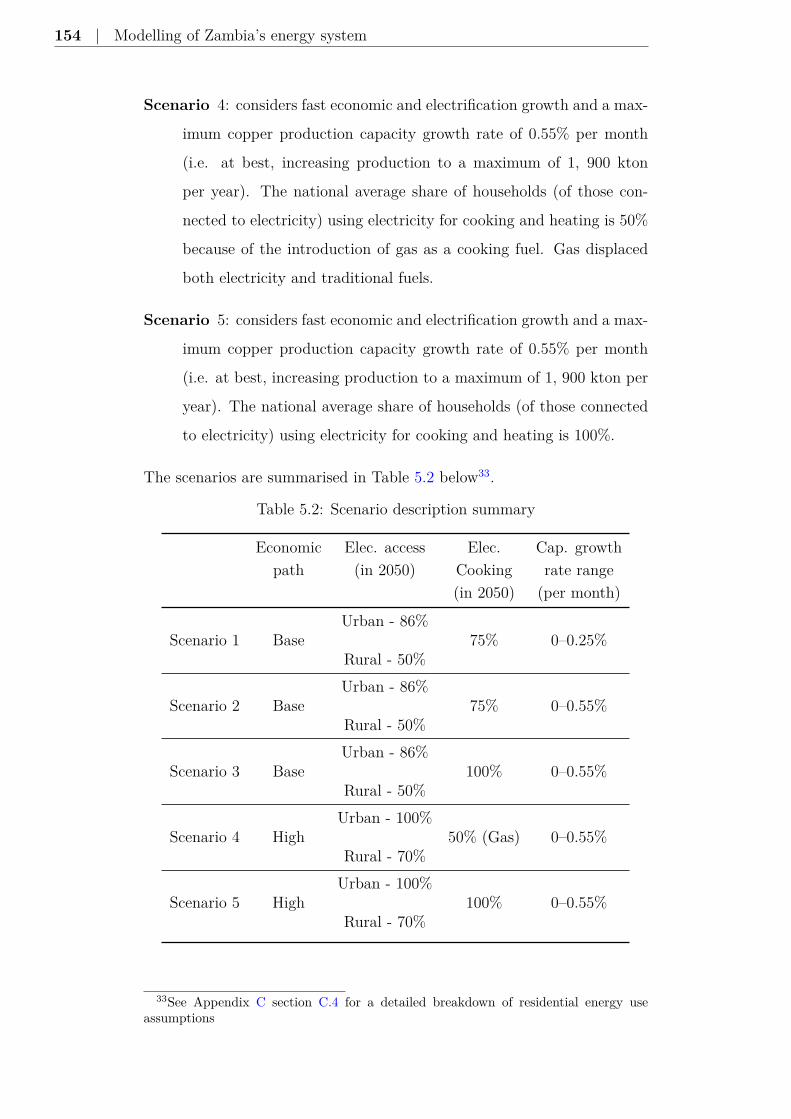
154 | Modelling of Zambia’s energy system
Scenario 4: considers fast economic and electrification growth and a max-
imum copper production capacity growth rate of 0.55% per month
(i.e. at best, increasing production to a maximum of 1, 900 kton
per year). The national average share of households (of those con-
nected to electricity) using electricity for cooking and heating is 50%
because of the introduction of gas as a cooking fuel. Gas displaced
both electricity and traditional fuels.
Scenario 5: considers fast economic and electrification growth and a max-
imum copper production capacity growth rate of 0.55% per month
(i.e. at best, increasing production to a maximum of 1, 900 kton per
year). The national average share of households (of those connected
to electricity) using electricity for cooking and heating is 100%.
The scenarios are summarised in Table 5.2 below33.
Table 5.2: Scenario description summary
Economic Elec. access Elec. Cap. growthpath (in 2050) Cooking rate range
(in 2050) (per month)
Urban - 86%Scenario 1 Base 75% 0–0.25%
Rural - 50%Urban - 86%
Scenario 2 Base 75% 0–0.55%Rural - 50%Urban - 86%
Scenario 3 Base 100% 0–0.55%Rural - 50%
Urban - 100%Scenario 4 High 50% (Gas) 0–0.55%
Rural - 70%Urban - 100%
Scenario 5 High 100% 0–0.55%Rural - 70%
33See Appendix C section C.4 for a detailed breakdown of residential energy useassumptions
5.4 Chapter summary | 155
5.4 Chapter summary
This chapter discussed the methods used and challenges of estimating fu-
ture energy demand. It then described the steps that were taken to model
Zambia’s energy demand. The demand model (LEAP model) focused on
the residential sector because the Zambian government has ambitious plans
of increasing access to clean energy and also because energy consumption
in this sector (use of traditional fuels) is directly linked to deforestation.
Demand in the residential sector was captured at end-use service level, this
enabled capture of different government policy targets (such as electrifica-
tion). Other sectors (transport, services etc) were modelled in a stylised
way because of limited data and statistics. The chapter also highlighted
the role that availability of fuel plays in energy transition, as CSO re-
ports showed that fuel transition was not only driven by affordability but
also by location (availability). A description of how investment decisions
of electricity generation technologies are made in the supply model was
given. The supply model focused on the resources and technologies that
were available to satisfy the demand and also on the costs that come with
satisfying this demand. Finally, the main scenarios used in this research
were described.

Chapter 6
Modelling of strategic
investment decisions
6.1 Introduction
This chapter addresses the second theme of the research, which focused
on understanding decision making in mining firms and also on the devel-
opment of a mining model. The purpose of this model was to simulate
different energy demand and copper production scenarios and analyse how
the copper industry would evolve over time. The model captures decision
rules and processes as described by the mining firms (see section 6.2) and
supplemented by literature (see Chapter 4).
The chapter has three aims: Firstly, to describe and present the steps
that were taken to identify the key decision variables and the decision pro-
cesses that mining firms in Zambia take when making strategic investment
decisions (section 6.2). Secondly, to define and describe the key interactions
within the mining model and also identify exogenous interactions that in-
fluence decision making (section 6.3). Thirdly, to describe the method that
is used to analyse the mining model, a system dynamics model (section
6.4). The chapter then concludes with a chapter summary (section 6.5).
158 | Modelling of strategic investment decisions
These three aims helped to answer the sub-research questions1 below:
• How do mining firms in Zambia make strategic investment decisions?
• What are the key decision variables in the mining sector in Zambia?
• What techniques are used by mining firms when evaluating strategic
investment options?
• What is the outlook for Zambia’s mining sector?
6.2 Identification of decision processes
This section describes the research design that was used to study decision
making in Zambia’s copper industry. As mentioned earlier (in Chapter
1), the research is divided into two themes: development of the energy
system and decision making in the mining sector. The research design
used to study the energy system is described in Chapter 5. The second
theme, which is the focus of this Chapter, focuses on understanding how
mining firms make decisions and simulate how these decisions would impact
the firm’s copper production. In order to capture the different aspects of
this complex process (i.e. the decision making process), a mixed method
approach was used.
This approach combines both qualitative and quantitative methods.
The qualitative method (in form of semi-structured interviews) was used
to capture the description of the decision processes in a mining firm, the
techniques used to evaluate their investment options and what the deci-
sion makers thought the key variables were in their organisation’s decision
making process. This was necessary because what literature says and what
happens on the ground could be variant. Secondly, it was important be-
cause decision making is context dependent and thus key decision variables
vary from one context to another. The information collected using the
semi-structured interviews2 and industry’s statistics3 formed part of the1Chapter 4 gives a description of how organisations make strategic decisions.2See section D.1 for the interview questions that were used.3See section 6.3.1 for the statistics that were collected.
6.2 Identification of decision processes | 159
basis of relationship definitions in the mining model; are given in sub-
section 6.2.1. Interviews were conducted in September to October of 2013
and again in August to October of 2014. In-country mining firms’ repre-
sentatives4, aligned government departments and agencies, and Zambia’s
mining industry experts were interviewed.
Apart from getting the description of the decision processes, the inter-
views with mining firms focused on understanding how they perceive their
energy use and production costs, the decision rules they use when evalu-
ating investment options, what they thought were key threats and drivers
to their operations, what they thought about government policies and reg-
ulations, how they thought their future costs structures would change and
finally how they would respond to presented scenarios (three scenarios were
presented to them)5. Interviews with representatives of government de-
partments and agencies focused on understanding what the government
thinks are key factors in mine operation’s profitability and how govern-
ment policies would help enable long-term planning and investment in the
local industry6. Finally, local industry experts interviews covered the issues
discussed with representatives of the mining firms and government. Know-
ing what the local experts think about the industry is important because
they are critical players in policy development in the country.
A summary of key findings of these interviews is given below in sub-
section 6.2.1. These interviews helped to parameterise decision rules and
also to capture key relationships and behaviours in the mining industry.
These findings together with the statistics (see the immediate paragraph
below) were then integrated into a system dynamics7 model (i.e. the mining
model)8. This model was used to analyse how decision rules could affect
the industry’s copper production and the profitability of the industry over
4See section B.2 for the list of mining companies operating in Zambia.5See Appendix D in section D.1.3 part 4 for the questions that were asked and section
D.4.5 for the summarised responses to the questions.6The government’s view on energy use and efficiency in the mining sector was also
discussed during the interviews.7The system dynamics model was built using Vensim (Ventana, 2015).8See section 4.3 of Chapter 4 for why an SD approach was used to study decision
making.
160 | Modelling of strategic investment decisions
time. Description of the SD model is given in section 6.3 below.
Further, during the course of the study, industry statistics (both lo-
cal and international) had been collected from various sources: the mining
companies, government departments and agencies, energy suppliers and
different international organisations. A description of key statistics is pre-
sented in section 6.3.1 below. Details of all statistics used in this chapter
are presented in Appendices B and D.
6.2.1 Key interview findings
This sub-section presents key findings of the interviews.9 The interviews
helped to frame how strategic investment decisions are made in the mining
model. The key aspects were: decision making process, project evaluation,
project financing and operational behaviour.
The decision making process informed the study on the motivation and
procedures used when making strategic decisions. This aspect highlighted
that while decision making process can be modelled in various ways (such
as rational, bounded rational, politics and power, and garbage can choice
paradigms), in the mining industry this process is a deliberate and directed
process. Mining firms have concrete procedures and guidelines of how in-
vestment options should be evaluated and steps that should be followed
when making strategic investments. Overall, ore grade, recoverable copper
from the ore, copper price and local policy environment (such as stability
of the policies and level of taxation) were identified as key factors (by the
firms) that determine whether an investment would be made or not.
It was found that main method of evaluating strategic investment de-
cisions was the Discounted Cash Flow (DCF) technique; while IRR and
pay-back analysis are optional. The importance of the DCF technique is
also confirmed in literature as an acceptable method of evaluating projects
in the industry. It was also found that all projects that mining firms in
Zambia invest in, have a return on investment (RoI) of at least 15%. How-
ever, not all investment options that meet this criterion are implemented9Summary findings of the interviews are given in section D.4 of Appendix D.
6.2 Identification of decision processes | 161
because the firm has to consider the country risks; such as political risks and
consistency in fiscal policies. Furthermore, apart from the analytic tech-
niques used to evaluate investment options, it was found that experience
(judgement) of key decision makers play a critical role in the investment
decision process. This, therefore, implies that final investment decisions in
mining firms are not optimal.
While local policy environment could greatly impact the profitability of
a project, it was found (from a financier’s perspective) funding of projects
is largely determined by the long term outlook of the industry, not short-
term policy inconsistencies. Financiers also consider three other additional
factors when approving funding and analysing risk of an investment op-
portunity in Zambia namely: 1. who their off-taker [the buyer of their
produce] is; 2. the role that the Zambian asset plays in the group (in
terms of value); and 3. the parent organisation of the firm. Thus, access-
ing finance for projects in Zambia’s industry is more determined by global
factors (basically the outlook of the copper price) and the organisation’s
structure than local policies because firm’s market is outside the country.
The other key finding was on the operational behavioural of the mining
firms. It was found that while the price of copper plays a key role in their
production and decision making, change in copper price does not always
lead to change in their production patterns. This is so because production
level of a firm is determined using thresholds set by the firm itself and not
relative to change in profitability. That is to say, even though profitability
of an operation could reduce because of the reduction in copper price, this
could not lead to change in production patterns because the price change
would be with the firm’s acceptable range. It was also found that firms
have options of suspending their operations in order to reduce the losses as
a result of lower copper price (relative to their unit cost of production). The
rules that govern the decision to suspend or re-start their operations are
determined by the firms themselves. For instance, firms do not suspend
the operations at first sight of losses and similarly, they do not re-start
their operations at first sight of high copper price (after suspending the
162 | Modelling of strategic investment decisions
operations). These behaviours were captured in the mining model.
6.3 Mining model
This section describes and defines the formal relationships and the dynam-
ics of the copper mining model. The model is used to study how investment
decisions change over time as key decision drivers (such as ore grade and
copper price) change.10 To comprehensively capture the dynamics of the
industry, the model has two modules: material and financial.
The material module focused on the material production process par-
ticularly on variables such as the quantity of ore resources available, type of
ore resources, ore grade, methods of mining and capacity of mining equip-
ment (Mudd et al., 2013; Norgate and Jahanshahi, 2010; Northey et al.,
2014). This module captured mining activities at ore production level (Nor-
gate and Haque, 2010; Norgate and Jahanshahi, 2010), instead of copper
cathode production level as was done in other studies (Saygin et al., 2011).
This is important because mining capacity investments are measured by
the quantity of ore the production line can handle and not by the copper
contained in the ore. In addition, by modelling at ore level, the impact of
reducing ore grade can be properly analysed.
The financial module focused on the investments and profitability of
the firm’s production capacity and operations (Auger and Ignacio Guzmán,
2010; Boulamanti and Moya, 2016). This module captured the production
costs and the impact they have on the decision making process via decision
rules. The production costs are categorised into two: operational costs
and capital costs. The operational costs cover all direct costs of producing
copper, these costs are short-term focused and include costs such as energy
and labour costs. On the other hand, capital costs have a long-term focus
and account for the costs that a mining firm incurs to keep producing
copper over a period of time, costs such as capital investment cost of mining
capacity.10See section D.6.1 in Appendix D for five extreme tests that were used to test the
behaviour of the mining model.
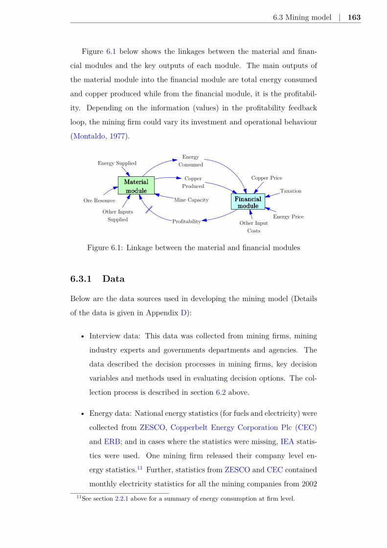
6.3 Mining model | 163
Figure 6.1 below shows the linkages between the material and finan-
cial modules and the key outputs of each module. The main outputs of
the material module into the financial module are total energy consumed
and copper produced while from the financial module, it is the profitabil-
ity. Depending on the information (values) in the profitability feedback
loop, the mining firm could vary its investment and operational behaviour
(Montaldo, 1977).
MaterialMaterialMaterialMaterialmodulemodulemodulemodule
FinancialFinancialFinancialFinancialmodulemodulemodulemodule
EnergyConsumed
CopperProduced
Other InputCosts
Energy Supplied
ProfitabilityEnergy Price
Copper Price
Other InputsSupplied
TaxationOre Resource Mine Capacity
Figure 6.1: Linkage between the material and financial modules
6.3.1 Data
Below are the data sources used in developing the mining model (Details
of the data is given in Appendix D):
• Interview data: This data was collected from mining firms, mining
industry experts and governments departments and agencies. The
data described the decision processes in mining firms, key decision
variables and methods used in evaluating decision options. The col-
lection process is described in section 6.2 above.
• Energy data: National energy statistics (for fuels and electricity) were
collected from ZESCO, Copperbelt Energy Corporation Plc (CEC)
and ERB; and in cases where the statistics were missing, IEA statis-
tics were used. One mining firm released their company level en-
ergy statistics.11 Further, statistics from ZESCO and CEC contained
monthly electricity statistics for all the mining companies from 200211See section 2.2.1 above for a summary of energy consumption at firm level.
164 | Modelling of strategic investment decisions
through to 2013. Statistics from ERB contain information on energy
prices (for both fuels and electricity).
• Resource data: This contained statistics of how much copper cath-
odes were produced in a particular year (or quarter), the average ore
grade and type of ore that was mined, the quantity and grade of
ore resources. This data was collated from mining companies annual
reports and SNL Metals and Mining (SNL) database.
• Technology cost data: Technology costs were obtained from technical
reports of mining projects evaluations (from SNL database). These
technical reports covered different projects in Zambia and also other
countries such as DR Congo and Chile. These reports also give an
indication of the RoI or IRR that is considered acceptable for project
development. Where specific data was not available in these reports,
journal articles data was used.
• Commodity price data: Commodity price data were collected from
The World Bank Group (World Bank) and SNL database.
• Copper production costs data: Companies annual reports were the
main sources of production costs statistics. However, because all
of these statistics (production costs from annual reports) were ag-
gregated, a KCM Valuation report (Rothschild, 2008) was used to
calibrate the costs of each process stage and end-use service. Journal
articles were also used in calibrating the cost of production at mining
grouping and industry levels.
6.3.2 General Assumptions
Being a stylised representation of a real system12, assumptions were made
in developing the mining model. These assumptions focused on aspects of
the mining model that directly impact the firm’s profitability (i.e. the focus
12See section 3.1 for a discussion of what models are and why they are used
6.3 Mining model | 165
of the model being decision making). Below are the main assumptions of
the model:
• Time: The model is a dynamic model, meaning decision environment
of time t1 would be different from that of time t2. An aggregate time
step of one month13 was used and with a time horizon up to 2050.
The model base year is 2010. This base year was used because of the
availability of reliable data.
• Model aggregation: The mining firms are aggregated into three, using
mining method: Copperbelt Underground, Copperbelt Open-pit and
North-Western Open-pit.14 This is because all mines (using same
mining methods) have similar ore characteristics and production cost
profiles.
• Model boundaries: The model covers copper production from mining
ore to production of cathodes: from cradle to gate. It does not model
the processing of associated mineral and products, but the credits of
these copper by-products (such as gold and cobalt) are only accounted
for in a stylised manner. In addition, Zambia’s industry is thought
of as a copper price taker (not a determinant of the price), largely
because it accounts for less than 8% of the global copper production.
Thus, the copper price is an exogenous input to the model.
• Capital investments: Two types of capital investments are consid-
ered: ore production capacity and energy efficient motors invest-
ments. These investments are mutually exclusive.
6.3.3 Framework of a mining firm
A group copper mining firm15, Mi, owns a mine with two types of ore: oxide
and sulphide. These ore types are hosted in one mine16, where mining of one
type leads to the mining of another. Further, the costs of processing each13The life cycle of copper processing from cradle to gate is between four to six weeks14The resource profile of each group category is given in section B.3 of Appendix B.15Based on model aggregation in section 6.3.2 above.16This is a simplification because some mines only have one ore type.
166 | Modelling of strategic investment decisions
ore type are different and the processes require different inputs. However,
because of the way the ore is hosted (in the rock), the firm’s profit, Πi,
depends on the profitability of each ore type. The profit varies every time
step, t, and in each time step the firm could make decisions (capital and/or
operational decisions) which have implication on current and future profits.
The capital investment decisions are long term and have technology lock-
in effects while the operational decision are short term and based on the
current copper price and production costs.
Under capital investment decisions, there are three investment options:
capacity replacement, new capacity (expansion) and efficient electric motor
investments. Capacity replacement options focus on sustaining the current
capacity stock. Say if the stock had a capacity of one million tonnes of ore
per year in time t0, this capacity option will ensure that it is maintained at
one million tonnes per year through to time tn. New capacity development
option includes the capacity replacement option plus additional capacity
development. An example of capacity expansion would be maintaining the
one million tonnes of ore per year plus additional 10% of the current stock
in the next n years. Under the capacity replacement option, as ore grade
reduces the production of copper cathodes also reduces. This is because
the quantity of copper in ore reduces. However, under the capacity expan-
sion option, the quantity of copper in ore can reduce, increase or remain
constant. The expansion option, therefore, means more capital cost and in-
creased investment risk. Finally, the efficient motor option, focuses on how
the firm can reduce its production costs (via energy costs) by increasing
the share of efficient electric motors. This can be done through replace-
ment of existing motors if the production capacity stock is maintained or
by investing directly in efficient motors if the production capacity stock is
expanded.
Under operational decisions, the firm decides whether to maintain or
reduce its ore production based on its production capacity stock. The de-
cision is dependent on the profitability of the mining activity. Similar to
capital investment decisions, this decision is driven by profitability. How-
6.3 Mining model | 167
ever, the length of time, tT , used to calculate profitability is much shorter.
This length, tT , is dependent on the loss tolerance of the firm (see Equations
6.7 - 6.9 below.).
Further, capital and operational decisions impact each other. For in-
stance, when a firm makes a decision to scale down its ore production in
time t, that firm cannot make a decision to replace or increase its ore pro-
duction17 in that time step (t). However, because of the project lead time,
tL, in developing capacity projects (see Equations 6.26 - 6.41), the firm’s
capacity could increase in time t. This is because of a technology lock-in
mechanism. Another example of the interactions between capital and op-
erational decisions is postponing of a scaling down decision because energy
efficient technologies have come online, thus increasing the profitability
(via reducing energy costs) even when there is no significant change in the
market conditions.
The interactions between these decisions (capital and operational de-
cisions) therefore influence how much ore is produced in each time step
t. A firm’s generic ore production function, qt, is defined below (detailed
description of the function is given in the sections 6.3.4 and 6.3.5 below)
qt = F (Yt, Kt, Qt) (6.1)
Yt = F (Yt−tL, IYt−tL
, RYt−tL) (6.2)
Kt = F (Πt−1, ηt−1, tT ) (6.3)
where,
qt is the quantity of ore (in tonnes) produced in time t,
F is a function defining the relationship between variables,
t0, t and tL are initial time, current time step and project lead time
respectively,
Yt is the availability ore production capacity (in tonnes) in time t,17Which will come online in time t + tL.
168 | Modelling of strategic investment decisions
Yt−tlis the availability ore production capacity (in tonnes) in time t−tL,
IYt−tLis size of ore production capacity (in tonnes) that the firm in-
vested into in time t− tL,
RYt−tLis the size of ore production capacity (in tonnes) that is retired
between time t− tL and t,
Kt is the profitability function,
Πt−1 is the firm’s profit in time t− 1,
ηt−1 is the average energy efficiency of the firm’s energy system,
tT is the firm’s loss tolerance time, and
Qt is the available ore resources (in tonnes) in time t.
6.3.4 Material module
This module describes the processes that copper processing goes through
from ore (mining) to cathode (refining).
Ore resources function: The size (measured in tonnes of ore (tonOre))
of the available ore resources ( Qt) at any time t is determined by the initial
resources ( Qt0) minus the sum of all produced ore (Brennan and Schwartz,
1985; William et al., 2012). Defined below as
Qt = (Qt0 ± ϵQ) −t−1∑i=t0
qi (6.4)
with, the physical constraint of Qt ∈ (0, Qt0), Qt0 being the initial ore
resources (has a margin of error ϵQ) and qi being the rate of ore production
(extraction) at time ti.
Ore extraction function: The quantity of ore produced (qt) in time
t is a function of installed capacity, profitability and available ore. The
function is defined below
qt = min (Ymax,t, YP,t, Qt, YV,t) (6.5)
where,
The physical constraint is qt ∈ (0, qmax),
6.3 Mining model | 169
Ymax,t is the installed ore capacity of a firm (measured in tonOre). This
represents the maximum quantity of ore that a firm can extract at any time
t,
YP,t is the maximum quantity of ore (in tonOre) that a firm is willing
to extract (produce). This is defined in Equations 6.6 - 6.9 below,
Qt is the available ore resources (in tonOre) at any time t (defined in
Equation 6.4 above), and
YV,t is the available inventory space (in tonOre) at any time t. This is
defined in Equations 6.10 - 6.15 below.
Profitability function: The firm directly determines the size of the
installed capacity through its capital investment decisions (to replace or
expand). On the other hand, the maximum quantity of ore a firm is willing
to produce ( YP ) is determined by the financial position of the firm at any
time t. This represents the endogenous short-term operational decisions
that a firm could make to reduce its losses during fluctuations in the market
prices. The YP function is defined below
YP,t = Ymax,t ×Kt (6.6)
Kt =
1 if kPt ≤ aT
(1−kPt)1−aT
otherwise(6.7)
kPt =t−1∑
i=t−tT −1
P Ci
RViif RV > 0
kPrefiotherwise
(6.8)
kPref = PCref
RVref
(6.9)
where,
Ymax,t is the installed ore capacity (in tonOre) of a firm at any time t,
Kt is the profitability function,
1 represents normal production patterns,
aT is the firm’s tolerance threshold, that indicates change in the firm’s
170 | Modelling of strategic investment decisions
production patterns due to its financial position,
tT is the firm’s loss tolerance time,
RV is the gross revenue (in US$) realised from the sales of copper and
related by-products (see Equation 6.23 below),
PC is the total costs (in US$) that are incurred in producing copper
and related by-products (see Equation 6.24 below),
RVref is the gross revenue (in US$) that would be realised from the
sales of copper and related by-products, and
PCref is the total costs (in US$) that would be incurred in producing
copper and related by-products.
Inventory function: The size of inventory space (in tonnes of ore)
varies between firms and it is a critical link between ore production capacity
( Ymax) and down-stream capacities such as smelter ( Ysmelt) and refinery (
Yref ). This link is important because it describes how materials flow from
one stage to the next. It is necessary to describe the material flow in details
because of the feedback loop in the flow (between stages) and also to enable
analysis of how different export policies could affect the production of ore.
The size of the inventory space is determined by the firm’s trading
strategy18. However, in this research, it was assumed that all firms’ inven-
tory space is determined by a constant inventory factor ( ξ). The firm’s
inventory space ( YV ) is described below
YV,t = V st,hydro
OGt,hydro
+ V st,pyro
(OGt,pyro × CG) (6.10)
qCt,hydro = qt × υ ×OGt,hydro (6.11)
V st,hydro = min (qCt,hydro, Yt,hydro,cath) × (1 + ξ) (6.12)
qCt,pyro = qt × (1 − υ) ×OGt,pyro (6.13)18For instance, does the firm stockpile when the price is depressed and for how long
does it stockpile?
6.3 Mining model | 171
qCt,smelt = qCt,pyro − qCt,export (6.14)
V st,pyro = min(qCt,smelt
CG, Yt,smelt
)× (1 + ξ) (6.15)
qCt = qCt,hydro + qCt,pyro (6.16)
where,
OG is the ore grade (measured as tonnes of contained copper (ton-
ContCu)/tonOre19) in time t (it can either be ore processed using hydro-
metallurgy or pyro-metallurgy),
CG is the constant concentrate grade (measured as tonContCu/tonnes
of copper concentrate (tonConc)),
qt is the quantity of ore produced (in tonOre) in time t,
υ is the share ore that follows the hydro-metallurgy route,
qChydro is the quantity of contained copper that is processed using
hydro-metallurgy (in tonContCu),
qCpyro is the quantity of contained copper that is processed using pyro-
metallurgy (in tonContCu),
qCsmelt is the quantity of contained copper sent to the smelter (in ton-
ContCu),
qCexport is the quantity of contained copper exported (in tonContCu),
V shydro is measured in tonContCu,
Yref,hydro is the installed refinery capacity of electro-winning facility,
measured in tonnes of copper cathodes (tonCath),
Ysmelt is the installed smelter capacity,
V spyro and Ysmelt are measured in tonConc,
ξ is the inventory factor, and
qCt is the total contained copper mined.20
19tonOre is an abbreviation of tonnes of ore.20If there are no process losses (as assumed in this case), then it is the same quantity
as copper cathode produced (measured in tonCath).
172 | Modelling of strategic investment decisions
Ore grade function: This is an endogenous function that depends
on the ore production activities (i.e. the ore grade only changes when
ore has been produced). The ore reduction model used in this research
assumed that firms tend to extract higher ore grade first then move to the
lower grade ore. An alternative ore reduction model which responds to
copper price is presented in Krautkraemer (1988; 1989) and Farrow and
Krautkraemer (1989).
Below is the definition of the ore reduction model used in this research
OGt0 =(OGavg ± ϵOGavg
)× γ (6.17)
OGt0 > OGavg (6.18)
OGt =
OGt0 if t = t0
AqCt
Qt± ϵOGt otherwise
(6.19)
AqCt =(Qt0 ×
[OGavg ± ϵOGavg
])− TqCt (6.20)
TqCt =t−1∑i=t0
(qi ×OGi) (6.21)
where,
OGt0 is the initial ore grade of the ore resources at time t0,
OGavg is the estimated average ore grade of the ore resources ( Qt0),
ϵOGavg is the average ore grade estimation error, and
γ is the estimation factor for the initial ore grade (relative to the average
ore grade (γ > 1 )),
AqCt is the available contained copper (in tonContCu) in the ore re-
sources ( Qt),
ϵOGt represents the uncertainty in the ore grade distribution in the ore,
Qt0 is the available ore resources (in tonOre) at time t0, and
TqCt is the total mined contained copper from time t0 to t.
6.3 Mining model | 173
6.3.5 Financial module
This module defines the costs and revenue streams of a firm and it also
describes how the firm makes investment decisions.21
Profit function: This is a cash-flow function of a firm in time t, and
it is driven by copper price, the quantity of cathode copper produced22 and
the production costs. Production costs consist of labour, cost of capital,
repair and maintenance, energy, inventory, consumables, mineral royalty
tax (MRT) and other on-site costs (as identified in section 3.3.3 above). In
this research, the costs of suspending and re-starting operations were not
accounted for. Nonetheless, during the period of suspended operations, the
firm continues to service the loans of capital (cost of capital). The profit
function (Π) is defined below
Πt = RVt − PCt (6.22)
RVt = qCt × Pt,Cu (6.23)
PCt =∑
i=ore
[UCi]t × [qt] +MRTt × qCt − CCt (6.24)
UP Ct = PCt
qCt
(6.25)
where,
Πt is the firms profit in time t,
RVt is the gross revenue (US$) of a firm at time t,
PCt is the total production costs (US$) of a firm at time t,
qCt is the total produced cathodes at time t (see Equation 6.16 above),
Pt,Cu is the copper price (in US$ per tonCath) at time t,
[UCi]t is a set containing unit costs (measure in US$/tonnes23) of labour,21See sections D.4 and D.5 below for indicative financial thresholds used by Zambian
mining firms when making investment decisions.22If a firm exports its produce, then the revenue is calculated based on the contained
copper in the exported quantity.23This tonnage could be measured intonOre, tonContCu, tonConc and tonCath de-
174 | Modelling of strategic investment decisions
energy, Repair and Maintenance (R&M), consumables etc,
[qt] is set containing quantities (in tonnes) of ore, concentrates and
copper cathodes,
MRTt is mineral royalty tax (in US$ per tonCath)24 at time t. This
is determined by the host government and it changes frequently due to
market (copper price changes) and lobbying reasons,
CCt is the cost of capital (US$) that a firm is servicing at time t, and
UP Ct is the unit production cost (US$ per tonCath) at time t.
Capital investment modelling: Having defined how operational de-
cisions are made (see Equations 6.6 - 6.9 above), this part focuses on mod-
elling how investment decisions (production capacity and electric motor
stock) in a firm are made. It considers investment options of replacing
retired ore production stock, expanding the available ore production stock
and investing in efficient motors. It does not consider retrofitting option
because of lack of cost information for retrofitting options. However, the
investment process for retrofitting and the new stock is not different except
that retrofit options tend to be cheaper in the short term while new stock
options tend to be cheaper in the long term.
The replacing option is defined first then the expansion option and fi-
nally the efficient motors decision process. The first two options focus on
ore production capacity investment options, which are driven by the value
of the available mineral resources, the copper price (usually an average of
three or five year period25) and the obtaining operational status of the firm
(determined by the profitability function). Further, it is based on these
ore production capacity (upstream) investment decisions that investment
decisions for downstream (smelter and refinery) production facilities de-
cisions are made. Investment decision in motors (generally) is based on
the installed ore production capacity, as electric motors are supporting
equipment. Further, investment in efficient motors is driven by the energy
pending on the variable being considered.24This is set as a share of copper price, such as a rate of 6%.25This period is approximately the half life factor of the copper price, see Table E.4.
6.3 Mining model | 175
efficiency gap and the energy price.
All capital stock investments (ore production and electric motors) de-
cisions are determined by specified investment thresholds driven by the
financial position of the firm and the equipment economics. These thresh-
olds vary between firms. The use of thresholds (not optimal way of making
decisions) in decision making is common place in firms as was found in
industry technical reports and literature (see Chapter 4) and also during
industry interviews26. This approach was used because the firms that were
interviewed stated that a positive Net Present Value (NPV) in itself does
not mean a positive investment decision. This is contrary to how decisions
are modelled in single objective function models, particularly in optimisa-
tion models.
Further, whereas in optimisation models the decision maker seeks to find
an optimal solution, the results from the interviews and also from literature
review show that decision makers in mining firms seek for solutions that are
sufficient (which could even be sub-optimal). See Chapter 4 for details of
how organisations make strategic investment decisions and also sections 6.2
(above) and D.4 (in Appendix D) for the findings of the industry interviews.
Ore production capacity investments: Ore production capital
stock investment decision making are defined in Equations 6.26 to 6.41.
Capacity replacement and expansion decisions are expressed as IYt−tL,Rep
and IYt−tL,Exp respectively. The only difference between the replacement
and expansion options is the way the size of the proposed project is calcu-
lated. If the value of ETt = 0, all decisions under this condition are replace-
ment decisions while ET > 0 condition leads to expansion decisions. In
this case, ET is the maximum desired percent increase of copper cathode
production based on the current production as described in Equation 6.35.
26Firms operating in Zambia were interviewed on how they make decisions.
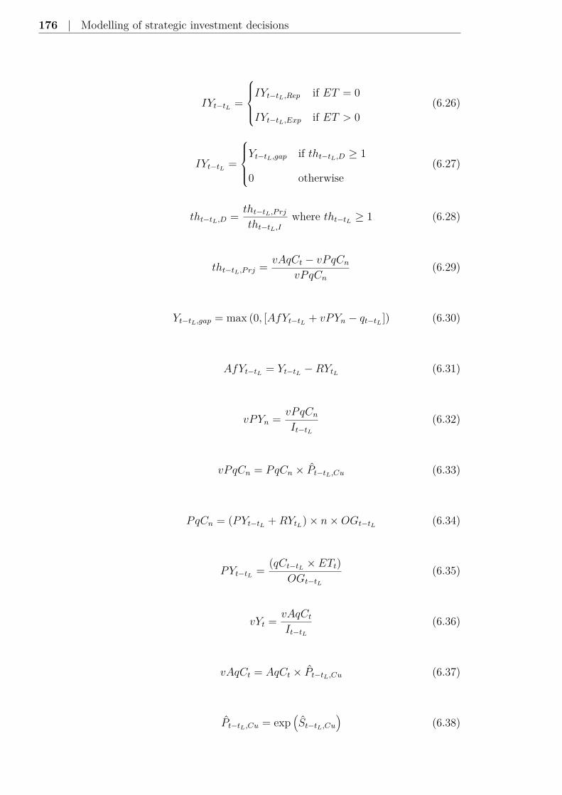
176 | Modelling of strategic investment decisions
IYt−tL=
IYt−tL,Rep if ET = 0
IYt−tL,Exp if ET > 0(6.26)
IYt−tL=
Yt−tL,gap if tht−tL,D ≥ 1
0 otherwise(6.27)
tht−tL,D = tht−tL,P rj
tht−tL,I
where tht−tL≥ 1 (6.28)
tht−tL,P rj = vAqCt − vPqCn
vPqCn
(6.29)
Yt−tL,gap = max (0, [AfYt−tL+ vPYn − qt−tL
]) (6.30)
AfYt−tL= Yt−tL
−RYtL(6.31)
vPYn = vPqCn
It−tL
(6.32)
vPqCn = PqCn × Pt−tL,Cu (6.33)
PqCn = (PYt−tL+RYtL
) × n×OGt−tL(6.34)
PYt−tL= (qCt−tL
× ETt)OGt−tL
(6.35)
vYt = vAqCt
It−tL
(6.36)
vAqCt = AqCt × Pt−tL,Cu (6.37)
Pt−tL,Cu = exp(St−tL,Cu
)(6.38)

6.3 Mining model | 177
AqCt = AqCt−tL−DqCtL
(6.39)
AqCt−tL= Qt−tL
×OGt−tL(6.40)
DqCtL= qt−tL × tL ×OGt−tL
(6.41)
where,
t and tL are current time and project lead time respectively,
n is the life span of the stock,
IYt−tLis the total ore production capacity (in tonOre) that will be
developed,
ETt is the desired percent increase of copper cathode production based
on the current production at time t. If ET = 0, this investment option
take a form of the capacity replacement option,
Yt−tL,gap is the available investment capacity gap (in tonnes),
tht−tL,P rj is the estimated investment threshold of a project,
tht−tL,I is the investment threshold set by the firm (this could also vary
between time steps),
vAqCt is the total value of contained copper (in tonContCu) at time t,
Yt−tLis the installed ore production capacity (in tonOre) at time t− tL,
RYtLis the ore production capacity (in tonOre) that will be retired
between time t − tL and t. This is calculated endogenously based on the
age profile of the stock,
AYt−tLis the ore production capacity (in tonOre) that will be available
after some capacity has been retired,
vIYt−tLis the capacity in tonnes of ore (tonOre) that can be invested
in using the value of copper after the project lead time ( tL),
qt−tLis the total maximum possible ore production rate (in tonOre) in
time t− tL,
vYt−tLis the ore production capacity (in tonOre) that can be invested
in using the value of copper after the lead time ( tL),
178 | Modelling of strategic investment decisions
It−tLis the total capital investment cost (US$) of the capacity at time
t− tL,
AqCt and AqCt−tLare the available contained copper (in tonContCu)
in the ore resources (Qt and Qt−tL) at time t and t− tL respectively,
Pt−tL,Cu is the moving average copper price using the half life of price
shock (see section 3.3.5 for how this is calculated),
DqCtLis the estimated contained copper (in tonContCu) that could be
produced during the project lead time tL, and
OG is the ore grade (as a percentage (%)).
From Equations 6.37, 6.40 and 6.41 it can be seen that the value of
the investments options vary between time steps and that it is significantly
influenced by the historical movements in the copper price ( Pt,Cu), ore
grade ( OGt), available ore resources ( Qt) and the profitability ( Kt) and
inventory ( YV,t) feedback loops.
Electric motor investments: Similar to the ore capacity investment
decisions, investment decisions for energy efficient motors are influenced
by investment thresholds. There are two thresholds used for motor in-
vestments: profit and project thresholds. The profit threshold determines
whether or not a firm would invest if its operation’s profit margin is at a cer-
tain level. As Prain (1975) observed if a mining firm achieves its set profit
margin objective, it seldom invests in efficient technologies to maximise its
profits. The project threshold focuses on the economics of efficient motors.
It is based on the energy efficiency gap available in the electric motor sys-
tem of the firm and the electricity price. The energy efficiency gap is the
difference between energy demand by the average motor system efficiency
of the firm and the efficiency of efficient motors (as defined in Equation
6.52 below). The monetary value of this gap is calculated by multiplying it
by the price of electricity ( Pt,elec). A decision maker could decide to invest
either in standard or efficient motors. At all times, the firm will have a
specified number of motors depending on the ore production capacity (The
motor-ore capacity ratio is assumed to remain constant). Further, because
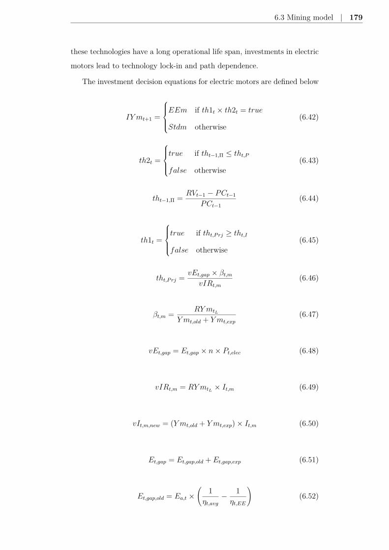
6.3 Mining model | 179
these technologies have a long operational life span, investments in electric
motors lead to technology lock-in and path dependence.
The investment decision equations for electric motors are defined below
IY mt+1 =
EEm if th1t × th2t = true
Stdm otherwise(6.42)
th2t =
true if tht−1,Π ≤ tht,P
false otherwise(6.43)
tht−1,Π = RVt−1 − PCt−1
PCt−1(6.44)
th1t =
true if tht,P rj ≥ tht,I
false otherwise(6.45)
tht,P rj = vEt,gap × βt,m
vIRt,m
(6.46)
βt,m = RYmtL
Y mt,old + Y mt,exp
(6.47)
vEt,gap = Et,gap × n× Pt,elec (6.48)
vIRt,m = RYmtL× It,m (6.49)
vIt,m,new = (Y mt,old + Y mt,exp) × It,m (6.50)
Et,gap = Et,gap,old + Et,gap,exp (6.51)
Et,gap,old = Ea,t ×(
1ηt,avg
− 1ηt,EE
)(6.52)
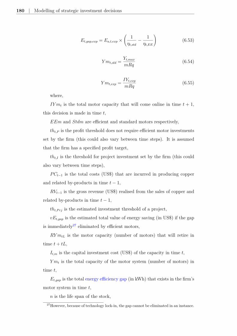
180 | Modelling of strategic investment decisions
Et,gap,exp = Ea,t,exp ×(
1ηt,std
− 1ηt,EE
)(6.53)
Y mt,old = Yt,max
mRq(6.54)
Y mt,exp = IYt,exp
mRq(6.55)
where,
IY mt is the total motor capacity that will come online in time t + 1,
this decision is made in time t,
EEm and Stdm are efficient and standard motors respectively,
tht,P is the profit threshold does not require efficient motor investments
set by the firm (this could also vary between time steps). It is assumed
that the firm has a specified profit target,
tht,I is the threshold for project investment set by the firm (this could
also vary between time steps),
PCt−1 is the total costs (US$) that are incurred in producing copper
and related by-products in time t− 1,
RVt−1 is the gross revenue (US$) realised from the sales of copper and
related by-products in time t− 1,
tht,P rj is the estimated investment threshold of a project,
vEt,gap is the estimated total value of energy saving (in US$) if the gap
is immediately27 eliminated by efficient motors,
RYmtL is the motor capacity (number of motors) that will retire in
time t+ tL,
It,m is the capital investment cost (US$) of the capacity in time t,
Y mt is the total capacity of the motor system (number of motors) in
time t,
Et,gap is the total energy efficiency gap (in kWh) that exists in the firm’s
motor system in time t,
n is the life span of the stock,27However, because of technology lock-in, the gap cannot be eliminated in an instance.
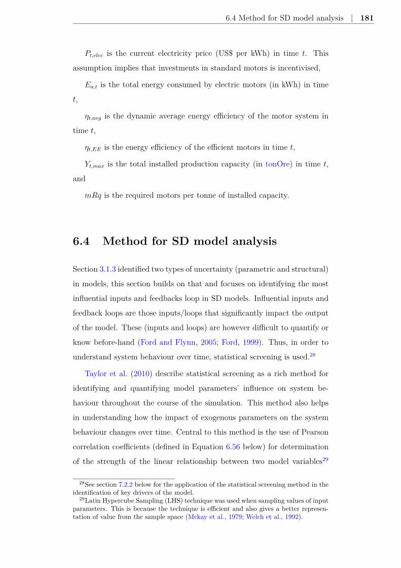
6.4 Method for SD model analysis | 181
Pt,elec is the current electricity price (US$ per kWh) in time t. This
assumption implies that investments in standard motors is incentivised,
Ea,t is the total energy consumed by electric motors (in kWh) in time
t,
ηt,avg is the dynamic average energy efficiency of the motor system in
time t,
ηt,EE is the energy efficiency of the efficient motors in time t,
Yt,max is the total installed production capacity (in tonOre) in time t,
and
mRq is the required motors per tonne of installed capacity.
6.4 Method for SD model analysis
Section 3.1.3 identified two types of uncertainty (parametric and structural)
in models, this section builds on that and focuses on identifying the most
influential inputs and feedbacks loop in SD models. Influential inputs and
feedback loops are those inputs/loops that significantly impact the output
of the model. These (inputs and loops) are however difficult to quantify or
know before-hand (Ford and Flynn, 2005; Ford, 1999). Thus, in order to
understand system behaviour over time, statistical screening is used.28
Taylor et al. (2010) describe statistical screening as a rich method for
identifying and quantifying model parameters’ influence on system be-
haviour throughout the course of the simulation. This method also helps
in understanding how the impact of exogenous parameters on the system
behaviour changes over time. Central to this method is the use of Pearson
correlation coefficients (defined in Equation 6.56 below) for determination
of the strength of the linear relationship between two model variables29
28See section 7.2.2 below for the application of the statistical screening method in theidentification of key drivers of the model.
29Latin Hypercube Sampling (LHS) technique was used when sampling values of inputparameters. This is because the technique is efficient and also gives a better represen-tation of value from the sample space (Mckay et al., 1979; Welch et al., 1992).
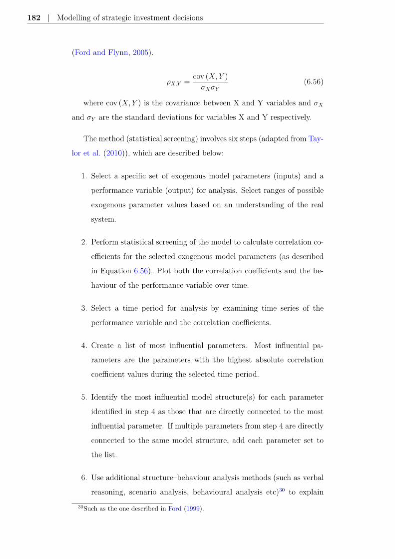
182 | Modelling of strategic investment decisions
(Ford and Flynn, 2005).
ρX,Y = cov (X, Y )σXσY
(6.56)
where cov (X, Y ) is the covariance between X and Y variables and σX
and σY are the standard deviations for variables X and Y respectively.
The method (statistical screening) involves six steps (adapted from Tay-
lor et al. (2010)), which are described below:
1. Select a specific set of exogenous model parameters (inputs) and a
performance variable (output) for analysis. Select ranges of possible
exogenous parameter values based on an understanding of the real
system.
2. Perform statistical screening of the model to calculate correlation co-
efficients for the selected exogenous model parameters (as described
in Equation 6.56). Plot both the correlation coefficients and the be-
haviour of the performance variable over time.
3. Select a time period for analysis by examining time series of the
performance variable and the correlation coefficients.
4. Create a list of most influential parameters. Most influential pa-
rameters are the parameters with the highest absolute correlation
coefficient values during the selected time period.
5. Identify the most influential model structure(s) for each parameter
identified in step 4 as those that are directly connected to the most
influential parameter. If multiple parameters from step 4 are directly
connected to the same model structure, add each parameter set to
the list.
6. Use additional structure–behaviour analysis methods (such as verbal
reasoning, scenario analysis, behavioural analysis etc)30 to explain30Such as the one described in Ford (1999).
6.5 Chapter summary | 183
how each parameter or set of parameters and the structures they
influence drive the behaviour of the system.
6.5 Chapter summary
In this chapter, processes used to study how strategic investment deci-
sions are made in Zambia’s mining sector were described. Key decision
variables and rules were identified and defined. The chapter also identi-
fied endogenous (such as how ore production leads to the reduction of ore
grade) and exogenous (such as how fluctuations in copper markets impact
the firm’s profitability) interactions that could impact decision making in
mining firms were defined. Identification of key decision variables, rules and
interactions was necessary in order to explore how Zambia’s mining sector
would grow. The chapter then discussed and described the method used
to analyse the mining model that was developed as part of this research.

Chapter 7
Results and discussion
This chapter presents and discusses the main findings of this research. It
has four sections: section 7.1 presents and discusses the results of the energy
models (LEAP (Heaps, 2016) and OSeMOSYS (Howells et al., 2011) models
for demand and supply modelling respectively) described in Chapter 5 while
section 7.2 presents and discusses the results of the mining model (described
in Chapter 6), a model which was built on a Vensim platform (Ventana,
2015). Section 7.3 gives a discussion summary of the findings. Finally,
section 7.4 gives a summary of the results and highlights the main findings.
The results output of both the energy and mining models were analysed
using R Core Team (2017).
7.1 Energy system results
This section addresses the first research question: How would Zambia’s en-
ergy sector evolve by 2050? and its related sub-questions given in Chapter
5. This question focuses on understanding how changes in energy demand
would impact investments in supply technology stock and the electricity
price (via the average generation cost). Demand and supply scenarios are
described in section 5.3. A range of sensitivity tests were applied to the
supply model to check for factors that have the most impact. Results for
186 | Results and discussion
sensitivity tests are given in section 7.1.3 below.
7.1.1 Energy demand
Having argued the importance of correctly modelling energy demand in
section 3.2.5 (Chapter 3) and the impact that fuel switching would have on
the development of the energy system in section 5.1.1 (Chapter 5), this sub-
section presents and discusses the results of the demand model described
in Chapter 5. Three key dimensions of energy demand are presented: total
energy demand, total electricity demand and total forest cover which would
be lost1 due to use of wood and charcoal for each demand scenario. In-
depth results of the residential sector are then given. Residential sector
results focus on the impact that increasing access to clean energy and fuel
switching would have on the sector’s electricity demand.
Figure 7.1 shows the total final energy demand (all sectors) for each
scenario. Energy demand is projected to grow from 162 PJ2 in 2010 to be-
tween 370 and 466 PJ in 2050, depending on the scenario considered3. The
variance in total energy demand by 2050 is a result of the use of different
economic growth rates, energy access rates and fuel transition assumptions.
For instance, the rate of economic growth has a direct bearing on the total1Forest re-growth through regeneration was considered, reforestation was not.2The 162 PJ figure is estimated based on the calibrated model (using data from IEA
(2012), ZESCO (2013) and CSO (1994; 1996; 2003; 2005; 2012)), however, IEA (2012)estimates it to have been 230 PJ in 2010. The main difference between the calibratedvalue and the IEA value was in the wood and charcoal values.
3Demand scenarios:Scenario 1: considers a slow economic and electrification growth, with low mining
output. The national average share of households (of those connected to electricity)using electricity for cooking and heating is 75%.
Scenario 2: considers slow economic and electrification growth, with high miningoutput. The national average share of households (of those connected to electricity)using electricity for cooking and heating is 75%.
Scenario 3: considers slow economic growth but with fast electrification growth andhigh mining output. The national average share of households (of those connected toelectricity) using electricity for cooking and heating is 75%.
Scenario 4: considers fast economic and electrification growth and high mining out-put. The national average share of households (of those connected to electricity) usingelectricity for cooking and heating is 50% because of the introduction of gas as a cookingfuel. Gas displaced both electricity and traditional fuels.
Scenario 5: considers fast economic and electrification growth and high mining out-put. The national average share of households (of those connected to electricity) usingelectricity for cooking and heating is 100%.
– see section 5.3 of Chapter 5 for details.
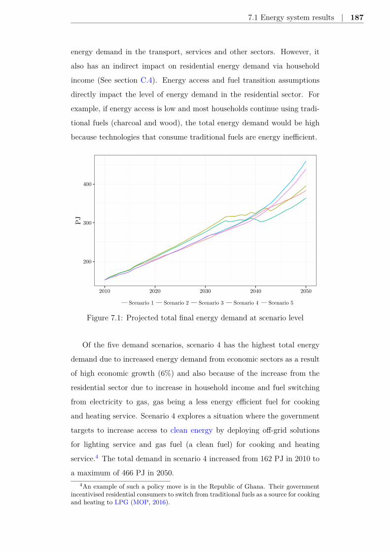
7.1 Energy system results | 187
energy demand in the transport, services and other sectors. However, it
also has an indirect impact on residential energy demand via household
income (See section C.4). Energy access and fuel transition assumptions
directly impact the level of energy demand in the residential sector. For
example, if energy access is low and most households continue using tradi-
tional fuels (charcoal and wood), the total energy demand would be high
because technologies that consume traditional fuels are energy inefficient.
200
300
400
2010 2020 2030 2040 2050
PJ
Scenario 1 Scenario 2 Scenario 3 Scenario 4 Scenario 5
Figure 7.1: Projected total final energy demand at scenario level
Of the five demand scenarios, scenario 4 has the highest total energy
demand due to increased energy demand from economic sectors as a result
of high economic growth (6%) and also because of the increase from the
residential sector due to increase in household income and fuel switching
from electricity to gas, gas being a less energy efficient fuel for cooking
and heating service. Scenario 4 explores a situation where the government
targets to increase access to clean energy by deploying off-grid solutions
for lighting service and gas fuel (a clean fuel) for cooking and heating
service.4 The total demand in scenario 4 increased from 162 PJ in 2010 to
a maximum of 466 PJ in 2050.4An example of such a policy move is in the Republic of Ghana. Their government
incentivised residential consumers to switch from traditional fuels as a source for cookingand heating to LPG (MOP, 2016).
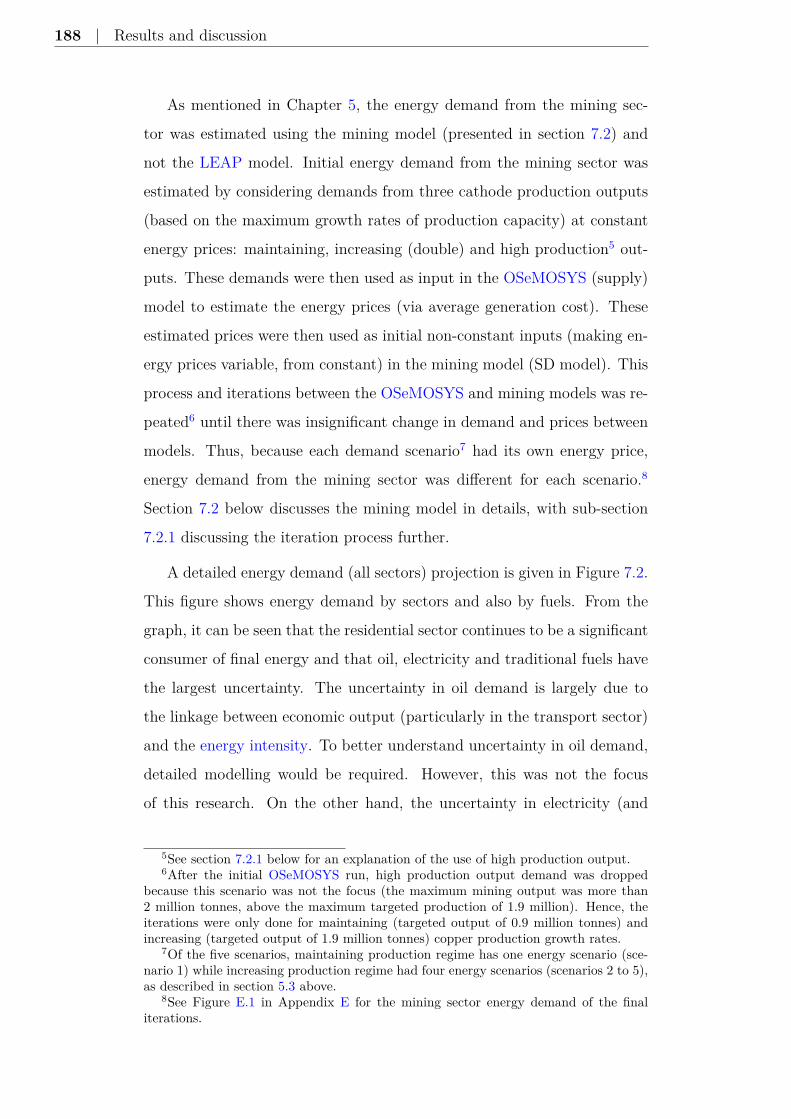
188 | Results and discussion
As mentioned in Chapter 5, the energy demand from the mining sec-
tor was estimated using the mining model (presented in section 7.2) and
not the LEAP model. Initial energy demand from the mining sector was
estimated by considering demands from three cathode production outputs
(based on the maximum growth rates of production capacity) at constant
energy prices: maintaining, increasing (double) and high production5 out-
puts. These demands were then used as input in the OSeMOSYS (supply)
model to estimate the energy prices (via average generation cost). These
estimated prices were then used as initial non-constant inputs (making en-
ergy prices variable, from constant) in the mining model (SD model). This
process and iterations between the OSeMOSYS and mining models was re-
peated6 until there was insignificant change in demand and prices between
models. Thus, because each demand scenario7 had its own energy price,
energy demand from the mining sector was different for each scenario.8
Section 7.2 below discusses the mining model in details, with sub-section
7.2.1 discussing the iteration process further.
A detailed energy demand (all sectors) projection is given in Figure 7.2.
This figure shows energy demand by sectors and also by fuels. From the
graph, it can be seen that the residential sector continues to be a significant
consumer of final energy and that oil, electricity and traditional fuels have
the largest uncertainty. The uncertainty in oil demand is largely due to
the linkage between economic output (particularly in the transport sector)
and the energy intensity. To better understand uncertainty in oil demand,
detailed modelling would be required. However, this was not the focus
of this research. On the other hand, the uncertainty in electricity (and
5See section 7.2.1 below for an explanation of the use of high production output.6After the initial OSeMOSYS run, high production output demand was dropped
because this scenario was not the focus (the maximum mining output was more than2 million tonnes, above the maximum targeted production of 1.9 million). Hence, theiterations were only done for maintaining (targeted output of 0.9 million tonnes) andincreasing (targeted output of 1.9 million tonnes) copper production growth rates.
7Of the five scenarios, maintaining production regime has one energy scenario (sce-nario 1) while increasing production regime had four energy scenarios (scenarios 2 to 5),as described in section 5.3 above.
8See Figure E.1 in Appendix E for the mining sector energy demand of the finaliterations.
7.1 Energy system results | 189
consequently, traditional fuels) demand9 (which was one of the foci of the
research) is a result of various compounding factors such as population
growth, increased energy access and copper production, among others.
As discussed in section 5.1.1, the projections of transport, services and
other sectors are solely determined by the assumed sectoral growth rate.
Thus, energy projections from these three sectors can be explained relative
to the economic growth rate assumption, that is, there are no other interac-
tions that drive energy demand within the model. However, energy demand
in mining and residential sectors is driven by a multiple of factors. In the
residential sector, these factors are population growth, household income,
fuel switching and energy access10; while in the mining sector factors such
as reduction in ore grade, mining method and ore type influence demand.
Detailed results for these two sectors are given and discussed below.
9See Figure E.3 in Appendix for the projected electricity, charcoal and wood demandfor each scenario.
10See section C.4 and Appendix C for the assumptions.
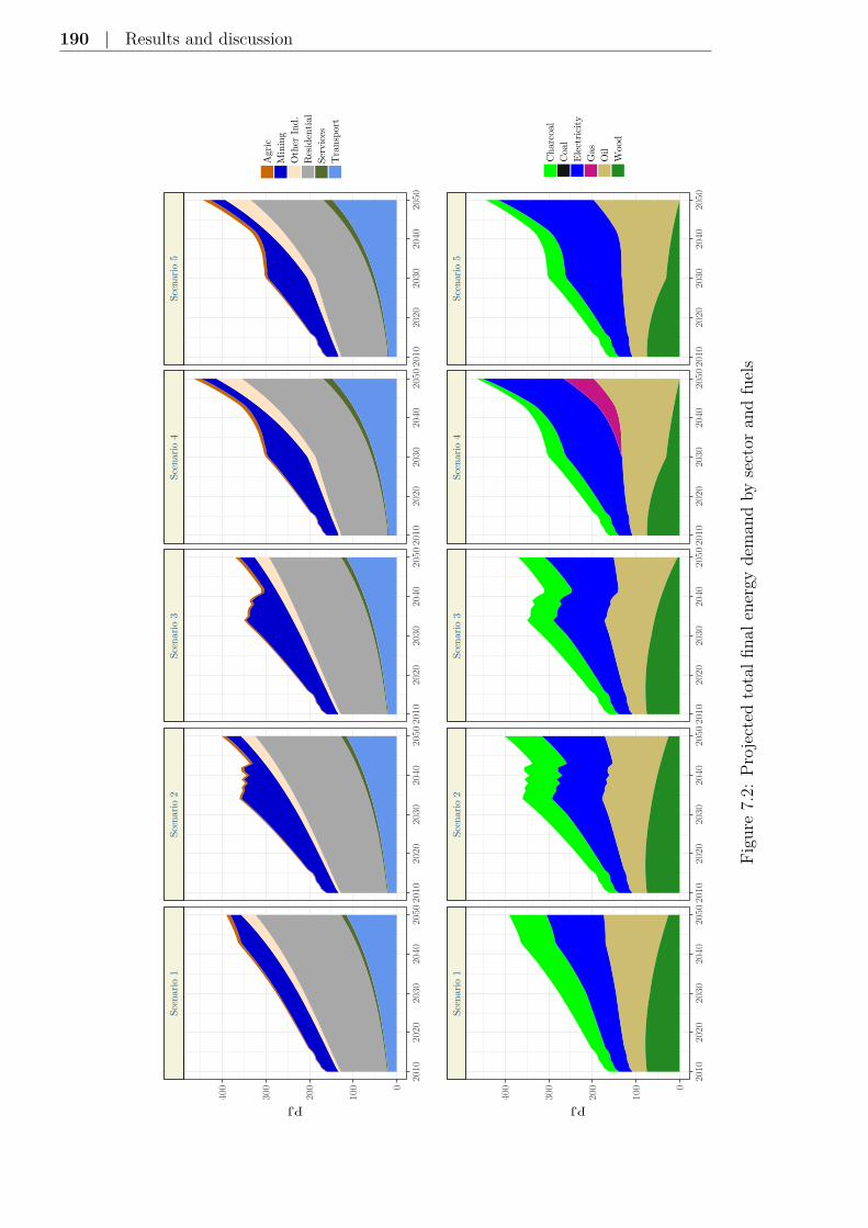
190 | Results and discussion
Scen
ario
1Sc
enar
io 2
Scen
ario
3Sc
enar
io 4
Scen
ario
5
2010
2020
2030
2040
2050
2010
2020
2030
2040
2050
2010
2020
2030
2040
2050
2010
2020
2030
2040
2050
2010
2020
2030
2040
2050
0
100
200
300
400
PJ
A
gric
Min
ing
Oth
er In
d.R
esid
entia
lSe
rvic
esT
rans
port
Scen
ario
1Sc
enar
io 2
Scen
ario
3Sc
enar
io 4
Scen
ario
5
2010
2020
2030
2040
2050
2010
2020
2030
2040
2050
2010
2020
2030
2040
2050
2010
2020
2030
2040
2050
2010
2020
2030
2040
2050
0
100
200
300
400
PJ
C
harc
oal
Coa
lEl
ectr
icity
Gas
Oil
Woo
d
Figu
re7.
2:Pr
ojec
ted
tota
lfina
lene
rgy
dem
and
byse
ctor
and
fuel
s

7.1 Energy system results | 191
In scenario 111, it was assumed12 that electricity access rate in the res-
idential sector increased to 70% (by 2050) and that 75% of the households
which had access to electricity also used it for their cooking and heating
services. Under this scenario, total residential energy demand grew from
106.7 PJ (in 2010) to 195.8 PJ (in 2050) and final electricity demand also
grew from 8.8 PJ to 84.5 PJ during this same period as shown in Figure 7.3
below. To put it into context, residential electricity demand is projected
(by 2050) to be twice as much the value of the country’s total electricity
demand of 2010 (which was 39 PJ).
0
50
100
150
200
2010 2020 2030 2040 2050
PJ
Charcoal Electricity Oil Wood
Figure 7.3: Residential energy demand projection for scenario 1
Electricity growth was driven by increased population13, access to elec-
tricity and household income relative to the base year (2010). With popu-
lation increase of 270%, electricity demand would increase by 23.5 PJ (by
2050) if all things are held constant; because the total number of households
needing electricity would have increased. Increased access to electricity also
leads to cooking and heating fuel transition (from wood and charcoal to
electricity), as could be seen in Figure 7.4a, while increase in household
income (from US$ 850 in 2010 to US$ 1, 600 in 2050) enabled households11All the key scenario drivers were loosely based on GRZ (2006), see the scenarios
description in section 5.312See section 5.1.1 of Chapter 5 for the current energy use patterns in Zambia.13The household size was kept constant throughout the time horizon.
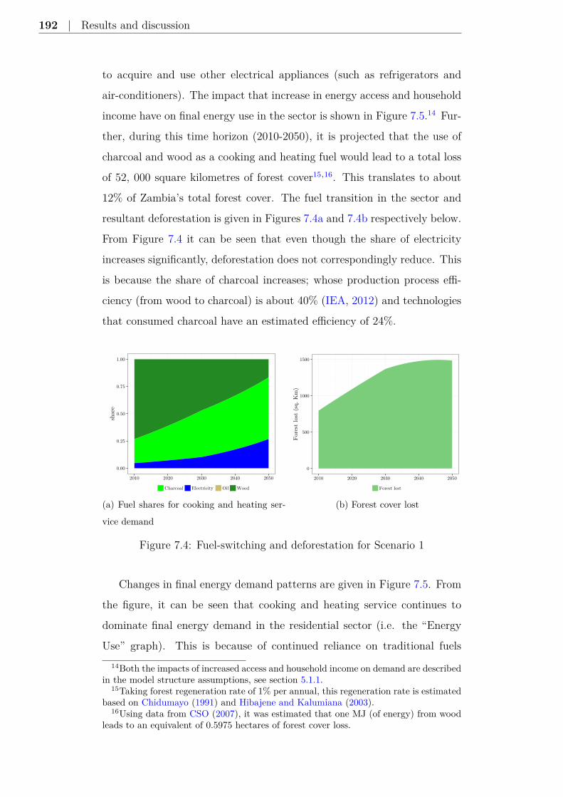
192 | Results and discussion
to acquire and use other electrical appliances (such as refrigerators and
air-conditioners). The impact that increase in energy access and household
income have on final energy use in the sector is shown in Figure 7.5.14 Fur-
ther, during this time horizon (2010-2050), it is projected that the use of
charcoal and wood as a cooking and heating fuel would lead to a total loss
of 52, 000 square kilometres of forest cover15,16. This translates to about
12% of Zambia’s total forest cover. The fuel transition in the sector and
resultant deforestation is given in Figures 7.4a and 7.4b respectively below.
From Figure 7.4 it can be seen that even though the share of electricity
increases significantly, deforestation does not correspondingly reduce. This
is because the share of charcoal increases; whose production process effi-
ciency (from wood to charcoal) is about 40% (IEA, 2012) and technologies
that consumed charcoal have an estimated efficiency of 24%.
0.00
0.25
0.50
0.75
1.00
2010 2020 2030 2040 2050
shar
e
Charcoal Electricity Oil Wood
(a) Fuel shares for cooking and heating ser-
vice demand
0
500
1000
1500
2010 2020 2030 2040 2050
Fore
st lo
st (
sq. K
m)
Forest lost
(b) Forest cover lost
Figure 7.4: Fuel-switching and deforestation for Scenario 1
Changes in final energy demand patterns are given in Figure 7.5. From
the figure, it can be seen that cooking and heating service continues to
dominate final energy demand in the residential sector (i.e. the “Energy
Use” graph). This is because of continued reliance on traditional fuels14Both the impacts of increased access and household income on demand are described
in the model structure assumptions, see section 5.1.1.15Taking forest regeneration rate of 1% per annual, this regeneration rate is estimated
based on Chidumayo (1991) and Hibajene and Kalumiana (2003).16Using data from CSO (2007), it was estimated that one MJ (of energy) from wood
leads to an equivalent of 0.5975 hectares of forest cover loss.
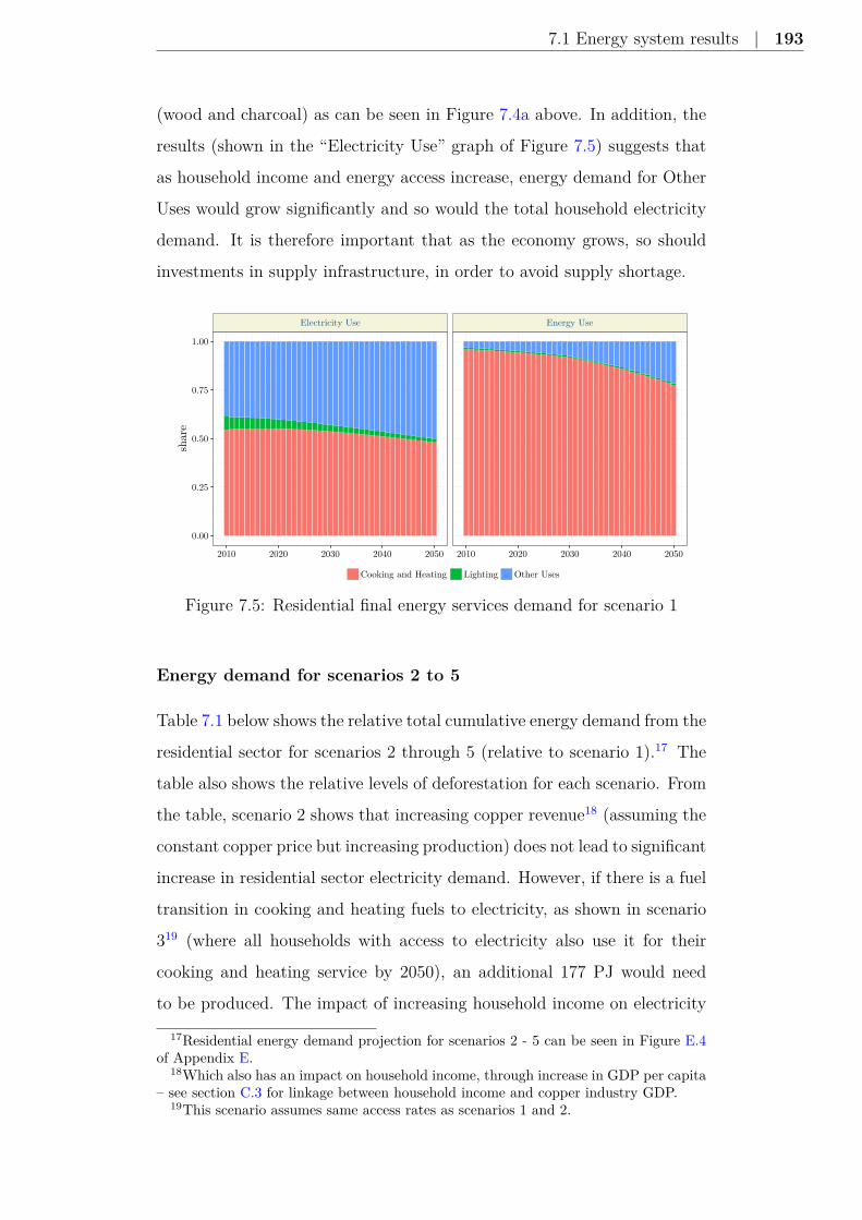
7.1 Energy system results | 193
(wood and charcoal) as can be seen in Figure 7.4a above. In addition, the
results (shown in the “Electricity Use” graph of Figure 7.5) suggests that
as household income and energy access increase, energy demand for Other
Uses would grow significantly and so would the total household electricity
demand. It is therefore important that as the economy grows, so should
investments in supply infrastructure, in order to avoid supply shortage.
Electricity Use Energy Use
0.00
0.25
0.50
0.75
1.00
2010 2020 2030 2040 2050 2010 2020 2030 2040 2050
shar
e
Cooking and Heating Lighting Other Uses
Figure 7.5: Residential final energy services demand for scenario 1
Energy demand for scenarios 2 to 5
Table 7.1 below shows the relative total cumulative energy demand from the
residential sector for scenarios 2 through 5 (relative to scenario 1).17 The
table also shows the relative levels of deforestation for each scenario. From
the table, scenario 2 shows that increasing copper revenue18 (assuming the
constant copper price but increasing production) does not lead to significant
increase in residential sector electricity demand. However, if there is a fuel
transition in cooking and heating fuels to electricity, as shown in scenario
319 (where all households with access to electricity also use it for their
cooking and heating service by 2050), an additional 177 PJ would need
to be produced. The impact of increasing household income on electricity
17Residential energy demand projection for scenarios 2 - 5 can be seen in Figure E.4of Appendix E.
18Which also has an impact on household income, through increase in GDP per capita– see section C.3 for linkage between household income and copper industry GDP.
19This scenario assumes same access rates as scenarios 1 and 2.
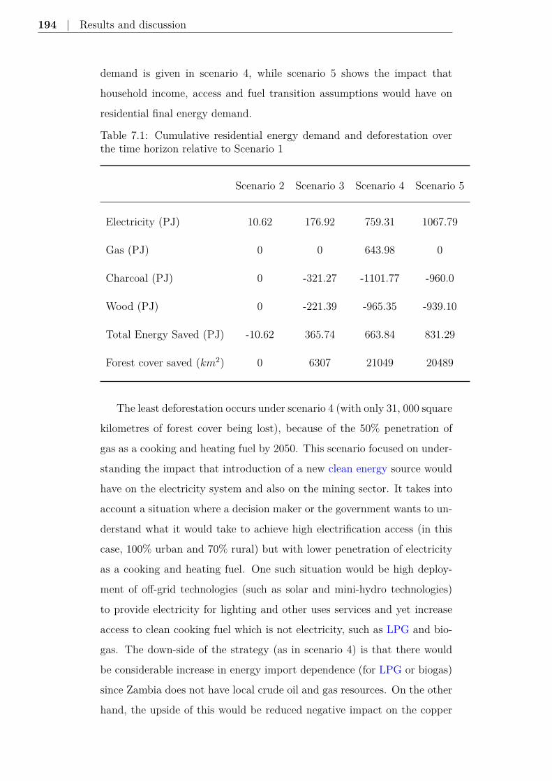
194 | Results and discussion
demand is given in scenario 4, while scenario 5 shows the impact that
household income, access and fuel transition assumptions would have on
residential final energy demand.
Table 7.1: Cumulative residential energy demand and deforestation overthe time horizon relative to Scenario 1
Scenario 2 Scenario 3 Scenario 4 Scenario 5
Electricity (PJ) 10.62 176.92 759.31 1067.79
Gas (PJ) 0 0 643.98 0
Charcoal (PJ) 0 -321.27 -1101.77 -960.0
Wood (PJ) 0 -221.39 -965.35 -939.10
Total Energy Saved (PJ) -10.62 365.74 663.84 831.29
Forest cover saved (km2) 0 6307 21049 20489
The least deforestation occurs under scenario 4 (with only 31, 000 square
kilometres of forest cover being lost), because of the 50% penetration of
gas as a cooking and heating fuel by 2050. This scenario focused on under-
standing the impact that introduction of a new clean energy source would
have on the electricity system and also on the mining sector. It takes into
account a situation where a decision maker or the government wants to un-
derstand what it would take to achieve high electrification access (in this
case, 100% urban and 70% rural) but with lower penetration of electricity
as a cooking and heating fuel. One such situation would be high deploy-
ment of off-grid technologies (such as solar and mini-hydro technologies)
to provide electricity for lighting and other uses services and yet increase
access to clean cooking fuel which is not electricity, such as LPG and bio-
gas. The down-side of the strategy (as in scenario 4) is that there would
be considerable increase in energy import dependence (for LPG or biogas)
since Zambia does not have local crude oil and gas resources. On the other
hand, the upside of this would be reduced negative impact on the copper
7.1 Energy system results | 195
industry (as discussed in section 7.2.3 below).
Uncertainty in electricity demand
The aggregated mining energy demand for scenarios 1 - 5 (taking a con-
stant copper price of US$7, 000 per tonne) are given in Figure 7.6 below.
Energy demand for scenario 1 reduces towards the end of the simulation as
production from North-Western open pit becomes less profitable. Further,
despite having the same expansion target, energy demand for scenarios 2
to 5 varies because of each scenario is exposed to a different energy price
(price that is driven by both endogenous and exogenous activities to the
mining sector). The reduction in diesel consumption (in scenarios 2 - 5)
after 2040 was because production from North-Western open pit had signif-
icantly reduced. A discussion on the disaggregated behaviour of the mining
model is given section 7.2 below.
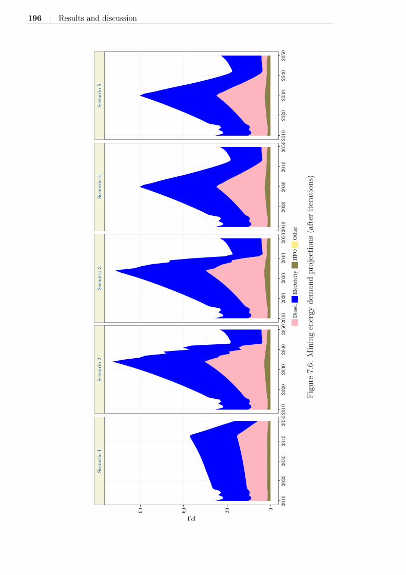
196 | Results and discussion
Scen
ario
1Sc
enar
io 2
Scen
ario
3Sc
enar
io 4
Scen
ario
5
0306090
2010
2020
2030
2040
2050
2010
2020
2030
2040
2050
2010
2020
2030
2040
2050
2010
2020
2030
2040
2050
2010
2020
2030
2040
2050
PJ
D
iese
lEl
ectr
icity
HFO
Oth
er
Figu
re7.
6:M
inin
gen
ergy
dem
and
proj
ectio
ns(a
fter
itera
tions
)
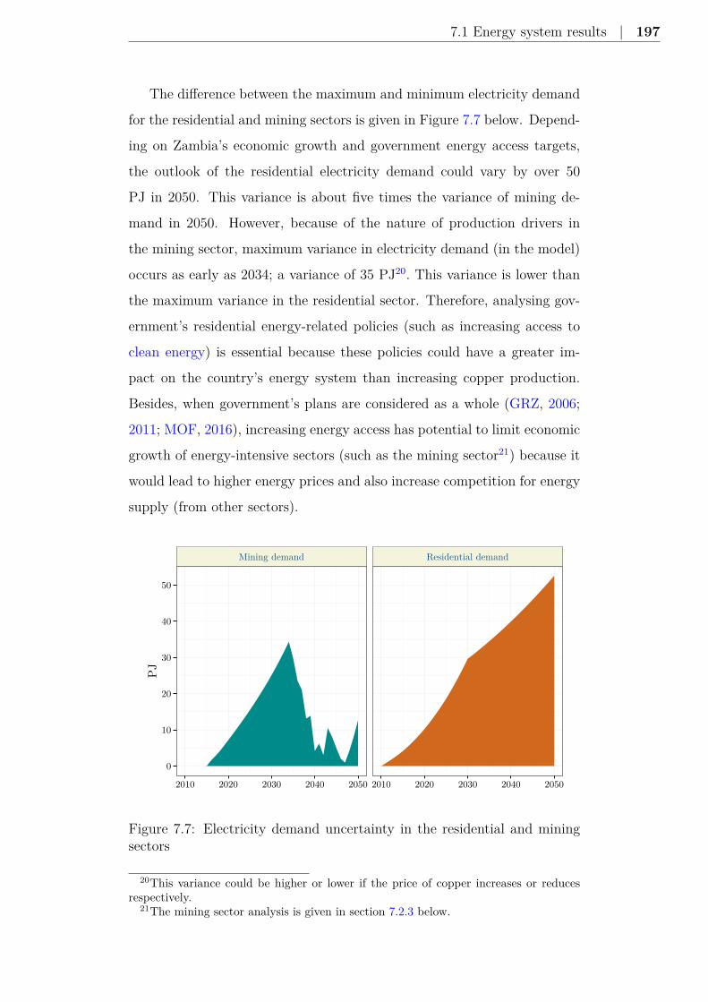
7.1 Energy system results | 197
The difference between the maximum and minimum electricity demand
for the residential and mining sectors is given in Figure 7.7 below. Depend-
ing on Zambia’s economic growth and government energy access targets,
the outlook of the residential electricity demand could vary by over 50
PJ in 2050. This variance is about five times the variance of mining de-
mand in 2050. However, because of the nature of production drivers in
the mining sector, maximum variance in electricity demand (in the model)
occurs as early as 2034; a variance of 35 PJ20. This variance is lower than
the maximum variance in the residential sector. Therefore, analysing gov-
ernment’s residential energy-related policies (such as increasing access to
clean energy) is essential because these policies could have a greater im-
pact on the country’s energy system than increasing copper production.
Besides, when government’s plans are considered as a whole (GRZ, 2006;
2011; MOF, 2016), increasing energy access has potential to limit economic
growth of energy-intensive sectors (such as the mining sector21) because it
would lead to higher energy prices and also increase competition for energy
supply (from other sectors).
Mining demand Residential demand
0
10
20
30
40
50
2010 2020 2030 2040 2050 2010 2020 2030 2040 2050
PJ
Figure 7.7: Electricity demand uncertainty in the residential and miningsectors
20This variance could be higher or lower if the price of copper increases or reducesrespectively.
21The mining sector analysis is given in section 7.2.3 below.
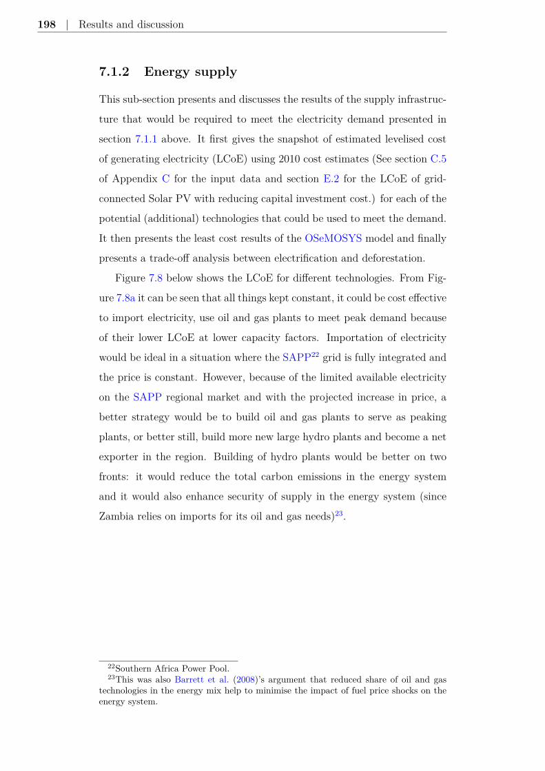
198 | Results and discussion
7.1.2 Energy supply
This sub-section presents and discusses the results of the supply infrastruc-
ture that would be required to meet the electricity demand presented in
section 7.1.1 above. It first gives the snapshot of estimated levelised cost
of generating electricity (LCoE) using 2010 cost estimates (See section C.5
of Appendix C for the input data and section E.2 for the LCoE of grid-
connected Solar PV with reducing capital investment cost.) for each of the
potential (additional) technologies that could be used to meet the demand.
It then presents the least cost results of the OSeMOSYS model and finally
presents a trade-off analysis between electrification and deforestation.
Figure 7.8 below shows the LCoE for different technologies. From Fig-
ure 7.8a it can be seen that all things kept constant, it could be cost effective
to import electricity, use oil and gas plants to meet peak demand because
of their lower LCoE at lower capacity factors. Importation of electricity
would be ideal in a situation where the SAPP22 grid is fully integrated and
the price is constant. However, because of the limited available electricity
on the SAPP regional market and with the projected increase in price, a
better strategy would be to build oil and gas plants to serve as peaking
plants, or better still, build more new large hydro plants and become a net
exporter in the region. Building of hydro plants would be better on two
fronts: it would reduce the total carbon emissions in the energy system
and it would also enhance security of supply in the energy system (since
Zambia relies on imports for its oil and gas needs)23.
22Southern Africa Power Pool.23This was also Barrett et al. (2008)’s argument that reduced share of oil and gas
technologies in the energy mix help to minimise the impact of fuel price shocks on theenergy system.
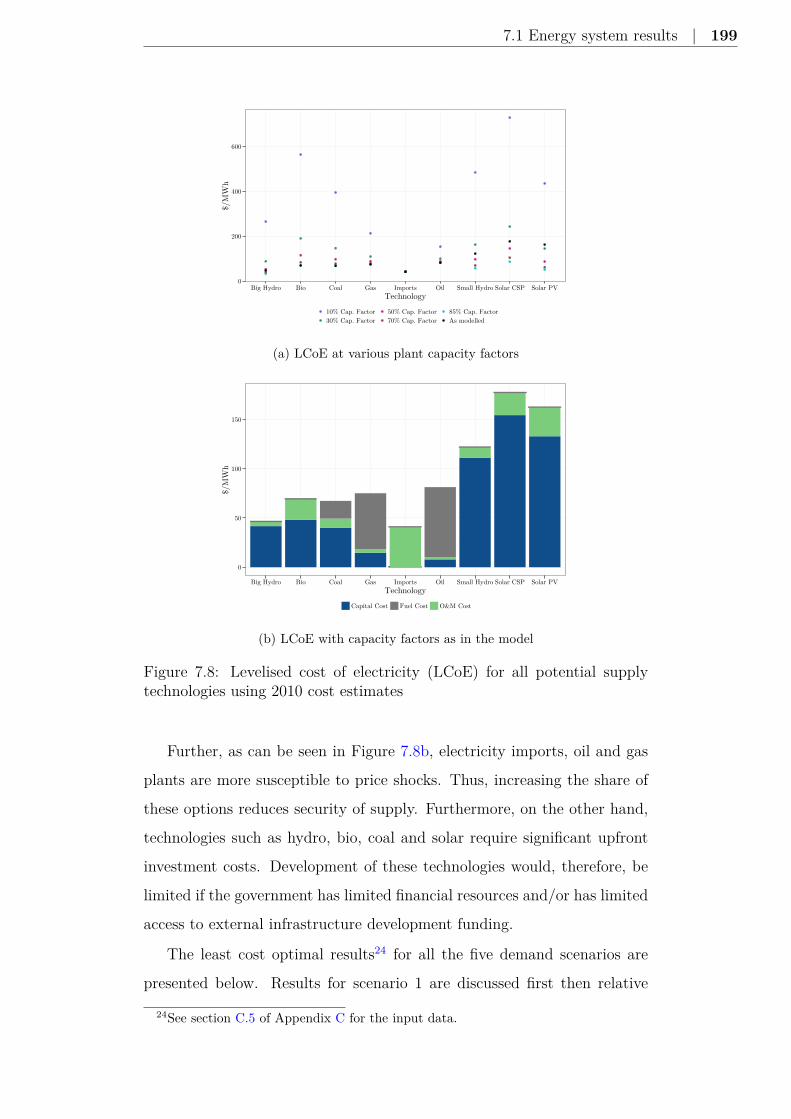
7.1 Energy system results | 199
0
200
400
600
Big Hydro Bio Coal Gas Imports Oil Small Hydro Solar CSP Solar PVTechnology
$/M
Wh
10% Cap. Factor30% Cap. Factor
50% Cap. Factor70% Cap. Factor
85% Cap. FactorAs modelled
(a) LCoE at various plant capacity factors
0
50
100
150
Big Hydro Bio Coal Gas Imports Oil Small Hydro Solar CSP Solar PVTechnology
$/M
Wh
Capital Cost Fuel Cost O&M Cost
(b) LCoE with capacity factors as in the model
Figure 7.8: Levelised cost of electricity (LCoE) for all potential supplytechnologies using 2010 cost estimates
Further, as can be seen in Figure 7.8b, electricity imports, oil and gas
plants are more susceptible to price shocks. Thus, increasing the share of
these options reduces security of supply. Furthermore, on the other hand,
technologies such as hydro, bio, coal and solar require significant upfront
investment costs. Development of these technologies would, therefore, be
limited if the government has limited financial resources and/or has limited
access to external infrastructure development funding.
The least cost optimal results24 for all the five demand scenarios are
presented below. Results for scenario 1 are discussed first then relative
24See section C.5 of Appendix C for the input data.
200 | Results and discussion
results (to scenario 1) are presented and discussed. These results consider
the total developed capacity, the type of technology developed, production
of electricity from each technology, average generation cost (LCoE) and the
total carbon emissions.
Figure 7.9 shows the total supply capacity for scenario 1. The gen-
eration capacity development is projected to grow from 1, 900 MW (in
2010) to 10, 100 MW (in 2050). As expected (building up from Figure 7.8)
the capacity development is dominated by hydro technologies because they
have a lower LCoE. After all the hydro potential is exhausted, biomass
technology is developed (to a maximum of 500 MW) thereafter, capacity
development is dominated by coal technology. As a result, the carbon in-
tensity of Zambia’s electricity system is projected to increase to about 300
gCO2eq/kWh by 2050, from 4.25 gCO2eq/kWh in 2010. The total carbon
emission during this time horizon is 145 Mt of CO2eq.
0
2500
5000
7500
10000
2010 2020 2030 2040 2050
MW
BioCoal
GasNew Hydro
OilOld Hydro
Solar
Figure 7.9: Least cost capacity mix for scenario 1
The required total capital investment cost for the scenario (over the
time horizon) is US$ 35 billion. This on average (per year) translates to
3.4% of Zambia’s total GDP. The quantity of electricity generated by each
technology has a similar profile as that of capacity development, with total
production increasing from 12, 000 GWh (in 2010) to 59, 000 GWh (in
2050) as can be seen in Figure 7.10.
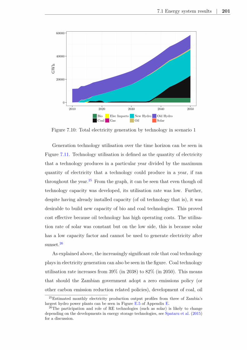
7.1 Energy system results | 201
0
20000
40000
60000
2010 2020 2030 2040 2050
GW
h
BioCoal
Elec ImportsGas
New HydroOil
Old HydroSolar
Figure 7.10: Total electricity generation by technology in scenario 1
Generation technology utilisation over the time horizon can be seen in
Figure 7.11. Technology utilisation is defined as the quantity of electricity
that a technology produces in a particular year divided by the maximum
quantity of electricity that a technology could produce in a year, if ran
throughout the year.25 From the graph, it can be seen that even though oil
technology capacity was developed, its utilisation rate was low. Further,
despite having already installed capacity (of oil technology that is), it was
desirable to build new capacity of bio and coal technologies. This proved
cost effective because oil technology has high operating costs. The utilisa-
tion rate of solar was constant but on the low side, this is because solar
has a low capacity factor and cannot be used to generate electricity after
sunset.26
As explained above, the increasingly significant role that coal technology
plays in electricity generation can also be seen in the figure. Coal technology
utilisation rate increases from 39% (in 2038) to 82% (in 2050). This means
that should the Zambian government adopt a zero emissions policy (or
other carbon emission reduction related policies), development of coal, oil25Estimated monthly electricity production output profiles from three of Zambia’s
largest hydro power plants can be seen in Figure E.5 of Appendix E.26The participation and role of RE technologies (such as solar) is likely to change
depending on the developments in energy storage technologies, see Spataru et al. (2015)for a discussion.
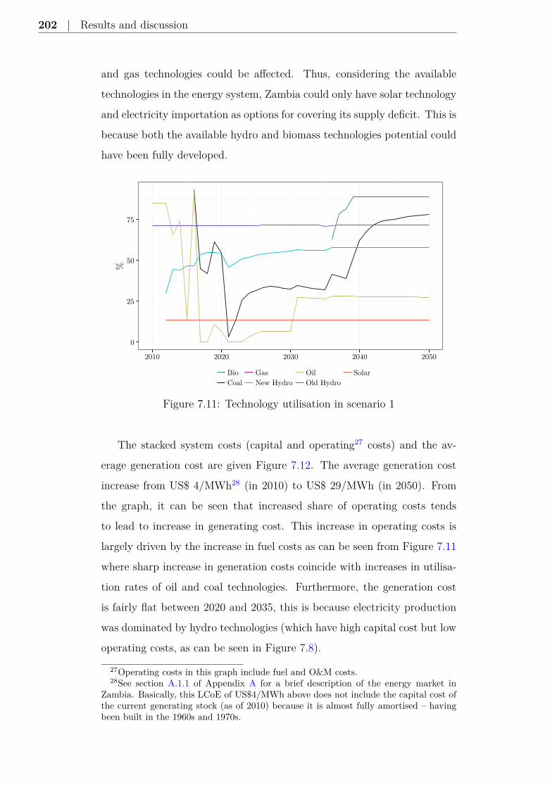
202 | Results and discussion
and gas technologies could be affected. Thus, considering the available
technologies in the energy system, Zambia could only have solar technology
and electricity importation as options for covering its supply deficit. This is
because both the available hydro and biomass technologies potential could
have been fully developed.
0
25
50
75
2010 2020 2030 2040 2050
%
BioCoal
GasNew Hydro
OilOld Hydro
Solar
Figure 7.11: Technology utilisation in scenario 1
The stacked system costs (capital and operating27 costs) and the av-
erage generation cost are given Figure 7.12. The average generation cost
increase from US$ 4/MWh28 (in 2010) to US$ 29/MWh (in 2050). From
the graph, it can be seen that increased share of operating costs tends
to lead to increase in generating cost. This increase in operating costs is
largely driven by the increase in fuel costs as can be seen from Figure 7.11
where sharp increase in generation costs coincide with increases in utilisa-
tion rates of oil and coal technologies. Furthermore, the generation cost
is fairly flat between 2020 and 2035, this is because electricity production
was dominated by hydro technologies (which have high capital cost but low
operating costs, as can be seen in Figure 7.8).
27Operating costs in this graph include fuel and O&M costs.28See section A.1.1 of Appendix A for a brief description of the energy market in
Zambia. Basically, this LCoE of US$4/MWh above does not include the capital cost ofthe current generating stock (as of 2010) because it is almost fully amortised – havingbeen built in the 1960s and 1970s.
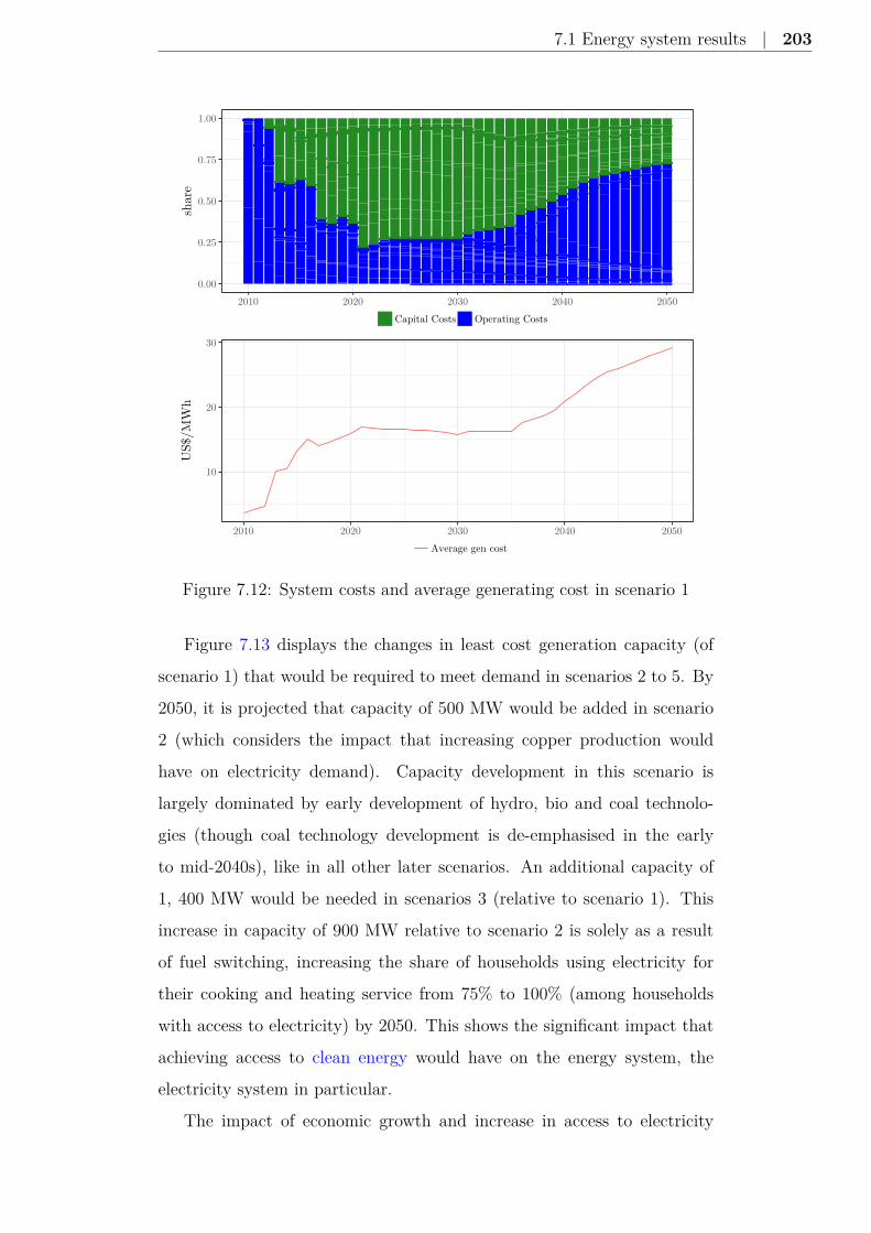
7.1 Energy system results | 203
0.00
0.25
0.50
0.75
1.00
2010 2020 2030 2040 2050
shar
e
Capital Costs Operating Costs
10
20
30
2010 2020 2030 2040 2050
US$
/MW
h
Average gen cost
Figure 7.12: System costs and average generating cost in scenario 1
Figure 7.13 displays the changes in least cost generation capacity (of
scenario 1) that would be required to meet demand in scenarios 2 to 5. By
2050, it is projected that capacity of 500 MW would be added in scenario
2 (which considers the impact that increasing copper production would
have on electricity demand). Capacity development in this scenario is
largely dominated by early development of hydro, bio and coal technolo-
gies (though coal technology development is de-emphasised in the early
to mid-2040s), like in all other later scenarios. An additional capacity of
1, 400 MW would be needed in scenarios 3 (relative to scenario 1). This
increase in capacity of 900 MW relative to scenario 2 is solely as a result
of fuel switching, increasing the share of households using electricity for
their cooking and heating service from 75% to 100% (among households
with access to electricity) by 2050. This shows the significant impact that
achieving access to clean energy would have on the energy system, the
electricity system in particular.
The impact of economic growth and increase in access to electricity

204 | Results and discussion
(with reduced number of households using electricity for their cooking and
heating service) is given in scenario 4. An additional capacity of 3, 050
MW would be required (relative to scenario 1). However, the significance
of increasing the number of households using electricity for their cooking
and heating under high rates of access to electricity is emphasised in a
comparison between scenarios 4 and 5. An additional 2, 950 MW (relative
to scenario 4) would be required by 2050 to meet cooking and heating
service demand under high electricity access rate. Therefore, increasing
access to electricity at the same time as increasing the share of households
using electricity for their cooking and heating service would prove to be a
significant investment challenge.
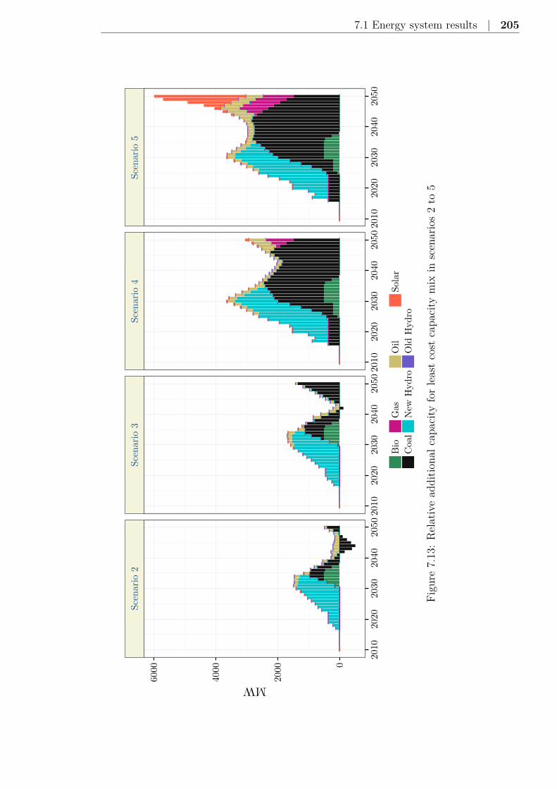
7.1 Energy system results | 205
Scen
ario
2Sc
enar
io 3
Scen
ario
4Sc
enar
io 5
0
2000
4000
6000
2010
2020
2030
2040
2050
2010
2020
2030
2040
2050
2010
2020
2030
2040
2050
2010
2020
2030
2040
2050
MW
Bi
oC
oal
Gas
New
Hyd
roO
ilO
ld H
ydro
Sola
r
Figu
re7.
13:
Rel
ativ
ead
ditio
nalc
apac
ityfo
rle
ast
cost
capa
city
mix
insc
enar
ios
2to
5
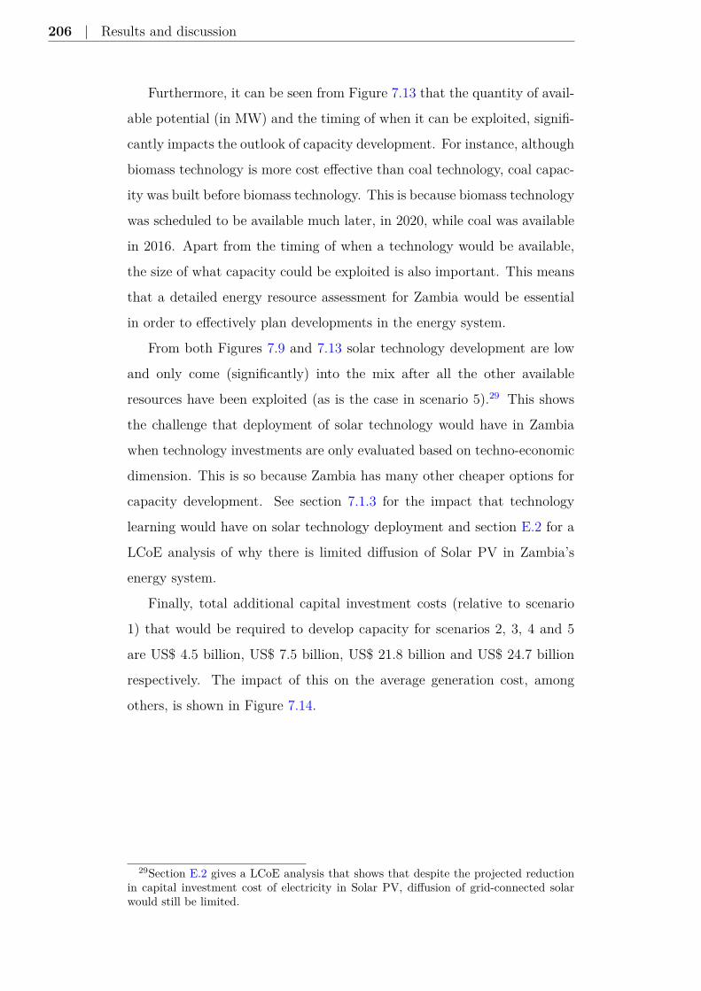
206 | Results and discussion
Furthermore, it can be seen from Figure 7.13 that the quantity of avail-
able potential (in MW) and the timing of when it can be exploited, signifi-
cantly impacts the outlook of capacity development. For instance, although
biomass technology is more cost effective than coal technology, coal capac-
ity was built before biomass technology. This is because biomass technology
was scheduled to be available much later, in 2020, while coal was available
in 2016. Apart from the timing of when a technology would be available,
the size of what capacity could be exploited is also important. This means
that a detailed energy resource assessment for Zambia would be essential
in order to effectively plan developments in the energy system.
From both Figures 7.9 and 7.13 solar technology development are low
and only come (significantly) into the mix after all the other available
resources have been exploited (as is the case in scenario 5).29 This shows
the challenge that deployment of solar technology would have in Zambia
when technology investments are only evaluated based on techno-economic
dimension. This is so because Zambia has many other cheaper options for
capacity development. See section 7.1.3 for the impact that technology
learning would have on solar technology deployment and section E.2 for a
LCoE analysis of why there is limited diffusion of Solar PV in Zambia’s
energy system.
Finally, total additional capital investment costs (relative to scenario
1) that would be required to develop capacity for scenarios 2, 3, 4 and 5
are US$ 4.5 billion, US$ 7.5 billion, US$ 21.8 billion and US$ 24.7 billion
respectively. The impact of this on the average generation cost, among
others, is shown in Figure 7.14.
29Section E.2 gives a LCoE analysis that shows that despite the projected reductionin capital investment cost of electricity in Solar PV, diffusion of grid-connected solarwould still be limited.
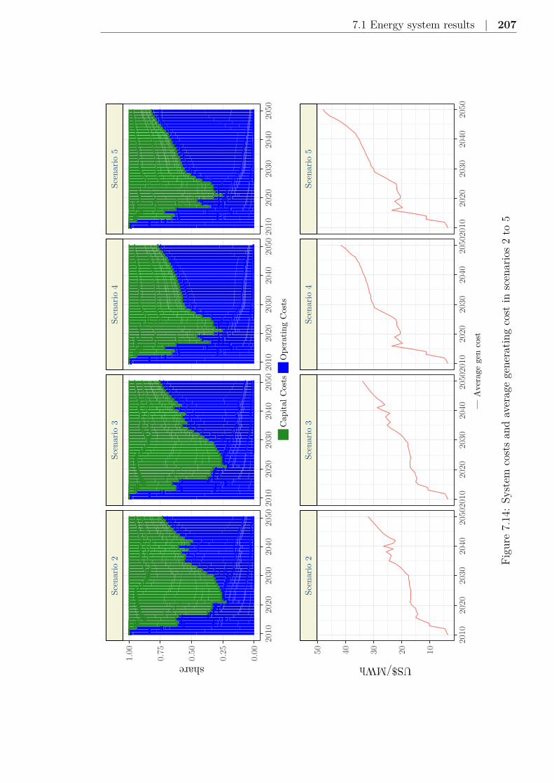
7.1 Energy system results | 207
Scen
ario
2Sc
enar
io 3
Scen
ario
4Sc
enar
io 5
2010
2020
2030
2040
2050
2010
2020
2030
2040
2050
2010
2020
2030
2040
2050
2010
2020
2030
2040
2050
0.00
0.25
0.50
0.75
1.00
share
C
apita
l Cos
tsO
pera
ting
Cos
ts
Scen
ario
2Sc
enar
io 3
Scen
ario
4Sc
enar
io 5
2010
2020
2030
2040
2050
2010
2020
2030
2040
2050
2010
2020
2030
2040
2050
2010
2020
2030
2040
2050
1020304050
US$/MWh
Ave
rage
gen
cos
t
Figu
re7.
14:
Syst
emco
sts
and
aver
age
gene
ratin
gco
stin
scen
ario
s2
to5
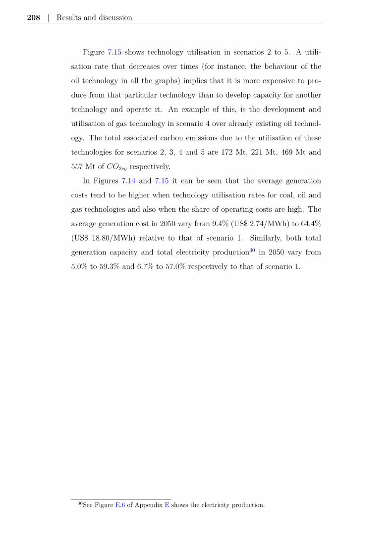
208 | Results and discussion
Figure 7.15 shows technology utilisation in scenarios 2 to 5. A utili-
sation rate that decreases over times (for instance, the behaviour of the
oil technology in all the graphs) implies that it is more expensive to pro-
duce from that particular technology than to develop capacity for another
technology and operate it. An example of this, is the development and
utilisation of gas technology in scenario 4 over already existing oil technol-
ogy. The total associated carbon emissions due to the utilisation of these
technologies for scenarios 2, 3, 4 and 5 are 172 Mt, 221 Mt, 469 Mt and
557 Mt of CO2eq respectively.
In Figures 7.14 and 7.15 it can be seen that the average generation
costs tend to be higher when technology utilisation rates for coal, oil and
gas technologies and also when the share of operating costs are high. The
average generation cost in 2050 vary from 9.4% (US$ 2.74/MWh) to 64.4%
(US$ 18.80/MWh) relative to that of scenario 1. Similarly, both total
generation capacity and total electricity production30 in 2050 vary from
5.0% to 59.3% and 6.7% to 57.0% respectively to that of scenario 1.
30See Figure E.6 of Appendix E shows the electricity production.
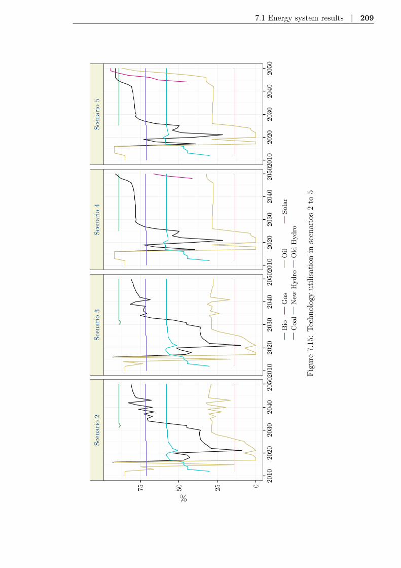
7.1 Energy system results | 209
Scen
ario
2Sc
enar
io 3
Scen
ario
4Sc
enar
io 5
0255075
2010
2020
2030
2040
2050
2010
2020
2030
2040
2050
2010
2020
2030
2040
2050
2010
2020
2030
2040
2050
%
Bi
oC
oal
Gas
New
Hyd
roO
ilO
ld H
ydro
Sola
r
Figu
re7.
15:
Tech
nolo
gyut
ilisa
tion
insc
enar
ios
2to
5
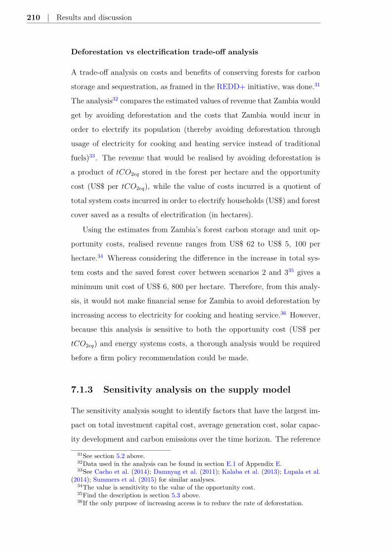
210 | Results and discussion
Deforestation vs electrification trade-off analysis
A trade-off analysis on costs and benefits of conserving forests for carbon
storage and sequestration, as framed in the REDD+ initiative, was done.31
The analysis32 compares the estimated values of revenue that Zambia would
get by avoiding deforestation and the costs that Zambia would incur in
order to electrify its population (thereby avoiding deforestation through
usage of electricity for cooking and heating service instead of traditional
fuels)33. The revenue that would be realised by avoiding deforestation is
a product of tCO2eq stored in the forest per hectare and the opportunity
cost (US$ per tCO2eq), while the value of costs incurred is a quotient of
total system costs incurred in order to electrify households (US$) and forest
cover saved as a results of electrification (in hectares).
Using the estimates from Zambia’s forest carbon storage and unit op-
portunity costs, realised revenue ranges from US$ 62 to US$ 5, 100 per
hectare.34 Whereas considering the difference in the increase in total sys-
tem costs and the saved forest cover between scenarios 2 and 335 gives a
minimum unit cost of US$ 6, 800 per hectare. Therefore, from this analy-
sis, it would not make financial sense for Zambia to avoid deforestation by
increasing access to electricity for cooking and heating service.36 However,
because this analysis is sensitive to both the opportunity cost (US$ per
tCO2eq) and energy systems costs, a thorough analysis would be required
before a firm policy recommendation could be made.
7.1.3 Sensitivity analysis on the supply model
The sensitivity analysis sought to identify factors that have the largest im-
pact on total investment capital cost, average generation cost, solar capac-
ity development and carbon emissions over the time horizon. The reference
31See section 5.2 above.32Data used in the analysis can be found in section E.1 of Appendix E.33See Cacho et al. (2014); Damnyag et al. (2011); Kalaba et al. (2013); Lupala et al.
(2014); Summers et al. (2015) for similar analyses.34The value is sensitivity to the value of the opportunity cost.35Find the description is section 5.3 above.36If the only purpose of increasing access is to reduce the rate of deforestation.
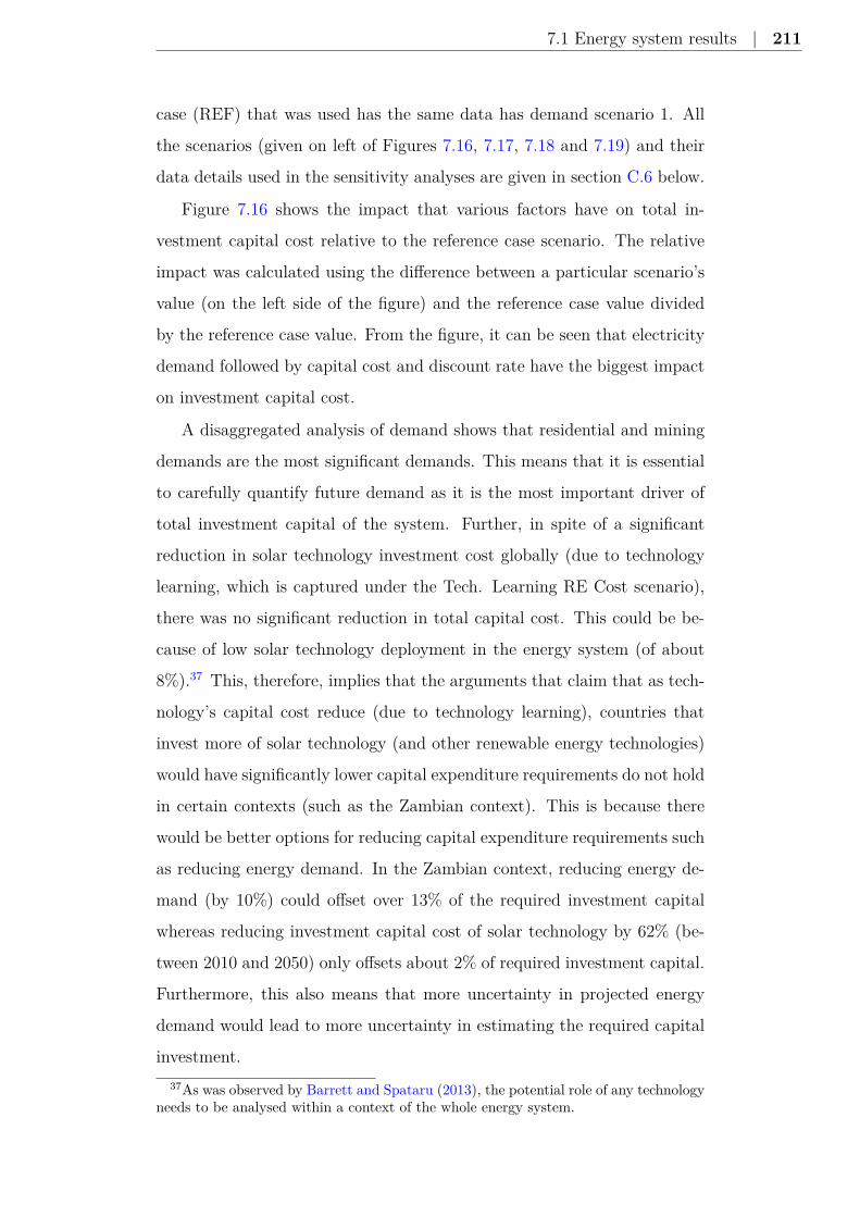
7.1 Energy system results | 211
case (REF) that was used has the same data has demand scenario 1. All
the scenarios (given on left of Figures 7.16, 7.17, 7.18 and 7.19) and their
data details used in the sensitivity analyses are given in section C.6 below.
Figure 7.16 shows the impact that various factors have on total in-
vestment capital cost relative to the reference case scenario. The relative
impact was calculated using the difference between a particular scenario’s
value (on the left side of the figure) and the reference case value divided
by the reference case value. From the figure, it can be seen that electricity
demand followed by capital cost and discount rate have the biggest impact
on investment capital cost.
A disaggregated analysis of demand shows that residential and mining
demands are the most significant demands. This means that it is essential
to carefully quantify future demand as it is the most important driver of
total investment capital of the system. Further, in spite of a significant
reduction in solar technology investment cost globally (due to technology
learning, which is captured under the Tech. Learning RE Cost scenario),
there was no significant reduction in total capital cost. This could be be-
cause of low solar technology deployment in the energy system (of about
8%).37 This, therefore, implies that the arguments that claim that as tech-
nology’s capital cost reduce (due to technology learning), countries that
invest more of solar technology (and other renewable energy technologies)
would have significantly lower capital expenditure requirements do not hold
in certain contexts (such as the Zambian context). This is because there
would be better options for reducing capital expenditure requirements such
as reducing energy demand. In the Zambian context, reducing energy de-
mand (by 10%) could offset over 13% of the required investment capital
whereas reducing investment capital cost of solar technology by 62% (be-
tween 2010 and 2050) only offsets about 2% of required investment capital.
Furthermore, this also means that more uncertainty in projected energy
demand would lead to more uncertainty in estimating the required capital
investment.37As was observed by Barrett and Spataru (2013), the potential role of any technology
needs to be analysed within a context of the whole energy system.
212 | Results and discussion
High Cap. Inv. Cost
High coal and high import price
High coal and low import price
High Disc. Rate
High elec. demand
High fixed Costs
High mining elec. demand
High other elec. demand
High resid. elec. demand
High variable Costs
Low Cap. Inv. Cost
Low coal and high import price
Low coal and low import price
Low coal and no imports
Low Disc. Rate
Low elec. demand
Low fixed Costs
Low mining elec. demand
Low other elec. demand
Low resid. elec. demand
Low variable Costs
Tech. Learning RE Cost
Zero mining demand by 2030
Zero mining demand by 2040
Zero mining demand by 2050
-20 -10 0 10Percent ( % ) change in total capital inv. cost
Figure 7.16: Effects on total capital investment relative to the REF case

7.1 Energy system results | 213
Figure 7.17 presents the impact that various factors have on the average
generation cost relative to the reference case scenario. It can be seen that
average generation cost is mainly driven by the discount rate (a variance
of over 30%) followed by capital investment cost (7% variance) and energy
demand (6.5% variance). Whereas technology learning did not have a sig-
nificant impact on the system’s total investment capital requirement 38 (see
Figure 7.16), it had a considerable effect on reducing the average genera-
tion cost of the system (reduced it by about 4.8%). In addition, adopting a
policy39 that limits electricity production from coal technology would have
a noticeable impact on the average generation cost (ranging from 2.8% to
4.5%).
38Section E.2 gives a LCoE analysis that shows that despite the projected reductionin capital investment cost of electricity in Solar PV, diffusion of grid-connected solarwould still be limited.
39Such as local coal and no imports, local coal and low import price and local coaland high import price scenarios.
214 | Results and discussion
High Cap. Inv. Cost
High coal and high import price
High coal and low import price
High Disc. Rate
High elec. demand
High fixed Costs
High mining elec. demand
High other elec. demand
High resid. elec. demand
High variable Costs
Low Cap. Inv. Cost
Low coal and high import price
Low coal and low import price
Low coal and no imports
Low Disc. Rate
Low elec. demand
Low fixed Costs
Low mining elec. demand
Low other elec. demand
Low resid. elec. demand
Low variable Costs
Tech. Learning RE Cost
Zero mining demand by 2030
Zero mining demand by 2040
Zero mining demand by 2050
-20 0 20Percent ( % ) change in average gen. cost
Figure 7.17: Effects on average generation cost relative to the REF case
Figure 7.18 displays the impact that various factors have on solar de-
ployment relative to the reference case scenario. As anticipated, the drivers
for increased solar deployment into the energy system are technology learn-
ing (reducing investment capital cost) followed by low production from coal
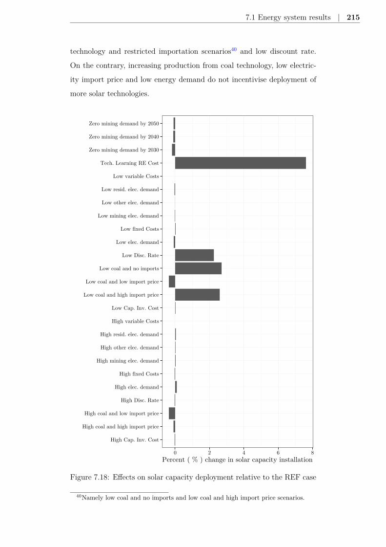
7.1 Energy system results | 215
technology and restricted importation scenarios40 and low discount rate.
On the contrary, increasing production from coal technology, low electric-
ity import price and low energy demand do not incentivise deployment of
more solar technologies.
High Cap. Inv. Cost
High coal and high import price
High coal and low import price
High Disc. Rate
High elec. demand
High fixed Costs
High mining elec. demand
High other elec. demand
High resid. elec. demand
High variable Costs
Low Cap. Inv. Cost
Low coal and high import price
Low coal and low import price
Low coal and no imports
Low Disc. Rate
Low elec. demand
Low fixed Costs
Low mining elec. demand
Low other elec. demand
Low resid. elec. demand
Low variable Costs
Tech. Learning RE Cost
Zero mining demand by 2030
Zero mining demand by 2040
Zero mining demand by 2050
0 2 4 6 8Percent ( % ) change in solar capacity installation
Figure 7.18: Effects on solar capacity deployment relative to the REF case
40Namely low coal and no imports and low coal and high import price scenarios.

216 | Results and discussion
Figure 7.19 gives the impact that various factors have on total carbon
emissions relative to the reference case scenario. It can be seen that the
easiest way to reduce carbon emissions from Zambia’s electricity system
is by importing electricity. However, the largest exporter of electricity in
the SAPP regional market is South Africa, whose electricity production is
dominated by coal technology. For that reason, using imported electricity
to reduce emissions would not be the best option. Besides that, there is a
shortage of electricity in the SAPP region. There are, therefore, three other
ways to reduce carbon emissions: reducing demand, limit production from
coal technology and deploy more solar technology (as the investment cap-
ital cost reduces). Conversely, increasing energy demand increases carbon
emissions.
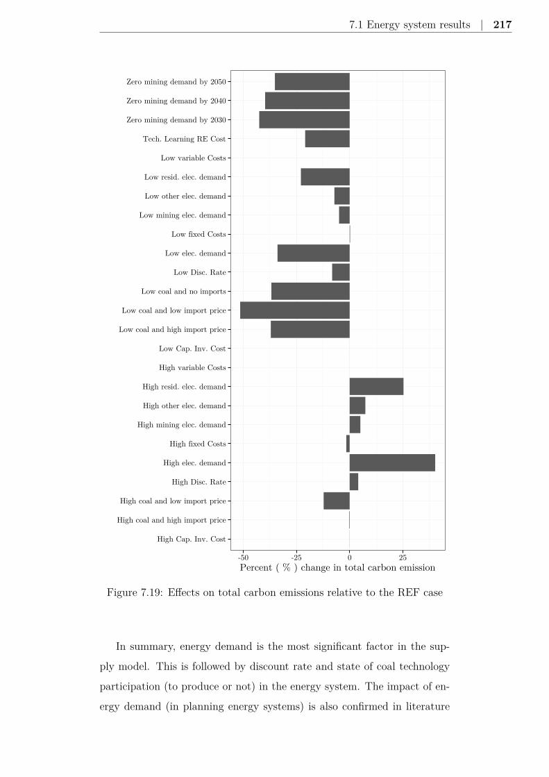
7.1 Energy system results | 217
High Cap. Inv. Cost
High coal and high import price
High coal and low import price
High Disc. Rate
High elec. demand
High fixed Costs
High mining elec. demand
High other elec. demand
High resid. elec. demand
High variable Costs
Low Cap. Inv. Cost
Low coal and high import price
Low coal and low import price
Low coal and no imports
Low Disc. Rate
Low elec. demand
Low fixed Costs
Low mining elec. demand
Low other elec. demand
Low resid. elec. demand
Low variable Costs
Tech. Learning RE Cost
Zero mining demand by 2030
Zero mining demand by 2040
Zero mining demand by 2050
-50 -25 0 25Percent ( % ) change in total carbon emission
Figure 7.19: Effects on total carbon emissions relative to the REF case
In summary, energy demand is the most significant factor in the sup-
ply model. This is followed by discount rate and state of coal technology
participation (to produce or not) in the energy system. The impact of en-
ergy demand (in planning energy systems) is also confirmed in literature
218 | Results and discussion
by Rosnes and Vennemo (2012). This (impact of demand on supply model)
emphasises the importance of using appropriate methods when estimating
future energy demand, which was done in this research. Further, some of
the results presented in this sub-section seem trivial and obvious, but for
completeness, it is important that these results are presented.
7.2 Mining model results
Having looked at how Zambia’s energy system could evolve in the above
section and considered how mining firms make decisions in Zambia, this
section sought to address the research question: What impact does increas-
ing access to clean energy have on mining sector’s profitability? Further,
building on from the research findings above, this section also provides an
analysis which helps to identify decision variables that are most significant
in Zambia’s mining industry (based on the mining model). The methods
used to develop and analyse the model are described in Chapter 6.
7.2.1 Indicative production scenarios
In this sub-section, the discussion focuses on a range of possible (from 1200
simulation runs) copper production outputs (based on copper production
growth rates), selection of outputs to focus on for further analysis and de-
scribes how electricity prices to use in the mining model were estimated.
The initial simulated production outputs consider different industry’s pro-
duction capacity growth rates41, the uncertainty in ore grade, available
ore resources and copper price. It assumes that mineral royalty tax, en-
ergy prices and all other inputs remain constant. This stylised approached
was used in order to establish the possible extremes of copper production
at industry level, particularly the maximum production output. It was
important to establish the technically feasible maximum production out-
put, as this production statistic was useful for estimating maximum energy
41Capacity expansion was done independently at firm level, in this case, NW-OP,CB-OP and CB-UG level, see section 7.2.5 for a detailed description.
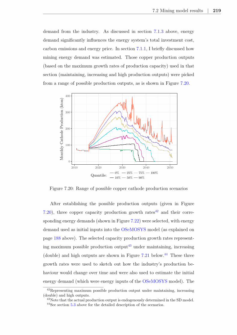
7.2 Mining model results | 219
demand from the industry. As discussed in section 7.1.3 above, energy
demand significantly influences the energy system’s total investment cost,
carbon emissions and energy price. In section 7.1.1, I briefly discussed how
mining energy demand was estimated. Those copper production outputs
(based on the maximum growth rates of production capacity) used in that
section (maintaining, increasing and high production outputs) were picked
from a range of possible production outputs, as is shown in Figure 7.20.
0
100
200
300
400
2010 2020 2030 2040 2050
Mon
thly
Cat
hode
Pro
duct
ion
(kto
n)
Quantile: 0%10%
25%50%
75%90%
100%
Figure 7.20: Range of possible copper cathode production scenarios
After establishing the possible production outputs (given in Figure
7.20), three copper capacity production growth rates42 and their corre-
sponding energy demands (shown in Figure 7.22) were selected, with energy
demand used as initial inputs into the OSeMOSYS model (as explained on
page 188 above). The selected capacity production growth rates represent-
ing maximum possible production output43 under maintaining, increasing
(double) and high outputs are shown in Figure 7.21 below.44 These three
growth rates were used to sketch out how the industry’s production be-
haviour would change over time and were also used to estimate the initial
energy demand (which were energy inputs of the OSeMOSYS model). The42Representing maximum possible production output under maintaining, increasing
(double) and high outputs.43Note that the actual production output is endogenously determined in the SD model.44See section 5.3 above for the detailed description of the scenarios.
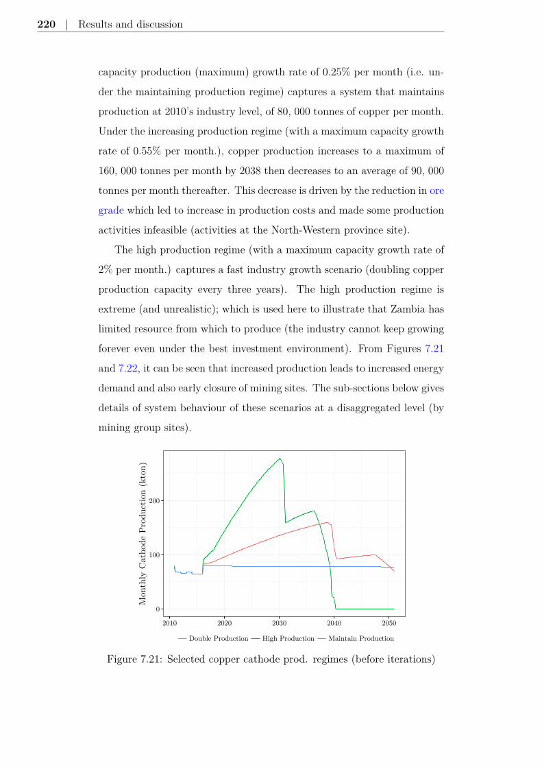
220 | Results and discussion
capacity production (maximum) growth rate of 0.25% per month (i.e. un-
der the maintaining production regime) captures a system that maintains
production at 2010’s industry level, of 80, 000 tonnes of copper per month.
Under the increasing production regime (with a maximum capacity growth
rate of 0.55% per month.), copper production increases to a maximum of
160, 000 tonnes per month by 2038 then decreases to an average of 90, 000
tonnes per month thereafter. This decrease is driven by the reduction in ore
grade which led to increase in production costs and made some production
activities infeasible (activities at the North-Western province site).
The high production regime (with a maximum capacity growth rate of
2% per month.) captures a fast industry growth scenario (doubling copper
production capacity every three years). The high production regime is
extreme (and unrealistic); which is used here to illustrate that Zambia has
limited resource from which to produce (the industry cannot keep growing
forever even under the best investment environment). From Figures 7.21
and 7.22, it can be seen that increased production leads to increased energy
demand and also early closure of mining sites. The sub-sections below gives
details of system behaviour of these scenarios at a disaggregated level (by
mining group sites).
0
100
200
2010 2020 2030 2040 2050
Mon
thly
Cat
hode
Pro
duct
ion
(kto
n)
Double Production High Production Maintain Production
Figure 7.21: Selected copper cathode prod. regimes (before iterations)
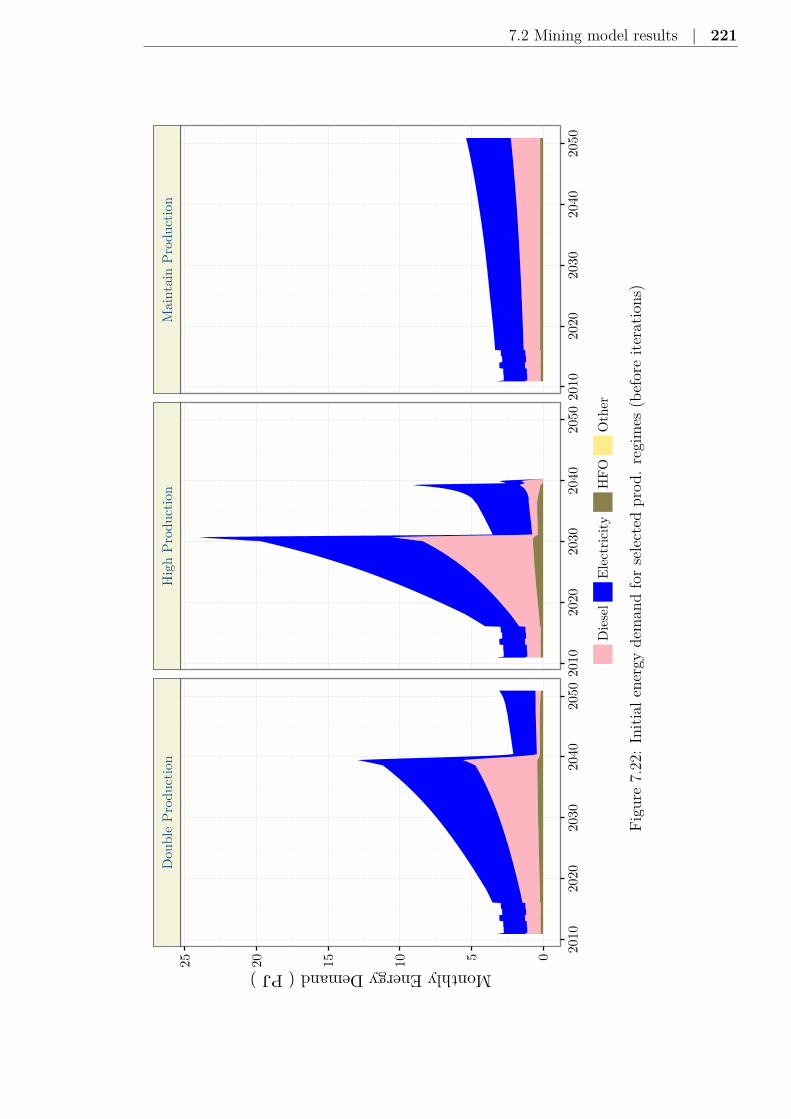
7.2 Mining model results | 221
Dou
ble
Prod
uctio
nH
igh
Prod
uctio
nM
aint
ain
Prod
uctio
n
0510152025
2010
2020
2030
2040
2050
2010
2020
2030
2040
2050
2010
2020
2030
2040
2050
Monthly Energy Demand ( PJ )
D
iese
lEl
ectr
icity
HFO
Oth
er
Figu
re7.
22:
Initi
alen
ergy
dem
and
for
sele
cted
prod
.re
gim
es(b
efor
eite
ratio
ns)
222 | Results and discussion
The OSeMOSYS model was then run with these initial energy demands
in order to estimate the electricity price (via average generation cost) for
each of the production regime. The SD model (mining model) was then
run with the newly estimated electricity prices for each of the five energy
scenarios. Maintaining production regime has one energy scenario (scenario
1) while increasing production regime had four energy scenarios (scenarios
2 to 5), as described in section 5.3 above. The high production regime
was used to estimate the first back-stop energy price45 (this production
regime was however not included in the iteration process).46 The iteration
process between the OSeMOSYS model (for energy prices) and SD model
(for energy demands) was repeated until the model output converged (i.e.
no change in energy demand and price between iterations). Figure 7.23
below shows the annual average electricity generation cost and electricity
demand for all the five demand scenarios for selected iterations runs.47
45The second back-stop energy price assumes a production regime higher than that ofhigh production regime – thus it is higher than the first back-stop price. It is calculatedby multiplying the first back-stop price by a factor.
46See Figure E.2 for mining production outputs of the initial (under constant energyprices) and final iterations for each scenario.
47See Figure E.1 for the mining sector energy demand (by fuels) of the final iterations.

7.2 Mining model results | 223
Scen
ario
1Sc
enar
io 2
Scen
ario
3Sc
enar
io 4
Scen
ario
5
2010
2020
2030
2040
2050
2010
2020
2030
2040
2050
2010
2020
2030
2040
2050
2010
2020
2030
2040
2050
2010
2020
2030
2040
2050
1020304050 US$/MWh
Scen
ario
1Sc
enar
io 2
Scen
ario
3Sc
enar
io 4
Scen
ario
5
2010
2020
2030
2040
2050
2010
2020
2030
2040
2050
2010
2020
2030
2040
2050
2010
2020
2030
2040
2050
2010
2020
2030
2040
2050
20406080 PJ
Firs
t It
erat
ion
Initi
al r
unLa
st It
erat
ion
Figu
re7.
23:
Aver
age
gene
ratio
nco
stan
del
ectr
icity
dem
and
for
sele
cted
itera
tions
224 | Results and discussion
The electricity prices were estimated by relating the known electric-
ity prices48, from 2010 to 2015, and the estimated average generation cost
(from the model) for the same period. Then by keeping this relationship
constant, the future price was estimated based on the profile of the gen-
eration costs for each energy demand scenario. This approach was used
because there was no solid analytic basis of understanding how electricity
prices in Zambia are estimated. This is because electricity price in Zambia
is a negotiated price (through the regulator49), not a cost reflective price.
Thus, using a marginal cost approach would grossly over-estimate the price.
Detailed results (after the models had converged) of the energy model are
given in section 7.1 above.
7.2.2 Identification and impacts of key drivers
Having earlier (in section 7.2.1 above) assumed that mineral royalty tax,
energy prices and all other inputs remain constant, this sub-section relaxes
this assumption and considers a range of different values for variables. This
was done to enable identification of variables and relationships that signif-
icantly impact copper cathode production in the model.50 A total of 1200
simulation runs were done and an analysis of the same is given below.
These runs also helped identify inputs that influence the unit cost of pro-
duction. A total of 77 inputs51 were varied, see section D.5 in Appendix D
for details.
Figures 7.24 - 7.27 below shows a summary of all the 1200 runs at site
level. Under same copper and energy prices, the production behaviour
and profitability of each mining site vary. This, therefore, suggests that
while factors that influence production and profitability are the same, their48See Table A.1 in Appendix A for the historical electricity prices.49ZESCO (the public utility) applies for price adjustments to the regulator (ERB),
who (ERB) then invites comments from the public. The main focus from public andERB is usually the current business performance of the utility, as ERB only uses a maxof six-year economic outlook of the country and the impact that the proposed pricewould have on it.
50See section 6.4 for an approach that is used in the identification process of keyvariables and relationships in this mining model.
51Ranging from energy intensities, energy prices, capital cost, operational costs, ex-pansion strategies, ore resource quality and quantity.
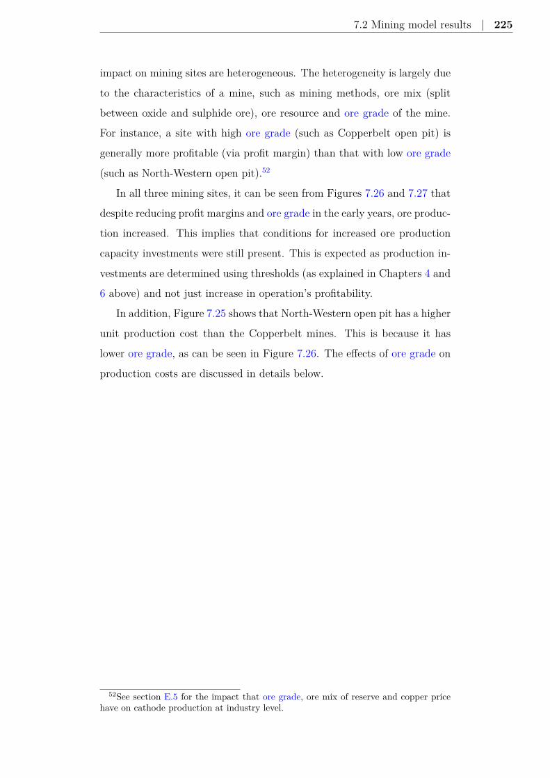
7.2 Mining model results | 225
impact on mining sites are heterogeneous. The heterogeneity is largely due
to the characteristics of a mine, such as mining methods, ore mix (split
between oxide and sulphide ore), ore resource and ore grade of the mine.
For instance, a site with high ore grade (such as Copperbelt open pit) is
generally more profitable (via profit margin) than that with low ore grade
(such as North-Western open pit).52
In all three mining sites, it can be seen from Figures 7.26 and 7.27 that
despite reducing profit margins and ore grade in the early years, ore produc-
tion increased. This implies that conditions for increased ore production
capacity investments were still present. This is expected as production in-
vestments are determined using thresholds (as explained in Chapters 4 and
6 above) and not just increase in operation’s profitability.
In addition, Figure 7.25 shows that North-Western open pit has a higher
unit production cost than the Copperbelt mines. This is because it has
lower ore grade, as can be seen in Figure 7.26. The effects of ore grade on
production costs are discussed in details below.
52See section E.5 for the impact that ore grade, ore mix of reserve and copper pricehave on cathode production at industry level.
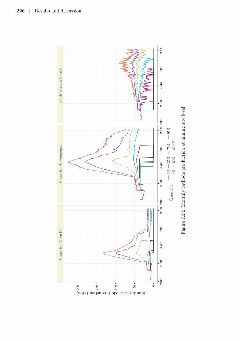
226 | Results and discussion
Cop
perb
elt
Ope
n Pi
tC
oppe
rbel
t U
nder
grou
ndN
orth
-Wes
tern
Ope
n Pi
t
050100
150
200 20
1020
2020
3020
4020
5020
1020
2020
3020
4020
5020
1020
2020
3020
4020
50
Monthly Cathode Production (kton)
Qua
ntile
: 0% 5%
25%
50%
75%
87.5
%95
%
Figu
re7.
24:
Mon
thly
cath
ode
prod
uctio
nat
min
ing
site
leve
l

7.2 Mining model results | 227
Cop
perb
elt
Ope
n Pi
tC
oppe
rbel
t U
nder
grou
ndN
orth
-Wes
tern
Ope
n Pi
t
0
2000
4000
6000
8000
2010
2020
2030
2040
2050
2010
2020
2030
2040
2050
2010
2020
2030
2040
2050
Unit Prod. Cost (US$/ton)
Qua
ntile
: 0% 5%
25%
50%
75%
87.5
%95
%
Figu
re7.
25:
Uni
tpr
oduc
tion
cost
atm
inin
gsit
ele
vel
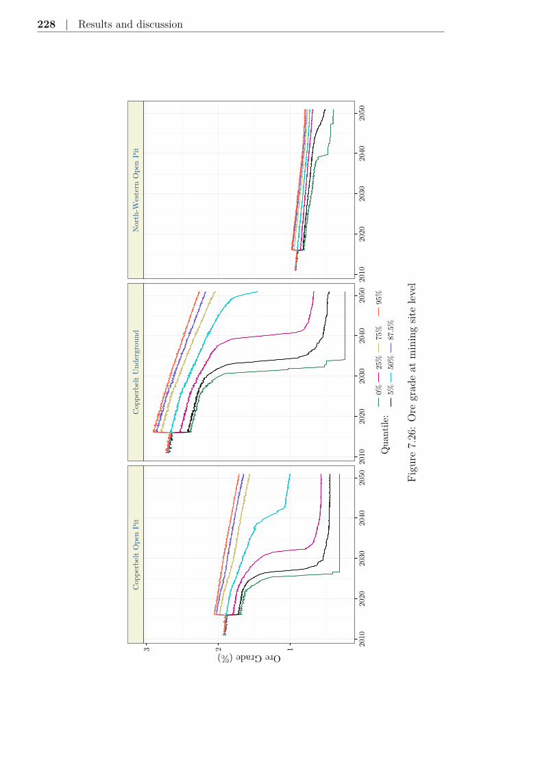
228 | Results and discussion
Cop
perb
elt
Ope
n Pi
tC
oppe
rbel
t U
nder
grou
ndN
orth
-Wes
tern
Ope
n Pi
t
123 2010
2020
2030
2040
2050
2010
2020
2030
2040
2050
2010
2020
2030
2040
2050
Ore Grade (%)
Qua
ntile
: 0% 5%
25%
50%
75%
87.5
%95
%
Figu
re7.
26:
Ore
grad
eat
min
ing
site
leve
l
7.2 Mining model results | 229
Cop
perb
elt
Ope
n Pi
tC
oppe
rbel
t U
nder
grou
ndN
orth
-Wes
tern
Ope
n Pi
t
1234 2010
2020
2030
2040
2050
2010
2020
2030
2040
2050
2010
2020
2030
2040
2050
Monthly Ore Production (Mton)
Cop
perb
elt
Ope
n Pi
tC
oppe
rbel
t U
nder
grou
ndN
orth
-Wes
tern
Ope
n Pi
t
0
100
200
300
400 20
1020
2020
3020
4020
5020
1020
2020
3020
4020
5020
1020
2020
3020
4020
50
Profit Margin (%)
Figu
re7.
27:
Aver
age
mon
thly
ore
prod
uctio
nan
dpr
ofit
mar
gin
atm
inin
gsit
ele
vel
230 | Results and discussion
From literature and also in practice, copper cathode production is largely
determined by the energy supply capacity53, ore production capacity, avail-
able ore, ore grade and profitability of an operation. The energy supply
capacity, in the model, is not explicitly expressed except through the en-
ergy prices (which were estimated as explained above)54. The impact of
energy prices is given in section 7.2.3 below. However, the ore production
capacity, ore grade, available ore and profitability are explicitly captured
endogenously. Thus, based on the model structure, ore production ca-
pacity, available ore and profitability55 could be said to be drivers of ore
production.56 Further, ore grade influences ore production through prof-
itability. Apart from that, cathode production is a function of produced
ore and ore grade57.
Figure 7.28 shows the correlation58 (based on the 1, 200 simulation runs
described in the first paragraph of this sub-section) between ore production
and its drivers. This correlation can be explained as follows: “0” means
no relationship, “+1” means a strong limiting influence and “-1” means a
weak limiting influence (i.e. enhance more ore production). It can be seen
that there is a strong correlation between ore production and profitability
capacity; this shows the strong influence that copper price has on produc-
tion. The profitability capacity59 is a function of revenue and production
costs60, with time delays61. For Copperbelt sites, installed capacity also
has a strong correlation in earlier years but the relationship tails off later.
This is expected as can be seen from the figure that production and in-
53The quantity of energy and energy capacity available to support copper productionprocess.
54Because the focus the research was to estimate the size of supply capacity thatwould need to be developed in order to meet demand, it was assumed that all requiredenergy would be met at a price.
55The profitability function is defined in Equations 6.7 – 6.9 and 6.22 – 6.25 above.56There are many more factors that drive ore production in actual copper industry
such as adopted business strategy, lobbying tactics and industry politics.57See Figure E.12 (Appendix E) for the graph on average ore grade, ore and cathode
production of 1200 simulation runs.58Correlation (defined in Equation 6.56) was calculated using the statistical screening
methods which are described on page 182 above.59See Equations 6.9 - 6.6 for a definition.60Ore grade has an indirect effect on production costs.61The time delay in the prof. capacity is the same as the loss tolerance time (tr).

7.2 Mining model results | 231
stalled capacity gap grows in later years. In the North-Western open pit,
there is a weak relationship between ore production and installed capacity,
this is because the site is a marginal cost mine. Further, because all sites
have substantial ore resources, the impact of available ore on production is
insignificant though it slightly increases towards the end of the simulation
for Copperbelt sites62. This is because of ore resource depletion.
62See Figure E.13 (Appendix E) for the gap between available ore, mined ore and oreproduction capacities.
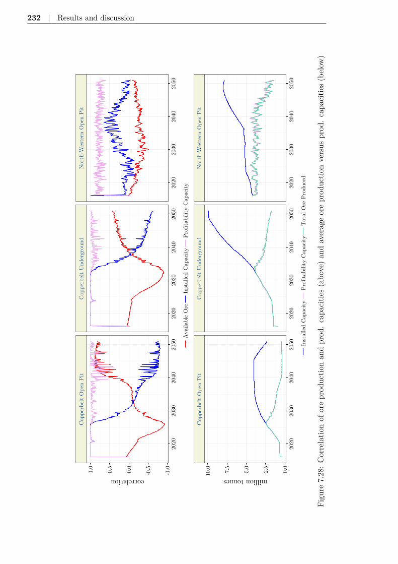
232 | Results and discussion
Cop
perb
elt
Ope
n Pi
tC
oppe
rbel
t U
nder
grou
ndN
orth
-Wes
tern
Ope
n Pi
t
-1.0
-0.50.0
0.5
1.0
2020
2030
2040
2050
2020
2030
2040
2050
2020
2030
2040
2050
correlation
A
vaila
ble
Ore
Inst
alle
d C
apac
ityPr
ofita
bilit
y C
apac
ity
Cop
perb
elt
Ope
n Pi
tC
oppe
rbel
t U
nder
grou
ndN
orth
-Wes
tern
Ope
n Pi
t
0.0
2.5
5.0
7.5
10.0
2020
2030
2040
2050
2020
2030
2040
2050
2020
2030
2040
2050
million tonnes
In
stal
led
Cap
acity
Prof
itabi
lity
Cap
acity
Tot
al O
re P
rodu
ced
Figu
re7.
28:
Cor
rela
tion
ofor
epr
oduc
tion
and
prod
.ca
paci
ties
(abo
ve)
and
aver
age
ore
prod
uctio
nve
rsus
prod
.ca
paci
ties
(bel
ow)

7.2 Mining model results | 233
While change in ore grade is driven by production (an endogenous fac-
tor), dynamics of profitability are driven by both exogenous factors (cop-
per price, mineral royalty tax and input costs) and endogenous factors (ore
grade and loss tolerance time) to the mining firm. It is, therefore, impor-
tant to understand how this loop (production–ore grade–profitability loop)
re-enforces itself.
The impact of the firm’s loss tolerance time63, tr, (defined in Equa-
tion 6.8) on ore production is given in Figure 7.29. It can be seen that
the shorter the loss tolerance time, the more variance there is in produc-
tion from one period to the next. This behaviour is more pronounced in
marginal mining operations such as the North-Western open pit, which try
to protect themselves from losses over an extended time period.
63Loss tolerance time is the duration a firm is willing to keep its operation going whilein a loss making position (where copper price is less than the unit production cost).
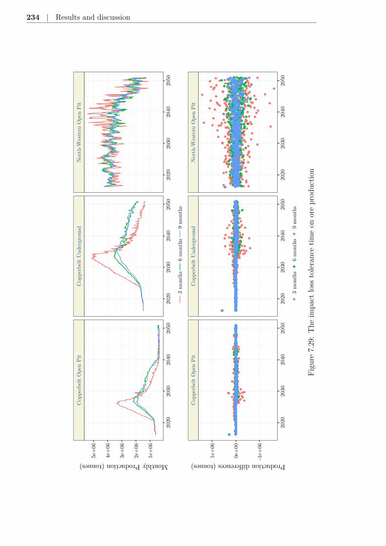
234 | Results and discussion
Cop
perb
elt
Ope
n Pi
tC
oppe
rbel
t U
nder
grou
ndN
orth
-Wes
tern
Ope
n Pi
t
1e+
06
2e+
06
3e+
06
4e+
06
5e+
06
2020
2030
2040
2050
2020
2030
2040
2050
2020
2030
2040
2050
Monthly Production (tonnes)
3 m
onth
s6
mon
ths
9 m
onth
s
Cop
perb
elt
Ope
n Pi
tC
oppe
rbel
t U
nder
grou
ndN
orth
-Wes
tern
Ope
n Pi
t
-1e+
06
0e+
00
1e+
06
2020
2030
2040
2050
2020
2030
2040
2050
2020
2030
2040
2050
Production differences (tonnes)
3 m
onth
s6
mon
ths
9 m
onth
s
Figu
re7.
29:
The
impa
ctlo
ssto
lera
nce
time
onor
epr
oduc
tion
7.2 Mining model results | 235
Being a function of total revenue and total production costs, profitabil-
ity can be expressed and analysed in terms of copper price and unit pro-
duction cost. The components of unit production cost64 are given in Figure
7.30. It can be seen that other production costs65 (which is disaggregated in
Figure 7.31 below) is the biggest share. This is followed by the by-products
credits, which play a significant role in reducing the unit cost of produc-
tion in the North-Western open pit. The share of mineral royalty tax is
similar in all three sites because it is applied at cathode level. Hence, it
is not affected by ore grade. Furthermore, because the new capital invest-
ment cost is amortised over a life span of the capacity (15 years for electric
motors and 25 years for all other mining equipment), the impact of loan
repayments relative to other costs is insignificant.66 However, should the
mine halt its operations, the mining firm would have to service the loan
accrued to facilitate capacity investment. There is, therefore, a tendency
in the mining industry to use a shorter pay-back period when amortising
their capital investments in order to avoid servicing loans when the mine
halts its operation.
64The correlation between total production costs and ore production is shown in FigureE.15 (Appendix E).
65This includes labour, energy, transport and other operating costs.66Apart from using loans to finance investment into new capacity, a firm could also
use its financial resources as was the case in this model.
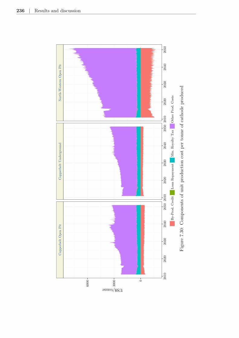
236 | Results and discussion
Cop
perb
elt
Ope
n Pi
tC
oppe
rbel
t U
nder
grou
ndN
orth
-Wes
tern
Ope
n Pi
t
0
3000
6000
2010
2020
2030
2040
2050
2010
2020
2030
2040
2050
2010
2020
2030
2040
2050
US$/tonne
By-P
rod.
Cre
dit
Loan
Rep
aym
ent
Min
. Roy
alty
Tax
Oth
er P
rod.
Cos
ts
Figu
re7.
30:
Com
pone
nts
ofun
itpr
oduc
tion
cost
per
tonn
eof
cath
ode
prod
uced
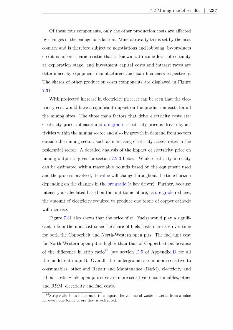
7.2 Mining model results | 237
Of these four components, only the other production costs are affected
by changes in the endogenous factors. Mineral royalty tax is set by the host
country and is therefore subject to negotiations and lobbying, by-products
credit is an ore characteristic that is known with some level of certainty
at exploration stage, and investment capital costs and interest rates are
determined by equipment manufacturers and loan financiers respectively.
The shares of other production costs components are displayed in Figure
7.31.
With projected increase in electricity price, it can be seen that the elec-
tricity cost would have a significant impact on the production costs for all
the mining sites. The three main factors that drive electricity costs are:
electricity price, intensity and ore grade. Electricity price is driven by ac-
tivities within the mining sector and also by growth in demand from sectors
outside the mining sector, such as increasing electricity access rates in the
residential sector. A detailed analysis of the impact of electricity price on
mining output is given in section 7.2.3 below. While electricity intensity
can be estimated within reasonable bounds based on the equipment used
and the process involved, its value will change throughout the time horizon
depending on the changes in the ore grade (a key driver). Further, because
intensity is calculated based on the unit tonne of ore, as ore grade reduces,
the amount of electricity required to produce one tonne of copper cathode
will increase.
Figure 7.31 also shows that the price of oil (fuels) would play a signifi-
cant role in the unit cost since the share of fuels costs increases over time
for both the Copperbelt and North-Western open pits. The fuel unit cost
for North-Western open pit is higher than that of Copperbelt pit because
of the difference in strip ratio67 (see section D.5 of Appendix D for all
the model data input). Overall, the underground site is more sensitive to
consumables, other and Repair and Maintenance (R&M), electricity and
labour costs, while open pits sites are more sensitive to consumables, other
and R&M, electricity and fuel costs.67Strip ratio is an index used to compare the volume of waste material from a mine
for every one tonne of ore that is extracted.
238 | Results and discussion
Cop
perb
elt
Ope
n Pi
tC
oppe
rbel
t U
nder
grou
ndN
orth
-Wes
tern
Ope
n Pi
t
0.00
0.25
0.50
0.75
1.00
2010
2020
2030
2040
2050
2010
2020
2030
2040
2050
2010
2020
2030
2040
2050
share
C
onsu
mab
les,
Oth
er a
nd R
&M
Cos
tsEl
ectr
icity
Cos
tFu
el C
osts
Labo
ur C
osts
Tra
nspo
rt C
osts
Figu
re7.
31:
Com
pone
nts
ofO
ther
Prod
uctio
nC
osts
per
tonn
eof
cath
ode
prod
uced
7.2 Mining model results | 239
In summary, cathode production is determined by available ore produc-
tion capacity, ore grade and profitability.68 The interactions of these three
factors and also taking into account time delays69 within the production
process affect how much copper cathode is produced in a particular time-
step. Exogenous factors such as mineral royalty tax, energy prices and raw
input costs impact the unit cost of production. This unit cost is further
significantly impacted by the ore grade (an endogenous factor). When the
unit cost of production is considered in the light of copper price (an ex-
ogenous factor), profitability of a mining activity can be calculated. By
considering profitability, a mining firm can decide whether to produce or
not and also on whether to invest in more ore production capacity.
7.2.3 Impact of increasing access to clean energy
The analysis in this sub-section and also in sub-sections 7.2.4 and 7.2.5
focus on the five scenarios that are described in section 5.3. This was done
in order to give easy to understand context and analysis. This sub-section
presents and discusses results of the impact that increasing access to clean
energy would have on the mining firm’s total cathode production and profit.
It considers price increase relative to that constant electricity price (that
was used to simulate production in Figure 7.20) and the estimated prices
of the five energy demand scenarios, described in section 5.3.70 The impact
was estimated by taking the difference between the total cumulative sum of
a scenario (say scenario 1) and that of the scenario with constant electricity
price and dividing it with the total cumulative sum of the scenario with
constant electricity price.
Taking a constant copper price of US$7, 000 per tonne, Figure 7.3268There are many more factors that could impact ore production and capacity in-
vestments in the actual copper industry such as the firm’s adopted business strategy,lobbying tactics, industrial relations and other industry politics. However, these werenot analysed because the focus of the research was on how increasing access to cleanenergy in residential sector would impact the copper industry and also because therewould not have been enough time during the PhD process to address all these otherdrivers.
69Such as loss tolerance time and the firm’s tolerance threshold defined in Eq. 6.7.70The constant price is the price of the Initial run while the estimated price is the
price of the Last Iteration as shown in Figure 7.23 above.

240 | Results and discussion
shows the effect that different electricity prices have on cathode produc-
tion at mining site level. While cathode production patterns do not signif-
icantly change relative to the initial scenario (with the constant electricity
price) across energy scenarios for Copperbelt mining sites, increasing ac-
cess to clean energy affects North-Western mines considerably. This is
because of the low ore grade that North-Western open pit has (see the dis-
cussion in section 7.2.2 above). Thus, marginal mining firms, such as the
North-Western mines, would be the most impacted by policies that target
increasing access to clean electricity.
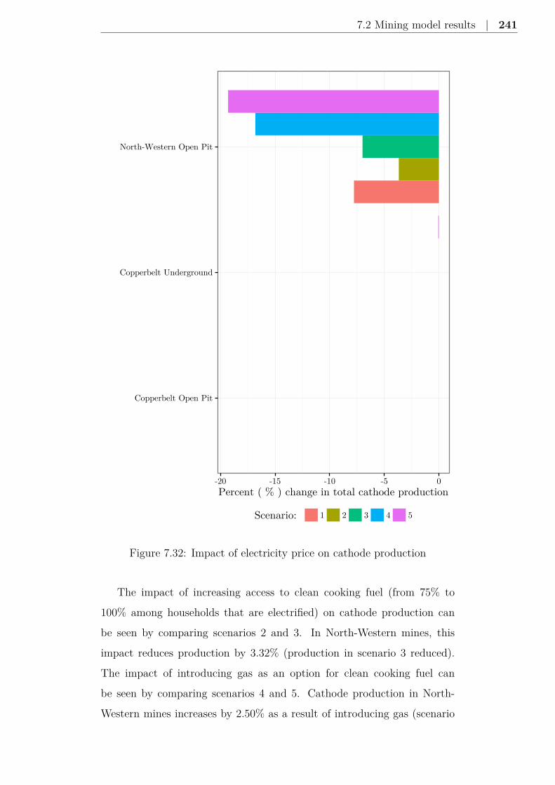
7.2 Mining model results | 241
Copperbelt Open Pit
Copperbelt Underground
North-Western Open Pit
-20 -15 -10 -5 0Percent ( % ) change in total cathode production
Scenario: 1 2 3 4 5
Figure 7.32: Impact of electricity price on cathode production
The impact of increasing access to clean cooking fuel (from 75% to
100% among households that are electrified) on cathode production can
be seen by comparing scenarios 2 and 3. In North-Western mines, this
impact reduces production by 3.32% (production in scenario 3 reduced).
The impact of introducing gas as an option for clean cooking fuel can
be seen by comparing scenarios 4 and 5. Cathode production in North-
Western mines increases by 2.50% as a result of introducing gas (scenario
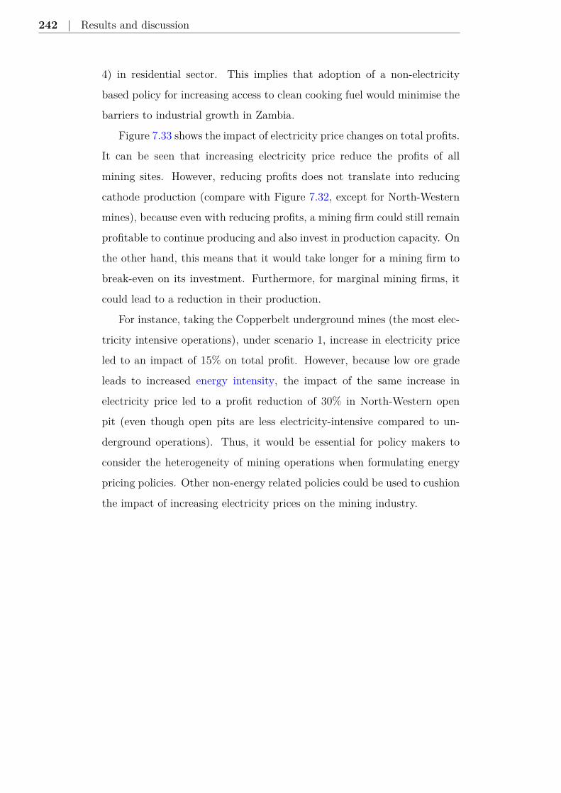
242 | Results and discussion
4) in residential sector. This implies that adoption of a non-electricity
based policy for increasing access to clean cooking fuel would minimise the
barriers to industrial growth in Zambia.
Figure 7.33 shows the impact of electricity price changes on total profits.
It can be seen that increasing electricity price reduce the profits of all
mining sites. However, reducing profits does not translate into reducing
cathode production (compare with Figure 7.32, except for North-Western
mines), because even with reducing profits, a mining firm could still remain
profitable to continue producing and also invest in production capacity. On
the other hand, this means that it would take longer for a mining firm to
break-even on its investment. Furthermore, for marginal mining firms, it
could lead to a reduction in their production.
For instance, taking the Copperbelt underground mines (the most elec-
tricity intensive operations), under scenario 1, increase in electricity price
led to an impact of 15% on total profit. However, because low ore grade
leads to increased energy intensity, the impact of the same increase in
electricity price led to a profit reduction of 30% in North-Western open
pit (even though open pits are less electricity-intensive compared to un-
derground operations). Thus, it would be essential for policy makers to
consider the heterogeneity of mining operations when formulating energy
pricing policies. Other non-energy related policies could be used to cushion
the impact of increasing electricity prices on the mining industry.
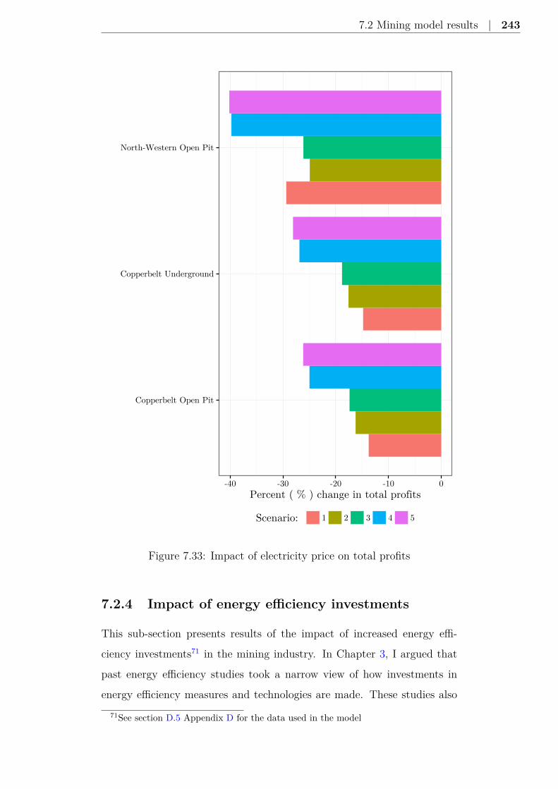
7.2 Mining model results | 243
Copperbelt Open Pit
Copperbelt Underground
North-Western Open Pit
-40 -30 -20 -10 0Percent ( % ) change in total profits
Scenario: 1 2 3 4 5
Figure 7.33: Impact of electricity price on total profits
7.2.4 Impact of energy efficiency investments
This sub-section presents results of the impact of increased energy effi-
ciency investments71 in the mining industry. In Chapter 3, I argued that
past energy efficiency studies took a narrow view of how investments in
energy efficiency measures and technologies are made. These studies also71See section D.5 Appendix D for the data used in the model
244 | Results and discussion
presented the energy cost as being significant such that investing in efficient
measures and technologies would alter the production and profitability of
the industry. Further, because they found that despite investment oppor-
tunities being available but with limited investments happening, they then
focused on recommendations of how to overcome these investment barriers.
In line with the observation by Haglund (2010), I argued that past
energy efficiency investments studies did not capture the broad spectrum
of investment options that a firm could use to reduce its production cost.
And based on the interviews’ findings, I further argued that some of the
factors considered as investment barriers may not be barriers in themselves.
This is because as Prain (1975) observed that mining firms investments
are driven by the firm’s desired investment and profit margin threshold.
That is, a firm that achieves its desired profit margins would not invest
in technology that could help it to further increase its margins. Thus, I
argued, some energy efficient opportunities would go untapped.
Figure 7.34, 7.35 and 7.36 below shows the cumulative impact of solely
investing in standard motors and efficient motors on total cathode produc-
tion, total profits and total electricity demand respectively.72 From these
three Figures, it can be seen that while solely investing in efficient mo-
tors would lead to increased total profits (and investing in standard motors
would reduce total profits); the overall impact on production is only notice-
able in North-Western open pits. Furthermore, if a marginal mine (such as
North-Western open pit) overlooks investing in energy efficient measure and
technologies, its operational life could be reduced as can be inferred from
Figures 7.34 and 7.36. On the whole, comparing the impacts of increase in
electricity price (due to increase in access to clean energy) and increase in
energy efficient investment, the impact of price would be significant. This
could explain why interviewed mining firms were more concerned about
electricity price than on mitigation options (such as investing in efficient
technologies). Furthermore, these Figures confirmed my argument that in-72The impact was estimated by taking the difference between the total cumulative
sum of the normal motor investment rule and that of either standard motor investmentonly rule or efficient motor investment only rule and dividing it with the total cumulativesum of the normal motor investment rule.
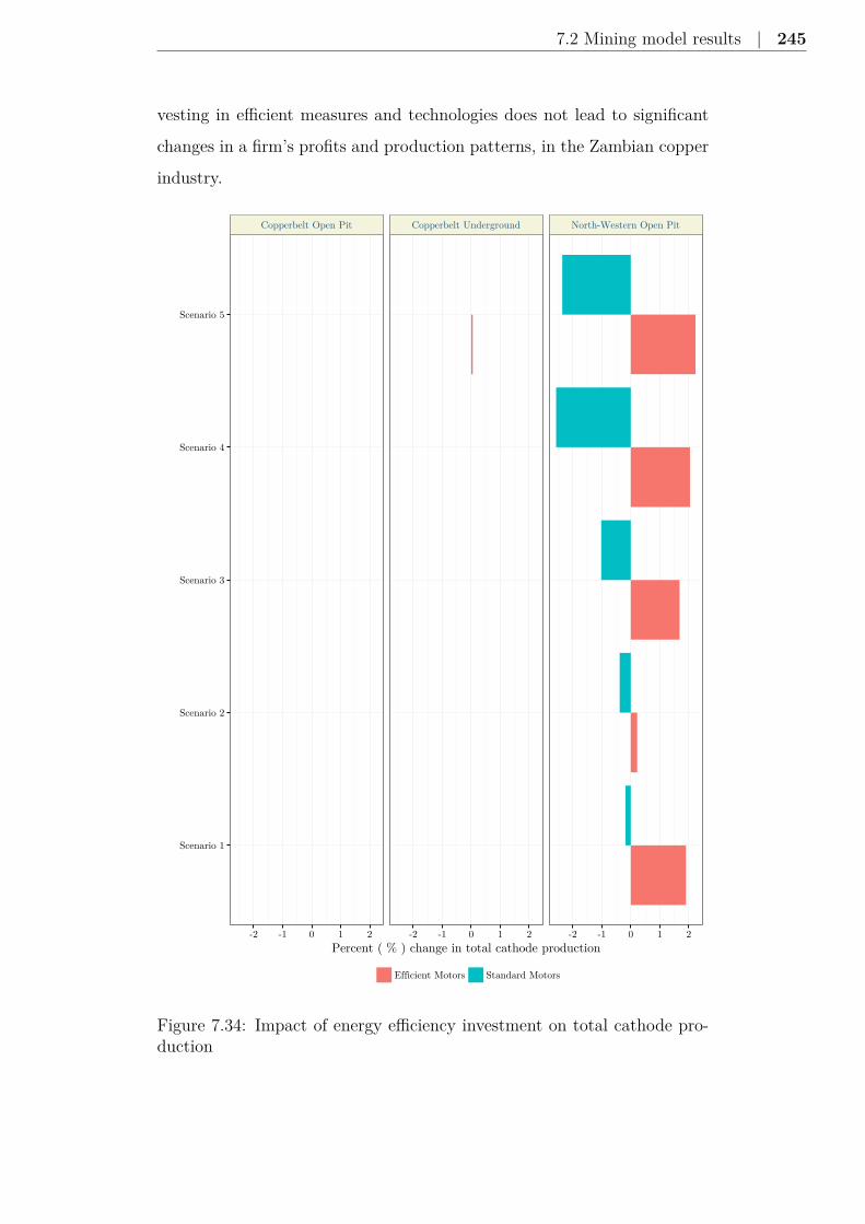
7.2 Mining model results | 245
vesting in efficient measures and technologies does not lead to significant
changes in a firm’s profits and production patterns, in the Zambian copper
industry.
Copperbelt Open Pit Copperbelt Underground North-Western Open Pit
Scenario 1
Scenario 2
Scenario 3
Scenario 4
Scenario 5
-2 -1 0 1 2 -2 -1 0 1 2 -2 -1 0 1 2Percent ( % ) change in total cathode production
Efficient Motors Standard Motors
Figure 7.34: Impact of energy efficiency investment on total cathode pro-duction
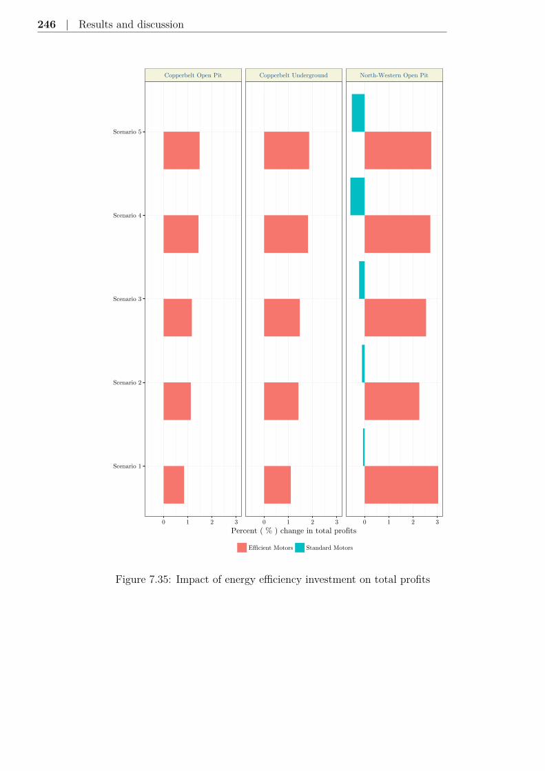
246 | Results and discussion
Copperbelt Open Pit Copperbelt Underground North-Western Open Pit
Scenario 1
Scenario 2
Scenario 3
Scenario 4
Scenario 5
0 1 2 3 0 1 2 3 0 1 2 3Percent ( % ) change in total profits
Efficient Motors Standard Motors
Figure 7.35: Impact of energy efficiency investment on total profits
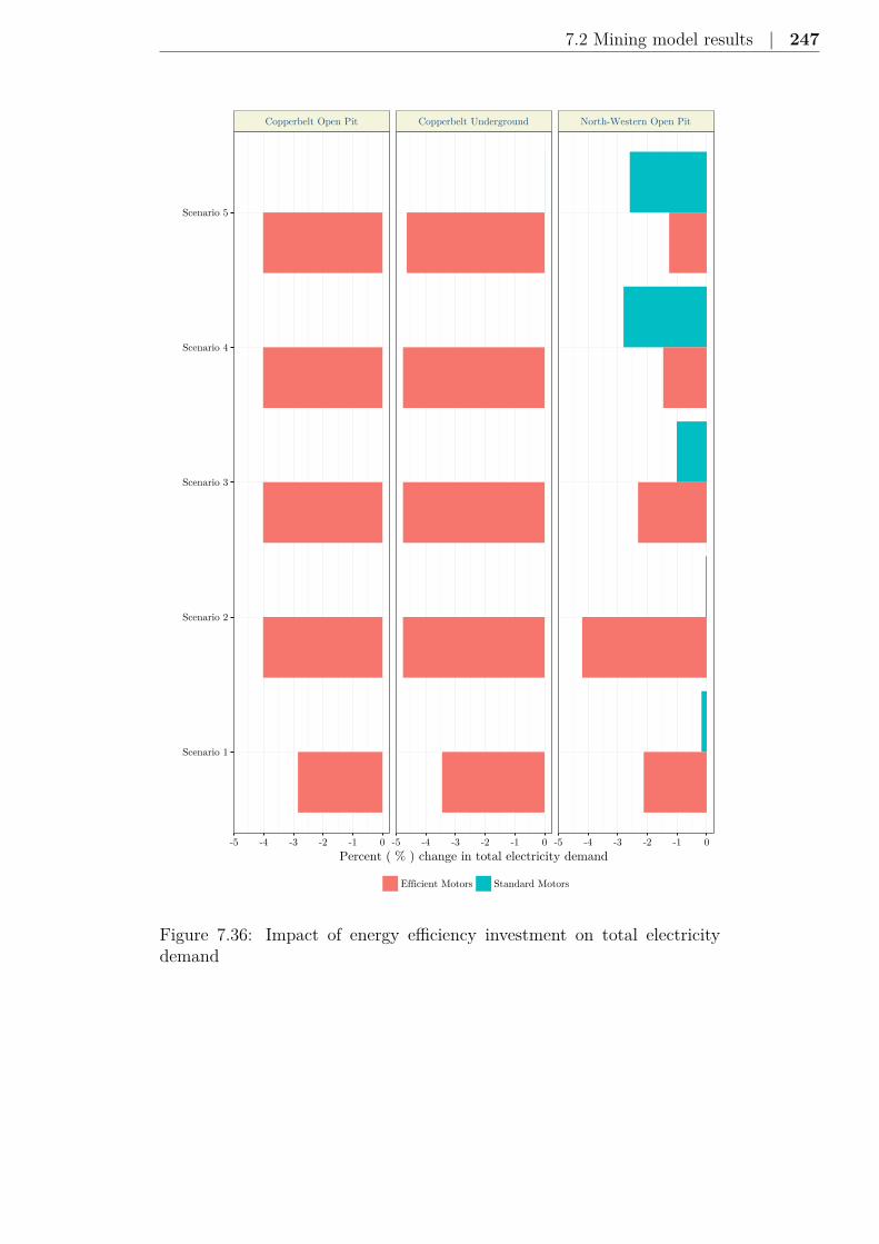
7.2 Mining model results | 247
Copperbelt Open Pit Copperbelt Underground North-Western Open Pit
Scenario 1
Scenario 2
Scenario 3
Scenario 4
Scenario 5
-5 -4 -3 -2 -1 0 -5 -4 -3 -2 -1 0 -5 -4 -3 -2 -1 0Percent ( % ) change in total electricity demand
Efficient Motors Standard Motors
Figure 7.36: Impact of energy efficiency investment on total electricitydemand
248 | Results and discussion
7.2.5 The impact of expansion strategies on the out-
look of the industry
As shown in section 7.2.1, the production output could vary enormously
based solely on the expansion strategy adopted by the industry. In this
sub-section, two expansion strategies were considered: the market-share
and profit-share expansion strategies. The market-share strategy (used
in section 7.2.1) is based on the firm’s independent expansion planning
decisions. It considers a firm that desires to grow at a certain rate based
on its own profitability and available copper ore. For instance, a firm that
wants to grow its cathode production at a maximum of 10% every year in
order to increase its market share73.
The profit-share strategy, on the other hand, considers a coordinated
expansion plan. The rate of expansion is driven by the desired industry
level output (not firm level) and the firm with the largest profit margin
is allocated the largest share of the proposed expansion. The strategy
assumes that the planner has full knowledge of the profitability of all the
firms that operate in the industry and plans their expansion in a way that
maximises the profit of the industry (in a particular time step). Similar to
the market-share strategy, a firm will expand (use up its allocated space)
based on the projected profitability of the expansion and the available ore.
Assuming a constant copper price of US$7, 000 per tonne, Figure 7.37
shows the cathode production at site level based on the expansion strate-
gies. From the Figure, it can be seen that if expansion is done based on
profit-share strategy, the industry produces more from Copperbelt open
pit in early years and de-emphasises production from North-Western open
pit until in later years. This behaviour confirms the initial position that
North-Western open pit is a high cost mine. Further, it can also be seen
that under a profit-share strategy, the longevity of the industry (particu-
larly for Copperbelt mines) could be shortened. Thus, if mining is to play a
73Within Zambia, because of different levels of firms’ profits, the rate of actual ex-pansion (not desired rate) will vary which in turn would lead to fluctuations in marketshare.
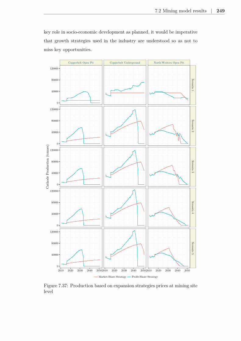
7.2 Mining model results | 249
key role in socio-economic development as planned, it would be imperative
that growth strategies used in the industry are understood so as not to
miss key opportunities.
Copperbelt Open Pit Copperbelt Underground North-Western Open Pit
0
40000
80000
120000
0
40000
80000
120000
0
40000
80000
120000
0
40000
80000
120000
0
40000
80000
120000
Scenario 1Scenario 2
Scenario 3Scenario 4
Scenario 5
2010 2020 2030 2040 20502010 2020 2030 2040 20502010 2020 2030 2040 2050
Cat
hode
Pro
duct
ion
(ton
nes)
Market-Share Strategy Profit-Share Strategy
Figure 7.37: Production based on expansion strategies prices at mining sitelevel
250 | Results and discussion
Under scenario 1 (which targets to keep cathode production output at
a maximum of 80, 000 tonnes per month), it can be seen that if the profit-
share strategy is used, it could be difficult to maintain the same level of
production through the simulation time horizon. This is because of the
difference in project lead time between underground (7 years) and open pit
(4 years) infrastructure development. Also, because the ore grades for each
mining site differ, if ore production capacity is developed in a site that has
high ore grade, then cathode production (at industry level) would increase.
More so, if the production gap was estimated based on a low ore grade
mining site.
7.2.6 Insights from the mining model analysis
From the sub-sections above, it is clear that there are various factors that
affect copper production and in turn decision making in the industry. Some
of these factors can be quantified (such as ore grade, copper and electricity
prices) while others are more qualitative in nature, such as the firm’s strate-
gic interactions with the host government and industrial labour relations.
This sub-section gives insights on operational and investment behaviours
of a mining firm. It considers combinations of five critical drivers in a mine
operation: ore grade, copper price, labour costs, energy costs and mineral
taxes.
From the research findings, copper price is the strongest predictor of the
state of a mining operation (to operate or not and to invest or not).74 That
is, a high copper price always favours copper production. For instance, if a
scenario where ore grade continues to reduce but mineral tax, copper price,
energy prices and labour costs increase is considered. The mining firm
will almost always continue to produce and invest in production capacity,
because the copper price is increasing. However, the level to change in ore
grade, mineral tax, energy price and labour costs would be of interest to
the decision maker.
In a scenario where the copper price reduces together with the ore grade,74While ore grade is a good predictor of unit production cost.
7.2 Mining model results | 251
the decision maker would need to re-evaluate the firm’s planned invest-
ments. This is because such a scenario has two critical drivers indicating a
negative trend. On one hand, the reduction in ore grade implies increase
in the firm’s production costs while on the other hand, reduction in copper
price means further reduction in a mining operation’s profitability. For a
firm to continue operating and investing in such a situation, it could be im-
portant that the firm takes mitigation actions such as investing in energy
efficiency measures or technologies (to reduce the energy cost). Another
option would be for the firm to strategically engage the host government,
in order for the government to re-look at the drivers (mineral royalty tax
and energy prices) under its control. This engagement is common practice
in Zambia’s industry as was also revealed from the interviews (see section
D.4 in Appendix D).
Whereas profitability of a mining operation is directly impacted by the
changes in any of the critical drivers, production patterns, on the other
hand, do not change linearly relative to the drivers. For instance, a change
in copper price does not always lead to a change in production levels.
This is because production is controlled by thresholds that determine the
operational behaviour of a mining firm.75 An example of such thresholds
could be, if the firm is making a profit margin of 20% or more, the firm
continues to operate normally regardless of the copper price; if the profit
margin is below 20% but above 10%, reduce production by 30% otherwise
suspend operations. Further, because a mining operation is a large and
discrete investment, reducing production linearly would lead to increase in
production costs.
75The behaviour is more like a step function (a mathematical term).
252 | Results and discussion
7.3 Discussion summary
This section discusses the findings (from literature and the two sections
above) of the research as a whole and shows how parts of the research are
linked.
From the reviewed literature, it was found that while most of the ar-
guments on energy demand and projections are around lack of statistics
(parametric uncertainty), little attention has been given to correct mod-
elling of energy demand in developing countries’ residential sector. Thus,
because of this incorrect modelling of demand, most energy research in-
forming policy (in developing countries) has been of little effect; because
it is vulnerable to conceptualisation errors (structural uncertainty). Two
categories of conceptualisation errors were identified: definition error and
key energy drivers.
Definition error has two parts: the definition of what electrification is
and the categorisation of types of energy use. Literature that has been
reviewed defined electrification in terms of getting access to electricity for
lighting service, when electrification is much more than lighting. This nar-
row definition was partly because some of the countries studied (see Ko-
matsu et al., 2011) already had access to clean energy (such as LPG and
natural gas) for their cooking and heating service. The other reason was
plainly just lack of knowledge of energy systems and how energy is used
in developing countries, particularly sub-Saharan Africa (see Rosnes and
Vennemo, 2012; Zeyringer et al., 2015). As a result, optimal solutions for
lighting service (such as off-grid solar systems) were presented as optimal
solutions for electrification (which covers cooking and heating, lighting and
other uses services). These studies failed to distinguish energy services that
can be met by different types of off-grid and grid solutions.
The other conceptualisation error was identification of key energy drivers
in the residential sector. Growth in energy demand was modelled as being
largely influenced by household income (see Rosnes and Vennemo, 2012;
Zeyringer et al., 2015) rather than government policy intervention. This is
because, one would suppose, of the desire to make energy use sustainable.
7.3 Discussion summary | 253
The challenges of increasing access to clean energy and electrification in a
sustainable way were studied by Barnes and Floor (1996). It has generally
been acknowledged that increasing of access to clean energy through gov-
ernment policy intervention is unsustainable, as government would need to
heavily subsidise energy use in order to keep the prices low. This, notwith-
standing, has continued to the case in many African countries (government
policy intervention); the importance of government intervention in facili-
tating fuel transition was argued in Hosier and Dowd (1987). In addition, if
energy demand is modelled as driven by household income, not only will it
grossly underestimate the required energy infrastructure investment efforts
but also signal that electricity and other clean energy forms demand will
grow at a slow pace. This is because household income increases at a slow
pace considering that it is a function of economic and population growth.
In the light of these identified conceptual limitations, this study used
a bottom-up method when estimating energy demand. Not only is this
method able to capture energy use at end-use level, possible government
policy interventions were captured and analysed. The energy demand sce-
narios considered76 looked at how much energy could be needed if certain
energy access targets were met. It was important that energy demand pro-
jections were properly estimated, as literature (Rosnes and Vennemo, 2012)
as well as this study found that energy demand projections have the largest
impact on the supply model (estimations of required capital investment).
In addition, by capturing energy use at end-use service level, it was possible
to model the transition from an inferior fuel to a superior fuel (as described
in the energy ladder literature).
It was also found that although there has been considerable research
on energy ladder (fuel transition), these studies assumed that the decision
maker had access to an array of energy fuels to choose from. This type
of research focused on understanding which factors were key influencers of
energy transition; which inevitably ended up focusing on the economics of
the household. However, it was found that while many rural households in
76See section 5.3 of Chapter 5.
254 | Results and discussion
Zambia could afford to use electricity (based on their income, see Chap-
ter 5), most households did not have access to electricity because it was
not available. It was, therefore, essential that energy use that is driven by
availability, and not only affordability, was also captured (this was facili-
tated by the bottom-up method). This is the other reason why considering
government policy intervention when analysing increasing energy access is
important.
The energy demand model that was developed for this study found that
apart from economic growth, income, access and fuel transition assump-
tions being important in the final energy projection estimates, population
growth assumptions were also impactful. It also found that although final
energy demand is projected to increase by at least 120% by 2050, electricity
demand, on the other hand, is expected to increase by at least 450%. In
contrast to the findings of Rosnes and Vennemo (2012), who found that
main driver of electricity demand in sub-Saharan African was economic
growth, this study found that growth in electricity demand in Zambia was
significantly influenced by the residential sector. This difference (of which
drivers are important) was as a result of different demand estimation meth-
ods: Rosnes and Vennemo (2012) used an econometric method (a top-down
approach) while in this thesis end-use method (a bottom-up approach) was
used which best captures the specifics of energy system in developing coun-
tries (Bhattacharyya and Timilsina, 2010; Pandey, 2002). This difference
further shows the impact that different modelling methods could have on
policy recommendations.
Having isolated the residential sector as a key player in future electricity
demand, an analysis that looked at the benefits of reduced deforestation as
a result of increased access to clean energy was undertaken. This analysis
is important because Zambia has in the past entered into agreements for
prevention of forest cover losses (under REDD+ initiative) on the premise
that it would reduce deforestation by increasing access to electricity. The
analysis found that such a premise is weak because Zambia would incur
a minimum cost of US$ 6, 800 per hectare while reaping maximum ben-
7.3 Discussion summary | 255
efits of US$ 5, 100 per hectare. This analysis, however, did not consider
other important benefits that come with the use of clean energy such as
reduced energy-related health illness (see Javadi et al., 2013). Therefore, it
would be important that further analysis is carried out before a firm policy
recommendation could be made.
Two other important findings on the supply side were that coal tech-
nology is projected to play a key role in electricity generation and that
technology learning for solar does not lead to significant penetration of so-
lar technology in the energy supply mix. The impact of technology learn-
ing is limited because there were other cheaper supply options available to
choose from (such as hydro technologies). On the other hand, because coal
technology is expected to play a significant role, implementation of carbon
emissions reduction targeted policies would have a noticeable impact on
the average generation costs but a positive impact on deployment of solar
technology.77
From the mining model analysis, it was found that increased electricity
price (due to increase in access to clean energy), would lead to reduced to-
tal profits in all the mining firms. However, apart from the North-Western
open pit (a marginal cost mine), production patterns and investment be-
haviour of the firms were not expected to change significantly. This is
because firms would still be enjoying healthy profit margins. This is in
agreement with Prain (1975) who noted that production behaviour of firms
is driven by the set objective and not maximisation of profits.
Furthermore, it was found that for marginal mines, the best way to keep
them profitable would be by introducing non-electricity based clean fuels
(such as LPG) in the residential sector. Such a decision would help reduce
the impact of electricity price on the mining sector. This is important
because not only would mining firms save on their energy costs but also
growth of this sector is expected to enhance growth in other sectors in
Zambia (see Chapter 1). In addition, such a measure would also help
cushion the impact of electricity price on the profitability of all economic
77See sections C.5 and C.6 in Appendix C for the input assumptions.
256 | Results and discussion
sectors and also on the affordability of electricity in the residential sector.
The level of cushion would vary depending on the specifics of the sector
being analysed.
Whereas electricity prices do not significantly change the production
patterns of the industry, production growth rates do, as can be seen in
both Figures 7.20 and 7.32 above. This implies that firms could derive
more benefits from their investments if the government focuses more on
reducing bottlenecks of industry growth rather than focusing on keeping
the electricity prices low. In the model, these industry bottlenecks (such
as the development of human capacity, better policies and regulations, rail
and road infrastructure) were represented by the production growth rate.
However, because growth and profitability of the sector are not solely
driven by the price of electricity, it was important that the decision mak-
ing process that leads to growth and profitable operations in the sector
was understood. It was found, in literature and during the fieldwork, that
firms have concrete guidelines on how strategic decisions should be made.
As part of the decision process, the firms use Discounted Cash Flow (DCF)
when evaluating investment options. This method (DCF) is the industry
standard, as was confirmed in literature, industry reports and by the min-
ing firms and experts that were interviewed during my fieldwork. Further,
the interviewed mining firms noted that the use of stochastic methods as
an evaluation method was not common. This could be in part because
final investment decisions are made at the firms’ headquarters (only per-
sonnel based in Zambia were interviewed). At headquarters, the submitted
proposed investment opportunities are further analysed relative to oppor-
tunities from other countries, then final decisions are made. While these
decisions are informed by analytic assessments, it was found that the judge-
ment of the final decision maker is critical in the process.
In order to effectively simulate copper production and growth of the
mining sector in Zambia, the guidelines used in the decision process were
implemented in a system dynamics (SD) model (see section 4.3). These
guidelines were formulated in form of thresholds, such as all opportunities
7.4 Chapter summary | 257
with a minimum of 15% RoI on technology assessment and when the firm’s
profit margin is less than 30% leads to a positive decision. This approach
(usage of simple decision rules – thresholds) was found to be a better rep-
resentation (than using an optimisation model) of how real decision makers
make decisions. This is what was found in literature (see Chapter 4) and
also during my fieldwork.
7.4 Chapter summary
This chapter presented and discussed the results of the energy and mining
models. The energy systems analysis found that total final energy demand
by 2050 would increase by between 120% to 190%, with residential sector
continuing to dominate energy demand. It also found that an increase of
450% in electricity demand would lead to about 700% increase in average
generating costs relative to 2010 value (of US$4/MWh).
Analysis of the semi-structured interviews (which were also used as in-
puts into the mining model) found78 that strategic decision making process
is a deliberate and procedural process that mining firms engage in. The key
factors (from the mining firm’s perspective) that influence decision mak-
ing were identified. Electricity price and taxation policy were found to be
the most contentious cost components in the industry. However, when dis-
cussing electricity pricing, the respondents seemed to be more focused on
the current price of electricity without considering the impact that future
electricity price could have on the industry.
An analysis of the impact that increasing electricity price would have
on the mining industry was carried out. The analysis found that not only
would increasing electricity price reduce the industry’s profitability and
cathode output, but also that it would render some mining operations
unprofitable. Further, under a scenario of constant energy prices and MRT,
the analysis found that ore grade, available ore production capacity and
a firm’s profitability (of which copper price is a key component) are key
78See sections 6.2 (of Chapter 6) and D.4 (in Appendix D) for the results.

258 | Results and discussion
determinants of how much copper cathodes could be produced. The impact
of energy efficiency investment and expansion strategy on the evolution of
the industry were also discussed.
Chapter 8
Conclusions
In this chapter, the main research findings and conclusions of the research
are presented. It then highlights how these findings contribute to knowledge
and finally concludes with suggestions for possible future research work.
8.1 Restatement of the research problem
This research hoped to address the policy challenges that Zambian govern-
ment decision makers face. They are faced with the challenge of balancing
between increasing access to clean energy and enhancing economic growth.
On one hand, increase in access to clean energy lead to increase in electric-
ity demand (as electricity is currently the only clean energy alternative).
Increase in electricity demand further exacerbates the ready existing sup-
ply shortage; thus to curb it, more capital investments would be required
in the energy sector. This translates to increase in electricity price.1 On
the other hand, the government hopes that growth in the economic sector
(particularly the mining sector) would provide the needed finance to facil-
itate increase to clean energy. However, because increase in clean energy
leads to increase in electricity price, growth of the economic sectors would1This takes in consideration that the current generation stock in Zambia’s electricity
sector has almost been amortised. Therefore, any capital investment in the sector leadsto increase in the electricity price.
260 | Conclusions
be hindered.
These complex interactions between the social goals (increasing access
to clean energy) and economic development (growth of the mining sector),
which are under-researched for many African countries, were analysed in
this study. This was important because the outcomes of these interactions
are not straightforward, as there are several feedback loops that would act
as barriers from realising these aspirations. Further, apart from the need to
expand the supply infrastructure, there is lack of knowledge of how mining
firms (the mining industry is central to these economic growth plans) in
Zambia make strategic decisions. Therefore, to effectively address these
challenges, three research questions were posed:
1. How would Zambia’s energy sector evolve by 2050?
2. How do mining organisations make strategic investment decisions and
what are the key decision variables in the mining sector?
3. What impact does increasing access to clean energy have on mining
sector’s profitability?
8.2 Main research findings
This section summarises the main findings of the research as a whole. Below
are the main findings of the research, grouped by research question.
8.2.1 Evolution of Zambia’s energy sector
Research question 1: “How would Zambia’s energy sector evolve by 2050?”
considered two parts. The demand part which focused on energy use and
how future energy demand is modelled, and the supply part which consid-
ered the capital investment cost required to meet projected demand, how
the generation costs would change and also the impact of inputs on the
supply model.
The main findings are:
8.2 Main research findings | 261
Demand modelling
1. Total final energy demand in Zambia would increase by at least 120%
(and as much as 190%) by 2050 relative to the 2010 demand (of
162 PJ). The projected demand is driven by population growth, fuel
transition, electricity access, economic growth and copper production
assumptions. In all the five scenarios considered, the residential sector
will continue to dominate demand. This dominance by the residential
sector is partly because of the continued use of traditional fuels in
scenarios 1 to 3, and also because of increased electricity consumption
due to fuel transition and increased household income in scenarios 4
to 5.
2. The residential sector is projected to be the main consumer of final
electricity by 2050, in all the five scenarios. This dynamic is largely
driven by population and electricity access (part of which is how
electricity is used within the sector) assumptions. Consumption in
the residential sector is projected to increase from 8.8 PJ to at least
84 PJ (in scenario 1) and to a maximum of 137 PJ (scenario 5)
while demand in the mining sector is only projected to increase to a
maximum of 63 PJ.
3. Of the total (all sectors) difference of 75 PJ (between scenarios) in
electricity demand in 2050, the residential sector accounts for 70% of
it. This shows that plans targeting increase in access to clean energy
need to carefully consider how population, income and energy use
patterns (both fuel transition and energy access) in the residential
sector would change. These assumptions have significant impacts on
the total demand. For instance, a scenario (scenario 4) that considers
introduction of gas as a cooking and heating fuel in the residential
sector leads to a saving of 30 PJ of electricity.
262 | Conclusions
Supply modelling
1. To meet electricity demand, the supply capacity would need to be
increased from 1, 900 MW (2010) to at least 10, 100 MW and a
maximum of 16, 100 MW. This would require a total investment cost
of US$ 35 billion and US$ 60 billion for the minimum and maximum
capacity development respectively.
2. As a result of increased capital investment, the average generation
cost is expected to increase from US$ 4/MWh (in 2010) to US$
29/MWh (minimum) and US$ 48/MWh (maximum) by 2050. Fur-
ther, it is projected that total electricity demand would increase by
600% in the scenario 5 (relative to 2010).
3. While hydro technology is projected to continue dominating electric-
ity supply (by at least 40%, from 99% in 2010), participation of coal
technology is projected to increase from 0% in 2010 to at least 27% in
2050 (under least cost assumptions). This would lead to an increase
in carbon intensity of between 300 gCO2eq/kWh (minimum) and 421
gCO2eq/kWh (maximum), from 4.25 gCO2eq/kWh in 2010.
4. A trade-off analysis between electrification and deforestation found
that to save a hectare of forest, it could cost a minimum of US$ 6,
800 while the possible benefit from that hectare would be a maxi-
mum of US$ 5, 100. Thus, it could not make financial sense if the
main purpose of electrification is to reduce deforestation. This is an
important finding because some African countries (such as Uganda
and Zambia) have in the past entered into forest cover preservation
agreements that are premised on increasing access to clean energy.
Supply model sensitivity analysis
1. Electricity demand has the most impact on the supply model. This
re-emphasises the importance of using appropriate methods when es-
timating energy demand. Two other important factors are discount
rate and the level of participation of coal technology.
8.2 Main research findings | 263
2. While technology learning could enhance penetration of renewable
energy, a reduction in investment capital cost of solar technology by
62% (between 2010 and 2050) only led to an additional penetration
of 8%. Thus, considering the available resources, the model is not
very sensitive to solar PV technology learning (i.e. the results of the
model did not change significantly despite this reduction in capital
cost as a result of technology learning).
8.2.2 Decision making in mining firms
Research question 2: “How do organisations make strategic investment
decisions and what are the key decision variables in the mining sector?”
also considered decision making in mining firms operating in Zambia. This
was important because decision making is content dependent. The main
findings included:
1. Decision making in mining firms is a deliberate and procedural pro-
cess a firm engages in. The process is always aided by analytic tools
and techniques. However, the technical evaluation notwithstanding,
the final decision could also be driven by the experience of the main
decision maker.
2. The main analytic method used in evaluating decision alternatives
in the copper industry is the Discounted Cash Flow (DCF) method.
This finding was confirmed literature, industry reports and also from
the data collected during my fieldwork.
3. Apart from requiring a minimum of 15% return on investment (RoI),
the decision maker also considers ore grade, recoverable copper from
the ore, copper price and local policy environment (i.e. taxation being
one of them) before a resource development decision would be made.
Copper price was found to be a key influencer in decision making
process; partly because access to project financing is dependent on
the long-term outlook of the price.
264 | Conclusions
4. Because mining firms operate in uncertain environment (the industry
is exposed to various kind of uncertainty such as price and policy) and
also considering that decision situations are made up of ill-structured
problems, it found that the bounded rationality model was best suited
for analysing decision making in organisations. This was found true
from empirical studies that showed that decision makers simplify their
decision rules because of limited time dedicated to a process. These
simple rules (heuristics) take a form of thresholds such as 15% RoI.
5. As from literature, it was found that labour, repair and maintenance,
energy costs, consumables, transport and taxation were the most sig-
nificant productions costs. In Zambian mining industry, there are
divergent opinions of what is considered a fair electricity tariff and
rate of taxation. This could be because the two costs are susceptible
to lobbying.
8.2.3 Impact of access to clean energy
Research question 3: “What impact does increasing access to clean energy
have on mining sector’s profitability?” considered the impact that increas-
ing access to clean energy (via increase in electricity price) would have on
the copper industry in Zambia. The main findings included:
1. Increasing access to clean energy (through electrification) has a sig-
nificant impact on the mining firm’s profit margin. In the five en-
ergy demand scenarios, this impact ranges between 13% and 41% as
shown in Figure 7.33. The impact is greatest in North-Western open
pit mine (a marginal mine), which is not even an electricity intensive
operation (being an open pit).
2. Even though the firm’s profit margins are impacted by increase in
electricity prices (due to increased access to clean energy), the impact
of electricity price on cathode production patterns is not significant
except for North-Western open pit (a marginal mine) because of its
8.3 Limitations and future work | 265
low ore grade. Among North-Western mines, the impacted is esti-
mated to be between 4% and 19%. However, if access to clean energy
is increased by using gas cathode production would be increased by
about 2.5% (i.e. comparing scenarios 4 and 5). Thus, adoption of
other fuel of clean energy would help minimise the barriers to indus-
trial growth in Zambia.
3. The three main factors that determine how much copper cathode
will be produced are available ore production capacity, ore grade and
profitability. While available ore production capacity is within the
control of the mining firm, and ore grade being an endogenous fac-
tor, profitability, on the other hand, is driven by both endogenous
and exogenous factor. The exogenous factors (such as copper, elec-
tricity and raw material input prices) are what influences a firm to
modify its behaviour in the short-term. Such a behaviour would be a
firm deciding whether to produce or not, how much to produce (if it
produces) and also on whether to invest or not in capital equipment.
8.3 Limitations and future work
While this research has presented important findings, there are some areas
that would need to be addressed to further improve the results.
8.3.1 Modelling of mineral royalty tax
In this study, mineral royalty tax was assumed to be independent of the
obtaining copper price. However, it has been observed in Zambia that the
government comes under pressure (from the general citizenry) to increase
the tax rates when the copper price is high and to reduce the rates when
the price is low (the latter pressure is from the mining firms and their lob-
bying associations). Thus, it could be important to capture this behaviour
endogenously in the model since mineral royalty tax is one of the critical
drivers of the industry; and has the potential of altering investment and
266 | Conclusions
operational behaviour of a mining firm. Apart from that, this would en-
hance the analysis of other strategic interactions and engagements between
the mining firms and the government.
8.3.2 Macroeconomic linkage
Much of this study focused on the impact that increasing access to clean
energy and copper production output would have on the copper industry.
However, to further strengthen the analysis, it is imperative to create a link
between copper production output, GDP growth (or reduction) and funds
required to increase access to clean energy. This could be done through
a macroeconomic analysis. Such an analysis would also help answer if at
all it is possible to achieve (in a sustainable way) the clean energy access
targets in Zambia.
8.3.3 Modelling of ore grade
Even though ore grade was endogenously modelled in the mining model, an
assumption was made that a firm produces high ore grade before producing
from low grade ore. However, this is not correct because mining firms
produce from the ore that is available and not from the high ore grade
then low grade ore. Further, by modelling ore grade the way it was done in
this research, the model shows that firms would make considerable profits
in early years which would make them capable of financing their capital
investments internally (no incentive to get external loan for the projects).
This implies that, on average, cost of capital had little impact on the unit
cost of production. If the ore grade is captured as in the actual industry,
the importance of cost of capital would be noticed and the firm’s unit cost
would be relatively higher than shown in this study. Capturing of ore
grade, as in the real industry, could, however, require more disaggregated
statistics and also further disaggregation of the mining model. For these
reasons, a stylised approach was used (in this study).
8.3 Limitations and future work | 267
8.3.4 Impacts of climate change
Having shown that electricity price would have a significant impact on
the profit margins of all the firms, it would be essential to consider the
impact that projected climate change patterns (see Arnell (2004); Harrison
and Whittington (2002); Mukheibir (2007); Ragab and Prudhomme (2002);
Tadross et al. (2005)) in Southern Africa would have on Zambia’s hydro-
power dominated electricity system. The evolution of the mining industry
could then be analysed under scenario settings that are also driven by
changes in climate. This is important because Spalding-Fecher et al. (2016;
2017) found that electricity production from hydro plants in the Zambezi
River basin would reduce due to climate change. In the light of this thesis,
such an analysis could bring to the fore two important questions: how
much additional effort would be required to increase access to clean energy
in Zambia? and, what impact would climate change effects have on the
growth of the mining industry in Zambia?
8.3.5 A comprehensive energy resource mapping
The research found that the timing (when a resource would be available)
and the size of the resource have an impact on how the energy system
would develop and also on the average generation cost. Thus, in order to
reduce uncertainty when estimating the required investment capital and
sudden spikes in the average generation cost, it would be essential to com-
prehensively map out the energy resources that are available in Zambia and
around Zambia. This would help minimise building of expensive technolo-
gies that serve as emergency power supply when all other capacities have
been exhausted in a time step. For instance, the building and operating of
oil technology between 2012 and 2016.
268 | Conclusions
8.4 Thesis conclusion
This thesis reviewed literature and used a systems approach to fill some
gaps in existing body of knowledge on the socio-economic challenges (with
respect to clean energy access and industrial growth) that small develop-
ing countries like Zambia2 face. It contributed to the body of knowledge of
how to model an energy system of a small developing country, whose access
to clean energy is low. It showed the challenges that countries that have
limited options for increasing access to clean energy (in this case, Zambia
only has electricity as a clean energy form) have. It found that beyond
the economics of a household (household’s ability to pay for clean energy),
increasing access to clean energy would require considerable capital invest-
ment into the energy system. Which if not properly planned, would impact
on the growth of the industrial sector, this, in turn, would make access to
clean energy unsustainable (because households would not afford to pay
for clean energy).
Furthermore, whereas past strategic investment studies in the mining
industry focused on either the financial part or the engineering part of a
firm, this thesis considered both parts and combined them when analysing
investment behaviour under uncertainty. The mining model that was de-
veloped is novel in that it implements a bounded rational simulation model
and captures the investment and operational behaviours of mining firms in
detail. This helped in isolating critical strategic decision making drivers in
the mining industry. It also considered the sequential and feedback loops
between decision environments that are usually not accounted when study-
ing decision making in firms. This thesis, therefore, devised a framework
that could be used to study a country that hopes to use its natural resources
to enhance its socio-economic development (an interdependence trade-off
analysis between sectors of an economy).
2This thesis produced energy and mining models and frameworks for critical analyt-ical thinking for Zambia that did not exist before.

References
Adler, R. W. (2000). Strategic Investment Decision Appraisal Techniques:
The Old and the New. Business Horizons, (November/December):15–22.
Agostini, C. A. (2006). Estimating Market Power in the US Copper Indus-
try. Review of Industrial Organization, 28:17–39.
Aguirregabiria, V. and Luengo, A. (2015). A Microeconometric Dynamic
Structural Model of Copper Mining Decisions.
Akbaba, M. (1999). Energy conservation by using energy efficient electric
motors. Applied Energy, 64:149–158.
Alkaraan, F. and Northcott, D. (2006). Strategic capital investment
decision-making: A role for emergent analysis tools? The British Ac-
counting Review, 38(2):149–173.
Alkaraan, F. and Northcott, D. (2007). Strategic investment decision mak-
ing: the influence of pre-decision control mechanisms. Qualitative Re-
search in Accounting & Management, 4(2):133–150.
Alvarado, S., Maldonado, P., Barrios, A., and Jaques, I. (2002). Long
term energy-related environmental issues of copper production. Energy,
27(2):183–196.
Alvarado, S., Maldonado, P., and Jaques, I. (1999). Energy and environ-
mental implications of copper production. Energy, 24(4):307–316.
Arnell, N. W. (2004). Climate change and global water resources: SRES
emissions and socio-economic scenarios. Global Environmental Change,
14(1):31–52.
Artinger, F., Petersen, M., and Gigerenzer, G. (2014). Heuristics as adap-
tive decision strategies in management. Organizational Behavior, (Au-
gust).
270 | References
Ashford;, R. W., Dyson;, R. G., and Hodges;, S. D. (1988). The Capital-
Investment Appraisal of New Technology: Problems, Misconceptions and
Research Directions. The Journal of the Operational Research Society,
39(7):637–642.
Auger, F. and Ignacio Guzmán, J. (2010). How rational are investment
decisions in the copper industry? Resources Policy, 35(4):292–300.
Auping, W. (2011). The uncertain future of copper. Masters thesis, Delft
University of Technology.
Barlas, Y. and Carpenter, S. (1990). Philosophml roots of model validation:
two paradigms. System Dynamics Review, 6(2):148–166.
Barnes, D. F. and Floor, W. M. (1996). Rural energy in developing coun-
tries: A Challenge for Economic. Annu. Rev. Energy Environ, 21:497–
530.
Barrett, M., Lowe, R., Oreszczyn, T., and Steadman, P. (2008). How to
support growth with less energy. Energy Policy, 36(12):4592 – 4599.
Foresight Sustainable Energy Management and the Built Environment
Project.
Barrett, M. and Spataru, C. (2013). Storage in energy systems. Energy
Procedia, 42(Supplement C):670 – 679. Mediterranean Green Energy
Forum 2013: Proceedings of an International Conference MGEF-13.
Bartrop, S. and White, A. (1995). Spade work: how miners value resources.
JASSA, pages 7–13.
Bearden, N. J., Murphy, R. O., and Rapoport, A. (2005). A multi-attribute
extension of the secretary problem: Theory and experiments. Mathemat-
ical Psychology, 49:410–422.
Bhappu, R. R. and Guzman, J. (1995). Mineral investment decision mak-
ing: study of practices. Engineering and Mining Journal, (July).
Bhattacharyya, S. C. (2006). Renewable energies and the poor: niche or
nexus? Energy Policy, 34:659–663.
Bhattacharyya, S. C. and Timilsina, G. R. (2009). Energy Demand Mod-
els for Policy Formulation: A Comparative Study of Energy Demand
Models.

References | 271
Bhattacharyya, S. C. and Timilsina, G. R. (2010). Modelling energy de-
mand of developing countries: Are the specific features adequately cap-
tured? Energy Policy, 38(4):1979–1990.
Bisschop, J. (2008). AIMMS: Optimization Modeling. Paragon Decision
Technology, ES Haarlem.
BNEF (2016). Scaling solar for Africa: Zambia’s 6-cent PV. Technical
report, Bloomberg Finance, New York.
Bortoni, E. D. C. (2009). Are my motors oversized? Energy Conversion
and Management, 50(9):2282–2287.
Botín, J. A., Castillo, M. F. D., Guzmán, R. R., and Smith, M. L. (2012).
Real options: a tool for managing technical risk in a mine plan. pages
1–7, Seattle. SME Annual Meeting.
Boulamanti, A. and Moya, J. A. (2016). Production costs of the non-ferrous
metals in the EU and other countries: Copper and zinc. Resources Policy,
49:112–118.
BoZ (2011). Annual Report 2011. Technical report, Bank of Zambia,
Lusaka.
Brennan, M. J. and Schwartz, E. S. (1985). Evaluating Natural Resource
Investments. The Journal of Business, 58(2):135–157.
Butler, R., Davies, L., Pike;, R., and Sharp;, J. (1991). Strategic invest-
ment decision-making: complexities, politics and processes. Journal of
Management Studies, 28(July):395–415.
Byron, M. (1998). Satisficing and Optimality. Ethics, 109(1):67–93.
Cabraal, R. A., Barnes, D. F., and Agarwal, S. G. (2005). Productive Uses
of Energy for Rural Development. Annual Review of Environment and
Resources, 30(1):117–144.
Cacho, O. J., Milne, S., Gonzalez, R., and Tacconi, L. (2014). Bene fi
ts and costs of deforestation by smallholders: Implications for forest
conservation and climate policy. Ecological Economics, 107:321–332.
Carpinelli, G. and Russo, A. (2014). Behavioral perspective of power sys-
tems’ decision makers. Electrical Power and Energy Systems, 58:111–119.
Cauwenbergh, A. V., Durinck, E., Martens, R., Laveren, E., and Bogaert,
272 | References
I. (1996). On the role and function of formal analysis in strategic in-
vestment decision processes: results from an empirical study in Belgium.
Management Accounting Research, 7:169–184.
CEC (2013). CEC Electricity Statistics.
Chidumayo, E. (1987). A Survey of Wood Stocks for Charcoal Production
in the Miombo Woodlands of Zambia. Forest Ecology and Management,
20:105–115.
Chidumayo, E. N. (1991). Woody Biomass Structure and Ufilisation for
Charcoal Production in a Zambian Miombo Woodland. Bioresource
Technology, 37:43–52.
Chidumayo, E. N. (2013). Forest degradation and recovery in a miombo
woodland landscape in Zambia: 22 years of observations on permanent
sample plots. Forest Ecology and Management, 291:154–161.
CIMVAL (2003). Standards and guidelines for valuation of mineral prop-
erties. Technical Report February.
Cochilco (2012). Mining Production Yearly Statistics Publications: 1997-
2010.
Cohen, M. D., March, J. G., and Olsen, J. P. (1972). A garbage can model
of organizational choice. Administrative Science Quarterly, 17(1):1–25.
CoM (2014). Presentation on the impacts of Vat Rule 18(b): Press Briefing.
Cooremans, C. (2012). Investment in energy efficiency: do the character-
istics of investments matter? Energy Efficiency, 5(4):497–518.
Cortazar, G. and Casassus, J. (1998). Optimal Timing of a Mine Expan-
sion: Implementing a Real Options Model. The Quarterly Review of
Economics and Finance, 38:755–769.
Covin, J. G., Slevin, D. P., and Heeley, M. B. (2001). Strategic decision
making in an intuitive vs. technocratic mode: structural and environ-
mental considerations. Journal of Business Research, 52(1):51–67.
Coyle, R. G. (1983). The technical elements of the system dynamics ap-
proach. European Journal of Operational Research, 14.
Craig, P. P., Gadgil, A., and Koomey, J. G. (2002). What can history
teach us? A Retrospective Examination of Long-Term Energy Forecasts
References | 273
for the United States. Annu. Rev. Energy Environ, 27(1):83–118.
Crowson, P. C. F. (2011). Mineral reserves and future minerals availability.
Mineral Economics, 24(1):1–6.
CSO (1994). Social dimensions of adjustment: priority survey II 1993.
Technical report, Central Statistics Office, Lusaka.
CSO (1996). Living Conditions Monitoring Survey-I 1996. Technical report,
Central Statistic Office, Lusaka.
CSO (2003). 2000 Census of population and housing. Technical report,
Central Statistics Office of Zambia, Lusaka.
CSO (2005). Living Conditions Monitoring Survey Report 2004. Technical
report, Central Statistics Office, Lusaka.
CSO (2007). Environment statistics in Zambia: Energy Statistics. Techni-
cal report, Central Statistics Office.
CSO (2012). National Descriptive Tables. Technical report, Central Statis-
tics Office.
CSO (2013). CSO Copper and Cobalt Production Statistics.
CSO (2016). Living Conditions Monitoring Survey Report 2015. Technical
report, Central Statistics Office, Lusaka.
Daioglou, V., Ruijven, B. J. V., and Vuuren, D. P. V. (2012). Model
projections for household energy use in developing countries. Energy,
37:601–615.
Daly, H. E., Scott, K., Strachan, N., and Barrett, J. (2015). Indirect
CO2 Emission Implications of Energy System Pathways: Linking IO
and TIMES Models for the UK. Environmental Science & Technology,
49(17):10701–10709.
Damnyag, L., Tyynelä, T., Appiah, M., Saastamoinen, O., and Pappinen,
A. (2011). Economic cost of deforestation in semi-deciduous forests - A
case of two forest districts in Ghana. Ecological Economics, 70(12):2503–
2510.
Davenport, W. G., King, M., Schlesinger, M., and Biswas, A. K. (2002).
Extractive Metallurgy of Copper. Pergamon Press, fourth edi edition.
de Almeida, A. T., Fonseca, P., and Bertoldi, P. (2003). Energy-efficient
274 | References
motor systems in the industrial and in the services sectors in the Euro-
pean Union: characterisation, potentials, barriers and policies. Energy,
28(7):673–690.
de Groot, H. L., Verhoef, E. T., and Nijkamp, P. (2001). Energy saving
by firms: decision-making, barriers and policies. Energy Economics,
23(6):717–740.
Dean, J. W. and Sharfman, M. P. (1996). Does decision process matter? A
study of strategic decision-making effectiveness. The Academy of Man-
agement Journal, 39(2):368–396.
Decanio, S. J. and Watkins, W. E. (1998). Investment in energy efficiency:
Do the characteristics of firms matter? The Review of Economics and
Statistics, 80(1):95–107.
DeCarolis, J., Daly, H., Dodds, P., Keppo, I., Li, F., McDowall, W., Pye,
S., Strachan, N., Trutnevyte, E., Usher, W., Winning, M., Yeh, S., and
Zeyringer, M. (2017). Formalizing best practice for energy system opti-
mization modelling. Applied Energy, 194(Supplement C):184–198.
DHEC (2011). Proposed Kabompo Gorge Hydro Electric Scheme: Envi-
ronmental Impact Statement. Technical report, DH Engineering Consul-
tants, Lusaka.
Dimitrakopoulos, R., Farrelly, C. T., and Godoy, M. (2002). Moving for-
ward from traditional optimization: grade uncertainty and risk effects in
open-pit design. Trans. Instn Min. Metall, 111(April).
Dimitrakopoulos, R. G. and Sabour, S. A. A. (2007). Evaluating mine plans
under uncertainty: Can the real options make a difference? Resources
Policy, 32:116–125.
DiNuzzo, P., Bertinshaw, R., and Daley, A. (2005). Technical report:
Lumwana Copper Project. Technical Report May, Aker Kvaerner Aus-
tralia Pty Ltd, Melbourne.
Dixit, A. and Pindyck, R. (1994). Investment Under Uncertainty. Princeton
University Press, Princeton, New Jersey.
Dutton, E., Walton, J., and Abrahamson, E. (1989). Important dimensions
of strategic issues: Separating the wheat from the chaff. Journal of
References | 275
Management Studies, 26(4):379–396.
Eisenhardt, K. M. and Zbaracki, M. J. (1992). Strategic Decision Making.
Strategic Management Journal, 13:17–37.
Ekholm, T., Krey, V., Pachauri, S., and Riahi, K. (2010). Determinants
of household energy consumption in India. Energy Policy, 38(10):5696–
5707.
ERB (2008). Energy Sector Report 2008. Technical report, Energy Regu-
lation Board, Lusaka.
ERB (2013). ERB Energy Prices and Consumption Statistics.
ERB (2015). Press Statement: Electricity tariff adjustments 2015.
ERB (2017). Press statement: Electricity tariff adjustment 2017.
ERC (2013). South African Times Model.
Fais, B., Sabio, N., and Strachan, N. (2016). The critical role of the indus-
trial sector in reaching long-term emission reduction, energy efficiency
and renewable targets. Applied Energy, 162(Supplement C):699–712.
Farrow, S. and Krautkraemer, J. A. (1989). Extraction at the intensive
margin: metal supply and grade selection in response to anticipated and
unanticipated price changes. Resources and Energy, 11:1–21.
Ferguson, T. S. (1989). Who Solved the Secretary Problem? Statistical
Science, 4(3):282–289.
Fleiter, T., Hirzel, S., and Worrell, E. (2012). The characteristics of energy-
efficiency measures - a neglected dimension. Energy Policy, 51:502–513.
Fleiter, T., Worrell, E., and Eichhammer, W. (2011). Barriers to energy
efficiency in industrial bottom-up energy demand models - A review.
Renewable and Sustainable Energy Reviews, 15(6):3099–3111.
Foley, P. T. and Clark, J. P. (1982). The Effects of State Taxation on
United States Copper Supply. Land Economics, 58(2):153–180.
Ford, A. and Flynn, H. (2005). Statistical screening of system dynamics
models. System Dynamics Review, 21(4):273–303.
Ford, D. N. (1999). A behavioral approach to feedback loop dominance
analysis. System Dynamics Review, 15(1):3–36.
Forrester, J. W. (1991). System Dynamics and the Lessons of 35 Years by.
276 | References
In Greene, K. B. D., editor, The Systemic Basis of Policy Making in the
1990s, pages 1–35.
Forrester, J. W. and Senge, P. M. (1980). Tests for building confidence in
system dynamics models. Management Science, 14:209–228.
Fraunhofer ISE (2015). Current and Future Cost of Photovoltaics. Long-
term Scenarios for Market Development, System Prices and LCOE of
Utility-Scale PV Systems. Study on behalf of Agora Energiewende. Tech-
nical report, Fraunhofer-Institute for Solar Energy Systems, Freiburg.
Fredrickson, J. W. and Mitchell, T. R. (1984). Strategic Decision Processes:
Comprehensiveness and Performance in an Industry with an Unstable
Environment. The Academy of Management Journal, 27(2):399–423.
Freeman, P. R. (1983). The Secretary Problem and Its Extensions: A
review. International Statistical Review, 51(2):169–206.
Fu, R., Feldman, D., Margolis, R., Woodhouse, M., , and Ardani, K. (2017).
U.S. Solar Photovoltaic System Cost Benchmark: Q1 2017. Technical
report, National Renewable Energy Laboratory, Denver.
Gaudet, G. (2007). Natural resource economics under the rule of Hotelling.
Canadian Journal of Economics, 40(4):1033–1059.
Giacone, E. and Mancò, S. (2012). Energy efficiency measurement in in-
dustrial processes. Energy, 38(1):331–345.
Giatrakos, G. P., Tsoutsos, T. D., and Zografakis, N. (2009). Sustainable
power planning for the island of Crete. Energy Policy, 37(4):1222–1238.
Gielen, D. and Taylor, M. (2007). Modelling industrial energy use: The
IEAs Energy Technology Perspectives. Energy Economics, 29(4):889–
912.
Godfrey-Smith, P. (2006). The strategy of model-based science. Biol Philos,
21:725–740.
GRZ (2006). Vision 2030. Technical Report December, Government of the
Republic of Zambia, Lusaka.
GRZ (2011). Sixth National Development Plan 2011-2015.
Gupta, C. K. (2003). Chemical Metallurgy: Principles and Practice. Wiley-
VCH Verlag GmbH & Co. KGaA, Weinheim.
References | 277
Haglund, D. (2010). Policy evolution and organisational learning in Zam-
bia’s. Phd thesis, University of Bath.
Harrison, G. P. and Whittington, H. W. (2002). Susceptibility of the Ba-
toka Gorge hydroelectric scheme to climate change. Journal of Hydrology,
264(1):230–241.
Haw, M. H. (2007). National Energy Modelling for Sustainable Develop-
ment Planning: ’Road Maps’ for South Africa’s Energy Future. Masters
thesis, KTH Royal Institute of Technology.
Heaps, C. G. (2016). Long-range Energy Alternatives Planning (LEAP)
system.
Hearne, J., Dodd, D., Evans, M., Broome, M., Hearne, J., and Kirk, L.
(2006). Kalukundi project: Technical Report. Technical report, RSG
Global.
Hibajene, S. H. and Kalumiana, O. S. (2003). Manual for charcoal produc-
tion in earth kilns in Zambia. Technical report, Ministry of Energy and
Water Development, Lusaka.
Hosier, R. H. and Dowd, J. (1987). Household fuel choice in Zimbabwe.
Resources and Energy, 9(4):347–361.
Howells, M. (2009). Contribution to the OSMOSYS forum Open Source en-
ergy MOdeling SYStem Working paper : Documentation for OSMOSYS
Model.
Howells, M., Rogner, H., Strachan, N., Heaps, C., Huntington, H., Kypreos,
S., Hughes, A., Silveira, S., DeCarolis, J., Bazillian, M., and Roehrl, A.
(2011). OSeMOSYS: The Open Source Energy Modeling System. Energy
Policy, 39(10):5850–5870.
IEA (2012). Energy Statistics of Non-OECD Countries: 2012 Edition.
IEA (2015). IEA Headline Global Energy Data.
IEA/NEA (2010). Projected Costs of Generating Electricity. Technical
report, OECD/IEA, Paris.
IMF (2008). Zambia: Selected Issues. Report No. 08/29. Technical Re-
port 08, International Monetary Fund, Washington.
IPA (2007). Revised ZESCO’s Cost of Service Report to ERB. Technical

278 | References
Report March, ERB, Lusaka.
Jaffe, A. B. and Stavins, R. N. (1994). The Energy Efficiency Gap: What
does it mean? Energy Policy, 22(10):804–810.
Javadi, F. S., Rismanchi, B., Sarraf, M., Afshar, O., Saidur, R., Ping,
H. W., and Rahim, N. A. (2013). Global policy of rural electrification.
Renewable and Sustainable Energy Reviews, 19:402–416.
Jebaraj, S. and Iniyan, S. (2006). A review of energy models. Renewable
and Sustainable Energy Reviews, 10:281–311.
JICA/MEWD (2009). Rural electrification master plan for Zambia 2008 -
2030. Technical report, MEWD, Lusaka.
Jindal, R., Swallow, B., and Kerr, J. (2008). Forestry-based carbon seques-
tration projects in Africa: Potential benefits and challenges. Natural
Resources Forum, 32:116–130.
JORC (2012). Australasian Code for Reporting of Exploration Results,
Mineral Resources and Ore Reserves (The JORC Code).
Kahneman, D. and Tversky, A. (1979). Prospect Theory: An Analysis of
Decision under Risk. Econometrica, 47(2):263–292.
Kalaba, F. K., Helen, C., John, A., and Vinya, R. (2013). Floristic compo-
sition, species diversity and carbon storage in charcoal and agriculture
fallows and management implications in Miombo woodlands of Zambia.
Forest Ecology and Management, 304:99–109.
Kerstholt, H. (1994). The effect of time pressure on decision-making in a
dynamic task environment. Acta Psychologica, 86:89–104.
Kesicki, F. (2012). Decomposing long-run carbon abatement cost curves -
robustness and uncertainty. Phd thesis, University College London.
Komatsu, S., Kaneko, S., Shrestha, R. M., and Ghosh, P. P. (2011). Non-
income factors behind the purchase decisions of solar home systems in
rural Bangladesh. Energy for Sustainable Development, 15(3):284–292.
Koppelaar, R. H., Keirstead, J., Shah, N., and Woods, J. (2016). A review
of policy analysis purpose and capabilities of electricity system models.
Renewable and Sustainable Energy Reviews, 59(Supplement C):1531 –
1544.
References | 279
Krautkraemer, J. A. (1988). The Cut-Off Grade and the Theory of Extrac-
tion. The Canadian Journal of Economics, 21(1):146–160.
Krautkraemer, J. A. (1989). Price Expectations, Ore Quality Selection,
and the Supply of a Nonrenewable Resource. Environmental Economics
and Management, 16:253–267.
Lambert, R. J. and Stone, B. G. (2008). Feasibility Technical Report: El
Morro Copper-Gold Project. Technical report, Pincock, Allen & Holt,
Lakewood.
Levy, H. and Wiener, Z. (2013). Prospect theory and utility theory: Tem-
porary versus permanent attitude toward risk. Journal of Economics
and Business, 68:1–23.
Li, F. (2013). Spatially explicit techno-economic optimisation modelling of
UK heating futures. Phd thesis, University College London.
Lupala, Z. J., Lusambo, L. P., and Ngaga, Y. M. (2014). Management,
Growth , and Carbon Storage in Miombo Woodlands of Tanzania. In-
ternational Journal of Forestry Research, 2014.
Marsden, J. O. (2008). Energy Efficiency & Copper Hydrometallurgy.
Masera, O. R., Saatkamp, B. D., and Kammen, D. M. (2000). From Linear
Fuel Switching to Multiple Cooking Strategies: A Critique and Alterna-
tive to the Energy Ladder Model. World Development, 28(12):2083–2103.
Mayer, Z. and Kazakidis, V. (2007). Decision Making in Flexible Mine
Production System Design Using Real Options. Journal of Construction
Engineering and Management, 133(February):169–181.
Mckay, M. D., Beckman, R. J., and Conover, W. J. (1979). A Comparison
of Three Methods for Selecting Values of Input Variables in the Analysis
of Output from a Computer Code. Technometrics, 21:239–245.
Mintzberg, H., Raisinghani, D., and Théorêt, A. (1976). The Structure of
"Un-structured" Decision Processes. Administrative Science Quarterly,
21(2):246–275.
MOF (2016). 2017 Budget Address by Honourable Felix C. Mutati, MP
Minister of Finance. Technical report, Ministry of Finance, Lusaka.
Montaldo, D. H. (1977). A system dynamics model of an underground
280 | References
metal mine. In System Dynamics Conference.
MOP (2016). Gas Master Plan of Ghana. Technical Report June, Ministry
of Petroleum of The Rep. of Ghana.
Moyen, N. and Slade, M. (1996). Valuing risk and flexibility A comparison
of methods. Resources Policy, 22(96):63–74.
Mudd, G. M., Weng, Z., and Jowitt, S. M. (2013). A Detailed Assessment
of Global Cu Resource Trends and Endowments. Economic Geology,
108:1163–1183.
Mukheibir, P. (2007). Possible climate change impacts on large hydroelec-
tricity schemes in Southern Africa. Journal of Energy in Southern Africa,
18(1):4–9.
Naill, R. F. (1992). A system dynamics model for national energy policy
planning. System Dynamics Review, 8(1):1–19.
Nexant (2007). SAPP Regional Generation and Transmission Expansion
Plan Study: Main Report. Technical Report October, Southern Africa
Power Pool (SAPP), Harare.
Norgate, T. and Haque, N. (2010). Energy and greenhouse gas impacts of
mining and mineral processing operations. Journal of Cleaner Produc-
tion, 18(3):266–274.
Norgate, T. and Jahanshahi, S. (2010). Low grade ores - Smelt, leach or
concentrate? Minerals Engineering, 23(2):65–73.
Northey, S., Mohr, S., Mudd, G. M., Weng, Z., and Giurco, D. (2014).
Modelling future copper ore grade decline based on a detailed assessment
of copper resources and mining. Resources, Conservation & Recycling,
83:190–201.
OECD/IEA (2010). Energy Poverty: How to make modern energy access
universal? Special Early Excerpt of the World Energy Outlook 2010
for the UN General Assembly on the Millennium Development Goals.
Technical Report September, Paris, France.
Osemosys (2013). Osemosys. http://osemosysmain.yolasite.com/.
Ouedraogo, B. I., Kouame, S., Azoumah, Y., and Yamegueu, D. (2015).
Incentives for rural off grid electrification in Burkina Faso using LCOE.
References | 281
Renewable Energy, 78:573–582.
Pandey, R. (2002). Energy policy modelling : agenda for developing coun-
tries. Energy Policy, 30:97–106.
Parker, C., Mitchell, A., Trivedi, M., and Mardas, N. (2009). The Little
REDD+ Book.
Patterson, M. G. (1996). What is energy efficiency? Concepts, indicators
and methodological issues. Energy Policy, 24(5):377–390.
Payne, J. W., Bettman, J. R., and Johnson, E. J. (1988). Adaptive Strategy
Selection in Decision Making. Experimental Psychology, 14(3):534–552.
Peck, M. and Chipman, R. (2007). Industrial energy and material effi-
ciency: What role for policies? In Industrial development for the 21st
century: sustainable development perspectives, pages 333–385. United
Nations: Department of Economic and Social Affairs.
Peters, B., Parker, H., Seibel, G., Jakubec, J., Lawson, M., Weissenberger,
A., and Marais, F. (2013). Preliminary economic assessment: Kamoa
copper project. Technical report, AMC Consultants Pty Ltd, ADE-
LAIDE.
Phelan, S. E. (1997). Exposing the illusion of confidence in financial anal-
ysis. Management Decision, 35(2):163–168.
Phylipsen, D., Blok, K., Worrell, E., and Beer, J. D. (2002). Benchmark-
ing the energy efficiency of Dutch industry: an assessment of the ex-
pected effect on energy consumption and CO2 emissions. Energy Policy,
30(8):663–679.
Prain, R. (1975). Copper: The anatomy of an industry. Mining Journal
Books Limited, 1st edition.
R Core Team (2017). R: A Language and Environment for Statistical Com-
puting. R Foundation for Statistical Computing, Vienna, Austria.
Radetzki, M. (2009). Seven thousand years in the service of humanity - the
history of copper, the red metal. Resources Policy, 34(4):176–184.
Ragab, R. and Prudhomme, C. (2002). Soil and Water: Climate Change
and Water Resources Management in Arid and Semi-arid Regions:
Prospective and Challenges for the 21st Century. Biosystems Engineer-

282 | References
ing, 81(1):3–34.
Ramana, M. and Kumar, A. (2009). Least cost principles and electricity
planning for Karnataka. Energy for Sustainable Development, 13(4):225–
234.
RECP (2017). Renewable Energy Potential.
Riekkola-Vanhanen, M. (1999). Finnish expert report on best available
techniques in copper production and by-production of precious metals.
Technical report, Finnish Environment Institute, Helsinki.
RMI (2015). Technology capital cost projections, 2010-2050.
Rohdin, P., Thollander, P., and Solding, P. (2007). Barriers to and drivers
for energy efficiency in the Swedish foundry industry. Energy Policy,
35(1):672–677.
Rosnes, O. and Vennemo, H. (2012). The cost of providing electricity to
Africa. Energy Economics, 34(5):1318–1328.
Ross, J. G. (2004). Risk and uncertainty in portfolio characterisation.
Petroleum Science and Engineering, 44:41–53.
Rothschild (2008). KCM Valuation Report: Prepared for ZCI Holdings SA
and Vedanta Resources Plc. Technical Report January, N M Rothschild
& Sons Limited, London.
Ruijven, B. V., Urban, F., Benders, R. M., Moll, H. C., Sluijs, J. P. V. D.,
Vries, B. D., and Vuuren, D. P. V. (2008). Modeling Energy and Devel-
opment: An Evaluation of Models and Concepts. World Development,
36(12):2801–2821.
Ruijven, B. V., Vries, B. D., Vuuren, D. P. V., and Sluijs, J. P. V. D. (2010).
A global model for residential energy use: Uncertainty in calibration to
regional data. Energy, 35(1):269–282.
Sabour, S. A. A. (2001). Dynamics of threshold prices for optimal switches
: the case of mining. Resources Policy, 27:209–214.
Saidur, R., Rahim, N., Masjuki, H., Mekhilef, S., Ping, H., and Jamaluddin,
M. (2009). End-use energy analysis in the Malaysian industrial sector.
Energy, 34(2):153–158.
Sarkar, A. and Singh, J. (2010). Financing energy efficiency in developing
References | 283
countries - lessons learned and remaining challenges. Energy Policy,
38(10):5560–5571.
Savolainen, J. (2016). Real options in metal mining project valuation:
Review of literature. Resources Policy, 50:49–65.
Saygin, D., Worrell, E., Patel, M., and Gielen, D. (2011). Benchmark-
ing the energy use of energy-intensive industries in industrialized and in
developing countries. Energy, 36(11):6661–6673.
Schleich, J. (2009). Barriers to energy efficiency: A comparison across
the German commercial and services sector. Ecological Economics,
68(7):2150–2159.
Sick, G. and Cassano, M. (2012). Forward Copper Price Models A Kalman
Filter Analysis.
Simon, H. A. (1955). A behavioral model of rational choice. Quarterly
Journal of Economics, 59:99–118.
Simon, H. A. and Newell, A. (1958). Heuristic Problem Solving: The Next
Advance in Operations Research. Operations Research, 6(1):1–10.
Slade, M. E. (1984). Tax Policy and the Supply of Exhaustible Resources:
Theory and Practice. Land Economics, 60(2):133–147.
Slade, M. E. (2001). Valuing Managerial Flexibility : An Application of
Real-Option Theory to Mining Investments. Environmental Economics
and Management, 41:193–233.
SNL (2015). SNL Metal and Mineral Database.
Sola, A. V. H. and Mota, C. M. D. M. (2012). A multi-attribute decision
model for portfolio selection aiming to replace technologies in industrial
motor systems. Energy Conversion and Management, 57:97–106.
Sola, A. V. H., Mota, C. M. D. M., and Kovaleski, J. L. (2011). A model for
improving energy efficiency in industrial motor system using multicriteria
analysis. Energy Policy, 39(6):3645–3654.
Spalding-Fecher, R., Chapman, A., Yamba, F., Walimwipi, H., Kling, H.,
Tembo, B., Nyambe, I., and Cuamba, B. (2016). The vulnerability of
hydropower production in the Zambezi River Basin to the impacts of
climate change and irrigation development. Mitigation and Adaptation
284 | References
Strategies for Global Change, 21(5):721–742.
Spalding-Fecher, R., Senatla, M., Yamba, F., Lukwesa, B., Himunzowa, G.,
Heaps, C., Chapman, A., Mahumane, G., Tembo, B., and Nyambe, I.
(2017). Electricity supply and demand scenarios for the Southern African
power pool. Energy Policy, 101(Supplement C):403–414.
Spataru, C., Kok, Y. C., Barrett, M., and Sweetnam, T. (2015). Techno-
economic assessment for optimal energy storage mix. Energy Procedia,
83(Supplement C):515 – 524. Sustainability in Energy and Buildings:
Proceedings of the 7th International Conference SEB-15.
Sterman, J. D. (2000). Systems Thinking and Modeling for a Complex
World. The McGraw-Hill Companies, Boston.
Stevens, H. J. (1903). The Copper Handbook. Horace J. Stevens, Houghton,
Michigan, vol. iii edition.
Strachan, N., Fais, B., and Daly, H. (2016). Reinventing the energy
modelling-policy interface. Nature Energy, 1:16012.
Suarez, M. M. and Fernandez, P. L. (2009). Commodities prices modeling
using gaussian poisson - exponential stochastic processes, a practical. In
Otamendi, J., Bargiela, A., Montes, J. L., and Pedrera, L. M. D., editors,
European Conference on Modelling and Simulation, number January. Eu-
ropean Conference on Modelling and Simulation.
Suganthi, L. and Samuel, A. a. (2012). Energy models for demand forecast-
ing - A review. Renewable and Sustainable Energy Reviews, 16(2):1223–
1240.
Summers, D. M., Bryan, B. A., Nolan, M., and Hobbs, T. J. (2015). Land
Use Policy The costs of reforestation: A spatial model of the costs of es-
tablishing environmental and carbon plantings. Land Use Policy, 44:110–
121.
Sverdrup, H. U., Vala, K., and Koca, D. (2014). On modelling the global
copper mining rates, market supply, copperprice and the end of copper
reserves. Resources, Conservation & Recycling, 87:158–174.
Tadross, M., Jack, C., and Hewitson, B. (2005). On RCM-based projections
of change in southern African summer climate. Geophysical Research
References | 285
Letters, 32(23):L23713.
Tanaka, K. (2011). Review of policies and measures for energy efficiency
in industry sector. Energy Policy, 39(10):6532–6550.
Taylor, T. R. B., Ford, N., and Ford, A. (2010). Improving model under-
standing using statistical screening. System Dynamics Review, 26(1):73–
87.
Tembo, B. (2012). Policy Options for the Sustainable Development of the
Power Sector in Zambia. Masters thesis, University of Cape Town.
Thirugnanasambandam, M., Hasanuzzaman, M., Saidur, R., Ali, M. B.,
and Rajakarunakaran, S. (2011). Analysis of electrical motors load fac-
tors and energy savings in an Indian cement industry. Energy, 36:4307–
4314.
Todd, P. M. and Gigerenzer, G. (2000). Précis of Simple heuristics that
make us smart. The Behavioral and Brain Sciences, 23(5):727–780.
Tole, L. and Koop, G. (2013). Strathprints Institutional Repository. Pro-
ductivity Analysis, 39(1):35–45.
Trianni, A. and Cagno, E. (2012). Dealing with barriers to energy efficiency
and SMEs: Some empirical evidences. Energy, 37(1):494–504.
Trianni, A., Cagno, E., Thollander, P., and Backlund, S. (2013). Barriers to
industrial energy efficiency in foundries: a European comparison. Journal
of Cleaner Production, 40:161–176.
UNIDO (2012). Energy efficiency in electric motor systems: Technology,
saving potentials and policy options developing countries. Technical re-
port, United Nations Industrial Development Organization, Vienna.
Urban, F., Benders, R. M. J., and Moll, H. C. (2007). Modelling energy
systems for developing countries. Energy Policy, 35:3473–3482.
USGS (2013). Commodity Statistics and Information.
Usher, W. (2016). The Value of Learning about Critical Energy System
Uncertainties. Phd thesis, University College London.
van Ruijven, B. J., Schers, J., and van Vuuren, D. P. (2012). Model-
based scenarios for rural electrification in developing countries. Energy,
38(1):386–397.
286 | References
Vedanta (2015). Vedanta Annual Report. Technical report, Vedanta Re-
sources, London.
Ventana (2015). Vensim Professional Version. www.vensim.com/.
Wang, K., Wang, C., Lu, X., and Chen, J. (2007). Scenario analysis on
CO2 emissions reduction potential in China’s iron and steel industry.
Energy Policy, 35:2320–2335.
Wang, X., van Dam, K. H., Triantafyllidis, C., Koppelaar, R. H., and Shah,
N. (2017). Water and energy systems in sustainable city development: A
case of sub-saharan africa. Procedia Engineering, 198(Supplement C):948
– 957. Urban Transitions Conference, Shanghai, September 2016.
Weber, L. (1997). Viewpoint: Some reflections on barriers to the efficient
use of energy. Energy Policy, 25(10):833–835.
Weisberg, M. (2007). Who is a Modeler? The British Journal for the
Philosophy of Science, 58(2):207–233.
Welch, W. J., Buck, R. J., Sacks, J., Wynn, H. P., Toby, J., Morris, M. D.,
Welch, W. J., Buck, R. J., Wynn, H. P., Mitchell, T. J., and Morris,
M. D. (1992). Screening, Predicting, and Computer Experiments. Tech-
nometrics, 34(1):15–25.
Welsch, M., Howells, M., Bazilian, M., DeCarolis, J. F., Hermann, S., and
Rogner, H. H. (2012). Modelling elements of Smart Grids - Enhancing
the OSeMOSYS (Open Source Energy Modelling System) code. Energy,
46(1):337–350.
William, G., Soltan, M. O., and Johnson, P. V. (2012). Mineral reserves
under price uncertainty. Resources Policy, 37(3):340–345.
Wilson, C. and Dowlatabadi, H. (2007). Models of Decision Making and
Residential Energy Use. Annual Review of Environment and Resources,
32(1):169–203.
Wolstenholme, E. F. (1982). System Dynamics in Perspective. The Journal
of the Operational Research Society, 33(6):547–556.
World Bank (2013). World Bank databases.
http://databank.worldbank.org/data/databases.aspx.
World Bank (2015). GEM Commodities. http://data.worldbank.org/data-
References | 287
catalog/commodity-price-data.
World Bank (2018). Renewable Energy Resource Mapping in Zambia.
https://www.esmap.org/node/3300.
Worrell, E. and Price, L. (2001). Policy scenarios for energy efficiency
improvement in industry. Energy Policy, 29(April 2001):1223–1241.
Worrell, E., Ramesohl, S., and Boyd, G. (2004). Advances in Energy Fore-
casting Models Based on Engineering Economics. Annual Review of En-
vironment and Resources, 29(1):345–381.
Young, D. (1992). Cost Specification and Firm Behaviour in a Hotelling
Model of Resource Extraction. The Canadian Journal of Economics,
25(1):41–59.
ZESCO (2008). Environmental Impact Assessment - Addendum of the
Itezhi Tezhi Hydroelectric Project. Technical report, ZESCO, Lusaka.
ZESCO (2009). General Description of the Electricity System.
ZESCO (2013). Zesco Electricity Statistics.
Zeyringer, M., Pachauri, S., Schmid, E., Schmidt, J., Worrell, E., and
Morawetz, U. B. (2015). Analyzing grid extension and stand-alone pho-
tovoltaic systems for the cost-effective electrification of Kenya. Energy
for Sustainable Development, 25:75–86.
ZRA (2013). Economic and Taxation Statistics.

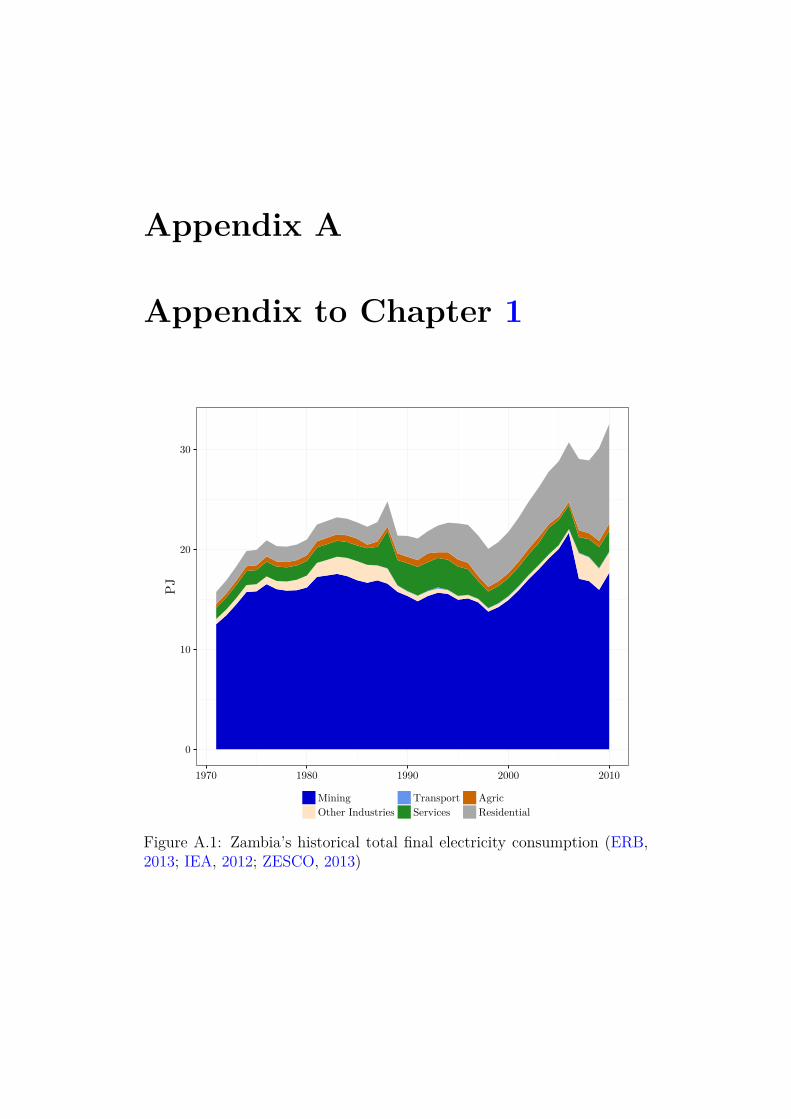
Appendix A
Appendix to Chapter 1
0
10
20
30
1970 1980 1990 2000 2010
PJ
MiningOther Industries
TransportServices
AgricResidential
Figure A.1: Zambia’s historical total final electricity consumption (ERB,2013; IEA, 2012; ZESCO, 2013)

290 | Appendix to Chapter 1
A.1 State of the electricity sector in Zambia
Zambia’s electricity sector is dominated by hydro-power technologies. As
of 31st March 2013, 99% of all electricity supply came from hydro tech-
nologies, most of which were built in the 1960s and 1970s. Even though
Zambia’s generation sub-sector has been privatised, the participation of In-
dependent Private Producer (IPP) is still low. The most notable IPP are
CEC and Lunsemfwa Hydro Power Limited (LHPL). This is largely due
to the low electricity tariffs that have not encouraged investment into the
sector (ERB, 2015).
Furthermore, the role of hydro technologies is projected to continue
playing a critical role in the energy sector as most of its available resource
(of 4, 500 MW) requires low capital investment cost. Apart from hydro,
a number of coal and solar projects have been identified. However, there
have been no sites for wind, natural gas and nuclear technologies that have
been earmarked for development.
A.1.1 Energy markets
Zambia’s electricity supply is sourced from within the country and it is also
one of the major electricity exporters in the SAPP region. Local electricity
tariff is regulated by ERB while the export price is determined by supply
and demand on the SAPP market. The local electricity tariffs have for
a long time not been cost reflective as was acknowledged by ERB (2015;
2017). These low tariffs were as a result of the desire to stimulate economic
growth (through the Mining sector) after the country had experienced eco-
nomic down turn for about three decades, prior to privatisation of the
mines (which happened in the late 1990s and early 2000s). Apart from
that, electricity tariff is a sensitive political issue (which could come with
significant electoral consequences) in Zambia, thus successive government
has been forced to continue subsidising the sector.
The electricity tariffs within Zambia between 2004 and 2011, ranged
between USc 1.91 and USc 5.44 per kWh. Local tariffs are quoted in
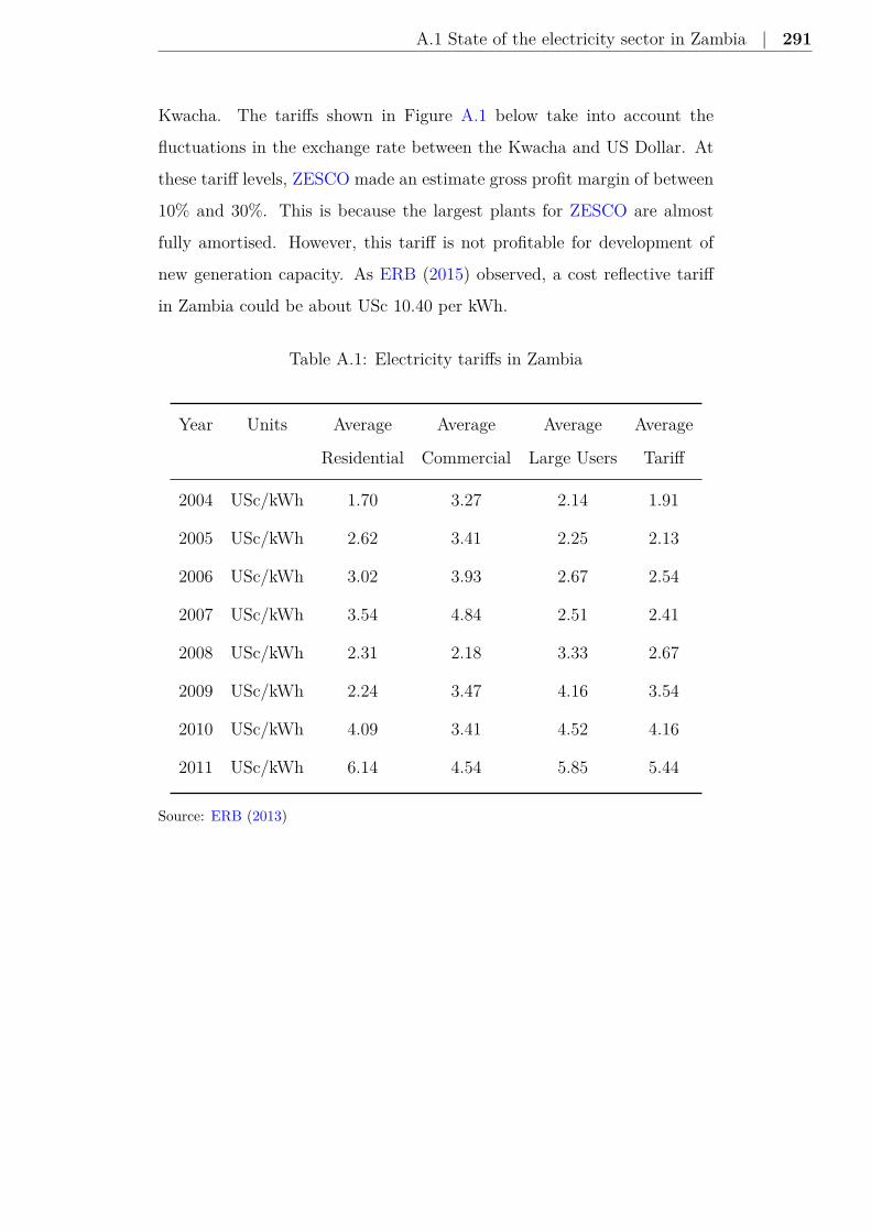
A.1 State of the electricity sector in Zambia | 291
Kwacha. The tariffs shown in Figure A.1 below take into account the
fluctuations in the exchange rate between the Kwacha and US Dollar. At
these tariff levels, ZESCO made an estimate gross profit margin of between
10% and 30%. This is because the largest plants for ZESCO are almost
fully amortised. However, this tariff is not profitable for development of
new generation capacity. As ERB (2015) observed, a cost reflective tariff
in Zambia could be about USc 10.40 per kWh.
Table A.1: Electricity tariffs in Zambia
Year Units Average Average Average Average
Residential Commercial Large Users Tariff
2004 USc/kWh 1.70 3.27 2.14 1.91
2005 USc/kWh 2.62 3.41 2.25 2.13
2006 USc/kWh 3.02 3.93 2.67 2.54
2007 USc/kWh 3.54 4.84 2.51 2.41
2008 USc/kWh 2.31 2.18 3.33 2.67
2009 USc/kWh 2.24 3.47 4.16 3.54
2010 USc/kWh 4.09 3.41 4.52 4.16
2011 USc/kWh 6.14 4.54 5.85 5.44
Source: ERB (2013)
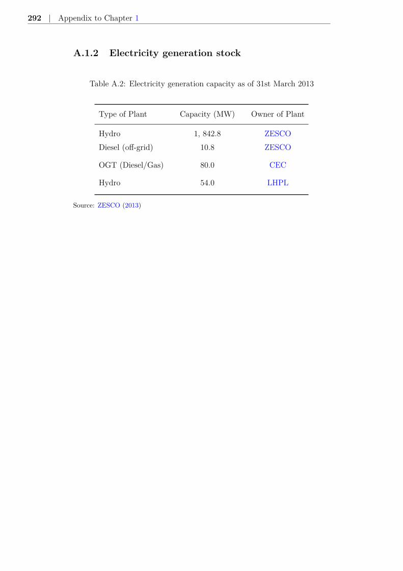
292 | Appendix to Chapter 1
A.1.2 Electricity generation stock
Table A.2: Electricity generation capacity as of 31st March 2013
Type of Plant Capacity (MW) Owner of Plant
Hydro 1, 842.8 ZESCODiesel (off-grid) 10.8 ZESCO
OGT (Diesel/Gas) 80.0 CEC
Hydro 54.0 LHPL
Source: ZESCO (2013)

Appendix B
Appendix to Chapter 2
B.1 Global consumption of copper
Table B.1: Copper consumption by country for 2011 (Cochilco, 2012)
Country Share (%) Country Share (%)
China 40.6 Spain 1.6USA 9.0 Poland 1.3Germany 6.4 Belgium 1.2Japan 5.2 Mexico 1.2South Korea 3.8 Thailand 1.2Russia 3.5 Indonesia 1.1Italy 3.1 Malaysia 1.1Taiwan 2.3 Iran 1.0Brazil 2.2 France 0.9India 2.1 Other 9.2Turkey 2.0
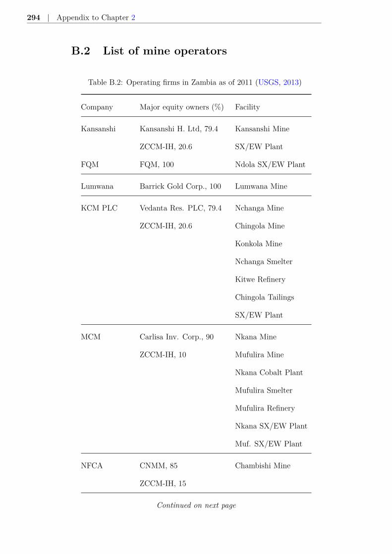
294 | Appendix to Chapter 2
B.2 List of mine operators
Table B.2: Operating firms in Zambia as of 2011 (USGS, 2013)
Company Major equity owners (%) Facility
Kansanshi Kansanshi H. Ltd, 79.4 Kansanshi Mine
ZCCM-IH, 20.6 SX/EW Plant
FQM FQM, 100 Ndola SX/EW Plant
Lumwana Barrick Gold Corp., 100 Lumwana Mine
KCM PLC Vedanta Res. PLC, 79.4 Nchanga Mine
ZCCM-IH, 20.6 Chingola Mine
Konkola Mine
Nchanga Smelter
Kitwe Refinery
Chingola Tailings
SX/EW Plant
MCM Carlisa Inv. Corp., 90 Nkana Mine
ZCCM-IH, 10 Mufulira Mine
Nkana Cobalt Plant
Mufulira Smelter
Mufulira Refinery
Nkana SX/EW Plant
Muf. SX/EW Plant
NFCA CNMM, 85 Chambishi Mine
ZCCM-IH, 15
Continued on next page
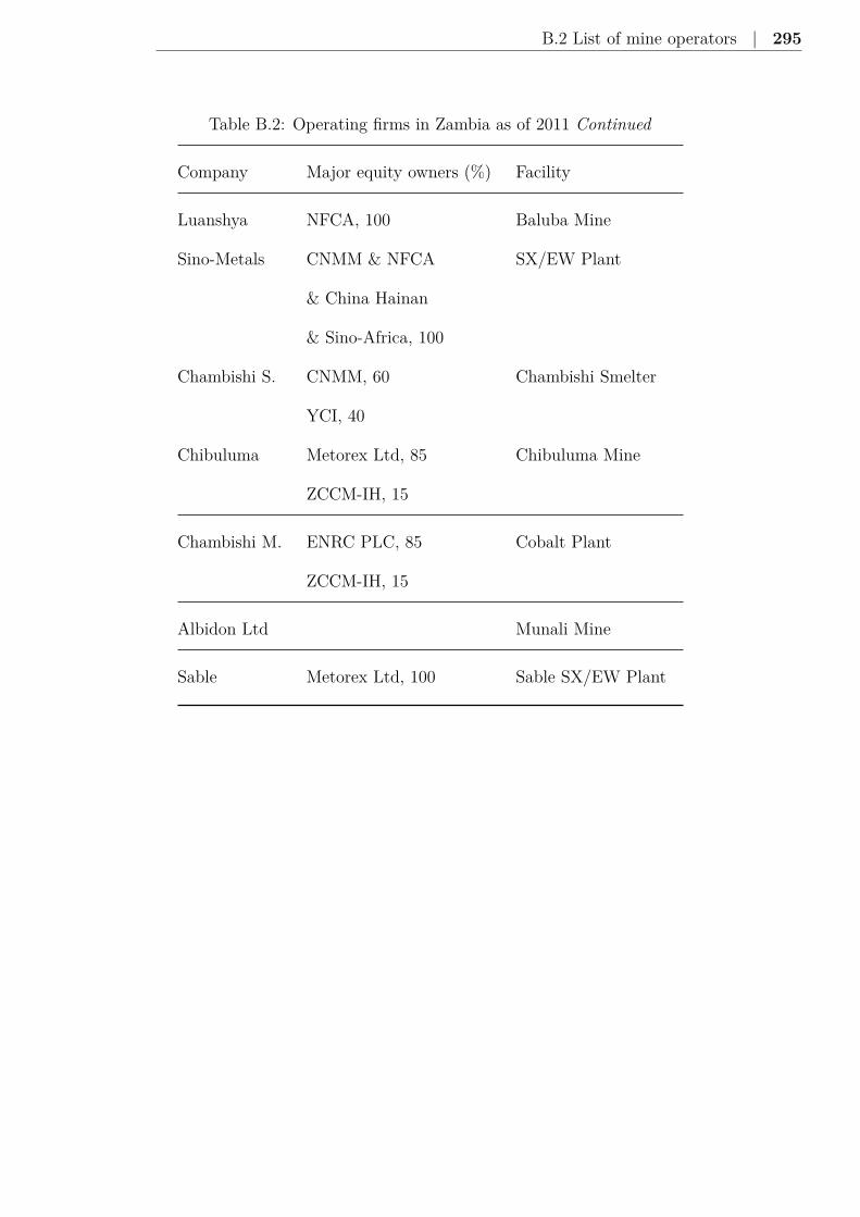
B.2 List of mine operators | 295
Table B.2: Operating firms in Zambia as of 2011 Continued
Company Major equity owners (%) Facility
Luanshya NFCA, 100 Baluba Mine
Sino-Metals CNMM & NFCA SX/EW Plant
& China Hainan
& Sino-Africa, 100
Chambishi S. CNMM, 60 Chambishi Smelter
YCI, 40
Chibuluma Metorex Ltd, 85 Chibuluma Mine
ZCCM-IH, 15
Chambishi M. ENRC PLC, 85 Cobalt Plant
ZCCM-IH, 15
Albidon Ltd Munali Mine
Sable Metorex Ltd, 100 Sable SX/EW Plant
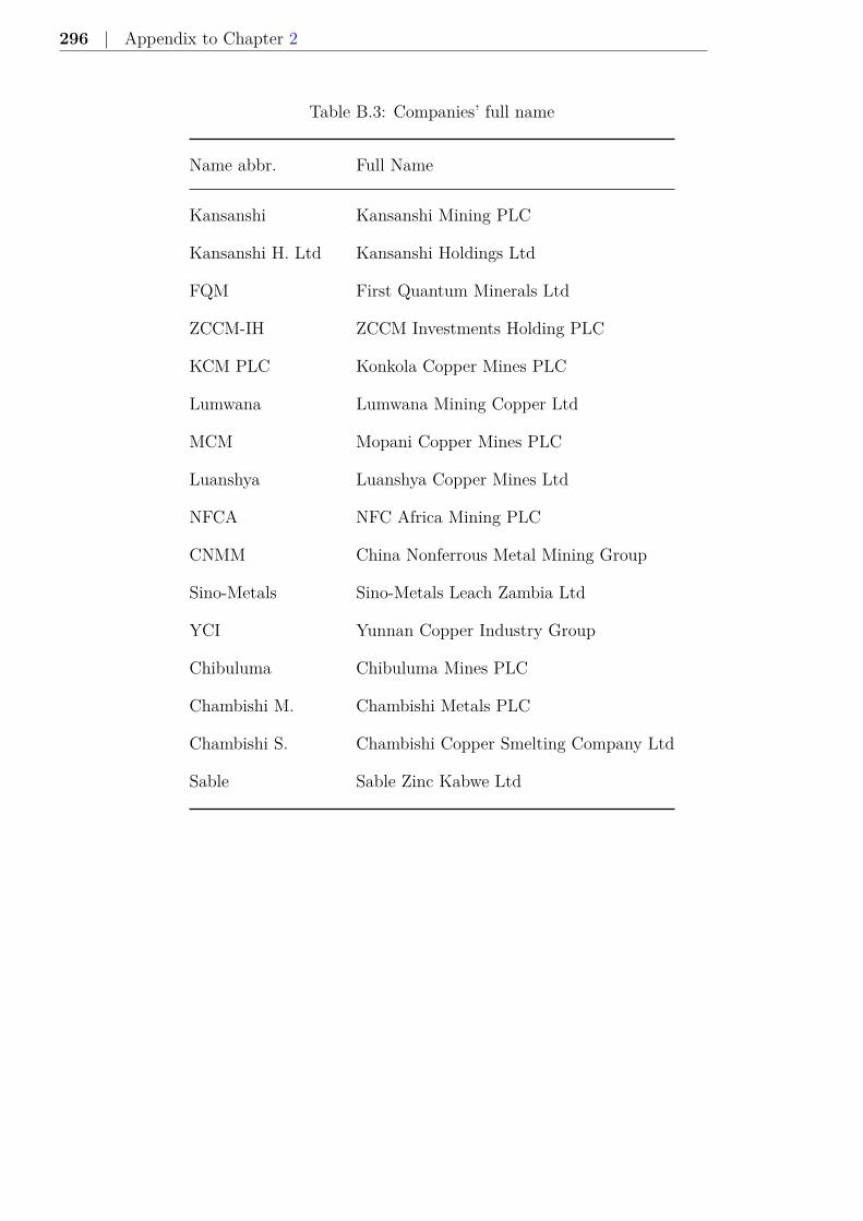
296 | Appendix to Chapter 2
Table B.3: Companies’ full name
Name abbr. Full Name
Kansanshi Kansanshi Mining PLC
Kansanshi H. Ltd Kansanshi Holdings Ltd
FQM First Quantum Minerals Ltd
ZCCM-IH ZCCM Investments Holding PLC
KCM PLC Konkola Copper Mines PLC
Lumwana Lumwana Mining Copper Ltd
MCM Mopani Copper Mines PLC
Luanshya Luanshya Copper Mines Ltd
NFCA NFC Africa Mining PLC
CNMM China Nonferrous Metal Mining Group
Sino-Metals Sino-Metals Leach Zambia Ltd
YCI Yunnan Copper Industry Group
Chibuluma Chibuluma Mines PLC
Chambishi M. Chambishi Metals PLC
Chambishi S. Chambishi Copper Smelting Company Ltd
Sable Sable Zinc Kabwe Ltd
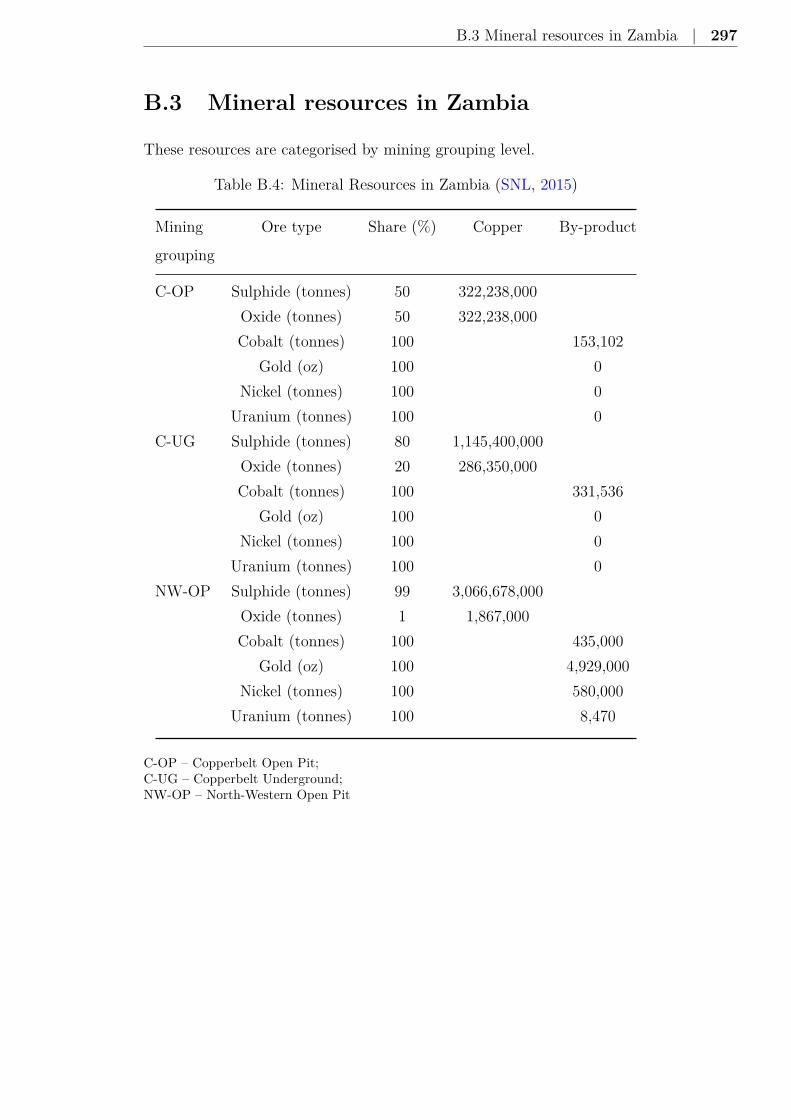
B.3 Mineral resources in Zambia | 297
B.3 Mineral resources in Zambia
These resources are categorised by mining grouping level.
Table B.4: Mineral Resources in Zambia (SNL, 2015)
Mining Ore type Share (%) Copper By-product
grouping
C-OP Sulphide (tonnes) 50 322,238,000Oxide (tonnes) 50 322,238,000Cobalt (tonnes) 100 153,102
Gold (oz) 100 0Nickel (tonnes) 100 0
Uranium (tonnes) 100 0C-UG Sulphide (tonnes) 80 1,145,400,000
Oxide (tonnes) 20 286,350,000Cobalt (tonnes) 100 331,536
Gold (oz) 100 0Nickel (tonnes) 100 0
Uranium (tonnes) 100 0NW-OP Sulphide (tonnes) 99 3,066,678,000
Oxide (tonnes) 1 1,867,000Cobalt (tonnes) 100 435,000
Gold (oz) 100 4,929,000Nickel (tonnes) 100 580,000
Uranium (tonnes) 100 8,470
C-OP – Copperbelt Open Pit;C-UG – Copperbelt Underground;NW-OP – North-Western Open Pit

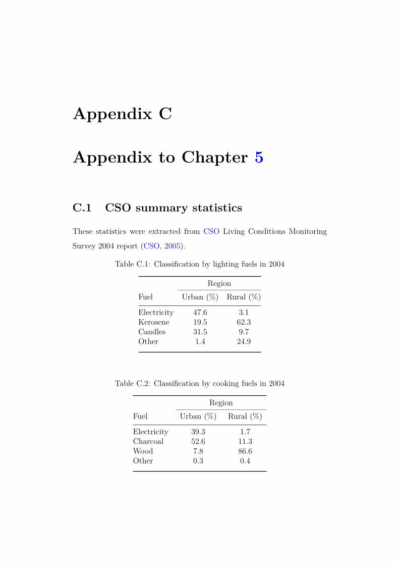
Appendix C
Appendix to Chapter 5
C.1 CSO summary statistics
These statistics were extracted from CSO Living Conditions Monitoring
Survey 2004 report (CSO, 2005).
Table C.1: Classification by lighting fuels in 2004
RegionFuel Urban (%) Rural (%)
Electricity 47.6 3.1Kerosene 19.5 62.3Candles 31.5 9.7Other 1.4 24.9
Table C.2: Classification by cooking fuels in 2004
RegionFuel Urban (%) Rural (%)
Electricity 39.3 1.7Charcoal 52.6 11.3Wood 7.8 86.6Other 0.3 0.4
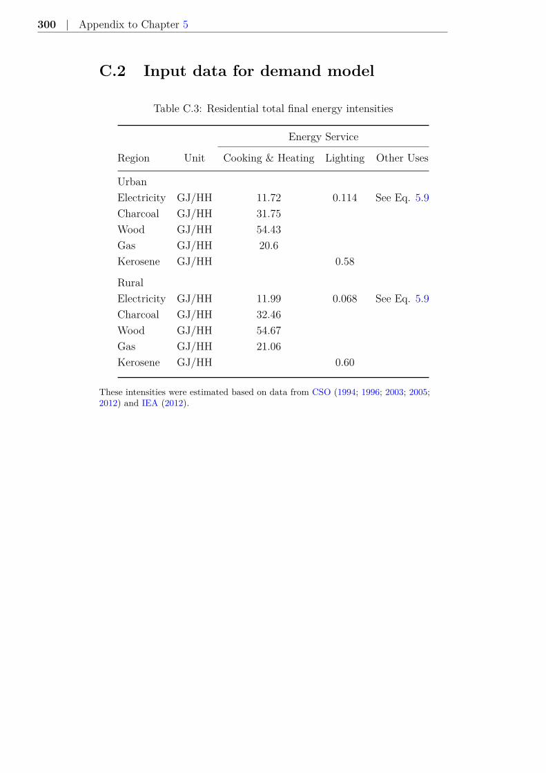
300 | Appendix to Chapter 5
C.2 Input data for demand model
Table C.3: Residential total final energy intensities
Energy Service
Region Unit Cooking & Heating Lighting Other Uses
UrbanElectricity GJ/HH 11.72 0.114 See Eq. 5.9Charcoal GJ/HH 31.75Wood GJ/HH 54.43Gas GJ/HH 20.6Kerosene GJ/HH 0.58
RuralElectricity GJ/HH 11.99 0.068 See Eq. 5.9Charcoal GJ/HH 32.46Wood GJ/HH 54.67Gas GJ/HH 21.06Kerosene GJ/HH 0.60
These intensities were estimated based on data from CSO (1994; 1996; 2003; 2005;2012) and IEA (2012).
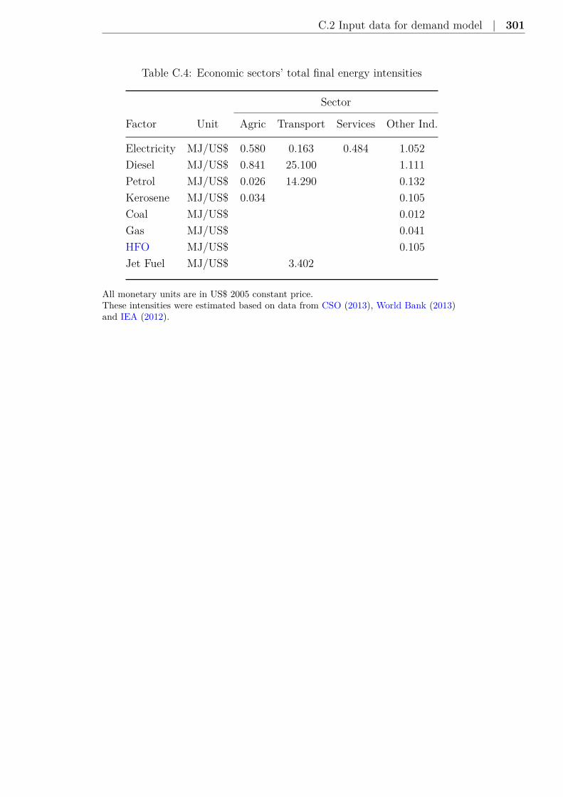
C.2 Input data for demand model | 301
Table C.4: Economic sectors’ total final energy intensities
Sector
Factor Unit Agric Transport Services Other Ind.
Electricity MJ/US$ 0.580 0.163 0.484 1.052Diesel MJ/US$ 0.841 25.100 1.111Petrol MJ/US$ 0.026 14.290 0.132Kerosene MJ/US$ 0.034 0.105Coal MJ/US$ 0.012Gas MJ/US$ 0.041HFO MJ/US$ 0.105Jet Fuel MJ/US$ 3.402
All monetary units are in US$ 2005 constant price.These intensities were estimated based on data from CSO (2013), World Bank (2013)and IEA (2012).
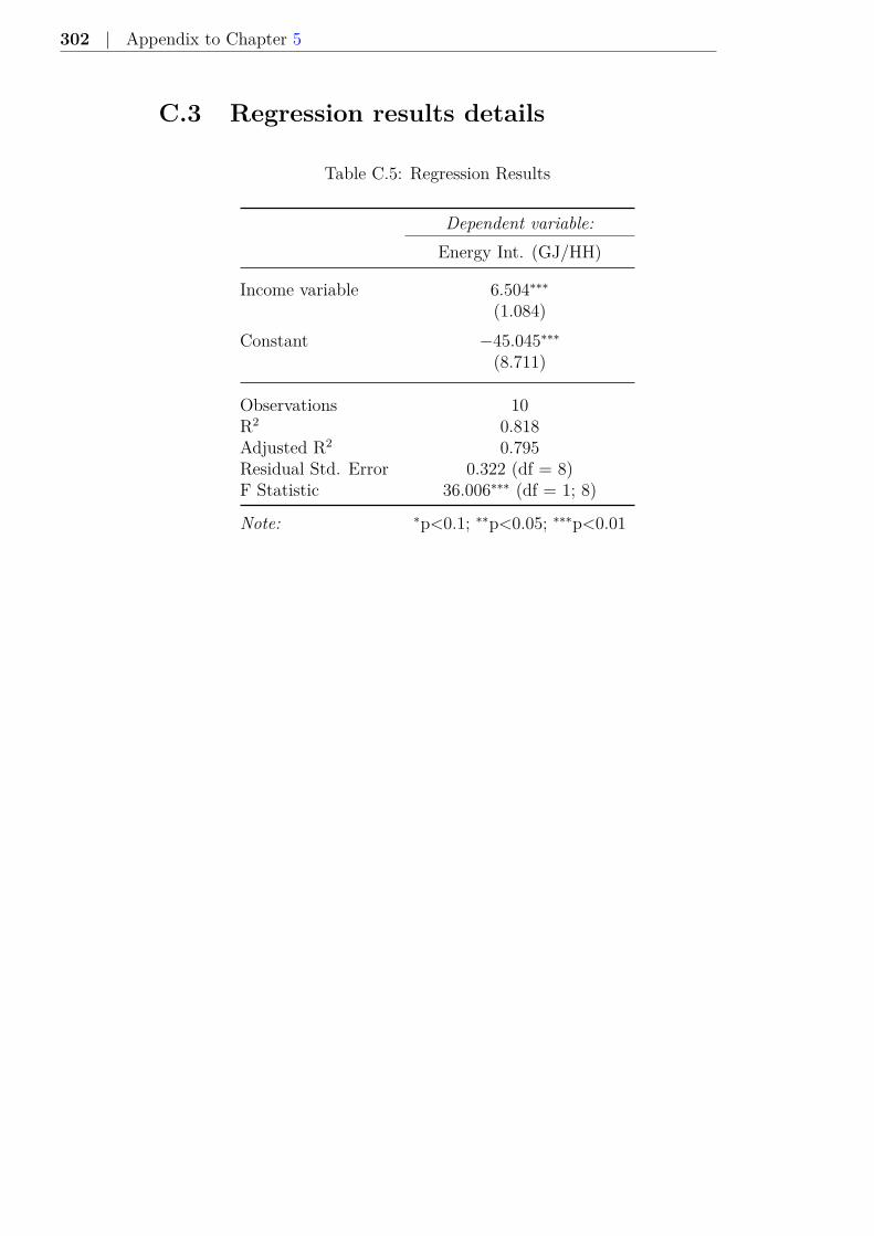
302 | Appendix to Chapter 5
C.3 Regression results details
Table C.5: Regression Results
Dependent variable:Energy Int. (GJ/HH)
Income variable 6.504∗∗∗
(1.084)Constant −45.045∗∗∗
(8.711)
Observations 10R2 0.818Adjusted R2 0.795Residual Std. Error 0.322 (df = 8)F Statistic 36.006∗∗∗ (df = 1; 8)
Note: ∗p<0.1; ∗∗p<0.05; ∗∗∗p<0.01
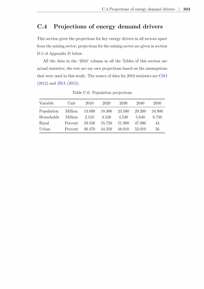
C.4 Projections of energy demand drivers | 303
C.4 Projections of energy demand drivers
This section gives the projections for key energy drivers in all sectors apart
from the mining sector; projections for the mining sector are given in section
D.5 of Appendix D below.
All the data in the ‘2010’ column in all the Tables of this section are
actual statistics, the rest are my own projections based on the assumptions
that were used in this study. The source of data for 2010 statistics are CSO
(2012) and ZRA (2013).
Table C.6: Population projections
Variable Unit 2010 2020 2030 2040 2050
Population Million 13.090 18.300 23.500 29.200 34.900Households Million 2.510 3.520 4.530 5.640 6.750Rural Percent 59.530 55.750 51.990 47.990 44Urban Percent 40.470 44.250 48.010 52.010 56
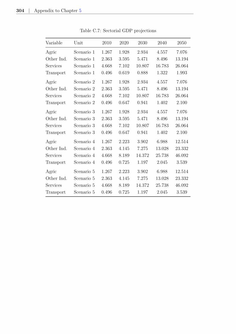
304 | Appendix to Chapter 5
Table C.7: Sectorial GDP projections
Variable Unit 2010 2020 2030 2040 2050
Agric Scenario 1 1.267 1.928 2.934 4.557 7.076Other Ind. Scenario 1 2.363 3.595 5.471 8.496 13.194Services Scenario 1 4.668 7.102 10.807 16.783 26.064Transport Scenario 1 0.496 0.619 0.888 1.322 1.993
Agric Scenario 2 1.267 1.928 2.934 4.557 7.076Other Ind. Scenario 2 2.363 3.595 5.471 8.496 13.194Services Scenario 2 4.668 7.102 10.807 16.783 26.064Transport Scenario 2 0.496 0.647 0.941 1.402 2.100
Agric Scenario 3 1.267 1.928 2.934 4.557 7.076Other Ind. Scenario 3 2.363 3.595 5.471 8.496 13.194Services Scenario 3 4.668 7.102 10.807 16.783 26.064Transport Scenario 3 0.496 0.647 0.941 1.402 2.100
Agric Scenario 4 1.267 2.223 3.902 6.988 12.514Other Ind. Scenario 4 2.363 4.145 7.275 13.028 23.332Services Scenario 4 4.668 8.189 14.372 25.738 46.092Transport Scenario 4 0.496 0.725 1.197 2.045 3.539
Agric Scenario 5 1.267 2.223 3.902 6.988 12.514Other Ind. Scenario 5 2.363 4.145 7.275 13.028 23.332Services Scenario 5 4.668 8.189 14.372 25.738 46.092Transport Scenario 5 0.496 0.725 1.197 2.045 3.539
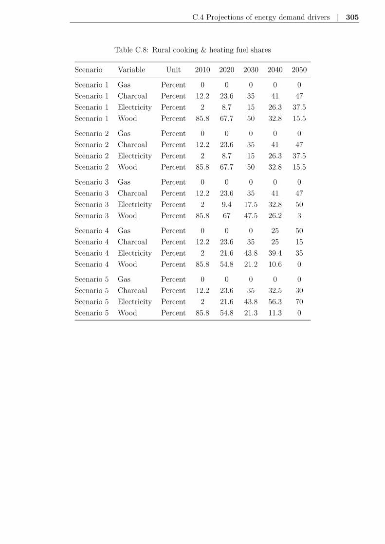
C.4 Projections of energy demand drivers | 305
Table C.8: Rural cooking & heating fuel shares
Scenario Variable Unit 2010 2020 2030 2040 2050
Scenario 1 Gas Percent 0 0 0 0 0Scenario 1 Charcoal Percent 12.2 23.6 35 41 47Scenario 1 Electricity Percent 2 8.7 15 26.3 37.5Scenario 1 Wood Percent 85.8 67.7 50 32.8 15.5
Scenario 2 Gas Percent 0 0 0 0 0Scenario 2 Charcoal Percent 12.2 23.6 35 41 47Scenario 2 Electricity Percent 2 8.7 15 26.3 37.5Scenario 2 Wood Percent 85.8 67.7 50 32.8 15.5
Scenario 3 Gas Percent 0 0 0 0 0Scenario 3 Charcoal Percent 12.2 23.6 35 41 47Scenario 3 Electricity Percent 2 9.4 17.5 32.8 50Scenario 3 Wood Percent 85.8 67 47.5 26.2 3
Scenario 4 Gas Percent 0 0 0 25 50Scenario 4 Charcoal Percent 12.2 23.6 35 25 15Scenario 4 Electricity Percent 2 21.6 43.8 39.4 35Scenario 4 Wood Percent 85.8 54.8 21.2 10.6 0
Scenario 5 Gas Percent 0 0 0 0 0Scenario 5 Charcoal Percent 12.2 23.6 35 32.5 30Scenario 5 Electricity Percent 2 21.6 43.8 56.3 70Scenario 5 Wood Percent 85.8 54.8 21.3 11.3 0
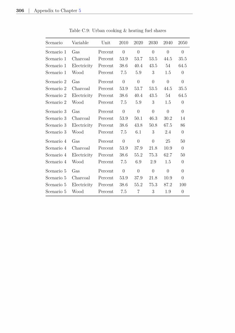
306 | Appendix to Chapter 5
Table C.9: Urban cooking & heating fuel shares
Scenario Variable Unit 2010 2020 2030 2040 2050
Scenario 1 Gas Percent 0 0 0 0 0Scenario 1 Charcoal Percent 53.9 53.7 53.5 44.5 35.5Scenario 1 Electricity Percent 38.6 40.4 43.5 54 64.5Scenario 1 Wood Percent 7.5 5.9 3 1.5 0
Scenario 2 Gas Percent 0 0 0 0 0Scenario 2 Charcoal Percent 53.9 53.7 53.5 44.5 35.5Scenario 2 Electricity Percent 38.6 40.4 43.5 54 64.5Scenario 2 Wood Percent 7.5 5.9 3 1.5 0
Scenario 3 Gas Percent 0 0 0 0 0Scenario 3 Charcoal Percent 53.9 50.1 46.3 30.2 14Scenario 3 Electricity Percent 38.6 43.8 50.8 67.5 86Scenario 3 Wood Percent 7.5 6.1 3 2.4 0
Scenario 4 Gas Percent 0 0 0 25 50Scenario 4 Charcoal Percent 53.9 37.9 21.8 10.9 0Scenario 4 Electricity Percent 38.6 55.2 75.3 62.7 50Scenario 4 Wood Percent 7.5 6.9 2.9 1.5 0
Scenario 5 Gas Percent 0 0 0 0 0Scenario 5 Charcoal Percent 53.9 37.9 21.8 10.9 0Scenario 5 Electricity Percent 38.6 55.2 75.3 87.2 100Scenario 5 Wood Percent 7.5 7 3 1.9 0
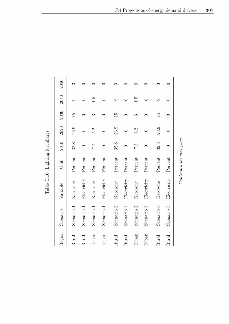
C.4 Projections of energy demand drivers | 307
Tabl
eC
.10:
Ligh
ting
fuel
shar
es
Reg
ion
Scen
ario
Varia
ble
Uni
t20
1020
2020
3020
4020
50
Rura
lSc
enar
io1
Ker
osen
ePe
rcen
t32.8
23.9
159
3
Rura
lSc
enar
io1
Elec
tric
ityPe
rcen
t0
00
00
Urb
anSc
enar
io1
Ker
osen
ePe
rcen
t7.
55.
23
1.5
0
Urb
anSc
enar
io1
Elec
tric
ityPe
rcen
t0
00
00
Rura
lSc
enar
io2
Ker
osen
ePe
rcen
t32.8
23.9
159
3
Rura
lSc
enar
io2
Elec
tric
ityPe
rcen
t0
00
00
Urb
anSc
enar
io2
Ker
osen
ePe
rcen
t7.
55.
23
1.5
0
Urb
anSc
enar
io2
Elec
tric
ityPe
rcen
t0
00
00
Rura
lSc
enar
io3
Ker
osen
ePe
rcen
t32.8
23.9
159
3
Rura
lSc
enar
io3
Elec
tric
ityPe
rcen
t0
00
00
Con
tinue
don
next
page

308 | Appendix to Chapter 5
Tabl
eC
.10:
Ligh
ting
fuel
shar
esC
ontin
ued
Reg
ion
Scen
ario
Varia
ble
Uni
t20
1020
2020
3020
4020
50
Urb
anSc
enar
io3
Ker
osen
ePe
rcen
t7.
55.
23
1.5
0
Urb
anSc
enar
io3
Elec
tric
ityPe
rcen
t0
00
00
Rura
lSc
enar
io4
Ker
osen
ePe
rcen
t32.8
23.9
159
3
Rura
lSc
enar
io4
Elec
tric
ityPe
rcen
t0
00
00
Urb
anSc
enar
io4
Ker
osen
ePe
rcen
t7.
55.
23
1.5
0
Urb
anSc
enar
io4
Elec
tric
ityPe
rcen
t0
00
00
Rura
lSc
enar
io5
Ker
osen
ePe
rcen
t32.8
23.9
159
3
Rura
lSc
enar
io5
Elec
tric
ityPe
rcen
t0
00
00
Urb
anSc
enar
io5
Ker
osen
ePe
rcen
t7.
55.
23
1.5
0
Urb
anSc
enar
io5
Elec
tric
ityPe
rcen
t0
00
00
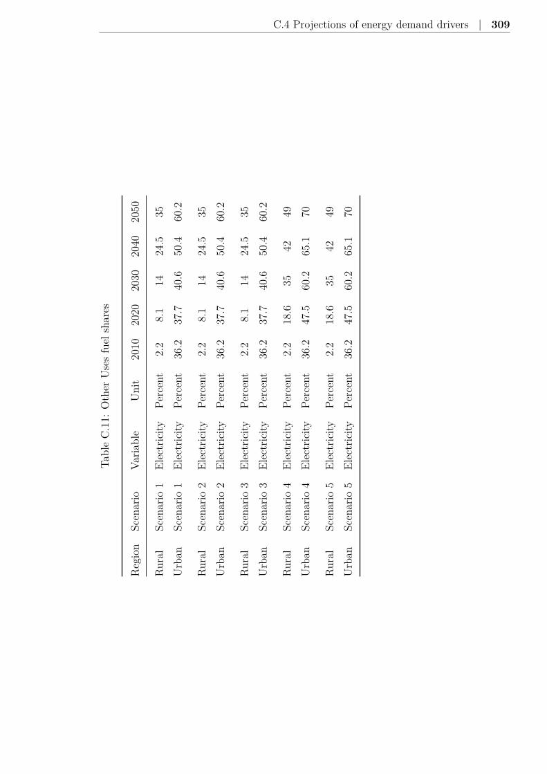
C.4 Projections of energy demand drivers | 309
Tabl
eC
.11:
Oth
erU
ses
fuel
shar
es
Reg
ion
Scen
ario
Varia
ble
Uni
t20
1020
2020
3020
4020
50
Rura
lSc
enar
io1
Elec
tric
ityPe
rcen
t2.
28.
114
24.5
35U
rban
Scen
ario
1El
ectr
icity
Perc
ent
36.2
37.7
40.6
50.4
60.2
Rura
lSc
enar
io2
Elec
tric
ityPe
rcen
t2.
28.
114
24.5
35U
rban
Scen
ario
2El
ectr
icity
Perc
ent
36.2
37.7
40.6
50.4
60.2
Rura
lSc
enar
io3
Elec
tric
ityPe
rcen
t2.
28.
114
24.5
35U
rban
Scen
ario
3El
ectr
icity
Perc
ent
36.2
37.7
40.6
50.4
60.2
Rura
lSc
enar
io4
Elec
tric
ityPe
rcen
t2.
218.6
3542
49U
rban
Scen
ario
4El
ectr
icity
Perc
ent
36.2
47.5
60.2
65.1
70
Rura
lSc
enar
io5
Elec
tric
ityPe
rcen
t2.
218.6
3542
49U
rban
Scen
ario
5El
ectr
icity
Perc
ent
36.2
47.5
60.2
65.1
70
310 | Appendix to Chapter 5
C.5 Input data for supply model
Note that wind technology was not included on the list of possible tech-
nologies because there is no recorded wind resource suitable for electricity
production in Zambia (RECP, 2017).
• The transmission and distribution losses were estimated to average
15%.
• Input to biomass technology was assumed to come from the sugar
industry, not from the forestry sector (This is based on the charac-
teristic of the bio-technology as described in Nexant (2007)).
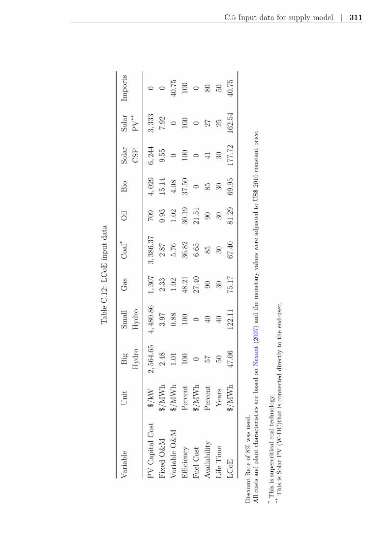
C.5 Input data for supply model | 311
Tabl
eC
.12:
LCoE
inpu
tda
ta
Varia
ble
Uni
tBi
gSm
all
Gas
Coa
l*O
ilBi
oSo
lar
Sola
rIm
port
sH
ydro
Hyd
roC
SPPV
**
PVC
apita
lCos
t$/
kW2,
564.
654,
480.
861,
307
3,38
6.37
709
4,02
96,
244
3,33
30
Fixe
dO
&M
$/M
Wh
2.48
3.97
2.33
2.87
0.93
15.1
49.
557.
920
Varia
ble
O&
M$/
MW
h1.
010.
881.
025.
761.
024.
080
040.7
5Effi
cien
cyPe
rcen
t10
010
048.2
136.8
230.1
937.5
010
010
010
0Fu
elC
ost
$/M
Wh
00
27.4
06.
6521.5
10
00
0Av
aila
bilit
yPe
rcen
t57
4090
8590
8541
2780
Life
Tim
eYe
ars
5040
3030
3030
3025
50LC
oE$/
MW
h47.0
612
2.11
75.1
767.4
081.2
969.9
517
7.72
162.
5440.7
5
Disc
ount
Rat
eof
8%w
asus
ed.
All
cost
san
dpl
ant
char
acte
ristic
sar
eba
sed
onN
exan
t(2
007)
and
the
mon
etar
yva
lues
wer
ead
just
edto
US$
2010
cons
tant
pric
e.
*T
his
issu
perc
ritic
alco
alte
chno
logy
.**
Thi
sis
Sola
rPV
(W-D
C)t
hat
isco
nnec
ted
dire
ctly
toth
een
d-us
er.
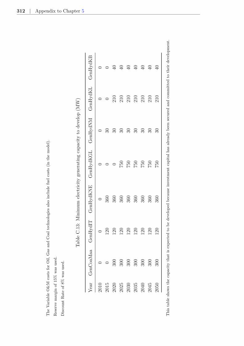
312 | Appendix to Chapter 5
The
Varia
ble
O&
Mco
sts
for
Oil,
Gas
and
Coa
ltec
hnol
ogie
sal
soin
clud
efu
elco
sts
(inth
em
odel
).
Res
erve
mar
gin
of15
%w
asus
ed.
Disc
ount
Rat
eof
8%w
asus
ed.
Tabl
eC
.13:
Min
imum
elec
tric
ityge
nera
ting
capa
city
tode
velo
p(M
W)
Year
Gen
Coa
Maa
Gen
Hyd
ITG
enH
ydK
NE
Gen
Hyd
KG
LG
enH
ydN
MG
enH
ydK
LG
enH
ydK
B
2010
00
00
00
020
150
120
360
030
00
2020
300
120
360
030
210
4020
2530
012
036
075
030
210
4020
3030
012
036
075
030
210
4020
3530
012
036
075
030
210
4020
4030
012
036
075
030
210
4020
4530
012
036
075
030
210
4020
5030
012
036
075
030
210
40
Thi
sta
ble
show
sth
eca
paci
tyth
atis
expe
cted
tobe
deve
lope
dbe
caus
ein
vest
men
tca
pita
lhas
alre
ady
been
secu
red
and
com
mitt
edto
thei
rde
velo
pmen
t.
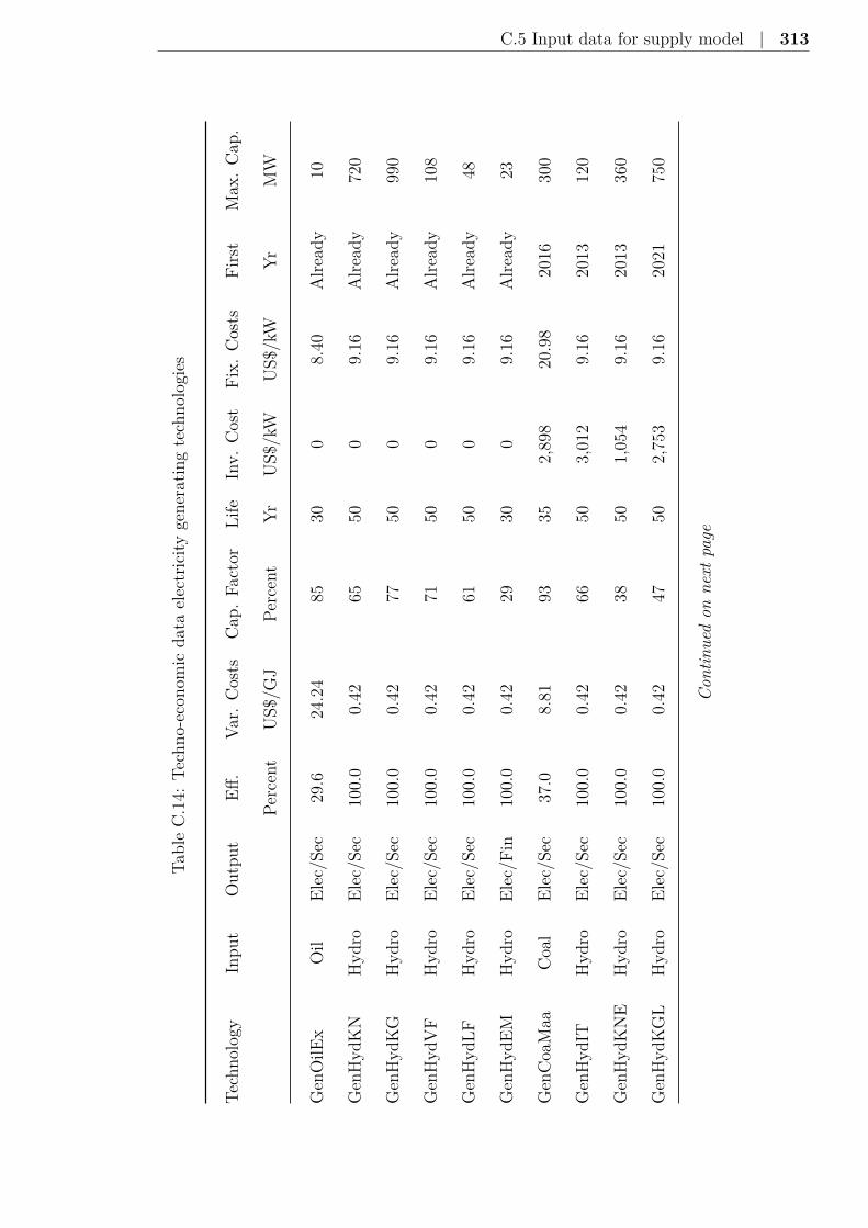
C.5 Input data for supply model | 313
Tabl
eC
.14:
Tech
no-e
cono
mic
data
elec
tric
ityge
nera
ting
tech
nolo
gies
Tech
nolo
gyIn
put
Out
put
Eff.
Var.
Cos
tsC
ap.
Fact
orLi
feIn
v.C
ost
Fix.
Cos
tsFi
rst
Max
.C
ap.
Perc
ent
US$
/GJ
Perc
ent
YrU
S$/k
WU
S$/k
WYr
MW
Gen
OilE
xO
ilEl
ec/S
ec29
.624
.24
8530
08.
40A
lread
y10
Gen
Hyd
KN
Hyd
roEl
ec/S
ec10
0.0
0.42
6550
09.
16A
lread
y72
0
Gen
Hyd
KG
Hyd
roEl
ec/S
ec10
0.0
0.42
7750
09.
16A
lread
y99
0
Gen
Hyd
VF
Hyd
roEl
ec/S
ec10
0.0
0.42
7150
09.
16A
lread
y10
8
Gen
Hyd
LFH
ydro
Elec
/Sec
100.
00.
4261
500
9.16
Alre
ady
48
Gen
Hyd
EMH
ydro
Elec
/Fin
100.
00.
4229
300
9.16
Alre
ady
23
Gen
Coa
Maa
Coa
lEl
ec/S
ec37
.08.
8193
352,
898
20.9
820
1630
0
Gen
Hyd
ITH
ydro
Elec
/Sec
100.
00.
4266
503,
012
9.16
2013
120
Gen
Hyd
KN
EH
ydro
Elec
/Sec
100.
00.
4238
501,
054
9.16
2013
360
Gen
Hyd
KG
LH
ydro
Elec
/Sec
100.
00.
4247
502,
753
9.16
2021
750
Con
tinue
don
next
page
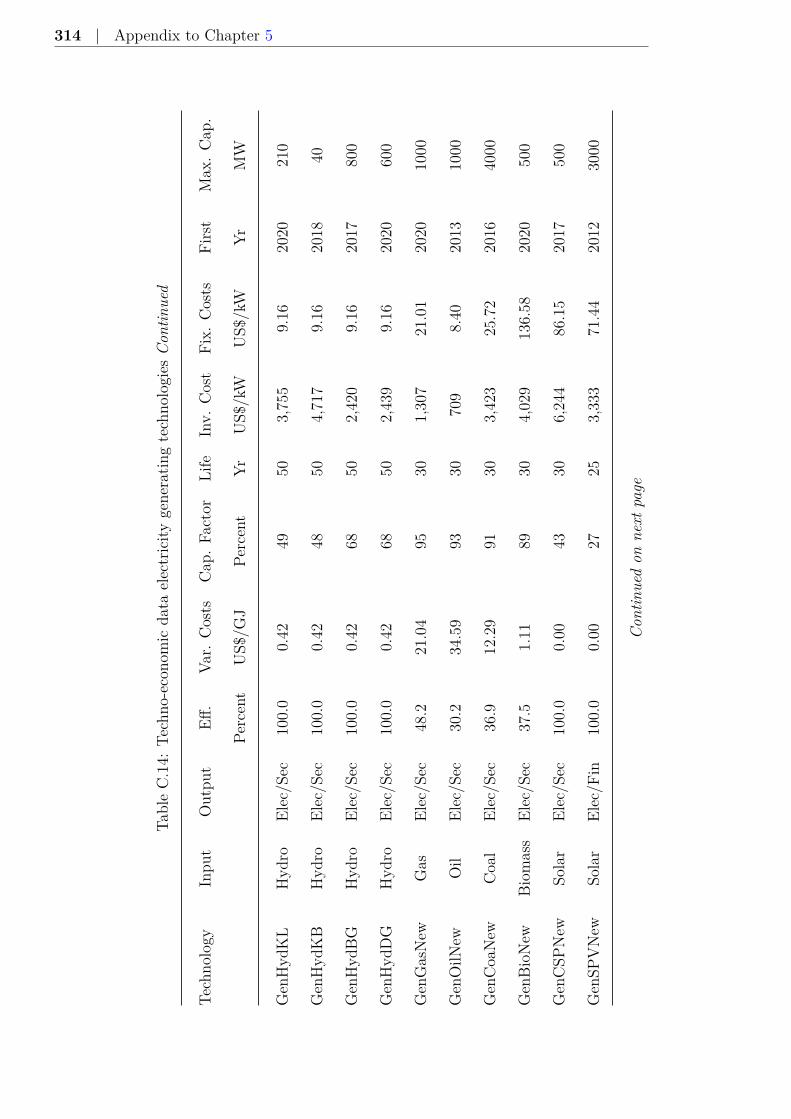
314 | Appendix to Chapter 5
Tabl
eC
.14:
Tech
no-e
cono
mic
data
elec
tric
ityge
nera
ting
tech
nolo
gies
Con
tinue
d
Tech
nolo
gyIn
put
Out
put
Eff.
Var.
Cos
tsC
ap.
Fact
orLi
feIn
v.C
ost
Fix.
Cos
tsFi
rst
Max
.C
ap.
Perc
ent
US$
/GJ
Perc
ent
YrU
S$/k
WU
S$/k
WYr
MW
Gen
Hyd
KL
Hyd
roEl
ec/S
ec10
0.0
0.42
4950
3,75
59.
1620
2021
0
Gen
Hyd
KB
Hyd
roEl
ec/S
ec10
0.0
0.42
4850
4,71
79.
1620
1840
Gen
Hyd
BGH
ydro
Elec
/Sec
100.
00.
4268
502,
420
9.16
2017
800
Gen
Hyd
DG
Hyd
roEl
ec/S
ec10
0.0
0.42
6850
2,43
99.
1620
2060
0
Gen
Gas
New
Gas
Elec
/Sec
48.2
21.0
495
301,
307
21.0
120
2010
00
Gen
OilN
ewO
ilEl
ec/S
ec30
.234
.59
9330
709
8.40
2013
1000
Gen
Coa
New
Coa
lEl
ec/S
ec36
.912
.29
9130
3,42
325
.72
2016
4000
Gen
BioN
ewBi
omas
sEl
ec/S
ec37
.51.
1189
304,
029
136.
5820
2050
0
Gen
CSP
New
Sola
rEl
ec/S
ec10
0.0
0.00
4330
6,24
486
.15
2017
500
Gen
SPV
New
Sola
rEl
ec/F
in10
0.0
0.00
2725
3,33
371
.44
2012
3000
Con
tinue
don
next
page

C.5 Input data for supply model | 315
Tabl
eC
.14:
Tech
no-e
cono
mic
data
elec
tric
ityge
nera
ting
tech
nolo
gies
Con
tinue
d
Tech
nolo
gyIn
put
Out
put
Eff.
Var.
Cos
tsC
ap.
Fact
orLi
feIn
v.C
ost
Fix.
Cos
tsFi
rst
Max
.C
ap.
Perc
ent
US$
/GJ
Perc
ent
YrU
S$/k
WU
S$/k
WYr
MW
Gen
Hyd
NM
Hyd
roEl
ec/F
in10
0.0
0.00
3025
4,16
671
.44
2012
30
Gen
Hyd
NL
Hyd
roEl
ec/S
ec10
0.0
0.00
6050
2,75
847
.76
2015
1490
Sour
ce:
Nex
ant
(200
7),E
RB
(200
8),Z
ESC
O(2
008;
2009
),JI
CA
/MEW
D(2
009)
and
DH
EC(2
011)
.
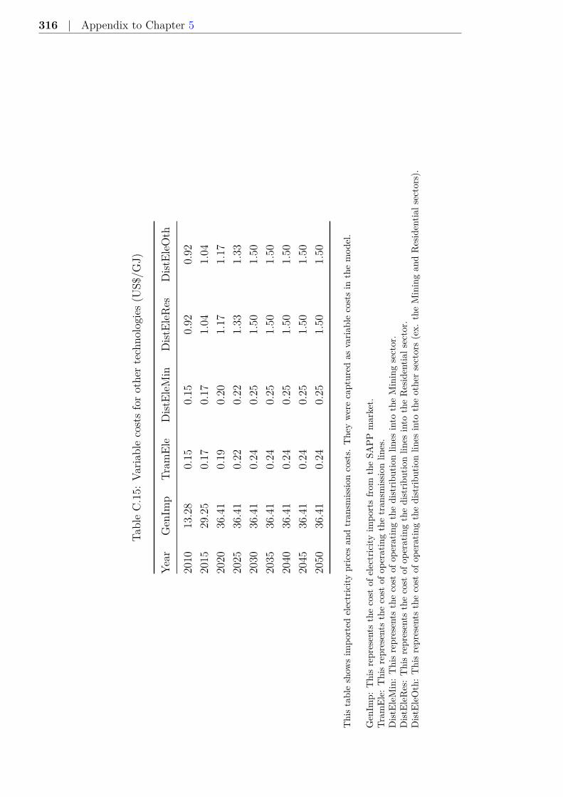
316 | Appendix to Chapter 5
Tabl
eC
.15:
Varia
ble
cost
sfo
rot
her
tech
nolo
gies
(US$
/GJ)
Year
Gen
Imp
Tram
Ele
Dist
EleM
inD
istEl
eRes
Dist
EleO
th
2010
13.2
80.
150.
150.
920.
9220
1529.2
50.
170.
171.
041.
0420
2036.4
10.
190.
201.
171.
1720
2536.4
10.
220.
221.
331.
3320
3036.4
10.
240.
251.
501.
5020
3536.4
10.
240.
251.
501.
5020
4036.4
10.
240.
251.
501.
5020
4536.4
10.
240.
251.
501.
5020
5036.4
10.
240.
251.
501.
50
Thi
sta
ble
show
sim
port
edel
ectr
icity
pric
esan
dtr
ansm
issio
nco
sts.
The
yw
ere
capt
ured
asva
riabl
eco
sts
inth
em
odel
.
Gen
Imp:
Thi
sre
pres
ents
the
cost
ofel
ectr
icity
impo
rts
from
the
SAPP
mar
ket.
Tram
Ele:
Thi
sre
pres
ents
the
cost
ofop
erat
ing
the
tran
smiss
ion
lines
.D
istEl
eMin
:T
his
repr
esen
tsth
eco
stof
oper
atin
gth
edi
strib
utio
nlin
esin
toth
eM
inin
gse
ctor
.D
istEl
eRes
:T
his
repr
esen
tsth
eco
stof
oper
atin
gth
edi
strib
utio
nlin
esin
toth
eR
esid
entia
lsec
tor.
Dist
EleO
th:
Thi
sre
pres
ents
the
cost
ofop
erat
ing
the
dist
ribut
ion
lines
into
the
othe
rse
ctor
s(e
x.th
eM
inin
gan
dR
esid
entia
lsec
tors
).
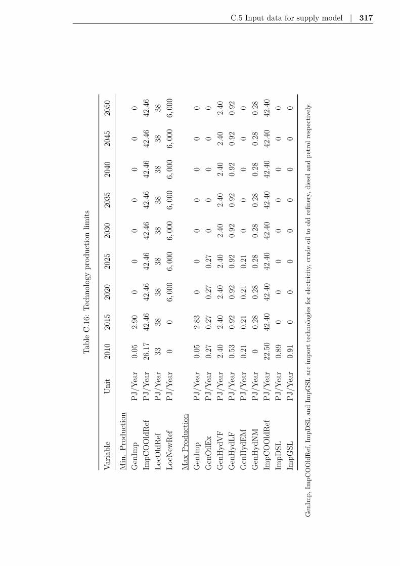
C.5 Input data for supply model | 317
Tabl
eC
.16:
Tech
nolo
gypr
oduc
tion
limits
Varia
ble
Uni
t20
1020
1520
2020
2520
3020
3520
4020
4520
50
Min
.Pr
oduc
tion
Gen
Imp
PJ/Y
ear
0.05
2.90
00
00
00
0Im
pCO
Old
Ref
PJ/Y
ear
26.1
742.4
642.4
642.4
642.4
642.4
642.4
642.4
642.4
6Lo
cOld
Ref
PJ/Y
ear
3338
3838
3838
3838
38Lo
cNew
Ref
PJ/Y
ear
00
6,00
06,
000
6,00
06,
000
6,00
06,
000
6,00
0
Max
Prod
uctio
nG
enIm
pPJ
/Yea
r0.
052.
830
00
00
00
Gen
OilE
xPJ
/Yea
r0.
270.
270.
270.
270
00
00
Gen
Hyd
VF
PJ/Y
ear
2.40
2.40
2.40
2.40
2.40
2.40
2.40
2.40
2.40
Gen
Hyd
LFPJ
/Yea
r0.
530.
920.
920.
920.
920.
920.
920.
920.
92G
enH
ydEM
PJ/Y
ear
0.21
0.21
0.21
0.21
00
00
0G
enH
ydN
MPJ
/Yea
r0
0.28
0.28
0.28
0.28
0.28
0.28
0.28
0.28
ImpC
OO
ldR
efPJ
/Yea
r22.5
042.4
042.4
042.4
042.4
042.4
042.4
042.4
042.4
0Im
pDSL
PJ/Y
ear
0.89
00
00
00
00
ImpG
SLPJ
/Yea
r0.
910
00
00
00
0
Gen
Imp,
ImpC
OO
ldR
ef,I
mpD
SLan
dIm
pGSL
are
impo
rtte
chno
logi
esfo
rel
ectr
icity
,cru
deoi
lto
old
refin
ery,
dies
elan
dpe
trol
resp
ectiv
ely.
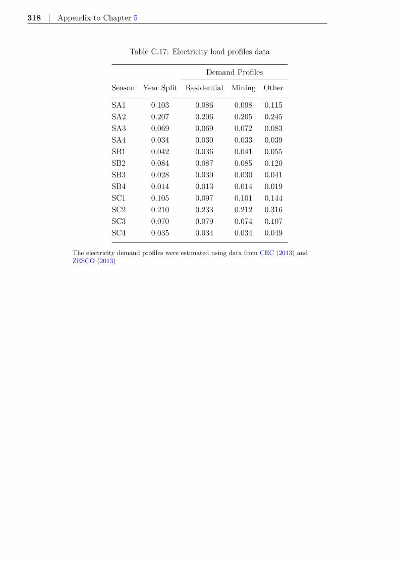
318 | Appendix to Chapter 5
Table C.17: Electricity load profiles data
Demand Profiles
Season Year Split Residential Mining Other
SA1 0.103 0.086 0.098 0.115SA2 0.207 0.206 0.205 0.245SA3 0.069 0.069 0.072 0.083SA4 0.034 0.030 0.033 0.039SB1 0.042 0.036 0.041 0.055SB2 0.084 0.087 0.085 0.120SB3 0.028 0.030 0.030 0.041SB4 0.014 0.013 0.014 0.019SC1 0.105 0.097 0.101 0.144SC2 0.210 0.233 0.212 0.316SC3 0.070 0.079 0.074 0.107SC4 0.035 0.034 0.034 0.049
The electricity demand profiles were estimated using data from CEC (2013) andZESCO (2013)
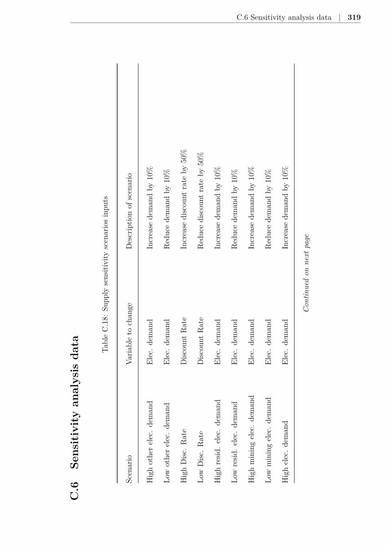
C.6 Sensitivity analysis data | 319
C.6
Sens
itiv
ity
anal
ysis
data
Tabl
eC
.18:
Supp
lyse
nsiti
vity
scen
ario
sin
puts
Scen
ario
Varia
ble
toch
ange
Des
crip
tion
ofsc
enar
io
Hig
hot
her
elec
.de
man
dEl
ec.
dem
and
Incr
ease
dem
and
by10
%
Low
othe
rel
ec.
dem
and
Elec
.de
man
dR
educ
ede
man
dby
10%
Hig
hD
isc.
Rat
eD
iscou
ntR
ate
Incr
ease
disc
ount
rate
by50
%
Low
Disc
.R
ate
Disc
ount
Rat
eR
educ
edi
scou
ntra
teby
50%
Hig
hre
sid.
elec
.de
man
dEl
ec.
dem
and
Incr
ease
dem
and
by10
%
Low
resid
.el
ec.
dem
and
Elec
.de
man
dR
educ
ede
man
dby
10%
Hig
hm
inin
gel
ec.
dem
and
Elec
.de
man
dIn
crea
sede
man
dby
10%
Low
min
ing
elec
.de
man
dEl
ec.
dem
and
Red
uce
dem
and
by10
%
Hig
hel
ec.
dem
and
Elec
.de
man
dIn
crea
sede
man
dby
10%
Con
tinue
don
next
page
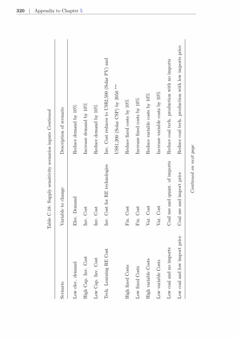
320 | Appendix to Chapter 5
Tabl
eC
.18:
Supp
lyse
nsiti
vity
scen
ario
sin
puts
Con
tinue
d
Scen
ario
Varia
ble
toch
ange
Des
crip
tion
ofsc
enar
io
Low
elec
.de
man
dEl
ec.
Dem
and
Red
uce
dem
and
by10
%
Hig
hC
ap.
Inv.
Cos
tIn
v.C
ost
Incr
ease
dem
and
by10
%
Low
Cap
.In
v.C
ost
Inv.
Cos
tR
educ
ede
man
dby
10%
Tech
.Le
arni
ngR
EC
ost
Inv.
Cos
tfo
rR
Ete
chno
logi
esIn
v.C
ost
redu
ces
toU
S$2,
500
(Sol
arPV
)an
d
US$
1,20
0(S
olar
CSP
)by
2050
∗∗∗
Hig
hfix
edC
osts
Fix.
Cos
tR
educ
efix
edco
sts
by10
%
Low
fixed
Cos
tsFi
x.C
ost
Incr
ease
fixed
cost
sby
10%
Hig
hva
riabl
eC
osts
Var.
Cos
tR
educ
eva
riabl
eco
sts
by10
%
Low
varia
ble
Cos
tsVa
r.C
ost
Incr
ease
varia
ble
cost
sby
10%
Low
coal
and
noim
port
sC
oalu
sean
dqu
ant.
ofim
port
sR
educ
eco
alte
ch.
prod
uctio
nw
ithno
impo
rts
Low
coal
and
low
impo
rtpr
ice
Coa
luse
and
impo
rtpr
ice
Red
uce
coal
tech
.pr
oduc
tion
with
low
impo
rts
pric
e
Con
tinue
don
next
page

C.6 Sensitivity analysis data | 321
Tabl
eC
.18:
Supp
lyse
nsiti
vity
scen
ario
sin
puts
Con
tinue
d
Scen
ario
Varia
ble
toch
ange
Des
crip
tion
ofsc
enar
io
Low
coal
and
high
impo
rtpr
ice
Coa
luse
and
impo
rtpr
ice
Red
uce
coal
tech
.pr
oduc
tion
with
high
impo
rts
pric
e
Zero
min
ing
dem
and
by20
50M
inin
gde
man
dR
educ
eal
ldem
and
toze
roby
2050
Zero
min
ing
dem
and
by20
40M
inin
gde
man
dR
educ
eal
ldem
and
toze
roby
2040
Zero
min
ing
dem
and
by20
30M
inin
gde
man
dR
educ
eal
ldem
and
toze
roby
2030
Hig
hco
alan
dlo
wim
port
pric
eC
oalu
sean
dim
port
pric
eIn
crea
seco
alte
ch.
prod
uctio
nw
ithlo
wim
port
spr
ice
Hig
hco
alan
dhi
ghim
port
pric
eC
oalu
sean
dim
port
pric
eIn
crea
seco
alte
ch.
prod
uctio
nw
ithhi
ghim
port
spr
ice
∗∗∗
Dat
afo
rso
lar
tech
nolo
gyle
arni
ng(in
v.co
st)
was
from
RM
I(2
015)
.


Appendix D
Appendix to Chapter 6
D.1 Interview questions
D.1.1 Interviews with industry consultants
Industry financiers
Part 1: “Details of the Informant”
• What is your job title?
• What is your core responsibility within the organisation?
Part 2: “Funding Process”
1. How do the current fiscal policies and regulations (in Zambia) affect
long-term investments in the copper industry?
2. What industry performance indicators are critical in approving loans
to the mining companies?
3. How are risk and profitability of a proposed investment option eval-
uated during the approval process?
4. Are mining firms required to submit analytic reports of proposed
projects?
Part 3: “Any other Comments”

324 | Appendix to Chapter 6
• Any other issues that we have not discussed that you would like to
mention?
Thank you very much for your time.
Local experts
Part 1: “Details of the Informant”
• What is your job title?
• What is your core responsibility within the organisation?
Part 2: “Mining Investments”
1. Generally, in the copper industry, relative to the copper prices, what
is the maximum share of unit production cost that would be consid-
ered profitable?
2. What are the major cost centres in the Mining Industry?
3. How does the current policy environment (in Zambia) affect long-
term investments in the copper industry?
4. What mechanisms or aspects if in place would further encourage the
mining companies to invest more in long term projects?
Part 3: “Hypothetical Situations”
The section deals with hypothetical situations and assumes that ore
grade, copper prices, labour costs, energy costs and mineral taxes are the
key determinants of company’s profitability and survival.
What do you think a mining investment decision-maker in Zambia’s
copper industry would do?
• Ops 1 Scenario: If the ore grade continues to reduce while, mineral
taxes remain constant, but copper prices, energy prices and labour
costs increase?
• Ops 2 Scenario: If the ore grade continues to reduce while, the
copper prices, mineral taxes, energy prices and labour costs increase?

D.1 Interview questions | 325
• Ops 3 Scenario: If the ore grade continues to reduce and copper
prices fall, while the mineral taxes, energy prices and labour costs
increase?
Part 4:“Any other Comments”
• Any other issues that we have not discussed that you would like to
mention?
Thank you very much for your time.
D.1.2 Interviews with government agencies
Taxation agency
Part 1: “Details of the Informant”
• What is your job title?
• What is your core responsibility within the organisation?
Part 2: “Mining Taxation”
1. How do the current fiscal policies and regulations (in Zambia) affect
long-term investments in the copper industry?
2. Is Zambia getting the maximum possible tax revenue from the mining
industry? If no, what can be done to maximise tax revenue?
3. How adaptive are the mineral taxes to fluctuating copper prices?
Part 3: “Any other Comments”
• Any other issues that we have not discussed that you would like to
mention?
Thank you very much for your time.

326 | Appendix to Chapter 6
Energy agency
Part 1: “Details of the Informant”
• What is your job title?
• What is your core responsibility within the organisation?
Part 2: “Energy Management”
1. How is energy system expansion planning done in Zambia? How is
this impacted by regulation by ERB?
2. When designing or approving energy prices, what aspects of the econ-
omy are explicitly considered? What other aspects should be consid-
ered?
3. According to the National Energy Policy, there is very little work
that is being done to promote efficient use of energy in industry and
residential sectors. What are the challenges or barriers that hinder
such work?
4. In the National Energy Strategy, it was proposed that poor load factor
should be penalised. What legislation or regulation has been put in
place to ensure that mining company improve their load factor?
Part 3: “Any other Comments”
• Any other issues that we have not discussed that you would like to
mention?
Thank you very much for your time.
Mining agency
Part 1: “Details of the Informant”
• What is your job title?
• What is your core responsibility within the organisation?

D.1 Interview questions | 327
Part 2: “Mining Investments”
1. What are the main interests of this organisation in the copper indus-
try?
2. Generally, in the copper industry, relative to the copper prices, what
is the maximum share of unit production cost that would be consid-
ered profitable?
3. How does the current policy environment (in Zambia) affect long-
term investments in the copper industry?
4. How adaptive are the Zambia’s policies and regulations towards move-
ments in international copper prices and copper production?
Part 3: “Any other Comments”
• Any other issues that we have not discussed that you would like to
mention?
Thank you very much for your time.
D.1.3 Interviews with mining firms
Part 1: “Details of the Informant”
• What is your job title?
• What is your core responsibility within the company?
• How many years have you worked in the copper industry?
Part 2: “Investment Process”
1. What motivates your organisation to invest in capital equipment?
2. How does your company assess and evaluate investment options?
3. How does the current policy environment (in Zambia) affect long-
term investments in your company?

328 | Appendix to Chapter 6
4. What mechanisms or aspects if in place would further encourage the
company to invest more in long-term projects?
Part 3: “Energy Use”
1. How important is energy to your organisation and how has this
changed over the past 5, 10 years?
2. Which activities consume the most energy in your organisation?
3. How are these activities projected to change in the future (say 10
years or more from now)?
4. Does your company have any energy consumption reduction targets?
• i. If yes, how were these targets set and how do you hope to achieve
them
Part 4: “Hypothetical Situations”
The section deals with hypothetical situations and assumes that ore
grade, copper prices, labour costs, energy costs and mineral taxes are the
key determinants of company’s profitability and survival.
As an investment decision-maker, what would you do:
• Ops 1 Scenario: If the ore grade continues to reduce while, mineral
taxes remain constant, but copper prices, energy prices and labour
costs increase?
• Ops 2 Scenario: If the ore grade continues to reduce while, the
copper prices, mineral taxes, energy prices and labour costs increase?
• Ops 3 Scenario: If the ore grade continues to reduce and copper
prices fall, while the mineral taxes, energy prices and labour costs
increase?
Part 5: “Any other Comments”
• Any other issues that we have not discussed that you would like to
mention?
Thank you very much for your time.

D.2 Information and consent form | 329
D.2 Information and consent form
Information Sheet for MPhil/PhD in Research Studies
Title of Project: ENERGY EFFICIENCY IN ZAMBIA’S COPPER INDUSTRYENERGY EFFICIENCY IN ZAMBIA’S COPPER INDUSTRYENERGY EFFICIENCY IN ZAMBIA’S COPPER INDUSTRYENERGY EFFICIENCY IN ZAMBIA’S COPPER INDUSTRY
This study has been approved by the UCL Research Ethics Committee (Project ID Number): 6116/0016116/0016116/0016116/001
Name Bernard Tembo
Work Address UCL Energy Institute, 14 Upper Woburn Place, London, WC1H 0NN, UK
Contact Details [email protected]
(+44) 203 108 5938
We would like to invite you to participate in this research project.
This research investigates how changing energy drivers will impact on energy demand and profitability of Zambia’s copper industry, and how the effects of the changes can be mitigated by investing in energy efficient technologies. This research is funded by UCL Institute of Sustainable Resources (http://www.bartlett.ucl.ac.uk/sustainable), and is supervised by Prof. Neil Strachan and Dr. Ilkka Keppo both from University College London (UCL).
The copper industry is critical Zambia’s economy. In 2010, the industry contributed 10% to the GDP and accounted for over 80% of the country’s foreign exchange earnings. Furthermore, the industry consumes over 50% of the country’s commercial energy. Therefore, not only is the industry important to the economy, it is also important to the energy sector. With the projected growth in national energy demand, the energy prices are expected to rise. Also, the reduction in ore grade and changes in mining methods in the industry would lead to an increase in energy demand and also change in types of energy used. Thus, apart from increase in industry’s production costs, the development of the energy system will also be affected.
This research will therefore focus on identifying the main drivers of energy demand in the industry and the key decision variables that the mine operators consider when making investment decision in energy consuming technologies. These two aspects will help develop a model that can be used to propose mechanisms, policies or regulations that would protect both the industry and the national economy.
The interview process will take approximately 40 minutes.
Any information you provide will be treated as confidential and handled in accordance with the UK Data Protection Act 1998. Unless stated otherwise, participants will not be identified by name nor by their organisation in any outputs from this research. If for any reason you want to withdraw from this study, you may do so at any time. More details of UK’s data protection policy can be found on the following link: http://www.ucl.ac.uk/informationsecurity/policy/public-policy/Data_protection_policy_ISC_20110215
If you have any questions or comments about this study, please feel free to ask me. My contact details can also be found at the top of this information sheet. Thank you
Kind regards,
Bernard Tembo

330 | Appendix to Chapter 6
Informed Consent Form for MPhil/PhD in Research Studies
Please complete this form after you have read the Information Sheet and/or listened to an explanation about the research. Please complete this form after you have read the Information Sheet and/or listened to an explanation about the research. Please complete this form after you have read the Information Sheet and/or listened to an explanation about the research. Please complete this form after you have read the Information Sheet and/or listened to an explanation about the research.
Title of Project: ENERGY EFFICIENCY IN ZAMBIA’S COPPER INDUSTRYENERGY EFFICIENCY IN ZAMBIA’S COPPER INDUSTRYENERGY EFFICIENCY IN ZAMBIA’S COPPER INDUSTRYENERGY EFFICIENCY IN ZAMBIA’S COPPER INDUSTRY
This study has been approved by the UCL Research Ethics Committee (Project ID Number): 6116/0016116/0016116/0016116/001
Thank you for your interest in taking part in this research. Before you agree to take part, the person organising the research must explain the project to you.
If you have any questions arising from the Information Sheet or explanation already given to you, please ask the researcher before you to decide whether to join in. You will be given a copy of this Consent Form to keep and refer to at any time.
ParticiParticiParticiParticipant’s Statement pant’s Statement pant’s Statement pant’s Statement
I
• have read the notes written above and the Information Sheet, and understand what the study involves.
• understand that if I decide at any time that I no longer wish to take part in this project, I can notify the researchers involved and withdraw immediately.
• consent to the processing of my personal information for the purposes of this research study.
• understand that such information will be treated as strictly confidential and handled in accordance with the provisions of the UK Data Protection Act 1998.
• agree that the research project named above has been explained to me to my satisfaction and I agree to take part inthis study.
Signed: Date:
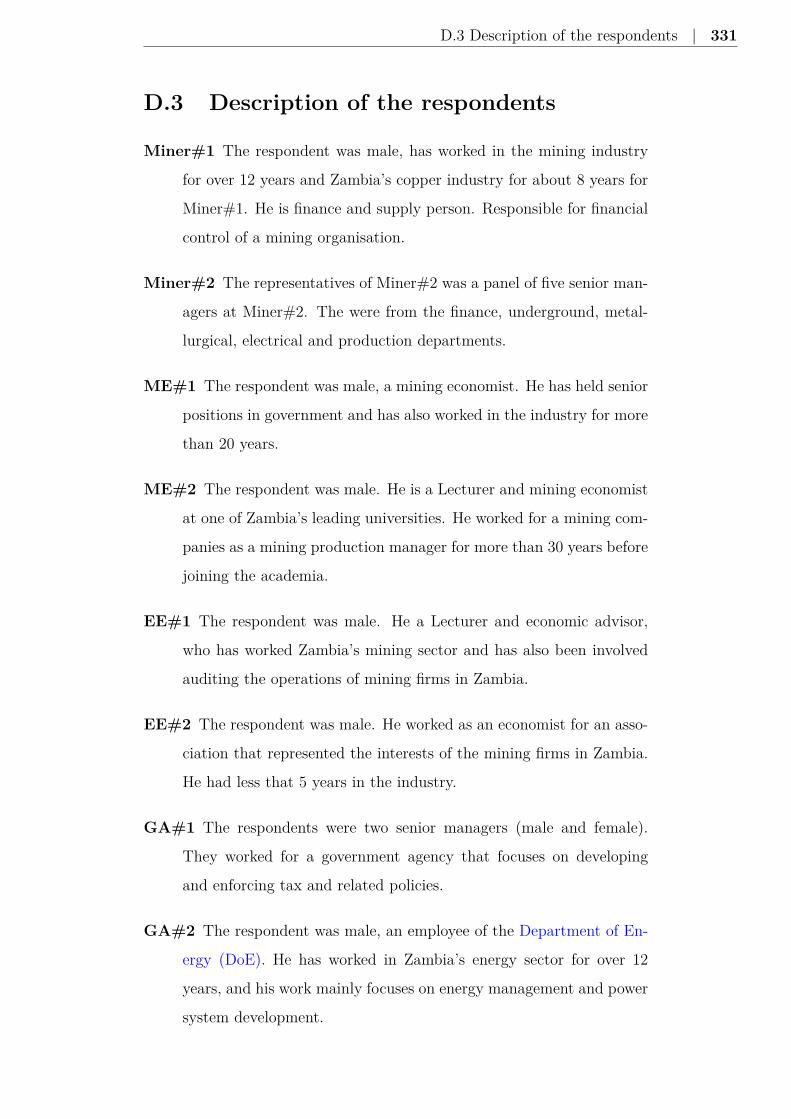
D.3 Description of the respondents | 331
D.3 Description of the respondents
Miner#1 The respondent was male, has worked in the mining industry
for over 12 years and Zambia’s copper industry for about 8 years for
Miner#1. He is finance and supply person. Responsible for financial
control of a mining organisation.
Miner#2 The representatives of Miner#2 was a panel of five senior man-
agers at Miner#2. The were from the finance, underground, metal-
lurgical, electrical and production departments.
ME#1 The respondent was male, a mining economist. He has held senior
positions in government and has also worked in the industry for more
than 20 years.
ME#2 The respondent was male. He is a Lecturer and mining economist
at one of Zambia’s leading universities. He worked for a mining com-
panies as a mining production manager for more than 30 years before
joining the academia.
EE#1 The respondent was male. He a Lecturer and economic advisor,
who has worked Zambia’s mining sector and has also been involved
auditing the operations of mining firms in Zambia.
EE#2 The respondent was male. He worked as an economist for an asso-
ciation that represented the interests of the mining firms in Zambia.
He had less that 5 years in the industry.
GA#1 The respondents were two senior managers (male and female).
They worked for a government agency that focuses on developing
and enforcing tax and related policies.
GA#2 The respondent was male, an employee of the Department of En-
ergy (DoE). He has worked in Zambia’s energy sector for over 12
years, and his work mainly focuses on energy management and power
system development.
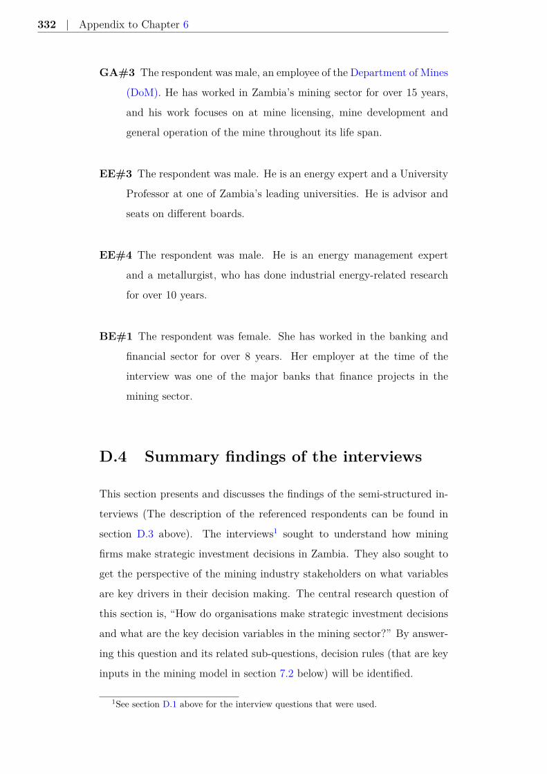
332 | Appendix to Chapter 6
GA#3 The respondent was male, an employee of the Department of Mines
(DoM). He has worked in Zambia’s mining sector for over 15 years,
and his work focuses on at mine licensing, mine development and
general operation of the mine throughout its life span.
EE#3 The respondent was male. He is an energy expert and a University
Professor at one of Zambia’s leading universities. He is advisor and
seats on different boards.
EE#4 The respondent was male. He is an energy management expert
and a metallurgist, who has done industrial energy-related research
for over 10 years.
BE#1 The respondent was female. She has worked in the banking and
financial sector for over 8 years. Her employer at the time of the
interview was one of the major banks that finance projects in the
mining sector.
D.4 Summary findings of the interviews
This section presents and discusses the findings of the semi-structured in-
terviews (The description of the referenced respondents can be found in
section D.3 above). The interviews1 sought to understand how mining
firms make strategic investment decisions in Zambia. They also sought to
get the perspective of the mining industry stakeholders on what variables
are key drivers in their decision making. The central research question of
this section is, “How do organisations make strategic investment decisions
and what are the key decision variables in the mining sector?” By answer-
ing this question and its related sub-questions, decision rules (that are key
inputs in the mining model in section 7.2 below) will be identified.
1See section D.1 above for the interview questions that were used.
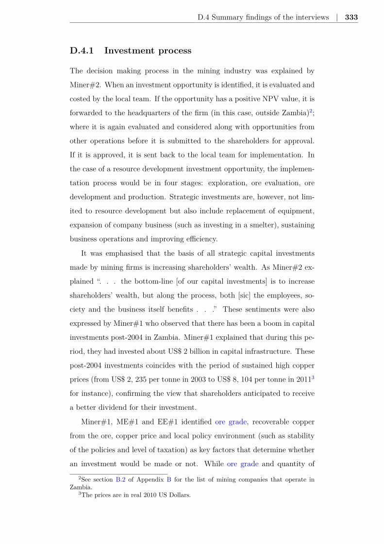
D.4 Summary findings of the interviews | 333
D.4.1 Investment process
The decision making process in the mining industry was explained by
Miner#2. When an investment opportunity is identified, it is evaluated and
costed by the local team. If the opportunity has a positive NPV value, it is
forwarded to the headquarters of the firm (in this case, outside Zambia)2;
where it is again evaluated and considered along with opportunities from
other operations before it is submitted to the shareholders for approval.
If it is approved, it is sent back to the local team for implementation. In
the case of a resource development investment opportunity, the implemen-
tation process would be in four stages: exploration, ore evaluation, ore
development and production. Strategic investments are, however, not lim-
ited to resource development but also include replacement of equipment,
expansion of company business (such as investing in a smelter), sustaining
business operations and improving efficiency.
It was emphasised that the basis of all strategic capital investments
made by mining firms is increasing shareholders’ wealth. As Miner#2 ex-
plained “. . . the bottom-line [of our capital investments] is to increase
shareholders’ wealth, but along the process, both [sic] the employees, so-
ciety and the business itself benefits . . .” These sentiments were also
expressed by Miner#1 who observed that there has been a boom in capital
investments post-2004 in Zambia. Miner#1 explained that during this pe-
riod, they had invested about US$ 2 billion in capital infrastructure. These
post-2004 investments coincides with the period of sustained high copper
prices (from US$ 2, 235 per tonne in 2003 to US$ 8, 104 per tonne in 20113
for instance), confirming the view that shareholders anticipated to receive
a better dividend for their investment.
Miner#1, ME#1 and EE#1 identified ore grade, recoverable copper
from the ore, copper price and local policy environment (such as stability
of the policies and level of taxation) as key factors that determine whether
an investment would be made or not. While ore grade and quantity of2See section B.2 of Appendix B for the list of mining companies that operate in
Zambia.3The prices are in real 2010 US Dollars.
334 | Appendix to Chapter 6
recoverable ore are geological characteristics, local policy environment is
determined by the host country. Thus, to attract more investment, the
host country would need to set-up attractive policies.
This was also noted by Miner#2 and EE#2 who argued that despite
being exposed to the same low copper prices, Anglo-America pulled out of
Zambia (in the early 2000s) to invest in the Democratic Republic of Congo
(DR Congo). They observed that during this period, even though the
DR Congo was not politically stable it still managed to attract investment
because of its good policies. However, there are alternative explanations
as to why Anglo-America decided to exit Zambia and invest in DR Congo
during this period.
As GA#1 explained that DR Congo has a weak fiscal regime that
favoured them (as investors) more than the host country and its general
citizenry. As GA#1 observes, Zambia has a stringent tax regime such as
restrictions on the length of time a firm is allowed to carry forward its
losses. This, they argue, is not the case in DR Congo hence investors in
DR Congo can carry forward their losses for a much longer period at the
expense of the host country which loses out on tax based revenue. Apart
from this, it can also be argued that because DR Congo has higher ore
grade (see Mudd et. al., 2013), production costs there would be lower than
in Zambia. Thus, minimising the losses an investor could incur if the copper
price is depressed for much longer. According to EE#1, this was the line
of argument that Anglo-America gave when exiting the Zambian industry.
The financial and economic reasoning notwithstanding, ME#1 argued that
companies (such as Anglo-America) can choose to invest or disinvest based
on their lobbying position. As he (ME#1) explained “. . . he [the then
President] gave Anglo-America the best package of mines after privatisa-
tion, but Anglo-America continuing to operate in Zambia was based on the
arrangement that they had a captive national leadership [who they had
bribed during privatisation process, according to ME#1] . . . but when
there was change of national leadership, they exited the Zambian industry.”
On the whole, the firm exiting an industry is driven by one of two
D.4 Summary findings of the interviews | 335
factors: local and global. Under the local factors, the conditions (such
as taxation and unit production cost) within a host country determines
whether it would be profitable for a firm to continue operating in the coun-
try. Such a case is Anglo-America’s decision to pull out of Zambia and
invest in DR Congo. The global factors, on the other hand, focus on the
impact that copper price (a global variable) has on the profitability of a
firm. A firm that exits an industry due to global factors almost always
struggles to find buyers for the mining site because the obtaining state of
the industry is not attractive regardless of the location and local conditions
of the mining site.
D.4.2 Project evaluation and financing
After the investment opportunity has been identified, it is evaluated using
the NPV/Discounted Cash Flow (DCF), IRR and pay-back period meth-
ods. According to both Miner#1 and Miner#2, while IRR and pay-back
analysis are optional, an NPV analysis has to be done on all big projects4.
This is because it is an acceptable method of evaluating projects in the in-
dustry. To address some limitation of the NPV method, IRR and pay-back
analysis could also be done.
It was found that a decision maker would be interested in developing
a project that has a return on investment (RoI) ranging between 15%-
30% (according to Miner#2 and ME#1), which according to ME#1 is
slightly higher than the global average of 10%-15%. Both Miner#2 and
ME#1 further argue that a positive RoI does not mean that the project
will be implemented because the company has to consider the country risks.
Risks such as political risks and consistency in fiscal policies. Miner#2 also
discussed the role of experience in decision making, they observed that
“gut-feeling” type of decisions can only be made by the top most persons
in an organisation. For them (Miner#2’s local team), they have to make
decisions based on technical evaluation analysis of the project.
After the project has been approved, a firm can either use its internal4Any project above US$ 5 million according to Miner#1.
336 | Appendix to Chapter 6
resources or approach a financial institution to finance the development of
the project. From a financier’s perspective, funding of projects is largely
determined by the long term outlook of the industry, not short-term policy
inconsistencies. As BE#1 said “ . . . we tend to rely so much on the
industry reports, that look at both the short and long-term industry out-
look. Generally, the view taken is that as long as the long term outlook is
positive, we will still continue to see investments into the copper industry.
I think we have seen FQM [the largest mining operation in Zambia] despite
the little hiccups we have had in regulation, they have still continued to
invest in the sector.”
The three main factors that are considered when approving funding for
a mining project in Zambia were identified: 1. who their off-taker [the
buyer of their produce] is; 2. the role that the Zambian asset plays in
the group (in terms of value); and 3. the parent organisation of the firm.
According to BE#1, accessing finance for projects in Zambia’s industry is
more determined by global factors and organisation structure than local
policies because firm’s market is outside the country (so access to foreign
exchange is guaranteed).
D.4.3 Production costs
Similar to literature reviewed, it was found that the seven main production
cost components were labour, repair and maintenance, energy costs, cost
of capital5, consumables, transport and mining royalty tax (MRT) costs.6
The view of what was the most important of these components and also
how these factors could change in future varied from one respondent to
another. For instance, Miner#2 thought that the best way to reduce the
labour cost (the largest cost component according to Rothschild (2008))
was to mechanise the mining operation. However, this would increase the
energy cost further, which according to Miner#1 was already high. Further,
5This is more relevant to the new entrants of the industry according to EE#1 andGA#1
6The cost structure of KCM (Zambia’s largest integrated mine operation) can befound in section E.3 of Appendix E.
D.4 Summary findings of the interviews | 337
Miner#1 said “. . . there is a lot that needs to be done in Zambia’s power
sector because there is a shortage [in power supply]. . . . despite the
stability agreement7, we have also seen an increase in electricity price by
300% to 400% . . .” Another way that would help to reduce the production
cost according to Miner#1 and ME#1 would be to have a functioning rail
system. As Miner#1 explained, “. . . if there is an efficient rail network,
we [Miner#1] would save at least 40%-50% on transport cost.”
Of the seven cost components, energy cost and MRT were the most
contentious. When discussing the energy cost (particularly the electricity
price), EE#3, EE#4, GA#2 and ME#1 argued that the current electricity
tariffs were low. GA#2 further argued that these low tariffs have acted as
barriers to energy efficient practises in the industry, because even after
using the energy inefficiently, the mining firms are still able to make a
profit. Apart from acting as a barrier to energy efficiency, ME#1 further
argued that these low tariffs have rendered development of new electricity
capacity impossible as the current tariffs are not attractive enough. EE#3
and EE#4 also added that the tariffs have been kept low because the
mining industry is a critical and powerful industry (both politically and
economically) in Zambia. For example, EE#3 observes that “. . . attempts
have been done to come up with recommendations that would make the
electricity industry viable [financially viable, via cost reflective tariffs] .
. . there is resistance from the industry, the copper industry especially
. . . they always refer to the agreements [stability agreements] which
they made a long time ago, which were not realistic in terms of the real
price of electricity”. On the fuels energy cost, GA#3 observed that the
Zambian firms pay more for each litre of fuel they use than those operating
in neighbouring countries to Zambia. He (GA#3) gave an example for
how Kalumbila mine (one of new North-Western open pits) plans to install
a dual energy consuming trolley system so that it can be switching to
electricity during the off-peak period in order to reduce its fuel expenditure.
This, on the other hand, implies that electricity is considerably cheaper7These are agreements that the government and the mining firms entered into during
privatisation that the government thought would make the industry more attractive.
338 | Appendix to Chapter 6
than fuel.
Conversely, Miner#1, Miner#2 and EE#2 felt that the price of elec-
tricity has considerable impact on the profitability of the industry. While
Miner#1 argued that government should honour the stability agreements,
EE#2’s argument focuses on economies of scale. He argues that “ . . . the
tariffs [to the mines] have to reflect the quantity of electricity consumed
by the industry.” Further, Miner#2 was more concerned about how the
future energy costs would impact its operations. They (Miner#2) however
observed that if they increase their mechanising levels, they would be able
to off-set the impact of increasing energy cost by reducing their labour
cost (on the total production cost); provided government invests in more
electricity supply infrastructure. However, when asked about the share of
electricity cost towards the total production cost, Miner#2 said “ . . .
before the electricity [price] was increased, the share of electricity was 4%
and now with the increment of 28% it just threw everything over board .
. . now the share of electricity is about 6% . . .” This, however, suggests
that electricity cost is not a significant cost and also not a very sensitive
input in Miner#2’s operations.
On taxation, there were two arguments: the way taxes are charged and
the rates of taxation. Taxes can be collected based on the firm’s gross
revenue or based on its profit. Gross revenue taxes such as MRT and Wind
Fall Tax (WFT) were favoured by ME#1 and EE#1. As EE#1 argues,
revenue based tax is ideal “. . . given the sophistications of operations
at Zambia Revenue Authority (ZRA), competencies ability or capacity to
handle multi-national companies trying to avoid or evade tax.” Similar
sentiments were expressed by ME#1, when he argued “ . . . it is the
easiest and most affordable way of taxing and I would encourage any mining
country which has no expertise in follow-up and auditing mining operations
to use WFT.”
The profit based taxes were favoured by Miner#1 and EE#2. As EE#2
argued “while the logic of WFT is fine, the trouble is where it is applied . .
. it would be better to tax it at net revenue, because that way profitability
D.4 Summary findings of the interviews | 339
of the mine operation is protected.” However, ME#2 was indifferent to
either taxation method and instead proposed a different tax regime that
could enhance the level of local content in the mining industry such as
passing regulations that require mining companies to buy certain inputs
locally.
From an efficiency perspective, a revenue based tax is better because it
forces the mining firm to minimise it process losses and also reduce wastage
such as inefficient use of electricity. For instance, if a firm operating at
60% can still make its desired profit margin, there would be no incentives
to increase its efficiency since it only pays for what it produces. As ME#2
observed “ . . . as the price [of copper] started increasing [post-2004
period], people [the firms] started doing things differently. They hired more
expensive labour, more expensive drilling and blasting . . . People [the
firms] started processing low grade ore that were previously unprofitable,
. . . which increased the total production costs.” This behaviour did not
cost the mining firms a lot of income because a significant portion of their
taxes was based on profits and not on revenue. In other words, the firms
were not incentivised to optimise their operations. This, I argue, is the
other advantage of the revenue based taxes. Besides, this is the view that
GA#1 missed when they said “ . . . we don’t tax losses [process losses].”
Apart from where the tax is applied, there are also opposing views on
what tax rates are fair. There is a consensus that the WFT which were
briefly introduced in 2008 had steep graduations and ill-timed. However,
the current rates of taxation are also in contention. Both ME#1 and EE#1
argued that the mining industry is currently not paying its fair share of
taxes while EE#2 argues that the industry is over taxed. Miner#2, on the
other hand, argues that the current structure8 of taxation is good for both
the government and the mining firms; it guarantees government predictable
tax revenue while providing a safe-net for a firm. However, Miner#1 was
more concerned with the stability of tax policies. As GA#3 agreed with
Miner#1, when he observed that “ . . . there has been frequent changes
8The current structure is a combination of both revenue based and profit based taxes.
340 | Appendix to Chapter 6
in the fiscal policy.”
D.4.4 Investment policy environment
There was a general consensus that the fiscal policy environment was less
predictable. Miner#1, Miner#2, BE#1, ME#1, EE#2 and GA#3 all
talked about how MRT rates have changed over the years and also the
Statutory Instruments (SIs) that the Ministry of Finance had put in place
only to reverse them. The respondents, however, had varying views of how
they thought this instability affected the mining industry. Miner#1 and
Miner#2 said it affected their evaluation of investment projects (since fiscal
policies were key inputs into the evaluation process) and also had a short-
term impact on their cash-flow. Further, the two miners felt that because
Zambia depends on foreign capital to grow its industry, this instability
would discourage investors from investing in the country. They hoped to
have a stable fiscal space (whether too high or low was secondary to them).
While EE#2 thought that instability greatly affected investment into
the industry, BE#1 argued that as financiers of industry project, invest-
ment into the industry was largely driven by the outlook of the global cop-
per industry. In addition, GA#3 observed that while there was instability
in the fiscal space, core policies in the sector were stable and predictable.
ME#1’s argument was that this instability was inevitable as the govern-
ment is still trying to find a fair rate at which to tax the mining firms as
the previous rate of 0.6% (of MRT) was too low. GA#1 further adds that
making the fiscal environment more responsive would in itself lead to insta-
bility in the fiscal space. Similar to the argument of ME#1, EE#1 argued
that instability in the fiscal policy was because of lack of transparency.
There is a perception (according to EE#1) that the mining firms are not
paying a fair share of taxes.

D.4 Summary findings of the interviews | 341
D.4.5 Industry drivers
This sub-section reviewed the responses to hypothetical scenarios9 10 pre-
sented to mining firms and experts on what they thought were critical
drivers of mining operations. Five drivers (ore grade, copper prices, labour
costs, energy costs and mineral taxes) were presented to the respondents.
Under ops 1 scenario, all the four respondents said they would continue
investing in the industry. Miner#2’s response focused on the level to which
the ore grade reduces while Miner#1 and ME#1 focused on the impact
of the copper prices. ME#1 further observed that significant increase in
price tends to change the behaviour of mining in the short-term. ME#2’s
response was largely driven by his argument that profitability of a firm is
determined by the business strategy that a firm decides to adopt. Thus,
his response was similar in all the three scenarios. Further, he (ME#2)
observes that increase in copper price is always a desirable thing.
For ME#1, ops 2 and 3 scenarios have the same end result: the firm
will exit the industry. He argued that at local level, the variable that
has the largest impact on decision making is taxation. For Miner#1 and
Miner#2, ops 2 scenario is still favourable for investments but the mag-
nitude of change in each of the variables would be of great importance.
Both miners observe that if the level of unit cost of production is high,
then the movement in the copper price would play an important role in
their decision making. Ops 3 scenario would lead to a bare minimum type
of operation for Miner#1 while Miner#2 said they would defer all their
planned investments.
Overall, from the analysis of the responses to the presented scenarios,
copper price, ore grade and taxation were identified as the most impactful
variables in decision making. The importance of the copper price was
9See section D.1 for the interview questions that were used.10Hypothetical scenarios (See section D.1 in Appendix D):Ops 1 scenario: If the ore grade continues to reduce while, mineral taxes remain
constant, but copper prices, energy prices and labour costs increase?Ops 2 scenario: If the ore grade continues to reduce while, the copper prices, mineral
taxes, energy prices and labour costs increase?Ops 3 scenario: If the ore grade continues to reduce and copper prices fall, while the
mineral taxes, energy prices and labour costs increase?
342 | Appendix to Chapter 6
elevated when the discussion was about marginal mines (high cost mines
that is).
In summary, the interviews revealed that strategic decision making in
firms is a deliberate and procedural process that a firm engages in. As part
of the decision process, various analytic techniques are applied when eval-
uating investment options, but the final decision does not solely depend on
the results of the analytic analysis as the experience of decision makers also
play a role in the process. The final decision is therefore determined by a
combination of different criteria and decision rules. Similar to the findings
in literature, NPV analysis is the most common and required technique for
evaluating investments in the Zambian copper industry (stochastic tech-
niques were not common).
While copper price11 and ore grade were acknowledged as key inputs
into the investment decision making process, the interviews found that the
respondents were more concerned with the price of electricity and taxation
policy. This could be because the respondents recognise that these two
inputs are susceptible to lobbying. On electricity price, their concerns were
immediate: the current electricity tariff and its past increments. How-
ever, all the respondents recommended increased capital investment into
the energy sector for two primary reasons: to satisfy the current electricity
demand and to facilitate mechanisation of the mining operations. Yet, not
much consideration was given to how increased capital investment in the
energy sector would impact the profitability of the mining industry.
On taxation, the main contentions were on the type of taxes, the rates of
taxes and the stability in the taxation policy. While instability in taxation
was widely thought to significantly impact investments, the respondents
from the banking and financial sector argued that the long-term outlook
of the industry (the outlook of the copper price that is) was the key deter-
minant to accessing funds for an investment project. However, instability11The copper price used when analysing the profitability of an investment is usually
based on a long-term forecast or historical average according to Miner#1 and EE#1.

D.4 Summary findings of the interviews | 343
can potentially reduce the profits that a firm realises from the investment.
Thus, all recommendations on how to enhance long-term investments in
the industry were focused on stabilisation of the fiscal policy.
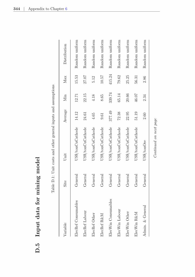
344 | Appendix to Chapter 6
D.5
Inpu
tda
tafo
rm
inin
gm
odel
Tabl
eD
.1:
Uni
tco
sts
and
othe
rge
nera
linp
uts
and
assu
mpt
ions
Varia
ble
Site
Uni
tAv
erag
eM
inM
axD
istrib
utio
n
Elec
Ref
Con
sum
able
sG
ener
alU
S$/t
onC
uCat
hode
14.1
212.7
115.5
3R
ando
mun
iform
Elec
Ref
Labo
urG
ener
alU
S$/t
onC
uCat
hode
24.6
122.1
527.0
7R
ando
mun
iform
Elec
Ref
Oth
erG
ener
alU
S$/t
onC
uCat
hode
4.65
4.18
5.12
Ran
dom
unifo
rm
Elec
Ref
R&
MG
ener
alU
S$/t
onC
uCat
hode
9.61
8.65
10.5
7R
ando
mun
iform
Elec
Win
Con
sum
able
sG
ener
alU
S$/t
onC
uCat
hode
377.
4933
9.74
415.
24R
ando
mun
iform
Elec
Win
Labo
urG
ener
alU
S$/t
onC
uCat
hode
72.3
865.1
479.6
2R
ando
mun
iform
Elec
Win
Oth
erG
ener
alU
S$/t
onC
uCat
hode
22.9
520.6
625.2
5R
ando
mun
iform
Elec
Win
R&
MG
ener
alU
S$/t
onC
uCat
hode
51.1
946.0
756.3
1R
ando
mun
iform
Adm
in.
&G
ener
alG
ener
alU
S$/t
onO
re2.
602.
342.
86R
ando
mun
iform
Con
tinue
don
next
page
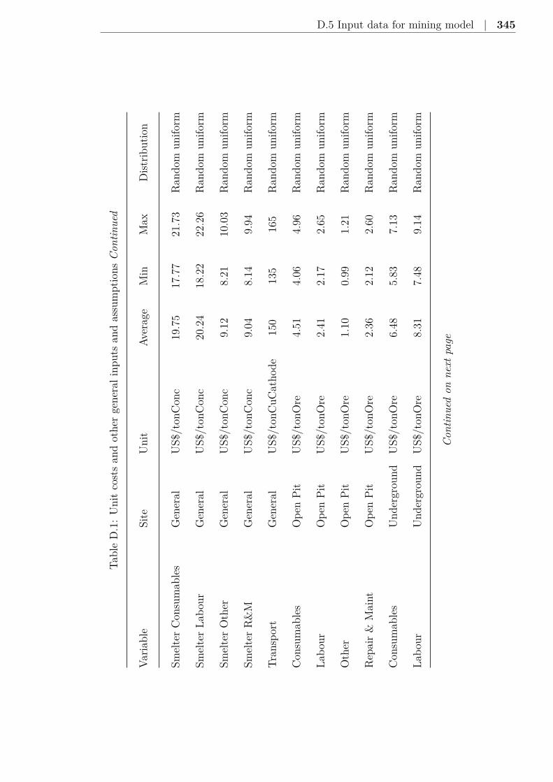
D.5 Input data for mining model | 345
Tabl
eD
.1:
Uni
tco
sts
and
othe
rge
nera
linp
uts
and
assu
mpt
ions
Con
tinue
d
Varia
ble
Site
Uni
tAv
erag
eM
inM
axD
istrib
utio
n
Smel
ter
Con
sum
able
sG
ener
alU
S$/t
onC
onc
19.7
517.7
721.7
3R
ando
mun
iform
Smel
ter
Labo
urG
ener
alU
S$/t
onC
onc
20.2
418.2
222.2
6R
ando
mun
iform
Smel
ter
Oth
erG
ener
alU
S$/t
onC
onc
9.12
8.21
10.0
3R
ando
mun
iform
Smel
ter
R&
MG
ener
alU
S$/t
onC
onc
9.04
8.14
9.94
Ran
dom
unifo
rm
Tran
spor
tG
ener
alU
S$/t
onC
uCat
hode
150
135
165
Ran
dom
unifo
rm
Con
sum
able
sO
pen
Pit
US$
/ton
Ore
4.51
4.06
4.96
Ran
dom
unifo
rm
Labo
urO
pen
Pit
US$
/ton
Ore
2.41
2.17
2.65
Ran
dom
unifo
rm
Oth
erO
pen
Pit
US$
/ton
Ore
1.10
0.99
1.21
Ran
dom
unifo
rm
Rep
air
&M
aint
Ope
nPi
tU
S$/t
onO
re2.
362.
122.
60R
ando
mun
iform
Con
sum
able
sU
nder
grou
ndU
S$/t
onO
re6.
485.
837.
13R
ando
mun
iform
Labo
urU
nder
grou
ndU
S$/t
onO
re8.
317.
489.
14R
ando
mun
iform
Con
tinue
don
next
page
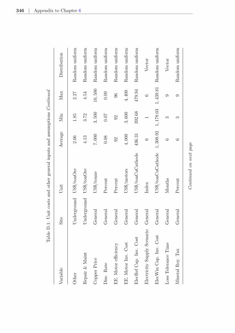
346 | Appendix to Chapter 6
Tabl
eD
.1:
Uni
tco
sts
and
othe
rge
nera
linp
uts
and
assu
mpt
ions
Con
tinue
d
Varia
ble
Site
Uni
tAv
erag
eM
inM
axD
istrib
utio
n
Oth
erU
nder
grou
ndU
S$/t
onO
re2.
061.
852.
27R
ando
mun
iform
Rep
air
&M
aint
Und
ergr
ound
US$
/ton
Ore
4.13
3.72
4.54
Ran
dom
unifo
rm
Cop
per
Pric
eG
ener
alU
S$/t
onne
7,00
03,
500
10,5
00R
ando
mun
iform
Disc
.R
ate
Gen
eral
Perc
ent
0.08
0.07
0.09
Ran
dom
unifo
rm
EE.M
otor
effici
ency
Gen
eral
Perc
ent
9292
96R
ando
mun
iform
EE.M
otor
Inv.
Cos
tG
ener
alU
S$/m
otor
s4,
000
3,60
04,
400
Ran
dom
unifo
rm
Elec
Ref
Cap
.In
v.C
ost
Gen
eral
US$
/ton
CuC
atho
de43
6.31
392.
6847
9.94
Ran
dom
unifo
rm
Elec
tric
itySu
pply
Scen
ario
Gen
eral
Inde
x6
16
Vect
or
Elec
Win
Cap
.In
v.C
ost
Gen
eral
US$
/ton
CuC
atho
de1,
308.
921,
178.
031,
439.
81R
ando
mun
iform
Loss
Tole
ranc
eT
ime
Gen
eral
Mon
ths
63
9Ve
ctor
Min
eral
Roy
.Ta
xG
ener
alPe
rcen
t6
39
Ran
dom
unifo
rm
Con
tinue
don
next
page
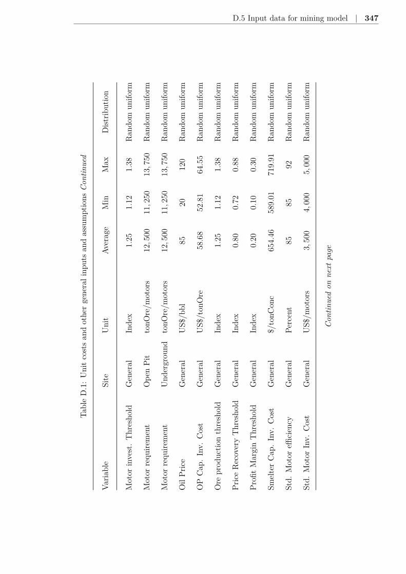
D.5 Input data for mining model | 347
Tabl
eD
.1:
Uni
tco
sts
and
othe
rge
nera
linp
uts
and
assu
mpt
ions
Con
tinue
d
Varia
ble
Site
Uni
tAv
erag
eM
inM
axD
istrib
utio
n
Mot
orin
vest
.T
hres
hold
Gen
eral
Inde
x1.
251.
121.
38R
ando
mun
iform
Mot
orre
quire
men
tO
pen
Pit
tonO
re/m
otor
s12,5
0011,2
5013,7
50R
ando
mun
iform
Mot
orre
quire
men
tU
nder
grou
ndto
nOre
/mot
ors
12,5
0011,2
5013,7
50R
ando
mun
iform
Oil
Pric
eG
ener
alU
S$/b
bl85
2012
0R
ando
mun
iform
OP
Cap
.In
v.C
ost
Gen
eral
US$
/ton
Ore
58.6
852.8
164.5
5R
ando
mun
iform
Ore
prod
uctio
nth
resh
old
Gen
eral
Inde
x1.
251.
121.
38R
ando
mun
iform
Pric
eR
ecov
ery
Thr
esho
ldG
ener
alIn
dex
0.80
0.72
0.88
Ran
dom
unifo
rm
Profi
tM
argi
nT
hres
hold
Gen
eral
Inde
x0.
200.
100.
30R
ando
mun
iform
Smel
ter
Cap
.In
v.C
ost
Gen
eral
$/to
nCon
c65
4.46
589.
0171
9.91
Ran
dom
unifo
rm
Std.
Mot
oreffi
cien
cyG
ener
alPe
rcen
t85
8592
Ran
dom
unifo
rm
Std.
Mot
orIn
v.C
ost
Gen
eral
US$
/mot
ors
3,50
04,
000
5,00
0R
ando
mun
iform
Con
tinue
don
next
page

348 | Appendix to Chapter 6
Tabl
eD
.1:
Uni
tco
sts
and
othe
rge
nera
linp
uts
and
assu
mpt
ions
Con
tinue
d
Varia
ble
Site
Uni
tAv
erag
eM
inM
axD
istrib
utio
n
UG
Cap
.In
v.C
ost
Gen
eral
US$
/ton
Ore
202.
7718
2.49
223.
05R
ando
mun
iform
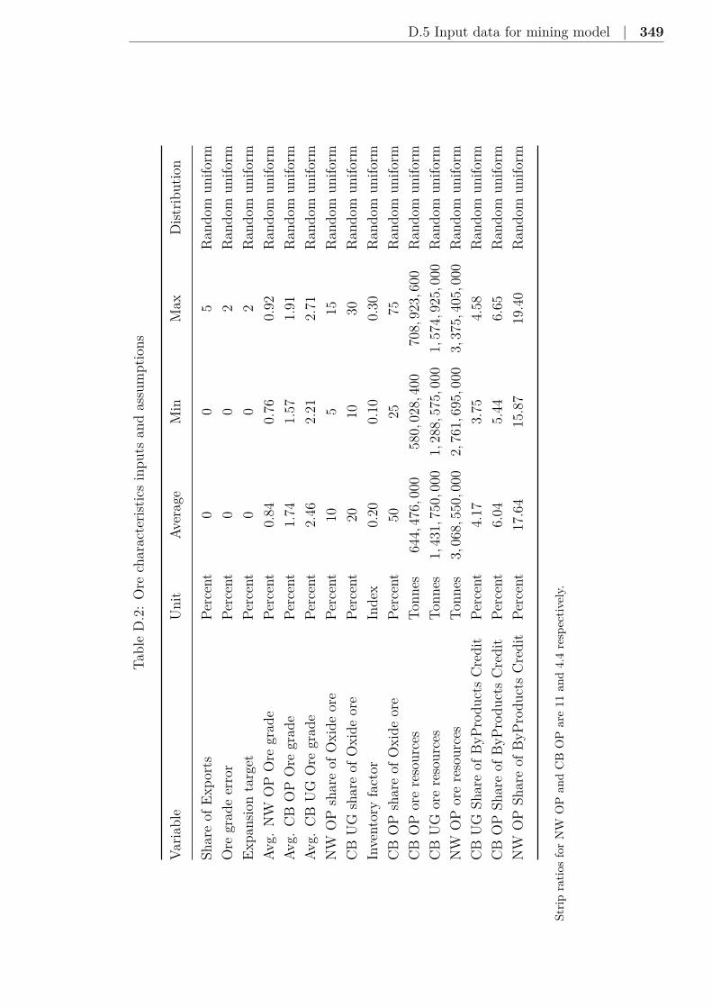
D.5 Input data for mining model | 349
Tabl
eD
.2:
Ore
char
acte
ristic
sin
puts
and
assu
mpt
ions
Varia
ble
Uni
tAv
erag
eM
inM
axD
istrib
utio
n
Shar
eof
Expo
rts
Perc
ent
00
5R
ando
mun
iform
Ore
grad
eer
ror
Perc
ent
00
2R
ando
mun
iform
Expa
nsio
nta
rget
Perc
ent
00
2R
ando
mun
iform
Avg.
NW
OP
Ore
grad
ePe
rcen
t0.
840.
760.
92R
ando
mun
iform
Avg.
CB
OP
Ore
grad
ePe
rcen
t1.
741.
571.
91R
ando
mun
iform
Avg.
CB
UG
Ore
grad
ePe
rcen
t2.
462.
212.
71R
ando
mun
iform
NW
OP
shar
eof
Oxi
deor
ePe
rcen
t10
515
Ran
dom
unifo
rmC
BU
Gsh
are
ofO
xide
ore
Perc
ent
2010
30R
ando
mun
iform
Inve
ntor
yfa
ctor
Inde
x0.
200.
100.
30R
ando
mun
iform
CB
OP
shar
eof
Oxi
deor
ePe
rcen
t50
2575
Ran
dom
unifo
rmC
BO
Por
ere
sour
ces
Tonn
es64
4,47
6,00
058
0,02
8,40
070
8,92
3,60
0R
ando
mun
iform
CB
UG
ore
reso
urce
sTo
nnes
1,43
1,75
0,00
01,
288,
575,
000
1,57
4,92
5,00
0R
ando
mun
iform
NW
OP
ore
reso
urce
sTo
nnes
3,06
8,55
0,00
02,
761,
695,
000
3,37
5,40
5,00
0R
ando
mun
iform
CB
UG
Shar
eof
ByPr
oduc
tsC
redi
tPe
rcen
t4.
173.
754.
58R
ando
mun
iform
CB
OP
Shar
eof
ByPr
oduc
tsC
redi
tPe
rcen
t6.
045.
446.
65R
ando
mun
iform
NW
OP
Shar
eof
ByPr
oduc
tsC
redi
tPe
rcen
t17.6
415.8
719.4
0R
ando
mun
iform
Strip
ratio
sfo
rN
WO
Pan
dC
BO
Par
e11
and
4.4
resp
ectiv
ely.
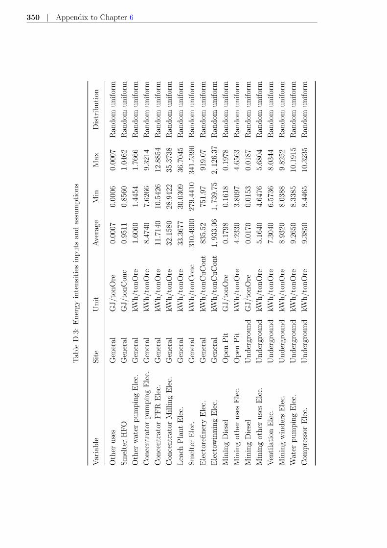
350 | Appendix to Chapter 6
Tabl
eD
.3:
Ener
gyin
tens
ities
inpu
tsan
das
sum
ptio
ns
Varia
ble
Site
Uni
tAv
erag
eM
inM
axD
istrib
utio
n
Oth
erus
esG
ener
alG
J/to
nOre
0.00
070.
0006
0.00
07R
ando
mun
iform
Smel
ter
HFO
Gen
eral
GJ/
tonC
onc
0.95
110.
8560
1.04
62R
ando
mun
iform
Oth
erwa
ter
pum
ping
Elec
.G
ener
alkW
h/to
nOre
1.60
601.
4454
1.76
66R
ando
mun
iform
Con
cent
rato
rpu
mpi
ngEl
ec.
Gen
eral
kWh/
tonO
re8.
4740
7.62
669.
3214
Ran
dom
unifo
rmC
once
ntra
tor
FFR
Elec
.G
ener
alkW
h/to
nOre
11.7
140
10.5
426
12.8
854
Ran
dom
unifo
rmC
once
ntra
tor
Mill
ing
Elec
.G
ener
alkW
h/to
nOre
32.1
580
28.9
422
35.3
738
Ran
dom
unifo
rmLe
ach
Plan
tEl
ec.
Gen
eral
kWh/
tonO
re33.3
677
30.0
309
36.7
045
Ran
dom
unifo
rmSm
elte
rEl
ec.
Gen
eral
kWh/
tonC
onc
310.
4900
279.
4410
341.
5390
Ran
dom
unifo
rmEl
ecto
refin
ery
Elec
.G
ener
alkW
h/to
nCuC
ont
835.
5275
1.97
919.
07R
ando
mun
iform
Elec
tow
inni
ngEl
ec.
Gen
eral
kWh/
tonC
uCon
t1,
933.
061,
739.
752,
126.
37R
ando
mun
iform
Min
ing
Die
sel
Ope
nPi
tG
J/to
nOre
0.17
980.
1618
0.19
78R
ando
mun
iform
Min
ing
othe
rus
esEl
ec.
Ope
nPi
tkW
h/to
nOre
4.23
303.
8097
4.65
63R
ando
mun
iform
Min
ing
Die
sel
Und
ergr
ound
GJ/
tonO
re0.
0170
0.01
530.
0187
Ran
dom
unifo
rmM
inin
got
her
uses
Elec
.U
nder
grou
ndkW
h/to
nOre
5.16
404.
6476
5.68
04R
ando
mun
iform
Vent
ilatio
nEl
ec.
Und
ergr
ound
kWh/
tonO
re7.
3040
6.57
368.
0344
Ran
dom
unifo
rmM
inin
gw
inde
rsEl
ec.
Und
ergr
ound
kWh/
tonO
re8.
9320
8.03
889.
8252
Ran
dom
unifo
rmW
ater
pum
ping
Elec
.U
nder
grou
ndkW
h/to
nOre
9.26
508.
3385
10.1
915
Ran
dom
unifo
rmC
ompr
esso
rEl
ec.
Und
ergr
ound
kWh/
tonO
re9.
3850
8.44
6510.3
235
Ran
dom
unifo
rm

D.6 Model Tests | 351
D.6 Model Tests
These model test are adapted from Sterman (2000), Table 21-3 in particu-
lar.
1. Boundary Adequacy test:
(a) Are the important concepts for addressing the problem endoge-
nous to the model?
(b) Does the behaviour of the model change significantly when
boundary assumptions are relaxed?
(c) Do the policy recommendations change when the model bound-
ary is extended?
2. Structure Assessment test:
(a) Is the model structure consistent with relevant descriptive
knowledge of the system?
(b) Is the level of aggregation appropriate?
(c) Does the model conform to basic physical laws such as conser-
vation laws?
(d) Do the decision rules capture the behaviour of the actors in the
system?
3. Dimensional Consistency test:
(a) Is each equation dimensionally consistent without the use of pa-
rameters having no real world meaning?
4. Parameter Assessment test:
(a) Are the parameter values consistent with relevant descriptive
and numerical knowledge of the system?
(b) Do all parameters have real world counterparts?
5. Extreme Conditions test:

352 | Appendix to Chapter 6
(a) Does each equation make sense even when its inputs take on
extreme values?
(b) Does the model respond plausibly when subjected to extreme
policies, shocks, and parameters?
6. Integration Error test:
(a) Are the results sensitive to the choice of time step or numerical
integration method?
7. Behaviour Reproduction test:
(a) Does the model reproduce the behaviour of interest in the system
(qualitatively and quantitatively)?
(b) Does it endogenously generate the symptoms of difficulty moti-
vating the study?
(c) Does the model generate the various modes of behaviour ob-
served in the real system?
(d) Do the frequencies and phase relationships among the variables
match the data?
8. Behaviour Anomaly test:
(a) Do anomalous behaviours result when assumptions of the model
are changed or deleted?
9. Family Member test:
(a) Can the model generate the behaviour observed in other in-
stances of the same system?
10. Surprise Behaviour test:
(a) Does the model generate previously unobserved or unrecognised
behaviour?
(b) Does the model successfully anticipate the response of the sys-
tem to novel conditions?
D.6 Model Tests | 353
11. Sensitivity Analysis test:
(a) Numerical sensitivity: Do the numerical values change signifi-
cantly . . .
(b) Behavioural sensitivity: Do the modes of behaviour generated
by the model change significantly . . .
(c) Policy sensitivity: Do the policy implications change signifi-
cantly . . .
(d) . . . when assumptions about parameters, boundary, and ag-
gregation are varied over the plausible range of uncertainty?
12. System Improvement test:
(a) Did the modelling process help change the system for the better?
D.6.1 Applied extreme test
In order to check that model behaves as expected, it was exposed to extreme
conditions12. Firstly, all the model mathematical equations and relation-
ships were inspected to check if they were logical and represented as those
in the real system. Then input variables of electricity price, oil price, min-
eral royalty tax and copper price were varied to check how the model would
behave. Table D.4 below shows the values of the variable used in the test.
Test 1 considers a situation where all inputs and copper price favour
continuous production, and from Figure D.1 it can be seen that all three
sites continue to produce copper ore. Test 2 shows the significance of
copper price in the model, production drops to zero once the copper price
drop to $1, 000/ton because this price is less that the unit production cost
incurred by a mining firm. Similar to Test 2, Tests 3 to 5, show that the
model behaves as expected (stopping production) once extreme values are
introduced (after 2015).12An analysis of inputs that are key driver in the model are given in sub-section 7.2.2
above.
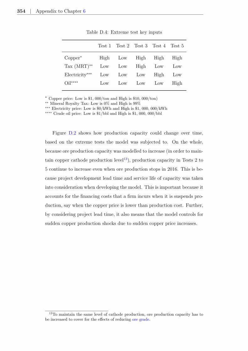
354 | Appendix to Chapter 6
Table D.4: Extreme test key inputs
Test 1 Test 2 Test 3 Test 4 Test 5
Copper∗ High Low High High HighTax (MRT)∗∗ Low Low High Low LowElectricity∗∗∗ Low Low Low High LowOil∗∗∗∗ Low Low Low Low High
∗ Copper price: Low is $1, 000/ton and High is $10, 000/ton)∗∗ Mineral Royalty Tax: Low is 0% and High is 99%∗∗∗ Electricity price: Low is $0/kWh and High is $1, 000, 000/kWh∗∗∗∗ Crude oil price: Low is $1/bbl and High is $1, 000, 000/bbl
Figure D.2 shows how production capacity could change over time,
based on the extreme tests the model was subjected to. On the whole,
because ore production capacity was modelled to increase (in order to main-
tain copper cathode production level13), production capacity in Tests 2 to
5 continue to increase even when ore production stops in 2016. This is be-
cause project development lead time and service life of capacity was taken
into consideration when developing the model. This is important because it
accounts for the financing costs that a firm incurs when it is suspends pro-
duction, say when the copper price is lower than production cost. Further,
by considering project lead time, it also means that the model controls for
sudden copper production shocks due to sudden copper price increases.
13To maintain the same level of cathode production, ore production capacity has tobe increased to cover for the effects of reducing ore grade.
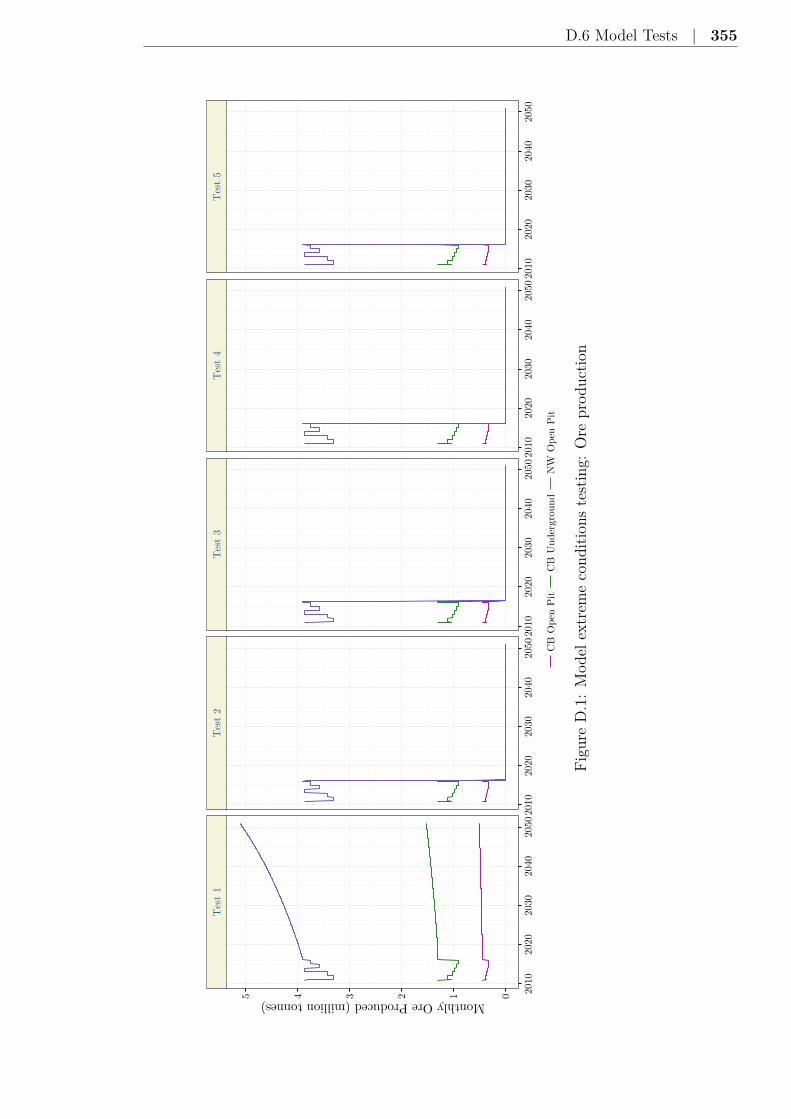
D.6 Model Tests | 355
Tes
t 1
Tes
t 2
Tes
t 3
Tes
t 4
Tes
t 5
012345 2010
2020
2030
2040
2050
2010
2020
2030
2040
2050
2010
2020
2030
2040
2050
2010
2020
2030
2040
2050
2010
2020
2030
2040
2050
Monthly Ore Produced (million tonnes)
C
B O
pen
Pit
CB
Und
ergr
ound
NW
Ope
n Pi
t
Figu
reD
.1:
Mod
elex
trem
eco
nditi
ons
test
ing:
Ore
prod
uctio
n
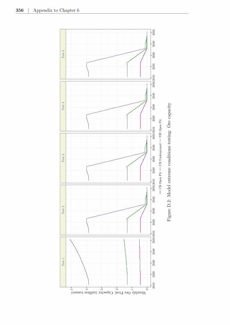
356 | Appendix to Chapter 6
Tes
t 1
Tes
t 2
Tes
t 3
Tes
t 4
Tes
t 5
012345 2010
2020
2030
2040
2050
2010
2020
2030
2040
2050
2010
2020
2030
2040
2050
2010
2020
2030
2040
2050
2010
2020
2030
2040
2050
Monthly Ore Prod. Capacity (million tonnes)
C
B O
pen
Pit
CB
Und
ergr
ound
NW
Ope
n Pi
t
Figu
reD
.2:
Mod
elex
trem
eco
nditi
ons
test
ing:
Ore
capa
city

Appendix E
Appendix to Chapter 7
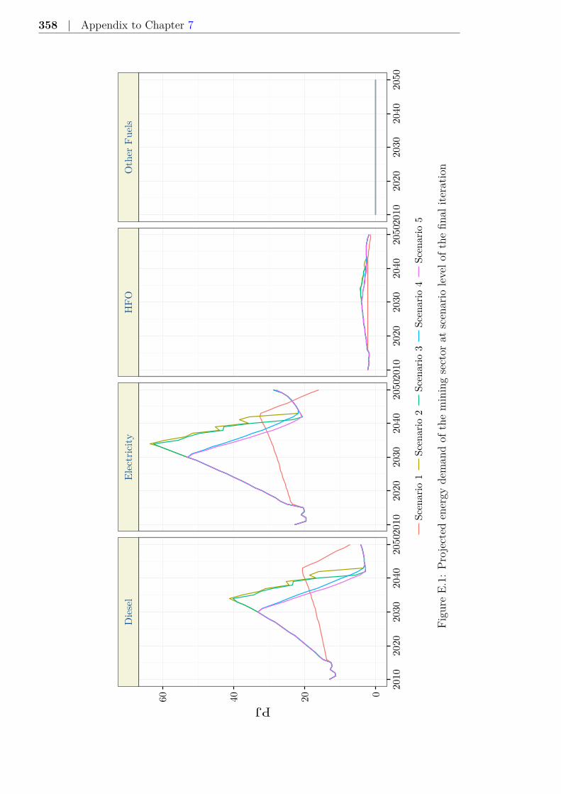
358 | Appendix to Chapter 7
Die
sel
Elec
tric
ityH
FOO
ther
Fue
ls
0204060
2010
2020
2030
2040
2050
2010
2020
2030
2040
2050
2010
2020
2030
2040
2050
2010
2020
2030
2040
2050
PJ
Sc
enar
io 1
Scen
ario
2Sc
enar
io 3
Scen
ario
4Sc
enar
io 5
Figu
reE.
1:Pr
ojec
ted
ener
gyde
man
dof
the
min
ing
sect
orat
scen
ario
leve
loft
hefin
alite
ratio
n
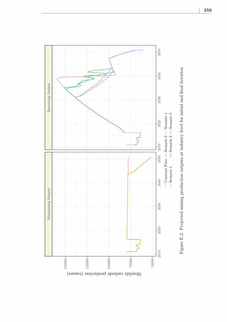
| 359
Mai
ntai
ning
Out
put
Incr
easin
g O
utpu
t
2010
2020
2030
2040
2050
2010
2020
2030
2040
2050
5000
0
7500
0
1000
00
1250
00
1500
00
Monthly cathode production (tonnes)
Con
stan
t Pr
ice
Scen
ario
1Sc
enar
io 2
Scen
ario
3Sc
enar
io 4
Scen
ario
5
Figu
reE.
2:Pr
ojec
ted
min
ing
prod
uctio
nou
tput
sat
indu
stry
leve
lfor
initi
alan
dfin
alite
ratio
n
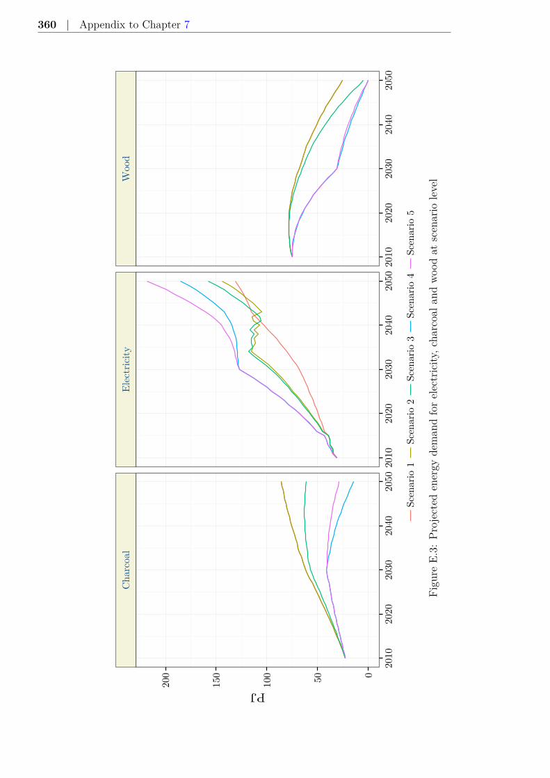
360 | Appendix to Chapter 7
Cha
rcoa
lEl
ectr
icity
Woo
d
050100
150
200
2010
2020
2030
2040
2050
2010
2020
2030
2040
2050
2010
2020
2030
2040
2050
PJ
Sc
enar
io 1
Scen
ario
2Sc
enar
io 3
Scen
ario
4Sc
enar
io 5
Figu
reE.
3:Pr
ojec
ted
ener
gyde
man
dfo
rel
ectr
icity
,cha
rcoa
land
wood
atsc
enar
iole
vel
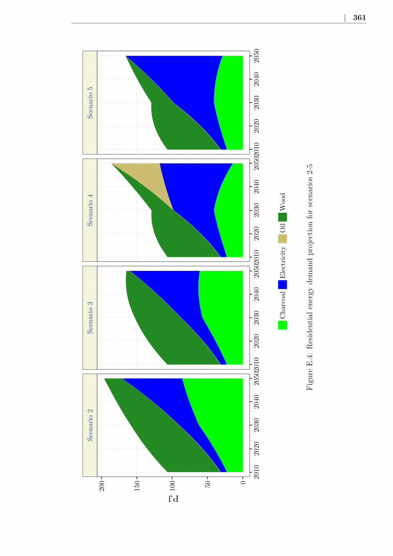
| 361
Scen
ario
2Sc
enar
io 3
Scen
ario
4Sc
enar
io 5
050100
150
200
2010
2020
2030
2040
2050
2010
2020
2030
2040
2050
2010
2020
2030
2040
2050
2010
2020
2030
2040
2050
PJ
C
harc
oal
Elec
tric
ityO
ilW
ood
Figu
reE.
4:R
esid
entia
lene
rgy
dem
and
proj
ectio
nfo
rsc
enar
ios
2-5
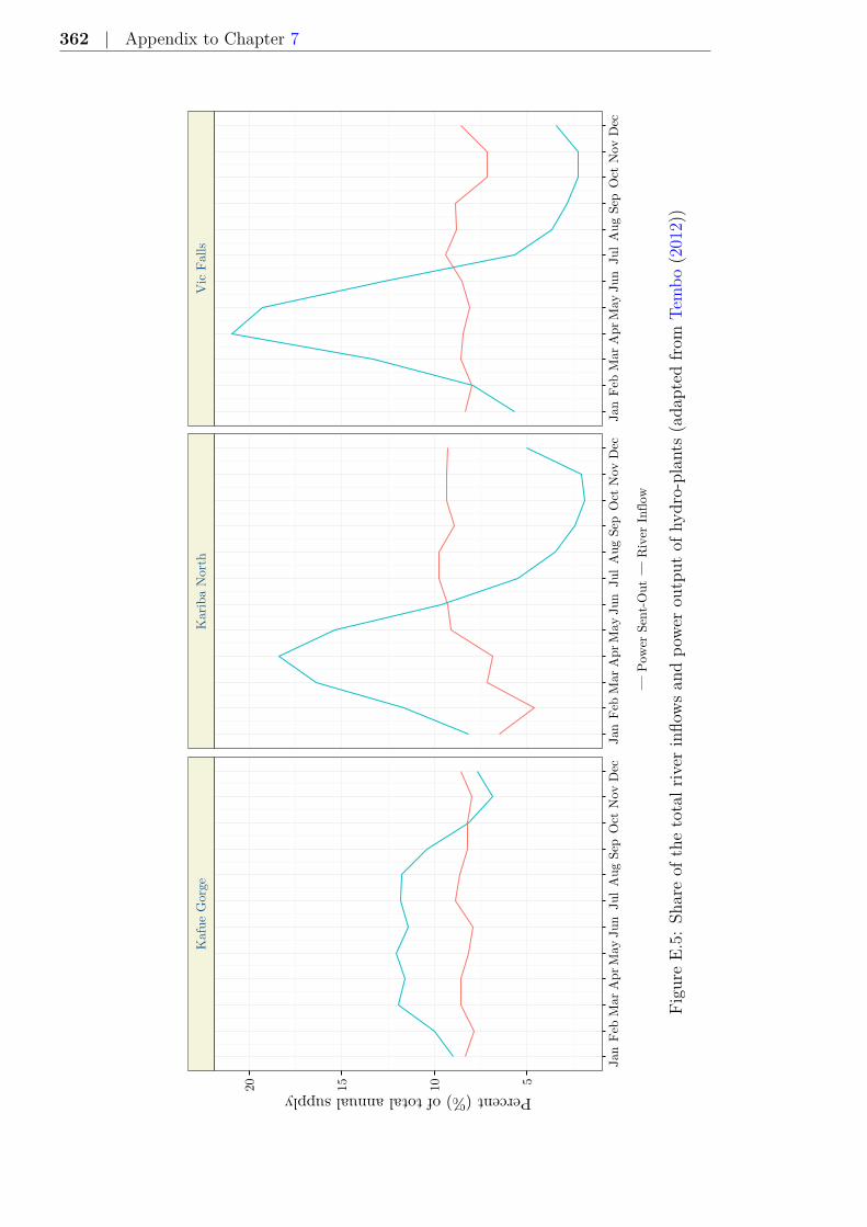
362 | Appendix to Chapter 7
Kaf
ue G
orge
Kar
iba
Nor
thV
ic F
alls
5101520
Jan
Feb
Mar
Apr
May
Jun
Jul
Aug
Sep
Oct
Nov
Dec
Jan
Feb
Mar
Apr
May
Jun
Jul
Aug
Sep
Oct
Nov
Dec
Jan
Feb
Mar
Apr
May
Jun
Jul
Aug
Sep
Oct
Nov
Dec
Percent (%) of total annual supply
Pow
er S
ent-
Out
Riv
er In
flow
Figu
reE.
5:Sh
are
ofth
eto
talr
iver
inflo
ws
and
powe
rou
tput
ofhy
dro-
plan
ts(a
dapt
edfro
mTe
mbo
(201
2))
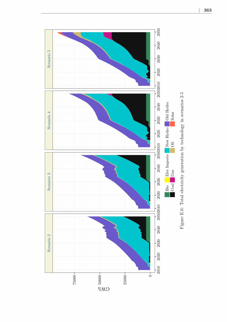
| 363
Scen
ario
2Sc
enar
io 3
Scen
ario
4Sc
enar
io 5
0
2500
0
5000
0
7500
0
2010
2020
2030
2040
2050
2010
2020
2030
2040
2050
2010
2020
2030
2040
2050
2010
2020
2030
2040
2050
GWh
Bi
oC
oal
Elec
Impo
rts
Gas
New
Hyd
roO
ilO
ld H
ydro
Sola
r
Figu
reE.
6:To
tale
lect
ricity
gene
ratio
nby
tech
nolo
gyin
scen
ario
s2-
5
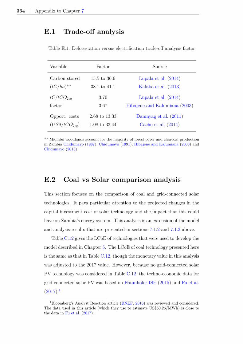
364 | Appendix to Chapter 7
E.1 Trade-off analysis
Table E.1: Deforestation versus electrification trade-off analysis factor
Variable Factor Source
Carbon stored 15.5 to 36.6 Lupala et al. (2014)(tC/ha)** 38.1 to 41.1 Kalaba et al. (2013)
tC/tCO2eq 3.70 Lupala et al. (2014)factor 3.67 Hibajene and Kalumiana (2003)
Opport. costs 2.68 to 13.33 Damnyag et al. (2011)(US$/tCO2eq) 1.08 to 33.44 Cacho et al. (2014)
** Miombo woodlands account for the majority of forest cover and charcoal productionin Zambia Chidumayo (1987), Chidumayo (1991), Hibajene and Kalumiana (2003) andChidumayo (2013)
E.2 Coal vs Solar comparison analysis
This section focuses on the comparison of coal and grid-connected solar
technologies. It pays particular attention to the projected changes in the
capital investment cost of solar technology and the impact that this could
have on Zambia’s energy system. This analysis is an extension of the model
and analysis results that are presented in sections 7.1.2 and 7.1.3 above.
Table C.12 gives the LCoE of technologies that were used to develop the
model described in Chapter 5. The LCoE of coal technology presented here
is the same as that in Table C.12, though the monetary value in this analysis
was adjusted to the 2017 value. However, because no grid-connected solar
PV technology was considered in Table C.12, the techno-economic data for
grid connected solar PV was based on Fraunhofer ISE (2015) and Fu et al.
(2017).1
1Bloomberg’s Analyst Reaction article (BNEF, 2016) was reviewed and considered.The data used in this article (which they use to estimate US$60.26/MWh) is close tothe data in Fu et al. (2017).
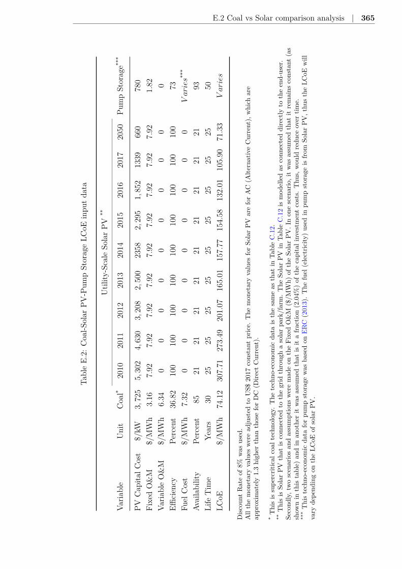
E.2 Coal vs Solar comparison analysis | 365
Tabl
eE.
2:C
oal-S
olar
PV-P
ump
Stor
age
LCoE
inpu
tda
ta
Util
ity-S
cale
Sola
rPV
**
Varia
ble
Uni
tC
oal*
2010
2011
2012
2013
2014
2015
2016
2017
2050
Pum
pSt
orag
e***
PVC
apita
lCos
t$/
kW3,
725
5,30
24,
630
3,20
82,
500
2358
2,29
51,
852
1339
660
780
Fixe
dO
&M
$/M
Wh
3.16
7.92
7.92
7.92
7.92
7.92
7.92
7.92
7.92
7.92
1.82
Varia
ble
O&
M$/
MW
h6.
340
00
00
00
00
0Effi
cien
cyPe
rcen
t36.8
210
010
010
010
010
010
010
010
010
073
Fuel
Cos
t$/
MW
h7.
320
00
00
00
00
Varies
***
Avai
labi
lity
Perc
ent
8521
2121
2121
2121
2121
93Li
feT
ime
Year
s30
2525
2525
2525
2525
2550
LCoE
$/M
Wh
74.1
230
7.71
273.
4920
1.07
165.
0115
7.77
154.
5813
2.01
105.
9071.3
3Varies
Disc
ount
Rat
eof
8%w
asus
ed.
All
the
mon
etar
yva
lues
wer
ead
just
edto
US$
2017
cons
tant
pric
e.T
hem
onet
ary
valu
esfo
rSo
lar
PVar
efo
rA
C(A
ltern
ativ
eC
urre
nt),
whi
char
eap
prox
imat
ely
1.3
high
erth
anth
ose
for
DC
(Dire
ctC
urre
nt).
*T
his
issu
perc
ritic
alco
alte
chno
logy
.T
hete
chno
-eco
nom
icda
tais
the
sam
eas
that
inTa
ble
C.1
2.**
Thi
sis
Sola
rPV
that
isco
nnec
ted
toth
egr
idth
roug
ha
sola
rpa
rk/f
arm
.T
heSo
lar
PVin
Tabl
eC
.12
ism
odel
led
asco
nnec
ted
dire
ctly
toth
een
d-us
er.
Seco
ndly
,tw
osc
enar
ios
and
assu
mpt
ions
wer
em
ade
onth
eFi
xed
O&
M($
/MW
h)of
the
Sola
rPV
.In
one
scen
ario
,it
was
assu
med
that
itre
mai
nsco
nsta
nt(a
ssh
own
inth
ista
ble)
and
inan
othe
rit
was
assu
med
that
isit
afr
actio
n(2
.04%
)of
the
capi
tali
nves
tmen
tco
sts.
Thu
s,w
ould
redu
ceov
ertim
e.**
*T
his
tech
no-e
cono
mic
data
for
pum
pst
orag
ew
asba
sed
onER
C(2
013)
.T
hefu
el(e
lect
ricity
)us
edin
pum
pst
orag
eis
from
Sola
rPV
,thu
sth
eLC
oEw
illva
ryde
pend
ing
onth
eLC
oEof
sola
rPV
.

366 | Appendix to Chapter 7
Figure E.7 below shows the changes in LCoE over time. It can be seen
that in three out of four LCoE projections, the LCoE for solar and solar
plus pump storage is expected to be cheaper than Coal’s LCoE by 2046.2
100
200
300
400
2010 2020 2030 2040 2050
US$
/MW
h
Coal Solar Constant Solar Reducing Solar+Pump Constant Solar+Pump Reducing
Figure E.7: LCoE analysis for coal, solar PV and pump storage
Having calculated the LCoE, this analysis now focuses on considering
what this means for solar and solar plus storage diffusion in the energy
system. Development of new coal capacity described in the five energy
scenarios (see section 5.3 for the scenario description) was used to analyse
how solar and solar plus storage could diffuse in Zambia’s energy system.
Basically, the analysis looks at how cost effective solar would be in replacing
coal technology in the system. The quantity of electricity produced from
coal (in these scenarios) was used as a basis for estimating the size of
capacity (in MW) of the replacement technology. Figures E.8 to E.11 below
show the estimated development of coal and the diffusion of solar and solar
plus storage in the system (after considering the calculated LCoE).2In Figure E.7, “Solar Constant” represents Solar PV with constant Fixed O&M
costs, “Solar Reducing” represents Solar PV with reducing Fixed O&M costs (a frac-tion (2.04%) of the capital investment costs), “Solar+Pump Constant” represents So-lar PV system with pump storage, which has constant Fixed O&M costs and finally“Solar+Pump Reducing” represents Solar PV system with pump storage, which hasreducing Fixed O&M costs (a fraction (2.04%) of the capital investment costs of SolarPV).
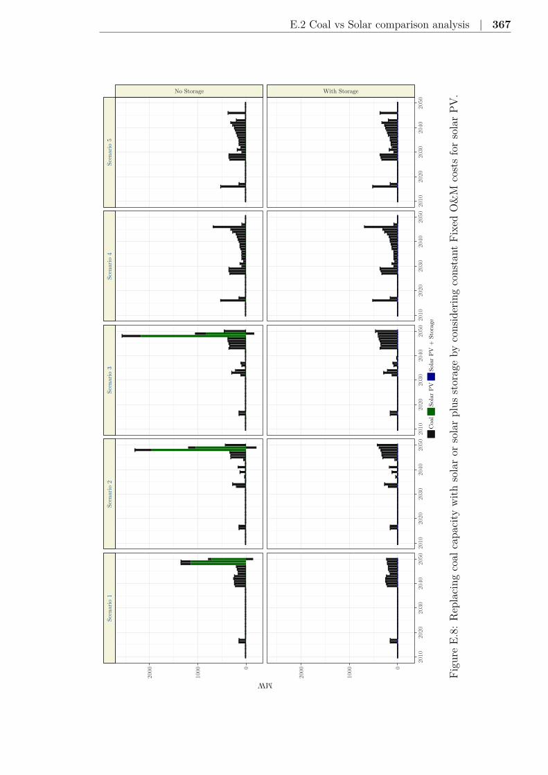
E.2 Coal vs Solar comparison analysis | 367
Scen
ario
1Sc
enar
io 2
Scen
ario
3Sc
enar
io 4
Scen
ario
5
No Storage With Storage
2010
2020
2030
2040
2050
2010
2020
2030
2040
2050
2010
2020
2030
2040
2050
2010
2020
2030
2040
2050
2010
2020
2030
2040
2050
0
1000
2000 0
1000
2000
MW
C
oal
Sola
r PV
Sola
r PV
+ S
tora
ge
Figu
reE.
8:R
epla
cing
coal
capa
city
with
sola
ror
sola
rpl
usst
orag
eby
cons
ider
ing
cons
tant
Fixe
dO
&M
cost
sfo
rso
lar
PV.
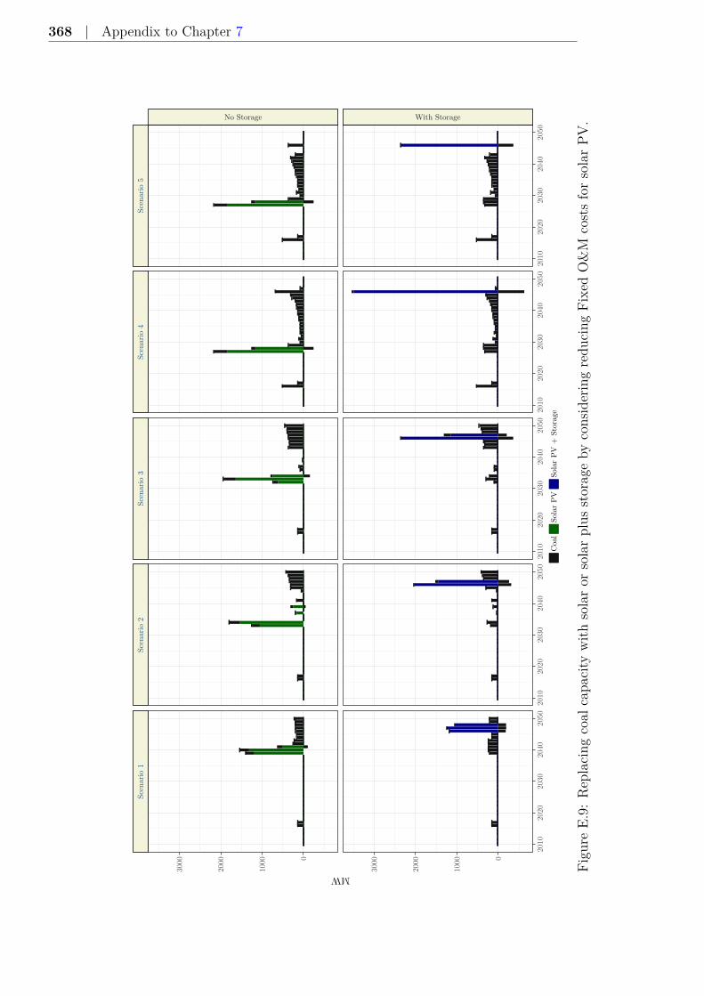
368 | Appendix to Chapter 7
Scen
ario
1Sc
enar
io 2
Scen
ario
3Sc
enar
io 4
Scen
ario
5
No Storage With Storage
2010
2020
2030
2040
2050
2010
2020
2030
2040
2050
2010
2020
2030
2040
2050
2010
2020
2030
2040
2050
2010
2020
2030
2040
2050
0
1000
2000
3000 0
1000
2000
3000
MW
C
oal
Sola
r PV
Sola
r PV
+ S
tora
ge
Figu
reE.
9:R
epla
cing
coal
capa
city
with
sola
ror
sola
rpl
usst
orag
eby
cons
ider
ing
redu
cing
Fixe
dO
&M
cost
sfo
rso
lar
PV.
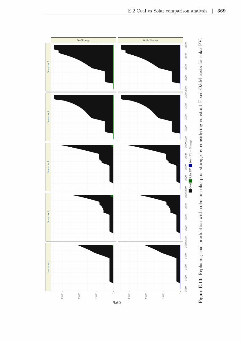
E.2 Coal vs Solar comparison analysis | 369
Scen
ario
1Sc
enar
io 2
Scen
ario
3Sc
enar
io 4
Scen
ario
5
No Storage With Storage
2010
2020
2030
2040
2050
2010
2020
2030
2040
2050
2010
2020
2030
2040
2050
2010
2020
2030
2040
2050
2010
2020
2030
2040
2050
0
1000
0
2000
0
3000
0 0
1000
0
2000
0
3000
0
GWh
C
oal
Sola
r PV
Sola
r PV
+ S
tora
ge
Figu
reE.
10:
Rep
laci
ngco
alpr
oduc
tion
with
sola
ror
sola
rpl
usst
orag
eby
cons
ider
ing
cons
tant
Fixe
dO
&M
cost
sfo
rso
lar
PV.
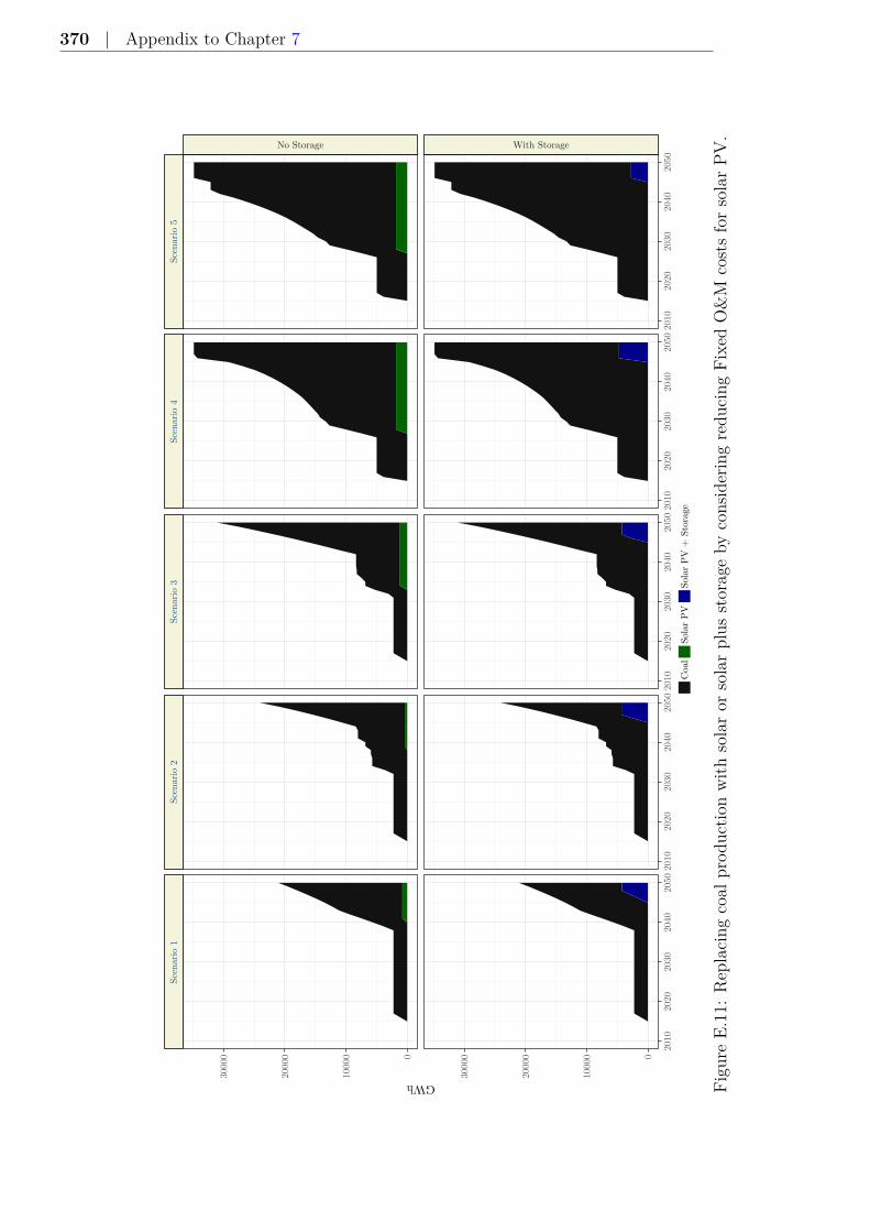
370 | Appendix to Chapter 7
Scen
ario
1Sc
enar
io 2
Scen
ario
3Sc
enar
io 4
Scen
ario
5
No Storage With Storage
2010
2020
2030
2040
2050
2010
2020
2030
2040
2050
2010
2020
2030
2040
2050
2010
2020
2030
2040
2050
2010
2020
2030
2040
2050
0
1000
0
2000
0
3000
0 0
1000
0
2000
0
3000
0
GWh
C
oal
Sola
r PV
Sola
r PV
+ S
tora
ge
Figu
reE.
11:
Rep
laci
ngco
alpr
oduc
tion
with
sola
ror
sola
rpl
usst
orag
eby
cons
ider
ing
redu
cing
Fixe
dO
&M
cost
sfo
rso
lar
PV.
E.2 Coal vs Solar comparison analysis | 371
From the Figures, it can be seen that despite having lower LCoE (in
three out of four LCoE projections), diffusion of both solar and solar with
storage into the Zambia’s energy system is still limited. This is mainly
because:
1. In the model, available maximum solar capacity was set to 3,000 MW
(and coal was set to 4,300 MW) – see Table C.14. Thus, the available
solar capacity is not enough to replace all the coal capacity. This is
even more true, when we take into account the quantity of electricity
that each capacity (of solar and coal technologies) is able to produce
based on their capacity factor.
2. By the time solar plus storage becomes cheaper, most of the coal
capacity would have already been deployed. Therefore, only a small
portion of coal gets replaced (i.e. solar plus storage is developed
instead of coal.)
The second point takes into consideration that even though solar (with-
out storage) would have a lower LCoE, it could not be possible to replace
coal capacity using it. This is because of the variability that comes with
solar technology. Thus, to effectively replace coal, solar would need to be
coupled with a storage technology. In this case, pump storage was consid-
ered. Pump storage (like all other technologies) has a cost to it and this
defers the decision to deploy solar technology to a later time.
In sub-section 8.3.5 (where I discussed possible future works), I recom-
mended that a comprehensive energy resource mapping for Zambia should
be done in order to improve the results of this thesis. Such an exercise
would help quantify the size of available resources for solar and other sim-
ilar technologies that could potentially be used to replace coal and other
similar carbon emitting technologies. To address this gap, the World Bank
is currently running a project called ‘Renewable Energy Resource Mapping
in Zambia’ (World Bank, 2018).
Further, while it was assumed that pump storage was available for de-
velopment in Zambia, there are no official records to that effect. But if it
372 | Appendix to Chapter 7
is assumed that Zambia’s hydro resources could be used to develop pump
storage technology, this assumption would break-down when the nature of
hydro resources in Zambia are taken into account. This is because the water
resources in Zambia, and generally the SADC region, are trans-boundary
resources. Therefore, development of any pump storage in Zambia would
require changes in laws and regulations of how these resources are utilised.
For instance, keeping water resources longer (through pump storage) in
Zambia could significantly impact the operations of Mozambican hydro
plants.
Thus, at the minimum, to effectively analyse how solar could replace
coal in Zambia, there would be need to have a comprehensive energy re-
source profile and also to have an array of inexpensive storage technologies
that could be deployed along side solar and other similar technologies.
E.3 KCM costs structure
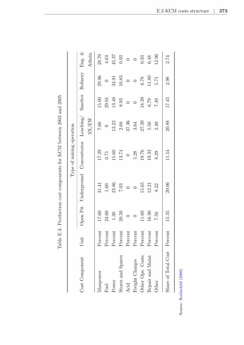
E.3 KCM costs structure | 373
Tabl
eE.
3:Pr
oduc
tion
cost
com
pone
nts
for
KC
Mbe
twee
n20
03an
d20
05
Type
ofm
inin
gop
erat
ion
Cos
tC
ompo
nent
Uni
tO
pen
Pit
Und
ergr
ound
Con
cent
rato
rLe
achi
ng/
Smel
ter
Refi
nery
Eng.
&SX
/EW
Adm
in.
Man
powe
rPe
rcen
t17.6
031.4
117.2
97.
6615.0
029.9
628.7
0Fu
elPe
rcen
t24.6
01.
600.
710
29.9
10
4.63
Powe
rPe
rcen
t1.
3023.8
615.6
013.2
213.4
834.9
145.3
7St
ores
and
Spar
esPe
rcen
t20.5
07.
0313.7
42.
688.
9310.8
30.
93A
cid
Perc
ent
00
037.3
60
00
Frei
ght
Cha
rges
Perc
ent
00
5.28
3.64
00
0O
ther
Ops
.C
osts
Perc
ent
11.6
015.6
519.7
627.3
918.3
96.
780.
93R
epai
ran
dM
aint
Perc
ent
16.9
012.2
119.3
35.
566.
7911.8
06.
48O
ther
Perc
ent
7.50
8.22
8.29
2.49
7.49
5.71
12.9
6
Shar
eof
Tota
lCos
tPe
rcen
t15.3
529.0
611.5
420.8
817.4
52.
982.
74
Sour
ce:
Rot
hsch
ild(2
008)
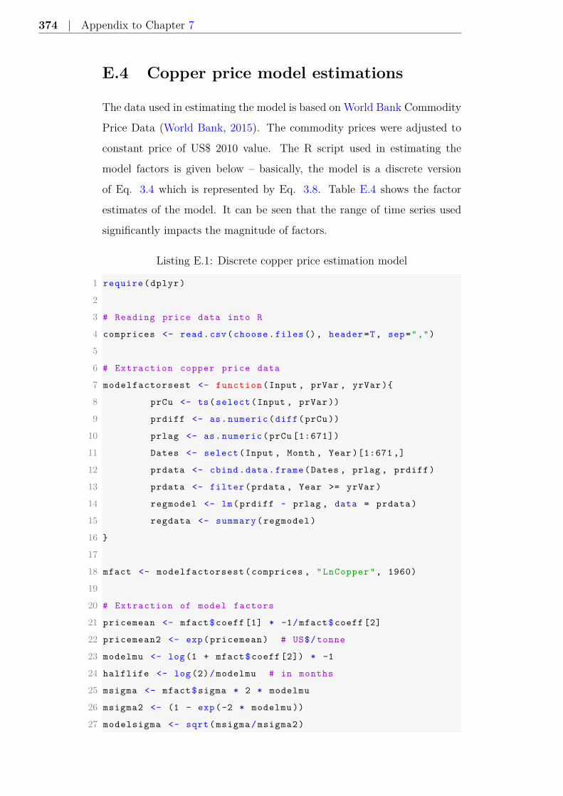
374 | Appendix to Chapter 7
E.4 Copper price model estimations
The data used in estimating the model is based on World Bank Commodity
Price Data (World Bank, 2015). The commodity prices were adjusted to
constant price of US$ 2010 value. The R script used in estimating the
model factors is given below – basically, the model is a discrete version
of Eq. 3.4 which is represented by Eq. 3.8. Table E.4 shows the factor
estimates of the model. It can be seen that the range of time series used
significantly impacts the magnitude of factors.
Listing E.1: Discrete copper price estimation model
1 require (dplyr)
2
3 # Reading price data into R
4 comprices <- read.csv( choose .files (), header =T, sep=",")
5
6 # Extraction copper price data
7 modelfactorsest <- function (Input , prVar , yrVar ){
8 prCu <- ts( select (Input , prVar ))
9 prdiff <- as. numeric (diff(prCu ))
10 prlag <- as. numeric (prCu [1:671])
11 Dates <- select (Input , Month , Year )[1:671 ,]
12 prdata <- cbind.data.frame(Dates , prlag , prdiff )
13 prdata <- filter (prdata , Year >= yrVar)
14 regmodel <- lm( prdiff ~ prlag , data = prdata )
15 regdata <- summary ( regmodel )
16 }
17
18 mfact <- modelfactorsest (comprices , " LnCopper ", 1960)
19
20 # Extraction of model factors
21 pricemean <- mfact$coeff [1] * -1/mfact$coeff [2]
22 pricemean2 <- exp( pricemean ) # US$/tonne
23 modelmu <- log (1 + mfact$coeff [2]) * -1
24 halflife <- log (2)/ modelmu # in months
25 msigma <- mfact$sigma * 2 * modelmu
26 msigma2 <- (1 - exp (-2 * modelmu ))
27 modelsigma <- sqrt( msigma / msigma2 )

E.4 Copper price model estimations | 375
Table E.4: Model estimates for Copper prices
Factor Unit 1960-2015 1980-2015 2000-2015
Mean Price Index 8.225796 8.148373 8.699925
Mean Price US$/ton 3736.10 3457.75 6002.46
Speed of reversion Index 0.012043 0.008987 0.013787
Half life Months 57.55 77.13 50.27
Std. Dev. Index 0.266581 0.256761 0.266566
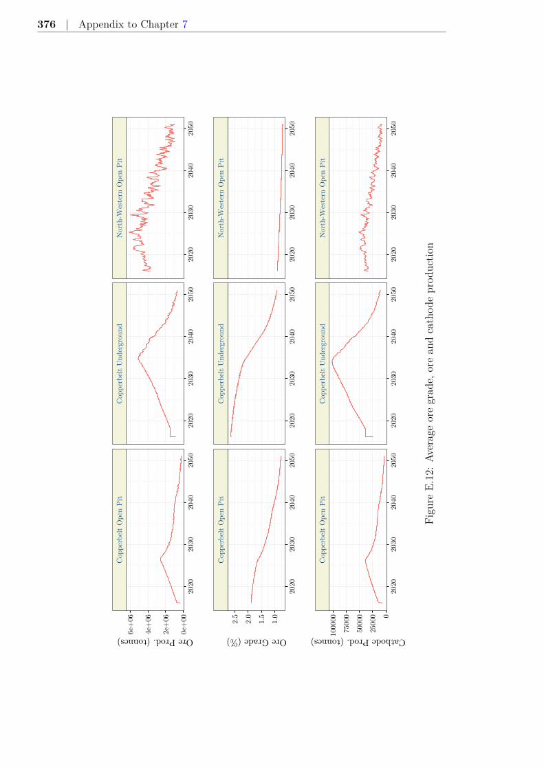
376 | Appendix to Chapter 7
Cop
perb
elt
Ope
n Pi
tC
oppe
rbel
t U
nder
grou
ndN
orth
-Wes
tern
Ope
n Pi
t
0e+
00
2e+
06
4e+
06
6e+
06
2020
2030
2040
2050
2020
2030
2040
2050
2020
2030
2040
2050
Ore Prod. (tonnes)
Cop
perb
elt
Ope
n Pi
tC
oppe
rbel
t U
nder
grou
ndN
orth
-Wes
tern
Ope
n Pi
t
1.0
1.5
2.0
2.5
2020
2030
2040
2050
2020
2030
2040
2050
2020
2030
2040
2050
Ore Grade (%)
Cop
perb
elt
Ope
n Pi
tC
oppe
rbel
t U
nder
grou
ndN
orth
-Wes
tern
Ope
n Pi
t
0
2500
0
5000
0
7500
0
1000
00
2020
2030
2040
2050
2020
2030
2040
2050
2020
2030
2040
2050
Cathode Prod. (tonnes)
Figu
reE.
12:
Aver
age
ore
grad
e,or
ean
dca
thod
epr
oduc
tion
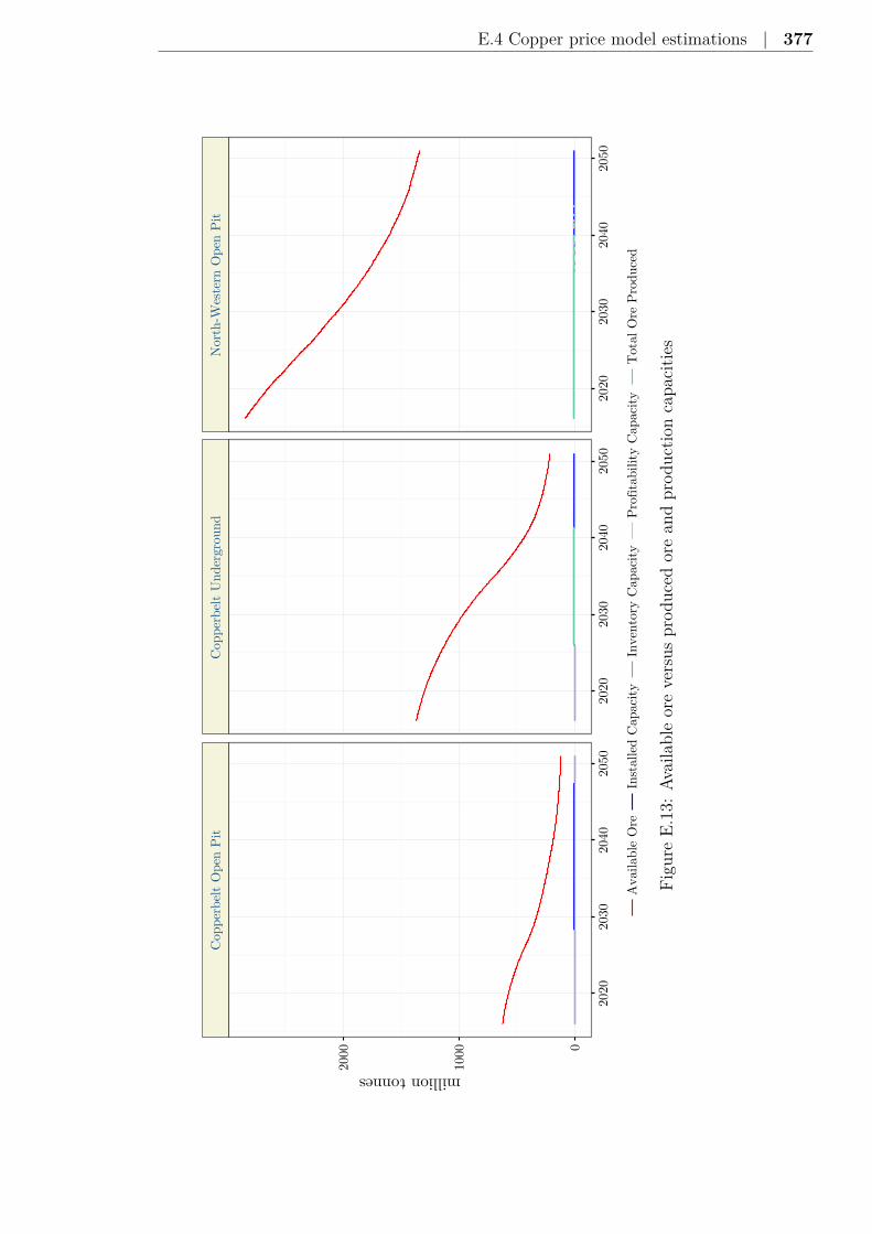
E.4 Copper price model estimations | 377
Cop
perb
elt
Ope
n Pi
tC
oppe
rbel
t U
nder
grou
ndN
orth
-Wes
tern
Ope
n Pi
t
0
1000
2000
2020
2030
2040
2050
2020
2030
2040
2050
2020
2030
2040
2050
million tonnes
A
vaila
ble
Ore
Inst
alle
d C
apac
ityIn
vent
ory
Cap
acity
Prof
itabi
lity
Cap
acity
Tot
al O
re P
rodu
ced
Figu
reE.
13:
Avai
labl
eor
eve
rsus
prod
uced
ore
and
prod
uctio
nca
paci
ties
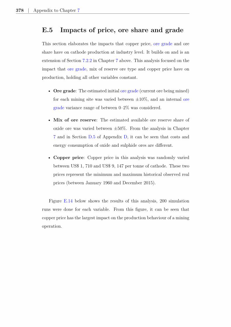
378 | Appendix to Chapter 7
E.5 Impacts of price, ore share and grade
This section elaborates the impacts that copper price, ore grade and ore
share have on cathode production at industry level. It builds on and is an
extension of Section 7.2.2 in Chapter 7 above. This analysis focused on the
impact that ore grade, mix of reserve ore type and copper price have on
production, holding all other variables constant.
• Ore grade: The estimated initial ore grade (current ore being mined)
for each mining site was varied between ±10%, and an internal ore
grade variance range of between 0–2% was considered.
• Mix of ore reserve: The estimated available ore reserve share of
oxide ore was varied between ±50%. From the analysis in Chapter
7 and in Section D.5 of Appendix D, it can be seen that costs and
energy consumption of oxide and sulphide ores are different.
• Copper price: Copper price in this analysis was randomly varied
between US$ 1, 710 and US$ 9, 147 per tonne of cathode. These two
prices represent the minimum and maximum historical observed real
prices (between January 1960 and December 2015).
Figure E.14 below shows the results of this analysis, 200 simulation
runs were done for each variable. From this figure, it can be seen that
copper price has the largest impact on the production behaviour of a mining
operation.
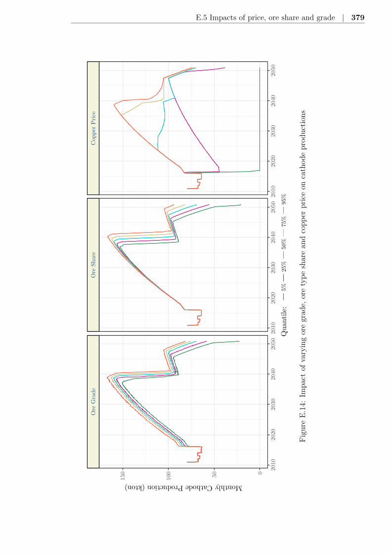
E.5 Impacts of price, ore share and grade | 379
Ore
Gra
deO
re S
hare
Cop
per
Pric
e
2010
2020
2030
2040
2050
2010
2020
2030
2040
2050
2010
2020
2030
2040
2050
050100
150
Monthly Cathode Production (kton)
Qua
ntile
: 5%
25%
50%
75%
95%
Figu
reE.
14:
Impa
ctof
vary
ing
ore
grad
e,or
ety
pesh
are
and
copp
erpr
ice
onca
thod
epr
oduc
tions
380 | Appendix to Chapter 7
Cop
perb
elt
Ope
n Pi
tC
oppe
rbel
t U
nder
grou
ndN
orth
-Wes
tern
Ope
n Pi
t
0.25
0.50
0.75
1.00
2020
2030
2040
2050
2020
2030
2040
2050
2020
2030
2040
2050
cor(Ore Production, Total Prod. Costs)
A
vaila
ble
Ore
Figu
reE.
15:
Cor
rela
tion
ofor
epr
oduc
tion
and
tota
lpro
duct
ion
cost

Top Related
Copyright © 2022 FDOKUMEN

