


Bahasa
Halaman
Hukum

www.elsevier.com/locate/ynimg
NeuroImage 23 (2004) S161–S169
Statistics on diffeomorphisms via tangent space representations
M. Vaillant,a,b,* M.I. Miller,a L. Younes,a,c and A. Trouved
aCenter for Imaging Science, The Johns Hopkins University, Baltimore, MD 21218, USAbDepartment of Biomedical Engineering, The Johns Hopkins University, Baltimore, MD 21218, USAcDepartment of Applied Mathematics and Statistics, The Johns Hopkins University, Baltimore, MD 21218, USAdCMLA (CNRS, UMR 8536), Ecole Normal Superieure de Cachan, Cedex, France
Available online 25 September 2004
In this paper, we present a linear setting for statistical analysis of
shape and an optimization approach based on a recent derivation of
a conservation of momentum law for the geodesics of diffeomorphic
flow. Once a template is fixed, the space of initial momentum
becomes an appropriate space for studying shape via geodesic flow
since the flow at any point along the geodesic is completely
determined by the momentum at the origin through geodesic
shooting equations. The space of initial momentum provides a linear
representation of the nonlinear diffeomorphic shape space in which
linear statistical analysis can be applied. Specializing to the landmark
matching problem of Computational Anatomy, we derive an
algorithm for solving the variational problem with respect to the
initial momentum and demonstrate principal component analysis
(PCA) in this setting with three-dimensional face and hippocampus
databases.
D 2004 Elsevier Inc. All rights reserved.
Keywords: Shape; Landmark matching; Splines; PCA
Introduction
In Computational Anatomy, the framework pursued is the
deformable template model pioneered by Grenander (1993). A
deformable template Ia corresponds to the orbit under a group of
diffeomorphisms G , of one selected and fixed object Ia a I . Theidea is to model comparison between elements in the orbit Ia via
the diffeomorphic transformations in G . The optimal diffeo-
morphism that matches two arbitrary elements in the orbit is
chosen from all curves /t, t a [0,1] in G connecting the two
elements via the group action. It is chosen as the curve that
minimizes an energy with respect to a measure of infinitesimal
variations in G . These energy minimizing paths (geodesics) induce
a metric on Ia (Miller et al., 2002) that provides a natural measure
1053-8119/$ - see front matter D 2004 Elsevier Inc. All rights reserved.
doi:10.1016/j.neuroimage.2004.07.023
* Corresponding author. Fax: +1 410 516 4594.
E-mail address: [email protected] (M. Vaillant).
Available online on ScienceDirect (www.sciencedirect.com.)
for comparison of anatomical objects. In this paper, we present
applications of a fundamental bconservation of momentumQproperty of these geodesics that has emerged recently (Miller et
al., in press). This property extends the analogous conservation of
momentum property in finite-dimensional mechanics and in the
infinite-dimensional setting studied by Arnold (1989). We focus on
the implications of this fundamental property in providing the
powerful capability to represent the entire flow of a geodesic in the
orbit by a template configuration and a momentum configuration
at a single instant in time. The approach is founded in the Lie
group point of view. The tangent space V at the identity id a G is
considered the bLie algebraQ of the group. The idea will be to use
its dual space V*, the space of momenta to model deformations,
given that geodesics can be generated from elements of V or V*.
The power of the approach comes in the dimensionality reduction
of geodesic flow to a single representative element, and in the fact
that the representative space is linear. Motivated by these
implications, we derive the variational problem of landmark
matching with respect to initial momentum at time t = 0, and
we setup the framework for applying linear statistical modeling in
this space. The linear statistical setting provides a natural
mechanism for coping with the nonlinear nature of the diffeomor-
phic shape space. Statistics on manifolds, in particular shape
manifolds, has been studied in, for example, Bhattacharya and
Patrangenaru (2002) and Le and Kume (2000). The representation
of shape via their Lie algebra has been applied in the statistical
learning setting in Gallivan et al. (2003) and Fletcher et al. (2003).
However, it has not been studied in the diffeomorphic setting.
We will first provide background that introduces the
diffeomorphic matching setting and the general conservation of
momentum principle. We then specialize to the landmark
matching problem and derive a new variational problem on
the initial momentum as well as a numerical gradient algorithm.
We then introduce the initial momentum as a natural setting for
linear statistical analysis, in particular we detail the implementa-
tion of principal component analysis (PCA). Results of the
optimization algorithm and a PCA analysis of three-dimensional
face and hippocampus databases are presented in the final
section.

M. Vaillant et al. / NeuroImage 23 (2004) S161–S169S162
Background
The group G is defined as follows. Let X be an open-bounded
set in RK that forms the background space. The fundamental object
of construction is a Hilbert space V of vector fields on X that
contain smooth vector fields with compact support in X. For all
time-dependent families of elements of V, written vt a V for t a[0,1], such that
Z10
k vt k Vdtbl;
the solution / t at time t = 1 of
BuBt
¼ vt B ut; ð1Þ
with /0(x) = x is a diffeomorphism (see Dupuis et al., 1998;
Trouve, 1995). The group G consists of all such solutions. The
geodesics of G provide the transformations that match objects in
the orbit and are characterized by extremals of the kinetic energy
1
2
Z10
k vt k 2Vdt:
We assume that there is an operator L defined on V such that its
restriction to sufficiently smooth v a V gives Lv a L2 (X) with
hv;wiV ¼ZX
hLv;wiRK ;
for all w a V. Lv can be considered as a mapping from V to R
through the identification Lv (w) = hv, wiV. In particular, for the
energy at time t, we have jjvtjjV2 = Lvt (vt). The mapping Lvt: V YR is called the momentum of the system at time t. For sufficiently
smooth Lvt, the Euler equation that is satisfied by the extremal
curves of the kinetic energy is given by
dLv
dtþ div Lv vð Þ þ dv4Lv ¼ 0;
where div (u v) = duv + div (v) u. The Euler equation has
been originally derived by Arnold (1966) for the case L = id
under the additional constraint div (v) = 0, and by Miller et al.
(in press). The Euler equation for more general momenta in the
deformable template setting has also been derived in Miller et
al. (in press). Also see Holm et al. (1998) and Holm et al.
(2004).
In Miller et al. (in press), it is shown that, with respect to a
change in variables, momentum is conserved along extremal
curves of the kinetic energy. This implies
Lvt wð Þ ¼ Lv0 dutð Þ1w B ut
� �;
for all w a V so in fact the momentum Lvt at time t is determined
by the momentum at time t = 0. The important consequence is that
the equations for geodesic evolution in the orbit It = / td I depend
only on a fixed template and the momentum at time 0. This
representation of It by Lv0 offers considerable dimensionality
reduction and suggests that the space of initial momenta is an
appropriate setting for focusing our modeling effort; in particular
for statistical analysis of shape, learning statistical models, and for
new optimization procedures that can incorporate these prior
models. In this paper, we investigate the diffeomorphic landmark-
matching problem to derive a new numerical procedure based on
the conservation of momentum property and to demonstrate
statistical analysis in the space of initial momenta.
Methods
Landmark matching
The diffeomorphic landmark matching problem has been well
formalized by Joshi and Miller (2000). We summarize briefly. Iconsists of all N-tuples ( q1,. . .,qN) of landmark points in X. The
orbit Ia is generated by the action of G on a template landmark
configuration Ia, where the group action is defined to be /d I = (/( q1),. . .,/( qN)).
Matching two elements in an orbit is accomplished by solving
the following variational problem. Let (x1,. . .,xN) and ( y1,. . .,yN)be template and target landmark configurations, respectively. We
seek to find the time-varying velocity field vt in V minimizing the
following energy functional
1
2
Z10
k vt k 2Vdt þ
1
2r2
XNi¼1
ku1 xi� �
yi k 2Rk ð2Þ
We assume that V is a reproducing kernel Hilbert space (RKHS),
and therefore we define the symmetric matrix valued reproducing
kernel K on X � X where for each x a X, K (x) is a map from RK
to V and
hK xð Þa; viV ¼ hv xð Þ; aiRK ; ð3Þ
for all a a RK and v a V. We make the following notational
conventions. Bold notation will continue to be used to denote
vectors in RK so that q a I can be written ( q1,. . .,qN). We will
also use an index notation, writing qik to denote q a I explicitly,
where k indexes the kth component of landmark i. When it is not
needed to distinguish a landmark from its components, we will
treat q as a vector in RNK and abuse the notation by using only one
index. That is, we write q = ( q1,. . .,qNK), where q1,. . .,qK denote
the coordinates of the first landmark, qK+1,. . .,q2K denote the
coordinates of the second landmark, and so forth. We construct the
NK � NK matrix-valued function S on I , consisting of the K � K
blocks K ( qi, qj) via S( q) = (K( qi, qj), i, j=1,. . .,N).
Letting qi (t) = /t (xi) for i = 1,. . .,N, an application of spline
theory (see Joshi and Miller, 2000) from the RKHS viewpoint
shows that the energy (Eq. (1)) is equivalent to
1
2
Z10
qq tð Þ4S q tð Þð Þ1qq tð Þdt þ 1
2r2k q 1ð Þ y k2
RNK ; ð4Þ
where * denotes the matrix transpose. The velocity is interpolated
over the entire domain X by
vt xð Þ ¼XNi¼1
K qi tð Þ; x� �
pi tð Þ; ð5Þ

M. Vaillant et al. / NeuroImage 23 (2004) S161–S169 S163
where p(t)=S( q(t))1 q (t). In the sequel, we will omit the time
variable when it is clear from context. An important consequence
of the system defined by Eqs. (4) and (5) is that the solution of our
variation problem over the entire domain X depends only on the
trajectories of the landmarks, thereby achieving substantial
dimensionality reduction. We also remark that the integrand of
the first term in Eq. (4),
L q; qq; tð Þ ¼ 1
2qq tð Þ4S q tð Þð Þ1
qq tð Þ ð6Þ
is in fact a pure kinetic energy Lagrangian on the configuration
space I (Marsden and Ratiu, 1999). Thus, after reduction to Eq.
(4), we find that the original variational problem is connected to the
variational principles of mechanics governing a system of NK
particles with Lagrangian given in Eq. (6).
Geodesic evolution equations for landmarks
Given a template configuration (x1,. . .,xN) and the initial
velocity v0 of a geodesic in the orbit, as written in Eq. (5), we
find
Lv0 wð Þ ¼ hv0;wiV ¼ hXNi¼1
K xi� �
pi;wiV
¼XNi¼1
hpi 0ð Þ;w xi� �
iR K :
Thus, the elements pi(0) represent the initial momenta. The
evolution equations describing the transport of the template
along the geodesic are derived in Miller et al. (in press) and
given by
qqi tð Þ ¼XNj¼1
K q j tð Þ; qi tð Þ� �
pj tð Þ
ppi tð Þ ¼ dqiðtÞvt
� �4pi tð Þ; ð7Þ
noting that by Eq. (5), dqi (t)vt is a function only of the
landmarks in the orbit. We remark that given the connection to
mechanics via the Lagrangian (Eq. (6)), the specialization of the
conservation of momentum to the landmark setting has produced
evolution equations that are in fact recognized as Hamilton’s
equations of classical mechanics. They can be derived directly by
applying the variational principle of Hamilton to Eq. (6) giving the
Euler equations of motion and the equivalent Hamiltonian system
(Eq. (7)) through a change of variables (see Marsden and Ratiu,
1999). We also recognize, stated above as our motivation for
pursing this formulation, that Eq. (7) is an initial value ODE
system. So, given initial values ( qi(0),pi(0)), we can solve this
system to give the unique solution ( qi(t), pi(t)) for all t a [0,1] and
hence vt (x) over all x a X via Eq. (5). We proceed in the
following section to further reduce the variation problem (Eq. (2))
with respect to the initial conditions ( qi(0), pi(0)).
Variational problem on initial momentum
Equipped with Eq. (7) as the evolution equations, our strategy
is to search for the initial conditions ( q(0), p(0)) that give rise to
the minimizing trajectories ( q(t), p(t)). Substituting q(t) = S( q(t))
p(t), we write Eq. (4) as a function of q(t) and p(t) obtaining
1
2
Z10
p tð Þ4S qtð Þp tð Þdt þ 1
2r2kq 1ð Þ yk2
RNK :
In mechanics, H( q(t), p(t)) = (1/2) p(t)*S(qt) p(t) is known as
the Hamiltonian. An important property along extremals of the
energy is that this Hamiltonian energy is conserved. That is,
H( q(t), p(t)) is a constant function of time. So, if q(0) = x and
p(0) = m, then H( q(t), p(t)) = H(x, m) for all t a [0,1]. We write
( q(x,m)(t), p(x,m)(t)) for the mapping (x,m) i ( q(t), p(t)) via Eq.
(7). With the template x fixed, the energy becomes solely a
function of m:
J mð Þ ¼ 1
2m4S xð Þm þ 1
2r2kq x; mð Þ 1ð Þ yk2RNK :
In the sequel, q and p will be solutions of Eq. (7) unless
otherwise noted, so we will often leave out the variables x and m (in
addition to t) when writing q(x, m)(t) and p(x,m)(t).
Gradient
The energy has now been reduced to a functional on RNK , so it
may be optimized using standard finite-dimensional nonlinear
optimization techniques. We consider gradient-based approaches
such as steepest descent and quasi-Newton, and now proceed by
computing the gradient of J in RNK . We first write our equations in
index notation that will allow us to produce an explicit formulation
that can more directly be translated to computer code. Recall that
qmn denotes the nth component of the mth landmark. We also
index the matrix S( q) by Sklmn( q) = Kln( qk, qm) in which case the
symmetry becomes Sklmn = Smnkl. We write Sklmn for S( q)1. So, in
terms of components, the energy becomes
J mð Þ ¼ 1
2
Xikjl
Sikjlmikmjl þ1
2r2
Xik
qik x; mð Þ 1ð Þ yik� �2
: ð8Þ
A simple computation gives
BJ
Bmrs¼ qqrs 0ð Þ þ 1
r2
Xik
Bqik 1ð ÞBmrs
qik 1ð Þ yik� �
; ð9Þ
where we have used the fact qqrs ¼P
jl Srsjlmjl . The first term is
immediately available and qik(1) is given via the evolution
equations. It is left to compute (Bqik(1)/Bmrs), which we obtain
by differentiating Eq. (7) to give a second set of differential
equations that describe the evolution of (Bqik(t)/Bmrs). Defining
B1kK x; yð Þ ¼ BK
Bxkx; yð Þ
Sjlmok ¼ BikK
lo q j; qm� �
Sjlmokp ¼ B1pBikK
lo q j; qm� �
; ð10Þ
M. Vaillant et al. / NeuroImage 23 (2004) S161–S169S164
we have
qqik ¼Xjl
Sikjlpjl
ppik ¼Xlmo
Silmok pilpmo ð11Þ
for the evolution equations.
Bqqik
Bmrs¼Xjlp
Sikjlp
Bqip
Bmrspjl þ Sjlikp
Bqjp
Bmrspjl
�þXjl
SikjlBpjl
Bmrs;
Bpik
Bmrs¼Xlmop
Silmokp
Bqip
Bmrspilpmo þ Smoilkp
Bqmp
Bmrspilpmo
�
þXlmo
Silmop
Bpil
Bmrspmo þ Silmop
Bpmo
Bmrspil
�; ð12Þ
which describe the evolution of (Bqk(t)/Bmi). In fact, these
equations can be further simplified because it is natural to
require invariance of hd ,d iV under rotations and translations,
which results in a simplified form for K. Indeed, K is
usually scalar, radial, and diagonal. That is, K is given by a
function g:[0, l)Y[0, l) that generates a positive definite
kernel via
Klo x; yð Þ ¼ g kx ykRKð Þdl0:
We typically use the Gaussian kernel which corresponds to
g tð Þ ¼ e t
2r2 :
Optimization algorithm
Let xik and yik be template and target landmarks, respectively.
The evolution Eqs. (11) and (12) are discretized in time and
numerically integrated to compute the gradient (Eq. (9)). Letting T
be the number of time steps, we have Dt = 1/(T 1). A simple
Euler integration procedure yields the following algorithm for
computing the gradient.
(1) Initialize the initial velocity of the landmark trajectories to
be the initial velocity of the straight line path.
qqik 0ð Þ ¼ Dt yik xik� �
:
Then, the remaining initial values become
pik 0ð Þ ¼ Sikjl qqjl 0ð Þ
Bpik 0ð ÞBmrs
¼ BmikBmrs
¼ dirdks
Bqik 0ð ÞBmrs
¼ 0:
(2) For t = 0 to t = T 2,
(a) Compute qik (t), pik (t), (Bqik(t)/Bmrs), and Bpik(t)/Bmrs viaEq. (11)
(b) Let
pik t þ 1ð Þ ¼ pik tð Þ þ Dtppik tð Þ
qik t þ 1ð Þ ¼ qik tð Þ þ Dtqqik tð Þ
Bpik t þ 1ð ÞBmrs
¼ Bpik tð ÞBmrs
þ DtBppikBmrs
Bqik t þ 1ð ÞBmrs
¼ Bqik tð ÞBmrs
þ DtBqqik
Bmrs
(3) Compute the gradient
BJ
Bmrs¼ qqrs 0ð Þ þ 1
r2
Xik
Bqik T 1ð ÞBmrs
qik T 1ð Þ yik� �
Equipped with this algorithm for computing the gradient, we
use an iterative gradient descent scheme to optimize the energy.
To obtain transformations that are invariant with respect to
rotations R and translations b, we compute the closed form
solution to
Arg minR;b
XNi¼1
kqi T 1ð Þ Ryi bk2RK
at each iteration of the descent procedure and replace yi with Ryi + b.
Linear statistics for shape space
Perhaps the most important application of the initial
momentum point of view is for the effective linearization of
the space of shapes. The shape space of landmark configurations
that we are working with is in fact a nonlinear metric space. For
example, there is no rigorous way to effectively add two
landmark configurations and be guaranteed that the resulting
configuration is a meaningful combination of the originals.
However, it is desirable to have a good linear approximation to
use linear statistical methods for studying shape variability. We
have shown that a landmark configuration yi can be represented
by a template configuration xi and the initial momenta mi that
minimize Eq. (8). The template remains fixed and the momenta
belong to a linear space. Therefore, once a template is fixed, it is
natural to use the representative space of initial momenta for linear
analysis.
A common linear analysis technique for multivariate data,
popularized in the stochastic deformable model literature by
Cootes et al. (1995), is principal component analysis (PCA).
PCA, which is also known as the Karhunen–Loeve decom-
position, computes a variance-maximizing basis of the linear
space. That is, basis vectors are oriented along directions of
maximal variance and ordered such that the first vector spans
the one-dimensional subspace of largest variation, the second
vector captures the next largest variation, and so forth. It is
therefore effective for analyzing variation in the data and for
dimensionality reduction. For example, by projecting a data
point onto a subspace spanned by the first D basis vectors, we
obtain an optimal D dimensional representation of the data. If a
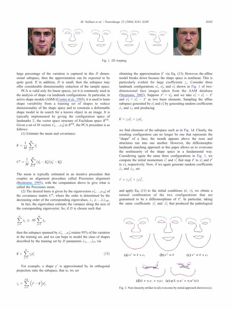
Fig. 1. 2D warping.
Fig. 2. Non-linearity artifact in (d) overcome by initial approach shown in (e).
M. Vaillant et al. / NeuroImage 23 (2004) S161–S169 S165
large percentage of the variation is captured in this D dimen-
sional subspace, then the approximation can be expected to be
quite good. If in addition, D is small, then the subspace may
offer considerable dimensionality reduction of the sample space.
PCA is valid only for linear spaces, yet it is commonly used in
the analysis of shape via landmark configurations. In particular, in
active shape models (ASM) (Cootes et al., 1995), it is used to learn
shape variability from a training set of shapes to reduce
dimensionality of the shape space and to constrain a deformable
shape model in its search for a known object in an image. It is
typically implemented by giving the configuration space of
landmarks I , the vector space structure of Euclidean space RNK .
Given a set of M vectors x1i,. . .,xM
i in RNK , the PCA procedure is as
follows:
(1) Estimate the mean and covariance:
xxi ¼ 1
M
XMj¼1
xij
Cij ¼ 1
M
XMk¼1
xik xxki
� �xjk xxk
j� �
The mean is typically estimated in an iterative procedure that
couples an alignment procedure called Procrustes alignment
(Bookstein, 1993), with the computation above to give what is
called the Procrustes mean.
(2) The desired basis is given by the eigenvectors e1i,. . .,eNK
i of
the covariance matrix Cij, where the order is determined by the
decreasing order of the corresponding eigenvalues, k1 z. . .zkNK.
In fact, the eigenvalues estimate the variance along the axis of
the corresponding eigenvector. So, if D is chosen such that
XDj¼1
kj z :95XMj¼1
kj;
then the subspace spanned by e1i,. . .,eD
i retains 95% of the variation
in the training set, and we can hope to model the class of shapes
described by the training set by D parameters k1,. . .,kD via
xxi þXDj¼1
cjeij: ð13Þ
For example, a shape yi is approximated by its orthogonal
projection onto the subspace, that is, we set
cj ¼XNK
i¼1
yi xxi
� �eij;
obtaining the approximation yi via Eq. (13). However, the affine
model breaks down because the shape space is nonlinear. This is
particularly evident for large coefficients cj. Consider three
landmark configurations x1i, x2
i, and x3i shown in Fig. 1 of two-
dimensional face images taken from the AAM database
(Stegmann, 2002). Suppose x i = x2i, and we take e1
i = x1i xi
and e3i = x3
i xi as two basis elements. Sampling the affine
subspace generated by e1i and e3
i by generating random coefficients
k1 and k3 and producing
xxi þ c1ei1 þ c3e
i3;
we find elements of the subspace such as in Fig. 1d. Clearly, the
resulting configuration can no longer be one that represents the
bshapeQ of a face; the mouth appears above the nose and
structures run into one another. However, the diffeomorphic
landmark matching approach in this paper allows us to overcome
the nonlinearity of the shape space in a fundamental way.
Considering again the same three configurations in Fig. 1, we
compute the initial momentum mi1 and mi
3 that map xi to x1i and xi
to x3i, respectively. Now, if we again generate random coefficients
k1 and k3, set
mi ¼ c1m1i þ c3m
3i ;
and apply Eq. (11) to the initial conditions (x, m), we obtain a
natural combination of the two configurations that are
guaranteed to be a diffeomorphism of xi. In particular, taking
the same coefficients k1i and k3
i that produced the pathological

M. Vaillant et al. / NeuroImage 23 (2004) S161–S169S166
model in Fig. 1d, we obtain Fig. 1e that clearly retains the structure
of a face.
Mean shape and PCA on initial momentum
Until this point, our PCA has been computed with respect
to the usual Euclidean norm on RNK . That is, we compute the
basis that minimizes the residual error of the project
approximation with respect to the Euclidean metric. In fact,
we can do better by obtaining a decomposition with respect to
the deformation energy. Recall that we measure the energy or
bsizeQ of a deformation by the first term in our energy
m*S(x)m. Equipping RNK with this norm jjmjjp2wm*S(x)minduces a natural metric on the initial momentum through the
deformation energy. It is therefore more appropriate to compute
PCAwith respect to this norm, so that the projected approximation
is optimal with respect to the deformation energy. A simple
computation shows that the only change to the above procedure is to
compute the eigen decomposition of Cs = CS(x) instead of C, where
CS(x) is the matrix product of the original matrix C and the matrix
S(x).
Equipped with the evolution equations and an optimization
procedure for computing diffeomorphic matching, it is straightfor-
ward to state PCA of shapes via initial momentum. Consider a set
of M landmark shapes x1i,. . .,xM
i, we apply the following procedure
to compute the mean shape:
(1) Set xi to an arbitrarily chosen landmark configuration.
(2) Find the initial momenta mi1,. . .,mi
M1 that represent the
diffeomorphisms that map xi to each of the M 1 remaining
configurations.
(3) Compute the mean momentum
mm i ¼XM1
j¼1
m ji
(4) Compute q(x, m)(t) and set x = q(x, m) (Eq. (1)).(5) Return to step 2 until kmmkRNK
converges to 0, that is until the
mean configuration does not change.
Because the space of initial momenta is linear, we simply apply
PCA to the resulting mi1,. . .,mi
M that have 0 mean, obtaining the
decomposition ei1,. . .,ei
NK. Now, applying Eq. (7) with xi and an
Fig. 3. Three-dimension
element of span {ei1,. . .,ei
D} as initial conditions will give a true
sample from the space of shapes. That is, span {ei1,. . .,ei
D}
represents a true subspace of shapes diffeomorphic to xi.
Experimental results
Shown in Fig. 2 is a two-dimensional example in the plane
where the landmarks are annotated features in photographs of
the face (data are from the AAM database; Stegmann, 2002).
The left panel shows the template landmark configuration
(straight lines connecting landmarks) overlayed on the corre-
sponding image of the face. The far right panel shows the
overlay of the target landmark configuration on its correspond-
ing image, and the center panels show snapshots from the time
sequence of deformation of the template configuration. We see
a smooth deformation as the template configuration moves
close to the target. Shown in the top row of Fig. 3 is a three-
dimensional example from the Morphable Faces database
(Blanz and Vetter, 1999) of landmarks annotated on a two-
dimensional face manifold. Again, the left panel shows the
template configuration with the flow sequence in the center
panels and the target in the right panels. The landmark
deformation interpolates a smooth deformation of the surface,
which matches the profile of the target nicely. In the bottom
row of Fig. 3 is shown another three-dimensional landmark
matching of two hippocampi. The hippocampi data are part of
the morphology test bed for the Biomedical Informatics
Research Network (BIRN, www.nbirn.net).
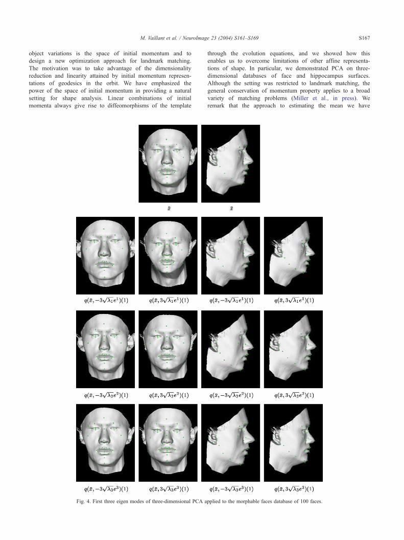
Shown in Fig. 4 is PCA via initial momentum of 100
annotated surfaces from the Morphable Faces database. The top
row shows the mean configuration in frontal and profile view
and the subsequent rows show deformation of the mean
configuration along the first three principal directions, respec-
tively. Presented in Fig. 5 is three-dimensional PCA applied to
the left hippocampus of 19 normal subjects. The mean is
shown in two views in the top row, and the deformation of the
mean along the first three eigen modes is shown in the
subsequent rows.
Discussion and conclusion
We have applied the conservation of momentum property to
illustrate that an appropriate setting for statistical models of
al deformations.
M. Vaillant et al. / NeuroImage 23 (2004) S161–S169 S167
object variations is the space of initial momentum and to
design a new optimization approach for landmark matching.
The motivation was to take advantage of the dimensionality
reduction and linearity attained by initial momentum represen-
tations of geodesics in the orbit. We have emphasized the
power of the space of initial momentum in providing a natural
setting for shape analysis. Linear combinations of initial
momenta always give rise to diffeomorphisms of the template
Fig. 4. First three eigen modes of three-dimensional PCA a
through the evolution equations, and we showed how this
enables us to overcome limitations of other affine representa-
tions of shape. In particular, we demonstrated PCA on three-
dimensional databases of face and hippocampus surfaces.
Although the setting was restricted to landmark matching, the
general conservation of momentum property applies to a broad
variety of matching problems (Miller et al., in press). We
remark that the approach to estimating the mean we have
pplied to the morphable faces database of 100 faces.

M. Vaillant et al. / NeuroImage 23 (2004) S161–S169S168
presented is analogous to the Lie group approaches of
computing the so-called intrinsic mean of a probability measure
on a Riemannian manifold (Miller et al., 2002) that has been
applied to shape in, for example, Gallivan et al. (2003) and
Fletcher et al. (2003). These other approaches differ in that
Fig. 5. First three eigen modes of three-dimensional PCA
their Lie algebra representations do not necessarily generate
diffeomorphisms of the template. Although the gradient
optimization scheme does not appear to achieve lower
computational complexity over other optimization approaches
(convergence properties have not yet been compared), it has
applied to 19 hippocampi from the BIRN project.
M. Vaillant et al. / NeuroImage 23 (2004) S161–S169 S169
several advantages. First, it readily allows statistically learned
information in the space of initial momentum to be incorpo-
rated in an active shape type approach for finding known
objects in images. Second, it is guaranteed to generate a
geodesic at every iteration, that is, q(x,m)(t) is always a
geodesic connecting x to q(x,m) (1) by definition of the evolution
equations. Lastly, the reduction to finite-dimensional nonlinear
optimization opens the door to explore well-formalized numerical
optimization procedures.
Acknowledgment
This work was supported by grants NIH (5 R01 MH69074-07,
P01-AG03991-16, 1 R01 MH60883-01, 1 R01 MH62626-01, 1
P41 RR15241-01A1, 1 R01 MH56584-04A1, 1 P20 MH62130-
01A1) and NSF NPACI.
Appendix A
In this appendix, we derive the evolution equations for the
gradient by differentiating the system (Eq. (11)) with respect to the
initial momentum mrs. Using the notational conventions introduced
in Eq. (10) we find,
Bqqik
Bmrs¼Xjlnp
BSikjl
BqnpBqnp
Bmrspjl þ
Xjl
SikjlBpjl
Bmrs
Bpik
Bmrs¼Xlmnop
BSilmok
BqnpBqnp
Bmrspilpmo
þXlmo
Silmok
Bpil
Bmrspmo þ Silmok
Bpmo
Bmrspil
�
by the chain rule. We may reduce the computations by exploiting
the fact that S is composed of symmetric kernels. We have
BSikjl
Bqnp¼ Bkkl
Bqnpqi; q j� �
¼ B1pKkl qi; q j� �
din þ B2pKkl qi; q j� �
djn
¼ B1pKkl qi; q j� �
din þ B1pKlk q j; qi� �
djn
¼ Sikjlp din þ Sjlikp djn;
where the third line follows from the symmetry of K. Also, by
equality of mixed partials and symmetry, again we find
BSilmok
Bqnp¼ B1pB1kK
lo qi; qm� �
din þ B2pB1kKlo qi; qm� �
dmn
¼ B1pB1kKlo qi; qm� �
din þ B1pB1kKol qm; qi� �
dmn
¼ Silomkp din þ Smoilkp dmn
So now
Bqqik
Bmrs¼Xjlp
Sikjlp
Bq ip
Bmrspjl þ Sjlikp
Bqjp
Bmrspjl
�þXjl
SikjlBpjl
Bmrs;
and
Bpik
Bmrs¼Xlmop
Silmokp
Bqip
Bmrspilpmo þ Smoilkp
Bqmp
Bmrspilpmo
�
þXlmo
Silmok
Bpil
Bmrspmo þ Silmok
Bpmo
Bmrspil
�:
References
Arnold, V.I., 1966. Sur la geomtrie differentielle des groupes de lie de
dimension infinie et ses applications a l’hydrodynamique des fluides
parfaits. Ann. Inst. Fourier (Grenoble) 16 (1), 319–361.
Arnold, V.I., 1989. Mathematical Methods of Classical Mechanics, 2nd ed.
Springer, New York. 1978.
Bhattacharya, R., Patrangenaru, V., 2002. Nonparametric estimation of
location and dispersion on Riemannian manifolds. J. Stat. Plan.
Inference 108, 23–25.
Blanz, V., Vetter, T.A., 1999. Morphable model for the synthesis of 3D
faces. Addison-Wesley: SIGGRAPH ’99 Conference Proceedings,
pp. 187–194.
Bookstein, F.L., 1993. Morphometric Tools for Landmark Data: Geometry
and biology. Cambridge Univ. Press, Cambridge.
Cootes, T.F., Taylor, C.J., Cooper, D.H., Graham, J., 1995. Active shape
models: their training and application. Comput. Vis. Image Underst. 61
(1), 38–59.
Dupuis, P., Grenander, U., Miller, M.I., 1998. Variational problems on flows
of diffeomorphisms for image matching. Q. Appl. Math. 56, 587–600.
Fletcher, P.T., Lu, C., Joshi, S., 2003. Statistics of shape via principal geodesic
analysis on lie groups. Proceedings of CVPR. IEEE, pp. 95–101.
Gallivan, K.A., Srivastava, A., Xiuwen, L., 2003. Efficient algorithms for
inferences on Grassmann manifolds. Proceedings of IEEE Conference
on Statistical Signal Processing. IEEE, pp. 315–318.
Grenander, U., 1993. General Pattern Theory. Oxford Univ. Press.
Holm, D.D., Marsden, J.E., Ratiu, T.S., 1998. The Euler–Poincare
equations and semidirect products with applications to continuum
theories. Adv. Math. 137, 1–81.
Holm, D.D., Ratnanather, J.T., Trouve, A., Younes, L., 2004. Soliton
dynamics in computational anatomy. NeuroImage 23 (Suppl. 1),
S170–S178.
Joshi, S.C., Miller, M.I., 2000. Landmark matching via large deformation
diffeomorphisms. IEEE Trans. Image Process. 9 (8), 1357–1370.
Le, H., Kume, A., 2000. The frechet mean shape and the shape of means.
Adv. Appl. Probab. (SGSA) 32, 101–113.
Marsden, J.E., Ratiu, T.S., 1999. Introduction to Mechanics and Symmetry,
2nd ed. Springer, New York.
Miller, M.I., Trouve, A., Younes, L., 2002. On metrics and Euler–
Lagrange equations of computational anatomy. Annu. Rev. Biomed.
Eng. 4, 375–405.
Miller, M.I., Trouve, A., Younes, L., 2003. Geodesic shooting for computa-
tional anatomy. J. Math. Imaging Vis. (in press).
Stegmann, M.B., 2002. Analysis and segmentation of face images using
point annotations and linear subspace techniques. Technical report,
Informatics and Mathematical Modelling. Technical University of
Denmark, DTU. August.
Trouve, A., 1995. An infinite dimensional group approach for physics
based model. Technical report (electronically available at http://
www.cis.jhu.edu).
Top Related
Copyright © 2022 FDOKUMEN

