STATISTICAL EVALUATION OF ARRHENIUS MODEL AND ITS APPLICABILITY IN PREDICTION

OF FOOD QUALITY LOSSES

ELI COHEN

Institute of Quality Control & Extension Services for the Food Industry

76 Mazeh Street Tel Aviv, 65789

Israel

and

ISRAEL SAGUY'

Department of Food Sciences Volcani Center

Agricultural Research Organization PO. Box 6

Bet Dagan 5@250 Israel

Received for Publication September 13, 1985

ABSTRACT

To minimize quality losses occurring during processing and storage and to predict shelplife, quantitative kinetic models, expressing the functional relationship between composition and environmental factors on food quality, are required The applicability o f these models is based on the accuracy of the model and its parameters. I n this paper, the calculation of the Arrhenius parameters and the accuracy of the derived model were compared, using three statistical methods, namely: linear least squares, nonlinear least squares and weighted nonlinear least squares. Results indicated that the traditional twustep linear method was the least accurate and the derived energy of activation and the preexponential factor had the largest confidence interval. The latter was shown to have a profound effect on the precision of the calculated rate constant and the predicted shelf life. Based on previous reports that indexes o f deterioration

'Address Correspondence to: Israel Saguy, The Pillsbury Company, 31 1 Second Street S. E., Minneapolis, MN 55414.

Journal ofFood Processing and Preservation 9 (1985) 273-290. All Rights Reserved OCopyright 1985 by Food & Nutrition Press, Inc., Westport, Connecticut.

273

274 COHEN AND SAGUY

are log-normal distributed, the unweighted nonlinear least squares method was applied in a singlestep on all the data points, following a logarithmic transformation. The overall better accuracy and superior performance of the nonlinear least squares method, suggests that this method should be utilized for routine kinetic data analysis.

INTRODUCTION

Foods are very sensitive and susceptible to quality losses due to chemical instability which depends both on compositional and environmental factors. To minimize quality losses occurring in processing and storage, to have a better understanding and an insight in these deleterious reactions, and to predict shelf life, kinetic models are utilized. The models express in a functional form the rate of the quality loss and its dependency on factors such as temperature, moisture content, water activity, concentration and others.

Compositional and/or environmental effects can be expressed by a functional relationship which applies only occasionally to several food systems and reactions. More often, food quality reactions are more complex and unique in their behavior, and the appropriate model must be derived for each product and food system individually.

Temperature is one of the main environmental factors which has a major impact and influence on quality loss rate. The most common and generally valid assumption is that temperature-dependency of food quality deterioration rate follows the Arrhenius model:

where: k is the rate constant; ko is a constant, independent of temperature (also known as pre-exponential or frequency factor); Ea is the activation energy; R is the gas constant; and T is the absolute temperature.

The Arrhenius equation is frequently used as a theoretical basis for the development of a mathematical model which describes the temperature sensitivity of a food product and for shelf-life prediction. However, such prediction has limited practical use if the large statistical confidence interval and error of the predicted shelf life is considered (Labuza and Kamman 1983). Furthermore, the activation energy generally depends on composition factors such as water activity, moisture content, solid concentration, pH and others (Cohen and Saguy 1983; Connor et aL 1981; Goldman et aL 1983; Labuza 1972; Saguy 1979; Saguy et al. 1979; 1980).

ARRHENIUS MODEL AND FOOD QUALITY LOSSES 275

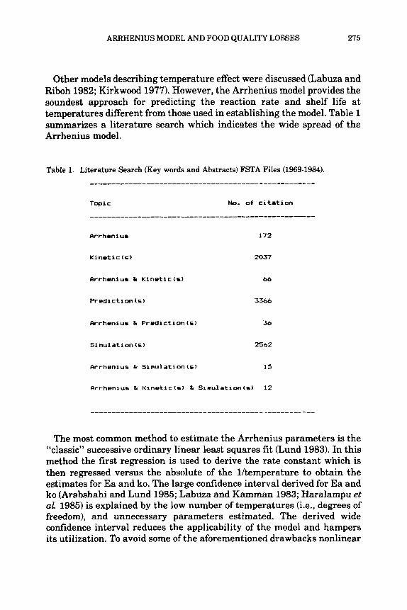
Other models describing temperature effect were discussed (Labuza and Riboh 1982; Kirkwood 1977). However, the Arrhenius model provides the soundest approach for predicting the reaction rate and shelf life at temperatures different from those used in establishing the model. Table 1 summarizes a literature search which indicates the wide spread of the Arrhenius model.

T o p i c No. of citation

Arrhoni us 172

Kinrtic (6) 2037

Arrhoniur & Kineticcr) 66

Predictim(s) 3366

Arrhenius & Prediction(s) 36

Si mu1 ati on (6 ) 2562

Arrhenius & Kinetic(6) L Sirulation(e) 12

The most common method to estimate the Arrhenius parameters is the “classic” successive ordinary linear least squares fit (Lund 1983). In this method the first regression is used to derive the rate constant which is then regressed versus the absolute of the lhemperature to obtain the estimates for Ea and ko. The large confidence interval derived for Ea and ko (Arabshahi and Lund 1985; Labuza and Kamman 1983; Haralampu et al. 1985) is explained by the low number of temperatures (Le., degrees of freedom), and unnecessary parameters estimated. The derived wide confidence interval reduces the applicability of the model and hampers its utilization. To avoid some of the aforementioned drawbacks nonlinear

276 COHEN AND SAGUY

least squares regression was suggested (Arabshahi 1982; Davies and Hudson 1981; Haralampu et al. 1985; Lund 1983; Nelson 1983). This approach increased the accuracy of the estimated Arrhenius parameters and ultimately improved the confidence interval of the predicted quality attribute.

This investigation was carried out with the overall goal of suggesting the most favorable method for deriving the Arrhenius parameters. Also, to compare the methods commonly utilized in the derivation of Ea and ko, and to establish their statistical confidence, limitation, drawbacks, implication, and applicability.

MATERIALS AND METHODS

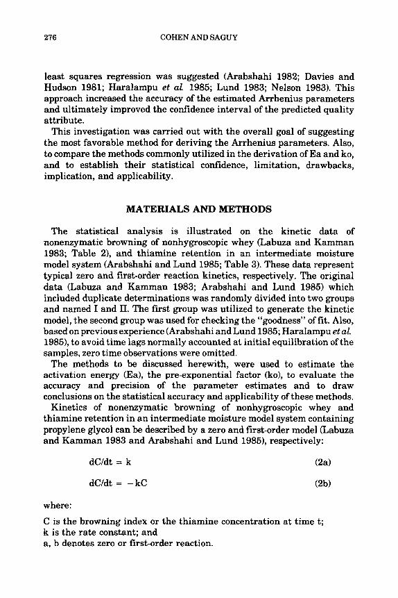
The statistical analysis is illustrated on the kinetic data of nonenzymatic browning of nonhygroscopic whey (Labuza and Kamman 1983; Table 2), and thiamine retention in an intermediate moisture model system (Arabshahi and Lund 1985; Table 3). These data represent typical zero and first-order reaction kinetics, respectively. The original data (Labuza and Kamman 1983; Arabshahi and Lund 1985) which included duplicate determinations was randomly divided into two groups and named I and 11. The first group was utilized to generate the kinetic model, the second group was used for checking the “goodness” of fit. Also, based on previous experience (Arabshahi and Lund 1985; Haralampu et al. 1985), to avoid time lags normally accounted at initial equilibration of the samples, zero time observations were omitted.

The methods to be discussed herewith, were used to estimate the activation energy (Ea), the pre-exponential factor (ko), to evaluate the accuracy and precision of the parameter estimates and to draw conclusions on the statistical accuracy and applicability of these methods.

Kinetics of nonenzymatic browning of nonhygroscopic whey and thiamine retention in an intermediate moisture model system containing propylene glycol can be described by a zero and first-order model (Labuza and Kamman 1983 and Arabshahi and Lund 19851, respectively:

dCldt = k (2a)

dC/dt = -kC (2b)

where:

C is the browning index or the thiamine concentration at time t; k is the rate constant; and a, b denotes zero or first-order reaction.

ARRHENIUS MODEL AND FOOD QUALITY LOSSES 277

Table 2. Browning data' for nonhygroscopic whey (h.0.44) as a function of storage temperature

TEWP . T I * Brorning value ( * C ) (days) (OD/g s o l i d ) X 1 0 2

Q r o u p I Q r a r p x x

25 30

60

90

120

150

180

210

35 10

20

30

40

50

60

70

95

4.3 4.1

6.1 6.3

7.4 7.6

9.6 9.8

11.8 12.0

12.7 12.5

14.5 14.8

5.0

7.9

10.5

13.7

16.5

20.2

23.2

27.7

5.2

7.9

10.6

13.8

16.5

20.1

23.4

27. 8

4s 2 5.2 5.2

4 7.1 7.0

7 22.4 22.4

11 2s. 2 2s. 3

18 31.7 31.7

28 44.4 44.2

35 50.9 50.7 _____-___-______________________________-__-----__--

'Adopted from Lab- and Kamman (1983).

Integration of Eq. (2) yields:

C = CO + kt

C = Co exp ( - kt)

(3a)

(3b)

where Co is the initial browning index or thiamine concentration.

278 COHEN AND SAGUY

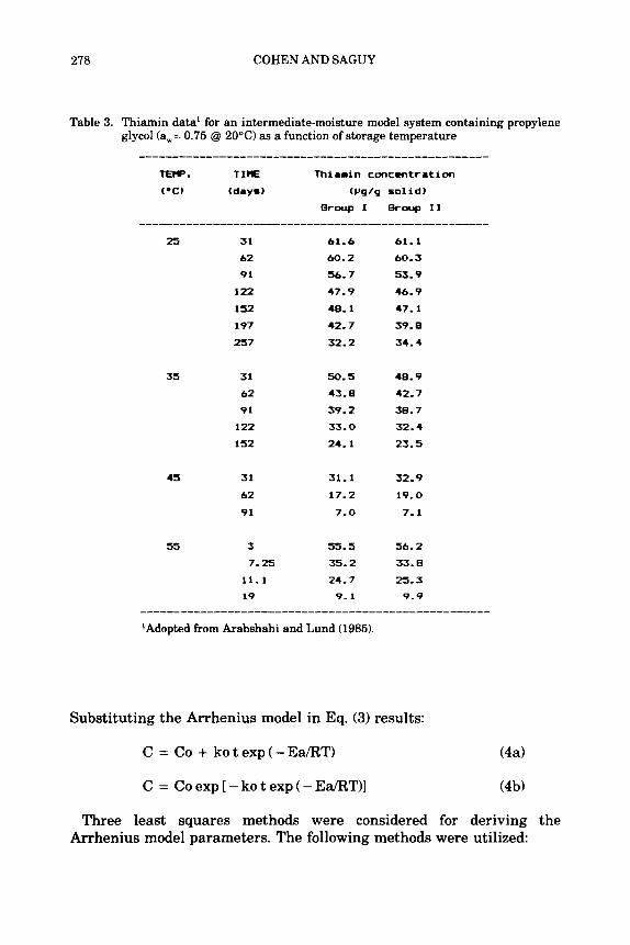
Table 3. Thiamin data' for an intermediate-moisture model system containing propylene glycol (a, = 0.75 Q 20°C) as a function of storage temperature

_-____-_________________________________-_-----_---- TEW. TIHE Thiamin concmtrrtion ( . C ) (drys) (Yg/g solid)

Q r o u p I Group11

25 31 62

91

122

IS2

197

257

61.6 61.1

60.2 60.3

56.7 53.9

47.9 46.9

48.1 47.1

42.7 39. 8

32.2 34.4

3s 31 50.5 48.9

62 43. 8 42.7

91 39.2 38.7

122 33.0 32.4

152 24.1 23.5

45 31

62

91

31.1 32.9

17.2 19.0

7.0 7.1

Substituting the Arrhenius model in Eq. (3) results:

C = Co + kotexp(-Ea/RT) (4a)

C = Coexp[-kotexp(-Ea/RT)I (4b)

Three least squares methods were considered for deriving the Arrhenius model parameters. The following methods were utilized:

ARRHENIUS MODEL AND FOOD QUALITY LOSSES 279

Method 1: Two-step Linear Least Squares

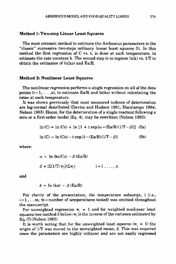
The most common method to estimate the Arrhenius parameters is the “classic” successive two-steps ordinary linear least squares fit. In this method the first regression of C vs. t, is done at each temperature, to estimate the rate constant k. The second step is to regress ln(k) vs. l!l’ to obtain the estimates of In(ko) and Ea/R.

Method 2: Nonlinear Least Squares

The nonlinear regression performs a single regression on all of the data points (i = 1, . . . ,n), to estimate Ea/R and ln(ko) without calculating the rates at each temperature.

It was shown previously that most measured indexes of deterioration are log-normal distributed (Davies and Hudson 1981; Haralampu 1984; Nelson 1983). Hence, for the deterioration of a single reactant following a zero or a first-order model (Eq. 4), may be rewritten (Nelson 1983):

In (C) = In (Co) + In { 1 + t exp [a - (Ea/R) (1pT - S>l} (5a)

In (C) = In (Co) - t exp [6 - ( E d ) (1PT - P)1 (5b)

where:

a = In (ko/Co) -0 (Ea/R)

p = [C(lrn) Wi1/(CWi) i = l , . . . , n

and

For clarity of the presentation, the temperature subscript, i (i.e., i = 1 , . . m; m = number of temperatures tested) was omitted throughout the manuscript.

For unweighted regression wi = 1 and for weighted nonlinear least squares (see method 3 below) wi is the inverse of the variance estimated by Eq. (7) (Nelson 1983).

It is worth noting that for the unweighted least squares (wi = 1) the origin of 1fl’ was moved to the unweighted mean, p. This was required since the parameters are highly colinear and are not easily regressed

280 COHEN AND SAGUY

directly (Haralampu et al. 1985; Nelson 1983). The latter transformation obviates in most cases the severe numerical difficulties in some nonlinear softw ares.

Finally, to avoid bias in the determination, Co was derived as a parameter (Haralampu et al. 1985). The COMPLEX method (Saguy 1983) was used to derive Co, Ea/R and ko.

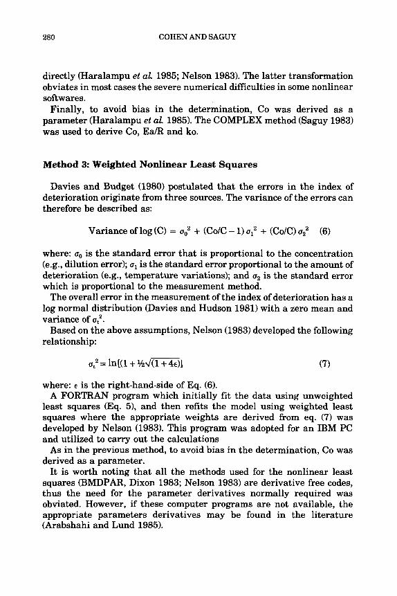
Method 3: Weighted Nonlinear Least Squares

Davies and Budget (1980) postulated that the errors in the index of deterioration originate from three sources. The variance of the errors can therefore be described as:

Variance of log (C) = u: + (Co/C - 1) u: + (Co/C) a; (6)

where: a, is the standard error that is proportional to the concentration (e.g., dilution error); u1 is the standard error proportional to the amount of deterioration (e.g., temperature variations); and u, is the standard error which is proportional to the measurement method.

The overall error in the measurement of the index of deterioration has a log normal distribution (Davies and Hudson 1981) with a zero mean and variance of u,".

Based on the above assumptions, Nelson (1983) developed the following relationship:

where: E is the right-hand-side of Eq. (6). A FORTRAN program which initially fit the data using unweighted

least squares (Eq. 5), and then refits the model using weighted least squares where the appropriate weights are derived from eq. (7) was developed by Nelson (1983). This program was adopted for an IBM PC and utilized to carry out the calculations

As in the previous method, to avoid bias in the determination, Co was derived as a parameter.

It is worth noting that all the methods used for the nonlinear least squares (BMDPAR, Dixon 1983; Nelson 1983) are derivative free codes, thus the need for the parameter derivatives normally required was obviated. However, if these computer programs are not available, the appropriate parameters derivatives may be found in the literature (Arabshahi and Lund 1985).

AFUZHENIUS MODEL AND FOOD QUALITY LOSSES 281

Statistical Evaluation

Statistical software BMDPlR and BMDPAR (Dixon 1983) were used for the linear and the nonlinear least squares, respectively. The joint confidence region of the parameters ( E m and In ko) was established following well documented methods (Draper and Smith 1981; Hunter 1981). The statistical tests may be performed on SAS (SAS, 1982).

RESULTS AND DISCUSSION

To evaluate the accuracy of the regression methods used in this study, two basic criteria were used, namely: the accuracy and precision of the parameters estimates, and the accuracy and precision of the quality losses expressed by their half-lives.

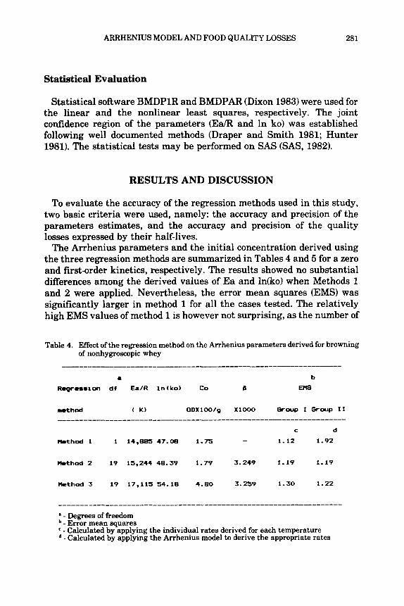
The Arrhenius parameters and the initial concentration derived using the three regression methods are summarized in Tables 4 and 5 for a zero and first-order kinetics, respectively. The results showed no substantial differences among the derived values of Ea and ln(ko) when Methods 1 and 2 were applied. Nevertheless, the error mean squares (EMS) was significantly larger in method 1 for all the cases tested. The relatively high EMS values of method 1 is however not surprising, as the number of

Table 4. Effect of the regression method on the Arrhenius parameters derived for browning of nonhygroscopic whey

_____________________I____________________----___---

a b

R l p r n m i o n df Ea/R I n ( k o ) Co 8 D18

wthod ( K) ODXl00/g XlOOO Oroup I Orwp XI

C d 1 14.885 47.08 1.75 - 1.12 1.92 kthod 1

?kthod 2 19 15,244 48.39 1.79 3.249 1.19 1.19

llethod 3 19 17,115 54.18 4.80 3.259 1.30 1.22

a - Degrees of freedom - Error mean squares - Calculated by applying the individual rates derived for each temperature - Calculated by applying the Arrhenius model to derive the appropriate rates

282 COHEN AND SAGUY

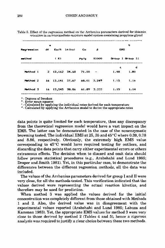
Table 5. Effect of the regression method on the Arrhenius parameters derived for thiamin retention in an intermediate-moisture model system containing propylene glycol

a b

Regression df Ea/R l n ( k o ) C o 4 EMS

Plrthod 2 16 13,141 37.67 68-01 3.249 1.15 1.16

Method 3 16 13.543 38.86 61.89 3.233 1.15 1.14 ..................................................................... a - Degrees of freedom

- Error mean squares - Calculated by applying the individual rates derived for each temperature - Calculated by applying the Arrhenius model to derive the appropriate rates

data points is quite limited for each temperature, thus any discrepancy from the theoretical regression model would have a vast impact on the EMS. The latter can be demonstrated in the case of the nonenzymatic browning tested. The individual EMS at 25,35 and 45°C where 0.39,0.78 and 8.86, respectively. Obviously, the extremely high EMS value corresponding to 45°C would have required testing for outliers, and discarding the data points that carry either experimental errors or others extraneous effects. The decision when to discard and omit data should follow proven statistical procedures (e.g., Arabshahi and Lund 1985; Draper and Smith 1981). Yet, in this particular case, to demonstrate the differences between the different regression methods, all the data was included.

The values of the Arrhenius parameters derived for group I and I1 were very close, for all the methods tested. This verification indicated that the values derived were representing the actual reaction kinetics, and therefore may be used for prediction.

When method 3 was applied the values derived for the initial concentration was completely different from those obtained with Methods 1 and 2. Also, the derived value was in disagreement with the experimental values reported (Arabshahi and Lund 1985; Labuza and Kamman 1983). Yet, the appropriate EMS values for method 3 were very close to those derived by method 2 (Tables 4 and 5), hence a rigorous analysis was required to justify a clear choice between these two methods.

ARRHENIUS MODEL AND FOOD QUALITY LOSSES 283

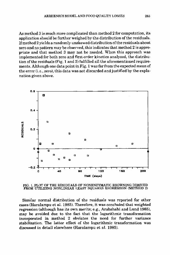
As method 3 is much more complicated than method 2 for computation, its application should be further weighed by the distribution of the residuals. If method 2 :yields a randomly unskewed distribution of the residuals about zero and no pattern may be observed, this indicates that method 2 is appro- priate and that method 3 may not be needed. When this approach was implemented for both zero and first-order kinetics analyzed, the distribu- tion of the residuals (Fig. 1 and 2) fulfilled all the aforementioned require- ments. Alth.ough one data point in Fig. 1 was far from the expected mean of the error h e . , zero), this data was not discarded and justified by the expla- nation given above.

0.4

U

tl U U

U

U

0 U U

U n u n

-0.2 o l , l l l l l l I TIME i ~ l T l . l . l (day.) a1 40 no 120 160 200

I I 1

I

FIG. 1. PLOT OF THE RESIDUALS OF NONENZYMATIC BROWNING DERIVED FROM UTILIZING NONLINEAR LEAST SQUARES REGRESSION (METHOD 2)

Similar normal distribution of the residuals was reported for other cases (Haralampu et al. 1985). Therefore, it was concluded that weighted regression (although has its own merits; e.g., Arabshahi and Lund 1985), may be avoided due to the fact that the logarithmic transformation incorporated in method 2 obviates the need for further variance stabilization. The latter effect of the logarithmic transformation was discussed in detail elsewhere (Haralampu et al. 1985).

284

-0.2 -

-

-0.4

COHEN AND SAGUY

0

0

c

I I I I I I I I I I I I

0.3

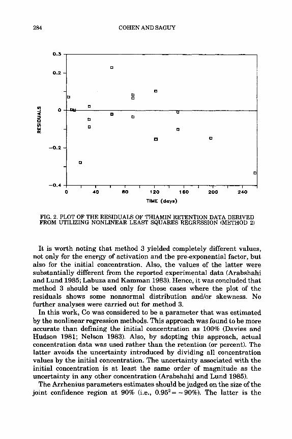
FIG. 2. PLOT OF THE RESIDUALS OF THIAMIN RETENTION DATA DERIVED FROM UTILIZING NONLINEAR LEAST SQUARES REGRESSION (METHOD 2)

It is worth noting that method 3 yielded completely different values, not only for the energy of activation and the pre-exponential factor, but also for the initial concentration. Also, the values of the latter were substantially different from the reported experimental data (Arabshahi and Lund 1985; Labuza and Kamman 1983). Hence, it was concluded that method 3 should be used only for those cases where the plot of the residuals shows some nonnormal distribution and/or skewness. No further analyses were carried out for method 3.

In this work, Co was considered to be a parameter that was estimated by the nonlinear regression methods. This approach was found to be more accurate than defining the initial concentration as 100% (Davies and Hudson 1981; Nelson 1983). Also, by adopting this approach, actual concentration data was used rather than the retention (or percent). The latter avoids the uncertainty introduced by dividing all concentration values by the initial concentration. The uncertainty associated with the initial concentration is at least the same order of magnitude as the uncertainty in any other concentration (Arabshahi and Lund 1985).

The Arrhenius parameters estimates should be judged on the size of the joint confidence region at 90% (i.e., 0.95'= -90%). The latter is the

ARRHENIUS MODEL AND FOOD QUALITY LOSSES 285

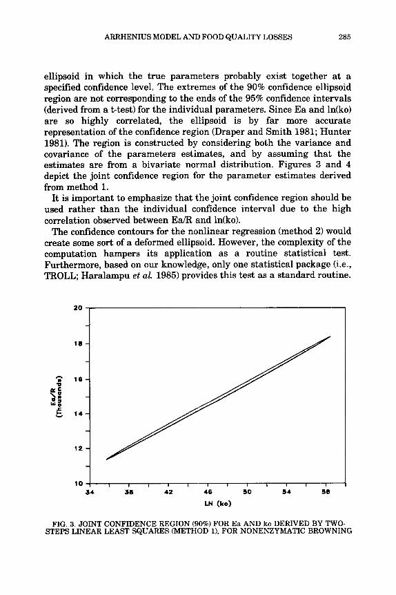
ellipsoid iin which the true parameters probably exist together at a specified Confidence level. The extremes of the 90% confidence ellipsoid region are not corresponding to the ends of the 95% confidence intervals (derived from a t-test) for the individual parameters. Since Ea and ln(ko) are so highly correlated, the ellipsoid is by far more accurate representation of the confidence region (Draper and Smith 1981; Hunter 1981). The region is constructed by considering both the variance and covariance of the parameters estimates, and by assuming that the estimates are from a bivariate normal distribution. Figures 3 and 4 depict the joint confidence region for the parameter estimates derived from meth'od 1.

It is important to emphasize that the joint confidence region should be used rather than the individual coflidence interval due to the high correlation observed between Ea/R and ln(ko).

The confidence contours for the nonlinear regression (method 2) would create some sort of a deformed ellipsoid. However, the complexity of the computation hampers its application as a routine statistical test. Furthermcire, based on our knowledge, only one statistical package (i.e., TROLL; Haralampu et aL 1985) provides this test as a standard routine.

20 -

10 -4- I I I I I I I

34 38 42 46 50 54 58

LN (ko)

FIG. 3. JOINT CONFIDENCE REGION (90%) FOR Ea AND ko DERIVED BY TWO- STEPS LINElAR LEAST SQUARES (METHOD 11, FOR NONENZYMATIC BROWNING

286 COHEN AND SAGUY

20

4 , I I I I I I I I I

LN (ko)

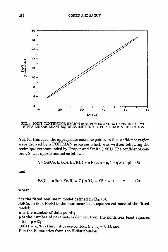
FIG. 4. JOINT CONFIDENCE REGION (90%) FOR Ea AND ko DERIVED BY TWO- STEPS LINEAR LEAST SQUARES (METHOD l), FOR THIAMIN RETENTION

Yet, for this case, the appropriate extreme points on the confidence region were derived by a FORTRAN program which was written following the technique recommended by Draper and Smith (1981). The confidence con- tour, s, was approximated as follows:

S = SS[Co, In (ko), Ea/Rl [1+ n F (p, n - p, 1 - qMn - p)1 (8)

and

SS[Co, In (ko), EaRI = C [In (CJ - f12 i = 1, . . ., n (9)

where:

f is the fitted nonlinear model defined in Eq. (5); SS[Co, In (ko), Ea/Rl is the nonlinear least squares estimate of the fitted model; n is the number of data points; p is the number of parameters derived from the nonlinear least squares

100 (1 - q) % is the confidence contour (i.e., q = 0.1); and F is the F-statistics from the F-distribution.

(i.e., p = 3);

ARRHENIUS MODEL AND FOOD QUALITY LOSSES 281

The extreme values of Ea/R and ln(ko) were derived using the COMPLEX method (i.e., nonlinear optimization; Saguy 1983). The appropriate values derived are summarized in Table 6. For most practical purposes the Confidence region may be evaluated by linearization of the model. The latter is a standard option of most statistical software (Dixon 1983; SAEl 1982).

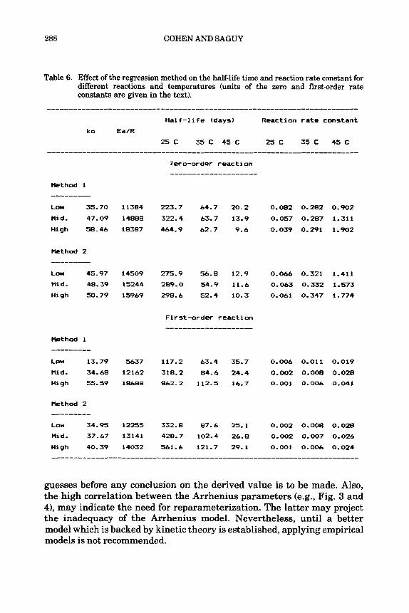
The accuracy of a rate constant for the prediction was estimated by first locating the extremes associated with the boundary of the confidence ellipsoid (Fig. 3 and 4) for Ea and ln(ko). In method 2 the appropriate values were derived by the procedure outlined previously. The extreme values (denoted as low and high), and the average of Ea and ln(ko) as derived from the regression procedure (denoted mid.) were used to calculate the appropriate half-life and the rate constant. These values are summarized in Table 6. For a first-order reaction, the half-life time is independent of the concentration (i,e., t,,2 = ln(2.)/k). In the case of a zero- order reaction, the half-life time was defined as the time required to reach an optical density of 0.2/g solids. This definition is obviously arbitrarily, and should be redefined for each case and system studied. Nevertheless, for comparison purposes, this value was quite appropriate.

Method 1 gave a much larger confidence region for Ea/R and ko. This large region resulted in a very wide span in the calculated values of Ea/R and k. Method 2 resulted in a much smaller confidence region and a better estimation of the half-life and the rate constant. The comparison also indicated that the traditional method for deriving the Arrhenius parameters agreed only partially with the values derived from method 2. Also, the half-life and k values were quite similar only for 35°C (i.e., the mid of the temperature range studied). This discrepancy not only projects the need for special attention when kinetics data is compared but also depicts the confidence of the determination. Hence, it may be difficult to connect energy of activation and entropy or any other thermodynamic quantities.

The confidence region of method 2 is much narrower when compared to the one derived from method 1. Yet, even in this improved case, prediction at temperature far from the average range used for deriving the kinetic model requires special caution. Since small errors in conducting the tests may be magnified if extrapolation is utilized. Hence, in this case, precaution should be reemphasized.

It is worth noting that method 2 is highly sensitive to the computation method. As the derivation of the parameters is based on nonlinear least squares, the procedures applied in the minimization of the sum of squares of the residuals, are very sensitive to the initial guess of the parameters and the criteria used for convergence. It is therefore strongly recommended that the computation should start at different initial

288 COHEN AND SAGUY

Table 6. Effect of the regression method on the half-life time and reaction rate constant for different reactions and temperatures (units of the zero and first-order rate constants are given in the text).

Method 1 --- ------ L O W 35.70

Mid . 47.09

High 58.46

Method 2 _----____ L O W 45.97

Mid. 48.39

High 50.79

Uethod 1 --------- Low 13.79

M i d . 34.68

High 55.59

Method 2 --------_ L O W 34.95

Mid . 37.67

High 40.39

11384

14888

18387

14509

15244

15969

223.7 64.7

322.4 63.7

464.9 62.7

275.9 56.8

289.0 54.9

298.6 52.4

20.2

13.9

9.6

12.9

11.6

10.3

5637 117.2

12162 318.2

18688 862.2

12255 332.8

13141 428.7

14032 561.6

0.082 0.282 0.902

0.057 0.287 1.311

0.039 0.291 1.902

0.066 0.321 1.411

0.063 0.332 1.573

0.061 0.347 1.774

63.4

84.6

112.5

87.6

102.4

121.7

35.7 0.006 0.011 0.019

24.4 0.002 0.008 0.028

16.7 0.001 0.006 0.041

25.1 0.002 0.008 0.028

26.8 0.002 0.007 0.026

29.1 0.001 0.006 0.024

guesses before any conclusion on the derived value is to be made. Also, the high correlation between the Arrhenius parameters (e.g., Fig. 3 and 4), may indicate the need for reparameterization. The latter may project the inadequacy of the Arrhenius model. Nevertheless, until a better model which is backed by kinetic theory is established, applying empirical models is not recommended.

ARRHENIUS MODEL AND FOOD QUALITY LOSSES 289

In conclusion, the traditional analysis (method 1) gave the least accurate estimates for the Arrhenius parameters. This inaccuracy is due probably to the need to estimate many intermediate values and by not considering the data as a whole set. Also, method 1 estimates unnecessary parameters and carry out regressions on regression parameters. Method 2 (i.e., nonlinear least squares) proved to be superior, as it gave unbiased and precise estimation of the parameters. It is undoubtfully the method of choice, and should be applied in kinetic studies. Yet, even this method has limitations mainly due to the computation complexity. Method 3 was much more difficult to apply and the values derived were different from those of methods 1 and 2, and thus should be used only for cases which do not fulfill the assumption of normality.

ACKNOWLEDGMENT

We wish to thank Dr. Peter R. Nelson, Searle, Research and Development for the FORTRAN program of weighted nonlinear least squares. A.lso, we would like to thank Mr. Steve Fahrenholtz, The Pills- bury Company for the useful statistical discussions.

REFERENCES

ARABSHAHI, A. 1982. Effect and interaction of environmental and composition variables on the stability of thiamin in intermediate moisture model systems. Ph. D. Thesis, Univ. of Wisconsin, Madison, Wisconsin.

ARABSHAHI, A. and LUND, D. 1985. Consideration in calculating kinetic parameters from experimental data. J. Food Proc. Eng. 7,209.

COHEN, E. and SAGUY, I. 1983. The effect of water activity and moisture content on the stability of beet powder pigments. J. Food Sci. 48, 703.

CONNORS, K. A., AMIDON, G. L. and KENNON, L. 1981. Chemical Stability of Pharmaceuticals. John Wiley & Sons, New York.

DAVIES, 0. L. and BUDGE", D. A. 1980. Accelerated storage tests on pharmaceutical products: effect of error structure of assay and errors in recorded temperature. J. Pharm. Pharmacol. 32, 155.

DAVIES, (3. L. and HUDSON, H. E. 1981. Stability of drugs: Accelerated storage tests. In: Statistics in the Pharmaceutical Industry. (C . R. Buncher and J. Y. Tsay, eds.), Marcel Dekker, New York.

290 COHEN AND SAGUY

DIXON, W. J. (ed.) 1983. BMDP-Statistical Sofiware. University of California Press, Berkeley, CA.

DRAPER, N. and SMITH, H. 1981. Applied Regression Analysis, 2nd ed., John Wiley & Sons, New York.

GOLDMAN, M., HOREV, B. and SAGUY, I. 1983. Decolorization of beta- carotene in model systems simulating dehydrated foods. Mechanism and principles. J. Food Sci. 48, 751.

HARALAMPU, S. G., SAGUY, I. and KAREL, M. 1985. Estimation of Arrhenius parameters using three least squares methods. J. Food Proc. Preserv. 9, 129.

HUNTER, J. S. 1981. Calibration and the straight line: Current statistical practices. J. Assoc. Off. Anal. Chem. 64, 574.

KIRKWOOD, T. B. L. 1977. Predicting the stability of biological standards and products. Biometrics 33, 736.

LABUZA, T. P. and RIBOH, D. 1982. Theory and application of Arrhenius kinetics to the prediction of nutrient losses in foods. Food Technol. 36(10), 66.

LABUZA, T. P. 1972. Nutrient losses during and storage of dehydrated foods, CRC Crit. Rev. Food Technol. 3(2), 217.

LABUZA, T. P. and KAMMAN, J. F. 1983. Reaction kinetics and accelerated tests simulation as a function of temperature. In Computer-Aided Techniques in Food Technology. (I. Saguy, ed.) Marcel Dekker, New York.

LUND, D. B. 1983. Consideration in modeling food processing. Food Technol. 37(1), 92.

NELSON, P. R. 1983. Stability prediction using Arrhenius model. Com. Programs in Biomedicine 16, 55.

SAGUY, I. 1979. Thermal stability of red beet pigments (betanine and vulgaxanthine I): Influence of pH and temperature. J. Food Sci. 44, 1554.

SAGUY, I. 1983. Optimization of dynamic systems using the maximum principle. In Computer-Aided Techniques of Food Technology. p. 343. Marcel Dekker, New York.

SAGUY, I., KOPELMAN, I. J. and MIZRAHI, S. 1979. Simulation of ascorbic acid stability during heat processing and concentration of grapefruit juice. J. Food Proc. Eng. 2, 213.

SAGUY, I., MIZRAHI, S., VILLOTA, R. and KAREL, M. 1978. Accelerated method for determining the kinetic model of quality deterioration during dehydration. J. Food Sci. 43, 1861.

SAS, 1982. The NLIN Procedure. SAS Users’s Guide: Statistics. Sas Inst. Cary, NC.