RESEARCH ARTICLE

Spatial sensitivity of species habitat patterns to scenariosof land use change (Switzerland)

Janine Bolliger Æ Felix Kienast Æ Reto Soliva ÆGillian Rutherford

Received: 2 March 2006 / Accepted: 16 January 2007 / Published online: 6 March 2007� Springer Science+Business Media B.V. 2007

Abstract Long-term societal trends which

include decreasing population in structurally

poorer regions and changes in agricultural poli-

cies have been leading to land abandonment in

various regions of Europe. One of the conse-

quences of this development includes spontane-

ous forest regeneration of formerly open-land

habitats with likely significant effects on plant and

animal diversity. We assess potential effects of

agricultural decline in Switzerland (41,000 km2)

and potential impacts on the spatial distribution

of seven open-land species (insects, reptile, birds)

under land-use change scenarios: (1) a business-

as-usual scenario that extrapolates trends

observed during the last 15 years into the future,

(2) a liberalisation scenario with limited regula-

tion, and (3) a lowered agricultural production

scenario fostering conservation. All scenarios

were developed in collaboration with socio-

economists. Results show that spontaneous

reforestation is potentially minor in the lowlands

since combinations of socio-economic (better

accessibility), topographic (less steep slopes),

and climatic factors (longer growing seasons)

favour agricultural use and make land abandonment

less likely. Land abandonment, spontaneous

reforestation, and subsequent loss of open-land,

however, are potentially pronounced in moun-

tainous areas except where tourism is a major

source of income. Here, socio-economic and

natural conditions for cultivation are more diffi-

cult, leading to higher abandonment and thus

reforestation likelihood. Evaluations for open-

land species core habitats indicate pronounced

spatial segregation of expected landscape change.

Habitat losses (up to 59%) are observed through-

out the country, particularly at high elevation

sites in the Northern Alps. Habitat gains under

the lowered agricultural production scenario

range between 12 and 41% and are primarily

observed for the Plateau and the Northern Alps.

Keywords Agricultural decline � Habitat

suitability maps � Species habitat distribution

modelling � Scenarios of land use change �Switzerland

Introduction

Land-use change is primarily driven by socio-

economic factors and significantly governs land-

scape structure, function, and dynamics (Wu and

Hobbs 2002; Wu 2006). Land-use change has

recently been identified to be a key research area

in landscape ecology (Wu and Hobbs 2002).

J. Bolliger (&) � F. Kienast � R. Soliva �G. RutherfordSwiss Federal Research Institute WSL, Zurcherstrasse111, CH-8903 Birmensdorf, Switzerlande-mail: janine.bolliger@wsl.ch

123

Landscape Ecol (2007) 22:773–789

DOI 10.1007/s10980-007-9077-7

The economic significance of agriculture has

decreased in many parts of Europe over the last

decades (Labaune and Magnin 2002; Dirnbock

et al. 2003; Dullinger et al. 2003a; Laiolo et al.

2004; van der Vaart 2005). This trend has been

prominent in mountainous areas since the 1950’s

(Meeus et al. 1991; Batzig 1996). Primary drivers

for this development are of socio-economic

nature (e.g., globalisation and mechanisation).

Consequences include reforestation of formerly

open land. Although reforestation may lead to a

short-term increase of species richness due to

increased landscape structure (Soderstrom et al.

2001), effects of pastoral abandonment may cause

habitat losses of open land species (Labaune and

Magnin 2002; Dirnbock et al. 2003; Dullinger

et al. 2003a) and potentially constitute a threat

for species diversity (Tilman et al. 2001; Dullinger

et al. 2003b). Thus, policies for maintaining open-

land environments to preserve species diversity

are needed if the maintenance of landscape and

plant–animal diversity is a priority (Bakker 1989;

Soderstrom et al. 2001). This requires detailed

understanding of the relationships between biota

and their environments to ensure that the eco-

logical characteristics of value to wildlife assem-

blages are maintained (McCracken and Bignal

1998; Lundstrom-Gillieron and Schlapfer 2003).

It has been claimed that more research is

needed to identify processes and consequences of

land use change and foster collaboration between

research areas beyond ecology to ensure truly

inter- and trans-disciplinary science (Wu and

Hobbs 2002). This study is an outcome of an

interdisciplinary research project in which socio-

economic experts constructed conservation and

agricultural policy scenarios. We investigate land-

use change (agricultural decline) as a process with

drivers that encompass policy options, societal

opinions and interests including agricultural,

environmental, and socio-economic factors to

benchmark potential consequences on species

distributions using land-use change scenarios.

Potential effects of the scenarios are inferred on

seven open-land animal species. The species

include butterflies (Erebia aethiops, Melanargia

galathea, Lysandra bellargus), grasshoppers

(Chorthippus scalaris), birds (Alauda arvensis,

Saxicola rubetra), and reptiles (Lacerta vivipara),

whose distribution data were available for Swit-

zerland (41,000 km2). The scenarios include (1)

business as usual, (2) liberalisation, and (3)

lowered agricultural production. For our scenar-

ios, two socio-economic drivers were identified

which jointly influence land-use: societal support

(state/federal subsidies) to agriculture and socie-

tal support to conservation. The business as usual

scenario extrapolates trends derived from land-

use changes during 1985–1997 into the future. The

scenario ‘‘lowered agricultural production’’ opti-

mises non-intensively used open land but allows

natural reforestation in marginal areas since

depopulation is an ongoing process even in

heavily subsidised areas. The liberalisation sce-

nario relies on the assumption that no public

support is given to both agriculture and conser-

vation and that the agricultural markets are fully

liberalised following WTO requirements.

We address the following questions: what are

the potential landscape-pattern changes under

scenarios of land-use change? What are likely

magnitudes and spatial distribution patterns of

change for selected open-land species?

Materials and methods

Study area

Switzerland covers ca. 41,000 km2 (Statistisches

Jahrbuch der Schweiz 1997). The climate is

temperate humid. Conditions vary regionally

due to the mountainous influence and range from

intra-alpine dry and continental climate regime

(Central Alps) to oceanic high elevation (North-

ern Alps, Jura Mountains) and low-elevation

climate (Plateau). The southern Alps in Switzer-

land are dominated by an insubrian climate type

with relatively mild and dry winters and warm-

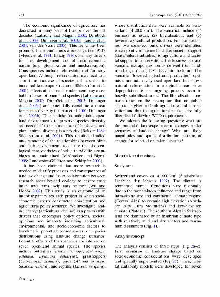
humid summers (Fig. 1).

Analysis concept

The analysis consists of three steps (Fig. 2a–c).

First, scenarios of land-use change based on

socio-economic considerations were developed

and spatially implemented (Fig. 2a). Then, habi-

tat suitability models were developed for seven

774 Landscape Ecol (2007) 22:773–789

123

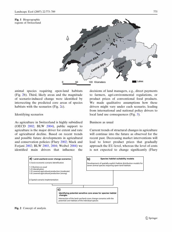
animal species requiring open-land habitats

(Fig. 2b). Third, likely areas and the magnitude

of scenario-induced change were identified by

intersecting the predicted core areas of species

habitats with the scenarios (Fig. 2c).

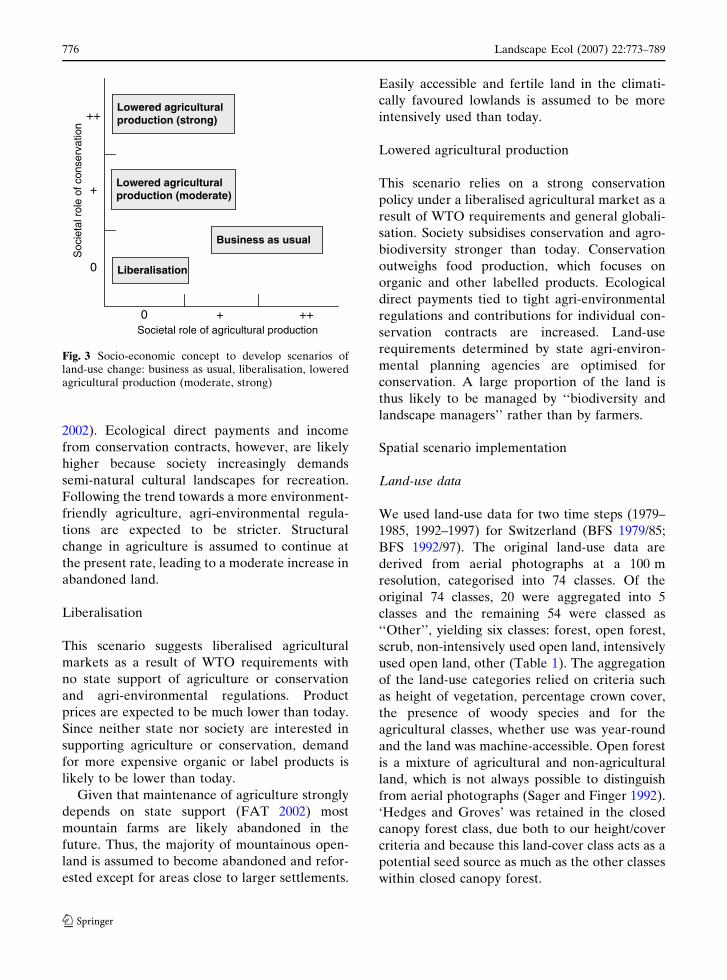
Identifying scenarios

As agriculture in Switzerland is highly subsidised

(OECD 2002; BLW 2004), public support to

agriculture is the major driver for extent and rate

of agricultural decline. Based on recent trends

and possible future developments in agricultural

and conservation policies (Flury 2002; Mack and

Ferjani 2002; BLW 2003, 2004; Weibel 2004) we

identified main drivers that influence the

decisions of land managers, e.g., direct payments

to farmers, agri-environmental regulations, or

product prices of conventional food products.

We made qualitative assumptions how these

drivers might vary under each scenario, leading

from international and national policy drivers to

local land use consequences (Fig. 3).

Business as usual

Current trends of structural changes in agriculture

will continue into the future as observed for the

recent past. Decreasing market interventions will

lead to lower product prices that gradually

approach the EU-level, whereas the level of costs

is not expected to change significantly (Flury

Fig. 1 Biogeographicregions of Switzerland

Land-use/land-cover change scenarios

1) Socio-economic scenario identification

1.1) Business as usual1.2) Liberalisation1.3) Lowered agricultural production (moderate) 1.4) Lowered agricultural production (strong)

2) Spatial scenario implementation

Species habitat suitability models

Development of spatially explicit habitat distribution models for seven animal species requiring open-land habitats

Identifying potential sensitive core areas for species habitatchanges

Intersection of the land-use/land-cover change scenarios with the potential core habitats of the individual species

a) b)

c)

Fig. 2 Concept of analysis

Landscape Ecol (2007) 22:773–789 775

123

2002). Ecological direct payments and income

from conservation contracts, however, are likely

higher because society increasingly demands

semi-natural cultural landscapes for recreation.

Following the trend towards a more environment-

friendly agriculture, agri-environmental regula-

tions are expected to be stricter. Structural

change in agriculture is assumed to continue at

the present rate, leading to a moderate increase in

abandoned land.

Liberalisation

This scenario suggests liberalised agricultural

markets as a result of WTO requirements with

no state support of agriculture or conservation

and agri-environmental regulations. Product

prices are expected to be much lower than today.

Since neither state nor society are interested in

supporting agriculture or conservation, demand

for more expensive organic or label products is

likely to be lower than today.

Given that maintenance of agriculture strongly

depends on state support (FAT 2002) most

mountain farms are likely abandoned in the

future. Thus, the majority of mountainous open-

land is assumed to become abandoned and refor-

ested except for areas close to larger settlements.

Easily accessible and fertile land in the climati-

cally favoured lowlands is assumed to be more

intensively used than today.

Lowered agricultural production

This scenario relies on a strong conservation

policy under a liberalised agricultural market as a

result of WTO requirements and general globali-

sation. Society subsidises conservation and agro-

biodiversity stronger than today. Conservation

outweighs food production, which focuses on

organic and other labelled products. Ecological

direct payments tied to tight agri-environmental

regulations and contributions for individual con-

servation contracts are increased. Land-use

requirements determined by state agri-environ-

mental planning agencies are optimised for

conservation. A large proportion of the land is

thus likely to be managed by ‘‘biodiversity and

landscape managers’’ rather than by farmers.

Spatial scenario implementation

Land-use data

We used land-use data for two time steps (1979–

1985, 1992–1997) for Switzerland (BFS 1979/85;

BFS 1992/97). The original land-use data are

derived from aerial photographs at a 100 m

resolution, categorised into 74 classes. Of the

original 74 classes, 20 were aggregated into 5

classes and the remaining 54 were classed as

‘‘Other’’, yielding six classes: forest, open forest,

scrub, non-intensively used open land, intensively

used open land, other (Table 1). The aggregation

of the land-use categories relied on criteria such

as height of vegetation, percentage crown cover,

the presence of woody species and for the

agricultural classes, whether use was year-round

and the land was machine-accessible. Open forest

is a mixture of agricultural and non-agricultural

land, which is not always possible to distinguish

from aerial photographs (Sager and Finger 1992).

‘Hedges and Groves’ was retained in the closed

canopy forest class, due both to our height/cover

criteria and because this land-cover class acts as a

potential seed source as much as the other classes

within closed canopy forest.

0

0

+

++

+

Soc

ieta

l rol

e of

con

serv

atio

n

Societal role of agricultural production++

Liberalisation

Lowered agriculturalproduction (strong)

Business as usual

Lowered agriculturalproduction (moderate)

Fig. 3 Socio-economic concept to develop scenarios ofland-use change: business as usual, liberalisation, loweredagricultural production (moderate, strong)

776 Landscape Ecol (2007) 22:773–789

123

Spatially explicit transitions

Transition probabilities were derived from GLMs

(General Linear Models). We used a logit link

function to relate land-use change between 1985

and 1997 to various variables (e.g., topography,

slope, composition of the surrounding neighbour-

hoods). For each land-use transition a logistic

regression model was calibrated for the land-use

categories forest, open forest, scrub, non-inten-

sively used and intensively used open land. The

transition probabilities yield the probability of

any pixel with land-use type x to be transformed

to land-use type y under given constraints. The

predicted response surfaces take values of prob-

ability of change between 0 and 1.

Magnitude of change

The magnitude of land-use change is the number

of pixels, which switched to another category

between 1985 and 1997 (BFS 1979/85; BFS 1992/

97). The inferred magnitude of change depends

on the scenario and is determined on the basis of

socio-economic judgment (Table 2a–e).

The business as usual scenario assumes a

continuation of observed changes in land-use for

1985–1997. The magnitude of change is thus

the same as observed between 1985 and 1997

(Table 2a).

The liberalisation scenario was subdivided

into two variants: lowlands (<900 m asl)

(Table 2b), mountain tourist areas (>900 m asl)

(Table 2c). No forest changes are assumed in

the lowlands and in important mountain tourist

resorts as these areas are likely to remain settled

and managed due to higher infrastructure avail-

ability and easy accessibility. A tourist resort is

defined as more than 30,000 overnight guests in

1998. For mountain regions, the liberalisation

scenario assumes a high percentage of pixels

transforming from scrub and open forest to

closed forest. In the lowlands an almost com-

plete transformation of agriculture from non-

intensively to intensively used open land is

assumed (Table 2b, c).

Both variants of the lowered agricultural pro-

duction scenario (moderate and strong) assume

transformation of intensive to non-intensive agri-

culture, allowing changes in forest cover due to

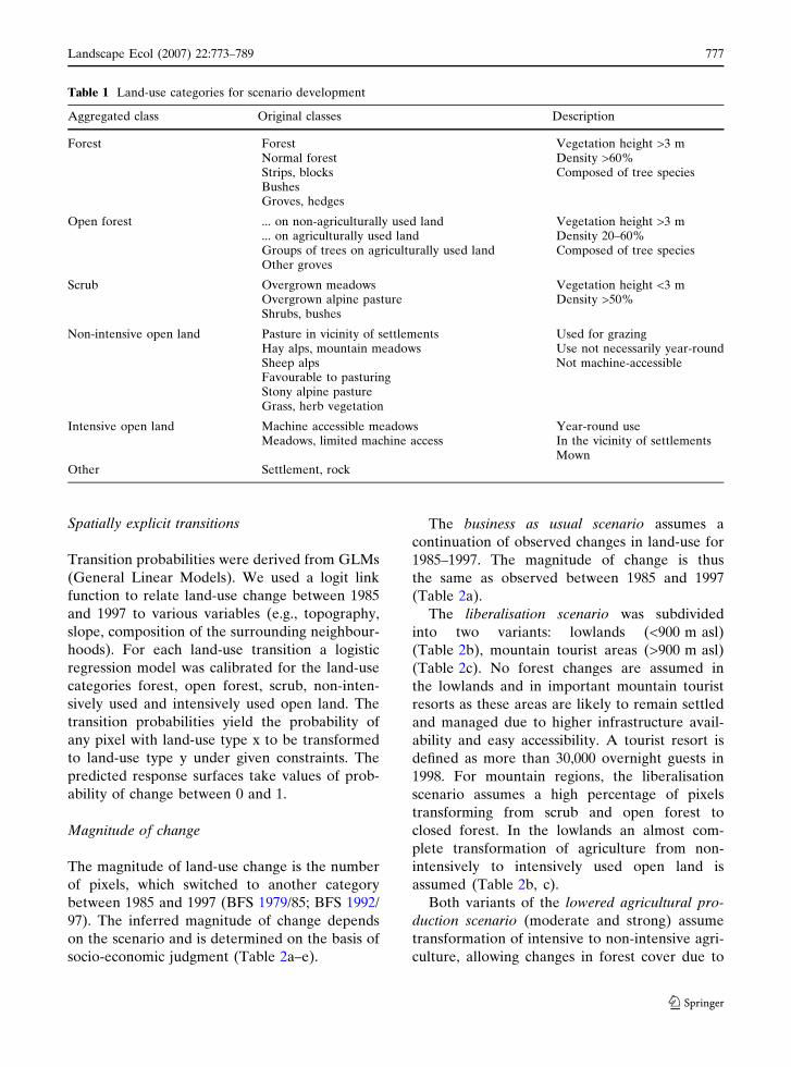
Table 1 Land-use categories for scenario development

Aggregated class Original classes Description

Forest Forest Vegetation height >3 mNormal forest Density >60%Strips, blocks Composed of tree speciesBushesGroves, hedges

Open forest ... on non-agriculturally used land Vegetation height >3 m... on agriculturally used land Density 20–60%Groups of trees on agriculturally used land Composed of tree speciesOther groves

Scrub Overgrown meadows Vegetation height <3 mOvergrown alpine pasture Density >50%Shrubs, bushes

Non-intensive open land Pasture in vicinity of settlements Used for grazingHay alps, mountain meadows Use not necessarily year-roundSheep alps Not machine-accessibleFavourable to pasturingStony alpine pastureGrass, herb vegetation

Intensive open land Machine accessible meadows Year-round useMeadows, limited machine access In the vicinity of settlements

MownOther Settlement, rock

Landscape Ecol (2007) 22:773–789 777

123

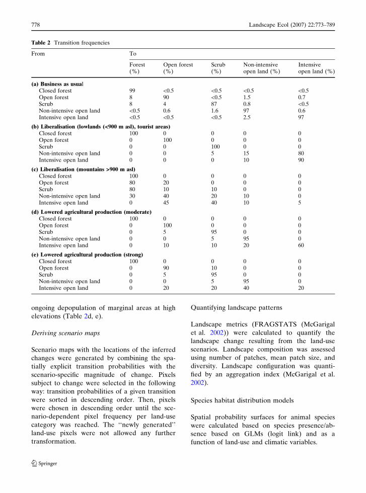
ongoing depopulation of marginal areas at high

elevations (Table 2d, e).

Deriving scenario maps

Scenario maps with the locations of the inferred

changes were generated by combining the spa-

tially explicit transition probabilities with the

scenario-specific magnitude of change. Pixels

subject to change were selected in the following

way: transition probabilities of a given transition

were sorted in descending order. Then, pixels

were chosen in descending order until the sce-

nario-dependent pixel frequency per land-use

category was reached. The ‘‘newly generated’’

land-use pixels were not allowed any further

transformation.

Quantifying landscape patterns

Landscape metrics (FRAGSTATS (McGarigal

et al. 2002)) were calculated to quantify the

landscape change resulting from the land-use

scenarios. Landscape composition was assessed

using number of patches, mean patch size, and

diversity. Landscape configuration was quanti-

fied by an aggregation index (McGarigal et al.

2002).

Species habitat distribution models

Spatial probability surfaces for animal species

were calculated based on species presence/ab-

sence based on GLMs (logit link) and as a

function of land-use and climatic variables.

Table 2 Transition frequencies

From To

Forest(%)

Open forest(%)

Scrub(%)

Non-intensiveopen land (%)

Intensiveopen land (%)

(a) Business as usualClosed forest 99 <0.5 <0.5 <0.5 <0.5Open forest 8 90 <0.5 1.5 0.7Scrub 8 4 87 0.8 <0.5Non-intensive open land <0.5 0.6 1.6 97 0.6Intensive open land <0.5 <0.5 <0.5 2.5 97

(b) Liberalisation (lowlands (<900 m asl), tourist areas)Closed forest 100 0 0 0 0Open forest 0 100 0 0 0Scrub 0 0 100 0 0Non-intensive open land 0 0 5 15 80Intensive open land 0 0 0 10 90

(c) Liberalisation (mountains >900 m asl)Closed forest 100 0 0 0 0Open forest 80 20 0 0 0Scrub 80 10 10 0 0Non-intensive open land 30 40 20 10 0Intensive open land 0 45 40 10 5

(d) Lowered agricultural production (moderate)Closed forest 100 0 0 0 0Open forest 0 100 0 0 0Scrub 0 5 95 0 0Non-intensive open land 0 0 5 95 0Intensive open land 0 10 10 20 60

(e) Lowered agricultural production (strong)Closed forest 100 0 0 0 0Open forest 0 90 10 0 0Scrub 0 5 95 0 0Non-intensive open land 0 0 5 95 0Intensive open land 0 20 20 40 20

778 Landscape Ecol (2007) 22:773–789

123

Biotic dependent variables

Seven animal species were chosen as biotic

dependent variables (Table 3). Requirements

for species selection were sensitivity to open-land

habitats and satisfying data availability for the

whole country. Insects, reptile, and butterfly data

were derived from the Centre Suisse de la Faune

(CSCF), Neuchatel, Switzerland. Bird data was

obtained from the Swiss Ornithological Institute,

Sempach, Switzerland.

Skylark (Alauda arvensis, L. 1758) and whin-

chat (Saxicola rubetra, L. 1758) are birds prefer-

ring non intensive land-use and varied vegetation

(Orlowski 2004; Jepsen et al. 2005; Moreira et al.

2005; Muller et al. 2005).

In Switzerland, the syklark’s main distribution

range encompasses the western and northern

Plateau between 400 and 700 m asl (Schmid

et al. 1998). Increasing intensification of agricul-

tural areas and insecticides have significantly

weakened the populations (Jenny 1990; Tucker

and Heath 1994). Whinchats inhabit non-inten-

sive meadows with low mowing frequencies

(Schmid et al. 1998) and are primarily observed

between 1200 and 2000 m asl (Schmid et al.

1998). Whinchats are largely missing from the

northern Jura mountains and the Plateau where

agriculture has intensified (Schmid et al. 1998).

Three butterfly species are considered. Scotch

Argus (Erebia aethiops, Esper 1777) is widely

distributed including non-intensive meadows and

fields in the lowlands (400 m asl) to subalpine

meadows (2000 m asl) (Gonseth 1987). The spe-

cies is threatened on the Plateau (Gonseth 1987).

Habitats of the Adonis Blue (Lysandra bellargus,

Rottemburg 1775) are non-intensively used

meadows between 400 and 2000 m asl (Gonseth

1987). The species’ habitat range has been

reduced on the Plateau due to intensive agricul-

ture. The Marbled White (Melanargia galathea, L.

1758) occurs between 400 and 1800 m asl and

prefers non-intensively used meadows.

The Large Mountain Grasshopper (Chorthip-

pus scalaris, Fischer-Waldheim 1846) inhabits

non-intensively used prairies and meadows,

sun-exposed clearcuts and shrubby meadows,

preferably in subalpine habitats but it is generally

observed between 230 and 2230 m asl (Thorens

and Nadig 1997).

The Common Lizard (Zootoca vivipara, Jac-

quin 1787) occurs in various habitats ranging

between the lowlands up to 2000 m asl. It inhabits

open forests, forest borders, and open areas in the

lowlands.

Many species inventories inform about species

presence only, whereas absences are rarely

accounted for. Since logistic regression requires

information on species absences, various methods

have been suggested to develop pseudo-absences

(Zaniewski et al. 2002; Engler et al. 2004; Lutolf

et al. 2006).

For this study, observed presences and

absences were available for bird species (Schmid

et al. 1998). For the remaining species only

empirically assessed presences were available,

requiring the derivation of pseudo-absences. The

pseudo-absences were generated based on expert

habitat assessments for each species (Heller-

Kellenberger et al. 1997, 2004). To identify likely

species absences, we first eliminated areas where

the species is observed or is likely to be observed

following expert judgement. The remaining areas

where the species is unlikely to occur were

systematically sampled at a 5 km raster (Table 3).

Independent variables

Climate

Climatic variables were available as continuous

surface maps, based on spatially interpolated data

Table 3 Species data: species absences assessed empiri-cally (++), by experts (+)

Number of observations

Presence Absence Total

AvesAlauda arvensis 963 1683++ 2646Saxicola rubetra 443 2203++ 2646ReptiliaLacerta vivipara 1484 2345+ 3829LepidopteraErebia aethiops 543 9818+ 10361Melanargia galathea 1627 6408+ 8035Lysandra bellargus 820 5867+ 6687SaltatoriaChorthippus scalaris 935 3957+ 4892

Landscape Ecol (2007) 22:773–789 779

123

from standardised meteorological recordings and

digital elevation models (DEM, 25 m). We con-

sidered thermic (fost frequency, degree day sum)

and hygric variables (mean monthly precipitation

sum, water budget in July, and indicators for

continentality (global radiation in July, Gams

angle, July cloudiness) (Zimmermann and

Kienast 1999; Bolliger et al. 2000).

Land-use data

Land-use data used for species habitat suitability

modelling relies on an aggregation of 34 classes

out of the 74 available classes in the Swiss wide

land-use data (BFS 1979/85, 1992/97). The 34

classes were chosen to mirror open-land habitats

for species habitat suitability modeling.

Model calibration

Selection of the set of variables to predict a

species included (a) stepwise logistic regression

where criteria for entry and retention thresholds

were set at a level of significance of 0.05, (b)

correlation matrices where only variables with

correlation coefficients of less than 0.5 were

chosen.

Model performance

Confusion matrices were applied to evaluate the

accuracy of the predicted versus the observed

presence or absence of a species by relating the

proportions of correct model predictions for

presence (sensitivity) and absence (specificity)

with respect to the observed data (Fielding and

Bell 1997). The discriminative ability of the

model to distinguish between species presence

and absence was assessed using ROC plot and

AUC statistics. ROC (Receiver Operating Char-

acteristics) plots evaluate the discriminative

ability of the models by plotting the sensitivity

(true presences) against their equivalent (1-

specificity) that express false presences for all

thresholds (Fielding and Bell 1997). The AUC

value provides a single measure of overall model

accuracy that is independent of a cut-off thresh-

old (Deleo 1993). AUC ranges between 0.5 (no

improvement in determining event presence/

absence in comparison with chance) and 1 (high

model improvement with respect to chance). We

applied a modified version of the AUC value,

the Gini coefficient (Copas 1999). Values range

between 0 and 1, where 0 indicates no prediction

success and 1 indicates high prediction success

for both presence and absence.

Ideally, an independent data set is used to test

a model’s predictive ability. In the absence of

independent data sets, alternative methods are

applied, e.g., a 10 fold cross-evaluation (Verbyla

and Litvaitis 1989). The original data set was

randomly split into 10 data subsets of roughly

equal size. Then a logistic model was estimated

from 9/10 of the data and applied to the

remaining 1/10. The procedure was repeated for

all 10 data subsets to subject all data points to

projections of a quasi independently estimated

model.

The predictive abilities of these models was

then assessed by AUC’eval (mean and standard

deviation) and compared to the predictions

originating from the full calibration data set

(AUC’cal). AUC’eval was calculated using

SimTest (Zimmermann 2001).

Species habitat distributions under land-use

change scenarios

We mapped the highest decile (upper 10%, core

habitat) of species occurrence to identify sensi-

tive areas to land-use change. The resulting

species core habitat maps were then spatially

intersected with the scenarios. The expected

scenario-induced shifts were measured as the

difference of the potential future area of the

core habitat in comparison to the core habitat

occupied in 1997. Gains are assessed for the

expansion of the habitat (i.e., more pixels occupy

suitable habitat for the species), whereas losses

are reported if the core habitats under the

scenarios deteriorated relative to 1997 (i.e.,

conversion to closed forest, scrub, intensive

land-use). Gains and losses are reported in

%pixel habitat gain or habitat loss. For example,

an increase in forested pixels is considered

negative for S. rubetra, which requires open-land

habitats, whereas an increase in non-intensively

780 Landscape Ecol (2007) 22:773–789

123

used open-land pixels is evaluated as habitat

gains.

Results

Land-use change scenarios

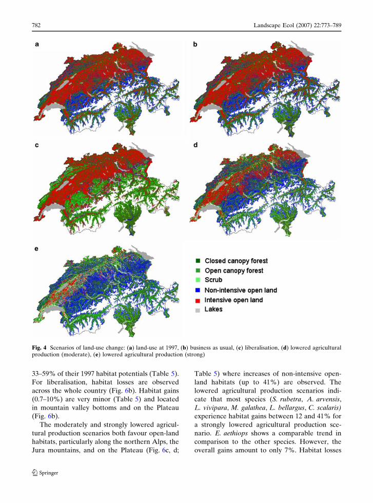
As at 1997 (Fig. 4a), forests prevail in mountain-

ous areas of Switzerland (Northern, Central,

Southern Alps, Fig. 1), whereas the valleys and

the Plateau are intensively used (agriculture,

settlements). Non-intensive land-use is observed

in the Jura mountains, Northern pre-Alps, and at

higher elevations of the Central and Southern

Alps (Fig. 4a).

The business as usual scenario would not

significantly change the spatial distribution of

land-use classes compared to 1997, except for

valley bottoms in the southern part of the Alps

which would transform from intensively to non-

intensively used open land (Fig. 4b; Table 2a).

The liberalisation scenario suggests spatial

segregation between mountains and lowlands:

intensive land-use would prevail in the lowlands

and valley bottoms of the Alps (Fig. 4c, Table 2b,

c). Areas at higher elevations (Northern, Central,

Southern Alps) would become forested, reducing

open forest, scrub, and particularly non-inten-

sively used open-land (Fig. 4c, Table 2c).

The lowered agricultural production scenarios

represent a moderate to strong increase in non-

intensive open-land (Fig. 4d, e, Table 2d, e). Both

scenarios suggest the conversion of intensive to

non-intensive open land, particularly in the low-

lands (Fig. 4d, e, Table 2d, e). Mountain areas

would be dominated by scrub and forests

(Table 2d, e), whereas non-intensively used

open-land in high elevations would decrease only

slightly.

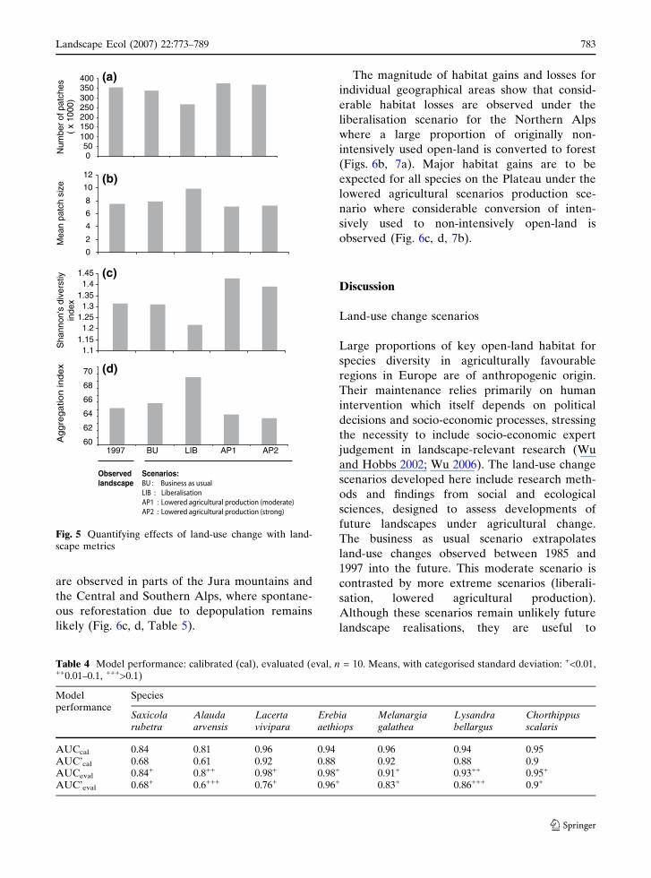
The overall changes in scenario-based land-

scape composition as quantified by landscape

metrics indicate fewer patch numbers, larger

patch sizes and lower landscape-pattern diversity

for the business as usual and the liberalisation

scenario compared to the 1997 landscape

(Fig. 5a–c). Higher patch numbers, smaller patch

sizes and higher landscape-pattern diversity sug-

gest a more complex landscape composition for

the lowered agricultural production scenarios

(Fig. 5a–c). Under the liberalisation scenario the

landscape would be spatially more aggregated,

whereas the lowered agricultural production sce-

narios show disaggregated landscapes compared

to 1997 (Fig. 5d). Thus, the lowered agricultural

production scenarios exhibit structurally the most

diverse and least aggregated landscape compared

to 1997.

Species habitat suitability models:

performance

The model’s discriminative abilities between spe-

cies presence and absence as measured by the

AUC ranges between 0.81 and 0.96 (Table 4),

indicating that all models are good predictors for

any threshold for species presence/absence. Tests

for the model’s predictive ability show that mean

and standard deviation for AUC values from 10

fold cross-validation are statistically reproducible

and compare well to the values obtained from the

initial model calibration (Table 4).

Species habitat distributions under land-use

change scenarios

Effects of the business as usual scenario on

species habitats are generally minor. For most

species, habitat gains and losses are approxi-

mately levelled out, except for S. rubetra and

E. aethiops for which habitat gains are slightly

higher than losses (Table 5). For A. arvensis,

overall losses exceed gains (Table 5). Consider-

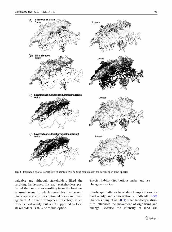
ing the spatial effect of the business as usual

scenario for all seven species, habitat gains are

observed primarily along valley bottoms in the

southern, northern and central Alps (Fig. 6a).

Habitat losses are observed for higher elevations

in the Jura mountains, Central and Southern

Alps, and for hilly regions on the Plateau

(Fig. 6a).

Effects of the liberalisation and the lowered

agricultural production scenarios are severe and

may lead to significant habitat changes of the

species with habitat reductions for all species

(Table 5). Some species (L. vivipara, S. rubetra,

M. galathea, L. bellargus, C. scalaris) may lose

Landscape Ecol (2007) 22:773–789 781

123

33–59% of their 1997 habitat potentials (Table 5).

For liberalisation, habitat losses are observed

across the whole country (Fig. 6b). Habitat gains

(0.7–10%) are very minor (Table 5) and located

in mountain valley bottoms and on the Plateau

(Fig. 6b).

The moderately and strongly lowered agricul-

tural production scenarios both favour open-land

habitats, particularly along the northern Alps, the

Jura mountains, and on the Plateau (Fig. 6c, d;

Table 5) where increases of non-intensive open-

land habitats (up to 41%) are observed. The

lowered agricultural production scenarios indi-

cate that most species (S. rubetra, A. arvensis,

L. vivipara, M. galathea, L. bellargus, C. scalaris)

experience habitat gains between 12 and 41% for

a strongly lowered agricultural production sce-

nario. E. aethiops shows a comparable trend in

comparison to the other species. However, the

overall gains amount to only 7%. Habitat losses

Fig. 4 Scenarios of land-use change: (a) land-use at 1997, (b) business as usual, (c) liberalisation, (d) lowered agriculturalproduction (moderate), (e) lowered agricultural production (strong)

782 Landscape Ecol (2007) 22:773–789

123

are observed in parts of the Jura mountains and

the Central and Southern Alps, where spontane-

ous reforestation due to depopulation remains

likely (Fig. 6c, d, Table 5).

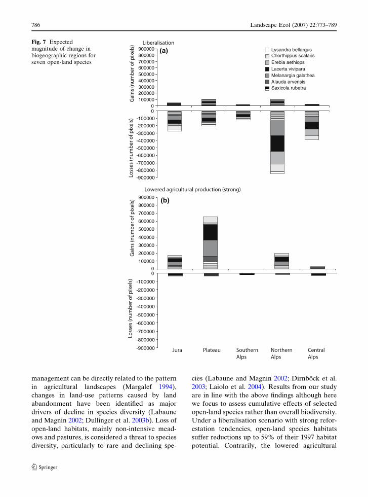
The magnitude of habitat gains and losses for

individual geographical areas show that consid-

erable habitat losses are observed under the

liberalisation scenario for the Northern Alps

where a large proportion of originally non-

intensively used open-land is converted to forest

(Figs. 6b, 7a). Major habitat gains are to be

expected for all species on the Plateau under the

lowered agricultural scenarios production sce-

nario where considerable conversion of inten-

sively used to non-intensively open-land is

observed (Fig. 6c, d, 7b).

Discussion

Land-use change scenarios

Large proportions of key open-land habitat for

species diversity in agriculturally favourable

regions in Europe are of anthropogenic origin.

Their maintenance relies primarily on human

intervention which itself depends on political

decisions and socio-economic processes, stressing

the necessity to include socio-economic expert

judgement in landscape-relevant research (Wu

and Hobbs 2002; Wu 2006). The land-use change

scenarios developed here include research meth-

ods and findings from social and ecological

sciences, designed to assess developments of

future landscapes under agricultural change.

The business as usual scenario extrapolates

land-use changes observed between 1985 and

1997 into the future. This moderate scenario is

contrasted by more extreme scenarios (liberali-

sation, lowered agricultural production).

Although these scenarios remain unlikely future

landscape realisations, they are useful to

050

100150200250300350400

0

2

4

6

8

10

12

1.11.151.2

1.251.3

1.351.4

1.45

60

62

64

66

68

70

1997 BU LIB AP1 AP2

(a)

(b)

Mea

n pa

tch

size

(d)

Aggre

gatio

n in

dex

(c)

Observedlandscape

Scenarios:BU : Business as usualLIB : LiberalisationAP1 : Lowered agricultural production (moderate)AP2 : Lowered agricultural production (strong)

Num

ber

of p

atch

es

( x

1000

)S

hann

on's

div

erst

iy

inde

x

Fig. 5 Quantifying effects of land-use change with land-scape metrics

Table 4 Model performance: calibrated (cal), evaluated (eval, n = 10. Means, with categorised standard deviation: +<0.01,++0.01–0.1, +++>0.1)

Modelperformance

Species

Saxicolarubetra

Alaudaarvensis

Lacertavivipara

Erebiaaethiops

Melanargiagalathea

Lysandrabellargus

Chorthippusscalaris

AUCcal 0.84 0.81 0.96 0.94 0.96 0.94 0.95AUC’cal 0.68 0.61 0.92 0.88 0.92 0.88 0.9AUCeval 0.84+ 0.8++ 0.98+ 0.98+ 0.91+ 0.93++ 0.95+

AUC’eval 0.68+ 0.6+++ 0.76+ 0.96+ 0.83+ 0.86+++ 0.9+

Landscape Ecol (2007) 22:773–789 783

123

benchmark development extremes to quantify

potential effects on the landscape. Caveats

include that the temporal dimension of the

scenarios cannot explicitly be accounted for.

Estimations as to when the respective landscape

states may be reached range from approximately

20 to 30 years for the business as usual scenario,

30–50 years for the lowered agricultural produc-

tion scenarios, and between 100 and 200 years

for the liberalisation scenario.

Results show that likely consequences of agri-

cultural change are spatially segregated with

lower reforestation tendencies in the lowlands

due to favourable socio-economic, topographic

and climatic conditions, which foster agricultural

land-use. Strong reforestation tendencies and loss

of open-land are more pronounced in mountain-

ous areas (Jura mountains, Alps).

Scenario-derived changes in landscape compo-

sition and configuration were assessed statistically

by landscape metrics, which measure pixel

densities and distributions numerically. The land-

scape changes indicate that the lowered agricul-

tural production scenarios would exhibit highest

compositional and configuration diversity,

whereas the liberalisation scenario may lead to

aggregated and less diverse landscapes with large

patches and increased homogenisation. Use and

limitation of landscape metrics have been dis-

cussed in detail elsewhere (Gustafson 1998;

McGarigal et al. 2002; Li and Wu 2004). In

general, landscape metrics are considered valu-

able tools to describe statistical landscape char-

acteristics, whereas details on the ecological

implications for organisms cannot be easily

assessed.

Scale effects have been identified to be of great

relevance in landscape research (Wu and Hobbs

2002) and various aspects of scale have been

studied intensively (Wu 1999, 2004; Wu et al.

2002). It has been stated that the relevant spatial

pattern is revealed only if the scale of analysis

approaches the operational scale of the phenom-

enon under study (Wu 1999, 2004) referring to the

dependence of spatial pattern on the scale of

observation and analysis. In this study, both the

scale of analysis and the operational scale of the

phenomenon (land-use, species distributions) is

the landscape scale (41,000 km2). This ensures

agreement between the scale of analysis and the

operational scale of the phenomenon (land-use,

species distributions) as required for the detection

of the relevant patterns in a multi-scale landscape.

The drivers of the land-use change scenarios,

however, were selected independently of the

spatial scale (scale invariant) so that they are

important for both, the local and the landscape

scale. Drivers include e.g., depopulation tenden-

cies, farm abandonment (Soliva et al. accepted).

In a qualitative acceptability assessment the local-

scale social relevance of the scenarios was tested.

Local visualisations of the land-use change sce-

narios were presented to stakeholders in a

mountain area. Although less labour intensive

and low-cost, stakeholders rejected the liberalisa-

tion scenario due to loss of landscape quality. At

the same time, stakeholders did not accept the

social, economic and cultural price of a scenario

that puts conservation and biodiversity first

although increased biodiversity was considered

Table 5 Gains and losses of species habitats (% pixelscompared to 1997)

Businessas usual

Libera-lisation

Loweredagriculturalproduction(moderate)

Loweredagriculturalproduction(strong)

(a) Saxicola rubetraGains 2.04 6.57 13.0 20.31Losses 1.81 34.3 2.8 2.8

(b) Alauda arvensisLand-useGains 0.15 0.68 2.07 12.0Losses 0.51 4.45 0.97 0.8

(c) Lacerta viviparaGains 2.91 10.29 21.26 39.46Losses 3.00 59.23 4.65 4.66

(d) Erebia aethiopsGains 1.7 4.09 6.08 7.2Losses 1.3 41.5 2.07 2.0

(e) Melanargia galatheaGains 3.05 10.58 21.43 41.1Losses 3.04 53.15 4.71 4.71

(f) Lysandra bellargusGains 2.17 9.13 19.03 32.50Losses 2.15 34.06 3.33 3.34

(g) Chorthippus scalarisGains 1.87 5.84 11.00 17.82Losses 1.94 33.37 3.00 2.99

784 Landscape Ecol (2007) 22:773–789

123

valuable and although stakeholders liked the

resulting landscapes. Instead, stakeholders pre-

ferred the landscapes resulting from the business

as usual scenario, which resembles the current

landscape and ensures continued open-land man-

agement. A future development trajectory, which

favours biodiversity, but is not supported by local

stakeholders, is thus no viable option.

Species habitat distributions under land-use

change scenarios

Landscape patterns have direct implications for

biodiversity and conservation (Lindbladh 1999;

Haines-Young et al. 2003) since landscape struc-

ture influences the movement of organisms and

energy. Because the intensity of land use

Fig. 6 Expected spatial sensitivity of cumulative habitat gains/losses for seven open-land species

Landscape Ecol (2007) 22:773–789 785

123

management can be directly related to the pattern

in agricultural landscapes (Margalef 1994),

changes in land-use patterns caused by land

abandonment have been identified as major

drivers of decline in species diversity (Labaune

and Magnin 2002; Dullinger et al. 2003b). Loss of

open-land habitats, mainly non-intensive mead-

ows and pastures, is considered a threat to species

diversity, particularly to rare and declining spe-

cies (Labaune and Magnin 2002; Dirnbock et al.

2003; Laiolo et al. 2004). Results from our study

are in line with the above findings although here

we focus to assess cumulative effects of selected

open-land species rather than overall biodiversity.

Under a liberalisation scenario with strong refor-

estation tendencies, open-land species habitats

suffer reductions up to 59% of their 1997 habitat

potential. Contrarily, the lowered agricultural

00

100000

200000

300000

400000

500000

600000

700000

800000

900000 (b)

Lowered agricultural production (strong)

Gai

ns

(nu

mb

er o

f pix

els)

Loss

es (n

um

ber

of p

ixel

s)

Jura Plateau SouthernAlps

NorthernAlps

CentralAlps

Lysandra bellargusChorthippus scalarisErebia aethiopsLacerta viviparaMelanargia galathea

Saxicola rubetraAlauda arvensis

Gai

ns

(nu

mb

er o

f pix

els)

Loss

es (n

um

ber

of p

ixel

s)

Liberalisation

0100000200000300000400000500000600000700000800000900000

-900000

-800000

-700000

-600000

-500000

-400000

-300000

-200000

-100000

-900000

-800000

-700000

-600000

-500000

-400000

-300000

-200000

-100000

0

(a)Fig. 7 Expectedmagnitude of change inbiogeographic regions forseven open-land species

786 Landscape Ecol (2007) 22:773–789

123

production scenario increases potential habitat

areas between up to 41%. In addition, a scenario-

induced spatial segregation of the sensitive core

habitat areas is observed. Whereas areas for

habitat gains are primarily located on the Plateau

and the Northern Alps, losses of open-land

species habitats are observed for the whole

country, but particularly for mountainous areas

(Jura, Alps). Such spatial segregation of the

magnitude of land-use change has been

observed for a variety of other mountainous

areas (Brown 2003).

The method applied to assess potential effects

of land-use change due to agricultural decline

relies on species habitat suitability models. The

models exhibit satisfying model performance. It

has been claimed that predicting species

responses to habitat changes is a challenges for

ecologists (Travis 2002; Thuiller et al. 2004).

Among methods, predictive modelling has been

an important tool to assess management or

conservation strategies for biota e.g., for incon-

spicuous species (Edwards et al. 2005), or biota

under changing environments (Dirnbock et al.

2003; Araujo et al. 2004). Among predictive

models, logistic regression is well established

and has been applied to a broad variety of

research topics and conservation issues (Bolliger

et al. 2000; Guisan and Hofer 2003; McKenzie

et al. 2003). It has been claimed that a broad

variety of approaches are required to successfully

identify ecological complexity (Loehle 2004).

Thus, an approach which predicts species distri-

butions as a function of climatic and land-use

information may over- or under-predict species

habitats since dynamic biotic interactions, adap-

tive genetic variation, dispersal and migration

cannot be accounted for with such a parsimonious

method (Hannah et al. 2002; Hampe 2004).

However, since details on species-specific life-

history attributes or environment are not usually

available for large spatial scales, the parsimonious

regression approach may be seen as a trade-off

between predictions at large scales and data

availability which holds true for landscape scales

where strong (environmental) gradients drive the

biotic patterns as it is the case for Switzerland

(Bolliger et al. 2000; Thuiller et al. 2003). Thus,

habitat models from regressions can provide a

suitable approach to identify potential impacts of

landscape change on species habitats. Use and

limitations of species distribution modelling have

been discussed in detail elsewhere (e.g., Guisan

and Zimmermann 2000; Hampe 2004; Segurado

and Araujo 2004; Guisan and Thuiller 2005) and

will thus not be repeated here.

Conclusions

The study shows that it is crucial for open-land

species that agricultural and conservation policy

allow for non-intensively used open-land habitats

to be maintained and managed in a sustainable

way. We suggest that the lowered agricultural

production scenario is most beneficial for open-

land species however, its social acceptability is

limited due to high costs. Combinations of the

business as usual and lowered agricultural produc-

tion scenario would be adequate: farmers would

continue to receive public support, which is

more tightly linked to current regionally adapted

agri-environmental schemes focussing on the

non-intensive use the land. Combining ecological

analysis with socio-economic investigations of

stakeholder’s scenario-assessments may thus

provide useful input for future regional develop-

ment and conservation, facilitating an integrated

approach to biodiversity conservation.

Acknowledgements Many thanks to the Centre Suisse deCartographie de la Faune, Neuchatel (Simon Capt, YvesGonseth) for their expert advice and for providing thespecies data. We would also like to thank Thomas Niemzfor kindly conducting some of the GIS analyses. Thisresearch was supported by the BioScene project funded bythe European Union (EVK2-2001-00354).

References

Araujo MB, Cabeza M, Thuiller W, Hannah L, WilliamsPH (2004) Would climate change drive species out ofreserves? An assessment of existing reserve-selectionmethods. Glob Change Biol 10:1618–1626

Bakker J (1989) Nature management by grazing andcutting. Kluwer Academic Publishers, London

Batzig W (1996) Landwirtschaft im Alpenraum unverzichtbar,aber zukunftslos? Eine alpenweite Bilanz der aktuellenProbleme und der moglichen Losungen. In: Batzig W

Landscape Ecol (2007) 22:773–789 787

123

(ed) Landwirtschaft im Alpenraum—unverzichtbar, aberzukunftslos? Europaische Akademie Bozen, FachbereichAlpine Umwelt, Blackwell, Wien, pp 9–11

BFS (1979/85) Arealstatistik, Bundesamt fur Statistik,Servicestelle GEOSTAT, CH-Neuchatel

BFS (1992/97) Arealstatistik, Bundesamt fur Statistik,Servicestelle GEOSTAT, CH-Neuchatel

BLW (2003) Verordnungspaket 2007. Ausfuhrungsbes-timmungen zur Agrarpolitik 2007. Informationsve-ranstaltung vom 5.12.2003, Bundesamt furLandwirtschaft, Bern

BLW (2004) Agrarbericht 2004, Bundesamt fur Land-wirtschaft, Bern

Bolliger J, Kienast F, Zimmermann NE (2000) Risks ofglobal warming on montane and subalpine forests inSwitzerland. Region Environ Change 1:99–111

Brown DG (2003) Land use and forest cover on privateparcels in the Upper Midwest USA, 1970 to 1990.Landscape Ecol 18:777–790

Copas J (1999) The effectiveness of risk scores: the logitrank plot. J Roy Stat Soc Ser C-Appl Stat 48:165–183

Deleo JM (1993) Receiver operating characteristic labo-ratory (ROCLAB): software for developing decisionstrategies that account for uncertainty. Proceedings ofthe first international symposium on uncertaintymodelling and analysis. IEEE, Computer SocietyPress, College Park, MD, pp 318–325

Dirnbock T, Dullinger S, Grabherr G (2003) A regionalimpact assessment of climate and land-use change onalpine vegetation. J Biogeogr 30:401–417

Dullinger S, Dirnbock T, Grabherr G (2003a) Patterns ofshrub invation into high mountain grasslands of theNorthern calcareous Alps, Austria. Arct Antarct AlpRes 35:434–441

Dullinger S, Dirnbock T, Greimler S, Grabherr G (2003b)A resampling approach to evaluate effects of summerfarming on subalpine plant species diversity. J Veg Sci14:243–252

Edwards TC, Cutler R, Zimmermann NE, Geiser L,Alegria J (2005) Model-based stratification forenhancing the detection of rare ecological events.Ecology 86:1081–1090

Engler R, Guisan A, Rechsteiner L (2004) Predicting thedistribution of rare and endangered species from occur-rence and pseudo-absence data. J Appl Ecol 41:263–274

FAT (2002) Zentrale Auswertung von Buchhaltungsdaten,Tanikon

Fielding AH, Bell JF (1997) A review of methods for theassessment of prediction errors in conservation pres-ence/absence models. Environ Conserv 24:38–49

Flury C (2002) Zukunftsfahige Landwirtschaft im Alpen-raum, Diss. ETH Nr. 14528: Zurich

Gonseth Y (1987) Verbreitungsatlas der Tagfalter derSchweiz (Leptidoptera, Rhopalocera), 6. DocumentaFaunistica Helvetica

Guisan A, Hofer U (2003) Predicting reptile distributionsat the mesoscale: relation to climate and topography.J Biogeogr 30:1233–1243

Guisan A, Thuiller W (2005) Predicting species distribu-tions: offering more than simple habitat models. EcolLett 8:993–1009

Guisan A, Zimmermann NE (2000) Predictive habitatdistribution models in ecology. Ecol Model 135:147–186

Gustafson EJ (1998) Quantifying landscape spatial pattern:what is the state of the art? Ecosystems 1:143–156

Haines-Young R et al (2003) Changing landscapes, hab-itats and vegetation diversity across Great Britain.J Environ Manage 67:267–281

Hampe A (2004) Bioclimate envelope models: what theydetect and what they hide. Global Ecol Biogeogr13:469–476

Hannah L et al (2002) Conservation of biodiversity in achanging climate. Conserv Biol 16:264–268

Heller-Kellenberger I, Kienast F, Obrist M, Walter T(1997) Raumliche Modellierung der potentiellenfaunistischen Biodiversitat mit einem Expertensys-tem. Informationsblatt des ForschungsbereichesLandschaft 36

Heller-Kellenberger I, Kienast F, Obrist MK, Walther TA(2004) Biodiversity hostspots—modeling potentialfaunistic biodiversity with a spatially explicit expertsystem. Swiss Federal Research Institute WSL

Jenny M (1990) Populationsdynamik der Feldlerche Alau-da arvensis in einer intensiv genutzten Agrarlands-chaft. J Ornithol 131:241–265

Jepsen JU, Topping CJ, Odderskaer P, Andersen PN(2005) Evaluating consequences of land-use strategieson wildlife populations using multiple-species predic-tive scenarios. Agric Ecosyst Environ 105(4):581–594

Labaune C, Magnin F (2002) Pastoral management vs.land abandonment in Mediterranean uplands: impacton snail communities. Global Ecol Biogeogr Lett11:237–245

Laiolo P, Dondero F, Ciliento E, Rolando A (2004)Consequences of pastoral abandonment for the struc-ture and diversity of the alpine avifauna. J Appl Ecol41:294–304

Li H, Wu J (2004) Use and misuse of landscape indices.Landscape Ecol 19:389–399

Lindbladh M (1999) The influence of former land-use onvegetation and biodiversity in the boreo-nemoral zoneof Sweden. Ecography 22:485–498

Loehle C (2004) Challenges of ecological complexity. EcolComplexity 1:3–6

Lundstrom-Gillieron C, Schlapfer R (2003) Hareabundance as an indicator for urbanisation andintensification of agriculture in Western Europe. EcolModel 168:283–301

Lutolf M, Kienast F, Guisan A (2006) Strategies toimprove species distribution model performance usingoccurrence data. J Appl Ecol 43:802–815

Mack G, Ferjani A (2002) Auswirkungen der Agrarpolitik(2007) Modellrechnungen fur den Agrarsektor mitHilfe des Prognosesystems SILAS, FAT, Tanikon

Margalef R (1994) Dynamic aspects of diversity. J Veg Sci5:451–456

McCracken DI, Bignal EM (1998) Applying the resultsof ecological studies to land-use policies and practices.J Appl Ecol 35:961–967

McGarigal K, Cushman SA, Neel MC, Ene E (2002)FRAGSTATS: Spatial pattern analysis program forcategorial maps. Computer software program

788 Landscape Ecol (2007) 22:773–789

123

produced by the authors at the University of Massa-chusetts, Amherst, MA, USA. http://www.umass.edu/landeco/research/fragstats/fragstats.html

McKenzie D, Peterson DW, Peterson DL, Thornton PE(2003) Climatic and biophysical controls on coniferspecies distributions in mountain forests of Washing-ton State, USA. J Biogeogr 30:1093–1108

Meeus J, Van Der Ploeg JD, Wijermans M (1991)Changing agricultural landscapes in Europe: continu-ity, deterioration or rupture? IFLA conference, Rot-terdam, The Netherlands

Moreira F et al (2005) Effects of field managementand landscape context on grassland wintering birdsin Southern Portugal. Agricult Ecosyst Environ109:59–74

Muller M, Spaar R, Schifferli L, Jenni L (2005) Effets ofchanges in farming of subalpine meadows on agrassland bird, the whinchat (Saxicola rubetra). JOrnithol 146(1):14–23

OECD (2002) Agricultural Policies in OECD countries.Monitoring and Evaluation, Paris

Orlowski G (2004) Abandoned cropland as a habitat forthe Whinchat Saxicola rubetra in SW Poland. ActaOrnithologica 39:59–66

Sager J, Finger A (1992) Die Bodennutzung der Schweiz.Arealstatistik 1979/85. Kategorienkatalog. 002-8502,Bundesamt fur Statistik, Bern. 191 pp

Schmid H, Luder R, Naef-Daenzer B, Graf R, Zbinden N(1998) Schweizer Brutvogelatlas. Verbreitung derBrutvogel in der Schweiz und im Furstentum Liech-tenstein 1993–1996. Schweizerische Vogelwarte,Sempach

Segurado P, Araujo MB (2004) An evaluation of methodsfor modelling species distributions. J Biogeogr31:1555–1568

Soderstrom B, Svensson B, Vessby K, Glimskar A (2001)Plants, insects, and birds in semi-natural pastures inrelation to local habitat and landscape factors. Bio-divers Conserv 10:1839–1863

Soliva R, Rønningen K, Bella I, Bezak P, Cooper T, FløBE, Marty P, Potter C. Envisioning Upland Futures:Stakeholder responses to scenarios for Europe’smountain landscapes. J Rural Stud (accepted)

Statistisches Jahrbuch der Schweiz (1997) 104. VerlagNeue Zurcher Zeitung, Zurich

Thorens P, Nadig A (1997) Verbreitungsatlas der Orth-opteren der Schweiz

Thuiller W, Araujo MB, Lavorel S (2003) Generalizedmodels vs. classification tree analysis: predictingspatial distributions of plant species at different scales.J Veg Sci 14:669–680

Thuiller W, Araujo MB, Lavorel S (2004) Do we needland-cover data to model species distributions inEurope? J Biogeogr 31:353–361

Tilman D et al (2001) Forecasting agriculturally drivenglobal environmental change. Science 292:281–284

Travis JMJ (2002) Climate change and habitat destruction:a deadly anthropogenic cocktail. Proc R Soc Lond B270:467–473

Tucker GM, Heath MF (1994) Birds in Europe: theirconservation status. Series No. 3. BirdLife Interna-tional, Cambridge

van der Vaart JHP (2005) Towards a new rural landscape:consequences of non-agricultural re-use of redundantfarm buildings in Friesland. Landscape Urban Plan70:143–152

Verbyla DL, Litvaitis JA (1989) Resampling methods forevaluation classification accuracy of wildlife habitatmodels. Environ Manage 13:783–787

Weibel U (2004) Bauern, die Biodiversitat produzieren.Ornis 2:4–8

Wu J (1999) Hierarchy and scaling: extrapolating infor-mation along a scaling ladder. Int J Remote Sensing25:367–380

Wu J (2004) Effects of changing scale on landscape patternanalysis: scaling relations. Landscape Ecol 19:125–138

Wu J (2006) Landscape ecology, cross-disciplinarity, andsustainability science. Landscape Ecol 21:1–4

Wu J, Hobbs R (2002) Key issues and research priorities inlandscape ecology: an idiosyncratic synthesis. Land-scape Ecol 17:355–365

Wu J, Shen W, Sun W, Tueller PT (2002) Empiricalpatterns of the effects of changing scale on landscapemetrics. Landscape Ecol 17:761–782

Zaniewski AE, Lehmann A, Overton JM (2002) Predictingspecies spatial distributions using presence-only data:a case study of native New Zealand ferns. Ecol Model157:261–280

Zimmermann NE (2001) SimTest. http://www.wsl.ch/staff/niklaus.zimmermann/programs/fort10_1.html, WSL,Birmensdorf

Zimmermann NE, Kienast F (1999) Predictive mapping ofAlpine grasslands in Switzerland: species versus com-munity approach. J Veg Sci 10:469–482

Landscape Ecol (2007) 22:773–789 789

123