Simultaneous Segmentation and MotionRecovery in 3D Cardiac Image Analysis

Ling Zhuang1, Huafeng Liu1,2, Wei Chen1, Hujun Bao1 and Pengcheng Shi2

1State Key Laboratory of CAD & CGZhejiang University, Hangzhou, China

zhuangling@cad.zju.edu.cn

eeliuhf@ust.hk

chenwei@cad.zju.edu.cn

bao@cad.zju.edu.cn2Department of Electrical and Electronic Engineering

Hong Kong University of Science and Technology, Clear Water Bay, Hong Kongeeship@ust.hk

Abstract. Accurate and robust estimation of the three-dimensional leftventricular geometry and deformation has important clinical implicationsfor better diagnosis and understanding of ischemic heart diseases. So far,most image analysis efforts have performed the shape recovery and themotion tracking tasks in separate steps, typically in sequential fashion. Inthis paper, we present a continuum biomechanics model based frameworkthat performs simultaneous segmentation and motion analysis of theleft ventricle from 3D image sequences, achieved through the trackingof the spatiotemporal evolution of a 3D active region model driven byimaging data, statistical priors of the left ventricular boundaries, andcyclic motion models of the myocardial tissue elements. Experiments on3D canine and human MR image sequences have shown the superiorityof the strategy.

1 Introduction

With the rapid development of medical imaging technology, 3D images of themoving heart have become increasingly available from several different imagingmodalities such as MR tagging, phase contrast MRI, and cine CT. These imagesprovide the spatiotemporal tomographic insights of the cardiac states of health,and the computer assisted analysis of these images offers quantitative tools forthe diagnosis of ischemic cardiomyopathy, the leading fatal disease in the world.

Since ischemic heart diseases often manifest as abnormalities of ventriculargeometry, wall kinematics, and myocardial mechanics, there have been manyimage analysis efforts over the last twenty years devoted to the shape and motionrecovery of the heart [1–3]. While it has been argued that there are advantagesto treat the spatial boundary finding and the spatiotemporal motion trackingas a coherent and unified process to reduce the possibility of error propagationfrom one step to another, most of the existing efforts do not attempt to tacklethe segmentation and motion problems simultaneously, but rather sequentially.

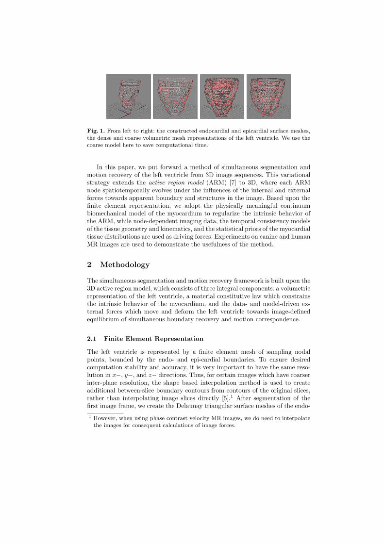
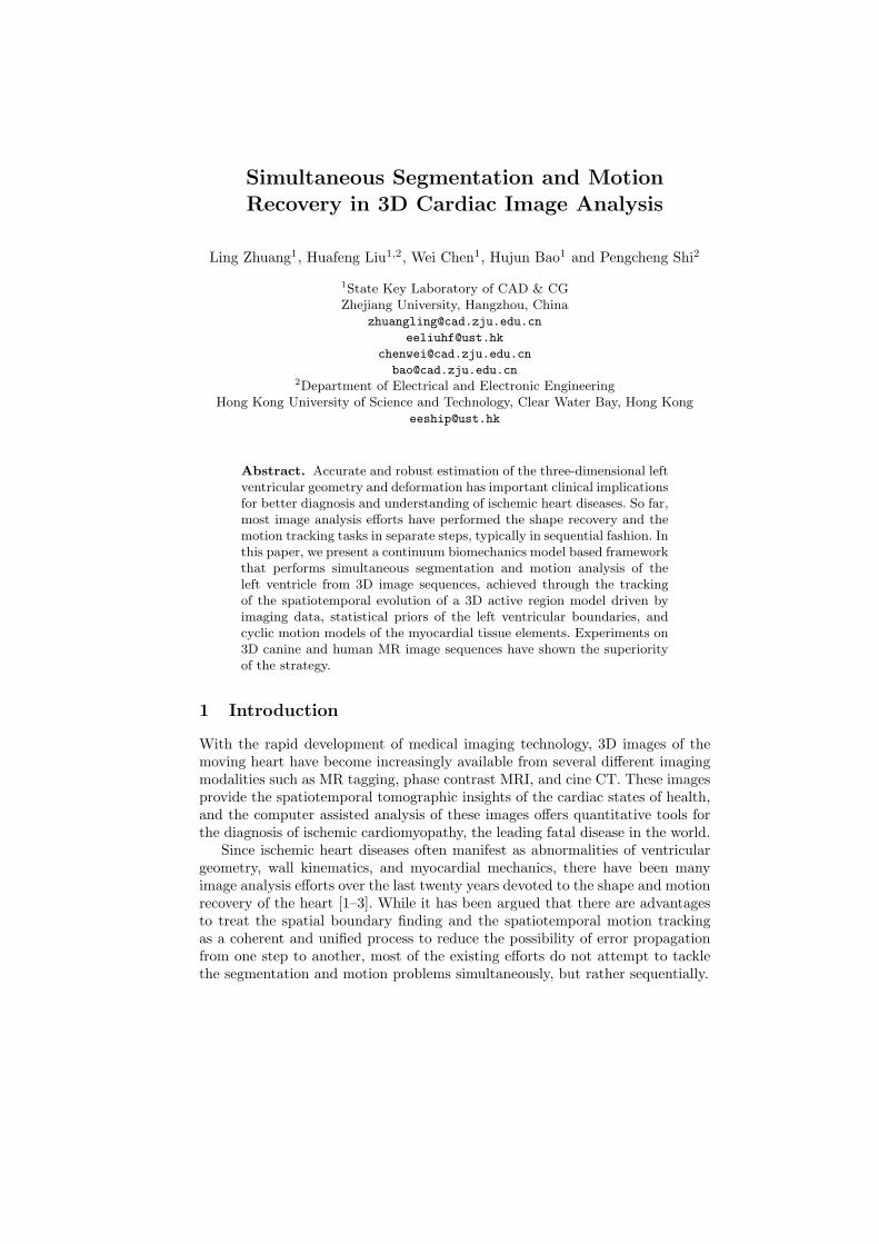
Fig. 1. From left to right: the constructed endocardial and epicardial surface meshes,the dense and coarse volumetric mesh representations of the left ventricle. We use thecoarse model here to save computational time.

In this paper, we put forward a method of simultaneous segmentation andmotion recovery of the left ventricle from 3D image sequences. This variationalstrategy extends the active region model (ARM) [7] to 3D, where each ARMnode spatiotemporally evolves under the influences of the internal and externalforces towards apparent boundary and structures in the image. Based upon thefinite element representation, we adopt the physically meaningful continuumbiomechanical model of the myocardium to regularize the intrinsic behavior ofthe ARM, while node-dependent imaging data, the temporal consistency modelsof the tissue geometry and kinematics, and the statistical priors of the myocardialtissue distributions are used as driving forces. Experiments on canine and humanMR images are used to demonstrate the usefulness of the method.

2 Methodology

The simultaneous segmentation and motion recovery framework is built upon the3D active region model, which consists of three integral components: a volumetricrepresentation of the left ventricle, a material constitutive law which constrainsthe intrinsic behavior of the myocardium, and the data- and model-driven ex-ternal forces which move and deform the left ventricle towards image-definedequilibrium of simultaneous boundary recovery and motion correspondence.

2.1 Finite Element Representation

The left ventricle is represented by a finite element mesh of sampling nodalpoints, bounded by the endo- and epi-cardial boundaries. To ensure desiredcomputation stability and accuracy, it is very important to have the same reso-lution in x−, y−, and z− directions. Thus, for certain images which have coarserinter-plane resolution, the shape based interpolation method is used to createadditional between-slice boundary contours from contours of the original slices,rather than interpolating image slices directly [5].1 After segmentation of thefirst image frame, we create the Delaunay triangular surface meshes of the endo-1 However, when using phase contrast velocity MR images, we do need to interpolate

the images for consequent calculations of image forces.

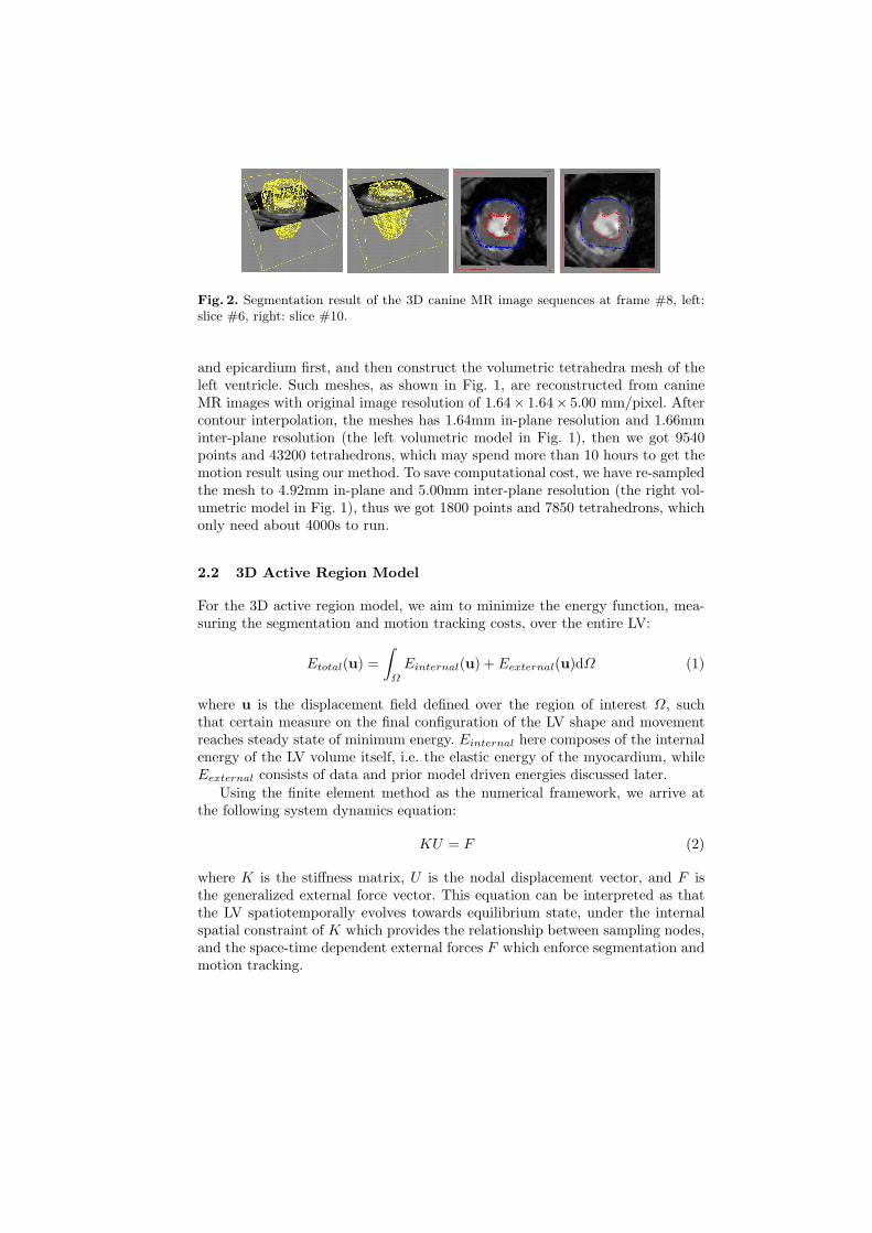
Fig. 2. Segmentation result of the 3D canine MR image sequences at frame #8, left:slice #6, right: slice #10.

and epicardium first, and then construct the volumetric tetrahedra mesh of theleft ventricle. Such meshes, as shown in Fig. 1, are reconstructed from canineMR images with original image resolution of 1.64× 1.64× 5.00 mm/pixel. Aftercontour interpolation, the meshes has 1.64mm in-plane resolution and 1.66mminter-plane resolution (the left volumetric model in Fig. 1), then we got 9540points and 43200 tetrahedrons, which may spend more than 10 hours to get themotion result using our method. To save computational cost, we have re-sampledthe mesh to 4.92mm in-plane and 5.00mm inter-plane resolution (the right vol-umetric model in Fig. 1), thus we got 1800 points and 7850 tetrahedrons, whichonly need about 4000s to run.

2.2 3D Active Region Model

For the 3D active region model, we aim to minimize the energy function, mea-suring the segmentation and motion tracking costs, over the entire LV:

Etotal(u) =∫

Ω

Einternal(u) + Eexternal(u)dΩ (1)

where u is the displacement field defined over the region of interest Ω, suchthat certain measure on the final configuration of the LV shape and movementreaches steady state of minimum energy. Einternal here composes of the internalenergy of the LV volume itself, i.e. the elastic energy of the myocardium, whileEexternal consists of data and prior model driven energies discussed later.

Using the finite element method as the numerical framework, we arrive atthe following system dynamics equation:

KU = F (2)

where K is the stiffness matrix, U is the nodal displacement vector, and F isthe generalized external force vector. This equation can be interpreted as thatthe LV spatiotemporally evolves towards equilibrium state, under the internalspatial constraint of K which provides the relationship between sampling nodes,and the space-time dependent external forces F which enforce segmentation andmotion tracking.

Fig. 3. Segmentation of the 3D canine MR image sequences (mesh intersections witha middle ventricle slice for illustration): frames #1, #3, #5, #7 and #9 (out of 16frames).

By applying the principles from Lagrangian mechanics, we can update thedisplacement vector with time step τ :

(I + τK)U t = (U t−1 + τF t−1) (3)

where I is an identity matrix and U t is the displacement at time t. The iterationstops when ‖U t − U t−1‖ is below certain threshold.

2.3 Continuum Biomechanical Models

We use continuum biomechanical model of the myocardium, instead of the geo-metrical deformable models, to construct the stiffness matrix K. For computa-tional feasibility, we use linear isotropic material model where the stress (σ) andstrain (ε) tensors obey the constitutive law:

[σ] = [C][ε] (4)

with:

[ε] =

∂∂x 0 00 ∂

∂y 00 0 ∂

∂z∂∂y

∂∂x 0

0 ∂∂z

∂∂y

∂∂z 0 ∂

∂x

uvw

= [B

′]u (5)

and the material matrix [C]:

[C] =E

(1 + ν)(1− 2ν)

1−ν ν ν 0 0 0ν 1−ν ν 0 0ν ν 1−ν 0 0 00 0 0 1−2ν 0 00 0 0 0 1−2ν 00 0 0 0 0 1−2ν

(6)

where E and ν are material dependent parameters. The internal energy of thelinear isotropic ARM model thus can be expressed as:

Einternal =12

∫∫∫

Ω

[ε]T [σ]dV

=12

∫∫∫

Ω

uT [B′]T [C][B

′]udV

(7)

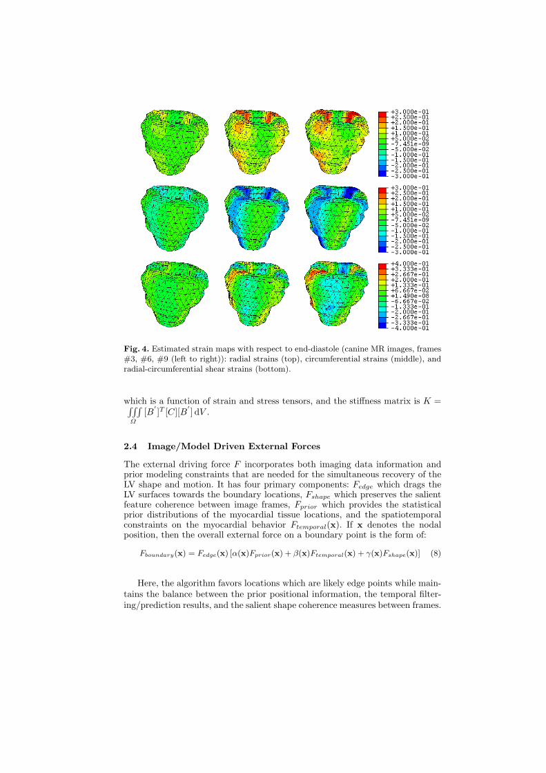
Fig. 4. Estimated strain maps with respect to end-diastole (canine MR images, frames#3, #6, #9 (left to right)): radial strains (top), circumferential strains (middle), andradial-circumferential shear strains (bottom).

which is a function of strain and stress tensors, and the stiffness matrix is K =∫∫∫Ω

[B′]T [C][B

′] dV .

2.4 Image/Model Driven External Forces

The external driving force F incorporates both imaging data information andprior modeling constraints that are needed for the simultaneous recovery of theLV shape and motion. It has four primary components: Fedge which drags theLV surfaces towards the boundary locations, Fshape which preserves the salientfeature coherence between image frames, Fprior which provides the statisticalprior distributions of the myocardial tissue locations, and the spatiotemporalconstraints on the myocardial behavior Ftemporal(x). If x denotes the nodalposition, then the overall external force on a boundary point is the form of:

Fboundary(x) = Fedge(x) [α(x)Fprior(x) + β(x)Ftemporal(x) + γ(x)Fshape(x)] (8)

Here, the algorithm favors locations which are likely edge points while main-tains the balance between the prior positional information, the temporal filter-ing/prediction results, and the salient shape coherence measures between frames.

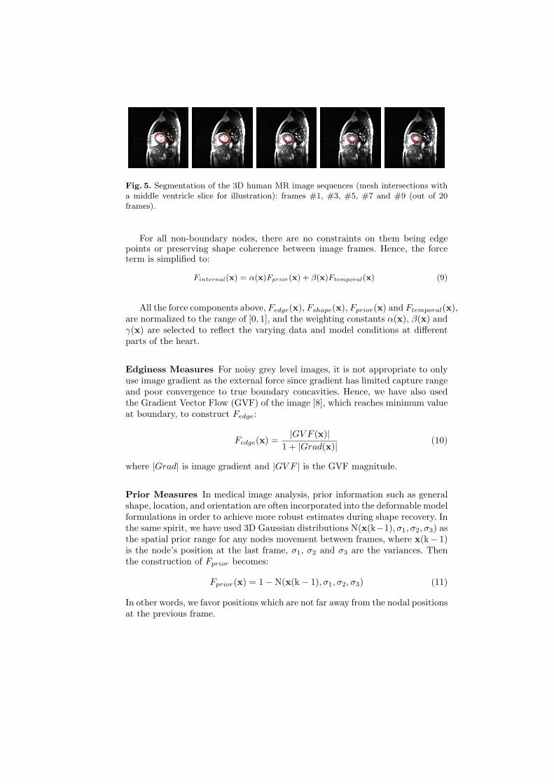
Fig. 5. Segmentation of the 3D human MR image sequences (mesh intersections witha middle ventricle slice for illustration): frames #1, #3, #5, #7 and #9 (out of 20frames).

For all non-boundary nodes, there are no constraints on them being edgepoints or preserving shape coherence between image frames. Hence, the forceterm is simplified to:

Finternal(x) = α(x)Fprior(x) + β(x)Ftemporal(x) (9)

All the force components above, Fedge(x), Fshape(x), Fprior(x) and Ftemporal(x),are normalized to the range of [0, 1], and the weighting constants α(x), β(x) andγ(x) are selected to reflect the varying data and model conditions at differentparts of the heart.

Edginess Measures For noisy grey level images, it is not appropriate to onlyuse image gradient as the external force since gradient has limited capture rangeand poor convergence to true boundary concavities. Hence, we have also usedthe Gradient Vector Flow (GVF) of the image [8], which reaches minimum valueat boundary, to construct Fedge:

Fedge(x) =|GV F (x)|

1 + |Grad(x)| (10)

where |Grad| is image gradient and |GV F | is the GVF magnitude.

Prior Measures In medical image analysis, prior information such as generalshape, location, and orientation are often incorporated into the deformable modelformulations in order to achieve more robust estimates during shape recovery. Inthe same spirit, we have used 3D Gaussian distributions N(x(k−1), σ1, σ2, σ3) asthe spatial prior range for any nodes movement between frames, where x(k− 1)is the node’s position at the last frame, σ1, σ2 and σ3 are the variances. Thenthe construction of Fprior becomes:

Fprior(x) = 1−N(x(k− 1), σ1, σ2, σ3) (11)

In other words, we favor positions which are not far away from the nodal positionsat the previous frame.

Shape Coherence Measures It has been shown in earlier works that shapecoherence is a valid criterion in motion recovery of the left ventricular bound-ary [6]. Thus, we enforce geometrical consistency to establish point correspon-dence between image frames. Under iso-intensity assumption, we can computethe Gaussian curvature of 3D point directly from image (one frame in the 4Dimage) [4]:

κx =1(

f2x + f2

y + f2z

)32det

fxx fxy fxz

fxy fyy fyz

fxz fyz fzz

(12)

where fx, fy, and fz are the first derivatives of the 3D image intensity, and fxx,fxy, fxz, fyy, fyz, and fzz are the second derivatives. Since the construction ofFshape is based on shape coherence, the resulting point should has close curvatureto the corresponding point at last frame:

Fshape = |κ(x+δx)(k+1) − κx(k)| (13)

where (x + δx) indicates local search window.

Temporal Measures Temporal constraints can be put into the model sincethe heart motion is periodic. A standard Kalman predictor is used to estimatethe state vector at frame k+1 through: z(k+1|k) = Cz(k|k), where z = [x,x, x]is the state vector (position, displacement and velocity), z(k+1|k)and z(k|k) arethe estimated state vectors for frame k + 1 and k respectively, the constructionof C is based on the trajectory functions followed by each node, and x should beupdated during each estimation. In our experiments, the velocity informationadopts the motion fields from the MR phase contrast velocity images or thespatio-temporal intensity flow between images. The phase velocity data shouldbe regularized first to get rid of the noises.

The estimated possible node position x is used to construct a rotated 3DGaussian distribution N(x, σi, σj , σk, θ(x), φ(x)), where σi, σj and σk are thevariances in the rotated major directions, and θ, φ are the angles of the lineformed by x(k − 1)and x(k) with respect to the cartesian coordinate. Then wecan get the temporal force as follow:

Ftemporal(x) = 1−N(x, σi, σj , σk, θ(x), φ(x)) (14)

3 Experiments and Conclusions

We have implemented the algorithm and performed initial experiments on nor-mal canine and human cardiac MRI data sets. For both human and canine cases,myocardium is modeled as an isotropic linear elastic material with Young’s mod-ulus 75,000 Pascal and Poisson ratio 0.47 [9]. The left ventricle is represented bylinear finite element mesh constructed from the Delaunay triangulation of thesampled points, Fig. 1 shows the final model constructed from the normal caninedata.

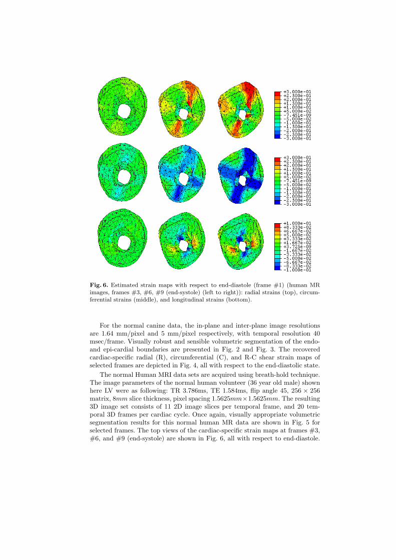
Fig. 6. Estimated strain maps with respect to end-diastole (frame #1) (human MRimages, frames #3, #6, #9 (end-systole) (left to right)): radial strains (top), circum-ferential strains (middle), and longitudinal strains (bottom).

For the normal canine data, the in-plane and inter-plane image resolutionsare 1.64 mm/pixel and 5 mm/pixel respectively, with temporal resolution 40msec/frame. Visually robust and sensible volumetric segmentation of the endo-and epi-cardial boundaries are presented in Fig. 2 and Fig. 3. The recoveredcardiac-specific radial (R), circumferential (C), and R-C shear strain maps ofselected frames are depicted in Fig. 4, all with respect to the end-diastolic state.

The normal Human MRI data sets are acquired using breath-hold technique.The image parameters of the normal human volunteer (36 year old male) shownhere LV were as following: TR 3.786ms, TE 1.584ms, flip angle 45, 256 × 256matrix, 8mm slice thickness, pixel spacing 1.5625mm×1.5625mm. The resulting3D image set consists of 11 2D image slices per temporal frame, and 20 tem-poral 3D frames per cardiac cycle. Once again, visually appropriate volumetricsegmentation results for this normal human MR data are shown in Fig. 5 forselected frames. The top views of the cardiac-specific strain maps at frames #3,#6, and #9 (end-systole) are shown in Fig. 6, all with respect to end-diastole.

As expected for normal heart, the magnitudes of the radial, circumferential, andlongitudinal strains increase during the cardiac deformation from ED to ES. Thelongitudinal strains are relatively small compared with other strains. These in-dicate that the myocardium is primarily thickened in the radial direction andshortened in the circumferential direction.

These preliminary results demonstrate that the proposed algorithm can beused to perform 3D segmentation and motion field tracking simultaneously. Withfurther experiments and validations, we expect that 3D active region model willfind a valuable role for myocardial segmentation and motion analysis.

Acknowledgement

This work is supported in part by the National Natural Science Foundation ofChina(60403040), by the Hong Kong Research Grant Council under CompetitiveEarmarked Research Grant HKUST6031/01E for PCS, by the National BasicResearch Program of China (2003CB716104), and by the NSF of China forInnovative Research Groups (60021201).

References

1. A.J. Frangi, W.J. Niessen, and M.A. Viergever. Three-dimensional modeling forfunctional analysis of cardiac images: A review. IEEE Transactions on MedicalImaging, 20(1):2–25, 2001.

2. T. McInerney and D. Terzopolous. Deformable models in medical image analysis:a survey. Medical Image Analysis, 1(2):91–108, 1996.

3. J. Montagnat and H. Delingette. 4d deformable models with temporal constraints:application to 4d cardiac image segmentation. Journal of Medical Image Analysis,9:87–100, 2005.

4. Stanley Osher and James A. Sethian. Fronts propagating with curvature dependentspeed: Algorithms based on hamilton-jacobi formulations. Journal of ComputationalPhysics, 76:12–49, 1988.

5. P. Shi, A. Sinusas, R. T. Constable, and J. Duncan. Volumetric deformation anal-ysis using mechanics-based data fusion: Applications in cardiac motion recovery.International Journal of Computer Vision, 35(1):87–107, 1999.

6. P. Shi, A. Sinusas, R. T. Constable, E. Ritman, and J. Duncan. Point-trackedquantitative analysis of left ventricular motion from 3D image sequences. IEEETransactions on Medical Imaging, 19(1):36–50, 2000.

7. L.N. Wong, H. Liu, A. Sinusas, and P. Shi. Spatio-temporal active region modelfor simultaneous segmentation and motion estimation of the whole heart. In IEEEWorkshop on Variational, Geometric and Level Set Methods in Computer Vision,pages 193–200, 2003.

8. C. Xu and L. Prince. Snakes, shapes, and gradient vector flow. IEEE Transactionson Image Processing, 7(3):359–369, 1998.

9. H. Yamada. Strength of Biological Material. The Williams and Wilkins Company,Baltimore, 1970.