Revised Algorithm for Estimating Light Extinction fromIMPROVE Particle Speciation Data

Marc PitchfordNational Oceanic and Atmospheric Administration, Las Vegas, NV

William Malm and Bret SchichtelNational Park Service, Fort Collins, CO

Naresh KumarElectric Power Research Institute, Palo Alto, CA

Douglas LowenthalDesert Research Institute, Reno, NV

Jenny HandCooperative Institute Research in the Atmosphere, Colorado State University, Fort Collins, CO

ABSTRACTThe Interagency Monitoring of Protected Visual Environ-ments (IMPROVE) particle monitoring network consistsof approximately 160 sites at which fine particulate mat-ter (PM2.5) mass and major species concentrations andcourse particulate matter (PM10) mass concentrations aredetermined by analysis of 24-hr duration sampling con-ducted on a 1-day-in-3 schedule. A simple algorithm toestimate light extinction from the measured species con-centrations was incorporated in the 1999 Regional HazeRule as the basis for the haze metric used to track hazetrends. A revised algorithm was developed that is moreconsistent with the recent atmospheric aerosol literatureand reduces bias for high and low light extinction ex-tremes. The revised algorithm differs from the originalalgorithm in having a term for estimating sea salt lightscattering from Cl� ion data, using 1.8 instead of 1.4 forthe mean ratio of organic mass to measured organic car-bon, using site-specific Rayleigh scattering based on siteelevation and mean temperature, employing a split com-ponent extinction efficiency associated with large and

small size mode sulfate, nitrate and organic mass species,and adding a term for nitrogen dioxide (NO2) absorptionfor sites with NO2 concentration information. Light scat-tering estimates using the original and the revised algo-rithms are compared with nephelometer measurements at21 IMPROVE monitoring sites. The revised algorithm re-duces the underprediction of high haze periods and theoverprediction of low haze periods compared with theperformance of the original algorithm. This is most ap-parent at the hazier monitoring sites in the eastern UnitedStates. For each site, the PM10 composition for days selectedas the best 20% and the worst 20% haze condition days arenearly identical regardless of whether the basis of selectionwas light scattering from the original or revised algorithms,or from nephelometer-measured light scattering.

INTRODUCTIONAtmospheric light extinction is a fundamental metricused to characterize air pollution impacts on visibility. Itis the fractional loss of intensity in a light beam per unitdistance due to scattering and absorption by the gases andparticles in the air. Light extinction (bext) can be expressedas the sum of light scattering by particles (bs,p), scatteringby gases (bs,g), absorption by particles (ba,p) and absorp-tion by gases (ba,g). Traditionally, for visibility-protectionapplications, the most sensitive portion of the spectrumfor human vision (550 nm) has been used to characterizelight extinction and its components.

Light extinction due to the gaseous components ofthe atmosphere are relatively well understood and wellestimated for any atmospheric conditions. Absorption ofvisible light by gases in the atmosphere is primarily bynitrogen dioxide (NO2) and can be directly and accuratelyestimated from NO2 concentrations by multiplying bythe absorption efficiency. Scattering by gases is described

IMPLICATIONSConcerns raised about the use of the original IMPROVE algo-rithm for estimating light extinction from particle compositiondata for calculating the metric for tracking trends for theRegional Haze Rule (RHR) have been addressed in the formu-lation of a revised algorithm. The new algorithm reduces bi-ases at the upper and lower extremes, which are of particularconcern with regards to the RHR, which mandates reducingthe impacts of manmade emissions on the 20% worst hazedays while avoiding degradation of the 20% best haze con-ditions. The revised algorithm is likely to be adopted by moststates for the technical assessments and modeling supportingtheir RHR state implementation plans.

TECHNICAL PAPER ISSN:1047-3289 J. Air & Waste Manage. Assoc. 57:1326–1336DOI:10.3155/1047-3289.57.11.1326Copyright 2007 Air & Waste Management Association

1326 Journal of the Air & Waste Management Association Volume 57 November 2007

by the Rayleigh scattering theory. Rayleigh scattering de-pends on the density of the atmosphere, with the highestvalues at sea level (about 12 Mm�1) and diminishing withelevation (8 Mm�1 at about 4 km), and varies somewhat atany elevation because of atmospheric temperature and pres-sure variations. Rayleigh scattering can be accurately deter-mined for any elevation and meteorological conditions.

Particle light extinction is more complex than thatcaused by gaseous components. Light-absorbing carbon(e.g., diesel exhaust, soot, and smoke) and some crustalminerals are the only commonly occurring airborne par-ticle components that absorb light. All particles scatterlight, and generally particle light scattering is the largestof the four light extinction components. The amount oflight scattered by an ensemble of particles can be quiteaccurately estimated using Mie theory when its size dis-tribution and index of refraction are known.1 Mie theorydescribes how electromagnetic energy (light as a functionof wavelength) interacts with a particle as it passesthrough and around the particle. The scattering and ab-sorption of the ensemble of particles is then calculated bysumming over all particles with their various known op-tical and physical properties.2 However, it is rare that theintrinsic optical and physical properties of each particleare known, so simplified calculation schemes are typicallyused to make extinction estimates.

The Interagency Monitoring of Protected Visual Envi-ronments (IMPROVE) particle monitoring provides 24-hrduration mass concentrations for coarse (PM10) and fine(PM2.5) particulate matter (PM), as well as most of thePM2.5 component concentrations on a 1-day-in-3 sched-ule. These data are routinely available at each of theapproximately 160 IMPROVE monitoring sites for use inestimating light extinction. At 21 IMPROVE monitoringsites (Table 1), hourly averaged nephelometer and relativehumidity (RH) data are also routinely available. Data from

these sites have been key to evaluating the performance ofthe original IMPROVE algorithm, as well as for develop-ment and performance evaluation of various alternativerevised algorithms.

The IMPROVE algorithm for estimating light extinc-tion was adopted by the U.S. Environmental ProtectionAgency (EPA) as the basis for the regional haze metricused to track progress in reducing haze levels for visibility-protected areas under the 1999 Regional Haze Rule(RHR).3 As a result, the IMPROVE algorithm has beencarefully scrutinized to assess deficiencies that could biasthe implementation of the RHR.

The RHR uses the IMPROVE algorithm to estimatelight extinction, which is then converted to the deciviewhaze index (i.e., a logarithmic transformation of bext). TheRHR then calls for the determination of the mean of theannual 20% best and 20% worst haze days for each of theIMPROVE monitoring sites that represent the visibility-protected areas. States are asked to manage emissions sothat over a 60-yr period the worst haze days will improveto natural conditions without degrading visibility condi-tions for the best haze days. For consistency, the sameapproach (i.e., IMPROVE algorithm and conversion to thedeciview haze index) is also used to estimate natural hazelevels for each representative monitoring site using esti-mates of the natural concentration levels for the majorparticle components. For each location, the linear rate ofreduction of the deciview values for the worst haze daysduring the baseline period (2000–2004) that is needed toreach the estimated worst haze days under natural condi-tions by 2064 must be determined. This linear rate is usedas a guide to pace the desired rate of haze reduction and todetermine interim visibility goals that are compared tothe monitoring data trends of the best and worst hazedays.

The RHR emphasizes the extremes of light extinctionthrough its requirement to estimate best and worst hazedays for the baseline period and for estimates of naturalworst haze conditions. Also, the use of the deciview indexmeans that additive biases in the light extinction esti-mates (e.g., the use of a standard Rayleigh scattering termfor all sites regardless of elevation) will affect the calcula-tion of a linear glide slope, which is a guide used to set thepace of emission reductions. Use of the IMPROVE algo-rithm for the RHR elicited concerns about possible biasesin the apportionment among the various major particlecomponents. Such issues have been the subject of a num-ber of critical reviews of the use of the IMPROVE algo-rithm in the RHR.4,5

In light of the concerns raised by its use in the RHR,the IMPROVE Steering Committee initiated an internalreview, including recommendations for revisions of theIMPROVE algorithm for estimating light extinction. Thefull report of this review is available elsewhere.6 Subse-quently, the IMPROVE Steering Committee established asubcommittee to develop a revised algorithm that reducesbiases in light extinction estimates and is as consistent aspossible with the current scientific literature, while con-strained by the need to use only those data that areroutinely available from the IMPROVE particle monitor-ing network. The resulting algorithm was accepted for useby the IMPROVE Steering Committee and is being used by

Table 1. IMPROVE monitoring sites with nephelometers used to evaluatealgorithm performance.

Abbreviation Name State Region

ACAD Acadia National Park Maine EastBIBE Big Bend National Park Texas WestBOWA Boundary Waters Canoe Area Minnesota EastCORI Columbia River Gorge Washington WestDOSO Dolly Sods/Otter Creek Wilderness West Virginia EastGICI Gila Wilderness New Mexico WestGRCA Grand Canyon National Park Arizona WestGRGU Great Gulf Wilderness New Hampshire EastGRSM Great Smoky Mountains Tennessee EastJARB Jarbidge Wilderness Nevada WestLOPE Lone Peak Wilderness Utah WestLYBR Lye Brook Wilderness Vermont EastMACA Mammoth Cave National Park Kentucky EastMORA Mount Rainier National Park Washington WestMOZI Mount Zirkel Wilderness Colorado WestOKEF Okefenokee National Wildlife Refuge Georgia EastSHEN Shenandoah National Park Virginia EastSHRO Shining Rock Wilderness North Carolina EastSNAP Snoqualamie Pass Wilderness Washington WestTHIS Three Sisters Wilderness Oregon WestUPBU Upper Buffalo Wilderness Arkansas East

Pitchford et al.

Volume 57 November 2007 Journal of the Air & Waste Management Association 1327

most states in their implementation of the RHR. Theprimary purpose of this paper is to describe the revisedalgorithm, summarize the rationale for each of thechanges from the original algorithm, and characterize theperformance of the original and revised algorithms.

Original IMPROVE AlgorithmThe original IMPROVE algorithm for estimating light ex-tinction from IMPROVE particle monitoring data assumesthat absorption by gases (ba,g) is zero, that Rayleigh scat-tering (bs,g) is 10 Mm�1 for each monitoring site regard-less of site elevation and meteorological condition, andthat particle scattering and absorption (bs,p and ba,p) canbe estimated by multiplying the concentrations of each ofsix major components by typical component-specificmass extinction efficiencies. The six major componentsare sulfate (assumed to be ammonium sulfate), nitrate(assumed to be ammonium nitrate), organic compounds(based on measured organic carbon [OC] mass), elementalor black carbon (directly measured), fine soil (crustal ele-ments plus oxides) and coarse mass (the difference be-tween PM10 and PM2.5 mass concentrations). The compo-nent dry mass extinction efficiency values are expressedas single significant digit constants, reflecting the level ofuncertainty of these values. The sulfate and nitrate massextinction efficiency terms include a water growth factorthat is a function of RH (displayed as f(RH)) multiplied bya constant dry extinction efficiency. Monthly averagedwater growth terms for each site were developed becausemost monitoring sites do not include on-site RH moni-toring. Expressed as an equation, the original algorithmfor estimating light extinction from IMPROVE data takesthe following form where the particle component con-centrations are indicated in the brackets. The formulas forthe composite components are available elsewhere.7

bext � 3 � f�RH� � �Sulfate� � 3 � f�RH� � �Nitrate�

� 4 � �Organic Mass�

� 10 � �Elemental Carbon�

� 1 � �Fine Soil� � 0.6 � �Coarse Mass�

� 10

(1)

The units for light extinction and Rayleigh scattering areinverse megameters (1/106 m usually written Mm�1);component concentrations shown in brackets are in mi-crogram per meter cubed (�g/m3); dry mass extinctionefficiency terms are in units of meters squared per gram(m2/g); and the water growth terms, f(RH), are unitless.

Among the implicit assumptions for this formulationof the algorithm are that

• Six particle component terms plus a constantRayleigh scattering term are sufficient for a goodestimate of light extinction;

• Constant dry mass extinction efficiency termsrounded to one significant digit for each of thesix particle components (e.g., for both sulfate andnitrate the value is 3) works adequately for alllocations and times; and

• Light extinction contributed by the individualparticle components can be adequately estimatedas separate terms as they would if they were incompletely separate particles (externally mixed),though they often are known to be internallymixed in particles.

A relatively simple algorithm for estimating light ex-tinction using only the available monitoring data requiresassumptions such as these.

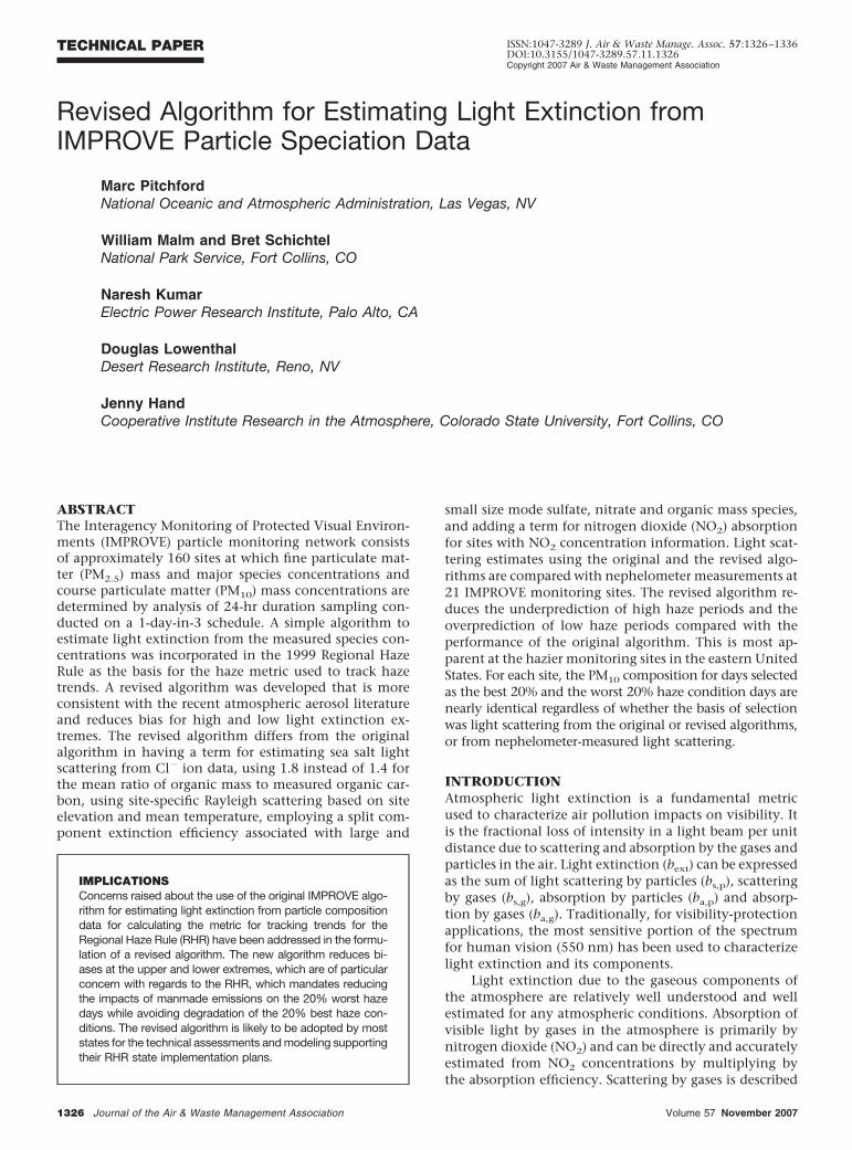
Estimates of particle scattering by this algorithm (i.e.excluding the light absorbing carbon and Rayleigh terms)have been compared with directly measured particle scat-tering data at the 21 monitoring sites that have hourlyaveraged nephelometer and RH data. As shown in Figure1, the algorithm performs reasonably well over a broadrange of particle light scattering values and monitoringlocations. The algorithm tends to underestimate the high-est extinction values and to overestimate the lowest ex-tinction values. Since its first use,7 the original algorithm hasbeen a useful tool that significantly contributed to a betterunderstanding of haze levels and the relative magnitude ofhaze contribution by the various particle components.

Revised IMPROVE AlgorithmA revised algorithm was developed to address issues raisedconcerning the original algorithm. The revised algorithmmeets many of the overall design criteria of the original,

0

50

100

150

200

250

300

350

0 50 100 150 200 250 300 350

Measured Bsp (Mm-1)

IMP

RO

VE

Bsp

(Mm

-1) R2 = 0.88

Bias = 0.26

Figure 1. A scatter plot of the original IMPROVE algorithm estimated particle light scattering vs. measured particle light scattering.

Pitchford et al.

1328 Journal of the Air & Waste Management Association Volume 57 November 2007

including that it is a relatively simple algorithm thatproduces consistent estimates of light extinction for allremote-area IMPROVE aerosol monitoring sites and per-mits the individual particle component contributions tolight extinction to be separately estimated. Five majorrevisions were made to the original IMPROVE algorithmfor estimating light extinction from IMPROVE particlespeciation data. They include

• Addition of a sea salt term, which is a particularconcern for coastal monitoring locations inwhich the sum of the major components of lightextinction and mass has been deficient;

• Change of the assumed organic compound massto OC mass ratio from 1.4 to 1.8 to reflect morerecent peer-reviewed literature on the subject;

• Use of site-specific Rayleigh scattering based onthe elevation and annual average temperature ofthe monitoring sites;

• Development and use of a split component ex-tinction efficiency model for sulfate, nitrate, andOC components, including new water growthterms for sulfate and nitrate to better estimatelight extinction at the high and low extremes ofthe range; and

• Addition of a NO2 light absorption term thatwould only be used at sites with available NO2

concentration data.The technical rationale for making each of these

changes is described in separate sections below.

Sea SaltThe original IMPROVE protocol for estimating light ex-tinction does not include light scattering (bsp) by sea saltaerosols. Lowenthal and Kumar4 demonstrated that inclu-sion of elements from sea salt (e.g., sodium [Na], chlorine[Cl]) increased the accuracy of mass reconstruction atcoastal IMPROVE sites. Contributions of sea salt particlesto light extinction at some coastal IMPROVE sites may besignificant, especially because bsp by sea salt particlesshould be significantly enhanced by hygroscopic growthin humid environments. Lowenthal and Kumar8 foundthat fine sea salt aerosols accounted for 43% of estimatedbsp at the U.S. Virgin Islands IMPROVE site. Coastal areasea salt is a natural source of haze that will increase inrelative importance as anthropogenic contributions arereduced.

To include sea salt in the IMPROVE light extinctionequation, it is necessary to: (1) estimate the sea salt massconcentration; (2) specify a dry sea salt mass scatteringefficiency; and (3) specify an f(RH) curve for sea salt rep-resenting the enhancement of sea salt scattering by hy-groscopic growth as a function of RH.

Sea Salt Mass Concentration. Estimating sea salt mass re-quires a sea salt marker species measured in IMPROVEaerosol samples. The most obvious markers are Na and Cl,because NaCl is the main component in seawater and seasalt. Based on the composition of sea water, pure sea saltmass is Na multiplied by 3.1 or Cl multiplied by 1.8.9However, Na is poorly quantified by the X-ray fluores-cence (XRF) used by IMPROVE and Cl can be depleted inambient aerosol samples by acid-base reactions between

sea salt particles and sulfuric and nitric acids.10 Withoutaccurate measurement of both Na (or other conservativetracers) and Cl, it is not possible to estimate how much Clhas been replaced by nitrate and/or sulfate in ambientsamples. Further, without chemical speciation of thePM10 sample (Module D of the IMPROVE sampler), it isnot possible to estimate coarse sea salt scattering.

Given these limitations, the revised algorithm esti-mates the PM2.5 sea salt concentration as the concentra-tion of chloride ion (Cl�) measured by ion chromatogra-phy multiplied by 1.8. If the chloride measurement isbelow the detection limit, missing, or invalid, then thePM2.5 sea salt concentration should be estimated as theconcentration of Cl measured by XRF multiplied by 1.8.

Although the XRF measurement can detect Cl atlower concentrations, the A-module sample for XRF ismore exposed to reactive losses because acidic gases arenot removed from the airstream and any HCl they releasefrom the sample is not retained by the Teflon filter. Unlessspeciated data become available for PM10, coarse sea saltmass and light scattering will not be considered. To thedegree that Cl� has been replaced by sulfate or nitrate inambient particles, this approach will underestimate themass and scattering contributed by the substituted sea saltthat results (e.g. NaNO3, NaHSO4, or Na2SO4). This massis partially accounted for by ammonium sulfate and am-monium nitrate in the IMPROVE equation. However, thesubstituted Na salt mass is underestimated because am-monium is lighter than sodium. The scattering is alsounderestimated because the sodium salts absorb morewater than does ammonium sulfate above 60% RH. Onthe other hand, the 1.8 factor accounts for sea salt con-stituents such as calcium (Ca) and magnesium (Mg),which are included in the fine soil aerosol compositecomponent, resulting in a small double counting of mass.Given the limitations of the available data, 1.8 times Cl�

provides a reasonable and likely lower-limit to the fine seasalt mass.

Sea Salt Dry Mass Scattering Efficiency. To estimate the drymass scattering efficiency and f(RH) for sea salt aerosols,their dry mass size distribution must be known. Althoughthis has not been measured at most IMPROVE sites, ex-tensive sea salt size distribution measurements have beenmade in the remote marine environment during cruise-based experiments.11–13 On the basis of these studies, adry log-normal mass size distribution with a geometricmean diameter (Dg) of 2.5 �m and geometric standarddeviation (�g) of 2 is recommended. A dry scattering effi-ciency for PM2.5 sea salt of 1.7 m2/g was calculated usingthe Mie theory on the basis of this size distribution as-suming a sea salt refractive index of [1.55� i0] and adensity of 1.9 g � cm�3 recommended by Quinn et al.11

Sea Salt f(RH). Tang et al.14 determined hygroscopicgrowth curves for aerosols generated from Long Island,NY, and Atlantic Ocean seawater. The water absorptioncurves for sea salt were nearly identical to that of NaCl.The NaCl growth factors derived from the AIM3 thermo-dynamic equilibrium model15 are shown in Table 2 as afunction of RH. Below the crystallization point (RH 47%), the growth factor is set to 1. Values are presented to

Pitchford et al.

Volume 57 November 2007 Journal of the Air & Waste Management Association 1329

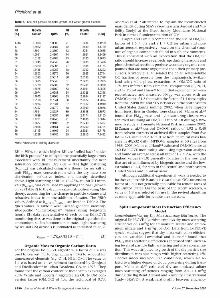
RH 95%, to which higher RH are “rolled back” underthe RHR protocol3 to mitigate the potentially large errorsassociated with RH measurement uncertainty for nearsaturation conditions. Dry (RH 0%) light scattering(bsp(Dry)) was calculated using Mie theory for sea salt atunit PM2.5 mass concentration with the dry mass sizedistribution, refractive index, and density describedabove. Light scattering at RH 46–95% at unit RH inter-vals (bsp(RH)) was calculated by applying the NaCl growthcurve (Table 2) to the dry mass size distribution using Mietheory, accounting for the change in particle volume andrefractive index from the addition of water. The f(RH)values, defined as bsp(RH)/bsp(Dry), are listed in Table 2. Thef(RH) values in Table 2 were used to generate monthly,site-specific “climatological” values using long-termhourly RH data representative of each of the IMPROVEmonitoring sites, as was done in the original algorithm forammonium sulfate/ammonium nitrate. Light scatteringby sea salt (SS) aerosols is estimated as indicated in eq 2.

bsp(SS) � 1.7fSS(RH)�1.8 � Cl � � (2)

Organic Mass to Organic Carbon RatioFor the original IMPROVE algorithm, a factor of 1.4 wasused to convert OC to organic mass (OM) to account forunmeasured elements (e.g. O, H, N) in OM. The value of1.4 was based on an experiment conducted by Grosjeanand Friedlander16 in urban Pasadena, CA, in 1973. Theyfound that the carbon content of these samples averaged73%. White and Roberts17 suggested an OC to OM con-version factor (OM/OC) of 1.4, the reciprocal of 0.73.

Andrews et al.18 attempted to explain the reconstructedmass deficit during SEAVS (Southeastern Aerosol and Vis-ibility Study) at the Great Smoky Mountains NationalPark in terms of underestimation of OM.

Turpin and Lim19 recommended the use of OM/OCfactors of 1.6 0.2 and 2.1 0.2 for urban and non-urban aerosol, respectively, based on the chemical struc-ture of organic compounds found in such environments.This is consistent with an expectation that the OM/OCratio should increase as aerosols age during transport andphotochemical reactions produce secondary organic com-pounds that are more oxygenated than their primary pre-cursors. Krivacsy et al.20 isolated the polar, water-solubleOC fraction of aerosols from the Jungfraujoch, Switzer-land using solid phase extraction. An OM/OC ratio of1.91 was inferred from elemental composition (C, N, H,and S). Poirot and Husar21 found that agreement betweenreconstructed and measured PM2.5 was closer with anOM/OC ratio of 1.8 than with the factor of 1.4 for samplesfrom the IMPROVE and STN networks in the northeasternUnited States during summer 2002, when large impactsfrom forest fires in Quebec were observed. Malm et al.22

found that PM2.5 mass and light scattering closure wasachieved assuming an OM/OC ratio of 1.8 during a two-month study at Yosemite National Park in summer 2002.El-Zanan et al.23 derived OM/OC ratios of 1.92 0.40from solvent extracts of archived filter samples from fiveIMPROVE sites and 2.07 0.32 from chemical mass bal-ance in 40,532 daily IMPROVE samples at 50 sites from1988–2003. Malm and Hand24 estimated OM/OC ratios at160 IMPROVE monitoring sites using regression analysisand found an average across all sites of 1.7 2.4, with thehighest values (�1.9) generally for sites in the west andthat are often influenced by biogenic smoke and the low-est values (�1.4) for sites in the central and northeasternUnited States and in urban areas.

Although additional experimental work is needed tofurther explore this issue, it is clear that an OC conversionfactor of 1.4 is not generally applicable for remote areas ofthe United States. On the basis of the recent research, avalue of 1.8 was selected for use in the revised algorithmas more applicable for remote area datasets.

Split Component Mass Extinction EfficiencyModel

Concentration-Varying Dry Mass Scattering Efficiencies. Theoriginal IMPROVE algorithm employs dry mass scatteringefficiencies of 3 m2/g for ammonium sulfate and ammo-nium nitrate and 4 m2/g for OM. Data from IMPROVEspecial studies suggest that dry mass extinction efficien-cies are variable. Lowenthal and Kumar25 found thatPM2.5 mass scattering efficiencies increased with increas-ing levels of particle light scattering and mass concentra-tion. This was attributed to growth of the dry particle sizedistribution into size ranges with higher scattering effi-ciencies under more-polluted conditions, which are re-lated to a higher degree of cloud processing during trans-port. Malm et al.26 estimated dry ammoniated sulfatemass scattering efficiencies ranging from 2.4–4.1 m2/gduring the Big Bend Aerosol and Visibility ObservationalStudy (BRAVO). A weak relationship between efficiency

Table 2. Sea salt particle diameter growth and water growth function.

RH(%)

GrowthFactora f (RH )

RH(%)

GrowthFactor f (RH )

1–46 1.0000 1.0000 71 1.8434 3.126947 1.5922 2.3584 72 1.8589 3.172948 1.6001 2.3799 73 1.8751 3.205549 1.6081 2.4204 74 1.8921 3.245950 1.6162 2.4488 75 1.9100 3.267351 1.6245 2.4848 76 1.9288 3.347852 1.6329 2.5006 77 1.9488 3.417453 1.6415 2.5052 78 1.9700 3.520254 1.6503 2.5279 79 1.9925 3.574455 1.6593 2.5614 80 2.0166 3.632956 1.6685 2.5848 81 2.0423 3.690557 1.6779 2.5888 82 2.0701 3.808058 1.6875 2.6160 83 2.1001 3.950559 1.6974 2.6581 84 2.1328 4.039860 1.7075 2.6866 85 2.1684 4.112761 1.7179 2.7341 86 2.2077 4.282462 1.7286 2.7834 87 2.2512 4.494063 1.7397 2.8272 88 2.2999 4.607864 1.7511 2.8287 89 2.3548 4.857365 1.7629 2.8594 90 2.4174 5.116566 1.7751 2.8943 91 2.4898 5.384467 1.7877 2.9105 92 2.5749 5.745768 1.8008 2.9451 93 2.6769 6.170469 1.8145 3.0105 94 2.8021 6.717870 1.8286 3.0485 95 2.9610 7.3492

Notes: aDiameter at RH/dry diameter.

Pitchford et al.

1330 Journal of the Air & Waste Management Association Volume 57 November 2007

and ammoniated sulfate mass concentration was re-ported. Malm and Hand24 using regression analysis foundthat organic and inorganic fine mass dry mass scatteringefficiencies have a functional dependence on mass con-centration at most of the 21 sites with collocated IM-PROVE aerosol and nephelometer measurements.

The revised IMPROVE algorithm accounts for the in-crease of ammonium sulfate/ammonium nitrate and OMefficiencies with concentration using a simple mixingmodel in which the concentrations of ammonium sulfate,ammonium nitrate, and OM are each comprised of exter-nal mixtures of mass in small and large particle sizemodes. The large mode represents aged and/or cloud pro-cessed particles, whereas the small mode representsfreshly formed particles. These size modes are describedby log-normal mass size distributions with Dg and geo-metric standard deviations (�g) of 0.2 �m and 2.2 forsmall mode and 0.5 �m and 1.5 for the large mode,respectively. The dry mass PM2.5 scattering efficiencies forsmall- and large-mode ammonium sulfate (2.2 and 4.8m2/g), ammonium nitrate (2.4 and 5.1 m2/g), and OM(2.8 and 6.1 m2/g) were calculated using the Mie theory ata wavelength of 550 nm based on the log-normal masssize distribution parameters described above. The ammo-nium sulfate, ammonium nitrate, and OM densities andrefractive indexes used in this calculation are 1.77, 1.73,and 1.4 g/cm3, respectively, and 1.53 � i0, 1.55 � i0, and1.55 � i0, respectively. No attempt was made to accountfor possible difference in composition between the twosize modes of these particles.

Use of the split component approach requires amethod to estimate the apportionment of the total fineparticle concentration of each of the three measured spe-cies into the concentrations of the small and large sizefractions. The selected method was empirically developedand evaluated using the light scattering and compositiondata for the 21 monitoring sites with nephelometer data(Table 1). The fraction of the fine particle component

(sulfate, nitrate, or organic mass) that is in the large modeis estimated by dividing the total concentration of thecomponent by 20 �g/m3 (e.g., if the total fine particulateOC concentration is 4 �g/m3, the large mode concentra-tion is calculated to be one-fifth of 4 �g/m3 or 0.8 �g/m3,leaving 3.2 �g/m3 in the small mode). If the total concen-tration of a component exceeds 20 �g/m3, all of it isassumed to be in the large mode. Alternate values weretested for the 20-�g/m3 value used in this empirical ap-proach, including use of species-specific values designedto improve the performance in estimating light scatter-ing. The modest performance improvements associatedwith the best of these alternate values was not consideredsufficient justification for trying to further tune thesevalues to fit the available light scattering dataset.

f(RH). The original IMPROVE algorithm applies a singlef(RH) curve to ammonium sulfate and ammonium nitratescattering, which is based on a hygroscopic growth curve[D(RH)/D(Dry), the particle diameter at ambient RH dividedby the dry particle diameter] for pure ammonium sulfatethat was smoothed between the deliquescence and efflo-rescence branches.3 The revised IMPROVE algorithm con-tains f(RH) curves for small- and large-mode ammoniumsulfate that are also applied to small and large modeammonium nitrate. The f(RH) for OM is assumed to be 1at all RH for small and large OM modes. This assumptionis based principally on a lack of evidence for water growthby ambient particulate OM. Additional experimentalwork is needed to further explore this issue. The f(RH) forammonium sulfate and ammonium nitrate are based onthe hygroscopic growth curve for pure ammonium sulfatederived from the AIM thermodynamic equilibrium model.15

This growth curve represents the upper branch, also re-ferred to as the efflorescence or hysteresis branch, of theammonium sulfate growth curve. The upper branch is

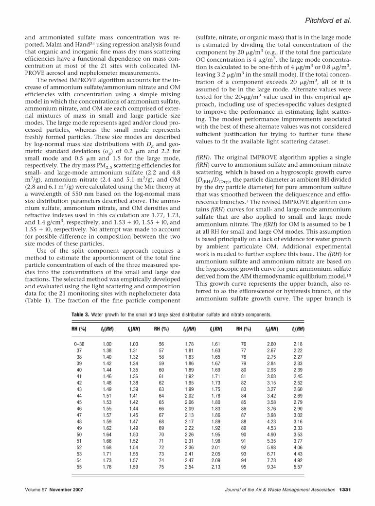
Table 3. Water growth for the small and large sized distribution sulfate and nitrate components.

RH (%) fS(RH ) fL(RH ) RH (%) fS(RH ) fL(RH ) RH (%) fS(RH ) fL(RH )

0–36 1.00 1.00 56 1.78 1.61 76 2.60 2.1837 1.38 1.31 57 1.81 1.63 77 2.67 2.2238 1.40 1.32 58 1.83 1.65 78 2.75 2.2739 1.42 1.34 59 1.86 1.67 79 2.84 2.3340 1.44 1.35 60 1.89 1.69 80 2.93 2.3941 1.46 1.36 61 1.92 1.71 81 3.03 2.4542 1.48 1.38 62 1.95 1.73 82 3.15 2.5243 1.49 1.39 63 1.99 1.75 83 3.27 2.6044 1.51 1.41 64 2.02 1.78 84 3.42 2.6945 1.53 1.42 65 2.06 1.80 85 3.58 2.7946 1.55 1.44 66 2.09 1.83 86 3.76 2.9047 1.57 1.45 67 2.13 1.86 87 3.98 3.0248 1.59 1.47 68 2.17 1.89 88 4.23 3.1649 1.62 1.49 69 2.22 1.92 89 4.53 3.3350 1.64 1.50 70 2.26 1.95 90 4.90 3.5351 1.66 1.52 71 2.31 1.98 91 5.35 3.7752 1.68 1.54 72 2.36 2.01 92 5.93 4.0653 1.71 1.55 73 2.41 2.05 93 6.71 4.4354 1.73 1.57 74 2.47 2.09 94 7.78 4.9255 1.76 1.59 75 2.54 2.13 95 9.34 5.57

Pitchford et al.

Volume 57 November 2007 Journal of the Air & Waste Management Association 1331

used because deliquescence is rarely observed in the en-vironment. Because pure ammonium sulfate crystallizesat 37% RH, it is assumed that there is no hygroscopicgrowth and that the f(RH) is one below this RH.

Dry (RH 0%) light scattering (bsp(Dry)) was calcu-lated using Mie theory for small- and large-mode ammo-nium sulfate. Light scattering at RH 37–95% at unit RHintervals (bsp(RH)) was calculated by applying the AIMammonium sulfate growth curve to the small and largedry mode size distributions using Mie theory, accountingfor the change in particle volume and refractive indexfrom the addition of water. The f(RH), defined as bsp(RH)/bsp(Dry), are listed in Table 3 for the small (f(S)RH) and large(f(L)RH) modes. Values are presented to RH 95%, towhich higher RH are “rolled back” under the RHR proto-col.3 The same f(RH) are applied to small- and large-modeammonium sulfate and ammonium nitrate.

Site-Specific Rayleigh ScatteringRayleigh scattering refers to the scattering of light fromthe molecules of the air, and a constant value of 10 Mm�1

is used in the original IMPROVE algorithm. However,Rayleigh scattering depends on the density of the air andthus varies with temperature and pressure. Site-specificRayleigh scattering was estimated using a Rayleigh Scat-tering Calculator developed by Air Resource Specialists,Inc. that calculates Rayleigh scattering as a function oftemperature and pressure. For each IMPROVE site, weused the standard U.S. atmospheric pressure correspond-ing to the monitoring site elevation, and an estimatedannual mean temperature. The temperature data wereobtained from the nearest weather stations for time peri-ods encompassing 10–30 yr and were interpolated to the-monitoring site location. Site-specific Rayleigh scatteringcalculated using this procedure is available for each IM-PROVE monitoring site on the IMPROVE and VIEWS Websites.27 These are integer-rounded, site-specific values thatrange from 8 Mm�1 for sites at about 4 km elevation to 12Mm�1 for sites near sea level.

NO2 AbsorptionAn NO2 absorption efficiency term (PAENO2) was calcu-lated by dividing the sum of the products of the relativeobserver photopic response values, PR( ), for viewing an

image of 2° angular size and the spectral NO2 absorptionefficiency values, AE( ), by the sum of the photopic re-sponse values over the wavelength range of 350–755 nm,as shown in eq 3.

PAENO2 �

�350

750

PR� � � AE� �

�350

750

PR� � (3)

The spectral NO2 absorption efficiency values are fromDixon28 and available in the PLUVUE Users Manual,29

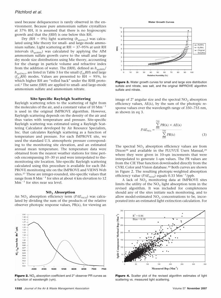
where they were given in 10-�m increments that wereinterpolated to generate 1-�m values. The PR values arefrom the CIE Ybar function downloaded directly from theCVRL Color and Vision database.30 Both curves are shownin Figure 2. The resulting photopic-weighted absorptionefficiency value (PAENO2) equals 0.33 Mm�1/ppb.

A lack of NO2 monitoring data at IMPROVE siteslimits the utility of the NO2 light absorption term in therevised algorithm. It was included for completenessshould any of the sites initiate such monitoring, and toallow model-estimated NO2 concentrations to be, incor-porated into an estimated light extinction calculation. For

Figure 2. NO2 absorption coefficient and 2o observer PR curves asa function of wavelength (�m).

Water Growth Curves

0

1

2

3

4

5

6

7

8

9

10

0 10 20 30 40 50 60 70 80 90 100

Relative Humidity (%)

f(R

H)

fS(RH)

fL(RH)

Original

fSS(RH)

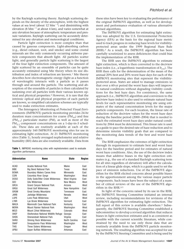
Figure 3. Water growth curves for small and large size distributionsulfate and nitrate, sea salt, and the original IMPROVE algorithmsulfate and nitrate.

0

50

100

150

200

250

300

350

0 50 100 150 200 250 300 350

Measured Bsp (Mm-1)

Split

Com

pone

nt M

etho

d B

sp (

Mm

-1)

R2 = 0.86Bias = 0.18

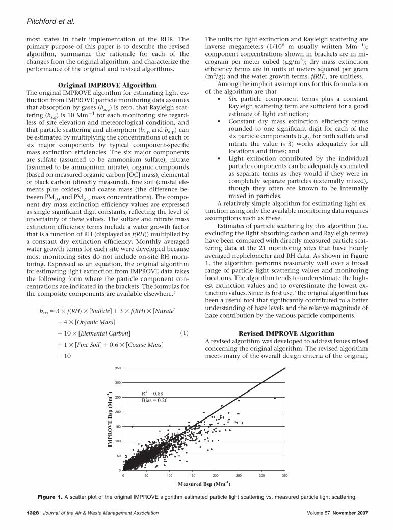
Figure 4. Scatter plot of the revised algorithm estimates of lightscattering vs. measured light scattering.

Pitchford et al.

1332 Journal of the Air & Waste Management Association Volume 57 November 2007

remote areas, the relative NO2 contributions to light ex-tinction are generally considered too small to justify theirassessment. However, the NO2 concentrations in plumesand layers near sources with good particle emission con-trols could make significant contributions to the totallight extinction and produce a noticeable brown appear-ance to the plume or layer.

Revised AlgorithmThe revised algorithm is shown in eq 4, with the new andchanged terms printed in boldface to emphasize the dif-ference from the original IMPROVE algorithm.

bext � 2.2 � fS(RH) � [Small Sulfate]

� 4.8 � fL(RH) � [Large Sulfate]

� 2.4 � fS(RH) � [Small Nitrate]

� 5.1 � fL(RH) � [Large Nitrate]

� 2.8 � [Small Organic Mass]

� 6.1 � [Large Organic Mass]

� 10 � �Elemental Carbon� � 1 � �Fine Soil�

� 1.7 � fSS(RH) � [Sea Salt]

� 0.6 � �Coarse Mass�

� Rayleigh Scattering (Site Specific)

� 0.33 � [NO2 (ppb)]

(4)

Comparing this to the original algorithm (eq 1), noticethat the three split components (i.e. sulfate, nitrate, andorganic mass) have dry mass extinction efficiencies that

are smaller than the original dry mass extinction effi-ciency values for the small particle size modes and largerthan the original values for the large particle size modes.This permits the new algorithm to perform better thanthe original algorithm with its single dry mass extinctionefficiency at the concentration extremes where either thesmall or large particle size modes will dominate, resultingin less or more efficient particle light scattering.

The water growth curves for the large and small par-ticle size modes for sulfate and nitrate, and for sea salt areshown in Figure 3 along with the water growth curve usedin the original algorithm for sulfate and nitrate. The largeand small particle size mode growth curves exceed theoriginal algorithm growth curve for RH less than approx-imately 60% because the original growth curve was esti-mated to be an average of the upper and lower hysteresisbranches of the ammonium sulfate curve, whereas thecurves used for the revised algorithm are solely the upperbranch of the ammonium sulfate curve. At higher RH, thelarge particle size mode f(RH) is below the original curve,whereas the small particle size mode f(RH) is above theoriginal curve.

Algorithm Performance EvaluationPerformance of the original and revised algorithm forestimating extinction can be assessed in a number of wayseach of which serves to answer different questions. Re-duction of the biases in light scattering estimates at theextremes (i.e. underestimation of the high values andoverestimation of the low values) when compared withnephelometer measurements was one of the most com-pelling reasons for development of a new algorithm, socomparisons of bias for the original and revised algorithmare one way to evaluate performance.

Table 4. Average fractional bias by quintiles for the original and revised algorithms for sites east and west of the 100th meridian.

Region

Quintile 1 Quintile 2 Quintile 3 Quintile 4 Quintile 5

Original Revised Original Revised Original Revised Original Revised Original Revised

East 0.63 0.47 0.24 0.14 0.15 0.09 0.06 0.06 �0.11 �0.01West 1.04 0.81 0.35 0.23 0.17 0.07 0.07 0.01 �0.08 �0.10

Scatter Plot for SHEN using IMPROVE Algorithm

1

10

100

1000

1 10 100 1000

Measured Bsp (Mm-1)

Pre

dic

ted

Bsp

(Mm

-1)

Scatter Plot for SHEN using New Algorithm

1

10

100

1000

1 10 100 1000

Measured Bsp (Mm-1)

Pre

dic

ted

Bsp

(M

m-1

)

(a) (b)

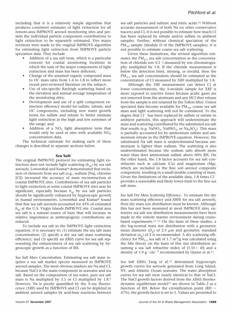
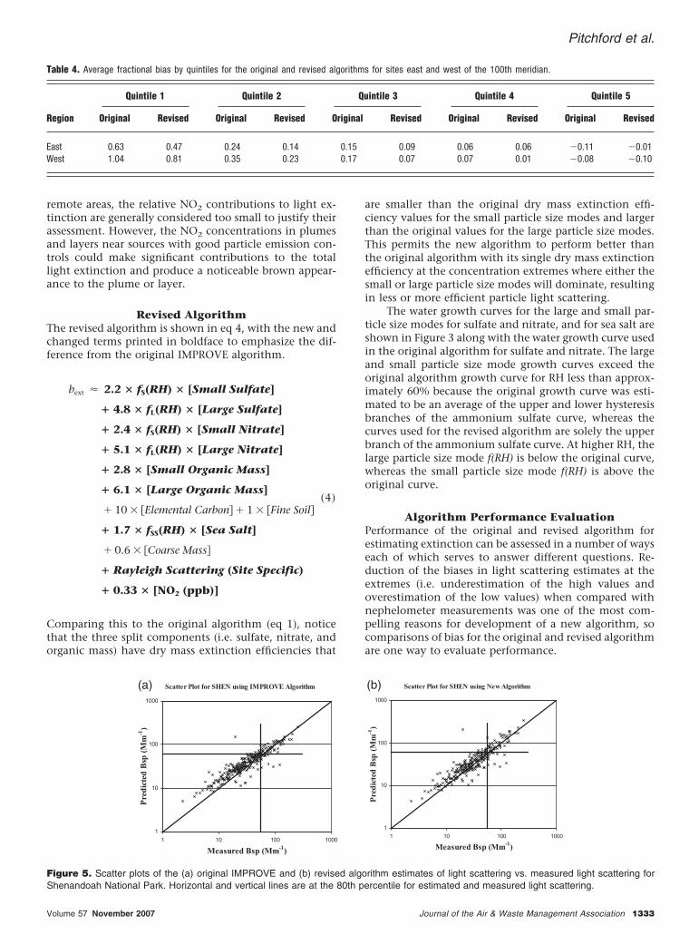
Figure 5. Scatter plots of the (a) original IMPROVE and (b) revised algorithm estimates of light scattering vs. measured light scattering forShenandoah National Park. Horizontal and vertical lines are at the 80th percentile for estimated and measured light scattering.

Pitchford et al.

Volume 57 November 2007 Journal of the Air & Waste Management Association 1333

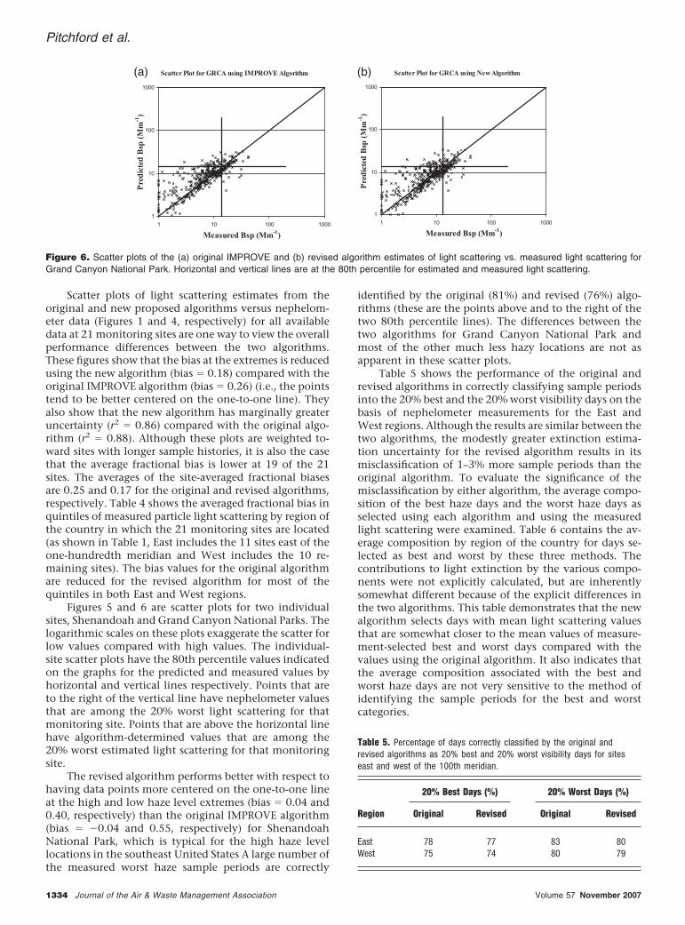
Scatter plots of light scattering estimates from theoriginal and new proposed algorithms versus nephelom-eter data (Figures 1 and 4, respectively) for all availabledata at 21 monitoring sites are one way to view the overallperformance differences between the two algorithms.These figures show that the bias at the extremes is reducedusing the new algorithm (bias 0.18) compared with theoriginal IMPROVE algorithm (bias 0.26) (i.e., the pointstend to be better centered on the one-to-one line). Theyalso show that the new algorithm has marginally greateruncertainty (r2 0.86) compared with the original algo-rithm (r2 0.88). Although these plots are weighted to-ward sites with longer sample histories, it is also the casethat the average fractional bias is lower at 19 of the 21sites. The averages of the site-averaged fractional biasesare 0.25 and 0.17 for the original and revised algorithms,respectively. Table 4 shows the averaged fractional bias inquintiles of measured particle light scattering by region ofthe country in which the 21 monitoring sites are located(as shown in Table 1, East includes the 11 sites east of theone-hundredth meridian and West includes the 10 re-maining sites). The bias values for the original algorithmare reduced for the revised algorithm for most of thequintiles in both East and West regions.

Figures 5 and 6 are scatter plots for two individualsites, Shenandoah and Grand Canyon National Parks. Thelogarithmic scales on these plots exaggerate the scatter forlow values compared with high values. The individual-site scatter plots have the 80th percentile values indicatedon the graphs for the predicted and measured values byhorizontal and vertical lines respectively. Points that areto the right of the vertical line have nephelometer valuesthat are among the 20% worst light scattering for thatmonitoring site. Points that are above the horizontal linehave algorithm-determined values that are among the20% worst estimated light scattering for that monitoringsite.

The revised algorithm performs better with respect tohaving data points more centered on the one-to-one lineat the high and low haze level extremes (bias 0.04 and0.40, respectively) than the original IMPROVE algorithm(bias �0.04 and 0.55, respectively) for ShenandoahNational Park, which is typical for the high haze levellocations in the southeast United States A large number ofthe measured worst haze sample periods are correctly

identified by the original (81%) and revised (76%) algo-rithms (these are the points above and to the right of thetwo 80th percentile lines). The differences between thetwo algorithms for Grand Canyon National Park andmost of the other much less hazy locations are not asapparent in these scatter plots.

Table 5 shows the performance of the original andrevised algorithms in correctly classifying sample periodsinto the 20% best and the 20% worst visibility days on thebasis of nephelometer measurements for the East andWest regions. Although the results are similar between thetwo algorithms, the modestly greater extinction estima-tion uncertainty for the revised algorithm results in itsmisclassification of 1–3% more sample periods than theoriginal algorithm. To evaluate the significance of themisclassification by either algorithm, the average compo-sition of the best haze days and the worst haze days asselected using each algorithm and using the measuredlight scattering were examined. Table 6 contains the av-erage composition by region of the country for days se-lected as best and worst by these three methods. Thecontributions to light extinction by the various compo-nents were not explicitly calculated, but are inherentlysomewhat different because of the explicit differences inthe two algorithms. This table demonstrates that the newalgorithm selects days with mean light scattering valuesthat are somewhat closer to the mean values of measure-ment-selected best and worst days compared with thevalues using the original algorithm. It also indicates thatthe average composition associated with the best andworst haze days are not very sensitive to the method ofidentifying the sample periods for the best and worstcategories.

Table 5. Percentage of days correctly classified by the original andrevised algorithms as 20% best and 20% worst visibility days for siteseast and west of the 100th meridian.

Region

20% Best Days (%) 20% Worst Days (%)

Original Revised Original Revised

East 78 77 83 80West 75 74 80 79

Scatter Plot for GRCA using IMPROVE Algorithm

1

10

100

1000

1 10 100 1000

Measured Bsp (Mm-1)

Pre

dic

ted

Bsp

(M

m-1

)

Scatter Plot for GRCA using New Algorithm

1

10

100

1000

1 10 100 1000

Measured Bsp (Mm-1)

Pre

dic

ted

Bsp

(M

m-1

)

(a) (b)

Figure 6. Scatter plots of the (a) original IMPROVE and (b) revised algorithm estimates of light scattering vs. measured light scattering forGrand Canyon National Park. Horizontal and vertical lines are at the 80th percentile for estimated and measured light scattering.

Pitchford et al.

1334 Journal of the Air & Waste Management Association Volume 57 November 2007

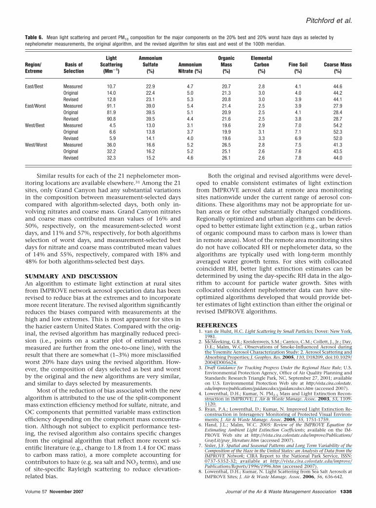
Similar results for each of the 21 nephelometer mon-itoring locations are available elsewhere.31 Among the 21sites, only Grand Canyon had any substantial variationsin the composition between measurement-selected dayscompared with algorithm-selected days, both only in-volving nitrates and coarse mass. Grand Canyon nitratesand coarse mass contributed mean values of 16% and50%, respectively, on the measurement-selected worstdays, and 11% and 57%, respectively, for both algorithmsselection of worst days, and measurement-selected bestdays for nitrate and coarse mass contributed mean valuesof 14% and 55%, respectively, compared with 18% and48% for both algorithms-selected best days.

SUMMARY AND DISCUSSIONAn algorithm to estimate light extinction at rural sitesfrom IMPROVE network aerosol speciation data has beenrevised to reduce bias at the extremes and to incorporatemore recent literature. The revised algorithm significantlyreduces the biases compared with measurements at thehigh and low extremes. This is most apparent for sites inthe hazier eastern United States. Compared with the orig-inal, the revised algorithm has marginally reduced preci-sion (i.e., points on a scatter plot of estimated versusmeasured are further from the one-to-one line), with theresult that there are somewhat (1–3%) more misclassifiedworst 20% haze days using the revised algorithm. How-ever, the composition of days selected as best and worstby the original and the new algorithms are very similar,and similar to days selected by measurements.

Most of the reduction of bias associated with the newalgorithm is attributed to the use of the split-componentmass extinction efficiency method for sulfate, nitrate, andOC components that permitted variable mass extinctionefficiency depending on the component mass concentra-tion. Although not subject to explicit performance test-ing, the revised algorithm also contains specific changesfrom the original algorithm that reflect more recent sci-entific literature (e.g., change to 1.8 from 1.4 for OC massto carbon mass ratio), a more complete accounting forcontributors to haze (e.g. sea salt and NO2 terms), and useof site-specific Rayleigh scattering to reduce elevation-related bias.

Both the original and revised algorithms were devel-oped to enable consistent estimates of light extinctionfrom IMPROVE aerosol data at remote area monitoringsites nationwide under the current range of aerosol con-ditions. These algorithms may not be appropriate for ur-ban areas or for other substantially changed conditions.Regionally optimized and urban algorithms can be devel-oped to better estimate light extinction (e.g., urban ratiosof organic compound mass to carbon mass is lower thanin remote areas). Most of the remote area monitoring sitesdo not have collocated RH or nephelometer data, so thealgorithms are typically used with long-term monthlyaveraged water growth terms. For sites with collocatedcoincident RH, better light extinction estimates can bedetermined by using the day-specific RH data in the algo-rithm to account for particle water growth. Sites withcollocated coincident nephelometer data can have site-optimized algorithms developed that would provide bet-ter estimates of light extinction than either the original orrevised IMPROVE algorithms.

REFERENCES1. van de Hulst, H.C. Light Scattering by Small Particles; Dover: New York,

1981.2. McMeeking, G.R.; Kreidenweis, S.M.; Carrico, C.M.; Collett, J., Jr.; Day,

D.E.; Malm, W.C. Observations of Smoke-Influenced Aerosol duringthe Yosemite Aerosol Characterization Study: 2. Aerosol Scattering andAbsorbing Properties; J. Geophys. Res. 2005, 110, D18209, doi:10.1029/2004JD005624.

3. Draft Guidance for Tracking Progress Under the Regional Haze Rule; U.S.Environmental Protection Agency, Office of Air Quality Planning andStandards: Research Triangle Park, NC, September 27, 2001; availableon U.S. Environmental Protection Web site at http:/vista.cira.colostate.edu/improve/publications/guidancedocs/guidancedocs.htm (accessed 2007).

4. Lowenthal, D.H.; Kumar, N. PM2.5 Mass and Light Extinction Recon-struction in IMPROVE; J. Air & Waste Manage. Assoc. 2003, 53, 1109-1120.

5. Ryan, P.A.; Lowenthal, D.; Kumar, N. Improved Light Extinction Re-construction in Interagency Monitoring of Protected Visual Environ-ments; J. Air & Waste Manage. Assoc. 2005, 55, 1751-1759.

6. Hand, J.L.; Malm, W.C. 2005: Review of the IMPROVE Equation forEstimating Ambient Light Extinction Coefficients; available on the IM-PROVE Web site at http://vista.cira.colostate.edu/improve/Publications/GrayLit/gray_literature.htm (accessed 2007).

7. Sisler, J.F. Spatial and Seasonal Patterns and Long Term Variability of theComposition of the Haze in the United States: an Analysis of Data from theIMPROVE Network; CIRA Report to the National Park Service, ISSN:0737-5352-32; available at http://vista.cira.colostate.edu/improve/Publications/Reports/1996/1996.htm (accessed 2007).

8. Lowenthal, D.H.; Kumar, N. Light Scattering from Sea Salt Aerosols atIMPROVE Sites; J. Air & Waste Manage. Assoc. 2006, 56, 636-642.

Table 6. Mean light scattering and percent PM10 composition for the major components on the 20% best and 20% worst haze days as selected bynephelometer measurements, the original algorithm, and the revised algorithm for sites east and west of the 100th meridian.

Region/Extreme

Basis ofSelection

LightScattering

(Mm�1)

AmmoniumSulfate

(%)AmmoniumNitrate (%)

OrganicMass(%)

ElementalCarbon

(%)Fine Soil

(%)Coarse Mass

(%)

East/Best Measured 10.7 22.9 4.7 20.7 2.8 4.1 44.6Original 14.0 22.4 5.0 21.3 3.0 4.0 44.2Revised 12.8 23.1 5.3 20.8 3.0 3.9 44.1

East/Worst Measured 91.1 39.0 5.4 21.4 2.5 3.9 27.9Original 81.9 39.5 5.1 20.9 2.5 4.1 28.4Revised 90.8 39.5 4.4 21.6 2.5 3.8 28.7

West/Best Measured 4.5 13.0 3.1 19.6 2.9 7.0 54.2Original 6.6 13.8 3.7 19.9 3.1 7.1 52.3Revised 5.9 14.1 4.0 19.6 3.3 6.9 52.0

West/Worst Measured 36.0 16.6 5.2 26.5 2.8 7.5 41.3Original 32.2 16.2 5.2 25.1 2.6 7.6 43.5Revised 32.3 15.2 4.6 26.1 2.6 7.8 44.0

Pitchford et al.

Volume 57 November 2007 Journal of the Air & Waste Management Association 1335

9. Pytkowicz, R.M.; Kester, D.R. The Physical Chemistry of Sea Water;Oceanogr. Mar. Biol. Ann. Rev. 1971, 9, 11-60.

10. McInnes, L.M.; Covert, D.S.; Quinn, P.K.; Germani, M.S. Measure-ments of Chloride Depletion and Sulfur Enrichment in IndividualSea-Salt Particles Collected from the Remote Marine Boundary Layer;J. Geophys. Res. 1994, 99, 8257-8268.

11. Quinn, P.K.; Marshall, S.F.; Bates, T.S.; Covert, D.S.; Kapustin, V.N.Comparison of Measured and Calculated Aerosol Properties Relevantto the Direct Radiative Forcing of Tropospheric Sulfate Aerosol onClimate; J. Geophys. Res. 1995, 100, 8977-8991.

12. Quinn, P.K.; Kapustin, V.N.; Bates, T.S.; Covert, D.S. Chemical andOptical Properties of Marine Boundary Layer Aerosol Particles of theMid-Pacific in Relation to Sources and Meteorological Transport; J.Geophys. Res. 1996, 101, 6931-6951.

13. Quinn, P.K.; Coffman, D.J.; Kapustin, V.N.; Bates, T.S.; Covert, D.S.Aerosol Optical Properties in the Marine Boundary Layer During theFirst Aerosol Characterization Experiment (ACE 1) and the UnderlyingChemical and Physical Aerosol Properties; J. Geophys. Res. 1998, 103,16547-16563.

14. Tang, I.N.; Tridico, A.C.; Fung, K.H. Thermodynamic and OpticalProperties of Sea Salt Aerosols; J. Geophys. Res. 1997, 102, 23269-23275.

15. Clegg, S.L.; Brimblecombe, P.; Wexler, A.S. A Thermodynamic Modelof the System H�-NH4-Na�-SO4

2�-NO3�-Cl�-H2O at 298.15 K; J. Phys.Chem. 1998, 102, 2155-2171.

16. Grosjean, D.; Friedlander, S.K. Gas-Particle Distribution Factors forOrganic and Other Pollutants in the Los Angeles Atmosphere; J. AirPollut. Control Assoc. 1975, 25, 1038-1044.

17. White, W.H.; Roberts P.T. On the Nature and Origins of Visibility-Reducing Aerosols in the Los Angeles Air Basin; Atmos. Environ. 1977,11, 803-812.

18. Andrews, E.; Saxena, P.; Musarra, S.; Hildemann, L.M.; Koutrakis, P.;McMurry, P.H.; Olmez, I.; White, W.H. Concentration and Composi-tion of Atmospheric Aerosols from the 1995 SEAVS Experiment and aReview of the Closure between Chemical and Gravimetric Measure-ments; J. Air & Waste Manage. Assoc. 2000, 50, 648-664.

19. Turpin, B.J.; Lim, H.-J. Contributions to PM2.5 Mass Concentrations:Revisiting Common Assumptions for Estimating Organic Mass; Aero-sol. Sci. Technol. 2001, 35, 602-610.

20. Krivacsy, Z.; Gelencser, A.; Kiss, G.; Mezaros, E.; Molnar, A.; Hoffer, A.;Mezaros, T.; Sarvari, Z.; Temesi, D.; Varga, B.; Baltensperger, U.; Nyeki,S.; Weingartner, E. Study on the Chemical Character of Water SolubleOrganic Compounds in Fine Atmospheric Aerosol at the Jungfraujoch;J. Atmos. Chem. 2001, 39, 235-259.

21. Poirot, R.L.; Husar, R.B. Chemical and Physical Characteristics ofWood Smoke in the Northeastern U.S. during July 2002: Impacts fromQuebec Forest Fires. Presented at the A&WMA Specialty Conference:Regional and Global Perspectives on Haze: Causes, Consequences andControversies, Ashville, NC, October 25–29, 2004; Paper No. 94.

22. Malm, W.C.; Day, D.E.; Carrico, C.; Kreidenweis, S.M.; Collett, J.L., Jr.;McMeeking, G.; Lee; Carillo, J. Intercomparison and Closure Calcula-tions Using Measurements of Aerosol Species and Optical Propertiesduring the Yosemite Aerosol Characterization Study; J. Geophys. Res.2005, 110, D14302, doi:10.1029/2004JD005494.

23. El-Zanan, H.S.; Lowenthal, D.H.; Zielinska, B.; Chow, J.C.; Kumar, N.Determination of the Organic Aerosol Mass to Organic Carbon Ratioin IMPROVE Samples; Chemosphere 2005, 60, 485-496.

24. Malm, W.C.; Hand, J.L. An Examination of the Physical and OpticalProperties of Aerosols Collected in the IMPROVE Program; Atmos.Environ., 2007, 41, 3404-3427.

25. Lowenthal, D.H.; Kumar, N. Variation of Mass Scattering Efficienciesin IMPROVE; J. Air & Waste Manage. Assoc. 2005, 54, 926-934.

26. Malm, W.C.; Day, D.E.; Kreidenweis, S.M.; Collett, J.L.; Lee, T. Humid-ity-Dependent Optical Properties of Fine Particles during the Big BendRegional Aerosol and Visibility Study J. Geophys. Res. 2003, 108, 4279.

27. IMPROVE Web site; available at http://vista.cira.colostate.edu/improve/;VIEWS Web site; available at http://vista.cira.colostate.edu/views/.

28. Dixon, J.K. The Absorption Coefficient of Nitrogen Dioxide in theVisible Spectrum; J. Chem. Phys. 1940, 8, 157-161.

29. Draft Final Report: User’s Manual For The Plume Visibility Model (PLU-VUE); Systems Applications, Inc.: Alexandria, VA, July 1980.

30. 2-deg Color Matching Function; CIE (1931); available on CVRL Colorand Vision Database Web site at http://www-cvrl.ucsd.edu/cmfs.htm (ac-cessed 2007).

31. Revised IMPROVE Algorithm for Estimating Light Extinction from Particle Specia-tion Data; Report to the IMPROVE Steering Committee; available at http://vista.cira.colostate.edu/improve/publications/grayLit/019_revisedIMPROVEeq/revisedIMPROVEalgorithm3.doc (accessed January 2006).

About the AuthorsMarc Pitchford is a meteorologist with the National Oceanicand Atmospheric Administration, Las Vegas, NV. WilliamMalm, a research physicist, and Bret Schichtel, a physicalscientist, are with the National Park Service, Fort Collins,CO. Naresh Kumar is an area manager in air quality with theElectric Power Research Institute, Palo Alto, CA. DouglasLowenthal is an associate research professor with theDesert Research Institute, Reno, NV. Jenny Hand is a re-search scientist with the Cooperative Institute Research inthe Atmosphere, Colorado State University Fort Collins,CO. Please address correspondence to Marc Pitchford,National Oceanic and Atmospheric Administration, Air Re-search Laboratories, c/o Desert Research Institute, LasVegas, NV 89119-7363; phone: �1-702-862-5432; fax: �1-702-862-5507; e-mail: marcp@dri.edu.

Pitchford et al.

1336 Journal of the Air & Waste Management Association Volume 57 November 2007