Reliability of Different Mark-Recapture Methods forPopulation Size Estimation Tested against ReferencePopulation Sizes Constructed from Field DataAnnegret Grimm1,2*, Bernd Gruber1,3, Klaus Henle1

1 Department of Conservation Biology, UFZ – Helmholtz Centre for Environmental Research, Leipzig, Germany, 2 Institute for Biology, Faculty of Biosciences, Pharmacy

and Psychology, University of Leipzig, Leipzig, Germany, 3 Institute for Applied Ecology, Faculty of Applied Sciences, University of Canberra, Australian Capital Territory,

Canberra, Australia

Abstract

Reliable estimates of population size are fundamental in many ecological studies and biodiversity conservation. Selectingappropriate methods to estimate abundance is often very difficult, especially if data are scarce. Most studies concerning thereliability of different estimators used simulation data based on assumptions about capture variability that do notnecessarily reflect conditions in natural populations. Here, we used data from an intensively studied closed population ofthe arboreal gecko Gehyra variegata to construct reference population sizes for assessing twelve different population sizeestimators in terms of bias, precision, accuracy, and their 95%-confidence intervals. Two of the reference populations reflectnatural biological entities, whereas the other reference populations reflect artificial subsets of the population. Sinceindividual heterogeneity was assumed, we tested modifications of the Lincoln-Petersen estimator, a set of models inprograms MARK and CARE-2, and a truncated geometric distribution. Ranking of methods was similar across criteria. Modelsaccounting for individual heterogeneity performed best in all assessment criteria. For populations from heterogeneoushabitats without obvious covariates explaining individual heterogeneity, we recommend using the moment estimator orthe interpolated jackknife estimator (both implemented in CAPTURE/MARK). If data for capture frequencies are substantial,we recommend the sample coverage or the estimating equation (both models implemented in CARE-2). Depending on thedistribution of catchabilities, our proposed multiple Lincoln-Petersen and a truncated geometric distribution obtainedcomparably good results. The former usually resulted in a minimum population size and the latter can be recommendedwhen there is a long tail of low capture probabilities. Models with covariates and mixture models performed poorly. Ourapproach identified suitable methods and extended options to evaluate the performance of mark-recapture population sizeestimators under field conditions, which is essential for selecting an appropriate method and obtaining reliable results inecology and conservation biology, and thus for sound management.

Citation: Grimm A, Gruber B, Henle K (2014) Reliability of Different Mark-Recapture Methods for Population Size Estimation Tested against Reference PopulationSizes Constructed from Field Data. PLoS ONE 9(6): e98840. doi:10.1371/journal.pone.0098840

Editor: Brock Fenton, University of Western Ontario, Canada

Received August 20, 2013; Accepted May 7, 2014; Published June 4, 2014

Copyright: � 2014 Grimm et al. This is an open-access article distributed under the terms of the Creative Commons Attribution License, which permitsunrestricted use, distribution, and reproduction in any medium, provided the original author and source are credited.

Funding: The research of Annegret Grimm was funded by the German National Academic Foundation. (http://www.studienstiftung.de/). The funders had no rolein study design, data collection and analysis, decision to publish, or preparation of the manuscript.

Competing Interests: The authors have declared that no competing interests exist.

* E-mail: annegret.grimm@ufz.de

Introduction

Knowledge of population size is of key importance in many

fields of animal ecology, evolution, and conservation biology. For

natural populations of animals, it is rarely possible to count all

individuals. Thus, usually estimation methods have to be used.

Capture-mark-recapture (CMR) is a commonly used approach for

estimating population size [1,2,3,4,5]. Meanwhile, a huge range of

different statistical models exists for analysing CMR data [5,6,7,8].

Field biologists are faced with the difficulty of deciding which

approach to use and how reliable the selected method is for the

populations they study [5,6,8]. This problem is exacerbated by the

existence of a range of alternative methods using similar biological

assumptions about the capture process. Consequently, good

recommendations based on field data for the most suitable

methods for various natural populations are needed to validate

and complement simulation studies.

The performance of CMR models depends on their assump-

tions, how these assumptions can be met in the field, and on the

robustness of the estimators to violations of the underlying

assumptions. Critical assumptions are whether capture probability

remains constant, changes with time or as behavioural response to

previous experience, or varies among individuals [2,4,7]. Because

population size must be known to assess the performance of

estimators, assessments usually rely on virtual CMR studies that

create capture histories under different assumptions about capture

probabilities [9,10,11]. The advantage of such simulation studies is

that they allow assessment of the performance of estimators by

systematically varying capture probability.

An important limitation of simulation studies is that it is unclear

to which extent the variation in capture probability implemented

reflects the variation occurring in nature [11,12]. Thus, it is

important to study the performance of various estimators under

field conditions. For this purpose, it is essential to have populations

of known size available. As this is rarely the case, few such studies

PLOS ONE | www.plosone.org 1 June 2014 | Volume 9 | Issue 6 | e98840

exist and most compared only a small number of methods. These

studies either used penned populations of known size

[12,13,14,15,16,17] or compared estimates to the number of

individuals obtained in complete removals from areas of limited

size, e.g., small pools [18], ant nests [19], or fenced-off areas [20].

Intensively studied closed populations and the use of a subset of

the data to estimate population size may offer an additional

opportunity that seems not to have been used so far. Here we

explore this approach using a very intensively studied closed

population of the Australian gecko Gehyra variegata [21]. We

assessed the performance of ten different methods without

covariates and two different sets of methods including covariates.

As behavioural observations suggested that individual heteroge-

neity may be present [22], we focused on methods that allow

individual heterogeneity. We evaluated a set of models in

programs MARK [23,24], the most widely used tool to estimate

population size, and CARE-2 [25] that allow, in addition to

individual heterogeneity, temporal and behavioural change of

capture probability. We also assessed a truncated geometric

distribution [3] as this distribution has been used in earlier studies

to estimate population size of our model species [21]. We further

included three modifications of the Lincoln-Petersen estimator

since this is a simple, still frequently used method. We predicted

that models incorporating individual heterogeneity would perform

better than other models studied and that models using covariates

or mixture approaches would outperform models that account for

heterogeneity in a more simple way.

Materials and Methods

Data collectionThis research was carried out under permit number A478 NSW

National Parks and Wildlife Service. This licence covered all

animal ethics considerations as well as a permit to capture and

mark the animals.

Mark-recapture data collected from a population of the

arboreal, nocturnal gecko Gehyra variegata (Dumeril & Bibron,

1836) living at the huts of the station in Kinchega National Park

(32u289 S, 142u209 E), western New South Wales, Australia,

provided the basis for the evaluation of the selected population size

estimators [21].

The study site included seven huts where geckos were caught by

hand at night, measured, sexed, and marked by toe-clipping and

with a dorsal colour mark for short-term identification. Toe-

clipping had no influence on survival (Hohn et al., accepted). Data

collection followed a robust design [26]. The population was

sampled intensively bimonthly (primary periods) for two years

from September 1985 to March 1987 except July 1986 due to the

inactivity of the species. Each primary period consisted of five to

sixteen secondary periods (usually consecutive nights).

Potential habitat within a strip of 50 m around the huts was

surveyed to detect dispersing individuals [21]. In parallel, a second

population living in riverine woodland in a distance of approx-

imately 30 m from the huts was studied and provided additional

opportunity to discover dispersing individuals. Over the whole

time span, only one subadult gecko moved from the closest tree

into the study area and back again within a two month period,

implying that there was negligible emigration and immigration,

allowing construction of reference population sizes. This conclu-

sion is further corroborated by movement studies in the second

population that showed that longer distance movement is very rare

[21,27].

Construction of reference population sizesWe used two approaches to create reference population sizes

assessing whether the relative performance of the evaluated

methods remains consistent. In both approaches we determined

a reference population for each but the last primary period. In the

first approach based on partly independent data, we counted all

individuals marked throughout the study period. We then

excluded all individuals only captured in previous primary periods.

We further excluded juveniles born in later primary periods (as

they were not yet part of the population). Juveniles can be

identified reliably by size during the first two years after birth [21].

These reference populations are only partly independent from the

data used for estimating population size because some animals

were only present in the primary period used for analyses (i.e. for

these animals the same capture was used to include them in the

reference population and to estimate population size). In a second

approach, we created a fully independent reference population by

excluding additionally all animals captured in, but not after the

period analysed. Consequently, we also excluded these individuals

from the capture data used for population estimation. By the

exclusion of these individuals no capture was used both for

constructing the reference population and to estimate the

reference population.

Because of the high capture intensity few, if any, individuals

should have been missed in creating the reference populations for

the first 1–2 primary period(s). Thus they represent the biologically

relevant entire number of individuals present that have non-zero

capture probability (partially independent data set) respectively the

part of the population that survived at least to the next primary

period (fully independent data set). Reference populations for later

primary periods will increasingly ignore individuals with very low

capture probability, which are known to create enormous

challenges for capture-recapture analysis [28]. We used these

reference populations reflecting artificial subsets of the population

to assess whether the relative performance of the tested methods

change when few individuals with low capture probability are

present. They thus need to be understood as biological entities that

provide an alternative way of constructing distributions of capture

probabilities that may be generalized in future simulation studies.

To assess whether we may have missed individuals with very

low capture probability in our reference populations, we calculated

a threshold for daily capture probability (ptr) above which the

expected level of inclusion was at least 95% of all individuals:

ptr~1{ffiffiffiffiffiffiffiffiffiffiffiffiffiffiffiffiffiffiffiffi(1{95%)n

pð1Þ

with n being the number of capture occasions used to determine

reference population sizes.

Assessment of population size estimatorsWe used data from November 1985, 1986, January 1986, 1987,

and March 1986, 1987 for estimating population sizes since geckos

were most active during these months [21]. Minimizing variation

of capture probability over time, we combined occasions with very

low sampling rates [4].

Our evaluation of estimator performance focussed on models

that account for individual heterogeneity since from our experi-

ence in the field we expected substantial individual heterogeneity

due to different catchabilities among individuals. To mathemat-

ically assess whether individual heterogeneity was considerable, we

calculated a coefficient of variation (CV) in capture probabilities as

suggested by Chao et al. (1992) and Lee and Chao (1994) using

program CARE-2 [25,29,30]. The CV is a nonnegative parameter

Population Size Estimation

PLOS ONE | www.plosone.org 2 June 2014 | Volume 9 | Issue 6 | e98840

that indicates individual heterogeneity, which is larger for higher

degrees of heterogeneity among individuals. If and only if

individuals are equally catchable, the CV is zero. This heteroge-

neity is relevant for some of the coverage estimators evaluated and

also to understand the different performance of the evaluated

estimators.

In total, we assessed twelve estimators. Table 1 provides an

overview of the estimators, their characteristics, and where

relevant methods select among alternatives within a specific

estimation approach. We did not include the spatially explicit

capture-recapture (SECR) method [31,32] although this method

reduces individual heterogeneity at spatial level as there is a

complex unknown relationship between distances and capture

probabilities among individuals making this method not applicable

to our data. The first three estimators assessed are from a set of

models implemented in programs CAPTURE and MARK [2.24].

The models in CAPTURE make complementary assumptions

about capture probability. Capture probability may be constant

(M0), variable in time (Mt), among individuals (Mh), or due to trap

shyness or trap happiness (Mb), and all pairwise combinations

thereof. There is no estimator for the most general model, Mtbh.

Model selection is made by a discriminant function that builds on

several specific model tests [2]. Besides the estimator chosen by the

discriminant function [Appropriate], we evaluated the two Mh

models implemented in CAPTURE: the interpolated jackknife

estimator [IntJK] [33,34] and the moment estimator [ME] of

Chao (1987, 1988), which sometimes is also referred to as the

lower bound estimator[35,36]. Both estimators use capture

frequencies to estimate population size. Whereas the nonparamet-

ric jackknife estimator is based on linear combinations of all

capture frequencies [33], Chao’s moment estimator is exclusively

based on f1 and f2, which are the number of individuals captured

once or twice [35,36,37].

We further evaluated the first [SC1] and the second sample

coverage estimator [SC2] of Lee and Chao (1994) [29], the

estimating equation [EE] of Chao et al. (2001) [11], as well as a set

of models that allow inclusion of covariates (sub-program

GSRUN) as implemented in program CARE-2 [CARE/GSRUN]

[25]. The sample coverage estimator is a nonparametric estima-

tion technique that builds on the proportion of individual capture

probabilities included in the data by the animals captured. The

population size estimation is further based on an estimation of the

degree of individual heterogeneity, i.e. the coefficient of variation

of individual capture probabilities [29,30].

The estimating equation developed by Chao et al. (2001) uses

behavioural response, individual heterogeneity, and temporal

changes as parameters to model capture probabilities. Hence,

calculating population size for different combinations of model

assumptions is possible by using only one formula. Currently, no

selection process among alternative models is available [5,11], so

we evaluated model Mh. This estimator can also be seen as an

extension to the sample coverage estimator. The calculation of the

other set of models (GSRUN) is based on a conditional likelihood

approach [38,39] using the Horvitz-Thompson population size

estimator [40]. For that estimator, we used the following

covariates: age (juveniles, subadults, adults) and five different

types of huts identified according to similar structures, which may

result in similar capture probabilities. The model with the lowest

AIC was chosen [41].

Moreover, we tested Pledger’s (2000) finite mixture model

[Finite mixtures][42], which is also implemented in program

MARK [24,43]. The approach models individual differences in

capture probabilities using a flexible beta-distribution. The general

model is denoted as p(.)p(t)c(t)N(.), with p being the probability

that an individual belongs to mixture A, p is capture probability for

the first capture and c for the following ones, thus allowing for trap

response, t signifies that the variable is time specific, and N is

population size [43]. We used AIC values for model selection [44].

The final four models assessed are the truncated geometric

distribution [Tr. geometric distribution] [3] and three versions of

the Lincoln-Petersen estimate. In the first approach, population

size is estimated by fitting capture frequencies to a truncated

Table 1. Overview on all tested population size estimators including their references, basics, and model selection procedures.

Estimator Reference Basics Model selection

Linconln-Petersen (LP) [3,4] Lincoln-Petersen corrected by Chapman no model selection

Multiple Lincoln-Petersen (MLP) [3] andrecent study

repeated Lincoln-Petersen estimator no model selection

Mean Petersen Estimate (MPE) [3] mean Petersen estimate for each sampling stage no model selection

MARK Appropriate [2] running all models discriminant function building on severalspecific model tests

MARK Mh Interpolated Jackknife(IntJK)

[31,32] linear combinations of all capture frequencies no model selection

MARK Mh Moment Estimator (ME) [33,34,35] capture frequencies of individuals captured once (f1)or twice (f2)

no model selection

CARE Mh Sample Coverage 1 (SC1) [29] overall proportion of individual capture probabilitiesand degree of individual heterogeneity

no model selection

CARE Mh Sample Coverage 2 (SC2) [29] bias-corrected form of SC1 no model selection

CARE Mh Estimating Equation (EE) [11] behavioural response, individual heterogeneity, and temporalchanges as parameters to model capture probabilities

no model selection

Truncated geometric distribution [3] fitting capture frequencies to a geometric distribution no model selection

Finite mixtures [28] models individual differences in capture probabilities usinga flexible beta-distribution

AIC

CARE/GSRUN [25] conditional likelihood approach using the Horvitz-Thompsonpopulation size estimator

AIC

doi:10.1371/journal.pone.0098840.t001

Population Size Estimation

PLOS ONE | www.plosone.org 3 June 2014 | Volume 9 | Issue 6 | e98840

geometric distribution [3]. We wrote an R [45] package for this

purpose which was submitted to CRAN [46]. This estimator was

tested as it has been used frequently in the past, including for our

data set [1,14,21,47,48].

Lincoln-Petersen estimators are known to be very vulnerable to

deviations from equal catchability, but since they are easy to

calculate and therefore often used, we included them in these

comparisons. We calculated the Lincoln-Petersen estimator [LP]

with the adjustments suggested by Chapman [3,4]. For an odd

number of occasions, we split the data in such a way that the

difference in number of captures between the two samples was

minimized [9]. We also evaluated the mean Petersen estimate

[MPE] [3], which is the mean of the Petersen estimates calculated

for each stage of sampling, with the number of marked individuals

in the population based on the combined data of all previous

sampling occasions of the primary period. This approach results in

k-1 estimates (with k denoting the number of trapping samples).

Ignoring covariances, as they should be low compared to

variances, the variance of the MPE is the sum of all single

variances divided by (k-1)2 [3]. As an alternative version, we

invented a new way to estimate population size using repeated

Lincoln-Petersen estimators, which we call multiple Lincoln-

Petersen [MLP]. We took the average of k-1 Lincoln-Peterson

population size estimates that were calculated by pooling the data

as follows: for the first case, we used data from the first occasion as

n1 and pooled all remaining occasions for n2; we then pooled

occasions one and two for n1 and the remaining occasions (three to

k) for n2 and so on. We calculated the variance of this multiple

Lincoln-Petersen estimate in the same way as suggested by Seber

(1982) for MPE. By combining the data from several occasions, all

capture probabilities will be increased and the range of capture

probabilities will be reduced, thus also reducing heterogeneity.

Both should result in improved estimates. Furthermore, this

approach should correct for time effects as it uses different

combinations of the occasions. In contrast to MPE, this effect

applies also to n2; thus we expected that it should improve the

performance of the Lincoln-Peterson approach.

Estimator rankingWe compared the performance of the estimators based on the

coverage of the reference population sizes by their 95%-confidence

intervals (CI), the mean span of these confidence intervals, either

as provided by the programs or calculated from the variance of the

estimated population size. We further ranked them based on the

mean of their bias, precision, and accuracy [49] across the

reference populations:

relative bias ~

Xn

i~1

(NNi{Ni;ref

Ni;ref

)

nð2Þ

relative precision ~

Xn

i~1

(NNi{Ni;ref

Ni;ref

)2{(Xn

i~1

(NNi{Ni;ref

Ni;ref

))2

n(n{1)ð3Þ

relative accuracy ~Drelative precision Dz(relative bias)2 ð4Þ

with NNi being the estimated population size, Ni;ref the reference

population size, and n the number of reference populations used to

evaluate the estimators.

Relative bias measures the divergence from the reference

population size, and relative precision (or relative variance) can be

interpreted as the variation in estimates of the reference

population size. Relative accuracy combines both measures and

can be interpreted as mean square error. These values were

computed over all primary periods except the last one (as there

was no reference population size).

We ranked all estimation methods using all four criteria,

whereby the closer a value is to zero the better is the performance

of the estimator. These rankings were done in R [45].

Results

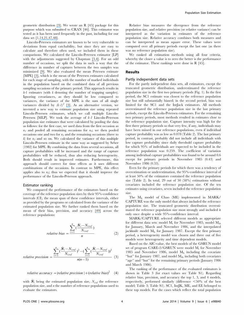
Partly independent data setsFor the partly independent data sets, all estimators, except the

truncated geometric distribution, underestimated the reference

population size in the first two primary periods (Fig. 1). In the first

period, the SC1 estimate was closest to the reference population

size but still substantially biased; in the second period, bias was

limited for the SC1 and the IntJack estimators. All methods

overestimated the reference population size in the last primary

periods, except the Lincoln-Petersen estimators. For the remaining

two primary periods, most methods resulted in estimates close to

the reference population size. Capture intensity was high for the

first three primary periods so that very few, if any, individuals may

have been missed in our reference populations, even if individual

capture probability was as low as 0.078 (Table 2). The last primary

period, in contrast, probably did not include all individuals with

low capture probability since daily threshold capture probability

for which 95% of individuals are expected to be included in the

reference population was 0.259. The coefficient of variation

among individual capture probabilities was found to be around 0.6

except for primary periods in November 1985 (0.43) and

November 1986 (0.33).

Even for the primary periods for which there was a tendency of

overestimation or underestimation, the 95%-confidence interval of

at least 50% of the estimators contained the reference population

size (Table 2). In total, 29 out of 50 (58%) estimations without

covariates included the reference population size. Of the ten

estimates using covariates, seven included the reference population

size.

The Mh model of Chao (ME) implemented in MARK/

CAPTURE was the only model that always included the reference

population size. The truncated geometric distribution overesti-

mated the reference population size most strongly and included it

only once despite a wide 95%-confidence interval.

MARK/CAPTURE selected different models as appropriate

for different data sets: model Mt for November 1985, model Mth

for January, March and November 1986, and the interpolated

jackknife model Mh for January 1987. Except the first primary

period, a heterogeneity model was chosen and three out of five

models were heterogeneity and time dependent models.

Based on the AIC-value, the best models of the GSRUN model

set of program CARE-2/GSRUN were model Mt for November

1985 and November 1986, model Mh including the covariate

‘‘hut’’ for January 1987, and model Mth including both covariates

‘‘age’’ and ‘‘hut’’ for the remaining primary periods (January 1986

and March 1986).

The ranking of the performance of the evaluated estimators is

shown in Table 3 (for exact values see Table S1). Regarding

relative bias, precision, and accuracy the top 1, 3, and 4 models,

respectively, performed similarly (difference ,50% of the best

model; Table 3; Table S1). SC1, IntJK, ME, and EE belonged to

these top models. For the cases which reflect the total population

Population Size Estimation

PLOS ONE | www.plosone.org 4 June 2014 | Volume 9 | Issue 6 | e98840

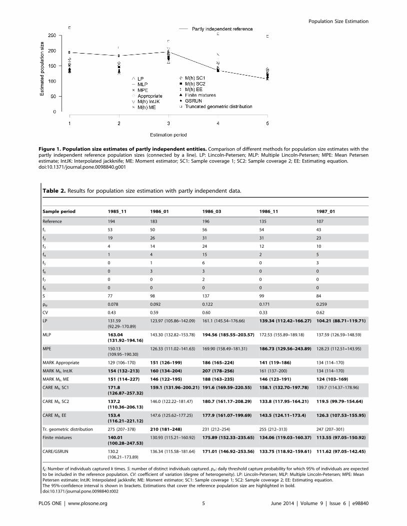
Figure 1. Population size estimates of partly independent entities. Comparison of different methods for population size estimates with thepartly independent reference population sizes (connected by a line). LP: Lincoln-Petersen; MLP: Multiple Lincoln-Petersen; MPE: Mean Petersenestimate; IntJK: Interpolated jackknife; ME: Moment estimator; SC1: Sample coverage 1; SC2: Sample coverage 2; EE: Estimating equation.doi:10.1371/journal.pone.0098840.g001

Table 2. Results for population size estimation with partly independent data.

Sample period 1985_11 1986_01 1986_03 1986_11 1987_01

Reference 194 183 196 135 107

f1 53 50 56 54 43

f2 19 26 31 31 23

f3 4 14 24 12 10

f4 1 4 15 2 5

f5 0 1 6 0 3

f6 0 3 3 0 0

f7 0 0 2 0 0

f8 0 0 0 0 0

S 77 98 137 99 84

ptr 0.078 0.092 0.122 0.171 0.259

CV 0.43 0.59 0.60 0.33 0.62

LP 131.59(92.29–170.89)

123.97 (105.86–142.09) 161.1 (145.54–176.66) 139.34 (112.42–166.27) 104.21 (88.71–119.71)

MLP 163.04(131.92–194.16)

143.30 (132.82–153.78) 194.56 (185.55–203.57) 172.53 (155.89–189.18) 137.59 (126.59–148.59)

MPE 150.13(109.95–190.30)

126.33 (111.02–141.63) 169.90 (158.49–181.31) 186.73 (129.56–243.89) 128.23 (112.51–143.95)

MARK Appropriate 129 (106–170) 151 (126–199) 186 (165–224) 141 (119–186) 134 (114–170)

MARK Mh IntJK 154 (132–213) 160 (134–204) 207 (178–256) 161 (137–200) 134 (114–170)

MARK Mh ME 151 (114–227) 146 (122–195) 188 (163–235) 146 (123–191) 124 (103–169)

CARE Mh SC1 171.8(126.87–257.32)

159.1 (131.96–200.21) 191.6 (169.59–220.55) 158.1 (132.70–197.78) 139.7 (114.37–178.96)

CARE Mh SC2 137.2(110.36–206.13)

146.0 (122.22–181.47) 180.7 (161.17–208.29) 133.8 (117.95–164.21) 119.5 (99.79–154.64)

CARE Mh EE 153.4(116.21–221.12)

147.6 (125.62–177.25) 177.9 (161.07–199.69) 143.5 (124.11–173.4) 126.3 (107.53–155.95)

Tr. geometric distribution 275 (207–378) 210 (181–248) 231 (212–254) 255 (212–313) 247 (207–301)

Finite mixtures 140.01(100.28–247.53)

130.93 (115.21–160.92) 175.89 (152.33–235.65) 134.06 (119.03–160.37) 113.55 (97.05–150.92)

CARE/GSRUN 130.2(106.21–173.89)

136.34 (115.58–181.64) 171.01 (146.92–253.56) 133.75 (118.92–159.61) 111.62 (97.05–142.45)

fk: Number of individuals captured k times. S: number of distinct individuals captured. ptr: daily threshold capture probability for which 95% of individuals are expectedto be included in the reference population. CV: coefficient of variation (degree of heterogeneity). LP: Lincoln-Petersen; MLP: Multiple Lincoln-Petersen; MPE: MeanPetersen estimate; IntJK: Interpolated jackknife; ME: Moment estimator; SC1: Sample coverage 1; SC2: Sample coverage 2; EE: Estimating equation.The 95%-confidence interval is shown in brackets. Estimations that cover the reference population size are highlighted in bold.doi:10.1371/journal.pone.0098840.t002

Population Size Estimation

PLOS ONE | www.plosone.org 5 June 2014 | Volume 9 | Issue 6 | e98840

(sample periods 1 and 2), SC1 came closest to the true population.

The truncated geometric distribution performed worst and LP,

GSRUN, and the Finite mixtures model ranked among the lowest

on all three criteria.

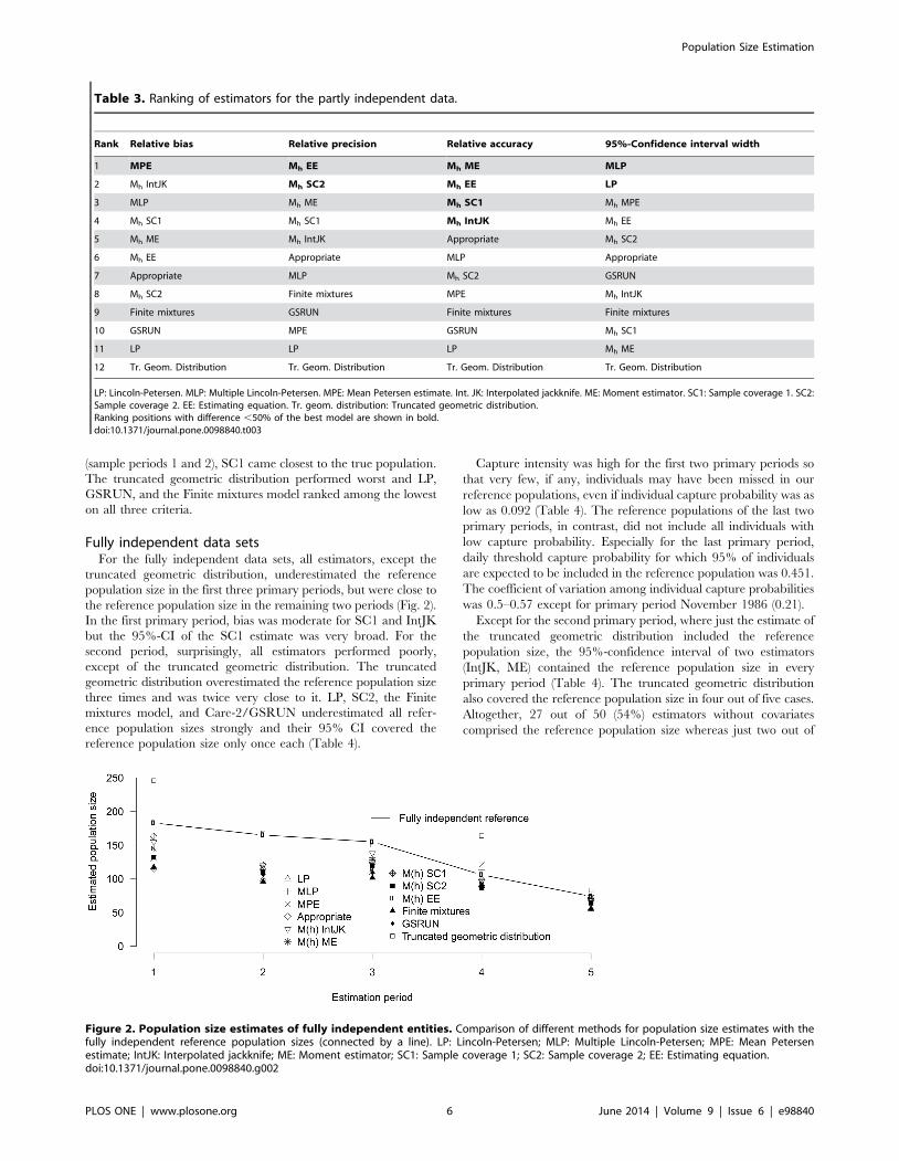
Fully independent data setsFor the fully independent data sets, all estimators, except the

truncated geometric distribution, underestimated the reference

population size in the first three primary periods, but were close to

the reference population size in the remaining two periods (Fig. 2).

In the first primary period, bias was moderate for SC1 and IntJK

but the 95%-CI of the SC1 estimate was very broad. For the

second period, surprisingly, all estimators performed poorly,

except of the truncated geometric distribution. The truncated

geometric distribution overestimated the reference population size

three times and was twice very close to it. LP, SC2, the Finite

mixtures model, and Care-2/GSRUN underestimated all refer-

ence population sizes strongly and their 95% CI covered the

reference population size only once each (Table 4).

Capture intensity was high for the first two primary periods so

that very few, if any, individuals may have been missed in our

reference populations, even if individual capture probability was as

low as 0.092 (Table 4). The reference populations of the last two

primary periods, in contrast, did not include all individuals with

low capture probability. Especially for the last primary period,

daily threshold capture probability for which 95% of individuals

are expected to be included in the reference population was 0.451.

The coefficient of variation among individual capture probabilities

was 0.5–0.57 except for primary period November 1986 (0.21).

Except for the second primary period, where just the estimate of

the truncated geometric distribution included the reference

population size, the 95%-confidence interval of two estimators

(IntJK, ME) contained the reference population size in every

primary period (Table 4). The truncated geometric distribution

also covered the reference population size in four out of five cases.

Altogether, 27 out of 50 (54%) estimators without covariates

comprised the reference population size whereas just two out of

Table 3. Ranking of estimators for the partly independent data.

Rank Relative bias Relative precision Relative accuracy 95%-Confidence interval width

1 MPE Mh EE Mh ME MLP

2 Mh IntJK Mh SC2 Mh EE LP

3 MLP Mh ME Mh SC1 Mh MPE

4 Mh SC1 Mh SC1 Mh IntJK Mh EE

5 Mh ME Mh IntJK Appropriate Mh SC2

6 Mh EE Appropriate MLP Appropriate

7 Appropriate MLP Mh SC2 GSRUN

8 Mh SC2 Finite mixtures MPE Mh IntJK

9 Finite mixtures GSRUN Finite mixtures Finite mixtures

10 GSRUN MPE GSRUN Mh SC1

11 LP LP LP Mh ME

12 Tr. Geom. Distribution Tr. Geom. Distribution Tr. Geom. Distribution Tr. Geom. Distribution

LP: Lincoln-Petersen. MLP: Multiple Lincoln-Petersen. MPE: Mean Petersen estimate. Int. JK: Interpolated jackknife. ME: Moment estimator. SC1: Sample coverage 1. SC2:Sample coverage 2. EE: Estimating equation. Tr. geom. distribution: Truncated geometric distribution.Ranking positions with difference ,50% of the best model are shown in bold.doi:10.1371/journal.pone.0098840.t003

Figure 2. Population size estimates of fully independent entities. Comparison of different methods for population size estimates with thefully independent reference population sizes (connected by a line). LP: Lincoln-Petersen; MLP: Multiple Lincoln-Petersen; MPE: Mean Petersenestimate; IntJK: Interpolated jackknife; ME: Moment estimator; SC1: Sample coverage 1; SC2: Sample coverage 2; EE: Estimating equation.doi:10.1371/journal.pone.0098840.g002

Population Size Estimation

PLOS ONE | www.plosone.org 6 June 2014 | Volume 9 | Issue 6 | e98840

ten estimates using covariates included the reference population

size.

MARK/CAPTURE selected different models as appropriate:

model Mt for November 1985, Mth for January 1986 and 1987 as

well as March 1986 (for the last two no differences between Mth

and Mh were detected) and M0 for November 1986. A

heterogeneity model was chosen in three out of five primary

periods. According to the AIC-values, the best models of the

GSRUN model set in program CARE-2/GSRUN were model Mt

for November 1985 and January 1987, model Mth with both

covariates ‘‘age’’ and ‘‘hut’’ for January and March 1986, and

model M0 for November 1986. Hence, in two out of five primary

periods a heterogeneity model was chosen.

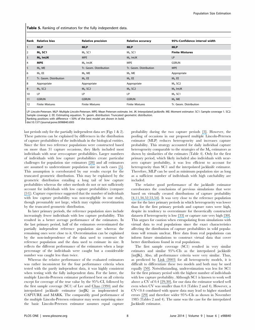
The ranking of the performance of the evaluated estimators for

fully independent data sets is shown in Table 5 (for exact values see

Table S1). MLP and SC1 performed best and second best,

respectively, regarding all criteria except the width of the

confidence interval, for which the latter performed comparably

badly. IntJK and MPE followed with performance values similar

to SC1 (Table 2, Table S1). Expectedly, LP did rank very low but

surprisingly, the models using covariates obtained the lowest

ranking positions.

MLP had the lowest width of the confidence interval, followed

by the Finite mixtures model of Pledger (2000). However, the

Finite mixtures performed worst for all other criteria.

Discussion

The few studies that evaluated the performance of different

estimators using data collected from populations of at least almost

known size indicate that usually heterogeneity models perform

better than models that ignore individual heterogeneity in capture

probability [12,13,15,18,20]. Link (2003) anticipated that it may

be very difficult to select among heterogeneity models because he

expected that most will perform similarly well [50]. Our novel

approach to create reference population sizes for evaluating the

performance of population size estimators showed that the two

best performing estimators resulted in rather similar estimates and

confidence intervals but that there were considerable differences to

other heterogeneity models for some reference populations. The

assumption of individual heterogeneity was confirmed by a CV

between 0.50 and 0.62 except for November datasets, which

showed a CV between 0.21 and 0.50. A lower degree of

heterogeneity in November each year might be caused by the

absence of newly hatched juveniles [21].

Both approaches of creating reference populations resulted in

similarities and differences in the overall pattern of performance of

estimators. All estimators, except the truncated geometric distri-

bution, underestimated the reference population size in the first

two primary periods and were closer to it in the following primary

periods. They overestimated the reference population size in the

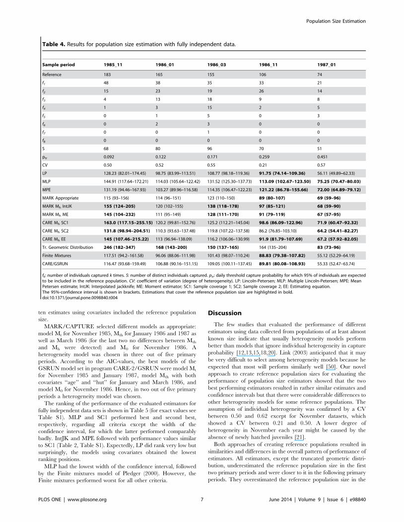
Table 4. Results for population size estimation with fully independent data.

Sample period 1985_11 1986_01 1986_03 1986_11 1987_01

Reference 183 165 155 106 74

f1 48 38 35 33 21

f2 15 23 19 26 14

f3 4 13 18 9 8

f4 1 3 15 2 5

f5 0 1 5 0 3

f6 0 2 3 0 0

f7 0 0 1 0 0

f8 0 0 0 0 0

S 68 80 96 70 51

ptr 0.092 0.122 0.171 0.259 0.451

CV 0.50 0.52 0.55 0.21 0.57

LP 128.23 (82.01–174.45) 98.75 (83.99–113.51) 108.77 (98.18–119.36) 91.75 (74.14–109.36) 56.11 (49.89–62.33)

MLP 144.91 (117.64–172.21) 114.03 (105.64–122.42) 131.52 (125.30–137.73) 113.09 (102.67–123.50) 75.25 (70.47–80.03)

MPE 131.19 (94.46–167.93) 103.27 (89.96–116.58) 114.35 (106.47–122.23) 121.22 (86.78–155.66) 72.00 (64.89–79.12)

MARK Appropriate 115 (93–156) 114 (96–151) 123 (110–150) 89 (80–107) 69 (59–96)

MARK Mh IntJK 155 (124–205) 120 (102–155) 138 (118–178) 97 (85–121) 68 (59–90)

MARK Mh ME 145 (104–232) 111 (95–149) 128 (111–170) 91 (79–119) 67 (57–95)

CARE Mh SC1 163.0 (117.15–255.15) 120.2 (99.81–152.76) 125.2 (112.21–145.04) 98.6 (86.09–122.96) 71.9 (60.47–92.32)

CARE Mh SC2 131.8 (98.94–204.51) 110.3 (93.63–137.48) 119.8 (107.22–137.58) 86.2 (76.85–103.10) 64.2 (54.41–82.27)

CARE Mh EE 145 (107.46–215.22) 113 (96.94–138.09) 116.2 (106.06–130.99) 91.9 (81.79–107.69) 67.2 (57.92–82.05)

Tr. Geometric Distribution 246 (182–347) 168 (143–200) 150 (137–165) 164 (135–204) 83 (73–96)

Finite Mixtures 117.51 (94.2–161.58) 96.06 (88.06–111.98) 101.43 (98.07–110.24) 88.83 (79.38–107.82) 55.12 (52.29–64.19)

CARE/GSRUN 116.47 (93.68–159.49) 106.88 (90.16–151.15) 109.05 (100.11–137.45) 89.81 (80.08–108.93) 55.33 (52.47–63.74)

fk: number of individuals captured k times. S: number of distinct individuals captured. ptr: daily threshold capture probability for which 95% of individuals are expectedto be included in the reference population. CV: coefficient of variation (degree of heterogeneity). LP: Lincoln-Petersen; MLP: Multiple Lincoln-Petersen; MPE: MeanPetersen estimate; IntJK: Interpolated jackknife; ME: Moment estimator; SC1: Sample coverage 1; SC2: Sample coverage 2; EE: Estimating equation.The 95%-confidence interval is shown in brackets. Estimations that cover the reference population size are highlighted in bold.doi:10.1371/journal.pone.0098840.t004

Population Size Estimation

PLOS ONE | www.plosone.org 7 June 2014 | Volume 9 | Issue 6 | e98840

last periods only for the partially independent data set (Figs 1 & 2).

These patterns can be explained by differences in the distribution

of capture probabilities of the individuals in the biological entities.

Since the first two reference populations were constructed based

on more than 31 capture occasions, they likely included most

individuals with near zero-capture probabilities. Larger numbers

of individuals with low capture probabilities create particular

challenges for population size estimators [28] and all estimators

are assumed to underestimate population size in such cases [5].

This assumption is corroborated by our results except for the

truncated geometric distribution. This may be explained by the

geometric distribution entailing a long tail of low capture

probabilities whereas the other methods do not or not sufficiently

account for individuals with low capture probabilities (compare

[51]). Capture experience suggested that the number of individuals

with low capture probability was non-negligible in our study,

though presumably not large, which may explain overestimation

by the truncated geometric distribution.

In later primary periods, the reference population sizes include

increasingly fewer individuals with low capture probability. This

resulted in a better average performance of the estimators. In

the last primary period, half of the estimators overestimated the

partially independent reference population size whereas the

remaining ones were close to it. Overestimation can be explained

by the non-independence of the data used to construct the

reference population and the data used to estimate its size. It

reflects the different performance of the estimators when a large

percentage of the individuals were caught but a considerable

number was caught less than twice.

Whereas the relative performance of the evaluated estimators

was rather inconsistent for the four performance criteria when

tested with the partly independent data, it was highly consistent

when testing with the fully independent data. For the latter, the

multiple Lincoln-Petersen estimator performed best on all criteria

except for coverage of the true value by the 95%-CI, followed by

the first sample coverage (SC1) of Lee and Chao (1994) and the

interpolated jackknife estimator (intJK) as implemented in

CAPTURE and MARK. The comparably good performance of

the multiple Lincoln-Petersen estimator may seem surprising since

the basic Lincoln-Petersen estimator assumes equal capture

probability during the two capture periods [3]. However, the

pooling of occasions in our proposed multiple Lincoln-Petersen

estimator (MLP) reduces heterogeneity and increases capture

probability. This strategy accounted for daily individual capture

heterogeneity comparable to the strategies of the Mh estimators as

shown by similarities of the estimates (Table 4). Only for the first

primary period, which likely included also individuals with near-

zero capture probability, it was less efficient to account for

heterogeneity than SC1 and the interpolated jackknife estimator.

Therefore, MLP can be used as minimum population size as long

as a sufficient number of individuals with high catchability are

included.

The relative good performance of the jackknife estimator

corroborates the conclusions of previous simulations that were

based on virtually created distributions of capture probability

[4,11,34,52,53,54]. It was very close to the reference population

size for the later primary periods in which heterogeneity was lower

than for the first primary periods and capture rates were high,

despite its tendency to overestimate for theoretically constructed

datasets if heterogeneity is low [33] or capture rate very high [30].

This argues for caution when extrapolating from simulations with

virtual data to real populations since the exact characteristics

affecting the distribution of capture probabilities in wild popula-

tions will remain unclear. Here data from real populations can

inform future simulations to construct virtual data that cover

better distributions found in real populations.

The first sample coverage (SC1) resulted in very similar

estimates and similar 95%-CIs as the interpolated jackknife

[intJK]. Also, all performance criteria were very similar. Thus,

as predicted by Link (2003) for all heterogeneity models, it is

difficult to differentiate these two models and both may be used

equally [50]. Notwithstanding, underestimation was less for SC1

for the first primary period with the highest number of individuals

with low capture probability. Although SC1 is known to work well

above a CV of 0.4 [29,30], for our data the estimator worked well

even when CV was smaller than 0.4 (Tables 2 and 4). However, a

CV,0.4 combined with sparse data may lead to higher standard

errors [29] and therefore wider 95%-CIs as shown in November

1985 (Tables 2 and 4). The same was the case for the interpolated

Jackknife estimator.

Table 5. Ranking of estimators for the fully independent data.

Rank Relative bias Relative precision Relative accuracy 95%-Confidence interval width

1 MLP MLP MLP MLP

2 Mh SC1 Mh SC1 Mh SC1 Finite Mixtures

3 Mh IntJK MPE Mh IntJK LP

4 MPE Mh IntJK MPE GSRUN

5 Mh ME Tr. Geom. Distribution Tr. Geom. Distribution MPE

6 Mh EE Mh ME Mh ME Appropriate

7 Tr. Geom. Distribution Mh EE Mh EE Mh EE

8 Appropriate Appropriate Appropriate Mh SC2

9 Mh SC2 Mh SC2 Mh SC2 Mh IntJK

10 LP LP LP Mh SC1

11 GSRUN GSRUN GSRUN Mh ME

12 Finite Mixtures Finite Mixtures Finite Mixtures Tr. Geom. Distribution

LP: Lincoln-Petersen. MLP: Multiple Lincoln-Petersen. MPE: Mean Petersen estimate. Int. JK: Interpolated jackknife. ME: Moment estimator. SC1: Sample coverage 1. SC2:Sample coverage 2. EE: Estimating equation. Tr. geom. distribution: Truncated geometric distribution.Ranking positions with difference ,50% of the best model are shown in bold.doi:10.1371/journal.pone.0098840.t005

Population Size Estimation

PLOS ONE | www.plosone.org 8 June 2014 | Volume 9 | Issue 6 | e98840

Chao et al. (1992) and Lee & Chao (1994) indicated that it may

be difficult to select between SC1 and SC2 [29,30]. For our data

SC1 covered the reference population more often than SC2 and its

accuracy was considerably higher than that of SC2 (Table S1). Its

tendency to underestimate was much stronger than that of SC1,

for the partially independent data set even stronger than that of

the moment estimator (ME).

For ME, most performance criteria were similar to those of the

interpolated jackknife and SC1 (Table S1). It covered the

reference population more often for the partly independent data

set than the interpolated jackknife showing at the same time the

highest accuracy among all estimators. However, it performed

slightly less good than the interpolated jackknife and SC1 in terms

of precision for both data sets (Table S1). In terms of the width of

the confidence interval, it ranked lowest and second lowest of all

estimators (Table 5).

Chao (1988, 1989) suggested that the moment estimator should

work comparably well, if many individuals are captured just once

or twice (low overall capture probability), as it is based on f1 and f2(i.e. individuals captured once or twice) while the interpolated

jackknife estimator should work best when many individuals are

captured more than twice because it uses a linear combination of

all capture frequencies [36,37]. However, for our data set with the

fewest individuals captured more than twice (November 1985), it

underestimated the reference population more than the interpo-

lated jackknife and considerably more than SC1. Rather, our

results support the idea that ME is negatively biased and can be

seen as lower bound estimator in the presence of capture

heterogeneity [36,37]. Furthermore, smaller population size that

reduces the capture frequencies as in our fully independent dataset

leads to an increased standard error of the ME [36] resulting in a

very large 95%-CI.

The estimating equation [EE] requires a large number of

capture-recapture data to obtain reliable estimates of time,

individual heterogeneity, and behaviour effects [11]. This clearly

explains the better performance in partly independent in

comparison to fully independent data (Tables 2 and 4). For this

data set it showed a very good accuracy and a small confidence

interval.

The poorest relative performance was exhibited by the Finite

mixtures model of Pledger (2000), followed by GSRUN [25],

Chapman’s Lincoln-Petersen estimate [LP] [3,4], the second

sample coverage of Lee and Chao (1994), and the model selected

as appropriate by CAPTURE. The relative poor performance of

the latter confirms that the model selection procedure of

CAPTURE does not work satisfactorily [4,9,11,53]; Stanley &

Burnham (1998) even stated that this procedure in CAPTURE

selects an inappropriate model [55].

While the poor performance of the LP estimate was expected

because of its assumption of equal capture probability, we were

surprised that GSRUN and the Finite mixtures model showed a

rather poor performance. Not only did they tend to strongly

underestimate, their 95%-CI included only once the reference

population size for the fully independent reference populations.

For the partly independent reference populations, they also did not

perform well. The relative poor performance of GSRUN might be

explained by having selected the wrong covariates. However, we

selected covariates that, based on AIC values and direct

observations, likely explain part of the heterogeneity observed in

capture probability. Huts with their differences in structure as an

expected explanatory variable were included only for a few

datasets in the best models (based on AIC) but did not improve the

performance of the estimators. This may be explained by our

capture experience showing that the preferred position individuals

occupied at the huts influenced the chance of capturing them. This

factor varied more within than across huts and is difficult to model

as covariate but likely had a stronger effect than the covariates we

could measure. Fitting models with covariates under such

conditions remains challenging [56].

Presence of individuals with low capture probabilities and

absence of a structure that allows clear groupings of capture

probabilities in finite groups may also be the reason why the

mixture model of Pledger (2005) [28] performed on average

relatively poorly. In line with this explanation, it was among the

best for the partially independent data sets in which most or all of

the individuals with low capture probability were removed.

Pledger’s (2005) model also performed less well than the

appropriate model in CAPTURE in a study of the giant day

gecko (Phelsuma madagascariencsis grandis) population of known size

released in the Masoala rainforest exhibit (Zurich Zoo) [12].

With the advent of a range of estimation methods that model

temporal, behavioural, and individual variability of capture

probabilities, the estimation of population size by fitting recapture

frequencies to mathematical distributions has fallen into disfavour.

Notwithstanding, a truncated geometric distribution may result

from modelling the capture process, e.g., if average capture rate is

proportional to home range area [3]. Also, recently Nitwitpong et

al. (2013) suggested based on theoretical and simulation results

that the truncated geometric distribution should approximate

capture frequencies well, and better than other distributions, when

there is a long tail of low capture probabilities [51]. Our results

showed that for such reference populations, it was the only method

that did not underestimate the reference population size. While the

method may be recommended for such data, it did overestimate

the reference population substantially for several other reference

populations, especially for the partly independent data set. A

further disadvantage was the worst performance in terms of

confidence interval width. To better understand under which

conditions the truncated geometric distribution may be used

appropriately and avoid underestimation, we suggest further

simulations for data with a long tail of low capture probabilities

and applications to populations of known size for which it is also

known that many individuals have low capture probability.

Conclusion

Selecting the most appropriate population size estimator and

obtaining reliable estimates requires sufficient capture information.

There is no single estimator that performs best and results in very

good estimates for all data sets. If individual heterogeneity is high

(CV.0.4) either the interpolated jackknife [33] as implemented in

CAPTURE/MARK or SC1 [29] may be selected, both perform-

ing very similarly and adequately for most of our data sets. Only

for the first primary period, which likely included the largest

percentage of individuals with near-zero capture probability, was

its bias clearly less. As the first primary period corresponds to the

complete real population (partially independent data) or the real

number of individuals surviving from the first to later primary

periods (fully independent data), SC1 may be preferable for

populations similar to the geckos in this study, unless the wide

95%-CI is of more concern than bias. If few individuals with low

capture probabilities are present, the moment estimator [35]

implemented in CAPTURE/MARK may be a better choice.

If in contrast underestimation is of concern, e.g. when assessing

the impact of an invasive species, and if it is expected that a

considerable number of individuals have low capture probability,

the truncated geometric distribution may be the best choice when

used together with the moment estimator to also get an estimate of

Population Size Estimation

PLOS ONE | www.plosone.org 9 June 2014 | Volume 9 | Issue 6 | e98840

the lower bound of population size. If a large number of capture

occasions can be pooled and the number of individuals with very

low capture probability is likely limited, our new multiple Lincoln-

Petersen estimate may be a strategy that deals with heterogeneity

as good to modelling individual capture heterogeneity; however,

further tests with populations of known size and simulation studies

are needed to corroborate this conclusion.

To improve the robustness of guidelines for the selection of

suitable estimators for field data, we recommend similar studies for

other species as the distribution of their capture probabilities may

deviate from the geckos in our study. Capture frequency

distributions from real populations may also profitably be used

to construct virtual capture data for simulation studies that

realistically reflect the variability of capture probabilities in real

populations.

Supporting Information

Table S1 Ranking values of each estimator calculatedfor the first five periods.(DOCX)

Acknowledgments

The research by Henle (1990) was carried out under permit number A478

NSW National Parks and Wildlife Service. Our special thanks are due to

their staff at Kinchega National Park for logistic support.

Author Contributions

Conceived and designed the experiments: AG BG KH. Performed the

experiments: AG. Analyzed the data: AG KH. Contributed reagents/

materials/analysis tools: AG BG KH. Wrote the paper: AG KH.

Programming of estimators: AG BG.

References

1. Eberhardt LL (1969) Population estimates from recapture frequencies. J Wildl

Manage 33: 28–39.

2. Otis DL, Burnham KP, White GC, Anderson DR (1978) Statistical interence

from capture data on closed animal populations. Wildlife Monographs 62: 1–

135.

3. Seber GA (1982) The estimation of animal abundance and related parameters.

London: Griffin.

4. Pollock KH, Nichols JD, Brownie C, Hines JE (1990) Statistical inference for

capture-recapture experiments. Wildlife Monographs 107: 3–97.

5. Amstrup SC, McDonald TL, Manly BFJ (2005) Handbook of capture-recapture

analyses. Princeton and Oxford: Princeton University Press.

6. Schwarz CJ, Seber GA (1999) Estimating animal abundance: Review III. 14:

427–456.

7. Williams BK, Nichols JD, Conroy MJ (2002) Analysis and management of

animal populations. San Diego: Academic Press.

8. Pine WE, Pollock KH, Hightower JE, Kwak TJ, Rice JA (2003) A review of

tagging methods for estimating fish population size and components of mortality.

Fisheries 28: 10–23.

9. Menkens GE, Anderson Jr SH (1988) Estimation of small-mammal population

size. Ecol 69: 1952–1959.

10. Norris JL, Pollock KH (1996) Nonparametric MLE under two closed capture-

recapture models with heterogeneity. Biometrics 52: 639–649.

11. Chao A, Yip PS, Lee SM, Chu W (2001) Population size estimation based on

estimating functions for closed capture-recapture models. J Stat Plan Inference

92: 213–232.

12. Wagner TC, Motzke I, Furrer SC, Brook BW, Gruber B (2009) How to monitor

elusive lizards: comparison of capture-recapture methods on giant day geckos

(Gekkonidae, Phelsuma madagascariensis grandis) in the Masoala rainforest

exhibit, Zurich Zoo. Ecol Res 24: 345–353.

13. Eberhardt L, Peterle TJ, Schonfield R (1963) Problems in a rabbit population

study. Wildlife Monographs 10: 3–51.

14. Carothers AD (1973) Capture-recapture methods applied to a population with

known parameters. J Anim Ecol 42: 125–146.

15. Vincent JP, Hewison AJ, Angibault JM, Cargnelutti B (1996) Testing density

estimators on a fallow deer population of known size. J Wildl Manage 60: 18–28.

16. Peterson NP, Cederholm CJ (1984) A comparison of the removal and mark-

recapture methods of population estimation for juvenile Coho salmon in a small

stream. N Am J Fish Manage 4: 99–109.

17. Rodgers JD, Solazzi MF, Johnson SL, Buckman MA (1992) Comparison of

three techniques to estimate juvenile Voho salmon populations in small streams.

N Am J Fish Manage 12: 79–86.

18. Jung RE, Dayton GH, Williamson SJ, Sauer JR, Droege S (2002) An evaluation

of population index and estimating techniques for tadpoles in desert pools.

J Herpetol 36: 465–472.

19. Chen YH, Robinson EH (2013) A comparison of mark-release-recapture

methods for estimating colony size in the wood ant Formica lugubris. Insect Soc

60: 351–359.

20. Rodda GH, Perry G, Rondeau RJ, Lazell J (2001) The densest terrestrial

vertebrate. J Trop Ecol 17: 331–338.

21. Henle K (1990) Population ecology and life history of the arboreal gecko Gehyra

variegata in arid Australia. Herpetological Monographs 4: 30–60.

22. Gruber B, Henle K (2008) Analysing the effect of movement on local survival: a

new method with an application to a spatially structured population of the

arboreal gecko Gehyra variegata. Oecologia 154: 679–690.

23. White GC (2008) Closed population estimation models and their extensions in

program MARK. Environ Ecol Stat 15: 89–99.

24. White GC (2010) Program MARK. Available: http://www.phidot.org/

software/mark/ Accessed 2010 Apr 05.

25. Chao A, Yang HC (2003) Program CARE-2. Available: http://chao.stat.nthu.

edu.tw/blog/software-download/care/ Accessed 2010 May 10.

26. Pollock KH (1982) A capture-recapture design robust to unequal probability of

capture. J Wildl Manage 46: 752–757.

27. Gruber B, Henle K (2004) Linking habitat structure and orientation in anarboreal species Gehyra variegata (Gekkonidae). Oikos 107: 406–413.

28. Pledger S (2005) The performance of mixture models in heterogeneous closedpopulation capture-recapture. Biometrics 61: 868–876.

29. Lee SM, Chao A (1994) Estimating population size via sample coverage forclosed capture-recapture models. Biometrics 50: 88–97.

30. Chao A, Lee SM, Jeng SL (1992) Estimating population size for capture-

recapture data when capture probabilities vary by time and individual animal.

Biometrics 48: 201–216.

31. Efford MG, Dawson DK, Borchers DL (2009) Population density estimatedfrom locations of individuals on a passive detector array. Ecology 90: 2676–

2682.

32. Efford MG, Fewster RM (2013) Estimating population size by spatially explicit

capture-recapture. Oikos 122: 918–928.

33. Burnham KP, Overton WS (1978) Estimation of the size of a closed population

when capture probabilities vary among animals. Biometrika 65: 625–633.

34. Burnham KP, Overton WS (1979) Robust estimation of population size whencapture probabilities vary among animals. Ecol 60: 927–936.

35. Chao A (1987) Estimating the population size for capture-recapture data withunequal catchability. Biometrics 43: 783–791.

36. Chao A (1988) Estimating animal abundance with capture frequency data.J Wildl Manage 53: 295–300.

37. Chao A (1989) Estimating populations size for sparse data in capture-recapture

experiments. Biometrics 45: 427–438.

38. Huggins RM (1989) On the statistical analysis of capture experiments.

Biometrika 76: 133–140.

39. Huggins RM (1991) Some practical aspects of a conditional likelihood approach

to capture experiments. Biometrics 47: 725–732.

40. Horvitz DG, Thompson DJ (1952) A generalization of sampling without

replacement from a finite universe. J Am Stat Assoc 47: 663–685.

41. Chao A, Yang HC (2006) User guide for program CARE-2. Version 1.5. Hsin-Chu, Taiwan: National Tsing Hua University.

42. Pledger S (2000) Unified maximum likelihood estimate for closed capture-recapture models using mixtures. Biometrics 56: 434–442.

43. Cooch E, White G (2010) Program MARK. "A gentle introduction". Colorado:

Colorado State University.

44. Anderson DR, Burnham KP, White GC (1994) AIC model selection in

overdispersed capture-recapture data. Ecol 75: 1780–1793.

45. R Development Core Team (2011) R: A Language and Environment for

Statistical Computing. Available: http://www.R-project.org Accessed 2011 Jan06.

46. Grimm A, Henle K (2013) FREQ: Estimate population size from capturefrequencies. Available: http://cran.r-project.org/web/packages/FREQ/index.

html.

47. Edwards WR, Eberhardt L (1967) Estimating cottontail abundance from

livetrapping data. J Wildl Manage 31: 87–96.

48. Nixon CM, Edwards WR, Eberhardt L (1967) Estimating squirrel abundancefrom livetrapping data. J Wildl Manage 31: 96–101.

49. Hellmann J, Fowler G (1999) Bias, precision, and accuracy of four measures ofspecies richness. Ecol Appl 9: 824–834.

50. Link WA (2003) Nonidentifiability of population size from capture-recapture

data with heterogenous detection probabilities. Biometrics 59: 1123–1130.

51. Nitwitpong S, Bohning D, van der Hejden PG, Holling H (2013) Capture-

recapture estimation based upon the geometric distribution allowing for

heterogeneity. Metrika 76: 495–519.

Population Size Estimation

PLOS ONE | www.plosone.org 10 June 2014 | Volume 9 | Issue 6 | e98840

52. Pollock KH, Otto MC (1983) Robust estimation of population size in closed

animal populations from capture-recapture experiments. Biometrics 39: 1035–1049.

53. Don BA (1984) Empirical evaluation of several population size estimates applied

to the grey squirrel. Acta Theriol 29: 187–203.54. Boulinier T, Nichols JD, Sauer JS, Hines JE, Pollock KH (1998) Estimating

species richness: the importance of heterogeneity in species detectability. Ecol79: 1018–1028.

55. Stanley TR, Burnham KP (1998) Infirmation-theoretic model selection and

model averaging for closed-population capture-recapture studies. Biom J 40:

475–494.

56. Dorazio RM, Royle JA (2005) Estimating size and composition of biological

communities by modeling the occurence of species. J Am Stat Assoc 100: 389–

398.

Population Size Estimation

PLOS ONE | www.plosone.org 11 June 2014 | Volume 9 | Issue 6 | e98840