REACH-SCALE SEDIMENT TRANSFERS 889

Copyright © 2003 John Wiley & Sons, Ltd. Earth Surf. Process. Landforms 28, 889–903 (2003)

Earth Surface Processes and Landforms

Earth Surf. Process. Landforms 28, 889–903 (2003)Published online in Wiley InterScience (www.interscience.wiley.com). DOI: 10.1002/esp.1011

REACH-SCALE SEDIMENT TRANSFERS: AN EVALUATION OF TWO

MORPHOLOGICAL BUDGETING APPROACHES

IAN C. FULLER1*, ANDREW R. G. LARGE2, MARTIN E. CHARLTON2, GEORGE L. HERITAGE3 AND DAVID J. MILAN4

1 Division of Geography, Northumbria University, Newcastle upon Tyne, NE1 8ST, UK2 Department of Geography, University of Newcastle upon Tyne, NE1 7RU, UK

3 Division of Geography, University of Salford, Manchester, M5 4WT, UK4 School of Environment, University of Gloucestershire, Cheltenham, GL50 4AZ, UK

Received 6 December 2001; Revised 23 July 2002; Accepted 2 October 2002

ABSTRACT

This paper compares two approaches used to derive measures of annual sediment transfers within a 1 km long piedmontreach of the gravel-bed River Coquet in Northumberland, northern England. The techniques utilize: (i) channel planform andcross-section surveys based on a theodolite/electronic distance measurement (EDM) survey of 21 monumented channelcross-sections and channel and gravel bar margins; and (ii) theodolite-EDM survey generating a series of x,y,z coordinates,from which digital elevation models (DEMs) of the reach were constructed. Calculating the difference between DEMsurfaces provided a measure of volumetric change between surveys carried out during the spring of 1999 and 2000. Theuse of kriging in DEM generation and differencing permits computation of estimate variances and confidence intervalsfor sediment transfer. Error analysis, validating the DEMs using surveyed cross-sections, indicated a mean error betweensurveyed and DEM-generated cross-sections of around twice the value of the D50 of the surface sediment in the reach.Comparison of sediment volumes derived from the two approaches suggests that, compared with the DEM method, monumentedcross-sections underestimate the magnitude of volumetric changes that occur within the reach. The cross-section approachrelies on a simplistic integration of the volumes, whereas DEM differencing provides an estimate at a resolution under thecontrol of the analyst. Furthermore, the cross-section approach does not permit a reliable estimate of the uncertainty of thevolumes calculated. In addition, the DEM methodology based on the morphological unit scale provides an explicit identi-fication of spatial patterns of erosion and deposition, a feature that cross-section-based approaches may fail to include.Copyright © 2003 John Wiley & Sons, Ltd.

KEY WORDS: gravel-bed river; morphological budget; DEM; kriging; sediment transfer

INTRODUCTION

Quantification of changes in channel morphology, which take place in response to sediment erosion, transfer and

deposition (Ashmore and Church, 1998), provides a means by which bedload volumes can be monitored (Davies,

1987). Use of this time–space integrated measure avoids some of the complications caused by spatial and temporal

variability of bedload transport (Hubbell, 1987) and provides a means of estimating sediment transport, which also

yields information on storage and displacement of bed material, important in assessing channel stability (Ashmore

and Church, 1998). Investigation of three-dimensional morphological change in gravel-bed rivers requires repeat

survey of bed elevation and planform adjustments. The majority of research in this field has focused on the bar

scale (e.g. Neill, 1987; Ferguson and Ashworth, 1992; Ferguson et al., 1992; Lane et al., 1994).

Brewer and Passmore (2002) present budgeting techniques designed to evaluate sediment transfers at inter-

mediate reach scales (1–3 km) which are typical of major instability zones in UK piedmont rivers. This approach

also discriminates between morphological units (channel and bar) within the reach, allowing more accurate

determination of sediment fluxes and storage in these instability zones. Wathen et al. (1997) note that reach-scale

sediment storage is rarely quantified in sediment budget studies, but recognize that it has a significant effect on

the precision of morphological methods of bedload estimation at the reach scale.

* Correspondence to: I. C. Fuller, Geography Programme, School of People, Environment and Planning, Massey University, Private Bag11-222, Palmerston North, New Zealand. E-mail: I.C.Fuller@massey.ac.nz

890 I. C. FULLER ET AL.

Copyright © 2003 John Wiley & Sons, Ltd. Earth Surf. Process. Landforms 28, 889–903 (2003)

To date, application of the ‘morphologic approach’ (sensu Ham and Church, 2000) to reach-scale sediment

budgeting in its various forms (e.g. Goff and Ashmore, 1994; Martin and Church, 1995; Paige and Hickin, 2000;

Ham and Church, 2000; Brewer and Passmore, 2002; Fuller et al., 2002), has largely relied upon channel cross-

sections to provide the morphological information required to calculate volumetric changes. Lane et al. (1994)

suggest that this emphasis on the channel cross-section is a legacy of hydraulic geometry, and may represent

a weakness in the approach. Extrapolating changes measured along a cross-section to areas of channel and bars

which may be tens of metres from a section may be problematic, as this assumes the cross-section is an adequate

representation of the units it bisects (Fuller et al., 2002). Furthermore, the cross-section may not adequately

reflect downstream change in channel morphology (Lane et al., 1994), and may fail to accommodate the

potential effects of downstream sedimentological structures on channel processes (Naden and Brayshaw, 1987;

Wittenberg, 2002). This has led Brasington et al. (2000) to note that, ‘the implicitly cross-stream emphasis gives

rise to a high degree of uncertainty in reach-scale sediment budgets derived through the interpolation of cross-

section data’. Some morphological approaches (e.g. Lane et al., 1994; Eaton and Lapointe, 2001) have moved

towards a ‘distributed terrain-sensitive survey’ (Ashmore and Church, 1998) to generate reach-scale digital

elevation models (DEMs), while others, such as Westaway et al. (2000) and Lane (2001), have examined cross-

sections extracted directly from DEMs. However, few comparisons between DEMs and independently surveyed

ground survey data (here cross-sections) have yet been made in the context of morphological budgeting. Using

this approach, this paper assesses the reliability of a cross-section-dependent morphological approach to

quantifying sediment transfers in the wandering, gravel-bedded River Coquet, Northumberland, UK.

One of the reasons for the traditional reliance on cross-stream approaches to reach-scale sediment budgeting

lay in the practical difficulties of topographic data acquisition, storage and analysis at resolutions which

adequately reflect channel morphology (Brasington et al., 2000). Cross-section-derived budgets, which can

be acquired and processed rapidly (Brewer and Passmore, 2002), have thus formed the traditional ‘backbone’

of this research to date. Recent developments have led to the production of high resolution DEMs of fluvial

environments (e.g. Lane et al., 1994; Milne and Sear, 1997; Heritage et al., 1998; Brasington et al., 2000; Eaton

and Lapointe, 2001), where acquisition of high-resolution topographic information is central to effective con-

struction of such DEMs (Westaway et al., 2000). However, it is important to note that volumes derived from

morphological budgeting represent lower-bound estimates of sediment transfer. Firstly, sediment may move

through or within a reach without any surface morphological expression. Secondly, significant negative bias in

volumes of scour-fill can be produced by localized scour-fill compensation (Lindsay and Ashmore, 2002).

STUDY SITE

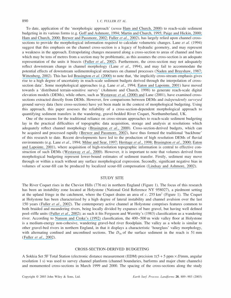
The River Coquet rises in the Cheviot Hills (776 m) in northern England (Figure 1). The focus of this research

has been an instability zone located at Holystone (National Grid Reference NY 958027), a piedmont setting

at the upland fringe in the catchment, where the Coquet drains an area of c. 255 km2 (Figure 1). The Coquet

at Holystone has been characterized by a high degree of lateral instability and channel avulsion over the last

150 years (Fuller et al., 2002). The contemporary active channel at Holystone comprises features common to

both braided and meandering rivers, being locally divided by expanses of bare gravel, but having well defined

pool–riffle units (Fuller et al., 2002); as such it fits Ferguson and Werritty’s (1983) classification as a wandering

river. According to Nanson and Croke’s (1992) classification, the 400–500 m wide valley floor at Holystone

is a medium-energy non-cohesive, wandering gravel-bed river floodplain. The valley as a whole is similar to

other gravel-bed rivers in northern England, in that it displays a characteristic ‘hourglass’ valley morphology,

with alternating confined and unconfined sections. The D50 of the surface sediment in the reach is 51 mm

(Fuller et al., 2002).

CROSS-SECTION-DERIVED BUDGETING

A Sokkia Set 5F Total Station (electronic distance measurement (EDM) precision ±(5 + 5 ppm × D)mm, angular

resolution 1 s) was used to survey channel planform (channel boundaries, barforms and major chute channels)

and monumented cross-sections in March 1999 and 2000. The spacing of the cross-sections along the study

REACH-SCALE SEDIMENT TRANSFERS 891

Copyright © 2003 John Wiley & Sons, Ltd. Earth Surf. Process. Landforms 28, 889–903 (2003)

Figure 1. River Coquet catchment, identifying location and 1999 planform of the study reach at Holystone. The division of the reach into18 subreaches by cross-sections is shown

reach was designed to ensure that channel bed elevation was measured at regular intervals through the reach

and that each bar in the reach was crossed by at least one cross-section. This provided the means of assessing

the vertical changes, produced by sediment gain or loss, which occurred across the morphological units in the

reach. The locations of the cross-sections dividing the site into subreaches are shown overlaid on the 1999

channel planform (Figure 1). Cross-section data for each survey were incorporated into a geographical informa-

tion system (GIS) using ArcInfo™ to facilitate the validation described later in this paper.

Sediment budgets

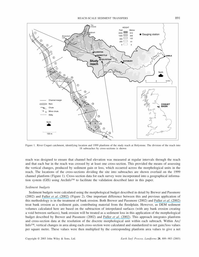
Sediment budgets were calculated using the morphological budget described in detail by Brewer and Passmore

(2002) and Fuller et al. (2002) (Figure 2). One important difference between this and previous application of

this methodology is in the treatment of bank erosion. Both Brewer and Passmore (2002) and Fuller et al. (2002)

treat bank erosion as a sediment gain, contributing material from the floodplain. However, as DEM sediment

volumes calculated here are based on the subtraction of interpolated surfaces (with any bank erosion creating

a void between surfaces), bank erosion will be treated as a sediment loss in this application of the morphological

budget described by Brewer and Passmore (2002) and Fuller et al. (2002). This approach integrates planform

and cross-section data at the resolution of the discrete morphological unit within each subreach. Within Arc/

Info™, vertical changes in area along each cross-section were calculated and standardized to net gain/loss values

per square metre. These values were then multiplied by the corresponding planform area values to give a net

892 I. C. FULLER ET AL.

Copyright © 2003 John Wiley & Sons, Ltd. Earth Surf. Process. Landforms 28, 889–903 (2003)

Figure 2. Derivation of sediment budgets using channel cross-sections and outline planform (after Brewer and Passmore, 2002, reproducedby permission of the Geological Society Publishing House).

gain/loss value (cubic metres) for each morphological unit within the subreach. Where morphological units

are bounded by two cross-sections (e.g. large bar and main channel units), the planform area was halved and

multiplied by the upstream and downstream cross-section data respectively. The results of this budgeting are

shown alongside those derived from the DEM budget approach described below.

REACH-SCALE SEDIMENT TRANSFERS 893

Copyright © 2003 John Wiley & Sons, Ltd. Earth Surf. Process. Landforms 28, 889–903 (2003)

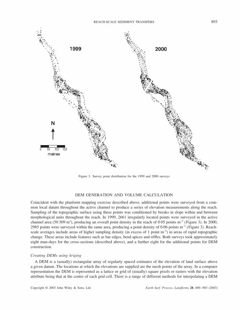
Figure 3. Survey point distribution for the 1999 and 2000 surveys

DEM GENERATION AND VOLUME CALCULATION

Coincident with the planform mapping exercise described above, additional points were surveyed from a com-

mon local datum throughout the active channel to produce a series of elevation measurements along the reach.

Sampling of the topographic surface using these points was conditioned by breaks in slope within and between

morphological units throughout the reach. In 1999, 2661 irregularly located points were surveyed in the active

channel area (50 509 m2), producing an overall point density in the reach of 0·05 points m−2 (Figure 3). In 2000,

2985 points were surveyed within the same area, producing a point density of 0·06 points m−2 (Figure 3). Reach-

scale averages include areas of higher sampling density (in excess of 1 point m−2) in areas of rapid topographic

change. These areas include features such as bar edges, bend apices and riffles. Both surveys took approximately

eight man-days for the cross-sections (described above), and a further eight for the additional points for DEM

construction.

Creating DEMs using kriging

A DEM is a (usually) rectangular array of regularly spaced estimates of the elevation of land surface above

a given datum. The locations at which the elevations are supplied are the mesh points of the array. In a computer

representation the DEM is represented as a lattice or grid of (usually) square pixels or rasters with the elevation

attribute being that at the centre of each grid cell. There is a range of different methods for interpolating a DEM

894 I. C. FULLER ET AL.

Copyright © 2003 John Wiley & Sons, Ltd. Earth Surf. Process. Landforms 28, 889–903 (2003)

from irregularly spaced data, but where error estimates are required kriging is an option. Wackernagel (1995,

p. 89) points to three advantages of spatial interpolation using kriging: (i) the process begins with an analysis

of spatial structure of the data which is then used in the estimation procedure; (ii) ordinary kriging is an exact

interpolator; and (iii) kriging provides an estimate of the estimation error. Kriged estimates of the interpolated

surface between sampling points were made at those locations which represent the centre of each grid cell;

corresponding variances were also computed at the same locations. These variance estimates can be used to

create a confidence interval around the elevation estimates (which are themselves means). They can also be used

to provide an estimate of the propagated uncertainty associated with GIS operations (such as addition or

differencing) and this will be discussed below.

Each survey point consists of a triple {xi,yi,zi} in which xα = {xα,yα} corresponds to a measurement of location

and Z(xα) = z corresponds to some measure of the elevation at that location. Elevation from these measurements,

at any location in the study area, can be estimated using Equation 1:

Z w Zn

*( ) ( )x x0

1

==

∑ α αα

(1)

where x0 is the location at which the estimate Z* is required. The kriged estimate is effectively a locally

weighted mean. This form of kriging is known as Ordinary Kriging.

The weights wα are required to sum to unity to ensure that the results are unbiased. The weights are computed

from the semivariogram function γ (h) which returns the value of the variance between locations at distance h

apart. The semivariogram is zero when h is zero and rises to a maximum (the sill) at a distance known as the

range. The assumption is that a second-order stationary process is being modelled, otherwise the value of γ (h)

would vary in different parts of the study reach. The variance of the elevation prediction, Z*(x0) at the location

x0 is calculated from Equation 2:

σ γα αα

20 0

1

( ) ( ) x x x= − +=

∑ w mn

(2)

where m is a Lagrange multiplier to ensure unbiasedness and x0 − xα is the distance between the location at

which the variance is desired and that of the αth sample point.

The elevation estimates and their associated variances may be generated from the weighted mean of all

the data (the unique neighbourhood) or a local sample (moving neighbourhoods). The variances are likely to be

higher with moving neighbourhoods because the sample sizes are smaller. The size of this sample may be in

terms of a fixed number of nearest neighbours or a fixed radius. In the former case the method can be considered

as being adaptive to the local spatial configuration of the data, while with a fixed radius the approach is justified

if the sampling density of the measurements is not too variable across the study area.

An experimental semivariogram can be estimated using Equation 3 (Bailey and Gatrell, 1995, p. 164):

γ̂

( ) ( )

( )hh

h

= −− =∑1

2

2

nz zi j

x xi j

(3)

in which the squared differences of all point pairs which are a distance h apart are summed and divided by twice

the number n(h) of such points. The 2 in the denominator ensures that this is a semivariance rather than a

variance estimate.

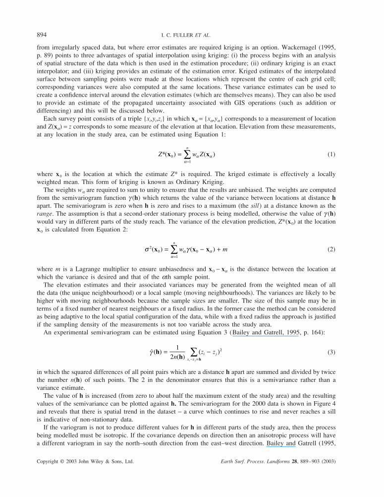
The value of h is increased (from zero to about half the maximum extent of the study area) and the resulting

values of the semivariance can be plotted against h. The semivariogram for the 2000 data is shown in Figure 4

and reveals that there is spatial trend in the dataset – a curve which continues to rise and never reaches a sill

is indicative of non-stationary data.

If the variogram is not to produce different values for h in different parts of the study area, then the process

being modelled must be isotropic. If the covariance depends on direction then an anisotropic process will have

a different variogram in say the north–south direction from the east–west direction. Bailey and Gatrell (1995,

REACH-SCALE SEDIMENT TRANSFERS 895

Copyright © 2003 John Wiley & Sons, Ltd. Earth Surf. Process. Landforms 28, 889–903 (2003)

Figure 4. Experimental semivariogram for the 2000 surveyed data

p. 180) indicate two varieties of anisotropy: geometric, in which the range changes with direction; and zonal,

in which the sill is dependent on direction. In the case of the relatively straight (and narrow) river reach under

study, anisotropy need not be considered problematic.

Drift

Whilst kriging assumes a second-order stationary process, measurements of gravel-bed river morphology

are rarely stationary in this sense, as the data will exhibit a slight downward trend between upstream and down-

stream measurements within a reach. The existence of drift means that the value of the semivariance depends

on where it has been estimated in the reach. This invalidates the assumption of stationarity and alternative

approaches to dealing with this should be considered. The drift may either be modelled with a linear model and

Ordinary Kriging applied to the residuals from the trend, or Universal Kriging may be used. If the former option

is chosen, the linear trend has then to be added back into the estimated DEM to produce the final surface (Bailey

and Gatrell, 1995). A suitable trend model is expressed in Equation 4:

z i* = α + βxi + γ yi + εi (4)

where xi and yi are the coordinates of the ith sample point whose elevation is zi, εi is a random error term, and

α, β, and γ are coefficients to be estimated.

However, modelling of a spatial process in this fashion can be problematic and should sensu strictu be under-

taken using a generalized least-squares estimate of the parameters α, β and γ, although ordinary regression may

suffice. In this case the trend has been modelled with ordinary least-square regression to give an indication

of the nature of the trend. The fitted values are shown in Table I. The residuals for each sample point form the

spatially detrended dataset.

Universal Kriging assumes that the z values are a combination of a deterministic component (drift), and a

random residual function which is itself assumed to exhibit second-order stationarity. The drift is often modelled

as either a linear or quadratic function of location. The spatial covariance structure may then be modelled with

a suitable semivariogram. Universal Kriging splits the random function into two components: the first is a

896 I. C. FULLER ET AL.

Copyright © 2003 John Wiley & Sons, Ltd. Earth Surf. Process. Landforms 28, 889–903 (2003)

deterministic component which represents the drift and the second is a random component which represents the

residual function. Kriging generally gives more precise predictions than those based on trend surface models

because the Universal Kriging weights are optimal (Cressie, 1990: 164). The ArcInfoTM Universal Kriging option

used here uses a linear trend model with a linear semivariogram model.

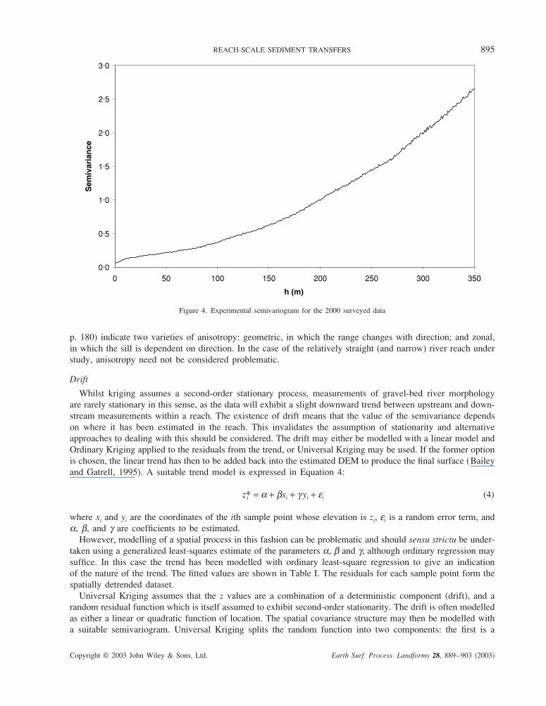
As a further check on whether the use of Universal Kriging was appropriate, the semivariogram for the

detrended data was estimated to determine whether it informally suggested stationarity in the variance estimate:

this semivariogram is shown in Figure 5. This semivariogram corresponds in shape to the ‘classic’ semivariogram

for a second-order stationary process which can be modelled (e.g. Wackernagel, 1995, p. 43). This semivariogram

exhibits a small nugget effect of about 0·06 m, and a sill at about 0·17 m at a range of about 50 m. The nugget

effect corresponds to measurement errors at small ranges, and a semivariance of 0·06 m corresponds to a

standard deviation of 0·035 m. This compares with the estimate of measurement error of 0·026 m by Brasington

et al. (2000).

Grid size

An important consideration in DEM generation and differencing is the grid size of the computed DEMs –

DEMs with finer grids take longer to compute than those with coarser grids, but volume estimates under finer

grids may be more accurate than those made under coarser grids, as coarse grid intervals may lead to the loss

of potentially important breaks in slope within the channel environment (Brasington et al., 2000). However,

Brasington and Richards (1998) suggest that the use of very fine grids may incorporate ‘spurious artefacts’

Table I. Parameter estimates for ordinary least-squares linear trend models

Survey date Intercept (α) Easting (β ) Northing (γ ) r2

1999 129·03 −0·004256 −0·004574 0·90842000 128·91 −0·004226 −0·004624 0·9057

Figure 5. Experimental semivariogram for the 2000 surveyed data after linear trend removal

REACH-SCALE SEDIMENT TRANSFERS 897

Copyright © 2003 John Wiley & Sons, Ltd. Earth Surf. Process. Landforms 28, 889–903 (2003)

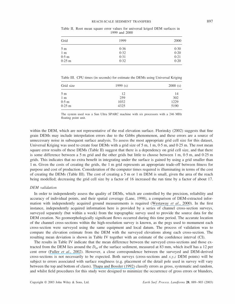
Table II. Root mean square error values for universal kriged DEM surfaces in1999 and 2000

Grid 1999 2000

5 m 0·36 0·301 m 0·32 0·200·5 m 0·31 0·210·25 m 0·32 0·20

within the DEM, which are not representative of the real elevation surface. Florinsky (2002) suggests that fine

grain DEMs may include interpolation errors due to the Gibbs phenomenon, and these errors are a source of

unnecessary noise in subsequent surface analysis. To assess the most appropriate grid cell size for this dataset,

Universal Kriging was used to create four DEMs with a grid size of 5 m, 1 m, 0·5 m, and 0·25 m. The root mean

square error results of these DEMs (Table II) suggest that there is a dependency on grid cell size, and that there

is some difference between a 5 m grid and the other grids but little to choose between 1 m, 0·5 m, and 0·25 m

grids. This indicates that no extra benefit in integrating under the surface is gained by using a grid smaller than

1 m. Given the costs of creating the grids, the 1 m grid represents an appropriate trade-off between fitness for

purpose and cost of production. Consideration of the computer times required is illuminating in terms of the cost

of creating the DEMs (Table III). The cost of creating a 5 m or 1 m DEM is small, given the area of the reach

being modelled; decreasing the grid cell size by a factor of 16 increased the run time by a factor of about 17.

DEM validation

In order to independently assess the quality of DEMs, which are controlled by the precision, reliability and

accuracy of individual points, and their spatial coverage (Lane, 1998), a comparison of DEM-extracted infor-

mation with independently acquired ground measurements is required (Westaway et al., 2000). In the first

instance, independently acquired information here is provided by a series of channel cross-section surveys,

surveyed separately (but within a week) from the topographic survey used to provide the source data for the

DEM creation. No geomorphologically significant flows occurred during this time period. The accurate location

of the channel cross-sections within the high-resolution survey is known, as the pegs used to monument each

cross-section were surveyed using the same equipment and local datum. The process of validation was to

compare the elevation estimate from the DEM with the surveyed elevations along each cross-section. The

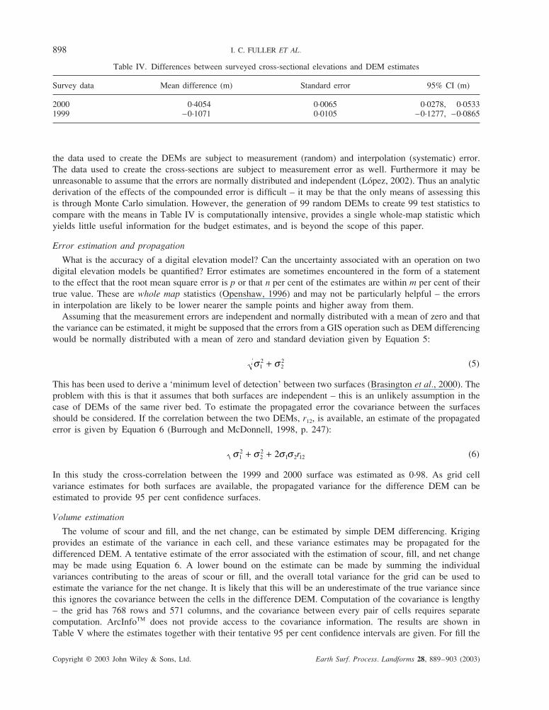
resulting mean deviation is shown in Table IV together with an estimate of the confidence interval (CI).

The results in Table IV indicate that the mean difference between the surveyed cross-sections and those ex-

tracted from the DEM lies around the D84 of the surface sediment, measured at 83 mm, which itself has a 12 per

cent error (Fuller et al., 2002). However, a close correspondence between the surveyed and DEM-derived

cross-sections is not necessarily to be expected. Both surveys (cross-sections and x,y,z DEM points) will be

subject to errors associated with surface roughness (e.g. placement of the detail pole used in survey will vary

between the top and bottom of clasts). Thapa and Bossler (1992) classify errors as gross, systematic and random,

and whilst field procedures for this study were designed to minimize the occurrence of gross errors or blunders,

Table III. CPU times (in seconds) for estimate the DEMs using Universal Kriging

Grid size 1999 (s) 2000 (s)

5 m 12 141 m 259 3020·5 m 1032 12290·25 m 4325 5190

The system used was a Sun Ultra SPARC machine with six processors with a 246 MHzfloating point unit.

898 I. C. FULLER ET AL.

Copyright © 2003 John Wiley & Sons, Ltd. Earth Surf. Process. Landforms 28, 889–903 (2003)

Table IV. Differences between surveyed cross-sectional elevations and DEM estimates

Survey data Mean difference (m) Standard error 95% CI (m)

2000 0·4054 0·0065 0·0278, 0·05331999 −0·1071 0·0105 −0·1277, −0·0865

the data used to create the DEMs are subject to measurement (random) and interpolation (systematic) error.

The data used to create the cross-sections are subject to measurement error as well. Furthermore it may be

unreasonable to assume that the errors are normally distributed and independent (López, 2002). Thus an analytic

derivation of the effects of the compounded error is difficult – it may be that the only means of assessing this

is through Monte Carlo simulation. However, the generation of 99 random DEMs to create 99 test statistics to

compare with the means in Table IV is computationally intensive, provides a single whole-map statistic which

yields little useful information for the budget estimates, and is beyond the scope of this paper.

Error estimation and propagation

What is the accuracy of a digital elevation model? Can the uncertainty associated with an operation on two

digital elevation models be quantified? Error estimates are sometimes encountered in the form of a statement

to the effect that the root mean square error is p or that n per cent of the estimates are within m per cent of their

true value. These are whole map statistics (Openshaw, 1996) and may not be particularly helpful – the errors

in interpolation are likely to be lower nearer the sample points and higher away from them.

Assuming that the measurement errors are independent and normally distributed with a mean of zero and that

the variance can be estimated, it might be supposed that the errors from a GIS operation such as DEM differencing

would be normally distributed with a mean of zero and standard deviation given by Equation 5:

σ σ1

222+ (5)

This has been used to derive a ‘minimum level of detection’ between two surfaces (Brasington et al., 2000). The

problem with this is that it assumes that both surfaces are independent – this is an unlikely assumption in the

case of DEMs of the same river bed. To estimate the propagated error the covariance between the surfaces

should be considered. If the correlation between the two DEMs, r12, is available, an estimate of the propagated

error is given by Equation 6 (Burrough and McDonnell, 1998, p. 247):

σ σ σ σ1

222

1 2 122+ + r (6)

In this study the cross-correlation between the 1999 and 2000 surface was estimated as 0·98. As grid cell

variance estimates for both surfaces are available, the propagated variance for the difference DEM can be

estimated to provide 95 per cent confidence surfaces.

Volume estimation

The volume of scour and fill, and the net change, can be estimated by simple DEM differencing. Kriging

provides an estimate of the variance in each cell, and these variance estimates may be propagated for the

differenced DEM. A tentative estimate of the error associated with the estimation of scour, fill, and net change

may be made using Equation 6. A lower bound on the estimate can be made by summing the individual

variances contributing to the areas of scour or fill, and the overall total variance for the grid can be used to

estimate the variance for the net change. It is likely that this will be an underestimate of the true variance since

this ignores the covariance between the cells in the difference DEM. Computation of the covariance is lengthy

– the grid has 768 rows and 571 columns, and the covariance between every pair of cells requires separate

computation. ArcInfoTM does not provide access to the covariance information. The results are shown in

Table V where the estimates together with their tentative 95 per cent confidence intervals are given. For fill the

REACH-SCALE SEDIMENT TRANSFERS 899

Copyright © 2003 John Wiley & Sons, Ltd. Earth Surf. Process. Landforms 28, 889–903 (2003)

Table V. Net volumes between 1999 and 2000 DEMs compared with gains and losses derived from a cross-section-basedmorphological budget for the same period; 95 per cent confidence interval computed from kriged variance estimates

DEM volume (m3) Confidence interval Cross-section volume (m3)

Gain 1539 1388–1689 1227Loss 9423 9129–9716 2177Net change −7884 −8213 to −7554 −950

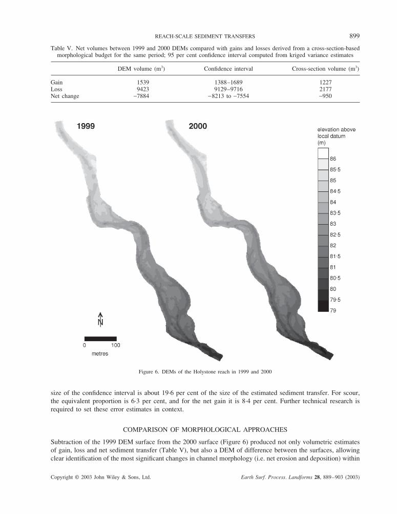
Figure 6. DEMs of the Holystone reach in 1999 and 2000

size of the confidence interval is about 19·6 per cent of the size of the estimated sediment transfer. For scour,

the equivalent proportion is 6·3 per cent, and for the net gain it is 8·4 per cent. Further technical research is

required to set these error estimates in context.

COMPARISON OF MORPHOLOGICAL APPROACHES

Subtraction of the 1999 DEM surface from the 2000 surface (Figure 6) produced not only volumetric estimates

of gain, loss and net sediment transfer (Table V), but also a DEM of difference between the surfaces, allowing

clear identification of the most significant changes in channel morphology (i.e. net erosion and deposition) within

900 I. C. FULLER ET AL.

Copyright © 2003 John Wiley & Sons, Ltd. Earth Surf. Process. Landforms 28, 889–903 (2003)

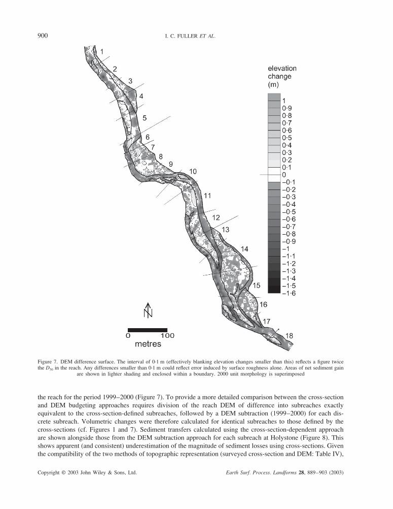
Figure 7. DEM difference surface. The interval of 0·1 m (effectively blanking elevation changes smaller than this) reflects a figure twicethe D50 in the reach. Any differences smaller than 0·1 m could reflect error induced by surface roughness alone. Areas of net sediment gain

are shown in lighter shading and enclosed within a boundary. 2000 unit morphology is superimposed

the reach for the period 1999–2000 (Figure 7). To provide a more detailed comparison between the cross-section

and DEM budgeting approaches requires division of the reach DEM of difference into subreaches exactly

equivalent to the cross-section-defined subreaches, followed by a DEM subtraction (1999–2000) for each dis-

crete subreach. Volumetric changes were therefore calculated for identical subreaches to those defined by the

cross-sections (cf. Figures 1 and 7). Sediment transfers calculated using the cross-section-dependent approach

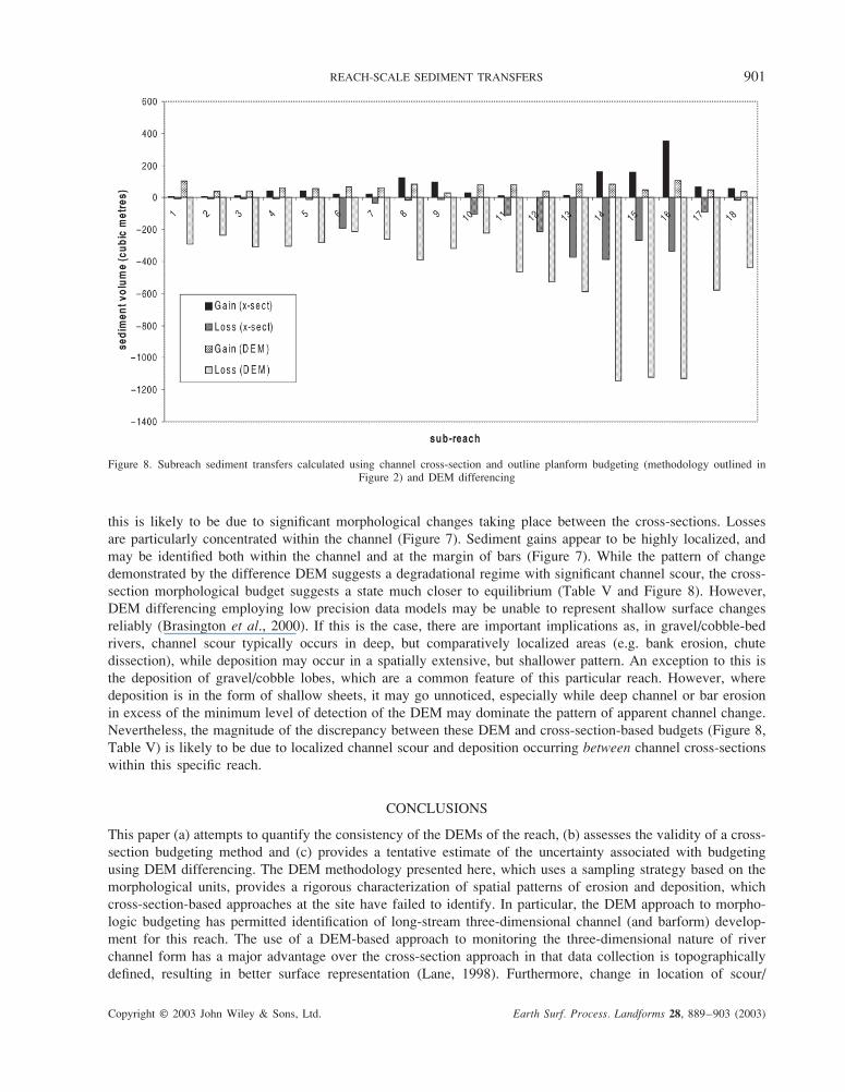
are shown alongside those from the DEM subtraction approach for each subreach at Holystone (Figure 8). This

shows apparent (and consistent) underestimation of the magnitude of sediment losses using cross-sections. Given

the compatibility of the two methods of topographic representation (surveyed cross-section and DEM: Table IV),

REACH-SCALE SEDIMENT TRANSFERS 901

Copyright © 2003 John Wiley & Sons, Ltd. Earth Surf. Process. Landforms 28, 889–903 (2003)

Figure 8. Subreach sediment transfers calculated using channel cross-section and outline planform budgeting (methodology outlined inFigure 2) and DEM differencing

this is likely to be due to significant morphological changes taking place between the cross-sections. Losses

are particularly concentrated within the channel (Figure 7). Sediment gains appear to be highly localized, and

may be identified both within the channel and at the margin of bars (Figure 7). While the pattern of change

demonstrated by the difference DEM suggests a degradational regime with significant channel scour, the cross-

section morphological budget suggests a state much closer to equilibrium (Table V and Figure 8). However,

DEM differencing employing low precision data models may be unable to represent shallow surface changes

reliably (Brasington et al., 2000). If this is the case, there are important implications as, in gravel/cobble-bed

rivers, channel scour typically occurs in deep, but comparatively localized areas (e.g. bank erosion, chute

dissection), while deposition may occur in a spatially extensive, but shallower pattern. An exception to this is

the deposition of gravel/cobble lobes, which are a common feature of this particular reach. However, where

deposition is in the form of shallow sheets, it may go unnoticed, especially while deep channel or bar erosion

in excess of the minimum level of detection of the DEM may dominate the pattern of apparent channel change.

Nevertheless, the magnitude of the discrepancy between these DEM and cross-section-based budgets (Figure 8,

Table V) is likely to be due to localized channel scour and deposition occurring between channel cross-sections

within this specific reach.

CONCLUSIONS

This paper (a) attempts to quantify the consistency of the DEMs of the reach, (b) assesses the validity of a cross-

section budgeting method and (c) provides a tentative estimate of the uncertainty associated with budgeting

using DEM differencing. The DEM methodology presented here, which uses a sampling strategy based on the

morphological units, provides a rigorous characterization of spatial patterns of erosion and deposition, which

cross-section-based approaches at the site have failed to identify. In particular, the DEM approach to morpho-

logic budgeting has permitted identification of long-stream three-dimensional channel (and barform) develop-

ment for this reach. The use of a DEM-based approach to monitoring the three-dimensional nature of river

channel form has a major advantage over the cross-section approach in that data collection is topographically

defined, resulting in better surface representation (Lane, 1998). Furthermore, change in location of scour/

902 I. C. FULLER ET AL.

Copyright © 2003 John Wiley & Sons, Ltd. Earth Surf. Process. Landforms 28, 889–903 (2003)

deposition from the originally identified ‘sensitive’ areas, which directed cross-section location, may account

for some errors, as whilst cross-sections were carefully selected at the outset of the investigation in 1997, these

positions remain fixed, irrespective of later channel development and shifts in areas of activity. The consequence

of this dynamism was such that by 2000, some cross-sections were no longer effectively identifying geomor-

phological activity in the Coquet channel. This does not suggest that cross-section-derived budgets as a whole

have a tendency to underestimate losses, but rather reflects local processes operating within the Holystone reach

during the survey period, and may well be a function of cross-section spacing at this site.

Lane et al. (1994) suggest that much more detailed information on river bed topography is needed to

accommodate the increasing recognition of spatially distributed form–process feedback in fluvial environ-

ments and to provide a more rigorous linkage between channel topography and sediment transport processes.

The use of DEMs in a 1 km reach of the River Coquet at Holystone provides a much improved representa-

tion of channel morphology, and in the context of morphological budgeting, a more reliable means of linking

changes in channel morphology with sediment transport processes. Furthermore, this paper demonstrates

that DEMs of the channel topography may be a reliable representation of morphological units (within the

limitations imposed by surface sediment characteristics), and can be used not only to estimate volumes of

sediment transfer up to the 1 km reach scale, but also to quantify the uncertainty associated with these estimates.

Uncertainty can be viewed as one component of DEM reliability and this paper provides some initial steps

towards dealing with this in the context of morphological budgeting. The results here point to the need for

a more explicit consideration of error propagation in the production of morphological sediment budgets for

gravel-bed rivers.

ACKNOWLEDGEMENTS

We thank Mr Guy Renwick and Mr Brian Little for granting access to the reach. We also thank Ann Rooke for

drafting Figures 1 and 2. I.C.F. acknowledges financial support for fieldwork from 1996 RAE monies to the

Division of Geography & Environmental Management, University of Northumbria. Chris Brunsdon provided

helpful statistical advice. We acknowledge the helpful comments of two anonymous referees.

REFERENCES

Ashmore PE, Church MA. 1998. Sediment transport and river morphology: a paradigm for study. In Gravel-Bed Rivers in the Environment,Klingemann PC, Beschta RL, Komar PD, Bradley JB (eds). Water Resources Publications: Highlands Ranch, Colorado; 115–148.

Bailey TC, Gatrell, AC. 1995. Interactive Spatial Data Analysis. Longman: Harlow.Brasington J, Richards KS. 1998. Interactions between model predictions, parameters and DTM scales for TOPMODEL. Computers and

Geosciences 24: 299–314.Brasington J, Rumsby BT, McVey RA. 2000. Monitoring and modelling morphological change in a braided gravel-bed river using high

resolution GPS-based survey. Earth Surface Processes and Landforms 25: 973–990.Brewer PA, Passmore DG. 2002. Sediment budgeting techniques in gravel bed rivers. In Sediment Flux to Basins: Causes, Controls and

Consequences, Jones S, Frostick, LE (eds) Special Publication 191. Geological Society: London; 97–113.Burrough PA, McDonnell RA. 1998. Principles of Geographical Information Systems. Oxford University Press: Oxford.Cressie NEC. 1993. Statistics for Spatial Data. Wiley: New York.Davies THR. 1987. Problems of bedload transport in braided gravel-bed rivers. In Sediment Transport in Gravel-Bed Rivers, Thorne CR,

Bathurst JC, Hey RD (eds). Wiley: Chichester; 793–828.Eaton BC, Lapointe MF. 2001. Effects of large floods on sediment transport and reach morphology in the cobble-bed Sainte Marguerite

River. Geomorphology 40: 291–309.Ferguson RI, Ashworth PJ. 1992. Spatial patterns of bedload transport and channel change in braided and near braided rivers. In Dynamics

of Gravel-bed Rivers, Billi P, Hey RD, Thorne CR, Tacconi P (eds). Wiley: Chichester; 477–496.Ferguson RI, Werritty A. 1983. Bar development and channel changes in the gravelly River Feshie. In Modern and Ancient Fluvial Systems,

Collinson JD, Lewin J (eds). Special Publication 6. International Association of Sedimentologists: 133–143.Ferguson RI, Ashmore PE, Ashworth PJ, Paola C, Prestegaard KL. 1992. Measurements in a braided river chute and lobe, I, flow pattern,

sediment transport and channel change. Water Resources Research 28: 1877–1886.Florinsky IV. 2002. Errors of signal processing in digital terrain modeling. International Journal of Geographical Information Science 16:

475–502.Fuller IC, Passmore DG, Heritage GL, Large ARG, Milan DJ, Brewer PA. 2002. Annual sediment budgets in an unstable gravel bed river:

the River Coquet, northern England. In Sediment Flux to Basins: Causes, Controls and Consequences, Jones S, Frostick, LE (eds) SpecialPublication 191. Geological Society: London; 115–131.

Goff JR, Ashmore PE. 1994. Gravel transport and morphological change in braided Sunwapta river, Alberta, Canada. Earth Surface

Processes and Landforms 19: 195–213.

REACH-SCALE SEDIMENT TRANSFERS 903

Copyright © 2003 John Wiley & Sons, Ltd. Earth Surf. Process. Landforms 28, 889–903 (2003)

Ham DG, Church M. 2000. Bed-material transport estimated from channel morphodynamics: Chilliwack River, British Columbia. Earth

Surface Processes and Landforms 25: 1123–1142.Heritage GL, Fuller IC, Charlton ME, Brewer PA, Passmore DG. 1998. CDW photogrammetry of low relief fluvial features: accuracy and

implications for reach-scale sediment budgeting. Earth Surface Processes and Landforms 23: 1219–1233.Hubbell D. 1987. Bed load sampling and analysis. In Sediment Transport in Gravel-Bed Rivers, Thorne CR, Bathurst JC, Hey RD (eds).

Wiley: Chichester; 89–118.Lane SN. 1998. The use of digital terrain modelling in the understanding of dynamic river channel systems. In Landform Monitoring,

Modelling & Analysis, Lane SN, Richards KS, Chandler JH (eds). John Wiley & Sons: Chichester; 311–342.Lane SN. 2001. The measurement of gravel-bed river morphology.� In Gravel-bed Rivers V, Mosley MP (ed.). New Zealand Hydrological

Society: Wellington; 291–320.Lane SN, Chandler JH, Richards KS. 1994. Developments in monitoring and terrain modelling small-scale river-bed topography. Earth

Surface Processes and Landforms 19: 349–368.Lindsay JB, Ashmore PE. 2002. The effects of survey frequency on estimates of scour and fill in a braided river model. Earth Surface

Processes and Landforms 27: 27–43.López C. 2002. An experiment of the elevation accuracy of photogrammetrically derived DEM. International Journal of Geographical

Information Science 16: 361–376.Martin Y, Church M. 1995. Bed-material transport estimated from channel surveys: Vedder River, British Columbia. Earth Surface Pro-

cesses and Landforms 20: 347–361.Milne JA, Sear DA. 1997. Modelling river channel topography using GIS. International Journal of Geographical Information Science 11:

499–519.Naden P, Brayshaw AC. 1987. Bedforms in gravel-bed rivers. In River Channels: Environment and Process, Richards KS (ed). IBG Special

Publication 18. Blackwell: Oxford; 249–271.Nanson GC, Croke JC. 1992. A genetic classification of floodplains. Geomorphology 4: 459–486.Neill CR. 1987. Sediment balance considerations linking long-term transport and channel processes. In Sediment Transport in Gravel-Bed

Rivers, Thorne CR, Bathurst JC, Hey RD (eds). Wiley: Chichester; 225–240.Openshaw S. 1996. Developing GIS-relevant zone-based spatial analysis methods. In Spatial Analysis: Modelling in a GIS Environment,

Longley P, Batty M (eds). Wiley: New York; 55–73.Paige AD, Hickin EJ. 2000. Annual bed-elevation regime in the alluvial channel of Squamish River, southwestern British Columbia, Canada.

Earth Surface Processes and Landforms 25: 991–1009.Thapa K, Bossler J. 1992. Accuracy of spatial data used in Geographic Information Systems. Photogrammetric Engineering and Remote

Sensing 58: 835–841.Wackernagel H. 1995. Multivariate Geostatistics. Springer-Verlag: Berlin.Wathen SJ, Hoey TB, Werritty A. 1997. Quantitative determination of the activity of within-reach sediment storage in a small gravel-bed

river using transit time and response time. Geomorphology 20: 113–134.Westaway RM, Lane SN, Hicks DM. 2000. The development of an automated correction procedure for digital photogrammetry for the study

of wide, shallow, gravel-bed rivers. Earth Surface Processes and Landforms 25: 209–226.Wittenberg L. 2002. Structural patterns in coarse gravel river beds: typology, survey and assessment of the roles of grain size and river

regime. Geografiska Annaler 84A: 25–37.