Processing Event-Monitoring Queries in Sensor Networks

Vassilis StoumposUniversity of Athens

Athens, Greecestoumpos@di.uoa.gr

Antonios DeligiannakisUniversity of Athens

Athens, Greeceadeli@di.uoa.gr

Yannis KotidisAthens University of

Economics and Businesskotidis@aueb.gr

Alex DelisUniversity of Athens

Athens, Greecead@di.uoa.gr

Abstract

In this paper we present algorithms for building andmaintaining efficient collection trees that provide the con-duit to disseminate data required for processing monitor-ing queries in a wireless sensor network. While prior tech-niques base their operation on the assumption that the sen-sor nodes that collect data relevant to a specified queryneed to include their measurements in the query result atevery query epoch, in many event monitoring applicationssuch an assumption is not valid. We introduce and formal-ize the notion of event monitoring queries and demonstratethat they can capture a large class of monitoring applica-tions. We then show techniques which, using a small set ofintuitive statistics, can compute collection trees that mini-mize important resources such as the number of messagesexchanged among the nodes or the overall energy consump-tion. Our experiments demonstrate that our techniques canorganize the data collection process while utilizing signifi-cantly lower resources than prior approaches.

1 IntroductionMany pervasive applications rely on sensory devices that

are able to observe their environment and perform simplecomputational tasks. Driven by constant advances in mi-croelectronics and the economy of scale it is becoming in-creasingly clear that our future will incorporate a plethora ofsuch sensing devices that will participate and help us in ourdaily activities. Even though each sensor node will be ratherlimited in terms of storage, processing and communicationcapabilities, they will be able to accomplish complex tasksthrough intelligent collaboration.

Nevertheless, building a viable sensory infrastructurecannot be achieved through mass production and deploy-ment of such devices without addressing first the techni-cal challenges of managing such networks. In this paperwe focus in developing the necessary data collection infras-tructure for supporting data-hungry applications that needto acquire and process readings from a large scale sensornetwork. While previous work has focused on optimizingspecific types of queries such as aggregate [13], join [2],model-based [8, 12] and select-all [7, 19] queries, we pro-pose a data dissemination framework that can address the

needs of multiple, concurrent data acquisition requests in anefficient manner.

It is generally agreed that one cannot simply move thereadings necessary for processing an application request outof the network and then perform the required processing ina designated node such as abase station. Wireless sensornodes have limited energy capacity and such an approachwill not only result in overburdening their radio links, butwill also quickly drain their energy as radio transmission isby far the most important factor in energy consumption [14].Thus, most recent proposals rely on building some type ofad-hoc interconnect for answering a query such as theag-gregation tree[13, 24]. This is a paradigm of in-networkprocessing that can be applied to non-aggregate queries aswell [7]. In this paper we concentrate on building and main-taining efficientdata collection treesthat will provide theconduit to disseminate all data required for processing manyconcurrent queries in a sensor network, including long-termand ad-hoc type of queries, while minimizing important re-sources such as the number of messages exchanged amongthe nodes or the overall energy consumption.

While prior work [4, 20, 22] has also tackled similarproblems, previous techniques base their operation on theassumption that the sensor nodes that collect data relevantto the specified query need to include their measurements(and, thus, perform transmissions) in the query result at ev-ery queryepoch. However, in many monitoring applicationssuch an assumption is not valid. Monitoring nodes are of-ten interested in obtaining either the actual readings, or theiraggregate values, from sensor nodes that detect interestingevents. The detection of such events can often be identifiedby the readings of each sensor node. For example, in vehicletracking and monitoring applications high noise levels mayindicate the proximity of a vehicle. In military applications,high levels of detected chemicals can be used to warn nearbytroops. In other applications, as in the case of approximateevaluation of queries over the sensor data [6, 15, 18], anevent is defined when the current sensor reading deviates bymore than a given threshold from the last transmitted value.In all of these scenarios, each sensor node is not forced toinclude its measurements in the query output at each epoch,but rather such aquery participationis evaluated on a perepoch basis, depending on its readings and the definition

1

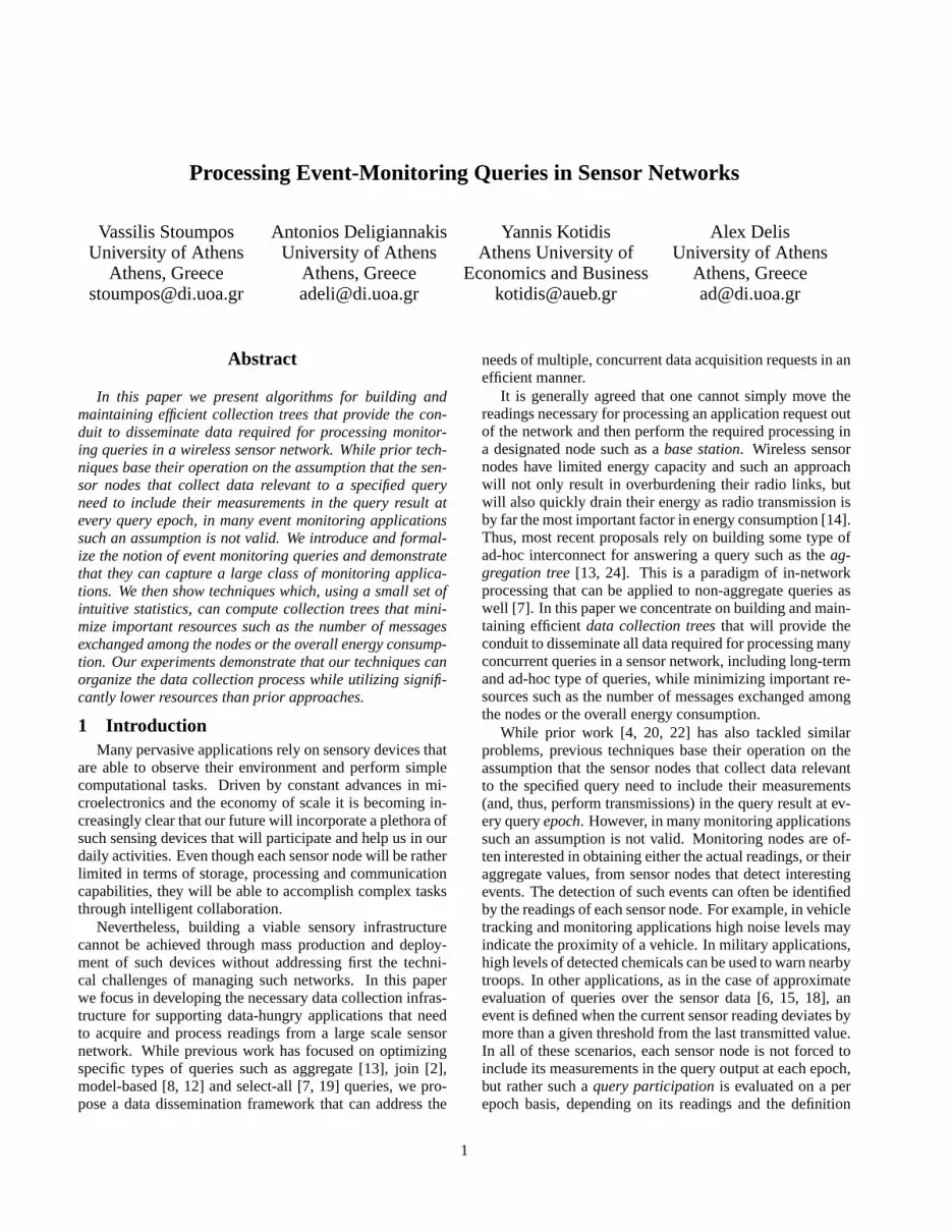
Aggregate Query Non-Aggregate Query

SELECT AggrFun(s.value) SELECT s.id, s.valueFROM Sensors s FROM Sensors sWHERE inclusionConditions(s) = trueWHERE inclusionConditions(s) = trueSAMPLE PERIOD e FOR t SAMPLE PERIOD e FOR t

Table 1: An Aggregate and a non-Aggregate Queryover the Values Collected by the Sensor Nodes.

of interesting events. In this paper we term the monitoringqueries where the participation of a node is based on the de-tection of an event of interest asevent monitoring queries(EMQs).

Our techniques base their operation on collecting sim-ple statistics during the operation of the sensor nodes. Thecollected statistics involve the number of events (or, equiv-alently, their frequency) that each sensor detected in the re-cent past. Our algorithms utilize these statistics as hints forthe behavior of each sensor in the near future and periodi-cally reorganize the collection tree in order to minimize cer-tain metrics of interest, such as the overall number of trans-missions or the overall energy consumption in the network.Our contributions are summarized as follows:

1. We introduce the notion of EMQs in sensor networks.EMQs are a superset of existing monitoring queries, but arehandled uniformly in our framework, irrespectively of theminimization metric of interest.2. We present detailed algorithms for minimizing impor-tant network resources such as the number of messages ex-changed or the energy consumption during the execution ofan EMQ. The presented algorithms are based on the collec-tion and transmission of a small, and of constant size, set ofstatistics. We introduce our algorithms along with a succinctmathematical justification.3. We extend our framework for the case of multiple con-current EMQs of different types.4. We present a detailed experimental evaluation of our al-gorithms. Our results demonstrate that our techniques canachieve a significant reduction in the number of transmittedmessages, or the overall energy consumption, compared toalternative algorithms.

2 Motivational ExampleIn Table 1 we present examples of the two main classes of

monitoring queries in sensor networks. We borrow the syn-tax of TinyOS [13] to denote the epoch duration (e) and thelifetime of the query (t). The predicateinclusionConditionshas been added in order to specify which sensor nodes willparticipate in the query evaluation per epoch. At each queryepoch, all the sensor nodes that include their collected datain the query result are termed in our framework asepochparticipating nodes. For queries that wish to collect datafrom all the sensor nodes at each epoch, the above predicatealways evaluates totrue.

When a monitoring query specifies inclusion predicates,these may contain either static or dynamic predicates (or

both) regarding the sensor nodes. Examples of static pred-icates may involve, but are not limited to, the collection ofmeasurements from: (i) Sensors with specific identifiers; (ii)Immobile sensors in a specific area; or (iii) Sensors moni-toring a specific quantity, in cases of sensor networks withdiverse types of sensor nodes that monitor different quan-tities. Static predicates are very useful in a variety of ap-plications and have received the focus of the bulk of pastresearch [13, 24].

However, there is a large class of monitoring queries thatcannot be expressed using static inclusion conditions. Ex-amples include vehicle tracking and equipment monitoringapplications where inclusion predicates need to be condi-tioned on readings taken by the sensor nodes such as noiselevels or temperature readings. In its most simple forma dynamic inclusion predicate may be a condition of theform “current reading> threshold”. More complex formsmay require the evaluation of a user defined function overa history of accumulated readings. We call such predicates,whose evaluation depends also on the readings taken by thenodes, as dynamic predicates as they specify which nodesshould include their response in the query evaluation at eachepoch (i.e., nodes whose values exceed a given threshold,or deviate significantly from previous readings). We termthose monitoring queries that contain dynamic predicatesasevent monitoring queries(EMQs). Given a monitoringquery, existing techniques seek to developcollection treesthat specify the way that the data is forwarded from the sen-sor nodes to theRoot node. Periodically these collectiontrees may be reorganized in order to adapt to evolving datacharacteristics [18].

An important characteristic of EMQs, which is not takeninto account by existing algorithms that design collectiontrees, is that each sensor node may participate in the queryevaluation, by including its reading in the query result, onlya limited number of times, based on how often the inclu-sion conditions are satisfied. We can thus associate anepochparticipation frequency Pi with each sensor nodeSi , whichspecifies the fraction of epochs that this node participated inthe query result in the recent past.

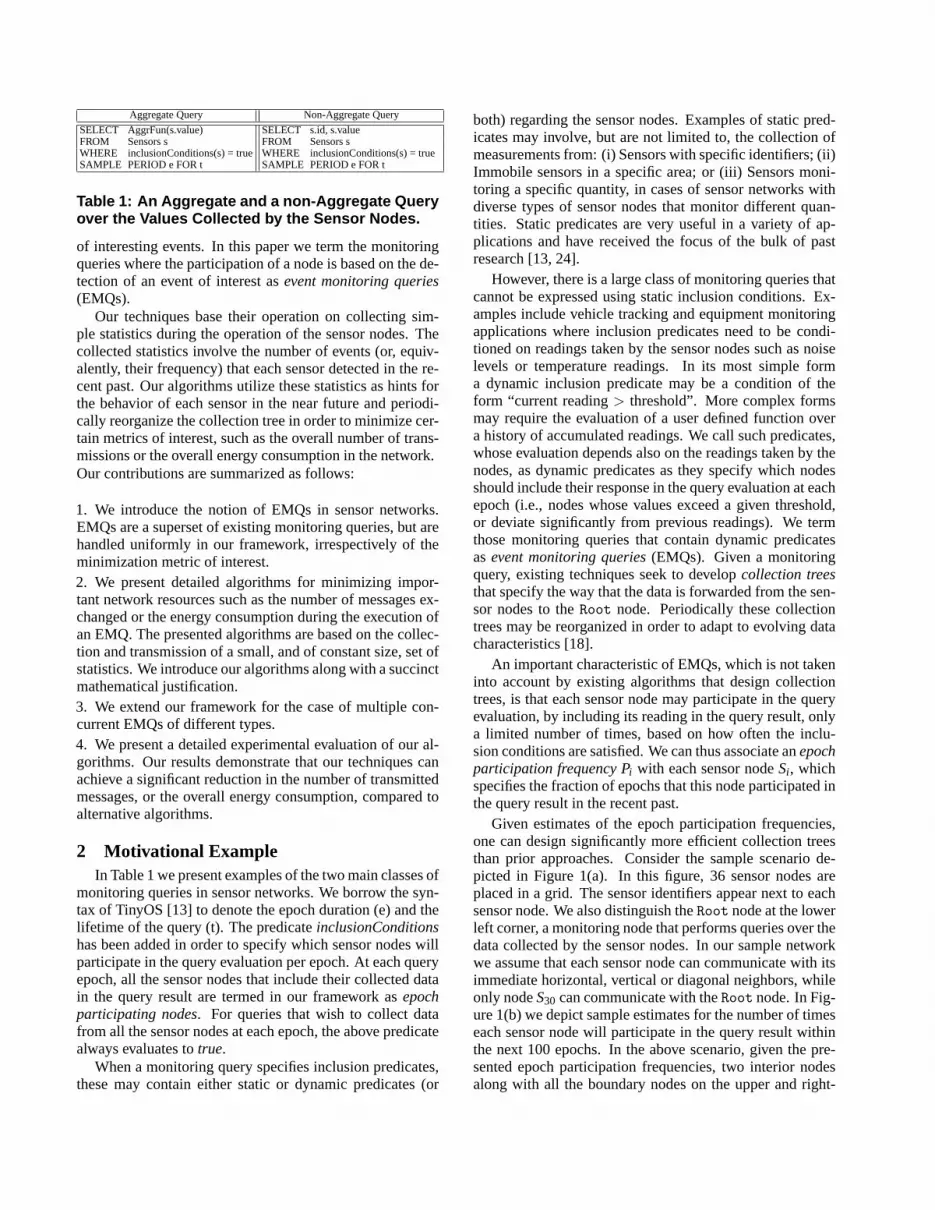
Given estimates of the epoch participation frequencies,one can design significantly more efficient collection treesthan prior approaches. Consider the sample scenario de-picted in Figure 1(a). In this figure, 36 sensor nodes areplaced in a grid. The sensor identifiers appear next to eachsensor node. We also distinguish theRoot node at the lowerleft corner, a monitoring node that performs queries over thedata collected by the sensor nodes. In our sample networkwe assume that each sensor node can communicate with itsimmediate horizontal, vertical or diagonal neighbors, whileonly nodeS30 can communicate with theRoot node. In Fig-ure 1(b) we depict sample estimates for the number of timeseach sensor node will participate in the query result withinthe next 100 epochs. In the above scenario, given the pre-sented epoch participation frequencies, two interior nodesalong with all the boundary nodes on the upper and right-

(a) (b) (c) (d)

Figure 1: (a) Identifiers of sensors in grid arrangement; (b) Estimated number of participations in queryresult in 100 epochs; (c) Collection tree for MinHops algorithm. Cost = 3130 transmissions; (d) Collectiontree for our algorithm. Cost = 1900 transmissions.

most edges of the network always detect events, while theremaining interior nodes detect events with a lower prob-ability, whose average value is about 5%. For the afore-mentioned sample scenario, in Figure 1(c) we depict a sam-ple collection tree chosen by an algorithm, termed asMin-Hops that seeks to minimize the number of hops that eachnode’s data needs to traverse until it reaches theRoot node.Next to each node we depict the actual number of transmis-sions that each node performed within these 100 epochs.Similarly, in Figure 1(d) we present the collection tree thatour algorithms created for the evaluation of the SUM aggre-gate. A significant observation is that our algorithm seeksto forward the query results from nodes with high epochparticipation frequencies through a limited number of inte-rior nodes, compared to theMinHopsalgorithm. One caneasily establish the significant reduction in the number oftransmissions that our algorithm achieved (1900 vs 3130 or,equivalently, a 65% reduction).

3 Problem FormulationWe first introduce the types of EMQs that our framework

supports and then present the optimization problems tackledin this paper. We then present the cost model used in ouralgorithms in order to estimate the energy consumption of asensor node during the transmission process.

3.1 Supported Queries

In Table 1 we presented the two main classes of SQLqueries that our framework supports. It is important to em-phasize at this point that even non-participating nodes maytake part in the query evaluation process by forwarding mes-sages towards theRoot node. However, the collected val-ues of non-participating nodes influence neither the reportedquery result nor its size.

The first class of supported queries involve non-aggregate queries over the values of epoch participating sen-sor nodes. In this type of queries the amount of data trans-mitted by any node of the collection tree depends on thenumber of epoch-participating sensors that are descendantsof that sensor node.

The second class of supported queries involves aggregatefunctions over the measurements collected by the participat-

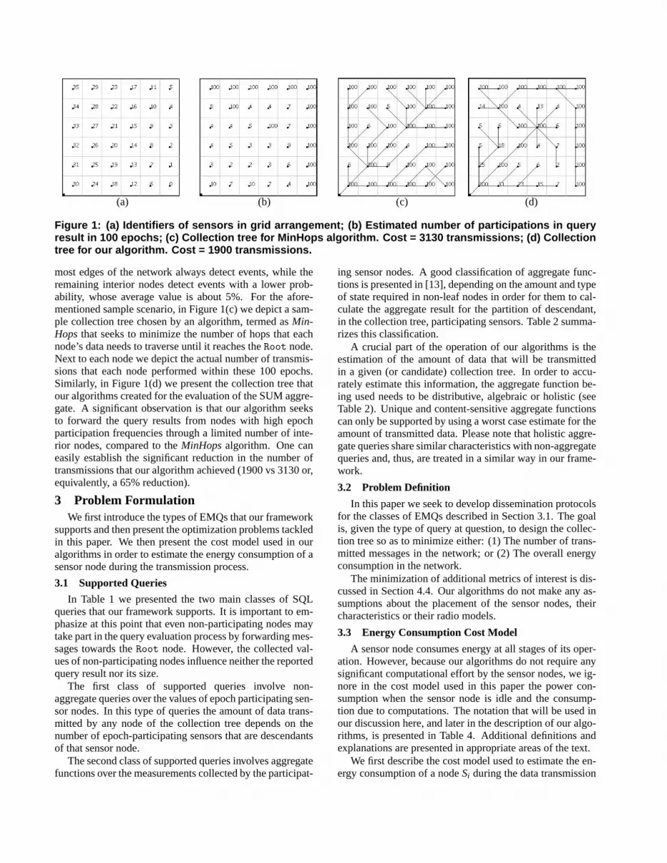
ing sensor nodes. A good classification of aggregate func-tions is presented in [13], depending on the amount and typeof state required in non-leaf nodes in order for them to cal-culate the aggregate result for the partition of descendant,in the collection tree, participating sensors. Table 2 summa-rizes this classification.

A crucial part of the operation of our algorithms is theestimation of the amount of data that will be transmittedin a given (or candidate) collection tree. In order to accu-rately estimate this information, the aggregate function be-ing used needs to be distributive, algebraic or holistic (seeTable 2). Unique and content-sensitive aggregate functionscan only be supported by using a worst case estimate for theamount of transmitted data. Please note that holistic aggre-gate queries share similar characteristics with non-aggregatequeries and, thus, are treated in a similar way in our frame-work.

3.2 Problem Definition

In this paper we seek to develop dissemination protocolsfor the classes of EMQs described in Section 3.1. The goalis, given the type of query at question, to design the collec-tion tree so as to minimize either: (1) The number of trans-mitted messages in the network; or (2) The overall energyconsumption in the network.

The minimization of additional metrics of interest is dis-cussed in Section 4.4. Our algorithms do not make any as-sumptions about the placement of the sensor nodes, theircharacteristics or their radio models.

3.3 Energy Consumption Cost Model

A sensor node consumes energy at all stages of its oper-ation. However, because our algorithms do not require anysignificant computational effort by the sensor nodes, we ig-nore in the cost model used in this paper the power con-sumption when the sensor node is idle and the consump-tion due to computations. The notation that will be used inour discussion here, and later in the description of our algo-rithms, is presented in Table 4. Additional definitions andexplanations are presented in appropriate areas of the text.

We first describe the cost model used to estimate the en-ergy consumption of a nodeSi during the data transmission

Category Type of Partial State Needed State Size Examples

Distributive Aggregate values for descendants Constant MAX, MIN, COUNT, SUMAlgebraic Aggregate values for descendants, Constant AVG

but for different aggregate functionHolistic Entire Data of descendants Proportional to MEDIAN

#epoch-participating descendantsUnique Distinct Values of descendants Data-Dependent COUNT DISTINCT

Content-Sensitive Aggregate-Specific Data-Dependent Histogram of Values

Table 2. Characteristics and Examples of Aggregate Function Types.

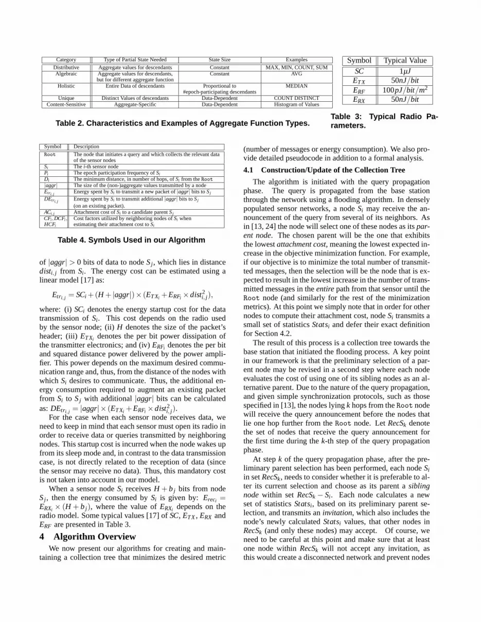
Symbol Typical ValueSC 1µJETX 50nJ/bitERF 100pJ/bit/m2

ERX 50nJ/bit

Table 3: Typical Radio Pa-rameters.

Symbol Description

Root The node that initiates a query and which collects the relevant dataof the sensor nodes

Si The i-th sensor nodePi The epoch participation frequency ofSi

Di The minimum distance, in number of hops, ofSi from theRoot|aggr| The size of the (non-)aggregate values transmitted by a nodeEtri, j Energy spent bySi to transmit a new packet of|aggr| bits toSj

DEtri, j Energy spent bySi to transmit additional|aggr| bits toSj

(on an existing packet).ACi, j Attachment cost ofSi to a candidate parentSj

CFi ,DCFi , Cost factors utilized by neighboring nodes ofSi whenHCFi estimating their attachment cost toSi

Table 4. Symbols Used in our Algorithm

of |aggr| > 0 bits of data to nodeSj , which lies in distancedisti, j from Si . The energy cost can be estimated using alinear model [17] as:

Etr i, j = SCi +(H + |aggr|)× (ETXi +ERFi ×dist2i, j),

where: (i)SCi denotes the energy startup cost for the datatransmission ofSi . This cost depends on the radio usedby the sensor node; (ii)H denotes the size of the packet’sheader; (iii)ETXi denotes the per bit power dissipation ofthe transmitter electronics; and (iv)ERFi denotes the per bitand squared distance power delivered by the power ampli-fier. This power depends on the maximum desired commu-nication range and, thus, from the distance of the nodes withwhich Si desires to communicate. Thus, the additional en-ergy consumption required to augment an existing packetfrom Si to Sj with additional|aggr| bits can be calculatedas:DEtr i, j = |aggr|× (ETXi +ERFi ×dist2i, j).

For the case when each sensor node receives data, weneed to keep in mind that each sensor must open its radio inorder to receive data or queries transmitted by neighboringnodes. This startup cost is incurred when the node wakes upfrom its sleep mode and, in contrast to the data transmissioncase, is not directly related to the reception of data (sincethe sensor may receive no data). Thus, this mandatory costis not taken into account in our model.

When a sensor nodeSi receivesH + b j bits from nodeSj , then the energy consumed bySi is given by: Ereci =ERXi × (H + b j), where the value ofERXi depends on theradio model. Some typical values [17] ofSC, ETX, ERX andERF are presented in Table 3.

4 Algorithm OverviewWe now present our algorithms for creating and main-

taining a collection tree that minimizes the desired metric

(number of messages or energy consumption). We also pro-vide detailed pseudocode in addition to a formal analysis.

4.1 Construction/Update of the Collection Tree

The algorithm is initiated with the query propagationphase. The query is propagated from the base stationthrough the network using a flooding algorithm. In denselypopulated sensor networks, a nodeSi may receive the an-nouncement of the query from several of its neighbors. Asin [13, 24] the node will select one of these nodes as itspar-ent node. The chosen parent will be the one that exhibitsthe lowestattachment cost, meaning the lowest expected in-crease in the objective minimization function. For example,if our objective is to minimize the total number of transmit-ted messages, then the selection will be the node that is ex-pected to result in the lowest increase in the number of trans-mitted messages in theentirepath from that sensor until theRoot node (and similarly for the rest of the minimizationmetrics). At this point we simply note that in order for othernodes to compute their attachment cost, nodeSi transmits asmall set of statisticsStatsi and defer their exact definitionfor Section 4.2.

The result of this process is a collection tree towards thebase station that initiated the flooding process. A key pointin our framework is that the preliminary selection of a par-ent node may be revised in a second step where each nodeevaluates the cost of using one of its sibling nodes as an al-ternative parent. Due to the nature of the query propagation,and given simple synchronization protocols, such as thosespecified in [13], the nodes lyingk hops from theRoot nodewill receive the query announcement before the nodes thatlie one hop further from theRoot node. LetRecSk denotethe set of nodes that receive the query announcement forthe first time during thek-th step of the query propagationphase.

At stepk of the query propagation phase, after the pre-liminary parent selection has been performed, each nodeSiin setRecSk, needs to consider whether it is preferable to al-ter its current selection and choose as its parent asiblingnodewithin set RecSk −Si . Each node calculates a newset of statisticsStatsi , based on its preliminary parent se-lection, and transmits aninvitation, which also includes thenode’s newly calculatedStatsi values, that other nodes inRecSk (and only these nodes) may accept. Of course, weneed to be careful at this point and make sure that at leastone node withinRecSk will not accept any invitation, asthis would create a disconnected network and prevent nodes

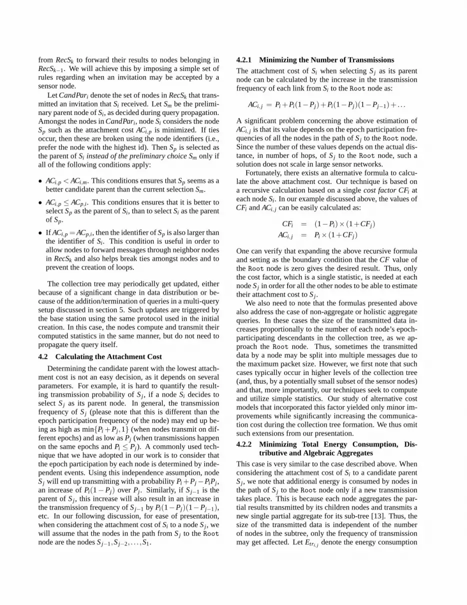
from RecSk to forward their results to nodes belonging inRecSk−1. We will achieve this by imposing a simple set ofrules regarding when an invitation may be accepted by asensor node.

LetCandPari denote the set of nodes inRecSk that trans-mitted an invitation thatSi received. LetSm be the prelimi-nary parent node ofSi , as decided during query propagation.Amongst the nodes inCandPari , nodeSi considers the nodeSp such as the attachment costACi,p is minimized. If tiesoccur, then these are broken using the node identifiers (i.e.,prefer the node with the highest id). ThenSp is selected asthe parent ofSi instead of the preliminary choice Sm only ifall of the following conditions apply:

• ACi,p < ACi,m. This conditions ensures thatSp seems as abetter candidate parent than the current selectionSm.

• ACi,p ≤ ACp,i . This conditions ensures that it is better toselectSp as the parent ofSi , than to selectSi as the parentof Sp.

• If ACi,p = ACp,i , then the identifier ofSp is also larger thanthe identifier ofSi . This condition is useful in order toallow nodes to forward messages through neighbor nodesin RecSk and also helps break ties amongst nodes and toprevent the creation of loops.

The collection tree may periodically get updated, eitherbecause of a significant change in data distribution or be-cause of the addition/termination of queries in a multi-querysetup discussed in section 5. Such updates are triggered bythe base station using the same protocol used in the initialcreation. In this case, the nodes compute and transmit theircomputed statistics in the same manner, but do not need topropagate the query itself.

4.2 Calculating the Attachment Cost

Determining the candidate parent with the lowest attach-ment cost is not an easy decision, as it depends on severalparameters. For example, it is hard to quantify the result-ing transmission probability ofSj , if a nodeSi decides toselectSj as its parent node. In general, the transmissionfrequency ofSj (please note that this is different than theepoch participation frequency of the node) may end up be-ing as high as min{Pi +Pj ,1} (when nodes transmit on dif-ferent epochs) and as low asPj (when transmissions happenon the same epochs andPi ≤ Pj ). A commonly used tech-nique that we have adopted in our work is to consider thatthe epoch participation by each node is determined by inde-pendent events. Using this independence assumption, nodeSj will end up transmitting with a probabilityPi +Pj −PiPj ,an increase ofPi(1−Pj) over Pj . Similarly, if Sj−1 is theparent ofSj , this increase will also result in an increase inthe transmission frequency ofSj−1 by Pi(1−Pj)(1−Pj−1),etc. In our following discussion, for ease of presentation,when considering the attachment cost ofSi to a nodeSj , wewill assume that the nodes in the path fromSj to theRootnode are the nodesSj−1,Sj−2, . . . ,S1.

4.2.1 Minimizing the Number of Transmissions

The attachment cost ofSi when selectingSj as its parentnode can be calculated by the increase in the transmissionfrequency of each link fromSi to theRoot node as:

ACi, j = Pi +Pi(1−Pj)+Pi(1−Pj)(1−Pj−1)+ . . .

A significant problem concerning the above estimation ofACi, j is that its value depends on the epoch participation fre-quencies of all the nodes in the path ofSj to theRoot node.Since the number of these values depends on the actual dis-tance, in number of hops, ofSj to theRoot node, such asolution does not scale in large sensor networks.

Fortunately, there exists an alternative formula to calcu-late the above attachment cost. Our technique is based ona recursive calculation based on a singlecost factor CFi ateach nodeSi . In our example discussed above, the values ofCFi andACi, j can be easily calculated as:

CFi = (1−Pi)× (1+CFj)ACi, j = Pi × (1+CFj)

One can verify that expanding the above recursive formulaand setting as the boundary condition that theCF value oftheRoot node is zero gives the desired result. Thus, onlythe cost factor, which is a single statistic, is needed at eachnodeSj in order for all the other nodes to be able to estimatetheir attachment cost toSj .

We also need to note that the formulas presented abovealso address the case of non-aggregate or holistic aggregatequeries. In these cases the size of the transmitted data in-creases proportionally to the number of each node’s epoch-participating descendants in the collection tree, as we ap-proach theRoot node. Thus, sometimes the transmitteddata by a node may be split into multiple messages due tothe maximum packet size. However, we first note that suchcases typically occur in higher levels of the collection tree(and, thus, by a potentially small subset of the sensor nodes)and that, more importantly, our techniques seek to computeand utilize simple statistics. Our study of alternative costmodels that incorporated this factor yielded only minor im-provements while significantly increasing the communica-tion cost during the collection tree formation. We thus omitsuch extensions from our presentation.

4.2.2 Minimizing Total Energy Consumption, Dis-tributive and Algebraic Aggregates

This case is very similar to the case described above. Whenconsidering the attachment cost ofSi to a candidate parentSj , we note that additional energy is consumed by nodes inthe path ofSj to theRoot node only if a new transmissiontakes place. This is because each node aggregates the par-tial results transmitted by its children nodes and transmits anew single partial aggregate for its sub-tree [13]. Thus, thesize of the transmitted data is independent of the numberof nodes in the subtree, only the frequency of transmissionmay get affected. LetEtr i, j denote the energy consumption

when Si transmits a message toSj consisting of a headerand the desired aggregate value(s) - based on whether thisis a distributive or an algebraic aggregate function. The en-ergy consumption follows the cost model presented in Sec-tion 3.3, where thePRFi value may depend on the distancebetweenSi andSj (thus, the two indices used above). Usingthe above notation, and similarly to the previous discussion,the attachment costACi, j is calculated as:

ACi, j = Pi ×Etr i, j +Pi × (1−Pj)×Etr j, j−1 +

Pi × (1−Pj)× (1−Pj−1)×Etr j−1, j−2 + . . .

= Pi × (Etr i, j +CFj), where

CFi = (1−Pi)× (Etr i, j +CFj)

If one wishes to take the receiving cost of messages intoaccount, all that is required is to replace in the above formu-las the symbols of the formEtrk,p with (Etrk,p +Erecp), sinceeach message transmitted bySk to Sp will consume energyduring its reception bySp.

4.2.3 Minimizing Total Energy Consumption, HolisticAggregate and Non-Aggregate Queries

When considering the attachment cost ofSi to a candidateparentSj , we need not only consider the new messages gen-erated in the path fromSj to theRoot node, but also theenergy consumption due to the increase in the length of mes-sages that would have been transmitted anyway. Please re-call that the energy consumption for each transmission of|aggr| bits bySi to Sj is given by:DEtr i, j = |aggr|× (PTXi +PRFi × dist2i, j). Calculating the aforementioned number ofmessages is simple, as we have already discovered a similarrecursive formula that estimates the attachment cost whenonly considering the transmission of new messages. So, wewill utilize two new recursively computed statistics. TheDCF value of a node will be similar to theCF value, butwill use theDEtr∗,∗ transmission costs, instead of theEtr∗,∗transmission costs used in theCF formula. TheHCF valueof a node will be equal to the sum of theDEtr∗,∗ values in thenodes path to theRoot node. One can verify that the energyconsumption due to the enlargement of messages, becauseof the attachment ofSi to Sj , that would have been transmit-ted anyway is:Pi × (HCFj −DCFj). The required formulasare presented below:

CFi = (1−Pi)× (Etr i, j +CFj)HCFi = DEtr i, j +HCFj

DCFi = (1−Pi)× (DEtr i, j +DCFj)

ACi, j = Pi × (Etr i, j +CFj)+Pi × (HCFj −DCFj)

4.2.4 Summary

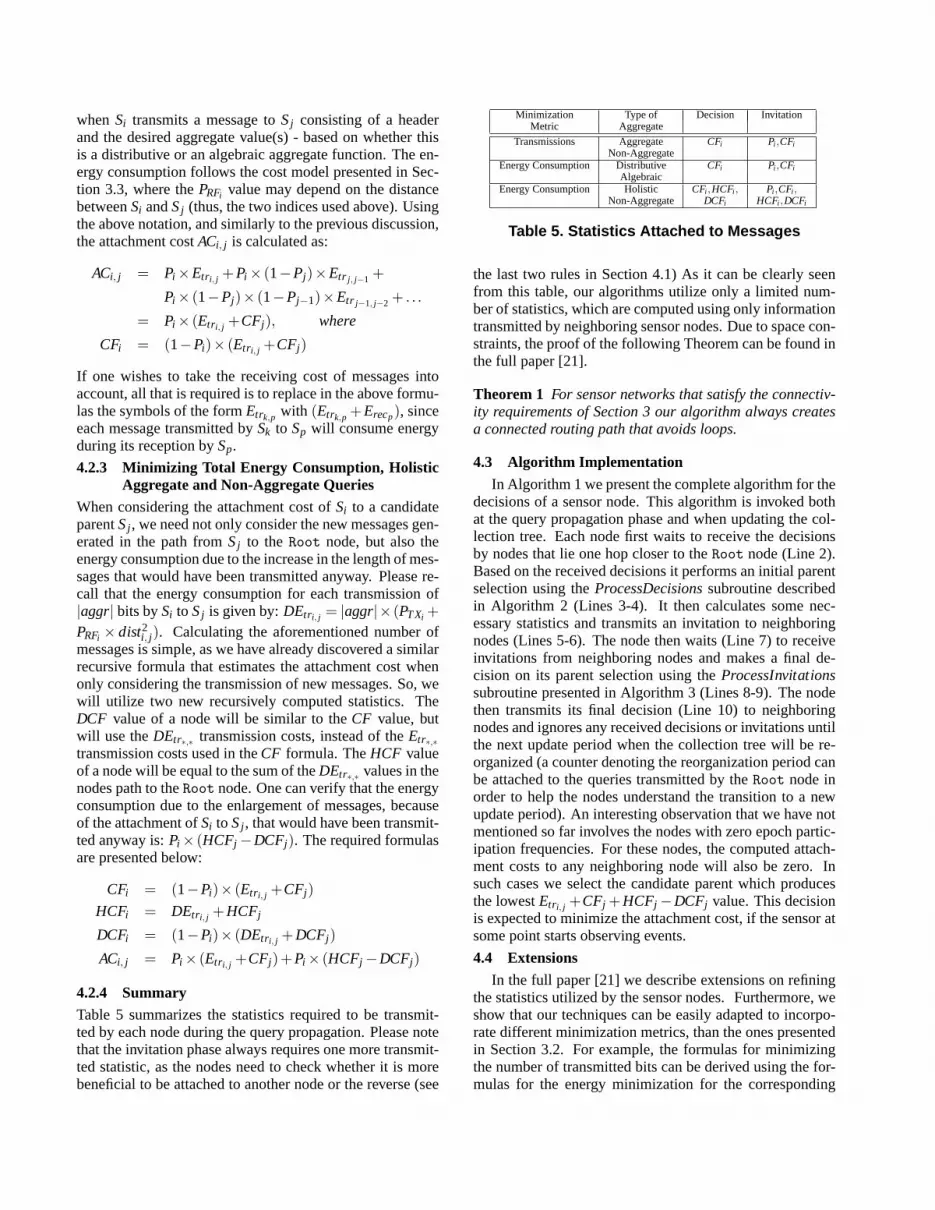
Table 5 summarizes the statistics required to be transmit-ted by each node during the query propagation. Please notethat the invitation phase always requires one more transmit-ted statistic, as the nodes need to check whether it is morebeneficial to be attached to another node or the reverse (see

Minimization Type of Decision InvitationMetric Aggregate

Transmissions Aggregate CFi Pi ,CFiNon-Aggregate

Energy Consumption Distributive CFi Pi ,CFiAlgebraic

Energy Consumption Holistic CFi ,HCFi , Pi ,CFi ,Non-Aggregate DCFi HCFi ,DCFi

Table 5. Statistics Attached to Messages

the last two rules in Section 4.1) As it can be clearly seenfrom this table, our algorithms utilize only a limited num-ber of statistics, which are computed using only informationtransmitted by neighboring sensor nodes. Due to space con-straints, the proof of the following Theorem can be found inthe full paper [21].

Theorem 1 For sensor networks that satisfy the connectiv-ity requirements of Section 3 our algorithm always createsa connected routing path that avoids loops.

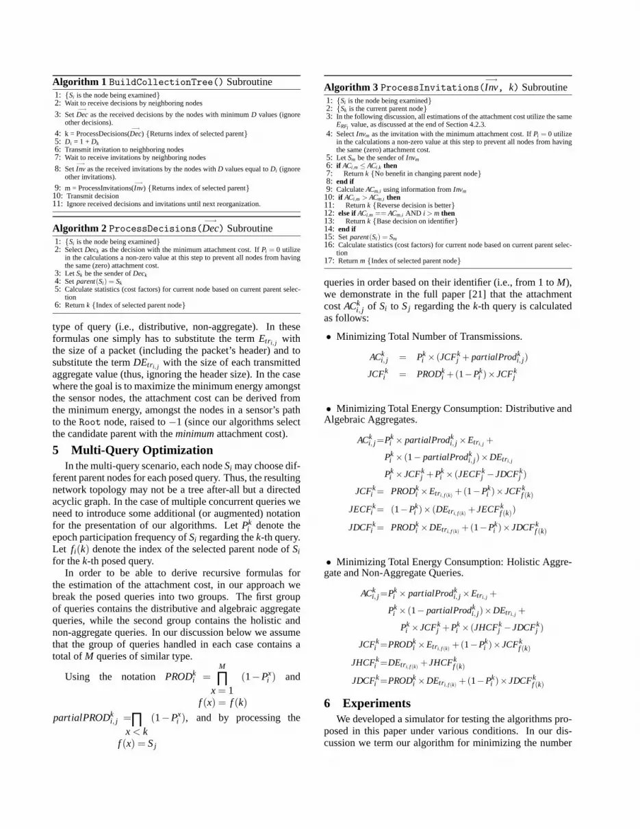
4.3 Algorithm Implementation

In Algorithm 1 we present the complete algorithm for thedecisions of a sensor node. This algorithm is invoked bothat the query propagation phase and when updating the col-lection tree. Each node first waits to receive the decisionsby nodes that lie one hop closer to theRoot node (Line 2).Based on the received decisions it performs an initial parentselection using theProcessDecisionssubroutine describedin Algorithm 2 (Lines 3-4). It then calculates some nec-essary statistics and transmits an invitation to neighboringnodes (Lines 5-6). The node then waits (Line 7) to receiveinvitations from neighboring nodes and makes a final de-cision on its parent selection using theProcessInvitationssubroutine presented in Algorithm 3 (Lines 8-9). The nodethen transmits its final decision (Line 10) to neighboringnodes and ignores any received decisions or invitations untilthe next update period when the collection tree will be re-organized (a counter denoting the reorganization period canbe attached to the queries transmitted by theRoot node inorder to help the nodes understand the transition to a newupdate period). An interesting observation that we have notmentioned so far involves the nodes with zero epoch partic-ipation frequencies. For these nodes, the computed attach-ment costs to any neighboring node will also be zero. Insuch cases we select the candidate parent which producesthe lowestEtr i, j +CFj +HCFj −DCFj value. This decisionis expected to minimize the attachment cost, if the sensor atsome point starts observing events.

4.4 Extensions

In the full paper [21] we describe extensions on refiningthe statistics utilized by the sensor nodes. Furthermore, weshow that our techniques can be easily adapted to incorpo-rate different minimization metrics, than the ones presentedin Section 3.2. For example, the formulas for minimizingthe number of transmitted bits can be derived using the for-mulas for the energy minimization for the corresponding

Algorithm 1 BuildCollectionTree() Subroutine1: {Si is the node being examined}2: Wait to receive decisions by neighboring nodes

3: Set−→Decas the received decisions by the nodes with minimumD values (ignore

other decisions).

4: k = ProcessDecisions(−→Dec) {Returns index of selected parent}

5: Di = 1 + Dk6: Transmit invitation to neighboring nodes7: Wait to receive invitations by neighboring nodes

8: Set−→Inv as the received invitations by the nodes withD values equal toDi (ignore

other invitations).

9: m = ProcessInvitations(−→Inv) {Returns index of selected parent}

10: Transmit decision11: Ignore received decisions and invitations until next reorganization.

Algorithm 2 ProcessDecisions(−→Dec) Subroutine

1: {Si is the node being examined}2: SelectDeck as the decision with the minimum attachment cost. IfPi = 0 utilize

in the calculations a non-zero value at this step to prevent all nodes from havingthe same (zero) attachment cost.

3: Let Sk be the sender ofDeck4: Setparent(Si) = Sk5: Calculate statistics (cost factors) for current node based on current parent selec-

tion6: Returnk {Index of selected parent node}

type of query (i.e., distributive, non-aggregate). In theseformulas one simply has to substitute the termEtr i, j withthe size of a packet (including the packet’s header) and tosubstitute the termDEtr i, j with the size of each transmittedaggregate value (thus, ignoring the header size). In the casewhere the goal is to maximize the minimum energy amongstthe sensor nodes, the attachment cost can be derived fromthe minimum energy, amongst the nodes in a sensor’s pathto theRoot node, raised to−1 (since our algorithms selectthe candidate parent with theminimumattachment cost).

5 Multi-Query OptimizationIn the multi-query scenario, each nodeSi may choose dif-

ferent parent nodes for each posed query. Thus, the resultingnetwork topology may not be a tree after-all but a directedacyclic graph. In the case of multiple concurrent queries weneed to introduce some additional (or augmented) notationfor the presentation of our algorithms. LetPk

i denote theepoch participation frequency ofSi regarding thek-th query.Let fi(k) denote the index of the selected parent node ofSifor thek-th posed query.

In order to be able to derive recursive formulas forthe estimation of the attachment cost, in our approach webreak the posed queries into two groups. The first groupof queries contains the distributive and algebraic aggregatequeries, while the second group contains the holistic andnon-aggregate queries. In our discussion below we assumethat the group of queries handled in each case contains atotal ofM queries of similar type.

Using the notation PRODki =

M

∏x = 1

f (x) = f (k)

(1−Pxi ) and

partialPRODki, j =∏

x < kf (x) = Sj

(1−Pxi ), and by processing the

Algorithm 3 ProcessInvitations(−→Inv, k) Subroutine

1: {Si is the node being examined}2: {Sk is the current parent node}3: In the following discussion, all estimations of the attachment cost utilize the same

ERFi value, as discussed at the end of Section 4.2.3.4: SelectInvm as the invitation with the minimum attachment cost. IfPi = 0 utilize

in the calculations a non-zero value at this step to prevent all nodes from havingthe same (zero) attachment cost.

5: Let Sm be the sender ofInvm6: if ACi,m ≤ ACi,k then7: Returnk {No benefit in changing parent node}8: end if9: CalculateACm,i using information fromInvm10: if ACi,m > ACm,i then11: Returnk {Reverse decision is better}12: else ifACi,m == ACm,i AND i > m then13: Returnk {Base decision on identifier}14: end if15: Setparent(Si) = Sm16: Calculate statistics (cost factors) for current node based on current parent selec-

tion17: Returnm{Index of selected parent node}

queries in order based on their identifier (i.e., from 1 toM),we demonstrate in the full paper [21] that the attachmentcostACk

i, j of Si to Sj regarding thek-th query is calculatedas follows:

• Minimizing Total Number of Transmissions.

ACki, j = Pk

i × (JCFkj + partialProdk

i, j )

JCFki = PRODk

i +(1−Pki )×JCFk

j

• Minimizing Total Energy Consumption: Distributive andAlgebraic Aggregates.

ACki, j =Pk

i × partialProdki, j ×Etr i, j +

Pki × (1− partialProdk

i, j )×DEtr i, j

Pki ×JCFk

j +Pki × (JECFk

j −JDCFkj )

JCFki = PRODk

i ×Etr i, f (k) +(1−Pki )×JCFk

f (k)

JECFki = (1−Pk

i )× (DEtr i, f (k) +JECFkf (k))

JDCFki = PRODk

i ×DEtr i, f (k) +(1−Pki )×JDCFk

f (k)

• Minimizing Total Energy Consumption: Holistic Aggre-gate and Non-Aggregate Queries.

ACki, j =Pk

i × partialProdki, j ×Etr i, j +

Pki × (1− partialProdk

i, j )×DEtr i, j +

Pki ×JCFk

j +Pki × (JHCFk

j −JDCFkj )

JCFki =PRODk

i ×Etr i, f (k) +(1−Pki )×JCFk

f (k)

JHCFki =DEtr i, f (k) +JHCFk

f (k)

JDCFki =PRODk

i ×DEtr i, f (k) +(1−Pki )×JDCFk

f (k)

6 ExperimentsWe developed a simulator for testing the algorithms pro-

posed in this paper under various conditions. In our dis-cussion we term our algorithm for minimizing the number

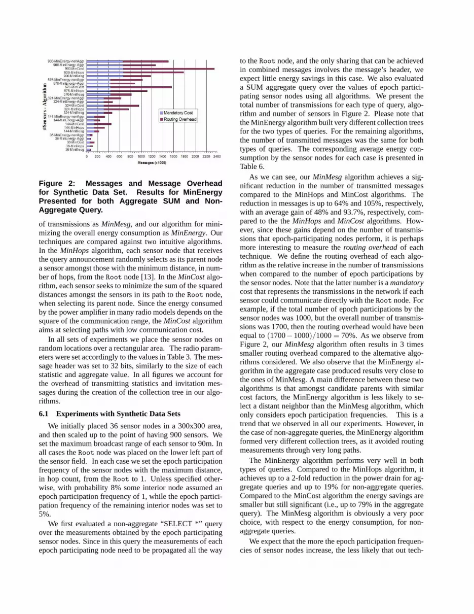
Figure 2: Messages and Message Overheadfor Synthetic Data Set. Results for MinEnergyPresented for both Aggregate SUM and Non-Aggregate Query.

of transmissions asMinMesg, and our algorithm for mini-mizing the overall energy consumption asMinEnergy. Ourtechniques are compared against two intuitive algorithms.In the MinHopsalgorithm, each sensor node that receivesthe query announcement randomly selects as its parent nodea sensor amongst those with the minimum distance, in num-ber of hops, from theRoot node [13]. In theMinCostalgo-rithm, each sensor seeks to minimize the sum of the squareddistances amongst the sensors in its path to theRoot node,when selecting its parent node. Since the energy consumedby the power amplifier in many radio models depends on thesquare of the communication range, theMinCostalgorithmaims at selecting paths with low communication cost.

In all sets of experiments we place the sensor nodes onrandom locations over a rectangular area. The radio param-eters were set accordingly to the values in Table 3. The mes-sage header was set to 32 bits, similarly to the size of eachstatistic and aggregate value. In all figures we account forthe overhead of transmitting statistics and invitation mes-sages during the creation of the collection tree in our algo-rithms.

6.1 Experiments with Synthetic Data Sets

We initially placed 36 sensor nodes in a 300x300 area,and then scaled up to the point of having 900 sensors. Weset the maximum broadcast range of each sensor to 90m. Inall cases theRoot node was placed on the lower left part ofthe sensor field. In each case we set the epoch participationfrequency of the sensor nodes with the maximum distance,in hop count, from theRoot to 1. Unless specified other-wise, with probability 8% some interior node assumed anepoch participation frequency of 1, while the epoch partici-pation frequency of the remaining interior nodes was set to5%.

We first evaluated a non-aggregate “SELECT *” queryover the measurements obtained by the epoch participatingsensor nodes. Since in this query the measurements of eachepoch participating node need to be propagated all the way

to theRoot node, and the only sharing that can be achievedin combined messages involves the message’s header, weexpect little energy savings in this case. We also evaluateda SUM aggregate query over the values of epoch partici-pating sensor nodes using all algorithms. We present thetotal number of transmissions for each type of query, algo-rithm and number of sensors in Figure 2. Please note thatthe MinEnergy algorithm built very different collection treesfor the two types of queries. For the remaining algorithms,the number of transmitted messages was the same for bothtypes of queries. The corresponding average energy con-sumption by the sensor nodes for each case is presented inTable 6.

As we can see, ourMinMesgalgorithm achieves a sig-nificant reduction in the number of transmitted messagescompared to the MinHops and MinCost algorithms. Thereduction in messages is up to 64% and 105%, respectively,with an average gain of 48% and 93.7%, respectively, com-pared to the theMinHopsandMinCostalgorithms. How-ever, since these gains depend on the number of transmis-sions that epoch-participating nodes perform, it is perhapsmore interesting to measure therouting overheadof eachtechnique. We define the routing overhead of each algo-rithm as the relative increase in the number of transmissionswhen compared to the number of epoch participations bythe sensor nodes. Note that the latter number is amandatorycost that represents the transmissions in the network if eachsensor could communicate directly with theRoot node. Forexample, if the total number of epoch participations by thesensor nodes was 1000, but the overall number of transmis-sions was 1700, then the routing overhead would have beenequal to(1700−1000)/1000= 70%. As we observe fromFigure 2, ourMinMesgalgorithm often results in 3 timessmaller routing overhead compared to the alternative algo-rithms considered. We also observe that the MinEnergy al-gorithm in the aggregate case produced results very close tothe ones of MinMesg. A main difference between these twoalgorithms is that amongst candidate parents with similarcost factors, the MinEnergy algorithm is less likely to se-lect a distant neighbor than the MinMesg algorithm, whichonly considers epoch participation frequencies. This is atrend that we observed in all our experiments. However, inthe case of non-aggregate queries, the MinEnergy algorithmformed very different collection trees, as it avoided routingmeasurements through very long paths.

The MinEnergy algorithm performs very well in bothtypes of queries. Compared to the MinHops algorithm, itachieves up to a 2-fold reduction in the power drain for ag-gregate queries and up to 19% for non-aggregate queries.Compared to the MinCost algorithm the energy savings aresmaller but still significant (i.e., up to 79% in the aggregatequery). The MinMesg algorithm is obviously a very poorchoice, with respect to the energy consumption, for non-aggregate queries.

We expect that the more the epoch participation frequen-cies of sensor nodes increase, the less likely that out tech-

Aggregate SUM Query Non-Aggregate “SELECT *” QuerySensors MinMesg MinEnergy MinHops MinCost MinMesg MinEnergy MinHops MinCost

36 109.339 109.341 161.278 136.354 381.483 292.231 335.920 303.270144 70.129 68.971 139.821 121.640 515.215 344.489 390.806 344.213324 71.662 68.703 146.425 106.416 687.083 444.157 523.670 448.816576 65.921 64.717 127.315 104.156 624.817 457.788 547.147 471.845900 67.107 64.077 128.299 102.708 756.902 549.262 640.830 559.183

Table 6: Average Power Consumption (in mJ) for SyntheticDataset

# Sensors MinMesg MinEnergy MinHops MinCost

150 73.607 67.821 111.751 91.990600 58.131 58.273 97.958 85.1581350 50.418 49.350 89.231 76.099

Table 7: Average Power Consumption (inmJ) for SchoolBuses Dataset

0 0.05 0.1 0.15 0.2 0.25 0.3 0.35 0.4 0.45 0.5 0.55 0.6 0.65 0.7 0.75 0.8 0.85 0.9Participation Frequency of Nodes with P <> 1

400000

500000

600000

700000

800000

900000

1000000

1100000

1200000

1300000

Mes

sage

s

MinMesgMinHopsMinCost

Figure 3: Transmissions Varying the Epoch Partic-ipation Frequency

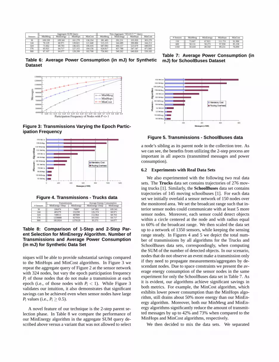
Figure 4. Transmissions - Trucks dataTransmissions Average Energy Consumption

# Sensors MinEnergy-1Step MinEnergy MinEnergy-1Step MinEnergy

36 106474 79887 147.882 109.341144 405279 232298 126.374 68.971324 749013 487889 112.964 68.703576 1258888 827959 101.935 64.717900 1812024 1279129 93.273 64.077

Table 8: Comparison of 1-Step and 2-Step Par-ent Selection for MinEnergy Algorithm. Number ofTransmissions and Average Power Consumption(in mJ) for Synthetic Data Set

niques will be able to provide substantial savings comparedto the MinHops and MinCost algorithms. In Figure 3 werepeat the aggregate query of Figure 2 at the sensor networkwith 324 nodes, but vary the epoch participation frequencyPi of those nodes that do not make a transmission at eachepoch (i.e., of those nodes withPi < 1). While Figure 3validates our intuition, it also demonstrates that significantsavings can be achieved even when sensor nodes have largePi values (i.e.,Pi ≥ 0.5).

A novel feature of our technique is the 2-step parent se-lection phase. In Table 8 we compare the performance ofour MinEnergy algorithm in the aggregate SUM query de-scribed above versus a variant that was not allowed to select

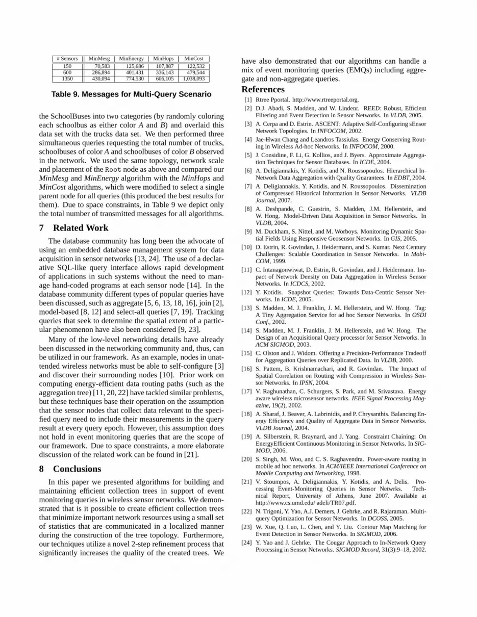
Figure 5. Transmissions - SchoolBuses data

a node’s sibling as its parent node in the collection tree. Aswe can see, the benefits from utilizing the 2-step process areimportant in all aspects (transmitted messages and powerconsumption).

6.2 Experiments with Real Data Sets

We also experimented with the following two real datasets. TheTrucks data set contains trajectories of 276 mov-ing trucks [1]. Similarly, theSchoolBusesdata set containstrajectories of 145 moving schoolbuses [1]. For each dataset we initially overlaid a sensor network of 150 nodes overthe monitored area. We set the broadcast range such that in-terior sensor nodes could communicate with at least 5 moresensor nodes. Moreover, each sensor could detect objectswithin a circle centered at the node and with radius equalto 60% of the broadcast range. We then scaled the data setup to a network of 1350 sensors, while keeping the sensingrange steady. In Figures 4 and 5 we depict the total num-ber of transmissions by all algorithms for the Trucks andSchoolBuses data sets, correspondingly, when computingthe SUM of the number of detected objects. In our scenario,nodes that do not observe an event make a transmission onlyif they need to propagate measurements/aggregates by de-scendant nodes. Due to space constraints we present the av-erage energy consumption of the sensor nodes in the sameexperiment for only the SchoolBuses data set in Table 7. Asit is evident, our algorithms achieve significant savings inboth metrics. For example, the MinCost algorithm, whichexhibits lower power consumption than the MinHops algo-rithm, still drains about 50% more energy than our MinEn-ergy algorithm. Moreover, both our MinMesg and MinEn-ergy algorithms significantly reduce the amount of transmit-ted messages by up to 42% and 73% when compared to theMinHops and MinCost algorithms, respectively.

We then decided to mix the data sets. We separated

# Sensors MinMesg MinEnergy MinHops MinCost

150 70,583 125,686 107,887 122,532600 286,894 401,431 336,143 479,5441350 430,094 774,530 606,105 1,038,093

Table 9. Messages for Multi-Query Scenario

the SchoolBuses into two categories (by randomly coloringeach schoolbus as either colorA and B) and overlaid thisdata set with the trucks data set. We then performed threesimultaneous queries requesting the total number of trucks,schoolbuses of colorA and schoolbuses of colorB observedin the network. We used the same topology, network scaleand placement of theRoot node as above and compared ourMinMesgandMinEnergyalgorithm with theMinHopsandMinCostalgorithms, which were modified to select a singleparent node for all queries (this produced the best results forthem). Due to space constraints, in Table 9 we depict onlythe total number of transmitted messages for all algorithms.

7 Related WorkThe database community has long been the advocate of

using an embedded database management system for dataacquisition in sensor networks [13, 24]. The use of a declar-ative SQL-like query interface allows rapid developmentof applications in such systems without the need to man-age hand-coded programs at each sensor node [14]. In thedatabase community different types of popular queries havebeen discussed, such as aggregate [5, 6, 13, 18, 16], join [2],model-based [8, 12] and select-all queries [7, 19]. Trackingqueries that seek to determine the spatial extent of a partic-ular phenomenon have also been considered [9, 23].

Many of the low-level networking details have alreadybeen discussed in the networking community and, thus, canbe utilized in our framework. As an example, nodes in unat-tended wireless networks must be able to self-configure [3]and discover their surrounding nodes [10]. Prior work oncomputing energy-efficient data routing paths (such as theaggregation tree) [11, 20, 22] have tackled similar problems,but these techniques base their operation on the assumptionthat the sensor nodes that collect data relevant to the speci-fied query need to include their measurements in the queryresult at every query epoch. However, this assumption doesnot hold in event monitoring queries that are the scope ofour framework. Due to space constraints, a more elaboratediscussion of the related work can be found in [21].

8 ConclusionsIn this paper we presented algorithms for building and

maintaining efficient collection trees in support of eventmonitoring queries in wireless sensor networks. We demon-strated that is it possible to create efficient collection treesthat minimize important network resources using a small setof statistics that are communicated in a localized mannerduring the construction of the tree topology. Furthermore,our techniques utilize a novel 2-step refinement process thatsignificantly increases the quality of the created trees. We

have also demonstrated that our algorithms can handle amix of event monitoring queries (EMQs) including aggre-gate and non-aggregate queries.

References[1] Rtree Pportal. http://www.rtreeportal.org.[2] D.J. Abadi, S. Madden, and W. Lindenr. REED: Robust, Efficient

Filtering and Event Detection in Sensor Networks. InVLDB, 2005.[3] A. Cerpa and D. Estrin. ASCENT: Adaptive Self-Configuring sEnsor

Network Topologies. InINFOCOM, 2002.[4] Jae-Hwan Chang and Leandros Tassiulas. Energy Conserving Rout-

ing in Wireless Ad-hoc Networks. InINFOCOM, 2000.[5] J. Considine, F. Li, G. Kollios, and J. Byers. Approximate Aggrega-

tion Techniques for Sensor Databases. InICDE, 2004.[6] A. Deligiannakis, Y. Kotidis, and N. Roussopoulos. Hierarchical In-

Network Data Aggregation with Quality Guarantees. InEDBT, 2004.[7] A. Deligiannakis, Y. Kotidis, and N. Roussopoulos. Dissemination

of Compressed Historical Information in Sensor Networks.VLDBJournal, 2007.

[8] A. Deshpande, C. Guestrin, S. Madden, J.M. Hellerstein, andW. Hong. Model-Driven Data Acquisition in Sensor Networks. InVLDB, 2004.

[9] M. Duckham, S. Nittel, and M. Worboys. Monitoring Dynamic Spa-tial Fields Using Responsive Geosensor Networks. InGIS, 2005.

[10] D. Estrin, R. Govindan, J. Heidermann, and S. Kumar. Next CenturyChallenges: Scalable Coordination in Sensor Networks. InMobi-COM, 1999.

[11] C. Intanagonwiwat, D. Estrin, R. Govindan, and J. Heidermann. Im-pact of Network Density on Data Aggregation in Wireless SensorNetworks. InICDCS, 2002.

[12] Y. Kotidis. Snapshot Queries: Towards Data-Centric Sensor Net-works. InICDE, 2005.

[13] S. Madden, M. J. Franklin, J. M. Hellerstein, and W. Hong. Tag:A Tiny Aggregation Service for ad hoc Sensor Networks. InOSDIConf., 2002.

[14] S. Madden, M. J. Franklin, J. M. Hellerstein, and W. Hong. TheDesign of an Acquisitional Query processor for Sensor Networks. InACM SIGMOD, 2003.

[15] C. Olston and J. Widom. Offering a Precision-Performance Tradeofffor Aggregation Queries over Replicated Data. InVLDB, 2000.

[16] S. Pattem, B. Krishnamachari, and R. Govindan. The Impact ofSpatial Correlation on Routing with Compression in Wireless Sen-sor Networks. InIPSN, 2004.

[17] V. Raghunathan, C. Schurgers, S. Park, and M. Srivastava. Energyaware wireless microsensor networks.IEEE Signal Processing Mag-azine, 19(2), 2002.

[18] A. Sharaf, J. Beaver, A. Labrinidis, and P. Chrysanthis. Balancing En-ergy Efficiency and Quality of Aggregate Data in Sensor Networks.VLDB Journal, 2004.

[19] A. Silberstein, R. Braynard, and J. Yang. Constraint Chaining: OnEnergyEfficient Continuous Monitoring in Sensor Networks. InSIG-MOD, 2006.

[20] S. Singh, M. Woo, and C. S. Raghavendra. Power-aware routing inmobile ad hoc networks. InACM/IEEE International Conference onMobile Computing and Networking, 1998.

[21] V. Stoumpos, A. Deligiannakis, Y. Kotidis, and A. Delis. Pro-cessing Event-Monitoring Queries in Sensor Netwrks. Tech-nical Report, University of Athens, June 2007. Available athttp://www.cs.umd.edu/ adeli/TR07.pdf.

[22] N. Trigoni, Y. Yao, A.J. Demers, J. Gehrke, and R. Rajaraman. Multi-query Optimization for Sensor Networks. InDCOSS, 2005.

[23] W. Xue, Q. Luo, L. Chen, and Y. Liu. Contour Map Matching forEvent Detection in Sensor Networks. InSIGMOD, 2006.

[24] Y. Yao and J. Gehrke. The Cougar Approach to In-Network QueryProcessing in Sensor Networks.SIGMOD Record, 31(3):9–18, 2002.