Download - Principal Component and Cluster Analysis for determining diversification of bottom morphology based on bathymetric profiles from Brepollen (Hornsund, Spitsbergen)

Principal Component

and Cluster Analysis

for determining

diversification of bottom

morphology based on

bathymetric profiles from

Brepollen (Hornsund,

Spitsbergen)*

doi:10.5697/oc.56-1.059OCEANOLOGIA, 56 (1), 2014.

pp. 59–84.

©C Copyright by

Polish Academy of Sciences,

Institute of Oceanology,

2014.

KEYWORDS

Fjord morphologyBrepollenHornsundSvalbard

Principal Componentand Cluster Analyses

Mateusz Moskalik1

Jarosław Tęgowski2

Piotr Grabowiecki1

Monika Żulichowska3

1 Institute of Geophysics,Polish Academy of Sciences,Księcia Janusza 64, 01–452 Warsaw, Poland;

e-mail: [email protected]


2 Department of Oceanography and Geography,University of Gdańsk,al. Marszałka J. Piłsudskiego 46, 81–378 Gdynia, Poland;


3 Department of Biology and Earth Sciences,Jagiellonian University,Gronostajowa 7, 30–387 Kraków, Poland;

e-mail: m [email protected]

Received 24 May 2013, revised 24 September 2013, accepted 3 October 2013.

* The project was partly supported by The Polish Ministry of Sciences and HigherEducation Grant No. N N525 350038.

60 M. Moskalik, J. Tęgowski, P. Grabowiecki, M. Żulichowska

Abstract

Navigation charts of the post-glacial regions of Arctic fjords tend not to coverregions from which glaciers have retreated. Whilst research vessels can make de-tailed bathymetric models using multibeam echosounders, they are often too largeto enter such areas. To map these regions therefore requires smaller boats carryingsingle beam echosounders. To obtain morphology models of equivalent qualityto those generated using multibeam echosounders, new ways of processing datafrom single beam echosounders have to be found. The results and comprehensiveanalysis of such measurements conducted in Brepollen (Hornsund, Spitsbergen)are presented in this article. The morphological differentiation of the seafloor wasdetermined by calculating statistical, spectral and wavelet transformation, fractaland median filtration parameters of segments of bathymetric profiles. This set ofparameters constituted the input for Principal Component Analysis and then inthe form of Principal Components for the Cluster Analysis. As a result of thisprocedure, three morphological classes are proposed for Brepollen: (i) steep slopes(southern Brepollen), (ii) flat bottoms (central Brepollen) and gentle slopes (theStorebreen glacier valley and the southern part of the Hornbreen glacier valley),(iii) the morphologically most diverse region (the central Storebreen valley, thenorthern part of the Hornbreen glacier valley and the north-eastern part of centralBrepollen).

1. Introduction

The widespread use of multi-beam echosounders in scientific researchpermits the collection of complex information in a short time. Muchwork has been done in recent years in the Spitsbergen region using thistechnology, which has delivered very detailed maps as well as informationon the area’s morphological characteristics (e.g. Ottesen & Dowdeswell2006, 2009, Ottesen et al. 2007, 2008, Forwick et al. 2009, Dowdeswellet al. 2010). But such work requires the use of large vessels; this increasesthe costs of exploration and it also has its limitations. For reasons of safety,data recording is usually performed in areas already covered by marinepublications and charts (e.g. The Norwegian Hydrographic Service andNorwegian Polar Research 1990, United Kingdom Hydrographic Office 2007,Statens Kartverk 2008). It is often the case, however, that existing mapsdo not show areas from which glaciers have retreated and are insufficientlydetailed (Pastusiak 2010). Small boats with a shallow draught then haveto be employed, as they provide a safer working environment when sailingin unexplored areas. In such difficult measuring conditions it is usuallyonly single-beam echosounders that can be used. Direct interpolation ofthe profiles obtained enables geographical regionalisation in that individualbays, once influenced by glaciers, can be identified (Moskalik et al. 2013a)and their shapes characterised (Moskalik et al. 2013b). But again, theseproperties describe pre-glacial valleys in their entirety but not in fine detail.

Principal Component and Cluster Analysis for determining . . . 61

In the present work, the bathymetric profiles were analysed under theassumption that areal diversity is expressed by the diversity of regionalprofiles. Moreover, the density of depth measurements being far greaterthan that of the inter-profile distances, additional information can beobtained on the nature of the bottom forms.

2. Study area; selecting profiles for analysis

Brepollen, the region where this research was carried out, is the innerpart of the Hornsund Fjord, which itself is the most southerly fjord in

Figure 1. Map of Hornsund Fiord, Svalbard (a), locations of bathymetric profilesat Brepollen – grey dashed lines (b) and interpolated Brepollen bathymetry (c)


western Spitsbergen (Figure 1a). Bathymetric data were collected froma small boat equipped with a low-cost Lowrance LMS-527cDF echosounderduring the summers of 2007 and 2008. A total of 120 bathymetric sectionswith an overall length of 384 km were made (Figure 1c). An interpolatedbathymetry map for Brepollen (Figure 1b) was prepared on a 25 m grid(Moskalik et al. 2013a). It was assumed that it showed all forms largerthan ten times the size of the grid; forms smaller than 250 m thereforerequired detailed analysis. A consequence of this methodology was that thebathymetric profiles used in the analysis had a minimum length of 256 m.In order to select sections for analysis, two classifying parameters wereimplemented. Every measurement on a bathymetric profile could becomean Initial Profile Point (IPP) for the analysis on condition that there was anEnd Profile Point (EPP) on the profile 256 m distant along the measuringroute. The first parameter was calculated by finding the average deviation ofthe records between IPP and EPP from a linear fit between them. The lowerthe value of this parameter, the closer the location of a depth measurementto the straight segment. The other parameter was the real distance betweenIPP and EPP; this was used if measurements were being made while sailinghaphazardly in the vicinity of a specific point. It was assumed that whenthe average deviation from the linear fit was more than 2% of its lengthor the distance between IPP and EPP was less than 98% of its length, theprofiles did not fulfil the straightness requirement.

3. Methodology

The following data analysis scheme was employed to characterisemorphological seabed differences:

– calculation of mathematical parameters describing bathymetric sec-tion diversification;

– the first parameter reduction step, based on the analysis of entirebathymetric profiles; here, chaotic parameters were rejected; in thecase of correlated parameters, only one remained;

– standardisation of parameters;

– the second reduction step was based on Principal Component Analysis(PCA);

– determination of the number of clusters;

– assignment of individual profile sections to clusters, based on clusteranalysis;

– assignment of morphological feature classes to given clusters.


The paper describes all these steps in detail.Statistical, spectral and wavelet transformations, as well as fractal and

median filtration parameters were used in this work. These parameters weredetermined not for the depth profiles, but for the deviations from the meanvalue (MV), linear trend (LT) and square trend (ST) of all straight segmentsof profiles with a length of 256 m selected by the method described above(Figure 2).

Figure 2. Example segment of bathymetric profile, its mean value, linear, squaretrend and deviations

The usefulness of statistical parameters for describing morphologicaldiversification was shown in topographical analyses of a whole planet(Aharonson et al. 2001, Nikora & Goring 2004, 2005) but also of smallerregions (Moskalik & Bialik 2011).The following statistical parameters were determined:

– the average absolute value of deviations (DeMV, DeLT, DeST);

– standard deviation of deviations (σMV, σLT, σST);

– skewness of deviations (SkewMV, SkewLT, SkewST);

– kurtosis of deviations (KurtMV, KurtLT, KurtST);

and parameters based on semivariograms of deviations:

– linear regressions (SLRMV, SLRLT, SLRST);


– nugget of semivariogram linear regression (CMV0 , C

LT0 , C

ST0 ).

The range of interaction is the limit of increase in value of semivari-ograms (ωMV, ωLT, ωST), with its imposed limit of half of the length of thesegments analysed.The usefulness of spectral analysis for describing morphological features

was also demonstrated for planet topography (Nikora & Goring 2006) andalso for smaller regions like bathymetric maps (Lefebvre & Lyons 2011)and linear profiles (Goff et al. 1999, Goff 2000, Tęgowski & Łubniewski2002). The following parameters were determined for the bathymetricprofiles collected at Brepollen:– the total spectral energies in the form of integrals of power spectral

density deviations from the bathymetric profile (SMVk1 , S

LTk1 , S

STk1 ):

Sk1 =

kNy∫

0

Ckdk , (1)

where kNy is the Nyquist parameter and Ck is the normalised powerspectrum given by Pace & Geo (1988) in the form:

Ck =log10(10

5 S(k) Smax(k)−1 + 1)

log10(105 + 1)

, (2)

where S(k) is the power spectral density of the bathymetric profile;– relations of the spectral energy to the total spectral energy for each of

the deviations take the form:

Skm =1

Sk1

1

mkNy∫

0

Ckdk (3)

determined for m= 2, 4, 8, 16 (SMVkm , S

LTkm, S

STkm);

– the eight first spectral moments (MMVr , M

LTr , M

STr ) of order r= 0,

. . . , 7 defined as

Mr =

∞∫

0

kr S(k)dk ; (4)

– average values of wave numbers (kMV, kLT, kST):

k =M1

M0; (5)


– spectral widths (v2 MV, v2 LT, v2 ST, ǫ2 MV, ǫ2 LT, ǫ2 ST) describingthe concentration of power spectra around the average wave numbers

v2 =M0 ×M2

M1− 1 (6)

and

ǫ2 =M0 ×M4 −M2

2

M0 ×M4; (7)

– spectral skewness describing the shape of spectra (γMV, γLT, γST)

γ =M3

M3/22

. (8)

Additional analysis involved the use of wavelet transforms, also usedin the analysis of bathymetric measurements (Little et al. 1993, Little1994, Little & Smith 1996, Wilson et al. 2007). A fundamental problemin wavelet analysis is the selection of the mother wavelet function. Foranalysing the echo envelope of the acoustic signal, Ostrovsky & Tęgowski(2010) applied six differently defined mother functions. The use of so manydifferent functions did not yield a larger amount of information, however.In the present case, the number of wavelet mother functions was reducedto two: one symmetric and the other asymmetric. The Mexican Hat(mexh) was selected as the symmetric wavelet mother function, while thefamily of Daubechies wavelets exemplifies the asymmetric mother functions.A wavelet of the order of 7 (db7) was selected from this family. In order toaccount for wavelet asymmetry, profiles were analysed in both directions,in the same direction as the measurements according to (db7+) and in theopposite direction (db7−). The following parameters were determined foreach of the transforms:– wavelet energies for a given scaling parameter (EMV

j,wav, ELTj,wav, E

STj,wav):

Ej,wav =

bmax∫

0

C2(a, b)db , (9)

where

Ca, b =

∫

f(x)Ψ(a, b, x)dx (10)

is the wavelet transform of the bathymetric profile of f(x) and

Ψ(a, b, x) =1√a×Ψ

(

x− b

a

)

, a, b ∈ R, a �= 0 , (11)


where a is the scaling parameter corresponding to the stretching orcompression of the mother function, and b is the parameter specifying thewavelet location on the profile. Calculations were performed for waveletscales a = 2j for j = 1, . . . , 7. Larger values of parameter a could not beused, because for j = 7, the wavelet size is half the length of the bathymetricprofile under consideration;– the entropy of the bathymetric profiles (hMV

wav, hLTwav, h

STwav), defined as

hwav =

j=7∑

j=1

Ej,wav × ln(Ej,wav) . (12)

The use of a fractal dimension in the analysis of bottom bathymetryshould result from the following assumptions (Herzfeld et al. 1995):

– bathymetry has a non-trivial structure at every scale;

– it cannot be described by simple geometric figures;

– its topological dimension DT is smaller than the Hausdorff dimensionDH defined as:

DH = limr→0

− log10 N(r)

log10 r, (13)

where N(r) denotes the number of spheres of radius r needed to completelycover the object;

– it is self-similar in the stochastic sense.

It is evident that the bathymetry of a water body formed by numerousgeological processes has a non-trivial structure and that it cannot bedescribed by simple geometric figures. The work involving the analysis ofbathymetric profiles from the eastern Pacific (Herzfeld et al. 1995) indicatesthat bathymetry can be treated as a fractal because the assumption thatDH > DT is fulfilled; however, the assumptions of self-similarity are notsatisfied when the image scale is being changed. The fractal dimension isconsidered to be an appropriate parameter for describing the morphologicaldiversification of bottom surfaces (Wilson et al. 2007). In the case ofa flat bottom, the fractal dimension calculated for the bathymetric profileshould take a value equal to unity; as irregularities in the seafloor appearand their magnitudes change, its value will rise. In this work, thefractal dimension was determined using indirect methods, such as thebox dimension, semivariogram analysis of spectral parameters and waveletanalysis.


For determining the box fractal dimension of the deviations from thebathymetric profile segments (DMV

box , DLTbox, D

STbox), the definition given by

Hastings & Sugihara (1994) was used:

Dbox = lim∆s→0

log10 N(∆s)

− log10 ∆s, (14)

where N(∆s) determines the number of squares covering a depth profile ofa side length ∆s. In case of the bathymetric profiles, both the length anddepth have the same dimension.The proposed procedure for determining this parameter consists of four

consecutive steps:

– normalisation of the distance, taking the unit profile length to be256 m;

– normalisation of the depth, considering independently the unit max-imum difference in deviation of the depth on all analysed profilesegments for each type of deviations;

– determination of the number of squares covering the bathymetricprofile for the division of values normalised from 11 to 110 segments;

– determination of the slope coefficient of the curve defined by thedependence of log10(N(∆s)) on − log10(∆s), which is equivalent tothe box fractal dimension.

Application of a uniform standardisation is valid, taking a standarddistance and depth of 256 m, equal to the length of the analysed section.In such analyses, however, the depth differences were often too small incomparison with the length of the segment profile to use the same scale.For this reason, the maximum difference in depth of all segments was usedas the depth normalisation.The other methods used for determining the fractal dimension of

bathymetric profile deviations from the mean, linear and quadratic trendwere the analyses of (i) the semivariogram (DMV

sem , DLTsem, D

STsem), (ii) the

power spectral density (DMVFFT , D

LTFFT , D

STFFT ) and (iii) the wavelet transform

(DMVwav, D

LTwav, D

STwav). The following relationships can be derived from them:

Dsem = 2− α

2, (15)

where α is the semivariogram regression coefficient in the log-log scale (Wen& Sinding-Larsen 1997);

DFFT =5− β

2, (16)


where β is the regression coefficient of the spectral density in the log-logscale (Mandelbrot 1982, Wornell & Oppenheim 1992);

Dwav =3

2− γ , (17)

where γ is the regression coefficient of the wavelet transform coefficientC(a, b) averaged over the parameter b determining the location dependingon the scaling parameter a in the log-log scale (Mandelbrot 1982).A median filter was also used to analyse the diversity of bottom forms.

Operation of the filter resulted in replacement of all the values by the medianof the nearest values to each of them (White 2003, White & Hodges 2005).This filter is used to separate different sizes of morphological forms (e.g.Wessel 1998, Adam et al. 2005, Kim 2005, Hiller & Smith 2008, Kim& Wessel 2008). A window of width 2d with d increasing in geometricprogression was used in the study: d = 2 (MFMV

1 , MFLT1 , MF

ST1 ), 4 (MF

MV2 ,

MFLT2 , MFST2 ), 8 (MF

MV3 , MF

LT3 , MF

ST3 ), 16 (MF

MV4 , MF

LT4 , MF

ST4 ), 32

(MFMV5 , MF

LT5 , MF

ST5 ) and 64 (MF

MV6 , MF

LT6 , MF

ST6 ) metres. The next

filter, which cuts the size forms up to 128 m, could not be applied toa 256 m long profile segment. This parameter was determined by averagingthe absolute values of the residue after filtering.All the parameters defined above were identified for every profile. Some

of them were correlated or their shape was chaotic, providing no informationthat could define the seabed morphological diversity.The discussion includes all the parameters used, based on an exam-

ple bathymetric profile. This profile is characterised by including variedmorphology (Figure 3b). The profile’s depth varies within the range of 10–120 m. The maximum depth of 120 m was found in the central part ofBrepollen, and the profile end is positioned close to the Hyrne glacier calvingfront.

a b

Figure 3. Example profile with sections (b) and its localisation (black line) onthe Brepollen bathymetry map (a)


The following profile sections were identified:

– Section 1 – an almost flat seabed 1 km long with depths between115–120 m.

– Section 2 – a hill at the bottom of a 200 m wide slope more than 10 mhigh.

– Section 3 – an average slope of 4◦ to 5◦ with a slight roughness in itsupper parts.

– Section 4 – a hill 10 m high and 200 m wide in the upper part ofthe slope. The isolation of this section was the result of changes inroughness on the slope. It can be assumed that this is a continuationof section 3; the other slope of the hill is inclined towards section 5.

– Section 5 – a gently inclined sea bottom about 700 m long anddescending to a depth of 10 m.

– Section 6 – a hill with a slope steeper than 5◦.

– Section 7 – a singular convex form 2 km long with sharp elevationsand characteristically increasing of roughness in the direction of theHyrne glacier.

– Section 8 – part of the profile with forms 50–100 m wide and 10 mhigh.

– Section 9 – a hill before the glacier front with visibly smaller formsthan recorded in section 8.

Analysis of the statistical parameters for the example bathymetric profileindicates that its diversity is reflected by the variability in parameters De, σ,SLR for every type of deviation and CMV

0 . Analysis of the other parametersdoes not reflect this diversity, however: the variations are mostly chaotic.There was a significant correlation of σ withDe for every deviation (MV, LTand ST) independently (Figures 4a, 4b, 4c). The slope of the curve is almostthe same in every case. The range of values of parameters σLT and σST orDeLT and DeST might suggest the erroneous conclusion that they too arecorrelated, but the evidence for the non-dependence of these parameters isthe quantitative distribution of all possible pairs of σLT and σST (Figure 4d).Pairs of these parameters lie within almost the whole area below the linearrelation describing the equivalence of σST and σLT. A similar analysis wasconducted for the relationship between σ and SLR (Figures 4e, 4f, 4g): thisis exponential. A negative linear relationship was also found between CMV

0

and SLRMV (Figure 4h). The unequivocal inference from the foregoing isthat for every deviation only one of these parameters contributes clearlyindependent information on the morphological diversity of the seabed.


Figure 4. The relationship between: σ and De for MV (a), LT (b), ST deviations(c); SLR and σ for MV (e), LT (f), ST deviations (g); σLT and σST (d); CMV

0 andSLRMV (h). The colour scale represents the ratio of the number of pairs of theserelations to all pairs on the logarithmic scale

Spectral moments (Mi) and spectral skewness (γ) were found to be themost significant spectral parameters. The higher the order of a spectralmoment, the lower the difference between the values. These features arehighlighted by the correlation coefficients for Mi and Mj pairs for eachdeviation (Figure 5). There is also a correlation between the spectralmoments for LT and ST (Figure 5); the coefficient of this correlation, ofthe 2nd order, is close to 1. In view of the above, it was decided that only0 to 3rd order spectral moments would be used for every deviation.The similarities between σ and M0 were also investigated. Detailed

analysis showed that for every type of deviation there exists a lineardependence between σ2 andM0. It is clear from the above relationship thatwhen spectral analysis was used, the addition of characteristics emergingfrom statistical parameters did not contribute any new knowledge regardingthe sea bottom morphology in Brepollen.


Figure 5. Correlation between Mi and Mj spectral moments of orders 0 to 7 forall types of deviations (MV, LT, ST)

Determination of the wavelet energy for successive scaling parametersis an excellent method for isolating morphological forms on a bathymetricprofile, as it takes the magnitude of forms into consideration on the basis ofthe scaling parameter’s size. To verify the applicability of wavelet energies,the correlations between them were calculated (Figure 6). The correlationfor every type of wavelet was much less than 1, even in the case ofadjacent scaling parameters for the same type of wave. Analysis of thewavelet energies calculated for the example profile showed that the waveletenergy determined using the mexh wavelet for the scaling parameter a = 2i

resembled that of the db7 wavelet for the scaling parameter a = 2i+2 wheni = 1, . . . , 5. This observation was confirmed by wavelet correlation analysis(Figure 6).The final point in the discussion of the application of wavelets to

bathymetric profile analysis is the possible use of asymmetric wavelets,such as db7. The most effective approach seems to be to investigate the


Figure 6. Correlation between wavelet energies for all wavelet mother functions(mexh, db7+, db7-), scaling parameters (21, 22, 23, 24, 25, 26, 27) and types ofdeviations (MV, LT, ST) used

energy correlation between wavelet energies for the same scaling parameterof asymmetric wavelets calculated in both directions of a profile. Only the(E

(MV,LT,ST)1, db7+ , E(MV,LT,ST)

1, db7− ) correlation was less than 0.9 (Figure 6); in theother cases it was close to 1. It was shown that only the first two energiescalculated for db7 wavelets yielded suitable results, because for higherscaling parameters they were correlated with wavelet energies calculatedfrom mexh. It was decided to add three additional parameters, besides theenergies for db7, defined as:

Ei,db7± =Ei, db7+ + Ei,db7−

2for i = 1, 2

(18)

E1, |db7| = |E1, db7+ − E1,db7−|


for every deviation type MV, LT and ST.For the fractal dimension, the quality of the results obtained using

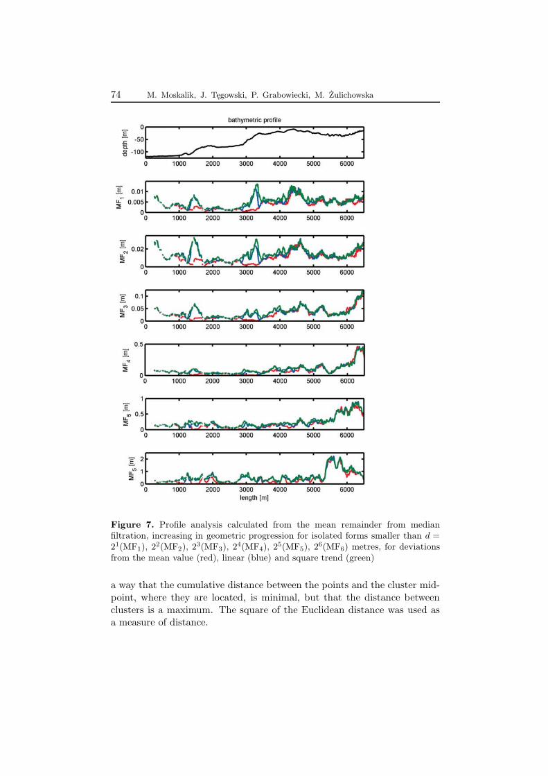
semivariograms, spectral and wavelet analyses was insufficient. Box sizecounts were found to be the most efficient methods. The application ofa median filter to bathymetric profile segments was also a good way offinding diverse forms on the example profile (Figure 7).The above analyses demonstrate that to describe the diverse morphology

of Brepollen the following parameters have to be taken into account: M0,M1, M2, M3, γ, E1,mexh, E2,mexh, E3,mexh, E4,mexh, E5,mexh, E6,mexh,E7,mexh, E1, db7±, E2, db7±, E1, |db7|, Dbox, MF1, MF2, MF3, MF4, MF5,MF6. As these parameters could still be independent, the input parameterswere reduced by Principal Component Analysis (PCA).Before embarking on PCA, the distributions of the values of each

parameter were analysed. Two types of calculated values were identified: (i)with data where quantity is encompassed within one order of magnitude (γ,Dbox, MF1, MF2, MF3, MF4, MF5, MF6) and (ii) with data whose valuesrange over several orders of magnitude (M0,M1, M2, M3, E1,mexh, E2,mexh,E3,mexh, E4,mexh, E5,mexh, E6,mexh, E7,mexh, E1, db7±, E2, db7±, E1, |db7|).For the second case the common logarithm was determined. The next stepincluded data normalisation:

xm =x− xsr

σx, (19)

where xm – new parameter value, x – its determined value, xsr – meanvalue of determined parameters, σx – standard deviation of determinedparameters.After such parameter transformation, the mean of each one will be equal

to zero and the standard deviation equal to one.Analysis of the variance of Principal Components (PCs) (Figure 8)

showed their diminishing influence on the overall value. For the independentanalysis of every deviation, the first ten PCs are sufficient for clusteranalysis. Together, these correspond to more than 98% of the cumulativevariance. In the analysis of deviation MV, this value was exceeded by thefirst nine PCs, but despite this, it was decided to use the same number asin the other two cases. When all the parameters were included, 98% of thecumulative variance was exceeded for the first 16 PCs, and this number ofparameters was utilised in the cluster analysis.Cluster analysis, a process for combining series of points into groups,

enables common features to be assigned to points on the bathymetric profile;every group represents one feature. The k-means method was used toperform the analysis. The algorithm gathers the cluster points in such


Figure 7. Profile analysis calculated from the mean remainder from medianfiltration, increasing in geometric progression for isolated forms smaller than d =21(MF1), 22(MF2), 23(MF3), 24(MF4), 25(MF5), 26(MF6) metres, for deviationsfrom the mean value (red), linear (blue) and square trend (green)

a way that the cumulative distance between the points and the cluster mid-point, where they are located, is minimal, but that the distance betweenclusters is a maximum. The square of the Euclidean distance was used asa measure of distance.


Figure 8. Variation of Principal Components obtained separately forparameters analysed for deviations from the mean value (MV), linear(LT) and square trend (ST) on segments of bathymetric profiles and theircumulative value (upper plot) and for all parameters as one data set (lowerplot)

The choice of the number of clusters is a tricky problem. The mostconvenient situation is when there are environmental pointers to thenumber of features investigated, as this will then be equal to thenumber of clusters formed. If such information is unavailable, one canemploy automated methods. Of 30 methods of cluster number choiceanalysed by Milligan & Cooper (1985), the method of Caliński & Harabasz(1974) was identified as one of the most reliable for determining themaximum of the Caliński-Harabasz index CHindex. It was defined as

CHindex =B

K − 1× N −K

W, (20)

where N – number of all points, K – number of clusters, B – distancebetween clusters and W – the distance within clusters.

The magnitudes of B and W are obtained as follows:


B =

K∑

k=1

nk‖zk − z‖2 ,

(21)

W =

K∑

k=1

nk∑

i=1

‖xi∈k − zk‖2 ,

where nk – number of points in cluster k, zk – position of the centre ofcluster k, z – position of the centre of all points, xi∈k – the i-th pointlocated in cluster k, and ‖ ‖ is the distance norm (Maulik & Bandyopadhyay2002).Ray & Turi (1999) derived another method of determining cluster

numbers. Their index makes direct use of the cluster assumption choiceand is defined as follows:

IIindex =intra

inter=

N−1∑K

k=1

∑nk

i=1 ‖xi∈k − zk‖2min (‖zi − zj‖2)

, (22)

Figure 9. Indices for obtaining the number of clusters


where ‘intra’ is the mean distance between the points and the centre of thecluster containing them, while ‘inter’ is the minimum distance between theclusters.In these cases the number of clusters involves finding the maximum of

CHindex or minimum of IIindex.Both indices were determined for numbers of clusters from 2 to 20 in

all the cases analysed (Figure 9). In general CHindex decreases and IIindexincreases with increasing numbers of clusters. Despite the many deviationsfrom the above trend for both indices it was difficult to define the clusternumber. A small number of clusters was found to be the most appropriate.To identify the maximum number of clusters, the total distance between

the points and each cluster centre (where they are located) was defined:

WK =

K∑

k=1

nk∑

i=1

‖xi∈k − zk‖2 . (23)

By analysing theWK −WK−1 dependence (Figure 9), on the assumptionthat the value must not be too high, 6 was chosen as the most appropriatevalue.

4. Results of clustering and discussion

Cluster analysis was performed for two to six clusters for deviationtypes MV, LT, ST separately and for all the types. In order to assigna specific cluster to a seabed morphological type, the results for the exampleprofile were analysed first. To distinguish individual clusters a markerC

(deviation type)n s was introduced, where the possible deviation types are MV,LT, ST or all for the whole set of parameters, n denotes the number ofclusters and s is the cluster number in a specific set. For example, CMV

4 3

signifies the third of four clusters for the deviation from the mean depth.For deviation type MV (Figure 10a) the most characteristic differentia-

tion is related to the slope of a hill. Clusters CMV2 1 , C

MV3 1 , C

MV4 4 , C

MV5 5 , C

MV6 1

correspond to the steepest slopes, while CMV2 2 corresponds to gentle slopes

and flat areas. For three clusters the steepness of a hillside decreases inthe sequence CMV

3 1 –CMV3 2 –C

MV3 3 . For a larger number of clusters, however, it

is hard to state whether the differentiation continues to indicate variationsin the global slope or whether it indicates more diverse sea bottoms. Nodirect interpretation of a seabed was obtained for the clusters calculated fordeviation types LT and ST (Figures 10b,c).The differentiation distribution of the example profile was the most

complete when all the parameters were taken into account (Figure 10d). Fortwo clusters the distribution was almost analogous to that of MV, that is, flat


Figure 10. Division of an example bathymetric profile into 2, 3, 4, 5 and 6 clustersbased on all profiles for MV (a), LT (b), ST (c) and all types of deviations (d)

or slightly inclined surfaces (Call2 2) and slopes (C

all2 1). Where three clusters

were determined, steep slopes (Call3 1), a flat seabed, gently sloping hillsides

with small morphological forms (Call3 3) and strongly undulating sections

(Call3 2) were distinguished. Adding a fourth cluster precluded further profileclassification. The greatest sea bottom diversity on this profile was foundwith five clusters. It was classified as follows: (i) a flat seabed (Call

5 5), (ii)sections with gently inclined slopes and small forms (Call

5 2), (iii) areas withdiverse morphology and numerous bottom forms (Call

5 3) and (iv) steep slopes(Call

5 1). No forms associated with cluster Call5 4 were found. With six clusters

the results were very difficult to interpret; increasing the number of clustersdid not improve the results any further.In order to draw a map with the morphological form classification on

the example profile, it was suggested that a new interpolation procedureshould be used. Since the results were quantified, the percentage of allclusters was identified at a distance of 500 m from every location. This wasdictated by the distance used for the Brepollen interpolation, as this allowsinformation from the whole research area to be used (Moskalik et al. 2013a).The maximum value cluster was used as the morphological differentiation


class corresponding to the sea bottom. Maps of seabed diversity from the2nd to the 5th class from the cluster analysis of all parameters were prepared(Figure 11).

Figure 11. Brepollen region divisions into 2, 3, 4 and 5 morphologicaldifferentiation classes, based on cluster analyses of all parameters where the coloursare defined as follows: blue – Call

(2,3,4,5) 1, light blue – Call(2,3,4,5) 2, light green –

Call(3,4,5) 3, yellow – C

all(4,5) 4, orange – C

all5 5

Analysis of the results revealed a rapid increase in information for threeclusters than for two. In comparison with the example profile, the resultsallow one to identify areas, such as: (i) steeply inclined areas (Call

3 1), (ii)almost flat and gently inclined areas (Call

3 3) and (iii) areas characterisedby a diverse bottom morphology (Call

3 2). Class Call3 1 areas are regarded as

post-glacial valleys, located in the south-central part of Brepollen. They


are characteristic of the area between central Brepollen and the Hornbreenglacier valley. There are ridges running NE-SW visible on the bathymetricmap (Figure 1c). Class Call

3 2 regions are mainly: (i) the Storbreen glaciervalley bottom, right down to its extension in central Brepollen, (ii) thenorthern part of the Hornbreen glacier valley, (iii) the outer part of theMendelejevbreen glacier valley, (iv) the Svalisbreen valley slopes (v) andthe Hyrnebreen glacier front. The final class Call

3 3 is located in (i) thecentral part of Brepollen, (ii) on the Storebreen glacier valley slopes, (iii) infront of the SE part of the Hornbreen glacier and (iv) in the centre of theMendelejevbreen glacier valley. The classes in the Mendelejevbreen glaciervalley defined the location of the glacier front after its charge in the year2000 (Głowacki & Jania 2008, Błaszczyk et al. 2009, 2013).The quality of the information on seabed differentiation obtained from

the identification of clusters 4 and 5 was poorer. The central Brepollenbottom and the Store and Horn glacier valleys were assigned to a singleclass, as when two clusters were determined (Figure 11). These classeshighlighted a distinct depression right by the Store glacier front (Figure 1c),at the point where a river flows out from under the glacier.As can be seen from this example, one should avoid the direct transfer

of cluster features from the example profile to the whole of Brepollen.Almost all the easily identified classes are located in (i) the central part ofBrepollen, (ii) the Storebreen glacier valley and (iii) the Hornbreen glaciervalley. Correct identification of similar classes in the rest of the region isdifficult because the distance used during the compilation of maps is nearlyhalf of the width of the glacier valleys. Since every class can occur in thesetwo valleys it can be assumed that similar forms are present in both.

5. Conclusions

Despite the rapid development of acoustic methods and the use oftechnologically advanced multibeam echosounders during seafloor scanningperformed from large vessels in post-glacial regions, it is still necessary tosupplement such activities using single beam echosounders from small boats.In this work the bottom morphology of Brepollen (Hornsund, Spitsbergen)was described by analysing 256 m segments of bathymetric profiles. Amongthe suggested statistical, spectral, wavelet, fractal dimension and medianfilter parameters, the following were identified as being the most useful:(i) low-order spectral moments, (ii) spectral skewness, (iii) wavelet energies,(iv) box fractal dimension, (v) mean of the remainder from median filtration.The other parameters were either significantly correlated with parameters(i)–(v), or else they could not be used directly to characterise the shape ofa bathymetric profile.


Cluster analysis revealed at least three morphological classes in Bre-pollen: (i) steep slopes (southern Brepollen), (ii) flat sea bottoms (centralBrepollen) and gentle slopes (the Store glacier valley and the southern partof the Horn glacier valley), (iii) the most morphologically diverse region (thecentral Store valley, the northern part of the Horn glacier valley and the NEpart of central Brepollen with the adjacent Horn and Store valleys).

Acknowledgements

We would like to thank the staff of the Polish Polar Station in Hornsundfor their practical assistance during this research. We are grateful to twoanonymous reviewers and to the editor for their critical comments on themanuscript.

References

Adam C., Vidal V., Bonneville A., 2005, MiFil: a method to characterize seafloorswells with application to the south central Pacific, Geochem. Geophy. Geosy.,6 (1), Q01003, 1–25, http://dx.doi.org/10.1029/2004GC000814.

Aharonson O., Zuber M.T., Rothman D.H., 2001, Statistics of Mars’ topographyfrom the Mars Orbiter Laser Altimeter: slopes, correlations and physicalmodels, J. Geophys. Res., 106 (E10), 23723–23735, http://dx.doi.org/10.1029/2000JE001403.

Błaszczyk M., Jania J.A., Hagen J.O., 2009, Tidewater glaciers of Svalbard: recentchanges and estimates of calving fluxes, Pol. Polar Res., 30 (2), 85–142.

Błaszczyk M., Jania J.A., Kolondra L., 2013, Fluctuations of tidewater glaciers inHornsund Fjord (Southern Svalbard) since the beginning of the 20th century,Pol. Polar Res., 34 (4), 327–352, http://dx.doi.org/10.2478/popore-2013-0024.

Caliński T., Harabasz J., 1974, A dendrite method for cluster analysis, Commun.Stat., 3, 1–27.

Dowdeswell J.A., Hogan K.A., Evans J., Noormets R., O’Cofaigh C., Ottesen D.,2010, Past ice-sheet flow east of Svalbard inferred from streamlined subglaciallandforms, Geology, 38 (2), 163–166, http://dx.doi.org/10.1130/G30621.1.

Forwick M., Baeten N. J., Vorren T.O., 2009, Pockmarks in Spitsbergen fjords,Norw. J. Geol., 89 (1–2), 65–77.

Głowacki P., Jania J.A., 2008, Nature of rapid response of glaciers to climatewarming in Southern Spitsbergen, Svalbard, [in:] The first InternationalSymposium on the Arctic Research (ISAR-1) – Drastic Change under GlobalWarming, Nat. Comm. Japan, Tokyo, 257–260.

Goff J.A., 2000, Simulation of stratigraphic architecture from statistical andgeometrical characterizations, Math. Geol., 32 (7), 765–786, http://dx.doi.org/10.1023/A:1007579922670.


Goff J.A., Orange D. L., Mayer L.A., Hughes Clarke J.E., 1999, Detailedinvestigation of continental shelf morphology using a high-resolution swathsonar survey: the Eel margin, northern California, Mar. Geol., 154 (1–4),255–269, http://dx.doi.org/10.1016/S0025-3227(98)00117-0.

Hastings H.M.G., Sugihara G., 1994, Fractals – a user’s guide for the naturalsciences, Oxford Univ. Press, Oxford, New York, 7–77.

Herzfeld U.C., Kim I. I., Orcutt J.A., 1995, Is the ocean floor a fractal?, Math.Geol., 27 (3), 421–462, http://dx.doi.org/10.1007/BF02084611.

Hiller J.K., Smith M., 2008, Residual relief separation: digital elevation modelenhancement for geomorphological mapping, Earth Surf. Proc. Land., 33 (14),2266–2276, http://dx.doi.org/10.1002/esp.1659.

Kim S.-S., 2005, Separation of regional and residual components of bathymetryusing directional median filtering, M. Sc. thesis, Univ. Hawaii, 49 pp.

Kim S.-S., Wessel P., 2008, Directional median filtering for regional-residualseparation of bathymetry, Geochem. Geophy. Geosy., 9 (3), Q03005, 11 pp.,http://dx.doi.org/10.1029/2007GC001850.

Lefebvre A., Lyons A.P., 2011, Quantification of roughness for seabedcharacterisation, [in:] Underwater Acoustic Measurements (4th UAM) –Technologies & Results, Kos, Greece, Proc. Book 4th Int. Conf. Exhibit., 1623–1630.

Little S.A., 1994, Wavelet analysis of seafloor bathymetry: an example, [in:]Wavelets in geophysics, E. Foufoula-Georgiou & P. Kumar (eds.), Acad. PressInc., San Diego, London, 167–182.

Little S.A., Carter P.H., Smith D.K., 1993, Wavelet analysis of a bathymetricprofile reveals anomalous crust, Geophys. Res. Lett., 20 (18), 1915–1918,http://dx.doi.org/10.1029/93GL01880.

Little S.A., Smith D.K., 1996, Fault scarp identification in side-scan sonarand bathymetry images from the Mid-Atlantic Ridge using wavelet-baseddigital filters, Mar. Geophys. Res., 18 (6), 741–755, http://dx.doi.org/10.1007/BF00313884.

Mandelbrot B.B., 1982, The fractal geometry of nature, W.H. Freeman & Co.,New York, 468 pp.

Maulik U., Bandyopadhyay S., 2002, Performance evaluation of some clusteringalgorithms and validity indices, IEEE T. Pattern Anal., 24 (12), 1650–1654,http://dx.doi.org/10.1109/TPAMI.2002.1114856.

Milligan G.W., Cooper M.C., 1985, An examination of procedures for determiningthe number of clusters in a data set, Psychometrica, 50 (2), 159–179, http://dx.doi.org/10.1007/BF02294245.

Moskalik M., Bialik R. J., 2011, Statistical analysis of topography of Isvika Bay,Murchisonfjorden, Svalbard, [in:] GeoPlanet: Earth and planetary sciences,experimental methods in hydraulic research, P. Rowiński (ed.), 1st edn.,Springer, Berlin–Heidelberg, 225–233.


Moskalik M., Błaszczyk M., Jania J., 2013b, Statistical analysis ofBrepollen bathymetry as a key to determine average depth on a glacierforeland, Geomorphology, http://dx.doi.org/10.1016/j.geomorph.2013.09.029,(in press).

Moskalik M., Grabowiecki P., Tęgowski J., Żulichowska M., 2013a, Bathymetryand geographical regionalization of Brepollen (Hornsund, Spitsbergen) basedon bathymetric profiles interpolations, Pol. Polar Res., 34 (1), 1–22, http://dx.doi.org/10.2478/popore-2013-0001.

Nikora V., Goring D., 2004, Mars topography: bulk statistics and spectralscaling, Chaos Solit. Fractals, 19 (2), 427–439, http://dx.doi.org/10.1016/S0960-0779(03)00054-7.

Nikora V., Goring D., 2005, Martian topography: scaling, craters, and high-order statistics, Math. Geol., 37 (4), 337–355, http://dx.doi.org/10.1007/s11004-005-5952-4.

Nikora V., Goring D., 2006, Spectral scaling in Mars topography: effectof craters, Acta Geophys., 54 (1), 102–112, http://dx.doi.org/10.2478/s11600-006-0009-8.

Ostrovsky I., Tęgowski J., 2010, Hydroacoustic analysis of spatial and temporalvariability of bottom sediment characteristics in Lake Kinneret in relation towater level fluctuation, Geo-Mar. Lett., 30 (3–4), 261–269, http://dx.doi.org/10.1007/s00367-009-0180-4.

Ottesen D., Dowdeswell J. A., 2006, Assemblages of submarine landforms producedby tidewater glaciers in Svalbard, J. Geophys. Res., 111, F01016, http://dx.doi.org/10.1029/2005JF000330.

Ottesen D., Dowdeswell J.A., 2009, An inter-ice-stream glaciated margin:submarine landforms and a geomorphic model based on marine-geophysicaldata from Svalbard, Geol. Soc. Am. Bull., 121 (11–12), 1647–1665, http://dx.doi.org/10.1130/B26467.1.

Ottesen D., Dowdeswell J. A., Benn D. I., Kristensen L., Christiansen H.H.,Christensen O., Hansen L., Lebesbye E., Forwick M., Vorren T.O., 2008,Submarine landforms characteristic of glacier surges in two Spitsbergen fjords,Quaternary Sci. Rev., 27 (15–16), 1583–1599, http://dx.doi.org/10.1016/j.quascirev.2008.05.007.

Ottesen D., Dowdeswell J. A., Landvik J.Y., Mienert J., 2007, Dynamics of theLate Weichselian ice sheet on Svalbard inferred from high-resolution sea-floormorphology, Boreas, 36 (3), 286–306, http://dx.doi.org/10.1111/j.1502-3885.2007.tb01251.x.

Pace N.G., Gao H., 1988, Swath seabed classification, IEEE J. Ocean. Eng., 13 (2),83–90, http://dx.doi.org/10.1109/48.559.

Pastusiak T., 2010, Issues of non-researched marine regions coverage by electronicmaps, Logistyka, 2, 2069–2086, (in Polish).

Ray S., Turi R.H., 1999,Determination of number of clusters in K-means clusteringand application in colour image segmentation, [in:] Advances in PatternRecognition and Digital Techniques (ICAPRDT’99), Calcutta, India, Proc.


4th Int. Conf., N.R. Pal, A.K. De & J. Das (eds.), Narosa Publ. House, NewDelhi, 137–143.

Statens Kartverk, 2008, Paper chart 526, Hornsund, scale 1:50 000.

Tęgowski J., Łubniewski Z., 2002, Seabed characterisation using spectral momentsof the echo signal, Acta Acust., 88 (5), 623–626.

The Norwegian Hydrographic Service and Norwegian Polar Research Institute,1990, Den Norske Los. Arctic Pilot, 7, (2nd edn.), U.K. Hydrogr. Office, 2007,NP11 Arctic Pilot Edition 2004, Correction 2007.

Wen R., Sinding-Larsen R., 1997, Uncertainty in fractal dimension estimated frompower spectra and variograms, Math. Geol., 29 (6), 727–753, http://dx.doi.org/10.1007/BF02768900.

Wessel P., 1998,An empirical method for optimal robust regional-residual separationof geophysical data, Math. Geol., 30 (4), 391–408, http://dx.doi.org/10.1023/A:1021744224009.

White L., 2003, Rivers bathymetry analysis in the presence of submerged largewoody debris, M. Sc. Eng. thesis, Univ. Texas, Austin, 157 pp.

White L., Hodges B.R., 2005, Filtering the signature of submerged large woodydebris from bathymetry data, J. Hydrol., 309 (1–4), 53–65, http://dx.doi.org/10.1016/j.jhydrol.2004.11.011.

Wilson M.F. J., O’Connell B., Brown C., Guinan J.C., Grehan A. J., 2007,Multiscale terrain analysis of multibeam bathymetry data for habitat mappingon the continental slope, Mar. Geod., 30 (1–2), 3–35, http://dx.doi.org/10.1080/01490410701295962.

Wornell G.W., Oppenheim A.V., 1992, Estimation of fractal signals from noisymeasurements using wavelets, IEEE T. Signal Proces., 40 (3), 611–623, http://dx.doi.org/10.1109/78.120804.