Download - On the Anomalous Behaviour of Scalar Flux–Variance Similarity Functions Within the Canopy Sublayer of a Dense Alpine Forest

Boundary-Layer Meteorol (2008) 128:33–57DOI 10.1007/s10546-008-9276-z

ORIGINAL PAPER

On the Anomalous Behaviour of Scalar Flux–VarianceSimilarity Functions Within the Canopy Sub-layerof a Dense Alpine Forest

D. Cava · G. G. Katul · A. M. Sempreviva ·U. Giostra · A. Scrimieri

Received: 3 August 2007 / Accepted: 14 April 2008 / Published online: 8 May 2008© Springer Science+Business Media B.V. 2008

Abstract Within the canopy sub-layer (CSL), variability in scalar sources and sinks areknown to affect flux–variance (FV) similarity relationships for water vapour (q) and car-bon dioxide (C) concentrations, yet large-scale processes may continue to play a significantrole. High frequency time series data for temperature (T ), q and C , collected within theCSL of an uneven-aged mixed coniferous forest in Lavarone, Italy, are used to investigatethese processes within the context of FV similarity. This dataset suggests that MOST scalingdescribes the FV similarity function of T even though the observations are collected in theCSL, consistent with other studies. However, the measured FV similarity functions for qand C appear to have higher values than their temperature counterpart. Two hypotheses areproposed to explain the measured anomalous behaviour in the FV similarity functions forq and C when referenced to T . Respired CO2 from the forest floor leads to large positiveexcursions in the C time series at the canopy top thereby contributing significantly to both Cvariance increase and C vertical flux decrease—both leading to an anomalous increase in the

D. Cava · A. ScrimieriCNR – Institute of Atmosphere Sciences and Climate, U.O. of Lecce, Lecce, Italy

G. G. Katul (B)Nicholas School of the Environment and Earth Sciences, Duke University, P.O. Box 90328, Durham,NC 27708-0328, USAe-mail: [email protected]

G. G. KatulDepartment of Civil and Environmental Engineering, Duke University, Durham, NC, USA

A. M. SemprevivaRisø National Laboratory, Department of Wind Energy, Technical University of Denmark, Roskilde,Denmark

A. M. SemprevivaCNR - Institute of Atmospheric Sciences and Climate, U.O. of Lamezia, Lamezia Terme, Italy

U. GiostraDepartment of Environmental Science, University of Urbino, Urbino, Italy

A. ScrimieriMaterial Science Department, University of Lecce, Lecce, Italy

123

34 D. Cava et al.

FV similarity function. For q , transport of dry air from the outer-layer significantly increasesboth the variance and the water vapour flux. However, the expected flux increase is muchsmaller than the variance increase so that the net effect remains an increase in the measuredFV similarity function for water vapour above its T counterpart. The hypothesis here is thatidentifying these events in the temporal and/or in the frequency domain and filtering themfrom the C and q time series partially recovers a scalar flow field that appears to followFV similarity theory scaling. Methods for identifying both types of events in the time andfrequency domains and their subsequent effects on the FV similarity functions and corollaryflow variables, such as the relative transport efficiencies, are also explored.

Keywords Canopy turbulence · Carbon dioxide transport · Flux–variance similarity ·Forest floor respiration · Outer-layer modulations · Scalar dissimilarity

1 Introduction

Flux-profile and flux–variance (FV) similarity theory and scaling behaviour of scalar varianceremains critical for developing and testing footprint and plume dispersion models. However,little is known about such scaling within the roughness sub-layer of forested canopies, atleast when compared to the atmospheric surface layer (ASL).

Over the past two decades, a large number of studies have shown that flux-profile and FVsimilarity functions for scalars such as temperature (T ) and water vapour concentration (q)

mainly differ due to source inhomogeneity at the ground (Thom et al. 1975; Garratt 1978;Raupach 1979; Raupach et al. 1979; Padro 1993; Kustas et al. 1994; Katul et al. 1995; Bink1996; Bink and Meesters 1999; Andreas et al. 1998; Mölder et al. 1999; Lyons et al. 2001).However, even over a homogeneous surface, several studies did not find FV functions for Tto be identical to those for q (De Bruin et al. 1993). Other studies suggested that some ofthe observed differences between FV similarity functions for T and q may be attributed tothe active role of temperature in the turbulent kinetic energy (TKE) budget (Katul and Hsieh1999). De Bruin et al. (1993) observed that when surface evaporation was sufficiently low,top-down processes related to entrainment were such that the local standard deviation of qwas no longer related to the local surface flux (Mahrt 1991a, b; Roth and Oke 1995; Asanumaet al. 2007). Similar conclusions were reported for the marine surface layer (Mahrt 1991a;Sempreviva and Gryning 2000; Katul et al. 2008). Hence, this lead a number of authorsto conclude that higher-order statistics similarity relationships (such as the FV similarityfunctions) measured in the ASL are sensitive to modulations from non-local effects suchas large-eddy convection and/or entrainment from the ‘free atmosphere’. These non-local(hereafter referred to as ‘outer-layer’) modulations are likely to affect significantly the scalarvariances, but less so vertical fluxes (Hogstrom 1990; Roth and Oke 1995; McNaughton andLaubach 1998; Hogstrom et al. 2002; McNaughton and Brunet 2002; Cullen et al. 2007).During daytime conditions, convective structures populate the outer layer (defined here asthat part of the atmospheric boundary layer that extends well above the ASL but just belowthe capping inversion). These convective structures transport to the surface dry and cold airfrom the upper mixed layer (as observed in Roth and Oke 1995) or dry and warm air entrainedfrom above the capping inversion. While much attention has thus far centered on the TKEbudget and FV similarity functions for T and q (Hogstrom et al. 1989; Leclerc et al. 1990;Lamaud and Irvine 2006), there is growing interest in exploring FV similarity relationshipsfor carbon dioxide concentration (C), in addition to T and q . Contemporary applications uti-lizing FV similarity functions for C include, (1) evaluating components of the turbulent

123

Anomalous Behaviour of Scalar Flux–Variance Similarity Functions 35

CO2 flux budget near the canopy top for testing higher-order turbulent closure models(Juang et al. 2006), (2) developing alternative gap-filling methods for estimating annualcarbon budgets (Choi et al. 2004), (3) comparing turbulent transport efficiencies betweenCO2 and other scalars such as T and q to inspect similarities in the transfer pathways nearthe ground.

This last application received significant attention in both vegetated and urban canopysub-layer (CSL) experiments. Several studies revealed that the standard relationships ofMonin-Obukhov similarity theory (MOST) require correction factors when used inside theCSL (Thom et al. 1975; Garratt 1978, 1980, 1983; Mölder et al. 1999). In fact in theCSL, variability in C , q , and T sources and sinks within the canopy are likely to influ-ence FV similarity relationships as well as other second-order flow statistics. For example,when only leaf stomata control the mass transfer, the turbulent transport efficiency of Cand q should be comparable in magnitude, and departures from this inequality may beused to assess respiratory contributions (Williams et al. 2007; Thomas et al. 2008). Inurban environments, linkages between differences in car and house emissions of C andrelease of q by urban vegetation were captured by differences in transport efficiencies(Moriwaki and Kanda 2006). Still, non-local modulations originating from the outer layermay continue to play a significant role in scalar dissimilarity above both urban and vege-tated canopies (De Bruin et al. 1993; Roth and Oke 1995; de Arellano et al. 2004; Moeneet al. 2006; Górska et al. 2006). Recently, Moene et al. (2006) explored the influence ofsurface heterogeneity and of entrainment effects on the deviation from MOST for tempera-ture, humidity and carbon dioxide concentration using observations made over a savannahlandscape in Ghana (West Africa). They confirmed MOST scaling during wet soil mois-ture conditions and deviations from MOST scaling during dry soil moisture conditions, andattributed these departures to entrainment processes from the outer layer, consistent withDetto et al. (2008) for a semi-arid ecosystem in Sardinia (Italy). Roth and Oke (1995) attri-buted the scalar dissimilarity above an urban area, in part, to the influence of convectivestructures that extended well above the surface layer and originated in the outer layer orabove the capping inversion.

Hence, further investigation on FV similarities within the CSL for these three scalars(T , q , and C) appears warranted to assess how the FV similarity functions are modified andwhether large-scale processes within the outer-layer continue to play a significant role inscalar similarity relationships within the CSL. In this context, large-scale processes refer toprocesses originating from the outer layer or above the capping inversion with integral lengthscales much larger than the local mixing length within the ASL.

As a case study, the FV similarity functions (and corollary statistics such as the transportefficiencies and scalar correlations) for T , q and C are considered within the CSL above analpine-forested site in Lavarone Italy, away from any major industrial or urban centre. Theunique attributes of the site and the study period include, (1) cloud free conditions duringmuch of the daytime, (2) sufficiently water stressed conditions so that latent heat fluxes (LE)were much smaller than their sensible heat flux (H) counterpart (enhancing dry convec-tive conditions previously reported to produce outer-layer modulations in the ASL), and (3)source-sink relationships for CO2 and water vapour are significantly different in this stand.The main q sources and C sinks reside in the foliage and are controlled by leaf stomata. ForC , however, there is an additional source due to forest floor respiration introducing significantdissimilarity in the C versus q sources and sinks. The forest floor evaporation for this denseand water stressed canopy is negligible compared to the latent heat flux from the canopytop. Hence, by using all three scalars here, the main turbulent mechanisms contributing tothe anomalous behaviour in FV similarity functions within the CSL are investigated. Two

123

36 D. Cava et al.

hypotheses are proposed to explain the measured anomalous behaviour in the FV similarityfunctions for q and C when referenced to T . Respired CO2 from the forest floor is shownto lead to large positive excursions in the C time series at the canopy top. This respirationcontribution significantly amplifies the FV similarity functions during daytime conditions byreducing the net vertical carbon dioxide flux (i.e. smaller negative value) and by increasingthe C variance. On the other hand, for unstable conditions, outer-layer modulations to theCSL can affect the FV similarity function for q . Transport of dry air from the outer layer sig-nificantly increases both the q variance and the latent heat flux consistent with other canopyturbulence studies (including urban). However, the expected flux increase is much smallerthan the variance increase (De Bruin et al. 1993) so that the net effect remains an increase inthe measured FV similarity function for water vapour above its classical behaviour.

Therefore, identifying these ‘anomalous’ events in the temporal and/or in the frequencydomain and filtering them from the C and q time series might partially recover a scalar flowfield that follows classical FV similarity theory. It should be noted that the analysis here doesnot consider the full range of possibilities known to induce anomalous scaling in FV similarityfunctions such as advective conditions (Kroon and De Bruin 1995; McNaughton and Laubach2000; Assouline et al. 2008). However, the interplay between outer-layer processes and dis-similarity in canopy scalar sources and sinks, the focus here, remains a logical first step in anybasic inquiry on FV similarity functions for carbon dioxide concentration within the CSL.

Unless otherwise stated, the following nomenclature is used: the longitudinal, lateral, andvertical coordinates are x , y, and z, respectively, and the instantaneous velocity componentsalong these three directions are u, v, and w, respectively. An overbar indicates time averagingand a prime denotes a fluctuation from the time average. Because the analysis is conductedfor the scalar statistics collected above the canopy, no spatial averaging is necessary.

2 Theory

Based on MOST for a stationary and planar homogeneous flow without subsidence, anydimensionless turbulence statistic depends on the atmospheric stability parameter, ζ = z−d

L ,where z is the height above the ground, d is the zero-plane displacement, and L is the Obukhovlength given by

L = − u3∗T

κgw′T ′ , (1)

where w′T ′ is the mean kinematic sensible heat flux, T is the mean air temperature, κ = 0.4is von Karman’s constant, g is the gravitational acceleration, and u∗ is the friction velocitygiven by

u∗ =(

u′w′2 + v′w′2)1/4

(2)

where u′, w′, and v′ are the turbulent fluctuations in the longitudinal, vertical, and lateralvelocities, respectively. The turbulent standard deviation of any scalar s, σs , can be expressedas a function of ζ (Tillman 1972; Businger 1973)

σs

|s∗| = φs(−ζ ) (3)

where s∗ = w′s′/u∗ is a scalar concentration scale. The function φs(−ζ ) must satisfy twolimits (De Bruin 1982; De Bruin et al. 1993, 1994; Albertson et al. 1995; Wesson et al. 2001):

123


(1) In the neutral case, −ζ → 0 and φs(−ζ ) approaches a constant.(2) In the free convection limit, −ζ → ∞ and σs/s∗ should become independent of u∗.

These two limits can be satisfied with an expression of the form

σs

s∗= C1(1 − C2ζ )−1/3, (4)

where C1 and C2 are similarity constants.For free convection conditions (e.g. −ζ > 5), Eq. 4 is well approximated by

σs

s∗≈ C3(−ζ )−1/3 (5)

where C3 ≈ 0.99 (corrected for κ = 0.4) originally determined elsewhere (Wyngaard et al.1971) and verified over a semi-arid area in the region called ‘La Crau’ in southern France(Kohsiek et al. 1993), over a uniform and flat and dry lakebed (Albertson et al. 1995),and for several canopies (Wesson et al. 2001). Although the φs (−ζ ) function was experi-mentally shown to be the same for T , q , and C over a uniform wheat field (Ohtaki 1985), DeBruin et al. (1999) studied the correlation coefficient between T and q over a dry vineyardin Spain and concluded that if non-local effects are of the same order as local effects, T andq will be dissimilar.

The functions φs(−ζ )for two scalars (e.g. q and C) can be related to their transportefficiency ratios by

σc

|c∗||q∗|σq

= φc(−ζ )

φq(−ζ )= σcw′q ′/u∗

σqw′c′/u∗= Rwq

Rwc, (6)

where Rws = w′s′/(σwσs) is the correlation coefficient between vertical velocity and anarbitrary scalar concentration. If expression (5) is used to represent the FV similarity func-tions, then the ratio of the transport efficiency of the two scalars becomes the inverse ratio ofthe FV similarity constants.

3 Experiment

Much of the experimental set-up is described elsewhere (Marcolla et al. 2003; Cava et al.2006), and only salient features most pertinent to the study objectives are repeated here forcompleteness. The experimental site is an uneven-aged mixed coniferous forest in Lavarone,Italy (45.96◦ N, 11.28◦ E; 1,300 m above sea level). This site is part of a long-term CO2 fluxmonitoring initiative known as CarboEuroflux (Valentini et al. 2000). The canopy is about28–30 m tall (= hc) and is primarily composed of Abies alba (70%), Fagus sylvatica (15%),and Picea abies (15%), with a maximum leaf area index of 9.6 m2 m−2 when expressed ashalf of the total leaf area per unit ground.

The data used for the analysis were collected as part of a summertime intensive measure-ment campaign performed in 2000 (from August 10 to September 8). The micrometeorologi-cal tower was situated on a gently rolling plateau, selected to ensure homogeneous vegetationwithin at least 1 km distance in all directions, except for a 45◦ sector in the south and south-west for which the vegetation extended uniformly some 300 m from the tower. The tower wasequipped with five eddy-covariance flux instruments situated at 33, 25, 17.5, 11, 4 m from theforest floor. The turbulent velocity and sonic anemometer temperature were sampled at 20 Hzfor the highest and the lowest levels by Gill R3 ultrasonic anemometers (Gill Instrument,

123

38 D. Cava et al.

Lymington, UK.). The water vapour and carbon dioxide concentration were sampled onlyat these two levels by the same data acquisition system using a LiCor 7500 open-path fastresponse infrared gas analyzer (IRGA) (LiCor Inc., Lincoln, NE, USA). Hence, the analysishere uses time series data collected at these two levels.

Half-hourly mean values of the main turbulence statistics were computed for each levelfollowing two coordinate rotations to ensure the mean lateral and vertical velocities were zero.These two rotations were needed because the interest here is not in the total mass transportbut in how turbulent fluxes relate to turbulent scalar variances. The Webb–Pearman–Leuningcorrection (Webb et al. 1980; Detto and Katul 2007) was used to separate ‘natural’ fluctua-tions from fluctuations induced by ‘external’ effects (i.e. air temperature and water vapourconcentration fluctuations) in the measured carbon dioxide and water vapour concentrations.

The analysis was performed on 19 days during daytime conditions (between 0900 and1500 local time) resulting in 228 30-minute runs, while those exhibiting clear non-stationa-rity were discarded. The atmospheric stability conditions were classified based on ζ = z − d

L ,where d ≈ 0.75hc is the zero-plane displacement height for momentum and L is mea-sured at the canopy top. For some analyses (see Sect. 4.2), atmospheric stability conditionswere not treated as a ‘continuum’ but clustered according to three classes: near neutral(−0.1 < ζ < 0); mildly unstable (−0.8 < ζ < −0.1); and unstable (ζ < −0.8).

4 Results

The similarity between scalars and flux–variance MOST scaling is first tested above thetop of the forested canopy (z = 32 m), and possible causes of dissimilarity are investigatedusing quadrant analysis and conditional sampling methods. Observations of scalar patternscollected near the forest floor (z = 4 m) are used as additional or ‘satellite’ signals for furtherconfirmation that some events are not statistical artefacts but are large-scale and coherent.

4.1 Flux–Variance Analysis

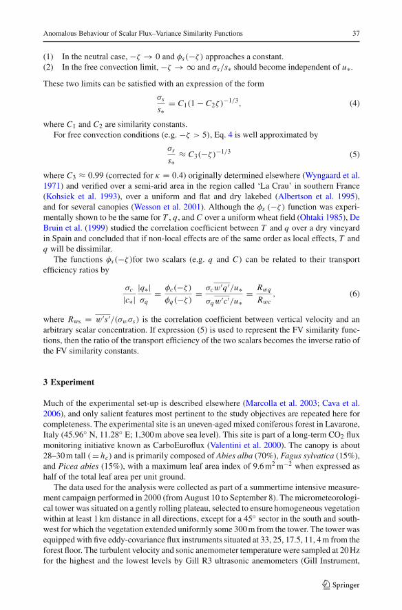
The dimensionless standard deviations for temperature, water vapour, and carbon dioxideconcentrations measured above the top of the forest (z = 32 m) are plotted against −ζ ,shown in Fig. 1. Overall, the temperature data follow a typical MOST FV scaling describedby Eq. 4 when C1 = 2.3 ± 0.1 and C2 = 9.5 ± 0.5 (the correlation coefficient R = 0.76).These coefficients compared well with coefficients derived for the ASL (C1 = 2, C2 = 9.5,as in Kaimal and Finnigan 1994). The error estimate of the model coefficients was derivedfrom Monte-Carlo simulations by randomizing these two coefficients and only acceptingcombinations in which R does not decrease with respect to its optimized value (R = 0.76).The measured FV similarity functions for the other two scalars exhibit significant scatter.

A number of studies, reviewed in the Appendix, have pointed out to the possible spuriousfunctional relationship between measured σs/s∗ and measured ζ because u∗ appears in thedependent variable (through s∗) and the independent variable (through L). The validity of thederived relationships has been tested (see Appendix) to assess the impact of such spuriouscorrelations arising from the fact that u∗ variability affects both dependent and independentvariables.

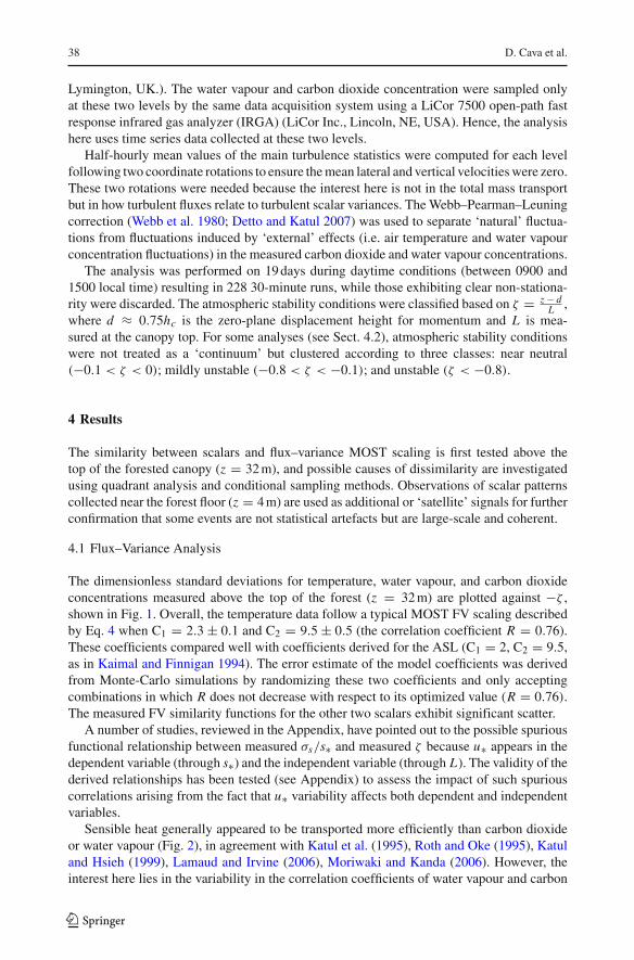
Sensible heat generally appeared to be transported more efficiently than carbon dioxideor water vapour (Fig. 2), in agreement with Katul et al. (1995), Roth and Oke (1995), Katuland Hsieh (1999), Lamaud and Irvine (2006), Moriwaki and Kanda (2006). However, theinterest here lies in the variability in the correlation coefficients of water vapour and carbon

123


Fig. 1 Dimensionless standarddeviation of (a) temperature (T ),(b) water vapour concentration(q) and (c) CO2 concentration(C), sampled above the canopytop (z = 32 m), versus thestability parameter −ζ . Blackstars refer to raw measurements,and grey full circles refer to datawith ‘anomalous events’ filteredout from the q and C time series.The black dashed lines representthe experimental similarityfunctions σs/s∗ =C1(1 − C2ζ )−1/3, whereC2 = 9.5 for all of the threescalars, whereas C1 = 2.3, 3.4and 2.8 for T , q, and C ,respectively. The black dottedlines represent the similarityfunctions for free convectionregime σs/s∗ = C3(ζ )−1/3

where C3 = C1C−1/32

dioxide (Fig. 3); it appears that the mode of this correlation is lower than unity (in absolutevalue) and the scatter is as significant as that of heat to water vapour comparisons.

In situations similar to those under investigation, the different behaviour of the T and qscalars may be partially explained by the active role of temperature in the transport (Katuland Hsieh 1999). However, this argument fails to explain the dissimilarity between q andC , especially given the fact the q is generally low and can be treated as a passive scalar.To explore the time scales at which these dissimilarities originate, the scalar spectra (forvariances) and cospectra are considered next.

4.2 Spectra and Cospectra

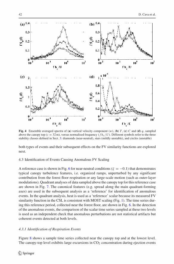
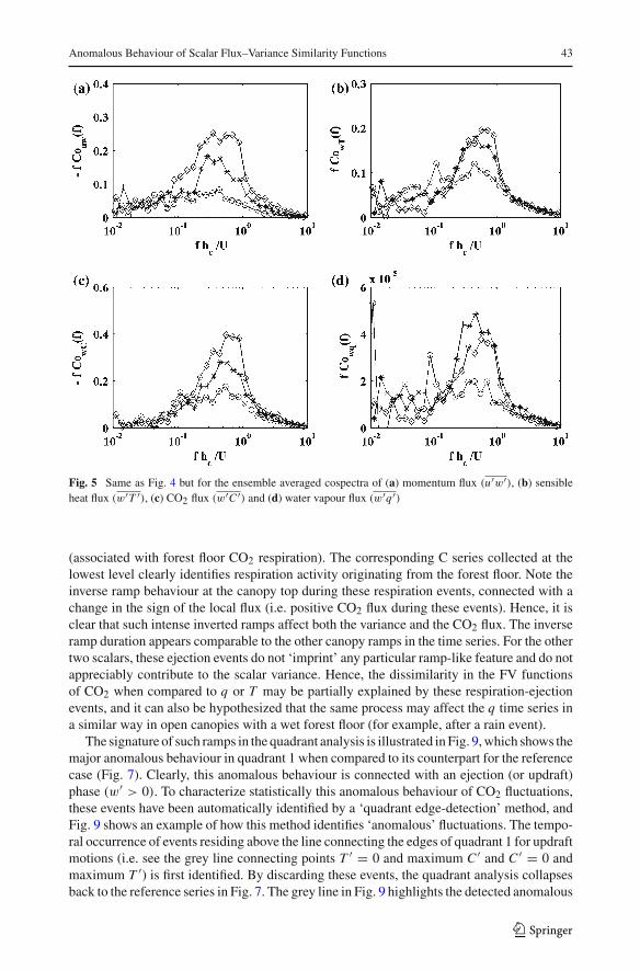
Spectral and cospectral analysis is used to explore the main mechanisms (i.e. phenomena andassociated scales) affecting variances and vertical fluxes of these three scalars for different sta-bility regimes. To minimize statistical uncertainty due to possible intermittent contributionsby large-scale motions comparable to the boundary-layer depth, the spectra and cospectra arecomputed using 5-h (from 1,000 to 1,500) windows for the three stability classes discussedin Sect. 3. To reduce the number of data points involved in the fast Fourier transform com-putation, the sampling frequency was reduced from 20 Hz to 2 Hz. The contribution of thesehigh frequencies to both variances and fluxes were found to be small (<10%). The ensembleaveraged spectra and cospectra for the three atmospheric stability classes are, respectively,plotted in Figs. 4 and 5.

123

40 D. Cava et al.

Fig. 2 Relative efficiency of (a)T and q, (b) T and C , and (c)q and C above the canopy top(z = 32 m) versus the stabilityparameter −ζ . Black stars andgrey full circles are defined inFig. 1

The spectral energy allows detection of scales that cause deviations of normalized variancesfrom their ASL states (Fig. 4). The spectrum of the vertical velocity component (computedfor reference) peaks at a scale consistent with the shear production length scale near thecanopy top (Raupach et al. 1996; Finnigan 2000; Poggi et al. 2004), and appears insensitiveto atmospheric stability variations consistent with other studies (Brunet and Irvine 2000).The spectrum of T exhibits similar behaviour to the w spectrum for near-neutral conditions,but as unstable atmospheric stability conditions are approached, more of the spectral energycontribution resides at lower frequencies. In the case of C , energy remains mainly concen-trated at canopy scales, but the effect of increased atmospheric stability is more pronouncedin ‘distributing’ energy across lower frequencies (when compared to w, for example). Thewater vapour variance exhibits the strongest dependence on atmospheric stability and, in par-ticular, under convective conditions much of the energy resides in the low-frequency rangeconsistent with boundary-layer scale eddies.

The cospectra (Fig. 5) show that canopy scales dominate the mass and momentum trans-port, with boundary-layer eddies contributing much less to scalar fluxes when compared totheir variance counterpart (i.e. they appear much less active in mass transport). However,their contribution increases as the flow becomes more convective, mainly for T and q . Con-tributions from scales commensurate with the boundary-layer height appear not to modifymuch the CO2 fluxes probably because carbon dioxide transport at the top of the atmosphericboundary layer is not appreciable given that the Lavarone site is remote from any majorindustrial or urban centre.

123


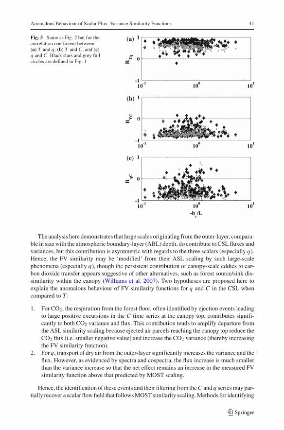
Fig. 3 Same as Fig. 2 but for thecorrelation coefficient between(a) T and q, (b) T and C , and (c)q and C . Black stars and grey fullcircles are defined in Fig. 1

The analysis here demonstrates that large scales originating from the outer-layer, compara-ble in size with the atmospheric boundary-layer (ABL) depth, do contribute to CSL fluxes andvariances, but this contribution is asymmetric with regards to the three scalars (especially q).Hence, the FV similarity may be ‘modified’ from their ASL scaling by such large-scalephenomena (especially q), though the persistent contribution of canopy-scale eddies to car-bon dioxide transfer appears suggestive of other alternatives, such as forest source/sink dis-similarity within the canopy (Williams et al. 2007). Two hypotheses are proposed here toexplain the anomalous behaviour of FV similarity functions for q and C in the CSL whencompared to T :

1. For CO2, the respiration from the forest floor, often identified by ejection events leadingto large positive excursions in the C time series at the canopy top, contributes signifi-cantly to both CO2 variance and flux. This contribution tends to amplify departure fromthe ASL similarity scaling because ejected air parcels reaching the canopy top reduce theCO2 flux (i.e. smaller negative value) and increase the CO2 variance (thereby increasingthe FV similarity function).

2. For q , transport of dry air from the outer-layer significantly increases the variance and theflux. However, as evidenced by spectra and cospectra, the flux increase is much smallerthan the variance increase so that the net effect remains an increase in the measured FVsimilarity function above that predicted by MOST scaling.

Hence, the identification of these events and their filtering from the C and q series may par-tially recover a scalar flow field that follows MOST similarity scaling. Methods for identifying

123

42 D. Cava et al.

Fig. 4 Ensemble averaged spectra of (a) vertical velocity component (w), (b) T , (c) C and (d) q, sampledabove the canopy top (z = 32 m), versus normalised frequency ( f hc/U ). Different symbols refer to the threestability classes defined in Sect. 3: diamonds (near-neutral), stars (mildly unstable), and circles (unstable)

both types of events and their subsequent effects on the FV similarity functions are explorednext.

4.3 Identification of Events Causing Anomalous FV Scaling

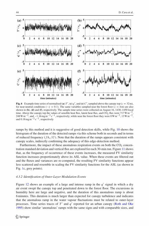
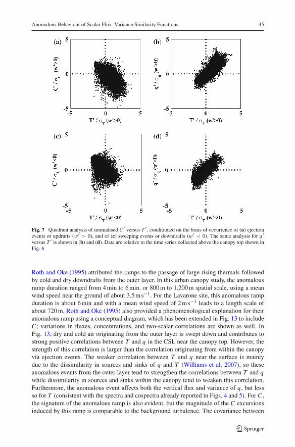
A reference case is shown in Fig. 6 for near-neutral conditions (ζ = −0.1) that demonstratestypical canopy turbulence features, i.e. organized ramps, unperturbed by any significantcontribution from the forest floor respiration or any large-scale motion (such as outer-layermodulations). Quadrant analyses of data sampled above the canopy top for this reference caseare shown in Fig. 7. The canonical features (e.g. spread along the main quadrant-formingaxes) are used in the subsequent analysis as a ‘reference’ for identification of anomalousevents. In the quadrant analysis, heat is used as a ‘reference’ scalar because its measured FVsimilarity function in the CSL is consistent with MOST scaling (Fig. 1). The time series dur-ing this reference period, collected near the forest floor, are shown in Fig. 6. In the detectionof the anomalous events, the comparison of the scalar time series sampled at these two levelsis used as an independent check that anomalous perturbations are not statistical artifacts butcoherent events detected at both levels.

4.3.1 Identification of Respiration Events

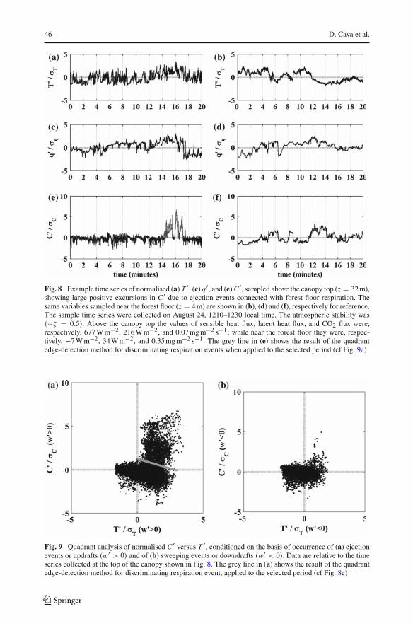
Figure 8 shows a sample time series collected near the canopy top and at the lowest level.The canopy-top level exhibits large excursions in CO2 concentration during ejection events

123


Fig. 5 Same as Fig. 4 but for the ensemble averaged cospectra of (a) momentum flux (u′w′), (b) sensibleheat flux (w′T ′), (c) CO2 flux (w′C ′) and (d) water vapour flux (w′q ′)

(associated with forest floor CO2 respiration). The corresponding C series collected at thelowest level clearly identifies respiration activity originating from the forest floor. Note theinverse ramp behaviour at the canopy top during these respiration events, connected with achange in the sign of the local flux (i.e. positive CO2 flux during these events). Hence, it isclear that such intense inverted ramps affect both the variance and the CO2 flux. The inverseramp duration appears comparable to the other canopy ramps in the time series. For the othertwo scalars, these ejection events do not ‘imprint’ any particular ramp-like feature and do notappreciably contribute to the scalar variance. Hence, the dissimilarity in the FV functionsof CO2 when compared to q or T may be partially explained by these respiration-ejectionevents, and it can also be hypothesized that the same process may affect the q time series ina similar way in open canopies with a wet forest floor (for example, after a rain event).

The signature of such ramps in the quadrant analysis is illustrated in Fig. 9, which shows themajor anomalous behaviour in quadrant 1 when compared to its counterpart for the referencecase (Fig. 7). Clearly, this anomalous behaviour is connected with an ejection (or updraft)phase (w′ > 0). To characterize statistically this anomalous behaviour of CO2 fluctuations,these events have been automatically identified by a ‘quadrant edge-detection’ method, andFig. 9 shows an example of how this method identifies ‘anomalous’ fluctuations. The tempo-ral occurrence of events residing above the line connecting the edges of quadrant 1 for updraftmotions (i.e. see the grey line connecting points T ′ = 0 and maximum C ′ and C ′ = 0 andmaximum T ′) is first identified. By discarding these events, the quadrant analysis collapsesback to the reference series in Fig. 7. The grey line in Fig. 9 highlights the detected anomalous

123

44 D. Cava et al.

Fig. 6 Example time series of normalised (a) T ′, (c) q ′, and (e) C ′, sampled above the canopy top (z = 32 m),for near-neutral conditions (−ζ = 0.1). The same variables sampled near the forest floor (z = 4 m) are alsoshown in (b), (d) and (f), respectively. The sample time series were collected on August 16, 1430–1450 localtime. Above the canopy top the values of sensible heat flux, latent heat flux, and CO2 flux were 717 W m−2,248 W m−2, and −1.16 mg m−2 s−1, respectively; while near the forest floor they were 8 W m−2, 13 W m−2,and 0.18 mg m−2 s−1, respectively

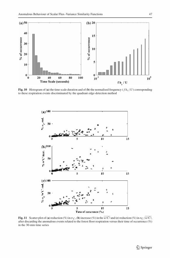
ramps by this method and it is suggestive of good detection skills, while Fig. 10 shows thehistogram of the duration of the detected ramps via this scheme both in seconds and in termsof reduced frequency ( f hc/U ). Note that the duration of the ramps appears consistent withcanopy scales, indirectly confirming the adequacy of this edge-detection method.

Furthermore, the impact of these anomalous respiration events on both the CO2 concen-tration standard deviation and vertical flux are explored for each 30-min run. Figure 11 showsthat, as the frequency of occurrence of these events increases, the measured FV similarityfunction increases proportionately above its ASL value. When these events are filtered outand the fluxes and variances are re-computed, the resulting FV similarity functions appearless scattered and resemble in scaling the FV similarity functions for the ASL (as shown inFig. 1c, grey points).

4.3.2 Identification of Outer-Layer Modulation Events

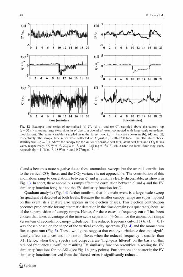
Figure 12 shows an example of a large and intense ramp in the q ′ signal in which a dryair event swept the canopy top and penetrated down to the forest floor. The excursions inhumidity here are large and negative, and the duration of this anomalous ramp is about6 minutes. This duration is much larger than expected for canopy turbulence and indicatesthat the anomalous ramp in the water vapour fluctuations must be related to outer-layerprocesses. Time series traces of T ′ and q ′ reported for an urban canopy (Roth and Oke1995) show similar ‘anomalous’ ramps with the same signs and with comparable sizes, and

123


Fig. 7 Quadrant analysis of normalised C ′ versus T ′, conditioned on the basis of occurrence of (a) ejectionevents or updrafts (w′ > 0), and of (c) sweeping events or downdrafts (w′ < 0). The same analysis for q ′versus T ′ is shown in (b) and (d). Data are relative to the time series collected above the canopy top shown inFig. 6

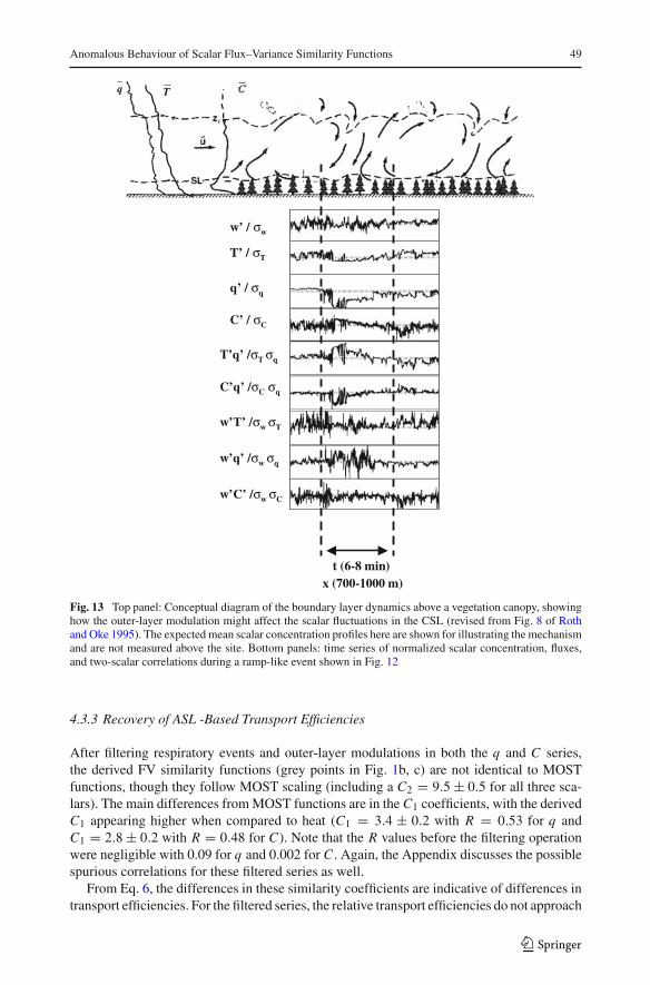
Roth and Oke (1995) attributed the ramps to the passage of large rising thermals followedby cold and dry downdrafts from the outer layer. In this urban canopy study, the anomalousramp duration ranged from 4 min to 6 min, or 800 m to 1,200 m spatial scale, using a meanwind speed near the ground of about 3.5 m s−1. For the Lavarone site, this anomalous rampduration is about 6 min and with a mean wind speed of 2 m s−1 leads to a length scale ofabout 720 m. Roth and Oke (1995) also provided a phenomenological explanation for theiranomalous ramp using a conceptual diagram, which has been extended in Fig. 13 to includeC ; variations in fluxes, concentrations, and two-scalar correlations are shown as well. InFig. 13, dry and cold air originating from the outer layer is swept down and contributes tostrong positive correlations between T and q in the CSL near the canopy top. However, thestrength of this correlation is larger than the correlation originating from within the canopyvia ejection events. The weaker correlation between T and q near the surface is mainlydue to the dissimilarity in sources and sinks of q and T (Williams et al. 2007), so theseanomalous events from the outer layer tend to strengthen the correlations between T and qwhile dissimilarity in sources and sinks within the canopy tend to weaken this correlation.Furthermore, the anomalous event affects both the vertical flux and variance of q , but lessso for T (consistent with the spectra and cospectra already reported in Figs. 4 and 5). For C ,the signature of the anomalous ramp is also evident, but the magnitude of the C excursionsinduced by this ramp is comparable to the background turbulence. The covariance between

123

46 D. Cava et al.

Fig. 8 Example time series of normalised (a) T ′, (c) q ′, and (e) C ′, sampled above the canopy top (z = 32 m),showing large positive excursions in C ′ due to ejection events connected with forest floor respiration. Thesame variables sampled near the forest floor (z = 4 m) are shown in (b), (d) and (f), respectively for reference.The sample time series were collected on August 24, 1210–1230 local time. The atmospheric stability was(−ζ = 0.5). Above the canopy top the values of sensible heat flux, latent heat flux, and CO2 flux were,respectively, 677 W m−2, 216 W m−2, and 0.07 mg m−2 s−1; while near the forest floor they were, respec-tively, −7 W m−2, 34 W m−2, and 0.35 mg m−2 s−1. The grey line in (e) shows the result of the quadrantedge-detection method for discriminating respiration events when applied to the selected period (cf Fig. 9a)

Fig. 9 Quadrant analysis of normalised C ′ versus T ′, conditioned on the basis of occurrence of (a) ejectionevents or updrafts (w′ > 0) and of (b) sweeping events or downdrafts (w′ < 0). Data are relative to the timeseries collected at the top of the canopy shown in Fig. 8. The grey line in (a) shows the result of the quadrantedge-detection method for discriminating respiration event, applied to the selected period (cf Fig. 8e)

123


Fig. 10 Histogram of (a) the time scale duration and of (b) the normalised frequency ( f hc/U ) correspondingto these respiration events discriminated by the quadrant edge-detection method

Fig. 11 Scatter plot of (a) reduction (%) in σC , (b) increase (%) in the w′C ′ and (c) reduction (%) in σC /w′C ′,after discarding the anomalous events related to the forest floor respiration versus their time of occurrence (%)in the 30-min time series

123

48 D. Cava et al.

Fig. 12 Example time series of normalised (a) T ′, (c) q ′, and (e) C ′, sampled above the canopy top(z = 32 m), showing large excursions in q ′ due to a downdraft event connected with large-scale outer-layermodulations. The same variables sampled near the forest floor (z = 4 m) are shown in (b), (d) and (f),respectively. The sample time series were collected on August 20, 1210–1230 local time. The atmosphericstability was −ζ = 0.3. Above the canopy top the values of sensible heat flux, latent heat flux, and CO2 fluxeswere, respectively, 677 W m−2, 203 W m−2, and −0.51 mg m−2 s−1; while near the forest floor they were,respectively, −11 W m−2, 18 W m−2, and 0.27 mg m−2 s−1

C and q becomes more negative due to these anomalous sweeps, but the overall contributionto the vertical CO2 fluxes and the CO2 variance is not appreciable. The contribution of thisanomalous ramp to correlations between C and q remains clearly discernable, as shown inFig. 13. In short, these anomalous ramps affect the correlation between C and q and the FVsimilarity function for q but not the FV similarity function for C .

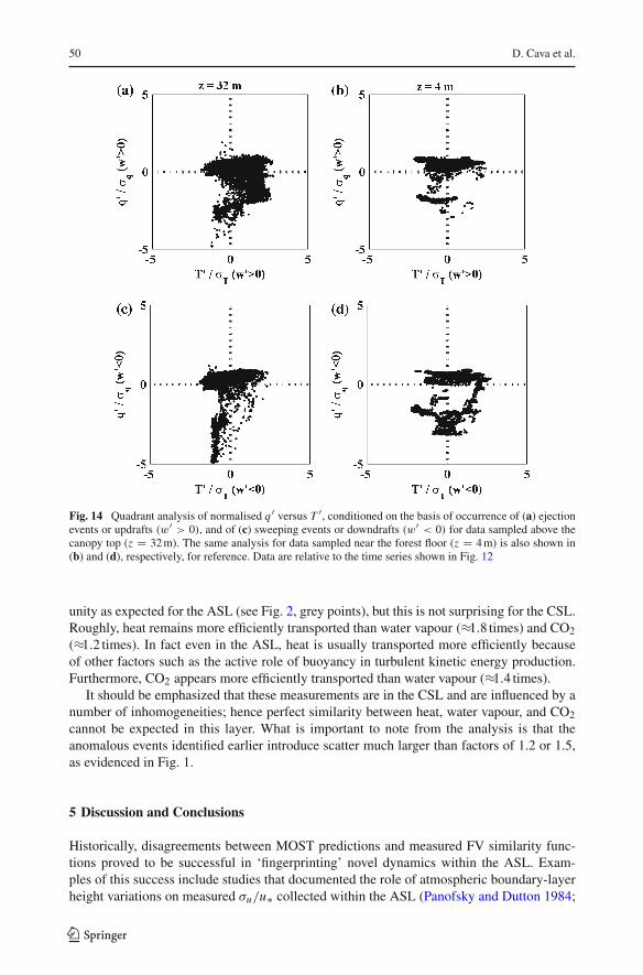
Quadrant analysis (Fig. 14) further confirms that this main event is a large-scale sweep(in quadrant 3) detected at both levels. Because the smaller canopy ramps are superimposedon this event, its signature also appears in the ejection phases. This ejection contributionbecomes problematic for any automatic detection in the time domain (via quadrants) becauseof the superposition of canopy ramps. Hence, for these cases, a frequency cut-off has beenchosen that takes advantage of the time-scale separation (4–6 min for the anomalous rampsversus tens of seconds for canopy turbulence). The reduced frequency cut-off ( f hc/U = 0.1)

was chosen based on the shape of the vertical velocity spectrum (Fig. 4) and the momentumflux cospectrum (Fig. 5). These two figures suggest that canopy turbulence does not signif-icantly affect variances and momentum fluxes when the reduced frequency is smaller than0.1. Hence, when the q spectra and cospectra are ‘high-pass filtered’ on the basis of thisreduced frequency cut-off, the resulting FV similarity function resembles in scaling the FVsimilarity functions for the ASL (see Fig. 1b, grey points). Furthermore, the scatter in the FVsimilarity functions derived from the filtered series is significantly reduced.

123


T’q’ /σT σq

w’ / σw

T’ / σT

q’ / σq

C’ / σC

C’q’ /σC σq

w’T’ /σw σT

w’q’ /σw σq

w’C’ /σw σC

t (6-8 min)x (700-1000 m)

q T

Fig. 13 Top panel: Conceptual diagram of the boundary layer dynamics above a vegetation canopy, showinghow the outer-layer modulation might affect the scalar fluctuations in the CSL (revised from Fig. 8 of Rothand Oke 1995). The expected mean scalar concentration profiles here are shown for illustrating the mechanismand are not measured above the site. Bottom panels: time series of normalized scalar concentration, fluxes,and two-scalar correlations during a ramp-like event shown in Fig. 12

4.3.3 Recovery of ASL -Based Transport Efficiencies

After filtering respiratory events and outer-layer modulations in both the q and C series,the derived FV similarity functions (grey points in Fig. 1b, c) are not identical to MOSTfunctions, though they follow MOST scaling (including a C2 = 9.5 ± 0.5 for all three sca-lars). The main differences from MOST functions are in the C1 coefficients, with the derivedC1 appearing higher when compared to heat (C1 = 3.4 ± 0.2 with R = 0.53 for q andC1 = 2.8 ± 0.2 with R = 0.48 for C). Note that the R values before the filtering operationwere negligible with 0.09 for q and 0.002 for C . Again, the Appendix discusses the possiblespurious correlations for these filtered series as well.

From Eq. 6, the differences in these similarity coefficients are indicative of differences intransport efficiencies. For the filtered series, the relative transport efficiencies do not approach

123

50 D. Cava et al.

Fig. 14 Quadrant analysis of normalised q ′ versus T ′, conditioned on the basis of occurrence of (a) ejectionevents or updrafts (w′ > 0), and of (c) sweeping events or downdrafts (w′ < 0) for data sampled above thecanopy top (z = 32 m). The same analysis for data sampled near the forest floor (z = 4 m) is also shown in(b) and (d), respectively, for reference. Data are relative to the time series shown in Fig. 12

unity as expected for the ASL (see Fig. 2, grey points), but this is not surprising for the CSL.Roughly, heat remains more efficiently transported than water vapour (≈1.8 times) and CO2

(≈1.2 times). In fact even in the ASL, heat is usually transported more efficiently becauseof other factors such as the active role of buoyancy in turbulent kinetic energy production.Furthermore, CO2 appears more efficiently transported than water vapour (≈1.4 times).

It should be emphasized that these measurements are in the CSL and are influenced by anumber of inhomogeneities; hence perfect similarity between heat, water vapour, and CO2

cannot be expected in this layer. What is important to note from the analysis is that theanomalous events identified earlier introduce scatter much larger than factors of 1.2 or 1.5,as evidenced in Fig. 1.

5 Discussion and Conclusions

Historically, disagreements between MOST predictions and measured FV similarity func-tions proved to be successful in ‘fingerprinting’ novel dynamics within the ASL. Exam-ples of this success include studies that documented the role of atmospheric boundary-layerheight variations on measured σu/u∗ collected within the ASL (Panofsky and Dutton 1984;

123


Hogstrom 1990; De Bruin et al. 1993). Such studies provided early evidence that inactiveeddy motion, originating from the outer layer, can affect ASL flow variables such as σu .Inactive eddy motion was also shown to modify the root-mean-squared turbulent pressurefluctuations within the ASL (Katul et al. 1996). McNaughton and Brunet (2002) even arguedthat interactions between such inactive and active eddy motions responsible for momentumtransfer are also possible within the ASL and proposed a simplified mechanism for its onset.Likewise, a large number of studies (Wesley 1988; Weaver 1990; Padro 1993; Andreas et al.1998) have shown how source-sink in-homogeneity at the ground induces departure betweenmeasured FV similarity functions and predictions from MOST.

The next logical extension is whether FV similarity analysis can be used to identify themain mechanisms modulating the CSL. While lacking the ‘niceties’ of MOST formulationsas a reference model for an idealized flow state, the FV similarity functions for scalars in theCSL may provide important clues about the role of outer-layer modulations and source-sinkdissimilarity in describing CSL turbulence. Mainly, the basic premise is that such complexmechanisms do not affect proportionally the scalar fluxes and their variances.

Our analysis showed that within the CSL of a dense vegetated canopy, both outer-layerprocesses and heterogeneities in sources and sinks within the canopy volume affect FV sim-ilarity functions. Spectral and cospectral analysis suggested that scalar variances were muchmore sensitive to these two mechanisms than scalar fluxes. For water vapour, the outer-layercontribution to scalar fluxes can be significant when the latent heat flux is small compared tothe sensible heat flux in agreement with recent studies (Lamaud and Irvine 2006). Becauseof the observed positive correlation between T and q (transport of dry and cold air), it canhypothesised that the effect of air directly entrained from the free atmosphere is less signif-icant than the effect of air transported from other zones within the outer layer (as observedin Roth and Oke 1995). Moreover, in the alpine forest studied here, where no major indus-try or urban centre is present, the contribution of outer-layer modulations to CO2 appearssmall compared to the intermittent accumulation-ejection cycle of CO2 inside the canopyvolume. In fact, respired CO2 from the forest floor was shown to lead to large positive excur-sions in the C time series at the canopy top thereby contributing significantly to both CO2

variance and vertical flux. The same process may affect the q time series in a similar wayin more open canopies and in the presence of a wet forest floor (for example, after a rainevent).

The data analysis here showed that if these large-scale outer-layer modulations andejection-accumulation events are ‘filtered out’ from the water vapour and CO2 concentrationtime series, respectively, MOST scaling is approximately recovered.

Finally, other important processes that can produce anomalous scaling in FV similarityfunctions, such as advection, were not considered. It is difficult to explore these processes viasingle tower measurements, though some theoretical and experimental attempts are presentedin Assouline et al. (2008) for heat and water vapour above small reservoirs. Recent studies(Feigenwinter et al. 2004; Aubinet et al. 2005; Sun et al. 2007) found that advection maybe significant even during daytime especially with low intensity turbulence. However, themain concern refers to nocturnal conditions when an underestimation of CO2 fluxes using theeddy-covariance technique frequently occurs because non-turbulent transport processes, nottaken into account by the eddy-covariance system, become significant. Under these condi-tions, quantifying and understanding advective transport processes may be important for theimprovement of flux measurements. It is possible that departures from MOST scaling for FVmay provide additional clues as to when CO2 advection is important. However, Feigenwinteret al. 2004, Aubinet et al. 2005, Sun et al. 2007 do not discuss the role of advection on FVsimilarity functions (only on CO2 fluxes via the mean scalar continuity).

123

52 D. Cava et al.

The broader implications of these findings are three-fold. The first pertains to the surfaceenergy balance studies and energy balance closure. If outer-layer modulation can be sig-nificant and detected in the water vapour concentration series, then it can also affect eddy-covariance water vapour turbulent flux measurements in the CSL. However, net radiationmeasurements are insensitive to such outer-layer modulations. Whether this mechanism alonemay explain the lack of surface energy balance closure is subject to some debate (Steinfeldet al. 2007). For example, the performed analysis showed that during a 6-min sweepingevent of dry and cold air from the outer layer, the local latent heat flux actually increased(not decreased). The contributions to sensible heat flux by such events may vary as well.Here, their contribution to sensible heat was not very significant when compared to fluxesoriginating from within the canopy.

The second pertains to the use of the energy balance closure for latent heat flux to ‘correct’or ‘adjust’ net ecosystem CO2 exchange (NEE) (Twine et al. 2000). Clearly, this approachlacks any theoretical basis given the spectral and cospectral dissimilarities of these two sca-lars in the CSL. While the measured FV similarity functions for CO2 and water vapourappeared higher than for heat, the mechanisms producing this increase were different. Forwater vapour, the increase was connected to the entrainment of dry air, while for CO2 itwas mainly connected with contributions from an ejection-accumulation cycle of respiredCO2. These two mechanisms differ in their contribution to the spectra and cospectra of watervapour and CO2 concentrations.

The third pertains to the inference of respiration events on NEE measurements within theCSL. It is clear that the main reason for the measured FV similarity function for CO2 appear-ing systematically larger than predictions by MOST is connected with the role of respiration(at this stand). This study demonstrated that when CO2 actually follows MOST scaling, therespiration contribution to NEE above the canopy is small. Hence, it is conceivable that acombination of conditional sampling schemes, quadrant analysis, and FV similarity functionsmay offer a promising method to extract daytime respiration from NEE time series abovethe canopy, at least for some limited observations. Given the existence of a large FluxNetdatabase (Baldocchi et al. 2001) already collected over the past decade, the latter implicationawaits systematic investigation.

Acknowledgements G. Katul acknowledges support from the US Department of Energy (DOE) throughthe Office of Biological and Environmental Research (BER) Terrestrial Carbon Processes (TCP) program(Grants # 10509-0152, DE-FG02-00ER53015, and DE-FG02-95ER62083), from the National Science Foun-dation (NSF-EAR 06-28342 and 06-35787), and from the Bi-national Agricultural and Research Development(BARD) fund (Grant #. IS3861-06). D. Cava acknowledges the Italian MIUR Project: ‘Sviluppo di un SistemaIntegrato Modellistica Numerica-Strumentazione e Tecnologie Avanzate per lo Studio e le Previsioni delTrasporto e della Diffusione di Inquinanti in Atmosfera’, grant “Bando 1105/2002 project n. 245” and supportfrom ‘Cooperazione Italia-USA su Scienza e Tecnologia dei Cambiamenti Climatici, Anno 2006-2008’.

Appendix: Verification of Spurious Correlations

An inherent problem in assessing MOST scaling, originally pointed out by Hicks (1978,1981), is related to ‘virtual’ or ‘spurious’ correlations arising because measured u∗ affectsboth the dependent and independent states being analysed. De Bruin (1982) and De Bruinet al. (1993) discussed this problem in the context of the FV method and showed that the−1/3 power-law dependence between σs/s∗ and ζ may be merely an artefact of the groupingvariables. In fact, s∗ contains u∗ and L contains u3∗. They concluded that the only way toshow that spurious correlation effects are not important is to compare the estimated fluxes

123


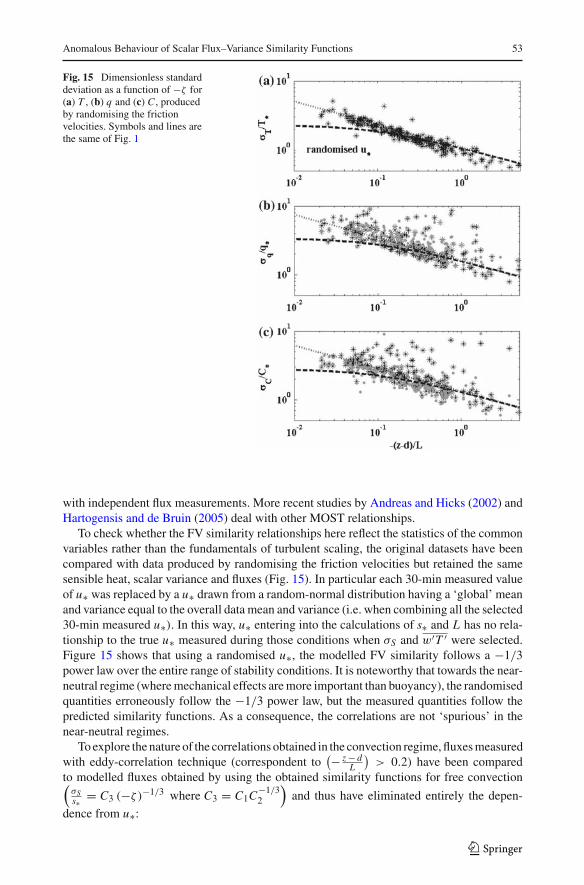
Fig. 15 Dimensionless standarddeviation as a function of −ζ for(a) T , (b) q and (c) C , producedby randomising the frictionvelocities. Symbols and lines arethe same of Fig. 1

with independent flux measurements. More recent studies by Andreas and Hicks (2002) andHartogensis and de Bruin (2005) deal with other MOST relationships.

To check whether the FV similarity relationships here reflect the statistics of the commonvariables rather than the fundamentals of turbulent scaling, the original datasets have beencompared with data produced by randomising the friction velocities but retained the samesensible heat, scalar variance and fluxes (Fig. 15). In particular each 30-min measured valueof u∗ was replaced by a u∗ drawn from a random-normal distribution having a ‘global’ meanand variance equal to the overall data mean and variance (i.e. when combining all the selected30-min measured u∗). In this way, u∗ entering into the calculations of s∗ and L has no rela-tionship to the true u∗ measured during those conditions when σS and w′T ′ were selected.Figure 15 shows that using a randomised u∗, the modelled FV similarity follows a −1/3power law over the entire range of stability conditions. It is noteworthy that towards the near-neutral regime (where mechanical effects are more important than buoyancy), the randomisedquantities erroneously follow the −1/3 power law, but the measured quantities follow thepredicted similarity functions. As a consequence, the correlations are not ‘spurious’ in thenear-neutral regimes.

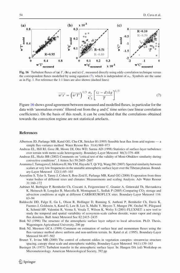
To explore the nature of the correlations obtained in the convection regime, fluxes measuredwith eddy-correlation technique (correspondent to

(− z − dL

)> 0.2) have been compared

to modelled fluxes obtained by using the obtained similarity functions for free convection(σSs∗ = C3 (−ζ )−1/3 where C3 = C1C−1/3

2

)and thus have eliminated entirely the depen-

dence from u∗:

123

54 D. Cava et al.

Fig. 16 Turbulent fluxes of (a) T , (b) q and (c) C , measured directly using eddy-correlation technique versusthe correspondent fluxes modelled by using equation (7), which is independent of u∗. Symbols are the sameas in Fig. 1. For reference the 1:1 lines are also shown (dashed lines)

w′s′ =(w′T ′

)1/3 σs

C3

[(z − d) kg

T

]1/3

(7)

Figure 16 shows good agreement between measured and modelled fluxes, in particular for thedata with ‘anomalous events’ filtered out from the q and C time series (see linear correlationcoefficients). On the basis of this result, it can be concluded that the correlations obtainedtowards the convection regime are not statistical artefacts.

References

Albertson JD, Parlange MB, Katul GG, Chu CR, Stricker H (1995) Sensible heat flux from arid regions — asimple flux-variance method. Water Resour Res 31(4):969–973

Andreas EL, Hill RJ, Gosz JR, Moore DI, Otto WD, Sarma AD (1998) Statistics of surface-layer turbulenceover terrain with metre-scale heterogeneity. Boundary-Layer Meteorol 86(3):379–408

Andreas EL, Hicks BB (2002) Comments on “critical test of the validity of Moni-Obukhov similarity duringconvective conditions”. J Atmos Sci 59:2605–2607

Asanuma J, Tamagawa I, Ishikawa H, Ma YM, Hayashi T, Qi YQ, Wang JM (2007) Spectral similarity betweenscalars at very low frequencies in the unstable atmospheric surface layer over the Tibetan plateau. Bound-ary-Layer Meteorol 122(1):85–103

Assouline S, Tyler S, Tanny J, Cohen S, Bou-Zeid E, Parlange MB, Katul GG (2008) Evaporation from threewater bodies of different sizes and climates: Measurements and scaling Analysis. Adv Water Resour31:160–172

Aubinet M, Berbigier P, Bernhofer Ch, Cescatti A, Feigenwinter C, Granier A, Grünwald Th, HavrankovaK, Heinesch B, Longdoz B, Marcolla B, Montagnani L, Sedlak P (2005) Comparing CO2 storage andadvection conditions at night at different CARBOEUROFLUX sites. Boundary-Layer Meteorol 116:63–94

Baldocchi DD, Falge E, Gu L, Olson R, Hollinger D, Running S, Anthoni P, Bernhofer Ch, Davis K,Fuentes J, Goldstein A, Katul G, Law B, Lee X, Malhi Y, Meyers T, Munger JW, Oechel W, PilegaardK, Schmid HP, Valentini R, Verma S, Vesala T, Wilson K, Wofsy S (2001) FLUXNET: a new tool tostudy the temporal and spatial variability of ecosystem-scale carbon dioxide, water vapor and energyflux densities. Bull Amer Meteorol Soc 82:2415–2435

Bink NJ (1996) The structure of the atmospheric surface layer subject to local advection. Ph.D. Thesis,Wageningen Agricultural University, 206 pp

Bink NJ, Meesters GCA (1999) Comment on estimation of surface heat and momentum fluxes using theflux-variance method above uniform and non-uniform terrain. In: Katul et al. (1995). Boundary-LayerMeteorol 84:497–502

Brunet Y, Irvine MR (2000) The control of coherent eddies in vegetation canopies: streamwise structurespacing, canopy shear scale and atmospheric stability. Boundary-Layer Meteorol 94(1):139–163

Businger JA (1973) Turbulent transfer in the atmospheric surface layer. In: Haugen DA (ed) Workshop onMicrometeorology. American Meteorological Society, 392 pp

123


Cava D, Katul GG, Scrimieri A, Poggi D, Cescatti A, Giostra U (2006) Buoyancy and the sensible heat fluxbudget within dense canopies. Boundary-Layer Meteorol 118(1):217–240

Choi TKJ, Lee H, Hong J, Asanuma J, Ishikawa H, Gao Z, Wang J, Koike T (2004) Turbulent exchange of heat,water vapor and momentum over a Tibetan praire by eddy covariance and flux-variance measurements.J Geophys Res-Atmos 109(D21):D21106

Cullen NJ, Steffen K, Blanken PD (2007) Nonstationarity of turbulent heat fluxes at Summit, Greenland.Boundary-Layer Meteorol 122(2):439–455

de Arellano JVG, Gioli B, Miglietta F, Jonker HJJ, Baltink HK, Hutjes RWA, Holtslag AAM (2004) Entrain-ment process of carbon dioxide in the atmospheric boundary layer. J Geophys Res-Atmos109(D18):D18110

De Bruin HAR (1982) The energy balance at the earth’s surface: a practical approach. Ph.D. thesis, WageningenAgricultural University. (also K.N.M.I., Sci. Rep. 81–1)

De Bruin HAR, Kohsiek W, Van Den Hurk BJJM (1993) A verification of some methods to determine thefluxes of momentum, sensible heat, and water-vapor using standard-deviation and structure parameterof scalar meteorological quantities. Boundary-Layer Meteorol 63(3):231–257

De Bruin HAR (1994) Analytic solutions of the equations governing the temperature fluctuation method.Boundary-Layer Meteorol 68:427–432

De Bruin HAR, Van Den Hurk BJJM, Kroon LJM (1999) On the temperature-humidity correlation and simi-larity. Boundary-Layer Meteorol 93:453–468

Detto M, Katul GG (2007) Simplified expressions for adjusting higher-order turbulent statistics obtained fromopen path gas analyzers. Boundary-Layer Meteorol 122(1):205–216

Detto M, Katul GG, Mancini M, Montaldo N, Albertson J (2008) Surface heterogeneity and its signature inhigher-order scalar similarity relationships. Agric For Meteorol (In press)

Finnigan J (2000) Turbulence in plant canopies. Ann Rev Fluid Mech 32:519–571Feigenwinter C, Bernhofer C, Vogt R (2004) The influence of advection on the short term CO2-budget in and

above a forest canopy. Boundary-Layer Meteorol 113:201–224Garratt JR (1978) Flux profile relations above tall vegetation. Quart J Roy Meteorol Soc 104:199–211Garratt JR (1980) Surface influence upon vertical profiles in the atmospheric near-surface layer. Quart J Roy

Meteorol Soc 106:803–819Garratt JR (1983) Surface influence upon vertical profiles in the nocturnal boundary layer. Boundary-Layer

Meteorol 26:69–80Górska M, de Arellano JV, LeMone MA (2006) The exchange of carbon dioxide between the atmospheric

boundary layer and the free atmosphere: observational and LES study. In: Extended abstract presentedon the 17th AMS Symposium on Boundary Layer and Turbulence, San Diego, paper 1.6

Hartogensis OK, De Bruin HAR (2005) Monin-Obukhov similaruty functions of the structure parameter oftemperature and turbulent kinetic energy dissipation rate in the stable boundary layer. Boundary-LayerMeteorol 116:253–276

Hicks BB (1978) Some limitations of dimensional analysis and power laws. Boundary-Layer Meteorol14:567–569

Hicks BB (1981) An examination of turbulence statistics in the surface boundary layer. Boundary-LayerMeteorol 21:389–402

Hogstrom U, Bergstrom H, Smedman AS, Halldin S, Lindroth A (1989) Turbulent exchange above a Pineforest. 1, fluxes and gradients. Boundary-Layer Meteorol 49(1–2):197–217

Hogstrom U (1990) Analysis of turbulence structure in the surface-layer with a modified similarity formulationfor near neutral conditions. J Atmos Sci 47(16):1949–1972

Hogstrom U, Hunt JCR, Smedman AS (2002) Theory and measurements for turbulence spectra and variancesin the atmospheric neutral surface layer. Boundary-Layer Meteorol 103(1):101–124

Juang JY, Katul GG, Siqueira MBS, Stoy PC, Palmroth S, McCarthy HR, Kim HS, Oren R (2006) Modelingnighttime ecosystem respiration from measured CO2 concentration and air temperature profiles usinginverse methods. J Geophys Res-Atmos 111(D8):D08s05

Kaimal JC, Finnigan JJ (1994) Atmospheric boundary layer flows. Oxford University Press, New York 289 ppKatul G, Goltz SM, Hsieh CI, Cheng Y, Mowry F, Sigmon J (1995) Estimation of surface heat and momentum

fluxes using the flux-variance method above uniform and nonuniform terrain. Boundary-Layer Meteorol74(3):237–260

Katul GG, Albertson JD, Hsieh CI, Conklin PS, Sigmon JT, Parlange MB, Knoerr KR (1996) The “inactive”eddy motion and the large-scale turbulent pressure fluctuations in the dynamic sublayer. J Atmos Sci53(17):2512–2524

Katul GG, Hsieh CI (1999) A note on the flux-variance similarity relationships for heat and water vapour inthe unstable atmospheric surface layer. Boundary-Layer Meteorol 90(2):327–338

123

56 D. Cava et al.

Katul GG, Sempreviva AM, Cava D (2008) The temperature-humidity covariance in the marine surface layer:a one-dimensional analytical model. Boundary-Layer Meteorol 126(2):263–278

Kohsiek W, De Bruin HAR, The H, Van Den Hurk B (1993) Estimation of the sensible heat flux of a semi-aridarea using surface radiative temperature measurements. Boundary-Layer Meteorol 63(3):231–230

Kroon LJM, De Bruin HAR (1995) The Crau field experiment—turbulent exchange in the surface-layer underconditions of strong local advection. J Hydrol 166(3–4):327–351

Kustas WP, Blanford JH, Stannard DI, Daughtry CST, Nichols WD, Weltz MA (1994) Local energy fluxestimates for unstable conditions using variance data in semiarid rangelands. Water Resour Res 30(5):1351–1361

Lamaud E, Irvine M (2006) Temperature-humidity dissimilarity and heat-to-water-vapour transport efficiencyabove and within a pine forest canopy: the role of the Bowen ratio. Boundary-Layer Meteorol 120(1):87–109

Leclerc MY, Beissner KC, Shaw RH, Den Hartog G, Neumann HH (1990) The influence of atmosphericstability on the budgets of the reynolds stress and turbulent kinetic energy within and above a deciduousforest. J Appl Meteorol 29:916–933

Lyons TJ, Fuqin L, Hacker JM, Cheng WL, Huang XM (2001) Regional turbulent statistics over contrastingnatural surfaces. Meteorol Atmos Phys 78(3–4):183–194

Mahrt L (1991a) Boundary-layer moisture regimes. Quart J Roy Meteorol Soc 117(497):151–176Mahrt L (1991b) Eddy asymmetry in the sheared heated boundary-layer. J Atmos Sci 48(3):472–492Marcolla B, Pitacco A, Cescatti A (2003) Canopy architecture and turbulence structure in a coniferous forest.

Boundary-Layer Meteorol 108(1):39–59McNaughton KG, Brunet Y (2002) Townsend’s hypothesis, coherent structures and Monin-Obukhov

similarity. Boundary-Layer Meteorol 102(2):161–175McNaughton KG, Laubach J (1998) Unsteadiness as a cause of non-equality of eddy diffusivities for heat and

vapour at the base of an advective inversion. Boundary-Layer Meteorol 88(3):479–504McNaughton KG, Laubach J (2000) Power spectra and cospectra for wind and scalars in a disturbed surface

layer at the base of an advective inversion. Boundary-Layer Meteorol 96(1–2):143–185Mölder M, Grelle A, Lindroth A, Halldin S (1999) Flux-profile relationships over a boreal forest—roughness

sublayer corrections. Agric For Meteorol 98(9):645–658Moene AF, Schüttemeyer D, Hartogensis OK (2006) Scalar similarity functions: the influence of surface hetero-

geneity and entrainment. In Extended abstract presented on the 17th AMS Symposium on Boundary Layerand Turbulence, San Diego, paper 5.1

Moriwaki R, Kanda M (2006) Local and global similarity in turbulent transfer of heat, water vapour, and CO2in the dynamic convective sublayer over a suburban area. Boundary-Layer Meteorol 120(1):163–179

Ohtaki E (1985) On the similarity in atmospheric fluctuations of carbon-dioxide, water-vapor and temperatureover vegetated fields. Boundary-Layer Meteorol 32(1):25–37

Padro J (1993) An investigation of flux-variance methods and universal functions applied to 3 land-use typesin unstable conditions. Boundary-Layer Meteorol 66(4):413–425

Panofsky HA, Dutton JA (1984) Atmospheric turbulence: models and methods for engineering applications.Wiley, New York, 397 pp

Poggi D, Porporato A, Ridolfi L, Albertson JD, Katul GG (2004) The effect of vegetation density on canopysub-layer turbulence. Boundary-Layer Meteorol 111(3):565–587

Raupach MR (1979) Anomalies in flux-gradient relationships over forest. Boundary-Layer Meteorol 16:467Raupach MR, Stewart JB, Thom AS (1979) Analysis of flux-profile relationships above tall vegetation -

alternative view—comments. Quart J Roy Meteorol Soc 105(446):1077–1078Raupach MR, Finnigan JJ, Brunet Y (1996) Coherent eddies and turbulence in vegetation canopies: the

mixing-layer analogy. Boundary-Layer Meteorol 78(3–4):351–382Roth M, Oke TR (1995) Relative efficiencies of turbulent transfer of heat, mass, and momentum over a patchy

urban surface. J Atmos Sci 52(11):1863–1874Sempreviva AM, Gryning SE (2000) Mixing height over water and its role on the correlation between tem-

perature and humidity fluctuations in the unstable surface layer. Boundary-Layer Meteorol 97:273–291Steinfeld G, Letzel MO, Raasch S, Kanda M, Inagaki A (2007) Spatial representativeness of single tower mea-

surements and the imbalance problem with eddy-covariance fluxes: results of a large-eddy simulationstudy. Boundary-Layer Meteorol 123(1):77–98

Sun J, Burns SP, Delany AC, Oncley SP, Turnipseed AA, Stephens BB, Lenschow DH, LeMone MA, MonsonRK, Anderson DE (2007) CO2 transport over complex terrain. Agric Forest Meteorol 145:1–21

Thom AS, Stewart JB, Oliver HR, Gash JHC (1975) Comparison of aerodynamic and energy budget estimatesof fluxes over a pine forest. Quart J Roy Meteorol Soc 101:93–105

123


Tillman JE (1972) The indirect determination of stability, heat and momentum fluxes in the atmosphericboundary layer from simple scalar variables during dry unstable conditions. J Appl Meteorol 11:783–792

Thomas C, Martin JG, Goeckede M, Siqueira MB, Foken T, Law BE, Loescher HW, Katul G (2008) Esti-mating daytime ecosystem respiration from conditional sampling methods applied to multi-scalar highfrequency turbulence time series. Agic For Meteorol (In press)

Twine TE, Kustas WP, Norman JM, Cook DR, Houser PR, Meyers TP, Prueger JH, Starks PJ,Wesely ML (2000) Correcting eddy-covariance flux underestimates over a grassland. Agric For Meteorol103(3):279–300

Valentini R, Matteucci G, Dolman AJ, Schulze ED, Rebmann C, Moors EJ, Granier A, Gross P, Jensen NO,Pilegaard K, Lindroth A, Grelle A, Bernhofer C, Grunwald T, Aubinet M, Ceulemans R, Kowalski AS,Vesala T, Rannik U, Berbigier P, Loustau D, Guomundsson J, Thorgeirsson H, Ibrom A, Morgenstern K,Clement R, Moncrieff J, Montagnani L, Minerbi S, Jarvis PG (2000) Respiration as the main determinantof carbon balance in European forests. Nature 404(6780):861–865

Weaver HJ (1990) Temperature and humidity flux-variances relations determined by one–dimensional eddy-correlation. Boundary-Layer Meteorol 53:77–91

Webb EK, Pearman GI, Leuning R (1980) Correction of flux measurements for density effects due to heat andwater-vapor transfer. Quart J Roy Meteorol Soc 106(447):85–100

Wesley ML (1988) Use of variance techniques to measure dry air-surface exchange rates. Boundary-LayerMeteorol 44:13–31

Wesson KH, Katul G, Lai CT (2001) Sensible heat flux estimation by flux variance and half-order time deriv-ative methods. Water Resource Res 37(9):2333–2343

Williams CA, Scanlon TM, Albertson JD (2007) Influence of surface heterogeneity on scalar dissimilarity inthe roughness sublayer. Boundary-Layer Meteorol 122(1):149–165

Wyngaard JC, Cote OR, Izumi Y (1971) Local free convection, similarity, and budgets of shear stress and heatflux. J Atmos Sci 37:271–284

123