


Bahasa
Halaman
Hukum

Navigation-based Optimization of Stochastic Strategies for Allocating a
Robot Swarm among Multiple Sites
Spring Berman, Adam Halasz, M. Ani Hsieh and Vijay Kumar
Abstract— We present a decentralized, communication-lessapproach to the dynamic allocation of a swarm of homogeneousrobots to a target distribution among multiple sites. Buildingon our work in [1], we optimize stochastic control policies forthe robots that cause the population to quickly redistributeamong the sites while adhering to a limit on inter-site trafficat equilibrium. We propose a way to account for delays due tonavigation between sites in our controller synthesis procedure.Control policies that are designed with and without the useof delay statistics are compared for a simulation in which 240
robots distribute themselves among four buildings.
I. INTRODUCTION
We address the problem of quickly and efficiently de-
ploying a swarm of homogeneous robots to occupy multiple
locations in a predefined distribution for parallel task execu-
tion at each site. The robots must autonomously redistribute
themselves among the sites to ensure task completion in the
presence of robot failures or changes in the environment.
This problem is relevant to applications such as the sur-
veillance of multiple buildings, search-and-rescue, and large-
scale environmental monitoring.
In the multi-robot domain, methods to optimally allocate
robots to tasks or resources often reduce to market-based
approaches [2], [3], in which robots execute complex bidding
schemes to determine an allocation based on perceived costs
and utilities. While these approaches have been successful in
various applications, optimality is often sacrificed to reduce
the computation and communication requirements, which
scale poorly as the number of robots and tasks increase. An-
other approach is to model the swarm as a partial differential
equation and use a centralized optimal control strategy [4].
As the number of robots increases, it becomes less
likely that resource-constrained robots will always have the
communication and computational capabilities required for
centralized control. It therefore makes sense to consider a
decentralized approach to allocation that is efficient, scalable
in the number of robots and sites, robust to changes in robot
population, and uses little to no communication. Some work
on task allocation has used the self-organized behavior of
S. Berman and V. Kumar are with the GRASP Laboratory, Univer-sity of Pennsylvania, 3330 Walnut Street, Philadelphia, PA 19104, USA,{spring, kumar}@grasp.upenn.edu
A. Halasz is with the Dept. of Mathematics, West VirginiaUniversity, 307G Armstrong Hall, Morgantown, WV 26506, USA,[email protected]
M. A. Hsieh is with the Dept. of Mechanical Engineering and Mechanics,Drexel University, 3141 Chestnut Street, Philadelphia, PA 19104, USA,[email protected]
We gratefully acknowledge partial support from NSF grants CSR-CPS0720801, IIS-0427313, NSF IIP-0742304, and IIS-0413138, ARO grantW911NF-05-1-0219, and ONR grant N00014-07-1-0829.
insect colonies as inspiration for decentralized strategies in
which robots switch between simple behaviors in response
to local sensing [5]–[7]. We have adopted this distributed
paradigm, inspired in particular by the process of house-
hunting in ant colonies [8].
In recent work on decentralized control for task allocation,
a physical multi-robot system is abstracted to an accurate dif-
ferential equation model [9], [10]. In contrast to this “bottom-
up” analysis procedure, our methodology is based on a
“top-down” design approach that gives theoretical guarantees
on performance. The robots in our scenario redistribute
themselves by switching stochastically between pairs of sites
at probability rates specific to each transition. Our strategy
is to use a continuous approximation of the system to design
these rates to achieve our global objective.
We first applied this approach to the design of ant-inspired
behaviors that produce a predefined swarm allocation be-
tween two sites [11], [12]. We extended our methodology to
the problem of redistributing a swarm among many sites [1]
and introduced quorum-based control policies [13]. In [1],
we noted the idea of including in the analysis the effects of
robot navigation between sites when the travel times are not
negligible compared to the waiting times for transitions. In
this work, we extend our controller design methodology to
account for inter-site travel times. We optimize the rates at
which robots switch between sites for fast convergence to
a desired distribution subject to a constraint on equilibrium
traffic between sites. We compare the resulting control poli-
cies using a four-site surveillance simulation in which robot
travel time distributions have significant variability.
II. PROBLEM STATEMENT
A. Definitions and Assumptions
Consider N robots to be distributed among M sites. We
denote the number of robots at site i ∈ {1, . . . ,M} at time tby ni(t) and the desired number of robots at site i by nd
i , a
positive integer. The population fraction at site i at time t is
xi(t) = ni(t)/N . Then the system state vector is given by
x(t) = [x1(t) ... xM (t)]T
. We define the target distribution
as a set of desired population fractions to occupy each site,
xd = [xd1 ... xd
M ]T , where xdi = nd
i /N . A specification
in terms of fractions rather than absolute robot numbers is
useful for scaling and for applications in which losses of
robots to attrition and breakdown are common.
The interconnection topology of the sites can be modeled
as a directed graph, G = (V, E), where V , the set of vertices,
represents sites {1, . . . ,M} and E , the set of NE edges,
represents physical one-way routes between sites. Sites i
Proceedings of the47th IEEE Conference on Decision and ControlCancun, Mexico, Dec. 9-11, 2008
ThTA17.6
978-1-4244-3124-3/08/$25.00 ©2008 IEEE 4376
and j are adjacent, denoted by i ∼ j, if robots can travel
from i to j. We represent this relation by the ordered pair
(i, j) ∈ V × V , with the set E = {(i, j) ∈ V × V | i ∼ j }.
More generally, we can define V as a set of M tasks and
E as the set of possible transitions between tasks; then
G models precedence constraints between the tasks. It is
assumed that G is strongly connected, i.e. a directed path
exists between any pair of distinct vertices. This property
facilitates redistribution by allowing robots to travel to any
site from any other site; no sites act as sources or sinks.
We consider x(t) to represent the distribution of the state
of a Markov process on G, for which V is the state space
and E is the set of possible transitions. Every edge in Eis assigned a constant positive transition rate, kij , which
defines the probability per unit time for one robot at site
i to go to site j. It follows that the number of transitions
between two adjacent sites in a time interval t has a Poisson
distribution with parameter kijt. We use constant kij in order
to be able to abstract the system to a continuous model (see
Section II-B). In general, kij 6= kji.
We assume that each robot has knowledge of G, all kij ,
and the task to perform at each site, as well as the behaviors
necessary to navigate between sites and execute the tasks. We
also assume that each robot has a map of the environment
and can localize itself and sense neighboring robots.
B. Base Model
Our strategy for redistributing robots among the sites is
to program each robot to switch stochastically from site i to
site j with probability kij∆t at each time step ∆t [1]. In the
limit N → ∞, the physical system of individual robots can
be abstracted to a linear ordinary differential equation (ODE)
model according to the theoretical justification provided by
[14]. The model quantifies xi(t) as the difference between
the total influx and total outflux of robots at site i,
xi(t) =∑
∀j|(j,i)∈E
kjixj(t) −∑
∀j|(i,j)∈E
kijxi(t) . (1)
Then the system of equations for all M sites is given by
x = Kx , (2)
where K ∈ RM×M is a matrix defined as
Kij =
kji if i 6= j , (j, i) ∈ E ,0 if i 6= j , (j, i) /∈ E ,−
∑
(i,l)∈E kil if i = j .(3)
Since the number of robots is conserved, the population
fractions satisfy the equation
1T x = 1 . (4)
We will refer to equation (2) subject to (4) as the switching
model, since it describes a system in which robots switch
instantaneously between sites. The following theorem was
proved in [1].
Theorem 1: If the graph G is strongly connected, then the
switching model has a unique, stable equilibrium x.
This equilibrium can be calculated as [15]:
xi = Kii/M∑
j=1
Kjj , i = 1, ...,M , (5)
where Kij is the cofactor of K obtained by deleting row iand column j.
Theorem 1 implies that we can achieve the target distri-
bution xd from any initial distribution by specifying that
x ≡ xd through the following constraint on K,
Kxd = 0 . (6)
When the kij are chosen to satisfy (6), robots that use the kij
as stochastic transition rules will collectively occupy the sites
in distribution xd at steady state, assuming instant switching.
C. Time-Delayed Model
In reality, the influx of robots to site j from site i is
delayed by the time taken to travel between the sites, τij .
If we assume a constant delay τij for each edge (i, j), this
effect can be included by rewriting equation (1) as a delay
differential equation (DDE):
xi(t) =∑
∀j|(j,i)∈E
kjixj(t−τji) −∑
∀j|(i,j)∈E
kijxi(t) . (7)
Modeling the time delays has the effect that 1T x(t) < 1 for
t > 0, since some robots are traveling between sites. Let
nij(t) be the number of robots traveling from site i to site
j at time t and yij(t) = nij(t)/N . Then the conservation
equation for this system is:
M∑
i=1
xi(t) +M∑
i=1
∑
∀j|(i,j)∈E
yij(t) = 1 . (8)
III. ANALYSIS
In application, robot travel times between sites can be
highly variable due to changes in navigation patterns caused
by collision avoidance, crowding, and errors in localization.
Hence, model (7) can be made more realistic by defining
the delays τij as random variables, Tij . A reasonable form
for the probability density of the Tij can be estimated from
an analogous scenario in which vehicles deliver items along
roads to various sites. Vehicle travel times in this system
have been modeled as following an Erlang distribution to
capture the properties that the times have minimum possible
values, a small probability of being large due to accidents,
breakdowns, and low energy, and their distributions tend to
be skewed toward larger values [16]. We assume that each
Tij follows this distribution with parameters ωij , a positive
integer, and θij , a positive real number:
g(t;ωij , θij) =θ
ωij
ij tωij−1
(ωij − 1)!e−θijt . (9)
In practice, the parameters are estimated by fitting empirical
travel time data to density (9).
Under this assumption, the DDE model (7) can be trans-
formed into an equivalent ODE model of the form (1), which
47th IEEE CDC, Cancun, Mexico, Dec. 9-11, 2008 ThTA17.6
4377
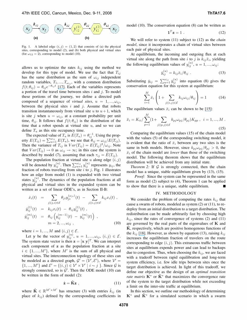
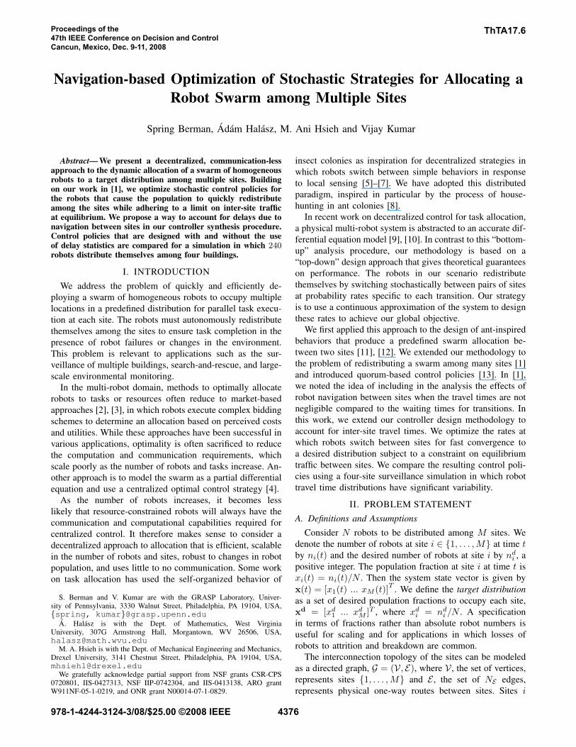
Fig. 1. A labeled edge (i, j) = (1, 2) that consists of (a) the physicalsites, corresponding to model (2), and (b) both physical and virtual sites(for ω12 = 2), corresponding to model (10).
allows us to optimize the rates kij using the method we
develop for this type of model. We use the fact that Tij
has the same distribution as the sum of ωij independent
random variables, T1, ..., Tωij, with a common distribution
f(t; θij) = θije−θijt [17]. Each of the variables represents
a portion of the travel time between sites i and j. To model
these portions of the journey, we define a directed path
composed of a sequence of virtual sites, u = 1, ..., ωij ,
between the physical sites i and j. Assume that robots
transition instantaneously from virtual site u to u+1, which
is site j when u = ωij , at a constant probability per unit
time, θij . It follows that f(t; θij) is the distribution of the
time that a robot spends at virtual site u, and so we can
define Tu as this site occupancy time.
The expected value of Tu is E(Tu) = θ−1ij . Using the prop-
erty E(Tij) =∑ωij
u=1 E(Tu), we see that θij = ωij/E(Tij).Then the variance of Tij is V ar(Tij) = E(Tij)
2/ωij . Note
that V ar(Tij) → 0 as ωij → ∞; in this case the system is
described by model (7), assuming that each τij = E(Tij).The population fraction at virtual site u along edge (i, j)
will be denoted by y(u)ij . Then
∑ωij
u=1 y(u)ij represents yij , the
fraction of robots traveling from site i to j. Fig. 1 illustrates
how an edge from model (1) is expanded with two virtual
states y(u)ij . The dynamics of the population fractions at all
physical and virtual sites in the expanded system can be
written as a set of linear ODE’s, as in Section II-B:
xi(t) =∑
j|(j,i)∈E
θjiy(ωji)ji (t) −
∑
j|(i,j)∈E
kijxi(t) ,
y(1)ij (t) = kijxi(t) − θijy
(1)ij (t) ,
y(m)ij (t) = θij
(
y(m−1)ij (t) − y
(m)ij (t)
)
,
m = 2, ..., ωij , (10)
where i = 1, ...,M and (i, j) ∈ E .
Let y be the vector of y(u)ij , u = 1, ..., ωij , (i, j) ∈ E .
The system state vector is then z = [x y]T . We can interpret
each component of z as the population fraction at a site
i ∈ {1, ...,M ′}, where M ′ is the sum of all physical and
virtual sites. The interconnection topology of these sites can
be modeled as a directed graph, G′ = (V ′, E ′), where V ′ ={1, ...,M ′} and E ′ = {(i, j) ∈ V ′ ×V ′ | i ∼ j }. Since G is
strongly connected, so is G′. Then the ODE model (10) can
be written in the form of model (2):
z = Kz , (11)
where K ∈ RM ′×M ′
has structure (3) with entries kij (in
place of kij) defined by the corresponding coefficients in
model (10). The conservation equation (8) can be written as
1T z = 1 . (12)
We will refer to system (11) subject to (12) as the chain
model, since it incorporates a chain of virtual sites between
each pair of physical sites.
At equilibrium, the incoming and outgoing flux at each
virtual site along the path from site i to j is kij xi, yielding
the following equilibrium values of y(u)ij , u = 1, ..., ωij :
y(u)ij = kij xi/θij . (13)
Substituting yij =∑ωij
u=1 y(u)ij into equation (8) gives the
conservation equation for this system at equilibrium:
M∑
i=1
xi
1 +∑
j|(i,j)∈E
kijωij/θij
= 1 (14)
The equilibrium values xi can be shown to be [15]:
xi = Kii/M∑
p=1
(1+∑
j|(p,j)∈E
kpjωpj/θpj)Kpp , i = 1, ...,M .
(15)
Comparing the equilibrium values (15) of the chain model
with the values (5) of the corresponding switching model, it
is evident that the ratio of xi between any two sites is the
same in both models. However, since kpjωpj/θpj > 0, the
xi of the chain model are lower than those of the switching
model. The following theorem shows that the equilibrium
distribution will be achieved from any initial state.
Theorem 2: If G is strongly connected, then the chain
model has a unique, stable equilibrium given by (13), (15).
Proof: Since the system can be represented in the same
form as model (2) subject to (4), Theorem 1 can be applied
to show that there is a unique, stable equilibrium.
IV. METHODOLOGY
We consider the problem of computing the rates kij that
cause a swarm of robots, modeled as system (2) or (11), to re-
deploy from an initial distribution to a target distribution. The
redistribution can be made arbitrarily fast by choosing high
kij , since the rates of convergence of systems (2) and (11)
are governed by the real parts of the eigenvalues of K and
K, respectively, which are positive homogenous functions of
the kij [18]. However, as shown by equation (13), raising kij
increases the equilibrium fraction of travelers on the route
corresponding to edge (i, j). This extraneous traffic between
sites at equilibrium expends power and can lead to backups
due to congestion. Thus, when choosing the kij , we are faced
with a tradeoff between rapid equilibration and long-term
system efficiency, i.e. few idle trips between sites once the
target distribution is achieved. In light of this tradeoff, we
define our objective as the design of an optimal transition
rate matrix K∗ or K∗ that maximizes the convergence rate
of the system to the target distribution while not exceeding
a limit on the inter-site traffic at equilibrium.
In this section, we outline our methodology of determining
K∗ and K∗ for a simulated scenario in which a swarm
47th IEEE CDC, Cancun, Mexico, Dec. 9-11, 2008 ThTA17.6
4378
of robots surveys the perimeters of several buildings while
reallocating to a target distribution among the buildings.
A. Surveillance simulation
1) Robot motion control: Each robot is represented as
a planar agent governed by a kinematic model. A robot
that is monitoring a building circulates around the perimeter
by aligning its velocity vector with the straight lines that
comprise the perimeter; this motion can also be achieved
with feedback controllers of the form given in [19]. The
robot slows down if a robot in front of it enters its sensing
range, which results in an approximately uniform distribution
of robots around the perimeter.
To implement inter-site navigation, we first performed a
convex cell decomposition of the free space. This resulted in
a discrete roadmap on which shortest-path computations be-
tween cells can be obtained using any standard graph search
algorithm. Each edge (i, j) ∈ E is defined as a sequence
of cells to be traversed by robots traveling from a distinct
exit point on the perimeter of building i to an entry point on
the perimeter of building j. We used Dijkstra’s algorithm to
compute the sequence with the shortest cumulative distance
between cell centroids, starting from the cell adjacent to the
exit at i and ending at the cell adjacent to the entrance at
j. The robots are provided a priori with the sequence of
cells corresponding to each edge. Navigation between cells is
achieved by composing local potential functions such that the
resulting control policy ensures arrival at the last cell in the
sequence [20]. We combine these navigation controllers with
ones derived from repulsive potential functions to achieve
inter-robot collision avoidance [21]. At each time step, the
robots compute the feedback controller to move from one cell
to the next based on their current position and the positions
of robots within their sensing ranges.
2) Site-to-site transitions: Gillespie’s Direct Method [14]
was used to simulate a sequence of robot site transition
events and their initiation times using the rates kij from the
switching model or chain model. Each event is identified with
the commitment of an individual robot to travel to another
site. A transition from building i to j is assigned to a random
robot on the perimeter of i. This robot continues to track the
perimeter until it reaches the exit for edge (i, j), at which
point it begins navigating to the entrance on building j. For
more details on this stochastic simulation, see [11] and [13].
The travel time τij is measured as the the sum of τaij ,
the time for a robot to reach the exit on building i from
the position at which it commits to the transition, and
τ bij , the travel time from the exit to building j’s entrance.
Because the robots at i are uniformly distributed around the
perimeter and are randomly selected for transitions, τaij has
a uniform distribution. The distribution of τ bij is affected by
the congestion on the roads and at the target sites, which
determines the amount of time spent avoiding collisions.
B. Computation of K∗ and K∗
We computed K∗ for the switching model and K∗ for two
versions of the chain model. To determine the parameters
of a full chain model that would most accurately emulate
the travel time distributions of the surveillance simulation,
we collected a set of τij from the simulation for each edge
(i, j), plotted a histogram of the τij , and then fit an Erlang
distribution (9) to the histogram to obtain ωij and θij . The
K∗ for this model is called K∗full. We also computed a K∗,
called K∗one, for a one-site chain model in which each ωij =
1 and each θij is 1/E(Tij) = θij/ωij from the full chain
model. In this case, the Erlang distribution reduces to an
exponential distribution with the same mean value.
We measure the degree of convergence to xd in terms of
the fraction of misplaced robots, defined as the 2-norm
∆(x) = ||x − xd||2 . (16)
We say that one system converges faster than another if it
takes less time for ∆(x) to decrease to a small fraction, such
as 0.1, of its initial value. We compute the transition rate
matrix that directly minimizes this convergence time using
Metropolis optimization [22] with the kij as the optimization
variables. This method was chosen for its simplicity and the
fact that it provides reasonable improvements in convergence
time with moderate computing resources.
Let x0 be the initial robot distribution among the sites.
We quantify the traffic associated with edge (i, j) as kijxi,
the fraction of robots per unit time that are exiting site i to
travel along the edge. For the switching model, the objective
is to find a K with structure (3) that minimizes the time
for ∆(x) to converge to 0.1∆(x0) subject to constraint (6)
and a limit c on the total traffic between sites at equilibrium,∑
(i,j)∈E kijxdi . At each iteration, the kij are perturbed by
random amounts such that the resulting K satisfies (6).
Then to apply the traffic constraint, the kij are multiplied
by c/∑
(i,j)∈E kijxdi , which maximizes the traffic capacity.
Since the model is a linear system, the convergence time
to 0.1∆(x0) can be easily calculated. The resulting K is
decomposed into its normalized eigenvectors and eigenval-
ues, system (2) is mapped onto the space spanned by the
normalized eigenvectors, and a transformation is applied to
compute x(t) using the matrix exponential of the diagonal
matrix of eigenvalues multiplied by time. Since the system is
stable by Theorem 1, ∆(x) always decreases monotonically
with time, so a Newton scheme can be used to calculate the
exact time when ∆(x)/∆(x0) = 0.1.
We use the same procedure to compute K∗ for the chain
models, with z in place of x, z0 = [x0T0]T , and the
target distribution zd defined as the null space of K at each
iteration. The θij are fixed and the kij are constrained such
that the portion of zd associated with the physical sites is a
fraction of xd (the remainder represents the travelers). The
same traffic constraint is applied so that the switching and
chain models have the same equilibrium traveler fraction,
which is necessary to have a basis for comparing the system
convergence rates due to the tradeoff between these proper-
ties that we discussed. Note that although this constraint is
formulated in terms of the xdi , in practice the total traffic at
equilibrium is actually∑
(i,j)∈E kijdxdi = dc, where d is the
population fraction at the physical sites (i.e., not in transit).
47th IEEE CDC, Cancun, Mexico, Dec. 9-11, 2008 ThTA17.6
4379
meters
me
ters
0 50 100 150 200 250 300 350
0
25
50
75
100
125
150
175
200
225 24
31
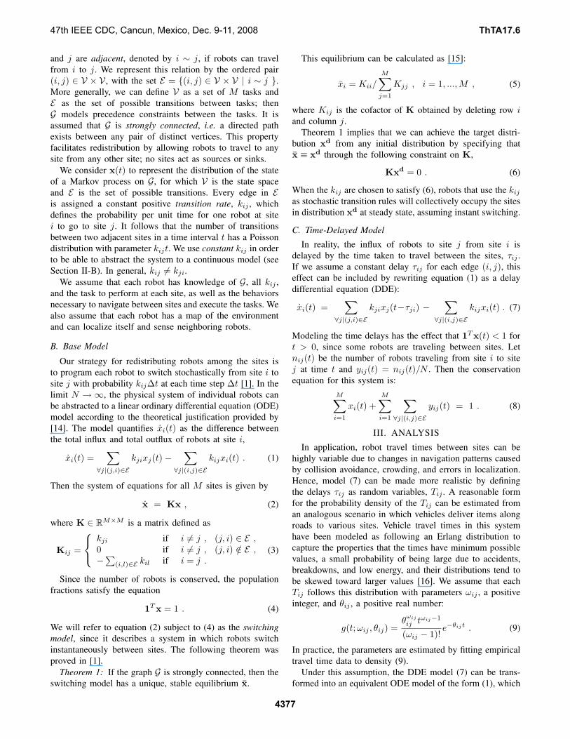
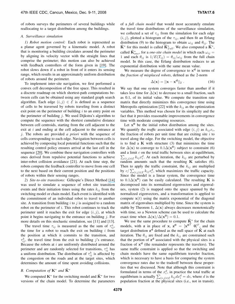
Fig. 2. Cell decomposition of the free space used for navigation. Thesurveyed buildings are highlighted and numbered.
1 sec 3000 sec
8000 sec 16000 sec
Fig. 3. Snapshots of a simulation using K∗. The maroon (dark) robots
are not engaged in a transition; the orange (light) robots have committed totravel or are in the process of traveling. Robots navigate between sites at 1.3m/s, which is attainable by some mobile robots that are suited to surveillance
tasks, such as PatrolBot R© and Seekur R©. The perimeter surveillance speedis 4.5 times slower. We set c = 0.06 robots/s.
V. RESULTS
To investigate the utility of the chain model in optimizing
the kij , we simulated a surveillance task as described in
Section IV-A with kij from the matrices K∗, K∗one, and
K∗full computed according to Section IV-B. The swarm
consists of 240 robots, and the four buildings to be monitored
are located on the section of the University of Pennsylvania
campus shown in Fig. 2. We used a graph G for these four
sites with the edges given in Table 1. The robots are initially
split equally between sites 3 and 4, and they are required
to redistribute to occupy all sites in equal fractions. Fig. 3
illustrates this redistribution for one trial.
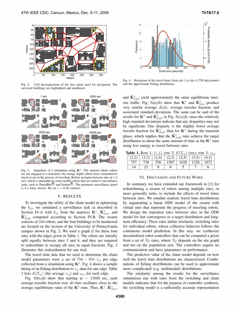
The travel time data that we used to determine the chain
model parameters were a set of 750 − 850 τij per edge
collected from a simulation using K∗. Fig. 4 shows a sample
fitting of an Erlang distribution to τij data for one edge. Table
1 lists E(Tij) (the average τij) and ωij for each edge.
Fig. 5(b),(d) show that starting at ∼ 15000 sec, each
average traveler fraction over 40 runs oscillates close to the
average equilibrium value of the K∗ runs. Thus, K∗, K∗one,
Travel time (seconds)
Fre
qu
en
cy
Pro
ba
bility
de
nsity
g(t,9
,0.0
16
2)
Fig. 4. Histogram of the travel times from site 1 to site 4 (758 data points)and the approximate Erlang distribution.
and K∗full yield approximately the same equilibrium inter-
site traffic. Fig. 5(a),(b) show that K∗ and K∗one produce
very similar average ∆(x), average traveler fraction, and
associated standard deviations. The same can be said of the
results for K∗ and K∗full in Fig. 5(c),(d), since the relatively
high standard deviations indicate that any disparities may not
be significant. One disparity is the slightly lower average
traveler fraction for K∗full than for K∗ during the transient
phase, which implies that the K∗full runs achieve the target
distribution in about the same amount of time as the K∗ runs
using less energy to travel between sites.
Table 1. Row 1: (i, j), row 2: E(Tij) (sec), row 3: ωij .
(1,2) (1,3) (1,4) (2,3) (2,4) (3,4) (4,1)
757 738 556 1507 1628 1228 1072
14 15 9 6 5 7 6
VI. DISCUSSION AND FUTURE WORK
In summary, we have extended our framework in [1] for
redistributing a swarm of robots among multiple sites, or
more generally tasks, to include the effects of travel times
between sites. We emulate realistic travel time distributions
by augmenting a linear ODE model of the swarm with
virtual sites that represent the progress of traveling robots.
We design the transition rates between sites in the ODE
model for fast convergence to a target distribution and long-
term efficiency. These rates define stochastic switching rules
for individual robots, whose collective behavior follows the
continuous model prediction. In this way, we synthesize
decentralized robot controllers that can be computed a priori
from a set of NE rates, where NE depends on the site graph
and not on the population size. The controllers require no
communication and have guarantees on performance.
The predictive value of the chain model depends on how
well the travel time distributions are characterized. Combi-
nations of Erlang distributions can be used to approximate
more complicated (e.g. multimodal) distributions.
The similarity among the results for the surveillance
simulations run with rates from the switching and chain
models indicates that for the purpose of controller synthesis,
the switching model is a sufficiently accurate representation
47th IEEE CDC, Cancun, Mexico, Dec. 9-11, 2008 ThTA17.6
4380

0 0.5 1 1.5 2
x 104
0
0.05
0.1
0.15
0.2
0.25
0.3
Time (sec)
0 0.5 1 1.5 2
x 104
0.2
0.3
0.4
0.5
0.6
0.7
0.8
0.9
1
Time (sec)
Fra
ctio
n o
f m
isp
lace
d r
ob
ots
(a) (b)
Uses
Uses
Uses
Uses
Tra
ve
ler
fra
ctio
n
0 0.5 1 1.5 2
x 104
0.2
0.3
0.4
0.5
0.6
0.7
0.8
0.9
1
Time (sec)
Fra
ctio
n o
f m
isp
lace
d r
ob
ots
0 0.5 1 1.5 2
x 104
0
0.05
0.1
0.15
0.2
0.25
0.3
Time (sec)
Tra
ve
ler
fra
ctio
n
(c) (d)
Uses
Uses
Uses
Uses
Fig. 5. (a),(c) Fraction of misplaced robots ∆(x) and (b),(d) fraction
of travelers vs. time for simulations using K∗, K
∗
one, and K∗
full. Thick
lines are averages over 40 simulation runs; thin lines mark the standarddeviations. The horizontal dashed lines mark the mean equilibrium travelerfraction, 0.237, measured from the K
∗ runs.
of our system. Hence, we can simply optimize the matrix K
and do not have to incur the greater computational expense
that is needed to optimize the larger matrix K. In ongoing
work on the switching model, we compare our Metropolis
K optimization method with others that maximize functions
of the eigenvalues of K, which govern the model’s rate
of convergence [23]. A possible extension of our work is
to design a time-dependent matrix K(t) that causes the
swarm to redistribute according to a trajectory of desired
configurations, xd(t). Also, we can devise an extension of
our quorum-based strategy [13] in which robots stop moving
between sites (and hence expending energy) once they detect
that a site is close enough to the target occupancy.
One avenue of future work is to investigate whether using
the chain model to optimize the rates improves performance
under different conditions. In our simulation, the average τij
for the edges are within a factor of 3 of each other. The K∗
for a scenario with larger differences between average τij
should assign much higher kij to edges with low τij than to
edges with high τij since this would speed up convergence;
the computation of K∗ does not account for the τij and so
would be expected to produce slower convergence. It may
also be fruitful to study scenarios in which, for each edge
(i, j), the ratio of the average τij to k−1ij , the average waiting
time at site i, is higher than in our simulations, in which the
highest ratio (over all sets of kij) is 0.31. Another aspect
to consider is the dependence of travel times on the robot
population, which may lead to a generalized definition of
“traffic capacity” that is not well described by a linear model.
REFERENCES
[1] A. Halasz, M. A. Hsieh, S. Berman, and V. Kumar, “Dynamicredistribution of a swarm of robots among multiple sites,” in Proc.
Int’l. Conf. on Intelligent Robots and Syst. (IROS’07), 2007, pp. 2320–2325.
[2] M. B. Dias, R. M. Zlot, N. Kalra, and A. Stentz, “Market-basedmultirobot coordination: a survey and analysis,” Proc. of the IEEE,vol. 94, no. 7, pp. 1257 – 1270, 2006.
[3] E. G. Jones, M. B. Dias, and A. Stentz, “Learning-enhanced market-based task allocation for oversubscribed domains,” in Proc. Int’l. Conf.
on Intelligent Robots and Syst. (IROS’07), 2007, pp. 2308–2313.[4] D. Milutinovic and P. Lima, “Modeling and optimal centralized control
of a large-size robotic population,” IEEE Trans. on Robotics, vol. 22,no. 6, pp. 1280–1285, 2006.
[5] T. H. Labella, M. Dorigo, and J.-L. Deneubourg, “Division of laborin a group of robots inspired by ants’ foraging behavior,” ACM Trans.
Auton. Adapt. Syst., vol. 1, no. 1, pp. 4–25, 2006.[6] M. J. B. Krieger, J.-B. Billeter, and L. Keller, “Ant–like task allocation
and recruitment in cooperative robots,” Nature, vol. 406, pp. 992–995,2000.
[7] W. Agassounon and A. Martinoli, “Efficiency and robustness ofthreshold-based distributed allocation algorithms in multi-agent sys-tems,” in Proc. First Int’l. Joint Conf. on Auton. Agents and Multi-
Agent Syst. (AAMAS’02), 2002, pp. 1090–1097.[8] N. Franks, S. C. Pratt, E. B. Mallon, N. F. Britton, and D. T. Sumpter,
“Information flow, opinion polling and collective intelligence in house-hunting social insects,” Phil. Trans. R. Soc. Lond. B, vol. 357, no. 1427,pp. 1567–1583, 2002.
[9] W. Agassounon, A. Martinoli, and K. Easton, “Macroscopic modelingof aggregation experiments using embodied agents in teams of constantand time-varying sizes,” Auton. Robots, vol. 17, no. 2-3, pp. 163–192,2004.
[10] K. Lerman, C. V. Jones, A. Galstyan, and M. J. Mataric, “Analysisof dynamic task allocation in multi-robot systems,” Int. J. of Robotics
Research, vol. 25, no. 3, pp. 225–241, 2006.[11] S. Berman, A. Halasz, V. Kumar, and S. Pratt, “Algorithms for the
analysis and synthesis of a bio-inspired swarm robotic system,” in 9th
Int’l. Conf. on the Simul. of Adapt. Behav. (SAB’06), Swarm Robotics
Workshop, vol. LNCS 4433, 2007, pp. 56–70.[12] ——, “Bio-inspired group behaviors for the deployment of a swarm
of robots to multiple destinations,” in Proc. Int’l. Conf. on Robotics
and Automation (ICRA’07), 2007, pp. 2318–2323.[13] M. A. Hsieh, A. Halasz, S. Berman, and V. Kumar, “Biologically
inspired redistribution of a swarm of robots among multiple sites,” toappear a Special Issue of the Swarm Intelligence Journal, 2008.
[14] D. Gillespie, “Stochastic simulation of chemical kinetics,” Annu. Rev.
Phys. Chem., vol. 58, pp. 35–55, 2007.[15] H. Othmer, Analysis of Complex Reaction Networks, Lecture Notes.
Minneapolis, MN: Sch. of Mathematics, Univ. Minnesota, Dec. 2003.[16] R. Russell and T. Urban, “Vehicle routing with soft time windows
and Erlang travel times,” vol. 59, no. 9, pp. 1220–1228, 2008, J.Operational Research Society.
[17] B. Harris, Theory of Probability. Reading, MA: Addison-Wesley,1966.
[18] J. Sun, S. Boyd, L. Xiao, and P. Diaconis, “The fastest mixingMarkov process on a graph and a connection to the maximum varianceunfolding problem,” SIAM Review, vol. 48, no. 4, pp. 681–699, 2006.
[19] M. A. Hsieh, S. Loizou, and V. Kumar, “Stabilization of multiplerobots on stable orbits via local sensing,” in Proc. Int’l Conf. on
Robotics and Automation (ICRA’07), Apr. 2007, pp. 2312–2317.[20] D. C. Conner, A. Rizzi, and H. Choset, “Composition of local potential
functions for global robot control and navigation,” in Proc. Int’l. Conf.
on Intelligent Robots and Syst. (IROS’03), vol. 4, 2003, pp. 3546–3551.[21] H. G. Tanner, A. Jadbabaie, and G. J. Pappas, “Flocking in fixed and
switching networks,” in IEEE Trans. on Automatic Control, vol. 52,no. 5, 2007, pp. 863–868.
[22] D. P. Landau and K. Binder, A guide to Monte-Carlo simulations in
statistical physics. Cambridge University Press, 2000.[23] S. Berman, A. Halasz, M. A. Hsieh, and V. Kumar, “Optimization of
stochastic strategies for redistributing a robot swarm among multiplesites,” under review for IEEE Trans. on Robotics.
47th IEEE CDC, Cancun, Mexico, Dec. 9-11, 2008 ThTA17.6
4381
Top Related
Copyright © 2022 FDOKUMEN

