


![Stephen Briggs [Compatibility Mode]](https://static.fdokumen.com/doc/165x107/6324c3005c2c3bbfa802dd10/stephen-briggs-compatibility-mode.jpg)

Bahasa
Halaman
Hukum


Mode Identification from CombinationFrequency Amplitudes in Pulsating White
Dwarf Stars
by
Celeste Marie Yeates
A dissertation submitted to the faculty of the University of North Carolina atChapel Hill in partial fulfillment of the requirements for the degree of Doctor ofPhilosophy in the Department of Physics & Astronomy.
Chapel Hill
2006
Approved by:
J. Christopher Clemens, AdvisorBruce W. Carney, ReaderCharles R. Evans, ReaderChristian G. Iliadis, ReaderRobert K. McMahan, ReaderDaniel E. Reichart, Reader

c©2006Celeste Marie Yeates
All Rights Reserved
ii

ABSTRACTCeleste Marie Yeates: Mode Identification from Combination Frequency
Amplitudes in Pulsating White Dwarf Stars(Under the Direction of J. Christopher Clemens)
The lightcurves of variable DA and DB white dwarf stars are usually multi-
periodic and non-sinusoidal, so that their Fourier transforms show peaks at
eigenfrequencies of the pulsation modes and at sums and differences of these
frequencies. These combination frequencies provide extra information about the
pulsations, both physical and geometrical, that is lost unless they are analyzed.
Several theories provide a context for this analysis by predicting combination
frequency amplitudes. In these theories, the combination frequencies arise from
nonlinear mixing of oscillation modes in the outer layers of the white dwarf,
so their analysis cannot yield direct information on the global structure of the
star as eigenmodes provide. However, their sensitivity to mode geometry does
make them a useful tool for identifying the spherical degree of the modes that
mix to produce them. In this dissertation, we analyze data from eight hot,
low-amplitude DAV white dwarfs and measure the amplitudes of combination
frequencies present. By comparing these amplitudes to the predictions of the
theory of Goldreich and Wu, we have verified that the theory is crudely con-
sistent with the measurements. We have also investigated to what extent the
combination frequencies can be used to measure the spherical degree (ℓ) of the
modes that produce them. We find that modes with ℓ > 2 are easily identifiable
as high ℓ based on their combination frequencies alone. Distinguishing between
ℓ = 1 and 2 is also possible using harmonics. These results will be useful for
conducting seismological analyses of large ensembles of ZZ Ceti stars, such as
those being discovered using the Sloan Digital Sky Survey. Because this method
relies only on photometry at optical wavelengths, it can be applied to faint stars
iii

using 4 m class telescopes. We present new data from the 4.1 m Southern As-
trophysical Research Telescope for the ZZ Ceti star L19-2. We use these data
to determine the limits for application of this theory on data from a 4 m class
telescope. We also analyze data for the hot, low-amplitude DBV EC 20058-5234
and demonstrate that the theory is applicable to both DAV and DBV white
dwarf stars.
iv

Dedicated to: Owen, Hyrum, and Claire
v

ACKNOWLEDGMENTS
Getting a Ph.D. has turned out to be hard work. I have wanted to give up
my pursuit of a Ph.D. in Physics and Astronomy several times in the last six
years. Although receiving a Ph.D. was one of my dearest goals, I sometimes
lacked the immediate desire and often doubted my abilities. However, around
the time of my first written exams (when I was ready to give up), my husband
Owen told me that I needed to decide then and there whether or not I wanted
to complete my degree — whether this was something that I was willing to put
forth all of my effort to finish. I made the decision to continue to the end. Since
then, there have been several times when I felt like I could not do it anymore
and that my tasks were unachievable. At those times, Owen would remind me
of my decision and assure me of my intelligence and capacity to accomplish my
tasks. I am certain that without the continual, unwavering support of Owen, I
would not have been able to achieve my goal of earning a Ph.D. in Physics and
Astronomy. Many people ask me, “How can you be a graduate student and a
mother of two children at the same time?” I simply tell them that I have an
extremely supportive husband. For these reasons and more, I have dedicated
this dissertation to Owen.
However, it is because of my Dad and Mom that I got started on this path
to begin with. Setting aside the fact that they helped finance my undergraduate
education at BYU, they instilled in me the faith, diligence, and determination
necessary to reach this point. My parents taught me values that embrace knowl-
edge as essential for this life. My Dad helped me with my homework and projects
throughout high school. He has always been genuinely interested in what I am
vi

studying and always made me feel very smart. While growing up, my Dad
provided bookshelves full of interesting books on math, astronomy, airplanes,
rockets, missiles, and every other fascinating topic. He taught me that there
is nothing wrong with being interested in everything. My Mom is my number-
one-fan. She has sacrificed and worked so hard to make sure that I have always
had everything I need. She remembers everything I tell her and worries about
everything that worries me. She sends me notes several times a week to remind
me that she loves me. She is patient, loving, thoughtful, and kind. I am unable
to communicate how it feels to know that no matter what, there is at least one
person who completely understands me. My parents think I am funny, intelli-
gent, hard working, . . . and a bunch of other good qualities. It is good to be
loved by them.
My five sisters are my best friends. I can go for a couple of months without
talking to them, but then when we talk it is as if no time has passed. My sisters
are my connection to the outside (non-academic) world. They have provided a
supplement to my non-academic life that would have otherwise suffered without
their help.
My thesis advisor, Chris Clemens, is the best advisor I could have picked.
He is the most intelligent and motivated scientist I have ever met, but he is also
humble, kind, and patient. Chris understands the most difficult concepts and
can explain them in ways that I can understand. Even then, he never seems
to mind that I ask him to repeat the same concept over and over again. Chris
is also an optimist. There were several times when I went into his office with
results that I was sure were going to ruin my project, but by the conclusion of
our meeting, I would feel refreshed and ready to look at the problem in a new
way. He taught me to be the kind of scientist who always questions conclusions
and receives satisfaction from considering new ideas and possibilities. Also, I
always appreciated having Chris along on observing runs; he made them much
more fun with his ability to recite Star Wars from start to finish.
vii

Most importantly, Chris not only advised me in scientific matters, but has
given me guidance on parenting, marriage, and spiritual matters, to name a few.
He has never complained that I like to work at home as much as possible so
that I can be with my children when they need me. In fact, he has gone out of
his way to accommodate my schedule and made himself available to meet with
me whenever I could. Without Chris’s support, I would not have completed my
Ph.D. requirements.
While we were observing at SOAR, Kepler Oliveira sat down and patiently
and carefully shared with me his wealth of knowledge about data reduction.
Then, when I was at home trying to reconstruct the data reductions that he
taught me, he patiently responded to all of my many emailed questions and
guided me through the difficult process without ever complaining. Kepler prob-
ably has no idea how grateful I am for his help.
I would like to acknowledge the help of Dr. Boka Wesley Hadzija, who funds
the Linda Dykstra Science Dissertation Fellowship. Additionally, I am grateful
to the North Carolina Space Grant Consortium, which funded my research with
fellowships for two consecutive summers.
Fellow graduate students are the greatest invention ever. You can rely on
them and ask them for help without worrying that they will think you are stupid.
I do not think that any of us could survive without each other — I certainly could
not have survived without them. First and foremost, I must acknowledge Dr.
Susan Thompson. She is my friend and mentor. If ever I run into astronomy
problems, I think, “What would Susan do?” Fergal Mullally is another graduate
student who is always ready with answers and computer programs when I ask him
for help with data reduction, observing, and anything else. Melissa Nysewander,
Jane Moran, and I were the only astronomers who came to UNC in August 2000.
Not only did we help each other through coursework and exciting adventures
in Arizona, they are my resident experts in IRAF, and they always know the
answers to my (sometimes-stupid) questions. I am also grateful to Rachel Rosen
viii

and Jennifer Weinberg-Wolf, who have always cheerfully helped me whenever I
asked them.
Hyrum and Claire are my two babies that were born while I was a graduate
student. They are so fabulous (not to mention strong-willed and determined).
They bring the joy and happiness into our home that we need to get through
the sometimes-arduous tasks of being graduate students. It is such a relief to
have them to love and spend time with as an escape from work. I acknowledge
them here as motivation to complete my dissertation as quickly as possible, and
I dedicate this work to them.
Finally, I should mention the perpetual support of my Father in Heaven. I
have great faith that He helps me daily. Let me give an example. Claire was
born in September 2005 (which, in and of itself, was a miraculous experience).
By that point, I had completed only two, albeit the largest two, chapters of
my dissertation. Then, in little more than one semester, I was able to write
four chapters of my dissertation, reduce new data from the SOAR Telescope,
adjust to having a newborn baby, adequately take care of my husband and son,
and defend my dissertation. Through it all, I was happy and only minimally
stressed. I could not have accomplished all this, while remaining the cheerful
individual that you know and love today, without Spiritual guidance.
Celeste Marie Yeates
July 6, 2006
ix

CONTENTS
Page
LIST OF TABLES . . . . . . . . . . . . . . . . . . . . . . . . . . . . . . . xiii
LIST OF FIGURES . . . . . . . . . . . . . . . . . . . . . . . . . . . . . . xiv
LIST OF ABBREVIATIONS . . . . . . . . . . . . . . . . . . . . . . . . . xvi
LIST OF SYMBOLS . . . . . . . . . . . . . . . . . . . . . . . . . . . . . . xvii
I. Introduction . . . . . . . . . . . . . . . . . . . . . . . . . . . . . . . 1
1.1 White Dwarf Stars . . . . . . . . . . . . . . . . . . . . . . . . 2
1.1.1 White Dwarf Pulsations . . . . . . . . . . . . . . . . . 4
1.1.2 Driving Mechanisms . . . . . . . . . . . . . . . . . . . 6
1.1.3 Asteroseismology . . . . . . . . . . . . . . . . . . . . . 7
1.1.4 Nonlinear Pulsations . . . . . . . . . . . . . . . . . . . 10
1.2 Mode Identification . . . . . . . . . . . . . . . . . . . . . . . . 12
1.2.1 Mode Identification from Combination Frequencies . . 13
1.2.2 Overview . . . . . . . . . . . . . . . . . . . . . . . . . 14
Chapter
II. Analytical Amplitudes for Combination Frequencies in theTheory of Yanqin Wu . . . . . . . . . . . . . . . . . . . . . . . . . . 16
2.1 Introduction . . . . . . . . . . . . . . . . . . . . . . . . . . . . 16
2.2 Theoretical Review . . . . . . . . . . . . . . . . . . . . . . . . 19
2.3 Conclusions . . . . . . . . . . . . . . . . . . . . . . . . . . . . 30
III. Mode Identification from Combination Frequency Ampli-tudes in ZZ Ceti Stars . . . . . . . . . . . . . . . . . . . . . . . . . 34
3.1 Introduction . . . . . . . . . . . . . . . . . . . . . . . . . . . . 34
3.2 Data Reduction and Analysis . . . . . . . . . . . . . . . . . . 37
x

3.2.1 Data Reduction . . . . . . . . . . . . . . . . . . . . . . 37
3.2.1.1 Published Data . . . . . . . . . . . . . . . . . 37
3.2.1.2 Unpublished Data and New Reductions . . . 37
3.2.2 Analysis . . . . . . . . . . . . . . . . . . . . . . . . . . 38
3.2.2.1 Stars With Detected Combination Frequencies 42
GD 66 . . . . . . . . . . . . . . . . . . . . . . 42
GD 244 . . . . . . . . . . . . . . . . . . . . . 49
G117-B15A . . . . . . . . . . . . . . . . . . . 55
G185-32 . . . . . . . . . . . . . . . . . . . . . 58
3.2.2.2 Stars Without Detected Combinations . . . . 64
L19-2 . . . . . . . . . . . . . . . . . . . . . . 64
GD 165 . . . . . . . . . . . . . . . . . . . . . 74
R548 . . . . . . . . . . . . . . . . . . . . . . . 76
G226-29 . . . . . . . . . . . . . . . . . . . . . 77
3.3 Conclusions . . . . . . . . . . . . . . . . . . . . . . . . . . . . 78
IV. Photometric Mode Identification for L19-2 with the SOAR Telescope 83
4.1 Introduction . . . . . . . . . . . . . . . . . . . . . . . . . . . . 83
4.2 Data Reduction and Analysis . . . . . . . . . . . . . . . . . . 85
4.2.1 Observations . . . . . . . . . . . . . . . . . . . . . . . . 85
4.2.2 Data Reduction . . . . . . . . . . . . . . . . . . . . . . 86
4.2.3 Mode Identification . . . . . . . . . . . . . . . . . . . . 90
4.3 Conclusions . . . . . . . . . . . . . . . . . . . . . . . . . . . . 92
V. Photometric Mode Identification for the DBV EC 20058-5234 . . . 95
5.1 Introduction . . . . . . . . . . . . . . . . . . . . . . . . . . . . 95
5.2 Data . . . . . . . . . . . . . . . . . . . . . . . . . . . . . . . . 96
5.3 Mode Identification . . . . . . . . . . . . . . . . . . . . . . . . 96
5.4 Conclusions . . . . . . . . . . . . . . . . . . . . . . . . . . . . 99
VI. Summary and Conclusions . . . . . . . . . . . . . . . . . . . . . . . 101
6.1 Harmonics Are the Key . . . . . . . . . . . . . . . . . . . . . . 103
xi

6.2 Verification of the Theory of Yanqin Wu . . . . . . . . . . . . 105
6.3 New Fourier Transforms for GD 66, GD 244, and L19-2 . . . . 106
6.4 Mode Identification for Published Data . . . . . . . . . . . . . 107
6.5 An Expedition to Cerro Pachon . . . . . . . . . . . . . . . . . 107
6.6 Applicable to DAV and DBV Stars . . . . . . . . . . . . . . . 108
6.7 Future Application . . . . . . . . . . . . . . . . . . . . . . . . 108
VII. Appendix A: Selected Solutions for Gmi±mj
ℓi ℓj/gmi
ℓig
mj
ℓj(Θ) . . . . . . 110
REFERENCES . . . . . . . . . . . . . . . . . . . . . . . . . . . . . . . . . 116
xii

LIST OF TABLES
3.1 Journal of Observations for GD 66 and GD 244 . . . . . . . . . . . . 39
3.2 Journal of Observations for L19-2 (WET Observations) . . . . . . . 40
3.3 Stellar Information . . . . . . . . . . . . . . . . . . . . . . . . . . . . 41
3.4 GD 66 Periods and Mode Identifications . . . . . . . . . . . . . . . . 59
3.5 GD 244 Periods and Mode Identifications . . . . . . . . . . . . . . . 60
3.6 Periods and Mode Identifications for Published Data withCombination Frequencies . . . . . . . . . . . . . . . . . . . . . . . . 61
3.7 L19-2 Periods and Mode Identifications (WET Observations) . . . . 65
3.8 Periods and Mode Identifications for Published Data withoutCombination Frequencies . . . . . . . . . . . . . . . . . . . . . . . . 75
4.1 Journal of Observations for L19-2 (SOAR Telescope Obser-vations) . . . . . . . . . . . . . . . . . . . . . . . . . . . . . . . . . . 87
4.2 L19-2 Periods and Mode Identifications (SOAR TelescopeObservations) . . . . . . . . . . . . . . . . . . . . . . . . . . . . . . . 92
5.1 EC 20058-5234 Periods and Mode Identifications . . . . . . . . . . . 97
A.1 Values of Gmi+mj
1 1 /gmi1 g
mj
1 (Θ) . . . . . . . . . . . . . . . . . . . . . . 112
A.2 Values of Gmi+mj
1 2 /gmi1 g
mj
2 (Θ) . . . . . . . . . . . . . . . . . . . . . . 113
A.3 Values of Gmi+mj
2 2 /gmi2 g
mj
2 (Θ) . . . . . . . . . . . . . . . . . . . . . . 114
A.4 Values of G0±0ℓi ℓj
/g0ℓig0
ℓj(Θ) . . . . . . . . . . . . . . . . . . . . . . . . 115
xiii

LIST OF FIGURES
1.1 Theoretical H-R Diagram emphasizing white dwarf cooling-track. . . 3
1.2 Theoretical propagation diagram for white dwarf star withTeff = 12, 000 K. . . . . . . . . . . . . . . . . . . . . . . . . . . . . . 9
2.1 Bolometric correction as a function of Teff , log g, and ℓ forbi-alkali photocathode. . . . . . . . . . . . . . . . . . . . . . . . . . . 23
2.2 Typical F dependence on frequency, normalized to one. . . . . . . . . 26
2.3 G with mi = mj = 0 plotted as a function of inclination angle (Θ0). . 27
2.4 G with ℓi = ℓj = 1 and mi + mj plotted as a function ofinclination angle (Θ0). . . . . . . . . . . . . . . . . . . . . . . . . . . 28
3.1 Lightcurve of GD 66. . . . . . . . . . . . . . . . . . . . . . . . . . . . 43
3.2 Fourier transform of GD 66. . . . . . . . . . . . . . . . . . . . . . . . 44
3.3 Deconstruction of F1 in GD 66. . . . . . . . . . . . . . . . . . . . . . 45
3.4 Prewhitened peaks of parent modes in GD 66 Fourier trans-form. . . . . . . . . . . . . . . . . . . . . . . . . . . . . . . . . . . . 47
3.5 Ratio of combination to parent mode amplitudes (Rc) for GD 66. . . 48
3.6 Lightcurve of GD 244. . . . . . . . . . . . . . . . . . . . . . . . . . . 50
3.7 Fourier transform of GD 244. . . . . . . . . . . . . . . . . . . . . . . 51
3.8 Deconstruction of F2 in GD 244. . . . . . . . . . . . . . . . . . . . . 52
3.9 Prewhitened peaks in GD 244 Fourier transform. . . . . . . . . . . . 53
3.10 Ratio of combination to parent mode amplitudes (Rc) for GD 244. . . 56
3.11 Ratio of combination to parent mode amplitudes (Rc) forG117-B15A. . . . . . . . . . . . . . . . . . . . . . . . . . . . . . . . . 57
3.12 Ratio of combination to parent mode amplitudes (Rc) forG185-32. . . . . . . . . . . . . . . . . . . . . . . . . . . . . . . . . . . 66
3.13 Lightcurve of L19-2 (WET observations). . . . . . . . . . . . . . . . . 67
3.14 Fourier transform of L19-2 (WET observations). . . . . . . . . . . . . 67
3.15 Deconstruction of F1 in L19-2. . . . . . . . . . . . . . . . . . . . . . . 68
3.16 Deconstruction of F2 in L19-2. . . . . . . . . . . . . . . . . . . . . . . 69
xiv

3.17 Deconstruction of F3 in L19-2. . . . . . . . . . . . . . . . . . . . . . . 70
3.18 Deconstruction of F4 in L19-2. . . . . . . . . . . . . . . . . . . . . . . 71
3.19 Deconstruction of F5 in L19-2. . . . . . . . . . . . . . . . . . . . . . . 72
3.20 Prewhitened peaks in L19-2 Fourier transform (WET obser-vations). . . . . . . . . . . . . . . . . . . . . . . . . . . . . . . . . . 73
3.21 Ratio of combination to parent mode amplitudes (Rc) forL19-2 (WET observations). . . . . . . . . . . . . . . . . . . . . . . . 74
3.22 Ratio of combination to parent mode amplitudes (Rc) for GD 165. . . 76
3.23 Ratio of combination to parent mode amplitudes (Rc) for R548. . . . 79
3.24 Ratio of combination to parent mode amplitudes (Rc) forG226-29. . . . . . . . . . . . . . . . . . . . . . . . . . . . . . . . . . . 80
4.1 Drawing of attachment for Apogee CCD camera. . . . . . . . . . . . 86
4.2 Photograph of attachment for Apogee CCD camera. . . . . . . . . . . 87
4.3 CCD image of L19-2. . . . . . . . . . . . . . . . . . . . . . . . . . . . 88
4.4 Lightcurve of L19-2 (SOAR Telescope observations). . . . . . . . . . 89
4.5 Fourier transform of L19-2 (SOAR Telescope observations). . . . . . . 90
4.6 Prewhitened peaks in L19-2 Fourier transform (SOAR Tele-scope observations). . . . . . . . . . . . . . . . . . . . . . . . . . . . 91
4.7 Ratio of combination to parent mode amplitudes (Rc) forL19-2 (SOAR Telescope observations). . . . . . . . . . . . . . . . . . 93
5.1 Ratio of combination to parent mode amplitudes (Rc) for EC20058-5234. . . . . . . . . . . . . . . . . . . . . . . . . . . . . . . . . 98
A.1 G with mi = mj = 0 plotted as a function of inclination angle (Θ). . 111
xv

LIST OF ABBREVIATIONS
AAS American Astronomical Society
AGB Asymptotic giant branch
BFW95 Brassard et al. (1995)
DAV Hydrogen atmosphere variable white dwarf star (ZZ Ceti)
DBV Helium atmosphere variable white dwarf star
DOV He II atmosphere variable white dwarf star
FT Fourier transform
H-R Hertzsprung-Russell
HST Hubble Space Telescope
PN Planetary nebula
PNN Planetary nebula nuclei
PNNV Planetary nebula nuclei variable star
SDSS Sloan Digital Sky Survey
S/N Signal to Noise ratio
SOAR Southern Astrophysical Research Telescope
UV Ultraviolet
WET Whole Earth Telescope
xvi

LIST OF SYMBOLS
ai Amplitude coefficient for pulsation modes
αλ Bolometric correction
2β + γ Fixed parameterization of the radiative region overlying the convec-tion zone in a white dwarf star
(δf/f) Observable flux change in a white dwarf star
F Term containing the physics of the model of Wu (2001)
G Geometrical term of the model of Wu (2001)
g Gravity
k Radial overtone number
ℓ Spherical degree associated with the spherical harmonic
m Azimuthal order associated with the spherical harmonic
Nmℓ Normalization factor of the spherical harmonic
〈P 〉 Average power over a given region of a Fourier transform
Θ0 Inclination of a star’s pulsation axis to the observer’s line of sight
ρmℓ Legendre Polynomials
τc0 Convective timescale
Teff Effective temperature
ωi Pulsation frequency
ψi Phase for pulsation modes
Y mℓ Spherical harmonics
xvii
Chapter 1
Introduction
Dana Barrett: You know, you don’t act like a scientist.
Dr. Peter Venkman: They’re usually pretty stiff.
Dana Barrett: You’re more like a game show host.
— Ghostbusters
In 1862, while testing his new telescope on the bright star Sirius, Alvin Gra-
ham Clark noticed its dim companion, Sirius B, thereby discovering the first
known white dwarf star. Sirius B is an extremely dense object with R =
0.0084±0.00025R⊙ (∼ 0.9R⊕) and M = 1.034±0.026M⊙ (Holberg et al., 1998).
The discovery of Sirius B marked the beginning of the study of a fascinating
new kind of star. White dwarf stars typically have log g ∼ 8 with a narrow
mass distribution centered on ∼ 0.56M⊙ (Koester et al., 1979; Bergeron et al.,
1992), with the bulk of the mass primarily in the carbon-oxygen core. Due to
the high-gravity environment, the heavy elements settle to the center of the star,
as confirmed by the purity of the observed atmospheres. In extreme cases, low
mass white dwarf stars (≤ 0.4M⊙) have helium cores and high mass white dwarf
stars (≥ 1.05M⊙) have oxygen-neon cores (Isern et al., 1998). For those white
dwarf stars with typical mass, a thin layer of pure helium surrounds the carbon-
oxygen core, and, for 75 percent of white dwarf stars, a thinner layer of pure
hydrogen surrounds the helium. The exact ratio of carbon to oxygen in the core

is unsettled primarily because of the uncertainties in the rate of the 12C(α, γ)16O
reaction during the asymptotic giant branch (AGB) phase of stellar evolution.
A high rate for this nuclear reaction means a greater abundance of oxygen in the
center then in the outer layers (Isern et al., 1998).
White dwarf stars are the end-product of all but the most massive stars. As
a consequence, understanding the origin and structure of white dwarf stars helps
us better understand the preceding stages of stellar evolution for low mass stars
(those ≤ 10 ± 2M⊙; see Isern et al., 1998). Indeed, white dwarf stars provide
a laboratory for understanding much of astrophysics. The compact interiors of
these stars supply a testing ground for extreme conditions of temperature and
pressure, while their surface temperatures unlock independent scales for the age
and history of galaxies.
As white dwarf stars thermally radiate their reservoir of energy into the in-
terstellar medium, they reach a temperature range in which certain conditions
trigger driven pulsations from deep within their interiors. These pulsations,
which we measure as surface temperature variations, equip us with a means of
delving in to the unseen interiors of white dwarf stars, similar to the seismologists
who use earthquakes to understand the internal layers of the Earth. This disser-
tation describes an important step forward for asteroseismologists, presenting a
simplified method for identifying individual pulsation modes in these stars that
utilizes the size of the nonlinearities present in the lightcurves of pulsating white
dwarf stars.
1.1 White Dwarf Stars
White dwarf stars evolve from low mass stars. Theories for the stellar evolu-
tion of a main sequence star into a white dwarf star are well known (see Mazzitelli
& D’Antona, 1986; D’Antona, 1989; Wood, 1990). In summary, following core H-
burning, the star ascends the giant branch, enters the core He-burning phase, and
2

then the double-shell-burning phase on the AGB. In a process that is not well-
understood (Mazzitelli & D’Antona, 1986), the planetary nebula (PN) is formed.
The nuclei (central stars) of the planetary nebulae (PNN) are the forerunners of
the white dwarf stars. After the nebula has been dispersed, the central star is
called a pre-white dwarf star and it descends onto the constant-radius cooling
track. Figure 1.1 contains a theoretical H-R Diagram emphasizing the white
dwarf cooling track.
Figure 1.1: Theoretical H-R Diagram emphasizing white dwarf cooling-track.The PNNV and DOV instability strips are possibly joined together into one strip.In this dissertation, we analyze stars within the DBV and DAV instability strips.We reproduce this figure by permission of the Journal of the Royal AstronomicalSociety of Canada (see Fig. 1 of Wood, 1990).
White dwarf stars fall into several spectroscopic groups, based on the com-
3

position of the outermost layer. The most common type of white dwarf stars,
classified as the DA group, shows only hydrogen lines. The DB group contains
white dwarf stars with mainly helium lines and the DO white dwarf stars show
strong He II lines. Other less common groups include DQ (with carbon features),
DZ (with metal lines), and DC (showing only continuum).
Fowler (1926) used electron degeneracy pressure to explain the high densities
in white dwarf stars. Immediately after, Chandrasekhar (1931, 1934a,b) began
evaluating stellar structure in white dwarf stars. He calculated gas pressures for
electrons at relativistic speeds and thereby determined the exact mass-radius re-
lation for degenerate, relativistic stars, finding a critical mass (the Chandrasekhar
limit) for the formation of white dwarf stars. Mestel (1952) proceeded to explain
the cooling theory of white dwarf stars and to describe their lifetimes based on
the latent heat. At the birth of a white dwarf star, the temperature and pressure
in the white dwarf is no longer adequate to produce the energy required for the
next phase of thermonuclear reactions. The compact core of the star is degener-
ate, with electrons providing the pressure support, and is an isothermal reservoir
of heat energy that is transferred by conduction. Energetic electrons have a
long mean free path because of the filled Fermi sea, providing the high thermal
conductivity. Non-degenerate surface layers surround the degenerate core, con-
trolling the outflow of the energy with high opacity. The high opacity results in
a lower mean free path for the photons, reducing the energy outflow. The en-
ergy transport in the outer layers is dominated by radiation, then by convection
resulting from the high opacity introduced by partial ionization regions.
1.1.1 White Dwarf Pulsations
After PNN stars evolve onto the constant-radius cooling track appropriate for
their degenerate masses, they become the cool white dwarf stars that we observe
(Mazzitelli & D’Antona, 1986). As they do so, they pass through three to four
instability strips (see Figure 1.1). Despite the differences in temperature and
4

surface composition, the pulsation periods and the appearance of the lightcurves
of these stars in the separate instability strips are similar. The pulsation periods
for these stars range from 100 to 1500 s, with different periods favored depend-
ing on temperature. The Planetary Nebula Nuclei variable (PNNV) stars, the
first instability region, have spectra dominated by He II and C IV, temperatures
greater than 100,000 K, and pulsation periods greater than 1000 s. These pre-
white dwarf stars provide the only way to study the production rate of plasmon
neutrinos (Winget, 1998). The DOV (pulsating PG 1159) stars have tempera-
tures greater than 100,000 K and have periods ranging from 300 to 850 s. These
stars have passed the effective temperature turning point in the H-R Diagram
(see Figure 1.1). Vauclair et al. (2002) call DOV stars direct descendants of PNN
stars. However, the PNNV and DOV stars are often grouped together since the
discovery of the hot pulsating PG 1159 star RXJ 2117.1 + 3412 (Vauclair et al.,
1993). The DBV and DAV stars are much cooler than the PNNV and DOV
stars and are similar to each other in temperature and mass. The DBV stars
have temperatures near 25,000 K and pulsation periods between 100 and 1000 s.
The PNNV and DOV stars (Grauer & Bond, 1984) and the DAV stars (Green-
stein, 1976, 1982) were noted to contain similar group spectroscopic properties
after discovery. However, Winget et al. (1982a) theoretically predicted the exis-
tence of pulsating DB stars prior to the discovery of the first DBV GD 358 by
Winget et al. (1982b).
Although the DAV stars (also known as ZZ Ceti stars) are a continuous group
with no temperature gap, they are subdivided into the HDAV (hot) stars and
CDAV (cool) stars centered around 12,000 and 11,000 K. The HDAV pulsation
periods are shorter (less than 500 s) than those of CDAV stars (200 to 1500
s). Although the pulsations of the HDAV stars are smaller in amplitude than
those of the CDAV stars, the HDAV pulsations are stable in both period and
amplitude (Winget & Fontaine, 1982; Clemens, 1994) such that we can measure
the change in their period when we monitor the stars over several decades. In this
5

dissertation, we focus primarily on the HDAV stars because of their pulsation
stability. However, the method for mode identification described in this work
readily applies to all pulsating white dwarf stars. Indeed, we have applied the
method to the DBV EC 20058-5234 in Chapter 5.
The variations we observe arise from the temperature changes associated
with non-radial gravity-mode pulsations (Robinson et al., 1982). Theoretical
tests performed by Kepler (1984) exclude r-modes (toroidal non-radial pulsations
where the Coriolis force is the restoring force) in favor of g-mode pulsations.
These g-modes, where gravity is the restoring force, have timescales coincident
with the observed periods of pulsating white dwarf stars. The motions are largely
horizontal on the surface of the star.
1.1.2 Driving Mechanisms
There are at least two competing views on the theoretical source of the driving
mechanisms for pulsating white dwarf stars, most notably the κ-γ mechanism and
convection. When astronomers discovered pulsations in white dwarf stars, many
theorists determined that the κ-γ mechanism, which drives the radial pulsations
of Cepheid variables, can be applied to explain the non-radial pulsations of the
DAV and DBV stars (Winget et al., 1981; Dolez & Vauclair, 1981; Dziembowski
& Koester, 1981; Winget et al., 1982a). The κ-γ mechanism allows the driving
to be caused by the hydrogen (for DAV) and helium (for DBV) partial ionization
zones. These theoretical analyses all individually argue that the g-modes can be
excited by this κ-γ mechanism.
However, Brickhill (1983) points out that the perturbation to the convec-
tive flux is neglected in the theoretical models mentioned above. He writes that
neglecting the perturbation to the convective flux inevitably results in strong
driving. In the models of Brickhill (1983), the ionization zone only excites pul-
sations when convection carries most of the flux. Because the time-scale of the
convective motions is much less than that of the oscillations, the efficiency of
6

convection could damp out any excitation due to the κ-γ mechanism. In fact,
his models show that many g-mode pulsations will be excited in stars where
convection carries all of the flux to the surface. The convection zone is able to
adjust instantaneously to the changing thermal structure (the time-scale is ap-
proximately one second), more swiftly than the oscillation time-scale (Brickhill,
1990). These driven pulsations are much stronger than those predicted by the
κ-γ mechanism when the convective perturbations are included, hence the term
“convective driving” (Brickhill, 1991a)1.
1.1.3 Asteroseismology
Asteroseismology is the study of the interiors of stars using their stellar pul-
sations. Because of its proximity, helioseismologists have comprehensively exam-
ined the oscillations of the Sun for the last fifty years. Christensen-Dalsgaard
(2002) describes measurements of the large-scale structure and rotation of the
solar interior, which is known to a precision that rivals our knowledge of the
interior of the Earth.
Winget (1998) reviews the asteroseismology of white dwarf stars. The “for-
ward technique” of asteroseismology is to perform a normal-mode analysis by
matching all observed frequencies to theoretical models for white dwarf interiors
and determine which model best fits the observed periods. Instability is be-
lieved to be an evolutionary stage for white dwarf stars (cf. Fontaine et al., 1982;
Mukadam et al., 2004a). The information gleaned from an asteroseismological
analysis of a white dwarf star is therefore applicable to all non-pulsating white
dwarf stars with the same mass.
The g-mode pulsation frequencies, ω, of pulsating white dwarf stars satisfy
1Pesnell (1987) also recognized that the convection zone had been neglected inthe κ-γ mechanism scenario. He introduced a driving mechanism called “convec-tive blocking” as a modification of the ionization driving mechanism. However,Brickhill (1991b) argues that the ZZ Ceti pulsations are much more powerfulthan the convective blocking scenario allows.
7

the conditions of the dispersion relation,
ω2 ≪ N2, L2ℓ , (1.1)
where N is the Brunt-Vaisala frequency and Lℓ is the Lamb, or acoustic, fre-
quency:
N2 = −g[
d ln ρ
dr− 1
Γ1
d lnP
dr
]
(1.2)
and
L2ℓ ≡ ℓ(ℓ+ 1)
r2
Γ1P
ρ=ℓ(ℓ+ 1)
r2c2s, (1.3)
where c2s is the speed of sound. For further description of these frequencies, refer
to Winget (1998). Figure 1.2, a propagation diagram, is a plot of N2 and L2ℓ
through the interior of a white dwarf star. The propagation diagram in Figure 1.2
is a theoretical model of a white dwarf star at Teff = 12, 000 K, as calculated
by P. A. Bradley. From the dispersion relation in equation 1.1, we see that the
region of propagation for the g-modes in a white dwarf star is under the two
solid lines in Figure 1.2. This propagation diagram shows that the pulsations are
global oscillations that reveal information about both the surface layers of the
star and the deep interiors. Also, Figure 1.2 shows that the periods we should
expect from g-mode oscillations range between about 100 and 1000 s.
Using the dispersion relation in equation 1.1, integration over the surface of
a white dwarf star yields an expression for g-mode frequencies,
ωk,ℓ,m ≈⟨
N2ℓ(ℓ+ 1)
k2r2
⟩1/2
+
(
1 − Ck
ℓ(ℓ+ 1)
)
mΩ, (1.4)
where ℓ and m are the spherical and azimuthal quantum numbers associated
with spherical harmonics, k is the radial overtone number, and r is the radius of
the star. The second term on the right-hand side of the expression describes the
effects of rotation on the g-mode frequencies, namely the non-degeneracy of m
8

Figure 1.2: Theoretical propagation diagram for white dwarf star with Teff =12, 000 K. The solid lines represent the squares of the Brunt-Vaisala frequency,N2, and the Lamb frequency, L2
ℓ , in s−2. The horizontal axis is pressure in dynescm−2, with the center of the star on the right. Gravity modes with frequencyω propagate with periods found in the region below the curves for N2 and L2
ℓ .These regions are marked with horizontal dashed lines for two ℓ = 1 modes withperiods of 134 and 1200 s, where ω = Lℓ and ω = N , respectively. The long-dashed line, N2 ∼ g/z, is an analytic approximation of Goldreich & Wu (1999).We reproduce this figure by permission of the American Astronomical Society(AAS) (see Fig. 1 of Goldreich & Wu, 1999).
9

producing 2ℓ+1 components for each pulsation mode. The term Ω is the rotation
frequency and the constant Ck is approximately one in most cases.
For the slow-rotation limit, the case for most white dwarf stars, the first term
in equation 1.4 dominates for the frequency. In a compositionally homogenous
white dwarf star, we can learn many things about the stellar interior by compar-
ing the observed pulsation properties of the star to the first term in equation 1.4.
The spacing of consecutive radial overtone g-modes for a given ℓ is uniform in
period, allowing identification of ℓ for each mode. This mean spacing in period
also depends on N2, and therefore gives the mass of the star. Deviations from the
mean spacing between modes provide information about “compositional stratifi-
cation,” allowing the measurement of the mass of surface and internal layers of
the star.
Identification of k, ℓ, and m for each pulsation mode is essential for astero-
seismological analyses of white dwarf stars. Historically, there are very few white
dwarf stars with complete seismological studies. Without correct identification
of ℓ for pulsation modes, there are too many theoretical models to fit to the
observed period spectra of white dwarf stars. Current methods for mode identi-
fication require the Hubble Space Telescope (HST) or large optical telescopes like
Keck. These methods are extremely expensive and time consuming and work for
only a limited number of stars. However, this dissertation provides a fast and in-
expensive method for the determination of the ℓ and m of these pulsation modes
for large quantities of white dwarf stars.
1.1.4 Nonlinear Pulsations
Linearly independent pulsation modes are an assumption of the asteroseismo-
logical models. The DAV and DBV stars have distinctive non-sinusoidal varia-
tions at large amplitude, and more linear behavior at small amplitude (McGraw,
1980). Consequently, the Fourier transforms (FTs) of DAV and DBV lightcurves
generally show power at harmonics and at sum and difference frequencies. These
10

“combination frequencies” are not in general the result of independent pulsation
eigenmodes, but rather of frequency mixing between eigenmodes in the outermost
layers (Brickhill, 1992b; Goldreich & Wu, 1999; Ising & Koester, 2001; Brassard
et al., 1995, hereafter BFW95), implying that the assumption of independent
modes is not unjustified. At some amplitude, the pulsations will appear non-
sinusoidal because of the T 4 dependence of the measured flux. The combination
frequencies that we measure in the white dwarf stars are larger than those ex-
pected from the T 4 nonlinearity, and require an additional nonlinear process in
the surface layers of the white dwarf.
The first attempt to identify the nonlinear process was Brickhill (1983, 1990,
1991a,b, 1992a,b), who explored the time dependent properties of the surface
convection zone. Using a numerical model of the surface convection zone, Brick-
hill (1992a) calculated the first non-sinusoidal theoretical shapes of ZZ Ceti
lightcurves. In his model, the nearly isentropic surface convection zone adjusts
its entropy on short timescales, attenuating and delaying any flux changes that
originate at its base. As the base of the convection zone is heated and it ab-
sorbs more energy, it absorbs more mass and consequently grows deeper. At the
top of the sinusoidal flux variation, the convection zone is thin. Therefore, the
thin convection zone introduces very little delay into the sinusoidal signal. How-
ever, at the bottom of the sinusoidal flux variation, the convection zone is cool
and deep. The deep convection zone introduces a greater delay at the bottom
of the sinusoidal variation as compared with the delay introduced at the top.
This causes the flux variation at the surface of the convection zone to have the
non-sinusoidal appearance that we observe in the lightcurves of ZZ Ceti stars.
This effect is more dramatic as the amplitude of the signal is increased. As the
convection zone changes thickness during a single pulsation cycle, the amount of
attenuation and delay changes as well, distorting sinusoidal input variations and
creating combination frequencies in the Fourier spectrum of the output signal.
Goldreich & Wu (1999) repeated and expanded Brickhill’s work using an
11

analytic approach. Wu (2001) was able to derive approximate expressions for
the size of combination frequencies that depend upon the frequency, amplitude,
and spherical harmonic indices of the parent modes,2 and upon the inclination of
the star’s pulsation axis to our line of sight. Her solutions yield physical insight
into the problem, and make predictions for individual stars straightforward to
calculate. Wu (2001) herself compared her calculations to measured combination
frequencies in the DBV GD 358 and the large-amplitude ZZ Ceti, G29-38, finding
good correspondence.
1.2 Mode Identification
In §1.1.3, we discussed that the uniform spacing of consecutive radial overtone
g-modes allows identification of ℓ for each mode. This is true only when large
numbers of observed modes are available and does not insure that each mode
in a pattern of evenly spaced modes is the same ℓ. For stars with few observed
modes, the case for many HDAVs, other methods can be applied to the data. The
ℓ-identification of single modes requires either using the HST (Robinson et al.,
1995) or time-resolved spectroscopy with very large optical telescopes (Clemens
et al., 2000). The HST method was pioneered by Robinson et al. (1995) using
observations in the UV. The method uses the large limb-darkening in the UV to
determine different ℓ values for modes by examining the behavior of amplitude as
a function of wavelength. Another method, ensemble asteroseismology (Clemens,
1994), combines modes from many individual HDAVs (correcting for differing
mass) to make it look like the mode distribution of one star. Kleinman et al.
(1998) (see also Kleinman, 1995) apply this method to the unstable CDAV G29-
38, combining modes that appear from season to season to find a large set of
modes for seismological analysis.
2The spherical harmonics describe the displacements of the atmosphere andthe temperature distribution over the stellar surface.
12

The method for mode identification that we introduce here is based on using
the nonlinearities present in the lightcurves. The nonlinearities arise from the
mixing of oscillation modes in the outer layers of the white dwarf, so their analysis
cannot yield direct information on the global structure of the star as eigenmodes
provide. However, their sensitivity to mode geometry does make them a useful
tool for identifying the spherical degree of the modes that mix to produce them.
1.2.1 Mode Identification from Combination Frequencies
We commenced this work after noticing a curious difference between two
otherwise similar stars, L19-2 and G185-32. Both stars are hot, low-amplitude
ZZ Ceti stars with nearly identical effective temperature and mass. They exhibit
pulsations at similar periodicities. However, whereas G185-32 has two detected
combination frequencies, L19-2 has none. What could cause G185-32 to excite
nonlinear pulsations and L19-2 to excite none? Is it a geometrical effect due to
the inclination of the star’s pulsation axis relative to the observer’s line of sight?
Alternatively, is there a more interesting cause — are the daughter combination
frequencies affected by the ℓ and m spherical harmonic indices of their parent
modes? Consequently, can we learn anything interesting about the ℓ and m of
the parent modes from their daughter combination frequencies? The answer is a
resounding “yes.”
Brickhill (1992b) first suggested that a reliable theory that could reproduce
combination frequency amplitudes would allow pulsation mode identification
based on combination frequency amplitudes alone. The purpose of this work
is to test the theory of Wu (2001) as a mode identification method. We will show
that the theory of Wu (2001), suitably calibrated, serves as a crude mode iden-
tification method that works most of the time. Because this is a simple method
requiring straightforward calculations, it can easily be applied to each pulsating
white dwarf and depends only upon photometric measurements that are easy to
make.
13

1.2.2 Overview
This work serves as an evaluation of the theory of Wu (2001) as a mode
identification method. We provide a detailed explanation of the analytical cal-
culations of Wu (2001) in Chapter 2. We discuss our method for estimating the
inclination of the stars’ pulsation axes to the observer’s line of sight. In Chapters
3 through 5, we have applied this theory to observations of pulsating white dwarf
stars. We present the data for each star individually and compare predictions
based on Wu’s equations with the observed amplitudes.
In Chapter 3, we examine a sample of eight hot, low-amplitude ZZ Ceti stars.
Of the stars that we studied, four exhibit detectable combination frequencies: GD
66, GD 244, G117-B15A, and G185-32. The remainder, L19-2, GD 165, R548,
and G226-29, do not show combination frequencies. The data that we present
in Chapter 3 are a combination of published Fourier spectra, new reductions of
archival Whole Earth Telescope (WET) data, and original data obtained with
the McDonald Observatory 2.1 m Struve Telescope.
Chapter 4 contains our analysis of new observations of L19-2 with the 4.1 m
Southern Astrophysical Research (SOAR) Telescope. The purpose of this chapter
is twofold. First, we test our hypothesis that larger telescope data on this star
might be useful as a further test of the reliability of the theory of Wu (2001)
for mode identification. Second, we gain further observational experience for the
author. In this chapter, we present the new L19-2 data and submit our analysis
of the pulsation modes.
In Chapter 5, we include an additional analysis of the DBV star EC 20058-
5234 to demonstrate that the method is both easy to use and applicable to DBV
stars.
Chapter 6 summarizes the results of this analysis and provides directions
and motivation for further application. We discuss future application of the
technique, emphasizing a prescription for applying the theory of Wu (2001) to
large samples of ZZ Ceti stars. We have also provided tabulated matrices of
14

combination frequency integrals for ℓ ≤ 4 in Appendix A.
As discussed in §1.1.3, pulsation mode identification is integral to astero-
seismology. Existing methods of mode identification require time-resolved spec-
troscopy using either very large optical telescopes or the HST. However, the
follow-up photometry of ZZ Ceti candidates from the Sloan Digital Sky Survey
(SDSS) is finding large numbers of these pulsators that will be too faint for
practical time-resolved spectroscopic methods (see Mukadam et al., 2004b; Mul-
lally et al., 2005). Determining a quick and inexpensive method for confidently
assigning values of the spherical degree (ℓ) and azimuthal order (m) to individ-
ual eigenfrequencies is therefore a crucial requirement in asteroseismology today.
The photometric mode identification method discussed in this dissertation can
be quickly applied to large samples of stars and provide the results necessary for
asteroseismological analysis.
15

Chapter 2
Analytical Amplitudes for
Combination Frequencies in the
Theory of Yanqin Wu
Dr. Peter Venkman: You’re always so concerned about your reputation.
Einstein did his best stuff when he was working as
a patent clerk!
Dr. Ray Stantz: Do you know how much a patent clerk earns?
— Ghostbusters
2.1 Introduction
There are three known classes of pulsating white dwarf stars in three different
instability strips: the pulsating PG 1159 stars at about 100,000 K, the DBV (He
I spectrum, variable) stars at 25,000 K, and the DAV (H) stars at 12,000 K.3
In spite of the differences in temperature and surface composition, the pulsa-
tion periods and the appearance of the lightcurves are similar. The DAV and
3This chapter is an expanded version of sections 1, 2, and 4 of Yeates et al.(2005) and is reproduced by permission of the AAS.

DBV stars in particular (with periods between 100 and 1000 s), have distinc-
tive non-sinusoidal variations at large amplitude, and more linear behavior at
small amplitude (McGraw, 1980). Consequently, the Fourier transforms (FTs)
of DAV and DBV lightcurves generally show power at harmonics and at sum
and difference frequencies. These “combination frequencies” are not in general
the result of independent pulsation eigenmodes, but rather of frequency mixing
between eigenmodes (Brickhill, 1992b; Goldreich & Wu, 1999; Ising & Koester,
2001, BFW95). In this chapter, we discuss how the amplitudes of combina-
tion frequencies can help identify the spherical harmonic indices of their parent
modes.
As discussed in §1.1.1, the variations we observe arise from the temperature
changes associated with non-radial gravity-mode pulsations (Robinson et al.,
1982). At some amplitude, these pulsations will appear non-sinusoidal because
of the T 4 dependence of the measured flux. The combination frequencies that we
measure in even low amplitude DAV white dwarfs are larger than those expected
from the T 4 nonlinearity, and require an additional nonlinear process in the
surface layers of the white dwarf.
The first attempt to identify the nonlinear process was Brickhill (1983, 1990,
1991a,b, 1992a,b), who explored the time dependent properties of the surface
convection zone. Using a numerical model of the surface convection zone, Brick-
hill (1992a) calculated the first non-sinusoidal theoretical shapes of ZZ Ceti
lightcurves. In his model, the nearly isentropic surface convection zone adjusts
its entropy on short timescales, attenuating and delaying any flux changes that
originate at its base. As the convection zone changes thickness during a single
pulsation cycle, the amount of attenuation and delay changes as well, distorting
sinusoidal input variations and creating combination frequencies in the Fourier
spectrum of the output signal.
Goldreich & Wu (1999) repeated and expanded Brickhill’s work using an
analytic approach. Wu (2001) was able to derive approximate expressions for
17

the size of combination frequencies that depend upon the frequency, amplitude,
and spherical harmonic indices of the parent modes, and upon the inclination of
the star’s pulsation axis to our line of sight. Her solutions yield physical insight
into the problem, and make predictions for individual stars straightforward to
calculate. Wu (2001) herself compared her calculations to measured combination
frequencies in the DBV GD 358 and the large-amplitude ZZ Ceti, G29-38, finding
good correspondence.
Subsequently, Ising & Koester (2001) extended the numerical simulations of
lightcurves of Brickhill (1992a,b), showing that for large amplitude pulsations
(δP/P > 5%) the numerical models must incorporate the time-dependence of
quantities that are held constant in the method of Brickhill (e.g., heat capacities).
In these full time-dependent calculations, the large amplitude variations begin
to show maxima in locations different from those described by the low-order
spherical harmonics. However, for the small amplitude variations we consider
in this dissertation, this effect is negligible, and the numerical results of Ising &
Koester (2001) are in agreement with Brickhill (1992a,b) and Wu (2001).
An entirely different model for explaining combination frequencies was pro-
posed by BFW95. Instead of changes in the convection zone, BFW95 invoke the
nonlinear response of the radiative atmosphere, ignoring the changes to the sur-
face convection zone. These radiative nonlinearities can be larger than expected
from the T 4 dependence of flux because of the sensitivity of the H absorption
lines to temperature. Vuille & Brassard (2000) compared the predictions of this
theory to those of Brickhill for the large amplitude pulsator G29-38, and found
that the combination frequencies in that star are too large to be explained by the
BFW95 theory. This does not necessarily invalidate the theory, but suggests that
some other mechanism is at work, at least in G29-38. Vuille & Brassard (2000)
left open the question of low amplitude pulsators, which have much smaller com-
bination frequencies. In one case at least (G117-B15A), the BFW95 theory was
able to account for the amplitude of the combination frequencies (Brassard et al.,
18

1993). However, this success relied on an exact match between the spectroscopic
temperature of the star and a narrow maximum in the theoretical predictions.
Using more recent spectroscopic temperature estimates for G117-B15A, which
differ from the old by only 850 K (see Bergeron et al., 2004), the theory un-
derestimates the combination frequency amplitudes by more than an order of
magnitude. In general, even for the low amplitude pulsators, the BFW95 theory
underestimates the sizes of combination frequencies by an order of magnitude or
more.
We begin in §2.2 by summarizing the analytical expressions of Wu (2001)
necessary for predicting the amplitudes of combination frequencies. We also
discuss our method for estimating the inclination of the stars’ pulsation axes to
the observer’s line of sight, and show that our result is insensitive to error in this
estimate. In §2.3, we discuss the sensitivity of this method to errors and provide
a prescription for applying the theory of Wu (2001) to large samples of ZZ Ceti
stars.
2.2 Theoretical Review
In this section, we will summarize the analytic model of Wu (2001) and ex-
plain how we apply her theory, along with an independent estimation of the
stellar inclination angle, to predict the amplitudes of combination frequencies.
The models of Wu (2001) rely upon an attenuation and a delay of the perturbed
flux within the convection zone to produce non-sinusoidal photospheric flux vari-
ations. The differential equation describing these effects (Wu, 2001) is:
(
δF
F
)
b
= X + τc0 [1 + (2β + γ)X]dX
dt, (2.1)
where (δF/F )b is the assumed sinusoidal flux perturbation at the base of the
convection zone, X ≡ (δF/F )ph is the flux variation at the photosphere and
is related to the photometric variations we observe, and τc0 is the time delay
19

introduced by the convection zone. Physically it represents the timescale over
which the convection zone can absorb a flux change (by adjusting its entropy)
instead of communicating it to the surface. In this dissertation, we approximate
τc0 by setting it equal to the longest observed mode period. This is a lower limit,
because modes with periods longer than τc0 cannot be driven, but the longest
observed period might not be quite as large as τc0 . Parameters β and γ are
fixed parameterizations of the radiative region overlying the convection zone,
and represent an attenuation of the flux. The mixing length models of Wu &
Goldreich (1999) yield β ∼ 1.2 and γ ∼ −15 in the temperature range of ZZ Ceti
stars (see their Figure 1).
The solution to equation 2.1 represents the detectable flux variation at the
photosphere, and has the assumed form:
(
δF
F
)
ph
= ai cos(ωit+ ψi) + a2i cos(2ωit+ ψ2i)
+aj cos(ωjt+ ψj) + a2j cos(2ωjt+ ψ2j)
+ai−j cos[(ωi − ωj)t+ ψi−j]
+ai+j cos[(ωi + ωj)t+ ψi+j ] + ... (2.2)
Solving equation 2.1 yields expressions for the amplitude coefficients (ai±j) and
the phases (ψi±j) at each combination frequency (ωi ± ωj). In this dissertation
we do not consider phases because they are impossible to recover from some of
the published data, and difficult to measure in the presence of noise. Thus, we
focus on the amplitudes represented by:
ai±j =nij
2
aiaj
2
| 2β + γ | (ωi ± ωj)τc0√
1 + [(ωi ± ωj)τc0 ]2, (2.3)
where nij = 2 for i 6= j and 1 otherwise.
These ai±j represent total flux amplitudes for the combination frequencies
and are given in terms of the total flux amplitudes of the parent modes (ai,
20
aj). Because we measure an integrated flux in a restricted wavelength range,
these amplitudes are not analogous to the ones we measure. However, they can
be transformed into quantities like those we measure by integrating over the
appropriate spherical harmonic viewed at some inclination (Θ0) in the presence
of an Eddington limb-darkening law, and then applying a bolometric correction
(αλ) appropriate for the detector and filter combination.
Calculating the integrated amplitude requires an expression for the flux in
the presence of limb darkening. For a parent mode, which is assumed to have
the angular dependence of a spherical harmonic, Wu (2001) gives:
gmℓ (Θ0) ≡
1
2π
∮ 2π
0
dφ
∫ 0
π/2
Re[Y mℓ (Θ,Φ)]
(
1 +3
2cos(θ)
)
cos(θ)d cos(θ), (2.4)
where (θ, φ) are in the coordinate system defined by the observer’s line of sight,
and (Θ,Φ) are aligned to the pulsation axis of the star. These two coordinate
systems are separated by the angle Θ0, which is the inclination of the star.
Evaluating this integral requires estimating this inclination, and applying the
appropriate coordinate transformation (see Appendix A of Wu (2001)).
For the combination frequencies, the integrated flux depends on the product
of the spherical harmonics of the parent modes:
Gmi±mj
ℓi ℓj(Θ0) ≡
NmiℓiN
mj
ℓj
2π
∮ 2π
0
dφ
∫ 0
π/2
ρmiℓi
(Θ)ρmj
ℓj(Θ) cos ((mi ±mj)Φ) ×
(
1 +3
2cos(θ)
)
cos(θ)d cos(θ), (2.5)
where the ρmℓ (Θ) are Legendre Polynomials, and the Nm
ℓ are the normalization
factors for the parent mode spherical harmonics. Our expression differs from that
of Wu (2001) slightly, in that we explicitly retain these normalization factors.
The bolometric correction is simpler, since it is only a numeric factor ex-
pressing the ratio of the amplitudes measured by the detector to the bolometric
21

variations given by the theory. We calculated this factor using model atmo-
spheres of different temperatures provided by D. Koester (discussed in Finley
et al., 1997). The observations we analyze in the following chapters are either
white light measurement using a bi-alkali photocathode or CCD measurements
with a red cutoff filter (BG40). We applied the known sensitivity curves of these
systems and the UV cutoff of the Earth’s atmosphere to the model spectra. In
Figure 2.1, we show the sensitivity of αλ to stellar Teff and log g values and to the
assumed ℓ value of the pulsation modes for the bi-alkali photocathode detector.4
The bolometric correction is approximately constant over the ranges of Teff and
log g that we consider (i.e., in the instability strip). Because of the wavelength
dependence of limb darkening these corrections depend upon the value of ℓ as-
sumed for the modes, but this dependence is weak at optical wavelengths for
low ℓ. The correction is roughly constant for low ℓ (ℓ ≤ 2), but decreases by
approximately a factor of 2 for ℓ = 3.
The sample of stars we consider in Chapter 3 are centered on Teff = 12, 000
K and their log g range between ∼ 8.00 and 8.25. We averaged the bolometric
correction that we calculated for these values of log g at 12,000 K and found
αλ = 0.46 and 0.42 for the bi-alkali photocathode and CCD, respectively. Our
values are calculated assuming ℓ = 1. They are so close to the value that Wu
(2001) used (0.4) that we have decided to retain her value of 0.4 to make our
results directly comparable to hers.
Now we can write the observable flux change at the photosphere in terms of
(
δf
f
)
i
= αλaigmiℓi
(Θ0) (2.6)
(
δf
f
)
i±j
= αλai±jGmi±mj
ℓi ℓj(Θ0) (2.7)
4The plot of the CCD plus filter bolometric correction is nearly identical tothe bi-alkali plot, with a slight downward shift.
22

Figure 2.1: Bolometric correction as a function of Teff , log g, and ℓ for bi-alkaliphotocathode. Each data point represents a discrete value of log g and the ℓassumed for the modes. The stars represent log g = 8.50, the crosses representlog g = 8.25, and the open squares represent log g = 8.00. Each of these groupsof stars, crosses, and open squares are connected point-to-point by a line repre-senting ℓ. The solid lines are ℓ = 1, the dotted lines are ℓ = 2, and the dashedlines are ℓ = 3. The plot of the CCD plus filter bolometric correction is nearlyidentical to the bi-alkali plot, with a slight downward shift.
so the predicted combination amplitude is:
(
δf
f
)
i±j
=nij
2
(
δff
)
i
(
δff
)
j
2αλ
| 2β + γ | (ωi ± ωj)τc0√
1 + [(ωi ± ωj)τc0 ]2
Gmi±mj
ℓi ℓj(Θ0)
gmi
ℓi(Θ0)g
mj
ℓj(Θ0)
. (2.8)
Equation 2.8 is the expression we use to calculate the predicted combination
frequency amplitudes for various assumptions of ℓ and m for the parent modes.
We reiterate that the bolometric corrections of the two parent modes are
really only equal if they are modes of the same ℓ. Moreover, the value for αλ for
the combination frequency amplitude in equation 2.7 will be a linear combination
23

of the bolometric corrections of the two parent modes. Consequently, the 1/αλ
dependence of (δf/f)i±j in equation 2.8 (and of Rc in equation 2.9) is only an
approximation.
In addition to αλ, calculating a prediction for the combination frequency
amplitudes requires six additional quantities, (δf/f)i, ωi, β, γ, τc0 , and Θ0. The
first two are the parent mode amplitude and frequency measured from the FT,
β and γ are theoretical atmospheric parameters defined by Wu (2001), and τc0
is the convective timescale estimated from the longest period mode. The final
quantity, Θ0, is the inclination, which we discuss later.
Physically, it is useful to rearrange equation 2.8 into the form:
Rc ≡
(
δff
)
i±j
nij
(
δff
)
i
(
δff
)
j
=
[
| 2β + γ | (ωi ± ωj)τc0
4αλ
√
1 + [(ωi ± ωj)τc0 ]2
]
Gmi±mj
ℓi ℓj(Θ0)
gmiℓi
(Θ0)gmj
ℓj(Θ0)
= F (ωi, ωj, τc0, 2β + γ)G
mi±mj
ℓi ℓj(Θ0)
gmi
ℓi(Θ0)g
mj
ℓj(Θ0)
= F G. (2.9)
The ratio Rc is a dimensionless ratio between the combination frequency and the
product of its parents, as introduced by van Kerkwijk et al. (2000). It is instruc-
tive to consider the two terms on the right hand side of equation 2.9 separately.
The first term (F) incorporates the physics particular to this model, i.e., the
thermal properties of the convection zone, while the second term (G) is geomet-
ric, and will be present in any theory that accounts for combination frequencies
using nonlinear mixing. In the theory of Wu (2001), the ℓ and m dependence
is entirely contained within this geometric term (except for the ℓ dependence of
the bolometric correction discussed before). Thus mode identification is possible
24

if changes in G with ℓ are large compared to the natural variations in F .
In this respect, the theory of Wu (2001) is promising. For any individual star
with multiple pulsation modes, the only parameter in F that changes from one
mode to another is ω. Moreover, the functional dependence on ω is such that
for typical ZZ Ceti sum frequencies the variations in F are so small that F ∼constant (see Figure 2.2). The same is not true for difference frequencies, which
lie at low frequencies and are therefore suppressed. For comparison between
modes in two different stars, the other parameters in F change slowly, so that
small adjustments to F should be able to reproduce a variety of stars with similar
temperature and mean pulsation period, such as the ensemble we consider in this
chapter.
The theory of BFW95 can be expressed in the same form as equation 2.9 by
replacing F with their tabulated atmospheric model parameters. However the
BFW95 F is independent of pulsation frequency for different modes in any single
star, so low frequency difference modes are not suppressed. For comparisons
between modes in different stars, the BFW95 theory is radically different from
that of Wu (2001). The BFW95 F term, which is normally an order of magnitude
smaller than in the Wu (2001) theory, grows to comparable size for a narrow range
of temperature that depends sensitively on stellar mass. Thus the expectation
of the BFW95 theory is that combination frequencies in most ZZ Ceti stars will
be smaller than in the theory of Wu (2001) (for the same ℓ). Moreover, the
temperature sensitivity of F makes mode identification more problematic if the
BFW95 theory is correct. Without very precise temperature measurements, it is
impossible to distinguish between large differences in F arising from temperature
differences, and large changes in G, the geometric term, arising from differences
in ℓ or Θ0.
For either theory, the calculation of G in equation 2.9 requires assigning a
value to the inclination of the pulsation axis to our line of sight. Following Pes-
nell (1985), we can estimate the inclination for each star by comparing finely split
25

Figure 2.2: Typical F dependence on frequency, normalized to one. F incorpo-rates the physics of the model of Wu (2001) (see equation 2.9). For a given star,it is only dependent on the frequency of the combination or harmonic. The onlyparameter in F whose value varies across stars is τc0, which affects the locationof the low frequency roll-off. The other component of Rc, G, depends upon ℓ, m,and Θ0 (see Figure 2.3).
modes of different m. This requires that we make potentially dubious assump-
tions about the relative intrinsic sizes of pulsation modes, but the final result is
not very sensitive to the assumptions. Figures 2.3 and 2.4 show why. Figure 2.3
shows the dependence of the geometric factor on inclination for m = 0 modes.
It varies very slowly over a large range, and then changes rapidly when we look
directly down upon a nodal line. For ℓ = 1, this occurs near Θ0 = 90, because
the parent modes are totally geometrically cancelled and the combination fre-
quencies are not. However, the apparent size of these modes, as opposed to the
ratio of their sizes, diminishes rapidly near 90, and they eventually fall below
the noise threshold of the FT. At the same viewing angle, if any m 6= 0 modes
26

Figure 2.3: G with mi = mj = 0 (see equation 2.9) plotted as a function ofinclination angle (Θ0). For low inclinations (Θ0 ≤ 25), the predicted amplitudesof the combination frequencies show only a gradual increase with ℓi = ℓj = 1(solid line), ℓi = ℓj = 2 (dashed line), and ℓi = 1, ℓj = 2 (dotted line).
27

Figure 2.4: G with ℓi = ℓj = 1 and mi + mj (see equation 2.9) plotted as afunction of inclination angle (Θ0). The amplitude of the combination frequenciesis insensitive to inclination when Θ0 ≥ 60 for mi = −mj (dotted line). Whenboth parent modes have the same m (solid line), the combination amplitude isalways independent of inclination. G with mi −mj can be obtained by lettingthe dotted line represent mi = mj and the solid line represent mi = −mj .
28

are present, they will dominate the power spectrum and so will their combination
frequencies. As Figure 2.4 shows, these combinations are not very sensitive to in-
clination for Θ0 near 90. In other words, the analysis of combination frequencies
requires that they be detectable. At low inclination, only m = 0 combination fre-
quencies are detectable and at low inclination these are insensitive to Θ0, and at
high inclinations only m 6= 0 modes are detectable and at high inclination these
are insensitive to Θ0. For higher ℓ the situation is more complicated, because
there are more nodal lines, but the basic argument still applies.
With this in mind, following Pesnell (1985), we have assumed that the intrin-
sic mode amplitudes are the same for all the modes within a multiplet. When
modes of a specific ℓ value are rotationally split into 2ℓ+ 1 modes (as described
by the second term in equation 1.4), the inclination of a star can be found by
equating the amplitude ratio of the m = 0 peak and an m 6= 0 peak with the
corresponding ratio of Nmℓ ρ
mℓ (Θ0) for both values of m. The Nm
ℓ are the coef-
ficients of the spherical harmonic, Y mℓ (Θ,Φ), and the ρm
ℓ (Θ0) are the Legendre
Polynomials. For an ℓ = 1 triplet, this ratio is:
(
δff
)0
1⟨(
δff
)⟩±1
1
=N0
1ρ01(Θ0)
N11ρ
11(Θ0)
=√
2cos(Θ0)
sin(Θ0). (2.10)
We estimated the inclination for each star by averaging the amplitudes of the
m = ±1 members of the largest amplitude ℓ = 1 multiplets in each star.
There are four stars in Chapter 3 with detected combination frequencies. For
three of these, the Pesnell (1985) method yields low inclination (Θ0 < 20). The
only combination frequencies detected in these stars are combinations of m = 0
parent modes, as established by their singlet nature or by their central location
in a frequency symmetric triplet. Figure 2.3 shows that except for at large in-
clination, the amplitudes of the combination frequencies are not very sensitive
to inclination for the central, m = 0, parent modes. The fourth star (GD 244)
has a high inclination (Θ0 ≥ 80), and shows only combinations of m 6= 0 parent
29

modes. Figure 2.4 shows that at high inclinations the amplitudes of combina-
tion frequencies are not very sensitive to inclination when the parent modes are
m = ±1 members of an ℓ = 1 triplet. In fact, for certain m combinations, the
amplitudes of combination frequencies are measured independent of inclination.
Therefore, for all stars that we analyze, the amplitudes of the combination fre-
quencies are at most weakly dependent on the inclination, as long as the value
of ℓ is small. Hence, the approximation of inclination is a small source of error
in our analysis.
With independent estimates of inclination, the only factor that remains un-
known in the factor G of the theory of Wu (2001) is the value of ℓ for each
mode. Thus we can compare the measured combination frequencies in the data,
if any, to the predicted amplitudes of combination frequencies under various as-
sumptions for the ℓ value of the parent modes. In this way we can hope to
constrain or actually measure the value of ℓ. We will see that harmonics of a
single mode are more valuable in this enterprise than combinations between two
different modes. This is because there is a greater contrast in the theory between
same-ℓ combinations, and for harmonics there is only one parent, and therefore
only one ℓ involved. In the following chapter, we apply the theory to eight hot,
low-amplitude ZZ Ceti stars, and show that it is possible to establish the values
of ℓ for most modes in these stars.
2.3 Conclusions
The main result of this chapter is that combination frequencies, particularly
harmonics, in the lightcurves of white dwarf stars can be used along with the
theory of Wu (2001) to constrain and in many cases to determine uniquely the
spherical harmonic index (ℓ) of the modes that produced them. We will show in
Chapter 3 that this mode identification method is a quick and easy diagnostic
tool that frequently yields definitive results.
30
The method we describe requires only time-series photometry and simple
calculations as presented in §2.2. The essential part of these calculations is
the evaluation of the geometric term in the theory of Wu (2001), which we
have named G. Calculating G requires the evaluation of integrals of spherical
harmonics in the presence of a limb darkening law. To assist others in application
of this technique, we have included tabulated matrices of combination frequency
integrals for ℓ ≤ 4 in Appendix A. Applying these requires a straightforward
estimation of the inclination, which we do using multiplet amplitudes, where
detected, and limits on the sizes of multiplet members where not detected. This
requires that we assume that modes of every m are excited to the same amplitude
in every mode, and that rotation always removes the frequency degeneracy of
multiplet members. Fortunately, our results are not highly sensitive to these
assumptions.
Both the observational and the calculated values of Rc (see equation 2.9)
contain parameters with varying levels of sensitivity to error. The observational
parameters are the measured amplitudes of the combination frequencies and
their parent modes from the FT of the data.5 The quantitative error associated
with these measured amplitudes are the formal errors of the least squares fit
used to calculate the frequency, amplitude, and phase for each pulsation mode.
The error bars in the figures depicting Rc in Chapters 3 through 5 contain these
formal errors of the measured amplitudes. These formal errors are often regarded
as underestimates (Winget et al., 1991), but our calculations for the reduced
χ2 suggest that instead they are a slight overestimate of the amplitude errors
in some cases. These errors are generally small compared with the measured
amplitudes, but the errors grow as the peak amplitude decreases to the level of
the noise. This is often the case for detected combination frequencies. Therefore,
the sensitivity of the observed Rc to the formal amplitude errors increases with
decreasing combination frequency amplitude.
5There is also the parameter nij , which is 1 for harmonics and 2 otherwise.
31

The predictions for Rc are dependent upon the physical and geometrical pa-
rameters contained in F and G (see equation 2.9). The function F consists of the
parameters 2β+γ, ω, τc0 , and αλ. The parameters β and γ are coupled as 2β+γ
in our evaluation of the theory. In Chapter 3, we will show that this parame-
ter, which describes the radiative region overlying the convection zone, can be
measured using combination frequencies. The value that we found for 2β + γ is
consistent with the theoretical values from Wu & Goldreich (1999) and the value
that Wu (2001) used to compare the theory to observations. The calculated Rc is
not very sensitive to the error in this parameter because when we normalize the
value of 2β+ γ using the star in our sample with the most detected combination
frequencies, GD 66, the theory reproduces all the observed values of Rc to better
than a factor of two. The parameter ω is the measured combination frequency
from the FT of the data and the errors are the formal errors for the least squares
fit as discussed for the amplitude in the previous paragraph. We estimate the
thermal time constant, τc0, with the longest period mode observed for a given
star. This value only effects the location of the low-frequency roll-off for Rc (see
Figure 2.2). It does not effect the predicted value of Rc in the region where we
detect combination frequencies, therefore our predicted Rc is insensitive to the
errors in τc0 . We discussed the error sensitivity of the bolometric constant, αλ, in
detail in the previous section. This parameter depends upon the Teff and log g
of the star and the ℓ values of the pulsation modes. The bolometric correction
is approximately constant over the range of Teff and log g that we consider (i.e.,
in the instability strip, see Figure 2.1). This correction is roughly steady for low
ℓ (ℓ ≤ 2), but varies as ℓ increases. We use the αλ for ℓ = 1, which means that
the sensitivity of Rc to the error in this parameter increases for high ℓ.
Finally, the function G contains the geometric parameters Θ0 and Y mℓ . Though
our estimation of the inclination of the stellar pulsation axis, Θ0, may not be ex-
act, the analysis of combination frequencies requires that they be detectable. At
low inclination, only m = 0 combination frequencies are detectable and at low
32

inclination these are insensitive to Θ0, and at high inclinations only m 6= 0 modes
are detectable and at high inclination these are insensitive to Θ0. The sensitiv-
ity of the calculated Rc to Θ0 is small, but grows for large ℓ because there are
more nodal lines. The spherical harmonics, Y mℓ , describe the displacements of
the atmosphere and the temperature distribution over the stellar surface. Ising
& Koester (2001) show that this approximation deteriorates as the amplitude
of modes increase, but this approximation is appropriate for the low amplitude
pulsation modes we consider in this work.
For convenience, we summarize application of the method as follows:
1. Calculate the inclination with the Pesnell (1985) method using the ratio of
the observed amplitudes in a given multiplet. Consult the sensitivity of G to
inclination (see Figures 2.3, 2.4, and A.1) to ensure that Rc is changing slowly
with inclination near this value.
2. Calculate the theoretical Rc for both ℓ = 1 and 2 by approximating τc0 with
the longest period mode and using the bolometric correction αλ = 0.4. We
use 2β + γ = −9.35 for hot, low-amplitude DA stars6, while Wu (2001) uses
2β + γ = −10 for the cool DA star G29-38.
3. Compare the calculated Rc with the measured value obtained with the am-
plitudes of the combinations and their parents.
6Please see the discussion of GD 66 in §3.2.2 for an explanation.
33

Chapter 3
Mode Identification from
Combination Frequency
Amplitudes in ZZ Ceti Stars
Dr. Peter Venkman: Back off, man. I’m a scientist.
— Ghostbusters
3.1 Introduction
The Fourier transforms (FTs) of non-sinusoidal DAV and DBV lightcurves
generally show power at harmonics and at sum and difference frequencies.7
These combination frequencies result from frequency mixing between eigenmodes
(Brickhill, 1992b; Goldreich & Wu, 1999; Ising & Koester, 2001, BFW95). In the
previous chapter, we have described a method for using the combination frequen-
cies found in the Fourier spectra of pulsating white dwarfs to infer the spherical
degree (ℓ) and azimuthal order (m) of the parent modes that mixed to produce
them. In this chapter, we will explore combination frequencies in the small am-
7This chapter is an expanded version of sections 1, 3, and 4 of Yeates et al.(2005) and is reproduced by permission of the AAS.

plitude DAV (ZZ Ceti) white dwarf stars. The combination frequency peaks
are smaller, and therefore harder to detect, than the combination frequencies in
large amplitude pulsators like G29-38, but they are more stable, and therefore
more likely to yield understandable and repeatable results. The small amplitude
DAVs are also the pulsators in which the origin of the combination frequencies
are most uncertain—they might arise from convective effects (Brickhill, 1992b)
or from nonlinearities in the radiative flux alone, as proposed by BFW95.
In this chapter, we compare the analytic theory of Wu (2001) to observations
of the hot, low-amplitude ZZ Ceti stars GD 66, GD 244, G117-B15A, G185-32,
L19-2, GD 165, R548, and G226-29 to determine how well this theory reproduces
the combination frequencies in hot DAV stars. If they correctly describe and pre-
dict the behavior of DAV pulsations, the analytical formulae of Wu (2001) will be
an important tool for mode identification in ZZ Ceti stars. Confidently assigning
values of the spherical degree (ℓ) and azimuthal order (m) to individual eigen-
frequencies has heretofore required time-resolved spectroscopy using either very
large optical telescopes (Clemens et al., 2000) or the HST (Robinson et al., 1995).
As Brickhill (1992b) first proposed, and BFW95 reiterated, a reliable theory for
combination frequency amplitudes allows pulsation mode identification based on
measurements of combination frequencies alone. Thus, if we can verify that the
predictions of Wu (2001) are consistent with observations, then they constitute
an uncomplicated method of mode identification that relies only upon broad-
band photometry rather than spectroscopy. Moreover, the theory of Goldreich
& Wu (and of Brickhill) implicitly contains a mode driving mechanism different
from that originally proposed for the DAV stars. Verification of the analytical
predictions of Wu (2001) will support this convective driving mechanism as the
source of pulsations in DAV stars.
For this chapter, we have used published Fourier spectra, new reductions of
archival WET data, and original data obtained with the McDonald Observatory
2.1 m Struve Telescope to measure combination frequency amplitudes or ampli-
35

tude limits for eight hot DAV stars. We have applied our best estimates of the
inclination of the pulsation axis to the observer’s line of sight and compared the
amplitudes of the combination frequencies to the analytical calculations of Wu
(2001). We find that the theory reproduces the relative amplitudes of combina-
tion frequencies in these stars very well, but over-predicts their absolute values
by a factor of about 1.4. The calculations of Wu (2001) include an adjustable
parameterization of the radiative atmosphere that can easily accommodate a fac-
tor this large. When we normalize its value using the star in our sample with
the most detected combination frequencies, GD 66, the theory reproduces all the
observed ratios of combination frequency to parent mode amplitudes to better
than a factor of two. This is easily sufficient to verify the high ℓ identification
for modes in G185-32, as established by Thompson et al. (2004) using time-
resolved spectroscopy from Keck and the HST. It is also sufficient in many cases
to distinguish between ℓ = 1 and ℓ = 2 by relying on mode harmonics. Based
on these results, we conclude that the theory of Wu (2001), suitably calibrated,
can function as a mode identification method for at least the hot ZZ Ceti stars.
This conclusion is important because the follow-up photometry of ZZ Ceti can-
didates from the SDSS is finding large numbers of these pulsators that will be
too faint for practical time-resolved spectroscopic methods (see Mukadam et al.,
2004b; Mullally et al., 2005). Our results suggest that time-series photometry
on 4 m class telescopes, augmented with multiplet splitting where available (e.g.,
Bradley, 2006), will be sufficient to classify modes in these stars.
In §3.2 we present the data for each of the eight stars individually and compare
predictions based on the equations of Wu (2001) with the observed amplitudes.
In §3.3 we summarize our results and discuss future application of the technique,
emphasizing a prescription for applying the theory of Wu (2001) to large samples
of ZZ Ceti stars.
36

3.2 Data Reduction and Analysis
The data we present in this section are a combination of published Fourier
spectra, new reductions of archival WET data, and original data obtained with
the McDonald Observatory 2.1 m Struve Telescope. They constitute all of the
currently-available data with frequency resolution sufficient to measure ampli-
tudes or amplitude limits for combination frequencies in hot DAV stars. The
purpose of this section is to extract mode frequencies and amplitudes via Fourier
methods. In principle, phase measurements are also possible, but in practice they
are too noisy to be useful. In cases where combination frequencies are not suffi-
ciently above the noise level to detect, we record the upper limit for comparison
to theory.
3.2.1 Data Reduction
3.2.1.1 Published Data
The stars for which we use published data include G117-B15A, G185-32, GD
165, R548, and G226-29 (Kepler et al., 1995b; Castanheira et al., 2004; Bergeron
et al., 1993; Mukadam et al., 2003; Kepler et al., 1995a). These stars were all
included as secondary target stars in Whole Earth Telescope campaigns (WET;
Nather et al., 1990) and the referenced papers present these WET data. Bergeron
et al. (1993) (GD 165) and Mukadam et al. (2003) (R548) also include Canada-
France-Hawaii Telescope (CFHT) observations, and Mukadam et al. (2003) in-
cludes supplemental McDonald Observatory observations. All of the published
data we have analyzed for combination frequencies are found in these publica-
tions, along with explanations of the reduction and analysis procedures.
3.2.1.2 Unpublished Data and New Reductions
We obtained time-series photometry data on both GD 66 and GD 244 in
2003 and 2004 with the McDonald Observatory 2.1 m Struve Telescope using the
37

prime-focus ARGOS CCD photometer with a BG40 Schott glass filter (Nather
& Mukadam, 2004). We observed GD 66 on fourteen nights during three observ-
ing runs totaling 155,130 s of data as indicated in the Journal of Observations,
Table 3.1. We used two integrations times (10 s for the 2003 October run and
5 s for the 2003 November and 2004 January runs, see Table 3.1). To combine
the runs into one lightcurve we binned the 5 s observations into 10 s bins. We
observed GD 244 on ten nights during three observing runs totaling 124,500 s of
data (see Table 3.1). We used an integration time of 5 s for all of our GD 244
observations. We performed a complete reduction of the original data for GD 66
and GD 244 using the methods described by Mukadam et al. (2004b).
The data for L19-2 were obtained as the secondary target for the WET cam-
paign XCov 12 in 1995 April (see Sullivan, 1995). The observations of L19-2
that were included in this reduction are listed in the Journal of Observations,
Table 3.2. The integration times of most runs were 10 s. We binned the 5 s
Mt. John Observatory (MJUO) observations into 10 s bins. We performed a
complete reduction of the original data using the methods described by Nather
et al. (1990) and Kepler (1993).
3.2.2 Analysis
Of the stars that we studied, four exhibit detectable combination frequencies:
GD 66, GD 244, G117-B15A, and G185-32. The remainder, L19-2, GD 165,
R548, and G226-29, do not show combination frequencies, though we will show
that the theory of Wu (2001) suggests that they must be just below the current
noise limits. The temperature and log g for each star from Bergeron et al. (2004)
are listed in Table 3.3. In §3.2.2.1 and §3.2.2.2, we will present the individual
analyses. We will describe our calculations of the inclination of each star and
compare the observed combination frequency amplitudes to the predictions of
the theory of Wu (2001).
38

Table 3.1: Journal of Observations for GD 66 and GD 244
Run Name Date Start Time Length Integration Time
(UT) (UT) (sec) (sec)
GD 66
A0726 2003 Oct 25 09:04:23 12750 10
A0729 2003 Oct 27 09:42:27 1870 10
A0730 2003 Oct 27 10:58:12 5420 10
A0733 2003 Oct 28 06:52:39 19530 10
A0738 2003 Oct 29 11:08:30 4560 10
A0742 2003 Oct 31 09:32:33 10720 10
A0746 2003 Nov 1 08:17:12 3970 10
A0755 2003 Nov 19 07:29:14 11475 5
A0767 2003 Nov 22 05:11:34 14785 5
A0789 2003 Nov 29 06:08:55 12045 5
A0793 2003 Nov 30 06:49:05 21585 5
A0795 2003 Dec 1 05:44:42 11940 5
A0835 2004 Jan 20 03:26:37 11715 5
A0838 2004 Jan 21 03:09:07 12765 5
GD 244
A0693 2003 Sep 2 08:42:35 10270 5
A0695 2003 Sep 3 04:21:55 7705 5
A0700 2003 Sep 4 05:23:28 9555 5
A0705 2003 Sep 5 04:50:31 15070 5
A0732 2003 Oct 28 01:30:10 18770 5
A0734 2003 Oct 29 00:53:42 12900 5
A0743 2003 Nov 1 00:58:45 10455 5
A0766 2003 Nov 22 00:54:49 14880 5
A0772 2003 Nov 24 00:58:49 12995 5
A0775 2003 Nov 25 01:10:11 11900 5
Note. − All observations were made with the McDonald
Observatory 2.1 m Struve Telescope.
39
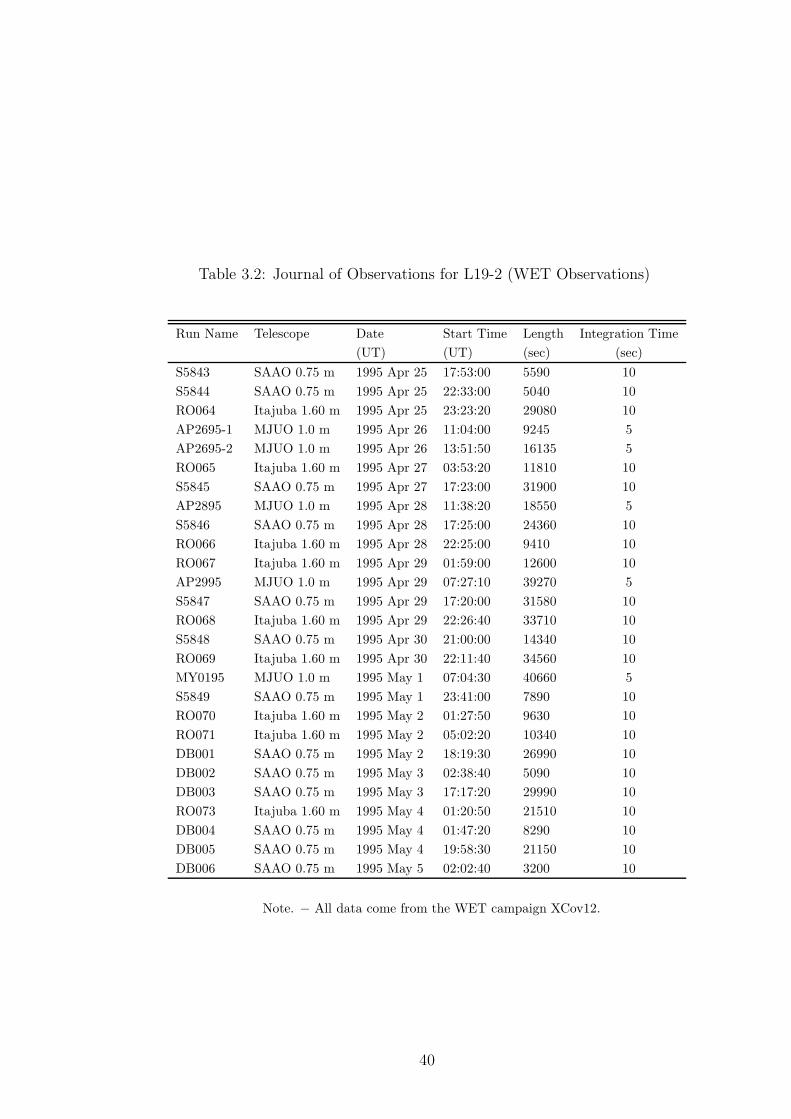
Table 3.2: Journal of Observations for L19-2 (WET Observations)
Run Name Telescope Date Start Time Length Integration Time
(UT) (UT) (sec) (sec)
S5843 SAAO 0.75 m 1995 Apr 25 17:53:00 5590 10
S5844 SAAO 0.75 m 1995 Apr 25 22:33:00 5040 10
RO064 Itajuba 1.60 m 1995 Apr 25 23:23:20 29080 10
AP2695-1 MJUO 1.0 m 1995 Apr 26 11:04:00 9245 5
AP2695-2 MJUO 1.0 m 1995 Apr 26 13:51:50 16135 5
RO065 Itajuba 1.60 m 1995 Apr 27 03:53:20 11810 10
S5845 SAAO 0.75 m 1995 Apr 27 17:23:00 31900 10
AP2895 MJUO 1.0 m 1995 Apr 28 11:38:20 18550 5
S5846 SAAO 0.75 m 1995 Apr 28 17:25:00 24360 10
RO066 Itajuba 1.60 m 1995 Apr 28 22:25:00 9410 10
RO067 Itajuba 1.60 m 1995 Apr 29 01:59:00 12600 10
AP2995 MJUO 1.0 m 1995 Apr 29 07:27:10 39270 5
S5847 SAAO 0.75 m 1995 Apr 29 17:20:00 31580 10
RO068 Itajuba 1.60 m 1995 Apr 29 22:26:40 33710 10
S5848 SAAO 0.75 m 1995 Apr 30 21:00:00 14340 10
RO069 Itajuba 1.60 m 1995 Apr 30 22:11:40 34560 10
MY0195 MJUO 1.0 m 1995 May 1 07:04:30 40660 5
S5849 SAAO 0.75 m 1995 May 1 23:41:00 7890 10
RO070 Itajuba 1.60 m 1995 May 2 01:27:50 9630 10
RO071 Itajuba 1.60 m 1995 May 2 05:02:20 10340 10
DB001 SAAO 0.75 m 1995 May 2 18:19:30 26990 10
DB002 SAAO 0.75 m 1995 May 3 02:38:40 5090 10
DB003 SAAO 0.75 m 1995 May 3 17:17:20 29990 10
RO073 Itajuba 1.60 m 1995 May 4 01:20:50 21510 10
DB004 SAAO 0.75 m 1995 May 4 01:47:20 8290 10
DB005 SAAO 0.75 m 1995 May 4 19:58:30 21150 10
DB006 SAAO 0.75 m 1995 May 5 02:02:40 3200 10
Note. − All data come from the WET campaign XCov12.
40

Table 3.3: Stellar Information
Star Teff log g Reference
(K) (cgs)
GD 66 11,980 8.05 1
GD 244 11,680 8.08 1
G117-B15A 11,630 7.97 1
G185-32 12,130 8.05 1
L19-2 12,100 8.21 1
GD 165 11,980 8.06 1
R548 11,990 7.97 1
G226-29 12,460 8.28 1
References. − (1) Bergeron et al. (2004).
41

3.2.2.1 Stars With Detected Combination Frequencies
GD 66
Apart from an analysis by Fontaine et al. (1985), little progress toward un-
derstanding GD 66 has been made since Dolez et al. (1983) first reported its
discovery. The relatively high number of combination frequencies identified in
the FT of GD 66 makes it an ideal star to include in this dissertation.
To identify the pulsation modes and combination frequencies of GD 66, we
computed an FT from the reduced and combined lightcurves listed in Table 3.1.
We have included a sample lightcurve in Figure 3.1 and the FT of all GD 66 data
in Figure 3.2. To identify closely spaced modes in the regions of obvious excess
power, we utilized a prewhitening technique similar to that of O’Donoghue &
Warner (1982) using an iterative nonlinear least squares procedure. For each
peak, we fitted the frequency, amplitude, and phase and then subtracted the fit
from the original lightcurve. We then fitted a second frequency to the altered
data, choosing in every case the largest remaining peak, and used the result of
this fit to conduct a simultaneous least squares fit to the original data. Thus at
each step in the prewhitening, the frequencies removed are from a simultaneous
fit to the original data.
The problems with applying such a procedure to a highly aliased data set
are well known (Nather et al., 1990), and we have no illusions that we can
successfully measure the correct frequencies of the smaller modes in the presence
of the contaminating window function. Nonetheless, the exercise provides two
pieces of information that are valuable and reliable. It tells us how many modes
are required to model the data, and gives us crude amplitudes for the members
of the multiplet that are useful in estimating inclination.
In Figure 3.3 we show the deconstruction of the 271 s pulsation mode (F1)
by prewhitening. The FT of the reduced data in the region of F1 is shown in
Figure 3.3a. The window function, in Figure 3.3b, is the FT of a lightcurve of
42

Figure 3.1: Lightcurve of GD 66. These data were acquired with the ARGOSCCD photometer on the McDonald Observatory 2.1 m Struve Telescope with anexposure time of 10 s.
a sinusoid with the same period, amplitude, and phase as the highest ampli-
tude peak in the original FT that has been sampled in the same manner as the
original data. Figure 3.3c shows the FT of the lightcurve with the largest peak
removed. Figures 3.3c and 3.3d are prewhitened FTs that reveal additional low
amplitude signals which were previously hidden in the window function of the
highest amplitude peak. Figure 3.3e, in which there is no remaining signal, is an
FT of a lightcurve with the three highest amplitude peaks fitted and removed
from the original lightcurve. It is gratifying that the frequencies identified by
this deconstruction form a frequency-symmetric triplet, but better sampling will
be required to measure all three frequencies with confidence.
A similar procedure showed that F2 was consistent with a single frequency,
to within the noise, and that F3 is a combination of at least three frequencies.
43
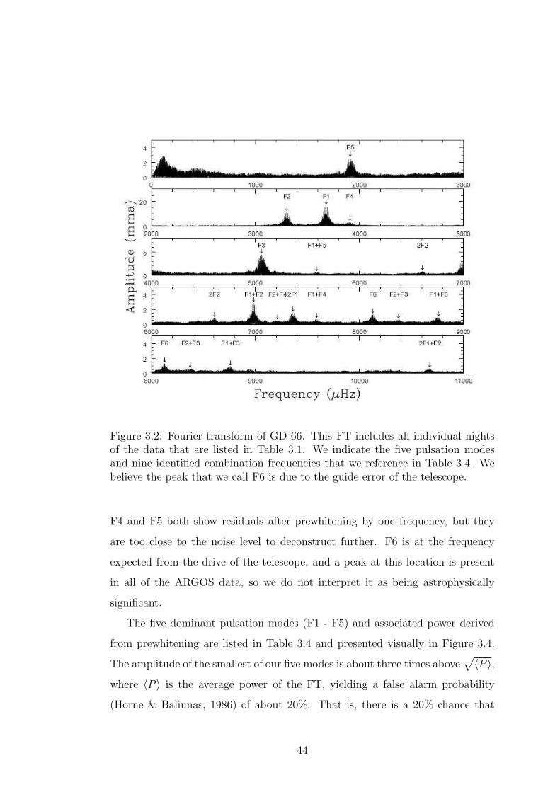
Figure 3.2: Fourier transform of GD 66. This FT includes all individual nightsof the data that are listed in Table 3.1. We indicate the five pulsation modesand nine identified combination frequencies that we reference in Table 3.4. Webelieve the peak that we call F6 is due to the guide error of the telescope.
F4 and F5 both show residuals after prewhitening by one frequency, but they
are too close to the noise level to deconstruct further. F6 is at the frequency
expected from the drive of the telescope, and a peak at this location is present
in all of the ARGOS data, so we do not interpret it as being astrophysically
significant.
The five dominant pulsation modes (F1 - F5) and associated power derived
from prewhitening are listed in Table 3.4 and presented visually in Figure 3.4.
The amplitude of the smallest of our five modes is about three times above√
〈P 〉,where 〈P 〉 is the average power of the FT, yielding a false alarm probability
(Horne & Baliunas, 1986) of about 20%. That is, there is a 20% chance that
44

Figure 3.3: Deconstruction of F1 in GD 66. a: A Fourier transform of GD 66 near271 s (F1). b: A window function obtained by taking an FT of a single sinusoid(with the same period and amplitude of the 271.71 s peak) that has been sampledin the same manner as the data. c: An FT near F1 with a period of 271.71 sremoved. d: An FT near F1 with periods of 271.71 and 272.20 s removed. e: AnFT near F1 with periods of 271.71, 272.20, and 271.23 s removed.
F5 is an artifact of noise. However, the existence of a combination frequency
at F1+F5 adds confidence to this detection. All the pulsation modes except F5
were also identified by Fontaine et al. (2001). There is a large peak near the
location of F5 in their data, but it was not formally significant against the noise
level of their FT.
In addition to the five modes detected, we identified nine combination fre-
quencies that were consistently present throughout the three month span of our
GD 66 observations, with one exception (F1+F4 was not identified in the 2003
October data set). We verified our identification of combination frequencies with
45

a computer program inspired by Kleinman (1995). Our program allows a user to
select pulsation modes in the data, calculates all possible combination frequen-
cies of these modes, and then searches for significant combination frequencies
in the data. The search is conducted over an estimated error range equal to
the resolution of the FT. We consider this a better estimate of the frequency
error than the smaller values from the least squares fit because the combina-
tion frequencies are usually low amplitude, i.e., only a few times as large as the
background. The frequencies of such small signals are pulled by the presence
of unresolved noise peaks, while the least squares fit formally assumes only a
single unblended frequency is present. The program successfully identified all
combination frequencies that we found by inspection in the data, and also found
some combinations that we had missed in our visual search. In some cases, the
highest amplitude peak among the combination frequency and its aliases did not
fall within the error range we established. In these cases, prewhitening a forced
fit of the expected combination frequency successfully removed the signal, and
we have listed the amplitude from the forced frequency fit. Our listed period er-
rors do not include the uncertainty in identifying the true peak among the alias
peaks and these dominate the error for combination frequencies.
Having identified and measured the amplitudes of the combination frequencies
allows us to calculate the ratio of combination to parent mode amplitudes (Rc,
see equation 2.9) and compare it to the theoretical predictions. Figure 3.5 shows
the observed Rc for all of the detected two-mode combination frequencies in GD
66. Where no combination was detected, we have plotted a limit equal to the 1
σ noise level in the FT. The observed Rc do not depend on any theory.
The theoretical calculations of Rc require that we supply an inclination es-
timate, an estimate of τc0 , and a value for the parameter 2β + γ. For the first,
a fit to the largest multiplet using the technique of Pesnell (1985) described in
§2.2 yielded Θ0 = 13, and we have used that value for all of the theoretical cal-
culations. The result is not very sensitive to this parameter as long as Θ0 ≤ 25
46
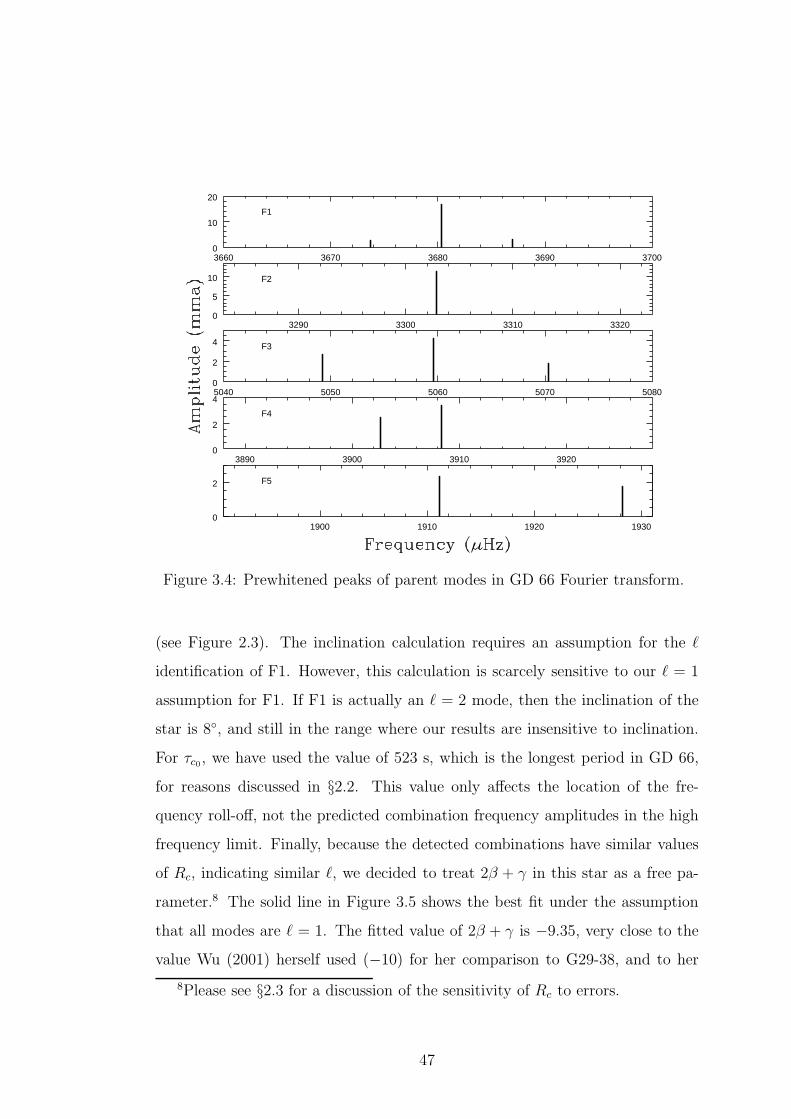
3660 3670 3680 3690 37000
10
20
F1
3290 3300 3310 33200
5
10 F2
5040 5050 5060 5070 50800
2
4 F3
3890 3900 3910 39200
2
4
F4
1900 1910 1920 19300
2 F5
Figure 3.4: Prewhitened peaks of parent modes in GD 66 Fourier transform.
(see Figure 2.3). The inclination calculation requires an assumption for the ℓ
identification of F1. However, this calculation is scarcely sensitive to our ℓ = 1
assumption for F1. If F1 is actually an ℓ = 2 mode, then the inclination of the
star is 8, and still in the range where our results are insensitive to inclination.
For τc0, we have used the value of 523 s, which is the longest period in GD 66,
for reasons discussed in §2.2. This value only affects the location of the fre-
quency roll-off, not the predicted combination frequency amplitudes in the high
frequency limit. Finally, because the detected combinations have similar values
of Rc, indicating similar ℓ, we decided to treat 2β + γ in this star as a free pa-
rameter.8 The solid line in Figure 3.5 shows the best fit under the assumption
that all modes are ℓ = 1. The fitted value of 2β + γ is −9.35, very close to the
value Wu (2001) herself used (−10) for her comparison to G29-38, and to her
8Please see §2.3 for a discussion of the sensitivity of Rc to errors.
47

theoretically calculated value (−12.6). Any other assumption for ℓ would yield
values of 2β+ γ different by a factor of ∼ 3 or more, and we do not consider this
a reasonable possibility. Using ℓ = 1, the detected combination frequencies fit
the model with a reduced χ2 of 0.78, which may indicate that we have slightly
overestimated our errors. We used the errors from the least square fits, which are
often regarded as underestimates (Winget et al., 1991), but we see no evidence
for that here.
Figure 3.5: Ratio of combination to parent mode amplitudes (Rc) for GD66. The lines are theoretical predictions for G0+0
1 1 /g01g
01(Θ0 = 13) (solid line),
G0+01 2 /g
01g
02(Θ0 = 13) (long-dashed line), and G0+0
2 2 /g02g
02(Θ0 = 13) (dashed
line). The data points are the detected harmonics or limits (filled squares),detected cross combination frequencies (stars), and limits for the cross combi-nations (crosses). The downward arrows on the limits indicate that the pointsrepresent maximum values. The upper limit for Rc of 2F5 lies at 124 (not shown).
Even though the data show tight scatter about the line representing com-
binations between two ℓ = 1 modes, we cannot conclude that all of the modes
48

are ℓ = 1 on that basis alone. The line representing ℓ = 1, 2 combinations (long
dashes in Figure 3.5) is close to the ℓ = 1, 1 line, and falls within the error bars for
some combinations. Fortunately, the theoretical lines for same-ℓ combinations
are well-separated, suggesting that harmonics, which are same-ℓ by definition,
might be able to constrain ℓ when cross combinations (i.e., all combinations that
are not harmonics) cannot. We have detected harmonics for F1 and F2, and mea-
sured limits for the harmonics of the remaining three modes. These are shown
in Figure 3.5 as filled squares. The measured Rc for F1 and F2 and the limits for
F3 and F4 are only consistent with ℓ = 1, and so we identify all of those modes
as ℓ = 1, F4 somewhat tentatively because the limit is not very stringent. The
limit for F5 is too large (Rc = 124) to fit on our plot and does not constrain
ℓ uniquely. Though our identification relies primarily on harmonics, the cross
combinations are all consistent with this conclusion. The m identifications we
assigned in Table 3.4 arise from frequency splitting only, and are not derived
from combination frequency amplitudes.
Finally, the Rc limits we have plotted at low frequency suggest that the roll-off
expected from the theory actually occurs, which eliminates from consideration
competing models, including the BFW95 theory, that predict no frequency de-
pendence for Rc.
GD 244
Fontaine et al. (2001) first reported the detection of variability in the DAV
white dwarf GD 244, but no subsequent observations have been published. The
FTs of GD 244 and GD 66 both contain large pulsation modes near 200, 256, and
300 s. The similarity of GD 244 to GD 66, including its relatively high number
of combination frequencies, makes it another ideal candidate to include in this
study.
To identify the pulsation modes and combination frequencies of GD 244, we
computed an FT from the reduced and combined lightcurves listed in Table 3.1.
49

We have included a sample lightcurve in Figure 3.6 and the FT of all GD 244
data in Figure 3.7. We used the prewhitening technique to identify pulsation
modes and combination frequencies in GD 244, as with GD 66. We also used
prewhitening to reveal the doublet structure in the two highest amplitude pulsa-
tion modes. As with GD 66, we do not expect that we have consistently measured
the correct frequencies of the modes in these doublets in the presence of the con-
taminating window function. However, the amplitudes are useful in estimating
the inclination.
Figure 3.6: Lightcurve of GD 244. These data were acquired with the ARGOSCCD photometer on the McDonald Observatory 2.1 m Struve Telescope with anexposure time of 5 s.
In Figure 3.8 we show the deconstruction of the 256 s pulsation mode (F2)
by prewhitening. The FT of the reduced data in the region of F2 is shown in
Figure 3.8a. The window function for the GD 244 data set is in Figure 3.8b. Fig-
ure 3.8c shows the FT of the lightcurve with the largest peak removed. Panel c
50

Figure 3.7: Fourier transform of GD 244. This FT includes all individual nightsof data included in Table 3.1. We indicate the four pulsation modes and allcombination frequencies that we reference in Table 3.5. F1+F3 is likely a blendwith guide error.
is a prewhitened FT that reveals additional low amplitude signal that was previ-
ously hidden in the window function of the highest amplitude peak. Figure 3.8d
is an FT of a lightcurve with the two highest amplitude peaks fitted and re-
moved from the original lightcurve. We were unable to fit any other statistically
significant signals from the FT in the bottom panel.
A similar procedure showed that F1 is also consistent with a doublet. F3,
however, is consistent with a single frequency, although any putative companion
peak would be in the noise if it scaled as the companions of F1 and F2. F4 is not
formally significant, with a false alarm probability near 1 in the whole data set,
but it appears above the noise at the same frequency in all three of the single
51
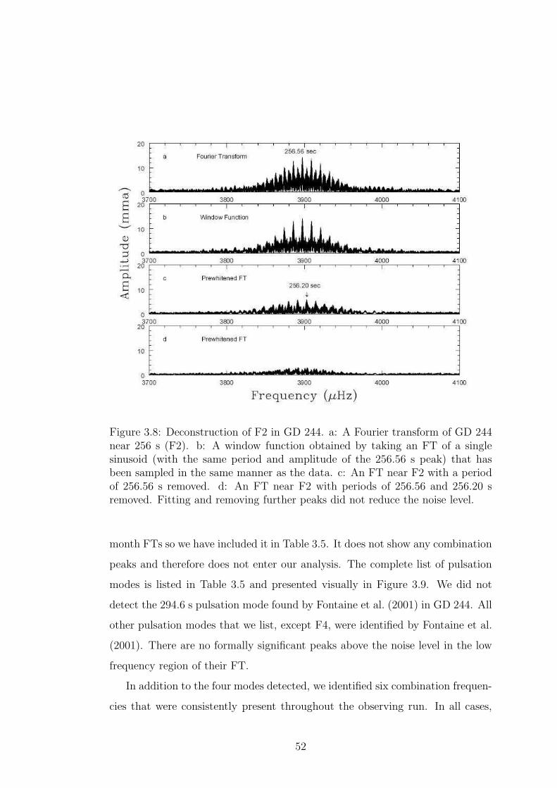
Figure 3.8: Deconstruction of F2 in GD 244. a: A Fourier transform of GD 244near 256 s (F2). b: A window function obtained by taking an FT of a singlesinusoid (with the same period and amplitude of the 256.56 s peak) that hasbeen sampled in the same manner as the data. c: An FT near F2 with a periodof 256.56 s removed. d: An FT near F2 with periods of 256.56 and 256.20 sremoved. Fitting and removing further peaks did not reduce the noise level.
month FTs so we have included it in Table 3.5. It does not show any combination
peaks and therefore does not enter our analysis. The complete list of pulsation
modes is listed in Table 3.5 and presented visually in Figure 3.9. We did not
detect the 294.6 s pulsation mode found by Fontaine et al. (2001) in GD 244. All
other pulsation modes that we list, except F4, were identified by Fontaine et al.
(2001). There are no formally significant peaks above the noise level in the low
frequency region of their FT.
In addition to the four modes detected, we identified six combination frequen-
cies that were consistently present throughout the observing run. In all cases,
52

3240 3250 3260 32700
10
20 F1
3890 3900 3910 39200
10 F2
4910 4920 4930 4940 49500
2
4 F3
1090 1100 1110 11200
1
2F4
6500 6510 6520 65300
2 2F1
Figure 3.9: Prewhitened peaks in GD 244 Fourier transform. In addition to theparent modes, we include one combination frequency (2F1) in which we resolvedfine structure.
the highest amplitude peak among the combination frequency and its aliases fell
within the error of the expected frequency. We list the frequencies of the highest
amplitude peaks in Table 3.5. The frequency errors were sufficiently small that
there was no confusion between the harmonic of the largest component (presumed
m = −1) and the sum of the m = −1 and m = +1 components.
We use the doublet structure at 307 s (F1) to estimate the inclination of
the pulsation axis of GD 244. We assume that the doublet structure in these
two pulsation modes results from viewing ℓ = 1 modes at high inclination so
that the third (central, m = 0) mode does not appear. As discussed previously,
our results do not depend sensitively on this assumption. Using the maximum
amplitude in the prewhitened FT of F1 as an estimate for the amplitude of the
m = 0 peak, we apply the Pesnell (1985) method and find a minimum possible
inclination of 80. Recall that Figure 2.4 shows that at high inclination, the
53

amplitudes of combination frequencies with ℓ = 1 and same-m parent modes
have no dependence on inclination.
Figure 3.10 is a plot of the theoretical predictions for GD 244 (Rc with Θ0 =
80) and the observed amplitudes of the six detected combination frequencies for
comparison. We also include the observed noise limit (indicated by crosses for
the same-m combinations and open squares for the different-m combinations) in
cases where there was no combination frequency detected. The downward arrows
imply an upper limit. When we apply the GD 66 calibration of 2β + γ = −9.35
to GD 244 (in Figure 3.10), the predictions for the ℓ = 1, 1 line resemble the
observations for our detected combination frequencies except for the Rc of 2F2.
The reduced χ2 is 16.9 if all the modes are assumed to be ℓ = 1, but 9.2 if we leave
out the combinations of F2. Obviously we could reduce χ2 further if we varied
2β + γ as before, but part of our exercise is to establish that we can conduct
mode identification without fitting parameters, so that it is possible to measure
the ℓ of hot ZZ Ceti stars with only a single detected combination frequency.
Turning to the harmonics, which are known to be same-ℓ and therefore to have
well-separated predictions for Rc, 2F1 and the limit for 2F3 demand that F1 and
F3 be ℓ = 1 modes. The high measurement for 2F2 suggests that ℓ may not be 1.
However, if we assume ℓF2 = 2, then χ2 > 400 because Rc for a harmonic of an
ℓ = 2, m = 1 mode is predicted to be near 90. Even if we relax the assumptions
used to calculate inclination and adjust it to minimize χ2 for the assumption of
ℓF2 = 2, then at Θ0 = 67, χ2 = 17.3. So even under the best assumptions, the
identification of F2 as ℓ = 2 would yield a worse fit than if we let it be ℓ = 1.
Moreover, its similar frequency splitting to F1 suggests that it is ℓ = 1, but
without better sampling with WET this is not a secure statement. Therefore,
we have left question marks next to the identification of F2 in Table 3.5. It
is possible that the harmonic of F2 is inflated by some independent unresolved
pulsation mode, but our data are insufficient to test this possibility. Finally, for
the smallest mode, F4, the limit on the harmonic constrains it to be ℓ ≤ 3, which
54

is not useful.
Because F1 and F2 are multiplets, we expect fine structure in their harmonics
and combinations, and indeed we observe secondary peaks near both harmonics
at the sum of the presumed m = −1 and m = 1 parent modes. Unfortunately,
the theoretical lines for these cross terms in m are not well-separated from similar
cross terms in an ℓ = 2 mode (see Figure 3.10). Likewise, the F1+F2 peak shows
multiplet structure, but we are unable to reliably dissect it into individual modes.
The limits we have measured for the cross terms of different-ms are all consistent
with the ℓ = 1 identifications, but would not be sufficient alone to reach that
conclusion.
G117-B15A
G117-B15A is one of the hottest known ZZ Ceti stars. McGraw & Robinson
(1976) confirmed the star’s variability and Kepler et al. (1982) found six pulsation
modes. The dominant mode, at 215 s, is stable in amplitude and phase such that
G117-B15A is the most precise optical clock known (Kepler et al., 2000a). We
use published measurements for G117-B15A obtained from the WET campaign
XCov 4 in 1990 May (Kepler et al., 1995b). They list the highest amplitude
modes as ℓ = 1.
The 215 s pulsation mode of G117-B15A has a large central peak and two
possible adjacent peaks regarded by Kepler et al. (1995b) as “low probability”
because they do not rise very far above the already low noise level. We have used
the size of the adjacent peaks to constrain the inclination of this star, under the
assumption that the central peak is an ℓ = 1, m = 0 mode. We find that the star
has a maximum inclination of 5 (nearly pole-on), and this result is not sensitive
to the assumption of ℓ = 1. In order to appear as a singlet, modes of any ℓ must
be viewed at low inclination.
Figure 3.11 is a plot of the theoretical predictions for G117-B15A (Rc with
Θ0 = 5) and the observed amplitudes of the four detected combination frequen-
55

Figure 3.10: Ratio of combination to parent mode amplitudes (Rc) for GD 244.The lines are theoretical predictions for G1+1
1 2 /g11g
12(Θ0 = 80) (long-dashed line),
G1+11 1 /g
11g
11(Θ0 = 80) (solid line), G1+0
2 2 /g12g
02(Θ0 = 80) (dot-long-dashed line),
G1−11 1 /g
11g
−11 (Θ0 = 80) (dot-dashed line), andG1+1
2 2 /g12g
12(Θ0 = 80) (dashed line).
The data points are the detected harmonics or limits (filled squares), detectedcross combination frequencies (stars), limits for the same-m cross combinations(crosses), and limits for the different-m cross combinations (open squares). Thedownward arrows on the limits indicate that the points represent maximum val-ues.
cies for comparison. We also include the observed noise limit (indicated by the
crosses) in cases where there was no combination frequency detected. The down-
ward arrows below the crosses indicate an upper limit. Just as with GD 66, the
theory of Wu (2001) predicts high amplitudes for all of the combination frequen-
cies that we detect and low amplitudes for those we do not detect. When we
apply the GD 66 calibration of 2β + γ = −9.35 to G117-B15A (in Figure 3.11),
the predictions are consistent with the observations for our detected combina-
tion frequencies, though the scatter is considerably worse than in GD 66. The
56

2F1
2F2
2F3
F1-F2
Figure 3.11: Ratio of combination to parent mode amplitudes (Rc) for G117-B15A. The lines are theoretical predictions for G0+0
1 1 /g01g
01(Θ0 = 5) (solid line),
G0+01 2 /g
01g
02(Θ0 = 5) (long-dashed line), and G0+0
2 2 /g02g
02(Θ0 = 5) (dashed line).
The data points are the detected harmonics or limits (filled squares), detectedcross combination frequencies (stars), and limits for the cross combinations(crosses). The downward arrows on the limits indicate that the points repre-sent maximum values. There are no error bars for F1-F2 because there werenone reported by Kepler et al. (1995b).
reduced χ2 is 3.14 if all the modes are assumed to be ℓ = 1. The combination
F1-F2, located in the lower left quadrant of Figure 3.11, is not included in this
χ2, because no formal errors were reported by Kepler et al. (1995b). If we as-
sume the error for the amplitude of this combination is greater than the largest
errors in the plot, then it gives no information about the ℓ of its parents, but is
consistent with the low frequency roll-off of the theory of Wu (2001).
Robinson et al. (1995) established that ℓ = 1 for F1 by comparing time-series
photometry observations in the UV and optical wavelengths. The amplitude
57

of the harmonic of this mode, combined with our analysis, confirms this ℓ = 1
identification; the observed Rc for the harmonic of F1 is too small to be consistent
with that for ℓi = ℓj = 2, which is 2.5 times greater than Rc for ℓi = ℓj = 1
and 5 greater than the Rc we observe. Likewise, the limit for the harmonic of
F2 is sufficiently low to constrain this mode to be ℓ = 1 with a 98.7 percent
confidence level. The limit for 2F3 is more ambiguous, but clearly requires that
ℓ ≤ 2 for F3. We list our mode identifications in Table 3.6. These results are
consistent with the seismological analyses of both Bradley (1998) and Brassard
et al. (1993), where the choice of ℓ = 1 for these three peaks yielded reasonable
physical parameters.
G185-32
McGraw et al. (1981) discovered the DA white dwarf G185-32 to be a rel-
atively low amplitude multi-periodic ZZ Ceti star on the basis of its (G − R)
colors (see Greenstein, 1976). The largest amplitude peaks have periods of 71,
73, 142, 216, 301, and 370 s. G185-32 is unique among the ZZ Cetis in that it
has a harmonic (at 71 s) that is sometimes measured to be larger than its parent
frequency (at 142 s). This has led to disagreement over whether the harmonic
is a pulse shape artifact, or whether there are resonances between real eigen-
modes that happen to be harmonically related (Castanheira et al., 2004). Most
recently, Thompson et al. (2004) has found that identifying the 142 s mode as
high ℓ (ℓ = 4) can explain all of the available observations, which include time-
resolved UV spectroscopy from HST (Kepler et al., 2000b), time-resolved optical
spectroscopy from Keck (Thompson et al., 2004), and time-series photometry
from WET (Castanheira et al., 2004). An ℓ = 4 mode cancels itself in the in-
tegration over the visible hemisphere for almost any value of inclination, but its
harmonic may not, because it has a surface distribution with characteristics of
lower ℓ. This allows a harmonic to appear larger than its fundamental. In our
analysis, we apply the theory of Wu (2001) under the assumption that the peak
58

Table 3.4: GD 66 Periods and Mode Identifications
Mode Frequency Period σp Amplitude σamp ∆fa ℓ mb
Label (µHz) (sec) (sec) (mma) (mma) (µHz)
F1 3673.753 272.2012 0.0004 2.50 0.17 -6.582? 1 -1
3680.335 271.7144 0.0001 16.70 0.16 1 0
3686.927 271.2286 0.0004 2.93 0.17 6.592? 1 +1
F2 3302.889 302.7653 0.0001 11.29 0.19 1 0
F3 5049.227 198.0501 0.0002 2.65 0.21 -10.355? 1 -1
5059.582 197.6448 0.0001 4.21 0.21 1 0
5070.3c 197.23 1.77 10.7? 1 +1?
F4 3902.680 256.2341 0.0004 2.48 0.21 -5.603? 1? -1?
3908.283 255.8668 0.0003 3.43 0.21 1? 0?
F5 1911.121 523.2533 0.0016 2.33 0.22 1 or 2 ?
1928.257 518.6029 0.0021 1.77 0.22 17.136? 1 or 2 ?
F6d 8127.845 123.0338 0.0002 1.30 0.22 guide
2F1 7360.670 135.8572 0.0002 1.57 0.22 0.001
F1+F2 6983.219 143.2004 0.0001 2.83 0.21 0.005
F1+F3 8747.254 114.3216 0.0002 0.88 0.22 -7.336
F1+F4 7588.604 131.7765 0.0004 0.64 0.22 0.015
F1+F5 5587.599 178.9678 0.0007 0.61 0.22 3.857
2F2 6605.802 151.3821 0.0004 0.80 0.22 -0.025
F2+F3 8362.479 119.5818 0.0004 0.53 0.22 -0.009
F2+F4 7210.499 138.6867 0.0006 0.48 0.22 0.672
2F1+F2 10675.6 93.6720 0.0002 0.52 0.22 -11.994
aFor pulsation modes, ∆f is the separation between the modes in the multiplets and
the m = 0 member. For combination frequencies, ∆f is the frequency difference between
the calculated and observed combination frequency (i.e., ∆f = F1 + F2 − [F1 + F2]).bThe m identifications in the table are based on the frequency splitting alone, not on
the size of the combination peaks.cWe were unable to obtain a simultaneous fit with this frequency and the other two
frequencies in the F3 triplet, though it does seem to be a significantly high amplitude
peak above the noise.dF6 is a formally significant peak that is due to the guide error of the telescope and
probably does not represent a pulsation mode originating at the star.
59

Table 3.5: GD 244 Periods and Mode Identifications
Mode Frequency Period σp Amplitude σamp ∆fa ℓ mb
Label (µHz) (sec) (sec) (mma) (mma) (µHz)
F1 3255.919 307.1329 0.0001 20.18 0.17 1 -1
3261.886 306.5712 0.0002 5.02 0.17 5.966? 1 +1
F2 3897.733 256.5594 0.0001 12.31 0.20 1? -1?
3903.255 256.1964 0.0001 6.73 0.20 5.522? 1? +1?
F3 4926.697 202.9758 0.0001 4.04 0.21 1 -1?
F4 1103.656 906.0795 0.0056 1.72 0.21 ≤ 3 ?
2F1− 6511.422 153.5763 0.0001 2.25 0.23 0.417
F1−+F1+ 6516.119 153.4656 0.0003 0.95 0.23 1.686
F1−+F2− 7153.211 139.7974 0.0001 2.30 0.21 0.442
F1−+F3−c 8182.615 122.2103 0.0002 0.96 0.21 0.001
2F2− 7795.472 128.2796 0.0001 2.44 0.21 -0.006
F2−+F3− 8824.598 113.3196 0.0003 0.53 0.21 -0.168
aFor real pulsation modes, ∆f is the separation between the modes in the doublets.
For combination frequencies, ∆f is the frequency difference between the calculated and
observed combination frequency (i.e., ∆f = F1 + F2 − [F1 + F2]).bThe m identifications in the table are based on frequency splitting alone, not on the
size of the combination peaks.cThe period of F1−+F3− in GD 244 is close to the period of F6 in GD 66 (see
Table 3.4), so it is probable that the amplitude and frequency of this combination
frequency are partially contaminated by the guide error of the telescope.
60

Table 3.6: Periods and Mode Identifications for Published Data with Combina-tion Frequencies
Mode Frequency Period σp Amplitude σamp ∆fa ℓ m Ref.
Label (µHz) (sec) (sec) (mma) (mma) (µHz)
G117-B15A
F1 4646.909 215.1968 0.0007 19.15 0.39 1 0 1
F2 3288.91 304.052 0.004 6.89 0.44 1 0 1
F3 3697.47 270.455 0.004 5.47 0.45 1? 0 1
2F1 9293.68 107.600 0.004 1.06 0.45 0.14 1
F1+F2 7956.59 125.682 0.006 0.90 0.45 -20.77 1
F1+F3 8344.74 119.836 0.003 1.60 0.45 -0.36 1
F1-F2 1357.6 736.60 0.90 0.4 1
G185-32
F1 4635.3 215.74 1.93 0.07 1 or 2 0 2
F2 2701.2 370.21 1.62 0.07 1 or 2 0 2
F3 7048.8 141.87 1.43 0.07 3 0 2
F4 3317.8 301.41 1.13 0.07 1 or 2 0 2
F5 3335.6 299.79 0.95 0.07 1 or 2 0 2
F6 13784.9 72.54 0.93 0.07 1 or 2 0 2
2F3 14097.7 70.93 0.69 0.07 -0.1 2
F3-F6 6736.1 148.45 0.57 0.07 0.0 2
Note. − We have not included a complete list of eigenmodes for each star. Instead,
we have only included eigenmodes relevant to this study. The ℓ and m identifications
are from our analysis.a∆f is the frequency difference between the calculated and observed combination
frequency (i.e., ∆f = F1 + F2 − [F1 + F2]).
References. − (1) Kepler et al. (1995b); (2) Castanheira et al. (2004).
61

at 142 s is the parent mode of a harmonic at 71 s. We use published measure-
ments for G185-32 obtained from the WET campaign XCov 8 in 1992 September
(Castanheira et al., 2004).
With the exception of the 142 s mode, Kepler et al. (2000b) identify all the
other modes as either ℓ = 1 or ℓ = 2 based on HST data alone. Using independent
temperature constraints they choose ℓ = 1 for all of these modes. Under this
identification, F19, at 215 s, is the highest amplitude ℓ = 1 mode, and we use it
to estimate the inclination. Castanheira et al. (2004) detect only one peak at 215
s, so we presume it to be the m = 0 component and use the neighboring noise
limit to approximate the size of the m = ±1 peaks. The Pesnell (1985) method
then yields Θ0 = 13. If the inclination were greater than this, we would see the
m = ±1 members of the multiplet above the noise. Our results are robust even
if the ℓ identification is not; if F1 is actually an ℓ = 2 mode, then the inclination
of the star is less than 7, and still in the range where our results are insensitive
to the inclination (see Figure 2.3).
Figure 3.12 is a plot of the theoretically predicted combination frequency
amplitude ratios for G185-32 (Rc with Θ0 = 13) and the observed amplitudes of
the detected combination frequencies for comparison. For clarity, the ℓ = 1, 1 and
ℓ = 2, 2 lines are not included in Figure 3.12, but fall below the lowest line shown
(ℓ = 1, 3). Unlike the harmonics found in GD 66, GD 244, and G117-B15A,
Rc for the harmonic of F3 in G185-32 is more than 50 times greater than the
prediction for ℓi = ℓj = 1 and more than 15 times the prediction for ℓi = ℓj = 2.
The best explanation for this is that F3 is a high ℓ mode, just as Thompson et al.
(2004) claim for independent reasons. The value of ℓ that best explains our Rc is
ℓ = 3 rather than ℓ = 4. However, in the case of high ℓ, our theory suffers from
two problems. First, the geometric factor in the theory of Wu (2001) varies more
9Our nomenclature (see Table 3.6) does not follow Thompson et al. (2004),Castanheira et al. (2004), nor Kepler et al. (2000b). We have labeled the modesin order of highest amplitudes from the WET data.
62

rapidly with inclination for ℓ = 3 and 4 (instead of the gradual changes for low
ℓ shown in Figure 2.3, see Figure A.1 in Appendix A). We have accommodated
this by including a range of inclinations about the 13 nominal value. We show
this range as dotted lines in Figure 3.12, which indicate how Rc for ℓi = ℓj = 3
changes between Θ0 = 0 and 20. Rc for 2F3 falls within the prediction for
ℓF3 = 3. The second problem is our use of a constant bolometric correction
that is really only appropriate for ℓ = 1. This is a limitation inherent to the
analytic theory as Wu (2001) presented it, and could be addressed by employing
numerical models, but this would be not be consistent with our objective of
having a quick and easily applicable method for mode identification in large
numbers of ZZ Ceti stars (see the discussion on error sensitivities in §2.3). We
have calculated bolometric corrections for higher ℓ, and the differences are not
large enough to change the ℓ = 3 identification for F3. So the inconsistency of
our ℓ = 3 identification and the ℓ = 4 identification of Thompson et al. (2004)
remains a mystery. Fortunately, for seismological work it is useful to identify a
mode as high ℓ, even if the exact value is unknown. The density of modes in the
models at high ℓ is so large that they do not contribute seismological constraints
because the radial overtone (k) is unknown, but misinterpreting a high ℓ mode as
ℓ = 1 or 2 would lead the models astray. So even if a mode identification method
based on measurements of Rc alone cannot identify high ℓ modes precisely, it is
still useful for its ability to discriminate between modes of high and low ℓ.
In addition to the identification of F3 as high ℓ, the limits on Rc for the
harmonics of F1, F2, F4, F5, and F6 constrain that ℓ ≤ 2 for these modes,
consistent with the tentative mode identifications of Castanheira et al. (2004).
Our results are also consistent with the seismological analysis of Bradley (2006),
including his high ℓ identification for F3, with the exception of his identification
of F6 as high ℓ. Unfortunately, we are not able to definitively assign any ℓ
values to these modes due to their intrinsically low amplitudes (see Clemens,
1994; Thompson et al., 2004). Likewise, the only detected cross term, which
63

is a combination with the high ℓ mode F3, is not able to narrow the choice of
ℓ. Indeed, we are not even able to determine whether the mode we call F6 is
a combination with F3 and a mode at 148 s or whether the latter is F3-F6.
We have used the latter identification in Table 3.6, following Castanheira et al.
(2004) and consistent with Bradley (2006).
3.2.2.2 Stars Without Detected Combinations
L19-2
McGraw (1977) discovered the variability of L19-2, a hot, low-amplitude ZZ
Ceti star. O’Donoghue & Warner (1982) presented a comprehensive analysis of
single site data, and were able to assign tentative values of ℓ to the pulsation
modes. Bradley (2001) revised these identifications in light of theoretical im-
provements, finding three modes of ℓ = 1 and two of ℓ = 2. L19-2 was the
subject of the WET campaign XCov 12 in 1995 April, on which Sullivan (1995)
presented a preliminary paper. We have re-reduced and analyzed the archival
WET data to search for combination frequencies, and found none detectable
above the noise limit of the FT. We have included a sample lightcurve in Fig-
ure 3.13 and the FT of all of the L19-2 WET data in Figure 3.14.
As with GD 66, we used the prewhitening technique to measure pulsation
frequencies in L19-2, and to reveal the multiplet structure in the highest ampli-
tude modes. In Figure 3.15 we show the 192 s pulsation mode (F1) as a typical
example. Figure 3.15a is the original FT in the region of F1. Figure 3.15b is
the window function of the 192.61 s peak. The remaining panels show the re-
sults of our iterative fitting and removal of three pulsation frequencies. Note
that there appears to be a significant residual near the m = −1 component.
This is mysterious, but not unprecedented (Kawaler et al., 1995). We show the
multiplet structure of the 113 s, 118 s, 350 s, and 143 s modes in Figures 3.16,
64

3.17, 3.18, and 3.19.10 The identified periods of L19-2 are listed in Table 3.7 and
presented visually in Figure 3.20. We do not detect any combination frequen-
cies in L19-2. However, the noise level is sufficiently low, that the non-existence
of combinations, particularly harmonics, constrains the ℓ values of the modes
present.
Table 3.7: L19-2 Periods and Mode Identifications (WET Observations)
Mode Frequency Period σp Amplitude σamp ∆fa ℓ mb
Label (µHz) (sec) (sec) (mma) (mma) (µHz)
F1 5179.362 193.0740 0.0019 0.973 0.064 -12.433 1 -1
5191.795 192.6116 0.0004 5.535 0.065 1 0
5204.160 192.1540 0.0015 1.216 0.063 12.365 1 +1
F2 8789.054 113.7779 0.0004 1.766 0.067 1 or 2 0
8828.619 113.2680 0.0024 0.271 0.067 39.565 1 or 2 +2
F3 8426.324 118.6757 0.0006 1.191 0.070 -11.109 1 or 2 -1
8437.433 118.5195 0.0005 1.641 0.071 1 or 2 0
8448.580 118.3631 0.0023 0.339 0.069 11.147 1 or 2 +1
F4 2855.785 350.1664 0.0073 0.918 0.068 1 or 2 0
2868.023 348.6722 0.0192 0.347 0.068 12.238 1 or 2 +1
F5 6954.415 143.7935 0.0047 0.228 0.069 -18.112 ≤ 3 -1?
6972.527 143.4200 0.0030 0.354 0.070 ≤ 3 0
6991.176 143.0375 0.0031 0.341 0.069 18.649 ≤ 3 +1
a∆f is the separation between the modes in the multiplets and the m = 0 member.bThe m identifications in the table are based on frequency splitting alone, not on the size
of the combination peak limits.
We have used the multiplet structure at 192 s (F1) in Figure 3.15 to estimate
the inclination of the pulsation axis of L19-2, finding an inclination of 16. In
Figure 3.21, we have plotted the theoretical predictions for combination frequency
amplitudes in L19-2 (Rc with Θ0 = 16). Instead of measured ratios for Rc, we
have included the observed noise limit (indicated by the filled squares, crosses,
open squares, and a star) at the frequencies where we expect combinations to
be detected. The downward arrows indicate that all data points are limits on
detections. The limit for the harmonic of F1 implies that mode is ℓ = 1, which
10The deconstruction of F5 (143 s) is particularly interesting because of theconfirmation of a peak at 143.79 s as predicted by O’Donoghue & Warner (1982).
65

2F2
2F4
2F5
2F1
2F6
F6
F3-F6
2F3
Figure 3.12: Ratio of combination to parent mode amplitudes (Rc) for G185-32. The lines are theoretical predictions for G0+0
3 3 /g03g
03(Θ0 = 13) (solid line),
G0+02 4 /g
02g
04(Θ0 = 13) (long-dashed line), G0+0
2 3 /g02g
03(Θ0 = 13) (dot-dashed line),
and G0+01 3 /g
01g
03(Θ0 = 13) (dot-long-dashed line). The data points are the de-
tected harmonics or limits (filled squares), detected cross combination frequencies(stars), and limits for the cross combinations involving the F3 pulsation modeonly (crosses). The downward arrows on the limits indicate that the points rep-resent maximum values. The dotted lines on either side of the ℓi = ℓj = 3 lineare the Rc predictions for extremum in inclination: Θ0 = 20 (top) and Θ0 = 0
(bottom). the predictions of Wu (2001) for G0+04 4 /g
04g
04(Θ0 = 13) are not shown
because they reach values above Rc ∼ 3600.
66

Figure 3.13: Lightcurve of L19-2 (WET observations). These data were acquiredas part of the WET campaign XCov 12 in 1995 April with an exposure time of10 s.
Figure 3.14: Fourier transform of L19-2 (WET observations). This FT includesall data listed in Table 3.2. We indicate the five pulsation modes that we referencein Table 3.7.
67

5100 5150 5200 5250 53000
5a Fourier Transform
192.61 sec
5100 5150 5200 5250 53000
5b Window Function
5100 5150 5200 5250 53000
1
2c Prewhitened FT
192.15 sec
5100 5150 5200 5250 53000
1
2d Prewhitened FT
193.07 sec
5100 5150 5200 5250 53000
1
2e Prewhitened FT
Figure 3.15: Deconstruction of F1 in L19-2. a: A Fourier transform of L19-2 near192 s (F1). b: A window function obtained by taking an FT of a single sinusoid(with the same period and amplitude of the 192.61 s peak) that has been sampledin the same manner as the data. c: An FT near F1 with a period of 192.61 sremoved. d: An FT near F1 with periods of 192.61 and 192.15 s removed. e: AnFT near F1 with periods of 192.61, 192.15, and 193.08 s removed.
68

8700 8750 8800 8850 89000
1
2
3
a Fourier Transform113.78 sec
8700 8750 8800 8850 89000
1
2
3
b Window Function
8700 8750 8800 8850 89000
0.2
0.4
0.6
c Prewhitened FT113.27 sec
8700 8750 8800 8850 89000
0.2
0.4
0.6
d Prewhitened FT
Figure 3.16: Deconstruction of F2 in L19-2. a: A Fourier transform of L19-2near 113 s (F2). b: A window function obtained by taking an FT of a singlesinusoid (with the same period and amplitude of the 113.78 s peak) that hasbeen sampled in the same manner as the data. c: An FT near F2 with a periodof 113.78 s removed. d: An FT near F2 with periods of 113.78 and 113.27 sremoved. Note that the peak of 113.27 in panel c was not the highest amplitudepeak remaining in the prewhitened FT. We chose this peak among the noisebecause of its pre-established presence in the FTs of O’Donoghue & Warner(1982).
69

8350 8400 8450 8500 85500
2 a Fourier Transform118.52 sec
8350 8400 8450 8500 85500
2 b Window Function
8350 8400 8450 8500 85500
2 c Prewhitened FT118.68 sec
8350 8400 8450 8500 85500
0.5 d Prewhitened FT118.36 sec
8350 8400 8450 8500 85500
0.5 e Prewhitened FT
Figure 3.17: Deconstruction of F3 in L19-2. a: A Fourier transform of L19-2 near118 s (F3). b: A window function obtained by taking an FT of a single sinusoid(with the same period and amplitude of the 118.52 s peak) that has been sampledin the same manner as the data. c: An FT near F3 with a period of 118.52 sremoved. d: An FT near F3 with periods of 118.52 and 118.68 s removed. e: AnFT near F3 with periods of 118.52, 118.68, and 118.36 s removed.
70

2750 2800 2850 2900 29500
0.5
1
1.5
a Fourier Transform350.17 sec
2750 2800 2850 2900 29500
0.5
1
1.5
b Window Function
2750 2800 2850 2900 29500
0.2
0.4
0.6
c Prewhitened FT348.67 sec
2750 2800 2850 2900 29500
0.2
0.4
0.6
d Prewhitened FT
Figure 3.18: Deconstruction of F4 in L19-2. a: A Fourier transform of L19-2near 350 s (F4). b: A window function obtained by taking an FT of a singlesinusoid (with the same period and amplitude of the 350.17 s peak) that hasbeen sampled in the same manner as the data. c: An FT near F4 with a periodof 350.17 s removed. d: An FT near F4 with periods of 350.17 and 348.67 sremoved.
71
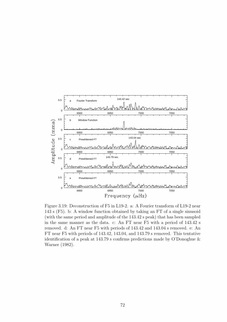
6900 6950 7000 70500
0.5 a Fourier Transform143.42 sec
6900 6950 7000 70500
0.5 b Window Function
6900 6950 7000 70500
0.5 c Prewhitened FT143.04 sec
6900 6950 7000 70500
0.5 d Prewhitened FT143.79 sec
6900 6950 7000 70500
0.5 e Prewhitened FT
Figure 3.19: Deconstruction of F5 in L19-2. a: A Fourier transform of L19-2 near143 s (F5). b: A window function obtained by taking an FT of a single sinusoid(with the same period and amplitude of the 143.42 s peak) that has been sampledin the same manner as the data. c: An FT near F5 with a period of 143.42 sremoved. d: An FT near F5 with periods of 143.42 and 143.04 s removed. e: AnFT near F5 with periods of 143.42, 143.04, and 143.79 s removed. This tentativeidentification of a peak at 143.79 s confirms predictions made by O’Donoghue &Warner (1982).
72

is consistent with how Bradley (2001) identified it based on its multiplet struc-
ture. The limits for F2, F3, and F4 imply that they are ℓ ≤ 2, again consistent
with the multiplet structure that suggests F2 is ℓ = 2 and F3 and F4 are ℓ = 1
(Bradley, 2001). The limit for 2F5 constrains F5 to be ℓ ≤ 3.
5160 5180 5200 5220 52400
5 F1
8740 8760 8780 8800 88200
1
2
F2
8400 8420 8440 8460 84800
1
2
F3
2820 2840 2860 2880 29000
0.5
1
F4
6940 6960 6980 7000 70200
0.2
0.4 F5
Figure 3.20: Prewhitened peaks in L19-2 Fourier transform (WET observations).
It is gratifying to find that non-detections of combination frequencies can
provide useful seismological information, and that these corroborate independent
methods in the case of L19-2. We note that the predictions of Wu (2001) suggest
that the WET data are at the threshold of detecting the combination frequencies
in L19-2. Larger telescope data on this star might be useful as a further test of
the reliability of the theory of Wu (2001) for mode identification.
73

2F1
2F3
2F2
Figure 3.21: Ratio of combination to parent mode amplitudes (Rc) for L19-2(WET observations). The lines are theoretical predictions for G0+0
1 1 /g01g
01(Θ0 =
16) (solid line), G0+01 2 /g
01g
02(Θ0 = 16) (dotted line), and G0+0
2 2 /g02g
02(Θ0 = 16)
(dashed line). The data points are the limits on the harmonics (filled squares)and limits for the cross combinations for the presumed (Bradley, 2001) ℓ = 1, 1combinations (crosses), ℓ = 1, 2 combinations (open squares), and an ℓ = 2, 2combination (star). The downward arrows on the limits indicate that the pointsrepresent maximum values.
GD 165
The pulsation pattern of GD 165 is very similar to that of L19-2. Both have
their two primary pulsations near 120 and 193 s. Bergeron & McGraw (1990)
discovered GD 165 to be a ZZ Ceti star as predicted by temperatures acquired
from spectroscopic analysis placing it within the theoretical ZZ Ceti instability
strip.
We included the data for GD 165 from WET observations (XCov 5, 1990
May) and from lightcurves obtained with the CFHT presented in an analysis by
74

Bergeron et al. (1993). The two primary pulsations of GD 165 have multiplet
structure, to which we applied the Pesnell (1985) method and found 25 for the
inclination.
Table 3.8: Periods and Mode Identifications for Published Data without Combi-nation Frequencies
Mode Frequency Period σp Amplitude σamp ∆fa ℓ mb Ref.
Label (µHz) (sec) (sec) (mma) (mma) (µHz)
GD 165
F1 8305.96 120.39543 1.76 -2.73 1? -1 1
8308.69 120.35585 4.79 1? 0 1
8311.24 120.31905 1.36 2.55 1? +1 1
F2 5187.02 192.78879 0.85 -2.98 1 or 2 -1 1
5190.00 192.67841 2.35 1 or 2 0 1
5192.82 192.57373 1.91 2.82 1 or 2 +1 1
F3c 3989.2 250.6797 0.6 -7.8 1 or 2 -1? 1
3997.0 250.1864 1.0 1 or 2 0 1
R548d
F1 4691.915 213.1326 6.7 1 -1 2
4699.946 212.7684 4.1 8.031 1 +1 2
F2 3639.348 274.7745 2.9 1 -1 2
3646.297 274.2508 4.1 6.949 1 +1 2
F3 2997.25 333.639 0.001 1.03 0.13 1 or 2 0? 2
F4 3143.92 318.074 0.001 1.10 0.13 1 or 2 0? 2
F5 5339.43 187.286 0.001 0.43 0.12 1 or 2 0? 2
G226-29
F1 9134.7234 109.47239 0.00019 2.82 0.10 -16.2175 1 -1 3
9150.9409 109.27838 0.00051 1.08 0.10 1 0 3
9167.0187 109.08672 0.00022 2.49 0.10 16.0778 1 +1 3
Note. − The ℓ identifications are from our analysis.a∆f is the separation between the modes in the multiplets and the m = 0 member.bThe m identifications for GD 165 are based on frequency splitting alone, not on the size of the
combination peak limits.cBergeron et al. (1993) listed F3 from the WET data set, but not from the combined CFHT
and WET data set. They identified the m = −1 member as questionable.dThe pulsation modes F3, F4, and F5 are those found in the 2001 data set of
Mukadam et al. (2003).
References. − (1) Bergeron et al. (1993); (2) Mukadam et al. (2003); (3) Kepler et al. (1995a).
Bergeron et al. (1993) did not report finding any combination frequencies
in the WET and CFHT combined data for GD 165. In Figure 3.22, we have
plotted the theoretical predictions for GD 165 (Rc with Θ0 = 25) along with
the observed noise limits for putative combination peaks. Once again the limits
75

alone are sufficient to constrain F1 tentatively as ℓ = 1, and the other modes to
be ℓ ≤ 2, consistent with the ℓ = 1 identifications for each mode determined by
Bradley (2001) based on the multiplet structure. We list our mode identifications
in Table 3.8.
2F1
2F2
Figure 3.22: Ratio of combination to parent mode amplitudes (Rc) for GD165. The lines are theoretical predictions for G0+0
1 1 /g01g
01(Θ0 = 25) (solid line),
G0+01 2 /g
01g
02(Θ0 = 25) (dotted line), and G0+0
2 2 /g02g
02(Θ0 = 25) (dashed line). The
data points are the limits on the harmonics (filled squares) and limits for thecross combinations (crosses). The downward arrows on the limits indicate thatthe points represent maximum values.
R548
R548, also called ZZ Ceti, is the prototype of this class of stars, and is one of
the brightest and hottest. Lasker & Hesser (1971) discovered R548 to be variable.
Its primary pulsation modes are doublets at 213 and 274 s. Like G117-B15A,
R548 has a very stable pulsation mode at 213 s (Mukadam et al., 2003).
76

The data for R548 were gathered in the WET campaigns XCov 18 in 1999
November and XCov 20 in 2000 November, with additional data from the CFHT
and the McDonald Observatory (Mukadam et al., 2003). The pulsation periods
and amplitudes for R548 have been taken from Mukadam et al. (2003) and are
listed in Table 3.8. As with our assumption for GD 244, Bradley (1998) suggests
that the doublet structure in F1 and F2 results from viewing ℓ = 1 modes at
high inclination so that the third (central, m = 0) mode does not appear. Using
the maximum amplitude of the prewhitened FT of F1, at 213 s, as an estimate
on the amplitude of the m = 0 peak, we find the minimum possible inclination
for R548 to be 79. Unlike GD 244, another high inclination star, we do not
detect combination frequencies in R548.
In Figure 3.23, we have plotted the predictions for R548 (Rc with Θ0 = 79).
We include the observed noise limit (indicated by the filled squares, crosses,
open squares, and stars) at the frequencies where we expect combinations to be
detected. The limits on the harmonics of F1 and F2 do not uniquely identify
these modes, but only require that ℓ ≤ 2 for both. 2F1− appears to constrain
F1 to be ℓ = 1, but the line below it at the bottom of the Figure is an ℓ = 2, 2
combination for m = 2. However, the limits on the cross combination peaks at
the sum of the m = −1 and m = +1 parent modes do require F1 and F2 to be
ℓ = 1 modes (see the circles in Figure 3.23), which agrees with the identifications
of Bradley (1998). The limits for the harmonics of the F3, F4, and F5 singlets
are sufficient to imply that they are ℓ ≤ 2 if m = 0, again consistent with the
ℓ = 2 identification of Bradley (1998). As with L19-2, the predictions of Wu
(2001) suggest that these data are on the threshold of detecting the combination
frequencies for the two dominant modes in R548.
G226-29
G226-29 is the brightest known ZZ Ceti star because of its proximity (d = 11.0
pc, mv = 12.22; Kepler et al., 1995a). J. T. McGraw & G. Fontaine (1980,
77

unpublished results) discovered its variability, finding only one pulsation mode
at 109 s that is rotationally split into a triplet. G226-29 is one of the hottest
of the 105 known single-star system ZZ Ceti stars (see Kepler et al., 2005; Voss
et al., 2006, and references therein), and Kepler et al. (2000b) suggest that we
are observing G226-29 just as it enters the instability strip.
We included data for G226-29 from the WET campaign XCov 7 in 1992
February presented in Kepler et al. (1995a). We found the inclination to be
74 by assuming the evenly spaced triplet is an ℓ = 1 mode. As discussed
previously, our results do not depend sensitively on this assumption. Kepler
et al. (1995a) did not detect combination frequencies in G226-29. In Figure 3.24,
we have plotted the predictions for G226-29 (Rc with Θ0 = 74). We include
the observed noise limit (indicated by the filled squares, crosses, and an open
square) at the frequencies where we expect combinations to be detected. The
limits for the harmonics of each member of the triplet do not uniquely identify
F1, but only require that ℓ ≤ 2. As with R548, another high inclination star with
detected m = ±1 multiplet members, it is the limit on the cross combination
peak at the sum of the m = −1 and m = +1 parent modes that require the
G226-29 F1 mode to be ℓ = 1. This result is consistent with the time-resolved
UV spectroscopy data from HST presented in Kepler et al. (2000b). As with
L19-2 and R548, the predictions of Wu (2001) suggest that these data are on the
threshold of detecting the combination frequencies in G226-29.
3.3 Conclusions
The main result of our study is that combination frequencies, particularly
harmonics, in the lightcurves of hot ZZ Ceti stars can be used along with the
theory of Wu (2001) to constrain and in many cases to determine uniquely the
spherical harmonic index (ℓ) of the modes that produced them. The first and
easiest result to achieve with this method is to identify those modes with ℓ > 2
78

Figure 3.23: Ratio of combination to parent mode amplitudes (Rc) for R548.The lines are theoretical predictions for G0±0
1 1 /g01g
01(Θ0 = 79) (long-short-dashed
line), G1+12 2 /g
12g
12(Θ0 = 79) (dot-dashed line), G0±0
2 2 /g02g
02(Θ0 = 79) (long-dashed
line), G2−22 2 /g
22g
−22 (Θ0 = 79) (bold long-dashed line), G1−1
1 1 /g11g
−11 (Θ0 = 79)
(dotted line), G1±01 2 /g
11g
02(Θ0 = 79) (dashed line), G1+1
1 1 /g11g
11(Θ0 = 79) (solid
line), G1±01 1 /g
11g
01(Θ0 = 79) (solid line, not labeled because of space), and
G2+22 2 /g
22g
22(Θ0 = 79) (dot-long-dashed line, not labeled). The data points are
the limits on the harmonics (filled squares), limits for the same-m cross combina-tions (crosses), limits for the different-m cross combinations (open squares), andlimits for the cross combinations between one of the doublet modes (F1 or F2)and one of the lower amplitude singlet modes (stars). The downward arrows onthe limits indicate that the points represent maximum values. The open squarelimits for F1−+F1+ and F2−+F2+ are circled for easier identification.
79

Figure 3.24: Ratio of combination to parent mode amplitudes (Rc) for G226-29.The lines are theoretical predictions for G0±0
2 2 /g02g
02(Θ0 = 74) (long-dashed line),
G2−22 2 /g
22g
−22 (Θ0 = 74) (long-short-dashed line), G0±0
1 1 /g01g
01(Θ0 = 74) (dashed
line), G1+12 2 /g
12g
12(Θ0 = 74) (dot-dashed line), G1−1
1 1 /g11g
−11 (Θ0 = 74) (dotted
line), G1+11 1 /g
11g
11(Θ0 = 74) (solid line), G1±0
1 1 /g11g
01(Θ0 = 74) (solid line), and
G2+22 2 /g
22g
22(Θ0 = 74) (dot-long-dashed line, not labeled because of space). The-
oretical lines for G2±02 2 /g
22g
02(Θ0 = 74) and G1±0
2 2 /g12g
02(Θ0 = 74) are not shown
because they are very near to the predictions for G1±01 1 /g
11g
01(Θ0 = 74). The data
points are the limits on the harmonics (filled squares), a limit for the nonzerodifferent-m cross combination (open square), and limits for the cross combina-tions between the m 6= 0 modes and the central m = 0 mode (crosses). Thedownward arrows on the limits indicate that the points represent maximum val-ues.
80

and those with ℓ ≤ 2. This alone is useful for significantly reducing the number
of seismological models that need to be considered for a given star (Bradley,
1996). The theoretical mode spectrum at ℓ = 3 and higher is so dense that there
are many possible model fits to the typically sparse number of detected modes.
By eliminating from consideration the high ℓ modes, the possibility of identifying
a unique fit is improved. With the exception of a few small amplitude modes, in
this chapter we have successfully eliminated ℓ > 2 identification for all modes in
seven of the eight stars in our study. The eighth star, G185-32, was previously
thought to have a high ℓ mode (Thompson et al., 2004), and our method confirms
this result (though we get ℓ = 3 instead of ℓ = 4).
For modes with sufficiently large amplitude, combination frequency ampli-
tudes are further able to discriminate between ℓ = 1 and ℓ = 2, primarily through
the use of harmonics. The harmonics are superior for this purpose because they
are known to be same-ℓ combinations, and because same-ℓ combinations are well-
separated in the theoretical plots of Rc. We were able to identify modes as ℓ = 1
in six of the eight stars, and in every case our identifications agreed with any
previous independent results.
The method we have used requires only time-series photometry and simple
calculations as presented in Chapter 2. The essential part of these calculations is
the evaluation of the geometric term in the theory of Wu (2001), which we have
named G. Calculating G requires the evaluation of integrals of spherical har-
monics in the presence of a limb darkening law. To assist others in application
of this technique, we have included tabulated matrices of combination frequency
integrals for ℓ ≤ 4 in Appendix A. Applying these requires a straightforward esti-
mation of the inclination, which we have done using multiplet amplitudes, where
detected, and limits on the sizes of multiplet members where not detected. This
has required that we assume that modes of every m are excited to the same
amplitude in every mode, and that rotation always removes the frequency de-
generacy of multiplet members. Fortunately, our results are not highly sensitive
81

to these assumptions.
In addition to our application of this method to eight stars, we have presented
analyses of new data on GD 66 and GD 244 that will be useful for seismological
study of these objects. We have not been able to definitively decompose the
multiplet structure in these stars with single-site data, but the mode periods we
have measured are given in Tables 3.4 and 3.5 for comparison to seismological
models.
More important than the results for these individual stars is our verification
of a quick and easy diagnostic tool that frequently yields definitive results. We
hope the method will find broad and immediate application in the study of
numerous ZZ Ceti stars being discovered with the SDSS (see Mukadam et al.,
2004b; Mullally et al., 2005). Most of these are fainter than the objects we
have measured, but photometry on a 4 m class telescope will be sufficient to
reach useful detection limits. For example, if the V=15.56 mag star GD 66 were
instead an 18th magnitude star, observations with a 4 m class telescope would
reveal four of the combination frequency peaks that we identified, including the
harmonics of the two highest amplitude peaks. Further study of the objects in
this chapter will also be useful, both to secure definitive ℓ identifications of the
smaller amplitude modes and to detect those combinations that hover just below
the detection limits of the present data. We discuss observations using the 4.1
m SOAR Telescope in Chapter 4.
82

Chapter 4
Photometric Mode Identification
for L19-2 with the SOAR
Telescope
Dr. Peter Venkman: Ray has gone bye-bye, Egon . . . what’ve you got
left?
Dr. Egon Spengler: Sorry, Venkman, I’m terrified beyond the capacity
for rational thought.
— Ghostbusters
4.1 Introduction
For nearly three decades, since its discovery by McGraw (1977), the hot, low-
amplitude DAV (H atmosphere, variable) white dwarf star L19-2 has been the
subject of study. O’Donoghue & Warner (1982, 1987) presented a comprehensive
analysis of extensive single site data, and were able to assign tentative values of
ℓ to the pulsation modes. Bradley (2001) revised these identifications in light of
theoretical improvements, finding three modes of ℓ = 1 and two of ℓ = 2. In 1995
April, L19-2 was the subject of the WET campaign XCov 12, on which Sullivan

(1995) presented a preliminary paper. In Chapter 3, we re-reduced and analyzed
the archival WET data to search for combination frequencies, and found none
detectable above the noise limit of the Fourier transform (FT). In general, these
combination frequencies, sum and difference frequencies and harmonics identified
in FTs, result from the nonlinear behavior of pulse shapes. In this chapter,
we apply our mode identification method that utilizes combination frequency
amplitudes to the small amplitude DAV (ZZ Ceti) white dwarf star L19-2. Here,
we present new data acquired in 2005 May from the 4.1 m SOAR Telescope.
L19-2 falls into the class of HDAV stars, which are low amplitude pulsators
that have been shown to lie at the high temperature end of the instability strip
and have short, stable pulsation periods (Winget & Fontaine, 1982; Clemens,
1994). The DAV stars are subdivided into the HDAV (hot) and CDAV (cool)
groups, based on their pulsation property differences. Although the stars in the
HDAV group exhibit fewer modes than those of the CDAV group, L19-2 has a
comparably rich mode spectrum with five eigenmodes.
Although L19-2 did not exhibit detectable combination frequencies within
the limits of the WET data discussed in Chapter 3, we showed that the limits of
non-detected harmonics can constrain the identity of the modes. We found the
highest amplitude mode at 192 s to be ℓ = 1, constrained the three modes at
113, 118, and 350 s to be ℓ ≤ 2, and constrained the lowest amplitude mode at
143 s to be ℓ ≤ 3. These results are all consistent with the analysis of Bradley
(2001).
The noise level of the L19-2 WET data set is low, very near the predicted de-
tection limit for the harmonics of the two largest amplitude modes (√
〈P 〉 ∼ 0.1
mma, where 〈P 〉 is the average power of the FT in the region of the harmonics).
In Chapter 3, we anticipated that observations with a 4 m class telescope would
reveal previously undetected harmonics for L19-2, further constraining mode
identifications for this star and justifying the theory of Wu (2001) as a reliable
mode identification method. However, we are unable to detect new harmonics
84

for L19-2. Because of weather and time constraints, we were only able to acquire
8.13 hours of data for L19-2 with the SOAR Telescope. As a consequence, the
noise level (√
〈P 〉) for the SOAR data presented in this chapter is twice that of
the WET data set considered in Chapter 3.
In §4.2 we present the new SOAR data for L19-2 and compare the theoretical
predictions of Wu (2001) with these observations. In §4.3 we summarize our
results and emphasize the need for future application of the technique to large
samples of ZZ Ceti stars.
4.2 Data Reduction and Analysis
In §4.2.1, we present and describe our observations of L19-2 with the SOAR
4.1 m Telescope. In §4.2.2, we give a full description of the data reduction process.
The purpose of this subsection is to extract mode frequencies and amplitudes via
Fourier methods. Finally, in §4.2.3, we provide our analysis using the theory of
Wu (2001) and present an updated evaluation of the modes in L19-2. We record
the upper limit of the noise level (√
〈P 〉) to compare the size of the harmonics
and combination frequencies to the theory.
4.2.1 Observations
We obtained time-series photometry data on L19-2 in 2005 with the SOAR
4.1 m Telescope using the Goodman High Throughput Spectrograph in imaging
mode with no filter (Clemens et al., 2004; Crain et al., 2004) and an Apogee AP10
CCD camera that we are temporarily using to commission the spectrograph (see
Lopez-Morales & Clemens, 2004, for camera characterization). At the time of
our observations, the dewar and detector for the Goodman Spectrograph were
not ready for use. We designed and built an attachment for the Apogee CCD
camera allowing us to use it with the Goodman Spectrograph. We show drawings
from our computer aided design in Figure 4.1. Figure 4.2 shows a photograph of
85
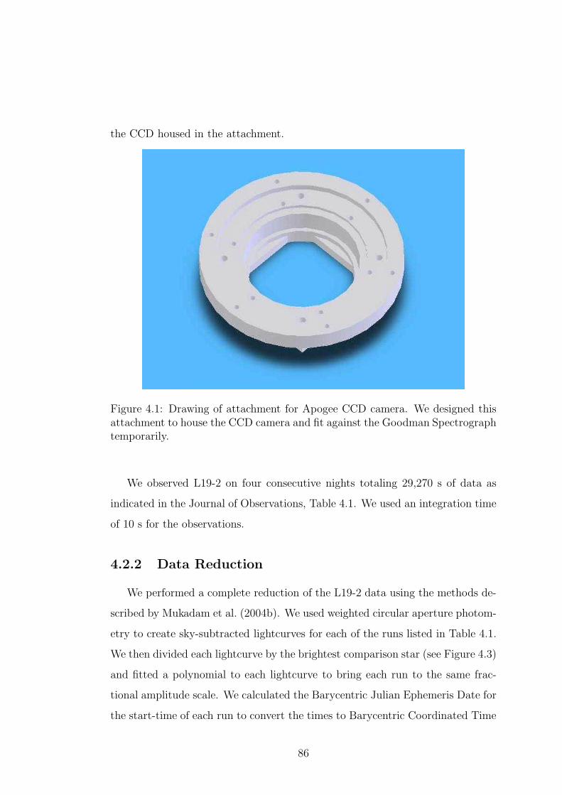
the CCD housed in the attachment.
Figure 4.1: Drawing of attachment for Apogee CCD camera. We designed thisattachment to house the CCD camera and fit against the Goodman Spectrographtemporarily.
We observed L19-2 on four consecutive nights totaling 29,270 s of data as
indicated in the Journal of Observations, Table 4.1. We used an integration time
of 10 s for the observations.
4.2.2 Data Reduction
We performed a complete reduction of the L19-2 data using the methods de-
scribed by Mukadam et al. (2004b). We used weighted circular aperture photom-
etry to create sky-subtracted lightcurves for each of the runs listed in Table 4.1.
We then divided each lightcurve by the brightest comparison star (see Figure 4.3)
and fitted a polynomial to each lightcurve to bring each run to the same frac-
tional amplitude scale. We calculated the Barycentric Julian Ephemeris Date for
the start-time of each run to convert the times to Barycentric Coordinated Time
86

Figure 4.2: Photograph of attachment for Apogee CCD camera. The CCD canbe seen in the center of the attachment.
Table 4.1: Journal of Observations for L19-2 (SOAR Telescope Observations)
Date Start Time Length Integration Time
(UT) (UT) (sec) (sec)
2005 May 19 07:31:59.7 7060 10
2005 May 20 09:01:58.7 3000 10
2005 May 21 02:23:28.7 16830 10
2005 May 22 07:41:30.0 2380 10
Note. − All observations were made with the SOAR
4.1 m Telescope.
87

(TCB). To identify the pulsation modes and possible combination frequencies
of L19-2, we combined all of the lightcurves and computed a discrete FT. We
have included a sample lightcurve in Figure 4.4 and the FT of all L19-2 data in
Figure 4.5.
Figure 4.3: CCD image of L19-2. This CCD image was acquired with the Good-man Spectrograph on the 4.1 m SOAR Telescope on 21 May 2005 with an ex-posure time of 10 s. L19-2 (circled) is located near the center of the image. Wedivided each lightcurve by the brightest comparison star, which is circled in thebottom-center of the image.
To identify closely spaced modes in the regions of obvious excess power, we
utilized a prewhitening technique similar to that of O’Donoghue & Warner (1982)
using an iterative nonlinear least squares procedure. For each peak, we fitted the
frequency, amplitude, and phase and then subtracted the fit from the original
lightcurve. We then fitted a second frequency to the altered data, choosing in
every case the largest remaining peak, and used the result of this fit to conduct
a simultaneous least squares fit to the original data. Thus at each step in the
88

Figure 4.4: Lightcurve of L19-2 (SOAR Telescope observations). These datawere acquired with the Goodman Spectrograph on the SOAR 4.1 m Telescopewith an exposure time of 10 s.
prewhitening, the frequencies removed are from a simultaneous fit to the original
data. Only two modes in the FT of these data actually show multiplet structure,
F1 and F3. We did not detect harmonics and combination frequencies in these
data. The five dominant pulsation modes (F1 - F5) and associated power derived
from prewhitening are listed in Table 4.2 and presented visually in Figure 4.6.
The four highest amplitude modes and associated multiplet structure are consis-
tent to within 2 µHz of those found in both the WET data set in Table 3.7 and
the modes found by O’Donoghue & Warner (1982).11 Figure 4.6 shows clearly
that the lowest amplitude mode, F5, is ∼ 30 µHz from the expected frequency.
However, the F5 mode is only two times as large as the background. The fre-
11However, O’Donoghue & Warner (1982) did not identify them = +1 memberof the F3 multiplet.
89

F1
F2
F3
F4F5
Window
-200 -100 0 100 2000
0.5
1
Figure 4.5: Fourier transform of L19-2 (SOAR Telescope observations). This FTincludes all individual nights of the data that are listed in Table 4.1. We indicatethe five pulsation modes that we reference in Table 4.2. The window function, inthe top right of the figure, is the FT of a lightcurve of a sinusoid that has beensampled in the same manner as the original data.
quency of such a small signal is pulled by the presence of unresolved noise peaks.
4.2.3 Mode Identification
Measuring the limits for the harmonics and combination frequencies in L19-2
allows us to calculate the ratio of combination to parent mode amplitudes and
compare it to the theoretical predictions (Rc, see equation 2.9). Figure 4.7 shows
the observed limit of Rc for the harmonics and combination frequencies. We have
plotted a limit equal to the 1 σ noise level in the FT. The observed Rc do not
depend on any theory.
The theoretical calculations of Rc require that we supply an inclination esti-
90

5160 5180 5200 5220 52400
5 F1
8740 8760 8780 8800 88200
1
2
F2
8400 8420 8440 8460 84800
1
2
F3
2820 2840 2860 2880 29000
0.5
1
F4
6940 6960 6980 7000 70200
0.2
0.4 F5
Figure 4.6: Prewhitened peaks in L19-2 Fourier transform (SOAR Telescopeobservations). The scale of this figure is the same as Figure 3.20 in Chapter 3for ease in direct comparison between these data and the WET data.
mate, an estimate of τc0 , and a value for the parameter 2β + γ. To be consistent
with our previous analysis of L19-2, we have used Θ0 = 16 for all of the theoret-
ical calculations, which is the value determined in Chapter 3 using the technique
of Pesnell (1985). The end result, Rc, is not very sensitive to this parameter
as long as Θ0 ≤ 25 (see Figure 2.4). For τc0, we have used the value of 350 s,
which is the longest period mode in L19-2. This value only affects the location
of the frequency roll-off, not the predicted combination frequency amplitudes in
the high frequency limit. Finally, we use 2β+γ = −9.35, which is the value that
we found in Chapter 3 by normalizing the parameter for the hot, low-amplitude
ZZ Ceti stars.
The theoretical lines for same-ℓ combinations are well-separated, suggesting
that harmonics, which are same-ℓ by definition, are better able to constrain ℓ
91

Table 4.2: L19-2 Periods and Mode Identifications (SOAR Telescope Observa-tions)
Mode Frequency Period σp Amplitude σamp ℓ ma
Label (µHz) (sec) (sec) (mma) (mma)
F1 5177.694 193.1362 0.0180 0.97 0.15 1 -1
5192.179 192.5973 0.0042 4.09 0.15 1 0
F2 8788.823 113.7809 0.0032 1.32 0.15 1 or 2 0
F3 8425.901 118.6817 0.0067 1.15 0.16 1 or 2 -1
8447.857 118.3732 0.0126 0.61 0.16 1 or 2 +1
F4 2856.599 350.0666 0.0691 0.58 0.16 ≤ 3 0
F5 7002.105 142.8142 0.0166 0.40 0.16 ≤ 3 0
aThe m identifications in the table are based on the frequency splitting
alone, not on the size of the combination peaks.
when cross combinations cannot. The limit on the harmonic of F1 is only con-
sistent with ℓ = 1, while the limits for the harmonics of F2 and F3 are consistent
with ℓ = 1 or ℓ = 2. These results are consistent with our analysis of the WET
L19-2 data set in Chapter 3, and with how Bradley (2001) identified them based
on the multiplet structure. The limits for the harmonics of F4 and F5 constrain
these modes to be ℓ ≤ 3. The m identifications we assigned in Table 4.2 arise
from frequency splitting only, and are not derived from combination frequency
amplitudes.
4.3 Conclusions
We acquired 8.13 hours of time-series photometry data on L19-2 in 2005 May
at the SOAR Telescope. We compared these data with the analytical predictions
of Wu (2001) by calculating the ratio of combination frequency to parent mode
amplitudes. These new data confirm conclusions from Chapter 3 that ℓ = 1 for
92

2F1
2F2
Figure 4.7: Ratio of combination to parent mode amplitudes (Rc) for L19-2 (SOAR Telescope observations). The lines are theoretical predictions forG0+0
1 1 /g01g
01(Θ0 = 16) (solid line), G0+0
1 2 /g01g
02(Θ0 = 16) (dotted line), and
G0+02 2 /g
02g
02(Θ0 = 16) (dashed line). The data points are the limits on the har-
monics (filled squares) and limits for the cross combinations for the presumed(Bradley, 2001) ℓ = 1, 1 combinations (crosses) and ℓ = 1, 2 combinations (opensquares). The downward arrows on the limits indicate that the points representmaximum values.
F1 and ℓ = 1 or ℓ = 2 for F2 and F3, consistent with the previous seismological
analysis of Bradley (2001).
It is unfortunate that we were not able to lower the L19-2 noise level with
our 4 m class telescope. The signal to noise ratio (S/N) for the WET data from
Chapter 3 is twice the S/N of the SOAR data presented in this chapter. Although
the SOAR 4.1 m Telescope collects photons sixteen times faster than the WET
1 m class telescopes, we observed L19-2 for ∼ 8 hours with the SOAR Telescope,
which is insufficient to reduce the noise level when compared with the ∼ 142
hours of data in the WET data set. The noise level goes down as the square root
93

of the number of data points, which is linearly related to the amount of time
spanned by the observations. Increasing our observation time by four times (to
32 hours) would equate the noise level to the WET data set. Decreasing the WET
noise level over the course of our five night observing run was an achievable goal,
had the weather and other factors cooperated. However, the primary purpose
of acquiring these data was to give the author further observational experience.
Most importantly, we have accumulated the skills necessary to take raw data and
extract useful information from it.
This chapter also verifies that this method for mode identification can be
applied to pulsating white dwarf stars with relatively little effort as a first check
on mode identifications. The first application of this method is to quickly dis-
criminate between modes with ℓ > 2 and those with ℓ ≤ 2. For modes with
sufficiently high amplitude, the amplitudes of their harmonics allow further dif-
ferentiation between ℓ = 1 and ℓ = 2 modes. Harmonics are known to be same-ℓ
combinations, and the theoretical predictions for same-ℓ combinations are well
separated in the theory of Wu (2001).
94

Chapter 5
Photometric Mode Identification
for the DBV EC 20058-5234
Dr. Peter Venkman: Ray, pretend for a moment that I don’t know any-
thing about metallurgy, engineering, or physics,
and just tell me what is going on.
Dr. Ray Stantz: You never studied.
— Ghostbusters
5.1 Introduction
EC 20058-5234 is one of the brightest members of the DBV group of pul-
sating stars. Koen et al. (1995) reported the discovery of the variability of EC
20058-5234 finding eight periodicities, including combination frequencies. EC
20058-5234 is a low-amplitude DBV with stable pulsation modes (Sullivan &
Sullivan, 2000). Beauchamp et al. (1999) present optical spectra of EC 20058-
5234, providing Teff ∼ 28, 000 K and log g ∼ 7.8, though the errors are large due
to instrumental problems with the detector used for the observations. In 1997
July, EC 20058-5234 was the secondary target star of the WET campaign XCov
15, on which Sullivan & Sullivan (2000) and Sullivan (2005) have presented pre-

liminary papers. The spectra of DB white dwarf stars are dominated by strong
He I lines. The DBV instability strip is centered on 25,000 K and its existence
was theoretically predicted by Winget et al. (1982a) before the discovery of the
first DBV.
In this chapter, we will present our analysis of the pulsation modes using
the combination frequencies amplitudes of the DBV EC 20058-5234. The the-
ory of Wu (2001) provides approximate expressions for the size of combination
frequencies that depend upon the frequency, amplitude, and spherical harmonic
indices of the parent modes. We use the relative amplitudes of the combination
frequencies to infer the spherical harmonic indices of their parent modes. In
§5.2, we present the data. In §5.3, we describe our analysis and resultant mode
identifications for EC 20058-5234. We summarize our results in §5.4.
5.2 Data
The data for EC 20058-5234 were obtained as the secondary target for the
WET campaign XCov 15 in 1997 July (for further information see Sullivan,
2005). Table 5.1 include data from this WET run, as well as further observations
acquired after 1997 as discussed in Sullivan (2005). In addition to interesting
measurements of the plasmon neutrino flux, these data are being used for an
asteroseismological analysis on this star. These data have been provided by
D. Sullivan (2006, private communication) and we have performed our mode
identification method to help facilitate the asteroseismology.
5.3 Mode Identification
Gathering the amplitudes for the harmonics and combination frequencies in
EC 20058-5234 allows us to calculate the ratio of combination to parent mode
amplitudes and compare it to the theoretical predictions (Rc, see Equation 2.9).
96

Table 5.1: EC 20058-5234 Periods and Mode Identifications
Mode Frequency Period Amplitude Combination? ℓ Rc
Labela (µHz) (s) (mma)
f1 1852.6 539.8 2.0 1 or 2
f2 1903.5 525.4 1.9 1 or 2
f3 2852.4 350.6 1.4 1 or 2
f4 2998.7 333.5 3.0 1 or 2
f5 3488.9 286.6 1.7
f6 3559.0 281.0 8.5 1
f7 3640.3 274.7 1.0
f8 3893.2 256.9 8.4 1?
f9 4887.8 204.6 2.7 1 or 2
f10 4902.2 204.0 1.7 f2+f4 149.12
f11 5128.6 195.0 2.5 1 or 2
f12 6557.6 152.5 0.6 f6+f4 11.76
f13 7452.2 134.2 1.7 f6+f8 11.90
f14 9021.7 110.8 0.9 f8+f11 21.43
f15 10030.7 99.7 0.7 f2+f4+f11
f16 4816.8 207.6 0.7 ≤3
f17 3924.2 254.8 0.5 ? ≤3
a 5462.5 ∼0.5 f6+f2 15.48
b 5745.8 ∼0.3 f8+f1 8.93
c 6745.6 ∼0.5 f8+f3 21.26
d 7118.0 ∼0.5 2f6 6.92
e 7533.5 ∼0.4 f8+f7 23.81
f 8127.3 ∼0.5 f4+f11 33.33
g 8446.8 ∼0.5 f6+f9 10.89
h 8461.2 ∼0.6 f6+f2+f4
i 8781.0 0.6 f8+f9 13.23
Note. − These data are primarily from the WET campaign XCov 15
and are provided courtesy of D. Sullivan (2006, private communication).aFor simplicity, we have retained the mode labeling system of D. Sullivan
(2006, private communication). Modes f5, f6, and f7 are believed to be
members of a rotationally split triplet centered on f6.
97

Figure 5.1 shows the measured Rc for the harmonics and combination frequencies.
For the non-detected harmonics, we have plotted a limit approximately equal to
the 1 σ noise level in the FT. The observed Rc do not depend on any theory.
Figure 5.1: Ratio of combination to parent mode amplitudes (Rc) for EC 20058-5234. The lines are theoretical predictions for G0±1
2 1 /g02g
±11 (Θ0 = 13) (dot-long-
dashed line), G0±11 1 /g
01g
±11 (Θ0 = 13) (dot-dashed line), G0±0
1 1 /g01g
01(Θ0 = 13)
(solid line), G0±01 2 /g
01g
02(Θ0 = 13) (dashed line), and G0±0
2 2 /g02g
02(Θ0 = 13) (long-
dashed line). The data points are the detected harmonics or limits (filled squares)and detected cross combination frequencies (stars). The downward arrows on thelimits indicate that the points represent maximum values.
The theoretical calculations of Rc require that we supply an inclination esti-
mate, an estimate of τc0, and a value for the parameter 2β + γ. We have used
Θ0 = 13 for the inclination of this star for all of the theoretical calculations.
We calculate this value by applying the technique of Pesnell (1985) to the rota-
tionally split triplet f5, f6, and f7 centered on f6. The end result, Rc, is not very
sensitive to this parameter as long as Θ0 ≤ 25 (see Figure 2.4). For τc0 , we have
98

used the value of 539.8 s, which is the longest period mode in EC 20058-5234.
This value only affects the location of the frequency roll-off, not the predicted
combination frequency amplitudes in the high frequency limit. Finally, we use
2β + γ = −10, which is the value that Wu (2001) uses for the DBV GD 358.
The theoretical lines for same-ℓ combinations are well-separated, suggesting
that harmonics, which are same-ℓ by definition, are better able to constrain
ℓ when cross combinations cannot. The harmonic of f6 and the limit on the
harmonic of f8, the two highest amplitude modes, are only consistent with ℓ = 1.
However, two modes this closely space in period (only 24 s apart) are not expected
to have the same ℓ. Indeed, Sullivan expects f8 to be an ℓ = 2 mode. We hoped
that the combination of f8 with f7, the proposed m = +1 member of the f6
triplet, would reveal more information about the ℓ of f8, but it falls well above the
predictions for an ℓ = 1 or 2,m = 0 mode with an ℓ = 1,m = +1 mode. However,
all other detected cross combination frequencies involving f8 are consistent with
ℓ = 2 for that mode. The limits on the harmonics of modes f1, f2, f3, f4, f9,
and f11 reveal that they are either ℓ = 1 or 2 modes. After close inspection of
Figure 5.1, one may be moved upon to say there is a distinct separation between
combination frequencies with Rc clustered around the ℓ = 2, 2 line and those
clustered around the ℓ = 1, 1 and ℓ = 1, 2 lines. If this is genuine, f2, f3, f4, and
f11 may be further constrained to be ℓ = 2 modes.
5.4 Conclusions
We have performed our mode identification method on the DBV EC 20058-
5234. We have constrained the highest amplitude mode to be ℓ = 1. We ten-
tatively identify the second highest amplitude mode as ℓ = 1, with some reser-
vation. We constrain six other modes to be ℓ ≤ 2 based on the limits of their
harmonics. Two low amplitude modes are found to be ℓ ≤ 3. These results will
be valuable to the current asteroseismological analysis being performed on this
99

star.
The most important result of this chapter is the proof that this method serves
as a quick and uncomplicated technique for mode identification for both DAV
and DBV stars. The first application of this method is to quickly discriminate
between modes with ℓ > 2 and those with ℓ ≤ 2. For modes with sufficiently
high amplitude, the amplitudes of their harmonics allow further differentiation
between ℓ = 1 and ℓ = 2 modes. Harmonics are known to be same-ℓ combina-
tions, and the theoretical predictions for same-ℓ combinations are well separated
in the theory of Wu (2001).
100
Chapter 6
Summary and Conclusions
Dr. Ray Stantz: Personally, I liked the university. They gave us
money and facilities, we didn’t have to produce
anything! You’ve never been out of college! You
don’t know what it’s like out there! I’ve worked in
the private sector. They expect results.
— Ghostbusters
Asteroseismology is a promising tool for using stellar pulsations to under-
stand the interiors of white dwarf stars. In practice, we perform a normal-mode
analysis by matching all observed frequencies to theoretical models for white
dwarf interiors and determine which model best fits the observed periods. Be-
cause instability is believed to be an evolutionary stage for white dwarf stars (cf.
Fontaine et al., 1982; Mukadam et al., 2004a), we apply the information gleaned
from this normal-mode analysis to all white dwarf stars with the same mass,
pulsating and non-pulsating white dwarf stars alike. Asteroseismology teaches
us about the interiors of white dwarf stars and we apply this information to de-
termine the age of the galaxy (both the disc and the halo), to formulate models
for nuclear fusion, and to probe into the crystallization of white dwarf star cores
as they cool. An accurate understanding for all of these interesting topics is only
possible with correct asteroseismological analyses for pulsating white dwarf stars.

All of asteroseismology depends upon the accurate pulsation mode identification
of the radial overtone number, k, and the spherical harmonic quantum numbers,
ℓ and m, for each individual pulsation mode.
Historically, there are very few seismological studies on white dwarf stars.
Without correct identification of ℓ for pulsation modes, there are too many theo-
retical models to fit to the observed period spectra of white dwarf stars. There are
at least three observational methods for mode identification. The first two meth-
ods require either time-resolved spectroscopy with very large aperture optical
telescopes (i.e., Keck, Clemens et al., 2000; Thompson et al., 2004) or time-series
photometry in the optical and UV wavelengths with the HST (Robinson et al.,
1995). These methods are time intensive and expensive. The intrinsically faint
white dwarf stars require large aperture telescopes for these methods. However,
the follow-up photometry of ZZ Ceti candidates from the Sloan Digital Sky Sur-
vey (SDSS) is finding large numbers of these pulsators that will be too faint
for practical time-resolved spectroscopic methods (see Mukadam et al., 2004b;
Mullally et al., 2005). We have determined a quick and inexpensive method
for confidently assigning values of the spherical degree (ℓ) and azimuthal order
(m) to individual eigenfrequencies. The method that we propose only requires
time-series photometry on 4 m class telescopes for the faint SDSS ZZ Ceti stars.
We use the size of the nonlinearities in the observed lightcurves to infer ℓ and
m for the eigenmodes. The method that we discuss in this dissertation can be
quickly applied to large samples of stars and provide the results necessary for
asteroseismological analysis. We have demonstrated that the technique works on
both DAV and DBV white dwarf stars and we have provided a routine for future
application on objects.
The Fourier transforms (FTs) of DAV and DBV lightcurves generally show
power at harmonics and at sum and difference frequencies. These “combination
frequencies” are not in general the result of independent pulsation eigenmodes,
but rather of frequency mixing between eigenmodes (Brickhill, 1992b; Goldreich
102

& Wu, 1999; Ising & Koester, 2001, BFW95). Wu (2001) was able to derive ap-
proximate expressions for the size of combination frequencies that depend upon
the frequency, amplitude, and spherical harmonic indices of the parent modes,
and upon the inclination of the star’s pulsation axis to our line of sight. Her
solutions yield physical insight into the problem, and make predictions for indi-
vidual stars straightforward to calculate. The routine that we present for mode
identification will significantly help asteroseismological analyses.
We have provided a detailed explanation of the analytical calculations of Wu
(2001) in Chapter 2. We discussed our method for estimating the inclination of
the stars’ pulsation axes to the observer’s line of sight. In Chapter 2, we lay
out a framework for using the theory of Wu (2001) for mode identification. In
Chapters 3 through 5, we have applied this theory to observations of pulsating
white dwarf stars. We have presented the data for each star individually and
compared the observed amplitudes with the predictions from the equations of Wu
(2001), finding good correspondence between the observations and theory. In the
following sections, we summarize the important achievements of this dissertation.
6.1 Harmonics Are the Key
The main result of this dissertation is that combination frequencies, particu-
larly harmonics, in the lightcurves of hot ZZ Ceti stars can be used along with
the theory of Wu (2001) to constrain and in many cases to determine uniquely
the spherical harmonic index (ℓ) of the modes that produced them. The first and
easiest result to achieve with this method is to identify those modes with ℓ > 2
and those with ℓ ≤ 2. This alone is useful for significantly reducing the number
of seismological models that need to be considered for a given star (Bradley,
1996). The theoretical mode spectrum at ℓ = 3 and higher is so dense that there
are many possible model fits to the typically sparse number of detected modes.
By eliminating from consideration the high ℓ modes, the possibility of identifying
103

a unique fit is improved.
For modes with sufficiently large amplitude, combination frequency ampli-
tudes are further able to discriminate between ℓ = 1 and ℓ = 2, primarily through
the use of harmonics. The harmonics are superior for this purpose because they
are known to be same-ℓ combinations, and because same-ℓ combinations are
well-separated in the theoretical plots of Rc.
The method we have used requires only time-series photometry and simple
calculations as presented in Chapter 2. The essential part of these calculations is
the evaluation of the geometric term in the theory of Wu (2001), which we have
named G. Calculating G requires the evaluation of integrals of spherical har-
monics in the presence of a limb darkening law. To assist others in application
of this technique, we have included tabulated matrices of combination frequency
integrals for ℓ ≤ 4 in Appendix A. Applying these requires a straightforward esti-
mation of the inclination, which we have done using multiplet amplitudes, where
detected, and limits on the sizes of multiplet members where not detected. This
has required that we assume that modes of every m are excited to the same
amplitude in every mode, and that rotation always removes the frequency de-
generacy of multiplet members. Fortunately, our results are not highly sensitive
to these assumptions.
For convenience, we summarize application of the method as follows:
1. Calculate the inclination with the Pesnell (1985) method using the ratio of
the observed amplitudes in a given multiplet. Consult the sensitivity of G to
inclination (see Figures 2.3, 2.4, and A.1) to ensure that Rc is changing slowly
with inclination near this value.
2. Calculate the theoretical Rc for both ℓ = 1 and 2 by approximating τc0 with
the longest period mode and using the bolometric correction αλ = 0.4. We
use 2β + γ = −9.35 for hot, low-amplitude DA stars, while Wu (2001) uses
2β + γ = −10 for the cool DA star G29-38.
3. Compare the calculated Rc with the measured value obtained with the am-
104

plitudes of the combinations and their parents.
6.2 Verification of the Theory of Yanqin Wu
Through our analysis, we have shown that the theory of Wu (2001) provides
the only available analytical predictions for combination frequencies that are
consistent with the amplitudes we measure. An entirely different model for ex-
plaining combination frequencies was proposed by BFW95. The BFW95 theory
invokes the nonlinear response of the radiative atmosphere, ignoring the changes
to the surface convection zone. We have shown that, in general, even for the low
amplitude pulsators, the BFW95 theory underestimates the sizes of combination
frequencies in most ZZ Ceti stars by an order of magnitude or more and that
they will be smaller than in the theory of Wu (2001) (for the same ℓ). Moreover,
without very precise temperature measurements, the temperature sensitivity of
the BFW95 theory makes mode identification problematic if the BFW95 theory
is correct. In addition, the BFW95 theory predicts that the size of the individual
combination frequencies is independent of the pulsation frequency in any single
star, unlike the theory of Wu (2001), so, contrary to observational evidence, low
frequency difference modes are not suppressed in the BFW95 theory.
Moreover, the theory of Goldreich & Wu (1999) (founded on the theory of
Brickhill (1992b)) implicitly contains a mode driving mechanism different from
that originally proposed for the DAV stars. Verification of the analytical predic-
tions of Wu (2001) supports the convective driving mechanism as the source of
pulsations in DAV stars.
105

6.3 New Fourier Transforms for GD 66, GD
244, and L19-2
In Chapter 3, we presented independent analyses of new data on the DAV
white dwarf stars GD 66 and GD 244 that will be useful for seismological study
of these objects. There are few published lightcurves and FTs for these two
stars and their period spectra were previously uncertain. The mode periods we
have measured and published are given in Tables 3.4 and 3.5 for comparison to
seismological models. Additionally, we have identified the ℓ values for each mode
to facilitate the seismological analyses. This is important because without correct
identification of ℓ for pulsation modes, there are too many theoretical models to
fit the observed period spectra of white dwarf stars. By identifying the ℓ for each
mode, we have helped to preemptively exclude incorrect seismological models.
We identified five independent pulsations modes and nine combination fre-
quencies for GD 66. We found that the four highest amplitude modes are only
consistent with a mode identification of ℓ = 1. We constrained the lowest am-
plitude mode to be ℓ ≤ 2. We identified four independent pulsation modes and
six combination frequencies for GD 244. The three highest amplitude pulsation
modes are consistent with ℓ = 1 and the lowest amplitude mode has ℓ ≤ 3.
We have presented new reductions for archival Whole Earth Telescope (WET)
data for L19-2, summarized in Table 3.7. The complete reduction for these data
are previously unpublished (for preliminary results, see Sullivan, 1995), though
Bradley (2001) has conducted a seismological analysis on these data. Our mode
identification results are consistent with how Bradley (2001) identified the L19-2
modes based on their multiplet structure. We identified five independent pul-
sation modes and did not detect combination frequencies in L19-2. Because we
were unable to use measured amplitudes of combination frequencies for our anal-
ysis, we included the observed noise limit as an upper bound for comparison to
theory. We found the highest amplitude mode to be ℓ = 1, the three intermedi-
106

ate amplitude modes to be ℓ ≤ 2, and the lowest amplitude mode to be ℓ ≤ 3.
It is gratifying to find that non-detections of combination frequencies can pro-
vide useful seismological information, and that these corroborate independent
methods in the case of L19-2.
6.4 Mode Identification for Published Data
In Chapter 3, we identified modes for five DAV white dwarf stars using pub-
lished data. G117-B15A and G185-32 have detectable combination frequencies,
while GD 165, R548, and G226-29 do not. We were able to identify modes as
ℓ = 1 in four of the five stars, and in every case our identifications agreed with
any previous independent results, making those ℓ identifications certain. With
the exception of a few small amplitude modes, we have successfully eliminated
ℓ > 2 identification for all modes in four of the five stars. The fifth star, G185-32,
was previously thought to have a high ℓ mode (Thompson et al., 2004), and our
method confirms this result (though we get ℓ = 3 instead of ℓ = 4). The details
of the mode identification for these published data are found in Tables 3.6 and
3.8.
6.5 An Expedition to Cerro Pachon
We acquired 8.13 hours of time-series photometry data on L19-2 in 2005 May
at the SOAR Telescope using the Goodman Spectrograph and presented this in-
formation in Chapter 4. These new data confirm conclusions from Chapter 3 that
ℓ = 1 for the highest amplitude mode and ℓ = 1 or ℓ = 2 for the next two highest
amplitude modes (the full results are listed in Table 4.2). This chapter verified
that this mode identification method can be applied to pulsating white dwarf
stars with relatively little effort as a first check on mode identifications. These
observations have paved the way for further mode identification investigations at
107

the SOAR Telescope.
At the time of our observations, the dewar and detector for the Goodman
Spectrograph were not ready for use. We designed and built an attachment for a
temporary Apogee AP10 CCD camera allowing us to use it with the Goodman
Spectrograph. We designed and built this attachment to house the CCD camera
and mate with the Goodman Spectrograph.
6.6 Applicable to DAV and DBV Stars
In Chapter 5, we included an analysis of the DBV star EC 20058-5234 to
demonstrate that the method is widely and easily applicable to all pulsating
white dwarf stars. We constrained the two highest amplitude modes to be ℓ = 1
and six other modes to be ℓ = 1 or 2 (see Table 5.1). These mode identifications
will be useful for an ongoing seismological analysis of this star.
6.7 Future Application
The pulsations of white dwarf stars equip us with a means of delving in to
the unseen interiors of white dwarf stars, similar to the seismologists who use
earthquakes to understand the internal layers of the Earth. This dissertation
describes an important step forward for asteroseismologists, presenting a simpli-
fied method for identifying individual pulsation modes in these stars that utilizes
the size of the nonlinearities present in the lightcurves of pulsating white dwarf
stars. Without identifying ℓ for each individual pulsation mode, we are unable
to unlock the secrets of the white dwarf stellar interiors.
We have presented a quick and inexpensive method for confidently assigning
values of ℓ and m to individual eigenfrequencies in pulsating white dwarf stars
using straightforward calculations. This method can be quickly applied to large
samples of stars. The follow-up photometry from the SDSS is providing large
108

numbers of ZZ Ceti stars that are simply too faint for practical time-resolved
spectroscopic mode identification analysis. Fortunately, these new ZZ Ceti stars
are an immediate source for further application of our new mode identification
method, easily applied with 4 m telescopes. This will provide an order of mag-
nitude increase of stars for immediate seismological analyses.
109

Appendix A
Selected Solutions for
Gmi±mj
ℓi ℓj/gmiℓigmj
ℓj(Θ)
The following tables contain solutions for Gmi±mj
ℓi ℓj/gmi
ℓig
mj
ℓj(Θ) (see equa-
tions 2.4, 2.5, and 2.9) for the values of ℓ and m that are potentially useful
for mode identification with photometry using the theory of Wu (2001).12 Ta-
ble A.1 contains solutions for ℓi = ℓj = 1. Tables A.2 and A.3 contain solutions
for ℓi = 1, ℓj = 2 and ℓi = ℓj = 2. Finally, Table A.4 contains solutions for ℓi = 3
or 4 and ℓj ≤ 4 with mi = mj = 0. For comparison with Figures 2.3 and 2.4, we
include a plot of the variations of G with inclination for ℓ = 3, 3 and ℓ = 4, 4 in
Figure A.1.
12This appendix was originally published as Appendix A of Yeates et al. (2005)and is reproduced by permission of the AAS.

Figure A.1: G with mi = mj = 0 (see equation 2.9) plotted as a function ofinclination angle (Θ). The scale of G for ℓi = ℓj = 4 (solid line) is a factor of tenlarger than the scale of G for ℓi = ℓj = 3 (dotted line). The predicted amplitudesof the combination frequencies show a dramatic increase for inclinations greaterthan 20, and the predictions less than 20 increase more rapidly than the casesfor ℓ = 1 and 2 (see Figures 2.3 and 2.4).
111

Table A.1: Values of Gmi+mj
1 1 /gmi1 g
mj
1 (Θ)
mi\mj -1 0 +1
-1 0.65 0.65 −0.65 − 0.90sin2(Θ)
0 0.65 0.65 + 0.45cos2(Θ)
-0.65
+1 −0.65 − 0.90sin2(Θ)
-0.65 0.65
Note. − For values of Gmi−mj
1 1 /gmi1 g
mj
1 (Θ), reverse the
sign of mj .
112

Table A.2: Values of Gmi+mj
1 2 /gmi1 g
mj
2 (Θ)
mi\mj -2 -1 0 +1 +2
-1 0.27 0.27 −0.81 sin2(Θ)−0.583 cos2(Θ)−1
−0.27 − 1.12sin2(Θ)
0.27 + 2.24sin2(Θ)
0 0.27 0.27 + 0.56cos2(Θ)
0.81 cos2(Θ)+1.973 cos2(Θ)−1
−0.27 − 0.56cos2(Θ)
0.27
+1 −0.27 − 2.24sin2(Θ)
−0.27 − 1.12sin2(Θ)
0.81 sin2(Θ)+0.583 cos2(Θ)−1
0.27 -0.27
Note. − For values of Gmi−mj
1 2 /gmi1 g
mj
2 (Θ), reverse the sign of mj.
113

Table A.3: Values of Gmi+mj
2 2 /gmi2 g
mj
2 (Θ)
mi\mj -2 -1 0 +1 +2
-2 -0.20 -0.200.59 cos4(Θ)+1.08 cos2(Θ)−1.67
sin2(Θ)(3 cos2(Θ)−1)0.20 − 1.87
sin2(Θ)
−0.20 sin4(Θ)+3.74 sin2(Θ)+2.66
sin4(Θ)
-1 -0.200.20 cos4(Θ)−0.66 cos2(Θ)+0.47
cos2(Θ) sin2(Θ)
−0.59 cos2(Θ)+1.13
3 cos2(Θ)−1−
0.20 cos4(Θ)+0.27 cos2(Θ)+1.13
cos2(Θ) sin2(Θ)−0.20 + 1.87
sin2(Θ)
00.59 cos4(Θ)+1.08 cos2(Θ)−1.67
sin2(Θ)(3 cos2(Θ)−1)
−0.59 cos2(Θ)+1.13
3 cos2(Θ)−1
−1.78 cos4(Θ)+6.80 cos2(Θ)+5.66
(3 cos2(Θ)−1)20.59 cos2(Θ)−1.13
3 cos2(Θ)−1
0.59 cos4(Θ)+1.08 cos2(Θ)−1.67
sin2(Θ)(3 cos2(Θ)−1)
+1 0.20 − 1.87sin2(Θ)
−0.20 cos4(Θ)+0.27 cos2(Θ)+1.13
cos2(Θ) sin2(Θ)
0.59 cos2(Θ)−1.13
3 cos2(Θ)−1
0.20 cos4(Θ)−0.66 cos2(Θ)+0.47
cos2(Θ) sin2(Θ)0.20
+2−0.20 sin4(Θ)+3.74 sin2(Θ)+2.66
sin4(Θ)−0.20 + 1.87
sin2(Θ)
0.59 cos4(Θ)+1.08 cos2(Θ)−1.67
sin2(Θ)(3 cos2(Θ)−1)0.20 -0.20
Note − For values of Gmi−mj2 2 /g
mi2 g
mj2 (Θ), reverse the sign of mj .
114

Table A.4: Values of G0±0ℓi ℓj
/g0ℓig0
ℓj(Θ)
ℓi\ℓj 3 4
1 −0.78 cos4(Θ)+3.82 cos2(Θ)−1.121.67 cos4(Θ)−cos2(Θ)
−6.18 cos4(Θ)+19.41 cos2(Θ)−9−11.67 cos4(Θ)+10 cos2(Θ)−1
2 −1.92 cos4(Θ)+4.87 cos2(Θ)+9.86(3 cos2(Θ)−1)(1.67 cos2(Θ)−1)
40.38 cos6(Θ)−73.72 cos4(Θ)+144.05 cos2(Θ)−39.04(3 cos2(Θ)−1)(−11.67 cos4(Θ)+10 cos2(Θ)−1)
3 5.56 cos6(Θ)−10 cos4(Θ)+15.17 cos2(Θ)+12.40(1.67 cos3(Θ)−cos(Θ))2
35 cos6(Θ)−75 cos4(Θ)+85 cos2(Θ)+153.69(1.67 cos2(Θ)−1)(−11.67 cos4(Θ)+10 cos2(Θ)−1)
4 35 cos6(Θ)−75 cos4(Θ)+85 cos2(Θ)+153.69(1.67 cos2(Θ)−1)(−11.67 cos4(Θ)+10 cos2(Θ)−1)
−1225 cos8(Θ)+2660 cos6(Θ)−2070 cos4(Θ)+1769.26 cos2(Θ)+1400.80(−11.67 cos4(Θ)+10 cos2(Θ)−1)2
115

REFERENCES
Beauchamp, A., Wesemael, F., Bergeron, P., Fontaine, G., Saffer, R. A., Liebert,
J., & Brassard, P. 1999, The Astrophysical Journal, 516, 887
Bergeron, P., Fontaine, G., Billeres, M., Boudreault, S., & Green, E. M. 2004,
The Astrophysical Journal, 600, 404
Bergeron, P., & McGraw, J. T. 1990, The Astrophysical Journal, Letters to the
Editor, 352, L45
Bergeron, P., Saffer, R. A., & Liebert, J. 1992, The Astrophysical Journal, 394,
228
Bergeron, P. et al. 1993, The Astronomical Journal, 106, 1987
Bradley, P. A. 1996, The Astrophysical Journal, 468, 350
—. 1998, The Astrophysical Journal, Supplement Series, 116, 307
—. 2001, The Astrophysical Journal, 552, 326
—. 2006, Memorie della Societa Astronomica Italiana, 77, 437
Brassard, P., Fontaine, G., & Wesemael, F. 1995, The Astrophysical Journal,
Supplement Series, 96, 545
Brassard, P., Fontaine, G., Wesemael, F., & Talon, A. 1993, in NATO ASIC
Proc. 403: White Dwarfs: Advances in Observation and Theory, ed. M. A.
Barstow, (Dordrecht: Kluwer Academic Publishers), 485

Brickhill, A. J. 1983, Monthly Notices of the RAS, 204, 537
—. 1990, Monthly Notices of the RAS, 246, 510
—. 1991a, Monthly Notices of the RAS, 251, 673
—. 1991b, Monthly Notices of the RAS, 252, 334
—. 1992a, Monthly Notices of the RAS, 259, 519
—. 1992b, Monthly Notices of the RAS, 259, 529
Castanheira, B. G. et al. 2004, Astronomy and Astrophysics, 413, 623
Chandrasekhar, S. 1931, The Astrophysical Journal, 74, 81
—. 1934a, The Observatory, 57, 93
—. 1934b, The Observatory, 57, 373
Christensen-Dalsgaard, J. 2002, Reviews of Modern Physics, 74, 1073
Clemens, J. C. 1994, Ph.D. Thesis, Univ. Texas, Austin
Clemens, J. C., Crain, J. A., & Anderson, R. 2004, in Proceedings of the SPIE,
5492: Ground-based Instrumentation for Astronomy, ed. A. F. M. Moorwood
& M. Iye, (The International Society for Optical Engineering), 331
Clemens, J. C., van Kerkwijk, M. H., & Wu, Y. 2000, Monthly Notices of the
RAS, 314, 220
Crain, J. A., Clemens, J. C., & Bayliss, M. 2004, in Proceedings of the SPIE,
5496: Optical, Infrared, and Millimeter Space Telescopes, ed. H. Lewis &
G. Raffi, (The International Society for Optical Engineering), 455
D’Antona, F. 1989, LNP Vol. 328: IAU Colloq. 114: White Dwarfs, 328, (New
York: Springer Verlag), 44
117

Dolez, N., & Vauclair, G. 1981, Astronomy and Astrophysics, 102, 375
Dolez, N., Vauclair, G., & Chevreton, M. 1983, Astronomy and Astrophysics,
121, L23
Dziembowski, W., & Koester, D. 1981, Astronomy and Astrophysics, 97, 16
Finley, D. S., Koester, D., & Basri, G. 1997, The Astrophysical Journal, 488,
375
Fontaine, G., Bergeron, P., Brassard, P., Billeres, M., & Charpinet, S. 2001, The
Astrophysical Journal, 557, 792
Fontaine, G., McGraw, J. T., Dearborn, D. S. P., Gustafson, J., & Lacombe, P.
1982, The Astrophysical Journal, 258, 651
Fontaine, G., Wesemael, F., Bergeron, P., Lacombe, P., Lamontagne, R., &
Saumon, D. 1985, The Astrophysical Journal, 294, 339
Fowler, R. H. 1926, Monthly Notices of the RAS, 87, 114
Goldreich, P., & Wu, Y. 1999, The Astrophysical Journal, 511, 904
Grauer, A. D., & Bond, H. E. 1984, The Astrophysical Journal, 277, 211
Greenstein, J. L. 1976, The Astronomical Journal, 81, 323
—. 1982, The Astrophysical Journal, 258, 661
Holberg, J. B., Barstow, M. A., Bruhweiler, F. C., Cruise, A. M., & Penny, A. J.
1998, The Astrophysical Journal, 497, 935
Horne, J. H., & Baliunas, S. L. 1986, The Astrophysical Journal, 302, 757
Isern, J., Garcıa-Berro, E., Hernanz, M., & Mochkovitch, R. 1998, Journal of the
Physics of Condensed Matter, 10, 11263
118

Ising, J., & Koester, D. 2001, Astronomy and Astrophysics, 374, 116
Kawaler, S. D. et al. 1995, The Astrophysical Journal, 450, 350
Kepler, S. O. 1984, The Astrophysical Journal, 286, 314
—. 1993, Baltic Astronomy, 2, 515
Kepler, S. O., Castanheira, B. G., Saraiva, M. F. O., Nitta, A., Kleinman, S. J.,
Mullally, F., Winget, D. E., & Eisenstein, D. J. 2005, Astronomy and Astro-
physics, 442, 629
Kepler, S. O., Mukadam, A., Winget, D. E., Nather, R. E., Metcalfe, T. S., Reed,
M. D., Kawaler, S. D., & Bradley, P. A. 2000a, The Astrophysical Journal,
Letters to the Editor, 534, L185
Kepler, S. O., Robinson, E. L., Koester, D., Clemens, J. C., Nather, R. E., &
Jiang, X. J. 2000b, The Astrophysical Journal, 539, 379
Kepler, S. O., Robinson, E. L., Nather, R. E., & McGraw, J. T. 1982, The
Astrophysical Journal, 254, 676
Kepler, S. O. et al. 1995a, The Astrophysical Journal, 447, 874
Kepler, S. O. et al. 1995b, Baltic Astronomy, 4, 221
Kleinman, S. J. 1995, Ph.D. Thesis, Univ. Texas, Austin
Kleinman, S. J. et al. 1998, The Astrophysical Journal, 495, 424
Koen, C., O’Donoghue, D., Stobie, R. S., Kilkenny, D., & Ashley, R. 1995,
Monthly Notices of the RAS, 277, 913
Koester, D., Schulz, H., & Weidemann, V. 1979, Astronomy and Astrophysics,
76, 262
119

Lasker, B. M., & Hesser, J. E. 1971, The Astrophysical Journal, Letters to the
Editor, 163, L89+
Lopez-Morales, M., & Clemens, J. C. 2004, Publications of the ASP, 116, 22
Mazzitelli, I., & D’Antona, F. 1986, The Astrophysical Journal, 308, 706
McGraw, J. T. 1977, The Astrophysical Journal, Letters to the Editor, 214, L123
—. 1980, Space Science Reviews, 27, 601
McGraw, J. T., Fontaine, G., Dearborn, D. S. P., Gustafson, J., Starrfield, S. G.,
& Lacombe, P. 1981, The Astrophysical Journal, 250, 349
McGraw, J. T., & Robinson, E. L. 1976, The Astrophysical Journal, Letters to
the Editor, 205, L155
Mestel, L. 1952, Monthly Notices of the RAS, 112, 583
Mukadam, A. S., Winget, D. E., von Hippel, T., Montgomery, M. H., Kepler,
S. O., & Costa, A. F. M. 2004a, The Astrophysical Journal, 612, 1052
Mukadam, A. S. et al. 2003, The Astrophysical Journal, 594, 961
—. 2004b, The Astrophysical Journal, 607, 982
Mullally, F., Thompson, S. E., Castanheira, B. G., Winget, D. E., Kepler, S. O.,
Eisenstein, D. J., Kleinman, S. J., & Nitta, A. 2005, The Astrophysical Journal,
625, 966
Nather, R. E., & Mukadam, A. S. 2004, The Astrophysical Journal, 605, 846
Nather, R. E., Winget, D. E., Clemens, J. C., Hansen, C. J., & Hine, B. P. 1990,
The Astrophysical Journal, 361, 309
O’Donoghue, D. E., & Warner, B. 1982, Monthly Notices of the RAS, 200, 563
120

—. 1987, Monthly Notices of the RAS, 228, 949
Pesnell, W. D. 1985, The Astrophysical Journal, 292, 238
—. 1987, The Astrophysical Journal, 314, 598
Robinson, E. L., Kepler, S. O., & Nather, R. E. 1982, The Astrophysical Journal,
259, 219
Robinson, E. L. et al. 1995, The Astrophysical Journal, 438, 908
Sullivan, D. J. 1995, Baltic Astronomy, 4, 261
—. 2005, in ASP Conf. Ser. 334: 14th European Workshop on White Dwarfs, ed.
D. Koester & S. Moehler, (Provo: Astronomical Society of the Pacific), 495
Sullivan, D. J., & Sullivan, T. 2000, Baltic Astronomy, 9, 81
Thompson, S. E., Clemens, J. C., van Kerkwijk, M. H., O’Brien, M. S., &
Koester, D. 2004, The Astrophysical Journal, 610, 1001
van Kerkwijk, M. H., Clemens, J. C., & Wu, Y. 2000, Monthly Notices of the
RAS, 314, 209
Vauclair, G., Belmonte, J. A., Pfeiffer, B., Chevreton, M., Dolez, N., Motch, C.,
Werner, K., & Pakull, M. W. 1993, Astronomy and Astrophysics, 267, L35
Vauclair, G. et al. 2002, Astronomy and Astrophysics, 381, 122
Voss, B., Koester, D., Østensen, R., Kepler, S. O., Napiwotzki, R., Homeier, D.,
& Reimers, D. 2006, Astronomy and Astrophysics, 450, 1061
Vuille, F., & Brassard, P. 2000, Monthly Notices of the RAS, 313, 185
Winget, D. E. 1998, The Journal of the Physics of Condensed Matter, 10, 11247
Winget, D. E., & Fontaine, G. 1982, in Pulsations in Classical and Cataclysmic
Variable Stars, ed. J. P. Cox & C. J. Hansen, (Boulder: Univ. Colorado), 46
121

Winget, D. E., Robinson, E. L., Nather, R. E., & Fontaine, G. 1982b, The
Astrophysical Journal, Letters to the Editor, 262, L11
Winget, D. E., van Horn, H. M., & Hansen, C. J. 1981, The Astrophysical
Journal, Letters to the Editor, 245, L33
Winget, D. E., van Horn, H. M., Tassoul, M., Hansen, C. J., Fontaine, G., &
Carroll, B. W. 1982a, The Astrophysical Journal, Letters to the Editor, 252,
L65
Winget, D. E. et al. 1991, The Astrophysical Journal, 378, 326
Wood, M. A. 1990, The Journal of the RAS of Canada, 84, 150
Wu, Y. 2001, Monthly Notices of the RAS, 323, 248
Wu, Y., & Goldreich, P. 1999, The Astrophysical Journal, 519, 783
Yeates, C. M., Clemens, J. C., Thompson, S. E., & Mullally, F. 2005, The
Astrophysical Journal, 635, 1239
122
Top Related
Copyright © 2022 FDOKUMEN

