


Bahasa
Halaman
Hukum


i
NASA TECHNICAL
MEMORANDUM
NA SA TM X- 73307
ASTRONAUTIC STRUCTURESMANUAL
VOLUMEIII
(NASA-T _-X-733|. 7) AS_FCNAUTIC ST?UCTUE_S
HANUA/, 90LU_E 3 (NASA) 676
00/98
N76-76168
Unclas
_4u02
Structures and Propulsion Laboratory
August 197 5
NASA
marshall Space
Space
_..,=-- I'IASA ST| FAClUiY '-"'
\% i.Pu_B_.c. i/
Flight Center
Flight Center, Alabama
MSFC - Form 3190 (Rev June 1971)


NASA TM X-73307
TECHN_,_AL REPORT STANDARD TITLE PAGE
2. GOVERNMENT ACCESSION NO. I 3. RECIP)ENT'S CATALOG NO.
15. REPORT DATET'.TLE "NO SUBTITLE
ASTRONAUTIC STRUCTURES MANUAL
VOLUME Ill
A____ust 197 56. PERF0qh_ING DPGANIZATION CODE
7. AI;T ur'P : 8._i-'_FORMING O_CANIZATIL')N REPD_r
t 9 _"PFC'-'.'ING ORGANIZATION NAME AND ADDRESS 10. _©Pt_ UNIT NO.i •
George C. Marshall Space Flight Center
Marshall Space Flight Center, Alabama 35812
" " S;-{,_JRING _,_JZ_N_,Y NAME AND AI3nREc;S
t National Aeronautics and Space Administration
i Washington, D.C. 20546
1. CONTRACT OR GRANT NO,
13. TYPE OF REPRR'_ & PERIOD COVE_ED
Technical Memorandum
I.% " ",,_O_," L, A,SENCY CCDE
• : ", '_LEMENTA:(" NCTLS
i , .
I
Prepared by Structures and Propulsion Laboratory, Science and Engineering
! This document (Volumes I, II, and III) presents a compilation of industry-wide methods in
; aerospace strength analysis that can be carried out by hand, that are general enough in scope to
I cover most structures encountered, and that are sophisticated enough to give accurate estimates
I of the actual strength expected. It provides analysis techniques for the elastic and inelasticP
stress ranges. It serves not only as a catalog of methods not usually available, but also as a
i reference source for the back_zround of the methods themselves.
i An overview of the manual is as follows: Section A is a Keneral introduction of methodsused and includes sections on loads, combined stresses, and interaction curves; Section 13 is
devoted to methods of strength analysis; Section C is devoted to the topic of structural stability;
Section D is on thermal stresses; Section E is on fatigue and fracture mechanics; Section F is
on composites; Section G is on rotating machinery; and Section H is on statistics.
These three volumes supersede Volumes I and II, NASA TM X-60041 and
NASA TM X-_on42, respectively.
17. KE_ WC_DS
OR_GII,_AL P._,.C._ ,Z,OF POOR QUALITY
!0. DI_T/{IGUT" "_ 5,,:T__',. :
Unclassified -- Unlimited
19. SECURITY CLASSIF.(of thll report_
Unclassified
SECURITY CLAS3IF. (,J _htl pa{_)
Unelas sifted
• -_I. "_3. OF _;,,ES 22. PRICf
673 NTIS
MSFC- Form 3292 (R..v December 1972) F'.)r,_ale by National 'reehnicnl lnf,,rm :,on ¢. ..,,,. c; i rm.-fi,'hl, Vir_,ini;, 221¢1

._i-

APPROVAL
ASTRONAUTIC STRUCTURESMANUAL
VOLUME III
The information in this report has been reviewed for security classifi-
cation. Review of any information concerning Department of Defense or
Atomic Energ:/ Commission programs has been made by the MSFC Security
Classification Officer. This report, in its entirety, has been determined to
be unclassified.
This document has also been reviewed and approved for technical
accuracy.
A. A. McCOOL
Director, Structures and Propulsion Laboratory
•t_ U.S. GOVERNMENT PRINTING OFFICE 1976-641-255,P448 REGION NO. 4

j
TABLE OF CONTENTS
Do THERMAL STRESSES ........
1.0
2.0
3.0
INTRODUCTION ....................
THERMOE LASTICITY ..................
2.0.1 Plane Stress Formulation .............
2.0.2 Plane Strain Formulation .............
2.0.3 Stress Formulation ................
2.0.3.1 Sohuli,'m (,f AiryVs Stress Function .....
I. Plane Stress .............
II. Plane Strain .............
STRENGTIt ()1,' MA'I'I,:I{IAI,b S()I,U'II()NS ..........
3.0.1 Unrestrained I_eam-Therm'd I,oads ¢)nly ......
3.0.1.1 Axial Stress .............
3.0.1.2 lfisl>lace)nmlts ..............
Page
1
1
3
3
4
4
5
5
5
7
7
7
:)
3.0.2 l/cstrained Bealn--Thernml I_(m(ls ()r, ly . ...... l(i
3.0.2.1 Ewlluation()f InteRrals for Vqrying
Cross Sections .............. 12
, • ) l,:xamples ........ 143.0.2.2 l,cstr;ine(1 Beam
Io
II.
lIl.
IV.
Simply Supported Beam ........ 14
Fixed- Fixed L_mm
F ixe d- 11in ged Be a m
......... 53
......... 56
Deflection Plots ........... 58
D-iii

TABLE OF CONTENTS (Continued)
Page
3.0.2.3 Representation of Temperature
Gradient by Polynomial .......... 70
I. Example Problem 1 .......... 74
II. Example Problem 2 .......... 76
3.0.3 Indeterminate Beams and Rigid Frames ....... 78
3.0.4 Curved Beams .................. 80
3.0.5 Rings ...................... 80
3.0.6 Trusses ..................... 80
3.0.6. i Statically Determinate .......... 80
3.0.6.2 Statically Indeterminate .......... 8i
3.0.7 Plates ...................... 81
3.0.7.1 Circular Plates .............. 81
I. Temperature Gradient Throughthe Thickness ............ 81
II. Temperature Difference as a Functionof the Radial Coordinates ..... 91
III. Disk with Central Shaft ........ 101
3.0.7.2 Rectangular Plates ............ 104
I. Temperature Gradient Throughthe Thickness ............ t04
II. Temperature Variation Overthe Surface ............. 119
D -iv

4.0
TABLE OF CONTENTS (Continued)
3.0.8
Page
Shells .................... . . 131
3.0.8.1 I,_(_tr()pic Circular Cylindrical Shells .... 132
],
II.
IlI.
Analogies with Isothcrnml Pcoblems . 133
Thermal Stresses and l)cllcctions--
Linear Radial Gradient, AxisymmctrieAxial G radie.nt ............ 149
Thermal Stresses and Deflections--
Constant l{adial Gradient,
Axis 5 mmetrie Axial Gradient ..... 170
3.0.8. '2 lsotropic ('onical Shells ..........
3.0.8.3 lsotropie Shells of Hevolution of
Arbitrary Shal)e .............
I. Sphere Under l{:,lial Temperature
Variations ..............
179
191
201
THEHM()EI,ASTIC STA BII3TY .............. 20"_
4,0.1 lleated lk;am Colunms .............. 20.'l
d.0.1.1 Ends Axially Unrestrained ........ 203
1. B,,)th Vnds Fixed ........... 20(;
II. Both Ends Simply Supported ..... 20(;
206III. Cantilever ...........
,1.0.1.2 Ends Axially Restrained ........ 20
2094.0.2 Thermal Buckling of Iqates ............
4.0.2.1 Circular l'latcs ............. 209
D-v

TABLE OF CONTENTS (Concluded)
Page
4.0.2.2 Rectangular Plates ............ 222
I. Heated Plates Loaded in Plane--
Edges Unrestrained in the Plane .... 222
II. Heated Plates Loaded in Plane--
Edges Restrained in the Plane ..... 225
III. Post-Buckling Deflections with
All Edges Simply Supported ...... 230
4.0.3 Thermal Buckling of Cylinders ........... 234
5.0 INELASTIC EFFECTS ................. 245
5.0. 1 Creep ...................... 246
5.0.1.1 Design Curves ............. 248
5.0.1.2 Stress Relaxation ............. 251
5.0.2 Viscoelasticity ................ 253
5.0.3 Creep Buckling .................. 253
5.0.3.1 Column of Idealized H-Cross Section .... 255
5.0.3.2 Rectangular Column ......... 255
5,0.3.3 Flat Plates and Shells of Revolution ..... 256
6.0 THERMAL SHOCK .................. 263
6 0.1 General ..................... 263
6.0.2 Stresses and Deformations ............. 264
REFERENCES .......................... 2_
D-vi
J

SECTION D
THERMAL STRESSES


r-
Symbol
A
A0
Amn,
DEFINITION OF SYMBOI_S
APq
Ai, A2, A3, A4
1
a
a0
a 0!
al
Bran, Bpq
Definition
Cross-sectional area; area
Cross-sectional area of beam at x = 0
Coefficients for the series by which the stresses are
expressed, in.
C(mstants based (m the boundary conditions, equations (9?0
and (96). dimensionless
Constants, psi (Figs. 5.0-8, 5.0-9)
l,imiting value (lower) for radius; inside radius or radius
of middle surface of cylinder
Maximum value of initial imperfection
Constant, ° l"
Constant, o F/in.
Coefficients lov the series by which the stresses arc
cxprcs3ed, in.
NOTES:
1. Bars over-'any lcttc)rs denote mi(hlle-surface_ values.
2. The subscript er denotes eritic:_l _alues for buckling.
3. The superscripts I' and C identify quantities associated with the
particular and complementary :mlutions, respectively.
4. The subscript R denotes w_lucs required to completely suppress
thermal deformation_.
D-vii
Symbol
BI, B2, BS
b.
b 0, bt, b_
CP
C1, C2t C3t C4
C-I'Co'Ct"'"
D
d ,d d,...-1 O' !
E
Eb
EP
DEFINITION OF SYMBOLS (Continued)
Definition
Constants, in./(in. ) ( hr)(Fig. 5.0-i0)
Breadth (or width) of cross section; limiting value (upper)
for radius; outside radius
Constants in polynomial representation of the temperature
T1(x ) ; ° F, o F/in., and • F/in.2, respectively
Specific heat of the material, Btu/(Ib) (°F)
Constants of integration, in.
Coefficients in polynomial representation of U P, In.-Ib, Ib,
Ib/in.,..., respectively, refer to equation (106)
Diameter
Plate bending stiffness or shell-wall bending stiffness
Constants in polynomial representation of the function T2(x ) ;
o F, ° F/in., and ° F/in. 2, respectively
Coefficients in polynomial representation of V P, in.,
dimensionless, 1/in. ,..., respectively; refer to
equatton (106)
Young t s modulus of elasticity
Young t s modulus of support-beams, psi
Young t s modulus of plate, psi
D-viii

Symbol
ES
E t
e
F. E.M.
FF
FS
G
G T
H
It A , H B
I
I b
I,Iy z
i
K
k
DEFINITION OF SYMBOLS (Continued)
Definition
Secant modulus, psi
Tanzcnt modulus, psi
llasc for natural logarithms, dimensionless (2. 718)
Fixed-end morn(rot
I" ixc(I- fixed
Fixed- s upl)ort ed
Variation in (lepth of beana along the length
Modulus of rigidity or shear modulus
V:/riation ha width of beam along the length
Running c(Igc forces acting normal to tile axis of r(woluti()n at
positions A and B , respectively (Figs. 3.0-51 and 3.0-52),
lb/in.
Moment of inertia
Support-beam centroidal moment of inertia
Area moments of inertia taken about the y and z axes,
respectively, in. 4
Imaginary number, _.-rTT-
Thermal diffusivity of the material, ft2/hr = k/C pP
An integer (1, 2,3,,1, ,5) exponent
D-ix

Symbol
k'
L
L( )
M
M A, M B
M T
M b
Mr, M0 , Mx, M_
Mr0
M r' ' M0'
M t
Mx, My
MY
Mz
M0
DEFINITION OF SYMBOLS (Continued)
Definition
Thermal conductivity of the material, Btu/(hr) (ft) (o F)
Length
Operator defined by equation (103)
Moment
Running edge moments acting at positions A and B ,
respectively ( Figs. 3.0-51 and 3.0-52), in.-lb/in.
Thermal moment
Thermal bending parameter, in.-Ib/in.
Running bending moment.';, in.-Ib/in.
Running twisting moment, in.-lb/in.
Bending-moment parameters (Table 3.0-5 and Figs. 3.0-15
through 3.0-19)
Temperature resultant, in.-lb/in.
Running bending moments acting on sections of the plate
which are perpendicular to the x and y directions,
respectively (positive when associated upper-fiber stresses
are compressive), in.-lb/in.
Moment about y axis
Moment about z axis
Moment in beam at x = 0
j"
D-x

Symbol
m
m k
me
N
N T
Nr, N O , N x, N
Nr0
N ' , N 0'r
N t
n
n k
l )
PT
P0
P
P,q
Q
DEHNITION OF SYMBOLS (Continued)
Definition
Temperature distribution in the z-direction
Moment coefficients, plotted in Figure 3.0-46, dimensionless
Surface moment (Fig. 3.0-53) in.-lb/in. 2
Exponent of thermal wtriation along the length of the beam;
also upl_er limit for summation indices, dimensionless
Axial load per unit length on plate edge
Ilunning mernbran(, loads, Ib/in.
ilunning membrane shear load, lb/in.
Membrane-force parameters (Table 3.0-6), dimensionless
Temperature resultant, lb/in.
Temperature distribution in the y-direction
Hoop-force coefficients, plotted in Figure 3.0-49,
_li mensionless
Axial Io r_'_
Axial Ior_'c resultin_ From temperature
Column load
Ila,lial pressure, psi
Summation indices, dimensionless
Heat input
D-xi

Symbol
Qx
q
qk
r
SS
S
S*
T
I
T
T D
Tedges
Tf
T i
Tm
I)E FINITION OF SYMBOLS (Continued)
Definition
I{unning transverse shear load, lb/in.
Temperature distribution in the x-direction
Shear coefficients, plotted in Figure 3.0-46, dimensionless
Radius
Simply supported
Meridional coordinate measured downward from top of the
truncated cone (Fig. 3.0-50), in.
Meridional coordinate measured upward from bottom ol the
truncated cone (Fig. 3.0-50), in.
Temperature
Average value for T, OF
Weighted average value for T, °F
Temperature difference between the plate faces, o F
Temperature at edges of the plate, °F
Final uniform temperature which the body reaches at
sufficiently long times
Inside temperature; also initial uniform temperature of
the body, ° F
Average value for temperature distribution across the wall
thickness at any single position, o F
D-xii

r-
.F
Symbol
TS
Txy
T O
T 1, T2
ter
u
V
Vp
V T
Vo
V
W
W i
I)EFINITION OF SYMBOLS (Continued)
Definition ..
Temperature of the supports, *F
Temperature at any location in the plate, ° F
Outside temperature
Temperature functions, °F
Time (hr) or thickness
Time to the onset of creel) buckling, hr
l)isl)lacement in the x-direction or r-direction .for
circular plate
Function representing temperature variation in y- and z-
directions; also rotations in a meridional plane for a shell
Component of deflection without therm_tl ('floors
Component of (h_flcction ineludin4a?" tbermal effects
Shear at x= 0
Displacement in lhc v-Hirection or O-direclion for
circular plate
Displacement in the z-direction
Deflection parameter (Table 3.0-5 and Figs. 3.0-15
through 3.0-19), (timcnsi<mlcss
D-xiii

I)I,',I,'INI'I'I(}N()F SYMBOLS(Continued)
Symbol
W
AW
w k
x
Y
Z
c_
(orT0b2/t2) cr
F
%
Definition
Displacement, in the z-direction, for the case where all edges
are simply supported, in. ; also radial deflection for shell
Displacement component, in the z-direction, in. (Note: The
superscript A is merely an identification symbol and is not
meant to be a generalized exponent.)
Deflection coefficients, plotted in Figure 3.0-45, dimensionless
Coordinate axis
Coordinate axis
Upper limit for the summation index k , dimensionless;
also surface loads, psi
Coordinate axis measured normal to undeformed plate
Coefficient of linear thermal expansion, in./(in. ) (° F)
Critical value of temperature parameter (value at which
initial thermal buckling occurs), dimensionless
Knockdown factor, dimensionless
Knockdown factor (Fig. 4.0-17), dimensionless
Shearing strain in planes parallel to and including the
x-y plane, in./in.
Time rate of change for "Yxy' in./(in.)(hr)
D-xiv
DEFINITION OF SYMBOLS(Continued)
Symbol
6
V
•°
1
_o
1
x y
0
o( )
Ok
X
F
P i
Definition
Maximum absolute value for deflection measured normal to
the x-y plane, in.
Del-operator
Unit strain
Strain intensity defined in equations (1), in./in.
l"ime rate of change for c. , in./(in.)(hr)1
Normal strains acting in the x and y directions,
respectively (positive when fibers len_hen), in./in.
Time rate of change for
in./(in. ) (hr)
• and E , respectively,x y
Function defined t)y equations (56) and (76), dimensionless
Plasticity reduction factor, dimensionless
Angular coordinate (Fig. 3.0-14), rad
Vunction defined by equ_tions (58) and (78), dimensionless
Slope coefficients, pl_tted in Fixture 3.0-46, dimensionless
A constant in str:_in--su,'ess re_l:_tionship
Poisson v s r'ltio (s(,me_imes written ;_,m )
,/(1-,)
l)en_ilv (>f l m,o matc':i:_l, It)/ft:
D-XV

Symbol
o'f
0",1
( i)cr
%,%,%,%
O"yz
T
xy
I)I,:FINITI()N()I,' SY M I_()I,S(Continued)
l)cfinition
Stress induced by restraint
Stress intensity defined in equations (1), psi
Critical value for the stress intensity
Axial stress due to the artificial force
(r i , psi
i
PB ' psi
Normal stresses acting in the r, t, O, and 0 directions,
respectively (positive in tension), psi
In-plane shear stress, psi
Normal stresses acting in the x an(1 y directions,
respectively (positive in tension), psi
Critical axial stress for buckling of the cylinder, psi
Lateral axial stresses
Plane stress
Shearing stress acting in planes parallel to and including
the x-y pl,'me, psi
Stress function [Airy* s stress function I(x,y) ] ; also denotes
"meridional"; also angular coordinate
Function defined in equations (76), dimensionless
Paramctcrs tabulated in Tables 6.0-1, 6.0-2, and 6.0-4,
respectively, dimensionless
D-xvi

Symbol
%,%
)
DEFINITION OF SYMBOLS (Concluded)
Definition
Parameters tabulated in Tables 6.0-3 and 6.0-5,
respectively, dimensionless
Parameter tabulated in Table 6.0-1, dimensionless
Value of _I,2 at r/R = 1, dimensionless
Value of _3 at r/R = 1 , dimensionless
Function dcfined in equations (78), dimensionless
D-xvii

_J

D° THERMAL STRESSES.
Section D
October 15,
Page 1
1970
1.0 INTRODUCTION.
Restrictions imposed on thermal expansion or contraction by continuityof the body or by the conditions at the boundaries induce thermal stresses in
the body. In the absence of constraints at boundaries, thermal stresses in a
body are self equilibrating.
Except for a few simple cases, the solution of the thermoelasticity
problem becomes intractable (see Ref. 1). Therefore, for thermal stress
analysis, further approximations leading to the strength of material and finite
element methods are used extensively. Depending upon its geometry, a
structural clement is classified as one of the following: rod, beam, curved
beam, plate, or shell. If a structure consists of one of the elements named
above, or of some simple combination of them, the metimd of strength of mate-
rials will yield good results. However, if the structure has a complex geomet-
rical shape, the finite element metimd is easier to use and yields satisfactory
results. The method of finite element analysis is suggested [or use on _n
idealized structure which can be represented by a large number of smaller,
simpler elements (rods, beams, triangular plates, rectangular plates, etc.)
connected at a finite number of points (e.g., only at vertices of triangles or
rectangles, or ends of rods, etc.) to provide approximately the configurationof the actual structure.
In a constrained structure, compressive stresses resulting from ti_cr-
real, or thermal and mechanical, loading may produce instability of the struc-
ture. The linear thermoclastic formulation of tile problem excludes the ques-
tion of large deformations. Thus, for buckling, or for problems where loads
depend upon deformation, nonlinearity ti_at is due to large deformations must
be incorporated in the problem formulation (e.g., beam-column analysis).
The extreme difficulties involved in solving the nonlinear thermoelastieity
problem have led the researchers to resort to the approximate methods of
streng*h of materials and finite elements.
One of the important problems associated with high temperature is th:_t
of creep deformation :md relaxation. The phenomenon of the increase in str:_ins
with time when the specimen is subject to constant stress and constant higl_
temper;tturc is called croci>. The general formulation remains the same :_s in
thcrmoclasticity or strength of matcri:_ls, except theft the stress-strain rela-
tion is expressed by a viscoelastic mode/. The linear viscoelastic model does
not represent many materials; but the complexities multiply if the nonlinear
SectionDOctober 15, 1970Page 2
model is used. Relatively little work has beendonetowards the solution of
nonlinear viscoelastic theory.
Vibrations that result from thermal shock are quite small in comparison
with those resulting from mechanical load. They are not considered here.
Section D
October 15, 1970
Page 3
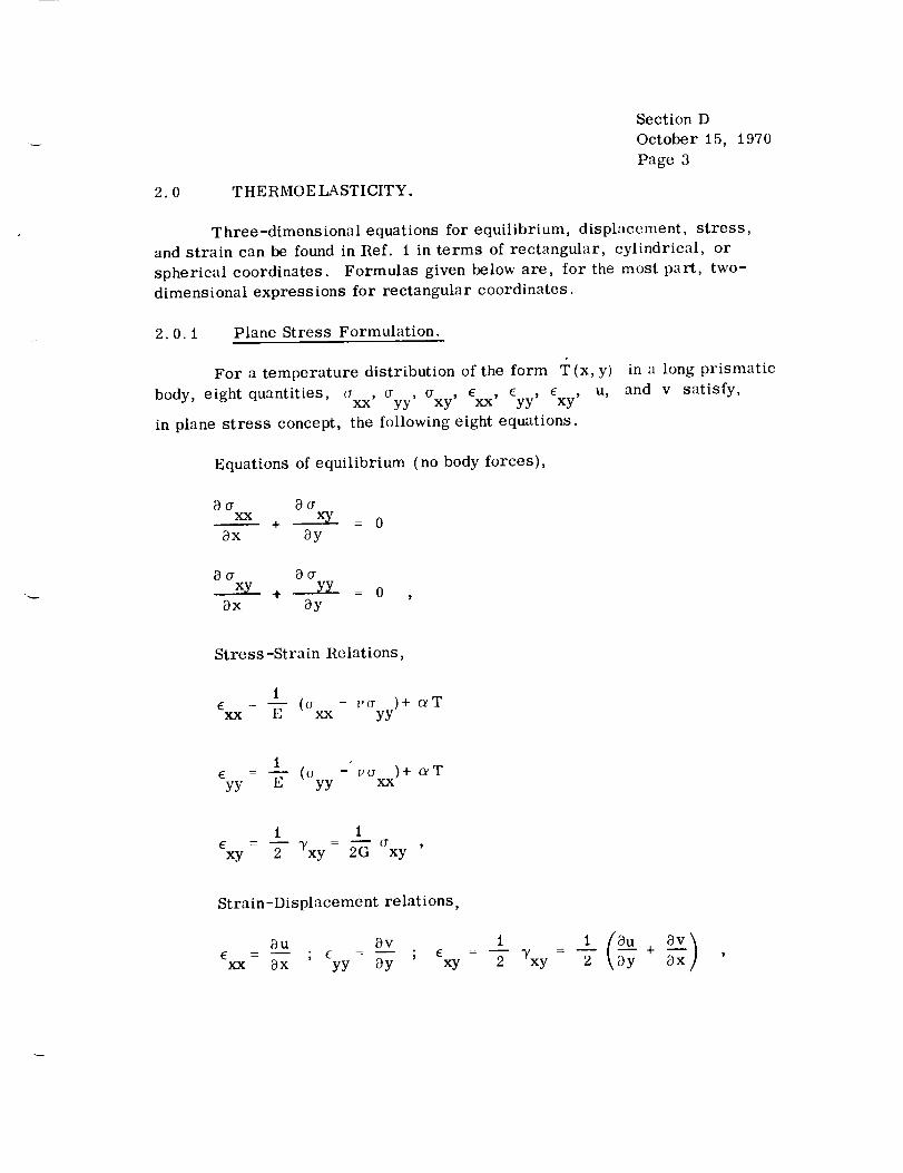
2.0 THERMOE LASTICITY.
Three-dimensional equations for equilibrium, displacement, stress,
and strain can be found in Ref. 1 in terms of rectangular, cylindrical, or
spherical coordinates. Formulas given below are, for the most part, two-
dimensional expressions for rectangular coordinates.
2.0.1 Plane Stress Formulation.
For a temperature distribution of the form T(x, y)
body, eight quantities, axx , Cryy, axy' Exx' eyy, Exy, u,
in plane stress concept, the following eight equations.
in a long prismatic
and v satisfy,
Equations of equilibrium (no body forces),
0a 0_xx + xy
Ox 3y= 0
Off _ff_÷ YY
Ox Oy= 0
Stress -Strain Relations,
1= _ (or - 1,a )+ aT
xx E xx yy
1
Cyy= _ (O-yy- vO-xx)+ ceT
1 1
¢xy = 2-Yxy- 2G axy '
Strain-Displacement relations,
Ou OvE =I ;¢ =_ ;
ax yy Oy
1
Exy = _ Yxy 2 3x

and in the case of plane stress,
Section D
October 15, 1970
Page 4
i
ff =ff =ff =0zz xz yz
v¢ - + aT
zz E (axx ayy)+
2.O. 2 Plane Strain Formulation.
In the case of plane strain defined by equations
u = u(x, y)
v = v(x, y)
w=O
replace E, v, and a of the stress-strain relations of plane stress formula-
E I'
tion by E 1, vl, and al, respectively, where E 1 = _ ; "1 = i--Z"_v ; and
a 1 = a( 1 + v). The equations of equilibrium and strain-displacement relations
remain unchanged.
2.0.3 Stress Formulation.
The solution of three partial differential equations satisfying the given
boundary condition gives the stress distribution, (r , (r , and (r in the×x xy yy
body. The equilibrium equations are
xx+ xy +ax Oy
X=O
a_ _cr
xy+ YY + Y=Oax 0y
and the compatibility condition is, for a simply connected body
(V 2 (axx + cr + o_ET)+ (t+ v) OX +yy ax
= o

Solution of Airy's Stress Function.
Plane Stress.
Section D
October 15,
Page 5
1970
For simply connected regions in the absence of the body forces, X, Y,
the solution of this problem is simplified considerably by using Airy's stress
function $(x,y). (See Section AI.3.6) Then
o- - OyV ; o • a -xx yy = _ ' xy Ox0y
The relations above satisfy the equilibrium equations identically, and substitu-
tion of these relations into the stress compatibility equation yields
V 44) + (xg V2T = 0 ,
whe re
V 4 4) - V2(V24)) =
i)24) 2 024) 044,
O-_x + + Oy-__)x_)y
For this problem the boundary conditions should be expressed in terms of the
stress function 4).
II. Plane Strain.
For plane strain problems the governing equation can be obtained from
those above by substituting E 1 and c_1 for E and _ respectively, where
E
El- 1 -y _ ; _1- _(1÷ p).
c_EV44) + _ V2T:: 0

'CEb NG pA¢-EBLANK
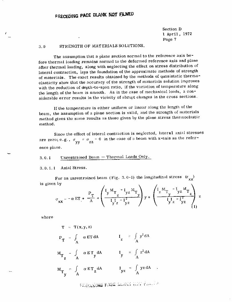
3.0 STR ENGTH OF MAT ERIA LS SOLUTIONS.
Section D
1 April, 1972
Page 7
The assumption that a plane section normal to the reference axis be-
fore thermal loading remains normal to the deformed reference axis and plane
after thermal loading, along with neglecting the effect on stress distribution of
lateral contraction, lays the foundation of the approximate methods of strength
of materials. The exact results obtained by the methods of quasistatic thermo-
elasticity show that the accuracy of the strength of materials solution improves
with the reduction of depth-to-span ratio, if the variation of temperature along
the length of the beam is smooth. As in the case of mechanical loads, a con-
siderable error results in the vicinity of abrupt changes in the cross sections.
If the temperature is either uniform or linear along the length of the
beam, the assumption of a plane section is valid, and the strength of materials
method gives the same results as those given by the plane stress thermoelasticmethod.
Since the effect of lateral contraction is neglected, lateral axial stresses
are zero; e.g., (r = a = 0 in the case of a beam with x-axis as the refer-yy zz
ence plane.
3.0.1 Unrestrained Beam -- Thermal Loads Only.
3.0.1.1 Axial Stress.
For an unrestrained beam (Fig. 3.0-1) the longitudin;d stress (axx)is given by
PT Iy z
(_ =-_ET+ --_-- +xx II -I zyz yz
y+ / Iz
M T - Iy z MTz_
where
T = T(x,y,z)
PT = f aETdA Iz : f y2dAA A
MT = J' (_ET dA I = f z 2dAz A Y Y A
MT = f aET dA I = f y zdAy A z yz A

Section DOctober 15,Page 8
1970
' /r_-A CENTROIDAL AXIS
I
o I
I,I_A
X,U Z,W
y,¥
z 1
\\
Figure 3.0-1. General unrestrained beam.
CASE a. The y-z axes are principal axes (I = 0)yz
PT MT MTz y
(rxx = -viEW+ _ + --T--y+--T- zz y
Yl
J
CENTROIO
(2)
CASE b. The y-z axes are not principal axes. A new coordinate system
Yl, zl is chosen which makes an angle 0 with y-z axes such that
tan 0 -
I MT - I MTy yzy z
I MT - I MTy yzz y
(3)
In the new coordinate system, which in general does not constitute
principal axes, the z axis becomes the neutral axis, and equation (1) in
this coordinate system reduces to
PT M T Yla = -aET + + zl
xx -7" I 'Zl
(4)
where
M T = fz 1 A
c_ ET (x 1 Yi zt) Yi dA1
f 2I = Yl dA1zl A

3.0.1.2
by
x is
Displacements.
Axial displacement u(x, y, z)
u(x,y,z) =u(0, y,z) +
Section D
1 April, 1972
Page 9
with respect to the u(0, y, z) is given
-g o
+ t Iz
The average displacement
+I MTz -Iy zM Yl
y T
IyI z - Iyz2 Y
(5)
dx
Uav(X) of the cross section at a distance
u (x) : u (o) +_tV aV
x P
1 T dx (6) f-x-0
Displacements v and w oftherefereneeaxis[v(x,y,z) v(x, 0,0);
w(x,y, z) = w(x, 0, 0)] are given by the following differential equations:
I M T - Iy z MTy 1
d2v 1 Y z
dx T- I-_, I I -I 2y z yz
dxYd2w E1 l Iz MTIIyS'z--I2IyzyzMTzt
(7)
If the y-z axes are principal, equations (7) reduce to
d2v
d2
MT
z
EIz
M
d2 w T yd2 l,:I
Y
(s)

In
Section D
October 15, 1970
Page 10
yl-zl axes, defined by equation (3), equations (7) reduce to
MTd2v
z£"_x - EI
zi
=0
(9)
3.0.2 Restrained Beam -- Thermal Loads Only.
Considered henceforth in this paragraph are cases of beam cross sec-
tions having y-z axes for the principal axes.
The values P, M , and M are the axial force and bending momentsy z
at any cross section resulting from the external forces and the reactions to the
restraints against thermal expansion; therefore, M and M depend only ony z
the constraining moments and shears at the restraints.
Mz = M°z + V°z x ,
My = MOy + VoyX ,
(10)
where the sign convention on moments and shears and M0 and V 0 are shownin Fig. 3.0-2.
y
M 0 V0
Figure 3.0-2.
v v
M M VM
Sign convention of moments and shears.

The displacements
M T + M zZ
EI
M +M
d2w T yYdx _" - EI
Y
v,w are given by
Section D
October 15,
Page 11
1970
(ii)
Solutions of equations (ii) for the special case described by equation
(10) are
x x2 M T (Yi)
z dx 1 dx 2 + + xv(x)=- f f _I (xl) c°z c'z - M°z0 0 z
x (x2_fo _) EIz(xl) dx2
X X 2
Xl dx 1 dx 2-V°z f f 'EI (x,)
0 0 z
x x 2 MT (xl)
w(xt =- f f _i y0 0 y (xl)
dx 1 dx 2 + +Coy Cly
X X 2x 1
-Voyf f l,:I (x,)0 0 y
dx 1 dx 2
x - Moy
(12)
X X 2
f/El (xO
0 0 y
The bending moment and shear force at any cross section are
d2v
M : - E1 - M TZ Z -_X '
Z
d2wM = -EI _ -My y dx _ T
Y
dM dMz =V = _ ; V
z dx y dx
(13)

Section D
October 15, 1970
Page 12
Each of the two equations (12) has four unknowns, Co, C1, M0, V0,
which are calculated from four boundary conditions, two at each end of a beam.
3.0.2.1 Evaluation of Integrals for Varying Cross Sections.
For a general cross section as shown in Fig. 3.0-3 the followingnotation is chosen:
b=boh (xl) h(xl) = 1+ H (-_)
d=dog(xl) g(xl) = i+G(-_) ,
xwhere b o and d o are reference width and depth at x_ O;x l- L
d o
b_
A = Aoh(xl) g(xl)
I I h(xO g3(xl)Z z 0
I = I h3(xl) g(xl)Y YO
....._,¢
Figure 3: 0-3. General cross section.
Letting the temperature variation bc represented by
T(x,y,z) = f(x l) V(y,z) ,

the necessary integrals become:
Section D
October 15,
Page 13
1970
2 T = f agTdA = ag f(xl) g(xl) h(xl) f VdA o ,
A A o
M T = f crETzdA = al_f(xl) g(xl) h(xl) f VzdA oy A A o
M T = f crET dA = crEf(xl) g(xl) h(x_) f VydA o ,z A Y A o
Mx T x 1
Ydx= ---E-aJ' EI f V zdA° J' _h (x1) dxl0 y Ioy A o 0
M Tx x 1
z dx o!f EI = _-- f VydA o j"0 z z o A 0 0
dx 1
x xl x x 1f xdx 1 x l (Ix) . ,f dx 1 dx 10 I_I - gI J h(xl) g°(xl) ' lg-"-i-"- gI 'f h(x 1) g'a(x 1)
z z 0 0 0 z z 0 0
The integrals necessary to evaluate PT' MT and M for a' Ty z
particular cross section and temperature distribution can be evaluated as
follows :
Let
F o = f VdAo ,
Ao
Fly : f VydAo ,Ao

and
Section D
October 15,
Page 14
1970
/.
F1 z = J V z dA 0A0
n m
Then, letting V(y, z) = VmnY z , which is a polynomial representation of
the temperature variation in the y- and z-directions, F0, Fly , and Flz can
be evaluated for common shapes. Table 3.0-1 gives these evaluations for
several common shapes and various values of m and n. Table 3.0-2 gives
values of F 0 and Fly for rectangular, triangular, elliptic, and diamond
cross sections when m= 0 and n= 0- 5. Table 3.0-3 gives values of F 0
and Fly for several standard shapes for various values of m and n.
3.0.2.2 Restrained Beam Examples.
In the following examples, since deflection, moment and shear equa-tions along the y- and z-directions are similar, only the results of the bound-
ary value problem in the y-direction are given (i. e., m = O).
I. Simply Supported Beam.
¥
tA i, .&--- "
I. I
A. Boundary Conditions:
v = 0@x=0, L
d2v
Mz = -EIz _ - MT =O@x=O, L
V o = M o = 0

TABLE 3.0-I.EXPRESSIONS FOR F0, Fly, AND Flz
RECTANGULAR
Section D
October 15, 1970
Page 15
FOR COMMON SHAPES.
F 0 =
Fly=
FIz=
• t
I_ I_
V_T2
7-
I 2
!
, 2
_I_
_N=I2
4Vmll
(re+l) (n+l)
,ITI- n+l
m, n: 0, '2, 4, 6..
m or n=l, 3, 5..
4Vinn
(m+l) (n+2)
n+2
re=l, :3, 5,.. n=0, 2, 4, 6
4V m+ 2
mo(m+2) (n+l) ' 2 ; ,
n+ 1

TABLE 3.0-1. (Continued)
TRIANGULAR
Section D
October 15,
Page t6
1970
Z =
Y
/ {°\I: "1
2 2
"_d o
do
F 0 =
2Vmn (__) m+l
0
where
]3. =
1
(n+l) '.
(m+2-i) I
["m+l
d°n+l [] _=1 B.+(-2)L
n! (_ _)n+,(n+i) I
n+m+2
m: 0,2,4
re=l, 3, 5
3,?
where
C. =1
2Vmn
I
(m+l) !
(m+2-i) '
d0n+2 [ _ +2- C. + (-2)
Lil '
n+m+3
,_+,,,(__)n+,+,_(n+l+i) :
Cm+2]m=0, 2, 4
m 1,3,5
FI2
0
2Vmn_ (_)m+_i_l Di+(
where
= _ n'. (, _)n+i_Di (m+3-i) ! (n+i) '

ORIGINAL PAGE IS
OF POOR QUALITY
TABLE 3.0-1. (Continued)
ELLIPTIC
Section D
October 15,
Page 17
1970
F 0
Fly
FI Z
r -r2 2
n
m--TT-\ =,/ \ _! (_)zn'. (re+n-l) (m+n-:l) .... (7) (:-,) (:_) (1)
n+m-l) v, (in+n÷2)(nl+n) .... (H)(I;)(,I)
m I)]" II 1, :;, 5...
Ill,n IJ,2,.l,(;
;In(l nI+ll II
m
7rVmn( 1_2)n/+l [d \n+2 ,-Tm+l \ 2 /"-_) (')"
(n+l)! (n+m)(n+m-2)... (7)(5)(:_)(t) .I o,2, 1,t;
(n÷m)_ (n+m+:_ (m+n+l)... (_)((;)14) u t,:l,5
n 0,2,.1,(i ¢_z" nl 1,::,S..
m+ l
"v,,,.( ,,,'CI+?.(__?'_'
o
n_ (n+nl)(n+,u-2)... (7)(5)(::)(1) m 1,::,7,
(n+Ili}'. (rn+n+:_) (llt_ll÷l)... (x)(I;)(.I) n O, 2,4
I) l,:t, 5 or m 11,2,4,1;

TABLE 3.0-I. (Continued)
DIAMOND
Section D
October 15,
Page 18
1970 v
2
FO
Vmn mi n!
4\ 2] \2]m, n=O, 2, 4..
m orn=l,3,5
4Vmnml(n+l) !
m=l, 3, 5..
Flz =
4V (m+l) !nlmn
(n+m+3) !
m=l, 3, 5..
n=0, 2, 4..
or n=0, 2, 4

TABLE 3.0-1. (Continued)
T-SECTION
SectionDOctober 15,Page 19
1970
F 0
Fly
w
b
_t
J
r
Z _----- 0 I¢
I I
I' '1b
2Vmn
(re+l) (n+l)
2Vmn
(re+l) (n+l)
0
,+,)_ +'m 1,3,5
c+w) n+l- c n+l]
n=0, 1, 2, :1
2VmB
(m+l) (n+2)
2Vmn
(re+l) (n+2)
0
{(-_--)m+l(an+2-cn+2)+ (-_-b2)m+l[cn+2- (c+w)n+2 ]
m 1,3,5 n 0,1,2,3,4
m O, 2,4, 6
n O, 2, 4, (i
m 0,2,4,6
n:l, :3, 5..
m 0,2,4
n 0,2,4
m:0, 2, 4
n 1, :3, 5

TABLE 3.0-1. (Continued)
I-SECTION
Section D
October 15,
Page 20
1970
_ [
• o o-t
w
t
b "[
F0
4 Vm n(_-) n+
)(m+l) (n+l)
0
1
m or n odd
m, n : even
Fly =
4V (d'_ n+2
mn\,-£-](m+l) (n+2)
n+2] } m=:evcn
0 m : odd or n even
NOTE: z-Section can be :Ipproximated by I-Section with respect to its
principal axes. The results above are applicable to this section.

TABLE 3.0-1. (Continued)
HAT -SECTION
Section D
October 15,
Page 21
1970
F 0
Fly = o
FIz - 0
y
L+ td
C
IT
b •
0
2Vmn
(n+l)(m+l)
m 1, 3, 5...
{ [(-c) n+l o (-c-w) n+L] I(_- + t + i)m÷ l - (_ + 1)m+ l 1
(_)'n+l[ n+l (a_k)n+l] } n, o. 2,,1...n 0,1,'> 3,4.
2VInn
(n+2) _ m+l)
m 1,3,5...
,, m,,(_5°+,](.__)m+ 1 [; (a_k)r_21 } ,,
n+2 m 0, 4.n 0,1, 2, 3, ,1. . .
2Vmn
(n+l) (m+2)
m 0,2,4...
{ [(-c) n+l- {-c-w)n+l] [(_-+ t +p) m+2 -([2 )-- +t) m+2]
[3 2 I m+2+ [an+l - ( -c-wj n+l] f{b + t)m+2 - ( J_-) ]

TABLE 3.0-1. (Continued)
CHANNE L
Section D
October 15, 1970
Page 22
1
_------ d -------_
F o = 0.0
2Vmn
(n+l) (m+l)
n=1,3,5...
{I(c_w)m÷i-cm+ll (b)n+i+ Ccr_l -(d-c-w)m÷ll,
. _ _ n:0,2,4...
m 0,1,2,3,4,5...
Fly = 0.0
2VmR
(n+2) (re+l)
n0,2,4...
I_c,+w ) m+l _cm+l 1 (__)b n+2 + [cm+l(d_c.w)m+l],
[(2b_) n+2 (b t)n+2]} m=0, I,2,3,4,5...n:1,3,5...
Flz = O. 0
2Vmn
(n+l) (m+2) { [(c+w)m+2- cm+2 ] (_-2b) n+l
r b ,+I b "+: ]
•
n-I,3,5...
+ [cm+2 - (d-c-w) m+2] *
n 0,2,4...
m:0,1,2,3,4,5...

TABLE 3.0-1. (Continued)
RECTANGULAR TUBE
Section D
October 15, 1970
Page 23
Y
T = Z
_t2
F0 0.0
= 0.{}
n 1,3,5...
m J,3, 5..
n 0,2,4...
m 0,2,4..
Fjy: 0.0
O. 0
4Vm n
(n+2} (re+l)
• n_2 b m+ 1
FI z0.0
0.o
4 Vmn
(n+l)(m+2)
n 0,2,4...
m 1,:LS..

TABLE 3.0-1. (Concluded)
CIRCULAR TUBES
Section D
October 15,
Page 24
1970
¥
b Z
m=5
F0 0.0 n 1,:1,5...
: 0.0 m l,:t,5
I'd "m+n+z b rn+n4 2 ] I_._4_mo[(:_)(b J' ....'m÷| - - Z{ 114 :l) ÷ _ (I',') ;_ )
- (m+l_l'n-!)_r_l-:l) {m÷J)(m-l_{m-:_(m-5 ) ]
4_(n+7) ÷ :IM4( n* !*)
n (1+2,4, , .
m 0, 2, 4
Fry0.0 n 0,2,4. ,
- 0.0 m 1,3,5
'Vmn [(_-)m+n+:'m+, -\-_](b_ .... IllljL n'-_z - _! • (re+l) { n,-l)_{ n*,i)
(n*¢l)(m-l)_n_-?:l + im*I)(_l_l)lm-:_}ln_-,%l /
4_(n+:_) :l_4(n+ 10) ]
n 1,:_,5 . .
m _L2.4
FIz = O. 0 n 1, :J, 5...
fl.O ell II, Z, 4
'"_,,[cor''_ c,,_....'][, o,._,.,,-,,,,- (*nlC2) illQ{in-2) (In¢2)(rni(_ll-_)itln-4) /
l_(n+7) + ;g_4l n*!O --J
n II+Z.4..,
m 1, :_, r,

TABLE 3.0-2.
RECTANGU LAR
VALUES OF F o AND Fly
COMMON SHAPES
Section D
October t5,
Page 25
FOR FOUR
TRIANGULAR
1970
Z I
I- ._ -: b02 3"
m--O
2
%2
2
m=O
_I-I
b_o2
1
2
Fo
bodo Voo
1 bd 3"_ o oVo2
Fly n
0 0
bod _ Vol 112
0 2
I bod_ Vo3 3
0 4
Fo
1
-_- bod o Voo
0
1 3b0do '_ o2
1 4bodo Vo3
27O
bod _ Vo4270
2 bod6o7(243) V°5
Fry
0
1 bod_ Vol
1 4
27"-_ b°d° v°3
1 bod_ Vo 3270
2 6
7(243) b°d° V°4
31 b dTv o(729) o o

E LLIPTIC
TABLE 3.0-2. (Concluded)
Section D
October 15, 1970
Page 26
DIA MO ND
Z =
2
2 2
m--O
n F o Fly
0 lr bod0 Voo 0
32 V°I
I b_ o2 _ 7r Vo2
bod_Vo33 6 12-_
b_ o4 I-_ V°4
5 0 15 _r bod_ V0532(256)
Z m
¥
J_
r
p
m=0
n Fo Fry
I bodo Voo 0o1 3
1 0 4--8 b0d0 v0l
I bod_Vo_ o2 4-_"
1 bod_ Vo 33 0 48--'6"
4 t__ bod_Vo4 o480
5 0 1 b "_28(i20) _oVo5

Section D
October 15, 1970
Page 27
TABLE 3.0-3 VALUES OF F o AND AND FOR• Fly F1 z
COMMON SECTIONS.
*----b = 2.00----_
! ,I
d!+I/ L
| I
!
F°- V 1 f VdAomn
0 2 4 6
0 0.531 0.207 0.121 0.093
2 0.084 0.030 0.011 0.004
4 0.050:0.018 0.006 0.002
6 0.036 0.013 0.004 0.002
1 f Vy dA oFly - V
mll
1 3 5 7
0 0.207 0.121 0.093 i0.084
2 0.030 0.011 0.004 0.001
4 0.018 0.006 0.002 0.001
6 0.013 0.004 0.002 0.001
--b = 2.00-----_
!
o+t o.,f,1/
I
t
m_ 0 2 4 6
0 0.719 0.784 1.379 3.117
2 0.084 0.079 0.075 0.073
4 0.050 0.047 0.044 0.042
6 0.036 0.034 0.032 0.030
i
td = 3.75
1I
m_ 1 3 5 7
0 0.784 1.379 3. 117 8. 152
2 0.079 0.075 0.073 0.076
4 0.047 0.044 0.042 0.039
6 0.034 0.032 0.030 0.028

TABLE 3.0-3. (Continued)
Section DOctober 15, 1970Page 28
_'-- 3.00 ---_
| |
3.0.1
| |
!
F o- V 1 fVdA omn
m_ 0 2 4 6
0 1.043 1.085 1.731 3. 603
2 0.352 0.326 0.303 0.285
4 0.474 0.438 0.405 0.376
6 0.762 0.704 0.652 0.605
1f Vy dA oFly:
mn
m_ 1 3 5 7
0 1.085 1.731 3. 603 8. 892
2 0.326 0.303 0.285 0.277
4 0.438 0.405 0.376 0.350
6 0.704 0.652 0.605 0.563
-- 3.5 ------_
I !
0.
L
t
m_ 0 2 4 6
0 t.750 1. 663 2. 323 4. 198
2 0.898 0.791 0.705 0.639
4 1.641 1.445 1.279 1.139
6 3. 590 3. 160 2. 798 2. 492
I3.5
l|
m_ 1 3 5 7
0 1.663 2. 323 4.198 9.096
2 0.791 0.705 0.639 0.600
4 1.445 1.279 11.139 1.021
6 3. 160 2. 798 2. 492 2. 232
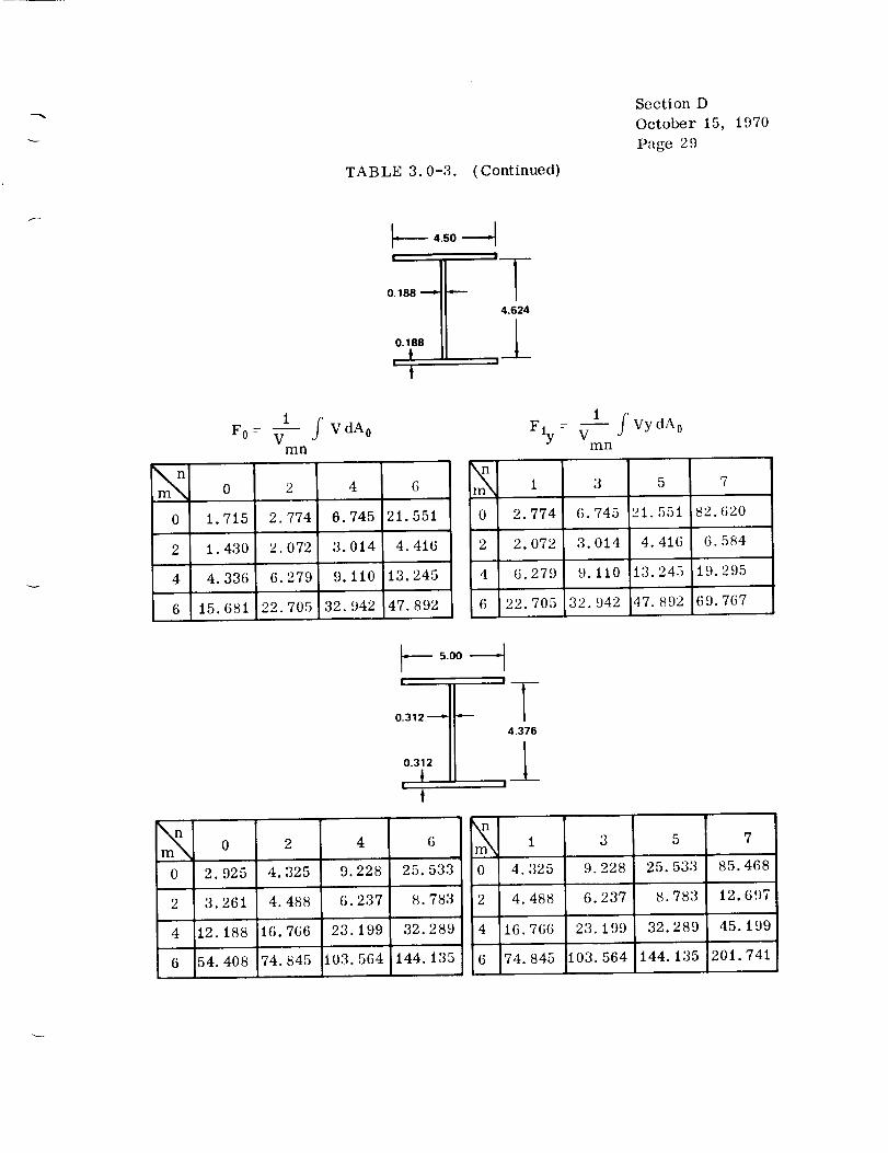
TABLE 3.0-3. (Continued)
Section D
October 15,
Page 29
1970
_---- 4.50 -_
o.. p5"11|
t
14.624
L|
0
2
4
6
1 $F 0 : _-- V dA omn
0 2 4 6
1.715 2.774 6.745 21.551
1.430 2.072 3.014 4.416
4.336 6.279 9.110 13.245
15.681 22.705 32.942 47.892
0
2
4
6
1 J VydAoFly -- V
Inn
1 3 5 7
2.774 6.745 21.551 82.620
2.072 3.014 4.416 6.584
6.279 9.110 13.245 19.295
22.705 32.942 47.892 69.767
0
2
4
6
---- 5.00 ----_
!
!
I
#__
I4.376
11
0 2 4 6
2. 925 4.325 9. 228 25. 533
3. 261 4.488 6. 237 8. 783
12. 188 16. 766 23. 199 32. 289
54. 408 74. 845 103. 564 144. 135
0
2
4
1 3 5 7
4. 325 9. 228 25. 533 85. 468
4. 488 6.237 5. 783 12. 697
16.766 23.199 32.289 45.199
74.845 103.564 144.135 201.741
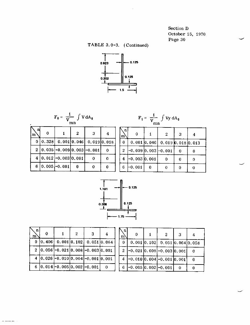
TABLE 3.0-3. (Continued)
t0.923 _ .,--- 0.125
t 0.125
0.202__t. _
. 1.5
Section D
October 15, 1970
Page 30J
1go= W- fVaAo
mn
0 1 2 3 4
0 0.328 0.001 0.046 0.019 0.018
2 0.035 -0.009!0.003 -0.001 0
4 0.012 -0.003i0.001 0 0
6 0.005 -0.001 0 0 0
1_1: V- fVydAo
inn
m_ 0 2 3 41
0 0.001 0.046 0.019 0.018 0.013
2 -0.009 0.003 -0.001 0 0
4 -0.003 0.001 0 0 0
6 -0.001 0 0 0 0
I----,. _ 0.125
1.191
0.309 0.125
__k .. !
_---- 1.75 -_
m_ 0 1 2 3 4
0 0.406 0.001 0.102 0.051 0.064
2 0.056 -0.021 0.008 -0.003 0.001
4 0.026 -0.010 0.004 -0.001 0.001
6 0.014 -0.005 0.002 -0.001 0
m_ 0 1 2 3 4
0 0.001 0.102 0.051!0.064 0.058
2 -0.021 0.008 -0.003 0.001 0
4 -0.010 0.004 -0.001 0.001 0
6 -0.005 0.002 -0.001 0 0

TABLE 3.0-3. (Continued)
Section D
October 15,
Page 31
1970
1O.788
t0.087
|
-.--- 0.125
0.125
|
2.oot---_
1
F°- Vmn
_ __ fVdA o
m_ 0 1 2 3 4
0 _.359 0.001 0.026 0.011 0.008
2 D. 083 -0.0 12i0. 020 0 0
4 D.050-0. 007 0. 001 0 0
6 0. 036 -0. 005 0. 001 0 0
0
2
4
6
F 1 -
0
0. 001
-0. 012
-0. 007
-0. 005
1f Vy dA 0
Vmn
1 2 3 4
0.026 0.011_0.008 0.005
0.020 0 0 0
0.001 0 0 0
0.001 0 0 0
10.985
t0.109
I
_'-"-- 2.50
m_ 0 1 2 3 4
0 0.561 0.002 0.064 0.034!0.030
2 0.203 -0.038 0.008-0.001 0
4 0.190 -0.036 0.007 -0.001 0
6 0.213 -0.040 0.008 -0.002 0
.,,-- 0.156
0.156
m_ 0 1 2 3 4
0 0.002 0.064 0.034 0.030 0.024
2 -0.038 0.008-0.001 0 0
4 -0.036 _.007-0.001 0 0
6 -0.040 D.008 -0.002 0 0

TABLE 3.0-3. (Continued)
Section DOctober 15, 1970Page32
11.544 ......4 _ 0.156
t0.30 0.156
....L 1 IJ
1 fVdA °F°- Vmn
m_ 0 1 2 3 4
0 0.756 0.002!0.261 0.195 0.284
2 0.352 -0.132 0.051 -0.019 0.008
4 0.474 -0.179 D.069-0.027 0.011
6 0.762 -0.288 0.110 -0.043 0.017
i/F 1 = _-- Vy dA omn
m_ 0
0 0.002
2 -0.132
4 -0.179
6 -0.288i
1 2 3 4
0.261 0.195 0.284 0.348
0.051 -0.019 0.008 -0.002
0.069 -0.027 0.011 -0.004
0. II0 -0.043 0.017 -0.007
m_ 0 1 2 3
0 1.281 0.007 1.049 1.115
2 1.004 -0.614 0.383 -0.233
4 2.406 -1.478 0.914 -0.570
6 6.875 -4.222 2.612 -1.629
I-- ',,--.-0.188
2.292
t 0.188
0.52
_t_, .. ] ,
4 m_ o
2.492 0 O.007
0.156 2 -0.614
0.358 4 -1.478
1.023 6 -4.222
1 2 3 4
1.049 1.115 2.492 4.471
0.383 -0.233 0.156 -0.081
0.914 -0.570 0.3581-0.226
2.612 -1.629 1.023 -0.647

OEiGINLL P#.C_ 15
OF. POOR QUALITY
TABLE 3.0-3. (Continued)
Section D
October 15, 1970
Page 33
0.125 ]
olYi0._25 L--1.75J _-1.0]
0
1
2
3
4
5
IllI]
0 1 2 3 4 5
0.656 0.7:}4 x 10 -3 0.55 _ 10 -I 0.165 × 10 -2 O. 559 x 10 -2 0.34 x 10 -3
0.0 0.0 0. [) [}. l) 0.0 0.0
O. 804 -0. 152 0.659 x 10 -1 -[). 135 × 10 -1 0.(;27 :,: 10 -2 -0. 125 x 10 -2
O. 0 O. 0 [I. l} [I. (} O. 0 O. 0
O. 172 × 101
0.0
-0. 449
0.0
0.14
If.I)
-I-0. 409 _ 10
IL l}
0. 1,1 / 10 -!
O. 0
-2-0. 393 _ 10
0. 0
0
1
2
3
4
5
0. 734 × 10 -3
O. 0
-(}. 152
1 f Vy (bX o
121n
O. 55 y 10- !
O. 0
0.66 × 10 -1
U. 1(;5 ,( 10 -2
0.0
-0. 135 x: 10 -1
-2I).559 x lO
0.0
O. 627 x 10 -j
o. 34 x 1 u -3
O. 11
-2-t}. 125 x 1(}
-3l)._;IZ - 10
0.0
,0. (;;_K x 10 -3
0, 0 O. 0 (}. (} 0. (} 0.0 0.1)
-0. 449 O. 1,Is -0. 409 x 10 -I 0. 14 x 10 -t -0. 393 x 10 -z 0.13U x 10 -z
0.0 0.0 0.0 0.0 0.0 0.0
1
.I' Vz (b% oFI AIi'(n
0 1 2 3 4 5
0
1
2
3
4
5
0.0 O. 0
0. G39 -0. 155
0.0 0.0
0. 158 × 1() 1
0.0
0. 455 x 101
-0.451
O. f}
-0. 134 x 101
O. 0 O. 0 O. 0 (}. 0
0.5S1 x 10 -I -0. 138 × 11) -1 O. 561 < 10 -2 -0. 13 10 -2
0. 0 0. 0 O. 0 0.0
O. 141
(1.0
0.40(i
-0.41:1 • 111-1
0.0
-(}. 123
-t0. 131 < 10
O, 0
O, :I,_|,_ 111-1
-0.397 z 10 -2
(1.0
-1-0. 11!1 _ 10

TABLE 3.0-3.
Y
(Continued)
Section D
October 15,
Page 34
1970
0
1
2
3
4
5
0
1
2
3
4
5
0
1
2
3
4
5
Fo = _-L fvdAomn
0 1 2
0.972 -0.901 × 10 -z 0.603
0.0 0.0 0.0
1. -0.534 0.554
0.0 0.0 0.0
O. 209 X 101 -0. 148 x 101 O. 118 × 101
0.0 0.0 0.0
3 4 5
0.161 0.517 0.289
0.0 0.0 0.0
-0.273 0.352 -0.121
0.0 0.0 0.0
-0.838 0.094 -0.476
0.0 0.0 0.0
0 1
-0. 901 × 10 -2 O. 603
0.0 0.0
-0. 534 O. 554
0.0 0.0
-0. 148 × 101 0. 118 × 101
0.0 0.0
Fly= _- fVydAon_n
2 3 4 5
0. 161 0. 517 0. 289 0. 514
0.0 0.0 0.0 0.0
-0. 273 0.352 -0. 121 O. 247
0.0 0.0 0.0 0.0
-0. 838 O. 694 -0. 476 O. 422
0.0 0.0 0.0 0.0
1 fVz dA_Flz =mn
0 1 2 3 4 5
0.0 0.0 0.0 0.0 0.0 0.0
0.82 -0.565 0.487 -0.305 0.304 -0.155
0.0 0,0 0.0 0.0 0.0 0.0
0.2×101 -0.140× 101 0.115×101 -0._54 0..67 -0.493
0.0 0.0 0.0 0.0 0.0 0.0
0.572×101 -0.431×101 0.327x 101 -0.248× 101 0.19×101 -0.145×101
r
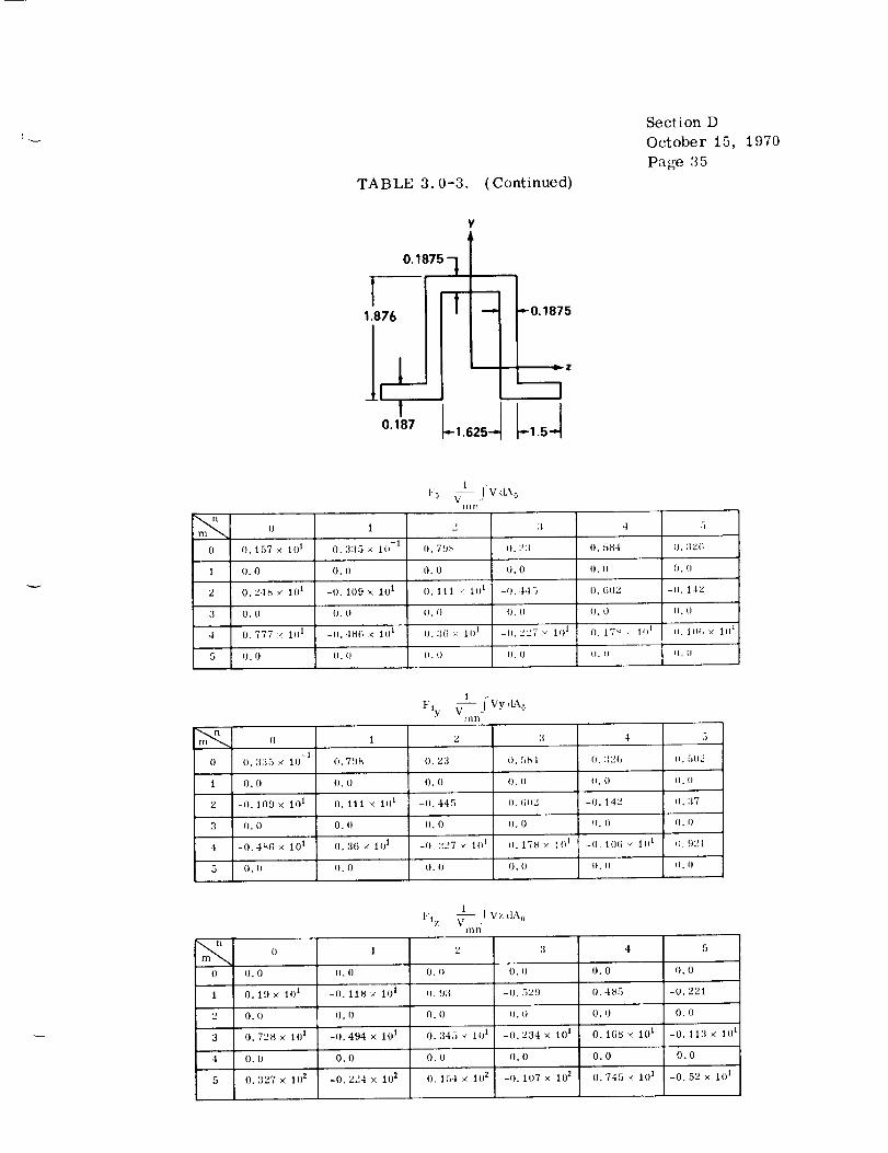
TABLE 3.0-3. (Continued)
Section D
October 15,
Page 35
1970
Y
1
O.187 1.625
""0.1875
laZ
0
1
2
3
4
5
1 f V dA oVo _-
IIIII
0 1 2 3 .t 5
0.157× 101 0,:135 x 10 -1 I}. 79,', 0.23 0.584 0.32(;
0.0 0.0 0.0 0.0 0. l} 0.0
O. 24_ x I_P -0. 109 × 10 t O. 1_ J >: 1_) t -0. 445 _). _)02 -_. 142
O. 0 O. 0 O. 0 O. 0 1).0 O. 0
0.777< 1<) l -1/..t8(; x 1111 0.3(; x_ I01 -(J. ZZT_ 101 0. 17 '_ ," ](jl _it. 10G ,_ iijl
0. 0 (I. 0 0. 0 (!. 0 t). (I 0. II
Fly & fVY,bXo
0 1 Z 3 4 5
0. 335 x 1() -1 0.7!)_ 0.23 0. 5_,t 0. 326 (I. 502
0. 0 0. 0 0. 0 0. (} o. 0 O. (_
-0.109_ 101 0.111 x 101 -I).445 0.fi02 -0.142 ().37
0.0 0.0 0.0 0.0 0+ (} (}. I)
-0.486 × 101 0.36x 101 -0.227 _ 101 0.178 _ l(i 1 -0+ 10(i'_ 101 (I.9:'1
0.0 0.0 0+ 0 0. <) II. 0 II. II '
0
1
2
3
4
5
0
1
2
3
4
5
0.0
0. 19 x 101
0.0
0. 728 x 101
l'Iz' _i •I V;' dA o
11113
0.0
-0. llS x 101
0. I)
-0. 494 x 101
0. 0
0+ 9:3
0.0
O. 345 _ i0 !
O. 0
-0. 529
U. 0
-1). 234 × I01
O. 0
0. 485
0.0
O. 16_ x I0 i
0.0
-0. 221
0.0
-0. 113 x 101
O. 0 O. 0 O. 0 O. 0 O. 0 O. 0
O. 327 x I02 -0. 224 x 102 O. 15,1 × 10² -0. 107 × 102 O. 745 x I01 -0.52 x 101
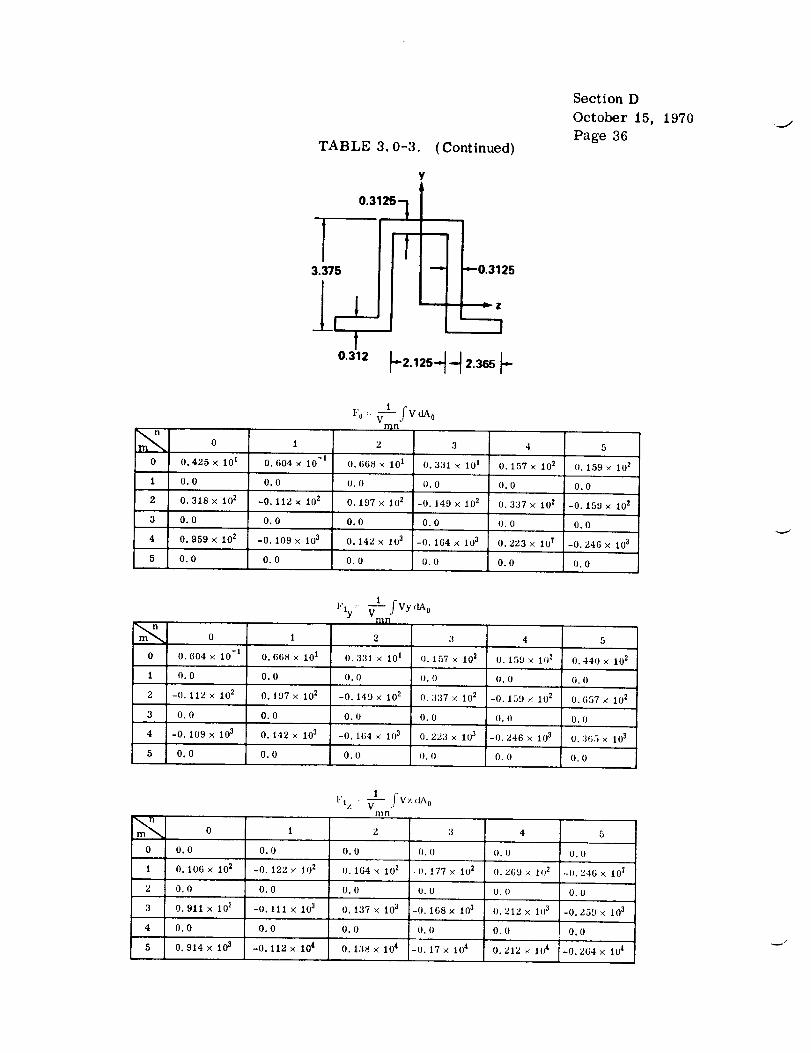
TABLE 3.0-3. (Continued)
y4
o,,,sq I
lit. 7 0.3125
1
Section D
October 15,
Page 36
1970.j
1
2
3
4
5
o
0.425 x lO 1
o.0
0. 318 x lO 2
o.o
0. 959 x 102
o.o
O. 604 × 10 -l
0.0
-0.112 4 10 2
0.0
-0.109 x 10³
0.0
2 3
0.668 x 101 0.331 x 101
0.0 0.0
0,197 4 10 z -0. 149 4 102
0.0 0.0
0.142 x 10³ -0.164 x 10³
0.0 0.0
0.157 4 102
0.0
0.337 × 10²
0.0
0. 223 x 10 ?
0.0
0. 159 × 102
0.0
-0. 159 × 102
0.0
-0.246 x 10³
0.0
o
1
2
3
4
5
1
}'l.y : ,-7=-vn_nf Vy (tA 0
0 1 2 3 4 5
0.6044 10 -1 0.6684 10 t 0.331 4 101 0.157 × l0 t 0.1594 10 z 0.440 x 10 z
O. 0 O. 0 O. 0 0.0 0.0 O. 0
-0. 112 × 102 0.197× 10² -0.1494 102 0.337 x 10² -0. 159 :< 102 0.(;574 102
O. 0 O. 0 O. 0 O. 0 0.0 O. 0
-0. 109 x 103 0. 142 4 103 -0. 164 4 103 0. 223 x 103 -0. 246 x 103 0. 365 x 103
0.0 0.0 0.0 0.0 0.0 0.0
0
1
2
3
4
5
11"1 : V-fw.,_
mn
0.0 0.0 0.0 0.0 0.0 0.0
O. 106 × lO t -0. 122 x 10 z O. 164 4 102 -[). 177 4 102 O. 269 x 102 -0. 246 × 10 /
0.0 0.0 0.0 0.0 0.0 0.0
0.911× 10² -0.111 × 10³ 0.137 × 10 a -0.168x 10³ 0.212x 10³ _-0.259× 10 a
0.0 0.0 0.0 0.0 0.0 0.0
0.914×10³ -0.1124104 0.138×10⁴ -0.17×10⁴ 0.212×10 ¢ -0.264x 10⁴
J

0
1
2
3
,t
5
0
0. 17,t x 10 -I
-0. 375 :< 10 -5
-0. 307 x 10 -3
-0. 925 x 10 -4
-4-0.22fi x 10
-0.5:27 x 10 -5
TABLE 3.0-3. (Continued)
y
]• _ 0.75
--." ---0,05
0.05
0.375
l"c) _- fVdA oIll n
1 2 3
I). 0 -0. 709 < 10 -_ O. 0
0.0 -0.24_ < 10 -:_ 0.0
-40.0 -0.598 x 10 0.0
O. 0 -0. 13.1 ,< It) -'i O. 0
-50.0 -0.2t)7 _ 10 0.0
O. 0 -0. (;65 × 1() -_ O. 0
4
-0. 15(J / 10 -3
-0.36(; _ 10 -¢
-0.792 ¢ 10 -t_
-0. 17 ,: 10 -5
-6-0. 371 < 10
-7-0. I_26 x 10
Section D
October 15,
Page 37
5
0.0
O. 0
It. 0
O. (I
II, 0
(). (i
1970
0
1
2
3
t
5
0
O. 0
0.0
0.0
O. 0
O. 0
O. 0
1
-3-0. 709 x 10
-0. 248 x 10 -3
-fi.5!)8 x 10 -4
-0. 1:3.1 × 10 -4
-I). 297 x 10 -5
-0. I;65 × 10 -6
1
Fly _-- .¢Vy dA ot;131
2 3
-3O. 0 -0. 156 x 10
O, 0 -0.3fit'i ," 10 -4
0.0 -0.792 _ 10 -5
O. 0 -(I. 17 y 10 -r)
-60.0 -li.371 x 10
o.4) -ll.82G × 10 -7
t
(I. 0
O. 0
{I. li
II. II
l).II
O. 0
5
-0.23 < 10 -4
-0. ,186 -.e 1[) -5
-0.101 < ll) -J
-6-0.214 _ III
-7-0. l(it .: 10
-7-0. 10:i ." 10
0
1
2
3
4
5
I I Vz cbk o]"l z _ .
ii111
0 1 2 3
-0.375,'< 10 -5 0.(} -0.248 :" 10 -3 0.0
-3-0. 307 × 10 O. 0 -0.59_ - 10 -4 O. 0
-0. 925 × 10 -¢ O. 0 -0. 13,1 ,< 10 -i O. 0
-4 r-0. 226 × 10 13.0 -0. 297 ,- 10 -_ O. 0
-0.527 )< 10 -5 [I.O -0.(765 _ I0 -G 0.0
-0. 122 x 10 -5 0,0 -0. 151 _ 10 -6 0.0
4
-0. 366 _ 10 -4
-5-0. 792 × 10
-0. 17 × 10 -5
-0. 271 '< 10 -6
-7-0. 826 _ 10
-7-0. i_8 x It)
5
O. 0
O. l)
O. 0
O, (I
o. 0
O, ()

OF POOk OIJAL_TY
TABLE 3.0-3. (Continued)
y
_ _ 0.125
! II
L
1.75
Section D
October 15, 1970
Page 38
iHn
m'_ 0 l 2 3 4 5
0 0.885 × [0 -1 0.0 -0.31)3 _ 10 -1 0.0 -0.318 × 10 -i 0.0
1 0,175× 10 -I ().1) -D. 3tD _ 11)-I (I.() -0.209× tO -I 0.0
2 -0. llH _< 10 -I U.0 - II.._!)_' - lU -1 0.0 -0. Z23 X 10 -1 0. U
3 -0.223 x 10 -1 I).0 -0.254 • lq) -I 0.0 -0.183 x l0 -1 (3 (I
4 -0. Z46 × lO -L (L0 -0._15 _ 10 -t 0,0 -0.15× 10 -i 0.0
5 -0,_35 _¢ |0 -I 0.(} (), ];"49' : 1() -[ I).1) -I). 125 × 10 -1 0.0
]1," Vl- f VydAo
n_n
m_ 0 1 2
0 0.0 -0.30:] _ 10 -_ 0. o
1 0.0 -0.311- lo -1 o.o
2 0.0 -0.292 _ 10 -1 O.r)
3 0.0 -(3. 254 _ 10 -t 0. I)
4 0.0 -o. _'15 _ lO 't o.o
5 0.0 -0. 1H2 - 11) I 0,11
3 4 5
-I-0.318 × 10 11.0 -0.24(;',, lU -I
-o.21i9 × 10 -1 (3.11 -0.197× JO -1
-0.223 _" i0 -! 0.0 -0.157 _ I0 -1-
-0. iN:| x* 11) -1 O. 0 -0. 127 y 10 -1
-0.|5 × 10 -1 0.0 -0.103 :< 10 -I
-0.125 _ tO -I 0.0 -0.847 , 10 -2
lrl z _- .I VZ d2_.0
ntn
m_ 0 1 " 3 4 5
O 0.175 _ 10 -t 0.0 -0.319x to -z 0.0 -I). 21;9 × 10 -! O.O
1 -0,118< 10 -I 0.0 -I). 292 x 11)-1 0,1) -U. 223 × 10 -1 0.0
2 -0.223 x 10 -1 0.0 -0.25.l × II) -I 0.0 -0. 1H3 × |0 -1 0.0
3 -0.246 x 10 -t 0.0 -0.215× I0 -1 0.0 -I).15 _ 10 -1 0.1)
4 -0.215 x 11) -t 0+0 -0. is2 × i0 -t o.0 -Ib+ 125× 10 -t 0.0
5 -(I.212× 10 -t 0.0 -0.154 _ [o -t 0.0 -0.104 × 10 -t 0.0
vl
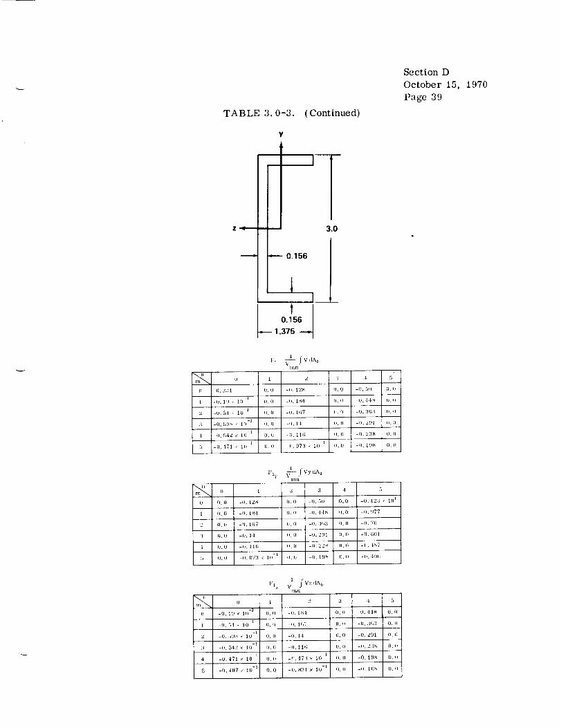
TABLE 3.0-3. (Continued)
Z _-.--
o +011.375
(J
1
2
3
4
5
tJ
O. 231
-0. I!_ - 10 3
-0.5.I , 10 l
-[h `542 _ l[) -1
-l). 171 , 1o I
I"r+ _ fV dA o
1 Z
O. 0 -o, 128
o. o -0. 1_4
t). (; -<1.1[;7
I). I) ql. I;
_h[J -0. 11(;
;; 4 5
0. (! -([. 5[I (h [)
th ql -o..14x o. f)
[h Ii -0. ;l(i3 [h 0
O, I_ -I). 2_1 _1. (I
O. I1 -I). '_3_ (1. II
I).0 -11. 9_| ,I 111-1 (L0 -0. l(J_ 0, ql
0 1
(9 (I. _1 -[I. 12;_
1 o, f) -[I. 1 _,1
2 I). I) -I). 11;7
3 lJ. 11 -(h 1,1
4 O.I) -I). Ill;
,5 11.0 -I).l)7;I _ 119 I
Fly F f VydAoIll II
V 3 4 5
4hO -0.50 0.0 -0. 123 + 131 +
¢). [1 -II..34_ I[. 0 -[h 977
I). i) -0. ;If|3 I). II -Ih 7ll
I[. [I -[J. 2ill IJ. 1) -(). (i([1
I). II -I1+ 2L_X IL l) -II. J,h7
[t. 0 -q[, 19_+ q). I_ -Ih loft
II
1
3
4
5
I)
-[9. 1_1 ,t |0 -3
-<h 51 -" 10 1
-0. 7)I+_ _ l0 -I
-[}. 542 / i() -I
-0. 471 _ 10 -1
-0.41t7 _ 10 -1
l"lz 1-- f Y_'. dAO
rllll
l 2 3 4 5
(i.o -i). lh4 (J.(P -0..|4_+ 0.0
iJ. 19 -th l[;Y I). _ -I;. 3(J3 I), l)
0.0 -0. 14 ()+ 0 -0. 291 O. 0
It. (3 -(1. 111; 0. [) -1t. 2;Ih 11, II
0. D -r+473 y 1[) -1 0.1) -[). 19_ 0.0
0.0 -[). 831 ;,+ 10 -1 0.0 -0, l[;h (I.0
Section D
October 15, 1970
Page 39

OR;GiN_.L P_,C,S IS
OF POOR QUALITY
TABLE 3.0-3. (Continued)
Y
I
*'-----0.5
I0.375
"------ 3.0------
6.(
I._z_
Section D
October 15, 1970
Page 40
=
{I
1
2
3
4
5
(}
1
2
:1
4
5
o l
0.161 _ IO _ o.0
{}.:175 _ IH -:I 0.(}
-0.149, lU 1 ¢I.11
-1}, :149 _ 101 0.{I
-(}.G_I , ](e I (I.0
-(I. ]_ , ](j' 0,1)
0 I
ILl} -{e, l!e?× lie l
0.0 -(),852. II) I
O. (e -0. 171 , lie:'
0.0 -0.31 _ Ill:_
O. 0 -(e. 562 _ 10 e
(}.{} -0.103× 10³
m"Q 0 !
0 0.375 _ 111-3 0.(}
1 -o. 149y 101 0.0
2 -0,349 × 1(} l {I.0
:| -0.681 _ 1(} ! 0.0
4 -(}. 12X _ 10" (I.O
5 -0.243× 10 _ 0,0
1 /. VdA0F° V---
mn
2 3
-(}. 197 • 1() O. le
-fl _52 _ |01 I}.(e
-0.171 _ lie :! (LIe
-0.31 - |fl:! {}. {}
-0. 5fi2 _ ll} ;' ft. {I
-0. IO:I × 103 {}. 0
1
FI Tn j V"r dA 0
3
0.0 -le. 3_ >: l(y !
O.I} -O,_t2 _ IU::
u.I} -n 144x |03
I}.O -(e, 25:1 × 10³
I}. (e -(). 451 x 10 3
le. (1 -0. 89t; • 103
1", z _ / Vzd>.o
tt]rl
2 :l
-(I. XSZ < 101 (LIe
-0.171 ¢ 11}? (e.(}
-0.:11 x 10 '! 0.0
-(), 5G2 × ]{l:' 0.(l
-I), 10:1 x J03 0. (}
-(L 1!}:1 _ 103 O. {I
4 5
-(}.:IXX • II) 2 1}.0
-0. 812 .' 102 O. re
-(}. 144 _ I(e :1 0.11
_lj.2r}3 _ |fl:l (}.{e
-II.45[ • I{I:[ (}.II
-0, _Z(; • 103 {I. _l
4 5
{e,(; -{). 38P¢ × 103
{}.1} -(}._i9, r} _, 1(} :1
(}.{I -(I. 118 _ l(l 4
(l, (1 -O, 2:0.1 , I0 4
¢1.0 -O._ll;:l _ 104
{l.O -O,(;fi3 _ 10 4
4 5
-I).8121 ,: 10 ;! 0.0
-I). 144× IIY _ 0.0
-0. 2.5:1_ 1113 1). I}
-0.45| _ lO :1 ILl}
-0. H2G x 11} 3 II. I)
-(). 154 _ |l} 4 ILl)

TABLE 3.0-3.
y
(Continued)
Section D
October 15,
Page 41
1970
{) (} 2"2: , I(Pf
1 -U. 1_;5 . IU -1
-II L||-I, ][0 I
:l --0. Sit; _ l(I _
4 -0.45 • I(}:
5 -I). 1:t7 , lt) :t
Z "lb--'_--
"---'- 0.375
I
1
r_ln/
I 2 :_
O. f) r). :_02 {1. i)
o.q) -0 :N)I - lh:' II H
(I.O -0. I(KL , 1(( I 0.0
() ql -4F. ;_, lo 3 o. o
{_. U -I). ;'_4 , 10 I (I. (I
O,() qP 2117 , 10 '1 (),0
F1 V
_ 0 1
t 0,0 -q).:_C)l _ |0;'
2 U, _) -0, 102 • IO :_
:1 {). I} -I). :l × IIF :t
4 0.0 -I)._4 _ 1_) :l
_ O.I) -(),2t;7 < I0 _'
0 -r} 1(;_ x Ill -I
I -IL 411 ,_ LO r
2 -(I. 14_; , ill:
:1 -045 x 11) 2
4 -(), J:_7 _ If) ;t
,% -0 12l; _ 103
I
V V,( l,'% 0
2 ::
{I. (} -I) 7Ut; - I D :l
()* {) --(J _2(!7 _ 10 4
(I.() -O._'}H{I _ Ill4
O. I} -D. I 72 - I o:'
I).f) -{).:-12 / ll) !]
1
I"1/ _-_mn J ",'z dA,
1 2 :t
q).o -¢} :I{I,| _ _l) 2! I).t)
o.o -o. lq_ _ 1H :d o,(}
(}.r) -(}. _'_4 _ 10:; 0,0
o.0 -q). 2_;7 104 ().0
I).(I -()._2!l , lq) 4 I).(}
-IL ll; - 1 ql:! ¢) (}
-4l 7o*;, IU _ i} cJ
-(I,:.ql7. l{p _ (t i)
-(} 7_!_ _" 1o 4 {) o
-i) 172 _ 1o _ _). {F
-o._2 x ]()[' {) t)
4 :,O.l? -I;. 3|!} - lip _
0.0 -H. 1.17 , I(I b
(I. _1 -I}, ,II1!} • LIF"
{).() -0 ll_ 10 b'
D. _} -I). 3:l., . |_1_;
(I 0 -{). 1_)1 - [0 7
1 5
-B 711G . Ill :t i).tl
-1).2!)7, _1}_ 0.0
-o, _t_9 l(/1 i],(i
-1}. 172 1415 {).{)
-{). h-' • ll) 5 O.I)
-0. IGI . I0 _: I]. (}
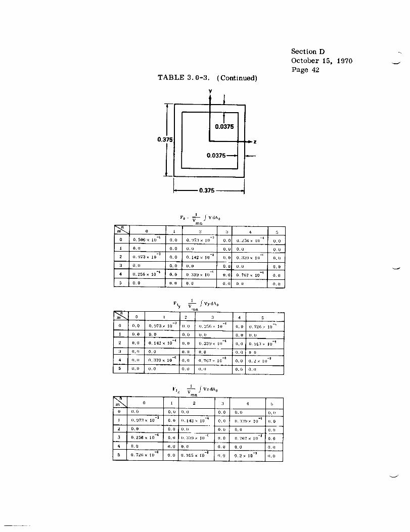
TABLE 3.0-3. (Continued)
0.37!
1
y
".'_----0.375
Section D
October 15, 1970
Page 42
0 1
0 0.506× 10 -t 0,0
1 0, 0 0.0
-32 0,973x 10 0.0
3 0.0 0.0
4 O. 256 x 10 -4 O. 0
5 0.0 0.0
F, v'--:v omn
'2 3 4 5
-30.973× l0 0.0 0.256x 10 -t' 0.0
0.0 0.0 0.0 0.0
0. 142 × 10 -4 O. 0 0. 339 × 10 -I; O. 0
0.0 0.0 0.0 0.0
0.339× 10 -_' 0.0 0.767>( 10 -_ 0.0
0.0 0.0 0.0 0.0
Fly Vfi--'- f VydAoqln
m_ 0 1 2 3 4
-3 -40 0.0 0..q73x 10 0.0 0.25(;× 10 0.0
I 0.0 0.0 0.0 0.0 0.0
2 0.0 0.142× 10 -4 0.0 0.339× 1(I -6 0.0
3 0.0 0.0 0.0 0.0 0.0
4 0.0 0.339x 10 -6 0.0 0.767× 10 -_ 0.0
5 0.0 0.0 0.0 0.0 0.0
5
0. 726 × I0 -_
O. 0
O. 013 × 10 -8
o. o
0.2 x 10 -_
0. o
Flz V1----- ;VzdAomn
m_ 0 1 2 ,'3 4 5
0 0.0 O. 0 O. 0 0.0 O. 0 0.0
1 0.973x 10 -3 0.0 0.142× 10 -4 0.0 0.3:Lq × 10 -_ 0,0
2 0.0 0.0 0. o 0.o 0.0 o.o
3 0.256x 10 -4 0. o (}.:;3!Jx 10 -c 0.0 o.7_;7× 10 -8 0.0
4 0.0 0.0 0.0 0.0 0.0 0.0
5 0.726x 10 "_ 0.0 0.915× 10 -_ 0.0 0.2× I0 -s 0.0

TABLE 3.0-3. (Continued)
1.0
L
y
I 0.049 ---,--
1.0 , I
_Z
Section D
October 15, 1970
Page 43
0 1
0 I). 1_(; O.I)
1 O. () 0, I)
-I'2 0.2x2 × tO [).0
:t I). (I I). l)
-24 0.577× III 0.0
O, l) ql )
0
1
Fo V-- Iv"a°rll n
2 :1 4 5
0.2x2x 111 ().0 I).577× Ill (I.(t
O. 0 {I. (I t1, I1 11. {t
I),:_2_ 10 l).(l 0.5X5_ l(l O.I)
It. I) I). 0 (i. (I U. I)
(I..r,X,rJ _ Ill II.t) 0.1 × III O.II
O. (I (I. I1 If. II f). 11
Fly @- J V'¢d),oill fl
t Z :t
-1l) O. l) O. 2N2 ,: lO (I, 0
1 o, I) (I. (1 (I, () I). 0
-22 O. 0 0. 212 X 10 I). l)
:_ (h 0 (I 0 O, I) (I. 0
4 I),(I 0.5K5 x lO -3 0.1)
5 I). 0 O. I) I). I) o. J)
I). 577 , 1o
O. 5x5 . 10
- 3
I1, I :_ ll}
4 5
(I. It 0, 125 _: 11)
11, 1) O. 0
_). 11 o. 1Z . I0
1). I) {I. I)
-4O. 11 O. I_IH × Ill
I). II O. I)
I) O, I)
-I1 t). 2'_2 ",( 10 O. 0
2 0 0 I). tl
:l 0.577 ,_ 10 -z 0.0
4 I). (I (I. 0
5 I). 125 x 10 -2 <LO
1
l",z _ I V/,L%Illn
!
O. I1
2 :f -1 5
4_. 1) (J, 11 11+ 0 O. 0
- 3
0.32× IO-' {1.0 1).5_5 )_ 11) f).O
O, I) I).(} [1, 0 O. (1
O.._,X5, I(l-_ 0.0 ILl< 1(t -_ 0.0
I1, (I (l. (} I). l) O, I1
0,12× I0 -'9 0.0 q).19!4× 10 -t O.I)

TABLE 3.0-3. (Continued)
i2.0
1
Y
1
10.095
0.095----
2.0
mn
m_ 0 1 2 3 4 5
0 0. 724 0, 0 0. 439 0.0 0. :36 0.0
| 0.0 0.0 0. 0 0. 0 0. 0 0. 0
2 0.4:1!) 0. 0 0.2 o. (9 0, 147 0. 0
3 0.0 (I. 0 0.0 0.0 0, o 0.0
4 0.3G 0, (, 0. 147 (I. 0 o. 1o1 0. (}
5 0.0 0, 0 0.0 o. 0 I} (I 0. o
0
0
!
2
3
4
5 (L o 0.0
Fly _ t VvdA,_
mn
1 >' :+ 4
O, 0 O. 439 O. 0 O. 3(; O. I)
I), 0 O. 0 O. 0 O. 0 O. 0
0.0 O. 2 O. 0 O, 1.17 (). 0
O. 0 _). I) O. 0 o. o (}. 0
O. 0 0. 147 0.0 O. 101 O. 0
0.0 O. 0 O. 0
3
0.'114
I).O
1}. 12
O.(l
0.7!)N _ 11} -1
O. l)
Vtz _ J WdAo
rI/n
1 '2 :}
n). (1 o. 0 a). o r). i)
m_ 0 4
0 O. I}
1 (}. 439 I). (I O. 2 O. 0 O. 147
2 (I. 0 I). 0 O. 0 O. () O. 0
3 O. 36 O. 0 O. 147 O. 0 0.101
4 O, 0 (}.0 O. o (),0 o.I}
-t5 0,314 0.0 (I. 12 o.0 O. 7!)8 × lO
5
O. 0
O. I)
O. t)
o. I)
O. {)
O. 0
Section D
October 15, 1970
Page 44
--..,.4"

OF POO;:i ;' .... _ ....'e_:,'-&i I Y
TABLE 3.0-3. (Continued)
Section D
October 15, 1970
Page 45
0 0. 177 _ ! 0 z (). 0
[ O, 0 0. (I
2 O, 24 * t [)l I). !1
:l 0, 0 0.0
,I O. 4,| _: IO I O, (I
5 O. 0 O. 0
Fo _, / V d.",oHin
2 3 4 5
(I.2|_ 1(I I 0,0 0.44× 1(I l O, II
0.1) 0.(I O.I) ().()
().24,_ ( I01 I),0 0.4:_ 101 (I.(I
I). (I O, 0 I). (l (I. 0
0.4,(t[) 1 0.0 O.GI5 _( 101 0.(I
(I. 0 O. 0 ¢1, 0 O. I_
0
1
F_y _ /vy,J,%11111
1 2 :1
I) O. [) (I. 24 < 1(I f (}. 0 O. _A , l(I I
J O. (I O, 0 O. 0 t}, 0
2 0.0 0.244_ 11) 1 0.0 11,4× 1(I I
3 (I. 0 O. (I o. o o, 0
,i 0.0 0.4x 11) l (I.0 IL(iI._,( [()1
5 0. 0 II. 0 I). 0 I). 0
4 5
(I.II O, XT)G × ltl _
O. o O. O
0 0 (I, 732 ,( 101
O. 0 O, I)
O. 0 O, 1 (19 _ [()_
O. 0 O, (I
(I
1
'2
4
5
0
I). (}
0.24 x 10 !
0.0
0. 44 x 101
0.0
O. 856 x 101
Ft z _ lvzdAoHIB
1 2 :] I 5
I). (I 0.1) O. I) (I. 0 O. I)
O. 0 O. 2'1,1 ",," l01 0. 0 I), 4 X 101 O. 0
0.0 O. 0 0.0 0.0 0.0
0.1) 0.4 _ ill I P.I) I).GJS* lO 1 (I,I)
0. O O. 0 0.0 (h 0 O. l)
II.() 0.732, 101 0.(} O. tO9x 102 0.0

TABLE 3.0-3. (Continued)
Section D
October 15, 1970
Page 46
V0.277
1_Z
0
1
2
3
4
5
1
Fo _ .j VdAomn
0 1 2 3 4 5
-I -3 -40.508x I0 0.0 0.712× l() 0.0 0.154× 10 0.(1
0.0 0.0 0.0 0.0 0.0 o.0-3 -7
0.679× 10 0.0 0.466× l0 -5 0.0 0,647 × 11) 0, o
0.0 0.0 0.0 O.O 0.0 0.0
0.143× 10 -4 0.0 0.7× 10 =7 0.0 O. XO!I'.< I() -i) ).0
O. 0 O. 0 O. 0 O. 0 O. o ). o
m'_ 0 !
-30 0,0 0.712× I0
1 0.0 0.0
-52 0.0 O. 466 x 10
") (}. o O. 0
-T4 0.0 0.7x I0
5 0.0 0.0
Fly V1--- [ VydA0mn
2 3 4 5
-4 _60.0 [I.154× 10 (1.0 (1.3_2× 10
0.0 O.() (,).0 0.0
-7 -80.0 (1.647× I0 0.0 0.113× I0
0.0 0.0 0.0 0.0
i0-9 i-I0
0.0 (1.809× 0,0 0.131 × lO
0.0 0.9 0.0 0.0
1
Flz "_mn VzdA°
m_ 0
0 0.0
-11 (I. 679 × 10
2 0.0
-43 0.143× 10
4 0.0
-65 0.339x 10 0.0 0,117× J0
I 2 3 4 5
0.(1 O.O 0.0 0.0 0.0
-5O.O O.4G(; ,< l(l O.O 0.G47× I(1-7 O.O
0.0 l).O 0,0 0.0 0.0
-7 -i)0.0 0.7,( I0 0.0 0.80;I× I0 0.0
O. 0 O. 0 O. 0 O. 0
0.0 O. 0
-8 0,87× I11 -|I j (.).0

TABLE 3.0-3. (Continued)
¥
Section D
October 15, 1970
Page 47
T-1.0
L=Z
= 1.5 •
I)
1
2
:1
5
t [ V(IA0
() 1 '2 :l
(). (J I). t} O. I_ O, (}
[), 1!)!9 I),l) 0.:Z(I_ _ l0 -1 (1.()
I). 0 (_. 0 (J. l) (I. 0
0.(;,| _ 10 (J.f] t)..l_.1:, 10 {9.0
O. () O, () {). 0 I). (}
4 5
-1(_, (_k - 10 (), l)
1). 0 (). I)
(). 447 ", lg) -_ O. 0
(). D O. q)
(). _7(; _. ll) I). ()
19. 19 I). (I
()
1
:l
4
5
1
FI _ I Vyd,\rjY
r_ln
1 2 :_ ,| 5
~1 -i(),l) (l,')()_ (I.(J (),(;_X _: 11) I).(I O.Zii4× 10
() IA (I. f) (). (9 It. (I 99.0 f). (1
iO -I _ -_I).(I 0.208 ,< O.I) 0..147× l(t O.q) ().12:1",_If)
D. 0 I). D 0. [) O. 0 0. 0 0. 0
-30.0 0.4_4 _ t0 -_ O. I) (I. _7(; × 1() -_ 0.0 0. 224 _ II)
O. 0 O. 0 O. 0 (I. 0 (I. 0 O. 0
1F_z _-- ] vxd,\o
r)lll
I)
1
2
:1
4
S) 0.2:_4× 119-I 0.0 1).127u 111-:! 0.(I I).t411× 10 -3
0 1
o. (I o, 0
(9.19!) o. o
O. 0 q). o
-I0.(;4 ;< 10 IP.0
(). o (I, o
2 :_ 4 5
II. () O. 0 (). I) O. I)
-_ 111-zII,2H8 _ 1() (I. 0 ().,1_)7 x 0.0
o. l) o. o o, o i), (i
my --_11..1_1 _ l tl I1.0 (I. xTI; × 10 0.0
O. (I O. 0 (I. () (I, 0
(I, (J

TABLE 3.0-3. (Continued)
y
2.75
L
Section D
October 15, 1970
Page 48
F 0 V1_ j VdAonln
m_ 0 I 2
0 0.114x l0 t 0.0 0.122× 10 J
1 0.0 0.0 0.0
2 0.116x 10 t 0.0 0.593
3 0.0 0.0 0.0
4 0. 183 x 101 0.0 0, I;47
5 0.0 0.0 0.0
m_ 0
0
1
2
3
4
5
:! 4
0.0 0. 19(; x lo t
0.0 0.0
o. 0 0. 597
0.0 o.o
o, 0 o. 53
0.0 0.0
5
o. 0
0.0
0. o
0.0
O. 0
0.0
Fly VI-_ J'VydAorI1FI
1 2 3 4 5
0.0 0.122x 101 0.0 0.196)_ 1111 0.0 0.352x l0 t
0.O 0.0 0.0 0.0 0.0 0. o
O. 0 0.593 0.0 0. 597 0.0 0. 744
0.0 0.0 0.0 0.0 0.0 0.0
0.0 0.647 0.0 0.5:] 0.11 o. 59_
0.0 0.0 0.0 0.9 0.0 0 0
Fiz= V1------ fVzdAo
mn
m_ 0 1 2 3 4 5
0 0.0 0.0 0.0 0.0 0.0 0.0
1 0. I16 x l0 t 0.0 0.593 0,0 0.597 0.0
2 0.0 0.0 0.0 0.0 0.0 0.0
3 O. 183 x l0 t 0.0 0.647 0.0 o.53 0.0
4 0.0 0.0 0,(] 0. o 0.0 0.0
5 0.313× 101 O.0 0.71i9 0,0 0.39x 0.0

f
OR,_,I,o,.... PAGE IS
OF POOR QUALITY
TABLE 3.0-3. (Continued)
5.844 _ z
Section D
October 15, 1970
Page 49
0
I
2
3
4
5
0 i
O. 147 × 101 O. 0
O. 0 I). 0
1). G34 x iO I I).kl
0.0 0.0
O. 42 x 10 _ O. 0
0.0 0.0 O. 0
F o V1_ j V dA o
llln
2 3 4 5
0.1;I;4"_ 101 ().1) 0.4522- 10 2 I).O
0. I) (}. 0 O. 0 O. (}
().l:ff;× 10 :! 0.0 0.5_> 102 0.0
O. 0 O. {t O. I} (I. (I
O. I;2_ _ ll) 2 O. 0 O. 21G _ 1113 (I. (j
O. 0 O. 0 (I. (}
F, _ [ Vvd.%y ' • •
nln
0 1 2 :l ,I 5, 0.[) 0.6fi4X 101 0.0 0.452x 10² 0.0 1).342x 103
1 O. O II. O (I. (} I). (J II. t) O. O
g (}.0 O.I:_G:_ 10 2 0. O 11.7,XX l(l:' H.O O.:tt}.l _ 10 3
3 1). (I O. l) O. i) I). O H. O O. O
.I 0.0 0.[128x 10 ;! 0.0 0.211; < 1(I '_ 0.0 0.102_ 1(} 4
5 (I. 0 I). 0 (}. It (I. 0 I). 0 (I. 0
I)
1
2
;I
4
5
F,z & j Vz¢'%
m r)
0 1 2 3 ,1 5
0. I) O. D O. r) O. 0 _). 0 o, 0
().(i_]4X I.I) 1 0.0 (I.l:_l; _ 10 e 0. l) I).SX* 102 (I,O
O. (I O. (3 O. 0 O. 0 O. II (L (I
0.42,{ t{} 2 0.0 0.1;2/8_ 11) _ 0.(I 0.216× 10³ O.0
{}. 0 O. 0 O. 0 l}. 0 (). 0 O. l)
0.:]0,I× 103 0.0 0.314v l(l 3 0.() 0.1;_,2 >_ 11) 3 0.0

0
I
2
3
4
5
0
I
2
3
4
5
0
l
2
3
4
5
TABLE 3.0-3. (Continued)
¥
-------6.0------*
z
! J' VdA oFo= _--mn
0 I 2 3 4
0.159× 10² 0.0 0.532× 10² 0.0 0.282× I03
0.0 0.0 0.0 0.0 0.0
0. 508 × I02 0.0 0. 851 × 102 0.0 0. 293 × 103
0.0 0.0 0.0 0.0 0.0
0.262x 10³ 0.0 0.317× 10³ 0.0 0.918× 10³
0.0 0.0 0.0 0.0 0.0
5
0.0
0.0
0.0
0.0
O. 0
O. 0
0
0.0
0,0
0. o
0.o
o. 0
0.0
l
Fry _ / VydAomfl
1
O. 533 x 102
0.0
O. 851 x 102
0.0
0.317 x 10³
0.0
2 3
0.0 0.2X2x 103
0.0 0.0
0.0 0.293x I03
0.0 O. 0
0.0 0.918 x i()3
0.0 0.0
4
0.0
0,0
O. 0
0.0
0.0
0.0
5
O. 173 × 104
O. 0
O. 12:) x 104
0.0
O. :175 x 104
O. 0
o
o.0
O. 508 x 102
0.0
O. 262 × 103
o.o
o. 154 x lO 4
1 j VzdAoFlz _ _ •mn
I 2 3
0.0 0.0 0.0
0.0 0._51 × 10 z 0.0
0. o 0. o o.0
o.o o.317× 1o 7 o.o
0.0 0. o o.0
0.0 0.133× Io4 0,0
4
0.0
0.29,3× 103
O. o
O. 91_ × 107
0.0
0.25× 10⁴
5
0.0
0.0
O. 0
0.0
0.0
0.0
Section D
October 15,
Page 50
1970
/
0
i
2
3
4
i 5
m \
0
1
2
3
4
5
[I
I
2
3
4
5
TABLE 3.0-3. (Concluded)
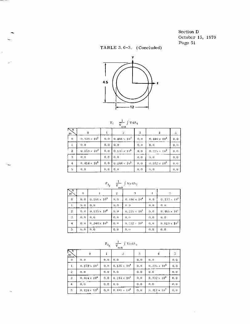
¥
I11n
0 1 2 3
O. 934 × 101 O. 0 O. 166 × 10 a O. (1
O. 0 O. 0 O. 0 O. 0
0.159x 10³ 0.0 0.135 × 1() 4 0.0
O. 0 O. 0 O. 0 O. 0
0.414w 10 '_ 0.0 0.244 × 10⁵ 0.0
O. 0 O. 0 O. 0 O. 0
4
O. 446 x 104
O. 0
O. 225 x 105
O. 0
O. :i32 x 106
O. 0
0
O. 0
O. 0
0.0
O. 0
O. 0
O. 0
Fly
1
O. lt;G × |0 3
O. 0
O. 135 × 104
O. 0
O. 244 × 105
O. 0
] VytlA oV , '
Inn
2 3
O. 0 O. 441; x 104
O. 0 (_. 0
O. 0 O. 225 "_" 105
O. 0 O. 0
0.0 0.:]:12 ,_ 10 I;
O. 0 O. 0
,t
O. [1
0.0
O. 0
O. 0
O. 0
O. 0
0
I). 0
0.159× 10³
O. 0
O. 414 x 104
0.0
O. 118 x 10 _
F1 z V 1 ./ Vz dA o
n/n
1 2 3
I). 0 O. (I O. [)
0.0 0.135 × 10⁴ 0.11
(}. 0 O. 0 O. 0
0.0 0.244x 10⁵ 0.(}
0.0 0.0 0.0
0.0 0.4_1 x lU G 0.0
4
0.0
0.225 _ 105
0.0
0.3:]2 × 10⁶
0.0
O. 412 × 107
5
0.0
O. 0
O. 0
0.0
O. 0
I). 0
5
O.l:_3x 1(I _:
I). II
O. 465 × 10 +;
O. 0
o. 619 x 107
O. 0
5
O. 0
0.0
O. [I
O. 0
O. (I
O. 0
Section D
October 15, 1970
Page 51

B. Results:
Section D
October i5, 1970
Page 52
x x2MT (xl) L x 2 MT (xl)Z
z ax,dx ÷±f fv(x) =-f0 f0 EIz (xl) L 0 0 zdx 1 dx 2
v(x) ="_ (_-II-IIx)L 2Io z
where
fl flI 1 =0 0 g'(Xl)
X X 2
dxldx 2 and Ilx= f f _ dxldx 20 0 g (xl)
u (x) 1 ?1 f_v :_-0_A
o_ET dA dx a F 0 L xj_= f(xl) dx 1A° 0
M (x) =0Z
PT
a = -nET+ -_ +XX
MT + My
Y + yIY
MY
may or may not be zero, depending upon the boundary condition.
If end B is hinged, then
Uav(X) = 0 ,
V 0 = M 0 = 0 ,
v(x) = same as above,
a = -nET+ +
= Iy \axial force P = /" c_ ETdA
A
Y _
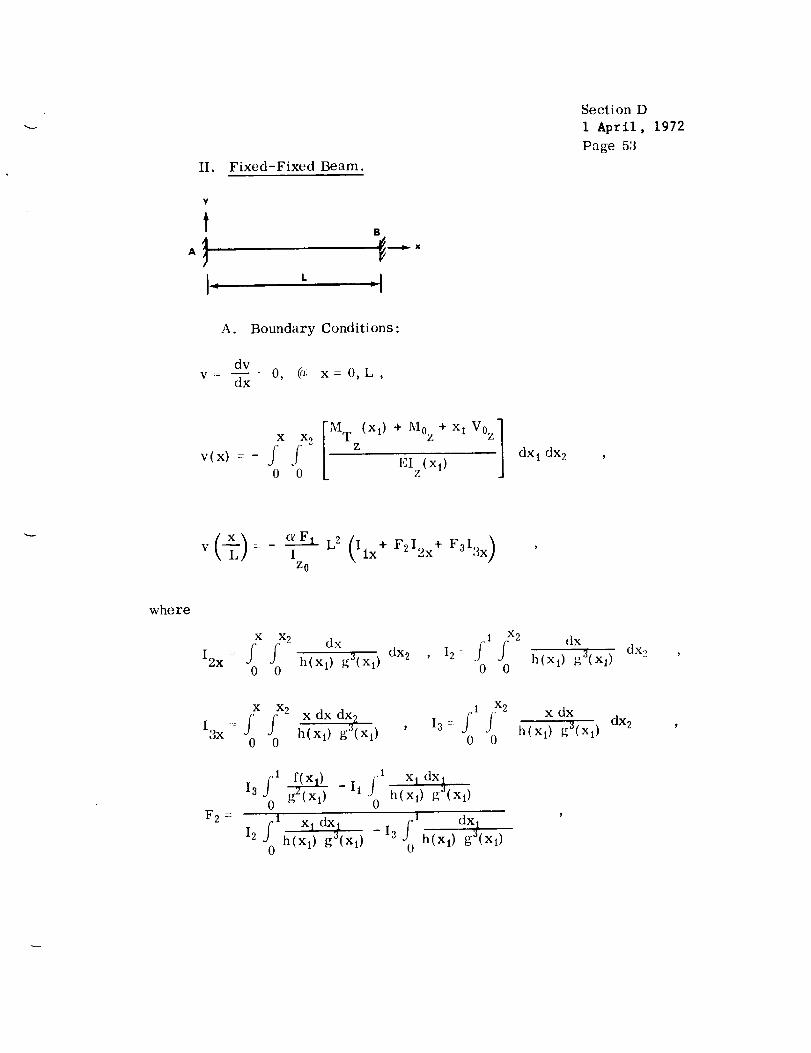
II. Fixed-Fixed Beam.
Section D
1 April, 1972
Page 53
¥
-tB
A. Boundary Conditions:
V --
dv
dx:.: O, (or x= O,L,
X X 2
0 0MTz(Xl) + M0 z + x 1 V°z I dx 1 dx2EI (xl)
Z
IZ0
where
x x2 dxdx 2 I2 :
0 0
dx _ dx,2j l jx2 h(_1) _a(x,)0 0
X2
I3x = f J h(_,) g_(×,) ' o o0 0
x dx
h(xl) g3(x_) dx2
F 2 -
j.1 1 x I dx_13 _ -I_ j' h(x,)_ (xl)g_(xl)
0 0
fl xl dx i fl dx ,,12 h(xl ) g3(xl) -13 h(x,) g_(xl)0 0

F 3 -
f!l dxl - 12 f(xl) dxlII h(Xl ) g_(xO gZ(xO
0 0
I2/ h(Xl)xldXt f'g _'xA_11 - I30 0
dx 1
t_(xO g_(xl)
Section D
October 15,
Page 54
1970L_
(Table 3.0-4 gives values for F2 and F 3)
M0z c_ E F 1 F 2 ,
o_
Voz = --_ E F 1 F3
Mz(X ) = MOz + x Voz
Uav(X)= _ "Jxl• A° 0
f(x 1) dXl
If the end B is restrained against longitudinal motion, then
Uav(X) = 0 ,
(.) (.M)M T My MT zz
cr = -a ET + Y z ÷ yxx I I
y z
v(x), Mo, Vo
CASE a: EI (x) = constant,z
(__) c_ F 1 x 2v - IZ
are same as above.
+n
2 _ E Fl(q-1)M° z - (q+l) (q+2)

TABLE 3
ORIGINI_.L PZ._E {3
OF POOR QUALITY
• 0-4. VALUES OF CONSTANTS F2, F3,
Section D
October 15, 1970
Page 55
A ND F 4
Notes :
II q II {_ s II I 14
; _ I , r--, T__-_-X-+-F--,., ]+-;.,_ -,+
t '+_:1 .... i .... _L::+-: 't ' "+"+++ "
i 1_ w) :__b_ -I ,hl o I_ 1 ,, ,l ,1,i -I 111 _l i,i I ,F
q 4< ,,I+,( I, r,,l. J ,+uJ, lh_IPll,,+h,,,ll
(; l++ Ii rl J L; I , , I, l +;
, +, 1+,,_ +, ,,,,+ . I,I I +J ,+ _.,1 , , _ -,+ 1,, I _+
o I . :+1; i, ,+.l_ u l lc I i, t _1 ZT:< + -i ,,,'+ -(_ I I U I
...... .----+- ..... +-- ..............
o, u u_ , . m_l -. t ;1, i . . ,+ +I ......i :+, ,_ + . + o--- + ........
w) i ii ut _ + ilL+ ii I '+J _ LI + WJ , _ I H,, -+I If; I H I
......... t p41 I H I I -I II'+_ =IF }L+:I IF I + ;I .it I II+l 0 l I [ +1
++ , <+ .:t, I lt_ . :, t h I + ,11'1 +-'"
- N .... -+..... +.... L-+j + +l :H. -I l,,, Tit I I ,l+ -. 1 + ii _.
......... +- + + ,
<+ r'r i+ : + ' i t'+ : (' i<,, = . ,' +, ++' :,;.._ -if+,. I '+'i ?
............ "_ ' "+; _,....+"' I /'L '2Z'_ .........-+''' _+_+, . .'i+, -I :,,,i t ,, Ir,t , '+ ,, .+_" -i ,+, [ ,H<, : . '+
........ _ ............ f---- 1
t o _ 'I'+ I :!++ i -..',- I 1 i, +_ '_' -I 7!, i +i l'''r [ I .I i
_, :1,, t , - q:i
- i- +1 _. ,_
_, ;1' _ ' 1,.
,, ; I h :' t
+ -- .
. ........ .: %.,.
h(,,,): ,.+,-,(4

6_EF1 qV°z = - (q+l) (q+2)L
M = 2_EF| F(i -z (q+1) (q+2)
CASE b:
M T (xl)Z
EI (xl)Z
= constant
v(x) = o ,
M0z = -M T ,Z
V0z 0 Mz = -M T = constant.Z
A
III.
Y
t
Id
Fixed-Hin_d Beam.
B
"l
A. Boundary Conditions:
dv
v- dx-0, @ x=0
MTd2v z
v= -_x + EI -0,Z
(_x=L
Section D
October 15, 1970
Page 56

L2[ ( )]v = - I Ix 1+ F4 Ix 2 -Ix 3z0
Section D
October 15,
Page 57
1970
where
F4 = I1 (refer to Table 3.0-4 for values of(I3 - IJ
= _ _ E F_ F 4V°z L '
F4) ,
M0z = c_ E F 1 F 4
FQ L {-Ix
Uav(X) = j f(xl) dx IA° 0
PT z y(r =-a ET+ -_ + y+xx I I
z y
If the end of B is hinged,
Uav(X) : 0 ,
MT z T My
:-aET+ z Y zxx I Y+ I
z y
CASE a:
EI = constantZ

Section D
October 15, 1970
Page 58
+ t >3t}Io z -
3_ EF 1V°z = (q+l) (q+2) L
3_EFIM°z - (q+l) (q+2) '
M -- -
z (q+l) (q+2)
CASE b:
MTZ
EIZ
(x) = constant ,
v(x) = aft xZ ( x)I _ 1--yZ
3 o_EF tV°z = L
3MOz = - __2 _EF1
Z _(,-_) o_,IV. Deflection Plots.
From the previous cases the deflection expressions were found to be
A. Simply Supported Beam:
v<_,:_ (_ _,-_,x)I0 z

B. Fixed-Fixed Beam:
v(x) :- F'L2I0z (Ilx+ F212x+ F313x)
Section D
October 15,
Page 59
1970
C. Fixed-Hinged Beam:
These expressions have been plotted for parameter variations (ff beam width,
depth, and degree of thermal gradient along the beam length. The plots are
made in nondimensional form with tile following designation:
and
FF:_- (Ilx + F212x + F313x )
Therefore the deflection,
FS, or FF by
Ia z
v(x), for any case can be found by multiplyinK, SS,
Figures 3.0-4 and 3.0-5 show the variation of FF and FS as a
function of lengthwise temperature gradient. In the figure, G II _- 0 (con-
stant cross section) and N equals the exponent of the thermal variation along
the leng_h of the beam;e.g., N= 0 means constant variation, N 1 means
linear variation, etc.
Figures 3.0-6 through 3.0-13 show the three deflection parameters SS,
FS, and FF for variation of parameters G, It, and N, where II equals
variation in width of beam along the length, G equals variation in depth at
x= O) (refer to Paragraph 3.0.3.1).

Section D
October 15, 1970
Page 60
ORIGINAL PAGE ;_OF POOR QUALITY
,ql
* .OO|
--4---4
.--t--i
* .O01 i s• i
* o00ql
----_--i
° ._1'
r--* *
" ._ ' .
" 4"-- f
O
_:, ,
'L'k
I
,
N-2 •N=3 _-N=4N'5N=6N=7N=8
.........
i --
I :
i •
I
:'.,4jk
[*I It
J: ,.
1
i
I
[
i :
J ' ' IIi . i
i
. . ÷
l
Figure 3.0-4. Deflection parameter FF versus distance along beam for
variation of lengthwise temperature gradient.

ORIGI_,7_. F,-,_ _
OF POOR QUALITY
Section D
October 15, 1970
Page 61
.01_4
.ors
Figure 3.0-5. Deflection parameter FS versus distance along beam for
variation of lengthwise temperature gradient.

Section D
October 15, 1970
Page 62
P
L
o
T
0F
s
$
f
S
F
=
P4
i
,n,8
*0t
.ll
* FF0 FS+ SS
_iiiii
_i ill
t _- %t--t-
• l
O.I
095 g_$
1,0
Figure 3.0-6. Values of SS, FS, FF versus values of T(x/L)
for H=0, G= 0, N= 1.

f---
OF POOR F_L!,_LI, V"
Section D
October 15, 1970
Page 63
.... r
.o$
P
k
0 ....
T
0 ....
F
$ .OZ
$
F
S
r
F
&
o
N
Z .0%
I
1,/!/
l i
I i I
III
ql
I VI
i ! !
iii
:
441
-t- + _-
i ioi,4-.
If'l--'
[IA_I/llll
!!!!: ) t I
t I 1 i
iiiiiiiiiJJi
d!!!
+ 4 *-
-+ -i 4- -4---
-+ : : :
: : : ..
--+ + • +--
'r : : :
it loi,
_ + _ _
V_LUE$ OK T
{)[}4 004
i :
q
Figure 3.0-7. Values of SS, FS, FF versus values of T
for II= 0, G-_ 0, N= 2.

Section D
October 15,
Page 64
1970
_5 _ Z _59_J6 996
VALU(S OF T
Figure 3.0-8. Values of SS, FS, FF versus values of T
for H= 0, G= 0.5, N= 1.
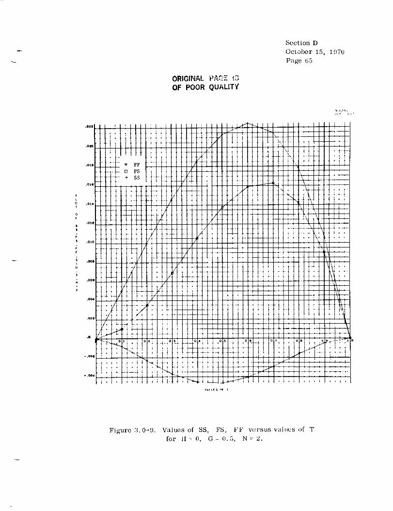
Ps,,:._. _:3ORIGINAL • '_'::
OF POOR QUALETY
Section D
October 15, 1970
Page 65
.DO4
.oolt
.0
- .004
J
/
..... t
i
II]i
'I
K
Q
j i
_., I? %q
Figure :_.0-9. Values of SS, FS, FF versus values of Tfor tI = 0, G- 0.5, N=: 2.

Section D
October 15,
Page 66
1970
_9Z2_
.084
.D|I
.Q$4
.850
.OO4
.0051
.OO4
V*LU(S (:_ I
Figure 3.0-10. Values of SS, FS, FF versus values of T
for H= 0, G= 1.0, N= i.
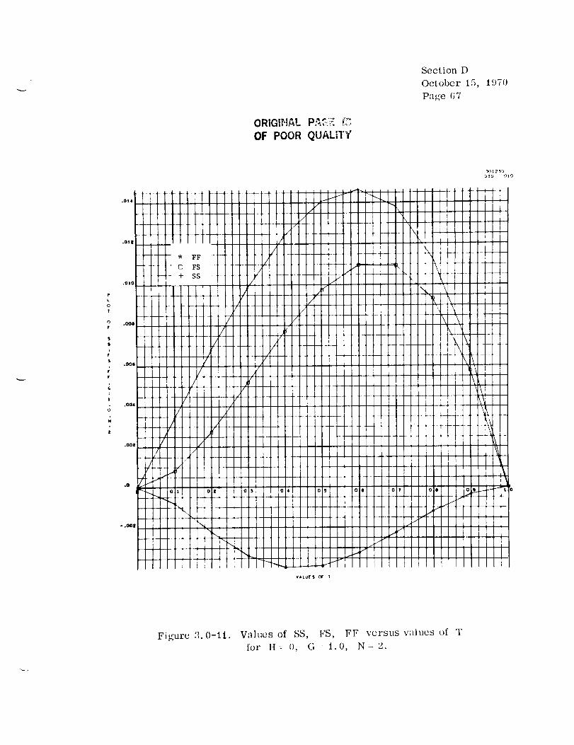
P:_,',;_. {LORIGINAL ""_: ....
OF POOR QUALET't'
Section D
October 15, 1970
Page (;7
919 919
VALUe'S* OF T
Figure 3.0-11. Values of SS,for It : O, G
FS, FF versus vulues of T
1.0, N =- 2.
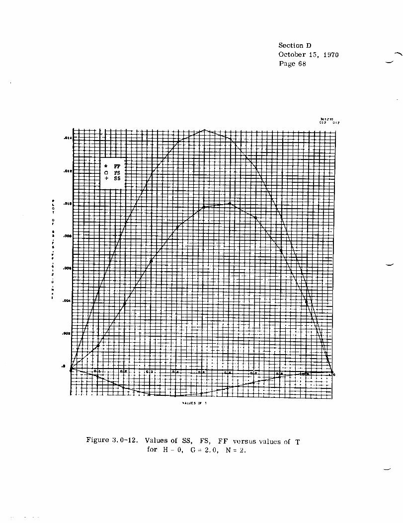
Section D
October 15, 1970
Page 68
.Ol4
.Oil
.OIO
.0OQ
.OOq
,OQ(
on
i ( , __
LLi- ....
iii i /iii!ii i /!!II I ,_[ i i /
i i
I
ii i :!i i [
______._ ._ _ ,*(
i : ; A
_-II /iii ii f!_ i! /
Lii /ii.-_- l r
F._-. !
r-iF
,-iW- / _.::J'-t-- ,2...
_" '--t _ ..........._ ._'_,l,,d--- _ _ "_-___ _ ......
b,,J-" !
/ i
i
[i
r _
f"
/-
/
-I
i ! ......
j
\
-\\
m__
J
-t- " "
q:: -.,I I
1_
i
FI
\\
\\
[\ \
\\\
3(_1Z_
[ : i
--j
i
!I
J1
i
i
I1
-t-"
g
!,
-4
ii :
I Ii I
)
Figure 3.0-12. Values of SS, FS, FF versus values of T
for H= 0, G= 2.0, N= 2.

ORIGINAt-OF POOR PAQ_ IS
QUALITy
Section D
October 15,
Page 69
1970
_33 '51)
°O0(
.001
o0
- .001
VALU[$ Of I
Figure 3.0-13. Values of SS, FS, FF versus values of
for H= 0, G= 2.0, N= 2.
T
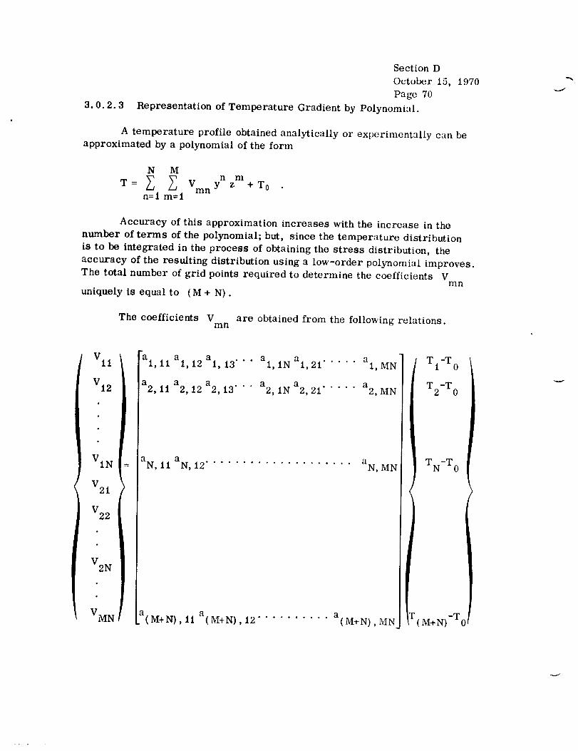
3.0.2.3
Section D
October 15, 1970
Page 70
Representation of Temperature Gradient by Polynomial.
A temperature profile obtained analytically or experimentally can be
approximated by a polynomial of the form
N M
omT= V y z +T Omnn=l m=l
Accuracy of this approximation increases with the increase in the
number of terms of the polynomial; but, since the temperature distribution
is to be integrated in the process of obtaining the stress distribution, the
accuracy of the resulting distribution using a low-order polynomial improves.
The total number of grid points required to determine the coefficients Vnl n
uniquely is equal to (M + N).
The coefficients V are obtained from the following relations.mn
VIN
V21
V22
V2N
VMN
al, ll al 12 al, 13" . a a a, " 1,1N 1,21 ..... 1, MN
a2,11 a2,12a2,13" " " a2,1Na2,21 ..... a2, MN
a a •N, 11 N, 12 .................... aN, MN
a(M+N) II a(M+N) 12 .......... a(M+N) MN
T I-T0
T2-T 0
TN-T o
M+N)-T0

n rn
where a. = Yi z.1, mn 1
point at temperature T.1
section.
Section D
October 15, 1970
Page 71
The values (Yi' z.)t = coordinates of the ith grid
and T o = temperature at the centroid of the cross
If the temperature difference (T.-T0) is continuous and symmetrict
about the z-axis, then Vml= Vm3 = Vm5 = . . . = 0, and if it is continuous
and antisymmetric Vm2 = Vm4 = Vm6 = . . . 0. Similarly, for temperature
differences that are symmetric about the y-axis, Vln = V:I n = Vsn = . . . 0,
_ : . • •and if it is antisymmetrie about the y-axis, V2n V4n V6n _ 0.
If the temperature varies only in one direction (e.g., for w_riation
along the y-direction only) along either the y- or z-axis, the polynomialreduces to
N
)2 nT-T0= V yn
n--1
V 1
V 2
V n
"all a12 ...... aln
a21 a22 ...... a2n
anl an2 ...... ann
/ T1-T 0
T 2.T 0
T -Tn 0
n
aln Yi
As before, if the temperature difference is continuous :md symmetric,
V l= V 3= V 5= . . . 0; and for continuous antisymmetrictemperature dif-
ferences V2 = V4 = V6= • • • 0.
If the grid points are equally spaced on the cross section, say atdistance dl, then the polynomial can be written in nondimensional form as
T 1 - TO= . V di nn=l n d I
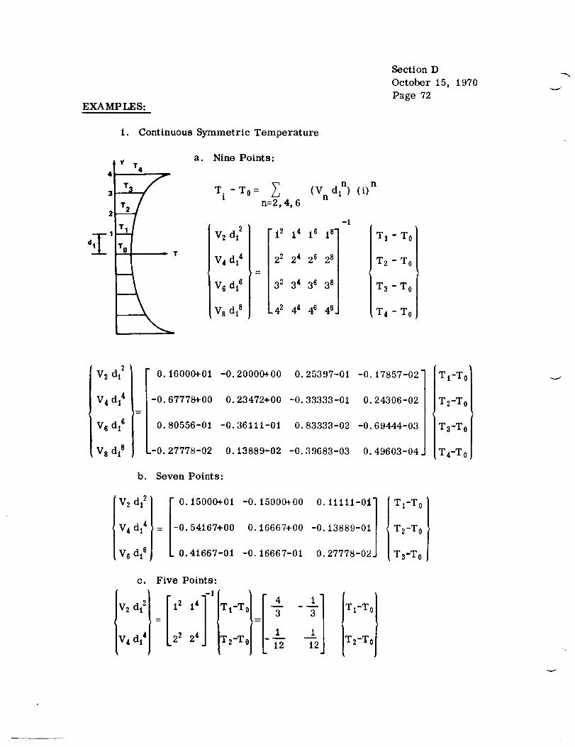
EXAMPLES:
Section D
October 15,
Page 72
1970
1. Continuous Symmetric Temperature
Y T 4
2
T_-_%,o! _,
a. Nine Points:
T. -To=l
n=2, 4, 6
V2 dt 2 12 14
V4 dl4 22 24
V6 di e 32 3 4
V 8 di s 42 44
( Vn di n)
-1
16 18"
2 e 28
36 38
4648"
n
(i)
T 1 - T O
T 2 - T O
T3 To
T4 To
V 2 dl 2
V 4 dl4
V 6 die
V 8 dis
O. 16000+01
-0. 67778+00
0. 80556-01
.-0. 27778-02
-0.20000+00
0.23472+00
-0.36111-01
0.13889-02
0.25397-01
-0.33333-01
0.83333-02
-0.39683-03
-0.17857-02"
0.24306-02
-0.69444-03
0.49603-04
b. Seven Points:
,v2,21[iiloo ololoo ooo.11111_ot1V4dl41 = - 54167+00 0.16667+00 -0.13889-01
IV dl eJ 41667-01 -0.16667-01 0.27778-02JTI-T o
T2-T o
T3-T o
c. Five Points:
:[TI-To
T2-T
TI-To 1
T2-To /

I
2. Continuous Antisymmetric Temperature
Section D
October 15,
Page 73
1970
-l--
d 1
!-
#--
Vi dl
V 3 dl3'
V s dis
V 7 dl7
a. Nine Points:T 4
V1 dl /
V3 dl3 / =
V s dls
V 7 dl 7
1 13 15 17-
2 23 25 27
3 3 3 35 37
4 43 45 47
-I
Ti-T o
T2-T 0
T3-T o
T4-T o
0.15003+01
-0.54209+00
0.41787-01
-0.86045-05
-0. 30031+00
0.33375+00
-0. 33454-01
0. 86045-05
0.33466-01
-0.41847-01
0.83850-02
-0.36876-05
-0.22126-04"
0.30116-04
-0.86045-05
0.61461-06
b. Seven Points:
Vld
V 3 d
V s d
:}[_!.i oo+oi= 54167+00
41667-01
c. Five Points:
I'dd. Three Points:
-0.30000+00
0.33333+00
-0.33333-01
0.33333-01
-0.41667-01
0.83333-02
+L++0/T 2-T 0)
T1-T° [
T2-T o
T3-T 0 [
TI-To ]
T2-To
T3-T 0
T4-T 0
Vi dl = T i - T O
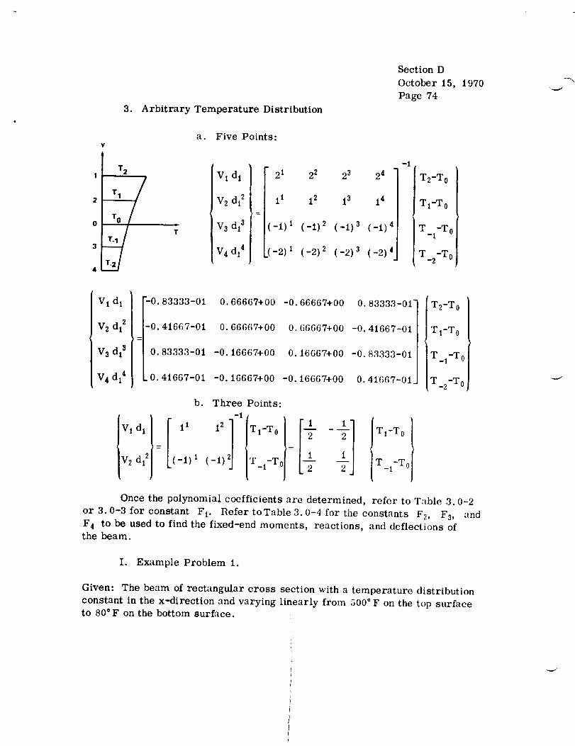
3. Arbitrary Temperature Distribution
Section D
October 15, 1970
Page 74
Y
1T 2
1 ! T12
3
4
/r
a. Five Points:
Vi dl 21
V 2 dl 2 11
V3 dl 3 -1) i
! 4iV4 dl -2) 1
2 2
12
(-1) 2
(-2) 2
2 3
13
(-1) 3
(-2) 3
24
14
(-1) 4
(-2) 4
-1,
T2-T 0
T1-T 0
T-i-T° ]
T-2-T0 I
VI dl
V2 dl 2
V 3 dl3
V 4 dl 4
-0. 66667+00
0. 66667+00
0. 16667+00
-0. 16667+00
-0. 83333-01
-0. 41667-01
0. 83333-01
0. 41667-01
b.
'lId l i t
dl 2 (-I) 1
0. 66667+00
0. 66667+00
-0. 16667+00
-0. 16667+00
Three Points:
-1
(-1),v Ii;]17 /
0.83333-01"
-0.41667-01
-0.83333-01
0.41667-01
T2-T 0
T1-T 0
T_l-To
T_2-T0
Once the polynomial coefficients are determined, refer to Table 3.0-2
or 3.0-3 for constant F 1. Refer toTable 3.0-4 for the constants F2, F3, and
F 4 to be used to find the fixed-end moments, reactions, and deflections ofthe beam.
I. Example Problem 1.
Given: The beam of rectangular cross section with a temperature distribution
constant in the x-direction and varying linearly from 500 ° F on the top surface
to 80°F on the bottom surface.
v"
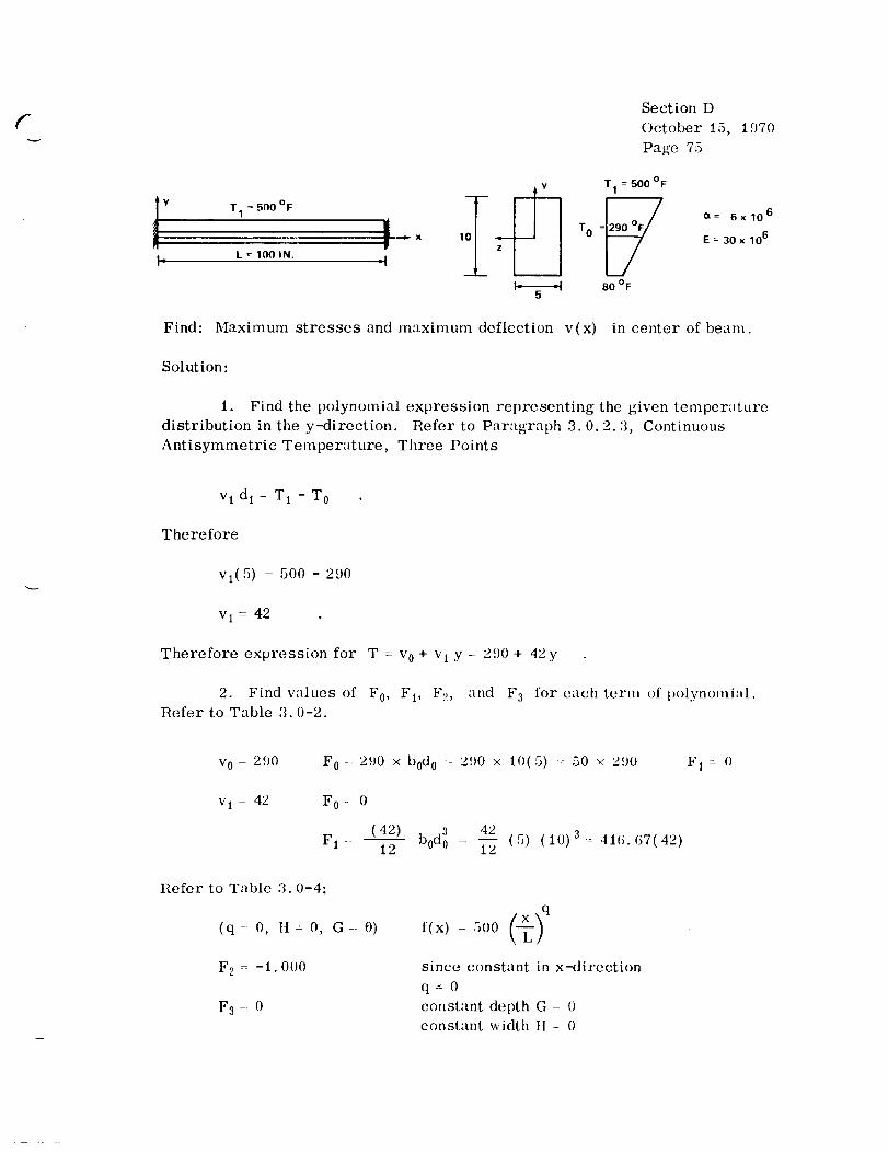
f
Y T 1 = 5N0 OF
L = 100 IN.,I
5
Section D
October 15, 1970
Page 75
T 1 = 500 OF
TO =_
80 OF
a= 6x 10 -6
E = 30 x 106
Find: Maximum stresses and maximum deflection v(x) in center of beam.
Solution:
1. Find the polynomial expression representing the given temperature
distribution in the y-direction. Refer to Paragraph 3.0.2.3, Continuous
Antisymmetric Temperature, Three Points
vt dt = T i - T O
Therefore
Vl(5) = 500 - 290
v 1 = 42
Therefore expression for T- v 0+ v ly- 290+ 42y
2. Find wllues of F0, F1, F2, and F 3 for each term of polynomi:ll.
Refer to Table 3.0-2.
F 0:= 290 × b0d 0 = 2')0 > 10(5) =--50 × 290
F0= 0
F1 (42) b0d30 4212 -- 1-_ (5) (10) 3= 415.67(42)
Fl= 0
Refer to Table 3.0-4:
(q-: 0, It= 0, G- 0)
F 2 = -1. 000
F3= 0
f(x) 500 (--_) q
since const_lnt in x-direction
q=0
constant depth G - 0
constant width II - 0
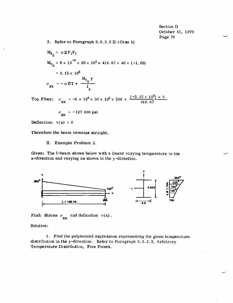
Section D
October 15, 1970
Page 76
3. Refer to Paragraph 3.0.2.2 II (Case b)
M0 z
M0 z
= _ EFIF 2
= 6× 10-6× 30× 106× 416.67× 40× (-i.00)
= 3.15× 10⁶
Mo z Y= - o_ET +
xx IZ
Top Fiber: a = -6 × 106× 30 × 106× 500 +XX
(-3.15x 10⁶ ) × 5416.67
a = -127 800 psiXX
Deflection: v(x) = 0
Therefore the beam remains straight.
II. Example Problem 2.
Given: The I-beam shown below with a linear varying temperature in the
x-direction and varying as shown in the y-direction.
Y
!_ L - 100 IN.
_'-_ 1'00°
| X
q
Y
t 350o
! 4.5 -*
Find: Stressxx
Solution:
and deflection v(x).
1. Find the polynomial expression representing the given temperature
distribution in the y-direction. Refer to Paragraph 3.0.2.3, ArbitraryTemperature Distribution, Five Points.

r
fr
V i d_
V 2 dl2
V 3 dl 3
V 4 dl4
%0.08333
-0.04167
0.08333
0.04167
0.6667 -0.6667 0.0833_
0.6667 0.6667 -0.04167
-0.16667 0.16667 -0.08333
-0.1667 -0. t6_67 0.04167
350-150
225-150
100-150
100-150
Section D
October 15, 1970
Page 77
62.5
10.42
: I0
2. 083
62.5 10.42 y2 2.083 y4T = 150+ 1.156 Y + (1.156) y + (1.156) 4
T = 150 + 54.1y + 7.81y 2 + 1.168y 4
2. Refer to Tables 3.0-2 and 3.0-4 for values of F0, F1, F2, F3, and
F 4 for each term of polynomial.
n = 0 V0 = 150 F 0 = 150(1. 715) = 257.3 F 1 = 0
n= 1 V l= 54.1 F 0= 54.1(0) = 0.0 F 1= 54.1(2.774)=150.0
n= 2 V2 = 7.81 F 0= 7.81(2.774)= 21.6 F l= 0
n = 4 V 4 = 1. 168 F 0 = 1. 168( 6. 745) - 7.9 F 1 = 0
Z F 0 = 286.8 F 1 = 150.0
.... 350 - 250f , L/
q= 0 F 2= -1.000 F 3= 0.0 F 4= -1.502
q= 1 F 2= 0.0 Fj = -1.0 F 4= -0.502
F 2= -1.000 F 3= -1.0 F 4= -2.004
3. Refer to Section 3.0.2.2-III (Case b).
M0z = -3/2 oL EF 1 = - 3/2 (180) (150)= - 40,500
M = M0z (1 -x/L) I = 10.55 in 4.Z Z
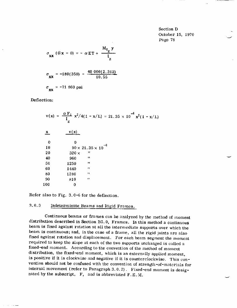
a (@x = 0) = - t_ET+XX
Moz Y
IZ
Section D
October 15,
Page 78
1970
& t'_ I't I ¢3t _" t',t _,
(7 = -_ou,..,ou, -_ F
XX
= -71 860 psiXX
Deflection:
40 000(2.312)10.55
v(x) = _ x2/4(1 -x/L) : 21 35 × 10 -6I
Z
x2( 1 - x/L)
x v(x)
0 0-6
10 90 × 21.35 × 10
20 320 × "
40 960 "
50 1250 "
60 1440 "
80 1280 "
90 810 "
100 0
Refer also to Fig. 3.0-6 for the deflection.
3.0.3 Indeterminate Beams and Rigid Frames.
Continuous beams or frames can be analyzed by the method of moment
distribution described in Section B5.0, Frames. In this method a continuous
beam is fixed against rotation at all the intermediate supports over which the
beam is continuous; and, in the case of a frame, all the rigid joints are also
fixed against rotation and displacement. For each beam segment the moment
required to keep the slope at each of the two supports unchanged is called a
fixed-end moment. According to the convention of the method of moment
distribution, the fixed-end moment, which is an externally applied moment,
is positive if it is clockwise and negative if it is counterclockwise. This con-
vention should not be confused with the convention of strength-of-materials for
internal movement (refer to Paragraph 3.0.2). Fixed-end moment is desig-
nated by the subscript, F, and is abbreviated F.E.M.

f-Section D
October 15,
Page 79
A B C A B C D
A B C A B C D
NO F.E.M.MFAB MFBA MFBc MFAB MFBA MFBc MFcB MFcD
1970
The magnitude of F. E. M. is obtained by analyzing the fixed-fixed
beam or the fixed-hinged beam cases of Paragraph 3.0.2. In that paragraph,
M0z is positive when counterclockwise; so, to convert M0z to F.E.M., one
must multiply by -l.
FIXED - FIXED BEAM FIXED - END MOMENTS
A B A B
V VLz = -M 0 = M LM0z °z MFAB z MFBA
M L =M 0 +L V 0Z Z z
FIXED - HINGED BEAM FIXED-END MOMENTS
A B A
T-. )M0 z V0 VL z = -M 0z MFAB •
A B A B
V 0 • MFBA= M o
With this information, a normal moment distribution technique can be
performed to solve any continuous beam or fr_ime.

3.0.4 Curved Beams.
Section D
October 15,
Page 80
1970
For a free curved beam of arbitrary, constant cross section, the
centerline of which is an arc of a circle lying in one of the centroidal principal
planes under a temperature distribution T(r, 0), the following comments canbe made.
J
1. For a small depth-to-radius ratio, straight-beam theory can be
used instead of the curved-beam theory.
2. Forlineartemperaturevariation(T=Ti-_-), theresultsof
curved-beam theory compare well with the solution obtained by exact thermo-
elasticity method; e. g., for a rectangular beam where the ratio of outside radius
to inside radius is equal to three, the maximum stress obtained by the curved-
beam theory differs from the maximum stress obtained by exact solution byonly 2.4 percent. Straight-beam theory, however, gives _ = 0, which is
00
considerably erroneous.
z 2
3. For quadratic temperature distribution T = T2 "_ , the difference
in maximum stress obtained by curved-beam theory and exact solution is only4.9 percent for a rectangular section where the ratio of outside to inside radiusis equal to 3.0.
For solutions other than those mentioned above, see Ref. 1.
3.0.5
A ring may be regarded as a closed, thin, curved beam, and can there-fore be studied by the methods given in 3.0.4 and in Ref. t.
3.0.6 Trusses.
3.0.6.1 Statically Determinate.
Every member of a pin-jointed determinate truss is not constrained to
elongate because of thermal loading. As a result, the net axial force in each
member is zero. Therefore, members of a pin-jointed determinate truss are
regarded as simply supported beams under thermal loading and should be
analyzed accordingly.
Deflections of joints of a truss can be obtained by the conventional"dummy-load" method described in Section B4.2.2.
F
Section D
July 1, 1972
Page 81
3.0.6.2 Statically indetermin'lte.
The forces in the bars of a statically indeterminate pin-jointed truss
are not zero, but are easily determined from the results of the previous
paragraph.
3.0.7 Plates.
The analysis of plates presented in this section is based on the
following classical theory of plates assumptions:
1. The material is isotropic, homogeneous, and linearly elastic.
2. The constant thickness of the plate is small when compared with its
other dimensions.
3. Plane sections, which before bending are normal to the median
plane of the plate, remain plane and normal to the median plane after bending.
4. The deflections of the plate are of the order of magnitude of the
plate thickness.
Solutions are given herein for circular and rectangular plates with
various boundary conditions ,_nd temperature distributions.
Analysis techniques for plates made of composite materials are given
in Section F.
3.0.7.1 Circular Plates.
I. Temperature Gradient Through the Thickness.
A. Configuration.
The design curves and equations presented here apply only to flat,
circular plates having central circular holes (Fig. 3.0-14). The plates must

Section DJuly 1, 1972Page 82
be of constant thickness, be made of an isotropic material, and obey t]ooke_s
law. Curves are given which deal with bendingphenomenafor a/b r._tios of
0.2, 0.4, 0.6, and0. San(! are basedon the assumption that v = 0.30. These
plots cover only n portion of the boundary conditions considered in connection
with bending behavior. The remainder of these conditions, as well as all the
membrane solutions, are given as closed-form algebraic equations which arc
valid for arbitrary values of Poisson t s ratio and the inner and outer radii of
the plate. When the ratio a/b approaches unity, the member is more properLy
identified as a ring.
N I
N8
N8
POSITIVE DIRECTIONS OF THE
I STRESSRESULTANTS.
_'_._.... SUR--FACEMIDDLE
NOTE: r, 8, z, u, v, and wz,w are positiveasshown.
N r
Figure 3.0-14. Circular flat plate.
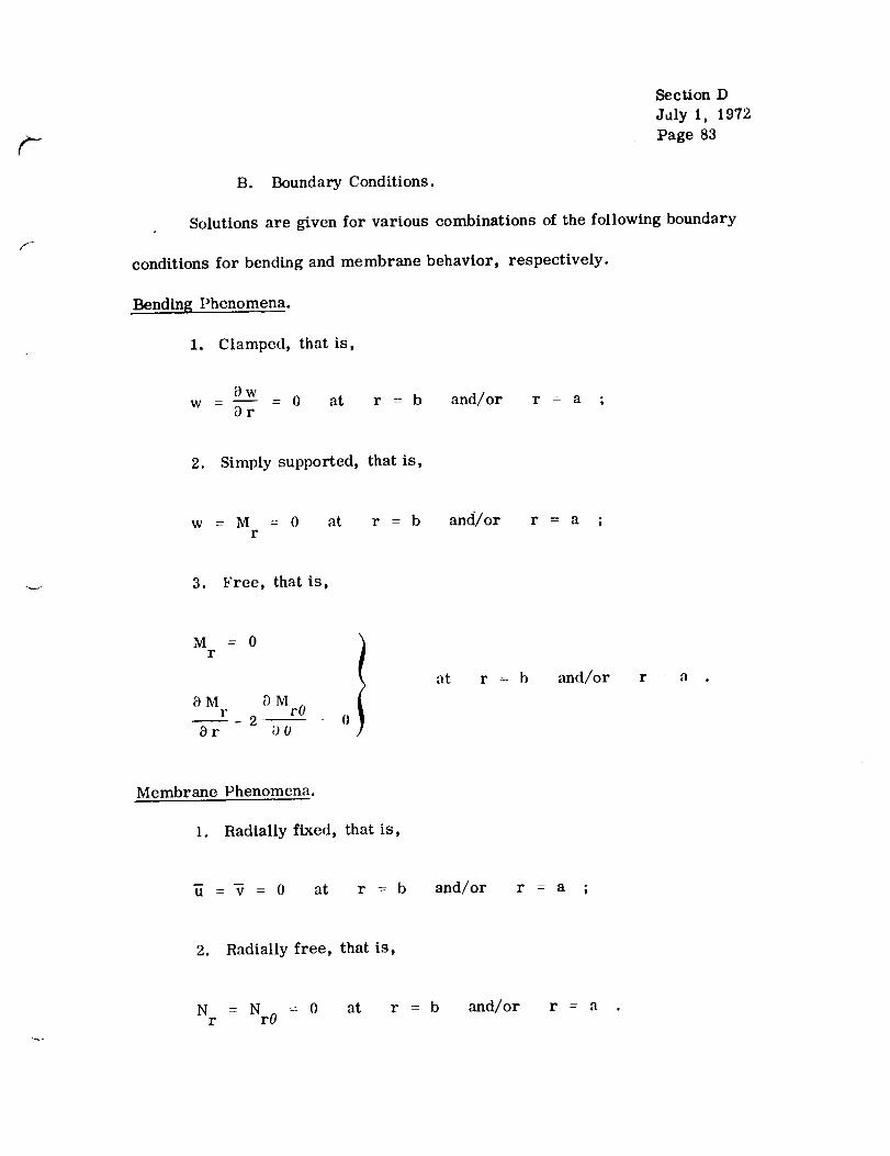
F
Section DJuly 1, 1972Page 83
B. Boundary Conditions.
Solutions are given for various combinations of the following boundary
conditions for bending and membrane behavior, respectively.
Bending Phenomena.
1. Clamped, that is,
0w
- - 0 at r = b and/or r = a ;w Or
2. Simply supported, that is,
w = M = 0 at r = b and/or r = a ;r
3. Free, that is,
M = 0r
aM OMr rO
Or ;)o: oI at r : b and/or r a .
Membrane Phenomena.
1. Radially fixed, that is,
= _ = 0 at r = b and/or r = a ;
2. Radially free, that is,
Nr = Nr0 = 0 at r = b and/or r = a

Section D
july 1, 1972
Page 84
C. Temperature Distribution.
Arbitrary t_mperaturc variations may be present through the plate
thickness. However, it is required that there be no gradients over the surface.
Hence, the permissible distributions can be expressed in the form
T = T(Z) .
D. Design Curves and Equations.
In Ref. 2, Newman and Forray present the simple method given here
to determine the thermal stresses and deflections for stable plates that satisfy
the foregoing requirements. This technique is based on classical small-
deflection theory and is an extension of the procedures published in Refs. 3
through 5 by the same authors. To perform the analysis, use is made of a
number of equations and design curves. These are provided in the summary
which follows.
It is assumed that Young's modulus and Poisson' s ratio are unaffected
by temperature variations. On the other hand, the temperature-dependence
of the thermal-expansion coefficient can be accounted for by recognizing that
it is the product _T which governs; that is, the actual temperature
distribution can bc suitably modified to compensate for variations ,:_ ,_.
E. Summary of Equations and Curves.
W _
w t a2M T
Db(1- v2)

and
Gr
NT 12z - +_ (_-- v)I Nr + +-- i- (i-.) t-v- r
Section D
Juiy 1, 1972
Page 85
% 1 NO + +7_ M0 + _= (i-.)
where
Et 3
Db -- 12 (1- p2)
t/2
= F_M T-t/2
Tz dz
t/2
= E_ I-NT-t/2
Tdz
M = -12 MTM" rr
M_ = -12 MTM 0' ,
N = NTN" rr
and
N O = NTN 0'

Section D
July 1, 1972
Page 86
The values for w', Mr' ' and M0t are obtained either from Table 3.0-5
or Figures 3.0-15 through 3.0-19. When the figures are used, Poisson' s
ratio must be taken to be 0.3 throughout the analysis of bending phenomena.
When Table 3.0-5 is employed, there are no restrictions on v . Also note
that, in most of the plots, the parameters include multiplication factors. The
values for N t and 1_ are obtained from Table 3.0-6 and are also valid "orr
any value of Poisson' s ratio.
F. Linear Gradient.
For the special case of a linear temperature gradient through the
thickness for a solid plate represented by
T(z) -- TO ÷ Tl + T° - T1Z2 2
the following solutions apply.
Unrestrained Solid Circular Plate.
0 =(7 = 0r 0
The plate becomes curved and fits a sphere _f radius inversely
proportional to the difference in surface temperatures and direct:y
proportional to the thickness.
Clamped Plate.
w = 0
7

c-
TABLE 3.0-5.
Section D
July I, 1972
Page 87
NONDIMENSIONAL PARAMETERS FOR
BENDING I)IIENOMENA
P
Boundary Conditions
Outer Edge Inner Edge
Free
Clamped
Simply
Supported
Free
Free
Clamped
l,'rec
Simply
Supported
W !
1(__ 1) (Relative toInner Boundary)
0
2
M tr
12(1- v)
0
Mo,
i.o(i- .)
TABLE 3.0-6. NONDIMENSIONAL PARAMETERS FOR
MEMBRANE PHENOMENA
Boundary Conditions
Outer Edge Inner Edge
Radially Free Radially Free
Radially Fixed
Radially Free
Radially Fixed
Radially Free
Radially Fixed
R,_dially Fixed
N !r
' 1 -_(1-v_
V(IL
No,
(i_-.) . (i- .)
• - +
(i-,)

Sectio_ D
July 1, 1972
Page 88
-_j
0

Section D
July 1, 1972
Page 89
i r

Section D
July 1, 1972
Page 90
i _ i,m i1,,,
II
[:1 ! I I/I ..V-i3;
J"H"5 '41"il [,,'1 1 1 1"--4-J1:I11II1!11:
I_'! I_1 .,f"I _i_L,.il I",V'I 1 _-_r_-!1 J"l I I ,_=..I--YII I I _",k_
i "--!!II pl"q • ql'
il
Q,I
I..i
0
i::l
0 _i::l v
..c:l 11)
J::ll::l,,
t,,.l
I::l., .,,--,4
.!i
I:::I
0
z_
A
°_,.,.i

t---
and
Section D
July 1, 1972
Page 91
f
rl %1max max
Simply Supported Plate.
Crr = _0 = o
and
W -ol (T,- T,,) (a2 r2 )2t
II. Temperature Difference as a Function of the Radial Coordinates.
A. Clamped Plate.
For the variation of temperature, ,assumed to be linear through the
thickness, and the variation with r given by the monomial,
Z KT = ---Ar +c
h K
where A and c are constants.K
I(: A r ,TD K
K
TD(a).. = AKa

Section D
July 1, 1972
Page 92
A
w = (K÷ 2)2 - + +2 '
Mr = 12(K + 2) +
and
Eh2OtTD(a) I ( K l+ulM0 - 12(K+2) K+ 1)(r) +l---'_J
where T D is the temperature difference between the surfaces.
Curves of nondtmenslonal deflection and moments are presented in
Figures 3.0-20 through 3.0-22 for K = 1,2,... 5 . Superposition may then be
used for T D given by polynomials in r. The determination of a polynomial
describing the radial variation of T D can be obtained in the same manner as
shown in Paragraph 3.0.2.3.
B. Radially Fixed or Radially Free Plate.
Configuration.
The design equations provided here apply only to flat, circular plates
which may or may not have a central circular hole. The plate must be of
constant thickness, be made of an isotropic material, and obey Hooket s law.
Formulas are given which cover the range
a0 _ - < 1
b

I
Section D
July 1, 1972
Page 93
w'--
3.2
2.8
2.4
2.0
1.6
1.2
0.8
0.4
0
Figure 3.0-20. Nondimensional deflection.
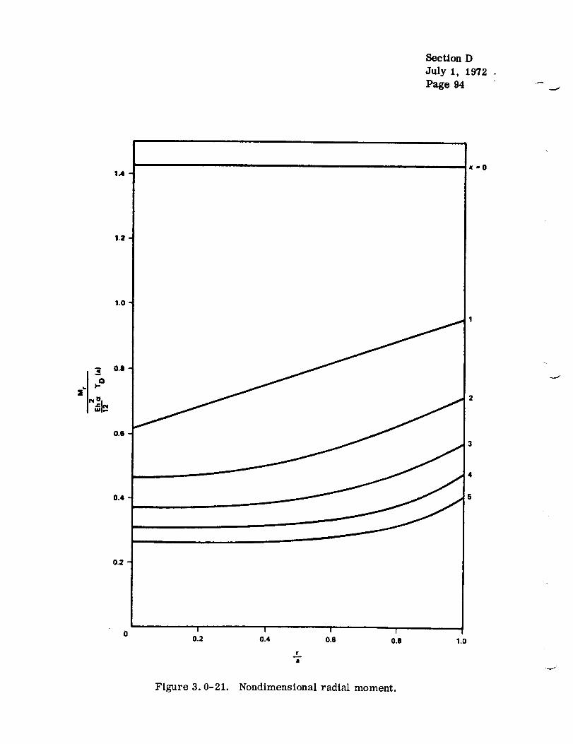
Section D
July 1, 1972
Page 94
1.4
1.2
1.0
x'0
0.8
0.6
0.4
0.2
iiI l I I
0.2 0.4 0.6 0.8
r
Figure 3.0-21. Nondimensional radial moment.
1.0
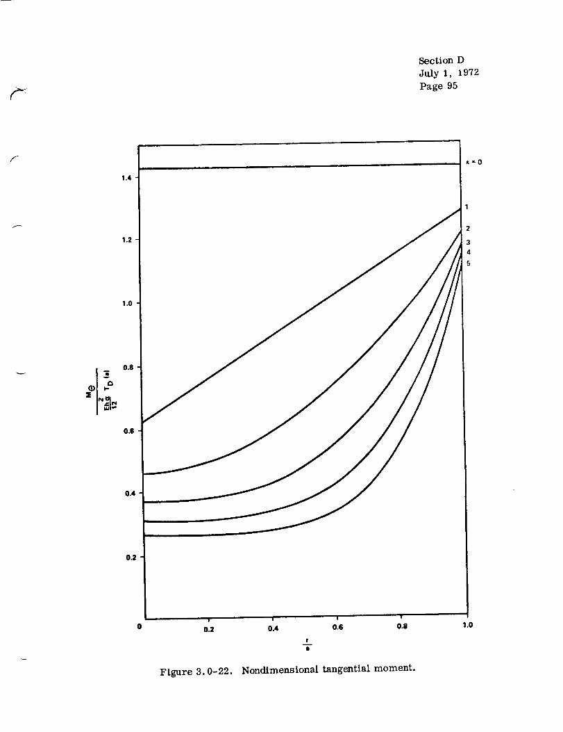
F
Section D
July 1, 1972
Page 95
f
1,4
1.2
1.0
0.8
0.S
0.4
0.2
x_0
| ! I I
O_ 0.4 0.6 0.8
f
II
1.0
Figure 3.0-22. Nondtmensional tangential moment.
Section D
July 1, 1972
Page 96
As this ratio approaches unity, the member is more properly identifiod as
a ring.
Botmdar_ Conditions.
Solutions are given for each of the following types of boundary
conditions.
1. Radially free; that is,
ar = ar8 = 0 at r = b
and
_: (rr = 0 at r = a(rr 0
if hole is present.
2. Cuter boundary radially fixed (if hole is present, the inner
boundary is radially free) ; that is,
u =v = 0 at r = b
and
ar _: ar^u = 0 at r a
ifhole is present.
Temperature Distribution.
The supposition is made that the temperature is uniform through the
thickness. However, the plate may be subjected to a surface distrioution
r

r-
(
f-
Section D
July I, 1972
Page 97
which has an arbitrary radial gradient but no circumferential variations.
Hence, the permissible distributions can be expressed in the form
T = T(r) .
Design Equations.
In this section, it is assumed that Youngts modulus and Poissonts
ratio are unaffected by temperature changes. Therefore, the user must select
single effective values for each of these properties by using some type of
averaging technique. The same approach may be taken with regard to the
coefficient of thermal expansion. On the other hand, the temperature-
dependence of this property can b_; accounted for by recognizing that it is the
product _T which governs; that is, the actual temperature distribution can
be suitably modified to compensate for variations in _.
The design equations are given in the summary which follows and are
based on classical small-deflection theory.
free plates were taken directly from Ref. 1.
The expressions for the radially
The equations for plates with
radially fixed outer boundaries were derived by superposition of the free-plate
formulas and the relationships given in Ref. 6 for cylinders subjected solely
to external radial pressure. Depending upon the complexity of the temperature
distribution, the required integrations may be performed either analytically
or by numerical procedures.

Summary of Equations.
Solid Plates (No Central Iiole).
1. Radially frec boundary:
Section D
July 1, 1972
Page 98
(lb lr )0"r = o_E _'_ f Trdr-r-- _ f TrdrO O
I_ I b I r z_a0 = c_E T+_ fTrdr+_ fTrdO 0
and
u = -- 1 + P) Tr fir ! (1 - v Tr dr
o o
These three equations are indetcrminate at r : 0 . However, by the
application of I t Hospital t s rule, it is found that [1]
(ar) = (aO) = orE 1 f Tr dr- _(T)r=Or=O r:O o
and
U ---"0 .r=O

2. l_adially fixed boundary:
r=_E
b 11 f Trdr-_Po
r _ _ _]f Trdr- b2(1 - v) f TrO O
Section D
July 1, 1972
Page 99
= aEf b 1
1 f Trdr+_-_T+_-_ °
b ]r 2 f Tr drf Wrdr-b2(l_v/ o
O
and
U = ot 1 +v) Tr dr- (1 +v)r o
b ]f Tr drO
These three equations are indeterminate at
of 1' Hospital' s rule, it is found that
r=0 . However, by the application
b
1
(ar) : (a0) -- aE _-_ fr=0 r=0 o
2
Tr dr -%2(1 _ v) b 1 1f T rdr-_Tr= 0O
and
U = 0 •
r=[}
Plates with Central Hole.
1. Both boundaries radially free:
O"r
= -_y ., f,q
Tr dr - r )f Tr dra
e

#0 ffi r'_ Trdr+ f Trdr- Tr 2 ,a a
8ec tim D
Jtfly 1, 1972
Page 100
and
_°[( iU = _ l+p) Trdr+(1- v) r 2+(l+u) a 2
b 2 _ a 2 b ]f Tr dr
a
2. Inner boundary radially free and outer boundary radially fixed:
Cr = _ Lb-t--_-f a Trdr- a/Trd +(O'r)r= b bS__ a I-_-_ ,
aE_ fbTrdr+ /Trdr_Tr2 ]
+ (err)r=b b2 - a2 + r7
U a [(1 +_)r
r (1- u)r 2+(l+v) a2 b
f Tr dr+ (b2- a_ f Tr dra a
where
o, 1 I + _)b
f Trdra

f
÷ (1- _,)b_÷ (1 ÷ v)a_(b2- a2) bf Trd
a
Section D
July 1, 1972
Page 101
and
III. Disk With Central Shaft.
Boundary conditions for this plane-stress problem are u[ r=a
= 0 •
Crrr [ r=a
=0
r - a_ I1
T = T b \b - a/ '
arr 1 \_-v- v
- 2 (l+v
¢rO0
ET b
rr
a ET b
+ r-2 T* [ a 2
_) - _ _-7_+_
2[Tb
r=a
a'/ T* 2T•_ (_-_)-_
= - +a 2 '-_ (i+_) _ (i-_)
°00IaET b r=a= _ + a2
r=b I_(1 _)[Tb 1 + (,_/a'-'__
and
r
T* =" 2r 2 _ a 2 f
a
Tr dr 2Tb (r- a_n [(n+l) r +a)- r + a \b-_-a] -(n+l)'(n+2)

Sectioo D
July 1, 1972
Pag e 102
where
2 b 2T b
T: = r_-_ _ f Trdr - a+ ba
[(n+l) b + a]
(n+l)(n+2)
Curves showing the variations ofrr
ETb r=aand
r=b
with n
and a/b are given in Figures 3.0-23 through 3.0-25.
_.ll!
-0.7
"0-6 1
-0.5
0
a/b0.80.6
0.40.20.1
2 3
Figure 3.0-23. Variation of tangential stress at outer boundary with n
and a/b for a disk on a shaft.
Additional cases that may be obtained from Refs. 7 and 8 are as follows:
1. Circular plate with asymmetrical temperature distribution
2. Circular disk with concentric hole subjected to asymmetrical
temperature distribution
3. Circular plate with a central hot spot.

q
Section D
July 1, 1972
Pagc 103
P
0.7
0.6
0.5
0.4
0.3
0.2
0.1
a/b+-0
0.10.2
_ 0.4
_ 0.6
0.8
0 1 2 3
0.2
o_
0.1
Figure 3.0-24. Variation of radial and tangential stress at inner
boundary of disk with n and a/b for a disk on a shaft.
-1.0zlb
-0.9 _ 0.8
.o.e _ _ o.6
•0.7 C O.2(ic o,
-0.5 -
/..o.,. /Z _-0.3
-0.2 _
-0.1 ....
0 I 2 3
Figure 3.0-25. Variation of tangential stress at outer boundary
of disk with n and a/b for a disk on a shaft.

Section D
July 1, 1972
Page 104
3.0.7.2 Rectangular Plates.
I. Temperature Gradient Through the Thickness.
A. Configuration.
The design curves and equations provided here apply only to flat, rect-
angular plates which are of constant thickness and are made of isotropic
material. The two long edges of the plate are supported by flexible beams.
It is assumed that both the plate and the support beams are free of holes and
that no stresses exceed the elastic limit in either of these members. The
design curves cover aspect ratios b/a of 1.0, 1.5, and 3.0.
B. Boundary Conditions.
The edges x = 0 and x = a are elastically supported by beams having
equal flexural sttffnesses EbI b . Both beams are simply supported at their
ends (Fig. 3.0-26) and are frec to undergo axial expansions or contractions.
These members offer no constraint to cnch of the following pl'itedeformations:
I. Edge- Hotntion
2. In-Place Edge-Displacements u and v.
The beams resist only transverse deflections w . The edges y = 0
and y = b are simply supported; that is,
w =My -- 0
along these two boundaries.

,f
I
y
_1a L
t
k
L Xr
z
- 4------
' [ i-V l NoTE
Section D
July 1, 1972
Page 105
ARBITRARYONE-DIMENSIONALTEMPERATUREDISTRIBUTION
r
o
x, y, z positive
m shown.
Figure 3.0-26. Rectangular flat plate with one-dimensional
temperature distribution over surface.
C. Temperature Distribution.
Separate coverage is provided for each of the following temperature
distributions through the thickness:
1. Linear gradient T = aJ + a{z
2. Arbitrary gradient T = f(z) .
It is assumed that there are no temperature variations in directions parallel
to the middle surface of the plate.
D. Design Curves and Equations.
In Ref. 9, Forray, et al., present the simple methods given here to
compute thermal stresses and deflections at virtually any point in fiat,

Section D
duly 1, 1972
Page 11)6
rectangular plates which comply with the foregoing specifications. These
techniques consist of a varicty of equations and curves, all of which arc based
on the conventional small-deflection theory of plates. It is assumed that
Young t s modulus and Poisson t s ratio are unaffected by temperature variations.
Hence, the user must select single effective values for each of these properties
by employing some type of averaging technique. The same approach may be
taken with regard to the coefficient of thermal expansion. On the other hand,
the temperature-dependence of this property can be accounted for by recogllizing
that it is the product T which governs; that is, the actual temperature distri-
buti(m can he suitably modified to compensate for variations in _. When this
approach is taken, the user must adopt the viewpoint that any mention of a
linear temperature distribution is actually referring to a straight-line variation
of the product a T .
Linear Temperature Gradient.
For a linear temperature gradient expressed by
T = a_ + a_ z
and with
T D = T(z=t/2 ) - T(z__t//2 )
E t _
D b = 12(1 p_ v2)

;P v
and
Section D
July 1, 1972
Page 107
F4Db_ TD(1 - u 2)
M =
The transverse deflections are expressed by
w = :(x,y) +wA(x,y) +wA(a-x,y)
where
W(x,y)
n=l, 3, . . .
sin osh n__: _a Y
nacosh n7r____bb.2a
wA(x,y) = _, G ,[__Xcoshmrrx ( 2 mTra mTra) _._]re=l,3 .... m ---_- 1--_+---_coth---_--- sinh sinm----_b
and
G *
121
4 M x_ mr a- _ sinh
mira k=l,3 .... 1 + b\ma/J
Db_._) sinhmTra (l_u)m_.a] ÷ 2 (Eblb_
The component N(x, y) is the deflection where all edges are simply supported.
The bending moments M and M can be obtained by substituting thex y
final deflection relation into the following equations:

F a2w a2w aT D "]
M x : -DbL_+P _+-7(1+P) J
Section D
July 1, 1972Page 108
and
[02WO_w OZTl) ]Y [(9.--7 I v _3x----7t t (1 + v
J
Forray et ",!. 191 used these (h;fh.ction and mom(;nt ex3_ressions to
generate the design eurw;s of l.'il,_ures 3.0-27 through 3.0-35, where it is
assumed that v _: 0.30 . Some of the curves are discontinued near the corners
of the plate x/a ---0, y/t) _ 0 since the conventional th. ,15. breaks ,',own at
these locations. Certain of these results also appear in Ref. 10, where a
different plotting format was used. In addition, the latter reference includes
supplementary curves for the c:::;c where EbIb/Dbb --- ¢0 This correspon(Is
to the condition of simple support on :dl four edges.
Because of symmetry about the centerlines (x = a/2 , y = t)/2) , it was
necessary to show only one quadrant of the plate in Figures _;. 0-27 -hr,_ugh
3.0-35. The assortment of curves covers a wide range of values in the vari-
ables and should accommodate most practical problems of this p,_rticular class.
For any situations where the plots prove to be inadequate, the equations c;m be
used to obtain solutions. However, a considerable amount of rather coutine
mathematics wouhl bc required in making the necessary substitutions to obtain
bending-moment equations in series form. Once the_e were available, it might

f_
OF POOR QUALITY
'f i +
0 0.1 0.2 0.3 0.4 0.5V/b
Section D
July 1, 1972
Page 109
0.24
0.20
0.16 x ,, 0.50
0 0.1 0.2 0.3 0.4 0.5y/b
0.24
0.20_,r?"'0.12_
0.__
0 0.1 0.2 0.3 0.4 0.5Y_
0.24
0 0.1 0.2 0.3 0.4 0.5y/b
0.24
0.20 _
,L?
0.__0.04 -= "
0 0.1 0.2 0.3 0.4 0.5y/b
• "0_
0 0.1 0.2 0.3 0.4 0.5y/b
Figure 3.0-27. Nondimensional deflections for a plate with two
opposite edges elastically supported and the other
two edges simply supported; b/a -- 1.0, v = _). 30.

SectionD
July 1, 1972
Page 110
Figure 3.0-28. Nondimensional bending moments Mx/M for a plate
with two opposite edges elasticallysupported and the other
two edges simply supported; b/a = 1.0, v = 0.30 .

0.28
0.26
0.24
0.22
O.2O
0.18
0.16
0.12
0.10
0.08
0.08
0.04
0.02
0
-0'.020
-I_b'b .o1-I-
_. ,--- X-o _
\_ a t
I I "_''-- I- 0.20 --
0.1 0.2 0.3 0.4 0.5y/b
ORIGi;_A;. "',_""
OF POOR QUALITY
7"1,
0.28
0.24
0.20
0.16
0.12
Section D
July 1, 1972
Page 111
1 ! 1
-IEb'bi_1-__ -006-
;\
0.08
0.04 - x. 0.20 :
0 0.1
x
r-_=O__
_ _-o6o:L '
0.2 0.3 0.4 0.5y/b
o28
0.16 .
0 0.1 0.2 0.3 0.4 0.5y/b
0.28
:[Eb'b!0.24 _
0.20
0.16
0.12
0.08
0.04
00 0.1
- x
"a " 0.50J i 1
0.2 0.3 0.4 0.5y/b
0.28
0.24
0.20
0.16
0.12
0.08
0.04
0 o
Eb I b
- 2.00
0.1 0.2 0.3 0.4 0.5Y_
o28_l%'b 5ool7--0.24 _ " "
0.20 _0.16
o.12 _i •
0.08 x ---
0 0.1 0.2 0.3 0.4 0.5y/b
Figure 3.0-29. Nondimensional bending moments M /M for a plateY
with two opposite edges elastically supported and the other
two edges simply supported; b/a -- 1.0, v = 0.30 .

Section D
July 1, 1972
Page 112
0.10
O.W
.1 0.2 0.3 0.4 O.I 0.1 0.2 0.3 0.4 0.6
y/b y/b
0.21 0.211
0.14 0._14
0.2O 0._
,+I+ ,F+o,.0.1:
Figure 3.0-30. Nandtmensional deflections for a plate with both
long edges etasticaUy supported and the short edges
simply supported; b/a = 1.5, v = 0.30.
+

F
_ :._'_ _'-
.OF POOR QUAL_y
O.28
0.24
O.2O
,,i z o.1e0.12
O.(Z
O,O4
00 6.1 0.2 0.3 0.4 _5
ylb
O.28
6.24
O.2O
60 0.1 6.2 0.3 0.4 0.§
y/b
0.28
0.24
6.20
0.16
0.12
0,04
Section D
July 1, 1972
Page 113
O.28
O.24
O.20
0.16
0.12
0.08
0.04
00 0.1 0.2 0.3 0.4 O.6
y/b
0.24
0.20
0.16
:F"I"0.12
o.'._.o.2o4_
0.04 _
0 0 O.1 0.2 0.3 0.4 0.5
y/b
0.24
0.20
0.16
6o._,_ _-_ _ oJy_
Figure 3.0-31. Nondimensional bending moments Mx/M for a plate
with both long edges elastically supported and the short
edges simply supported; b/a = 1.5, v = 0.30.

Section D
July 1, 1972
Page tl4
LM
- 6.OO
Figure 3.0-32. Nondimensional bending moments My/M for a plate
with both l(mg edges elastically supported and the short
edges simply supported; b/a = 1.5, v = 0.30.

C-ORIGI._,AL _:-.',,:.,._EtSOF POOR QUALITY
Section D
Jaly 1, 1972
Page 115
f
/
IJII
O.2O
0O.1 0.2 0.3 0.4 0.5
y/b
o.,-o.1 l-O.6
0.6
0.3
0.1
O0 O.1 0.2y/bO.3 0.4 0.5
1.0
O0 0.1 0.2 0.3 0.4 0.5y/b
Eblb " 0.50
0.38 ----
o_o.'_. 0._-,_
0.20
0.10
0.10 _0.05
00 0.1 0.2 0.3 0,4 0.5
y/b
0._
O.2O
i 0.12_
0._
0.1 0.2 0.3 0.4 0.5y_
0.28
0.2O
*_" 0.10
0._
0.04
O0 0.1 0.2 0.3 0.4 0.5V/b
Figure 3.0-33. Nondtmensional deflections for a plate with both
long edges elastically supported and the short edges
simply supported; b/a = 3.0, v = 0.30.
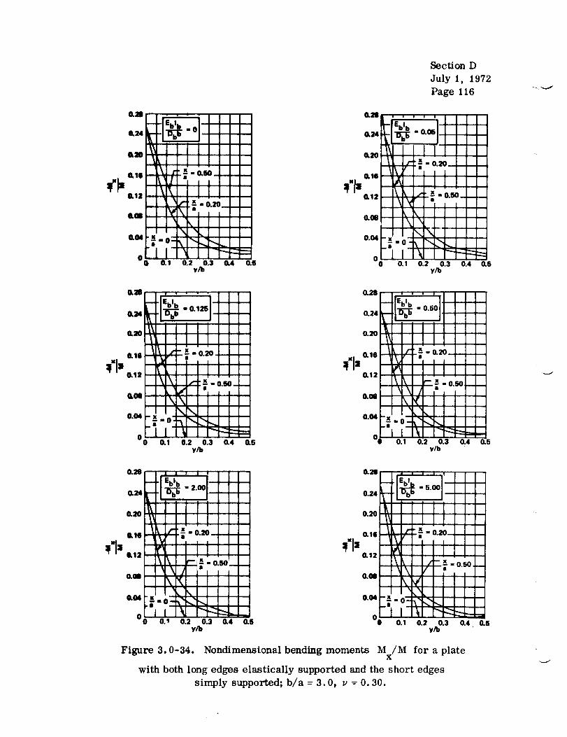
Section D
July 1, 1972
Page 116
• X
Figure 3.0-34. Nondimensional bending moments M /M for a platex
with both long edges elastically supported and the short edges
simply supported; b/a = 3.0, v = 0.30.

ORIGI_IAL F,_CE IS
OF POOR QUALITY
Section D
July t, 1972
Page 117
,J
1
0.=,
0.16
4. 0 0.1 0.2 0.3 0.4 0.5y/b
0..28
O.24
O.2O
0.16
0.12
0.08
0.04
0
m .
0.1 0.2 0.3 0.4 0.5Y_
0.28
O.24
O.20
0.16
0.12
0.00
O.O4
0 0.1 0.2 0.3 0,4 0.5y/t)
0.28[-I%,b I_E]Z Z
0.24
11.16
o.,2
0.04
O0 0.1 0.2 y/bO.3 0.4 0.6
0.32,
O.28
0.24
O.20
0.16
0.13
O.lU
0.04
0 0.1 0.2 0.3 0.4 0.6yro
O.28
O.24
O.20
0.16
0.12
0.00
O.O4
i
oi
[Ebl b ]
o.1 0.2 0.3 o.4 0.6y_
Figure 3.0-35. Nondimensional bending moments My/M for a plate
with both long edges elastically supported and the short edges
simply supported; b/a = 3.0, v = 0.30.
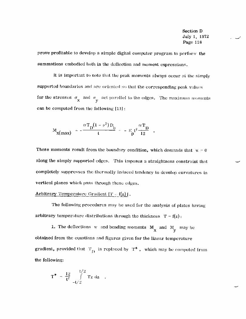
SectionDJuly 1, 1972Page 118
prove profitable to develop a simple digital computer program to perforn" the
summations embodiedboth in the deflection and momentexpressions.
It is import:mt to note th:lt the peak momentsalways occur ;it the simply
supported boundaries :rod .re' oricnt(_d s,_ that the corresponding peak valtlcs
for the stresses tr and ¢r :_ct p:_r_lllel to the edges. The maximun_ m,)mentsx y
can be computed from tile following [11] :
_ J
C_Tl)(l- v2)D b t_T DM .... E t 2
x(max) t p 12
These moments result from the boundary condition, which demands that w - 0
along the simply supported edges. This imposes a straightness constraint that
completely suppresses the therm:dly induced tendency to dcvelo|) curvatures in
vertical planes which pnss through these edges.
Arbitrary Temperature Gradient [T =- [(z)].
The following procedures may be used for the ;malysis of plates having
arbitrary temper.'|ture distributions through the thickness T = f(z) :
1. The deflections w and bending moments M and M may bex y
obtained from the cquntions ,_md figures given for the linear temperature
gradient, provided lhat TI) is repl:lced by T* , which may be computed troln
the following:
t/2T* 12 ;
tz !_ Tz dz-t/2

r
2. The normal stresses x and y
relations hips
x x _,"_-/ (l-v) +"_-
Section D
July 1, 1972
Page 119
may then be established from the
and
r + P -T+--- TCry = My _'_-7 (1- v) t
where
d/z-- 1 ?T Tdz
- d J-d/z
II. Temperature Variation Over the Surface.
A. Edges Free or Constrained Against In-Plane Bending.
Configuration.
The design equations provided here apply only to flat, rectangular plates
which are of constant thickness and are made of isotropic material. It is
assumed that the plate is free of holes and that no stresses exceed the elastic
limit. The equations are applicable only for large values of the aspect ratio
a/b .
Sectionl)July 1, 1972Page 120
Boundary Conditions.
Consideration is given to each of the following two types of boundary
conditions:
1. All edges are free.
2. Plate is fully constrained against in-plane bending but is otherwise
completely free.
Temperature Distribution.
The supposition is made that no thermal gradients exist through the
plate thickness but a one-dimensional, arbitrary variation occurs over the
surface; that is, the temperature is a function only of either x or y .
Design Equations.
It is assumed here that Young' s modulus is unaffected by temperature
changes. Therefore, in applying the contents of this section, a single effective
value must be selected for this property by using some type of averaging
technique. On the other hand, the results arc presented in a form such that
the user may fully account for temperature-dependence of the coefficient of
thermal expansion _.
The appropriate stress formulation is developed as follows for the
problem which was illustrated in Figure 3.0-26, which shows a rectangular
plate with a temperature distribution T(y) and free of any external constraints.
The results may be obtained by first imposing a fictitious stress distribution
J

a A on the edges x=4-a/2
suppressed. It follows that
Section D
July 1, 1972
Page 121
such that all thermal deformations are entirely
_A = - sET(y) .
These stresses may be integrated over the width b
arrive at the force
and the thickness t to
b/2
PA = - Et f sT(y) dy-b/2
and the moment about the z axis
b/2
= - Et if sT(y) ydyM A-b/2
Since, at this point in the derivation, it is assumed that no constraints are
present, the actual plate must be free of forces and moments on all edges.
To restore the plate to such a state, it is necessary to superimpose both a
force PB equal and opposite to PA and a moment M B which is equal and
opposite to MA . Hence,
PB = -PA
and
M B = -M A •

The stress corresponding to I' B is easily found to be
Section D
July 1, 1972
Page 122
PB PB
qPB =: _A : _bd ::
b/2Eb f c_'l'(y) dy
-b/2
The stress corresponding to M B is
b/2
MBY 12MBY, 12y E !" c_W(y)ydya - I - tb_ b 3MB z -b/
It should be noted thnt the procedure I)cing used constitutes an apl)lic:ation c_[
Saint-Venant Is principle. Hence, the stresses arid will i)c°'p B ffM B
accurate representations only at sufficient distances from the edges x = _ a/2 .
Subject to this limitation, the actual thermal stresses at various points in the
plate may be computed from the relationship
qA + CrPB += _MB
or
I)/2 t)/2F
a : -o_l':T(y)I f (_'l'(y) dy +1b-_3 E f (_T(y)y <ivx b- -b/2 -b/2
The foregoing discussion has been restricted to those cases where tne
temperature varies only in the y direction. How(:,:er, the same method

can be used to arrive at the following expression when T
of x:
Section D
July I, 1972
Page 123
is a function only
a/2tr -or ET(x) E 2 12x-- +-- oIT(x) dx+7 E f aT(x) xdx
y a -a/2 -a/2
Complex one-dimensional temperature distributions may often be encountered
which make it difficult to perform the integrations required by the preceding
equations. In such instances, numerical techniques can be used whereby the
integral signs arc replaced by summation symbols.
The equations were derived for rectangular plates having no edge
restraints. However, these relationships can easily be modified to apply when
the plate is fully constrained against in-plane bending but is otherwise
completely free. This is achieved simply by deleting the final terms from
each equation.
Summary of Equations.
1. All Edges Free.
T = T(y) ,
E b/2 12y _2a : -aET(y) + f aT(y) dy + b3 E crT(y)y dyx b--b/2 -b/2
T = T(x) ,

SectionDJuly 1, 1972
Page 124
and
a/2 a/2E 12x
o" = -aET(x) +-- f aT(x) dx+--_ E f ¢rT(x) xdxy a -a/2 -a/2
2. Plate Fully Constrained Against In-Plane Bending But Otherwise
Completely Free.
and
T = T(y) ,
b/2
l,: f ,v'l'(y) dy ,x : - a'ET(y). _ -b -b/2
T = T(x) ,
O _ .-
Y
a/2--o_H'(,,) , t._: f _'l'(×),I.,,
n -a/Z
1L l,:_l_cs Fixed.
Configuration.
The equations and sample solution provided here apply only to flat,
rectangular plates which are of constant thickness .and are made of isotropic
material (Fig. 3.0--36). It is assumed th, t the plate is free of holes and that
no stresses exceed the elastic limit. The _ c:uatians are applicable to any
aspect ratio a/b .

SecUon D
July 1, 1972
Page 125
r
FIXED
_= '
IXEDy,v
v
X,U
r,uJxm
LL
ill ii I I ii l
NOTE: x, y, z, u, v, andw arepositivem shown.
Figure 3.0-36. Rectangular fiat plate: all sides fully constrained
against in-plane displacements.
Boundarlr Conditions.
Consideration is given only to plates having all sides completely
restrained against in-plane displacements (fixed) ; that is, both of the
following conditions must be satisfied by each edge:

and
U = 0
Section D
July 1, t972
Page t26
V " 0 .
Temperature Distribution.
The supposition is made that no thermal gradients exist through the
plate thickness, tfowever, temperature variations over the surface may bc
arbitrary.
Design Equations.
As noted previously, a so-called body-force analogy exists between
certain isothermal problems and thermal stress problems for flat plates
which experience no transverse displacements w . This method is derived
in a number of different references [12, 13, 14] and is frequently referred to
as Duhamelts analogy. In Ref. 15, this approach is used to solve the
problem being treated here. Assuming that buckling does not occur, solutions
in series form were obtained for the in-plane stresses q , a and rx y xy
The series coefficients can be obtained by solving the following simultaneous
equations:
+ _ 2(1 • v) _ \_ mnpqmn 4 --_ /' Bpq(p2-m2)(n2-(l:')
p-1 q=l
= + v)
b b
f f_T mnx nny_x sin _ sin dx dya b0 0
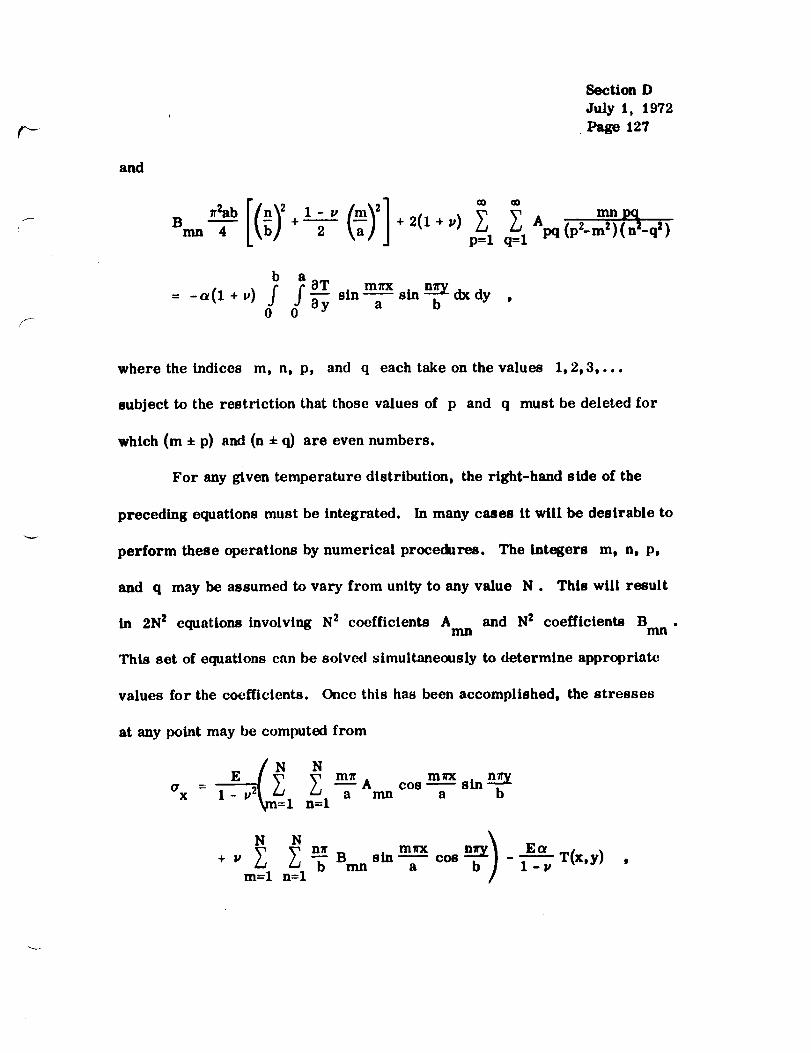
r
and
_2ab
Section D
July 1, 1972
• Page 127
co co
p=l q=l pq (P2-m2)(n2-qZ)
b a aT m_rx
= -_(1 +v) 0f 0f _y sin--a sin b dxdy ,
where the indices m, n, p, and q each take on the values 1,2,3,...
subject to the restriction that those values of p and q must be deleted for
which (m 4. p) and (n ± q) are even numbers.
For any given temperature distribution, the right-hand side of the
preceding equations must be integrated. In many cases it will be desirable to
perform these operations by numerical procedures. The integers m, n, p,
and q may be assumed to vary from unity to any value N. This will result
and N 2 coefficients B .in 2N z equations involving N 2 coefficients Anm mn
This set of equations can be solved simultaneously to determine appropriate
values for the coefficients. Once this has been accomplished, the stresses
at any point may be computed from
m_xm___A cos -- sin°'x - I- a mn a
I n=l
N _ n_ m_x n__h_ E c_+ V Z -'_ Smn sin-- cos - T(x,y)
m=l n=l a ../ _ '

{7Y
E
1 - v2 n_-_-B sin\m=l n=l mn
N N
+ P _ COSa mn
m=l n=l
m_xCOS
a b
\mrx sin n-n--_] Ea
a l-p
Section D
July I, 1972
Page 128
T(x,y) ,
and
NN( "rxy mn _ sinm=l n=l
mTrxCOS
a b
m cos _ sinmn a a
Then the strains at any point can be determined from
| - PO" )-- (Or x yx !':
1f _ (IT -
y E y IP°'x) '
and
T
_ x3,Txy - G' "
Example.
Let a rectangular plate having ali [our edges fixed (refer to Fig. 3.0-36)
be subjected to a temperature gradient

T(x,y) = T. -:,
Sec tlc_ D
July 1, 1972
Page 129
Then
0T 3'" and 0T0x a 0y
O •
Substituting these expressions into the right-hand side of the design equation,
the following is obtained after integration:
A _2ab 2 1 - vmn--4 ÷---_ -t 2(1 +u) _
p=l q=l
mnpqBpq (p2_m2) (n2_q2)
14(1 + u) b_T u
mn _2 if m and n are odd numbers
0 if m and n are even numbers ,
and
_2ab[(b)2 1-v(-_) 2]mn 4 2
N Nnm pq
+ 2 (1 + v) _ _ Apq (p2_m2)(n2_q2)p=l q=l
= 0
Let N = 2. Then the preceding equation becomes
_2ab4 A11 +--_ + 2(1 + _) B22 (22_1) ( 1_22) = 4 _2 ,

Section D
July 1, 1972
Page 130
1,:2×2
2(1 _ v) B2,_(22-I)
0 t
l 2x2 = 0
A21
0 ,
and
(li_1 2x2 = 0 ,
7r2ab Bi2 +4
Solving these equations gives the results,
At2 = A2t = A22 -= Bt I = B2t = B12 = 0 ,
and B22 earl be obtained [rorn the following relationships:while At_
_¢2a_b (1 ' 1 - v_ 8
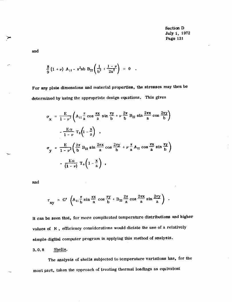
Section D
July 1, 1972
Page 131
and
8 (i + p) Air- _Zab B22 d = 09
For any plate dimensions and material properties, the stresses may then be
determined by hsing the appropriate design equations. This gives
O"x
- - -- cos -- Sin + v sln-- cos1 v 2 All a a -b- B22 a
-1?_
E (_ 2___ + p_ A11cos__ sin b__)- - p--_ B22 S in 2____XX _ _Xy 1 a cos b a a
- (1- v) T. 1--a '
and
Txy il_sin? cos ÷ B22 a cOS--a sin a "
R can be seen that, for more complicated temperature distributions and higher
values of N, efficiency considerations would dictate the use of a relatively
simple digital computer program in applying this method of analysis.
3.0.8 Shells.
The analysis of shells subjected to temperature variations has, for the
most part, taken the approach of treating thermal loadings as equivalent

Section DJuly 1, 1972
Page 132
mechanical loadings and hence solving the stresses and displacements by
techniques such as in Section B7.3. These approaches are discussed in
Refs. 7 and 8. Some of the more common temperature distributions in shells
will be discussed in the following section.
3.0.8.1 Isotropic Circular Cylindrical Shells.
This section covers the thermostructural analysis of thin-walled,
right circular, isotropic cylindrical shells. The middle-surface curvilinear
coordinate axes (x and y) are alw:lys taken parallel to the axis of revolution
and the circumferential direction, rcsl)eetively.
The organization of this section is somewhat different from that of
the sections which cover isotropic flat plates. This is due to certain funda-
mental differences between the physical behavior of flat plates and shells.
Flat-plate deformations are of such a nature that it is helpful to group the
solutions for stable constructions into the following categories:
1. Temperature gradients through the thickness
2. Uniform temperatures through the thickness.
Except for the special case of self-equilibrating gradients through the thick-
ness (N T -- 0, M T -- 0), the first of thcsc two cases involves out-of-plane
bending which is, of course, accompanied by displacements normal to the
middle surface of the undeformed plate. In case 1, the plate remains flat;
that is, the only displacements occur in directions parallel to the original
middle surface and no _ut-of-plane bending occurs. The governing differential

Section D
July 1, 1972
Page 133
equations in these two instances arc quite different and the indicated separation
of the cases is a logical format for the sections dealing with flat plates.
However, the situation is not the same for circular cylindrical shell structures.
For these components, a single governing differential equation includes the
phenomena related to both cases 1 and 2 and there is no need to isolate
these two types of thermal conditions. This is because either type of
temperature distribution, in conjunction with clamped or simply supported
boundaries, will lead to both membrane loading and bending about the shell-
wall middle surface. Consequently, for stable constructions which comply
with either case 1 or 2, the solutions are given in a single grouping as follows.
I. Analogies with Isothermal Problems.
A. Configuration.
This discussion is restricted to thin-walled, right circular cylinders
which are of constant thickness and are made of isotropic material. It is
assumed that the shell wall is free of holes and that it obeys Hooke t s law.
Figure 3.0-37 depicts the isotropic cylindrical shell configuration.
Figure 3.0-38 shows the sign convention for forces, moments, and pressure.
B. Boundary Conditions.
The following three types of boundary conditions are discussed:
1. Clamped edge; that is,
dww --u = 0 at x=0 and/or x= L (1)
dx
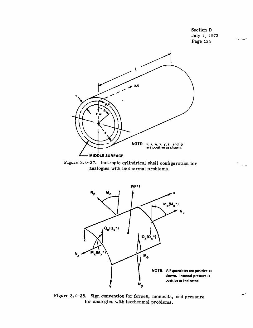
L
Section D
July 1, 1972
Page 134
NOTE: u, v, w, x, y, z, andare positive as shown.
MIDDLE SURFACE
Figure 3.0-37. Isotropic cylindrical shell configuration_ for
analogies with isothermal problems.
P(P*)
x
/_Mx(M x_ I
N X
" QxIQx*) If
QxIQx*]
N x
NOTE: All quantities are positive as
shown. Internal pressure ispositive N indicated.
Y N_
Figure 3.0-38. Sign convention for forces, moments, and pressure
for analogies with isothermal problems,

2. Simply supported edge; that is,
Section D
July 1, 1972
Page 135
w = M = 0 at x--O and/or x= Lx
(2)
3. Free edge; that is,
Mx = Qx = 0 at x =0 and/or x= L .
All possible combinations of these boundary conditions are permitted.
it is not required that those at x = 0 be the same as those at x = L.
every case, it is assumed that the cylinder is unrestrained in the axial
direction (N x = 0).
C. Temperature Distribution.
The temperature distribution must be axisymmetric but arbitrary
gradients may be present both through the wall thickness and in the axial
direction.
(3)
Hence,
In
The permissible distributions can therefore be expressed in the
form
T = T(x,z) . (4)
Any of the special cases for this equation are acceptable, including that where
the entire shell is at constant temperature.
D. Analogies.
It is helpful for the user to recognize that, for circular cylinders,
analogies exist between problems involving axisymmetric temperature

Section D
July 1, 1972
Page 136
distributions and certain problems where mechanical loading is present but
thermal effects are entirely absent (isothermal problems). The various types
of correspondencc are discussed herein where it is assumed that Young t s
modulus and Poissont s ratio are un_dfectcd by temperature changes. On the
other hand, one can account for temperature dependence of the thermal-
expansion coefficient (_ by observing that it is the product sT which governs;
that is, the actual temperature distribution can be suitably modified to
compensate for variations in c_. When this approach is taken, the user must
recognize that any reference to linear temperature distribution is actually a
reference to a straight-line variation of the product aT.
It is also helpful for the user to recognize that, regardless of the
complexity of a thermal gradient through the thickness, at any location (x,y)
the distribution can be resolved into
1. A self-equilibrating component, and/or
2. A uniform component, and/or
3. A nonuniform linear component passing through T = 0 at the
middle surface.
A self-equilibrating tempcr_t_ L-c component is one for which
t/2
-t _/2 T dz : 0

and
Section D
July I, 1972
Page 137
t/2
_t/i2 Tz dz = 0 .(5)
An example of such a distribution is illustrated in Figure 3.0-39.
j jT=0
Figure 3.0-39. Sample self-equilibrating temperature distribution.
From a practical viewpoint, it may be assumed that gradients of this type will
not cause any deformation of the cylinder. Their only influence will be on
and If, for example, a solution is available for anythe stresses crx a .
arbitrary temperature distribution T = T(x, z) , the effects can be easily
superimposed from a component Tl(x,z) which satisfies equations (5). It
is necessary only to algebraically add the stresses
E_TI_-- = - (6)
X 0-@ (1- V)
to the previously determined values for the appropriate locations (x, z).

Section D
July 1, 1972
Page 138
In this section, the following two categories are treated separately:
1. Uniform temperatures through the thickness with or without
axisymmetric, longitudinal gradients; that is,
T = T(X) . (7)
2. Nonuniform linear temperature gradients through the thickness,
passing through T = 0 at the middle surface with or without axisymmetric
longitudinal variations and possibly including self-equilibrating components;
that is,
Z
T = TI(X,Z ) + T2(x ) _- (8)
where T 1 satisfies equations (5).
Uniform Temperatures Through the Thickness IT = T(x)].
In Ref. 16, Tsui presents the small-deflection governing differential
equation for the subject shell. After conversion to the notation and sign
convention used here, this expression becomes
NT d2M Td4w p _ 1
+4_4w = - Db _b a- Db(_- - .) dx_"(9)
where
fl = _]'4D_a - _/ a't "_ '

and
t/2
N T = Ea -t/_2
MT = E_ t/j2
-t/2
Tdz
Tz dz
SecUon D
July 1, 1972
Page 139
(10)
Et 3
Db - 12(1- v 2)
An inspection of equation (9) reveals the key to an analogy which applies to
the problem under discussion. Note that, for the isothermal problem, this
equation reduces to
d4w .E... (11)_T +4_4w = - Db
For thermostructural problems where pressure differentials are absent and
the temperature is uniform through the wall thickness (M T = 0), one obtains
d4w N T
+4f14w = Dba (12)
A comparison of equations (II) and (12) suggests that the latter problem may
be treated by means of an isothermal model that is loaded by a pressure
differential, p = p*, where

Section DJuly 1, 1972Page 140
N'r Ttp*(x) a a "
With regard to the edges, it should be noted that, since M T = 0 , the boundary
conditions for the actual cylinder can be expressed as follows [16] :
1. Clamped edge:
dw . (14)w = m = 0 at x=0 and/or x= Ldx
2. Simply supported edge:
d_v (15)w - dx 2 -- 0 at x-=O and/or x--L
3. Free edge:
d2w daw
dx2 - dx3- 0 at x=-- 0 and/or x = L (16)
These relationships do not contain any temperature terms and arc therefore
identical to those for the corresponding isothermal cases. Therefore, the
major equivalence between the subject temperature distribution [T = T(x)]
and the isothermal model is bound up in the governing differential equation (9).
ttence, the desired :malogy is achieved by simply substituting p* for p in
equation (11). When this pressure is positive, it acts radially outward. It
is important to note, however, that the analogy is complete only insofar as
the radial deflections and the a):ial stresses are concerned; that is, the thermal

Section D
July 1, 1972
Page 141
deflections w and the thermal stresses _ will be identical to those duex
solely to a pressure p* acting on a cylinder having the same geometry and
boundary conditions as the actual structure. On the other hand, to determine
the thermal stress _@ , the quantity (-E(_T) must be added to the correspond-
ing value obtained from the pressure solution. This accounts for the fact that
strains _@ in the amount aT arc associated with stress-free thermal
growths or shrinkages.
To facilitate the application of this analogy, the user should refer to
Section 2.40 of Ref. 17, which includes solutions for numerous cases of
pressure-loaded cylindrical shells (a wide variety of pressure distributions
and boundary conditions are treated).
Temperature Gradients Through the Thickness [T = T(x, z)].
This subsection discusses factors associated with cylindrical shells
having nonuniform linear temperature gradients through the thickness, passing
through T : 0 at the middle surfacc, with or without axisymmetric longitudi-
nal variations, and possibly including self-equilibrating components; that is,
z (17)T = Ti(x,z) + T2(x) _-
where
t/2
-t ff2 T l dz = 0
and
Section D
July 1, 1972
Page 142
t/2
-t 1/_2 Ttz dz : 0(18)
Here again, it is helpful for the user to study the following small-deflection
governing differential equation which was obtained by converting the
corresponding formulation of Ref. 16 to the notation and sign o _l.vention 6f
this section:
where
d4w _ _J2 NT d2MTdx---Y + 4 fl4w --- 1
D b Dba- Db(1 - v) dx 2 (19)
4/ Et 4/3(1- v 2)
fl = _/ 4Dba2 - 4 aZtZ
t/2
/NT = Ea T dz , (201-t/2
t/2
M T = Ec_ f Tz dz-t/2
and
Et :_
Db - 12(1- z,2)

For the isothermal problem, this equation reduces to
Section D
July 1, 1972
Page 143
t,/-'_ d4w -P- (21)+4,_V = - Db
while, for the subject thermostructural problem,
NT = 0(22)
and equation (19) becomes
d_w 1 d2MT
_-T +4_ 4w = - Db({_ o) dxT "(23)
A comparison of equations (21) and (23) suggests that the latter problem may
be treated by means of an isothermal model that is loaded by a pressure
differential, p = p*, where
1 d'MT (24)p*(x) - (l-v) dx T- "
This does not, however, provide a complete basis for the desired analogy
since the boundary conditions which are likewise part of the problem formu-
lation must be considered. From a study of conventional types of boundaries,
it is clear that the simplest form of the subject analogy is that associated
with a cylinder having both ends clamped. In this case, both the radial
deflection and the related slope must vanish at the boundaries; that is,
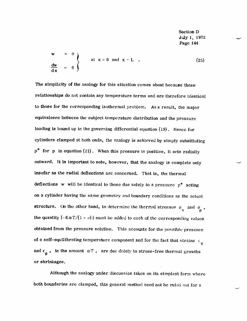
w °I_ 0
dx
Section D
July I, 1972
Page 144
at x = 0 nnd x- L . (25)
The simplicity of the analogy for this situation comes about because these
relationships do not contain any temperature terms and are therefore identical
to those for the corresponding isothermal problem. As a result, the major
equivalence between the subject temperature distribution and the pressure
loading is bound up in the governing differential equation (19). Hence for
cylinders clamped at both ends, the analogy is achieved by simply substituting
p* for p in equation (21). When this pressure is positive, it acts radially
outward. It is important to note, however, that the analogy is complete only
insofar as the radial deflections are concerned. That is, the thermal
deflections w will be identical to those due solely to a pressure p* acting
on a cylinder having the same geometry and boundary conditions as the actual
structure. On the other hand, to determine the thermal stresses a and cr ,x
the quantity [-E_T/(1 - r,) ] must be addcd to each of the corresponding values
obtained from the pressure solution. This accounts for the possible presence
of a self-equilibrating temperature component and for the fact that strains c x
and _ , in the amount c_T , are due dolely to stress-free thermal growths
or shrinkages.
Although the analogy under discussion takes on its simplest form where
both boundaries are clamped, this general method need not be ruled out for a

,f{
/-
Section D
July 1, 1972
Page 145
simply supported shell. In the latter case0 the _malo_ with respect to
equation (19) still holds true. The a_lcd complexity is introduced only thrtmgh
the boundary-condition formulations. In this connection, the bending moment
M may be expressed as follows [16i:X
M -- - Db d2w MTx _ - (i-v) ' (26)
This relationship is applicable anywhere in the shell, including positions
around the boundaries. Only the latter locations need be considered here. It
should be recalled that the condition of simple support includes the requirement
that
M = 0 at x=0 and/or x= L (27)X °
Suppose a uniformly distributed external bending moment
around such a boundary, as defined by the equation
M * is appliedX
, MT
MX - (1- v) " (28)
The user must remember that the sign convention being used specifies that
a positive bending moment causes compressive stresses ou the outer surface
of the shell wall (refer to Fig. 3.0-38). By superimposing moments M *X
around a simply supported end, the related expressions for the boundary
-- ccmdittons become
or
d2w M T M T
mx = -Db_- (1 v) ÷(1- v) - 0 at x =0
Section D
July 1, 1972
Page 146
and/or x = L
(29)
M = -D b 0 at x = 0 and/or x=: Lx dx 2 (30)
Equation (30) is the same as that for a simply supported boundary of a
cylinder which does not experience any thermal influences. Hence, for a
circular, cylindrical shell having both ends simply supported and subjected
to the temperature distribution defined by equations (17) and (18), thermal
deflections w can be obtained by superposition of the following:
1. The radi,_l de.flcctions of a siml)ly supported cylinder which is
Identical to the actual structure but is frec of any thermal influences and is
subjected to a pressure p* where
1 d2MT
p*(x) - (1- v) dx=_ (31)
and bursting pressures are positive.
2. The radial deflections of a cylinder which is free of thermal
influences,, is identical to the actual structure, and whose boundaries conform
with the condition of simple-support except for the application of uniformly
distributed moments M * at each end, whereX

f-
Section D
July 1, 1972
Page 147
MTM * (32)x - (l-v) "
The thermal stressesX and cr_ are found by adding the quantity
{-Ec_T/(1 - v)] to the algebraic sum of these stresses associated with steps
1 and 2. To facilitate the application of this analogy, the user should refer
to Section 2.40 of Ref. 17, which includes numerous solutions that will often
be useful in performing step 1. In addition, Hefs. 17, 11, and 18 provide
simple methods by which step 2 may be accomplished.
A sLtuation similar to the foregoing arises when both boundaries of
the shell are free. As before, the analogy with respect to equation (19)
remains valid but still greater complexity is introduced through the applicable
boundary-condition formulations. In this case, when the cylinder is subjected
to the temperature distribution defined by equations (17) and (18), thermal
deflections w can be obtained by superposLtion of the following:
1. The radial deflections of a cylinder which has both ends free and is
identical to the actual structure but is free of any thermal influences and is
subjected to a pressure p* where
1 d2MT
p*(x) - (1-v) dxT (33)
and bursting pressures are positive.

SectionDJuly 1, 1972Page 148
2. The radial deflection of a cylinder which is free of thermal influences,
is identical to the actual structure, and has the prescribed boundary conditions
except for the application of uniformly distributed moments M * at each end,X
where
MTM * (34)
x - (1-.)
3. The radial deflection of a cylinder which is free of thermal influences ,
is identical to the actm,l structure, and has the prescribed boundary conditions
except for the application of uniformly distributed shear forces Qx* at each
end, where
1 dMTQx* -- (1- .) " (35)
The thermal stresses Crx and a9 are found by adding the quantity
[-Ee_T/(1 - v) ] to the algebraic sum of these stresses associated with items
1 and 2. To facilitate the application of this analogy, the user should refer
to Section 2.40 of Ref. 17, which includes numerous solutions that will often
be useful in the accomplishment of step 1 . In addition, Refs. 17, 11, and 18
provide simple methods by which steps 2 and 3 may be accomplished.
Analogies of the types presented in this section perform a two-fold
function in that they can help the user to develop some physical insight into
thermostructural behavior and also enable him to solve thermal stress

Section D
July 1, 1972
Page 149
problems by using existing solutions for members subjected solely to
mechanical loading. Although the emphasis has been on cases where both
ends of the cylinder have the same boundary conditions, the user should find
it relatively easy to apply the same basic concepts when the two boundaries
are not identical (for example, one end clamped while the other is simply
supported).
If. Thermal Stresses and Deflections -- Linear Radial Gradient_
Axisymmetrlc Axial Gradlont.
A. Configuration.
The design equations provided here apply only to long (L -> 2_/_),
thin-walled, right circular cylinders which are of constant thickness and are
made of isotropic material. It is assumed that the shell wall is free of holes
and that it obeys Hookets law. Figure 3.0-37 depicts the lsotropic cylindrical
shell configuration. Figure 3.0--38 shows the sign convention used for the
stress resultants of interest.
B. Boundary Conditions.
The following types of boundary conditions are discussed:
1. Free edges
2. Simply supported edges
3. Clamped edges.
All possible combinations of these boundary conditions are permitted; that is,
it is not required that those at x = 0 be the same as those at x = L. However,
Section DJuly 1, 1972Page 150
in every case, it is assumed that the cylinder is unrestrained in the axial
direction (N-- 0).
C. Temperature Distribution.
The following types of temperature distributions may be present:
1. A radial gradient which is linear through the wall thickness and
need not vanish at the middle surface
2. Axisymmetric axial gradients.
The permissible distributions can therefore be expressed in the form
Z
T -- TI(x ) +T2(Y ) _- . (36)
Certain restrictions must sometimes be imposed on the complexities of the
functions Tl(x ) and T2(x ) , depending upon the method of analysis employed.
These conditions are explained in a subsequent paragraph. Any of the special
cases for equation (36) are acceptable; that is, either or both of Tl(x ) and
T2(x ) can be finite constants and either can be equal to zero.
D. Design Equations.
Throughout this section, it is assumed that Young ts modulus and
Poisson' s ratio are unaffected by temperature changes. Hence, the user
must select single effective values for each of these properties by employing
some type of averaging technique. The same approach may be taken with
regard to the coefficient of thermal expansion. On the other hand,

SectionDJaly 1, 1972Page 151
the temperature-dependenceof this property can beaccountedfor by
recognizing that it is the product of aT which governs; that is, the actual
temperature distribution can be suitably modified to compensate for variations
in a. When this approach is taken, the user must recognize that any
reference to a linear temperature distribution is actually a reference to a
straight-line variation of the product aT .
In addition, the several types of solutions cited here are based on
classical small-deflection theory. Therefore, it is important for the user to
be aware of this when applying the given methods to pressurized cylinders by
superimposing the thermal stresses and deflections upon the corresponding
values due solely to pressure; that is, because of their dependence upon
classical theory, the methods presented here cannot account for nonlinear
coupling between thermal deflections and the pressure-related meridtonal
loads.
The small-deflection governing differentialequation for the subject
cylindrical shell (refer to Fig. 3.0-37) can be written as follows [19]:
d4w NT 1 dZMT
+4_4w = -_- Db(1- v) dx 2(37)
where

Section DJuly 1, 1972Page 152
' ll-v'lfl = 44Dba2 - q a2t2
t/2
= Ea f T dzN T
-t/2
t/2
M T = E__t/f Tz dz ,
(38)
and
Et a
D b - 12(1 v2) •
If L >-2_/fl , then overlapping effects from boundary conditions at the two
ends of the cylinder can be neglected and the following approximate solutions
to equation (37) apply to each half of the structure:
CASE I (0 -< x -_L/2):
-fix aNT _ a 2 d2MTw = e (C 1 cos fix+ C 2sin fix) - Et Et(1- v) dx 2 ' (39)
CASE [I (L/2 -<x -< L):
e -fl(L-x)[C a cos_(L- x) +C 4 sinfl(L- x)|
aN T a 2 d2M T
Et Et(1 - v) dx z(40)
r
Section D
July 1. 1972
Page 153
The terms e'_X(Cz cos _ + C 2 sin/3x) and e-_(L-X){c s cos _L - x)
+ C 4 sin _(L - x)] comprise the respective complementary solutions to
equation (37)..All of the boundary-condition influences are embodied in these
terms. The remaining portions of equations (39) and (40) are the so-called
particular solutions and those given here are somewhat inexact. They were
obtained by Przemienieckl [20l as first-order approximations from an
asymptotic integration process and will give exact results only if the functions
Tx(x ) and T2(x ) are truly polynomials of second degree or lower; for example.
Ti(x ) =b 0+blx+b_ 2 and T2(x ) =d 0+dlx+d_ z.
When the temperature dlstrllmtlon Is such that polynomial expansions
of T I and/or T 2 require terms higher than the second degree, approximate
soluUons can be obtained by using either of the following two procedures:
1. Truncate the series by eliminating terms having exponents greater
than two and perform the analysis as though the resulting series were exact
representations of T1(x ) and T2(x ) .
2. Ignore the stated restriction on the polynomial expansions and use
the actual higher-degree formulations.
Either of these two possibilities will introduce inaccuracies and, at present,
no studies have been performed to determine the orders of magnitudes for
the errors associated with various ranges of the parameters involved. For
those cases where accurate results are required but equations (39) and (40)

/ Section D
July 1, 1972
Page 154
are inexact, the user can always resort to an alternative procedure whereby
these expressions are suitably modified. This can be accomplished by
retaining the foregoing complementary solutions but introducing more
appropriate particular solutions. The latter can be established by standard
mathematical operations such as variation of parameters or the method of
undetermined coefficients [21, 22].
For any case, the constants C 1 through C4 in the deflection relation-
ships must be evaluated from the boundary conditions. It therefore becomes
necessary to express the various physical possibilities by means of the
following •formulas:
1. Free edge:
Qx?M =0 .'°. X
2. Simply supported edge:
w -- M = 0 . (41)X
3. Clamped edge:
dwW - - 0 .
dx
where
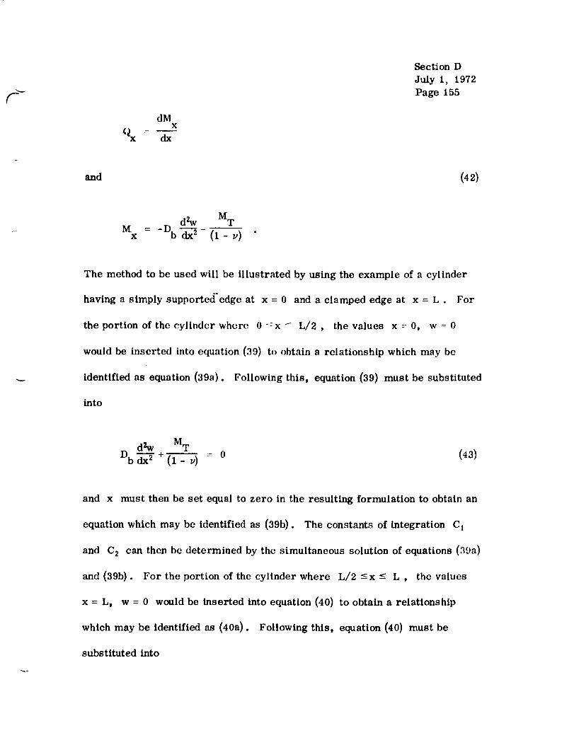
F
Section D
July 1, 1972
Page 155
dMX
Qx dx
and (42)
dZw MT
M = -D bx v)
The method to be used will be illustrated by using the example of a cylinder
having a simply supported'edge at
the portion of the cylindcr where
x= 0 and a clamped edge at x= L. For
0--x'_ L/2, the values x=:0, w =0
would be inserted into equation (39) to obtain a relationship which may be
identified as equation (39a). Following this, equation (39) must be substituted
into
d_v MT
Db_-_+(1- v) - 0 (43)
and x must then be set equal to zero in the resulting formulation to obtain an
equation which may be identified as (39b). The constants of integration C 1
and C 2 can then be determined by the simultaneous solution of equations (39a)
and (39b). For the portion of the cylinder where L/2 -<x -< L , the values
x = L, w = 0 would be inserted into equation (40) to obtain a relationship
which may be identified as (40a). Following this, equation (40) must be
substituted into

Section D
July 1, 1972
Page 156
dw- 0 (44)dx
and x must then be set equal to L in the resulting formulation to obtain an
equation which may be identified as (40b). The constants of integration C 3
and C4 can then be determined by the simultaneous solution of equations (40a)
and (40h).
Once the deflection equations have been found for both halves of the
cylinder, the bending moments M and M at any point can be establishedx
from
d2w M T
M = -D bx -(i
and (45)
dZw M T
M b = -uD b'_T- (I- p)
Then the stresses at any location are given by the following:
12z- t3 MX X
and (46)
12z

f-
where
Section D
July 1, 1972
Page 157
N¢ .N T w Eta(47)
Example No. i.
A thln-walled, right circular cylinder of length L(> 2_/fl) has both
ends simply supported and is subjected to the temperature distribution
z
T = do_- (48)
where d o is a constant, it is desired that the deflections and extreme-fiber
stresses be found, assuming that L = 40 in. and /3 = 0.2.
For the given temperature distribution, equations (38) yield
N T = 0
and (49)
E c_t2dRMT - 12
Then, for 0 _x -<L/2 , equation (39) becomes
-_xw = e (CIcosflx+c 2sln_x) .
At x = 0, the boundary condition of simple support requires that

Section D
July 1, 1972
Page 158
w = M = 0 (51)x
where
d2w MT
M : -D b - _-'--7-- . (52)x "_ (1 v)
From equations (50), (51), and (52), the constants C t and C 2 arc found to
be
CI = 0
and (53)
C2ataz_2
- (i(1- v) d0
Hence, equation (50) may now be rewritten as follows:
eet a2/_2w - 6(1 - Vi d° e-Bx sin fix . (54)
The function _(_x), tabulated by Timoshenko and Woinowsky-Krieger [111
may now be introduced to obtain
at a2_ 2
w - 0(1 - v) d,, ;(/ix) (55)
where
;(_x) = e-_x sin _x . (._.) -_

Section D
July I, 1972
Page 159
By substituting equation (55) into (45), the bending moments can be expressed
as
M E°tt2d0 [00_x) - lJ× - 12(1- v)
and (57)
E _ t2d IIM 12(1 - v) [v0(flx) - 1]
where the function _)(flx) is tabulated by Timoshenko and Woinowsky-Kricgcr
[11] and is defined _,s follows:
0(_×) = o-_X cos _x . (5s)
The extreme-fiber stresses can then be determined from
6MX
O" :: :Fx t-V-
and (5:))
where the upper signs correspond to the outermost fibers. By substituting
equation (55) and the first of equations (49) into (47), the following expression
is obtained for N9 :

Section D
July 1, 1972
Page 160
E a_!a_2N_ = - 6(1 ' _) do _(_x) . (_o)
For the other half of the cylinder (1,/2 " x :_ L), equation (40) must be used,
which, in view of equations (49), becomes
-_(L-x)w = e [Ca cos _(L- x) +C4 sin/3(L- x)] . (61)
At x = L , the boundary condition of simple support requires that
w = M -- 0 (62)X
where
(1% MTM =- - Db ([;:l)x (-_x2 -(1- v) *
From equations (61), (fi2), and (63), tile constants C 3 and C 4 are found to
be
C 3 = 0
and (64)
ata2_ 2C4 - 6(1-p) do "
Then, proceeding in the same manner as for the other half of the cylinder, the
following expressions are found for the deflections, moments, and extreme-
fiber stresses:

SectionD
July 1, 1972
Page 161
c_t a2_ 2w -- (_(1-v)d,, _(l,- ×)1 , ((;._)
E at2do
Mx - 12(1-,,) {O[O(L- x)l - 1}
E_t2d° (u0[fl(L- x)] - 1}M_b - 12(1- u)
6MX
O'x = TT '
((;6)
and 0;7)
where
N 6M
t t _
Eo_t2,a_ 2N@ =- 6(1- u) do r_[_(L- x)] . (68)
Here again, the upper signs in the stress formulas correspond to the outer-
most fibers.
The foregoing relationships for the two halves of the cylinder wcrc
used to obtain the nondimensionnl solution listed in Table 3.0-7. These
results are plotted in Figure 3.0-40.
Example No. 2.
A thin-walled, right circular cylinder of length L(> 27_/_) has both
ends clamped and is subjected to the temperature distribution
T = b 0+ blx (G9)

!
Vl "--
o.
_ 0
e_
I
c_
o
I
_4t-,-
0
_4
0
o
_4
0
I
I
0
!
0
I I I I
O
I
u_0
0
o
_D0,1
,-iq_
_4 _4
Section D
July 1, 1972
Page 162
I I I I I I
. i I
t"=
...,4_DC'.I
qOt"
c;
M
_4,i, I
_l _- II
I I
C".I
' _ _
N n
e,l H

Section D
July 1, 1972
Page 163
where b 0 and b I are constants. It is desired that the deflections and
extreme-fiber stresses be found, assuming that L = 40 in., fl = 0.2,
bl/bo= 2 .
For the given temperature distribution, equations (38) yield
N T = Eat(b 0+blx )
and
and
(70)
MT = 0 °
]B 0.4
P
-1.2
/ \
\\\\\
\
L\
0 10 20 30x(in.)
JJ/
/
//
//
/ IL -f Mx
(E_ 2doI/12(l-v)! l
40
Figure 3.0-40. Nondimensional deflections and axial bending
moments for example problem No. 1.
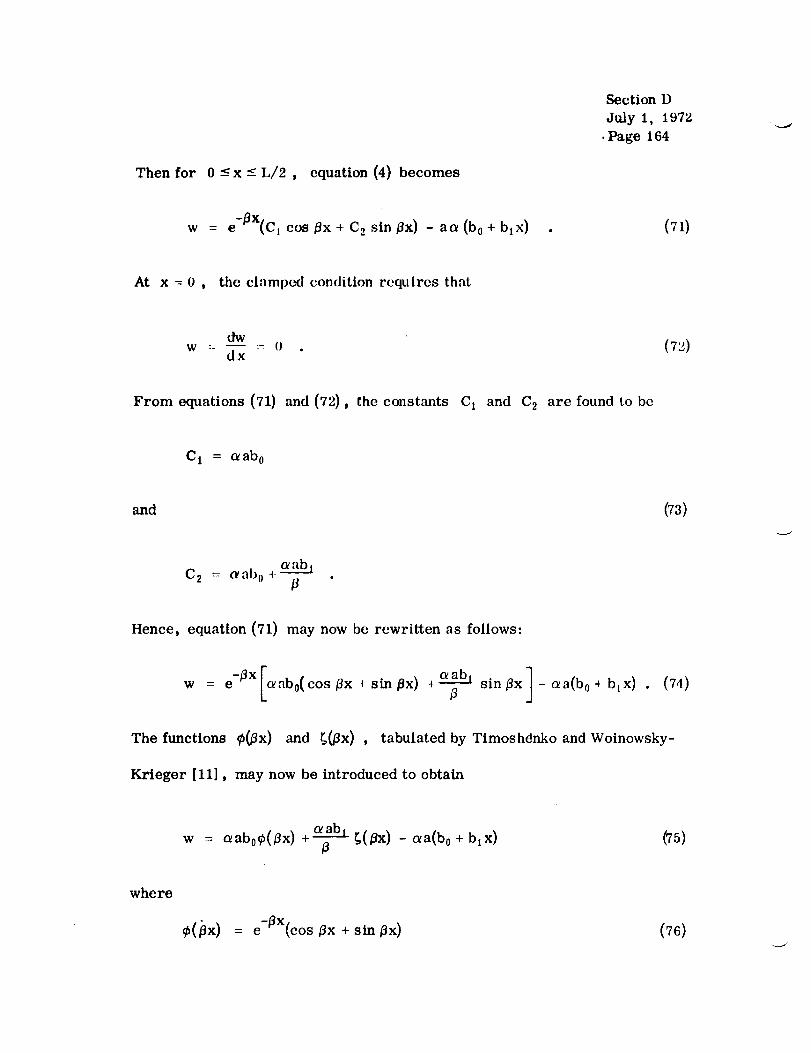
Then for 0 -< x _ L/2 , equation (4) becomes
Section D
July 1, 1972
•Page 164
w = e-#X(clcosflx+C 2sin fix) - acz(b 0+bix ) . (71)
At x = 0 , the clampc_l condition rcquircs that
dww .... o . (7:_)
dx
From equations (71) and (72), the constants C t and C 2 are found to bc
C t = ezab o
and (73)
C 2 = aab 0 +-==-=_-_
Hence, equation (71) may now be rewritten as follows:
lw = e o_ab0(cosflx+sin_x) +_abt sinflx -_a(b0_btx ) . (74)
The functions 9(fix) and _(flx) , tabulated by Timoshdnko and Woinowsky-
Krieger [11], may now be introduced to obtain
+_abt _(flx) - o_a(b 0 + blx )w = cxab09(flx) (7_)
where
¢(#_)= e-_X(cos _x +_m _x) (7s)

and
Section D
July 1, 1972
Page 165
P ;(Ox) -- e-Sxsin_x .
By substituting equation (75) into (45), the bending moments can be
expressed as
(76)
(Col_.)
M× Z {v:ll,,,J)tf_ [¢(fJ×)_ b-_Lb,,_o(r_x)]
and (77)
M = vMx
where the functions ¢(/3x) and 0(Bx) are tabulated by Timoshenko and
Woinowsky-Krieger [11] and are defined as follows:
¢(_x) : e-_*_(co._l*x- sin _x)
and (7S)
0(_x) : e-_x cos/_x
The extreme-fiber stresses can then be determined from
6MX
(7 X -- :1:-7. (79)

SectionDJuly 1, 1972Page 166
and
N (;M
--_ :_ t2 (79)a 0 t ( Con. )
where the upper signs correspond to the outermost fibers. By substituting
equations (75) and (70) into (47), the following expression is obtained for NO :
No = -Et_b0tO(13x) - Etrblt_ _(_x) . (so)
For the other half of the cylinder (L/2 _ x -< L), equation (40) must be used,
which, in view of equations (70), becomes
w = e -_(L-x) [C a cos_(L- x) 4 C 4sin/3(L- x)] -_a(b 0+bix) . (Sl)
At x = L , the clamped condition requires that
dww - - 0 . (82)
dx
From equations (81) and (82), the constants C a and C 4 are found to be
C 3 = c_a(b o + blL)
and (8:J)
C4 = _ _abt + aa(b 0 + btL) .

Section D
Juiy 1, 1972
Page 167
Then proceeding in the same manner as for the other half of the cylinder, the
following expressions are found for the deflections, moments, and extreme-
fiber stresses:
F
W -"
_ab°( 1 + b--ll')o[_(L-x)]brJ -_abf _[_(L-x)] -_ab°(l+b-_x)fl b:_
M 2a,_/t:"l,,I)l) {(l _-h 10 ¢[[_(1.- x) J t--h=0[_(l,-x) l _x I lJ(, - bfj_ I
M vM ,x
6MX
(y .-_× -it-
and (8(;)
N GM
where
NO -F_bl, t (1 + F-hboI_/ _l/3(l,-x) J + _fl _[/3(1,- x)] . (87)
Here again, the upper signs in the stress formulas correspond to the outer-
most fibers.
The foregoing relationships for the two halves of the cylinder were:
used to obtain the nondimensional solution shown in t_able 3.0-_. These
results are plotted in Figure 3.0-41.
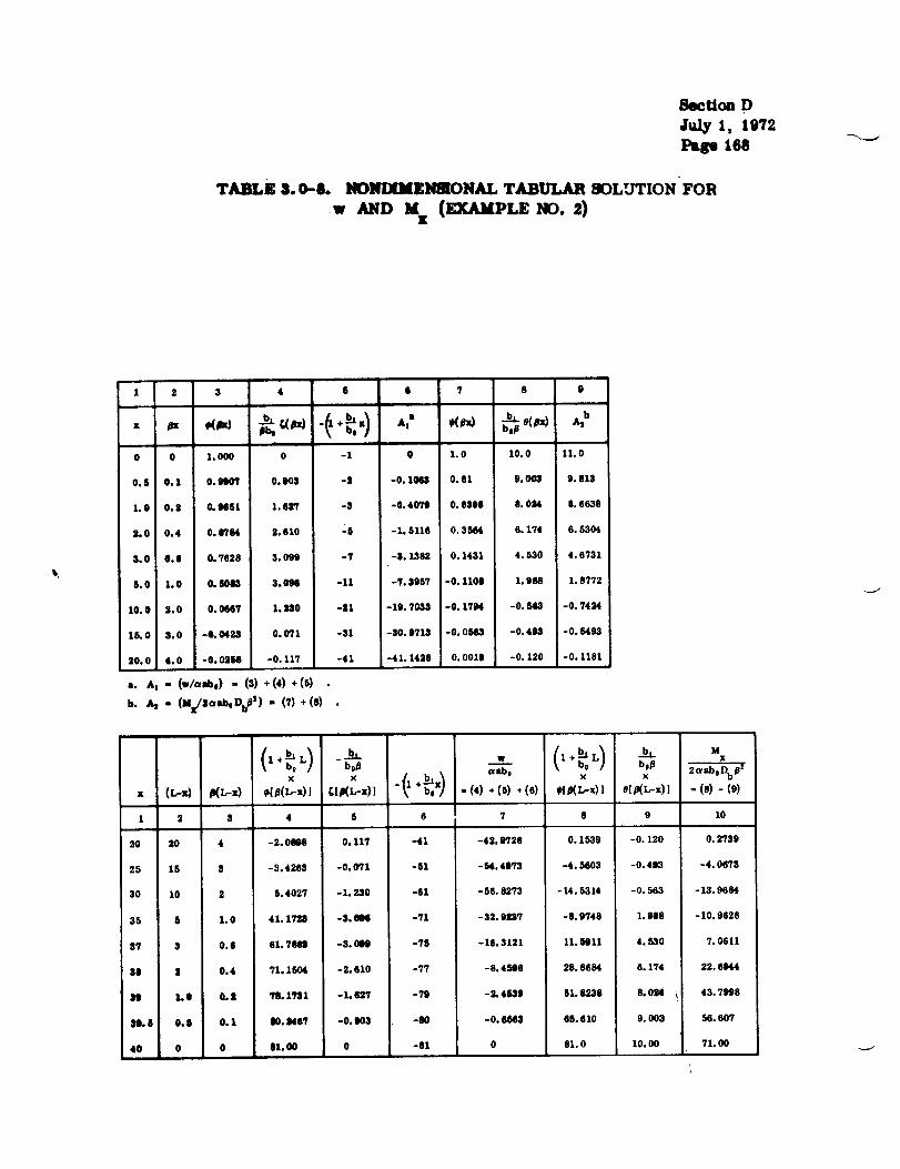
BecUon D
July 1, 19'/2
Pap 168
TABLE S. 0..8. [_OIlDIMi_NSIONAI, TABULAR 90LT_rYION FOR
w M (eXJLM1,LENO. 2)x
1 3 3
0 0 1.000
0.5 0.1 0.9110'1'
1.0 0.8 0.9651
8.0 0.4 0.85'84
8.0 0.8 0.'7628
6.0 1.0 0.6O03
10.0i 2,0 0.0607
15.0'3.0 -0.0423
20.0 4.0 -0. 036O
4
jb. r.(ox)
o
o. 0o3
1, 4:r?
2,81o
3.099
3.o!14
1.86o
o.o71
-o, 117
,. ,, . (,,/a-%) - (3) +(4)÷(8)
b. X, - (,,,_'lo-'.,nb_') - (7) ."(S)
X
x (L..q #(L-x) _l,e(_,0!
1 2 3
20 20 4 -3.06O8
25 16 8 -8.4283
30 10 2 5.4027
35 8 1.0 41.1';'1_
37 8 0.8 61.7849
88 8 0.4 71.1504
H LO 6.| 18.17:11
81, | O. $ 0.1 80. Me7
40 0 0 81,00
3
-I
-8
-$
-6
-7
-11
-91
-31
-41
0 7 8
A," ,(_) _ o(,e,0
0 1.0 10.0
-0.1063 0.61 9. 003
-O. 40'70 O.6308 8. OM
-1. 8118 O. 35414 6. 174
-8. 1382 O. 1431 4. 530
-?.9067 -0.1108 1.086
-19. 7033 -O. 1796 -0. 543
-80.0713 -O. ON3 -0.498
-41.1438 O. 0019 -0. 120
0
Asb
11.0
9.613
8.6638
6.53o4
4.6731
1.8772
-0.7424
-0.5493
-0.1181
_b,boD
X
_(p(L-x)] _x) uabo-{1+ -(4)+(_)+(0)
(,+L,,)X
_,1p(t,-x)I
b,
x
elp(L,-x)l
MX
2o_aboDbd_z
= 18) - 10)
4 5 6 7 8 9 10
0.11'/ -41 -49, 9'/28 0.1539 -0. 120
- 54.4073
- 56. 8273
- 32.995t7
-16.3121
-8.4506
-3.4639
-0. 8668
0
-4.5603
-14.5314
-8.9748
11.6Oll
28.8084
81.8238
68.610
61.0
-0.49_
-0. 563
1.988
4,530
0.174
8. 0P,4
9. 003
10.00
-0.071 -61
-1,230 -61
-8.0Oil -71
-8.099 -78
-2.010 -77
-1.037 -79
-0.908 -80
0 -81
0.0?39
-4. 0078
-13.9684
- 10, 9628
7, 0611
22. 6944
43.7988
56. 007
71.00

?---_
Section D
July 1, 1972
Page 169
/-J
00
/f I0m X
2__aboDb/32_
2O
0
"411
\\
\\
\\
\
_'° \
\
I I0 10_(o..)
\
/!
",,,_J/
\ /\
W
/1
/1
U
Figure 3.0-41. Nondtmensional deflections and axial bending
moments for example problem No. 2.
Section D
July 1, 1972
Page 170
III. Thermal Stresses and Deflections - Constant Radial Gradient,
Axisymmetric Axial Gradient.
A. Configuration.
The design curves and equations presented here apply only to thin-
walled, right circular cylinders which are of constant thickness and are made
of isotropic material. It is assumed that the shell wall is free of holes and
that it obeys Hooke v s law. The method is valid only when h - _ . Figure 3.0-
42 depicts the Isotropic cylinder shell configuration. Figure 3.0-43 shows the
sign convention for forces, moments, and pressures.
B. Boundary Conditions.
The following types of boundary conditions are discussed:
1. Free edge; that is,
Qx = Mx : 0 (88)
2. Simply supported edge; that is,
w = M = 0 . (89)X
3. Clamped edge; that is,
dw
w - dx 0 . (90)
All possible combinations of these boundary conditions are permitted.
itisnot required that those at x= 0 be the same as those at x= L.
Hence,
However,

Section D
July l, 1972
Page 171
NOTE: u,v,w,x,y,z, and _) arepositive as shown.
t
MIDDLE SURFACE
Figure 3.0-42. Isotropic cylindrical shell configuration forthermal stresses and deflections.
N_
Y _ Nx
x
N Mx_ J
NOTE: All quantities positive as shown.
N_
Figure 3.0-43. Sign convention for forces, moments, and
pressures for thermal stresses and deflections.

Section D
July 1, 1972
Page 172
in every case, it is assumed that the cylinder is unrcstr:dnetl in the axial
direction (N x 0) .
C. Temperature i)istribution.
The supposition is made that no temperature variations occur through
the wall thickness. However, the cylinder may have any axisymmetrie surface
gradient for which the product tyT can be adequately represented by a fifth-
degree (or lower) polynomial. Therefore, subject to that restriction, the
permissible distributions are of the form
,,'r : (x) "r(×) (.0
I). I)esig'n Curves and I,:qu:ltions.
In Ref. 23, Newman and Forray present the practical methtxl given
below to compute the thermal stresses, deflections, and rotations in circular
cylindrical shells which comply with the foregoing specifications. The primary
relationships are expressed in series form and the necessary term-by-term
coefficients can be obtained from Figures 3.0-44 through 3.0-49. As indicated
by equation (91), the product c_T will be a function of x and, in order to
apply this method, this function must first be approximated by the polynomial
where
Z
(_T = d 0+dz_ _ (12_ 2 _ °.. dz z = _ dk_k (:)2)k=0
is a dimensionless axial coordinate defined by the relationship
x (93)!!O
!
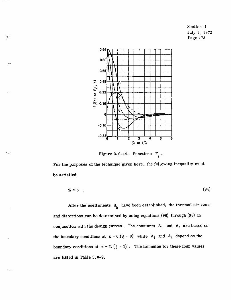
Section D
July 1, 1972
Page 173
0.48
I.l..
,.. 0.320
0.16.m
I,,t..
0 I 2 3 4 5 6_;_ or _'X
Figure 3.0-44. Functions F..1
For the purposes of the technique given here, the following inequality must
be satisfied:
z -<5 . (94)
After the coefficients d k have been established, the thermal stresses
and distortions can be determined by using equations (96) through (98) in
conjunction with the design curves. The constants A 1
the boundary conditions at x = 0 (_ = 0)
boundary conditions at x = L (_ = 1) .
are listed in Table 3.0-9.
and A 2 are based on
while A 3 and A 4 depend on the
The formulas for these four values

I
i-" o.IlII1
..- o.s.J0u
0.4
r.0w
_ 0.2UlQ
1
o.eII1mcJ-- 0.6ILUt
0¢J
_ O.4
ul
0.2WQ
-O.2
1
,n 0.8I
Z
_ 0.6
ul
_ 0.4
I-o 0.2W.JLk
00
-0.2 (_
/
"I_.o_
// //
//,//
_'3 -_._//3.5,
X> ,ss_
_._...._ _ "
i
,4//!
AiH
j///
AXIAL COORDINATE,
3.5
I...3.2 ,
i 3.5'-L 4-_[ 15"-.
,11
'_- 2.5
Z.J
w. 2iu
0
.1
_ 1.5
' /J
o/-
A z6IU.
! °0
0.2 0.4 0.6 0.8 1
Section D
July i, 1972
Page 174
Figure 3.0-45. Deflection
coefficients and k = 5, the
coefficient depends on h .
/
/f.,<._'/I
/
I t r
i
--..d_
I 3.5
_> _5_
/A/
,t
,///
///
//k'4/ /
i/
/
/2*
0_.
A/!///
-1
0 0.2 0.4 0.6 0.8 1
Figure 3.0-46. Slope coefficients
(for k = 5 , the coefficient
depends on )_ ) .

ZO
16
U
I |
_L
J--'_1
/
o 02 04 115
• AXIAL COORDINATE._
I,'i_rc 3. O-47.
J
/
/
//I
,,s/
//L2
_2!
10, I
oil
Moment coefficients.
Section D
July 1, 1972
Page 175
$0
u
0
0
Figure 3.0-48.
?/.//r
0Z 04 05 08
AXIAL COORDINATE.
Shear coefficients.
//
j/
0fi/0 02 04
J
I /
/
J
4q,
I
0,t,2,3_06 08
AXIAL COORDINATE.
/
Figure 3.0-49. Hoop-force coefficients.

Section D
July 1, 1972
Page 176
TABLE 3.0-9. FORMULAS FOR THE CONSTANTS A 1 THROUGtt A 4
Cylinder
End
l
_=0
(x = o)
4=1
(x = L)
4=1
(x = L)
_=1
(x - L)
A 1
Boundary
Condition Constants A t
Free
Si mph'
support
(!l;iml)ed
F re(,
Simple
support
Clampc_J
A 2
A I
Z
1 _ dkmk(0 )i-'ix'_I ,
z ] %(0)"_1 k_ dk mk(O) 4X" 2k_" =0 i
Z
2A_ k=0
Z
A:_ - _' dkWk(0 )k =0
z - IOk(O}..A t :: _ _ dk Wk(O) 'k---O
Z
dkWk(0)k -o
A 3
Z1
2_----_ _ dkmk(1)k-0
,zA 1 = _ _ dk qk(1) - ink(l) rk---O
Z
A_- _ E %%(_)2)'2 k=0
Z
A,=- Z dk_k(1)k=0
Z "1 "IA_ = _ d k i kOk(1) -Wk(1)k=0 -
Z
A, - - 2 _k (1)k=0
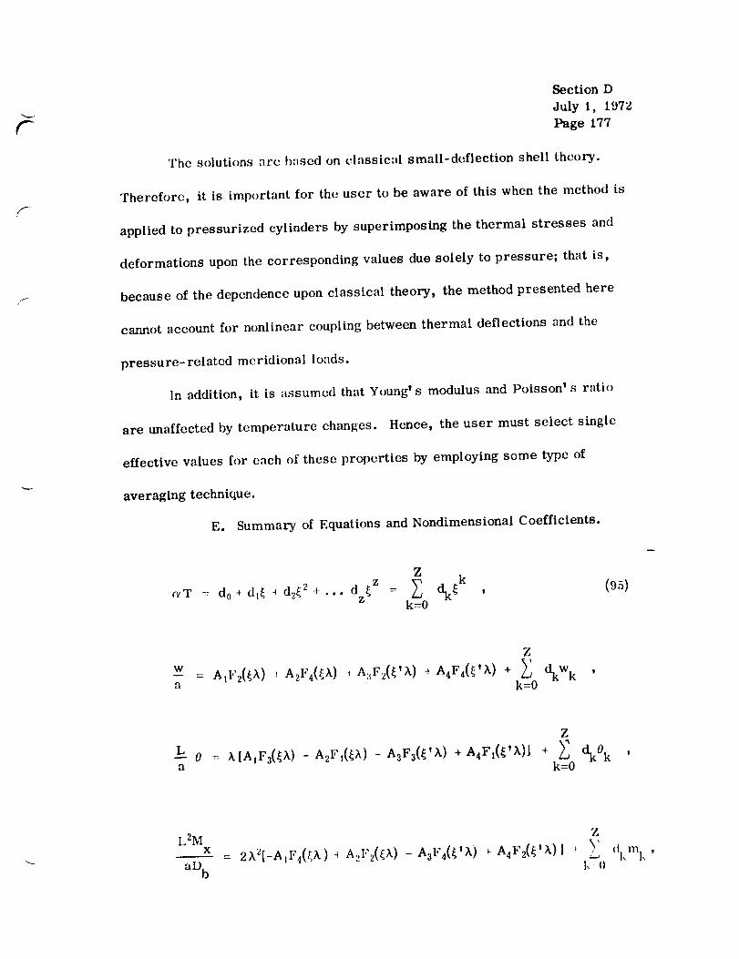
f
f
Section D
July 1, 1972
Page 177
The solutions arc b:ised on cl:lssical small-deflection shell theory.
Therefore, it is important for the user to be aware of this when the method is
applied to pressurized cylinders by superimposing the thermal stresses and
deformations upon the corresponding values due solely to pressure; that is,
because of the dependence upon classical theory, the method presented here
cannot account for nonlinear coupling between thermal deflections and the
pressure-related mcridional loads.
In addition, it is assumed that Youngt s modulus and Poissonl s ratio
are unaffected by temperature changes. Hence, the user must select single
effective values for each of these properties by employing some type of
averaging technique.
E. Summary of Equations and Nondimensional Coefficients.
Z
.T :: d o_ d_ _ d_ :+... d _z = _ _k , (95)z
k=0
Z
w _ AlI,,2(/;_. ) i A2F4(_h. ) , A:lF._(t_'X ) + A4F4(_'_. ) + _ dkW kak=0
Z
L 0 = XIA1F3(_, ) - A2Fi(_)C ) - A3F3(_'_. ) + h4Fl(f'X)l +a k=0
dk0 k
L2Mx
aD b_ 2;tZl-AiIe4(_2t) _ A.,F2(_X ) - A3F4(_l)t)
Z\,' diem k ,
k 0

Section D
July 1, 1972
Page 178
MO = VMx ' (96)
aD b
Z
2)_3[AIFI(_k) + A2F3(_)_) - A3FI(_'_,) - A4F3(_'k)]+ _ dkq kk=0
and
a2D b:: 4k4[AiF2(_2t) +A2F4(_k ) +A3F2(_tk ) 4 A4F4(_'X)] -
Z
dkn kk=O
where
h
Et 3
Db - 12(t- v2) (97)
x
L '
and
It = 1-4 •
The stresses at any location are given by the following:
12z% -- -V- M (98)

f.-
F
and
Section D
July 1, !972
Page 179
'79 Not -712z:: - M 9 . (98)(Con. )
3.0.8.2 Isotropic Conical Shells.
This section concerns the thermostructural analysis of thin-walled,
right circular, isotropic conical shells. The organization here is somewhat
different from that of previous sections which cover isotropic flat plates.
This is due tG certain fundamental differences between the physical behavior
of flat plates and shells. Flat-plate deformations are of such a nature that
it is helpful to group the solutions for stable constructions into the following
categories:
1. Temperature gradients through the thickness
2. Uniform teml)eraturcs through the thickness.
Except for the special case of self-equilibrating gradients through the
thickness (N T -: M T : 0), the first of these two cases involves out-of-plane
bending which is, of course, accompanied by displacements normal to the
middle surface of the undeformed plate. In case 2, the plate remains flat;
that is, the only displacements occur in directions parallel to the original
middle surface and no out-of-plane bending occurs. The indicated separation
of cases is therefore a logical format for the sections dealing with flat pl:_tes.
However, the situation is not the same for shell structures. For these com-
ponents, there is no need to isolate the foregoing types of thermal conditions.

Section D
July 1, 1972
Page 180
This is because either type of temperature distribution, in conjunction with
clamped or simply supported I)ounti:_ries, will load to both membrane loading
and bending about the shell-wall middle surface. Consequently, for stablc
shell constructions which comply with either case i or 2, the analysis methods
are given as follows as a single grouping.
Configuration.
The design equations provided here apply only to long (L -> 21r/hB),
thin-walled, truncated, right circular cones which are of constant thickness,
are made of isotropic material, and satisfy the inequality
xA>atcot . (9.'))
It is assumed that the shell wall is free of holes and obeys Hooke' s law.
Figure 3.0-50 depicts the subject configuration, as well as most of the nota-
tion and sign conventions of interest.
Boundary Conditions.
The method presented herr, can be applied where any of the following
boundary conditions are present:
1. Free edges
2. Simply supported edgcs
3. Clamped edges.
All possible combinations of these boundaries are permitted; that is, it is not
required that those at x A be the same as those at x B . However, in every
case, it is assumed that the cone is unrestrained in the axial direction.

Section D
July 1, 1972
Page 181
R2
NOTE: 1. s* = L-s
2. H A , HB, M A, M B,
V, and W are axisymmetric.3. All coordinates, forces,
moments, and deformations arepositive as shown.
, x HA
(R2)
a. Overall truncated cone.
HB
Me
Ne
N x
b. Positive directions for the stress resultants and coordinates.
Figure 3.0-50. Configuration, notation, and sign convention for conical shell.
Section i)
July l, 1972
Page 18?
Temperature Distribution.
The following types of temperature distributions may be present:
1. A linear gradient through the wall thickness subject to the provision
that the temperature change T need not vanish at the middle surface.
2. Axtsymmetric meridional gradients.
The permissible distributions can therefore be expressed in the form
Z
T = TI(s ) _ T2(s ) _- . (100)
Naturally, any of the special cases for this equation are applicable; that is,
either or both of Tl(s) and T2(s ) can be finite constants and either may bc
equal to zero.
Design Equations.
A number of methods for solving the subject problem have been pub-
lished, including those of Refs. 24 through 27. In the approach presented
here, particular solutions to the governing differential equations are found in
the manner suggested by Tsui [16]. As in Refs. 25 and 28, the complementary
solutions are obtained by an equivalent-cylinder approximation. When greater
accuracy is desired, the exact complementary solutions published by Johns
and Orange [29] may be used.
Throughout this section Itis assumed that Young' s modulus and
Polsson' s ratio are unaffected by temperature changes. Hence, the user must
select single effectivevalues for each of these properties by employing some
type of averaging technique. The same approach may be taken with regard to

f-
(
/
Section D
July 1, 1972
Page 183
the coefficient of thermal expansion. On the other hand, the temperature-
dependence of this property may be accounted for by recognizing that it is the
product sT which governs; that is, the actual temperature distribution can
be suitably modified to compensate for variations in _. When this approach
is taken, any mention of a linear temperature distribution is actually making
reference to a straight-line variation of the product o_T .
In addition, the method outlined here is based on classical small-
deflection theory. It is important to keep this in mind when applying to
pressurized cones by superimposing tbe thermal stresses and deformations
upon the corresponding values due solely to pressure; that is, because of the
dependence upon classical theory, the method of this manual cannot account
for nonlinear coupling between thermal deflections and pressure-related
meridional loads.
The governing differential equations for the subject cone are given by
Tsui [16] as follows:
L'(U) - VEt tandN T
dx
and (101)
1 1 cot__ dMT
L'(V) , U_b b cotO- -Db (1- _) dx
where

Section D
July 1, 19"/2
Page 184
Et 3
Db - 12 (I- v"_)
t/2
MT = E_ f-t/2
t/2
= E(_ fN T-t/2
Tz dz
Tdz
(102)
and
v -xQ x
and L' is the operator,
...,,=oot,[. (103)
To obtain the desired solution, a three-step procedure is employed as out-
lined below:
step 1,
Step 2.
Find a particular solution to equations (101).
Find a solution to the homogeneous equations,
L'(U) - VEt tan q) = 0
and (lO4)
L'(V) +U_bbCOtib -- 0 ,

Section D
July I, 1972
Page 185
such that superposition of these results upon those of Step 1 satisfies the
boundary conditions which can be expressed as follows:
Free edge: Q = M = 0 ."X X
f- Simply supported edge: W = M = 0 (105)X
Clamped edge: W = V = 0 .
The results from this step are referred to as the complementary solution.
Note that equations (104) are obtained by setting the right-hand sides of
equations (]01) equal to zero.
Step 3. Superimpose the particular and complementary solutions.
To accomplish the first of these steps, the functions N T and M T are first
approximated as polynomials. It is then assumed that the particular solutions
U P and VP can be expressed in the form
P nU = C_lx-l+ C 0÷ C1x+ C2x2+ C3x3+ . . . + C x
n
and (I0,;)
V P n= d_ix -i + d o t dlx _ d2x 2 + d3x 3 + . . . + d xn
where n is an integer whose value is a function of the polynomial degree
required for a sufficiently accurate representation of NT and MT . If these
formulations for N T, MT, U P, and V P are substituted into equations (101)

Section D
July 1, 1972
Page 186
and like powers of x are equated, a system of simultaneous equations is
obtained where the unknowns are the various polynomial coefficients. These
equations can be solved for C( ) and d( ) and hence U P and V P . The
associated radial deflection and stress resultants of interest can then be deter-
mined from
dU P P)--P c°s2 P x vU + aRTW - Et stn¢ _ - m
Qx P - U PX t
PN = Qx cot ¢X
(107)
d (R 2Qx)Nop])
dU=cotO dx
and
PM
X (d_+ v V P ) MTDb "_2 cot0 - (1:v)
where
PM 0 = DbP
V dVP) MTcot_b + v--'-_- - (;- _)
t/2
T =1 _m t -tT dz (108)
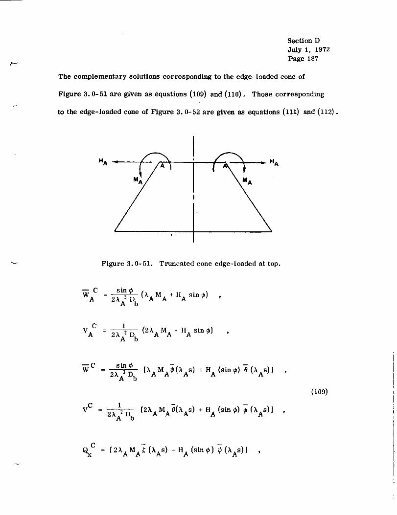
Section D
July 1, 1972
Page 187
The complementary solutions corresponding to the edge-loaded cone of
Figure 3.0-51 are given as equations (109) and (110). Those corresponding
to the edge-loaded cone of Figure 3.0-52 are given as equations (111) and (112).
HA A
Figure 3.0-51. Truncated cone edge-loaded at top.
_C = sin 92A/ D b (_'A MA + ItA sin _b)
V: - 1 (2_,A MA d HA sin q)2?,/ Db
--c sin9 [xA -W - 2A/D b MA¢(AA s)
V C _ 2_:2D b [2AAM AO(XAs)
m
+ HA (sin _) 0 (XAs)]
+ HA (sin q) 9 ()tAS) ]
(109)
CQx = [2k AM A_ (AAS) - H A (sin _b) _ (),AS)]
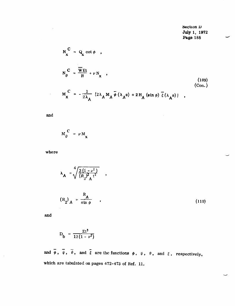
_ctlon D
July 1, 1972
Page 188
CNx = Qx cot
N C WEt- R +vN X
C 1
Mx = -_2k "[2hAA
MA¢ (XAs) + 2HA (sin ¢) _(XAs) J
(109)(Co..)
and
CM 0 = vM x
where
RA
(R2) A - sin9 (110)
and
Et 3
Db - 12(1- v 2)
E m
and 9, 3, O, and _ are the functions 9, @, 0, and _,
which are tabulated on pages 472-473 of Ref. 11.
respectively,
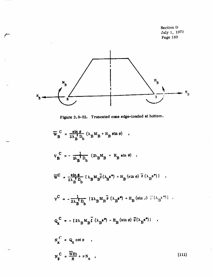
Section D
July 1, 1972
Page 189
MB }4B
HB
Figure 3.0-52. Truncated cone edge-loaded at bottom.
= (ABM B + HB sin _) .
V: =- _ (2ABMB + H B sln_) ,
_C = s___ b [ ABMB_(KBS,) + HB (sin _b) O (ABS')J
vC 1 - _.
= - _kB-'_Db [2ABMBS (ABe*) +HB(ehl _) ,,',(7,Be,*); :
_c . . [2AsMs _ (AS,,}. "B (sm_) _'(Ass*)j
= Q_, cot
w
c wzt (_i)N ---'_-+VNx '
= _ 1 I2ABMB_ (ABS,)
Section D
July 1, 1972Page 190
+ 2 HB (Sin ¢) "_ (ABS*)I
and
where
M c = vM x (111)
(Con.)
B B
(B2)B = s-_n¢ ' (112)
and
Et 3
Db - 12(1- v 2)
and 9", _', 0", and _" are the functions ¢, _, 8, and _, respectively,
which are tabulated on pages 472-473 of Ref. 11.
After the particular and complementary solutions have been super-
imposed, the final thermal stresses can be computed from the following
formulas:
12z N N 8x 12zcr = M +-- and (113)X _ X t or8 - ta MS+-_-.. '
.f--
Section D
July 1, 1972
Page 191
3.0.8.3 Isotropic Shells of Revolution of Arbitrary Shape.
The discussion presented here is concerned with approximate small-
deflection solutions for thin-walled shells of revolution having otherwise
arbitrary shapes and made of isotropic material. A typical configuration,
along with pertinent notation and sign conventions, is shown in Figure 3.0-53.
It is assumed that the shell wall is free of holes and obeys Hooke' s law. The
temperature distribution must be axisymmetric but arbitrary gradients may
be present both through thc wall thickness and in the meridional direction.
To determine the thermal stresses and deformations for the structures under
discussion, the following sets of equations are available:
1. Equilibrium equations
2. Strain-displacement relationships
3. Stress-strain relationships.
In principle, together with prescribed boundary conditions, these formulations
should provide a sufficient basis for the development of closed-form, small-
deflection solutions to the subject problems. However, it will often bc
extremely difficult, if not impossible, to achieve such solutions. Thcrcfore,
numerical integration procedures in conjunction with a digital computer pro-
gram are frequently used to achieve the desired solution. On the other hand,
still another approach may be taken by using approximations such as those
cited by Fitzgerald in Ref. 30 or Christensen in Ref. 31. Since these approxi-
mations avoid the need for sophisticated mathematical and/or numerical

Section D
July 1, 1972
Page 192
- f3 * ....
= •
MIDDLESURFACE
rl, r2, and _ are
positive as shown.
a. Overall shell of revolution.
MIDDLE deSURFACE
NOTE: x, y, and z arepositive asshown.
be Positive directions for forces,
moments, pressures, and
coordinates.
c. Element of shell wall.
Figure 3.0-53. Configuration, notation, and _ign convention for
arbitrary shell of revolution.

f"
/
Section D
July 1, 1972
Page 193
operations, they are well suited to a manual of this type. It would therefore
be desirable to prepare a section which outlines detailed procedures along
these lines. However, from a brief study of Refs. 30 and 31, it was concluded
that they should be thoroughly explored before specific recommendations arc
made. Consequently, in the following paragraphs only the related broad con-
cepts are presented.
The method of Ref. 30 relies heavily on the following set of equilibrium
equations, which, except for the term involving m_ , are derived in Ref. 11:
d__ (N_r0) _ N0rl cos _ - r0Q_b _ r0r 1 Y = 0
d
N br 0 +N0r 1 sin_ +_ (Q_br0) +Zrlr 0 : 0 , (114)
and
d = 0-_(M_r O) -Mor lc°sO-%rlrO+m_brlr 0
These expressions are used in the following manner:
1. First the assumption is made that membrane forces
N O = N0 = N R (115)
and bending moments

SectionD
July 1, 1972
Page 194
M 0 = M --- M R (116)
ar_: present which completely arrest all thermal displacements.
These forces and moments simply furnish a starting point for the com-
putations and do not represent the actual values which will be determined later
in the procedure.
It follows that
E t/2
N R = f _T dz (117)(1- v) _ti../_
and
t/2
MR = __1E- V) -t_Tz dz . (118)
2. In general, the above type of force and moment distribution will not
be in equilibrium unless one or more of the following is applied:
Q_ = (%). ,
Y = YB ' (,19)
Z = ZR ,
and
n1_ -- m r .

Section D
July i, 1972
Page 195
At this point, in order to achieve an approximate solution, Fitzgerald [30]
makes the assumption that
% = (Q_)R = 0 (120)
and justifies this practice by performing an order-of-magnitude study of the
error introduced. Then, proceeding with the analysis, equations (120) and
(115) through (118) are substituted into the equilibrium relationships (114) to
arrive at simple formulas for YR ' ZR ' and m R .
3. Recognizing that the actual shell is free of any of the above types of
loading, it is necessary to restore the structure to this state by application
of the following:
-YR; -ZR; -mR
This is done in a two-step procedure as outlined below.
4. The expressions
Y = - YR
and (121)
Z = -Z R
are inserted into the first two of the equilibrium equations (114) while the
assumption that
Section D
July 1, 1972
Page 196
Qo = o (122)
is retained. The resulting equationB are then solved for N 0 and N 0 . From
the stress-strain relationships, the corresponding strains can be determined.
After this, the strain-displacement formulations may be used to express the
related rotations and deflections of the shell wall in terms of N 0 and N0 .
The bending moments M8 and _ can then be established from the equations
M 0 = _ Db(X 0 +vX O)
and (123)
M 0 = - Db(X 0 +vX 0)
where
Et a
Vb -- 12(1- v2) ' (124)
while Xe and X0 are the curvature changes of the hoop and meridional fibers,
respectively.
5. One may now proceed to substitute
m 0 = - m R (125)
into the third of the equilibrium equations (114), along with the assumption
that
_o = Mo = o . (126)

f-Section D
July 1, 1972
Page 197
Simple transformation thon yields a formula for Q_ which, together with
equations (126) and the first two of (114), leads to simple expressions for
N O and N_ in terms of M R . The use of equations (126) in this phase of
the development is justified by Fitzgerald [30] on the basis of an error-
magnitude study. Using the stress-strain and strain-displacement relation-
ships, practical formulations can bc derived for the rotations and displacc-
ments associated with the membrane loads N O and N_ obtained in this step.
6. The final approximate values for the membrane loads, bending
moments, rotations, and displacements are found by superposition of appro-
priate values from steps 1, 4, and 5. The stresses due to these membrane
loads and bending moments must be augmented by those stresses associated
with any self-equilibrating temperature distributions which exist through the
thickness.
To focus attention on the general concepts involved in Fitzgeraldl s [30}
approach, no mention is made in the foregoing steps of the need to satisfy
prescribed boundary conditions in the problem solution. Therefore, it might
now be helpful to note that, for this method, it is probably best first to obtain
results under the assumption that no external constraints are present.
Following this, edge forces and/or moments may be superimposed which
enforce the required conditions at the boundaries.
The general philosophy behind the approach of Christensen [31] is
very similar to that of Fitzgerald, although the details are quite different.
Section DJuly 1, 1972Page 198
Chrimtmmen also relies heavily upon the equilibrium equations (114) but, for
pure thermostructural problems, he makea no use of the loadings Y, Z ,
and m#. Hence, these quantities are taken equal to zero throughout the
entire analysis, which is performed in the following manner:
1. First the assumption is made that
M e = M b = M B (127)
where
t/2E
f c_Tz dz . (128)MB = - (1- v) -t/2
Here again, these moments simply furnish a starting point for the computations
and do not represent the actual values which will be determined later in the
procedure. These moments are inserted into the equilibrium equations (114).
The third of these equations is then combined with the other two and two equa-
tions in the unknowns N 0 and N¢ are obtained.
2. By using the stress-strain and strain-displacement relationships,
the two equations from step 1 are rewritten in terms of the temperature dis-
tribution and the middle-surface displacements v and w, where v is
measured in the meridional direction and w is taken normal to the middle
surface.
f--
Section D
July I, 1972
Page 199
3. The two equations from step 2 are combined to arrive at a single
formulation in terms of v and the temperature distribution.
4. The equation from step 3 is then solved subject to the boundary con-
ditions at the shell apex. This is accomplished by assuming that v car be
expressed as a polynomial and then callingupon the method of undetermined
coefficients. The resulting expression for v must then be substitutedinto the
appropriate equation from step 2 to obtain a solution for the displacement w .
5. From Timoshenko [11], the bending moments M 0 and M_ which
are associated with the displacements v and w can be determined.
Christensen [31] refers to these as corrective moments and, ifthey are not
small with respect to M R , an iterativeprocess must be used whereby the
initiallyassumed moments are successively revised. However, the study
reported in Ref. 31 seems to indicate that the first cycle will oRen be suffi-
ciently accurate for most engineering applications.
6. From the stress-strain and strain-displacement relationships, the
membrane loads N O and N_ due to v and w can now be found.
7. The finalapproximate values for the bending moments, membrane
loads, and displacements are found as follows:
a. Final M 0--M R+corrective M 0 .
b. Final Me = M R + corrective M¢ .
c. Final N 0 and N¢ = obtained from step 6.
d. Final v and w = obtained from step 4.
(129)

Section D
July 1, 1972
Page 200
The total approximate values for the stresses are obtained by superimposing
those associated with the final bending moments, final membrane loads, and
any self-equilibrating temperature distributions through the wall thickness.
To focus attention on the general concepts proposed by Christensen
[33], no mention is made in the foregoing steps of the need to satisfy pre-
scribed boundary conditions at locations removed from'theapex. Therefore,
it might now be helpful to note that, for this method, it is probably best first
to obtain results under the assumption that no external constraints are
present at such positions. Following this, edge forces and/or moments may
be superimposed which enforce the required conditions at the boundaries.
The foregoing approaches are only two of a number of possibilities for
the subject problem and can be used to obtain approximate values without the
ueed for sophisticated mathematical and/or numerical operations. However,
solutions can also be obtained by the use of existing digital computer programs,
many c _which use either discrete-element or finite-difference methsds. Such
programs are probably the best approach for obtaining rapid, accurate solu-
tions. However, to retain a physical feel for the problem, it would be helpful
to convert temperature distributions into equivalent mechanical loadings, such
as was done for isotropic circular cylinders. It is recommended that future
efforts include work along these lines to arrive at the equivalent pressures for
shells of revolution having arbitrary shapes.

I. Sphere Under Radial Temperature Variation.
A. Hollow Sphere.
Inside radius = a.
Outside radius = b.
Section D
July 1, 1972
Page 201
2+F r3a3b rcr - - 1rr 1- _ (b_- _r_ f Tr2 dr - _-_ f It2 dr
a a
olE [ a3 + 2r3 f Tr 2 dr _5 Tr 2 draO0 = _ - 1- u [(b 3- a3)r 3 a + a -
U --1 + p_ 1 I a3 b b3 r_'__p/b3_a 3 "_ fTr2dr+ri fTr2dr
r a
b2(1- 2v)r f Tr2d r(i +p) a
T(r) : t o : constant,
_rr = a00 : _ :: o
and
u = _Tor .
I
I+
fI

B. Solid Sphere.
Section D
July 1, 1972
Page 202
l_'l b 1 r T/aS 2 f Trldr+._ f Tridr_°'00 = °'¢_b - 1-v 0 0
/l+v_[ 1 f Trldr +U = "_-_.v/ r-'i a (1 + v) Tri
Crrr(0 ) = _r0e(0) = _(0) - i-_" b1 0 - 3 '
T(r) = To = constant ,
Crrr = _00 = _ -- 0 ,
and
U = _Tor •

¢_----
i.
Secti(_n l)
July 1, 1972
Page 203
4.0 THERMOELASTIC STABILITY.
The thermoelastic problems considered in the previous paragraphs
have followed formulations of the linear theory of thermoelasticity; they have
thus excluded questions of buckling, problems in which the effect of the loading
depends on the deformations (as in the case of beam-columns), large deflec-
tions, and other similar effects. It is the purpose of this paragraph to discuss
some of the principal problems of this type. It should be remembered that
the solutions are approximate from the viewpoint of an exact thermoelastic
formulation. The nature of these approximations was treated in the previous
subsections,
4.0.1 Heated Beam Columns.
If a beam-column is subjected to the action of heat, the influence of
temperature must, in general, be taken into account, The analysis in the
cases in which the ends of the beam are restrained in the axial direction is
slightly different from that used when the ends are free to displace in that
direction. The latter case will be considered in paragraph 4.0.1.1 while the
former is considered in paragraph 4.0.1.2.
4.0.1.1 Ends Axially Unrestrained.
The buckling behavior of beams (and therefore also their behavior as
beam-columns under any combination of transverse and axial loads) depends
on the shape of the cross section: For example, a beam whose cross section
possesses no axes of symmetry can buckle only by a combination of twisting

Section D
July 1, 1972
Page 204
and bending, whereas in other cases some of the uncoupled modes arc also
possible. The general lormulation and solution of this problem are discussed
in Ref. 1, but for simplicity, the following analysis is restricted to doubly
symmetrical beams, with least principal moment of inertia under a transverse
distributed load p = p(x) acting in the xy plane, and subjected to a tempera-
ture distribution such that MT = 0. The beam will thus bend in the xy planeY
without twisting and with w = 0. The governing differential equation is
d_M T
(12 (_: d_v._ -, j, d'v z
It is convenient to obtain the solution in two parts, by separating the effects of
temperature and of transverse load• For this purpose vT is the deflection the
beam would undergo if only temperature and the axial load P were present
(transverse loads absent); it therefore satisfies the differential equation
dZ (E (12V'l' % (IZv'[' d2MT_7 l_.,-;_T_/ , I, - zdx _. dx 2 • (Z)
The quantity Vp is the dcl'lcction th(, Ix,,am would undergo if only transvers(:
loads and the axial load' P were present (temperature effects omitted); it
therefore satisfies the differential equation
d z (_ d2vp_ d2vp
_r \,:Iz_ / + P ,_--T-- p • (3)

Section D
July 1, 1972
Page 205
With the definitions, the solutions of the combined problem in which all loa(Is
are acting is
v= v T + vp .
The component deflection Vp represents the solution of the ordinary
!
isothermal beam-column problem and can often be found in the literature (see
Section B4.4). The determination of v T musjt, in general, be carried out
t
anew for each new problem, lIowcver, in the special case of uniform beam
under a temperature distribution of the form of a polynomial of a degree not
higher than the third in the spanwise direction, that is, when
MT = a 0 + alx ÷ a2 X2 + a3 X3 ,
z
then
MTZ
vT = _ p + % + clx + c 2 sin kx + c 3 cos kx
where k = _ and the constants ('0, ct, c2, and % are determinedZ
from the boundary conditions. Solutions for v T for three important special
examples for which
M T = a o + alxZ
are given as follows.

Section D
July 1, 1972Page 206
I. Both Ends Fixed.
_--_ i- _ _.L
L.. -I
F -!
4_ 2 EIZ
= - L2v T 0for P<Pcr
II. Both Ends Simply Supported.
and
y
IP ---b_,
t.
P•---.--e. X
VT /co.kL-1 )=- P \" si_kJ_ sinkx+l- coskx - P sinkL
7r2EIz
p - L[cr
III. Cantilever.
a0 1 - cos kx
VT = - _ cos kL
P
al[<kL_siokL) ]"_ cos kL (1 - cos kx) + kx - sin kx
and

f
lr_ EIZ
Pcr =
The axial stress is given by
=-_ET + _ +- MT +M + P{7xx A z v
Z Z
Section D
July 1, 1972
Page 207
In these analyses, the beam-column has been assumed to carry a compressive
axial load. If the load is tensile, the appropriate results may be obtained by
replacing the quantity P by (-P) in the corresponding expressions valid for
a compressive load: accordingly, the quantity (k) must be replaced by (ik),
(k 2) by (-k2), (sin kx) by (i sinh kx), (cos kx) by (cosh kx), (tan kx)
by (i tanh kx), etc. Here i = x/L'i- and the symbol k denotes
k= _ .'4 EI
Z
4.0° 1 ° _. Ends Axially Restrained.
In this case, the basic equation to be solved is still equation (1) o[
4.0° 1.1, but the magnitude of the load P is unknown and must be determined
from an additional condition concerning the axial displacements of the ends.
If both ends are rigidly fixed in the axial direction, these conditions shall be
stipulated: The axial distance between the ends of the bar must remain
unchanged and temperatures must remain constant along the span. Expressed
mathematically,

whe re
Section D
July 1, 1972
Page 208
L(P- PT ) A-'_ +A =0 (4)
- f dx . (5)A = 2 0
The analogous condition appropriate to the case in which the ends of the
bar are elastically restrained in the axial direction is easily derived. If, for
example, the ends are attached to linear springs with modulus K,
takes the form
P ÷ - A-E ÷ A -- o . (6)
The transverse deflection v appearing in the quantity A must be
calculated by the equations given in the preceding paragraph (4. 0. t. 1) ; as a
consequence, the analysis of beam-columns which have ends fixed in the axial
direction is quite cumbersome, since the unknown P and v must be deter-
mined by the simultaneous solution of equations (1) and (6). However, if the
temperature is expressed as a polynomial, the calculations are greatly facil-
itated by the use of a series of graphs in conjunction with a rapidly convergent
iteration procedure. This technique and its results are available in Ref. 7
within the following limits:
1. Distributed transverse loads are uniform over the span, whereas
equation (4)
concentrated loads are at the midspan.

SectionDJuly 1, 1972
Page 209
2. The temperature varies linearly through the depth and is constant
in a spanwise direction.
3. The beam is assumed to be simply supported at its ends for
bending and elastically restrained axially.
Tables of numerical results in nondimensional form are presented for
the cases of zero and full axial end restraint in rectangular beams. These
tables may be used to determine maximum deflections and bending moments.
4.0.2
4.0.2.1
General.
Thermal Buckling of Plates.
Circular Plates.
This section contains curves and data based on nonlinear, elastic be-
havior and involving the use of large-deflection theory. This is because plate
stresses and deflections in the post-buckled state represent the major
considerations. The basis for this is the well-known fact that certain com-
pression structures can support some increment of additional loading before
complete collapse and, in the process of so doing, accept increased stresses
and deflections. This can be readily seen by an inspection of the plate buckling
stress and allowable compression stress for specific materials, taken as a
function of the crippling parameter (a/t_. Particular considerations and
background, as developed by Newman and Forray in Refs. 32 and 33, are given
in the following paragraphs, along with the solution of an example problem for
demonstration of the methods involved.

Section D
July 1, 1972
Page 210
Confl_,uration.
The design curves and equations provided here apply only to fiat,
circular plates which are of constant thickness and are made of an isotropic
material. It is assumed that the plate is free of holes, obeys Hooke' s law,
and that Poisson_s ratio is equal to 0.3.
Boundary Conditions.
The solution is valid only where both of the following conditions are
satisfied:
1. The boundary is simple supported; that is,
w=M r=0atr=b . (7)
2. The middle surface of the plate is radially fixed; that is,
_=_'= 0 at r = b . _8)
Temperature Distribution.
The plate may have a thermal gradient through the thickness, provided
that the distribution is symmetrical about the middle surface. However, it is
required that the temperature be uniform over the surface. Therefore, the
permissible distributions can be expressed in the form
T = T(z) (9)
subject to the restriction that
T(+z) = T(-z) . (10)
Obviously, the special case of a plate at uniform temperature complies with
these specifications.

F
Section D
July 1, 1972
Page 211
Design Curves and Equations.
If a heated plate is constrained against free, in-plane expansion, com-
pressive stresses are developed in the plate. Initial out-of-plane buckling
occurs at very low temperature increments in the case of thin plates con-
strained in this manner. However, in many structural situations, the useful-
ness of the plate is not completely lost as a result of this initial buckling since
it is able to carry some additional load after it has reached the buckled state.
In view of this, cases may arise in which a knowledge of the magnitudes of the
post-buckled stresses and deflections would be most helpful. To determine
the stresses and deflections of a plate after initial buckling has occurred,
large deflection theory must be used in the analysis since the actual deflection
at that stage may be several times the thickness of the plate.
In Ref. 33 Newman and Forray present a large-deflection analysis of a
circular plate under mechanical and thermal loading. Since a closed-form
solution of the basic differential equations was not possible, they used a finite-
difference procedure to set up the governing differential equations for digital
computer solution. Numerical results were then obtained for a wide range of
temperature resultants, NT'. These results are presented in curve form in
Figures 4.0-1 through 4.0-5 for deflections, radial and tangential forces, and
moments for various temperature gradients, as defined in equations (9), (10),
and (16).

Section D
July 1, 1972
Page 212
Ip- 0.3.-- _
NT' " 100
1.0 _'_
U
0
\\
0.2 0.4 O,I 0,8 1.0
Figure 4.0-.1. Nondimennional deflection parameter.
i_ven though nonlinear analysis methods are used to find the post-
buckling deflectlonJ and stresses, these solutions hold since it has been shown
an Ref. 34 that initial buckling can occur when the edge compressive stress
oxceedm the lowest eigenvalue of the small deflection buckling prohtem.
Timoahmflco [ 35] ihows that this critical compressive stress for a circular
plate wtthv - O. 3 is given by

Section D
July 1, 1972
Page 213
I _t 7 /"l- III1#/_
1J
fii
/lldl1_!'/!/IJlo
q
ill,,.,,.- ,,-
i f00
¢o¢i
N0
0
° ° ,!I, ° 8 °l,, T °fl <"I I
,_N 'I.I::II3WYI:IVd 3_)UO_l - 3NVU_]I_]IAI lVI.I.N39NV.I.
hn
¢J
© !
z_c_
c_ ..Q
ga.
i '/ I
_<_- _ -iA"ii i
-- - _1.... i i i1[
, /'11i/'il r!' _i /
t .
1ID N 0 '_
p.!
,iN 'H:I1]INVHYd "dOHOd - _NVHSVd:_W "IYIQVI:I
_D
O
O ",-_
C
Z I

tl
II
"t-
t\\
\
\
k
\
\
\
%.
\
jt/tI I"/
I
il
/J
f
#
iI
! !
,0W '_3i31NVUVd J.NgWOW'ONIGN38 "IYIJ.N3DNYJ,
I
Section D
July 1, 197
Page 214
o.
¢$
o _
I
_°t_0
\'\ \< ---_
:\ :k 'j_"> \ /,,i ,,
//!"V
i if'
o.
_¢_
ci
o
I I I
•Jw 'H3131NYHYd 1N3WOW'ONION38 "lVl(]VH
I

F
f--
Section D
July I, 1972
Page 2 1 5
D b
(ar) = (2.05) 2cr
(11)
For the thermal problem, the compressive stress just before buckling is
given by
-N__T__= (12)
r t(1-v)
where
t/2
= Ea f T dz . (13)N T-t/2
From equations (11) and (12), the critical nondimensional value for N T at
buckling is given by
b 2R
(NT') = (NT) Db = 2.94 . (14)cr cr
Equation (14) shows that initial buckling of the plate will occur when
N T' = 2.94, provided that _ = 0.3. Hence, when N T' < 2.94, the plate will
remain fiat and the deflection w, as well as the bending moments M and M 0r
must equal zero. An inspection of equations (17) and (18) together with
Figures 4.0-4 and 4.0-5 reveals that this requirement is essentially satisfied
by the given method.
The deflection pattern of the buckled plate will consist of an axisym-
metric bulge which can occur in either the upward or downward direction.
In actual practice, the direction will be determined by the type of initial

Section DJuly 1, 1972Page216
imperfections present in the plate, the nature of external disturbances, etc.
The formulas and design curves associated with the deflections and the bending
moments are based on the assumption that the plate deflects downward. On
the other hand, the sense of the membrane forces (compressive versus tensile)
at any point will be independent of the bulge direction. Hence, the expressions
for N r and N_, taken in conjunction with Figures 4.0-2 and 4.0-3, are valid
for both types of deformation.
R is assumed that Young t s modulus and Poisson t s ratio are unaffected
by temperature variations. On the other hand, the temperature-dependence of
the thermal-expansion coefficient can be accounted for by recognizing that it
is the product _T which governs; that is, the actual temperature distribution
can be suitably modified to compensate for variations in _.
It should be noted that there is a typographical error in equation (5)
of Ref. 32 where the quantity (1 - v) z should be changed to (1 - v2). The
contents of this section have been corrected accordingly.
Example Problems.
For the first example problem, consider a circular steel plate which
is 0. t0 in. in thickness and has an outer radius a of 10.0 in. The outer
edges are fully restrained against in-plane expansion; however, they are
simply supported otherwise. The plate is heated such that the temperature
gradient is given by
T ffi 3.0 + G.0 (z/t) ! .

P
i
Section D
July 1, 1972
Page 217
Using a = 6.0 × I0"s in./(in.) (*F), P = 0.30, and E = 30.0 × 10⁶ psi,
determine whether buckling has occurred and find the stresses and deflections.
From equations (16)
NT,= 12(1-Et 3V2) b 2 F_ ttf/2- 2
and
12(I.0-0.09)(i0.0)2
(30.0 × I0_)(0.I0_)N T '
[3.0 +6.0(z/t) 2] dz ,
(30.0× 10⁶)(6.0× i0 -6)
6.0(z3)1 t/23.0(z) + (-iVS'J-t/2
[ (t t) ,t-)2"0 (__N ' = 6.55 3.0 + + ,_-':_,
T
NT' = 2.29 .
6.55(3.5) (t)
Since this is less than the critical buckling value given by equation (14), the
plate has not buckled and thus the deflection, as well as the bending moments
M r and M 0, are equal to zero.
However, from an inspection of equations (17) for the stresses and
knowing that, for NT'= 2.29, Mr' = M 0' = 0 and the values of Nr' and N 0' can
be obtained from Figures 4.0-2 and 4.0-3 as a function of (r/b), the stresses
may be easily calculated by inserting the appropriate values in the equations.
For a second example use the same plate as for the first; however,
apply a temperature gradient to the plate as follows:
T= 33.0+66.0(z/t) 2 .

Section D
July 1, 1972
Page 218
For this thermal loading
NT'= 6.55 [33.0(t) + 5.5(t)] = 6.55(38.5)(0.10)= 25.2 .
Since this is greater than the critical buckling value of 2.94, as given in
equation (15), the plate has buckled. Then, using Figures 4.0-1 through
4.0-5 the deflections, stress resultants and moments may be obtained for" the
4
calculated v'.due of NT . These values may then be substituted into equations
(17) to obtain the stresses and deflections. For this problem assume that the
stresses and deflections are needed for values of (r/b) = 0.3 and = 0.6. Then,
on the basis of NT' = 25.2, the following table gives values for the terms
needed in the stress and deflection calculations.
r/b
0.30
0.6O
1.75
1.2O
i !
r
(Fig. 4.0-2)
1.40
-1.70
N0 '
( Fig. 4.0-3)
-1.20
-10.00
M 5
r
(Fig. 4.0-4)
-12.7O
-12.0o
M 0 '
(Fig. 4.0-5)
Setting up equations (17) for calculation of the stresses and deflections lot this
problem,
w= w' (t) : o.10(w')
I -12z (M ')r (NT') (bt_T./= + -- - 12(1+v) c_T * (Nr')r t_j 6(1_v2) (l-v)
and
ff
Letting z = t/2; T = [33.0 + 66.0(0.5) =] = 49.5

Section DJuly 1, 1972Page 219
Thela,
Db 30. 0 x 10_ x (0.10) 3b_ = z2(z.o- 0.09) (]0.0)' (o.zo) = 27_.0
= 2750.0r
-12(0.a)(Mr')
_/6(z.o - 0.09)
25.2
+ (z.o- 0.3)
Z
(io.o - z2(z.o + 0.3) \o-T_/ (e.o x zo-'
r = l- 7060 (Mr') + 99000- 127 320+2750 (N r')]
(49. 5) + (N r'
, 1
and
= [-7060(Mr' ) + 2750 (Nr') - 28 320]r
Also,
a 0 --- [-7060 (M0') + 27_) (No') - 28 320]
Then, for (r/b) = 0.30,
w = o.zo (w') = o.zo (z.75) = 0.z75 in.
r
and
-- 70eo (-lz. 70) + _750 (z.40) - _8 3_0
= + 80 660 4 3850 - 28 320 = + 65 190 psi
Similarly,
¢0
for (r/b) = 0. 60
=+ 55 220 psi (Note that these are tension stresses. )

As before,
and
SectionDJuly t, 1972
Page 22O
w ffi 0.120 in.,
= + 51 720 psi,r
_0 = ÷ 31 720 psi .
The previously calculated stresses represent the critical tension values.
Critical compression stresses are found by letting z = - t/2 in the first stress
term. Then
_r = [ 7o60 (Mr') ÷ 2750 (N r' ) - 28 320]
and
cre = [ 7060 (Me') +2750 (Ns') - 28 3201 .
The following table gives the critical tensile and compressive stresses and
deflections at the plate stations.
w
(r/b) (in.) crr
0.30 0.175 +65 190
0.60 0.125 +51 720
Summary of Ecluations and Curves.
Critical Condition for Buckling.
(NT') = (2.94)cr v= 0.3
where
Tensile Stress (psi)
+55 220
+31 720
Compressive Stress (psi)
ffr
-114 130
-117 720
0"0
-118 460
-143 360
(i5)

_
f
N b 2,|,
N t ..
T I}b
T dz
and
t/2
N T = Ecx f-t/2
T dz.
Postbuckling Deflections and Stresses.
W= wVt
_etion D
July 1, 1972
Page 221
(16)
and
where
r
12zM t N 'r T
- I
td'_(1- ,,_) (1 - ,,)
o'0= 12 z M 0' N T '- +
t46(1 - ,,_) (1 - v)
M b 2
M '= - r 46(1 - v 2)r Dbt
d .(1- .M 0' = - I}bt
N b zr
r D b
t] l)bT + N r bZ---_-
(17)
b2 D b
- 12(1+ v) _ _T +N 0' b2--_-
and
N O b 2
NOt -D b
Section D
July 1, 1972
Page 222
The values for w', Mr,' M0' , Nr,' and N 0' are obtained from Figures
4.0-1 through 4.0-5 for the case of u = 0.3.
For values of u other than 0.3, the values of Mr' and M 0' may be
found by using equations (18) as shown:
v = 0.3 (
Similarly,
(Mo')v-- 1.o49 J (1- v2)
N ' and NOt are independent of v.r
4.0.2.2
I.
(M 0' )v= 0.3
= 1.049 _(1- v2)(M ')l"
Rectangular Plates
Heated Plates Loaded in Plane -- Ed[_es Unrestrained in the Plane.
Consider the plate strip, shown on the following page, loaded at the
ends by a uniformly distributed stress _0, subjected to a uniformly distributed
heat input Q, and reinforced along the edges (y = 0, y = b) by longitudinals.
The temperature in the plate will be higher in the center of the panel than near
the edges because of the heat sink provided by the longitudinals. For the
present purposes the temperature will be taken to be uniform across the
thickness and of the form
v=0.3 .
T=T0_TI co s (._) (19)

Section D
July 1, 1972
Page 223
in the plane of the plate, where T o and T 1 are constants to be adjusted to fit
the available data.
GO
a
I Oo
The following solution pertains to a single panel of the strip, extending
from x = 0 to x = a. This panel is assumed to be at a sufficient distance from
the ends of the strip, so that the stresses may be taken to be independent of
x. Transverse displacements are prevented at x = 0, a.
From the solution in Ref. 1 the critical combination of a and T0 1
(note: T Ohas no effect on buckling) is found by obtaining the determinant of
simultaneous equations. It was shown that the symmetric case corresponds
to the lower buckling load and that the problem can be solved approximately
by the interaction of two special cases. These cases are (1) T 1 = 0 and a 0
is acting alone and (2) a 0 = 0 and T is acting alone.
The solution to (1) is the standard plate buckling expression found in
Ref. 1; that is, when T 1 = 0,

where
=_ k_'lE 1 [ _ _(7
cr 0 12(1 - v z)
a
k =4 for b
Section D
July 1, 1972
Page 224
(20)
and
k= + for b
The solution to (2) when ¢r0
T 1 (= Tcr0 ).
•
= 0 is as follows. The critical value of
o Tor02 - 12(1- v _)
where k I is determined from Figure 4.0-6.
(21)
12
10
0 1 2 3 4 5
Figure 4.0-6• Values of the coefficient k t.
Then, for the general case in which both heat and edge stresses are
acting, the following interaction curve is used:__jr

F
ft
T ffcr
T Grcr 0
cr
Section D
July 1, !972
Page 225
- 1 . (22)
cr 0
IL Heated Plates Loaded in Plane -- Edges Restrained in the Plane.
A. Configuration.
The design curves presented here apply only to fiat, rectangular plates
which are of constant thickness and are made of isotropic material. It is
assumed that the plste is free of holes and that no stresses exceed the elastic
limit. The edge support members must have the same coefficient of thermal
expansion as the plate proper. The design curves cover aspect ratios a/b
from 1 through 4. tlowcvcr, since these plots become quite fiat at a/b = 4,
they must be used to obtain appro×imate results for aspect ratios greater than
4.
B. Boundary Conditions.
Solutions arc given for each of the following two types of boundary
conditions:
1. Type I -- The boundaries satisfy both the following conditions:
a. All edges of the plate are simply supported.
b. The edge Supports fully restrain in-plane plate displacements
such that these displacements are equal to the free thermal expansions (or
contractions) of the supports.
2. Type [I -- The boundaries satisfy both of the following conditions:
a. All edges of the plate are clamped.

Section D
July I, 1972
Page 226
b. The supports fullyrestrain in-plane edge displacements of the
plate such that these displacements are equal to the free thermal expansions
.. (or contractions) of the supports.
C. Temperature Distribution.
Itis assttmed that no thermal gradients exist through the plate thickness.
The following three types of temperature distributionsover the surface are
considered and are iDustrated in Figure 4.0-7:
1. Sinusoldal distributionswhich can be expressed mathematically as
T = T + T 1 sin 7r--_x_sin _y (23)o a b "
2. Parabolic distributions which can be expressed mathematically as
-T=To+T 1 1- -_'-1 1- 2Yb 1 . • (24)
3. Tent-like distributions which can be expressed mathematically as
a. b. Tent-like distribution.Sinusoidal or parabolic
distribution.
Figure 4.0-7. Selected temperature distributions over the
surface of a rectangtflar plb.te.

f-
Section 1)
July 1, 1972
Page 227
D. Design Curves.
In Ref. 36 Forray and Newman present the simple means given here to
compute the critical temperature values for the initial thermal buckling of fiat,
rectangular plates. Curves are given for the combinations of boundary condi-
tions and temperature distributions tabulated in Table 4.0-1. The temperature
variations were chosen to Ix; representative of what would be expec;tc(I if the
panel were subjected t(_ vapid heating. This condition is conducive to thcrm:d
buckling since it will usually cause the plate to be much hotter than the supports.
The results of Forray and Newman are plotted in Figure 4.0-8 for plates having
v = 0.3. The curves do not account for nonuniformities in the material proper-
ties such as those variations that arise because of temperature-dependence of
the material behavior. Hence, the user must select a single effective value
for _ by employing some type of averaging technique.
TABLE 4.0-1. " COMBINATIONS OF BOUNDARY CONDITIONS ANI)
T E M I)E ItATU RE DISTRIBUTIONS
BoundatT Conditions
Temperature Distributions
Over the urface
Type I
Sinusoidal
Parabolic
Tent-Like
Type lI
Parabolic
A nondimensional plot of the deflection at the center of rectangular
plates of various aspect ratios against temperature level is presented in Figlare
4.0-9 where

POOR QUALITY
Section D
July 1, 1972
Page 228
SIMPLY SUPPORTEDPLATE, |IMPLY fd.JPPORTEDPLATE,1.20 TENT DI|TRIBUTION 1.20
L uo _ L
+o. .To_ To--)- x__.= o.\0,410+ _ _ 0.40
0.20,
0 0$ 2 3 4 1 2 3 4
(I/hi (a/b)
1.20liMPLY KIRIOIPlTED PLATE.
81NUIQIDAL DIITRIBUTION
tOO '_2.40 .._
To--"--- ._
.._ ---.,+_... 0.61-- _oI - I..P 1.20 _,.+
_._ 2 OJlO
&ml_,U._m'"'""PED PLATE, ' "
2.10_ I PARAB.gLIC DISTFUBUTION
.\ ,,To _0
O.Sl
2
0.40 ¸
0i1 _1 3 4 1 2 3 4
Is/b) (fro)
Figure 4.0-8. Critical temperature parameter for rectangular plates.

Section DJuly 1, 1972Page229
1.0
" i//J
o.e _j- 1_.///
0.2 _ " __ .
0 0.2 0.4 0.6 0.8 _.U
Figure 4.0-9. Deflection w at the center of a rectangular plate for loads
In plane of plate (Poisson' s ratio v=l).
NT=a E
t/2f T dz, (26)
-t/2
and
t/2
-t/_.Tz dz , (27)
Et s
Dh" 12(1- vl)
In this figure, the noadimensional parametric indicating the temperature level
) , where N T , the value of N T at which buckling occurs, isIs NT/NTc r cr
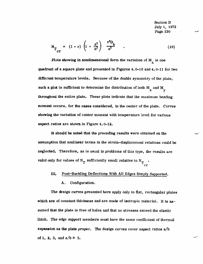
SectionDJuly 1, 1972
Page 230
1 aZ ) X2DbNT = (1- u) + b-_ _ " (28)cr
Plots showing in nondimensional form the variation of M in onex
quadrant of a square plate and presented in Figures 4.0-10 and 4.0-11 for two
different temperature levels. Because of the double symmetry of the plate,
such a plot is sufficient to determine the distribution of both M and Mx y
throughout the entire plate. These plots indicate that the maximum bending
moment occurs, for the cases considered, in the center of the plate. Curves
showing the variation of center moment with temperature level for various
aspect ratios are shown in Figure 4.0-12.
It should be noted that the preceding results were obtained on the
assumption that nonlinear terms in the strain-displacement relations could be
neglected. Therefore, as is usual in problems of this type, the results are
valid only for values of NT sufficiently small relative to N T .cr
III. Post-Buckling Deflections With All Ed_es Simpl_, Supported.
A. Configuration.
The design curves presented here apply only to fiat, rectangular plates
which are of constant thickness and are made of isotropic material. It is as-
sumed that the plate is free of holes and that no stresses exceed the elastic
limit. The edge support members must have the same coefficient of thermal
expansion as the plate proper. The design curves cover aspect ratios a/b
of 1, 2, 3, and a/b - 5.

f..-
Section D
OR|_II_L t_._,_G_ [$ July 1, 1972
OF POOR QUALITY Page 231
0 0.1 0.2 0.3 , 0.4 0.5
-o.61' 2,T _":'_I I I I . l ]
"0.25
Figure 4.0-10. Distribution of the bending moment M in a square plate forx
(NT - 0.25 Poissonts ratio v =
cr
B. Boundary Conditions.
The solution applies only to cases where both the following boundary
conditions are satisfied:
1. AU edges are simply supported.
2. Supports fully restrain in-plane edge displacement of the plate
such that these displacements arc equal to the free thermal expansions (or
contractions) of the SUl)lmrts,
C. Temperature Distribution.
It is assumed that no thermal gradients exist through the plate thickness.
Temperature distribution over the surface is taken to be parabolic (Fig.
4.0-13) and can be expressed mathematically as
(29)

Section D
July 1, 1972
Page 232 J
xw_,£ _I,LL
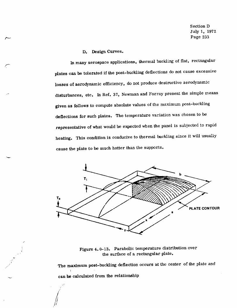
Section D
July 1, 1972
Page 233
F
/
/
/
J
D. Design Curves.
In many aerospace applications, thermal buckling of flat, rectangular
plates can be tolerated if the post-buckling deflections do not cause excessive
losses of aerodynamic efficiency, do not produce destructive aerodynamic
disturbances, etc. In Ref. 37, Newman and Forray present the simple means
given as follows to compute absolute values of the maximum post-buckling
deflections for such plates. The temperature variation was chosen to be
representative of what would be expected when the panel is subjected to rapid
heating. This condition is conducive to thermal buckling since it will usually
cause the plate to be much hotter than the supports.
Figure 4.0-13. Parabolic temperature distribution over
the surface of a rectangular plate.
The maximum post-buckling deflection occurs at the center of the plate and
can be calculated from the relationship

K2+_ (3-.5) l+--_.T
Section D
July 1, 1972
Page 234
bZ/] 6z+4v a-"_ "_
+ (3-_r) _z,
(_0)
J
where
b 2
K-- 1 + _ (31)
and
/_ - • (:_2)a (I-,,_)
Solutions to equation (30) arc plotted in Figures 4.0-14 and 4.0-15 for plates
having v = 0.30. Itis useful to note that, for given values of T O/Tl, initiai
thermal buckling occurs at T1/fl values corresponding to 6/t = 0. The
curves do not account for nonuniformiUes in the material properties such as
those variations that arise because of temperature-dependence of the material
behavior, Hence, the user must select a single effectivevalue for _ by
employing some type of averaging technique.
4.0.3 Thermal Buckling of Cylinders.
Configuration.
The design curves and equations provided here apply only to thin-
walled, right circular cylinders which satisfythe relationship
L/R _ 3.2 (33)

s
OF POOR QUALITY Section D
July 1, 1972
Psg8 235
6.k
5.6
_.8
k.0
_"1- 3.*
2.h
#Ib,l
/.//./
/o.8 __ - /
02 0.4 0.6 05 1.0 1.1
e/b ,2/
J ,0
///.0.5
0 02 0.4 03 0.11 10 1,
( 6/0 (6f0
4.0-14. __ oammNsrs br heated rectangular plates.
_.8
k.o
3.2
2.b
1.6
0.8
_/#,3
mm
Jj /
lJ ,5
04 011 tO I.a 0 oJt 04Ol
(d/t)
j/,02,l
)JL OJ I.O 12
6/t)
Figure 4. O-.1S. Post-buckling parameters for heated rectangutar prates.
.o

Section D
July 1, 1972
Page 236
and are made of isotropic material. It is assumed that the sheU wall is frcc
of holes, obeys Hooket s law, and is of constant thickness. Figure 4.0-16
depicts the isotropic cylindrical shell configuration. Figure 4.0-17 shows the
sign convention for forces, moments, and pressures.
Boundamj Conditions.
The following types of boundary conditions are covered:
1. Siml)lv supported c(Ige; that is,
w:- M :_ 0 :tt x 0 and/or x l,. (:_4)X
2. Clamped edge; that is,
w= -- = 0 atx= 0and/orx= L . (35)Ox
It is not required that the conditions at the two ends be the same. In ever),
case, it is assumed that the cylinder (including any end rings) is not subjected
to external axial constraints at any location around the boundaries at x = 0 and
x= L.
Temperature Distribtttion.
The supposition is made that no thermal gradients exist through the
wall thickness and in the axial direction. However, arbitrary circumferential
variations may be present.
expressed in the form
T=T (¢) .
The permissible distributions can therefore be
(36)
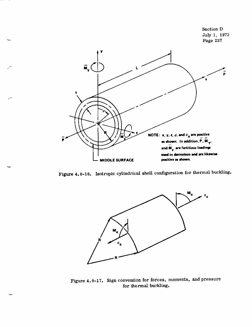
/.
Section D
July 1, 1972
Page 237
F
P
Figure 4.0-16.
MIDDLE SURFACE
. NOTE: x, y, z, _, and ax are positive
as shown. In addition, P, M y,
lind Mz are fictitious Ioldings
used in derivation ond are likewise
poeitive asshown.
Isotropic cylindrical shell configuration for thermal buckling.
Figure 4.0-17. Sign convention for forces, moments, and pressure
for thermal buckling.

Section D
July1, 1972
Page238
Hoop membrane compression may develop in regions adjacent to the two ends
becaus_ of e_ernal radial constraint. However, the buckling mode associated
with this condition is not considered. Because of this and the lack of external
axial constraints, the special case of a uniform temperature is of no interest
here.
Design Curves and Ec_uaUons.
It is assumed that Young' s modulus and Poisson' s ratio are unaffected
by temperature changes. Hence, in using the contents of this manual, the
user must select effective values for each of these properties by applying
engineering judgement. It will sometimes be desirable to employ different
effective moduli in each of the following operations_
1. Computation of the stresses _ present in the cylinderx
2. Computation of the critical buckling stress (_x) .cr
On the other hand, the results are presented in a form which enables the user
to fully account for temperature-dependence of the thermal-expansion coeffi-
cient a .
The appropriate formulation for _ can be obtained by first imposingx
a fictitious stress distribution _A around the boundaries at x = 0 and x = L
such that all axial thermal deformations are entirely suppressed.
that
(r A=-_ ET (9) •
R follows
(37)

f-
Section D
July 1, 1972
Page 239
These stresses may be integrated around the circumference and through the
wall thickness to arrive at the force
"PA =- EtR f aT(_) d_ (38)0
and the moments
2_
A 0aT(_) sin _ dcb
and(39)
A 0aT (_b)cos _ d_b
Since it is assumed that the shell is free of external axial constraints, the
conditions
=g = o (40)y z
must be satisfied at x = 0 and x = L. To restore the shell to such a state,
it is necessary to superimpose a force PB equal and opposite to as well
as moments (_,)y and (_z) , which are equal and opposite to (_)z andB B A
(_z) respectively. Hence,P
A
(41)

Section D
July 1, 1972
Page 240
and
.B A
The stress corresponding to "PB is easily found to be
The stresses due to (My) areB
E2_ j" aT(_) de . (42)
0
B I : -_R_t = _r\ y/ y 0 (43)
and thoJe due to (M) areZ
B
B (44)
The procedure being used constitutes an application of Saint-Venant' s principle.
Hence, the stresses from equations (42) through (44) will be accurate repre-
sentations only at sufficient distances from the ends x = 0 and x = L. If end
rings are present, the greater their resistance to out-of-plane bending, the
shorter will be this distance. Subject to these conditions, the actual longitudinal
thermal stresses at various points in the shell may be computed from the
relationship

Section D
July 1, 1972
Page 241
F
f,
or
_r X + O' ÷ + O
B B B
2z r
O.x=- aET(¢) + ;_-._ aT(c)
(45)
4-
2_
E sin _ f
0aT(_) sin_ d_
27
Ecos 9 f÷ a T (_) cos # d@ . (46)0
Complex distrihuUons may be encountered which make it difficult to perform
the required Integrations. In such instances, use can be made of numerical
techniques whereby the integral signs are replaced by summation symbols.
To investigate the stability of a particular shell, the maximum longi-
tudinal stress (Crx) must be compared against the critical value which canmax
be obtained from the formula
Et(or x) = y • (47)
er RJ 3(1 - v z)
For the design to be satisfactory, It is required that
(%) < (%) • (4s)max cr
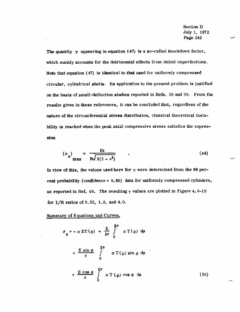
Section D
July 1, 1972
Page 242 -j
The quantity _/ appearing in equation (47) is a so-caUed knockdown factor,
which mainly accounts for the detrimental effects from initial imperfections.
Note that equation (47) is identical to that used for uniformly compressed
circular, cylindrical shells. Its application to the present problem is justified
on the basis of small-deflection studies reported in Refs. 38 and 39. From the
results given in these references, it can be concluded that, regardless of the
nature of the circumferential stress distribution, classical theoretical insta-
bility is reached when the peak axial compressive stress satisfies the expres-
sion
(O.x) _ Et (49)max R_] 3(1 - v 2) "
In view of this, the values used here for _, were determined from the 99 per-
cent probability (confidence = 0. 95) data for uniformly compressed cylinders,
as reported in Ref. 40. The resulting T values are plotted in Figure 4.0-18
for L/R ratios of 0.25, i. 0, and 4.0.
Summary of Equations and Curves.
2_E
¢r =-aET(¢) + _ f aT(C) d<bX0
÷
2_
E sin _. [J
0_T(¢) sin _ d¢
÷E cos
27r
f _T(_)cos¢0
d_ (50)
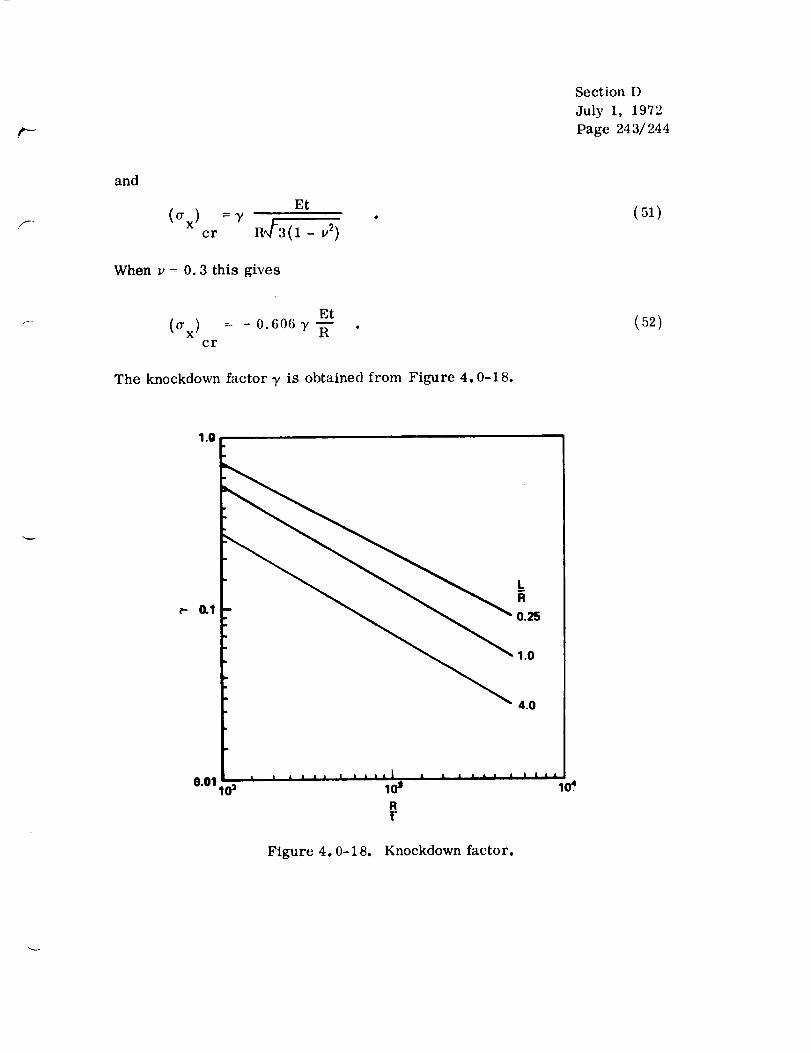
f---
Section D
July 1, 1972
Page 243/244
and
((7X) = Tcr
Et
R"]-3 (1 - v2)
When v = O. 3 this gives
(51)
Et
(Orx) = - 0.606T _"cr
The knockdown factor y is obtained from Figure 4.0-18.
(52)
1.0
_,- 0.1 0.25
1.0
4.0
,,.,1 I , , , , _ , , ,,,i , , ..... i ,,.o.v 102 101 104
RY
Figure 4o 0-18. Knockdown factor.

F
Section DJuly 1, 1972Page 245
5.0 INELASTIC EFFECTS.
In the preceding paragraphs, elastic behavior was assumed. This
assumption is sufficiently accurate for large classes of materials at relatively
low temperature and stress levels.
At higher temperature and for higher stress levels, however, the
divergence betweenthe behavior of real solids and that of the ideal elastic
solid increases and the elastic idealization becomesinadequate; the behavior
of the real solid is then said to be inelastic. To predict the inelastic behavior
of a solid under given thermal andloading conditions, it is necessary to
generalize the stress-strain relationship. There are three types of approaches
to this generalization, although the borderlines betweenthem are not well
defined.
1. The most basic studies of this problem make use of the concepts
and methods of solid-state physics. In this approach, the microstructure of
the material is taken into consideration and it is attempted to predict the
mechanical behavior of materials from this information.
2. It is also possible to disregard the microstructure of the material
and to regard it as a continuum; the general principles of mechanics and
thermodynamics as applied to continuaare then usedto determine the forms
of stress-strain relations which are compatible with theseprinciples.
3. The most direct procedure is to postulate simple inelastic stress-
strain relations; these define various ideal inelastic bodieswhich, thoughnot
Section D
July I, 1972
Page 246
representing any actual materials, nevertheless incorporate in simple com-
binations some of the different types of inelastic phenomena, such as creep,
relaxation, plastic flow, or work-hardening,
Although considerable progress has been made in methods 1 and 2,
thus far only the third approach has yielded information of direct utility to
the stress analyst. In this paragraph, inelastic stress-strain relations are
discussed from the third of these viewpoints.
s0.1
Creep is the time-dependent deformation that occurs under stress.
Creep is normally observed by placing a constant load on a specimen and
measuring its deformation with time at a constant elevated temperature. The
curve showing the deformation as a function of time is known as a creep curve.
Creep curves obtained for various materials, temperatures, and stresses have
certain common features, which are illustrated in Figure 5.0-1. These are:
1. From A to B, the specimen undergoes an initial, almost instan-
taneous, extension on loading.
2. From B to C, the specimen creeps at a rate that decreases with
time (primary stage or transient creep).
3. From C to D, the specimen creeps at a rate that is nearly con-
stant (secondary stage or viscous creep).
4. From D to E, the specimen creeps at a rate that increases with
time (tertiary stage or accelerating creep).
5. At E, the specimen fractures.
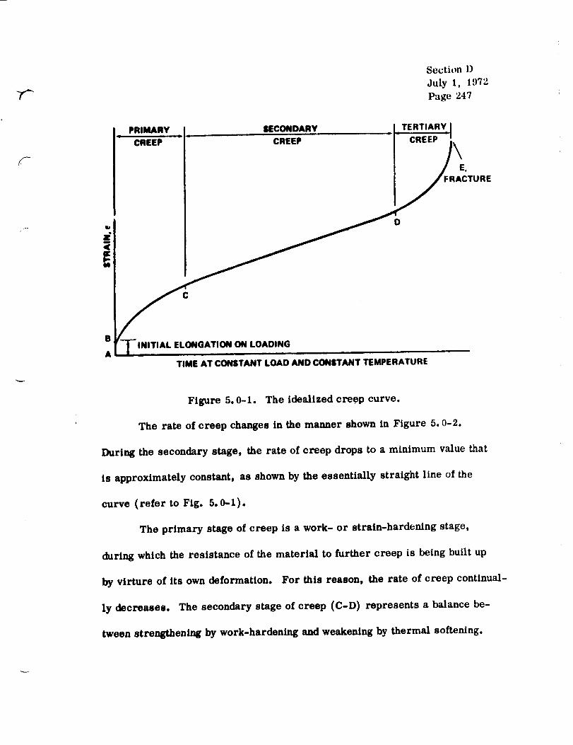
F
PRIMARYii
CREEP
C
SECONDARY
CREEP
Section D
July I, 1972
Page 247
0
B
AINITIAL ELONGATION ON LOADING
TIME AT CONSTANT LOAD AND CONSTANT TEMPERATURE
Figure 5. 0-1. The idealized creep curve.
The rate of creep changes in the manner shown in Figure 5.0-2.
During the secondary stage, the rate of creep drops to a minimum value that
is approximately constant, as shown by the essentially straight line of the
curve (refer to Fig. 5. 0--1).
The primary stage of creep is a work- or strain-hardening stage,
during which the resistance of the material to further creep is being built up
by vlrture of its own deformation. For this reason, the rate of creep continual-
ly decreases. The secondary stage of creep (C-D) represents a balance be-
tween strengthening by work-hardening and weakening by thermal softening.

Section D
July 1, 1972
Page 248
i8
TIME AT CONSTANT LOAD AND CONSTANT TEMPERATURE
Figure 5.0-2. Variation in rate of creep with time.
The tertiary stage, or accelerating rate of creep immediately before
fracture, is often caused by an increase in stress that accompanies the de-
crease in cross-sectional area of the specimen during creep under a constant
load. This decrease in the load-carrying area may be due either to the
decrease of the diameter of the specimen as it elongates or to the formation
of intercrystalline cracks. These cracks can also act as stress-raisers. In
other cases, the accelerating creep rate is due to a change in the metaUurgical
structure, such as recrystallization.
5. 0.1.1 Design Curves.
For engineering purposes, the results of tests at various stresses and
temperatures are summarized in more convenient form. Figure 5.0-3 shows
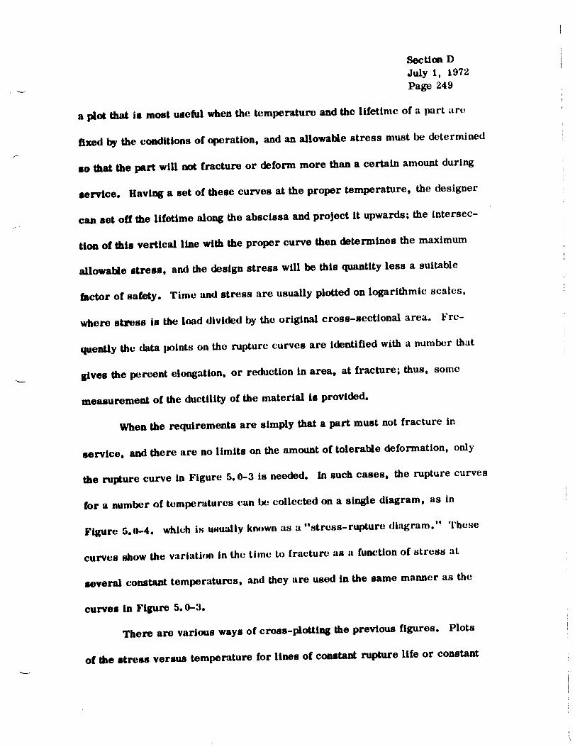
Sectlolt DJuly 1, 1972Page 249
a plot that is most useful when the temperature and the lifetime of a part :ire
fixed by the eoaditions of operation, and an allowable stress must be determined
so that the part will not fracture or deform more than a certain amount during
service. Having a set of these curves at the proper temperature, the designer
can set off the lifetime along the abscissa and project it upwards; the intersec-
tion of this vertical line with the proper curve then determines the maximum
allowable stress, and the design stress will be this quantity less a suitable
factor of safety. Time and stress are usually plotted on logarithmic scales,
where stress is the load divided by the original cross-sectional area. Fre-
quently the data points on the rupture curves are identified with a number that
gives the percent elongation, or reduction In area, at fracture; thus, some
meuuremeat of the ductility of the material is provided.
When the requirements are simply that a part must not fracture in
service, and there are no limits on the amount of tolerable deformation, only
the rupture curve in Figure 5. 0-3 is needed. In such cases, the rupture curves
for a number of temperatures can hc collected on a single diagram, as in
Figure 5.(_-4, which is usually km_wn as a"stress-rupture diagram." These
curves show the variation in the time to fracture as a function of stress at
several eotmtaat temperatures, and they are used in the same manner as the
curves in Figure 5.0-3.
There are various ways of cross-plotting the prev/ous figures. Plots
of the stress versus temperature for lines of coutant rupture life or constant

SectionDJuly 1, 1972Page250
T- CON$T. e3 > e2 > el
LOG t
Figure 5.0-3. Schematic presentation of creep-rupture data showing effectof stress at constant temperature on the time to rupture or specific
amounts of strain.
minimum creep rate are common, These curves are sometimes plotted on
the same diagram with curves showing results from short-time tensile tests,
as in Figure 5.0-5. Such diagrams give complete descriptions of the mechan-
ical behavior over wide temperature ranges. At low temperatures, where
creep is unimportant, designs are based on the results of short-time tenlile
tests; at higher temperatures, where the creep-rupture strength curves are
below the tensile test curves, designs must be based on the creep-rupture
behavior.
Curves of this type are readily available for most common metals in
MIL-HDBK -5 [4i].
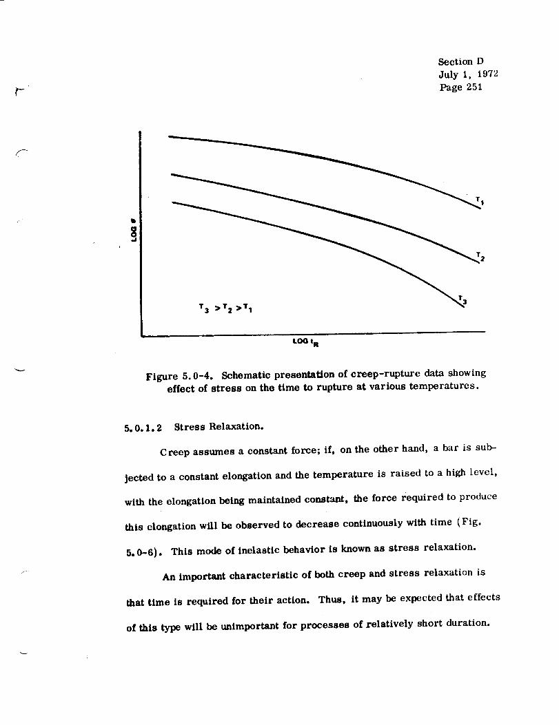
SectionD
July l, 1972
Page 251
b
LeQ tA
Figure 5.0-4. Schematic presentation of creep-rupture data showing
effect of stress on the time to rupture at various temperatures.
5.0.1.2 Stress Relaxation.
Creep assumes a constant force; if, on the other hand, a bar is sub-
jected to a constant elongation and the temperature is raised to a high level,
with the elongation being maintained constant, the force required to produce
this elongation will be observed to decrease continuously with time (Fig.
5. 0-6). This mode of inelastic behavior is known as stress relaxation.
An important characteristic of both creep and stress relaxation is
that time is required for their action. Thus, it may be expected that effects
of this type will be unimportant for processes of relatively short duration.

Sectic_lDJuly 1, 1972Page252
mwE
ULTIMATE TENSILE STRENGTH
YIELD STRENGTH
/
TEWERATURERANGE
FOR CONVENTIONAL DESIGN
100 - hr RUPTURE LIFE
10000-hr RUPTURE LIFE
TEMPERATURE
Figure 5. 0-5. Schematic presentation of tensile andcreep-rupture properties.

SectionDJuly 1, 1972
Page 253
, f LOW TEMPERATURE
P
!
Figure 5.0-6. Stress relaxation under constant deformation.
5. 0.2 ViscoelasUcit_:
Often, idealized bodies are defined which exhibit the characteristics of
creep and stress relaxation. These idealized bodies take the form of simple
mechanical models composed of springs and dashpots, whose deformation
defines the stress-strain relationship for the given material. This approach
is called viscoelasticity.
To represent the creep behavior of a material, many various mechanical
models can be formulated composed of different combinations of springs and
dashpots. Some of the more common ones can be found in Refs. 1 and 42.
5. 0.3 Creep Buckling.
Consider a column under a constant axial compressive load; if the
column is not perfectly straight initially (as is always the case because of
unavoidable manufacturing inaccuracies), then some bending will occur. The

Section DJuly 1, 1972Page254
bending stresses are accompanied by a certain strain rate, which irnjdies
increasing dellcctions; these in turn _.aust: higher stresses so that a self-
excited or unstable situation arises. This process leads to collapse at a
rialto critical time and is known as creep buckling.
The following observations apply to creep buckling (Ref. 1) :
1. The phenomenon of creep buckling is, both physically and mathe-
matically, quite different from the usual type of buckling phenomenon. The
usual buckling load represents a "point of bifurcation" on a load versus
deflection plot, a point beyond which more than one equilibrium configuration
is possible; _recp #m_'kiing is char:tctcrizcd by deflections increasing bcy,_n_!
all bounds.
2. Mathematic'_lly, creep buckling can occur at a finite time only if
the material follows a nonlinear creep law.
3. The column will undergo creep buckling at any value of the com-
pressive axial load, no matter how small.
4. Creep buckling will occur whenever the column has initial imper-
fecUonm, and only then.
5. The value of t depends on the initial deflection and on thecr
magnitude of the load; it has been found to be not too strongly affected by
changes in the former but very sensitive to changes in the latter.
6. The small-deflection analysis is, of course, not valid in the
immediatc neighborho_l of the critical time because the deflections are then

Secti,m DJuly 1, 1972Page 255
large, tlowever, calculations based on a small-deflection theory arc vali,I
up to times very close to the critical; they thus cover, in effect, the entire
range of practical interest.
5.0.3.1 Column of Idealized H-Cross Section.
The critical time for creep buckling to occur for a simply supported
column of idealized H-cross section [ two concentrated flanges, of area (A/2)
each, at a distance h apart] is given by:
where
k- 24
and
L = length of column ,
P0 = column load,
a 0 = maximum wdue of initial imperfection,
k = constant in the strain-stress relationship.
n
5.0.3.2 Rectangular Column.
Analysis of the critical buckling time for rectangular columns is very
difficult. A way of circumventing this difficulty has been established, whereby

Section D
July i, i972
Page 256
and lower bounds lot the critical time arc obtained (t*) and arc s,upper1 •
desigm_ed by the use o[ an as_rlsk.
Per a column with a rcctana_ar cross section of height h and wi_h
b, subjected to an average stress (r 0 = P0/bk and obeying a stress-strain
law of
= ( Ix) n ,
upper and lower bounds for the nondimensional critical time t*cr
are plotted
in Figure 5.0-7 against the ratio (z0/h) of the initial center-deflection to the
height of the bar. For small values of this ratio (say z0/h < 0.015) these
bounds may be determined from the asymptotic expression
ht* --log _ -,'_cr z0
with the values of the coefficient c listed in Table 5.0-1.
The spread between the bounds may be seen from Figure 5.0-7 to vary
with the ratio z0/h. However, from Ref. I, if cr o/or E > 0. 8, then the lower
bound will be a good approximation for t*cr, whereas if _ 0/_ E < 0.2, the
upper bound on t* will be a good approximation to the actual value of thecr
critical time. GrE = Euler buckling stress = _/ .
5. 0.3.3 Flat Plates and 8hells of Revolution.
The method presented here may be used to predict critical conditions
for the creep buckling of fiat plates and shells of revolution which satisfy the
followiJN; requirements:
\

TABLE 5.0-I. VALUES OF C
Section D
July 1, 1972
Page 257
f-n
3
4
5
6
7
For Lower Bound
,,
0.987
1.57
1.95
2.26
2.45
For Upper Bound
0.26
O. 56
O. 81
I.02
1.16
5,0 ./-- n = 3
/ '_ " _'' UPPER BOUND ON tcr I
4°1" -- II --£2_ _ /
1.0 _0_
0.006 0.01 0.02 0.04 0.06 0.10 0,20
=.___0h
Figure 5.0-7. Upper and lower bounds for the critical time t':-" forcr
creep buckling of a rectangular column.
1. The member is made of an isotropic mat,_11al.
2. The stress intensity a i [see equations (1)] is uniform throughout
the structure.
Section DJuly 1, 1972
Page 258
3. The configuration, boundary conditions, and type of loading are
such that appropriate formulas are available for room-temperature values of
both the critical stress intensity _l [ see equations (1)] and the plasticity re-
duction factor.
Temperature Distribution.
R is assumed that the member is at a uniform elevated temperature.
Method.
The method presented here is essentially that which was published by
Gerard in Ref. 43 and constitutes a classical stability approach based on the
concepts set forth by Rabotnov and Shesterikov [44]. In Ref. 45, Jahsman and
Field show comparisons of various theoretical predictions with column test
data. The theory attributed there to Gerard is that of Ref. 46, which was
published before llcf. 43 and has a different basis. On the other hand, the
curves which Jahsman and Field [4.r_] identify with the Rabotnov-Shcsterik_)v
label were developed from the method given in this paragraph. The afore-
mentioned comparisons seem to indicate that this technique will give con-
servative predictions. However, this conclusion could possibly be because:
1. The test data were corrected to eliminate the effects of initial
imperfections.
2. The analysis is concerned with the onset of instability, whereas
the experimental data arc for final collapse.

f?
Section D
July 1, 1972
Page 259
The presentation by Jahsman and Field includes plots obtained from each of three
different theoretical approaches [43, 46, 47]. Of these, the approach of Ref.
43 gave the most conservative predictions, This is a desirable situation in
view of the uncertainties associated with classical stability approaches to
creep buckling problems. For one thing, this general theoretical concept ignores
the detrimental effects from initial imperfections. However, to properly account
for this influence, much more complicated methods would be required and these
would not fall within the intended scope of this handbook. Therefore, in the
procedure recommended below, an attempt is made at least to partially account
for the imperfection effects in shells of revolution. This is done by the intro-
duction of available room-temperature knockdown factors.
Recommended Procedure.
Obtain from the literature, or a suitable test program, a family of
creep curves for specimens made of the desired material and subjected to
unaxial loading while at the appropriate service temperature. These curves
should be o[ the type shown in Figure 5.0-8 where a. and E. are the stress1 1
intensity and strain intensity, respectively, and are defined as follows for
plane- st ress conditions:
O', ---: O" + 0 .2 - or O" + 3T 2
l y x y xy
and
2 E2 +¢ £ +¢i- ,,f-3" + y x y
1/2(i)

Section D
J_y 1, 1972
Page 260
Using data obtained from these plots, create a family of curves similar to
those of Figure 5.0-9 where _i is the strain-rate intensity defined as follows
for a state of plane stress:
ci - +_2+_ _ + . • (2)_/-3 y x y
The dots indicate differentiation with respect to time; for example,
C /'a£ X_2x = k-_-/ • (3)
The results embodied in Figure 5.0-9 are then used to develop still another
family, which is illustrated in Figure 5.0-10. Following this, select appro-
priate formulations for conventional room-temperature values of both the
critical stress intensity (cri) and the plasticity reduction factor q. Forcr
example, in the case of an axially compressed, moderate-length, circular
cylinder, one obtains
=
(_i) = _ r Ehcr RJ 3(1 - V_e) (4)
and
1/2
_--'_ 1 E
where I" is the room-temperature knockdown factor and
E
v=o.5o- _ (0.50E - re)
(5)
(6)
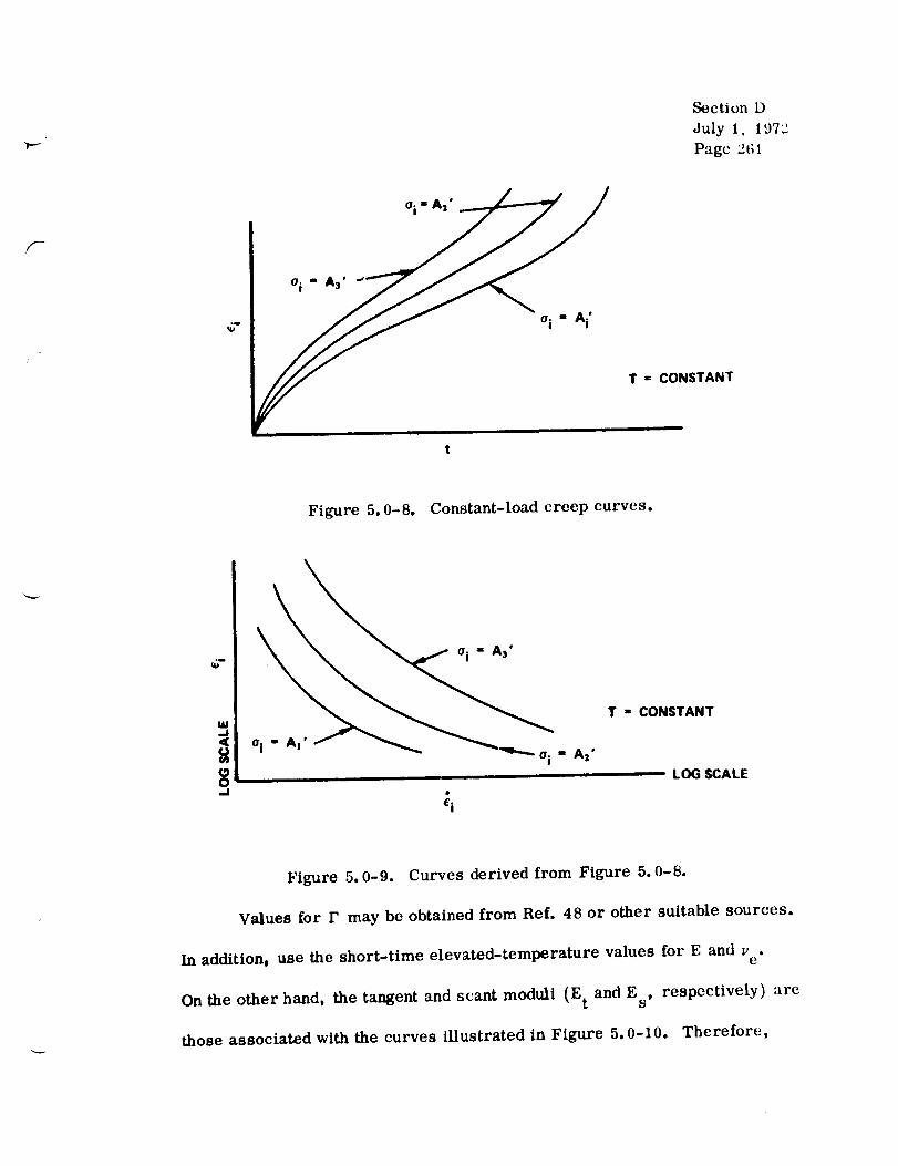
f-
Section DJuly 1, 1972Pagc 2fiI
o." A."
_" t t STANT
Figure 5.0-8. Constant-load creep curves.
u_- , °i " A3"
. ,, A2"
i iiii
,,J
T - CONSTANT
LOG SCALE
Figure 5.0-9. Curves derived from Figure 5. 0-8.
Values for F may be obtained from Ref. 48 or other suitable sources.
In addition, use the short-time elevated-temperature values for E and v .e
On the other hand, the tangent and scant moduli (E t and Es, respectively) _re
those associated with the curves illustrated in Figure 5.0-10. Therefore,

Section DJuly 1, 1972Page262
(=
""TANT
Figure 5.0-10. Curves derived from Figure 5.0-9.
working with this figure, proceed from left to right along the _. line cor-z
responding to the applied load and use a trial-and-error procedure to determine
the strain intensity c i at which
Eh
appliedcri= _ F R_3(1- V2e) (7)
FoUowing this, return to Figure 5.0-8 and establish the time t as-
sociated with this combination of _i and c i. This is the predicted time to the
onset of creep buckling and can be denoted as tcr.
Although the preceding presentation has dealt with the specific case of
an axially compressed circular cylinder, it should be obvious that this method
constitutes a general approach which can be used for the analysis of creep
buckling in various types of plates and shells subjected to an assortment of
loading conditions. It should be noted, however, that F = 1.0 for fiat plates
(and columns).

Section D
July 1, 1972
Page 263
6.0 TIIERMAI, SII(}{:K.
6.0.1 General.
Thermal shock rclers to the phenomenon whereby a body undergoes
sudden changes in temperature, usually caused by a rapid change in the ex-
ternal environment. It is the presence of severe transients that distinguishes
thermal shock from the more common conditions of steady-state and slowly
varying temperatures. Severe transients are experienced by reentry aero-
space structures, such as those of the space-shuttle variety. The selection
and comparison of candidate materials for structures of this type shouhl
be accomplished by means of a screening process that considers thermal-
shock resistance, which may be ewduatcd by both analytical and experimental
methods. The analytical method may include comparisons of thermal-shock
indices, as well as the theoretical analysis of simple models such as a flat slab
which is suddenly immersed in a hot medium. The experimental investigation
may be of similar scope. In the theoretical treatment of such models as well
as the actual complex configurations, it is usually unnecessary to perform a
true shock-type analysis which involves mass inertia effects. Generally, it
is sufficiently accurate to compute the pertinent thermal stresses by the same
methods as are used for steady-state problems, except that one must de-
termine the temperature and stress distributions at a number of time incre-
ments during the transient behavior. As a rule, however, it will be necessary
to consider the material strain-rate-sensitivity when allowable stresses are
established.

Section I)
July 1, 1972
Page 264
6.0o 2 Stresses and Deformations.
Configuration.
The equations and tables provided here cover each of the following,
as illustrated in Figure 6.0-1:
1. Flat slabs, of infinite extent, which are of uniform thickness and
are free of holes
2. Solid cylinders of infinite length
3. Solid spheres.
In all cases, it is assumed that Hooke' s law applies.
Boundary Conditions.
All bodies are free of any external constraint.
Temperature Distribution.
The supposition is made that the subject bodies experience a sudden
change in surface temperature. The upper and lower surfaces of the fiat slab
are always subjected to identical temperatures.
Equations and Tables.
This section is based on the assumption that Young' s modulus,
Poisson t s ratio, the thermal diffusivity, and the coefficient of thermal ex-
pansion are unaffected by temperature changes. Hence, the user must select
single effective values for each of these properties by employing some type
of averaging technique.
F
f
Section D
July i, 1972
Page 265
The method presented here was published by Adams and Waxler in ReL
49. Itcan be used to determine the temperature and stress distributions dur-
ing the subject transient phenomena. To accomplish this, several simple
formulas must be used in conjunction with appropriate tabulated values. All
of these are given in the summary which follows. In applying this method,
care should be taken to ensure that the units specified under NOTATION are
used.
The method makes use of a temperature function, _j, which may be
called the fractional temperature excess and is defined as follows:
T- Tf =I
j- T i- Wf j 1, 2, 3 • (1)
The subscripts 1, 2, and 3 denote that the _ value is for an infinite solid slab,
an infinite-length solid cylindcr, or a solid sphere, rcspectively. The tabu-
lations of _bj published by Adams and Waxier and appearing in the summary
of this section werc developed from a study of the heat transfer phenomena
associated with the subject configurations. The tables also include values for
the temperature parameters _I,_, _I,_, and ,I_ _, which are defined as follows:
Infinite Solid Slab.
' (a)@] = f _1 d0
Infinite-Length Solid Cylinder.
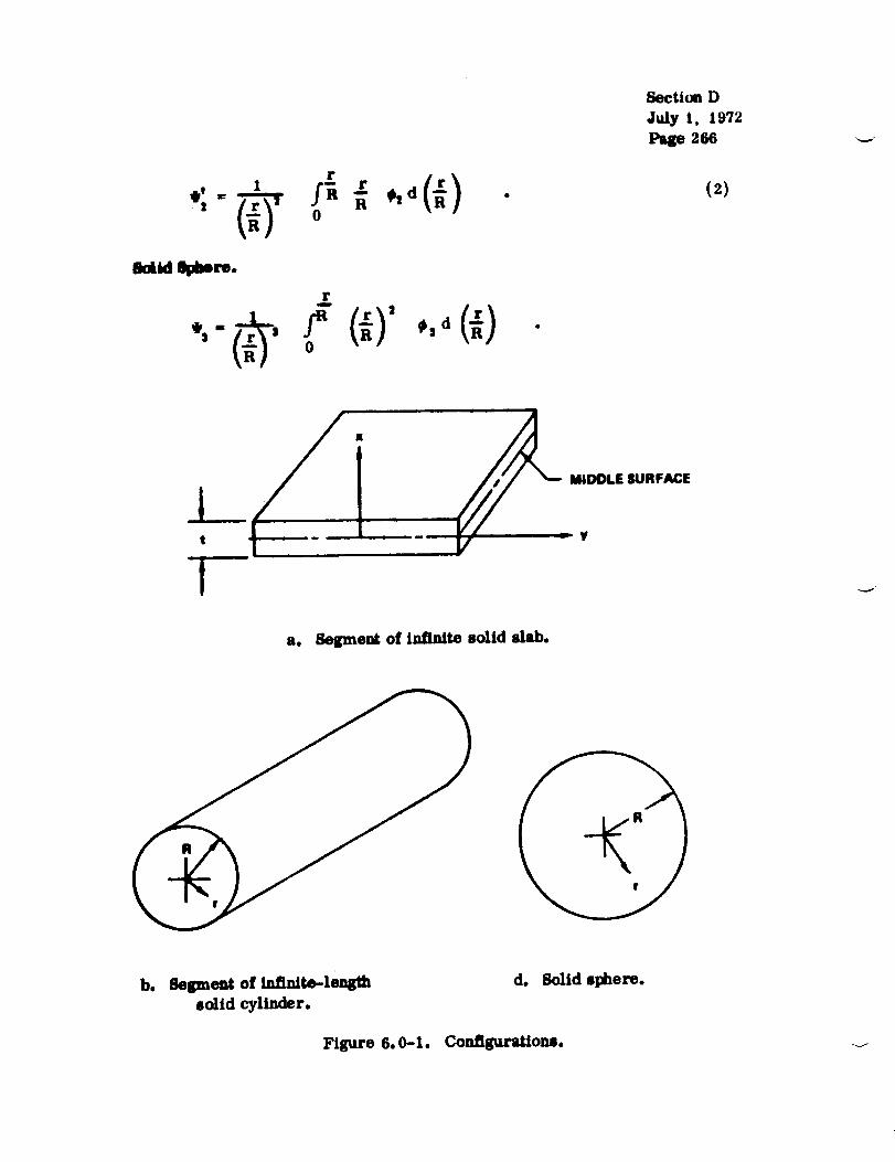
, r;-.,,d(_).¢' " _"_ o
r
• o
Section D
July 1, 1972
zse
(2)
a. Segment of infinite solid slab.
b. _egment o! infinite-length
solid cylinder.
d. Solid sphere.
Figure 6.0-1. Configurations. ..J
/:
Section D
July 1, 1972
Page 267
Summary of Equations and Tables.
The parameters q and fl, which appear in the tables, are defined as
follows:
and
tq : _ (:3)
where
k t
K- Cpp * (4)
Infinite Solid Slab,
T = _I (Ti - Tf) + Tf (5)
and
E(_ (T i -Tf):_ = (*I-_) (_;)
x y (I - v) J "
The values for _ i and ,I, [ are obtained from Table 6.0-1.
Infinite-Length Solid Cylinder.
T = q_2 (T i - Tf) + Tf , (7)
Err (T i - Tf)
(rr= (1 - v) (q_v2 - @2) , (8)
and
Err (T i - Tf)t
crt : (1 - v) (_I'2 ÷ _2 - _2) (9)
Section D
July 1, 1972
Page 268
where _ is the value of_ z at r/R = 1.
from Tables 6.0-2 and 6. o-3, respectively.
Solid Sphe re.
and
T= _b:j (T i- Tf) +Tf ,
2E_ (Ti-Tf)
_r = C1- v)
The values for #z andS2 are obtained
(lO)
(,;-,_) , (11)
E_(T i - Tf)
_t- (1 - _) (2_ +_:,- _3) (1_)
where _I,_ is the value of4_ 3 at r/R = 1. The values for ¢3 and _s are obtained
from Tables 6.0-4 and 6.0-5, respectively.

ORIGIN_£ FS:/i i:
OF.. POOR QUALITYSection D
July 1, 1972
Page 269
TABLE 6.0-1. SLAB-PARAMETERS _bl AND _t'
f
0.3000 0.3200 0,3400 0.3600 0.3_0o 0,400o o. 4200 0.4400 0.4800 0.4800
0. 0. 0013 0. 0031 0. 0061 q. 0109 0. 017't 0. 0270 0. 0386 0. 0526 0. 0690 0. 0875
0.10 0. 0013 o. 0030 0. 0061 0. ol08 o. o176 (). 0266 o. 0381 0. 0520 o. o682 0. 0665O. 20 O. 0013 O. 0029 0. 0058 0. 0104 O. 0 t_;9 (). o256 O. 0367 O. 0500 0 0656 O. 0932
O. 30 O. 0012 O. 0027 o, 0n55 O. 0097 O. ()158 O. 024 q (}. o344 O. 0469 O. 0615 O. 0780
O. 40 O. 0011 0. 0025 O, 0050 O. 0o88 O. 0144 O. 0218 0.03 12 O. 0428 O. 0558 O. 0708
0.50 O. 0010 O, 0022 0.0043 O. 0r,77 0.0126 O. 0191 O. 0273 O. 0372 O. O488 O. 0619
0, 60 o. 0008 0. 0018 0. 0036 o. 0o64 o. ol o.t 0. 0158 o, 0227 0. 0309 o. 0406 0.0515
O. 70 O. 0006 O. 0014 O. 0028 _. 0050 o. oo_1 o. o122 o. o175 O. 0239 O. 0313 O. 0397
0.80 0. 0004 O. 0010 0. 0019 0. 0034 0. 005:, o. q)08:1 0. (H19 0. 0163 0. 0213 0. 02700, 90 0. 0002 (). 0005 0. 0010 0. o017 o. (Io28 i) t1012 0. oo60 (i. 0082 0. 0106 0. 0137
1.00 0. 0000 0, 00(10 0.0oo0 0. olin0 i). (l[)oo i). (if}0() 0, 0000 (). 0()0o 0. 0000 0. 0000
O,
0.10
0.20
O. 30
0.4O
0.50
O. flO
0.70
0.80
O. 90
1. O0
%,
0.
0.10
0.1t9
0.30
0.400.50
0.800,70
0.90
O. 90
1. O0
O.
0.10
0.20
0.30
0.40
0.50
0.80
O, 70
O, 80
O. 90
1. O0
)_,
0. o009
O. 5000
o. lO_0
o. 1066
O. lO27
o. 0962
o. 0674
O. 0764
o. O635
O. 0490
0. 0334
0. 0169
O. 0000
O, 0687
O. 7000
O. 36160.3571
0. 3439
0. 3222
O. 2925O. 2557
0.2125
0. 1642
0. 1117
O. 0566
O. 000o
O, 2302
O. 9o0o
0.5941
0.5868
o. 5652
O. 5297
0.4911
0.4207
O. 3499
O. 2704
O. 1841
O. 0932
O. 00o0
O. 3786
0.0(120
O, 5200
o. 13Ol
o. 1285
O. 1237
O. 1159O. 1052
O. 0920
O. 0765
0. o591
o. n4()2
O. 0203
O, I)0(IO
o, 0828
o. 7200
O. 3H74
O. 11084
O. 3452
0.31:H
0. 2739
0. 2277
0. 1759
0. 1197
0. o6(16
O. 0000
O. 2466
O. 9200
O, 8137
O. 8062
O, 5_39
O. 5473
O. 4972
0.4346
O. 3617
O. 2795
O. 190',1
O. 0964
O. 0000
O. 3912
o. 0039
O,54o0
O. 1525
0. 1516
o. 1,160
o. 13_16
O. 1242
0. 10_6
0. 0902
o. f}GH7
o. o47,1
o. 0240
O. {)(ffl0
O. o977
O. 7400
0.4127
O. 4077
O. 3925
o. 3678
0. 3339
0.2919
O. 2426
0. 1H74
0. 1276
O. 0646
o. ()0rl(I
0. 2628
o. 9400
O, 6327
0. 6250O. 6020
O. 5643
O, 5127
O. 44h5
O. 3731
O. 2884
O. 1964
O. 0995
o. 0000
O. 4 034
0. o009 (}. (_113 0. Ol72 _). 0246 (). 0335 O. 0,439 0. 0557
O. 5(iq)() O, %qO(l (I. ,,Llr)(I H. G21)0
') l'/'_l O. 2(1:(5
l). 1759 v. :Ui)O
O. I(_9.1 q). 19:15
t,. 15_7 _). I_( _
o. I i_ I I_. It; 16
o. ]_59 O. I I:_!)
)I. I()17 O. I190
o. 0_o9 o. (P9_,I
(I. ()_511 (I, (i(;2fl
(I. 0279 0.031
O, ()(i()() (i. Of)l)((
0. I134 t). 1295
0.22!!5 ql. 2559
,_. 22¢;7 o. 2527
,i. _'I _') O. 2 i:(:l
'). '-)(145 O. 2:?_(I
". 1857 O. 2¢)7(,
O. 1023 O, I',(l!)
(). 17_49 O. 150.1
1). !042 t}. Jifi2
q). "7(19 t,..791
(L 07,59 I). 0400
O. O000 l). 61000
0. I,iC_I 14.162!)
o. )14oo o. 6600 o, 6800
0. 282,t 0.31}90 0. 3354
o. 2789 0, 3052 0. 3313
f). 26_6 0. 291t8 0. 3190
o. 2516 O. 2753 O. 2998
0.22_5 O. 2500 0.2713
II. 1997 9. 2185 O. 2372
o. 1660 O. 1_16 . O. 1971O, 12_2 0, 14011 O. 1523
O. ()'_73 O. 0955 O. 1036
o. 0"142 O. 0.483 O. 0525
O. 0000 0. 0000 O. 0000
o. 17!)_ o. 1967
.7(,(.) ':FL_0. ,I :',';'(; I). ,tfi ] !)
('. ,1:122 O. 45(;2O. 41112 O. 4393
O. :1_!)9 O..I 1 IG
O. 3541 o. :17:I7
o. 31}95 o. :_267
O. 257:_ (I. '_7IG
O. 19_7 II. 21)!1"(
0. 1353 0. 142_
o, 06_5 o. O723
0. t,0(}q 0. 000()
o. 27_(i o. 29,t 1
0.96o0
o.6509
0, 64:(0
O. 61115
o. ,5_o7
o. 527_
0,4617
O. 38,t 2
O. 297o
O. 2023
0.1025
O. 0o00
0.4153
_)..i '79)i
(I. 'I_; 1;q
O. 1:!27
O. :_92')
0. '14:15
O.2855
O. Y20G
(). 1501
O. 07,;0
(}. _q()(){i
O. 309'*
o, 2135
O. 50U6 I). 5310 0. 3527 O. 5738o. 5o'24 O. 5245 O. 5459 O. 5667
0.4 H:I_ o. 5051 0. 5258 G. 5456
0.,15 13 0.4733 0..1927 0.5115
0.4i16 0.4298 0.4474 0.4645
o, :(59_ 0. 3757 0. 3912 0.40fl2
¢). 2991 0.3124 0.11252 O. 3377
(). 2311 0.2413 0.2513 0. 2609
o. 1.572 0. 1643 O. 1711 O. 1777
0. H796 0. 0U32 0. 0866 0. 0900
0. O()I_O O. 0000 O. 0000 O. 0000
o. :_2:g9 0.3382 0.3521 0.3655
0, 9_(10 I, OO0o I. 02¢,) 1.04[)0 i, 0,_00 1. 0800
0.66_5 0. 6654 O. 7017 0. 71711 O, 7323 O. 7467
0.6(i(_4 0. 6772 0. *)',):_:; 0. 7087 O. 7936 O. 73780. 6363 O. (;525 (,.);(;_ t O. 11831 O. 6976 O. 7114
o. 5966 o. G119 0.62(i7 o. _,41o o. 6547 O. 6680
0.5423 O. 55114 o. 57o_) 0.5831 0.5958 0.6081
0,4746 0.4870 0.4901 0.51o_ 0.5221 0.5331
0.3950 0.4054 o.4156 0.4255 0.4351 0.4445
O. 3054 0. 3136 o. 3215 o. 3293 O. 3368 0._ 3442
O. 2081 0. 2137 0.2 t!)l O. 2245 O. 2297 O. 2348
0,1054 0.1082 o. 111o 0.1137 O, 1164 .0.1190
[). 0000 O,DO0() 0. 000(I O. ((01)0 0. 0000 0. 0000
0.4267 0.4378 0.4485 0.4588 0,4688 0.4784
I,. _21)0 l). _400 O. 8600 O. 8800
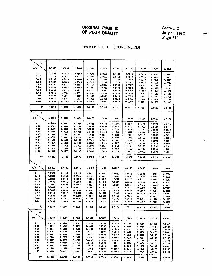
ORIGINAL PAGE IS
POOR QUALITY
TABLE 6.0-1. (CONTINUED)
Section D
July 1, 1972
Page 270
1. 1000 1. 1200 1. 1400 1. 1600 1. 1800 1. 2000 1. 2200 1. 2400 1. 2600 1. 2800
0. 0. 7804 0. 7736 0. 7662 0, 7982 0. 8097 0. 8206 O. 8311 0.8410 0. 8505 0. 8595
0. 10 0.7518 O. 7645 0. 7771 0. 7890 0. 8005 0.8114 0.8218 0.8318 0.8412 0. 8603
0.90 0.7248 0.7376 0.7498 0.7616 0.7729 0.7837 0.7941 0.8040 0.8135 0.8228
0.30 O. 680_ 0.6930 0.7048 0.7162 0.7272 0.7378 0.7480 0.7578 0.7672 0.7783
0.40 0.8200 0.6315 0.6426 0.6534 O. 6638 0,6739 0.6837 0.6932 0.7024 0.7113
0.60 0.5438 0.5542 0.5843 0.6741 0.5837 0.5930 0.6020 0.6109 0.6195 0.8280
0.60 0.4536 0.4625 0.4712 0.4797 0.4880 0.4962 O, 5042 0,5120 0.5197 0.52720.70 0.3814 0.3585 0.3655 0.372:] 0.3789 0.3855 0. :_920 0, 3984 0.4046 0.4109
0.80 O, 2398 0,2447 0.2496 0.2543 0.2590 0.2836 0.2682 0,2727 0.2772 0.2816
0. _) 0. 1218 0. 1241 0. 1266 0. 1291 0. 1315 0. 1339 0. 1362 0. 1386 0. 1408 0. 1432
1. O0 O. 0000 O. 0000 O. 0000 O. 0000 O. O00O O. 0000 O. OOO0 O. OOOO O. 0000 O. O00O
_t 0.4878 0.4968 0.5055 0,5140 0.5221 0.5301 0.5377 0.5451 0.5523 0,5593
1.3000 1.3200 1.3400 1.3600 1.3800 1.4000 1.4200 1.4400 1.4600 1.4800
0. _. _gSO O. 8761 O. 8838 O. 8911 O. 898o o. 9046 9.91o_ O. 9166 O, 9221 O. 9273
0. _.0 0:9689 0. 8670 0.8748 0. 8822 0. 8892 O. 8958 0. 9021 O. 9081 0, 9137 0. 91910.|0 0.8313 0,8396 0.8475 0.8551 0.8624 (,. 8693 (I.8759 0,8822 0.8882 0.8939
0.$0 0.7880 0.7935 0.8016 0.8094 0.8189 0.8242 0.8:]12 0.8379 0.8444 0, 8506
0. 40 O. 7200 O. 7283 O. 7365 O. 7444 O, 7521 O. 759(; 0.7668 O. 7739 0. 7808 O. 78740.60 0.6362 0.6443 0.6522 9.6599 9.6C74 0.6748 0.682! 0.6892 0.5962 0.7030
0. 60 O. 5846 O. 5419 O. 5491 O, 5562 O. 5632 O. 5701 0.57fi9 O. 5836 O. 5902 O. 5967
0.70 0,4170 0.4231 0.4291 0.4350 0.4409 0.4487 O. 452F, 0.4582 0.4839 O. 4696
0.80 0.2860 0.2904 0.2947 0.2990 0.303:! 0.3075 11.311_ 0.3160 0.3202 0.3243
O. gO 0. 1455 O. 1478 O. 1501 O. 1523 O. 1546 O. 1588 0, 1590 O. 1613 o. 1635 O. 1657
1.00 O. 0000 O. 0000 O. OOOO O. O00O O. 0000 O. 0000 O, 0000 O. 0000 O. 0000 O. O000
91t 0.8681 0.5726 0.5790 0.5852 0.5912 0.5970 0.8027 0.8082 0.6136 0.8188
1, 5000 1.5200 1.5400 1.5600 1.5800 1.6000 1.6200 1.6400 1.6600 116800
O. O. g322 O. 9368 O. 9412 O. 9453 O. 9491 O, 9527 0.9581 O. 9592 0. 9622 O. 9650
O. 10 O. 9241 O. 9289 O. 9334 O. 9377 O. 9417 O. 9485 0.9491 O. 9524 o. 9556 O. 9685
O. 20 O. 8994 O. 9046 O. 9096 O. 9143 O. 9188 0.9231 O. 9272 O. 9311 O. 9348 O. 9383
0.30 0.8566 0.8624 9.8680 0.8734 0.8785 0. 8835 0.8883 0.8930 0.8974 0.9017
O. 40 O. 7939 O, 8002 O. 8064 O. 8124 O. 8182 0.8239 0, 8294 O. 8:_48 O, 8400 O. 8451
O. 80 O. 7097 O. 7163 O. 7227 O. 7291 o. 7353 O. 7414 o. 7474 o. 7533 O. 7591 O. 7648
O. $0 O. 6032 O. 6095 O. 6158 O. 6221 O, 6282 O. 6343 O. 8403 O, 6462 O. 8521 O. 6579
0.70 0.4752 0.4807 0.4863 0,4918 0.4972 0.5026 o. 5n80 0.5123 0.5187 0.5240
O. 80 O. 3288 O. 3326 O. 3368 O. 3409 O. 3450 O. 3491 O. 3532 O. 3572 O. 3613 O. 3853
0. 90 0. 1679 0, 1702 O. 1724 0. 1746 O. 1768 0, 1790 0. 1812 0.1834 0. 1856 O. 1878
1. O0 O. O00O O. 0000 o. OOO0 O. O0OO O. 0o00 O. 0000 O. 0000 O. oo00 O. O00O O. 0000
Q'l_ 0.6239 0.6288 0.6336 0.8383 0.8429 0.6474 0.6517 0.8560 0.6601 0.6642
_a_ 1.7000 1.7200 1.74 O0 1, 7600 1. 7800 1.8000 1. 8200 1.84 oo 1.8600 1.8800
O. 0. 9676 O. 9700 O. 8"/23 O. 9744 O. 9763 O. 9782 0. 9799 O. 9815 O, 9829 O, 9843
O. 10 O. 9613 O, 9640 O. 9664 O. 9687 O. 9709 O. 9729 O. 9748 O. 9766 0.9783 O. 9798
O. 30 O. 9416 O. 9448 O. M,79 O. 9507 O. 9535 O. 9560 O. 9585 O. 9608 O. 9631 O. 9652
O. 30 O. 9068 O. 9098 O. 9136 O. 9173 O. 9209 O. 9243 O. 9276 O. 9308 O. 9336 O, 9367
0.40 O. 8601 O. 8849 O. 8696 O. 8642 O. 8686 O. 8730 O. 8772 O. 8813 O. 8853 O, 8891
0.50 0.7704 0.7758 0.7812 0.7865 0.7917 0.7968 0.8018 0.8067 0.8115 0,8162
O. 80 O. 0837 O. 8693 O. 6749 O. 6808 O. 6860 O. 6914 O. 6967 O. 7020 O. 7073 O, 7124
0.70 0. 8292 O. 5344 O. 5396 O. 5447 O. 5498 O. 5549 O. 5600 O. 5650 O. 5700 O. 5749
0.80 0.3693 0.3734 0.3774 0,3814 0.3854 0.3893 0.3933 0,3972 0.4912 0.4061
O. I)0 0. 1BOO O. 1922 O. 1944 O. 1966 O. 1987 O. 2009 O, 2031 O. 2053 O. 2075 O. 209_
1. O0 O. 0000 O. OOOO O. O00O O. O00O O. 0000 O. O000 O. 0000 O. OOOO O. 0000 O. 0000
tlt O. 6881 O. 6720 O. 6758 0.6794 O. 8830 O. 6868 0.6900 O. 6934 O. 6967 O. 6999
v _
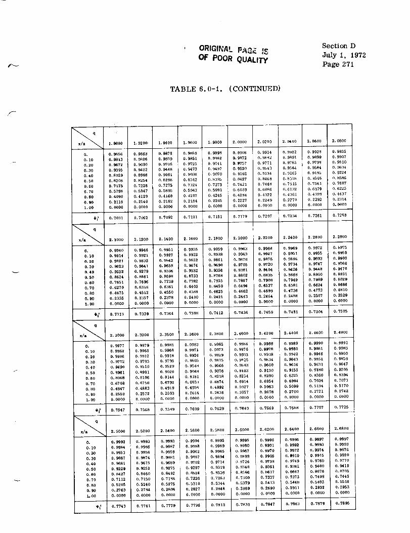
ORIGINAL p_c_. _,
OF POOR QUALITY
Section D
July I, 1972
Page 271
TABLE 6.0-1. (CONTINUED)
1. 9000 1. 9200" 1. 9400 1. 9600 1. 9800 2. O000 2. 0200 2. 0400 2. 0600 2. 0800
@_ 0.7031 0.7062 0.7092 0.7121 0.7151 0. 7179 0. 7207 0.7234 0.7261 0.7288
x/a_ 2.1000 2.1200 2.1400 2.1600 2.1900 2.2000 2.2200 2.2400 2.2600 2.2900
O. O. 9940 O. 9946 O. 9951 O. 9955 O, 9959 O. 9963 O. 9966 O. 9969 O. 9972 O. 9975
0.10 0.9914 0.9921 0.9927 0.9932 0.9938 0.9943 0.9947 0.9951 0.9955 0.9059
0.20 0. 9821 O. 9832 O. 9842 O. 9852 O. 9861 O. 9870 O. 9878 O. 9686 O. 9893 O. 9900
0.30 0.9623 0.9641 0.9658 0.9674 0.9690 0.9705 0.9720 0.9734 0.9747 0.9760
O. 40 O. 9252 O. 9279 O. 9306 O. 9332 0.9356 O. 9381 0.9404 0.9426 0.9448 0.9470
0.50 0.8624 0.8661 0.8698 0.9733 0.8768 0.8802 0.8835 0.8866 0.6900 0.6931
0.60 O. 7851 0.7696 0.7739 0.7782 O. 7825 0.7867 0.7908 0.7949 0.7989 0.8028
0.70 0.6270 0.6316 0.6361 0.6405 0.6450 0.6494 0.6537 0.6581 0.6624 0.6666
0.80 0.4475 0.4512 0.4550 0.4588 0.4625 0,4662 0.4899 0.4736 0.4773 0.4810
0,90 0.2335 0.2357 0.2378 0.2400 0.2421 0.2443 0.2464 0.2496 0.2507 0.2529
1.00 0.0000 0.0000 0.0000 0.0000 0.0000 0.0000 0.0000 0.0000 0.0000 0.0000
• _ 0,7313 0.7339 0.7364 0.7388 0.7412 0.7436 0.7459 0.7491 0.7504 0.7525
_a_ 2.3000 2.3200 2.3500 2.3600 2.3800 2.400O 2.42O0 2.4400 2.4600 2.4800
O. 0.9977 0.9979 0.9981 0.9983 0.9985 0.9986 0.9988 0.9989 0.9990 0.9991
O. 10 O. 9962 O. 9965 O. 9968 O. 9971 O. 9973 O. 9976 O. 9978 O. 9980 O. 9981 O. 9083
0.20 0.9906 0.9912 0.9918 0.9924 0.9929 0.9933 0.9938 0.9942 0.9946 0.9950
0.30 0.9772 0.9783 O. 9795 O. 9805 O. 9815 O. 9825 O. 9834 O. 9843 O. 9851 O. 9859
0.40 0.9490 0.9510 0.9529 0.954_ 0.9566 0.9583 0.9600 0.9616 0.9631 0.9647
O. 50 O. 8961 O. 6991 O. 9020 O. 9048 O. 9076 O. 9103 O. 9130 O. 9155 O, 9180 O. 9205
0.60 0.8060 0.8106 0.8144 0.8181 0.8218 0.8254 0.8290 0.8326 0.8360 0.9394
O. 70 O. 6708 O. 6750 O. 6792 O. 6833 O. 6874 O. 6914 O. 6954 O. 6994 O. 7034 O. 7073
0.80 0.4847 0.4883 0.4919 0.4956 0.4992 0.5027 0.5063 0,5099 0.5134 0.5170
0.90 0.2550 0.2572 0.2593 0.2614 0.2636 0.2657 0.2678 0,2700 0.2721 0.2742
1.00 0.0000 0.0000 0.0000 0.0000 0.0000 0.0000 0.0000 0.0000 0.0000 0.0000
• _ 0.7547 0.7568 0.75H9 0.7609 0.7629 0.7649 0.7669 0.7688 0.7707 0.7725
2.5000 2.5200 2.5400 2.5600 2.5800 2,6000 2.6200 2.6400 2.6600 2.6800
O. 9992 O. 9993 O. 9993 O. 9994 O. 9995 O. 9995 O. 9996 O. 9996 O. 9997 O. 9997
O. 9964 O. 9986 O. 99_7 O. 9988 O. 9989 0. 9990 O. 9991 O. 9992 0. 9993 O. 9993
O. 9953 O. 9956 O. 9959 O. 9962 O. 9965 O. 9967 O. 9970 O. 9972 0. 9974 O. 9976
O. 9867 0.9874 O. 9881 0.9887 O. 9894 O. 9899 O. 9905 O. 9910 O. 9915 O. 9920
0,9661 0.9675 0.9689 0.9702 0.9714 O. 9726 O. 9738 O. 9749 O. 9760 O. 9770
0.9229 0.9252 0.9275 0.9297 0.9319 0.9340 0.9361 0.9381 0.9400 0.9419
0.8427 0.8460 0.8492 0.9524 0,8556 0.8566 0.8617 0.8647 0.8676 0.8705
0.7112 0.7150 0.7188 0.7226 0.7263 0.7300 0.7337 0,7373 0.7409 0.7445
0.5205 0.5240 0,5275 0.5310 0.5344 0.5379 0.5413 0.5446 0.5482 0.5516
O. 2763 0.2784 0.2806 O. 2827 0.2848 O. 2869 O. 2890 0.2911 O. 2932 O. 2953
O. OOOO 0.0000 0.0000 O. O00O 0.0000 O. O00O 0.0000 0.0000 0.0000 0.0000
O. 7743 O. 7761 O. 7779 O. 7796 O. 7813 0. 7830 0. 7847 O. 7863 O. 7879 O. 7895
O.
O. 10
0.24)
0.30
0.40
0.50
O. 60
0.70
0.80
0.90
I., O0
O. 0.9856 0.9868 0.9678 0.9889 0.9898 0.9906 0.9914 0.9922 0.9928 0.9935
0.10 0.9613 0.9826 0.9639 0.9851 0.9862 9.9872 0.9882 0.9891 0.9999 0.9907
0.20 0.9672 0.9690 O. 9706 O. 9725 0.9741 6.9757 0.9771 O. 9785 0.9798 O. 9810
0.30 O. 9395 0.9422 0.9448 0.9473 0.9497 O. 9520 O. 9543 O. 9564 O. 9584 0.9604
O. 40 0. 8929 O. 8966 O. 9001 O. 9036 0. 9070 0. 9102 0. 9134 O. 9165 0. 9195 0. 9224
0.50 0.8208 0.8254 0.8298 0.8342 0.8385 0.8427 0.8468 0.850_ 0.8548 0.8586
0.60 0,7175 0.7226 0.7275 0.7324 0.7373 0.7421 0.7468 0.7515 0.7561 0.7607
0.70 0.5798 0.5847 0.5895 0.5943 0.5991 0.6039 0.6086 0.6132 0.6179 0.6225
0.80 0.4090 0.4129 0.4168 0,4207 0.4245 0.4284 0.4322 0.4361 0.4399 0.4437
0.90 O. 2118 O. 2140 O. 2162 O, 2184 O. 2205 0.2227 O. 2249 O. 2270 O. 2292 O. 2_I14
1.00 0.0000 0.0000 0.0000 0.0000 0.0000 0.0000 0.0000 0.0000 0.0000 0.0000

ORIGINAL F/;3E ;_
OF POOR QUALITY
Section D
July 1, 1972
Page 272
TABLE 6,,.0-1. (CONTINUED)
, _ q"
_a_ I. 7000
O. O. Mr97
O. 10 o. 2M14
0.|0 0,9_7
0.90 0.11125
O. 40 o. lffso
0.00 O. NM
0.10 0.8"5'33
O. 70 O. 7480
O.S@ 0.9841
O. I0 O. 91fl'41.00 O. 0000
t 0' o. 7010
2.0000 2.9800
O. O. _ O. 9899
O. 10 O. _ O. 9898
0.|0 O. IIHIO O. 9890
0.30 0.9810 0.9M2
0.40 O. 8_11 0.98800.10 0.982'? O. MII
O. @0 O. 8991 O, 90140.70 0.7814 0.7840
O. M@ O. 5870 O. 5911
O. 00 O. 3183 O. 3204
1. O0 O. 0000 O. 0000
t_ O. 0065 O. 8068 O. 8081
_a_ 3. 1900 3. 2000 3. 3000
O. 1. 0000 I. 0000 I. 0000
O. I0 O. 9999 1. 0000 1. 0000
O. 80 O. Mi,98 O. 9897 O, 9898
0.3@ O. MY/9 O. 9985 O. 9989
O. 40 O. 9815 O. 9934 O. 9949
0.00 O. V/10 O. ff/63 0.9804
O. lO 0. U98 0.9297 0.9381
O. 70 O. 8116 O. 8254 O. 8385
O. 80 O. 8194 O. 634a O. 8494
0.20 0.3388 0.3491 0.34599
1.98 O. 0000 O. 0000 O. 0000
q'/' O. 0180 O. 8237 O. 8290
_a_ 4. I000 4. 2000 4. 3000
9.7100 2.7400 2.7800 2.7800 2.8000 2.8200 2.8400
O. 9988 O. MHI@ O. M_,8 O. IHH)8 O. 9898 O. 9999 O. 9999
O. 08'94 O. _ O. _ O. _ O. 9996 O. 9997 O. 9997
O. 99'79 O. 9981 O. MM2 O. 9983 O. 9985 O. 9988 O. 9987O. m9 O. 9933 O. 9937 O. 9941 O. 9944 O. 9948 O. 9951
O. V/90 O. 9799 0. 9806 0.9817 O. 9825 0.9833 0.9840
O. 9454 O. 9473 O. 9410 O. 9507 O. 9923 O. 9539 O. 9654O. 8781 O. 8789 O. 8816 O. 8842 O. 8888 O. 8823 O. 8918
O. 751.15 O. 7650 O. 7584 O. 7818 O. 7651 O. 7685 O. 7718
O. 544583 O. 5417 O. 6060 O. 5403 O. 5716 O. 5749 O. 5782
O. 2998 O. 3010 O. 3037 O. 3068 O. 30'/9 O. 3100 O. 3120
O. G_O0 O. 0000 O. 0000 O. 0000 O. 0000 O. 0000 O. 0000
2.8600 2. 8800
O. 9999 O. 9999
O. 9997 O. 9997
O. 9988 O. 9989
0. 9954 O. 9958
O. 9848 O. 9855
O. 9589 O. 9683
O. 8943 O. 8987
O. 7750 O. 7782
0.5814 0.58470.3141 0.3162
O. 0000 O, 0000
O. 7986 O. 7941 O. 7958 O. 7971 O. 7985 O. 7999 O. 8013 O. 8027 O. 8041
8.9400 2.9900 2.9800 3.0000 3.0200 3.0400 3.0800 3,0800
0.9999 0._9 0.9909 1.0000 I. 0000 1. 0000 1.0000 1.0000
0.9998 0,_ 0.9998 0.9999 0.9999 0.9999 0.9999 O. 9999
0.9991 O.M_2 0.9_3 0.9999 0.9994 0.9994 0.9995 0.9995
0.9964 0.9066 0.2988 0.9970 0.9972 0.9974 0.9975 0.99770.9874 0.9880 0.9805 0.9891 0.9896 O. 9901 O. 9906 O. 9910
0. M24 0.9837 0.9849 0.9661 0. M73 0.9884 0.9895 0.9706
0.9037 0.9080 O. 8082 O. 9103 O. 9124 O. 9145 O. 9185 O. 9185
0.7877 0.7908 0.7939 0.7989 0.7998 O. 8029 O. 8058 O. 8087
0.5943 0.5075 0.6007 0.6038 O. 6070 O. 6101 0.6132 0.6163
O. 3224 O. 3945 O. 3286 O. 3280 O. 3307 O. 3327 O. 3348 O. 3369
0.0000 0.0000 0.0000 0.0000 0.0000 O. 0000 O. 0000 O. 0000
O. 8094 0.8107 0.8119 0.8132 0. 8144 0.8150 0.8168
3,4000 3.5000 3.8000 3.7000 3.8000 3. 9000 4.0000
1,0000 1,0000 1. 0000 1. 0000 1. 0000 1. 0000 1. 0000
1.0000 1.0000 1.0000 1. 0000 1. 0000 1. 0000 1.00000.9990 0.9989 1.0000 1.0000 1.0000 1.0000 1.0000
O. 92tMI 0.9898 O. 99_ O. 9998 O. 9998 0.9999 O. 9999
O. 9991 O. 99'/0 O, 9977 O. 9983 O. 9987 O. 9991 O. 9993O. 9838 O. 9867 O. 9891 O, 9911 O. 9928 O. 9942 O. 9953
O, 9466 O. 9923 O. 9883 O. 9837 O. 9684 O. 9'728 O, 9';'63
O. 8508 O. 8624 O. 8733 O. 8835 O. 8931 O. 9020 O. 9103
0. M38 O. 8778 0,6914 0.7047 0.7175 0.7300 O. 7421
0.3094 O. 3794 O. 3893 0.3992 0.4090 0.4187 0.42840.0000 0.0000 0.0000 0.0000 0.0000 0.0000 0.0000
0.8341 0.8388 0.8433 0.8475 0.8515 0.8553 0.8590
4.4000
O. 1.0000 1. 0000 1.0000 1.0000
O. 10 1. 0000 1. 0000 1. 0000 1.0000
O. 20 1.0000 1. O00O 1.0000 1.0000
O. S@ 1.0000 1. O00O 1. O00O 1.0000
0.40 O. 9M16 O.l_M 0,999'7 0._9
O. IHI 0._3 0.99'70 0.99"/0 0.9981
O. 80 O. 1_98 O. M20 O. 9880 O. 987|
0.70 0.0181 " O. 925| 0.9312 0.9981
O. 80 O. 75M O. 7661 O. 7701 O. 7845'/
O. tO O. 4.t80 O. 4478 O. 45011 O. 48S2
1.00 O. 0000 O. 0000 O. 0000 O. 0000
tiV 0. 8614 O. M67 O. 8@80 O. 8710
4. 5000 4. 9000 4. 7000
1. 0000 1. 0000 1. 0000
I. 0000 I. 0000 I. 0000
1.0000 1. 0000 1. 0000
I. 0000 I. 0000 I. 0000
O. 9999 O. 9902 O. 9999
O. I)985 O. MMI2 O. 9991
O. 9891 O. _ O. 9922
O. N38 O. 9490 O. 9639
O. 7M9 O. 8068 O. 8163
O. 4750 O. 4847 O. 4997
O. 0000 O. 0000 O. 0000
O. 8748 O. 8774 O. 8800
4.8000 4.9000 5.0000
1.0000 1.0000 1.0000
1.0000 1.0000 1. 0000I. 0000 1.0000 1.0000
1.0000 1.0000 1,00001.0000 1. 0000 1,0000
0.9993 0.9996 O. 9998
0.9934 O. 9944 O, 9953
0.9583 0.9824 0.9861
0.8254 0,8342 0.8427
0.5028 0.5117 0.5205
0,0000 0.0000 O. 0000
0.8825 0.8849 O. 8872

O_U_.?,5"i' ,-r .....
POOR QUALI Ey
TABLE 6.0-1. (CONTINUED)
Section D
July 1, 1972
Page 273
x/a_ 5.1000 5. 2000 5. 3000 5. 4000 5. 5000
O. 1. 0000 1. 0000 1. 0000 1. 0000 1. 0000
O. 10 1.0000 1. oooo 1. O000 1. 0000 1. 0000
O. 20 1. 0000 1, 0000 1. 0000 1. 0000 1. 0000
O. 30 1. 0000 1. 0000 1. 0000 1. 0000 1. 0000
O. 40 1. 0000 l. 0000 1. 0000 1. OOO0 1. 0000
O. 50 O. 9997 O. 9998 O. 9998 O. 9999 0. 9999
O. 00 O. 9961 O. 9967 O. 9973 O. 9977 O. 9981
O. 70 O. 9695 O. 9726 O. 9755 O. 9780 O. 9804
O. 80 O. 8508 0. 8587 O. 8661 O. 8733 O. 8802
O. 90 O. 5292 o. 5379 O. 5465 O. 5549 O. 5633
1. O0 O. 0000 O. 0000 O. O00O O, 01)00 O. 0000
'i'tt O. 8894 O. 8915 11. 8935 O. _955 0. 8974
_a_ 6. 1000 6. 2000
5. 6000 5. 7000 5. HO00 5. 9000 6. 0000
I. 0000 I. 0o00 I. 0000 1. 0000 I. 0o00
I. 0000 I. 0000 I. [)000 I. 0000 I- 00o0
1. 0000 1. 0000 1. 000o 1. 0000 1. 0000
1. 0000 1. 0000 1, 0000 1. 0000 1. ooo0
1. O00O I. 0000 1. 0000 1. 0000 1. 0000
O. 9999 O. 9999 I, (101}(I I. 01109 l. 0000
O. 9985 O. 9987 O. 9990 o, 9992 o. 9993
O. 9825 0. 9844 O. 9861 O. 9877 O. 9891
0. 8868 O. 8931 O. 8991 (}. 9048 O. 9103
O. 5716 O. 5978 9. 5879 0. 5959 I1. 6039
O. 0000 O- 0000 O. O000 [). 0000 O. 0000
O. 8993 O. 9010 O. 9027 o. 9044 o. 9060
6. :10o0 6. 4000 6. 5000 6. 6000 6. 7000
0. 1. 0000 1. 0000 1. 0000
O. 10 1. 0000 1. 0000 1. 9000
O. 20 I. 0000 I. 0000 I. 0000
O. 30 I. 0000 1. 0000 1. o000
O. 40 I. 0000 I. 0000 I. 0090
O. 50 1. 0000 1. 0000 1. 0000
O. 80 O. 9994 O. 9995 O. 9996
O. 70 O. 9903 O. 9915 O. 9925
O. 80 O. 9155 O. 9205 O. 9252
0.90 0.6117 0.6194 0.6270
1. O0 O. 0000 O. 0000 O. 0000
1. 0000 I. 0000 1. 0000 1. 0000
1. 0000 1. 0000 1. 0000 1. 001;.0
1. 0000 1. 0000 1. 0000 1. 0000
I. 0000 1. o000 1. 0000 I. 0000
1. 0000 1. 0000 1. 0000 1. 0000
I. 0000 I. I)000 i. 0000 1.0o00
O. 9997 O. 9998 O. 9998 o. 9998
0. 9934 O. 9942 O. 9949 I). 9955
0.9297 0.9340 0.9381 0.9419
0.6346 O. B420 0.6494 0.6566
O. 0000 0. 0000 O. 0000 O. 0090
$'1' 0.90'15 0.9090 0.9104 0.9118
7.3000 7.4000
6.8(}(1() 6.9000 7.0000
1. 0090 1. 0000 1. 0000
1. 0000 1. OOOO 1. 0000
1. 0000 1 . 0000 1. OOOO
1. 0000 I . 0000 I. 0000
1 •000(; 1 . OOO(} 1 . 0000
1.0000 I. 0000 I. 0000
O. 9999 O. 9999 ¢1. 9999
O. 9961 I}. 9966 (I. 9970
(}. 9450 O. 9490 O. 9523
O. 66218 O. 6708 9. 6778
O. 001)0 O. 0o00 {}. 0000
8.6000
1. 0000 1.0000 1.0000
1.0000 1.0000 1. 0000
1.0000 1.0000 1.0000
1.0000 1.0000 1.0000
1. 0000 1. 0000 1.0000 1-0000 1. OOOO
1. 0000 1. 0000 1.0000 1. 0000 1. OOOO
1.0000 1.0000 1.0000 1.0000 1.0000
0.9997 0,9998 0.9998 0.9998 0.9999
0. 9850 0.9861 0.9872 0.9882 0. 9891
0.7781 0.7814 0.7867 0.7916 0.7969
0.0000 0.0000 0.0000 0.0000 0.0000
0.9344 0.9351 0.9359 0. 9386 0. 9373
8.7000 8.8000 8.9000 9.0000
1.0000 1.0000
1.0000 1. OOO0
1.0000 1.0000
1.0000 1.0000
_ 0.9205 0.9216 0.9227 0.9238
8.1000 8.2000 8.3000 8.4000 8.5000
O. 1. OOOO 1.0000 1.0000 1.0000 1.0000
0.10 1.0000 1,0000 1.0000 1.0000 1. 0000
0.20 1.0000 1. 0000 1.0000 1.0000 1. 0000
0.30 1.0000 1.0000 1.0000 1.0000 1.0000
0.40 1. 0000 1. 0000 1.0000 1. 0000 1.0000
0.50 1.0000 1. 0000 1. 0000 1. 0000 1. 0000
0,60 1.0000 1.0000 1.0000 1.0000 1.0000
0.70 0.9994 O. 9995 0. 9996 0. 9996 0. 9997
0.80 0.9"/80 0.9796 0. 9811 0. 9825 0.9836
0._ 0. 7480 0. 7538 0. 7595 0. 7651 0. 7707
1.00 0.0000 0,0000 0.000O 0.0000 0.0000
_ 0.9303 0. 9312 0.9320 0.9328 0.9336
O. I. 0000 I. 0000 I. 0o00 I. 0000
O. I0 I. 0000 i, 0000 I. oo00 1. 0000
O. 20 I. 0000 i. 0000 I. o0o0 I. 0000
O. 30 1. 0000 1. 0000 1. I)11(10 1. I)1100
O. 40 1. 0000 1. 0000 1. 0000 1. 0000
0.50 1. 0000 1. O00O i. 0000 I. 0060
O. 60 0. 9999 I. 0000 1. 0000 1. 0000
0.70 0. 9974 0. 9977 0. 9980 O. 9983
O. 80 O. 9554 0. 9583 O. 9611 O. 9037
O. 90 O. 6847 O. 6914 O. 6981 O. 7047
1. O0 O. 0000 O. 0000 O. 0000 0. 0000
7.1000 7.2000 7. 5000 7. 6000 7. 7000 7. 800O 7, 9O00 8. I)000
1. [)000 1. D000 1,0000 I. 0(}00 1. 01100 1.01)00
I. 0900 I. 0000 I. 0000 1.00(io 1. 0000 I. 0o00
I. 0000 I. 0000 I. 0000 I. 0000 I. 0000 I. 0000
1. 0000 1. 00110 1. 0000 1.0o00 I. 0000 1. 00110
1.0o1}0 1. 0000 1. 0000 1. OOOO 1. O000 1. 0000
I. (10o0 i. 0000 I. 0000 1. 9000 I. 0000 I. 01)00
1. 0000 1. 0000 1. 0000 I. 0(Io0 I. 001}0 I. 0000
O. ,(1985 O. 9987 O. 9989 O. 9991 O. 9992 0. 9993
O. 9661 O. 9684 O. 9706 0. 9726 O. 9745 O. 976,'1
0.7112 0.7175 0.7238 0.7300 0.7361 0.7421
O. 0000 O. 0000 O. 0000 O. 000(I O. 0000 0. 0000
O. 9248 O. 9258 O. 9267 O. 9277 O. 9286 O. 9295
0. 9132 O. 9145 O. 9158 O. 917o O. 9182 O. 9194
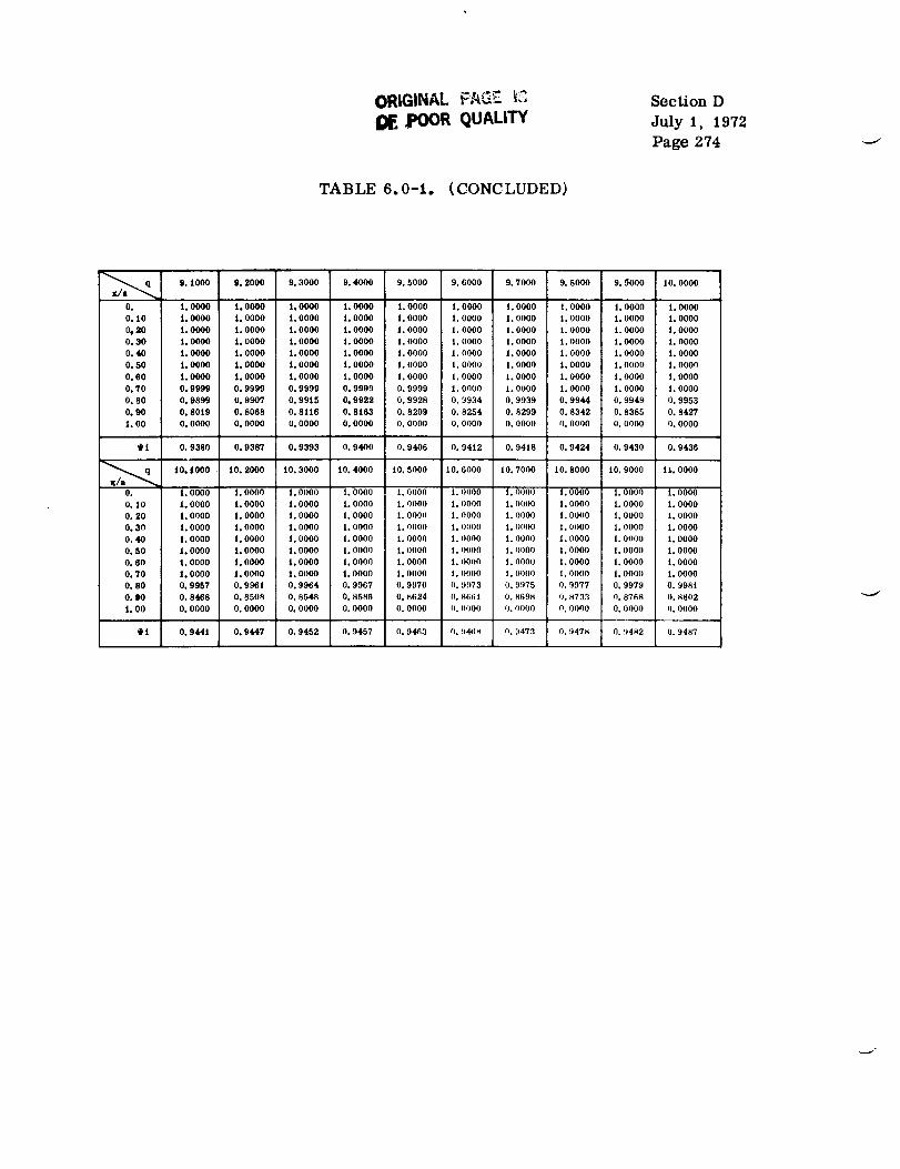
ORIGINAL F&_E L'_
pOOR QUALITY
Section D
July 1, 1972
Page 274
TABLE 6.0-1. (CONCLUDED)
9. I000 9. 2000 9. 3000 9. 4000 9. 5000
O. i. O000 1.0000 1.0000 1.0000 i. OOOO
0. I0 I. O000 1.0000 1.0000 1.0000 i. O000
0_20 I. 0000 i. 0000 I. 0000 I. 0000 I. 0000
0.30 i. 0000 i. 0000 1.0000 i. 0000 I. 0000
0.40 I. 0000 i. 0000 i. 0000 1. 0000 i. 0000
0.50 i. O000 1.0000 1.0000 l. O000 i. O000
O. 60 1. 0000 I. 0000 1. 0000 i. O000 1. 0000
0.70 0.9999 0.9999 0.9999 0.9999 0.9999
0.80 0.9899 0.9907 0.9915 0,9922 0.0928
0.90 0.9019 0.8068 0.81t6 0.8163 0.8209
1. O0 O. OOO0 O. 0000 O. 0000 O. OOO0 O. OOO0
0,9380 0.9387 0. 9393 0.9400 0.9406
9. 6000 9.7000 9. 8000 9. §000 10. 0000
i. O000 1.0000 l. O000 1.0000 1.0000
1.0000 1.0000 |.0000 1.0000 1.0000
I. OOOO I. 0000 i. 0000 I. OOO0 I. 0000
i. O000 1.0000 1.0000 1.0000 1.0000
I. 0000 I. 0000 I. 0000 I. 0000 i. 0000
I. 0000 I. 0000 I. OOO0 I. 0000 I. 0000
1.0000 I. 0000 1. O00O i. O000 I. 0000
1.0000 1.0000 1.0000 1.0000 1.0000
O. 9934 O. 9939 O. 9944 O. 9949 O. 9953
0. 8254 0. 8299 0. 8342 0. 8385 0. 8427
0.0000 0.0000 0.0000 0.0000 0.0000
0.9412 0.94i8 0.9424 0.9430 0.9436
I0, _000 10. 2000 |0. 3000 i0. 4000 I0. 5000 10. 6000 I0. 7000 iO. 8000 I0. 9000 1 i_ 0000
O. I. 0000 I. 0000 I. OOOO i. 0000 I. 0000 I. 0000 I. O000 I. 0000 I. O000 i. 0000
O. I0 I. 0000 I. 0000 I. O00O i. 0000 I. 0000 I. 0000 i. 0000 I. 0000 i. O00O i. 0000
O. 20 I. 0000 I. OOO0 I. OOOO I. O00O i. 0009 I. 0000 I. 0000 I. 0000 J. 0000 I. 0000
O. 30 i. 0000 I. 0000 I. 0000 I. 0000 i. 0000 I. 0000 I. oo00 I. 0000 I. 0000 i. 0000
O. 40 1. 0000 1. 0000 I. 0000 i. 0000 1. 0000 1. 0000 1. 0000 I. 0000 1. 0000 1. 0000
O. 50 I. 0000 I. O000 I. 0000 I. 0000 I. 0000 I. 0000 I. 0000 I. OOO0 I. 0000 I. O00O
O. 60 t. 0000 t. 0000 1. 0000 1. 0000 1. OOOO i. 0000 1. 0000 i. 0000 1. 0000 1. 0000
O. 70 1. 0000 1. 0000 1. 0000 1. OOOO 1. 0000 1. 0000 i. 00o0 1. 0000 1. 0000 1. 0000
O. 80 O. 9957 O. 996 i O. 9964 O. 9967 O. 9970 O. 9973 O. 9975 O. 9977 O. 9979 O. 9981
O. 90 O. 8468 O. 8508 O. 8548 O. 8586 O. 8624 O. 8661 O. _698 O. 8733 0. 6768 O. 8802
1. O0 O. OOOO O. 0000 O. 0000 O. 0000 O. 0000 9. I)000 O. 0000 O. 0000 O. 0000 _1. 0000
_1,t 0. 9441 0. 9447 0.9452 0. 9457 0.94_3 0. 946 _ o. 9473 0. 9478 0. !)482 0.9487
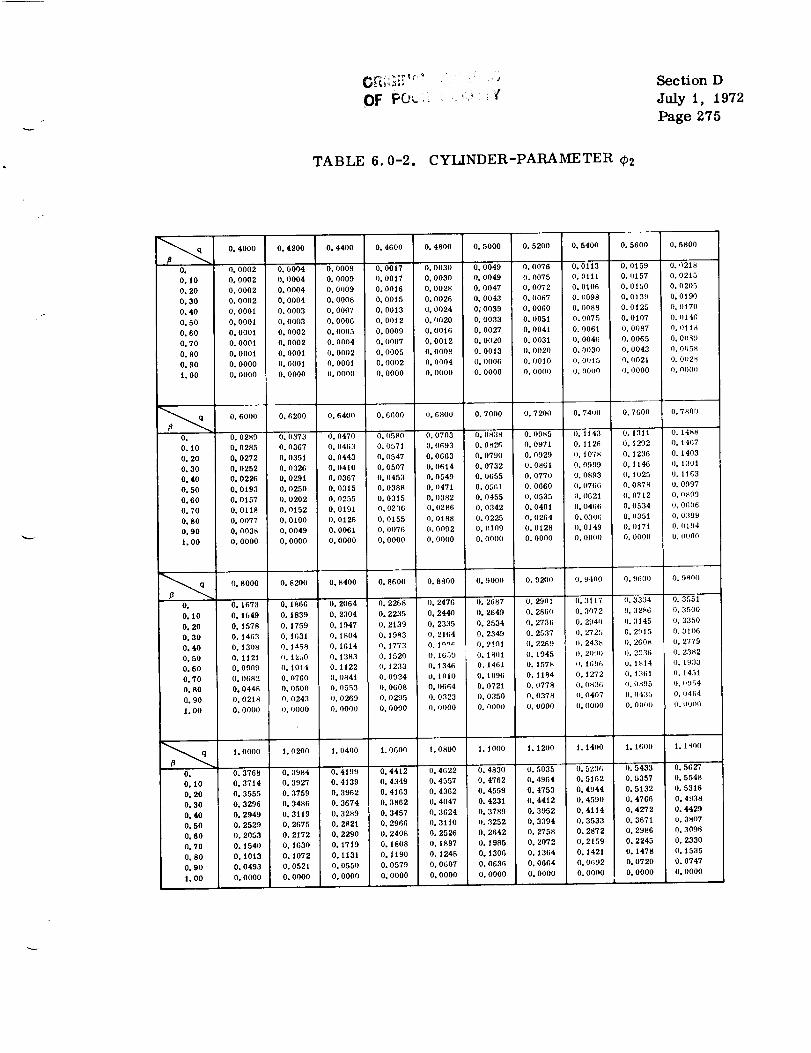
TABLE 6.0-2. CYLINDER-PARAMETER q)2
Section D
July 1, 1972
Page 275
0.4000 0.4200 0.4400 0.4500
0. 0.0'002 0. 0004 0. 0009 0. 0017
0. I0 0.0002 0.0004 0.0009 0.0017
0.20 0.0002 0.0004 0.0009 0.0016
0.30 0.0002 0.0004 0.0008 0.0015
0.40 0.0001 0.0003 0.0007 0,0013
0.50 O. 0001 0.0003 0.0000 0.0012
0. 60 0. 0001 0. 0002 0. 0005 0. 0009
O. 70 O. O00i O. 0002 O. 0004 O. 0007
O. 80 O. 0001 O. O00i O. 0002 O, 0005
0.90 0.0000 0.0001 0.0001 0.0002
1.00 0.0000 0.0000 0.0000 0.0000
0.4800 0.5000 0.5200 0.5400
0.0030 0.0049 0.0076 0.0113
0.0030 0.0049 0.0075 0.0111
0.0028 0.0047 0.0072 0.0100
0.0026 0.0043 0.0067 0.0098
0.0024 0;0039 0.0000 0.0088
0.0020 _ 0033 0. 0051 0.0O75
0.0016 0.0027 0.0041 0,0061
0.0012 0.0020 0.0031 O. O0_i
0.0008 0.0013 0.0020 0.0030
0.0004 0.0006 0.0010 0.0o15
0.0000 0.0000 0.0000 0.0000
0.6600 0.7000 0.7200 0.7400
0.0838 0.09_5 0.1143
0.0826 0.0971 0.1126
0.0790 0.0929 0,1078
0.0732 0.0861 0.0999
0.0655 0.0770 0.0893
0.0561 0.0660 0.0766
0.0455 0.0535 o. 0621
0.0342 0.0401 0.0466
0.0225 0.0264 0.0306
0. o109 0.0128 0.0149
0.0000 0.0000 0.0000
0.6000 0.6200 0.6400 0.6800
0. 0.0289 0.0373 0.0470 0.058(I 0.0703
0. i0 0.0285 0.0367 0.0463 0.0571 0.0693
0. 20 0.0272 0. 0351 0. 0443 0. 0547 0. 0653
0.30 0.0252 0.0326 0.0410 0.0507 0.0614
0. 40 0.0226 0. 0291 0. 0367 0. 0453 0. 0549
0.50 0.0193 0. O250 0.0315 0.0388 0.0471
0.60 0.0157 0.0202 0.0255 0.0315 0.0382
0.70 0.0|18 0.0132 0.0191 0.0236 0.0286
O. 80 O. 0077 0,0100 O. 0126 O, 0155 0.0188
0.90 0.0038 0.0049 0.0061 0.0076 0.0092
1.00 0.0000 0.0000 0.0000 0.0000 0.0000
0.5600 0.5800
0.0159 0.0218
0.0157 0.0215
0.0150 0.0205
0.0139 0.0190
0.0125 0.0170
0. 0107 0. 0146
0.0087 0. 011_
0. 0065 0. 0089
0.0043 0.0r)58
0.0021 0.0028
0. 0000 t}.0000
O. 7600 O. 7800
O. 1311 O. 14_8
O. 1292 O. 14(;7
O. 1236 O. 1403
O. 1146 0. 1301
0. 1025 0. 1163
0. 0878 0. 0997
0.0712 0.0_09
0.0534 0. 0606
0. (1351 0. 0399
0.0171 0.0194
O. 0000 0. 0o00
0.8000 0.8200 0.8400 0.8600 0.8800
0. 0.1673 0.1866 0. 2064 0. 2268 0.2476
0. 10 0. 1649 0. 1839 0. 2304 0. 2235 0. 2440
0.20 0.1578 0.1759 0.1947 0.2139 0. 2335
0.30 0.1463 0.|631 0.1804 0.1983 0.21(;4
0.40 0.1308 0.1458 0.1614 0.1773 0. In_c
0.50 0.1t21 0.1250 0.1383 0.1520 0.1630
0, 60 0.0909 0. i014 0. 1122 0. 1233 0. 1346
0.70 0.0682 0.0760 0.0841 0,0924 0.1010
0.80 0.0448 0.0500 0.0553 0.0608 0.0664
0.90 0.0218 0.0243 0.0269 0.0295 0.0323
1.00 0.0000 0.0000 0.0000 0,0000 0.0000
1.0000
O. 0.3768
0.|0 0.3714
0.20 0.3555
0.30 0.3296
0.40 0.2949
0.50 0.2529
0.60 0.2053
0.70 0.1540
0.80 0,10t3
0.9O 0.0493
1.00 0.0000
O. 9000 O. 9200 O. 9400 O. 9600 O. 9800
0. 2687 0. 2901 0.3117 o. 3334 0. 3551
0. 2649 0. 2860 0. 3072 0. 3286 0. 3500
0. 2534 0. 2736 0, 2940 0. :1145 0. 3350
O. 2349 O. 2537 O. 2725 O, 2915 0. 3106
O. 2'_01 O. 2269 0, 2431_ O. 200_ O. 2779
0. 1801 0. 1945 0. 2090 0. 2236 0.23_2
0.1401 0. 1578 t). 1696 0. 1_14 0. 1933
0. 1096 0. 1184 O. 1272 O. 1361 +}. 1451
0. 0721 0. (1778 0. 0836 0. O895 0. I}!)54
O. 0350 0. 0378 0. 0407 0. 0435 0. 041;4
O. 0000 O. 0000 O. 0000 O. 000o 0. (I0o0
1.0200 1.0400 1.0600 1.0800 1.1000
0.3984 0.4199 0,4412 0.4(;22 0.4830
0.3927 0.4139 0.4349 0.4557 0.4762
0.3759 0.3962 0,4163 0.4362 0.4559
0.3486 0.3674 0,3862 0.4047 0.4231
0.3119 0.3289 0.3457 0.3624 0.3789
0.2675 0.2821 0.2966 0.3110 (I. 3252
0.2172 0.2290 0.2408 0.2526 0.2642
0.1630 0.1719 0.1808 0.1897 0.1905
0.1072 0.1t31 0.1190 0.1248 0.1306
0.0521 0.0550 0.0579 0.0607 0.0636
0.0000 0.0000 0,0000 0.0000 0.0000
1. 1200 1.14o0 1.16o0 I. ISO0
0.5035 0.5236 I).5433 0.5627
0.4964 0.5162 0.5357 0.5548
0.4753 0. 4944 0. 5132 (}. 5316
0.4412 0.4590 0.4766 0.4038
0.3952 0.4114 0.4272 0.4429
0.3394 0.3533 0.3671 0.3807
0.2758 0.2872 0.2986 0.3098
0. 2072 0.2159 0,2245 0.2330
0.1364 0.1421 0.1478 0.1535
0. 0654 0. 0(;92 0. 0720 0. 0747I
O. 0000 O. OOOO i O. 0000 O. 0000
I

GRIGiNAL PAGE IS
OF POOR QUAUTY Section D
July 1, 1972
Page 276
TABLE 6.0-2. (CONTINUED)
t. 2000 1. 2200 1. 2400 1. 2600 1. 2800 1. 300 1. 3300 1. 3400 1. 3600 t. 3800
O. O. 5816 O. 6001 O. 6181 O. 6356 O. 6527 O. 6692 O. 6853 O. 7008 O. 7158 O. 7303
O. 10 O. 6735 O. 5918 O. 6096 O. 6270 O. 6439 O. 6603 O. 6762 O. 69t6 O. 7066 O. 7210
O. lO 0.5497 0.5673 0.5845 0.6014 0.6178 0.6337 0.6492 0,6643 0.6789 0.6931
O. 30 O. 5108 O. 5274 O. 5436 O. 5595 O. 5751 O. 5902 O. 6050 O. 6194 O. 6335 O. 6471O. 40 0. 4583 0. 4734 0. 4882 0. 5028 0. 5171 0. 531 ! 0. 5448 0. 5582 0. 5713 0. 5841
O. 50 O. 3941 O. 4073 O. 4204 O. 4332 O. 4458 O. 4582 O. 4703 O. 4823 O. 4941 O. 5056
O. 00 O. 3208 O. 3318 O. 3428 O. 3532 O. 3638 O. 3741 O. 3844 O. 3945 O. 4044 O. 4142
0. 70 O. 2414 0. 2497 0. 2580 0. 2662 0. 2743 0. 2823 0. 2902 0. 2980 0. 3058 0. 3 t35
O. 80 O. 1591 O. 1647 O. 1702 Oo 1756 O. 1811 O. 1864 O. 1915 O. 1971 O. 2023 O. 2075
0.90 0.0775 0.0802 0.0829 0.0856 0.0883 0.0909 0.0935 0.0962 0.0988 0. 1013
i. O0 0.0000 0. 0000 0. 0000 O. 0000 0.00OO 0. 0000 0.0000 0.0000 0.0000 0.0000
1.4000 I. 4200 i. 4400 1. 4600 I. 4800 I. 500 i.5200 I. 5400 i. 5600 I. 5800
0. 0. 7443 0. 7578 0. 7708 0. 7833 0. 7952 0. 8067 0. 8177 0. 8282 0. 8382 0. 847000. t0 0. 7349 0. 7484 0.76t3 0. 7738 0. 7857 0. 7972 0. 8082 0. 8188 0. 8289 0. 83868
0. 20 0. 7068 0. 7201 0. 7329 0, 7453 0. 7572 0. 7687 0. 7798 0. 7905 0. 8007 0. 8106
O. 30 0. 6604 0. 6733 0. 6858 0. 6980 0. 7097 0. 7212 0. 7322 0. 7429 0. 7533 0. 7633
0. 40 0. 5966 0. 6088 0. 6207 0. 6323 0. 6437 0. 6547 0. 6655 0. 6760 0. 6863 0. 6962
0, 50 0.5169 0. 5280 0. 5389 0. 5496 0. 560 t 0. 5704 0. 5805 0. 5905 0. 6002 0. 6097
0. 60 0. 4239 0. 4335 0. 4429 0. 4522 0. 46 i 3 0. 4704 0. 4793 0. 4881 0. 4967 0. 5053
0. 70 O. 3210 0. 3286 0. 3360 0. 3434 0. 3507 0. 3579 0. 3651 0. 3722 0. 3793 0. 3862
0.80 0. 2127 0. 2178 C. 2229 0. 2280 0. 2330 0. 2380 0. 2430 0. 2480 0. 2529 0. 2578
0.90 0.1039 0.1065 0.1090 0,1116 0.1141 0.1166 0.1191 0.12/6 0.1240 0.1265
I. O0 O. 0000 O. O00O O. 0000 O. 0000 O. 0000 O. 0000 O. 0000 O. 0000 O. 0000 O. 0000
1.6000 1.6200 t. 6400 1,6600 1.6800 1.700 1.7200 1.7400 1.7600 1.7600
0, 0. 8570 0. 8657 0. 8740 0. 8818 0. 8893 0. 8964 0. 9031 0. 9095 0. 9155 0, 9212
0.10 0. 8478 0. 5566 0. 8650 0. 8730 0. 8806 0. 8879 0. 8947 0. 9013 0. 9075 0. 9133
0. 20 0. 8200 0. 829! 0. 8378 0. 8461 0. 8541 0. 86|7 0. 8690 0. 8760 0. 8827 0. 8890
0. 30 0. 7730 0. 7823 0. 7914 0. 8001 0. 8085 0. 8166 0. 8244 0. 8320 0. 8393 0. 84630. 40 0. 7060 0. 7154 0. 7248 O. 7336 0. 7423 0. 7508 0. 7590 0. 7670 0. 7748 .0. 7824
0.50 0.6191 0.6282 0.6372 0.6460 0.6547 0.6631 0.6714 0.6796 0.6876 0.6954
0.60 0. 5137 0. 5220 0. 5302 0. 5383 O. 5463 0. 5542 0. 5620 0. 5697 0. 5772 0. 5847
0. 70 0. 593t O. 4000 O. 4068 0. 4135 0. 4202 0. 4268 0. 4334 0. 4399 0. 4464 0. 4528
0.80 0. 2626 0. 2674 0. 2723 0. 2770 0. 2818 0. 2865 0. 2913 0. 2960 0. 3006 0. 3053
0o 90 0. 1290 O. 1314 0. 1339 0. 1363 0. 1387 0. 1412 0. 1436 0. 1460 0. 1484 0. 1506
1. O0 O. 0000 O. 0000 O. 0000 O. 0000 O. 0000 O. 0000 O. 0000 O. 0000 O. 0000 O. 0000
1. 8000 1. 8200 1. 8400 t. 8600 1. 8800 1. 9000 1. 9200 1. 9400 1. 9600 t. 9800
0. 0. 9265 0. 9316 0. 9363 0. 9408 0. 9450 0. 9489 0. 9527 0. 9561 0. 9594 0. 9624
O. 10 O. 9t89 O. 9241 O. 9291 O. 9337 O. 9361 O. 9423 O. 9462 O. 9499 O. 9534 O. 9566
O. 20 0, 6951 0. 9006 O. 9063 0.9116 O. 916_ 0. 9213 0, 9258 O. 9301 0. 9341 0. 9380
0.50 0. 8530 0. 8595 0. 8657 0. 8717 0. 8775 0. 8830 O. 8884 0. 8935 0. 8984 0. 9031
0.40 0,7696 0,7969 0.8039 0.8106 0.8t72 0,8236 0,8297 0,8357 0.6416 0.8472
0.50 0.7030 0.7105 0.7179 0.7251 0.7322 0. 739| 0.7458 0.7525 0.7690 0.76530.60 0.6921 0.5994 0.6066 0.6t36 0.6206 0.6275 0.6343 0.64t0 0.6476 0.6542
0.70 0.4592 0.4655 0.4717 O. 4779 0.484t 0.4903 0.4963 0.5023 0.5082 0.5141
O. 80 O. 3099 O. 3145 O. 3191 O. 3237 O. 3282 O. 3328 O. 3373 O. 34t8 O. 3463 O, 3507
0. 90 0.1532 0. /556 0. 1580 0. 1604 0. 1628 0. 1651 0. 1675 0. 1699 0.1722 0. t746
i. O0 O. 0000 O. 0000 O. 0000 O. 0000 O. OOOO O. 0000 O. 0000 O. 0000 O. 0000 O. 0000

/
ORIGI_!AL _. _,:.... ,_....
OF POOR QU/4L_T't'
TABLE 6.0-2, (CONTINUED)
Section D
July l, 1972
Page 277
f
2. 0000 2. 0200 2. 0400 _0600 2. 0800 2, 1000 2. 1200 2. 1400 2. 1600 2. 1800
0. 0.9653 0.9679 0.9704 0.9727 0,9748 0.9766 0,9787 '0,9604 0.9820 0,9835
0.10 0.9597 0.9625 0.9652 0.9677 O, 970J O. 9723 0.9743 0,9762 O. 9780 0.9797
O. 20 0.9416 0,9451 O. 9484 0.9515 0.9544 O. 9572 O. 9598 O. 9623 O. 9646 0.9669
0.30 0,9077 0,9120 0.0t62 0°9202 0°9240 0.9276 0.9311 0.9345 0.9377 0.9408
0.40 0,8527 0.8580 0.8632 0.8682 0.8730 0.8777 0.8822 0.6866 0.8909 0.8950
0.50 0.7716 0.7776 0.7836 0.7894 0,7951 0.8007 0.6062 0.81t5 0.6i67 0.82t8
0.80 0,6606 0.6669 0.6732 0.6794 0.6654 0.6914 0.6973 0.7032 0.7089 0.7146
0.70 0.5200 0.5258 0.5316 0.5373 0.5430 0.5486 0,5542 0.5597 0.5652 0.5707
O. 80 O. 3552 O. 3596 O, 3640 O, 3684 O. 3728 O. 3771 O. 3815 O. 3858 O. 3901 O, 3944
0.90 0. t769 0.1793 0.1616 0.1840 0,1663 0.1987 O. 19tO 0.1933 0.1956 0.1980
1.00 0.0000 0.0000 0.0000 0.0000 0.0000 0.0000 0.0000 0,0000 0.0000 0.0000
2.2000 2.2200 2.2400 2.2600 2, 2800 2.3000 2.3200 2.3400 2.3600 2.3800
O. O. 9649 O. 966i 0. 9873 _'9884 O. 9894 O. 9903 O, 9912 O. 9920 O. 9927 O. 9933
O. t0 - O. 98i2 O. 9827 O. 9840 O. 9853 O, 9864 O, 9875 O. 9885 O. 9894 O. 9903 O. 9911
0.20 0.9690 0.9709 0.9728 0.9745 0.9762 0.9777 0,9792 0.9805 0.9816 0.9830
O. 30 0.9437 0.9466 O. 9492 0.95t8 O. 9543 O, 9566 O. 9588 0.9610 0.9630 O. 9650
O. 40 0.6990 0,9029 0.9066 0,9102 0,9137 O. 9171 0.9204 0,9235 0.9266 0.9295
0.50 0.8268 O, 8317 0.8365 O. 84tl O. 8457 O. 8501 O. 8544 O. 6587 0,6628 O. 8669
0.60 0.7202 0,7256 0.7311 0.7364 0,7416 0.7468 0.7519 0.7569 0.7619 0.7667
O. 70 O. 5760 O. 5814 O. 5867 O. 5920 O. 5972 O. 6023 O. 6075 O. 6125 O. 6176 O. 6226
0.80 0.3986 0.4029 0.407t 0.4113 0.4t55 0.4t97 0.4239 0.4260 0.4321 0.4362
0.90 0.2003 0.2026 0.2049 0.2072 0.2095 0.2118 0.2141 0.2164 0.2187 0.2210
1.00 0.0000 0.0000 0.0000 0.0000 0,0000 0.0000 0.0000 0.0000 0.0000 0.0000
2.4000 2.4200 2.4400 2.4600 2.4600 2.5000 2.5200 2.5400 2.5600 2.5800
0. 9939 O. 9945 0. 9950 O, 9955 0, 9959 _), 9963 O. 9966 O. 9970 O. 9972 O. 9975
0.10 0.9918 0.9925 0.9931 0,9937 0,9942 0,9947 0,9952 0.9956 0.9960 0.9963
O. 20 0.9842 0,9653 0.9863 0.9672 0.9681 0.9889 0.9897 0.9904 0.9911 0.9917
0.30 0.9668 0.9686 0.9703 0,9718 0,9734 0.9748 0.9762 0.9775 0.9787 0.9799
0.40 0.9324 0.9351 0.9377 0.9403 0°9428 0.9451 0.9474 0.9496 0.9517 0.9538
0.50 0,8709 0.8746 0.8784 0.8820 0,8856 0.8891 0.8925 0.8958 0.9990 0.9021
0.60 0.7715 0.7762 0,7809 0.7854 O. 7899 0.7943 0.7987 0. 8029 0.8072 0.8113
0,70 0,6275 0,6324 0.6373 O. 6421 0°6468 0.6515 0.6562 0.6608 0.6654 O. 6700
0. 80 0. 4403 0. 4444 0. 4485 0. 4525 0. 4565 0. 4605 0, 4645 0. 4685 0. 4724 0. 4764
0,90 0. 2233 O. 2256 O, 2279 O. 2301 O. 2324 0. 2347 O. 2370 O. 2392 0. 2415 0. 2437
i, O0 0.0000 0.0000 0,0000 0.0000 0.0000 0,0000 0.0000 0.0000 0.0000 0.0000
2. 6000 2. 6200 _ 6400 2. 6600 2. 6800 2.7000 2, 7200 _ 7400 _7600 2, 7800
O. 0.9978 0.9980 0.9982 0.9984 0.9985 0.9967 0.9986 0.9989 0.999t 0.9992
0. t0 0.9967 0,9970 0.9972 0.9975 0.9977 0.9979 0.9981 0.9983 0.9984 0.9986
0.20 0.9923 0.9928 0.9934 0.9938 0.9943 0°9947 0.9951 0.9955 0,9958 0.9961
0.30 0.9810 0.9621 0.9831 0.9841 0.9850 0.9859 0.9867 0.9875 0.9882 0.9689
O, 40 O. 9558 O. 9577 O. 9595 O. 9613 O. 9629 O. 9646 O. 9661 O. 9676 O. 9691 O. 9705
O, 50 O. 9052 O. 9082 O. 9111 O. 9139 O. 9166 O, 9193 O, 9219 O, 9244 O. 9269 O, 9293
0.60 O. 9|54 0.8193 0.6233 0.8271 0.8309 0.8346 O. 8383 O. 8419 0.8454 O. 8489
0. 70 O, 6745 O, 6789 0.6633 O, 6677 O. 6920 O. 6963 O. 7006 0.7048 O, 7089 O. 7131
0.80 0.4803 0.4842 0,468t 0.4919 0.4956 0.4996 0.5034 0.5072 0.5t10 0.5148
O. 90 O. 2460 O. 2483 O. 2505 O. 2528 O. 2550 O. 2572 O. 2595 O. 2617 0.2639 O. 2662
1.00 0.0000 0.0000 0.0000 0.0000 0.0000 0.0000 0.0000 0.0000 0.0000 0.0000

Section D
July 1, 1972
Page 278
TABLE 6.0-2. (CONTINUED)
2. 8600 2. 8800 2. 9000 2. 9200 2. 9400 2. 9600 2. 98002. 80O0 2. 8200 2. 640O
0. 0. 9993 0. 9993 0. 9994 0. 9995 0. 9995 0. 9996 0. 9996 9. 9997 0. 9997 0. 9997
0. 10 0. 9987 0. 9988 0. 9990 0. 9991 0. 9991 0. 9992 0. 9993 0. 9994 0. 9994 0. 9995
0. 20 0. 9964 0. 9967 0. 9969 0. 9972 0. 9974 0. 9976 0. 9978 0. 9979 0. 998t 0. 9983
0. 30 0. 9895 0. 9902 0. 994)8 0. 9913 0. 9918 0. 9923 0. 9928 0. 9932 0. 9937 0. 9941
0. 40 0. 9718 0. 9731 0. 9743 0. 9755 0. 9766 0. 9777 0. 9787 0. 9797 0. 9807 0. 9816
0. 50 0. 93t0 0. 9336 0. 9360 0. 9382 0. 9402 0. 9423 0. 9442 0. 946 J 0. 9480 0. 9497
0. 60 0. 8523 0. 8557 0. 8589 0. 8622 0. 8653 0. 8684 0. 8715 0. 8745 0. 8774 0. 8803
0.70 0.7171 0.7212 0.7251 0.7291 0.7330 0.7369 0.7407 0.7445 0.7482 0.75190. 80 0. 5t85 O. 5223 0. 5260 0. 5297 0. 5333 0. 5370 0. 5406 0. 5442 0. 5478 0. 5514
0. 90 0. 2684 0. 2706 0. 2728 0. 2751 0. 2773 0. 2795 0. 2817 0. 2839 0. 2861 0. 2883
I.O0 O. 0000 O. 0000 O. 0000 O. 0000 O. 0000 O.0000 O. 0000 O. 0000 O.0000 O,0000
3. 5000 3.6000 3. 7000 3.8000 3. 90003. 0000 3.1000 3. 2000 3. 3000 3. 4000
O. 0.9998 0.9999 0.9999 0.9999 1.0000 1. ooo0 1.0000 i. O000 1.0000 1.0000
0. t0 0.9998 0.9997 0.9998 0.9999 0.9999 1.0000 1.0000 l. OOOO |.0000 1.0000O. 20 O. 9984 O. 9990 O. 9993 O. 9996 O. 9997 O. 9998 O. 9999 O. 9999 1. 0000 1. 0000
0. 30 0. 9944 0.9960 0. 9971 0. 9980 0. 9986 0. 9990 0. 9993 0. 9995 0. 9997 0. 9998
0.40 0.9825 0.9863 0.9894 0.9918 0.9937 0.9952 0.9964 0.9973 0.9980 0.9985
0. 50 0. 9515 0. 9594 0. 9662 0. 9720 0. 9769 0. 9810 0. 9844 0. 9873 0. 9897 0. 9917
0.60 0.8831 0.8965 0.9086 0.9194 0.9292 0.9380 0.9458 0.9528 0.9590 0. 9645
0.70 0.7556 0.7733 0.790t 0.8058 0.8207 0. 8347 0.8478 0.8001 0.8716 0.8823
0. 60 0.5550 0. 5726 0. 5897 0.6064 0.6228 0.6384 0.6538 0.0687 0.6832 0.8972
0.90 0. 2905 0. 30t5 0. 3123 0. 323t 0. 3338 0. 3445 0. 3550 0. 3655 0. 3759 0. 3862
1.00 0.0000 0.0000 0.0000 0.0000 0.000O 0.0000 0.0000 0.0000 0.0000 0.0000
4.0000 4.1000 4. 2000 4.3000 4.4000 4.5000 4.6000 4.7000 4.8000 4.9000
O. 1.0000 1.0000 1.0000 l. OOOO 1.0o00 1.0000 1.0000 1.0000 1.o000 1.0000
0,10 t. 0000 1.0000 1.0000 i. O000 1.0000 1.0000 1.0000 1.0000 1.0000 1.000o0.20 1.0000 1.0000 1.0000 1.0000 1.0000 1.0000 1.0000 1.0000 1.00o0 1.0000
0.30 0.9999 0.9999 0.9999 1.0000 1.0000 1.0000 1.0000 1.0000 1.0oo0 1.0ooo
0.40 0.9989 0.9992 0.9994 0.9996 0.9997 0.9998 0.9999 0.9999 0.9999 i.0000
0.50 0.9933 0.9947 0.9958 0.9967 0.9973 0.9979 0.9984 0.9987 0.9990 0.9992
0.60 0.9693 0.9736 0.9773 0.9806 0.9834 0.9859 0. 9880 0.9899 0.9914 0.9928
0.70 0.8923 0.9016 0.9t03 0.9t83 0.9257 0.9325 0.9388 0.9446 0.9500 0.9549
0. 60 0. 7108 0. 7240 0. 7367 0. 7490 0. 7609 0. 7724 0. 7834 0. 7941 0. 8044 0. 81430.90 O. 3964 0.4066 O. 4166 O. 4266 O. 4366 O. 4463 O. 4560 0.4656 O. 4751 O. 4846
1. O0 0.0000 0.0000 0.0000 0.0000 0.0000 0.0000 0.0000 0.0000 0.0000 0.0000
5.0000 5.1000 5.2000 5.3000 5.4000 5.5000 5.6000 5.7000 5.8000 5.9000
O. t, 0000 t. 0000 t. 0000 t. 0000 J. 0000 i. 0000 |. 0000 1. 0000 t.0000 1. 0000
0.10 1.0000 1.0000 1.0000 1.0000 1.0000 1.0000 1.0000 1.0000 1.0000 1.0000
0.20 1.0000 1.0000 1.0000 1.0000 1.0000 1.0000 1.0000 1.0000 1.0000 1.0000
O. 30 I. 0000 I. 0000 I.0000 I.0000 I. 0000 I. 0000 I.0000 I.0000 I. 0000 i.0000
0.40 1.0000 1.0000 1.0000 1.0000 1.0000 1.0000 1.0000 1.0000 1.0000 i.O000
O. 50 O. 9994 O. 9996 O. 9997 0,9997 O, 9998 O. 9998 O. 9999 O. 9999 1, 0000 1. 0000
0.60 0. 9939 0.9949 0. 9958 0.9965 0,9971 0. 9976 0.9980 0. 9984 0. 9986 0. 9989
0,70 0. 9594 0.9635 0.9672 0.9706 0.9737 0. 9765 0.9790 0. 9813 0.9834 0. 98530.80 0.8238 0.8329 0.8416 0.8501 0.858i 0.8658 0.8732 0.8803 0.8870 0.8934
0,90 0.4939 0.5032 0.5t23 0.52t4 0.5303 0.5392 0.5480 0.5566 0.5662 0.5737
1.00 0.0000 _ 0000 0.0000 0.0000 0.0000 0.0000 0.0000 0.0000 0.0000 0.0000

OF.. POOR OUAi..IT_Section D
Jl_ I, 1972
279
/-
TABLE 6.0-2. (CONTINUED)
F
o.o. 1oo.loo.loo.41oo.6o0.soo.loO.90O.0OL99
5,0000 S. I000
i, OOO0 1. O00O|. 0000 1.0000 t. OOOO 1. OOOO1.0000 |. 0000 1. O00O 1.000o1.0099 1.0000 1.0000 1. OOC)O1.0_@ t. 0000 1. 00040 1. O000i. 00@0 i. 0000 I. 0000 I. 0000O. 11901 O. 9993 0, t994 0, 9996O. 98?0 O. 9864 O. 9998 O. 99100. 8994 0. 9054 0. 9t l0 0, 9183O.11010 O.5_103 O.6986 O.410650,O12O0 o. oooo O. OO9O O. 0000
4. 3000 It,.3000 9. 4000 6. 5000 4. 0000
.....t. 0000 1. 0900 i. 00._., 1.0_00 1. 0000
1. oooo
G. 7000
t. 00001. O00O |. 0000 _. 0000t. O000 I. 0000 L O00O i. 09001. 0000 |. 0000 1. 0000 1. O00O1. O000 |. 0000 1. 0000 1. O000L0000 i. 0000 I. 0000 i00000, 091M 0. 9997 O, 9998 0. 9998O.9921 O.9930 O.9939 O. 9946O.9213 O.9_Jl O.9:107 O.93500.01M 0. 0224 O. I_301 0.43780. O000 @.0000 O.0000 O.0000
8. 800¢ c+.9000
1. uOOO t. oot_u
1. _-ooo i. oooo1. _,000 1. 00091. oooo i. o_ooI. 0000 1. 0000I. oooo i. oooo0. 9999 O. 9999
O. 9953 O. 995_O. 0390 O.942_O.9453 O.662_O. O000 O. 0000
0.0.io0.m0.No.4o0.990.990. ?o0.1141.1os, ol
7.0000 7. iO00 7.JOOG 7.3000 7.4000
I. 0000i. 00001. 0000I. 0000t. 00001.04000, M1990.11440.14110. IMl010.OOOO
1.00o0 i. 0000 i. 0000 i. O0_LO000 i. 0000 I. 0000 1.0000LO000 1. OOQO LO000 LOO00
1.0000 i. 0000 1. OeO0 I.O00eI. 0000 i. 0000 I. 0000 i. 00@@1.0000 i. 0000 i. 0000 i. 0000O. 19111 1. oooo 1. oooo 1. ooooO. 9999 9. MY/$ 0. 91177 O.MN;O0.9600 9. 993;I 9.8664 0.9_0. 44174 O. _M O.0,,10 O.SSM0.OOOO 0.oooo 0.oooo o. ooo0
7. 6000 7. 8000 7. 7000 7. 8000 7. 9000
t. 0000 1. 0000 i. O000 1.0000 i. 0000
I. 0000 i. 0<300 i. 0000 J. 0000 f, 00001. 0000 LO000 LEO00 I. 0000 1. 00001._00 1.0000 I. 0000 i. 0000 1.0000|. 0000 I.000_9 I. 0000 I.0000 1.0000
1.0400 1.0000 1.0000 i. 0000 1.00001.9940 J, 0000 1.0000 1. 0000 i. 00000.14M10 O.9966 O.99_/ 0. 9989 O,99900.141/ 0. MM 0. MTi 0. M93 O.W/IS0.lllJ 0.7021 0.7087 0. 718_ 0.70170.0010 0. 0000 0.0000 0. 000_ O.0000
I.0. lO0.1e0.10O.4O0.800.1@0.?0O, 99O.99
1.00
,.oou _.i_o ,.,o_ ,.,990',.,me+L,
i.omo /.moo i. 990b /.moo i omo1.0400 l.O_O l.O_O 1.0000 1.0000
i, 0000 i.0000 1.0099 t. 0000 I._1.99ee t. 0000 L0000 t. 0000 1. M991,0000 I.0000 t.O_O t, 0000 i. 0010
i, 0000 I. 0000 1. 0000 LO000 i. 0000i.0000 i. 004_ 1.0004) I. 0000 i.0_
O. Mill O. II_ O. 90MI O. 9996 O. _ 0.0,,,lffM, 0.9764 0.9771 0. IrTSg O.IN4 0.M|90. _990 0.7_ 0,7404 0,7464 0,7_ O.7"dlli0.OOOO 0.OOOO 0. OeO0 0.OOOO
LIMe S.U0_ 8.'/000 S.8000 S.99_0
L@_O I.@@_ i. 00_0 t.M00 1.0000
l.eme i. ooeo _. ooee i+ ,o%_ "_.ooooi._ i._o@ I.ooo_,_ t. 9_O 1. ooooLMM 1.0@04 1. _o00@ i. 0099 LO000
LOM0 I, 0000 i. 0000 1.00_ 1. O0001.9990 i. 0000 1. 0000 1.0000 1. 00001.0440 t. _'..,000 L0000 1. 0000 LOO00
O.999"/ 0. 9997 0. 9998 0. 9998
O. 9832 O. 9846 O.9897 O. 9868O.7430 O.7008 0. 'rT_o O. 7806
0.11040 0.0000 O. 0000 O. 0000 0. 0000 0. 0000
0.ooo¢ 0.t_oo
0. I._ i.0_#0 i,0@0_
0.i0 i.9900 I.00_¢ J.9900
8,99 i._ 1.9900 1.0400
0.4_ /.ram l.eOm /.oomI,M. l.m L_99 Loo_@,_ Lifo 1,1441o I, OoM
t, t4_,NLN
s. SOO0 0. sooo 11.4OO0
i. 0000 i._i. 0000 /.le001.0040 1.99101.0_@ 1.99_1.0044 1.1404Le000 LMMI. 0000 /,MOO
LN_ 0._ 0. 990t 0.1m_ 0.1_e0.1_I _I,99M 0. I_IM 0.12_ 0.11119. T_M 0. 79/1 6. ?Ml 0. oolo 0. IoN0.MM 0._99 _._M 0. oooe O.MM
_._ 9.(1000 9.7000 9. 8000 0.9000
l.oem i. 0000 Loooo /.moo i ooooi. 0099 i. ooeo i oooo i. 0000 i. oooo1.0990 i. 0000 i. 0000 t. 9900 t, 0000I._ 1. oooe L0099 i, oeoo t. ooool.mm I. oooe Loom 1,99_ i. ooooLION LOOm _, oooo I. oooo /.mooL_ _._ I. oeoo i, oooe 1.oo<)oS.99N l.m_ t. oooo I.0099 i.0000I,,_ 0.NN 0.90,1|1 0._ 0.99_41.IIII 0. 9/19 O. 9J99 o. IIMI o. lJl_0. 0990 o.oo99 o.oo43o o. 0000 o.oo_

Section D
July 1, 1972
Page 280
TABLE 6.0-2. (CONCLUDED)
0.
0. t0
O. 200.30
O. 40
O. 50
0.00
O. 70
o. 80
O. 90
1. O0
10. 0000
1.0000
1.0000
1.0000
1.00001.0000
1.00001.0000
1.00oo
0.9948
0.8341
0.0000
I0. I000 10.2000 10.3000 10.4000 10.5000 I0.8000 10.7000 I I0.8000 [ 10.90o0
Ii. 0000 i.0000 I.0000 i. 0000 I. 0000 1.0000 1. 0000 1.0000 I.0000
I. 0000 i. 0000 I.0000 I. 0000 I. 0000 I. 0000 I. 0000 I.0060 I.0000
1.0000 1.0000 1.0000 1.0000 1.0000 1.0000 l. O000 1.0000 1.0000
1.0000 1.0000 1.0000 t.0000 1.0000 1.0000 1.0000 1. o000 1. o0_0
1.0000 1.0000 1.0000 1.0000 1.0000 1.0000 1.0000 1.0000 1.000o
I. 0000 1.0000 I.0000 1.0000 1.0000 1.0000 1.0000 I.0000 i.0000
i. 0000 I. 0000 1.0000 I. 0000 I. 0000 I. 0oo0 I.O00e I.0000 1.0000
1.00o0 1.0000 1.0000 1.0000 1.0000 1.0000 1.0000 1. o00o 1. i_000
o. 9952 o.9956 0. 9960 o. 9964 0. 9967 o. 9970 0. 9972 o. 9975 o. 9977
0. 8385 0.8427 0.8469 0.8510 o, 8549 O. 8588 O. 8627 O. 8664 o. 87oj
0.0000 0.0000 0.0000 0.000_ 0.0000 0.0000 0.0000 0.0000 _ U. O000
I

ORt_._I,.._L F.",Gi-'. _L;/1_ POOR QUALITY
TABLE 6.0-3. CY_NDER-PARAMETER _b2
Section D
July 1, 1972
Page 281
0.4000 0.4200 0.4400 0.4800 0.4800 0.5000 0.5200 0.5400 0.5600 O. 5800
O. 0.0001 0.0002 0.0005 0.0009 0.0015 0.0025 0.0038 0.0056 0.0080 0.0109
0.10 0.0001 0.0002 0.0005 0.0009 0.0015 0.0024 0.0038 0.0056 0.0079 0.0108
0.20 0.0001 0.0002 0.0004 0.0009 0.0015 0.0024 0.0037 0.0055 0.0077 0.0106
0.30 0.0001 0.0002 0.0004 0.0008 0,0014 0.0023 0,0036 0.0053 0.0075 0.0102
0.40 0.0001 0.0002 0.0004 0.0008 0.0013 0.0022 0.0034 0.0050 0.0071 0.0097
0.50 0.0001 0.0002 0.0004 0.0007 0.0013 0.0020 0.0032 0.0047 0.0066 0.0090
0.60 0.0001 0.0002 0.0003 0.0007 0.0011 0.0019 0.0029 0.0043 0.0061 0.0063
0.70 0.0001 0.0002 0.0003 0.0000 0.0010 0.0017 0.0026 0.0039 0.0055 0.0075
0.60 0.0001 0.0001 0.0003 0.0005 0.0009 0.0015 0.0023 0.0034 0.0048 0.0066
0.90 0.0000 0.0001 0.0002 0.0004 0.0008 0.0013 0.0020 0.0029 0.0041 0.0056
1.00 0.0000 0.0001 0.0002 0.0004 0.0007 0.0011 0.0016 0.0024 0.0034 0.0047
O. 6000 0.6200 O. 6400 O. 6600 O. 6800 O. 7000 O. 7200 O. 7400 O. 7600 0.7800
0, 0.0144 0.0186 0.0235 0.0200 0.0351 0.0419 0.0492 0.0571 0.0655 0.0744
0. t0 0.0143 0.0185 0.0233 0,0288 0.0349 0.0416 0.0489 0.0567 0.0651 O, 0739
0.20 0.0140 0.0181 0.0228 0.0282 0.0341 0.0407 0.0478 0.0555 0.0637 0.0723
0.30 0.0135 0.0174 0.0220 0.¢)271 0.0329 0.0392 0.0461 0,0535 0.0814 0.0997
0.40 0.0128 0.0166 0.0209 0.0258 0.0312 0.0372 0.0438 0.0508 0.0582 0.0661
O. 50 O. 0120 O. 0J55 0.1)195 O. 0211 0. 0292 0.0348 O. 0409 O. 0474 O. 0544 O. 0617
0.60 0.0110 0.0142 0.0179 0.0221 0.0267 0.0319 0.0375 0.0435 0.0499 0.0566
O. 70 O. 0099 O. 0128 Oo 0181 O. 0199 O. 0241 O. 0287 O. 0337 O, 0392 Oo 0449 O. 0510
0. 80 0. 0087 0. 0112 0. 0142 O. 0175 0. 0212 0. 0253 0. 0297 0. 0345 0.0396 0.0449
O. 90 O. 0075 O, 0097 0.0122 0.0150 Oo 0182 O. 0217 0.0255 O, 0296 O. 0340 O. 0386
t.00 0.0062 0.0080 0.0101 0.0125 0.0152 O. O1RI 0.0213 0,0247 0.0289 0.0321
0.8000 0.8200 0.8400 0.8600 0,8800 0.9000 0.9200 0,9400 0.9600 0.9800
0. 0.0837 0.0933 0.1032 0.1134 0.1238 0.1344 0.1451 0.1559 0.1667 0.1776
0. I0 0.0831 0.0926 0.1025 0.1126 0.1229 0.1334 0.]440 0.1547 0.1655 0.1763
0, 20 0.0813 0.0906 0.1002 0.1101 0.1203 (1.1305 0.1409 0,1514 0.1619 0.1725
0.30 0°0783 0.0873 0.0966 0.1062 0.1159 0.1258 0,1359 0,1460 0,1561 0.1663
0,40 0.0749 0.0829 0.0917 0.1008 0.1100 0.1194 0.1290 0.1386 0.1482 0,1579
0.50 0.0694 0.0774 0._56 0.0941 O. 1027 0.1115 0.1204 0,1294 0.1384 O. 1475
0.60 0.0637 0.0710 0.0786 0.0863 0.0943 0.1023 0.1105 0.1187 0.1270 0.1353
0.70 0.0573 0.0639 0.0707 0.0777 0.0848 0.0921 0.0995 0.1069 0.1t43 0.1218
0.80 0.0505 0.0563 0.0623 0.0684 0.0747 0.0811 0.0876 _ 0941 0.1007 0.1073
0.90 0.0434 0.0483 0.0535 0.0588 0.0642 0.0697 0.0752 0,0908 0.0865 0.0921
1. O0 O. 0301 O. 0403 O. 0446 O. 0490 O. 0535 O. 0580 0.0627 O. 0673 0.0721 O. 0768
1. 0000 1. 0200 1. 0400 1. 0600 1. 0900 1. 1000 1. 1200 1. 1400 1. JOOO 1. 1900
O, 0.1884 0.1992 O. 2100 O. 2206 O. 2311 O. 2415 O. 2517 O, 2618 O. 2717 O. 20t3
0°10 0.1871 0.1978 0.2085 9.2190 0.2295 0.2398 0.2500 0,2600 O. 2698 0.2794
0.20 O, 1831 O. 1936 O. 2040 O. 2144 O. 2246 O. 2347 O. 2447 0.2545 0.2641 0.2735
0.30 0.1765 0. i866 0. i967 0.2067 0.2166 O. 2264 0.2360 0.2455 0.2549 0.2640
O. 40 0.1675 0.1772 0.1868 0.1963 O. 2057 O. 2150 O. 2242 O. 2332 0.2422 O. 2509
O. 50 O. 150 O. 1655 O. 1745 O. 1834 O. 1922 O, 2009 O. 2095 O° 2180 O. 2204 O. 2346
O. 6C 0.143, O. t519 0,1602 0.1683 0.1765 0.1845 0.1924 O, 2003 0.2080 O. 2155
O. 70 O,_?)J O. 1368 O. 1442 O, 1516 0.1589 O. t662 O. 1733 O. t804 O. t874 O. 1943
O. flO 0.2139 O. 1205 O. 1270 O. 1335 O. 1400 O. 1464 0. 1528 O. 1590 0.1652 O. 1713
0.90 O. 0978 0.1035 0,1091 0.1147 0.1203 0.1258 O. 1313 O. 1367 O. 1420 0.1472
1. O0 O. 0815 O. 0862 O. 0909 O. 0956 O. 1002 O. t048 O. 1094 O, 1139 O. tt83 O. 1277
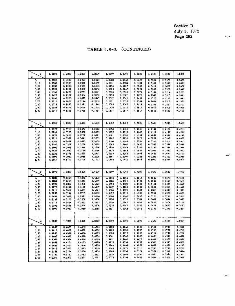
Section D
July 1, 1972
Page 282
TABLE 6.0-3. (CONTINUED)
I. 2000 i. 2200 I. 2400 I. 2600 I. 2800 I.3000 i. 3200 i. 3400 1.3600 i.3800
O. 0.2905 0.3009 0.3090 0.3179 0.3263 0.3346 0.3426 0.3504 0.3579 0.3652
0.10 O. 2888 0.2980 0.3069 0.3157 0.3241 0.3324 0.3404 0.3481 0.3556 0.3628
0.20 O. 2828 O. 29i8 0.3006 0.3092 0.3176 0.3257 0.3336 0.3412 0.3487 0.3558
0. 30 0.2729 0. 2817 0. 2903 0. 2986 0. 3068 0. 3147 0, 3224 0. 3299 0. 3372 0. 3443
0.40 0. 2595 0. 2679 0.2761 0. 2841 0. 2920 0. 2996 0. 3071 0. 3144 0. 32t4 0. 3283
0.50 0° 2427 0. 2507 0. 2584 O, 2660 O. 2735 0.2807 0. 2878 O. 2948 0. 30t5 0. 3081
0.60 0.223t 0.2305 0.2377 0.3447 0.25t7 0.2585 0. 2651 0.2716 0.2760 0. 28420°70 0.201t 0.2078 0.2144 0,2208 0.2271 0.2333 0.2394 0.2454 0.2512 0.2570
0. 80 0. t774 0. 1833 0. 189t 0. 1948 O. 2005 0. 2060 0.2i14 0. 2168 0. 2220 0. 277t
0. 90 0. 1524 0.1576 0.1626 0,1675 0.1724 0.1772 0. 18t9 0. 1865 0.1911 0.1955
1.00 0,1270 0.13|8 0.1355 0.1397 0,1437 0.1477 0. t517 0.1555 0.1593 0.1631
t. 4000 1. 4200 1. 4400 1. 4600 1. 4800 1. 5000 1. 5200 1. 5400 1. 5600 1. 5800
0. 0.3722 0.5789 0,3854 0.3916 0.3976 0.4033 0. 4088 0.4141 0.4191 0.4239
0.10 0.3698 0.3765 0.3530 0.3993 0.3952 0.40t0 0.4065 0.4117 0.4168 0.4216
0.20 0, 3628 0.3695 0. 3759 0. 3821 O. 3881 0. 3939 0. 3994 0. 4047 0. 4098 0. 4146
0.30 0.5611 0.3577 0.3641 0.3703 0.3762 0.3820 0.3875 0.3928 0.3980 0.4029
0,40 0. 3349 0. 3414 0. 3477 0. 3538 0. 3596 0. 3653 0. 3708 0. 3762 0. 3813 0. 3863
0.50 0.3145 0.3208 0.3268 9.3328 0.3385 0.3441 0.3495 0.3547 0.3598 0.3648
0. 60 0. 2902 0. 2961 0.3019 0. 3076 0. 3130 0. 3184 0. 3236 0. 3287 0. 3336 0. 3384
0.70 0.2626 0. 2680 0,2734 0. 2786 0. 2838 0. 2888 0. 2937 0. 2985 0. 3032 0.30770. 80 0. 2322 0. 2371 0. 2420 0, 2467 0. 2513 0. 2559 0. 2604 0. 2647 0. 2690 0. 2732
0.90 O. 1999 0. 2042 0. 2085 0. 2126 O. 2167 0. 2207 0. 2246 0. 2284 0. 2322 0. 2359t. 00 0.1667 0.1703 0.1739 0.1773 0. t808 0.1841 0. t874 0.1906 0.1938 0.1969
t. 6000 1. 6200 |. 6400 1. 6600 t. 6800 1. 7000 t. 7200 1. 7400 1. 7600 1.7800
O. O. 4285 O° 4328 O. 4370 O. 4409 O. 4446 O. 4482 O. 4516 O. 4547 O. 4577 O. 4606
0. 10 0. 4262 0.4306 0, 4347 o. 4387 0. 4425 0. 4461 0.4495 0. 4527 o. 4557 0. 4586
O. 20 O. 4193 O. 4237 O. 4280 O. 4320 O. 4359 O. 4396 0.4431 o. 4464 o. 4496 O. 4526
0.30 0.4076 0.4122 0.4165 0.4207 0.4247 0.4285 0.4322 0.4357 0.439o 0.4422
O. 40 O. 39tt O. 3957 0.4d)Ol o. 4044 O. 4085 O. 4125 o. 4164 O. 4200 o. 4236 o. 4270
0.50 0.3695 0.3742 0.3787 0.3830 0.3872 0.3913 0.3953 0.3991 0.4028 0.4063
0. 60 0. 343t 0.3477 0.352t 0. 3564 O. 3606 0. 3647 0. 3687 0. 3726 o. 3763 o. 3800
0.70 0.3122 0.3165 0.3208 0.3250 0.3290 0.3330 0.3369 0.3407 0.3444 0.3480
0.80 0.2773 0.28t4 0.2853 0.2892 0. 2930 o. 2967 0.3003 0.3039 0.3074 o. 3108
0. 90 0, 2395 0.243t 0. 2466 0. 2500 0. 2534 0. 2567 0. 2599 0. 263i 0. 2663 0. 2693
1.00 0. 2000 O. 2030 0. 2059 0. 2088 0. 2117 o. 2144 0. 2172 0. 2199 o. 2225 o. 2251
1.8000 |.8200 1.8400 1.8600 1.8800 1.9000 1.9200 1.9400 1.9600 1.9800
0. 0.4633 0. 4658 0. 4682 0. 4704 0. 4725 0. 4745 0. 4763 0. 4781 0. 4797 0. 4812
0. l0 0.4613 0,4639 0,4663 0°4686 0. 4708 0. 4728 0. 4747 0. 4765 0. 4782 0. 4798
0. 20 0.4555 0. 4582 0.4608 0.4632 0. 4655 0. 4677 0.4697 0.4717 0. 4735 0. 4752
0. 30 0.4453 0. 4482 0. 4510 0. 4536 0. 456t 0. 4585 0. 4608 0. 4630 0. 4651 0.4670
0.40 0.4302 0.4334 0.4364 0.4393 0.4421 0.4447 0.4473 0.4497 0.4520 0.4543
0.50 0.4098 0.4131 0.4t93 0.4195 0.4225 0.4254 0.4282 0.4309 0.4335 0.43600.60 0. 3835 0. 3870 O. 3904 0. 3936 0. 3968 0. 3999 0.4029 0. 4058 0. 4086 0. 4113
0.70 0.3515 0.3550 0.3583 0.3616 0,3649 0. 3679 0.3710 0.3740 0.3769 0.3798
0.80 0.3141 0.3174 0.2206 0.3238 0.3269 0.3299 0.3328 0.3359 0.3386 0.3414
0.90 0. 2723 _2753 0. 2782 0. 2811 0. 2839 0. 2866 0. 2893 0. 2920 0. 2946 0. 2972
1.00 0. 2277 0. 2302 0. 2327 0. 2351 0. 2375 0. 2396 0. 2421 0. 2444 0. 2466 0. 2488

OF Poor Qu u..i'ITSection D
July 1, 1972
Page 283
TABLE 6.0-3. (CONTINUED)
2.0000 2.0200 2.04{)(} 2.0600 2.0800 2.1000 2.1200 2.1400 2.1600 2.1800
O. 0.4826 0.4840 0.4852 0.4864 0.4874 0.4884 0.4894 0.4902 0.4910 0.4918
0.10 0.4812 0. 4826 0.4839 0. 4851 0. 4862 0.4873 0. 4883 0.4892 0. 4900 0. 4908
0. 20 0.4769 0.4784 0.47!}8 0.4812 0.4825 0.4837 0.4848 0.4858 0.4868 0.4877
0.30 0.4689 0.4707 0.4723 0.4739 0.4754 0.4769 0.4782 0.4795 0.4807 0.4819
O. 40 O. 4564 0. 45_5 O. 4_o5 O. 4623 0. 4641 O. 4659 0. 4675 O. 4691 O. 4706 O. 4720
O. 50 O. 4385 O. 44(}8 0. 4431 O. 4453 0. 4474 0. 4494 O. 4514 O. 4533 O. 4551 O. 4568
0.60 0,414o 0,416(; 0.4101 0. 42111 0.4239 0.4263 0.4285 0.4307 0.4328 0.4348
O. 70 O. 3825 O. 3853 O. 3879 0. 3905 O. 3931 O. 3955 O. 3979 O. 4003 O. 4026 O. 4049
0.80 0.3441 0.3468 0.3495 0.3521 0.3546 0.3571 0.3595 0.3619 0,3643 0.3666
O. 90 O. 2997 0.3022 0.3046 0.3070 0.3094 0.3117 0.3140 0.3162 0.3|84 0.3206
1.00 0.2510 0.2531 0.2552 0.2572 0.2592 0.2612 0.2632 0.2651 O. 2670 O. 2689
2.2000 2. 2200 2.2400 2.2600 2.2_00 2.30o0 2.3200 2.3400 2.3600 2.3800
O. 0.4924 0.4931 (L4937 0.4942 0.4947 0.4952 0.4956 0.4960 0,4963 0.4967
0. I0 0. 4!)15 0,4922 0,4928 0,4934 0,4940 0.4945 O. 4949 0,4954 0,4957 0.4961
0.20 0.4886 0.4894 0.4902 0.4909 0.4915 0.4922 0.4927 0.4933 0.4938 0.4942
0.30 0.4829 0.4840 0,4849 [).4859 0,4867 0.4875 0.4883 0.4890 0.4897 0.4904
0.40 0.4734 0.4747 0.4760 0,4772 0.47H3 0.4794 0,4804 0.4814 0.4824 0.4833
0.50 0.4585 0.4602 0.4617 0.4633 0.4647 0.4661 0.4875 0.4688 0.4700 0.4712
0.60 0.4368 0.4388 0.4406 O. 4425 0.4442 0.4459 0.4476 0.4492 0.4508 0.4523
0.70 0.4071 0.4092 0.4113 0.4134 0.4154 o. 4173 0.4192 0.4211 0,4229 0.4247
0.80 O. 3688 O. 3710 O. 3732 0.3753 O, 3774 0. 3795 0.3815 0.3_35 O. 3854 0.3873
0.90 0.3227 0.3248 0.321;9 0.3289 0.3309 0.3329 0.3348 0.3368 0.3386 0.3405
1.00 O. 27[)7 0.2725 0.2743 0.27¢;0 O. 2778 0.2795 0.2812 0.2828 0.2844 0.2860
2.4000 2.4200 2.4400 2.460o _ 4800 2.5000 2.5200 2.5400 2.5600 _ 5800
O. 0.4970 0.4972 0.4075 0.4977 0.4979 0.49_I 0.4983 0.4985 0.4986 0.4988
0. I0 0.4964 0.4967 0.4970 0.4973 0.4975 0.4978 0.4980 0.4081 0.4983 0.4985
O. 20 0.4947 0.4951 0.4954 0.4958 0.4961 0.4964 0. 4967 0.4970 0.4972 0.4974
0.30 0.4!)10 0.4915 0.4921 0.492(; 0.4931 0.4935 0.4939 0.4043 0.4947 0.4950
0.40 0.4841 0.4849 0.4857 0.4864 0.4871 0.4878 0.4884 0.4891 0.4896 0.4902
0.50 0.4724 0.4735 0.4746 0.4756 0.4766 0.4776 0.4785 0.4794 0.4802 0.4811
0.60 0.4538 0.4553 0.45(;6 0.4580 0.4593 0.4(;0(; 0.4618 0.4630 O. 4642 0.4653
0.70 0.4265 0.4282 0.4298 0.4315 0.4331 0.4346 0.4361 0.4376 0.4391 0.4405
O. 80 O. 3892 O. 3911 O. 3029 O. 3946 O. 3964 0. 3981 0. 3998 O. 4014 O. 4030 O. 4046
O. 90 O. 3423 O. 3441 O. 3459 O. 3476 O. 3493 0. 3510 O. 3527 O. 3543 O. 3559 O. 3575
1.00 0.2876 0.2892 0.2907 O. 2922 O. 2937 O. 2952 O. 2987 0.2981 O. 2995 0.3009
I
2. 6000 2. 6200 2. 6400 2. 6600 2. 6800 2. 7000 2. 7200 _ 7400 _ 7600 _ 7800
O. O. 4989 0, 499(} 0. 4991 O. 4992 0.4!)93 O. 4993 O. 4994 O. 4995 O. 4995 O. 4996
0. t0 0,4986 0.4987 0.4989 0.4990 0.499{ 0.4992 0.4992 0.4993 0.4994 0.4994
O. 20 0.4976 0.4978 0.4980 0.4982 0.4983 0.4984 0.4986 0.4987 0.4988 0.4989
0.30 0.4954 0.4957 0.4960 0.4062 0.4965 0.4967 0,4970 0.4972 0.4973 0.4975
0. 40 0,4907 0.49i2 0.4917 0.4921 0.4925 0.4930 0.4933 0,4037 0.4940 0.4944
0.50 0.4818 0.4826 0.4833 0.4840 0.4847 0.4H53 0.4860 0.4866 0.4871 0.4877
0,60 0.4664 0.4675 0.4685 0.4695 0.4705 0.4714 0.4723 0.4732 0.4741 0.4749
0.70 0.4419 0.4432 0.4445 0.4458 0.4471 0.4483 0.4495 0.4507 0.4519 0.4530
0.00 0.40(;2 0.4077 0.4092 0.4107 0.4122 0.4i36 0.4150 0.4|64 0.4178 0.4191
0.90 0.3591 0,3606 0.3621 0.3636 0.3651 0.36(;6 0.3680 0.3694 0.3708 0.3722
1. O0 O. 3023 O. 3036 O. 3050 O. 3063 O. 3076 O. 3089 O. 3iOi O. 3114 O. 3126 O. 3138
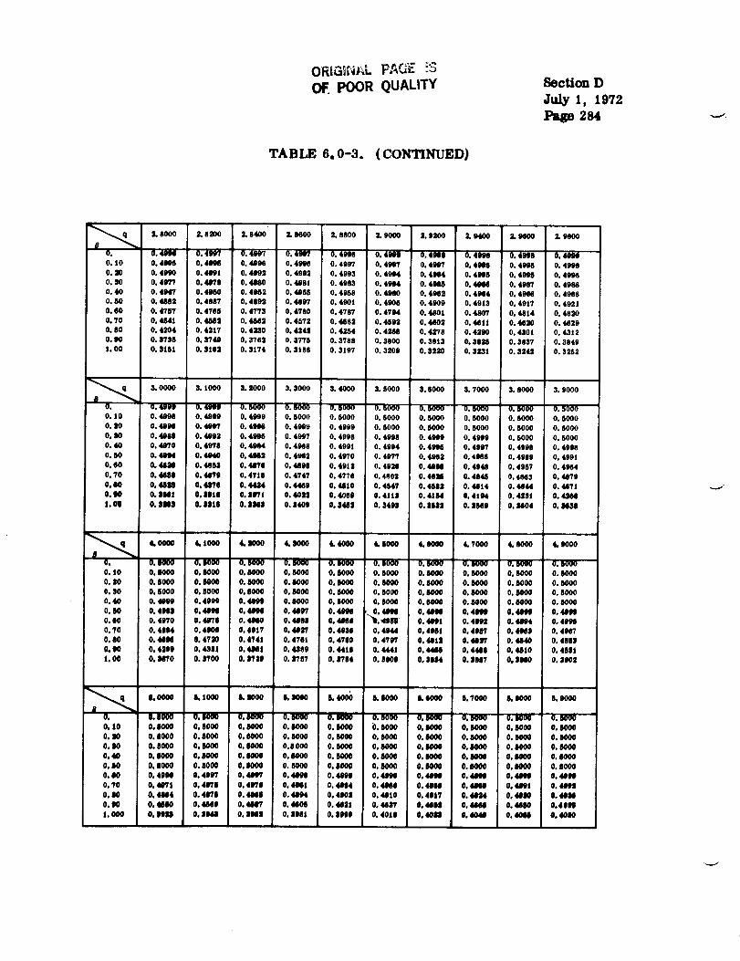
OF POOR qUALiTY Section D
July 1, 1972
Page 284
TABLE 6. 0-3. (CONTINUED)
3.9000 2.8100 3.9400 3.0600 2.9800 2.9000 3.9200 2,0400 2.9600 2.9000
O. 0. 4964 0. 4097 0. 4997 O. 4M_ O. 4000 O. 4009 O. 4909 O. 4009 O. 4998 O. 4M_
0. i0 0.4969 0.4998 0.4996 0.4994 0.499? 0. 4N't 0,4997 O. 4968 0.4996 0.4_8
0, 00 9. 4M0 0. 499| 0. 4992 0. 4992 O. 4993 0. 4964 0. 4M)4 0. 4965 0. 4M_ 0. 4996
0. 30 0. 4977 0. 40?9 0. 4260 0. 4081 O. 4983 0. 4264 0. 4985 O. _ 0. 4987 0. 4988
0.40 0. 494/ 0. 4960 0. 4962 0. 4966 0. 4960 O. 4940 9. 4982 0. 4964 0. 4986 o. 4968
0. 50 0. 4882 5. 4887 0. 4803 0. 4897 o. 4801 0. 4999 0. 4909 o. 4913 0. 49/7 o. 4921
0. 60 O. 4757 0. 4765 O. 4775 0. 4780 O. 479? O. 4794 O. 4a01 0. 480? O. 4614 O. 4830
0o70 0.4641 0.4582 0.4562 0.4572 0.4582 0.4592 0.4803 O. 4_1/ O. 4699 O. 4_20
0. 80 0. 4204 0. 4217 O. 4260 0. 4240 0. 4264 0.4266 0. 4278 O. 4399 0. 4601 0. 43120. 90 0. 9795 0. 3749 0. 376 '_ 0. 3770 O. 3788 0. 3800 0. 3813 0. 3026 0. 5837 O. 3849
I. 00 0. 0151 0. 5109 0. 3174 0. 3189 0. 319'7 0. 3208 0. 5230 0. $23! 0. 3242 0. 3252
3. 0000 3. 1000 6. Z000 3. 3000 3. 4000 3. 0000 6. 6000 3. 7000 3. 0000 3. 9000
0. 0. 499| 0. 401HI 0. 6000 0. §000 0. 5000 0. 6000 0. 500Q 0. 5000 0. 5000 0. 50000. 10 0.4969 0. 4990 0. 4990 O. 9000 0. 6000 0. 5000 0. 5000 0, 0000 O. S000 0. 6000
0. I0 O. 4998 0. _ 0. 496@ 0. 4969 O. 4099 0. 9000 0. 6000 O. 0000 O. 5000 0. 0000
O. 90 O. 4080 O. 41)93 O. 4996 O. 4997 0. 4998 O. 4998 O. 41199 0. 4999 O. 5000 O. 6000
O. 40 O. 411/0 O. 49?9 0. 4994 O. 4998 O. 4991 0. 4994 O. 4996 0. 499? O. 4908 O. 4999
O. 60 0, 41HI4 O. 41140 0. 49611 0.4982 O. 49?0 O. 4977 0. 4962 0. 4084 0. 4909 O. 4991
O. 00 O, 4826 O. 4853 O. 49T8 O. 482 II O. 491 | O. 4028 O. 4981 O. 4948 O. 4967 O. 4964
0.70 O, 4400 0, 44'/9 0. 47/6 0. 4747 0. 4778 0. 4fi02 0. 4091 O. 4046 0. 4863 0, 49790.80 0.489 6.44'/9 0.4434 0.4449 9,46/0 0.4847 0.4292 5.4614 0.4444 0.4471
0.00 6.1194| 0.110|11 0.09?/ 0.4090 0.4000 6,4113 0.4164 0.4/94 0.426/ 0.4N4
I. O0 O. 1110I O. 91119 O. I9111 O. 1140I O. 8400 5. 84t9 O. 09119 0. 0009 0. 9104 O. M110
6,
O. iOO. 90
O. $0
0.40
0,00
0.90
O. _0
O. 00
9.80
1.00
4.0000 4.1000 4.1000 4.8000 4.4000 4.11000 4.9000 4.7000 4.0000 4.9900
0.6000
0. 8000
0. 6000
0. 5000
0.4099
0. 4R110. 49?0
0. 4894
0. 4494
0. 4009
0. NT0
0, Ii000
0. S000
0.0000
0. 90000. 4990
O. ¢_ml0. 4971
O, 41NM
O. 4730
O. 48111
0. 9700
0. 5000
0.6000
0. 8OOO
0. S0000, 4009
0. MIN
0o 4U0
O. 4917
0, 4741
0. U�i
O. 11799
O. 9000 0. BOO0 O. 9000 O. 9000 O. |000 O. 6000 0. 00000.6000 0.9000 0.8000 5.6000 0.5000 0.8000 0.0000
0,9000 0.0000 0.6000 0.0000 0.6000 0.6000 0. SO00
O. 6000 O. lSO00 0. 6000 0. 0000 O. 6000 O. 9990 O. 9000
0. 0000 O. 5000 O. 0000 O. 6000 0. 6000 0, 6000 O, 0000
0. 40117 O. 4960 ,. O. 44911 O. 44111 O. 41_1 O. _ O. 4996
0. 4009 9. 4964 "_t. 0, 9601 O, 4002 0. 4964 0. 4091
O. 4097 O. 4926 O, 4944 O. 491| O. 409? O. 4NJ 0. 4267
0. 478/ 0. 4700 0. 4?07 0. 481J 0, 44:ff 0. 4440 0. 4098
0. 4389 0. 4418 5. 4441 0. 444# 0. 4489 0. 41)10 0. 4091
O. 0767 O. 1704 O. 9000 O. 5914 O. 0897 O. 0910 O. 900|
6. 0000 6.1000 6. I000 LJ000 L4000 &8990 L9000 0, 7000 6. I000 6._00
O, O. 6000 0,10g0 0. _ O. 6000 0. _ 0. 8000 0. S000 0, S000 0. I_00 O. 9900
0. J9 0. S000 0. 0000 0. 8000 0. 9000 0.1000 (). 0000 0. 9000 0.11000 5. 6000 9. J000
O. 110 O, 6000 O. 9000 O. 8000 O, 9000 O, 6000 O. 0000 O. 0000 O. 6000 O. 6000 O. 0000
0.90 0.9000 O. I000 0. S000 0.0000 0.6000 0.1_00 0.1000 0. _000 0,1000 0. S000
0.40 O. 9000 0.9000 0.9000 0.6000 5.6000 0.9000 0.0000 0,11000 0,6000 0,6000
0. I_ 0. 0000 0. 9000 0. _000 0. 0000 5. 8000 0. _000 0. 6000 0. _00 0. _000 0. 90005. _0 0. _ 9. 409? 0, 4_ 0. 4969 0. 4968 0. 4196 0. 49_ 0. 49_ 0. 49_ 0. 4009
0, T0 0. 4_'_I 0. 49?0 O. 49?9 0. iNS 0. 4964 0. 41HM 0. 4N0 0. 4910 0. 4961 0.
O, IO O, 4_4 O, 4670 O. 4_il O. 4964 O, 4990 O. 4915 O. 4917 O. 44_4 O, 40110 O. 4_91
0.90 0, M00 0.4_10 0.449? 0.4409 0.440t 0.4417 0,41011 0.44414 0.44110 0,4091
1.000 0.91111 0.9141 9.111419 O, 9961 0.8960 0.4019 9, 41011 0.4040 0.410411 0.4010
+

Section D
July 1, 1972
Page 285
TABLE 6.0-3. (CONTINUED)
6.0000 6.1000 6. 2000 6.3000 6.4000 6.5000 6.6000 6.7000 6.8000 6.9000
O. 0.5000 0.5000 0.5000 0.5000 0.5000 0.5000 0.5000 0.5000 0.5000 0.5000
0. t0 0.5000 0.5000 0.5000 0.5000 0.5000 O. 5000 0.5000 0.5000 0.5000 0.5000
O. 20 0.5000 0.5000 0.5000 0.5000 0.5000 0.5000 0.5000 0.5000 0.5000 0.5000
0,30 0.5000 0.5000 0.5000 0.5000 0.5000 0.5000 0.5000 0.5000 0.5000 0.5000
O. 40 0.5000 0.5000 0.5000 0.5000 0.5000 0.5000 0.5000 0.5000 0,5000 0.5000
0.50 0,5000 0.5000 0.5000 0.5000 0.5000 0.5000 0,5000 0.5000 0.5000 0,5000
0,60 0.4999 0.5000 0.5000 0,5000 0,5000 0.5000 0.5000 0,5000 0.5000 0,5000
0.70 0.4993 0.4994 0.4995 0.4996 0.4997 0,4997 0.4997 0.4998 0.4998 0.4998
O. 80 O, 4941 O. 4946 O. 4950 O. 4954 O, 4958 O. 4962 O, 4965 O, 4968 O, 4970 O. 4973
O. 90 0.4705 0.4717 O. 4728 O. 4739 0.4750 O. 4760 O. 4769 O. 4779 O. 4788 O. 4796
1.00 0.4095 O. 4109 0.4123 O. 4136 0.4_49 0o4162 O. 4174 0,4196 0.4199 0.4209
7.0000 7.1000 7.2000 7.3000 7.4000 7.5000 7.6000 7.7000 7.8000 7.9000
O. 0.5000 0.5000 0.5000 0.5000 0.5000 O. 5000 0.5000 0.5000 0.5000 0.5000
0. I0 0.5000 0.5000 0.5000 0,5000 0.5000 0.5000 0.5000 0.5000 0.5000 0.5000
0.20 0.5000 0.5000 0.5000 0.5000 0.5000 0.5000 0.5000 0.5000 0.5000 9.5000
0.30 0.5000 0.5000 0.5000 0.5000 0,5000 0.5000 0.5000 0.5000 0.5000 0.5000
0.40 0.5000 0.5000 0.5000 0.5000 0.5000 0.5000 0.5000 0.5000 0.5000 0.5000
0.50 0.501)0 0.5001) 0.50O0 0.5000 0.5000 0.5000 0.5000 0.5000 0.5000 0.5000
0.60 0.5000 0.501)0 0.5000 0.50O0 0.5000 0.5000 0.5000 0.5000 0.5000 0.5000
0.70 0.4999 0.4999 0.4909 0.4999 0.4999 0.4999 0.5000 0,5000 0.5000 0.5000
0.80 0.4975 0.4977 0.4979 0.4981 0.4983 0.4984 0.4985 0.4987 0.4988 0.4989
0.90 0.4804 0,4812 0.4819 0.4827 0.4834 0.4840 0.4847 0.4853 0.4859 0.4864
1.00 0.4220 0,4230 0.4241 0.4251 0.4261 0.4270 0.4279 0.4298 0.4297 0,4306
8,0000 8.1000 8.2000 8.3000 8.4000 8.5000 8.6000 8.7000 8.8000 8.9000
O. 0.5000 0.5000 0.5000 0.5000 0.5000 0.5000 0.5000 0.5000 0.5000 - 0.5000
0. i0 0.5000 0.5000 0.5000 0.5000 0.5000 0.5000 0.5000 0.5000 0.5000 0.5000
0.20 0.5000 0.5000 0.5000 0.5000 0.5000 0.5000 0.5000 0.5000 0.5000 0.5000
0.30 0.5000 0.5000 0.5000 0.5000 0.5000 0.5000 0,5000 O. 5000 0.5000 0.5000
0.40 0.5000 0.5000 0.5000 0.5000 0.5000 0.5000 0.5000 0.5000 0.5000 0,5000
0.50 0.5000 0,5000 0.5000 0.5000 0.5000 0.5000 0.5000 0.5000 0.5000 0.5000
0.60 0.5000 0.5000 0.5000 0.5000 0.5000 0.5000 0.5000 0.5000 0.5000 0.5000
0.70 0.5000 0.5000 0.5000 0.5000 0.5000 0.5001) 0.5000 0.5000 0.5000 O. 5000
0.80 0.4990 0.4991 0.4992 0.4993 0.4993 0.4994 0.4994 0.4995 0.4995 0.4996
0.90 0.4869 0. 4875 0.4880 O, 4884 O. 4999 O. 4893 O. 4898 O. 4902 0.4906 O. 4909
t.00 0.4315 0.4323 0.4331 0.4339 0.4346 0.4354 0.4361 O. 4368 O. 4375 0.4352
9.0000 9.1000 9.2000 9.3000 9.4000 9.5000 9.6000 9.7000 9.8000 9.9000
O. 0.5000 0.5000 0.5000 0.5000 0.5000 0.5000 0.5000 0.5000 0.5000 0.5000
0.10 0.5000 0.5000 0.5000 0.5000 0.5000 0.5000 0.5000 0.5000 0.5000 0.5000
O. 20 0.5000 0.5000 0.5000 0.5000 0.5000 0.5000 0.5000 0.5000 0.5000 O. 5000
0.30 0.5000 0.5000 0.5000 0.5000 0.5000 0.5000 0.5000 0.5000 0.5000 0.5000
O, 40 O. 5000 O. 5000 O. 5000 O. 5000 O. 5000 O, 5000 O. 5000 O. 5000 O. 5000 O. 5000
O. 50 O, 5000 0.5000 0.5000 O. 5000 O. 5000 O. 5000 O. 5000 O. 5000 0.5000 O. 5000
0.60 0.5000 0.5000 0.5000 0.5000 0.5000 0.5000 0.5000 0.5000 0.5000 0.5000
O. 70 O. 5000 O. 5000 O. 5000 O. 5000 O. 5000 O, 5000 O. 5000 O. 5000 O. 5000 O. 5000
0.80 0.4996 0.4997 0.4997 0.4997 0.4998 0°4998 0.4998 0.4998 0.4999 0.4999
O. 90 O. 4913 O. 4916 O. 4920 O. 4923 O. 4926 O. 4929 O. 4932 O. 4935 O. 4937 O. 4940
1. O0 O. 4389 O. 4395 O. 4401 O. 4408 O. 4414 O. 4420 O. 4426 O. 4431 0.4437 O, 4443

Section D
July 1, 1972
Page 286
TABLE 6.0-3. (CONCLUDED)
10.0000 10.1000 10, 3000 t0.3000 10.4000 10, 5000 I0. 5000 iO. 7000 J.O.5000 _0. 9000
O.
0,10
0.20
0, 50
0. 400, 50
0. 60
0, 70
0. 80
0. 90
1o 00
O. 5000 O. 5000 O. 5000 O. 5000 O. 5000 O. 5000 O. 5000 O. 5000 O. 5000 O. 5000
O. 5000 0. 5000 O. 5000 O. 5000 O. 8000 O. 5000 O. 5000 O. 5000 O. 5000 O. 5000
0. 5000 0. 5000 0. 5000 0. 5000 0. 5000 0. 5000 0. 5000 0. 5000 0. 5000 0. 5000
0. 5000 0. 5000 0. 5000 0. 5000 0. 5000 0. 5000 0. 5000 0. 8000 0. 5000 0. 5000
O. 5000 O, 5000 O. 5000 O. 5000 O. 5000 O. 5000 O. 5000 O. 5000 O. 5000 O. 5000
O, 5000 O. 5000 O. 5000 O. 5000 O. 5000 O. 5000 O. 5000 O. 5000 O. 5000 O. 5000
O. 5000 O. 5000 O. 5000 O, 5000 O. 5000 O. 5000 O. 5000 O. 5000 O. 5000 O. 5000
O. 5000 O. 5000 O. 5000 O. 5000 O. 5000 O. 5000 O. 5000 O. 5000 O. 5000 O. 5000
O. 4999 O. 4999 O. 4999 O. 4999 O. 4999 O. 5000 O. 5000 O. 5000 O. 5000 O. 5000O. 4942 O. 4945 O. 4947 O. 4949 O. 4951 O. 4953 O. 4955 O. 4957 O. 4958 O. 4960
O, 4448 O. 44_4 O. 4459 O, 4464 O, 4469 O. 4474 O. 4479 O. 4484 O. 4455 O. 4493

OF POOR QUALITYSection D
July 1, 1972
Page 287
TABLE 6.0-4. SPHERE-PARAMETER 03
O. 5000 O. 5200 O. 5400 O. 5600 O. 5800 O. 6000 O. 6200 O. 6400 O. 6600 O. 6800
0. 0.0001 0.0002 0.0004 0.0008 0.0013 0.002t 0.0033 0.0048 0.0069 0.0096
0.10 0,0001 0.0002 0.0004 0.0008 0,0013 0.0021 0.0032 0.0048 0.0088 0,0095
0.20 0.0001 0.0002 0.0004 0.0007 0.0012 0.0020 0,0031 0.0045 0.0065 0.0090
0,30 0.0001 0.0002 0.0004 0.0007 0.0011 0.0018 0.0028 0.0042 0.0060 0.0083
O. 40 0,0001 0.0002 0.0003 0.0006 0.0010 0.0016 0.0025 0.0037 O. 0052 O. 0073
0. 50 0.0001 0.0001 0.0003 0. 0005 0.0008 0.00t3 0. 0021 0, 0031 0, 0044 0. 0061
0.60 0.0001 0.0001 0.0002 0,0004 0.0007 0.00t1 0.0018 0.0024 0.0035 0. 0049
0.70 0.0000 0.0001 0.0002 0.0003 0.0005 0.0008 0.0012 0.0018 0.0026 0.0035
0.80 O. 0000 O. 0001 O. 0061 0.0002 0.0003 O. 0005 O. 0008 O. 0011 O. 0018 O. 0023
0.90 0.0000 0.0000 0.00o0 0.0001 0.0001 0.0002 0.0004 0.0005 0.0008 0.0011
1.00 0.0000 0.0000 0,0000 0.0000 O. O00O 0.0000 0.0000 0.0000 0.0000 0.0000
0.7000 0.7200 0.7400 0.7600 0.7800 0.8000 0.8200 0.8400 0.8600 0.8800
O. 0.0130 0.0171 0.0221 0.0279 0.0347 0.0423 0.0510 0.0606 0.0711 0.0827
0. t0 0.0128 0.0169 0.0217 0.0275 0.0341 0.0416 0.0501 0.0596 0.0700 0.0813
0.20 0.0122 0.0160 0.0207 0.0261 0.0324 0.0396 0,0477 0.0567 0.0666 0.0773
0.30 0.0112 0,0147 0.0190 0.0240 0.0297 0.0363 0.0438 0.0520 0.06tl 0.0709
0.40 0.0098 0.0130 0.0167 0.0211 0.0262 0,0320 0.0386 0.0459 0.0536 0.0626
O. 50 O. 0083 O. 0103 O. 0141 O. 0178 O, 0221 O, 0270 O. 0325 O. 0386 0.0453 O. 0526
0.60 0.0066 0.0086 0.0111 0.0141 0.0175 0.0214 0.0257 0.0306 0.0359 0.0417
0. 70 0. 0048 0. 0063 0. 0081 0. 0103 0. 0127 0. 0156 0. 0188 0. 0223 0, 0262 0. 0304
0.80 0.0030 0.0040 0.0052 0.0065 0.0061 0.0009 0.0119 0.0t42 0,0166 0.0193
0.90 0.0014 0.0019 0.0024 0.0031 0.0038 0.0046 0.0056 0.0066 0.0078 0.0990
1.00 0.0000 0.0000 O. OOO0 0.0000 0.0000 0,0000 0,0000 0.0000 0.0000 0.0000
0.9000 0.9200 0.9400 0.9600 0.9800 1.0000 1.0200 1.0400 1.0600 1.0800
O. 0.0951 0.1084 0.1225 0.1375 0.1531 0.1695 0.1865 0.2041 0,2222 0.2407
0.10 0.0935 0.1066 0.1205 0.1352 0.1506 0.1667 0,1835 0.21)08 0.2186 0.2368
0.29 0.0899 0.1014 0.1146 0.1286 0.1433 0.1586 0.1745 0.1910 0.2079 O. 2253
0.30 0.0816 0.0930 0.1052 0.11_0 0. t315 0.1455 0.1602 0.1753 0.1908 0.2068
0.40 0. 0720 0. 0820 0. 0927 0. 1041 0. t159 0.1283 0. 1412 0. 1546 0. 1683 0. 1824
0,50 0.0605 0.0690 0.0790 0.0875 0.0975 0.1080 0.1188 0.130t 0.1416 0.1535
0.60 0.0480 0.0547 0.0619 0.0694 0.0773 0.0856 0.0942 0.1031 0. t123 0,|217
0.70 0.0350 0.0309 0.0451 0.0506 0.0564 0.0624 0.0687 0.0752 0.0818 0.0888
0.80 0.0222 0.0254 0.0287 0.0322 0.0358 0.0397 0.0437 0.0478 0.0521 0.0565
0. 90 0. 0104 0. 0118 0. 0134 0. 0150 0, 0168 0. 0185 0. 0204 0. 0224 0, 0243 0, 0264
1.00 0.0000 0.0000 0.0000 0.0000 0.0000 0.0000 0.0000 0.0000 0.0000 0.0000
i. 1000 I. 1200 I. 1400 I. 1600 I. 1800 I. 2000 I. 2200 i. 2400 I. 2600 I. 2800
O. O. 2597 0.2790 O. 2986 0.3183 O. 3383 O. 3584 O. 3785 0.3986 0,4187 O. 4388
0.10 0.2555 0.2745 0.2937 0.3132 0.3328 0.3526 0.3724 0.3923 0.4121 0.4318
O. 20 O. 2430 O. 2611 O. 2795 O. 2980 O. 3168 O. 3356 O. 3545 O. 3735 O. 3924 O. 4113
0.30 0.2231 0.2398 O. 2566 O. 2737 O. 2910 0.3084 0.3218 0.3433 0.3809 0.3783
O. 40 O. 1968 O. 2115 O. 2265 O. 2416 O. 2569 O, 2723 O. 2875 O. 3034 O. 3t90 O. 3346
O. 50 O. 1657 O. 1781 O. 1907 O. 2035 O. 2164 O. 2295 O. 2426 O. 2559 O. 2691 O. 2624
O. 60 O. 1314 O. 1413 O. 1513 O. 1615 O. 1718 O. t822 O. 1927 O. 2032 0. 2139 O. 224_
0.70 0.0!J59 O. t031 0. t104 0. t179 0. t254 0. t331 0.1408 O. i496 0,1564 0. t642
O. 80 0.0610 0.0656 0.0702 0.0750 0.0798 O. 0847 0.0896 0.0946 O. 0998 O. 1047
O. 90 O. 0285 O. 0307 O. 0328 O. 0351 O. 0373 O. 0396 O. 0419 O. 0443 O. 0466 O. 0490
1.00 0.0000 0.0000 0.0000 0.0000 0.0000 0.0000 0.0000 0,0000 0.0000 0.0000

Section D
Jtdy I, 1972
Page 288
TABLE 6.0-4. (CONTINUED)
t. 3000 1. 3200 1. 3400
O. _ O. 4587 O. 4784 O. 4979O. I0 O. 4514 O. 4709 O. 4902
O. 20 O. 4301 O. 4488 O. 4673
O. 30 O. 3958 O. 4131 O. 4303
0.40 0.3502 0.3657 0.3811
O. 30 O. 2957 O, 3090 O. 3222
O. 60 O. 2353 O. 2460 O. 2566
O. 70 O. 1721 O. 1800 O. 1880
0. 80 O. 1097 O. 1148 O. 1199
O. 90 O. 0614 O. 0538 O. 0563
I.O0 O. O000 O. 0000 O. OOO0
I. 3500 I. 3800 I. 4000 I. 4200 I. 4400 I. 4600 i. 4800
O. 5172 O. 5362 O. 5850 O. 5734 O. 89t4 O. 6091 O. 6260O. 5099 O. 8280 O. 5465 O. 5647 O. 5825 O. 6000 0. 8171
O. 4856 O. 5036 O. 5215 O. 6390 O. 5563 O. 5732 O. 6899
O. 4474 O. 4648 O. 4810 O. 4974 O. 5137 O. 5297 O. 5454
0.3965 0.4117 0.4268 0.4417 0.4566 0.4711 0.4855
O. 3354 O. 3485 O. 3616 O. 8748 O. 3874 O. 4001 O. 4128
O. 2673 O. 2780 O. 2886 O. 2992 O. 3097 O. 3202 O. 3306
O. t959 O. 3038 O. 2117 O. 2197 O. 2776 O. 2354 O. 2433
O. 1250 O. 1302 O. i353 O. 1404 O. 1486 O. 1507 O. 1568
O, 0586 O, 0610 O. 0634 O. 0659 O. 0688 O. 0707 O. 0732
O. OOO0 O. 0000 O. 0000 O. 0000 O. 0000 O. 0000 O. 0000
1. 8000 t. 6200 t. 5400 t. 8500 t. 5800 1. 5000 1. 6200 1. 5400t. 6600 1. 6800
'0. 0,5432 0.6595 0.6756 0.69t2 O. 7083 0.7209 0.7350 0,7487 0.7618 O. 7746
0. t0 0.6339 0.8502 0.6661 0.6815 0.8965 0.7111 O. 7259 0.7388 0.7620 0.7647O. 20 O. 6061 O. 6220 O. 6375 O. 6627 O. 5674 O. 6818 O. 6957 O. 7093 O. 7224 O. 7381
O. 90 O. 5608 O. 5760 O. 8908 O. 8054 O. 6196 O. 6335 O. 6471 O. 6603 O. 6732 O. 6857
0.40 0.4997 0.5137 0.5275 0.54t0 0.5543 0.5674 0.6802 0.5928 0.6051 O. 6i72
0.50 0.4252 0.4376 0.4498 0.4619 0.4738 0.4856 0.4973 0.5086 0.5199 0.5310
O. 60 O. 3409 O. 3512 O. 3614 O. 37t5 O. 88t6 O. 3915 O. 40t3 O. 41tt O. 4208 O. 4304
O. 70 0. 2511 O. 2889 O. 2667 O. 2744 O. 2821 O. 2898 O. 2974 O. 3050 O. 3126 O. 3201
O. 80 O. 1609 O. 1661 O. 1712 O. 1753 O. 1814 O. 1868 O. 1915 O. 1966 O. 2017 O. 2057
O. gO O. 0756 O. 0780 O. 0508 O. 0829 O. 0854 O. 0878 O. 0902 O. 0927 O. 0951 O. 0976I. O0 e. 0000 O. 0000 O. OOO0 O. OOO0 O. OOO0 O. 0009 O. OOOO O. OOO0 O. OOO0 O. 0000
t. 7000 1. 7200 1. 7400 t. 7600 t. 7800 1. 8000 1. 8200 i. 8400 1. 8600 1. 8800
O. O. 7868 O. 7985 O. 8098 O. 8206 O. 8310 O. 8409 O. 8504 O. 8fi94 O. 8680 O. 8782
O. 10 O. 7770 O. 7888 O. 8001 O. 81t0 O. 8214 O. 5315 O. 8410 O. 8602 O. 8590 O. 8673
O. 20 O. 7474 O. 7593 O. 7707 O. 7818 O. 7928 O. 802"/ O. 8t26 O. 8221 O. 8312 O. 8400
O. 50 O. 6979 O. 7098 O. 7213 O. 732.5 O. 7434 O. 7539 O. 7641 O. 7740 O. 7835 O. 7927
O. 40 O. 6290 O. 6406 O. 6519 O. 6629 O. 6737 O. 6842 O. 6945 O. 7045 O. 7143 O. 7238
O. 50 O. 5420 O. 5527 O. 5633 O. 5738 O. 5840 O. 5941 O. 6040 O. 6137 O. 8233 O. 6327
O. 60 O. 4398 O. 4492 O. 4585 O, 46"/7 O. 4768 O. 4868 O. 4947 O. 5035 O. 5122 O. 5208
O. 70 O. 32'76 O. 3350 O. 3424 O. 3497 O. 3570 O. 3642 O. 3714 O. 3786 O. 3857 O. 3927
O. 80 O. 2117 O. 2167 O. 2317 O. 2267 O. 2317 O. 2367 O. 2416 O. 2465 O. 2515 O. 2564
0.90 O. lOOO 0.1024 0.1049 0.1073 0,1097 0.1122 0.1146 0.1170 O. i194 0.1218i. O0 O. 0000 O. O00O O. 0000 O. 0000 O. OOOO O. O000 O. 0000 O. 0000 O. 0000 O. 0000
1. 9000 1. 9200 1. 9400 t. 9600 t. 9800 2. O000 2. 0200 2. 0400 2. 0600 2. 0800
O, O. 8840 O. 89t4 O. 8984 O. 9051 O. 9114 O. 9173 O. 9230 O. 9283 O. 9333 O. 9380
O. 10 O. 8783 O. 8828 O. 8900 O. 8969 O. 9034 O. 9095 O. 9154 O. 9209 O. 9261 O. 9310
O. 20 O. 8484 O. 8564 O. 8641 O. 8715 O. 8786 O. 8852 O. 8916 O. 89/7 O, 9035 O. 9090O. 30 O. 8016 O. 8102 O. 8186 O. 8266 O. 8343 O. 8417 O. 8489 O. 8558 O. 862,4 O. 8688
O. 40 O. 7331 O. 7422 O. 7510 O. 7696 O. 7679 O, 7760 O. 7838 O. 7915 O. 7989 O. 8062
O. 50 O. 6419 O. 6509 O. 6598 O. 6686 O. 6771 O. 6854 O. 8937 O. 7017 O. 7096 O. 7173
O. 60 O. fi293 O. 5376 O. 5459 O. 5541 O. 5623 O. 5702 O. 6781 O. 5858 O. 8935 O. 6011
O. 70 O. 3997 O. 4067 O. 4136 O. 4205 O. 4273 O. 4341 O. 4408 O. 4475 O. 4541 O. 4607
O. 80 O. 2613 O. 2661 O. 2'710 O. 2/88 O. 2807 O. 2855 O. 2903 O. 2951 O. 2998 O. 3046
O. 90 O. 1243 O. 1267 O. 1291 O. 1315 O. 1339 O. t368 O. t387 O. 1412 O. 1436 O. 1460
I. O0 O. 0000 O. O00O O. O00O O. 0000 O. O000 O. O000 O. 0000 O. 0000 O. 0000 O. 0000

ORIGiI'_/_L P,._:; _o
POOR QUALITY
Section D
July 1, 1972
Page 289
TABLE 6.0-4. (CONTINUED)
2. 1000
0. 0.9424
9.10 0.93570. 20 0.9143
0.30 0.8750
0.40 0.8132
0.50 0.7249
O. 60 O. 6086
O.70
O. 80
O. 90
I. O0
2.1200 2.1400 2. 1600 2.1800 2. 2000
0. 9466 0. 9505 0. 9541 0. 9575 0. 9607
0. 9400 0.9442 0.948i 0.9517 0.9551
0. 9193 0. 9240 0. 9286 0. 9328 0. 9369
0. 8808 0. 8865 0. 8919 0. 8971 0. 9021
0.8200 0.6266 0,8330 0.8392 0.8452
0.7323 0.7396 0.7467 0.7536 0.7604
0.6160 0.6232 0.6304 0.6375 0.6445
0.4672 0.4737 0.4801 0.4865 0.4928 0.4991
0.3093 0.3141 0.3186 0.3235 0.3281 0.3328
0.1484 0.1508 0.1532 0.1555 0.1579 0.1603
0.0000 0.0000 0.0000 0.0000 0.0000 0.0000
2. 2200 2. 2400 2.2600 2. 2800
0.9637 0.9665 0.9691 0.9716
0.9583 0.9613 0.9642 0.9668
0.9407 0.9444 0.9476 O. 9511
0.9069 0.9115 0.9159 0.9201
O. 8510 0.8567 O. 8621 O. 8674
0.7671 0.7736 -0.7799 O. 7862
0.6514 0.6582 0.6648 0.6714
0.5053 0.5115 0.5177 0.5237
O. 3374 O. 3420 O. 3467 O. 3512
0. 1627 O. 1651 0. 1675 0. 1699
0.0000 0.0000 0.0000 0.0000
fl_ _ 3000 2.320o
O. 0.9738 0.9759
0.10 0.9693 o. 9716
0.20 0.9542 O. 9571
0.30 0.9241 0.9279
0.40 0.8726 0.8775
0.50 0.7922 0.7982
0.60 0.6779 0.6844
0.70 0.5298 0.5358
0.80 0.3558 0.3604
90 0.1722 0.1746
1.00 0.0000 0.0000
2.3400 2.3600
0.9779 0.9797
0.9737 0.9757
0.9598 0.9624
0.8316 0.935i
0.8823 0.8869
0 8040 0.8097
0.6907 0.6969
0.5417 0.5476
0.3649 0.3694
0.1770 0.1794
0.0000 0.0000
2. 3800 2. 4000 2. 4200 2. 4400 2.4600 2, 4800
0.98i4 0.9829 0.9844 0.9857
O. 9776 0,9794 0.9810 0.9825
0.9648 0.9671 0.9693 0.9713
0.9385 0.9417 0.9447 0.9477
0.8914 0.8957 0.8999 0.9040O. 8152 O. 8206 O. 8259 O. 8311
0.7030 0.7090 0,7150 0.7208
0.5534 0.5592 0.5649 0.5706
0.3739 0.3784 0.3829 0.3874
0. t817 0.1841 0.1865 0.1888
0.0000 0.0000 0.0000 0.0000
0.9869 0.9881
0.9839 0.9852
0.9732 0.9750
0.9504 0.9531
0.9079 0.91160.8361 0.8410
0.7266 0.7323
0.5763 0.5818
0.3916 0.3962
0.1912 0.1936
0.0000 0.0000
2. 5000 _ 5200
O. 0.9891 0.9901
0.10 0.9864 0.9875
0,20 0.9767 0.9783
0.30 0.9556 0.9580
0.40 0.9153 0.9t88
_50 0.8458 0.8505
0.00 0.7376 0.7433
0.70 0.5874 0.5929
O, 80 O. 4006 0.4050
0.90 0.1959 0. t983
1. O0 O. 0000 0. 0000
2.5400 _5600 2. 5800 2.6000 2. 6200
0.9910 0.9918 0.9925 0.9932 0.9938
0.9885 0.9895 0.9904 0.9912 0.9919
0.9798 O. 98J2 0.9825 0.9837 0.9849
O. 9603 0.9624 O. 9645 0.9665 O. 96840.922i 0.9254 0.9285 O. 9316 O. 9345
0.8550 0.8595 0.8638 0.8680 0.872t
O. 7487 O. 7540 O. 7593 O. 7644 O. 7695
0.5983 0.6037 0.6090 0.6143 0.6t95
O. 4094 O. 4137 O. 418t O. 4224 O. 4267
O. 2006 O. 2030 O. 2053 O. 2077 O. 2100
0.0000 0.0000 O. O000 0.0000 0.0000
2.6400 2.6600 2.6800
0.9944 0.9949 0.9954
0.9926 0.9932 0.99380.9859 0.9869 0.9679
0.9701 0.9718 0.9734
0.9373 0.9400 0.94260.8761 0.8800 0.8638
O. 7744 O. 7793 O. 7841
0.6247 0.6299 0.6350
0.4309 0.4352 0.4395
O. 2t23 O. 2147 O. 2170
O. O00O O. 0000 O. 0000
2. 7000 2. 7200 2. 7400
2. 7600 2.7800 2. 9000
O. O. 9958 O. 9962 O. 9966 O. 9969 O. 9972
O. 10 O. 9944 O. 9949 O. 9953 O. 9957 O. 9961
O. 20 O. 9888 O. 9896 O. 9903 O. 9910 O. 9917O. 50 O. 9749 O. 9764 O. 9777 O. 9790 O. 9803
O. 40 O. 9451 O. 9475 O. 9498 O. 9520 O. 9542
O. 50 O. 8875 O. 89t I O. 8946 O. 8980 O. 9013
O. 60 O. 7889 O. 7935 O.7991 O. 802_ O. 8070
O. 70 O. 5400 O. 6460 O. 5499 O. 6548 O. 6591
O. 90 O. 4437 O. 4479 O. 452t O. 4562 O. 4604
O. 90 O. 2194 O. 23t7 O. 2240 O. 2263 O. 2287
2.8200 2. 8400 _8600 2.9800
0.9975 0.99/8 0.9980 0.9982 0.9984
0.9965 O. 9968 0.9971 0.9974 0.9976
O. 9923 O. 9929 O. 9934 O. 9939 O. 9944
O. 9814 _9825 O. 9836 O. 984,5 O. 9855
O. 9562 O. 9582 0.9601 0.9619 0.9637
0.9046 0.9077 0.9t08 0.9t37 0.9166
0.8113 0.8t_ 0.8197 0.8218 0.82'/9
O. 6645 0.6692 O. 6739 0.6786 O. 68520.4645 0.4686 _ 4727 0.4768 0.4809
0.3310 O. 2333 0.2386 0.3379 0.24[03

Section D
July 1, 1972
Page 290
TABLE 6.0-4. (CONTINUED)
2. 9000 2. 0100 2. 9400 3. 9600 3. 9800 3. 0000 3. 0200 3. 0400 3. 04100 3. 0800
O. O, 9966 0. 998/ O. 9988 O. 9990 O. 9991 O. 9993 O. 9993 O. 9993 O. 1_94 O. 9995
O. t0 O. 9978 O. 9980 0. 9982 O. 9984 O. 9985 O. 8987 O. 9988 O. 9989 O. 8990 O. 999|
0. BO O. 9948 O. 9952 O. 9956 O. 9959 9. 9919 9.1966 O. 9968 8, 997| 0. 99'/5 O. 9975
O, 30 O. 1964 O. 9872 O. 9880 O. 9987 O. 9894 O. 9901 O. 990"/ O. 9913 O. 9918 O. 9923
0,40 0.N53 0.9609 0.9609 0.9700 0.9714 0,9727 0.9'740 0.9753 0.9"/95 0.9770O. 50 O. 9|94 O. 922! O. 9247 O. 9273 O. 9298 O. 9325 O. 9346 O. 9388 O. 9390 O. 9412:
O, 90 O. 8318 0. 8357 O. 8396 O. 9432 0. 8469 O. 8505 O. 8540 0. 8575 O. 8609 O. 8642
0,70 0.6878 0.692,3 O, 6968 0.7012 0.7055 0.7099 0.7141 0.7184 0.7226 0.7267
0. 80 O. 4849 O. 4889 O. 4929 O. 4969 O. 5009 O. 5048 O. 0088 O. 512/ O. 5155 O. 5204O. 90 O. 2425 O. _t48 O. 2471 O. 2494 O. 3917 O. 2840 O. 31919 O. 3988 O. _09 O. 2632
1. O0 O. OOO0 O. 0000 O. 0000 O. 0000 O. O00O O. O000 O. 0000 O. O000 O. 0000 O. 0009
3. 0000 3. iO00 3. 2000 3.3000 3. 4000 3, 5000 9. 41000 5. 7000 3. 8000 3. 9000
O. O. 9992 O. 9996 O. 999'/ O. 9999 O. 9998 L 0000 f. 00_ 11.0000 |. 0000 |. 0000O. I0 O. 998"/ O. 9992 O. I;992 O. 9997 O. 9991) O. 9999 i. 0000 i. 0000 #. 0000 I. 0000
0. IO O, 9995 O. 9977 O. 9986 O. 999t O. 9994 O. 99941 O. 9900 O. 91H5tl O. 9999 O. 99118
O. 30 O. 9901 O. 9939 O. 9949 O. 9964 O. 99"/5 O. 9982 O. 9988 O. 9992 O. 9994 O. 90_
O. 40 O. 9"/2'7 O. 9'787 O. 8834 O. 9872 O. 9903 O. 9925 O. 91)44 O. 91)6"/ O. 91)69 O. 9977
O. 50 O. 9321 0. 9432 O. 9527 O. 191608 O. 94'/6 O. 9734 0. 9752 O. 11825 0. 911511 O. 99114
O. 90 O. 8500 O. 84175 O. 0819 O. 8968 O. 90t53 O. 9205 O. 9806 O. 1994 O. 9474 O. 9544
O. 70 O. 7099 O. 7308 O. 7508 O. 7893 O. 78419 O. 80315 O. 8190 O. 838 O. 6472 0. 84500
O. 00 O. 5048 O. 53,43 O. 6432 O. 6617 0. 57V/ O. 5975 O. 5/43 O. 5309 0. 5469 0. 9628
0. 90 O. 2540 O. 24_58 O, 2768 O. 2981 O. 2999 O. 3|04 O. 53|5 O. 3324 O. 3433 O. 31543
1.00 0.0000 0.0000 0.0000 O. 0000 O. O000 0.0000 0, 0000 0. 0000 0. 0000 0. 0000
4.0000 4.1000 4.2000 4.3000 4.4000 4.5000 4.8000 4.1'000 4.8000 4.1)000
O. i. 0000 1. 0000 1. O000 1. O000 LO000 1.0000 LO000 I. 0000 LO000 i. 0000
O. 10 I. 0000 1.0000 1.0000 I. O00O 1. O000 I. 0000 $. 0000 I. 0000 i. 0000 1. 0000
0.10 1. 0000 i. 0000 I. 0000 1. 0000 1. 0000 t. 0000 1. 0000 1. 0000 1. 0000 1. 00000. 30 O. 999"1 O° 9998 0. 9999 O. 9999 O. 9999 1. OOOO 1. 0000 1. 0000 1. 0000 1, 0000
O. 40 O. 9983 O. 9987 O. 9991 0. 9993 O. 9995 O. 9997 O. 9919 O. 9999 O. 9199 O. 99911
0.60 0.9906 0.9925 0.9940 0.9953 0.9963 0.997| 0.99'/'/ 0.9192 0.9906 0.89511
0. 80 O. 9_,06 O. 9'660 O. 9708 O. 9'750 O. 9787 O. 9818 O. 9846 O. 9849 O. 9890 O. 8907
0.70 0.8719 0.8839 0.5932 O. 9Q27 0.9t15 0.9197 0.92'/2 0.9341 0.9404 O. 94d2
O. 80 0, 8776 O. 5923 O. 7064 O. 7201 O. 7334 O. 74181 O. 7586 O. 7703 O. 7816 O. 7928
O. 90 O. 3849 O. 3755 O. 3861 O. 385 O. 4088 O. 4173 O. 4P14 0. 4375 O. 4475 O. 4674
i. O0 O. O000 O. 0000 O. 0000 O, 0000 O. 0000 O. 0000 O. 0000 O. 0000 O. 0000 O. 0000
5. O00O 5. iO00 6. 5000 5. 3000 S. 4000 5. 6000 5. 4000 6. 7000 6. 8000 5. 9000
O. i. 0000 1. 0000 i. 0000 1. O000 1. 0000 1. 0000 1. CO00 1. 0000 i. 0000 1. 0000
0.|0 t. 0000 1.0000 i. 0000 i. 0000 1. 0000 1. 0000 J.. 0000 1. 0000 LO000 LO000
0.19 1. 0000 1. 0000 t. 0000 I. 0000 1. 0000 I. 0000 1. 0000 I. 0000 t. 0000 1. 0000
0. $0 i. O00O t. 0000 1. 0000 1. 0000 1. 0000 I. 0000 1. 0000 !. 0000 L 0000 1. O000
0.40 0.91911 t. O000 1, 0000 J, 0000 I. 0000 1, 0000 1.0000 I. 0000 |. 0000 1. O00Q
O. 60 O. 9992 O. 9994 O. 9996 O. 9996 O. 9997 O. 9998 O. _ 9. 9999 O. 0999 O. 99990. 60 O. 9n2 O. 9935 O. 5944 O. 1955 O. 11115 9. 9189 O. 99'74 O. 90'/5 O. 9983 O. 9MM
0. 70 O. 9616 0. 1555 O. 19011 0. 9649 O. 1986 O. 9"/39 O. 9760 O. 87Y7 O. 96011 O. 9824O. 50 O. 9034 O. 8t28 O. 8233 O. 531r'/ O. 8417 O. 9603 O. 96111[, O. 8603 O. 0'/39 9. 8810
0.19 0.4471 0.4759 0.486 0.4N! 0.5055 0.5148 O. SNO O. 6_11 0.6431 O. 56i0
LO0 0. 0000 O. 0000 O. 0000 0.0000 O. 0000 0.0000 0.0000 0.1900 0. 0000 O. 0000

ORIGINAL P2:.%}:-'._3OE POOR QUALITY
TABLE 6. 0-4, (CONTINUED)
Section D
July 1, 1972
Page 291
6.0000 6.1000 6.2000 6.3000 6.4000 6.5000 6.6000 6.7000 6. 8000 6.9000
O. 1.0000 1.0000 1.0000 1.0000 1.0000 1.0000 1.0000 1.0000 1.0000 1,0000
0.10 1.0000 1.0000 1.0000 1.0000 1.0000 t.0000 1.0000 1.0000 t. 0000 1,0000
0.20 1.0000 1.0000 1.0000 1.0000 1.0000 1.0000 1.0000 1.0000 t.0000 1.0000
0.30 1.000o 1.0000 1.0000 1.000o 1.0000 1.0000 1.0000 1.0000 1.0000 i. O000
0.40 1.0000 1.0000 1.0000 1.0000 l. O000 1.0000 1.0000 l. O000 1.0000 1.0000
0.50 1.0000 1.0000 1.0000 1.0000 1.0000 1.0000 1.0000 1.0000 1.0000 1.0000
O. 60 O. 9989 O. 9991 O. 9992 O. 9994 O. 9995 O. 9996 O. 9997 O. 9998 O. 9998 O. 9999
0. 70 0. 9844 0. 9862 0. 0878 0. 9893 0. 9905 0. 9917 0. 9927 0. 9936 0. 9944 0. 9951
0.80 0.8879 0.8944 0.9006 0.9065 0.9122 0.9175 O. 9226 0.9274 0.9319 0.9363
0.90 0.5598 0.5685 0.5771 0.5866 0.5940 0.6023 0.6104 0.6185 0.6264 0.6343
i. O0 0.0000 0.0000 0.0000 0.0000 O. O00O 0.0000 0.0000 0.0000 0,0000 0.0000
7.0000 7.1000 7.2000 7.3000 7.4000 7.5000 7.6000 7.7000 7.8000 7.9000
O. i. O000 1.0000 1.0000 t. 0000 t.0000 1.0000 J. O0OO 1.0000 1.0000 1.0000
O. t0 1. 0000 1.00o0 1. 0000 1. 0000 1. 0000 1. 0000 1. 0000 1. 0000 1. 0000 1. O000
O. 20 I. 0000 i. 0000 I. 000n I. 0000 I. 0000 i. 0000 I. O000 I. 0000 I. 0000 I. 0000
O. 30 1. 0000 1. 0000 1, 9000 1. 0000 1.0o00 J. 0000 1. 0000 1. 0000 t. O00O J. 0000
O. 40 1. 0000 1. 0000 I. 0000 1. 0000 1. OOO0 I. 0000 1. OOO0 1. 0000 1. 0000 1. 0000
50 1.0000 1.0000 1.0000 J. 0000 1. 0000 1.0000 1.0000 1. 0000 1,0000 1,0000
0.60 0.9999 0.9999 0.9999 1.0000 1.0000 1.0000 1.0000 1.0000 1.0000 1.0000
0.70 0.9957 0.9963 0.9968 0.9972 0.9976 0.9979 0.9982 0.9984 0.9987 0.9988
0.80 0.9403 0.9442 0.9478 0.9513 0.9546 O. 9576 0.9605 0.9632 0.9658 0.9682
0.90 0.6420 0.6496 0.6572 0.6646 0.6719 0.6791 0.6862 0.6931 0.7000 0.7068
1.00 0.0000 0.0000 0.0000 0.0000 0.0000 0.0000 0.0000 0.0000 0.0000 0.0000
8.0000 8.1000 8.2000 8.3000 8.4000 8.5000 8.6000 8.7000 8.8000 8.9000
O. |.0000 1.0000 1.0000 1.0000 1.0000 1.0000 i. O000 1.0000 1.0000 1.0000
0. I0 1.0000 1.0000 1.0000 1.0000 1.0000 1.0000 1.0000 1.0000 1.0000 1.0000
0.20 1.0000 1.0000 1.0000 1.0000 1.0000 1.0000 t.0000 1.0000 t. O00O 1.0000
O. 30 1. 0000 1. 0000 1. 0000 t. 0000 1. 0000 1. 0000 1. 0000 t. 0000 1. 0000 t. 0000
0.40 1.0000 1.0000 t.0000 1.0000 1.0000 1.0000 1.0000 1.0000 1.0000 1.0000
0.50 1.0000 1.0000 1.0000 1.0000 1.0000 l. O000 1.0000 1.0000 1.0000 1.0000
0.80 t. 0000 1.0000 1.0000 1.0000 1.0000 1.0000 t.0000 i. O000 t.0000 1.0000
0.70 0.9990 0.9991 0.9993 0.9994 0.9995 O. 9996 0.9996 0.9997 0.9997 0.9998
_80 O. 9704 O. 9726 O. 9745 O. 9764 O. 9781 O. 9797 O. 9813 O. 9827 O. 9840 O. 0852
0.90 O. 7135 O. 7200 0.7265 O. 7328 0.7391 O. 7452 O. 7512 O. 7572 O. 7630 O. 7687
i. O0 _ 0000 _ 0600 0.0000 0.0000 0.0000 _ 0000 _ 0000 _ 000_ _0000 0.0000
9.0000 9.1000 9.2000 9.3000 9.4000 9.5000 9.6000 9.7000 9.8000 9. 9000
O. |.0000 1.0000 1.0000 1.0000 1.0000 1.0000 |.0000 i. O000 i. O000 1.0000
0.10 1.0000 1.0000 1.0000 1.0000 1.0000 1.0000 1.0000 1.0000 1.0000 1.0000
0.20 t.0000 1.0000 t.0000 1.0000 1.0000 1.0000 t.0000 1.0000 1.0000 t.0000
0.30 1.0000 1.0000 1.0000 1.0000 1.0000 1.0000 1.0000 1.0000 1.0000 1.0000
_40 1. 0000 1. 0000 1, 0000 1, 0000 1, 0000 1. 0000 1, 0000 t, 0000 1. 0000 1. 0000
0.50 1.0000 1.0000 1.0000 1.0000 1.0000 1.0000 Io0000 1.0000 1.0000 1.0000
0.60 1.0000 1.0000 1.0000 1.0000 1.0000 1.0000 1.0000 1.0000 1.0000 1.0000
0.70 0.9998 0.9998 0.9999 0.9999 0.9999 0.9999 1.0000 1.0000 1.0000 1.0000
0.80 0.9864 0.9875 0.9885 0.9894 0.9902 0.9910 0.9918 0.9924 0.9930 0.9936
O. 90 O. 7743 O. 7799 O. 7853 O. 7906 O. 7959 O. 80t0 O. 8060 O. 8tt0 O. 6t58 O. 8206
I. O0 O. 0000 O. 0000 O. 0000 O. 0000 O. 0000 O. 0000 O. 0000 O. 0000 O. 0000 O. 0000

Section D
July 1, 1972
Page 292
TABLE 6,. 0-4. (CONCLUDED)
' q!
O.
O. 10
0.20
0. 300.40
O. 50
0.6O
O. 70
O, 80
0.90
1. O0
iO. O00O 10.1000
1. 0000 I. 0000
t. OOO0 t. OOOO
1.00O0 1. O000
1. O000 1.00001.0000 1. OOOO
1. OOO0 1. 0000
I. O000 I. O00O
I. 0000 I. OOO0
O. 9942 O. 9947
O. 8252 O. 8299
0. 0000 0. 0000
10. _000 10. 3000 10. 4000 10. SO00 10. 6000 10. '7000 t0. BOO0
1. 0000 I. 0000 1. 0000
t. 0000 1. OOOO 1. OOOO
1. OOO0 1.0000 1. O000
1. O000 I. 0000 1. 00001. O00O 1. 0000 1. 0000
1. O000 1. O000 1. O00O
1. OOO0 I. O00O 1. 0000
1.0000 I. 0000 I. 0000
O. 995t O. 9955 O. 9959
O. 8343 0. 9387 O. 8429
0. 0(300 O. 0009 0. 0000
1. O00O 1. O00O 1. O000 1. 0000
1. O00O t. O000 1. O00O t. OOOO
I. OOOO I. OOOO 1. O00O I. O00O
1. O000 I. O000 1. 0000 1. OOO0
1.0000 t. 0000 1, OOO0 1. 0000
1. 0000 1. 0000 1. 0000 1. 0000
t. 0000 1. O00O 1. OOO0 1. 0000
1. 0000 1. O000 1. 0000 1. O00O
O. 9963 O. 9966 0. 9969 O. 9972O. 9472 O. 8513 O. 8553 O. 8593
0. 0000 0. 0000 0, 0000 0. 0000
10.9000
1.0000
1.0000
1, 0000
1.0000
1.0000
1.0000
1. 0000
1.0000
0.9974o. 863t
0.0000

ORIGINAL PAGE. 13POOR QUALITY
Section D
Jttly 1, 1972
Page 293
TABLE 6.0-5. SPHERE-PARAMETER _b3
O. 5000 O. 5200 O. 5400 O. 5600 O. 5800 O. 6000 O. 6200 O. 6400 O, 0600 O, 6800
O, 0.0000 0_0001 0.0001 0,0003 0.0004 0.0007 O. OOit 0,0016 0,0023 0.0032
0.10 0.0000 0.0001 0.000t 0.0003 0.0004 0.0007 0,0011 0,0016 0,0023 0.0032
0.20 0.0000 0.0001 0.0001 0.0002 0.0004 0.0007 O. OOtO 0.0016 0.0022 0,0031
0.30 0,0000 O. O00t 0,0001 0.0002 0.0004 0.0006 0.0010 0.0015 0.0021 0.0029
0.40 0.0000 0.0001 O. O00i 0,0002 0.0004 0.0006 0.0009 0.0014 0.0020 0.0027
0.50 0,0000 0.0001 O. O00i 0,0002 0.0003 0,0005 0.0008 0.0012 0.0018 0,0025
0,60 0.0000 0.0000 0.0001 O. 0002 0.0003 O. 0005 0.0007 0.0011 0.0016 O, 0022
0.70 0.0000 0.0000 0.0001 0.0002 0.0003 0.0004 0.0006 0.0010 0.0014 0,0019
0.80 0.0000 0.0000 0.0001 0.0001 0.0002 0.0003 0.0005 0.0008 0.0011 0.0016
0.90 0.0o00 0.0000 0.0001 0.0001 0.0002 0.0003 0.0004 0.0006 0.0009 0.0013
1,00 0,0000 0,0000 0.0000 0,0001 0,0001 0.0002 0.0003 0.0005 0.0007 0.0010
0.7000 0.7200 0.7400 0.7600 0.7800 0.8000 0.8200 0.8400 0.8600 0,8800
O. O. 0043 O. 0557 O. 0074 O. 0093 O. 0116 O. 0t41 O. 0170 O. 0202 O. 0237 O, 0276
O. 10 O. 0043 O, 0057 O, 0073 O. 0092 O. 0114 O. 0140 O. 0168 O, 0200 O, 0235 O. 0273
0.20 0.0042 0,0055 0.0071 0.0089 0.0111 0,0136 0o0163 0.0194 0.0228 0.0265
0.30 0,01_40 0.0092 0.0067 0.0085 0.0106 0.0129 0.0155 0.0185 0.0217 0.0252
0.40 0.0(137 0.0049 0.0063 0.0079 0.0098 0,0120 0.0145 0.0172 0.0202 0.0234
O. 50 0,0(134 0.0044 0. 0057 O. 0072 0.0089 O, 0109 O. 0132 0.0i56 0.0184 O. 0213
0,60 0.0030 0,0039 0,0051 0.0064 0,0079 0,0097 0.0117 0.0130 0.0163 0.0189
0.70 0,0o26 0.0034 0.0044 0.0055 0.0068 0.0084 0.0101 0.0120 0.014t 0.0163
O, 80 O. 0021 O. 0028 O. 0036 0.0046 O. 0057 O. 0070 O. 0084 O. 0100 O. 0117 O. 0136
O, 90 O, 0017 O. 0023 O. 0029 0.0037 O. 0046 O. 0056 O. 0068 O. 0080 O. 0094 O. 0110
1.00 0.0013 0.00t7 0.0022 0.0028 0.0035 0.0043 0,0052 0.0061 0.0072 0,0084
0.9000 0.0200 0.9400 0.9600 0.9800 1,0000 1,0200 1,0400 1.0600 1.0800
O. 0.0317 0.0361 0.0408 0.0458 0,0510 0.0565 0.0622 0.0680 0.074t 0.0802
0. i0 0.0314 0.0358 0.0404 0.0454 0.0505 0.0559 0.0616 0.0674 0.0733 0,0795
O. 20 0.0305 0.0347 0.0392 0,0440 0.0491 0.0543 0.0598 0.0654 0.0712 0.0771
0.30 0.0290 0.0330 0.0373 0.0419 0.0467 0.0516 0,0568 0.0622 0.0677 0.0734
0.40 0.0270 0.0307 0.0347 0.0390 0,0434 0.0481 0.0529 0.0579 0.0630 0.0683
O. 50 O, 0246 O. 0280 O. 0316 O, 0355 _0395 _0438 O. 0481 O. 0527 O. 0574 O, 0622
0.60 0.0218 0,0240 0.0281 0.0315 0.0351 0.0388 0.0427 0.0468 0.0509 0.0552
0,70 0.018_ 0.0214 0.0242 0.0272 0.0303 0.0335 0.0369 0.0404 0.0440 O. 0477
O, 80 O. 0157 O. 0179 O, 0202 O. 0227 O. 0253 O, 0280 O, 0308 O. 0337 O. 0367 O, 0398
0.90 0,0126 0.0t44 0.0163 0.0i82 0.0203 0.0225 0.0248 0.027t 0.0295 0.0320
1.00 0,0096 0.0110 0.0124 0.0139 0.0155 0.0172 0.0189 0.0207 0.0226 0.0244
1. 1900 i, 1200 1. 1400 1. 1600 t. 1800 1. 2000 t. 2200 1. 2400 1,2600 1. 2800
O. O. 0866 O. 0930 O, 0995 0.1061 0,1128 0.1195 O. 1262 O. 1329 0.1_96 O, 1463
0.10 0.0857 0.0921 0.0985 0.1051 0.1117 0.1183 0.1249 0.1316 0.1382 0. t449
O. 20 O. 0832 O, 0894 O. 0967 O, 1020 O. 1084 O, 1149 O. 1214 O. 1278 O. 1343 O. 1407
0.30 0.0792 0.0851 0.0910 0.097t 0.1032 0,1093 0.1155 0.1217 0.1279 0,1340
O. 40 O, 0737 O, 0792 O. 0848 O. 0904 O, 0961 O, 1019 O. 1076 O. 1134 O, 1192 O, 1250
0.50 0.0671 0.0721 0.0772 0.0823 0.0875 0.0928 0.0981 0.1034 O. 1087 0.1140
0.60 0.0596 0.0640 0.0685 0.0731 0.0778 0.0824 0.0871 0.0919 0.0966 0.10t4
0.70 0.0514 0,0553 0.0592 0,0632 0.06?2 0,0712 0.0753 0.0794 0.0835 0,0876
0.80 0. 0430 0. 0462 0. 0495 0, 0528 0. 0562 0. 0596 0. 0630 0. 0664 0. 0699 O, 0733
0.90 0.0345 0.0371 0,0398 0.0424 _ 0451 0.0479 0.0506 0.0534 0.0562 0,0590
1. O0 O. 0264 O. 0284 O. 0304 O. 0324 O. 0345 O. 0366 O. 0387 O. 0408 O. 0429 0.0451
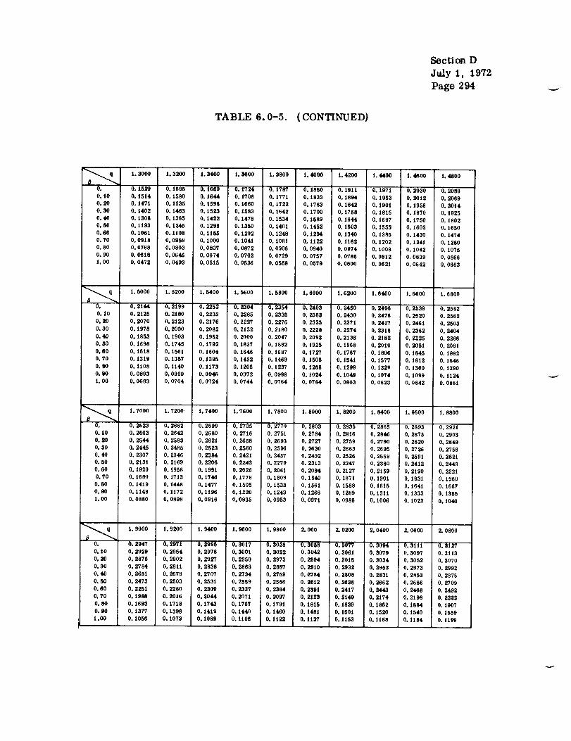
Section D
July 1, 1972
Page 294
TABLE 6.0-5. (CONTINUED)
1. 3000 1. 3200 1. 3400 1. 3600 1. 3800 1. 4000 t. 4200 1. 4400 1. 4800 t. 4800
O. O. 1529 O. t595 O. t680 O. 1724 O, 1787 O. 1850 O. 1911 O. 1971 O. 2030 O. 2088
0. 10 0. 1514 0. 1580 0. t644 0. 1708 0. t771 0. 1833 0. t894 0. 1953 0. 2012 0. 2069
0. 20 0. 147t 0. 1535 0. t598 0. 1660 0. 1722 0. 1783 0. t842 0. 190t 0. t958 0. 20t4
O, 30 0. 1402 0. 1463 0. t523 0. 1583 0. 1642 0. 1700 0. 1788 0. 1815 0. 1870 0. 1925
O. 40 O. t308 O. 1365 O. t422 O. t478 O. 1534 O. 1589 O. 1644 O. 1897 O. 1750 O. t802
O. 80 O. 1193 O. 1245 O. 1298 O. t350 O. 1401 O. t452 O. 1503 O. 1553 O. 1602 0. 1650
O• 80 O. 1061 O• 1108 O. 1155 O. t202 O. 1248 O. 1294 O. 1340 O. 1385 O. 1430 O. 1474O. 70 O. 0918 O, 0959 O. 1000 O. 1041 O. 1081 O. 1122 O. 1162 O. 1202 O. 1241 O. 1280
0. 80 0. 0768 0. 0803 0. 0837 0• 0872 0• 0906 0. 0940 0. 0974 0. 1008 0. t042 0. 1075
0. 90 0. 0618 0. 0646 0. 0674 0. 0702 0. 0729 0. 0757 0. 0785 0. 08t2 0. 0839 0. 0866
I.O0 O. 0472 O. 0492 O. 0515 O. 0536 O. 0558 O.0579 O. 0600 O. 0621 O. 0642 O. 0663
1. 5000 1. 5200 1. 5400 1.5600 1.5800 1, 6000 1. 6200 1. 8400 1. 6800 t. 6800• 0.2144 0.2199 0. 2252 0.2304 0.2354 0.2403 0.2450 0.2496 0.2539 0.2582
0. 10 0.2t25 0. 2180 0. 2233 0. 2285 0. 2335 0.2383 0.2430 0.2476 0. 2520 0. 2562
0.20 0. 2070 0. 2123 0. 2176 0. 2227 0. 2276 0. 2325 0.2371 0.2417 0.2461 0. 2503
0. 30 0. 1978 0. 2030 0.2082 0. 2132 0. 2180 0.2228 0. 2274 0. 23t8 0. 2362 0.2404
_40 0. 1853 0. 1903 0.1952 0,2000 0. 2047 0. 2093 O. 2138 0, 2182 0. 2225 0. 2266
0. 50 0. 1698 0. 1745 0. 1792 0. 1837 0. 1882 0. 1925 0. 1968 0. 2010 0. 2051 0.2091
0.80 0. t518 0. t561 0.1604 0.1646 0.1687 0.1727 0. J767 O. 1806 0.1845 O. t882
0. 70 0. 1319 0.1357 0. 1395 0. 1432 0. 1489 0. 1505 0. 1541 0. t577 0. 1612 0. 1646
0.80 O. t108 0. 1t40 0. tt73 O. 1205 O. 1237 0. 1268 0. 1299 0. 132_ 0. 1380 0. 1390
0.90 0. 0893 0. 0920 0. 0946 0. 0972 0. 0998 0, 1024 0, 1049 0, 1074 0. 1099 0. 1124
1.00 0. 0683 0. 0704 0. 0724 0. 0744 0. 0764 0. 0784 0. 0803 0. 0823 0. 0842 0. 0861
1. 7000 I. 7200 t. 7400 t. 7600 1. 7800 1. 8000 1. 8200 1. 8400 1. 8600 1. 8800
0. 0. 2623 0.2662 0. 2699 0.2735 0. 2770 0. 2803 0. 2835 0. 2865 0. 2893 0. 2921
0. 10 0. 2603 0. 2642 0. 2680 0.2716 0. 275t 0.2784 0. 2816 0. 2846 0. 2875 0. 2903
0.20 0.2544 0. 2583 0. 2621 0. 2658 0.2693 0.2727 0.2759 0.2790 0. 2820 0. 2849
0. 30 0.2445 0. 2485 0. 2523 0. 2560 0. 2596 0.2630 0.2663 0.2695 0. 2726 0.2756
0.40 0.2307 0,2346 0.2384 0.2421 0.2457 0.2492 0.2526 0.2559 O. 2591 0.262t0. 50 0. 2131 0. 2J69 0. 2206 0. 2243 0. 2279 0. 2313 0. 2347 0. 2380 0.2412 0. 2443
O. 60 O. 1920 0. t956 O. t99t 0.2026 O. 2061 O. 2094 O. 2127 O. 2t59 O. 2190 O. 2221
O. 70 O. 1680 O. 1713 O. 1746 O. 1778 O. 1809 O. 1840 O. 1871 O. 1901 O. 1931 O. 1960
O. 80 O. 1419 O. 1448 O. 1477 O. 1505 O. 1533 O. 1561 O. 1588 O. 1615 O. 1641 O. 1667
0.90 O. 1148 O. 1172 O. 1196 O. 1220 O. 1243 O. 1266 O. 1289 O. 1311 O. 1333 O. 1355
1.00 0.0880 0.0898 0.0916 0.0935 0.0953 0.0971 0.0988 0.1006 0.1023 0. i040
1.9000 I. 9200 1.9400 1.9600 1. 9800 _000 _0200 _0400 2.0600 2. 0800
0. 0. 2947 0. 2971 0.2995 0. 3017 0. 3038 0. 3058 0. 3077 0. 3094 0. 3t11 0.3t27
0.10 0.2929 0.2954 0.2978 0.3001 0.3022 0.3042 0.3061 0.3079 0.3097 0.31130.20 0.2876 0.2902 0.2927 0. 2950 0. 2973 0. 2994 0.3015 0.3034 0.3052 0.3070
0,30 0.2784 0. 2811 0. 2838 0. 2863 0. 2887 0. 2910 0.2932 0.2953 0. 2973 0. 2992
0.40 0. 2651 0.2679 0. 2707 0.2734 0,2759 0.2784 0. 2808 0. 283t 0. 2853 0. 28750.50 0,2473 0.2503 0. 2531 0. 2559 0. 2586 0.2812 0.2638 0.2662 0. 2686 0.2709
0. 80 0. 2251 0. 2280 0. 2309 0. 2337 0. 2364 0. 2391 0. 24t7 0.2443 0.2468 0. 2492
0. 70 0. 1988 0.2016 0.2044 O. 207t 0. 2097 0. 2123 0. 2149 O. 2t74 0. 2198 0. 2222
O. 80 O. t693 0. t7t8 O. 1743 O. 1767 O. 1791 O. 18t5 O. 1839 O. 1862 O. 1884 O. 1907
O. 90 O. 1377 O. 1398 O. 1419 O. 1440 O. 1460 O. 1481 O. 1501 O. 1520 O. 1540 O. 1559
t.00 O. 1056 0. t073 0.1089 O. 1t06 O. 1122 O. 1137 O. 1153 O. i168 0.1184 O. t199

OF POORQu JTY Section D
July 1, 1972
Page 295
TABLE 6.0-5. (CONTINUED}
2.1000 2.1200 2.1400 2,1600 2.1800 2.,2000 2.2200 2.2400 2. 2600 2. 2800
O. 0.3141 0.3t55 0.3168 0.3180 0.3t92 0.3202 0.3212 0.3222 0.3230 0.3239
0.10 0.3128 0.3142 0.3156 0.3168 0.3180 0.3191 0.3202 0.3211 0.3221 0.3229
0.20 0.3086 0.3102 0.3116 0.3130 0.3143 0.3156 0.3168 0.3179 0.3189 0.3199
0.30 0.3011 9.3028 0.3045 0.3061 0.3076 O. 3090 0.3104 0.3117 0.3129 0.3141
0.40 O. 2895 0.2915 0.2934 O. 2952 0.2969 O. 2986 0.3002 0.3018 0.3033 0.3047
O. 50 O. 2732 O. 2753 O. 2775 O. 2795 O. 2815 O. 2834 O. 2852 O. 2870 O. 2888 O. 2904
O. 60 O. 2515 O. 2539 O. 2561 O. 2583 O. 2604 O. 2625 O. 2645 O. 2665 O. 2685 0.2703
0.70 0, 2246 0. 2269 0, 2292 0, 2314 O. 2335 0.2357 O. 2378 0.2399 0. 2419 O. 2438
0.80 0.1929 0.1950 0.1972 0. 1993 0. 2014 0. 2034 0. 2054 0.2074 0.2093 0.2112
O. 90 O. 1578 O. 1597 O. 1615 6. 1634 O. 1652 O. 1670 O. 1687 O. 1704 O. 1722 O. 1738
1.00 0.1214 6,1228 0,1243 0.1257 0.1271 0,1285 0.1299 0.1313 0.1326 0.1340
2. 3000 2. 3200 2. 3400 2. 3600 2. 3800 _ 4000 2. 4200 2. 4400 2. 4600 2. 4800
O. O. 3246 O. 3253 O. 3260 O. 3266 O. 327t O. 3276 O. 3281 O. 3286 O. 3290 O. 3294
0.10 0.3237 0.3244 0.3251 0.3258 0.3264 0.3269 0.3274 0.3279 0.3284 0.3288
0.20 0,3208 0.3216 0.3225 0.3232 0.3239 0.3246 0.3252 0.3258 0.3263 0.3269
0.30 O. 3152 0.3163 0,3173 0.3162 0.3191 0.320o 0.3208 O. 3215 0.3223 0.3229
0.40 0.3060 o. 3073 0.3086 0.3098 0.3109 0.3120 0.3131 0.3141 0.3150 0.3159
0.50 0.2920 0. 2936 O. 2951 O. 2966 0. 2980 O. 2994 0.3007 0.30t9 0.3032 0.3043
0.60 O. 2722 O. 2739 0.2757 0. 2774 0.2790 O. 2806 O. 2822 O. 2837 O. 2852 O. 2866
0.70 O. 2458 O. 2477 O. 2495 O. 2514 O. 2531 O. 2549 O. 2566 O. 2583 O. 2599 0.2615
0.80 O. 2131 O, 2150 O. 2168 O. 2186 0.2204 0.2221 O. 2238 0.2255 O. 2272 0.2288
0.90 0.1755 0.1772 0.1788 0.1804 0.1820 0.1835 0.1851 0.1866 0.1881 0.1896
1.00 0.1353 0.1366 I).1379 0.1392 0.1404 0.1417 0,1429 0.1441 0.1453 0.1465
2. 5000 2.5200 2.5400 2.5600 2.5800 2.6000 2.6200 2.6400 2.6600 2.6800
O. 0.3297 0.3300 0.3303 0.3306 0.3309 0.3311 0.3313 0.3315 0.3316 0.3318
0. I0 0.3292 0.3295 0.3298 0.3301 0.3304 O. 3307 0.3309 0.3311 0.3313 0.3315
O. 20 O. 3273 O. 3279 O. 3282 O. 3286 O. 3289 O. 3293 O. 3296 O. 3299 O. 3301 O. 3304
0,30 0.3236 0.3242 0.3248 0.3253 0.3258 0.3263 0.3267 0.3272 0.3276 0.3279
0.40 O. 3168 0.3176 0.3184 0.3192 0.3199 0.3206 0.3212 0,3219 0.3225 0.3230
0.50 0.3055 0.3066 0.3076 0.3087 0.3(}96 0.3106 0,3115 O. 3124 0.3132 0.3141
0,60 O. 2880 0,2894 O. 2907 0,2920 0.2932 0.2944 _ 2956 O. 2968 O. 2979 O, 2990
0.70 O. 2631 O. 2646 O. 2662 O. 2676 O. 2691 O. 2705 O. 2719 0. 2733 0.2746 0.2759
O. 80 O. 2304 O. 2320 O. 2336 0.2351 0.2366 0. 2381 O. 2396 O. 2410 0. 2424 O. 2438
O. 90 0.1911 0.1925 0.1940 0.1954 0.1908 0.1981 0.1995 O. 2008 O. 2022 O. 2035
1.00 0.1477 0.1488 0. t500 0.1511 0.1522 0.1533 0.1544 0.1555 0.1566 O. 1576
2.7000 2.7200 2.7400 2.7600 2.7800 2.8000 2.8200 2.9400 2. 8600 2. 8800
O. O. 3319 O. 3321 O, 3322 O. 3323 O. 3324 O. 3325 O. 3326 O. 3327 O. 3327 O. 3328
0.10 O. 3317 0.3318 0.3320 0.3321 0.3322 0.3323 0.3324 0.3325 O. 3326 0.3326
0.20 0.3306 0.3308 0.3310 0.3312 0.3314 0.3315 0.3317 0.3318 0.3320 0.3321
O. 30 O. 3283 0.3286 O. 3289 O. 3292 0.3295 O. 3398 O. 3300 O. 3302 O. 3304 0.3306
0.40 O. 3236 O. 3241 O. 3246 O. 3250 O. 3255 O. 3259 O. 3263 O. 3267 O. 3270 O. 3274
O. 50 O. 3148 O. 3156 O. 3163 O. 3170 O. 3177 O. 3184 O. 3190 O. 3196 O. 3202 O. 3207
0.60 0.3000 0.3011 0o302! 0.3030 0.3040 0.3049 0,3058 0.3066 0.3075 0.3083
0.70 0.2772 O. 2784 O. 2797 O. 2809 O. 2820 O. 2832 O. 2843 O. 2854 O. 2805 O. 2876
O. 80 O. 2452 O. 2466 O. 2479 O. 2492 O. 2505 O. 2518 0.2530 0.2543 O. 2555 O. 2567
O. 90 O. 2048 O. 2061 O. 2073 O. 2086 O. 2098 O. 2110 O. 2122 O. 2134 O. 2146 O. 2157
1. O0 D. 1587 0. 1597 O. 1507 O. t617 0. 1627 O. 1637 O. 1647 O. 1657 O. 1666 O. 1676

TABLE 6.0-5. (CONTINUE D)
Section D
July 1, 1972
Page 296
2.9000 2.9200 2.9400 _9600 _ 9800 3.0000 3.0200 3.0400 3.0800 3.0800
O. O. 3328 O. 332_ O. 3329 O. 3330 O. 3330 O. 3331 O. 3331 O. 3331 O. 3331 O. 3332
0.10 0.3327 0.3328 0.3328 0. 3329 O. 3329 0.3330 O. 3330 O. 3330 O. 3331 O. 3331
0.20 O. 3322 O. 3323 O, 3324 O. 3324 O. 3325 O. 3326 O. 3327 O. 3327 O. 3328 O. 33280.30 0.3308 0.3310 0.3312 0.3313 0.3315 0.3316 0.3317 0.3318 0.3319 0.3320
0.40 0.3277 0.3280 0.3283 O. 3286 0.3259 0.3291 0.3293 0.329_ 0.3298 0.3300
0. 50 O. 32t2 0. 3218 0. 3223 0. 3227 0. 3232 0. 3238 0. 3240 0. 3244 0. 3248 0. 3252
O. 60 O. 3091 O. 3098 O. 3106 0.3113 O. 3120 O. 3127 O. 3t34 O. 3140 O. 3t46 O. 3152
O. 70 O. 2886 O. 2896 0.2906 O. 2916 O. 2925 O. 2934 O. 2944 O. 2952 O. 296i O. 2970
O. 80 O. 2578 O. 2590 0.2602 0.2613 0.2624 0.2635 0.2645 0.2656 0.2666 0.2677
0.90 O. 2169 0.2180 O. 219t O. 2203 O. 22t3 O. 2224 0.2235 O. 2245 0.2256 O. 22681.00 0.1685 0.1694 0.1703 0.17t3 0.1722 0.1730 0.1739 0.1745 0.1756 0.1765
3.0000 3. 1000 3. 2000 3. 3000 3.4000 3. 5000 3. 6000 3. 7000 3. 8000 3. 9000
O. 0.3331 0.3332 0,3332 0.3333 0.3333 0.3333 0.3333 0.3333 0.3333 0.3333
O. 10 O. 3330 O. 3331 O. 3332 O. 3333 O. 3333 O. 3333 O. 3333 O. 3333 O. 3333 O. 3333
0._0 O. 3326 O. 3329 0.3330 0. 3332 O. 3332 O. 3333 O. 3333 O. 3333 O. 3333 O. 3333
0.30 0.3316 0.3321 0.3325 0.3328 0.3330 0.3331 0.3332 0.3332 0.3333 0.3333
0.40 O. 3291 O. 3302 O. 3310 O. 33t6 O. 3321 O. 3324 O. 3327 O. 3328 0. 3330 O. 3331
O. 50 O. 3236 O. 3256 O. 3271 O. 3284 O. 3294 O. 3303 O. 3309 O. 3314 O. 3319 O. 3322
O. 80 O. 3127 O. 3t58 O. 3185 O. 3208 O. 3228 O. 3244 O. 3259 O. 3271 O. 3281 O. 3290
O. 70 O. 2934 O. 2978 O. 30t7 O. 3052 O. 3083 O. 31t2 O. 3137 O. 3159 O. 3179 O. 3197O. 80 0.2635 O. 2687 0.2735 0.2779 O. 2820 O. 2859 O. 2894 0.2927 0.2957 O. 2935
0.90 O. 2224 O. 2276 0.2326 O. 2372 O. 2416 O. 2457 0.2497 0.2634 O. 2569 0.2603
1.00 0. t730 0.1773 0.18t4 0.1853 0.1890 0.1925 0.1959 0.1991 O. 2022 O. 2051
4. 0000 4. 1000 4.2000 _3000 4.4000 4. 5000 4. 6000 4. 7000 4. 8000 _9000
O. 0.3333 0.3333 0.3333 O. 3333 0.3333 0.3333 0.3333 0.3333 0.3333 0.3333
0.10 0.3333 0.3333 0.3333 0.3333 0.3333 0.3333 0.3333 0.3333 0.3333 0.3333
0.20 0.3333 0.3333 0.3333 0.3333 0.3333 0.3333 0.3333 0.3333 0.3333 0.3333
0.30 0.3333 0.3333 0.3333 0.3333 0.3333 0.3333 0.3333 0.3333 0.3333 0.3333
0.40 O. 3331 0. 3332 0.3 332 O. 3333 O. 3333 O. 3333 O. 3333 O. 3333 O. 3333 0. 3333
O. 50 O. 3325 O. 3327 O. 3328 O. 3329 O. 3330 O. 3331 O. 3332 O. 3332 O. 3332 O. 3333O. 60 O. 3297 O. 3303 O. 3308 O. 3313 O. 3316 O. 3319 O. 3332 O. 3324 O. 3326 O. 3327
O. 70 O. 3213 O. 3227 O. 3239 O. 3251 O. 3261 O. 3270 O. 3277 O. 3284 O. 3290 O. 3296
O. 80 0.301t 0.3036 0.3058 O. 3079 O. 3098 0.31t6 O. 3t33 O. 3148 0.3162 O. 3175
0.90 0.2634 0.2665 0.2693 0.272t 0.2747 0.2771 0.2795 0.2818 0. 2839 0. 2859
1. O0 O. 2079 O. 2106 O. 2132 O. 2156 O. 2180 O. 2203 O. 2225 O. 2246 O. 2266 O. 2286
5.0000 5. 1000 5. 2000 5. 3000 _4000 5. 5000 5.6000 5.7000 5. 8000 5. 9000
O. O. 3333 O. 3333 O. 3333 0.3333 O. 3333 O. 3333 _3333 O. 3333 O. 3333 O. 3333
0.10 0.3333 0.3333 0.3333 0.3333 0.3333 O. 3333 0.3333 0.3333 0.3333 0.3333
0.20 0.3333 0.3333 0.3333 0.3333 0.3333 0.3333 0.3333 0.3333 0.3333 0.3333
0.30 0.3333 0.3333 0.3333 0.3333 0.3333 0.3333 0.3333 0.3333 0.3333 0.3333
O. 40 0.3333 0.3333 0.3333 0.3333 0.3333 0.3333 0.3333 0.3333 0,3333 0.33330.50 0.3333 0.3333 0.3333 0.3333 0.3333 0.3333 0.3333 0.3333 0.3333 0.3333
O. 60 O. 3328 O. 3329 0. 3330 O. 3331 O. 3331 O. 3332 O. 3332 O. 3332 O. 3332 O. 3333
0.70 0.3300 0.3305 0.3303 0.3312 0.33t4 0.33t7 0.3319 0.3321 0.3323 0,33240.80 0.3183 0.3199 0.3209 0.3219 0.3228 0.3236 0.3244 0.3251 0.3257 0.3263
0.90 O. 2879 O. 2897 0.2915 O. 2932 O, 2949 O. 2964 O. 2979 O. 2993 O. 3007 O. 3020
1.00 0.2303 O. 2323 O. 2341 0.2368 O. 2374 O. 2390 0.2406 O. 2420 0.2435 0.2449

J
Section D
July 1, 1972
Page 297
TABLE 6.0-5. (CONTINUED)
,f-
6.0000 6.1000 6. 2000 6.3000 6.4000 6.5000 6.6000 6.7000 6.8000 6. 9000
O. 0.3333 0.3333 0,3333 0.3333 0.3333 0.3333 0.3333 0.3333 0.3333 0.3333
0.10 0.3333 0.3333 0.3333 0.3333 0.3333 0.3333 0.3333 0.3333 0. 3333 0.3333
0.20 0.3333 0.3333 0.3333 0.3333 0.3333 0.3333 0.3333 0.3333 0.3333 0.3333
0.30 0.3333 0,3333 0.3333 0.3333 0.3333 0,3333 0.3333 0.3333 0.3333 0.3333
0.40 0.3333 0.3333 0,3333 0.3333 0.3333 0.3333 0.3333 0.3333 0.3333 0.3333
0.50 0.3333 0.3333 0.3333 0.3333 0.3333 0.3333 0.3333 0.3333 0.3333 0.3333
0.60 0.3333 0.3333 0.3333 0.3333 0.3333 0. 3333 0. 3333 0.3333 0.3333 0.3333
0. 70 0. 3326 0. 3327 0. 3328 0. 3329 0. 3329 0.3330 0. 3330 0. 333i 0. 3331 0. 3331
0.80 0,3269 0.3274 0.3279 0.3283 0.3288 0.3291 0.3295 0.3298 0,3301 0.3304
0.90 0.3033 0.3045 0.3056 0.3067 0.3077 0.3088 0.3097 0.3107 0.31t6 0.3124
1.00 0, 2462 0.2475 0.2488 0. 2501 0. 2513 0. 2525 0.2536 0. 2547 0. 2558 0. 2568
7. 0000 7. iO00 7.2000 7. 3000 7. 4000 7. 5000 7. 6000 7. 7000 7. 8000 7. 9000
O. 0.3333 0.3333 0.3333 0,3333 0.3333 0.3333 0.3333 0.3333 0.3333 0.3333
0.10 0.3333 0.3333 O. 3333 0.3333 0.3333 0.3333 0.3333 0.3333 0.3333 0.3333
0.20 0.3333 0.3333 0,3333 0.3333 0.3333 0.3333 0.3333 0.3333 0.3333 0.3333
0.30 0.3 333 0.3333 0.3333 0.3333 0.3333 0.3333 0,3333 0.3333 0.3333 0.3333
0.40 O. 3333 0.3333 0.3333 0.3333 0.3333 0.3333 0.3333 0.3333 0.3333 0,3333
0.50 0.3333 0.3333 O. 3333 0.3333 0.3333 0.3333 0.3333 0.3333 O. 3333 0.3333
0.60 0.3333 0.3333 0.3333 0.3333 0.3333 0.3333 0.3333 0.3333 O. 3333 0.3333
0.70 0.3332 0.3332 0.3332 0.3332 0.3333 0.3333 0,3333 0.3333 0.3333 0,3333
0.80 O. 3306 0.3309 0.3311 0.3313 0.3314 0.3316 0.3317 0.3319 0.3320 0.332t
O. 90 0.3i32 0,3140 0.3148 0.3155 0.3162 O. 3169 0.3175 0.3182 0,3188 0,3193
l. O0 O. 2578 O. 2588 O. 2598 O. 2607 O. 2616 O, 2625 O. 2634 O. 2643 0.2651 0.2659
8.0000 8. i000 8. 2000 8.3000 8.4000 8.5000 8.6000 8.7000 8.8000 8. 9000
O. 0.3333 0.3333 0.3333 0.3333 0.3333 0.3333 0.3333 0.3333 0.3333 0.3333
0.10 0.3333 0.3333 O. 3333 0.3333 0.3333 0.3333 0,3333 0.3333 0.3333 0.3333
0.20 0.3333 0,3333 0,3333 0,3333 0,3333 0.3333 0.3333 0.3333 0.3333 0.3333
0.30 0.3333 0.3333 0.3333 0.3333 0.3333 0.3333 0.3333 0.3333 0.3333 0.3333
0.40 0.3333 0.3333 0.3333 0.3333 0.3333 0.3333 0.3333 0.3333 0.3333 0.3333
0.50 0.3333 0.3333 0.3333 0.3333 0.3333 0.3333 O. 3333 O. 3333 9.3333 O. 3333
0.60 0.3333 0.3333 O. 3333 O. 3333 0.33:13 0.3333 0.3333 0.3333 0.3333 0.3333
0.70 0.3333 0.3333 0.3333 0.3333 0.3333 0,3333 0.3333 0.3333 0.3333 0.3333
O. 80 O. 3322 O. 3323 O. 3324 O. 3325 O. 3326 O. 3327 O. 3327 O. 3328 O. 3328 O. 3329
O. 90 0.3199 0.3204 0.3209 0.3214 0.3219 0.3223 O. 3227 0.3232 O. 3236 0.3240
1.00 O. 2667 0.2675 0.2682 0.2690 0.2697 0.2704 O. 2711 O. 2718 0.2724 0.2731
9. 0000 9.1000 9. 2000 9. 3000 9.4000 9. 5000 9.6000 9.7000 9. 8000 9. 9000
O. 0.3333 0.3333 0.3333 0.3333 0.3333 0.3333 0.3333 0.3333 0.3333 0.3333
O. iO 0.3333 0.3333 0.3333 0.3333 0,3333 O. 3333 0.3333 0.3333 0.3333 O. 3333
0.20 0.3333 0.3333 0.3333 0.3333 0.3333 0.3333 0.3333 0.3333 0.3333 0.3333
0.30 0.3333 0.3333 0.3333 0.3333 O. 3333 0.3333 0.3333 0,3333 0.3333 0.3333
0.40 0.3333 0.3333 0.3333 0.3333 0,3333 0.3333 0.3333 0.3333 0.3333 0.3333
O. 60 O. 3333 O. 3333 O. 3333 O. 3333 O. 3333 O. 3333 O. 3333 O. 3333 O. 3333 O. 3333
0.60 0.3333 0.3333 0.3333 0.3333 0.3333 O. 3333 0,3333 0.3333 O. 3333 0.3333
0.70 0.3333 0.3333 0.3333 0.3333 0.3333 O. 3333 0.3333 0.3333 O. 3333 0.3333
0.80 0.3329 0.3330 0.3330 0.3330 0.333i 0.3331 0.3331 0,3331 0,3332 0,3332
0.90 O. 3243 O. 3247 O. 3250 O. 3254 O. 3257 O. 3260 O. 3263 O. 3266 O. 3268 O. 327|
t.00 0.2737 0.2743 0.2749 0.2755 0.276t 0.2767 0.2773 0.2778 0,2783 0.2789

_ctton D
July 1, 1972
page 298
TABLE 6.0-5. (C_)NCLUDED)
0°
O, t00.10O.NO.4OO.SO0.60o.70o._)O, lOi.oO
10, 00o0
O. 1833O. 3835O. 38Mo. 1,1810.8383O. 38380.8,188o, millO. U$|O. 33'P3O. I"/N
10. lOOO to. moo
o. uu o. 33uo. uu o. 3333o. 3333 o. 3333o. 3333 o. 11,538o. 3831 o. 3838O, 8,538 O. 3_38O. 3338 O.81138O. 3305 O. 8881o. 3331 o, _l|o. 815'11 o. 335'8o. 2781 o. 3804
to, 3oo0 to. 4oo0 to. sooo 10.eooo ' 10. 7000 10, 80oo 10ogooo '
O. 3333 O. 3533 O. 2838 O. 0533 !+ O. 3338 O. 3333 O, a38$"O. 9338 O. 3333 O. 3838 O. 3333 O. 3383 O. 3333 O. 3338O. 3333 O. 3333 O. 3833 O. 33138 O, 3333 O. 3333 O. 3303O. 3038 O. 3338 O. 3333 O. 3333 O. 3333 O. 3333 O. 3333O. M338 O. 3833 O. 3338 O. 31333 O. 3333 O. 3333 0. 3383O. 3838 O, 3383 O.JI3AB O.3833 O. 3338 0,, 3+533 O. ,5,533
O.1338 O.3238 O, 3838 O.3838 O.Sa_ O.3333 O.3333O.3333 O,1238 0. _ O.33:12 O.3333 O,3333 o. 3333
O,2323 O.1338 O.32_12 O.3833 O.3333 0_.3333 O.3333O. 38110 O. 3338 O. 3384 O. 3388 O. 3288 O. 3290 O. 3893
o. Moll O.1614 o. 3811 o, 1818 o. 118211 o. 11832 op2837

0
.
0
o
o
.
.
.
Section D
July I, 1972
Page 299
REFERENCES
Boley, B. A. ; and Weiner, J. H. : Theory of Thermal Stresses.
John Wiley and Sons, Inc., New York, 1962.
Newman, M. and Forray, M. : Thermal Stresses in Circular Rings.
Machine Design, Nov. 8, 1962.
Newman, M. and Forray, M. : Bending Stresses Due to Temperature
in Hollow Circular Plates, Part I. Journal of the Aerospace Sciences,
October 1960.
Forray, M. and Newman, M. : Bending Stresses Due to Temperature
in Hollow Circular Plates, Part II. Journal of the Aerospace Sciences,
November 1960.
Newman, M. and Forray, M. : Bending Stresses Due to Temperature
in Hollow Circular Plates, Part III. Journal of the Aerospace Sciences,
December 1960.
Timoshenko, S. : Strength of Materials. Part II, Advanced Theory
and Problems. Third ed., D. Van Nostrand Co., Inc., New York,
1956.
Thermo-Structural Analysis Manual. Technical Report No. WADD-
TR-60-517, vol. I, August 1962.
Thermo-Structural Analysis Manual. Technical Report No. WADD-
TR-60-517, Vol. II, October 1962.

.
10.
11o
12o
13.
14.
15.
16.
Section D
July 1, 1972
Page 300
REFERENCES (Continued)
Forray, M. J. ; Newman, M. ; and Kossar, J. : Thermal Stresses and
Deflections in Rectangular Plates. Part 1, The Analysis and Test of
Rectangular Panels with Temperature Gradients Through the Thickness.
Technical Report No. ASD-TR-61-537 Part 1, Flight Dynamics
Laboratory, Aeronautical Systems Division, Air Force Systems
Command, Wright-Patterson Air Force Base, Ohio, December 1962.
Forray, M. ; and Newman, M. : Stress sad Deflection in Heated Plates
on Beam Supports° Machine Design, Feb. 15, 1962.
Tlmoshenko, S° ; and Woinowsky-Krieger, S. : Theory of Plates and
Shells. McGraw-Hill Book Co., New York, 1959.
Tlmoshenko, S. ; and Goodier, J.N. : Theory of Elasticity. McGraw-
Hill Book Co., Inc., New York, 1951.
Gatewood, B.E. : Thermal Stresses. McGraw-Hill Book Co., Inc.,
New York, 1957.
Morgan, A. J. A. : A Proof of Duhamel' s Analogy for Thermal
Stresses. Journal of the Aerospace Sciences, July 1958.
Dharmarajan, S. : In-Plane Thermal Stress Analysis. General
Dynamics, Convair Division, Memo No. SA-70-13, July 17, 1970.
Tsui, Y. W. : Stresses in Shells of Revolution. Pacific Coast
Publishers, Menlo Park, Calif., t968.

f_
17.
18.
19.
20.
21.
22.
23.
24.
25.
Section D
July 1, 1972
Page 301
REFERENCES (Continued)
Baker, E. H. ; Cappelli, A. P. ; Kovalevsky, L. ; Rish, F. L. ;and
Verette, R.M. ; Shed Analysis Manual. NASA CR-912, April 1968.
Hetenyi, M. : Beams on Elastic Foundation. The University of
Michigan Press, Ann Arbor, Mich., 1946.
Dharmarajan, S. N. : Thermal Stresses in Circular Cylindrical Shells.
General Dynamics, Convair Division, Stress Analysis Memo SA-70-
16, Aug. 28, 1970.
Przemieniecki, J. S. : Introduction to Structural Problems in Nuclear
Reactor Engineering. Chapter 8, Pergamon Press, New York, 1962.
Wylie, C. R. Jr. : Advanced Engineering Mathematics. McGraw-
Hill Book Co., Inc., New York, 1951.
Sokolnikoff, I. S. ;and Redheffer, R. M. : Mathematics of Physics
and Modern Engineering. McGraw-Hill Book Co., Inc., New York,
1958.
Newman, M. ;and Forray, M. : Thermal Stresses in Cylindrical Shells.
Machine Design, June 6, 1963.
Huth, J. H. : Thermal Stresses in Conical Shells. Journal of the
Aeronautical Sciences, September 19_3.
Nowacki, W. : Thermoelasticity. Addison-Wesley Publishing Co., Inc.,
Reading, Mass., 1962.

26.
27.
28.
29.
30.
31.
32.
33.
Kraus, H. :
York, 1967.
REFERENCES (Continued)
Thin Elastic Shells.
Section D
July I, 1972
Page 302
John Wiley and Sons, Inc., New
Switzky, H. ; Forray, M. ; and Newman, M. ; Thermo-Structural
Analysis Manual. Vol. I, WADD-TR-60-517, August 1962.
Smith, G. W. : Analysis of Multiple Discontinuities in Shells of
Revolution Including Coupled Effects of Meridional Load. General
Dynamics, Convair Division, Report No. GD/A 63-0044, July 31, 1963.
Johns, R. H. ;and Orange, T. W. ; Theoretical Elastic Stress Distri-
butions Arising from Discontinuities and Edge Loads in Several Shell-
Type Structures. NASA TR R-103, 1961.
Fitzgerald, E. A. : Thermal Stresses in Thin Shells of Revolution for
Axisymmetric Temperature Distributions. Report No. SM-42009,
Missiles and Space Systems Engineering, Douglas Aircraft Co., Inc.,
June 1962.
Christensen, R. M.: Thermal Stresses in Missile Nose Cones. Paper
No. 58-A-274, presented at the Annual Meeting of the ASME, New
York, N. Y., Nov. 30- Dec. 5, 1958.
Forray, M. : Thermal Buckling and Postbuckling of Circular Bulkheads.
Machine Design, March 12, 1964.
Newman, M. ; and Forray, M. : Axisymmetric Large Deflections of
Circular Plates Subjected to Thermal and Mechanical Loads. Journal
of the Aerospace Sciences, September 1962.
4.
35.
36.
37.
38.
39.
40.
41.
Section D
July 1, 1972
Page 303
REFERENCES (Continued)
Friedrichs, K. O. ; and Stoker, J. J. : The Nonlinear Boundary Value
Problem of the Buckled Plate. American Journal of Mathematics,
vol. 63, 1941, pp. 839-888.
Timoshenko, S. P. ; and Gere, J. M. : Theory of Elastic Stability.
McGraw-Hill Book Co., Inc., New York, 1961, p. 391.
Forray, M. ; and Newman, M. : Buckling of Heated Rectangular Plates.
Machine Design, June 7, 1962.
Newman, M. ; and Forray, M. ; Post-Buckling Deflection of Heated
Rectangular Plates. Machine Design, Dec. 5, 1963.
Bijlaard, P. P. ; and Gallagher, R. H. : Elastic Instability of a
Cylindrical Shell Under Arbitrary Circumferential Variation of Axial
Stress. Journal of the Aerospace Sciences, November 1960.
Abir, D. ; and Nardo, S. V. : Thermal Buckling of Circular Cylindrical
Shells Under Circumferential Temperature Gradients. Journal of
the Aerospace Sciences, December 1959.
Schumacher, J. G. : Development of Design Curves for the Stability
of Thin Pressurized and Unpressurized Circular Cylinders. General
Dynamics, Convair Division, Report No. AZS-27-275, May 8, 1959.
MIL-HDBK-5A, Metallic Materials and Elements for Aerospace
Vehicle Structures. February 8, 1966.
U S GOVERNMENT PRINTING OFFICE: 1972 - 746-624/4751 REGION NO, 4


SECTION E


SECTION El
FATIGUE

TABLE OF CONTENTS
1_1 FATIGUE ......................................
I.i INTRODUC TION ..............................
I.I.1 General Considerations for a Fatigue A_llysi8 .....
I.I.I.I Life Cycle Determination .... 0 . .° .....
1.1. i.2 Material Fatigue Data ............. , . .
i.I.1.3 Fatiguc Analysis .......... , ........
I.i.2 General Background on Fatigue ................
1.2 BASIC DE FINITIONS
1.2.1
1.2.2
1.2.3
• • • • • • • . , • • • • • • • • • • • • • • • • • •
Mechanism of Failure ......................
Fatigue Testing Techniques ..................
Presentation of Test Results .................
1.2.3.1 S-N Diagrams .....................
I.2.3.2 Goodman Diagrams ............. 0 . . .
1.3 FACTORS INFLUENCING FATIGUE STRENGTH ........
1.3. I Metallurgical Factors ......................
1.3. i.I Surface Defects ....................
I.3.I.2 Subsurface and Core Defects, Inhomogeneity
and Anisotropy .............. , .....1.3.1.3 Heat Treatment ...................
i.3.1.4 Localized Overheating ...............
I.3.1.5 Corrosion Fatigue ..................
].3.1.6 Fretting Corrosion ..... , ...........
1.3.1.7 Reworking ..................... , .
1.3.2 Processing Factors ................. , ......
1.3.2.1 Hardness ........ ..... , ..........
1.3.2.2 Forming ........................
I.3.2.3 Heat Treatment ............. , .......
1.3.2.4 Surface Finish ............... , .....
I.3.2.5 Cladding, Plating, Chemlcll Conversion
Coatings, and Anodizing ..............
1.3.2.6 Cold Working ...... . . . o ...........
1.3.3 Environment Effects ....... . ...............
1.3.3.1 Irradiation .......................
1.3.3.2 Vacuum .........................
I
I
I
4
7
8
I1
12
16
19
19
20
23
23
23
24
28
29
29
32
32
33
33
34
35
35
37
39
39
41
41
El-iii
TABLE OF CONTENTS (Continued)
1.4
1.5
1.3.4
1.3.5
1.3.6
1.3.7
1.3.3.3 Meteoroid Damage ..................
1.3.3.4 Solar Irradiation ...................
1.3.3.5 Temperature .....................
Design Effects ...........................
Welding E fleets ..........................
Size and Shape Effects .....................
Speed of Testing .........................
LOW CYCLE FATIGUE .........................
1.4..1 Below Creep Range .......................
I. 4.1.1 Practical Problem Solutions ...........
1.4.2 In Creep Range ..........................
1.4.2.1 Ductility Versus Creep Strength .........
1.4.2.2 Procedure for Estimating High-
Temperature, Low-Cycle Fatigue .......
I. Basis ........................
II. Method .......................
1.4.2.3 Method of Strain Partitioning ...........
1.4.2.,t Two-Slope Fatigue Low ..............
1.4.:3 Thermal Cycling .........................
1.4.3.1 Idealized Thermal-Cycle Model .........
1.4.3.2 Effect of Creep ....................
1.4. ;3.3 Comparison of Thermal-Stress Fatigue With
Mechanical Fatigue at Constant
Temperature .....................
1.,t.3.4 Summary ........................
CUMULATIVE FATIG1TE DAMAGF ..................
1.5.1 Theory ................................
1.5.2 Analysis of Data .........................
1.5.2. l P{,ak Counting Techniques .............
1.5.2.2 Statistical Methods of Random Load
Analysis ..........................
1.5.3 Examph, Problem (Paired Range Count Method) ....
Page
42
42
42
43
45
46
46
47
49
50
51
53
53
54
59
60
62
63
65
66
68
70
71
71
72
74
74
77
El -iv
TABLE OF CONTENTS (Concluded)
1.6 MATERIAL SELECTION TO RESIST FATIGUE ..........
1.6.1 High Cycle .............................
1.6.2 Low Cycle .............................
1.7 DESIGN GUIDES ..............................
REFERENCES .....................................
Page
81
81
81
87
89
El-v

1..J

f
OF_ POOR QUALITYSection E 1
I November 1972
E1 FATIGUE.
1.1 IN TRODUC TION.
1.1.1 General Considerations for a Fatigue Analysis.
Before detailing the many factors involved in a fatigue analysis and.
design, it is desirable to give an overview of the general considerations that
comprise a fatigue analysis. Often when a new vehicle, structure, etc., is
being considered, there are many concepts, designs, and configurations to be
cvaluatect, and the engineer must provide ready assistance in the selection of
materials, writing of preliminary test requirements and the life evaluation.
Figure El-1 shows a general flow diagram of information for'a fatigue
analysis. As can be seen from this figure, there are two primary groups of
information that are necessary as input to a fatigue analysis and/or determina-
tion of preliminary test requirements for a given structural component.
One group of information is the necessary data on the given material.
These data include curvcs, graphs, etc., of laboratory tests to determine
stress versus cycles to failure (S-N) diagrams, Modified Goodman diagrams
and other factors which would affect the life of the component in question. The
other information, which is usually the first information that is required, is
the life cycle or service history of the structural component. This is usually
presented in terms of stress-environment versus time curves which show
pressures, temperatures, and other environmental considerations. In general,
with these two groups of information a fatigue analysis and/or the preliminary
test requirements can be determined for the component. Actually, the pre-
liminary test requirements can usually be determined from the life cycle
information alone.
1.1.1.1 Life Cycle Determination.
The important elements in the formation of life cycle data are the design
life, mission profile (or condition lists), and significant fatigue loadings (see
Fig. El-l). The design or anticipated operational life and service loading
spectra are primary considerations in evaluating effects of fatigue on the struc-
tural component of a flight vehicle.
l)csi_n life is generally specified by contractual or managerial agree-
ments, or VAA and Military _;pecifieations, usually in terms of number of
[lights, landings, pressurizations, flight hours, etc.

ORIGI_IAL " '__ ;_
OF POOR QUALITY
Section 1,:1
1 November 1972
1)age 2
DESIGN LIFE (NUMaER OF FLIGHTS, PRESSURIZATIONS. HOURS. ETC.)
J MliStON PROFILE/CONDITION LIST (ACTIVITY VS TIME)"1 SIGNIFICANT FATIGUE LOADINGS (MOST IMPORTANTI
/ I AERODYNAMICS (HEATING, PRESSURES, LOADS
L _ DYNAMIC LOADS)
LIFE CYCLE
Irr R IFJ;S LEVkt. VS TIME REQUIREMENTSTEMP. V$ TIMEPRESSURE VS TIMEENVIRONMENT VS TOME
MATERIAL TEST DATA
$-N CURVES
CRACK PROPAGATION RATESBIAXIAL STRESS DATA
FLAW DATA. WELD DATACREEP-RUPTURE. DUCTILITYTOUGHNESS
&'TRESS-ENV.
TEST REQUIREMENTS
FOR
COMPONENTS
TEST LOAD SPECTRUMRESULTS NEEDED
l
TIME
FATIGUE ANALYSIS
:[,,/N
MARGINS OF SAFETY
SAFE LIFE
N (CYCLE||
-4k------
CUMULATED DAMAGEREPLACEMENT SCHEDULEINSPECTION METHODSDESIGN ALLOWABLE STRESSMATERIAL SELECTION
LIMITATIONS
FAIL-SAFE
INSPECTIONSREPAIRSTURNAROUND TIME
}FIGURE E]-I. PROCEDURE FOR TYPICAL FATIGUE ANALYSIS
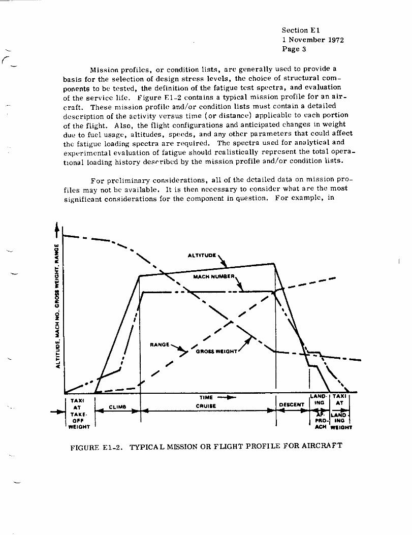
F
Section E I
1 November 1972
Page 3
Mission profiles, or condition lists, are generally used to provide a
basis for the selection of design stress levels, the choice of structural com-
ponents to be tested, the definition of the fatigue test spectra, and evaluation
of the service life. Figure E1-2 contains a typical mission profile for an air-
craft. These mission profile and/or condition lists must contain a detailed
description of the activity versus time (or distance) applicable to each portion
of the flight. Also, the flight configurations and anticipated changes in weight
due to fuel usage, altitudes, speeds, and any other parameters that could affect
the fatigue loading spectra are required. The spectra used for analytical and
experimental evaluation of fatigue should realistically represent the total opera-
tional loading history deseribed by the mission profile and/or condition lists.
For preliminary considerations, all of the detailed data on mission pro-
filesmay not be available. It is then necessary to consider what are the most
significantconsiderations for the component in question. For example, in
TAXI ]AT _.,TAKE-
| OFF-- WEIGHT
CLIMB
TIME
CRUISE
FIGURE E1-2. TYPICAL MISSION OR FLIGHT PROFILE FOR AIRCRAFT

Scction E 1
1 Novembcr 1972
Page 4
tankage, the most important factors may be pressure and temperature; for
wings, the most important factor may be only temperature.
Now, given all the information above, it is required to evaluate the
stress versus time curves for a given component. Ordinarily, the aerodynamic
data and dylmmie loads must be considered as input to aid in the evaluation of
load and stress levels. In conceptual designs, however, these may be "best-
guess" data. The stress-versus-time curves must, of course, reflect tem-
perature versus time, and other environmental factors present over part of a
mission profile. An example of a life cycle for a component is given in Fig.El-3.
A • C D
I p_._F TEST - . I - - I -
TIME
75 HOURS Ir '
• •320 ° F
FIGURE El-3. LIFI':-IIISTORY CURVE
Of c,)ur_e, the actual lift, cycle history for a given compom'nt may con-
tain many random type loads which must be condensed into a form which can
be used in fatigue life evaluation. Many techniques are available to accomplish
this, and thcywillbc discussed ina later section. For example, the spectrum
shown in Fig. 1:1-4 for an aircraft flight is simplified to a more. usable, form.
l. 1.1.'2 Material Fatigue Data.
The fatigue strength of a material may be defined as the maximum stress
that can be applit'd repeatedly to the matcrial without eausin_ failure in less
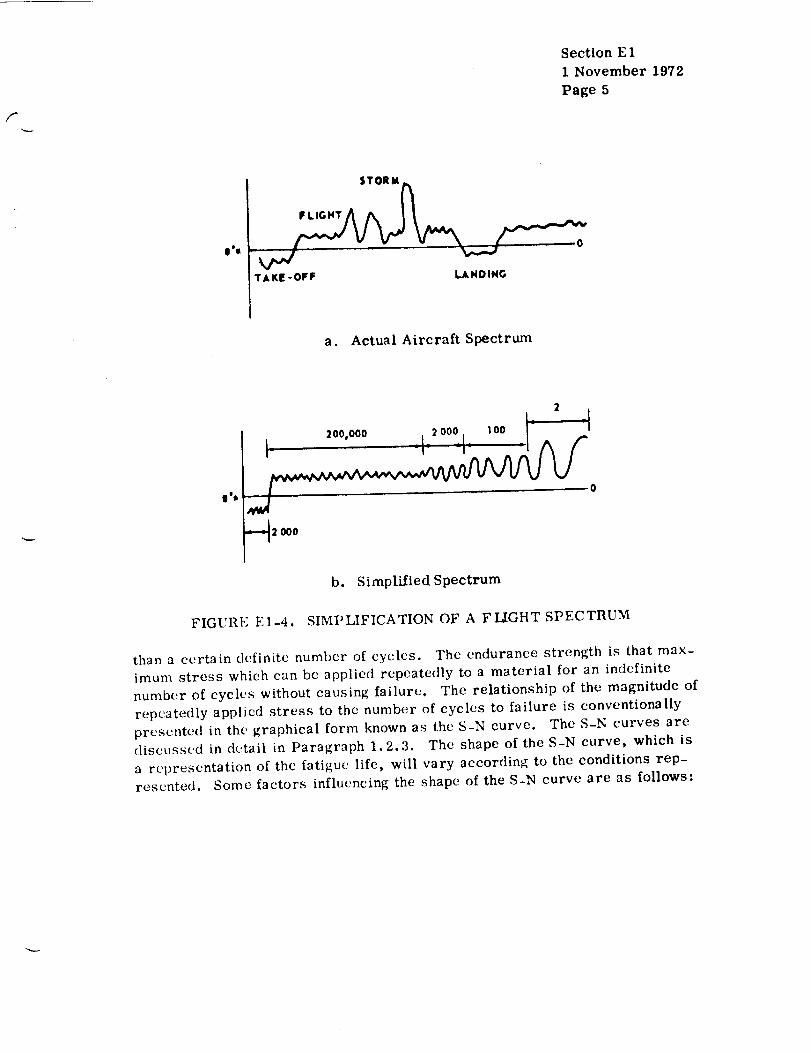
f
Section E 1
1 November 1972
Page 5
ieg
STORM
TAKE-OFF LANDING
a. Actual Aircraft Spectrum
IIS
2t_ I
2o0,0o0 2ooo i oo }- - I
l_l 1 1 ,
o
b. Simplified Spectrum
FIGURE E1-4. SIMPLIFICATION OF A FLIGHT SPECTRUM
than a certain definite number of cycles. The endurance strength is that max-
imum stress which can be applied repeatedly to a material for an indefinite
number of cycles without causing failure, The relationship of the magnitude of
repeatedly applied stress to the number of cycles to failure is conventionally
presented in the graphical form known as the S-N curve. The S-N curves are
discussed indc'tail in Paragraph 1.2.3. The shape of theS-N curve, which is
a re'presentation of the fatigue life, will vary according to the conditions rep-
resented. Some factors influencing the shape of the S-N curve are as follows:

1. Type of load
a. Tension
b. Compression
c. Torsion
d. Combined Loads
2. Relationship of maximum to minimum loads
3. Manner of load application
a. Axial
b. Flexural
c. Torsional
4. Rate of load application
5. Frequeney of repetition of loads
6. Temperature of the material under load
7. Environment
a. Corrosive
b. Abrasive
c. Inert
Material condition
a. Prior heat treatment
b. Prior cold work
Design of part or structure
Fabrication techniques
Q
Section E 1
1 November 1972
Page 6

Section E11 November 1972Page 7
Thus, it canbe seen that the mission profile or load spectra can dictatewhat type of S-N data are required for a fatigue analysis.
Other material information which may be necessary for input into afatigue analysis are low-cycle fatigue data, fracture toughness, crack propaga-tion rates, biaxial stress field data, welding, flaw size effects, and creeprupture data.
1.1.1.3 Fatigue Analysis.
Referring again to Fig. El-l, with the input as discussed above, afatigue analysis can be performed on the structural component or element in
question. Other information which may be required includes limitations on
inspection techniques, determination of a design (fail-safe or safe-life), and
reliability and safety.
Fatigue analysis is usually performed in two phases. The first is the
design phase, which is the structural sizing, material determination, and
factor-of-safety study phase. Usually, in this phase only preliminary data are
available concerning the life cycle and material properties; thus, best estimates
must be made. From this design phase, design stress levels and requirements
for developmental fatigue tests are determined.
The second phase of the fatigue analysis is the interpretation, in terms
of actual flight-measured data, of the results obtained from fatigue tests con-
ducted on structural elements. Also, the vehicle is assessed for damage and
qualified for reuse on subsequent missions.
The details of the fatigue analysis will be discussed in the following
paragraphs;but, _cncrally, the fatigue analysis will determine the safe life for
a structural compon¢'nt, will evaluate accumulated damage during service life,
will specify inspection requirements, and will determine allowable stresses
and/or test requirements.
Therefore, the analysis of fatigue life is a continuing process of study
and reevaluation in light of newly acquired data. Thc acquisition of new loading
and other cnvironm('ntal data can provide additional insight into the levels of
assurance that exist in the evaluation of the service life of structural components
on flight vehicles. Any significant variation between service-recorded loading
histories (and related environmental conditions) and the spectra used to deter-
mine fatigue life would require a reevaluation of anticipated structural life.

• I_° I _ _.., - _1 _
OF POOR Q._i;,_Lii i
Section E 1
1 November 1972
Page B
1.1.2 General Background on Fatigue.
A rapid growth of metallurgy, with it'on and steel coming into wide-
spread use in many types of machines and structures occurred during the mid-
dle of the ]9thcentury. During this time, engineers were confronted with
failures that occurred at calculated nominal stresses considerably below the
tt'nsile strength of the materials involved, and, although the materials were
considered ductile, the failures generally exhibited little or no ductility. It
was soon discovered that most of the brittle fractures developed only after the
structures had been subjected to many cycles of loading. Therefore, it came
to bc supposed that the metal degenerated and became fatigued under the action
of cyclical stresses and that its ductile behavior turned brittle, tlowt'ver, later
experiments showed that no degeneration or fatigue of the metal o(:currt,d as a
result of cyclical stressing and, therefore, the idea of metal fatigue is false.
H¢'nee the t(wm "fatigue" is still widely used although it has quite a different
nleatlJllg.
Generally speaking, fatigue can be defined as a progressive failure of
a part under repeated, cyclic, or fluctuating loads.
Fati;_uc failures may be simple or compound. Simple failures result
when a fatigue failure starts from a single crack and propagates until ultimate
failure occurs. A compound fatigue failure results when the origin of the
fatigue crack originates from two or more locations and propagates; the joint
effects cause total failure. The sequence in which failure occurs consists of
three parts: The initial damage occurs in a submicroscopic scale, the crack
initiates and propagates, and the final rupture takes place. The rate at which
the crack propagates varies considerably, depending upon the intensityof stress
and other related factors. Nevertheless, the rate is always much lower than
that observed for low-tcmpcrature brittlefractures in steel.
It has proved difficult, however, to detect progressive failures in the
part during its life; hence, fatigt, e _.ailure8 can occur with little warning and
can cause catastrophic failures. Also, periods of rest (the fatigue stress
removed) do not lead to a recovery from the effects of stress; in other words,
the fatigue damage is cumulative.
The criterion for fatigue failure is the simultaneous action of cyclic
stress, tensile stress, and plastic strain. If any one of these is eliminated,
fatigue is also eliminated.

Section E1
1 November 1972
Page 9/10
Rarely is a mechanical component or structural elt'ment sub ieeted to
constant loads throughout its entire service history. Cyclic loading can result
from vibration, variations in atmospheric b,:ust pattern, variable wind loadings,
repeated temperature changes, and repetition of design load, to mention onlya few.
Many fatigue failures that occur in service are only minor, but others,
such as those which result in the loss of a wing, propeller, or wheel, constitute
a serious threat to life or property. Such failures have become more prevalent
in recent years because of the following factors:
1. The continuing trend toward higher strength/weight ratios.
2. More refined static design techniques and the use of higher workingstress.
3. The use of materials of ultra-high static strength.
Good static design does not necessarily result in satisfactory perform-
ance under repeated loading, and the choice of a design stress close to, or
even higher than, the yield point of the material would almost inevitably result
in failure after a relatively short period of service. There is every possibility
that the fatigue problem will become more acute and that, consequently, the
limitin;_ strength criterion in many future designs will be adequate fatigue
resistance. Thcr(-fore, the likelihood of a fatigue failure should be an early
des ign consideration.
A major problem in designing to prevent fatigue failure lies in the
identification of all the factors that affect the life of a part. Even with the
knowledge of which problems to consider, one is still short of the goal: the
exact determination of fatigue life. Techniques are furnished in the following
sections to enable the engineer to develop fatigue data for a particular part.
All the basic definitions used in fatigue testing and failure are discussed
in Paragraph 1.2. The many types of effects which influence fatigue strength
are prt'sented in Paragraph 1.3. A separate section (Paragraph 1.4) is
de_oted to low-cycle fatigue because of its unique application and terminology.
Vari()us cumulative fatigue damage theories are discussed in Paragraph 1.5.
Paragraph 1.6 is a special section which will be uscful in selecting certain
mat(:rials to resist fatigue failures. Design guides are given in Paragraph 1.7.


Section E1
1 November 1972
Page 11
1.2 BASIC DEFINITIONS.
This paragraph describes the basic mechanism of a fatigue failure and
the general methods used in fatigue testing and documenting of the results.
The following definitions are some of the terms frequently used in this
discussion of fatigue analysis:
Stress Cycle Tiw smallest division of the stress-time func-
tion that is repeated. (See Fig. E1-5.)
Nominal Stress Obtained from the simple theory in tension,
bending, and torsion, neglecting geometric
discontinuities.
Maximum Stress
Minimum Stress
Mean Stress
Stress Range
Stress Amplitude
Stress Ratio
The largest or highest algebraic value of a
stress ill a stress cycle. Positive for tension.
Smax
The smallest or lowcst algebraic value of a
stress in a stress cycle. Positive for tension.
Srain
The algebraic mean of the maximum and mini-
mum stress in one cycle. Sm
The algebraic difference between the maximum
and minimum stresses in one cycle. Sr
Half the value of the algebraic difference
between the maximum and minimum stresses
in one cycle, or half the valuc of the stress
range. Sa
The ratio of minimum stress to maximum
stress.
Fatigue Life The number of stress cycles which can be sus-
tained for a given test condition.
Fatigue Strength The greatest number of stress cycles which
can be sustained by a member for a given
number of stress cycles without fracture.
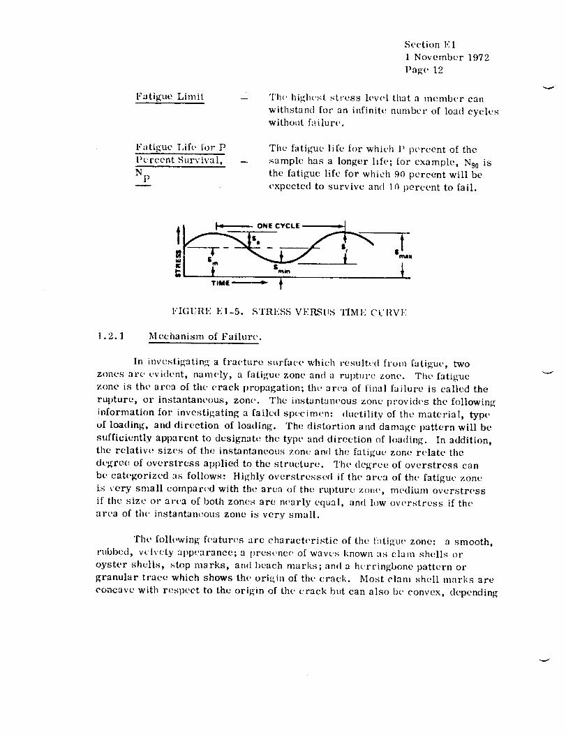
Fatigue Limit
Fatigue IAfe for P
Percent Survival, --
Np
Section E 1
1 November 1972
Page 12
"l'h(' highest stress level that a inember can
withstan(I for an infinite number of load cycleswithout failure.
The fatigue life for which I) pt'rccnt of the
sample has a longer life; lot example, Ng0 is
the fatigue life for which 90 percent will be
expected to survive and 10 percent to fail.
I_tt
lTIME :
1.2.1
FIGURE El-5. STRESS VERSUS TIME ('UI_VI'}
Mechanism of Failur('.
In investigating a fracture surface which resulted from fatigur, two
zones are evident, namely, a fatigue zone and a rul)turc zone,. The fatigue
zone is the area of the (,rack propagation; the area of final failure is called the
rupture, or instantaneous, zonr. The instantaneous zone provides the following
information for investigating a failed specimen: (hlctility of the material, type
of loading, and direction of loading. The distortion and damage pattern will be
sufficiently apparent to designate the type and direction of loading. In addition,
the relatiw; sizes of the instantaneous zorn. and the fatigue zone relate the
degree ofoverstrcss applied to the structure. The degree of overstress can
bc categorized an follows: Highly overstresscd if the, area of the fatigue zone
is very small compar(M with the area of the rul)ture zol,e, medium overstress
if the size or area of both zon(>._ are nearly equal, and low ovt'rstress if the
area of the instantam.'ous zone is very small.
The following f('atures arc characteristic of the t:ltigue zone: a smooth,
rubbed, velvrty al)pcarance; a presence of waw.s known as clam shells or
oyster shells, .stop marks, and beach marks; an(I a herringbone pattern or
granular trace which shows the oriuiin of the crack. Most clam shell marks are
concave with respect to the origin of the crack but can also bc convex, depending
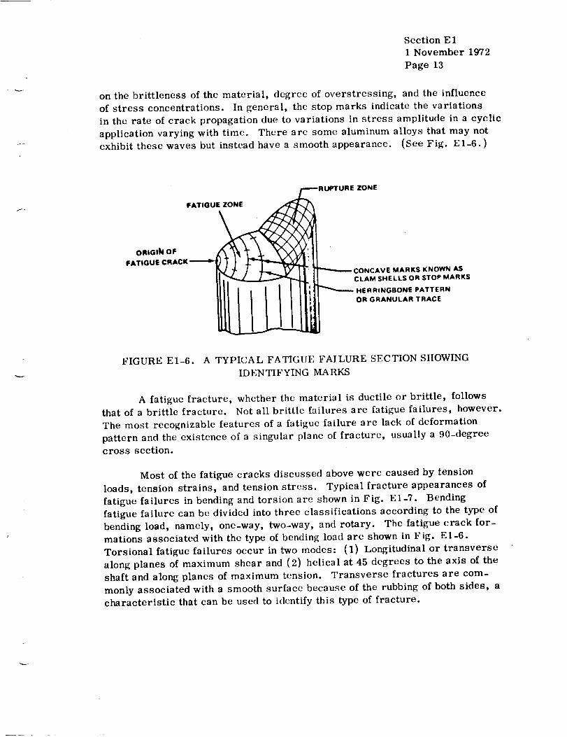
Section E 1
1 November 1972
Page 13
on the brittleness of the material, degree of overstressing, and the influence
of stress concentrations. In general, the stop marks indicate the variations
in the rate of crack propagation due to variations in stress amplitude in a cyclic
application varying with time. There arc some aluminum alloys that may not
exhibit these waves but instead have a smooth appearance. (See Fig. El-6.)
__RUPTURE ZONE
FATIGUE_ORIGI_4 OF _.
FATIGUE CRACK--_ 7_ / ./._k_ V if: |/_....._._CONC:AVEMARKSKNOWNAS
CLAM SHELLS OR STOP MARKS
HERRINGBONE PATTERN
OR GRANULAR TRACE
/
FIGURE El-6. A TYPICAL FATIGUE FAILURE SECTION SHOWING
IDENTIFYING MARKS
A fatigue fracture, whether the material is ductile or brittle, follows
that of a brittle fracture. Not all brittle failures are fatigue failures, however.
The most recognizable features of a fatigue failure are lack of deformation
pattern and the existence of a singular plane of fracture, usually a 90-degree
cross section.
Most of the fatigue cracks discussed above were caused by tension
loads, tension strains, and tension stress. Typical fracture appearances of
fatigue failures in bending and torsion are shown in Fig. El-7. Bending
fatigue failure can be divided into three classifications according to the type of
bending load, namely, one-way, two-way, and rotary. The fatigue crack for-
mations associated with the type of bending load are shown in Fig. El-6.
Torsional fatigue failures occur in two modes: (1) Longitudinal or transverse
along planes of maximum shear and (2) helical at 45 degrees to the axis of the
shaft and along planes of maximum tension. Transverse fractures are com-
monly associated with a smooth surface because of the rubbing of both sides, a
characteristic that can be used to identify this type of fracture.

Section E11 November 1972Page 14
0Z
7_
r.D
o
,<
0
L£r.J
[..,
i-!
0
o
m m
m _
.._ q)
0 _°_
" 00
r.)
_ o
/
©r-
./ 0
,-1bO
t_
I
0
3b_¢-
"D
!
o
.:.:./..:.
0
,.a
_ o
e.,

Section E1
1 November 1972
Page 15
However, a statement of the signs and features of fatigue fractures does
not explain the true nature of the physical changes which take place inside
metals under cyclical stress to cause their breakdown.
To understand these changes, it is necessary to study the internal
mechanism of fatigue behavior in the whole volume of the metal; but this sub-
ject has yet to be thoroughly investigated. A considerable amount of theory
has been written about fatigue fracture, and there are many interpretations as
to the process of metal fatigue. (See Rcf. 1.)
Fatigue is basically a property of crystalline solids, and the initiation
of fatigue cracking is a problem in dislocation physics. It is the result of the
motion and interaction of dislocations activated by cyclic stress. A simple
description of the mechanism of fatigue cracking is given in three stages:
Stage 1. During the early cycles of stressing, the dislocations orig-
inally present in the crystal grains multiply and their density increases sharply.
An irregular and disoriented cell wall, or subgrain boundary, starts to form.
The fine slip lines that appear at first in some favorably oriented grains are
thin and faint, according to the maximum resolved shear stress law. As the
number of stress cycles increases, slip lines become more numerous. Some
are localized, some continuously broaden, and the very pronounced ones
become the so-called persistent slip bands. Meanwhile, the crystals are dis-
torted and strain-hardened to saturation. Then, dislocation motion in one
direction may be fully reversed with the stress. New dislocations and their
movements are generated only in some local slip zones in which microstruc-tural features are not the same in both directions of motion. Sometimes
annihilation of dislocations, or other dislocation mechanisms, may lead to
relief of lattice strains or strain softening. Strain softening, local recrystalli-
zation, overaging, clustering of point defects, and other thermal activation
processes are considered to be secondary, or side effects.
Stage 2. After the persistent slip bands are fully matured, thin ribbon-
like protrusions, called extrusions, of metal are emitted from the free sur-
face, and fissures, called intrusions, appear. Both develop along the per-
sistcnt slip planes. Several dislocation models or mechanisms have been
proposed to explain how the extrusions and intrusions are formed. (See Ref.
1.) In some of the proposed models, dislocation cross slip is considered to
be a critical process.
Because the intrusion is the embryo of a crack, the crack initiates
along slip planes according to the maximum resolved shear. Sometimes cracks

Section E 1
1 November 1972
Page 16
may initiate at cell walls or grain boundaries, although the majority start at
the surface of a member.
Stage 3. The crack propagates in a zigzag4 transgranular path along
slip planes andeleava_e planes, from grain to grain, and maintains a general
direction perpendicular tothc maximum tensile stress. As much as 99 per-
cent of the fatigue lift; of a member is spent in the development of fissures into
microscopic cracks, and finally complete fracture ensues. Many factors
affcetin,_ fatigue properties arc those that mainly influence the rate of crack
propagation.
1. '2.2 I,'ati_ue Testing Techniques.
The only way to obtain a quantitative m|:asure of fati_4ue strength is to
carry out fatigue tests under controlled conditions. Thert, ar(, many different
methods of carrying out such tests, and numerous types of testing equipment
have b,,en developed.
Probably the most widely used method is the rotating bending test, in
which small cylindrical specimens, with or without notche,_;, are loaded either
as ('antilevt'rs or as beams under four-point loading. As the specimen is
rotated, the strc'ss at any point in it varies between upper and lower limits
which arc equal in magnitude, but opposite in siKn, the plane and direction of
the loads remaining constant throughout. A possible arranKement of such a test
is shown diagran_matieally in Fig. El-8. This type o[ test is simple to carry
out, generates results comparatively rapidly and mak[,s use of equipment and
sl)e('inlt_rls that are reasonably int;xpensive. It is particularly suitable for use
in detc'rmining what might be called the inherent fati_/ue strength of materials,
CYCLECOUNT E R
MOTORFLEXIBLE -,,,-7 MAIN
k., L
1
3
FIGURI': I.:! --8. GI,:NEtLAL ARRANGEMENT OF ROTATING I_ENDING
(CANTILEVEII TYPE) FATIGUE-TESTING MACIIINE
Section E 1
1 November 1972
Page 17
since in such work one is interested in the material itself,i.e., itscomposi-
tion, microstructure, etc., rather than its form in the engineering sense.
However, to provide data for design purposes, such tcsts are not of
great value since designs can rarely, if ever, be reduced to such a degree of
simplicity that it is necessary to know only the basic fatigue strength of the
material. To provide specific information for the designer, tests must be
carried out on the actual joint forms. This is true of structures fabricated by
any means, but is particularly relevant in the case of welding. The welding
process cannot satisfactorily be scaled down without simultaneously alteringsome of its effects.
Therefore, fatigue testing of welded components normally involves the
use of equipment of much larger capacity than that used for fundamental inves-
tigation. The method of loading is also different, the objective being at all
times to reproduce as faithfully as possible the type of loading that is likely to
occur in service. With this end in view, the loading conditions used in the
fatigue testing of welded joints and structures can be reduced essentially to
three types:
1. Axial load testing
2. Tests in bending, mainly on specimens in the form of beams
3. Pulsating pressure testing of pressure vessels and pipework.
All the numerous testing machines that are available and suitable for
carrying out such tests will not be described here in detail, but itmay be useful
to describe some of the essential features since, to some extent, the charac-
teristics of fatigue-testing machines have influenced the research work thathas been carried out.
Axial load fatigue-testing machines may be divided essentially into
three types according to the method by which they are driven, i.e., hydraul-
ically, mechanically, or electromagnetically. Hydraulic machines which give
higher loads than those operated either mechanically or electromagnetically
are available, but testing speeds are limited.
A mechanically opcrated machine which has been used extcnsively in
fatigue testing of welded components is the walking beam machine, first devel-
oped in the United States at the University of Illinois. The arrangement of this
machine is shown diagrammatically in Fig. El-9. It consists of a simple lever
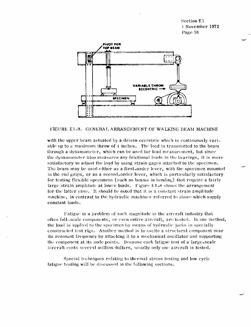
Section E 1
1 November 1972
Page 18
I I JA
I I _ ICC_NTmC--..,,- _
FIGURE El-9. GENERAL ARRANGEMENT OF WALKING BEAM MACtlINE
with the upper beam actuated by a driven eccentric which is continuously vari-
able uptoa maximum throw of 4 inches. The load is transmitted to the beam
through a dynamom(_ter, which can 1)o us('d for load n_('asurcment, but since
the dynan)onleter also measures any frictional loads in the bearings, it is more
satisfactory to adjust the load by using strain gages attached to the specimen.
The beam may be used either as a first-order lever, with the specimen mounte(l
in the end grips, or as a second-order lever, which is particularly satisfactory
for testing flexible specimens (such as beams in bending) that require a fairly
large strain amplitude at lower loads. Figure !.:1-8 shows the arrangement
for the latter case. It should be noted that it is a constant strain amplitude
machine, in contrast to the hydrauli(, machines referred t() above which supply
constant loads.
Fatigue is a problem ()f such magnitude in the aircraft industry that
often full-scale components, or even entire aircraft, are tested. In one method,
the load is appli('d to the sp(_'cimen by means of hydrauli(, jacks in specially
constructe(I t(_st rigs. Anoth(,r method is to excite, a structuraleomponcnt near
its resonant frequency by attaching it to a mechanical oscillator and supporting
the: compon('nt at its node points. B('cause each fatigue text of a large-scale
aircraft costs several million dollars, usually only on(' aircraft is tested.
Special techniques relating to thermal stress testing and low cycle
fatigue testing will l)e discussed in the following sections.

f/
Section E1
1 November 1972
Page 19
1.2. ? P resentation of Test Results.
1.2.5.1 S-N Diagrams.
Since the beginning of fatigue testing, S-N curves have been the back-
bone of fatigue data. S denotes stress amplitude or the maximum cyclic stress,
and N denotes the number of stress cycles to complete fracture. The linear S
versus log N scale is the most common and is used almost exclusively in engi-
neering. (See Fig. El-10.)
I4OOOO
|
Io I
10
m
m
I ,, I l -
10 2 10 3 10 4 10 5
NUMBER OF STRESS CYCLES TO FAILURE (LOG SCALE)
FIGURE El-10. GENERAL FORM OF S-N CURVE
Several attempts have been made to find general mathematical laws for
the relation between load and life, and several equations have been proposed to
express the S-N relations more or less empirically. Use of these equations
will embody the data in a mathematical form for data reduction, analysis, and
standardization of curve-fitting methods. It may also provide some under-
standing of the S-N relations.
For certain metals and alloys, including the ferrous group, the S-N
curve becomes asymptotic to a horizontal line. The stress value corresponding

Section E I
1 November 1972
Page 20
to this asymptote, or the stress corresponding to failure at an infinite number
of cycles, is called the fatigue (or endurance) limit.
The fatigue limit of a material teste, l in axial loading is usually lower
than that of the same material tested in reverse (rotating) bending. In axial
loading the stress is uniform throughout the cross sectmn; whereas, a large
stress gradient exists whena bending load is applied. Thus, in axial loading,
it is probable that the maximum stress will occur at a discontinuity in the
material. Fatigue tests in torsion or shear loading indicate that the torsional
fatigue limit of polished steel specimens is approximately 58 percent of the
flt,xural or tensile fatigue limit. This figure is consistent with the distortion-
energy theory which predicts that the shear properties of steels are 57.7 per-
cent of tensile properties.
1.2.3.2 Goodman Diagrams.
The prct'eding discussion on S-N curves and fatigue limits has dealt
with stress cycles that alternated about a zero mean stress. But the str('ss
cycle usually varies about a mean static value that may be positive, zero, or
negative. Whena cyclic stress varies about a nonzero:etatie value, prediction
of failure must consider the combination of static and varying stresses.
Several types of failure diagrams relate the range of operating stress
to the material properties ina general manner. All the diagrams indicate that
the allowable stress range decreases as the mean stress approaches some
maximum value.
The Goodman diagram was the first type proposed, and the modified
Goodman diagram is the [orm most commonly used. Because it consists of
straight lines, it is easy to construct. The Goodman equation is
a e (y
where S is the fatigue strength in terms of the stress amplitude, S isa m
the superimposed mcanstress, S is the endurance limit when S = 0, ande m
T is the ultimate tensile strength. This equation is plotted in Fig. EI-ll.

Section E 1
1 November 1972
Page 21
8 I
0S T.S.
RI
FIGURE El-If. GOODMAN DIAGRAM
In the modified Goodman failure diagrams (Fig. El-12), the range of
operating stresses is described by three values: mean stress, maximum
stress, and minimum stress.
I \..-,.o \ .,o_ ...___I
i "0
.60 -40 -30 -20 -10 0 10 20 30 40 60 60
MINIMUM STR ESS.ksi
FIGURE El-12. MODIFIED GOODMAN DIAGRAM

Section E 1
1 November 1972
Page 22
In the maximum-minimum form of motlified Goodman diagram, a stress
cycle is plotted as a point on the diagram instead of as a lint;. This form of
diagram is advantageous for it requires only the determination of the maximum
values of a half cycle; finding the mean cycle is not required.
In the maximum-minimum form of diagram, a stress cycle in which
stress is zero is plotted as a point on the line of zero mean stress. Similarly,
a stress cycle from zero stress to a tensile value is plotted as a point on the
maximum stress axis. Although these points have different mean stress values,
they represent equivalent reversed stress cycles. In this form of diagram, the
fatigue limit for reversed stress is plotted as a line of constant equivalent
reversed stress instead of being a point as in the other forms of failure
diagrams.
Section E 1
1 November 1972
Page 23
1.3 FACTORS INFLUENCING FATIGUE STRENGTH.
Fatigue properties obtained from a carefully polished specimen in the
ideal environment of the test laboratory are rarely achieved in practice. A
wide variety of factors affect the behavior of a member or assembly under
conditions of fatigue loading. The most obvious parameters are those that deal
with the sign, magnitude, and frequency of loading; the geometry and material
strength level of the structure, and the ambient service temperature. Those
processing and metallurgical factors that determine the cleanness and homo-
geneity of materials, the sign and distribution of residual stresses, and the
surface finish often are not considered. These processing and metallurgical
factors, however, may have an overriding influence on the fatigue performance
of the structure, to its benefit or detriment. The factors which influence
fatigue strength will be classified into four main groups for discussion in thissection:
1. Metallurgical Factors
2. Processing Factors
3. Environmental Factors
4. Design Factors
1.3.1 Metallurgical Factors.
The distinction between processing factors and metallurgical factors
is not always clear. In fact, it is rather arbitrary in some areas. In this
section, however, the focus is on regions within the material, either at the
surface or core, which adversely affect fatigue properties. These regions may
arise from melting practices or primary or secondary working of the material,
or may be characteristic of a particular alloy system. In nearly every instance
the detriment to fatigue properties results from a local stress-raising effect.
1.3.1.1 Surface Defects.
Primary and secondary working are often responsible for a variety of
surface defects that occur during the hot plasticworking of material when lap-
ping, folding, or turbulent flow is experienced. The resultant surface defects
bear such names as laps, seams, cold shuts, or metal flow through. Similar
defects are also noted in cold working, such as filletand thread rolling, in
which the terms lap and crest cracks apply. Other surface defects develop

Section E 1
1 November 1972
Pagt, 24
from the (,mbe(Iding o1 foreign luaterial under high pr('ssures during the
working process. Oxides, slivers, or chips ofthebase matt, rialare occa-
sionally roiled or forged into the surface. The surface defects in castings
might include entrapped die material, porosity, or shrinkage; in the extrusion
or drawing processes such surface defects as tears and seams are not
uncommon.
A 11 of the aforementioned surface defects produce a notch of varying
intensity which acts as a §tress-raiser under load to the detriment of fatigue
properties. Because most of these defects are present prior to final processing
and arc open to the surface, standard nondestructive testing procedures such
as penetrant and magnetic particle inspection will readily reveal thcir pres-
ence. If they are not detected, however, the defects may serve as a site for
corrosion or crack initiations during processing (in heat treating, cleaning,
etc. ), further compounding the deleterious effect on fatigue strength.
1.3.1.2 Subsurface and Core Defects, Inhomogeneity, and Anisotropy.
Subsurface and core defects considered here are those which originate
in the as-cast ingot. Voids resulting from gas entrapment (porosity) and
improper metal fill (shrinkage) arc not uncommon in cast materials. In
castings (ingots)that are to be subsequently hot and cold reduced, the portion
of the ingot containing the preponderance of voids is often removed and dis-
carded. The remaining internal defects normally weld shut under the combi-
nation of temperature and pressure involved in the reduction of the ingot,
resulting in a continuous, homogeneous product. Occasionally, when the sur-
faces of the defects are oxidized or otherwise contaminated, healing (welding)
of the opposite surfaces is precluded and the defective area is retained in the
wrought product. Terms such as unhealed porosity and laminations arc applied
to this condition. Since these defects existed before working, in the final
wrought product the major diameter of the oblate or rod-shaped flaw is parallel
with the direction of plastic deformation.
I.'atigue testing of high-strength ah, minum alloy specimens containing
defects of the type discussed in this section revealed the following trends:
I . Stressing parallel to the defect plane has a small effe('t on the
fatigue strength, provided the defect does not intersect a freesurface.
2. The effect of defect size on the fatigue strength in the short trans-
verse direction of testing (that is, _ith the plane of the grain flow
normaltothe direction of loading) is shown in Fig. E1-13.
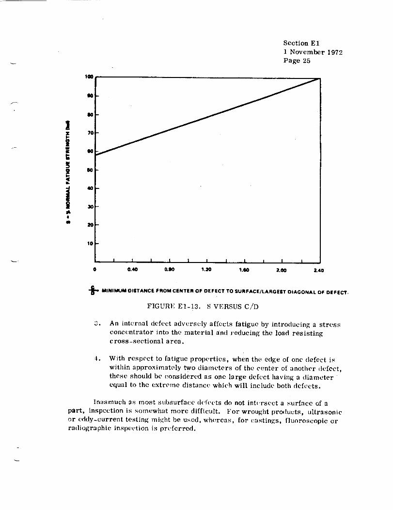
F ¸
IM
Section E 1
1 November 1972
Page 25
N
3o
|
g
10
i I I I i A I I I I I
0._ 0._ 1._ 1._ 2,_ 2.40
"_ MINIMUM OISTANCE FROM CENTER OF DEFECT TO SURFACE/LARGEST OIAGONAL OF DEFECT,
FIGURE E1-13. S VERSUS C/D
3.
.
An internal defect adversely affects fatigue by introducing a stress
concentrator into the material and reducing the load resisting
cross-sectional area.
With respect to fatigue properties, when the edge of one defect is
within approximately two diameters of the center of another defect,
these should be considered as one large defect having a diameter
equal to the extreme distance which will include both defects.
Inasmuch as most stLbsurface d('t'ccts do not int('rsect a surface of a
part, inspection is somewhat morc difficult. For wrought pro(Ita-ts, ultrasonic
or eddy-current testing might be used, whereas, for castings, fluoroscopic or
radiographic inspection is preferred.
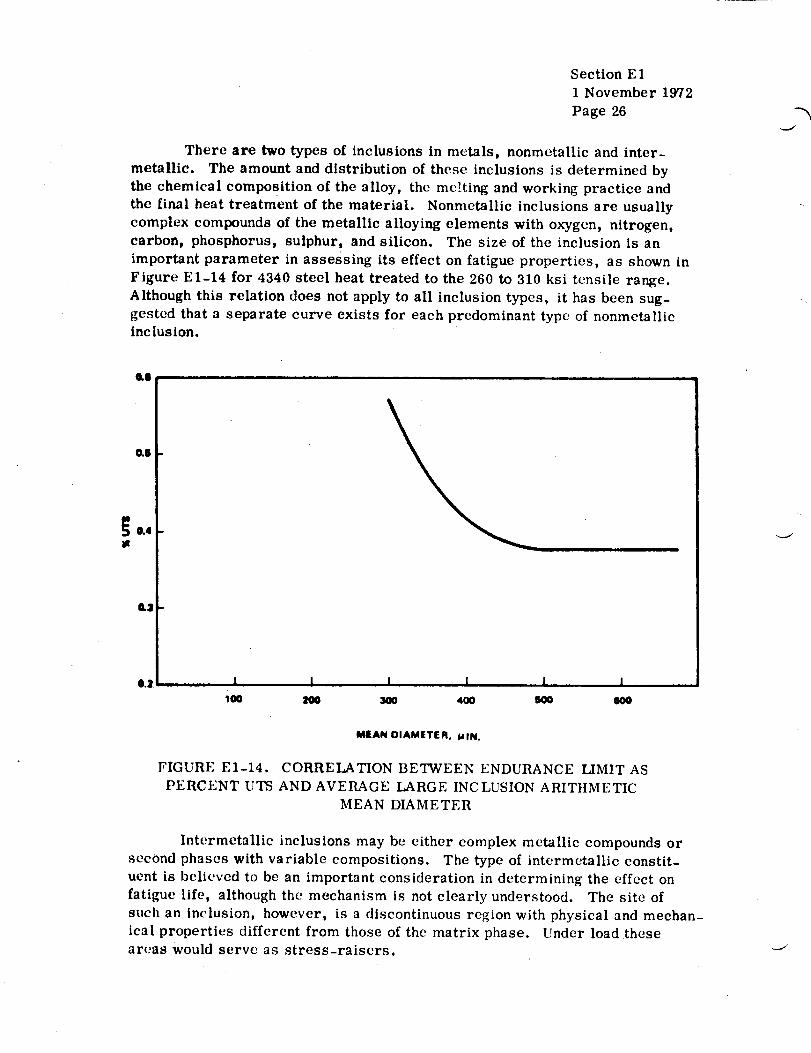
Section E 1
1 November 1972
Page 26
There are two types of inclusions in metals, nonmetallic and inter-
metallic. The amount and distribution of these inclusions is determined by
the chemical composition of the alloy, the melting and working practice and
the final heat treatment of the material. Nonmetallic inclusions are usually
complex compounds of the metallic alloying elements with oxygen, nitrogen,carbon, phosphorus, sulphur, and silicon. The size of the inclusion is an
important parameter in assessing its effect on fatigue properties, as shown in
Figure E1-14 for 4340 steel heat treated to the 260 to 310 ksi tensile range.
Although this relation does not apply to all inclusion types, it has been sug-
gested that a separate curve exists for each predominant type of nonmetallicinclusion.
_e
o.B
L2
I I I I I I
loo 2OO 3oo 4oo 640o qlO0
MEAN DIAMETER. 14IN.
FIGURE E1-14. CORRELATION BETWEEN ENDURANCE LIMIT AS
PERCENT UTS AND AVERAGE LARGE INCLUSION ARITHMETIC
MEAN DIAMETER
Intermetallic inclusions may be either complex metallic compounds or
second phases with variable compositions. The type of intermetallic constit-
uent is believed to be an important consideration in determining the effect on
fatigue life, although the mechanism is not clearly understood. The site of
such an inclusion, however, is a discontinuous region with physical and mechan-
ical properties different from those of the matrix phase. Under load theseareas would serve as stress-raisers.

Section E 1
1 November 1972
Page 27
Some alloy._ ar(: subject to miero._tructural banding which often has
an adverse effect on [atiguc properties. The banding is usually prc_luced by
local chemical segregration which stabilizes a phase not normally present in
the alloy at room temperature. The severity of the loss in fatigue properties
is dependent on the direction of the banding relative to the maximum stress
direction (the banding is always in the direction of prior working) and on the
degree of compatibility between the banded and matrix phases. Banded
retained austenite and delta ferrite are occasionally seen in a large number of
low-alloy and stainless steels. The presence of ferrite in these is intentional;
in others it is not. The loss in fatigue properties produced by ferrite stringers
in 431 stainless steel is shown in Fig. E1-15.
lm
m
N-
Jmte'
| !
I I L
1os TolCYCLE| TO FAILURE
dlkV
I0 T
FIGURE El-15. NOTCHED FATIGUE STRENGTH OF 431 STAINLESS
STEEL HEAT-TREATED TO THE 180 to 200 ksi RANGE WITH NO
FERRITE AND WITH 5 PERCENT FERRITE
k
Section E 1
1 November 1972
Page 28
Finally, the grain and subgrain structure may also reflect a preferen-
tial alignment. As previoiasly indicated, aniqotropy is most pronounced in the
short transverse grain direction. It has been shown in tests on 7075-T6 alumi-
num alloy forgings that the endurance limit is reduced by approximately 20
percent when testing in the short transverse direction as opposed to the longi-
tudinal direction.
For many material forms such as sheet, light plate, and extrusion, the
loading normal to the short transverse direction is low such that fatigue pro-
perties in this direction are not critical. For heavy plate, bar, and forgings,
however, directionality or anisotropy can be a crucial design consideration.
1.3.1.3 Heat Treatment.
The heat-treatment processes are potentially a source of hazard to a
i material because at the elevated temperatures encountered many diffusion con-
_trolled mechanisms arc operative that could harm the integrity of the alloy if
not properly controlled. If the furnace atmosphere is not controlled, the
chemical composition of the surface layer might be altered and, thus, produce
a low strength or brittle surface skin. The diffusion of hydrogen into alloys
during heat treatment has long been recognized as a serious problem. Hydro-gen embrittlement of low-alloy steels and titanium alloys can produce disas-
trous results in subsequent processing or in service. Hydrogen is also sus-
pect in the blistering mechanism in aluminum alloys. With respect specifi-
cally to fatigue properties, a brittle case will render an alloy susceptible to
surface cracking. The introduction of a shallow crack produces a notch effect,
so that the detriment to fatigue (life) is essentially one of a high surface
stress raiser in a layer of material with low fracture toughness.
If the heat-treating temperature is not properly controlled, grain
coarsening may occur which lowers fatigue properties of some alloys. Over-
heating of high-strength aluminum alloys is particularly disastrous, since
most of these alloys are subject to eutectic melting at temperatures only
marginally higher than the solution heat treatment temperature. Eutectic
molting results in a gross embrittlement of the alloy coupled with reduction in
_trength. The difficulties with austcnitizing or solution heat treating at too low
a temperature are associated with a lack of hardening potential for the sub-
sequent quench and age or temper treatments.
In order to develop full strength, most martensitic and age hardening
alloys must be rapidly cooled from high temperatures by quenching into a
liquid medium. There are at least two considerations in the quenching process
Section E11 November 1972Page 29
that could affect fatigue prol)erties, lligh residual quenchstresses are builtup in most materials and, if the geometry of the part bt_ing quenched is highly
irregular, the tensile strength of the material may be exceeded at points of
high stresses resulting in the not too uncommon quench cracks. On'the other
hand, if the quenching rate is for some reason retarded, preferential precipita-
tion may occur which adversely affects fatigue properties.
1.3.1.4 Localized Overheating.
There are some processes that are capable of developing high, localized
surface temperatures, the consequences of which are often difficult to detect and
occasionally are responsible for a failure in service. Grinding is one of these
processes.
The effect of severe grinding on the fatigue properties of high-strength
steel is shown in Fig. El-16. The rapid quenching of the material immediately
below the grinding wheel by the large mass of cold metal can produce cracks.
If actual cracking does not result, brittle, crack-prone, untempered martensite
might result or, with lower temperatures, softened, overtempered martensite.
High-strength steels (for which grinding is most often used) are particularly
sensitive to grinding techniques.
In the electroplating processes a plating burn sometimes is observed
as the result of arcing between the anode and the work piece. Such a burn
generally produces a larger heat-affected zone than improper grinding and is
often characterized by evidence of surface melting. The potential damage to
the substrate is similar to that discussed relative to grinding.
Electrical discharge machining (EDM) is a process of metal removal
that employs a spark-erosion principle. The intermittent spark produces
highly localized melting on the surface of the workpiecc and metal fragments
which are swept away by the dielectric coolant. Although the heat-affected
zone is shallow, surface cracking and untempered martensite are sometimes
observed on martensitic alloys along with eutcctie melting and other evidences
of overheating in aluminum alloys if the process is not properly controlled.
1.3.1.5 Corrosion Fatigue.
Corrosion fatigue is that peculiar interaction of a corrosive environ-
ment with an alternating stress field which causes accelerated crack initiation
and propagation, possibly where neither the environment nor the stress acting
alone would be sufficient to produce a crack. In the practical application of the
term, the corrosive environment usually serves to introduce stress raisers

i
t
Section E 1
1 November 1972
Page 30
1 I I I
It 8 II Ii
!81"Nlltii ImNnil_
©
e,D
.<,
e/3
Z
-...._eo m-I " _ >
-1 _ zm _
5
• ©
_ m
:5
I
I
M

_,.-.-r._,,,;_. PAGE ],_
OF POOR QLIAUTYSection E 1
1 November 1972
Page 31
in the surface in the form of corrosive attack. The irregular surface, in turn,
is detrimental to the fatigue properties of the part in a mechanical or geometric
sense. For materials susceptible to embrittlement by hydrogen or for parts
which are exposed to a fairly continuous corrosive environment with intermit-
tent applications of loading, the cicacking mechanism may be somewhat more
complex. An example of corrosion fatigue testing is presented in Fig. E1-17,
which illustrates the effect of a corrosive test environment on the fatigue pro-pcrties of precipitation-hardened stainless steels.
140
Im
lm
110
W
%
• • I l | • I J| | i I I I L I A i
\\
I l t J t Jl|
CYCLI[8 TO PAILUNIE
FIGURE E1-17. CORROSION FATIGUE AND AIR FATIGUE S-N CURVES
FOR PRECIPITATION HARDENING STAINLESS STEEL TESTED AT
ROOM TEMPERA TURE
1,/

Section E 1
1 November 1972
Page 32
1.3.1.6 Fretting Corrosion.
The fretting corrosion phenomem,n has been defined as that form of
damage that arises when two surfaces in contact and normally at rest undergo
relative periodic motion. In vacuum or inert atmospheres the process is
eomplett'ly mechanical, but in ordinary atmospheres oxidation is also involved.
Fretting is potentially dangerous because it can result from extremely small
surface monuments that often cannot be anticipated or even prevented. Motionswith amplitudes as low as 5 × 10⁻⁹ inch are sufficient for this mechanism to be
operatiw'.
Soft metals exhibit a higher susceptibility to fretting fatigue than hard
metals. Fretting corrosion increases with load-amplitude, number of load
cycles, contact pressure, and an increase of oxygen in the environment. The
oxidized particles that accumulate between the fretting surfaces lead to both
chemical and mechanical surface disintegrations which generate nuclei for
fatigue crack initiation. The presence of fretting may reduce fatigue strength
by 25 to 30 percent, (tependin._ on loading conditions. When a part or assembly
is known to be critical in fretting, one or a combination of the following factors
will be b('neficial in reducing or eliminating fretting corrosion:
1. l':lectroplating critical surfaces.
2. Case-hardening w(,aring surfaces.
3. Lubricating.
4. l.:liminating or dampening vibration.
5. Increasing fastener load or closeness of fit.
_;. Bonding elastic material to surface.
7. l':xcluding atmosphere.
I .3.1.7 Reworkin_.
'l'h,. success of any repair or rework procedure ix necessarily closely
(l¢'pend_'nt cm the analysis of the degrading mechanism. Only with a proper
_mderstanding of the cause of failure can a satisfactory permanent r_'work be
_l_'COmldishe, I. In the area of service damage caused b3 fatigue, in-service
failure, ,,rengineering test failure of a part usually provides tht: impetus to
-N
Section E 1
1 November 1972
Page 33
rework procedures. In general, these procedures can be separated into two
categories: those parts that contain actual cracks and those that are believed
to have undergone fatigue damage.
Usually, cracked structural parts are scrapped and replaced with a new
part. Occasionally, however, because of the location of the crack or other
circumstances, such a part is repaired. Repair would consist of removing the
crack or blunting its root and supporting or strengthening the damaged area
by means of doublers, straps, etc. Care must be taken in doubler design so
that new sites of fatigue cracking are avoided. Factors such as fretting cor-
rosion, dissimilar metal corrosion, detrimental stress redistribution, access,
and practicality are prime considerations in establishing such a rework method.
Procedures frequently used to remove minor stress concentrators are
those such as increasing a sharp edge, corner, or fillet radius, and grinding
or buffing out coarse tool marks, nicks, and scratches. If assembly stressesare high, a joint having mismatched surfaces might be planed or mechanically
realigned, or improved clearance could be provided. When fretting is contrib-
uting to fatigue cracking, a wear strip or lubricant may be inserted between the
working surfaces, or the fasteners may be tightened to reduce or eliminate
motion. Residual compressive stresses are often introduced into the critical
areas of fatigue by shot peening or coining operations.
Estimating the depth of fatigue damage on a surface or below the tip of
a fatigue crack is difficult and should be experimentally determined for all
alloy-forming-heat,treating conditions and the load spectrum. Preliminary
data indicate that the dcpth of fatigue damage beneath cracks for 7()75-T6
aluminum alloy is approximately 0. 003 inch. However, for high strength steel
it may be many times greater than 0.003 inch.
1.3.2 Processing Factors.
Fatigue usually initiates at a surface because stresses are normally
higher there, particularly since most parts undergo ben[ling loads resulting in
substantially higher stresses in the outermost fibers. The detrimental (or
beneficial) effect of processing on fatigue properties is usually manifest in its
effect on the strength level or resi, lual stress condition, or both, of the surface
ma te r ia 1.
1. "3.2.1 tlardness.
Str_'ngth of metals commonly us,.'d for enlzincering purposes is generally
high_,r with increased hardness, up to a point. In steel, for example, inereas(xl

Section E1
1 November 1972
Page 34
hardness does not necessarily indicate a higher fatigue limit because the
fatigue limit is also affected by the surface finish. Curves of average fatigue
limit values for a range of surface finishes are shown in Fig. El-18. Because
these curves represent average values, allowance should be made for size
effect (larger size generally means lower fatigue limit).
HAMONEll
ROCKWELL C 0 10 30 26 30 36 4O 4S 150
IIMIIMELL 100 100 240 280 3,?0 310 400 440 4410
100 1
POLl HED /"
•J .,, _LLED:--I
26 . -,OROEO SOR,ACE,.U,ERL,,,T•"FORGED SURFACES, LOWER LIM, T
o J I i
M tN 126 1_ 1_ 1N 200 2_ 34O
TENSILE STRENGTH (1031hi|
FIGURE E1-18. EFFECT OF HARDNESS AND SURFACE FINISH ON
FATIGUE LIMIT OF STEEL IN REVERSED BENDING
( 0.3-INCH-DIAM ETER SPECIMEN)
1.3.2.2 Forming.
By definition, the forming process produces plastic deformation (and
residual stresses) ina part to achieve a permanent change in configuration.
Occasionally these residual stresses may prove beneficial; howew'r, usually
there is some loss in fatigue life. Consequently, the residual stresses pro-
duced in forming (and their effect on fatigue) often dictate the forming limitsfor materia Is.

Section E11 November 1972Page 35
Residual forming stresses in th(_' ('ompl('tcd part at'(' (l(,i)endent on at
least three additional factors: The hcat-treatm('nt-forming sequence in proc-
essing, the temper of the material, and tile forming teml)eraturc. Parts formed
and subsequently completely heat treated arc free of prior forming stresses.
Parts formed and stress relieved contain reduced forming stresses, depending
upon the stress relieving temperature. The forming temperature and the mate-
rial temper, e.g., AQ, T-4, or T-6 for aluminum alloys, also influence the
magnitude of forming stresses to the extent that they affect the yield strength
of the material at the forming temperature. In general, the lower the yield
strength when forming occurs, the weaker the residual stress field generated.
1.3.2.3 Heat Treatment.
/
Residual stresses are both produced and relieved in many of the common
heat treat cycles for both ferrous and nonferrous alloys. The principal source
of residual stress occurs in quenching from high temperature solutioning oraustcnitizing treatments. Residual stresses are built up by nonuniform cool-
ing rates between surface and core. For aluminum alloys, differential coolingproduces residual surface compression and core tensile stresses. These sur-
face compressive stresses are of sufficient magnitude to produce slightlyhigher fatigue strengths.
Aging temperatures for aluminum alloys are too low to produce any
appreciable stress-relieving; however, most steels are tempered at tempera-
tures sufficiently high to affect residual quench stresses. Consequently, for
steels after tempering, quenching stresses are not recognized as a detrimental
factor. Quenching stresses in aluminum alloys, however, persist after com-
pletion of heat treatment, as indicated by distortion in machining, increased
susceptibility to stress corrosion and possible detrimental effects on fatigue
life. To minimize these effects in aluminum alloys, special processing
techniques have been developed, such as reducing section sizes by rough
machining before heat treatment, use of less severe quenches where possible,
and stress relief/equalization by cold working of quenched materials (for
example, stretch-stress relief tempers).
1.3.2.4 Surface Finish.
A given surface-finishing process influences the fatigue properties of a
part by affecting at least one of the following surface characteristics: smooth-
ness, residual stress level, and metallurgical structure. The effects of
surface finish on fatigue life for 7075-T6 extrusions are shown in Fig. El-19.
litre it can bc seen that, in general, fatigue life increases as the magnitude
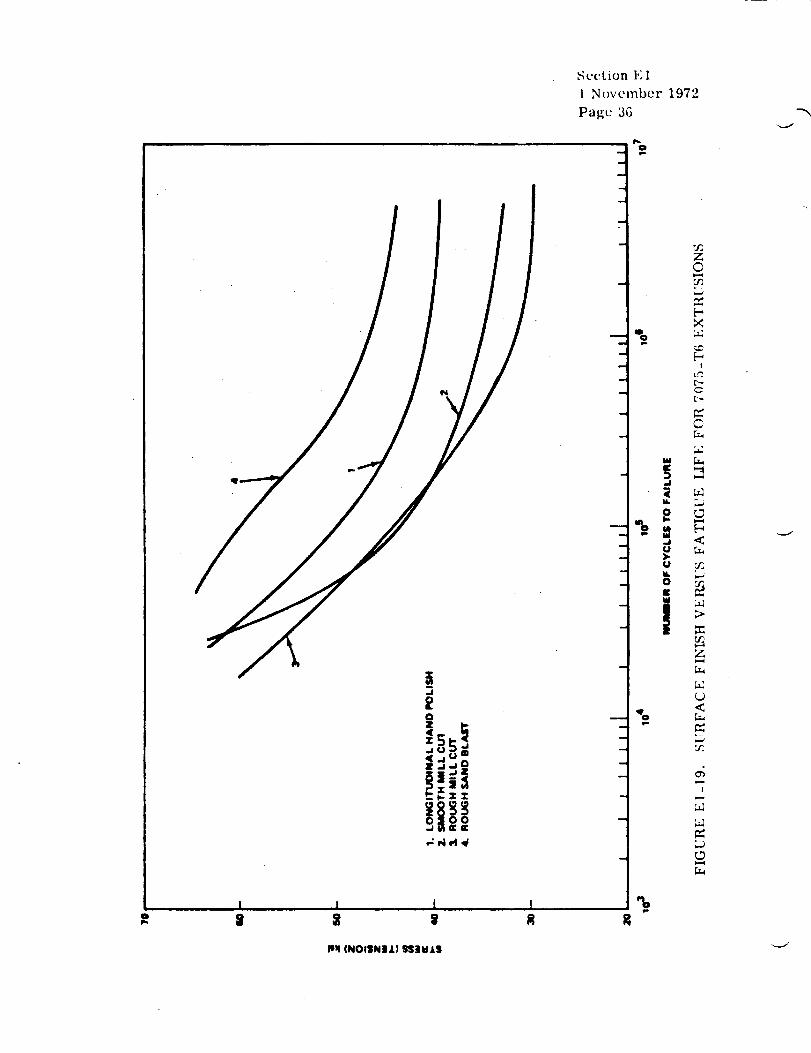
l ,1 J0
Section 1,:1
l November 1972
Page 36
l
O
m
N
u
Z©
,_a
[--,
- [..,-- t
u_
_ C"
[-..
©
- _ <
2:
<:
I
;D
%
IIM(NOIIN! 1} SS:IilJLI "_

Section E1
1 November 1972
Page 37
of surface roughness decreases. Decreasing surface roughness is seen as a
method of minimizing local stress raisers.
Aside from effect on surface roughness, the final surface finishing
process will be beneficial to fatigue life when it increases the depth and inten-
sity of the compressively stressed layer and detrimental when it decreases or
removes this desirable layer. Thus, sandblasting, glass-bead peening, and
other similar operations generally improve fatigue life properties. Conversely,
processes, such as electropolishing, chem-milling, and electrical-chemical
machining ( ECM), which rcmove metal without plastic deformation at the tool
point may reduce fatigue life properties.
Many local surface defects and irregularities occur in fabrication and
service that are difficult to anticipate, inspect for, or control. Stress con-
centrations resulting from small indentations on an otherwise smooth surface
in the form of accidental tool marks, grinding scratches, corrosion pits, or
service-related minor damage are occasionally as effective in reducing the
fatigue life of structural parts as large scale stress concentrations resulting
from design deficiencies, depending on the material, heat-treat range, design
margins, etc. Such unintentional stress-raiscrs are damaging in a structure
only if thcir notch effect is more severe than the most severe stress con-
centration arising from design, unless they are located so as to intensify the
stress-raising effect of the critical design feature. Usually the effect of
design stress concentrations far outweigh the effect produced by surface finish.
1.3.2.5 Cladding, Plating, Chemical Conversion Coatings, and Anodizing.
Clad sheets become progressively weaker than the bare sheets as the
lifetime increases, tlowever, the reduction in fatigue life for plain fatigue
specimens is not present to the same degree in built-up assemblies, where the
fabrication stress raisers overshadow the effect of claddding on fatigue strength.
Aluminum metal spraying is sometimes applied to extrusions and
forgings for added corrosion protection. The effect on fatigue properties is
quite similar to that observed for cladding. However, it has been found that
sprayed zinc finishes on aluminum alloys do not produce any measurable
reduction in fatigue life. Also, it is generally agreed that neither zinc nor
cadmium plating has any appreciable effect on fatigue properties.
Chemical conversion and anodic coatings which are applied to alumi-
num alloys for corrosion protection or wear resistance usually produce a
reduction in fatigue life ranging from a negligible amount up to 10 or 15 percent

Section E11 November 1972
Page 118
of the enduranc(_ limit. The methcxl of producing the coating further al[ects
fatigue properties. As an example, fatigue tests run on chromic acid anodized
7075-Tfi indicated that anodizing with a 5-percent dichromate seal offered a
slight but definite lowering in fatigue life as compared to that of unanc_lized
metal, whereas, a sulfuric type anodizing treatment resulted in a substantial
reduction in fatigue life as shown in Fig. E1-20.
E
Ie -
I. UNANOOI2ED2. SULFURIC ACID ANODIZED - BARE |DQEJI|. EULIFURIC ACID ANODIZED - ALL EURFACEII
I 1
FIGURE 1_:1-20. EFFECT OF SULFURIC ACID ANODIZE ON FATIGUE
PROPERTIES: 7075-T6 ALCLADSHEET 0.090IN. THICKNESS,R= +0.2
Fatigue tests of 7075-T6 bare sheet with an A lodine #1200 coating
show_.'d no loss in fatigue properties compared to untreated material.
Section E 1
1 November 1972
Page 39
1.3.2.6 C old Working.
Cold working of parts to induce residual surface compressive stresses
has been found to be an effective tool for improving the fatigue life of both
simple and complicated shapes. Methods of imparting cold work include
coining of holes, thread rolling, fillet rolling, peening, hole expansion, pre-
stressing, tumbling, and grit blasting.
It should be realized that residual surface compressive stresses are
most beneficial under loading conditions which produce high surface tensile
stresses, as in bending. Residual compressive stresses, however, are also
beneficial to the fatigue life of axially loaded specimens.
For the desirable effect of surface cold working to be maintained, the
cold-working process must be accomplished in the final heat-treated condition;
subsequent thermal treatment must be eliminated when feasible, but closelycontrolled when it i8 essential.
Perhaps the most widely used process for inducing residual compressive
stresses in surface material is shot peening. Its use is widespread because
of its low cost and relatively easy application to a wide variety of materials and
parts of varied size or configuration. As an example, peening might be used
before chrome plating or hard anodizing, or in special situations, after a heat
treatment which produced decarburization of a steel part.
When a part undergoes loads that are much higher in one direction than
in the opposite direction, prestresssing the part by applying an excessive load
in the direction of major service loading will often produce beneficial residual
surface compressive stresses and work hardening that will significantly improve
fatigue life properties. In reverse loading this effect is lost and a detriment
to fatigue life may result. In the aircraft industry, prestressing is often used
for torsion bars and bomb hooks, to name two examples. It has been shown
in some specimens that tensile prestressing to 90 percent of the tensile strength
increased the endurance limit about 100 percent.
Techniques involving other types of cold working can be found in Ref. 2.
1.3.3 Environment Effects.
The fatigue properties of a metal can be greatly influenced by the nature
of the environment, especially in long-time tests at low stresses and at low
frequencies. Even normal air has a deleterious effect on fatigue life properties,

Section E 1
1 November 1972
Page 40
and recent indications show that moisture and oxygen are the two print'ipal
adverse components. Moisture decreases the fatigue strength of copper,
aluminum, magnesium, and iron by 5 to 15 ;)erct'nt. An ('xample of the
influence of environmental air moisture on the fatigue properties of an
aluminum alloy is given in Fig. El-21.
l
44 i
I
i
al
i"
E
N
24
kit
lu'
i
-- _DllY INVINOfIMINT
- \
MILAN Ti[MIIL_ i[TR|m _
I[(_JAL C_I|.THIRO OF
IITREa AMPLITUOi.
, I J I ]10I 100 10)
CYCL|I TO FAILUlll
FIGURE E1-21. S-N CURVES FOR CLEAN SPECIMENS OF ALUMINUM
ALLOY 6060-T6 IN HIGH- AND LOW-HUMIDITY ENVIRONMENTS
It is generally agreed that the main effect of a normal atmosphere with
respect to fatigue life is on the propagation of cracks rather than in their

Section E 1
I November 1972
Page 41
initiation. The principal effect of the environment will be in its reaction to the
clean metal exposed at the tip of a fatigue crack. Cracks that would be of a
nonpropagativ.g vari,::tj in vacuum propagate in the presence of oxygen or mois-
ture; thereby, they lessen the fatigue resistance.
In environments that are more corrosive than air and that substantiallyreduce the resistance of the surface layers to fatigue crack initiation, both
initiation as vJc!l as propagation may be affected. Environments that lead to
stress-corrosion cracking may also adversely affect fatigue properties.
(Refer to Paragraph i. 3.1.5.)
1.3.3.1 irradiation.
Some investigations have been made with respect to the effect of nuclear
irradiation on mechanicaI fatigue properties of metals. Radiation-induced
changes are usually referred to as radiation damage since in many cases the
effects have been detrimental in one way or another. Damaging effects such as
loss in ductility have been noted for many metals. On the other hand, beneficial
effects evidenced increased yield and ultimate strengths, fatigue strength, and
surface hardening also have been noted. Rotating beam fatigue tests on 7075-T6 aluminum alloy (Ref. 3) indicate an improvement in life due to the effects
Gf a total integrated flux of 2 x 10¹⁸ fast neutrons per cm 2. Although the
amount of irradmtion received by the specimens in these tests is believed suf-
ficient to alter mechanical properties, it is not known if the results are signif-
icant for the characteristics of metals during the conjoint action of fatigue
straining and irradiation. Additional studies need to be undertaken for the
simultaneous action of irradiation and mechanical straining at low temperatures.
1.3.3.2 Vacuum.
It has been demonstrated experimentally that fatigue cracking under
uniaxial direct stressing of an aluminum alloy occurs in hard vacuum almost as
readily as within atmospheric pressure. This is contrary to general belief.
Experiments have disclosed trends toward increased crack growth rates in
vacuum which may eventually result in characteristics more critical than
growth rates obtained from in-air tests. Results on aluminum continuously
held in vacuum for periods greater than a week yielded drastic reductions in
fatigue properties. This strongly indicates the time dependency of the phenom-
enon. Results from short-time test exposures in vacuum have shown improved
properties. This is the usually accepted belief. However, for many cases an
extension of the vacuum outgassing time provides a more realistic environment
than do the short-time test exposures previously investigated. Because of this

Section E11November 1972Page 42
anomaly, prolonging the vacuum exposure is suggested as the only reliable
procedure at present for evaluating metals for service in space environment.
1.3.3,3 bleteoroid Damage.
In the environment of space, tiny meteoroids and micrometeoroids may
strike the surfaces of a space vehicle. At present, no information is available
as to this effect on fatigue properties. However, it can be reasoned that
indentations caused by these meteoroids provide ideal sites for the initiation of
fatigue cracks by reason of the increased stress concentration.
1.3.3.4 Solar Irradiation.
Solar irradiation will cause differential heating on orbiting spacecraft.
Over long periods of time, the thermal cycling and the resulting fatigue couldbecome a serious problem.
1.3.3.5 Temperature.
Elevated temperatures may cause metals to lose strength; low tem-
peratures may cause some metals to become notch sensitive and fail by brit-
tle fracture under load conditions that would be common at normal (standard)
temperature.
In general, the fatigue life of most metals will decrease with an
increase intempcrature (Fig. I':1-22). Studies have indicated that as the
temperature decreases, the crack nucleation period (or time to produce an
observable crack} increases. Moreover, as tt'mperaturedecreases, the'
I)eriod of observable fatigue crack growth decreases.
The rate of fatigue-crack propagation as affected by rate of cyclic
loading, and test-load frequency is an additional parameter to be considered.
In elevated-temperature fatigue testing, it is known that the number of cycles
to fracture decreases and the crack-growth rate increases as the speed or
frequency of cyclic loads is decreased. The damaging, thermally activated
mechanism of creep or creep cracking, acting conjointly with fatigue, is
responsible for this behavior. In general, this is true because, in the accu-
mulation of stress cycles, slower rates of load cycling result in exposure of
the metal to temperature for longer periods of time than do fast rates of load
cycling, tIowever, from cryogenic temperatures to room temperature, no
damaging, thermally activated mechanisms arc active. It is believed that
fatigue lives and crack-growth rates at cryogenic temperatures will be inde-
pendent of load frequency for most metals.

Section E11 November 1972Page 43
I
N, CYCI.EI TO FRACTURE
FIGURE E1-22. FATIGUE LIFE AS A FUNCTION OF TEST
TEMPERATURE (TkPICAL FOR MOST METALS)
Additional informatio_._ on thermal and creep effects will be given inParagraph 1.4.3.
1.3.4 Design Effects.
Manufactured parts often include abrupt changes in cross scction such
as grooves, fillcts, holes, and keyways; these cause a nonuniform distribution
of elastic strains and stresses. The maximum elastic stress at an abrupt
change in cross section is greater than the nominal stress obtained by calcula-
tion with either the direct stress, flexural, or torsional formulas.
Th,} geometric stress-concentration factor, K, is defined as the ratio
of the maximum stress in the section to the nominal, or average, stress.
Nominal stress is usually based on the net remaining section. Because of
exceptions, it is necessary to ascertain the basis upon which the nominal stress
is established before applying a stress concentration factor.
2'he full geometric stress-concentration factor is not always applicable
in fatigue loading. The actual fatigue limit of a notched member is frequentlyhigher than would be expected from the geometric stress-concentration factor.
This phenomenon is called notch sensitivity. Use of the notch-sensitivityfactor results in a fatigue stress-concentration factor that is determined from:

Sectioa E11 November 1972Page 44
.K 1" q (K t-t)+l •. '); . .
where Kf is the fatigue stress-concentratioa factor for direct tension or
bending; K t is the geometric stress concentration factor for direct tension, or
modified geometric stress-concentration factor for bending (Ref. 4) ; and q
is the notch sensitivity. Typical values of q versus notch radius for steels
of various strengths are shown in Fig. E1-23.
f
J
U
NOTCH IIIAOIU$. r |i_.)
FIGURE E1-23. NOTCH-SENSITIVITY CURVES FOR POLISHED STEEL
SPECIMENS OF VARIOUS STRENGTHS
The fatigue-stress concentration factor, Kf, represents the extent
to which a notch can be expected actually to reduce the fatigue limit of a part.
It is the ratio of the fatigue limit of the specimen without the notch to its
fatigue limit with the notch. Specimens must have the same effective section
when Kf is evaluated experimentally so that only the effect of the notch is
determined without including an effect which is due to reduction in the section.

Section E1
1 November 1972
Page 45
When one notch is located in the region of maximum influence of another
notch, the resulting stress-concentration factor is determined by multiplying
the two individual stress-concentration factors. Whether the maximum influ-
ence of one notch encounters the maximum influence of the other depends on
the stress patterns developed by the two notches and the extent of overlap.
When stress concentrations are adjacent to each other, but are not superim-
posed to the extent that one is placed in the region of maximum influence of the
other, the resulting stress concentration factor lies between the value of the
larger factor and the product of the two stress-concentration factors. In steel
members with numerous notches and discontinuities, a value of Kf= 3 is
applicable in most cases, and a value of Kf = 4 is the maximum likely to be
encountered.
1.3.5 Welding I.:ffects.
There exists a considerable amount of information on the fatigue pro-
perties of various welding effects in steel (Ref. 5). tIowevcr, the amount of
information on welding effects in nonferrous materials is relatively scarce,
primarily because of the late development of welding of aluminum alloys. As
a cons(_uence, the use of welded aluminum in fatigue-loaded structures has
been limited; however, it is becoming more extensive, particularly for applica-
tions where weight ,_avings is of importance. This frequently implies that
fatigue strength is the design criterion.
It has been found that by far the most important factor in the fatigue
behavior of welded joints in aluminum an(I steel is the geometrical shape, both
of the joint as a whole and of the weld bead. Parent material seems to be a
relatively unimportant variable.
The fatigue limit of welded high-strength steels is only slightly higher
than for low-strength steels if the weld bead is left in place, ttowever, if the
weld bead is removed, the fatigue limit is increased; the amount of increase
depends upon the smoothness of the finished surface. Even partial removal of
the weld reinforcement increases the fatigue limit considerably. For welded
steel with the weld undisturbed, fatigue limits of approximately 12 000 psi in
reversed bending and 23 000 psi in zero to maximum tension arc common.
These arc average values, and an allowance for a lower failure rate should be
made. Removal of weld beads also improves fatigue characteristics ofaluminum.

Section E11 November 1972
Page 46
1.3.6 Size and Shape Effects.
Usual specimens for fatigue tests arc in the range of 0.2- to 0.5-inch
diameter. Some reduction in fatigue limit with increasing size of specimen
has been observed. This reduction is generally attributed to the fact that larger
sizes stressed in bending or torsion have a larger volume of material in the
region of high stress. This increases the probability that a defect will occur in
the high stress region, leading, in turn, to a higher probability of failure in
larger sizes.
Fatigue tests in axial loading show relatively little size effect, prob-
ably because of the uniform stress across a section under an axial load.
Size has little effect upon the failure stress at 1000 cycles. Thus, a
size correction is neglected at the 1000 cycle point of the S-N curve and
applied only to the fatigue limit.
Shape of cross section has some effect on the flexural fatigue limit of
some materials. Steel beams of circular cross section have fatigue limits of
8 to 10 percent higher than square beams. Square beams loaded so that the
maximum stress occurred at the corners of the square exhibited fatigue limits
from 4 to 8 percent less than round beams.
1.3.7 Speed of Testing.
The effect of the speed of testing has been studied by a number of
investigators. In the range of from 200 to 7000 cycles per minute there
appeared to be little effect on the fatigue properties, except when temperature
increases in the specimens were encountered. At very low speeds a slight
decrease in fatigue strength was noted, while for very high speeds some
increase in strength was found.
Of course, the speed of testing is of great importance at the low-cycle
side of the stress-versus-life curve and also when thermal cycling or creep is
involved. These effects arc covered in Paragraphs 1.4.2 and 1.4.3.

Section E11 November 1972
Page 47
1.4 LOW-CYC LE FA TIGUE.
A complete S-N curve may be divided into two portions: the low-cycle
range and the high-cycle range. There is no sharp dividing line between the
two. Wc might arbitrarily say that from 0 to about 103 or 104 cycles is low
cycle and from about 103 or 104 cycles to 107 or higher is high cycle.
Until World War II little attention was paid to the low-cycle range, and
m_u, o.e t'_ c .... _l,lg results were for high cycles only. Then it was realized
ti_.at ;or some pressure vessels, missiles, spaceship launching equipment,
etc., only a short fatigue life was required. Consequently, the low-cycle
fatigue phenomenon began to gain attention.
T, ,i_c low-cycle range of fatigue life below approximately 10 000 cycles,
the primary parameter governing fatigue life appears to be plastic strain per
cycle as measured on a gross scale. For higher (cyclic) lives, elastic strain
also assumes importance; perhaps the governing variable is still plastic strain
per cycle, but the plastic strain is highly localized at imperfections in the
structure and is difficult to measure or compute. Beginning at approximately
10 000 cycles and continuing upward, it becomes more appropriate to regard
total strain (elastic plus plastic) as the primary variable. Alternatively, the
fatigue life can be regarded as being governed by stress range, and the ensuing
simple relationship between fatigue life and stress range appears to be valid
for most of the materials that have been tested to date, over a very large range
of life on both sides of 10 000 cycles. However, for most thermal-stress prob-
lems the stress range is less likely to be known than is the strain range; hence,
for practical purposes it is desirable to express life in terms of total strain
range. The relationships as applied to problems of both thermal and
mechanical loading are discussed below.
The failure mechanism in the low-cycle range is close to that in static
tension, but the failure mechanism in the high-cycle range is different and may
be termed "true fatigue." A comparison of the failure mechanisms in the two
ranges is made in Table El-1.
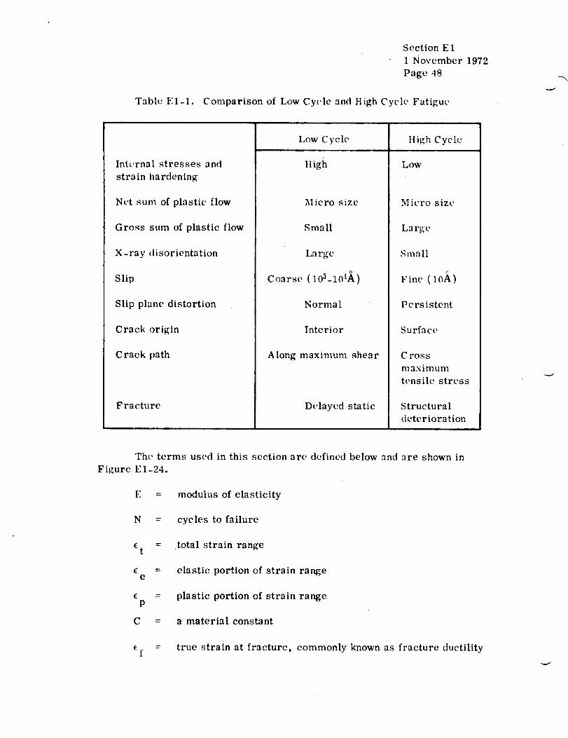
Table El-1.
Section E1
1 November 1972
Page 48
Comparison of Low Cycle and High Cycle Fatigue
Internal stresses and
stra in hardening
Net sum of plastic flow
Gross sum of plastic flow
X-ray disorientation
Slip
Slip plane distortion
Crack origin
Crack path
Fracture
Low Cycle
tIigh
Micro size
Small
Large
o
Coarse (103-10'IA)
N orma 1
Interior
Along maximum shear
Delayed static
liigh Cycle
Low
Micro size
Large
Small
F inc (1 0A )
Persistent
Surface
Cross
maximum
tensile stress
Structural
deterioration
The terms used in this section are defined below and are shown in
Figure E1-24.
E = modulus of elasticity
N = cycles to failure
ttotal strain range
eelastic portion of strain range
EP
C
plastic portion of strain range
a material constant
true strain at fracture, commonly known as fracture ductilityf

Section E1
1 November 1972
Page 49
1.4.1
S = _ E E t STRESS ///'AS stress amplitude
Se endurance limit
S u ultimate tensilestrength in ordinarytensile test
Sy yield strength /
Sut true stress at frac- L_ ..,! j
ture in tensile test L 'P "W"
Below Creep Range. "
In recent years, low-cycle
fatigue has been studied extensively
FIGURE E1-24. STRESS-STRAIN
C Y C LE
under conditions where little attention has been paid to temperature and tem-
perature effects. There now exists a fairly large body of information on the
subject obtained from laboratory experiments under room temperature con-
ditions (Ref. 6). The general procedure in such investigations is to control
the strain between fixed limits and, if desired, to measure the stress, while
cycling the specimen until failure is determined. Such tests may be under
conditions of controlled diametral strain, longitudinal strain, bending strain,
or torsional strain. The results can be represented in terms of total strain
range versus cycles to failure, or, if desired, of plastic strain range versus
cycles to failure. The former is most often used for direct design procedures,
while the latter is applied when one is primarily interested in real material
behavior. One of the more fascinating features of representing the results in
the form of plastic-strain range versus cycles to failure is the observation
that the curve (on logarithmic scales for both A_ and is of constantP Nf)
slope of value 0.5 to 0.65 (depending on the experimenter) and that the
vertical position of the curve relates to the tensile ductilityof the material.
A plotof this curve is shown in Fig. EI-25. The line in this figure can be
expressed by the equation
Ae q-_ = CP
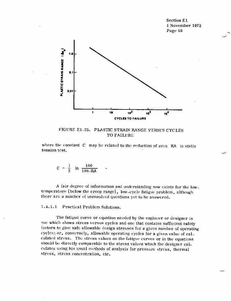
Section E I
1 November 1972
Page 50
1.0
E
• 0.1
i 0.01
m
1 ! I I i , ..
! 10 10 2 10 3 10 4
CYCLES TO FAILURE
FIGURE E1-25. PLASTIC STRAIN RANGE VERSUS CYCLES
TO FAILURE
where the, constant C may be rclated to the reduction of area RA in static
tension test.
I I00C = - In
2 100-RA
A fair degree of information and understanding now exists for the low-
temperature (below the creep range), low-cycle fatigue problem, although
ther(' are a number of unresolved questions yet to be answered.
1.4.1.1 Practical Problem Solutions.
The fatigue curve or equation needed by the engineer or designer is
one which shows stress versus cycles and one that contains sufficient safety
factors to givc safe allowable design stresses for a given number of operating
cycles; or, conversely, allowable operating cycles for a given value of cal-
culat(.(lstress. The stress values on the fatigue curves or in the equations
shoul(l be directly comparable to the stress values which the designer cal-
culates using his usual methods of analysis for pressure stress, thermal
stress, stress concentration, etc.

Section E 1
1 November 1972
Page 51
For fatigue below the creep rang(', Langer (Ref. 7) has proposed an
equation for plotting the fatigue curve for any material:
E 100S = -- In + S ,
100-RA e
(refer to Fig. E1-24 for definitions of terms).
For a design stress to represent a lower bound on the data, it is
recommended that the equation above be used with a safety factor of either 2
on stress or 10 on cycles, whichever is more conservative at each point. It
is believed that these safety factors arc sufficient to cover the effects of size,
environment, surface finish, and scatter of data.
It also has been shown that in the low cycle range (below 10 000 cycles),
mean stress has little or no effect on fatigue life; thus, this effect can be
ignored.
Some typical values of E and RA for various materials are given in
Table El-2. If information on the endurance limit (Se) is not available one-
half the value of the ultimate strength is often used.
If a more detailed fatigue analysis is required the techniques proposedin References 6 and 8 should be used.
1.4.2 In Creep Range.
The high-temperature, low-cycle fatigue problem is in quite a different
state. The material behavior becomes very much more complicated at ele-
vated temperatures because of the occurrence of creep and other diffusion proc-
esses. At temperatures in the creep range of a material, the test results will
be very strongly frequency dependent. Citing the fact that frequency is impor-
tant in high-temperature, low-cycle fatigue is the same thing as saying that
the strain rate of the test is important. A somewhat related situation occurs
if one introduces a hold time into the cycle, say, at the point where the tensile
stress is a maximum. While the strain is held constant, the peak stress
relaxes for some period of time. Results of prolonged hold times during strain
cycling show that the fatigue life decreases with increasing hold times, other
conditions beingthe same. A common observation is that, as the temperature
is raised and the rate decreased (or hold time increased), the character of
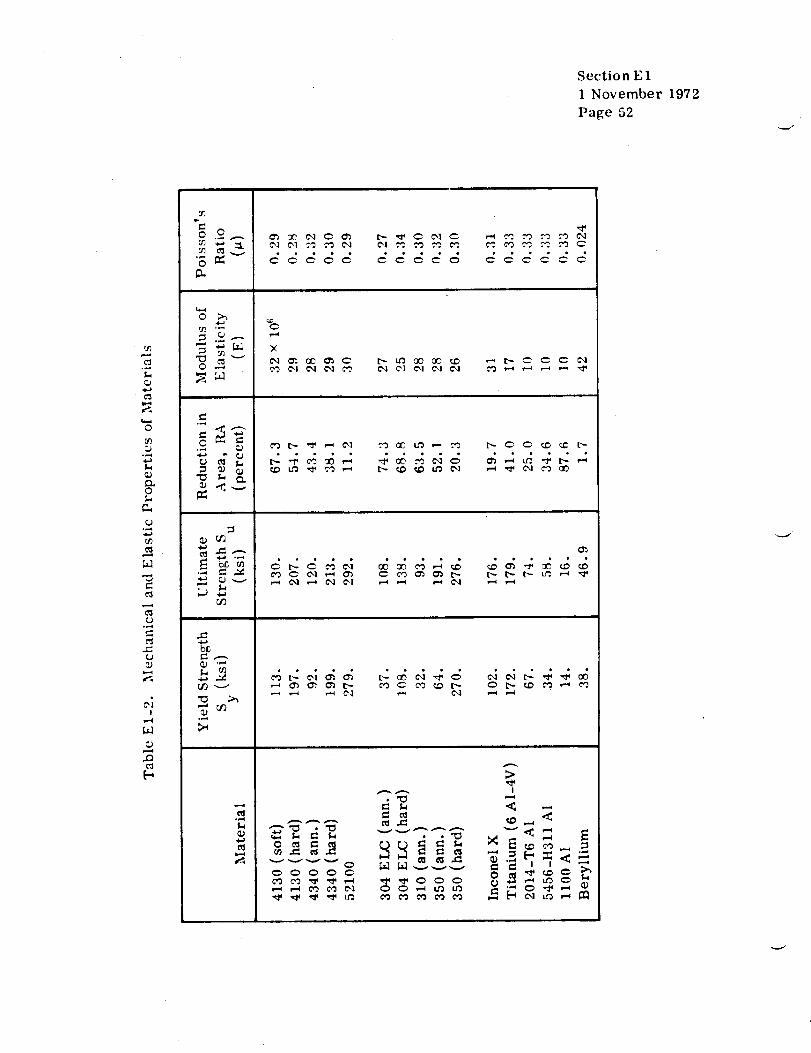
Sectio n E 1
1 November 1972
Page 52
O
tD=9
_D
0
0
M
c'l
c,;!
,.Q
"3
o3
C
...d
b_
°_,_
t_
__IC
CCO_O
×
__I _ _
0000_
.-.:.-_cc
¢0 CO _ ¢_ C':,
>I
< --

ORI,G;,"L:'L _""" :: '
OF.POOR q Section E1
1 November 1972
Page 53
the fracture changes from one which is tr_,nsgranular in nature to one which
is largely intergranular. This suggests vc,cy strongly that the problem is, to
a largcclegree, metallurgical innatur(,. A close resemblance can be seen
bctween these observations and those found in creep and stress rupture.
A second important, and certainly related, effect which must be appre-
ciated when dealing with high-temperature fatigue is the change in metallurgi-
cal structure which occurs with time at temperature and stress.
Plastic strain an(l, in the present instance, cyclic plastic strain can
have an important bearing on the precipitation and strengthening effects which
taM' place in the metal structure. The term "strain-ag(, hardening" describes
the eflcct that plastic strainhas on devc_loping additional strength. It is well
known, for example, that the level of strength reached by applying a fixed
amount of strain to a metal which strain ages is greatcr if the strain is applied
at th(, aging temperature. In designing an alloy for creep, advantage can be
taken of strain-age hardening provided the strain involved is the creep strain
sclectcd for the design.
l. 4.2.1 Ductility \.'crsus Crcep Strength.
As mentioned above, creep strengthening van I)e aecomplishe¢l for
,_l)_'ei[ic alloys at various rcgions of tcmperaturc's. Ilowcvc'r, it should be
notc(i that, simultaneously with strengthening, tlwse sam_' regions show
rc(tu(,e(I fraetur(' ductility.
This well-known behavior of metals, the invc_rse relationship between
slrenlzth and ductility, introduces a dilemma into the scl_'ction of materials for
hi_h-temt)erature service. It is necessary, to optimize the strength, to
_,mploy alloy additions and heat treatments so as to develop the precipitate
._tructtlre in the metal, but this will lower the ductility, l)uctility is of prime
c.onsidcration in low-cycle fatigue and, to optimize fatigue resistance, it is
desirable to have the material in as ductile a condition as possible (a condition
which results in low creep strength). Itowever, one' wants both creep strength
anal fatigue resistane(', and it is apparent that the best that can be achieved is
some' compromise condition.
1.4.2.2 Procedure for Estimating Iligh-Tcmperature, I,ow-Cycle Fatigue.
The proct_dure given h('re is taken from Rcfe.renees 9 and 10. It is a
i)roc('(lure for estimating the high-temperature, reversed-strain-cycling
fatigue characteristics of laboratory specimens. It shoul(I bt' emphasized that

Section E 1
1 November 1972
Page 54
the method is intended to give only first-approximation estimates as a guide to
material selection. Final design of important equipment should be based on
actual fatigue data generated under conditior, s which simulate as closely as
possible those to be encountered in service.
I. Basis.
Figure E1-26 illustrates the method of universal slopes. The total
strain range is divided into its elastic and plastic components, and each com-
poncnt is plotted against cyclic life on log-log coordinates. Straight lines
usually result for each of these components. The method of universal slopes
prescribes that the slopes of these lines arc assumed to be the same for all
materials. The plastic components-are taken to have an average slope value of
-0.6, and the elastic components an average slope value of -0.12. Again, it
should be emphasized that these values arc not always -0.6 and -0.12 for all
materials; values betwecn -0.4 and -0.8 have been obtained for various mate-
rials for the plastic component, and values between -0.08 and -0.16 have
been found for the elastic components. When average values of -0.6 and -0.12
arc chosen for the plastic and elastic components, reasonable results are
obtained.
r 00"I
! 1 1
CYCLES TO FAILURE. Nf (LOG SCALE)
' ,(,)I ](l': 1':1--26. M E THOD OF UNW ERSA L S I.OPES FOR FSTIMA TING
AXIAL FATIGUE LIFE

Section E11 November 1972Page 55
Having decided on the slopes, it is necessary to determine the inter-
cepts of the two straight lines. In general, it has been found that the property
which most significantly governs the intercept of the plastic line is the ductility100
D, where D= in IO0-RA
For the elastic line, the governing property for the intercept is a /E,u
where a is the ultimate tensile strength and E the elastic modulus. Theu
total strain range, given as the sum of the elastic and plastic components, thusbecomes
3.5(7
_ u -o. 12 DO.6 )-0.6Act E (Nf) + (Nf
as shown in Fig. E1-26.
Good agreement has been obtained with this formula for many materials
(Ref. 9). However, the question arises: Can one use this procedure at high
temperatures within the creep range of the material? In general, it has been
found that the procedure almost always yields fatigue life predictions higher
than those actually obtained by testing. The explanation for the unconservative
results is, of course, very complex. The relationship between high-
temperature, low-cycle fatigue and intercrystalline cracking is very important.
It has been shown that intercrystalline cracking due to a creep effect
occurs early in the fatigue life, and thereby bypasses the transcrystalline
crack-initiation period; thus, the total fatigue life is approximately equal toonly the crack-propagation period.
This concept has yielded the 10-percent rule. In this method, crack
initiation and propagation are not regarded as functions of fatigue life; rather
it is assumed that, on the average, only 10 percent of the fatigue life com-
puted by the method of universal slopes will actually be realized at tempera-
tures within the creep range.
Generally, it has been found that such a computation yields conserva-
tive results; that is, in most cases, it leads to a lower bound on fatigue life.
ttowevcr, there are cases in which even the 10-percent rule predicts lives that
are higher than those actually achieved in test. This observation (together
with the fact that the 10-percent rule approach inherently excludes the pos-
sibility of taking into account frequency effects, hold-time effects, mean load,

Section E 1
1 November 1972
Page 56
etc. ) causes one to seek further for simple methods of estimation that art,not as limited.
The simplified analysis that has been adopted can be explained by the
following. The creep damage effect is taken as the ratio of tile time actually
spent at stress to the time required to cause rupture at that stress value.
Since the stress and temperature are presumably known, this rupture time can
be obtained directly from the creep-rupture curve of the material. The fatigue
damage effect is taken as the ratio of the number of cycles actually applied to
the number that would be sustained in the absence of creep effect according to
the method of universal slopes. Since the test frequency yields a definite rela-
tion between the time of the test and number of cycles sustained, a closed-form
analytical expression for the number of cycles to failure can be obtained. This
description is shown in the following derivation:
where
(C reep-Rupture Damage) + (Fatigue Damage) = I
kt'= --f Nf'
1/m
tr : A = A(Nf)..-0.12/m
hence,
AF(Nf)-0"12/'n + \Nf/
= 1
OF
Nf
N' ,1 _ k/AF(Nf)__ (m + .12)/m

Section E 1
1 November 1972
Page 57
Here
Nf' = number of cycles to failure under combined fatigue and creep
Nf number of cycles to failure in fatigue, based on method of
universal slopes, using ductility, ultimate tensile strength and
elastic modulus from uniaxial tests at strain rates comparable
to that undergone by the metal in the fatigue test. Where appro-priate data are not available, use may be made of data fromconventional tensile tests.
k empirical constant, assumed to be 0.3, but adjustable as moreinformation becomes available.
slope of straight line-creep-rupture curve on log-log coordi-
nates, that is, representing curve by ar = 1.75 au (tr/A)m
as shown in the insert in Fig. E1-27.
A = coefficient in creep-rupture relation
F = frequency of cycling, cycles per unit time.
Table El-3 contains some of the information above, obtained from various test
conditions (Ref. 9).
_" o.x _- l._,,u / .
>o.3o L°ae' *''A _ /
LOG t r
SCHEMATIC ITRES4i I_ /-
0.24IqUPTUR! CUR'VI _ _ USE 10_ N FOR: -- LowER,o'u,,o
:o,. :,:....:::o.,, , . _. J,t,J.I J . I._,z.I i , I,l,_.l I , ,,l,l,i
10"2 10 "1 10 0 101 10 2 113
PRODUCT OF CREEP.RUP'rURE COEFFICIENT AND FREQUENCY. AF
FIGURE EI-27. CRITERION TO ESTABLISH NEED FOR
CRE EP-RUPTURE CORREC TION

Table E 1-3.
ORIG|NAL ' ......
O(: POOR QUALHY
Section E 1
1 November 1972
Page 58
Alloys, Test Conditions, and Pertinent Properties
Test Test
'l't,mperatu rt_ Frequencyh Ih,v
I)t'nignat ion (F) ( _:pm )
A-2_(i - C11 114f_) 1000 5 to 50
1200 5 to 50a
A-2_6 -- AgL_I 1200 5 to 50
1400 20
,, ,
A -2_(1
lrl¢'o 901 1400 20
I)-:179 1260 5 to 5¢)
Cr-Mo-V Stc¢,] 1050 I, IO
I-6¢15 1000 5, 50
1200 5, 50
304 Sta inie_n { 000 10
Sh,e| 12041 3 to IH
1500 ;1 to 27
:',47 SLalnh*_n 1110
N i niilnle 7fl { 200 { [}
1:18ll Ill
I f{ 00 1 ¢i
I;400 10
Nimtmle 00 1200 I0
1:180 0.1, 10
1000 0.1, 10
I_0(1 0. I, 1o
N im.nic 105 1200 10
[; j;,,,((| lO
1()00 l 0
1H00 |fl
U¢llm,'t 700 1400 1 to 2
A _t roloy 1400 20
lm'c, nel 1500 0.017, rl. 1
In 10o
(I'll 47 C¢lill)
MAlt M 2011
(I)WA 17 (,c_,t)
I% 19(}fl
( I'WA .17 Co.t)
1000
1700
2¢)00
1300
1700
1300
1700
2000
C rcep-Ruptu re'l't.nsile E la ,tic
,tA Strength Modulus S hipt' Intercept, A
(<_) (1_i) (10 "_ k_i) (-m} (mini (sl.,(.) '
31. 1_12. 26.R <0. 12
.28. 167. 211. 1 " 0. 1'2
18. 115. 23.0 0.12
57.6 75. 19.0 O. 20 I.;I 7_.
16.I 104. 20.8 ¢). 135 0,028 n. 17
42.0 179. 22.0 <0. 12
70.[) 69.5 24.0 <0.12
4H.2 106.0 27.0 -0,12
47.1 95.4 25.0 ,0.12
67.3 55.5 2;I.0 .0.12
58.0 41.0 22.0 (]. IR 15.0 9oo.
42.0 20.0 19.0 0. I H li/I 1'4. t)
67.7 55.0 22.0 ¢1.12
29.5 _ I. 5 20. ;1
42.0 53.1 15.4
62.5 28.0 12.2
66.0 16.2 1.7
24.5 144.¢) 26.5 < O. 12
12.0 119.0 25.0 ¢i. 135 0,16 9.fi
14.0 76.0 23.0 l).24 2.5 150.
94.0 1¢i.0 21.0 0.25 4.0 240.
13.7 142.0 25.0 <0.12
lR.0 151.0 23.5 -0.12
32.5 99.5 22.0 o. 16 0.0S 4.
Ii_4.0 39.2 19.0 0.2a 3.7 222.
31.0 155.0 23.0 _0.12
l
29.6 141.0 23.0 -0.12
63.3 25.0 18.0 O. 15 1.0 60.
l.:t 121.0 27.1 "0.12
11.0 ._.0 22.7 0.17 0. II 6.6
10.3 26._1 10.3 0.22 !.3 _/q.
5. 120.0 26.5 <0.12
4. 77.0 23,7 _0.12
5. 145.0 25.50. 12
:t. 95.0 23.0 0.17 o.75 45.
II. 35.0 20.5 O. 26 7. :i t40.
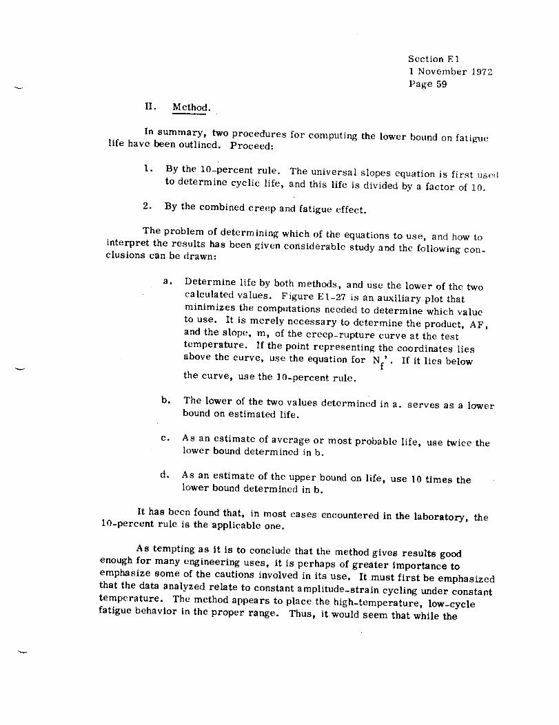
Section E 1
1 November 1972
Page 59
II. Method.
In summary, two procedures for computing the lower bound on fatiguelife have been outlined. Proceed:
1. By the 10-percent rule. The universal slopes equation is first us_,l
to determine cyclic life, and this life is divided by a factor of 10.
2. By the combined creep and fatigue effect.
The problem of determining which of the equations to use, and how to
interpret the results has been given considerable study and the following con-clusions can be drawn:
a. Determine life by both methods, and use the lower of the two
calculated values. Figure E1-27 is an auxiliary plot that
minimizes the computations needed to determine which value
to use. It is merely necessary to determine the product, AF,
and the slope, m, of the creep-rupture curve at the test
temperature. If the point representing the coordinates lies
above the curve, use the equation for Nf'. If it lies below
the curve, use the 10-percent rule.
b. The lower of the two values determined in a. serves as a lower
bound on estimated life.
c. As an estimate of average or most probable life, use twice thelower bound determined in b.
d. As an estimate of the upper bound on life, use 10 times thelower bound determined in b.
It has been found that, in most cases encountered in the laboratory, the
10-percent rule is the applicable one.
As tempting as it is to conclude that the method gives results good
enough for many engineering uses, it is perhaps of greater importance to
emphasize some of the cautions involved in its use. It must first be emphasized
that the data analyzed relate to constant amplitude-strain cycling under constant
temperature. The method appears to place the high-temperature, low-cycle
fatigue behavior in the proper range. Thus, it would seem that while the

Section E 1
1 November 1972
Page 60
method may be regarded as very goo(I for ,_;creening materials, important
material ehoict's shouhl be made on the baqis o[ actual tests from amon_ the
more promisint_ materials. And, wheneve:'possible, the complexiti_'s of
stress and temperature history expected in service should be included in the
test evaluation.
1.4.2. "] Method of Strain-Partitioning.
In their continuing examination of high-temperatur(,, low-cycle fatigue,
Manson and co-workers (the 10-percent rule) have deveb_pcd a method which
attempts to analyze directly the effects of creep and plastic flow on cyclic
life (Ref. 11). This method was developed because of the highly time-
dependent nature of the creep effect and because the life-reducing effects of
creep depend, to a large extent, upon where within a cycle the creep is intro-
duced and whether it is reversed by plastic flow or by creep.
In this method, the completely reversed cyc!ir inelastic strain is
divided into four parts. These are (1) A¢ -- t,'_ile plastic flow revers,',!PP
by compressive plastic flow, (2) Ae -- tensile creep reversed by compr,'_-cp
sire plastic flow, (3) AE -- tensile plastic flow reversed by compressivepc
creep, and (4) A¢ -- tensile creep rcversud by compressive creep.CC
In any arbitrary hysteresis loop, such an .qhown in Fig. E1-28, the
tensile inelastic strain (AD) can bc separated into plastic (AC) and ('reM_
iCl)) components. Likewise, theeempr,'ssive inel,_¢tic strain (DA) can
also b,_ separated into its plastic (]_i_) and ert'cp (t_--A) components. In
zeneral, neither the two plastic compon('nts (AC and DB) nor the two creup
components (C-D and B-A) will be equal. It is nt_cessary only that the entir¢_
tensile inelastic strain (A-'D) be equal to the entire compressive inelasticI
_train (DA) since we are dealing witha closed hysteresis loop. The parti-
tiont_d strain ranges are obtained in the following manner. The completely
reversed plastic strain range, Ae , is the smaller of the two plastic com-PP
_:_mt_ts and in this _,xample is equal to DB. The complet¢qy reversed cr,'ep
._'rain range, AE , is equal to the smaller of the two creep component._cc
and becomes CD. As can be seen graphically, the difference between the two
plastic components must be equal to the difference between the two creep
components, or AC - DB = BA - CD. This difference is then equal to Aepc
or A( in accordance with the notation just stated. For this example, it i,_cp
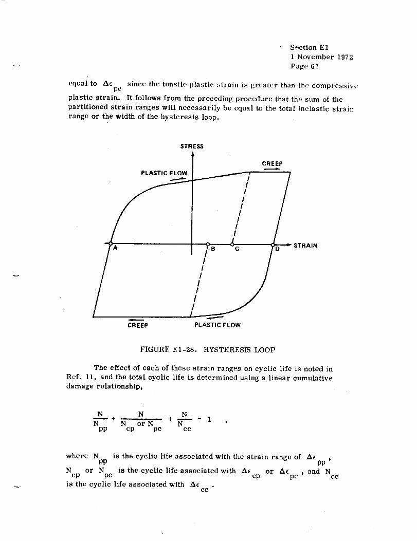
Section E 1
1 November 1972
Page 61
equal to Aepc since the tensile plastic strain is greater than the compressiw_
plastic strain. It follows from the preceding procedure that the sum of the
partitioned strain ranges will necessarily be equal to the total inelastic strain
range or the width of the hysteresis loop.
STRESS
CREEP
CREEP PLASTIC FLOW
FIGURE E1-28. HYSTERESIS LOOP
The effect of each of these strain ranges on cyclic life is noted in
Ref. 11, and the total cyclic life is determined using a linear cumulative
damage relationship,
N N N
N N or N Npp cp pc cc
where N is the cyclic life associated with the strain range of Ac ,PP PP
N or N is the cyclic life associated with A_ or AE , and Ncp pc cp pc cc
is the cyclic life associated with AE .cc

Section E1
1 November 1972
Page 62
This method differs from the' 10-perc('nt rule in that it attempts to
deal directly with the phenomena occurring at high-temperature, low-cycle
fatigue rather than u,_ing an estimate base.1 on low-temperature, low-cycle
fatigue findings. It differs from other metno(Is which partition damage effects
at high temperatures in that all relations use(I are strain range versus cyclic
life rather than a combination of that and stress versus time life. The gener-
ation of strain range versus cyclic life data is required in this method where
the 10-percent rule requires only static tensile properties. This mt'thod
agrees well with the 10-percent rule for the materials tested and may prove
abasis for that rule. This method is also useful in explaining frequency
effects and hohl-time, effects. Finally, to quote the authors of this method,
"The method is in an early stage of development, and many questions must
be answered before its merits canbe evaluated" (i(cl. 11).
1.4.2.4 Two-Slope Fatigue Law.
Coffin and Manson have' proposed the follc)win_* fatigu,' law for plastic
strain:
NfI_' A,- = c , ( 1)P
wh('r_' N[ in the cycles, to failure, A¢11 is thc, i)lastic strain range, and fl ,
C arc the constants. This has been modified to inclu(h_ the effect of frequency
in hi<h-temp(Tature, low-cycle fatigue,
k- 1)I_N[ v A< P : C 2 , (2)
k-Iwh('re v is th(' frequency, I< , C_ are the eonstants, anti Nfv is defined
as the fr(_qucney-modifit_d fatigue life. The frequency cffectwas ext('nde(t
further to include lhe stress range,
A(7 ::: A (_()'_v Iq (a)P

and
Section E 1
1 November 1972
Page 63
Aa = stress range
where A, rl, and k arc constants. Combining equations (2) and (3) and
generalizing for the total strain range
AE = (AC27?/E)Nf -flrlkl+ (1-k)fl_ + C2Nf-flv (1-k)fl , (4)
where E is the elastic modulus.
Coffin reports in Rcf. 12 that with increasing tcmpcraturc the exponent
/3 increases approaching one and the constant C correlates less well with the
tensile ductility. Because of the high exponent for 13 in equation (1) reported
for many materials at elevated temperature, extrapolation to low lives could
lead to plastic strain ranges exceeding the tensile ductility. Because this
situation is highly unlikely, there must be a break in the curve of the AcP
versus Nf relationship so that it will pass through the tcnsile ductility value
at Nf = 1/4 (Fig. E1-29). This change in slope is due to a change in the
mode of crack propagation. In less ductile materials this change in slope is
due to a change in the fracture mode resulting from environmental interaction.
In ductile materials this change in slope at high temperatures results from a
change from intergranular to transgranular fracture and as can be seen in
Fig. E1-30, as temperature increases the change in slope is more drastic.
The main Benefit of the two-slope fatigue law is that it gives a more
accurate description of the occurrences in plastic strain and leads to a clearer
recognition of the operative physical process. A recognition of the causes of
the two-slope phenomenon emphasizes the importance of the environment and
of time in the environment (frequency and hold time), tIowever, the constants
of the equations are highly material dependent and temperature dependent and
if experimental data are not available, these constants cannot be determined.
1.4.3 Thermal Cycling.
The prcvious sections have considered mechanical strain or stress
cycling at a constant temperature; this section will consider mechanical

111
Z<e¢Zm<er
¢t)
oV-¢0<-t
I_a<1
0.1
0.01
0.0010.1
Section F 1
1 November 1972
Page 64
I I I I
1010 STEEL
600°C
_= o.5
,,°'_-_'_ _ -1/8 in. 1/4 in. FREQUENCY "_,
_ [ -X- 0.2 cpm .,
® x ,o°., '_,;x_=o.,,-
I , I i i1 10 100 1000
FREQUENCY MODIFIED FATIGUE LIFE -- Nf v k'l
FIGURE E1-29. PLASTIC STRAIN RANGE VERSUS FREQUENCY
MODIFIED FATIGUE LIFE --AISI CI010 STEEL, 600°C
;=.. ' '-,2 ' ' i .... r .... = .... I .... I ...._"0_ A,S,- 3o4ss
' _ ' TEMP. CODE
_ 430 ° 0_o °
_=o.,L-
o.o11- .
0.1 1 10 ' 100 1000 10 000 100 000
FREQUENCY MODIFIED FATIGUE LIFE -- Nf vk'l
FIGURE E 1-30. PLASTIC STRAIN RANGE VERSUS FREQUENCY
MODIFIED FATIGUE LIFE -- AISI 304 STAINLESS STEEL

Section E 1
1 November 1972
Page 65
strains induced bycyclic thermal stresses. Failure under repetitive appli-
cation of thermal stress has been termed thermal stress fatigue.
The principal activity in which analysts have, until recently, engaged
whenever thermal-stress problems were encountered has been the computation
of elastic stresses. The treatment of this subject may be found in Section D,
Thermal Stresses. While such computations constitute a necessary and desir-
able first step in any practical analysis, they unfortunately do not provide
s_ffficient information for a final evaluation when dealing with ductile materials.
Thus, it is important not only to take into account plastic-flow effects that
occur when the yield point is exceeded but to consider how such plastic flow
might change during progressive thermal and load cycling of the material.
Recent contributions have made a valuable start toward an understanding of
this problem. Not only have new computational techniques been developed
for taking into account inelastic, effects such as creep and plastic flow, but a
start has been made toward inc'ludim_ cyclic effects both in computational
procedure and in the interpretation in terms of material behavior. The fail-
ure criterion for brittle materials is, of course, different from the criterion
for ductile materials. From an engineering point of view, the problem is to
detcrmine suitable working st res ses.
1.4.3.1 hlealizcd Thermal-Cyc le Model.
A model will bc chosen [n which all the thermal strain is converted to
mc'chanieal strqin. The case is shown in Fig. I::1-31 in which a bar is fixed
at its ends between two immovable plates so that the length of the bar must
remain constant. To approach the problem realistically, the model should
show strain hardening, and the effects of stress relaxation that occurs during
any hold period that may be imposed at high temperature.
R(efcrring to Fig. E1-31, the bar is assumed clamped when hot, so
that tensile stress is developed along OAF during the first cooling. Plastic
flow is initiated at A, but the stress continues to increase to F because of
strain hardening. At F the specimen is held for a dwell period, but no stress
change occurs (relaxation), since the temperg_turc is i)resumed to be low
enough to make creep and anclasticity negligibh,. Upon reheating of the speci-
men, the stress-strain relation proceeds alton I'GE, yielding atG, at which
time there is a much lower stress than there is at A because of the Bauschingcr
effect. (The Bauschinger cflect states that plastic flow in one direction
rcduccs the stress at which yielding will occur in the opposite direction.)

Section E11 November 1972
Page 66
t/H// IHl iH I ll//l// l lleA. WiT. CONSTRAINEDENOSI_
A
--.----" COOLING
HEATINGI
I
F
TOTAL
MECHANICAL
STRAIN
FIGURF 1':1-31. SCHEMATIC STRESS-
STRAIN RELATIONSItIP FOR FIRST
FEW CYCLES OF TIIERMAL
CYCLING OF CONSTRAINED BAR
When the initial high temperature is
restored, the state of the material is
at p(_int E, where a compressive elastic
strain is necessary to offset the tensile
plastic flow that occurred during AF
and, thereby, return the specimen to
a net strain of zero. This elastic
strain introduces the stress OE. Any
hold period at the high temperature and
stress may convert this elastic strain
to inelastic strain-creep and anelas-
ticity, thereby reducing the stress.
Thus, point E moves to point E' by
the time the specimen starts to cool
again. The cooling causes the path
E' F' to be traversed. Reheating
results in the path F' E". The hold
period at the high temperature converts
e"toE''', etc. After a fcwcycles,
the stress-strain path may settle down
to an essentially unchanging loop. For
illustrative purposes this loop may betaken as E' ' ' F' l':"I,:' ' '. This corre-
sponds to an asymptotic hysteresis
loop and takes into account not only all
the hardening or softening character-
istics but also creep and anelasticity
effects as well as effects due to changing
temperature and metallurgy.
1.4.:3.2 Effect of Creep.
In the experiments that have been performed to date, analysis of the
thermal-stress fatigue behavior has been made largely by relating the plastic
strain per cycle to the number of cycles to failure. Normally, the plastic
strain is determined by subtracting the elastic-strain range l rom the total-
strain range, which in turn is computed by divi(ling the stress range by the
rlastic modulus. When creep occurs during the high temperature portion of
the cycle, this procedure produces inaccuracies. Not only is the plastic flow
improperly computed if creep is neglected, but the omission of the creep can
s_,riously affect the computation of cyclic life because the effect of creep strain
on life differs appreciably from the effect of slip-type plastic flow.

F"
Section I£ 1
1 Noven_bcr 1972
Page 67
Consider Fig. E1-32, which shows the stress-strain rclationshil)s lor
two idealized cases. In Fig. 1,',1-32 (a) no creel) is assumed to take place.
Then,
A_
e P = ff T O -
where Aa is the stress range and E is the elastic modulus. (The elastic
modulus is assumed to be constant over the entire temperature range;
(a) (b)
FIGURE E1-32. PLASTIC-STRAIN AND STRESS-RANGE
RE LA TIONSHIP FOR (a) NO CREEP RE LA.KATION
DURING HOLD PERIOD AND (b) CREEP
RELAXATION DURING HOLD PERIOD

Section E11 November 1972Page 68
assumption of a temperature-dependent elastic modulus complicates the
problem even further. )
tlowever, when cree l) occurs during a hold period I Fig. l:1-32(b) ], the
plastic strain per cycle is not directly related to the total stress range. For
the tensile portion of the cycle, the plastic strain ¢ ' isP
T
£ P = O_ T O _IE
where A(_l is the stress range developed during the cooling portion of the
cycle only. In the heating portion of the cycle, the stress rang(, is larger,
thus reducing the direct compressive plastic strain _ '" ttowever, the totalP
plastic strain ¢ " also includes the creep E '" during the hoht period. ThisP P
creep strain replaces the elastic strain relaxed during the creep and is, there-
fore, equal to (Aa 2 - A%)/E. Thus,
£ vt = £ q'vl + E vvvl' __ _ TO -P P P E F E p
Therefore, the plastic strain in compression is equal to that in tension, but
these strains are not dirc'ctly related to the total stress range.
1.4.3.3 Comparison of Thermal-Stress Fatigue with Mechanical Fatigue
at Constant Temperature.
Several experiments in which mechanical fatigue at various temper-
atures was compared with thermal-stress fatigue have been conducted (Refs.
13 and 14). Fatigue tests were conducted at several constant hight('mpera-
tures by loading mechanically, and the results of the tests were compared
with thermal-stress fatigue tests in which the temperature naturally varied
over an appreciable range. The results era test are shown in Fig. E1-33 and
are analyzed in terms of cyclic life at a given measured plastic strain. The
mechanical-fatigue tests are shown at 350 °, 500 °, and 600 °C, whereas in
the thermal-stress tests the specimen was completely constrained and cycled
between 200 ° and 500 °C, so that the mean temperature was 350 °C, As can
be seen from the figure, at equal values of cyclic plastic strain the number of
cycles to failure was much less for the thermally cycled specimen than for one
mechanically cycled at :;50 ° C and even for one' mechanically cycled at 000 ° C,
even though no part of the specimen in the 200" to 500 °C th['rmal-strcss

F
Section 1':1e-r,)l Novcmbcr 19__
PaK_' 69
0.1
----,-- CONSTANT TEMPERATURE FATIGUE
-,, -- CYCLIC TEMPERATURE THERMAL-STRESS FATIGUE
%
0.001021 103 104 108 10 li
CYCLES TO FAILURE Nf
FIGURE E1-33. CYCLES TO FAILURE IN TIIERMAL-STRESS FATIGUE
COMPARED WITH CYCLES AT CONSTANT TEMPERATURE IN
SIMILAR PLASTIC STRAIN RANGE
fatigue test ever reached 600 ° C. Reasons for this discrepancy have been
generally attributed to nonuniformities of temperature along the specimen
and the sensitivity of the properties of the materials to temperature in the
range traversed by the thermal-cycling tests.
For this reason it would appear that, until further tests clarify the
problem, the temperature for the mechanical-fatigue tests should be taken
as the highest temperature of the thermal-stress test. In this way, metal-
lurgical phenomena will not be overlooked and pessimistically low values of
life will be indicated; this appears to be necessary on the basis of most testsconducted to date.
Spera (Ref. 15) has presented a method for calculation of thermal-
fatigue life based on accumulated creep damage. He proposes that thermal-
fatigue life can be determined from the basic mechanical properties of a
material by calculating lines for each of two distinct and independent failure
modes: (1) cyclic creep-rupture, using a modification of the well-known life-
fraction role proposed by Robinson and Taira, and (2) conventional low-cycle
fatigue, using the empirical equations of the Method of Universal Slopes
developed by Manson (Refs. 9 and 10). Equations are presented in sufficient
detail to define completely the analytical procedure.

HeetionEiI Noveml_er1972Pag,' 70
1.4.:¢.4 Summary.
Whenplastic strains are introduced by constraint of thermal expansion,l atigue ultimately results. The number of cycles that can be withstood depends
on the plastic strain and the temperatures at which these strains are induced.
Whether tension or compression occurs at the high temperature seems to have
little effect on fatigue life. Probably the most important single variable is the
maximum temperature of the cycle, particularly if it is higil enough to cause
metallurgical effects to take place. Increasing the maximum temperature for
a given temperature range will generally cause a much greater reduction in
cycles to failure than increasing the temperature range by the same amount
and maintaining the same maximum temperature. The time at which the max-
imum temperature is maintained can also have an effect on fatigue life, but of
smaller magnitude. The effect can be beneficial or detrimental to fatigue life,
depemling on the material, temperature, and life rang(-'.
Limited data indicate that fatigue life in a thermal-stress fatigu¢' test
is sometimes considerably less than the fatigue life of a mechanically strain-
cycled specimen having the same total strain as the thermally fatigued speci-
men and tested at a constant temperature equal to the average temperature of
the thermal-stress fatigue test.
The effect of prior thermal cycling on specimens subsequently evaluated
for stress rupture depends greatly on the material and the number of prior
cycles. In general, the effect can be expected to be detrim('ntal; howevcr, in
some cases it may actually be beneficial.
Fach of the materials that has been studied to date -- type :_47 stainless
steel, the cobalt-base alloyS-816, andthe nickel-base alloys Inconcland
Inconel 550 -- displays characteristics considerably different from the others
in thermal-stress fatigue, and prediction of distinctions in the behavior of one
l rom that of another is difficult. Hence, more classes of materials must be
investigated before a reasonably complete: i)icture of the thcrmal-fatilgue
hehavi()r of materials, in general, canbe understood. For specific irfforma-
tion on behavior of the various types of materials, investigate Refs. 13, 14,
l(;, 17, 18, 19, and 20.
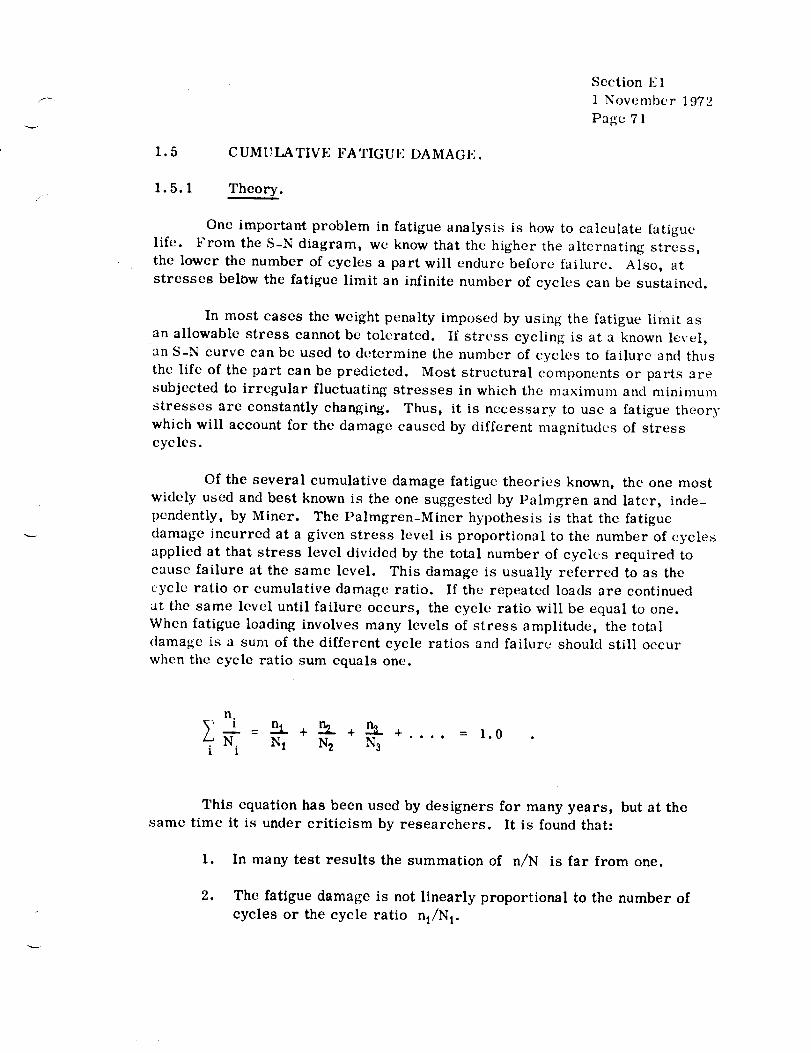
Section E 1
1 November 1972
Page 71
1.5 CUMULATIVE FATIGUE DAMAGE.
1.5.1 Theory.
One important problem in fatigue analysis is how to calculate fatigue
life. From the S-N diagram, we know that the higher the alternating stress,
the lower the number of cycles a part will endure before failure. Also, at
stresses belbw the fatigue limit an infinite number of cycles can be sustained.
In most cases the weight penalty imposed by using the fatigue limit as
an allowable stress cannot be tolerated. If stress cycling is at a known level,
an S-N curve can be used to determine the number of cycles to failure and thus
the life of the part can be predicted. Most structural components or parts are
subjected to irregular fluctuating stresses in which the maximum and minimum
stresses are constantly changing. Thus, it is necessary to use a fatigue theory
which will account for the damage caused by different magnitudes of stress
cycles.
Of the several cumulative damage fatigue theories known, the one most
widely used and best known is the one suggested by Palmgren and later, inde-
pendently, by Miner. The Palmgren-Miner hypothesis is that the fatigue
damage incurred at a given stress level is proportional to the number of cycles
applied at that stress level divided by the total number of cycles required to
cause failure at the same level. This damage is usually referred to as the
cycle ratio or cumulative damage ratio. If the repeated loads are continued
at the same level until failure occurs, the cycle ratio will be equal to one.
When fatigue loading involves many levels of stress amplitude, the total
damage is a sum of the different cycle ratios and failure should still occur
when the cycle ratio sum equals one.
n.
, = Lt. + n,2+2. Ni N,1 1
+ .... = 1.0
This equation has been used by designers for many years, but at the
same time it is under criticism by researchers. It is found that:
1. In many test results the summation of n/N is far from one.
2. The fatigue damage is not linearly proportional to the number of
cycles or the cycle ratio nl/N 1.

Section E11Nt)veml)(,r 1972Page72
:3. Thcru is interaction in the fatigue (lamages l)etwecn various stress
levels which Miner neglected. In the interaction there is alsoa
sequence effect which means tha; the fatigue damage resulting from
the high load first, with the low load next, will be different from
the damage resulting from the low load first, with the high loadnext.
Aware of its limitations, designers still use Miner's (,quation as a
preliminary guide because of its simplicity, versatility, and sufficient accu-
racy, commensurate with the data currently available for this type of analysis.
What are the consequences when Miner's equation is used for random-
loading conditions ? Random-load fatigue testing is time-consuming and costly,
and the scant data- available do not permit a general clear-cut answer to this
question. According to Freudenthal (Ref. 21), the sum g n/N is always less
than one. In some cases the sum is as low as 0.13 but it is mostly between
0.20 and 0.60. The primary reason for this discrepancy, according to
Freudenthal, is the interaction of fatigue damages between various load
a mplitudes.
On the other hand, it has been found that notched parts generally give
a summation value greater than one. Since practically all of the structural
fatigue failures originate in some form of notch, the question of what value to
use in place of 1.0 has been asked.
The National Aeronautics and Spac 9 Administration conducted full-scale
fatigue tests on C-46 transport airplane win_s and their summation of cycle
ratios was 1.4 (Ref. 22).
ttowever, until more information becomes available, Miner's equation
is recommended for preliminary analysis.
1.5.2 Analysis of I)ata.
Numerical simplifying assumptions are often needed to speed up the
analyzing of data. Mainly, these assumptions have to do with primary and
secondary cycles. The following four conventions serve to establish and define
primary and secondary cycles:
lo A mean value of stress, S for the entire record is approxi-mean
mat(.d. Although a time average and a peak point average generally
yield different average values, the two may be assumed to be equal.
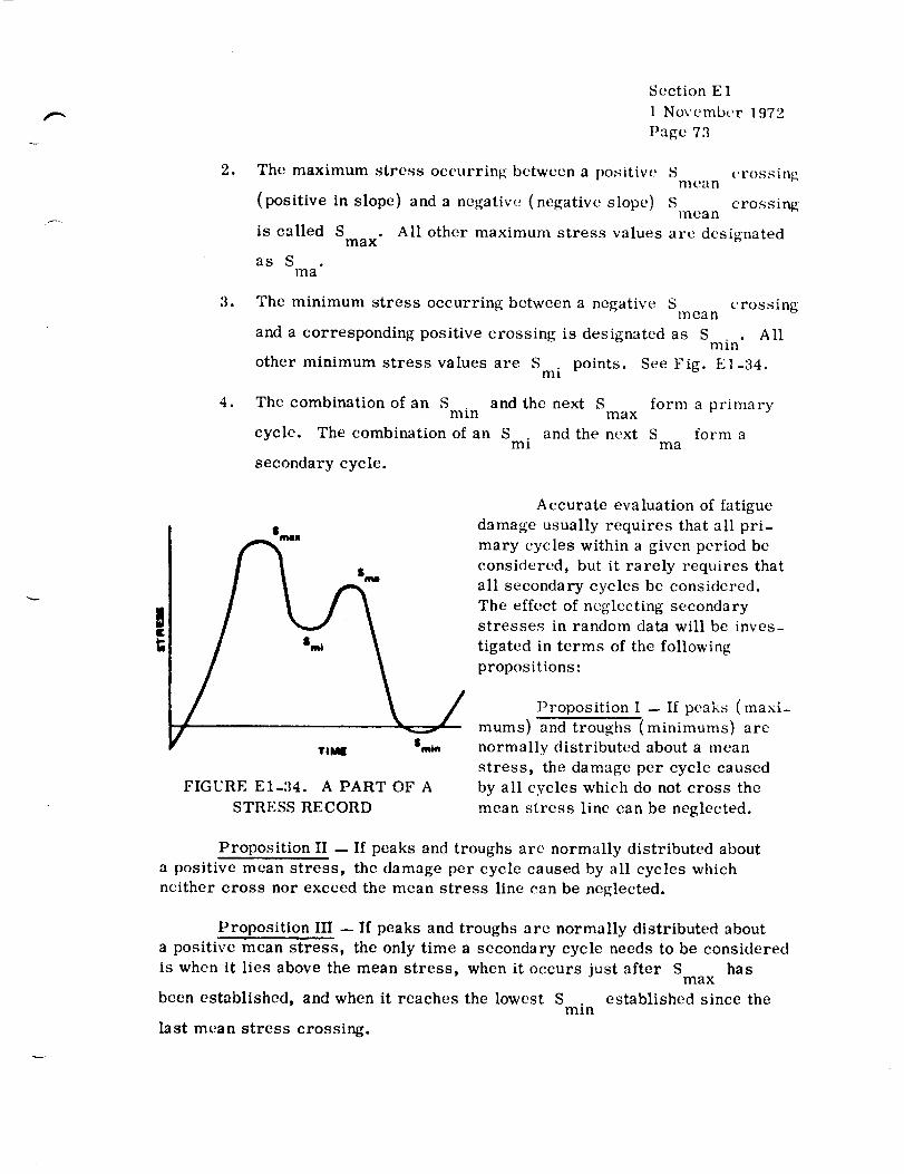
Section E1I November 1972Page 73
. The maximum stress occurrinl_ between a positiw' S _'rossingmean
{positive in slope} and a negative (negative slope) S crossingmean
is called S . All other maximum stress values are designatedmax
as Sma
e The minimum stress occurring between a negative S crossingmean
and a corresponding positive crossing is designated as Smi n. All
other minimum stress values are Smi points. See Fig. E1-34.
1 The combination of an Smin and the next S form a primarymax
cycle. The combination of an S and the next S form ami ma
secondary cycle.
I __ $mu
t
Y TI MI Snt_n
FIGURE E1-34. A PARTOF A
STRESS RECORD
Accurate eva luation of fatigue
damage usually requires that all pri-
mary cycles within a given period be
considered, but it rarely requires that
all secondary cycles be considered.
The effect of neglecting secondarystresses in random data will be inves-
tigated in terms of the following
propositions:
Proposition I -- If peaks (maxi-
mums) and troughs (minimums) are
normally distributed about a mean
stress, the damage per cycle caused
by all cycles which do not cross the
mean stress line can be neglected.
Proposition II -- If peaks and troughs are normally distributed about
a positive mean stress, the damage per cycle caused by all cycles which
neither cross nor exceed the mean stress line can be neglected.
Proposition III -- If peaks and troughs are normally distributed about
a positive mean stress, the only time a secondary cycle needs to be considered
is when it lies above the mean stress, when it occurs just after S hasmax
been established, and when it reaches the lowest S established since themin
last mean stress crossing.

Section E11 November 1972Page74
Usually for random data, on(; of these propositions can be considered
valid. Fig. E1-35 illustrates several more or less useful approximations,
some of which are generally valid, and all ,ff which are usually more valid
than the half-cycle rearrangement described above. In each case, a heavybase line is used to indicate a mean stress line.
1.5.2.1 Peak Counting Techniques.
Figure E1-36 shows the three most commonly used cycle counting
methods among a considerably greater number which have been proposed and
used. Some of the others arc modifications of the ones shown. For example,
the first one is frequently modified so that positive and negative half cycles
are counted and tabulated separately. The second method pairs off succec(ling
positive and negative amplitudes so that each cycle mean can be calculated.
The third method, without refinement, is not very accurate unless only
one frequency is present. If a low and a high frequency appear with equal
amplitudes, the high-frequency, low-range (amplitude) activity will mask the
low-frequency, high-range component; the result will be in(listinguishablc from
a high-frequency, high-amplitude loading which is very damaging. See Case 3
of Fig. E1-36.
Ilowever, an important refinement to th(, third m(.thod of Fig. E1-36
is the use of zones and the counting of passages from one, zone to another,
i)articularly to a nonadjacent zone. This method, which is listed as method
,_a in the figure, is equivalent to metho(1 2 if a large numb¢'r of zones and zone
sel)arations are used and prop('rly r('cor(led.
1.5.2.2 Statistical M(,thods of Random Load Analysis.
Most of the fundamental concepts of fatigue indicate that some typ(_ of
cycle-counti|N technique is nee(led to evaluate the fatigue damage caused by
random loading. Direct techniques of this type, such as peak counts and range
('ounts art, simple and accurate but often quite cumbersome to apply. Other,
less direct methods are sometimes sought to estimate the same information
less laboriously. Two such indirect methods are presented in Rcfs. 2 and 3,
in which sampling or alternative measurements are ust,d andconverted into a
useful form by statistical means. In general, these methods have not been as
accurate in evaluating cumulative fatigue damage as the more direct methods.
Ilowever, their use with large quantities of data makes the loss of accuracyacceptable.

I'lrREM VERIU| TIME AND HYPOTHETICAL EOUIVALEIIT
Scdion 1':1
1 Novcnlb_,r 1972
Palzc 75
|UPPO R TII_0
PROIl_el T ION
Al, II, li|
V
iU
^^AA, AA^ VVvv V V
NONE
IINVALIO)
NONE
ilNVALIO|
FIGURE E1-35. FIVE DATA-REDUCING APPROXIMATIONS OF VARYING
DEGRE [':S OF VALIDITY
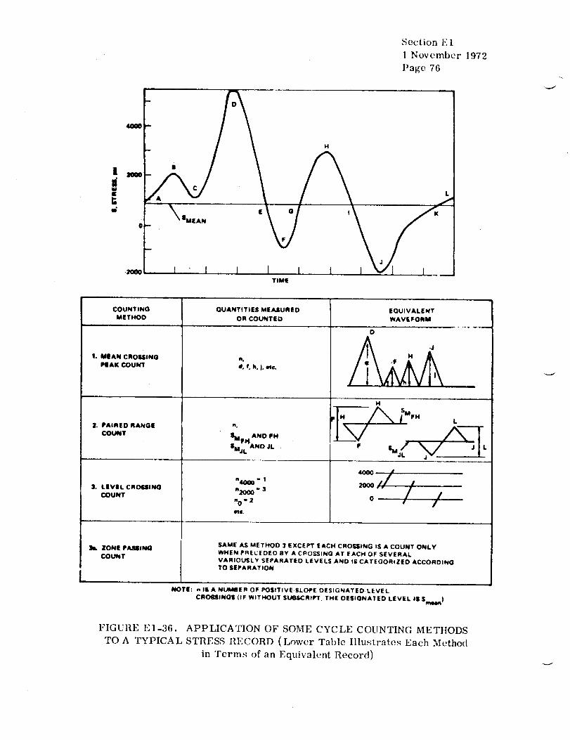
Section E I
1 November 1972
Page 76
H
i K L
-a_@@
TIME
COUNTING QUANTITIES MEASURED EQUIVALENT
METHOD OR COUNTED WAVEFORM
1. MEAN ClIO&SING
PEAK COUNT
2. PAIRED RANGE
COUNT
3. LEVEL CROImlINO
COUNT
3L ]'ONE PASEING
COUNT
n,
IMIIH AND FH
IMj L AND JL
n4000 - 1
nZO00 " 3
n0 " Z
MG.
D
H
S M
-yo, / /
SAME AS METHO0:3 EXCEPT EACH CROSSING IS A COUNT ONLY
WHEN PRECEDED BY A CI_O_ING AT EACH OF SEVERAL
VARIOUSLY SEPARATED LEVELS AND I£ CATEGORIZED ACCORDINGTO SEPARATION
NOTE: nlEANt.RAIIER OF POSITIVE SLOPE DESIGNATED LEVEL
CROSSINGS (IF WITHOUT StJ6SCRIIrlr THE DESIGNATED LEVEL JS Sme4m)
FIGURE El-36. APPLICATION OF SOME CYCLE COUNTING METItODS
TO A TYPICAL STRESS RECORD (Lower Table Illustrates Each Method
in Terms of an Equivalent Record)

Section E 1
1 November 1972
Page 77
1.5.3 Example Problem (Paired Range Count M(,tho(l).
To evaluate the damage caused by complex stress-time cycles, it is
necessary to correct for the difference in mean stress, S , for the variousm
stress alternaticns, S • Four c c:astantamplitudeS-N curves for differenta
mean stresses are shown in Fig. E i-37. A complex stress-time hisotry for
an identical specimen is shown in Fig. 17:1-38.
The first step is to determine the damage caused by the smaller varia-
tions which are crosshatched in Fig. E1-38(a). The largest mean stress is
approximately 20ksiand, as shown in Fig E1-37, for this mean stress an
alternating stress of 4ksior less causes no damage. At an) mean stress less
than 20 ksi, the alternating stress which causes no damage increases so that
any alternating stress of 4 ksi or le._s can be omitted. Thus, variations BC,
DE, GIt, JK, NO, PQ, and _T cau_,;e he fatigue damage. The stress-time
hi_tory is repl¢),_ted in Fig. E1-38(b), with the previously evaluated variationsremoved.
The second 3tep is to evaluate the smallest remaining stress variations
IL _nd RU _or iL, the alternating stress is 5 ksi and the mean stress is 10
ksi. Referring to Fig. F1-37, under these conditions failure would result inl() 7 cycles. !tence the damage is n/N = 1/107 = 10 -7. Calculating the damage
caused by RU inthe same mannqr n/N= 1/2.2 x 104= 4.55x 10 -5 The
'_trcss-time hiutory is again reptotted in Fig. El-aS(e), with the evaluated
variationJ removed.
The third step is to evaluate the remaining cycle, FM, with S = 20 ksia
and S = 5 ksi. Interpolating between S = (t and S = 10, failure would113 rn m
r('sult in 3.5x 10a cycles, tlence, the damage caused is 1/3.5x 103= 2.86 x
10 -4 The last step is to sum the damage caused by all the variations. In
this ease,
10 .7 + 4.5 x 10 -5 4 2.86 x 10 -4 = 3.316 x 10 -4
Using the cumulative damage theory with E n/N = 1.0, the stress-time history
con be repeated 3000 times (1.0/3.316 x 10-4= 3000).
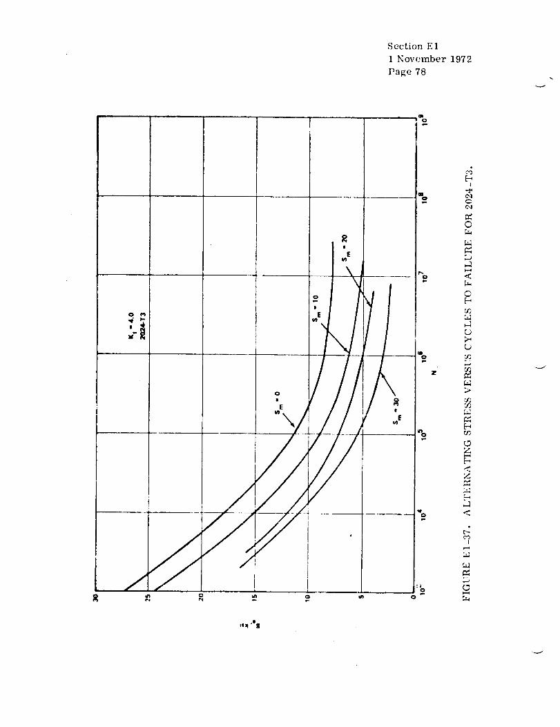
Section E1
1 November 1972
Page 78
8|
E
)
/
,%
I
C'1
cg©
©
c)>_L)
5C
_2
Z
Z
"o <
O
I
_3
tilt '0 9

Section E1
1 November 1972
Page 79/_J0
N O J L li
(a)
M
i '°10
0
4
.10
-11
R
M
v
U
(b)
i i'It/ - \ v
(o)
FIGURE EI-38. STRESS-TIME HISTORY CURVES

-.,!,4
-.....J
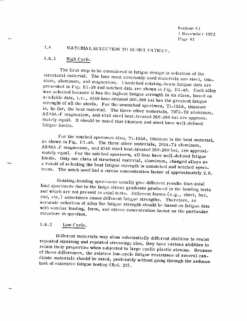
Section E 1
l Novemi)er 1972
l)a_,( ' 81
1 .(; MATERIAL SELECTION TO I{I:SIST I'ATIGUI:.
1.6.1 High Cycle.
The first step to be considered in fatigue design is selection of the
structural material. The four most commonly used materials are steel, tita-
nium, aluminum, and magnesium. Unnotched rotating-beam fatigue data are
presented in Fig. E1-39 and notched data are shown in Fig. El-40. Each alloy
was selected because it has the highest fatigue strength in its class, based on
available data, i.e., 4340 heat-treated 260-280 ksi has the greatest fatigue
strength of all the steels. For the unnotched specimen, Ti-155A, titanium
is, by far, the best material. The three other materials, 7075-T6 aluminum,
AZS0A-F magnesium, and 4340 steel heat-treated 260-280 ksi are approxi-
mately equal. It should be noted that titanium and steel have well-defined
fatigue limits.
For the notched specimen also, Ti-155A, titanium is the best material,
as shown in Fig. El-40. The three other materials, 2024-T4 aluminum,
AZSOA-F magnesium, anal 4340 steel heat-treated 260-280 ksi, are approxi-
mately equal. For the notched specimen, all four have well-defined fatigue
limits. Only one class of structural material, aluminum, changed alloys as
a result of selecting the best fatigue strength in unnotched and notched speci-
mens. The notch used had a stress concentration factor of approximately 2.8.
Rotating-bending specimens usually give different results than axial
load specimens due to the large stress gradients produced in the bending tests
and which arc not present in axial tests. Different forms (e.g., sheet, bar,
rod, etc.) sometimes cause different fatigue strengths. Therefore, an
accurate selection of alloy for fatigue strength should be based on fatigue data
with similar loading, form, and stress concentration factor as the particular
structure in question.
1.6.2 Low Cycle.
Different materials may show substantially different abilities to resist
repeated straining and repeated stressing; also, they have various abilities to
retain their properties when subjected to large cyclic plastic strains. Because
of these differences, the relative low-cycle fatigue resistance of several can-
didate materials should be rated, preferably without going through the arduous
task of extensive fatigue testing (Ref. 23).
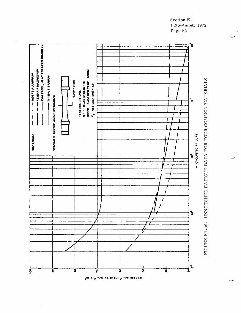
Section E11 November 1972Page82
U
_ ,
ti -
/t/111
I!
III
/
/t
1 ,I
IIJ !
/,!
I
I
I
Il
s
.... /
8
i
/ //
pOI, X _'u_lqt "ALI|N|O /i_'u!/q! '_]WIS|
//_/ /
/
/,/
l
%
Z©v--4
©
©
t, <
0
©Z
I
L_
0
%

OF POOR Ql.:,c_.,,-i-y
Section E1
1 November 1972
Page 83
,,dIJ
=- L_
<D..
CZ
I
b4
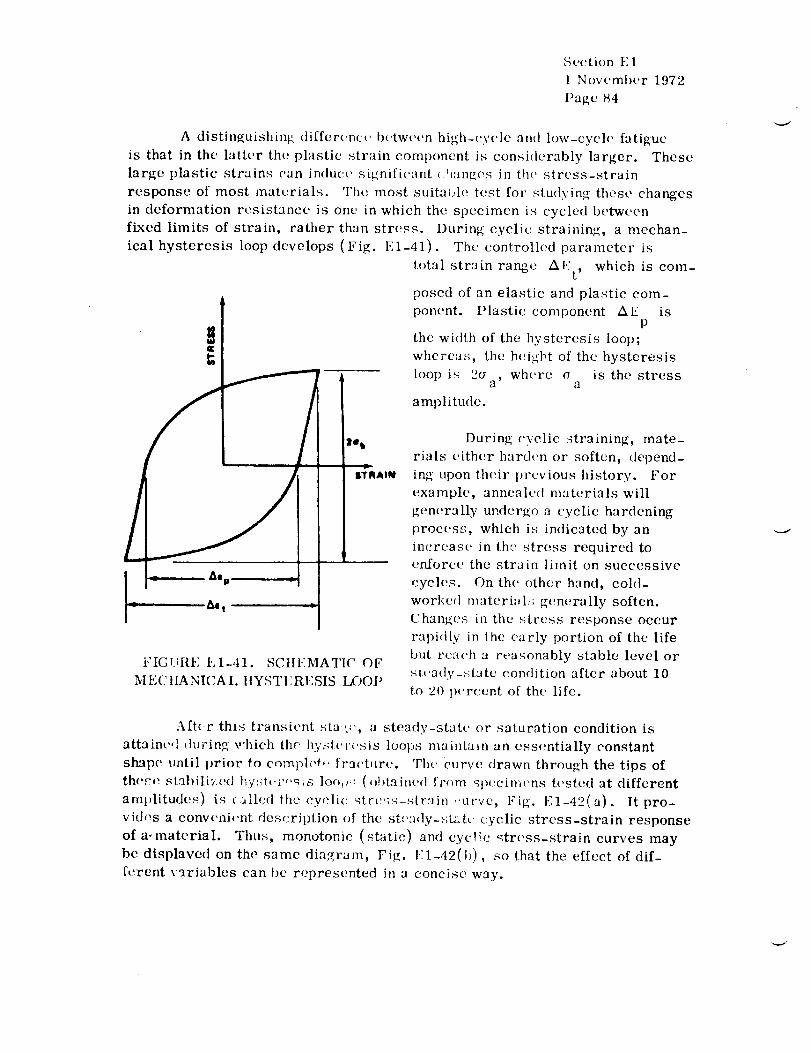
Section E 1
1 November 1972
Page 84
A distinguishing differ(race' between high-cycle an(I low-cycle fatigue
is that in the latter the plastic strain component is consi(lerably larger. These
large plastic strains can induce significant ( _mngcs in the stress-strain
response of most mate, rials. The, most suita_Jle test for _tu(lying these changes
in deformation resistance is one in which the specimen is cycled between
fixed limits of strain, rather than stress. During cyclic straining, a mechan-
ical hysteresis loop develops (Fig. E1-41). The controlled parameter is
/I _ "%p .
i - 6at "
Z# b
ITRAIN
FIGURE E1-41. SCtlI;:MATIC OF
*IE('HANICAL IIYSTERESIS LOOP
total strain range Al,;t, which is com-
posed of an elastic and plastic com-
ponent. Plastic component AE isP
the width of the hysteresis loop;
whereas, the height of the hysteresis
loop is 2(Ya, wh¢'re a is the stressa
amplitude.
During cyclic straining, mate-
rials either harden or soften, depend-
ing upon t h(_'ir previous history. For
example, annealed materials will
generally undergo a cyclic hardening
process;, which is indicated by an
increase in th,'_ stress required to
enforce the strain limit on successive
cycles. On the other hand, cold-
worked materia l_; gent rally soften.
Changes in the stress response occur
rapidly in lhe early portion of the life
but reach a reasonably stable level or
stt,ady-:-:tate condition after about 10
to 20 p('rcent of the life.
After this transient sta:,_', a steady-state or saturation condition is
attaine,l during which the hy,_;lercsis loops maintain an essentially constant
shape until prior to c,_mplo_- fract_lrc. The Curve drawn through the tips of
the,:e st:abiliz."d hV:_tcr,'qis lo%r-' (,_btained fr_m _p,'cin_t,ns tested at different
aml)litudcs ) is c:_lled the cyclic utre:;_-sirain ,:urve, Fig. E1-42(a). It pro-
vidos a conv('ni_'nt description of the st',*ady-:;tat_ cyclic stress-strain response
of a-material. Thus, monotonic (static) and cyclic _trcss.strain curves may
be displayed on the same diagram, Fig. E1-42(1)), so that the effect of dif-
ferent variables can be represented in a concise way.

Section 1':11 November 1972Page85
/
CYCLIC ITRi#
ITRAIN CURVE
\
/STAIILE
LOOPS
IP
_9Lu_rI--
MONOTONIC-COLD WORKED
_NIC-ANNEALED
STRAIN
(a) (b)
FIGtTI{I,: E1-42. CYCLIC S'I'RESS-STIUkIN CURVE, AS I)I:TERMINEI)
FROM SEVI.;RAL IIYSTI.:RESIS LOOPS, (a). COMPARISON WITIt
MONOTONIC CURVE, (b)
Although metals may un(lergo cyclic har(lening or softening, the prob-
h'm oi softening is more important, :_incc the strength properties of the mate-
rial (lurin_ low-eych' fatigue may b(' appreciably less than one would expect
from the static stress-strain curve. Two questions, therefore, seem tobe
important: Will the material cyclically soften? If so, how much will it soften?
A component, or a critical location in a structure, may undergo either
repeated straining or repcatcc[ stressing, depending upon the geometry and
load environment. Some materials show good strain resistance, whereas
others show gnod stress resistance. It is, therefore, necessary to decide
whether a design requires a strain-resistant or stress-resistant material.
The relation between the total strain amplitude, Act/2, and the cycles
to failur(', Nf, is given by
A, Ac
t ^, P -- _- ' (2N[)C'2 2 [
where c is the fatigu(' ductility exponent.

Section 1':1
1 Nero.tuber 1972
Page 86
Thus, the short-life strain resistance of materials depends m:Jinly
v and c. Using typical experimentalupon the fatigue ductility coefficient, ef ,
values for the constants, it is apparent thai. ,_ material with a large value of
Ef t` and a small value of c has the best resistance to repeated straining.
The fact that a material shows good strain resistance does not neces-
sarily imply that it has a good cyclic stress resistance. To point out the
importance of deciding whether the material to be selected must resist repeated
strains or repeated stresses, seven materials were tested for both stress and
strain resistance in Ref. 23. The material with the highest stress resistance
was fourth in ability to resist cyclic strain. Likewise, the mat( rial third
best in cyclic strain resistance dropped to sixth in stress resistance.

j.
1.7 I)I,:SIGN GI TII)I,',S.
Section E1
1 Noveml)er 1972
Page B7
At the ))resent level or' knowlvdge, it is impractical to establish quanti-
tatively the limiting fatigue design rules for specific structural configurations.
The diversity in missions, loads, stresses, materials, and environments
certainly suggests this to be an impracticable, if not impossible, task. Quali-
tatively, however, the practices to be followed in the design of fatigue resist-
ant strueturc'can be defined, and if strict adherence to these established
practices is maintained, potential fatigue problems can be reduced in the initial
stage of structural design.
In general, the basic rules used in the airframe industry will apply in
thcdt, sign o[ space vehicle systems. Past experience and learnin_ from the
one field can be carried over to the other, although some precautions should
be taken. Old designs may be unsuited to a new environment.
When procedures are proposed, they o[ten become general rules which
regulate structural design, even though they may be inappropriate. Recom-
mendations used in the sense of "design rules" are far more appropriate.
With this interpretation, a few of the more pertinent guides for the design of
space vehicle systems may be listed:
1. Keep the design simple.
2. Provide for multiple load paths when feasible.
3. Give extra consideration to tension-loaded fittings anti components.
4. Apply fitting factors of safety to net stresses around holes and
cutouts.
5. Laboratory test all newly designed joints and compare with "time-
tried" structures.
6. Utilize longitudinal grain direction of materials whenever possible
(particularly for aluminum and steel alloys).
7. Provide generous fillets and radii.
8. Break all sharp cdl_es; polish critical regions if it is considered
necessary.
t Reduce bearing stresses in riveted and bolted members to design
minimums.

Section E1
1 November 1972
Page 88
10. Take precautions to protect parts from corrosion.
11. Whenever possible, reduce e(eentricity of joints and fittings.
12. Ensure that doublers and structural reinforcements result in
gradual, rather than abrupt, changes in cross section.
13. Provide easy access for service inspection of structure.
14. Provide inspection procedures during fabrication and assembly ofstructure.
15. When oractical, produce parts and fittings from forged material
rather than from extrusions or machined plate stock.
16. Design parts for minimum mismatch or installation; this results
in lower residual and preload tensile strains.
17. Avoid superposition of "notches" in design.
18. Make a proper selection of materials with cost, strength allow-
ables, fabricability, and environmental effects in mind.
19. Pay close attention to fabrication techniques for optimum formingof components.
20. Establish reliable welding techniques for reproducibility of jointsstrengths.
21. Construct rigid and precision tooling for the manufacturer of pro-duction parts.
Undoubtedly, there are additional useful fatigue guides which could be
added to the list above. Many such guides are unwritten and only intuitively
known by the most experienced design specialists. Excellence in design, how-
ever, is not accomplished by the designer alone. It requires the close cooper-
ation of specialists able to perform complex dynamic stress analyses: acous-
ticians, vibration engineers, metallurgists, specialists in structural testing
and reliability analysis, as well as those experienced in tooling andmanufacturing.
i'hese guides and recommended practices for designers are suggested
for the sole purpose of reducing the overall development time from preliminarydesig_ l:lv_JL_t to assembly in production.

REFERENCES
Section E1
1 November 1972
Page 89
.
1
.
4,
.
o
o
.
Q
10.
11.
12.
Kennedy, A. J.: Processes of Creep and Fatigue in Metals. John Wiley
and Sons, Inc., New York, 1963.
Madayag, A. F. : Metal Fatigue: Theory and Design. John Wiley and
Sons, Inc., New York, 1969.
Fatigue Design Criteria for Launch and Spacecraft Structures. Douglas
Missile and Space Systems Division, Paper No. 3290, January 1965.
Peterson, R. E. : Stress Concentration Design Factors. John Wiley
and Sons, Inc., New York, 1953.
Gurney, M. A.:
Press, 1968.
Fatigue of Welded Structures. Cambridge University
Manson, S. S. : Thermal Stress and Low-Cycle Fatigue. McGraw-Hill
Book Company, 1966.
Langer, B. F. : Design of Pressure Vessels for Low-Cycle Fatigue.
J. of Basic Engr., Transactions of ASME, September 1962.
Smith R. W., Hirschberg, M. H., and Manson, S. S. : Fatigue
Behavior of Materials under Strain Cycling in Low and Intermediate
Life Range. NASA TN D-1574, April 1963.
Manson, S. S., and tialford, G. : h Method of Estimating High
Temperature Low-Cycle Fatigue Behavior of Metals. NASA
TM X-52270, June 1967.
Manson, S. S. : A Simple Procedure for Estimating High-Temperature,
Low-Cycle Fatigue. Experimental Mechanics, August 1968.
Manson, S. S., Halford, G. F., and Hirschberg, M. H. : Creep-
Fatigue Analysis by Strain-Range Partitioning. NASA TM X-67838,
May 1971.
Coffin, L. F., Jr. : A Note on Low Cycle Fatigue Laws. Journal of
Materials, JMLSA, Vol. 6, No. 2, June 1971, pp. 388-402.

REFERENCES (Concluded)
Section E 1
1 November 1972
Page 90
13.
14.
15.
16.
17.
18.
19.
20.
2].
22.
23.
Baldwin, E. E., Sokol, G. J., and (:offin, L. F. Jr. : Cyclic Strain
Fatigue Studies on AISI Type 347 Stainless Steel. Trans. ASTM, Vol.
57, 1957, pp. 567-586.
Clauss, Francis J., and Freeman, James W. : Thermal Fatigue of
Ductile Materials, I and II. NASA Tech. Notes 4160 and 4165, 1958.
Spera, D. A. : Calculation of Thermal-Fatigue Life Based on Accumu-
lated Creep Damage. NASA TN D-5489, October 1969.
Majors, Itarry, Jr. : Thermal and Mechanical Fatigue of Nickel and
Titanium. Trans. Am. Soc. Metals, Vol. 51, 1959, pp. 421-437.
Clauss, F. J. : Thermal Fatigue of Ductile Materials, III. NASA
Tech. Note D-69, October 1969.
Coffin, L. F., Jr,: The Problem of Thermal-Stress Fatigue in
Austenitic Steels at Elevated Temperatures; ASTM Spec. Tech. Publ.
165, 1954, pp. 31-49.
Liu, S. I., Lynch, J. T., Ripling, E. J., and Sachs, G.: Low Cycle
Fatigue of Aluminum AHoy 24ST in Direct Stress. Trans. AIME,
Vol. 175, 1958, p. 469.
Avery, It. S.: Discussion of Cyclic TemperaturcAccelerationof
Strain in Heat-Resisting Alloys. Trans. Am. Soc. Metals, Vet. 30,
1942, pp. 1130-1133.
Freudenthal, A. M.: Some R('marks on Cumulative Damage in Fatigue
Testing and Fatigue Design. Welding in the World, Vol. 6, No. 4,
1968.
Bruhn, E. H. : Analysis and Design of Flight Vehicle Structures.
Tri-State Offset Company, Cincinnati, Ohio, 1965.
Feltner, C. E. and Landgraf, R. W. : Selecting Materials to Resist
Low Cycle Fatigue. ASME Paper No. 69-DE-59.
_" U. II. GOVERNMF.NT PRINTING OFFICIrl 1973--746_Z7/4779 "_"_

SECTION E2
FRACTURE MECHANICS


_'_ TABLE OF CONTENTS
,f-E2 FRACTURE _ EC HANICS ..........................
2.1 GENERAL .................................
2.1.1 Comparison of Fatigue and Fracture Mechanics . . .
2.2 STRESS-INTENSITY FACTORS ...................
2.2.1 Plane Strain . . . ........................
2.2.1.1 Correction for Deep Surface Flaws ......
2.2.2 Plane Stress ...........................
2.2.2.1 Through-the-Thickness C racks ........
2.2.3 Experimental Determination ................
2.3 FLAW GROWTtI .............................
2.3.1 Sustained Load Flaw Growth ................
2.3.1.1 Environmental Effects ..............
2.3.2 Cyclic Load FlawGrowth ..................
2.3.2.1 Theories .......................
I. Paris ......................
II. Foreman ....................
III. Tiffany .....................
2.3.2.2 Crack Growth Retardation ............
I. Wheeler's Retardation Parameter ....
II. The Signi[icancc of Fatigue Crack
Closure .....................
2,3.2.3 Transition from Partial-Thickness Cracks
to Through-Thickness Cracks .........
2.3.3 Combined Cyclic and Sustained Flaw Growth ......
2.4 APPLICATION OF FRACTURE MECIIANICS
TECHNOLOGY ..............................
2.4.1 Selection of Materials ....................
2.4.1.1 Static Loading ....................
I. Example Problem A .............
2.4.1.2 Cyclic orSustaine(I Loading ..........
1. Example l)roblem A .............
II. Example Problem B .............
Page
5
6
10
16
2O
21
23
23
24
25
25
27
29
32
32
32
35
39,/40
39/40
41
41
44
45
49
49
57
E2-iii
,$ _', 2
PRECEDING PAGE _,.,_k_,_('_.O'f FtcJ_r..l.)
TABLE OF CONTENTS (Concluded) _J
Page
2.4.2
2.4.3
Predicting Critical Flaw Sizes ............... 592.4.2.1 Surface Cracks ................... 60
I. Example Problem A ............. 61
II. Example Problem B ............. 62
2.4.2.2 Embedded Flaws .................. 64
2.4.2.3 Through-the-Thickness C racks ........ 66
I. Example Problem A ............. 66
Structure Design ........................ 69
2.4.3.1 Service Life Requirements and
Predictions ..................... 69
I. Example Problem A (Thick-Walled
Vessel) ..................... 76
II. Example Problem B (Thin-Walled
Vessel) ..................... 80
2.4.3.2 Allowable Initial Flaw Size ........... 87
I. Example Problem A .............. 88
2.4.3.3 Nondestructive Inspection Acceptance
Limits ........................ 89
2.4.3.4 Proof-Test Factor Selection .......... 94
I. Example Problem A ............. 97
REFERENCES .................................... 100
E2-iv

E2
2.1
Section E2
1 November 1972
FRACTURE MECHANICS.
GENERAL.
Structures subjected to constant loads at moderate temperatures have
been designed primarily on the basis of the yield strength and/or ultimate
strength of the material. Many of these structures have failed prematurely at
stresses below the yield strength, with disastrous consequences. These
brittle failures have occurred in such diverse structures as storage tanks,
suspension bridges, aircraft landing gears, and rocket motor cases. An
examination of such failures indicated one predominant fcature: A small
defect or flaw was usually found at the failure origin.
Therefore, the key to brittle fracture control lies in understanding both
the weakening effects of flaws and cracks in metals and those factors that
influence this effect. To be useful in an engineering sense, this understanding
must be translated into the types of tests and structural mechanics familiar
to the metal producer and designer. The body of knowledge concerning this
type of failure has become known as fracture mechanics.
Basic to fracture mechanics is the understanding of the state of stress
near the tip of a sharp crack and the relationship between gross stress and
flaw geometry. These concepts are discussed in subsection 2.2, Stress-
Intensity Factors.
Flaw growth or crack propagation under cyclic loads is a basic problem
which is handled best by fracture mechanics concepts. A thorough discussion
of flaw growth is given in subsection 2.3.
Finally, subsection 2.4, Application of Fracture Mechanics Technology,
relates stress-intensity factors and flaw growth to the engineering design and
analysis of structures. Particular attention is given to pressure-vessel design
because of its importance in the acrospace industry.

Section E21 November 1972
Page 2
2.1.1 Comparison of Fatigue and Fracture Mechanics.
Similarities and dissimilarities between fatigue and fracture mechanics
are summarized in Table E2-1. Both fatigue and fracture mechanics depend
primarily on results of laboratory tests; however, the fracture mechanics
concept makes it possible to handle fracture considerations in a quantitative
manner and has shown greater applicability to fatigue crack propagation.
o
o
b_
o
g_
°_.._
0,.._
.,-_
0,-.4
E°,.,_
IOq
0
[/1
,_ 0
0
0
o
°,.._
O9°_._
o
0
.,.._
o
0
o
0,.._
I _:_
_._
< _
d
_d
• ._0 m
Section E2
1 November 1972
Page 3/4
_-_
_ 0r/l
0
0 _
2o
• ,"_ _
m
>
%
0 ""'_
0_ o
_ m
o o
o o
_ m
I_, m o
o
o "_
_ bD
r/l .,_
0
_d
o>
o
m
bl.,.-i
°,-t
00,...I
• 0
o
f.) .,._• o -_tm _
- _ _ o
o o
oo
0 _ _
o _ o o
o o _ o
• ,-i _
o o
[/1
_o
0 -_
,x_ m_x2 2"d
0_ "oo
z'_ .n
tm .,_ _S •
0 _, "_ b_
•,_ _ _ _ -,_ _,_ .,._
b.O "_ _ _ >
O< _ _ _ < ._
_=_ _o
.g


Section E2
1 November 1972
Page 5
2.2 STRE SS-INTENSITY FAC TORS.
To understand how fracture mechanics is used in design, it is helpful
first to learn some of the theory on which it is based.
The precise goal of fracture mechanics can be stated concisely: It
attempts to provide a quantitative measure of resistance to unstable crack
propagation. This measure must be independent of the size and shape of the
crack, the geometry of the part containing the crack, and the manner in which
external loads are applied to the part.
The search for a quantitative value focuses on the conditions in the
vicinity of the crack tip where fracture takes place.
The stress fields near crack
tips can be divided into three basic . __.,_/
types, each associated with a local
mode of deformation, as shown in
Fig. E2-1. The opening mode, I, is
associated with a local displacement
in which the crack surfaces move a. Mode I. b. Mode II.
directly apart. The edge-sliding
mode, II, is characterized by dis-
placements in which the crack sur-
faces slide over one another. In
mode III, tearing, the crack sur-
faces slide with respect to one
another parallel to the leading edge.
Mode I is the most critical mode and
is the only one to be discussed in this
section.
J
c. Mode III.
FIGURE E2-1. THREE DISPLACE-
MENT MODES FOR CRACK
SURFACES
For information on modes II and III, see Ref. 1.

2.2.1 Plane Strain.
Section E 2
1 November 1972
Page 6
The stress conditions, or plane-strain elastic stress field, at the crack
tip for mode I are defined by the expressions shown in Fig. E2-2 (Ref. 2).
These equations give the components of stress (a = normal stress, r = shear
stress) in terms of the polar coordinates r and _ for opening-mode (per-
pendicular) crack surface displacements. Only the first term of each equation
y
mweeI-
I Ox _-_---_ Ox
CRACK r O!
HORIZONTAL DISTANCE FROM CRACK FRONT
Oy - (2 lr r)1/2 2 2 /
Ox" (21rr)1/2 (_
",,v" costs' cosT "'"
FIGURE E2-2. RELATIONSHIP BETWEEN STRESS-INTENSITY FACTOR,
KI, AND STRESS COMPONENTS IN THE XrICINITY OF A CRACK
t/
Section E2
1 November 1972
Page 7
is shown. The complete equations are power series in r/a (crack tip radius/
crack half-length). For practical purposes, all terms beyond the first are
negligible.
All the three stress components are proportional to a scalar quantity
that has been designated the stress-intensity factor, K I. This factor is
independent of r and _ and therefore gives a single description of the stress
intensity at any point near the crack tip. It is a purely numerical quantity
which, if known, provides complete knowledge of the stress field at the crack
tip.
The basic assumption in fracture mechanics is that an unstable frac-
ture occurs when KI reaches a critical value designated Kic, commonly
called fracture toughness. It is important to appreciate the difference
between K I and Kic. The stress-intensity factor K is simply a coefficient
in an equation describing the elastic stresses in the vicinity of a crack tip.
Fracture toughness Kic is a particular value of K I corresponding to
unstable propagation of the crack. This value is a material property and
reflects a material's ability to withstand a given stress at a crack tip. The
difference between K I and Kic is analogous to the difference between stress
and strength for a body free of discontinuities.
Irwin (Ref. 3) used the expressions shown in Fig. E2-2 with the Green
and Sneddon analysis (Ref. 4) to show that the expression for the stress
intensity around the crack periphery for the embedded elliptical flaw (Fig.
E2-3) is
KI = T a_a [a 2 cos 2 _b + c2 sin 2 9]
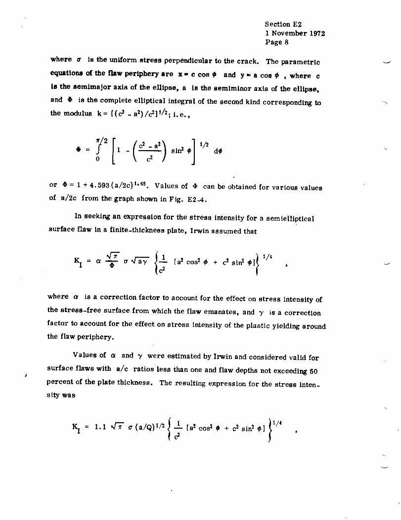
Section E2
1 November 1972
Page 8
where _ is the uniform stress perpendicular to the crack. The parametric
equations of the flaw periphery are g - c cos _ and y = a cos _ , where c
is the semimajor axis of the ellipse, a is the semtminor axis of the ellipse,
and • is the complete elliptical integral of the second kind corresponding to
the modulus k= [(c 2 -a2)/c_]t/2; i.e.,
\
= _2 1 - " sln2 q d@
0 c2
or • = 1 + 4.593(a/2c) t"_s. Values of 4)
of a/2c from the graph shown in Fig. E2-4.
In seeking an expression for the stress intensity for a semielliptical
surface flaw in a finite-thickness plate, Irwin assumed that
i
can be obtained for various values
K I = a T cr_ [a2 cos_ _b +
i/4
where a is a correction factor to account for the effecton stress intensityof
the stress-free surface from which the flaw emanates, and _ is a correction
factor to account for the effecton stress intensityof the plasticyielding around
the flaw periphery.
Values of a and _/ were estimated by Irwin and considered valid for
surface flaws with a/c ratios less than one and flaw depths not exceeding 50
percent of the plate thickness. The resulting expression for the stress inten-
sitywas
I 1 It/4K I = 1.1 _ cr(a/Q)I/2 _- [a2 cos2 @ + c2 sin 2 _1
v

Section E2
1 November 1972
Page 9
vfI /"
\\\\
/ I/ I
/III
FIGURE E2-3. EMBEDDI':D ELLII)TICAL-SIIAPI':D CRACK UNDER
UNIFORM TFNSILI': STRESS IN y-DIRECTION
0.1 .,_,
jr
0.010.001
J
f
/" l
JJ
111II
"1Ill!11II
l
0.01 0.1 1
_2.1
FIGURE E2-4. SIIAPE FACTOR VALUES

Section E 2
1 November 1972
Page 10
where Q = _2 _ 0.212 (a/a YS)2, and a ys is the uniaxial yield strength
of the material. Figure E2-5 shows the relationship between Q and the flaw
depth-to-width ratio.
The maximum value of K I occurs at the end of the semiminor axis
of the ellipse and has a value of
K I = 1.1 _ a (a/Q) 1/2
At some value of a the flaw size becomes unstable and propagates
rapidly. The value of K I computed at the inception of this instability is
called the critical value of K I and is designated KIc. Thus, Kic is the
stress intensity necessary to cause fracture under plane-strain conditions
and is commonly called the plane-strain fracture toughness. Thus,
Kic = 1.1 _a (a/Qcr) l/2 .
Figure E2-6 is a graphical representation of this equation. Some typical
values of Kic for space shuttle materials are shown in Table E2-2.
Stress-intensity factors for other shapes of cracks, different loading
conditions, and crack location are given in Table E2-3.
2.2.1.1 Correction for Deep Surface Flaws.
For surface flaws that are deep with respect to plate thickness, that
is, when the crack approaches the opposite surface, Irwin's equation has been
modified by Kobayashi (Ref. 5) as follows:
where
KI = 1.1 Mk _-a (a/Q)1/2
M k is the magnification factor for deep flaw effects.

f-
Ot: pOOR QUA_._TY
Section E2
1 November 1972
Page 11
,F
0Zl.
"o
o _=._oi
@[
I
I
i
i
- j
('Nt
0
(3
_.- uai"UJ
,o •
o.
, • _
"1-
,,d
0_.
ol
e_ ci o
<2;
<
_9<
m
©
>
M
r_
_dI
M

i
!
Section E2
1 November 1972
Page 12
_j
FLAW SIZE RATIO (a/Q)
FIGURE E2-6. APPLIED STRESS VERSUS CRITICAL FLAW SIZE RATIO
Experimental data obtained on several materials with varying flaw sizes
and shapes appear to provide a fair degree of substantiation of the Kobayashi
magnification factor; however, more experimental investigations are being
performed. Typical curves for M k for two different materials are shown in
Figs. E2-7 and E2-8.
2.2.2 Plane Stress.
An important consideration in fracture mechanics is the "state of
stress," or simply the directions and magnitudes of the applied stresses and
strains. In general, the state of stress in a body is three-dimensional, that
is, stresses and strains exist in all three principal directions.
For thin sheet specimens subjected to in-plane external loads which
do not vary through the thickness, a condition of plane stress is thought to
prevail. As such, strain in the thickness direction is virtually unsuppressed
and considerable plastic flow attends the cracking process.

f_-k
Table E2-2.
Section E2
1 November 1972
Page 13
Properties of Typical Materials Considered
for Use on Space Shuttle
Alloy
4340 (High Strength)
4340 (Low Strength)
D6AC (High Strength)
D6AC (Low Strength)
18 Ni (250)
18 Ni (200)
12 Ni
9Ni-4 Cr
HY - 150
T-1
2014-T6
2024-T4
2219-T87
6061-T6
7075-T6
6AI-4V (STA)
5A1-2.5 Sn
Ftu
(ksi)
260
180
275
218
263
206
190
190
150
115
66
62
63
42
76
169
125
Fty
(ksi)
217
158
231
203
253
198
180
180
140
100
60
47
51
36
69
158
118
52
100
61
112
76
100
226
160
250
180
23
28
27
71
26
51
120

Table E2-3. Stress-Intensity Factors
Section E2
1 November 1972
Page 14
Infinite crackedIheet with uniform
normal stress at
infinity
__.if, xI = o.,/;TKII = Kll I = f)
r
r
" o <> _ -.:
"---"--- LC_ 4
Periodic array of cracks along a line ina sheet, uniform stress at infinity
K I o _ 2h na= tan
KII = Kil I = 0
Cam 2Infinite crackedsheet with uniform
1 _:_ " IT in'plane shear atT infinity
• _ KII
• K I = Kll I = 0
r
r
Case 5
Periodic array _ff cracks along a line in
a sheet, uniform in-plaue shear stress atinfinity
% = ,,,_7 _ ,an:_/
K I = Ktl I = 0
i
_'.] (.9 (9 _ r
CIII3
Infinite sheet with
tunnel crack =u_ect
to out.of.plane ahem
at infinity
K I ffi KII = 0
. --dzo_-- _eo_ .-teor-,_
cl_e
Periodic array of cracks along a line ina sheet, unitorm trot-of-plane shear
at infinity
/2h _¢ra ) _AKll I = ¢ _Vr_'l 7r--_- tan
K I = KII = 0
Case 7
Concentrated force on the
slirlace of a crack in an
infinite sheet
KI = P (a+ h )½2v_- \a - b
' (:/KII = 2 nx/_' + II
K = 3.4 v (for plane strain)
Y
r p f
.2,/;7 \, , ,/
2,/E\. - _/
I
I
i
Case 8
Curved crack m equal hi-axial stress licld
a
t_
(,,oo(,•
i
¢

Table E2-3. (Continued)
Section E2
1 November 1972
Page 15
CaN g
Inclined crack in uniform
tension in infinite sheet
K I = o sin 2 _
Kll = o sin_cosCv"_a
CaN 10
Crack in infinite sheet
subject to arbitrary torce
and couple at a remote
point
:%-"_L
L--2o:..tAt right end
I [I (P + iO) aK= 2x/;_ (t +,O _-a 2
(a + zo) "1(_02 _a2), A I + Ja(P-iQ)(ro-Zo) + ai(I +_)M
,I
(_o- a)(_2 _ a' )'_
tt = (3-v)/(l+v)forplanesereas x = 3.4vforplanestrain
zn = go + iYo _ = Xo- iyo
-- One Crack -- --Two Crack - Case 11
L/r EL/r) f(L/r) Cracks from hole in
Uniaxial Biaxial Uniaxial Biaxial infinite sheet
Stress Stress Stress Stress KI = ov,_- _- f(+)0 3.39 2.26 3.39 2.26
0.1 2.73 1.98 2.73 I.()8 = 00,2 2.30 1.82 2,4l 1.83 KII
0.3 2.04 1.67 2.15 1.70
0.4 1.86 1.58 I.q6 1.61 w_-'_"_e e
0.5 1.73 1.49 1.83 1.57 l'__ _
0.6 1.64 1.42 1.71 1£2
0.8 1.47 1.32 1,58 1.43
I.O 1.37 1.22 1.45 1.38
1.5 1.1_ 1.06 1.20 1.26
2.0 1.06 1.01 1.21 1.20
3.0 0.94 0.93 I. 14 I. 13
5.0 0.81 0.81 1.07 1.06
10.0 0.75 0.75 1.03 1.03
** 0.707 0.707 IO0 1.00
Ca,,e 12
Edge crack m a semi-in-
finite body subjecte(t h>shear
K I = KII = 0
Kll | = r x/_'_"
•--------- b
Case 13
Central crack in strip snbiecl
to tension (finite widlhl
K I = o _X/'_flX)
X = a/b
7, fO,)
0074 I (100.207 I 0_
0.275 1.05
0.337 I Oq
0.410 1.13
0.466 I. I0.535 1.25
0.592 1.31
Case 14
Notched beam in bending
6M
KI = (h a)*/2 g(a/h)
KII = Kll I = [)
a/h g(a/h
().05 0.3t_
0.1 0.49
0.2 060
0.3 0 t,6
0.4 ()6q(}.5 0.72
0.6 073
> 0.6 073
ORIGINAL PAGE IS
OF POOR QUALITY
Table E2-3. (Concluded)
Section E2
1 November 1972
Page 16
f(alb) f(alh) flalb)a/h L/b = I L/h = 3 L/h -o,,
Cose 15
I)_,.hle-edge nolch
OI 1.13 1.12 l 12
02 1.13 I.II 1.12 _"
(14 l 16 I +Of+ I 14
0.5 1.14 1.02 115
06 I I0 1.01 1.22
07 IO2 1.00 134
O.K l.Ol I00 I.<;7 --2b---
()') I .IX) I .O0 2 0')
f,
2h na ) '/-'K I = u _ _ tan _-_ I(:J/h)
kll = gll I = O
l.r L _ _ LISt:
= um _ + O lsin --
C4.. 16
_+'lll+¢lllpllCal Still'ace crack i11 plate SLII')+_CI |o gC|leral exlensH)rl
,+[,.0.,+,I,-+>]
KII = ()
r n_/_a (21 +r;,) 'kKill = d)'_ _kn-'-_- tan
where 'b, isglVell by
'_,, = ./" I-_ h_ ]_i,_=++ do0
Caa 17
lwl) Cqtlal t'l_line;ir cracks in an in_inill2 _heel _uhlec{ h+ llnll(+llM IL'n_IIHI
At lhe heal <'l}d_
-_ r
'T.
K I = +I_
KII = +
i h 2 _ ;,2 )'_
h 2 _ _ a J
KIp)
(h _ -a2l .
A! the lar ends
KI = ov/_-£(._ E(p)pKIp) )
gll = rvr_ #Kip)
1E anti K are Ihe Ctilllplclc elllplic inlegrals F4#) and
K(_) of Ihe firs! and _cond kinds fespedwely
Corn 10 K I = " V_ f(a/b)
Stogie-edge notch
KII = Kll I = O
a/h f(a/b) Ra/h)
OI 115 114
O+2 I?O I.Iq
0.3 1.2') 1,29
0.4 I.t7 1.37
0.5 1,51 1.50
0.6 1 6M I_+
07 I,_lg I;'17
_,r 08 2.14 2.12
{) q 246 2 44
I O 2K6 •_.X.
C=w 19 K I = One I V_ fid/DI
r(mnd hal m lenslt)n
wilh c'lrC'lllnlerenlial = 0c,ack KII = KIll
_ diD Rd/D) d/D lid/D)
o o (I 7o (; 24_l
OI OJII 0.75 O2"_7
l)2 0.I s.i o.80 ( 2(); ()IX'; 0 x5 0 225il4 O21_) (]ql) 0 2()5
It 5, 0227 (),15 0 1(+2
ILl+ ()2IX 0')7 (1 IR)
lib (; 0-_40 I IK) (I
Case20
('Irclll;tr crauk Ill +Ill t oinrinllc b(,tly _ublecl / \--_.,
Ill Illlll_/lll I('n_lon /" / "_"
..---. /2S
KII : Kill : ') ,.... _*_"_" //,'/'/
5/"
l'11iph_;d _ra_k ID lhhnHC +" "
body Mlhlecl I,+ tllI+10llll _-++ / \ " "'"" --
I E'll%il III
I'o1 ilqllrll _)TI klilt_ k III!C
dL'ft'l Illlllt'dby /lll_e
K = -- I%1II (3 t" LOS 2I '1). \
kll - Kll I = ()
<I,,, - \.__._.. /_6
de

r OF POOR QU,_J.iTY
Section E2
1 November 1972
Page 17
2.2
2.0
1.8 m •
_lr 1.8 •
"1:i _*-o=,_ ,,_
1.2 •
al2c_ 0.06
o/2c 0.10
I f IIBASED ON TILTS OF O.I_.in.-THICK BASE METAL(TRANSVERSE GRAIN) AND WELD METAL AAT -_°F AND -42301:]
alZc = 0.20
ad2c = 0.30
o/2c = 0.40
1.0
0 0.10 0.20 0.310 0.40 0.50 0.60 0.70 0.80 0.90
a/t
FIGURE E2-7. M k CURVES FOR 5A1-2.5Sn (ELI) TITANIUM ALLOY
Jr
2.0
1.4
I•,/2c - 0.o6
- 0.40
1.0
0 0.1 0.2 0.3 0.4 0.6 0.| 0.7 0.| O.O
a/t
FIGURE E2-8. M k CURVES FOR 2219-T87 ALUMINUM ALLOY

Section E2
1 November 1972
Page 18
For thick specimens, strain in the thickness direction is suppressed
considerably by the very thickness of the material and noticeably less plastic
flow is associated with the cracking process.
A laboratory plate specimen is seldom completely in either plane stress
or plane strain but rather in some proportion of both. At the free surfaces of
the plate there are no transverse stresses to restrain plastic flow (a condition
of plane stress). In contrast, at mid-thickness, plane-strain conditions prevail
and much less plastic flow occurs. A schematic representation of the crack-
tip plastic zone in a plate specimen is shown in Fig. E2-9.
SHADED AREA = CRACK SURFACEThe size of the plane stress HEAVY SOLID LINE = CRACK FRONT//'_
plastic zone is thought to be related to 7-----_A/", .J_-fZ
the amount of shear tip left at the THICKNESS __/ //_//_
fracture surface. Thus, the appear- OF SPEC_/MEN /J//
ance of the fracture will vary accord- / /f_'_
/
and plane strain conditions through the
thickness of the plate.
FIGURE E2-9. REPRESENTATIONThe influence of stress state
OF PLASTICALLY DEFORMED
(and associated plasticity) on the frac- REGION AT A CRACK FRONT
ture toughness is illustrated in Fig.
E2-10, which shows the effect of plate thickness on the toughness and fracture
appearance. This figure shows that the larger thicknesses are characterized
by low values of toughness. This corresponds to a completely square (brittle-
appearing) fracture appearance.
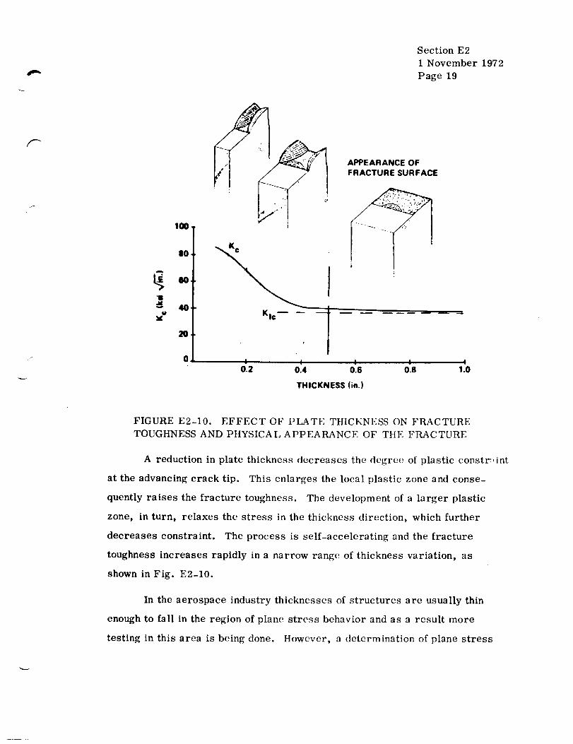
f--
|0
U
0
Section E2
1 November 1972
Page 19
I
Kic
! l0.2 0.4
APPEARANCE OFFRACTURE SURFACE
I! 1 I
0.6 0.8 1.0
THICKNESS (in.)
FIGURE E2-10. EFFECT OF PLATE TIIICKNESS ON FRACTURE
TOUGHNESS AND PHYSICAL APPEARANCE OF THE FRACTURE
A reduction in plate thickness decreases the degree of plastic constr',int
at the advancing crack tip. This enlarges the local plastic zone and conse-
quently raises the fracture toughness. The development of a larger plastic
zone, in turn, relaxes the stress in the thickness direction, which further
decreases constraint. The process is self-accelerating and the fracture
toughness increases rapidly in a narrow range of thickness variation, as
shown in Fig. E2-10.
In the aerospace industry thicknesses of structures are usually thin
enough to fall in the region of plane stress behavior and as a result more
testing in this area is being done. However, a determination of plane stress

Section E2
1 November 1972
Page 20
intensity factors is far more complicated than was first supposed and consider-
able research is needed. It is very hard to determine when unstable crack
propagation occurs because the unstable condition is approached very gradually
as crack length increases.
At present there is no direct method for translating laboratory data for
the mixed mode fracture condition to useful numbers for designing practical
hardware.
2.2.2.1 Through-the-Thickness C racks.
In thin-walled structures, cracks may grow through the thickness
before catastrophic failure occurs or a through-the-thickness crack may
exist before any load is applied. The basic plane stress equation for through-
thickness cracks corrected for plastic zone in an infinitely wide plate is
_ 1 Kc2K 2 =if2 lr c +
c T
where _ is the length of the through-thickness crack at failure (in.) a ise t
the stress normal to the plane of the crack at failure (ksi), a is the yieldY
strength (ksi), and K is the critical plane-stress stress intensity (ksi 4-_.)e
The critical plane stress intensity for a finite-width panel containing
a through-thickness crack is
{ [(K = a wtan _rc _ n + II
c nff y2
where w is the width of the panel (in.).

Section E21 November 1972Page 21
2.2.3 Experimental Determination.
Among the most important recent progress in fracture mechanics is
the improved understanding of how the behavior of test specimens relates to
the design of structural components. Numerous tests have been performed on
a variety of specimen types, some of which are shown in Table E2-4. The
tests were designed to determine the specimen types, procedures, and data
analysis which result in Kic determinations that are independent of crack
and specimen geometry and manner of external loading.
At present no fracture mechanics test is universally used to determine
KIc values because no one test gives valid data for all materials; each of the
tests has its limitations. For instance, ASTM committee No. E-24 has been
working for several years to bring out a standard (E399-70T is proposed),
but this test may not be valid for low-strength, high-toughness materials.
Table E2-4 describes some types of fracture specimens, the data
obtained, and their uses and limitations. For detailed information on these and
other specimens, how to set up and conduct the tests, what data to obtain, and
how to analyze data, see Refs. 1, {I, and 7.

Table E2-4°
Section E2
1 November 1972
Page 22
Seven Common Types of Fracture Specimens
Specimen Loading Data Obtained Uses/Limitations
_to w
Single-Edge Crack
Double- Edge C rack
Io ,J
Central Through-Crack
Round Bar Notched
C racldine-Loaded Wedge
Opening, or CompactTension
oL_
Partial-Thickness Crack
ASTM Cracked Slow Bend
Uniaxial tension,
induced bending
Uniaxial tension
Uniaxial tension
(statie or eyclie)
Uniaxial tension
(cyclic or static)
or rotating
flexure fatigue
Tension with
induced bending
Uniaxial tension
(static or cyclic)
Breaking stresses,
Kic
Breaking stresses,
KIc
Breaking stresses, K ,c
flaw growth rates,
Kie,_ ,10 e
Breaking stresses,
Kic
KIc, Kii
C racks must be equal
in size
Simulates penetrationflaw in har(h_art,.
K Is width (lept'ndt,nt.C
Simulates bolts and
shafts. Difficult to
form concentric
prccraek.
Compact
Breaking stresses,
flaw sizes, apparent
Kic
Simulates natural
flaws in hardware.
Difficult to analyze.
May not provide
valid KIc values.
Three-pointloading
Kic Only standardized
test for Kic. Not
applicable to most
thin and tough
materials.

f--
//
Section E2
1 November 1972
Page 23
2.3 FLAW GROWTH.
2.3.1 Sustained Load F law Growth.
One of the most serious structural problems that can arise in the aero-
space industry is the delayed time failure of pressure vessels caused by
sustained pressurization. In some cases, through-the-thickness cracks have
formed and the vessels leaked under sustained loading. In other cases, small
surfaces cracks or embedded flaws grew to critical sizes before growing through
the thickness of the shell. When this happens, complete catastrophic fracture
ensues. To predict such failures one must know the conditions under which
subcritical flaw growth can occur, as well as either the actual initial flaw size
or the maximum possible initial flaw size in the vessel when it is placed into
service.
When the sustained stress flaw growth is environmentally induced, it
is often termed stress corrosion.
The surface-flawed or "part-through" type of cracked specimen has
probably found the widest use in evaluating sustained stress flaw growth in
both "thick- and thin-walled" aerospace pressure vessels. With this specim .,
the initial flaw closely simulates the type of flaws often encountered in service
and it can be oriented to suit the flaw growth characteristics desired.
A procedure for laboratory evaluation of sustained stress flaw growth
using surface flawed specimens is schematically illustrated in Fig. E2-11.
The Kic for the material is first established from static (pull) tests. Then,
using a batch of flawed specimens, each flawed specimen is loaded with differ-
ent initial loads (various fractions of Kic ) and the time required for failure
observed, e.g., specimens 1 and 2, illustrated in Fig. E2-11. If failure does
not occur in a reasonable time (e.g., specimens 3 and 4), it is still possible
to obtain crack growth information by "marking" the crack front (applying
some low-stress fatigue cycles) and pulling the specimen apart.

Ki
Kk_
KTH
Section E2
1 November 1972
Page 24
5
6
• FAILED
GROWTH. NO FAILURE
NO GROWTH, NO FAILURE
LOG TIME
r
FIGURE E2-11. SCHEMATIC ILLUSTRATION OF A PROCEDURE
FOR LABORATORY EVALUATION OF SUSTAINED-STRESS FLAW
GROWTH USING SURFACE FLAWED SPECIMENS
A point is finally reached at which neither failure nor flaw growth
occurs. The highest level of K for which this condition occurs is called the
threshold stress intensity, KTH; or Kiscc ifdue to stress corrosion
cracking.
2.3.1.1 Environmental Effects.
The discovery of a unique KTH can be 80 percent of Kic or higher
in relatively inert environments; hostile media can reduce the value to less
than half of Kic.
Considerable evidcnce indicates that sustained load flaw growth is
most severe under conditions of plane strain with KTH values determined
from through-the-thickness cracked specimen tests increasing with a decrease
in specimen thickness.

Section E2
1 November 1972
Page 25
Studies of flaw growth and stress intensity in aggressive environments
indicate a monotonic relation between increasing stress intensity and growth
rate and design correlations have been determined for the critically important
materials, titanium, and high-strength steels. In these tests for KTH , a
wide scatter, abnormally short times to failure, and very marked dependence
on environmental characteristics (media and temperature) are encountered.
During the past few years a considerable amount of sustained load
flaw growth data has been obtained on a number of different material-
environment combinations. A summary of some KTH information is given
in Table E2-5.
2.3.2 Cyclic Load Flaw Growth.
Understanding crack propagation under cyclic loads is a basic require-
ment for the application of fracture mechanics to the design of structures for
service life. Subcritical flaw-growth characteristics for various materials
are generally determined through the laboratory testing of flawed specimens.
These empirical data are then correlated to various crack-propagation theories
which have been proposed. The following is a discussion of some of the mor(,
prominent theories.
2.3.2.1 Theories.
A number of studies dealing with fatigue crack propagation have shown
that the stress intensity factor K is the most important variable affecting
fatigue crack growth rates. The availability of a master curve for a partic-
ular material relating fatigue crack-growth rate and range of stress-intensity
factor would enable a designer to predict growth rates for any cracked body
configuration.
Numerous "laws" of fatigue crack growth have been published during
the last 10 years. Basically, all the various equations that have been obtained
are simply the attempt of an individual investigator to obtain a curve that will

Table E2-5.
Section E2
1 November 1972
Page 26
Typical Threshold Stress-Intensity Data for VariousMaterial-Environment Combinations
Material
6A I-4V Titanium
Forging - STA
Temp. a ys Typ. KIe
(" 1") (ksi) (ksi _'i'_. )
R.T. ! 6O 44
it.. T. 16o 44
R.T. 16o 44
R.T. 16o 44
It. T. 160 44
R.T. ! 60 44
It. T. 16o 44
It. T. 16O ,14
It. T. 16o 44
9O 16O 44
90 160 .t-i
105 i 6O .14
11 (I 16(I 44
6A I-4V Titanium R.T. 126
Weldments (llcat- It. T. 126
Affected Zones ) R.T. 126
II. T. 126
5A1-2.5 Sn (ELI) -32o 1 St}
Titanium Plate -:12o 1 I_o
-423 210
2219-TI47 Aluminum It. T. 5t4
Plate -320 66
-423 72
4:;:10 Steel R.T. 205
4340 Steel R.T. -20o
39
39
39
39
Fluid Environment
Methanol
Freon M. F.
N204 (o. 30f_o NO)
N:O 4 (o. 6o% NO)
[[_o (distilled) + Na2CrO 4
lt,O (distilled)
lh.lium, Air, or GOX
Aerozine 50
Fre,m T. l".
N:O I (ii.:lli',rO NO)
N:()_ (ll.i;ll<o NO)
Monomcthylhydrazinc
Ai,rozine 50
Mt_ttlanoi
I,'l'con M. I,'.
II,(J (liistilled)
II,O (l)istilled) _ Na,2CrO I
KTII/KIc
0.24
O. 58
0.74
O. 8:1
O. _2
O. _6
ft. 9o
II, H2
O. B0
0.7t
ti. 75
o. 75
0.75
0.28
I). 4 II
O. I'16
0. _2
64 LN: (¢r ," I'vol). lAir, it) _0.90
64 LN, ((r ". Prop. Limit) o. l_2
52 Lll, -0.90
36 Air ii. fill
41 I,N;! II. 1,2 a
44 LII, -0. _,_:[
90 Water O. 24
"--60 Salt W:itCI' <0. 20
GTA Welds
1i'1 Ni (200) Steel II.T. 200 1:|0
18 Ni (250) Steel It.T. 235 75
12 Ni-5 CR-3 Mo Steel R.T. 170 1 55
9 Ni-4 Co-2.5C Steel R.T. 17(] 120
5 NI-Cr-Mo Steel R.T. 140 "_2011
Salt-water Slira _'
S;lit-v, ate r Spray
Salt-water Spray
Salt-ware r Slirav
Stilt- wattH" Spray
lneonel 71 8 R.T. 165
2219-T851 Alumimlm R.T. 50
Plate
2021-T851 Aluminum II. T. 65
?late
-0.70
">l). 7h
-(I. 70
_0.70
",l:lli Gaseous tlydroileo at 5o00 psig o. 25
N '(it O. 70
30. 5 N.O_ 0.35
a. No failure KTI l ; some growth observed at lower values.
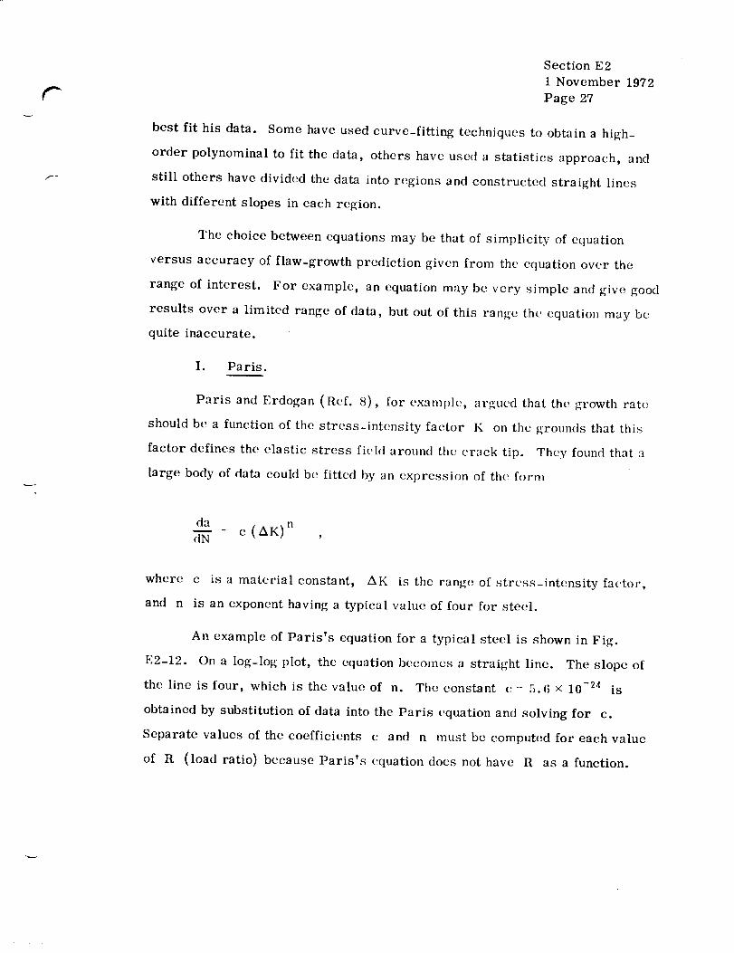
r
Section E2
1 November 1972
Page 27
best fit his data. Some have used curve-fitting techniques to obtain a high-
order polynominal to fit the data, others have used a statistics approach, and
still others have divided the data into regions and constructed straight lines
with different slopes in each region.
The choice between equations may be that of simplicity of equation
versus accuracy of flaw-growth prediction given from the equation over the
range of interest. For example, an equation may be very simple and give good
results over a limited range of data, but out of this range the equation may be
quite inaccurate.
I. Paris.
Paris and Erdogan (Ref. 8), for examph', argued that the growth rate
should be a function of the stress-intensity factor K on the grounds that this
factor defines the elastic stress field around the crack tip. They found that a
large body of data could be fitted by an expression of the form
da
- c (AK) n(IN
where c is a material constant, AK is the range of strcss-intensity factor,
and n is an exponent having a typical value of four for steel.
An example of Paris's equation for a typical steel is shown in Fig.
E2-12. On a log-log plot, the equation becomes a straight line. The slope of
the line is four, which is the value of n. The constant e- 5.(; x 10 .24 is
obtained by substitution of data into the Paris equation and solving for c.
Separate values of the coefficients c and n must be computed for each value
of R (load ratio) because Paris's equation does not have R as a function.

POOR QUALITY
Section E 2
1 November 1972
Page 28
W -- AIS! 1048 STEEL __
oys - 37 _ lid_*F AIR ENVIRONMENT
10 Wdes/_
2
10 20 40 80 80 100STRESS-INTENSITY FACTOR RANGE, AK (ksi_'n.)
FIGURE E2-12. FATIGUE CRACK GROWTH RATE VERSUS STRESS-
INTENSITY FACTOR RANGE FOR AISI 1045 STEEL
P
+

F
Section E2
1 November 1972
Page 29
II. Foreman.
The Paris fourth-power crack growth rate equation was modified by
Foreman et al. (Ref. 9) to account for the observed behavior that crack growth
rates tend to increase rapidly toward an apparent instability as thc maximum
applied stress intensity approaches the fracture toughness of the material.
Foreman also modified the Paris law to account for the observed behavior and
to explicitly express the effect of load ratio, R = K . /K . The Foremanmm max
expression for plane-stress conditions is
da c (AK) n
dN (1 - R)K _ AKC
where c and n are constants dependent on material and test conditions.
AK = (Kmax - Kmin) during a load cycle.
K = plane stress fracture toughness of the material.C
A comparison of Paris_s and Foreman's equations was made by Hudson
in Ref. 10 for 2024-T3 and 7075-T6 aluminum. It was found that the 7075-T6
data fell into an S shape or reflex type of curvature. A reflex curvature is
also obtained from Foreman's equation; it is induced by AK approaching
(1 - R) K in the denominator. This intrinsic shape is the primary reasonc
for the excellent fit of the data by using Foremants equation. Paris's equation
does not provide for this reflex curvature; consequently, the equation cannot
fit the data at high or low growth rates as well as ForemanVs equations.
The constant n in Foreman's equation is the slope of the curve in the
straight-line midrange and c is determined from the substitution of data

bectlon E2
1 November 1972
Page 30
value into the equation. It should be noted that n and c will change, depend-
ing on the type of plot used. Generally, a log-log plot of AK in psi _/-_m.
and da/dN in microinches/inch is used.
Foreman's equation for 2219-T87 is shown in Fig. E2-13 and some
typical values of c and n for other common materials are given in Table
E2-6.
Table E2-6. Crack Propagation Coefficients for Foreman's Equation
da c (AK) n
d"_" : (1 - R) K _ ANc
da/dN in./cycle
AK and K psi x/_n.C
Material
2219-T87 R°T.
:_00
-320
1.4 x 10 -il
1.5 × 10 -li
9.0X 10 -13
2.5
2.47
2.7
KIc
psi
33,000
31, 600
36, 200
TI-6A1-4V R.T. 7.8 x 10 -t4 3.0 81,000
2024-T3 R.T. 3.22 x 10-i4 3.38
7075-T6 R.T. 2.13 x i0- 13 3.21
517A(TI)
The solution of the Foreman equation can be formulated as an initial-
value problem and can bc solved by direct numerical integration using the
Runge-Kutta method. For most practical problems, an initial crack size is
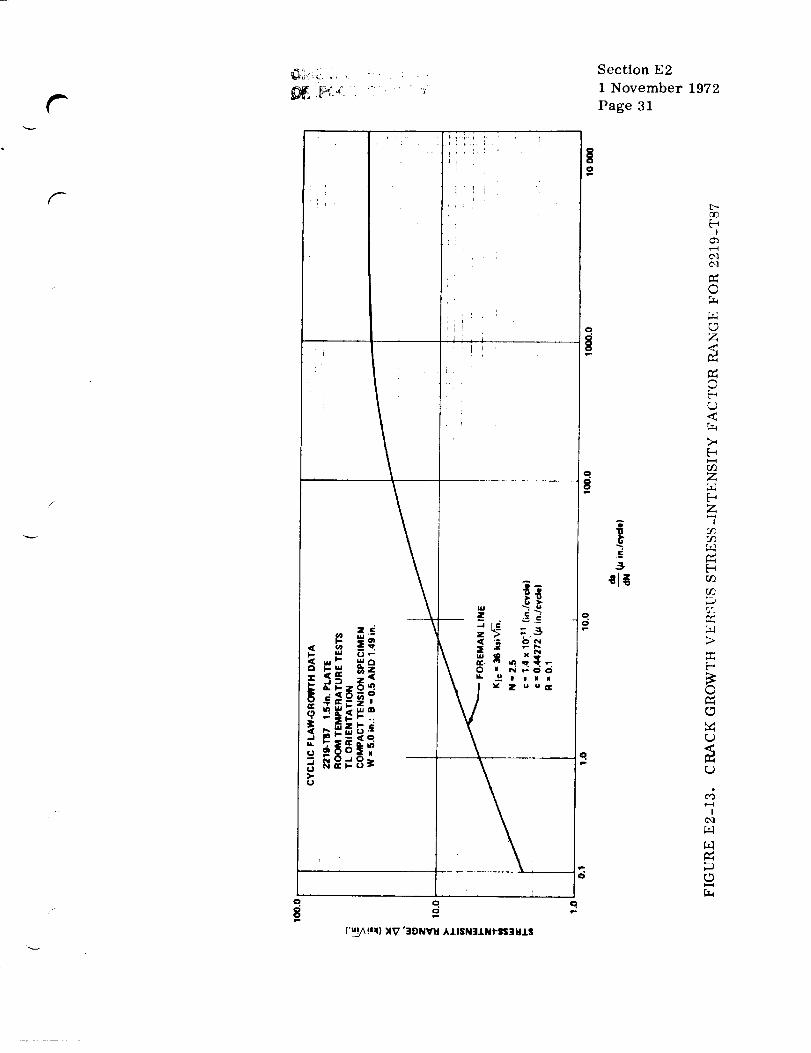
¢-
,': !
r i
I:
..zn_c.u
.I-
_g_'"
IIi, i
, :!I
• r
..1 c '-
z _ :,,_'
I&. _ m # II le
U ,U _
0
0F-
('ua_!"l))IV '3ONW_I AJ.ISN31J.NI-Sl;]WJ.$
qi,-
§
Section E2
1 November 1972
Page 31
o.g
,E
_C
!
¢d
0
_D
(3
r..)
.<
Z
2;I
r_2
dI
I..,,4

Section E2
1 November 1972
Page 32
known at an initial value of N, such as N = 0. The problem is to determine
the crack length (or additionally the stress-intensity factor) after a given
number of cycles.
III. Tiffany.
An alternate approach to plane-strain flaw-growth rates has been
presented by Tiffany (Ref. 11). Tiffany noted that the cyclic lives of speci-
mens were primarily a function of the ratio of maximum initial stress intensity
applied to the flaw during the first loading cycle (KIi) to the plane-strain
fracture toughness of the material (Kic) . Accordingly, cyclic life data were
plotted on Kii/Kic versus cycles-to-failure graphs, where it was observed
that data for particular test conditions and material-cnvironment combinations
could be reasonably represented by a unique curve. Flaw-growth rates were
computed using the slopes of the cyclic life curves. Because the analysis
required knowledge of only the initial and final conditions for each test, the
Tiffany method was called an end-point analysis. The use of Kii/Kic versus
cycles-to-failure curves for practical design problems is common in the
aerospace industry (Ref. 12). Figure E2-14 shows a Kii/Kic versus cycles-
to-failure curve for 2219-T87 at room temperature.
2.3.2.2 Crack Growth Retardation.
• I. Wheeler's Retardation Parameter.
The retardation of crack growth is a phenomenon which occurs because
of varying load levels. Retardation has been shown to occur particularly after
a high level of load followed by a lower level of load.
Many papers have discussed crack growth retardation to some extent
but a computational technique has not been presented which is sufficiently
simple and accurate to gain widespread use (Ref. 13).

Section E2
1 November 1972
Page 33
/
/
qP
w.o o
q.o
|
8
R
C
..JI
L,_
Ob-
..Jt_)-
b4<
00
<
oo
F_
o,1
0
0
0
r..)
r_
r..)
4I

Section E2
1 November 1972
Page 34
Wheeler (Ref. 13) suggests that more accurate crack growth predictions
can be made by introducing a retardation parameter in the crack growth
equation, which serves to delay the crack growth after a high load application.
His equation for crack length is
r
r o pii=1
where a is the crack length after r load applications, a is the initialr o
crack length, Cpi is the retardation parameter at ith load, and AK is1
the change in the stress-intensity factor at ith load. The retardation param-
eter is taken in the following form:
Ra')mC = Y_ , a + R <a
P p Y P
C = 1 , and a + R >- aP Y P
where R is the extent of the current yield zone, a - a is the distanceY P
from crack tip to elastic-plastic interface (Fig. E2-15), and m is the shaping
exponent dependent upon material and test data.
This parameter has been used successfully to predict the growth of
cracks in specimens subjected to six different spectra, having three different
physical configurations, and made of two materials (Ref. 13). It is believed
that this approach represents a useful improvement on the idea of linear
cumulative crack growth, which can be used with confidence in design and
ana lysis.

f-
Section E2
1 November 1972
Page 35
/ \J
/ \
4ira
\ J /iNTERFACE /
= My ":_ .l.\ I i
!
FIGURE E2-15. CRACK TIP YIELD ZONES
The computational scheme for incorporating this retardation parameter
in crack growth predictions requires that the crack be grown one load applica-
tion at a time. This amounts to a piecewise linearization of a highly nonlinear
process. The use of a high-speed digital computer is obviously required to
perform any realistic analysis. This technique has been incorporated into
the computer program CRACKS (see the Computer Utilization Manual).
II. The Significance of Fatigue Crack Closure.
Recent work by Elber (Refs. 14 and 15) has shown that fatigue cracks
in sheets of aluminum alloy close before all tensile load is removed. Significant
compressive stresses are transmitted across the crack at zero load. In pre-
vious work, usually the assumption has been made implicitly that a crack is
closed under compressive loads and open under tensile loads. The deter-
mination of the crack closure stress must, therefore, be a necessary step in
the stress analysis of a cracked structure.
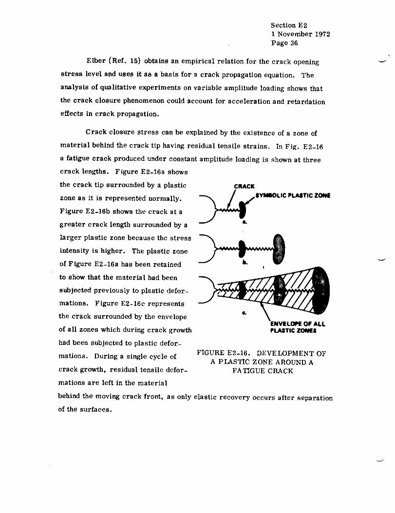
Section E21 November 1972
Page 36
EIber (Ref. 15) obtains an empirical relation for the crack opening
stress level and uses it as a basis for a crack propagation equation. The
analysis of qualitative experiments on variable amplitude loading shows that
the crack closure phenomenon could account for acceleration and retardation
effects in crack propagation.
Crack closure stress can be explained by the existence of a zone of
material behind the crack tip having residual tensile strains. In Fig. E2-16
a fatigue crack produced under constant amplitude loading is shown at three
crack lengths. Figure E2-16a shows
the crack tip surrounded by a plastic
zone as it is represented normally.
Figure E2-16b shows the crack at a
greater crack length surrounded by a
larger plastic zone because the stress
intensity is higher. The plastic zone
of Figure E2-16a has been retained
to show that the material had been
subjected previously to plastic defor-
mations. Figure E2-16c represents
the crack surrounded by the envelope
of all zones which during crack growth
had been subjected to plastic defor-
mations. During a single cycle of
crack growth, residual tensile defor-
mations are left in the material
CRACK
|YMBOLIC FLAITIC ZONE
ENVELOPE OF ALLPLASTIC ZONIEI
FIGURE E2-16. DEVELOPMENT OF
A PLASTIC ZONE AROUND A
FATIGUE CRACK
behind the moving crack front, as only elastic recovery occurs after separation
of the surfaces.

,f
Section E2
1 November 1972
Page 37
Crack propagation can occur only during that portion of the loading
cycle in which the crack is fully open at the crack tip; therefore, in attempting
to analytically predict crack propagation rates, it seems reasonable that the
crack opening stress level should be used as a reference stress level from
which an effective stress range could be obtained. The effective stress range
is defined there as
ASef f = S - Smax op
where S is the crack opening stress.op
An effective stress range ratio is then dcfined as
C _.
(Sma x - Sop) ASef f
(S ASmax - Smin)
Constant amplitude loading tests were conducted to establish the
relationship between U and three variables which were anticipated to have
a significant effect on U , namely, stress-intensity range, crack length, and
stress ratio.
For the given range of testing conditions, only the stress ratio R is a
significant variable. The relation between U and R is linear and can be
expressed as
U = 0.5 + 0.4R where -0.1 < R< 0.7
for 2024-T3 aluminum alloy.

Section E2
1 November 1972
Page 38
One of the most important problems in aircraft structures is the inability
to predict accurately the rate of fatigue crack propagation under variable ampli-
tude loading. In attempts to calculate these crack rates on the basis of constant
amplitude data, interaction effects are usually ignored, leading to errors of
significant magnitude.
Crack closure may be a significant factor in causing these interaction
effects. This can be shown by the following example. Assume that a crack
in 2024-T3 aluminum is propagating under the conditions R = 0 and K --max
20 MN/m 3/2. Under these conditions the crack opening level is at Kop =
10 MN/m3P. If the stress-intensity range suddenly is halved, the new con-
ditions are K = 10 MN/m3/2 and R = 0. The crack opening level, how-max
ever, is still at Kop 10 MN/m3/2 , equal to the new peak stress intensity,
so the crack does not open. Therefore, the crack does not propagate until
the crack opening level changes. The behavior of the crack opening stress
level under variable amplitude loading must therefore be investigated.
It has been observed that a crack will continue to grow for some time
after a high load application followed by loads of smaller magnitude. This has
been termed delayed retardation. Such retardation of crack growth after a
single high load can be explained by examining the behavior of the large plastic
zone left by the high-load cycle ahead of the crack tip. The elastic material
surrounding this plastic zone acts like a clamp on this zone, causing the
compressive residual stresses. As long as this plastic zone is ahead of the
crack tip, this clamping action does not influence the crack opening. As the
crack propagates into the plastic zone, the clamping action will act on the
new fracture surfaces. This clamping action, which builds up as the crack
propagates into the plastic zone, requires a larger, externally applied stress
to open the crack; hence, the crack will propagate at a decreasing rate into
this zone and may come to a standstill.

Section E2
1 November 1972
Page 39/40
2.3.2.3 Transition from Partial-Thickness C racks to Through-ThicknessCracks.
It was shown in Section 2.2 that the stress intensity was different for
partial-thickness cracks and for through-the-thickness cracks. Also, for
through-the-thickness cracks, corrections must be made for a finite plate
within the stress intensity equation (Table E2-2, Case 13).
Often in crack propagation problems a crack will initially be a partial-
thickness crack and will grow until it extends through the thickness. When
this occurs, corrections in the stress-intensity expression must be made.
The transition from a surface flaw to a through crack is chosen to
be the point when the plastic zone reaches the back face of the material. The
value of a (crack length) for which this occurs is _iven as
1at= t - _-\ ys /
2.3.3 Combined Cyclic and Sustained Flaw Growth.
Tiffany and Masters (Ref l) hypothesized that below the sustained stress
threshold stress-intensity value (KTH), cyclic speed (or hold time at maximum
load) probably would not affect the cyclic flaw growth rate, but above KTH
it could have a large effect. In other words, the minimum cyclic lifc was
limited to the number of cycles required to increase the initial stress intensity
Kii to the KTH value, and above the KTH level, failure could occur in
one additional cycle if the hold time were sufficiently long.
To date there is only a limited amount of experimental data to sub-
stantiate this prediction. However, the data do tend to support the original
Tiffany-Masters hypothesis of no significant effect of cyclic speed on flaw
growth rates below the sustained stress threshold stress intensity.


f-
f_
Section E2
1 November 1972
Page 41
APPLICATION OF FRACTURE MECHANICS TECHNOLOGY.
Selection of Materials.
In the material selection and design of a tension-loaded structure, such
as a pressure vessel, the following questions must be considered:
1. What are the criticalflawsizes (sizes which cause failure) in the
different parts of the structure at expected operational stress levels ?
2. What are the maximum initial flaw sizes likely to exist in the
structure before service ?
3. Will these initial flaws grow to critical size and cause failure
during the expected service life of the structure ?
The answers to these questions depend heavily upon the inherent
fracture toughness and subcritical flaw-growth characteristics of the structural
material. Fracture toughness data derived from test specimens are used in
fracture mechanics analysis to predict critical flaw sizes, evaluate subcritical
flaw growth, and estimate structural life. They can also be used to determine
the maximum possible initial flaw size in a structure after a [)roof load.
As previously mentioned (Section 2.2), the types of flaws encountered
in fabricated structures can be categorized as surface flaws, embedded flaws,
and through-the-thickness cracks. For surface and embedded flaws, the
degree of constraint at the crack leading edge is high, and plane-strain con-
ditions generally prevail. The initial flaws may or may not reach critical
size before growing through the thickness, depending upon the plane-strain
fracture toughness (KIe) value, the applied stress levels, and the materialp
thickness. If the calculated critical flaw size is small with respect to the
wall thickness, the formation of a through-the-thickness crack before frae-
ture is not likely.
Section E21 November 1972Page 42
For through-the-thickness cracks, the mode of fracture for a given
material, stress level, and test temperature depends upon the material thick-
ness. If the material is relatively thin, plane-stress conditions generally
predominate. With increasing thickness, the fracture appearance changes
from that of full shear to an essentially flat or plane-strain fracture. Thus,
for thin sections containing through-the-thickness cracks, the plane-stress
fracture thoughness (Kc) values are important, and as the thickness is
increased the plane-strain (Kic) values should be used. The theory of this
has been discussed in detail (Section 2.2.2).
The common types of fracture specimens and their requirements have
also been discussed (Section 2.2.3). It is appropriate to point out the signifi-
cance of end-hardware application and material anisotropy on specimen selec-
tion and to show fracture-toughness correlations among several of the more
common specimens.
Just as conventional mechanical properties generally vary to some
degree among various forms and grain directions in a given basic alloy, it
has been found from fracture tests performed thus far on various materials
that fracture toughness values also vary. In a rolled plate or forging, six
directions of flaw propagation are possible, and plane-strain toughness (Kic)
values may differ in each of these directions (Fig. E2-17). The need to
determine the Kic values in each of these directions depends on the direction
of the applied stresses in the hardware.
Considering the banding and delamination problems in some thick
plates, it appears that the Kic values can be different between the A and
B directions and, likewise, the C and D directions. This has actually
been found to be the case from investigation (Ref. 16) and tends to explain
the differences in KIc values obtained using surface-flawed and round-notched-
bar or single-edge-notched fracture specimens. The surface-flawed specimen

Section E2
1 November 1972
Page 43
r-"
SHORTTRANSVERSE*
LONGITUDINAL- LONG TRANSVERSE*
JE / F FORWARD "_
/ UP/ , OUTBOARD
A
UP
A - F: DIRECTIONS OF FLAW PROPAGATION
*GRAIN DIRECTION
FIGURE E2-17. STRESS FIELD, GRAIN DIRECTIONS, AND
POSSIBLE DIRECTIONS OF FLAW PROPAGATION
is normally used to measure toughness in either the A or C directions, and
the single-edge-notched or center-cracked (pop-in) specimens measure
toughness in the B or D directions. The round notched bar (removed so
that its longitudinal axis is parallel to the plate surface) measures the lower
of either the A or B directions or the lower of either the C or D direc-
tions. For material where there are no pronounced directional effects, the
same toughness should be obtained regardless of which specimen is used.
In the short transverse direction of materials, there appears to be no reason
for a significant difference in Kic values between the E and F directions,
although there is no apparent experimental substantiation of this.
Section E 2
1 November 1972
Page 44
For weldments, it is known that there can be differences in fracture
toughness between the weld centerline and the heat-affected zone. In addition,
it is considered probable that fracture toughness as well as subcritical flaw
growth characteristics vary within the heat-affected zone so that for the
establishment of realistic allowable flaw sizes, the minimum Kic values must
be determined.
The foregoing discussion makes clear the necessity for insuring the
use of comparable valid fracture toughness and subcritical flaw growth data
when they are available, or the selection of proper specimen types to obtain
the desired directional data, in comparing materials for selection. While
round-notched-bar specimens might be considered desirable because they
automatically obtain the lower toughness values in either the A or B direc-
tions or the lower in either the C or D directions, it may not always be
possible to use the specimen type because of material thickness limitations
(i. e., the required specimen diameter for valid Kic exceeds the hardware
wall thickness). In such a case, the single-edge-notched specimen might
be used for toughness in the B and D directions and the surface-flawed
specimen in the A and C directions.
In summary, it presently appears that there is no single "best fracture
specimen" to use in all situations where toughness data are needed for material
comparisons and selection, nor is such required. Of primary importance
is that the selected specimen toughness data for different materials provide
a valid comparison for selection and be representative of toughness and flaw
growth characteristics of the material as used in the hardware application.
2.4.1.1 Static Loading.
An evaluation of the resistance of materials to catastrophic brittle
fracture requires the following basic material properties:
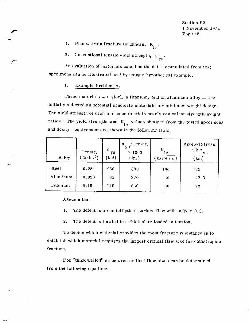
Section E21 November 1972Page 45
1. Plane-strain fracture toughness, Kic.
2. Conventional tensile yield strength, (rys
An evaluation of materials based on the data accumulated from test
specimens can be illustrated best by using a hypothetical example.
I. Example Problem A.
Three materials -- a steel, a titanium, and an aluminum alloy -- are
initially selected as potential candidate materials for minimum weight design.
The yield strength of each is chosen to attain nearly equivalent strength/weight
ratios. The yield strengths and Kic values obtained from the tested specimens
and design requirement are shown in the following table.
Alloy
Steel
Alum inure
Titanium
Density
( [b/in. 3)
ys
(ksi)
a /Densityys
× 1000
(in.)
0. 284 250 880
0. 098 85 870
0. 163 140 860
Kic,
(ksi 4 in.)
1oo
30
80
Applied Stress
1/2ys
(ksi)
125
42.5
7O
Assume that
1. The defect is a semielliptical surface flaw with a/2c = 0.2.
2. The defect is located in a thick plate loaded in tension.
To decide which material provides the most fracture resistance is to
establish which material requires the largest critical flaw size for catastrophic
fracture.
For "thick walled" structures criticalflaw sizes can be determined
from the following equation:

(a/Q)er i.
Section E2
1 November 1972
Page 46
or
cr 1.217r
where the shape factor parameter can be obtained from Fig. E2-5.
comparison, Q = 1.26.
The results are shown in the following table.
For this
Alloy
Steel
A luminum
Titanium
Depth, acr
(in.)
0.212
O. 165
0.432
Length, 2c
(in.)
1.06
0.83
2.16
Conclusion.
The titanium alloy is most fracture resistant in terms of requiring
the largest critical flaw size defect, a for catastrophic fracture.er'
This conclusion could have been reached by considering the Kic/Crys
ratios for the various materials shown in the following table.
Alloy Kic/O'y s (_m.)
Steel
Aluminum
Titanium
0.400
0. 353
0. 572

F
The titanium, having the highest Kic/ay s
be the toughest material for the given application.
Section E2
1 November 1972
Page 47
ratio, could be expected to
Tiffany and Masters (Ref. 17) showed that for screening several
materials, Kic data are often plotted as shown in Fig. E2-18a. Recognizing
that the operating stress levels are generally controlled to a fixed percentage
of the unflawed tensile strength by the design safety factor, the data shown in
Fig. E2-18a might be more appropriately plotted as shown in Fig. E2-18b.
The ordinate is directly proportional to the critical flaw size, thus placing
the influence of varying materials strength in better perspective. From
Fig. E2-18b the three materials can be compared upon the basis of equal
critical flaw size. For example, structures desi,_ned from a 200-ksi steel,
a 135-ksi titanium, and a 70-ksi aluminum would all have approximately the
same critical flaw size. Considering the effect of weight, one might wish to
make the comparison shown in Fig. E2-18c. This shows that titanium pro-
vides a somewhat lighter tank on the basis of equal flaw size.
Based on considerations of the practical capability of available
nondestructive inspection (NDI) techniques, the resistance to catastrophic
fracture could also be evaluated by calculating the maximum allowable applJ_d
stress for equivalent defects in each material.
Reevaluate the preceding example, assuming that the minimum
detectable flaw is 0.15 in. deep by 0.75 in. long.
Rearranging the basic equation results in
Kic 2 (Q)0-2 =
1.21 (a)
The resulting critical fracture stresses and other pertinent information are
summarized in the following table.

Section E 2
1 November 1972
Page 48
160
0i 1
50 100 150 20( 250 300
ULTIMATE STRENGTH (Ftu) (ksi)
aD
0 50 100 150 200 250 300
ULTIMATE STRENGTH (Ftu) (ksi)
be
1.5
¢4
-"_ 0.5
0
_ ,_STEEL I
.......... ,50 100 150 200 250 300
EQUIVALENT ULTIMATE STRENGTH IN STEEL
Co
FIGURE E2-18. MATERIAL COMPARISONS (BASE METAL,
ROOM-TEMPERA TURE TRENDS)

f--
Alloy
Steel
Aluminum
Titanium
ys
(ksi)
250
85
140
Section E2
1 November 1972
Page 49
Design Stress
0.5_ys
(ksi)
125
42.5
70
Fracture Stress
(7
(ksi)
Safety Factor
_/0.5ys
144
43
112
1.15
1.01
1.60
From the above data it is apparent that the titanium provided the
greatest safety factor and resistance to fracture.
2.4.1.2 Cyclic or Sustained Loading.
An evaluation of the resistance of materials to fracture requires the
consideration of the crack growth rate characteristics in addition to other
material propertics.
Some examples of data obtained from tests are shown in Figs. E2-19
and E2-20 (Rcf. 18). The realistic and practical approach for comparing
materials is to evaluate their crack growth characteristics under a given
application condition. Let us consider the following hypothetical example.
I. Example Problem A.
1. Materials to be considered are the steel and aluminum alloys for
which the data are given in Figs. E2-19 and E2-20.
2. The component of interest is a thick plate cyclic loaded in tension
under stresses that vary from zero to maximum tension during each cycle.
3. The design fixes a as one-half thc yield strength for eachmax
material: 88 ksi for steel and 32 ksi for aluminum.
4. The worst possible type of flaw that is envisioned is a semi-
elliptical surface flaw with a/2c = 0.20.

140,
,_ 100
c"
|W1-
40ttwmrt- 20M
1 I I ! I I I i 1 I
HP-0-4-25 STEEL, 1.0 in. THICK 0.25 YJ. - 175 lui
AVG. CRITICAL STRESS - INTENSITY FACTOR
KIt - 144 ksi%/_.ROOM TEMPERATURE DATA (75°F)
I I
/
J
//
Section E2
1 November 1972
Page 50
r
01 2 4 6 S 10 20 40 SO 100 200 400 000 1000
CRACK GROWTH RATE Zb4/AN (mils/1000 cydes)
FIGURE E2-19. CRACK GROWTH RATE FOR HP-9-4-25 STEEL
t I I I I 1 1
7079-T6 ALUMINUM, 1.0 in. THICK
32 -- 0.2 Y,$.- _51ui /
CRITICAL STRESS- INTENSITY FACTORK[c 34 ksiVi-n.
211 ROOM TEMPERATURE DATA (75°F) "__/
I ///
I
i,.I /"
/
m
IIwmeI,-
;1 2 4 IS 8 10 29 40 IN) 100 200 400
CRACK GROWTH RATE _a/_N Imils]1000 cycles)
FIGURE E2-20. CRACK GROWTH RATE FOR 7079-T6 ALUMINUM

¢-
f-.-.11
Section E2
1 November 1972
Page 51
5. The minimum size flaw that could be detected by the NDI technique
is 0.15 in. deep by 0.72 in. long. Therefore, each material is assumed to
contain this flaw.
Under these circumstances, which material has the longest life ?
Solution.
Step 1.
intensity, KIi,
and stress. The appropriate expression for
component geometry is
The first step is to compute the value of the initial stress
for each material for the prevailing conditions of defect size
Kii for the stipulated defect and
1.21 _a a 2
KIi 2 - Q
where
a = crack = 0.15 in. -- specified,
= applied stress (maximum during cycle) = 1/2ys
steel = 88 ksi, aluminum = 32 ksi,
{Y
each materia",
= yield strength, steel = 175 ksi, aluminum = 65 ksi,ys
and
Q = 1.26 for specified flaw geometry.
The calculations reveal the following:
1.21r (0.15) (88 000) 2KIi = 1.26

and
Section E21 November 1972Page 52
Kii = 59 000 psi
for steel, and
1.217r (0.15) (32 000) 2KIi 2 = 1.26
and
Kii = 21 500 psi
for aluminum.
The crack growth rates for the two materials at the beginning of life
can now be determined from Figs. E2-19 and E2-20 using their respective
K I values for the imposed conditions. The results are shown in the following
table.
Alloy
Steel
Aluminum
59 000
21 500
C rack Growth Rates
(mils/cycle)
0.035
0.030
However, a knowledge of the crack growth rates at the beginning of
life is not sufficient to determine the respective life expectancy of each
material. One must consider the change in K I and the associated change in
crack growth rates for each material as the crack grows during service as
well as the threshold stress intensity, KTH.

r
f
Section E2
1 November 1972
Page 53
Step 2. The growth rate data illustrated in the form shown in Figs.
E2-21 and E2-22 (Ref. 18) provide a convenient method for c'valuating the life
expectancy without becoming intimately involved with changes in K andI
growth rates. Figures E2-21 and E2-22 are constructed from the same basic
test data as were used to construct Figs. E2-19 and E2-20. To utilize Figs.
E2-21 and E2-22 it is necessary to know the ratio of Kii to Kic. The previous
calculations in Step 1 showed that K I is 59 ksi i_'_'_'_'_'_'_'_'mT,for steel and 21.5 ksi
for aluminum. Since the KIe values for each material were known
from static toughness tests, the Kii/Kic ratios are readily determined:
KIi 59 000
Kic 144 000- 0.41
for steel, and
KIi 21 500
KIc 34 000- 0.63
for aluminum.
The cyclic life corresponding to these KIi/KIe values may be deter-
mined directly from Figs. E2-21 and E2-22 -- steel, 1800 cycles, and
aluminum, 4000 cycles, if the time at maximum stress is short (luring each
cycle.
Thus, for this specific example where both materials contained the
same given size and type of defect and both were stressed to one-half their
yield strengths, the aluminum has the greatest life expectancy.
It should bc emphasized that the result of this example cannot be used
to generalize the relative behavior of the two materials. For other conditions
of initial defect sizes and/or applied stresses, it is possible that the steel

1.0 I
0.11--
0.1
0.7 '_
0.|
0.4
O.3
O.2
0.1
00.1 0.2
I I I I I I I I II'1P-1.4-215STEEL, 1.0 in. THICK
Klc " 144 kj_'_. 0.2'1+Y.I. = 17t kai
ROOM TEMPERATURE DATA (76°F|i i i i t
0.4 0.60.81 2 4 6 810 20
N. NO. OF CY(:LES TO FAILURE x 10.3
Section E 2
1 November 1972
Page 54
I
FIGURE E2-21. COMBINED CYCLIC FLAW GROWTH DATA FOR
HP-9-4-25 STEEL PLATE
FIGURE E2-22.
I i i I I I I I1.0 AT <_100 CYCLES
7079-T8 ALUMINUM, 1.0 in. THICKKlc= 34 ksi_/_. 0.2% Y.$. - 16_IOON TEMPERATURE DATA |75°FI
4 S 8 10 20 40 e0 100 200
N, NO. OF CYCLES TO FAILURE x I(Y _1
440
COMBINED CYCLIC FLAW GROWTH DATA FOR
7079-T6 ALUMINUM PLATE
+

I
Section E2
1 November 1972
Page 55
could have the greater life expectancy. This is demonstrated in the following
table, which shows the life expectancy of the two materials for a wide range
of initial defect sizes and for a constant applied stress of a /2.ys
Initial
Defect
Depth
ai
(in.)
0.05
0.07
0.10
0.15
0.20
0.25
Initial Stress-
Intensity Factor
Kii
(ksi i_'_n. )
Steel Aluminum
19.6 7.2
27.5 10.1
39.4 14.3
59.0 21.5
78.8 28.7
98.4 35.9
Kii
KIc
Steel
0. 136 0. 210
0. 191 0. 297
0.274 0. 420
0.410 0.632
O. 540 O. 845
O. 683 > 1.0
Cycles to Failure
N
( Life Expectancy)
Aluminum Steel Aluminum
>>300 × 103
>100 × 10 '_
30 × 10 :_
1.8 × 10³
0.37 × 10 a
0.25 x 10 a
300 x 103
100 x 10 a
21 x 103
4x 10³
1.SX 10 a
From the table it is seen that when the initial defect depth is 0.15 in.
or larger, the aluminum will have the longer life N. IIowever, when the
initial defect depth is 0.10 in. or smaller, the steel will have the greater lift _
expectancy. Although the steel has the larger absolute value of fracture
toughness, Kic , and therefore has the largest critical crack size for
catastrophic failure, it also has a greater crack growth rate for a given
change in K as seen from the differences in slope of the growth rate curves
shown in Figs. E2-23 and E2-24 (Ref. 18). Therefore, it is possible to have
a "crossover" situation between the life expectancies of steel and aluminum,
as noted in the table.
Again, the life expectancies in preceding table reflect short time at
maximum cyclic stress. If the time at maximum stress is long, the portion
of time that the stress-intensity level is above the threshold stress intensities

Section E2
1 November 1972
Page 56
m
10"4 10-6 10"4 IO-S
CRACK GROWTH RATE _N (in./cycie)
FIGURE E2-23. CRACK GROWTH RATE AS A FUNCTION OF STRESS
INTENSITY FOR HP-9-4-25 STEEL
M. '_-
i
1104 10.1 10-4 104
A_
CRACK GROWTH RATE _ (in./cyde)ZIN
FIGURE E2-24. CRACK GROWTH RATE AS A FUNCTION OF STRESS
INTENSITY FOR 7079-T6 ALUMINUM

Section E2
1 November 1972
Page 57
for the steel and aluminum would cause reductions in the cyclic lives for the
different initial defect sizes.
The materials could also be compared in another manner by using the
data provided in Figs. E2-21 and E2-22 to answer the question of which
material could tolerate the largest initial defect (of a given type) that would
not grow to a critical size during some given minimum lifetime for the
component.
II. Example Problem B.
Known Information:
Plate cyclic loaded (sinusoidal) in tension.
Required life -- 50 000 cycles.
Applied stress (maximum stress during cycle) one-half yield
strength:
steel = 88 000 psi.
aluminum = 32 000 psi.
Type of defect -- semiclliptical surface flaw with a/c -- 0.4.
Fracture toughness, Kic:
steel = 144 000 psi
aluminum = 34 000 psi
Unknown Information: Which material can tolerate the largest initial
defect ?
Solution.
Step 1. From Figs. E2-21 and E2-22, find the Kii/Kic ratio
corresponding to the desired life of 50 000 cycles:
Kliat 50 000 cycles = 0.25

for steel, and
Kiiat 50 000 cycles = 0.34
Section E2
1 November 1972
Page 58
for aluminum.
Step 2. Knowing the
cycles, solve for Kii:
Kic and Kii/Kic ratio corresponding to 50 000
KIi = 0.25 Kic = 0.25 (144 000psi_m.) = 36 000psi
for steel, and
Kii = 0.34 KIc = 0.34 (34 000psi_/'_n.m.) = 11 500psi i_n.
for aluminum.
Step 3. Since Kii depends upon stress and defect size, it is now
possible to solve for defect size knowing stress. For semielliptical surface
defects with a/c = 0.4, the following expression is appropriate:
(Q)a. =i 1.21 _ ¢2
for steel,
(36000)2(1.26)a._= i.2i. (SS000)'2
and
Section E2
1 November 1972
Page 59
a. = O. 056 in.1
when the defect is 0. 056 in. deep by 0.28 in. long; for aluminum,
(11 500) 2 (1.26)a -
i 1.21 7r(32 000)2
and
a = 0.043 in.i
when the defect is 0. 043 in. deep by 0. 215 in. long.
Thus, it is apparent that for the condition imposed, the steel could
tolerate a slightly larger initial defect than could the aluminum. Since the
difference in the maximum allowable initial defect size is not great, the
ultimate choice of a material for this situation may depend more heavily on
other comparative factors, i.e., the applicability and capability of NDI
techniques, the type and size of insidious defects as related to the maximum
allowable initial defect size, availability, ease of fabrication, costs, etc.
2.4.2 Predicting Critical Flaw Sizes.
As mentioned in Section 2.2.3, plane-strain stress intensity (Kic)
values can be obtained from several types of specimens. With valid data for a
given material form, heat treatment, test temperature, and environment,
critical flaw sizes can be calculated for given hardware operating stresses.
The engineering usefulness of the basic stress-intensity concept in the pre-
diction of critical flaw sizes and the use of a/Q to describe flaw size has

Section E21 November 1972Page 60
beensupportedby a number of hardware correlations, some of which are
shownin Refs. 17and 19. Comparisons betweenmeasuredcritical flaw
sizes on test hardware and predicted critical flaw sizes basedon test speci-
men plane-strain toughnessdata have showngoodcorrelation.
From the equationshownin Fig. E2-6, it is apparent that critical flaw
size is equally as dependentonapplied stress as on the material fracture
toughness. The following sections showapproachesfor calculating critical
flaw sizes for the three basic types of initial flaws (surface, embedded,or
through-the-thickness) basedon the appropriate fracture toughnessvalues
measured from valid specimen tests.
2.4.2.1 Surface Cracks.
Calculations for surface flaws canbe carried out by rearranging the
stress-intensity equationdevelopedby Irwin (Section 2.2.1),
(a/Q)cr 1.21rr
for a "thick-walled" structure ( i. e., flaw depth less than half of the material
thickness) where KIc is the plane-strain fracture toughness obtained from
fracture toughness specimen tests, a is the applied stress in structure
normal to the plane of flaw, a is the critical flaw depth, Q is the flawcr
shape parameter (obtained from Fig. E2-5), and (a/Q)c r is critical flaw
size.
Since the flaw size is an unknown quantity, it is necessary to assume
a flaw aspect ratio, a/2c, to determine Q. Using the preceding equation,
the critical flaw depth, a can be determined for a specific value of acr'
and Kic.

/
J
Section E2
1 November 1972
Page 61
I. Example Problem A.
Aluminum alloy 2219-T87 is selected as the material for use in a
20-in.-diam spherical gas bottle. The bottle is to operate at 4000 psig and
be stored in a liquid-nitrogen propellant tank.
What is the critical flaw size ?
A. Assumptions.
1. The defect is a semielliptical surface flaw with a/2c = 0.2.
2. The operating stress is a = 80 percent (yield strength of the
material).
B. Solution.
The yield strength and Iic
mens are as follows:
values obtained from the tested speci-
a = 60 ksiys
and
Kic = 37 ksi
The operating stress is
a = 0.80 (ays) = 0.80 (60)
The wall thickness required is
= 48 ksi
vR (4000) (lO)treq 2a (2) (48 000)
= 0.417 in.

For thick-walled structures,
Section E2
1 November 1972
Page 62
a 0cr 1.21
where the shape parameter Q can be found from Fig. E2-5. For this problem
Q = 1.18; then
1.18 /37_ 2a = = O. 184 in.cr 1.21
and
2c = a/0.20 = 0.184/0.2 = 0.92 in. .
For surface flaws that are deep with respect to material thickness,
the flaw magnification factor, Mk, can be applied to give a more accurate
critical flaw size,
(a/Q) --- 1 (KIc _ 2
for thin-walled structures.
II. Example Problem B.
Use the same design that was shown in Example Problem A except that
the spherical diameter of the bottle is 15 in. The wall thickness required is
t _ Pa _ 4000 (7.5) = 0.313 in.req 2a 2 (48 000)

(-.
For thin-walled structures,
Section E2
1 November 1972
Page 63
f
cr 1.21, t,Mk<,/
Flaw magnification factors, Mk, for the 2219-T87 aluminum are available
from Fig. E2-8. Since the critical flaw depth, a is unknown a "trial-and-cr'
error" iterative solution is necessary to determine the magnification factor
corresponding to the critical flaw depth.
Without a magnification factor,
For a/t = 0. 184/0.313 = 0.59,
a = 0. 184 in.cr
M k = 1.21,
(Example Problem A).
2
[ 1cr 1.21 n 1.21 (48)0.126 in. < 0.184 in.
0.184 + 0.126Take an average a = = 0.155 in.
2
For a/t = 0. 155/0. 313 -- 0.50, M k = 1.15,
a - 1"18137] 2. . --cr 1.217r 1.15 t48)O. 139 in. < O. 155 in.
0.155 + 0.139Take an average a = = 0.147 in.
2
For a/t = 0.147/0.313 = 0.47, M k = 1.13,
a -1"18[ 37 ] 2cr 1.21 7r 1.13 (48)= 0.144 _ 0.147 in.
Further reiteration will provide more accuracy if desired.
Section E 2
1 November 1972
Page 64
If adequate flaw magnification values are not available for a particular
material, a reasonable estimate for M k is the approximate Kobayashi solu-
tion shown in Fig. E2-25. However, it should be understood that its use can
result in somewhat conservative answers for more ductile materials and
perhaps unconservative answers for more brittle materials.
2.4.2.2 Embedded Flaws.
The calculations for embedded flaws in thick-walled structures will
be the same as for surface flaws except that a is the one-haft criticalcr
flaw depth of the embedded flaw, and the correction factor of 1.21 for the
effect on stress intensity of the stress-free surface (Section 2.2.1) is elimi-
nated. Thus the equation for one-half critical internal flaw size is
'a'O'erAlthough flaw magnification effects have been studied for deep surface
flaws, apparently no similar research has been done for internal flaws with
large flaw-depth-to-material-thickness ratios. The fact that internal flaws
are hidden, making their size difficult if not impossible to accurately deter-
mine, presents a problem in the study of internal flaw magnification effects.
The assumption might be made that the same flaw magnification factors,
M k, used for deep surface flaws might be applied to the equation for critical
embedded flaw sizes. However, there is no evidence of how conservative or
unconservative this assumption is.
On the other hand, to account for the lack of knowledge about flaw
geometry and orientation, it can be conservatively assumed that flaws are
surface (or barely subsurface) flaws and that they are long in relation to
depth (Q _ 1.0).

Scction E21 November 1972Page 65
if--
%
\\
\
i
I
L_.
N
I
\\
\
b-..J
--3>'.
_ U v
o.
w.O
0
0
o
oO
?:
0
r_
0E_
.<
Z
Z
z
z!
I

Section E2
1 November 1972
Page 66
2.4.2.3 Through-the-Thickness Cracks.
To calculate through-the-thickness critical crack length, the basic
plane stress equation for through-the-thickness cracks in an infinitely wide
plate (Section 2.2.2.1) can be rearranged to give
/2=1_ 1
cr , _" \ ys /
where K is the plane stress fracture toughness obtained from an edge-c
notched or center-cracked specimen, a is the applied stress in the structure
normal to the plane of the crack, a is the tensile yield strength of theys
material, and ! is the critical crack length.cr
I. Example Problem A.
Aluminum alloy 2219-T87 is selected as the material for use in a 15-
in. diameter compressed air cyclinder. The cylinder is to operate at 1000
psig in ambient room atmosphere.
What is the critical flaw size ?
A. Assumptions.
1. The defect is a semielliptical surface flaw with a/2c =
0.2.
yield strength.
2. The operating stress is a = 80 percent of material
B. Solution.
The yield strength and __KIc
mens are as follows:
a = 50 ksiys
values obtained from test speci-

¢--and
Section E2
1 November 1972
Page 67
. Kic = 32 ksi
An estimate of K versus material thickness based onC
2219-T87 test specimens is shown in Fig. E2-26 (Refs. 20 and 21).
The operating stress is
= o.so (o ) : o.8o (so) = 40 ksiys
The wall thickness required is
PR 10oo(7.5)t -- --
req _ 40 000- O.188 in.
For thick-wa llcd structures,
cr 1.21 7r
From Fig. E2-5, Q= 1.18; then
1.18 _¢32/2
acr - 1.21 _ \4-01= 0.199 > 0.188 in.
Therefore, the critical flaw is apparently a through-the-thickness crack and
the tank will leak before failure. The critical crack length of failure is pre-
dicted to be

Section E2
1 November 1972
Page 68
v_t
lOO
so
I
II
IRWIN'S APPROXIMATION OF TRANSITION MODE
Kc'Kic 1+1.4 K 2 " 1/3
DATA POINT FROM REF. 21, P. 112
TA POINT FROM REF. 20_TABLE V
K]c " 32.0 ksi_'n,
FIGURE E2-26.
1.0 2.0
t (in.)
ESTIMATE OF K VERSUS t FOR 2219-T87 ALUMINUMC
(W= 70'F, KIe= 32.0ksi_)
f-
is 84 ksi
= 2_cr 7r
\ ys/
The plane-stress fracture toughness value, K ,C
Section E2
1 November 1972
Page 69
from Fig. E2-26,
.... 2.81cr _
- 0.91 = 1.90 in.
2.4.3 Structure Design.
2.4.3.1 Service Life Requirements and Predictions.
With pressure cycles and time at stress, an initial flaw or defect in a
structure will grow in size until it attains the critical size at the applied oper-
ating stress level, and failure will result. The flaw-growth potential (in
inches) is equal to the critical size minus the initial size. The life of the
structure directly depends upon this flaw-growth potential and the subcritical
flaw-growth characteristics of the material.
The determination of the initial flaw sizes generally relies upon the
use of NDI procedures; however, the conventional proof test can be considered
to be one of the most positive inspection procedures available. A successful
proof test actually defines the maximum possible initial flaw size that exists
in the vessel. This results from the functional relationship between stress
level and flaw size as defined by the critical stress intensity (Kic) and illus-
trated in Fig. E2-6.
Probably the most predominant types of subcritical flaw growth are
fatigue growth resulting from cyclic stress and environmentally induced
sustained stress growth. Also, growth may occur even in the absence of
severe environmental effects if the initial flaw size approaches the critical
flaw size.

Section E2
1 November 1972
Page 70
The technique used for predicting the subcritical cyclic or sustained
stress flaw growth makes use of fracture specimen testing and the stress-
intensity concept.
It has been shown (Refs. 6 and 17) that the time or cycles to failure at
a given maximum applied gross stress level depends on the magnitude of the
initial stress intensity at the flaw tip, Kii, compared with the critical stress
intensity, Kic [that is, cycles or time to failure = f (Kii/Kic) ]. Also, it is
seen that the ratio of initial flaw size to critical flaw size is related to the
stress-intensity ratio as folIows:
a.
l
Qcr
Thus, if cyclic or sustained stress fracture specimens are used to
obtain experimentally the KIi/KIc versus cycles or time curves for a material,
the cycles or time required for any given initial flaw to grow to critical size
can be predicted. Conversely, if the required life of the structure is known
in terms of stress cycles or time at stress, the maximum allowable initial
flaw size can be determined.
The cyclic flaw-growth data are plotted in terms of stress-intensity
ratio, KIi/Kic , versus log of cycles, as shown schematically in Fig. E2-27a.
By squaring the ordinate value, the plot of the ratio of initial flaw size to
critical flaw size versus the log of cycles (Fig. E2-27b) can be obtained. It
should also be recognized that flaw size can be determined after any incre-
mental number of cycles. For example, if the initial flaw-size ratio was
0.40, the flaw would have grown in A cycles, increasing the ratio to 0.6;
in B cycles, it would have grown to 0.8, etc.

u_g
X
1.0
0.4
0.2
\
1.0
0.8
0.6
Section E2
1 November 1972
Page 71
0.2
10 100 1000 10
CYCLES CYCLES
a. b.
IO0 tOO0
FIGURE E2-27. SCHEMATIC REPRESENTATION OF CYCLIC
F LAW GROWTH
Cyclic flaw-growth data have been obtaincd on a number of materials
used in the aerospace industry. Some such data are shown in Figs. E2-28
and E2-29.
The application of fracture-specimen testing to define the effects of
sustained load on flaw growth is essentially the same as used in defining cyclic
flaw growth. A constant load is applied to a flawed specimen such that the
initial stress intensity is less than the critical value and the time to [ailure
is recorded. The Kii/Kic values are computed and the Kii/Kic ratio is
plotted versus log of time to failure.
Kii/ versus log of time for most materials indicate thePlots of Kic
existence of a threshold stress-intensity level below which sustained stress
growth does not occur. Figure E2-30 shows data for 17-7 Ptt steel tested in
both dry and wet environments, and Fig. E2-31 shows surface-flawed speci-
men data for 2219-T87 aluminum tested in liquid nitrogen. In neither case
does it seem that the environment played an important role in the sustained
stress growth. In both cases the apparent threshold stress-intensity levels
are quite high.
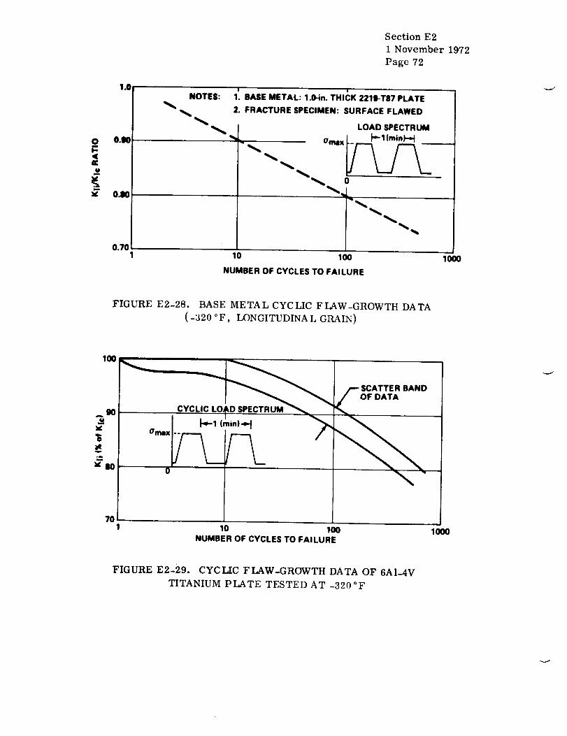
oI--4(le
v
1.0
0.B0
0.O0
0.70
Section E2
1 November 1972
Page 72
1! k• BASE METAL: 1.0-in. THICK 2219-TB7 PLATENOTES:
2. FRACTURE SPECIMEN: SURFACE FLAWED
LOAD SPECTRUM
Omex I"" l(minF-_4.
10 100
NUMBER OF CYCLES TO FAILURE
1000
FIGURE E2-28. BASE METAL CYCLIC FLAW-GROWTH DATA
( -320 °F, LONGITUDINAL GRAIN)
100
..9Ou
_g
,tN
7O
Omx
oJ
CYCLIC LO,
_-1 (min)._
Fl__/--l_
-- SCATTE R BAND
OF DATA
10 100
NUMBER OF CYCLES TO FAILURE1000
FIGURE E2-29. CYCLIC FLAW-GROWTH DATA OF 6A1-4V
TITANIUM PLATE TESTED AT -320°F
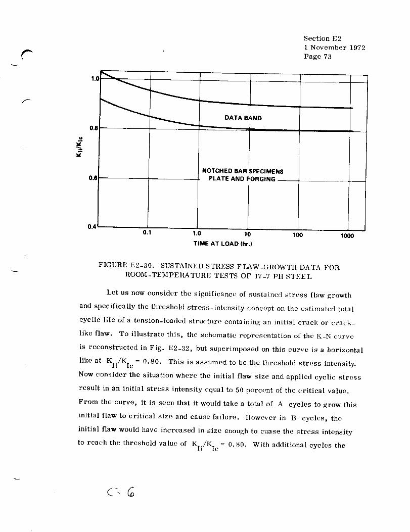
6-.
rz
1.0
2
0.8
0.6
Section E2
1 November 1972
Page 73
0.4
DATA BAND
•.-- ._.
NOTCHED BAR SPECIMENS
PLATE ANO FORGING
0.1 1.0 10
TIME AT LOAD (hr.)
100 1000
FIGURE E2-30. SUSTAINED STRESS FLAW-GROWTtt DATA FOR
ROOM-TEMPERATURE TESTS OF 17-7 Ptt STEEL
Let us now consider the significance of sustained stress flaw growth
and specifically the threshold stress-intensity concept on the cstimated total
cyclic life of a tension-loaded structure containing an initial crack or crack-
like flaw. To illustrate this, the schematic representation of the K-N curve
is reconstructed in Fig. E2-32, but superimposed on this curve is a horizontal
like at Kii/Kic -- 0.80. This is assumed to be the threshold stress intensity.
Now consider the situation where the initial flaw size and applied cyclic stress
result in an initial strcss intensity equal to 50 percent of the critical value.
From the curve, it is seen that it would take a total of A cycles to grow this
initial flaw to critical size and cause failure. However in B cycles, the
initial flaw would have increased in size enough to cuase the stress intensity
to rcach the threshold value of KIi/KIc = 0.80. With additional cycles the

t_
0.S
,S -'
Section E2
1 November 1972
Page 74
DATA BAND _m
NOTE: BASE METAL: 2219-T67 1.0-in.-THICK PLATE
0.01 0.1 1.0 10 100
TIME TO FAILURE (hr)
FIGURE E2-31. SUSTAINED STRESS FLAW-GROWTH DATA FOR
2219-T87 ALUMINUM AT -320 °F
1.0____,__ COMBINED TIME I
I -_ AND II _ CYCLEGROWTHI
A CYCLES LIr I
TOTAL CYCLIC LIFE
FIGURE E2-32. COMBINED CYCLIC AND SUSTAINED STRESS FLAW
GROWTH SCHEMATIC INTERPRETATION

r
.
Section E2
1 November 1972
Page 75
stress intensity would further increase and, if the stress were sustained
sufficiently long, it appears possible that failure could occur on the (B + 1)
cycle.
If, on the other hand, the cycles were applied with little time at
maximum cyclic stress, it appears that the total of A cycles couht be
realized. It is hypothesized that below the threshold K-value, the time at
sustained stress has little or no effect on cyclic life. Above the threshold
value there will be an interaction such that failure could occur anywhere
within the range of (B ÷ 1) to A cycles, depending on the time the maximum
stress is held (luring each cycle. The development of the exact time-cycle
interaction curvcs above the threshold value wouhl be a complex and expensive
task and, as applied to most tankage structure, may not be of grcat importance.
It appears more rational to determine the basic cyclic data and the threshold-
intensityvalues and then verify (through prolonge(l-time specimen cyclic
tests) that time at load is not of major significance below the threshold value.
In the application of the data to fatigue-lifeestimation, thc maximum allowable
stress intensitywould be limited to the threshold value as determincd for the
material in question and for the applicable service environment. Ifthe
threshold is very low, steps should be taken to protect the material from the
environment.
The operational cyclic lifeof pressure vessels can be determined if
the following data are available:
1. Proof-test factor a .
2. Maximum design operating stress a
3.
4.
op"
Fracture toughness Kic.
Experimental cyclic and sustained stress flaw growth for the
vessel material.

Section E2
1 November 1972
Page 76
If the cycles to be applied to the vessel have short hold time at the maximum
stress aop , the stress intensity at aop can be allowed to reach the critical
¢alue Kic and therefore the allowable flaw growth potential is a - a.. Forer 1
long hold times at the maximum stress, the stress intensity could not be
allowed to exceed the sustained stress threshold value KTH and the allowable
flaw growth potential is ath _ a.., Typical threshold stress-intensity data
can be obtained from Refs. 12 and 22.
I. Example Problem A (Thick-Walled Vessel).
Cyclic life prediction can be made by utilizing the proof-test factor and
the relationships between Kii/Kic and cycles to failure for various values of
R (ratio of minimum to maximum stress during a cycle) for the material-
environment combination.
The procedure for assessing the structural integrity of the thick-
walled vessels follows. In the first analysis for the assessment of the struc-
tural integrity of the thick-walled vessel, it is always assumed that all the
pressure cycles are applied at R = 0. Since the analysis based on R = 0
will always show the remaining cyclic life less than that based on the analysis
of R ¢ 0 (actual R ratios), the prediction of cyclic life based on the analysis
of R = 0 is invariably conservative. If the pressure vessel is shown unsatis-
factory for the flight based on R = 0, then the prediction analysis for the
remaining cyclic life is conducted based on the actual R values at which the
cycles are applied. An excellent illustrative example abstracted from Ref. 12
is given as follows.
Suppose that a thick-waUed 6A1-4V (STA) titanium helium tank is
successfully proof tested at a proof-test factor of 1.50 times the maximum
design operating stress. Suppose that the proof-tested tank is subjected to the
following pressure cycles before the flight, as shown in Fig. E2-33:

f--/
1.5
1.0
0.5
UJ
a.
0
Section E2
1 November 1972
Page 77
CYCLE
ANTICIPATED PREFLIGHT SERVICE LIFE
200 CYCLES 40 CYCLES
I,[email protected] Oop @ OopD
4300 CYCLES 260 CYCLES
@ Oop @0.95 0oi)
R . =0.,
=o DB
CYCLES
FIGURE E2-33. CYCLIC IHSTORY OF A THICK-WAI,I, ED VESSEL
( I,:XAMPLI.: PROBLI<M A)
1. 200 loading cycles with the maximum stress as 90 percent of
and R= 0.1.
O"
()1)
0.7.
2. 4300 loading cycles with the maximum stress as _ andop
1l=
3. 260 loading cycles with the maximum stress as 95 percent of _r
and R= 0.4.op
4. 40 loading cycles with the maximum stress as (r and It= 0.1.op
The cyclic life curves for 6Al-4V (STA) titanium for the environment
of room-temperature air are reproduced for R = 0.0, R = 0.1, R = 0.4, and
R = 0.7 in Fig. E2-34. The dif[erence between the plots of cyclic life against
iK'i/KIe for R= 0 and R-0.1 is negligible for this material-c'nvironment

_OE
_ ]_
O
8.Cp
'1
m
m
Section E2
1 November 1972
Page 78
oq _ o0 0 0 0
:JI)i/xmu (r[)i)
,," ©
..J _
0 @
y)Lu _•.J _).
o_v
o
!

Section E2
1 November 1972
Page 79
combination, and hence both are shown by the same plot in Fig. E2-34. The
threshold stress-intensity level for the material in the environment of room-
temperature air is 90 percent of Kic.
The maximum possible KIi/KIc ratio that could exist in the vessel
after the proof test at a is 1/or = 0.667. It can be seen from the R = 0op
plot in Fig. E2-34 that the maximum cycles to failure are about 600 atop
if the hold times at maximum stress are small. If the analysis is based on
R = 0 instead of actual R, the pressure-cycle history shows that the vessel
is critical. In the following, the assessment of the vessel is marie based on
the appropriate values of R.
At the beginning of 200 loading cycles with the maximum stress as
0.90 a the maximum KIi/KIc is given by 0.90 x 0.667= 0.60. Thisop'
point is indicated by E on R = 0.1 curve. The 200 loading cycles of 0.90
Crop and R = 0.1 change the KIi/KIe ratio from Point E to Point D on the
Kii/ ratio at the end of 200 loading cycles ofplot of R= 0.1. The KIe
R= 0.1 is 0.63.
The stress is increased by 10 percent at the end of 201} cycles, ttence,
the Kii/Kic ratio at the beginning of 4300 cycles at Sop and R = 0.7 is
(1.0/0.9) × 0.63= 0.70. This is shown by Point D on the plot of R= 0.7.
The 4300 loading cycles at Sop and R = 0.7 change the KIi/KIe ratio from
Point DtoPointC on the plot of R= 0.7, where its value is 0.78.
The stress is decreased by 5 percent at the end of 4300 cycles. Hence
the Kii/Kic ratio at the beginning of 260 cycles at 0.95 (top is (0.95/1.0) ×
0.78= 0.74, which is shown by PointC on the R= 0.4 plot. The 260 cycles
at 0.95 Sop and R = 0.4 change the Kii/Kic ratio from Point C to Point B
on the R= 0.4 plot, where its value is 0.80.

Section E2
1 November 1972
Page 80
The stress is increased by 5 percent at the end of 260 cycles. Hence,
the Kii/Kic__ ratio at the beginning of 40 cycles at aop is (1.0/0.95) x 0.80 =
0.84, which is illustrated by Point B on the R = 0.1 plot. The 40 cycles at
aop and R = 0.1 increase the liK'i/K'c ratio from 0.84 to 0.875, which is
shown by Point A in Fig. E2-34.
Since the stress intensity at the end of 40 cycles at or is less thanop
the threshold stress intensity, the vessel is considered to be safe for the
flight. It will take 20 loading cycles at or and R = 0.1 to increaseop
Kii/Kic from 0.875 to 0.90 Thus, the estimated minimum cyclic life
remaining for the vessel is 20 cycles.
II. Example Problem B (Thin-Walled Vessel).
In thin-waUed vessels the flaw depth becomes deep with respect to the
wall thickness prior to reaching the critical size. Therefore, Kobayashits
magnification factor for deep surface flaws M k must be considered. In
thin-walled vessels it is assumed that the flaws are long with respect to their
depth and, consequently, Q is assumed to be equal to unity in the Kobayashi
equation.
To determine the cyclic life of a thin-walled vessel, the following
relations are required (Ref. 22).
1. Proof-test factor, orop' Kic, and KTH.
2. The or versus a curve, similar to Fig. E2-35, to determine the
flaw size, ai, acr, and aTh. The curve is obtained from the following
equation:
Or
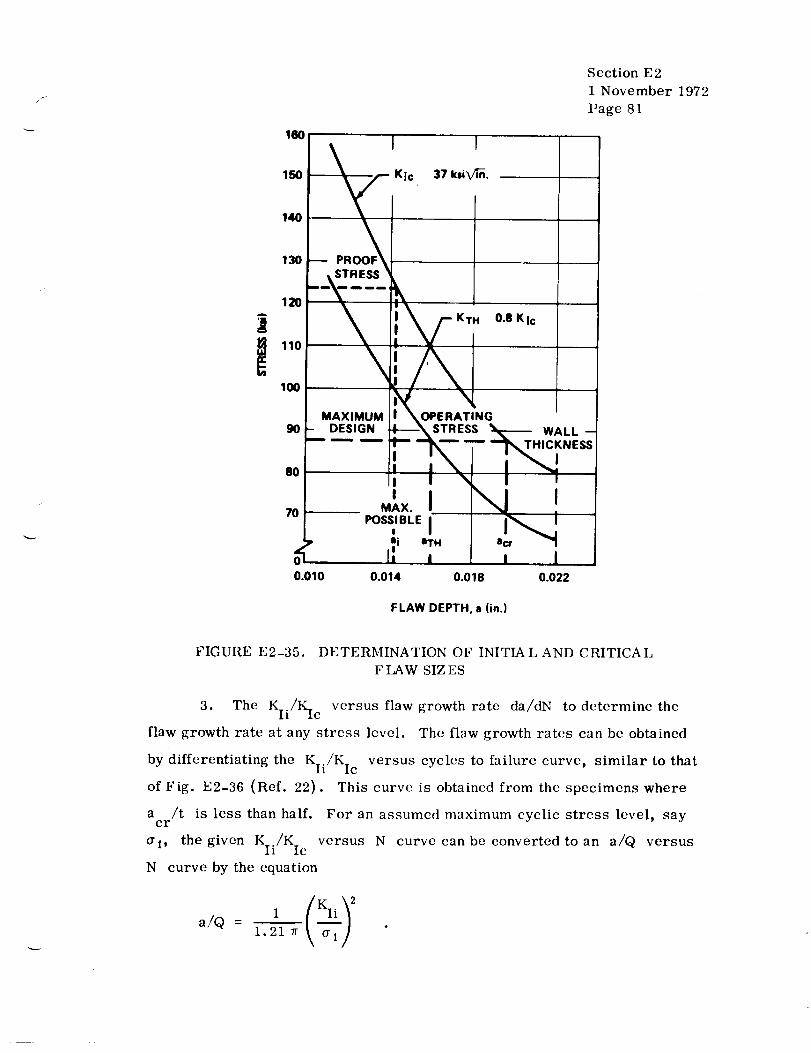
160 I
150 --_ K]c
140 J
I
37 kziV_.
Section E 2
1 November 1972
Page 81
130 _ PROOF_
'_ \ ;\ ,-_,H o,_,_
io .MAXIMUM I _OPERATING
90- DESIGN -I----_STRESS _ WALL--- "-" -- 1"-- --alk--" -- _ THICKNESS
- ! i\ l, _ I
70 MAX.
POSSIBLE II
• [!i aTH0 I
0.010 0.014 0.018
a
cr 1
i I0.022
FLAW DEPTH, a (in.)
FIGURE E2-35. DETERMINATION OF INITIAL AND CRITICAL
F LAW SIZ ES
3. The Kii/Kic versus flaw growth rate da/dN to determine the
flaw growth rate at any stress level. The flaw growth rates can be obtained
by differentiating the KIi/Kic versus cycles to failure curve, similar to that
of Fig. E2-36 (Ref. 22). This curve is obtained from the specimens where
a /t is less than half. For an assumed maximum cyclic stress level, saycr
al, the given Kii/Kic versus N curve can be converted to an a/Q versus
N curve by the equation
a/Q - 1.21 _ \ _'1/

1.0
0.1
0.7
CYCLIC LIFE CURVE (1 qlm) FOR
Section E2
1 November 1972
Page 82
, _1) TITANIUM
"--'" J----'-- -- "1 .... _ .....
LESTIMATED THRESHOLD LEVEL
ILOAD PROFILE
O.I--
Omx+
T,ME----- J0 I I I , I I II I I J I l I I11 i I I I I111
1 10 100 1000
CYCLE$ TO FAILURE
FIGURE E2-36. COMBINED SUSTAINED AND CYCLIC STRESS
LIFE DATA [5 A1 -- 2 1/2 Sn (ELI) TITANIUM
AT -320 °F]
The slope of the a/Q versus N curve gives the plot for the flaw growth rate
d/dN (a/Q) versus Kii/Kic for the stress level a 1. From the preceding
equation for a given Kii , a/Q at the stress level a 2 is related with a/Q
at al as
From this equation it can be concluded that the flaw growth rate at any stress
level cr2 is related to the growth rate at a I as follows:
[d/dN (a/Q)] a 2 = (al/a2)2 [d/dN (a/Q)] a 1 .

Section E2
1 November 1972
Page 83
The prediction of the remaining cycle life and the structural integrity
of the thin-walled vessel is demonstrated by an illustrative example abstracted
from Ref. 22 and is given as follows.
Suppose that a thin-walled 6AI-4V titanium (STA) propellant tank
containing N204 at room temperature is successfully proof tested with water
at room temperature to a proof-test factor of 1.41 times the maximum design
operating stress, Sop. Suppose that the proof-tested tank is subjected to the
following pressure cycles before the flight:
1. Twenty loading cycles with the maximum stress as 90 percent of
op
(1 o
op
2. Twelve loading cycles with the maximum stress as 95 percent of
3. Five loading cycles with the maximum stress asop
It is desired to assess the structural integrity of the prcssure vessel
from the fracture mechanics standpoint and estimate the minimum cyclic life
remaining for the vessel at Sop" This example is treated with specific
numbers since the stress-intensity factor has to be corrected for the a/t
ratio according to Fig. E2-25. The thickness of the tank is 0.022 in. The
maximum design operating stress, (7op, is 87.5 ksi. The material of this
gage under the above-mentioned environmental conditions has the minimum
fracture toughness of 37 ksi _ and the threshold stress intensity of 80
percent of Kic.
The _ versus a plots are given for Kic and KTH = 0.80 KIc in
Fig. E2-35. Since the proof stress is 1.41 × cr = 123.6 ksi, it is clearop
from Fig. E2-35 that the maximum possible a that could exist is 0.01431
in. Here it is assumed that the depressurization from the proof pressure is

Section E2
1 November 1972
Page 84
rapid enough so that no significant flaw growth occurs during the depressur-
ization. Also, as shown in Fig. E2-35, for the stress level of a aop' cr
is 0.0196 in. and aTH is 0.0160 in.
The plot of the Kii/Kic versus flaw growth rate for 6A L-4V titanium
at room temperature is reproduced in Fig. E2-37 for a = 100 ksi. The 99-
percent confidence level flaw growth rate curve is obtained from the cyclic
data of R = 0.0; it is assumed in this example that all the cycles are applied
at R= 0.0.
Taking into account the effect of stress level on the flaw growth rates,
the rates are arithmetically integrated from a. = 0. 0143 in. to a = 0. 01961 er
in. according to Fig. E2-38 to calculate the cycles to failure for the stress
level of aop. The plot of flaw depth against cycles to failure for the stress
level of a is shown in Fig. E2-39.op
When the maximum cyclic stress is 0.95 a a is still 0 0143 in.op' i
but acr is 0.0208 in. and aTH = 0.0167 in. from Fig. E2-35. Based on
the stress level of 0.95 a the flaw growth rates are integrated fromop'
a. = 0. 0143 in. to a = 0.208 in. to calculate the cycles to failure. A1 cr
similar procedure is followed to obtain the relation of flaw depth against
cycles to failure for the stress level of 0.90 aop. These plots are shown in
Fig. E2-39.
At the end of the proof cycle and the beginning of the first cycle at the
maximum cyclic stress of 0.90 a the maximum possible flaw depth isop'
0. 0143 in. This is shown by Point D in Fig. E2-39. The 20 loading cycles
with the maximum stress as 0.90 aop
on the plot of 0.90 a (Fig. E2-39).op
change a from Point D to Point C

f
0.4
0.2
0.110
Section E2
1 November 1972
Page 85
(BASE
100 1000
d(a/O)/dN (/_ in./cycle)
FIGURE E2-37. CYCLIC FLAW-GROWTH RATES
(FOR a --- 100 ksi)max
n Aa I/t MkI
01 aS/t Mkl
a2 • as
II2 a2/t Mk 2
• 3" '2 I I
., I I I
Kb MEANK
KS K1 + K.._____22
K2 K2 +K__.3
I 2I II II II I
a. Obtain from Kobayashi's solution of Mk vs sit
b. K = 1.1q/_r'o(a) 1/2 M k
c. Obtain from beeic K vs de/dN curve.
MEAN c
de/dN
de 1-2/dN
de 2.3 IdN
IIII
Z_N
_Ns
AN 2
IIIIt
N
I
ANs
_NI+
_Nz÷
_N 3
1
FIGURE E2-38. ARITHMETIC INTEGRATION OF FLAW-GROWTH-RATE
DATA (DEEP FLAWS IN TItIN-WALLED VESSELS)

Section E2
1 November 1972
Page 86
|
Cut) • 1,1,131(1MY'IJ
!
Section E2
1 November 1972
Page 87
The tank-wall stress is increased by 5 percent at the end of 20 loading
cycles with the maximum stress as 0.90 a The flaw size remains theop"
same during the stress increase. This is shown by Point C on the plot of
0.95 a in Fig. E2-39.op
The 12 loading cycles with the maximum stress as 0.95 a changeop
a from Point C to Point B on the plot of 0.95 a in Fig. E2-39.op
At the end of 12 loading cycles with the maximum strc_ss as 0.95 crop'
the stress is increased by5 percent. This is shown by I)oint B on the plot
of _ in Fig. E2-'19.op
The live loading cycles with the maximum stress as _ change aop
from Point B to Point A on the plot of tr in Fig. I':2-39. The flaw del)thop
at A is 0.01534 in. This is smaller than aTli, which is 0.0160 in. IIence
the vessel is considered to be safe for the flight. Also from Fig. E2-39, it
will take seven cycles at a to increase tire flaw depth from 0. 01534 in.op
to 0.0160 in. Hence, the minimum estimated cyclic life remaining for the
vessel is seven cycles.
2.4.3.2 Allowable Initial Flaw Size.
Allowable initial flaw sizes in a designed structure depend on the
service life requirements for the structure and fracture toughness properties
of the material selected. The prevention of failure requires that either the
actual initial flaw sizes or the maximum possible initial flaw size be known.
Nondestructive inspection provides the only means of determining actual
initial flaw sizes. A successful proof test specifies the maximum possible
initial flaw size which can exist after the proof test and, in turn, provides the
maximum possible initial to critical stress-intensity ratio, Kii/Kic. To
determine the maximum allowable initial flaw size, the initial to critical
stress-intensity ratio, based on the service life requirements, must be
determined.

Section E2
1 November 1972
Page 88
The calculation of allowable initial flaw size is demonstrated by the
following example.
I. Example Problem A.
A cyclic loaded pressure vessel of aluminum alloy must meet the
following design conditions:
1. Required minimum life, 40 000 cycles.
2. Maximum stress in a cycle 1/2 o = 35 000 psi.ys
3. Kic of weld metal= 15 000 psi
4. Semielliptical surface defect (length 4 x depth).
What is the allowable initial flaw size which will grow to a critical
size in 40 000 cycles ?
Solution.
From Fig. E2-40 (Ref. 18), the KIi/Kic ratio corresponding to
40 000 cycles of life is 0.36. The initial stress intensity can now be
determined:
Kii
KIi/KIc : 0.36 : 15 000
and
Kii = 0.36 (15 000) = 5400psi _ .
Knowing the design stress of 35 000 and the expression of the type of
defect, it is now possible to find the defect size corresponding to a Kii of
5400 psi _ :

2
_g
1.0
0.11
0.8
0.7
0.6
0.S
0.4,
03i
0.2
0.1
N\
z , , [ i [ IHYPOTHETICAL DATA
70.-kzi YIELD STRENGTH ALUMINUM
- WELD METAL, K]c,,15kzi i_n.
z I I
!
INITIAL STRESS-INTENSITY FACTOR
CRITICAL STRESS-INTENSITY FACTOR
2 4 6 8 10 20 40 60 80100 200 400
N, NO. OF CYCLES TO FAILURE x 10 .3
Section E2
1 November 1972
Page 89
FIGURE E2-40. CYCLIC FIAW-GROWTtI DATA FOR
A LUMINUM A LLOY
KIi 2 Q (5400) _ (1 4)a. - - " - 0.0088 in.
I 1.21 _2 1.21 _ (:15 000) _
The value of Q -- 1.4
and a /a = 1/2= 0.50.ys
is taken from Fig. 1':2-5 for a/2e = 1/4 = 0.25
2e. = 4a. = 4 (0.0088) = 0.0352 in.1 1
Therefore, the size of an initial flaw which will just grow to a critical
size in 40 000 cycles is 0. 0088 in. deep by 0.0352 in. long.
2.4.3.3 Nondestructive Inspection Acceptance Limits.
The NDI requirements for any I_ivcn structure are a function of the
allowable flaw sizes. They are limited by any economic or schedule impli-
cations associated with a proof-test failure and by the reliability of the
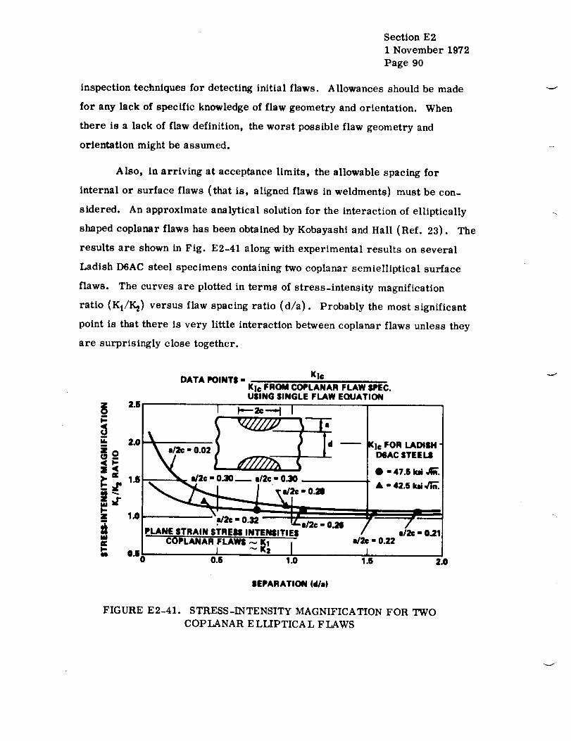
Section E2
1 November 1972
Page 90
inspection techniques for detecting initial flaws. Allowances should be made
for any lack of specific knowledge of flaw geometry and orientation. When
there is a lack of flaw definition, the worst possible flaw geometry and
orientation might be assumed.
Also, in arriving at acceptance limits, the allowable spacing for
internal or surface flaws (that is, aligned flaws in weldments) must be con-
sidered. An approximate analytical solution for the interaction of elliptically
shaped coplanar flaws has been obtained by Kobayashi and Hall (Ref. 23). The
results are shown in Fig. E2-41 along with experimental results on several
Ladish D6AC steel specimens containing two coplanar semielliptical surface
flaws. The curves are plotted in terms of stress-intensity magnification
ratio (Kt/K_) versus flaw spacing ratio (d/a). Probably the most significant
point is that there is very little interaction between coplanar flaws unless they
are surprisingly close together.
DATA POINTS - Kic
Klc FROM COPLANAR FLAW SPEC.USING SINGLE FLAW EQUATION
,/2¢ - 0.321o0
[ PLANE STRAIN STREI|S INTENSITIEI
! COPLANAR FLAWS _ _1 jOAO 0.6 1.0
FOR LADISH 'D@ACSTEELS
SEPARATION (d/a)
FIGURE E2-41. STRESS-INTENSITY MAGNIFICATION FOR TWO
COP LANAR E LLIPTICA L F LAWS

Section E2
1 November 1972
Page 91
The establishment of NDI acceptance limits when service life require_
ments are known might best be shown by an illustrative example involving a
hypothetical pressure vessel that is expected to encounter a rather complex
loading history.
Figure E2-42a shows the assumed service life requirement con-
sisting of one proof-test cycle (at a stress level of _ times the operating
stress) followed by 1000 cycles and then 100 hr, both at a constant operating
stress level of (a = 1.0). To define the minimum inspection standards
required prior to service, it is necessary to determine the critical flaw size,
(a/Q) , at the end of service (Section 2.4 2) and work backwards evaluatingcr " ,
all portions of the loading profile that can cause flaw growth.
Figure E2-42b represents a dimensionless relationship of stress-to-
flaw size as shown previously (Fig. E2-6). The ordinate now is plotted in
terms of percentage of critical flaw size at operating stress. Figures E2-42e
and d are schematic representations of the cyclic load flaw growth and sus-
rained load flaw growth, respectively.
The approach is as follows:
1. The critical flaw size at operating stress is represented as 10O
percent of critical and is the maximum allowed at time T D (at the end of the
service life).
2. Maximum allowed flaw size at time T C is shown by Point C and
represents the maximum allowable flaw size at the start of the 100-hr sus-
tained stress period.
3. The effect of cyclic loading is shown in Fig. E2-42c by moving
1000 cycles from T C to T B. Point B then represents the maximum allowable
size at time T B or at the start of the 1000-cycle period. This size is the
maximum allowable size before the vessel is placed in service.
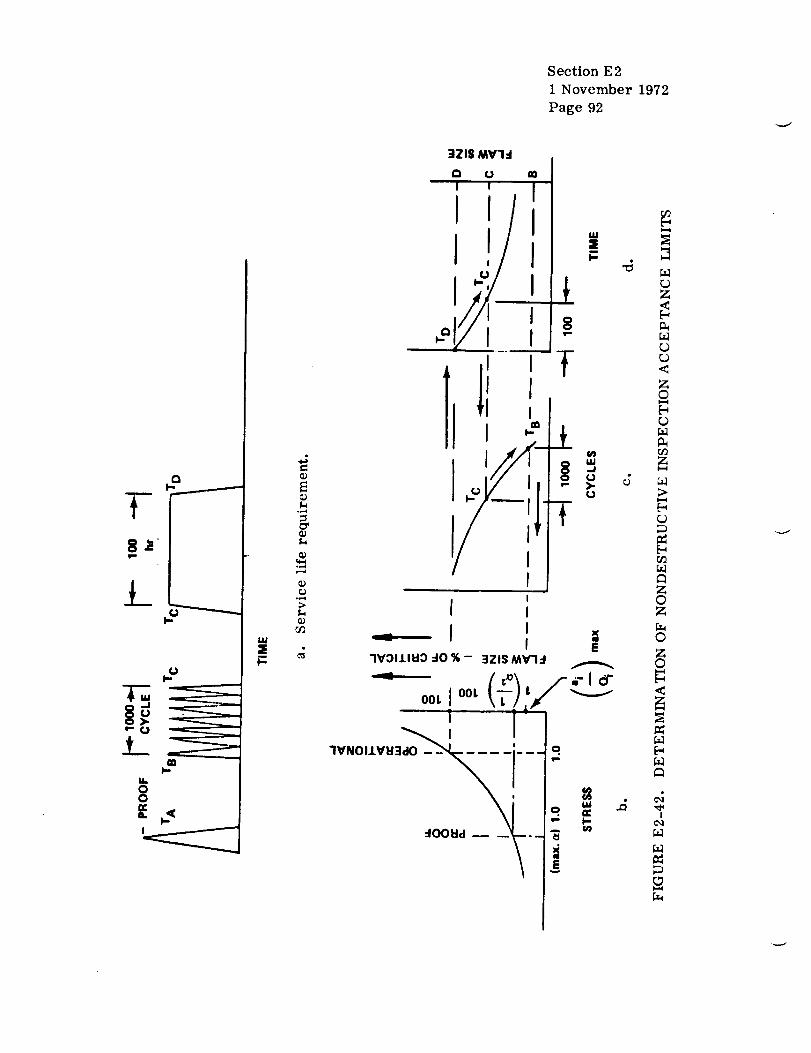
Section E2
1 l_ovember 1972
page 92
:_ZlS MV'ld

f-
Section E2
1 November 1972
Page 93
4. It can be shown that the previous one-cycle proof test generally
has a negligible effect on flaw growth compared with the chosen service life.
Note in this schematic illustration that the maximum allowable flaw
size is less than that which could have been present during a successful proof
test, and thus the proof test could not guarantee successful fulfillment of the
service life requirement. As a result, NDI must be capable of detecting flaws
as small as (ai/Qi)max.
If it is determined that inspection technique limitations preclude the
assurance of service life reliability, then either the proof-test factor must
be increased to assure that (ai/Qi) max is the largest possible existing flaw
size at the beginning of service life, or conservative assumptions might be
made about flaw geometry and orientation to account [or the inability to detect
small flaw depths. For example, the length (L) of an in(lication seen in X-ray
inspection could be assumed to bc the minor axis of an elliptical flaw where tho
major axis is large with respect to the minor axis (i.e., I,- 2a, Q _ 1.0).
Consequently, the critical flaw size must be larger (and the operating stress
lower) in order to meet the service life requirements. In other words, both
and (a/Q) move higher upthe ordinate of Fig. E2-42b.(ai/Qi) max cr
It should be noted that in terms of "percentage of critical," flaw siz¢"
is independent of actual stress and toughness values. Obviously, the deter-
mination of finite maximum allowable flaw sizes (or smallest flaw size for
NDI detection) requires a detailed knowledge of applied stresses in the various
tank locations and of the fracture toughness of the materials used. This has
been illustrated by the Example Problem A in Section 2.4.3.2 in which the
allowable initial flaw size in an aluminum alloy pressure vessel is calculated
based on a required service life. In the case where NDI acceptance limits
are being considered, the calculated initial flaw depth and length are the
minimum demensions which NDI must be capable of detecting.

Section E2
1 November 1972
Page 94
2.4.3.4 Proof-Test Factor Selection.
It has been previously noted that a successful proof test determines
the maximum possible flaw size which can exist after the proof test and prior
to the beginning of service. The proof test is the most powerful inspection test
presently available and offers the most reliable method for guaranteed service
life.
Figure E2-43 shows a schematic theoretical relationship between the
critical flaw size, (a/Q)cr'. and the corresponding fracture stress, as pre-
viously illustrated in Fig. E2-6, along with a similar relationship between
initial flaw size (a/Q). and stress level. The relationships hold true for
applied stresses below the yield strength of the material. For stresses above
]
wii,
aw
al.0
1.0
°ult
MAX--
ta/Q) i I
II
PROOF
OPERATING
s Ktc- 1.1 o( Q)cr (a/Qlcr
]
1.0
FLAW SIZE, _O
FLAW GROWTH
POTENTIAL
(1-1/a 2)
FIGURE E2-43. TYPICAL MATERIAL STRESS-INTENSITY
RE LA TIONSHIP

Section E2
1 November 1972
Page 95
the yield value the relationships follow some experimentally determined curve
up to the ultimate strength, aul t. If proof pressure is a times the operating
pressure, the critical flaw size is
(a/Q) = max(a/Q) _ 1 /K \i. _ .) 2
Crproo f iopcr 1.21 _ \c_ oper/
and
( ic)_ 1 a
(a/Q)croper 1.21----7 \ oper/
Thus the proof-test factor, a , is a function of the maximum initial flaw size
and critical flaw size for the operating pressure level
(a/Q).1oper
croper
1
_2
Since subcritical flaw growth is a function of the initial stress intensity as
compared with the critical value, the proof-test factor can be related as
1.1 _n" a (a/Q)!/2
max Kii _ oper 'oper
KIc 1.1 _'a a (a/Q)! _oper 1
oper
1
where Kii is the initial stress intensity at the operating stress level and
temperature, and K is the fracture toughness value at proof testIe
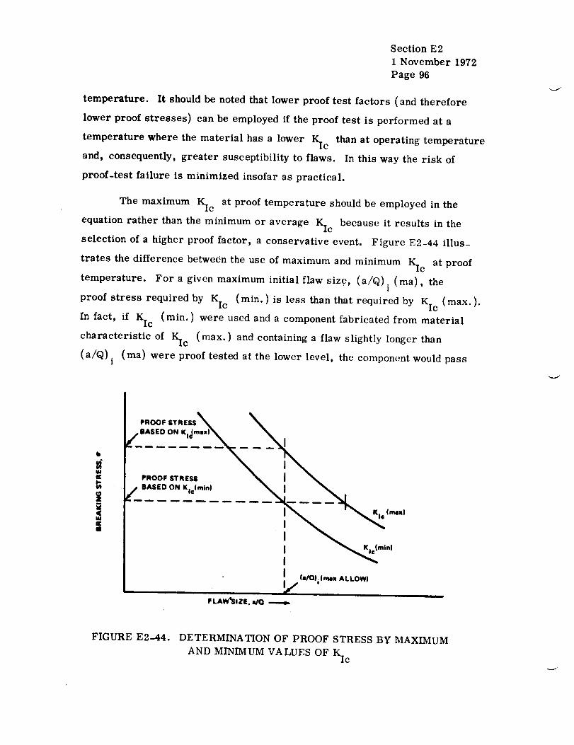
Section E2
1 November 1972
Page 96
temperature. It should be noted that lower proof test factors (and therefore
lower proof stresses) can be employed if the proof test is performed at a
temperature where the material has a lower Kic than at operating temperature
and, consequently, greater susceptibility to flaws. In this way the risk of
proof-test failure is minimized insofar as practical.
The maximum Kic at proof temperature should be employed in the
equation rather than the minimum or average Kic because it results in the
selection of a higher proof factor, a conservative event. Figure E2-44 illus-
trates the difference between the use of maximum and minimum Kic at proof
temperature. For a given maximum initial flaw size, (a/Q). (ma), thel
proof stress required by Kic (min.) is less than that required by Kic (max.).
In fact, if Kic (rain.) were used and a component fabricated from material
characteristic of Kic (max.) and containing a flaw slightly longer than
(a/Q) i (ma) were proof tested at the lower level, the component would pass
b
i|
\ I \
Z""°°N""'-
:/la/Olilmmz ALLOW)
I mr-
F LAWQSI ZE. alO
FIGURE E2-44. DETERMINATION OF PROOF STRESS BY MAXIMUM
AND MINIMUM VALUES OF IK-c

Section E2
1 November 1972
Page 97
the proof test successfully but probably would fail in service. The use of
Kic (max) in the proof-factor equation precludes this.P
It has been shown by analysis that regardless of the structural wall
thickness, the required minimum proof-test factor _ is always 1 --
allowable Kii/Kic. However, the value of the proof test in providing assur-
ance against service failure changes with decreasing wall thickness and/or
increasing fracture toughness, Kic, the same as occurs with the predicted
pressure vessel failure mode. This is discussed in more detail inRef. 22
and illustrated in Fig. E2-45.
ttaving experimentally obtained the cyclic and sustained flaw growth
for a material under consideration, the necessary proof-test factor can be
determined to assure that the structure will meet the service life requirements.
Proof-factor determination can be applied to at least two general problem areas
in the design of structural components:
1. Evaluation and modification of proof-test conditions for current
components for which operating stress and mission are already fixed.
2. Preliminary design of components intended for known missions,
including selection of material, maximum operating stress, minimum proof
stress, and proof temperature.
The following sample problem illustrates the proper selection of a proof-test
factor for a hypothetical pressure vessel design.
I. Example Problem A.
Suppose that a thick-walled liquid nitrogen 5A1-2.5Sn (ELI) titanium
pressure vessel must meet a service life requirement of 600 pressure cycles
where the pressure is sustained for a prolonged period during each cycle. The
vessel has already been successfully proof tested with LN 2 to a proof factor

Section E2
1 November 1972
Page 98
! II
= \- _I! i_ "J , .
u' _i-- _i _ _ _._
_ -!o uli'_ "
IIo_ o_
_" t t,. 0
Ik •
• ,., _._3 •_= _ii_
00
0
<
2;
r_
M
0
o
I
0

Section E21 November 1972
Page 99
= 1.25. Will this proof factor assure that no failure occurs during the
service life and if not, what proof factor is required ?
The cyclic life curve for 5A1-2.5Sn (ELI) titanium is reproduced in
Fig. E2-36. The estimated threshold stress-intensity value for sustained-
stress flaw growth (KTH/KIc) is approximately 0.92.
For long hold time, max. Kii/Kic = 1/_ = 1/1.25 = 0.80. From
Fig. E2-36 for Kii/Kic = 0.80, N= 300 cycles. For KTH/KIc = 0.92,
N = 100 cycles.
In 300 cycles minus 100 cycles, or 200 cycles, the stress intensity
would have reached the estimated threshold value for sustained-stress flaw
growth. Thus the predicted minimum life would be only 200 cycles and the
proof factor of 1.25 will not assure a service life of 600 cycles.
For 100 cycles plus 600 cycles, or 700 cycles,
KI /K I = 0.70 = 1i c (_
and
1- = 1.43
0.70
Thus, the 600-cycle service life requires a proof-test factor of 1.43
times the operating pressure.

REFERENCES
Section E2
1 November 1972
Page 100
.
.
'
.
e
.
1
.
.
10.
Fracture Toughness Testing and itsApplications. ASTM Special
Technical Publication No. 381, American Society for Testing and
Materials, April 1965.
Irwin, G. R. : Fracture and Fracture Mechanics Report No. 202,
T&AM Department of Theoretical and Applied Mechanics, University
of Illinois,October 1961.
Irwin, G. R. : Crack Extension Force for a Part-Through Crack in a
Plate. Journal of Applied Mechanics, Vol. 84 E, No. 4,
December 1962.
Green, A. E. ; and Sneddon, I. N. : The Distribution of Stress in the
Neighborhood of a Flat Elliptical Crack in an Elastic Solid. Proceed-
ings of the Cambridge Philosophical Society, Vol. 46, 1959.
Kobayashi, A. S. : On the Magnification Factors of Deep Surface
Flaws. Structural Development R_search Memorandum No. 16,
The Boeing Co., December 1965.
Plane Strain Crack Toughness Testing. ASTM Special Technical
Publication No. 410, American Society for Testing and Materials,
December 1967.
Review of Developments in Plane Strain Fracture Toughness Testing.
ASTM Special Technical Publication No. 463, American Society for
Testing and Materials, September 1970.
Paris, P. C. ; and Erdogan, F.: A Critical Analysis of Crack
Propagation Laws. Journal of Basic Engineering, Transactions of
the ASME, Series D, Vol. 85, 1963.
Foreman, R. G. ; Kearney, V. E. ; and Engle, R. M. : Numerical
Analysis of Crack Propagation in Cyclic-Loaded Structures. Journal
of Basic Engineering, Transactions of the ASME, September 1967.
Hudson, M. C. : Effect of Stress Ratio on Fatigue-Crack Growth in
7075-T6 and 2024-T3 Aluminum-Alloy Specimens. NASA TN D-5390,
August 1969.

REFERENCES(Continued)
Section E21 November 1972Page 101
11.
12.
13.
14.
15.
16.
17.
18.
19.
20.
Tiffany, C. F. ; Lorenz, P. M. ; and ttall, L. R. : Investigation of
Plane-Strain Flaw Growth in Thick-Wall_d Tanks. NASA CR-54837,
1966.
Fracture Control of Metallic Pressure Vessels. NASA SP-8040,
May 1970.
Wheeler, O. E. : Spectrum Loading and Crack Growth. Transactions
of the ASME, Journal of Basic Engineering, March 1972.
Elber, W. : Fatigue Crack Closure Under Cyclic Tension. Engineering
Fracture Mechanics, Vol. II, No. 1, Pergamon Press, July 1970.
Elber, Wolf: The Significance of Fatigue Crack Closure. Damage
Tolerance in Aircraft Structures, ASTM Special Technical Publications
486, American Society for Testing and Materials, 1971, pp. 230-242.
Pellissier, G. E. : S/ome Microstructural Aspects of Maraging Steelin Relation to Strength and Toughness. Technical Documentary Report
RTD-TDR-63-4048. Air Force Materials Laboratory, Wright-
Patterson Air Force Base, Ohio, November 1963.
Tiffany, C. F.;andMasters, J. N.: Applied Fracture Mechanics.
ASTM Special Technical Publication No. 381, American Society for
Testing and Materials, April 1965.
Wessel, E. T., et al. Engineering Methods for the Design and
Selection of Materials Against Fracture. ADS01005, June 1966.
Progress in the Measurement of Fracture Toughness and the Application
of Fracture Mechanics to Engineering Problems. American Society
for Testing and Materials Special Committee on Fracture Testing of
High-.Strength Metallic Materials, Materials Research and Standards,
Vol. 4, No. 3, March 1964, p. 107.
Pyle, R. ; Schillinger, D. E. ; and Carman, C. M. : Plane Strain
Fracture Toughness and Mechanical Properties of 2219-T87 Aluminum
and 5AL-2.5Sn(ELI) Titanium Alloy Weldments and One Inch Thick
5AL-2.5Sn(ELI) Titanium Alloy Plate. NASA CR-72154, Department
of the Army, Frankfort Arsenal, September 1968.

REFERENCES (Concluded)
Section E 2
1 November 1972
page 102
21.
22.
23.
Wilhem, D. P. : Fracture Mechanics Guidelines for Aircraft
Structural Applications. AFFDL-TR-69_111, Northrop Corp.,February 1970.
Shah, R. C. : Fracture Mechanics Assessment of Apollo Launch
Vehicle and Spacecraft Pressure Vessels. Vol. 1, Report D2-114248-1,The Boeing Co., November 1968.
Kobayashi, A. S. ; and Hall, L. R. : On the Correction of Stress
Intensity Factors for Two Embedded Cracks. Structural Development
Research Memorandum No. 9, The Boeing Co., 1963.
r_

SECTION F
COMPOSITES

-,q...1

SECTION FI
COMPOSITES CONCEPTS

,,..j,f

f--,F1.0
TABLE OF CONTENTS
COMPOSITES - BASIC CONCEPTS AND NOTATIONS . . . ....
1. i Basic Concepts ........................... , •
1. 1. 1 Stress and Strain ......................
1. 1.2 Generalized Hooke's Law .................
1.1.2.1
1.1.2.2
1.1.2.3
1.1.2.4
1.1.2.5
1.1.2.6
Homogeneous Isotropic Material .....
Elastic Linear Anisotropic Material...
Monoclinic Material .............
Orthotropic Material .............
Isotropic Material ...............
Transformation of Stiffness Matrix ....
1.2 Mechanics of Laminated Composites ..............
1.2. 1 Micromechanics .......................
1.2. 2 Macromechanics .......................
1.2.2.1
1.2.2.2
1.2.3
Lamina Constitutive Relationship .....
Laminate Constitutive Relationship ....
Example Calculations ....................
1.2. 3. 1 Example Problem 1 ..............
1.2. 3.2 Example Problem 2 ..............
Page
1
17
17
20
20
20
2.2
22
25
27
33
33
34
35
41
50
5O
54
"-_ FI -iii

1.3
TABLE OF CONTENTS (Concluded)
Page
Laminate Coding ........................... 57
i. 3. 1 Standard Code Elements ................. 57
1.3.2 Codes for Various Types of Laminates ....... 59
Computer Programs in Composite Analysis ......... 61
References ............................... 63/64
F_ -iv

DEFINITION OF SYMBOLS
Symbol
[Al
[a]
[A*]
[B]
[Cl
[c*]
tc* ]
[C']
[c'l
C°,
11
m
oil
[D]
E
Eij
Definition
extensional rigidity matrix of laminate - equation (F 1. 2-18)
average laminate extensional rigidity matrix - equation
(F1. 2-28)
laminate compliance matrix - equation (F1. 2-30)
coupling matrix - equations (F1. 2- i 8) and ( F 1. 2-19j
lamina stiffness matrix - equation (F1. 1-6)
column form of the stiffness matrix -equation (F 1. 1-27)
column form of the transformed stiffness matrix -
equation (Ft. 1-28)
transformed stiffness matrix of [C] - equation (F1.2-15)
modified form of lamina stiffness matrix - equation
(Ft. 2-I)
transformed matrix of the modified stiffness matrix -
equation (Ft. 2-10)
components of the stiffness matrix [C], [C r]
components of the transformed stiffness matrix [C],
[c'l, [c'l
laminate flexural rigidity matrix - equation (F1.2-19)
YoungVs modulus of elasticity
Young's modulus of laminae in lamina principal direction
- equation (F 1. 1-15)
>-_ F1 -v

S_mbol
Gij
J
K
M
N
[sl
sij
[TI
dA
h K
t
X
Y
Z
O_
T
DEFINITION OF SYMBOLS (Continued)
Definition
shear moduli in the i-j plane - equation (F 1. 1-15)
invariants of stiffness matrix transformations - equation
(Ft. 2-12)
lamina index indicating position in laminate
laminate bending and twisting moments - equation (F1.2-17)
laminate forces - equation (Ft. 2-16)
lamina compliance matrix - equation (F1. 1-7)
components of the lamina compliance matrix
stress and strain transformation matrix - equation
(F1. 1-3)
differential area - equation (F1.1-1)
distance from reference surface to plane separating
laminae K and K+I - Fig. F1.2-3
laminate total thickness - Fig. F1.2-3
principal longitudinal laminate axis (Fig. F1.0-1)
principal transverse laminate axis (Fig. F1.0-1)
principal normal laminate axis (Fig. F 1.0-1)
principal longitudinallamina axis (Fig. FI. 0-2)
principal transverse lamina axis (Fig. FI. 0-2)
shear strain
Fl-vi
F"
Symbol
03/
E
0E
[el
0
O"
[cr]
T
SUBSCRIPTS
1,2,3
x,y,z
ij
DEFINITION OF SYMBOLS (Concluded)
Definition
shear strain of laminate middle surface - equation
(F!. 2-13)
strain
strain of laminate middle surface - equation (FI. 2-13)
strain column matrix - (FI. 1-10)
shear coupling ratios - equation (FI. 1-15)
angular orientationof a lamina in a laminate, i.e., the
angle between the x and a axis - positive is
counterclockwise
Poisson's ratio
st r es s
stress column matrix - equation (F1. 1-9)
shear stress
curvature of laminate middle surface - equation (F1. 2-13)
arbitrary local coordinate system
lamina principal axes
laminate reference axes
the (i-j) position in a sequence where i and j varybetween 1 and 3
._ F1 -vii


F1.0 COMPOSITES - BASIC CONCEPTS AND NOTATIONS.
The purpose of this section is to present state-of-the-art techniques
utilized in the design and stress analysis of advanced composite structures.
An attempt was made to keep the analytical developments and material as
elementary as possible. However, the stress analysis of composite materials
is more complex than that of conventional materials, and, as a result, the
analysis techniques and concepts may seem rather involved.
In order to understand the mechanics of laminated composites, one
must have a knowledge of certain basic definitions. These definitions, obtained
primarily from References 1, 2, and 3, are intended to serve not only as a
reference for this section but also as a guide to general literature on composite
materials.
AEOLOTROPY See anisotropic.
ANGLEPLY Any filamentary laminate constructed with
equal numbers of pairs of laminae with
symmetry about the coordinate (x, y) axis.
An alternate definition used frequently in
current literature, but not in this section,
is a laminate consisting of an even number
of layers having the same thickness, and
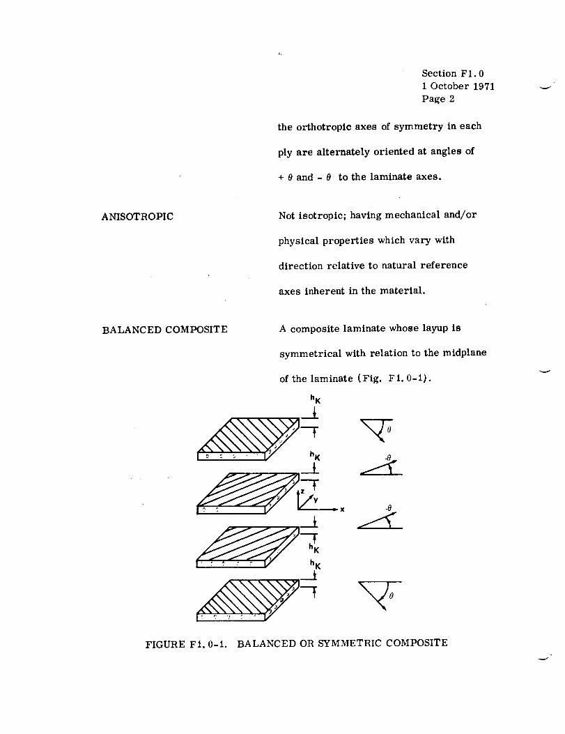
i,
Section F1.0
1 October 1971
Page 2
the orthotropic axes of symmetry in each
ply are alternately oriented at angles of
+ e and - 0 to the laminate axes.
ANISOTROPIC Not isotropic; having mechanical and/or
physical properties which vary with
direction relative to natural reference
axes inherent in the material.
BALANCED COMI_SITE A composite laminate whose layup is
symmetrical with relation to the midplane
of the laminate (Fig. F1.0-1).
hK
_3_
z: _.3.
_ hK
FIGURE F1.0-1. BALANCED OR SYMMETRIC COMPOSITE

BUCKLING
COMPLIANCE MATRIX
COMPOSITE MATERIAL
Section F1.0
1 October 1971
Page 3
Buckling is a mode of failure characterized
generally by an unstable lateral deflection
caused by compressive action on the
structural element involved. In advanced
composites, buckling may take the form not
only of conventional general instability and
local instability but also of a microinstability
of individual fibers.
The compliance matrix is defined by the
equation e. = S..a., where S.. are the1 D J U
components of the compliance matrix; may
be obtained by inverting the stiffness matrix.
Composites are considered to be
combinations of materials differing in
composition or form on a macroscale. The
constituents retain their identities in the
composite; that is, they do not dissolve or
otherwise merge completely into each other
although they act in concert. Normally,
the components can be physically identified

Section F1.0
1 October 1971
Page 4
and lead to an interface between components
(Fig. FI. 0-2).
Z
FIGURE F1.0-2.
CONSTITUENT
CONSTITUTIVE
CROSSPLY
MATRIX(1
FIBER
PRINCIPAL CONSTITUENTS OF COMPOSITE
LAMINA AND PRINCIPAL AXES
In general, an element of a larger grouping;
in advanced composites, the principal
constituents are the fibers and the matrix
(refer to Fig. F1.0-2).
Refers to the stress-strain (Hooke's Law)
relationships for a material because the
stress-strain relations actually describe
the mechanical constitution of the material.
Any filamentary laminate constructed with
equal numbers of pairs of laminae at angles
of 0 deg and 90 deg to the laminate axes.

DE LA MINA TION
FIBER
FIBER CONTENT
Section F1.0
1 October 1971
Page 5
An alternate definition used frequently in
current literature, but not in this section,
is a laminate consisting of an even number
of layers all of the same thickness with the
orthotropic axes of symmetry in each ply
alternately oriented at angles of 0 deg and
90 deg to the laminate axes.
The separation of the layers of material in
a laminate.
A single homogeneous strand of material,
essentially one-dimensional in the
macrobehavior sense, used as a principal
constituent in advanced composites because
of its high axial strength and modulus
{refer to Fig. F1.0-2).
The amount of fiber present as
reinforcement in a composite. This is
usually expressed as a percentage volume
fraction or weight fraction of the composite.

FIBER DIRECTION
Section F1.0
1 October 1971
Page 6
The orientation or alignment of the
longitudinal axis of the fiber with respect
to a stated reference axis (Fig. F1.0-3).
a
X
FIGURE FI. 0-3. LAMINA AXIS ORIENTATION
FILAMENT A variety of fibers characterized by
extreme length, such that there are
normally no filament ends within a part
except at geometric discontinuities.
Filaments are used in filamentary

Section F1.01 October 1971Page 7
composites and are also used in filament
winding processes, which require long,
continuousstrands.
FILAMENTARY COMPOSITES Composite materials of laminae in which
the continuousfilaments are in nonwovcn,
parallel, uniaxial arrays. Individual
uniaxial laminae are combined into
specifically oriented multia×ial laminates
for application to specific envelopesof
stren_,_thand stiffness requirements
(Fig. F1.0-4).
Z
o o o o _ C'-,,'"."-_(I oo ooooooo o__
FIGURE F1.0-4. FILAMENTARY COMPOSITE
GENERALLY ORTHOTROPIC Descriptive term for a lamina for which
the constitutive equation, when transformed

Section F1.0
1 October 1971
Page 8
to an arbitrary set of axes, is fully
populated. That is, for
u
-0.x 1 K F_ll -E12 _16
' L0.y ' = C12 _22 _26
• ] °xy 16 _26 _66
1E x
EyI
YxyJ ,
C16 _ O, C26 _e O,
HENCKY-VON MISES
DISTORTIONAL ENERGY
THEORY
Yield criterion using distortional energy
for isotropic materials:
(al_ o.2)2+ (a 2- o.3)2+ (0.3- °"1)2+ 6(0" 122+0.232+0.sl 2)= 2o"02 .
HETEROGENEOUS Descriptive term for a material consisting
of dissimilar contituents separately
identifiable; a medium consisting of regions
of unlike properties separated by internal
boundaries; not homogeneous.
HILL Generalized yon Mtses yield criterion to
account for anisotropy:

/
where
Section F1.0
1 October 1971
Page 9
A! ((72 - 0"3) 2 +A 2 ((73 - o"1) 2 + A 3 ((71 - o-2) 2 + 2A4o'232
+ 2A5CT312 + 2A6cT122 = 1 ,
2f(oij ) = the plastic potential,
2A 1 = (F2)-2 + (F3)-2 _ (F1)-2
2A 2 = (F3)-2+ (F1) -2_ (F2) -2
2A 3 = (F1) -2+ (F2) -2_ (F3) -2
2A 4 = (F23) -2 ,
2A 5 = (F31) -2 ,
2A6 = (F12) -2 ,
and F1, F 2, and F 3 are determined from unia×ial tension or compression tests,
and FI2, F23, and F31 are determined from pure shear tests.
HOMOGENEOUS Descriptive term for a material of uniform
composition throughout; a medium which has
no internal physical boundaries; a material
whose properties are constant and isotropic
at every point.
HOMOGENEOUS ANISOTROPIC Descriptive term for a material which has
no plane of material symmetry such as the
orthotropic material.
HOMOGENEOUSGENERALLYORTHOTROPIC
HOMOGENEOUSISOTROPIC
HORIZONTAL SHEAR
INTERFACE
INTERLAMINAR SHEAR
ISOTROPIC
LAMINA
Section FI. 0
1 October 1971
Page I0
Descriptive term for a lamina which behaves
in a manner similar to the anisotropic
lamina.
Descriptive term for a lamina which has
a constant modulus of elasticity and the
C16 = C26 = 0 in its constitutive equation.
See interlaminar shear.
The boundary between the individual,
physically distinguishable constituents of
a composite.
Shear force which tends to produce a
relative displacement between two laminae
in a laminate along the plane of their
interface.
Descriptive term for a material which has
uniform material properties in all
directions.
A single ply or layer in a laminate made of
a series of layers (Fig. F1.0-5}.

Section F1.0
1 October 1971
Page 11
f
/-
N
I II /
Vi.l.l
l-
z
--i
//
//
/
X
//
I
//
Z0
0Z
Z
_q
L_I
o
.J
r_
©
LAMINAE
LAMINATE
LAMINATE ORIE NTATION
LAYUP
MACRO
MATRIX
Section F1.0
1 October 1971
Page 12
Plural of lamina (refer to Fig. FI. 0-5).
A product made by bonding together two or
more layers of laminae of material or
materials (refer to Fig. F1.0-5).
The configuration of crossplied composite
laminate with regard to the angles of
crossplying, the number of laminate at each
angle, and the exact sequence of the
individual laminae.
A process of fabrication involving the
placement of successive layers of materials.
In relation to composites, denotes the gross
properties of a composite as a structural
element but does not consider the individual
properties or identity of the constituents.
The essentially homogeneous material in
which the fibers or filaments of a composite
are imbedded {refer to Fig. F1.0-2).
\
W"
F-
f-
MICRO
ORTHOTROPIC
PRINCIPAL AXES
QUASI-ISOTROPIC
SPECIALLY ORTHOTROPIC
TENSOR
Section FI. 0
I October 1971
Page 13
In relation to composites, denotes the
properties of the constituents and their
effect on the composite properties.
Descriptive term for a material which has
three mutually perpendicular planes of
elastic symmetry.
The set of axes in a lamina which is
parallel and perpendicular to the filament
direction is called the lamina principal
axes (refer to Fig. F1.0-2).
Descriptive term for a laminate which has
essentially isotropic stiffnesses and
perhaps st rengeth.
Descriptive term for lamina for which
the Cl6 : C26 0 in its constitutive
equation.
A tensor is a physical entity in nature
which obeys certain transformation
relations. There are different orders of

TRANSVERSELY ISOTROPIC
VON-MISES DISTORTIONA L
ENERGY THEORY
x-AXIS
y-AXIS
Section F1.0
1 October 1971
Page 14
tensors, and each order has its own
transformation relations.
Descriptive term for a material exhibiting
a special case of orthotropy in which
properties are identical in two orthotropic
dimensions, but not in the third; having
identical properties in both transverse
directions but not the longitudinal
direction.
See Hencky-von Mises Distortional Energy
Theory.
An axis in the plane of the laminate which
is used as the 0 deg reference for
designating the angle of lamina (refer to
Fig. F1.0-5).
The axis in the plane of the laminate which
is perpendicular to the x-axis (refer to
Fig. FI.0-5).

z-AXIS
Section F1.0
1 October 1971
Page 15/16
The reference axis normal to the plane of
the laminate (refer to Fig. F1.0-5).
f
f
J


f-
Section F1.0
1 October 1971
Page 17
1. 1 BASIC CONCEPTS.
Some of the basic concepts applicable to all continuums, in particular
composites, are presented in this subsection. These include the concepts of
stress and strain at a point and their transformation relations.
i. I. 1 STRESS AND STRAIN.
Following the guide of Ilefcrence i, stress and strain relations at a
point will be reviewed to form a firm base for the analytical development for
composites.
A tensor, as defined previously, is some physical entity in nature
which obeys certain transformation relations. A scalar, for example, is a
tensor of zero-th order, and a vector is a tensor of first order. Itis well
known that the components of a vector change when the coordinate system is
altered or rotated. This change in the components of the vector is governed
by certain mathematical relations or transformations. Each order of tensors
has its own transformation relations; therefore, it is necessary only to
establish that a physical entity is a tensor and determine its order, and the
transformation relations are defined.
Stress and strain are both second-order tensors and their transformation
relations are well known (the graphical form of the transformation is the Mohr's
circle). These transformation relations may be derived from the equilibrium
relations of a small element. Consider a two-dimensional problem as shown

in Fig. FI. 1-1.
equation results:
Section FI. 0
i October 1971
Page 18
By summing forces in the "1" direction, the following
_ldA-_ (cosSdA) (cos e) - _ (sinedA) (sine)x y
-_ (sin0dA) (cos 8) - T (cos 0dA) (sin0) = 0 ,xy xy
or
_I = _ cos29 + o sin 28+ r (2 sin#cos 8) (FI.I-I)x y xy
2
o2 /'
Y
m X
Jo¥
FIGURE FI. I-i.
2
_r12/,_°1 o2 T12A
"rxylJ A _dA
"T-Oy ov
STRESS COORDINATE ROTATION
O x
In a similar manner, the other transformed stresses, cr2 and rt2 , may be
determined. These equations may be written in a form convenient for later
developments, a matrix form. Thus,

[ lj_2
Tt
cos 2 0
sin 2 0
-sin 0 cos 0)
sin 2 0 (2 sin 0 cos 0) 1
cos 2 0 (-2 sin 0 cos 0)
(sin 0 cos 0) (cos20 - sin 20)
Section F1.0
1 October 1971
Page 19
_y . (F1. 1-2)
7
Using a more compact notation, we may write equation (F1.1-2) as
¢r2 I = [TI (FI. 1-3)
T12 J L xy
where [T] is the symbol for the transformation matrix. Equation (F1. 1-3) is the
transformation relation for the stress tensor when reduced to a two-dimensional
space. Equation (F1. 1-3) is the necessary relationship required to transform
any two-dimensional stress state from one set of coordinates to another set.
With a slight modification, the two-dimensional strain may be
transformed by the same transformation:
1¢2 ! = LT] _y ]
½":,2J J_ 2 xy
(F1. 1-4)

Section F1.01 October 1971Page 20
1.1.2 GENERALIZED HOOKE'SLAW.
In this paragraph the constantsof proportionality betweenstress and
strain {Hooke's law constants} are shownto be componentsof a fourth-order
tensor andtherefore have a set of transformation relations different from those
for stress and strain. Several forms of the Hooke's law relationships andthe
elastic constantswill be shownfor the various material conditions.
1.1.2. 1 Homogeneous Isotropic Material.
For the familiar homogeneous isotropic material in a one-dimensional
stress state [1], the Hooke's law relationship is
= EE . (FI. i-5)
The proportionality constant (E) is Young's modulus, or the modulus
of elasticity, and is a scalar value.
1.1.2. 2 Elastic Linear Anisotropic Material.
Consider the most general material, but require elasticity and
linearity, which is the anisotropic material. This material has 21 elastic
constants. The constitutive equation (Hooke's law) is [2]
m
C11 C12 C13 C14 C15 C16
C22 Cn C24 C2s C2_
C33 C34 C3s C36
C44 C45 C46
SymmetricCss Cs6
C66-- a
[a] = [_] . (F1.1-6)

Section FI. 0
1 October 1971
Page 21
The components C.. are called components of the "stiffness" matrix. The11
equation may be written as
'where
m
Sit S12 St3 $14 $15 $16
822 S23 824 S25 $26
$33 $34 $35 $36
Symmetric $44 $45 $46
Sss Ss6
S66
[(_1 (F1. 1-7)
[C] = IS] -1 . (F1. 1-8)
The components S.. are called components of the "compliance" matrix.1]
[ _] conventionally symbolizes [ 3]
The
- _rl
I
[or] = °3 I (F1. 1-9)
Similarly,
[E] =
T23I?13 I
I_ T12J
;--El "7
e2 II
_3
I
_/23
_13
__/12J
(FI. i-I0)

Section F1.0
1 October 1971
Page 22
1.1. 2. 3 Monoclinic Material.
If a material possesses one plane of symmetry, it is termed a
monoclinic material and has 13 independent elastic constants. If the plane of
symmetry is assumed to be the x-y plane, the constitutive equations are [ 2]
and
[a]
CtICz2Ct3 0 0 Ct6"
C22 C23 0 0 C26
C3s 0 0 C38
C44 C4$ 0
SymmetricC55 0
C66
[c] (rl. i-li)
[c] =
Sit St2 St3 0 0 S16
$22S23 0 0 $26
833 0 0 836
$44 S4s 0
SymmetricSss 0
866m
[a]. (FI. 1-12)
m
1.1.2. 4 OrthotroDic Material.
If the anisotropic material possesses two orthogonal planes of symmetry,
assuming x = 0 and z = 0, the material is termed orthotropic. In this
condition, there are only nine independent elastic constants. Note that ff a
material has two orthogonal planes of symmetry, three orthogonal planes of
symmetry exist. The constitutive equations of the orthotropic material are

and
[=J
-C11 C12 C13 0 0 0-
C22 C23 0 0 0
C33 0 0 0
C44 0 0
Symmetric Css 0
C66m
Section F1.0
1 October 1971
Page 23
[(1 (F1.1-13)
[_]
Sll S12 S13 0 0 0
$22 $23 0 0 0
$33 0 0 0
$44 0 0
Symmetric Sss 0
S66B u
[el • (F1. 1-14)
Since most composite structures will be constructed of orthotropic
laminates, this material is of particular interest. The engineering constants,
values which are establishable from uniaxial and pure shear tests, may easily
be equated to the components of the compliance matrix. The compliance
components are then
1 l 1
$11 = 1El-- ' $22- E22 ' $33- E33
= =-vaX_S_3 :L22_ S31S12 = El I E22 E33
_-v_l__ , :Lv__ , =:._V_I__ (FI. 1-15)E22 E33 Ell "
1 1 1
S6_ = 2GI--' $55 = 3Gl_ $44- G23
= :Sl 6 _ S26 7726 836 =
El I ' E22 ' E33

where
Section FI. 0
1 October 1971
Page 24
Eft, E22, E33 = Young's moduli in the I, 2, and 3 (x, y, and z)
directions, respectively,
v.. = Poisson's rationlj
strain in the j directionstrain in the i direction
caused by a stress in the i direction,
Gij = shear moduli in the i-j plane,
_ij = shear coupling ratios.
Note that the SI6, S26, and S36 terms are used for a "monoclinic"
material. From equation (F1. 1-8), the components of the stiffness matrix may
be determined as
and
Cll = (I - v23 _32) VEIl ,
C22-= (I - v31 v13) VE22 ,
C33= (I - vi2 v21) VE33 ,
C12 = (v21 + v23v31) VEIl ,
= (VlZ + vI3 v32) VE_2 ,
C13 = (v31 + v21v32) VEil ,
= (vla + v23 v12) VE33 ,
C23 = (v32 + v12 v31) VE22 ,
= (v23 + vZl v13) VE33 ,
C44 = G23 ,
C55 = G31 ,
C66 = G12 ,
(FI. 1-16)

(
where
Section F1.0
1 October 1971
Page 25
V-- (1 - 1_12 t_21 - /"23 P32 - 1)31 /_13 - 2te12P23t_'31) -1
For an orthotropic material in a state of plane stress, the constitutive
equation is [ 1]
_r 1
(_2
712
icllc10111= C12 C22 0 (2
0 0 C66 3/12
(F1. 1-17)
where
EllCll =
(1- _12v21)
E22 -- (El. 1-18)C22 = (1 - _12_21) '
21E11 l' 12E22
C12 = (i- 71_,21) = (i - .12.21) '
and
C66 = G12
1. 1.2.5 Isotropic Material.
For an isotropic material, there are only two independent elastic
constants. The constitutive rel:_tions are [3]

and
[_] =
Ctl C12 Ct3 0
Ctt Ct2 0
Ctt 0
½ (ctl- ct2)
m
0 0
0 0
0 0
0 0
0
½ (c. - ci_)
Symmetric ½ (Ctt - Ct2)
[c]
Section FI. 0
1 October 1971
Page 26
(F1.1-19)
[_]
i
SIt S12 S12 0 O 0
Sll $12 0 0 0
Symmetric Sit 0 0 0
2 (Slt- St2) 0 0
2 (Sll- S12 ) 0
2 (Stl - St2)
[_] (FI. 1-20)
The constitutiveconstants may be defined in terms of the engineering
constants as
(l-u) E
Cit =C22 =Csa = (1+ v) (I- 2v)
rE
Ct2 =CI3 =C2s = (1 + v) (1 - 2v) ' (Ft. 1-21)
C44=C55 =C66=G =E
2(1+v) '
1
Stt=S22=S3a=_ ,
St2 ---Sis = $23 = E

and
1 2(1 + v)$44 = $55 = $66 ---G_- E
Section F1.0
1 October 1971
Page 27
If the isotropic material is assumed to be in a two-dimensional stress state
(plane stress), equation (F1. 1-19) may be written as [ 1]
(Y2
T12
Cll C12 0
C 12 C 22 0
0 0 C66
1E1
£2
I
. "F12
(F1. 1-22)
where
E
C11=C22- (1-,2)
E
(1 - v 2'J '
(F1. 1-23)
and
- G
1.1.2.6 Transformation of Stiffness Matrix.
In Reference 1, the elastic constants (stiffness) for a material are
stated to be components of a fourth-order tensor and consequently, must obey
certain transformation relations. The transformation of a general anistropic
material, in three dimensions and rotated an angle 0 about the z-axis, is
given in Reference 2 as
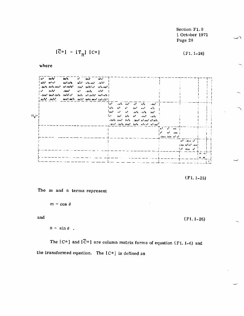
Section F1.01 October 1971Page 28
-_iN
where
[_*1 = [TRI [C*l (F1.1-24)
I tara! m*+a4 rant.man rata t man-ma t
II-_an 2man-_tm! m*.$manz 2ma) 3mtaZ-n*I n4 2m_
J._n ! 2mat. 2rata
{II
ITR]= 1
I[I
tl_n 2 "-I" .......
-m'n' Im_n-mn$ I
-2rant m_ -2man m_ t ]
3manl.n 4 2mtn ma-3m_ t rand-man J
ennt-_'nan 4m _nz _ a-_rana (m_-n:l) 1 I
.................. -T_T--_ ma,--..-r-_}mln m ! n j mn 2 mn t
J,_, _._ m' -_ -_'nJn I roll I man m ] -ran !
l-2m_ 2ran 2 2m_n -2ran t mr-ran _ nt-m ta
I-2ran 2 -2man 2ran t 2rain mtn-n t mr-ran lj-_'mt
; rI rIt-- ........... -_
1
I
F!
l.__
_ran l
_nta
roll I
.mZn
[_J,
T .... "_
I
I{i[
[
IJ]J
n ! mn I
r _ _t -ran;-_, zma m2-o'I I
I Ima m'._' -m_t I [i I., zma n' I ] I
I t° ml__j
(F1. 1-25)
The m and n terms represent
m= cos 0
and
n = sin 0
(Fl. 1-26)
The [C*] and [C':'I are column matrix forms of equation (F1.1-6) and
the transformed equation. The [C*] is defined as

[C*] =
m
Cll
C12
2C16
C22
2C26
4C66
C14
C15
C24
C25
2C46
2C56
C13
C23
2C36
C44
C45
C55
C34
C35
C33
Section FI. 0
1 October 1971
Page 29
(FI. i"-27)

Section F1.0
1 October 1971
Page 30
and the [_'*] is defined as
m m -.-,,i
rl !
_. ;12 I
2C16 I
C2_ I
2C2s I
4C66 I
_24 I
_25 I
2C_ 1
2Cs6 I-- ,,"-_13 I
'_23 I
2Cae
1244
C45
C65
C34
C35
C33
(FI. 1-28)
The transformation of the stiffness matrix for an orthotropic material
in a plane stress state is of particular interest since this will be of direct
applicability to fibrous composites. As shown in Reference 1, when the
elastic constants are needed with respect to some axis other than the material
axis, the transformed elastic constants are
J_

f-and
Cli =
C22 =
C12 =
C66 =
C16 =
m
C26 =
Section F1.0
1 October 1971
Page 31/32
Cll cos 4 0 + 2 [C12 + 2C66 ] sin 2 0 cos 2 0 + C2 2 sin 4 0 ,
Cll sin 4 6 + 2 [C12 + 2C66 ] sin 2 0 cos 2 0 + C22 COS 4 0' (F1. 1-29)
[Cll+C22- 4C66 ] sin 2 0 cos 2 0 + C12 [sin 40 + cos 4 0] ,
[Cll ÷ C22 - 2C12 - 2C66 ] sin 2 0 cos 2 0 + C66 [sin 4 0 + cos 4 O] ,
[CII- C12- 2C66] sin 0 cos 3 0 + [C12- C22 + 2C66 ] sin 3 0 cos _)
[Cli - C12 - 2C66] sin 3 0 cos 0 + [C12 - C22 + 2C66 ] sin 0 cos 3 0 .
The angle of rotation (0) is about the z-axis and assumed positive in
the counterclockwise direction.


¢.-Section F1.0
1 October 1971
Page 33
i. 2 MECHANICS OF LAMINATED COMPOSITES.
Two types of mathematical models [ 1] are normally utilized to predict
the stress-strain response of a constituent lamina of a laminated composite
m mieromodels and macromodeis. The mieromechanics approach to the
problem models the individual lamina as a periodic, or possibly a random,
array of filaments in a matrix. The average stress-strain response of the
lamina is a function of the elastic constants of the fiber and the matrix and
their respective geometries. The macromechanics approach ignores the
fiber-matrix behavior and models the individual lamina as a thin homogeneous
orthotropic medium (sheet) under a state of plane stress.
1.2. 1 MICROMECttANICS.
The strength and structural behavior of fibrous composites are
directly related to the elastic properties of the fiber and matrix, as well as
the micro-geometry of the laminate [ 1]. The field of micromechanics
encompasses the study of the internal stress distribution in the fiber and matrix
as a result of external loading. The objective of any mieromechanies effort is
to predict the intrinsic macroscopic (average) material properties of a
laminate from the material and geometric properties of the constituents and
perhaps provide the basis for understanding failure modes and establishing
failure criteria from the predicted stress states.
With the present state-of-the-art, a mieromeehanies approach to
composites for aerospace application does not give the designer a design tool
whieh can be utilized to design aerospace structures. It is feasible that at

Section F1.0
1 October 1971
Page 34
some time in the future, the aerospace designer will begin his creation at the
fiber and matrix level and will use the analytical tools of micromechanics to
determine his design parameters. However, at present the advanced
composites come to the fabrication stage in a preimpregnated tape form with
the filament spacing and other parameters established. Of course, some of
the predictions resulting from micromechanic analyses were utilized in
establishing a good filament spacing to insure good transverse and shear
properties in the final laminate; however, this represents a limited
application of micromechanics to designs.
I.2. 2 MACROMECHANICS.
With the present state-of-the-art, the macromechanic approach [1] to
the mechanics of filamentary composites is the most usable technique for the
aerospace designer or stress analyst. The elastic constants and stress-strain
response of an individual lamina may be determined experimentally, and these
data may subsequently be used to determine the stress-strain response of a
laminate composed of any orientation of the characterized laminae.
\

z-Section FI. 0
1 October 1971
Page 35
I.2.2.i Lamina Constitutive Relationship.
For a filamentary composite (Fig. FI. 2-I), the constituent laminae
have three mutually perpendicular planes
of elastic symmetry [1]. As discussed
previously, a material with three
mutually perpendicular planes of
symmetry was termed orthotropic;
FIGURE F1.2-1. FILAMENTARY
COMPOSITE WITH THREE
MUTUALLY PERPENDICULAR
PLANES OF SYMMETRY
therefore, the possibility exists to
model the lamina as a homogeneous
orthotropic medium. Since the
thickness of an individuallamina is small relative to its other dimensions, it
may be considered to be in a state of plane stress. The constitutive equation
for the K-th lamina is then given by equation (FI. 1-17) or
(7t_
(Tp
T
L
K K KCtt C12 0
C 12 C22 0
0 0 2C66
£o{
(F1.2-1)
The lamina stiffness matrix terms were defined in equation (F1. 1-18) and are
rewritten here as
ElL ...C,, - (i - v,2v_1)
E 2?.
C22- (1 - "12"2,)(F1. 2-2)
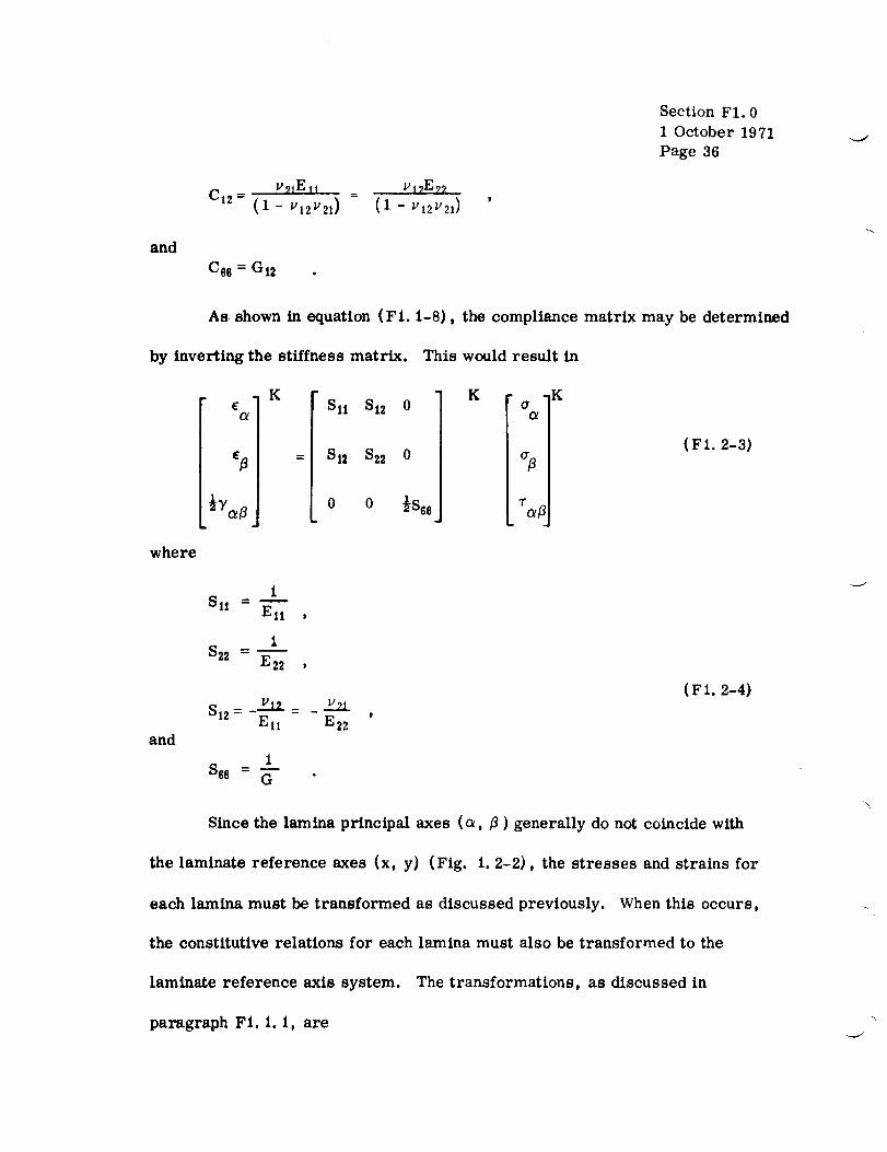
and
P21E11 = v1_E_c12= (i- v,2v21) (1 - v,2v2,)
C66 = Gi2
Section FI. 0
1 October 1971
Page 36
As shown in equation (F1.1-8), the compliance matrix may be determined
by inverting the stiffness matrix. This would result in
E] K
½_ ]
Sll S12 0
= S12
0
$22 0
½S66
K -KOr
(FI. 2-3)
where
and
1m
$11 = El I ,
I$22 --
E22 ,
_v_la = v__$12 = El I - E22
1
s_e = b-" "
(F1.2-4)
Since the lamina principal axes (c_,_ ) generally do not coincide with
the laminate reference axes (x, y) (Fig. i.2-2), the stresses and strains for
each lamina must be transformed as discussed previously. When this occurs,
the constitutiverelations for each lamina must also be transformed to the
laminate reference axis system. The transformations, as discussed in
paragraph FI. 1.1, are

Section F1.0
1 October 1971
Page 37
a
1¢
\ \\
FIGURE F1.2-2. GENEllAL LAMINAE ORIENTATION
WITH LAMINATE REFERENCE AXIS
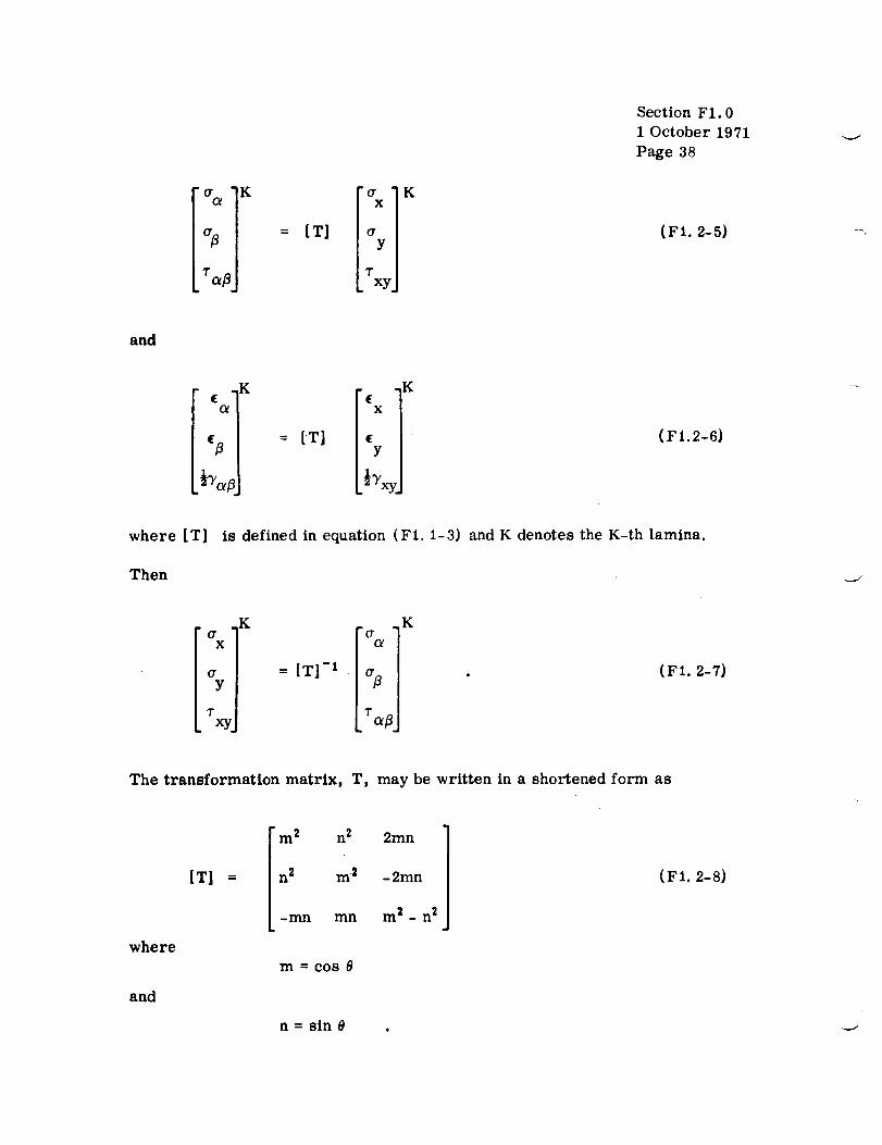
'_ "K
= [T] (7Y
T
• xy.
Section FI. 0
1 October 1971
Page 38
(F1.2-5)
and
,KE
Ot
cfi : [T]
-,KE °
X
Y
.½"Y_
(FI.2-6)
where [T] is defined in equation (FI. i-3) and K denotes the K-th lamina.
Then
. .K . ,KO" (7
x (_
a = IT] -tY aft . (F1.2-7)
T. xy Ta,a
The transformation matrix, T, may be written in a shortened form as
where
and
IT]
"m 2 n2 2ran
n2 m 2 -2mn
-mn mn m 2 - n 2
m = C08 0
(F1.2-S)
n = sin 0 . _

Section F1.0
1 October 1971
Page 39
Note that the inverse of the T matrix, [T] -1, may be obtained by
substituting for the positive angle 0 a negative angle 0 (refer to Fig. 1.2-2).
Using equations (F1.2-1), (F1.2-6), and (F1.2-7), the lamina
constitutive equation, when transformed to the laminate reference axes, is
%
"rx:
- K
: [T]-' [C'I K tTI i e l
!Yl
The transformed lamina stiffness matrix [C'] is defined as
(FI. 2-9)
[_,]K = IT]- 1 [c,]K [T] =
16
C12 C22 2C26
el6 C26 2C66
(FI. 2-10)
where the terms _.. are given by equation (F1. 1-29). The-C' matrix,E
which is now fully populated (C16 ¢ C26 ¢ 0), appears to have six elastic
constants which govern the lamina behavior; however, C16 and C26 are not
independent as they are linear combinations of the four basic elastic constants.
In the transformed coordinate system, the C ' matrix is similar in appearance
to the C matrix for a fully anisotropic lamina (C16 ¢ 0 and C26 ¢ 0), and the
lamina is said to be "generally" orthotropic. Therefore, equation (F1.2-9)
is said to be the constitutive equation for a "generally" orthotropic lamina.

Section F1.0
1 October 1971
Page 40
Equation (Ft. 2-I) is referred to as the constitutive equation for a "specially"
orthotropic lamina (CIe = C2s = 0).
For convenience, equation (FI. 1-29) may be written as
and
Clt = (3J1 + J2) + J! cos 2 8 + J4 cos 4 0,
m
C22 = (3J1 +J2) - Jscos 20 +J4cos 40,
C12 = (Jl - J2) - J4 cos 4 0,
m
C66 = (J1 + J2) - J4 cos 4 8,
C16 = _ J3 sin 2 0 + J4 sin 4 0,
m
C26=½Jssin2 e- J4sin4 0
(Fi.2-ii)
where
and
Jl=Jf [Cll + C22 + 2C12] ,
J2 = [c.- clzl ,
J3 =_ [Cl1-C22] ,
(F1.2-12)
J4=_ [C11+C22- 2C_-4Css] .
Note that CII, C_0 CIZ° and Css are composed of a term independent
of the angle of rotation (0) and a term dependent on the angle of rotation.
Therefore, it is evident that there are certain inherent lamina properties
which are only dependent on the material being used.
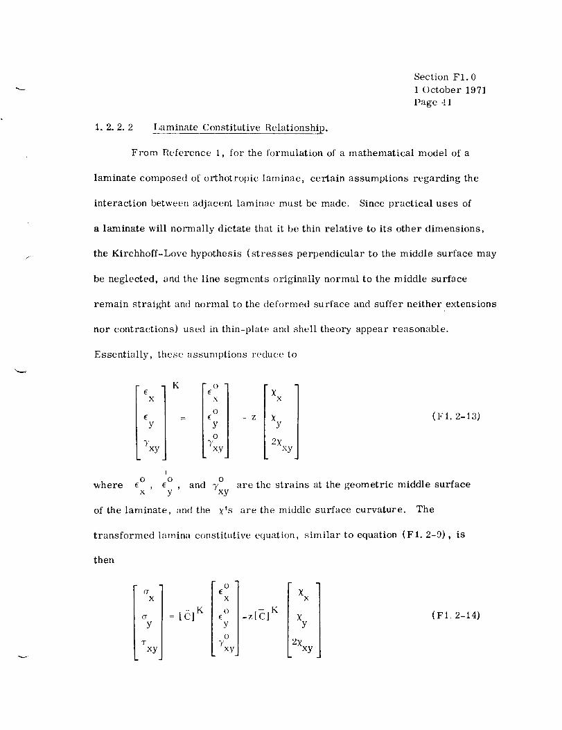
f
Section F1.0
1 October 1971
Page 41
1.2. 2.2 Laminate Constitutive Relationship.
From Reference 1, for the formulation of a mathematical model of a
laminate composed of orthotropic laminae, certain assumptions regarding the
interaction between adjacent laminae must be made. Since practical uses of
a laminate will normally dictate that it be thin relative to its other dimensions,
the Kirchhoff-Love hypothesis (stresses perpendicular to the middle surface may
be neglected, and the line seg_ments originally normal to the middle surface
remain straight and normal to the deformed surface and suffer neither extensions
nor contractions) used in thin-plate and shell theory appear reasonable.
Essentially, these assumptions reduce to
E
X
E
Y
Txy
K
Xl X
= _ - Z X
V- Y j21o i
, 2Xxy
(F1. 2-13)
I0 0 0
where • , e , andx y Txy
are the strains at the geometric middle surface
of the laminate, and the X's are the middle surface curvature. The
transformed lamina constitutive equation, similar to equation (F1. 2-9), is
then
] ocy £x x
[_1K ocr = (
Y I Y
1 orxy Tx
×x
_z[Cl K × (FI. 2-14)Y
2×xy
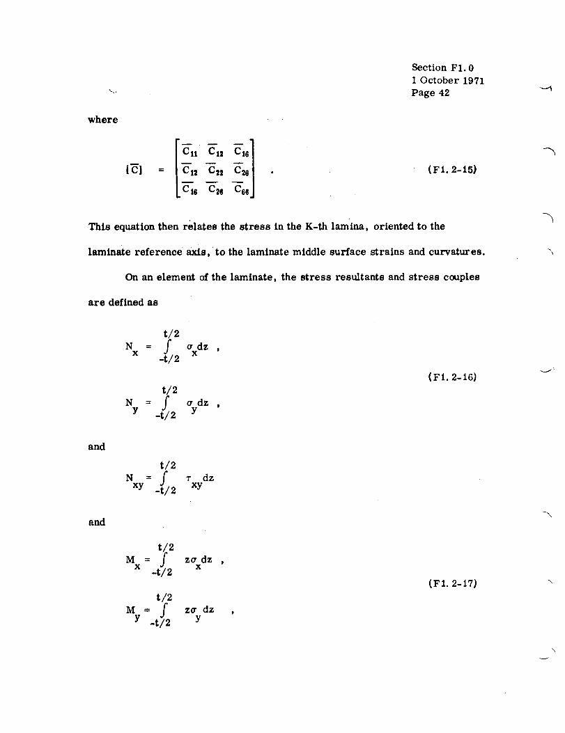
where
Section F1.0
1 October 1971
Page 42
C1e C2s CseJ
(Fi. 2-15)
This equation then relates the stress in the K-th lamina, oriented to the
laminate reference axis,to the laminate middle surface strains and curvatures.
On an element of the laminate, the stress resultants and stress couples
are defined as
-A
t/2
N = f o dzX J X
-t/2
t/2N = I o dz
Y -t/2J Y
(FI. 2-16)
and
and
t/2
N = [ _ dz
xy -t/J2 xy
t/2M = _ zo dz
PX _' X
-t/2
t/2
M = f zodzY -t/2 Y
(F1.2-17)
\

Section F1.0
1 October 1971
Page 43
and
t/2
M = ] zT dz
xy -t/2J xy
,f-
These integrals may be evaluated by integrating ov,:r each lamina and summing
the results of each integration. By substituting equation (F1. 2-14) into
equations (F1.2-16) and (F1.2-17),
where
and
NX
NY
Nxy
LAijl =
[Bij ] =
All A12 A1G
A12 A22 A26
Ale) A2_ Ac)6
Bll B12 I31_
B12 B22 B26
Big B26 B6g
" O "E
X
O
Y
0
7xy
!" 0 °£
X
O
£
Y
O
Txy
n ]K[C (hK 1)K=I ij - hK-
n K )' E [C..] (h2K h2K_ I-2
K = 1 lj
n -- ]K )= -_- E [C.. (hBK- h3K_l° K=I U
"_Bll
- B12
B16
B12 B16
]322 B26
B26 B66
r
DI_ DI2 DI6
])12 D22 D26
DI_ D26 DG_
XX
XY
2×xy
XX
Xy
(F1.2-18)
( F1. 2-19)
(F1.2-20)
(F1. 2-21)
(Ft. 2-22)
Refer to Figure F1. 2-3.

Section F1.0
1 October 1971
Page 44
.¥
t
kit.._J_
FIGURE F1.2-3. LAMINATE ELEMENT
Equations (F1.2-18) and (FI. 2-19) are the constitutive equations for a
laminated composite. They may be written as
I:l I::1I:°J (F1.2-23)
This is the general constitutiveequation for laminated composites and
is mathematically equivalent to the constitutiveequation for a heterogeneous
anisotropic medium. In this general form, the significantpoint is that there
is coupling between extensional (membrane) deformation and bending

Section F1.0
1 October 1971
Page 45
deformation caused by the existence of the B matrix (Fig. F1-2. 4). In other
words, even _.ithin the limits of small deflection theory, forced curvatures
within the laminate induce in-plane loads through
FIGURE F1. 2-4.
COUPLING OF
DEFORI\LATION DUE TO
B MA TtlLX
this type of coupling. This coupling is caused by the
neutral axis and the midplane of the laminate not
being coincident.
With various combinations of laminae,
varying degrees of coupling may be caused. If the
laminate is fabricated symmetric about the midl)lane (balanced), the B matrix
will be identically zero, and the constitutive equation reduces to
and
[N] = [a] [e°] (I.'1 2-24)
[hi] : -[DI [xl (F1.2-25)
These equations are mathematically equivalent to the constitutive equations
of a homogeneous anisotropic material, llcnee, this type of laminate is
referred to as homogeneous anisotropic (Fig. F1.2-5). At this stage the A
and D matrices are fully populated and anisotropie in nature, and a second
type of coupling still exists. For the A matrix the A1G and A26 terms couple
the normal strains and shear stress, or the shear strains and normal stress.

Section F1.0
1 October 1971
Page 46
FIGURE FI. 2-5.
COUPLING EFFECTS IN
A HOMOGENEOUS
ANISOTROPIC LAMINATE
For the D matrix the Dis and D_s terms couple the
normal bending moments and twisting curvatures,
and vice versa. If the laminate is symmetric about
the x-y (laminate) axis (Fig. Fi. 2-6)', this coupling
may be reduced.
When the laminate has equal numbers
of pairs of laminae symmetric about the x-y axis (termed angleply laminate),
\ \ \_\\\\
\\\\\\\\
\\\
\\\\\\\\
8
FIGUR E F 1.2-6.
"4+8
LAMINATE SYMMETRIC ABOUT THE x-y AXIS
the A matrix is orthotropic in nature (Ale= A26 = 0) (Fig. FI. 2-7). The
D matrix is stillfullypopulated and anisotropic in nature. When the laminate
has equal numbers of pairs of laminae at angles of 0 deg and 90 deg to the

Section F1.0
1 October 1971
Page 47
x-y axis (termed erossply laminate), the D matrix
and the A matrix are orthotropic in nature.!
,_[_Y_ ._)z' Because of the warpage which will occur
__;_;_ during the fab,ication process when symmetry does,:r,_"
not exist, the. laminates should be designed
FIGURE F1.2-7.
LAMINATE EXtIIBITING symmetric about the midplane, or nearly so.ORTHOTI{OPIC
CHARACTERISTICS Since most laminates are symmetric
about the midplane, and because the majority of applications of advanced
composites experience relatively low transverse shear strength, a
reexamination of equation (F1.2-24) is warranted. Equation (F1. 2-24) may
be written as
N1X
N : [A]y i
_ xyj
when no bending occurs.
yields
i-£
X
E
Y
Txy
(F1. 2-26)
Dividing both sides by the total laminate thickness
O"
X
(7
Y
i 1[A]
t li11¢-
3xy
(Ft. 2-27)
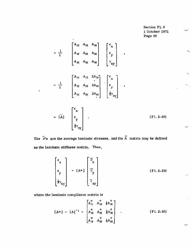
1
t
"A n AI2 Ai6"
At2 A22 A26
Ai6 A_s A66
"E -s
x I
YI
Section F1.0
1 October 1971
Page 48
1
t
"All A12 2A16"
!
A 12 A22 2A26
A16 A26 2A66
"E "1
E I
m
= [A]
E X
Cy(Ft. 2-28)
m
The ¢Ws ore the average laminate stresses, and the A matrix may be defined
as the laminate stiffness matrix. Thus,
i
x
Y= [A*]
o"x
(F1.2-29)Y
T. xy
where the laminate compliance matrix is
Atl At= ½At_
[A*] = [A] -1 A* * *= 12 A22 ½A26
Ai6 A_ ½A6_
(Ft. 2-30)

Section F1.0
1 October 1971
Page 49
f-
The gross or average(, laminnte elastic moduli may be obtained trom the
laminate compliance matrix. For a balanced angleply laminate,
[A] A12 A22 0 [._] 1__ AI2 A22 0' t
0 0 A66 0 0 2A66
and
[ A ::-_] =
ai a_i 0
L° ,) ½,\
(F1.2-31)
Then, comparing equation (F1. 2-29) with equation (F1.2-3), the gross
laminate elastic constants are
1I'; = --
XX :":
1
YY A 22
1G
xy A _:r.
= _ !xaz
xy A n
'_}xyx A2 2
(F1.2-32)
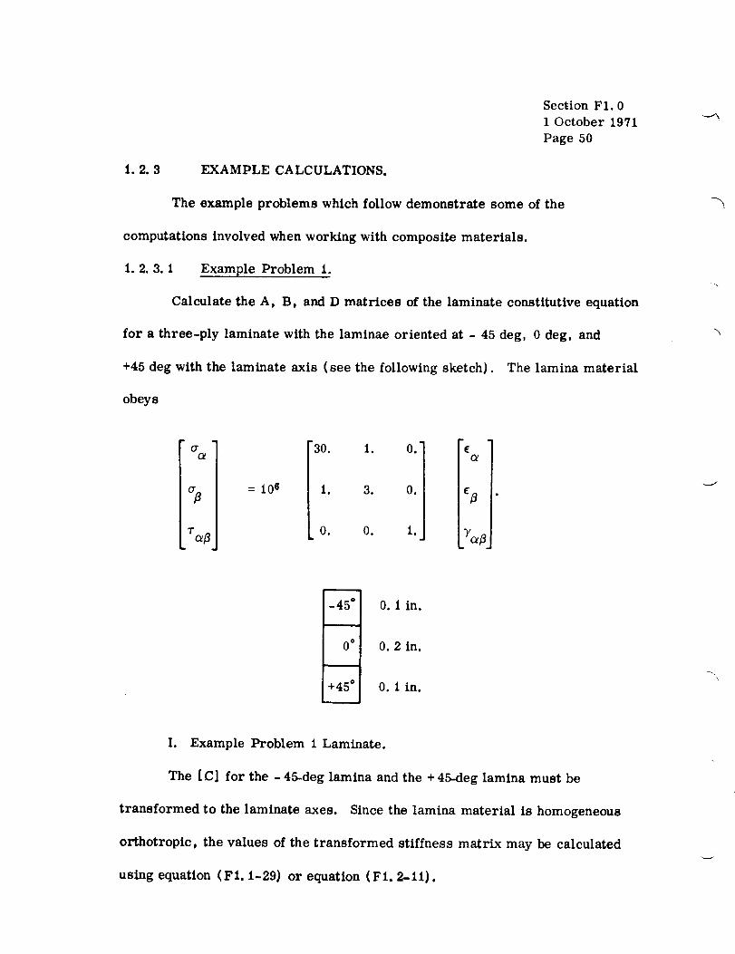
Section FI. 0
1 October 1971
Page 50
i. 2. 3 EXAMPLE CALCULATIONS.
The example problems which follow demonstrate some of the
computations involved when working with composite materials.
i. 2. 3. I Example Problem I.
Calculate the A, B, and D matrices of the laminate constitutive equation
for a three-ply laminate with the laminae oriented at - 45 deg, 0 deg, and
+45 deg with the laminate axis (see the following sketch). The lamina material
obeys
O" "30. i. 0."
i. 3. 0.
0. 0. l.
EOL
I
-45 ° ] 0. I in.
0 ° ] 0.21n.
+45°I 0.1 in.
I. Example Problem 1 Laminate.
The [ C] for the - 45-deg lamina and the + 45-deg lamina must be
transformed to the laminate axes. Since the lamina material is homogeneous
orthotropic, the values of the transformed stiffness matrix may be calculated
using equation (FI. 1-29) or equation (FI. 2-11).

Section F1.0
1 October 1971
Page 51
Using equation (F1. 1-29), the C..1j
for the 45-deg lamina are
terms of equation (F1. 2-157
C-11= 106 [30. cos 4 (-45) + 2(1. + 2.) sin 2 (-45) cos 2 (-457 + 3. sin 4 (-45)]
= 9. 75 x 106
C26= 106 [ (30.-i.-2.7 sin 3 (-45) cos (-45) + (I.-3.+2.7 sin (-457 cos 3 (-45) ]
= -G. 75 × 106
Then,
1106[975777][C] = 7.75 9.75 -6.75
-6.75 -6.75 7.75
Similarly, for the +45-deg lamina
L_](37 = 1069.75 7.75 6.751
J7.75 9.75 6.75
6.75 6.75 7.75
For the O-deg lamina
[_I(2): [cl= i,)630. i. 0. ]
1. 3. 0.0. 0. 1.
From equation (FI. 2-20),
n
A = Z (C..7 (K)44
l]"J K = i(hK - hK_i7
0.1 [c..]D
(1)+ 0.2 [C..J(2)-- "
1J

Section F1.0
1 October 1971
Page 52
Thus p
All = 10e [9.75x0. I+ 30. x0.2+9.75×0. I] = 7.95×10⁶
A6e = I0617.75x 0. I+I. x0.2+7.75×0. I] = 1.75×10⁶ .
[A] = I0s
7.95 I.75 0. 1
I.75 2.55 0.
0. 0. i.75
From equation (FI. 2-21)
x
n
Bij = _ 2; (_ij)(K) (h2K_h2K_I)K=I
= 0.015 [(Cij)(3), (_ij) (1) 1
Thus t
Bil = 106×0.015 [9.75- 9.75] = 0
and
B66 = 0.
[B] = I0e
0. O.
O. O.
O. 2025 O. 2025
0. 2025"
0. 2025
0.

From equatioa (Ft. 2-22)
Section F1.0
1 October 1971
Page 53
n
Dij = _ Z (_..) (K) (h3K i)K=I I] - h3K-
O. 00233 [C-..] (1) ](2)+ 0. 00066 [C..1J 1J
+ 0. 00233 [_..](3)IJ
Thus,
Dll
D86
: 106 [9.75 × 0. 00233 + 30. × 0.00066 + 9. 75× 0.00233]
O. 06522 × 106
tO _ [7.75× 0.00233 + i. × 0. 000(;6 + 7.75× 0.00233]
0. 03676 × 10 6
[ D] tO _
0. 06522 O. 03675 O.
0. 03676 0.0474 0.
O. 0. O. 03(;76
Combining the results above, the constitutive equation may be written as
xy|
M[M x
MY I
_ xy]
= 106
7. 95 1.75 O.
i. 75 2. 55 0.
O. O.
O. 0.
O. O. O. 2025
1.75 O. 2025 O. 2025
0. 2025' 0.06522 0.03676I
I
0.2025, 0.03676 0.0474
I
I
O. , O. 0.
0. O.
O. O°
O. 2025 0. 2025
m
0O. 2025
X
0E
Y
0
O. Yxy
O. ×X
0. Xy
0. 03676 2×_2 xy
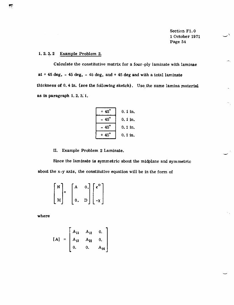
Section FI. 0
1 October 1971
Page 54
._=i \
1.2. 3. 2 Example Problem 2.
Calculate the constitutive matrix for a four-ply laminate with laminae
at + 45 deg, - 45 deg, - 45 deg, and + 45 deg and with a total laminate
thickness of 0. 4 in, {see the following sketch). Use, the same lamina material
as in paragraph 1.2. 3. 1.
+ 45" 0. 1 in.
- 45" 0. 1 in.
- 45" 0. 1 in.
+ 45" 0.1 in.
II. Example Problem 2 Laminate.
Since the laminate is symmetric about the midplane and symmetric
about the x-y axis, the constitutiveequation will be in the form of
where
[A]All A12 0. ]
= Ai2 A22 0.
0. 0. A6s

Section F1.0
1 October 1971'
Page 55
and
[D] Dil DI2 Di6= DI2 D22 D26
L DI6 D26 D66
Similar to paragraph 1.2. 3. 1,
[_l (I) [_l (4) 1o6
9.75
7.75
6.75
7.75
9.75
6.75
6.75
6.75
7.75
and
[_] (2) = [_] (3) = 106
_9.75
7.75
6.75
7.75
9.75
-6.75
-6.75
-6:75
7.75
Using equations (F1.2-20) and (F1.2-22)
and
!1.9 3.1 0.
[A] = 1() _; 3.1 3.9 0.
). 0. 3.
[D] = 106
(). 05187
0. 04123
0. 027
0. O4123
0. _51S7
0. 027
0. 027
0. 027
0. 04123
Therefore,
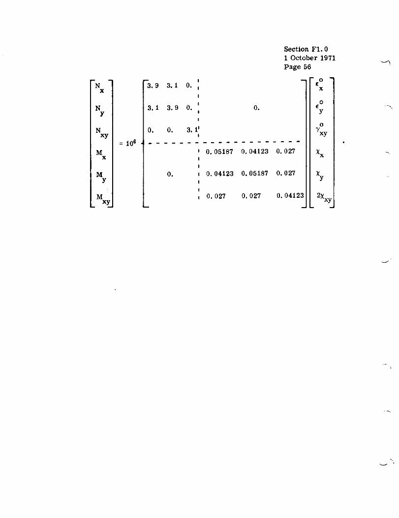
n
NX
NY
Nxy
MX
MY
Mxy
m
= I0e
-3.9
3.1
Oo
3.1 O.
3.9 O.
I 0.05187
e 0.04123
0. 027
Section F1.0
1 October 1971
t
0.04123 0.027
0.05187 O.027
Page 56
m
0.027 0.04123
i
O m
EX
OE
Y
O
Yxy
X X
Xy
2Xxy
y-,
-,.._j

Section F1.0
1 October 1971
Page 57
1.3 LAMINATE CODING.
In Reference 2 a laminate orientation code was devised for filamentary
composites which provided both a concise reference and a positive identification
of any laminate. As expressed in that reference, the following type of coding
is intended to provide a means of achieving conciseness in engineering
presentations and communications; however, it is neither recommended nor
discouraged that this code be employed on shop drawings since that policy is an
internal one which must be decided by each using organization.
1.3. 1 STANDARD CODE FLEMENTS.
The formulation of the code must be adequate to specify as concisely
as possible (1) the angles of laminae relative to a reference axis (the x-axis),
(2} the number of laminae at each angle, and (3) the exact geometric sequence
of laminae.
The basic laminate code will adhere to the following gaaidelines [2]:
1. Each lamina is denoted by a number representing its orientation
in degrees between its filament direction (refer to Fig. FI. 0-3) and the
x-axis.
2. Individual adjacent laminae are separated by a slash if their
angles are different.
3. The laminae are listed in sequence from one laminate face to the
other, with brackets indicating the beginning and end of the code. The first
lamina should be the most positive lamina in the z direction (refer to Fig.
F1.2-3).

Section FI. 0
1 October 1971
Page 58
4. /Adjacent laminae of the same angle are deonoted by a numerical
subscript.
5. A subscript T to the bracket indicates that the total laminate is
shown.
When adjacent laminae are of the same angle but opposite in sign, the
appropriate use of + or - signs may be employed. Each + or - sign
represents one lamina and supersedes the use of the numerical subscript,
which is used only when the directions are identical. Note that positive angles
are assumed to be counterclockwise.
Several examples are shown demonstrating the basic coding.
! 45r-----i 0m
-60u
-60N
3O
+45
-45
-30
+30
0
+45
+45
-45
-45
Code
[ 45/0/-602/30] T
[,45/_30/0/+(452) ] T
_r

Section FI. 0
1 October 1971
Page 59
I. 3.2 CODES FOR VARIOUS TYPES OF LAMINATES.
As discussed in previous sections, laminates may be formed of
arbitrarily arranged laminae, but more often the laminae assume standard
arrangements. The more common standard arrangements arc symmetric
(balanced) laminates and sets of laminae.
Similar to the total laminate as shown in paragraph I.3. l, the
symmetric (balanced) code has an S as a subscript, and the coding sequence
starts at the most positive z lamina and stops at the plane of symmetry.
The S indicates that only one-half of the laminate is shown:
Laminate Code
90 190/0_/45] S
0
0
45
45
0
o
i 90
If the symmetric laminate has an odd number of laminae, the code denoting
the center lamina is overlined, indicating that half of the laminate lies on
either side of that lamina:
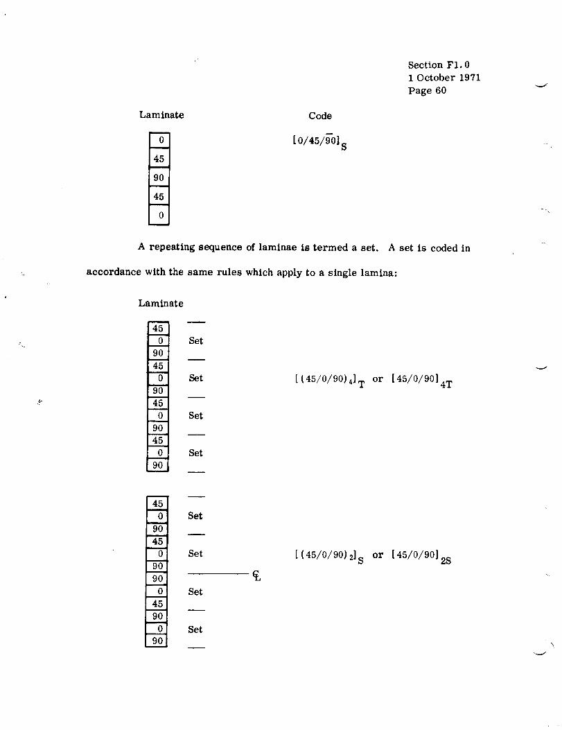
Section F1.0
1 October 1971
Page 60
Laminate
0m
45n
90
45
0m
Code
10/45/90] S
A repeating sequence of laminae is termed a set. A set is coded in
accordance with the same rules which apply to a single lamina:
Laminate
m
45u
0
9O
45u
0
9O
45
0
9O
45
0m
9O
m
Set
Set
Set
Set
[ (45/0/90)4]T or [45/0/9014T
=
01
901
01
901
Set
Set
Set
Set
[ (45/0/90) 2] S or [45/0/90]2S

Secti(m F1.0
1 October 1971
Page 61
1.4 COMPUTER PROGRAMS IN COMPOSITE ANALYSIS.
Several computer programs have been made available to MSFC and
support personnel to assist in analyzing composite material elements. These
programs have been I or are currently being) documented in Ileferences 4 and
5. The program names and a brief comment on each are sho_vn in Table
F1.4-1.

TABLE F1.4-1.
Section F1.0
1 October 1971
Page 62
Computer Programs in Composite Analysis
Program Name Comment
CDLAMA
GDLAMT
GREPPA
INTACT
LAMCHK
LAP
LAPI
MMBCK
PANBUCKII
STAB
Yield analysis of composite plates composed of
orthotropic lamina with in-plane loading. -
Yield analysis of composite plates composed of
orthotropic lamina with in-plane loading.
Design composite skin/stringer/frame compre.ssionpanel.
Locates optimum strength envelopes for laminates
under the action of combined loading.
Laminate check - computes margins of safety for
specified 0-deg, 90-deg, + 45-deg boron epoxy
laminates under combined loading.
Analysis of single overlap bonded joints with Metlbond329 adhesive mechanical behavior.
Analyzes single overlap bonded joints and accepts
arbitrary applied loads and incorporates the Bbasis correction factor.
Calculates the buckling loads of radially
inhomogeneous anisotropic, cylindrical shells
wherein the effects of boundary conditions are notconsidered.
Panel buckling -- calculates critical buckling loads
and mode for orthotropically layered, rectangular,
anisotropic plates and honeycomb sandwich panels.
Also computes local instability modes of failure for
composite panels.
Stability analysis -- local instability analysis of
orthotropic honeycomb panels, columns, and beams
-- failure-mode analysis for filament rupture,
intercell dimpling, and layer instability.

1.5 REFERENCES.
Section F1.0
1 October 1971
Page 63/64
.
.
.
.
.
Petit, P. H.: Basic Concepts in the Design and Stress Analysis of
Laminated Composites. I{el)ortNo. SMN 239, Lockheed-Georgia
Co., division of Lockheed Aircraft Corp. , Marietta, Ga. , March
19(;8.
Structural Design Guide for Advanced Composite Applications.
Advanced Composites Division, Air Force Materials Laboratory,
Air Force Systems Command, Wright-Patterson Air Force Base,
Ohio, August 1969.
Ashton, J. C. ; Halpin, J. C. ; and Petit, P. lt.: Primer on Composite
Materials: Analysis. Technomic Publishing Co. , Inc. , Stamford,
Conn. , 1969.
Structural Analysis Computer Utilization Manual. Analytical
Mechanics Division, Astronautics Laboratory, George C. Marshall
Space Flight Center (NASA).
Strength Analysis Computer Program Description Manual.
Mechanics Division, Astronautics Laboratory, George C.
Space Flight Center (NASA).
Analytical
Marshall

._J

SECTION F2
LAMINATED COMPOSITES


F2.0
TABLE OF CONTENTS
STRENGTtI OF LAMINATED COMPOSITES ..........
2. 1 Yield Strength ..........................
2. 1.1 Distortional l':ner_w Theory ............
2. 1. 2 Maximum Strain Criteria .............
2. 2 Ultimate Strength ........................
2. 3 lleferenees ............................
Page
1
3
4
6
11/12
13
F2-iii

F2. 0 STRENGTH OF LAMINATED COMPOSITES.
The strength of laztiaa_ed con_,posites must be related to the individual
lamina [i]. This is because it is easier to determine _here nonlinearity and
degradation begin to occur on a unidirectional test specimen than on some
general laminate test. For this reason the trend in determining the strength
of advanced composites is to establish strength allowables for the orthotropic
lamina and then to utilize analytical methods to predict the yield or the
ultimate strength of the laminate.


Section F2.0
1 October 1971
Page 3
2.i YIELD STRENGTH.
The available yield strength theories for laminated composites are at
best tentativeat this time [2]. Only a minimal amount of test data is
available to substantiate any of the yield theories for advanced composites.
Ifthe yield point is defined as the onset of inelasticaction, itis
apparent that the prediction ofthe yield strength of an orthotropic lamina is a
linear problem. Several yield theories of failure have been hypothesized for
anisotropic materials, of which two will be discussed (the distortionalenergy
theory and the maximum strain theory).
Before the discussion of yield theories, the basic difference between
the yield surfaces for an isotropic and for an orthotropic or anisotropic
material must be explained. For an isotropic material, any biaxial stress
state, crx, Cry, TXy , may be resolved into two principal stresses, _1 andP
and some angle, 0; therefore, a plot of the principal stresses that cause{Y2 'P
yield will give the required yield surface. The result is a two-dimensional
figure with al and a2 as axes. When considering the yield surface for anP P
orthotropic lamina, the stresses must be referred to the lamina principal axes;
therefore, for biaxial stress states three stress components may appear in the
yield criteria. The resulting yield surface will appear as a three-dimension_
figure with the directions of
(Fig. F2.1-1).
_rl, or2, and T12 as reference coordinates
_REcED|NG PAGE [;LANi( NOT F_ lip

o_
1"12
FIGURE F2. 1-1. THREE-
DIMENSIONAL YIELD SURFACE FOR
AN ORTHOTROPIC LAMINA
Section F2.0
1 October 1971
Page 4
2. 1.1 DISTORTIONAL ENERGY
THEORY.
Cira, Norris, and Hill
independently developed their
generalizations of the yon Mises
lsotropic distortional energy yield
criterion,
(_1 - _z)2+ (_ _ (_ 2 + (_3 - o'1)_
+ 6 (_121 + rl31 + Tsi 2) : 2or I (F2. 1-1)0 *
to account for the anisotropy of their
respective problems [3]. Hill was
concerned with the tendency of isotropic
metals to exhibit certain anlsotropic properties when undergoing meted working
involving severe strains. Hill claimed he had a physical interpretation of yon
Mises t "plastic potential," which allowed him to generalize yon Mises' yield
criterion for application to anisotropic metals. The plastic potential or yield
criterion has the form
2f (_iJ) = AI (cT2 - o3) = + A2 (_s - (_I) 2 + A3 (_I - o2) 2 + p..A4T2S=
+ 2._5"/'312 + 2AsT121 = I
(F2. 1-2)

where
Section F2.0
1 October 1971
Page 5
and
2f (a..) = the plastic potential,1j
2A 1 = (F2)-2 + (F3)-2 _ (FI)-2
2A 2 : (F3)-2+ (F1)-2_ (F2j-2
2A 3 : (F1)-2+ (F2)-2_ (F3)-2
2A 4 = (F23) -2 ,
2A s = (F31)-2 ,
2A 6 = (F12) -2
F 1, F2, and F 3 are determined from either uniaxial tension or compression
tests, and F12 , F23 , and F31 are determined from pure shear tests.
Tsai [2] adapted this criterion as a yield and failure criterion for
laminated composites. The failure criterion for a laminated composite is
based on the strengths of the individual orthotropie lamina referred to the
lamina principal axes since the yield strengths are established experimentally
with reference to these axes. The Hill criterion reduces to
2 2_ -- + T12y%y r %yCrly Cr2y
for an orthotropic material in plane stress. Note that
1 (F2. 1-3)
r(F2. 1-4)
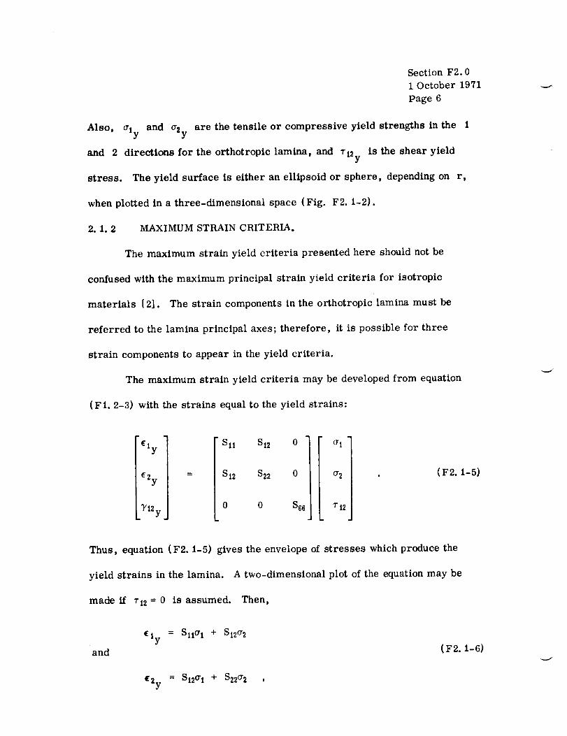
Section F2.01October 1971Page6
Also, and are the tensile or compressive yield strengths in thealy a2y
and 2 directions for the orthotropic lamina, and TI2 is the shear yieldY
stress. The yield surface is either an ellipsoid or sphere, depending on r,
when plotted in a three-dimensional space (Fig. F2. 1-2).
2. 1.2 MAXIMUM STRAIN CRITERIA.
The maximum strain yield criteria presented here should not be
confused with the maximum principal strain yield criteria for isotropic
materials [2]. The strain components in the orthotropic lamina must be
referred to the lamina principal axes; therefore, it is possible for three
strain components to appear in the yield criteria.
The maximum strain yield criteria may be developed from equation
(F1.2-3) with the strains equal to the yield strains:
E1Y
C2y
Y12y
S11 $12 0
S12 $22 0
0 0 S6e
0"1
o-2 . ( F2. 1-5)
T12
Thus, equation (F2.1-5) gives the envelope of stresses which produce the
yield strains in the lamina.
made if r12 = 0 is assumed.
A two-dimensional plot of the equation may be
Then,
and
ely Sll°rl + 8|2(_ 2
(F2. 1-6)
C2y = S|2o-I + $22o'2 ,

/
Section F2.0
1 October 1971
Page 7
o_/_J2 y
1.0
10o july
FIGURE F2.1-2. ItlLLYIELD SURFACE

or
Section F2.0
1 October 1971
Page 8
Si2 Si2cri
and (F2. 1-7)
$22 $22_2 •
Equations (F2. 1-7) are the equations of two lines in the _1 - _2 coordinate
system which define yield of an orthotropic lamina. After defining the yield
strengths as
Ely E11Crly = $II = CZy
and (F2. I-8)
_2y $2 2 _2y E22
equations (F2.1-7) may be put in a form similar to the Hillequation:
and
E1
c2 $12 $12Cr2y y C2y O'ly
C2y St1 _ly_2y C2y
(F2. 1-9)

Section F2.0
1 October 1971
Page 9/10
Equations (F2. 1-7) may be plotted on a _1 - _2 set of coordinates since it was
assumed that the shear stress component, T12, was zero. Such a plot might
appear as shown in Fig. F2. 1-3.
(J,
u = (}
i. Ol
FIGURE F2. 1-3. LAMINA YIELD SURFACE


Section F2.0
1 October 1971
Page 11/12
2. 2 ULTIMATE STRENGTH.
Until recently, attempts to predict the ultimate or rupture load for a
laminate were based on linear theory; that is, the laminate ultimate load was
based upon the assumption that the laminate stress-strain response is linear
to failure or that upon yield of a constituent lamina, some (or all) of the
lamina moduli are reduced to some arbitrarily small value or set equal to
zero. Recently, some computer programs have been written with relatively
simple techniques, and new methods that determine the ultimate stren_,_h of
laminates have been developed. These programs and methods are usually for
specialized laminates, and sufficient test data are not available at this time to
verify their accuracy for general use.


2.3 REFERENCES.
Section F2.0
1 October 1971
Page 13
i*
*
*
Ashton, J. C; Halpin, J. C. ; and Petit, P. H. : Primer on Composite
Materials: Analysis. Technomic Publishing Co., Inc. , Stamford,
Conn., 1969.
Petit, P. It. Basic Concepts in the Design and Stress Analysis of
Laminated Composites. Report No. SMN 239, Lockheed-Georgia
Co. , a division of Lockheed Aircraft Corp. , Marietta, Ga. , March
1968.
Kaminski, B. E. ; and Lantz, I/. B. : Strength Theories of Failure for
Anisotropic Materials. Composite Materials: Testing and Design.
Report STP 4(;0, American Society of Testing Materials, 1969.


SECTION G
ROTATINGMACHINERY

.......d
-.._4-
SECTIONGI.2
SOLID DISCS

".,--.4"

TABL£ OF CONTENTS
Gi. 2 SOLID DISKS.i
i. 2. i CONSTANT (UNIFORM) THICKNESS ...........
i. 2.2 VARIABLE THICKNESS ....................
1.2.3 EF_AMPLE PROBLEMS FOR ROTATING SOLID
CIRCULAR DISKS ........................
I. Example Problem I .....................
If. Example Problem 2 .....................
REFERENCES ......................................
Page
2
3
4
4
7
10
r GI. 2-iii

DEFINITIONOFSYMBOLS
Symbol
b
g
h (r)
r
P
r
%
Rim radius
Gravity constant
Disk thickness at location r
Distance from axis of revolution
PoissonTs ratio
Disk material density
Stress in radial direction;
positive denotes tension
Stress in tangential (hoop)
direction; positive denotes tension
Constant angular velocity, rad/sec
I
Gl. 2-iv "-_

SectionGi. 21 May, i97t
G1.2 SOLID DISKS.
In this section some of the methods of analyzing rotating circular disks
are presented. The disks rotate about an axis which is perpendicular to the
disk. Because the methods for a final analysis of turbomachinery-type
hardware are quite involved, only methods for preliminary analysis which
assume constant stress across the disk thickness are considered. Since the
methods are preliminary, no modes of failure will be discussed at this time.
The geometry, coordinates, and stresses for a rotating circular disk
are shown in Figure G1.2-1.
FIGURE Gi.2-i. CONFIGURATION OF SOLID CIRCULAR DISK

Section Gi. 2
i May, 197i
Page 2
i.2.i CONSTANT (UNIFORM) THICKNESS.
For solid circular disks rotating at a constant angular velocity with
uniform thicknesses and temperature fields, the radial and tangential
stresses (Ref. i) are
= _pv=) 13+_) (i-x _)r 8g
(1)
-\
and
(Dv2) (3+/_)It (l+3#a) x21a0 = 8g - 3+/a (2)
where
rx = - (3)
b
and
v =be0 . (4)
The maximum stress occurs at the center of the disk (r = 0) and is given by
(ao) max = ( at)max =IP v2)_3 ÷/a)
• (5)8g
H the disk is centrally clamped (Fig. Gi.2.i-i), the in-plane stresses
(Ref. 2) become

SectionG1.2I May 1971Page 3
f--
//
and
where
and
(i -_,) pW2a 2b 2_l= 8
(3 +,)pJh= S
7
r2_ ..._t._ _i,*3p_ r4|_2 3+/_ J
[((_+.)b_- (1+.) a_]1 + p) b2 + (1 p) a 2
(7)
(8)
(9)
for values of r greater than a.
f
FIGURE G1.2. I-I.
[CONFIGURATION OF DISK WITH FULLY CLAMPED HUB

Section Gi. 2
i May i97i
Page 4
For a solid disk with a uniform thickness and a varying temperature
field, the radial and tangential stresses are calculated using the procedure
given in Paragraph i .3.2 (Disks with a Hole at the Center -- Variable Thickness)
with the modifications described in Paragraph i .2.2.
i.2.2 VARIABLE THICKNESS.
For a solid circular disk rotating at a constant angular velocity with a
varying thickness or a varying temperature field, the radial and tangential
stresses (Ref. 3) are calculated using the procedure given in Paragraph i.3.2
(Disks with a Hole at the Center -- Variable Thickness) with the following
modifications:
i, Station point i should be chosen at 5 percent of the rim radius (b).
2. The initial value in column 33 should be i .0.
3. The stresses at the center of the disk (r = 0) are assumed equal
to the stresses at station point i.
i.2.3. EXAMPLE PROBLEMS FOR ROTATING SOLID CIRCULAR DISKS.
I. Example Problem i.
Find the radial and tangential stresses for the solid circular disk
shown in the following sketch.
I

Section Gi. 2
i May, 1971
Page 5
16 000 rpm
Q_)MATERIAL 6AI-4V TITANIUM
ROOM TEMPERATURE
Solution:
E = i6.0 x 106 Ib/in. 2
p = 0. i6 Ib/in.3.
/_= 0.3i3
g = 32.2 ft/sec 2= 386.4 in./sec 2 .
u)= 16 000 rpm = 266.7 r/sec = i675.52/sec .
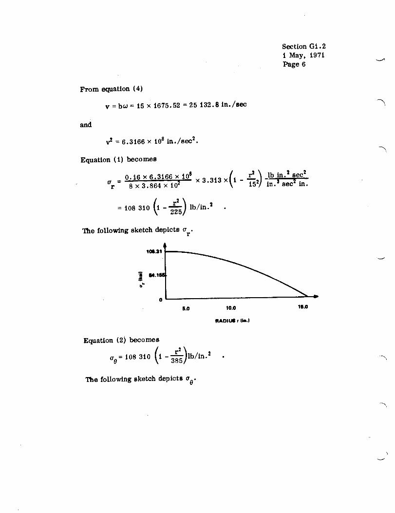
Section Gt. 2
1 May, 1971
Page 6
From equation (4)
v = bw = t5 × t675.52 = 25 132.8 ln./sec
and
v 2 = 6.3166 × 108 in./sec 2.
Equation (1) becomes
0. t6 x 6.3i66 × 10 se = • x 3.3t3 x
r 8x3.864 × 102 ( _552) lb in'2 sec2t - -In. s sec 2 in.
/h- lb/in.'= t08 3t0 k 225/
The following sketch depicts cr .r
1(_.31
v
6.0 I0.0 16.0
RADIUt r fin.)
Equation (2) becomes
108 r2_0 = 310 (1 - 3-_)lb/ln.
The following sketch depicts e 0.

Section G1.2
I May, 1971
Page 7
F"
100.31
64.16e
o I t 0=5.0 10.0 15.0
RACHUS r (in.)
II. Example Problem 2.
Find the radial and tangential stresses for the solid circular disk shown
in the following sketch.
MATERIAL 6AI-4V TITANIUM
ROOM TEMPERATURE
el------ 16 in.
/

Section Gi. 2
1 May, 1971
Page 8
J
Solution:
E = i6.0xl0 elb/in.2 .
p = 0.i61b/ln. $ .
= 0.3i3 .
g = 386.4 in./sec 2 .
o_ = 16 000 rpm
= t.675.52/sec.
The idealizationfor the finite-dlfference-typeanalysis is given in
the following sketch.
1076.62/m
1 2 _; 4 s
1_ 0.76
6.376---.-D
10.0
12.6
• 16.0 7-
NOTE: DIMENSIONS ARE IN INCHEE.
The computations for the finite-difference-typeanalysis are given in
Table Gi .2.3-i.

OF i:_O_ QUALirf Section G1.2
1 May, 1971
Page 9
Fg_
O
,,'.'4
o
O
o
u]
"4,...<
<
¢9
_9
(D
I
*,..4
I
¢,q
.Q
r_
_n
T
T
w
_c
,"3
+
-_i4-
7.
c_ = : :
_odddd
r_ _3
_d:" =" d d
d d _ d
o
-s s :_ :
:: - - •
:' - :: d d
d d d =: d
%
-" d d d

Section Gi. 2
i May, 1971
Page i0
Ii
o
a
REFERENCES
Timoshenko, S. : Strength of Materials, Part If. D. Van Nostrand and
Company, Inc., New York, i956, p. 2i8.
Eversman, W.; and Dodson, Jr., R. O. : Free Vibration of a Centrally
Clamped Spinning Circular Disk. AIAA Journal, vol. 7, no. i0, Oct.
1969, pp. 2010- 2012.
Manson, S. S. : Determination of Elastic Stresses in Gas-Turbine Disks.
NACA Report 87i, Cleveland, Ohio, Feb. 27, i947.
'\

TABLE OFCONTENTS
Gi.3 DISKS WITH A HOLE AT 1"HE CENTER ...............
1.3.1 CONSTANT (UNIFORM) THICKNESS ...........
1.3.2 VARIABLE THICKNESS ....................
1.3.3 EXAMPLE PROBLEMS FOR ROTATING CIRCULAR
DISKS WITH CENTER HOLES. ...............
I. Example Problem i ....................
II. Example Problem 2 ....................
REFERENCES .....................................
Pa ge
li
li
13
16
16
2O
24
G1.3-iii
Symbol
a
b
E
g
h (r)
n
r
T
C_
P
ffr
DEFINITIONOFSYMBOLS
Definition
Inner surface radius
Rim radius
Modulus of elasticity
Gravity constant
Disk thickness at location r.
Node (station) index
Distance from axis of revolution
Temperature (° F)
Coefficient of thermal expansion
Poisson's ratio
Disk material density
Stress in radial direction;
positive denotes tension
Stress in tangential (hoop) direction;
positive denotes tension
Constant angular velocity (rad/sec)
Gi. 3-iv

f
Section Gi. 3
i May, i971
Page 11
Gi.3 DISKS WITH A HOLE AT THE CENTER.
In this section some of the methods of analyzing rotating circular disks
with circular cutouts at the center are presented. The disks rotate about an
axis which is perpendicular to the disk. Because the methods for a final
analysis of turbomarchinery-type hardware are quite involved, only methods
for preliminary analysis which assume constant stress, or linearly varying
stress, across the disk thickness are considered. Since the methods are
preliminary, no modes of failure will be discussed at this time.
The geometry, coordinates, and stresses for a rotating circular disk
are shown in Figure GI.3-i.
i.3.i CONSTANT (UNIFORM) THICKNESS.
For circular disks with a center hole that rotate at a constant
angular velocity with uniform thickness and temperature fields, the radial and
tangential stresses (Ref. 1) are
r 8g (1)
and
whe re
= (P_V2)(3 +_)(1 +y2- (t +3u)x2 + x_- ) (2)_0 8g 3 + ]a
a (3)2/ b '
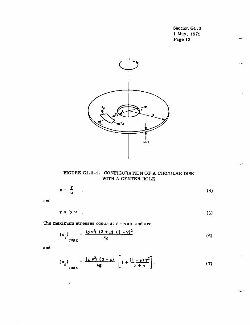
Section GI. 3
I May, 1971
Page 12
and
FIGURE GI. 3-I.
r
b '
CONFIGURATION OF A CIRCULAR DISK
WITH A CENTER HOLE
(4)
v= boo .
The maximum stresses occur at r = _aab
(or 2) (3+/z) (I-7} 2(_) =
r 8gmax
and
and are
(_e) = (ov_ (3+/_) Ii+(f-u)'v21max 4g 3 +/_ "
(5)
(6)
(7)
r/
Section GI. 3
i May. 1971
Page 13
The stresses may be determined by the computer pr(_gram documented in
a NASA technical note. 1
For a disk with a uniform thickness and a varying temperature field,
the radial and tangential stresses are calculated using the procedure given in
Paragraph 1.3.2.
1.3.2 VARIABLE THICKNESS.
The stresses in a circular disk with a center hole and a variable
thickness or a variable temperature fieldmay be determined using a finite-
difference method (Ref. 2) . This method considers the point-to-point
variation in thickness, temperature, and material properties. The
computations are easily executed in a tabular format.
An idealizationof the disk is made (Fig. GI.3.2-I) by selecting
stations along the radius. Station i lies on the inner surface, and stationN
lies on the outer (rim) surface.
Intermediate stations should be located at distances of 1, 2, 3, and 5
percent of the rim diameter from the inside boundary and at locations of
thickness, temperature, or material property variations. The radius at each
Byron Foster and Jerrell Thomas: Automated Shell Theory for Rotating
Structures (ASTROS). NASA TN-D-, Marshall Space Flight Center, to be
published.

Section Gi. 3
i May, i97i
Page i4
1 2 3 ..- N
FIGURE Gi.3.2-i. IDEALIZATION OF DISK FOR
FINITE-DIFFERENCE ANALYSIS
station is entered in column i (Table Gi.3.2-i). In column 2 the idealized
thickness is entered. Ifa sharp discontinuity in thickness occurs, such as an
abrupt flange, the thickness should be faired in the disk contour, and the
faired disk used in determining the thickness. The mass density (corrected
ifin a faired section) multiplied by the square of the rotational speed is entered
in column 3. 1_oisson's ratio and the modulus of elasticityare entered in
columns 4 and 5, respectively. The coefficientof thermal expansion, which
must be an average value applicable to the range between the temperature
actually existing and the temperatures at which there is no thermal stress, is
entered in column 6. The difference between the actual temperature and the
temperature at which there is no thermal stress is entered in column 7.
The manipulations required in columns 8 through 34 are shown in the

_.,i:__¸" ..... Section GI. 3
i May, i97i
Page i5
O
t_
<(D
_J
!aJ
o_
Io,1
¢9
q
"7
+
T
×
y
/
i
_2
_J
"I
e
%

Section G1.3
i May, 1971
Page i6
respective columns. Columns 33 and 34 are calculated simultaneously, with
column 33 having an initial value of 0.000 and column 34 having an initial value
of 1.000. Columns 35 and 36 are also calculated simultaneously, but each has
an initial-value of 0.000.
In column 37, the term _ denotes the blade loading at the rim andr,b
is obtained by dividing the total centrifugal force at the roots of the blades by
the total rim peripheral area.
The radial stress, _r' at each station is calculated in column 38. The
tangential stress, cre, at each station is calculated in column 39.
In using the finite-difference method, the accuracy of the results
increases as the number of station points increases. The stresses may also
be determined by the computer program already cited. _
i.3.3 EXAMPLE PROBLEMS FOR ROTATING CIRCULAR DISKS
WITH CENTER HOLES
I. Example Problem i.
Find the radial and tangential stresses for the following circular disk:
2. Ibid.

Section Gi. 3
t May, i971
Page 17
Solution:
MATERIAL 6AI-4V TITANIUM
ROOM TEMPERATURE
0.26 in.
E = i6.0× 106 psi,
p = 0.i6 Ib/in. 3,
= 0.313,
g = 386.4 in./sec 2,
w = 16 000 rpm = 1675.52/sec,
2T - 15 - 0.t333,
and
v = 15 × i675.52 in./sec = 25 132.8 in./see.
v2= 6.3167 × 10⁸ in2/sec2 .

Section GI. 3
I May, 1971
Page 18
Equation (I) becomes
( 0.16x 6.3167x 10s)(3.0 + 0.313) (I
_y =
r 2 4. 005+ O. 1333 z - 225 - r-T--/
r 3091.2
= 1.0832x 10 s (1.0178-0,00444r2-_ "Q_)
The following sketch depicts a .r
psi.
psi
2.6 5.0 7.5 10.0 12.5 15.0
RADIUS r (in.)
Equation (2) becomes
a 0= t.0832 x 105. /l +0.13332-I + 0.939_
(3 + 0.313) 225psi.
/
= 1.0832 x 10⁵ _1.0t78-0.00444 r2I
The following sketch depicts a0 .
4. 005psi.
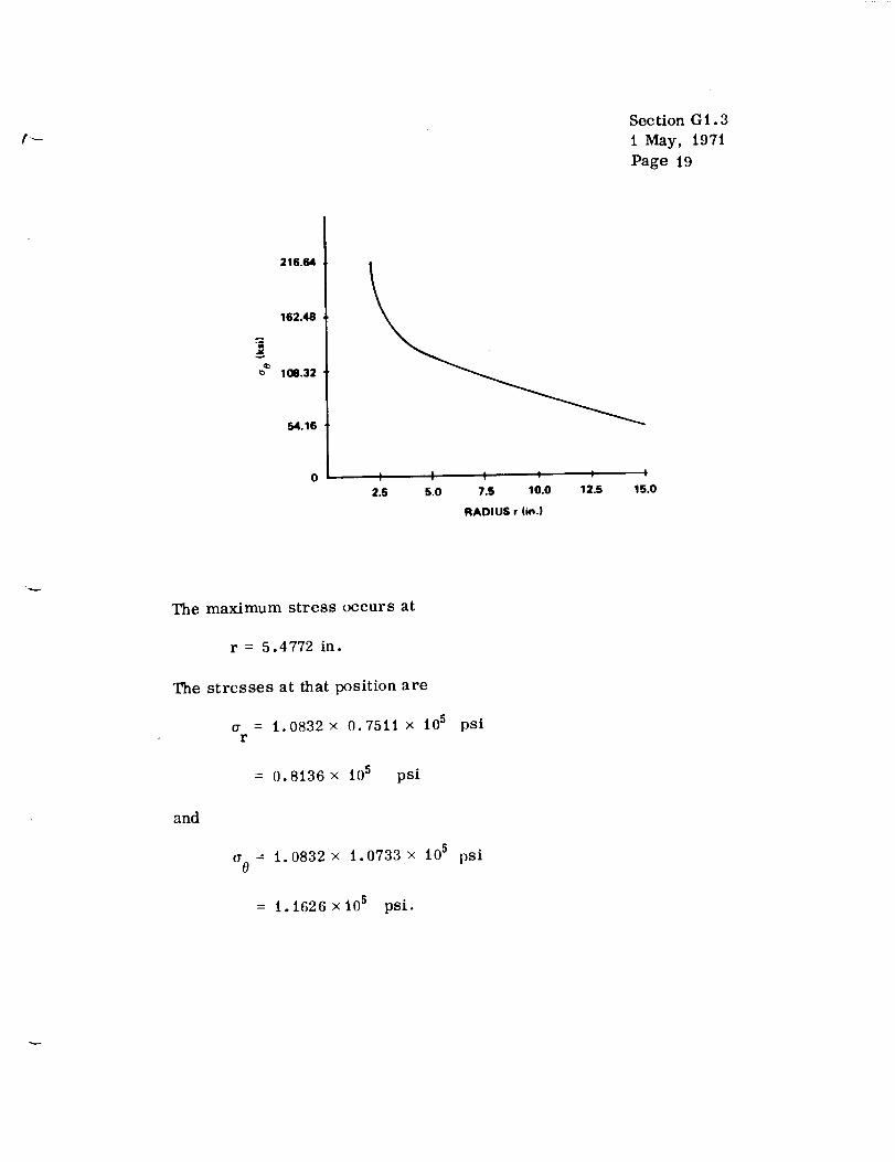
Section G1.3
1 May, 1971
Page i9
216.64
162.48
108.32
54.16
2.5 5.0 7.5 10.0 12.5 15.0
RADIUS r (in.)
The maximum stress occurs at
r = 5.4772 in.
The stresses at that position are
= 1.0832× 0.7511 × l0 sr
= 0.8136x 10⁵ psi
and
= 1.0832x 1.0733 × 105
= i.1626xi05 psi.
psi
psi

SectionGi. 3
i May, 197i
Page 20
If. Example Problem 2.
Find the radial and tangentialstresses for the following circular disk.
Solution:
E=
la_w
0.25 in.
i6.0 x i06 psi.
p = O.i61b/in.S
/_= 0.313.
g = 386.4 in./secz.
co= 16 000 rprn = 1675.52/sec.

Section Gl. 3
1 May, 1971
Page 2 i
The idealization for the finite-difference-type analysis is given in the
following sketch.
123 6 8 9 b
[' ..... ' I
lip_--2.3--_ ii•-- 2.45_ Iel.---.- 2.75
" 5.0: 5.5
10.0i-" 12.5_-" 15.0
NOTE: DiMENSiONS ARE iN iNCHES
The computations for the finite-difference-type analysis are given in
Table G1,3.3-i.

N
t0=4C)
nn
.o,jJ
t_
°l=d
I
•Jq
I
,==.
q=4
÷
×
x
v
N
A
× .=
I
0
X _
v
I;I
oooo,,°o°
×
• o • • , • o • • o
o•ooo•ooo°
• • • , • o • o • o
oo•°o,o,oo
Section Gi.3
i May, 1971
Page 22
(oZ©co
I
,,P-I
rO¢)
,--,,4
.D
T
t
_ _ _ _ _ _ _ _ "_ _ _
"7×
"7×
x
___
+
× ×
x ×
' _ _ _ _ _ _ _
_ _ N N N N N N N N
÷ _
_4_j'_
Section G1.3
t May, 1971
Page 23
× _
b
"7
x +
××
m
" "7m
××
m
i
_ _ _ _ _ _ '_ _ _ _
• _ _ _ _ ,_ • . .
_ E _ E _ E £ 4 4 E
_, _ _ _ _ _ _ _ _ _
_ _ _ _ _ _ _ _, _
, _ _ _ _..._ _ _ = =

Section G1.3
I May, i97i
Page 24
REFERENCES
I. Timoshenko, S. : Strength of Materials, l_art II. D. Van Nostrand
Company, Inc., New York, 1956.
2. Manson, S. S. : Determination of Elastic Stresses in Gas-Turbine Disks.
NACA Report 871, Cleveland, Ohio, Feb. 27, 1947.
v

SECTION HI
STATISTICAL METHOD S

j _a
f
r
Hi
TABI,E OF CONTENTS
STA TISTICA L ME THODS ...........................
i.t INTRODUCTION .............................
1.2 METHODS FOR MEASURING PERFORMANCE
O F A MA'rEI',IA L ............................
1.2.1 Normal Probability Curve ................. 3
i.2.i.3
i.2.1.4
i.2.i.5
i.2.1.6
1.2.i.7
1.2.1.8
i.2.1.9
i.2.i.iO
Properties .................... 3
Estimate of Average
Performance ................... 4
Example Problem i .............. 4
Estimate of Standard Deviation ....... 5
Confidence Interval Estimate ........ 5
Example Problem 2 .............. 5
Example Problem 3 .............. 6
Estimating Variability
Example Problem ................ 8Number of Measurements
Required ...................... 11
Tolerance Limits ................ 13
1.2.2 Log-Normal Probability Curve .............. 16
1.2.2.1
i.2.2.2
1.2.2.3
1.2.2.4
1.2.2.5
1.2.2.6
1.2.2.7
Properties .................... i6
Estimate of Average Performance ..... 17
Example Problem 4 .............. 17Estimate of Standard Deviation ....... 17
Interval Estimates ................ i8
Example Problem 5 ............... 21
Example Problem 6 ............... 2i
i.3 REFERENCES ............................... 23
Page
1
1
Hi-ill
Jalq_CE_lltG PAGE BLANK NOT Ffl.MED

Figure
Hi-i.
Hi -2.
Hi-3.
Hi-4.
Hi-5.
Hi--6.
_Hi- .
HI-8.
Hi-9.
LIST OF ILLUSTRATIONS
Title P_go
HISTOGRAM ............................. 2
DISTRIBU TION FUNC TION FRO M
"FAIRED"HISTOGRAM ...................... 2
NORMAL (GAUSSIAN) DISTRIBUTION
CURVE ................................ 3
PARAMETERS AND PERFORMANCE
GUIDES FOR NORMAL DISTRIBUTION ........... 3
NUMBER OF DEGREES OF FREEDOM
REQUIRED TO ESTIMATE THE STANDARD
DEVIATE)N WITHIN P PERCENT OF ITS
TRUE VALUE WITH CONFIDENCE
COEFFICIENT y ......................... 13
FACTOR FOR DETERMINING DATA
POINT RANGE ........................... 19
PROBABILITY FACTOR kpT FOR T = 0.95 ...... i9
PROBABILITY FACTOR kp,/ FOR "y : 0.90 ...... 20
PROBABILITY FACTOR kpy FOR 7 - 0.50 ...... 20
Hi-iv

Table
Hi-1.
Hi -2.
HI-3.
LIST OF TABLES
Ti fie Page
Ultimate Strength of Product "A" ................ 4
Percentiles of the "t" Distribution ............... 7
Factors for Computing Two-sided ConfidenceLimits for a ............................. 9
H1-4. Factors for One-sided Tolerance Limits
for Normal Distributions ..................... 14
Hi -5. Fatigue Life of Product "B" ................... t7
Hi-v
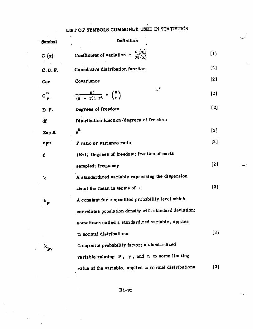
.Symbol
c (x)
C.D.F.
Coy
nC
r
D.F.
df
Exp X
. _fF I!
f
k
kp
LIBT OF SYMBOLS COMMONLY USED IN STATISTICS
Definition
Coefficient of variation =M(x)
Cumulative distribution function
Covariance
(n - r) _. r:
Degrees of freedom
Distribution function/degrees of freedom
Ke
F r_Uo or variance ratio
(N-l) Degrees of freedom; fraction of parts
sampled; frequency
A standardized variable expressing the dispersion
about the mean In terms of o
A constant for a specified probability level which
correlates population density with standard deviation;
sometimes called a standardized variable, applies
to normal distributions
Composite probability factor; a standardized
variable relating P, 7, and n to some limiting
value of the variable, applied to normal distributions
ill
[2l
[2]
[21
[2J
[21
[21
[2]
[3]
[3]
[3]
Hi -vt

f
M.G,F.
Me
m
N
N@
N 1
Npy
lqg
I
NU
N 4
_4
LIST OF SYMBOLS COMMONLY USED IN STATISTICS (Continued)
Defin[ lion
The mean of a stochastic variable x
Moment generating function
Mode
Population mean
Sample size [ 2] ; number of loading cycles to
failure [ 3]
An arbitrary lifetime to which fatigue test data
are to be extrapolated
Same relationship to N as x l has to x
Lower limiting life above which any test value
can be expected to fall with a probability of P
and a confidence of ,/
Arithmetic mean of test sample lives
Arithmetic mean lifo that could be expected if
, an infinite number of samples could be tested
Number of loading cycles at which weakest of
four specimens fails
Arithmetic mean of least-of-four test sample
lives
[ll
[2]
[21
[ 4]
[3]
L3]
[31
[31
[3]
[3l
[3l
Hi -vii

LIST OF SYMBOLSCOMMONLYUSEDIN STATISTICS (Cofitinued)
Symbol
n
n t.
n 4
(;)P
P (x)
P4
R. M.S.,
r
S
Sa
SD
Se
Definition
Number of independent single test specimens
Factorial n = i x 2 × ... x (n-I)xn
Number of least-of-four test points
(:) n'.C = (n-r) 1.r'.
Probability; the percent of a group of specimens
expected to fallwithin a certain range
Probability of an event x occurring
Probability of four consecutive testvalues
exceeding some specified limiting value
Root mean square
Correlation coefficient
Loading stress level at which failure occurs at
some number of cycles (N) in fatiguework
A value of stress on the estimated average
S-N curve corresponding to some arbitrary test
point life,N.l
Standard deviation of a sample
A value of stress on the estimated average
S-N curve ccrresponding to the lifetime (Ne) to
which fatiguedata are to be extrapolated
[3]
[21
[3]
[2]
[3]
[2]
[3]
[2]
[2]
[3]
[3l
[2]
[31
Hi-viii
I,[S'I'()F SYMB()[,S COMMONLY USEI) IN STATISTICS {Continued)
S3:ml)ol 1)c/'i n t tl on
S.
1An at'l)itral'y value of stt'ess occul'J'ing in a
l)a.t'tictflat • pt'oblen_ at lifetime N.l
S.
112
A derived stress value at lifetime (N)(2
COl't'esl)oll([ing to an ol)sct'vcd stress va.luo
S. at lifetime N.1 1
SS
8 2
U
Stan(lavd (2vvov of the stan(lat'd deviation
Va_'iance ()f :t samp[(2
Stu(lent's "t" statistic
Stanclar(li ze(I v:u'iablex -
o
V
W
X
£
X°
1
xP
Xpy
Coeftici(2nt of variation
Often used for l"ange
A random statistical variable
Arithmetic mean of x-values vcgav(lless of the
numl)er of values involved
Any arbitrary value o[ x oc,curl'ing in a sl)ecifi(2d
17roble m
A variable expressed as a function of P and o-
A limiting value of x dependent on p, Y , n, and _:
[:;1
[:_]
[2]
tel
[2]
[1]
[2]
[2]
[a]
[n]
[.-,]
[ ._,1
Hl-ix

LIST OF SYMBOLS COMMONLY USED IN STA TIS'FlCS (Continued)
Symbol
X
S
U
Y
,f
Ot
otPi
ot1,
1,
¢y
Defini tion
Arithmetic mean of values from a limited sample size
Arithmetic mean that could be expected from an
infinite number of specimens
Frequency of occurrence of test points in given
intervals of the variable _Ax!
Percentage frequency; percentage of total
number of test points in a given variable increment
t_ risk, Type I error
Limiting value of standardized variable for a
given probability and an unknown distribution
Limiting value of standardized variation of the
mean for a given confidence and an unknown
distribution
B risk, Type II error; also equals I1 - a)
Confidence; the percentage of sample mean
values falling within a given range of the universe mean
[3]; associated with the tolerance limit tables [2]
Population mean
Mean of a stochastic variable x = M{x}
Standard deviation of variable x about ,_
13]
[31
131
131
tin1
131
13l
12]
[21
[11
[31
Hi-x
LIST OF SYMBOLS COMMONLY USED IN STATISTICS (Concluded)
Symbol
oc
_4
uS
LrU
OU 4
(3_
X
(5 4
o2
)(2
Defini tion
Standard deviation of a limited number of
derived stress points about Se
Standard error of least-of-four mean (N4)
Standard error of the standard deviation [2] ;
standard deviation computed from a limited
sample size [3]
Unbiased standard deviation of the universe;
corresponds to an infinite sample size
Standard deviation of universe of least-of-
four points
Standard deviation of x , about x ; sometimesS U
called the standard errol of the mean
Standard deviation of least-of-four test
failure points
Variance of a population
Chi-square
[31
[3]
[31
tel
[2J
Hi-xi
Alternative IIypothcsis
AOQL (Average Outgoing
Quality Limit)
A Posteriori Probability
A Priori Probability
LIST OF DEFINITIONS COMMON IN t'SI':I) IN: STATISTI('S
I)cfinition
Possible true alternate answer to the hyl)othe-
sis I×,ing statistically tested. The larger the
sample size, the greater the I)ossibility of
rejecting a hypothesis when an alternate answe_
is true [2J.
UPl)er limit on outgoing quality th:tt may bc
CXl)ect(:d in the long run, when all rejected
lots are subjected to 100 percent insl)ection,
with all defective articles removed and
replaced by good articles [ 2].
If in a number of trials an event has occurred
N times and failed M times, the probability
Nof its occurring in the next trial is
M + N
[2].
Let N bc the number of exhaustive, mutually
exclusive, and equally likely cases of an event
under a given set of conditions. If M of these
cases are known as the event A, then the
mathematical, or a priori probability of event
Hi -xii

f
LIST OF DEFINITIONS COMMONLY USED IN STATISTICS (Continued)
AQL (Acceptable Quality
Level
Biased Sample
Class Interval
Confidence Intervals
Definitions
A occurring under the given set of conditions
is M/N [2].
Percentage of defective items in an inspection
lot that a sampling plan will accept with (in
the usual case) an associated _ Risk of 0.05
[2].
If some individuals in the Universe are more
likelyto be chosen than others, the sample
is said to be biased.
When the number of observations is large,
the range of the data can be broken into a
limited number of segments of equal length.
The segments are lmown as class intervals or
cells [ 2] .
This provides a method of stating how close an
estimate is to the true value [ 2]. It is the
interval associated with a prescribed confi-
dence coefficient. The confidence coefficient
is the proportion of samples of size n for
Hl-xiii

LIST OF DEFINITIONS COMMONLY USED IN STATISTICS (Co_Unued)
Continuous Distribution
Cumulative Distribution
Curve Fitting
Degree of Freedom
Discrete Distribution
Definition
which intervals computed by the prescribed
metht)ds may be expected to bracket a value [ 4].
One in whtch tim only limit to si_._ tatervsls
measured is the oensltivity of the measuring
apparatus [ 2].
Indicates by its magnitude the proportion of
the Univeroe (or sample) to the Left of that.
point [Zl.
Method utilizing computed statistics as spprox*
imate parameters for theoretical distributions
[21.
Number of free variables (unrestricted and
independent in the sense of random sampling)
entering into a statistic. In the case of a
sample of size N, from a UniverN, there
are N°! degrees of freedom [ 2].
If a random variable has only a finite amber
of possible values, then it will form a discretB
distribution [ 2].
H i-xiv

f-
LIST OF DEFINITIONS COMMONLY USED IN STATISTICS (Continued)
Definition
Double Sampling Involves the possibility of putting off the
disposition of an inspection lot until a second
test sample is taken. A lot will be accepted
on the basis of the first sample if the results
are very good or will be rejected if the results
are very poor. If the results from the first
sample are of a borderline nature (between
,: good and poor}, a second sample must be
taken.
On the basis of the results of the combined
first and second samples, the lot is either
accepted or rejected [2].
Error In statistics there are two types of error. If
we reject the null hypothesis when it is true,
then we make an Error of the First Kind. If
we fail to reject a null hypothesis when it is
false, then we make an Error of the Second
Kind [ 4].
"F" Distribution Sampling distribution of the variance [ 2].
H l -xv

LIST OF DEFINITIDNB COMMONLY USED IN STATISTICS (Continued)
Definition
Frequency Table _ Tabulation of the number of observations that
Histogram
Hypothesis '
Inference
Latin Square
Least Squares
occur in each class interval of a histogram [ 2].
Block representation of data arranged to show the
dispersion of the data [ 2].
Statement formulated in such a way that it may be
refuted through statistics.
Based on the theory of probability, statistical
inference is that mathematical framework which
supplies a technique for description, prediction,
and rational design decisions despite the compli-
cations which arise because of variation [ 2].
"Analysis of Variance" ordering technique of
observed values in an experiment, allowing control
of several sources of variability [ 2].
Method based upon the principle that the best value
of a quantity that can be deduced from a set of
measurements or observations is that for which
the sum of the squares of the deviations of the
observations (from it) is a minimum [ 2].
\
Ht-xvi

r
Lot
LTPD (Lot Tolerance
Percent Defective)
Mean
Mean Deviation
Median
Midrange
Mode
LIST OF I)EFINITIONS COMMONLY USED IN STATISTICS (Continued)
Definition
Group of manufactured articles which are essentially
alike, such as 1 day's production [2].
Usually refers to the incoming quality, above which
there is a small chance that a lot will be accepted.
It is usually taken with a consumer's l"isk of
= 0.1012].
The arithmetic average of a gl'ouv of observations
[2]. It is the location parameter o[ ,tnormal
distributionlocating the "centel"of _1'avity"of the
distribution[4].
Arithmetic mean of the absolute distance of each
observation from tilemean [2].
Middle value of a group of obscl'vations. In the case
of an even numbered set of obsel'vations, itis tile
aver_tge of the middle pair [2].
Arithmetic average of the extreme values of a set
of observations [2].
Most frequent value of a set of obserwltions [2].
Hl-xvii

LIST OF DFFINITIONS COMMONIN USI,:D IN STATISTICS (Continued)
Definition
Moments In statistics, moments arc analogous to moments
' in mechanics in several ways. Just as some
Nonparametrte Statistics
Normal (GaussianJ
Curve
ix_dies are completely characterized by their
moments, some probability distributions are
completely characterized by their moments. The
first moment about the origin is equivalent to the
expected value (the mean) of the random variable.
The first moment is also the center of gravity
of the probability mass. The second moment
above the mean is also known as the moment of
inertia and variance [2].
Statistical techniques developed to test hypotheses
without the assumption of normality, or any other
assumption, other than that of continuity of a
distribution [ 2].
Bell-shaped curve from the Gaussian probability
distribution. It is a two parameter distribution
requiring the mean and the variance for its
description [ 2].
Hi-xviii

OC Curves (Operating
Characteristics Cmwes)
Population
LIST OF DEFINITIONS COMMONLY USED IN STATISTICS (Continued)
Definition
Normal Probability Paper Special graph paper which reduces the
cumtflativenormal curve to a straight line.
The log-normal probability paper does the
same with log values as the normal paper
does with linear values [2].
Give the chance of accepting a hypothesis [2].
Proof
Random Digits
Randomization
Any set of individuals (or objects) having
some common observable characteristic. It
is synonymous with Universe [2].
Differs from mathematical proof as itdoes
not fallwithin the framework mathematics,
but results from experimentation, with an
accompanying probability statement [2].
Digits picked in such a way that each digithas
an equal chance of occurring at any time [2].
Assignment of a sequence of operations to a
test program by the use of some technique,
such as random tables, to avoid bias in the
test results [2].
Hi -xix

LIST OF DEFINITIONS COMMONLY USEI) IN STATISTICS (Continued)
Random Sample
Range
Root Mean Square
Sample
Sampling Distribution
Sequential Samplings
Significance Level
Definition
Picked in such a way that all members of
the population have an equal chance of
sclcctioa [ 2].
Absolut_ difference Ix_tween the extreme
values of a set of observations [2].
Square root of the average of the sum of the
squares of a set of observations [ 2].
X.• l
R MS :
Set of observations chosen from a population
[2].
Distribution of a statistic in the set of all
samples of a specific size from a given
Universe [2].
Acceptance plans permitting from three, up
to an unlimited number of samples [ 2].
This expresses our reluctance to give up
or "reject" the null hypothesis and is given
by the magnitude of the _ Risk. The
Hi-xx

f_
LIST OF DEFINITIONS COMMONLY USED IN STATISTICS (Continued)
Single Samphng
Standard Deviation
Statistic
Stochastic Variable
"t"Distribution
Tolerance Limits
Unbiased Estimate
Definition
smaller the magnitude of significance the less
we are willing to reject the null hypothesis [ 4].
When the decision as to the disposition of an
inspection lot is always made on the evidence
of only one sample, the acceptance plan is
described as a single sampling plan [ 2].
Positive square root of the variance [ 2].
Estimation of a population parameter, computed
entirely from a sample [ 2].
In general, any variable which may have a
probability function is a chance or stochastic
variable, even though the frequency function
is not knmvn [2].
Sampling distribution of the mean [ 2].
Limits such that a certain portion of the
population shall lie within or above them with
a specified probability [ 2].
Estimate o[ a parameter which has been
corrected l or sample size effects and is
equivalent to the total population parameter [ 3].
H i-xxi
lIST OF DEFINITIONS COMMONLY USED IN STATISTICS (Concluded)
Universe
Variables Sampling
Variance
a Error
/_ Error
Definition
Comprised of any set of individualshaving
some common observable characteristic [2].
When a record is made of an actual measured
quality characteristic, such as a dimension
expressed in thousandths of an inch, itis
known as variables sampling [2].
Sum of the squares of the deviations from the
mean divided by the number of observations
less than one [2].
Risk of rejecting a true hypothesis. This is
also known as an a Risk, Consumer's Risk,
or Type I [2].
Risk of accepting a false hypothesis. This
is also known as #3 risk, Prodttcerts
Risk, or Type IIError [2]. Equals
(1 -a) .
HI -xxii

f Section II1
I May J 972
Ill STA TIST] CA L ME TItODS
f-1.1 1NTI/OI)UC TION
"One of the main objectives of statistics is to give a mathematical
description of observed data in such a maturer that the observed phenomena
and the method of observation are characterized by a few numbers" [ 1].
\Vhile a single observation cannot be reproduced, experience has shown that
a set of obscrwltions, resulting from the repetition of some process, produces
certain characteristic features which can be reproduced; and it is these
characteristic fetttures that statistics attempt to describe.
Various methods of describing characteristic features h_tve been
developed, and one method includes the use of a histogram. Consider a
hypothetical set of recorded test values as being laid off in ascending order
of magnitude along a horizontal axis to form the abscissa of a graph. Now
let the range of values be divided into equal intervals and a count m_tde of the
number of test points in each interval. The number of points per interval is
known as the frequency. If the various frequencies are now laid eli on a
overtical scale, a histogTam is produced (Fig. ltl-1). From the histogram
a h'equency distribution curve may be obtained by fairing a smooth line
through the shape of the histogram (Fig. tI1-2). Several frequency distribution
curves (Normal, ling-Normal, )¢_, "t", Weibuli) have been est:dflished,
but only two (Normal and Log-Normal) will be discussed here.

Section I11
1 May 1 !)7"2
I k l go: 2
).
WtatDOtutrL
MEASURED VALUE
I"IGUI{E Ill-1. IIISTO(;IUkM.
MEASURED VALUE
FIGUI{E 11l-2 I)ISTItlI_UTI()N I,'UNCTI()N I.'I{()M "I:AII_.FI)" II1ST()GRAM
The statistical melhod_ discussed will be limited to those methods
necessary for evaluating material, fatigue, and fracture mechanics data. It
has been found that material data obey normal dJ:_tribution and that fatigue [ 31
and fracture [ 5] data obey log-normal distributions.
__
Suction H1
1 May 1!)72
I>:tge ;I
1.2 ,_II':TII()I)S FOIl _II.:A,S['I_IN(; t_I.:III.'()IIMANCI.; ()I," ,k _IA'I'I,]IIL\I,
1.2.1 Normal I>rol)ability Curve
1.2.1.1 Prol)ovties
The nornutl, or (;aussi:m, curve is a t\vo-lmr:tmctcv curve (l,'i_,. I11-32.
It is (IoI'incd by tho mean \\hich h)czttcs the curxc anti the <lcxi:ttion \vhich
defines the sln'cad of the curve.
one. The relation of the mean
significance level (o:)
The at'ca under the cttJ'vc is :t[\v:tyb equal to
(p) , the stan(t',tL'd <lcviation (tr) , ;in(I the
is shown in Fig. 111-4.
VARIATION OF
o o I I-3o -2o -o o 20 30
FIGURE lIl-:l. NOIIMAI_ (GAUSSIAN) I)ISTI{II'I;TI()N CUIIVI.].
It
VARIATION OF _ I_ STANDARD ERROR OF THE MEAN
POPU LAT ION _ _<k-%-x_--,_ _
._"_'_._'x._._"_'__'_'_. / V ARIATION OF THE
EVIATION
I t I I I I I 4
-3o -20 -o o 20 72.5 PERCENT OF AREA FOR a = 0.05
2.5 PERCENT OF AREA FOR o_,, 0.05
LEVEL OF SIGNIFICANCE a- 0.05
FIGURE Itl-4. PAIC\3[ETI.:I{S AND t)I.:III.'C)IIMANCI.: GUII)I.:%
FOIl NOII_L\ l. I)ISTI'dI'UTION.

Section II1
1 May 1972
Page 4
1.2.1.2 Estimate of Average Performance
The most common and ordinarily the Imst single estimate of the 1)o;,:- -
lation mean, m , is simply tile arithmetic mean of the measurements.
n
nl i=_l xi "m _ x = -
1.2.1.3 E_mmple Problem 1
Determine the mean value of the ultimate streng'th of product "A"
havhlg the test results in Table H 1-1 [ 3].
1
n
Table HI-1. Ultimate Strength of Product "A"
Test Specimen
1
2
3
4
5
6
7
8
9
10
Ultimate Strength
x. (lb)t
578
572
570
568
572
570
570
572
596
584
n = 10 _ x i = 57522
n
VX° _"
l
1.---: (5752) = 575.2 lb = t'tlean value

Section HI
I May 1972
Page 5
level. Confidence levels y commonly used are 99 percent and 95 percent
which correspond to a = 0.01 and c_ = 0.05.
1.2.1.6 Example Problem 2
Using the data in Table Hi-i, what is the two-sided 100 (1 - c_)
percent confidence interval for the true mean m of the total population [ 4] ?
1.2.1.4 Estimate of Standard Deviation
The estimate of the standard deviation is usually taken as the square
root of the best unbiased estimate of variance [ 4].
x. - x ii l
a _ s = (2)n(n - 1)
1.2.1.5 Confidence Interval Estimate
When we take a sample from a lot or a population, the sample average
will seldom be exactly the same as the lot or population average. We do hope
that it is fairly close, and we would like to state an interval which we are
confident will bracket the lot mean. If our intervals included the true average
95 percent of the time, we would be operating at a 95 percent confidence
level, and our intervals would be called 95 percent confidence intervals. In
general, if in the long run we expect 100 (1 - a) percent of our intervals to
contain the true value, we are operating at the 100 (1 - a) percent confidence
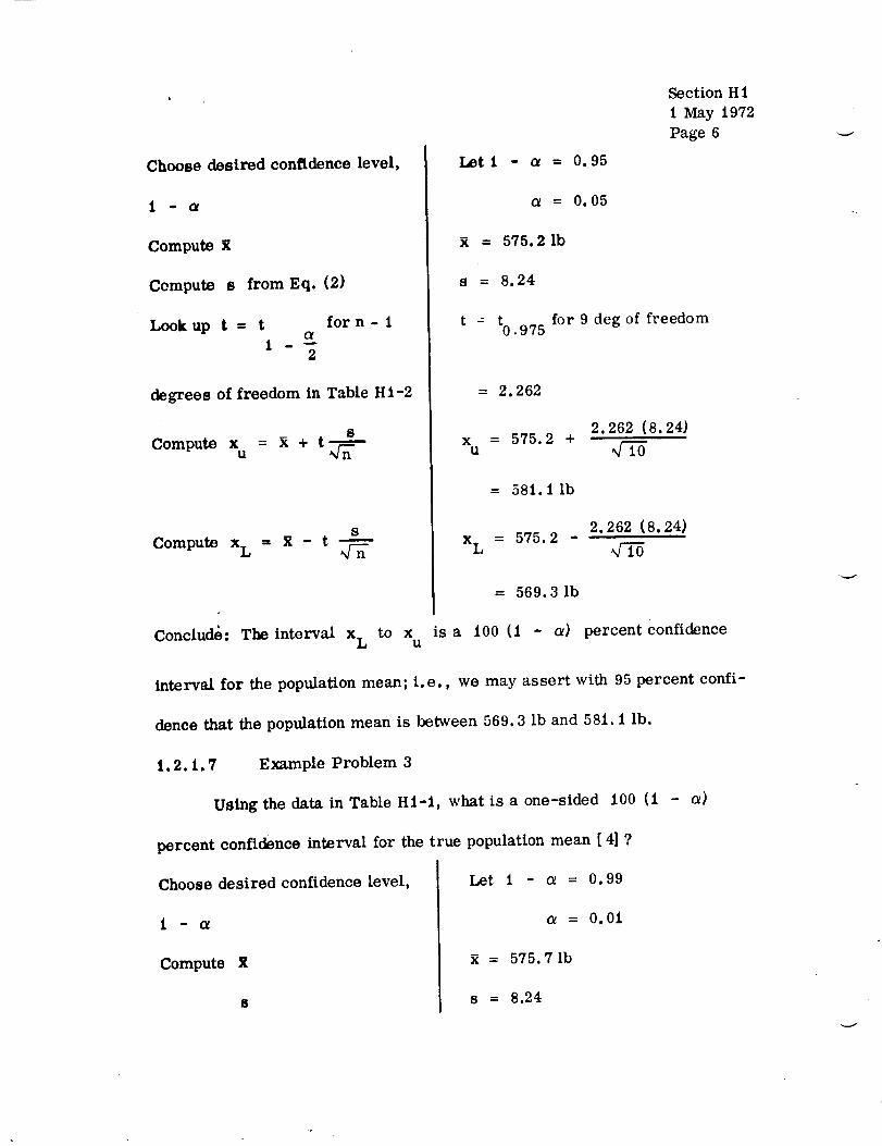
Choose desired confidence level,
Compute X
Compute s from Eq. (2)
Look up t = t forn- 1ot
2
degrees of freedom in Table HI-2
S
Compute Xu = X + t
S
Compute x L = X - t _nn
Conclude: The interval x L to x u
Let i 0.95
Section H i
i May 1972
Page 6
= 0.05
X = 575.2 lb
S
t =
8.24
t for 9 deg of freedomO. 975
= 2.262
x = 575.2 +u JT6
= 581.1 Ib
x L -- 575.2 -
= 569.3 Ib
isa i00 (I - a)
2.262 (8.24)
2.262 (8.24)
percent confidence
interval for the population mean; i.e., we may assert with 95 percent confi-
dence that the population mean is between 569.3 lb and 581.1 lb.
t. 2. t. 7 Example Problem 3
Using the data in Table Hi-t, what is a one-sided 100 (1 - _)
percent confidence interval for the true population mean [ 4] ?
Choose desired confidence level,
Compute X
S
Let 1 - _ = 0.99
= 0.0t
= 575.7 lb
s = 8.24

r
df
6
7
9
10
11
6O 1
oo
O. 325
0.289
0.277
0.271
0.267
0.265
0.263
0.262
0.261
0.260
O. 260
0.259
0.259
0.258
0.258
0.258
0.257
0.257
0.257
0.257
0.257
0.256
0.256
O. 256
0.256
0.256
0. 256
0.256
0.256
0. 256
0.255
0.254
0.254
0.253
OF POOR QUi,LiCV
Table II1-2.
to.7o
[).727
0.617
0.584
0. 569
0.559
0. 553
0.549
0.546
0.5,1:3
0.542
0.5t0
0.539
0.538
0,537
0. 536
0. 535
0.534
0.5:34
O. 53:3
O. 5:33
0.532
0.532
0.532
0.531
0.5:31
0.531
0.5:31
0. 530
0.530
0.530
0.529
0.527
0.526
0.524
Percentiles of tile "t" Distributiol_
to. 80
1. 376
1.061
0.978
0.941
0.920
.906
.8!)6
• a89
._3
.s79
. S76
.873
.8 70
.868
.866
0.865
0. 863
0.862
0.861
0. 860
0.
O.
O.
O.
O.
859
858
858
857
856
0.856
0.855
0.855
0.854
O.854
0.851
0.848
0.845
0.842
tO. 90
3. 078
1.88(;
1.638
l. 533
1.476
1. 440
1.415
1.397
l .:;_3
l. ;372
1.363
1.356
1. 350
1. 345
1.3t l
1. 337
1. 333
1. 330
1.328
1.325
1. 323
i .321
1.319
1. 318
1. 316
1.315
1.314
1.313
1.311
1.310
1.303
1.296
1.289
1.282
to. 95
6.314
2.920
2. 353
2. 132
2.015
l .943
1. 895
1. ,q60
1 .,_3:1
1.812
1.79(;
1. 782
1.771
1.761
1. 753
1. 746
1. 740
1.734
1. 729
1. 725
1.721
1.717
1.714
1.711
1. 708
1. 706
1. 703
i .701
1.699
1.697
1.6_4
1.671
1.658
1.645
:'.
975
12.706
4 .303
3.182
2. 776
2.571
2.447
2. 365
2. 306
2. 262
2.228
2.201
2. 179
2. 160
2.145
2. 131
2. 120
2. 110
2.101
2. 093
2.0 $6
2 .O80
2.0 7,t
2. O69
2.064
2. O60
2.056
2.052
2.048
2.045
2.042
2.021
2.000
1.980
1.690
to.99
31.821
6.965
4.541
3.747
3. 365
3.t43
2.998
2. 896
2._21
2. 764
2.718
2.681
2.650
2.624
2.602
2. 583
2. 567
2.552
2. 539
2.528
2.518
2. 508
2.50O
2.492
2.485
2.479
2.473
2.467
2.462
2.457
2.423
2. 390
2.358
2. 326
Section 111
1 May 1972
Page 7
tO.99.5
63.657
9.925
5.841
4.604
4.032
3. 707
3.499
3. :355
3.250
3. 169
3. 106
3.055
3.012
2. 977
2.947
2.921
2. 898
2 .S78
2. U61
2.845
2.831
2.819
2.807
2.797
2.787
2. 779
2.771
2. 763
2. 756
2.750
2.704
2.660 }
2.617 1

Look up t = t I . a for n - I
deg of freedom in Table Hi-2
Compute x L = 2 - t 4n._ 'i_ "
rcompute u = x + t
_.99
Section Hi
I May 1972
Page 8
for 9 deg of freedom
= 2.82!
!
x L = 575.7 -
= 568.4 lb
Conclude: We are i00 (! - a) percent confident that the population mean
!
is greater than x L ; i.e., we may assert with 99 percent confidence that the
population mean is greater than 568.4 lb.
i. 2. I. 8 Estimating Variability Example Problem
We have estimated the standard deviation; and, in a manner similar
to determining the confidence interval for the mean, we may determine a
confidence interval for the deviation which is termed the variability. Using
the data in Table Hi-l, determine an interval which brackets the true value
of the standard deviation [ 4].
Choose the desired confidence level,
I - at
Compute s
_Lookup B u and B L for n - 1
deg of freedom in Table HI-3
Let 1 - eL =
s = 8.24
0.95
0.05I
for 9 deg of freedom
B L = 0.6657
B = t.746U
k
\

Table H 1-3.
O_ PO0_ (_U,kL(,'/ Section HI1 May 1972
Page 9
Factors for Computing Two-sided Confidence Limits for
Degrees a- 0.05 _ 0.0t _- 0.00i
of
Freedom
df BU BL BU BL BU BL
0.3576 86.31 0. 29691
2
3
4
5
6
7
8
9
io
tl
12
13
14
15
10
17
18
19
20
21
22
23
24
25
26
27
28
29
30
31
32
33
34
35
36
37
38
39
40
41
42
43
44
45
46
47
48
49
50
17.79
4. H59
3. i83
2.567
2.248
2,052
1.91S
I.X20
I. 746
I, 686
1.638
1,598
1.5!; 4
I •534
t. 5([9
t. 486
1.466
_.448
1 • 432
1.4t7
I. 404
1,391
I. 3 _0
1,370
1. 360
t.351
1.343
1. 335
1.327
1.321
1.314
t. 308
1.302
1 • 296
t,29t
I • 286
1.281
i•277
I•272
i•268
1.2[;4
I • 260
1.257
1,253
1.249
I. 246
l. 243
1 • 240
I. 237
1.234
0.45_1
0.5178
0 •5590
0,5899
0.6143
0.6344
0.6513
0.6657
0.6784
0.6896
0.6995
0.7084
0.7166
0.7240
0.7308
0.7372
0.7430
0.74A4
0.7535
0.7582
0.7627
0.7660
0.7709
0.7747
0.7703
0.7817
0.7849
0,7880
0.7909
0.7937
0.79_4
0.7990
0.8015
0.8039
0.8P_62
0.8085
0.8106
0.q126
0.8146
0.8166
0.8{84
0.8202
0.8220
0.8237
0.8253
0.8269
0.82_5
0._300
0.8314
10.70
5.449
3. X!}2
3. 175
2.764
2.49H
2.311
2.173
2.0_5
1.98O
I, 9O0
1.851
1.8[11
1• 77, 8
1.721
1.6X8
1.115½
I .li32
I • 609
1. 587
I. 56fl
l. 550
I. 533
1.518
!. 504
1.491
1.479
1.467
1.457
1.447
1.437
1,428
1,420
1.412
1. 404
1. 397
1 • 300
1 • 383
|..177
1,371
|.3C;3
1.360
1. 355
1.349
1.345
I • 340
1. 335
1.331
1. 327
0.3879
0.4453
0.48_5
0.51X2
i).5437
0.5650
0.5830
0.5987
0.6125
0.6248
0.6358
0.6458
0.6540
0.6632
0.6710
0.6781
0.6848
0,6909
6.(1968
0.7022
0.7674
0.7122
0.7169
0.7212
O.7253
0.7293
0.7331
0.7_17
0.7401
0.7434
0.7467
0.7497
0.7526
0.7554
0.7582
0.760X
0.7633
0.7658
0.7681
0.7705
0.7727
0.774_
0.7769
0.7789
0.7809
0.7_28
0.7X47
O. 7064
0.7882
844.4
33.29
11.65
6.938
5.085
4.128
3.551
3.167
2.804
2.680
2.530
2.402
2,298
2.2|0
2.136
2.073
2,017
1.968
1.925
1.8_6
t.851
1.820
1.791
1.765
1.741
1.719
1.89_
1,670
1.861
1.645
1.629
1.615
1.601
1.5X8
1.576
1.564
1.553
1.543
1.533
1.523
1.515
1.506
1.498
1.490
1.482
1.475
1.468
1.462
1.455
1.449
II. 2481_
0.3291
0.3_24
0.4218
11.4fi29
0.47_4
o. 50O[)
6.51_
6.5:14_
6.5492
6.562|
0.5738
0.5845
O. 5042
0.6032
0.6116
0.6266
0,6333
_1.6307
0.6437
0.6514
0.8566
0.6619
1'.8668
0.6713
(1.675_
0. 6800
0.6841
0.8917
0.6953
0.69_7
o. 7020
0.7652
o. 7083
0 •7113
0.7141
O. 7169
0.7107
0.7223
O. 7248
0.7273
0.7207
O. 7320
0.7342
0 • "_364
0.7386
O. 7407
0.7427

OR|GiNAL P_,,C£ _;OF POOR QU ..iTY
Table H1-3 (Continued)
Section H1
1 May 1972
Page 10
DII_ a = 0.05 • - 0.01 a - 0.911
of
Freedom
_d BU II L B U B L B U BL
51
53
53
54
50
M
37
M
50
00
01
0|
113
114
85
64
01'
08
80
I0
71
79
73
74
79
?6
17
78
79
8O
81
82
83
84
05
38
57
91
N
O0
111
N
03
N
M
07
91
M
i00
i.532
i.228
i.2N
i.224
i.221
i.219
1.2i7
1.2i4
i.Zi5
iotiO
1.208
i.JOe
1.204
1.202
1.500
i.191
1.i57
I.i00
1.194
I • i02
1.191
I.tm
1.i87
i.i88
i,184
i.i88
1.183
1.iOi
1.179
1. i 78
i,i78
i.179
i.i74
I.i74
L.i73
i.1?i
1.170
1,108
I.i07
I. i00
1.105
1.154
|,100
1.152
1,101
1.180
1.159
i.150
I,i85
1.i57
0 • 8320
0.8342
0.838
0.2370
0.0383
0.8308
0,8400
O. 8420
0.0431
0.8442
0.8454
0.8445
0.84?5
0.0486
0.8438
0.0506
0.8518
0.8525
0,0535
0.8544
0.85U
0.882
0.8571
0.0880
0 • 8588
0.0588
0.8804
0.8812
0 • 8620
0.3827
0 • 0838
0 • 8842
0.9150
0.8857
0.6664
0.6471
0.86?8
0 • 8884
O.MS!
0 • 6697
0.8704
0.87i0
0.8710
q.8_20.8721
0.8734
0.0741
0.8744
0.8762
0,8757
1.323
1.319
1.315
1.31i
1. 308
1.304
i,30i
1. 290
1 • 295
1 • 292
t.289
i,388
1.282
i.238
i.2?7
i.279
i.272
i.270
i,918
1. 208
1.242
i.20i
t.250
i.257
i.258
1.253
1.25i
1.242
1.247
i.245
i .|40
i.241
i .239
1.238
1.28
1.235
1.232
1.221
1.230
1.228
1.227
1.228
1.224
1.222
1.221
1.210
1,210
1.217
1.210
1.214
0 • 70041
0.7910
O. 7922
0 • 7940
0 • 7984
0 • 7279
0 • 7914
0 • 8000
0 • 8022
0. |091
O. 8060
0.I_82
0 • 8076
O. 80N
0.810i
0.8112
0.8120
0.8137
0.0148
0.8159
0.21_0
O.SiOi
0.819i
0.8202
0.0212
0,8222
0.2222
0.8242
0.0252
O.Sml
0 • 0270
0.2279
0.8288
0.8297
0.8388
0.8314
0.8212
0.0301
0.5338
0.0:144
0.0354
0.8382
0.0370
0.2377
0.8385
0.8392
0.$391
0.8406
0.8413
0.8420
1.443
i.437
1.482
1,4Zg
1,421
1.410
1.41i
i.491
i.402
1.307
1.388
1,088
i.206
1.311
1.377
1.374
1.370
1.344
1.363
1.910
i.291
! .3U
1.280
1.347
1.244
1,341
1.330
1.338
1.330
1.230
1.320
!.326
1.220
1.320
1.318
1.318
1.2i$
1.211
1,291
1.307
1.305
I. 302
1.301
i.291
t .207
1.215
i.293
1.201
1.289
1.288
0.7441
O. 7491
0.74 03
0.7503
0.7621
O. 7991
0.75M
0.7579
O. 7591
0 • 7008
0.7821
0.768
0.7081
O. _91
O. 79e0
0.7694
0 • 7708
O. 7722
O. 7738
0 • 7740
0.7711
O. 7774
O. 7717
0.77110
0.7911
0. 791"_
O. 7114
O. 7840
0.798
0 • 738|
O. 7171
0.7138
o. 7991
0.7109
0.7938
0.7930
0.7991
0.7940
0.7169
0,7942
0.79?7
0.7917
0.71111
0.11004
0.8813
0.8822
0.8021
0.0029
0.8847
0.3850

Compute s L = BLS
s = BsU U
s L = (8.24) (0.6657)
= 5.48
s = (8.24) (1.746)U
= 14.38
Section HI
I May 1972
Page II
the mean [4].
Choose d,
error, and
estimate of
more
Look up t =
the allowable margin of
c_ , the risk that our
m will be off by d or
t for df deg of(X
2
freedom in Table tti-2
Let d = 0.2
c_ = 0.05
t : t0.975 for 9 deg of freedom
= 2. 262
Conclude: The interval from s L to Su is a two-sided 100 (1 - a) percent
confidence interval estimate for (r ; i.e., we may assert with 95 percent
confidence that (r is between 5.48 and 14.38.
1.2. i. 9 Nmnber of Measurements Required
In planning experiments, we may need to lmow how many measurements
to take in order to determine a parameter of some distribution with pre-
scribed accuracy. If an estimate s or cr is available or if we are willing to
assume a (y ; we may ascertain the required sample size n for determining

t2 s 2
Compute n - d2
(2.262):'(s.24J_
((1.2) 2
s7()[)
Conciu(le: We may conclude that if we now ('Omlmtc the mean
Sc_'tion II 1
1 .May 1972
Page 12
._ O[" ;I l'tllldolli
sample of size n = 8700 , we may ha\e 95 l)el'c'ent confidence that the
interval ._ - 0.2 to _ + 0.2 will include the lot mean.
A similar procedure may be used when computing the st:mdard (levia-
tion. As an e,'m_ple, how large a sample would be required to estimate the
standard deviation within 20 percent of its tt'ue value, with confidence coeffi-
cient equal to 0.95 [ 4] ?
Specify P , the allowable percentage
deviation of the estimated standard
deviation from its true value
Choose y, the confidence coefficient
in Figure Hi-5, find P on the
horizontal scale, and use the curve
for the appropriate _/ . Read on
the vertical scale the required degree
of freedom
n=df + i
Let P = 20 percent
Let -y = 0.95
For y : I).95,
df = 46
P = 20 percent
n : 46 + 1 = 47
-x

OF POOR '_ _ ' "'"
10008OO
_00 % X
500 x400 • \ \
\ \
300 \ \ "
\\ \\\=,2oo \ \
..a o
.. 80 _ .o
w 60 .o_,,, \ \¢¢ 50 .... x0 \ \ \,- 40
30 k \\\ ",
% \ \
\\ \\\ \
lo ...... \ \\
8 \ ,,
5
FIGUILI,: 111-5.
Section It 1
1 May 1972
Page i 3
5 8 8 10 20 30 40 50P PERCENT
NUMI_I_It ()1" I)EGI_I,_I,_S ()l" I'I{I,',I"_D()M lll"QUII_.I,'D TO
ESTIMa\TE Till'] S'I'ANi)Alll) I)I.]VtATI()N \\'ITIIIN I ) PEIICI.:NT OF ITS
TI/UE VAI,UL" \V1TI! ('ONI"IDI"NCI', COF. I,'FICII.:NT 3/ .
1.2.1.10 Tolerance Limits
Sometimes \\'e al'e II_()l'C inh, reste(I in the approximate range of values
in a lot or population than \re :tro i1._ :/vc,.v:t;,;e. v,llue. Statistical tolerance
limits furnish limits l)(,(\_eon, :,l>)ve. ())'l)('l<,\v which wo c,.)nfident!v cxpocL
to find a prescribedl)J'opovtion o[ in(lixi(l_utl items of a population. Thus, we
might be able to give :l v:lluc ,\ :/I)o\e which :It I(,:t,_t a proportion P of the
population will lie (one-side(I limit). In this case, x L ,_ _ - Ks will be
the one-sided lower limit. The al)l)VOl),iatc values l'or N. are given in Table
H1-4 [4]. As anexa.ml)le, consi(lei the (Iztt:t in example lwoblem 1 and find a

Table Hi-4. Factors for One-sided Tolerance
Limits for Normal Distributions
Section Hi
i May i972
Page i4
Factors K such that the probability Is T that at least a proportion P of
the distribution will be less than _ + Ks (or greater than _ - Ks), where
i_ and s are estimates of the mean and the standard
deviation computed from a sample size of n .
- 0.75 _ = 0.90
0.75 0.90 0.95 0.99 0.999 0.75 0.90 0.95 0.99 0.999
9 1.464 2.501 3.152 4.356 5.805 2.002 4.258 5.310 7.340 9.051
4 1.250 2.134 2.600 3.726 4.910 i.972 3.i07 3,957 5.437 7.128
5 1.152 1.961 2.463 3.421 4.507 1.698 2.742 3.400 4.666 0.112
0 1.087 1.000 2.336 3.243 4.273 1.540 2.494 3.091 4.242 6.556
7 1.043 1.791 2.250 3.126 4.1i8 1,435 2.333 2.894 3.972 5.201
S 1.010 1.740 2.190 3.042 4.008 1.360 2.219 2.755 3.783 4.955
9 0.984 t.702 2. 141 2.977 3.924 i.302 2.133 2.649 3.64i 4.772
|0 0.964 1.67/ 2.|03 2.92? 3.858 1.257 2.065 2.508 3.582 4.629
I| 0.947 1.846 2.073 2.885 3.804 i.219 2.012 2.503 3.444 4.515
13 0.033 /.624 2.048 2.851 3.700 1.188 1.960 2.448 3.371 4.420
13 0.919 |.006 2.020 2.822 3.722 1.162 /.928 2.403 3.310 4.341
14 0.909 t.891 2.007 2.796 3.690 /.139 t.895 2.363 3.257 4.274
15 0.899 1.577 1.991 2.776 3.661 i.il9 1.866 2.329 3.2i2 4.215
t0 0.891 |.566 i.977 2.756 3.637 l.iOl 1.842 2.299 3.172 4.164
17 0.883 1.554 1.964 2.739 3.615 1.085 1.820 2.272 3.136 4.118
i8 0.876 1.644 t.051 2.723 3.596 i.07t t.800 2.249 3.t06 4.078
19 0.870 1.536 i.942 2.7/0 3.577 1.058 1.78| 2.228 3.078 4.04t
20 0.865 /.528 1.933 2.697 3.56t 1.046 i.765 2.208 3.052 4.009
21 0.859 1.520 1.923 2.686 3.545 1.035 t.750 2,190 3.028 3.979
22 0.854 1.514 1.916 2.075 3.532 1.025 1.736 2./74 3.007 3.952
23 0.849 t.508 1.907 2.665 3.520 t.016 1.724 2.t59 2.987 3.927
24 0.848 1.502 1.901 2.656 3.509 1.007 1.712 2.145 2.969 3.904
25 0.842 1.496 1.895 2.647 3.497 0.999 1.702 2.132 2.952 3.882
30 0.825 1.475 1.869 2.613 3.454 0.966 i.657 2,080 2.884 3.794
35 0.812 1.458 1.849 2.588 3.42/ 0.942 1.023 2,041 2.833 3.730
40 0.803 t.445 t.834 2.568 3.395 0.923 1.598 2.0i0 2.793 3.079
45 0.795 1.435 1.82/ 2.552 3.375 0.908 i.577 i.956 2.762 3.638
50 0.788 1.426 1.8ii 2.538 3.358 0.894 1.560 1.965 2.735 3.604
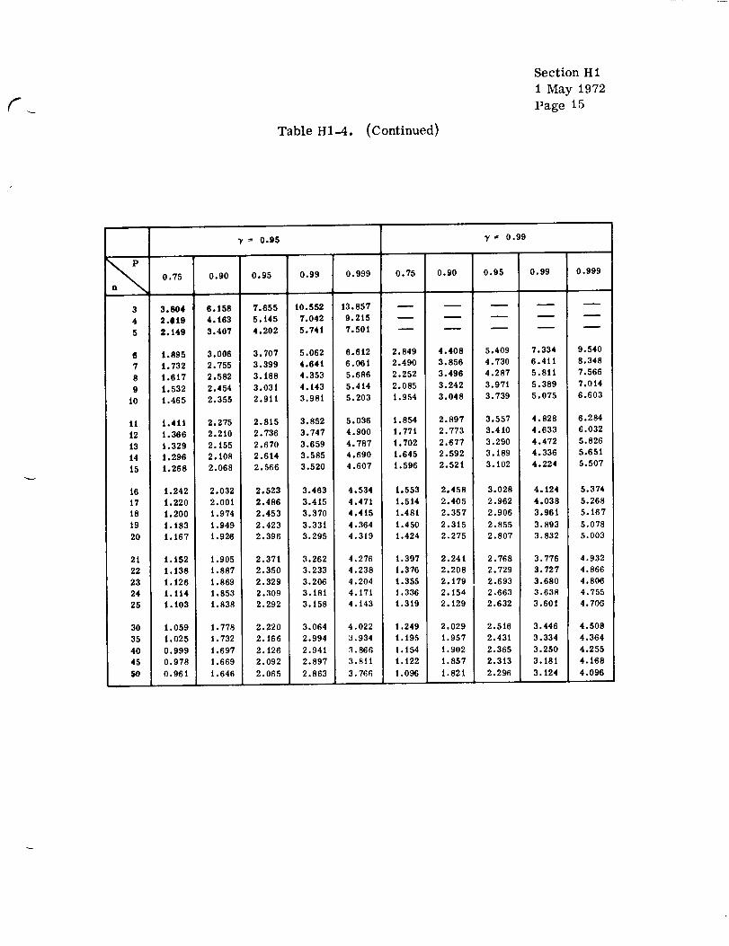
Table H 1 .-4. (Continued)
Section H I
i May 1972
Page 15
7 = 0.95 7 = 0.99
0.75 0.90 0.95 0.99 0.999 0.75 0.90 0.95 0.99 0.999
3 3.804 6.158 7.655 t0.552 13.857 .....
4 2.619 4.163 5.145 7.042 9.215 .....
5 2.149 3.407 4.202 5.741 7.501 .....
6 1.895 3.006 3.707 5.062 6.612 2.849 4.408 5.409 7.334 9.540
7 1.732 2.755 3.399 4.64t 6.061 2.490 3.856 4.730 6.411 8.348
8 1.617 2.582 3. t88 4.353 5.686 2.252 3.496 4.287 5.8tt 7.566
9 t.532 2.454 3.031 4.t43 5.4t4 2.085 3.242 3.97t 5.389 7.014
10 1.465 2.355 2.911 3.981 5.203 1.954 3.048 3.739 5.075 6.603
II i.411 2,275 2.815 3.852 5.036 1.854 2.897 3.557 4.828 6.284
t2 1.366 2.2i0 2.736 3.747 4.900 t.77t 2.773 3.410 4.633 6.032
t3 1.329 2.155 2.670 3.659 4.787 1.702 2.677 3.290 4.472 5.826
t4 1.296 2.108 2,6t4 3.585 4.690 i.645 2.592 3.189 4.336 5.651
15 1.268 2.068 2.566 3.520 4.607 1.596 2.521 3.102 4.224 5.507
16 i.242 2.032 2.523 3.483 4.534 1.553 2.458 3.028 4.124 5.374
17 1.220 2.00i 2.486 3.415 4.471 1.514 2.405 2.962 4.038 5.268
18 1.200 1.974 2.453 3.370 4.4i5 t.48i 2.357 2.906 3.961 5.167
19 1.183 1.949 2.423 3.33i 4.364 1.450 2.315 2.855 3.893 5.078
20 1.167 1.926 2.396 3.295 4.319 1.424 2.275 2.807 3.832 5.003
21 1.152 t.905 2.371 3.262 4.276 1.397 2.241 2.768 3.776 4.932
22 1.t38 t.887 2.350 3.233 4.238 1.376 2.208 2.729 3.727 4.866
23 1.126 1.869 2.329 3.206 4.204 1.355 2.179 2.693 3.680 4.806
24 1.114 1.853 2.309 3.181 4.171 1.336 2.154 2.663 3.638 4.755
25 1.103 1.838 2.292 3.158 4.143 1.319 2.129 2.632 3.601 4.705
30 t.059 t.778 2.220 3.064 4.022 t.249 2.029 2.516 3.446 4.508
35 1.025 1.732 2.166 2.994 3.934 1.195 1.957 2.431 3.334 4.364
40 0.999 1.697 2.126 2.941 3.866 i.154 1.902 2.365 3.250 4.255
45 0.978 1.669 2.092 2.897 3.811 1.122 1.857 2.313 3.181 4.168
50 0.961 1.646 2.065 2.863 3.766 1.096 1.821 2.296 3.124 4.096

Section H l
1 May 1972
Page 16
single value above which we may predict with 90 percent confidence that 99
percent of the population will lie.
Choose P the proportion, and _/
the confidence coefficient
Compute
s
Look up K in Table H1-4 for
appropriate n, -f, and P
Compute x L = £ - Ks
Let P = 0.99
T = 0.90
= 575.7 lb
s = 8.24
n= i0,P =
K = 3. 532
x L = 546.6 lb
0.99 ,'y : 0.90
Thus we are 90 percent confident
that 99 percent of the material
ultimate strengths for product
"A" will be above 546.6 lb.
This same procedure is used in Ref. [ 6] to determine the "A" and "B" values
for the primary strength properties
Fbry) •
1.2.2
1.2.2.1 Properties
(Ftu, Fty, Fcy, Fsu, Fbr u, and
LoG-Normal Probability Curve
A log-normal distribution is the frequency distribution curve resulting
from the use of the logarithm of a variable rather than the variable itself.
The log-normal distribution curve is bell shaped like the normal probability
curve and has the properties of a normal distribution.
J

f
Section HI
1 May 1972
Page 17
1.2.2.2 Estimate of Average Performance
Similar to the normally distributed variables, the best single estimate
of the population mean, m , is simply the arithmetic mean of the measure-
ments [ 3].
n1
Iogm _IogR = -- _ Iogx. (3)n
i=l
1.2.2.3 Example Problem 4
Using the fatigue lives for a constant stress level (50 ksi) given in
Table H1-5, estimate the mean of the parent universe [ 3].
Table HI-5. Fatigue Life of Product '_B"
Test Specimen N. (Cycles) Log N.1 1
1
2
3
4
5
13000
13100
24000
28000
40000
4.1139
4.1173
4.3802
4.4472
4.6021
n = 5 _logN. = 21. 66071
log N
N =
1.2.2.4
1 1: : ,log Ni : : (21.6607;
antilog 4. 3321 = 21485cycles
Estimate of Standard Deviation
= 4.3321 = Mean log value
Again, similar to normally distributed variables, the best unbiased
estimate of the standard deviation is thc square root of the estimate of
variance [3l •
Section H1i May 1972
Page i8
logx i 2 _ _ logx i
a_ S_ = i=ln (n - 1) (4)
1.2.2.5 Interval Estimates
Confidence intervals may be determined for log-normal distributions.
The range of a percentage of data points may be computed for the sample
mean coinciding with the population mean, which occurs with a confidence
of 50 percent. The range is computed as
m
logx = logx + kps , (5)
where kp is defined in Fig. H1-6. A lower limit (one-sided confidence
interval) may be computed as
log x L = o_ - kpTs , (6)
where kpT is defined in Figs. Hi-7 through HI-9 as a function of the sample
size, the percentage of data points occurring above the lower limit, and the
confidence value.

0.60
0.40w
n,L
Ewo
..<. 0.2oK¢(
<
w
0.1o
_
Section H 1
t May 1972
Page 19
0 1 2 3 4 5
FIGURE H 1-6.
h,
FACTOR FOR DETERMINING DATA POINT RANGE,
/ CENT
--... P " 99 PERCENTI "-'------
_ P " 90PERCENT
,_--.-__ P - 50 PERCENT
6 7 10 20 30 5Q
NUMBER OF SAMPLES
100
FIGURE ttl-7. PROBABILITY FACTOR kpT FOR 7 = 0.95.
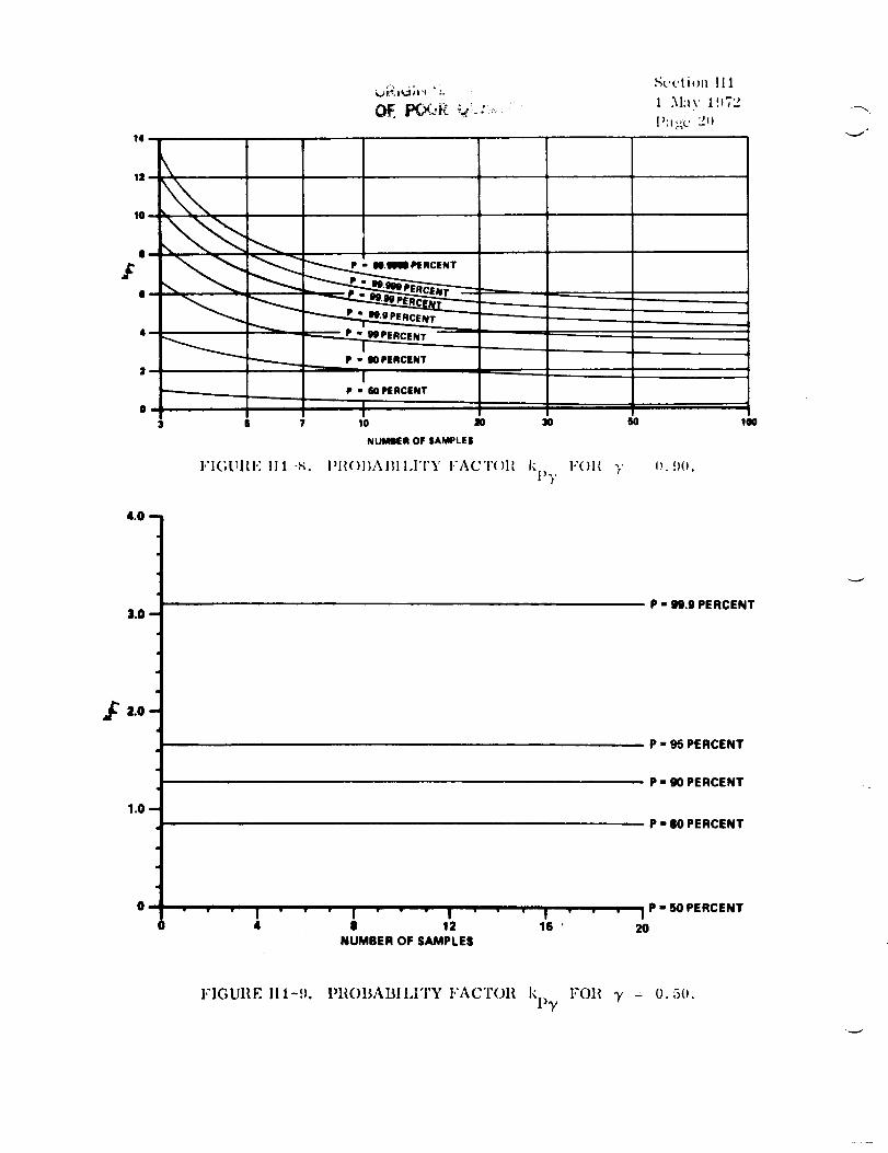
14
12
m
P " NPIERCENT "--------.----.
Sc,(.ti_m ]!1
1 May 1.),_
P - IIOPIERCIENT
IP - 60 PERCENT
10 IO 30 60 100
NUMIEIt OF SAMPLES
l,'l(;I.;Itl,:lll-x. I'I{()]LA.IHI.I'I'Y I:AC'I'()]| k l.'()l{_, ().!)().1)-_,
I
0
3 S 7
4.0
3.O
.,,_ 2.0
1.0
a
,i
ii
P - 99.9 PERCENT
P-95PERCENT
P-90PERCENT
P-80PERCENT
"' "' I " " " I " I ' I " " " 1 P'SOPERCENT
4 II 12 16 ' 20
NUMBER OF SAMPLES
FIGURE 111-9. IHtOI3ABILITY l,'AC'r(.)ll ki) Y FOI{ y = 0.50.

Section H1
1 May 1972
Page 21
1.2.2.6 Example Problem 5
Using the data in Table H1-5, determine the range within which 68
percent of all points fall [ 3].
logN = 4. 3321
s = 0. 213
From Figure H1-6, kp = 1.0
logN = 4.3321 * 0.213 = ,;.545 N = 35100cyclesmax lnax
log Nmi n = 4. 3321 - 0.21;I = ,:. 11.9 Nmi n = 13700 cycles
Conclude: The interval x L to Xu is :l 100 (1 - a)percent confidence
interval for P percent of the pol)u]:',ti,)n; i.e., we may assert with 50 percent
confidence the 68 percent of the i)opulation will fall within 13700 < N < 35100
cycles.
1.2.2.7 Example Problem 6
Using the data in Table II1-5, determine the life above which 90 percent
of all points in the total population will lie with a confidence of 95 percent.
Choose desired confidence level
Choose P percent of data points
which should exceed the lower limit.
Compute log x
I__t 1 - o_ = 0.95
c_ = 0.05
Let P = 90 percent
logN = 4.3321

Compute s
Find rk_y in Figure HI-7
Compute logN L = LogN - kpys
Conclude: We are 100 (1 - a)
?
data points are greater than x L
Section HI
i May 1972
Page 22
s = 0.213
for P = 90 percent, y = 95 percent,
n = 5 kpy = 3.35
logN L = 3.61855
N L = 4155 cycles
percent confident that P percent of the
; i. e., we may assert with 95 percent confi-
dence that 90 percent of the lives are greater than 4155 cycles.

1.3
HI-I.
HI-2.
HI-3.
H1-4.
H1-5.
H1-6,
Section H1
1 May 1972
Page 23
REFERENCES
Hald, A. : Statistical Theory with Engineering Application.
John Wiley, 1952.
Structures Manual. Convair, Fort Worth, Texas.
Structural Methods Handbook. Temco Aircraft Corporation,
Report no. 00.80.39, 1956.
Natrella, M. G. : Experimental Statistics, National Bureau of
Standards Handbook 91, August 1, 1963.
Liu, A. F. : Statistical Variation in Fracture Touglmess Data of
Airframe Materials. Proceedings of the Air Force Conference on
Fatigue and Fracture of Aircraft Structures and Materials,
AFFDL TR 70-144, December 1969.
Metallic Materials and Elements for Aerospace Vehicle Structures.
Department of Defense, MIL-HDBK-5A, February 8, 1966.
¢t U. S. GOVERNMENT PRINTING OFFICE: 1972-74,5-386/Region No. 4

!
Top Related
Copyright © 2022 FDOKUMEN

