


Bahasa
Halaman
Hukum

Low hanging fruit: A subset of human cSNPs is both highly
non-uniform and predictable
Monica M. Horvatha,c,e,*, John W. Fondon IIIa,c,e, Harold R. Garnera,b,c,d
aMcDermott Center for Human Growth and Development, The University of Texas Southwestern Medical Center, 5323 Harry Hines Blvd,
Dallas, TX 75390-8591, USAbCenter for Biomedical Inventions, The University of Texas Southwestern Medical Center, 5323 Harry Hines Blvd, Dallas, TX 75390-8591, USA
cDepartment of Biochemistry, The University of Texas Southwestern Medical Center, 5323 Harry Hines Blvd, Dallas, TX 75390-8591, USAdDepartment of Internal Medicine, The University of Texas Southwestern Medical Center, 5323 Harry Hines Blvd, Dallas, TX 75390-8591, USAeProgram in Molecular Biophysics, The University of Texas Southwestern Medical Center, 5323 Harry Hines Blvd, Dallas, TX 75390-8591, USA
Received 14 December 2002; received in revised form 2 April 2003; accepted 15 April 2003
Received by S. Salzberg
Abstract
We present a point mutation classification method that contrasts SNP databases and has the potential to illuminate the relative mutational
load of genes caused by codon bias. We group point variation gleaned from public databases by their wild-type and mutant codons, e.g. codon
mutation classes (CMCs, 576 possible such as ACG ! ATG), whose frequencies in a database are assembled into a BLOSUM-style matrix
describing the likelihood of observing all possible single base codon changes as tuned by the intertwined effects of mutation rate and
selection. The rankings of the CMCs in any database are reshuffled according to the population stratification of the typical genotyping
experiment producing that resource’s data. Analysis of four independent databases reveals that a considerable fraction of mutation in
functional genes can be described by a few CMCs regardless of gene identity or population stratification in the genotyping experiment. For
example, the top 5% (29/576) of CMCs account for 27.4% of the observed variants in dbSNP while the bottom 5% account for only 0.02%.
For non-synonymous disease-causing mutation, 40.8% are described by the top 5% of all possible non-silent CMCs (22/438). Overall, the
most observed polymorphism is a G ! A transition at CpG dinucleotides causing ACG, TCG, GCG, and CCG to frequently undergo silent
mutation in any gene due to the putative lack of impact on the protein product. In order to assess how well CMC spectrums estimate the
aggregate non-synonymous mutational trends of a single gene, a CMC matrix was applied to seven unrelated genes to compute the most
likely point mutations. In excess of 87% of these mutation predictions are historically known to play an important role in a disease state
according to published literature. CMC-based mutation prediction may aid design and execution of direct association genotyping studies.
q 2003 Elsevier Science B.V. All rights reserved.
Keywords: Point variant; Codon bias; Mutation prediction; BLOSUM matrix; Mutation spectrum
1. Introduction
Efforts to catalog cSNPs (coding SNPs) have accelerated
due to their presumed value in phenotype association studies
(Sachidanandam et al., 2001). Formally, a SNP is a point
mutation of at least 1% frequency in a population (Brookes,
1999), but the genomics community has tended to use the
terms SNP, variant, and point mutation interchangeably due
to the variety of cohorts chosen to undergo genotyping
experiments (Wang and Moult, 2001). The occurrence of a
point mutation event is well-known to be highly dependent
on the local DNA sequence context (Cooper and Krawczak,
1990). Capitalizing on this, a recent set of studies calculated
0378-1119/03/$ - see front matter q 2003 Elsevier Science B.V. All rights reserved.
doi:10.1016/S0378-1119(03)00628-0
Gene 312 (2003) 197–206
www.elsevier.com/locate/gene
* Corresponding author. Tel.: þ1-214-648-1674; fax: þ1-214-648-1666.
E-mail address: [email protected] (M.M. Horvath).
Abbreviations: CFTR, cystic fibrosis transmembrane receptor gene;
CGAP-GAI, Cancer Genome Anatomy Project Genomic Annotation
Initiative database; CMC, codon mutation class; cSNP, coding region
single nucleotide polymorphism; F9, factor 9 gene; GBJ1, connexin 32
gene; HGMD, Human Genome Mutation Database; HMBS,
hydroxymethylbilane synthase gene; nt, nucleotide; PAX6, paired box
homeotic 6 gene; pred(s), prediction(s); SERPINA1, alpha-1-antitrypsin
gene; SNP, single nucleotide polymorphism; TMC, trinucleotide mutation
class; TSC, the SNP Consortium database; XPA, xeroderma pigmentosum
complementation group A gene.
a hierarchy of mutability preferences for di- and tri-
nucleotide sequences from a dataset of known somatic
point mutations in immunoglobulin variable region genes
(Shapiro et al., 1999). This distribution of mutability
preferences was cleverly exploited to successfully predict
coding-region point mutations in other immunoglobulin
V-genes (Shapiro et al., 2002). The goal of this study is to
similarly mine large cSNP databases for associations
between mutation and coding sequence context to realize
any general coding region mutability trends in the human
genome.
When sorting cSNPs according to a set of sequence
context categories with the goal of pinpointing any
unusually well- or underpopulated categories, several issues
must be carefully considered. Most importantly, cSNP
identification and subsequent deposition into a database is
not simply a matter of the inherent mutation rate, but
depends substantially upon the structure of the genotyped
population as well as the effect of selection on the new
allele. Therefore deconvolution of a cSNP database into a
distribution of mutation preferences for cSNP categories is
best used to relatively compare cSNP datasets of differing
origins. Additionally a biologically relevant cSNP classifi-
cation method must be chosen. In this study a frame-
dependent, codon-focused, trinucleotide classification
metric is most appropriate since the coding regions of
genes are being examined. Finally, a cSNP dataset must be
large enough so that every cSNP category statistically has
had a chance to be sampled multiple times.
The largest public SNP database available to derive such
trends is NCBI’s dbSNP project (Smigielski et al., 2000),
which catalogs polymorphisms from any genotyping
experiment. Most of the alleles, however, are quite common
for they have been discovered through reduced represen-
tation shotgun sequencing of less than ten individuals
(Altshuler et al., 2000) or detection of bacterial clone
overlap as a by-product of the human genome project (,24
individuals) (Mullikin et al., 2000). The SNP Consortium
(TSC) resource (Sachidanandam et al., 2001) details human
point variants identified by sequencing DNA from an
ethnically diverse group of 20 individuals for construction
of a high-density genomic SNP map. NCI’s Cancer Genome
Anatomy Project (CGAP) has created the Genomic
Annotation Initiative (GAI) (Riggins and Strausberg,
2001) to locate human and mouse germline point variants
in cancer-relevant genes by implementing EST alignment
methods that flag high quality discrepancies as SNPs
(Buetow et al., 1999). Considering that as few as five
individuals’ ESTs compose this alignment, the database
presumably contains mostly high frequency alleles. The
human gene mutation database (HGMD) is a specialized
resource detailing non-synonymous, disease-causing
point mutations manually culled from published studies
(Krawczak et al., 2000).
We show that each database exhibits a profile of point
variants dependent on the resource’s typical genotyping
experiment, which is a function of population stratification-
cohort size, cohort scope, and degree of sample pooling.
This phenomena exists because the spectrum of observed
variants in such experiments is an inseparable function of
both a mutation’s intrinsic rate and typical impact on the
encoded protein. We compare the databases in light of their
point variation spectrums and then demonstrate that this
information may be applied to predict a large fraction of
variation in individual genes, which has implications for
steering directed genotyping, estimating relative gene
mutational load, and developing hypotheses about mutation
discovery and population structure.
2. Materials and methods
2.1. Retrieval of cSNPs
Dataset statistics are shown in Table 1. Within each
database, identical alleles at a nucleotide position were
counted only once. Annotated non-synonymous mutations
designated as causative of a clinical phenotype (15,118
total) were retrieved from the HGMD website (http://www.
hgmd.org, 5/24/2002 build) (Krawczak et al., 2000).
To collect only reviewed dbSNP cSNPs, NCBI’s
LocusLink (Pruitt and Maglott, 2001) (build 10/13/2002)
was queried for human, protein-coding, non-pseudogene
loci. The corresponding RefSeq (Pruitt and Maglott, 2001)
cDNA GenBank accession numbers were collated. Anno-
tated cSNPs were obtained by parsing all ‘/variation’ tags in
GenBank records and sorted by reference ID (rs#) to obtain
42,237 non-redundant mutations. The major allele was
assumed to be the nucleotide in the reference sequence.
Multi-allelic SNPs were included as independent mutation
events that happen to occur at identical nucleotide positions.
Unique Mus musculus SNPs (4,232) were obtained from
the CGAP-GAI web site (http://lpgws.nci.nih.gov:82/perl/
snp2ref, 4/17/2002) which maps discovered alleles onto
RefSeq cDNAs. Only non-pseudogene mutations with a
SNP confidence score, the chance that the given nucleotide
is correctly called as calculated from sequence quality
values, $0.99 were considered (Clifford et al., 2000). The
authors of the CGAP-GAI project also assume that the
major allele is that in the associated RefSeq cDNA.
The SNP Consortium (TSC) database tables (release 10)
were downloaded (Sachidanandam et al., 2001) and
1,148,402 human SNPs with at least 50 bases each of 50
and 30 flanking sequence were extracted. Gapped BLAST
(Altschul et al., 1997) was used to map the variants to
protein coding RefSeq cDNA sequences (RefSeq, build 3/
15/2002). A mapped cSNP was defined as any match whose
alignment had no gaps and at least 95% sequence identity
over 60 nucleotides or more (6,016 cSNPs total). Although
these stringent parameters likely eliminated genuine cSNPs,
they afforded high confidence in the annotation. As with the
M.M. Horvath et al. / Gene 312 (2003) 197–206198
other datasets, the cDNA reference sequence was assumed
to contain the major allele.
2.2. Elucidation of codon mutation class frequencies
For each database point variants were categorized
according to their resulting codon changes, referred to as
codon mutation classes (CMCs, e.g. ACG ! ATG). Since
the mechanisms invoking a NNX ! NNY mutation may be
distinct from those causing a NNY ! NNX variant, CMCs
have directionality and assume both a wild-type and mutant
allele. The usage-weighted frequency of each CMC was
computed as (# mutations assigned to a CMC)/(total #
mutations in the database)/(wild-type codon usage) and then
normalized so that the net frequency of all CMCs from a
database equaled 1. The wild-type Mus musculus and human
codon usage tables were obtained from the Codon Usage
Database (Nakamura et al., 2000). This set of NNX ! NNY
usage-weighted frequencies can be considered as a 64 codon
X 64 codon matrix where most of the 4,096 possible values
are zero because more than one mutation would be required
to generate the mutant codon. Overall, the CMC matrix has
576 non-zero values because there are 3 £ 3 £ 43 total ways
the 64 codons can point mutate. All CMC matrices for each
of the databases are available as supplementary data at
http://innovation.swmed.edu/snide.htm.
If all mutational events are equally observable upon
genotyping, the CMC distribution can be considered as a
classic mutation spectrum, which is expected to follow a
multinomial distribution with respect to the number of
cSNPs in each class (Adams and Skopek, 1987). To evaluate
the departure of each database’s CMC distribution from this
null hypothesis, each point variant was randomly assigned
to one of the 576 possible CMCs producing a multinomial
distribution. During this procedure the fraction of all
database mutations assigned to each CMC was used as the
null model frequency for that CMC and graphed in Fig. 1.
2.3. Statistical comparison of cSNP databases
To determine the statistical significance of CMC
dispersion differences between any pair of databases, the
two-tailed non-parametric Mann–Whitney U-test (Table 2)
was employed using the normal approximation to correct
ties (Zar, 1996). In this test the CMCs of each of two
compared databases are ranked separately and the ranks
then used to compute the Mann–Whitney U statistic,
U ¼ n1n2 þ 0.5n1(n1 þ 1) 2 R1, where n1 is the number of
CMCs in the first dataset, n2 is the number of CMCs in the
second dataset, and R1 is the sum of the ranks of CMCs in
the first dataset. The probability of erroneously rejecting the
null hypothesis (that there is no significant difference in
CMC dispersion for the two datasets) was evaluated in
U-test tables at the 95% confidence level (Zar, 1996).
2.4. Prediction of disease-causing point mutation
To determine if mined cSNP trends encoded in CMC
frequencies have predictive power, gene sequences were
chosen and HGMD CMC frequencies were used as an
estimate of the likelihood of that event at the wild-type
codon. Since a codon classification of cSNPs is employed,
HGMD CMC frequencies as computed in Section 2.2 would
lack information concerning the influence of codon-
bridging sequence context on point mutation events.
Therefore, a total of three matrices are required: One for
the actual coding frame (frame 1, CMC matrix) plus two
representing the non-coding trinucleotide frames due to a
þ1 or þ2 base frameshift (trinucleotide mutation class
(TMC) matrices 1 and 2, respectively). These non-coding
matrices allows the mutation data to be categorized in the
context of its contiguous codons. TMC frequencies
represent mutation propensity influenced by the 50 and 30
codons. The HGMD CMC matrix was calculated as
described in Section 2.2. To calculate the HGMD TMC1
and TMC2 matrices the cDNA sequence of each HGMD
gene was frameshifted þ1 or þ2 bases, respectively. Then
each HGMD point mutation was evaluated to determine its
trinucleotide mutation class after the frameshift. The usage-
weighted frequency of each TMC was computed as (#
mutations assigned to a TMC)/(total # mutations in the
database)/(wild-type trinucleotide usage) and then normal-
ized so that the net frequency of all TMCs equaled 1.
Genome-wide non-coding frame trinucleotide usages were
calculated directly from 104,170 non-pseudogene, non-
hypothetical unique human cDNAs retrieved from UniGene
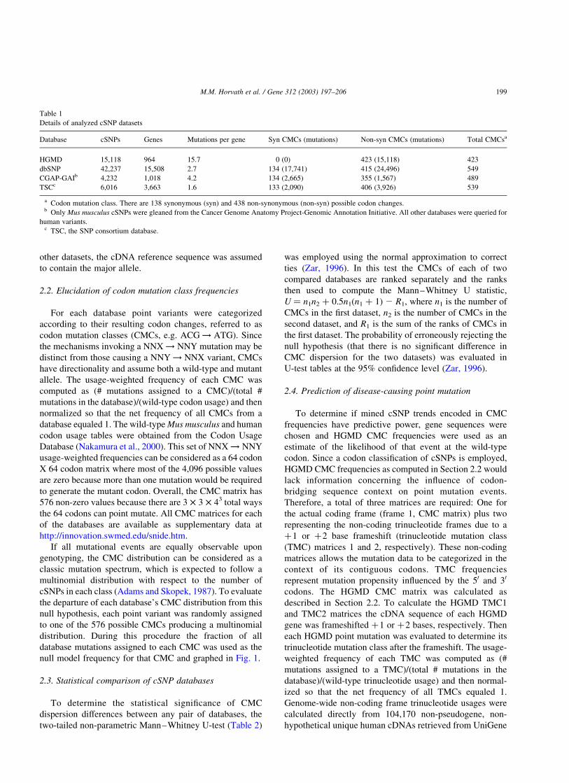
Table 1
Details of analyzed cSNP datasets
Database cSNPs Genes Mutations per gene Syn CMCs (mutations) Non-syn CMCs (mutations) Total CMCsa
HGMD 15,118 964 15.7 0 (0) 423 (15,118) 423
dbSNP 42,237 15,508 2.7 134 (17,741) 415 (24,496) 549
CGAP-GAIb 4,232 1,018 4.2 134 (2,665) 355 (1,567) 489
TSCc 6,016 3,663 1.6 133 (2,090) 406 (3,926) 539
a Codon mutation class. There are 138 synonymous (syn) and 438 non-synonymous (non-syn) possible codon changes.b Only Mus musculus cSNPs were gleaned from the Cancer Genome Anatomy Project-Genomic Annotation Initiative. All other databases were queried for
human variants.c TSC, the SNP consortium database.
M.M. Horvath et al. / Gene 312 (2003) 197–206 199
(Hs.seq.uniq, 8/20/2002 (Schuler, 1997)) where the cDNAs
were frameshifted þ1 or þ2 bases before calculating the
frequency of all 64 possible non-coding trinucleotides.
To examine mutation prediction ability of the HGMD
matrices seven genes representing a range of inheritance
modes were chosen (Table 3). Coding and non-coding
mutation class matrices were recalculated from the HGMD
data as above but with mutations from the seven genes
excluded. Each possible non-synonymous mutation for a
gene was computationally assigned an observation like-
lihood. Fig. 2 illustrates this process for a GCG-CGG-TGG
portion of a coding sequence where the bolded cytosine of
codon CGG mutates to a thymine. The mutation class of the
point variant is evaluated for each frame (one coding and
two non-coding) and then assigned a frequency by
referencing the appropriate frame-specific matrix. The
three frequency values are averaged to obtain a mean
likelihood of observing the C ! T variant given its DNA
sequence context. For a whole coding sequence, the entire
body of possible non-synonymous cSNPs are ranked by
descending mean observation likelihood and a top fraction
of predictions per gene (0.25, 0.5, 2.5, and 5%) were
referenced in the HGMD to determine the rate at which they
are experimentally observed. Accuracy (the percentage of
predictions detailed in the HGMD) and completeness (the
percentage of all HGMD-detailed point mutations predicted
by our methods) statistics were reported in Table 3.
The accuracies in Table 3, however, only have meaning
in contrast to the accuracy rate of predicting mutations
randomly. If a gene is saturated with mutations (i.e. nearly
all existing germline mutations have been discovered), as
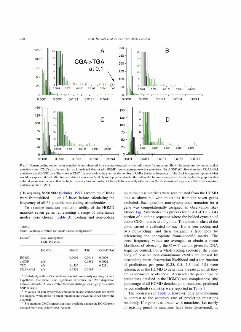
Fig. 1. Human coding region point mutation is not observed in a manner expected by the null model for mutation. Shown in green are the human codon
mutation class (CMC) distributions for each analyzed dataset (A) HGMD (non-synonymous-only) mutations (B) dbSNP (C) Mus musculus CGAP-GAI
mutations and (D) TSC data. The x-axis is CMC frequency while the y-axis is the number of CMCs that have frequency x. The black histograms represent what
would be expected if the CMCs for each dataset were equally likely to be populated under the null model for mutation spectra. Insets display the graphs with a
reduced y-axis maximum so that the high frequency bars are visible. CGA ! TGA is actually off-axis in A (break shown) and represents 10% of all causative
mutation in the HGMD.
Table 2
Mann–Whitney P-values for cSNP dataset comparisonsa
Datasetb Non-synonymous
CMC P-values
HGMD dbSNP TSC CGAP-GAI
HGMD – 0.0001 0.0014 0.0006
dbSNP n/ac – 0.0382 0.9012
TSC n/a 0.4559 – 0.2231
CGAP-GAI n/a 0.7851 0.7193 –
a Probability at the 95% confidence level of erroneously rejecting the null
hypothesis, that there is no significant difference in CMC dispersion
between datasets. A low P-value therefore distinguishes highly dissimilar
SNP datasets.b P-values for non-synonymous mutation dataset comparisons are above
the diagonal while those for silent mutation are shown italicized below the
diagonal.c Synonymous CMC comparison is not available against the HGMD for it
contains only non-synonymous variants.
M.M. Horvath et al. / Gene 312 (2003) 197–206200

Table 3
A portion of disease-causing cSNPs can be accurately predicteda
GENE (# possible non-synonymous mutations) Ratiob
Percent accuracy for cSNP predictionc;
Percent accuracy using the null (random) modeld;
Percent completenesse
Top 0.25% Top 0.5% Top 2.5% Top 5%
F9f (3,275) 100% (8/8) 93.8% (15/16) 65.4% (53/81) 61.6% (101/164) 6.3
15.7 ^ 12.9% 15.9 ^ 9.1% 16.0 ^ 4.0% 16.2 ^ 2.8%
1.6% (8/515) 2.9% (15/515) 14.2% (73/515) 19.6% (101/515)
CFTRg (10,391) 88.5% (23/26) 69.2% (36/52) 40.0% (104/260) 28.7% (149/519) 16.3
5.4 ^ 4.4% 5.4 ^ 3.1% 5.4 ^ 2.2% 5.4 ^ 1.8%
4.1% (23/565) 6.4% (36/565) 18.4% (104/565) 26.4% (149/565)
GJB1h (1,942) 100.0% (5/5) 60.0% (6/10) 37.5% (18/48) 24.7% (24/97) 23.3
4.3 ^ 9.1% 4.3 ^ 6.4% 4.3 ^ 2.9% 4.3 ^ 2.0%
5.9% (5/85) 7.1% (6/85) 21.2% (18/85) 28.2% (24/85)
HMBSi (2,471) 100% (6/6) 75.0% (12/16) 45.6% (37/81) 36.0% (58/161) 30.5
3.3 ^ 7.2% 4.9 ^ 5.3% 4.9 ^ 2.3% 4.9 ^ 1.7%
7.4% (6/81) 7.6% (12/157) 23.6% (37/157) 36.9% (58/157)
PAX6j (2,925) 85.7% (6/7) 57.1% (8/14) 20.5% (15/73) 11.0% (16/146) 61.7
1.4 ^ 4.5% 1.4 ^ 3.0% 1.4 ^ 1.4% 1.4 ^ 0.9%
14.6% (6/41) 19.5% (8/41) 36.6% (10/73) 39.0% (16/41)
SERPINA1k (2,927) 71.4% (5/7) 46.7% (7/15) 13.7% (10/73) 7.5% (11/146) 77.0
0.9 ^ 3.0% 1.0 ^ 2.5% 0.9 ^ 1.1% 0.9 ^ 0.8%
18.5% (5/27) 25.9% (7/27) 37.0% (10/27) 40.7% (11/27)
XPAl (1,953) 60.0% (3/5) 30.0% (3/6) 6.1% (3/49) 3.7% (3/97) 181.0
0.3 ^ 2.0% 0.3 ^ 2.2% 0.3 ^ 0.8% 0.3 ^ 0.6%
50.0% (3/6) 50.0% (3/6) 50.0% (3/6) 50.0% (3/6)
a The frequencies of HGMD CMCs were used to blindly predict non-synonymous (non-syn) coding region point mutations for each gene as described in
Section 2.4.b Ratio of (% accuracy of cSNP prediction)/(% accuracy of null model) for the top 0.25% mutation prediction threshold level.c Percentage of predicted point mutations that have been experimentally observed according to the HGMD. (# correct predictions / # predictions
made) ^ 100%.d Calculated as in (b) but using the null model, which predicts mutations randomly (see Section 2.4).e Percentage of HGMD-detailed point mutations that were predicted for each gene using HGMD CMC frequencies. (# correct predictions / # known
mutations) ^ 100%.f Factor 9.g Cystic fibrosis transmembrane receptor.h Connexin 32.i Hydroxymethylbilane synthase.j Paired box homeotic 6.k Alpha-1-antitrypsin.l Xeroderma pigmentosum, complementation group A.
Fig. 2. Shown is a demonstration of the sequence context-dependent cSNP prediction method where a hypothetical gene sequence undergoes HGMD-like
mutation. To predict a C/T cSNP (lower case) based on point mutation trends calculated from the HGMD database, the putative variant is first classified by each
of the three possible trinucleotide contexts. Outlined in black are the boundaries of each trinucleotide for the (a) protein coding frame and non-coding frames
upon a (b) þ1 and (c) þ2 nucleotide frameshift of the gene sequence. For reference, the true protein coding frame is represented by the shaded boxes in all
three sequence representations. The frequency of the cSNP’s codon mutation class is referenced in the HGMD CMC matrix for (a), and the frequency of the
trinucleotide housing the cSNP according to the other two trinucleotide mutation classes (TMCs) (b,c) are referenced in the TMC1 and TMC2 matrices
respectively. X’s represent the remainder of the hypothetical sequence. The averaged frequency value is the likelihood of observing this specific C/T cSNP in a
population similarly stratified as those which compose the HGMD.
M.M. Horvath et al. / Gene 312 (2003) 197–206 201
would be the case for historically well-studied genes such a
hemoglobin-b, random prediction accuracy would also be
high therefore indicating that the empirical method
presented here does not lend a mutation prediction
improvement. To simulate prediction by this random, null
model, all mean likelihood values for the body of HGMD
non-synonymous mutation predictions were scrambled and
randomly assigned back to each prediction. These re-
assigned mutations were ranked by descending probability
and accuracy was computed at the thresholds in Table 3.
This procedure was repeated for 10,000 cycles to acquire an
average prediction accuracy for the null model.
3. Results and discussion
3.1. Codon classification effectively characterizes SNP
databases
The major objectives in studying gene mutation spectra
are to define hypermutable regions and contrast different
genes’ mutation propensities. Ideally if enough data were
available for each gene in the genome, one would be able to
contrast mutation spectra and correlate findings to the
underlying sequence context directly. Unfortunately few (if
any) genes satisfy this criteria, so a classification system
must be defined to categorize cSNPs by local sequence
context and engender discovery of coding region mutation
trends. Classification by a cSNP’s codon, its position in that
codon, and the identity of the resultant codon (a non-
synonymous or synonymous change) is chosen given that
selection operates on each position in a codon differently
depending on the impact of the amino acid replacement. For
any given codon in a functional gene, it is impossible to
know the intrinsic mutation rate at each position because
many variants are quickly selected against and consequently
never achieve an appreciable frequency in a population. As
a result, the perceived quantity of neutral mutation, such as
most silent variants, is disproportionately high compared to
the number of non-synonymous mutations found (Cargill
et al., 1999). A genotyping experiment that probes a large
number of individuals has greater power to detect
deleterious alleles that exist at low frequencies. Therefore,
representing a database by its codon mutation class (CMC)
distribution not only contrasts the relative mutation
tendencies of codons, but allows quantitative comparison
of the efficiency of different genotyping experiments using
statistical methods.
Because there are 64 codons in the genetic code, for each
database cSNPs are sorted into 3 £ 3 £ 43 ¼ 576 possible
CMCs as described in Section 2.2. The raw number of
mutations per CMC is converted to a frequency statistic
which is adjusted by wild-type codon usage given that
considerable codon bias exists in genomes (out of the four
possible proline codons human CCG is used only 11.5% of
the time). This frequency value is considered to be an
estimate of the probability of such a mutation being
observed during a genotyping experiment of a cohort
having similar population structure as the source database.
When all such CMC frequencies for a wild-type codon are
summed, this is an estimate of the relative mutational load of
that trinucleotide. Likewise, the summed CMC frequencies
for each codon in a gene equals the point mutational load
relative to other genes.
From evolution’s viewpoint two inseparable properties
shape observed CMC frequency: the new allele’s impact on
the encoded protein and the rate of point mutation due to
cellular mechanisms. On a superficial level this statement
seems to conflate the distinct phenomena of mutation rate,
selection, and phenotypic consequence. But this problem
cannot be avoided. Selection acts to suppress a fitness-
decreasing mutation by penalizing its allele frequency
(perhaps even to zero). Attempts to estimate basal mutation
rates in real populations via genotyping suffer from an
inability to disentangle the intertwined effects of phenotype
impact and selection from the underlying mutation rate,
especially when a variant may have a role in a complex
phenotype (Cooper and Krawczak, 1990). Instead of
improperly equating a CMC frequency to a mutation rate,
it is best described as the projected incidence of that point
variant class in an experimental cohort of similar size and
breadth as the training SNP dataset. If a CMC frequency is
quite high, such a mutation type is likely to be found in
another population of similar stratification because the
typical impact of that mutation on the numerous genes
within each dataset will be the same.
This is analogous to the philosophy behind creating
BLOSUM substitution matrices to score pairwise BLAST
protein alignments. To develop this matrix, a ‘population’
of protein homologs is aligned and the usage-weighted
frequency of each amino acid at each position in the
alignment estimates the probability of one amino acid
substituting another in a homolog (Wilbur, 1985; Henikoff
and Henikoff, 1993). The BLOSUM protein ‘population’
varies depending on the sequence identity limit for any two
proteins in the alignment, such as 62% for BLOSUM62.
BLOSUM scores indicate that on average Ile to Leu will
occur more often in a multiple alignment of homologs than
a charge altering mutation such as Asp to Leu. It is
understood that this assumption will not be valid for all
proteins at all positions; however, BLOSUM scoring
matrices are used extensively in studies as the first attempt
to quantify whether a mutation preserves or disrupts the
function of a protein. Likewise, a matrix of 576 CMC
frequencies derived from categorizing a database’s cSNPs
performs the same function by stating the average like-
lihood of finding a new allele due to the intertwined effects
of mutation rate and selection. Thus the CMC frequency
matrix enables one to classify mutations, compare gene
mutational load, and contrast SNP databases populated by
different genotyping methods.
M.M. Horvath et al. / Gene 312 (2003) 197–206202

3.2. A significant fraction of cSNPs can be described by a
handful of CMCs
The frequency of CMC observation exhibits a highly
non-uniform distribution in all four databases examined.
According to classic mutation spectra analysis, if all cSNP
events are equally likely to be observed, the null model
states that the CMCs should follow a multinomial
distribution with respect to the number of variants in each
class (Adams and Skopek, 1987). For all cases the observed
distribution of CMCs is non-uniform having a set of classes
that are more or less likely to be found in a given database
relative to the null model. This fact in itself is not surprising,
but what is intriguing is the extremely high departure from
uniformity in all datasets. For example, only the top 5% (29/
576) of CMCs account for 27.4% of the observed variants in
dbSNP while the bottom 5% account for only 0.02% of
dbSNP variants. By contrast, the expected values for the top
and bottom 5% taken by sampling all 576 possible CMCs
with equal probability 42,237 times (the number of variants
in dbSNP, Section 2.2) are 6.3 and 3.9%, respectively. Fig. 1
graphs the observed and expected distributions which shows
the dramatic difference in CMC dispersion. The other
databases have similar statistics where the top 5% of CMCs
describe 28.8% of TSC variants, 34.2% of CGAP variants,
and 40.8% (22/438 non-synonymous classes) of disease-
causing HGMD mutations. The null model expects that
these values should be only 8.5, 9.4, and 5.1%, respectively.
This convergent result from four independent datasets
shows that a considerable fraction of point mutation in
functional genes can be described by a handful of CMCs.
Such sequence contexts have high propensity for observable
cSNPs regardless of gene, population stratification in
the genotyping experiment, or specialized nature of the
database, such as the HGMD, where only disease-causing
mutations are detailed. Consequently, relative gene muta-
tional load may be estimated by examining a gene’s coding
sequence to register how many of these ‘hotspot’ CMCs are
possible.
3.3. SNP databases differ by the relative quantity of non-
synonymous variants
In order to quantitatively determine whether a preference
for neutral variants is the major component causing
differences in CMC distribution among the four databases,
the two-tailed Mann–Whitney U-test is employed. Each
database is bisected into non-synonymous- and synonymous-
only subsets. The latter is assumed to be nearly all neutral in
impact on the encoded protein and the former to be a mixture
of both neutral and function-altering alleles. Table 2 shows
that synonymous CMC matrices from all databases are
statistically identical, as expected if silent substitutions were
effectively neutral. It is then the non-synonymous CMC
frequencies that create the differences between databases,
that is, the frequency differentials are due to the impact of the
amino acid substitution. The TSC spectrum is statistically
different from dbSNP dataset (.95% confidence level).
Since the TSC resource examines at least 20 individuals, the
allele frequency detection limit is much lower than that of
dbSNP which results in a large reshuffling of CMC rankings.
These observations reaffirm that the discovered non-synon-
ymous point mutations during a genotyping study will vary
significantly depending on the population stratification used
(Glatt et al., 2001).
The most mutation-prone codons contain CpG dinucleo-
tides, which are known to be hypermutable via deamination
of methylated cytosine to yield thymine (Cooper and
Krawczak, 1993). In the three SNP databases with silent
alleles, the most observed synonymous CMCs are those
involving such a mutation: TCG ! TCA (Ser), CC
G ! CCA (Pro), GCG ! GCA (Ala), and ACG ! ACA
(Thr). These four classes alone represent 16.5% of all silent
cSNPs observed in a mouse or human genome (if silent
mutation occurs randomly, this value would be 2.9%).
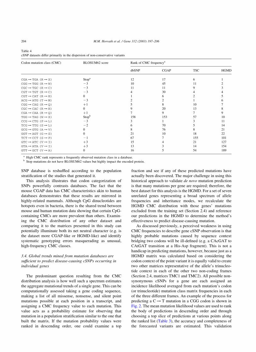
Table 4 details the top ten non-synonymous CMCs from
each dataset. Note that frequent CMCs of one SNP database
often rank highly in any one of the other databases. In fact,
only 18 CMCs describe the top ten most observable events
in all four resources. BLOSUM62 values are given to
provide a rough estimate of the typical impact magnitude of
the amino acid substitution. Nearly all highly ranked CMCs
involve CpG dinucleotides, but three prominent classes
(GGT ! AGT (G ! S), GTC ! ATC (V ! I), and
GTA ! ATA (V ! I)) involve G ! A transitions at non-
CpG sites. Upon manual investigation of individual
mutations in these classes it was found that a substantial
portion of this variation was due to a 50 cytosine that would
create a codon-spanning CpG site. When totaled for all four
cSNP datasets, 109/245 (44.5%), 196/295 (66.4%), and 72/
160 (45.0%) cSNPs in each of these classes, respectively,
occurred at such a CpG dinucleotide (see supplementary
data referenced in Section 2.2). Naively, such results may
prove a weakness of our SNP classification method because
the mutational information contributed by codon-bridging
CpG’s will be diluted over a number of CMCs. While this
may be true, this error is consistent in all CMC distributions
meaning differences in CMC rankings are significant
results. The two V ! I CMCs in Table 4 are affected by
this issue yet there is quite a difference between their
rankings in the CGAP and HGMD resources. Because of the
conservative nature of the replacement (BLOSUM62 score
¼ þ3), V ! I is more frequent in CGAP than in the
HGMD. The CGAP mouse data is dominated by con-
servative CMCs and an excess of silent mutations which is a
consequence of the small, unstratified population examined
by CGAP’s EST-alignment process. Such a low-throughput
method will have power to detect only extremely common
and therefore mostly benign alleles. This data illustrates
how mutation rate and impact are inseparably coupled to
shape the observable allele frequencies in a genotyping
study. The identities of the most observable CMCs in any
M.M. Horvath et al. / Gene 312 (2003) 197–206 203
SNP database is reshuffled according to the population
stratification of the studies that generated it.
This analysis illustrates that codon categorization of
SNPs powerfully contrasts databases. The fact that the
mouse CGAP data has CMC characteristics akin to human
databases demonstrates that these results are mirrored in
highly-related mammals. Although CpG dinucleotides are
hotspots even in bacteria, there is the shared trend between
mouse and human mutation data showing that certain CpG-
containing CMCs are more prevalent than others. Examin-
ing the CMC distribution of any other dataset and
comparing it to the matrices presented in this study can
potentially illuminate both its net neutral character (e.g. is
the dataset more CGAP-like or HGMD-like) and identify
systematic genotyping errors masquerading as unusual,
high-frequency CMC classes.
3.4. Global trends mined from mutation databases are
sufficient to predict disease-causing cSNPs occurring in
individual genes
The predominant question resulting from the CMC
distribution analysis is how well such a spectrum estimates
the aggregate mutational trends of a single gene. This can be
computationally assessed taking a gene coding sequence,
making a list of all missense, nonsense, and silent point
mutations possible at each position in a transcript, and
assigning a CMC frequency value to each mutation. This
value acts as a probability estimate for observing that
mutation in a population stratification similar to the one that
built the matrix. If the mutation probability values were
ranked in descending order, one could examine a top
fraction and see if any of these predicted mutations have
actually been discovered. The major challenge in using this
historical approach to validate de novo mutation prediction
is that many mutations per gene are required; therefore, the
best dataset for this analysis is the HGMD. For a set of seven
unrelated genes representing a broad spectrum of allele
frequencies and inheritance modes, we recalculate the
HGMD CMC distribution with those genes’ mutations
excluded from the training set (Section 2.4) and reference
our predictions in the HGMD to determine the method’s
effectiveness to predict disease-causing mutation.
As discussed previously, a perceived weakness in using
CMC frequencies to describe gene cSNP observation is that
highly probable mutations caused by sequence context
bridging two codons will be ill-defined (e.g. a CAcGAT to
CAtGAT transition at a His-Asp fragment). This is not a
handicap in predicting mutations, however, because just as a
HGMD matrix was calculated based on considering the
codon context of the point variant it is equally valid to create
two other matrices representative of the allele’s trinucleo-
tide context in each of the other two non-coding frames
(Section 2.4, matrices TMC1 and TMC2). All possible non-
synonymous cSNPs for a gene are each assigned an
incidence likelihood averaged from each mutation’s codon
(or trinucleotide) mutation class matrix frequencies in each
of the three different frames. An example of the process for
predicting a C ! T mutation in a CGG codon is shown in
Fig. 2. The mean mutation likelihood values are used to rank
the body of predictions in descending order and through
choosing a top slice of predictions at various points along
the ranked list (Table 3), the accuracy and completeness of
the forecasted variants are estimated. This validation
Table 4
cSNP datasets differ primarily in the dispersion of non-conservative variants
Codon mutation class (CMC) BLOSUM62 score Rank of CMC frequencya
dbSNP CGAP TSC HGMD
CGA! TGA (R! X) Stopa 12 17 6 1
CGG! TGG (R! W) 23 10 45 11 2
CGC! TGC (R! C) 23 11 11 9 3
CGT! TGT (R! C) 23 4 30 4 4
CGT! CAT (R! H) 0 1 6 2 5
ACG! ATG (T! M) 23 2 2 1 6
CGG! CAG (R! Q) þ1 5 8 10 7
CGC! CAC (R! H) 0 9 20 13 8
CGA! CAA (R! Q) þ1 7 9 7 9
TGG! TAG (W! X) Stopb 158 153 57 10
CCG! CTG (P! L) 23 3 1 3 11
TCG! TTG (S! L) 22 6 70 5 14
GCG! GTG (A! V) 0 8 76 8 21
GGT! AGT (G! S) 0 21 10 18 22
TCT! CCT (S! P) 21 67 7 155 101
GTC! ATC (V! I) þ3 15 4 21 127
GTA! ATA (V! I) þ3 13 3 14 154
GTT! GCT (V! A) 0 16 5 54 189
a High CMC rank represents a frequently observed mutation class in a database.b Stop mutations do not have BLOSUM62 values but highly impact the encoded protein.
M.M. Horvath et al. / Gene 312 (2003) 197–206204

technique suffers from the fact that for no gene are all of the
disease-relevant alleles known; therefore, the perceived
accuracy will be a lower estimate only.
As Table 3 shows, all seven genes have an easily-
predicted volume of mutational space despite the wide
spectrum of allele inheritance modes represented, which
illustrates the generality of point mutation trends. When
considering only the top quarter percentile of ranked non-
synonymous substitutions to be potential disease-causing
alleles, 56/64 predictions (87.5%) in this select fraction are
already known to cause disease. Depending on a gene’s
cSNP saturation, this method is between 6.3 to 181-fold
more accurate than predicting causative cSNPs using the
null model of mutation (Table 3), which assumes that all
cSNPs are equally likely to occur and therefore predicts
mutations randomly. There is an obvious correlation
between prediction accuracy and the number of clinically
identified alleles; therefore, we believe that many of the
false positive mutations predicted in Table 3 (i.e. they are
not detailed in the HGMD) exist and cause disease but either
have not yet been discovered or are annotated in a separate
database. Although a tedious task given the non-uniformity
of both central and locus-specific mutation databases
(Claustres et al., 2002), matching our predictions against
any other known polymorphisms would increase accuracy
to even higher rates than reported here. For example,
manual searching of the CFTR Mutation Database
(Bobadilla et al., 2002) reveals that three unconfirmed
predictions at the 0.5% level in Table 3 do exist: 31R ! H,
170R ! H, and 1453R ! Q (HGMD base numbering
used), but their relation to disease is uncertain. But in
terms of predicting real mutations in CFTR, the accuracy
rate increases to 39/52 predictions or 75.0%.
Since the original CMC matrix frequencies were
calculated, 2,052 additional point mutations have been
entered into the HGMD as of 10/17/2002. Often many
of these new entries were recognized from the
unverified prediction list of the older dataset. For each
gene AR, RPE65, DMD, CHM, MSH2, KEL, MCOLN1,
and ATP7A two to three out of the top five most likely
but uncataloged mutations (18/40 predictions) were
described in the HGMD as causative of disease over
the next 5 months (e.g. KEL R128 ! X (Lee et al.,
2001), RPE65 R91 ! W (Morimura et al., 1998), and
ATP7A R980 ! X (Gu et al., 2001)). If the same test
was performed another six months from now with a
current list of unverified predictions, it stands to reason
that a similar fraction will have been annotated in the
HGMD. Based on these results, for a newly discovered,
poorly characterized gene in the human genome one can
immediately predict a handful of point variants that are
both likely to exist and cause disease. With candidate
disease alleles in hand, a researcher can employ high-
throughput genotyping technologies, such as oligonu-
cleotide microarrays (Bell et al., 2002), mass spec-
troscopy (Buetow et al., 2001), or Pyrosequencing
(Ahmadian et al., 2000), where the identity of a single
user-defined DNA base is queried (instead of a whole
amplicon). These methods can determine thousands of
genotypes a day if they have the foreknowledge of the
exact base that is expected to be multiallelic. Targeted
bases could be acquired from the prediction methods
presented here to boost success of association studies,
especially when the number of candidate genes is quite
large. Once a few mutations are found researchers may
then elect to sequence the entire gene. The advantage in
this protocol is that candidate genes are first screened at
the most likely places of variation to decrease the
number of amplicons undergoing costly and lengthy
resequencing. The CMC method therefore has the power
to tell a researcher today what disease-causing alleles
will be found tomorrow by guiding genotyping
experiments.
Since the mutation propensity of genes is based upon
sequence context, the cumulative mutation likelihood for
genes or gene fragments implies how codon bias is
modulated in those objects so that the chance of and type
of point mutation would be skewed towards that required by
selection pressures, either towards a more stable or more
hypermutable sequence. Using our methods a de novo-
mutation spectra estimated from empirical data is available
to approximate the relative mutability of genes.
4. Conclusions
(1) Convergent data from four independent datasets
shows a general, gene-independent pattern of point
mutation where a considerable fraction of cSNPs can be
described and consistently predicted by a handful of
trinucleotide sequence contexts.
(2) cSNP databases differ in the distribution of non-
synonymous mutations where as the cohort genotyped
decreases in size and individuals are more randomly
selected, non-conservative mutations rarify while the
proportion of observed conservative mutations and silent
substitutions dramatically increases.
(3) Since sequence diversity is not only a result of
intrinsic mutation rates but also of the evolutionary
forces that act on the targeted DNA sequence, mutation
rates cannot be calculated directly from cSNP databases.
However, deconvolution of a cSNP database into a
distribution of mutation preferences for cSNP sequence
contexts allows relative comparison of cSNP datasets
detected in differing species, populations, and
environments.
(4) Trinucleotide mutation preferences gleaned from
cSNP databases permits prediction of the most likely
handful of human mutations that will be found in a
similarly stratified population and may shed light on how
the relative mutation likelihood of gene families differ
and steer genotyping studies.
M.M. Horvath et al. / Gene 312 (2003) 197–206 205
Acknowledgements
This work was supported by the National Institutes of
Health grant no. CA-81656, Program in Genomic Appli-
cations grant P50 CA70907, contract DAAD13-02-C-0079
from the Soldier Biological Chemical Command: APG to
the Biological Chemical Countermeasures program of The
University of Texas, and the State of Texas Advanced
Technology Program. We thank Alex Pertsemlidis, M. Ryan
Weil, Jeff Schageman, and Jonathan Wren for critical
reading of the manuscript.
References
Adams, W.T., Skopek, T.R., 1987. Statistical test for the comparison of
samples from mutational spectra. J. Mol. Biol. 194, 391–396.
Ahmadian, A., et al., 2000. Analysis of the p53 tumor suppressor gene by
pyrosequencing. Biotechniques (28), 140–147.140-144, 146-147.
Altschul, S.F., et al., 1997. Gapped BLAST and PSI-BLAST: a new
generation of protein database search programs. Nucleic Acids Res. 25,
3389–3402.
Altshuler, D., et al., 2000. An SNP map of the human genome generated by
reduced representation shotgun sequencing. Nature 407, 513–516.
Bell, P.A., et al., 2002. SNPstream UHT: ultra-high throughput SNP
genotyping for pharmacogenomics and drug discovery. Biotechniques
Suppl., 70–77.70-72, 74, 76-77.
Bobadilla, J.L., et al., 2002. Cystic fibrosis: a worldwide analysis of CFTR
mutations–correlation with incidence data and application to screening.
Hum. Mutat. 19, 575–606.
Brookes, A.J., 1999. The essence of SNPs. Gene 234, 177–186.
Buetow, K.H., et al., 1999. Reliable identification of large numbers of
candidate SNPs from public EST data. Nat. Genet. 21, 323–325.
Buetow, K.H., et al., 2001. High-throughput development and character-
ization of a genome wide collection of gene-based single nucleotide
polymorphism markers by chip-based matrix-assisted laser desorption/
ionization time-of-flight mass spectrometry. PNAs 98, 581–584.
Cargill, M., et al., 1999. Characterization of single-nucleotide polymorph-
isms in coding regions of human genes. Nat. Genet. 22, 231–238.
Claustres, M., et al., 2002. Time for a unified system of mutation
description and reporting: a review of locus-specific mutation
databases. Genome Res. 12, 680–688.
Clifford, R., et al., 2000. Expression-based genetic/physical maps of single-
nucleotide polymorphisms identified by the cancer genome anatomy
project. Genome Res. 10, 1259–1265.
Cooper, D.N., Krawczak, M., 1990. The mutational spectrum of single
base-pair substitutions causing human genetic disease: patterns and
predictions. Hum. Genet. 85, 55–74.
Cooper, D.N., Krawczak, M., 1993. Human Gene Mutation, BIOS
Scientific Publishers Ltd.,, Oxford.
Glatt, C.E., et al., 2001. Screening a large reference sample to identify very
low frequency sequence variants: comparisons between two genes. Nat.
Genet. 27, 435–438.
Gu, Y.H., et al., 2001. ATP7A gene mutations in 16 patients with Menkes
disease and a patient with occipital horn syndrome. Am. J. Med. Genet.
99, 217–222.
Henikoff, S., Henikoff, J.G., 1993. Performance evaluation of amino acid
substitution matrices. Proteins 17, 49–61.
Krawczak, M., et al., 2000. Human Gene Mutation Database–A
Biomedical Information and Research Resource. Hum. Mutat. 15,
45–51.
Lee, S., et al., 2001. Molecular defects underlying the Kell null phenotype.
J. Biol. Chem. 276, 27281–27289.
Morimura, H., et al., 1998. Mutations in the RPE65 gene in patients with
autosomal recessive retinitis pigmentosa or leber congenital amaurosis.
Proc. Natl. Acad. Sci. USA 95, 3088–3093.
Mullikin, J.C., et al., 2000. An SNP map of human chromosome 22. Nature
407, 516–520.
Nakamura, Y., et al., 2000. Codon usage tabulated from international DNA
sequence databases: status for the year 2000. Nucleic Acids Res. 28,
292.
Pruitt, K.D., Maglott, D.R., 2001. RefSeq and LocusLink: NCBI gene-
centered resources. Nucleic Acids Res. 29, 137–140.
Riggins, G.J., Strausberg, R.L., 2001. Genome and genetic resources from
the Cancer Genome Anatomy Project. Hum. Mol. Genet. 10, 663–667.
Sachidanandam, R., et al., 2001. A map of human genome sequence
variation containing 1.42 million single nucleotide polymorphisms.
Nature 409, 928–933.
Schuler, G.D., 1997. Pieces of the puzzle: expressed sequence tags and the
catalog of human genes. J. Mol. Med. 75, 694–698.
Shapiro, G.S., et al., 1999. Predicting regional mutability in antibody V
genes based solely on di- and trinucleotide sequence composition.
J. Immunol. 163, 259–268.
Shapiro, G.S., et al., 2002. Evolution of Ig DNA sequence to target specific
base positions within codons for somatic hypermutation. J. Immunol.
168, 2302–2306.
Smigielski, E.M., et al., 2000. dbSNP: A database of single nucleotide
polymorphisms. Nucleic Acids Res. 28, 352–355.
Wang, Z., Moult, J., 2001. SNPs, protein structure, and disease. Hum.
Mutat. 17, 263–270.
Wilbur, W.J., 1985. On the PAM matrix model of protein evolution. Mol.
Biol. Evol. 2, 434–447.
Zar, J.H., 1996. Biostatistical Analysis, 3, Prentice-Hall, Upper Saddle
River.
M.M. Horvath et al. / Gene 312 (2003) 197–206206
Top Related
Copyright © 2022 FDOKUMEN

