


Bahasa
Halaman
Hukum


Industry Dynamics and the Distributionof Firm Sizes: A Non-Parametric Approach
Francesca Lotti*
andEnrico Santarelli †
* St.Anna School of Advanced Studies, Pisa, Italy† University of Bologna, Department of Economics, Italy
2001/14 October 2001
LLEEMM
Laboratory of Economics and ManagementSant’Anna School of Advanced StudiesVia Carducci, 40 - I-56127 PISA (Italy)Tel. +39-050-883-341 Fax +39-050-883-344Email: [email protected] Web Page: http://lem.sssup.it
Working Paper Series

1
INDUSTRY DYNAMICS AND THE DISTRIBUTION
OF FIRM SIZES: A NON-PARAMETRIC APPROACH*
by
Francesca Lotti
St’Anna School of Advanced Studies – Pisa, Italy
and
Harvard University, Department of Economics – Cambridge, MA
Enrico Santarelli
University of Bologna, Department of Economics
Abstract
The aim of this paper is to analyze the evolution of the size distribution of young firms within some selected industries, trying to assess the empirical implications of different models of industry dynamics: the model of passive learning (Jovanovic 1982), the model of active learning (Ericson and Pakes, 1995), and the evolutionary model (Audretsch, 1995). We use a non-parametric technique, the Kernel density estimator, applied to a data set from the Italian National Institute for Social Security (INPS), consisting in 12 cohorts of new manufacturing firms followed for 6 years. Since the patterns of convergence to the limit distribution are different between industries, we conclude that the model of passive learning is consistent with some of them, the active exploration model with others, the evolutionary model with all of them.
Keywords: Cohorts; Gibrat’s Law; Kernel; Industry Dynamics; Non-parametric; Shakeouts.
JEL Classification: L11, L60
This version: October 9, 2001
Francesca Lotti Laboratory of Economics and Management, St'Anna School of Advanced Studies, Via Carducci, 40 56127 Pisa, Italy. [email protected]
Enrico Santarelli Economics Department, University of Bologna, Strada Maggiore, 45 40125 Bologna, Italy, [email protected]
* Previous versions of this paper were presented at the Econometrics Seminars at UC Riverside (18 May 2001), and the XXVIII Annual E.A.R.I.E. Conference (Dublin, 31 August - 2 September 2001). We wish to thank the audience for valuable comments. Discussions with Giovanni Dosi, Samuel Kortum, Josè Mata, Markus Mobius, Ariel Pakes, Jack Porter, Aman Ullah and Marco Vivarelli have been very helpful. Financial support from MURST (“Cofinanziamento 2000”, responsible E. Santarelli) is gratefully acknowledged.

2
1 - Introduction
Analysis of the size-growth relationship is a commonly used approach to the study of the
evolution of market structure. In fact, the firm size distribution (FSD) has received considerable
attention - since the seminal works of Herbert Simon and his co-authors between the late 1950s and
the 1970s (cf. Simon and Bonini, 1958; and Ijiri and Simon, 1964, 1977) - in most theoretical and
empirical studies dealing with the overall process of industry dynamics. The empirical evidence
showed a FSD highly skewed to the right, meaning that the size distribution of firms is lognormal,
both at the industry level and in the overall economy. This piece of evidence is coherent with the
so-called Law of Proportionate Effect (or Gibrat’s (1931) Law): as Simon and Bonini (1958) point
out, if one “…incorporates the law of proportionate effect in the transition matrix of a stochastic
process, […] then the resulting steady-state distribution of the process will be a highly skewed
distribution”. Recent evidence based on more complete data sets, suggests that Gibrat’s Law is not
confirmed, either for new-born or established firms (for a survey, cf. Geroski, 1995; Lotti et al.,
1999), since smaller firms grow more than proportionally with respect to larger ones. This finding
should be consistent with a departure of the FSD from the lognormal distribution.
In this paper - using quarterly data for 12 cohorts of new manufacturing firms - we account
for the evolution of the FSD over time in the case of young firms. Moreover, we try to assess the
empirical implications of different models of industry dynamics. The work is organized as follows.
Section 2 contains a review of the empirical evidence about Gibrat’s Law and the FSD, as well as
an overview of some recent models of industry dynamics. Section 3 describes the data and the
methodology used, whereas Section 4 summarizes the main empirical findings. Finally, Section 5
contains some concluding remarks.
2 - Theory or Stylized Facts?
Gibrat’s Law, applied to the analysis of market structure, represents the first attempt to
explain in stochastic terms the systematically skewed pattern of the size distribution of firms within
an industry (Sutton, 1997). In effect, the Law cannot be rejected if a) firm growth follows a random
process and is independent from initial size, and b) the resulting distributions of firms’ size are
lognormal1. Although, from a theoretical viewpoint, labeled as “unrealistic” since Kalecki’s (1945)
study on the size distribution of factories in US manufacturing, this result was initially consistent
with some empirical studies dealing with incumbent, large firms (Hart and Prais, 1956; Simon and
Bonini, 1958; Hymer and Pashigian, 1962). In recent years, most studies have instead shown that
these exhibit a different behavior, identifying an overall negative relationship between initial size
and post-entry rate of growth (cf., among others, Mata, 1994; Hart and Oulton, 1999). However,
Lotti et al. (2001. (a) e (b)) found that, in the case of new-born firms, the growth rates are
1 Of course, a FSD skewed to the right implies only that Gibrat’s Law cannot be rejected. However, one cannot a priori exclude that the skewness is the result of turbulence, namely of the presence of new-born small firm in the right tail of the distribution.

3
negatively correlated with their initial size only during their infancy: Gibrat’s Law fails to hold in the years immediately following start-up, when smaller firms have to rush in order to reach a size
large enough to enhance their likelihood of survival; but in the subsequent years, the patterns of
growth of entrants do not differ significantly from the landscape of the industry as a whole.
One possible way to explain this phenomenon of self-selection, is to consider the firms’
learning and evolution processes put forward by Jovanovic (1982), Ericson and Pakes (1995), and
Audretsch (1995). By following such perspectives, entrants are uncertain about their relative level
of efficiency, and only once into the market they learn about their possibilities of survival and
growth. The main advantage of these models is that they allow for a) heterogeneity among firms, b)
idiosyncratic sources of uncertainty and discrete possible events, c) entry and exit.
Boyan Jovanovic’s model of passive learning hypothesizes that firms are initially endowed
with uncertain, time-invariant characteristics (i.e. efficiency parameters), of which the firm does not
know the distribution. But, once into the market, the firm learns passively about the true efficiency parameter. As a consequence, in every period the firm has to decide its strategy: whether to exit,
continue with the same size, grow in size, or reduce its productive capacity. One of the
consequences of this model is that, due to a particular kind of selection process, the most efficient
firms survive and grow, while the others are bound to shrink or to exit from the market.
Like in the passive learning model, Richard Ericson and Ariel Pakes’s model of active
learning (1995) assumes that all the decisions taken by the firms are meant to maximize the
expected discounted value of the future net cash, conditional on the current information set. Unlike
in Jovanovic’s model, a firm knows its own characteristics and its competitors’ ones, along with the
future distribution of industry structure, conditional on the current structure. Accordingly, this
model can be usefully employed in explanation of ‘entry mistakes’ (as defined by Cabral, 1997),
namely the fact that in every period and every industry more firms enter than the market can
sustain. Within an active learning perspective, such mistakes occur due to lags in observation of rivals’ entry decision or just because entry investments take time (Cabral, 1997). In a subsequent
work, Pakes and Ericson (1998), using two cohorts of firms from Wisconsin, belonging to the retail
and the manufacturing industries, found that the structure of the former industry is compatible with
the passive learning model, while that of the latter with their model of active exploration (learning).
The retail cohort, after eight years seems to have reached the size distribution of the industry as a
whole, while the manufacturing one, even if showing higher growth rates, after that period is still
far from the limit distribution.
David Audretsch (1995) expanded the passive learning approach put forward by Jovanovic
(1982) into an evolutionary perspective, allowing for inter-industry differences in the likelihood of
survival of newborn firms. Accordingly, industry-specific characteristics, such as scale economies
and the endowment of innovative capabilities, exert a significant impact on entry, exit, and the
likelihood of survival of newborn firms. For example, in industries characterized by higher minimum efficient scale (MES) levels of output, smaller firms face higher costs that are likely to
push them out of the market within a short period after start-up. Thus, only the most efficient
among newborn firms will survive and grow, whereas the other are pushed out of the market (cf.

4
Audretsch et al., 1999). In this case, the presence of more potential entrants than firms with a significant likelihood to survive in the long run can bring about a shakeout (cf. Klepper and Miller,
1995). In turn, a shakeout occurring at a certain point in the industry’s history is likely to affect the
long-run size distribution of firms within the same industry, depending on “how the opportunities
vacated by exited firms are reallocated among surviving firms” (Sutton, 1998, p. 260; cf. also
Klepper and Graddy, 1990). Conversely, in industries with a lower MES level of output the
likelihood of survival will be independent of the firms’ ability to grow (cf. Amaral et al., 1977;
Brock, 1999).
With this theoretical and empirical background in mind, we look at the evolution of 12
cohorts of newborn firms in selected industries, in order to analyze the process of convergence of
the firm size distribution, in terms of number of employees, with respect to the overall industry
landscape. The aim of this analysis is to show i) whether the findings by Herbert Simon and his co-
authors concerning the Skewness to the right of the FSD are confirmed also in the case of newborn, small firms and ii) whether the FSD resulting from application of the Kernel density estimator is
consistent with models of industry dynamics - such as those surveyed above - which identify in the
learning processes occurring at the firm level, and in the level of sunk costs that characterizes each
industry, some possible theoretical explanations for these facts.
3 - Data and Methodology
We use a data set from the Italian National Institute for Social Security (INPS), dealing with
12 cohorts of new manufacturing firms (with at least one paid employee) born in each month of
1987, and their follow up until December 1992.
Since all private Italian firms are compelled to pay national security contributions for their
employees to INPS, the registration of a new firm as “active” signals an entry into the market, while
the cancellation of a firm denotes an exit (this happens when a firm finally stops paying national security contributions). For administrative reasons - delays in payment, for instance, or uncertainty
about the current status of the firm - some firms are classified as “suspended”. In the present work
we consider these suspended firms as exiting from the market at the moment of their transition from
the status of “active” to that of “suspended”, while firms which have stopped their activity only
temporarily were included again in the sample once they turned back active. We carry out also an
accurate cleaning procedure, aimed at identifying internal inconsistencies and entry or exit due to
firm transfers and acquisitions. As regards acquisitions, these are denoted as “extraordinary
variations” in the INPS database, and firms involved in such activities can therefore be easily
identified and cancelled from the database itself. A correct identification of firms disappeared via
acquisitions permitted to avoid acquiring firms to be drawn disproportionately from the low end of
the size distribution. As pointed out by Sutton (1998; cf. also Hart and Prais, 1956; Hymer and
Pashigian, 1962) this would have caused a violation in the proposed bound and altered the significance of the overall analysis.
We focus our analysis on four industries - Electrical & Electronic Engineering, Instruments,
Food, and Footwear & Clothing - mainly for two main reasons: the first one concerns their very

5
different market structure in terms of cost of entry (sunk costs), and the second the fact that the latter two industries are less technologically progressive than the former two ones2.
To examine the effect of firms’ age on the distribution of their sizes, we study each cohort at
each quarter after start-up, and this for their first six years in the market. In Tables 1A-1D and in
Table 2 some descriptive statistics are reported. In general, all industries experience a shakeout
period during which the number of survivors, among new entrants, declines by 40 per cent or more.
From Tables 1A, B, C, and D it turns out that, on average, the survival rate at the end of the period
(i.e., after 21 quarters) is much higher within the cohorts belonging to the Electrical & Electronic
Engineering and the Instruments industries, than it is the case with the Food and the Footwear &
Clothing industries. Thus, consistently with Audretsch’s (1995) hypothesis, industry specific
characteristics, such as the commitment to innovative activities, seem to set in motion a pre-entry
selection mechanism that selects only those start-ups that find in their endowment of innovative
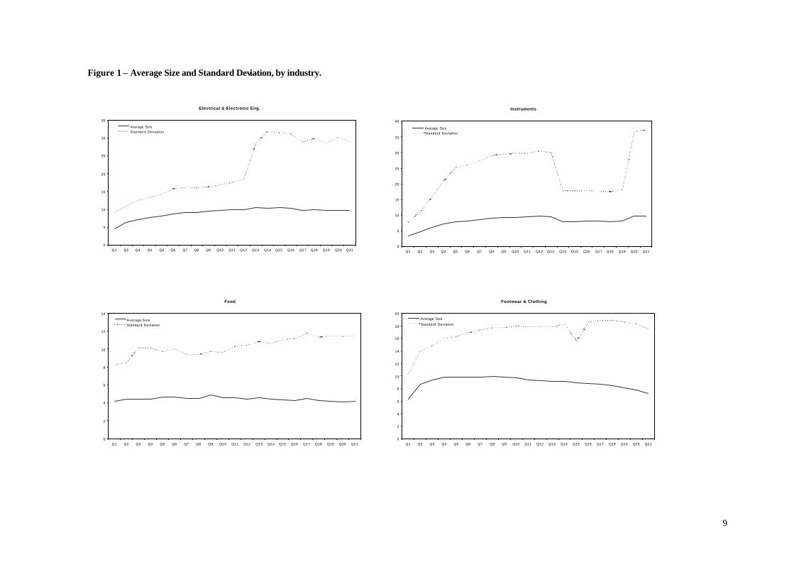
capabilities a possible competitive advantage. Looking at Table 2 Figure 1, one immediately observes that - with the sole exception of the
Food industry - the standard deviation of firm sizes is much higher at the end of the relevant period
than in the first quarter. Dispersion of firm sizes tends therefore to widen as surviving firms reach
the MES level of output and specialize in one of the many clusters of products which - according to
John Sutton's (1998, pp. 597-605) "independent submarkets" hypothesis - characterize each
industry. In turn, firm size increases along with its age for the Electrical & Electronic Engineering
and the Instruments industries, but only for the first 13 and 12 quarters respectively, corresponding
with a period comprised approximately between December 1989 and January 19913. Afterwards, a
decline in average firm size emerges, which is consistent with views of recessions (the period
between 1991 and 1993 has been characterized in Italy by a significant slowdown in the GDP
growth rates) as times of “cleansing” (cf. Boeri and Bellmann, 1995). In fact, the sectoral data
reported in Table 3 show for both industries a significant decrease in the growth rates of value added since 1989, with a trough in 1993. This pro-cyclical pattern of the average firm size is even
more marked in the Footwear & Clothing industry, in which the average size starts to decline after
the eight quarter in the market (as early as 1989, that is the initial year of the recession). The data on
the Footwear & Clothing industry show a substantial stability of the average firm size over time.
This result is to some extent consistent with the dynamics of value added in the same industry:
Table 3 points out alternate peaks and troughs in the Footwear & Clothing industry growth rates
that are unlikely to affect firm size, since this needs time to adjust its patterns to variations in value
added.
2 And this would allow to draw some conclusions on whether the FSD is or is not sensitive to technological factors. 3 In effect, since the 12 cohorts include firms born in each month of 1987, each column in Table 2 deals with all firms and all cohorts.

6
Table 1A - Number of firms active at the end of each quarter – Electrical & Electronic Engineering
Q1 Q2 Q3 Q4 Q5 Q6 Q7 Q8 Q9 Q10 Q11 Q12 Q13 Q14 Q15 Q16 Q17 Q18 Q19 Q20 Q21
Cohort 1 128 125 121 120 117 113 112 109 108 107 106 105 104 103 102 102 97 95 93 92 90 Cohort 2 64 61 59 56 53 51 52 51 50 50 50 50 49 47 44 43 40 38 36 37 38 Cohort 3 72 68 65 62 60 61 61 61 57 55 53 53 53 51 51 48 48 48 48 47 43 Cohort 4 49 46 47 47 47 47 45 43 43 43 42 41 40 41 41 39 38 34 33 33 33 Cohort 5 59 53 53 52 53 50 50 47 46 48 46 44 44 43 41 40 37 37 35 34 34 Cohort 6 71 68 65 64 62 62 63 59 58 55 49 49 49 48 47 45 44 42 41 37 36 Cohort 7 41 41 41 41 39 38 38 37 37 36 34 30 30 29 28 27 27 27 25 24 23 Cohort 8 18 18 18 17 17 17 17 17 16 15 15 15 15 15 14 14 14 14 14 12 12 Cohort 9 72 67 63 63 64 62 60 58 58 57 57 57 55 56 52 52 53 52 50 50 49 Cohort 10 60 58 54 50 49 50 52 49 47 47 44 44 44 41 42 42 42 42 40 39 38 Cohort 11 57 53 55 53 53 51 51 51 50 48 46 46 43 42 40 41 39 38 39 39 39 Cohort 12 29 28 26 25 25 25 25 26 25 25 24 23 23 23 23 22 22 22 21 20 19 Total 720 686 667 650 639 627 626 608 595 586 566 557 549 539 525 515 501 489 475 464 454
Table 1B - Number of firms active at the end of each quarter – Instruments
Q1 Q2 Q3 Q4 Q5 Q6 Q7 Q8 Q9 Q10 Q11 Q12 Q13 Q14 Q15 Q16 Q17 Q18 Q19 Q20 Q21
Cohort 1 62 61 60 60 59 56 56 56 55 53 51 51 50 50 48 46 43 41 40 42 40 Cohort 2 38 37 35 36 35 35 34 34 34 33 32 29 28 27 27 27 26 24 24 25 25 Cohort 3 34 32 33 33 31 31 30 30 28 27 27 26 24 23 22 21 19 20 20 20 20 Cohort 4 26 26 25 24 23 23 20 19 19 18 18 17 17 17 17 16 17 17 17 17 17 Cohort 5 20 20 20 19 19 19 19 19 18 19 18 17 17 15 14 14 14 14 14 13 13 Cohort 6 33 33 32 31 28 28 28 27 27 25 24 23 21 21 21 21 21 21 21 17 19 Cohort 7 35 34 30 30 30 28 27 25 25 25 24 25 25 24 23 23 22 21 21 22 22 Cohort 8 11 11 10 10 10 10 10 10 10 10 10 10 10 10 10 10 8 7 7 7 6 Cohort 9 27 27 25 24 24 23 23 23 23 22 22 22 21 20 20 20 19 20 18 18 18 Cohort 10 32 30 28 26 26 27 25 24 23 24 22 21 21 20 19 18 18 18 18 17 17 Cohort 11 26 25 25 24 24 22 22 19 19 19 18 17 17 17 17 17 16 16 15 15 15 Cohort 12 18 18 17 16 15 14 14 14 14 14 14 13 13 12 11 11 11 11 11 11 10 Total 362 354 340 333 324 316 308 300 295 289 280 271 264 256 249 244 234 230 226 224 222

7
Table 1C - Number of firms active at the end of each quarter – Food
Q1 Q2 Q3 Q4 Q5 Q6 Q7 Q8 Q9 Q10 Q11 Q12 Q13 Q14 Q15 Q16 Q17 Q18 Q19 Q20 Q21
Cohort 1 93 88 88 83 78 76 73 72 70 70 68 67 65 63 61 59 58 56 57 55 54 Cohort 2 47 43 40 37 34 34 33 33 29 28 28 27 24 24 24 24 22 23 23 21 21 Cohort 3 46 43 42 39 40 37 37 34 34 33 30 27 26 27 25 21 21 23 23 19 19 Cohort 4 40 35 30 29 30 29 29 29 28 28 29 27 26 25 23 19 19 20 20 19 19 Cohort 5 41 38 35 33 34 35 34 32 29 28 27 27 25 24 23 22 22 21 21 21 19 Cohort 6 44 42 37 35 32 29 29 29 28 28 25 25 25 25 25 25 24 24 24 24 22 Cohort 7 46 35 35 34 38 35 33 33 35 30 30 27 25 24 24 23 22 21 22 22 21 Cohort 8 20 16 15 15 14 13 12 8 9 8 8 8 8 8 8 8 9 7 7 7 7 Cohort 9 30 27 22 19 20 19 18 17 18 19 17 18 16 17 15 15 14 15 14 13 13 Cohort 10 51 40 34 32 32 30 30 26 29 26 23 24 26 21 19 18 23 19 18 16 19 Cohort 11 110 65 53 47 72 49 42 40 67 40 32 31 40 33 31 30 57 38 30 28 43 Cohort 12 80 42 23 23 47 29 21 18 49 19 12 12 22 10 10 9 37 25 12 11 27 Total 684 514 454 426 471 415 391 371 425 357 329 320 328 301 288 273 328 292 271 256 284
Table 1D - Number of firms active at the end of each quarter – Footwear & Clothing
Q1 Q2 Q3 Q4 Q5 Q6 Q7 Q8 Q9 Q10 Q11 Q12 Q13 Q14 Q15 Q16 Q17 Q18 Q19 Q20 Q21
Cohort 1 164 159 158 156 145 143 136 132 129 126 121 120 113 112 110 110 103 100 98 95 93 Cohort 2 92 89 84 80 74 69 68 67 61 55 55 55 53 50 46 46 43 42 40 37 35 Cohort 3 85 79 76 73 71 65 62 60 59 56 51 50 48 45 45 41 40 40 38 38 37 Cohort 4 97 91 83 77 72 70 69 64 64 62 58 51 51 45 40 40 37 36 35 34 34 Cohort 5 100 93 86 83 83 79 78 74 74 70 68 66 67 65 59 55 55 48 40 49 45 Cohort 6 89 87 81 77 74 72 72 70 69 64 63 59 58 53 51 50 49 45 44 43 41 Cohort 7 88 80 73 69 69 65 63 60 57 55 54 55 53 52 48 44 43 43 42 41 41 Cohort 8 36 28 24 26 25 23 22 23 22 21 19 18 17 16 15 13 13 13 13 12 12 Cohort 9 97 95 87 84 78 75 70 68 67 63 65 63 60 59 57 56 55 55 52 51 49 Cohort 10 104 99 88 81 78 75 78 71 66 62 61 62 61 56 56 55 54 52 46 46 43 Cohort 11 96 93 86 78 75 68 63 61 61 57 54 51 49 47 43 41 40 40 38 37 34 Cohort 12 51 46 43 41 39 35 34 34 35 31 29 27 28 28 27 26 26 26 26 24 20 Total 1099 1039 969 925 883 839 815 784 764 722 698 677 658 628 597 577 558 540 522 506 484
8
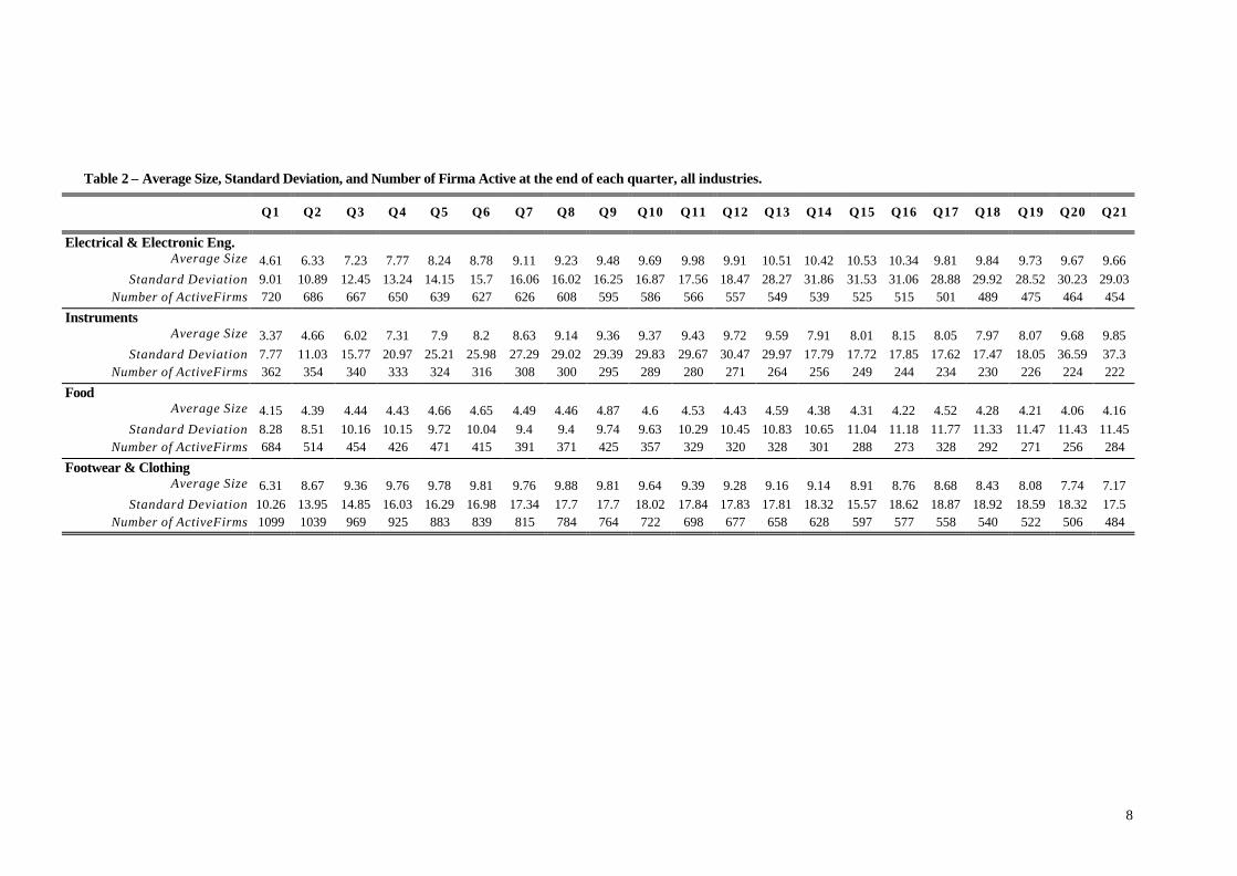
Table 2 – Average Size, Standard Deviation, and Number of Firma Active at the end of each quarter, all industries.
Q1 Q2 Q3 Q4 Q5 Q6 Q7 Q8 Q9 Q10 Q11 Q12 Q13 Q14 Q15 Q16 Q17 Q18 Q19 Q20 Q21
Electrical & Electronic Eng. Average Size 4.61 6.33 7.23 7.77 8.24 8.78 9.11 9.23 9.48 9.69 9.98 9.91 10.51 10.42 10.53 10.34 9.81 9.84 9.73 9.67 9.66
Standard Deviation 9.01 10.89 12.45 13.24 14.15 15.7 16.06 16.02 16.25 16.87 17.56 18.47 28.27 31.86 31.53 31.06 28.88 29.92 28.52 30.23 29.03 Number of ActiveFirms 720 686 667 650 639 627 626 608 595 586 566 557 549 539 525 515 501 489 475 464 454
Instruments Average Size 3.37 4.66 6.02 7.31 7.9 8.2 8.63 9.14 9.36 9.37 9.43 9.72 9.59 7.91 8.01 8.15 8.05 7.97 8.07 9.68 9.85
Standard Deviation 7.77 11.03 15.77 20.97 25.21 25.98 27.29 29.02 29.39 29.83 29.67 30.47 29.97 17.79 17.72 17.85 17.62 17.47 18.05 36.59 37.3 Number of ActiveFirms 362 354 340 333 324 316 308 300 295 289 280 271 264 256 249 244 234 230 226 224 222
Food Average Size 4.15 4.39 4.44 4.43 4.66 4.65 4.49 4.46 4.87 4.6 4.53 4.43 4.59 4.38 4.31 4.22 4.52 4.28 4.21 4.06 4.16
Standard Deviation 8.28 8.51 10.16 10.15 9.72 10.04 9.4 9.4 9.74 9.63 10.29 10.45 10.83 10.65 11.04 11.18 11.77 11.33 11.47 11.43 11.45 Number of ActiveFirms 684 514 454 426 471 415 391 371 425 357 329 320 328 301 288 273 328 292 271 256 284
Footwear & Clothing Average Size 6.31 8.67 9.36 9.76 9.78 9.81 9.76 9.88 9.81 9.64 9.39 9.28 9.16 9.14 8.91 8.76 8.68 8.43 8.08 7.74 7.17
Standard Deviation 10.26 13.95 14.85 16.03 16.29 16.98 17.34 17.7 17.7 18.02 17.84 17.83 17.81 18.32 15.57 18.62 18.87 18.92 18.59 18.32 17.5 Number of ActiveFirms 1099 1039 969 925 883 839 815 784 764 722 698 677 658 628 597 577 558 540 522 506 484
9
Figure 1 – Average Size and Standard Deviation, by industry.
Electrical & Electronic Eng.
0
5
10
15
20
25
30
35
Q1 Q2 Q3 Q4 Q5 Q6 Q7 Q8 Q9 Q10 Q11 Q12 Q13 Q14 Q15 Q16 Q17 Q18 Q19 Q20 Q21
Average SizeStandard Deviation
Instruments
0
5
10
15
20
25
30
35
40
Q1 Q2 Q3 Q4 Q5 Q6 Q7 Q8 Q9 Q10 Q11 Q12 Q13 Q14 Q15 Q16 Q17 Q18 Q19 Q20 Q21
Average SizeStandard Deviation
Food
0
2
4
6
8
10
12
14
Q1 Q2 Q3 Q4 Q5 Q6 Q7 Q8 Q9 Q10 Q11 Q12 Q13 Q14 Q15 Q16 Q17 Q18 Q19 Q20 Q21
Average SizeStandard Deviation
Footwear & Clothing
0
2
4
6
8
10
12
14
16
18
20
Q1 Q2 Q3 Q4 Q5 Q6 Q7 Q8 Q9 Q10 Q11 Q12 Q13 Q14 Q15 Q16 Q17 Q18 Q19 Q20 Q21
Average Size
Standard Deviation
10
Table 3 – Growth rates (%) of Value added in constant (1995) prices
Industries 1986 1987 1988 1989 1990 1991 1992 1993 1994
Electrical & Electronic Engineer. - 0,5 2,9 5,1 3,9 0,2 - 1,3 0,2 - 8,7 6,1 Instruments 5,9 5,3 7,8 4,9 3,7 2,6 - 1,2 - 4,2 6,5 Food 7,0 2,3 5,8 2,4 5,9 3,3 7,4 1,7 0,0 Footwear & Clothing 0,2 2,4 4,7 1,1 2,6 1,8 0,4 - 2,7 6,8 Source: ISTAT, National Statistical Office of Italy
In a recent paper by Machado and Mata (2000) the Box-Cox quantile regression method is
used to estimate the distribution of firm sizes and, accordingly, to analyze industry dynamics in Portugal. This approach consists in modelling each quantile as a function of a number of industry
characteristics that are expected to affect firm size. Since our database doesn’t provide any details
about industry characteristics, in the present study we use instead a non-parametric approach. The
basic idea is to look if, with the passing of time, the empirical distribution of firm sizes converges
towards a lognormal distribution, under the hypothesis that this represents the limit distribution.
Since the aim of this work was to look for empirical regularities and stylized facts, we employed a
simple non-parametric technique of density estimation. The advantage of this methodology is that
no specified functional form of the density in exam is required. In this approach the density is
estimated directly on the data and represents the most natural way to compare, also graphically, the
empirical distribution to some a priori known distribution. To characterize the distribution, we
used the Kernel density estimator (Pagan and Ullah, 1999), which can be summarized as follows.
Let f(x) be the unknown density to be estimated. In such a non-parametric approach, there is no need to postulate the true parametric distribution of f, while f(x) is directly estimated through the
data. As a consequence, the estimates will have a stepwise nature.
The general formulation of a Kernel density estimator is:
( ) ( )∑∑==
=
−=
n
ii
n
i
i Knhh
xxK
nhxf
11
11ˆ ψ
where the Kernel function K(•) is defined in such a way that:
( ) 1=∫∞
∞−
ψψ dK i , and ( )
hxx i
i
−=ψ
with h denoting the window-width (or the smoothing parameter, or band-width) and n the
size of the sample. There are several ways to estimate non-parametrically a distribution: we used
the Gaussian distribution as Kernel function (as in Cabral and Mata, 1996).

11
We used also different kernel functions, such as the Epanechnikov kernel, but we found out that the shape of the nonparametric estimate of the FSD was not sensitive to such choice.
More crucial is instead the choice of the band-width parameter. Usually some criterions are
followed: minimizing the Integrated Squared Error or the Integrated Mean Squared Error, or some
cross-validation techniques. We used a band-width parameter, given by the formula:
5
9.0
n
mh =
where n is the number of observations in the sample, and
m = min ( )
349.1)x(
,xVar
Heuristically, according to Silverman (1986), this automatic band-width parameter performs
very well in the case of unknown densities that are a mixtures of normal distributions, or heavily
skewed or bimodal.
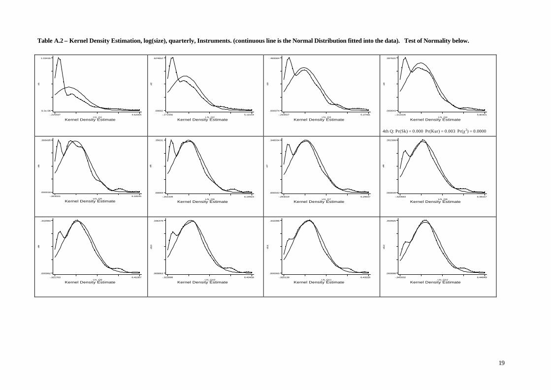
Accordingly, for each quarter, and each industry, we estimated the distribution of the
logarithm of the firms’ size, and checked if a tendency towards a normal distribution does emerge.
The results are shown in Tables A in the Appendix. Moreover, in order to test statistically the
conformity of the empirical distribution to the normal, we computed some tests of normality. First
of all, we estimated the Skewness and Kurtosis statistics, since they represent very good descriptive and inferential indexes for measuring normality. The Skewness and the Kurtosis indexes are the
third and the fourth standardized moments of the distribution.
In particular, the literature refers to the Skewness index as:
( )3
3
1 σµβ −= XE
and to the Kurtosis index as:
( )4
4
2 σµβ −= XE
where µ and σ are, the mean and the standard deviation of the distribution under exam. Since for a normal distribution they are equal to 0 and 3 respectively, a natural way to evaluate the
nonnormality of a distribution is to look at the difference of such moments from those values.
The Skewness index measures the degree of symmetry of a distribution: if 01 >β it’s
skewed to the right, while 01 <β corresponds to skewness to the left. Looking at Table 4, one
can note that for three industries out of four (the only exception being the Footwear & Clothing
one) the FSD tends to become more symmetric over time, with different patterns of convergence.
But even after 21 quarters, the FSD in the Electrical & Electronic Engineering, the Instruments and
interquartile range

12
the Food industries is still skewed to the right, while in the Footwear & Clothing industry, starting from a distribution skewed to the right, it turns out to be skewed to the left.
The Kurtosis index represents a measure of the curvature: distributions with 32 >β show
thicker tails than the normal distribution and tend to exhibit higher peaks in the center of the
distribution, whereas distributions with 32 <β tend to have lighter tails and to have broader peaks
than the normal4 For all industries (see Table 4), the Kurtosis index shows a convergence towards
the normal distribution, although in the case of the Electrical & Electronics and the Instruments industries, at the end of the relevant period, it appears to be more concentrated around the mean
than in that of the other two industries, for which it tends to be more spread.
Aimed at evaluating the pattern of convergence to a normal distribution, we computed also different
tests for normality. First, we used a simple test based on the Skewness and Kurtosis indexes
(D’Agostino et al. 1990), which allow to test statistically null hypothesis 0: 1 =βoH and
3: 2 =βoH . The results are reported, in terms of significance, in the first two lines of Table 4. In
the third line the results from Kolmogorov-Smirnov5 test are reported: we used this test to compare
statistically the empirical distribution to the normal distribution. Subsequently, two omnibus tests
were computed: the Shapiro-Wilk W test (Shapiro and Wilk, 1965) and the D’Agostino-Pearson K2
(D’Agostino and Pearson, 1973). By omnibus, following D’Agostino et al. (1990) we mean a test
that is able to detect deviations from normality due to either skewness or kurtosis. The results suggest a strong departure from normality of the FSD for all industries during
their infancy. With the passing of time and the mechanism of self-selection, the Electrical &
Electronics and the Instruments industries show a certain degree of normality at the end of the
relevant period, even if with different timings, while for the Food and the Footwear & Clothing
industries no significant converge does emerge.
4 We usually refer to them as leptokurtic distributions in the first case and to platykurtic in the latter. 5 We computed such test even if we are aware of its poor properties when testing for normality.

13
Table 4 –Test for Normality for each quarter, all industries.
Q 1 Q 2 Q 3 Q 4 Q 5 Q 6 Q 7 Q 8 Q 9 Q10 Q11 Q12 Q13 Q14 Q15 Q16 Q17 Q18 Q19 Q20 Q21
Electr. & Electronic Eng. Skewnessa
1.23*** 0.68*** 0.55*** 0.44*** 0.36*** 0.34*** 0.31*** 0.26*** 0.24** 0.25** 0.24** 0.27** 0.27** 0.24** 0.23** 0.19* 0.19* 0.16 0.13 0.07 0.11
Kurtosisb 3.86*** 2.83*** 2.78 2.66** 2.71* 2.76 2.79 2.86 2.90 2.92 3.03 3.02 3.30 3.31 3.29 3.23 3.09 3.15 3.11 3.14 3.12
Kolmogorov-Smirnov 0.26*** 0.15*** 0.11*** 0.10*** 0.08*** 0.08*** 0.07*** 0.06*** 0.06** 0.05** 0.05* 0.06** 0.04* 0.05* 0.05* 0.05* 0.05** 0.05* 0.04* 0.04 0.04
Shapiro -Wilk 0.95*** 0.98*** 0.98*** 0.99*** 0.99*** 0.99*** 0.99*** 0.99*** 0.99*** 0.99*** 0.99*** 0.99*** 0.98*** 0.98*** 0.98*** 0.99*** 0.99*** 0.99** 0.99** 0.99*** 0.99***
D’Agostino 38.54***
37.02***
26.91***
20.41***
14.29***
12.13***
1.039*** 7.20** 5.72* 6.31** 5.38* 6.59** 8.04** 6.89** 6.50** 4.65* 3.31 2.98 1.77 1.07 1.43
Instruments
Skewnessa 1.85*** 1.29*** 1.12*** 0.96*** 0.96*** 0.91*** 0.83*** 0.79*** 0.75*** 0.75*** 0.70*** 067*** 0.61*** 0.44*** 0.40** 0.33** 0.32** 0.34** 0.30* 0.50*** 0.47***
Kurtosisb 6.43*** 4.60*** 4.40*** 4.04*** 4.27*** 4.09*** 3.81** 3.75** 3.61* 3.61* 3.61* 3.60* 3.55* 2.98 2.93 2.89 2.84 2.85 2.80 3.50 3.44
Kolmogorov-Smirnov 0.33*** 0.23*** 0.18*** 0.16*** 0.12*** 0.11*** 0.11*** 0.10*** 0.10*** 0.09*** 0.08** 0.08** 0.08** 0.08** 0.07* 0.07* 0.07* 0.06 0.06 0.06 0.06
Shapiro -Wilk 0.90*** 0.94*** 0.95*** 0.96*** 0.96*** 0.96*** 0.96*** 0.96*** 0.97*** 0.97*** 0.97*** 0.97*** 0.97*** 0.98*** 0.98*** 0.98*** 0.98*** 0.98*** 0.98*** 0.97*** 0.98***
D’Agostino 65.44***
60.88***
48.89***
37.89***
38.55***
34.03***
27.73***
25.29***
22.17***
21.91***
19.59***
17.84***
15.09*** 7.64** 6.28** 4.59 4.21 4.68* 3.81 10.05**
* 8.88**
Food
Skewnessa 1.39*** 0.83*** 0.75*** 0.69*** 0.72*** 0.56*** 0.52*** 0.49*** 0.57*** 0.40*** 0.40*** 0.41*** 0.42*** 0.37*** 0.38*** 0.39*** 0.60*** 0.46*** 0.40*** 0.42*** 0.54***
Kurtosisb 4.49*** 3.02 2.91 2.81 2.88 2.61* 2.50** 2.48*** 2.57** 2.41*** 2.39*** 2.36*** 2.33*** 2.37*** 2.39*** 2.38*** 2.68 2.52** 2.42** 2.35*** 2.55*
Kolmogorov-Smirnov 0.26*** 0.18*** 0.17*** 0.15*** 0.15*** 0.13*** 0.13*** 0.12*** 0.12*** 0.11*** 0.12*** 0.12*** 0.12*** 0.11*** 0.13*** 0.12*** 0.12*** 0.11*** 0.11*** 0.12*** 0.12***
Shapiro -Wilk 0.94*** 0.97*** 0.97*** 0.97*** 0.97*** 0.98*** 0.97*** 0.98*** 0.97*** 0.98*** 0.98*** 0.98*** 0.97*** 0.98*** 0.97*** 0.97*** 0.97*** 0.97*** 0.98*** 0.97*** 0.97***
D’Agostino 43.52***
37.99***
28.82***
24.46***
28.41***
19.65***
19.39***
17.66***
21.26***
16.23***
15.81***
16.85***
18.44***
14.35***
13.20***
13.32***
16.62***
12.18***
11.92***
13.69***
13.89***
Footwear & Clothing
Skewnessa 0.71*** 0.31*** 0.14* 0.07 0.05 0.00 -0.02 -0.04 -0.05 -0.05 -0.05 -0.09 -0.12 -0.15 -0.14 -0.12 -0.09 -0.11 -0.10 -0.13 -0.11
Kurtosisb 2.53*** 2.23*** 2.15*** 2.28*** 2.30*** 2.33*** 2.36*** 2.40*** 2.35*** 2.44*** 2.45*** 2.43*** 2.44*** 2.51*** 2.45*** 2.45*** 2.46*** 2.46*** 2.40*** 2.38*** 2.31***
Kolmogorov-Smirnov 0.20*** 0.11*** 0.10*** 0.09*** 0.08*** 0.08*** 0.08*** 0.07*** 0.07*** 0.06*** 0.06*** 0.06*** 0.06*** 0.06*** 0.06*** 0.06*** 0.06*** 0.07*** 0.06*** 0.07*** 0.08***
Shapiro -Wilk 0.98*** 0.99*** 0.99*** 0.99*** 0.99*** 0.99*** 0.99*** 0.99*** 0.99*** 0.99*** 0.99*** 0.99*** 0.99*** 0.98*** 0.98*** 0.99*** 0.99*** 0.99*** 0.98*** 0.98*** 0.98***
D’Agostino 84.03***
72.09***
58.61***
43.27***
36.40***
29.53***
26.13***
21.22***
25.12***
16.04***
14.58***
16.29***
15.57***
11.74***
13.79***
13.24***
11.69***
11.74***
14.15***
15.51***
19.65***
***, **, * mean statistically significant at α = 0.01, α = 0.05 and α = 0.10 respectively. a, b = The values are the Skewness and Kurtosis indexes. We reported the significance level of the D’Agostino et al. test.

14
4 - Empirical Findings
The alleged structural and technological differences among the industries taken into account
allow for the somewhat contradictory results obtained from the Kernel density estimates. Thus, for
the Electrical & Electronic Engineering industry, the shape of the normal distribution begins to
emerge after the 8th quarter, as confirmed by the normality test (see Table A.1 in Appendix A). The
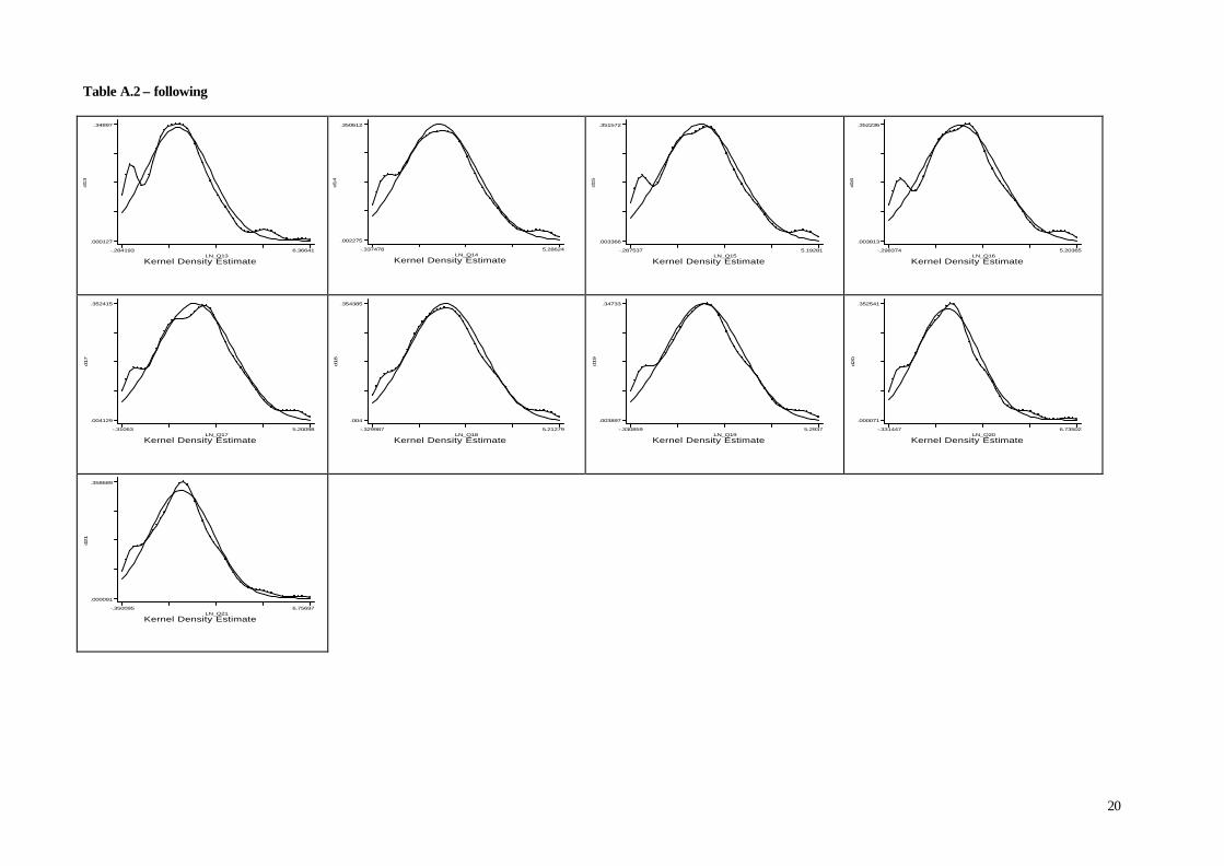
convergence towards the normal distribution begins instead to be clear only after the 13th quarter in
the case of the Instruments industry (see Table A.2 in Appendix A). Thus, firm’s age is a major
factor affecting the FSD in these industries: as the normal distribution of sizes is reached with the
passing of time, Gibrat’s Law turns out to hold when firms are in their second and third year in the
market, respectively for the Electric & Electronics and the Food industries.
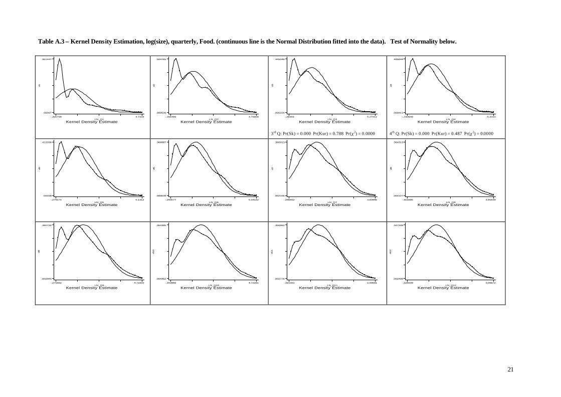
Different is the case of the Food and the Footwear & Clothing industries (see Table A.3 and
A.4 in Appendix A), for which no significant patterns of convergence do emerge. After 6 years of
observation, these two industries are still far from the limit distribution and, moreover, the
distributions of firm sizes are still bimodal. In the Footwear & Clothing industry, in particular, the shakeout after entry is less drastic than in the former two industries. For this reason, at the end of
the relevant period, the FSD exhibits two modes: one identifies the “core” of the industry, while the
second is located at the fringe of the industry, suggesting the existence of an evolutionary process of
active learning that allows firms below the MES level of output to survive and grow.
A possible explanation of the contrasting results obtained for the two groups of industries is
that the selection and learning processes are much slower in the traditional consumer goods
industries than it is the case with two technologically progressive industries such as the Electrical &
Electronic Engineering and the Instruments ones. Thus, in the Food and the Footwear & Clothing
industries the process of industry dynamics should be allowed to run for more periods before a
convergence to the normal distribution begins to emerge. Unfortunately, our data do not allow
observing the behavior of newborn firms in these industries beyond their 21st quarter in the market.
With the aim of measuring the evolution of the FSD over time, we looked also at the moments of this distribution. In particular, we studied the patterns of evolution of the Skewness
and Kurtosis indexes, to see if and how a convergence to the normal distribution does emerge. The
results confirm, coherently with the Kernel estimations, and the normality tests, the different
patterns of the evolution of the size distribution of firms in the various industries. Accordingly,
following Pakes and Ericson (1998), we may argue that the evolution of the FSD in the Food and
the Footwear & Clothing industries is consistent with the active learning model, while in the
Electrical & Electronic Engineering and the Instruments industries it turns out to be consistent with
the passive learning model put forward by Jovanovic (1982). Nevertheless, both groups of
industries display a dynamics that is to a large extent consistent with the evolutionary approach
developed by Audretsch (1995).

15
5 - Conclusions In this paper we examine the evolution of the FSD for 12 cohorts of newborn firms, to draw
some conclusions about which model of industry dynamics is more consistent with the size
distribution of young firms in four selected industries. In general, the process of convergence
towards the limit distribution appears to be just a matter of time, although, unfortunately, our data
set allows us to follow the post-entry performance of these firms only for their first 6 years in the
industry.
However, we take into account four industries very different from the point of view a) of the
productive capacity required for entering the market at the MES level of output, and b) of their
technological content and characteristics. Differences in industry-specific characteristics concerning
the levels of sunk costs and the rate of entry allow for differences in the way a convergence towards
a lognormal distribution does or does not arise. This Bayesian perspective helps to explain the
different speed of convergence of the FSD to a lognormal distribution. In particular, it is consistent with our empirical finding that only in the most technologically advanced industries - in which
smaller entrants tend to invest in their capacity more gradually, after exploring their efficiency level
with respect to their competitors - a convergence towards the lognormal distribution emerges with
the passing of time. Conversely, in the most traditional industries the same tendency is less marked.
Whether this is due to the fact that the selection and learning processes are much slower in the
traditional consumer goods industries than it is the case with the technologically progressive ones
could be detected only when and if new data will be forthcoming allowing a thorough analysis of
the behavior on new-born firms in these industries beyond their 21st quarter in the market.
References
Amaral L. A. N., Buldyrev S. V., Havlin S., Leschborn H., Maass P., Salinger M. A., Stanley H. E., Stanley M. H. R., 1997, “Scaling Behavior in Economics: I. Empirical Results for Company Growth”, Journal of Physics, 7, pp.621-633.
Audretsch, D. B., 1995, Innovation and Industry Evolution, Cambridge (MA), MIT Press. Audretsch, D.B., E. Santarelli and M. Vivarelli, 1999, “Start-up Size and Industrial Dynamics: Some Evidence from
Italian Manufacturing”, International Journal of Industrial Organization, 17(7), pp. 965-983. Boeri, T. and L. Bellmann, 1995, “Post-entry Behaviour and the Cycle: Evidence from Germany”, International
Journal of Industrial Organization, 13(4), pp. 483-500. Brock W. A., 1999, “Scaling in Economics: A Reader’s Guide”, Industrial and Corporate Change, 8(3), 409-446. Cabral, J., and J. Mata, 1996, “On the Evolution of the Firm Size Distribution”, paper presented at the 23rd Annual
E.A.R.I.E. Conference, Vienna, September. Cabral, L., 1997, “Entry Mistakes”, Centre for Economic Policy Research, Discussion Paper No. 1729, November. D'Agostino, R. B., A. Balanger and R. B. D'Agostino jr., 1990, “A Suggestion for Using Powerful and Informative
Tests for Normality”', The American Statistician, 44(4), 316-21. Ericson, R., and A. Pakes, 1995, “Markov-Perfect Industry Dynamics: a Framework for Empirical Work”, Review of
Economic Studies, 62(1), pp. 53-82. Geroski, P., 1995, “What Do We Know About Entry?”, International Journal of Industrial Organization, 13(4), pp.
421-440. Gibrat, R., 1931, Les Inegalites Economiques, Paris, Librairie du Recueil Sirey. Hart, P. E. and N. Oulton, 1999, “Gibrat, Galton and Job Generation”, International Journal of the Economics of
Business, 6(2), pp. 149-164. Hart, P. E. and S.J. Prais, 1956, “The Analysis of Business Concentration: A Statistical Approach”, Journal of the
Royal Statistical Society, 119, series A, pp. 150-191.

16
Hymer, S., and P. Pashigian, 1962, “Firm Size and the Rate of Growth”, Journal of Political Economy , 70(4), pp. 556-569.
Ijiri, Y., and H. Simon, 1974, “Interpretations of Departures from the Pareto Curve Firm-Size Distribution”, Journal of Political Economy , 82(2), Part 1, pp. 315-331.
Ijiri, Y., and H. Simon, 1977, Skew Distribution and the Sizes of Business Firms, Amsterdam, North-Holland Publishing.
Jovanovic, B., 1982, “Selection and Evolution of Industry”, Econometrica, 50(3), pp. 649-670. Kalecki, M., 1945, “On the Gibrat Distribution”, Econometrica, 13(2), pp. 161-170. Klepper, S., and J.H. Miller, 1995, “Entry, Exit, and Shakeouts in the United States in New Manufactured
Products”, International Journal of Industrial Organization, 13(4), pp. 567-591. Klepper, S., and K. Graddy, 1990, “The Evolution of New Industries and the Determinants of Market Structure”,
Rand Journal of Economics, 21(1), pp. 27-44 Lotti F., E. Santarelli, M. Vivarelli, 1999, “Does Gibrat's Law Hold in the Case of Young, Small Firms?”,
University of Bologna, Department of Economics, Working Paper No. 361; presented at the 28th Annual E.A.R.I.E. Conference, Lausanne, September 2000.
Lotti F., E. Santarelli, M. Vivarelli, 2001, (a) “The Relationship Between Size and Growth: The Case of Italian Newborn Firms”, Applied Economics Letters, 8(7), pp. 451-454.
Lotti F., E. Santarelli, M. Vivarelli, 2001, (b) “Is It Really Wise to Design Policies in Support of New Firm Formation?”, in L. Lambertini (ed.), Current Issues in Regulation and Competition Policies, Houndmills, Basingstoke, Palgrave, forthcoming.
Machado, J. A. F., and J. Mata, 2000, “Box-Cox Quantile Regression and the Distribution of Firm Sizes”, Journal of Applied Econometrics, 15(3), pp. 253-274.
Mata, J., 1994, “Firm Growth During Infancy”, Small Business Economics, 6(1), pp. 27-40. Pagan, A., and A. Ullah, 1999, Nonparametric Econometrics, Cambridge, Cambridge University Press. Pakes, A., and R. Ericson, 1998, “Empirical Implications of Alternative Models of Firms Dynamics”, Journal of
Economic Theory, 79(1), pp. 1-45. Shapiro, S. S., and Wilk, M. B., 1965, “An Analysis of Variance Test for Normality (Complete Samples)”,
Biometrika, 52, pp. 591-611. Simon, H. A. and C. P. Bonini, 1958, “The Size Distribution of Business Firms”, American Economic Review,
58(4), pp. 607-617. Sutton, J., 1997, “Gibrat’s Legacy”, Journal of Economic Literature, 35(1), pp. 40-59. Sutton, J., 1998, Technology and Market Structure: Theory and History, Cambridge and London, MIT Press.

17
Appendix A
Table A.1 – Kernel Density Estimation, log(size), quarterly, Electrical & Electronic Eng. (continuous line is the Normal Distribution fitted into the data). Test of
Normality below.
d1
Kernel Density EstimateLN_Q1
-.243354 4.82832
.000145
.76299
d2
Kernel Density EstimateLN_Q2
-.26122 4.88619
.001052
.429982
d3
Kernel Density EstimateLN_Q3
-.251995 5.20782
.000696
.370051
d4
Kernel Density EstimateLN_Q4
-.268374 5.31823
.000775
.365845
d5
Kernel Density EstimateLN_Q5
-.266404 5.51343
.000498
.370163
d6
Kernel Density EstimateLN_Q6
-.26714 5.7436
.000298
.370607
d7
Kernel Density EstimateLN_Q7
-.239122 5.74445
.000309
.374916
d8
Kernel Density EstimateLN_Q8
-.256629 5.74969
.000298
.383009
d9
Kernel Density EstimateLN_Q9
-.25774 5.73001
.000361
.38555
d10
Kernel Density EstimateLN_Q10
-.262792 5.71383
.000476
.381786
d11
Kernel Density EstimateLN_Q11
-.235254 5.68199
.000596
.407565
d12
Kernel Density EstimateLN_Q12
-.264156 5.88093
.000317
.394876

18
Table A.1 – following
d13
Kernel Density EstimateLN_Q13
-.236693 6.63529
.000024
.409879
d14
Kernel Density EstimateLN_Q14
-.237653 6.85906
.000012
.406529
d15
Kernel Density EstimateLN_Q15
-.245488 6.83853
.000017
.389453
d16
Kernel Density EstimateLN_Q16
-.253139 6.83516
.000017
.390652
d17
Kernel Density EstimateLN_Q17
-.27752 6.79075
.000017
.376148
d18
Kernel Density EstimateLN_Q18
-.255681 6.81812
.000014
.377866
d19
Kernel Density EstimateLN_Q19
-.269731 6.76801
.000021
.396547
d20
Kernel Density EstimateLN_Q20
-.282974 6.85386
.000021
.382259
d21
Kernel Density EstimateLN_Q21
-.278261 6.78105
.000032
.400216
19
Table A.2 – Kernel Density Estimation, log(size), quarterly, Instruments. (continuous line is the Normal Distribution fitted into the data). Test of Normality below.
d1
Kernel Density EstimateLN_Q1
-.225597 4.62005
9.2e-06
1.03435
d2
Kernel Density EstimateLN_Q2
-.271556 5.19154
.00002
.624652
d3
Kernel Density EstimateLN_Q3
-.293507 5.37491
.000074
.469364
d4
Kernel Density EstimateLN_Q4
-.312026 5.90301
.000043
.397631
4th Q: Pr(Sk) = 0.000 Pr(Kur) = 0.003 Pr(χ2) = 0.0000
d5
Kernel Density EstimateLN_Q5
-.263021 6.18191
.000018
.368495
d6
Kernel Density EstimateLN_Q6
-.264339 6.19923
.00003
.35631
d7
Kernel Density EstimateLN_Q7
-.294019 6.29047
.000042
.346034
d8
Kernel Density EstimateLN_Q8
-.320683 6.38447
.000049
.352399
d9
Kernel Density EstimateLN_Q9
-.321763 6.41307
.000062
.342984
d10
Kernel Density EstimateLN_Q10
-.323088 6.43456
.000063
.336379
d11
Kernel Density EstimateLN_Q11
-.325139 6.43216
.000065
.342386
d12
Kernel Density EstimateLN_Q12
-.345932 6.44849
.000088
.350925
20
Table A.2 – following
d13
Kernel Density EstimateLN_Q13
-.284193 6.36641
.000127
.34897
d14
Kernel Density EstimateLN_Q14
-.337478 5.28624
.002275
.350612
d15
Kernel Density EstimateLN_Q15
-.287537 5.19281
.003366
.351572
d16
Kernel Density EstimateLN_Q16
-.298374 5.20365
.003813
.352236
d17
Kernel Density EstimateLN_Q17
-.31063 5.20098
.004129
.352415
d18
Kernel Density EstimateLN_Q18
-.329987 5.21279
.004
.354385
d19
Kernel Density EstimateLN_Q19
-.330859 5.2937
.003897
.34733
d20
Kernel Density EstimateLN_Q20
-.331447 6.73502
.000071
.352541
d21
Kernel Density EstimateLN_Q21
-.350095 6.75697
.000091
.358689
21
Table A.3 – Kernel Density Estimation, log(size), quarterly, Food. (continuous line is the Normal Distribution fitted into the data). Test of Normality below.
d1
Kernel Density EstimateLN_Q1
-.200798 4.7334
.00007
.951447
d2
Kernel Density EstimateLN_Q2
-.266489 4.79909
.000539
.504765
d3
Kernel Density EstimateLN_Q3
-.28369 5.27412
.000226
.445048
3rd Q: Pr(Sk) = 0.000 Pr(Kur) = 0.788 Pr(χ2) = 0.0000
d4
Kernel Density EstimateLN_Q4
-.290648 5.2033
.000413
.405044
4th Q: Pr(Sk) = 0.000 Pr(Kur) = 0.487 Pr(χ2) = 0.0000
d5
Kernel Density EstimateLN_Q5
-.279174 5.1312
.00038
.412036
d6
Kernel Density EstimateLN_Q6
-.293577 5.19142
.000639
.366087
d7
Kernel Density EstimateLN_Q7
-.296662 4.83996
.002156
.366913
d8
Kernel Density EstimateLN_Q8
-.301685 4.65839
.004127
.364313
d9
Kernel Density EstimateLN_Q9
-.275682 4.71833
.002945
.365732
d10
Kernel Density EstimateLN_Q10
-.303968 4.72281
.004462
.364385
d11
Kernel Density EstimateLN_Q11
-.315561 5.00691
.002776
.356962
d12
Kernel Density EstimateLN_Q12
-.326039 5.09672
.002499
.347349

22
Table A.3 – following
d13
Kernel Density EstimateLN_Q13
-.330384 5.10107
.002784
.341229
d14
Kernel Density EstimateLN_Q14
-.330597 5.02194
.003608
.346798
d15
Kernel Density EstimateLN_Q15
-.338105 5.02024
.004093
.342039
d16
Kernel Density EstimateLN_Q16
-.345728 5.02786
.004519
.337975
d17
Kernel Density EstimateLN_Q17
-.302677 5.01221
.002813
.342929
d18
Kernel Density EstimateLN_Q18
-.334414 5.04394
.003336
.345207
d19
Kernel Density EstimateLN_Q19
-.346665 5.11735
.003687
.33799
d20
Kernel Density EstimateLN_Q20
-.358946 5.14644
.003969
.330228
d21
Kernel Density EstimateLN_Q21
-.34377 5.13956
.002716
.337629

23
Table A.4 – Kernel Density Estimation, log(size), quarterly, Footwear & Clothing. (continuous line is the Normal Distribution fitted into the data). Test of Normality below.
d1
Kernel Density EstimateLN_Q1
-.247807 4.78041
.001651
.581436
d2
Kernel Density EstimateLN_Q2
-.258221 5.75539
.000408
.346372
d3
Kernel Density EstimateLN_Q3
-.265542 5.82237
.000661
.3417
d4
Kernel Density EstimateLN_Q4
-.26554 5.85279
.000752
.344707
d5
Kernel Density EstimateLN_Q5
-.267594 5.82828
.000932
.345516
d6
Kernel Density EstimateLN_Q6
-.271028 5.91294
.00088
.344462
d7
Kernel Density EstimateLN_Q7
-.273136 5.90076
.00101
.343606
d8
Kernel Density EstimateLN_Q8
-.274043 5.8462
.001342
.345438
d9
Kernel Density EstimateLN_Q9
-.277699 5.84604
.001456
.342595
d10
Kernel Density EstimateLN_Q10
-.275 5.86971
.001359
.349868
d11
Kernel Density EstimateLN_Q11
-.275927 5.86691
.001376
.351274
d12
Kernel Density EstimateLN_Q12
-.282834 5.80829
.001713
.344931

24
Table A.4 – following
d13
Kernel Density EstimateLN_Q13
-.284064 5.80553
.001791
.345228
d14
Kernel Density EstimateLN_Q14
-.287061 5.85541
.001731
.344743
d15
Kernel Density EstimateLN_Q15
-.29608 5.86823
.001788
.337686
d16
Kernel Density EstimateLN_Q16
-.295355 5.85604
.001905
.341262
d17
Kernel Density EstimateLN_Q17
-.296711 5.86123
.001942
.342317
d18
Kernel Density EstimateLN_Q18
-.300745 5.84592
.002268
.339717
d19
Kernel Density EstimateLN_Q19
-.307011 5.8404
.002347
.335186
d20
Kernel Density EstimateLN_Q20
-.31487 5.83633
.002457
.32893
d21
Kernel Density EstimateLN_Q21
-.321095 5.76351
.002884
.325365
Top Related
Copyright © 2022 FDOKUMEN

